arX

iv:1

210.

3586

v1 [

cond

-mat

.sof

t] 1

2 O

ct 2

012

Local elastic response measured near the colloidal glass transitionD. Anderson1, D. Schaar1, H. G. E. Hentschel1, J. Hay1, Piotr Habdas2, and Eric R. Weeks111 Department of Physics, Emory University, Atlanta, GA 303222 Department of Physics, Saint Joseph’s University, Philadelphia, PA 19131

(Dated: 15 October 2012)

We examine the response of a dense colloidal suspension to a local force applied by a small magnetic bead.For small forces, we find a linear relationship between the force and the displacement, suggesting the mediumis elastic, even though our colloidal samples macroscopically behave as fluids. We interpret this as a measureof the strength of colloidal caging, reflecting the proximity of the samples’ volume fractions to the colloidalglass transition. The strain field of the colloidal particles surrounding the magnetic probe appears similarto that of an isotropic homogeneous elastic medium. When the applied force is removed, the strain relaxesas a stretched exponential in time. We introduce a model that suggests this behavior is due to the diffusiverelaxation of strain in the colloidal sample.

I. INTRODUCTION

Glass is an amorphous solid: despite the lack of long-range order, a glassy material is elastic rather than vis-cous. As a glass-forming material is cooled, its viscosityrises dramatically by many orders of magnitude; flow be-comes difficult and slow. The elastic behavior of a glass,then, could be reframed as the material being probedon time scales too quickly for liquid-like flow to occur.The origins of this elasticity and the nature of the glasstransition are a quite active area of research1–5.

A related question is to what extent the macroscopicelastic behavior extends to the microscopic scale. For ex-ample, simulations have seen that the elastic moduli arespatially heterogeneous in some cases6,7. Certainly themacroscopic elastic response treats the material as a con-tinuum, whereas on a scale of the constituent moleculesthis could be a poor approximation.

Colloids are a simple model system which can beused to study the glass transition and the propertiesof glassy materials8–10. Colloidal suspensions are com-posed of solid particles in a liquid. The particles dif-fuse due to Brownian motion, but this diffusion is im-peded at high particle concentration. In many experi-ments, colloidal particles only have short-range repulsiveinteractions, and the particles can be approximated ashard spheres11,12. In such samples the control param-eter is the volume fraction φ and glasses are found forφ > φg ≈ 0.5810,11. Near the glass transition, the viscos-ity rises quite dramatically, although some evidence sug-gests that perhaps it truly diverges at a point above φg

13.In particular, an alternative divergence point is “randomclose packing” (rcp). This is the largest volume fractionpossible for a sample that is still amorphously packed(rather than crystalline)14. The volume fraction φrcp isknown through simulations and taken to be ≈ 0.64, whichagrees with early experiments done with ball bearings15.

Of course, the presence of the continuous liquid sur-rounding the colloidal particles is important for under-standing the flow properties of colloids. Approachingthe colloidal glass transition from φ < φg, samples areviscoelastic16. Their properties are described by both vis-

cous and elastic moduli which are frequency-dependent.The viscosity mentioned above is understood to be thelow-frequency limit. Indeed, if a glass is defined as anamorphous solid – a sample that does not flow – thenit is important to recognize that whether or not it flowsdepends on the time scale of observation10.

While macroscopically one considers viscous and elas-tic behavior, microscopically one considers diffusion. Amolecule or tracer particle in a fluid sample has a nonzerodiffusion constant, which decreases to zero as the glasstransition is approached. The decrease of the diffusioncoefficient is attributed to caging. On short time scales,particles diffuse in a “cage” formed by their neighbors.On longer time scales, these cages rearrange and particlescan move throughout the sample. As the glass transitionis approached, the cage rearrangements occur less fre-quently, thus decreasing the diffusivity17–19. These cagesprovide a sort of elasticity for individual particles20–22.Particles which try to move away from the centers oftheir cage experience a restoring force18–20. If a constantexternal force is exerted on a particle, it will slowly movethrough the colloidal suspension as cages rearrange, al-though the force needs to be kept small when φ is closeto φg to avoid nonlinear behavior23–27. If a sufficientlyhigh external force is applied to a particle, it can breakthe cages and move through the sample more freely (typ-ically with a nonlinear relationship between the force andresulting velocity)25,26,28–32, disturbing and rearrangingparticles as it moves28,33.

In this paper we probe the elastic response of a densecolloidal suspension by locally exerting a small force on amagnetic bead. Our studies are conducted on a time scalefaster than the sample can relax due to diffusion. We findthat the sample responds elastically, with a Young’s mod-ulus E that rises as the glass transition is approached,and a Poisson ratio σ equal to 1/2. We also study the re-laxation of the magnetic bead after it has been displacedand the force removed. This relaxation is faster for highervolume fraction samples. We present a model that cap-tures the stretched exponential character of the relax-ation, by assuming that in our colloidal sample stressdiffuses away to infinity at long times.

2

II. EXPERIMENTAL METHODS

The colloidal suspensions are made of poly-(methylmethacrylate) particles, sterically stabilizedby a thin layer of poly-12-hydroxystearic acid34. Theparticles have a radius a = 1.55 µm, a polydispersityof ∼5%, and are dyed with rhodamine35. The uncer-tainty of the mean particle radius is ±0.01 µm. Theparticles are slightly charged, but their glass transitionis still at φg = 0.58 ± 0.01, signaled by the diffusionof particles going to zero on experimental time scales(several hours). The colloidal particles are suspended ina mixture of cyclohexylbromide/cis- and trans- decalinwhich nearly matches both the density and the indexof refraction of the colloidal particles35. The density ofthis solvent is 1.232 g/cm3, the index of refraction is1.495, and the viscosity is η = 2.18 mPa·s. The particlesare fluorescently labeled for visualization35. Beforebeginning experiments, we stir the sample with an airbubble to break up any pre-existing crystalline regions,then wait 20 minutes before taking data.A small quantity of superparamagnetic beads (Dynal

M450, coated with glycidyl ether reactive groups) witha radius of 2.25 µm are added to the colloidal suspen-sion. We do not observe attraction or repulsion betweenthe colloidal particles and the magnetic beads, in eitherdilute or concentrated samples. The beads are not com-pletely monodisperse in their magnetic properties, andour calibration finds the variability in the effective mag-netic force applied to different beads to be less than 10%.Also, the magnetic beads are not density matched, andtheir effective weight is 0.1 pN. This is a factor of tensmaller than the smallest horizontally applied magneticforces in our experiments. We study isolated magneticbeads at least 35 µm from the sample chamber boundaryand from other magnetic beads.For some of the data (Figs. 1,2 in particular), we use

a conventional Leica DMIRB inverted microscope witha CCD camera. A magnetic bead appears as a largedark circle in our images and its position as a func-tion of time is found using standard particle trackingtechniques36. For these experiments, the typical imagesize is 15 × 40 µm2, with images taken at a rate of 30frames per second. The magnetic bead position is re-solved to within 0.04 µm; see Fig. 1 for example.For other data, we use a ThermoNoran Oz confocal

microscope. With this microscope, we acquire imagesof area 80 µm × 75 µm at a rate of 30 frames per sec-ond (256 × 240 pixels2). The magnetic beads are notfluorescent and thus appear black on the background ofdyed colloidal particles (see Fig. 4). Again, we use parti-cle tracking procedures to follow the motion of the mag-netic particle with a resolution of 0.04 µm. With eitherthe confocal microscope or the video microscope, we onlytrack the motion of particles in 2D: for the experiments inthis paper, the magnetic particle position always remainswith the imaging plane of the microscope.We additionally use the confocal microscope to take

three-dimensional images of these samples to determinethe volume fraction35. We count the particles within theimaged volume, and convert from the measured numberdensity n to volume fraction φ using φ = (4π/3)na3.Due to our uncertainty of the mean value of the particleradius a, we have a systematic uncertainty of 2% of ourφ values37. That is, our φ values are fairly accurate whencompared with each other, but a reported value of φ =0.50 is uncertain by ±0.01.We use a strong Neodymium permanent magnet

mounted on a micrometer positioner to control the forceapplied to the magnetic beads. The micrometer accu-rately reproduces the magnet position and thus our un-certainty in the force between different experiments islimited by the magnetic bead variability, rather than themagnet positioning. For many experiments, a computer-controlled stepper motor attached to the micrometer al-lows us to slowly and controllably vary the applied forceover two orders of magnitude.For other experiments, we want to apply a short-

duration magnetic force. We mount the magnet on alinear actuator (Ultra Motion D-A.25-HT17). The mag-net is then brought close to the magnetic bead resultingin a high force acting on the magnetic bead for a shorttime; the details are discussed below.Our experiments are controlled-force experiments, in

contrast to controlled displacement38,39. For example,this means that particles do not necessarily need to movein the direction of the applied force, although we dis-cuss below that they appear to always do so. Priorwork by other groups used laser tweezers to move probeparticles through colloidal suspensions at a controllablevelocity40–43, finding many interesting results such asanisotropy of the disturbed region around the movingparticle40 and a decoupling of structural and hydrody-namic influences on the particle motion43. These priorexperiments studied probe particles as they moved overlong distances, in contrast to our experiments describedbelow where the magnetic bead always remains close toits equilibrium position.

III. LINEAR ELASTIC RESPONSE

In our earlier work, we applied a constant force and ob-served the steady-state motion of the magnetic bead29.For large forces, the velocity of the magnetic bead grewnonlinearly with increasing force, consistent with shear-thinning. We also observed that the velocity was es-sentially zero below a threshold force. The thresh-old force grew dramatically as the glass transition wasapproached29.To test the behavior of the sample below the thresh-

old force for motion, we vary the magnetic force withina range of forces that are below the threshold force formotion. To ensure that the forces used are below thethreshold force for motion, each increase in the force wasfollowed by a waiting period of 160 s to observe the sub-

3

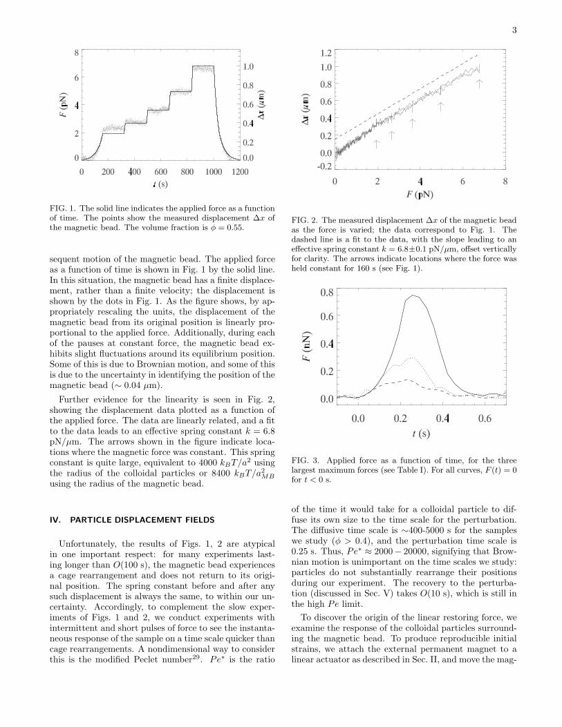
FIG. 1. The solid line indicates the applied force as a functionof time. The points show the measured displacement ∆x ofthe magnetic bead. The volume fraction is φ = 0.55.

sequent motion of the magnetic bead. The applied forceas a function of time is shown in Fig. 1 by the solid line.In this situation, the magnetic bead has a finite displace-ment, rather than a finite velocity; the displacement isshown by the dots in Fig. 1. As the figure shows, by ap-propriately rescaling the units, the displacement of themagnetic bead from its original position is linearly pro-portional to the applied force. Additionally, during eachof the pauses at constant force, the magnetic bead ex-hibits slight fluctuations around its equilibrium position.Some of this is due to Brownian motion, and some of thisis due to the uncertainty in identifying the position of themagnetic bead (∼ 0.04 µm).

Further evidence for the linearity is seen in Fig. 2,showing the displacement data plotted as a function ofthe applied force. The data are linearly related, and a fitto the data leads to an effective spring constant k = 6.8pN/µm. The arrows shown in the figure indicate loca-tions where the magnetic force was constant. This springconstant is quite large, equivalent to 4000 kBT/a

2 usingthe radius of the colloidal particles or 8400 kBT/a

2MB

using the radius of the magnetic bead.

IV. PARTICLE DISPLACEMENT FIELDS

Unfortunately, the results of Figs. 1, 2 are atypicalin one important respect: for many experiments last-ing longer than O(100 s), the magnetic bead experiencesa cage rearrangement and does not return to its origi-nal position. The spring constant before and after anysuch displacement is always the same, to within our un-certainty. Accordingly, to complement the slow exper-iments of Figs. 1 and 2, we conduct experiments withintermittent and short pulses of force to see the instanta-neous response of the sample on a time scale quicker thancage rearrangements. A nondimensional way to considerthis is the modified Peclet number29. Pe∗ is the ratio

FIG. 2. The measured displacement ∆x of the magnetic beadas the force is varied; the data correspond to Fig. 1. Thedashed line is a fit to the data, with the slope leading to aneffective spring constant k = 6.8±0.1 pN/µm, offset verticallyfor clarity. The arrows indicate locations where the force washeld constant for 160 s (see Fig. 1).

FIG. 3. Applied force as a function of time, for the threelargest maximum forces (see Table I). For all curves, F (t) = 0for t < 0 s.

of the time it would take for a colloidal particle to dif-fuse its own size to the time scale for the perturbation.The diffusive time scale is ∼400-5000 s for the sampleswe study (φ > 0.4), and the perturbation time scale is0.25 s. Thus, Pe∗ ≈ 2000− 20000, signifying that Brow-nian motion is unimportant on the time scales we study:particles do not substantially rearrange their positionsduring our experiment. The recovery to the perturba-tion (discussed in Sec. V) takes O(10 s), which is still inthe high Pe limit.

To discover the origin of the linear restoring force, weexamine the response of the colloidal particles surround-ing the magnetic bead. To produce reproducible initialstrains, we attach the external permanent magnet to alinear actuator as described in Sec. II, and move the mag-

4

TABLE I. The five different maximum forces applied, and theintegrated impulse I =

∫

F (t)dt. The calibration procedure(described in the text) has an intrinsic Fmax uncertainty of±0.05 nN and an I uncertainty of ±0.005 nN·s. Due to vari-ability between different magnetic beads, for a given magneticbead there is also an overall systematic uncertainty of ±10%.Graphs of F (t) for the three largest values of Fmax are shownin Fig. 3.

Fmax (nN) I (nN s)

0.042 0.011

0.077 0.020

0.13 0.036

0.29 0.068

0.75 0.17

net toward the sample and then away at maximum speed.The force applied is ramped up to a maximum value andthen just as rapidly reduced. To calibrate the force asa function of time, F (t), we use this procedure to exerta force on magnetic beads suspended in glycerol. Suchbeads move with velocity v(t), from which we deducethe force F (t) using Stokes’ Law, F = 6πηaMBv, withthe viscosity of glycerol η = 0.934 Pa·s. The resultingF (t) data are plotted in Fig. 3 for the three largest Fmax.These correspond to the cases where the external magnetis moved the closest to the sample. For example, the topcurve in Fig. 3 takes longer to reach its peak and longerto return to F = 0, as the magnet has farther to move.

The peaks of the curves, Fmax, are confirmed by mea-suring the velocity of magnetic beads in glycerol whilethe external magnet is fixed in its closest distance to thesample for a given forcing protocol. Those results agreequite well with the values measured from the F (t) data.In the results that follow, we refer to the different F (t) bytheir maximum values Fmax which are listed in Table I.An additional way to quantify the F (t) is by their timeintegral, I =

∫

F (t)dt, yielding an impulse which is ap-plied to the magnetic bead. These values are also listedin Table I. In each case, the ratio I/Fmax = 0.25 ± 0.03s, suggesting that our choice of using Fmax is correctlyrepresenting I as well, and that the effective pulse du-ration is a quarter of a second. This time scale is shortcompared to the Brownian time scale a2MB/DMB = 110 s.

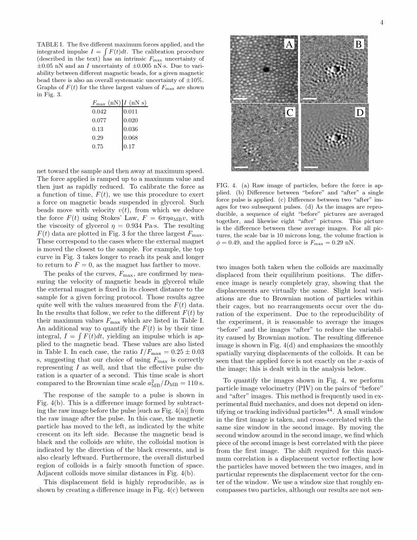
The response of the sample to a pulse is shown inFig. 4(b). This is a difference image formed by subtract-ing the raw image before the pulse [such as Fig. 4(a)] fromthe raw image after the pulse. In this case, the magneticparticle has moved to the left, as indicated by the whitecrescent on its left side. Because the magnetic bead isblack and the colloids are white, the colloidal motion isindicated by the direction of the black crescents, and isalso clearly leftward. Furthermore, the overall disturbedregion of colloids is a fairly smooth function of space.Adjacent colloids move similar distances in Fig. 4(b).

This displacement field is highly reproducible, as isshown by creating a difference image in Fig. 4(c) between

A B

C D

FIG. 4. (a) Raw image of particles, before the force is ap-plied. (b) Difference between “before” and “after” a singleforce pulse is applied. (c) Difference between two “after” im-ages for two subsequent pulses. (d) As the images are repro-ducible, a sequence of eight “before” pictures are averagedtogether, and likewise eight “after” pictures. This pictureis the difference between these average images. For all pic-tures, the scale bar is 10 microns long, the volume fraction isφ = 0.49, and the applied force is Fmax = 0.29 nN.

two images both taken when the colloids are maximallydisplaced from their equilibrium positions. The differ-ence image is nearly completely gray, showing that thedisplacements are virtually the same. Slight local vari-ations are due to Brownian motion of particles withintheir cages, but no rearrangements occur over the du-ration of the experiment. Due to the reproducibility ofthe experiment, it is reasonable to average the images“before” and the images “after” to reduce the variabil-ity caused by Brownian motion. The resulting differenceimage is shown in Fig. 4(d) and emphasizes the smoothlyspatially varying displacements of the colloids. It can beseen that the applied force is not exactly on the x-axis ofthe image; this is dealt with in the analysis below.

To quantify the images shown in Fig. 4, we performparticle image velocimetry (PIV) on the pairs of “before”and “after” images. This method is frequently used in ex-perimental fluid mechanics, and does not depend on iden-tifying or tracking individual particles44. A small windowin the first image is taken, and cross-correlated with thesame size window in the second image. By moving thesecond window around in the second image, we find whichpiece of the second image is best correlated with the piecefrom the first image. The shift required for this maxi-mum correlation is a displacement vector reflecting howthe particles have moved between the two images, and inparticular represents the displacement vector for the cen-ter of the window. We use a window size that roughly en-compasses two particles, although our results are not sen-

5

(A)

(B)

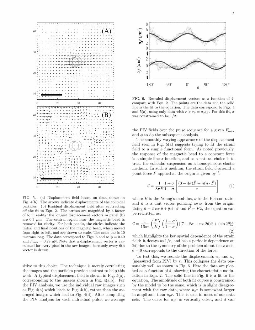
FIG. 5. (a) Displacement field based on data shown inFig. 4(b). The arrows indicate displacements of the colloidalparticles. (b) Residual displacement field after subtractingoff the fit to Eqn. 2. The arrows are magnified by a factorof 5; in reality, the longest displacement vectors in panel (b)are 0.3 µm. The central region near the magnetic bead isremoved for clarity. For both panels, the circles indicate theinitial and final positions of the magnetic bead, which movedfrom right to left, and are drawn to scale. The scale bar is 10microns long. The data correspond to Figs. 5 and 6: φ = 0.49and Fmax = 0.29 nN. Note that a displacement vector is cal-culated for every pixel in the raw images; here only every 6thvector is drawn.

sitive to this choice. The technique is merely correlatingthe images and the particles provide contrast to help thiswork. A typical displacement field is shown in Fig. 5(a),corresponding to the images shown in Fig. 4(a,b). Forthe PIV analysis, we use the individual raw images suchas Fig. 4(a) which leads to Fig. 4(b), rather than the av-eraged images which lead to Fig. 4(d). After computingthe PIV analysis for each individual pulse, we average

FIG. 6. Rescaled displacement vectors as a function of θ;compare with Eqn. 2. The points are the data and the solidline is the fit to the equation. The data correspond to Figs. 4and 5(a), using only data with r > r0 = aMB . For this fit, σwas constrained to be 1/2.

the PIV fields over the pulse sequence for a given Fmax

and φ to do the subsequent analysis.The smoothly varying appearance of the displacement

field seen in Fig. 5(a) suggests trying to fit the strainfield to a simple functional form. As noted previously,the response of the magnetic bead to a constant forceis a simple linear function, and so a natural choice is totreat the colloidal suspension as a homogeneous elasticmedium. In such a medium, the strain field ~u around a

point force ~F applied at the origin is given by45:

~u =1

8πE

1 + σ

1− σ

[

(3− 4σ)~F + n(n · ~F )

r

]

(1)

where E is the Young’s modulus, σ is the Poisson ratio,and n is a unit vector pointing away from the origin.

Using n = x cos θ+ y sin θ and ~F = F x, the equation canbe rewritten as:

~u =1

16πr

(

F

E

)(

1 + σ

1− σ

)

[(7 − 8σ + cos 2θ)x+ (sin 2θ)y]

(2)which highlights the key spatial dependence of the strainfield: it decays as 1/r, and has a periodic dependence on2θ, due to the symmetry of the problem about the x-axis.θ = 0 corresponds to the direction of the force.

To test this, we rescale the displacements ux and uy

(measured from PIV) by r. This collapses the data rea-sonably well, as shown in Fig. 6. Here the data are plot-ted as a function of θ, showing the characteristic modu-lation in Eqn. 2. The solid line in Fig. 6 is a fit to theequation. The amplitude of both fit curves is constrainedby the model to be the same, which is in slight disagree-ment with the raw data, where uxr is somewhat largerin amplitude than uyr. This is seen in most of our datasets. The curve for uxr is vertically offset, and it can

6

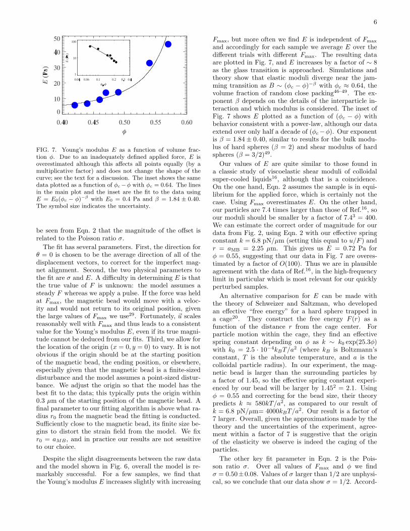
FIG. 7. Young’s modulus E as a function of volume frac-tion φ. Due to an inadequately defined applied force, E isoverestimated although this affects all points equally (by amultiplicative factor) and does not change the shape of thecurve; see the text for a discussion. The inset shows the samedata plotted as a function of φc−φ with φc = 0.64. The linesin the main plot and the inset are the fit to the data usingE = E0(φc − φ)−β with E0 = 0.4 Pa and β = 1.84 ± 0.40.The symbol size indicates the uncertainty.

be seen from Eqn. 2 that the magnitude of the offset isrelated to the Poisson ratio σ.

The fit has several parameters. First, the direction forθ = 0 is chosen to be the average direction of all of thedisplacement vectors, to correct for the imperfect mag-net alignment. Second, the two physical parameters tothe fit are σ and E. A difficulty in determining E is thatthe true value of F is unknown: the model assumes asteady F whereas we apply a pulse. If the force was heldat Fmax, the magnetic bead would move with a veloc-ity and would not return to its original position, giventhe large values of Fmax we use29. Fortunately, ~u scalesreasonably well with Fmax and thus leads to a consistentvalue for the Young’s modulus E, even if its true magni-tude cannot be deduced from our fits. Third, we allow forthe location of the origin (x = 0, y = 0) to vary. It is notobvious if the origin should be at the starting positionof the magnetic bead, the ending position, or elsewhere,especially given that the magnetic bead is a finite-sizeddisturbance and the model assumes a point-sized distur-bance. We adjust the origin so that the model has thebest fit to the data; this typically puts the origin within0.3 µm of the starting position of the magnetic bead. Afinal parameter to our fitting algorithm is above what ra-dius r0 from the magnetic bead the fitting is conducted.Sufficiently close to the magnetic bead, its finite size be-gins to distort the strain field from the model. We fixr0 = aMB, and in practice our results are not sensitiveto our choice.

Despite the slight disagreements between the raw dataand the model shown in Fig. 6, overall the model is re-markably successful. For a few samples, we find thatthe Young’s modulus E increases slightly with increasing

Fmax, but more often we find E is independent of Fmax

and accordingly for each sample we average E over thedifferent trials with different Fmax. The resulting dataare plotted in Fig. 7, and E increases by a factor of ∼ 8as the glass transition is approached. Simulations andtheory show that elastic moduli diverge near the jam-ming transition as B ∼ (φc − φ)−β with φc ≈ 0.64, thevolume fraction of random close packing46–49. The ex-ponent β depends on the details of the interparticle in-teraction and which modulus is considered. The inset ofFig. 7 shows E plotted as a function of (φc − φ) withbehavior consistent with a power-law, although our dataextend over only half a decade of (φc−φ). Our exponentis β = 1.84 ± 0.40, similar to results for the bulk modu-lus of hard spheres (β = 2) and shear modulus of hardspheres (β = 3/2)49.

Our values of E are quite similar to those found ina classic study of viscoelastic shear moduli of colloidalsuper-cooled liquids16, although that is a coincidence.On the one hand, Eqn. 2 assumes the sample is in equi-librium for the applied force, which is certainly not thecase. Using Fmax overestimates E. On the other hand,our particles are 7.4 times larger than those of Ref.16, soour moduli should be smaller by a factor of 7.43 = 400.We can estimate the correct order of magnitude for ourdata from Fig. 2, using Eqn. 2 with our effective springconstant k = 6.8 pN/µm (setting this equal to u/F ) andr = aMB = 2.25 µm. This gives us E = 0.72 Pa forφ = 0.55, suggesting that our data in Fig. 7 are overes-timated by a factor of O(100). Thus we are in plausibleagreement with the data of Ref.16, in the high-frequencylimit in particular which is most relevant for our quicklyperturbed samples.

An alternative comparison for E can be made withthe theory of Schweizer and Saltzman, who developedan effective “free energy” for a hard sphere trapped ina cage20. They construct the free energy F (r) as afunction of the distance r from the cage center. Forparticle motion within the cage, they find an effectivespring constant depending on φ as k ∼ k0 exp(25.3φ)with k0 = 2.5 · 10−4kBT/a

2 (where kB is Boltzmann’sconstant, T is the absolute temperature, and a is thecolloidal particle radius). In our experiment, the mag-netic bead is larger than the surrounding particles bya factor of 1.45, so the effective spring constant experi-enced by our bead will be larger by 1.452 = 2.1. Usingφ = 0.55 and correcting for the bead size, their theorypredicts k ≈ 580kT/a2, as compared to our result ofk = 6.8 pN/µm= 4000kBT/a

2. Our result is a factor of7 larger. Overall, given the approximations made by thetheory and the uncertainties of the experiment, agree-ment within a factor of 7 is suggestive that the originof the elasticity we observe is indeed the caging of theparticles.

The other key fit parameter in Eqn. 2 is the Pois-son ratio σ. Over all values of Fmax and φ we findσ = 0.50±0.08. Values of σ larger than 1/2 are unphysi-cal, so we conclude that our data show σ = 1/2. Accord-

7

ingly, we fix this value and redo the fits to Eqn. 2, andthe values of E that result are the ones shown in Fig. 7and correspond to the fit curves shown in Fig. 6. Thephysical meaning of σ = 1/2 is that volume is conservedduring deformation: were this sample to be strained inone direction, the sides would contract sufficient to con-serve volume. This is plausible, as the sample itself is anincompressible fluid with solid particles, and addition-ally one assumes the volume fraction stays homogeneousduring simple deformations.As noted above, we allow the direction of the force to

be a free parameter when performing the fit. This angleis fairly constant, with a standard deviation of only 4◦

between the different experiments. This variability likelyreflects measurement error.The fit shown in Fig. 6 is not perfect, and some sys-

tematic deviations from the fit can be seen. The differ-ence between the fit and the measurements is shown inFig. 5(b). The displacement vectors are stretched by afactor of 5, and thus greatly exaggerate the difference.Nonetheless, this picture looks similar to the locally non-affine elastic behaviors seen in some simulations6,50–52

and also images of “floppy-modes,” localized normalmodes, and “soft spots” known to be present nearjamming53–57. We stress that the majority of the totaldisplacement field shown in Fig. 5(a) is well-fit by Eqn. 2.

V. DECAY OF STRAIN

A. Experimental observations

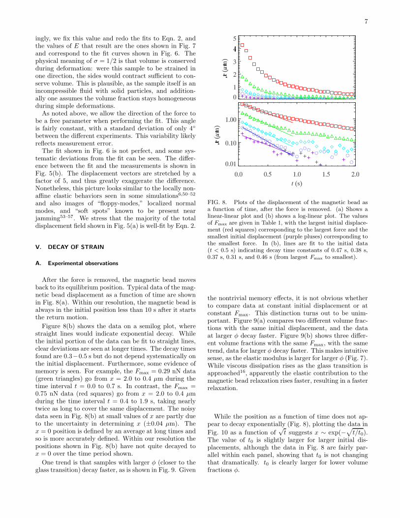
After the force is removed, the magnetic bead movesback to its equilibrium position. Typical data of the mag-netic bead displacement as a function of time are shownin Fig. 8(a). Within our resolution, the magnetic bead isalways in the initial position less than 10 s after it startsthe return motion.

Figure 8(b) shows the data on a semilog plot, wherestraight lines would indicate exponential decay. Whilethe initial portion of the data can be fit to straight lines,clear deviations are seen at longer times. The decay timesfound are 0.3−0.5 s but do not depend systematically onthe initial displacement. Furthermore, some evidence ofmemory is seen. For example, the Fmax = 0.29 nN data(green triangles) go from x = 2.0 to 0.4 µm during thetime interval t = 0.0 to 0.7 s. In contrast, the Fmax =0.75 nN data (red squares) go from x = 2.0 to 0.4 µmduring the time interval t = 0.4 to 1.9 s, taking nearlytwice as long to cover the same displacement. The noisydata seen in Fig. 8(b) at small values of x are partly dueto the uncertainty in determining x (±0.04 µm). Thex = 0 position is defined by an average at long times andso is more accurately defined. Within our resolution thepositions shown in Fig. 8(b) have not quite decayed tox = 0 over the time period shown.

One trend is that samples with larger φ (closer to theglass transition) decay faster, as is shown in Fig. 9. Given

FIG. 8. Plots of the displacement of the magnetic bead asa function of time, after the force is removed. (a) Shows alinear-linear plot and (b) shows a log-linear plot. The valuesof Fmax are given in Table 1, with the largest initial displace-ment (red squares) corresponding to the largest force and thesmallest initial displacement (purple pluses) corresponding tothe smallest force. In (b), lines are fit to the initial data(t < 0.5 s) indicating decay time constants of 0.47 s, 0.38 s,0.37 s, 0.31 s, and 0.46 s (from largest Fmax to smallest).

the nontrivial memory effects, it is not obvious whetherto compare data at constant initial displacement or atconstant Fmax. This distinction turns out to be unim-portant. Figure 9(a) compares two different volume frac-tions with the same initial displacement, and the dataat larger φ decay faster. Figure 9(b) shows three differ-ent volume fractions with the same Fmax, with the sametrend, data for larger φ decay faster. This makes intuitivesense, as the elastic modulus is larger for larger φ (Fig. 7).While viscous dissipation rises as the glass transition isapproached16, apparently the elastic contribution to themagnetic bead relaxation rises faster, resulting in a fasterrelaxation.

While the position as a function of time does not ap-pear to decay exponentially (Fig. 8), plotting the data in

Fig. 10 as a function of√t suggests x ∼ exp(−

√

t/t0).The value of t0 is slightly larger for larger initial dis-placements, although the data in Fig. 8 are fairly par-allel within each panel, showing that t0 is not changingthat dramatically. t0 is clearly larger for lower volumefractions φ.

8

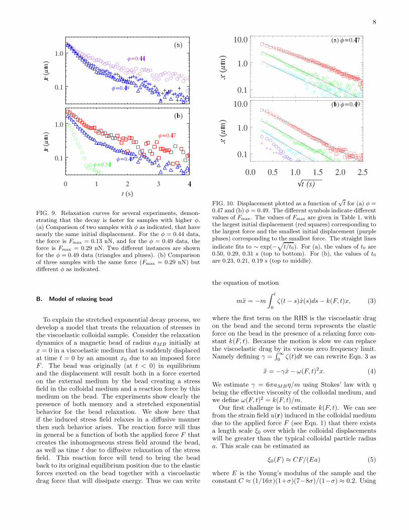
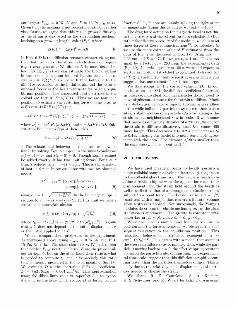
FIG. 9. Relaxation curves for several experiments, demon-strating that the decay is faster for samples with higher φ.(a) Comparison of two samples with φ as indicated, that havenearly the same initial displacement. For the φ = 0.44 data,the force is Fmax = 0.13 nN, and for the φ = 0.49 data, theforce is Fmax = 0.29 nN. Two different instances are shownfor the φ = 0.49 data (triangles and pluses). (b) Comparisonof three samples with the same force (Fmax = 0.29 nN) butdifferent φ as indicated.

B. Model of relaxing bead

To explain the stretched exponential decay process, wedevelop a model that treats the relaxation of stresses inthe viscoelastic colloidal sample. Consider the relaxationdynamics of a magnetic bead of radius aMB initially atx = 0 in a viscoelastic medium that is suddenly displacedat time t = 0 by an amount x0 due to an imposed forceF . The bead was originally (at t < 0) in equilibriumand the displacement will result both in a force exertedon the external medium by the bead creating a stressfield in the colloidal medium and a reaction force by thismedium on the bead. The experiments show clearly thepresence of both memory and a stretched exponentialbehavior for the bead relaxation. We show here thatif the induced stress field relaxes in a diffusive mannerthen such behavior arises. The reaction force will thusin general be a function of both the applied force F thatcreates the inhomogeneous stress field around the bead,as well as time t due to diffusive relaxation of the stressfield. This reaction force will tend to bring the beadback to its original equilibrium position due to the elasticforces exerted on the bead together with a viscoelasticdrag force that will dissipate energy. Thus we can write

FIG. 10. Displacement plotted as a function of√t for (a) φ =

0.47 and (b) φ = 0.49. The different symbols indicate differentvalues of Fmax. The values of Fmax are given in Table 1, withthe largest initial displacement (red squares) corresponding tothe largest force and the smallest initial displacement (purplepluses) corresponding to the smallest force. The straight lines

indicate fits to ∼ exp(−√

t/t0). For (a), the values of t0 are0.50, 0.29, 0.31 s (top to bottom). For (b), the values of t0are 0.23, 0.21, 0.19 s (top to middle).

the equation of motion

mx = −m

∫ t

0

ζ(t− s)x(s)ds− k(F, t)x, (3)

where the first term on the RHS is the viscoelastic dragon the bead and the second term represents the elasticforce on the bead in the presence of a relaxing force con-stant k(F, t). Because the motion is slow we can replacethe viscoelastic drag by its viscous zero frequency limit.Namely defining γ =

∫∞

0ζ(t)dt we can rewrite Eqn. 3 as

x = −γx− ω(F, t)2x. (4)

We estimate γ = 6πaMBη/m using Stokes’ law with ηbeing the effective viscosity of the colloidal medium, andwe define ω(F, t)2 = k(F, t)/m.Our first challenge is to estimate k(F, t). We can see

from the strain field u(r) induced in the colloidal mediumdue to the applied force F (see Eqn. 1) that there existsa length scale ξ0 over which the colloidal displacementswill be greater than the typical colloidal particle radiusa. This scale can be estimated as

ξ0(F ) ≈ CF/(Ea) (5)

where E is the Young’s modulus of the sample and theconstant C ≈ (1/16π)(1+σ)(7−8σ)/(1−σ) ≈ 0.2. Using

9

our largest Fmax = 0.75 nN and E ≈ 15 Pa, ξ0 ≈ 4a.Given that the medium is not perfectly elastic but ratherviscoelastic, we argue that this region grows diffusivelyas the strain is dissipated in the surrounding medium,leadaing to a growing length scale ξ(F, t) where

ξ(F, t)2 = ξ0(F )2 + 6Dt. (6)

In Eqn. 6 D is the diffusion constant characterizing mo-tion that can relax the strain, which does not requirecage rearrangements. We discuss D in more detail be-low. Using ξ(F, t) we can estimate the typical strainsin the colloidal medium induced by the bead. Thesestrains ǫ ≈ x/ξ(F, t) reduce with time both due to thediffusive relaxation of the initial strain and the reducedimposed forces as the bead returns to its original equi-librium position. The associated elastic stresses in thecolloid are then ≈ Ex/ξ(F, t). Thus we are now in aposition to estimate the restoring force on the bead ask(F, t)x ≈ 4πR2Ex/ξ(F, t) or

ω(F, t)2 ≈ 4πR2E/(mξ(F, t)) = ω20/√

(1 + t/τ), (7)

where ω20 = 4πR2E/(mξ0(F )) and τ = ξ0(F )2/6D. Sub-

stituting Eqn. 7 into Eqn. 4 then yields

x = −γx− ω20x/

√

(1 + t/τ). (8)

The relaxational behavior of the bead can now befound by solving Eqn. 8 subject to the initial conditionsx(t = 0) = x0 and x(t = 0) = 0. Though Eqn. 8 cannotbe solved exactly, it has two limiting forms. For t ≪ τEqn. 8 reduces to x = −γx − ω2

0x. This is the equationof motion for an linear oscillator with two overdampedmodes

x(t) = (x0/2){α+ exp [−γα−t/2]

+α− exp [−γα+t/2]}, (9)

using α± = 1±√

1− 4ω20/γ

2. In the limit t ≫ τ Eqn. 8

reduces to x = −γx− ω20

√

τ/tx. In this limit we have astretched exponential solution

x(t) ≈ (x0/2)α+ exp (−√

t/t0) (10)

where t0 = γ2/(ω40τ) = (27/2)η2D/(a2MBE

2). Signifi-cantly, t0 does not depend on the initial displacement xor the initial applied force F .We can compare these predictions to the experiment.

As mentioned above, using Fmax = 0.75 nN and E ≈15 Pa, ξ0 ≈ 4a. The discussion in Sec. IV makes clearthat neither Fmax nor this inferred E are the proper val-ues for Eqn. 5, but on the other hand their ratio is whatis needed to compute ξ0 and it is precisely this ratiothat is directly measured in the experiments of Sec. IV.We estimate D as the short-time diffusion coefficient,D ≈ kBT/6πηa = 0.064 µm2/s. This approximationusing the dilute-limit value is imperfect due to hydro-dynamic interactions which reduce D at larger volume

fractions58–61, but we are mainly seeking the right orderof magnitude. Using this D and ξ0 we find τ ≈ 100 s.The drag force acting on the magnetic bead is not due

to the viscosity η of the solvent (used to calculate D) butrather the effective viscosity of the medium, which is≈ 50times larger at these volume fractions13. To calculate t0we use the more correct value of E estimated from thedata of Fig. 2 as discussed in Sec. IV. Using aMB =2.25 µm and E = 0.72 Pa we get t0 = 1 ms. This is toosmall by a factor of ∼ 200 from the experimental data(Fig. 10). Likewise, given τ ≈ 100 s, we would expect tosee the asymptotic (stretched exponential) behavior for√

(t) ≫ 10 in Fig. 10: that we see it at earlier time scalessuggests that our estimate for τ is too large.We thus reconsider the correct value of D. In our

model, we assume D is the diffusion coefficient for strain.In practice, individual colloidal particles do not need tomove significant distances for the strain to diffuse. Muchas a dislocation can move rapidly through a crystallinelattice while individual particles stay close to their latticesites, a slight motion of a particle (∆r < a) changes thestrain over a neighborhood ∼ a in scale. If we assumethat particles diffusing a distance of a/20 is sufficient forthe strain to diffuse a distance a, then D becomes 400times larger. This decreases τ to 0.2 s and increases t0to 0.4 s, bringing our model into more reasonable agree-ment with the data. The distance a/20 is smaller thanthe cage size (which is about a/3)19.

VI. CONCLUSIONS

We have used magnetic beads to locally perturb adense colloidal sample at volume fractions φ < φg, closeto the colloidal glass transition. The magnetic beads havea linear relationship between the applied force and theirdisplacement, and the strain field around the beads iswell-described as that of a homogeneous elastic mediumsubject to a point force. The Poisson ratio is σ = 1/2,consistent with a sample that conserves its total volumewhen a stress is applied. Not surprisingly, the Young’smodulus describing the elastic medium grows as the glasstransition is approached. The growth is consistent withpower-law in (φc − φ), where φc = φrcp > φg.When the bead is moved away from its equilibrium

position and the force is removed, we observed the sub-sequent relaxation to the equilibrium position. Thisrelaxation behaves as a stretched exponential, x ∼exp(−(t/t0)

1/2). This agrees with a model that assumesthe stress can diffuse away to infinity: thus, while the par-ticle is moving back to x = 0, the effective spring constantacting on the particle is also diminishing. The experimen-tal time scales suggest that this diffusion is rapid, occur-ring faster than the particles themselves diffuse. This islikely due to the relatively small displacements of parti-cles needed to change the strain.We thank R. E. Courtland, S. A. Koehler,

K. S. Schweizer, and M. Wyart for helpful discussions.

10

We thank A. Schofield for providing our colloidal sam-ples. The work of D. A., D. S., P. H., and J. H. was sup-ported by NASA (NAG3-2284). The work of E. R. W.was supported by NSF (CHE-0910707).

1J. C. Dyre, Rev. Mod. Phys. 78, 953 (2006).2C. A. Schuh, T. C. Hufnagel, and U. Ramamurty,Acta Materialia 55, 4067 (2007).

3V. Lubchenko and P. G. Wolynes, Ann. Rev. Phys. Chem. 58,235 (2007).

4A. Cavagna, Phys. Rep. 476, 51 (2009).5L. Berthier and G. Biroli, Rev. Mod. Phys. 83, 587 (2011),arXiv:1011.2578.

6F. Leonforte, A. Tanguy, J. P. Wittmer, and J. L. Barrat,Phys. Rev. Lett. 97, 055501 (2006).

7M. Tsamados, A. Tanguy, C. Goldenberg, and J. L. Barrat,Phys. Rev. E 80, 026112 (2009).

8F. Sciortino and P. Tartaglia, Adv. Phys. 54, 471 (2005).9P. N. Pusey, J. Phys.: Cond. Matt. 20, 494202 (2008).

10G. L. Hunter and E. R. Weeks, Rep. Prog. Phys. 75, 066501(2012).

11P. N. Pusey and W. van Megen, Nature 320, 340 (1986).12C. P. Royall, W. C. K. Poon, and E. R. Weeks, Soft Matter, DOI:10.1039/C2SM26245B(2012).

13Z. Cheng, J. Zhu, P. M. Chaikin, S.-E. Phan, and W. B. Russel,Phys. Rev. E 65, 041405 (2002).

14S. Torquato, T. M. Truskett, and P. G. Debenedetti,Phys. Rev. Lett. 84, 2064 (2000).

15J. D. Bernal, Proc. Roy. Soc. London. Series A 280, 299 (1964).16T. G. Mason and D. A. Weitz, Phys. Rev. Lett. 75, 2770 (1995).17E. Rabani, J. D. Gezelter, and B. J. Berne, J. Chem. Phys. 107,6867 (1997).

18B. Doliwa and A. Heuer, Phys. Rev. Lett. 80, 4915 (1998).19E. R. Weeks and D. A. Weitz, Chem. Phys. 284, 361 (2002).20K. S. Schweizer and E. J. Saltzman, J. Chem. Phys. 119, 1181(2003).

21K. S. Schweizer and G. Yatsenko, J. Chem. Phys. 127, 164505(2007).

22D. M. Sussman and K. S. Schweizer, J. Chem. Phys. 134, 064516(2011).

23S. R. Williams and D. J. Evans, Phys. Rev. Lett. 96, 015701(2006).

24I. Gazuz, A. M. Puertas, T. Voigtmann, and M. Fuchs,Phys. Rev. Lett. 102, 248302 (2009).

25M. V. Gnann, I. Gazuz, A. M. Puertas, M. Fuchs, and T. Voigt-mann, Soft Matter 7, 1390 (2011).

26D. Winter, J. Horbach, P. Virnau, and K. Binder,Phys. Rev. Lett. 108, 028303 (2012).

27M. V. Gnann and T. Voigtmann, Phys. Rev. E 86, 011406(2012).

28M. B. Hastings, C. J. Olson Reichhardt, and C. Reichhardt,Phys. Rev. Lett. 90, 098302 (2003).

29P. Habdas, D. Schaar, A. C. Levitt, and E. R. Weeks, Europhys.Lett. 67, 477 (2004).

30I. C. Carpen and J. F. Brady, J. Rheo. 49, 1483 (2005).31C. Reichhardt and C. J. O. Reichhardt, Phys. Rev. Lett. 96,028301 (2006).

32C. J. Olson Reichhardt and C. Reichhardt, Phys. Rev. E 82,051306 (2010).

33J. A. Drocco, M. B. Hastings, C. J. O. Reichhardt, and C. Re-ichhardt, Phys. Rev. Lett. 95, 088001 (2005).

34L. Antl, J. W. Goodwin, R. D. Hill, R. H. Ottewill, S. M. Owens,S. Papworth, and J. A. Waters, Colloid Surf. 17, 67 (1986).

35A. D. Dinsmore, E. R. Weeks, V. Prasad, A. C. Levitt, and D. A.Weitz, App. Optics 40, 4152 (2001).

36J. C. Crocker and D. G. Grier, J. Colloid Interf. Sci. 179, 298(1996).

37W. C. K. Poon, E. R. Weeks, and C. P. Royall, Soft Matter 8,21 (2012).

38T. M. Squires and J. F. Brady, Phys. Fluids 17, 073101 (2005).39A. S. Khair and J. F. Brady, J. Fluid Mech. 557, 73 (2006).40A. Meyer, A. Marshall, B. G. Bush, and E. M. Furst, J. Rheo.50, 77 (2006).

41L. G. Wilson, A. W. Harrison, A. B. Schofield, J. Arlt, andW. C. K. Poon, J. Phys. Chem. B, J. Phys. Chem. B 113, 3806(2009).

42I. Sriram, A. Meyer, and E. M. Furst, Phys. Fluids 22, 062003(2010).

43L. G. Wilson, A. W. Harrison, W. C. K. Poon, and A. M. Puertas,Europhys. Lett. 93, 58007 (2011).

44E. R. Weeks, in Experimental and Computational Techniques in

Soft Condensed Matter Physics, edited by J. S. Olafsen (Cam-bridge University Press, 2010) pp. 1–24, ISBN 978-0-521-11590-2.

45L. D. Landau, L. P. Pitaevskii, E. M. Lifshitz, and A. M. Kose-vich, Theory of Elasticity, Third Edition, 3rd ed. (Butterworth-Heinemann, 1986) ISBN 075062633X.

46D. J. Durian, Phys. Rev. Lett. 75, 4780 (1995).47D. J. Durian, Phys. Rev. E 55, 1739 (1997).48C. S. O’Hern, L. E. Silbert, A. J. Liu, and S. R. Nagel,Phys. Rev. E 68, 011306 (2003).

49C. Brito and M. Wyart, Europhys. Lett. 76, 149 (2007).50A. Tanguy, J. P. Wittmer, F. Leonforte, and J. L. Barrat,Phys. Rev. B 66, 174205 (2002).

51J. P. Wittmer, A. Tanguy, J. L. Barrat, and L. Lewis,Europhys. Lett. 57, 423 (2002).

52F. Leonforte, R. Boissiere, A. Tanguy, J. P. Wittmer, and J. L.Barrat, Phys. Rev. B 72, 224206 (2005).

53W. G. Ellenbroek, E. Somfai, M. van Hecke, and W. van Saarloos,Phys. Rev. Lett. 97, 258001 (2006).

54C. Brito and M. Wyart, J. Stat. Mech. 2007, L08003 (2007).55A. Widmer-Cooper, H. Perry, P. Harrowell, and D. R. Reichman,Nat Phys 4, 711 (2008).

56R. Candelier, A. W. Cooper, J. K. Kummerfeld, O. Dauchot,G. Biroli, P. Harrowell, and D. R. Reichman, Phys. Rev. Lett.105, 135702 (2010).

57M. L. Manning and A. J. Liu, Phys. Rev. Lett. 107, 108302(2011).

58P. N. Pusey and R. J. A. Tough, Faraday Discuss. Chem. Soc.76, 123 (1983).

59I. Snook, W. van Megen, and R. J. A. Tough, J. Chem. Phys.78, 5825 (1983).

60C. W. J. Beenakker and P. Mazur, Phys. Lett. A 98, 22 (1983).61C. W. J. Beenakker and P. Mazur, Physica A 126, 349 (1984).