Local adaptation and maladaptation to pollinators in a generalist geographic mosaic

L E T T E RLocal adaptation and maladaptation to pollinators in

a generalist geographic mosaic

Jose M. Gomez,1* M. Abdelaziz,2

J. P. M. Camacho,2 A. J. Munoz-

Pajares2 and F. Perfectti2

1Dpto de Ecologıa, Universidad

de Granada, E-18071 Granada,

Spain2Dpto de Genetica, Universidad

de Granada, E-18071, Granada,

Spain

*Correspondence: E-mail:

[email protected]

Abstract

The Geographic Mosaic Theory of Coevolution predicts the occurrence of mosaics of

interaction-mediated local adaptations and maladaptations. Empirical support to this

prediction has come mostly from specialist interactions. In contrast, local adaptation is

considered highly unlikely in generalist interactions. In this study, we experimentally test

local adaptation in a generalist plant-pollinator geographic mosaic, by means of a

transplant experiment in which plants coming from two evolutionary hotspots and two

coldspots were offered to pollinators at the same four localities. Plants produced in the

hotspots attracted more pollinators in all populations, whereas coldspot plants attracted

fewer pollinators in all populations. Differences in adaptation were not related to genetic

similarity between populations, suggesting that it was mainly due to spatial variation in

previous selective regimes. Our experiment provides the first strong support for a

spatially structured pattern of adaptation and maladaptation generated by a generalist

free-living mutualism.

Keywords

Generalist systems, geographic mosaics of coevolution, local adaptation, maladaptation,

pollination.

Ecology Letters (2009) 12: 672–682

I N T R O D U C T I O N

Most species are formed by a collection of genetic and

ecologically differentiated populations inserted in a complex

landscape. The Geographic Mosaic Theory of Coevolution

(GMTC) subsumes this idea and considers that populations

differ in evolutionary dynamics due to spatial variation in

selective regimes (Thompson 2005). The GMTC argues that

the overall coevolutionary dynamics of such interactions are

driven by three components of geographic structure:

selection mosaics, coevolutionary hotspots, and trait remix-

ing (Thompson 1994; Gomulkiewicz et al. 2000). This

theory visualizes the landscape as a mosaic of coevolution-

ary hotspots, populations where reciprocal selection is

strong and coevolution is ongoing, embedded in a broader

matrix of coevolutionary coldspots, where local selection is

weak, non-reciprocal or where only one of the participants

occurs (Thompson 2005). The GMTC predicts that these

three processes lead to three observable patterns: spatial

variation in the traits mediating an interspecific interaction,

trait mismatching among interacting species and few species

level coevolved traits (Thompson 2005). Consequently, the

GMTC suggests the occurrence of a spatial pattern of

interaction-mediated local adaptation and maladaptation

(defined as deviation from adaptive peaks) (Gomulkiewicz

et al. 2000, 2007; Nuismer et al. 2000; Thompson et al. 2002;

Thompson 2005).

Theoretical models suggest that the spatial pattern of

local adaptations and maladaptations is a complex conse-

quence of the interplay of several non-exclusive factors,

including spatially varying selection, patterns of gene flow,

but also selection mosaic and relative proportion of

hotspots and coldspots (Holt & Gomulkiewicz 1997;

Thompson et al. 2002; Kawecki & Ebert 2004; Nuismer

2006). Empirical support to these theoretical predictions has

come mostly from specialist antagonistic interactions, like

parasitism and endophytic herbivory, where the two

interacting organisms are tightly engaged in arm races

(Van Zandt & Mopper 1998; Hoeksema & Forde 2008). In

this kind of system, the outcome of the interaction

dramatically changes among localities and causes the

occurrence of spatially divergent selection (Kaltz & Shykoff

1998; Mopper & Strauss 1998; Van Zandt & Mopper 1998;

Kaltz et al. 1999; Kawecki & Ebert 2004). These intense

Ecology Letters, (2009) 12: 672–682 doi: 10.1111/j.1461-0248.2009.01324.x

� 2009 Blackwell Publishing Ltd/CNRS

selection regimes can maintain the levels of local adaptation

even under strong gene flow (Kawecki & Ebert 2004).

Contrasting with specialist symbiotic interactions, free-

living generalist interactions are formed by multispecies

assemblages of interacting organisms that vary spatially in

composition but that generate selection with similar strength

in all localities. Extreme reciprocal specialization between

pairs of species is rare in these interactions (Thompson 1994).

In contrast, free-living interactions form interspecific net-

works (Thompson 2005). Consequently, multispecific selec-

tion and diffuse coevolution are prevalent in generalist

interactions (Strauss & Irwin 2004; Strauss et al. 2005). Under

these circumstances, many evolutionary biologists think that

local adaptation is less likely in generalist interactions

(Lajeunesse & Forbes 2002; Kawecki & Ebert 2004).

In this study, we explore the possibility of local

adaptation in a generalist mutualistic system. In 2005, we

detected a geographic mosaic of selection occurring for a

pollination-generalist plant (Erysimum mediohispanicum, Brass-

icaceae), which inhabits a patchy environment in Sierra

Nevada (southeast Spain) (Gomez et al. 2009a). This plant is

visited by pollinator assemblages differing in composition

across nearby populations. Due to between-pollinator

differences in preference patterns, this spatial difference in

pollinator fauna causes spatially divergent selection on some

plant traits (Gomez et al. 2008a). As a consequence, the

landscape is composed of populations having strong

pollinator-mediated selective regimes (evolutionary hot-

spots, hereafter) mingled with populations having weak

pollinator-mediated selective regimes (evolutionary cold-

spots, hereafter; Gomez et al. 2009a). Under these circum-

stances, we hypothesize that, if gene flow is not high, plants

from populations where pollinator-mediated selection is

strong (hostpots) will have phenotypes more adapted to

attract pollinators than plants from populations were

pollinator-mediated selection is weak (coldspots). Note that

these hotspots and coldposts are not proper coevolutionary

spots but evolutionary spots, as there is not yet information

on the reciprocal effects of the plant on the pollinators

(Thompson 2005). To investigate local adaptation, we

reciprocally translocated plants coming from hotspots and

coldspots to quantify their ability in attracting pollinators in

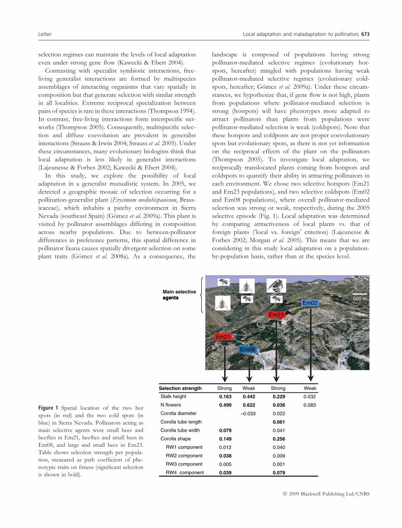
each environment. We chose two selective hotspots (Em21

and Em23 populations), and two selective coldspots (Em02

and Em08 populations), where overall pollinator-mediated

selection was strong or weak, respectively, during the 2005

selective episode (Fig. 1). Local adaptation was determined

by comparing attractiveness of local plants vs. that of

foreign plants (�local vs. foreign� criterion) (Lajeunesse &

Forbes 2002; Morgan et al. 2005). This means that we are

considering in this study local adaptation on a population-

by-population basis, rather than at the species level.

500 mMain selective agents

Em02

Em23

agents

Em21

Em08

Selection strength WeakWeakStrong Strong

Stalk height 0.0320.163 0.229

N flowers 0.0830.499 0.036

Corolla diameter 0.022

Corolla tube length 0.061

0.442

0.622

–0.033

Corolla tube width 0.079 0.041

Corolla shape 0.149 0.256

RW1 component 0.012 0.040




Figure 1 Spatial location of the two hot

spots (in red) and the two cold spots (in

blue) in Sierra Nevada. Pollinators acting as

main selective agents were small bees and

beeflies in Em21, beeflies and small bees in

Em08, and large and small bees in Em23.

Table shows selection strength per popula-

tion, measured as path coefficient of phe-

notypic traits on fitness (significant selection

is shown in bold).

Letter Local adaptation and maladaptation to pollinators 673


M E T H O D S

Study system

Erysimum mediohispanicum is a biannual, monocarpic herb

endemic to the Iberian Peninsula. In southeast Spain,

E. mediohispanicum is found in montane forests and subalpine

scrublands. Individual plants grow for 2–3 years as vegetative

rosettes, and then die after producing 1–8 reproductive stalks

bearing up to several hundred hermaphroditic, bright yellow

flowers. Erysimum mediohispanicum is self-compatible, but

requires pollen vectors for full seed set (Gomez 2005). Mean

seed dispersal distance is lower than 20 cm (Gomez 2007).

Experimental design

We assessed local adaptation to pollinators using reciprocal

field translocations based on previous information on the

strength of pollinator-mediated selection across several

localities of a selection mosaic (Gomez et al. 2009a). Local

adaptation was tested for by comparing pollinator attrac-

tiveness (pollinator visitation rate) with the experimental

plants in each population of destination. Pollinator attrac-

tiveness is appropriate to test for local adaptation in

E. mediohispanicum due to several non-exclusive reasons.

First, pollinator abundance at flowers is conceptually similar

to parasite abundance at hosts or parasite load, two major

metrics to test for local adaptation in host–parasite systems

(Kawecki & Ebert 2004; Hoeksema & Forde 2008).

Furthermore, pollinator visitation rate is a good proxy of

E. mediohispanicum fitness in the study area, as it significantly

correlates with the overall seed production (Gomez et al.

2006, 2008a, 2009a). In fact, we found a significant

relationship between pollinator visitation rate and overall

number of seeds produced per plant in the four experimental

populations [log (seed ⁄ plants) = 4.705 + 0.169*visits ⁄ hour,

F = 3.46, n = 179 plants, P = 0.0007; General Linear

Model]. This relationship was similar across the four

populations, as the interaction between pollinator abundance

and population was not significant (F = 0.19, P = 0.903;

General Linear Model). In addition, pollinator visitation rate

is a good estimate of female fitness as, in the study area,

E. mediohispanicum seed production is pollen-limited. Thus, in

an experiment conducted in the studied populations, pollen-

supplemented flowers had higher fitness (15.46 ± 0.75 seeds

per flower, n = 136 plants) than both control (12.67 ± 0.64,

n = 139 plants) and procedural control flowers

(10.77 ± 1.18, n = 55 plants; F = 6.66, df = 2, 327,

P = 0.0001; one-way ANOVA; author�s unpublished data).

Finally, several studies have shown that pollinators are

important selective agents for many E. mediohispanicum floral

traits (Gomez et al. 2006, 2008a,b, 2009a).

As focal populations for our experiment, we selected four

populations: two populations where overall pollinator-

mediated selection was strong during the 2005 selective

episode (hotspots, Em21 and Em23), and two populations

where overall selection was weak during the 2005 selective

episode (coldspots, Em02 and Em08) (Gomez et al. 2009a).

Em08 was considered as a pollinator-mediated selective

coldspot because the observed selection acting on the

number of flowers was exclusively due to its direct effect on

seed production, rather than its pollinator-mediated effects.

In addition, in this latter population much of the selection

acting on stalk height was due to its correlation with the

number of flowers rather than the pollinator effect (Gomez

et al. 2009a).

At the end of the 2005 reproductive season, we collected

seeds from the plants where selection had been determined

in these four populations. The seeds were sowed during

autumn 2005 in individual pots and randomly located in a

common garden at the Facultad de Ciencias, University of

Granada (720 m altitude). Seedlings started to emerge

quickly that autumn and were growing until spring 2007,

when they started to flower. Then, we randomly selected 20

plants per population (80 in total). Flowering plants were

carried out together to the four populations (pollination

scenarios) from which the seeds had been collected.

Flowering period of the experimental plants overlapped

with the natural flowering period of the species in the study

area. We used the same 80 plants throughout the experi-

ment, to control for individual phenotype effect in

pollinator attraction. In each pollination scenario, the 80

experimental plants were arranged at random in a grid of

20 · 4 plants separated from each other by 0.5 m. The

experiment was conducted during the whole flowering

period of the experimental plants (15 days), and plants were

in the field every two days, until some experimental plants

started to fruit and lose many flowers. The experimental

trials started at 10 am, and the plants were offered to

pollinators for a 2-h period per pollination scenario, for an

overall daily period of 8 h. We randomly changed the order

in which each pollination scenario was tested to avoid biases

due to circadian differences in pollinator identity and

activity. All insects landing on the flowers and contacting

anthers and stigma, but not those thieving nectar from

below the corolla, were recorded. We visually identified

almost all floral visitors to the species level, using previous

information gathered during the last 11 years (Gomez et al.

2008a,b, 2009a).

Quantification of floral traits

Plant phenotype was characterized in the greenhouse,

before the beginning of the experiment, to avoid any

putative plastic response of the experimental plants to the

new environments. The following phenotypic traits were

determined for the experimental plants.

674 J. M. Gomez et al. Letter


(1) Stalk height, quantified as the height of the tallest stalk,

measured to the nearest 0.5 cm as the distance from

the ground to the top of the highest open flower.

(2) Flower number, counting the entire production of

flowers of each plant.

(3) Corolla diameter, estimated as the distance in millime-

tre between the edges of two opposite petals.

(4) Corolla tube length, the distance in millimetre between

the corolla tube aperture and the base of the sepals.

These two latter traits were also measured with a digital

caliper with ±0.1 mm resolution.

(5) Corolla tube width, the diameter of the corolla tube

aperture, estimated as the distance between the bases of

two opposite petals.

(6) Corolla shape, determined in each of the plants by

means of geometric morphometric tools, using a

landmark-based methodology (Zelditch et al. 2004).

We took a digital photograph of the same flower as

before using a standardized procedure (front view and

planar position). The flowers were photographed at anthesis

to avoid ontogenetic effects. We defined 32 co-planar

landmarks located along the outline of the flowers and the

aperture of the corolla tube, the number of landmarks being

chosen to provide comprehensive coverage of the flower

shape (Zelditch et al. 2004). Landmarks were defined by

reference to the midrib, primary veins, and secondary veins

of each petal as well as the connection between petals. We

captured the landmarks using the software tpsDig vs. 1.4

(available in the Stony Brook Morphometrics website at:

http://life.bio.sunysb.edu/morph/morphmet.html). After-

wards, the two-dimensional coordinates of these landmarks

were determined for each plant, and the generalized

orthogonal least-squares Procrustes average configuration

of landmarks was computed using the Generalized Pro-

crustes Analysis (GPA) superimposition method. This

procedure was performed using the software tpsRelw vs.

1.11 (available in the Stony Brook Morphometrics website

at: http://life.bio.sunysb.edu/morph/morphmet.html). In

these analyses, we considered the flower as a non-articulated

structure because the relative position of the petals does not

change during their functional life. After GPA, the relative

warps (RW, which are principal components of the

covariance matrix of the partial warp scores) were computed

(Adams et al. 2004). Unit centroid size was used as the

alignment-scaling method and the orthogonal projection as

the alignment projection method. This procedure generates

a consensus configuration, the central trend of an observed

sample of landmarks, which is similar to a multidimensional

average. In addition, this procedure generates 2p – 4

orthogonal RW (p is the number of landmarks). Each RW

is characterized by its singular value, and explains a given

variation in shape among specimens. Thus, RW summarize

shape differences among specimens (Adams et al. 2004), and

their scores can be saved to be used as a data matrix to

perform standard statistical analyses (Zelditch et al. 2004).

Analysis of pollinator assemblages

We determined pollinator assemblage in the four studied

populations during four years (2005–2008), including the

year in which we performed the translocation experiment.

For this, we recorded all insects visiting the flowers of

E. mediohispanicum during 2 h samplings per population.

These samplings were distributed throughout the entire

flowering period (10–15 days per population). Only insects

landing on the flowers and contacting anthers and stigma,

but not those thieving nectar from below the corolla, were

recorded. In total, we sampled each population at least for

10 h per reproductive season. In total, 3662 insects were

recorded in these four populations during the four years.

Pollinators were identified in the field, and samples of each

pollinator species were captured for further identification in

the laboratory (Gomez et al. 2009a). Nevertheless, we did not

collect many specimens, to avoid a depletion of the insect

populations. Some closely related species (notably among

Apiformes) could not be told apart in the field, and thus

some of our taxa include more than one species. We grouped

pollinator species into seven functional groups according to

their similarity in size, foraging behaviour and feeding habits:

(i) large bees, mostly pollen- and nectar-collecting females

measuring 10 mm in body length or larger; (ii) small bees,

mostly pollen- and nectar-collecting females smaller than

10 mm; (iii) beeflies, long-tongued nectar-collecting Bomby-

liidae; (iv) hoverflies, nectar- and pollen-collecting Syrphidae

and short-tongued Bombyliidae; (v) beetles, including species

collecting nectar and ⁄ or pollen; (vi) butterflies, mostly

Ropalocera, all nectar collectors; and (vii) Others, mostly

nectar-feeding Muscoid flies, ants and bugs.

Genetic analyses

We analysed molecular markers in order to evaluate the

genetic differentiation and infer the historic gene flow

among the experimental populations. Sixty-five milligram of

silica-gel-dried leaf tissue per individual was disrupted in

liquid nitrogen. DNA was extracted using the GenEluteTM

Plant Genomic DNA Miniprep Kit (Sigma-Aldrich,

St Louis, MO, USA).

We determined randomly amplified polymorphic DNA

(RAPD) in 10 individuals from each plant population (40

individuals in total). RAPD amplification was performed

using Operon primers (Operon Technologies, Alameda,

CA, USA): OPA01 (5¢-CAGGCCCTTC-3¢), OPA02 (5¢-TG

CCGAGCTG-3¢), OPA03 (5¢-AGTCAGCCAC-3¢), OPA04



(5¢- AATCGGGCTG-3¢), OPA06 (5¢-GGTCCCTGAC-3¢),OPA07 (5¢-GAAACGGGTG-3¢), OPA08 (5¢-GTGACG-

TAGG-3¢), OPA09 (5¢-GGGTAACGCC-3¢), OPA10(5¢-GTGATCGCAG-3¢), OPA11 (5¢-CAATCGCCGT-3¢),OPA12 (5¢-TCGGCGATAG-3¢), OPA13 (5¢-CAGCACC-

CAC-3¢), OPA14 (5¢-TCTGTGCTGG-3¢), OPA19 (5¢-CAAACGTCGG-3¢), OPA20 (5¢-GTTGCGATCC-3¢).

The following 13 primer combinations were used:

OPA01–OPA01, OPA01–OPA03, OPA01–OPA06, OPA01–

OPA07, OPA02–OPA08, OPA04–OPA14, OPA07–OPA14,

OPA08–OPA13, OPA09–OPA12, OPA09–OPA19,

OPA10–OPA10, OPA11–OPA12 and OPA19–OPA20.

Polymerase chain reaction (PCR) was performed in 25 lL

final volume containing 2.5 lL of 10· buffer (New England

Biolabs, Beverly, MA, USA), 2.5 lL of 2 mM dNTP (Sigma-

Aldrich), 1.25 lL of each 10 lM primer, 0.4 lL of 5 U lL–1

Taq-polymerase (New England BioLabs) and 1 lL of

10 ng lL–1 DNA. PCR was performed using a MJ Mini

Personal Thermal Cycler (Bio-Rad, Richmond, CA, USA)

with the following profile: 2 min at 94 �C, followed by 38

cycles of 15 s at 94 �C, 15 s at 36 �C, 30 s at 72 �C,

followed by 2 min at 72 �C. RAPD products were electro-

phoresed in 1.5% agarose gels containing SYBR-Green in 1·TBE buffer at 4.7 V cm–1, and photographed with a Gel

Doc TM XR (Bio-Rad). We scored 160 different markers,

determined by using a standard ladder (50 bp; Sigma) with

the Quantity One-4,6 1D Analysis Software. Weaker bands

were omitted from the scoring protocol and some of the

amplifications were repeated to control for repeatability. The

bands were scored for each primer as either present (1) or

absent (0). Nei genetic distances were determined with

GenAlEx 6.1 (http://www.anu.edu.au/BoZo/GenAlEx/)

and Gst with Hickory (Holsinger et al. 2002).

Analysis of cpDNA trnL-F region was performed in five

individuals per population (20 individuals in total), using

tabC and tabF primers (Taberlet et al. 1991). PCR was

carried out in a final volume of 50 lL containing 5 lL of

10· buffer (New England BioLabs), 0.1 mM of each dNTP

(Sigma-Aldrich), and 0.02 U lM–1 of Taq (New England

BioLabs). PCR was carried out on a Gradient Master Cycler

Pro S (Eppendorf, Westbury, NY, USA) as follows: one

cycle at 94 �C for 3 min, 35 cycles of 94 �C for 15 s, 58 �C

for 30 s, and 72 �C for 1 min 30 s, and a final cycle at 72 �C

for 3 min; then, 4 �C until reactions were taken off the

thermocycler. PCR products were electrophoresed on 1.5%

agarose gel to check the results and then the amplification

products were purified by centrifugation at 4 �C with 0.15

volume sodium acetate 3 M (pH 4.6) and three volumes of

95% ethanol. Sequencing was done with BigDye-Termina-

tor-v3.1 (Applied Biosystems, Foster City, CA, USA), using

tabF primer and the fragments were visualized on an ABI

PRISM 3100-avant automated sequencer. Chromatograms

were visualized with Finch TV version 1.4.0 (Geospiza Inc.,

Seattle, WA, USA). Sequences were adjusted and aligned by

hand, using bioedit version 7.0.5.3 (Hall 1999). All positions,

including indel regions, were used as input to estimate

distances among populations with Arlequin version 3.1

(CMPG, University of Berna). We used this region because

of its high variability among individuals, even at the

intrapopulation level.

Data analysis

To test for local adaptation, we used a Generalized Mixed

Model where we included the type of population of origin

(hotspot vs. coldspot), destination and their interaction as

fixed factors, population identity as random factor nested in

the two previous fixed factors, and visitation rate of

pollinators as the dependent variable. The models were

performed for all pollinators pooled together and for each

pollinator functional type separately. All analyses were

performed using the package lme4 in R (R Development

Core Team 2008).

We performed a canonical discriminant function analysis

to explore between-population differences in plant pheno-

type. In this analysis, the different phenotypic traits

quantified for each experimental plant was included as the

dependent variable. A discriminant function analysis was

also used to classify the four studied populations according

to the composition, in terms of functional groups, of their

pollinator fauna. In this analysis, we included the abundance

of each pollinator functional group as dependent variables,

population as independent variable and the annual data as

observation units. After that, using the Mahalanobis

distances, we predicted the probability of each experimental

population of destination belonging to the actual population

where experimental plants were located according to the

pollinator assemblage composition.

The effect of plant phenotype on pollinator attraction was

also analysed with a Generalized Linear Model, including all

phenotypic traits and the type of population of origin as

explanatory variables and visitation rate of pollinators as the

dependent variable. As the dependent variable was, in all

cases, the number of insects per experimental plant, we fitted

its residuals to a Poisson distribution with log as the link

function. The models were performed for all pollinators

pooled together and for each pollinator functional type

separately. All analyses were performed using the package

lme4 in R (R Development Core Team 2008).

The relationship between genetic distances and pollinator

attractiveness differences across populations was tested by

Mantel test using the package vegan in R (R Development

Core Team 2008). Between-population differences in

attractiveness were calculated as the Euclidean pairwise

differences in the number of pollinators visiting the plants at

each experimental population.



R E S U L T S

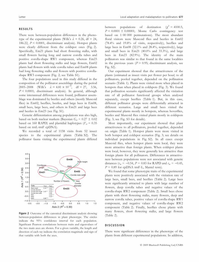
There were between-population differences in the pheno-

type of the experimental plants (Wilk�s k = 0.26, df = 24,

186.22, P < 0.0001, discriminant analysis). Hotspot plants

were clearly different from the coldspot ones (Fig. 2).

Specifically, Em21 plants had short flowering stalks, with

small flowers having long and narrow corolla tubes and

positive corolla-shape RW1 component, whereas Em23

plants had short flowering stalks and large flowers, Em02

plants had flowers with wide corolla tubes and Em08 plants

had long flowering stalks and flowers with positive corolla-

shape RW3 component (Fig. 2; see Table S1).

The four populations used in this study differed in the

composition of the pollinator assemblage during the period

2005–2008 (Wilk�s k = 4.81 · 10)9, df = 27, 3.56,

P < 0.0001; discriminant analysis). In general, although

some interannual differences were found, pollinator assem-

blage was dominated by beetles and others (mostly Muscoid

flies) in Em02, beeflies, beetles, and large bees in Em08,

small bees, large bees, and others in Em21 and large bees

and beetles in Em23 (see Fig. S1).

Genetic differentiation among populations was also high,

based on both nuclear markers (Bayesian Gst = 0.27 ± 0.02

based on 160 RAPD) and plastidial haplotypes (Fst = 0.35

based on trnL-trnF cpDNA).

We recorded a total of 1158 visits from 52 insect

species to the experimental plants (Table S2). The

pollinator fauna visiting the experimental plants differed

between populations of destination (v2 = 4100.5,

P < 0.0001 ± 0.00001; Monte Carlo contingency test

based on 1 00 000 permutations). The most abundant

floral visitors were Muscoid flies and beetles in Em02

(78.4% and 19.8% of visits, respectively), beeflies and

large bees in Em08 (32.1% and 28.4%, respectively), large

and small bees in Em21 (40.0% and 33.3%), and large

bees in Em23 (82.9%). The identity of the main

pollinators was similar to that found in the same localities

in the previous years (P > 0.95; discriminant analysis, see

Fig. S2).

Our experiment showed that the attractiveness of the

plants (estimated as insect visits per flower per hour) to all

pollinators, pooled together, depended on the pollination

scenario (Table 1). Plants were visited more when placed in

hotspots than when placed in coldspots (Fig. 3). We found

that pollination scenario significantly affected the visitation

rate of all pollinator functional groups when analysed

separately, except beeflies (Table 1). But, in this case,

different pollinator groups were differentially attracted in

different scenarios. Large and small bees visited the

experimental plants mostly in hotspots, whereas hoverflies,

beetles and Muscoid flies visited plants mostly in coldspots

(Fig. 3; see Fig. S3 for details).

Most importantly, our experiment showed that plant

attractiveness to all pollinators, pooled together, depended

on origin (Table 1). Hotspot plants were more visited in

both hotspot and coldspot scenarios (Fig. 3; see details on

individual populations in Fig. S2). In all cases except

Muscoid flies, when hotspot plants were local, they were

more attractive than foreign plants. When coldspot plants

were local, however, they were generally less attractive than

foreign plants for all pollinators. Differences in attractive-

ness between populations were not associated with genetic

distances (rm = )0.54, P = 0.83 for RAPD and rm = )0.45,

P = 0.89 for cpDNA trnF-L, Mantel tests).

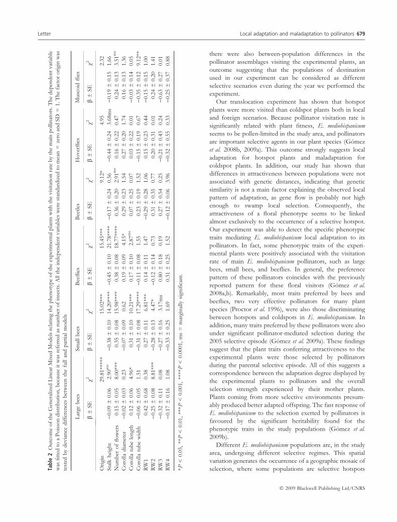
We found that some phenotypic traits of the experimental

plants were positively associated with the visitation rate of

large bees, small bees, and beeflies (Table 2). Large bees

were significantly attracted to plants with large number of

flowers, deep corolla tubes and negative values of the

corolla-shape RW2 component (Table 2). Small bees chose

plants with short flowering stalks, many flowers, deep and

narrow corolla tubes, positive values of corolla-shape RW1

component, and negative values of corolla-shape RW2

component (Table 2). Finally, beeflies chose plants with

many flowers, short flowering stalks, and large flowers

(Table 2).

D I S C U S S I O N

There were significant differences in the phenotype of the

plants from different experimental populations. In addition,

–1.0

–0.5

0.0

0.5

1.0

1.5

2.0

2.5

3.0

3.5

4.0

Stalk height

Number of flowers

Corollatubelength

RW1

RW2Corolla

diameter

RW3

RW4

Em08

Em23

–2.5 –2.0 –1.5 –1.0 –0.5 0.0 0.5 1.0 1.5

Em21 Em02

Axis 2 (R 2 = 0.30)

Axi

s 1

(R2

= 0

.56)

Traits

Stalk heightCorolla diameterCorolla tube lengthCorolla tube widthRW1RW2RW3

rAxis1

0.76****

0.42***

0.58****

rAxis2

0.52****0.34***-0.34***0.28*-0.42****0.34***

Corolla tube width

Figure 2 Outcome of the canonical discriminant analysis showing

between-population differences in plant phenotype. The circles

indicate the 95% confidence interval for each population.

Significant Pearson correlations between traits and eigenvalues of

the two main axes are shown. For a given variable, the length and

direction of each ray indicate the correlation magnitude and sign of

that variable with both the axes.



Table 1 Outcome of the Generalized Linear Mixed Models testing the effect of origin and destination in plant attractiveness to main

pollinator functional groups, quantified as number of visits per flower and 4 h. Values are likelihood ratio tests. Dependent variable was fitted

to a Poisson distribution (log as link function), and all variables were standardized variables prior analyses

Source df Total Large bees Small bees Beeflies Hoverflies Muscoids Beetles

Origin 1 14.69**** 10.84**** 5.36** 5.71** 4.7* 0.97 5.19**

Destination 1 10.85**** 36.46**** 6.43** 0.57 5.86** 23.71**** 10.18***

Origin*destination 1 1.83 3.88* 3.22 0.88 3.37 1.02 3.73*

Population [origin] 2 2.88 1.85 0.93 0.27 1.20 2.64 0.35

Population [destination] 2 11.46** 10.61** 22.43*** 27.21*** 21.26**** 0.78 8.66*

Deviance 300 2.28*** 0.57**** 0.28**** 0.16**** 0.01 0.0099 0.04***

*P < 0.05, **P < 0.01, ***P < 0.001, ****P < 0.0001.

0.00

0.01

0.02

0.03

0.04

0.05

0.06

0.07

0.08

0.09

0.10

0.11

0.00

0.01

0.02

0.03

0.04

0.05

0.06

0.07

0.000

0.005

0.010

0.015

0.020

0.025

0.030

0.000

0.005

0.010

0.015

0.020

0.000

0.001

0.002

0.003

0.004

0.005

0.006

0.007

0.000

0.001

0.002

0.003

0.000

0.002

0.004

0.006

0.008

0.010

0.012

All pollinators

Large bees Small bees Beeflies

Hoverflies Beetles Muscoid flies

ScenariosColdspot Hotspot Coldspot Hotspot Coldspot Hotspot

4 ×

Vis

itatio

n ra

te (

Inse

cts·

flow

er–1

·hr–1

)

Figure 3 Outcome of the translocation experiment. Charts show the attractiveness (estimated as mean ± 1SD pollinator visitation rate) of

plants from different origin (blue dots, coldspots; red dots, hotspots) in each of the two scenarios (blue background, coldspots; red

background, hotspots). Note the difference in Y-scale between the panels. The log-likelihood ratio tests from the Generalized Linear Mixed

Models are also shown (O, population of origin; D, population of destination; O · D: interaction term; *P < 0.05, **P < 0.01, ***P < 0.001,

****P < 0.0001).



there were also between-population differences in the

pollinator assemblages visiting the experimental plants, an

outcome suggesting that the populations of destination

used in our experiment can be considered as different

selective scenarios even during the year we performed the

experiment.

Our translocation experiment has shown that hotspot

plants were more visited than coldspot plants both in local

and foreign scenarios. Because pollinator visitation rate is

significantly related with plant fitness, E. mediohispanicum

seems to be pollen-limited in the study area, and pollinators

are important selective agents in our plant species (Gomez

et al. 2008b, 2009a). This outcome strongly suggests local

adaptation for hotspot plants and maladaptation for

coldspot plants. In addition, our study has shown that

differences in attractiveness between populations were not

associated with genetic distances, indicating that genetic

similarity is not a main factor explaining the observed local

pattern of adaptation, as gene flow is probably not high

enough to swamp local selection. Consequently, the

attractiveness of a floral phenotype seems to be linked

almost exclusively to the occurrence of a selective hotspot.

Our experiment was able to detect the specific phenotypic

traits mediating E. mediohispanicum local adaptation to its

pollinators. In fact, some phenotypic traits of the experi-

mental plants were positively associated with the visitation

rate of main E. mediohispanicum pollinators, such as large

bees, small bees, and beeflies. In general, the preference

pattern of these pollinators coincides with the previously

reported pattern for these floral visitors (Gomez et al.

2008a,b). Remarkably, most traits preferred by bees and

beeflies, two very effective pollinators for many plant

species (Proctor et al. 1996), were also those discriminating

between hotspots and coldspots in E. mediohispanicum. In

addition, many traits preferred by these pollinators were also

under significant pollinator-mediated selection during the

2005 selective episode (Gomez et al. 2009a). These findings

suggest that the plant traits conferring attractiveness to the

experimental plants were those selected by pollinators

during the parental selective episode. All of this suggests a

correspondence between the adaptation degree displayed by

the experimental plants to pollinators and the overall

selection strength experienced by their mother plants.

Plants coming from more selective environments presum-

ably produced better adapted offspring. The fast response of

E. mediohispanicum to the selection exerted by pollinators is

favoured by the significant heritability found for the

phenotypic traits in the study populations (Gomez et al.

2009b).

Different E. mediohispanicum populations are, in the study

area, undergoing different selective regimes. This spatial

variation generates the occurrence of a geographic mosaic of

selection, where some populations are selective hotspotsTab

le2

Ou

tco

me

of

the

Gen

eral

ized

Lin

ear

Mix

edM

od

els

rela

tin

gth

ep

hen

oty

pe

of

the

exp

erim

enta

lp

lan

tsw

ith

the

vis

itat

ion

rate

by

the

mai

np

olli

nat

ors

.T

he

dep

end

ent

var

iab

le

was

fitt

edto

aP

ois

son

dis

trib

uti

on

,b

ecau

seit

was

refe

rred

asn

um

ber

of

inse

cts.

All

the

ind

epen

den

tvar

iab

les

wer

est

and

ard

ized

tom

ean

=ze

roan

dS

D=

1.T

he

fact

or

ori

gin

was

test

edb

yd

evia

nce

dif

fere

nce

sb

etw

een

the

full

and

par

tial

mo

del

s

Lar

geb

ees

Sm

all

bee

sB

eefl

ies

Bee

tles

Ho

ver

flie

sM

usc

oid

flie

s

b±

SE

v2b

±S

Ev2

b±

SE

v2b

±S

Ev2

b±

SE

v2b

±S

Ev2

Ori

gin

29.8

1**

***

15.0

2**

*15.4

5**

*9.1

2*

4.9

52.3

2

Sta

lkh

eigh

t)

0.0

9±

0.0

62.9

0m

s)

0.3

8±

0.1

014.2

0**

**)

0.4

5±

0.1

021.7

8**

**)

0.1

7±

0.2

40.5

6)

0.4

4±

0.2

43.6

8m

s)

0.1

9±

0.1

51.6

6

Nu

mb

ero

ffl

ow

ers

0.1

5±

0.0

58.0

0**

*0.3

5±

0.0

815.9

8**

**0.3

8±

0.0

818.7

7**

**0.3

6±

0.2

02.9

1m

s0.1

6±

0.2

20.4

70.2

4±

0.1

33.5

1m

s

Co

rolla

dia

met

er)

0.0

2±

0.0

30.2

3)

0.0

7±

0.0

90.6

20.1

9±

0.0

94.1

5*

0.2

9±

0.2

31.5

40.2

7±

0.2

01.7

40.1

6±

0.1

31.3

6

Co

rolla

tub

ele

ngt

h0.1

2±

0.0

64.9

6*

0.3

1±

0.1

010.2

1**

*0.1

7±

0.1

02.8

7m

s0.0

7±

0.2

50.0

70.0

3±

0.2

20.0

1)

0.0

3±

0.1

40.0

5

Co

rolla

tub

ew

idth

)0.0

6±

0.0

51.5

1)

0.3

1±

0.0

817.2

9**

**)

0.1

1±

0.0

81.5

50.2

3±

0.1

91.5

2)

0.1

5±

0.1

90.6

7)

0.3

5±

0.1

29.1

2**

RW

10.4

2±

0.6

80.3

80.2

7±

0.1

16.8

1**

*0.1

4±

0.1

11.4

7)

0.2

9±

0.2

81.0

60.1

5±

0.2

30.4

4)

0.1

5±

0.1

51.0

0

RW

2)

0.2

5±

0.0

88.8

1**

*)

0.2

8±

0.1

34.4

7*

)0.1

2±

0.1

40.7

30.3

1±

0.3

50.7

70.2

0±

0.3

10.0

10.2

4±

0.2

01.4

1

RW

3)

0.3

2±

0.1

10.0

8)

0.2

7±

0.1

63.1

7m

s0.8

0±

0.1

80.1

90.2

7±

0.5

40.2

5)

0.2

1±

0.4

30.2

4)

0.6

3±

0.2

70.0

1

RW

4)

0.1

7±

0.1

61.0

8)

0.3

3±

0.2

51.6

90.3

1±

0.2

51.5

2)

0.1

2±

0.0

63.9

6)

0.3

2±

0.5

50.3

3)

0.2

5±

0.3

70.8

8

*P<

0.0

5,

**P

<0.0

1,

***P

<0.0

01,

****

P<

0.0

001,

ms

=m

argi

nal

lysi

gnif

ican

t.



whereas others are selective coldspots (Gomez et al. 2009a).

Under these circumstances, as the current experiment

suggests an association between selection strength and

adaptation, the landscape can be visualized for E. mediohis-

panicum as a mosaic of populations, some of them constituted

by plants displaying attractive phenotypes and others

composed of plants with non-attractive phenotype. Long-

term persistence of this spatial pattern of adaptation requires,

nevertheless, temporal stability in the pollinating selective

agents across localities (Nuismer et al. 2000). This situation

has been demonstrated for some highly specialist mutualisms

like the interaction between Greya politella and Lithophragma

parviflorum (Thompson & Fernandez 2006) and between

mycorrhizal fungi and nitrogen-fixing bacteria (Parker 1999).

However, reaching this kind of stability in the spatial pattern

of adaptation and maladaptation is unlikely in generalist

systems, as in these systems there is frequent temporal

variation in the identity and abundance of the most

important selective agents that causes strong fluctuations in

the selective regimes (Waser et al. 1996; Gomez & Zamora

2006; but see Alcantara et al. 2007). In contrast, we postulate

that in generalist systems, the occurrence of spatially and

temporally shifting patterns of local adaptations and malad-

aptations is more probable. However, further studies are

necessary to test this possibility.

Spatially structured adaptation has been detected mostly at

large spatial scales (Lajeunesse & Forbes 2002; Alcantara

et al. 2007). However, in this study we have found local

adaptation at a very small spatial scale, as experimental

populations were separated by only hundreds of metres.

Small spatial scale local adaptation is favoured when gene

flow, a main factor preventing local adaptation (Lajeunesse &

Forbes 2002; Savolainen et al. 2007), is restricted. In fact,

small-scale local adaptation has been found only for

pathosystems where gene flow is very limited (Capelle &

Neema 2005). In E. mediohispanicum, gene flow via seed is

probably low, as seed dispersal is very short (usually less than

0.5 m, Gomez 2007). We do not have information about the

extent of pollen flow in this plant species, as it is pollinated

by many different insects, some of them showing high

movement ability (i.e. Anthophora spp., Osmia spp., Macroglos-

sum stellatarum, etc.), but many others displaying narrow home

ranges (i.e. Dasytes spp., Bombylius spp., Malachius spp., etc.).

Nevertheless, the high genetic differentiation detected

among populations suggests that, in spite of their relative

proximity, gene flow among experimental populations is low.

Two important consequences emerge from our study.

First, local adaptation is not exclusive of specialist interac-

tions. A geographically structured pattern of local adaptation

and maladaptation can also be associated to generalist

facultative mutualisms where multispecific selection is

prevalent (Gomez et al. 2009a). In these systems, despite a

species interacting simultaneously with multiple species, the

interaction with a spatially variable subset of organisms

exerting strong selection may eventually lead to divergent

selection (Thompson 2005; Gomez et al. 2009a). Second,

the spatial pattern of adaptation can operate at fairly small

spatial scales, highlighting the importance of considering the

microscale as a relevant template to study evolutionary

processes in generalist systems. We presume that this

outcome is indeed more likely in generalist than in specialist

systems, as a slight modification in the community of

organisms interacting with generalist species can have

intense effects in the overall interaction outcome. Consid-

ering these two consequences in future, empirical and

theoretical studies will surely contribute to broadening the

conceptual framework of the geographical mosaic of

coevolution.

A C K N O W L E D G E M E N T S

The authors thank Belen Herrador for laboratory assistance;

Dr Jordi Bosch for field help and insect identification; and

Dr John N. Thompson, Dr Pedro Rey and two anonymous

reviewers for comments. The Consejerıa de Medio Ambi-

ente (Junta de Andalucıa) facilitated working in the Sierra

Nevada Protected Area. The authors acknowledge the

support of the Spanish Ministerio de Ciencia e Innovacion

(GLB200604883 ⁄ BOS; CONSOLIDER CSD 200800040),

Spanish Ministerio de Medio Ambiente y Medio Rural y

Marino (078 ⁄ 2007) and Junta de Andalucıa PAI (RNM 220

and CVI 165).

R E F E R E N C E S

Adams, D.C., Rohlf, F.J. & Slice, D.E. (2004). Geometric mor-

phometrics: ten years of progress following the �revolution�. Ital.

J. Zool., 71, 5–16.

Alcantara, J., Rey, P., Manzaneda, A., Boulay, R., Ramırez, J. &

Fedriani, J. (2007). Geographic variation in the adaptive land-

scape for seed size at dispersal in the myrmecochorus Helleborus

foetidus. Evol. Ecol., 21, 411–430.

Capelle, J. & Neema, C. (2005). Local adaptation and population

structure at a micro-geographical scale of a fungal parasite on its

host plant. J. Evol. Biol., 18, 1445–1454.

Gomez, J.M. (2005). Non-additive effects of pollinators and her-

bivores on Erysimum mediohispanicum (Cruciferae) fitness. Oecolo-

gia, 143, 412–418.

Gomez, J.M. (2007). Dispersal-mediated selection on plant height

in an autochorously-dispersed herb. Plant. Syst. Evol., 268, 119–

130.

Gomez, J.M. & Zamora, R. (2006). Ecological factors that promote

the evolution of generalization in pollination systems. In: Plant-

pollinator interactions, from specialization to generalization (eds Waser,

N.M. & Ollerton, J.). Univ of Chicago Press, Chicago, pp. 145–

165.

Gomez, J.M., Perfectti, F. & Camacho, J.P.M. (2006). Natural

selection on Erysimum mediohispanicum flower shape: insights into

the evolution of zygomorphy. Am. Nat., 168, 531–545.



Gomez, J.M., Bosch, J., Perfectti, F., Fernandez, J.D., Abdelaziz,

M. & Camacho, J.P.M. (2008a). Spatial variation in selection on

corolla shape in a generalist plant is promoted by the preference

of its local pollinators. Proc. R. Soc. Lond. B, 275, 2241–2249.

Gomez, J.M., Bosch, J., Perfectti, F., Fernandez, J.D., Abdelaziz,

M. & Camacho, J.P.M. (2008b). Association between floral traits

and reward in Erysimum mediohispanicum (Brassicaceae). Ann. Bot.,

101, 1413–1420.

Gomez, J.M., Perfectti, F., Bosch, J. & Camacho, J.P.M. (2009a). A

geographic selection mosaic in a generalized plant–pollinator–

herbivore system. Ecol. Monogr., 79, 245–263.

Gomez, J.M., Abdelaziz, M., Munoz-Pajares, A.J. & Perfectti, F.

(2009b). Heritability and genetic correlation of corolla shape and

size in Erysimum mediohispanicum. Evolution, in press.

Gomulkiewicz, R., Thompson, J.N., Holt, R.D., Nuismer, S.L. &

Hochberd, M.E. (2000). Hotspots, coldspots, and the geo-

graphic mosaic theory of coevolution. Am. Nat., 156, 156–174.

Gomulkiewicz, R., Drown, D.M., Dybdahl, M.F., Godsoe, W.,

Nuismer, S.L., Pepin, K.M. et al. (2007). Dos and don�ts of

testing the geographic mosaic theory of coevolution. Heredity, 98,

249–258.

Hall, T.A. (1999). BioEdit: a user-friendly biological sequence

alignment editor and analysis program for Windows 95 ⁄ 98 ⁄ NT.

Nucleic Acid. Symp. Ser., 41, 95–98.

Hoeksema, J.D. & Forde, S.E. (2008). A meta-analysis of factors

affecting local adaptation. Am. Nat., 171, 275–290.

Holsinger, K.E., Lewis, P.O. & Dey, D.K. (2002). A Bayesian

method for analysis of genetic population structure with domi-

nant marker data. Mol. Ecol., 11, 1157–1164.

Holt, R.D. & Gomulkiewicz, R. (1997). How does immigration

influence local adaptation? A reexamination of a familiar para-

digm. Am. Nat., 149, 563–572.

Kaltz, O. & Shykoff, J.A. (1998). Local adaptation in host–parasite

systems. Heredity, 81, 361–370.

Kaltz, O., Gandon, S., Michalakis, Y. & Shykoff, J.A. (1999). Local

maladaptation in the anther-smut fungus Microbotryum violaceum to

its host plant Silene latifolia: evidence from a cross-inoculation

experiment. Evolution, 53, 395–407.

Kawecki, T.J. & Ebert, D. (2004). Conceptual issues in local

adaptation. Ecol. Lett., 7, 1225–1241.

Lajeunesse, M.J. & Forbes, M.R. (2002). Host range and local

parasite adaptation. Proc. R. Soc. Lond. B, 269, 703–710.

Mopper, S. & Strauss, S.Y. (1998). Genetic Structure and Local

Adaptation in Natural Insect Populations: Effects of Ecology, Life His-

tory, and Behavior. Chapman and Hall, New York.

Morgan, A., Gandon, S. & Buckling, A. (2005). The effect of

migration on local adaptation in a coevolving host–parasite

system. Nature, 437, 253–256.

Nuismer, S.L. (2006). Parasite local adaptation in a geographic

mosaic. Evolution, 60, 24–30.

Nuismer, S.L., Thompson, J.N. & Gomulkiewicz, R. (2000).

Coevolutionary clines across selection mosaic. Evolution, 54,

1102–1115.

Parker, M.A. (1999). Mutualism in metapopulations of legumes and

rhizobia. Am. Nat., 153, S48–S60.

Proctor, M., Lack, A. & Yeo, P. (1996). The Natural History of

Pollination. Harper Collins, New York.

R Development Core Team (2008). R : A Language and Environment

for Statistical Computing. R Foundation for Statistical Computing,

Vienna; Url: http://www.R-project.org.

Savolainen, O.T., Hajarvi, P. & Knurr, T. (2007). Gene flow and

local adaptation in trees. Ann. Rev. Ecol. Evol. Syst., 38, 595–619.

Strauss, S.Y. & Irwin, R.E. (2004). Ecological and evolutionary

consequences of multispecies plant–animal interactions. Ann.

Rev. Ecol. Evol. Syst., 35, 435–466.

Strauss, S.Y., Sahli, H. & Conner, J.K. (2005). Toward a more trait-

centered approach to diffuse (co)evolution. New Phytol., 165, 81–

90.

Taberlet, P., Gielly, L., Pautou, G. & Bouvet, J. (1991). Universal

primers for amplification of three non-coding regions of chlo-

roplast DNA. Mol. Plant Biol., 17, 1105–1109.

Thompson, J.N. (1994). The Coevolutionary Process. The University of

Chicago Press, Chicago, USA.

Thompson, J.N. (2005). The Geographic Mosaic of Coevolution. The

University of Chicago Press, Chicago, USA.

Thompson, J.N. & Fernandez, C.C. (2006). Temporal dynamics of

antagonism and mutualism in a geographically variable plant–

insect interaction. Ecology, 87, 103–112.

Thompson, J.N., Nuismer, S.L. & Gomulkiewicz, R. (2002).

Coevolution and maladaptation. Integr. Comp. Biol., 42, 381–387.

Van Zandt, P.A. & Mopper, S. (1998). A meta-analysis of adaptive

deme formation in phytophagous insect populations. Am. Nat.,

152, 595–604.

Waser, N.M., Chitkka, L., Price, M.V., Williams, N.M. & Ollerton,

J. (1996). Generalization in pollination systems, and why it

matters. Ecology, 77, 1043–1060.

Zelditch, M.L., Swiderski, D.L., Sheets, H.D. & Fink, W.L. (2004).

Geometric Morphometrics for Biologists: A Primer. Elsevier Academic

Press, San Diego.

S U P P O R T I N G I N F O R M A T I O N

Additional Supporting Information may be found in the

online version of this article:

Figure S1 Proportion of visits made by insects, belonging to

each functional group, to natural plants of Erysimum

mediohispancum during 4 years (2005–2008) and to experi-

mental plants used in the transplant experiment. Others

were Muscoid flies in the experimental plants, but comprise

muscoid flies, ants, bugs, and some grasshoppers in the

natural populations.

Figure S2 Outcome of the canonical discriminant analysis

showing between-population differences in pollinator

assemblages. The circles indicate the 95% confidence

interval for each population. For a given variable, the

length and direction of each ray indicate the correlation

magnitude and sign of that variable with both the axes. The

red circles refer to the position in the space of the four

experimental populations. The squared Mahalanobis dis-

tances from the position of each experimental population to

the centroid of its corresponding population is shown in the

graph.

Figure S3 Outcome of the translocation experiment consid-

ering the four studied population. Figures show the mean

(±1SD) visitation rate by pollinators to plants from different



origin in each of the four populations of destination. The

uppermost rightmost panel shows the average visitation rate

to plants from different origin, pooling together all

populations of destination. Different superscript letters

indicate statistical significance at a < 0.05. Red dots indicate

hot spots, whereas blue dots indicate cold spots. Note the

difference in Y-scale between panels. The log-likelihood

ratio tests from the Generalized Mixed Models are also

shown (O, population of origin; D, population of destina-

tion; O · D: interaction term; *P < 0.05, **P < 0.01,

***P < 0.001, ****P < 0.0001).

Table S1 Among-population differences in plant pheno-

typic traits (n = 20 plants per population). Figures are

mean ± 1SE.

Table S2 Composition of the pollinator assemblage visiting

the flowers of Erysimum mediohispanicum during the experi-

ment. Figures represent the number of visits of each

pollinator species to plants from different origin (pooling

together all populations of destination).

Please note: Wiley-Blackwell are not responsible for the

content or functionality of any supporting materials supplied

by the authors. Any queries (other than missing material)

should be directed to the corresponding author for the article.

Editor, Marcel Holyoak

Manuscript received 3 March 2009

First decision made 27 March 2009

Manuscript accepted 3 April 2009



Local adaptation and maladaptation to pollinators in a generalist geographic mosaic

Documents

Transcript of Local adaptation and maladaptation to pollinators in a generalist geographic mosaic