
Lk18
22
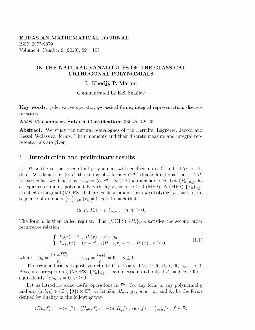
EURASIAN MATHEMATICAL JOURNAL ISSN 2077-9879 Volume 4, Number 2 (2013), 82 – 103 ON THE NATURAL q-ANALOGUES OF THE CLASSICAL ORTHOGONAL POLYNOMIALS L. Kh´ eriji, P. Maroni Communicated by E.S. Smailov Key words: q-derivative operator, q-classical forms, integral representation, discrete measure. AMS Mathematics Subject Classification: 33C45, 42C05. Abstract. We study the natural q-analogues of the Hermite, Laguerre, Jacobi and Bessel D-classical forms. Their moments and their discrete measure and integral rep- resentations are given. 1 Introduction and preliminary results Let P be the vector space of all polynomials with coefficients in C and let P be its dual. We denote by u, f the action of a form u ∈P (linear functional) on f ∈P . In particular, we denote by (u) n := u, x n ,n ≥ 0 the moments of u. Let {P n } n≥0 be a sequence of monic polynomials with deg P n = n, n ≥ 0 (MPS). A (MPS) {P n } n≥0 is called orthogonal (MOPS) if there exists a unique form u satisfying (u) 0 =1 and a sequence of numbers {r n } n≥0 (r n =0,n ≥ 0) such that u, P m P n = r n δ n,m , n, m ≥ 0. The form u is then called regular. The (MOPS) {P n } n≥0 satisfies the second order recurrence relation P 0 (x)=1 ,P 1 (x)= x - β 0 , P n+2 (x)=(x - β n+1 )P n+1 (x) - γ n+1 P n (x) ,n ≥ 0, (1.1) where β n = u, xP 2 n r n ; γ n+1 = r n+1 r n =0, n ≥ 0. The regular form u is positive definite if and only if ∀n ≥ 0,β n ∈ R,γ n+1 > 0. Also, its corresponding (MOPS) {P n } n≥0 is symmetric if and only if β n =0,n ≥ 0 or, equivalently (u) 2n+1 =0,n ≥ 0. Let us introduce some useful operations in P . For any form u, any polynomial g and any (a, b, c) ∈ (C \{0}) × C 2 , we let Du, H q u, gu, h a u, τ b u and δ c , be the forms defined by duality in the following way Du, f := -u, f , H q u, f := -u, H q f , gu, f := u, gf ,f ∈P ,
Transcript of Lk18
EURASIAN MATHEMATICAL JOURNALISSN 2077-9879Volume 4, Number 2 (2013), 82 – 103
ON THE NATURAL q-ANALOGUES OF THE CLASSICALORTHOGONAL POLYNOMIALS
L. Kheriji, P. Maroni
Communicated by E.S. Smailov
Key words: q-derivative operator, q-classical forms, integral representation, discretemeasure.
AMS Mathematics Subject Classification: 33C45, 42C05.
Abstract. We study the natural q-analogues of the Hermite, Laguerre, Jacobi andBessel D-classical forms. Their moments and their discrete measure and integral rep-resentations are given.
1 Introduction and preliminary results
Let P be the vector space of all polynomials with coefficients in C and let P ′ be itsdual. We denote by 〈u, f〉 the action of a form u ∈ P ′ (linear functional) on f ∈ P .In particular, we denote by (u)n := 〈u, xn〉 , n ≥ 0 the moments of u. Let {Pn}n≥0 bea sequence of monic polynomials with degPn = n, n ≥ 0 (MPS). A (MPS) {Pn}n≥0
is called orthogonal (MOPS) if there exists a unique form u satisfying (u)0 = 1 and asequence of numbers {rn}n≥0 (rn 6= 0, n ≥ 0) such that
〈u, PmPn〉 = rnδn,m , n,m ≥ 0.
The form u is then called regular. The (MOPS) {Pn}n≥0 satisfies the second orderrecurrence relation{
P0(x) = 1 , P1(x) = x− β0 ,Pn+2(x) = (x− βn+1)Pn+1(x)− γn+1Pn(x) , n ≥ 0,
(1.1)
where βn =〈u, xP 2
n〉rn
; γn+1 =rn+1
rn6= 0, n ≥ 0.
The regular form u is positive definite if and only if ∀n ≥ 0, βn ∈ R, γn+1 > 0.Also, its corresponding (MOPS) {Pn}n≥0 is symmetric if and only if βn = 0, n ≥ 0 or,equivalently (u)2n+1 = 0, n ≥ 0.
Let us introduce some useful operations in P ′. For any form u, any polynomial gand any (a, b, c) ∈ (C \ {0})× C2, we let Du, Hqu, gu, hau, τbu and δc, be the formsdefined by duality in the following way
〈Du, f〉 := −〈u, f ′〉 , 〈Hqu, f〉 := −〈u,Hqf〉 , 〈gu, f〉 := 〈u, gf〉 , f ∈ P ,

Hq-classical forms 83
〈hau, f〉 := 〈u, haf〉 , 〈τbu, f〉 := 〈u, τ−bf〉 , 〈δc, f〉 := f(c) , f ∈ P ,
where(Hqf)(x) =
f(qx)− f(x)
(q − 1)x, q ∈ C :=
{z ∈ C, z 6= 0, zn 6= 1, n ≥ 1
},
(haf)(x) = f(ax), (τ−bf)(x) = f(x+ b) [9,11]. Furthermore, the orthogonality is keptby shifting: let {Pn := a−n(ha◦τ−bPn)}n≥0 , a 6= 0, b ∈ C be orthogonal with respect tou = ha−1 ◦ τ−bu, then the recurrence elements βn, γn+1, n ≥ 0 of the sequence {Pn}n≥0
areβn =
βn − b
a, γn+1 =
γn+1
a2, n ≥ 0.
Let {Pn}n≥0 be a (MPS) and O be a lowering operator on P . The sequence {Pn}n≥0
is said to be O-classical when {Pn}n≥0 is orthogonal and {OPn+1}n≥0 is also orthogonal(the Hahn property). The concept of O-classical orthogonal polynomials was exten-sively studied by the second author and his coworkers for O = D the derivative operator[11,12], O = Dω the divided difference operator [1], and O = Hq the q-derivative one[9] via the following distributional equation satisfied by the regular form u associatedwith such a sequence:
O(Φ(x)u) + Ψ(x)u = 0 (1.2)
where Φ is a monic polynomial, deg Φ ≤ 2 and Ψ a polynomial deg Ψ = 1.
Now, let us recall the D-classical forms; there are four canonical situations [11,12].
1) The Hermite form H and its (MOPS) having the following properties
βn = 0 , γn+1 = n+12, n ≥ 0,
D(H) + 2xH = 0,
(H)2n+1 = 0 , (H)2n = (2n)!22nn!
, n ≥ 0,
〈H, f〉 = 1√π
∫ +∞
−∞exp(−x2)f(x)dx, f ∈ P .
(1.3)
2) The Laguerre form L(α) (α 6= −n− 1, n ≥ 0) and its (MOPS) satisfying
βn = 2n+ α+ 1 , γn+1 = (n+ 1)(n+ α+ 1), n ≥ 0,
D(xL(α)) + (x− 1− α)L(α) = 0,
(L(α))n = Γ(n+α+1)Γ(α+1)
, n ≥ 0,
〈L(α), f〉 = 1Γ(α+1)
∫ +∞
0
xα exp(−x)f(x)dx, f ∈ P , <α > −1.
(1.4)
3) The shifted Jacobi form h− 12◦ τ−1J (α, β) := J (α, β) (α 6= −n − 1, β 6= −n −

84 L. Kheriji, P. Maroni
1, α+ β 6= −n− 2, n ≥ 0) and its (MOPS) satisfying
β0 = β+1α+β+2
, βn+1 = 12− α2−β2
2(2n+α+β+2)(2n+α+β+4), n ≥ 0,
γn+1 = (n+1)(n+α+β+1)(n+α+1)(n+β+1)(2n+α+β+1)(2n+α+β+2)2(2n+α+β+3)
, n ≥ 0,
D(x(x− 1)J (α, β)
)+(−(α+ β + 2)x+ β + 1
)J (α, β) = 0,
(J (α, β))n = Γ(n+β+1)Γ(α+β+2)Γ(n+α+β+2)Γ(β+1)
, n ≥ 0,
〈J (α, β), f〉 = Γ(α+β+2)Γ(α+1)Γ(β+1)
∫ +1
0
xβ(1− x)αf(x)dx, f ∈ P , <α > −1, <β > −1.
(1.5)
4) The regular Bessel form B(α) (α 6= −n2, n ≥ 0) and its (MOPS) having the
following properties
β0 = − 1α
, βn+1 = 1−α(n+α)(n+α+1)
, n ≥ 0,
γn+1 = − (n+1)(n+2α−1)(2n+2α−1)(n+α)2(2n+2α+1)
, n ≥ 0,
D(x2B(α))− 2(αx+ 1)B(α) = 0,
(B(α))n = (−1)n2n Γ(2α)Γ(n+2α)
, n ≥ 0,
〈B(α), f〉 = S−1α
∫ +∞
0
1
x2
∫ +∞
x
(xt
)2α
exp(2t− 2
x
)s(t)dt f(x) dx,
for f ∈ P , α ≥ 6( 2π)4
(1.6)
with
Sα =
∫ +∞
0
1
x2
∫ +∞
x
(xt
)2α
exp(2t− 2
x
)s(t) dt dx
and s given by (1.13), see below.Our objective is to highlight the natural q-analogues of the Hermite, Laguerre,
Jacobi and Bessel D-classical forms defined in [5, 9], to calculate their moments, andto derive discrete measure and integral representations. In particular, when q → 1 werecover formulas (1.3)-(1.6). In fact, the problem of defining q-analogue of orthogonalsequences has been of interest for several authors, see [2, 3, 10, 13, 14, 15].
A form u is called Hq-classical when it is regular and there exist two polynomialsΦ and Ψ, Φ monic, deg Φ ≤ 2, deg Ψ = 1 such that [9]
Hq(Φu) + Ψu = 0 (1.7)
with Ψ′(0)− 12Φ′′(0)[n]q 6= 0, n ≥ 0 where
[n]q :=qn − 1
q − 1, n ≥ 0. (1.8)
By using (1.7) it easy to see that the moments of u satisfy the second order q-differenceequation
Ψ′(0)(u)1 + Ψ(0) = 0,
Hq-classical forms 85
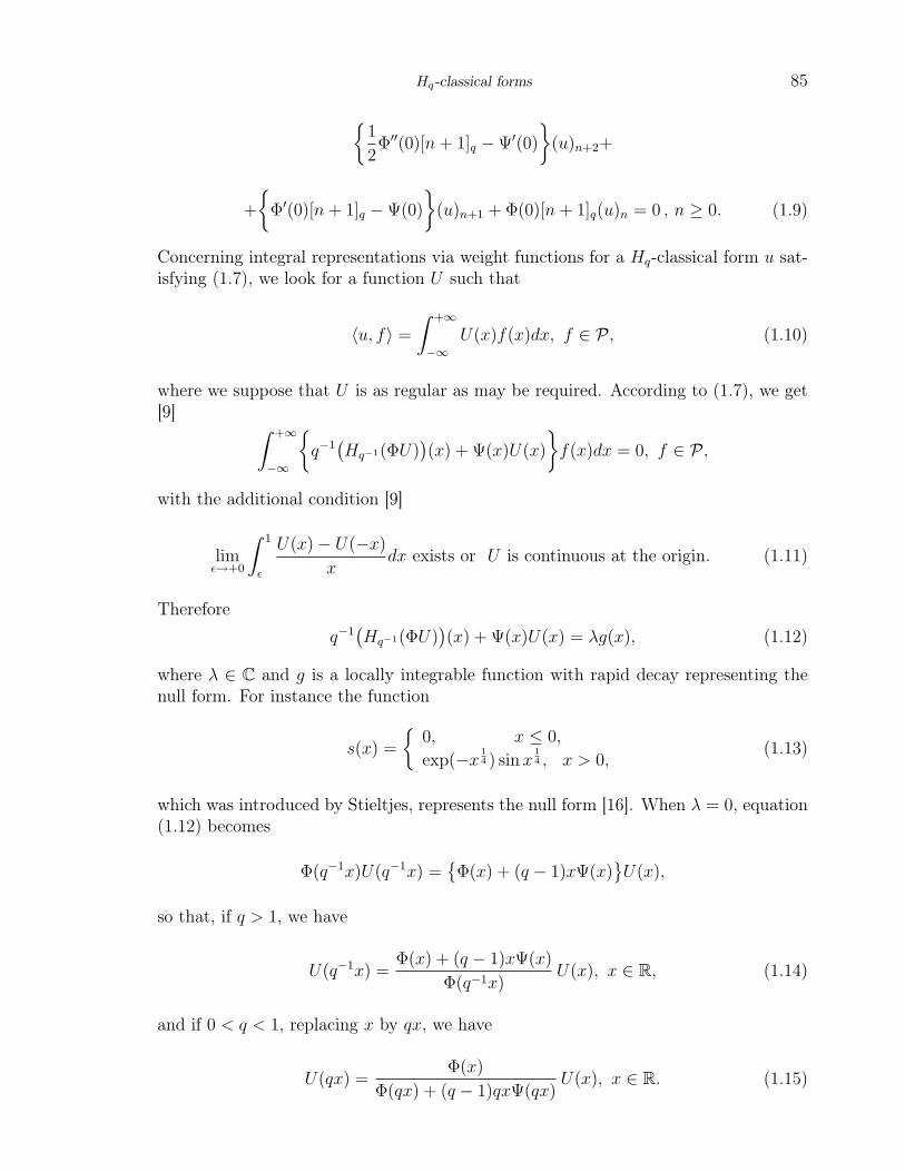
{1
2Φ′′(0)[n+ 1]q −Ψ′(0)
}(u)n+2+
+
{Φ′(0)[n+ 1]q −Ψ(0)
}(u)n+1 + Φ(0)[n+ 1]q(u)n = 0 , n ≥ 0. (1.9)
Concerning integral representations via weight functions for a Hq-classical form u sat-isfying (1.7), we look for a function U such that
〈u, f〉 =
∫ +∞
−∞U(x)f(x)dx, f ∈ P , (1.10)
where we suppose that U is as regular as may be required. According to (1.7), we get[9] ∫ +∞
−∞
{q−1(Hq−1(ΦU)
)(x) + Ψ(x)U(x)
}f(x)dx = 0, f ∈ P ,
with the additional condition [9]
limε→+0
∫ 1
ε
U(x)− U(−x)x
dx exists or U is continuous at the origin. (1.11)
Thereforeq−1(Hq−1(ΦU)
)(x) + Ψ(x)U(x) = λg(x), (1.12)
where λ ∈ C and g is a locally integrable function with rapid decay representing thenull form. For instance the function
s(x) =
{0, x ≤ 0,
exp(−x 14 ) sinx
14 , x > 0,
(1.13)
which was introduced by Stieltjes, represents the null form [16]. When λ = 0, equation(1.12) becomes
Φ(q−1x)U(q−1x) ={Φ(x) + (q − 1)xΨ(x)
}U(x),
so that, if q > 1, we have
U(q−1x) =Φ(x) + (q − 1)xΨ(x)
Φ(q−1x)U(x), x ∈ R, (1.14)
and if 0 < q < 1, replacing x by qx, we have
U(qx) =Φ(x)
Φ(qx) + (q − 1)qxΨ(qx)U(x), x ∈ R. (1.15)
86 L. Kheriji, P. Maroni
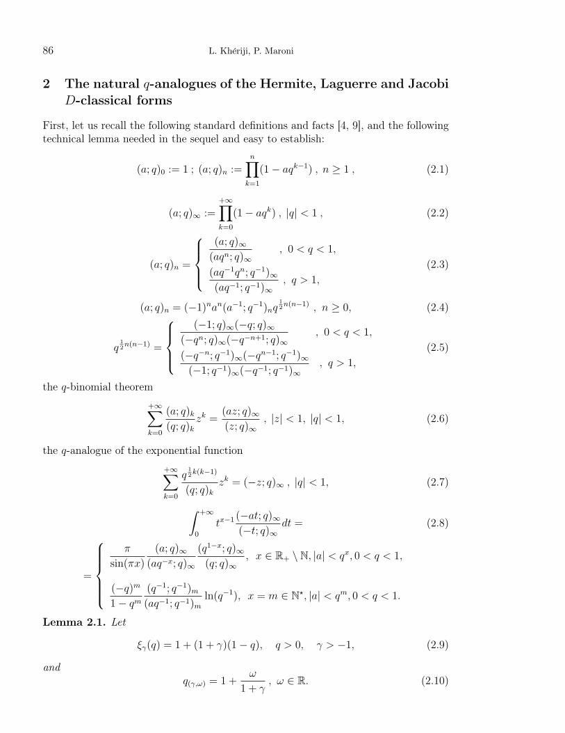
2 The natural q-analogues of the Hermite, Laguerre and JacobiD-classical forms
First, let us recall the following standard definitions and facts [4, 9], and the followingtechnical lemma needed in the sequel and easy to establish:
(a; q)0 := 1 ; (a; q)n :=n∏k=1
(1− aqk−1) , n ≥ 1 , (2.1)
(a; q)∞ :=+∞∏k=0
(1− aqk) , |q| < 1 , (2.2)
(a; q)n =
(a; q)∞
(aqn; q)∞, 0 < q < 1,
(aq−1qn; q−1)∞(aq−1; q−1)∞
, q > 1,
(2.3)
(a; q)n = (−1)nan(a−1; q−1)nq12n(n−1) , n ≥ 0, (2.4)
q12n(n−1) =
(−1; q)∞(−q; q)∞
(−qn; q)∞(−q−n+1; q)∞, 0 < q < 1,
(−q−n; q−1)∞(−qn−1; q−1)∞(−1; q−1)∞(−q−1; q−1)∞
, q > 1,
(2.5)
the q-binomial theorem
+∞∑k=0
(a; q)k(q; q)k
zk =(az; q)∞(z; q)∞
, |z| < 1, |q| < 1, (2.6)
the q-analogue of the exponential function
+∞∑k=0
q12k(k−1)
(q; q)kzk = (−z; q)∞ , |q| < 1, (2.7)
∫ +∞
0
tx−1 (−at; q)∞(−t; q)∞
dt = (2.8)
=
π
sin(πx)
(a; q)∞(aq−x; q)∞
(q1−x; q)∞(q; q)∞
, x ∈ R+ \ N, |a| < qx, 0 < q < 1,
(−q)m
1− qm(q−1; q−1)m(aq−1; q−1)m
ln(q−1), x = m ∈ N?, |a| < qm, 0 < q < 1.
Lemma 2.1. Let
ξγ(q) = 1 + (1 + γ)(1− q), q > 0, γ > −1, (2.9)
andq(γ,ω) = 1 +
ω
1 + γ, ω ∈ R. (2.10)

Hq-classical forms 87
We haveξγ(q) = 1 ⇐⇒ q = 1,
ξγ(q) = 0 ⇐⇒ q = q(γ,1),
ξγ(q) = −1 ⇐⇒ q = q(γ,2),
ξγ(q) < −1 ⇐⇒ q ∈]q(γ,2),+∞[,
−1 < ξγ(q) < 0 ⇐⇒ q ∈]q(γ,1), q(γ,2)[,
0 < ξγ(q) < 1 ⇐⇒ q ∈]1, q(γ,1)[,
ξγ(q) > 1 ⇐⇒ q ∈]0, 1[.
(2.11)
2.1 The natural q-analogue of the Hermite form
The natural q-analogue of the Hermite form is the Hq-classical form H(q) defined by{βn = 0 , γn+1 = 1
2qn[n+ 1]q, n ≥ 0,
Hq(H(q)) + 2xH(q) = 0.
(See [9].) When q → 1, we recover the Hermite D-classical form H see (1.3).In [9], we calculated the moments and derived integral representations for H(q):
(H(q))2n =1
2n(q; q2)n(1− q)n
, (H(q))2n+1 = 0, n ≥ 0,
for f ∈ P , q > 1
〈H(q), f〉 =
√2
π(q − 1)1/2 (q−2; q−2)∞
(q−1; q−2)∞
∫ +∞
−∞
f(x)(−2(q − 1)x2; q−2
)∞dx, (2.12)
〈H(q), f〉 = K
∫ + 1
q√
2(1−q)
− 1
q√
2(1−q)
(2q2(1− q)x2; q2
)∞f(x)dx, f ∈ P , 0 < q < 1, (2.13)
where K = 12
(∫ + 1
q√
2(1−q)
0
(2q2(1− q)x2; q2
)∞dx
)−1
.
In [8], the authors give the following discrete measure representations of H(q):
H(q) =1
2(q−1; q−2)∞
+∞∑k=0
(−1)kq−k2
(q−2; q−2)k
{δ −iqk√
2(q−1)
+ δ iqk√2(q−1)
}, q > 1,
and
H(q) =(q; q2)∞
2
+∞∑k=0
qk
(q2; q2)k
{δ −qk√
2(1−q)
+ δ qk√2(1−q)
}, 0 < q < 1.
Remarks. 1. By using the above representations of H(q) and (2.12)-(2.13), one canwrite
2〈H(q), f〉 =
√2
π(q − 1)1/2 (q−2; q−2)∞
(q−1; q−2)∞
∫ +∞
−∞
f(x)(−2(q − 1)x2; q−2
)∞dx+
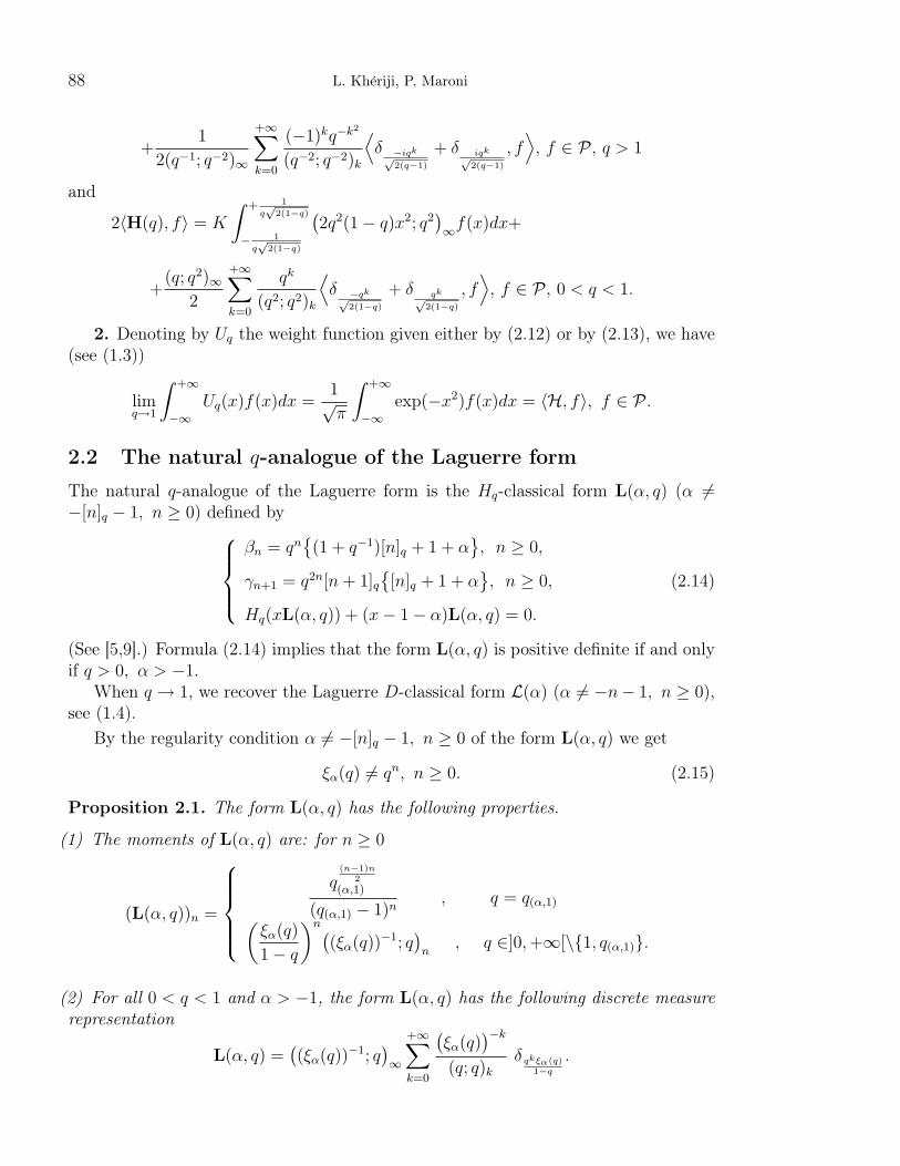
88 L. Kheriji, P. Maroni
+1
2(q−1; q−2)∞
+∞∑k=0
(−1)kq−k2
(q−2; q−2)k
⟨δ −iqk√
2(q−1)
+ δ iqk√2(q−1)
, f⟩, f ∈ P , q > 1
and
2〈H(q), f〉 = K
∫ + 1
q√
2(1−q)
− 1
q√
2(1−q)
(2q2(1− q)x2; q2
)∞f(x)dx+
+(q; q2)∞
2
+∞∑k=0
qk
(q2; q2)k
⟨δ −qk√
2(1−q)
+ δ qk√2(1−q)
, f⟩, f ∈ P , 0 < q < 1.
2. Denoting by Uq the weight function given either by (2.12) or by (2.13), we have(see (1.3))
limq→1
∫ +∞
−∞Uq(x)f(x)dx =
1√π
∫ +∞
−∞exp(−x2)f(x)dx = 〈H, f〉, f ∈ P .
2.2 The natural q-analogue of the Laguerre form
The natural q-analogue of the Laguerre form is the Hq-classical form L(α, q) (α 6=−[n]q − 1, n ≥ 0) defined by
βn = qn{(1 + q−1)[n]q + 1 + α
}, n ≥ 0,
γn+1 = q2n[n+ 1]q{[n]q + 1 + α
}, n ≥ 0,
Hq(xL(α, q)) + (x− 1− α)L(α, q) = 0.
(2.14)
(See [5,9].) Formula (2.14) implies that the form L(α, q) is positive definite if and onlyif q > 0, α > −1.
When q → 1, we recover the Laguerre D-classical form L(α) (α 6= −n− 1, n ≥ 0),see (1.4).
By the regularity condition α 6= −[n]q − 1, n ≥ 0 of the form L(α, q) we get
ξα(q) 6= qn, n ≥ 0. (2.15)
Proposition 2.1. The form L(α, q) has the following properties.
(1) The moments of L(α, q) are: for n ≥ 0
(L(α, q))n =
q
(n−1)n2
(α,1)
(q(α,1) − 1)n, q = q(α,1)(
ξα(q)
1− q
)n((ξα(q))
−1; q)n
, q ∈]0,+∞[\{1, q(α,1)}.
(2) For all 0 < q < 1 and α > −1, the form L(α, q) has the following discrete measurerepresentation
L(α, q) =((ξα(q))
−1; q)∞
+∞∑k=0
(ξα(q)
)−k(q; q)k
δ qkξα(q)1−q
.
Hq-classical forms 89
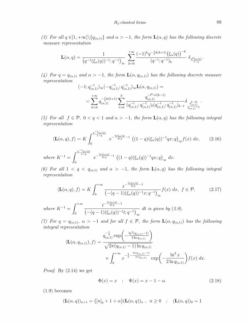
(3) For all q ∈]1,+∞[\{q(α,1)} and α > −1, the form L(α, q) has the following discretemeasure representation
L(α, q) =1(
q−1(ξα(q))−1; q−1)∞
+∞∑k=0
(−1)kq−12k(k+1)
(ξα(q)
)−k(q−1; q−1)k
δ qkξα(q)1−q
.
(4) For q = q(α,1) and α > −1, the form L(α, q(α,1)) has the following discrete measurerepresentation
(−1; q−1(α,1))∞(−q−1
(α,1); q−1(α,1))∞L(α, q(α,1)) =
=+∞∑k=0
q− 1
2k(k+1)
(α,1)
k∑l=0
q−l2+l(k−1)(α,1)
(q−1(α,1); q
−1(α,1))l(q
−1(α,1); q
−1(α,1))k−l
δ qk−2l(α,1)
q(α,1)−1
.
(5) For all f ∈ P , 0 < q < 1 and α > −1, the form L(α, q) has the following integralrepresentation
〈L(α, q), f〉 = K
∫ q−1ξα(q)1−q
0
x−ln ξα(q)
ln q−1((1− q)(ξα(q))
−1qx; q)∞f(x) dx, (2.16)
where K−1 =
∫ q−1ξα(q)1−q
0
x−ln ξα(q)
ln q−1((1− q)(ξα(q))
−1qx; q)∞ dx.
(6) For all 1 < q < q(α,1) and α > −1, the form L(α, q) has the following integralrepresentation
〈L(α, q), f〉 = K
∫ +∞
0
x−ln ξα(q)
ln q−1(
−(q − 1)(ξα(q))−1x; q−1)∞f(x) dx, f ∈ P , (2.17)
where K−1 =
∫ +∞
0
t−ln ξα(q)
ln q−1(
−(q − 1)(ξα(q))−1t; q−1)∞dt is given by (2.8).
(7) For q = q(α,1), α > −1 and for all f ∈ P, the form L(α, q(α,1)) has the followingintegral representation
〈L(α, q(α,1)), f〉 =
q− 1
8
(α,1) exp
(− ln2(q(α,1)−1)
2 ln q(α,1)
)√
2π(q(α,1) − 1) ln q(α,1)
×∫ +∞
0
x− 3
2−
ln(q(α,1)−1)
ln q(α,1) exp
(− ln2 x
2 ln q(α,1)
)f(x) dx.
Proof. By (2.14) we get
Φ(x) = x ; Ψ(x) = x− 1− α. (2.18)
(1.9) becomes
(L(α, q))n+1 =([n]q + 1 + α
)(L(α, q))n , n ≥ 0 ; (L(α, q))0 = 1
90 L. Kheriji, P. Maroni
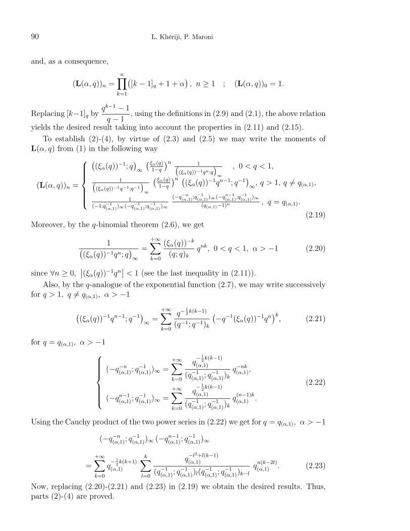
and, as a consequence,
(L(α, q))n =n∏k=1
([k − 1]q + 1 + α
), n ≥ 1 ; (L(α, q))0 = 1.
Replacing [k−1]q byqk−1 − 1
q − 1, using the definitions in (2.9) and (2.1), the above relation
yields the desired result taking into account the properties in (2.11) and (2.15).To establish (2)-(4), by virtue of (2.3) and (2.5) we may write the moments of
L(α, q) from (1) in the following way
(L(α, q))n =
((ξα(q))
−1; q)∞
( ξα(q)1−q
)n 1((ξα(q))−1qn;q
)∞
, 0 < q < 1,
1((ξα(q))−1q−1;q−1
)∞
( ξα(q)1−q
)n ((ξα(q))
−1qn−1; q−1)∞, q > 1, q 6= q(α,1),
1(−1;q−1
(α,1))∞(−q−1
(α,1);q−1
(α,1))∞
(−q−n(α,1)
;q−1(α,1)
)∞(−qn−1(α,1)
;q−1(α,1)
)∞
(q(α,1)−1)n , q = q(α,1).
(2.19)Moreover, by the q-binomial theorem (2.6), we get
1((ξα(q))−1qn; q
)∞
=+∞∑k=0
(ξα(q))−k
(q; q)kqnk, 0 < q < 1, α > −1 (2.20)
since ∀n ≥ 0,∣∣(ξα(q))−1qn
∣∣ < 1 (see the last inequality in (2.11)).Also, by the q-analogue of the exponential function (2.7), we may write successively
for q > 1, q 6= q(α,1), α > −1
((ξα(q))
−1qn−1; q−1)∞ =
+∞∑k=0
q−12k(k−1)
(q−1; q−1)k
(−q−1(ξα(q))
−1qn)k, (2.21)
for q = q(α,1), α > −1(−q−n(α,1); q
−1(α,1))∞ =
+∞∑k=0
q− 1
2k(k−1)
(α,1)
(q−1(α,1); q
−1(α,1))k
q−nk(α,1),
(−qn−1(α,1); q
−1(α,1))∞ =
+∞∑k=0
q− 1
2k(k−1)
(α,1)
(q−1(α,1); q
−1(α,1))k
q(n−1)k(α,1) .
(2.22)
Using the Cauchy product of the two power series in (2.22) we get for q = q(α,1), α > −1
(−q−n(α,1); q−1(α,1))∞ (−qn−1
(α,1); q−1(α,1))∞
=+∞∑k=0
q− 1
2k(k+1)
(α,1)
k∑l=0
q−l2+l(k−1)(α,1)
(q−1(α,1); q
−1(α,1))l(q
−1(α,1); q
−1(α,1))k−l
qn(k−2l)(α,1) . (2.23)
Now, replacing (2.20)-(2.21) and (2.23) in (2.19) we obtain the desired results. Thus,parts (2)-(4) are proved.
Hq-classical forms 91
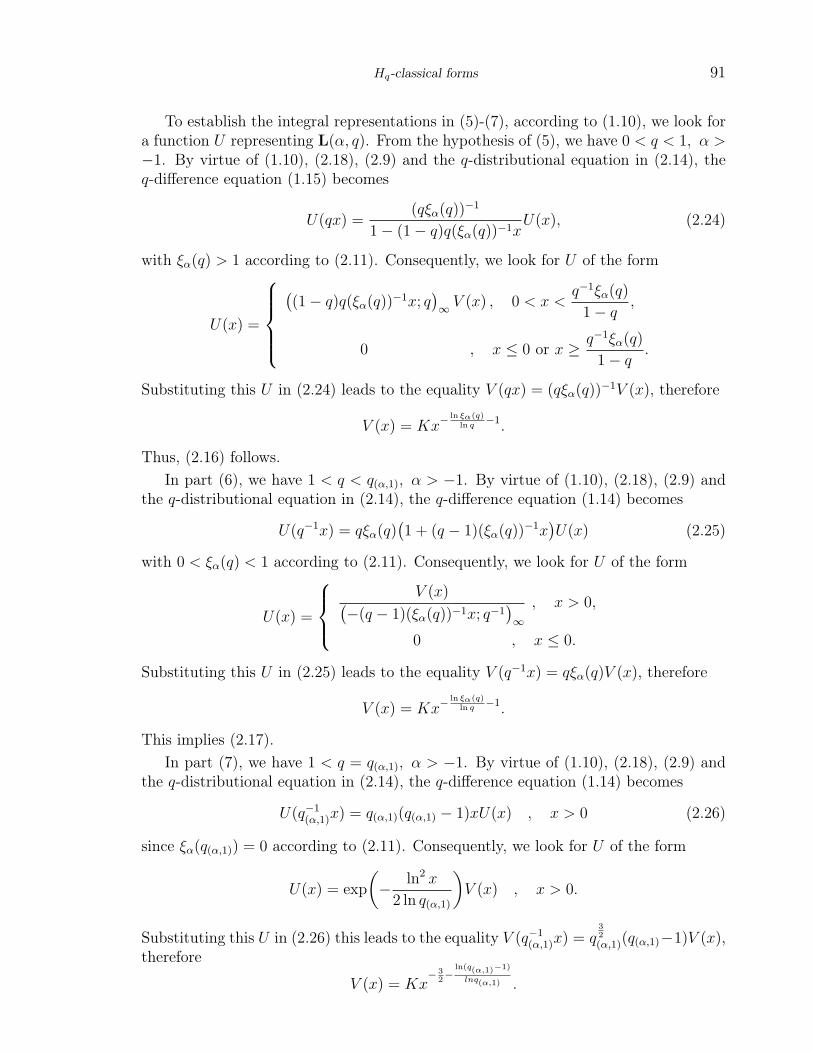
To establish the integral representations in (5)-(7), according to (1.10), we look fora function U representing L(α, q). From the hypothesis of (5), we have 0 < q < 1, α >−1. By virtue of (1.10), (2.18), (2.9) and the q-distributional equation in (2.14), theq-difference equation (1.15) becomes
U(qx) =(qξα(q))
−1
1− (1− q)q(ξα(q))−1xU(x), (2.24)
with ξα(q) > 1 according to (2.11). Consequently, we look for U of the form
U(x) =
((1− q)q(ξα(q))
−1x; q)∞ V (x) , 0 < x <
q−1ξα(q)
1− q,
0 , x ≤ 0 or x ≥ q−1ξα(q)
1− q.
Substituting this U in (2.24) leads to the equality V (qx) = (qξα(q))−1V (x), therefore
V (x) = Kx−ln ξα(q)
ln q−1.
Thus, (2.16) follows.In part (6), we have 1 < q < q(α,1), α > −1. By virtue of (1.10), (2.18), (2.9) and
the q-distributional equation in (2.14), the q-difference equation (1.14) becomes
U(q−1x) = qξα(q)(1 + (q − 1)(ξα(q))
−1x)U(x) (2.25)
with 0 < ξα(q) < 1 according to (2.11). Consequently, we look for U of the form
U(x) =
V (x)(
−(q − 1)(ξα(q))−1x; q−1)∞, x > 0,
0 , x ≤ 0.
Substituting this U in (2.25) leads to the equality V (q−1x) = qξα(q)V (x), therefore
V (x) = Kx−ln ξα(q)
ln q−1.
This implies (2.17).In part (7), we have 1 < q = q(α,1), α > −1. By virtue of (1.10), (2.18), (2.9) and
the q-distributional equation in (2.14), the q-difference equation (1.14) becomes
U(q−1(α,1)x) = q(α,1)(q(α,1) − 1)xU(x) , x > 0 (2.26)
since ξα(q(α,1)) = 0 according to (2.11). Consequently, we look for U of the form
U(x) = exp
(− ln2 x
2 ln q(α,1)
)V (x) , x > 0.
Substituting this U in (2.26) this leads to the equality V (q−1(α,1)x) = q
32
(α,1)(q(α,1)−1)V (x),therefore
V (x) = Kx− 3
2−
ln(q(α,1)−1)
lnq(α,1) .

92 L. Kheriji, P. Maroni
Let us now compute the constant K−1:
K−1 =
∫ +∞
0
x− 3
2−
ln(q(α,1)−1)
ln q(α,1) exp
(− ln2 x
2 ln q(α,1)
)dx.
By the change of variable: t = lnx√2 ln q(α,1)
we get
K−1 =√
2 ln q(α,1)
∫ +∞
−∞exp
(−
ln((q(α,1) − 1)2q(α,1)
)√2 ln q(α,1)
t− t2)dt.
Consequently, using the change of variable u = t+ 12
ln((q(α,1)−1)2q(α,1)
)√
2 ln q(α,1)
and taking into
account that∫ +∞
−∞exp(−u2) du =
√π, we get
K−1 =√
2π(q(α,1) − 1) ln q(α,1) q18
(α,1) exp
(ln2(q(α,1) − 1)
2 ln q(α,1)
),
whence the desired integral representation in (7).
Remarks. 1. Taking into account the representations in Proposition 2.2., we maywrite successively
2〈L(α, q), f〉 = K
∫ q−1ξα(q)1−q
0
x−ln ξα(q)
ln q−1((1− q)(ξα(q))
−1qx; q)∞f(x) dx+
+((ξα(q))
−1; q)∞
+∞∑k=0
(ξα(q)
)−k(q; q)k
〈δ qkξα(q)1−q
, f〉, f ∈ P , 0 < q < 1, α > −1,
2〈L(α, q), f〉 = K
∫ +∞
0
x−ln ξα(q)
ln q−1(
−(q − 1)(ξα(q))−1x; q−1)∞f(x) dx+
1(q−1(ξα(q))−1; q−1
)∞×
+∞∑k=0
(−1)kq−12k(k+1)
(ξα(q)
)−k(q−1; q−1)k
〈δ qkξα(q)1−q
, f〉, f ∈ P , 1 < q < q(α,1), α > −1,
and
2〈L(α, q(α,1)), f〉 =
q− 1
8
(α,1) exp
(− ln2(q(α,1)−1)
2 ln q(α,1)
)√
2π(q(α,1) − 1) ln q(α,1)×∫ +∞
0
x− 3
2−
ln(q(α,1)−1)
ln q(α,1) exp
(− ln2 x
2 ln q(α,1)
)f(x) dx+
1
(−1; q−1(α,1))∞(−q−1
(α,1); q−1(α,1))∞
×
+∞∑k=0
q− 1
2k(k+1)
(α,1)
k∑l=0
q−l2+l(k−1)(α,1)
(q−1(α,1); q
−1(α,1))l(q
−1(α,1); q
−1(α,1))k−l
〈δ qk−2l(α,1)
q(α,1)−1
, f〉, f ∈ P , α > −1.
2. Denoting by Uq the weight function given either by (2.16) or by (2.17), we have (see(1.4))
limq→1
∫ +∞
−∞Uq(x)f(x)dx =
1
Γ(α+ 1)
∫ +∞
0
xα exp(−x)f(x)dx = 〈L(α), f〉, f ∈ P .
Hq-classical forms 93
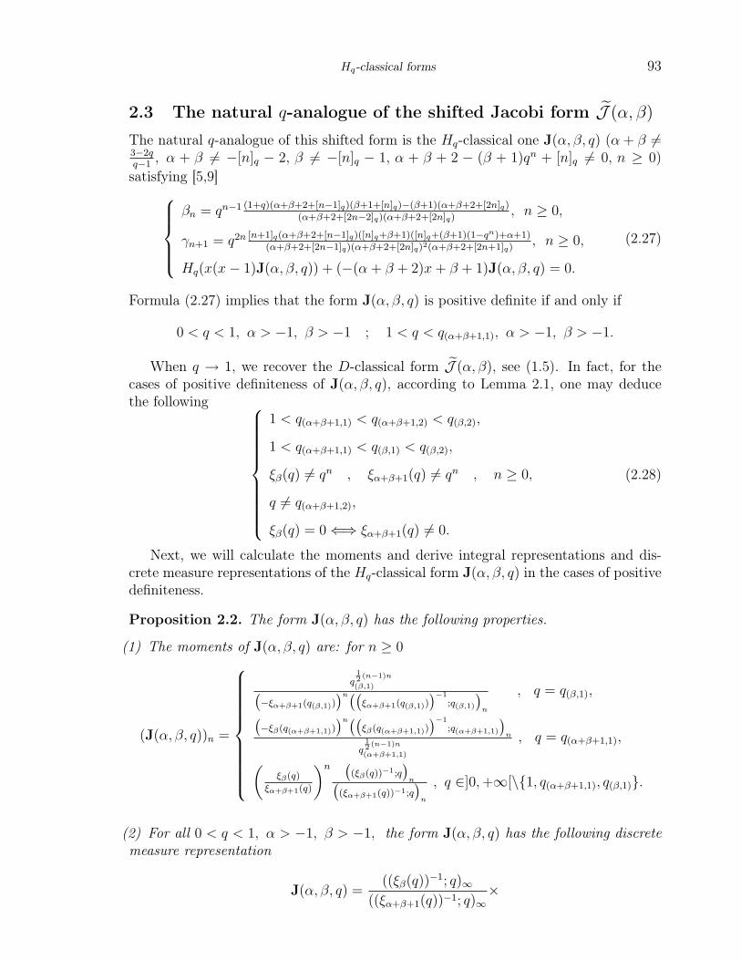
2.3 The natural q-analogue of the shifted Jacobi form J (α, β)
The natural q-analogue of this shifted form is the Hq-classical one J(α, β, q) (α + β 6=3−2qq−1
, α + β 6= −[n]q − 2, β 6= −[n]q − 1, α + β + 2 − (β + 1)qn + [n]q 6= 0, n ≥ 0)satisfying [5,9]
βn = qn−1 (1+q)(α+β+2+[n−1]q)(β+1+[n]q)−(β+1)(α+β+2+[2n]q)
(α+β+2+[2n−2]q)(α+β+2+[2n]q), n ≥ 0,
γn+1 = q2n [n+1]q(α+β+2+[n−1]q)([n]q+β+1)([n]q+(β+1)(1−qn)+α+1)
(α+β+2+[2n−1]q)(α+β+2+[2n]q)2(α+β+2+[2n+1]q), n ≥ 0,
Hq(x(x− 1)J(α, β, q)) + (−(α+ β + 2)x+ β + 1)J(α, β, q) = 0.
(2.27)
Formula (2.27) implies that the form J(α, β, q) is positive definite if and only if
0 < q < 1, α > −1, β > −1 ; 1 < q < q(α+β+1,1), α > −1, β > −1.
When q → 1, we recover the D-classical form J (α, β), see (1.5). In fact, for thecases of positive definiteness of J(α, β, q), according to Lemma 2.1, one may deducethe following
1 < q(α+β+1,1) < q(α+β+1,2) < q(β,2),
1 < q(α+β+1,1) < q(β,1) < q(β,2),
ξβ(q) 6= qn , ξα+β+1(q) 6= qn , n ≥ 0,
q 6= q(α+β+1,2),
ξβ(q) = 0 ⇐⇒ ξα+β+1(q) 6= 0.
(2.28)
Next, we will calculate the moments and derive integral representations and dis-crete measure representations of the Hq-classical form J(α, β, q) in the cases of positivedefiniteness.
Proposition 2.2. The form J(α, β, q) has the following properties.
(1) The moments of J(α, β, q) are: for n ≥ 0
(J(α, β, q))n =
q12 (n−1)n
(β,1)(−ξα+β+1(q(β,1))
)n((ξα+β+1(q(β,1))
)−1
;q(β,1)
)n
, q = q(β,1),(−ξβ(q(α+β+1,1))
)n((ξβ(q(α+β+1,1))
)−1
;q(α+β+1,1)
)n
q12 (n−1)n
(α+β+1,1)
, q = q(α+β+1,1),(ξβ(q)
ξα+β+1(q)
)n ((ξβ(q))−1;q
)n(
(ξα+β+1(q))−1;q)
n
, q ∈]0,+∞[\{1, q(α+β+1,1), q(β,1)}.
(2) For all 0 < q < 1, α > −1, β > −1, the form J(α, β, q) has the following discretemeasure representation
J(α, β, q) =((ξβ(q))
−1; q)∞((ξα+β+1(q))−1; q)∞
×
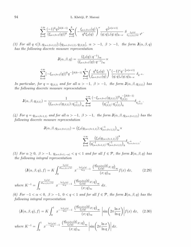
94 L. Kheriji, P. Maroni
+∞∑k=0
(−1)kq12k(k−1)
(ξα+β+1(q))k
k∑ν=0
(−ξα+β+1(q)
qkξβ(q)
)νq
12ν(ν+1)
(q; q)ν(q; q)k−νδ ξβ(q)
ξα+β+1(q)qk.
(3) For all q ∈]1, q(α+β+1,1)[∪]q(α+β+1,1), q(β,2)[, α > −1, β > −1, the form J(α, β, q)has the following discrete measure representation
J(α, β, q) =(ξβ(q); q
−1)∞(ξα+β+1(q); q−1)∞
×
+∞∑k=0
(−ξα+β+1(q))kq−
12k(k−1)
k∑ν=0
(qkξβ(q)
ξα+β+1(q)
)ν(−1)νq−
12ν(ν+1)
(q; q)ν(q; q)k−νδq−k .
In particular, for q = q(β,1) and for all α > −1, β > −1, the form J(α, β, q(β,1)) hasthe following discrete measure representation
J(α, β, q(β,1)) =1(
ξα+β+1(q(β,1)); q−1(β,1)
)∞
+∞∑k=0
(−ξα+β+1(q(β,1)))kq− 1
2k(k−1)
(β,1)(q−1(β,1); q
−1(β,1)
)k
δq−k(β,1)
.
(4) For q = q(α+β+1,1) and for all α > −1, β > −1, the form J(α, β, q(α+β+1,1)) has thefollowing discrete measure representation
J(α, β, q(α+β+1,1)) =(ξβ(q(α+β+1,1)); q
−1(α+β+1,1)
)∞×
+∞∑k=0
(ξβ(q(α+β+1,1))
)k(q−1(α+β+1,1); q
−1(α+β+1,1)
)k
δq−k(α+β+1,1)
.
(5) For α ≥ 0, β > −1, q(α+β+1,−α) < q < 1 and for all f ∈ P, the form J(α, β, q) hasthe following integral representation
〈J(α, β, q), f〉 = K
∫ ξβ(q)
qξα+β+1(q)
0
x−ln ξβ(q)
ln q−1
( qξα+β+1(q)
ξβ(q)x; q)∞
(x; q)∞f(x) dx, (2.29)
where K−1 =
∫ ξβ(q)
qξα+β+1(q)
0
x−ln ξβ(q)
ln q−1
( qξα+β+1(q)
ξβ(q)x; q)∞
(x; q)∞dx.
(6) For −1 < α < 0, β > −1, 0 < q < 1 and for all f ∈ P, the form J(α, β, q) has thefollowing integral representation
〈J(α, β, q), f〉 = K
∫ 1
0
x−ln ξβ(q)
ln q−1
( qξα+β+1(q)
ξβ(q)x; q)∞
(x; q)∞
∣∣∣∣sin(2πlnx
ln q
)∣∣∣∣f(x) dx, (2.30)
where K−1 =
∫ 1
0
x−ln ξβ(q)
ln q−1
( qξα+β+1(q)
ξβ(q)x; q)∞
(x; q)∞
∣∣∣∣sin(2πlnx
ln q
)∣∣∣∣ dx.
Hq-classical forms 95
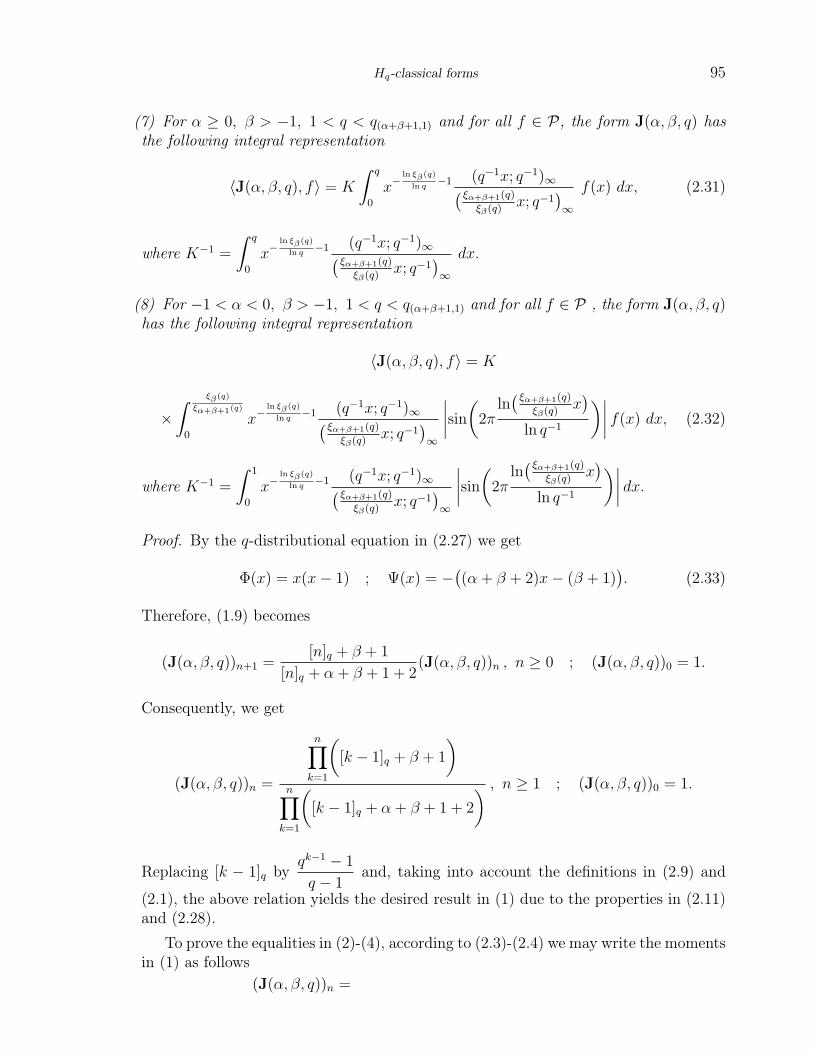
(7) For α ≥ 0, β > −1, 1 < q < q(α+β+1,1) and for all f ∈ P, the form J(α, β, q) hasthe following integral representation
〈J(α, β, q), f〉 = K
∫ q
0
x−ln ξβ(q)
ln q−1 (q−1x; q−1)∞( ξα+β+1(q)
ξβ(q)x; q−1
)∞
f(x) dx, (2.31)
where K−1 =
∫ q
0
x−ln ξβ(q)
ln q−1 (q−1x; q−1)∞( ξα+β+1(q)
ξβ(q)x; q−1
)∞
dx.
(8) For −1 < α < 0, β > −1, 1 < q < q(α+β+1,1) and for all f ∈ P , the form J(α, β, q)has the following integral representation
〈J(α, β, q), f〉 = K
×∫ ξβ(q)
ξα+β+1(q)
0
x−ln ξβ(q)
ln q−1 (q−1x; q−1)∞( ξα+β+1(q)
ξβ(q)x; q−1
)∞
∣∣∣∣sin(2πln( ξα+β+1(q)
ξβ(q)x)
ln q−1
)∣∣∣∣ f(x) dx, (2.32)
where K−1 =
∫ 1
0
x−ln ξβ(q)
ln q−1 (q−1x; q−1)∞( ξα+β+1(q)
ξβ(q)x; q−1
)∞
∣∣∣∣sin(2πln( ξα+β+1(q)
ξβ(q)x)
ln q−1
)∣∣∣∣ dx.Proof. By the q-distributional equation in (2.27) we get
Φ(x) = x(x− 1) ; Ψ(x) = −((α+ β + 2)x− (β + 1)
). (2.33)
Therefore, (1.9) becomes
(J(α, β, q))n+1 =[n]q + β + 1
[n]q + α+ β + 1 + 2(J(α, β, q))n , n ≥ 0 ; (J(α, β, q))0 = 1.
Consequently, we get
(J(α, β, q))n =
n∏k=1
([k − 1]q + β + 1
)n∏k=1
([k − 1]q + α+ β + 1 + 2
) , n ≥ 1 ; (J(α, β, q))0 = 1.
Replacing [k − 1]q byqk−1 − 1
q − 1and, taking into account the definitions in (2.9) and
(2.1), the above relation yields the desired result in (1) due to the properties in (2.11)and (2.28).
To prove the equalities in (2)-(4), according to (2.3)-(2.4) we may write the momentsin (1) as follows
(J(α, β, q))n =
96 L. Kheriji, P. Maroni
((ξβ(q))
−1; q)∞(
(ξα+β+1(q))−1; q)∞
(ξβ(q)
ξα+β+1(q)
)n ((ξα+β+1(q))−1qn; q
)∞(
(ξβ(q))−1qn; q)∞
, 0 < q < 1,(ξβ(q); q
−1)∞(
ξα+β+1(q); q−1)∞
(ξα+β+1(q)q
−n; q−1)∞(
ξβ(q)q−n; q−1)∞
, q > 1.
(2.34)
For the first case of (2.34), by (2.6)-(2.7) and since ∀n ≥ 0, |(ξβ(q))−1qn| < 1 (see(2.11)); we get for all 0 < q < 1, α > −1, β > −1, n ≥ 0
(J(α, β, q))n =
((ξβ(q))
−1; q)∞(
(ξα+β+1(q))−1; q)∞
(ξβ(q)
ξα+β+1(q)
)n×
+∞∑k=0
(ξβ(q))−k
(q; q)kqnk
+∞∑k=0
(−1)kq12k(k−1)(ξα+β+1(q))
−k
(q; q)kqnk.
Hence we get the desired discrete measure representation in (2).For the second case of (2.34), by (2.6)-(2.7) and since ∀n ≥ 0, |(ξβ(q))−1qn| < 1
(see (2.11)); we get for all q ∈]1, q(β,2)[, α > −1, β > −1, n ≥ 0
(J(α, β, q))n =
(ξβ(q); q
−1)∞(
ξα+β+1(q); q−1)∞×
+∞∑k=0
(ξβ(q))k
(q−1; q−1)kq−nk
+∞∑k=0
(−1)kq−12k(k−1)(ξα+β+1(q))
k
(q−1; q−1)kq−nk.
The Cauchy product implies the desired first representation in (3). Moreover, thesecond representation in (3) is a direct corollary of the first one with q = q(β,1).
On the other hand, taking q = q(α+β+1,1) in the second equality of (2.34), it becomes
(J(α, β, q(α+β+1,1))n =
(ξβ(q(α+β+1,1)); q
−1(α+β+1,1)
)∞(
ξβ(q(α+β+1,1))q−n(α+β+1,1); q
−1(α+β+1,1)
)∞
(2.35)
because ξα+β+1(q(α+β+1,1)) = 0.
According to (2.9)-(2.10) and to the fact that q(α+β+1,1) > 1, α > −1, β > −1 wehave
∀n ≥ 0,
∣∣∣∣ξβ(q(α+β+1,1))q−n(α+β+1,1)
∣∣∣∣ < ∣∣ξβ(q(α+β+1,1))∣∣ =
α+ 1
α+ β + 2< 1.
By (2.6), (2.35) becomes
(J(α, β, q(α+β+1,1))n =(ξβ(q(α+β+1,1)); q
−1(α+β+1,1)
)∞
+∞∑k=0
(ξβ(q(α+β+1,1))
)kq−nk(α+β+1,1)(
q−1(α+β+1,1); q
−1(α+β+1,1)
)k
from which we deduce the discrete measure representation in (4).

Hq-classical forms 97
To establish the integral representations in (5)-(6), taking into account (1.10), welook for a function U representing J(α, β, q).
By virtue of (1.10), (2.33), (2.9) and the q-distributional equation in (2.27), theq-difference equation (1.15) becomes
U(qx) = (qξβ(q))−1 1− x
1− qξα+β+1(q)
ξβ(q)xU(x). (2.36)
But, taking α > −1, β > −1, 0 < q < 1 it is quite straightforward to get the followingequivalences
0 <ξβ(q)
qξα+β+1(q)< 1 ⇐⇒ q >
β + 2
α+ β + 2= q(α+β+1,−α),
0 < q(α+β+1,−α) < 1 ⇐⇒ α ≥ 0, (2.37)
andq(α+β+1,−α) > 1 ⇐⇒ α < 0. (2.38)
Consequently, if α ≥ 0, β > −1, q(α+β+1,−α) < q < 1, we look for U of the form
U(x) =
xη
(qξα+β+1(q)
ξβ(q)x;q)∞
(x;q)∞, 0 < x <
ξβ(q)
qξα+β+1(q),
0 , x ≤ 0 or x ≥ ξβ(q)
qξα+β+1(q).
Substituting this U in (2.36) leads to the equality η = − ln ξβ(q)
ln q− 1, and we get the
result in (2.29).Also, if −1 < α < 0, β > −1, 0 < q < 1, we look for U of the form
U(x) =
x−ln ξβ(q)
ln q−1
(qξα+β+1(q)
ξβ(q)x;q)∞
(x;q)∞V (x) , 0 < x < 1,
0 , x ≤ 0 or x ≥ 1.
(2.39)
Substituting this U in (2.36) leads to the equality V (qx) = V (x). Taking into account(2.39), we may choose
V (x) = K
∣∣∣∣sin(2πlnx
ln q
)∣∣∣∣.Thus (2.30) follows.
From the hypotheses of (7)-(8), we have α > −1, β > −1, 1 < q < q(α+β+1,1). Byvirtue of (1.10), (2.33), (2.9) and the q-distributional equation in (2.27), the q-differenceequation (1.14) becomes
U(q−1x) = qξβ(q)1− ξα+β+1(q)
ξβ(q)x
1− q−1xU(x). (2.40)
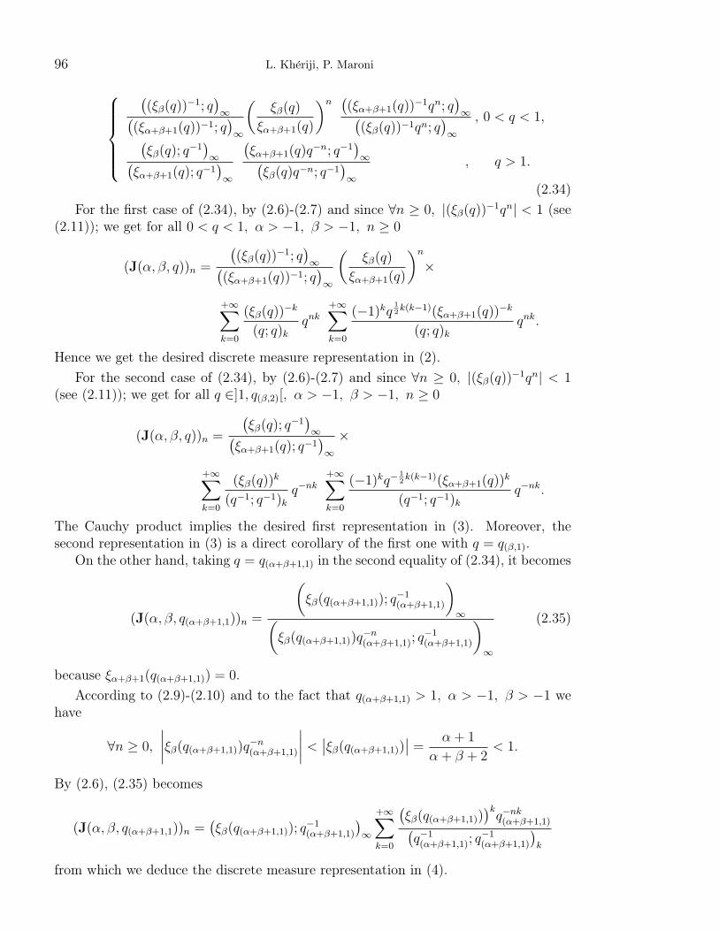
98 L. Kheriji, P. Maroni
According to (2.11), (2.28) and (2.37)-(2.38), we have
0 < ξα+β+1(q) < ξβ(q) < 1 , 1 < q < q(α+β+1,1),
ξβ(q)
ξα+β+1(q)> q ⇐⇒ q > q(α+β+1,−α).
Therefore, if α ≥ 0, β > −1, 1 < q < q(α+β+1,1) we get
U(x) =
Kx−
ln ξβ(q)
ln q−1 (q−1x;q−1)∞(
ξα+β+1(q)
ξβ(q)x;q−1
)∞
, 0 < x < q,
0 , x ≤ 0 or x ≥ q,
from which we obtain the result in (2.31).Finally, if −1 < α < 0, β > −1, 1 < q < min
(q(α+β+1,1), q(α+β+1,−α)
)= q(α+β+1,1), we
look for U of the form
U(x) =
x−
ln ξβ(q)
ln q−1
(q−1x; q−1
)∞( ξα+β+1(q)
ξβ(q)x; q−1
)∞
V (x) , 0 < x <ξβ(q)
ξα+β+1(q),
0 , x ≤ 0 or x ≥ ξβ(q)
ξα+β+1(q).
(2.41)
Substituting this U in (2.40) leads to the equality V (qx) = V (x). Taking into account(2.41), we may choose
V (x) = K
∣∣∣∣sin(2πln( ξα+β+1(q)
ξβ(q)x)
ln q−1
)∣∣∣∣.Thus (2.32) follows.
Remark. Denoting by Uq the weight function given either by (2.29) or by (2.31), wehave for all f ∈ P (see (1.5))
limq→1
∫ +∞
−∞Uq(x)f(x)dx =
Γ(α+ β + 2)
Γ(α+ 1)Γ(β + 1)
∫ 1
0
xβ(1− x)αf(x)dx = 〈J (α, β), f〉.
3 The natural q-analogue of the Bessel D-classical form
The natural q-analogue of the Bessel form is the Hq-classical form B(α, q) (α 6= 12(q −
1)−1, α 6= −12[n]q, n ≥ 0) satisfying [5,9]
βn = −2qn 2α+(1+q−1)[n−1]q−q−1[2n]q(2α+[2n−2]q)(2α+[2n]q)
, n ≥ 0,
γn+1 = −4q3n [n+1]q(2α+[n−1]q)
(2α+[2n−1]q)(2α+[2n]q)2(2α+[2n+1]q), n ≥ 0,
Hq(x2B(α, q))− 2(αx+ 1)B(α, q) = 0.
(3.1)
By (3.1), the form B(α, q) is not positive definite for any value of its parameter α.When q → 1, we recover the Bessel D-classical form B(α) in (1.6).Due to the regularity conditions α 6= 1
2(q − 1)−1, α 6= −1
2[n]q, n ≥ 0 we get
ξ2α−1(q) 6= 0 ; ξ2α−1(q) 6= qn , n ≥ 0. (3.2)
Hq-classical forms 99
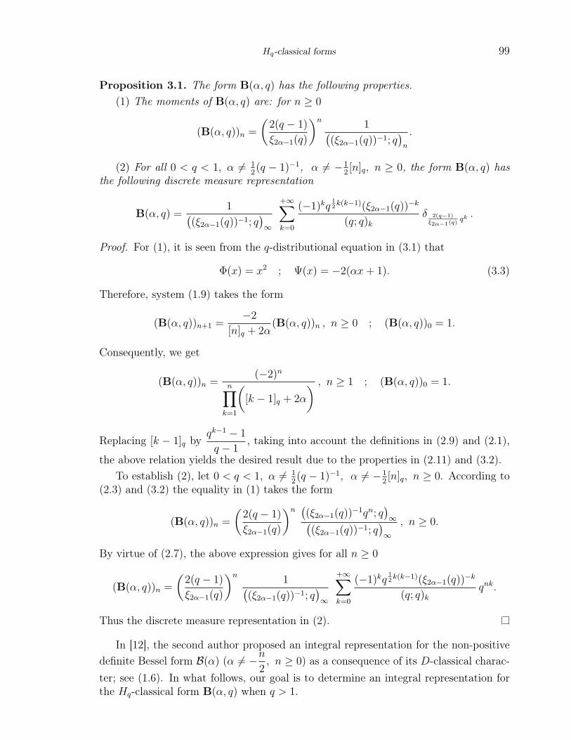
Proposition 3.1. The form B(α, q) has the following properties.(1) The moments of B(α, q) are: for n ≥ 0
(B(α, q))n =
(2(q − 1)
ξ2α−1(q)
)n1(
(ξ2α−1(q))−1; q)n
.
(2) For all 0 < q < 1, α 6= 12(q − 1)−1, α 6= −1
2[n]q, n ≥ 0, the form B(α, q) has
the following discrete measure representation
B(α, q) =1(
(ξ2α−1(q))−1; q)∞
+∞∑k=0
(−1)kq12k(k−1)(ξ2α−1(q))
−k
(q; q)kδ 2(q−1)
ξ2α−1(q)qk .
Proof. For (1), it is seen from the q-distributional equation in (3.1) that
Φ(x) = x2 ; Ψ(x) = −2(αx+ 1). (3.3)
Therefore, system (1.9) takes the form
(B(α, q))n+1 =−2
[n]q + 2α(B(α, q))n , n ≥ 0 ; (B(α, q))0 = 1.
Consequently, we get
(B(α, q))n =(−2)n
n∏k=1
([k − 1]q + 2α
) , n ≥ 1 ; (B(α, q))0 = 1.
Replacing [k − 1]q byqk−1 − 1
q − 1, taking into account the definitions in (2.9) and (2.1),
the above relation yields the desired result due to the properties in (2.11) and (3.2).To establish (2), let 0 < q < 1, α 6= 1
2(q − 1)−1, α 6= −1
2[n]q, n ≥ 0. According to
(2.3) and (3.2) the equality in (1) takes the form
(B(α, q))n =
(2(q − 1)
ξ2α−1(q)
)n ((ξ2α−1(q))−1qn; q
)∞(
(ξ2α−1(q))−1; q)∞
, n ≥ 0.
By virtue of (2.7), the above expression gives for all n ≥ 0
(B(α, q))n =
(2(q − 1)
ξ2α−1(q)
)n1(
(ξ2α−1(q))−1; q)∞
+∞∑k=0
(−1)kq12k(k−1)(ξ2α−1(q))
−k
(q; q)kqnk.
Thus the discrete measure representation in (2).
In [12], the second author proposed an integral representation for the non-positivedefinite Bessel form B(α) (α 6= −n
2, n ≥ 0) as a consequence of its D-classical charac-
ter; see (1.6). In what follows, our goal is to determine an integral representation forthe Hq-classical form B(α, q) when q > 1.
100 L. Kheriji, P. Maroni
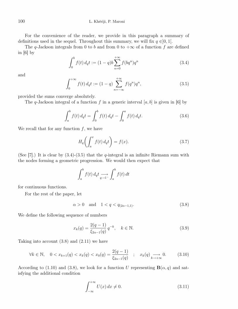
For the convenience of the reader, we provide in this paragraph a summary ofdefinitions used in the sequel. Throughout this summary, we will fix q ∈]0, 1[.
The q-Jackson integrals from 0 to b and from 0 to +∞ of a function f are definedin [6] by ∫ b
0
f(t) dqt := (1− q)b+∞∑n=0
f(bqn)qn (3.4)
and ∫ +∞
0
f(t) dqt := (1− q)+∞∑
n=−∞
f(qn)qn, (3.5)
provided the sums converge absolutely.The q-Jackson integral of a function f in a generic interval [a, b] is given in [6] by∫ b
a
f(t) dqt =
∫ b
0
f(t) dqt−∫ a
0
f(t) dqt. (3.6)
We recall that for any function f , we have
Hq
(∫ x
a
f(t) dqt
)= f(x). (3.7)
(See [7].) It is clear by (3.4)-(3.5) that the q-integral is an infinite Riemann sum withthe nodes forming a geometric progression. We would then expect that∫ b
a
f(t) dqt −→q→1−
∫ b
a
f(t) dt
for continuous functions.For the rest of the paper, let
α > 0 and 1 < q < q(2α−1,1). (3.8)
We define the following sequence of numbers
xk(q) =2(q − 1)
ξ2α−1(q)q−k, k ∈ N. (3.9)
Taking into account (3.8) and (2.11) we have
∀k ∈ N, 0 < xk+1(q) < xk(q) < x0(q) =2(q − 1)
ξ2α−1(q); xk(q) −→
k→+∞0. (3.10)
According to (1.10) and (3.8), we look for a function U representing B(α, q) and sat-isfying the additional condition ∫ +∞
−∞U(x) dx 6= 0. (3.11)
Hq-classical forms 101
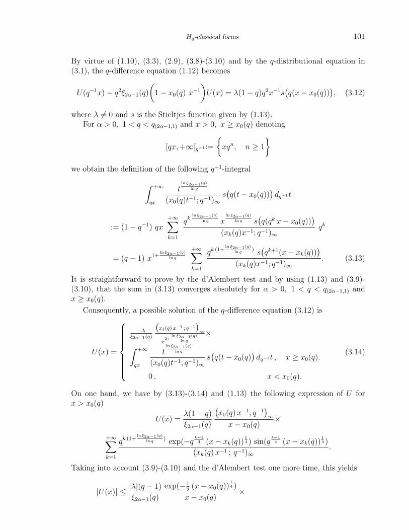
By virtue of (1.10), (3.3), (2.9), (3.8)-(3.10) and by the q-distributional equation in(3.1), the q-difference equation (1.12) becomes
U(q−1x)− q2ξ2α−1(q)
(1− x0(q) x
−1
)U(x) = λ(1− q)q2x−1s
(q(x− x0(q))
), (3.12)
where λ 6= 0 and s is the Stieltjes function given by (1.13).For α > 0, 1 < q < q(2α−1,1) and x > 0, x ≥ x0(q) denoting
[qx,+∞[q−1 :=
{xqn, n ≥ 1
}we obtain the definition of the following q−1-integral∫ +∞
qx
tln ξ2α−1(q)
ln q
(x0(q)t−1; q−1)∞s(q(t− x0(q))
)dq−1t
:= (1− q−1) qx+∞∑k=1
qkln ξ2α−1(q)
ln q xln ξ2α−1(q)
ln q s(q(qk x− x0(q))
)(xk(q)x−1; q−1)∞
qk
= (q − 1) x1+ln ξ2α−1(q)
ln q
+∞∑k=1
qk (1+ln ξ2α−1(q)
ln q) s(qk+1(x− xk(q))
)(xk(q)x−1; q−1)∞
. (3.13)
It is straightforward to prove by the d’Alembert test and by using (1.13) and (3.9)-(3.10), that the sum in (3.13) converges absolutely for α > 0, 1 < q < q(2α−1,1) andx ≥ x0(q).
Consequently, a possible solution of the q-difference equation (3.12) is
U(x) =
−λξ2α−1(q)
(x1(q)x−1 ; q−1
)∞
x2+
ln ξ2α−1(q)
ln q
×∫ +∞
qx
tln ξ2α−1(q)
ln q
(x0(q)t−1; q−1)∞s(q(t− x0(q)
)dq−1t , x ≥ x0(q).
0 , x < x0(q).
(3.14)
On one hand, we have by (3.13)-(3.14) and (1.13) the following expression of U forx > x0(q)
U(x) =λ(1− q)
ξ2α−1(q)
(x0(q)x
−1; q−1)∞
x− x0(q)×
+∞∑k=1
qk (1+ln ξ2α−1(q)
ln q) exp(−q k+1
4 (x− xk(q))14 ) sin(q
k+14 (x− xk(q))
14 )
(xk(q)x−1 ; q−1)∞.
Taking into account (3.9)-(3.10) and the d’Alembert test one more time, this yields
|U(x)| ≤ |λ|(q − 1)
ξ2α−1(q)
exp(−12(x− x0(q))
14 )
x− x0(q)×
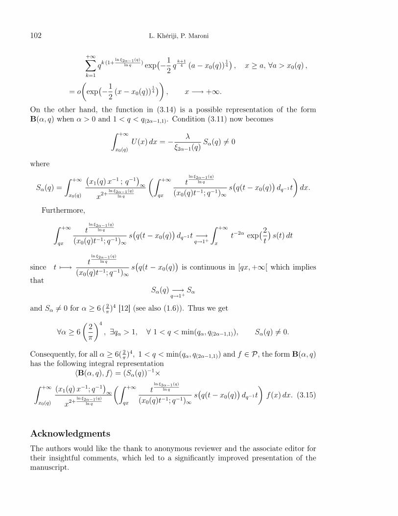
102 L. Kheriji, P. Maroni
+∞∑k=1
qk (1+ln ξ2α−1(q)
ln q) exp
(−1
2q
k+14 (a− x0(q))
14
), x ≥ a, ∀a > x0(q) ,
= o
(exp(−1
2(x− x0(q))
14
)), x −→ +∞.
On the other hand, the function in (3.14) is a possible representation of the formB(α, q) when α > 0 and 1 < q < q(2α−1,1). Condition (3.11) now becomes∫ +∞
x0(q)
U(x) dx = − λ
ξ2α−1(q)Sα(q) 6= 0
where
Sα(q) =
∫ +∞
x0(q)
(x1(q)x
−1 ; q−1)∞
x2+ln ξ2α−1(q)
ln q
(∫ +∞
qx
tln ξ2α−1(q)
ln q
(x0(q)t−1; q−1)∞s(q(t− x0(q)
)dq−1t
)dx.
Furthermore,∫ +∞
qx
tln ξ2α−1(q)
ln q
(x0(q)t−1; q−1)∞s(q(t− x0(q)
)dq−1t −→
q→1+
∫ +∞
x
t−2α exp(2t
)s(t) dt
since t 7−→ tln ξ2α−1(q)
ln q
(x0(q)t−1; q−1)∞s(q(t − x0(q)
)is continuous in [qx,+∞[ which implies
thatSα(q) −→
q→1+Sα
and Sα 6= 0 for α ≥ 6 ( 2π)4 [12] (see also (1.6)). Thus we get
∀α ≥ 6
(2
π
)4
, ∃qα > 1, ∀ 1 < q < min(qα, q(2α−1,1)), Sα(q) 6= 0.
Consequently, for all α ≥ 6( 2π)4, 1 < q < min(qα, q(2α−1,1)) and f ∈ P , the form B(α, q)
has the following integral representation〈B(α, q), f〉 = (Sα(q))
−1×∫ +∞
x0(q)
(x1(q)x−1; q−1
)∞
x2+ln ξ2α−1(q)
ln q
(∫ +∞
qx
tln ξ2α−1(q)
ln q
(x0(q)t−1; q−1)∞s(q(t− x0(q)
)dq−1t
)f(x) dx. (3.15)
Acknowledgments
The authors would like the thank to anonymous reviewer and the associate editor fortheir insightful comments, which led to a significantly improved presentation of themanuscript.
Hq-classical forms 103
References
[1] F. Abdelkarim, P. Maroni, The Dω-classical orthogonal polynomials, Results in Math. 32 (1997),1-28.
[2] C. Berg, M.E.H. Ismail, q-Hermite polynomials and classical orthogonal polynomials, Canad. J.Math. 48 (1996), no. 1, 43-63.
[3] C. Berg, A. Ruffing, Generalized q-Hermite polynomials, Commun. Math. Phy. 223 (2004), no.1, 29-46.
[4] G. Gasper, M. Rahman, Basic hypergeometric series, Cambridge University Press, Cambridge,1990.
[5] A. Ghressi, L. Kheriji, The symmetrical Hq-semiclassical orthogonal polynomials of class one,SIGMA. 5 (2009), 076, 22 pages.
[6] F.H. Jackson, On a q-definite integrals, Quarterly J. Pure Appl. Math. 41 (1910), 193-203.
[7] V.G. Kac, P. Cheung, Quantum calculus, Universitext, Springer-Verlag, New York, 2002.
[8] O.F. Kamech, M. Mejri, Some discrete representations of q-classical linear forms, Appl. Math.E-notes. 9 (2009), 34-39.
[9] L. Kheriji, P. Maroni, The Hq-classical orthogonal polynomials, Acta. Appl. Math. 71 (2002),no. 1, 49-115.
[10] R. Koekoek, R.F. Swarttouw, The Askey-scheme of hypergeometric orthogonal polynomials andits q-analogue, Reports of the Faculty of Technical Mathematics and Informatics. Report 98-17.Delft University of Technology, TU Delft 1998.
[11] P. Maroni, Variations around classical orthogonal polynomials. Connected problems, J. Comput.Appl. Math. 48 (1993), 133-155.
[12] P. Maroni, An integral representation for the Bessel form, J. Comp. Appl. Math. 57 (1995),251-260.
[13] P. Maroni, M. Mejri, Some semiclassical orthogonal polynomials of class one, Eurasian Math. J.2 (2011), no.2, 108-128.
[14] M. Mejri, q-Extension of some symmetrical and semi-classical orthogonal polynomials of classone, Appl. Anal. Discrete Math. 3 (2009), 78-87.
[15] D.S. Moak, The q-analogue of the Laguerre polynomials, J. Math. Anal. Appl. 81 (1981), no. 1,20-47.
[16] T.J. Stieltjes, Recherches sur les fractions continues, Ann. Fac. Sci. Toulouse. 8 (1894), J. 1-122;9 (1895) A1-A47.
Lotfi KherijiInstitut Superieur des Sciences Appliquees et de Technologie de GabesRue Omar Ibn El Khattab 6072-Gabes, Tunisia.E-mail: [email protected] or [email protected] MaroniUMR 7598 Laboratoire Jacques-Luis LionsUniversite Pierre et Marie Curie Paris 6, CNRSBoite courrier 18775252 Paris cedex 05, FranceE-mail: [email protected] Received: 25.05.2011