Multinucleon mechanisms in (gamma,N) and (gamma,NN) reactions
Upload
independentCategory
view
2download
0
arX
iv:n
ucl-
th/9
9120
60v1
24
Dec
199
9
1
Lippmann-Schwinger Resonating-Group Formalism for NN andY N Interactions in an SU6 Quark Model
Yoshikazu Fujiwara, Michio Kohno∗, Tadashi Fujita, Choki Nakamoto∗∗ andYasuyuki Suzuki∗∗∗
Department of Physics, Kyoto University, Kyoto 606-8502∗Physics Division, Kyushu Dental College, Kitakyushu 803-8580, Japan
∗∗Suzuka National College of Technology, Suzuka 510-0294, Japan∗∗∗Department of Physics, Niigata University, Niigata 950-2181, Japan
(Received July 30, 2013)
We formulate a Lippmann-Schwinger-type resonating-group equation to calculate invari-ant amplitudes of the quark-model baryon-baryon interaction. When applied to our recentSU6 quark model for the nucleon-nucleon and hyperon-nucleon interactions, this techniqueyields very accurate phase-shift parameters for all partial waves up to the energies of severalGeV. The technique also has a merit of a straightforward extension to the G-matrix equa-tion. A new analytic method is proposed to calculate the quark-exchange Born kernel forthe momentum-dependent two-body interaction. The partial-wave decomposition in the mo-mentum representation is carried out numerically. The invariant amplitudes are then usedto calculate single-nucleon potentials in normal nuclear matter for high incident momentaq1 ≥ 3 fm−1, in which the so-called teffρ prescription is found to be a good approximationto the single-particle potentials directly calculated in the lowest-order Brueckner theory.
§1. Introduction
Though the quantum chromodynamics (QCD) is believed to be the fundamentaltheory of the strong interaction, it is still too difficult to apply it directly to two-baryon systems. At this stage a number of effective models have been proposed tounderstand the nucleon-nucleon (NN) and hyperon-nucleon (Y N) interactions frombasic elements of quarks and gluons. 1) Among them the non-relativistic quark modelhas a unique feature that it enables us to take full account of a dynamical motionof the two composite baryons within a framework of the resonating-group method(RGM). 2) The model describes confinement with a phenomenological potential anduses quark-quark (qq) residual interactions consisting of a color analogue of theFermi-Breit (FB) interaction. In the last several years, it was found that a properincorporation of the meson-exchange effect is essential to make such a model realisticfor the description of the NN and Y N interactions. 3), 4), 5), 6), 7), 8), 9), 10)
We have recently achieved a simultaneous description of the NN and Y N in-teractions in the RGM formulation of the spin-flavor SU6 quark model. 3), 4), 5), 6), 7)
In this model the meson-exchange effect of scalar (S) and pseudo-scalar (PS) mesonnonets is incorporated in the quark Hamiltonian in the form of effective meson-exchange potentials (EMEP) acting between quarks. The flavor symmetry breakingfor the Y N system is explicitly introduced through the quark-mass dependence ofthe Hamiltonian, as well as the flavor dependence of the exchanged meson masses.

2 Y. Fujiwara, M. Kohno, T. Fujita, C. Nakamoto and Y. Suzuki
An advantage of introducing the EMEP at the quark level lies in the stringent re-lationship of the flavor dependence, which is revealed in the various pieces of theNN and Y N interactions. In this way we can utilize our rich knowledge of the NNinteraction to minimize the ambiguity of model parameters, which originates fromthe scarcity of the present experimental data for the Y N interaction.
We already have three different versions called RGM-F 3), 4), FSS 5), 6), 7) andRGM-H 6), 7), differing in the treatment of the EMEP. The model called RGM-Fintroduces, besides the central force of the S-meson nonet, only the tensor componentgenerated from the π- and K-meson exchanges, and uses some approximations inevaluating the spin-flavor factors of the quark-exchange RGM kernel. On the otherhand, FSS and RGM-H calculate the spin-flavor factors explicitly at the quark level,and include the spin-spin terms originating from all members of the PS-meson nonet.The SU3 relation of the coupling constants emerges as a natural consequence of theSU6 quark model. For S-mesons, the F/(F +D) ratio turns out to take the SU6 valueof purely electric type. This is too restrictive to reproduce existing experimental datafor the low-energy Y N cross sections. We relax this restriction in two ways; one isto change the mixing angle of the flavor-singlet and octet scalar mesons only forthe ΣN(I = 3/2) channel, and the other is to employ the same approximation asRGM-F solely for the isoscalar S-mesons, ǫ and S∗. We call these models FSS andRGM-H, respectively. Predictions of these two models are not very different exceptfor the roles of the LS(−) force in the ΛN - ΣN(I = 1/2) coupled-channel system.The SU3 parameters of EMEP, S-meson masses, and the quark-model parameters aredetermined to fit the NN S-wave and P -wave phase shifts under the constraint thatthe deuteron binding energy and the 1S0 scattering length are properly reproduced.The low-energy cross section data for Y N scattering are also employed to fix theparameters in the strangeness sector, especially the up-down to strange quark-massratio λ = ms/mud. The reader is referred to the original papers 6), 7) for a full accountof the models and the model parameters.
So far we have solved the coupled-channel (CC) RGM equation in the improvedvariational method developed by Kamimura 11). In this method each Gaussian ba-sis function is smoothly connected to the positive- or negative-energy asymptoticwaves, which are obtained by numerically solving a “local” CC Schrodinger equationconsisting of the long-range one-pion tensor force and the other EMEP. Althoughthis technique gives accurate results at laboratory energies up to about 300 MeV, itseems almost inaccessible to higher energies due to the rapid oscillation of the rela-tive wave functions. In this paper we formulate an alternative method to solve theCC RGM equation in the momentum representation; namely, we derive a Lippmann-Schwinger-type RGM equation which we call an LS-RGM equation.∗) In this methodall the necessary Born amplitudes (or the Born kernel) for the quark-exchange kernelare analytically derived by using a new transformation formula, which is specificallydeveloped for momentum-dependent two-body interactions acting between quarks.The partial wave decomposition of the Born kernel is carried out numerically in the
∗) The idea to solve the RGM equation in the momentum representation, in order to avoid the
rapid oscillation of relative wave functions at higher energies, is not new. See, for example, Ref. 12).

Lippmann-Schwinger RGM Formalism 3
Gauss-Legendre integral quadrature. The LS-RGM equation is then solved by usingthe techniques developed by Noyes 13) and Kowalski 14). Although this method re-quires more CPU time than the variational method, it gives very stable and accurateresults over a wide energy range. Since we first calculate the Born amplitudes of theRGM kernel, it is almost straightforward to proceed to the G-matrix calculation. 15)
As an application of the present formalism, we discuss single-particle (s.p.) po-tentials in normal nuclear matter. This application is motivated by the G-matrixcalculation of the NN and Y N interactions in the continuous prescription of inter-mediate spectra 15). The s.p. potentials of the nucleon and hyperons predicted bythe model FSS have a flaw that they are too attractive in the momentum regionq1 = 5 ∼ 20 fm−1. We will show that this particular feature of FSS is related tothe ill-behavior of the spin-independent central invariant amplitude at the forwardangles, which is traced back to too simple S-meson exchange EMEP in this model.We analyze this problem by using an approximation of the s.p. potential in theasymptotic momentum region, in terms of the T -matrix solution of the LS-RGMequation. This technique is sometimes called the teffρ prescription. We find thatthis procedure gives a fairly good approximation of the s.p. potentials predictedby the G-matrix calculation, even for such a small momentum as q1 ∼ 3 fm−1
(Tlab ∼ 200 MeV), as long as the real part of the s.p. potential is concerned.In the next section we start from the standard RGM equation for the (3q)-(3q)
system and derive the LS-RGM equation in the momentum space. Appendix A givesa convenient formula to calculate the Born kernel of the quark-exchange RGM kernel.The formula is especially useful in the case of the momentum-dependent qq force.The Born kernel of FSS is explicitly given in § 2.2 and in Appendix B. Since theflavor dependence of the spin-flavor factors plays an essential role in the applicationof the present formalism to the NN and Y N interactions, the structure of the Bornkernel and the scattering amplitudes is carefully described in § 2.3 in terms of thePauli-spinor invariants. Some useful expressions of the partial wave decompositionof the Born kernel and the invariant amplitudes are given in Appendices C and D,respectively. The teffρ prescription is derived in § 2.4 as a method to calculate theasymptotic behavior of the s.p. potentials in the G-matrix calculation. In § 3 wecompare the phase-shift parameters obtained by the LS-RGM formalism with thoseby the improved variational method. The system we choose as an example is themost complicated system of the ΛN - ΣN(I = 1/2) channel coupling. The invariantamplitudes and the scattering observables of the NN system in the intermediateenergies between Tlab = 400 ∼ 800 MeV are discussed in § 4. The s.p. potential of thenucleon in normal nuclear matter is calculated in § 5, by using the teffρ prescription.It is shown that the behavior of the spin-independent central invariant amplitude atthe forward angles is related to the attractive behavior of the s.p. potentials aroundq1 = 5 ∼ 20 fm−1 region. Also shown is a preliminary result of s.p. potentials inan improved model, which incorporates momentum-dependent higher-order terms ofthe S and vector (V) meson EMEP. Finally, § 6 is devoted to a brief summary.
4 Y. Fujiwara, M. Kohno, T. Fujita, C. Nakamoto and Y. Suzuki
§2. Formulation
2.1. LS-RGM equation
As mentioned in the Introduction, FSS 5), 6), 7), RGM-H 6), 7) and their precedingversion RGM-F 3), 4) are formulated in the (3q)-(3q) RGM applied to the system oftwo (0s)3 clusters. The qq interaction is composed of the full FB interaction withexplicit quark-mass dependence, a simple confinement potential of quadratic powerlaw and EMEP acting between quarks. The RGM equation for the parity-projectedrelative wave function χπ
α(R) is derived from the variational principle 〈δΨ |E−H|Ψ〉 =0, and it reads as 6)
[εα +
h2
2µα
(∂
∂R
)2]
χπα(R) =
∑
α′
∫dR′ Gαα′(R,R′;E) χπ
α′(R′) , (2.1)
where Gαα′(R,R′;E) is composed of various pieces of the interaction kernels as wellas the direct potentials of EMEP:
Gαα′(R,R′;E) = δ(R − R′)
∑
β
V(CN)βαα′ D (R) +
∑
β
V(SN)βαα′ D (R)
+∑
β
V(TN)βαα′ D (R) (S12)αα′
+
∑
Ω
M(Ω)αα′(R,R′) − εα MN
αα′(R,R′) . (2.2)
The subscript α stands for a set of quantum numbers of the channel wave function;α = [1/2(11) a1, 1/2(11)a2 ] SSzY IIz;P, where 1/2(11)a is the spin and SU3 quan-tum number in the Elliott notation (λµ), a(= Y I) is the flavor label of the octetbaryons (N = 1(1/2), Λ = 00, Σ = 01 and Ξ = −1(1/2)), and P is the flavor-exchange phase. 3) In the NN system with a1a2 = NN , P becomes redundant sinceit is uniquely determined by the isospin as P = (−1)1−I . The relative energy εα inthe channel α is related to the total energy E of the system through εα = E − Eint
α
with Eintα = Eint
a1+ Eint
a2. In Eq. (2.2) the summation over Ω for the exchange ker-
nel M(Ω)αα′ involves not only the exchange kinetic-energy (K) term, but also various
pieces of the FB interaction, as well as several components of EMEP. The FB in-teraction involves the color-Coulombic (CC) piece, the momentum-dependent Breitretardation (MC) piece, the color-magnetic (GC) piece, the symmetric LS (sLS)piece, the antisymmetric LS (aLS) piece, and the tensor (T ) piece, The EMEPcontains the central (CN) component from the S-mesons, and the spin-spin (SN)and tensor (TN) terms originating from the PS mesons. The contribution from aparticular meson exchange is denoted by β in Eq. (2.2) only for the direct part ofGαα′(R,R′;E). The explicit form of these qq forces is given in Refs. 6) and 16), andthe corresponding basic Born kernel defined through
MBαα′(qf ,qi;E) = 〈 eiqf ·R |Gαα′(R,R′;E) | eiq i·R′〉
= 〈 eiqf ·RηSFα |G(R,R′;E) | eiq i·R′
ηSFα′ 〉 (2.3)
Lippmann-Schwinger RGM Formalism 5
is given in the next subsection and Appendix B. Here ηSFα is the spin-flavor wave
function at the baryon level, which is defined in Eq. (2.9) of Ref. 17).To start with, we use the well-known Green function to convert the RGM equa-
tion Eq. (2.1) to an integral equation which has a parity-projected incident planewave in the α channel:
χπγα(R,kα) = δγ,α
[eikα·R + (−1)SαPα e−ikα·R
]
− 1
4π
2µγ
h2
∫dR′ eikγ |R−R′|
|R − R′|∑
β
∫dR′′ Gγβ(R′,R′′;E) χπ
βα(R′′,kα) . (2.4)
Here π = (−1)SαPα = (−1)SβPβ = (−1)SγPγ , because of the parity conservation.The asymptotic wave of Eq. (2.4) with R → ∞ is given by
χπγα(R,kα) ∼ δγ,α
[eikα·R + (−1)SαPα e−ikα·R
]
+1
kα
√vα
vγ
eikγR
R
[Mγα(kγ ,kα;E) + (−1)SαPα Mγα(kγ ,−kα;E)
], (2.5)
with kγ = kγR and
Mγα(kγ ,kα;E) = −√
µγµαkγkα
4πh2
×∑
β
∫dR
∫dR′ e−ikγ ·R Gγβ(R,R′;E) χπ
βα(R′,kα) . (2.6)
The Born amplitude is obtained by approximating
χπβα(R,kα) ∼ δβ,α
[eikα·R + (−1)SαPα e−ikα·R
](2.7)
in Eq. (2.6). Though kα and kγ are related to the total energy E by the on-shellcondition
E = Eintγ +
h2
2µγk2
γ = Eintα +
h2
2µαk2
α , (2.8)
it is convenient to relax this condition in order to define a more general Born am-plitude. Namely, kγ and kα are denoted by k and k′, respectively, in what follows.Then the Born amplitude reads as∗)
MBornγα (k,k′;E) = −
√µγµαkk′
4πh2
[MB
γα(k,k′;E) + (−1)SαPα MBγα(k,−k′;E)
].
(2.9)The Born amplitude Eq. (2.9) has a high degree of symmetries which can be directly
derived from those of Eq. (2.3). First MBornγα (k,k′;E) is a function of k2, k′2 and
cos θ = k · k′ with real coefficients, and satisfies the symmetry
MBornγα (k,k′;E) = MBorn
γα (k,k′;E)∗ = MBornαγ (k′,k;E) . (2.10)
∗) In Eqs. (2.9), (2.19) and (2.21), the relative energy εγ in the basic Born kernel (in the prior
form) should be calculated from the total energy E through εγ = E − Eintγ .

6 Y. Fujiwara, M. Kohno, T. Fujita, C. Nakamoto and Y. Suzuki
The parity conservation implies
MBornγα (k,k′;E) = MBorn
γα (−k,−k′;E)
= (−1)SγPγ MBornγα (−k,k′;E)
= (−1)SαPα MBornγα (k,−k′;E) , (2.11)
with (−1)SγPγ = (−1)SαPα = π.We now move to the momentum representation in Eq. (2.4) through
χπγα(R,kα) =
∫dk eik·R χπ
γα(k,kα) . (2.12)
Then Eq. (2.6) is expressed as
Mγα(kγ ,kα;E) = −√
µγµαkγkα
4πh2
∑
β
∫dk′ Vγβ(kγ ,k′;E) χπ
βα(k′,kα) , (2.13)
where the Born kernel Vγβ(k,k′;E) defined by
Vγβ(k,k′;E) =1
2
[MB
γβ(k,k′;E) + (−1)SβPβ MBγβ(k,−k′;E)
](2.14)
is related to the Born amplitude through
MBornγα (k,k′;E) = −
√µγµαkγkα
2πh2 Vγα(k,k′;E) (2.15)
We write Eq. (2.13) as
Mγα(kγ ,kα;E) = −√
µγµαkγkα
2πh2 Tγα(kγ ,kα;E) (2.16)
and define the on-shell T -matrix by
Tγα(kγ ,kα;E) =1
2
∑
β
∫dk′ Vγβ(kγ ,k′;E) χπ
βα(k′,kα) . (2.17)
Then the momentum representation of Eq. (2.4) reads as
χπγα(k,kα) = δγ,α
[δ(k − kα) + (−1)SαPα δ(k + kα)
]
+1
(2π)32µγ
h2
1
k2γ − k2 + iε
2 Tγα(k,kα;E) . (2.18)
If we use Eq. (2.18) in Eq. (2.17) and release the on-shell condition Eq. (2.8), wefinally obtain
Tγα(p,q;E) = Vγα(p,q;E) +∑
β
1
(2π)3
∫dk Vγβ(p,k;E)
×2µβ
h2
1
k2β − k2 + iε
Tβα(k,q;E) , (2.19)
Lippmann-Schwinger RGM Formalism 7
which we call an LS-RGM equation.The partial-wave decomposition of the scattering amplitudes etc. are carried
out in the standard way 18). For example, we have ∗)
Tγα(k,k′;E) =′∑
JMℓℓ′
4π T JγS′ℓ′,αSℓ(k, k′;E)
×∑
m′
〈ℓ′m′S′S′z|JM〉 Yℓ′m′(k)
∑
m
〈ℓmSSz|JM〉 Y ∗ℓm(k′) , (2.20)
where γ = [1/2(11) c1 , 1/2(11)c2 ] S′S′zY IIz;P ′. The prime on the summation symbol
indicates that ℓ (ℓ′) is limited to such values that satisfy the condition (−1)ℓ =(−1)SP ( (−1)ℓ
′
= (−1)S′P ′ ). We write the spin quantum numbers S and S′ of the
T−matrix explicitly for the later convenience, although these are already included inthe definition of α and γ. The partial-wave decomposition of the LS-RGM equationyields
T JγS′ℓ′,αSℓ(p, q;E) = V J
γS′ℓ′,αSℓ(p, q;E) +′∑
βS′′ℓ′′
4π
(2π)3
∫ ∞
0k2 d k
×V JγS′ℓ′,βS′′ℓ′′(p, k;E)
2µβ
h2
1
k2β − k2 + iε
T JβS′′ℓ′′,αSℓ(k, q;E) , (2.21)
where E = Eintβ + (h2/2µβ)k2
β and V JγS′ℓ′,αSℓ(p, q;E) is the partial-wave decompo-
sition of Vγα(p,q;E). The Lippmann-Schwinger equation Eq. (2.21) involves a poleat k = kβ in the Green function. A proper treatment of such a singularity for posi-tive energies is well known in the field of few-body problems. 13), 14), 20) Here we usethe technique developed by Noyes 13) and Kowalski 14), and separate the momentumregion of k (and also p and q) into two pieces. After eliminating the singularity, wecarry out the integral over 0 ≤ k ≤ kβ by the Gauss-Legendre 15-point quadratureformula, and the integral over kβ ≤ k < ∞ by using the Gauss-Legendre 20-pointquadrature formula through the mapping, k = kβ + tan(π/4)(1 + x).
2.2. Basic Born kernel
In this subsection we explain how to obtain the basic Born kernel, Eq. (2.3), indetail. In fact the calculation of the kernel is rather tedious and a careful check ofthe calculation must be made. Recent modern techniques, especially developed inthe microscopic nuclear cluster theory of light nuclei 21), 22), 23), have greatly reducedthe labor of tedious calculations. Since two-body forces used in such applications areusually momentum-independent central and spin-orbit forces of the Gaussian radialdependence, one needs to extend the technique to more general two-body forcesinvolving various types of the tensor forces and Yukawa functions 24), 25). Appendix
∗) In this paper we use the phase convention of the S-matrix defined through the partial wave
decomposition in terms of the time reversal state iℓYℓm(r) in the coordinate space. This phase
convention is different from the standard one by Blatt and Biedenharn 19) by the factor iℓ−ℓ′ , and
introduces an extra minus sign for the mixing parameter ǫJ for the NN scattering. Similarly, all
the Pauli-spinor invariants in Eq. (2.29) are taken to be “real” operators 17).
8 Y. Fujiwara, M. Kohno, T. Fujita, C. Nakamoto and Y. Suzuki
A gives a very general formula to calculate the Born kernel directly from such two-body forces by simple Gaussian integrations.
Another important technical development in our quark-model approach to theNN and Y N interactions is motivated by the rich flavor contents of the spin-flavorSU6 wave functions of baryons. The operator formalism introduced in Refs. 26) and27) makes it possible to represent this flavor dependence in a transparent form byusing abstract SU3 operators expressed by the basic electric- and magnetic-typeSU6 unit vectors. This formalism is also useful to deal with the flavor symmetrybreaking.∗)
Keeping in mind the operator formalism of spin-flavor factors, we can expressthe basic Born kernel in Eq. (2.3) as
MB(qf ,qi;E) = 〈 eiqf ·R |G(R,R′;E) | eiqi ·R′〉= MCN
D (qf ,qi) + MSND (qf ,qi) + MTN
D (qf ,qi)S12(k,k)
+∑
Ω
MΩ(qf ,qi)OΩ(qf ,qi) − ε MN (qf ,qi) , (2.22)
where ε is the relative energy in the final channel (in the prior form) when the channelmatrix elements are taken at the baryon level. Each component of the Born kernelEq. (2.22) is given in Appendix B in terms of the transferred momentum k = qf −qi
and the local momentum q = (qf + qi)/2. In Eq. (2.22) the space-spin invariantsOΩ = OΩ(qf ,qi) are given by Ocentral = 1 and∗∗)
OLS = in · S , OLS(−)= in · S(−) , OLS(−)σ = in · S(−) Pσ ,
with n = [qi × qf ] , S =1
2(σ1 + σ2) , S(−) =
1
2(σ1 − σ2) ,
and Pσ =1 + σ1 · σ2
2. (2.23)
For the tensor part, it would be convenient to take three natural operators definedby
OT = S12(k,k) , OT ′
= S12(q,q) , OT ′′
= S12(k,q) , (2.24)
where S12(a, b) = (3/2)[ (σ1 ·a)(σ2 ·b)+(σ2 ·a)(σ1 ·b) ]−(σ1 ·σ2)(a·b). The invariantBorn kernel MΩ(qf ,qi) in Eq. (2.22) consists of various types of spin-flavor factorsXΩ
T and the spatial functions fΩT (θ) calculated for the quark-exchange kernel of the
FB interaction.∗∗∗) It is explicitly given in Appendix B and is generally expressed as
MΩ(qf ,qi) =∑
TXΩ
T fΩT (θ) . (2.25)
Here we should note that the spin-flavor factors depend on the isospin and that thespatial function fΩ
T (θ) is actually a function of q2f , q2
i and the relative angle θ: cos θ =
∗) The full account of the operator formalism for the spin-flavor factors of the RGM kernel will
be published elsewhere.∗∗) Here we use a slightly different notation for Ω from that used in § 2.1, but the correspondence
is almost apparent.∗∗∗) Here we will show only the expressions for the quark sector. Those for the EMEP sector are
easily obtained by some trivial modifications.

Lippmann-Schwinger RGM Formalism 9
qf ·qi. The sum over T in Eq. (2.25) is with respect to the quark-exchange interactiontypes 23) T = E, S, S′, D+ and D−. The factors XΩ
E (possible only for the centralforce) should be replaced with −XΩ
S′ , because of the subtraction of the internal-energy contribution in the prior form. Finally the partial-wave decomposition of theBorn kernel, V JΩ
S′ℓ′,Sℓ(qf , qi) can be calculated by using∗)
fΩT ℓ =
1
2
∫ 1
−1fΩT (θ)Pℓ(cos θ) d(cos θ) , (2.26)
as follows:
V J central ΩS′ℓ′,Sℓ (qf , qi) = δℓ′,ℓδS′,S
∑
TXΩ
T fΩT ℓ with (σ1 · σ2) = 2S(S + 1) − 3 ,
V J LSS′ℓ′,Sℓ(qf , qi) = δℓ′,ℓδS′,SδS,1 qfqi
1
2(2ℓ + 1)[ℓ(ℓ + 1) + 2 − J(J + 1)]
×∑
TXLS
T (fLST ℓ+1 − fLS
T ℓ−1) ,
V J LS(−)
S′ℓ′,Sℓ (qf , qi)
V J LS(−)σS′ℓ′,Sℓ (qf , qi)
=
−1
(−1)S
δℓ′,ℓδJ,ℓ qfqi
√J(J + 1)
2J + 1
×∑
T
XLS(−)
TXLS(−)σ
T
(fLS
T J+1 − fLST J−1) for S, S = 1, 0 or 0, 1 ,
V J T totalS′ℓ′,Sℓ (qf , qi) = δS′,SδS,1 (S12)
Jℓ′,ℓ
× q2
fVT (ff)ℓ + q2
i VT (ii)ℓ′ + qfqi
VT (fi)J
12ℓ+1
[(ℓ − 1
2
)V
T (fi)ℓ+1 +
(ℓ + 3
2
)V
T (fi)ℓ−1
]
for
ℓ′ = ℓ ± 2 and J = ℓ ± 1
ℓ = ℓ′ = J, J ± 1. (2.27)
Here the tensor component is the sum over Ω = T , T ′ and T ′′ and
VT (ff)ℓ
VT (ii)ℓ
=
91
1
4XT
S fTSℓ +
19
1
4XT
S′ fTS′ℓ + XT
D+ fTD+ℓ +
1
4XT
D− fTD−ℓ ,
VT (fi)ℓ = −3
2
[XT
S fTSℓ + XT
S′ fTS′ℓ
]− 2XT
D+ fTD+ℓ +
1
2XT
D− fTD−ℓ . (2.28)
Furthermore, (S12)Jℓ′,ℓ is the standard tensor factor. In Eqs. (2.25), (2.27) and (2.28),
the spin-flavor factors XΩT should be replaced with XΩ
x=1T for the EMEP exchangeterms, Ω = CN, SN and TN . Also, the direct term with x = 0 is possible only forT = D+.
2.3. Invariant amplitudes
Since the three vectors, k = qf − qi, q = (qf + qi)/2 and n = qi × qf = q × k
are not mutually orthogonal for the Y N interaction, we use k = qf − qi, n = q × k
∗) We use the Gauss-Legendre 20-point quadrature formula to carry out the numerical integra-
tion of Eq. (2.26) over cos θ = −1 ∼ 1.

10 Y. Fujiwara, M. Kohno, T. Fujita, C. Nakamoto and Y. Suzuki
and P = k × n = k2q − (k · q)k to define the invariant amplitudes of Eq. (2.13):
M(qf ,qi;E) = g0 + h0 i(σ1 + σ2) · n + h− i(σ1 − σ2) · n+hn (σ1 · n) · (σ2 · n) + hk (σ1 · k) · (σ2 · k) + hP (σ1 · P ) · (σ2 · P )
+f+
(σ1 · k)(σ2 · P ) + (σ1 · P )(σ2 · k)
+f−(σ1 · k)(σ2 · P ) − (σ1 · P )(σ2 · k)
. (2.29)
The eight invariant amplitudes, g0, · · · , f−, are complex functions of the total energyE and the scattering angle, cos θ = qi · qf . Three of the eight invariant amplitudes,h−, f+ and f−, do not appear for the NN scattering due to the identity of twoparticles (h− and f−) and the time-reversal invariance (f− and f+). These threeterms correspond to the non-central forces characteristic in the Y N scattering; i.e.,h− corresponds to LS(−), f+ to S12(r,p), and f− to LS(−)σ, respectively. 17) Inparticular, the antisymmetric LS interactions, LS(−) and LS(−)σ, involve the spinchange between 0 and 1, together with the transition of the flavor-exchange symmetryP 6= P ′. In the NN scattering this process is not allowed, since the flavor-exchangesymmetry is uniquely specified by the conserved isospin: P = (−1)1−I . On thecontrary, these interactions are in general all possible in the Y N scattering, whichgives an intriguing interplay of non-central forces.
The invariant amplitudes are expressed by the S-matrix elements through thepartial-wave decomposition of the scattering amplitude Eq. (2.13). If we write it as
Mγα(qf ,qi;E) =′∑
JMℓℓ′
4π RJγS′ℓ′,αSℓ
×∑
m′
〈ℓ′m′S′S′z|JM〉 Yℓ′m′(qf )
∑
m
〈ℓmSSz|JM〉 Y ∗ℓm(qi) , (2.30)
the partial-wave component RJγS′ℓ′,αSℓ = (1/2i)(SJ
γS′ℓ′,αSℓ− δγ,αδS′,Sδℓ′,ℓ) is obtainedfrom the relationship in Eq. (2.16):
RJγS′ℓ′,αSℓ = −
√µγµαqfqi
2πh2 T JγS′ℓ′,αSℓ(qf , qi;E) (2.31)
where εγ = (h2/2µγ)q2f , εα = (h2/2µα)q2
i and E = Eintγ + εγ = Eint
α + εα. Theformulae given in Appendix D are then used to reconstruct the invariant amplitudesby the solution of the LS-RGM equation Eq. (2.21). All the scattering observablesare expressed in terms of these invariant amplitudes. For example, the differentialcross section and the polarization of the scattered particle are given by
dσ
dΩ= σ0(θ) = |g0|2 + |h0 + h−|2 + |h0 − h−|2 ,
+|hn|2 + |hk|2 + |hP |2 + |f+ + f−|2 + |f+ − f−|2
P (θ) = 2ℑm [g0(h0 + h−)∗ + hn(h0 − h−)∗]
+2ℑm [hk(f+ − f−)∗ − hP (f+ + f−)∗] . (2.32)

Lippmann-Schwinger RGM Formalism 11
[ k
F
> q
1
case ]
W (q
1
; q)
1
0 q
k
F
q
1
1 +
k
F
+ q
1
1 +
[ k
F
< q
1
case ]
W (q
1
; q)
0
B
B
@
q
2
q
2
1
k
2
F
1 +
;
1
2
0
B
B
@
1
v
u
u
u
t
1
k
F
q
1
!
2
1
C
C
A
1
C
C
A
0 q
q
1
k
F
1 +
q
1
+ k
F
1 +
Fig. 1. The weight function W (q1, q) in Eq. (2.37) as a function of q.
2.4. teffρ prescription for single-particle potentials
In this subsection we will derive an approximate formula to calculate s.p. po-tentials appearing in the lowest-order Brueckner theory. The Bethe-Goldstone (BG)equation for the G-matrix solution is given by 15)
GJγS′ℓ′,αSℓ(p, q;K,ω) = V J
γS′ℓ′,αSℓ(p, q;E) +′∑
βS′′ℓ′′
4π
(2π)3
∫ ∞
0k2 d k
×V JγS′ℓ′,βS′′ℓ′′(p, k;E)
Qβ(k,K)
eβ(k,K;ω)GJ
βS′′ℓ′′,αSℓ(k, q;K,ω) . (2.33)
where we assume E = Eintα + (h2/2µα)q2. In Eq. (2.33), Qβ(k,K) stands for the
angle-averaged Pauli operator and eβ(k,K;ω) is the energy denominator given by∗)
eβ(k,K;ω) = ω − Eb(k1) − EN (k2) , (2.34)
with the s.p. energy Eb(k):
Eb(k) = Mb +h2
2Mbk2 + Ub(k) . (2.35)
The s.p. potential Ub(k) is calculated from
Ua(q1) = (1 + δa,N )(1 + ξ)3∑
I
2I + 1
2(2Ia + 1)
×∑
JℓS
(2J + 1)1
2π2
∫ qmax
0q2 d q W (q1, q) GJ
aSℓ,aSℓ(q, q;K,ω) , (2.36)
where qmax = (kF + ξq1)/(1+ ξ) with ξ = (MN/Ma) and W (q1, q) is the phase spacefactor given by
W (q1, q) =1
2( 1 − [−1|x0|1] ) , x0 =
ξ2q21 + (1 + ξ)2q2 − k2
F
2ξ(1 + ξ)q1q, (2.37)
∗) For s.p. potentials, we use the notation b1 = b and a1 = a to specify baryons.

12 Y. Fujiwara, M. Kohno, T. Fujita, C. Nakamoto and Y. Suzuki
with [a|b|c] ≡ max(a,min(b, c)) 28). The profile of W (q1, q) is illustrated in Fig. 1.The starting energy ω in Eq. (2.34) is a sum of the s.p. energies of two interactingbaryons:
ω = Ea(q1) + EN (q2)
= Ma + MN +h2
2(Ma + MN )K2 +
h2
2µαq2 + Ua(q1) + UN (q2) , (2.38)
where K and q are the total and relative momenta corresponding to the initial s.p.momenta q1 and q2. Once q1 and q are given, the values of K and ω in Eq. (2.36)are calculated through
K = (1 + ξ)[q21 + q2 − q1q (1 + [−1|x0|1])
] 12 ,
q2 =
[ξ
1 + ξK2 + (1 + ξ)q2 − ξq2
1
] 12
,
ω = Ea(q1) + EN (q2) . (2.39)
Let us specialize the system to NN and consider the asymptotic behavior of thes.p. potential UN (q1) in symmetric nuclear matter. When q1 is sufficiently large, theweight function W (q1, q) shows a delta-function like behavior around q = q1/2 withrespect to the variable q. (See Fig. 1.) We can replace the G-matrix in Eq. (2.36)with the one evaluated at q = q1/2, and carry out the integration over q by
∫ qmax
0q2 d q W (q1, q) =
k3F
3
1
(1 + ξ)3. (2.40)
On the other hand, the G-matrix equation Eq. (2.33) for q → ∞ should approachthe LS-RGM equation Eq. (2.21), since the Pauli operator Qβ(k,K) plays a minorrole in such a high momentum region, and the s.p. potentials in the energy de-nominator eβ(k,K;ω) is relatively unimportant in comparison with the large kineticenergies. Thus we can expect that the s.p. potential in the high momentum re-gion is well approximated by a product of the on-shell T -matrix with q = q1/2 andthe density of nuclear matter, which is related to the Fermi momentum kF withρ = (2/3π2) k3
F . It should be noted that only the spin-isospin independent part ofthe T -matrix contributes, since we take spin-isospin sum for the target nucleons. Ifwe note the relationship Eq. (2.31) and use the partial-wave decomposition of theinvariant amplitude g0 given in Eq. (D.2), we can easily show
UN (q1) =1
4U0
N (q1)+3
4U1
N (q1) with U IN (q1) = 2ρ gI
0(q = q1/2, θ = 0) , (2.41)
except for the overall factor −(2πh2/µq). This relationship is also shown in terms ofnp and pp invariant amplitudes:
UN (q1) = (ρ/2)(g00(q1/2, 0) + g1
0(q1/2, 0))
+ (ρ/2)2g10 (q1/2, 0)
= (ρ/2)(gnp0 (q1/2, 0) + gpp
0 (q1/2, 0)) , (2.42)
Lippmann-Schwinger RGM Formalism 13
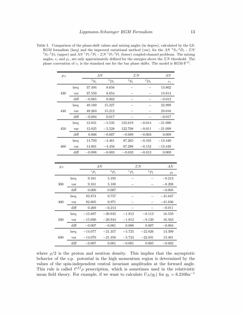
Table I. Comparison of the phase-shift values and mixing angles (in degree), calculated by the LS-
RGM formalism (lseq) and the improved variational method (var), for the ΛN 3S1-3D1 - ΣN
3S1-3D1 (upper) and ΛN 1P1-
3P1 - ΣN 1P1-3P1 (lower) coupled-channel problems. The mixing
angles, ǫ1 and ρ1, are only approximately defined for the energies above the ΣN threshold. The
phase convention of ǫ1 is the standard one for the bar phase shifts. The model is RGM-F 4).
pΛ ΛN ΣN ΛN3S1
3D13S1
3D1 ǫ1
lseq 37.494 8.656 − − 13.802
430 var 37.559 8.654 − − 13.814
diff −0.065 0.002 − − −0.012
lseq 49.169 15.227 − − 22.999
440 var 49.263 15.212 − − 23.016
diff −0.094 0.017 − − −0.017
lseq 12.831 −5.535 122.619 −0.014 −21.090
450 var 12.825 −5.528 122.708 −0.011 −21.099
diff 0.006 −0.007 −0.089 −0.003 0.009
lseq 14.793 −4.461 87.265 −0.165 −13.440
460 var 14.801 −4.458 87.298 −0.152 −13.449
diff −0.008 −0.003 −0.033 −0.013 0.009
pΛ ΛN ΣN ΛN1P1
3P11P1
3P1 ρ1
lseq 9.161 5.195 − − −8.213
300 var 9.161 5.188 − − −8.208
diff 0.000 0.007 −0.005
lseq 82.874 0.757 − − −41.647
400 var 82.605 0.971 − − −41.636
diff 0.269 −0.214 − − −0.011
lseq −15.697 −20.945 −1.812 −8.113 16.559
500 var −15.690 −20.944 −1.812 −8.120 16.563
diff −0.007 −0.001 0.000 0.007 −0.004
lseq −14.077 −21.357 −5.725 −22.826 13.399
600 var −14.070 −21.358 −5.724 −22.831 13.401
diff −0.007 0.001 −0.001 0.005 −0.002
where ρ/2 is the proton and neutron density. This implies that the asymptoticbehavior of the s.p. potential in the high momentum region is determined by thevalues of the spin-independent central invariant amplitudes at the forward angle.This rule is called teffρ prescription, which is sometimes used in the relativisticmean field theory. For example, if we want to calculate UN (q1) for q1 = 6.210fm−1

14 Y. Fujiwara, M. Kohno, T. Fujita, C. Nakamoto and Y. Suzuki
in nuclear matter of the normal density with kF = 1.35 fm−1 (ρ = (2/3π2) k3F =
0.1662 fm−3), we only need to derive the invariant amplitude (g00(θ = 0) + 3g1
0(θ =0)) for Tlab = 800 MeV (q = q1/2 = 3.105 fm−1) and multiply it by the factor,−(4π/q)(h2/MN )(ρ/2) = −(4π/3.105) · 41.47 · 0.0831 = −13.95.
§3. Comparison with the improved variational method
As a check of the LS-RGM formalism, we consider the phase-shift parametersof the ΛN -ΣN(I = 1/2) coupled-channel system, and compare them with the pre-dictions by the improved variational method. Here we consider two different typesof the ΛN -ΣN(I = 1/2) couplings. The first one is the 3S1-
3D1 channel couplingby the tensor force, which dominantly comes from the EMEP, especially, from theone-pion exchange tensor force. The other is the 1P1 - 3P1 coupling by the LS(−)
force originating from the FB interaction. Since the quark model usually predictsvery strong LS(−) force, the Λp scattering observables involve very rich informationon the characters of the non-central forces in the Y N interaction.
Table I shows a comparison between the phase-shift values predicted by the LS-RGM formalism (lseq) and the improved variational method (var) with respect tothe ΛN 3S1-
3D1-ΣN 3S1-3D1 (upper) and ΛN 1P1-
3P1-ΣN 1P1-3P1 (lower) coupled-
channel problems. The mixing angle ǫ1 (ρ1) between the 3S1 and 3D1 (1P1 and 3P1)channels of ΛN is also compared. The model is RGM-F 4), which gives the ΣNthreshold energy at pΛ = 445 MeV/c. In spite of the prominent resonance behaviorin this energy region, the two methods give very similar values for the phase shifts.The difference (diff) is less than 0.1 for the 3S1-
3D1 coupling. For the 1P1-3P1
coupling, we find that the accuracy deteriorates because of the strong resonance inthe ΛN 1P1 channel. If we avoid this energy region, the accuracy is very good. Thedifference is usually less than 0.01.
Since the resonance behavior in the above two coupled-channel systems is largelymodel-dependent, we summarize it in Table II for the three versions of our quarkmodel. Here V C
ΣN(1/2)(3S) indicates the strength of the central attraction in the
ΣN(I = 1/2) channel, which is evaluated from the 3S effective potential obtainedthrough the p = 0 Wigner transform of the exchange kernel. We find that the ΛN3S1 resonance in RGM-F appears as a cusp, when the attraction of the ΣN(I = 1/2)channel is not strongly attractive as in FSS and RGM-H. Similarly, the ΣN(I = 1/2)3P1 resonance does not move to the ΛN 1P1 state in RGM-H, which has the weakestcentral attraction in the ΣN(I = 1/2) channel among our three models.
§4. NN invariant amplitudes at intermediate energies
Figures 2 and 3 compare with the experimental data 29) the model predictionsof the elastic differential cross sections and the polarizations for the the np and ppscattering in the Tlab = 400 ∼ 800 MeV range. These observables in the lowerenergies are given in Ref. 7). The model in Fig. 2 is FSS for the np scattering, andthat in Fig. 3 is RGM-H for the pp scattering. The Coulomb force for the pp scattering

Lippmann-Schwinger RGM Formalism 15
Table II. Resonance behavior near the ΣN threshold for the I = 1/2 states, predicted by RGM-F 4),
FSS 5), 6) and RGM-H 6). “step” denotes the step-like resonance and “disp” the dispersion-like
resonance.
model RGM-F FSS RGM-H
EthΣN (MeV) 39 77 77
V CΣN(1/2)(
3S) −38 −24 −18
ΛN 3S1 step cusp cusp
ΛN 3D1 disp disp disp
ΣN 3S1 δ = 180 ↓ δ <∼ 60 δ <
∼ 45
ΣN 3D1 δ <∼ 0 δ <
∼ 0 δ <∼ 0
ΛN 1P1 step step disp
ΛN 3P1 disp disp disp
ΣN 1P1 δ <∼ 0 δ <
∼ 0 δ ∼ 0 → 60
ΣN 3P1 δ < 0 δ <∼ 0 δ <
∼ 40
is neglected, since it only affects the extreme forward and backward angles in thishigh energy region. The solid curve indicates the predictions obtained by solving theLS-RGM equation, while the dashed curve the results of the Born approximation.The latter approximation is apparently inappropriate even at these high energies.However, it is outstanding that the calculated Born invariant amplitudes, leadingto these cross sections in the Born approximation, have almost the same order ofmagnitude as the empirical amplitudes determined from the phase-shift analysis 29).Note that the polarization vanishes in the Born approximation. In these calculationsno imaginary potential is introduced. The theory overestimates the np differentialcross sections at backward angles. The np polarization has an unpleasant oscillationaround θc.m. ∼ 110. There appears a symmetry in the pp scattering because ofthe identity of two protons: The differential cross section becomes symmetric withrespect to θc.m = 90, and the polarization is symmetric with an opposite sign.The pp polarization for Tlab ≥ 400 MeV shows an oscillation around 90, which isnot present in the experiment. Except for these disagreements, the characteristicbehavior of the energy dependence and the angular distribution is reasonably wellreproduced within the wide energy range up to 800 MeV. These results indicate thatthe LS-RGM technique is very useful for investigating the baryon-baryon interactionabove 300 MeV.
Figure 4 shows the five invariant amplitudes, g0(θ) ∼ hP (θ), as a function ofthe c.m. angle θ, predicted by FSS for the np scattering at Tlab = 800 MeV. Theleft column displays the real part, while the right column the imaginary part. Thepredictions by the Paris potential 30) are also shown in the dashed curve for com-parison. In these calculations the partial waves up to J = 8 are included.∗) The
∗) Actually Jmax = 8 is not big enough for Tlab = 800 MeV, as seen from the small ripples of
the solid and dashed curves in Fig. 4. The partial-wave contributions for J > Jmax from the Born

16 Y. Fujiwara, M. Kohno, T. Fujita, C. Nakamoto and Y. Suzuki
0.1
1
10
Tlab = 400 MeV
FullBorn
− 0.4
− 0.2
0
0.2
0.4
0.6Tlab = 400 MeV
0.1
1
10
Tlab = 500 MeV
dσ/d
Ω (
mb/
sr)
P
− 0.4
− 0.2
0
0.2
0.4
0.6Tlab = 500 MeV
0.1
1
10
Tlab = 600 MeV − 0.4
− 0.2
0
0.2
0.4
0.6Tlab = 600 MeV
0.1
1
10
0 30 60 90 120 150
θc.m. (deg)
Tlab = 800 MeV − 0.4
− 0.2
0
0.2
0.4
0.6
0 30 60 90 120 150 180
θc.m. (deg)
Tlab = 800 MeV
Fig. 2. The differential cross sections and polarization for the elastic np scattering at Tlab = 400 ∼
800 MeV. The model is FSS. The solid curve denotes the full calculation with LS-RGM, while
the dashed curve the one with the Born approximation. Experimental data are from 29).
amplitudes are added to obtain the results in Figs. 2 and 3.

Lippmann-Schwinger RGM Formalism 17
dotted curve (Arndt) is the empirical value, which is calculated from the solution ofthe phase-shift analysis 31) by using the real part of the phase-shift parameters upto J ≤ 6 and the partial-wave expansion of the invariant amplitudes Eq. (D.2). It
0.1
1
10
Tlab = 400 MeV
FullBorn
− 0.4
− 0.2
0
0.2
0.4
0.6Tlab = 400 MeV
0.1
1
10
Tlab = 500 MeV
dσ/d
Ω (
mb/
sr)
P
− 0.4
− 0.2
0
0.2
0.4
0.6Tlab = 500 MeV
0.1
1
10
Tlab = 600 MeV − 0.4
− 0.2
0
0.2
0.4
0.6Tlab = 600 MeV
0.1
1
10
0 30 60 90 120 150
θc.m. (deg)
Tlab = 800 MeV − 0.4
− 0.2
0
0.2
0.4
0.6
0 30 60 90 120 150 180
θc.m. (deg)
Tlab = 800 MeV
Fig. 3. The same as Fig. 2, but for the elastic pp scattering in model RGM-H. The Coulomb force
is neglected.

18 Y. Fujiwara, M. Kohno, T. Fujita, C. Nakamoto and Y. Suzuki
is clear that the most prominent disagreement between the FSS prediction and theother predictions appears in the real part of the spin-independent central invariantamplitude ℜe g0(θ) at the forward angle. FSS predicts ℜe g(0) ∼ 1.25, while theParis potential and the phase-shift analysis predict ℜe g(0) ∼ −1. If we use the teffρprescription discussed in § 2.4, these values correspond to the nucleon s.p. potentialin normal nuclear matter, −17 MeV for FSS and +14 MeV for the latter two, as a
− 2
− 1.5
− 1
− 0.5
0
0.5
1
1.5
2
0 30 60 90 120 150 180
Rea
l g0
(θ)
θcm (deg)
np Tlab=800MeV J≤8
FSSParisArndt
− 3
− 2
− 1
0
1
2
3
0 30 60 90 120 150 180
Imag
g0
(θ)
θcm (deg)
np Tlab=800MeV J≤8
FSSParisArndt
− 2
− 1.5
− 1
− 0.5
0
0.5
1
1.5
2
0 30 60 90 120 150 180
Rea
l h0
(θ)
θcm (deg)
np Tlab=800MeV J≤8
FSSParisArndt
− 2
− 1.5
− 1
− 0.5
0
0.5
1
1.5
2
0 30 60 90 120 150 180
Imag
h0
(θ)
θcm (deg)
np Tlab=800MeV J≤8
FSSParisArndt
− 2
− 1.5
− 1
− 0.5
0
0.5
1
1.5
2
0 30 60 90 120 150 180
Rea
l hn
(θ)
θcm (deg)
np Tlab=800MeV J≤8
FSSParisArndt
− 2
− 1.5
− 1
− 0.5
0
0.5
1
1.5
2
0 30 60 90 120 150 180
Imag
hn
(θ)
θcm (deg)
np Tlab=800MeV J≤8
FSSParisArndt
Fig. 4. The real (left) and imaginary (right) parts of the five invariant amplitudes, g0(θ) ∼ hP (θ),
for the np elastic scattering at Tlab = 800 MeV, predicted by model FSS. The dashed curve
stands for predictions by the Paris potential 30), and the dotted curve those by the phase-shift
analysis SP82 by Arndt et al. 31). The partial waves included are J ≤ 6 for SP82, and J ≤ 8
otherwise.

Lippmann-Schwinger RGM Formalism 19
− 2
− 1.5
− 1
− 0.5
0
0.5
1
1.5
2
0 30 60 90 120 150 180
Rea
l hk
(θ)
θcm (deg)
np Tlab=800MeV J≤8
FSSParisArndt
− 2
− 1.5
− 1
− 0.5
0
0.5
1
1.5
2
0 30 60 90 120 150 180
Imag
hk
(θ)
θcm (deg)
np Tlab=800MeV J≤8
FSSParisArndt
− 2
− 1.5
− 1
− 0.5
0
0.5
1
1.5
2
0 30 60 90 120 150 180
Rea
l hP (
θ)
θcm (deg)
np Tlab=800MeV J≤8
FSSParisArndt
− 2
− 1.5
− 1
− 0.5
0
0.5
1
1.5
2
0 30 60 90 120 150 180
Imag
hP (
θ)
θcm (deg)
np Tlab=800MeV J≤8
FSSParisArndt
Fig. 4. -continued
contribution from the unlike nucleons.∗) We here find that the attractive behavior ofthe FSS s.p. potentials around this energy region is related to the wrong sign of thereal part of the spin-independent central invariant amplitude ℜe g0(θ) at the forwarddirection. This difference does not impair the differential cross sections very much,since the invariant amplitude has an appreciable magnitude for the imaginary part asseen in Fig. 4. This should, however, affect some particular polarization observables,and cause a large disagreement compared to experiment.
§5. Nucleon and hyperon single-particle potentials in nuclear matter
Figure 5 illustrates s.p. potentials UB(q1), as a function of the incident momen-tum q1, which are obtained for B = N , Λ and Σ from the G-matrix calculationswith the model FSS. The normal density with kF = 1.35 fm−1 is assumed for nu-clear matter. The left panels are the results with QTQ prescription for intermediateenergy spectra, while the right panels are those with the continuous prescription. 15)
The upper panels are for the momentum q1 < 4 fm−1, while the lower panels forq1 < 20 fm−1. In the QTQ prescription, the self-consistency of the s.p. potentialsis not respected in the momentum region q1 > kF = 1.35 fm−1. On the other hand,
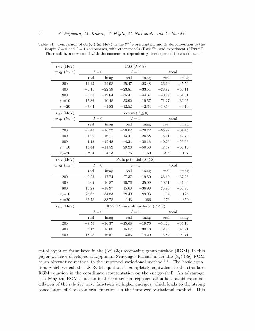
∗) These are consistent with the numbers given in Table VI. Namely, if we add up the I = 0
contribution and one-third of the I = 1 contribution to the real part of the s.p. potentials at 800
MeV, the potential depth becomes −17.4 MeV for FSS, 15.5 MeV for the Paris potential, and 14.5
MeV for SP99.

20 Y. Fujiwara, M. Kohno, T. Fujita, C. Nakamoto and Y. Suzuki
− 100
− 80
− 60
− 40
− 20
0
20
40
0 1 2 3 4
UB(q
1) (
MeV
)
q1 (fm-1)
FSS (QTQ)
NΛΣ
− 100
− 80
− 60
− 40
− 20
0
20
40
0 5 10 15 20
UB(q
1) (
MeV
)
q1 (fm-1)
FSS (QTQ)
NΛΣ
− 100
− 80
− 60
− 40
− 20
0
20
40
0 1 2 3 4
UB(q
1) (
MeV
)
q1 (fm-1)
FSS (cont)
NΛΣ
− 100
− 80
− 60
− 40
− 20
0
20
40
0 5 10 15 20
UB(q
1) (
MeV
)
q1 (fm-1)
FSS (cont)
NΛΣ
Fig. 5. The nucleon and hyperon (Λ, Σ) s.p. potentials predicted by the G-matrix calculation of
model FSS. The results in the left panels are obtained by using QTQ prescription, while those in
the right panels by the continuous prescription for intermediate energy spectra. The momentum
interval is 0 < q1 < 4 fm−1 in the upper panels, and 0 < q1 < 20 fm−1 in the lower panels. The
Fermi momentum kF = 1.35 fm−1 is assumed.
it is fully accounted for in the continuous prescription.∗) This implies that we firstcalculate UN (q1), and then UΛ(q1) and UΣ(q1) are determined self-consistently byusing the result of UN (q1). The partial waves included are for J ≤ 9. We can seefrom Fig. 5 that the s.p. potentials predicted by FSS is fairly strongly attractive inthe momentum interval q1 = 5 ∼ 20 fm−1 for all the baryons. In particular, UN (q1)in the continuous prescription becomes almost −80 MeV at q1 = 10 fm−1. Thismomentum interval corresponds to the incident energy Tlab = 500 MeV ∼ 8 GeVin the NN scattering (see Table III). We therefore need to examine the invariantamplitudes carefully in this energy region.
Let us first examine whether the teffρ prescription discussed in § 2.4 is a goodapproximation to the s.p. potentials predicted by the G-matrix calculation. TableIII shows such a comparison with respect to the nucleon s.p. potential UN (q1) (inMeV) predicted by the model FSS. Here we find that the maximum value of the totalangular momentum Jmax = 7 is actually too small, when the incident momentum
∗) In Ref. 15) we have assumed UB(q1) = UB(q1 = 3.8 fm−1) for q1 ≥ 3.8 fm−1, in order to avoid
the unrealistic behavior of the s.p. potentials in the high momentum region. Here q1 = 3.8 fm−1
corresponds to Tlab = 300 MeV in the NN scattering.

Lippmann-Schwinger RGM Formalism 21
Table III. Comparison of s.p. potential UN(q1) (in MeV), obtained by teffρ prescription (T -
matrix) and by G-matrix calculation in the continuous choice 15). The model is FSS 5), 6).
(Real part)
Tlab q1 T -matrix G-matrix (cont.)
(MeV) (fm−1) J ≤ 9 J ≤ 9 J ≤ 7
187 3 −37.49 −38.98 −36.76
332 4 −27.81 −26.08 −23.75
518 5 −30.19 −35.79 −33.01
2074 10 −79.90 −78.00 −54.20
8295 20 −14.81 −16.07 −7.82
(Imaginary part)
Tlab q1 T -matrix G-matrix (cont.)
(MeV) (fm−1) J ≤ 9 J ≤ 9 J ≤ 7
187 3 −44.91 −29.71 −29.53
332 4 −52.88 −39.64 −39.43
518 5 −60.51 −44.68 −44.88
2074 10 −34.91 −36.81 −29.77
8295 20 −22.96 −21.07 −2.92
Table IV. Decomposition of UN (q1) (in MeV) in Table III to the isospin I = 0 and I = 1 compo-
nents. The total angular momentum included is J ≤ 9. The model is FSS 5), 6).
(Real part)
Tlab q1 I = 0 I = 1
(MeV) (fm−1) T -matrix G-matrix T -matrix G-matrix
187 3 −11.91 −15.25 −25.58 −23.73
332 4 −5.98 −7.53 −21.83 −18.55
518 5 −5.04 −9.65 −25.16 −26.14
2074 10 −28.72 −27.93 −51.18 −50.07
8295 20 −2.37 −3.60 −12.44 −12.47
(Imaginary part)
Tlab q1 I = 0 I = 1
(MeV) (fm−1) T -matrix G-matrix T -matrix G-matrix
187 3 −22.02 −15.85 −22.89 −13.86
332 4 −22.66 −17.69 −30.22 −21.57
518 5 −22.21 −19.69 −38.30 −24.99
2074 10 −15.27 −14.83 −19.63 −21.99
8295 20 −20.62 −18.78 −2.34 −2.29

22 Y. Fujiwara, M. Kohno, T. Fujita, C. Nakamoto and Y. Suzuki
Table V. Reduction factors of the S-meson central attraction due to the momentum-dependent q2
term.
q ∼ kcm Tlab 0.0243 q2
2 332 MeV 0.097
3.1 800 MeV 0.23
5 2 GeV 0.61
7.5 4.7 GeV 1.37
q1 ≥ 10 fm−1. However, if we take the same Jmax in the two calculations, the accu-racy of the teffρ prescription seems to be fairly good even for the large momentumaround q1 ∼ 10 fm−1. Quite surprisingly, this approximation is very good even atsuch a small energy as Tlab = 200 MeV, as long as the real part of the s.p. potentialis concerned. This agreement between the two prescriptions becomes clearer, if weexamine each isospin component with I = 0 and I = 1, separately, as seen fromTable IV. As to the imaginary part of the s.p. potential, the teffρ prescriptionseems to overestimate the values by the G-matrix calculation.
From this comparison and the behavior of the invariant amplitudes in the preced-ing section, we have found that the attractive behavior of UN (q1) in the momentuminterval q1 = 5 ∼ 20 fm−1 in FSS is related to the wrong sign (of the real part)of the spin-independent central invariant amplitude at the forward direction. Weexpect that this situation is common even for the Λ and Σ hyperons, and it is aflaw of our present quark model (not only FSS, but also RGM-H and RGM-F).It should be mentioned that the quantitative aspect of the present non-relativisticsingle-channel calculation in the above momentum region is not entirely trustable.The corresponding energy region of the NN scattering is already the relativisticenergy region, where many inelastic channels are open. Nevertheless, a repulsivebehavior of the s.p. potential at q1 = 5 ∼ 20 fm−1 seems to be a mandatory re-quirement even in the single-channel calculation, since channel-coupling effects areexpected to work attractive to the s.p. potential. Although this energy region mayalready be out of the applicability of our non-relativistic quark model, we need s.p.potentials for the intermediate states with quite high momenta when the G-matrixcalculation is carried out in the continuous prescription.
In order to solve this problem, we use an advantage of our quark model that theeffect of the short-range correlation is rather moderate compared with that of thestandard meson-exchange potentials like the Paris potential. Namely, an improve-ment of the Born amplitudes is clearly reflected to the improvement of the solutionof the LS-RGM equation. In particular, the intermediate-range attraction from thescalar-meson exchange has the Born kernel
V C(k,q) = − g2
k2 + m2
[1 − q2
2M2+
k2
8M2
](5.1)
with k = qf −qi and q = (qf +qi)/2, in the approximation up to the order of (v/c)2.Here m and M are the meson mass and the baryon mass, respectively. So far we

Lippmann-Schwinger RGM Formalism 23
have used only the leading term 1 in the square bracket of Eq. (5.1) and neglectedq2 and k2 terms. A dominant contribution to the spin-independent central invariantamplitude at the forward angle comes from the q2 term, which becomes importantin the high-energy region. In fact, if we set k2 → −m2 as usual, modify the squarebracket of Eq. (5.1) as
[1 − q2
2M2+
k2
8M2
]−→
[1 − q2
2M2− m2
8M2
]
=
(1 − m2
8M2
)[1 − 1
1 − m2/8M2
q2
2M2
], (5.2)
and redefine g2 including the(1 − m2/8M2
)factor, we find the momentum depen-
dence like 1 − 0.0243 q2 for the mass mc2 = 800 MeV of the ǫ meson in FSS. Here|q| is in units of fm−1. This non-static term of the S mesons plays a role to reducethe strength of the intermediate-range attraction by about 20 % at 800 MeV. (SeeTable V.) Actually the momentum q is not directly related to the total energy, northe direct Born term is good enough to discuss the reduction of the central attrac-tion at higher energies. We also have contributions from the inherent zero-pointoscillation of the cluster wave functions and those from the quark-exchange kernel,since our EMEP are acting between quarks. Nevertheless, the discussion here is stillvalid, since the dominant contribution to the intermediate attraction is the directterm of the ǫ-meson exchange potential. Bryan-Scott 32) carefully examined theseq2 momentum-dependent terms in the S-meson and V-meson exchange potentials.They found that the inclusion of these terms has a favorable effect of making the non-relativistic approximation uniform to order q2, although the main effect is almostcompensated for by a slight change in the coupling constants. Since these terms areincluded in the Paris potential 30) and all the Nijmegen soft-core potentials 33), 34),it would be useful to incorporate these terms in our quark model, in order to de-scribe correctly the asymptotic behavior of the s.p. potentials in the high-momentumregion.
As an example of the quark model with the momentum-dependent q2 term, weshow in Table VI the result of the s.p. potential UN (q1) in the teffρ prescription,calculated by a new model (present). In this new model V-mesons are also incor-porated as the EMEP acting between quarks. The phase-shift parameters of the npscattering is largely improved in comparison with those of FSS. The details of thisnew model will be published elsewhere. In Table VI predictions of the Paris poten-tial 30) and of the phase-shift analysis SP99 29), together with the decomposition toI = 0 and I = 1 contributions, are also shown for comparison. We find that the newmodel is still slightly too attractive around Tlab ∼ 800 MeV, but the flaw of FSS withtoo attractive asymptotic behavior in the high-momentum region is clearly removed.
§6. Summary
In the quark-model study of the nucleon-nucleon (NN) and hyperon-nucleon(Y N) interactions, a variational method is usually used to solve an integro-differ-
24 Y. Fujiwara, M. Kohno, T. Fujita, C. Nakamoto and Y. Suzuki
Table VI. Comparison of UN (q1) (in MeV) in the teffρ prescription and its decomposition to the
isospin I = 0 and I = 1 components, with other models (Paris 30)) and experiment (SP99 29)).
The result by a new model with the momentum-dependent q2 term (present) is also shown.
Tlab (MeV) FSS (J ≤ 8)
or q1 (fm−1) I = 0 I = 1 total
real imag real imag real imag
200 −11.43 −22.08 −25.47 −23.48 −36.90 −45.56
400 −5.11 −22.59 −23.81 −33.51 −28.92 −56.11
800 −5.58 −19.64 −35.41 −44.37 −40.99 −64.01
q1=10 −17.36 −10.48 −53.92 −19.57 −71.27 −30.05
q1=20 −7.04 −1.83 −12.52 −2.34 −19.56 −4.16
Tlab (MeV) present (J ≤ 8)
or q1 (fm−1) I = 0 I = 1 total
real imag real imag real imag
200 −9.40 −16.72 −26.02 −20.72 −35.42 −37.45
400 −1.90 −16.11 −13.41 −26.58 −15.31 −42.70
800 4.18 −15.48 −4.24 −38.18 −0.06 −53.63
q1=10 13.44 −11.52 29.23 −50.58 42.67 −62.10
q1=20 39.4 −47.3 176 −150 215 −197
Tlab (MeV) Paris potential (J ≤ 8)
or q1 (fm−1) I = 0 I = 1 total
real imag real imag real imag
200 −9.23 −17.74 −27.37 −19.50 −36.60 −37.25
400 0.65 −16.87 −10.76 −25.09 −10.11 −41.96
800 10.28 −18.97 15.68 −36.98 25.96 −55.95
q1=10 25.67 −34.83 78.49 −89.93 104 −125
q1=20 32.78 −83.78 143 −266 176 −350
Tlab (MeV) SP99 (Phase shift analysis) (J ≤ 7)
I = 0 I = 1 total
real imag real imag real imag
200 −8.56 −16.37 −25.68 −19.76 −34.24 −36.13
400 3.12 −15.08 −15.87 −30.13 −12.76 −45.21
800 13.28 −16.51 3.53 −74.20 16.82 −90.71
ential equation formulated in the (3q)-(3q) resonating-group method (RGM). In thispaper we have developed a Lippmann-Schwinger formalism for the (3q)-(3q) RGMas an alternative method to the improved variational method 11). The basic equa-tion, which we call the LS-RGM equation, is completely equivalent to the standardRGM equation in the coordinate representation on the energy-shell. An advantageof solving the RGM equation in the momentum representation is to avoid rapid os-cillation of the relative wave functions at higher energies, which leads to the strongcancellation of Gaussian trial functions in the improved variational method. This

Lippmann-Schwinger RGM Formalism 25
feature of the LS-RGM formalism naturally makes it possible to obtain an accurateS-matrix even for the relativistic energies Tlab ≥ 350 MeV, where many inelasticchannels open. Since the S-matrix is very accurate also in the low-energy region,an extension to the coupled-channel systems with different threshold energies is verysuccessful.
In this formulation the Born kernel is analytically calculated for all pieces of di-rect and exchange terms, which are composed of the kinetic-energy term and variouspieces of quark-quark (qq) interactions. The qq interactions are further divided intothe phenomenological confinement potential, a color analogue of the Fermi-Breit(FB) interaction, and the effective meson-exchange potentials (EMEP) acting be-tween quarks. The Born kernel is then decomposed into partial-wave componentsand the resultant LS-RGM equation is solved by using the techniques developedby Noyes 13) and Kowalski 14). Since calculations are always carried out in the mo-mentum representation, the present formalism has no difficulty to incorporate themomentum-dependent qq interaction such as the momentum-dependent Breit retar-dation term of the FB interaction, the higher-order terms of the central scalar-mesonand vector-meson exchange potentials, and the quadratic LS force. A convenienttransformation formula to derive spatial functions for the direct and exchange kernelsis given for a very general type of two-body interactions. The numerical evaluation ofthe partial-wave Born kernel is also best suited to convert the LS-RGM equation tothe G-matrix (Bethe-Goldstone) equation 15), in which the Pauli principle is treatedexactly at the baryon level.
The accuracy of the LS-RGM formalism has been examined in the ΛN -ΣN(I =1/2) coupled-channel system. In this system the 3S1-
3D1 coupling caused by the verystrong one-pion tensor force yields a prominent cusp structure for the ΛN phase-shiftparameters at the ΣN threshold. On the other hand, a resonance appears either inΛN 1P1 state or in ΣN 3P1 state by the strong effect of the antisymmetric LS force(LS(−) force) originating from the FB interaction. The behavior of these resonancesis rather sensitive to the characteristics of the model, particularly to the strength ofthe central attraction of the ΣN(I = 1/2) channel. We have examined the modelRGM-F and obtained a satisfactory agreement of the phase-shift parameters betweenthe LS-RGM method and the improved variational method, in the wide momentumregion plab = 0 ∼ 1 GeV/c.
Using the same parameter set determined at Tlab = 0 ∼ 250 MeV, we haveextended our calculation of the differential cross sections and the polarization forthe NN scattering to the intermediate energies Tlab = 400 ∼ 800 MeV. Althoughagreement with the experimental data becomes gradually worse as the energy be-comes higher, the characteristic behavior of the energy dependence and the angulardistribution of these observables for the elastic np and pp scattering are reasonably re-produced within this energy range. In particular, the invariant amplitudes predictedby model FSS for the np scattering at Tlab = 800 MeV reproduce reasonably well theempirical invariant amplitudes determined from the phase shift analysis, except fora few typical disagreements. The most prominent disagreement appears in the realpart of the spin-independent central invariant amplitude g0(θ) at the forward anglesθ ∼ 0. This amplitude is related to the single-particle (s.p.) potential obtained from

26 Y. Fujiwara, M. Kohno, T. Fujita, C. Nakamoto and Y. Suzuki
the G-matrix calculation through the teffρ prescription, when the incident momen-tum is high. The wrong sign of ℜeg0(θ) at θ = 0 in our model is correlated to tooattractive s.p. potentials in the momentum region q1 = 5 ∼ 20 fm−1.
We have also examined the accuracy of the teffρ prescription by using the G-matrix solution 15) and the present LS-RGM formalism. This prescription is a goodapproximation for the real part of the s.p. potentials in the energy region fromTlab = 200 MeV to several GeV (q1 = 3 fm−1 ∼ 20 fm−1), as long as the maximumvalue of the angular-momentum cut for partial waves is commonly taken. On theother hand, the imaginary parts of the s.p. potentials are usually overestimated inthe teffρ prescription.
Perhaps the most striking feature of the quark model found in this investigationis a moderate effect of the short-range correlation. In the standard meson-exchangemodels, the observed phase-shifts are reproduced as a cancellation of very strongrepulsive and attractive local potentials, and the Born amplitudes of the Paris po-tential, for example, are one or two order of magnitude large, compared to theempirical invariant amplitudes. On the other hand, the short-range repulsion in thequark model originates mainly from the nonlocal kernel of the color-magnetic termof the FB interaction. Born amplitudes of the quark model therefore have almostthe same order of magnitude as the empirical amplitudes obtained by solving theLS-RGM equation. This implies that the short-range correlation in the quark modelis rather moderate compared with the meson-exchange models. It can also be seenin our recent quark-model study of the s.p. spin-orbit potentials for the nucleon andhyperons. In Ref. 35) we have calculated the strength factor, SB, of the s.p. spin-orbit potentials by using the G-matrix solutions and found that SN does not obtainmuch effect of the short-range correlation, on the contrary to the standard potentialmodels like the Reid soft-core potential with the strong short-range repulsive core.Since the Born amplitudes in the quark model reflect rather faithfully characteristicsof the LS-RGM solution, it is easy to find missing ingredients that impair the model.In fact, we have discussed that the wrong sign of the invariant amplitude ℜe g0(θ) inour quark model is related to our neglect of higher-order momentum-dependent cen-tral term of the scalar-meson exchange EMEP. A preliminary result of a new model,which incorporates this term as well as the vector-meson EMEP, shows that the s.p.potentials in the teffρ prescription have a correct repulsive behavior in the asymp-totic momentum region. The details of this model will be given in a forthcomingpaper.
Appendix A
A transformation formula to the Born kernel for momentum-dependent
two-body interactions
As to the general procedure how to calculate the RGM kernel for two-clustersystems composed of s-shell clusters, Refs. 22) and 23) should be referred to. Herewe use the same notation as Ref. 23) and give a convenient formula to calculate theBorn kernel for two-body interactions with momentum dependence.
Suppose a two-body interaction of the RGM Hamiltonian is given by vij = uijwij

Lippmann-Schwinger RGM Formalism 27
with the spatial part u = u(r, ∂/∂r) and the spin-flavor-color part wij = wSFij wC
ij .The full Born kernel for this interaction is defined by
〈 eiqf ·r φ |6∑
i<j
vijA′ | eiq i·r φ〉 , (A.1)
where φ = φspace ξ with ξ = ξSF ξC is the harmonic-oscillator (h.o.) internal wavefunction of the (3q)-(3q) system and A′ is the antisymmetrization operator betweentwo clusters. This expression is reduced to the form Eq. (2.14) by the use of thedouble coset expansion A′ → (1/2)(1 − 9P36)(1−P0) with P0 = P14P25P36, yieldingthe basic Born kernel Eqs. (2.22) and (2.25) with
M(qf ,qi) =∑
xTXxT MxT (qf ,qi) . (A.2)
Here the superscript Ω for specifying the type of the interaction is omitted forsimplicity, and the sum over x is only for x = 0 and 1. Furthermore, XxT is thespin-flavor-color factor defined through
XxT = Cx〈zx ξ |T∑
i<j
wij | ξ〉
=
XC0T 〈 ξSF | ∑T
i<j wSFij | ξSF 〉
(−9)XC1T 〈 P36 ξSF | ∑T
i<j wSFij | ξSF 〉
for x =
0
1, (A.3)
where x = 0 with z0 = 1 and C0 = 1 corresponds to the direct term and x = 1 withz1 = P36 and C1 = −9 the (one-quark) exchange term. The suffix T stands for theinteraction type T = E, S, S′, D+ or D−, for which the (i, j) pairs are properlyselected. The color-factors XC
xT = 〈zx ξC |wCij | ξC〉 for each (i, j) ∈ T are given as
follows. For the quark sector with wCij = (1/4)(λC
i λCj ), XC
0E = −(2/3), XC0D+
= 0,
and XC1E = XC
0S = XC0S′ = −(2/9), XC
1D+= 1/9, XC
1D−= 4/9. For the EMEP
sector with wCij = 1, XC
0T = 1 and XC1T = 1/3. The spin-flavor-color factor for the
exchange normalization kernel is defined by XN = (−3)〈P36 ξSF | ξSF 〉. We alsoneed XK = 24〈P36 ξSF |Y (6)−Y (5) | ξSF 〉 for the exchange kinetic-energy kernel ofthe Y N systems. On the other hand, the spatial part of the Born kernel is definedby
MxT (qf ,qi) = 〈 zx eiqf ·r φspace |uij | eiq i·r φspace〉 with (i, j) ∈ T , (A.4)
which we now evaluate.The standard procedure is to use the h.o. generating function
Aγ(r,z) =
(2γ
π
) 34
e−γ(r−z/√
γ)2+z2/2 , (A.5)
and first to calculate the so-called complex GCM kernel defined by
IxT (z,z′) = 〈 zx Aγ(r,z) φspace |uij |Aγ(r,z′) φspace〉 . (A.6)

28 Y. Fujiwara, M. Kohno, T. Fujita, C. Nakamoto and Y. Suzuki
This GCM kernel is divided into the general form of the norm kernel and the inter-action function T (z,z′):
IxT (z,z′) = e(1− x
µ
)z·z′
T (z,z′) ,
T (z,z′) = 〈(0s)Sα |(0s)S′
β〉−1〈(0s)Sγ |(0s)S′
δ〉−1
×〈(0s)Sα(0s)Sγ |u | (0s)S′
β(0s)S′
δ〉 . (A.7)
Here (0s)S stands for a localized (0s) wave function around x = S, and Sα etc.are the generator coordinates specifying the position of clusters 23). For a simpleGaussian two-body interaction u(r) ∼ e−κr2
, T (z,z′) is given by
T (z,z′) =
(ν
ν + κ
) 32
e−λ2(pz∗+qz′)2 × (polynomial terms) , (A.8)
where ν = 1/2b2 is the h.o. constant of the (0s) clusters and λ is given by λ =(1/2µ)(κ/(ν + κ)) with γ = µν and µ = 3 · 3/(3 + 3) = 3/2. The parameters p and qare 0, 1 or −1, depending on T , which are explicitly given in TABLE II of Ref. 23).The transformation to the Born kernel is achieved through
MxT (qf ,qi) =
(γ
2π
) 32
e14γ
(q2f+q2
i )∫
da db e−γ2(a2+b2) e−iqf ·a+iqi·b
×IxT (√
γa,√
γb) . (A.9)
When u involves momentum-dependence, it is convenient to use the momentumrepresentation and write
〈p |u |p′ 〉 =1
(2π)3u(k′,q′) with k′ = p − p′, q′ =
1
2(p + p′) . (A.10)
Then the interaction function in Eq. (A.7) is given by
T (z,z′) =1
(2π)3
(1
πν
) 32∫
dk′ dq′ e−1ν (q′2+ 1
4k′2) e
14νr2+iq′·r eik′·X u(k′,q′)
with r = − 1√γ
(pz∗ − qz′), X = − 1
2√
γ(pz∗ + qz′) . (A.11)
If we use Eq. (A.11) in Eq. (A.9), the integration over a and b can be carried outand we obtain the following formula after some rearrangement of terms:
MxT (qf ,qi) = MNx (qf ,qi)
(1
2π
)3 ∫dk′ exp
−(
1 +α
2µ
)1
4νk′2 − 1
2√
γV k′
×(
1
πν
1
1 − α/2µ
)3/2 ∫dq′ exp
−1
ν
1
1 − α/2µq′2
×u
(k′,q′ − ε
4µk′ − ν
2√
γA
). (A.12)

Lippmann-Schwinger RGM Formalism 29
Here MNx (qf ,qi) is the normalization kernel given by
MNx (qf ,qi) =
(2π
γ
1
1 − τ2
)3/2
exp
− 1
2γ
(1 − τ
1 + τq2 +
1 + τ
1 − τ
1
4k2)
, (A.13)
with τ = 1 − x/µ, k = qf − qi and q = (qf + qi)/2, and the coefficients appearingin Eq. (A.12) are defined by
α =p2 + q2 − 2τpq
1 − τ2, α =
p2 + q2 + 2τpq
1 − τ2, ε =
p2 − q2
1 − τ2,
V =1√γ
(p − q
1 + τq +
p + q
1 − τ
1
2k
), A =
1√γ
(p + q
1 + τq +
p − q
1 − τ
1
2k
). (A.14)
Let us specialize the two-body interaction to the Yukawa function and the Gaus-sian function:
u(k,q) =
4π
k2 + m2u(k,q)
(πκ
) 32 e−
14κ
k2u(k,q)
. (A.15)
Here u(k,q) stands for a polynomial function of k and q, and the degree of thepolynomial is usually at most the second order in q. The Born kernel for the Yukawafunction is calculated from the formula for the Gaussian function through the integralrepresentation
4π
k2 + m2= m
1√π
∫ ∞
0du e−
1u2
(π
κ
) 32
e−14κ
k2with κ =
(mu
2
)2
. (A.16)
The resultant Born kernel is expressed by generalized Dawson’s integrals hn(x) andmodified Yukawa functions Yα(x), Zα(x) etc., which are given by the error functionof the imaginary argument:
hn(x) = (2n + 1) e−x2∫ 1
0ex2t2 t2n dt = (2n + 1)
e−x2
x2n+1
∫ x
0eu2
u2n du ,
Yα(x) = eα−x2∫ 1
0e−
αt2
+x2t2 dt ,
Zα(x) = eα−x2∫ 1
0e−
αt2
+x2t2 t4 dt . (A.17)
For the Gaussian kernel Eq. (A.12) is reduced into
MxT (qf ,qi) = MNx (qf ,qi)
(ν
ν + κ
1
1 + λα
) 32
exp
1
2
λ
1 + λαV 2
P(qf ,qi) ,
(A.18)where the polynomial part is given by
P(qf ,qi) =
(1 + λα
8πγλ
) 32∫
k′ exp
−1 + λα
8γλk′2

30 Y. Fujiwara, M. Kohno, T. Fujita, C. Nakamoto and Y. Suzuki
×(
1
πν
1
1 − α/2µ
)3/2 ∫dq′ exp
−1
ν
1
1 − α/2µq′2
×u
(k′ + 2
√γV ,q′ − ε
4µk′ +
ν
2√
γW
). (A.19)
Here u(k′,q′) = u(−k′,−q′) and the simplified notation
V =λ
1 + λαV , W = A − εV (A.20)
are used. If u(k,q) does not involve q-dependence, the q′ integral is carried out inEq. (A.19) and we obtain
P(qf ,qi) =
(1 + λα
8πγλ
) 32∫
k′ exp
−1 + λα
8γλk′2
u(k′ + 2
√γV
). (A.21)
Appendix B
Born kernel
In this appendix we show the invariant Born kernel Eq. (2.25) obtained by us-ing the transformation formula in Appendix A. These are functions of k2, q2 andk · q with k = qf − qi, q = (qf + qi)/2, and expressed by the special functionsgiven in Eq. (A.17). Only θ with cos θ = qf · qi is explicitly written in the spatialfunctions fΩ
T (θ). The S′-type spatial function fΩS′(θ) is obtained from fΩ
S (θ) withk → −k. There is no E-type possible for the non-central forces. The partial wavedecomposition of the Born kernel is carried out numerically through Eq. (2.26). Thespin-flavor-color factors in the quark sector are also shown in the operator form inthe isospin space.
B.1. Quark sector
Exchange normalization kernel
MN (qf ,qi) = XN f(θ) , (B.1)
with
f(θ) = (√
3πb)3 exp
−b2
3(q2 + k2)
. (B.2)
Exchange kinetic-energy kernel
MK(qf ,qi) = XN
[1
3
(2 +
1
λ
)+
1
6
(1 − 1
λ
)Y
]fK1(θ) + XK
1
6
(1 − 1
λ
)fK2(θ),
(B.3)where λ = (ms/mud), Y is the hypercharge of the total system, and
fK1(θ)fK2(θ)
=
3
4x2mudc
2 f(θ)
[−1 + 1
3b2(2q2 + k2)]
14
[1 + 2
3b2(q2 − k2)] , (B.4)

Lippmann-Schwinger RGM Formalism 31
with x = (h/mudcb).
Color-Coulombic term
MCC(qf ,qi) = XN
[2(fCC
E (θ) − fCCS (θ) − fCC
S′ (θ))
+ fCCD+
(θ) + fCCD−
(θ)]
,
(B.5)where
fCCT (θ) =
√2
παSxmudc
2 4
3(√
3πb)3
×
(811
) 12 exp
− 2
11b2[
43(q2 + k2) − k · q
]h0
(1√11
b|q + k|)
(12
) 12exp
−1
3b2(q2 + 1
4k2)
h0
(12b|k|
)
(23
) 12 exp
−1
3b2k2
h0
(1√3b|q|
)for T =
SD+
D−.
(B.6)
The E-type factor is given by fCCE (θ) =
√2/παSxmudc
2 (4/3) f(θ).
Breit retardation term
MMC(qf ,qi) = XMCE
(fMC
E (θ) − 4
9fGC
E (θ)
)+ XMC
S′
(fMC
S′ (θ) − 4
9fGC
E (θ)
)
+XMCS fMC
S (θ) + XMCD+
fMCD+
(θ) + XMCD−
fMCD−
(θ) , (B.7)
where
fMCT (θ) =
√2
παSx3mudc
2 2
9(√
3πb)3
×
exp−1
3b2(q2 + k2) [
52 − (bq)2
]for T = E
(811
) 12 exp
− 2
11b2[
43(q2 + k2) − k · q
]
×[H0
(1√11
b|q + k|)− 3
4b2(k · q)H1
(1√11
b|q + k|)
+ 322b4(q2 + k · q)(k2 + k · q)H2
(1√11
b|q + k|)]
for T = S(
12
) 12 exp
−1
3b2(q2 + 1
4k2) [
−12H0
(12b|k|
)
+34(bq)2H1
(12b|k|
)− 3
8b4(k · q)2H2
(12b|k|
)]for T = D+
(23
) 12 exp
−1
3b2k2 [
−2H0
(1√3b|q|
)+ 3
4 (bk)2H1
(1√3b|q|
)
−12b4(k · q)2H2
(1√3b|q|
)]for T = D− .
(B.8)
The functions Hn(x) with n = 0, 1, 2 are expressed by hn(x) through
H0(x) = h0(x)
H1(x) = h0(x) +1
3h1(x)
H2(x) =1
3h1(x) − 1
5h2(x) . (B.9)

32 Y. Fujiwara, M. Kohno, T. Fujita, C. Nakamoto and Y. Suzuki
The function fGCE (θ) is given below.
Color-Magnetic term
MGC(qf ,qi) = −XGCS′ fGC
E (θ) +∑
T 6=E
XGCT fGC
T (θ) , (B.10)
where fGCE (θ) =
√2/παSx3mudc
2 f(θ) and
fGCT (θ) =
√2
παSx3mudc
2(√
3πb)3
×
(811
) 32exp
− 2
11b2[
43 (q2 + k2) − k · q
]
(12
) 32 exp
−1
3b2(q2 + 1
4k2)
(23
) 32 exp
−1
3b2k2
for T =
SD+
D−
.
(B.11)
LS termIn general there are three different types of LS terms in the Y N interaction;
i.e., Ω = LS, LS(−) and LS(−)σ. 17) These are different only for the spin-flavor-colorfactors. For each type we have
MΩ(qf ,qi) =∑
T 6=E
XΩT fLS
T (θ) , (B.12)
where
fLST (θ) = −
√2
παSx3mudc
2 1
2(3π)
32 b5
×
(811
) 32 exp
− 2
11b2[
43(q2 + k2) − k · q
]h1
(1√11
b|q + k|)
(12
) 32 exp
−1
3b2(q2 + 1
4k2)
h1
(12b|k|
)
(23
) 32 exp
−1
3b2k2
h1
(1√3b|q|
)for T =
SD+
D−.
(B.13)
Tensor termThere are three different types of tensor terms as in Eq. (2.24). 17) These are
given by
MT (qf ,qi)
MT ′
(qf ,qi)
= XT
S fTS (θ) + XT
S′ fTS′(θ) +
XT
D+fT
D+(θ)
XTD−
fTD−
(θ),
MT ′′
(qf ,qi) = 2[XT
S fTS (θ) − XT
S′ fTS′(θ)
], (B.14)

Lippmann-Schwinger RGM Formalism 33
where
fTT (θ) = −
√2
παSx3mudc
2 2
5(3π)
32 b5
×
(811
) 32 1
11 exp− 2
11b2[
43(q2 + k2) − k · q
]h2
(1√11
b|q + k|)
(12
) 32 1
4 exp−1
3b2(q2 + 1
4k2)
h2
(12b|k|
)
(23
) 32 1
3 exp−1
3b2k2
h2
(1√3b|q|
)for T =
SD+
D−.
(B.15)
B.2. EMEP sector
Direct termsThe S-meson central (CN), PS-meson spin-spin (SN) and PS-meson tensor
(TN) terms are given by
MCND (qf ,qi) = XCN
0D+fCN
D (θ) ,
MSND (qf ,qi) = XT
0D+(σ1 · σ2) fSN
D (θ) ,
MTND (qf ,qi) = XT
0D+fTN
D (θ) , (B.16)
where
fCND (θ) = −4πhc
1
m2 + k2e−
13(bk)2 ,
fSND (θ) = 4πhc
1
3
(1
m2 + k2− cδ
1
m2
)e−
13(bk)2 ,
fTND (θ) = −4πhc
1
3m2
1
m2 + k2e−
13(bk)2 =
1
3m2fCN
D (θ) . (B.17)
Here m (= mc/h) is the meson mass, and the relationship XSN0D+
= XT0D+
(σ1 ·σ2) isused in Eq. (B.16). The factor cδ in Eq. (B.17) is a reduction factor for the spin-spincontact term of the PS-mesons.
Exchange terms
M (CNSN
)(qf ,qi) = −X(CN
SN)
1S′ f(CN
SN)
E (θ) +∑
T 6=E
X(CN
SN)
1T f(CN
SN)
T (θ) ,
MTN (qf ,qi)
MTN ′
(qf ,qi)
= XT
1S fTNS (θ) + XT
1S′ fTNS′ (θ) +
XT
1D+fTN
D+(θ)
XT1D−
fTND−
(θ),
MTN ′′
(qf ,qi) = 2[XT
1S fTNS (θ) − XT
1S′ fTNS′ (θ)
], (B.18)
where
fCNT (θ)
fSNT (θ)
= −4π
1−1
3
(3
2
) 32
hcb2

34 Y. Fujiwara, M. Kohno, T. Fujita, C. Nakamoto and Y. Suzuki
×
exp−1
3b2(q2 + k2) [
YαE(0) −
0
cδ1
2αE
]for E
(811
) 12 exp
− 2
11b2[
43(q2 + k2) − k · q
] [YαS
(1√11
b|q + k|)−
0cδ
12αS
]
for T = S(
12
) 12 exp
−1
3b2(q2 + 1
4k2) [
YαD+
(12b|k|
)−
0cδ
12αD+
]for T = D+
(23
) 12exp
−1
3b2k2[
YαD−
(1√3b|q|
)−
0cδ
12αD
−
]for T = D− ,
fTNT (θ) = −4π
(3
2
) 12
hcb2(
h
mc
)2
×
(811
) 32 1
11 exp− 2
11b2[
43(q2 + k2) − k · q
]ZαS
(1√11
b|q + k|)
for T = S(
12
) 32 1
4 exp−1
3b2(q2 + 1
4k2)
ZαD+
(12b|k|
)for T = D+
(23
) 32 1
3 exp−1
3b2k2
ZαD−
(1√3b|q|
)for T = D− .
(B.19)
The coefficients αT are given by αS = αS′ = (11/8)αE , αD+ = 2αE , and αD−=
(3/2)αE , with αE = (mb)2/2 = (1/2)(mcb/h)2.
B.3. Spin-flavor-color factors in the quark sector
The spin-flavor-color factors in the quark sector for the NN system are given inEq. (B.6) of Ref. 25). We should note that XT there is actually XGC
T for T = D+
and D−, and XGCS = XGC
S′ = −XE. (Note that XE is not XGCE .) Furthermore,
XMCD−
= XMCD+
= XN , XMCS = XMC
S′ = −2XN , XMCE = −XN , and XK = 0 for
NN . The spin-orbit and tensor factors for Y N systems are found in Appendix C ofRef. 17). Here we list up the one-quark exchange (x = 1) central factors (XΩ
T )B3B1
in Eq. (A.3), with respect to the quark sector of the ΛN , ΣN and ΞN systems. Thespin-flavor factors in the EMEP sector and the detailed derivation of these factorswill be published elsewhere. In the following, the parameter λ (= ms/mud
∗)) controlsthe flavor symmetry breaking of the FB interaction. The spin and isospin operators,σi and τi, are with respect to the two baryons Bi with i = 1 or 2 in the initial state,and the flavor exchange operator PF is supposed to operate on the ket state. Weassume B2 = B4 = N . The spin-flavor-color factor for the exchange normalizationkernel is given by XN = XMC
D−
(λ = 1). The factors of the interaction type T = S′
are discussed in § 5 of Ref. 17).
[ B3B1 = ΛΛ ]
XK = 1 − (1 + σ1 · σ2)PF ,
XMCD−
= −1
4
[2 +
1
λ(1 + σ1 · σ2) PF
],
∗) λ = mud/ms in Ref. 17) is a misprint.

Lippmann-Schwinger RGM Formalism 35
XMCD+
= −1
4
[1 +
1
λ+ (1 + σ1 · σ2) PF
],
XMCS =
1
4
[3 +
1
λ+
(1 +
1
λ
)(1 + σ1 · σ2) PF
],
XGCD−
=1
2+
1
24
[(1 +
4
λ+
1
λ2
)+ (σ1 · σ2)
(1 − 4
3λ+
1
λ2
)]PF ,
XGCD+
=1
72
[(13 +
3
λ2
)+ 6PF + (σ1 · σ2)
(4
3λ+ 6PF
)],
XGCS = − 1
72
(1 +
3
λ2
)+ 3
(3 +
1
λ2
)PF + (σ1 · σ2)
[4
3λ+ 3
(3 +
1
λ2
)PF
].
(B.20)
[ B3B1 = ΣΣ ]
XK = 1 +1
3τ1 · τ2 −
1
3(1 + τ1 · τ2)PF + (σ1 · σ2)
2
9
[1 +
5
3τ1 · τ2 −
1
6(1 + τ1 · τ2)PF
],
XMCD−
= −1
2
1 +
1
3τ1 · τ2 +
1
6λ(1 + τ1 · τ2)PF
+ (σ1 · σ2)2
9
[1 +
5
3τ1 · τ2 +
1
12λ(1 + τ1 · τ2)PF
],
XMCD+
= −1
4
(1 +
1
λ
)[1 +
1
3τ1 · τ2 + (σ1 · σ2)
2
9
(1 +
5
3τ1 · τ2
)]
− 1
12
(1 +
1
9σ1 · σ2
)(1 + τ1 · τ2)PF ,
XMCS =
1
4
(3 +
1
λ
)[1 +
1
3τ1 · τ2 + (σ1 · σ2)
2
9
(1 +
5
3τ1 · τ2
)]
+1
12
(1 +
1
λ
)(1 +
1
9σ1 · σ2
)(1 + τ1 · τ2)PF ,
XGCD−
=1
2
(1 +
1
3τ1 · τ2
)+
1
72
(1 +
4
λ+
1
λ2
)(1 + τ1 · τ2)PF
+ (σ1 · σ2)1
81
[1 +
5
3τ1 · τ2 +
1
8
(1 − 4
3λ+
1
λ2
)(1 + τ1 · τ2)PF
],
XGCD+
=1
3 · 72
(23 +
8
λ+
9
λ2
)+
1
3
(31 − 8
λ+
9
λ2
)τ1 · τ2 +
34
3(1 + τ1 · τ2)PF
+ (σ1 · σ2)2
3
[(13 − 2
λ+
3
λ2
)+
1
3
(41 +
2
λ+
15
λ2
)τ1 · τ2 +
11
3(1 + τ1 · τ2)PF
],
XGCS = − 1
72
(17 − 8
λ+
3
λ2
)+
(11 − 8
3λ+
1
λ2
)τ1 · τ2
+1
3
(1 − 8
λ+
3
λ2
)(1 + τ1 · τ2)PF + (σ1 · σ2)
1
9
[6
(11 − 2
3λ+
1
λ2
)
+2
(39 − 10
3λ+
5
λ2
)τ1 · τ2 +
1
3
(1 − 8
λ+
3
λ2
)(1 + τ1 · τ2)PF
]. (B.21)

36 Y. Fujiwara, M. Kohno, T. Fujita, C. Nakamoto and Y. Suzuki
[ B3B1 = ΞΞ ]
XK = 1 +1
3τ1 · τ2 − (σ1 · σ2)
1
9
(1 +
5
3τ1 · τ2
), XN = −1
4XK ,
XMCD−
= XN , XMCD+
=1
λXN , XMC
S = −(
1 +1
λ
)XN ,
XGCD−
=1
4
[1 +
1
3τ1 · τ2 − (σ1 · σ2)
1
81
(1 +
5
3τ1 · τ2
)],
XGCD+
=1
3 · 72
(9 +
8
λ+
9
λ2
)+
1
3
(9 − 8
λ+
9
λ2
)τ1 · τ2
− (σ1 · σ2)1
3
[(3 − 8
λ+
3
λ2
)+
1
3
(15 +
8
λ+
15
λ2
)τ1 · τ2
],
XGCS = − 1
72
(5 − 8
λ+
3
λ2
)+
1
3
(13 − 8
λ+
3
λ2
)τ1 · τ2
− (σ1 · σ2)1
9
[(13 − 8
λ+
3
λ2
)+
1
3
(41 − 40
λ+
15
λ2
)τ1 · τ2
]. (B.22)
[ B3B1 = ΛΣ and ΣΛ ]
XK = PF − (σ1 · σ2)1
3
(5
3+ PF
),
XMCD−
=1
4
[1
λPF + (σ1 · σ2)
1
3
(10
3− 1
λPF
)],
XMCD+
=5
36
(1 +
1
λ
)(σ1 · σ2) +
1
4
(1 − 1
3σ1 · σ2
)PF ,
XMCS = − 5
36
(3 +
1
λ
)(σ1 · σ2) −
1
4
(1 +
1
λ
)(1 − 1
3σ1 · σ2
)PF ,
XGCD−
= − 5
2 · 81 (σ1 · σ2) −1
24
[(1 +
4
λ+
1
λ2
)− (σ1 · σ2)
1
3
(1 − 4
3λ+
1
λ2
)]PF ,
XGCD+
= − 1
3 · 36
[(2
λ+ 9PF
)+ (σ1 · σ2)
1
6
(49 +
15
λ2− 18PF
)],
XGCS =
172
4λ +
(9 − 8
λ + 3λ2
)PF
+ (σ1 · σ2)13
[(39 − 40
3λ+ 5
λ2
)−(
9 − 8λ
+ 3λ2
)PF
]
172
4λ +
(1 + 3
λ2
)PF
+ (σ1 · σ2)13
[(373 + 40
3λ + 5λ2
)−(
1 + 3λ2
)PF
]
for
ΛΣ
ΣΛ
. (B.23)

Lippmann-Schwinger RGM Formalism 37
Appendix C
Partial-wave decomposition of the Born kernel
In this appendix we derive some formulae for the partial-wave decomposition ofthe Born kernel. Suppose the basic Born kernel Eq. (2.22) is expanded into partialwaves as
M(qf ,qi) =∑
Ω
MΩ(qf ,qi)OΩ(qf ,qi)
=∑
JMℓℓ′SS′
4π RJS′ℓ′,Sℓ(qf , qi) Y(ℓ′S′)JM (qf ; spin)Y∗
(ℓS)JM (qi; spin) , (C.1)
where Y(ℓS)JM (q; spin) = [Yℓ(q)χS(spin)]JM is the standard space-spin function.We can show that the partial-wave components are given by
RJS′ℓ′,Sℓ(qf , qi) =
∑
Ω
RΩJS′ℓ′,Sℓ(qf , qi) ,
RΩJS′ℓ′,Sℓ(qf , qi) =
1
2
∫ 1
−1MΩ(qf ,qi) IΩJ
S′ℓ′,Sℓ(θ) d (cos θ) , (C.2)
with cos θ = (qf · qi) and
IΩJS′ℓ′,Sℓ(θ) =
4π
2J + 1
∑
M
〈Y(ℓ′S′)JM (qf ; spin)|OΩ(qf ,qi)|Y(ℓS)JM (qi; spin)〉spin ,
(C.3)by using the rotational invariance of RΩJ
S′ℓ′,Sℓ(qf , qi). In Eq. (C.3) the matrix elements
are with respect to the spin variables. For the spin-independent central (OCC = 1)and the spin-spin (OSS = (σ1 · σ2)) terms, the factors Eq. (C.3) are given by
ICC
SS J
S′ℓ′,Sℓ (θ) = δS′,Sδℓ′,ℓ
1
[2S(S + 1) − 3]
Pℓ(cos θ) . (C.4)
For the LS and tensor terms with Eqs. (2.23) and (2.24), some calculations using theangular-momentum algebra yield
ILS JS′ℓ′,Sℓ(θ) = −δS,1δS′,Sδℓ′,ℓqfqi
1
2
[1 +
2 − J(J + 1)
ℓ(ℓ + 1)
]
× sin θ P 1ℓ (cos θ) for ℓ = J, J ± 1 ,
I
LS(−)
LS(−)σ
J
S′ℓ′,Sℓ (θ) = δJ,ℓδℓ′,ℓ
1
[S(S + 1) − 1]
qfqi
1√J(J + 1)
sin θ P 1J (cos θ)
for S′, S = 0, 1 or 1, 0 ,
I T
T ′ J
1ℓ′,1ℓ (θ) =
114
(S12)
Jℓ′,ℓ
[qf
2Pℓ(cos θ) + qi2Pℓ′(cos θ)
∓2qfqi
PJ (cos θ)
cos θPℓ(cos θ) + 32
1ℓ(ℓ+1) sin θP 1
ℓ (cos θ)
]

38 Y. Fujiwara, M. Kohno, T. Fujita, C. Nakamoto and Y. Suzuki
for
ℓ′ = ℓ ± 2 and J = ℓ ± 1
ℓ = ℓ′ = J, J ± 1,
IT ′′ J1ℓ′,1ℓ(θ) =
1
2(S12)
Jℓ′,ℓ
[qf
2Pℓ(cos θ)− qi2Pℓ′(cos θ)
]. (C.5)
Here P 1J (cos θ) = sin θ P ′
J(cos θ) is the associated Legendre function of the first kindwith degree 1, and (S12)
Jℓ′,ℓ is the standard tensor matrix elements. The final braces
in IT/T ′J1ℓ′,1ℓ (θ) in Eq. (C.5) are applied to the choice of ℓ and ℓ′. Note that the LS
and tensor components are non-zero only for the spin triplet states, while the LS(−)
and LS(−)σ components are accompanied with the spin transition between S = 0and 1.
The partial-wave components of the full Born kernel, V J ΩS′ℓ′,Sℓ(qf , qi) in Eqs. (2.27)
and (2.28), are easily obtained from the above formulae.
Appendix D
Partial-wave decomposition of invariant amplitudes
Reconstruction of the invariant amplitudes in terms of the S-matrices is anopposite process to the partial-wave decomposition of the Born amplitudes, givenin the preceding appendix. We can use the same formulae, Eqs. (C.4) and (C.5),to derive the following result for the partial-wave decomposition of the invariantamplitudes.
Suppose the invariant amplitudes Eq. (2.29) in the isospin basis has the followingdecomposition:
Mca(qf ,qi) =√
(1 + δc1,c2)(1 + δa1,a2)
×∑
JMℓℓ′SS′
4π RJγS′ℓ′,αSℓ Y(ℓ′S′)JM (qf ; spin)Y∗
(ℓS)JM (qi; spin) . (D.1)
Here a = (a1, a2) and c = (c1, c2) imply two-baryon configurations corresponding
to the initial and final states, α and γ, respectively. The front factor,√
(1 + δc1,c2)
×√
(1 + δa1,a2), is a factor for two identical particles, and is 2 for NN , for example.
Without this trivial factor, the invariant amplitudes for a fixed ca are given by
g0
gss
=
1
4
∑
JℓS
(2J + 1)
1
13 [2S(S + 1) − 3]
RJ
Sℓ,Sℓ Pl(cos θ) ,
h0 = −1
4
∑
J
(2J + 1)
J(J + 1)
[RJ
1J,1J P 1J (cos θ)
+J RJ1J+1,1J+1 P 1
J+1(cos θ)− (J + 1)RJ1J−1,1J−1 P 1
J−1(cos θ)]
,
h− =1
4
∑
J
(2J + 1)√J(J + 1)
[RJ
1J,0J + RJ0J,1J
]P 1
J (cos θ) ,
f− = −1
4
∑
J
(2J + 1)√J(J + 1)
[RJ
1J,0J − RJ0J,1J
]P 1
J (cos θ) ,
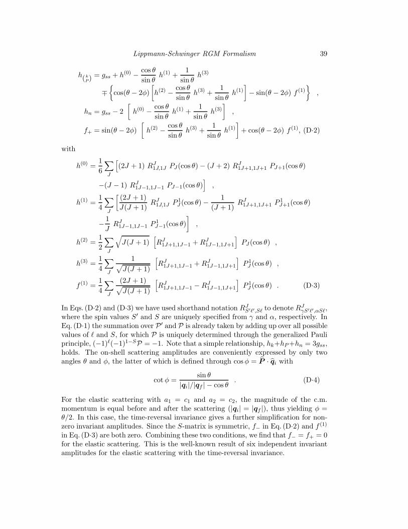
Lippmann-Schwinger RGM Formalism 39
h(kP) = gss + h(0) − cos θ
sin θh(1) +
1
sin θh(3)
∓
cos(θ − 2φ)
[h(2) − cos θ
sin θh(3) +
1
sin θh(1)
]− sin(θ − 2φ) f (1)
,
hn = gss − 2
[h(0) − cos θ
sin θh(1) +
1
sin θh(3)
],
f+ = sin(θ − 2φ)
[h(2) − cos θ
sin θh(3) +
1
sin θh(1)
]+ cos(θ − 2φ) f (1), (D.2)
with
h(0) =1
6
∑
J
[(2J + 1) RJ
1J,1J PJ(cos θ) − (J + 2) RJ1J+1,1J+1 PJ+1(cos θ)
−(J − 1) RJ1J−1,1J−1 PJ−1(cos θ)
],
h(1) =1
4
∑
J
[(2J + 1)
J(J + 1)RJ
1J,1J P 1J (cos θ) − 1
(J + 1)RJ
1J+1,1J+1 P 1J+1(cos θ)
− 1
JRJ
1J−1,1J−1 P 1J−1(cos θ)
],
h(2) =1
2
∑
J
√J(J + 1)
[RJ
1J+1,1J−1 + RJ1J−1,1J+1
]PJ (cos θ) ,
h(3) =1
4
∑
J
1√J(J + 1)
[RJ
1J+1,1J−1 + RJ1J−1,1J+1
]P 1
J (cos θ) ,
f (1) =1
4
∑
J
(2J + 1)√J(J + 1)
[RJ
1J+1,1J−1 − RJ1J−1,1J+1
]P 1
J (cos θ) . (D.3)
In Eqs. (D.2) and (D.3) we have used shorthand notation RJS′ℓ′,Sℓ to denote RJ
γS′ℓ′,αSℓ,where the spin values S′ and S are uniquely specified from γ and α, respectively. InEq. (D.1) the summation over P ′ and P is already taken by adding up over all possiblevalues of ℓ and S, for which P is uniquely determined through the generalized Pauliprinciple, (−1)ℓ(−1)1−SP = −1. Note that a simple relationship, hk+hP +hn = 3gss,holds. The on-shell scattering amplitudes are conveniently expressed by only twoangles θ and φ, the latter of which is defined through cos φ = P · qi with
cot φ =sin θ
|qi|/|qf | − cos θ. (D.4)
For the elastic scattering with a1 = c1 and a2 = c2, the magnitude of the c.m.momentum is equal before and after the scattering (|qi| = |qf |), thus yielding φ =θ/2. In this case, the time-reversal invariance gives a further simplification for non-zero invariant amplitudes. Since the S-matrix is symmetric, f− in Eq. (D.2) and f (1)
in Eq. (D.3) are both zero. Combining these two conditions, we find that f− = f+ = 0for the elastic scattering. This is the well-known result of six independent invariantamplitudes for the elastic scattering with the time-reversal invariance.

40 Y. Fujiwara, M. Kohno, T. Fujita, C. Nakamoto and Y. Suzuki
References
[1] F. E. Close, An Introduction to Quarks and Partons (Academic, London, 1979).[2] M. Oka and K. Yazaki, in Quarks and Nuclei, ed. W. Weise (World Scientific, Singapore,
1984), p.489; K. Shimizu, Rep. Prog. Phys. 52 (1989), 1; C. W. Wong, Phys. Rep. 136
(1986), 1.[3] C. Nakamoto, Y. Suzuki and Y. Fujiwara, Prog. Theor. Phys. 94 (1995), 65.[4] Y. Fujiwara, C. Nakamoto and Y. Suzuki, Prog. Theor. Phys. 94 (1995) 215, 353.[5] Y. Fujiwara, C. Nakamoto and Y. Suzuki, Phys. Rev. Lett. 76 (1996), 2242.[6] Y. Fujiwara, C. Nakamoto and Y. Suzuki, Phys. Rev. C54 (1996), 2180.[7] T. Fujita, Y. Fujiwara, C. Nakamoto and Y. Suzuki, Prog. Theor. Phys. 100 (1998), 931.[8] Y. W. Yu, Z. Y. Zhang, P. N. Shen and L. R. Dai, Phys. Rev. C52 (1995), 3393.[9] Z. Y. Zhang, Y. W. Yu, P. N. Shen, L. R. Dai, Amand Faessler and U. Straub, Nucl. Phys.
A625 (1997), 59.[10] S. Yang, P. N. Shen, Z. Y. Zhang and Y. W. Yu, Nucl. Phys. A635 (1998), 146.[11] M. Kamimura, Prog. Theor. Phys. Suppl. No. 62 (1977) 236.[12] K. Kume and S. Yamaguchi, Phys. Rev. C48 (1993), 2097.[13] H. P. Noyes, Phys. Rev. Lett. 15 (1965), 538.[14] K.L. Kowalski, Phys. Rev. Lett. 15 (1965), 798. [Erratum 15 (1965), 908.][15] M. Kohno, Y. Fujiwara, T. Fujita, C. Nakamoto and Y. Suzuki, submitted to Nucl. Phys.
A (1999).[16] Y. Suzuki, Nucl. Phys. A430 (1984), 539.[17] Y. Fujiwara, C. Nakamoto, Y. Suzuki and Zhang Zong-ye, Prog. Theor. Phys. 97 (1997),
587.[18] M. I. Haftel and F. Tabakin, Nucl. Phys. A158 (1970),1.[19] J. M. Blatt, and L. C. Biedenharn, Rev. Mod. Phys. 24 (1952), 258.[20] G. E. Brown and A. D. Jackson, The Nucleon-Nucleon Interaction (North Holland, Ams-
terdam, 1976).[21] K. Ikeda, R. Tamagaki, S. Saito, H. Horiuchi, A. Tohsaki-Suzuki and M. Kamimura, Prog.
Theor. Phys. Suppl. No. 62 (1977), 1.[22] Y. Suzuki, Nucl. Phys. A405 (1983), 40.[23] Y. Fujiwara and Y. C. Tang, Memoirs of the Faculty of Science, Kyoto University, Series A
of Physics, Astrophysics, Geophysics and Chemistry, Vol. XXXIX, No. 1, Article 5 (1994),91.
[24] Y. Fujiwara and K. T. Hecht, Nucl. Phys. A456 (1986), 669.[25] Y. Fujiwara and K. T. Hecht, Nucl. Phys. A462 (1987), 621.[26] Y. Fujiwara, Prog. Theor. Phys. Suppl. No. 91 (1987), 160.[27] Y. Fujiwara, Prog. Theor. Phys. 88 (1992), 933.[28] H.-J. Schulze, M. Baldo, U. Lombardo, J. Cugnon and A. Lejeune, Phys. Rev. C57 (1998),
704.[29] R. A. Arndt, Scattering Analysis Interactive Dial-up (SAID), Virginia Polytechnic Insti-
tute, Blacksburg, Virginia (private communication).[30] M. Lacombe, B. Loiseau, J. M. Richard, R. Vinh Mau, J. Cote, P. Pires and R. de Tourreil,
Phys. Rev. C21 (1980), 861.[31] R. A. Arndt, L. D. Roper, R. A. Bryan, R. B. Clark, B. J. VerWest and P. Signell, Phys.
Rev. D28 (1983), 97.[32] R. A. Bryan and B. L. Scott, Phys. Rev. 164 (1967), 1215.[33] P. M. M. Maessen, Th. A. Rijken and J. J. de Swart, Phys. Rev. C40 (1989), 2226.[34] Th. A. Rijken, V. G. J. Stoks and Y. Yamamoto, Phys. Rev. C59 (1999), 21.[35] Y. Fujiwara, M. Kohno, T. Fujita, C. Nakamoto and Y. Suzuki, submitted to Nucl. Phys.
A (1999).
Copyright © 2022 FDOKUMEN