Linking depth to lightness and anchoring within the differentiation-integration formalism

This article appeared in a journal published by Elsevier. The attachedcopy is furnished to the author for internal non-commercial researchand education use, including for instruction at the authors institution

and sharing with colleagues.

Other uses, including reproduction and distribution, or selling orlicensing copies, or posting to personal, institutional or third party

websites are prohibited.

In most cases authors are permitted to post their version of thearticle (e.g. in Word or Tex form) to their personal website orinstitutional repository. Authors requiring further information

regarding Elsevier’s archiving and manuscript policies areencouraged to visit:

http://www.elsevier.com/copyright

http://www.elsevier.com/copyright

Author's personal copy

Linking depth to lightness and anchoring within the differentiation–integrationformalism

Naoki Kogo a,b,*, Luc Van Gool b,c, Johan Wagemans a

a Katholieke Universiteit Leuven, Laboratory of Experimental Psychology, B-3000 Leuven, Belgiumb Katholieke Universiteit Leuven, ESAT/PSI, B-3001 Heverlee, Belgiumc ETH, Computer Vision Laboratory (BIWI), Zürich, Switzerland

a r t i c l e i n f o

Article history:Received 18 September 2009Received in revised form 29 April 2010

Keywords:Surface reconstructionKanizsa figureVisual illusionsDepth perceptionLightness perceptionAnchoringDifferentiationIntegrationNeural signals

a b s t r a c t

Recently we developed a model that reproduces the Kanizsa square illusion based on two principles: (1) aspatial 2-D integration of luminance ratio and differentiated depth signals creates a ‘‘primary” lightnessmap and a depth map, respectively, which is then followed by (2) a modification of the primary lightnessvalues under influence of the perceived depth (Kogo, Strecha, Van Gool, & Wagemans, 2010). Within thismodel, the process of the spatial integration inevitably introduced an arbitrary offset. In order to obtainabsolute values of depth and lightness, the offset values needed to be determined by other constraints.This is the anchoring problem of the depth and lightness measurements. Here we report the anchoringrules that were established by investigating the model’s responses to the Kanizsa square and its widerange of variations. For the primary lightness map, the highest value rule was applied, while the area ruleappeared most plausible for the depth map. By applying the same principles to simple figures consistingof black and white areas of different size ratios, the model succeeded in reproducing published empiricalresults on lightness anchoring (Li & Gilchrist, 1999).

� 2010 Elsevier Ltd. All rights reserved.

1. Introduction

Lightness is the perceived reflectance of a surface. How do weknow the reflectance of a surface by seeing it? This is not a simplequestion to answer. To start, the well-known underconstrained in-verse-optics problem needs to be solved: two values, illuminationand reflectance, need to be computed from a single measurement,luminance. The visual system needs to use extra information tojudge whether the luminance of a surface is due to the reflectanceof the surface or the illumination on the surface (for reviews, seeGilchrist, 2006 and Gilchrist et al., 1999). Furthermore, a carefulanalysis suggested elaborate mechanisms underlying our lightnessperception. It was found that the lightness of two abutting surfacesdepends on the luminance ratio between them (relative values),not on their absolute luminance values (Wallach, 1948). If light-ness perception is based on relative values, certain rules are re-quired to compute the absolute values of lightness: Afterdetecting the relative values, they need to be ‘‘anchored” to someabsolute values. This ‘‘anchoring problem” must be solved by inter-nal mechanisms in the visual system. Phenomenologically, Li andGilchrist (1999) have demonstrated two rules of anchoring by

which the perceived lightness values are determined. They coveredthe entire visual field of a subject by a dome inside of which thearea was divided in two areas with different gray scales and theyobserved the following two principles. First, the area with the high-er luminance is valued as white when its surface area is larger thanthe other. Second, when the surface area with the lower luminancebecomes greater than the other one, the lightness value assigned toit increases while the one assigned to the surface area with thehigher luminance becomes slightly higher than white. In otherwords, the final lightness values reflect the relative (but not theabsolute) values of luminance and are ‘‘anchored” following thesetwo rules. The observed phenomena are systematic and, therefore,they are considered to be revealing the internal mechanisms oflightness computation.

The fact that lightness perception depends on the ratio betweenthe luminance values at borderlines reveals the relational charac-ter of our perception as described in Gestalt psychology, i.e. theobservation that the relative values (differences of measurements)but not the absolute values (measurements themselves) of inputsignals determine our perception (Koffka, 1935). This relationalpoint of view leads to the argument that the information aboutsurfaces is stored at the borderlines and can be extracted later fromthem. This view has been discussed theoretically (Arend, 1973;Gilchrist, Delman, & Jacobsen, 1983; Land & McCann, 1971; Ross& Pessoa, 2000; Wallach, 1948) as well as supported experimen-

0042-6989/$ - see front matter � 2010 Elsevier Ltd. All rights reserved.doi:10.1016/j.visres.2010.05.007

* Corresponding author at: Katholieke Universiteit Leuven, Laboratory of Exper-imental Psychology, B-3000 Leuven, Belgium. Fax: +32 16 326099.

E-mail address: [email protected] (N. Kogo).

Vision Research 50 (2010) 1486–1500

Contents lists available at ScienceDirect

Vision Research

journal homepage: www.elsevier .com/locate /v isres


tally (Arend, 1973; Gilchrist, 1979; Hung, Ramsden, Chen, & Roe,2001; Krauskopf, 1963; Whittle & Challands, 1969). Retinex theory(Land & McCann, 1971), for instance, was proposed to reconstructsurfaces based on the ratio of luminance values measured at theborderlines. With this way of constructing surfaces from the rela-tive values, one degree of freedom is inevitably introduced, the off-set value, because the result is independent of the absolute values.In our view, the phenomena observed by Li and Gilchrist reflect theway in which the offset values are determined by the computa-tional mechanisms of the visual system.

To investigate the anchoring mechanisms, it is worth here con-sidering the relational aspect of vision in terms of neural mecha-nisms. From the beginning of the history of neural recordingsfrom the visual cortex, it has been known that neurons respondto borderlines of objects but not to the surface interior betweenthe borderlines (Hubel & Wiesel, 1959). Although this is a quitecharacteristic property of neurons in general, it is a bit puzzlingin the sense that the interior surface, while it is perceived, doesnot itself excite neurons (Hubel, 1988, p. 87). However, some neu-rons in V1 are sensitive to the polarity of contrast (Hubel & Wiesel,1962) and some neurons in V2 and V4 are even able to signal thepolarity of the depth differences (‘‘border-ownership”, Zhou,Friedman, & von der Heydt, 2000). This implies that the relationalproperty of perception may be based on the neural signals thatrepresent the original input in the form of ‘‘differentiated” signals.Although neurons appear to respond to borderlines of images, theiractivities actually contain information about the interior betweenthe borderlines in implicit form. It follows that their spatial ‘‘inte-gration” can make the information explicit by constructing the sur-faces attached to the borderlines. In the process of the integration,naturally, an offset value needs to be determined, which corre-sponds to the anchoring problem. In terms of the neural architec-ture for visual perception, the ‘‘differentiation–integration”strategy might indeed be a plausible strategy for the visual system.Within this approach, the lower-level visual cortex only needs todetect the local properties by measuring the ‘‘difference” of the in-puts between neighbors (e.g., the differences of luminance ordepth). By assigning these difference values to individual locations,in effect it constructs a ‘‘2-D differentiated” signal map. The higherlevel, on the other hand, two-dimensionally ‘‘integrates” the sig-nals of these relative measurements to determine the macroscopicproperties.

Investigating the anchoring mechanism is essential to articulatethe differentiation–integration process in the visual system. Themechanisms underlying the lightness perception phenomenafound by Li and Gilchrist are, however, not known. Recently, wedeveloped a model, called the ‘‘DISC” (Differentiation–Integrationfor Surface Completion) model, which reproduces the perceptionof Kanizsa figures such as an illusory square in an array with fourpacmen. It also reproduces our perception of its variation figuresincluding non-illusory figures (Kogo, Strecha, Van Gool, &Wagemans, 2010). The DISC model is fully based on the differenti-ation–integration approach reflecting the relational viewmentioned above: From the integration of luminance ratio basedvalues, it creates a lightness map. It also detects occlusion cuesand computes the border-ownership (BOWN) signals that indicatedepth differences, and the integration of them creates a depth map.The development of the model, therefore, necessitated us toarticulate the anchoring mechanisms so that they could be imple-mented in the model.

In search for the correct implementation of the anchoring rulesfor these maps, we realized that, by analyzing the behavior of theDISC model responding to the variations of the Kanizsa figure,the use of this well-known and fundamental illusion can provideinsight in the relationship between depth-lightness linkageand the anchoring rules, and their connection to figure-ground

segregation. In this way, we were able to narrow down the possibleanchoring rules used in the primary lightness map and depth map.Furthermore, based on the final lightness map, the validity of theserules can be analyzed by comparison with empirical data. In otherwords, we argue that the framework of the DISC model, the inter-action of the anchored primary lightness map and the anchoreddepth map to compute the final lightness, may explain the mech-anisms that determine the phenomenological rules of anchoringmentioned above. This paper is to investigate the plausibility ofthese anchoring mechanisms implemented in the model and tocompare the behavior of the model with previously publishedempirical data.

In sum, we believe that the Kanizsa figure provides the possibil-ity to develop specific methods for anchoring and for depth-lightness linkage because the results can be evaluated against thewell-established perception of these stimuli. We first discuss theframework of the theory and the model, described in more detailselsewhere (Kogo et al., 2010). We then describe how the anchoringrules were determined heuristically by using the Kanizsa figurevariations as guiding examples. In addition, the responses of themodel to objects with varying sizes are described and comparedwith previously reported empirical data of the anchoring rules inlightness perception.

2. Theory and computational model

The principle of the DISC model to reproduce the Kanizsa illusionis simple: the depth perception of the image modifies the lightnessperception. The lightness map created at first by the integration ofthe luminance ratio is called a ‘‘primary” lightness map. This is fur-ther modified by the depth map to reflect the fact that lightnessperception is influenced by depth perception (depth-lightness link-age). This creates the final lightness map. In the integration pro-cesses of the primary lightness map and the depth map, naturally,it was necessary to determine the offset values of these maps. Toinvestigate the most plausible rules to determine the offset valuesis the focus of this paper. In this section, first, we explain the differ-entiation–integration approach as a concept and explain how thisapproach implies the anchoring problem (determination of the off-set values). This is then followed by the description of the methodsto implement this concept into a computational model.

2.1. Differentiation–integration approach and anchoring problem

Anchoring is, clearly, a general problem when the ‘‘differentia-tion–integration” approach is taken because the offset value afterthe integration needs to be determined by additional constraints.The problem can be described in a general form as follows. Assumethat the visual system processes a certain property, F, of a visualimage. First, the visual system constructs a differentiated map ofthe property

rF ¼ @F@x;@F@y

� �ð1Þ

This differentiated map is later spatially integrated to create theperception of the input property FP:

FP ¼Z

arF � d~r þ C ð2Þ

a is the integration pathway, r with an arrow on the top: unit vectorin space, C is a constant

As indicated, this integration introduces an extra constant, C,which is an offset for FP. In Eq. (2), C is arbitrary as far as thereare no additional constraints to determine a particular value forit. To determine the value for C is exactly equivalent to solvingthe anchoring problem.

N. Kogo et al. / Vision Research 50 (2010) 1486–1500 1487


We hypothesize that the visual system first creates relativemaps in the lightness and the depth domains. These are then inte-grated to create the lightness and the depth maps. This integratedlightness map is further modified to compute the final lightnessmap. The lightness maps before and after the modification arecalled ‘‘primary lightness map” and ‘‘lightness map”, respectively.Note that the visual system’s surface completion mechanism doesnot always create flat surfaces but sometimes surfaces with grad-ual changes. It is known that when the distance of the pacmen inKanizsa figure is increased, the illusion is reduced (i.e., the supportratio effect; see Shipley & Kellman, 1992). Also, when the pacmenare misaligned, the edges of the perceived central surface appearsmoother (Stanley & Rubin, 2003). The surface construction by spa-tial integration, therefore, should differ from the mathematicalintegration in this regard. That is, when a pulse-like signal is math-ematically integrated, for instance, a step-wise signal is created(causal integration). Human vision, on the other hand, seems toperform a completion with a gradual decay in distance instead.We implemented, therefore, a mathematical technique, called ‘‘lea-ky integration” (Claerbout, 1992), which is similar to causal inte-gration except that the integrated values decay with distance.This leaky integration operator (Q) in two-dimensional space is ap-plied to the relative depth map R and the luminance ratio map K tocreate the depth map D and the primary lightness map LP,respectively:

D ¼ QfRg þ CD

LP ¼ expða � QfKg þ CLÞK ¼ logðI0Þ0

ð3Þ

The relative depth map R is computed as the border-ownershipmap described later. The (log-) luminance ratio map K is a differen-tiation of the logarithm of the input luminance I0. a is a constant.Once again, the integration introduces the constants CD and CL,which have to be determined by the anchoring process. The goalof this paper is to investigate how these two values for CD and CL

should be determined.

2.2. The DISC model

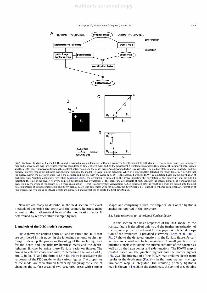
The basic structure of the DISC model is shown in Fig. 1A (seeKogo et al., 2010 for more details). The model first creates a log-luminance ratio map of the image. First, the logarithm of the inputluminance is taken and the difference values between neighboringpixels are taken. This is done so that the lightness value computedat the later stage of the model depends on the luminance ratio(Horn, 1974; Land & McCann, 1971) to reflect the dependency ofour lightness perception on the luminance ratio but not on theluminance difference (Wallach, 1948). The result is called thelog-luminance ratio map. The log-luminance ratio map is fed intotwo channels, the geometric channel and the photometric channelthat compute the depth and the lightness maps, respectively. Notethat only where there is a luminance value difference between twoneighboring pixels, the luminance ratio map has non-zero values.In the depth channel, therefore, the model first normalizes theluminance ratio map to create the borderline map. It then looksfor occlusion cues (junctions) by detecting changes of directionsof the borderlines. Even when a junction is small and is constitutedby two borderlines around a pixel, it is detected as a junction.Amplitudes of all junction signals are normalized to a value ofone regardless of the size of the junctions. The L-junction signalstentatively indicate the relative depth based on the properties ofthe junctions (Fig. 1B). (For simplification purpose, T-junctiondetection is omitted in this paper. The original model detectsL- and T-junctions.) It is assumed that the area on the side of thenarrower angle of a junction (90� at J) is the ‘‘occluding” area

(S1), while the one with the wider angle (270�) is being the‘‘occluded” area (S2).

Next, the ‘‘ownership” of the borderlines (BOWN) is determinedby reflecting the global configuration of the figures, i.e. the layoutof the borderlines and the junctions (for details, see Kogo et al.,2010). This is done by adopting and modifying an algorithm pub-lished by Zhaoping (2005). The basic idea is that the BOWN signalsinteract with each other in the entire space so that those that are inagreement enhance each other. At each pixel on a borderline, twoopposing BOWN signals are possible at first, indicating that theareas on both sides of the borderline can be the owner. First, eachBOWN signal (e.g., B1 at x in Fig. 1C) is compared with the junctionmap. If a junction is located and oriented so that the occlusion sug-gested by the junction is in agreement with the ownership theBOWN signal is indicating (e.g., J1), the BOWN signal is enhanced.The strength of this enhancement decays exponentially with thedistance of the two points. This first result of the junction-basedBOWN map is passed onto an iteration process where the BOWNsignals are enhanced further when other BOWN signals in agree-ment are found (e.g., B2 in Fig. 1D). In this way, the final BOWN sig-nals reflect the macroscopic configuration of the input image. Theresult shows the dominance of the ownership by one side of thearea compared to the other. The BOWN signals of two opposingsides are compared and the one that obtained the larger value be-comes the final owner of the borderline at each location and its va-lue is normalized (winner-take-all). In a simple closed figure suchas a disk or a rectangle this process creates BOWN signals indicat-ing that the inside area is the owner of the borderline. Further-more, this process successfully obtains BOWN signals of Kanizsafigure and the wide range of its variations, including illusory andnon-illusory figures (Kogo et al., 2010).

The final BOWN map indicates which side of the individual bor-derline is its owner (closer to the viewer) and hence indicates thedepth order at each location. This computed BOWN map is consid-ered as a differentiated depth map in the model and the integrationof the BOWN map gives the depth map. Hence, the 2-D leaky inte-gration is applied to the final BOWN map. The leaky integration isachieved by the use of a Gaussian function which is cut in half atzero. Convolution of this ‘‘half Gaussian” function with a pulse-likesignal creates a step change at the location that decays graduallywith distance (the decay is determined by the standard deviationof the Gaussian). A summation of the leaky integration in all360� different orientations and its average (excluding the integra-tion pathways that do not create any signals) constructs surfacesbetween borderlines. Furthermore, the bilateral filter (Tomasi,1998) is applied to smooth the surface. This creates the final depthmap. In the Z-axis of the map, the higher the value of a surface isthe closer to the viewer.

The same integration process is applied to the log-luminanceratio map that results in the primary lightness map, LP. It is called‘‘primary” lightness map because (1) it gives a basic structure ofthe lightness map but (2) it is further modified by reflecting thedepth values computed in the geometric channel. Thus, the finallightness map L is created by modifying this primary lightnessmap based on the depth-lightness linkage. For this purpose, a so-called modification factor M is constructed as a function of thedepth map D. This is multiplied with the primary lightness mapLP to obtain the final lightness L:

L ¼ LP �MðDÞ ð4Þ

Eq. (4) indicates that the perceived lightness of the image isdetermined by modifying the primary lightness values at eachpoint according to their perceived depth values. Here, LP and Dare underlined to explicitly indicate that these values need to beanchored (determination of the offset values).

1488 N. Kogo et al. / Vision Research 50 (2010) 1486–1500


Now we are ready to describe, in the next section, the exactmethods of anchoring the depth and the primary lightness mapsas well as the mathematical form of the modification factor Mdetermined by representative example figures.

3. Analysis of the DISC model’s responses

Fig. 2 shows the Kanizsa figure (A) and its variations (B–E) thatare considered in this paper. In the following sections, we first at-tempt to develop the proper methodology of the anchoring rulesfor the depth and the primary lightness maps and the depth-lightness linkage by using these Kanizsa variation figures. Theaim is to achieve consistent rules to determine the values of CD

and CL in Eq. (3) and the form of M in Eq. (4) by investigating theresponses of the DISC model to the various figures. The propertiesof the model are then studied further by analyzing the effect ofchanging the surface areas of two separated areas with simpler

shapes and comparing it with the empirical data of the lightnessanchoring reported in the literature.

3.1. Basic responses to the original Kanizsa figure

In this section, the basic responses of the DISC model to theKanizsa figure is described only to aid the further investigation ofthe response properties relevant for this paper. A detailed descrip-tion of the responses is provided elsewhere (Kogo et al., 2010).Fig. 2F shows the detected junctions in the Kanizsa figure. As cur-vatures are considered to be sequences of small junctions, thejunction signals exist along the curved contours of the pacmen aswell as on the large center and side junctions. The BOWN map iscreated based on the junction signals and the border signals(Fig. 2G). The integration of the BOWN map (relative depth map)results in the depth map (Fig. 2H). In the same manner, the log-luminance map is integrated. The resulting primary lightnessmap is shown in Fig. 2I. In the depth map, the central area obtains

Fig. 1. (A) Basic structure of the model. The model is divided into a photometric (left) and a geometric (right) channel. In both channels, relative value maps (log-luminancemap and relative depth map) are created. They are considered as differentiated maps and, by the subsequent 2-D integration process, they become the primary lightness mapand the depth map, respectively. Based on the contrast polarity map and the depth map, a ‘‘modification factor” is constructed. The product of the modification factor and theprimary lightness map is the lightness map, the final output of the model. (B) Occlusion cue detection. When an L-junction (J) is detected, the model tentatively decides thatthe surface within the narrower angle (S1) is the occluder and the one with the wider angle (S2) is the occluded area. (C) BOWN computation based on the distribution ofocclusion cues. Adapting Zhaoping’s convention (Zhaoping, 2005), the ownership is signaled by the arrow indicating the orientation of the borderline and the side finindicating the side of the owner. At every point on borderlines, two ownerships of the borderline are possible at first. Consider the BOWN signal B1 at x indicating theownership by the inside of the square (S1). If there is a junction (J1) that is concave when viewed from x, B1 is enhanced. (D) The resulting signals are passed onto the nextiteration process of BOWN computation. The BOWN signal, B1 at x is in agreement with, for instance, the BOWN signal B2. Hence, they enhance each other. After iteration ofthis process, the two opposing BOWN signals are subtracted and normalized to create the final BOWN map.



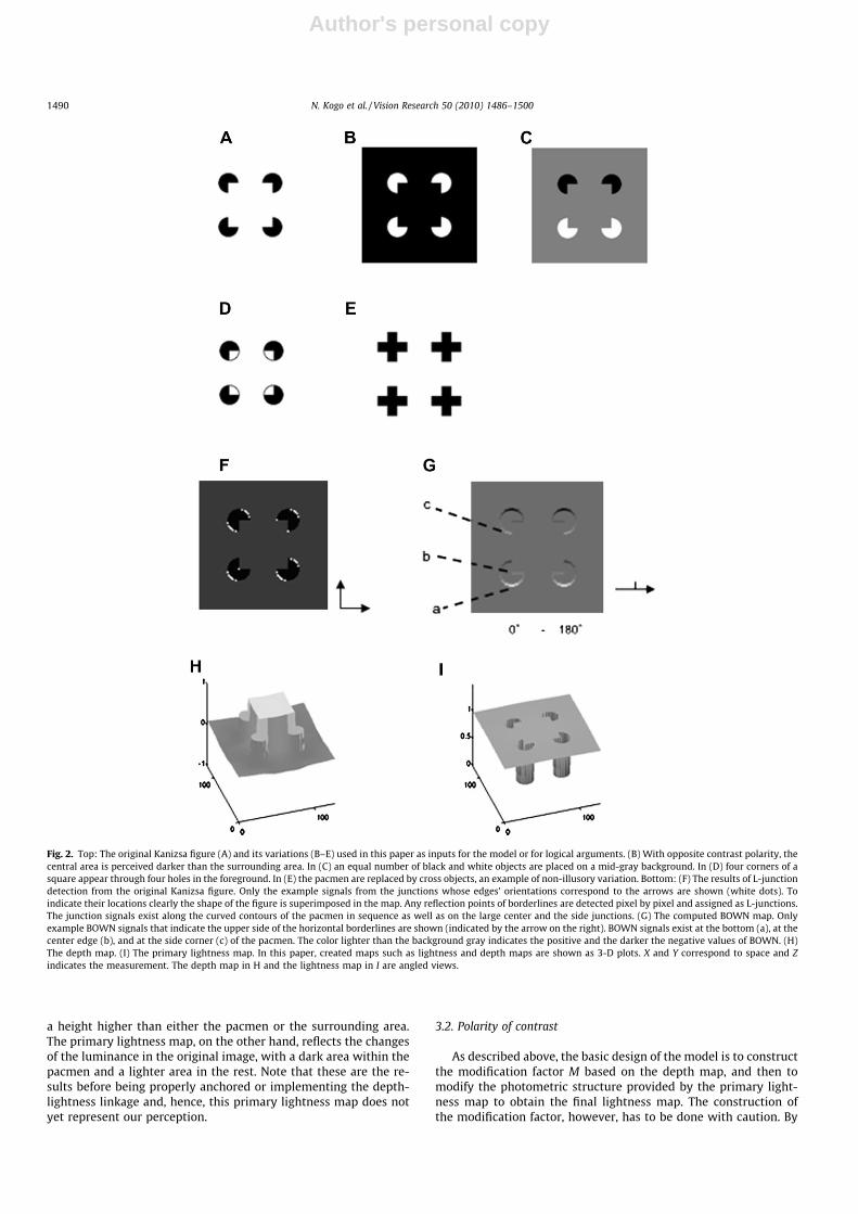
a height higher than either the pacmen or the surrounding area.The primary lightness map, on the other hand, reflects the changesof the luminance in the original image, with a dark area within thepacmen and a lighter area in the rest. Note that these are the re-sults before being properly anchored or implementing the depth-lightness linkage and, hence, this primary lightness map does notyet represent our perception.

3.2. Polarity of contrast

As described above, the basic design of the model is to constructthe modification factor M based on the depth map, and then tomodify the photometric structure provided by the primary light-ness map to obtain the final lightness map. The construction ofthe modification factor, however, has to be done with caution. By

Fig. 2. Top: The original Kanizsa figure (A) and its variations (B–E) used in this paper as inputs for the model or for logical arguments. (B) With opposite contrast polarity, thecentral area is perceived darker than the surrounding area. In (C) an equal number of black and white objects are placed on a mid-gray background. In (D) four corners of asquare appear through four holes in the foreground. In (E) the pacmen are replaced by cross objects, an example of non-illusory variation. Bottom: (F) The results of L-junctiondetection from the original Kanizsa figure. Only the example signals from the junctions whose edges’ orientations correspond to the arrows are shown (white dots). Toindicate their locations clearly the shape of the figure is superimposed in the map. Any reflection points of borderlines are detected pixel by pixel and assigned as L-junctions.The junction signals exist along the curved contours of the pacmen in sequence as well as on the large center and the side junctions. (G) The computed BOWN map. Onlyexample BOWN signals that indicate the upper side of the horizontal borderlines are shown (indicated by the arrow on the right). BOWN signals exist at the bottom (a), at thecenter edge (b), and at the side corner (c) of the pacmen. The color lighter than the background gray indicates the positive and the darker the negative values of BOWN. (H)The depth map. (I) The primary lightness map. In this paper, created maps such as lightness and depth maps are shown as 3-D plots. X and Y correspond to space and Zindicates the measurement. The depth map in H and the lightness map in I are angled views.



comparing the two Kanizsa figures with opposite contrast polari-ties (Fig. 2A and B), an important aspect of this illusion can be ob-served: The central area in the ‘‘black pacmen on whitebackground” (black-on-white) configuration is perceived as lighterthan the surrounding area, while in the ‘‘white pacmen on blackbackground” (white-on-black) configuration, it is perceived as dar-ker. In addition, the variations of the Kanizsa figure shown inFig. 2C with mid-gray background and equal numbers of blackand white pacmen (mid-gray Kanizsa figure) do not yield any dif-ferent lightness in the central area compared with the surroundingarea.

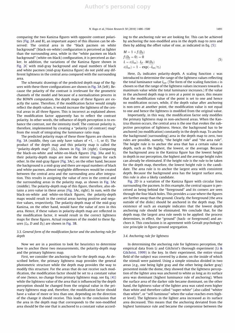
The schematic drawings of the predicted depth map of the fig-ures with these three configurations are shown in Fig. 3A (left). Be-cause the polarity of the contrast is irrelevant for the geometricchannels of the model and because of a normalization process inthe BOWN computation, the depth maps of these figures are ex-actly the same. Therefore, if the modification factor would simplyreflect the depth values, it would increase the lightness of the cen-tral areas in all three figures. This is incorrect as explained above.The modification factor apparently has to reflect the contrastpolarity. In other words, the influence of depth perception is to en-hance the contrast, not the intensity itself. The contrast polarity is,therefore, implemented by creating a ‘‘polarity (of contrast) map”from the result of integrating the luminance ratio map.

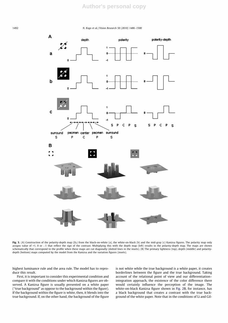
The predicted polarity maps of these three figures are shown inFig. 3A (middle, they can only have values of +1, �1, or 0). Theproduct of the depth map and this polarity map is called the‘‘polarity-depth map” (DP), shown in Fig. 3A (right). Comparingthe black-on-white and white-on-black figures (Fig. 3Aa and b),their polarity-depth maps are now the mirror images for eachother. In the mid-gray figure (Fig. 3Ac), on the other hand, becausethe background is a mid-gray and there are equal numbers of blackand white pacmen, almost negligible differences would be createdbetween the central area and the surrounding area after integra-tion. This results in assigning the value of zero in the central andthe surrounding areas in the polarity map, as shown in Fig. 3Ac(middle). The polarity-depth map of this figure, therefore, also ob-tains a zero value in these areas (Fig. 3Ac, right). In sum, with theblack-on-white and white-on-black figures, the polarity-depthmaps would result in the central areas having positive and nega-tive values, respectively. The polarity-depth map of the mid-grayKanizsa, on the other hand, would have the value of zero in thisarea. Hence, if these values in polarity-depth map are reflected inthe modification factor, it would result in the correct lightnessmaps for these figures. Actual responses of the model to these fig-ures (LP, D and DP) are shown in Fig. 3B.

3.3. General form of the modification factor and the anchoring rule fordepth

Now we are in a position to look for heuristics to determinehow to anchor these two measurements, the polarity-depth mapand the primary lightness map.

First, we consider the anchoring rule for the depth map. As de-scribed before, the primary lightness map provides the generalphotometric structure while the depth map provides the way tomodify this structure. For the areas that do not receive such mod-ification, the modification factor should be set to a constant valueof one (hence, no change from primary lightness map, see Eq. (4))while the lightness value of the area that is influenced by the depthperception should be changed from the original value in the pri-mary lightness map and, therefore, the modification factor shouldhave a value of more or less than one, depending on the directionof the change it should receive. This leads to the conclusion thatthe area in the depth map that corresponds to the non-modifiedarea should be the one that is anchored to a constant value accord-

ing to the anchoring rule we are looking for. This can be achievedby anchoring the non-modified area in the depth map to zero andthen by adding the offset value of one, as indicated in Eq. (5):

M ¼ 1þ f ðDPÞf ðDP ¼ 0Þ ¼ 0L ¼ eðItotÞ � LP �MðDPÞeðItotÞ ¼ 1� expð�Itot=sIÞ

ð5Þ

Here, DP indicates polarity-depth. A scaling function e wasintroduced to determine the range of the lightness values reflectingthe total luminance value Itot. (The form of the scaling function e ischosen so that the range of the lightness values increases towards amaximum value while the total luminance increases.) If the valuein the anchored depth map is zero at a point in space, this meansthat the modification value of the point is set to one and henceno modification occurs, while, if the depth value after anchoringis non-zero at another point, the modification value is not equalto one and hence the lightness is modified from the original value.

Importantly, in this way, the modification factor only modifiesthe primary lightness map in non-anchored areas. When the Kan-izsa illusion occurs, the central area is the one that evokes the sub-jective perception of lightness. Hence, the background has to beanchored (no modification) constantly in the depth map. To anchorthe background (surrounding) area in the depth map to zero, tworules are possible, namely, ‘‘the height rule” and ‘‘the area rule”.The height rule is to anchor the area that has a certain value indepth, such as the highest, the lowest, or the average. Becausethe background area in the Kanizsa figure has the lowest heightin depth in our perception, the highest and the average height rulescan already be eliminated. If the height rule is the rule to be takenfor the depth map, therefore, the lowest height rule is the candi-date. The area rule is to anchor the largest area with consistentdepth. Because the background area has the largest surface area,this rule is also a likely candidate.

Fig. 2D is a variation of the Kanizsa figure with circular linessurrounding the pacmen. In this example, the central square is per-ceived as being behind the ‘‘foreground” and its corners are seenthrough the four black holes. This provides a case where the figuresare further away than the ground. Clearly, the foreground (the areaoutside of the disks) should be anchored in the depth map. Theexistence of such an example indicates that the lowest depthanchoring rule should be eliminated. We conclude that, for thedepth map, the largest area rule needs to be applied: the processdetermines, in effect, the ‘‘ground” (back- or foreground) and an-chors it. This conclusion is in agreement with Gestalt psychology’ssize principle in figure-ground segregation.

3.4. Anchoring rule for lightness

In determining the anchoring rule for lightness perception, theempirical data from Li and Gilchrist’s thorough experiment (Li &Gilchrist, 1999) is the key. In their experiment, the entire visualfield of the subject was covered by a dome, on the inside of whichthe stimuli were painted. Using a simple stimulus divided in twoareas (e.g., one being light gray and the other being darker gray)presented inside the dome, they showed that the lightness percep-tion of the lighter area was anchored to white as long as its surfacearea was dominant (highest luminance rule of anchoring). Whenthe surface area of the darker side became dominant, on the otherhand, the lightness value of the lighter area was rated even higherthan white and therefore called ‘‘super-white” (also called ‘‘whiterthan white”, or ‘‘self-luminous” when the value reaches even high-er level). The lightness in the lighter area increased as its surfacearea decreased. This means that the anchoring deviated from thehighest luminance rule and became the compromise between the



highest luminance rule and the area rule. The model has to repro-duce this result.

First, it is important to consider this experimental condition andcompare it with the conditions under which Kanizsa figures are ob-served. A Kanizsa figure is usually presented on a white paper(‘‘true background” as oppose to the background within the figure).If the background within the figure is white, then, it blends into thetrue background. If, on the other hand, the background of the figure

is not white while the true background is a white paper, it createsborderlines between the figure and the true background. Takingaccount of the relational point of view and our differentiation–integration approach, the existence of the color difference therewould certainly influence the perception of the image. Thewhite-on-black Kanizsa figure shown in Fig. 2B, for instance, hasa black background that creates a contrast with the true back-ground of the white paper. Note that in the conditions of Li and Gil-

Fig. 3. (A) Construction of the polarity-depth map (DP) from the black-on-white (a), the white-on-black (b) and the mid-gray (c) Kanizsa figures. The polarity map onlyassigns value of +1, 0 or �1 that reflect the sign of the contrast. Multiplying this with the depth map (left) results in the polarity-depth map. The maps are shownschematically that correspond to the profile when these maps are cut diagonally (dotted lines in the insets). (B) The primary lightness (top), depth (middle) and polarity-depth (bottom) maps computed by the model from the Kanizsa and the variation figures (insets).



christ’s dome experiment, this problem is probably eliminated be-cause the stimuli continued all the way to the end of the visualfield. Corresponding to this, when the variations of the Kanizsa fig-ure were given to our model, the contrast between the backgroundof the figure and the true background was also neglected. Thismeans that the model shows responses in an environment that isequivalent to the dome experiment. In other words, the black, grayor white background of a figure is assumed to cover the entire vi-sual field.

In this condition, the figures with four black objects (e.g., pac-men) on a white background are assured to correspond to the stim-ulus in the dome experiment with the surface area of the lighterarea being dominant. The figures with white objects on black, onthe other hand, correspond to the stimulus when the black surfacearea is dominant. This argument leads to the conclusion that, in allthe variations of the Kanizsa figure with the black-on-white config-uration, the area that is white in the original stimulus should beperceived as white. With the Kanizsa figure in this configuration,however, this should be determined carefully because the centralarea is perceived lighter than the surrounding. Which area, centeror surround, is, then, perceived as white? Note that, in the non-illusory variation figures (e.g. Fig. 2E), this lightness differencebetween the center and surround areas does not exist. Clearly, inthese non-illusory figures, the areas that are originally whiteshould all be perceived as white, according to the rule found byLi and Gilchrist. By placing the original Kanizsa figure with thenon-illusory figure side-by-side, it becomes clear that the percep-tion of lightness in the surrounding area should be consistentand that it is the central area of the original Kanizsa figure whichdiffers from the others. In other words, the background color seemsto have constancy, while in the central area, the subjective or mod-ified lightness should occur. The anchoring rules for the primarylightness and depth maps, as well as the depth-lightness linkagein our model, therefore, should lead to the same result in theblack-on-white configuration: the surrounding area is assignedwhite and the center area of the Kanizsa figure should have the as-signed value of higher than white.

As discussed in the previous section, the modification factor isset to one in the surrounding area (no modification by the depthmap). Considering Eq. (4) and the fact that the lightness in this areashould be set to ‘‘white”, the surface in the primary lightness mapshould be anchored to a value so that it results in ‘‘white” in thelightness map. Because the central area and the background areaboth have almost equal values in the primary lightness map(Fig. 3B top) both areas would be anchored in the map. Thereare, again, two possible rules to obtain this result, namely, to an-chor the area based on the value in the primary lightness map(the highest value rule) or based on the largest area with consistentvalue (the area rule).

While we determined, by inference from the perception of theKanizsa figure, that the area rule is used for the depth map, sofar two anchoring rules appear possible for the primary lightnessmap, i.e. the highest value rule and the area rule. To determinewhich of these two possible rules to follow, further investigationof other example figures is necessary.

3.5. Further clues from the Kanizsa variation figures

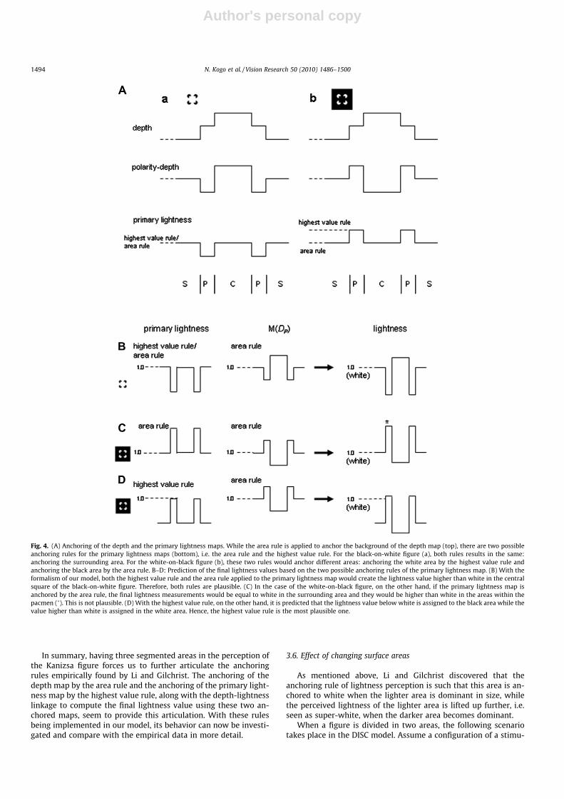
Using the Kanizsa figures with the opposite contrast polarity,i.e. black-on-white and white-on-black Kanizsa figures (Fig. 2Aand B), the possible anchoring rules for the primary lightnessmap can be discussed further. In Fig. 4A, the predicted polarity-depth and primary lightness in the surrounding (S), the pacmen(P), and the central (C) areas are schematically plotted one-dimen-sionally. As discussed before, the area anchored in the depth mapdoes not modify the lightness (Eq. (5)), and, if, in addition, the same

area is anchored in the primary lightness map, then it is perceivedas ‘‘white”. In other words, when an area is anchored in both thedepth and the primary lightness maps, the area is perceived aswhite.

The two figures in question create exactly the same depthmaps and hence their polarity-depth maps are each other’s mirrorimages due to the opposite contrast polarity. These maps are an-chored at the surrounding areas (the background, indicated bydashed lines in Fig. 4A). In addition, the surrounding area in theblack-on-white Kanizsa figure has the quality of both the highestprimary lightness and the largest surface area and, hence, be-comes anchored in the primary lightness no matter whichanchoring rule is taken (Fig. 4Aa). The key difference betweenthe two figures is the fact that the surrounding area in thewhite-on-black Kanizsa figure does no longer possess the highestprimary lightness (Fig. 4Ab bottom). If the area rule is applied tothe primary lightness map in this figure, the surrounding areawill be anchored. If, on the other hand, the highest value rule isapplied, the areas inside the pacmen would be anchored in theprimary lightness map.

This difference is further explained in Fig. 4B. In Fig. 4B, theanchoring of the primary lightness and the polarity-depth mapsfrom the black-on-white Kanizsa figure is shown. In both maps,the surrounding area is anchored. As a result, the final lightnessmap shows the surrounding area anchored to the value of one(white) and the central area gains a value higher than white(‘‘super-white”). In Fig. 4C and D, two possible ways of anchoringare shown for the white-on-black Kanizsa figure. If the area ruleis applied to the primary lightness map of this figure, as shownin Fig. 4C, the surrounding area is anchored. Because the polar-ity-depth map does not provide any modifications in this area, thisarea in the final lightness map would be assigned as white (1.0times 1.0). The areas inside the pacmen, on the other hand, wouldreceive values higher than the surrounding area in both the pri-mary lightness and the depth maps. This would result in assigninga value much higher than white in these areas (1.x times 1.x). Thisis completely against our perception of the figure. On the otherhand, if the highest value rule is applied to the primary lightnessmap of this figure, as shown in Fig. 4D, the areas within the pacmenare anchored. Because the surrounding area in the polarity-depthmap is anchored, the area does not receive any modification whenthe lightness is computed. The areas within the pacmen gain a va-lue of one in the primary lightness map and a value higher thanone in the polarity-depth map. Therefore, they gain the lightnessvalue slightly higher than white. Clearly, the second rule matchesour experience better.

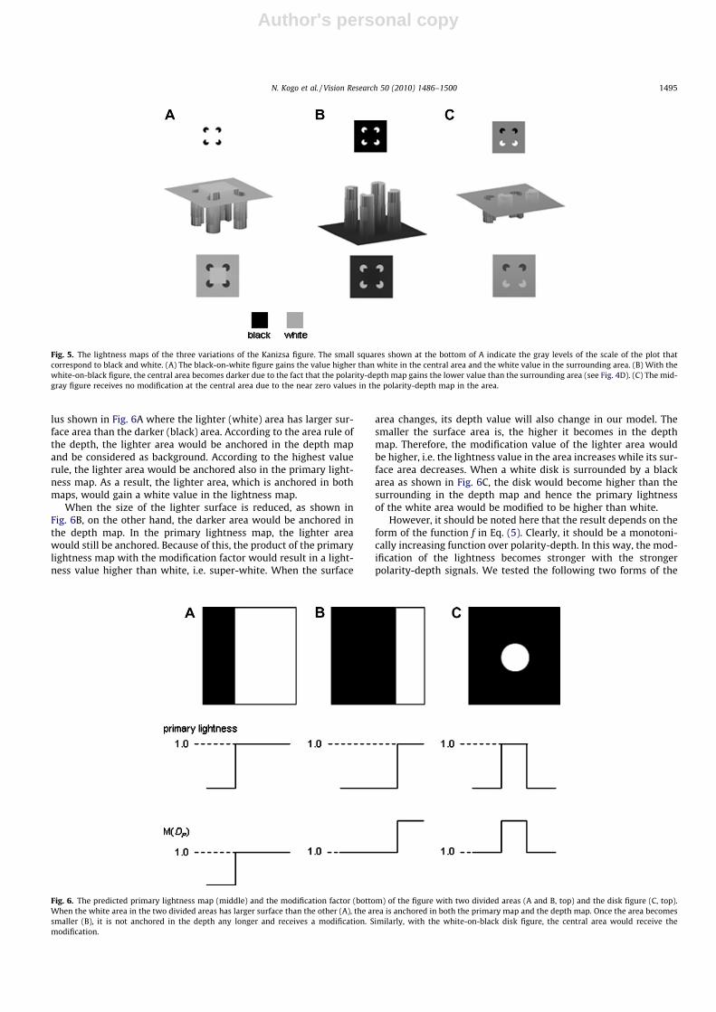
The arguments above lead to the choice of the highest value rulein anchoring the primary lightness map. When compared with Liand Gilchrist’s dome experiment, the black-on-white configurationof the Kanizsa figure is equivalent to the condition with the lighterarea being dominant. In both cases, the lighter area is anchored aswhite. An exception is that the central area of this Kanizsa figure isassigned as ‘‘super-white”. Note that in the Kanizsa figure, the fig-ure is in effect divided into three areas, the surrounding area, theareas within the pacmen, and the central area. In other words,when there are two segmented areas with the same luminancehigher than the rest, the one that belongs to the background is an-chored to white and the other being closer to the viewer, gains avalue higher than white. The white-on-black Kanizsa figure, onthe other hand, corresponds to the condition when the darker areais dominant. The areas within the pacmen have smaller surfacearea in total than the rest. They gain a lightness value higher thanwhite, corresponding to Li and Gilchrist’s data. The final lightnessmaps of the variation figures are shown in Fig. 5. (Note that theexponential function to obtain the modification factor discussedin the next section is used for these results.)



In summary, having three segmented areas in the perception ofthe Kanizsa figure forces us to further articulate the anchoringrules empirically found by Li and Gilchrist. The anchoring of thedepth map by the area rule and the anchoring of the primary light-ness map by the highest value rule, along with the depth-lightnesslinkage to compute the final lightness value using these two an-chored maps, seem to provide this articulation. With these rulesbeing implemented in our model, its behavior can now be investi-gated and compare with the empirical data in more detail.

3.6. Effect of changing surface areas

As mentioned above, Li and Gilchrist discovered that theanchoring rule of lightness perception is such that this area is an-chored to white when the lighter area is dominant in size, whilethe perceived lightness of the lighter area is lifted up further, i.e.seen as super-white, when the darker area becomes dominant.

When a figure is divided in two areas, the following scenariotakes place in the DISC model. Assume a configuration of a stimu-

Fig. 4. (A) Anchoring of the depth and the primary lightness maps. While the area rule is applied to anchor the background of the depth map (top), there are two possibleanchoring rules for the primary lightness maps (bottom), i.e. the area rule and the highest value rule. For the black-on-white figure (a), both rules results in the same:anchoring the surrounding area. For the white-on-black figure (b), these two rules would anchor different areas: anchoring the white area by the highest value rule andanchoring the black area by the area rule. B–D: Prediction of the final lightness values based on the two possible anchoring rules of the primary lightness map. (B) With theformalism of our model, both the highest value rule and the area rule applied to the primary lightness map would create the lightness value higher than white in the centralsquare of the black-on-white figure. Therefore, both rules are plausible. (C) In the case of the white-on-black figure, on the other hand, if the primary lightness map isanchored by the area rule, the final lightness measurements would be equal to white in the surrounding area and they would be higher than white in the areas within thepacmen (�). This is not plausible. (D) With the highest value rule, on the other hand, it is predicted that the lightness value below white is assigned to the black area while thevalue higher than white is assigned in the white area. Hence, the highest value rule is the most plausible one.



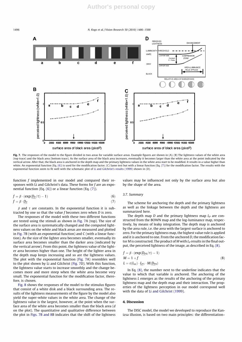
lus shown in Fig. 6A where the lighter (white) area has larger sur-face area than the darker (black) area. According to the area rule ofthe depth, the lighter area would be anchored in the depth mapand be considered as background. According to the highest valuerule, the lighter area would be anchored also in the primary light-ness map. As a result, the lighter area, which is anchored in bothmaps, would gain a white value in the lightness map.

When the size of the lighter surface is reduced, as shown inFig. 6B, on the other hand, the darker area would be anchored inthe depth map. In the primary lightness map, the lighter areawould still be anchored. Because of this, the product of the primarylightness map with the modification factor would result in a light-ness value higher than white, i.e. super-white. When the surface

area changes, its depth value will also change in our model. Thesmaller the surface area is, the higher it becomes in the depthmap. Therefore, the modification value of the lighter area wouldbe higher, i.e. the lightness value in the area increases while its sur-face area decreases. When a white disk is surrounded by a blackarea as shown in Fig. 6C, the disk would become higher than thesurrounding in the depth map and hence the primary lightnessof the white area would be modified to be higher than white.

However, it should be noted here that the result depends on theform of the function f in Eq. (5). Clearly, it should be a monotoni-cally increasing function over polarity-depth. In this way, the mod-ification of the lightness becomes stronger with the strongerpolarity-depth signals. We tested the following two forms of the

Fig. 5. The lightness maps of the three variations of the Kanizsa figure. The small squares shown at the bottom of A indicate the gray levels of the scale of the plot thatcorrespond to black and white. (A) The black-on-white figure gains the value higher than white in the central area and the white value in the surrounding area. (B) With thewhite-on-black figure, the central area becomes darker due to the fact that the polarity-depth map gains the lower value than the surrounding area (see Fig. 4D). (C) The mid-gray figure receives no modification at the central area due to the near zero values in the polarity-depth map in the area.

Fig. 6. The predicted primary lightness map (middle) and the modification factor (bottom) of the figure with two divided areas (A and B, top) and the disk figure (C, top).When the white area in the two divided areas has larger surface than the other (A), the area is anchored in both the primary map and the depth map. Once the area becomessmaller (B), it is not anchored in the depth any longer and receives a modification. Similarly, with the white-on-black disk figure, the central area would receive themodification.



function f implemented in our model and compared their re-sponses with Li and Gilchrist’s data. These forms for f are an expo-nential function (Eq. (6)) or a linear function (Eq. (7)).

f ¼ b � ðexpðDP=sÞ � 1Þ ð6Þf ¼ b � DP ð7Þ

b and s are constants. In the exponential function it is sub-tracted by one so that the value f becomes zero when D is zero.

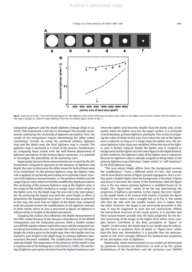
The responses of the model with these two different functionsare tested using the stimuli as shown in Fig. 7A (top). The size ofthe surface area is systematically changed and the computed light-ness values on the white and black areas are measured and plottedin Fig. 7B (with an exponential function) and C (with a linear func-tion). As the size of the lighter area becomes smaller, eventually itssurface area becomes smaller than the darker area (indicated bythe vertical arrow). From this point, the lightness value of the light-er area becomes higher than one. The height of the lighter area inthe depth map keeps increasing and so are the lightness values.The plot with the exponential function (Fig. 7A) resembles wellto the plot shown by Li and Gilchrist (Fig. 7D). With this function,the lightness value starts to increase smoothly and the change be-comes more and more steep when the white area become verysmall. The exponential function for the modification factor, there-fore, is chosen.

Fig. 8 shows the responses of the model to the stimulus figuresthat consist of a white disk and a black surrounding area. The re-sults of the lightness measurements of the figure by the model alsoyield the super-white values in the white area. The change of thelightness value is the largest, however, at the point when the sur-face area of the white area becomes smaller than the black area (don the plot). The quantitative and qualitative difference betweenthe plot in Figs. 7B and 8B indicates that the shift of the lightness

values may be influenced not only by the surface area but alsoby the shape of the area.

3.7. Summary

The scheme for anchoring the depth and the primary lightnessas well as the linkage between the depth and the lightness aresummarized here.

The depth map D and the primary lightness map LP are con-structed from the BOWN map and the log-luminance map, respec-tively, by means of leaky integration. The depth map is anchoredby the area rule, i.e. the area with the largest surface is anchored tozero. For the primary lightness map, the highest value rule is appliedand it is anchored to one. From the anchored D, the modification fac-tor M is constructed. The product of M with LP results in the final out-put, the perceived lightness of the image, as described in Eq. (8).

f ¼ b � ðexpðDP 0=sÞ � 1ÞM ¼ 1þ f

L ¼ eðItotÞ � LP 1 �MðDP 0Þð8Þ

In Eq. (8), the number next to the underline indicates that thevalue to which that variable is anchored. The anchoring of thelightness L emerges as the results of the anchoring of the primarylightness map and the depth map and their interaction. The prop-erties of the lightness perception in our model correspond wellwith the data of Li and Gilchrist (1999).

4. Discussion

The DISC model, the model we developed to reproduce the Kan-izsa illusion, is based on two main principles: the differentiation–

Fig. 7. The responses of the model to the figure divided in two areas for variable surface areas. Example figures are shown in (A). (B) The lightness values of the white area(top trace) and the black area (bottom trace). As the surface area of the black area increases, eventually it becomes larger than the white area at the point indicated by thevertical arrow. After that, the black area is anchored in the depth map and the primary lightness values in the white area start to be modified. It results in a value higher thanwhite. An exponential function (Eq. (6)) is used for the modification factor. (C) Same test but with a linear function (Eq. (7)) for the modification factor. The results with theexponential function seem to fit well with the schematic plot of Li and Gilchrist’s results (1999) shown in (D).



integration approach and the depth-lightness linkage (Kogo et al.,2010). This framework is the key to investigate the possible mech-anisms underlying the anchoring of lightness perception. First, theresults of the integrations require determining the offset values(anchoring). Second, by using the anchored primary lightnessmap and the depth map, the final lightness map is created. Thelightness map is anchored as a result of the process. Furthermore,by comparing these results with the well-known phenomena oflightness perception of the Kanizsa figure variations, it is possibleto investigate the plausibility of the anchoring rules.

Importantly, because these measurements are created by the dif-ferentiation–integration approach in the domains of lightness anddepth, the rules to determine the offset values for both of them needto be established. For the primary lightness map, the highest valuerule is applied. Its anchoring and scaling are to provide a basic struc-ture of the lightness measurements, i.e. the position of white and therange of gray scales, which are further modified by depth perception.The anchoring of the primary lightness map at the highest value isthe origin of the model’s tendency to assign (near) white values tothe lighter area. For the depth map, the area rule is the most plausi-ble. By anchoring the largest area with the same height, in effect, itdetermines the background area (back- or foreground, in general).In this way, the areas that are higher in the depth map comparedwith the ground receive the modifications in the lightness domain.In other words, when an area is perceived as figure, its lightness isinfluenced by its height in the depth perception.

Changing the surface area influences the depth measurement inthe DISC model because of the distance-dependency of the BOWNcomputation and the integration process. With a smaller surfacearea, BOWN signals enhance each other more and the integrated val-ues decay less within the area. The smaller the surface area, the moreheight the surface gains in the depth map. Once the smaller area hasstarted to gain height in the depth map, its primary lightness mea-surement becomes modified. The modification becomes strongerwith the height. The importance of this behavior of the model is thatit explains one of the findings by Li and Gilchrist (1999): The anchor-ing of lightness perception deviates from the highest luminance rule

when the lighter area becomes smaller than the darker area. In themodel, when the lighter area has the larger surface, it is anchoredin both domains, primary lightness and depth. This results in assign-ing the value of white in this area. Even when the size of the lighterarea is reduced, as long as it is larger than the darker area, the pri-mary lightness value stays non-modified. When the size of the light-er area is further reduced, finally the darker area is assigned asbackground and the lighter area becomes figure in the depth domain.In this condition, the lightness value of the lighter area is enhanced.Because its lightness value is already assigned to being white in theprimary lightness map, it becomes ‘‘super-white” or ‘‘self-luminous”in the final lightness map.

‘‘The area whose height differs from the background receivesthe modification.” From a different point of view, this conceptcan be described in terms of figure-ground segregation. Once a sur-face gains a height higher than the background, it becomes a figureand hence it becomes the owner of the borderlines. And the figurearea is the one whose primary lightness is modified based on itsheight. The ‘‘figure-ness” seems to be the key determining theproperties of lightness perception. In this regard, the term ‘‘depth”in the model needs to be treated with caution. Consider the figuredivided in two halves with a straight line as in Fig. 6. The modeltells that the side with the smaller surface area is higher thanthe other. However, the image is not necessarily perceived in thisway. It may be suggested as such, but not conclusively. Withinthe hierarchical structure of the visual system, it is possible thatthese measurements provide only the basic properties for the fur-ther processing of the image at the higher level where more com-plex factors contribute to the final perception of ‘‘figure” or‘‘depth”. In that sense, the depth map in our model may be indicat-ing the basic or primitive form of depth or ‘‘figure-ness” ratherthan the final one. Nevertheless, it is possible that the measure-ments at this level strongly influence the fundamental propertiesof our perception such as lightness.

Importantly, depth measurements in our model are determinedby junctions (occlusion-cue detections) as well as by the spatialdistributions of the borderlines and the occlusion cues (BOWN

Fig. 8. Same test as in Fig. 7 but with the disk figure (A). The lightness value of the white area becomes super-white as the lighter area becomes smaller than the darker area.The way it changes is, however quite different from the two-halves figure shown in Fig. 7.



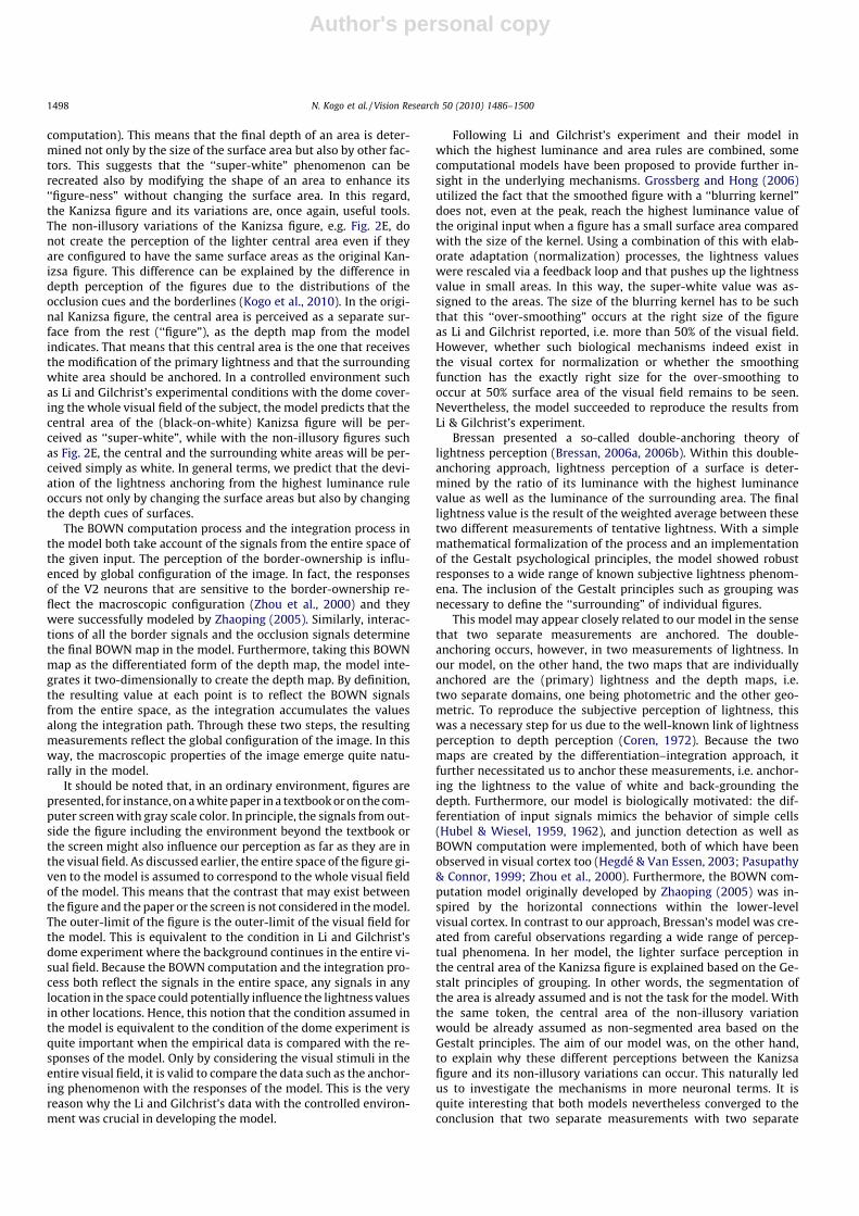
computation). This means that the final depth of an area is deter-mined not only by the size of the surface area but also by other fac-tors. This suggests that the ‘‘super-white” phenomenon can berecreated also by modifying the shape of an area to enhance its‘‘figure-ness” without changing the surface area. In this regard,the Kanizsa figure and its variations are, once again, useful tools.The non-illusory variations of the Kanizsa figure, e.g. Fig. 2E, donot create the perception of the lighter central area even if theyare configured to have the same surface areas as the original Kan-izsa figure. This difference can be explained by the difference indepth perception of the figures due to the distributions of theocclusion cues and the borderlines (Kogo et al., 2010). In the origi-nal Kanizsa figure, the central area is perceived as a separate sur-face from the rest (‘‘figure”), as the depth map from the modelindicates. That means that this central area is the one that receivesthe modification of the primary lightness and that the surroundingwhite area should be anchored. In a controlled environment suchas Li and Gilchrist’s experimental conditions with the dome cover-ing the whole visual field of the subject, the model predicts that thecentral area of the (black-on-white) Kanizsa figure will be per-ceived as ‘‘super-white”, while with the non-illusory figures suchas Fig. 2E, the central and the surrounding white areas will be per-ceived simply as white. In general terms, we predict that the devi-ation of the lightness anchoring from the highest luminance ruleoccurs not only by changing the surface areas but also by changingthe depth cues of surfaces.

The BOWN computation process and the integration process inthe model both take account of the signals from the entire space ofthe given input. The perception of the border-ownership is influ-enced by global configuration of the image. In fact, the responsesof the V2 neurons that are sensitive to the border-ownership re-flect the macroscopic configuration (Zhou et al., 2000) and theywere successfully modeled by Zhaoping (2005). Similarly, interac-tions of all the border signals and the occlusion signals determinethe final BOWN map in the model. Furthermore, taking this BOWNmap as the differentiated form of the depth map, the model inte-grates it two-dimensionally to create the depth map. By definition,the resulting value at each point is to reflect the BOWN signalsfrom the entire space, as the integration accumulates the valuesalong the integration path. Through these two steps, the resultingmeasurements reflect the global configuration of the image. In thisway, the macroscopic properties of the image emerge quite natu-rally in the model.

It should be noted that, in an ordinary environment, figures arepresented, for instance, on a white paper in a textbook or on the com-puter screen with gray scale color. In principle, the signals from out-side the figure including the environment beyond the textbook orthe screen might also influence our perception as far as they are inthe visual field. As discussed earlier, the entire space of the figure gi-ven to the model is assumed to correspond to the whole visual fieldof the model. This means that the contrast that may exist betweenthe figure and the paper or the screen is not considered in the model.The outer-limit of the figure is the outer-limit of the visual field forthe model. This is equivalent to the condition in Li and Gilchrist’sdome experiment where the background continues in the entire vi-sual field. Because the BOWN computation and the integration pro-cess both reflect the signals in the entire space, any signals in anylocation in the space could potentially influence the lightness valuesin other locations. Hence, this notion that the condition assumed inthe model is equivalent to the condition of the dome experiment isquite important when the empirical data is compared with the re-sponses of the model. Only by considering the visual stimuli in theentire visual field, it is valid to compare the data such as the anchor-ing phenomenon with the responses of the model. This is the veryreason why the Li and Gilchrist’s data with the controlled environ-ment was crucial in developing the model.

Following Li and Gilchrist’s experiment and their model inwhich the highest luminance and area rules are combined, somecomputational models have been proposed to provide further in-sight in the underlying mechanisms. Grossberg and Hong (2006)utilized the fact that the smoothed figure with a ‘‘blurring kernel”does not, even at the peak, reach the highest luminance value ofthe original input when a figure has a small surface area comparedwith the size of the kernel. Using a combination of this with elab-orate adaptation (normalization) processes, the lightness valueswere rescaled via a feedback loop and that pushes up the lightnessvalue in small areas. In this way, the super-white value was as-signed to the areas. The size of the blurring kernel has to be suchthat this ‘‘over-smoothing” occurs at the right size of the figureas Li and Gilchrist reported, i.e. more than 50% of the visual field.However, whether such biological mechanisms indeed exist inthe visual cortex for normalization or whether the smoothingfunction has the exactly right size for the over-smoothing tooccur at 50% surface area of the visual field remains to be seen.Nevertheless, the model succeeded to reproduce the results fromLi & Gilchrist’s experiment.

Bressan presented a so-called double-anchoring theory oflightness perception (Bressan, 2006a, 2006b). Within this double-anchoring approach, lightness perception of a surface is deter-mined by the ratio of its luminance with the highest luminancevalue as well as the luminance of the surrounding area. The finallightness value is the result of the weighted average between thesetwo different measurements of tentative lightness. With a simplemathematical formalization of the process and an implementationof the Gestalt psychological principles, the model showed robustresponses to a wide range of known subjective lightness phenom-ena. The inclusion of the Gestalt principles such as grouping wasnecessary to define the ‘‘surrounding” of individual figures.

This model may appear closely related to our model in the sensethat two separate measurements are anchored. The double-anchoring occurs, however, in two measurements of lightness. Inour model, on the other hand, the two maps that are individuallyanchored are the (primary) lightness and the depth maps, i.e.two separate domains, one being photometric and the other geo-metric. To reproduce the subjective perception of lightness, thiswas a necessary step for us due to the well-known link of lightnessperception to depth perception (Coren, 1972). Because the twomaps are created by the differentiation–integration approach, itfurther necessitated us to anchor these measurements, i.e. anchor-ing the lightness to the value of white and back-grounding thedepth. Furthermore, our model is biologically motivated: the dif-ferentiation of input signals mimics the behavior of simple cells(Hubel & Wiesel, 1959, 1962), and junction detection as well asBOWN computation were implemented, both of which have beenobserved in visual cortex too (Hegdé & Van Essen, 2003; Pasupathy& Connor, 1999; Zhou et al., 2000). Furthermore, the BOWN com-putation model originally developed by Zhaoping (2005) was in-spired by the horizontal connections within the lower-levelvisual cortex. In contrast to our approach, Bressan’s model was cre-ated from careful observations regarding a wide range of percep-tual phenomena. In her model, the lighter surface perception inthe central area of the Kanizsa figure is explained based on the Ge-stalt principles of grouping. In other words, the segmentation ofthe area is already assumed and is not the task for the model. Withthe same token, the central area of the non-illusory variationwould be already assumed as non-segmented area based on theGestalt principles. The aim of our model was, on the other hand,to explain why these different perceptions between the Kanizsafigure and its non-illusory variations can occur. This naturally ledus to investigate the mechanisms in more neuronal terms. It isquite interesting that both models nevertheless converged to theconclusion that two separate measurements with two separate



anchorings were necessary to reproduce lightness perception, be-sides the fact that the domains of anchoring are different andhence the detailed computations of the final results are different.Whether the anchoring has to be done in the domains of lightnessand depth (or ‘‘figure-ness”) as in our model or in two separatemeasurements of lightness as in Bressan’s model will require addi-tional psychophysical testing.

Our model is also closely related to the ‘‘selective integration”model by Ross and Pessoa (2000). Their approach was to integratethe information at the borderlines in a ‘‘context-sensitive” manner.In other words, if two surfaces belong to the same group (such as inthe same depth plane), the integration was made to enhance thecontrast between them and otherwise it was suppressed. In thisway, the contrast in the same group is more meaningful than thecontrast from different groups. As stated before, the major differ-ence between our model and theirs (as well as Gilchrist et al.’s(1983) and Land and McCann’s (1971) is that their models com-puted the lightness perception by their integration method, whileour model applies this differentiation–integration approach toboth the lightness and the depth computation. This very aspectof our model necessitated the anchoring in two separate domainsthat enabled our model to reproduce the lightness perception ob-served by Li and Gilchrist (1999). Furthermore, our model com-putes the border-ownerships based on the macroscopicconfigurations of the image, and hence reflects its context. Thishas not been done in any of these models. Nevertheless, the suc-cess of Ross and Pessoa’s model in various figures indicates the‘‘explanatory power” by the inclusion of the depth measurementin the lightness computation. In general terms, this supports ourapproach of constructing the lightness and the depth maps andtheir interaction determining the final lightness values.

It should be noted that, as a general rule, the interaction be-tween lightness perception and depth perception can be mutual.However, our hypothesis is that the influence of the depth on thelightness plays the ‘‘fundamental role” in creating the Kanizsa illu-sion (and thus differentiating the illusory and non-illusory varia-tions). This is in line with Coren (1972). Also, using fMRI,Mendola, Dale, Fischl, Liu, and Tootell (1999) showed that brainareas that are active when participants are seeing Kanizsa figuresoverlap with those that are active during depth recognition tasks.Nevertheless, the mutual interaction between lightness and depthperception as well as the top-down feedback mechanism influenc-ing the depth and the lightness perceptions may need to be consid-ered for more general applications. Further investigation on thistopic is necessary.

There are many other stimuli that were not considered in thisstudy but still may give some insights in the underlying mecha-nisms of lightness perception. Clearly, to investigate the applicabil-ity of the model to the lightness perception of the wider range ofimages is also necessary. However, to show the general applicabil-ity of the model to various images is not the aim of this paper. Theexample figures in this paper were used specifically to reasonabout how to determine the details in the algorithms. By analyzingthese figures step-by-step, the algorithm of the lightness computa-tion with anchoring process was articulated within the frameworkof the DISC model. It started from the reflection of the depth mea-surement by the analysis Kanizsa figure and its non-illusory varia-tion, the reflection of the contrast polarity by the analysis of theblack-on-white vs. white-on-black Kaniza figures and the mid-grayKanizsa figure, to the determination of the function of the modifi-cation factor by the analysis of the data by Li and Gilchrist (1999).The aim of the current paper was to provide the framework of thisanchoring and the lightness computation.

In the future, however, the applicability of the frameworkshould be tested with a wider range of figures. The variations ofthe Kanizsa figure with mixed contrast polarities (Albert, 2001;

Spehar, 2000), for example, appear to support the framework ofthe DISC model. Albert (2001) used figures with the surroundingobjects consisting of black and white overlapping surfaces (e.g.,Figs. 8 and 9 of his paper) and showed a significant reduction ofthe illusion. Note that, by this overlap of the surfaces, T-junctionsare created. Importantly, the orientations of these T-junctions arenot consistent with the central area being the occluding surface.Spehar (2000) also used other ‘‘mixed-polarity” configurations. Inthe examples shown in Fig. 1 of her paper, the borderline betweenthe two different colors merges to the apex of the centralL-junction of the pacman which results in creating a Y-junction.The data showed a significant reduction of the illusion. In contrast,with the examples shown in Fig. 4 in her paper, the position of theborderline between the two colors is shifted so that it creates aT-junction with the straight borderline of the pacman and in thesecases the Kanizsa illusion remained. With the former examples, theY-junctions surrounding the central area creates ambiguous per-ception of the depth of the central area (it is equally possible thatthe area is perceived as closer or further from the viewer) whilewith the latter examples, all the orientations of the T-junctionsare consistent with the central area being the occluding surface.In other words, these examples are consistent with the frameworkof the DISC model because (1) the BOWN computation reflects theproperties of the junctions, (2) based on the BOWN computation,the depth maps are constructed and (3) the emergence of theillusion depends on the development of the depth differencebetween the central area and the surrounding. In our view, there-fore, these examples indeed indicate the influence of the occlusion/depth cues (T- and Y-junctions) on the emergence and non-emergence of the Kanizsa illusion. We intend to expand the appli-cation of the model to such examples as well as the well-knownfigures such as Benary’s cross (1924) and White’s illusion (1979).

Perceiving spontaneous splitting of a surface with homoge-neous color is another important phenomenon that the modelshould be able to reproduce (see Singh, Hoffman, & Albert,1999). In these configurations, the surface tends to split at thelocations where no borderlines exist following Petter’s rule(1956). When the DISC model is applied to the Kanizsa figure,the illusory BOWN signals (contours) develop as follows. Afterthe initial BOWN computation, the BOWN signals at the side (L-)junctions of the pacmen become inconsistent, i.e. among theBOWNs of the two borderlines that constitute the junction, oneindicates the pacman as the owner while the other indicatesthe central surface as the owner. This condition is called the illu-sory T-junction in the model and the existence of them leads todevelop the illusory BOWN signals. It should be, therefore, inves-tigated whether the model creates an illusory T-junction condi-tion in these spontaneously splitting surfaces as well. It ispossible that when one part of the surface is significantly nar-rower than the other (hence the perception of splitting accordingto Petter’s rule), the BOWN computation may result in the illu-sory T-junction condition. In addition to the illusory contours, itshould be noted that the split surfaces are perceived to be threedimensionally curved. The model, therefore, has to be able to cre-ate the depth map with the gradual changes of the depth alongthe surfaces to reflect such depth perception. Further research isneeded to investigate the performance of the BOWN computationin these images and to develop the approaches that reproduce thecorrect depth profiles of the curved surfaces.

The model was able to reproduce the schematic plot of thelightness perception phenomena reported by Li and Gilchrist(1999). Quantitative details of the phenomena are, however, notknown due to the technical difficulties of the experiments control-ling the whole visual field with varying levels of luminance, such asthe dome experiment. The exact profile of the plot may, therefore,be different and it may also vary depending on the shape of the



stimuli (Bressan, 2006b). In fact, the model predicts that other fac-tors that determine depth perception, other than surface area,would also influence the profile of the plot quantitatively. Theoverall trend, however, seems to be robust as Li and Gilchrist’s dataclearly indicated: the lighter side is anchored to white and, with itsdecreasing surface area, the lightness value increases higher thanwhite while the darker area is perceived more and more to be closeto white. In computational modeling, all of the details of a theoryhave to be articulated, while precise details of the mechanismsare not yet available in the empirical data of neuronal responses.The functions implemented in the model, such as the functionsfor the modification factor and the scaling factor, were chosen tofit the overall trend. It is also possible that higher-level visual pro-cessing to articulate figure-ground segregation and depth percep-tion as well as the involvement of the top-down feedback mayneed to be considered to be able to reproduce the robustness ofour lightness perceptions of a wider range of figures. Only futurestudies will tell how the neuronal machinery works at each stageof computation to arrive at the final lightness perception.

Acknowledgments

N.K. was supported by Fellowships from the Research Fund ofthe University of Leuven (F/01/043, F/02/104, DB/04/047, and DB/06/008). This research was supported by Grants from the EuropeanScience Foundation (CNCC-Boundaries, G.0688.06), and from theMethusalem program (METH/08/02) to J.W.

References

Albert, M. K. (2001). Cue interactions, border ownership and illusory contours.Vision Research, 41, 2827–2834.

Arend, L. E. (1973). Spatial differential and integral operations in human vision:Implications of stabilized retinal image fading. Psychological Review, 80(5),374–395.

Benary, W. (1924). Beobachtungen zu einem Experiment uber Helligkeitskontrast.Psychologische Forschung, 5, 131–142.

Bressan, P. (2006a). Inhomogeneous surrounds, conflicting frameworks, and thedouble-anchoring theory of lightness. Psychonomic Bulletin & Review, 13(1),22–32.

Bressan, P. (2006b). The place of white in a world of grays: A double-anchoringtheory of lightness perception. Psychological Review, 113(3), 526–553.

Claerbout, J. (1992). Earth soundings analysis: Processing versus inversion (PVI).Oxford: Blackwell.

Coren, S. (1972). Subjective contours and apparent depth. Psychological Review,79(4), 359–367.

Gilchrist, A. (1979). Perception of surface blacks and whites. Scientific American,240(3), 112–122.

Gilchrist, A. (2006). Seeing black and white. New York: Oxford University Press.Gilchrist, A., Delman, S., & Jacobsen, A. (1983). The classification and integration of

edges as critical to the perception of reflectance and illumination. Perception &Psychophysics, 33(5), 425–436.

Gilchrist, A., Kossyfidis, C., Bonato, F., Agostini, T., Cataliotti, J., Li, X., et al. (1999). Ananchoring theory of lightness perception. Psychological Review, 106(4), 795–834.

Grossberg, S., & Hong, S. (2006). A neural model of surface perception: Lightness,anchoring, and filling-in. Spatial Vision, 19(2–4), 263–321.

Hegdé, J., & Van Essen, D. C. (2003). Strategies of shape representation in macaquevisual area V2. Visual Neuroscience, 20(3), 313–328.

Horn, B. (1974). Determining lightness from image. Computer Graphics and ImageProcessing, 3(1), 277–299.

Hubel, D. H. (1988). Eye, brain, and vision (Vol. 22). New York: W.H. Freeman & Co.(Sd).

Hubel, D. H., & Wiesel, T. N. (1959). Receptive fields of single neurones in the cat’sstriate cortex. Journal of Physiology, 148, 574–591.

Hubel, D. H., & Wiesel, T. N. (1962). Receptive fields, binocular interaction andfunctional architecture in the cat’s visual cortex. Journal of Physiology, 160,106–154.

Hung, C. P., Ramsden, B. M., Chen, L. M., & Roe, A. W. (2001). Building surfaces fromborders in areas 17 and 18 of the cat. Vision Research, 41(10–11), 1389–1407.

Koffka, K. (1935). Principles of Gestalt psychology. New York: Harcourt Brace &World.

Kogo, N., Strecha, C., Van Gool, L., & Wagemans, J. (2010). Surface construction by a2-D differentiation-integration process: A neurocomputational model forperceived border ownership, depth, and lightness in Kanizsa figures.Psychological Review, 117(2), 406–439.

Krauskopf, J. (1963). Effect of retinal image stabilization on the appearance ofheterochromatic targets. Journal of the Optical Society of America, 53, 741–744.

Land, E. H., & McCann, J. J. (1971). Lightness and retinex theory. Journal of the OpticalSociety of America, 61, 1–11.

Li, X. J., & Gilchrist, A. L. (1999). Relative area and relative luminance combine toanchor surface lightness values. Perception & Psychophysics, 61(5), 771–785.

Mendola, J. D., Dale, A. M., Fischl, B., Liu, A. K., & Tootell, R. B. H. (1999). Therepresentation of illusory and real contours in human cortical visual areasrevealed by functional magnetic resonance imaging. Journal of Neuroscience,19(19), 8560–8572.

Pasupathy, A., & Connor, C. E. (1999). Responses to contour features in macaquearea V4. Journal of Neurophysiology, 82(5), 2490–2502.

Petter, G. (1956). Nuove ricerche sperimentali sulla totalizzazione percettiva. Rivistadi Psicologia, 50, 213–227.

Ross, W. D., & Pessoa, L. (2000). Lightness from contrast: A selective integrationmodel. Perception & Psychophysics, 62(6), 1160–1181.

Shipley, T. F., & Kellman, P. J. (1992). Strength of visual interpolation depends on theratio of physically specified to total edge length. Perception & Psychophysics,52(1), 97–106.

Singh, M., Hoffman, D. D., & Albert, M. K. (1999). Contour completion and relativedepth: Petter’s rule and support ratio. Psychological Science, 10(5), 423–428.

Spehar, B. (2000). Degraded illusory contour formation with non-uniform inducersin Kanizsa configurations: the role of contrast polarity. Vision Research, 40,2653–2659.

Stanley, D. A., & Rubin, N. (2003). FMRI activation in response to illusory contoursand salient regions in the human lateral occipital complex. Neuron, 37(2),323–331.

Tomasi, C. (1998). Bilateral filtering for gray and color images. In Proceedings of the1998 IEEE international conferences on computer vision (pp. 836–846).

Wallach, H. (1948). Brightness constancy and the nature of achromatic colors.Journal of Experimental Psychology, 38, 310–324.

White, M. (1979). A new effect of pattern on perceived lightness. Perception, 8,413–416.

Whittle, P., & Challands, P. D. (1969). The effect of background luminance on thebrightness of flashes. Vision Research, 9(9), 1095–1110.

Zhaoping, L. (2005). Border ownership from intracortical interactions in visual areaV2. Neuron, 47(1), 143–153.

Zhou, H., Friedman, H. S., & von der Heydt, R. (2000). Coding of border ownership inmonkey visual cortex. Journal of Neuroscience, 20(17), 6594–6611.


Linking depth to lightness and anchoring within the differentiation-integration formalism

Documents

Transcript of Linking depth to lightness and anchoring within the differentiation-integration formalism