This article was downloaded by: [University of Florida]On: 11 June 2012, At: 05:20Publisher: Taylor & FrancisInforma Ltd Registered in England and Wales Registered Number: 1072954 Registeredoffice: Mortimer House, 37-41 Mortimer Street, London W1T 3JH, UK

International Journal of RemoteSensingPublication details, including instructions for authors andsubscription information:http://www.tandfonline.com/loi/tres20

Linking vegetation response toseasonal precipitation in theOkavango–Kwando–Zambezi catchmentof southern AfricaAndrea E. Gaughan a , Forrest R. Stevens b , Cerian Gibbes c , JaneSouthworth b & Michael W. Binford ba Division of Biology, University of Missouri, Columbia, MO, 65211,USAb Department of Geography & Land-use and Environmental ChangeInstitute, University of Florida, Gainesville, FL, 32611, USAc Department of Geography and Environmental Studies, Universityof Colorado, Colorado Springs, CO, 80918, USA

Available online: 11 Jun 2012

To cite this article: Andrea E. Gaughan, Forrest R. Stevens, Cerian Gibbes, Jane Southworth& Michael W. Binford (2012): Linking vegetation response to seasonal precipitation in theOkavango–Kwando–Zambezi catchment of southern Africa, International Journal of Remote Sensing,33:21, 6783-6804

To link to this article: http://dx.doi.org/10.1080/01431161.2012.692831

PLEASE SCROLL DOWN FOR ARTICLE

Full terms and conditions of use: http://www.tandfonline.com/page/terms-and-conditions

This article may be used for research, teaching, and private study purposes. Anysubstantial or systematic reproduction, redistribution, reselling, loan, sub-licensing,systematic supply, or distribution in any form to anyone is expressly forbidden.

The publisher does not give any warranty express or implied or make any representationthat the contents will be complete or accurate or up to date. The accuracy of anyinstructions, formulae, and drug doses should be independently verified with primarysources. The publisher shall not be liable for any loss, actions, claims, proceedings,

demand, or costs or damages whatsoever or howsoever caused arising directly orindirectly in connection with or arising out of the use of this material.

Dow

nloa

ded

by [

Uni

vers

ity o

f Fl

orid

a] a

t 05:

20 1

1 Ju

ne 2

012

International Journal of Remote SensingVol. 33, No. 21, 10 November 2012, 6783–6804

Linking vegetation response to seasonal precipitation in theOkavango–Kwando–Zambezi catchment of southern Africa

ANDREA E. GAUGHAN*†, FORREST R. STEVENS‡, CERIAN GIBBES§,JANE SOUTHWORTH‡ and MICHAEL W. BINFORD‡

†Division of Biology, University of Missouri, Columbia, MO 65211, USA‡Department of Geography & Land-use and Environmental Change Institute, University

of Florida, Gainesville, FL 32611, USA§Department of Geography and Environmental Studies, University of Colorado at

Colorado Springs, Colorado Springs, CO 80918, USA

(Received 30 August 2011; in final form 13 April 2012)

Understanding how intra-annual precipitation variability affects seasonal vegeta-tion dynamics is critical for assessing the potential impacts of climate variabilityon vegetation structure and composition. This is important in semi-arid andarid ecosystems of southern Africa, where water is a limiting resource and tim-ing of seasonal rainfall combined with the water storage capacity of differentplant vegetation types affects remotely measured phenological cycles. Various lagsand leads of savanna vegetation response to rainfall have been identified usingremotely sensed data, but little attention has been given to vegetation greennessleading into the dry season. Vegetation production at the onset of the dry sea-son interacts with the availability of water resources affecting fire dynamics, foragematerials for wildlife and wildlife movement throughout the dry season. This isimportant for southern Africa as large proportions of the human population andeconomy are dependent on wildlife tourism. This study investigates the responseof the end of the wet season vegetation production, as measured by ModerateResolution Imaging Spectroradiometer (MODIS) normalized difference vegeta-tion index (NDVI) greenness, to the different months of wet season rainfall fordifferent savanna vegetation types in a regional catchment of southern Africa.We estimated monthly precipitation using Tropical Rainfall Monitoring Mission3B43 data and used MODIS 13A1 NDVI at a monthly time step for the years2000–2009. Our model estimated greenness at the beginning of the dry season fromthe prior rainy season (October–April) precipitation using geographically weightedregression (GWR). The results show intra-annual wet season rainfall accounts forsignificant amounts of April NDVI variation. Overall intra-annual rainfall has astronger effect for areas with greater proportions of grassland and dry, deciduouswoodlands than for wetter, evergreen woodlands. These findings support previousresearch by highlighting the stronger association of grassland and open canopywoodlands to the end of the wet season monthly rainfall. This relationship isimportant for understanding seasonal precipitation effects on different savannavegetation covers.

*Corresponding author. Email: aegaughan@gmail.com

International Journal of Remote SensingISSN 0143-1161 print/ISSN 1366-5901 online © 2012 Taylor & Francis

http://www.tandfonline.comhttp://dx.doi.org/10.1080/01431161.2012.692831

Dow

nloa

ded

by [

Uni

vers

ity o

f Fl

orid

a] a

t 05:

20 1

1 Ju

ne 2

012

6784 A. E. Gaughan et al.

1. Introduction

Variability in inter- and intra-annual precipitation affects ecosystem structure andfunction in all climates (Huxman et al. 2004, Scanlon et al. 2005, Merbold et al. 2009).In dryland ecosystems, water availability is the most important climate constraint onplant growth (Prince et al. 1995, Nemani et al. 2003). Dryland areas, including arid,semi-arid and dry sub-humid regions, cover 40% of the Earth’s land surface, includingabout half of the African continent (Reynolds et al. 2007). Under different scenarios offuture climate change, many dryland regions may become even drier and precipitationtiming and amount may shift (IPCC 2007). The underlying dryland mechanisms thatgovern atmosphere–plant–soil processes are strongly influenced by water availabilityand any subtle shift in precipitation will influence the ability of plants to respond tosuch a change (Scholes and Walker 1993). The relationships between vegetation pro-duction and precipitation for such regions are determined not only by total rainfallbut also by precipitation timing and variability. An understanding of the relation-ships between current precipitation variability, especially within seasons, and differentsavanna vegetation types is important because of the effects that various woody specieshave on savanna processes (Sankaran et al. 2008).

All dryland areas in southern Africa are water limited for part of the year andthe often unpredictable pattern and timing of water distribution plays an impor-tant role in the structure and function of savanna vegetation (Scholes and Walker1993).Characterized by a continuous herbaceous layer and interspersed woody vege-tation cover, different savanna types result from the interaction of multiple ecologicalfactors (precipitation, soil nutrients, fire and herbivory) over space and time (Skarpe1992, House et al. 2003). Water is not the only limiting resource controlling ecosystemdynamics but is a necessary component for every physiological process (Rodriguez-Iturbe 2000). Across much of southern Africa, the strong seasonal response to wetand dry periods (Scholes and Walker 1993) is largely controlled by the movementof the Inter-Tropical Convergence Zone (ITCZ) (Scholes and Archer 1997). Otherparts of the water cycle, such as soil moisture, evapotranspiration and flooding alsocontribute to dryland vegetation growth but are dependent on the quantity, timingand frequency of rainfall. In the same way, other biotic factors (ex. fire, herbivory)that contribute to driving landscape change also depend on the underlying hydro-meteorological factors to maintain coexistence of grasslands and woody vegetation indryland areas (Breshears and Barnes 1999, Wang 2003, Sankaran et al. 2005).

A common approach to examine the relationship between precipitation and vegeta-tion production at a broad landscape level is with the normalized difference vegetationindex (NDVI) (Tucker and Sellers 1986, Sims et al. 2006, 2008, Sjostrom et al.2009). NDVI is a normalized ratio of the red (Red) and near-infrared (NIR) spectralwavelengths as follows:

NDVI = (NIR − Red)(NIR + Red)

, (1)

where ‘NIR’ and ‘Red’ represent estimates of surface reflectance as measured by thesatellite instrument. The normalized difference of these reflectances is an index ofecosystem production and provides a robust means to estimate vegetation health anddynamics by quantifying the ‘greenness’ of vegetation in a landscape (Tucker 1979).NDVI as a measure of vegetation greenness can be problematic in tropical forests asits calculated value can saturate at high foliage biomass, but this is less of a concern in

Dow

nloa

ded

by [

Uni

vers

ity o

f Fl

orid

a] a

t 05:

20 1

1 Ju

ne 2

012

Vegetation and seasonal precipitation dynamics in Africa 6785

the semi-arid region studied here (Nicholson and Farrar 1994, Richard and Poccard1998). However, it is not only leaf absorption and scatter that are measured by NDVIbut also other factors such as bare soil, leaf litter type, vegetation structure and com-position (Farrar et al. 1994). These factors make NDVI a composite measurement ofleaf chlorophyll, canopy cover, vegetation structure and background reflectance, there-fore encompassing more than just leaf chlorophyll in its measurement of vegetationgreenness (Nicholson and Farrar 1994, Plummer 2000, Chapin et al. 2002). NDVI isalso affected by sources of noise, ranging from sensor attributes to atmospheric con-ditions, which influence the remote observations of greenness (Azzali and Menenti2000). Despite this, a strong correlation exists between vegetation production indexedby NDVI and average climatic distribution of precipitation (Goward and Prince 1995,Scanlon et al. 2005, Hellden and Tottrup 2008), making it useful for understand-ing the effects of wet season months on vegetation greenness leading into the dryseason.

Previous studies of NDVI association with rainfall exist across a wide range of tem-poral and spatial scales (Nicholson et al. 1990, Fuller and Prince 1996, Richard andPoccard 1998, Fuller 1999, Zhang 2005, Chamaille-Jammes et al. 2006, Martiny et al.2006, Archibald and Scholes 2007, Richard et al. 2008). In general, peak NDVI lagsmore than 1.5 months after the height of the rainy season (February) in southernAfrica (Martiny et al. 2006). The response of savanna vegetation to precipitation willvary, however, depending on the tree cover fraction (Fuller and Prince 1996). The vari-ation in response emphasizes the different behaviours of various savanna vegetationtypes to the onset of the rainy season. It is well known that the grassland response tothe start of the rainy season (October) is more tightly coupled with precipitation. Thiscontrasts with woody vegetation leaf expansion, which can occur up to two monthsprior to the first rains (Fuller and Prince 1996, Archibald and Scholes 2007). Studiesthat have examined the relationship at the beginning of the dry season (as opposedto the beginning of the wet season) found that the timing of leaf flush peak has largeinter-annual variation (Do et al. 2005) with vegetation dormancy occurring with alag of three months after the end of the rainy season (Zhang 2005), again suggestingthat more research is needed to tease out the different responses of various savannavegetation types to timing of seasonal rainfall.

In this study, we examine the response of April NDVI, an estimate of greennessleading into the dry season, to monthly variation in wet season rainfall. Vegetationgreenness at the beginning of the dry season influences the availability of waterresources and other important forage materials for wildlife, therefore affecting wildlifespecies throughout the dry season. This is important in southern Africa where largeproportions of the human population and economy are dependent on wildlife tourism(Barnes et al. 2002). In addition, the timing and amount of precipitation during therainy season may influence savanna vegetation types differently which, in turn, affectother savanna ecosystem processes (Sankaran et al. 2005, Martiny et al. 2006).

Prior studies that have examined the NDVI–rainfall relationship for other parts ofthe rainy season identified a lag of zero to two months in overall NDVI response torainfall. Therefore, we suggest that February, March and April rainfall should havethe strongest association to the beginning of dry season (April) NDVI. However, thestrength of this relationship may vary across savanna vegetation types. To identifythese patterns, we examined the response of April NDVI to month-by-month pre-cipitation variability during the wet season within the Okavango–Kwando–Zambezi(OKZ) catchment of southern Africa, using two remotely sensed data sets. NDVIestimates were from Moderate Resolution Imaging Spectroradiometer (MODIS)

Dow

nloa

ded

by [

Uni

vers

ity o

f Fl

orid

a] a

t 05:

20 1

1 Ju

ne 2

012

6786 A. E. Gaughan et al.

13A1 (vegetation indices) data and mean monthly precipitation estimates from theTropical Rainfall Monitoring Mission (TRMM) 3B43 monthly rainfall product.We hypothesized that savanna land cover with more grass would show a strongerpositive response to precipitation later in the rainy season than vegetation with pro-portionally more woody plants. The main focus was the regional relationship betweenmean monthly rainfall and NDVI at the beginning of the dry season across the OKZcatchment. We addressed the following questions.

1. What is the relationship of NDVI measured at the beginning of the dry seasonto the seven previous wet season months’ precipitation?

2. How much variation in NDVI is explained by relationships between vegetationand different months of wet season rainfall?

3. And what coupling relationships exist between different vegetation responsegroups to seasonal precipitation from 2000 to 2009?

Current consensus in the literature emphasizes the complex and distinctly differentphenological responses that tree and grass species have to inter- and intra-annual pre-cipitation for savanna ecosystems. Being able to differentiate the influence of whichwet season months of rainfall are important to vegetation production leading into thedry season provides a crucial link to better understanding of precipitation–vegetationinteraction in savanna ecosystems.

2. Materials and methods

2.1 Study region

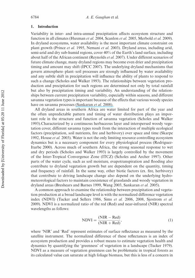
The study region comprises the OKZ catchment, situated in subtropical southernAfrica, and covers a total area of ∼700 000 km2 with an annual precipitation rangeof 400–2200 mm yr–1 (figure 1). The high variability of intra-annual and inter-annualrainfall across the three catchments is due to the influence of variations in the move-ments of the Inter-Tropical Convergence Zone (ITCZ) and atmospheric circulationpatterns (Mccarthy et al. 2000). The southern part of the study region is semi-arid,defined by scarce and typically unpredictable patterns of precipitation, while thenorthern part of the region has a higher average annual precipitation and lower inter-annual variability. The majority of the Okavango and Kwando catchments and allthree headwaters are located in Angola, although a good portion of the Zambezicatchment is in western Zambia. Soils typically range from ferralsols in upland areas ofAngola and Zambia to sandy arenosols in mid-elevation regions, and clay-containinggleysols throughout lower, flatter areas of the catchments (Batjes 2000). The mid-elevation area, which makes up the majority of the region, consists of deep Aeolian,Kalahari sand deposits, longitudinal dune remnants, pans and fossil valleys with thevariations in vegetation type along the north–south, high–low rainfall gradient (Dubeand Pickup 2001).

The OKZ catchment is located in the future Kavango–Zambezi TransboundaryConservation Area (KAZA). KAZA is a politically defined conservation area thatspans Angola, Zambia, Namibia, Botswana and Zimbabwe. The transboundary con-servation area is designed to provide vital wildlife corridors among multiple protectedareas. Topography is very flat across the southern portion of the region. The topogra-phy of the southern area (especially the Caprivi Strip and northern Botswana) makesit difficult to clearly separate these different catchments, because hydrological flowsare inconsistent across the flat terrain.

Dow

nloa

ded

by [

Uni

vers

ity o

f Fl

orid

a] a

t 05:

20 1

1 Ju

ne 2

012

Vegetation and seasonal precipitation dynamics in Africa 6787

Fig

ure

1.St

udy

regi

onde

pict

ing

the

thre

eca

tchm

ent

area

sof

inte

rest

wit

hel

evat

ion

from

adi

gita

lel

evat

ion

mod

el(S

ourc

e:W

orld

Wild

life

Fun

dH

ydro

SHE

DS

proj

ect)

,wit

ha

spat

ialr

esol

utio

nof

15ar

csec

onds

.

Dow

nloa

ded

by [

Uni

vers

ity o

f Fl

orid

a] a

t 05:

20 1

1 Ju

ne 2

012

6788 A. E. Gaughan et al.

2.2 Data sets

The study region was delineated hydrologically into three neighbouring watershedswith void-filled Shuttle Radar Topography Mission (SRTM) DEM data, as well asderived flow direction and accumulation grids at a spatial resolution of 15 arcsec-onds from the World Wildlife Fund HydroSHEDS project (Lehner et al. 2006). Thesedata were processed using the ArcHydro data model and toolset (Maidment 2002) toextract drainage networks and basin delineations, which form the geographic units forfurther analyses.

We examined the long- and short-run precipitation patterns across the region usingthe TRMM 3B43 data set (version 6). TRMM 3B43 data are best estimates of averagedaily rainfall rate by month (Kummerow et al. 2000), combining the TRMM instru-ment rain calibration algorithm estimates (3B42) and several rain-gauge data sourcesusing the Huffman et al. (1997) method. Daily instrument data are severely limited interms of availability and quality in this study region. Although at a relatively coarsescale of 0.25◦ × 0.25◦, TRMM 3B43 data are comparable to rain-gauge estimates andshow very little bias in West Africa (Nicholson et al. 2003). The TRMM 3B43 productalso shows favourable results across a region of India for investigation of intra-annualprecipitation studies (Nair et al. 2009). The TRMM 3B43 data product has the leastbias of any data across both season and region and shows a high degree of associa-tion with regional rain-gauge estimates (Adeyewa and Nakamura 2003). Average dailyrainfall rates by month were converted to total monthly rainfall in millimetres forfurther analyses.

We used NDVI from MODIS 13A1 data (version 5) with 500 m × 500 m spa-tial resolution to measure vegetation greenness at the beginning of the dry season(April). The delineated study region included two full MODIS 16-day composite foot-prints downloaded from the Land Processes Distributed Active Archive Center (LPDAAC), which is a component of NASA’s Earth Observing System (EOS) Data andInformation System (EOSDIS). Data were acquired for each year 2000–2009 andencompassed dates between 23 April and 8 May for each composite (see Leeuwenet al. 1999 for a detailed description of the compositing algorithm).

2.3 Data sampling and standardization

A temporal and spatial scale mismatch exists between the monthly TRMM precipi-tation pixels (predictor variables) measured at 0.25◦ × 0.25◦ and the MODIS NDVIpixels (response variable) measured at 500 m × 500 m. Each of the 1790 TRMM pixelsin the study region overlaps many MODIS pixels (∼3600). To address the scalar mis-match, we averaged April MODIS pixel values within each TRMM pixel. Therefore,across the ten water years, we observed a total of 17 900 average April NDVI values.

Since this research was primarily concerned with terrestrial, semi-arid vegetation,we used a 5 km buffer around permanent and seasonally flooded areas to excludesamples that may contain water and riparian vegetation, resulting in a final sampleof 15 466 observation points. Although a smaller buffer may have been sufficient, the5 km buffer was selected based on field observations regarding the spatial extent of sea-sonal water presence and flood-affected vegetation. The buffer safely excluded knownperennial water sources and many seasonally flooded areas. These areas become inun-dated after rainfall events at various lags and were removed from the analysis becauseof the high variability in NDVI estimates caused by the presence of semi-permanentwater.

Dow

nloa

ded

by [

Uni

vers

ity o

f Fl

orid

a] a

t 05:

20 1

1 Ju

ne 2

012

Vegetation and seasonal precipitation dynamics in Africa 6789

2.4 Modelling approach

We were interested in the association between variability in each month’s rainfall dur-ing the rainy season and the variation in the beginning of the dry season vegetationgreenness across a large geographic area. Because rainfall effects on vegetation green-ness may interact with a large number of other potential covariates, themselves varyingat multiple grains and extents, we performed two data manipulation steps prior tomodelling the rainfall/greenness association. The first was to spatially de-trend theApril NDVI measurements to remove the slowly changing, large-scale effects of latentcovariates such as soil type, elevation, mean annual precipitation, among many oth-ers. The second step was to standardize the monthly rainfall estimates (subtract themonthly precipitation mean and divide by the standard deviation) (table 1). The rea-son for doing so was to be able to compare the coefficient estimates not in terms ofmillimetres of rainfall, but instead in terms of standard units, asking how above- orbelow-normal rainfall in any one month affects April vegetation greenness.

We fit a trend surface using least squares regression to April NDVI to spatiallyde-trend the data. This minimized broad-scale spatial patterns across the catchment(Lichstein et al. 2002). Our trend surface included all third-degree polynomial termsof spatial coordinates x and y for sampled NDVI observation points:

NDVIApr = β0 + β1x + β2y + β3x2 + β4xy + β5y2 + β6x3 + β7x2y + β8xy2 + β9y3,(2)

where NDVIApr represents the response variable of April vegetation greenness, β0−β9

are the estimated coefficients and x and y variables represent Albers equal-areaprojected coordinates for each sample location. Data were standardized prior toestimation. After estimating the coefficients and predicting NDVI from the trend sur-face alone, the prediction residuals are therefore spatially de-trended observations forassessing how vegetation greenness is associated with precipitation.

After removing the broad-scale spatial trend, we used a geographically weightedregression (GWR) model to minimize the effects of finer spatial-scale autocorrela-tion. GWR accounts for spatial non-stationarity in the relationship between rainfalland the beginning of the dry season vegetation productivity to minimize the effect ofunmeasured, spatially varying covariates (Brunsdon et al. 1998, Foody 2003). GWRextends the traditional regression framework by allowing local model parameters tobe estimated at any point within the study area by incorporating a spatial weighting ofobservations and allowing the estimated models to vary across space (Fotheringhamet al. 2000). Observations are weighted by their proximity to the point at which therelationship is estimated so that the weighting of an observation is not constant,

Table 1. Monthly average rainfall values and their standard deviations by which the data werenormalized prior to analysis.

October November December January February March April

Average (mm) 37.61 86.07 129.06 178.78 155.62 106.82 46.47Standard deviation 50.54 59.20 81.14 100.00 83.94 64.34 45.58

Note: TRMM monthly precipitation values were averaged and standard deviations werecalculated for the entire OKZ basin prior to excluding water and riparian vegetation areas.

Dow

nloa

ded

by [

Uni

vers

ity o

f Fl

orid

a] a

t 05:

20 1

1 Ju

ne 2

012

6790 A. E. Gaughan et al.

but varies with each location. GWR models assume that observations nearest theestimation point are more informative than those further away (Harris et al. 2010).

Sampled TRMM data were standardized prior to running the GWR by subtract-ing the long-term mean and dividing by the overall standard deviation. The unitlessmeasures of within-month variation were used to assess the explanatory power of vari-ation in monthly rainfall on NDVI rather than the effect on a per millimetre basis.The relationship between the estimated, de-trended April MODIS NDVI (depen-dent variable, residuals, from estimated equation (2)) and standardized (Wheeler andTiefelsdorf 2005) TRMM values for seven months of preceding rainfall (seven inde-pendent variables) varies across space, minimizing the effects of any unmeasured,important covariates while enabling us to compare the relative importance of eachmonth’s rainfall for explaining variation in the beginning of the dry season vegetationproductivity. The GWR model for April NDVI is

dNDVIApr (u)=β0 (u)+β1 (u) RainOct + β2 (u) RainNov+ · · · +β7 (u) RainApr+ ε (u),(3)

where dNDVIApr(u) represents the de-trended, standardized NDVI for April at loca-tion u, and β0(u) . . . β7(u)RainApr are the intercept and regression coefficients specificfor the model with error ε(u) at the same location, estimated using distance-weightedobservations from that location. Locations need not be coincident with observationpoints, and from the stratified sample across space and time, regression surfaces for alleight estimated coefficients were used to predict April NDVI on a 500 m × 500 m gridfor each year 2000–2009.

During estimation, GWR requires the choice of a kernel and its associated dis-tance weighting function identified by the bandwidth size (Fotheringham et al. 2002).Kernel selection may either be a fixed distance or a fixed number of local observa-tions and will dictate the final bandwidth size used in the GWR calculation (Harriset al. 2010). The kernel and bandwidth parameters may be set explicitly if a strongtheoretical basis exists or through quantitative methods that use either a fixed or vari-able kernel function and derive a bandwidth parameter through the minimization ofan objective function (Akaike information criterion (AIC), for example) (Brunsdonet al. 1998, Foody 2003). We used a Gaussian, fixed kernel with an optimal bandwidthchosen to minimize the corrected Akaike information criterion (AICc) of the esti-mated model. The Gaussian, fixed kernel incorporates all observations into each localmodel calculation, but weights each observation by the distance from each regres-sion point according to a Gaussian decay model. The weighting decay function foreach observation (i) and its influence on parameter estimates at point j is calculatedas a function of the distance between the point and each observation (dij) and thebandwidth parameter (b):

Weight of observation i for estimation at point j = e(−d2

ij

/b2

). (4)

To determine the bandwidth parameter used in the weighting decay function, theAICc function and global spatial autocorrelation of residuals, measured by Moran’sI , were used as diagnostics. These were calculated for the model at bandwidthsacross a range of 18–90 km at equal 1 km steps. The results were used to iden-tify the bandwidth parameter value with the lowest model AICc and that locally

Dow

nloa

ded

by [

Uni

vers

ity o

f Fl

orid

a] a

t 05:

20 1

1 Ju

ne 2

012

Vegetation and seasonal precipitation dynamics in Africa 6791

Table 2. Global OLS model diagnostics compared with those of the GWR.

Model typeSum-squared

residuals R2 Adjusted R2 �AICcParametersestimated

Bandwidthparameter (m)

Global OLS 182.72 0.107 0.107 −21852.00 8 N/AGWR 25.77 0.874 0.817 0.00 4750.30∗ 30 333.41∗

Notes: GWR fits the data across the catchment much better as indicated by the delta AICc andincrease in adjusted R2.∗The ‘parameters estimated’ for the global OLS model (8) is the number of predictor variablesin the model; for GWR this is the ‘effective number’, which varies with the chosen bandwidthparameter. As the bandwidth gets very large, the ‘effective number’ approaches the numberof parameters in the model. As the bandwidth decreases to zero, the ‘effective number’ willapproach the total number of observations (15 466). The bandwidth parameter (here fixed, inmetres) controls the distance-based decay of the Gaussian spatial weighting (see equation (4))(Fotheringham et al. 2002).

minimized spatial autocorrelation. Using this strategy, an ideal bandwidth parametervalue was identified (∼30 000 m, see table 2) for use in the weighting decay function(equation (4)).

We fit the final GWR model in ArcGIS 9.3 (ESRI 2008) using standardized obser-vations to compare the influence of prior monthly rainfall on April NDVI. To answerthe questions proposed, we must necessarily look at the local coefficient estimates.Wheeler and Tiefelsdorf (2005) showed how collinearity in estimators may yield spuri-ous correlations in local coefficient estimates, potentially biasing further interpretationof those estimates. We conducted post hoc examinations of local coefficient estimatesand predictors and determined at the optimal bandwidth that some multicollinearitypersisted only at the extreme coefficient values. Overall trends showed little correlationand further interpretation based on coefficient estimates should contain little bias.

2.5 Model comparison across vegetation classes

The coupling between precipitation and vegetation varies by vegetation type(Archibald and Scholes 2007). The results of the GWR model create a continu-ous gradient of coefficients for each rainfall predictor in the model. We extractedand compiled coefficient estimates across the study region and for each class of theSAFARI 2000 National Botanical Institute (NBI) vegetation map of the savannasof southern Africa, which is a compilation of six independent subregional veg-etation coverages (Rutherford et al. 2005) (figure 2). As a result of combinedsubregional coverages, some anomalies of land cover are evident based on polit-ical boundaries (e.g. Zambia/Angola border). Others, however, such as the spa-tial pattern of Colophospermum mopane woodland in the southern part of thebasin, were verified through extensive fieldwork, with land cover observed dur-ing ground data collection from 2006 to 2009. We used the SAFARI NBI mapbecause it provides the most recent compendium of the best sources of differ-ent vegetation maps in southern Africa and includes improved, smaller scale workfor countries like Zambia. The SAFARI NBI map also provides a more detailedbreakdown of woodland groups and defines a transition area between uplandMiombo woodland and dry deciduous and secondary grasslands in the south-ern part of the OKZ basin. We extracted sample points of estimated NDVI and

Dow

nloa

ded

by [

Uni

vers

ity o

f Fl

orid

a] a

t 05:

20 1

1 Ju

ne 2

012

6792 A. E. Gaughan et al.

Figure 2. SAFARI NBI vegetation map highlighting different land covers in the OKZcatchment (Source: Rutherford et al., 2005).

precipitation estimates within ten vegetation classes: Baikiaea woodland, Miombowoodland, Dry evergreen forest, C. mopane woodland, humid mesic woodlands,woodland savanna mosaic, mesic savanna woodland, Loudetia grassland, floodedgrassland and Panicum and Hyparrhenia grassland. Vegetation types with <15 sam-ple points were excluded from analysis. We compared the coefficient values ofeach predictor month by land-cover classification to determine the relationshipbetween each month’s rainfall and NDVI across different vegetation covers. Analyseswere conducted with R 2.10.1 (R Development Core Team 2009) and ENVI 4.3(ITT 2007).

3. Results

3.1 Spatial and temporal relationships between NDVI and rainfall

Average pixel-by-pixel calculation indicates higher NDVI values in the upper catch-ment and a gradient of increasing precipitation from southwest to northeast(figure 3). The darker band of values that stretches down the centre of the basinis a low-lying floodplain region that corresponds to mostly flooded grassland in theSAFARI NBI vegetation map. The higher NDVI values correspond approximately toMiombo woodland and the wooded savanna mosaic vegetation types. These areas inthe upland part of the OKZ basin also receive the highest amount of total precipitation

Dow

nloa

ded

by [

Uni

vers

ity o

f Fl

orid

a] a

t 05:

20 1

1 Ju

ne 2

012

Vegetation and seasonal precipitation dynamics in Africa 6793

Fig

ure

3.M

ean

valu

esac

ross

each

grid

cell

wer

eca

lcul

ated

from

tim

ese

ries

ofea

chpi

xel

of(a

)m

ean

Apr

ilN

DV

Ian

d(b

)to

tal

mea

nw

etse

ason

prec

ipit

atio

n(T

RM

M),

resp

ecti

vely

,fro

m20

00to

2009

.The

spat

iald

istr

ibut

ion

high

light

sth

ehi

ghes

tm

ean

prec

ipit

atio

nin

the

nort

heas

tof

the

OK

Zba

sin

and

the

high

erA

pril

ND

VI

valu

esfo

rpr

edom

inan

tly

woo

dlan

dar

eas.

Dow

nloa

ded

by [

Uni

vers

ity o

f Fl

orid

a] a

t 05:

20 1

1 Ju

ne 2

012

6794 A. E. Gaughan et al.

during the rainy season (October–April). While parts of the Okavango Delta, locatedat the bottom of the OKZ basin, have areas with high NDVI values, we excluded theseareas, along with other wetland and riparian areas, since NDVI values within theseareas are highly influenced by basin-wide precipitation and flooding rather than thelocal precipitation patterns.

Mean April NDVI for each vegetation type and mean total wet season precipita-tion (October–April) for the 9 years covered by the MODIS data set (2000–2009) areshown in figure 4. Vegetation types with similar responses were grouped togetherresulting in six main vegetation types. Mixed woodland includes Miombo woodland,dry evergreen forest, humid mesic woodlands and woodland savanna mosaic covers.The mixed woodland group has the highest, most consistent average April NDVI val-ues (ranges 0.66–0.69). In contrast, the mean April NDVI in woodland increases and

0.2

0.3

0.4

0.5

0.6

0.7

0.8

0

200

400

600

800

1000

1200

Ap

ril

ND

VI

Water year (October–April)

Mesic savanna

0.2

0.3

0.4

0.5

0.6

0.7

0.8

0

200

400

600

800

1000

1200

Ap

ril

ND

VI

Water year (October–April)

Mix floodplain grasses

0.2

0.3

0.4

0.5

0.6

0.7

0.8

0

200

400

600

800

1000

1200

Ap

ril

ND

VI

Water year (October–April)

Colophospermum mopane

0.2

0.3

0.4

0.5

0.6

0.7

0.8

0

200

400

600

800

1000

1200

Ap

ril

ND

VI

Water year (October–April)

Baikiaea

0.2

0.3

0.4

0.5

0.6

0.7

0.8

0

200

400

600

800

1000

1200

Ap

ril

ND

VI

Water year (October–April)

Panicum and Hyparrhenia

grasses

0.2

0.3

0.4

0.5

0.6

0.7

0.8

0

2000

2001

2002

2003

2004

2005

2006

2007

2008

2009

2000

2001

2002

2003

2004

2005

2006

2007

2008

2009

2000

2001

2002

2003

2004

2005

2006

2007

2008

2009

2000

2001

2002

2003

2004

2005

2006

2007

2008

2009

2000

2001

2002

2003

2004

2005

2006

2007

2008

2009

2000

2001

2002

2003

2004

2005

2006

2007

2008

2009

200

400

600

800

1000

1200

Ap

ril

ND

VI

Pre

cip

ita

tio

n (

mm

)

Pre

cip

ita

tio

n (

mm

)

Pre

cip

ita

tio

n (

mm

)P

re

cip

ita

tio

n (

mm

)

Pre

cip

ita

tio

n (

mm

)P

re

cip

ita

tio

n (

mm

)

Water year (October–April)

Mix woodland

Figure 4. Time series of averaged April NDVI (black line) for each SAFARI NBI vegetationtype plotted against total average precipitation (grey bars) for each wet season (October–April)across 2000–2009.

Dow

nloa

ded

by [

Uni

vers

ity o

f Fl

orid

a] a

t 05:

20 1

1 Ju

ne 2

012

Vegetation and seasonal precipitation dynamics in Africa 6795

decreases with average wet season precipitation, ranging from 0.41 to 0.60. Similarly,the Panicum and Hyparrhenia grasses also tend to increase or decrease with corre-sponding change in precipitation, though, over a lower range than mopane woodland(0.36–0.54). The different April NDVI patterns across the ten years indicate that vary-ing amounts of precipitation influence the overall greenness of the array of savannavegetation types leading into the dry season.

3.2 GWR model

A comparison of the results from a global ordinary least squares (OLS) linear regres-sion with the GWR regression is presented in table 2 after accounting for broad spatialtrends. The results of the global OLS linear regression indicate that previous monthsof wet season rainfall explain 11% (adjusted R2) of the variation in April NDVI.The strength of the relationship between NDVI and rainfall increases substantiallywith the local GWR model, with rainfall explaining 82% (adjusted R2) of the varia-tion in April NDVI. Table 2 shows that the difference between AICc values for theglobal OLS and local GWR models is very large, indicating that the two models arenot equivalent in their explanatory power. Residuals from subtracting the modelledApril NDVI predictions from the observed April NDVI show the de-trended GWRmodel reduces the spatial autocorrelation (spatial pattern in the residuals), althoughit does not completely eliminate it (figure 5). While not all spatial autocorrelations areaccounted for in the GWR model, the spatial dependence in model errors is greatlyreduced resulting in better predictions of April NDVI than using a global model, suchas OLS regression, that does not account for local variation (Foody 2003).

Figure 5. Residuals from estimates of the GWR model. Spatial autocorrelation still exists inhigh/low residuals in the GWR but is minimized across the OKZ basin.

Dow

nloa

ded

by [

Uni

vers

ity o

f Fl

orid

a] a

t 05:

20 1

1 Ju

ne 2

012

6796 A. E. Gaughan et al.

3.3 GWR results by land cover

We sampled the standardized coefficient surfaces for each point of the original randomsample within each vegetation type of the SAFARI NBI vegetation map (figure 2) andplotted them as ‘bean’ plots (Kampstra 2008) (figure 6). The standardized monthlyrainfall coefficients represent the effects of lower or higher than average monthly rain-fall on April NDVI. It is apparent that the estimated intercept values and their rangesacross the vegetation types are generally non-zero and reflect the mean April greennessof each vegetation type relative to the others. Since the bandwidth parameter severelydiscounts observations further than 30.3 km from each set of model estimates, theseintercept values can also be interpreted to represent the smaller scale local deviationfrom the mean vegetation greenness after the effects of monthly precipitation varia-tion and the broad spatial trend in NDVI are accounted for. Because these coefficientestimates are standardized, we can directly compare effect sizes between them.

The bean plots illustrate the variation in the coupling between rainy season monthsand NDVI for different savanna vegetation types. Model estimates for the mixedwoodland group are less affected by variability in monthly precipitation (i.e. the medi-ans of most predictor coefficients on the bean plots are near zero and the distributionof coefficients indicated by the bean plot histograms straddle zero evenly). This vege-tation type also has the highest average NDVI and is located across the northern partof the OKZ basin. The model estimates for Baikiaea woodland also exhibit minimaleffects of monthly precipitation on April NDVI, although there is a slight positiveassociation in December, February and March and a slight negative association inOctober and April. Mesic savanna woodland and mopane woodland estimates sug-gest that these woodlands have a much stronger response to monthly rainfall withFebruary–April months having the largest positive association with April NDVI.December model estimates are also quite high for mopane woodland. October rainfallestimates show a slight negative association with April NDVI in mesic savanna wood-land and a bit stronger negative effect in mopane woodland. These two woodlandtypes are located across the southern, lower elevation parts of the OKZ. The mixedfloodplain grassland model estimates show a minimal effect on April NDVI, only aslight positive association in February, while the Panicum and Hyparrhenia grasslandshows a disproportionately large positive association with April greenness not onlyfor the months February–April but also December. February precipitation was themost common month positively associated with April NDVI for all land covers in theOKZ basin, although the strength of association varies by vegetation type. Anothercommon pattern shown in the bean plots is the slight negative association in Octoberprecipitation for all vegetation types except mixed woodland and the mixed floodplaingrassland.

4. Discussion

Our results indicate that precipitation patterns within the wet season strongly influencevegetation greenness leading into the dry season, with different rainy season monthsmore strongly associated with greenness for some vegetation types than others. Mixedwoodland, the savanna vegetation type with the highest tree cover fraction, shows min-imal response to April NDVI across all wet season months. The correlation strengthbetween late wet season rainfall (February–April) and April NDVI increases for vege-tation types with a more mixed tree–shrub–grass composition. The savanna vegetationtypes with more mixed composition are also located in the southern half of the basin,

Dow

nloa

ded

by [

Uni

vers

ity o

f Fl

orid

a] a

t 05:

20 1

1 Ju

ne 2

012

Vegetation and seasonal precipitation dynamics in Africa 6797

Panicum and hyparrhenia grasslands

I'cept Oct Nov Dec Jan Feb Mar Apr

Predictor variable

–0.4

–0.2

0.0

0.2

0.4

Sta

ndar

dize

d co

effic

ient

val

ue

Mixed floodplain grasslands

I'cept Oct Nov Dec Jan Feb Mar Apr

Predictor variable

–0.4

–0.2

0.0

0.2

0.4

Sta

ndar

dize

d co

effic

ient

val

ue

Baikiaea woodlands

I'cept Oct Nov Dec Jan Feb Mar Apr

Predictor variable

–0.4

–0.2

0.0

0.2

0.4

Sta

ndar

dize

d co

effic

ient

val

ue

–0.4

–0.2

0.0

0.2

0.4

I'cept Oct Nov Dec Jan Feb Mar Apr

Mixed woodlands

Predictor variable

Sta

ndar

dize

d co

effic

ient

val

ue

I'cept Oct Nov Dec Jan Feb Mar Apr

Predictor variable

–0.4

–0.2

0.0

0.2

0.4S

tand

ardi

zed

coef

ficie

nt v

alue

Mesic savanna woodlands

I'cept Oct Nov Dec Jan Feb Mar Apr

Predictor variable

–0.4

–0.2

0.0

0.2

0.4

Sta

ndar

dize

d co

effic

ient

val

ue

Colophospermum mopane woodlands

Figure 6. ‘Bean plots’ of the GWR coefficients for monthly precipitation variables as predic-tors of April NDVI for each of the SAFARI NBI vegetation types. Each sample point has itsown GWR model. The median coefficient for the Y-intercepts and each month is indicated bythe long horizontal bar above each month (independent variable). Each individual local modelis represented by the spread of short horizontal bars above and below the median value and thedistribution for each predictor variable is shown with vertical histograms.

Dow

nloa

ded

by [

Uni

vers

ity o

f Fl

orid

a] a

t 05:

20 1

1 Ju

ne 2

012

6798 A. E. Gaughan et al.

which has a lower overall mean annual precipitation. These vegetation types includePanicum and Hyparrhenia grassland, mesic savanna woodland and mopane woodland.

In general, the end of the rainy season occurs in April and is relatively uni-form across southern Africa (Zhang et al. 2005). The positive and negative modelcoefficient patterns for each month (October–April) for respective vegetation types(figure 6) identify lags in April NDVI response to the different months of prior wetseason rainfall. With regard to the large intercept values relative to monthly rain-fall coefficients, one might conclude that it indicates a lack of explanatory power formonthly rainfall on variation in April NDVI. However, across vegetation types, onlymixed woodland and mixed floodplain grassland show a trend for the intercept to belarger than the sum total of absolute rainfall coefficient values, indicating that above orbelow average rainfall of one standard unit throughout the rainy season would affectdeviations in NDVI less than the local trend in NDVI alone (the intercept value) foronly two of the six vegetation types. We think this is reasonable evidence to concludethat variability in monthly rainfall does have a large degree of explanatory power afterlarge- and small-scale spatial variability in April vegetation greenness and other latentcovariates are accounted for by using the GWR approach. Mesic savanna woodlandcharacterizes the middle of the tree–grass savanna continuum and covers much of thecentral portion of the OKZ basin. The NDVI–rainfall relationship for this savannavegetation type has positive coefficient values for the months February–April, indi-cating that rainfall during these three months is more strongly correlated with April‘greenness’, as measured by NDVI, than the beginning of the wet season. This sug-gests that there is a zero to two-month lag in the response of April NDVI to above- orbelow-average rainfall, which is also noticeable in the model coefficients for mopanewoodland and Panicum and Hyparrhenia grassland. Baikiaea woodland also has apositive association for February and March rainfall, although not April, and mixedwoodland and flooded grassland have a minimal positive response of April NDVI toonly February rainfall.

The zero to two-month lag in vegetation response to rainfall agrees in general tothe vegetation response to rainfall measured for other parts of the growing seasonin southern Africa (Goward and Prince 1995, Fuller and Prince 1996, Richard andPoccard 1998, Martiny et al. 2006). However, our results emphasize the differences invegetation responses for different savanna vegetation types. The variation in savannavegetation response most likely results from a set of ecosystem processes that differ atthe level of vegetation type (Williams et al. 2009). Different types of savanna wood-land species adapt different coping mechanisms and strategies to deal with the highlyvariable and seasonal savanna environment (Fuller 1999, Shackleton 1999). For themixed woodland class, the minimal effect of variation in February rainfall may sug-gest a short-term storage of water and carbohydrate reserves that are accessed whenthe rainy season ends and provides an indication of how sensitive the ecosystem maybe to within-wet season rainfall (Schwinning et al. 2004). Additionally, the effect maybe minimal with a stronger, inter-annual impact on vegetation response dependingon the number of previous dry years or high water stress prior to rainfall (Martinyet al. 2005, Richard et al. 2008). A longer inter-annual lag that may be present woulddepend on ecological processes that influence nutrient and water cycling (Martinyet al. 2005, Williams et al. 2009), although further investigation is necessary to deter-mine how vegetation types respond to inter-annual variation within the OKZ basin.In contrast to only February having a slight positive association with the mixed wood-land class, mopane woodland has a stronger association with multiple months of wet

Dow

nloa

ded

by [

Uni

vers

ity o

f Fl

orid

a] a

t 05:

20 1

1 Ju

ne 2

012

Vegetation and seasonal precipitation dynamics in Africa 6799

season rainfall for April NDVI. This strong seasonal response of mopane woodlandcorresponds to previous studies that use field and remotely sensed data to show theintra-annual rainfall effect on these woodlands (Fuller and Prince 1996, Fuller 1999).Mopane woodland, in general, has a more open canopy than the mixed woodlandclass and the different vegetation response to month-by-month wet season rainfallmay result from differences in foliage type and the spread and angle of leaf coverage(Fuller 1999).

There also exists a strong positive response of April NDVI to the latter half of therainy season (February–April) for Baikiaea woodland, mesic savanna woodland andPanicum and Hyparrhenia grassland. These savanna vegetation types have smaller treecover fractions than mixed woodland and the stronger zero to two-month associationsof February–April precipitation with April NDVI may be due to the higher depen-dence that grasslands have on rainfall for seasonal productivity patterns (Scanlonet al. 2002). The access to and the utilization of soil water by grasses may be moresensitive to temporal and spatial variations in water availability, making the timing ofrainfall, rather than total amount, and its effects important on regulating ecosystemfunction specific to herbaceous plants (Sher et al. 2004). The variation in soil–waterstorage capacity along a savanna gradient will influence the process and duration ofphotosynthesis, thereby affecting the measure of April NDVI greenness for the differ-ent savanna vegetation types (Scholes and Archer 1997). The negative association ofOctober rainfall with April NDVI might be a result of an increase in early wet sea-son rainfall leading to earlier senescence of mopane woodland, Baikiaea woodlandand Panicum and Hyparrhenia grassland. The possible relationship could mask NDVIgreenness late in the wet season (Scholes and Walker 1993, Fuller 1999).

Regardless of positive or negative association of April NDVI with different monthsof wet season rainfall, the associations are stronger for the southwest region ofthe OKZ basin, where precipitation is more variable. This corresponds to previousfindings in southern Africa that used Advanced Very High Resolution Radiometer(AVHRR) imagery to study vegetation–rainfall dynamics from 1981 to 1990 (Fullerand Prince 1996).

Our study complements previous studies that identify the importance of vegeta-tion response to different rainfall regimes (Nicholson et al. 1990, Martiny et al. 2006)by emphasizing that this relationship is further broken down by savanna vegetationtype. Timing of wet season rainfall on NDVI leading into the dry season is a vitalcomponent to understanding the shifting dynamics of dryland ecosystems (Fuller andPrince 1996, Scanlon et al. 2005, Archibald and Scholes 2007), as illustrated in thisresearch. The measure of April NDVI provides an indication of how different monthsof wet season rainfall influence the greenness of different savanna vegetation typesat the outset of an extended period or dryness. Month-by-month rainfall variabilityaffects system drivers, such as soil moisture or fuel load, in turn influencing AprilNDVI differently for various savanna vegetation types. If less rainfall occurs at theend of the rainy season, our results suggest it will more strongly influence April NDVIfor savanna vegetation in grassland and open canopy woodland, potentially leadingto more frequent and intense fires early in the dry season due to a drier fuel load.However, the use of average monthly precipitation is an arbitrary means to identify theeffects of rainfall on April NDVI and a finer analysis in rainfall events may highlightother important interactions between wet season rainfall and NDVI greenness. In thisstudy, greenness was not directly linked to vegetation productivity on the ground, butby separating the response of NDVI greenness by broad savanna vegetation types andby expressing wet season precipitation by standardized monthly values, we were able

Dow

nloa

ded

by [

Uni

vers

ity o

f Fl

orid

a] a

t 05:

20 1

1 Ju

ne 2

012

6800 A. E. Gaughan et al.

to show how months in the beginning, middle and end of the rainy season influencegreenness in vegetation covered as measured by NDVI leading into the dry season.

This study also used a GWR regression approach to identify the NDVI–rainfallrelationship at a local scale. The GWR model provides a useful statistical tool to min-imize the effects of unmeasured, spatially varying factors and the negative impacts ofautocorrelation on conventional models. The focus on April NDVI greenness providesinsight into vegetation status leading into the dry season that will affect ecosys-tem processes such as nutrient cycling, water–energy budgets and forage availabilitythroughout the dry season. Therefore, quantifying the timing of the prior month’srainfall and whether that rainfall is above or below average may be an important fac-tor of April vegetation greenness which, in turn, may greatly impact a variety of dryseason vegetation processes.

One significant result from the GWR approach is that the optimal bandwidthparameter chosen (30 333 m) was very similar to the pixel size used as the pri-mary observational unit (TRMM 3B43 data). Although the bandwidth parameter waschosen using AICc as an objective, and local predictions show reduced spatial auto-correlation with a low degree of collinearity in coefficient estimates, there may stillbe some scale dependency involved with the data and modelling technique employed.Such a dependency has been noted in other research involving vegetation and climateassociations (Propastin et al. 2008). Analyses using simulated or aggregated data atmultiple scales may yield further insight into these results; however, since all reason-able diagnostics were used to make sure that the GWR technique employed is validwe feel confident in the degree of explanatory power achieved in measuring monthlyrainfall on observed April NDVI.

5. Conclusion

This study demonstrates the importance of within-season precipitation variabilityto vegetation greenness leading into months with no rainfall. The difficulty of thelandscape-level approach is mitigated by the analysis of finer taxonomic scale classesof savanna vegetation, which shows how timing of rainfall during the wet seasoninfluences vegetation types with varying tree cover fractions along the tree–savannacontinuum.

Rainfall is only one environmental variable that influences the growth and functionof vegetation, but is usually the most limiting factor in savanna ecosystems. Usinga geostatistical approach, this study is consistent with previous findings that intra-annual variability in rainfall explains a large amount of observed variation in AprilNDVI and that the relative importance of different months of rainfall on savanna veg-etation type varies throughout the wet season. The importance of wet season rainfallon vegetation greenness was stronger for areas with greater proportions of grasslandand deciduous woodlands, with the strongest positive association most prevalent formonths at the end of the wet season (February, March, April). This study highlightsthe importance of understanding that the link between precipitation and vegetation forboth beginning and end of the rainy season is important for anticipating the effects offuture climate change.

AcknowledgementsThe research was primarily funded by a NASA Land Cover/Land Use Change grant:Understanding and Predicting the Impact of Climate Variability and Climate Change

Dow

nloa

ded

by [

Uni

vers

ity o

f Fl

orid

a] a

t 05:

20 1

1 Ju

ne 2

012

Vegetation and seasonal precipitation dynamics in Africa 6801

on Land-Use/Land-Cover Change via Socio-Economic Institutions in SouthernAfrica (No. NNX09AI25G) and also through continued support from Universityof Florida National Science Foundation Interdisciplinary Graduate Education andResearch Traineeship grants (Nos 0504422 and 0801544). We thank our reviewers andother contributors for their help in refining and focusing our research.

ReferencesADEYEWA, Z.D. and NAKAMURA, K., 2003, Validation of TRMM radar rainfall data

over major climatic regions in Africa. Journal of Applied Meteorology, 42,pp. 331–347.

ARCHIBALD, S. and SCHOLES, R.J., 2007, Leaf green-up in a semi-arid African savanna – sepa-rating tree and grass responses to environmental cues. Journal of Vegetation Science, 18,pp. 583–594.

AZZALI, S. and MENENTI, M., 2000, Mapping vegetation-soil-climate complexes in southernAfrica using temporal Fourier analysis of NOAA-AVHRR NDVI data. InternationalJournal of Remote Sensing, 21, pp. 973–996.

BARNES, J.I., MACGREGOR, J. and WEAVER, L.C., 2002, Economic efficiency and incentives forchange within Namibia’s community wildlife use initiatives. World Development, 30, pp.667–681.

BATJES, N.H., 2000, Global Soil Profile Data (ISRIC-WISE) [Global Soil Profile Data(International Soil Reference and Information Centre – World Inventory of Soil EmissionPotentials)] (Oak Ridge, TN: Oak Ridge National Laboratory).

BRESHEARS, D.D. and BARNES, F.J., 1999, Interrelationships between plant functional typesand soil moisture heterogeneity for semiarid landscapes within the grassland/forestcontinuum: a unified conceptual model. Landscape Ecology, 14, pp. 465–478.

BRUNSDON, C., FOTHERINGHAM, S. and CHARLTON, M., 1998, Geographically weighted regres-sion – modelling spatial non-stationarity. Journal of the Royal Statistical Society SeriesD-the Statistician, 47, pp. 431–443.

CHAMAILLE-JAMMES, S., FRITZ, H. and MURINDAGOMO, F., 2006, Spatial patterns of theNDVI-rainfall relationship at the seasonal and interannual time scales in an Africansavanna. International Journal of Remote Sensing, 27, pp. 5185–5200.

CHAPIN, F.S., MATSON, P.A. and MOONEY, H.A., 2002, Principles of Terrestial EcosystemEcology (New York: Springer).

DO, F.C., GOUDIABY, V.A., GIMENEZ, O., DIAGNE, A.L., DIOUF, M., ROCHETEAU, A. andAKPO, L.E., 2005, Environmental influence on canopy phenology in the dry tropics.Forest Ecology and Management, 215, pp. 319–328.

DUBE, O.P. and PICKUP, G., 2001, Effects of rainfall variability and communal and semi-commercial grazing on land cover in southern African rangelands. Climate Research,17, pp. 195–208.

ESRI, 2008, ArcMap 9.3 (Redlands, CA: ESRI).FARRAR, T.J., NICHOLSON, S.E. and LARE, A.R., 1994, The influence of soil type on the rela-

tionships between NDVI, rainfall, and soil-moisture in semiarid Botswana. 2. NDVIresponse to soil-moisture. Remote Sensing of Environment, 50, pp. 121–133.

FOODY, G.M., 2003, Geographical weighting as a further refinement to regression modeling: anexample of focused on the NDVI-rainfall relationship. Remote Sensing of Environment,88, pp. 283–293.

FOTHERINGHAM, A.S., BRUNSDON, C. and CHARLTON, M.E., 2000, Quantitative Geography(London: Sage).

FOTHERINGHAM, A.S., BRUNDSDON, C. and CHARLTON, M., 2002, Geographically WeightedRegression. The Analysis of Spatially Varying Relationships (Chichester: Wiley).

FULLER, D.O., 1999, Canopy phenology of some mopane and miombo woodlands in easternZambia. Global Ecology and Biogeography, 8, pp. 199–209.

Dow

nloa

ded

by [

Uni

vers

ity o

f Fl

orid

a] a

t 05:

20 1

1 Ju

ne 2

012

6802 A. E. Gaughan et al.

FULLER, D.O. and PRINCE, S.D., 1996, Rainfall and foliar dynamics in tropical southern Africa:potential impacts of global climatic change on savanna vegetation. Climatic Change, 33,pp. 69–96.

GOWARD, S.M. and PRINCE, S.D., 1995, Transient effects of climate on vegetation dynamics:satellite observations. Journal of Biogeography, 22, pp. 549–563.

HARRIS, P., FOTHERINGHAM, A.S., CRESPO, R. and CHARLTON, M., 2010, The use of geo-graphically weighted regression for spatial prediction: an evaluation of models usingsimulated data sets. Mathematical Geosciences, 42, pp. 657–680.

HELLDEN, U. and TOTTRUP, C., 2008, Regional desertification: a global synthesis. Global andPlanetary Change, 64, pp. 169–176.

HOUSE, J.I., ARCHER, S., BRESHEARS, D.D. and SCHOLES, R.J., 2003, Conundrums in mixedwoody-herbaceous plant systems. Journal of Biogeography, 30, pp. 1763–1777.

HUFFMAN, G.J., ADLER, R.F., ARKIN, P., CHANG, A., FERRARO, R., GRUBER, A., JANOWLAK,J., MCNAB, A., RUDOLF, B. and SCHNEIDER, U., 1997, The global precipitation cli-matology project (GPCP) combined precipitation dataset. Bulletin of the AmericanMeteorological Society, 78, pp. 5–20.

HUXMAN, T.E., SMITH, M.D., FAY, P.A., KNAPP, A.K., SHAW, M.R., LOIK, M.E., SMITH, S.D.,TISSUE, D.T., ZAK, J.C., WELTZIN, J.F., POCKMAN, W.T., SALA, O.E., HADDAD, B.M.,HARTE, J., KOCH, G.W., SCHWINNING, S., SMALL, E.E. and WILLIAMS, D.G., 2004,Convergence across biomes to a common rain-use efficiency. Nature, 429, pp. 651–654.

IPCC, 2007, Climate Change 2007: The Physical Science Basis, Contribution of Working GroupI to the Fourth Assessment Report of the Intergovernmental Panel on Climate Change(Geneva: IPCC).

ITT VISUAL INFORMATION SOLUTIONS, 2007, ENVI 4.4 and IDL 6.4.1. In Products and Services(Boulder, CO: ITT Visual Information Solutions).

KAMPSTRA, P., 2008, Beanplot: a boxplot alternative for visual comparison of distributions.Journal of Statistical Software, 28, pp. 1–9.

KUMMEROW, C., SIMPSON, J., THIELE, O., BARNES, W., CHANG, A.T.C., STOCKER, E., ADLER,R.F., HOU, A., KAKAR, R., WENTZ, F., ASHCROFT, P., KOZU, T., HONG, Y., OKAMOTO,K., IGUCHI, T., KUROIWA, H., IM, E., HADDAD, Z., HUFFMAN, G., FERRIER, B.,OLSON, W.S., ZIPSER, E., SMITH, E.A., WILHEIT, T.T., NORTH, G., KRISHNAMURTI,T. and NAKAMURA, K., 2000, The status of the tropical rainfall measuring mission(TRMM) after two years in orbit. Journal of Applied Meteorology, 39, pp. 1965–1982.

LEEUWEN, W.J.D., HUETE, A.R. and LAING, T.W., 1999, MODIS vegetation index composit-ing approach: a prototype with AVHRR data. Remote Sensing of Environment, 69, pp.264–280.

LEHNER, B., VERDIN, K. and JARVIS, A., 2006, HydroSHEDS Technical Documentation(Washington, DC: World Wildlife Fund).

LICHSTEIN, J.W., SIMONS, T.R., SHRINER, S.A. and FRANZREB, K.E., 2002, Spatial auto-correlation and autoregressive models in ecology. Ecological Monographs, 72, pp.445–463.

MAIDMENT, D.R., 2002, Arc Hydro GIS for Water Resources, 203 p. (Redlands, CA: ESRIPress).

MARTINY, N., CAMBERLIN, P., RICHARD, Y. and PHILIPPON, N., 2006, Compared regimesof NDVI and rainfall in semi-arid regions of Africa. International Journal of RemoteSensing, 27, pp. 5201–5223.

MARTINY, N., RICHARD, Y. and CAMBERLIN, P., 2005, Interannual persistence effects invegetation dynamics of semi-arid Africa. Geophysical Research Letters, 32, pp. 1–54.

MCCARTHY, T.S., COOPER, G.R.J., TYSON, P.D. and ELLERY, W.N., 2000, Seasonal floodingin the Okavango Delta, Botswana – recent history and future prospects. South AfricanJournal of Science, 96, pp. 25–33.

MERBOLD, L., ARDO, J., ARNETH, A., SCHOLES, R.J., NOUVELLON, Y., DE GRANDCOURT, A.,ARCHIBALD, S., BONNEFOND, J.M., BOULAIN, N., BRUEGGEMANN, N., BRUEMMER,

Dow

nloa

ded

by [

Uni

vers

ity o

f Fl

orid

a] a

t 05:

20 1

1 Ju

ne 2

012

Vegetation and seasonal precipitation dynamics in Africa 6803

C., CAPPELAERE, B., CESCHIA, E., EL-KHIDIR, H.A.M., EL-TAHIR, B.A., FALK, U.,LLOYD, J., KERGOAT, L., LE DANTEC, V., MOUGIN, E., MUCHINDA, M., MUKELABAI,M.M., RAMIER, D., ROUPSARD, O., TIMOUK, F., VEENENDAAL, E.M. and KUTSCH,W.L., 2009, Precipitation as driver of carbon fluxes in 11 African ecosystems.Biogeosciences, 6, pp. 1027–1041.

NAIR, S., SRINIVASAN, G. and NEMANI, R., 2009, Evaluation of multi-satellite TRMM derivedrainfall estimates over a western state of India. Journal of the Meteorological Society ofJapan, 87, pp. 927–939.

NEMANI, R.R., KEELING, C.D., HASHIMOTO, H., JOLLY, W.M., PIPER, S.C., TUCKER, C.J.,MYNENI, R.B. and RUNNING, S.W., 2003, Climate-driven increases in global terrestrialnet primary production from 1982 to 1999. Science, 300, pp. 1560–1563.

NICHOLSON, S.E., DAVENPORT, M.L. and MALO, A.R., 1990, A comparison of the vegetationresponse to rainfall in the Sahel and East-Africa, using normalized difference vegetationindex from NOAA AVHRR. Climatic Change, 17, pp. 209–241.

NICHOLSON, S.E. and FARRAR, T.J., 1994, The influence of soil type on the relationshipsbetween NDVI, rainfall, and soil-moisture in semiarid Botswana.1. NDVI response torainfall. Remote Sensing of Environment, 50, pp. 107–120.

NICHOLSON, S.E., SOME, B., MCCOLLUM, J., NELKIN, E., KLOTTER, D., BERTE, Y., DIALLO,B.M., GAYE, I., KPABEBA, G., NDIAYE, O., NOUKPOZOUNKOU, J.N., TANU, M.M.,THIAM, A., TOURE, A.A. and TRAORE, A.K., 2003, Validation of TRMM and otherrainfall estimates with a high-density gauge dataset for West Africa. Part I: validationof GPCC rainfall product and pre-TRMM satellite and blended products. Journal ofApplied Meteorology, 42, pp. 1337–1354.

PLUMMER, S.E., 2000, Perspectives on combining ecological process models and remotelysensed data. Ecological Modelling, 129, pp. 169–186.

PRINCE, S.D., GOETZ, S.J. and GOWARD, S.N., 1995, Monitoring primary production from earthobserving satellites. Water Air and Soil Pollution, 82, pp. 509–522.

PROPASTIN, P., KAPPAS, M. and ERASMI, S., 2008, Application of geographically weightedregression to investigate the impact of scale on prediction uncertainty by modelingrelationship between vegetation and climate. International Journal of Spatial DataInfrastructures Research, 3, pp. 73–94.

R DEVELOPMENT CORE TEAM, 2009, R: A Language and Environment for Statistical Computing(Vienna: R Development Core Team, R Foundation for Statistical Computing).

REYNOLDS, J.F., STAFFORD SMITH, D.M., LAMBIN, E.F., TURNER, B.L., MORTIMORE, M.,BATTERBURY, S.P.J., DOWNING, T.E., DOWLATABADI, H., FERNANDEZ, R.J., HERRICK,J.E., HUBER-SANNWALD, E., JIANG, H., LEEMANS, R., LYNAM, T., MAESTRE, F.T.,AYARZA, M. and WALKER, B., 2007, Global desertification: building a science fordryland development. Science, 316, pp. 847–851.

RICHARD, Y., MARTINY, N., FAUCHEREAU, N., REASON, C., ROUAULT, M., VIGAUD, N. andTRACOL, Y., 2008, Interannual memory effects for spring NDVI in semi-arid SouthAfrica. Geophysical Research Letters, 35, L13704, doi: 10.1029/2008GL034119.

RICHARD, Y. and POCCARD, I., 1998, A statistical study of NDVI sensitivity to seasonal andinterannual rainfall variations in Southern Africa. International Journal of RemoteSensing, 19, pp. 2907–2920.

RODRIGUEZ-ITURBE, I., 2000, Ecohydrology: a hydrologic perspective of climate-soil-vegetationdynamics. Water Resources Research, 36, pp. 3–9.

RUTHERFORD, M.C., O’FARREL, P., GOLDBERG, K.B., MIDGLEY, G.F., POWRIE, L.W.,RINGROSE, S., MATTHESON, W. and TIMBERLAKE, J., 2005, SAFARI 2000 NBIVegetation Map of the Savannas of Southern Africa. (Oak Ridge, TN: Oak RidgeNational Laboratory Distributed Active Archive Center).

SANKARAN, M., HANAN, N.P., SCHOLES, R.J., RATNAM, J., AUGUSTINE, D.J., CADE, B.S.,GIGNOUX, J., HIGGINS, S.I., LE ROUX, X., LUDWIG, F., ARDO, J., BANYIKWA, F.,BRONN, A., BUCINI, G., CAYLOR, K.K., COUGHENOUR, M.B., DIOUF, A., EKAYA, W.,FERAL, C.J., FEBRUARY, E.C., FROST, P.G.H., HIERNAUX, P., HRABAR, H., METZGER,

Dow

nloa

ded

by [

Uni

vers

ity o

f Fl

orid

a] a

t 05:

20 1

1 Ju

ne 2

012

6804 A. E. Gaughan et al.

K.L., PRINS, H.H.T., RINGROSE, S., SEA, W., TEWS, J., WORDEN, J. and ZAMBATIS,N., 2005, Determinants of woody cover in African savannas. Nature, 438, pp.846–849.

SANKARAN, M., RATNAM, J. and HANAN, N., 2008, Woody cover in African savannas: the roleof resources, fire and herbivory. Global Ecology and Biogeography, 17, pp. 236–245.

SCANLON, T.M., ALBERTSON, J.D., CAYLOR, K.K. and WILLIAMS, C.A., 2002, Determiningland surface fractional cover from NDVI and rainfall time series for a savannaecosystem. Remote Sensing of Environment, 82, pp. 376–388.

SCANLON, T.M., CAYLOR, K.K., MANFREDA, S., LEVIN, S.A. and RODRIGUEZ-ITURBE, I., 2005,Dynamic response of grass cover to rainfall variability: implications for the function andpersistence of savanna ecosystems. Advances in Water Resources, 28, pp. 291–302.

SCHOLES, R.J. and ARCHER, S.R., 1997, Tree-grass interactions in savannas. Annual Review ofEcology and Systematics, 28, pp. 517–544.

SCHOLES, R.J. and WALKER, B.H., 1993, An African Savanna. Synthesis of the Nylsvley Study(Cambridge: Cambridge University Press).

SCHWINNING, S., SALA, O.E., LOIK, M.E. and EHLERINGER, J.R., 2004, Thresholds, mem-ory, and seasonality: understanding pulse dynamics in arid/semi-arid ecosystems.Oecologia, 141, pp. 191–193.

SHACKLETON, C.M., 1999, Rainfall and topo-edaphic influences on woody community phenol-ogy in South African savannas. Global Ecology and Biogeography, 8, pp. 125–136.

SHER, A.A., GOLDBERG, D.E. and NOVOPLANSKY, A., 2004, The effect of mean and variancein resource supply on survival of annuals from mediterranean and desert environments.Oecologia, 141, pp. 353–362.

SIMS, D.A., LUO, H.Y., HASTINGS, S., OECHEL, W.C., RAHMAN, A.F. and GAMON, J.A.,2006, Parallel adjustments in vegetation greenness and ecosystem CO2 exchange inresponse to drought in a Southern California chaparral ecosystem. Remote Sensing ofEnvironment, 103, pp. 289–303.

SIMS, D.A., RAHMAN, A.F., CORDOVA, V.D., EL-MASRI, B.Z., BALDOCCHI, D.D., BOLSTAD,P.V., FLANAGAN, L.B., GOLDSTEIN, A.H., HOLLINGER, D.Y., MISSON, L., MONSON,R.K., OECHEL, W.C., SCHMID, H.P., WOFSY, S.C. and XU, L., 2008, A new modelof gross primary productivity for North American ecosystems based solely on theenhanced vegetation index and land surface temperature from MODIS. Remote Sensingof Environment, 112, pp. 1633–1646.

SJOSTROM, M., ARDO, J., EKLUNDH, L., EL-TAHIR, B.A., EL-KHIDIR, H.A.M., HELLSTROM,M., PILESJO, P. and SEAQUIST, J., 2009, Evaluation of satellite based indices for grossprimary production estimates in a sparse savanna in the Sudan. Biogeosciences, 6, pp.129–138.

SKARPE, C., 1992, Dynamics of savanna ecosystems. Journal of Vegetation Science, 3, pp.293–300.

TUCKER, C.J., 1979, Red and photographic infrared linear combinations for monitoringvegetation. Remote Sensing of Environment, 8, pp. 127–150.

TUCKER, C.J. and SELLERS, P.J., 1986, Satellite remote-sensing of primary production.International Journal of Remote Sensing, 7, pp. 1395–1416.

WANG, G.L., 2003, Reassessing the impact of North Atlantic oscillation on the sub-Saharanvegetation productivity. Global Change Biology, 9, pp. 493–499.

WHEELER, D. and TIEFELSDORF, M., 2005, Multicollinearity and correlation among localregression coefficients in geographically weighted regression. Journal of GeographicSystems, 7, pp. 161–187.

WILLIAMS, C.A., HANAN, N., SCHOLES, R.J. and KUTSCH, W., 2009, Complexity in water andcarbon dioxide fluxes following rain pulses in an African savanna. Oecologia, 161, pp.469–480.

ZHANG, X., FRIEDL, M.A., SCHAAF, C.B. and STRAHLER, A.H., 2005, Monitoring the responseof vegetation phenology to precipitation in Africa by coupling MODIS and TRMMinstruments. Journal of Geophysical Research, 110, D12103, doi:10.1029/2004JD005263.

Dow

nloa

ded

by [

Uni

vers

ity o

f Fl

orid

a] a

t 05:

20 1

1 Ju

ne 2

012