LionSealWhite

Linear Systems, 2019 - Lecture 3

Controllability

Observability

Controller and Observer Forms

Balanced Realizations

Rugh, chapters 9,13, 14 (only pp 247-249) and (25)

1 / 43

LionSealWhite

Controllability

How should controllability be defined ?

Some (not used) alternatives:

By proper choice of control signal u

any state x0 can be made an equilibrium

any state trajectory x(t) can be obtained

any output trajectory y(t) can be obtained

The most fruitful definition has instead turned out to be the following

2 / 43

LionSealWhite

Controllability

The state equation

x(t) = A(t)x(t) +B(t)u(t), x(t0) = x0

is called controllable on (t0, tf ), if for any x0, there exists u(t) suchthat x(tf ) = 0 (“Controllable to origin”)

Question: Is this equivalent to the following definition:

“for x0 = 0 and any x1, there exists u(t) such that x(tf ) = x1”

(“Controllable from origin”)

The audience is thinking!

Hint: x(tf ) = Φ(tf , t0)x(t0) +∫ tft0 Φ(tf , t)B(t)u(t)dt

3 / 43

LionSealWhite

Controllability Gramian

The matrix function

W (t0, tf ) =∫ tf

t0Φ(t0, t)B(t)B(t)TΦ(t0, t)Tdt

is called the controllability Gramian.

A main result is the following

4 / 43

LionSealWhite

Th.1 Controllability Criterion (Rugh 9.2)

The state equation is controllable on (t0, tf ) if and only if thecontrollability Gramian W (t0, tf ) is invertible.

Remark: We will see later (Lec.6) that the minimal (squared) controlenergy, defined by ‖u‖2 :=

∫ tft0 |u|

2dt, needed to move fromx(t0) = x0 to x(tf ) = 0 equals xT0 W (t0, tf )−1x0.

5 / 43

LionSealWhite

Proof of Th.1

i) Suppose first W is invertible. Given x0 the control signal

u(t) = −BTΦT (t0, t)W−1(t0, tf )x0

will give x(tf ) = 0 (check!). Hence the system is controllable.

ii) Suppose instead the system is controllable. Want to show Winvertible, i.e. that Wx0 = 0 implies x0 = 0.

Find u so 0 = Φx0 +∫

ΦBudt, i.e. x0 = −∫ tft0 Φ(t0, t)B(t)u(t)dt

xT0 x0 = −∫ tf

t0xT0 Φ(t0, t)B(t)︸ ︷︷ ︸

:=z(t)

u(t)dt

But this shows x0 = 0 since

‖z(t)‖2 =∫ tf

t0xT0 Φ(t0, t)B(t)BT (t)ΦT (t0, t)x0dt = xT0 Wx0 = 0

6 / 43

LionSealWhite

Th2. LTI Controllability Test - (Rugh 9.5)

The following four conditions are equivalent:

(i) The system x(t) = Ax(t) +Bu(t) is controllable.

(ii) rank[B AB A2B . . . An−1B] = n.

(iii) λ ∈ C, pTA = λpT , pTB = 0 ⇒ p = 0.

(iv) rank [λI −A B] = n ∀λ ∈ C.

The conditions (iii) and (iv) are called the PBH test(Popov-Belevitch-Hautus), see p221.

Notation: C(A,B) := [B AB A2B . . . An−1B]

7 / 43

LionSealWhite

Th.3 LTI Uncontrollable System Decomposition

Suppose that 0 < q < n and

rank[B AB A2B . . . An−1B

]= q < n

Then there exists an invertible P ∈ Rn×n such that

P−1AP =[A11 A120 A22

], P−1B =

[B110

]

where A11 is q × q, B11 is q ×m, and

rank[B11 A11B11 . . . Aq−111 B11] = q

8 / 43

LionSealWhite

Range and Null Spaces

Range space (Image) of M : X → Y :

R(M) = {Mx : x ∈ X} ⊂ Y

Null space (Kernal) of M : X → Y :

N (M) = {x : Mx = 0} ⊂ X

Example:

R([

1 20 0

])=

{α

[10

]: α ∈ R

}

N([

1 20 0

])=

{α

[2−1

]: α ∈ R

}

9 / 43

LionSealWhite

Cayley-Hamilton Theorem

Let p(s) := det(sI −A) be the char. polynomial of the square matrixA, then

p(A) = 0

This means that An, where n is the size of A, can be written as alinear combination of Ak of lower order

An = −an−1An−1 − . . .− a1A− a0I

10 / 43

LionSealWhite

Proof Th. 3

Use the n× n matrix P = [P1 P2] where P1 is an n× q matrix withlin. indep. columns taken from C(A,B) and P2 is any n× (n− q)matrix making P invertible. Introduce the notation

P−1 =[MN

], then

[MN

][P1 P2] =

[Iq 00 In−q

]. Note NP1 = 0.

R(B) ⊂ R(P1)⇒ NB = 0⇒ B = P−1B =[MN

]B =

[B10

]

R(AP1) ⊂ R(P1)⇒ NAP1 = 0⇒ A = P−1AP =[MN

]AP =

[A11 A120 A22

]

rank C(A11, B1) = rank C(A,B) = q

11 / 43

LionSealWhite

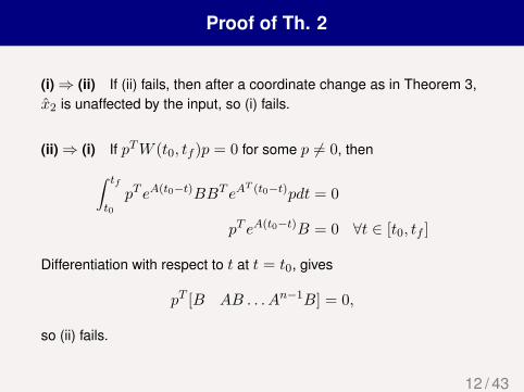
Proof of Th. 2

(i)⇒ (ii) If (ii) fails, then after a coordinate change as in Theorem 3,x2 is unaffected by the input, so (i) fails.

(ii)⇒ (i) If pTW (t0, tf )p = 0 for some p 6= 0, then∫ tf

t0pT eA(t0−t)BBT eA

T (t0−t)pdt = 0

pT eA(t0−t)B = 0 ∀t ∈ [t0, tf ]

Differentiation with respect to t at t = t0, gives

pT [B AB . . . An−1B] = 0,

so (ii) fails.

12 / 43

LionSealWhite

Proof Th2 continued

(ii)⇒ (iii) If iii fails, i.e. pTA = λpT and pTB = 0 for p 6= 0then pT [B AB . . . An−1B] = 0, so (ii) fails.

(iii)⇒ (ii) If rank[B . . . An−1B] = q < n then let P be defined asin Theorem 3 and let p2

T A22 = λp2T and pT = [0 p2

T ]P−1. Then

pTB = [0 p2T ][B110

]= 0

pTA = [0 p2T ][A11 A120 A22

]P−1 = λ[0 p2

T ]P−1 = λpT

so (iii) fails.

(iv)⇔{pT [λ−A B] = 0 ⇒ p = 0

}⇔ (iii)

13 / 43

LionSealWhite

Tank example - controllable?

x =[−1 00 −1

]x+

[11

]u

x =[−1 00 −2

]x+

[11

]u

14 / 43

LionSealWhite

Tank example - controllable?

x =

−1 0 00 −1 00 0 −1

x+

1 01 10 1

u

15 / 43

LionSealWhite

Example - Single Input Diagonal Systems

For which λi, bi is this system controllable?

x =

λ1 0

λ2. . .

0 λn

x+

b1b2...bn

uMethod 1: When is the controllability matrix invertible?

C(A,B) =

b1 b1λ1 b1λ

21 . . . b1λ

n−11

b2 b2λ2 b2λ22 . . . b2λ

n−12

...bn bnλn bnλ

2n . . . bnλ

n−1n

After some work: When all λi are distinct and all bi nonzero.

Method 2: The PBH-test gives you this result immediately!16 / 43

LionSealWhite

LTV Reachability

The equation

x(t) = A(t)x(t) +B(t)u(t), x(t0) = 0

is called reachable on (t0, tf ), if for any xf , there exists u(t) such thatx(tf ) = xf .

The matrix function

Wr(t0, tf ) =∫ tf

t0Φ(tf , t)B(t)B(t)TΦ(tf , t)Tdt

= Φ(tf , t0)W (t0, tf )Φ(tf , t0)T

is called the reachability Gramian.

Continuous time controllability and reachability are equivalent

17 / 43

LionSealWhite

LTV Observability

The equation

x(t) = A(t)x(t), x(t0) = x0

y(t) = C(t)x(t)

is called observable on [t0, tf ] if any initial state x0 is uniquelydetermined by the output y(t) for t ∈ [t0, tf ].

It is called reconstructable on [t0, tf ] if the state x(tf ) is uniquelydetermined by the output y(t) for t ∈ [t0, tf ].

In continuous time, observability and reconstrubality are equivalent(why?)

18 / 43

LionSealWhite

Observability Gramian

The matrix function

M(t0, tf ) =∫ tf

t0Φ(t, t0)TC(t)TC(t)Φ(t, t0)dt

is called the observability Gramian of the system

x(t) = A(t)x(t)y(t) = C(t)x(t)

Remark: Operator interpretation (see later)

M(t0, tf ) = L∗L

where L : Rn → Lm2 (t0, tf ) with

(Lx0)(t) = C(t)Φ(t, t0)x0, x0 ∈ Rn

19 / 43

LionSealWhite

Theorem 4 (Rugh 9.8) - Observability Criterion

The following two conditions are equivalent

(i) The system {A(t), C(t)} is observable on [t0, tf ].(ii) M(t0, tf ) > 0

20 / 43

LionSealWhite

Th. 5 (Rugh 9.11) - LTI Observability

The following four conditions are equivalent:

(i) The system x(t) = Ax(t), y(t) = Cx(t) is observable.

(ii) rank

CCA

...CAn−1

= n.

(iii) λ ∈ C : Ap = λp, Cp = 0 ⇒ p = 0

(iv) rank[λI −AC

]= n ∀λ ∈ C.

21 / 43

LionSealWhite

Theorem 6 - Unobservable State Equation

Suppose that rank

CCA

...CAn−1

= l < n

Then there exists an invertible Q ∈ Rn×n such that

Q−1AQ =[A11 0A21 A22

], CQ =

[C11 0

]

where A11 is l × l, C11 is p× l, and rank

C11

C11A11...

C11Al−111

= l.

22 / 43

LionSealWhite

LTI Controller Canonical Form - Single Input

Suppose (A, b) is controllable. There is an invertible P such that astate transformation will bring the system to the form

PAP−1 = Ac =

0 1 . . . 0...

.... . .

...0 0 . . . 1−a0 −a1 . . . −an−1

, PB = Bc =

0...01

det(sI −A) = sn + an−1s

n−1 + . . .+ a1s+ a0

23 / 43

LionSealWhite

Proof

Introduce some notation for C−1(A, b):M1...Mn

:=[b Ab . . . An−1b

]−1⇒ MnA

kb = 0, k = 0, . . . , n− 2MnA

n−1b = 1

We can use the transformation z = Px where

P =

Mn

MnA...

MnAn−1

That P is invertible follows from calculation of PC (the newcontrollability matrix)

24 / 43

LionSealWhite

Proof

PC =

Mn

MnA...

MnAn−1

[b Ab . . . An−1b

]=

0 . . . 0 1...

... . . . ?0 1 ? ?1 ? . . . ?

PA =

MnAMnA

2

...MnA

n

=

0 1 . . . 0...

.... . .

...0 0 . . . 1−a0 −a1 . . . −an−1

Mn

MnA...

MnAn−1

= AcP

PB =

MnbMnAb

...MnA

n−1b

=

0...01

= Bc

25 / 43

LionSealWhite

Controllability Index

To construct the corresponding controller form when we have multipleinputs (m > 1) we need the following

Definition: Let B = [B1 . . . Bm]. For j = 1, . . . ,m, thecontrollability index ρj is the smallest integer such that AρjBj islinearly dependent on the column vectors occuring to the left of it in thecontrollability matrix[

B AB . . . An−1B]

26 / 43

LionSealWhite

Notation for Controller Form

Given a contr. system {A,B}, with controllability indices ρ1, . . . ρm,define

M =

M1...Mn

:=[B1 AB1 . . . A

ρ1−1B1 . . . Bm . . . Aρm−1Bm]−1

P =

P1...Pm

, Pi =

Mρ1+···+ρi

Mρ1+···+ρiA...

Mρ1+···+ρiAρi−1

Notice that it is rather easy to write Matlab code for this.

See Rugh 13.9 for the proof of the following result

27 / 43

LionSealWhite

Theorem 7, Controller Form - Multiple Inputs

The transformation z = Px gives (Ac, Bc) with

Ac =

1. . .

1? . . . . . . ? ? . . . . . . ? ? . . . . . . ?

1. . .

1? . . . . . . ? ? . . . . . . ? ? . . . . . . ?

28 / 43

LionSealWhite

Theorem 7, Controller Form - Multiple Inputs

Bc =

1 ? . . . ?

0 1 ? ?

0 . . . 0 1

The block sizes equal the controllability indices ρi.

If B is not full rank, Bc will have a stair-case form.

29 / 43

LionSealWhite

LTI Feedback & Eigenvalue Assignment (Rugh 14.9)

Using the controller form it is now easy to prove

Suppose (A,B) is controllable. Given a monic polynomial p(s) thereis a feedback control u = −Kx so that

det(sI −A−BK) = p(s).

Proof We can get rid of the ? elements in Bc by writing Bc = BcTwhere T is an upper triangular matrix with right inverse. Introduce thenew control signal u = Tu. By state feedback we can now changeeach line of stars in Ac. We can for instance transform Ac to acontroller form with one big block, with the last row containing thecoefficients of p(s).

30 / 43

LionSealWhite

Definition - Observability Index

Let CT = [C1T . . . Cp

T ]T . For j = 1, . . . , p, the observability indexηj is the smallest integer such that CjAηj is linearly dependent on therow vectors occuring above it in the observability matrix

CCA

...CAn−1

31 / 43

LionSealWhite

Theorem 8 -Observer form

Suppose (C,A) is observable. Then there is a transformationz = Px, to the form z = Aoz, y = Coz with

Ao = transpose of the form for Ac above

Co = transpose of the form for Bc above

The size of the blocks equals the observability indices ηj .

32 / 43

LionSealWhite

Theorem 9 - Time-Invariant Gramian

Let A be exponentially stable. Then, the reachability GramianWr(−∞, 0) equals the unique solution P to the matrix equation

PAT +AP = −BBT

Similarly, the observability Gramian M(0,∞) equals the solution Q of

QA+ATQ = −CTC

33 / 43

LionSealWhite

Proof of Theorem 9

Let P = Wr(−∞, 0) =∫∞

0 eAσBBT eAT σdσ. Then

PAT +AP =∫ ∞

0

∂

∂σ

(eAσBBT eA

T σ)dσ

=[eAσBBT eA

T σ]∞

0

= −BBT

The linear operator (Lyapunov 1893)

L(P ) = AP + PAT

hasR(L) = Rn×n so N (L) = {0} and the solution P is unique.

The equation for the observability Gramian is obtained by replacingA,B with AT , CT .

34 / 43

LionSealWhite

Balanced Realization

For the stable system (A,B,C), with Gramians P and Q, the variabletransformation x = Tx gives

P = TPT ∗

Q = T−∗QT−1

Choosing R, T , unitary U and diagonal Σ from

Q = R∗R (Choleski Factorisation)

RPR∗ = UΣ2U∗ (Singular Value Decomposition)

T = Σ−1/2U∗R

gives (check)

P = Q = Σ

The corresponding realization (A, B, C) is called a balancedrealization of the system (A,B,C).

35 / 43

LionSealWhite

Truncated Balanced Realization

Let the states be sorted such that Σ is decreasing. The diagonalelements of Σ measure “how controllable and observable” thecorresponding states are. With

A =[A11 A12A21 A22

], B =

[B1B2

]C =

[C1 C2

]

Σ =[Σ1 00 Σ2

]

the system (A11, B1, C1) is called a truncated balanced realization ofthe system (A,B,C).

If Σ1 >> Σ2 the truncated system is probably a good approximation.Choose either D = 0 or to get correct DC-gain.

36 / 43

LionSealWhite

Example (done with balreal in MATLAB)

C(sI −A)−1B = 1− ss6 + 3s5 + 5s4 + 7s3 + 5s2 + 3s+ 1

Σ = diag{1.98, 1.92, 0.75, 0.33, 0.15, 0.0045}

C(sI − A)−1B = 0.20s2 − 0.44s+ 0.23s3 + 0.44s2 + 0.66s+ 0.17

37 / 43

LionSealWhite

Bonus: Full Kalman Decomposition

Simultaneous controller and observer decomposition

Use P =[P1 P2 P3 P4

]where Pi has ni columns with

Columns of[P1 P2

]basis forR(C)

Columns of P2 basis forR(C) ∩N (O)Columns of

[P2 P4

]basis for N (O)

Columns of P3 chosen so P invertible.

A =

A11 0 A13 0A21 A22 A23 A240 0 A33 00 0 A43 A44

, B =

B1B200

C =

[C1 0 C3 0

]38 / 43

LionSealWhite

Kalman’s Decomposition Theorem

The system (A11, B1, C1) is both controllable and observable.

It is of minimal order, n1

The transfer function equals C1(sI − A11)−1B1.

39 / 43

LionSealWhite

Bonus: More on Controllability

A,B is controllable if and only if

The only C for which C(sI −A)−1B = 0, ∀s is C = 0

A,C is observable if and only if

The only B for which C(sI −A)−1B = 0, ∀s is B = 0

Proof: 0 = C(sI −A)−1B =∞∑k=0

CAkB/sk+1 ⇔ 0 = CAkB, ∀k ⇔

0 = C[B AB . . . An−1B

]⇔ 0 =

CCA

...CAn−1

B

40 / 43

LionSealWhite

Bonus: Parallel Systems

Let G1(s) = C1(sI −A1)−1B1 and G2(s) = C2(sI −A2)−1B2

If A1 and A2 have no common eigenvalues then

G1(s) +G2(s) ≡ 0 =⇒ G1(s) = G2(s) = 0

Proof: Can assume both systems are minimal. From

G1(s) +G2(s) =[C1 C2

] [sI −A1 00 s−A2

]−1 [B1B2

]= 0

and the fact that[C1 C2

],

[A1 00 A2

]is observable (PBH-test), the

previous frame shows that

[B1B2

]=[00

]

41 / 43

LionSealWhite

Bonus: System Zeros (SISO)

Assume (A, b, c) minimal and that z is not an eigenvalue of A.

Then the following are equivalent

G(z) = c(zI −A)−1b+ d = 0With u0 arbitrary and x0 := (zI −A)−1bu0 we have[

zI −A −bc d

] [x0u0

]= 0

The following matrix looses rank[zI −A −bc d

]

42 / 43

LionSealWhite

Bonus: Series Connection SISO

Given two minimal systems ni(s)/di(s) = ci(sI −Ai)−1bi, i = 1, 2

Then the series connection n2(s)d2(s)

n1(s)d1(s) is

uncontrollable⇐⇒ there is z so n1(z) = d2(z) = 0unobservable⇐⇒ there is z so n2(z) = d1(z) = 0

Proof:

Controllable, check when rank[zI −A1 0 b1−b2c1 zI −A2 0

]≤ n

Observable, check when rank

zI −A1 0−b2c1 zI −A2

0 c2

≤ n

43 / 43