Linear stability analysis of miscible two-fluid flow in a channel with velocity slip at thewallsSukhendu Ghosh, R. Usha, and Kirti Chandra Sahu Citation: Physics of Fluids (1994-present) 26, 014107 (2014); doi: 10.1063/1.4862552 View online: http://dx.doi.org/10.1063/1.4862552 View Table of Contents: http://scitation.aip.org/content/aip/journal/pof2/26/1?ver=pdfcov Published by the AIP Publishing

This article is copyrighted as indicated in the article. Reuse of AIP content is subject to the terms at: http://scitation.aip.org/termsconditions. Downloaded to IP: 14.139.65.5

On: Mon, 27 Jan 2014 08:23:58

PHYSICS OF FLUIDS 26, 014107 (2014)

Linear stability analysis of miscible two-fluid flowin a channel with velocity slip at the walls

Sukhendu Ghosh,1 R. Usha,1,a) and Kirti Chandra Sahu2

1Department of Mathematics, Indian Institute of Technology Madras, Chennai 600036, India2Department of Chemical Engineering, Indian Institute of Technology Hyderabad,Yeddumailaram 502 205, Andhra Pradesh, India

(Received 20 August 2013; accepted 5 January 2014; published online 24 January 2014)

The linear stability characteristics of pressure-driven miscible two-fluid flow withsame density and varying viscosities in a channel with velocity slip at the wall areexamined. A prominent feature of the instability is that only a band of wave numbers isunstable whatever the Reynolds number is, whereas shorter wavelengths and smallerwave numbers are observed to be stable. The stability characteristics are differentfrom both the limiting cases of interface dominated flows and continuously stratifiedflows in a channel with velocity slip at the wall. The flow system is destabilizingwhen a more viscous fluid occupies the region closer to the wall with slip. For thisconfiguration a new mode of instability, namely the overlap mode, appears for highmass diffusivity of the two fluids. This mode arises due to the overlap of critical layerof dominant instability with the mixed layer of varying viscosity. The critical layercontains a location in the flow domain at which the base flow velocity equals the phasespeed of the most unstable disturbance. Such a mode also occurs in the correspondingflow in a rigid channel, but absent in either of the above limiting cases of flow in achannel with slip. The flow is unstable at low Reynolds numbers for a wide rangeof wave numbers for low mass diffusivity, mimicking the interfacial instability ofthe immiscible flows. A configuration with less viscous fluid adjacent to the wall ismore stable at moderate miscibility and this is also in contrast with the result for thelimiting case of interface dominated flows in a channel with slip, where the aboveconfiguration is more unstable. It is possible to achieve stabilization or destabilizationof miscible two-fluid flow in a channel with wall slip by appropriately choosing theviscosity of the fluid layer adjacent to the wall. In addition, the velocity slip atthe wall has a dual role in the stability of flow system and the trend is influencedby the location of the mixed layer, the location of more viscous fluid and the massdiffusivity of the two fluids. It is well known that creating a viscosity contrast in aparticular way in a rigid channel delays the occurrence of turbulence in a rigid channel.The results of the present study show that the flow system can be either stabilized ordestabilized by designing the walls of the channel as hydrophobic surfaces, modeledby velocity slip at the walls. The study provides another effective strategy to controlthe flow system. C© 2014 AIP Publishing LLC. [http://dx.doi.org/10.1063/1.4862552]

I. INTRODUCTION

The stability of a parallel two-fluid flow with viscosity stratification is relevant in numerousnatural and industrial applications, such as the generation of water waves by wind, pipeline lubri-cation, air-water flow in nuclear reactor cooling towers, primary atomization of jets, and extrusion.There are different ways of achieving a viscosity stratification which include (i) considering immis-cible fluids in contact with each other and in this case, there is a discontinuity in viscosity across a

a)Author to whom correspondence should be addressed. Electronic mail: ushar@iitm.ac.in

1070-6631/2014/26(1)/014107/21/$30.00 C©2014 AIP Publishing LLC26, 014107-1

This article is copyrighted as indicated in the article. Reuse of AIP content is subject to the terms at: http://scitation.aip.org/termsconditions. Downloaded to IP: 14.139.65.5

On: Mon, 27 Jan 2014 08:23:58

014107-2 Ghosh, Usha, and Sahu Phys. Fluids 26, 014107 (2014)

sharp interface, (ii) varying continuously the temperature or concentration in which case a diffusiveinterface of nonzero thickness occurs, and (iii) using a non-Newtonian fluid. The instabilities arisingdue to viscosity stratification are discussed in detail in a recent review article by Govindarajan andSahu.1 As mentioned in this article, apart from gaining knowledge about the nonlinear stages ofgrowth and transition to turbulence, there is lot more to understand and principal questions to beaddressed on the effect of viscosity stratification even in the linear regime. This motivates furtherstudies to understand instability characteristics of viscosity stratified flows that can improve theperformance of many industrial processes. The present study attempts to provide some informationon the instability that arises in miscible three-layer channel flow with velocity slip at the walls.

Yih2 is the first to consider the stability of a Couette-Poiseuille flow in a rigid channel withsharp jump in viscosity. He focused on long waves and observed an interfacial mode of instability atany Reynolds number. Since then, there have been several studies addressing many aspects of thisinterfacial instability.3–12 The essence of these studies is that, in order to achieve a linearly stableflow, one should place the less viscous fluid in a thin layer close to the wall to stabilize long wavesand provide enough interfacial tension to stabilize short waves.

There are also investigations in stratified flows in a rigid channel in which the fluid propertiesvary over the entire domain or at least over a large portion of it.13–15 Wall and Wilson15 studiedthe influence of continuous viscosity variation due to a temperature gradient in a rigid channel andshowed that the Peclet number has little influence on the stability and that the base state viscosityinfluences the Tollmien-Schlichting (TS) mode. The experiments16–20 on miscible two-fluid flowin different geometries revealed interesting instabilities. At low miscibility, instabilities driven byviscosity stratified flow are observed to be qualitatively similar to those in immiscible fluids.16–18

The miscible two-fluid flow in which the fluid layers are separated by a finite-thickness mixedlayer also falls under the class of viscous stratified flows and has been examined by Ranganathan andGovindarajan,16 Ern et al.,17 Govindarajan,18 and Sahu et al.19 Ern et al.17 considered the influenceof diffusion and mixed layer thickness in the miscible two-fluid Couette flow with a high degree ofstratification in the mixed layer. They showed that growth rate exhibits a non-monotonic behaviourwith respect to diffusion and that flows at intermediate Peclet numbers are more unstable thanthose without diffusion, when the thickness of the mixed layer was not too large. Govindarajan andco-workers16, 18 investigated the effects of a thin viscosity layer created by miscibility of two fluidsof same density but different viscosity for symmetric flow through a rigid channel and examinedthe effects of diffusion. They identified a new mode of instability associated with the overlap ofcritical layer and the viscosity stratified layer. This mode was found to be very sensitive to theeffects of diffusion when the viscosity stratified mixed layer and the critical layer overlap witheach other. The flow was shown to become more stable or unstable depending on the viscosityratio. Their results18 showed that the flow becomes unstable at Reynolds number much lower thanthat for the corresponding immiscible configuration. The stability properties were similar to thatof the interfacial mode at low values of diffusivity, but the behaviour was qualitatively differentfor higher values of diffusivity. Recently, Talon and Meiburg20 investigated the linear stability ofmiscible viscosity-stratified plane Poiseuille flow in the Stokes flow regime. They demonstrated thatinstabilities develop due to the effects of diffusion. Further, they showed that at large wave numbers,the instability occurs even when the highly viscous layer is in the core of the pipe.

The above efforts were aimed at understanding the effects of a stratification of viscosity inlaminar channel flows with rigid walls. There are many situations and important applications, suchas lubrication, microfluidics,21, 22 biological and technological drag reduction surfaces,23, 24 high-speed rarefied flow,25, 26 polymer melt,27 and drag reduction in microchannel flows28–30 where thevelocity of a viscous fluid exhibits a tangential slip on the wall. It would be reasonable to thinkof slip in terms of a relation between slip velocity and the wall shear stress. The slip length isthe equivalent local distance below the rigid surface where the no-slip condition at the surface canbe satisfied if the flow field were extended linearly outside the physical domain. Measurementsof boundary slip of Newtonian liquids have been the subject of recent research. The experimentalpredictions by Zhu and Granick21 and molecular dynamic simulations by Thompson and Troian22

suggest the possibility of slip at the solid boundary. The slip boundary conditions are applicablein the investigations of problems where fluids interact with solids at small length scales and this

This article is copyrighted as indicated in the article. Reuse of AIP content is subject to the terms at: http://scitation.aip.org/termsconditions. Downloaded to IP: 14.139.65.5

On: Mon, 27 Jan 2014 08:23:58

014107-3 Ghosh, Usha, and Sahu Phys. Fluids 26, 014107 (2014)

includes flows in microfluidics, porous media, and biological system, such as arterial flows. TheNavier’s concept of slip has been commonly used in many investigations,27 which states that therelative velocity of the fluid with respect to the wall (slip velocity) is proportional to the shear rateat the wall. Reports by a number of recent experiments on microscale flows driven by pressure-gradient indicate an apparent break-down of the no-slip condition with slip lengths as large asmicrometers.31–33 There are also investigations of pressure-driven fluid flow in channels that displayresults consistent with slip at the solid boundary.34 This suggests that it is relevant to consider theeffects of slip on the linear stability of wall bounded shear flow of a fluid system in a channelwith slippery walls. In the case of Poiseuille flow bounded by the walls at y = ±h, the Navier slipconditions are described as u + β1 uy = 0 at y = +h and u − β2 uy = 0 at y = −h where β1, β2 aredifferent slip coefficients at the wall boundaries.

In fact, the slip effects have been incorporated in plane Poiseuille flow of a single fluid withboth symmetric and asymmetric slip conditions. Gersting35 reported that wall slip has a stabilizingeffect on the flow dynamics. The study by Spille and Rauh36 confirms the above conclusion. Theresults of Gan and Wu37 indicate that the wall slip causes short wave instability while the slip-flowmodel is stable for long waves. Lauga and Cossu38 formulated the linear stability of plane Poiseuilleflow with different slip coefficients β1 , β2 (β1 �= β2) at the wall boundaries but focused on thecases of symmetric slip (β1 = β2 = β) and asymmetric slip (β1 = β, β2 = 0). Such differencesin the wall slip can arise when the surface wettability, surface chemistry, and surface roughness atthe walls of the channel are distinct.39 Their results showed that the presence of slip at the wallsignificantly increases the critical Reynolds number for linear stability. Ling et al.40 extended thestudy by Lauga and Cossu38 by considering an asymmetric slip boundary condition at the wallswith β1, β2 �= 0. They found that depending on the slip length, the slip plays a dual role by eitherstabilizing or destabilizing the flow system, depending on the slip length. For the symmetric slipboundary conditions, their results showed a similar stabilizing trend of Lauga and Cossu38 forβ > 0.0011. However, for β < 0.0011 the slip has a destabilizing effect. A similar behaviour isobserved for asymmetric case also. In the case of microflows mentioned above, the amount ofslip at the wall is linearly proportional to the gradient of the tangential velocity at the wall, withproportionality coefficient defined as the slip length.25, 41 If the slip wall conditions are used, theNavier-Stokes equations are valid for slip length up to 0.1.41

Motivated by the results of Lauga and Cossu,38 Sahu et al.42 analyzed the relative rolls ofangle of divergence and velocity slip in the linear stability of a diverging channel flow. Using theMaxwell velocity slip boundary conditions43 at the walls, they showed that unlike the flow in astraight channel, wall slip has a destabilizing influence in flow through diverging channel at lowKnudsen numbers (Kn). The Maxwell slip boundary conditions43 are given by u ± Kn ∂u/∂y = 0 aty = ±h, where Kn is the ratio of slip length to the local half-width of the channel. As in the previousinvestigations,37, 38, 44, 45 they also considered Kn less than 0.1.

You and Zheng46 investigated the effects of boundary slip on the stability of viscosity-stratifiedmicrochannel flow in which two immiscible fluids are separated by a sharp interface. Their resultsrevealed that the stability of stratified microchannel flow is enhanced by boundary slip. The slipeffects were observed to be strong at small and large viscosity contrasts and were relatively weakwhen viscosity contrast is close to one.

A linear stability analysis of pressure-driven flow in a plane channel with slip at the boundaryexamined by Webber,47 in the presence of temperature variation is analogous to that of Wall andWilson14 in a rigid channel. Taking viscosity dependence on temperature to be linear, they concludedthat boundary slip is linearly stabilizing. For a fixed value of slip parameter, an increase in temperatureenhanced stability; but the critical Reynolds number decreases and then increases with temperature.

The aim of the present study is to examine the linear stability of a symmetric Poiseuille flowof two miscible fluids of equal densities and different viscosities (say μ1 and μ2) separated by amixed layer (in which viscosity varies continuously from μ1 to μ2) through a channel with velocityslip at the walls. The analysis is restricted to symmetric slip cases. The results for the flow systemin a rigid channel are recovered in the limit β = 0. It extends the investigations by Ern et al.,17

Govindarajan,18 and Sahu et al.19 for a miscible two-fluid flow in a rigid channel, where the effectsof a continuous variation of concentration across a layer subject to diffusion have been studied. To

This article is copyrighted as indicated in the article. Reuse of AIP content is subject to the terms at: http://scitation.aip.org/termsconditions. Downloaded to IP: 14.139.65.5

On: Mon, 27 Jan 2014 08:23:58

014107-4 Ghosh, Usha, and Sahu Phys. Fluids 26, 014107 (2014)

the best of our knowledge, the present study is a first attempt to clarify the above effects in a channelwith velocity slip at the walls.

In view of the discussion and the available investigations in the literature on flow in a channelwith slip at the walls, the study can be thought of as describing the effects of a hydrophobic surfaceon stability in wall bounded viscosity-stratified flow, where the hydrophobic surface is representedby a slip boundary condition on the surface44 and the velocity of the fluid exhibits a tangential slipon the walls. The results generated can be used according to the applications for which they arerelevant. For example, if a PDMS (Polydimethylsiloxane) channel is hosting an oil-water flow, thentwo possible configurations can be considered for the stability analysis by using the formulation inthe present study (see Sec. II A). In the first configuration, water flows adjacent to the hydrophobicwall and oil flows in the core region of the channel. As a result, the contact angle will be high(more than 90◦ and up to 150◦) and the surface energy will be less. Then the effect of the wallslip to reduce wall shear is more, which in turn stabilizes the flow system. Note that in the firstconfiguration, fluid with lower viscosity (water) is adjacent to the hydrophobic channel wall. In thesecond configuration, oil (more viscous fluid) flows adjacent to hydrophobic wall, thus the contactangle will be less and the surface energy will be high. Therefore, the effect of wall slip is less toreduce wall shear. This causes the flow system to be more unstable. The above conclusions areconfirmed by the analysis/results presented in Sec. III.

The paper is organized as follows. The mathematical formulation of the base state and thelinear stability analysis are presented in Sec. II. The results of the stability analysis are discussed inSec. III. The conclusions are presented in Sec. IV.

II. MATHEMATICAL FORMULATION

A. Governing equations

The linear stability of a pressure-driven laminar two-dimensional flow of two miscible, Newto-nian, incompressible fluids in a horizontal plane channel with wall slip is considered. The two fluidshave the same density ρ but different viscosities. They are separated by a mixed layer of viscosity-stratified fluid. The flow is symmetric about the centerline of the channel, thus the formulation ispresented for the upper half of the channel (see Fig. 1). A Cartesian coordinate system is chosenwith x and y directions along and perpendicular to the centerline of the channel (y = 0). The wallsof the channel are located at y = ±H. The fluids of viscosities μ1 and μ2 occupy the regions 0 ≤ y≤ h and h + q ≤ y ≤ H, respectively. There is a thin layer where the two fluids mix-up and a localstratification of viscosity is created. This layer is referred to as a mixed layer of thickness q and itoccupies the region h ≤ y ≤ h + q. The downstream growth of the mixed layer thickness is neglectedunder the assumption that the two fluids diffuse into each other very slowly (i.e., the Peclet number,defined later in this section, is high; also see Appendices A and B). The basic viscosity is relatedto the basic concentration profile and it varies monotonically between the two fluids with viscosity

x

y

fluid 2

fluid 1Mixed region

S=S2

S=S1

-H

H

FIG. 1. Schematic of the flow system considered. The core and annular regions of the slippery channel contain the fluids“1” and “2,” respectively. Here fluid “1” occupies the region −h ≤ y ≤ h and both the fluids are separated by a mixed layerof uniform thickness q. The slippery walls of the channel are located at y = ±H.

This article is copyrighted as indicated in the article. Reuse of AIP content is subject to the terms at: http://scitation.aip.org/termsconditions. Downloaded to IP: 14.139.65.5

On: Mon, 27 Jan 2014 08:23:58

014107-5 Ghosh, Usha, and Sahu Phys. Fluids 26, 014107 (2014)

μ1 (viscosity of fluid-1) and μ2 (viscosity of fluid-2) in the mixed layer. In the present study, anexponential dependence of the viscosity μ on the concentration is assumed48 and is given by

μ = μ1 exp

[Rs

(S − S1

S2 − S1

)], (1)

where Rs = (S2 − S1)d

ds(ln μ) is the log-mobility ratio of the scalar S. The scalar S (can also be

temperature) takes the values S1 and S2 in the regions 0 ≤ y ≤ h and h + q ≤ y ≤ H, respectively.This defines the basic viscosity as follows:

μ =⎧⎨⎩

μ1 if 0 ≤ y ≤ hμm(y) if h ≤ y ≤ h + qμ2 if h + q ≤ y ≤ H

, (2)

where μ2 = μ1eRs and μm(y) = μ1eRs

(S−S1

S2−S1

). The governing equations are the continuity and the

Navier-Stokes equations together with a scalar-transport equation for the concentration of the scalar.The boundary conditions are the symmetry condition at the centerline and the velocity slip conditionat the channel wall, which are given by

∂u

∂y= 0, v = 0 at y = 0, (3)

u = −β1∂u

∂y, v = 0 at y = H. (4)

Here (u, v) are the components of the velocity along the x and y directions, respectively, and β1

is the dimensional slip parameter. The equations and the boundary conditions governing the flowdynamics are made dimensionless by using the following scales:

x∗ = x

H, y∗ = y

H, t∗ = Q

H 2t, (u∗, v∗) = H

Q(u, v), p∗ = H 2

ρQ2p,

μ∗ = μ

μ1, h∗ = h

H, q∗ = q

H, m = μ2

μ1, β = β1

H, S∗ = S − S1

S2 − S1, μ∗

m = μm(y)

μ1, (5)

where Q is the total volume flow rate per unit distance in the spanwise direction, p is pressure, and tis time. They are given by (after suppressing ∗)

ux + vy = 0, (6)

ut + uux + vuy = ∂

∂x

[−p + 2

Reμux

]+ ∂

∂y

[1

Reμ(uy + vx )

], (7)

vt + uvx + vvy = ∂

∂x

[1

Reμ(uy + vx )

]+ ∂

∂y

[−p + 2

Reμuy

], (8)

st + usx + vsy = 1

Pe[sxx + syy], (9)

uy = 0, v = 0 at y = 0, (10)

u = −βuy, v = 0 at y = 1, (11)

where Pe = Q/D is the Peclet number, D is the mass diffusivity, Re = ρQ/μ1 is the Reynoldsnumber, and Sc = Pe/Re is the Schmidt number.

This article is copyrighted as indicated in the article. Reuse of AIP content is subject to the terms at: http://scitation.aip.org/termsconditions. Downloaded to IP: 14.139.65.5

On: Mon, 27 Jan 2014 08:23:58

014107-6 Ghosh, Usha, and Sahu Phys. Fluids 26, 014107 (2014)

B. Base state

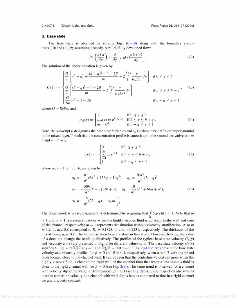
The base state is obtained by solving Eqs. (6)–(9) along with the boundary condi-tions (10) and (11) by assuming a steady, parallel, fully developed flow:

Re

(d PB

dx

)= d

dy

[μB(y)

dUB(y)

dy

]. (12)

The solution of the above equation is given by

UB(y) =

⎧⎪⎪⎪⎪⎪⎪⎪⎪⎨⎪⎪⎪⎪⎪⎪⎪⎪⎩

G

2

[y2 − h2 + (h + q)2 − 1 − 2β

m− 2

h+q∫h

y

μm(y)dy

]if 0 ≤ y ≤ h

G

2

[(h + q)2 − 1 − 2β

m− 2

h+q∫y

y

μm(y)dy

]if h ≤ y ≤ h + q

G

2m(y2 − 1 − 2β) if h + q ≤ y ≤ 1

, (13)

where G = RePBx and

μB(y) =⎧⎨⎩

1 if 0 ≤ y ≤ hμm(y) = eRs sB (y) if h ≤ y ≤ h + qm = eRs if h + q ≤ y ≤ 1

. (14)

Here, the subscript B designates the base state variables and sB is taken to be a fifth order polynomialin the mixed layer,48 such that the concentration profile is smooth up to the second derivative at y =h and y = h + q:

sB(y) =

⎧⎪⎪⎨⎪⎪⎩

0 if 0 ≤ y ≤ h6∑

i=1ai yi−1 if h ≤ y ≤ h + q

1 if h + q ≤ y ≤ 1

, (15)

where ai, i = 1, 2, . . . , 6, are given by

a1 = −h3

q5(6h2 + 15hq + 10q2), a2 = 30h2

q5(h + q)2,

a3 = −30h

q5(h + q) (2h + q), a4 = 10

q5(6h2 + 6hq + q2),

a5 = −15

q5(2h + q), a6 = 6

q5.

(16)

The dimensionless pressure-gradient is determined by requiring that1∫

0UB(y)dy = 1. Note that m

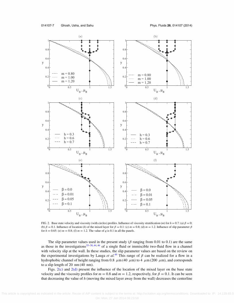
> 1 and m < 1 represent situations when the highly viscous fluid is adjacent to the wall and coreof the channel, respectively; m = 1 represents the situation without viscosity stratification. Also m= 1.2, 1, and 0.8 correspond to Rs = 0.1823, 0, and −0.2231, respectively. The thickness of themixed layer, q, is 0.1. The value has been kept constant in this study. However, halving the valueof q does not change the result qualitatively. The profiles of the typical base state velocity UB(y)and viscosity μB(y) are presented in Fig. 2 for different values of m. The base state velocity UB(y)satisfies UB(y) = β

∂UB (y)∂y at y = 1 and ∂UB (y)

∂y = 0 at y = 0. Figs. 2(a) and 2(b) present the base statevelocity and viscosity profiles for β = 0 and β = 0.1, respectively, when h = 0.7 with the mixedlayer located close to the channel wall. It can be seen that the centerline velocity is more when thehighly viscous fluid is close to the rigid wall of the channel than that when a less viscous fluid isclose to the rigid channel wall for β = 0 (see Fig. 2(a)). The same trend is observed for a channelwith velocity slip at the wall, i.e., for example, β = 0.1 (see Fig. 2(b)). Close inspection also revealsthat the centerline velocity in a channel with wall slip is less as compared to that in a rigid channelfor any viscosity contrast.

This article is copyrighted as indicated in the article. Reuse of AIP content is subject to the terms at: http://scitation.aip.org/termsconditions. Downloaded to IP: 14.139.65.5

On: Mon, 27 Jan 2014 08:23:58

014107-7 Ghosh, Usha, and Sahu Phys. Fluids 26, 014107 (2014)

0 0.5 1 1.5U

B , μΒ

0

0.2

0.4

0.6

0.8

1

y

m = 0.80m = 1.00m = 1.20

0 0.5 1 1.5U

B , μΒ

0

0.2

0.4

0.6

0.8

1

y

m = 0.80m = 1.00m = 1.20

0 0.5 1 1.5U

B , μΒ

0

0.2

0.4

0.6

0.8

1

y

h = 0.3h = 0.6h = 0.7

0 0.5 1 1.5U

B , μΒ

0

0.2

0.4

0.6

0.8

1

y

h = 0.3h = 0.6h = 0.7

0 0.5 1 1.5U

B , μΒ

0

0.2

0.4

0.6

0.8

1

yβ = 0.0β = 0.01β = 0.05β = 0.1

0 0.5 1 1.5U

B , μΒ

0

0.2

0.4

0.6

0.8

1

yβ = 0.0β = 0.01β = 0.05β = 0.1

(a) (b)

(c) (d)

(e) (f)

FIG. 2. Base state velocity and viscosity (with circles) profiles. Influence of viscosity stratification (m) for h = 0.7: (a) β = 0;(b) β = 0.1. Influence of location (h) of the mixed layer for β = 0.1: (c) m = 0.8; (d) m = 1.2. Influence of slip parameter β

for h = 0.65: (e) m = 0.8; (f) m = 1.2. The value of q is 0.1 in all the panels.

The slip parameter values used in the present study (β ranging from 0.01 to 0.1) are the sameas those in the investigations35–38, 44, 46 of a single fluid or immiscible two-fluid flow in a channelwith velocity slip at the wall. In these studies, the slip parameter values are based on the review onthe experimental investigations by Lauga et al.49 This range of β can be realized for a flow in ahydrophobic channel of height ranging from 0.8 μm (40 μm) to 4 μm (200 μm), and correspondsto a slip length of 20 nm (40 nm).

Figs. 2(c) and 2(d) present the influence of the location of the mixed layer on the base statevelocity and the viscosity profiles for m = 0.8 and m = 1.2, respectively, for β = 0.1. It can be seenthat decreasing the value of h (moving the mixed layer away from the wall) decreases the centerline

This article is copyrighted as indicated in the article. Reuse of AIP content is subject to the terms at: http://scitation.aip.org/termsconditions. Downloaded to IP: 14.139.65.5

On: Mon, 27 Jan 2014 08:23:58

014107-8 Ghosh, Usha, and Sahu Phys. Fluids 26, 014107 (2014)

velocity when the less viscous fluid is adjacent to the wall (m = 0.8). However, the opposite trendis observed when the highly viscous fluid is adjacent to the wall (m = 1.2). The effects of β on thebase state velocity and viscosity profiles are shown in Figs. 2(e) and 2(f) for m = 0.8 and m = 1.2,respectively. It can be observed that increasing the velocity slip at the wall decreases the centerlinevelocity for both the viscosity ratios considered. It can also be observed that the centerline velocityfor m = 0.8 is smaller than that for m = 1.2 for each value of β. Further, a slip at the wall reducesthe wall shear.

C. Linear stability analysis

The temporal evolution of the base flow (UB(y), μB(y), PB(x)) described by Eqs. (13)–(16) isexamined using linear stability analysis. The flow variables are split into the base state quantitiesand two-dimensional perturbations (designated by a hat) as

(u, v, p, s) = (UB(y), 0, PB(x), sB(y)) + (u, v, p, s)(y)ei(αx−ωt), (17)

where i ≡ √−1, α is the streamwise disturbance wave number, ω = αc is the frequency of the two-dimensional disturbance, and c is the complex phase speed. The flow is linearly unstable if Im(ω) =ωi > 0, stable if Im(ω) = ωi < 0, and neutrally stable if Im(ω) = ωi = 0. It is to be noted that theperturbation viscosity μ is given by μ = ∂μB

∂sBs. The velocity perturbations are expressed in terms

of the stream function perturbation φ as (u, v) = (φy ,−φx ). Modified Orr-Sommerfeld system isthen derived from the non-dimensional governing equations (6)–(9) and the boundary conditions(10)–(13) using a standard procedure50 and are given by (after suppressing hat ( ˆ ) symbols)

iα Re[φ′′(UB − c) − α2φ(UB − c) − UB

′′φ] = μBφ′′′′ + 2μB

′φ′′′ + (μB′′ − 2α2μB)φ′′ −

2α2μB′φ′ + (α2μB

′′ + α4μB)φ + UB′μ′′ + 2UB

′′μ′ + (UB′′′ + α2UB

′)μ, (18)

iα Pe[(UB − c)s − sB

′φ] = (s ′′ − α2s), (19)

φ′ = −βφ′′, φ = s = 0 at y = 1, (20)

φ′ = φ′′′ = s ′ = 0 at y = 0 (sinuous mode), (21)

where prime (′) denotes differentiation with respect to y. The above equations incorporate the termsthat arise due to the continuous variations of the base flow velocity and viscosity perturbations.Equations (18)–(21) constitute an eigenvalue problem and determine the linear stability of infinitesi-mal two-dimensional disturbances of the miscible three-layer pressure-driven flow in a channel withwall slip. The classical Orr-Sommerfeld equation is recovered50 for constant viscosity case. Themodified Orr-Sommerfeld system is numerically solved by using Chebyshev spectral collocationmethod (Canuto et al.51) and the public domain software, LAPACK. The results are presented forsinuous mode (described by Eq. (21) at the centerline of the channel) as it was observed to be thedominant mode for the range of parameters considered. A large number of grid points are taken inthe mixed layer, since the gradients are large in this layer. This is achieved by using the stretchingfunction (Govindarajan18)

y j = a

sinh(by0)[sinh{(yc − y0)b} + sinh(by0)], (22)

where yj are the locations of the grid points, a is the mid point of the mixed layer, and yc is aChebyshev collocation point, given by

yc = 0.5

{cos

[π

( j − 1)

(n − 1)

]+ 1

}, (23)

This article is copyrighted as indicated in the article. Reuse of AIP content is subject to the terms at: http://scitation.aip.org/termsconditions. Downloaded to IP: 14.139.65.5

On: Mon, 27 Jan 2014 08:23:58

014107-9 Ghosh, Usha, and Sahu Phys. Fluids 26, 014107 (2014)

and

y0 = 1

2bln

[1 + (eb − 1)a

1 + (e−b − 1)a

], (24)

where n is the number of collocation points and b is the degree of clustering. In the present study,the computations are performed with b = 8 and using 121 collocation points. This gives an accuracyof at least five decimal places in the range of parameters considered.

III. RESULTS

In this section, the effects of location of the mixed layer, velocity slip at the walls, and level ofdiffusivity on the stability properties of the flow system are examined. The correctness and accuracyof the developed numerical code are first assessed by examining the neutral stability curves for singlefluid channel flow with rigid walls and walls with slip (Fig. 3). The computations are performed forsinuous mode at the centerline y = 0 with m = 1 both for β = 0 (rigid wall) and β �= 0 (walls withslip). We found that the critical Reynolds number, Recr, for β = 0 is 3848.16 and it is to be notedthat in the present study, the Reynolds number is based on the mass flux Q. The critical Reynoldsnumber based on the maximum velocity is 5772.2 (Drazin and Reid50) and two thirds of this is thecritical Reynolds number obtained in the present case, for β = 0. The results show an excellentagreement with the available results for β = 0. In the case of wall-slip (β �= 0), the neutral stabilityboundaries are shifted towards larger values of Reynolds number as compared to that for β = 0(see Fig. 3(a)). The critical Reynolds number (Recr) as a function of β is presented in Fig. 3(b). Inview of the choice of characteristic velocity scale as maximum velocity by Lauga and Cossu,38 Recr

in the present study (Fig. 3(b)) is 23 (1 + 3β) times that obtained by Lauga and Cossu,38 for β �= 0.

Figs. 3(a) and 3(b) reveal the stabilizing effect of velocity slip at the wall.Further, the computations are carried out and stability boundaries are obtained for the problem

analyzed by Govindarajan,18 where the effects of miscibility on the linear stability of two-fluidchannel have been examined by taking the walls of the channels to be rigid and imposing noslip condition. In the investigation by Govindarajan,18 the mean viscosity is taken to be a fifth-orderpolynomial whereas in the present study, it is assumed to vary exponentially. The results are obtainedindependently for the above two choices of viscosity profiles. The stability boundaries obtained withthe latter choice of viscosity profile are presented in Figs. 4(a), 4(b), and 4(c) for q = 0.1, Sc = 0, m= 1.2 and are observed to be qualitatively similar to those presented in Figure 2 of Govindarajan.18

It is to be noted that in her result the stability boundaries are presented in α–Rav plane, where Rav isthe Reynolds number based on the spatially averaged viscosity across the channel with rigid walls.

In Fig. 4(a), for small h (h = 0.2), there is a TS mode instability similar to that observed for aflow of a single fluid in a planar rigid channel. As the location of the mixed layer moves closer to the

0 5000 10000 15000 20000Re

0.6

0.8

1

1.2

α

β = 0.0β = 0.01β = 0.02β = 0.03

0 0.01 0.02 0.03 0.04β

0

10000

20000

30000

Recr

(a) (b)

FIG. 3. (a) The neutral stability boundaries for a single fluid flow in a channel with no-slip (β = 0) and slip β �= 0.(b) Critical Reynolds number as a function of slip parameter β.

This article is copyrighted as indicated in the article. Reuse of AIP content is subject to the terms at: http://scitation.aip.org/termsconditions. Downloaded to IP: 14.139.65.5

On: Mon, 27 Jan 2014 08:23:58

014107-10 Ghosh, Usha, and Sahu Phys. Fluids 26, 014107 (2014)

0 2500 5000 7500 10000Re

0.5

1

1.5

2

2.5

3

α

h = 0.2, β = 0.0

TS

0 2500 5000 7500 10000Re

0.5

1

1.5

2

2.5

3

α

h = 0.65, β = 0.0

I

O

TS

0 2500 5000 7500 10000Re

1

1.5

2

2.5

3

α

h = 0.656, β = 0.0

O

I

TS

(a) (b) (c)

FIG. 4. ((a)–(c)) The neutral stability boundaries for q = 0.1, Sc = 0, and m = 1.2 for miscible two-fluid flow in a rigidchannel.

rigid wall (Fig. 4(b), h = 0.65), three modes of instability occupying distinct and sizable regions ofα–Re plane are observed. They are referred to as the TS mode, the “I” or inviscid mode appearing atshorter wavelengths and the “O” or the overlap mode that becomes unstable at low Reynolds number.The “O” mode of instability arises due to the overlap of the critical layer of dominant instability withthe mixed layer of varying viscosity, where the critical layer associated with a particular disturbanceeigenmode is one that contains a critical location at which the base flow velocity equals the phasespeed. In Fig. 4(b), the location of the critical layer (y = 0.7) overlaps the mixed region of the fluids(0.65 ≤ y ≤ 0.75). At h = 0.656 (Fig. 4(c)), the “O” mode and the “I” mode are seen to be merged andthe stability loop contains a bifurcation point. As the location of the mixed region goes further closerto the wall, all the three modes of instability coalesce and there is a large region of instability (see β

= 0 curve in Fig. 7(f)). The agreement with the available results18, 38, 50 gives sufficient confidence inusing the code for further study and the results for the present study are furnished below. The resultspresented for Sc = 0 help us to compare the instabilities in miscible two-fluid flow in a channel withslippery wall with the available result in a rigid channel.18 In addition, the computations are carriedout for Sc > 0 to understand the effects of diffusion.

The eigenspectra for Re = 400 is shown in Fig. 5(a) (for β = 0.0, 0.01) and Fig. 5(b) (for β =0.0, 0.05), respectively, for h = 0.2 and 0.65, with the other parameters as α = 1.35, q = 0.1, andSc = 1. When h = 0.2, the mixed layer and the critical layer of the dominant disturbance are wellseparated. Figs. 5(a) and 5(b) show that the growth rate (ωi = αci) is negative and the two-fluid flowin both the rigid channel and the channel with wall slip is stable. When h = 0.65, the two layersoverlap. In this case, the growth rate of the disturbance is positive for two-fluid miscible flow in arigid channel (β = 0; Figs. 5(a) and 5(b)). At this Re (=400), this is not so for two-fluid channelflow with wall slip. For β = 0.01, the growth rate is positive (Fig. 5(a)) while for β = 0.05, it isnegative (Fig. 5(b)). The growth rate is more for flow in a rigid channel than in a channel with wall

0.4 0.6 0.8 1 1.2 1.4c

r

-1.5

-1

-0.5

0

ci

h = 0.2, β = 0.0h = 0.2, β = 0.01h = 0.65, β = 0.0h = 0.65, β = 0.01

0.4 0.6 0.8 1 1.2 1.4c

r

-1.5

-1

-0.5

0

ci

h = 0.2, β = 0.0h = 0.2, β = 0.05h = 0.65, β = 0.0h = 0.65, β = 0.05

(a) (b)

FIG. 5. Eigenspectra for m = 1.2 for two different values of h. The other parameters are α = 1.35, q = 0.1, Sc = 1, and Re= 400. (a) β = 0.0, 0.01; (b) β = 0.0, 0.05.

This article is copyrighted as indicated in the article. Reuse of AIP content is subject to the terms at: http://scitation.aip.org/termsconditions. Downloaded to IP: 14.139.65.5

On: Mon, 27 Jan 2014 08:23:58

014107-11 Ghosh, Usha, and Sahu Phys. Fluids 26, 014107 (2014)

0.8 1.2 1.6 2α

-0.1

-0.05

0

ωi β = 0.0

β = 0.01β = 0.03β = 0.05

0 0.4 0.8 1.2 1.6 2α

-0.2

-0.1

0

ωi

β = 0.0β = 0.01β = 0.03β = 0.05

(a) (b)

FIG. 6. Effects of slip parameter, β, on the growth rate (ωi) as a function of wave number (α) for Re = 400: (a) m = 1.2 and(b) m = 0.8. Here, h = 0.65, q = 0.1, and Sc = 1.

slip for viscosity contrast m = 1.2. This suggests that one can expect interesting instabilities to occurin the case when more viscous fluid is adjacent to the wall (m = 1.2) and when the mixed layerand the critical layers overlap. It is of interest to observe what happens when m < 1 under overlapconditions.

The growth rate (ωi) as a function of wave number α is presented in Figs. 6(a) and 6(b) form = 1.2 and m = 0.8, respectively, for Re = 400. The other parameters are h = 0.65, q = 0.1,and Sc = 1. In Fig. 6(a), there is a range of wave numbers in which ωi decreases as β increases,indicating the stabilizing role of the slip parameter β. A slip at the wall reduces the shear as canbe seen from Figs. 2(e) and 2(f). This suggests that the wall slip stabilizes the flow by decreasingthe shear rate. Also note that only a band of wave numbers is unstable; disturbances of shorterwavelengths and small wave numbers are stable. The range of unstable wave numbers decreaseswith increase in β. Further, the growth rate for m = 1.2 is positive for all β ≤ 0.03 whereas this isnot the case for β > 0.03. However, in Fig. 6(b) (m = 0.8), the growth rate is negative for all valuesof the slip parameter β considered. For each β, this behaviour is due to a decrease in wall shear form = 0.8 as compared to that for m = 1.2 (see Figs. 2(a), 2(b), 2(e), and 2(f)). In view of the above,the focus is on the case for m = 1.2 to understand the instabilities that occur and to study the effectsof the parameters on each mode of instability.

The influence of the slip parameter β on the stability boundaries for m = 1.2, Sc = 0.1,q = 0.1 is examined in Fig. 7 for different locations of the mixed layer. The configuration correspondsto viscosity increasing towards the wall with slip at y = 1. For small h (h = 0.2), the mixed layeris away from the channel wall and only a TS mode of instability appears at high Reynolds number(Fig. 7(a)) as in the case of a single fluid flow in a channel (Fig. 3(a)) or as in the two-layer misciblefluid flow in a planar rigid channel18 (see Fig. 4(a)). An increase in β delays the appearance of theTS mode and increases the stability region. It is evident that the critical Reynolds number for thetwo-fluid miscible layer flow in a channel with wall slip is higher than that in the correspondingmiscible two-fluid flow (Fig. 7(a); β = 0) and single-fluid flow (Fig. 3(a)) in a rigid channel. Further,in this configuration, the two-fluid miscible channel flow is more stable than the single-fluid flow ina channel with wall slip (from Figs. 7(a) and 3(a) for each β).

As the location of the mixed layer is slightly shifted towards the slippery wall (h = 0.4,m = 1.2), a new mode of instability appears at shorter wavelengths (“I” mode; not shown here).With further increase in h (h = 0.63), for m = 1.2 and q = 0.1, three modes of instabilities, namely,the TS mode, the “I” mode and the “O” mode occupying distinct regions in α–Re plane (Fig. 7(b);β = 0.01) are observed as in the case of two-fluid rigid channel flow.18 At this location of the mixedlayer (h = 0.63), the inviscid “I” mode becomes dominant for higher Re and shorter wavelength.The overlap “O” mode becomes dominant for relatively smaller Re and wave numbers of order one.The stability boundaries of the “I” mode and the “O” mode are presented for different values of β

in Figs. 7(c) and 7(d), respectively, for h = 0.63, q = 0.1 and m = 1.2. It can be seen in Fig. 7(c)

This article is copyrighted as indicated in the article. Reuse of AIP content is subject to the terms at: http://scitation.aip.org/termsconditions. Downloaded to IP: 14.139.65.5

On: Mon, 27 Jan 2014 08:23:58

014107-12 Ghosh, Usha, and Sahu Phys. Fluids 26, 014107 (2014)

0 5000 10000 15000Re

0.6

0.8

1

1.2

1.4

1.6

α

β = 0.0β = 0.01β = 0.02β = 0.03

TS

0 2500 5000 7500 10000Re

0.5

1

1.5

2

2.5

3

α

h = 0.63, β = 0.01

O

I

TS

2500 5000 7500Re

1.5

2

2.5

3

α

β = 0.0β = 0.01β = 0.02β = 0.03

I

500 1000 1500 2000Re

0.8

1

1.2

1.4

1.6

1.8

2

α

β = 0.0β = 0.01β = 0.02β = 0.03

O

0 2500 5000 7500 10000Re

0.5

1

1.5

2

2.5

3

α

h = 0.66, β = 0.01

O

I

TS

0 2000 4000 6000Re

0.5

1

1.5

2

2.5

α

β = 0.0β = 0.01β = 0.02β = 0.03

600 800 1000Re

1

1.5

α

β = 0.0β = 0.01β = 0.02β = 0.03

(a) (b)

(c)

(e) (f) (g)

(d)

FIG. 7. The neutral stability boundaries for q = 0.1, m = 1.2, and Sc = 0.1. (a) The effects of β for h = 0.2, (b) three distinctmodes for h = 0.63; β = 0.01, (c) effects of β on the “I” mode instability for h = 0.63, (d) the effects of β on the “O” modeinstability for h = 0.63, (e) the coalescence of the “I” and the “O” modes for h = 0.66; β = 0.01, (f) the effects of β for h =0.75, and (g) zoom of the region 500 ≤ Re ≤ 1200 in Fig. 7(f).

that the range of unstable wave numbers decreases with increase in β for the “I” mode of instabilityand it increases the stable region for the “I” mode. Also, as the value of β increases, the regionof instability for the “O” mode decreases and is limited to relatively smaller Reynolds numbers,but there is no significant change in the critical Reynolds number as β increases. The instabilityoccurs at wave numbers of O(1) (Fig. 7(d)) at lower Re for all values of β considered and the rangeof unstable wave numbers decreases with increase in Re for each β. As β increases, the criticalReynolds number increases, indicating that increasing slip delays the onset of “O” mode instability.As h is increased further, the “O” mode and the “I” mode conjoin together (Fig. 7(e)), but the TSmode occupies a distinct region at higher Reynolds number and smaller wave numbers (Fig. 7(e); β

= 0.01, h = 0.66, m = 1.2, and q = 0.1). The stability boundaries for different values of β presentedin Fig. 7(f) (h = 0.75, q = 0.1, m = 1.2) shows that when the mixed layer is much more closerto the wall, one large region of instability appears due to the coalescence of the three modes ofinstability. It is noted that, a small increase in β destabilizes the flow system, which is stabilized

This article is copyrighted as indicated in the article. Reuse of AIP content is subject to the terms at: http://scitation.aip.org/termsconditions. Downloaded to IP: 14.139.65.5

On: Mon, 27 Jan 2014 08:23:58

014107-13 Ghosh, Usha, and Sahu Phys. Fluids 26, 014107 (2014)

0 2500 5000 7500 10000Re

1

2

3

α Sc = 0.1Sc = 1Sc = 1000

TS

0 200 400 600 800 1000Re

0

1

2

3

4

α

Sc = 1Sc = 1000

(a) (b)

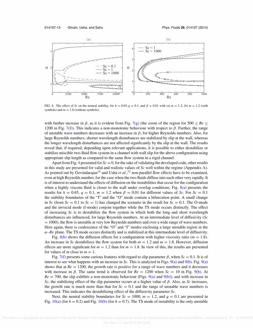
FIG. 8. The effect of Sc on the neutral stability, for h = 0.65, q = 0.1, and β = 0.01 with (a) m = 1.2; (b) m = 1.2 (withsymbols) and m = 1.8 (without symbols).

with further increase in β, as it is evident from Fig. 7(g) (the zoom of the region for 500 ≤ Re ≤1200 in Fig. 7(f)). This indicates a non-monotonic behaviour with respect to β. Further, the rangeof unstable wave numbers decreases with an increase in β, for higher Reynolds numbers. Also, forlarge Reynolds numbers, shorter wavelength disturbances are stabilized by slip at the wall, whereasthe longer wavelength disturbances are not affected significantly by the slip at the wall. The resultsreveal that, if required, depending upon relevant applications, it is possible to either destabilize orstabilize miscible two-fluid flow system in a channel with wall slip for the above configuration usingappropriate slip length as compared to the same flow system in a rigid channel.

Apart from Fig. 4 presented for Sc = 0, for the sake of validating the developed code, other resultsin this study are presented for valid and realistic values of Sc well within the regime (Appendix A).As pointed out by Govindarajan18 and Usha et al.,52 non-parallel flow effects have to be examined,even at high Reynolds number, for the case when the two fluids diffuse into each other very rapidly. Itis of interest to understand the effects of diffusion on the instabilities that occur for the configurationwhen a highly viscous fluid is closer to the wall under overlap conditions. Fig. 8(a) presents theresults for h = 0.65, q = 0.1, m = 1.2 when β = 0.01 for different values of Sc. For Sc = 0.1the stability boundaries of the “I” and the “O” mode contain a bifurcation point. A small changein Sc (from Sc = 0.1 to Sc = 1) has changed the scenario in the result for Sc = 0.1. The O-modeand the inviscid mode (I-mode) conjoin together while the TS mode occurs distinctly. The effectof increasing Sc is to destabilize the flow system in which both the long and short wavelengthdisturbances are influenced, for large Reynolds numbers. At an intermediate level of diffusivity (Sc= 1000), the flow is unstable at very low Reynolds numbers and over a wide range of wave numbers.Here again, there is coalescence of the “O” and “I” modes enclosing a large unstable region in theα–Re plane. The TS mode occurs distinctly and is stabilized at this intermediate level of diffusivity.

Fig. 8(b) shows the diffusion effects for a configuration with higher viscosity ratio (m = 1.8).An increase in Sc destabilizes the flow system for both m = 1.2 and m = 1.8. However, diffusioneffects are more significant for m = 1.2 than for m = 1.8. In view of this, the results are presentedfor values of m close to m = 1.

Fig. 7(f) presents some curious features with regard to slip parameter β, when Sc = 0.1. It is ofinterest to see what happens with an increase in Sc. This is analyzed in Figs. 9(a) and 9(b). Fig. 9(a)shows that at Re = 1200, the growth rate is positive for a range of wave numbers and it decreaseswith increase in β. The same trend is observed for Re = 1200 when Sc = 10 in Fig. 9(b). AtRe = 700, the slip exhibits a non-monotonic behaviour (Figs. 9(a) and 9(b)); and with increase inSc, the stabilizing effect of the slip parameter occurs at a higher value of β. Also, as Sc increases,the growth rate is much more than that for Sc = 0.1 and the range of unstable wave numbers isincreased. This indicates the destabilizing effect of the diffusivity parameter Sc.

Next, the neutral stability boundaries for Sc = 1000, m = 1.2, and q = 0.1 are presented inFig. 10(a) (for h = 0.2) and Fig. 10(b) (for h = 0.7). The TS mode of instability is the only unstable

This article is copyrighted as indicated in the article. Reuse of AIP content is subject to the terms at: http://scitation.aip.org/termsconditions. Downloaded to IP: 14.139.65.5

On: Mon, 27 Jan 2014 08:23:58

014107-14 Ghosh, Usha, and Sahu Phys. Fluids 26, 014107 (2014)

0.8 1.2 1.6 2α

-0.05

0

0.05

ωi

β = 0.0β = 0.01β = 0.02β = 0.03

0.8 1.2 1.6 2α

-0.05

0

0.05

0.1

ωi β = 0.0

β = 0.01β = 0.02β = 0.03β = 0.05

(a) (b)

FIG. 9. Growth rate curves for h = 0.75, q = 0.1, m = 1.2, Re = 700 (without symbols), and Re = 1200 (with symbols):(a) Sc = 0.1; (b) Sc = 10.

mode for the case h = 0.2 and the critical Reynolds number for each β for Sc = 1000 is slightlysmaller than that for Sc = 0.1 (see Fig. 7(a)). This indicates the destabilizing role of Sc for h = 0.2.As h is increased to h = 0.7 (see Fig. 10(b)) the diffusivity parameter exhibits a stronger influenceon destabilizing the flow. In this case, the flow becomes unstable for smaller Reynolds number andhigher wave numbers as compared to the corresponding results for Sc = 0.1 (not shown here). ForSc = 1000 (Fig. 10(b)), the coalescence of the “O,” “I” modes and the TS mode instability exist indistinct regions of α–Re plane. Fig. 10(c) presents a zoom of the region 0 ≤ Re ≤ 400 in Fig. 10(b).

0 5000 10000 15000Re

0.6

0.8

1

1.2

α

β = 0.0β = 0.01β = 0.02

0 2500 5000 7500Re

1

1.5

2

2.5

3

α

β = 0.0β = 0.01β = 0.02

0 100 200 300 400Re

1

1.5

2

2.5

3

αβ = 0.0β = 0.01β = 0.02β = 0.03β = 0.05

(a) (b)

(c)

FIG. 10. The neutral stability boundaries for different values of β with Sc = 1000, m = 1.2, and q = 0.1; (a) h = 0.2; (b) h= 0.7, and (c) zoom of the region 0 ≤ Re ≤ 400 in Fig. 10(b).

This article is copyrighted as indicated in the article. Reuse of AIP content is subject to the terms at: http://scitation.aip.org/termsconditions. Downloaded to IP: 14.139.65.5

On: Mon, 27 Jan 2014 08:23:58

014107-15 Ghosh, Usha, and Sahu Phys. Fluids 26, 014107 (2014)

0 5000 10000 15000Re

0.6

0.8

1

1.2

1.4

1.6

α

β = 0.0β = 0.01β = 0.02

TS

O

0 2500 5000 7500 10000Re

0.6

0.8

1

1.2

1.4

1.6

1.8

α

β = 0.0β = 0.01β = 0.02

TS

O

0 5000 10000 15000Re

0.6

0.8

1

1.2

1.4

1.6

α

β = 0.0β = 0.01β = 0.02

0 5000 10000 15000Re

0.6

0.8

1

1.2

1.4

1.6

α

β = 0.0β = 0.01β = 0.02

(a) (b)

(c) (d)

FIG. 11. Effects of β on the neutral stability boundaries for (a) Sc = 1 and (b) Sc = 1000, for m = 1.05 and h = 0.75; (c) Sc= 1 and (d) Sc = 1000, for m = 0.95 and h = 0.75. In all the panels, the value of q is 0.1.

The critical Reynolds number decreases with increase in β, indicating the destabilizing role of β atthis value of Sc.

Now, the effects of diffusivity are examined for two different viscosity contrasts (m = 1.05 andm = 0.95). Fig. 11(a) shows the results for different β when the fluid adjacent to the wall is highlyviscous (m = 1.05) for h = 0.75, q = 0.1, and Sc = 1. The TS and the “O” modes are conjoined anda large region of instability appears for moderate to large Reynolds number for β = 0.0 and 0.01.However, the “O” mode and TS mode occupy distinct regions in the α–Re plane for β = 0.02. It isalso observed that the “I” mode does not exist for this set of parameters. This is in striking contrastwith the results presented in Fig. 8 for Sc = 1, h = 0.65, β = 0.01, where the “I” mode existsand conjoins with the “O” mode and the TS mode occupies a distinct region. The critical Reynoldsnumber (Recr) for the onset of instability increases with an increase in wall slip, characterized byβ. The critical Reynolds number (Recr) for miscible two-fluid channel flow with no-slip/slip at thewall is much lower than that for a single fluid flow in a channel with no-slip/slip at the wall (seeFig. 3(a)). This indicates the destabilizing role of viscosity stratified layer when it is located closerto the channel wall. As Sc increases (Sc = 1000; intermediate level of diffusivity), it can be seen inFig. 11(b) that the “O” mode instability occurs and for each value of β, it appears in a domain distinctfrom that of the TS mode. The unstable region of the “O” mode instability decreases with increase inthe value of β. At this Sc, the “O” mode is the dominant mode of instability. This instability occursfor higher wave numbers for Sc = 1000 than for Sc = 1, for each β. The Reynolds number at whichinstabilities arise for Sc = 1000 is much smaller than the corresponding Reynolds number for Sc = 1.This indicates the destabilizing role of the diffusivity parameter (Sc) for this configuration (m = 1.05and h = 0.75). The critical Reynolds number decreases with increase in β for the values of β shownin figure, indicating the destabilizing effect of β.

This article is copyrighted as indicated in the article. Reuse of AIP content is subject to the terms at: http://scitation.aip.org/termsconditions. Downloaded to IP: 14.139.65.5

On: Mon, 27 Jan 2014 08:23:58

014107-16 Ghosh, Usha, and Sahu Phys. Fluids 26, 014107 (2014)

0 2500 5000 7500 10000Re

0.8

1

1.2

1.4

1.6

α

Sc = 0Sc = 10Sc = 100

FIG. 12. The effect of Sc on the neutral stability boundaries, for h = 0.75, q = 0.1, m = 1.05, and β = 0.01.

The corresponding results for the case when a fluid with lower viscosity is adjacent to the wall(m = 0.95) are presented in Figs. 11(c) and 11(d) for Sc = 1 and Sc = 1000, respectively, for h= 0.75 and q = 0.1. The results show that the TS mode is the dominating mode of instability andthe flow is stabilized as Sc increases from 1 (Fig. 11(c)) to 1000 (Fig. 11(d)). It is apparent that anon-zero value of β is stabilizing the flow dynamics for both the Sc values considered.

The “O” mode and TS mode occupy distinct regions in the α–Re plane for Sc = 1 (Fig. 11(a))when β ≥ 0.02 while this happens for β ≥ 0.0 when Sc = 1000 (Fig. 11(b)). The characteris-tics of these modes for different values of Sc between Sc = 1 and Sc = 1000 when m = 1.05,h = 0.75 are displayed in Fig. 12. The result for Sc = 0 is also incorporated and in this case, the twomodes are conjoined to form a single region. At high diffusivity level (Sc = 10), the TS and overlapmodes occupy distinct regions for β = 0.01 which is in contrast to that for Sc = 1, β = 0.01 (seeFig. 11(a)). At a level of diffusivity corresponding to Sc = 100, the same trend as above is observed.The critical Reynolds number decreases indicating the destabilizing effect of Sc and the unstableregion for “O” mode extends to higher wave numbers and shrinks to small Reynolds numbers for Sc= 100 than for Sc = 10.

Fig. 13 presents the influence of diffusivity on the critical Reynolds number for the viscosityratio m = 1.2 for h = 0.7, q = 0.1. The flow is unstable in the region above a given curve. Thecritical Reynolds number decreases with increase in Sc beyond Sc = 0.1, indicating the destabilizingeffect of the decreasing diffusivity for m = 1.2. For this viscosity contrast, there is a non-monotonicbehaviour with respect to slip parameter β up to Sc = 0.1; the flow is destabilized in a channel withvelocity slip beyond Sc = 0.1 as compared to that in a rigid channel.

The computations presented so far show that small changes in the viscosity ratio (m) close to1 significantly affect the stability properties of the fluid. The effects of viscosity contrast on the

10-5

10-3

10-1

101

103

Sc

100

200

300

400

500

600

Recr

β = 0.0β = 0.01β = 0.02

FIG. 13. The critical Reynolds number as a function of Sc for h = 0.7, q = 0.1, and m = 1.2.

This article is copyrighted as indicated in the article. Reuse of AIP content is subject to the terms at: http://scitation.aip.org/termsconditions. Downloaded to IP: 14.139.65.5

On: Mon, 27 Jan 2014 08:23:58

014107-17 Ghosh, Usha, and Sahu Phys. Fluids 26, 014107 (2014)

0 1 2 3m

102

103

104

105

Recr

β = 0.0β = 0.01β = 0.02

0.3 0.4 0.5 0.6 0.7 0.8h

0

2000

4000

6000

8000

10000

Recr

β = 0.0β = 0.01β = 0.02

1 1.2 1.4 1.6m

103

104

Recr

β = 0.0β = 0.01β = 0.02

0.6 0.65 0.7 0.75h

500

750

Recr

β = 0.0β = 0.01β = 0.02

(a) (b)

(c) (d)

FIG. 14. (a) The critical Reynolds number as a function of m. The computations are performed with (h, m) = (0.6, >1.8),(0.65, 1.8), (0.7, 1.2), (0.75, 1.05), (0.85, 0.95), (0.87, 0.8), and (0.89, 0.6). (b) The critical Reynolds number as a functionof h and m = 1.2. (c) Zoomed portion of Fig. 14(a) close to m = 1. (d) Zoomed region of Fig. 14(b) for 0.55 ≤ h ≤ 0.8. Inall the panels q = 0.1 and Sc = 1.

critical Reynolds number presented in Fig. 14(a) also confirm this result. The velocity slip at thewall stabilizes the flow slightly for m ≤ 1.15 and a reverse trend is displayed for m ≥ 1.15 (highlyviscous fluid is close to the channel wall), under overlap conditions of the critical and the mixedlayers (see Fig. 14(c); zoom of the region close to m = 1 in Fig. 14(a)). In Fig. 14(b), the effects oflocation of the mixed layer on the critical Reynolds number are examined for different values of β

with m = 1.2. There is a drastic decrease in the value of Recr around h = 0.4 up to which the TSmode is the dominant mode. Beyond h = 0.4 to 0.6 the inviscid mode (“I” mode) dominates. Thecritical layer falls in the region of the viscosity stratified layer for h > 0.6. This causes the emergenceof the overlap mode as discussed above, which is the most unstable mode. Inspection of this plotalso reveals the destabilizing effect of the slip at the channel wall for the “O” mode instability (seeFig. 14(d); zoomed portion for 0.55 ≤ h ≤ 0.8 in Fig. 14(b)). On the other hand, the flow is stabilizedby the velocity slip at the wall for the TS and the inviscid modes.

IV. CONCLUSIONS

The present study examines the effects of wall slip on the instabilities in plane Poiseuille flowof two miscible layers of fluids of same density but different viscosities, in a channel with velocityslip at the wall. The wall slip has been shown to have significant effect on the stability of the flowsystem. The slippery wall plays a dual role of either stabilizing or destabilizing the flow system ascompared to that in a rigid channel.

An overlap mode has been shown to appear when the critical layer of the dominant disturbanceoverlaps the viscosity stratified layer, for high mass diffusivity of the two fluids, in the absenceof velocity slip at the walls by Govindarajan.18 Such a mode also appears in the present case for

This article is copyrighted as indicated in the article. Reuse of AIP content is subject to the terms at: http://scitation.aip.org/termsconditions. Downloaded to IP: 14.139.65.5

On: Mon, 27 Jan 2014 08:23:58

014107-18 Ghosh, Usha, and Sahu Phys. Fluids 26, 014107 (2014)

moderate wave numbers and small Reynolds numbers. Figs. 5(a) and 5(b) in which eigenvaluespectra are presented for Re = 400 when the mixed layer is located at h = 0.2 and h = 0.65 clearlyindicate that the overlap instability occurs due to destabilization of an existing mode. This may beattributed to the increase in the disturbance kinetic energy due to the effect of overlap of viscositystratified layer with the critical layer. The spectra in the two cases (Fig. 5) appear similar but theflow is unstable when the mixed layer and the critical layer of dominant instability overlap witheach other (for h = 0.65), whereas for h = 0.2 all the modes are stable. It can also be seen that theunstable mode for h = 0.65 is not a new eigenmode (like in case of pure interfacial flows), but astable mode (for h = 0.2) becoming unstable due to the overlap of viscosity stratified layer with thecritical layer. The unstable region for “O” mode decreases with increase in the value of β, but thecritical Reynolds number is not affected much by the slip parameter β.

The dimensionless Schmidt number characterizing the diffusivity affects the overlap modesignificantly and at any fixed value of slip parameter, β, the degree of destabilization increases withincrease in Schmidt number (Sc). There is stabilization of the flow system for the slip parameter β

≥ 0.02 when Sc ≤ 0.1 and destabilization of the flow system as the slip at the wall increases whenSc > 0.1 (see Fig. 13).

The effects of slip on the TS mode and the inviscid mode which exist along with the overlap modeunder certain conditions on the location of the viscosity stratified layer have also been examined asdiffusivity, the ratio of viscosities, and the location of the viscosity-stratified layer are varied.

The two-fluid miscible flow in a slippery channel is more stable than either the correspondingtwo-fluid miscible flow in a rigid channel or a single fluid flow in a rigid/slippery channel (seeFigs. 3(a) and 7(a)), when a higher viscous fluid is adjacent to the wall and the mixed layer andthe critical layer are well separated. With the same viscosity contrast when the mixed layer andthe critical layer overlap, the miscible two-fluid channel flow with slip/no-slip at the wall is moreunstable than the corresponding single fluid flow in a channel with slip/no-slip (see Figs. 3(a) and11(a)). Further, the stability characteristics of the miscible two-fluid channel flows with slip aredifferent from both the limiting cases of viscosity-stratified flows with sharp jump and continuouslystratified flows in a channel with slip. The overlap mode instability is absent in both the limitingcases. In the present study, a configuration with less viscous fluid closer to the wall is more stablethan that with highly viscous fluid adjacent to the wall. On the other hand, the critical Reynoldsnumber increases with increase in viscosity ratio for the interface dominated flow in a channel withslip,46 indicating a reverse trend as compared to that in the present study.

Although the present results are analogous to those in Govindarajan for a rigid channel, themessage from the present study is that the flow system considered by Govindarajan18 can be furtherstabilized or destabilized if one imposes velocity slip at the channel wall. It is well known thatcreating a small viscosity stratification in the fluid is one of the effective controlling strategiesfor delaying the occurrence of fluid flow turbulence. It has been shown by several investigatorsthat a laminar wall-bounded shear flow consisting of two layers of fluids of different viscosities issignificantly stabilized whenever the fluid with less viscosity is adjacent to the wall, provided thatthe viscous interface is located near the critical layer. The present study shows that the stabilizingor destabilizing effect can be further enhanced by taking the channel with velocity slip at thewall.

The theoretical studies by Kim and Kim,30 Gan and Wu,37 and the experimentalinvestigations28, 29 show that flow over a hydrophobic surface can be analyzed by the Navier-Stokesequations with slip boundary condition. We also infer from Beskok and Karniadkis41 that if the slipconditions are used, the Navier-Stokes equations are valid for slip length up to 0.1. This suggeststhat the results of the present study may be used for understanding the stability of miscible two-fluidflow in a channel with hydrophobic surface which can be modeled as surfaces with velocity slip atthe wall. The present study also could be useful in micro-electromechanical systems and flow inmicrofluidic channels, where there is an increasing evidence that the boundary condition of slip typeis needed rather than no-slip boundary condition at the walls to model the flow dynamics accurately.

In view of the relevance of the nonmodal stability analysis than the modal stability analysisin the subcritical transition in channel flows, it is of interest to quantify the effect of wall slip onthe nonmodal analysis for the present flow system and this will be explored in our future study.

This article is copyrighted as indicated in the article. Reuse of AIP content is subject to the terms at: http://scitation.aip.org/termsconditions. Downloaded to IP: 14.139.65.5

On: Mon, 27 Jan 2014 08:23:58

014107-19 Ghosh, Usha, and Sahu Phys. Fluids 26, 014107 (2014)

The present study also opens the possibility of accurate experimental set up and direct numericalsimulation.

ACKNOWLEDGMENTS

The authors thank the referees for their very useful, valuable comments and suggestions. Thediscussions with Professor Rama Govindarajan have been very inspiring and the authors thank herfor this. The authors also thank the Editor, Professor L. Gary Leal for his encouraging and supportingremarks and suggestions.

APPENDIX A: VALIDITY OF PARALLEL FLOW ASSUMPTION

The present study is based on the parallel flow assumption in the mixed layer. This is equivalentto considering that the variations of the gradients in flow variables at the steady state and the thicknessq of the mixed region have a much larger length scale than the disturbance wavelength. The followingdiscussion shows that the above assumption is justified for slow diffusion of the fluids (higher valuesof Peclet numbers).

Let a splitter plate be located at x < x0, at a constant y and let the parallel streams of two misciblefluids flow on both sides of this plate. The streams come into contact with each other at x = x0. Thetwo fluids begin to mix with each other for x > x0, thus producing a stratified layer. The thickness“q” of this layer grows as the fluids move downstream and therefore q is a function of x. In whatfollows, it is shown that the thickness of the mixed layer varies slowly in x, i.e., ∂q/∂x 1.

At any location, the steady mean concentration satisfies the equation

U∂s

∂x+ V

∂s

∂y= 1

Pe

[∂2s

∂x2+ ∂2s

∂y2

]. (A1)

Under the boundary layer approximation, V U and ∂2

∂x2 ∂2

∂y2 and this yields

U∂s

∂x� 1

Pe

∂2s

∂y2. (A2)

Also using the same approximation, we know that U ∼ O(1), y ∼ √ν, where ν is the viscosity.

Therefore, qs ∼ O(y2) since s is the mean concentration over the mixed layer of thickness q. Thisimplies that ∂s/∂x � 1

q O(1/Pe) (from Eq. (A2)). So, for large values of Pe, ∂s/∂x is very small,showing that the downstream variation of s is very small which in turn implies that the changes inthe thickness q of the mixed layer along the x-direction is very small.

Alternatively, if we assume a similar solution s(y/q(x)) � s(ξ ) (where ξ = (y/q(x))) for Eq. (A2),we will get

Uds

dξ

(− ξ

q

dq

dx

)� 1

Pe

(d2s

dξ 2

1

q2

). (A3)

As a consequence,

1

q

dq

dx∼ 1

q2 Pe⇒ dq

dx∼ 1

qO(Pe)−1. (A4)

Thus, the downstream growth of mixed layer is inversely proportional to the Peclet number as Uand ξ are of O(1) and O( ds

dξ) � O( d2s

dξ 2 ), which confirms that for the Reynolds and Schmidt numbersconsidered in the present study, the assumption of uniform thickness of viscosity stratified layer isjustified.

This article is copyrighted as indicated in the article. Reuse of AIP content is subject to the terms at: http://scitation.aip.org/termsconditions. Downloaded to IP: 14.139.65.5

On: Mon, 27 Jan 2014 08:23:58

014107-20 Ghosh, Usha, and Sahu Phys. Fluids 26, 014107 (2014)

APPENDIX B: RELATION TO THE INTERFACIAL PERTURBATIONIN THE IMMISCIBLE LIMIT

The whole viscosity field is perturbed by introducing a viscosity perturbation μ (expressed interms of “s”) to the base state viscosity. In view of this, there is no need to separately perturb theinterface variable h between the fluid i (i = 1, 2) and the mixed layer.

In what follows, we show that, in the absence of diffusion (i.e., Pe → ∞), the viscosityalong a particle path (the perturbed interface) is constant. Consider the linearized equation for theperturbation in viscosity (Eq. (19)). The condition that the viscosity along a particle path changesonly by viscosity diffusion yields the equation

D

Dt(μB + μ) = 1

Pe∇2(μB + μ), (B1)

where DDt ≡ ∂

∂t + (UB + u) ∂∂x + (v) ∂

∂y . In the absence of diffusion (Pe → ∞), the equation gives

D

Dt(μB + μ) = 0, (B2)

which shows that the lines of constant viscosity are the same as the particle paths. By definition, theperturbed interface between fluid i (i = 1, 2) and the mixed layer is a line of constant viscosity andtherefore follows a particle path (Eq. (B1)).

This result is the same as that in the case of immiscible configurations, as in immiscible systemsthe equation for the interface perturbation h states that the viscosity along a particle path, namely,the perturbed interface, is constant. This clearly establishes the relation to the interfacial disturbancein the immiscible limit.

1 R. Govindarajan and K. C. Sahu, “Instabilities in viscosity-stratified flows,” Annu. Rev. Fluid Mech. 46, 331–353 (2014).2 C. S. Yih, “Instability due to viscous stratification,” J. Fluid Mech. 27, 337 (1967).3 A. P. Hooper and W. G. C. Boyd, “Shear flow instability at the interface between two fluids,” J. Fluid Mech. 128, 507

(1983).4 E. J. Hinch, “A note on the mechanism of the instability at the interface between two shearing fluids,” J. Fluid Mech. 144,

463 (1984).5 Y. Renardy, “Viscosity and density stratification in vertical Poiseuille flow,” Phys. Fluids 30, 1638 (1987).6 D. D. Joseph and Y. Y. Renardy, Fundamentals of Two-Fluid Dynamics. Part II. Lubricated Transport, Drops and Miscible

Fluids, Interdisciplinary Applied Mathematics Vol. 4 (Springer, New York, 1992).7 M. J. South and A. P. Hooper, “Linear growth in two-fluid plane Poiseuille flow,” J. Fluid Mech. 381, 121 (1999).8 S. G. Yiantsios and B. G. Higgins, “Linear stability of plane Poiseuille flow of two superposed fluids,” Phys. Fluids 31,

3225 (1988).9 S. G. Yiantsios and B. G. Higgins, “Erratum: Linear stability of plane Poiseuille flow of two superposed fluids [Phys.

Fluids 31, 3225 (1988)],” Phys. Fluids A 1(5), 897 (1989).10 A. Pinarbasi and A. Liakopoulos, “Stability of two-layer Poiseuille flow of Carreau-Yasuda and Bingham-like fluids,” J.

Non-Newtonian Fluid Mech. 57, 227 (1995).11 S. N. Timoshin and A. P. Hooper, “Mode coalescence in a two-fluid boundary layer stability problem,” Phys. Fluids 12,

1969 (2000).12 P. Laure, H. Le. Meur, Y. Demay, J. C. Saut, and S. Scotto, “Linear stability of multilayer plane Poiseuille flows of Oldroyd

B fluids,” J. Non-Newtonian Fluid Mech. 71, 1 (1997).13 A. R. Wazzan, T. T. Okamura, and A. M. O. Smith, “The stability of water flow over heated and cooled flat plates,” Trans.

ASME C: Heat Trans. 90, 109 (1968).14 D. P. Wall and S. K. Wilson, “The linear stability of channel flow of fluid with temperature dependent viscosity,” J. Fluid

Mech. 323, 107 (1996).15 D. P. Wall and S. K. Wilson, “The linear stability of flat-plate boundary layer flow of fluid with temperature dependent

viscosity,” Phys. Fluids 9, 2885 (1997).16 B. T. Ranganathan and R. Govindarajan, “Stabilisation and destabilisation of channel flow by location of viscosity-stratified

fluid layer,” Phys. Fluids 13(1), 1 (2001).17 P. Ern, F. Charru, and P. Luchini, “Stability analysis of a shear flow with strongly stratified viscosity,” J. Fluid Mech. 496,

295 (2003).18 R. Govindarajan, “Effect of miscibility on the linear instability of two-fluid channel flow,” Int. J. Multiphase Flow 30,

1177 (2004).19 K. C. Sahu, H. Ding, P. Valluri, and O. K. Matar, “Linear stability analysis and numerical simulation of miscible channel

flows,” Phys. Fluids 21, 042104 (2009).20 L. Talon and E. Meiburg, “Plane Poiseuille flow of miscible layers with different viscosities: instabilities in the Stokes flow

regime,” J. Fluid Mech. 686, 484 (2011).21 Y. Zhu and S. Granick, “Rate-dependent slip of Newtonian liquid at smooth surfaces,” Phys. Rev. Lett. 87, 096105 (2001).

This article is copyrighted as indicated in the article. Reuse of AIP content is subject to the terms at: http://scitation.aip.org/termsconditions. Downloaded to IP: 14.139.65.5

On: Mon, 27 Jan 2014 08:23:58

014107-21 Ghosh, Usha, and Sahu Phys. Fluids 26, 014107 (2014)

22 P. A. Thompson and S. M. Troian, “A general boundary condition for liquid flow at solid surfaces,” Nature 389, 360 (1997).23 J. W. Hoyt, “Hydrodynamic drag reduction due to fish slimes,” Swimming and Flying in Nature (Springer, 1975), Vol. 2,

p. 653.24 D. W. Bechert, M. Bruse, W. Hage, and R. Meyer, “Fluid mechanics of biological surfaces and their technological

applications,” Naturwissenschaften 87, 157 (2000).25 E. H. Kennard, Kinetic Theory of Gases (McGraw-Hill, New York, 1938).26 G. A. Bird, Molecular Gas Dynamics and the Direct Simulation of Gas Flows (Oxford University Press, Great Clarendon

Street, Oxford, 1994).27 M. M. Denn, “Extrusion instabilities and wall slip,” Annu. Rev. Fluid Mech. 33, 265 (2001).28 D. C. Tretheway and C. D. Meinhart, “Apparent fluid slip at hydrophobic microchannel walls,” Phys. Fluids 14, L9 (2002).29 C. H. Choi, K. J. A. Westin, and K. S. Breur, “Apparent slip flows in hydrophilic and hydrophobic microchannels,” Phys.

Fluids 15, 2897 (2003).30 J. Kim and C. J. Kim, “Nanostructured surfaces for dramatic reduction of flow resistance in droplet-based microfluidics,”

in Technical Digest, IEEE Conference on MEMS, Las Vegas, NV (IEEE, 2002), p. 479.31 Y. K. Watanabe and H. Mizunuma, “Slip of Newtonian fluids at solid boundary,” JSME Int. J., Ser. B 41, 525 (1998).32 R. Pit, H. Hervet, and L. Leger, “Direct experimental evidence of slip in hexadecane: solid interfaces,” Phys. Rev. Lett. 85,

980 (2000).33 E. Bonaccurso, M. Kappl, and H. J. Butt, “Hydrodynamic force measurements: boundary slip of hydrophobic surfaces and

electrokinetic effects,” Phys. Rev. Lett. 88, 076103 (2002).34 O. I. Vinogradova, “Slippage of water over hydrophobic surfaces,” Int. J. Miner. Process. 56, 31 (1999).35 J. M. Gersting, “Hydrodynamic stability of plane porous slip flow,” Phys. Fluids 17, 2126 (1974).36 A. Spille and H. B. A. Rauh, “Critical curves of plane Poiseuille flow with slip boundary conditions,” Nonlinear Phenom.

Complex Syst. 3, 171 (2000).37 C. J. Gan and Z. N. Wu, “Short-wave instability due to wall slip and numerical observation of wall-slip instability for

microchannel flows,” J. Fluid Mech. 550, 289 (2006).38 E. Lauga and C. Cossu, “A note on the stability of slip channel flows,” Phys. Fluids 17, 088106 (2005).39 Y. X. Zhu and S. Granick, “Limits of hydrodynamic no-slip boundary condition,” Phys. Rev. Lett. 88, 106102 (2002).40 R. Ling, C. Jian-Guo, and Z. Ke-Qin, “Dual role of wall slip on linear stability of plane Poiseuille flow,” Chin. Phys. Lett.

25, 601 (2008).41 A. Beskok and G. E. Karniadkis, Micro Flows Fundamentals and Simulation (Springer, London, 2002).42 K. C. Sahu, A. Sameen, and R. Govindarajan, “The relative roles of divergence and velocity slip in the stability of plane

channel flow,” Eur. Phys. J.: Appl. Phys. 44, 101 (2008).43 J. C. Maxwell, “On stresses in varefied gases arising from inequalities of temperature,” Philos. Trans. R. Soc. London 170,

231 (1879).44 T. Min and J. Kim, “Effects of hydrophobic surface on stability and transition,” Phys. Fluids 17, 108106 (2005).45 A. K. H. Chu, “Instability of Navier slip flow of liquids,” C. R. Mec. 332, 895 (2004).46 X. Y. You and J. R. Zheng, “Stability of liquid-liquid stratified microchannel flow under the effects of boundary slip,” Int.

J. Chem. React. Eng. 7, A85 (2009).47 M. Webber, “Instability of fluid flows, including boundary slip,” Doctoral thesis (Durham University, 2007), Available at

Durham E-Theses Online: http://etheses.dur.ac.uk/2308/.48 K. C. Sahu and R. Govindarajan, “Linear stability of double-diffusive two-fluid channel flow,” J. Fluid Mech. 687, 529

(2011).49 E. Lauga, M. P. Brenner, and H. A. Stone, in Handbook of Experimental Fluid Dynamics, edited by J. F. Foss, C. Tropea,

and A. Yarin (Springer, New York, 2005).50 P. G. Drazin and W. H. Reid, Hydrodynamic Stability (Cambridge University Press, Cambridge, 1985).51 C. Canuto, M. Y. Hussaini, A. Quarteroni, and T. A. Zang, Spectral Methods in Fluid Dynamics, 1st ed. (Springer Verlag,

New York, 1987).52 R. Usha, O. Tammisola, and R. Govindarajan, “Linear stability of miscible two-fluid flow down an incline,” Phys. Fluids

25, 104102 (2013).

This article is copyrighted as indicated in the article. Reuse of AIP content is subject to the terms at: http://scitation.aip.org/termsconditions. Downloaded to IP: 14.139.65.5

On: Mon, 27 Jan 2014 08:23:58