Linear Algebra with Applications
527
-
Upload
khangminh22 -
Category
Documents
-
view
0 -
download
0
Transcript of Linear Algebra with Applications

Linear Algebra with Applications

This page intentionally left blank

Linear Algebra with ApplicationsFifth Edition
Otto BretscherColby College

Editor in Chief: Christine Hoag Cover Designer: Suzanne DudaSenior Acquisitions Editor: William Hoffman Cover Art: Colorization by JorgensenExecutive Marketing Manager: Jeff Weidenaar Fernandez/NASAMarketing Assistant: Caitlin Crain Full-Service Project Management:Senior Production Project Manager: Integra Software Services, Ltd.
Beth Houston Composition: Integra Software Services, Ltd.Manager, Cover Visual Printer/Binder: Edwards Brothers Malloy
Research and Permissions: Jayne Conte Cover Printer: Lehigh/Phoenix
The cover shows the Mars rover Curiosity, casting a long shadow onto Gale crater, facing Aeolis Mons. LinearAlgebra plays a central role in many aspects of the planning, design, and control of a space mission. For example,data compression is used for interplanetary communication (see Page 411), and error-correction codes increase thereliability of data transmission (see Page 121).
Credits and acknowledgments borrowed from other sources and reproduced, with permission, in this textbook appearon the appropriate page within text.
Copyright © 2013, 2009, 2005 by Pearson Education, Inc. All rights reserved. Manufactured in the United States ofAmerica. This publication is protected by Copyright, and permission should be obtained from the publisher prior toany prohibited reproduction, storage in a retrieval system, or transmission in any form or by any means, electronic,mechanical, photocopying, recording, or likewise. To obtain permission(s) to use material from this work, pleasesubmit a written request to Pearson Education, Inc., Permissions Department, One Lake Street, Upper Saddle River,New Jersey 07458, or you may fax your request to 201-236-3290.
Many of the designations by manufacturers and sellers to distinguish their products are claimed as trademarks.Where those designations appear in this book, and the publisher was aware of a trademark claim, the designationshave been printed in initial caps or all caps.
Library of Congress Cataloging-in-Publication DataBretscher, Otto.
Linear algebra with applications / Otto Bretscher. – 5th ed.p. cm.
Includes index.ISBN-13: 978-0-321-79697-4ISBN-10: 0-321-79697-71. Algebras, Linear–Textbooks. I. Title.QA184.2.B73 2013512’.5–dc23
2012017551
10 9 8 7 6 5 4 3 2 1 EBM 16 15 14 13 12
ISBN-10: 0-321-79697-7ISBN-13: 978-0-321-79697-4

To my parentsOtto and Margrit Bretscher-Zwicky
with love and gratitude

This page intentionally left blank

ContentsPreface ix
1 Linear Equations 11.1 Introduction to Linear Systems 11.2 Matrices, Vectors, and Gauss–Jordan Elimination 81.3 On the Solutions of Linear Systems; Matrix Algebra 25
2 Linear Transformations 412.1 Introduction to Linear Transformations and Their
Inverses 412.2 Linear Transformations in Geometry 582.3 Matrix Products 752.4 The Inverse of a Linear Transformation 88
3 Subspaces of Rn and Their Dimensions 1103.1 Image and Kernel of a Linear Transformation 1103.2 Subspaces of Rn; Bases and Linear Independence 1223.3 The Dimension of a Subspace of Rn 1333.4 Coordinates 147
4 Linear Spaces 1664.1 Introduction to Linear Spaces 1664.2 Linear Transformations and Isomorphisms 1784.3 The Matrix of a Linear Transformation 186
5 Orthogonality and Least Squares 2025.1 Orthogonal Projections and Orthonormal Bases 2025.2 Gram–Schmidt Process and QR Factorization 2185.3 Orthogonal Transformations and Orthogonal Matrices 2255.4 Least Squares and Data Fitting 2365.5 Inner Product Spaces 249
vii

viii Contents
6 Determinants 2656.1 Introduction to Determinants 2656.2 Properties of the Determinant 2776.3 Geometrical Interpretations of the Determinant;
Cramer’s Rule 294
7 Eigenvalues and Eigenvectors 3107.1 Diagonalization 3107.2 Finding the Eigenvalues of a Matrix 3277.3 Finding the Eigenvectors of a Matrix 3397.4 More on Dynamical Systems 3477.5 Complex Eigenvalues 3607.6 Stability 375
8 Symmetric Matrices and Quadratic Forms 3858.1 Symmetric Matrices 3858.2 Quadratic Forms 3948.3 Singular Values 403
9 Linear Differential Equations 4159.1 An Introduction to Continuous Dynamical Systems 4159.2 The Complex Case: Euler’s Formula 4299.3 Linear Differential Operators and Linear Differential
Equations 442
Appendix A Vectors 457Appendix B Techniques of Proof 467Answers to Odd-Numbered Exercises 471Subject Index 499Name Index 507

Preface (with David Steinsaltz)
Apolice officer on patrol at midnight, so runs an old joke, notices a mancrawling about on his hands and knees under a streetlamp. He walks overto investigate, whereupon the man explains in a tired and somewhat slurred
voice that he has lost his housekeys. The policeman offers to help, and for the nextfive minutes he too is searching on his hands and knees. At last he exclaims, “Areyou absolutely certain that this is where you dropped the keys?”
“Here? Absolutely not. I dropped them a block down, in the middle of thestreet.”
“Then why the devil have you got me hunting around this lamppost?”“Because this is where the light is.”
It is mathematics, and not just (as Bismarck claimed) politics, that consists in “theart of the possible.” Rather than search in the darkness for solutions to problems ofpressing interest, we contrive a realm of problems whose interest lies above all inthe fact that solutions can conceivably be found.
Perhaps the largest patch of light surrounds the techniques of matrix arithmeticand algebra, and in particular matrix multiplication and row reduction. Here wemight begin with Descartes, since it was he who discovered the conceptual meeting-point of geometry and algebra in the identification of Euclidean space with R3; thetechniques and applications proliferated since his day. To organize and clarify thoseis the role of a modern linear algebra course.
Computers and ComputationAn essential issue that needs to be addressed in establishing a mathematical method-ology is the role of computation and of computing technology. Are the proper sub-jects of mathematics algorithms and calculations, or are they grand theories andabstractions that evade the need for computation? If the former, is it important thatthe students learn to carry out the computations with pencil and paper, or should thealgorithm “press the calculator’s x−1 button” be allowed to substitute for the tradi-tional method of finding an inverse? If the latter, should the abstractions be taughtthrough elaborate notational mechanisms or through computational examples andgraphs?
We seek to take a consistent approach to these questions: Algorithms and com-putations are primary, and precisely for this reason computers are not. Again andagain we examine the nitty-gritty of row reduction or matrix multiplication in or-der to derive new insights. Most of the proofs, whether of rank-nullity theorem, thevolume-change formula for determinants, or the spectral theorem for symmetricmatrices, are in this way tied to hands-on procedures.
The aim is not just to know how to compute the solution to a problem, but toimagine the computations. The student needs to perform enough row reductions byhand to be equipped to follow a line of argument of the form: “If we calculate thereduced row-echelon form of such a matrix . . . ,” and to appreciate in advance thepossible outcomes of a particular computation.
ix

x Preface
In applications, the solution to a problem is hardly more important than recog-nizing its range of validity and appreciating how sensitive it is to perturbations of theinput. We emphasize the geometric and qualitative nature of the solutions, notionsof approximation, stability, and “typical” matrices. The discussion of Cramer’s rule,for instance, underscores the value of closed-form solutions for visualizing a sys-tem’s behavior and understanding its dependence on initial conditions.
The availability of computers is, however, neither to be ignored nor regretted.Each student and instructor will have to decide how much practice is needed to besufficiently familiar with the inner workings of the algorithm. As the explicit com-putations are being replaced gradually by a theoretical overview of how the algo-rithm works, the burden of calculation will be taken up by technology, particularlyfor those wishing to carry out the more numerical and applied exercises.
Examples, Exercises, Applications, and HistoryThe exercises and examples are the heart of this book. Our objective is not just toshow our readers a “patch of light” where questions may be posed and solved, butto convince them that there is indeed a great deal of useful, interesting material tobe found in this area if they take the time to look around. Consequently, we haveincluded genuine applications of the ideas and methods under discussion to a broadrange of sciences: physics, computer science, chemistry, biology, economics, and,of course, mathematics itself. Often we have simplified them to sharpen the point,but they use the methods and models of contemporary scientists.
With such a large and varied set of exercises in each section, instructors shouldhave little difficulty in designing a course that is suited to their aims and to the needsof their students. Quite a few straightforward computation problems are offered,of course. Simple (and, in a few cases, not so simple) proofs and derivations arerequired in some exercises. In many cases, theoretical principles that are discussedat length in more abstract linear algebra courses are here found broken up in bite-size exercises.
The examples make up a significant portion of the text; we have kept abstractexposition to a minimum. It is a matter of taste whether general theories shouldgive rise to specific examples or be pasted together from them. In a text such as thisone, attempting to keep an eye on applications, the latter is clearly preferable: Theexamples always precede the theorems in this book.
Scattered throughout the mathematical exposition are quite a few names anddates, some historical accounts, and anecdotes. Students of mathematics are toorarely shown that the seemingly strange and arbitrary concepts they study are theresults of long and hard struggles. It will encourage the readers to know that amere two centuries ago some of the most brilliant mathematicians were wrestlingwith problems such as the meaning of dimension or the interpretation of eit, andto realize that the advance of time and understanding actually enables them, withsome effort of their own, to see farther than those great minds.
Continuing Text Features• Linear transformations are introduced early on in the text to make the dis-
cussion of matrix operations more meaningful and easier to visualize.

Preface xi
• Visualization and geometrical interpretation are emphasized extensivelythroughout.
• The reader will find an abundance of thought-provoking (and occasionallydelightful) problems and exercises.
• Abstract concepts are introduced gradually throughout the text. The majorideas are carefully developed at various levels of generality before the studentis introduced to abstract vector spaces.
• Discrete and continuous dynamical systems are used as a motivation foreigenvectors, and as a unifying theme thereafter.
New Features in the Fifth EditionStudents and instructors generally found the fourth edition to be accurate and wellstructured. While preserving the overall organization and character of the text, somechanges seemed in order:
• A large number of exercises have been added to the problem sets, from theelementary to the challenging and from the abstract to the applied. For ex-ample, there are quite a few new exercises on “Fibonacci matrices” and theireigenvectors and eigenvalues.
• Throughout the text, we have added an ongoing discussion of the mathemati-cal principles behind search engines and the notion of PageRank in particular,with dozens of examples and exercises. Besides being an interesting and im-portant contemporary application of linear algebra, this topic allows for anearly and meaningful introduction to dynamical systems, one of the mainthemes of this text, naturally leading up to a discussion of diagonalizationand eigenvectors.
• In a new appendix, we offer a brief discussion of the proof techniques ofinduction and contraposition.
• There have been hundreds of small editorial improvements – offering a hintin a challenging problem for example, or choosing a more sensible notationin a definition.
Outline of the TextChapter 1 This chapter provides a careful introduction to the solution of systemsof linear equations by Gauss–Jordan elimination. Once the concrete problem issolved, we restate it in terms of matrix formalism and discuss the geometric prop-erties of the solutions.
Chapter 2 Here we raise the abstraction a notch and reinterpret matrices as lin-ear transformations. The reader is introduced to the modern notion of a func-tion, as an arbitrary association between an input and an output, which leads intoa discussion of inverses. The traditional method for finding the inverse of a matrixis explained: It fits in naturally as a sort of automated algorithm for Gauss–Jordanelimination.

xii Preface
Chapters 1 to 3:Linear Algebra in
5.1, 5.2, 5.3Orthogonality in
6.1, 6.2Determinants
Chapter 4Linear Spaces
(Vector Spaces)
6.3Geometry of Determinants
5.5Inner Product
Spaces
5.4Least
Squares
Chapter 8SymmetricMatrices
7.1, 7.2, 7.3, 7.4Real Eigenvalues
7.5, 7.6Complex
Eigenvalues, Stability
Chapter 9Linear Differential
Equations
n
n
We define linear transformations primarily in terms of matrices, since that ishow they are used; the abstract concept of linearity is presented as an auxiliary no-tion. Rotations, reflections, and orthogonal projections in R2 are emphasized, bothas archetypal, easily visualized examples, and as preparation for future applications.
Chapter 3 We introduce the central concepts of linear algebra: subspaces, imageand kernel, linear independence, bases, coordinates, and dimension, still firmlyfixed in Rn .
Chapter 4 Generalizing the ideas of the preceding chapter and using an abundanceof examples, we introduce abstract vector spaces (which are called linear spaceshere, to prevent the confusion some students experience with the term “vector”).
Chapter 5 This chapter includes some of the most basic applications of linearalgebra to geometry and statistics. We introduce orthonormal bases and the Gram–Schmidt process, along with the QR factorization. The calculation of correlationcoefficients is discussed, and the important technique of least-squares approxima-tions is explained, in a number of different contexts.
Chapter 6 Our discussion of determinants is algorithmic, based on the countingof patterns (a transparent way to deal with permutations). We derive the propertiesof the determinant from careful analysis of this procedure, tying it together withGauss–Jordan elimination. The goal is to prepare for the main application of deter-minants: the computation of characteristic polynomials.
Chapter 7 This chapter introduces the central application of the latter halfof the text: linear dynamical systems. We begin with discrete systems and arenaturally led to seek eigenvectors, which characterize the long-term behavior of thesystem. Qualitative behavior is emphasized, particularly stability conditions. Com-plex eigenvalues are explained, without apology, and tied into earlier discussions oftwo-dimensional rotation matrices.

Preface xiii
Chapter 8 The ideas and methods of Chapter 7 are applied to geometry. We dis-cuss the spectral theorem for symmetric matrices and its applications to quadraticforms, conic sections, and singular values.
Chapter 9 Here we apply the methods developed for discrete dynamical systemsto continuous ones, that is, to systems of first-order linear differential equations.Again, the cases of real and complex eigenvalues are discussed.
Solutions Manuals• Student’s Solutions Manual, with carefully worked solutions to all odd-
numbered problems in the text (ISBN 0-13-600927-1)• Instructor’s Solutions Manual, with solutions to all the problems in the text
(ISBN 0-13-600928-X)
AcknowledgmentsI first thank my students and colleagues at Harvard University, Colby College, andKoc University (Istanbul) for the key role they have played in developing this textout of a series of rough lecture notes. The following colleagues, who have taughtthe course with me, have made invaluable contributions:
Attila Askar Jan Holly David MumfordPersi Diaconis Varga Kalantarov David SteinsaltzJordan Ellenberg David Kazhdan Shlomo SternbergMatthew Emerton Oliver Knill Justin SukiennikEdward Frenkel Leo Livshits Richard TaylorAlexandru Ghitza Ben Mathes George WelchFernando Gouvea Barry Mazur Robert Winters
I am grateful to those who have taught me algebra: Peter Gabriel, VolkerStrassen, and Bartel van der Waerden at the University of Zurich; John Tate atHarvard University; Maurice Auslander at Brandeis University; and many more.
I owe special thanks to John Boller, William Calder, Devon Ducharme, RobertKaplan and Philip Prosapio for their thoughtful review of the manuscript.
I wish to thank Sylvie Bessette, Dennis Kletzing, Laura Lawrie for the carefulpreparation of the manuscript and Paul Nguyen for his well-drawn figures.
Special thanks go to Kyle Burke, who has been my assistant at Colby Collegefor three years, having taken linear algebra with me as a first-year student. Payingclose attention to the way his students understood or failed to understand the mate-rial, Kyle came up with new ways to explain many of the more troubling concepts(such as the kernel of a matrix or the notion of an isomorphism). Many of his ideashave found their way into this text. Kyle took the time to carefully review variousiterations of the manuscript, and his suggestions and contributions have made thisa much better text.
I am grateful to those who have contributed to the book in many ways: MarilynBretscher, Menoo Cung, Srdjan Divac, Devon Ducharme, Robin Gottlieb, LukeHunsberger, George Mani, Bridget Neale, Alec van Oot, Akilesh Palanisamy, RitaPang, Esther Silberstein, Radhika de Silva, Jonathan Tannenhauser, Ken Wada-Shiozaki, Larry Wilson, and Jingjing Zhou.

xiv Preface
I have received valuable feedback from the book’s reviewers for the variouseditions:
Hirotachi Abo, University of IdahoGlenn D. Appleby, Santa Clara UniversityLoren Argabright, Drexel UniversityStephen Bean, Cornell CollegeFrank Beatrous, University of PittsburghTracy Bibelnieks, University of MinnesotaPrzemyslaw Bogacki, Old Dominion UniversityJohn Chollet, Towson UniversityDavid Dorman, Middlebury CollegeJeff D. Farmer, University of Northern ColoradoMichael Goldberg, Johns Hopkins UniversityHerman Gollwitzer, Drexel UniversityFernando Gouvea, Colby CollegeDavid G. Handron, Jr., Carnegie Mellon UniversityChristopher Heil, Georgia Institute of TechnologyWilly Hereman, Colorado School of MinesKonrad J. Heuvers, Michigan Technological UniversityCharles Holmes, Miami UniversityMatthew Hudelson, Washington State UniversityThomas Hunter, Swarthmore CollegeMichael Kallaher, Washington State UniversityRalph Kaufmann, Purdue UniversityYoungmi Kim, Jacksonville State UniversityDaniel King, Oberlin CollegeRichard Kubelka, San Jose State UniversityGennady Lyubeznik, University of MinnesotaMichael G. Neubauer, California State University–NorthridgePeter C. Patton, University of PennsylvaniaJack Perry, University of Southern MississippiV. Rao Potluri, Reed CollegeJeffrey M. Rabin, University of California, San DiegoDaniel B. Shapiro, Ohio State UniversityJody Sorensen, Augsburg CollegeDavid Steinsaltz, Technische Universitat BerlinJustin Sukiennik, Colby CollegeJames A. Wilson, Iowa State UniversityGregory A. Wisloski, Indiana University of PennsylvaniaDarryl Yong, Harvey Mudd CollegeJay Zimmerman, Towson University

Preface xv
I’m grateful to Bill Hoffman, Beth Houston, and all the other kind andwonderful people at Pearson who have helped make this book the teaching toolI wished it to be. I thank Anandakrishnan Natarajan at Integra Software Services,Ltd. for meticulously typesetting the text.
The development of this text has been supported by a grant from the Instruc-tional Innovation Fund of Harvard College.
I love to hear from the users of this text. Feel free to write to [email protected] any comments or concerns.
Otto Bretscher

This page intentionally left blank

Linear Algebra with Applications

This page intentionally left blank

C H A P T E R
1Linear Equations
1.1 Introduction to Linear Systems
Traditionally, algebra was the art of solving equations and systems of equations.The word algebra comes from the Arabic al-jabr ( ), which means restoration(of broken parts).1 The term was first used in a mathematical sense by Mohammedal-Khowarizmi (c. 780–850), who worked at the House of Wisdom, an academyestablished by Caliph al-Ma’mun in Baghdad. Linear algebra, then, is the art ofsolving systems of linear equations.
The need to solve systems of linear equations frequently arises in mathematics,statistics, physics, astronomy, engineering, computer science, and economics.
Solving systems of linear equations is not conceptually difficult. For small sys-tems, ad hoc methods certainly suffice. Larger systems, however, require more sys-tematic methods. The approach generally used today was beautifully explained2,000 years ago in a Chinese text, the Nine Chapters on the Mathematical Art(Jiuzhang Suanshu, ).2 Chapter 8 of that text, called Method of Rectan-gular Arrays (Fang Cheng, ), contains the following problem:
The yield of one bundle of inferior rice, two bundles of medium-grade rice,and three bundles of superior rice is 39 dou of grain.3 The yield of onebundle of inferior rice, three bundles of medium-grade rice, and two bundlesof superior rice is 34 dou. The yield of three bundles of inferior rice, twobundles of medium-grade rice, and one bundle of superior rice is 26 dou.What is the yield of one bundle of each grade of rice?
In this problem the unknown quantities are the yields of one bundle of inferior,one bundle of medium-grade, and one bundle of superior rice. Let us denote thesequantities by x , y, and z, respectively. The problem can then be represented by the
1At one time, it was not unusual to see the sign Algebrista y Sangrador (bone setter and blood letter)at the entrance of a Spanish barber’s shop.2Shen Kangshen et al. (ed.), The Nine Chapters on the Mathematical Art, Companion andCommentary, Oxford University Press, 1999.3The dou is a measure of volume, corresponding to about 2 liters at that time.
1

2 CHAPTER 1 Linear Equations
following system of linear equations:∣∣∣∣∣∣
x + 2y + 3z = 39x + 3y + 2z = 34
3x + 2y + z = 26
∣∣∣∣∣∣.
To solve for x , y, and z, we need to transform this system from the form∣∣∣∣∣∣
x + 2y + 3z = 39x + 3y + 2z = 34
3x + 2y + z = 26
∣∣∣∣∣∣into the form
∣∣∣∣∣∣
x = . . .y = . . .
z = . . .
∣∣∣∣∣∣.
In other words, we need to eliminate the terms that are off the diagonal, those circledin the following equations, and make the coefficients of the variables along thediagonal equal to 1:
x + 2y♥+ 3z♥= 39
x♥+ 3y + 2z♥= 34
3x♥+ 2y♥+ z = 26.
We can accomplish these goals step by step, one variable at a time. In the past,you may have simplified systems of equations by adding equations to one anotheror subtracting them. In this system, we can eliminate the variable x from the secondequation by subtracting the first equation from the second:
∣∣∣∣∣∣
x + 2y + 3z = 39x + 3y + 2z = 34
3x + 2y + z = 26
∣∣∣∣∣∣
−→−1st equation
∣∣∣∣∣∣
x + 2y + 3z = 39y − z = −5
3x + 2y + z = 26
∣∣∣∣∣∣.
To eliminate the variable x from the third equation, we subtract the first equationfrom the third equation three times. We multiply the first equation by 3 to get
3x + 6y + 9z = 117 (3 × 1st equation)
and then subtract this result from the third equation:∣∣∣∣∣∣
x + 2y + 3z = 39y − z = −5
3x + 2y + z = 26
∣∣∣∣∣∣
−→
−3 × 1st equation
∣∣∣∣∣∣
x + 2y + 3z = 39y − z = −5
− 4y − 8z = −91
∣∣∣∣∣∣.
Similarly, we eliminate the variable y above and below the diagonal:∣∣∣∣∣∣
x + 2y + 3z = 39y − z = −5
− 4y − 8z = −91
∣∣∣∣∣∣
−2 × 2nd equation−→
+4 × 2nd equation
∣∣∣∣∣∣
x + 5z = 49y − z = −5
− 12z = −111
∣∣∣∣∣∣.
Before we eliminate the variable z above the diagonal, we make the coefficient of zon the diagonal equal to 1, by dividing the last equation by −12:
∣∣∣∣∣∣
x + 5z = 49y − z = −5
− 12z = −111
∣∣∣∣∣∣−→
÷ (−12)
∣∣∣∣∣∣
x + 5z = 49y − z = −5
z = 9.25
∣∣∣∣∣∣.
Finally, we eliminate the variable z above the diagonal:∣∣∣∣∣∣
x + 5z = 49y − z = −5
z = 9.25
∣∣∣∣∣∣
−5 × third equation+ third equation
−→
∣∣∣∣∣∣
x = 2.75y = 4.25
z = 9.25
∣∣∣∣∣∣.
The yields of inferior, medium-grade, and superior rice are 2.75, 4.25, and 9.25 douper bundle, respectively.

1.1 Introduction to Linear Systems 3
By substituting these values, we can check that x = 2.75, y = 4.25, z = 9.25is indeed the solution of the system:
2.75 + 2 × 4.25 + 3 × 9.25 = 392.75 + 3 × 4.25 + 2 × 9.25 = 34
3 × 2.75 + 2 × 4.25 + 9.25 = 26.
Happily, in linear algebra, you are almost always able to check your solutions.It will help you if you get into the habit of checking now.
Geometric InterpretationHow can we interpret this result geometrically? Each of the three equations of thesystem defines a plane in x–y–z-space. The solution set of the system consists ofthose points (x, y, z) that lie in all three planes (i.e., the intersection of the threeplanes). Algebraically speaking, the solution set consists of those ordered triples ofnumbers (x, y, z) that satisfy all three equations simultaneously. Our computationsshow that the system has only one solution, (x, y, z) = (2.75, 4.25, 9.25). Thismeans that the planes defined by the three equations intersect at the point (x, y, z) =(2.75, 4.25, 9.25), as shown in Figure 1.
point ofintersection
Figure 1 Three planes in space, intersecting at a point.
While three different planes in space usually intersect at a point, they may havea line in common (see Figure 2a) or may not have a common intersection at all, asshown in Figure 2b. Therefore, a system of three equations with three unknownsmay have a unique solution, infinitely many solutions, or no solutions at all.
Figure 2(a) Three planes having a line incommon.
Figure 2(b) Three planes with no commonintersection.

4 CHAPTER 1 Linear Equations
A System with Infinitely Many SolutionsNext, let’s consider a system of linear equations that has infinitely many solutions:
∣∣∣∣∣∣
2x + 4y + 6z = 04x + 5y + 6z = 37x + 8y + 9z = 6
∣∣∣∣∣∣.
We can solve this system using the method of elimination as previously dis-cussed. For simplicity, we label the equations with Roman numerals.
∣∣∣∣∣∣
2x + 4y + 6z = 04x + 5y + 6z = 37x + 8y + 9z = 6
∣∣∣∣∣∣
÷ 2−→
∣∣∣∣∣∣
x + 2y + 3z = 04x + 5y + 6z = 37x + 8y + 9z = 6
∣∣∣∣∣∣
−→−4 (I)−7 (I)
∣∣∣∣∣∣
x + 2y + 3z = 0− 3y − 6z = 3− 6y − 12z = 6
∣∣∣∣∣∣
−→÷ (−3)
∣∣∣∣∣∣
x + 2y + 3z = 0y + 2z = −1
− 6y − 12z = 6
∣∣∣∣∣∣
−2 (II)−→
+6 (II)∣∣∣∣∣∣
x − z = 2y + 2z = −1
0 = 0
∣∣∣∣∣∣−→
∣∣∣∣x − z = 2
y + 2z = −1
∣∣∣∣
After omitting the trivial equation 0 = 0, we are left with only two equationswith three unknowns. The solution set is the intersection of two nonparallel planesin space (i.e., a line). This system has infinitely many solutions.
The two foregoing equations can be written as follows:∣∣∣∣x = z + 2y = −2z − 1
∣∣∣∣ .
We see that both x and y are determined by z. We can freely choose a value of z, anarbitrary real number; then the two preceding equations give us the values of x andy for this choice of z. For example,
• Choose z = 1. Then x = z + 2 = 3 and y = −2z − 1 = −3. The solution is(x, y, z) = (3, −3, 1).
• Choose z = 7. Then x = z + 2 = 9 and y = −2z − 1 = −15. The solutionis (x, y, z) = (9, −15, 7).
More generally, if we choose z = t , an arbitrary real number, we get x = t + 2and y = −2t − 1. Therefore, the general solution is
(x, y, z) = (t + 2, −2t − 1, t) = (2, −1, 0) + t (1, −2, 1).
This equation represents a line in space, as shown in Figure 3.
(2, −1, 0) for t = 0(3, −3, 1) for t = 1
(9, −15, 7) for t = 7
Figure 3 The line (x , y, z ) = (t + 2, −2t − 1, t ).

1.1 Introduction to Linear Systems 5
A System without SolutionsIn the following system, perform the eliminations yourself to obtain the resultshown: ∣∣∣∣∣∣
x + 2y + 3z = 04x + 5y + 6z = 37x + 8y + 9z = 0
∣∣∣∣∣∣−→
∣∣∣∣∣∣
x − z = 2y + 2z = −1
0 = −6
∣∣∣∣∣∣.
Whatever values we choose for x , y, and z, the equation 0 = −6 cannot besatisfied. This system is inconsistent; that is, it has no solutions.
EXERCISES 1.1GOAL Set up and solve systems with as many as threelinear equations with three unknowns, and interpret theequations and their solutions geometrically.
In Exercises 1 through 10, find all solutions of the lin-ear systems using elimination as discussed in this section.Then check your solutions.
1.∣∣∣∣
x + 2y = 12x + 3y = 1
∣∣∣∣ 2.∣∣∣∣4x + 3y = 27x + 5y = 3
∣∣∣∣
3.∣∣∣∣2x + 4y = 33x + 6y = 2
∣∣∣∣ 4.∣∣∣∣2x + 4y = 23x + 6y = 3
∣∣∣∣
5.∣∣∣∣2x + 3y = 04x + 5y = 0
∣∣∣∣ 6.
∣∣∣∣∣∣
x + 2y + 3z = 8x + 3y + 3z = 10x + 2y + 4z = 9
∣∣∣∣∣∣
7.
∣∣∣∣∣∣
x + 2y + 3z = 1x + 3y + 4z = 3x + 4y + 5z = 4
∣∣∣∣∣∣8.
∣∣∣∣∣∣
x + 2y + 3z = 04x + 5y + 6z = 07x + 8y + 10z = 0
∣∣∣∣∣∣
9.
∣∣∣∣∣∣
x + 2y + 3z = 13x + 2y + z = 17x + 2y − 3z = 1
∣∣∣∣∣∣10.
∣∣∣∣∣∣
x + 2y + 3z = 12x + 4y + 7z = 23x + 7y + 11z = 8
∣∣∣∣∣∣
In Exercises 11 through 13, find all solutions of the linearsystems. Represent your solutions graphically, as intersec-tions of lines in the x– y-plane.
11.∣∣∣∣
x − 2y = 23x + 5y = 17
∣∣∣∣ 12.∣∣∣∣
x − 2y = 32x − 4y = 6
∣∣∣∣
13.∣∣∣∣
x − 2y = 32x − 4y = 8
∣∣∣∣
In Exercises 14 through 16, find all solutions of the linearsystems. Describe your solutions in terms of intersectingplanes. You need not sketch these planes.
14.
∣∣∣∣∣∣
x + 4y + z = 04x + 13y + 7z = 07x + 22y + 13z = 1
∣∣∣∣∣∣15.
∣∣∣∣∣∣
x + y − z = 04x − y + 5z = 06x + y + 4z = 0
∣∣∣∣∣∣
16.
∣∣∣∣∣∣
x + 4y + z = 04x + 13y + 7z = 07x + 22y + 13z = 0
∣∣∣∣∣∣
17. Find all solutions of the linear system∣∣∣∣
x + 2y = a3x + 5y = b
∣∣∣∣ ,
where a and b are arbitrary constants.
18. Find all solutions of the linear system∣∣∣∣∣∣
x + 2y + 3z = ax + 3y + 8z = bx + 2y + 2z = c
∣∣∣∣∣∣,
where a, b, and c are arbitrary constants.
19. Consider the linear system∣∣∣∣∣∣
x + y − z = −23x − 5y + 13z = 18
x − 2y + 5z = k
∣∣∣∣∣∣,
where k is an arbitrary number.a. For which value(s) of k does this system have one or
infinitely many solutions?b. For each value of k you found in part a, how many
solutions does the system have?c. Find all solutions for each value of k.
20. Consider the linear system∣∣∣∣∣∣
x + y − z = 2x + 2y + z = 3x + y + (k2 − 5)z = k
∣∣∣∣∣∣,
where k is an arbitrary constant. For which value(s)of k does this system have a unique solution? Forwhich value(s) of k does the system have infinitelymany solutions? For which value(s) of k is the systeminconsistent?
21. The sums of any two of three real numbers are 24, 28,and 30. Find these three numbers.
22. Emile and Gertrude are brother and sister. Emile hastwice as many sisters as brothers, and Gertrude has justas many brothers as sisters. How many children arethere in this family?

6 CHAPTER 1 Linear Equations
23. Consider a two-commodity market. When the unitprices of the products are P1 and P2, the quantities de-manded, D1 and D2, and the quantities supplied, S1 andS2, are given by
D1 = 70 − 2P1 + P2,D2 = 105 + P1 − P2,
S1 = −14 + 3P1,S2 = −7 + 2P2.
a. What is the relationship between the two commodi-ties? Do they compete, as do Volvos and BMWs, ordo they complement one another, as do shirts andties?
b. Find the equilibrium prices (i.e., the prices for whichsupply equals demand), for both products.
24. The Russian-born U.S. economist and Nobel laureateWassily Leontief (1906–1999) was interested in the fol-lowing question: What output should each of the indus-tries in an economy produce to satisfy the total demandfor all products? Here, we consider a very simple exam-ple of input–output analysis, an economy with only twoindustries, A and B. Assume that the consumer demandfor their products is, respectively, 1,000 and 780, in mil-lions of dollars per year.
Industry A Industry B
Consumer
1,000 780
What outputs a and b (in millions of dollars peryear) should the two industries generate to satisfy thedemand? You may be tempted to say 1,000 and 780,respectively, but things are not quite as simple as that.We have to take into account the interindustry demandas well. Let us say that industry A produces electricity.Of course, producing almost any product will requireelectric power. Suppose that industry B needs 10c/ worthof electricity for each $1 of output B produces and thatindustry A needs 20c/ worth of B’s products for each $1of output A produces. Find the outputs a and b neededto satisfy both consumer and interindustry demand.
Industry A(output a)
Consumer
1,000 780
Industry B(output b)
0.2a
0.1b
25. Find the outputs a and b needed to satisfy the consumerand interindustry demands given in the following figure.See Exercise 24:
Industry A
Consumer
310 100
Industry B
0.5a
0.3b
26. Consider the differential equation
d2xdt2 − dx
dt− x = cos(t).
This equation could describe a forced damped oscilla-tor, as we will see in Chapter 9. We are told that thedifferential equation has a solution of the form
x(t) = a sin(t) + b cos(t).
Find a and b, and graph the solution.
27. Find all solutions of the system∣∣∣∣
7x − y = λx−6x + 8y = λy
∣∣∣∣ , for
a. λ = 5 b. λ = 10, and c. λ = 15.
28. On a sunny summer day, you are taking the scenicboat ride from Stein am Rhein, Switzerland, toSchaffhausen, down the Rhein River. This nonstop triptakes 40 minutes, but the return trip to Stein, upstream,will take a full hour. Back in Stein, you decide to stayon the boat and continue on to Constance, Germany,now traveling on the still waters of Lake Constance.How long will this nonstop trip from Stein to Constancetake? You may assume that the boat is traveling at aconstant speed relative to the water throughout and thatthe Rhein River flows at a constant speed between Steinand Schaffhausen. The traveling distance from Stein toSchaffhausen is the same as from Stein to Constance.
29. On your next trip to Switzerland, you should take thescenic boat ride from Rheinfall to Rheinau and back.The trip downstream from Rheinfall to Rheinau takes20 minutes, and the return trip takes 40 minutes; thedistance between Rheinfall and Rheinau along the riveris 8 kilometers. How fast does the boat travel (relativeto the water), and how fast does the river Rhein flowin this area? You may assume both speeds to be con-stant throughout the journey.
30. In a grid of wires, the temperature at exterior meshpoints is maintained at constant values (in C), as shownin the accompanying figure. When the grid is in thermalequilibrium, the temperature T at each interior meshpoint is the average of the temperatures at the fouradjacent points. For example,
T2 = T3 + T1 + 200 + 04
.

1.1 Introduction to Linear Systems 7
Find the temperatures T1, T2, and T3 when the grid isin thermal equilibrium.
0°
0° 400°
200°
200°
0°
0°
T1
T3T2
31. Find the polynomial of degree 2 [a polynomial of theform f (t) = a + bt + ct2] whose graph goes throughthe points (1,−1), (2, 3), and (3, 13). Sketch the graphof this polynomial.
32. Find a polynomial of degree ≤ 2 [of the form f (t) =a + bt + ct2] whose graph goes through the points(1, p), (2, q), (3, r), where p, q , r are arbitrary con-stants. Does such a polynomial exist for all values ofp, q , r?
33. Find all the polynomials f (t) of degree ≤ 2 [of the formf (t) = a + bt + ct2] whose graphs run through thepoints (1, 3) and (2, 6), such that f ′(1) = 1 [wheref ′(t) denotes the derivative].
34. Find all the polynomials f (t) of degree ≤ 2 [of the formf (t) = a + bt + ct2] whose graphs run through thepoints (1, 1) and (2, 0), such that
∫ 21 f (t) dt = −1.
35. Find all the polynomials f (t) of degree ≤ 2 [of the formf (t) = a + bt + ct2] whose graphs run through thepoints (1, 1) and (3, 3), such that f ′(2) = 1.
36. Find all the polynomials f (t) of degree ≤ 2 [of the formf (t) = a + bt + ct2] whose graphs run through thepoints (1, 1) and (3, 3), such that f ′(2) = 3.
37. Find the function f (t) of the form f (t) = ae3t + be2t
such that f (0) = 1 and f ′(0) = 4.
38. Find the function f (t) of the form f (t) = a cos(2t) +b sin(2t) such that f ′′(t)+2 f ′(t)+3 f (t) = 17 cos(2t).(This is the kind of differential equation you might haveto solve when dealing with forced damped oscillators,in physics or engineering.)
39. Find the circle that runs through the points (5, 5), (4, 6),and (6, 2). Write your equation in the form a+bx+cy+x2 + y2 = 0. Find the center and radius of this circle.
40. Find the ellipse centered at the origin that runs throughthe points (1, 2), (2, 2), and (3, 1). Write your equationin the form ax2 + bxy + cy2 = 1.
41. Find all points (a, b, c) in space for which the system∣∣∣∣∣∣
x + 2y + 3z = a4x + 5y + 6z = b7x + 8y + 9z = c
∣∣∣∣∣∣
has at least one solution.
42. Linear systems are particularly easy to solve when theyare in triangular form (i.e., all entries above or belowthe diagonal are zero).a. Solve the lower triangular system
∣∣∣∣∣∣∣
x1 = −3−3x1 + x2 = 14
x1 + 2x2 + x3 = 9−x1 + 8x2 − 5x3 + x4 = 33
∣∣∣∣∣∣∣
by forward substitution, finding x1 first, then x2,then x3, and finally x4.
b. Solve the upper triangular system∣∣∣∣∣∣∣
x1 + 2x2 − x3 + 4x4 = −3x2 + 3x3 + 7x4 = 5
x3 + 2x4 = 2x4 = 0
∣∣∣∣∣∣∣.
43. Consider the linear system∣∣∣∣∣∣
x + y = 1
x + t2
y = t
∣∣∣∣∣∣,
where t is a nonzero constant.a. Determine the x- and y-intercepts of the lines
x +y = 1 and x +(t/2)y = t ; sketch these lines. Forwhich values of the constant t do these lines inter-sect? For these values of t , the point of intersection(x, y) depends on the choice of the constant t ; thatis, we can consider x and y as functions of t . Drawrough sketches of these functions.
x
t
1
1 2
y
t
1
1 2

8 CHAPTER 1 Linear Equations
Explain briefly how you found these graphs.Argue geometrically, without solving the system al-gebraically.
b. Now solve the system algebraically. Verify that thegraphs you sketched in part (a) are compatible withyour algebraic solution.
44. Find a system of linear equations with three unknownswhose solutions are the points on the line through(1, 1, 1) and (3, 5, 0).
45. Find a system of linear equations with three unknownsx , y, z whose solutions are
x = 6 + 5t, y = 4 + 3t, and z = 2 + t,
where t is an arbitrary constant.
46. Boris and Marina are shopping for chocolate bars. Borisobserves, “If I add half my money to yours, it willbe enough to buy two chocolate bars.” Marina naivelyasks, “If I add half my money to yours, how manycan we buy?” Boris replies, “One chocolate bar.” Howmuch money did Boris have? (From Yuri Chernyak andRobert Rose, The Chicken from Minsk, Basic Books,1995.)
47. Here is another method to solve a system of linear equa-tions: Solve one of the equations for one of the vari-ables, and substitute the result into the other equations.Repeat this process until you run out of variables orequations. Consider the example discussed on page 2:
∣∣∣∣∣∣
x + 2y + 3z = 39x + 3y + 2z = 34
3x + 2y + z = 26
∣∣∣∣∣∣.
We can solve the first equation for x :
x = 39 − 2y − 3z.
Then we substitute this equation into the other equa-tions: ∣∣∣∣
(39 − 2y − 3z) + 3y + 2z = 343(39 − 2y − 3z) + 2y + z = 26
∣∣∣∣ .
We can simplify:∣∣∣∣
y − z = −5−4y − 8z = −91
∣∣∣∣ .
Now, y = z − 5, so that −4(z − 5) − 8z = −91, or
−12z = −111.
We find that z = 11112
= 9.25. Then
y = z − 5 = 4.25,
and
x = 39 − 2y − 3z = 2.75.
Explain why this method is essentially the same as themethod discussed in this section; only the bookkeepingis different.
48. A hermit eats only two kinds of food: brown rice andyogurt. The rice contains 3 grams of protein and 30grams of carbohydrates per serving, while the yogurtcontains 12 grams of protein and 20 grams of carbohy-drates.a. If the hermit wants to take in 60 grams of protein
and 300 grams of carbohydrates per day, how manyservings of each item should he consume?
b. If the hermit wants to take in P grams of proteinand C grams of carbohydrates per day, how manyservings of each item should he consume?
49. I have 32 bills in my wallet, in the denominations ofUS$ 1, 5, and 10, worth $100 in total. How many do Ihave of each denomination?
50. Some parking meters in Milan, Italy, accept coins in thedenominations of 20c/, 50c/, and C 2. As an incentiveprogram, the city administrators offer a big reward (abrand new Ferrari Testarossa) to any meter maid whobrings back exactly 1,000 coins worth exactly C 1,000from the daily rounds. What are the odds of this rewardbeing claimed anytime soon?
1.2 Matrices, Vectors, and Gauss–Jordan Elimination
When mathematicians in ancient China had to solve a system of simultaneous linearequations such as4
∣∣∣∣∣∣
3x + 21y − 3z = 0−6x − 2y − z = 62
2x − 3y + 8z = 32
∣∣∣∣∣∣,
4This example is taken from Chapter 8 of the Nine Chapters on the Mathematical Art; see page 1. Oursource is George Gheverghese Joseph, The Crest of the Peacock, Non-European Roots of Mathematics,3rd ed., Princeton University Press, 2010.

1.2 Matrices, Vectors, and Gauss–Jordan Elimination 9
they took all the numbers involved in this system and arranged them in a rectangularpattern (Fang Cheng in Chinese), as follows:5
3 21 −3 0
−6 −2 −1 62
2 −3 8 32
All the information about this system is conveniently stored in this array ofnumbers.
The entries were represented by bamboo rods, as shown below; red and blackrods stand for positive and negative numbers, respectively. (Can you detect how thisnumber system works?) The equations were then solved in a hands-on fashion, bymanipulating the rods. We leave it to the reader to find the solution.
Today, such a rectangular array of numbers,⎡
⎣3 21 −3 0
−6 −2 −1 622 −3 8 32
⎤
⎦ ,
is called a matrix.6 Since this particular matrix has three rows and four columns, itis called a 3 × 4 matrix (“three by four”).
The four columns of the matrix
! ❯
The three rows of the matrix
⎡
⎣3 21 −3 0
−6 −2 −1 622 −3 8 32
⎤
⎦
Note that the first column of this matrix corresponds to the first variable of thesystem, while the first row corresponds to the first equation.
It is customary to label the entries of a 3 × 4 matrix A with double subscriptsas follows:
A =
⎡
⎣a11 a12 a13 a14
a21 a22 a23 a24
a31 a32 a33 a34
⎤
⎦ .
The first subscript refers to the row, and the second to the column: The entry ai j islocated in the i th row and the j th column.
Two matrices A and B are equal if they are the same size and if correspondingentries are equal: ai j = bi j .
If the number of rows of a matrix A equals the number of columns (A is n ×n),then A is called a square matrix, and the entries a11, a22, . . . , ann form the (main)diagonal of A. A square matrix A is called diagonal if all its entries above and below
5Actually, the roles of rows and columns were reversed in the Chinese representation.6It appears that the term matrix was first used in this sense by the English mathematicianJ. J. Sylvester, in 1850.

10 CHAPTER 1 Linear Equations
the main diagonal are zero; that is, ai j = 0 whenever i = j . A square matrix A iscalled upper triangular if all its entries below the main diagonal are zero; that is,ai j = 0 whenever i exceeds j . Lower triangular matrices are defined analogously.A matrix whose entries are all zero is called a zero matrix and is denoted by 0(regardless of its size). Consider the matrices
A =[
1 2 34 5 6
], B =
[1 23 4
], C =
⎡
⎣2 0 00 3 00 0 0
⎤
⎦ ,
D =[
2 30 4
], E =
⎡
⎣5 0 04 0 03 2 1
⎤
⎦ .
The matrices B, C , D, and E are square, C is diagonal, C and D are upper triangu-lar, and C and E are lower triangular.
Matrices with only one column or row are of particular interest.
Vectors and vector spacesA matrix with only one column is called a column vector, or simply a vector.The entries of a vector are called its components. The set of all column vectorswith n components is denoted by Rn; we will refer to Rn as a vector space.
A matrix with only one row is called a row vector.In this text, the term vector refers to column vectors, unless otherwise stated.
The reason for our preference for column vectors will become apparent in thenext section.
Examples of vectors are⎡
⎢⎢⎣
1291
⎤
⎥⎥⎦ ,
a (column) vector in R4, and[1 5 5 3 7
],
a row vector with five components. Note that the m columns of an n × m matrix arevectors in Rn .
In previous courses in mathematics or physics, you may have thought aboutvectors from a more geometric point of view. See the Appendix for a summary ofbasic facts on vectors. Let’s establish some conventions regarding the geometricrepresentation of vectors.
(x, y)
xyv =
0
Figure 1
Standard representation of vectorsThe standard representation of a vector
v =[
xy
]
in the Cartesian coordinate plane is as an arrow (a directed line segment) fromthe origin to the point (x, y), as shown in Figure 1.
The standard representation of a vector in R3 is defined analogously.In this text, we will consider the standard representation of vectors, unless
stated otherwise.

1.2 Matrices, Vectors, and Gauss–Jordan Elimination 11
Occasionally, it is helpful to translate (or shift) a vector in the plane (preservingits direction and length), so that it will connect some point (a, b) to the point (a +x, b + y), as shown in Figure 2.
(x, y)
(a, b)
(a + x, b + y)
x
y
v
translated v
Figure 2
When considering an infinite set of vectors, the arrow representation becomes
impractical. In this case, it is sensible to represent the vector v =[
xy
]simply by
the point (x, y), the head of the standard arrow representation of v.
For example, the set of all vectors v =[
xx + 1
](where x is arbitrary) can be
represented as the line y = x + 1. For a few special values of x we may still use thearrow representation, as illustrated in Figure 3.
y = x + 1
12v = , for x = 1
−2−1v = , for x = −2
Figure 3
In this course, it will often be helpful to think about a vector numerically, as alist of numbers, which we will usually write in a column.
In our digital age, information is often transmitted and stored as a string ofnumbers (i.e., as a vector). A 10-second clip of music on a CD is stored as a vectorwith 440,000 components. A weather photograph taken by a satellite is transmittedto Earth as a string of numbers.
Consider the system ∣∣∣∣∣∣
2x + 8y + 4z = 22x + 5y + z = 54x + 10y − z = 1
∣∣∣∣∣∣.
Sometimes we are interested in the matrix⎡
⎣2 8 42 5 14 10 −1
⎤
⎦ ,
which contains the coefficients of the variables in the system, called its coefficientmatrix.
By contrast, the matrix⎡
⎣2 8 4 22 5 1 54 10 −1 1
⎤
⎦ ,
which displays all the numerical information contained in the system, is called itsaugmented matrix. For the sake of clarity, we will often indicate the position of theequal signs in the equations by a dotted line:

12 CHAPTER 1 Linear Equations
⎡
⎣2 8 4 22 5 1 54 10 −1 1
⎤
⎦ .
To solve the system, it is more efficient to perform the elimination on theaugmented matrix rather than on the equations themselves. Conceptually, the twoapproaches are equivalent, but working with the augmented matrix requires lesswriting yet is easier to read, with some practice. Instead of dividing an equationby a scalar,7 you can divide a row by a scalar. Instead of adding a multiple of anequation to another equation, you can add a multiple of a row to another row.
As you perform elimination on the augmented matrix, you should always re-member the linear system lurking behind the matrix. To illustrate this method, weperform the elimination both on the augmented matrix and on the linear system itrepresents:
⎡
⎣2 8 4 22 5 1 54 10 −1 1
⎤
⎦÷ 2
∣∣∣∣∣∣
2x + 8y + 4z = 22x + 5y + z = 54x + 10y − z = 1
∣∣∣∣∣∣
÷ 2
↓ ↓⎡
⎣1 4 2 12 5 1 54 10 −1 1
⎤
⎦ −2 (I)−4 (I)
∣∣∣∣∣∣
x + 4y + 2z = 12x + 5y + z = 54x + 10y − z = 1
∣∣∣∣∣∣−2 (I)−4 (I)
↓ ↓⎡
⎣1 4 2 10 −3 −3 30 −6 −9 −3
⎤
⎦ ÷ (−3)
∣∣∣∣∣∣
x + 4y + 2z = 1−3y − 3z = 3−6y − 9z = −3
∣∣∣∣∣∣÷ (−3)
↓ ↓⎡
⎣1 4 2 10 1 1 −10 −6 −9 −3
⎤
⎦−4 (II)
+6 (II)
∣∣∣∣∣∣
x + 4y + 2z = 1y + z = −1
−6y − 9z = −3
∣∣∣∣∣∣
−4 (II)
+6 (II)↓ ↓
⎡
⎣1 0 −2 50 1 1 −10 0 −3 −9
⎤
⎦÷ (−3)
∣∣∣∣∣∣
x − 2z = 5y + z = −1
−3z = −9
∣∣∣∣∣∣ ÷ (−3)
↓ ↓⎡
⎣1 0 −2 50 1 1 −10 0 1 3
⎤
⎦+2 (III)− (III)
∣∣∣∣∣∣
x − 2z = 5y + z = −1
z = 3
∣∣∣∣∣∣
+2 (III)− (III)
↓ ↓⎡
⎣1 0 0 110 1 0 −40 0 1 3
⎤
⎦
∣∣∣∣∣∣
x = 11y = −4
z = 3
∣∣∣∣∣∣.
7In vector and matrix algebra, the term scalar is synonymous with (real) number.

1.2 Matrices, Vectors, and Gauss–Jordan Elimination 13
The solution is often represented as a vector:⎡
⎣xyz
⎤
⎦ =
⎡
⎣11−4
3
⎤
⎦ .
Thus far we have been focusing on systems of three linear equations with threeunknowns. Next we will develop a technique for solving systems of linear equationsof arbitrary size.
Here is an example of a system of three linear equations with five unknowns:∣∣∣∣∣∣
x1 − x2 + 4x5 = 2x3 − x5 = 2
x4 − x5 = 3
∣∣∣∣∣∣.
We can proceed as in the example on page 4. We solve each equation for the leadingvariable:
∣∣∣∣∣∣
x1 = 2 + x2 − 4x5x3 = 2 + x5x4 = 3 + x5
∣∣∣∣∣∣.
Now we can freely choose values for the nonleading variables, x2 = t and x5 = r ,for example. The leading variables are then determined by these choices:
x1 = 2 + t − 4r, x3 = 2 + r, x4 = 3 + r.
This system has infinitely many solutions; we can write the solutions in vectorform as
⎡
⎢⎢⎢⎣
x1x2x3x4x5
⎤
⎥⎥⎥⎦=
⎡
⎢⎢⎢⎣
2 +t −4rt
2 +r3 +r
r
⎤
⎥⎥⎥⎦.
Again, you can check this answer by substituting the solutions into the originalequations, for example, x3 − x5 = (2 + r) − r = 2.
What makes this system so easy to solve? The following three properties areresponsible for the simplicity of the solution, with the second property playing akey role:
• P1: The leading coefficient in each equation is 1. (The leading coefficient isthe coefficient of the leading variable.)
• P2: The leading variable in each equation does not appear in any of theother equations. (For example, the leading variable x3 of the second equationappears neither in the first nor in the third equation.)
• P3: The leading variables appear in the “natural order,” with increasing in-dices as we go down the system (x1, x3, x4 as opposed to x3, x1, x4, for ex-ample).
Whenever we encounter a linear system with these three properties, we can solvefor the leading variables and then choose arbitrary values for the other, nonleadingvariables, as we did above and on page 4.
Now we are ready to tackle the case of an arbitrary system of linear equations.We will illustrate our approach by means of an example:

14 CHAPTER 1 Linear Equations
∣∣∣∣∣∣∣
2x1 + 4x2 − 2x3 + 2x4 + 4x5 = 2x1 + 2x2 − x3 + 2x4 = 4
3x1 + 6x2 − 2x3 + x4 + 9x5 = 15x1 + 10x2 − 4x3 + 5x4 + 9x5 = 9
∣∣∣∣∣∣∣.
We wish to reduce this system to a system satisfying the three properties (P1, P2,and P3); this reduced system will then be easy to solve.
We will proceed from equation to equation, from top to bottom. The leadingvariable in the first equation is x1, with leading coefficient 2. To satisfy property P1,we will divide this equation by 2. To satisfy property P2 for the variable x1, we willthen subtract suitable multiples of the first equation from the other three equationsto eliminate the variable x1 from those equations. We will perform these operationsboth on the system and on the augmented matrix.
∣∣∣∣∣∣∣
2x1 + 4x2 − 2x3 + 2x4 + 4x5 = 2x1 + 2x2 − x3 + 2x4 = 4
3x1 + 6x2 − 2x3 + x4 + 9x5 = 15x1 + 10x2 − 4x3 + 5x4 + 9x5 = 9
∣∣∣∣∣∣∣
÷ 2 ⎡
⎢⎣
2 4 −2 2 4 21 2 −1 2 0 43 6 −2 1 9 15 10 −4 5 9 9
⎤
⎥⎦
÷ 2
↓ ↓∣∣∣∣∣∣∣
x1 + 2x2 − x3 + x4 + 2x5 = 1x1 + 2x2 − x3 + 2x4 = 4
3x1 + 6x2 − 2x3 + x4 + 9x5 = 15x1 + 10x2 − 4x3 + 5x4 + 9x5 = 9
∣∣∣∣∣∣∣
− (I)−3 (I)−5 (I)
⎡
⎢⎣
1 2 −1 1 2 11 2 −1 2 0 43 6 −2 1 9 15 10 −4 5 9 9
⎤
⎥⎦ − (I)−3 (I)−5 (I)
↓ ↓∣∣∣∣∣∣∣
x1 + 2x2 − x3 + x4 + 2x5 = 1x4 − 2x5 = 3
x3 − 2x4 + 3x5 = −2x3 − x5 = 4
∣∣∣∣∣∣∣
⎡
⎢⎣
1 2 −1 1 2 10 0 0 1 −2 30 0 1 −2 3 −20 0 1 0 −1 4
⎤
⎥⎦
Now on to the second equation, with leading variable x4. Since the leading coeffi-cient is 1 already, all we need to do is eliminate x4 from the other equations. Thenwe will proceed to the third equation and use the same approach.
∣∣∣∣∣∣∣
x1 + 2x2 − x3 + x4 + 2x5 = 1x4 − 2x5 = 3
x3 − 2x4 + 3x5 = −2x3 − x5 = 4
∣∣∣∣∣∣∣
− (II)
+2 (II)
⎡
⎢⎣
1 2 −1 1 2 10 0 0 1 −2 30 0 1 −2 3 −20 0 1 0 −1 4
⎤
⎥⎦
− (II)
+2 (II)
↓ ↓∣∣∣∣∣∣∣
x1 + 2x2 − x3 + 4x5 = −2x4 − 2x5 = 3
x3 − x5 = 4x3 − x5 = 4
∣∣∣∣∣∣∣
+ (III)
− (III)
⎡
⎢⎣
1 2 −1 0 4 −20 0 0 1 −2 30 0 1 0 −1 40 0 1 0 −1 4
⎤
⎥⎦
+ (III)
− (III)
↓ ↓∣∣∣∣∣∣∣
x1 + 2x2 + 3x5 = 2x4 − 2x5 = 3
x3 − x5 = 40 = 0
∣∣∣∣∣∣∣
⎡
⎢⎣
1 2 0 0 3 20 0 0 1 −2 30 0 1 0 −1 40 0 0 0 0 0
⎤
⎥⎦
There are no variables left in the fourth equation, and we are almost done. Oursystem now satisfies properties P1 and P2, but not P3: The leading variables x3 and

1.2 Matrices, Vectors, and Gauss–Jordan Elimination 15
x4 appear in reversed order. This is not a big problem, though: We can rearrange theorder of the equations, swapping equations (II) and (III).
∣∣∣∣∣∣∣
x1 + 2x2 + 3x5 = 2x3 − x5 = 4
x4 − 2x5 = 30 = 0
∣∣∣∣∣∣∣
⎡
⎢⎣
1 2 0 0 3 20 0 1 0 −1 40 0 0 1 −2 30 0 0 0 0 0
⎤
⎥⎦
Our system now satisfies properties P1, P2, and P3. We can solve each equation forits leading variable:
∣∣∣∣∣∣
x1 = 2 − 2x2 − 3x5x3 = 4 + x5x4 = 3 + 2x5
∣∣∣∣∣∣.
If we let x2 = t and x5 = r , then the infinitely many solutions are of the form
⎡
⎢⎢⎢⎣
x1x2x3x4x5
⎤
⎥⎥⎥⎦=
⎡
⎢⎢⎢⎢⎣
2 −2t −3rt
4 + r3 +2r
r
⎤
⎥⎥⎥⎥⎦.
Let us summarize.
Solving a system of linear equationsWe proceed from equation to equation, from top to bottom.
Suppose we get to the i th equation, with leading variable x j and leading(nonzero) coefficient c, so that the equation will be of the form cx j + . . . = b.
Divide the i th equation by c to bring it into the form x j + . . . = b/c.Eliminate x j from all the other equations, above and below the i th equation,
by subtracting suitable multiples of the i th equation.Now proceed to the next equation.If an equation zero = nonzero emerges in this process, then the system is
inconsistent, and there are no solutions.If you get through the system without encountering an inconsistency, then
rearrange the equations so that the leading variables appear in the “natural order”(see property P3; this can be accomplished by a sequence of swaps of equations).
Solve each equation for its leading variable. You may freely choose valuesfor the nonleading variables; the leading variables are then determined by thesechoices.
Take another look at the preceding example to see how this algorithm works inpractice.
This process can be performed on the augmented matrix. As you do so, justimagine the linear system lurking behind the matrix.
In the preceding example, we reduced the augmented matrix
M =
⎡
⎢⎣
2 4 −2 2 4 21 2 −1 2 0 43 6 −2 1 9 15 10 −4 5 9 9
⎤
⎥⎦ to E =
⎡
⎢⎣
1 2 0 0 3 20 0 1 0 −1 40 0 0 1 −2 30 0 0 0 0 0
⎤
⎥⎦ .
We say that the final matrix E is the reduced row-echelon form of M , written E =rref(M).

16 CHAPTER 1 Linear Equations
You can use computational software (Mathematica, MATLAB, Maple, etc.) orthe computational search engine Wolfram Alpha to find the reduced row-echelonform of a given matrix.
Reduced row-echelon formA matrix is said to be in reduced row-echelon form (rref) if it satisfies all of thefollowing conditions:
a. If a row has nonzero entries, then the first nonzero entry is a 1, called theleading 1 (or pivot) in this row.
b. If a column contains a leading 1, then all the other entries in that columnare 0.
c. If a row contains a leading 1, then each row above it contains a leading 1further to the left.
Condition c implies that rows of 0’s, if any, appear at the bottom of the matrix.
Conditions a, b, and c defining the reduced row-echelon form correspond to theconditions P1, P2, and P3 that we imposed on the system.
Note that the leading 1’s in the matrix
E =
⎡
⎢⎢⎢⎢⎢⎣
1 2 0 0 3 2
0 0 1 0 −1 4
0 0 0 1 −2 3
0 0 0 0 0 0
⎤
⎥⎥⎥⎥⎥⎦
correspond to the leading variables in the reduced system,∣∣∣∣∣∣∣∣∣
x1♠ + 2x2 + 3x5 = 2
x3♠ − x5 = 4
x4♠ − 2x5 = 3
∣∣∣∣∣∣∣∣∣
.
Here we draw the staircase formed by the leading variables. This is where the nameechelon form comes from. According to Webster, an echelon is a formation “like aseries of steps.”
The operations we perform when bringing a matrix into reduced row-echelonform are referred to as elementary row operations. Let’s review the three types ofsuch operations.
Types of elementary row operations• Divide a row by a nonzero scalar.• Subtract a multiple of a row from another row.• Swap two rows.
Consider the following system:∣∣∣∣∣∣∣
x1 − 3x2 − 5x4 = −73x1 − 12x2 − 2x3 − 27x4 = −33
−2x1 + 10x2 + 2x3 + 24x4 = 29−x1 + 6x2 + x3 + 14x4 = 17
∣∣∣∣∣∣∣.
1.2 Matrices, Vectors, and Gauss–Jordan Elimination 17
The augmented matrix is⎡
⎢⎢⎣
1 −3 0 −5 −73 −12 −2 −27 −33
−2 10 2 24 29−1 6 1 14 17
⎤
⎥⎥⎦ .
The reduced row-echelon form for this matrix is⎡
⎢⎢⎣
1 0 0 1 00 1 0 2 00 0 1 3 00 0 0 0 1
⎤
⎥⎥⎦ .
(We leave it to you to perform the elimination.)Since the last row of the echelon form represents the equation 0 = 1, the system
is inconsistent.This method of solving linear systems is sometimes referred to as Gauss–
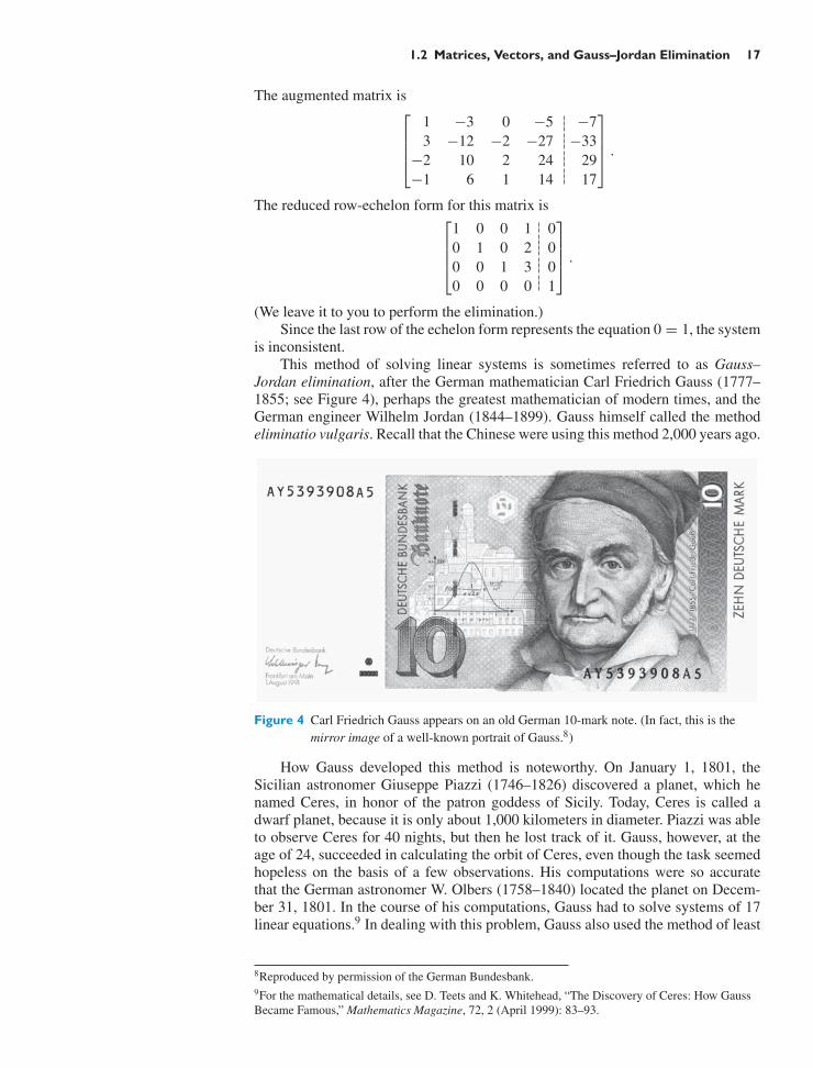
Jordan elimination, after the German mathematician Carl Friedrich Gauss (1777–1855; see Figure 4), perhaps the greatest mathematician of modern times, and theGerman engineer Wilhelm Jordan (1844–1899). Gauss himself called the methodeliminatio vulgaris. Recall that the Chinese were using this method 2,000 years ago.
Figure 4 Carl Friedrich Gauss appears on an old German 10-mark note. (In fact, this is themirror image of a well-known portrait of Gauss.8)
How Gauss developed this method is noteworthy. On January 1, 1801, theSicilian astronomer Giuseppe Piazzi (1746–1826) discovered a planet, which henamed Ceres, in honor of the patron goddess of Sicily. Today, Ceres is called adwarf planet, because it is only about 1,000 kilometers in diameter. Piazzi was ableto observe Ceres for 40 nights, but then he lost track of it. Gauss, however, at theage of 24, succeeded in calculating the orbit of Ceres, even though the task seemedhopeless on the basis of a few observations. His computations were so accuratethat the German astronomer W. Olbers (1758–1840) located the planet on Decem-ber 31, 1801. In the course of his computations, Gauss had to solve systems of 17linear equations.9 In dealing with this problem, Gauss also used the method of least
8Reproduced by permission of the German Bundesbank.9For the mathematical details, see D. Teets and K. Whitehead, “The Discovery of Ceres: How GaussBecame Famous,” Mathematics Magazine, 72, 2 (April 1999): 83–93.

18 CHAPTER 1 Linear Equations
squares, which he had developed around 1794. See Section 5.4. Since Gauss at firstrefused to reveal the methods that led to this amazing accomplishment, some evenaccused him of sorcery. Gauss later described his methods of orbit computation inhis book Theoria Motus Corporum Coelestium (1809).
The method of solving a linear system by Gauss–Jordan elimination is calledan algorithm.10An algorithm can be defined as “a finite procedure, written in a fixedsymbolic vocabulary, governed by precise instructions, moving in discrete Steps, 1,2, 3, . . . , whose execution requires no insight, cleverness, intuition, intelligence, orperspicuity, and that sooner or later comes to an end” (David Berlinski, The Adventof the Algorithm: The Idea That Rules the World, Harcourt Inc., 2000).
Gauss–Jordan elimination is well suited for solving linear systems on a com-puter, at least in principle. In practice, however, some tricky problems associatedwith roundoff errors can occur.
Numerical analysts tell us that we can reduce the proliferation of roundofferrors by modifying Gauss–Jordan elimination, employing more sophisticated re-duction techniques.
In modifying Gauss–Jordan elimination, an interesting question arises: If wetransform a matrix A into a matrix B by a sequence of elementary row operationsand if B is in reduced row-echelon form, is it necessarily true that B = rref(A)?Fortunately (and perhaps surprisingly), this is indeed the case.
In this text, we will not utilize this fact, so there is no need to present thesomewhat technical proof. If you feel ambitious, try to work out the proof yourselfafter studying Chapter 3. See Exercises 3.3.86 through 3.3.89.
10 The word algorithm is derived from the name of the mathematician al-Khowarizmi, who introducedthe term algebra into mathematics (see page 1).
EXERCISES 1.2GOAL Use Gauss–Jordan elimination to solve linearsystems. Do simple problems using paper and pencil, anduse technology to solve more complicated problems.
In Exercises 1 through 12, find all solutions of the equa-tions with paper and pencil using Gauss–Jordan elimina-tion. Show all your work.
1.∣∣∣∣
x + y − 2z = 52x + 3y + 4z = 2
∣∣∣∣ 2.∣∣∣∣3x + 4y − z = 86x + 8y − 2z = 3
∣∣∣∣
3. x + 2y + 3z = 4 4.
∣∣∣∣∣∣
x + y = 12x − y = 53x + 4y = 2
∣∣∣∣∣∣
5.
∣∣∣∣∣∣∣
x3 + x4 = 0x2 + x3 = 0
x1 + x2 = 0x1 + x4 = 0
∣∣∣∣∣∣∣
6.
∣∣∣∣∣∣
x1 − 7x2 + x5 = 3x3 − 2x5 = 2
x4 + x5 = 1
∣∣∣∣∣∣
7.
∣∣∣∣∣∣∣
x1 + 2x2 2x4 + 3x5 = 0x3 + 3x4 + 2x5 = 0x3 + 4x4 − x5 = 0
x5 = 0
∣∣∣∣∣∣∣
8. Solve this system for the variables x1, x2, x3, x4, andx5.
∣∣∣∣x2 + 2x4 + 3x5 = 0
4x4 + 8x5 = 0
∣∣∣∣
9.
∣∣∣∣∣∣
x4 + 2x5 − x6 = 2x1 + 2x2 + x5 − x6 = 0x1 + 2x2 + 2x3 − x5 + x6 = 2
∣∣∣∣∣∣
10.
∣∣∣∣∣∣∣
4x1 + 3x2 + 2x3 − x4 = 45x1 + 4x2 + 3x3 − x4 = 4
−2x1 − 2x2 − x3 + 2x4 = −311x1 + 6x2 + 4x3 + x4 = 11
∣∣∣∣∣∣∣
11.
∣∣∣∣∣∣∣
x1 + 2x3 + 4x4 = −8x2 − 3x3 − x4 = 6
3x1 + 4x2 − 6x3 + 8x4 = 0− x2 + 3x3 + 4x4 = −12
∣∣∣∣∣∣∣

1.2 Matrices, Vectors, and Gauss–Jordan Elimination 19
12.
∣∣∣∣∣∣∣∣∣
2x1 − 3x3 + 7x5 + 7x6 = 0−2x1 + x2 + 6x3 − 6x5 − 12x6 = 0
x2 − 3x3 + x5 + 5x6 = 0− 2x2 + x4 + x5 + x6 = 0
2x1 + x2 − 3x3 + 8x5 + 7x6 = 0
∣∣∣∣∣∣∣∣∣
Solve the linear systems in Exercises 13 through 17. Youmay use technology.
13.
∣∣∣∣∣∣
3x + 11y + 19z = −27x + 23y + 39z = 10
−4x − 3y − 2z = 6
∣∣∣∣∣∣
14.
∣∣∣∣∣∣
3x + 6y + 14z = 227x + 14y + 30z = 464x + 8y + 7z = 6
∣∣∣∣∣∣
15.
∣∣∣∣∣∣
3x + 5y + 3z = 257x + 9y + 19z = 65
−4x + 5y + 11z = 5
∣∣∣∣∣∣
16.
∣∣∣∣∣∣
3x1 + 6x2 + 9x3 + 5x4 + 25x5 = 537x1 + 14x2 + 21x3 + 9x4 + 53x5 = 105
−4x1 − 8x2 − 12x3 + 5x4 − 10x5 = 11
∣∣∣∣∣∣
17.
∣∣∣∣∣∣∣∣∣
2x1 + 4x2 + 3x3 + 5x4 + 6x5 = 374x1 + 8x2 + 7x3 + 5x4 + 2x5 = 74
−2x1 − 4x2 + 3x3 + 4x4 − 5x5 = 20x1 + 2x2 + 2x3 − x4 + 2x5 = 26
5x1 − 10x2 + 4x3 + 6x4 + 4x5 = 24
∣∣∣∣∣∣∣∣∣
18. Determine which of the matrices below are in reducedrow-echelon form:
a.
⎡
⎢⎢⎣
1 2 0 2 00 0 1 3 00 0 1 4 00 0 0 0 1
⎤
⎥⎥⎦ b.
⎡
⎣0 1 2 0 30 0 0 1 40 0 0 0 0
⎤
⎦
c.
⎡
⎣1 2 0 30 0 0 00 0 1 2
⎤
⎦ d.[0 1 2 3 4
]
19. Find all 4 × 1 matrices in reduced row-echelon form.
20. For which values of a, b, c, d , and e is the followingmatrix in reduced row-echelon form?
A =
⎡
⎣0 a 2 1 b0 0 0 c d0 0 e 0 0
⎤
⎦
21. For which values of a, b, c, d , and e is the followingmatrix in reduced row-echelon form?
A =
⎡
⎣1 a b 3 0 −20 0 c 1 d 30 e 0 0 1 1
⎤
⎦
22. We say that two n ×m matrices in reduced row-echelonform are of the same type if they contain the same num-ber of leading 1’s in the same positions. For example,
[1 2 00 0 1
]and
[1 3 00 0 1
]
are of the same type. How many types of 2×2 matricesin reduced row-echelon form are there?
23. How many types of 3 × 2 matrices in reduced row-echelon form are there? See Exercise 22.
24. How many types of 2 × 3 matrices in reduced row-echelon form are there? See Exercise 22.
25. Suppose you apply Gauss–Jordan elimination to a ma-trix. Explain how you can be sure that the resultingmatrix is in reduced row-echelon form.
26. Suppose matrix A is transformed into matrix B bymeans of an elementary row operation. Is there anelementary row operation that transforms B into A?Explain.
27. Suppose matrix A is transformed into matrix B by asequence of elementary row operations. Is there a se-quence of elementary row operations that transforms Binto A? Explain your answer. See Exercise 26.
28. Consider an n×m matrix A. Can you transform rref(A)into A by a sequence of elementary row operations? SeeExercise 27.
29. Is there a sequence of elementary row operations thattransforms⎡
⎣1 2 34 5 67 8 9
⎤
⎦ into
⎡
⎣1 0 00 1 00 0 0
⎤
⎦?
Explain.
30. Suppose you subtract a multiple of an equation in a sys-tem from another equation in the system. Explain whythe two systems (before and after this operation) havethe same solutions.
31. Balancing a chemical reaction. Consider the chemicalreaction
a NO2 + b H2O → c HNO2 + d HNO3,
where a, b, c, and d are unknown positive integers. Thereaction must be balanced; that is, the number of atomsof each element must be the same before and after thereaction. For example, because the number of oxygenatoms must remain the same,
2a + b = 2c + 3d.
While there are many possible values for a, b, c, and dthat balance the reaction, it is customary to use the smal-lest possible positive integers. Balance this reaction.
32. Find the polynomial of degree 3 [a polynomial of theform f (t) = a + bt + ct2 + dt3] whose graph goesthrough the points (0, 1), (1, 0), (−1, 0), and (2,−15).Sketch the graph of this cubic.
33. Find the polynomial of degree 4 whose graph goesthrough the points (1, 1), (2,−1), (3,−59), (−1, 5),and (−2,−29). Graph this polynomial.

20 CHAPTER 1 Linear Equations
34. Cubic splines. Suppose you are in charge of the designof a roller coaster ride. This simple ride will not makeany left or right turns; that is, the track lies in a verti-cal plane. The accompanying figure shows the ride asviewed from the side. The points (ai , bi ) are given toyou, and your job is to connect the dots in a reasonablysmooth way. Let ai+1 > ai , for i = 0, . . . , n − 1.
(a0, b0)
(a1, b1)
(a2, b2)
(an, bn)
One method often employed in such design problems isthe technique of cubic splines. We choose fi (t), a poly-nomial of degree ≤ 3, to define the shape of the ridebetween (ai−1, bi−1) and (ai , bi ), for i = 1, . . . , n.
(ai − 1, bi − 1)
(ai + 1, bi + 1)
fi(t)
(ai, bi)fi + 1(t)
Obviously, it is required that fi (ai ) = bi andfi (ai−1) = bi−1, for i = 1, . . . , n. To guarantee asmooth ride at the points (ai , bi ), we want the firstand second derivatives of fi and fi+1 to agree at thesepoints:
f ′i (ai ) = f ′
i+1(ai ) andf ′′i (ai ) = f ′′
i+1(ai ), for i = 1, . . . , n − 1.
Explain the practical significance of these conditions.Explain why, for the convenience of the riders, it is alsorequired that
f ′1(a0) = f ′
n(an) = 0.
Show that satisfying all these conditions amounts tosolving a system of linear equations. How many vari-ables are in this system? How many equations? (Note:It can be shown that this system has a unique solution.)
35. Find the polynomial f (t) of degree 3 such thatf (1) = 1, f (2) = 5, f ′(1) = 2, and f ′(2) = 9, wheref ′(t) is the derivative of f (t). Graph this polynomial.
36. The dot product of two vectors
x =
⎡
⎢⎢⎢⎣
x1x2...
xn
⎤
⎥⎥⎥⎦and y =
⎡
⎢⎢⎢⎣
y1y2...
yn
⎤
⎥⎥⎥⎦
in Rn is defined by
x · y = x1 y1 + x2 y2 + · · · + xn yn .
Note that the dot product of two vectors is a scalar.We say that the vectors x and y are perpendicular ifx · y = 0.
Find all vectors in R3 perpendicular to⎡
⎣13
−1
⎤
⎦ .
Draw a sketch.
37. Find all vectors in R4 that are perpendicular to the threevectors
⎡
⎢⎢⎣
1111
⎤
⎥⎥⎦ ,
⎡
⎢⎢⎣
1234
⎤
⎥⎥⎦ ,
⎡
⎢⎢⎣
1997
⎤
⎥⎥⎦ .
See Exercise 36.
38. Find all solutions x1, x2, x3 of the equation
b = x1v1 + x2v2 + x3v3,
where
b =
⎡
⎢⎢⎣
−8−1
215
⎤
⎥⎥⎦ , v1 =
⎡
⎢⎢⎣
1475
⎤
⎥⎥⎦ , v2 =
⎡
⎢⎢⎣
2583
⎤
⎥⎥⎦ , v3 =
⎡
⎢⎢⎣
4691
⎤
⎥⎥⎦ .
39. For some background on this exercise, see Exer-cise 1.1.24.
Consider an economy with three industries, I1, I2,I3. What outputs x1, x2, x3 should they produce to sat-isfy both consumer demand and interindustry demand?The demands put on the three industries are shown inthe accompanying figure.
Industry I1(output x1)
Industry I2(output x2)0.2x2
0.1x1
Industry I3(output x3)
Consumer
0.2x1 0.5x20.4x30.3x3
320 150 90
40. If we consider more than three industries in an input–output model, it is cumbersome to represent all thedemands in a diagram as in Exercise 39. Supposewe have the industries I1, I2, . . . , In , with outputsx1, x2, . . . , xn . The output vector is

1.2 Matrices, Vectors, and Gauss–Jordan Elimination 21
x =
⎡
⎢⎢⎢⎣
x1x2...
xn
⎤
⎥⎥⎥⎦.
The consumer demand vector is
b =
⎡
⎢⎢⎢⎣
b1b2...
bn
⎤
⎥⎥⎥⎦,
where bi is the consumer demand on industry Ii . Thedemand vector for industry I j is
v j =
⎡
⎢⎢⎢⎣
a1 ja2 j...
anj
⎤
⎥⎥⎥⎦,
where ai j is the demand industry I j puts on industry Ii ,for each $1 of output industry I j produces. For exam-ple, a32 = 0.5 means that industry I2 needs 50c/ worthof products from industry I3 for each $1 worth of goodsI2 produces. The coefficient aii need not be 0: Produc-ing a product may require goods or services from thesame industry.a. Find the four demand vectors for the economy in
Exercise 39.b. What is the meaning in economic terms of x j v j ?c. What is the meaning in economic terms of
x1v1 + x2v2 + · · · + xn vn + b?d. What is the meaning in economic terms of the equa-
tion
x1v1 + x2v2 + · · · + xn vn + b = x?
41. Consider the economy of Israel in 1958.11 The threeindustries considered here are
I1 : agriculture,I2 : manufacturing,I3 : energy.
Outputs and demands are measured in millions ofIsraeli pounds, the currency of Israel at that time. Weare told that
b =
⎡
⎣13.217.6
1.8
⎤
⎦ , v1 =
⎡
⎣0.2930.0140.044
⎤
⎦ ,
v2 =
⎡
⎣00.2070.01
⎤
⎦ , v3 =
⎡
⎣00.0170.216
⎤
⎦ .
a. Why do the first components of v2 and v3 equal 0?b. Find the outputs x1, x2, x3 required to satisfy
demand.
42. Consider some particles in the plane with position vec-tors r1, r2, . . . , r n and masses m1, m2, . . . , mn .
m1
m2
mn
r2
r1
rn
The position vector of the center of mass of this systemis
r cm = 1M
(m1r1 + m2r2 + · · · + mnrn),
where M = m1 + m2 + · · · + mn .Consider the triangular plate shown in the accom-
panying sketch. How must a total mass of 1 kg bedistributed among the three vertices of the plate so that
the plate can be supported at the point[
22
]; that is,
r cm =[
22
]? Assume that the mass of the plate itself is
negligible.
23
12
41
rcm =22
43. The momentum P of a system of n particles in spacewith masses m1, m2, . . . , mn and velocities v1, v2, . . . ,vn is defined as
P = m1v1 + m2v2 + · · · + mn vn .
Now consider two elementary particles with velocities
v1 =
⎡
⎣111
⎤
⎦ and v2 =
⎡
⎣47
10
⎤
⎦ .11 W. Leontief, Input–Output Economics, Oxford University Press,1966.

22 CHAPTER 1 Linear Equations
The particles collide. After the collision, their respec-tive velocities are observed to be
w1 =
⎡
⎣474
⎤
⎦ and w2 =
⎡
⎣238
⎤
⎦ .
Assume that the momentum of the system is conservedthroughout the collision. What does this experimenttell you about the masses of the two particles? See theaccompanying figure.
Particle 2
Particle 1
Collision
44. The accompanying sketch represents a maze of one-way streets in a city in the United States. The trafficvolume through certain blocks during an hour has beenmeasured. Suppose that the vehicles leaving the areaduring this hour were exactly the same as those enter-ing it.
?
?
?
?
300400
100
250
120
150
300
320
JFK Street
Dunster Street
Mt. Auburn Street
Winthrop Street
What can you say about the traffic volume at thefour locations indicated by a question mark? Can youfigure out exactly how much traffic there was on eachblock? If not, describe one possible scenario. For eachof the four locations, find the highest and the lowestpossible traffic volume.
45. Let S(t) be the length of the t th day of the year 2013in Mumbai (formerly known as Bombay), India (mea-sured in hours, from sunrise to sunset). We are giventhe following values of S(t):
t S(t)
47 11.574 12
273 12
For example, S(47) = 11.5 means that the timefrom sunrise to sunset on February 16 is 11 hours and30 minutes. For locations close to the equator, the func-tion S(t) is well approximated by a trigonometric func-tion of the form
S(t) = a + b cos(
2π t365
)+ c sin
(2π t365
).
(The period is 365 days, or 1 year.) Find this approxima-tion for Mumbai, and graph your solution. Accordingto this model, how long is the longest day of the year inMumbai?
46. Kyle is getting some flowers for Olivia, his Valentine.Being of a precise analytical mind, he plans to spendexactly $24 on a bunch of exactly two dozen flowers.At the flower market they have lilies ($3 each), roses($2 each), and daisies ($0.50 each). Kyle knows thatOlivia loves lilies; what is he to do?
47. Consider the equations∣∣∣∣∣∣
x + 2y + 3z = 4x + ky + 4z = 6x + 2y + (k + 2)z = 6
∣∣∣∣∣∣,
where k is an arbitrary constant.a. For which values of the constant k does this system
have a unique solution?b. When is there no solution?c. When are there infinitely many solutions?
48. Consider the equations∣∣∣∣∣∣
y + 2kz = 0x + 2y + 6z = 2
kx + 2z = 1
∣∣∣∣∣∣,
where k is an arbitrary constant.a. For which values of the constant k does this system
have a unique solution?b. When is there no solution?c. When are there infinitely many solutions?
49. a. Find all solutions x1, x2, x3, x4 of the systemx2 = 1
2 (x1 + x3), x3 = 12 (x2 + x4).
b. In part (a), is there a solution with x1 = 1 andx4 = 13?
50. For an arbitrary positive integer n ≥ 3, find all solutionsx1, x2, x3, . . . , xn of the simultaneous equations x2 =12 (x1+x3), x3 = 1
2 (x2+x4), . . . , xn−1 = 12 (xn−2+xn).
Note that we are asked to solve the simultaneous equa-tions xk = 1
2 (xk−1 + xk+1), for k = 2, 3, . . . , n − 1.
51. Consider the system∣∣∣∣∣∣
2x + y = C3y + z = C
x + 4z = C
∣∣∣∣∣∣,
where C is a constant. Find the smallest positive integerC such that x , y, and z are all integers.

1.2 Matrices, Vectors, and Gauss–Jordan Elimination 23
52. Find all the polynomials f (t) of degree ≤ 3 such thatf (0) = 3, f (1) = 2, f (2) = 0, and
∫ 20 f (t) dt = 4.
(If you have studied Simpson’s rule in calculus, explainthe result.)
Exercises 53 through 62 are concerned with conics. Aconic is a curve in R2 that can be described by an equationof the form f (x, y) = c1 + c2x + c3 y + c4x2 + c5x y +c6 y2 = 0, where at least one of the coefficients ci isnonzero. Examples are circles, ellipses, hyperbolas, andparabolas. If k is any nonzero constant, then the equa-tions f (x, y) = 0 and k f (x, y) = 0 describe the sameconic. For example, the equation −4 + x2 + y2 = 0 and−12 + 3x2 + 3 y2 = 0 both describe the circle of radius 2centered at the origin. In Exercises 53 through 62, find allthe conics through the given points. If there is a uniqueconic, make a rough sketch. If there are infinitely manyconics, sketch two of them.
53. (0, 0), (1, 0), (2, 0), (0, 1), and (0, 2).
54. (0, 0), (2, 0), (0, 2), (2, 2), and (1, 3).
55. (0, 0), (1, 0), (2, 0), (3, 0), and (1, 1).
56. (0, 0), (1, 1), (2, 2), (3, 3), and (1, 0).
57. (0, 0), (1, 0), (0, 1), and (1, 1).
58. (0, 0), (1, 0), (0, 1), and (1,−1).
59. (5, 0), (1, 2), (2, 1), (8, 1), and (2, 9).
60. (1, 0), (2, 0), (2, 2), (5, 2), and (5, 6).
61. (0, 0), (1, 0), (2, 0), (0, 1), (0, 2), and (1, 1).
62. (0, 0), (2, 0), (0, 2), (2, 2), (1, 3), and (4, 1).
63. Students are buying books for the new semester. Eddiebuys the environmental statistics book and the set the-ory book for $178. Leah, who is buying books for her-self and her friend, spends $319 on two environmentalstatistics books, one set theory book, and one educa-tional psychology book. Mehmet buys the educationalpsychology book and the set theory book for $147 intotal. How much does each book cost?
64. Students are buying books for the new semester.Brigitte buys the German grammar book and the Ger-man novel, Die Leiden des jungen Werther, for C64 intotal. Claude spends C98 on the linear algebra text andthe German grammar book, while Denise buys the lin-ear algebra text and Werther, for C76. How much doeseach of the three books cost?
65. At the beginning of a political science class at a largeuniversity, the students were asked which term, liberalor conservative, best described their political views.They were asked the same question at the end of thecourse, to see what effect the class discussions hadon their views. Of those that characterized themselvesas “liberal” initially, 30% held conservative views atthe end. Of those who were conservative initially, 40%
moved to the liberal camp. It turned out that there werejust as many students with conservative views at the endas there had been liberal students at the beginning. Outof the 260 students in the class, how many held liberaland conservative views at the beginning of the courseand at the end? (No students joined or dropped the classbetween the surveys, and they all participated in bothsurveys.)
66. At the beginning of a semester, 55 students have signedup for Linear Algebra; the course is offered in twosections that are taught at different times. Because ofscheduling conflicts and personal preferences, 20% ofthe students in Section A switch to Section B in thefirst few weeks of class, while 30% of the students inSection B switch to A, resulting in a net loss of 4 stu-dents for Section B. How large were the two sectionsat the beginning of the semester? No students droppedLinear Algebra (why would they?) or joined the courselate.
Historical Problems
67. Five cows and two sheep together cost 10 liang12 ofsilver. Two cows and five sheep together cost eightliang of silver. What is the cost of a cow and a sheep,respectively? (Nine Chapters,13 Chapter 8, Problem 7)
68. If you sell two cows and five sheep and you buy 13 pigs,you gain 1,000 coins. If you sell three cows and threepigs and buy nine sheep, you break even. If you sellsix sheep and eight pigs and you buy five cows, youlose 600 coins. What is the price of a cow, a sheep,and a pig, respectively? (Nine Chapters, Chapter 8,Problem 8)
69. You place five sparrows on one of the pans of a balanceand six swallows on the other pan; it turns out that thesparrows are heavier. But if you exchange one sparrowand one swallow, the weights are exactly balanced. Allthe birds together weigh 1 jin. What is the weight ofa sparrow and a swallow, respectively? [Give the an-swer in liang, with 1 jin = 16 liang.] (Nine Chapters,Chapter 8, Problem 9)
70. Consider the task of pulling a weight of 40 dan14 up ahill; we have one military horse, two ordinary horses,and three weak horses at our disposal to get the jobdone. It turns out that the military horse and one of theordinary horses, pulling together, are barely able to pull
12 A liang was about 16 grams at the time of the Han Dynasty.13See page 1; we present some of the problems from the NineChapters on the Mathematical Art in a free translation, withsome additional explanations, since the scenarios discussed ina few of these problems are rather unfamiliar to the modernreader.141 dan = 120 jin = 1,920 liang. Thus, a dan was about30 kilograms at that time.

24 CHAPTER 1 Linear Equations
the weight (but they could not pull any more). Likewise,the two ordinary horses together with one weak horseare just able to do the job, as are the three weak horsestogether with the military horse. How much weight caneach of the horses pull alone? (Nine Chapters, Chap-ter 8, Problem 12)
71. Five households share a deep well for their water sup-ply. Each household owns a few ropes of a certainlength, which varies only from household to household.The five households, A, B, C, D, and E, own 2, 3, 4,5, and 6 ropes, respectively. Even when tying all theirropes together, none of the households alone is able toreach the water, but A’s two ropes together with oneof B’s ropes just reach the water. Likewise, B’s threeropes with one of C’s ropes, C’s four ropes with one ofD’s ropes, D’s five ropes with one of E’s ropes, and E’ssix ropes with one of A’s ropes all just reach the water.How long are the ropes of the various households, andhow deep is the well?Commentary: As stated, this problem leads to a systemof five linear equations in six variables; with the giveninformation, we are unable to determine the depth ofthe well. The Nine Chapters gives one particular solu-tion, where the depth of the well is 7 zhang,15 2 chi, 1cun, or 721 cun (since 1 zhang = 10 chi and 1 chi =10 cun). Using this particular value for the depth of thewell, find the lengths of the various ropes.
72. “A rooster is worth five coins, a hen three coins, and3 chicks one coin. With 100 coins we buy 100 of them.How many roosters, hens, and chicks can we buy?”(From the Mathematical Manual by Zhang Qiujian,Chapter 3, Problem 38; 5th century A.D.)Commentary: This famous Hundred Fowl Problem hasreappeared in countless variations in Indian, Arabic,and European texts (see Exercises 73 through 76); it hasremained popular to this day. See Exercise 46 of thissection.
73. Pigeons are sold at the rate of 5 for 3 panas, sarasabirdsat the rate of 7 for 5 panas, swans at the rate of 9 for 7panas, and peacocks at the rate of 3 for 9 panas. A manwas ordered to bring 100 birds for 100 panas for theamusement of the Prince. How much does he pay foreach of the various kinds of birds he buys? (From theGanita-Sara-Sangraha by Mahavira, India; 9th centuryA.D.) Find one solution to this problem.
74. A duck costs four coins, five sparrows cost one coin,and a rooster costs one coin. Someone purchases100 birds for 100 coins. How many birds of each kindcan he buy? (From the Key to Arithmetic by Al-Kashi;15th century)
75. “A certain person buys sheep, goats, and hogs, to thenumber of 100, for 100 crowns; the sheep cost him12 a crown a-piece; the goats, 1 1
3 crown; and the hogs
3 12 crowns. How many had he of each?” (From the
Elements of Algebra by Leonhard Euler, 1770)
76. A gentleman runs a household of 100 people and or-ders that they be given 100 measures of grain. He di-rects that each man should receive three measures, eachwoman two measures, and each child half a measure.How many men, women, and children are there in thishousehold? We are told that there is at least one man,one woman, and one child. (From the Problems forQuickening a Young Mind by Alcuin [c. 732–804], theAbbot of St. Martins at Tours. Alcuin was a friend andtutor to Charlemagne and his family at Aachen.)
77. A dying father gave to his sons 30 barrels, of which 10were full of wine, 10 were half-full, and the last 10 wereempty. Divide the wine and flasks so that there will beequal division among the three sons of both wine andbarrels. Find all the solutions of this problem. (FromAlcuin)
78. Make me a crown weighing 60 minae from a mixtureof gold, bronze, tin, and wrought iron. Let the goldand bronze together form two-thirds of the weight, thegold and tin together three-fourths, and the gold andiron three-fifths. Tell me how much gold, tin, bronze,and iron you must use. (From the Greek Anthology byMetrodorus, 6th century A.D.)
79. Three merchants find a purse lying in the road. Onemerchant says, “If I keep the purse, I will have twiceas much money as the two of you together.” “Giveme the purse and I will have three times as muchas the two of you together,” said the second mer-chant. The third merchant said, “I will be much bet-ter off than either of you if I keep the purse, I willhave five times as much as the two of you together.”If there are 60 coins (of equal value) in the purse,how much money does each merchant have? (FromMahavira)
80. 3 cows graze 1 field bare in 2 days,7 cows graze 4 fields bare in 4 days, and3 cows graze 2 fields bare in 5 days.It is assumed that each field initially provides the sameamount, x , of grass; that the daily growth, y, of thefields remains constant; and that all the cows eat thesame amount, z, each day. (Quantities x , y, and z aremeasured by weight.) Find all the solutions of this prob-lem. (This is a special case of a problem discussed byIsaac Newton in his Arithmetica Universalis, 1707.)
15 1 zhang was about 2.3 meters at that time.

1.3 On the Solutions of Linear Systems; Matrix Algebra 25
1.3 On the Solutions of Linear Systems; Matrix Algebra
In this final section of Chapter 1, we will discuss two rather unrelated topics:
• First, we will examine how many solutions a system of linear equations canpossibly have.
• Then, we will present some definitions and rules of matrix algebra.
The Number of Solutions of a Linear System
EXAMPLE 1 The reduced row-echelon forms of the augmented matrices of three systems aregiven. How many solutions are there in each case?
a.
⎡
⎢⎢⎣
1 2 0 00 0 1 00 0 0 10 0 0 0
⎤
⎥⎥⎦ b.
⎡
⎣1 2 0 10 0 1 20 0 0 0
⎤
⎦ c.
⎡
⎣1 0 0 10 1 0 20 0 1 3
⎤
⎦
Solutiona. The third row represents the equation 0 = 1, so that there are no solutions.
We say that this system is inconsistent.b. The given augmented matrix represents the system
∣∣∣∣x1 + 2x2 = 1
x3 = 2
∣∣∣∣ , or∣∣∣∣x1 = 1 − 2x2x3 = 2
∣∣∣∣ .
We can assign an arbitrary value, t , to the free variable x2, so that the systemhas infinitely many solutions,
⎡
⎣x1
x2
x3
⎤
⎦ =
⎡
⎣1 − 2t
t2
⎤
⎦ , where t is an arbitrary constant.
c. Here there are no free variables, so that we have only one solution, x1 = 1,x2 = 2, x3 = 3. !
We can generalize our findings:16
Theorem 1.3.1 Number of solutions of a linear system
A system of equations is said to be consistent if there is at least one solution; itis inconsistent if there are no solutions.
A linear system is inconsistent if (and only if) the reduced row-echelon formof its augmented matrix contains the row
[0 0 · · · 0 1
], representing the
equation 0 = 1.If a linear system is consistent, then it has either• infinitely many solutions (if there is at least one free variable), or• exactly one solution (if all the variables are leading).
16Starting in this section, we will number the definitions we give and the theorems we derive. The nththeorem stated in Section p.q is labeled as Theorem p.q.n.

26 CHAPTER 1 Linear Equations
Example 1 illustrates what the number of leading 1’s in the echelon form tellsus about the number of solutions of a linear system. This observation motivates thefollowing definition:
Definition 1.3.2 The rank of a matrix17
The rank of a matrix A is the number of leading 1’s in rref(A), denoted rank(A).
EXAMPLE 2 rank
⎡
⎣1 2 34 5 67 8 9
⎤
⎦ = 2, since rref
⎡
⎣1 2 34 5 67 8 9
⎤
⎦ =
⎡
⎣1 0 −10 1 20 0 0
⎤
⎦ !
Note that we have defined the rank of a matrix rather than the rank of a linearsystem. When relating the concept of rank to a linear system, we must be carefulto specify whether we consider the coefficient matrix or the augmented matrix ofthe system.
EXAMPLE 3 Consider a system of n linear equations with m variables, which has a coefficientmatrix A of size n × m. Show that
a. The inequalities rank(A) ≤ n and rank(A) ≤ m hold.b. If the system is inconsistent, then rank(A) < n.c. If the system has exactly one solution, then rank(A) = m.d. If the system has infinitely many solutions, then rank(A) < m.
Solutiona. By definition of the reduced row-echelon form, there is at most one leading
1 in each of the n rows and in each of the m columns of rref(A).b. If the system is inconsistent, then the rref of the augmented matrix will con-
tain a row of the form [ 0 0 . . . 0 1 ], so that rref(A) will contain a row ofzeros. Since there is no leading 1 in that row, we find that rank(A) < n, asclaimed.
c. For parts c and d, it is worth noting that(
number offree variables
)=
(total numberof variables
)−
(number of
leading variables
)= m − rank(A).
If the system has exactly one solution, then there are no free variables (seeTheorem 1.3.1), so that m − rank(A) = 0 and rank(A) = m as claimed.
d. If the system has infinitely many solutions, then there is at least one freevariable, so that m − rank(A) > 0 and rank(A) < m, as claimed. !
EXAMPLE 4 It is useful to think about the contrapositives of the statements in parts b through dof Example 3.18
17This is a preliminary, rather technical definition. In Chapter 3, we will gain a better conceptualunderstanding of the rank.18The contrapositive of the statement “if p then q” is “if not-q then not-p.” A statement and itscontrapositive are logically equivalent. For example, the contrapositive of “If you live in New YorkCity, then you live in the Unites States” is “If you don’t live in the United States, then you don’t live inNew York City.” Here is a more convoluted example: On the service truck of a plumbing company weread, “If we can’t fix it, then it ain’t broken.” The contrapositive of this claim is, “If it is broken, thenwe can fix it” (not quite as catchy!).

1.3 On the Solutions of Linear Systems; Matrix Algebra 27
b. If rank(A) = n, then the system is consistent.c. If rank(A) < m, then the system has no solution or infinitely many solutions.d. If rank(A) = m, then the system has no solution or exactly one solution. !In Theorems 1.3.3 and 1.3.4, we will discuss two important special cases of
Example 3.
Theorem 1.3.3 Number of equations vs. number of unknowns
a. If a linear system has exactly one solution, then there must be at leastas many equations as there are variables (m ≤ n with the notation fromExample 3).
Equivalently, we can formulate the contrapositive:
b. A linear system with fewer equations than unknowns (n < m) has eitherno solutions or infinitely many solutions.
The proof of part (a) is based on parts (a) and (c) of Example 3: m = rank(A) ≤n, so that m ≤ n as claimed.
To illustrate part b of Theorem 1.3.3, consider two linear equations in threevariables, with each equation defining a plane. Two different planes in space eitherintersect in a line or are parallel (see Figure 1), but they will never intersect at apoint! This means that a system of two linear equations with three unknowns cannothave a unique solution.
(a) (b)
Figure 1 (a) Two planes intersect in a line. (b) Two parallel planes.
EXAMPLE 5 Consider a linear system of n equations with n variables. When does this systemhave exactly one solution? Give your answer in terms of the rank of the coefficientmatrix A.
SolutionIf the system has exactly one solution, then rank(A) = m = n by Example 3c.
Conversely, if rank(A) = n, then there will be a leading 1 in each row and ineach column, and these leading 1’s will be lined up along the diagonal:
rref(A) =
⎡
⎢⎢⎣
1 0 . . . 00 1 . . . 0...
.... . .
...0 0 . . . 1
⎤
⎥⎥⎦ .
This system will have exactly one solution. !

28 CHAPTER 1 Linear Equations
Theorem 1.3.4 Systems of n equations in n variables
A linear system of n equations in n variables has a unique solution if (and onlyif) the rank of its coefficient matrix A is n. In this case,
rref(A) =
⎡
⎢⎢⎢⎢⎢⎣
1 0 0 · · · 00 1 0 · · · 00 0 1 · · · 0...
......
. . ....
0 0 0 · · · 1
⎤
⎥⎥⎥⎥⎥⎦,
the n × n matrix with 1’s along the diagonal and 0’s everywhere else.
Matrix AlgebraWe will now introduce some basic definitions and rules of matrix algebra. Our pre-sentation will be somewhat lacking in motivation at first, but it will be good to havethese tools available when we need them in Chapter 2.
Sums and scalar multiples of matrices are defined entry by entry, as for vectors.See Definition A.1 in the Appendix.
Definition 1.3.5 Sums of matrices
The sum of two matrices of the same size is defined entry by entry:⎡
⎢⎣a11 . . . a1m...
...
an1 . . . anm
⎤
⎥⎦ +
⎡
⎢⎣b11 . . . b1m...
...
bn1 . . . bnm
⎤
⎥⎦ =
⎡
⎢⎣a11 + b11 . . . a1m + b1m
......
an1 + bn1 . . . anm + bnm
⎤
⎥⎦ .
Scalar multiples of matricesThe product of a scalar with a matrix is defined entry by entry:
k
⎡
⎢⎣a11 . . . a1m...
...
an1 . . . anm
⎤
⎥⎦ =
⎡
⎢⎣ka11 . . . ka1m
......
kan1 . . . kanm
⎤
⎥⎦ .
EXAMPLE 6[
1 2 34 5 6
]+
[7 3 15 3 −1
]=
[8 5 49 8 5
]!
EXAMPLE 7 3[
2 1−1 3
]=
[6 3
−3 9
]!
The definition of the product of matrices is less straightforward; we will givethe general definition later in Section 2.3.
Because vectors are special matrices (with only one row or only one column),it makes sense to start with a discussion of products of vectors. The reader may befamiliar with the dot product of vectors.

1.3 On the Solutions of Linear Systems; Matrix Algebra 29
Definition 1.3.6 Dot product of vectors
Consider two vectors v and w with components v1, . . . , vn and w1, . . . , wn , re-spectively. Here v and w may be column or row vectors, and the two vectorsneed not be of the same type. The dot product of v and w is defined to be thescalar
v · w = v1w1 + · · · + vnwn.
Note that our definition of the dot product isn’t row-column-sensitive. The dotproduct does not distinguish between row and column vectors.
EXAMPLE 8[1 2 3
]·
⎡
⎣312
⎤
⎦ = 1 · 3 + 2 · 1 + 3 · 2 = 11 !
Now we are ready to define the product Ax , where A is a matrix and x is avector, in terms of the dot product.
Definition 1.3.7 The product Ax
If A is an n × m matrix with row vectors w1, . . . , wn , and x is a vector in Rm ,then
Ax =
⎡
⎢⎣− w1 −
...
− wn −
⎤
⎥⎦ x =
⎡
⎢⎣w1 · x
...
wn · x
⎤
⎥⎦ .
In words, the i th component of Ax is the dot product of the i th row of A with x .Note that Ax is a column vector with n components, that is, a vector in Rn .
EXAMPLE 9[
1 2 31 0 −1
]⎡
⎣312
⎤
⎦ =[
1 · 3 + 2 · 1 + 3 · 21 · 3 + 0 · 1 + (−1) · 2
]=
[111
]!
EXAMPLE 10
⎡
⎣1 0 00 1 00 0 1
⎤
⎦
⎡
⎣x1
x2
x3
⎤
⎦ =
⎡
⎣x1
x2
x3
⎤
⎦ for all vectors
⎡
⎣x1
x2
x3
⎤
⎦ in R3 !
Note that the product Ax is defined only if the number of columns of matrix Amatches the number of components of vector x :
n × m︷︸︸︷A
m × 1︷︸︸︷x︸ ︷︷ ︸
n × 1
.
EXAMPLE 11 The product Ax =[
1 2 31 0 −1
] [31
]is undefined, because the number of columns
of matrix A fails to match the number of components of vector x . !In Definition 1.3.7, we express the product Ax in terms of the rows of the matrix
A. Alternatively, the product can be expressed in terms of the columns.
30 CHAPTER 1 Linear Equations
Let’s take another look at Example 9:
Ax =[
1 2 31 0 −1
]⎡
⎣312
⎤
⎦ =[
1 · 3 + 2 · 1 + 3 · 21 · 3 + 0 · 1 + (−1) · 2
]
=[
1 · 31 · 3
]+
[2 · 10 · 1
]+
[3 · 2
(−1) · 2
]= 3
[11
]+ 1
[20
]+ 2
[3
−1
].
We recognize that the expression 3[
11
]+1
[20
]+2
[3
−1
]involves the vectors v1 =
[11
], v2 =
[20
], v3 =
[3
−1
], the columns of A, and the scalars x1 = 3, x2 = 1,
x3 = 2, the components of x . Thus, we can write
Ax =
⎡
⎣| | |v1 v2 v3
| | |
⎤
⎦
⎡
⎣x1
x2
x3
⎤
⎦ = x1v1 + x2v2 + x3v3.
We can generalize:
Theorem 1.3.8 The product Ax in terms of the columns of A
If the column vectors of an n × m matrix A are v1, . . . , vm and x is a vector inRm with components x1, . . . , xm , then
Ax =
⎡
⎣| |v1 . . . vm
| |
⎤
⎦
⎡
⎢⎣x1...
xm
⎤
⎥⎦ = x1v1 + · · · + xm vm .
Proof As usual, we denote the rows of A by w1, . . . , wn and the entries by ai j . It sufficesto show that the i th component of Ax is equal to the i th component of x1v1 + · · · +xm vm , for i = 1, . . . n. Now
(i th component of Ax) =︸︷︷︸step 1
wi · x = ai1x1 + · · · aim xm
= x1(i th component of v1) + · · ·+xm(i th component of vm)
=︸︷︷︸step 4
i th component of x1v1 + · · · + xm vm .
In Step 1 we are using Definition 1.3.7, and in step 4 we are using the fact thatvector addition and scalar multiplication are defined component by component. !
EXAMPLE 12 Ax =
⎡
⎣1 2 34 5 67 8 9
⎤
⎦
⎡
⎣2
−42
⎤
⎦ = 2
⎡
⎣147
⎤
⎦ + (−4)
⎡
⎣258
⎤
⎦ + 2
⎡
⎣369
⎤
⎦
=
⎡
⎣28
14
⎤
⎦ −
⎡
⎣8
2032
⎤
⎦ +
⎡
⎣6
1218
⎤
⎦ =
⎡
⎣000
⎤
⎦
Note that something remarkable is happening here: Although A isn’t the zeromatrix and x isn’t the zero vector, the product Ax is the zero vector. (By contrast,the product of any two nonzero scalars is nonzero.) !

1.3 On the Solutions of Linear Systems; Matrix Algebra 31
The formula for the product Ax in Theorem 1.3.8 involves the expressionx1v1 + · · · + xm vm , where v1, . . . , vm are vectors in Rn , and x1, . . . , xm are scalars.Such expressions come up very frequently in linear algebra; they deserve a name.
Definition 1.3.9 Linear combinations
A vector b in Rn is called a linear combination of the vectors v1, . . . , vm in Rn
if there exist scalars x1, . . . , xm such that
b = x1v1 + · · · + xm vm .
EXAMPLE 13 Is the vector b =
⎡
⎣111
⎤
⎦ a linear combination of the vectors v =
⎡
⎣123
⎤
⎦ and
w =
⎡
⎣456
⎤
⎦?
SolutionAccording to Definition 1.3.9, we need to see whether we can find scalars x and y
such that
⎡
⎣111
⎤
⎦ = x
⎡
⎣123
⎤
⎦ + y
⎡
⎣456
⎤
⎦ =
⎡
⎣x + 4y
2x + 5y3x + 6y
⎤
⎦. We need to solve the linear
system
∣∣∣∣∣∣
x + 4y = 12x + 5y = 13x + 6y = 1
∣∣∣∣∣∣, with augmented matrix M =
⎡
⎣1 4 12 5 13 6 1
⎤
⎦ and rref(M) =⎡
⎣1 0 −1/30 1 1/30 0 0
⎤
⎦.
It turns out that the system is consistent, with x = −1/3 and y = 1/3. Thevector b is indeed a linear combination of v and w, with b = − 1
3 v + 13 w. !
Note that the product Ax is the linear combination of the columns of A withthe components of x as the coefficients:
Ax =
⎡
⎣| |v1 . . . vm
| |
⎤
⎦
⎡
⎢⎣x1...
xm
⎤
⎥⎦ = x1v1 + · · · + xm vm .
Take a good look at this equation, because it is the most frequently used for-mula in this text. Particularly in theoretical work, it will often be useful to write theproduct Ax as the linear combination x1v1 +· · ·+ xm vm . Conversely, when dealingwith a linear combination x1v1 + · · · + xm vm , it will often be helpful to introducethe matrix
A =
⎡
⎣| |v1 . . . vm
| |
⎤
⎦ and the vector x =
⎡
⎢⎣x1...
xm
⎤
⎥⎦
and then write x1v1 + · · · + xm vm = Ax .Next we present two rules concerning the product Ax . In Chapter 2 we will see
that these rules play a central role in linear algebra.

32 CHAPTER 1 Linear Equations
Theorem 1.3.10 Algebraic rules for Ax
If A is an n × m matrix, x and y are vectors in Rm , and k is a scalar, then
a. A(x + y) = Ax + Ay, andb. A(kx) = k(Ax).
We will prove the first equation, leaving the second as Exercise 45.Denote the i th row of A by wi . Then
(i th component of A(x + y)
)= wi · (x + y)
step 2︷︸︸︷= wi · x + wi · y= (i th component of Ax) + (i th component of Ay)= (i th component of Ax + Ay).
In step 2 we are using a rule for dot products stated in Theorem A.5b, in the Ap-pendix.
Our new tools of matrix algebra allow us to see linear systems in a new light,as illustrated in the next example. The definition of the product Ax and the conceptof a linear combination will be particularly helpful.
EXAMPLE 14 Consider the linear system∣∣∣∣3x1 + x2 = 7
x1 + 2x2 = 4
∣∣∣∣ , with augmented matrix[
3 1 71 2 4
].
We can interpret the solution of this system as the intersection of two lines in thex1x2-plane, as illustrated in Figure 2.
(2, 1)
3x1 + x2 = 7
x1 + 2x2 = 4
x2
x1
Figure 2
Alternatively, we can write the system in vector form, as[
3x1 + x2
x1 + 2x2
]=
[74
]or
[3x1
x1
]+
[x2
2x2
]=
[74
]or x1
[31
]+ x2
[12
]=
[74
].
We see that solving this system amounts to writing the vector[
74
]as a linear com-
bination of the vectors[
31
]and
[12
]. See Definition 1.3.9. The vector equation

1.3 On the Solutions of Linear Systems; Matrix Algebra 33
x1
[31
]+ x2
[12
]=
[74
]
and its solution can be represented geometrically, as shown in Figure 3. The prob-
lem amounts to resolving the vector[
74
]into two vectors parallel to
[31
]and
[12
],
respectively, by means of a parallelogram.
74
31
12= 2 + 1
312
12
31
Figure 3
We can go further and write the linear combination
x1
[31
]+ x2
[12
]as
[3 11 2
] [x1
x2
]
so that the linear system
x1
[31
]+ x2
[12
]=
[74
]takes the form
[3 11 2
] [x1
x2
]=
[74
],
the matrix form of the linear system.Note that we started out with the augmented matrix
[A b
]=
[3 1 71 2 4
],
and we ended up writing the system as[
3 11 2
]
︸ ︷︷ ︸A
[x1
x2
]
︸︷︷︸x
=[
74
]
︸︷︷︸b
, or Ax = b. !We can generalize:
Theorem 1.3.11 Matrix form of a linear system
We can write the linear system with augmented matrix[
A b]
in matrix formas
Ax = b.
Note that the i th component of Ax is ai1x1 + · · · + aim xm , by Definition 1.3.7.Thus, the i th component of the equation Ax = b is
ai1x1 + · · · + aim xm = bi ;this is the i th equation of the system with augmented matrix
[A b
].

34 CHAPTER 1 Linear Equations
Solving the linear system Ax = b amounts to expressing vector b as a linearcombination of the column vectors of matrix A.
EXAMPLE 15 Write the system ∣∣∣∣2x1 − 3x2 + 5x3 = 79x1 + 4x2 − 6x3 = 8
∣∣∣∣in matrix form.
Solution
The coefficient matrix is A =[
2 −3 59 4 −6
], and b =
[78
]. The matrix form is
Ax = b, or[
2 −3 59 4 −6
]⎡
⎣x1
x2
x3
⎤
⎦ =[
78
].
!Now that we can write a linear system as a single equation, Ax = b, rather than
a list of simultaneous equations, we can think about it in new ways.For example, if we have an equation ax = b of numbers, we can divide both
sides by a to find the solution x :
x = ba
= a−1b (if a = 0).
It is natural to ask whether we can take an analogous approach in the case of theequation Ax = b. Can we “divide by A,” in some sense, and write
x = bA
= A−1b?
This issue of the invertibility of a matrix will be one of the main themes ofChapter 2.
EXERCISES 1.3GOAL Use the reduced row-echelon form of the aug-mented matrix to find the number of solutions of a linearsystem. Apply the definition of the rank of a matrix. Com-pute the product Ax in terms of the rows or the columnsof A. Represent a linear system in vector or matrixform.
1. The reduced row-echelon forms of the augmentedmatrices of three systems are given here. How many so-lutions does each system have?
a.
⎡
⎣1 0 2 00 1 3 00 0 0 1
⎤
⎦ b.[
1 0 50 1 6
]
c.[
0 1 0 20 0 1 3
]
Find the rank of the matrices in Exercises 2 through 4.
2.
⎡
⎣1 2 30 1 20 0 1
⎤
⎦ 3.
⎡
⎣1 1 11 1 11 1 1
⎤
⎦ 4.
⎡
⎣1 4 72 5 83 6 9
⎤
⎦
5. a. Write the system∣∣∣∣
x + 2y = 73x + y = 11
∣∣∣∣
in vector form.b. Use your answer in part (a) to represent the system
geometrically. Solve the system and represent thesolution geometrically.
6. Consider the vectors v1, v2, v3 in R2 (sketched in theaccompanying figure). Vectors v1 and v2 are parallel.How many solutions x , y does the system
x v1 + yv2 = v3
have? Argue geometrically.
v3
v1
v2

1.3 On the Solutions of Linear Systems; Matrix Algebra 35
7. Consider the vectors v1, v2, v3 in R2 shown in the ac-companying sketch. How many solutions x , y does thesystem
x v1 + yv2 = v3
have? Argue geometrically.
v3
v1
v2
8. Consider the vectors v1, v2, v3, v4 in R2 shown in theaccompanying sketch. Arguing geometrically, find twosolutions x , y, z of the linear system
x v1 + yv2 + zv3 = v4.
How do you know that this system has, in fact, infinitelymany solutions?
v3
v1
v2v4
9. Write the system∣∣∣∣∣∣
x + 2y + 3z = 14x + 5y + 6z = 47x + 8y + 9z = 9
∣∣∣∣∣∣
in matrix form.
Compute the dot products in Exercises 10 through 12(if the products are defined).
10.
⎡
⎣123
⎤
⎦ ·
⎡
⎣1
−21
⎤
⎦ 11.[1 9 9 7
]·
⎡
⎣666
⎤
⎦
12.[1 2 3 4
]·
⎡
⎢⎢⎣
5678
⎤
⎥⎥⎦
Compute the products Ax in Exercises 13 through 15 us-ing paper and pencil. In each case, compute the producttwo ways: in terms of the columns of A (Theorem 1.3.8)and in terms of the rows of A (Definition 1.3.7).
13.[
1 23 4
] [7
11
]14.
[1 2 32 3 4
]⎡
⎣−1
21
⎤
⎦
15.[1 2 3 4
]
⎡
⎢⎢⎣
5678
⎤
⎥⎥⎦
Compute the products Ax in Exercises 16 through 19using paper and pencil (if the products are defined).
16.[
0 13 2
] [2
−3
]17.
[1 2 34 5 6
] [78
]
18.
⎡
⎣1 23 45 6
⎤
⎦[
12
]19.
⎡
⎣1 1 −1
−5 1 11 −5 3
⎤
⎦
⎡
⎣123
⎤
⎦
20. a. Find
⎡
⎣2 34 56 7
⎤
⎦ +
⎡
⎣7 53 10 −1
⎤
⎦.
b. Find 9[
1 −1 23 4 5
].
21. Use technology to compute the product⎡
⎢⎢⎣
1 7 8 91 2 9 11 5 1 51 6 4 8
⎤
⎥⎥⎦
⎡
⎢⎢⎣
1956
⎤
⎥⎥⎦ .
22. Consider a linear system of three equations with threeunknowns. We are told that the system has a unique so-lution. What does the reduced row-echelon form of thecoefficient matrix of this system look like? Explain youranswer.
23. Consider a linear system of four equations with threeunknowns. We are told that the system has a unique so-lution. What does the reduced row-echelon form of thecoefficient matrix of this system look like? Explain youranswer.
24. Let A be a 4 × 4 matrix, and let b and c be two vec-tors in R4. We are told that the system Ax = b has aunique solution. What can you say about the number ofsolutions of the system Ax = c?
25. Let A be a 4×4 matrix, and let b and c be two vectors inR4. We are told that the system Ax = b is inconsistent.What can you say about the number of solutions of thesystem Ax = c?
26. Let A be a 4 × 3 matrix, and let b and c be two vec-tors in R4. We are told that the system Ax = b has aunique solution. What can you say about the number ofsolutions of the system Ax = c?
27. If the rank of a 4 × 4 matrix A is 4, what is rref(A)?
28. If the rank of a 5 × 3 matrix A is 3, what is rref(A)?
In Problems 29 through 32, let x =
⎡
⎣53
−9
⎤
⎦ and y =
⎡
⎣201
⎤
⎦.
29. Find a diagonal matrix A such that Ax = y.
30. Find a matrix A of rank 1 such that Ax = y.
31. Find an upper triangular matrix A such that Ax = y,

36 CHAPTER 1 Linear Equations
where all the entries of A on and above the diagonal arenonzero.
32. Find a matrix A with all nonzero entries such thatAx = y.
33. Let A be the n × n matrix with all 1’s on the diagonaland all 0’s above and below the diagonal. What is Ax ,where x is a vector in Rn?
34. We define the vectors
e1 =
⎡
⎣100
⎤
⎦ , e2 =
⎡
⎣010
⎤
⎦ , e3 =
⎡
⎣001
⎤
⎦
in R3.a. For
A =
⎡
⎣a b cd e fg h k
⎤
⎦ ,
compute Ae1, Ae2, and Ae3.b. If B is an n × 3 matrix with columns v1, v2, and v3,
what are Be1, Be2, and Be3?
35. In Rm , we define
ei =
⎡
⎢⎢⎢⎢⎢⎢⎢⎢⎢⎣
00...
1...
0
⎤
⎥⎥⎥⎥⎥⎥⎥⎥⎥⎦
← i th component.
If A is an n × m matrix, what is Aei ?
36. Find a 3 × 3 matrix A such that
A
⎡
⎣100
⎤
⎦ =
⎡
⎣123
⎤
⎦ , A
⎡
⎣010
⎤
⎦ =
⎡
⎣456
⎤
⎦ ,
and A
⎡
⎣001
⎤
⎦ =
⎡
⎣789
⎤
⎦ .
37. Find all vectors x such that Ax = b, where
A =
⎡
⎣1 2 00 0 10 0 0
⎤
⎦ and b =
⎡
⎣210
⎤
⎦ .
38. a. Using technology, generate a random 3 × 3 matrixA. (The entries may be either single-digit integersor numbers between 0 and 1, depending on the tech-nology you are using.) Find rref(A). Repeat this ex-periment a few times.
b. What does the reduced row-echelon form of most3 × 3 matrices look like? Explain.
39. Repeat Exercise 38 for 3 × 4 matrices.
40. Repeat Exercise 38 for 4 × 3 matrices.
41. How many solutions do most systems of three linearequations with three unknowns have? Explain in termsof your work in Exercise 38.
42. How many solutions do most systems of three linearequations with four unknowns have? Explain in termsof your work in Exercise 39.
43. How many solutions do most systems of four linearequations with three unknowns have? Explain in termsof your work in Exercise 40.
44. Consider an n × m matrix A with more rows thancolumns (n > m). Show that there is a vector b in Rn
such that the system Ax = b is inconsistent.
45. Consider an n × m matrix A, a vector x in Rm , and ascalar k. Show that
A(kx) = k(Ax).
46. Find the rank of the matrix⎡
⎣a b c0 d e0 0 f
⎤
⎦ ,
where a, d , and f are nonzero, and b, c, and e are arbi-trary numbers.
47. A linear system of the form
Ax = 0
is called homogeneous. Justify the following facts:a. All homogeneous systems are consistent.b. A homogeneous system with fewer equations than
unknowns has infinitely many solutions.c. If x1 and x2 are solutions of the homogeneous sys-
tem Ax = 0, then x1 + x2 is a solution as well.d. If x is a solution of the homogeneous system
Ax = 0 and k is an arbitrary constant, then kxis a solution as well.
48. Consider a solution x1 of the linear system Ax = b.Justify the facts stated in parts (a) and (b):a. If x h is a solution of the system Ax = 0, then
x1 + x h is a solution of the system Ax = b.b. If x2 is another solution of the system Ax = b, then
x2 − x1 is a solution of the system Ax = 0.c. Now suppose A is a 2 × 2 matrix. A solution vector
x1 of the system Ax = b is shown in the accom-panying figure. We are told that the solutions of thesystem Ax = 0 form the line shown in the sketch.Draw the line consisting of all solutions of the sys-tem Ax = b.

1.3 On the Solutions of Linear Systems; Matrix Algebra 37
x1
solutions of Ax = 00
If you are puzzled by the generality of this problem,think about an example first:
A =[
1 23 6
], b =
[39
], and x1 =
[11
].
49. Consider the accompanying table. For some linear sys-tems Ax = b, you are given either the rank of the co-efficient matrix A, or the rank of the augmented matrix[
A b]. In each case, state whether the system could
have no solution, one solution, or infinitely many solu-tions. There may be more than one possibility for somesystems. Justify your answers.
Number of Number of Rank RankEquations Unknowns of A of
[A b
]
a. 3 4 — 2b. 4 3 3 —c. 4 3 — 4d. 3 4 3 —
50. Consider a linear system Ax = b, where A is a 4 × 3matrix. We are told that rank
[A b
]= 4. How many
solutions does this system have?
51. Consider an n × m matrix A, an r × s matrix B, and avector x in Rp . For which values of n, m, r , s, and p isthe product
A(Bx)
defined?
52. Consider the matrices
A =[
1 01 2
]and B =
[0 −11 0
].
Can you find a 2 × 2 matrix C such that
A(Bx) = Cx,
for all vectors x in R2?
53. If A and B are two n × m matrices, is
(A + B)x = Ax + Bx
for all x in Rm?
54. Consider two vectors v1 and v2 in R3 that are not paral-lel. Which vectors in R3 are linear combinations of v1and v2? Describe the set of these vectors geometrically.Include a sketch in your answer.
55. Is the vector
⎡
⎣789
⎤
⎦ a linear combination of
⎡
⎣123
⎤
⎦ and
⎡
⎣456
⎤
⎦?
56. Is the vector
⎡
⎢⎢⎢⎢⎣
30−1385662
⎤
⎥⎥⎥⎥⎦
a linear combination of
⎡
⎢⎢⎢⎢⎣
17194
⎤
⎥⎥⎥⎥⎦,
⎡
⎢⎢⎢⎢⎣
56328
⎤
⎥⎥⎥⎥⎦,
⎡
⎢⎢⎢⎢⎣
92352
⎤
⎥⎥⎥⎥⎦,
⎡
⎢⎢⎢⎢⎣
−2−5
479
⎤
⎥⎥⎥⎥⎦?
57. Express the vector[
711
]as the sum of a vector on the
line y = 3x and a vector on the line y = x/2.
y = 3xy
y = x/2
x
711
58. For which values of the constants b and c is the vector
⎡
⎣3bc
⎤
⎦ a linear combination of
⎡
⎣132
⎤
⎦,
⎡
⎣264
⎤
⎦, and
⎡
⎣−1−3−2
⎤
⎦?

38 CHAPTER 1 Linear Equations
59. For which values of the constants c and d is
⎡
⎢⎢⎣
57cd
⎤
⎥⎥⎦ a lin-
ear combination of
⎡
⎢⎢⎣
1111
⎤
⎥⎥⎦ and
⎡
⎢⎢⎣
1234
⎤
⎥⎥⎦?
60. For which values of the constants a, b, c, and d is
⎡
⎢⎢⎣
abcd
⎤
⎥⎥⎦
a linear combination of
⎡
⎢⎢⎣
0030
⎤
⎥⎥⎦,
⎡
⎢⎢⎣
1040
⎤
⎥⎥⎦, and
⎡
⎢⎢⎣
2056
⎤
⎥⎥⎦?
61. For which values of the constant c is
⎡
⎣1cc2
⎤
⎦ a linear
combination of
⎡
⎣124
⎤
⎦ and
⎡
⎣139
⎤
⎦?
62. For which values of the constant c is
⎡
⎣1cc2
⎤
⎦ a linear
combination of
⎡
⎣1aa2
⎤
⎦ and
⎡
⎣1bb2
⎤
⎦, where a and b are
arbitrary constants?
In Exercises 63 through 68, consider the vectors v and win the accompanying figure.
v
w
63. Give a geometrical description of the set of all vectorsof the form v + cw, where c is an arbitrary real number.
64. Give a geometrical description of the set of all vectorsof the form v + cw, where 0 ≤ c ≤ 1.
65. Give a geometrical description of the set of all vectorsof the form av + bw, where 0 ≤ a ≤ 1 and 0 ≤ b ≤ 1.
66. Give a geometrical description of the set of all vectorsof the form av + bw, where a + b = 1.
67. Give a geometrical description of the set of all vectorsof the form av+bw, where 0 ≤ a, 0 ≤ b, and a+b ≤ 1.
68. Give a geometrical description of the set of all vectorsu in R2 such that u · v = u · w.
69. Solve the linear system∣∣∣∣∣∣
y + z = ax + z = bx + y = c
∣∣∣∣∣∣,
where a, b, and c are arbitrary constants.
70. Let A be the n × n matrix with 0’s on the main diago-nal, and 1’s everywhere else. For an arbitrary vector bin Rn , solve the linear system Ax = b, expressing thecomponents x1, . . . , xn of x in terms of the componentsof b. See Exercise 69 for the case n = 3.
Chapter One Exercises
TRUE OR FALSE?19
Determine whether the statements that follow are true orfalse, and justify your answer.
1. If A is an n × n matrix and x is a vector in Rn , then theproduct Ax is a linear combination of the columns ofmatrix A.
2. If vector u is a linear combination of vectors v andw, then we can write u = av + bw for some scalarsa and b.
3. Matrix
⎡
⎣1 2 00 0 10 0 0
⎤
⎦ is in reduced row-echelon form.
4. A system of four linear equations in three unknowns isalways inconsistent.
5. There exists a 3 × 4 matrix with rank 4.
6. If A is a 3 × 4 matrix and vector v is in R4, then vectorAv is in R3.
7. If the 4 × 4 matrix A has rank 4, then any linear systemwith coefficient matrix A will have a unique solution.
19 We will conclude each chapter (except for Chapter 9) with sometrue–false questions, over 400 in all. We will start with a group ofabout 10 straightforward statements that refer directly to definitionsand theorems given in the chapter. Then there may be somecomputational exercises, and the remaining ones are moreconceptual, calling for independent reasoning. In some chapters, afew of the problems toward the end can be quite challenging. Don’texpect a balanced coverage of all the topics; some concepts arebetter suited for this kind of questioning than others.

Chapter One Exercises 39
8. There exists a system of three linear equations withthree unknowns that has exactly three solutions.
9. There exists a 5 × 5 matrix A of rank 4 such that thesystem Ax = 0 has only the solution x = 0.
10. If matrix A is in reduced row-echelon form, then at leastone of the entries in each column must be 1.
11. The system
⎡
⎣1 2 34 5 60 0 0
⎤
⎦ x =
⎡
⎣123
⎤
⎦ is inconsistent.
12. There exists a 2 × 2 matrix A such that A[
12
]=
[34
].
13. If A is a nonzero matrix of the form[
a −bb a
], then the
rank of A must be 2.
14. rank
⎡
⎣1 1 11 2 31 3 6
⎤
⎦ = 3
15. The system Ax =
⎡
⎢⎢⎣
0001
⎤
⎥⎥⎦ is inconsistent for all 4 × 3
matrices A.
16. There exists a 2 × 2 matrix A such that
A[
11
]=
[12
]and A
[22
]=
[21
].
17. rank
⎡
⎣2 2 22 2 22 2 2
⎤
⎦ = 2
18.[
11 13 1517 19 21
]⎡
⎣−1
3−1
⎤
⎦ =
⎡
⎣131921
⎤
⎦
19. There exists a matrix A such that A[−1
2
]=
⎡
⎣357
⎤
⎦.
20. Vector
⎡
⎣123
⎤
⎦ is a linear combination of vectors
⎡
⎣456
⎤
⎦ and
⎡
⎣789
⎤
⎦ .
21. If the system Ax = b has a unique solution, then Amust be a square matrix.
22. If A is any 4 × 3 matrix, then there exists a vector b inR4 such that the system Ax = b is inconsistent.
23. There exist scalars a and b such that matrix
⎡
⎣0 1 a
−1 0 b−a −b 0
⎤
⎦
has rank 3.
24. If v and w are vectors in R4, then v must be a linearcombination of v and w.
25. If u, v, and w are nonzero vectors in R2, then w mustbe a linear combination of u and v.
26. If v and w are vectors in R4, then the zero vector in R4
must be a linear combination of v and w.
27. If A and B are any two 3 × 3 matrices of rank 2, then Acan be transformed into B by means of elementary rowoperations.
28. If vector u is a linear combination of vectors v and w,and v is a linear combination of vectors p, q, and r , thenu must be a linear combination of p, q , r , and w.
29. A linear system with fewer unknowns than equationsmust have infinitely many solutions or none.
30. The rank of any upper triangular matrix is the numberof nonzero entries on its diagonal.
31. There exists a 4 × 3 matrix A of rank 3 such that
A
⎡
⎣123
⎤
⎦ = 0.
32. The system Ax = b is inconsistent if (and only if)rref(A) contains a row of zeros.
33. If A is a 4 × 3 matrix of rank 3 and Av = Aw for twovectors v and w in R3, then vectors v and w must beequal.
34. If A is a 4 × 4 matrix and the system Ax =
⎡
⎢⎢⎣
2345
⎤
⎥⎥⎦ has a
unique solution, then the system Ax = 0 has only thesolution x = 0.
35. If vector u is a linear combination of vectors v and w,then w must be a linear combination of u and v.
36. If A =[
u v w
]and rref(A) =
⎡
⎣1 0 20 1 30 0 0
⎤
⎦, then
the equation w = 2u + 3v must hold.
37. If A and B are matrices of the same size, then theformula rank(A + B) = rank(A) + rank(B) musthold.

40 CHAPTER 1 Linear Equations
38. If A and B are any two n ×n matrices of rank n, then Acan be transformed into B by means of elementary rowoperations.
39. If a vector v in R4 is a linear combination of u and w,and if A is a 5 × 4 matrix, then Av must be a linearcombination of Au and Aw.
40. If matrix E is in reduced row-echelon form, and if weomit a row of E , then the remaining matrix must be inreduced row-echelon form as well.
41. The linear system Ax = b is consistent if (and only if)rank(A) = rank
[A b
].
42. If A is a 3 × 4 matrix of rank 3, then the system
Ax =
⎡
⎣123
⎤
⎦ must have infinitely many solutions.
43. If two matrices A and B have the same reduced row-echelon form, then the equations Ax = 0 and Bx = 0must have the same solutions.
44. If matrix E is in reduced row-echelon form, and if weomit a column of E , then the remaining matrix must bein reduced row-echelon form as well.
45. If A and B are two 2 × 2 matrices such that the equa-tions Ax = 0 and Bx = 0 have the same solutions, thenrref(A) must be equal to rref(B).
46. A lower triangular 3 × 3 matrix has rank 3 if (and onlyif) the product of its diagonal entries is nonzero.
47. If ad−bc = 0, then the matrix[
a bc d
]must have rank 2.
48. If vector w is a linear combination of u and v, thenu + v + w must be a linear combination of u and u + v.
49. If the linear system Ax = b has a unique solution andthe linear system Ax = c is consistent, then the linearsystem Ax = b + c must have a unique solution.
50. A matrix is called a 0–1-matrix if all of its entriesare ones and zeros. True or false: The majority of the0–1-matrices of size 3 × 3 have rank 3.

C H A P T E R
2Linear Transformations
2.1 Introduction to Linear Transformations and Their Inverses
Imagine yourself cruising in the Mediterranean as a crew member on a Frenchcoast guard boat, looking for evildoers. Periodically, your boat radios its position toheadquarters in Marseille. You expect that communications will be intercepted. So,before you broadcast anything, you have to transform the actual position of the boat,
[x1
x2
]
(x1 for Eastern longitude, x2 for Northern latitude), into an encoded position[
y1
y2
].
You use the following code:
y1 = x1 + 3x2y2 = 2x1 + 5x2.
For example, when the actual position of your boat is 5 E, 42 N, or
x =[
x1
x2
]=
[5
42
],
your encoded position will be
y =[
y1
y2
]=
[x1 + 3x2
2x1 + 5x2
]=
[5 + 3 · 42
2 · 5 + 5 · 42
]=
[131220
].
See Figure 1.The coding transformation can be represented as
[y1
y2
]
︸︷︷︸y
=[
x1 + 3x2
2x1 + 5x2
]=
[1 32 5
]
︸ ︷︷ ︸A
[x1
x2
]
︸︷︷︸x
,
41

42 CHAPTER 2 Linear Transformations
Marseille
actual position
encoded position
x1x2
542=
y1y2
131220=
Figure 1
or, more succinctly, as
y = Ax .
The matrix A is called the (coefficient) matrix of the transformation.A transformation of the form
y = Ax
is called a linear transformation. We will discuss this important concept in greaterdetail later in this section and throughout this chapter.
As the ship reaches a new position, the sailor on duty at headquarters in Mar-seille receives the encoded message
b =[
133223
].
He must determine the actual position of the boat. He will have to solve the linearsystem
Ax = b,
or, more explicitly,∣∣∣∣
x1 + 3x2 = 1332x1 + 5x2 = 223
∣∣∣∣ .
Here is his solution. Is it correct?
x =[
x1
x2
]=
[4
43
]
As the boat travels on and dozens of positions are radioed in, the sailor gets alittle tired of solving all those linear systems, and he thinks there must be a generalformula to simplify the task. He wants to solve the system
∣∣∣∣x1 + 3x2 = y1
2x1 + 5x2 = y2
∣∣∣∣
when y1 and y2 are arbitrary constants, rather than particular numerical values. Heis looking for the decoding transformation
y → x,

2.1 Introduction to Linear Transformations and Their Inverses 43
which is the inverse1 of the coding transformation
x → y.
The method of finding this solution is nothing new. We apply elimination as wehave for a linear system with known values y1 and y2:
∣∣∣∣x1 + 3x2 = y1
2x1 + 5x2 = y2
∣∣∣∣−→
−2 (I)
∣∣∣∣x1 + 3x2 = y1
−x2 = −2y1 + y2
∣∣∣∣−→
÷ (−1)
∣∣∣∣x1 + 3x2 = y1
x2 = 2y1 − y2
∣∣∣∣−3 (II)−→
∣∣∣∣x1 = −5y1 + 3y2
x2 = 2y1 − y2
∣∣∣∣ .
The formula for the decoding transformation is
x1 = −5y1 + 3y2,x2 = 2y1 − y2,
or
x = B y, where B =[−5 3
2 −1
].
Note that the decoding transformation is linear and that its coefficient matrix is
B =[−5 3
2 −1
].
The relationship between the two matrices A and B is shown in Figure 2.
x y
Coding, with matrix A = 12
35
Decoding, with matrix B = −52
3−1
Figure 2
Since the decoding transformation x = B y is the inverse of the coding trans-formation y = Ax , we say that the matrix B is the inverse of the matrix A. We canwrite this as B = A−1.
Not all linear transformations[
x1
x2
]→
[y1
y2
]
are invertible. Suppose some ignorant officer chooses the code
y1 = x1 + 2x2y2 = 2x1 + 4x2
with matrix A =[
1 22 4
]
for the French coast guard boats. When the sailor in Marseille has to decode aposition, for example,
b =[
89178
],
1We will discuss the concept of the inverse of a transformation more systematically in Section 2.4.

44 CHAPTER 2 Linear Transformations
he will be chagrined to discover that the system∣∣∣∣
x1 + 2x2 = 892x1 + 4x2 = 178
∣∣∣∣
has infinitely many solutions, namely,[
x1
x2
]=
[89 − 2t
t
],
where t is an arbitrary number.Because this system does not have a unique solution, it is impossible to recover
the actual position from the encoded position: The coding transformation and thecoding matrix A are noninvertible. This code is useless!
Now let us discuss the important concept of linear transformations in greaterdetail. Since linear transformations are a special class of functions, it may be helpfulto review the concept of a function first.
Consider two sets X and Y . A function T from X to Y is a rule that associateswith each element x of X a unique element y of Y . The set X is called the domainof the function, and Y is its target space. We will sometimes refer to x as the inputof the function and to y as its output. Figure 3 shows an example where domain Xand target space Y are finite.
X Y
T
Figure 3 Domain X and target space Y of a function T .
In precalculus and calculus, you studied functions whose input and output arescalars (i.e., whose domain and target space are the real numbers R or subsets ofR); for example,
y = x2, f (x) = ex , g(t) = t2 − 2t − 1
.
In multivariable calculus, you may have encountered functions whose input or out-put were vectors.
EXAMPLE 1 y = x21 + x2
2 + x23
This formula defines a function from the vector space R3 to R. The input is the
vector x =
⎡
⎣x1
x2
x3
⎤
⎦, and the output is the scalar y. !
EXAMPLE 2 r =
⎡
⎣cos(t)sin(t)
t
⎤
⎦
This formula defines a function from R to the vector space R3, with input t andoutput r . !

2.1 Introduction to Linear Transformations and Their Inverses 45
We now return to the topic of linear transformations.
Definition 2.1.1 Linear transformations2
A function T from Rm to Rn is called a linear transformation if there exists ann × m matrix A such that
T (x) = Ax,
for all x in the vector space Rm .
It is important to note that a linear transformation is a special kind of function.The input and the output are both vectors. If we denote the output vector T (x) byy, we can write
y = Ax .
Let us write this equation in terms of its components:⎡
⎢⎢⎢⎣
y1
y2...
yn
⎤
⎥⎥⎥⎦=
⎡
⎢⎢⎢⎣
a11 a12 · · · a1m
a21 a22 · · · a2m...
......
an1 an2 · · · anm
⎤
⎥⎥⎥⎦
⎡
⎢⎢⎢⎣
x1
x2...
xm
⎤
⎥⎥⎥⎦=
⎡
⎢⎢⎢⎢⎣
a11x1 + a12x2 + · · · + a1m xm
a21x1 + a22x2 + · · · + a2m xm...
......
an1x1 + an2x2 + · · · + anm xm
⎤
⎥⎥⎥⎥⎦,
or
y1 = a11x1 + a12x2 + · · · + a1m xm
y2 = a21x1 + a22x2 + · · · + a2m xm... =
......
...
yn = an1x1 + an2x2 + · · · + anm xm .
The output variables yi are linear functions of the input variables x j . In somebranches of mathematics, a first-order function with a constant term, such asy = 3x1 − 7x2 + 5x3 + 8, is called linear. Not so in linear algebra: The linear func-tions of m variables are those of the form y = c1x1 + c2x2 + · · · + cm xm , for somecoefficients c1, c2, . . . , cm . By contrast, a function such as y = 3x1 − 7x2 + 5x3 + 8is called affine.
EXAMPLE 3 The linear transformationy1 = 7x1 + 3x2 − 9x3 + 8x4y2 = 6x1 + 2x2 − 8x3 + 7x4y3 = 8x1 + 4x2 + 7x4
(a function from R4 to R3) is represented by the 3 × 4 matrix
A =
⎡
⎣7 3 −9 86 2 −8 78 4 0 7
⎤
⎦ . !
2This is one of several possible definitions of a linear transformation; we could just as well havechosen the statement of Theorem 2.1.3 as the definition (as many texts do). This will be a recurringtheme in this text: Most of the central concepts of linear algebra can be characterized in two or moreways. Each of these characterizations can serve as a possible definition; the other characterizationswill then be stated as theorems, since we need to prove that they are equivalent to the chosendefinition. Among these multiple characterizations, there is no “correct” definition (althoughmathematicians may have their favorite). Each characterization will be best suited for certain purposesand problems, while it is inadequate for others.

46 CHAPTER 2 Linear Transformations
EXAMPLE 4 The coefficient matrix of the identity transformation
y1 = x1y2 = x2...
. . .
yn = xn
(a linear transformation from Rn to Rn whose output equals its input) is the n × nmatrix
⎡
⎢⎢⎢⎣
1 0 . . . 00 1 . . . 0...
.... . .
...
0 0 . . . 1
⎤
⎥⎥⎥⎦.
All entries on the main diagonal are 1, and all other entries are 0. This matrix iscalled the identity matrix and is denoted by In:
I2 =[
1 00 1
], I3 =
⎡
⎣1 0 00 1 00 0 1
⎤
⎦ , and so on. !
We have already seen the identity matrix in other contexts. For example, wehave shown that a linear system Ax = b of n equations with n unknowns has aunique solution if and only if rref(A) = In . See Theorem 1.3.4.
02
10
Figure 4
EXAMPLE 5 Consider the letter L (for Linear?) in Figure 4, made up of the vectors[
10
]and
[02
].
Show the effect of the linear transformation
T (x) =[
0 −11 0
]x
on this letter, and describe the transformation in words.
SolutionWe have
T[
10
]=
[0 −11 0
] [10
]=
[01
]and T
[02
]=
[0 −11 0
] [02
]=
[−2
0
],
as shown in Figure 5.
02
10
01
−20
01
−10
Figure 5

2.1 Introduction to Linear Transformations and Their Inverses 47
The L is rotated through an angle of 90 in the counterclockwise direction.
Let’s examine the effect of transformation T on an arbitrary vector x =[
x1
x2
]:
T (x) =[
0 −11 0
]x =
[0 −11 0
] [x1
x2
]=
[−x2
x1
].
We observe that the vectors x and T (x) have the same length,√
x21 + x2
2 =√
(−x2)2 + x21 ,
and that they are perpendicular to one another, since the dot product equals zero.See Definition A.8 in the Appendix:
x · T (x) =[
x1
x2
]·[−x2
x1
]= −x1x2 + x2x1 = 0.
Paying attention to the signs of the components, we see that if x is in the first
quadrant (meaning that x1 and x2 are both positive), then T (x) =[−x2
x1
]is in the
second quadrant. See Figure 6.
Tx1x2
x =
−x2x1
T(x) =
Figure 6
We can conclude that T (x) is obtained by rotating vector x through an angle of
90 in the counterclockwise direction, as in the special cases x =[
10
]and x =
[02
]
considered earlier. (Check that the rotation is indeed counterclockwise when x is inthe second, third, or fourth quadrant.) !
EXAMPLE 6 Consider the linear transformation T (x) = Ax , with
A =
⎡
⎣1 2 34 5 67 8 9
⎤
⎦ .
Find
T
⎡
⎣100
⎤
⎦ and T
⎡
⎣001
⎤
⎦ ,
where for simplicity we write T
⎡
⎣100
⎤
⎦ instead of T
⎛
⎝
⎡
⎣100
⎤
⎦
⎞
⎠.

48 CHAPTER 2 Linear Transformations
SolutionA straightforward computation shows that
T
⎡
⎣100
⎤
⎦ =
⎡
⎣1 2 34 5 67 8 9
⎤
⎦
⎡
⎣100
⎤
⎦ =
⎡
⎣147
⎤
⎦
and
T
⎡
⎣001
⎤
⎦ =
⎡
⎣1 2 34 5 67 8 9
⎤
⎦
⎡
⎣001
⎤
⎦ =
⎡
⎣369
⎤
⎦ .
Note that T
⎡
⎣100
⎤
⎦ is the first column of the matrix A and that T
⎡
⎣001
⎤
⎦ is its thirdcolumn. !
We can generalize this observation:
Theorem 2.1.2 The columns of the matrix of a linear transformation
Consider a linear transformation T from Rm to Rn . Then, the matrix of T is
A =
⎡
⎢⎢⎢⎢⎣
| | |
T (e1) T (e2) · · · T (em)
| | |
⎤
⎥⎥⎥⎥⎦, where ei =
⎡
⎢⎢⎢⎢⎢⎢⎢⎢⎣
00...
1...
0
⎤
⎥⎥⎥⎥⎥⎥⎥⎥⎦← i th
.
To justify this result, write
A =
⎡
⎢⎢⎢⎢⎣
| | |
v1 v2 · · · vm
| | |
⎤
⎥⎥⎥⎥⎦.
Then
T (ei ) = Aei =
⎡
⎢⎢⎢⎢⎣
| | | |
v1 v2 · · · vi · · · vm
| | | |
⎤
⎥⎥⎥⎥⎦
⎡
⎢⎢⎢⎢⎢⎢⎢⎢⎣
00...
1...
0
⎤
⎥⎥⎥⎥⎥⎥⎥⎥⎦
= vi ,
by Theorem 1.3.8.The vectors e1, e2, . . . , em in the vector space Rm are sometimes referred to as
the standard vectors in Rm . The standard vectors e1, e2, e3 in R3 are often denotedby i , j , k.

2.1 Introduction to Linear Transformations and Their Inverses 49
EXAMPLE 7 Consider a linear transformation T (x) = Ax from Rm to Rn .
a. What is the relationship among T (v), T (w), and T (v + w), where v and ware vectors in Rm?
b. What is the relationship between T (v) and T (kv), where v is a vector in Rm
and k is a scalar?
Solutiona. Applying Theorem 1.3.10, we find that
T (v + w) = A(v + w) = Av + Aw = T (v) + T (w).
In words, the transform of the sum of two vectors equals the sum of thetransforms.
b. Again, apply Theorem 1.3.10:
T (kv) = A(kv) = k Av = kT (v).
In words, the transform of a scalar multiple of a vector is the scalar multipleof the transform. !
Figure 7 illustrates these two properties in the case of the linear transformationT from R2 to R2 that rotates a vector through an angle of 90 in the counterclock-wise direction. Compare this with Example 5.
T
(a)
T(v + w) =T(v) + T(w)
v + w
v
w
T(w)
T(v)T
(b)
T(kv) = kT(v)
v kv
T(v)
Figure 7 (a) Illustrating the property T (v + w) = T (v) + T (w).(b) Illustrating the property T (kv) = kT (v).
In Example 7, we saw that a linear transformation satisfies the two equationsT (v+w) = T (v)+T (w) and T (kv) = kT (v). Now we will show that the converseis true as well: Any transformation from Rm to Rn that satisfies these two equationsis a linear transformation.
Theorem 2.1.3 Linear transformations
A transformation T from Rm to Rn is linear if (and only if)
a. T (v + w) = T (v) + T (w), for all vectors v and w in Rm , andb. T (kv) = kT (v), for all vectors v in Rm and all scalars k.
Proof In Example 7, we saw that a linear transformation satisfies the equations in (a)and (b). To prove the converse, consider a transformation T from Rm to Rn thatsatisfies equations (a) and (b). We must show that there exists a matrix A such that
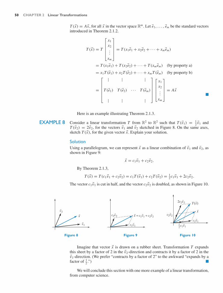
50 CHAPTER 2 Linear Transformations
T (x) = Ax , for all x in the vector space Rm . Let e1, . . . , em be the standard vectorsintroduced in Theorem 2.1.2.
T (x) = T
⎡
⎢⎢⎢⎣
x1
x2...
xm
⎤
⎥⎥⎥⎦= T (x1e1 + x2e2 + · · · + xmem)
= T (x1e1) + T (x2e2) + · · · + T (xmem) (by property a)
= x1T (e1) + x2T (e2) + · · · + xm T (em) (by property b)
=
⎡
⎢⎢⎢⎢⎣
| | |
T (e1) T (e2) · · · T (em)
| | |
⎤
⎥⎥⎥⎥⎦
⎡
⎢⎢⎢⎣
x1
x2...
xm
⎤
⎥⎥⎥⎦= Ax !
Here is an example illustrating Theorem 2.1.3.
EXAMPLE 8 Consider a linear transformation T from R2 to R2 such that T (v1) = 12 v1 and
T (v2) = 2v2, for the vectors v1 and v2 sketched in Figure 8. On the same axes,sketch T (x), for the given vector x . Explain your solution.
SolutionUsing a parallelogram, we can represent x as a linear combination of v1 and v2, asshown in Figure 9:
x = c1v1 + c2v2.
By Theorem 2.1.3,
T (x) = T (c1v1 + c2v2) = c1T (v1) + c2T (v2) = 12 c1v1 + 2c2v2.
The vector c1v1 is cut in half, and the vector c2v2 is doubled, as shown in Figure 10.
v2
v1
x
Figure 8
c2v2
c1v1
x = c1v1 + c2v2
Figure 9
2c2v2
c2v2
c1v1
x
T(x)
c1v112
Figure 10
Imagine that vector x is drawn on a rubber sheet. Transformation T expandsthis sheet by a factor of 2 in the v2-direction and contracts it by a factor of 2 in thev1-direction. (We prefer “contracts by a factor of 2” to the awkward “expands by afactor of 1
2 .”) !We will conclude this section with one more example of a linear transformation,
from computer science.

2.1 Introduction to Linear Transformations and Their Inverses 51
EXAMPLE 9 Let’s develop a simple model of how people might surf the World Wide Web, byfollowing links. To keep things manageable, we consider a “mini-Web” with onlyfour pages, labeled 1, 2, 3, 4, linked as shown in the diagram below:
1 ! 2
↓ ↑3 → 4.
Let x1, x2, x3, and x4 be the proportions of the surfers who find themselves on eachof the four pages initially; we can collect this information in the distribution vector
x =
⎡
⎢⎢⎣
x1
x2
x3
x4
⎤
⎥⎥⎦. For example, the initial distribution might be x =
⎡
⎢⎢⎣
0.40.10.30.2
⎤
⎥⎥⎦,
meaning that 40% of the surfers are on page 1, and so forth. The components of adistribution vector add up to 1, or 100%, of course.
At a predetermined time, at the blow of a whistle, each surfer will randomlyfollow one of the links: If several links are available out of a web page, then an equalproportion of the surfers will follow each of them. For example, the proportion ofsurfers taking each of the two links out of page 1 (to pages 2 and 3) will be x1
2 .Let the vector y, with components y1, y2, y3, y4, represent the distribution of
the surfers after the transition. According to the rules stated above, we will have
y1 = 12 x2
y2 = 12 x1 + x4
y3 = 12 x1 + 1
2 x2
y4 = x3
,
or y = Ax in vector form, where
A =
⎡
⎢⎢⎢⎢⎣
0 12 0 0
12 0 0 112
12 0 0
0 0 1 0
⎤
⎥⎥⎥⎥⎦,
showing that y = T (x) is a linear transformation. Matrix A is referred to as thetransition matrix of this transformation.
For example, the equation y2 = 12 x1 + x4 reflects the fact that half of the surfers
from page 1 and all of the surfers from page 4 will follow the links to page 2.Alternatively, we can construct the matrix A column by column. The j th col-
umn of A tells us where the surfers go from page j . For example, the second columnof A is
⎡
⎢⎢⎢⎣
12
012
0
⎤
⎥⎥⎥⎦,
indicating that half of the surfers from page 2 take the link to page 1, and the otherhalf go to page 3. Thus, the entries in each column of A must add up to 1.
Let’s discuss the structure of matrix A more formally. Let c j be the numberof links going out of page j . For example, we have c2 = 2 and c3 = 1 for our

52 CHAPTER 2 Linear Transformations
mini-Web. Then the proportion of the surfers taking a link from page j to page iwill be x j
c j, since the initial population x j of page j gets distributed equally among
the c j outgoing links. We see that the i j th entry of A is 1c j
if there is a link frompage j to page i ; the other entries are 0. Thus, we have
ai j =
1/c j if there is a link j → i0 otherwise.
We might wonder whether this system has any equilibrium distributions, that is,distributions x such that Ax = x . The distribution after the transition is required tobe exactly the same as before. To find out, we have to solve the linear system∣∣∣∣∣∣∣∣∣∣∣
12 x2 = x1
12 x1 + x4 = x2
12 x1 + 1
2 x2 = x3
x3 = x4
∣∣∣∣∣∣∣∣∣∣∣
or
∣∣∣∣∣∣∣∣∣∣∣
−x1 + 12 x2 = 0
12 x1 − x2 + x4 = 012 x1 + 1
2 x2 − x3 = 0
x3 − x4 = 0
∣∣∣∣∣∣∣∣∣∣∣
with augmented matrix M =
⎡
⎢⎢⎢⎢⎣
−1 12 0 0 0
12 −1 0 1 012
12 −1 0 0
0 0 1 −1 0
⎤
⎥⎥⎥⎥⎦and rref(M) =
⎡
⎢⎢⎣
1 0 0 −2/3 00 1 0 −4/3 00 0 1 −1 00 0 0 0 0
⎤
⎥⎥⎦. The solutions are x1 = 2t3 , x2 = 4t
3 , x3 = x4 = t ,
where t is an arbitrary real number. Since we are looking for a distribution vector,we want x1 + x2 + x3 + x4 = 4t = 1, so t = 1
4 . The equilibrium distribution is
xequ =
⎡
⎢⎢⎢⎣
1/61/31/41/4
⎤
⎥⎥⎥⎦≈
⎡
⎢⎢⎢⎣
16.7%33.3%25%25%
⎤
⎥⎥⎥⎦.
In this context, an interesting question arises: If we iterate our transition, lettingthe surfers move to a new page over and over again, following links at random,will the system eventually approach this equilibrium state xequ , regardless of theinitial distribution? Perhaps surprisingly, the answer is affirmative for the mini-Webconsidered in this example, as well as for many others: The equilibrium distributionrepresents the distribution of the surfers in the long run, for any initial distribution.We will further discuss these important issues in Theorem 2.3.11 and then again inChapter 7.
In 1998, Sergey Brin and Lawrence Page, then at Stanford University, publisheda landmark paper, “The Anatomy of a Large-Scale Hypertextual Search Engine,”where they present a prototype of the search engine Google. The key feature of thissearch engine is a “quality ranking” of each web page, which measures its “linkpopularity.” They call this ranking PageRank, after the second author of the paper.
The basic idea is to define the popularity of a web page as the likelihood thatrandom surfers find themselves on that web page in the long run. But this is exactlythe corresponding component of the equilibrium vector xequ we found above. In ourexample, page 2 is the most popular, with a PageRank of 1/3, while page 1 is onlyhalf as popular, with a PageRank of 1/6.
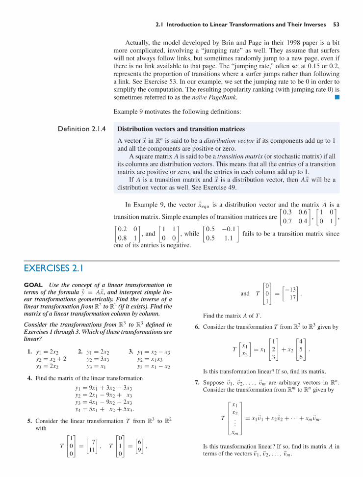
2.1 Introduction to Linear Transformations and Their Inverses 53
Actually, the model developed by Brin and Page in their 1998 paper is a bitmore complicated, involving a “jumping rate” as well. They assume that surferswill not always follow links, but sometimes randomly jump to a new page, even ifthere is no link available to that page. The “jumping rate,” often set at 0.15 or 0.2,represents the proportion of transitions where a surfer jumps rather than followinga link. See Exercise 53. In our example, we set the jumping rate to be 0 in order tosimplify the computation. The resulting popularity ranking (with jumping rate 0) issometimes referred to as the naıve PageRank. !Example 9 motivates the following definitions:
Definition 2.1.4 Distribution vectors and transition matrices
A vector x in Rn is said to be a distribution vector if its components add up to 1and all the components are positive or zero.
A square matrix A is said to be a transition matrix (or stochastic matrix) if allits columns are distribution vectors. This means that all the entries of a transitionmatrix are positive or zero, and the entries in each column add up to 1.
If A is a transition matrix and x is a distribution vector, then Ax will be adistribution vector as well. See Exercise 49.
In Example 9, the vector xequ is a distribution vector and the matrix A is a
transition matrix. Simple examples of transition matrices are[
0.3 0.60.7 0.4
],[
1 00 1
],
[0.2 00.8 1
], and
[1 10 0
], while
[0.5 −0.10.5 1.1
]fails to be a transition matrix since
one of its entries is negative.
EXERCISES 2.1
GOAL Use the concept of a linear transformation interms of the formula y = Ax , and interpret simple lin-ear transformations geometrically. Find the inverse of alinear transformation from R2 to R2 (if it exists). Find thematrix of a linear transformation column by column.
Consider the transformations from R3 to R3 defined inExercises 1 through 3. Which of these transformations arelinear?
1. y1 = 2x2y2 = x2 + 2y3 = 2x2
2. y1 = 2x2y2 = 3x3y3 = x1
3. y1 = x2 − x3y2 = x1x3y3 = x1 − x2
4. Find the matrix of the linear transformation
y1 = 9x1 + 3x2 − 3x3y2 = 2x1 − 9x2 + x3y3 = 4x1 − 9x2 − 2x3y4 = 5x1 + x2 + 5x3.
5. Consider the linear transformation T from R3 to R2
with
T
⎡
⎣100
⎤
⎦ =[
711
], T
⎡
⎣010
⎤
⎦ =[
69
],
and T
⎡
⎣001
⎤
⎦ =[−13
17
].
Find the matrix A of T .
6. Consider the transformation T from R2 to R3 given by
T[
x1x2
]= x1
⎡
⎣123
⎤
⎦ + x2
⎡
⎣456
⎤
⎦ .
Is this transformation linear? If so, find its matrix.
7. Suppose v1, v2, . . . , vm are arbitrary vectors in Rn .Consider the transformation from Rm to Rn given by
T
⎡
⎢⎢⎢⎣
x1x2...
xm
⎤
⎥⎥⎥⎦= x1v1 + x2v2 + · · · + xm vm .
Is this transformation linear? If so, find its matrix A interms of the vectors v1, v2, . . . , vm .

54 CHAPTER 2 Linear Transformations
8. Find the inverse of the linear transformationy1 = x1 + 7x2y2 = 3x1 + 20x2.
In Exercises 9 through 12, decide whether the given ma-trix is invertible. Find the inverse if it exists. In Exercise12, the constant k is arbitrary.
9.[
2 36 9
]10.
[1 24 9
]
11.[
1 23 9
]12.
[1 k0 1
]
13. Prove the following facts:a. The 2 × 2 matrix
A =[
a bc d
]
is invertible if and only if ad − bc = 0. Hint: Con-sider the cases a = 0 and a = 0 separately.
b. If[
a bc d
]
is invertible, then[
a bc d
]−1
= 1ad − bc
[d −b
−c a
].
[The formula in part (b) is worth memorizing.]
14. a. For which values of the constant k is the matrix[2 35 k
]invertible?
b. For which values of the constant k are all entries of[2 35 k
]−1
integers?
See Exercise 13.
15. For which values of the constants a and b is the matrix
A =[
a −bb a
]
invertible? What is the inverse in this case? See Exer-cise 13.
Give a geometric interpretation of the linear transforma-tions defined by the matrices in Exercises 16 through 23.Show the effect of these transformations on the letter Lconsidered in Example 5. In each case, decide whether thetransformation is invertible. Find the inverse if it exists,and interpret it geometrically. See Exercise 13.
16.[
3 00 3
]17.
[−1 0
0 −1
]18.
[0.5 0
0 0.5
]
19.[
1 00 0
]20.
[0 11 0
]21.
[0 1
−1 0
]
22.[
1 00 −1
]23.
[0 2
−2 0
]
Consider the circular face in the accompanying figure. Foreach of the matrices A in Exercises 24 through 30, drawa sketch showing the effect of the linear transformationT(x) = Ax on this face.
1
1
24.[
0 −11 0
]25.
[2 00 2
]26.
[0 11 0
]
27.[
1 00 −1
]28.
[1 00 2
]29.
[−1 0
0 −1
]
30.[
0 00 1
]
31. In Chapter 1, we mentioned that an old German billshows the mirror image of Gauss’s likeness. What lineartransformation T can you apply to get the actual pictureback?
32. Find an n × n matrix A such that Ax = 3x , for all xin Rn .
33. Consider the transformation T from R2 to R2 thatrotates any vector x through an angle of 45 in the coun-terclockwise direction, as shown in the following figure:
T(x)
x45°
You are told that T is a linear transformation. (This willbe shown in the next section.) Find the matrix of T .
34. Consider the transformation T from R2 to R2 that ro-tates any vector x through a given angle θ in the coun-terclockwise direction. Compare this with Exercise 33.You are told that T is linear. Find the matrix of T interms of θ .

2.1 Introduction to Linear Transformations and Their Inverses 55
35. In the example about the French coast guard in this sec-tion, suppose you are a spy watching the boat and listen-ing in on the radio messages from the boat. You collectthe following data:
• When the actual position is[
542
], they radio
[8952
].
• When the actual position is[
641
], they radio
[8853
].
Can you crack their code (i.e., find the coding matrix),assuming that the code is linear?
36. Let T be a linear transformation from R2 to R2. Let v1,v2, and w be three vectors in R2, as shown below. Weare told that T (v1) = v1 and T (v2) = 3v2. On the sameaxes, sketch T (w).
v2
v1
w
37. Consider a linear transformation T from R2 to R2. Sup-pose that v and w are two arbitrary vectors in R2 andthat x is a third vector whose endpoint is on the linesegment connecting the endpoints of v and w. Is theendpoint of the vector T (x) necessarily on the line seg-ment connecting the endpoints of T (v) and T (w)? Jus-tify your answer.
T(x )
T(w)
T(v)
w
x
v
T
Hint: We can write x = v + k(w − v), for some scalark between 0 and 1.
We can summarize this exercise by saying that alinear transformation maps a line onto a line.
38. The two column vectors v1 and v2 of a 2 × 2matrix A are shown in the accompanying sketch. Con-sider the linear transformation T (x) = Ax , from R2 toR2. Sketch the vector
T[
2−1
].
v1v2
O
39. Show that if T is a linear transformation from Rm toRn , then
T
⎡
⎢⎢⎢⎣
x1x2...
xm
⎤
⎥⎥⎥⎦= x1T (e1) + x2T (e2) + · · · + xm T (em),
where e1, e2, . . . , em are the standard vectors in Rm .
40. Describe all linear transformations from R (= R1) to R.What do their graphs look like?
41. Describe all linear transformations from R2 to R(= R1). What do their graphs look like?
42. When you represent a three-dimensional object graphi-cally in the plane (on paper, the blackboard, or a com-puter screen), you have to transform spatial coordinates,
⎡
⎣x1x2x3
⎤
⎦ ,
into plane coordinates,[
y1y2
]. The simplest choice is a
linear transformation, for example, the one given by thematrix
⎡
⎣− 12 1 0
− 12 0 1
⎤
⎦ .
a. Use this transformation to represent the unit cubewith corner points
⎡
⎣000
⎤
⎦ ,
⎡
⎣100
⎤
⎦ ,
⎡
⎣010
⎤
⎦ ,
⎡
⎣001
⎤
⎦ ,
⎡
⎣110
⎤
⎦ ,
⎡
⎣011
⎤
⎦ ,
⎡
⎣101
⎤
⎦ ,
⎡
⎣111
⎤
⎦ .
Include the images of the x1, x2, and x3 axes in yoursketch:
y2
y1−1
−1
1
1
b. Represent the image of the point
⎡
⎢⎢⎣
11212
⎤
⎥⎥⎦ in your fig-
ure in part (a).(part c on next page)

56 CHAPTER 2 Linear Transformations
c. Find all the points⎡
⎣x1x2x3
⎤
⎦ in R3
that are transformed to[
00
]. Explain.
43. a. Consider the vector v =
⎡
⎣234
⎤
⎦. Is the transformation
T (x) = v · x (the dot product) from R3 to R linear?If so, find the matrix of T .
b. Consider an arbitrary vector v in R3. Is the transfor-mation T (x) = v · x linear? If so, find the matrix ofT (in terms of the components of v).
c. Conversely, consider a linear transformation T fromR3 to R. Show that there exists a vector v in R3 suchthat T (x) = v · x , for all x in R3.
44. The cross product of two vectors in R3 is given by⎡
⎣a1a2a3
⎤
⎦ ×
⎡
⎣b1b2b3
⎤
⎦ =
⎡
⎣a2b3 − a3b2a3b1 − a1b3a1b2 − a2b1
⎤
⎦ .
See Definition A.9 and Theorem A.11 in theAppendix. Consider an arbitrary vector v in R3. Is thetransformation T (x) = v × x from R3 to R3 linear?If so, find its matrix in terms of the components of thevector v.
45. Consider two linear transformations y = T (x) andz = L(y), where T goes from Rm to Rp and L goesfrom Rp to Rn . Is the transformation z = L
(T (x)
)lin-
ear as well? [The transformation z = L(T (x)
)is called
the composite of T and L .]
46. Let
A =[
a bc d
]and B =
[p qr s
].
Find the matrix of the linear transformation T (x) =B(Ax). See Exercise 45. Hint: Find T (e1) and T (e2).
47. Let T be a linear transformation from R2 to R2. Threevectors v1, v2, w in R2 and the vectors T (v1), T (v2)are shown in the accompanying figure. Sketch T (w).Explain your answer.
w
x2
x1
T
v1
v2
y2
y1
T(v1)
T(v2)
48. Consider two linear transformations T and L from R2
to R2. We are told that T (v1) = L(v1) and T (v2) =L(v2) for the vectors v1 and v2 sketched below. Showthat T (x) = L(x), for all vectors x in R2.
v1
v2
49. Prove that if A is a transition matrix and x is a distribu-tion vector, then Ax is a distribution vector as well.
For each of the mini-Webs in Exercises 50 through 52,a. find the transition matrix A as defined in Example 9,b. find the equilibrium distribution, andc. find the web page(s) with the highest (naıve) Page-
Rank.Feel free to use technology throughout.
50. 1 ! 2↓ ↑3 → 4
51. 1 → 2
! !
3 ! 4
52. 1 ! 2↓ 3
53. As in Example 9, consider the mini-Web with the linkstructure shown in the diagram below:
1 ! 2↓ ↑3 → 4.
Again, let vector x represent the distribution of surfersamong the various pages at a given time. Following the1998 paper by Brin and Page (see Example 9), we con-sider a more sophisticated model of transition: At theblow of a whistle, 80% of the surfers on a given pagewill randomly follow a link, while the remaining 20%will randomly “jump” to a web page (even if no link isavailable). The jumpers have the option to stay on thecurrent page. For example, of the surfers that are ini-tially on page 2, 40% will follow the link to page 1,40% will follow the link to page 3, and 5% will jump toany of the four webpages. If we add up the jumpers andthe link-followers, we see that 45% will move to page 1;another 45% go to page 3; 5% will jump to page 4; and5% will stay put on page 2. Thus, the second column ofthe transition matrix B will be

2.1 Introduction to Linear Transformations and Their Inverses 57
⎡
⎢⎢⎣
0.4 + 0.050.05
0.4 + 0.050.05
⎤
⎥⎥⎦ =
⎡
⎢⎢⎣
0.450.050.450.05
⎤
⎥⎥⎦ .
↑ link jumpers
followers
Let y be the distribution vector after the transition; wehave y2 = 0.45x1 + 0.05x2 + 0.05x3 + 0.85x4, forexample.a. Find the transition matrix B such that y = Bx .b. Explain why B = 0.2
N E + 0.8A = 0.05E + 0.8A,where A is the matrix we found in Example 9, E isthe matrix whose entries are all 1, and N is the totalnumber of web pages.
c. Find the equilibrium distribution xequ , such thatBxequ = xequ . Feel free to use technology. (Thecomponents of this equilibrium solution representthe PageRank of the various web pages, as definedin the 1998 paper by Brin and Page.)
For each of the mini-Webs in Exercises 54 through 56,a. find the transition matrix B as defined in Exercise
53 (with a jumping rate of 20%),b. find the equilibrium distribution for the transition
matrix B, andc. find the web page(s) with the highest PageRank
(with a jumping rate of 20%).Feel free to use technology throughout.
54. 1 ! 2↓ ↑3 → 4
55. 1 → 2
! !
3 ! 4
56. 1 ! 2↓ 3
57. Some parking meters in downtown Geneva, Switzer-land, accept 2 Franc and 5 Franc coins.a. A parking officer collects 51 coins worth 144
Francs. How many coins are there of each kind?b. Find the matrix A that transforms the vector
[number of 2 Franc coinsnumber of 5 Franc coins
]
into the vector[
total value of coinstotal number of coins
].
c. Is the matrix A in part (b) invertible? If so, find theinverse (use Exercise 13). Use the result to checkyour answer in part (a).
58. A goldsmith uses a platinum alloy and a silver alloy tomake jewelry; the densities of these alloys are exactly20 and 10 grams per cubic centimeter, respectively.a. King Hiero of Syracuse orders a crown from this
goldsmith, with a total mass of 5 kilograms (or5,000 grams), with the stipulation that the platinumalloy must make up at least 90% of the mass. Thegoldsmith delivers a beautiful piece, but the king’sfriend Archimedes has doubts about its purity. Whiletaking a bath, he comes up with a method to checkthe composition of the crown (famously shouting“Eureka!” in the process, and running to the king’spalace naked). Submerging the crown in water, hefinds its volume to be 370 cubic centimeters. Howmuch of each alloy went into this piece (by mass)?Is this goldsmith a crook?
b. Find the matrix A that transforms the vector
[mass of platinum alloy
mass of silver alloy
]
into the vector[
total masstotal volume
],
for any piece of jewelry this goldsmith makes.c. Is the matrix A in part (b) invertible? If so, find the
inverse (use Exercise 13). Use the result to checkyour answer in part (a).
59. The conversion formula C = 59 (F − 32) from
Fahrenheit to Celsius (as measures of temperature) isnonlinear, in the sense of linear algebra (why?). Still,there is a technique that allows us to use a matrix torepresent this conversion.a. Find the 2 × 2 matrix A that transforms the vector[
F1
]into the vector
[C1
]. (The second row of A
will be[
0 1].)
b. Is the matrix A in part (a) invertible? If so, find theinverse (use Exercise 13). Use the result to write aformula expressing F in terms of C .
60. In the financial pages of a newspaper, one can some-times find a table (or matrix) listing the exchange ratesbetween currencies. In this exercise we will considera miniature version of such a table, involving onlythe Canadian dollar (C$) and the South African Rand(ZAR). Consider the matrix
A =[ C$ ZAR
1 1/88 1
]C$
ZAR

58 CHAPTER 2 Linear Transformations
representing the fact that C$1 is worth ZAR8 (as ofSeptember 2012).a. After a trip you have C$100 and ZAR1,600 in your
pocket. We represent these two values in the vec-
tor x =[
1001,600
]. Compute Ax . What is the practi-
cal significance of the two components of the vectorAx?
b. Verify that matrix A fails to be invertible. For whichvectors b is the system Ax = b consistent? Whatis the practical significance of your answer? If thesystem Ax = b is consistent, how many solutions xare there? Again, what is the practical significanceof the answer?
61. Consider a larger currency exchange matrix (see Exer-cise 60), involving four of the world’s leading curren-cies: Euro (C), U.S. dollar ($), Chinese yuan (¥), andBritish pound (£ ).
A =
⎡
⎢⎣
C $ ¥ £∗ 0.8 ∗ ∗∗ ∗ ∗ ∗∗ ∗ ∗ 10
0.8 ∗ ∗ ∗
⎤
⎥⎦
C$¥£
The entry ai j gives the value of one unit of the j thcurrency, expressed in terms of the i th currency. Forexample, a34 = 10 means that £1 = ¥10 (as ofAugust 2012). Find the exact values of the 13 missingentries of A (expressed as fractions).
62. Consider an arbitrary currency exchange matrix A. SeeExercises 60 and 61.a. What are the diagonal entries aii of A?b. What is the relationship between ai j and a ji ?c. What is the relationship among aik , ak j , and ai j ?d. What is the rank of A? What is the relationship
between A and rref(A)?
63. Solving a linear system Ax = 0 by Gaussian elimina-tion amounts to writing the vector of leading variablesas a linear transformation of the vector of free variables.Consider the linear system
x1 − x2 + 4x5 = 0x3 − x5 = 0
x4 − 2x5 = 0.
Find the matrix B such that
⎡
⎣x1x3x4
⎤
⎦ = B[
x2x5
].
64. Consider the linear system
x1 + 2x2 + x3 + 7x4 = 0
x1 + 2x2 + 2x3 + 11x4 = 0
x1 + 2x2 + 3x3 + 15x4 = 0
x1 + 2x2 + 4x3 + 19x4 = 0.
Find the matrix B such that[
x1x3
]= B
[x2x4
]. See
Exercise 63.
2.2 Linear Transformations in Geometry
In Example 2.1.5 we saw that the matrix[
0 −11 0
]represents a counterclockwise
rotation through 90 in the coordinate plane. Many other 2 × 2 matrices definesimple geometrical transformations as well; this section is dedicated to a discussionof some of those transformations.
EXAMPLE 1 Consider the matrices
A =[
2 00 2
], B =
[1 00 0
], C =
[−1 0
0 1
],
D =[
0 1−1 0
], E =
[1 0.20 1
], and F =
[1 −11 1
].
Show the effect of each of these matrices on our standard letter L,3 and describeeach transformation in words.
3See Example 2.1.5. Recall that vector[
10
]is the foot of our standard L, and
[02
]is its back.

2.2 Linear Transformations in Geometry 59
a.
02
10
04
20
20
02A =
The L gets enlarged by a factor of 2; we will call this transformation a scal-ing by 2.
b.
02
10
10
10
00B =
The L gets smashed into the horizontal axis. We will call this transformationthe orthogonal projection onto the horizontal axis.
c.
02
10
02
−10
−10
01C =
The L gets flipped over the vertical axis. We will call this the reflection aboutthe vertical axis.
d.
02
10
0−1
10D =
0−1
20

60 CHAPTER 2 Linear Transformations
The L is rotated through 90, in the clockwise direction (this amounts to arotation through −90). The result is the opposite of what we got in Exam-ple 2.1.5.
e.
02
10
0.42
10
10
0.21E =
The foot of the L remains unchanged, while the back is shifted horizontallyto the right; the L is italicized, becoming L. We will call this transformationa horizontal shear.
f.
02
10
−22
11
11
−11F =
There are two things going on here: The L is rotated through 45 and also enlarged(scaled) by a factor of
√2. This is a rotation combined with a scaling (you may
perform the two transformations in either order). Among all the possible compositesof the transformations considered in parts (a) through (e), this one is particularlyimportant in applications as well as in pure mathematics. See Theorem 7.5.3, forexample. !
We will now take a closer look at the six types of transformations we encoun-tered in Example 1.
ScalingsFor any positive constant k, the matrix
[k 00 k
]defines a scaling by k, since
[k 00 k
]x =
[k 00 k
] [x1
x2
]=
[kx1
kx2
]= k
[x1
x2
]= kx .
This is a dilation (or enlargement) if k exceeds 1, and it is a contraction (orshrinking) for values of k between 0 and 1. (What happens when k is negative orzero?)

2.2 Linear Transformations in Geometry 61
Orthogonal Projections4
Consider a line L in the plane, running through the origin. Any vector x in R2 canbe written uniquely as
x = x∥ + x⊥,
where x∥ is parallel to line L , and x⊥ is perpendicular to L . See Figure 1.
xll
x⊥ (translated)
x
O
L
Figure 1
xllx⊥
L⊥
x
O
L
Figure 2
The transformation T (x) = x∥ from R2 to R2 is called the orthogonal projec-tion of x onto L , often denoted by projL(x):
projL(x) = x∥.
You can think of projL(x) as the shadow that vector x casts on L if you shine a lightstraight down on L .
Let L⊥ be the line through the origin perpendicular to L . Note that x⊥ is par-allel to L⊥, and we can interpret x⊥ as the orthogonal projection of x onto L⊥, asillustrated in Figure 2.
We can use the dot product to write a formula for an orthogonal projection.Before proceeding, you may want to review the section “Dot Product, Length,Orthogonality” in the Appendix.
To find a formula for x∥, let w be a nonzero vector parallel to L . Since x∥ isparallel to w, we can write
x∥ = kw,
for some scalar k about to be determined. Now x⊥ = x − x∥ = x − kw is perpen-dicular to line L , that is, perpendicular to w, meaning that
(x − kw) · w = 0.
It follows that
x · w − k(w · w) = 0, or k = x · w
w · w.
We can conclude that
projL(x) = x∥ = kw =(
x · w
w · w
)w.
4The term orthogonal is synonymous with perpendicular. For a more general discussion ofprojections, see Exercise 33.

62 CHAPTER 2 Linear Transformations
See Figure 3. Consider the special case of a unit vector u parallel to L . Then theformula for projection simplifies to
projL(x) =(
x · uu · u
)u = (x · u)u
since u · u = ∥u∥2 = 1 for a unit vector u.
xll = projL(x) =
x⊥ = x − xll (translated)
x
O
L
w
wx ⋅ ww ⋅ w
Figure 3
Is the transformation T (x) = projL(x) linear? If so, what is its matrix? If we write
x =[
x1
x2
]and u =
[u1
u2
],
then
projL(x) = (x · u)u =([
x1
x2
]·[
u1
u2
]) [u1
u2
]
= (x1u1 + x2u2)
[u1
u2
]
=[
u21x1 + u1u2x2
u1u2x1 + u22x2
]
=[
u21 u1u2
u1u2 u22
] [x1
x2
]
=[
u21 u1u2
u1u2 u22
]x .
It turns out that T (x) = projL(x) is indeed a linear transformation, with matrix[u2
1 u1u2
u1u2 u22
]. More generally, if w is a nonzero vector parallel to L , then the
matrix is P = 1w2
1 + w22
[w2
1 w1w2
w1w2 w22
]. See Exercise 12.
EXAMPLE 2 Find the matrix P of the orthogonal projection onto the line L spanned by w =[
34
].
Solution
P = 1w2
1 + w22
[w2
1 w1w2
w1w2 w22
]= 1
25
[9 12
12 16
]=
[0.36 0.480.48 0.64
]!
Let us summarize our findings.

2.2 Linear Transformations in Geometry 63
Definition 2.2.1 Orthogonal Projections
Consider a line L in the coordinate plane, running through the origin. Any vectorx in R2 can be written uniquely as
x = x∥ + x⊥,
where x∥ is parallel to line L , and x⊥ is perpendicular to L .The transformation T (x) = x∥ from R2 to R2 is called the orthogonal pro-
jection of x onto L , often denoted by projL(x). If w is a nonzero vector parallelto L, then
projL(x) =(
x · w
w · w
)w.
In particular, if u =[
u1
u2
]is a unit vector parallel to L, then
projL(x) = (x · u)u.
The transformation T (x) = projL(x) is linear, with matrix
P = 1w2
1 + w22
[w2
1 w1w2
w1w2 w22
]=
[u2
1 u1u2
u1u2 u22
].
ReflectionsAgain, consider a line L in the coordinate plane, running through the origin, and letx be a vector in R2. The reflection refL(x) of x about L is shown in Figure 4: Weare flipping vector x over the line L . The line segment joining the tips of vectorsx and refL x is perpendicular to line L and bisected by L. In previous math coursesyou have surely seen examples of reflections about the horizontal and vertical axes[when comparing the graphs of y = f (x), y = − f (x), and y = f (−x), forexample].
We can use the representation x = x∥ + x⊥ to write a formula for refL(x). SeeFigure 4.
x
xll
O
L
x⊥ (translated)
−x⊥ (translated)
refL(x)
Figure 4
We can see that
refL(x) = x∥ − x⊥.
Adding up the equations x = x∥ + x⊥ and refL(x) = x∥ − x⊥, we find that x +refL(x) = 2x∥ = 2projL(x), so
refL(x) = 2projL(x) − x = 2Px − x = (2P − I2)x,

64 CHAPTER 2 Linear Transformations
where P is the matrix representing the orthogonal projection onto the line L . SeeDefinition 2.2.1. Thus, the matrix S of the reflection is
S = 2P − I2 =[
2u21 2u1u2
2u1u2 2u22
]−
[1 00 1
]=
[2u2
1 − 1 2u1u22u1u2 2u2
2 − 1
],
It turns out that this matrix S is of the form[
a bb −a
], where a2 + b2 = 1 (we leave
the straightforward verification as Exercise 13). Conversely, any matrix of the form[a bb −a
], with a2 + b2 = 1, represents a reflection about a line. See Exercise 17.
We are not surprised to see that the column vectors[
ab
]and
[b
−a
]of a re-
flection matrix are unit vectors, with a2 + b2 = b2 + (−a)2 = 1. Indeed, the
column vectors are the reflections of the standard vectors,[
ab
]= refL(e1) and
[b
−a
]= refL(e2), by Theorem 2.1.2. Since the standard vectors e1 and e2 are unit
vectors and a reflection preserves length, these column vectors will be unit vectorsas well. Also, it makes sense that the column vectors are perpendicular, with dot
product[
ab
]·[
b−a
]= ab + b(−a) = 0, since the reflection preserves the right
angle between e1 and e2. See Figure 5.
refL(e2)bL
–a= refL(e1)a
b=
e1
e2
Figure 5
Definition 2.2.2 Reflections
Consider a line L in the coordinate plane, running through the origin, and letx = x∥ + x⊥ be a vector in R2. The linear transformation T (x) = x∥ − x⊥ iscalled the reflection of x about L , often denoted by refL(x):
refL(x) = x∥ − x⊥.
We have a formula relating refL(x) to projL(x):
refL(x) = 2projL(x) − x = 2(x · u)u − x .
The matrix of T is of the form[
a bb −a
], where a2 + b2 = 1. Conversely, any
matrix of this form represents a reflection about a line.

2.2 Linear Transformations in Geometry 65
Use Figure 6 to explain the formula refL(x) = 2projL(x) − x geometrically.
x
O
L
refL(x)
projL(x)
Figure 6
Orthogonal Projections and Reflections in SpaceAlthough this section is mostly concerned with linear transformations from R2 toR2, we will take a quick look at orthogonal projections and reflections in space,since this theory is analogous to the case of two dimensions.
Let L be a line in coordinate space, running through the origin. Any vector xin R3 can be written uniquely as x = x∥ + x⊥, where x∥ is parallel to L , and x⊥ isperpendicular to L . We define
projL(x) = x∥,
and we have the formula
projL(x) = x∥ = (x · u)u,
where u is a unit vector parallel to L . See Definition 2.2.1.Let L⊥ = V be the plane through the origin perpendicular to L; note that the
vector x⊥ will be parallel to L⊥ = V . We can give formulas for the orthogonalprojection onto V , as well as for the reflections about V and L , in terms of theorthogonal projection onto L:
projV (x) = x − projL(x) = x − (x · u)u,
refL(x) = projL(x) − projV (x) = 2projL(x) − x = 2(x · u)u − x, and
refV (x) = projV (x) − projL(x) = −refL(x) = x − 2(x · u)u.
See Figure 7, and compare with Definition 2.2.2.
x
O V = L⊥
L
projL(x)
projV(x)
Figure 7

66 CHAPTER 2 Linear Transformations
EXAMPLE 3 Let V be the plane defined by 2x1 +x2 −2x3 = 0, and let x =
⎡
⎣54
−2
⎤
⎦. Find refV (x).
SolutionNote that the vector v =
⎡
⎣21
−2
⎤
⎦ is perpendicular to plane V (the components of v
are the coefficients of the variables in the given equation of the plane: 2, 1, and −2).Thus,
u = 1∥v∥
v = 13
⎡
⎣21
−2
⎤
⎦
is a unit vector perpendicular to V , and we can use the formula we derived earlier:
refV (x) = x − 2(x · u)u =
⎡
⎣54
−2
⎤
⎦ − 29
⎛
⎝
⎡
⎣54
−2
⎤
⎦ ·
⎡
⎣21
−2
⎤
⎦
⎞
⎠
⎡
⎣21
−2
⎤
⎦
=
⎡
⎣54
−2
⎤
⎦ − 4
⎡
⎣21
−2
⎤
⎦
=
⎡
⎣54
−2
⎤
⎦ −
⎡
⎣84
−8
⎤
⎦
=
⎡
⎣−3
06
⎤
⎦ . !
RotationsConsider the linear transformation T from R2 to R2 that rotates any vector x througha fixed angle θ in the counterclockwise direction,5 as shown in Figure 8. RecallExample 2.1.5, where we studied a rotation through θ = π/2.
x
T (x)
Figure 8
x
y
T (x)
Figure 9
5We can define a rotation more formally in terms of the polar coordinates of x . The length of T (x)equals the length of x , and the polar angle (or argument) of T (x) exceeds the polar angle of x by θ .

2.2 Linear Transformations in Geometry 67
Now consider Figure 9, where we introduce the auxiliary vector y, obtained
by rotating x through π/2. From Example 2.1.5 we know that if x =[
x1
x2
], then
y =[−x2
x1
]. Using basic trigonometry, we find that
T (x) = (cos θ)x + (sin θ)y = (cos θ)
[x1
x2
]+ (sin θ)
[−x2
x1
]
=[(cos θ)x1 − (sin θ)x2
(sin θ)x1 + (cos θ)x2
]
=[
cos θ − sin θ
sin θ cos θ
] [x1
x2
]
=[
cos θ − sin θ
sin θ cos θ
]x .
This computation shows that a rotation through θ is indeed a linear transformation,with the matrix
[cos θ − sin θ
sin θ cos θ
].
Theorem 2.2.3 Rotations
The matrix of a counterclockwise rotation in R2 through an angle θ is[
cos θ − sin θ
sin θ cos θ
].
Note that this matrix is of the form[
a −bb a
], where a2 + b2 = 1. Conversely,
any matrix of this form represents a rotation.
EXAMPLE 4 The matrix of a counterclockwise rotation through π/6 (or 30) is[
cos(π/6) − sin(π/6)
sin(π/6) cos(π/6)
]= 1
2
[√3 −11
√3
]. !
Rotations Combined with a Scaling
EXAMPLE 5 Examine how the linear transformation
T (x) =[
a −bb a
]x
affects our standard letter L. Here a and b are arbitrary constants.
SolutionFigure 10 suggests that T represents a rotation combined with a scaling. Think polar
coordinates: This is a rotation through the polar angle θ of vector[
ab
], combined

68 CHAPTER 2 Linear Transformations
with a scaling by the magnitude r =√
a2 + b2 of vector[
ab
]. To verify this claim
algebraically, we can write the vector[
ab
]in polar coordinates, as
[ab
]=
[r cos θ
r sin θ
],
02
10
−2b2a
ab
ab
−ba
Figure 10
as illustrated in Figure 11. Then[
a −bb a
]=
[r cos θ −r sin θ
r sin θ r cos θ
]= r
[cos θ − sin θ
sin θ cos θ
].
It turns out that matrix[
a −bb a
]is a scalar multiple of a rotation matrix, as
claimed. !
ab
r sin
r cos
r
Figure 11
Theorem 2.2.4 Rotations combined with a scaling
A matrix of the form[
a −bb a
]represents a rotation combined with a scaling.
More precisely, if r and θ are the polar coordinates of vector[
ab
], then
[a −bb a
]represents a rotation through θ combined with a scaling by r .
ShearsWe will introduce shears by means of some simple experiments involving a rulerand a deck of cards.6
In the first experiment, we place the deck of cards on the ruler, as shown inFigure 12. Note that the 2 of diamonds is placed on one of the short edges of theruler. That edge will stay in place throughout the experiment. Now we lift the othershort edge of the ruler up, keeping the cards in vertical position at all times. Thecards will slide up, being “fanned out,” without any horizontal displacement.
6Two hints for instructors:• Use several decks of cards for dramatic effect.• Hold the decks together with a rubber band to avoid embarrassing accidents.

2.2 Linear Transformations in Geometry 69
2
2Ruler
Figure 12
Figure 13 shows a side view of this transformation. The origin represents theruler’s short edge that is staying in place.
RulerO O
T
Figure 13
Such a transformation T is called a vertical shear. If we focus on the side viewonly, we have a vertical shear in R2 (although in reality the experiment takes placein 3-space).
Now let’s draw a vector x =[
x1
x2
]on the side of our deck of cards, and let’s find
a formula for the sheared vector T (x), using Figure 14 as a guide. Here, k denotesthe slope of the ruler after the transformation:
T (x) = T([
x1
x2
])=
[x1
kx1 + x2
]=
[1 0k 1
] [x1
x2
]=
[1 0k 1
]x .
Ruler
T
O O
x
x2
x1
Slope k
T(x)
x2
kx1x1
Deck of Cards
Figure 14
We find that the matrix of a vertical shear is of the form[
1 0k 1
], where k is an
arbitrary constant.Horizontal shears are defined analogously; consider Figure 15.
Ruler
Deck ofCards
OO
Figure 15

70 CHAPTER 2 Linear Transformations
We leave it as an exercise for the reader to verify that the matrix of a horizontal
shear is of the form[
1 k0 1
]. Take another look at part (e) of Example 1.
Oblique shears are far less important in applications, and we will not considerthem in this introductory text.
Theorem 2.2.5 Horizontal and vertical shears
The matrix of a horizontal shear is of the form[
1 k0 1
], and the matrix of a
vertical shear is of the form[
1 0k 1
], where k is an arbitrary constant.
Let us summarize the main definitions of this section in a table.
Transformation Matrix
Scalingby k
k I2 =[
k 00 k
]
Orthogonal projectiononto line L
[u2
1 u1u2
u1u2 u22
], where
[u1u2
]is a unit vector
parallel to L
Reflectionabout a line
[a bb −a
], where a2 + b2 = 1
Rotationthrough angle θ
[cos θ − sin θsin θ cos θ
]or
[a −bb a
], where a2 + b2 = 1
Rotation through angle θcombined with scaling by r
[a −bb a
]= r
[cos θ − sin θsin θ cos θ
]
Horizontal shear[
1 k0 1
]
Vertical shear[
1 0k 1
]
The Scottish scholar d’Arcy Thompson showed how the shapes of relatedspecies of plants and animals can often be transformed into one another, using lin-ear as well as nonlinear transformations.7 In Figure 16 he uses a horizontal shear totransform the shape of one species of fish into another.
Argyropelecus olfersi. Sternoptyx diaphana.
Figure 16
7 Thompson, d’Arcy W., On Growth and Form, Cambridge University Press, 1917. P. B. Medawar callsthis “the finest work of literature in all the annals of science that have been recorded in the Englishtongue.”
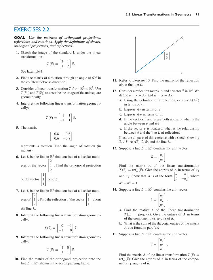
2.2 Linear Transformations in Geometry 71
EXERCISES 2.2GOAL Use the matrices of orthogonal projections,reflections, and rotations. Apply the definitions of shears,orthogonal projections, and reflections.
1. Sketch the image of the standard L under the lineartransformation
T (x) =[
3 11 2
]x .
See Example 1.
2. Find the matrix of a rotation through an angle of 60 inthe counterclockwise direction.
3. Consider a linear transformation T from R2 to R3. UseT (e1) and T (e2) to describe the image of the unit squaregeometrically.
4. Interpret the following linear transformation geometri-cally:
T (x) =[
1 1−1 1
]x .
5. The matrix[−0.8 −0.6
0.6 −0.8
]
represents a rotation. Find the angle of rotation (inradians).
6. Let L be the line in R3 that consists of all scalar multi-
ples of the vector
⎡
⎣212
⎤
⎦. Find the orthogonal projection
of the vector
⎡
⎣111
⎤
⎦ onto L .
7. Let L be the line in R3 that consists of all scalar multi-
ples of
⎡
⎣212
⎤
⎦. Find the reflection of the vector
⎡
⎣111
⎤
⎦ about
the line L .
8. Interpret the following linear transformation geometri-cally:
T (x) =[
0 −1−1 0
]x .
9. Interpret the following linear transformation geometri-cally:
T (x) =[
1 01 1
]x .
10. Find the matrix of the orthogonal projection onto theline L in R2 shown in the accompanying figure:
L
43
11. Refer to Exercise 10. Find the matrix of the reflectionabout the line L .
12. Consider a reflection matrix A and a vector x in R2. Wedefine v = x + Ax and w = x − Ax .a. Using the definition of a reflection, express A(Ax)
in terms of x .b. Express Av in terms of v.c. Express Aw in terms of w.d. If the vectors v and w are both nonzero, what is the
angle between v and w?e. If the vector v is nonzero, what is the relationship
between v and the line L of reflection?Illustrate all parts of this exercise with a sketch showingx , Ax , A(Ax), v, w, and the line L .
13. Suppose a line L in R2 contains the unit vector
u =[
u1u2
].
Find the matrix A of the linear transformationT (x) = refL (x). Give the entries of A in terms of u1
and u2. Show that A is of the form[
a bb −a
], where
a2 + b2 = 1.
14. Suppose a line L in R3 contains the unit vector
u =
⎡
⎣u1u2u3
⎤
⎦ .
a. Find the matrix A of the linear transformationT (x) = projL (x). Give the entries of A in termsof the components u1, u2, u3 of u.
b. What is the sum of the diagonal entries of the matrixA you found in part (a)?
15. Suppose a line L in R3 contains the unit vector
u =
⎡
⎣u1u2u3
⎤
⎦ .
Find the matrix A of the linear transformation T (x) =refL (x). Give the entries of A in terms of the compo-nents u1, u2, u3 of u.

72 CHAPTER 2 Linear Transformations
16. Let T (x) = refL (x) be the reflection about the line L inR2 shown in the accompanying figure.a. Draw sketches to illustrate that T is linear.b. Find the matrix of T in terms of θ .
L
17. Consider a matrix A of the form A =[
a bb −a
], where
a2 + b2 = 1. Find two nonzero perpendicular vectorsv and w such that Av = v and Aw = −w (write theentries of v and w in terms of a and b). Conclude thatT (x) = Ax represents the reflection about the line Lspanned by v.
18. The linear transformation T (x) =[
0.6 0.80.8 −0.6
]x is
a reflection about a line L . See Exercise 17. Find theequation of line L (in the form y = mx).
Find the matrices of the linear transformations from R3 toR3 given in Exercises 19 through 23. Some of these trans-formations have not been formally defined in the text. Usecommon sense. You may assume that all these transfor-mations are linear.
19. The orthogonal projection onto the x–y-plane.
20. The reflection about the x–z-plane.
21. The rotation about the z-axis through an angle of π/2,counterclockwise as viewed from the positive z-axis.
22. The rotation about the y-axis through an angle θ , coun-terclockwise as viewed from the positive y-axis.
23. The reflection about the plane y = z.
24. Rotations and reflections have two remarkable prop-erties: They preserve the length of vectors and theangle between vectors. (Draw figures illustrating theseproperties.) We will show that, conversely, any lineartransformation T from R2 to R2 that preserves lengthand angles is either a rotation or a reflection (about aline).a. Show that if T (x) = Ax preserves length and
angles, then the two column vectors v and w of Amust be perpendicular unit vectors.
b. Write the first column vector of A as v =[
ab
]; note
that a2 + b2 = 1, since v is a unit vector. Show thatfor a given v there are two possibilities for w, thesecond column vector of A. Draw a sketch showingv and the two possible vectors w. Write the compo-nents of w in terms of a and b.
c. Show that if a linear transformation T from R2 to R2
preserves length and angles, then T is either a rota-tion or a reflection (about a line). See Exercise 17.
25. Find the inverse of the matrix[
1 k0 1
], where k is an
arbitrary constant. Interpret your result geometrically.
26. a. Find the scaling matrix A that transforms[
2−1
]into
[8
−4
].
b. Find the orthogonal projection matrix B that trans-
forms[
23
]into
[20
].
c. Find the rotation matrix C that transforms[
05
]into
[34
].
d. Find the shear matrix D that transforms[
13
]into
[73
].
e. Find the reflection matrix E that transforms[
71
]into
[−5
5
].
27. Consider the matrices A through E below.
A =[
0.6 0.80.8 −0.6
], B =
[3 00 3
],
C =[
0.36 −0.48−0.48 0.64
], D =
[−0.8 0.6−0.6 −0.8
],
E =[
1 0−1 1
]
Fill in the blanks in the sentences below.We are told that there is a solution in each case.Matrix represents a scaling.Matrix represents an orthogonal projection.Matrix represents a shear.Matrix represents a reflection.Matrix represents a rotation.
28. Each of the linear transformations in parts (a) through(e) corresponds to one (and only one) of the matrices Athrough J . Match them up.a. Scaling b. Shear c. Rotationd. Orthogonal projection e. Reflection
A =[
0 00 1
], B =
[2 11 0
], C =
[−0.6 0.8−0.8 −0.6
],
D =[
7 00 7
], E =
[1 0
−3 1
], F =
[0.6 0.80.8 −0.6
],

2.2 Linear Transformations in Geometry 73
G =[
0.6 0.60.8 0.8
], H =
[2 −11 2
], I =
[0 01 0
],
J =[
0.8 −0.60.6 −0.8
]
29. Let T be a function from Rm to Rn , and let L be a func-tion from Rn to Rm . Suppose that L
(T (x)
)= x for all
x in Rm and T(
L(y))
= y for all y in Rn . If T is a lin-ear transformation, show that L is linear as well. Hint:v + w = T
(L(v)
)+ T
(L(w)
)= T
(L(v) + L(w)
)
since T is linear. Now apply L on both sides.
30. Find a nonzero 2 × 2 matrix A such that Ax is parallel
to the vector[
12
], for all x in R2.
31. Find a nonzero 3 × 3 matrix A such that Ax is perpen-
dicular to
⎡
⎣123
⎤
⎦, for all x in R3.
32. Consider the rotation matrix D =[
cos α − sin α
sin α cos α
]
and the vector v =[
cos β
sin β
], where α and β are arbi-
trary angles.
a. Draw a sketch to explain why Dv =[
cos(α + β)
sin(α + β)
].
b. Compute Dv. Use the result to derive the additiontheorems for sine and cosine:
cos(α + β) = . . . , sin(α + β) = . . . .
33. Consider two nonparallel lines L1 and L2 in R2.Explain why a vector v in R2 can be expresseduniquely as
v = v1 + v2,
where v1 is on L1 and v2 on L2. Draw a sketch. Thetransformation T (v) = v1 is called the projection ontoL1 along L2. Show algebraically that T is linear.
34. One of the five given matrices represents an orthogonalprojection onto a line and another represents a reflec-tion about a line. Identify both and briefly justify yourchoice.
A = 13
⎡
⎣1 2 22 1 22 2 1
⎤
⎦ , B = 13
⎡
⎣1 1 11 1 11 1 1
⎤
⎦ ,
C = 13
⎡
⎣2 1 11 2 11 1 2
⎤
⎦ , D = −13
⎡
⎣1 2 22 1 22 2 1
⎤
⎦ ,
E = 13
⎡
⎣−1 2 2
2 −1 22 2 −1
⎤
⎦
35. Let T be an invertible linear transformation from R2 toR2. Let P be a parallelogram in R2 with one vertex atthe origin. Is the image of P a parallelogram as well?Explain. Draw a sketch of the image.
x2
x1
P
36. Let T be an invertible linear transformation from R2 toR2. Let P be a parallelogram in R2. Is the image of Pa parallelogram as well? Explain.
P
x2
x1
37. The trace of a matrix[
a bc d
]is the sum a + d of its
diagonal entries. What can you say about the trace of a2 × 2 matrix that represents a(n)a. orthogonal projection b. reflection about a linec. rotation d. (horizontal or vertical) shear.In three cases, give the exact value of the trace, and inone case, give an interval of possible values.
38. The determinant of a matrix[
a bc d
]is ad − bc (we
have seen this quantity in Exercise 2.1.13 already). Findthe determinant of a matrix that represents a(n)a. orthogonal projection b. reflection about a linec. rotation d. (horizontal or vertical) shear.What do your answers tell you about the invertibility ofthese matrices?
39. Describe each of the linear transformations defined bythe matrices in parts (a) through (c) geometrically, asa well-known transformation combined with a scaling.Give the scaling factor in each case.
a.[
1 11 1
]b.
[3 0
−1 3
]
c.[
3 44 −3
]
40. Let P and Q be two perpendicular lines in R2. Fora vector x in R2, what is projP (x) + projQ(x)? Give

74 CHAPTER 2 Linear Transformations
your answer in terms of x . Draw a sketch to justify youranswer.
41. Let P and Q be two perpendicular lines in R2. Fora vector x in R2, what is the relationship betweenrefP (x) and refQ(x)? Draw a sketch to justify youranswer.
42. Let T (x) = projL (x) be the orthogonal projection ontoa line in R2. What is the relationship between T (x) andT
(T (x)
)? Justify your answer carefully.
43. Use the formula derived in Exercise 2.1.13 to find theinverse of the rotation matrix
A =[
cos θ −sin θ
sin θ cos θ
].
Interpret the linear transformation defined by A−1 geo-metrically. Explain.
44. A nonzero matrix of the form A =[
a −bb a
]repre-
sents a rotation combined with a scaling. Use the for-mula derived in Exercise 2.1.13 to find the inverse ofA. Interpret the linear transformation defined by A−1
geometrically. Explain.
45. A matrix of the form A =[
a bb −a
], where a2 + b2 =
1, represents a reflection about a line. See Exercise 17.Use the formula derived in Exercise 2.1.13 to find theinverse of A. Explain.
46. A nonzero matrix of the form A =[
a bb −a
]repre-
sents a reflection about a line L combined with a scal-ing. (Why? What is the scaling factor?) Use the formuladerived in Exercise 2.1.13 to find the inverse of A. Inter-pret the linear transformation defined by A−1 geomet-rically. Explain.
47. In this exercise we will prove the following remark-able theorem: If T (x) = Ax is any linear transfor-mation from R2 to R2, then there exist perpendicularunit vectors v1 and v2 in R2 such that the vectors T (v1)and T (v2) are perpendicular as well (see the accom-panying figure), in the sense that T (v1) · T (v2) =0. This is not intuitively obvious: Think about thecase of a shear, for example. For a generalization, seeTheorem 8.3.3.
For any real number t , the vectors[
cos tsin t
]and
[− sin tcos t
]will be perpendicular unit vectors. Now we
can consider the function
f (t) =(
T[
cos tsin t
])·(
T[
− sin tcos t
])
=(
A[
cos tsin t
])·(
A[
− sin tcos t
]).
It is our goal to show that there exists a number c such
that f (c) =(
T[
cos csin c
])·(
T[
− sin ccos c
])= 0. Then
the vectors v1 =[
cos csin c
]and v2 =
[− sin ccos c
]will
have the required property that they are perpendicularunit vectors such that T (v1) · T (v2) = 0.a. Show that the function f (t) is continuous. You may
assume that cos t , sin t , and constant functions arecontinuous. Also, sums and products of continuous
functions are continuous. Hint: Write A =[
a bc d
].
b. Show that f(
π2
)= − f (0).
c. Show that there exists a number c, with 0 ≤ c ≤ π2 ,
such that f (c) = 0. Hint: Use the intermediatevalue theorem: If a function f (t) is continuous fora ≤ t ≤ b and if L is any number between f (a) andf (b), then there exists a number c between a and bwith f (c) = L .
x2
x1
y2
y1
T
T(v1)
T(v2)
v1
v2
48. If a 2×2 matrix A represents a rotation, find perpendic-ular unit vectors v1 and v2 in R2 such that the vectorsT (v1) and T (v2) are perpendicular as well. See Exer-cise 47.
For the linear transformations T in Exercises 49through 52, do the following:a. Find the function f (t) defined in Exercise 47 and
graph it for 0 ≤ t ≤ π2 . You may use technology.
b. Find a number c, with 0 ≤ c ≤ π2 , such that
f (c) = 0. (In Problem 50, approximate c to threesignificant digits, using technology.)
c. Find perpendicular unit vectors v1 and v2 in R2
such that the vectors T(v1) and T(v2) are per-pendicular as well. Draw a sketch showing v1, v2,T(v1), and T (v2).
49. T (x) =[
2 21 −4
]x
50. T (x) =[
1 10 1
]x
51. T (x) =[
2 11 2
]x

2.3 Matrix Products 75
52. T (x) =[
0 45 −3
]x
53. Sketch the image of the unit circle under the lineartransformation
T (x) =[
5 00 2
]x .
54. Let T be an invertible linear transformation from R2 toR2. Show that the image of the unit circle is an ellipsecentered at the origin.8 Hint: Consider two perpendicu-lar unit vectors v1 and v2 such that T (v1) and T (v2) areperpendicular. See Exercise 47. The unit circle consistsof all vectors of the form
v = cos(t)v1 + sin(t)v2,
where t is a parameter.
55. Let w1 and w2 be two nonparallel vectors in R2. Con-sider the curve C in R2 that consists of all vectors ofthe form cos(t)w1 + sin(t)w2, where t is a parameter.
Show that C is an ellipse. Hint: You can interpret C asthe image of the unit circle under a suitable linear trans-formation; then use Exercise 54.
C
w2
w1
O
56. Consider an invertible linear transformation T from R2
to R2. Let C be an ellipse in R2. Show that the imageof C under T is an ellipse as well. Hint: Use the resultof Exercise 55.
2.3 Matrix Products
Recall the composition of two functions: The composite of the functions y =sin(x) and z = cos(y) is z = cos
(sin(x)
), as illustrated in Figure 1.
y
y = sin(x)
z = cos(sin(x))
z = cos(y)
x
z
Figure 1
Similarly, we can compose two linear transformations.To understand this concept, let’s return to the coding example discussed in Sec-
tion 2.1. Recall that the position x =[
x1
x2
]of your boat is encoded and that you
radio the encoded position y =[
y1
y2
]to Marseille. The coding transformation is
y = Ax, with A =[
1 23 5
].
In Section 2.1, we left out one detail: Your position is radioed on to Paris, as youwould expect in a centrally governed country such as France. Before broadcastingto Paris, the position y is again encoded, using the linear transformation
8An ellipse in R2 centered at the origin may be defined as a curve that can be parametrized as
cos(t)w1 + sin(t)w2,
for two perpendicular vectors w1 and w2. Suppose the length of w1 exceeds the length of w2. Then wecall the vectors ± w1 the semimajor axes of the ellipse and ± w2 the semiminor axes.
Convention: All ellipses considered in this text are centered at the origin unless stated otherwise.
O
w1
w2

76 CHAPTER 2 Linear Transformations
z = B y, with B =[
6 78 9
]
this time, and the sailor in Marseille radios the encoded position z to Paris. SeeFigure 2.
z = By, where B =
Paris: z
Boat: x
Marseille: y
y = Ax, where A =
68
79
13
25
Figure 2
We can think of the message z received in Paris as a function of the actualposition x of the boat,
z = B(Ax),
the composite of the two transformations y = Ax and z = B y. Is this transforma-tion z = T (x) linear, and, if so, what is its matrix? We will show two approaches tothese important questions: (a) using brute force, and (b) using some theory.
a. We write the components of the two transformations and substitute:
z1 = 6y1 + 7y2z2 = 8y1 + 9y2
andy1 = x1 + 2x2y2 = 3x1 + 5x2
so that
z1 = 6(x1 + 2x2) + 7(3x1 + 5x2) = (6 · 1 + 7 · 3)x1 + (6 · 2 + 7 · 5)x2
= 27x1 + 47x2,
z2 = 8(x1 + 2x2) + 9(3x1 + 5x2) = (8 · 1 + 9 · 3)x1 + (8 · 2 + 9 · 5)x2
= 35x1 + 61x2.
This shows that the composite is indeed linear, with matrix[
6 · 1 + 7 · 3 6 · 2 + 7 · 58 · 1 + 9 · 3 8 · 2 + 9 · 5
]=
[27 4735 61
].
b. We can use Theorem 1.3.10 to show that the transformation T (x) = B(Ax)is linear:
T (v + w) = B(
A(v + w))
= B(Av + Aw)
= B(Av) + B(Aw) = T (v) + T (w),
T (kv) = B(
A(kv))
= B(k(Av)
)= k
(B(Av)
)= kT (v).
Once we know that T is linear, we can find its matrix by computing thevectors T (e1) = B(Ae1) and T (e2) = B(Ae2); the matrix of T is then[T (e1) T (e2)
], by Theorem 2.1.2:
T (e1) = B(Ae1) = B(first column of A) =[
6 78 9
] [13
]=
[2735
],
T (e2) = B(Ae2) = B(second column of A) =[
6 78 9
] [25
]=
[4761
].
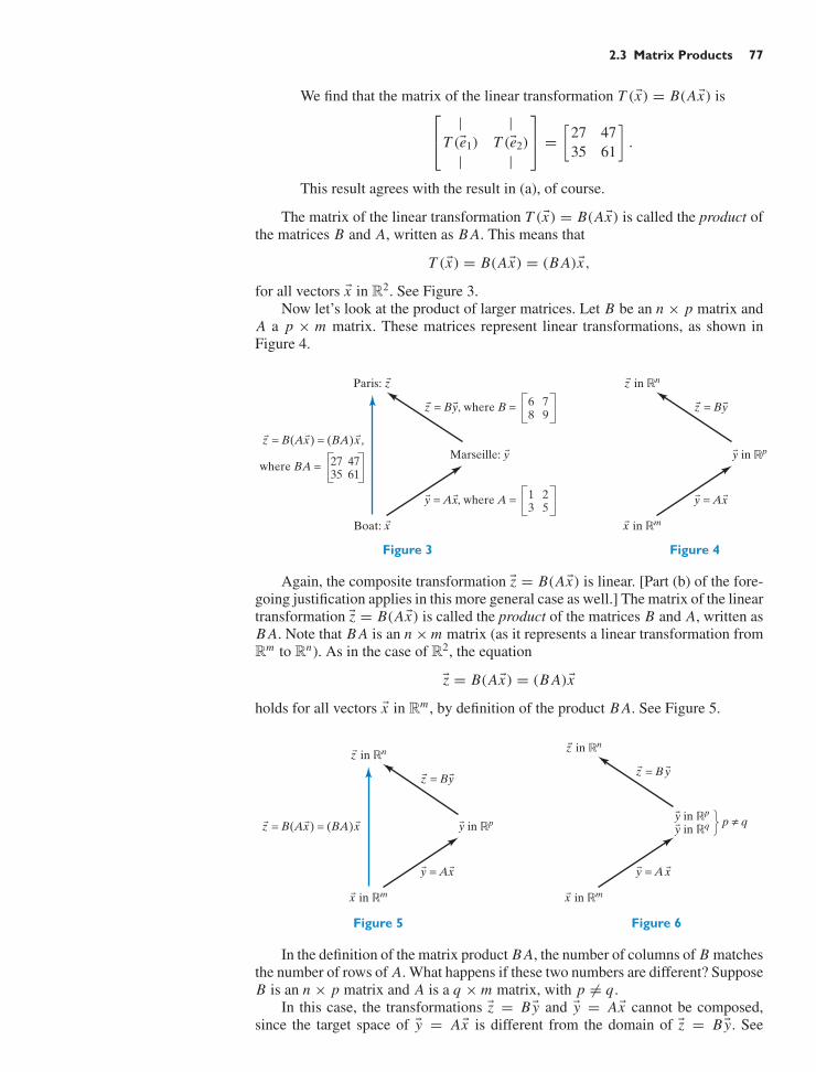
2.3 Matrix Products 77
We find that the matrix of the linear transformation T (x) = B(Ax) is⎡
⎣| |
T (e1) T (e2)
| |
⎤
⎦ =[
27 4735 61
].
This result agrees with the result in (a), of course.
The matrix of the linear transformation T (x) = B(Ax) is called the product ofthe matrices B and A, written as B A. This means that
T (x) = B(Ax) = (B A)x,
for all vectors x in R2. See Figure 3.Now let’s look at the product of larger matrices. Let B be an n × p matrix and
A a p × m matrix. These matrices represent linear transformations, as shown inFigure 4.
Paris: z
Boat: x
Marseille: y
z = By, where B = 68
79
z = B(Ax) = (BA)x ,
where BA = 2735
4761
y = Ax, where A = 13
25
Figure 3
z = By
z in !n
x in !m
y in !p
y = Ax
Figure 4
Again, the composite transformation z = B(Ax) is linear. [Part (b) of the fore-going justification applies in this more general case as well.] The matrix of the lineartransformation z = B(Ax) is called the product of the matrices B and A, written asB A. Note that B A is an n × m matrix (as it represents a linear transformation fromRm to Rn). As in the case of R2, the equation
z = B(Ax) = (B A)x
holds for all vectors x in Rm , by definition of the product B A. See Figure 5.
z = B(Ax) = (BA)x
z = By
z in !n
x in !m
y in !p
y = Ax
Figure 5
z = By
z in !n
x in !m
y = A x
y in !p
y in !q p ≠ q
Figure 6
In the definition of the matrix product B A, the number of columns of B matchesthe number of rows of A. What happens if these two numbers are different? SupposeB is an n × p matrix and A is a q × m matrix, with p = q.
In this case, the transformations z = B y and y = Ax cannot be composed,since the target space of y = Ax is different from the domain of z = B y. See

78 CHAPTER 2 Linear Transformations
Figure 6. To put it more plainly: The output of y = Ax is not an acceptable inputfor the transformation z = B y. In this case, the matrix product B A is undefined.
Definition 2.3.1 Matrix multiplication
a. Let B be an n × p matrix and A a q × m matrix. The product B A isdefined if (and only if) p = q.
b. If B is an n × p matrix and A a p × m matrix, then the product B A isdefined as the matrix of the linear transformation T (x) = B(Ax). Thismeans that T (x) = B(Ax) = (B A)x , for all x in the vector space Rm .The product B A is an n × m matrix.
Although this definition of matrix multiplication does not give us concreteinstructions for computing the product of two numerically given matrices, suchinstructions can be derived easily from the definition.
As in Definition 2.3.1, let B be an n × p matrix and A a p × m matrix. Let’sthink about the columns of the matrix B A:
(i th column of B A) = (B A)ei
= B(Aei )
= B(i th column of A).
If we denote the columns of A by v1, v2, . . . , vm , we can write
B A = B
⎡
⎢⎣| | |v1 v2 · · · vm
| | |
⎤
⎥⎦ =
⎡
⎢⎣| | |
Bv1 Bv2 · · · Bvm
| | |
⎤
⎥⎦ .
Theorem 2.3.2 The columns of the matrix product
Let B be an n × p matrix and A a p × m matrix with columns v1, v2, . . . , vm .Then, the product B A is
B A = B
⎡
⎢⎣| | |v1 v2 · · · vm
| | |
⎤
⎥⎦ =
⎡
⎢⎣| | |
Bv1 Bv2 · · · Bvm
| | |
⎤
⎥⎦ .
To find B A, we can multiply B by the columns of A and combine theresulting vectors.
This is exactly how we computed the product
B A =[
6 78 9
] [1 23 5
]=
[27 4735 61
]
on page 76, using approach (b).For practice, let us multiply the same matrices in the reverse order. The first
column of AB is[
1 23 5
] [68
]=
[2258
]; the second is
[1 23 5
] [79
]=
[2566
]. Thus,
AB =[
1 23 5
] [6 78 9
]=
[22 2558 66
].
Compare the two previous displays to see that AB = B A: Matrix multiplica-tion is noncommutative. This should come as no surprise, in view of the fact that
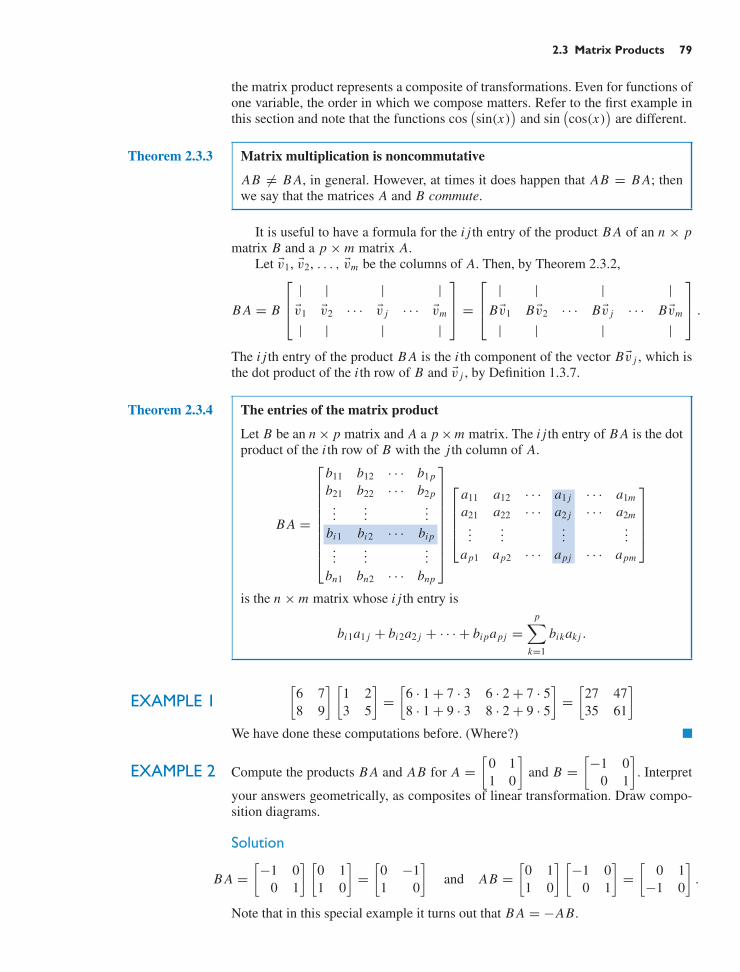
2.3 Matrix Products 79
the matrix product represents a composite of transformations. Even for functions ofone variable, the order in which we compose matters. Refer to the first example inthis section and note that the functions cos
(sin(x)
)and sin
(cos(x)
)are different.
Theorem 2.3.3 Matrix multiplication is noncommutative
AB = B A, in general. However, at times it does happen that AB = B A; thenwe say that the matrices A and B commute.
It is useful to have a formula for the i j th entry of the product B A of an n × pmatrix B and a p × m matrix A.
Let v1, v2, . . . , vm be the columns of A. Then, by Theorem 2.3.2,
B A = B
⎡
⎢⎣| | | |v1 v2 · · · v j · · · vm
| | | |
⎤
⎥⎦ =
⎡
⎢⎣| | | |
Bv1 Bv2 · · · Bv j · · · Bvm
| | | |
⎤
⎥⎦ .
The i j th entry of the product B A is the i th component of the vector Bv j , which isthe dot product of the i th row of B and v j , by Definition 1.3.7.
Theorem 2.3.4 The entries of the matrix product
Let B be an n × p matrix and A a p × m matrix. The i j th entry of B A is the dotproduct of the i th row of B with the j th column of A.
B A =
⎡
⎢⎢⎢⎢⎢⎢⎢⎢⎣
b11 b12 · · · b1p
b21 b22 · · · b2p...
......
bi1 bi2 · · · bip...
......
bn1 bn2 · · · bnp
⎤
⎥⎥⎥⎥⎥⎥⎥⎥⎦
⎡
⎢⎢⎢⎣
a11 a12 · · · a1 j · · · a1m
a21 a22 · · · a2 j · · · a2m...
......
...
ap1 ap2 · · · apj · · · apm
⎤
⎥⎥⎥⎦
is the n × m matrix whose i j th entry is
bi1a1 j + bi2a2 j + · · · + bipapj =p∑
k=1
bikak j .
EXAMPLE 1[
6 78 9
] [1 23 5
]=
[6 · 1 + 7 · 3 6 · 2 + 7 · 58 · 1 + 9 · 3 8 · 2 + 9 · 5
]=
[27 4735 61
]
We have done these computations before. (Where?) !
EXAMPLE 2 Compute the products B A and AB for A =[
0 11 0
]and B =
[−1 0
0 1
]. Interpret
your answers geometrically, as composites of linear transformation. Draw compo-sition diagrams.
Solution
B A =[−1 0
0 1
] [0 11 0
]=
[0 −11 0
]and AB =
[0 11 0
] [−1 0
0 1
]=
[0 1
−1 0
].
Note that in this special example it turns out that B A = −AB.
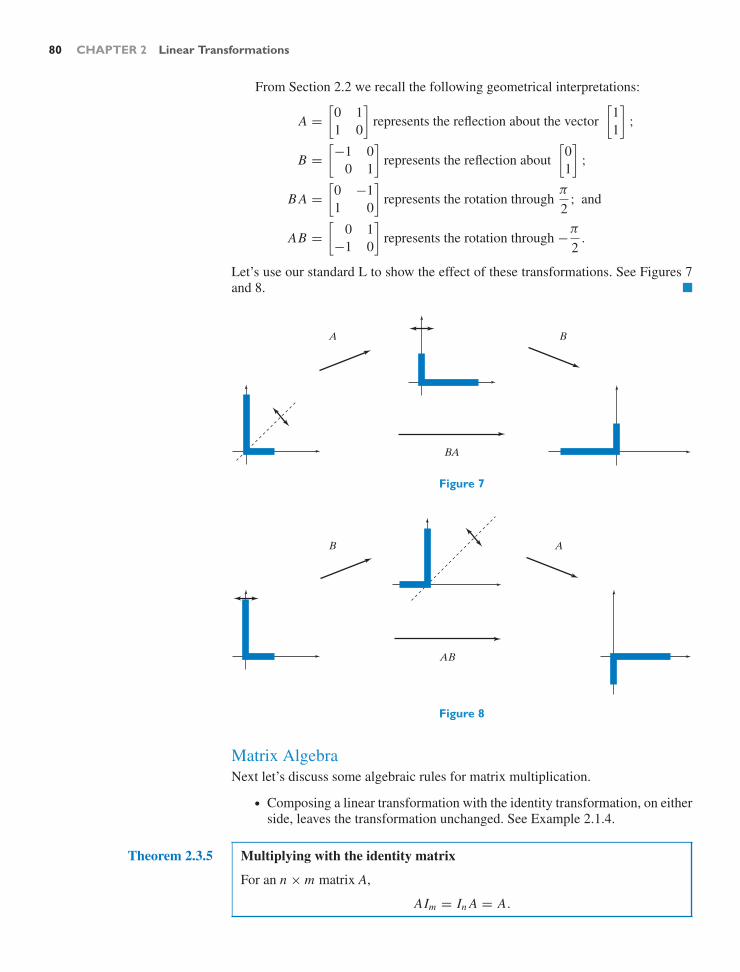
80 CHAPTER 2 Linear Transformations
From Section 2.2 we recall the following geometrical interpretations:
A =[
0 11 0
]represents the reflection about the vector
[11
];
B =[−1 0
0 1
]represents the reflection about
[01
];
B A =[
0 −11 0
]represents the rotation through
π
2; and
AB =[
0 1−1 0
]represents the rotation through −π
2.
Let’s use our standard L to show the effect of these transformations. See Figures 7and 8. !
A B
BA
Figure 7
AB
AB
Figure 8
Matrix AlgebraNext let’s discuss some algebraic rules for matrix multiplication.
• Composing a linear transformation with the identity transformation, on eitherside, leaves the transformation unchanged. See Example 2.1.4.
Theorem 2.3.5 Multiplying with the identity matrix
For an n × m matrix A,
AIm = In A = A.

2.3 Matrix Products 81
• If A is an n × p matrix, B a p × q matrix, and C a q × m matrix, what is therelationship between (AB)C and A(BC)?
One way to think about this problem (although perhaps not the mostelegant one) is to write C in terms of its columns: C =
[v1 v2 · · · vm
].
Then
(AB)C = (AB)[v1 v2 · · · vm
]=
[(AB)v1 (AB)v2 · · · (AB)vm
],
and
A(BC) = A[
Bv1 Bv2 · · · Bvm]
=[
A(Bv1) A(Bv2) · · · A(Bvm)].
Since (AB)vi = A(Bvi ), by definition of the matrix product, we find that(AB)C = A(BC).
Theorem 2.3.6 Matrix multiplication is associative
(AB)C = A(BC)
We can simply write ABC for the product (AB)C = A(BC).
A more conceptual proof is based on the fact that the composition of functionsis associative. The two linear transformations
T (x) =((AB)C
)x and L(x) =
(A(BC)
)x
are identical because, by the definition of matrix multiplication,
T (x) =((AB)C
)x = (AB)(Cx) = A
(B(Cx)
)
and
L(x) =(
A(BC))x = A
((BC)x
)= A
(B(Cx)
).
The domains and target spaces of the linear transformations defined by the matricesA, B, C , BC , AB, A(BC), and (AB)C are shown in Figure 9.
B
BC
C A
(AB)C
A(BC)
AB
!n!p!q!m
Figure 9
Theorem 2.3.7 Distributive property for matrices
If A and B are n × p matrices, and C and D are p × m matrices, then
A(C + D) = AC + AD, and(A + B)C = AC + BC.
You will be asked to verify this property in Exercise 27.
Theorem 2.3.8 If A is an n × p matrix, B is a p × m matrix, and k is a scalar, then
(k A)B = A(k B) = k(AB).
You will be asked to verify this property in Exercise 28.
Block Matrices (Optional)In the popular puzzle Sudoku, one considers a 9×9 matrix A that is subdivided intonine 3 × 3 matrices called blocks. The puzzle setter provides some of the 81 entriesof matrix A, and the objective is to fill in the remaining entries so that each row ofA, each column of A, and each block contains each of the digits 1 through 9 exactlyonce.

82 CHAPTER 2 Linear Transformations
5 3 7
1
1
9 5
5
66
9
9
8
8 6
8
2
2
3
3
647
6
8
8
4 1 9
7
This Sudoku puzzle is an example of a block matrix (or partitioned matrix), that is,a matrix that is partitioned into rectangular submatrices, called blocks, by means ofhorizontal and vertical lines that go all the way through the matrix.
The blocks need not be of equal size.For example, we can partition the matrix
B =
⎡
⎣1 2 34 5 66 7 9
⎤
⎦ as B =
⎡
⎣1 2 34 5 66 7 9
⎤
⎦ =[
B11 B12
B21 B22
],
where B11 =[
1 24 5
], B12 =
[36
], B21 =
[6 7
], and B22 = [9].
A useful property of block matrices is the following:
Theorem 2.3.9 Multiplying block matrices
Block matrices can be multiplied as though the blocks were scalars (i.e., usingthe formula in Theorem 2.3.4):
AB =
⎡
⎢⎢⎢⎢⎢⎢⎢⎢⎣
A11 A12 · · · A1p
A21 A22 · · · A2p...
......
Ai1 Ai2 · · · Aip...
......
An1 An2 · · · Anp
⎤
⎥⎥⎥⎥⎥⎥⎥⎥⎦
⎡
⎢⎢⎢⎣
B11 B12 · · · B1 j · · · B1m
B21 B22 · · · B2 j · · · B2m...
......
...
Bp1 Bp2 · · · Bpj · · · Bpm
⎤
⎥⎥⎥⎦
is the block matrix whose i j th block is the matrix
Ai1 B1 j + Ai2 B2 j + · · · + Aip Bpj =p∑
k=1
Aik Bkj ,
provided that all the products Aik Bkj are defined.
Verifying this fact is left as an exercise. A numerical example follows.
EXAMPLE 3[
0 11 0
−11
]⎡
⎢⎣1 24 5
36
7 8 9
⎤
⎥⎦
=[[
0 11 0
] [1 24 5
]+
[−1
1
] [7 8
] [0 11 0
] [36
]+
[−1
1
] [9]]
=[−3 −3 −3
8 10 12
].

2.3 Matrix Products 83
Compute this product without using a partition, and see whether you find thesame result. !
In this simple example, using blocks is somewhat pointless. Example 3 merelyillustrates Theorem 2.3.9. In Example 2.4.7, we will see a more sensible usage ofthe concept of block matrices.
Powers of Transition MatricesWe will conclude this section with an example on transition matrices. See Defini-tion 2.1.4.
EXAMPLE 4 Let’s revisit the mini-Web we considered in Example 9 of Section 2.1:
1 ! 2↓ ↑3 → 4
with the transition matrix
A =
⎡
⎢⎢⎢⎣
0 12 0 0
12 0 0 112
12 0 0
0 0 1 0
⎤
⎥⎥⎥⎦.
At a predetermined time, all the surfers will follow one of the available links, in themanner described in Example 2.1.9. If the initial distribution of the surfers amongthe four pages is given by the vector x , then the distribution after this transition willbe Ax . Now, let’s iterate this process: Imagine an event of “speed surfing,” where,every few minutes, at the blow of a whistle, each surfer will follow an available link.After two transitions, the distribution will be A(Ax) = A2 x , and after m transitionsthe distribution will be given by the vector Am x . Let’s use technology to computesome of the powers Am of matrix A:
A2 =
⎡
⎢⎢⎢⎣
14 0 0 1
2
0 14 1 0
14
14 0 1
212
12 0 0
⎤
⎥⎥⎥⎦, A10 ≈
⎡
⎢⎢⎢⎣
0.173 0.172 0.172 0.1500.344 0.345 0.301 0.3440.247 0.247 0.270 0.2360.236 0.236 0.258 0.270
⎤
⎥⎥⎥⎦,
A20 ≈
⎡
⎢⎢⎢⎣
0.16697 0.16697 0.16650 0.166230.33347 0.33347 0.33246 0.333930.25008 0.25008 0.25035 0.249480.24948 0.24948 0.25068 0.25035
⎤
⎥⎥⎥⎦.
These powers Am will be transition matrices as well; see Exercise 68.In Exercises 69 through 72, you will have a chance to explore the significance
of the entries of these matrices Am , in terms of our mini-Web and its graph.As we take a closer look at the matrix A20, our attention may be drawn to the
fact that the four column vectors are all close to the vector⎡
⎢⎢⎣
1/61/31/41/4
⎤
⎥⎥⎦ ,

84 CHAPTER 2 Linear Transformations
which happens to be the equilibrium distribution xequ for the matrix A, as discussedin Example 2.1.9. We might conjecture that the limit of the column vectors of Am
is xequ as m goes to infinity. !Before we address this issue, let’s introduce some terminology.
Definition 2.3.10 Regular transition matrices
A transition matrix is said to be positive if all its entries are positive (meaningthat all the entries are greater than 0).
A transition matrix is said to be regular (or eventually positive) if the matrixAm is positive for some positive integer m.
For example, the transition matrix[
0.4 0.70.6 0.3
]is positive (and therefore also
regular; let m = 1 in Definition 2.3.10). The transition matrix A =[
0 1/21 1/2
]fails
to be positive, but it is regular since A2 =[
1/2 1/41/2 3/4
].
The matrix A in Example 4 fails to be positive, but it is regular since A10 is
positive. The reflection matrix A =[
0 11 0
]fails to be regular since Am =
[1 00 1
]
for even m and Am = A =[
0 11 0
]for odd m.
Now we can address the conjecture we made at the end of Example 4.
Theorem 2.3.11 Equilibria for regular transition matrices
Let A be a regular transition matrix of size n × n.
a. There exists exactly one distribution vector x in Rn such that Ax = x .This is called the equilibrium distribution for A, denoted xequ . All thecomponents of xequ are positive.
b. If x is any distribution vector in Rn , then limm→∞
(Am x) = xequ .
c. limm→∞
Am =
⎡
⎣| |
xequ · · · xequ| |
⎤
⎦, which is the matrix whose columns are all
xequ .9
Part (b) states that in the long run the system will approach the equilibriumdistribution xequ , regardless of the initial distribution; we say that xequ is theglobally stable equilibrium distribution.
We will outline a proof of parts (a) and (b) in Chapter 7. Parts (b) and(c) are easily seen to be equivalent. If we assume that part (b) holds, thenlim
m→∞( j th column of Am) = lim
m→∞(Ame j ) = xequ since e j is a distribution vector. In
Exercise 73, you are asked to derive part (b) from part (c).
9This limit is defined entry by entry. We claim that any entry of Am converges to the corresponding
entry of the matrix
⎡
⎣| |
xequ · · · xequ
| |
⎤
⎦ as m goes to infinity.

2.3 Matrix Products 85
EXERCISES 2.3GOAL Compute matrix products column by columnand entry by entry. Interpret matrix multiplication interms of the underlying linear transformations. Use therules of matrix algebra. Multiply block matrices.
If possible, compute the matrix products in Exercises 1through 13, using paper and pencil.
1.[
1 10 1
] [1 23 4
]2.
⎡
⎣1 −10 22 1
⎤
⎦[
3 21 0
]
3.[
1 2 34 5 6
] [1 23 4
]4.
[1 −1
−2 2
] [7 53 1
]
5.
⎡
⎣1 00 10 0
⎤
⎦[
a bc d
]6.
[0 10 0
] [0 10 0
]
7.
⎡
⎣1 0 −10 1 11 −1 −2
⎤
⎦
⎡
⎣1 2 33 2 12 1 3
⎤
⎦
8.[
a bc d
] [d −b
−c a
]9.
[1 22 4
] [−6 8
3 −4
]
10.
⎡
⎣123
⎤
⎦ [1 2 3
]11.
[1 2 3
]⎡
⎣321
⎤
⎦
12.[
1 0 −1]⎡
⎣1 22 11 1
⎤
⎦
13.[
0 0 1]⎡
⎣a b cd e fg h k
⎤
⎦
⎡
⎣010
⎤
⎦
14. For the matrices
A =[
1 11 1
], B =
[1 2 3
],
C =
⎡
⎣1 0 −12 1 03 2 1
⎤
⎦ , D =
⎡
⎣111
⎤
⎦ , E =[5],
determine which of the 25 matrix products AA, AB,AC , . . . , E D, E E are defined, and compute those thatare defined.
Use the given partitions to compute the products in Exer-cises 15 and 16. Check your work by computing the sameproducts without using a partition. Show all your work.
15.
⎡
⎢⎣1 00 1
00
1 3 4
⎤
⎥⎦
⎡
⎢⎣12
00
3 4
⎤
⎥⎦
16.
⎡
⎢⎢⎢⎣
1 00 1
1 00 1
0 00 0
1 00 1
⎤
⎥⎥⎥⎦
⎡
⎢⎢⎢⎣
1 23 4
2 34 5
0 00 0
1 23 4
⎤
⎥⎥⎥⎦
In the Exercises 17 through 26, find all matrices that com-mute with the given matrix A.
17. A =[
1 00 2
]18. A =
[2 3
−3 2
]
19. A =[
0 −22 0
]20. A =
[1 20 1
]
21. A =[
1 22 −1
]22. A =
[1 11 1
]
23. A =[
1 32 6
]24. A =
⎡
⎣2 0 00 2 00 0 3
⎤
⎦
25. A =
⎡
⎣2 0 00 3 00 0 2
⎤
⎦ 26. A =
⎡
⎣2 0 00 3 00 0 4
⎤
⎦
27. Prove the distributive laws for matrices:
A(C + D) = AC + AD
and
(A + B)C = AC + BC.
28. Consider an n × p matrix A, a p × m matrix B, and ascalar k. Show that
(k A)B = A(k B) = k(AB).
29. Consider the matrix
Dα =[
cos α − sin α
sin α cos α
].
We know that the linear transformation T (x) = Dα x isa counterclockwise rotation through an angle α.a. For two angles, α and β, consider the products
Dα Dβ and Dβ Dα . Arguing geometrically, describethe linear transformations y = Dα Dβ x and y =Dβ Dα x . Are the two transformations the same?
b. Now compute the products Dα Dβ and Dβ Dα . Dothe results make sense in terms of your answer inpart (a)? Recall the trigonometric identities
sin(α ± β) = sin α cos β ± cos α sin β
cos(α ± β) = cos α cos β ∓sin α sin β.
30. Consider the lines P and Q in R2 in the accompany-ing figure. Consider the linear transformation T (x) =refQ
(refP (x)
); that is, we first reflect x about P and
then we reflect the result about Q.
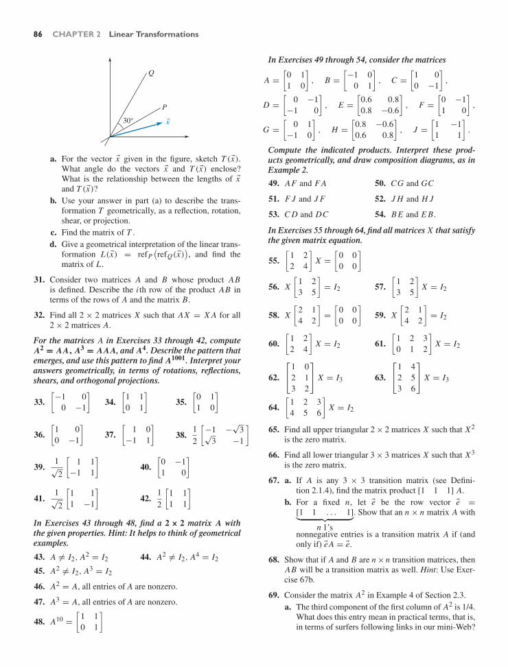
86 CHAPTER 2 Linear Transformations
x
P
Q
30°
a. For the vector x given in the figure, sketch T (x).What angle do the vectors x and T (x) enclose?What is the relationship between the lengths of xand T (x)?
b. Use your answer in part (a) to describe the trans-formation T geometrically, as a reflection, rotation,shear, or projection.
c. Find the matrix of T .d. Give a geometrical interpretation of the linear trans-
formation L(x) = refP(refQ(x)
), and find the
matrix of L .
31. Consider two matrices A and B whose product ABis defined. Describe the i th row of the product AB interms of the rows of A and the matrix B.
32. Find all 2 × 2 matrices X such that AX = X A for all2 × 2 matrices A.
For the matrices A in Exercises 33 through 42, computeA2 = AA, A3 = AAA, and A4. Describe the pattern thatemerges, and use this pattern to find A1001. Interpret youranswers geometrically, in terms of rotations, reflections,shears, and orthogonal projections.
33.[−1 0
0 −1
]34.
[1 10 1
]35.
[0 11 0
]
36.[
1 00 −1
]37.
[1 0
−1 1
]38.
12
[−1 −
√3√
3 −1
]
39.1√2
[1 1
−1 1
]40.
[0 −11 0
]
41.1√2
[1 11 −1
]42.
12
[1 11 1
]
In Exercises 43 through 48, find a 2 × 2 matrix A withthe given properties. Hint: It helps to think of geometricalexamples.
43. A = I2, A2 = I2 44. A2 = I2, A4 = I2
45. A2 = I2, A3 = I2
46. A2 = A, all entries of A are nonzero.
47. A3 = A, all entries of A are nonzero.
48. A10 =[
1 10 1
]
In Exercises 49 through 54, consider the matrices
A =[
0 11 0
], B =
[−1 0
0 1
], C =
[1 00 −1
],
D =[
0 −1−1 0
], E =
[0.6 0.80.8 −0.6
], F =
[0 −11 0
],
G =[
0 1−1 0
], H =
[0.8 −0.60.6 0.8
], J =
[1 −11 1
].
Compute the indicated products. Interpret these prod-ucts geometrically, and draw composition diagrams, as inExample 2.
49. AF and F A 50. CG and GC
51. F J and J F 52. J H and H J
53. C D and DC 54. B E and E B.
In Exercises 55 through 64, find all matrices X that satisfythe given matrix equation.
55.[
1 22 4
]X =
[0 00 0
]
56. X[
1 23 5
]= I2 57.
[1 23 5
]X = I2
58. X[
2 14 2
]=
[0 00 0
]59. X
[2 14 2
]= I2
60.[
1 22 4
]X = I2 61.
[1 2 30 1 2
]X = I2
62.
⎡
⎣1 02 13 2
⎤
⎦ X = I3 63.
⎡
⎣1 42 53 6
⎤
⎦ X = I3
64.[
1 2 34 5 6
]X = I2
65. Find all upper triangular 2 × 2 matrices X such that X2
is the zero matrix.
66. Find all lower triangular 3 × 3 matrices X such that X3
is the zero matrix.
67. a. If A is any 3 × 3 transition matrix (see Defini-tion 2.1.4), find the matrix product [1 1 1] A.
b. For a fixed n, let e be the row vector e =[1 1 . . . 1]︸ ︷︷ ︸
n 1’s
. Show that an n × n matrix A with
nonnegative entries is a transition matrix A if (andonly if) eA = e.
68. Show that if A and B are n ×n transition matrices, thenAB will be a transition matrix as well. Hint: Use Exer-cise 67b.
69. Consider the matrix A2 in Example 4 of Section 2.3.a. The third component of the first column of A2 is 1/4.
What does this entry mean in practical terms, that is,in terms of surfers following links in our mini-Web?

2.3 Matrix Products 87
b. When is the i j th entry of A2 equal to 0? Give youranswer both in terms of paths of length 2 in thegraph of the mini-Web and also in terms of surfersbeing able to get from page j to page i by followingtwo consecutive links.
70. a. Compute A3 for the matrix A in Example 2.3.4.b. The fourth component of the first column of A3 is
1/4. What does this entry mean in practical terms,that is, in terms of surfers following links in ourmini-Web?
c. When is the i j th entry of A3 equal to 0? Give youranswer both in terms of paths in the graph of themini-Web and also in terms of surfers being able toget from page j to page i by following consecutivelinks.
d. How many paths of length 3 are there in thegraph of the mini-Web from page 1 to page 2?How many surfers are taking each of these paths,expressed as a proportion of the initial population ofpage 1?
71. For the mini-Web in Example 2.3.4, find pages i and jsuch that it is impossible to get from page j to page iby following exactly four consecutive links. What doesthe answer tell you about the entries of A4?
72. For the mini-Web in Example 2.3.4, find the smallestpositive integer m such that all the entries of Am arepositive; you may use technology. What does your an-swer tell you in terms of paths in the graph of the mini-Web and also in terms of surfers following consecutivelinks?
73. Use part (c) of Theorem 2.3.11 to prove part (b): If A isa regular transition matrix of size n×n with equilibriumdistribution xequ , and if x is any distribution vector inRn , then lim
m→∞(Am x) = xequ .
74. Suppose A is a transition matrix and B is a positive tran-sition matrix (see Definition 2.3.10), where A and B areof the same size. Is AB necessarily a positive transitionmatrix? What about B A?
75. Prove the following: If A is a transition matrix and Am
is positive, then Am+1 is positive as well.
76. For the mini-Web graphed below, find the equilibriumdistribution in the following way: Write the transitionmatrix A, test high powers of A to come up with a con-jecture for the equilibrium distribution xequ , and thenverify that Axequ = xequ . (This method, based on The-orem 2.3.11, is referred to as the power method forfinding the equilibrium distribution of a regular transi-tion matrix.) Also, find the page with the highest naıvePageRank. You may use technology.
1 ! 2 ↓
3 ← 4
77. Consider the transition matrix
A =
⎡
⎢⎣0.4 0.2 0.7
0 0.6 0.1
0.6 0.2 0.2
⎤
⎥⎦ .
Verify that A is a regular transition matrix and then usethe power method (see Exercise 76) to find the equilib-rium distribution. You may use technology.
78. Let’s revisit the mini-Web with the graph
1 ! 2
↓ ↑3 → 4 ,
but here we consider the surfing model with a “jump-ing rate” of 20%, as discussed in Exercise 2.1.53. Thecorresponding transition matrix is
B =
⎡
⎢⎢⎢⎣
0.05 0.45 0.05 0.05
0.45 0.05 0.05 0.85
0.45 0.45 0.05 0.05
0.05 0.05 0.85 0.05
⎤
⎥⎥⎥⎦.
This transition matrix is positive and therefore regular,so that Theorem 2.3.11 applies. Use the power method(see Exercise 76) to find the equilibrium distribution.You may use technology. Write the components of xequas rational numbers.
79. Give an example of a transition matrix A such that thereexists more than one distribution vector x with Ax = x .
80. Give an example of a transition matrix A such thatlim
m→∞Am fails to exist.
81. If Av = 5v, express A2v, A3v, and Am v as scalar mul-tiples of the vector v.
82. In this exercise we will verify part (b) of Theo-rem 2.3.11 in the special case when A is the transi-
tion matrix[
0.4 0.30.6 0.7
]and x is the distribution vector
[10
]. [We will not be using parts (a) and (c) of Theo-
rem 2.3.11.] The general proof of Theorem 2.3.11 runsalong similar lines, as we will see in Chapter 7.
a. Compute A[
12
]and A
[1
−1
]. Write A
[1
−1
]as a
scalar multiple of the vector[
1−1
].
b. Write the distribution vector x =[
10
]as a linear
combination of the vectors[
12
]and
[1
−1
].
c. Use your answers in parts (a) and (b) to write Ax as
a linear combination of the vectors[
12
]and
[1
−1
].
More generally, write Am x as a linear combination

88 CHAPTER 2 Linear Transformations
of the vectors[
12
]and
[1
−1
], for any positive
integer m. See Exercise 81.d. In your equation in part (c), let m go to infinity
to find limm→∞
(Am x). Verify that your answer is theequilibrium distribution for A.
83. If Ax = x for a regular transition matrix A and a distri-bution vector x , show that all components of x must be
positive. (Here you are proving the last claim of Theo-rem 2.3.11a.)
84. Consider an n × m matrix A of rank n. Show that thereexists an m × n matrix X such that AX = In . If n < m,how many such matrices X are there?
85. Consider an n × n matrix A of rank n. How many n × nmatrices X are there such that AX = In?
2.4 The Inverse of a Linear Transformation
Let’s first review the concept of an invertible function. As you read these abstractdefinitions, consider the examples in Figures 1 and 2, where X and Y are finite sets.
y0y0
X Y
T
X Y
R
x1x2
X Y
S
Figure 1 T is invertible. R is not invertible: The equation R (x ) = y0 has two solutions, x1 and x2. S is notinvertible: There is no x such that S (x ) = y0.
X Y
T
X Y
T −1
x y x y
Figure 2 A function T and its inverse T −1.
Definition 2.4.1 Invertible Functions
A function T from X to Y is called invertible if the equation T (x) = y has aunique solution x in X for each y in Y .
In this case, the inverse T −1 from Y to X is defined by
T −1(y) =(the unique x in X such that T (x) = y
).
To put it differently, the equation
x = T −1(y) means that y = T (x).
Note that
T −1(T (x))
= x and T(T −1(y)
)= y
for all x in X and for all y in Y .Conversely, if L is a function from Y to X such that
L(T (x)
)= x and T
(L(y)
)= y
for all x in X and for all y in Y , then T is invertible and T −1 = L .If a function T is invertible, then so is T −1 and (T −1)−1 = T .

2.4 The Inverse of a Linear Transformation 89
If a function is given by a formula, we may be able to find the inverse by solvingthe formula for the input variable(s). For example, the inverse of the function
y = x3 − 15
(from R to R)
isx = 3
√5y + 1.
Now consider the case of a linear transformation T from Rn to Rn given by
y = T (x) = Ax,
where A is an n × n matrix. (The case of an n × m matrix will be discussed inExercise 48.)
According to Definition 2.4.1, the linear transformation y = T (x) = Ax isinvertible if the linear system
Ax = y
has a unique solution x in Rn for all y in the vector space Rn . By Theorem 1.3.4,this is the case if (and only if) rank(A) = n or, equivalently, if
rref(A) =
⎡
⎢⎢⎢⎢⎢⎣
1 0 0 . . . 00 1 0 . . . 00 0 1 . . . 0...
......
. . ....
0 0 0 . . . 1
⎤
⎥⎥⎥⎥⎥⎦= In.
Definition 2.4.2 Invertible matrices
A square matrix A is said to be invertible if the linear transformationy = T (x) = Ax is invertible. In this case, the matrix10 of T −1 is denoted byA−1. If the linear transformation y = T (x) = Ax is invertible, then its inverse isx = T −1(y) = A−1 y.
Theorem 2.4.3 Invertibility
An n × n matrix A is invertible if (and only if)
rref(A) = In
or, equivalently, ifrank(A) = n.
The following proposition follows directly from Theorem 1.3.4 and Exam-ple 1.3.3d.
Theorem 2.4.4 Invertibility and linear systems
Let A be an n × n matrix.
a. Consider a vector b in Rn . If A is invertible, then the system Ax = bhas the unique solution x = A−1b. If A is noninvertible, then the systemAx = b has infinitely many solutions or none.
10The inverse transformation is linear. See Exercise 2.2.29.

90 CHAPTER 2 Linear Transformations
Theorem 2.4.4 Invertibility and linear systems (Continued)
b. Consider the special case when b = 0. The system Ax = 0 has x = 0as a solution. If A is invertible, then this is the only solution. If A isnoninvertible, then the system Ax = 0 has infinitely many solutions.
EXAMPLE 1 Is the matrix
A =
⎡
⎣1 1 12 3 23 8 2
⎤
⎦
invertible?
Solution⎡
⎣1 1 12 3 23 8 2
⎤
⎦ −2(I)−3(I)
→
⎡
⎣1 1 10 1 00 5 −1
⎤
⎦− (II)
−5(II)→
⎡
⎣1 0 10 1 00 0 −1
⎤
⎦÷ (−1)
→
⎡
⎣1 0 10 1 00 0 1
⎤
⎦− (III)
→
⎡
⎣1 0 00 1 00 0 1
⎤
⎦ = I3 = rref(A)
Matrix A is invertible since rref(A) = I3. !Let’s find the inverse of the matrix
A =
⎡
⎣1 1 12 3 23 8 2
⎤
⎦
in Example 1 or, equivalently, the inverse of the linear transformation
y = Ax or
⎡
⎣y1
y2
y3
⎤
⎦ =
⎡
⎣x1 + x2 + x3
2x1 + 3x2 + 2x3
3x1 + 8x2 + 2x3
⎤
⎦ .
To find the inverse transformation, we solve this system for the input variables x1,x2, and x3: ∣∣∣∣∣∣
x1 + x2 + x3 = y12x1 + 3x2 + 2x3 = y23x1 + 8x2 + 2x3 = y3
∣∣∣∣∣∣
−→−2(I)−3(I)
∣∣∣∣∣∣
x1 + x2 + x3 = y1x2 = −2y1 + y2
5x2 − x3 = −3y1 + y3
∣∣∣∣∣∣
− (II)−→
−5(II)∣∣∣∣∣∣
x1 + x3 = 3y1 − y2x2 = −2y1 + y2
− x3 = 7y1 − 5y2 + y3
∣∣∣∣∣∣
−→
÷ (−1)∣∣∣∣∣∣
x1 + x3 = 3y1 − y2x2 = −2y1 + y2
x3 = −7y1 + 5y2 − y3
∣∣∣∣∣∣
− (III)−→
∣∣∣∣∣∣
x1 = 10y1 − 6y2 + y3x2 = −2y1 + y2
x3 = −7y1 + 5y2 − y3
∣∣∣∣∣∣.

2.4 The Inverse of a Linear Transformation 91
We have found the inverse transformation; its matrix is
B = A−1 =
⎡
⎣10 −6 1−2 1 0−7 5 −1
⎤
⎦ .
We can write the preceding computations in matrix form:⎡
⎣1 1 1 1 0 02 3 2 0 1 03 8 2 0 0 1
⎤
⎦−→−2(I)−3(I)
⎡
⎣1 1 1 1 0 00 1 0 −2 1 00 5 −1 −3 0 1
⎤
⎦− (II)−→
−5(II)⎡
⎣1 0 1 3 −1 00 1 0 −2 1 00 0 −1 7 −5 1
⎤
⎦−→
÷ (−1)
⎡
⎣1 0 1 3 −1 00 1 0 −2 1 00 0 1 −7 5 −1
⎤
⎦− (III)−→
⎡
⎣1 0 0 10 −6 10 1 0 −2 1 00 0 1 −7 5 −1
⎤
⎦ .
This process can be described succinctly as follows.
Theorem 2.4.5 Finding the inverse of a matrix
To find the inverse of an n × n matrix A, form the n × (2n) matrix[
A In]
andcompute rref
[A In
].
• If rref[
A In]
is of the form[
In B], then A is invertible, and A−1 = B.
• If rref[
A In]
is of another form (i.e., its left half fails to be In), then Ais not invertible. Note that the left half of rref
[A In
]is rref(A).
Next let’s discuss some algebraic rules for matrix inversion.
• Consider an invertible linear transformation T (x) = Ax from Rn to Rn . ByDefinition 2.4.1, the equation T −1(T (x)) = x holds for all x in Rn . Written inmatrix form, this equation reads A−1 Ax = x = In x . It follows that A−1 A =In . Likewise, we can show that AA−1 = In .
Theorem 2.4.6 Multiplying with the inverse
For an invertible n × n matrix A,
A−1 A = In and AA−1 = In.
• If A and B are invertible n × n matrices, is B A invertible as well? If so, whatis its inverse?
To find the inverse of the linear transformation
y = B Ax,
we solve the equation for x in two steps. First, we multiply both sides of theequation by B−1 from the left:
B−1 y = B−1 B Ax = In Ax = Ax .
Now, we multiply by A−1 from the left:
A−1 B−1 y = A−1 Ax = x .

92 CHAPTER 2 Linear Transformations
This computation shows that the linear transformation
y = B Ax
is invertible and that its inverse is
x = A−1 B−1 y.
Theorem 2.4.7 The inverse of a product of matrices
If A and B are invertible n × n matrices, then B A is invertible as well, and
(B A)−1 = A−1 B−1.
Pay attention to the order of the matrices. (Order matters!)
To verify this result, we can multiply A−1 B−1 by BA (in either order), andcheck that the result is In:
B AA−1 B−1 = B In B−1 = B B−1 = In, andA−1 B−1 BA = A−1 A = In.
Everything works out!To understand the order of the factors in the formula (B A)−1 = A−1 B−1, think
about our French coast guard story again.To recover the actual position x from the doubly encoded position z, you first
apply the decoding transformation y = B−1 z and then the decoding transformationx = A−1 y. The inverse of z = B Ax is therefore x = A−1 B−1 z, as illustrated inFigure 3.
B
A−1
B−1
A−1B−1
A
BA Marseille: y
Paris: z
Boat: x
Figure 3
The following result is often useful in finding inverses:
Theorem 2.4.8 A criterion for invertibility
Let A and B be two n × n matrices such that
B A = In.
Then
a. A and B are both invertible,b. A−1 = B and B−1 = A, andc. AB = In .

2.4 The Inverse of a Linear Transformation 93
It follows from the definition of an invertible function that if AB = In andB A = In , then A and B are inverses; that is, A = B−1 and B = A−1. Theorem 2.4.8makes the point that the equation B A = In alone guarantees that A and B areinverses. Exercise 107 illustrates the significance of this claim.
Proof To demonstrate that A is invertible, it suffices to show that the linear system Ax = 0has only the solution x = 0 (by Theorem 2.4.4b). If we multiply the equationAx = 0 by B from the left, we find that B Ax = B0 = 0. It follows that x =In x = B Ax = 0, as claimed. Therefore, A is invertible. If we multiply the equationB A = In by A−1 from the right, we find that B = A−1. Matrix B, being the inverseof A, is itself invertible, and B−1 = (A−1)−1 = A. See Definition 2.4.1. Finally,AB = AA−1 = In .
You can use Theorem 2.4.8 to check your work when computing the inverse ofa matrix. Earlier in this section we claimed that
B =
⎡
⎣10 −6 1−2 1 0−7 5 −1
⎤
⎦ is the inverse of A =
⎡
⎣1 1 12 3 23 8 2
⎤
⎦ .
Let’s use Theorem 2.4.8b to check our work:
B A =
⎡
⎣10 −6 1−2 1 0−7 5 −1
⎤
⎦
⎡
⎣1 1 12 3 23 8 2
⎤
⎦ =
⎡
⎣1 0 00 1 00 0 1
⎤
⎦ = I3.
!
EXAMPLE 2 Suppose A, B, and C are three n × n matrices such that ABC = In . Show that B isinvertible, and express B−1 in terms of A and C .
SolutionWrite ABC = (AB)C = In . We have C(AB) = In , by Theorem 2.4.8c. Sincematrix multiplication is associative, we can write (C A)B = In . Applying Theo-rem 2.4.8 again, we conclude that B is invertible, and B−1 = C A. !
EXAMPLE 3 For an arbitrary 2×2 matrix A =[
a bc d
], compute the product
[d −b
−c a
] [a bc d
].
When is A invertible? If so, what is A−1?
Solution[d −b
−c a
] [a bc d
]=
[ad − bc 0
0 ad − bc
]= (ad − bc)I2.
If ad − bc = 0, we can write(
1ad − bc
[d −b
−c a
])
︸ ︷︷ ︸B
[a bc d
]
︸ ︷︷ ︸A
= I2.
It now follows from Theorem 2.4.8 that A is invertible, with A−1 =1
ad − bc
[d −b
−c a
]. Conversely, if A is invertible, then we can multiply the
equation[
d −b−c a
] [a bc d
]= (ad − bc)I2 with A−1 from the right, finding
[d −b
−c a
]= (ad − bc)A−1. Since some of the scalars a, b, c, d are nonzero
(being the entries of the invertible matrix A), it follows that ad − bc = 0. !

94 CHAPTER 2 Linear Transformations
Theorem 2.4.9 Inverse and determinant of a 2 × 2 matrix
a. The 2 × 2 matrix
A =[
a bc d
]
is invertible if (and only if) ad − bc = 0.Quantity ad − bc is called the determinant of A, written det(A):
det(A) = det[
a bc d
]= ad − bc.
b. If
A =[
a bc d
]
is invertible, then[
a bc d
]−1
= 1ad − bc
[d −b
−c a
]= 1
det(A)
[d −b
−c a
].
In Chapter 6 we will introduce the determinant of a square matrix of arbitrarysize, and we will generalize the results of Theorem 2.4.9 to n × n matrices. SeeTheorems 6.2.4 and 6.3.9.
acv =
−cavrot =
bdw =
2−
Figure 4
What is the geometrical interpretation of the determinant of a 2 × 2 matrix A?
Write A =[
a bc d
], and consider the column vectors v =
[ac
]and w =
[bd
]. It
turns out to be helpful to introduce the auxiliary vector vrot =[−c
a
], obtained by
rotating vector v =[
ac
]through an angle of
π
2. Let θ be the (oriented) angle from
v to w, with −π < θ ≤ π . See Figure 4. Then
det A = ad − bc =︸︷︷︸step 2
vrot · w =︸︷︷︸step 3
∥vrot∥ cos(π
2− θ
)∥w∥ = ∥v∥ sin θ∥w∥.
In steps 2 and 3 we use the definition of the dot product and its geometrical inter-pretation. See Definition A.4 in the Appendix.
Theorem 2.4.10 Geometrical interpretation of the determinant of a 2 × 2 matrix
If A =[v w
]is a 2 × 2 matrix with nonzero columns v and w, then
det A = det[v w
]= ∥v∥ sin θ∥w∥,
where θ is the oriented angle from v to w, with −π < θ ≤ π . It follows that
• |det A| = ∥v∥ |sin θ | ∥w∥ is the area of the parallelogram spanned by vand w. See Figure 5,
• det A = 0 if v and w are parallel, meaning that θ = 0 or θ = π ,• det A > 0 if 0 < θ < π , and• det A < 0 if −π < θ < 0.
v
w
w sin
Figure 5
In Chapter 6 we will go a step further and interpret det A in terms of the lineartransformation T (x) = Ax .

2.4 The Inverse of a Linear Transformation 95
EXAMPLE 4 Is the matrix A =[
1 32 1
]invertible? If so, find the inverse. Interpret det A geo-
metrically.
SolutionWe find the determinant det(A) = 1 · 1 − 3 · 2 = −5 = 0, so that A is indeedinvertible, by Theorem 2.4.9a. Then
A−1 = 1det A
[d −b
−c a
]= 1
(−5)
[1 −3
−2 1
]=
[− 1
535
25 − 1
5
],
by Theorem 2.4.9b.Furthermore, |det A| = 5 is the area of the shaded parallelogram in Figure 6,
and det A is negative since the angle θ from v to w is negative. !
12v =
31w =
Figure 6
EXAMPLE 5 For which values of the constant k is the matrix A =[
1 − k 24 3 − k
]invertible?
SolutionBy Theorem 2.4.9a, the matrix A fails to be invertible if det A = 0. Now
det A = det[
1 − k 24 3 − k
]= (1 − k)(3 − k) − 2 · 4
= k2 − 4k − 5 = (k − 5)(k + 1) = 0
when k = 5 or k = −1. Thus, A is invertible for all values of k except k = 5 andk = −1. !
EXAMPLE 6 Consider a matrix A that represents the reflection about a line L in the plane. Usethe determinant to verify that A is invertible. Find A−1. Explain your answer con-ceptually, and interpret the determinant geometrically.
Solution
By Definition 2.2.2, a reflection matrix is of the form A =[
a bb −a
], where
a2 + b2 = 1. Now det A = det[
a bb −a
]= −a2 − b2 = −1. It turns out that
A is invertible, and A−1 = 1(−1)
[−a −b−b a
]=
[a bb −a
]= A. It makes good
sense that A is its own inverse, since A(Ax) = x for all x in R2, by definition of areflection. See Figure 7.
L
x = A(Ax)
Ax
Figure 7
Lw = Ae2 v = Ae1
e1
e2
2−
2
Figure 8
To interpret the determinant geometrically, recall that v =[
ab
]= Ae1 and
w =[
b−a
]= Ae2. The parallelogram spanned by v and w is actually a unit
square, with area 1 = |det A|, and θ is −π
2since the reflection about L reverses the
orientation of an angle. See Figure 8. !
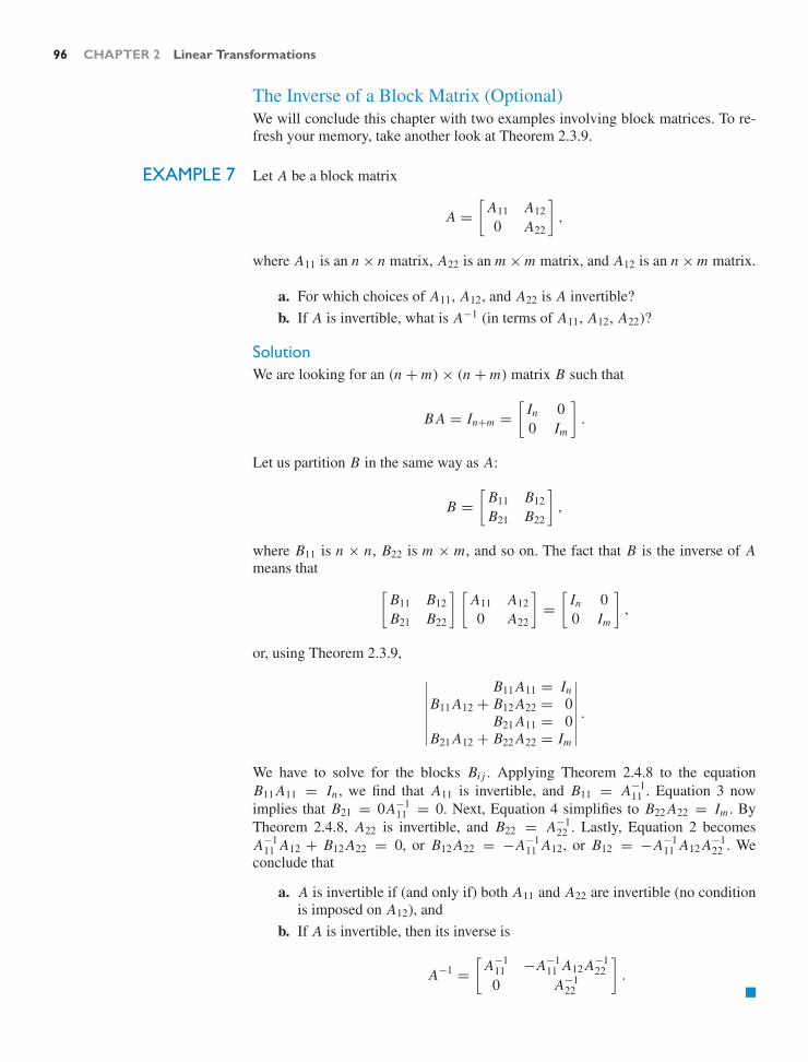
96 CHAPTER 2 Linear Transformations
The Inverse of a Block Matrix (Optional)We will conclude this chapter with two examples involving block matrices. To re-fresh your memory, take another look at Theorem 2.3.9.
EXAMPLE 7 Let A be a block matrix
A =[
A11 A12
0 A22
],
where A11 is an n × n matrix, A22 is an m × m matrix, and A12 is an n × m matrix.
a. For which choices of A11, A12, and A22 is A invertible?b. If A is invertible, what is A−1 (in terms of A11, A12, A22)?
SolutionWe are looking for an (n + m) × (n + m) matrix B such that
B A = In+m =[
In 00 Im
].
Let us partition B in the same way as A:
B =[
B11 B12
B21 B22
],
where B11 is n × n, B22 is m × m, and so on. The fact that B is the inverse of Ameans that
[B11 B12
B21 B22
] [A11 A12
0 A22
]=
[In 00 Im
],
or, using Theorem 2.3.9,
∣∣∣∣∣∣∣
B11 A11 = InB11 A12 + B12 A22 = 0
B21 A11 = 0B21 A12 + B22 A22 = Im
∣∣∣∣∣∣∣.
We have to solve for the blocks Bi j . Applying Theorem 2.4.8 to the equationB11 A11 = In , we find that A11 is invertible, and B11 = A−1
11 . Equation 3 nowimplies that B21 = 0A−1
11 = 0. Next, Equation 4 simplifies to B22 A22 = Im . ByTheorem 2.4.8, A22 is invertible, and B22 = A−1
22 . Lastly, Equation 2 becomesA−1
11 A12 + B12 A22 = 0, or B12 A22 = −A−111 A12, or B12 = −A−1
11 A12 A−122 . We
conclude that
a. A is invertible if (and only if) both A11 and A22 are invertible (no conditionis imposed on A12), and
b. If A is invertible, then its inverse is
A−1 =[
A−111 −A−1
11 A12 A−122
0 A−122
].
!
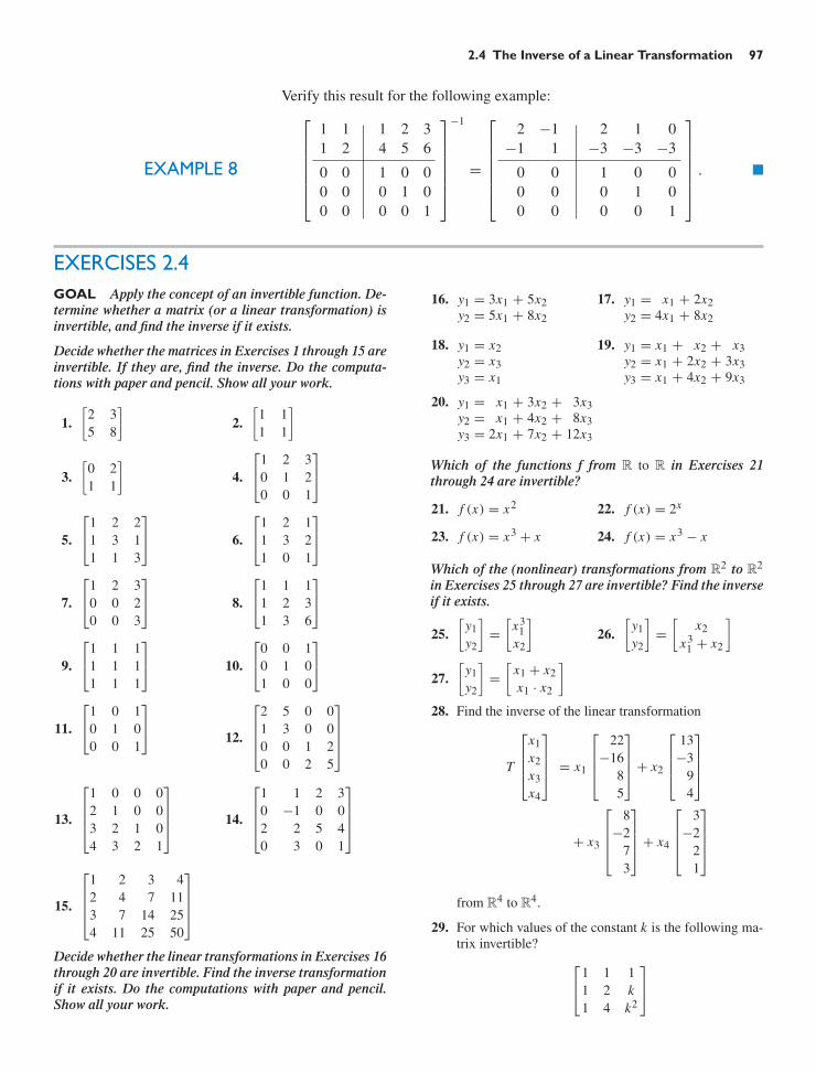
2.4 The Inverse of a Linear Transformation 97
Verify this result for the following example:
EXAMPLE 8
⎡
⎢⎢⎢⎢⎢⎣
1 11 2
1 2 34 5 6
0 00 00 0
1 0 00 1 00 0 1
⎤
⎥⎥⎥⎥⎥⎦
−1
=
⎡
⎢⎢⎢⎢⎢⎣
2 −1−1 1
2 1 0−3 −3 −3
0 00 00 0
1 0 00 1 00 0 1
⎤
⎥⎥⎥⎥⎥⎦. !
EXERCISES 2.4GOAL Apply the concept of an invertible function. De-termine whether a matrix (or a linear transformation) isinvertible, and find the inverse if it exists.
Decide whether the matrices in Exercises 1 through 15 areinvertible. If they are, find the inverse. Do the computa-tions with paper and pencil. Show all your work.
1.[
2 35 8
]2.
[1 11 1
]
3.[
0 21 1
]4.
⎡
⎣1 2 30 1 20 0 1
⎤
⎦
5.
⎡
⎣1 2 21 3 11 1 3
⎤
⎦ 6.
⎡
⎣1 2 11 3 21 0 1
⎤
⎦
7.
⎡
⎣1 2 30 0 20 0 3
⎤
⎦ 8.
⎡
⎣1 1 11 2 31 3 6
⎤
⎦
9.
⎡
⎣1 1 11 1 11 1 1
⎤
⎦ 10.
⎡
⎣0 0 10 1 01 0 0
⎤
⎦
11.
⎡
⎣1 0 10 1 00 0 1
⎤
⎦12.
⎡
⎢⎢⎣
2 5 0 01 3 0 00 0 1 20 0 2 5
⎤
⎥⎥⎦
13.
⎡
⎢⎢⎣
1 0 0 02 1 0 03 2 1 04 3 2 1
⎤
⎥⎥⎦ 14.
⎡
⎢⎢⎣
1 1 2 30 −1 0 02 2 5 40 3 0 1
⎤
⎥⎥⎦
15.
⎡
⎢⎢⎣
1 2 3 42 4 7 113 7 14 254 11 25 50
⎤
⎥⎥⎦
Decide whether the linear transformations in Exercises 16through 20 are invertible. Find the inverse transformationif it exists. Do the computations with paper and pencil.Show all your work.
16. y1 = 3x1 + 5x2y2 = 5x1 + 8x2
17. y1 = x1 + 2x2y2 = 4x1 + 8x2
18. y1 = x2y2 = x3y3 = x1
19. y1 = x1 + x2 + x3y2 = x1 + 2x2 + 3x3y3 = x1 + 4x2 + 9x3
20. y1 = x1 + 3x2 + 3x3y2 = x1 + 4x2 + 8x3y3 = 2x1 + 7x2 + 12x3
Which of the functions f from R to R in Exercises 21through 24 are invertible?
21. f (x) = x2 22. f (x) = 2x
23. f (x) = x3 + x 24. f (x) = x3 − x
Which of the (nonlinear) transformations from R2 to R2
in Exercises 25 through 27 are invertible? Find the inverseif it exists.
25.[
y1y2
]=
[x3
1x2
]26.
[y1y2
]=
[x2
x31 + x2
]
27.[
y1y2
]=
[x1 + x2x1 · x2
]
28. Find the inverse of the linear transformation
T
⎡
⎢⎢⎣
x1x2x3x4
⎤
⎥⎥⎦ = x1
⎡
⎢⎢⎣
22−16
85
⎤
⎥⎥⎦ + x2
⎡
⎢⎢⎣
13−3
94
⎤
⎥⎥⎦
+ x3
⎡
⎢⎢⎣
8−2
73
⎤
⎥⎥⎦ + x4
⎡
⎢⎢⎣
3−2
21
⎤
⎥⎥⎦
from R4 to R4.
29. For which values of the constant k is the following ma-trix invertible?
⎡
⎣1 1 11 2 k1 4 k2
⎤
⎦
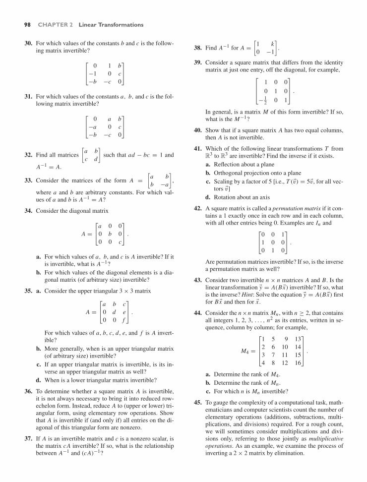
98 CHAPTER 2 Linear Transformations
30. For which values of the constants b and c is the follow-ing matrix invertible?
⎡
⎣0 1 b
−1 0 c−b −c 0
⎤
⎦
31. For which values of the constants a, b, and c is the fol-lowing matrix invertible?
⎡
⎣0 a b
−a 0 c−b −c 0
⎤
⎦
32. Find all matrices[
a bc d
]such that ad − bc = 1 and
A−1 = A.
33. Consider the matrices of the form A =[
a bb −a
],
where a and b are arbitrary constants. For which val-ues of a and b is A−1 = A?
34. Consider the diagonal matrix
A =
⎡
⎣a 0 00 b 00 0 c
⎤
⎦ .
a. For which values of a, b, and c is A invertible? If itis invertible, what is A−1?
b. For which values of the diagonal elements is a dia-gonal matrix (of arbitrary size) invertible?
35. a. Consider the upper triangular 3 × 3 matrix
A =
⎡
⎣a b c0 d e0 0 f
⎤
⎦ .
For which values of a, b, c, d , e, and f is A invert-ible?
b. More generally, when is an upper triangular matrix(of arbitrary size) invertible?
c. If an upper triangular matrix is invertible, is its in-verse an upper triangular matrix as well?
d. When is a lower triangular matrix invertible?
36. To determine whether a square matrix A is invertible,it is not always necessary to bring it into reduced row-echelon form. Instead, reduce A to (upper or lower) tri-angular form, using elementary row operations. Showthat A is invertible if (and only if) all entries on the di-agonal of this triangular form are nonzero.
37. If A is an invertible matrix and c is a nonzero scalar, isthe matrix cA invertible? If so, what is the relationshipbetween A−1 and (cA)−1?
38. Find A−1 for A =[
1 k0 −1
].
39. Consider a square matrix that differs from the identitymatrix at just one entry, off the diagonal, for example,
⎡
⎢⎣1 0 00 1 0
− 12 0 1
⎤
⎥⎦ .
In general, is a matrix M of this form invertible? If so,what is the M−1?
40. Show that if a square matrix A has two equal columns,then A is not invertible.
41. Which of the following linear transformations T fromR3 to R3 are invertible? Find the inverse if it exists.a. Reflection about a planeb. Orthogonal projection onto a planec. Scaling by a factor of 5 [i.e., T (v) = 5v, for all vec-
tors v]d. Rotation about an axis
42. A square matrix is called a permutation matrix if it con-tains a 1 exactly once in each row and in each column,with all other entries being 0. Examples are In and
⎡
⎣0 0 11 0 00 1 0
⎤
⎦ .
Are permutation matrices invertible? If so, is the inversea permutation matrix as well?
43. Consider two invertible n × n matrices A and B. Is thelinear transformation y = A(Bx) invertible? If so, whatis the inverse? Hint: Solve the equation y = A(Bx) firstfor Bx and then for x .
44. Consider the n×n matrix Mn , with n ≥ 2, that containsall integers 1, 2, 3, . . . , n2 as its entries, written in se-quence, column by column; for example,
M4 =
⎡
⎢⎢⎣
1 5 9 132 6 10 143 7 11 154 8 12 16
⎤
⎥⎥⎦ .
a. Determine the rank of M4.b. Determine the rank of Mn .c. For which n is Mn invertible?
45. To gauge the complexity of a computational task, math-ematicians and computer scientists count the number ofelementary operations (additions, subtractions, multi-plications, and divisions) required. For a rough count,we will sometimes consider multiplications and divi-sions only, referring to those jointly as multiplicativeoperations. As an example, we examine the process ofinverting a 2 × 2 matrix by elimination.

2.4 The Inverse of a Linear Transformation 99
[a b 1 0c d 0 1
]÷ a, requires 2 multiplicative
operations: b/a and 1/a
↓[
1 b′ e 0c d 0 1
](where b′ = b/a, and e = 1/a)− c (I), requires 2 multiplicative
operations: cb′ and ce↓[
1 b′ e 00 d ′ g 1
]
÷ d ′, requires 2 multiplicativeoperations↓
[1 b′ e 00 1 g′ h
]− b′ (II), requires 2 multiplicative
operations
↓[
1 0 e′ f0 1 g′ h
]
The whole process requires eight multiplicative opera-tions. Note that we do not count operations with pre-dictable results, such as 1a, 0a, a/a, 0/a.a. How many multiplicative operations are required to
invert a 3 × 3 matrix by elimination?b. How many multiplicative operations are required to
invert an n × n matrix by elimination?c. If it takes a slow hand-held calculator 1 second to
invert a 3 × 3 matrix, how long will it take the samecalculator to invert a 12 × 12 matrix? Assume thatthe matrices are inverted by Gauss–Jordan elimina-tion and that the duration of the computation is pro-portional to the number of multiplications and divi-sions involved.
46. Consider the linear system
Ax = b,
where A is an invertible matrix. We can solve this sys-tem in two different ways:• By finding the reduced row-echelon form of the aug-
mented matrix[
A b],
• By computing A−1 and using the formula x = A−1b.
In general, which approach requires fewer multiplica-tive operations? See Exercise 45.
47. Give an example of a noninvertible function f from Rto R and a number b such that the equation
f (x) = b
has a unique solution.
48. Consider an invertible linear transformation T (x) =Ax from Rm to Rn , with inverse L = T −1 from Rn toRm . In Exercise 2.2.29 we show that L is a linear trans-formation, so that L(y) = B y for some m × n matrixB. Use the equations B A = In and AB = Im to show
that n = m. Hint: Think about the number of solutionsof the linear systems Ax = 0 and B y = 0.
49. Input–Output Analysis. (This exercise builds on Exer-cises 1.1.24, 1.2.39, 1.2.40, and 1.2.41). Consider theindustries J1, J2, . . . , Jn in an economy. Suppose theconsumer demand vector is b, the output vector is x ,and the demand vector of the j th industry is v j . (Thei th component ai j of v j is the demand industry J j putson industry Ji , per unit of output of J j .) As we have seenin Exercise 1.2.40, the output x just meets the aggregatedemand if
x1v1 + x2v2 + · · · + xn vn + b︸ ︷︷ ︸aggregate demand
= x︸︷︷︸output
.
This equation can be written more succinctly as
⎡
⎢⎣| | |
v1 v2 · · · vn
| | |
⎤
⎥⎦
⎡
⎢⎢⎢⎣
x1x2...
xn
⎤
⎥⎥⎥⎦+ b = x,
or Ax + b = x . The matrix A is called the technologymatrix of this economy; its coefficients ai j describe theinterindustry demand, which depends on the technologyused in the production process. The equation
Ax + b = x
describes a linear system, which we can write in thecustomary form:
x − Ax = b
In x − Ax = b
(In − A)x = b.
If we want to know the output x required to satisfy agiven consumer demand b (this was our objective inthe previous exercises), we can solve this linear system,preferably via the augmented matrix.
In economics, however, we often ask other ques-tions: If b changes, how will x change in response?If the consumer demand on one industry increases by1 unit and the consumer demand on the other indus-tries remains unchanged, how will x change?11 If we
11 The relevance of questions like these became particularlyclear during World War II, when the demand on certainindustries suddenly changed dramatically. When U.S.President F. D. Roosevelt asked for 50,000 airplanes to bebuilt, it was easy enough to predict that the country wouldhave to produce more aluminum. Unexpectedly, the demandfor copper dramatically increased (why?). A copper shortagethen occurred, which was solved by borrowing silver fromFort Knox. People realized that input–output analysis can beeffective in modeling and predicting chains of increaseddemand like this. After World War II, this technique rapidlygained acceptance and was soon used to model the economiesof more than 50 countries.

100 CHAPTER 2 Linear Transformations
ask questions like these, we think of the output x as afunction of the consumer demand b.
If the matrix (In−A) is invertible,12 we can expressx as a function of b (in fact, as a linear transformation):
x = (In − A)−1b.
a. Consider the example of the economy of Israel in1958 (discussed in Exercise 1.2.41). Find the tech-nology matrix A, the matrix (In − A), and its inverse(In − A)−1.
b. In the example discussed in part (a), suppose theconsumer demand on agriculture (Industry 1) is 1unit (1 million pounds), and the demands on theother two industries are zero. What output x is re-quired in this case? How does your answer relate tothe matrix (In − A)−1?
c. Explain, in terms of economics, why the diagonalelements of the matrix (In − A)−1 you found in part(a) must be at least 1.
d. If the consumer demand on manufacturing increasesby 1 (from whatever it was), and the consumer de-mand on the other two industries remains the same,how will the output have to change? How does youranswer relate to the matrix (In − A)−1?
e. Using your answers in parts (a) through (d) as aguide, explain in general (not just for this exam-ple) what the columns and the entries of the matrix(In − A)−1 tell you, in terms of economics. Thosewho have studied multivariable calculus may wishto consider the partial derivatives
∂xi
∂b j.
50. This exercise refers to Exercise 49a. Consider the en-try k = a11 = 0.293 of the technology matrix A. Ver-ify that the entry in the first row and the first columnof (In − A)−1 is the value of the geometrical series1 + k + k2 + · · · . Interpret this observation in termsof economics.
51. a. Consider an n × m matrix A with rank(A) < n.Show that there exists a vector b in Rn such thatthe system Ax = b is inconsistent. Hint: For E =rref(A), show that there exists a vector c in Rn suchthat the system Ex = c is inconsistent; then, “workbackward.”
b. Consider an n × m matrix A with n > m. Show thatthere exists a vector b in Rn such that the systemAx = b is inconsistent.
52. For
A =
⎡
⎢⎢⎣
0 1 20 2 40 3 61 4 8
⎤
⎥⎥⎦ ,
find a vector b in R4 such that the system Ax = b isinconsistent. See Exercise 51.
53. Let A =[
3 13 5
]in all parts of this problem.
a. Find a scalar λ (lambda) such that the matrix A−λI2fails to be invertible. There are two solutions; chooseone and use it in parts (b) and (c).
b. For the λ you chose in part (a), find the matrixA − λI2; then find a nonzero vector x such that(A − λI2)x = 0. (This can be done, since A − λI2fails to be invertible.)
c. Note that the equation (A − λI2)x = 0 can be writ-ten as Ax − λx = 0, or Ax = λx . Check that theequation Ax = λx holds for your λ from part (a)and your x from part (b).
54. Let A =[
1 10−3 12
]. Using Exercise 53 as a guide, find
a scalar λ and a nonzero vector x such that Ax = λx .
In Exercises 55 through 65, show that the given matrixA is invertible, and find the inverse. Interpret the lineartransformation T(x) = Ax and the inverse transforma-tion T−1( y) = A−1 y geometrically. Interpret det A geo-metrically. In your figure, show the angle θ and the vectorsv and w introduced in Theorem 2.4.10.
55.[
2 00 2
]56.
[cos α − sin α
sin α cos α
]
57.[
cos α sin α
sin α − cos α
]58.
[−3 0
0 −3
]
59.[
0.6 −0.80.8 0.6
]60.
[−0.8 0.6
0.6 0.8
]
61.[
1 1−1 1
]62.
[1 −10 1
]
63.[−3 4
4 3
]64.
[3 4
−4 3
]
65.[
1 01 1
]
66. Consider two n × n matrices A and B such that theproduct AB is invertible. Show that the matrices Aand B are both invertible. Hint: AB(AB)−1 = In and(AB)−1 AB = In . Use Theorem 2.4.8.
For two invertible n × n matrices A and B, determinewhich of the formulas stated in Exercises 67 through 75are necessarily true.
67. (A + B)2 = A2 + 2AB + B2
68. (A − B)(A + B) = A2 − B2
69. A + B is invertible, and (A + B)−1 = A−1 + B−1
70. A2 is invertible, and (A2)−1 = (A−1)2
71. AB B−1 A−1 = In
12 This will always be the case for a “productive” economy. SeeExercise 103.

2.4 The Inverse of a Linear Transformation 101
72. AB A−1 = B
73. (AB A−1)3 = AB3 A−1
74. (In + A)(In + A−1) = 2In + A + A−1
75. A−1 B is invertible, and (A−1 B)−1 = B−1 A
76. Find all linear transformations T from R2 to R2 suchthat
T[
12
]=
[21
]and T
[25
]=
[13
].
Hint: We are looking for the 2 × 2 matrices A such that
A[
12
]=
[21
]and A
[25
]=
[13
].
These two equations can be combined to form the ma-trix equation
A[
1 22 5
]=
[2 11 3
].
77. Using the last exercise as a guide, justify the followingstatement:Let v1, v2, . . . , vm be vectors in Rm such that the ma-trix
S =
⎡
⎢⎣| | |
v1 v2 · · · vm
| | |
⎤
⎥⎦
is invertible. Let w1, w2, . . . , wm be arbitrary vectorsin Rn . Then there exists a unique linear transforma-tion T from Rm to Rn such that T (vi ) = wi , for alli = 1, . . . , m. Find the matrix A of this transformationin terms of S and
B =
⎡
⎢⎣| | |
w1 w2 · · · wm
| | |
⎤
⎥⎦ .
78. Find the matrix A of the linear transformation T fromR2 to R3 with
T[
12
]=
⎡
⎣753
⎤
⎦ and T[
25
]=
⎡
⎣123
⎤
⎦ .
Compare with Exercise 77.
79. Find the matrix A of the linear transformation T fromR2 to R2 with
T[
31
]= 2
[31
]and T
[12
]= 3
[12
].
Compare with Exercise 77.
80. Consider the regular tetrahedron sketched below, whosecenter is at the origin.
0P3 =
−1−11
P2 =−11
−1P1 =
1−1−1
P0 =111
Let T from R3 to R3 be the rotation about the axisthrough the points 0 and P2 that transforms P1 into P3.Find the images of the four corners of the tetrahedronunder this transformation.
P0T→
P1 → P3
P2 →P3 →
Let L from R3 to R3 be the reflection about the planethrough the points 0, P0, and P3. Find the images of thefour corners of the tetrahedron under this transformation.
P0L→
P1 →P2 →P3 →
Describe the transformations in parts (a) through(c) geometrically.a. T −1 b. L−1
c. T 2 = T T (the composite of T with itself)d. Find the images of the four corners under the trans-
formations T L and L T . Are the two transforma-tions the same?
P0T L→
P1 →P2 →P3 →
P0LT→
P1 →P2 →P3 →
e. Find the images of the four corners under the trans-formation L T L . Describe this transformationgeometrically.
81. Find the matrices of the transformations T and L definedin Exercise 80.
82. Consider the matrix
E =
⎡
⎣1 0 0
−3 1 00 0 1
⎤
⎦
and an arbitrary 3 × 3 matrix
A =
⎡
⎣a b cd e fg h k
⎤
⎦ .

102 CHAPTER 2 Linear Transformations
a. Compute E A. Comment on the relationship be-tween A and E A, in terms of the technique of elim-ination we learned in Section 1.2.
b. Consider the matrix
E =
⎡
⎢⎣1 0 00 1
4 00 0 1
⎤
⎥⎦
and an arbitrary 3×3 matrix A. Compute E A. Com-ment on the relationship between A and E A.
c. Can you think of a 3 × 3 matrix E such that E A isobtained from A by swapping the last two rows (forany 3 × 3 matrix A)?
d. The matrices of the forms introduced in parts (a),(b), and (c) are called elementary: An n × n matrixE is elementary if it can be obtained from In by per-forming one of the three elementary row operationson In . Describe the format of the three types of ele-mentary matrices.
83. Are elementary matrices invertible? If so, is the inverseof an elementary matrix elementary as well? Explainthe significance of your answers in terms of elementaryrow operations.
84. a. Justify the following: If A is an n × m matrix, thenthere exist elementary n × n matrices E1, E2, . . . ,E p such that
rref(A) = E1 E2 · · · E p A.
b. Find such elementary matrices E1, E2, . . . , E p for
A =[
0 21 3
].
85. a. Justify the following: If A is an n × m matrix, thenthere exists an invertible n × n matrix S such that
rref(A) = S A.
b. Find such an invertible matrix S for
A =[
2 44 8
].
86. a. Justify the following: Any invertible matrix is aproduct of elementary matrices.
b. Write A =[
0 21 3
]as a product of elementary
matrices.
87. Write all possible forms of elementary 2 × 2 matricesE . In each case, describe the transformation y = Exgeometrically.
88. Consider an invertible n × n matrix A and an n × n ma-trix B. A certain sequence of elementary row operationstransforms A into In .a. What do you get when you apply the same row op-
erations in the same order to the matrix AB?
b. What do you get when you apply the same row op-erations to In?
89. Is the product of two lower triangular matrices a lowertriangular matrix as well? Explain your answer.
90. Consider the matrix
A =
⎡
⎣1 2 32 6 72 2 4
⎤
⎦ .
a. Find lower triangular elementary matrices E1,E2, . . . , Em such that the product
Em · · · E2 E1 A
is an upper triangular matrix U . Hint: Use elemen-tary row operations to eliminate the entries belowthe diagonal of A.
b. Find lower triangular elementary matrices M1,M2, . . . , Mm and an upper triangular matrix U suchthat
A = M1 M2 · · · MmU.
c. Find a lower triangular matrix L and an upper trian-gular matrix U such that
A = LU.
Such a representation of an invertible matrix iscalled an LU -factorization. The method outlinedin this exercise to find an LU -factorization can bestreamlined somewhat, but we have seen the ma-jor ideas. An LU -factorization (as introduced here)does not always exist. See Exercise 92.
d. Find a lower triangular matrix L with 1’s on the di-agonal, an upper triangular matrix U with 1’s onthe diagonal, and a diagonal matrix D such thatA = L DU . Such a representation of an invertiblematrix is called an L DU -factorization.
91. Knowing an LU -factorization of a matrix A makes itmuch easier to solve a linear system
Ax = b.
Consider the LU -factorization
A =
⎡
⎢⎢⎣
1 2 −1 4−3 −5 6 −5
1 4 6 20−1 6 20 43
⎤
⎥⎥⎦
=
⎡
⎢⎢⎣
1 0 0 0−3 1 0 0
1 2 1 0−1 8 −5 1
⎤
⎥⎥⎦
⎡
⎢⎢⎣
1 2 −1 40 1 3 70 0 1 20 0 0 1
⎤
⎥⎥⎦
= LU.
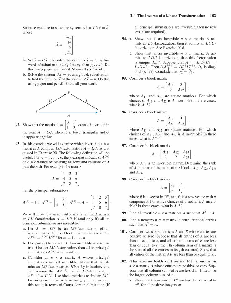
2.4 The Inverse of a Linear Transformation 103
Suppose we have to solve the system Ax = LU x = b,where
b =
⎡
⎢⎢⎣
−314
933
⎤
⎥⎥⎦ .
a. Set y = U x , and solve the system L y = b, by for-ward substitution (finding first y1, then y2, etc.). Dothis using paper and pencil. Show all your work.
b. Solve the system U x = y, using back substitution,to find the solution x of the system Ax = b. Do thisusing paper and pencil. Show all your work.
U
A
L
x b
y
92. Show that the matrix A =[
0 11 0
]cannot be written in
the form A = LU , where L is lower triangular and Uis upper triangular.
93. In this exercise we will examine which invertible n × nmatrices A admit an LU -factorization A = LU , as dis-cussed in Exercise 90. The following definition will beuseful: For m = 1, . . . , n, the principal submatrix A(m)
of A is obtained by omitting all rows and columns of Apast the mth. For example, the matrix
A =
⎡
⎣1 2 34 5 67 8 7
⎤
⎦
has the principal submatrices
A(1) = [1], A(2) =[
1 24 5
], A(3) = A =
⎡
⎣1 2 34 5 67 8 7
⎤
⎦ .
We will show that an invertible n × n matrix A admitsan LU -factorization A = LU if (and only if) all itsprincipal submatrices are invertible.a. Let A = LU be an LU -factorization of an
n × n matrix A. Use block matrices to show thatA(m) = L(m)U (m) for m = 1, . . . , n.
b. Use part (a) to show that if an invertible n × n ma-trix A has an LU -factorization, then all its principalsubmatrices A(m) are invertible.
c. Consider an n × n matrix A whose principalsubmatrices are all invertible. Show that A ad-mits an LU -factorization. Hint: By induction, youcan assume that A(n−1) has an LU -factorizationA(n−1) = L ′U ′. Use block matrices to find an LU -factorization for A. Alternatively, you can explainthis result in terms of Gauss–Jordan elimination (if
all principal submatrices are invertible, then no rowswaps are required).
94. a. Show that if an invertible n × n matrix A ad-mits an LU -factorization, then it admits an L DU -factorization. See Exercise 90 d.
b. Show that if an invertible n × n matrix A ad-mits an L DU -factorization, then this factorizationis unique. Hint: Suppose that A = L1 D1U1 =L2 D2U2. Then U2U−1
1 = D−12 L−1
2 L1 D1 is diag-onal (why?). Conclude that U2 = U1.
95. Consider a block matrix
A =[
A11 00 A22
],
where A11 and A22 are square matrices. For whichchoices of A11 and A22 is A invertible? In these cases,what is A−1?
96. Consider a block matrix
A =[
A11 0A21 A22
],
where A11 and A22 are square matrices. For whichchoices of A11, A21, and A22 is A invertible? In thesecases, what is A−1?
97. Consider the block matrix
A =[
A11 A12 A130 0 A23
],
where A11 is an invertible matrix. Determine the rankof A in terms of the ranks of the blocks A11, A12, A13,and A23.
98. Consider the block matrix
A =[
In v
w 1
],
where v is a vector in Rn , and w is a row vector with ncomponents. For which choices of v and w is A invert-ible? In these cases, what is A−1?
99. Find all invertible n × n matrices A such that A2 = A.
100. Find a nonzero n × n matrix A with identical entriessuch that A2 = A.
101. Consider two n × n matrices A and B whose entries arepositive or zero. Suppose that all entries of A are lessthan or equal to s, and all column sums of B are lessthan or equal to r (the j th column sum of a matrix isthe sum of all the entries in its j th column). Show thatall entries of the matrix AB are less than or equal to sr .
102. (This exercise builds on Exercise 101.) Consider ann × n matrix A whose entries are positive or zero. Sup-pose that all column sums of A are less than 1. Let r bethe largest column sum of A.a. Show that the entries of Am are less than or equal to
rm , for all positive integers m.

104 CHAPTER 2 Linear Transformations
b. Show that
limm→∞
Am = 0
(meaning that all entries of Am approach zero).c. Show that the infinite series
In + A + A2 + · · · + Am + · · ·
converges (entry by entry).d. Compute the product
(In − A)(In + A + A2 + · · · + Am).
Simplify the result. Then let m go to infinity, andthus show that
(In − A)−1 = In + A + A2 + · · · + Am + · · · .
103. (This exercise builds on Exercises 49, 101, and 102.)a. Consider the industries J1, . . . , Jn in an economy.
We say that industry J j is productive if the j th col-umn sum of the technology matrix A is less than 1.What does this mean in terms of economics?
b. We say that an economy is productive if all of itsindustries are productive. Exercise 102 shows thatif A is the technology matrix of a productive econ-omy, then the matrix In − A is invertible. What doesthis result tell you about the ability of a productiveeconomy to satisfy consumer demand?
c. Interpret the formula
(In − A)−1 = In + A + A2 + · · · + Am + · · ·
derived in Exercise 102d in terms of economics.
104. The color of light can be represented in a vector⎡
⎣RGB
⎤
⎦ ,
where R = amount of red, G = amount of green, andB = amount of blue. The human eye and the braintransform the incoming signal into the signal
⎡
⎣ILS
⎤
⎦ ,
where
intensity I = R + G + B3
long-wave signal L = R − G
short-wave signal S = B − R + G2
.
a. Find the matrix P representing the transformationfrom
⎡
⎣RGB
⎤
⎦ to
⎡
⎣ILS
⎤
⎦ .
b. Consider a pair of yellow sunglasses for water sportsthat cuts out all blue light and passes all red andgreen light. Find the 3 × 3 matrix A that representsthe transformation incoming light undergoes as itpasses through the sunglasses. All the entries of yourmatrix A will be 0’s and 1’s.
c. Find the matrix for the composite transformationthat light undergoes as it first passes through the sun-glasses and then the eye.
d. As you put on the sunglasses, the signal you receive(intensity, long- and short-wave signals) undergoesa transformation. Find the matrix M of this transfor-mation. Feel free to use technology.
Light passes through eyes only.
A
P
M
P
Light passes through glasses and then through eyes.
105. A village is divided into three mutually exclusivegroups called clans. Each person in the village belongsto a clan, and this identification is permanent. Thereare rigid rules concerning marriage: A person from oneclan can only marry a person from one other clan. Theserules are encoded in the matrix A below. The fact thatthe 2–3 entry is 1 indicates that marriage between a manfrom clan III and a woman from clan II is allowed. Theclan of a child is determined by the mother’s clan, asindicated by the matrix B. According to this scheme,siblings belong to the same clan.
Husband’s clanI II III
A =
⎡
⎣0 1 00 0 11 0 0
⎤
⎦IIIIII
Wife’sclan
Mother’s clanI II III
B =
⎡
⎣1 0 00 0 10 1 0
⎤
⎦IIIIII
Child’sclan
The identification of a person with clan I can be repre-sented by the vector
e1 =
⎡
⎣100
⎤
⎦ ,

2.4 The Inverse of a Linear Transformation 105
and likewise for the two other clans. Matrix A trans-forms the husband’s clan into the wife’s clan (if x repre-sents the husband’s clan, then Ax represents the wife’sclan).a. Are the matrices A and B invertible? Find the in-
verses if they exist. What do your answers mean, inpractical terms?
b. What is the meaning of B2, in terms of the rules ofthe community?
c. What is the meaning of AB and B A, in terms of therules of the community? Are AB and B A the same?
d. Bueya is a young woman who has many male firstcousins, both on her mother’s and on her father’ssides. The kinship between Bueya and each of hermale cousins can be represented by one of the fourdiagrams below:
Bueya
Her mother An aunt on the mother’s side
A male first cousin
In each of the four cases, find the matrix that givesyou the cousin’s clan in terms of Bueya’s clan.
e. According to the rules of the village, could Bueyamarry a first cousin? (We do not know Bueya’s clan.)
106. As background to this exercise, see Exercise 45.a. If you use Theorem 2.3.4, how many multiplica-
tions of scalars are necessary to multiply two 2 × 2matrices?
b. If you use Theorem 2.3.4, how many multiplicationsare needed to multiply an n × p and a p×m matrix?
In 1969, the German mathematician Volker Strassensurprised the mathematical community by showing thattwo 2 × 2 matrices can be multiplied with only sevenmultiplications of numbers. Here is his trick: Suppose
you have to find AB for A =[
a bc d
]and B =
[p qr s
]. First compute
h1 = (a + d)(p + s)h2 = (c + d)ph3 = a(q − s)h4 = d(r − p)h5 = (a + b)sh6 = (c − a)(p + q)h7 = (b − d)(r + s).
Then
AB =[
h1 + h4 − h5 + h7 h3 + h5h2 + h4 h1 + h3 − h2 + h6
].
107. Let N be the set of all positive integers, 1, 2, 3, . . . . Wedefine two functions f and g from N to N:
f (x) = 2x, for all x in N
g(x) =
x/2 if x is even(x + 1)/2 if x is odd.
Find formulas for the composite functions g(
f (x))
andf(g(x)
). Is one of them the identity transformation
from N to N? Are the functions f and g invertible?
108. Geometrical optics. Consider a thin biconvex lens withtwo spherical faces.
This is a good model for the lens of the human eye andfor the lenses used in many optical instruments, such asreading glasses, cameras, microscopes, and telescopes.The line through the centers of the spheres defining thetwo faces is called the optical axis of the lens.
Center of spheredefining the right face
Center of spheredefining the left face
Optical axis
In this exercise, we learn how we can track the path ofa ray of light as it passes through the lens, provided thatthe following conditions are satisfied:• The ray lies in a plane with the optical axis.• The angle the ray makes with the optical axis is small.

106 CHAPTER 2 Linear Transformations
To keep track of the ray, we introduce two referenceplanes perpendicular to the optical axis, to the left andto the right of the lens.
Left referenceplane
Right referenceplane
< L > < R >
We can characterize the incoming ray by its slope m andits intercept x with the left reference plane. Likewise, wecharacterize the outgoing ray by slope n and intercept y.
< L >
slope m
x y
slope n
< R >
We want to know how the outgoing ray depends on theincoming ray; that is, we are interested in the transfor-mation
T : R2 → R2;[
xm
]→
[yn
].
We will see that T can be approximated by a linear trans-formation provided that m is small, as we assumed. Tostudy this transformation, we divide the path of the rayinto three segments, as shown in the following figure:
IIIIII
< L >
m
x y
n
< R >
v w
We have introduced two auxiliary reference planes, di-rectly to the left and to the right of the lens. Our trans-formation
[xm
]→
[yn
]
can now be represented as the composite of three sim-pler transformations:
[xm
]→
[v
m
]→
[w
n
]→
[yn
].
From the definition of the slope of a line, we get therelations v = x + Lm and y = w + Rn.
L
LmSlope m
x x
v
[v
m
]=
[x + Lm
m
]=
[1 L0 1
] [xm
]
[yn
]=
[1 R0 1
] [w
n
]
[xm
]−−−−−→[
1 L0 1
]
[v
m
]−−−−−→
[w
n
]−−−−−→[
1 R0 1
]
[yn
]
It would lead us too far into physics to derive a formulafor the transformation
[v
m
]→
[w
n
]
here.13 Under the assumptions we have made, the trans-formation is well approximated by
[w
n
]=
[1 0
−k 1
] [v
m
],
for some positive constant k (this formula implies thatw = v).
[xm
]−−−−−→[
1 L0 1
]
[v
m
]−−−−−→[
1 0−k 1
]
[w
n
]−−−−−→[
1 R0 1
]
[yn
]
13 See, for example, Paul Bamberg and Shlomo Sternberg, ACourse in Mathematics for Students of Physics 1, CambridgeUniversity Press, 1991.

Chapter Two Exercises 107
The transformation[
xm
]→
[yn
]is represented by the
matrix product[
1 R0 1
] [1 0
−k 1
] [1 L0 1
]
=[
1 − Rk L + R − kL R−k 1 − kL
].
a. Focusing parallel rays. Consider the lens in the hu-man eye, with the retina as the right reference plane.In an adult, the distance R is about 0.025 meters(about 1 inch). The ciliary muscles allow you to varythe shape of the lens and thus the lens constant k,within a certain range. What value of k enables youto focus parallel incoming rays, as shown in the fig-ure? This value of k will allow you to see a distantobject clearly. (The customary unit of measurementfor k is 1 diopter = 1
1 meter .)
R
Slope m
y
Hint: In terms of the transformation[
xm
]→
[yn
],
you want y to be independent of x (y must dependon the slope m alone). Explain why 1/k is called thefocal length of the lens.
b. What value of k enables you to read this text from adistance of L = 0.3 meters? Consider the followingfigure (which is not to scale).
RL
c. The telescope. An astronomical telescope consists oftwo lenses with the same optical axis.
D
k1 k2
Left referenceplane
Right referenceplane
Find the matrix of the transformation[
xm
]→
[yn
],
in terms of k1, k2, and D. For given values of k1 andk2, how do you choose D so that parallel incomingrays are converted into parallel outgoing rays? Whatis the relationship between D and the focal lengthsof the two lenses, 1/k1 and 1/k2?
Chapter Two Exercises
TRUE OR FALSE?
1. The matrix[
5 6−6 5
]represents a rotation combined
with a scaling.
2. If A is any invertible n × n matrix, then A commuteswith A−1.
3. The function T[
xy
]=
[x − yy − x
]is a linear trans-
formation.
4. Matrix[
1/2 −1/21/2 1/2
]represents a rotation.
5. If A is any invertible n × n matrix, then rref(A) = In .
6. The formula (A2)−1 = (A−1)2 holds for all invertiblematrices A.
7. The formula AB = B A holds for all n × n matrices Aand B.
8. If AB = In for two n × n matrices A and B, then Amust be the inverse of B.
9. If A is a 3 × 4 matrix and B is a 4 × 5 matrix, then ABwill be a 5 × 3 matrix.
10. The function T[
xy
]=
[y1
]is a linear transformation.

108 CHAPTER 2 Linear Transformations
11. Matrix[
k −25 k − 6
]is invertible for all real numbers k.
12. There exists a real number k such that the matrix[k − 1 −2−4 k − 3
]fails to be invertible.
13. There exists a real number k such that the matrix[k − 2 3−3 k − 2
]fails to be invertible.
14. A =[
1 1/20 1/2
]is a regular transition matrix.
15. The formula det(2A) = 2 det(A) holds for all 2 × 2matrices A.
16. There exists a matrix A such that[1 23 4
]A
[5 67 8
]=
[1 11 1
].
17. Matrix[
1 23 6
]is invertible.
18. Matrix
⎡
⎣1 1 11 0 11 1 0
⎤
⎦ is invertible.
19. There exists an upper triangular 2 × 2 matrix A such
that A2 =[
1 10 1
].
20. The function T[
xy
]=
[(y + 1)2 − (y − 1)2
(x − 3)2 − (x + 3)2
]is a
linear transformation.
21. There exists an invertible n × n matrix with two identi-cal rows.
22. If A2 = In , then matrix A must be invertible.
23. There exists a matrix A such that A[
1 11 1
]=
[1 21 2
].
24. There exists a matrix A such that[
1 21 2
]A =
[1 11 1
].
25. The matrix[
1 11 −1
]represents a reflection about a
line.
26. For every regular transition matrix A there exists a tran-sition matrix B such that AB = B.
27. The matrix product[
a bc d
] [d −b
−c a
]is always a
scalar multiple of I2.
28. There exists a nonzero upper triangular 2 × 2 matrix A
such that A2 =[
0 00 0
].
29. There exists a positive integer n such that[
0 −11 0
]n
= I2.
30. There exists an invertible 2 × 2 matrix A such that
A−1 =[
1 11 1
].
31. There exists a regular transition matrix A of size 3 × 3such that A2 = A.
32. If A is any transition matrix and B is any positive tran-sition matrix, then AB must be a positive transition ma-trix.
33. If matrix
⎡
⎣a b cd e fg h i
⎤
⎦ is invertible, then matrix
[a bd e
]must be invertible as well.
34. If A2 is invertible, then matrix A itself must be invert-ible.
35. If A17 = I2, then matrix A must be I2.
36. If A2 = I2, then matrix A must be either I2 or −I2.
37. If matrix A is invertible, then matrix 5A must be invert-ible as well.
38. If A and B are two 4 × 3 matrices such that Av = Bvfor all vectors v in R3, then matrices A and B must beequal.
39. If matrices A and B commute, then the formula A2 B =B A2 must hold.
40. If A2 = A for an invertible n ×n matrix A, then A mustbe In .
41. If A is any transition matrix such that A100 is positive,then A101 must be positive as well.
42. If a transition matrix A is invertible, then A−1 must bea transition matrix as well.
43. If matrices A and B are both invertible, then matrixA + B must be invertible as well.
44. The equation A2 = A holds for all 2 × 2 matrices Arepresenting a projection.
45. The equation A−1 = A holds for all 2 × 2 matrices Arepresenting a reflection.
46. The formula (Av) · (Aw) = v · w holds for all invertible2 × 2 matrices A and for all vectors v and w in R2.
47. There exist a 2 × 3 matrix A and a 3 × 2 matrix B suchthat AB = I2.
48. There exist a 3 × 2 matrix A and a 2 × 3 matrix B suchthat AB = I3.
49. If A2 +3A +4I3 = 0 for a 3×3 matrix A, then A mustbe invertible.
50. If A is an n × n matrix such that A2 = 0, then matrixIn + A must be invertible.

Chapter Two Exercises 109
51. If matrix A commutes with B, and B commutes with C ,then matrix A must commute with C .
52. If T is any linear transformation from R3 to R3,then T (v × w) = T (v) × T (w) for all vectors v andw in R3.
53. There exists an invertible 10 × 10 matrix that has 92ones among its entries.
54. The formula rref(AB) = rref(A) rref(B) holds for alln × p matrices A and for all p × m matrices B.
55. There exists an invertible matrix S such that
S−1[
0 10 0
]S is a diagonal matrix.
56. If the linear system A2 x = b is consistent, then the sys-tem Ax = b must be consistent as well.
57. There exists an invertible 2 × 2 matrix A such thatA−1 = −A.
58. There exists an invertible 2 × 2 matrix A such that
A2 =[
1 00 −1
].
59. If a matrix A =[
a bc d
]represents the orthog-
onal projection onto a line L , then the equationa2 + b2 + c2 + d2 = 1 must hold.
60. If A is an invertible 2×2 matrix and B is any 2×2 ma-trix, then the formula rref(AB) = rref(B) must hold.
61. There is a transition matrix A such that limm→∞
Am failsto exist.
62. For every transition matrix A there exists a nonzero vec-tor x such that Ax = x .

C H A P T E R
3Subspaces of Rn and Their Dimensions
3.1 Image and Kernel of a Linear Transformation
You may be familiar with the notion of the image1 of a function.
Definition 3.1.1 Image of a function
The image of a function consists of all the values the function takes in its targetspace. If f is a function from X to Y , then
image ( f ) = f (x): x in X= b in Y : b = f (x), for some x in X.
EXAMPLE 1 A group X of students and a group Y of professors stand in the yard. Each studentthrows a snowball at one of the professors (and each snowball hits its intendedtarget). Consider the function y = f (x) from X to Y that associates with eachstudent x the target y of his or her snowball. The image of f consists of thoseprofessors that are hit. See Figure 1. !
X: the domain of f Y: the target space of f
f
image ( f )
Figure 1
1Some authors use the term range for what we call the image, while others use the term range forwhat we call the target space. Because of this ambiguity, we will not use the term range at all. Makesure to check which definition is used when you encounter the term range in a text.
110

3.1 Image and Kernel of a Linear Transformation 111
EXAMPLE 2 The image of the exponential function f (x) = ex from R to R consists of allpositive real numbers. Indeed, f (x) = ex is positive for all x , and every positivenumber b can be written as b = eln b = f (ln b). See Figure 2. !
b
ln(b)
f(x) = ex
Figure 2
More generally, the image of a function f (x) from R to R consists of all realnumbers b such that the line y = b intersects the graph of f (take another look atFigure 2). The image of f is the orthogonal projection of the graph of f onto thevertical axis.
EXAMPLE 3 The image of the function
f (t) =[
cos tsin t
]from R to R2
is the unit circle centered at the origin. See Figure 3. Indeed,[
cos tsin t
]is a unit vector
for all t , since cos2 t + sin2 t = 1, and, conversely, any unit vector u in R2 can be
written in polar coordinates as u =[
cos tsin t
], where t is its polar angle. !
t
0 10
f(t) = cos tsin t
Figure 3
The function f in Example 3 is called a parametrization of the unit circle. Moregenerally, a parametrization of a curve C in R2 is a function g from R to R2 whoseimage is C .

112 CHAPTER 3 Subspaces of Rn and Their Dimensions
EXAMPLE 4 If the function f from X to Y is invertible, then the image of f is Y . Indeed, forevery b in Y , there exists one (and only one) x in X such that b = f (x), namely,x = f −1(b):
b = f(
f −1(b)).
See Figure 4. !
X
x = f −1(b)
Y
f
b
Figure 4
EXAMPLE 5 Consider the linear transformation T from R3 to R3 that projects a vector x orthog-
onally into the x1–x2-plane, meaning that T
⎡
⎣x1
x2
x3
⎤
⎦ =
⎡
⎣x1
x2
0
⎤
⎦. See Figure 5.
T(x)x1
x2
x3
x
Figure 5
The image of T is the x1–x2-plane in R3, consisting of all vectors of the form⎡
⎣x1
x2
0
⎤
⎦. !
EXAMPLE 6 Describe the image of the linear transformation
T (x) = Ax from R2 to R2, where A =[
1 32 6
].
SolutionThe image of T consists of all the values of T , that is, all vectors of the form
T[
x1
x2
]= A
[x1
x2
]=
[1 32 6
] [x1
x2
]= x1
[12
]+ x2
[36
]
= x1
[12
]+ 3x2
[12
]= (x1 + 3x2)
[12
].

3.1 Image and Kernel of a Linear Transformation 113
Since the vectors[
12
]and
[36
]are parallel, the image of T is the line of all scalar
multiples of the vector[
12
], as illustrated in Figure 6. !
image(T )
12
36
Figure 6
EXAMPLE 7 Describe the image of the linear transformation
T (x) = Ax from R2 to R3, where A =
⎡
⎣1 11 21 3
⎤
⎦ .
SolutionThe image of T consists of all vectors of the form
T[
x1
x2
]=
⎡
⎣1 11 21 3
⎤
⎦[
x1
x2
]= x1
⎡
⎣111
⎤
⎦ + x2
⎡
⎣123
⎤
⎦ ,
that is, all linear combinations of the column vectors of A,
v1 =
⎡
⎣111
⎤
⎦ and v2 =
⎡
⎣123
⎤
⎦ .
The image of T is the plane V “spanned” by the two vectors v1 and v2, that is,the plane through the origin and the endpoints (1, 1, 1) and (1, 2, 3) of v1 and v2,respectively. See Figure 7. !
0
Vv2
v1
x2v2
x1v1
x1v1 + x2v2
Figure 7

114 CHAPTER 3 Subspaces of Rn and Their Dimensions
The observations we made in Examples 6 and 7 motivate the followingdefinition.
Definition 3.1.2 Span
Consider the vectors v1, . . . , vm in Rn . The set of all linear combinationsc1v1 + · · · + cm vm of the vectors v1, . . . , vm is called their span:
span(v1, . . . , vm) = c1v1 + · · · + cm vm : c1, . . . , cm in R .
Theorem 3.1.3 Image of a linear transformation
The image of a linear transformation T (x) = Ax is the span of the columnvectors of A.2 We denote the image of T by im(T ) or im(A).
To prove this theorem, we write the transformation T in vector form as in Ex-amples 6 and 7:
T (x) = Ax =
⎡
⎢⎣| |v1 · · · vm
| |
⎤
⎥⎦
⎡
⎢⎣x1...
xm
⎤
⎥⎦ = x1v1 + · · · + xm vm .
This shows that the image of T consists of all linear combinations of the columnvectors v1, . . . , vm of matrix A. Thus, im(T ) is the span of the vectors v1, . . . , vm .
The image of a linear transformation has some noteworthy properties.
Theorem 3.1.4 Some properties of the image
The image of a linear transformation T (from Rm to Rn) has the followingproperties:
a. The zero vector 0 in Rn is in the image of T .b. The image of T is closed under addition: If v1 and v2 are in the image
of T , then so is v1 + v2.c. The image of T is closed under scalar multiplication: If v is in the image
of T and k is an arbitrary scalar, then kv is in the image of T as well.
Proof a. 0 = A0 = T (0).b. There exist vectors w1 and w2 in Rm such that v1 = T (w1) and v2 = T (w2).
Then v1 + v2 = T (w1) + T (w2) = T (w1 + w2), so that v1 + v2 is in theimage of T as well.
c. If v = T (w), then kv = kT (w) = T (kw). !It follows from properties (b) and (c) that the image of T is closed under linear
combinations: If some vectors v1, . . . , v p are in the image and c1, . . . , cp are arbi-trary scalars, then c1v1 +· · ·+cpv p is in the image as well. In Figure 8 we illustratethis property in the case when p = 2 and n = 3 (that is, the target space of Tis R3).
EXAMPLE 8 Consider an n × n matrix A. Show that im(A2) is a subset of im(A); that is, eachvector in im(A2) is also in im(A).
2The image of T is also called the column space of A.

3.1 Image and Kernel of a Linear Transformation 115
SolutionConsider a vector b = A2v = AAv in the image of A2. We can writeb = A(Av) = Aw, where w = Av. The equation b = Aw shows that b is inthe image of A. See Figure 9. !
0
V
v2
v1c1v1
c2v2
c1v1 + c2v2
Figure 8 If v1 and v2 are in the image, then so are all vectorsin the plane V in R3 spanned by v1 and v2.
v
w
b
A A
A2
Figure 9
The Kernel of a Linear TransformationWhen you study functions y = f (x) of one variable, you are often interested inthe zeros of f (x), that is, the solutions of the equation f (x) = 0. For example, thefunction y = sin(x) has infinitely many zeros, namely, all integer multiples of π .
The zeros of a linear transformation are of interest as well.
Definition 3.1.5 Kernel
The kernel 3 of a linear transformation T (x) = Ax from Rm to Rn consists of allzeros of the transformation, that is, the solutions of the equation T (x) = Ax = 0.See Figure 10, where we show the kernel along with the image.
In other words, the kernel of T is the solution set of the linear system
Ax = 0.
We denote the kernel of T by ker(T ) or ker(A).
T
Rm Rn
ker(T) 0im(T)
Figure 10
For a linear transformation T from Rm to Rn ,
• im(T ) = T (x) : x in Rm is a subset of the target space Rn of T , and• ker(T ) = x in Rm : T (x) = 0 is a subset of the domain Rm of T .
3The kernel of T is also called the null space of A.

116 CHAPTER 3 Subspaces of Rn and Their Dimensions
EXAMPLE 9 Consider the linear transformation T from R3 to R3 that projects a vector orthogo-nally into the x1–x2-plane. See Example 5 and Figure 5.
The kernel of T consists of the solutions of the equation T (x) = 0, that is,the vectors whose orthogonal projection onto the x1–x2-plane is zero. Those are thevectors on the x3-axis, that is, the scalar multiples of e3. See Figure 11. !
x
T(x)
ker(T)
x3
x1
x2
Figure 11
EXAMPLE 10 Find the kernel of the linear transformation
T (x) =[
1 1 11 2 3
]x from R3 to R2.
SolutionWe have to solve the linear system
T (x) =[
1 1 11 2 3
]x = 0.
Since we have studied this kind of problem carefully in Section 1.2, we can be brief.
rref[
1 1 1 01 2 3 0
]=
[1 0 −1 00 1 2 0
]
∣∣∣∣x1 − x3 = 0
x2 + 2x3 = 0
∣∣∣∣ , or∣∣∣∣x1 = x3x2 = −2x3
∣∣∣∣⎡
⎣x1
x2
x3
⎤
⎦ =
⎡
⎣t
−2tt
⎤
⎦ = t
⎡
⎣1
−21
⎤
⎦ , where t is an arbitrary constant.
The kernel of T is the line spanned by
⎡
⎣1
−21
⎤
⎦ in R3. !
Consider a linear transformation T (x) = Ax from Rm to Rn , where m exceedsn (as in Example 10, where m = 3 and n = 2). There will be free variables forthe equation T (x) = Ax = 0; that is, this system has infinitely many solutions.Therefore, the kernel of T consists of infinitely many vectors. This agrees withour intuition: We expect some collapsing to take place as we transform the “large”vector space Rm into the “smaller” Rn . (Recall that the kernel consists of everythingthat “collapses to zero.”)

3.1 Image and Kernel of a Linear Transformation 117
EXAMPLE 11 Find the kernel of the linear transformation T (x) = Ax from R5 to R4, where
A =
⎡
⎢⎢⎣
1 2 2 −5 6−1 −2 −1 1 −1
4 8 5 −8 93 6 1 5 −7
⎤
⎥⎥⎦ .
SolutionWe have to solve the linear system
T (x) = Ax = 0.
We leave it to the reader to verify that
rref[A | 0] =
⎡
⎢⎢⎣
1 2 0 3 −4 00 0 1 −4 5 00 0 0 0 0 00 0 0 0 0 0
⎤
⎥⎥⎦ .
The kernel of T consists of the solutions of the system∣∣∣∣x1 + 2x2 + 3x4 − 4x5 = 0
x3 − 4x4 + 5x5 = 0
∣∣∣∣ or∣∣∣∣x1 = −2x2 − 3x4 + 4x5x3 = 4x4 − 5x5
∣∣∣∣ .
The solutions are the vectors of the form
x =
⎡
⎢⎢⎢⎢⎣
x1
x2
x3
x4
x5
⎤
⎥⎥⎥⎥⎦=
⎡
⎢⎢⎢⎢⎣
−2s −3t +4rs
4t −5rt
r
⎤
⎥⎥⎥⎥⎦= s
⎡
⎢⎢⎢⎢⎣
−21000
⎤
⎥⎥⎥⎥⎦+ t
⎡
⎢⎢⎢⎢⎣
−30410
⎤
⎥⎥⎥⎥⎦+ r
⎡
⎢⎢⎢⎢⎣
40
−501
⎤
⎥⎥⎥⎥⎦,
where s, t , and r are arbitrary constants. Using the concept of the span introducedin Definition 3.1.2, we can write
ker(T ) = span
⎛
⎜⎜⎜⎜⎝
⎡
⎢⎢⎢⎢⎣
−21000
⎤
⎥⎥⎥⎥⎦,
⎡
⎢⎢⎢⎢⎣
−30410
⎤
⎥⎥⎥⎥⎦,
⎡
⎢⎢⎢⎢⎣
40
−501
⎤
⎥⎥⎥⎥⎦
⎞
⎟⎟⎟⎟⎠. !
The kernel has some remarkable properties, analogous to the properties of theimage listed in Theorem 3.1.4.
Theorem 3.1.6 Some properties of the kernel
Consider a linear transformation T from Rm to Rn .
a. The zero vector 0 in Rm is in the kernel of T .b. The kernel is closed under addition.c. The kernel is closed under scalar multiplication.
The verification of Theorem 3.1.6 is left as Exercise 49.
EXAMPLE 12 For an invertible n × n matrix A, find ker(A).

118 CHAPTER 3 Subspaces of Rn and Their Dimensions
SolutionBy Theorem 2.4.4b, the system
Ax = 0
has the sole solution x = 0, so that ker(A) = 0. !Conversely, if A is a noninvertible n × n matrix, then ker(A) = 0, meaning
that the kernel consists of more than just the zero vector (again by Theorem 2.4.4b).
EXAMPLE 13 For which n × m matrices A is ker(A) = 0? Give your answer in terms of therank of A.
SolutionIt is required that there be no free variables for the system Ax = 0, meaning thatall m variables are leading variables. Thus, we want rank(A) = m, since the rank isthe number of leading variables. !
Let’s summarize the results of Examples 12 and 13.
Theorem 3.1.7 When is ker(A) = 0?a. Consider an n × m matrix A. Then ker(A) = 0 if (and only if)
rank(A) = m.b. Consider an n × m matrix A. If ker(A) = 0, then m ≤ n. Equivalently,
if m > n, then there are nonzero vectors in the kernel of A.c. For a square matrix A, we have ker(A) = 0 if (and only if) A is
invertible.
We conclude this section with a summary that relates many concepts we haveintroduced thus far.
SUMMARY 3.1.8 Various characterizations of invertible matrices
For an n × n matrix A, the following statements are equivalent; that is, for agiven A, they are either all true or all false.
i. A is invertible.ii. The linear system Ax = b has a unique solution x , for all b in Rn .
iii. rref(A) = In .iv. rank(A) = n.v. im(A) = Rn .
vi. ker(A) = 0.
In Figure 12 we briefly recall the justification for these equivalences.

3.1 Image and Kernel of a Linear Transformation 119
Example 1.3.3b andExercise 2.4.51 *
Definition of rank (1.3.2)Theorem 2.4.3
Definition ofinvertibility
(2.4.1 and 2.4.2)
Theorem 3.1.7c
(iv) (v)(iii)(i)
(ii)
(vi)
*Note that b is in the image of A if and only if the system Ax = b is consistent (by definition of the image).
Figure 12
EXERCISES 3.1GOAL Use the concepts of the image and the kernel ofa linear transformation (or a matrix). Express the imageand the kernel of any matrix as the span of some vectors.Use kernel and image to determine whether a matrix isinvertible.
For each matrix A in Exercises 1 through 13, find vectorsthat span the kernel of A. Use paper and pencil.
1. A =[
1 23 4
]2. A =
[1 2 3
]
3. A =[
0 00 0
]4. A =
[2 36 9
]
5. A =
⎡
⎣1 1 11 2 31 3 5
⎤
⎦ 6. A =[
1 1 11 2 3
]
7. A =
⎡
⎣1 2 31 3 23 2 1
⎤
⎦ 8. A =
⎡
⎣1 1 11 1 11 1 1
⎤
⎦
9. A =
⎡
⎣1 11 21 3
⎤
⎦
10. A =
⎡
⎢⎢⎣
1 −1 −1 1 1−1 1 0 −2 2
1 −1 −2 0 32 −2 −1 3 4
⎤
⎥⎥⎦
11. A =
⎡
⎢⎢⎣
1 0 2 40 1 −3 −13 4 −6 80 −1 3 4
⎤
⎥⎥⎦
12. A =
⎡
⎣1 2 3 40 1 2 30 0 0 1
⎤
⎦
13. A =
⎡
⎢⎢⎢⎢⎣
1 2 0 0 3 00 0 1 0 2 00 0 0 1 1 00 0 0 0 0 00 0 0 0 0 0
⎤
⎥⎥⎥⎥⎦
For each matrix A in Exercises 14 through 16, find vectorsthat span the image of A. Give as few vectors as possible.Use paper and pencil.
14. A =
⎡
⎣1 2 31 2 31 2 3
⎤
⎦
15. A =[
1 1 1 11 2 3 4
]16. A =
⎡
⎢⎢⎣
1 11 21 31 4
⎤
⎥⎥⎦
For each matrix A in Exercises 17 through 22, describethe image of the transformation T(x) = Ax geometrically(as a line, plane, etc. in R2 or R3).
17. A =[
1 23 4
]18. A =
[1 43 12
]
19. A =[
1 2 3 4−2 −4 −6 −8
]
20. A =
⎡
⎣2 1 33 4 26 5 7
⎤
⎦ 21. A =
⎡
⎣4 7 31 9 25 6 8
⎤
⎦
22. A =
⎡
⎣1 1 11 1 11 1 1
⎤
⎦
Describe the images and kernels of the transformations inExercises 23 through 25 geometrically.
23. Reflection about the line y = x/3 in R2
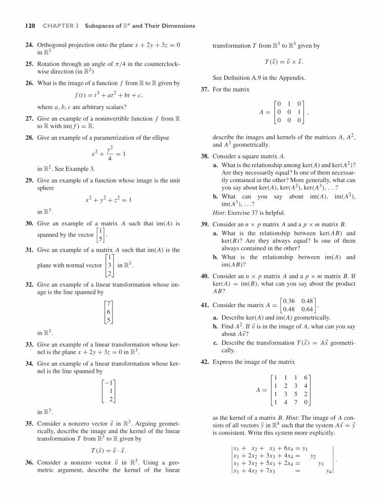
120 CHAPTER 3 Subspaces of Rn and Their Dimensions
24. Orthogonal projection onto the plane x + 2y + 3z = 0in R3
25. Rotation through an angle of π/4 in the counterclock-wise direction (in R2)
26. What is the image of a function f from R to R given by
f (t) = t3 + at2 + bt + c,
where a, b, c are arbitrary scalars?
27. Give an example of a noninvertible function f from Rto R with im( f ) = R.
28. Give an example of a parametrization of the ellipse
x2 + y2
4= 1
in R2. See Example 3.
29. Give an example of a function whose image is the unitsphere
x2 + y2 + z2 = 1
in R3.
30. Give an example of a matrix A such that im(A) is
spanned by the vector[
15
].
31. Give an example of a matrix A such that im(A) is the
plane with normal vector
⎡
⎣132
⎤
⎦ in R3.
32. Give an example of a linear transformation whose im-age is the line spanned by
⎡
⎣765
⎤
⎦
in R3.
33. Give an example of a linear transformation whose ker-nel is the plane x + 2y + 3z = 0 in R3.
34. Give an example of a linear transformation whose ker-nel is the line spanned by
⎡
⎣−1
12
⎤
⎦
in R3.
35. Consider a nonzero vector v in R3. Arguing geomet-rically, describe the image and the kernel of the lineartransformation T from R3 to R given by
T (x) = v · x .
36. Consider a nonzero vector v in R3. Using a geo-metric argument, describe the kernel of the linear
transformation T from R3 to R3 given by
T (x) = v × x .
See Definition A.9 in the Appendix.
37. For the matrix
A =
⎡
⎣0 1 00 0 10 0 0
⎤
⎦ ,
describe the images and kernels of the matrices A, A2,and A3 geometrically.
38. Consider a square matrix A.a. What is the relationship among ker(A) and ker(A2)?
Are they necessarily equal? Is one of them necessar-ily contained in the other? More generally, what canyou say about ker(A), ker(A2), ker(A3), . . .?
b. What can you say about im(A), im(A2),im(A3), . . .?
Hint: Exercise 37 is helpful.
39. Consider an n × p matrix A and a p × m matrix B.a. What is the relationship between ker(AB) and
ker(B)? Are they always equal? Is one of themalways contained in the other?
b. What is the relationship between im(A) andim(AB)?
40. Consider an n × p matrix A and a p × m matrix B. Ifker(A) = im(B), what can you say about the productAB?
41. Consider the matrix A =[
0.36 0.480.48 0.64
].
a. Describe ker(A) and im(A) geometrically.b. Find A2. If v is in the image of A, what can you say
about Av?c. Describe the transformation T (x) = Ax geometri-
cally.
42. Express the image of the matrix
A =
⎡
⎢⎢⎣
1 1 1 61 2 3 41 3 5 21 4 7 0
⎤
⎥⎥⎦
as the kernel of a matrix B. Hint: The image of A con-sists of all vectors y in R4 such that the system Ax = yis consistent. Write this system more explicitly:
∣∣∣∣∣∣∣
x1 + x2 + x3 + 6x4 = y1x1 + 2x2 + 3x3 + 4x4 = y2x1 + 3x2 + 5x3 + 2x4 = y3x1 + 4x2 + 7x3 = y4
∣∣∣∣∣∣∣.

3.1 Image and Kernel of a Linear Transformation 121
Now, reduce rows:∣∣∣∣∣∣∣
x1 − x3 + 8x4 = 4y3 − 3y4x2 + 2x3 − 2x4 = − y3 + y4
0 = y1 − 3y3 + 2y40 = y2 − 2y3 + y4
∣∣∣∣∣∣∣.
For which vectors y is this system consistent? The an-swer allows you to express im(A) as the kernel of a 2×4matrix B.
43. Using your work in Exercise 42 as a guide, explain howyou can write the image of any matrix A as the kernelof some matrix B.
44. Consider a matrix A, and let B = rref(A).a. Is ker(A) necessarily equal to ker(B)? Explain.b. Is im(A) necessarily equal to im(B)? Explain.
45. Consider an n × m matrix A with rank(A) = r < m.Explain how you can write ker(A) as the span of m − rvectors.
46. Consider a 3×4 matrix A in reduced row-echelon form.What can you say about the image of A? Describe allcases in terms of rank(A), and draw a sketch for each.
47. Let T be the projection along a line L1 onto a line L2.See Exercise 2.2.33. Describe the image and the kernelof T geometrically.
48. Consider a 2 × 2 matrix A with A2 = A.a. If w is in the image of A, what is the relationship
between w and Aw?b. What can you say about A if rank(A) = 2? What if
rank(A) = 0?c. If rank(A) = 1, show that the linear transforma-
tion T (x) = Ax is the projection onto im(A) alongker(A). See Exercise 2.2.33.
49. Verify that the kernel of a linear transformation is closedunder addition and scalar multiplication. See Theo-rem 3.1.6.
50. Consider a square matrix A with ker(A2) = ker(A3). Isker(A3) = ker(A4)? Justify your answer.
51. Consider an n × p matrix A and a p × m matrix B suchthat ker(A) = 0 and ker(B) = 0. Find ker(AB).
52. Consider a p × m matrix A and a q × m matrix B, andform the block matrix
C =[
AB
].
What is the relationship among ker(A), ker(B), andker(C)?
53. In Exercises 53 and 54, we will work with the binarydigits (or bits) 0 and 1, instead of the real numbers R.Addition and multiplication in this system are definedas usual, except for the rule 1 + 1 = 0. We denote this
number system with F2, or simply F. The set of all vec-tors with n components in F is denoted by Fn ; note thatFn consists of 2n vectors. (Why?) In information tech-nology, a vector in F8 is called a byte. (A byte is a stringof eight binary digits.)
The basic ideas of linear algebra introduced so far(for the real numbers) apply to F without modifications.
A Hamming matrix with n rows is a matrix thatcontains all nonzero vectors in Fn as its columns (inany order). Note that there are 2n − 1 columns. Here isan example:
H =
⎡
⎣1 0 0 1 0 1 10 1 0 1 1 0 10 0 1 1 1 1 0
⎤
⎦,3 rows23 − 1 = 7 columns.
a. Express the kernel of H as the span of four vectorsin F7 of the form
v1 =
⎡
⎢⎢⎢⎢⎢⎢⎢⎢⎣
∗∗∗1000
⎤
⎥⎥⎥⎥⎥⎥⎥⎥⎦
, v2 =
⎡
⎢⎢⎢⎢⎢⎢⎢⎢⎣
∗∗∗0100
⎤
⎥⎥⎥⎥⎥⎥⎥⎥⎦
, v3 =
⎡
⎢⎢⎢⎢⎢⎢⎢⎢⎣
∗∗∗0010
⎤
⎥⎥⎥⎥⎥⎥⎥⎥⎦
, v4 =
⎡
⎢⎢⎢⎢⎢⎢⎢⎢⎣
∗∗∗0001
⎤
⎥⎥⎥⎥⎥⎥⎥⎥⎦
.
b. Form the 7 × 4 matrix
M =
⎡
⎣| | | |
v1 v2 v3 v4| | | |
⎤
⎦ .
Explain why im(M) = ker(H). If x is an arbitraryvector in F4, what is H(Mx)?
54. See Exercise 53 for some background. When informa-tion is transmitted, there may be some errors in thecommunication. We present a method of adding extrainformation to messages so that most errors that occurduring transmission can be detected and corrected.Such methods are referred to as error-correcting codes.(Compare these with codes whose purpose is to concealinformation.) The pictures of man’s first landing on theMoon (in 1969) were televised just as they had beenreceived and were not very clear, since they containedmany errors induced during transmission. On latermissions, much clearer error-corrected pictures wereobtained.
In computers, information is stored and processedin the form of strings of binary digits, 0 and 1. Thisstream of binary digits is often broken up into “blocks”of eight binary digits (bytes). For the sake of simplicity,we will work with blocks of only four binary digits (i.e.,with vectors in F4), for example,
· · · 1 0 1 1 1 0 0 1 1 0 1 0 1 0 1 1
1 0 0 0 · · · .

122 CHAPTER 3 Subspaces of Rn and Their Dimensions
Suppose these vectors in F4 have to be transmitted fromone computer to another, say, from a satellite to groundcontrol in Kourou, French Guiana (the station of theEuropean Space Agency). A vector u in F4 is first trans-formed into a vector v = Mu in F7, where M is the ma-trix you found in Exercise 53. The last four entries of vare just the entries of u; the first three entries of v areadded to detect errors. The vector v is now transmittedto Kourou. We assume that at most one error will oc-cur during transmission; that is, the vector w receivedin Kourou will be either v (if no error has occurred) orw = v + ei (if there is an error in the i th component ofthe vector).a. Let H be the Hamming matrix introduced in
Exercise 53. How can the computer in Kourou useHw to determine whether there was an error inthe transmission? If there was no error, what isHw? If there was an error, how can the com-puter determine in which component the error wasmade?
b. Suppose the vector
w =
⎡
⎢⎢⎢⎢⎢⎢⎢⎢⎣
1010100
⎤
⎥⎥⎥⎥⎥⎥⎥⎥⎦
is received in Kourou. Determine whether an errorwas made in the transmission and, if so, correct it.(That is, find v and u.)
M
encode
H
F3
F4F7F7F7F4
correct error
detect error
decode
transmission
possible error
Kourou
Satellite
u w uv v
3.2 Subspaces of Rn; Bases and Linear Independence
In the last section, we saw that both the image and the kernel of a linear transfor-mation contain the zero vector (of the target space and the domain, respectively),are closed under addition, and are closed under scalar multiplication. Subsets of thevector space Rn with these three properties are called (linear) subspaces of Rn .
Definition 3.2.1 Subspaces of Rn
A subset W of the vector space Rn is called a (linear) subspace of Rn if it hasthe following three properties:
a. W contains the zero vector in Rn .b. W is closed under addition: If w1 and w2 are both in W , then so is w1 +
w2.c. W is closed under scalar multiplication: If w is in W and k is an arbitrary
scalar, then kw is in W .
Properties (b) and (c) together mean that W is closed under linear combina-tions: If vectors w1, . . . , wm are in W and k1, . . . , km are scalars, then the linearcombination k1w1 + · · · + kmwm is in W as well.
Theorems 3.1.4 and 3.1.6 tell us the following:
Theorem 3.2.2 Image and kernel are subspaces
If T (x) = Ax is a linear transformation from Rm to Rn , then• ker(T ) = ker(A) is a subspace of Rm , and• image (T ) = im(A) is a subspace of Rn .

3.2 Subspaces of Rn; Bases and Linear Independence 123
EXAMPLE 1 Is W =[
xy
]in R2: x ≥ 0 and y ≥ 0
a subspace of R2?
SolutionNote that W consists of all vectors in the first quadrant of the x–y-plane, includingthe positive axes and the origin, as illustrated in Figure 1.
W contains the zero vector and is closed under addition, but it is not closedunder multiplication with a negative scalar. See Figure 2. Thus, W fails to be asubspace of R2. !
y
x
W
Figure 1
y
x
W
v in W
−v = (−1)v
Figure 2
EXAMPLE 2 Show that the only subspaces of R2 are R2 itself, the set 0, and any of the linesthrough the origin.
SolutionSuppose W is a subspace of R2 that is neither 0 nor a line through the origin.We have to show that W must equal R2. Consider a nonzero vector v1 in W . (Wecan find such a vector since W = 0.) The line L spanned by v1 is a subset ofW , since W is closed under scalar multiplication; but W does not equal L , sinceW isn’t a line. Consider a vector v2 in W that isn’t on L . See Figure 3. Using aparallelogram, we can express any vector v in R2 as a linear combination of v1 andv2. Therefore, v belongs to W , since W is closed under linear combinations. Thisshows that W = R2, as claimed. !
L
0
v1
v2
v
Figure 3
Similarly, the only subspaces of R3 are R3 itself, the planes through the origin,the lines through the origin, and the set 0. See Exercise 5. Note the hierarchy of

124 CHAPTER 3 Subspaces of Rn and Their Dimensions
subspaces, arranged according to their dimensions. (The concept of dimension willbe made precise in the next section.)
Subspaces of R2 Subspaces of R3
Dimension 3 R3
Dimension 2 R2 Planes through 0Dimension 1 Lines through 0 Lines through 0Dimension 0 0 0
We have seen that both the kernel and the image of a linear transformationare subspaces (of the domain and target space, respectively). Conversely, can weexpress any subspace V of Rn as the kernel or the image of a linear transformation(or, equivalently, of a matrix)?
Let us consider an example.
EXAMPLE 3 Consider the plane V in R3 given by the equation x1 + 2x2 + 3x3 = 0.
a. Find a matrix A such that V = ker(A).b. Find a matrix B such that V = im(B).
Solutiona. We can write the equation x1 + 2x2 + 3x3 = 0 as
[1 2 3
]⎡
⎣x1
x2
x3
⎤
⎦ = 0, sothat V = ker
[1 2 3
].
b. Since the image of a matrix is the span of its columns, we need to describeV as the span of some vectors. For the plane V , any two nonparallel vectors
will do, for example,
⎡
⎣−2
10
⎤
⎦ and
⎡
⎣−3
01
⎤
⎦. Thus, V = im
⎡
⎣−2 −3
1 00 1
⎤
⎦.
!A subspace of Rn is usually given either as the solution set of a homogeneous
linear system (that is, as a kernel), as in Example 3, or as the span of some vec-tors (that is, as an image). Sometimes, a subspace that has been defined as a kernelmust be given as an image (as in part b of Example 3), or vice versa. The transi-tion from kernel to image is straightforward: Using Gaussian elimination, we canrepresent the solution set as the span of some vectors. See Examples 10 and 11 ofSection 3.1. A method of writing the image of a matrix as a kernel is discussed inExercises 3.1.42 and 3.1.43.
Bases and Linear IndependenceEXAMPLE 4 Consider the matrix
A =
⎡
⎣1 2 1 21 2 2 31 2 3 4
⎤
⎦ .
Find vectors in R3 that span the image of A. What is the smallest number of vectorsneeded to span the image of A?

3.2 Subspaces of Rn; Bases and Linear Independence 125
SolutionWe know from Theorem 3.1.3 that the image of A is spanned by the four columnvectors of A,
v1 =
⎡
⎣111
⎤
⎦ , v2 =
⎡
⎣222
⎤
⎦ , v3 =
⎡
⎣123
⎤
⎦ , v4 =
⎡
⎣234
⎤
⎦ .
0
v2v1
v3v4
im(A)
Figure 4
Figure 4 illustrates that the image of A is a plane; we don’t need all four vectorsto span im(A). We observe that v2 = 2v1 and v4 = v1 + v3, so that the vectors v2and v4 are “redundant” as far as the span is concerned:
im
⎡
⎣1 2 1 21 2 2 31 2 3 4
⎤
⎦ = span(v1, v2, v3, v4) = span(v1, v3).
The image of A can be spanned by two vectors, but not by one vector alone.Let us verify the equation span(v1, v2, v3, v4) = span(v1, v3) algebraically. If
a vector v is in span(v1, v2, v3, v4), then
v = c1v1 + c2v2 + c3v3 + c4v4
= c1v1 + c2(2v1) + c3v3 + c4(v1 + v3)
= (c1 + 2c2 + c4)v1 + (c3 + c4)v3,
showing that v is in span(v1, v3), as claimed. !The preceding example motivates the following important definitions.
Definition 3.2.3 Redundant vectors4; linear independence; basis
Consider vectors v1, . . . , vm in Rn .
a. We say that a vector vi in the list v1, . . . , vm is redundant if vi is a linearcombination of the preceding vectors v1, . . . , vi−1.5
b. The vectors v1, . . . , vm are called linearly independent if none of them isredundant. Otherwise, the vectors are called linearly dependent (meaningthat at least one of them is redundant).6
c. We say that the vectors v1, . . . , vm in a subspace V of Rn form a basis ofV if they span V and are linearly independent.7
Let’s take another look at Example 4: In the list
v1 =
⎡
⎣111
⎤
⎦ , v2 =
⎡
⎣222
⎤
⎦ , v3 =
⎡
⎣123
⎤
⎦ , v4 =
⎡
⎣234
⎤
⎦
4The notion of a redundant vector is not part of the established vocabulary of linear algebra. However,we will find this concept quite useful in discussing linear independence.5We call the first vector, v1, redundant if it is the zero vector. This agrees with the convention that theempty linear combination of vectors is the zero vector.6A list of alternative characterizations of linear independence will be presented in Summary 3.2.9. Inmany texts, characterization (iv) of that list is used to define linear independence.7An alternative characterization of a basis will be presented in Theorem 3.2.10.

126 CHAPTER 3 Subspaces of Rn and Their Dimensions
of column vectors of A, the vectors v2 and v4 are redundant, since v2 = 2v1 andv4 = v1 + v3. If we omit the redundant vectors from the list, then the remainingvectors
v1 =
⎡
⎣111
⎤
⎦ , v3 =
⎡
⎣123
⎤
⎦
are linearly independent; they form a basis of V = image (A).We can generalize the result of Example 4.
Theorem 3.2.4 Basis of the image
To construct a basis of the image of a matrix A, list all the column vectors of A,and omit the redundant vectors from this list.
But how can we identify the redundant column vectors? In simple cases, thiscan often be done by inspection (as in Example 4); in the next section we willdevelop a general algorithm, based on Gaussian elimination.
EXAMPLE 5 Are the following vectors in R7 linearly independent?
v1 =
⎡
⎢⎢⎢⎢⎢⎢⎢⎢⎣
7040190
⎤
⎥⎥⎥⎥⎥⎥⎥⎥⎦
, v2 =
⎡
⎢⎢⎢⎢⎢⎢⎢⎢⎣
6071480
⎤
⎥⎥⎥⎥⎥⎥⎥⎥⎦
, v3 =
⎡
⎢⎢⎢⎢⎢⎢⎢⎢⎣
5062317
⎤
⎥⎥⎥⎥⎥⎥⎥⎥⎦
, v4 =
⎡
⎢⎢⎢⎢⎢⎢⎢⎢⎣
4533224
⎤
⎥⎥⎥⎥⎥⎥⎥⎥⎦
SolutionLet’s look for redundant vectors in this list. Vectors v1 and v2 are clearly nonredun-dant, since v1 is nonzero and v2 fails to be a scalar multiple of v1 (look at the fourthcomponents). Looking at the last components, we realize that v3 cannot be a linearcombination of v1 and v2, since any linear combination of v1 and v2 will have a 0in the last component, while the last component of v3 is 7. Looking at the secondcomponents, we can see that v4 isn’t a linear combination of v1, v2, v3. Thus, thevectors v1, v2, v3, v4 are linearly independent. !
We will frequently use the approach of Example 5 to show linear independence.
Theorem 3.2.5 Linear independence and zero components
Consider vectors v1, . . . , vm in Rn . If v1 is nonzero, and if each of the vectors vi(for i ≥ 2) has a nonzero entry in a component where all the preceding vectorsv1, . . . , vi−1 have a 0, then the vectors v1, . . . , vm are linearly independent.
To understand what we are trying to say in Theorem 3.2.5, take another look atthe vectors in Example 5.

3.2 Subspaces of Rn; Bases and Linear Independence 127
⎡
⎢⎢⎢⎢⎢⎢⎢⎢⎢⎣
7040190
⎤
⎥⎥⎥⎥⎥⎥⎥⎥⎥⎦
,
⎡
⎢⎢⎢⎢⎢⎢⎢⎢⎢⎣
6071480
⎤
⎥⎥⎥⎥⎥⎥⎥⎥⎥⎦
,
⎡
⎢⎢⎢⎢⎢⎢⎢⎢⎢⎣
5062317
⎤
⎥⎥⎥⎥⎥⎥⎥⎥⎥⎦
,
⎡
⎢⎢⎢⎢⎢⎢⎢⎢⎢⎣
4533224
⎤
⎥⎥⎥⎥⎥⎥⎥⎥⎥⎦
EXAMPLE 6 Are the vectors
v1 =
⎡
⎣123
⎤
⎦ , v2 =
⎡
⎣456
⎤
⎦ , v3 =
⎡
⎣789
⎤
⎦
linearly independent?
SolutionTheorem 3.2.5 doesn’t help here, since these vectors don’t have any zero compo-nents. The vectors v1 and v2 are clearly nonredundant, as v1 is nonzero and v2fails to be a scalar multiple of v1. To see whether vector v3 is redundant, we need toexamine whether v3 can be written as v3 = c1v1+c2v2. Considering the augmentedmatrix
M =
⎡
⎣1 4 72 5 83 6 9
⎤
⎦ , with rref(M) =
⎡
⎣1 0 −10 1 20 0 0
⎤
⎦ ,
we find the unique solution c1 = −1, c2 = 2, so that
v3 = −v1 + 2v2.
It turns out that vector v3 is redundant, making vectors v1, v2, v3 linearly dependent.!
For good reasons, mathematicians like to write their equations in the form
(Something) = 0.
Applying this principle,8 we can write the equation v3 =−v1+2v2 from Example 6as
v1 − 2v2 + v3 = 0.
This equation is called a linear relation among the vectors v1, v2, and v3.
Definition 3.2.6 Linear Relations
Consider the vectors v1, . . . , vm in Rn . An equation of the form
c1v1 + · · · + cm vm = 0
is called a (linear) relation among the vectors v1, . . . , vm . There is always thetrivial relation, with c1 = · · · = cm = 0. Nontrivial relations (where at least onecoefficient ci is nonzero) may or may not exist among the vectors v1, . . . , vm .
8This method was popularized by Descartes, and is often credited to him, but it was used earlierby the English geographer Thomas Harriot (1560–1621). For more on “Harriot’s Principle,” seeW. P. Berlinghoff and F. Q. Gouvea, Math Through the Ages, Oxton House Publishers and MAA,2004.

128 CHAPTER 3 Subspaces of Rn and Their Dimensions
Example 6 suggests the following result.
Theorem 3.2.7 Relations and linear dependence
The vectors v1, . . . , vm in Rn are linearly dependent if (and only if) there arenontrivial relations among them.
Proof • Suppose vectors v1, . . . , vm are linearly dependent, and vi = c1v1 + · · · +ci−1vi−1 is a redundant vector in this list. Then we can generate a nontrivialrelation by subtracting vi from both sides: c1v1+· · ·+ci−1vi−1+(−1)vi = 0.
• Conversely, if there is a nontrivial relation c1v1 +· · ·+ci vi +· · ·+cm vm = 0,where i is the highest index such that ci = 0, then we can solve for vi andthus express vi as a linear combination of the preceding vectors:
vi = −c1
civ1 − · · · − ci−1
civi−1.
This shows that vector vi is redundant, so that vectors v1, . . . , vm are linearlydependent, as claimed. !
EXAMPLE 7 Suppose the column vectors of an n × m matrix A are linearly independent. Findthe kernel of matrix A.
SolutionWe need to solve the equation
Ax = 0 or
⎡
⎢⎣| |v1 · · · vm
| |
⎤
⎥⎦
⎡
⎢⎣x1...
xm
⎤
⎥⎦ = 0 or x1v1 + · · · + xm vm = 0.
We see that finding the kernel of A amounts to finding the relations among thecolumn vectors of A. By Theorem 3.2.7, there is only the trivial relation, withx1 = · · · = xm = 0, so that ker(A) = 0. !
Let us summarize the findings of Example 7.
Theorem 3.2.8 Kernel and relations
The vectors in the kernel of an n ×m matrix A correspond to the linear relationsamong the column vectors v1, . . . , vm of A: The equation
Ax = 0 means that x1v1 + · · · + xm vm = 0.
In particular, the column vectors of A are linearly independent if (and only if)ker(A) = 0, or, equivalently, if rank(A) = m. This condition implies thatm ≤ n.
Thus, we can find at most n linearly independent vectors in Rn .

3.2 Subspaces of Rn; Bases and Linear Independence 129
EXAMPLE 8 Consider the matrix
A =
⎡
⎣1 4 72 5 83 6 9
⎤
⎦
to illustrate the connection between redundant column vectors, relations among thecolumn vectors, and the kernel. See Example 6.
Redundant column vector:
⎡
⎣789
⎤
⎦ = −
⎡
⎣123
⎤
⎦ + 2
⎡
⎣456
⎤
⎦
Relation among column vectors: 1
⎡
⎣123
⎤
⎦ − 2
⎡
⎣456
⎤
⎦ + 1
⎡
⎣789
⎤
⎦ = 0
Vector
⎡
⎣1
−21
⎤
⎦ is in ker(A), since
⎡
⎣1 4 72 5 83 6 9
⎤
⎦
⎡
⎣1
−21
⎤
⎦ =
⎡
⎣000
⎤
⎦!
In the following summary we list the various characterizations of linearindependence discussed thus far (in Definition 3.2.3b, Theorem 3.2.7, and Theo-rem 3.2.8). We include one new characterization, (iii). The proof of the equivalenceof statements (iii) and (iv) is left to the reader as Exercise 35; it is analogous to theproof of Theorem 3.2.7.
SUMMARY 3.2.9 Various characterizations of linear independence
For a list v1, . . . , vm of vectors in Rn , the following statements are equivalent:
i. Vectors v1, . . . , vm are linearly independent.ii. None of the vectors v1, . . . , vm is redundant, meaning that none of them
is a linear combination of preceding vectors.iii. None of the vectors vi is a linear combination of the other vectors
v1, . . . , vi−1, vi+1, . . . , vm in the list.iv. There is only the trivial relation among the vectors v1, . . . , vm , mean-
ing that the equation c1v1 + · · · + cm vm = 0 has only the solutionc1 = · · · = cm = 0.
v. ker
⎡
⎣| |v1 · · · vm
| |
⎤
⎦ = 0.
vi. rank
⎡
⎣| |v1 · · · vm
| |
⎤
⎦ = m.
We conclude this section with an important alternative characterization of abasis. See Definition 3.2.3c.

130 CHAPTER 3 Subspaces of Rn and Their Dimensions
EXAMPLE 9 If v1, . . . , vm is a basis of a subspace V of Rn , and if v is a vector in V , how manysolutions c1, . . . , cm does the equation
v = c1v1 + · · · + cm vm
have?
SolutionThere is at least one solution, since the vectors v1, . . . , vm span V (that’s part of thedefinition of a basis). Suppose we have two representations
v = c1v1 + · · · + cm vm
= d1v1 + · · · + dm vm .
By subtraction, we find
(c1 − d1)v1 + · · · + (cm − dm)vm = 0,
a relation among the vectors v1, . . . , vm . Since the vectors v1, . . . , vm are linearlyindependent, this must be the trivial relation, and we have c1 − d1 = 0, . . . ,cm − dm = 0, or c1 = d1, . . . , cm = dm . It turns out that the two representa-tions v = c1v1 + · · · + cm vm and v = d1v1 + · · · + dm vm are identical. We haveshown that there is one and only one way to write v as a linear combination of thebasis vectors v1, . . . , vm . !
Let us summarize.
Theorem 3.2.10 Basis and unique representation
Consider the vectors v1, . . . , vm in a subspace V of Rn .The vectors v1, . . . , vm form a basis of V if (and only if) every vector v in
V can be expressed uniquely as a linear combination
v = c1v1 + · · · + cm vm .
(In Section 3.4, we will call the coefficients c1, . . . , cm the coordinates of v withrespect to the basis v1, . . . , vm .)
Proof In Example 9 we have shown only one part of Theorem 3.2.10; we still need toverify that the uniqueness of the representation v = c1v1 + · · · + cm vm (for every vin V ) implies that v1, . . . , vm is a basis of V . Clearly, the vectors v1, . . . , vm spanV , since every v in V can be written as a linear combination of v1, . . . , vm .
To show the linear independence of vectors v1, . . . , vm , consider a relationc1v1 + · · · + cm vm = 0. This relation is a representation of the zero vectoras a linear combination of v1, . . . , vm . But this representation is unique, withc1 = · · · = cm = 0, so that c1v1 + · · · + cm vm = 0 must be the trivial relation. Wehave shown that vectors v1, . . . , vm are linearly independent. !
Consider the plane V = im(A) = span(v1, v2, v3, v4) introduced in Exam-ple 4. (Take another look at Figure 4.)
We can writev4 = 1v1 + 0v2 + 1v3 + 0v4
= 0v1 + 0v2 + 0v3 + 1v4,
illustrating the fact that the vectors v1, v2, v3, v4 do not form a basis of V . However,every vector v in V can be expressed uniquely as a linear combination of v1 and v3alone, meaning that the vectors v1, v3 do form a basis of V .
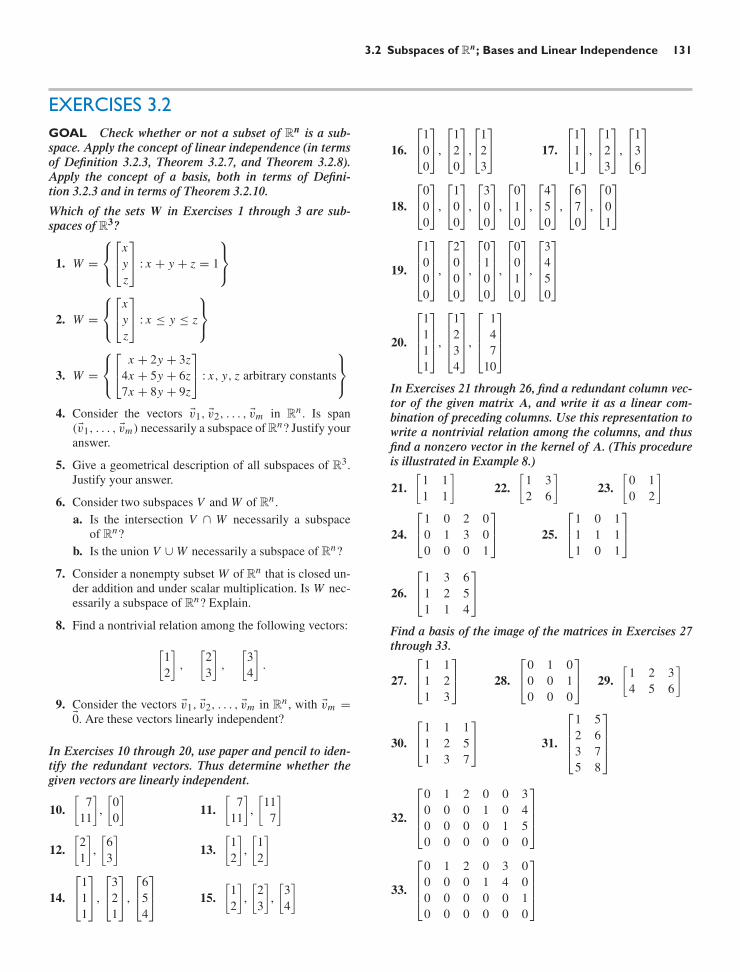
3.2 Subspaces of Rn; Bases and Linear Independence 131
EXERCISES 3.2GOAL Check whether or not a subset of Rn is a sub-space. Apply the concept of linear independence (in termsof Definition 3.2.3, Theorem 3.2.7, and Theorem 3.2.8).Apply the concept of a basis, both in terms of Defini-tion 3.2.3 and in terms of Theorem 3.2.10.
Which of the sets W in Exercises 1 through 3 are sub-spaces of R3?
1. W =
⎧⎨
⎩
⎡
⎣xyz
⎤
⎦ : x + y + z = 1
⎫⎬
⎭
2. W =
⎧⎨
⎩
⎡
⎣xyz
⎤
⎦ : x ≤ y ≤ z
⎫⎬
⎭
3. W =
⎧⎨
⎩
⎡
⎣x + 2y + 3z
4x + 5y + 6z7x + 8y + 9z
⎤
⎦ : x, y, z arbitrary constants
⎫⎬
⎭
4. Consider the vectors v1, v2, . . . , vm in Rn . Is span(v1, . . . , vm) necessarily a subspace of Rn? Justify youranswer.
5. Give a geometrical description of all subspaces of R3.Justify your answer.
6. Consider two subspaces V and W of Rn .a. Is the intersection V ∩ W necessarily a subspace
of Rn?b. Is the union V ∪ W necessarily a subspace of Rn?
7. Consider a nonempty subset W of Rn that is closed un-der addition and under scalar multiplication. Is W nec-essarily a subspace of Rn? Explain.
8. Find a nontrivial relation among the following vectors:
[12
],
[23
],
[34
].
9. Consider the vectors v1, v2, . . . , vm in Rn , with vm =0. Are these vectors linearly independent?
In Exercises 10 through 20, use paper and pencil to iden-tify the redundant vectors. Thus determine whether thegiven vectors are linearly independent.
10.[
711
],[
00
]11.
[7
11
],[
117
]
12.[
21
],[
63
]13.
[12
],[
12
]
14.
⎡
⎣111
⎤
⎦,
⎡
⎣321
⎤
⎦,
⎡
⎣654
⎤
⎦ 15.[
12
],[
23
],[
34
]
16.
⎡
⎣100
⎤
⎦,
⎡
⎣120
⎤
⎦,
⎡
⎣123
⎤
⎦ 17.
⎡
⎣111
⎤
⎦,
⎡
⎣123
⎤
⎦,
⎡
⎣136
⎤
⎦
18.
⎡
⎣000
⎤
⎦,
⎡
⎣100
⎤
⎦,
⎡
⎣300
⎤
⎦,
⎡
⎣010
⎤
⎦,
⎡
⎣450
⎤
⎦,
⎡
⎣670
⎤
⎦,
⎡
⎣001
⎤
⎦
19.
⎡
⎢⎢⎣
1000
⎤
⎥⎥⎦,
⎡
⎢⎢⎣
2000
⎤
⎥⎥⎦,
⎡
⎢⎢⎣
0100
⎤
⎥⎥⎦,
⎡
⎢⎢⎣
0010
⎤
⎥⎥⎦,
⎡
⎢⎢⎣
3450
⎤
⎥⎥⎦
20.
⎡
⎢⎢⎣
1111
⎤
⎥⎥⎦,
⎡
⎢⎢⎣
1234
⎤
⎥⎥⎦,
⎡
⎢⎢⎣
147
10
⎤
⎥⎥⎦
In Exercises 21 through 26, find a redundant column vec-tor of the given matrix A, and write it as a linear com-bination of preceding columns. Use this representation towrite a nontrivial relation among the columns, and thusfind a nonzero vector in the kernel of A. (This procedureis illustrated in Example 8.)
21.[
1 11 1
]22.
[1 32 6
]23.
[0 10 2
]
24.
⎡
⎣1 0 2 00 1 3 00 0 0 1
⎤
⎦ 25.
⎡
⎣1 0 11 1 11 0 1
⎤
⎦
26.
⎡
⎣1 3 61 2 51 1 4
⎤
⎦
Find a basis of the image of the matrices in Exercises 27through 33.
27.
⎡
⎣1 11 21 3
⎤
⎦ 28.
⎡
⎣0 1 00 0 10 0 0
⎤
⎦ 29.[
1 2 34 5 6
]
30.
⎡
⎣1 1 11 2 51 3 7
⎤
⎦ 31.
⎡
⎢⎢⎣
1 52 63 75 8
⎤
⎥⎥⎦
32.
⎡
⎢⎢⎣
0 1 2 0 0 30 0 0 1 0 40 0 0 0 1 50 0 0 0 0 0
⎤
⎥⎥⎦
33.
⎡
⎢⎢⎣
0 1 2 0 3 00 0 0 1 4 00 0 0 0 0 10 0 0 0 0 0
⎤
⎥⎥⎦

132 CHAPTER 3 Subspaces of Rn and Their Dimensions
34. Consider the 5 × 4 matrix
A =
⎡
⎣| | | |
v1 v2 v3 v4| | | |
⎤
⎦ .
We are told that the vector
⎡
⎢⎢⎣
1234
⎤
⎥⎥⎦ is in the kernel of A.
Write v4 as a linear combination of v1, v2, v3.
35. Show that there is a nontrivial relation among the vec-tors v1, . . . , vm if (and only if) at least one of the vec-tors vi is a linear combination of the other vectorsv1, . . . , vi−1, vi+1, . . . , vm .
36. Consider a linear transformation T from Rn to Rp andsome linearly dependent vectors v1, v2, . . . , vm in Rn .Are the vectors T (v1), T (v2), . . . , T (vm) necessarilylinearly dependent? How can you tell?
37. Consider a linear transformation T from Rn to Rp andsome linearly independent vectors v1, v2, . . . , vm inRn . Are the vectors T (v1), T (v2), . . . , T (vm) necessar-ily linearly independent? How can you tell?
38. a. Let V be a subspace of Rn . Let m be the largestnumber of linearly independent vectors we can findin V . (Note that m ≤ n, by Theorem 3.2.8.) Chooselinearly independent vectors v1, v2, . . . , vm in V .Show that the vectors v1, v2, . . . , vm span V and aretherefore a basis of V . This exercise shows that anysubspace of Rn has a basis.
If you are puzzled, think first about the specialcase when V is a plane in R3. What is m in this case?
b. Show that any subspace V of Rn can be representedas the image of a matrix.
39. Consider some linearly independent vectors v1, v2, . . . ,vm in Rn and a vector v in Rn that is not contained inthe span of v1, v2, . . . , vm . Are the vectors v1, v2, . . . ,vm , v necessarily linearly independent? Justify youranswer.
40. Consider an n × p matrix A and a p × m matrix B. Weare told that the columns of A and the columns of B arelinearly independent. Are the columns of the productAB linearly independent as well? Hint: Exercise 3.1.51is useful.
41. Consider an m × n matrix A and an n × m matrix B(with n = m) such that AB = Im . (We say that A is aleft inverse of B.) Are the columns of B linearly inde-pendent? What about the columns of A?
42. Consider some perpendicular unit vectors v1, v2, . . . ,vm in Rn . Show that these vectors are necessarily lin-early independent. Hint: Form the dot product of vi andboth sides of the equation
c1v1 + c2v2 + · · · + ci vi + · · · + cm vm = 0.
43. Consider three linearly independent vectors v1, v2, v3in Rn . Are the vectors v1, v1 + v2, v1 + v2 + v3 linearlyindependent as well? How can you tell?
44. Consider linearly independent vectors v1, v2, . . . , vmin Rn , and let A be an invertible m × m matrix. Are thecolumns of the following matrix linearly independent?
⎡
⎣| | |
v1 v2 . . . vm| | |
⎤
⎦ A
45. Are the columns of an invertible matrix linearly inde-pendent?
46. Find a basis of the kernel of the matrix[
1 2 0 3 50 0 1 4 6
].
Justify your answer carefully; that is, explain how youknow that the vectors you found are linearly indepen-dent and span the kernel.
47. Consider three linearly independent vectors v1, v2, v3in R4. Find
rref
⎡
⎣| | |
v1 v2 v3| | |
⎤
⎦ .
48. Express the plane V in R3 with equation 3x1 + 4x2 +5x3 = 0 as the kernel of a matrix A and as the image ofa matrix B.
49. Express the line L in R3 spanned by the vector
⎡
⎣111
⎤
⎦ as
the image of a matrix A and as the kernel of a matrix B.
50. Consider two subspaces V and W of Rn . Let V + W bethe set of all vectors in Rn of the form v + w, where vis in V and w in W . Is V + W necessarily a subspaceof Rn?
If V and W are two distinct lines in R3, what isV + W ? Draw a sketch.
51. Consider two subspaces V and W of Rn whose inter-section consists only of the vector 0.a. Consider linearly independent vectors v1, v2, . . . ,
v p in V and w1, w2, . . . , wq in W . Explain why thevectors v1, v2, . . . , v p , w1, w2, . . . , wq are linearlyindependent.
b. Consider a basis v1, v2, . . . , v p of V and a ba-sis w1, w2, . . . , wq of W . Explain why v1, v2, . . . ,v p, w1, w2, . . . , wq is a basis of V + W . See Exer-cise 50.
52. For which values of the constants a, b, c, d , e, and fare the following vectors linearly independent? Justifyyour answer.

3.3 The Dimension of a Subspace of Rn 133
⎡
⎢⎢⎣
a000
⎤
⎥⎥⎦ ,
⎡
⎢⎢⎣
bc00
⎤
⎥⎥⎦ ,
⎡
⎢⎢⎣
def0
⎤
⎥⎥⎦
53. Consider a subspace V of Rn . We define the orthogo-nal complement V ⊥ of V as the set of those vectors win Rn that are perpendicular to all vectors in V ; that is,w · v = 0, for all v in V . Show that V ⊥ is a subspaceof Rn .
54. Consider the line L spanned by
⎡
⎣123
⎤
⎦ in R3. Find a basis
of L⊥. See Exercise 53.
55. Consider the subspace L of R5 spanned by the givenvector. Find a basis of L⊥. See Exercise 53.
⎡
⎢⎢⎢⎢⎣
12345
⎤
⎥⎥⎥⎥⎦
56. For which values of the constants a, b, . . . , m are thegiven vectors linearly independent?
⎡
⎢⎢⎢⎢⎢⎢⎣
abcd10
⎤
⎥⎥⎥⎥⎥⎥⎦,
⎡
⎢⎢⎢⎢⎢⎢⎣
e10000
⎤
⎥⎥⎥⎥⎥⎥⎦,
⎡
⎢⎢⎢⎢⎢⎢⎣
fghij1
⎤
⎥⎥⎥⎥⎥⎥⎦,
⎡
⎢⎢⎢⎢⎢⎢⎣
km1000
⎤
⎥⎥⎥⎥⎥⎥⎦
57. Consider the matrix
A =
⎡
⎢⎢⎣
0 1 2 0 0 3 00 0 0 1 0 4 00 0 0 0 1 5 00 0 0 0 0 0 0
⎤
⎥⎥⎦ .
Note that matrix A is in reduced row-echelon form.For which positive integers j = 1, . . . , 7 does
there exist a vector x in the kernel of A such that thej th component x j of x is nonzero, while all the compo-nents x j+1, . . . , x7 are zero?
58. Consider an n×m matrix A. For which positive integersj = 1, . . . , m does there exist a vector x in the kernelof A such that the j th component x j of x is nonzero,while all the components x j+1, . . . , xm are zero? UseExercise 57 as a guide. Give your answer in terms ofthe redundant column vectors of A.
3.3 The Dimension of a Subspace of Rn
Consider a plane V in R3. Using our geometric intuition, we observe that allbases of V consist of two vectors. (Any two nonparallel vectors in V will do; seeFigure 1.) One vector is not enough to span V , and three or more vectors are linearlydependent. It turns out that, more generally, all bases of a subspace V of Rn consistof the same number of vectors. In order to prove this important fact, we need anauxiliary result.
0
v1
v2V
Figure 1 The vectors v1, v2 form a basis of V .

134 CHAPTER 3 Subspaces of Rn and Their Dimensions
Theorem 3.3.1 Consider vectors v1, . . . , v p and w1, . . . , wq in a subspace V of Rn . If the vec-tors v1, . . . , v p are linearly independent, and the vectors w1, . . . , wq span V ,then q ≥ p.
For example, let V be a plane in R3. Our geometric intuition tells us that wecan find at most two linearly independent vectors in V , so that 2 ≥ p, and we needat least two vectors to span V , so that q ≥ 2. Therefore, the inequality q ≥ p doesindeed hold in this case.
Proof This proof is rather technical and not very illuminating. In the next section, whenwe study coordinate systems, we will gain a more conceptual understanding of thismatter.
CB
A!p !n
!q
Figure 2
Consider the matrices
A =
⎡
⎣| |v1 · · · v p
| |
⎤
⎦ and B =
⎡
⎣| |
w1 · · · wq
| |
⎤
⎦ .
Note that im(B) = V , since the vectors w1, . . . , wq span V . The vectors v1, . . . , v pare in the image of B, so that we can write
v1 = Bu1, . . . , v p = Bu p
for some vectors u1, . . . , u p in Rq . We can combine these equations and write
A =
⎡
⎣| |v1 · · · v p
| |
⎤
⎦ = B
⎡
⎣| |
u1 · · · u p
| |
⎤
⎦
︸ ︷︷ ︸C
, or A = BC.
See Figure 2.The kernel of C is a subset of the kernel of A (if Cx = 0, then Ax = BCx = 0).
But the kernel of A is 0, since the vectors v1, . . . , v p are linearly independent.Therefore, the kernel of C is 0 as well. Theorem 3.1.7b now tells us that the q × pmatrix C has at least as many rows as it has columns, that is, q ≥ p, as claimed. !
Theorem 3.3.2 Number of vectors in a basis
All bases of a subspace V of Rn consist of the same number of vectors.
Proof Consider two bases v1, . . . , v p and w1, . . . , wq of V . Since the vectors v1, . . . , v pare linearly independent and the vectors w1, . . . , wq span V , we have q ≥ p, byTheorem 3.3.1. Likewise, since the vectors w1, . . . , wq are linearly independent andthe vectors v1, . . . , v p span V , we have p ≥ q. Therefore, p = q. !
Consider a line L and a plane V in R3. A basis of L consists of just one vector(any nonzero vector in L will do), while all bases of V consist of two vectors.A basis of R3 consists of three vectors. (The standard vectors e1, e2, e3 are onepossible choice.) In each case, the number of vectors in a basis corresponds to whatwe intuitively sense to be the dimension of the subspace.

3.3 The Dimension of a Subspace of Rn 135
Definition 3.3.3 Dimension
Consider a subspace V of Rn . The number of vectors in a basis of V is called thedimension of V , denoted by dim(V ).9
This algebraic definition of dimension represents a major advance in thedevelopment of linear algebra, and indeed of mathematics as a whole: It allowsus to conceive of spaces with more than three dimensions. This idea is oftenpoorly understood in popular culture, where some mysticism still surrounds higher-dimensional spaces. The German mathematician Hermann Weyl (1855–1955) putit this way: “We are by no means obliged to seek illumination from the mystic doc-trines of spiritists to obtain a clearer vision of multidimensional geometry” (Raum,Zeit, Materie, 1918).
The first mathematician who thought about dimension from an algebraic pointof view may have been the Frenchman Jean Le Rond d’Alembert (1717–1783). Inthe article on dimension in the Encyclopedie, he wrote the following:
The way of considering quantities having more than three dimensions is justas right as the other, because letters can always be viewed as representingnumbers, whether rational or not. I said above that it was not possible toconceive more than three dimensions. A thoughtful gentleman [un hommed’esprit] with whom I am acquainted believes that nevertheless one couldview duration as a fourth dimension. . . . This idea may be challenged, but ithas, it seems to me, some merit, were it only that of being new [cette ideepeut etre contestee, mais elle a, ce me semble, quelque merite, quand ce neseroit que celui de la nouveaute]. (Encyclopedie, vol. 4, 1754)
This homme d’esprit was no doubt d’Alembert himself, afraid of being attackedfor what appeared as a risky idea at that time.
The idea of dimension was later studied much more systematically by theGerman mathematician Hermann Gunther Grassmann (1809–1877), who intro-duced the concept of a subspace of Rn . In fact, most of the concepts discussedin this chapter can be traced back to Grassmann’s work. Grassmann presented hisideas in 1844 in the book Die lineare Ausdehnungslehre, ein neuer Zweig der Math-ematik (The Theory of Linear Extension, a New Branch of Mathematics). Grass-mann’s methods were only slowly adopted, partly because of his obscure writing.He used unfamiliar authentic German terms, rather than the customary Latin, formathematical concepts; he writes about “Schatten,” shadows, for example, ratherthan projections. While his ideas have survived, most of his terminology has not.
Similar work was done by the Swiss mathematician Ludwig Schlafli (1814–1895), a contemporary of Grassmann.
Today, dimension is a standard and central tool in mathematics, as well as inphysics and statistics. The concept can be applied to certain nonlinear subsets ofRn , called manifolds, generalizing the idea of curves and surfaces in R3.
After this brief historical digression, let us return to the more mundane: Whatis the dimension of Rn? We expect this dimension to be n, of course. This is indeedthe case: The vectors e1, . . . , en form a basis, called the standard basis of Rn .
A plane V in R3 is two dimensional. Earlier, we mentioned that we cannotfind more than two linearly independent vectors in V and that we need at least two
9For this definition to make sense, we have to be sure that any subspace of Rn has a basis. Thisverification is left as Exercise 3.2.38a.

136 CHAPTER 3 Subspaces of Rn and Their Dimensions
vectors to span V . If two vectors in V are linearly independent, then they form abasis of V . Likewise, if two vectors span V , then they form a basis of V .
We can generalize these observations as follows:
Theorem 3.3.4 Independent vectors and spanning vectors in a subspace of Rn
Consider a subspace V of Rn with dim(V ) = m.a. We can find at most m linearly independent vectors in V .b. We need at least m vectors to span V .c. If m vectors in V are linearly independent, then they form a basis of V .d. If m vectors in V span V , then they form a basis of V .
Part (a) allows us to define the dimension of V alternatively as the maximalnumber of linearly independent vectors in V . Likewise, part (b) tells us that thedimension of V is the minimal number of vectors needed to span V .
In parts (c) and (d) we make the following point: By Definition 3.2.3, somevectors v1, . . . , vm in V form a basis of V if they are linearly independent and spanV . However, if we are dealing with “the right number” of vectors (namely, m, thedimension of V ), then it suffices to check only one of the two properties; the otherwill then follow “automatically.”
Proof We prove Theorem 3.3.4, parts (a) and (c). We leave the proofs of parts (b) and (d)as Exercises 80 and 81.
a. Consider linearly independent vectors v1, v2, . . . , v p in V , and letw1, w2, . . . , wm be a basis of V . Since the vectors w1, w2, . . . , wm spanV , we have p ≤ m, by Theorem 3.3.1, as claimed.
c. Consider linearly independent vectors v1, . . . , vm in V . We have to showthat the vectors v1, . . . , vm span V . If v is any vector in V , then the m + 1vectors v1, . . . , vm, v will be linearly dependent, by part (a). Since vectorsv1, . . . , vm are linearly independent and therefore nonredundant, vector vmust be redundant in the list v1, . . . , vm, v, meaning that v is a linear com-bination of v1, . . . , vm . Since v is an arbitrary vector in V , we have shownthat vectors v1, . . . , vm span V , as claimed. !
In Section 3.2, we saw that the kernel and image of a linear transformation aresubspaces of the domain and the target space of the transformation, respectively.We will now examine how we can find bases of the image and kernel and thusdetermine their dimensions.
Finding Bases of Kernel and ImageEXAMPLE 1 Consider the matrix
A =
⎡
⎢⎢⎣
1 2 2 −5 6−1 −2 −1 1 −1
4 8 5 −8 93 6 1 5 −7
⎤
⎥⎥⎦ .
a. Find a basis of the kernel of A, and thus determine the dimension of thekernel.
b. Find a basis of the image of A, and thus determine the dimension of theimage.

3.3 The Dimension of a Subspace of Rn 137
Solutiona. We will solve the linear system Ax = 0, by Gaussian elimination. From
Example 3.1.11 we know that
B = rref(A) =
⎡
⎢⎢⎣
1 2 0 3 −40 0 1 −4 50 0 0 0 00 0 0 0 0
⎤
⎥⎥⎦ .
Note that ker(A) = ker(B), by the definition of the reduced row-echelonform. In Chapter 1 we learned to solve the equation Ax = 0 by solving thesimpler equation Bx = 0 instead. In Example 3.1.11 we saw that the vectorsin ker(A) = ker(B) are of the form
x =
⎡
⎢⎢⎢⎢⎣
x1
x2
x3
x4
x5
⎤
⎥⎥⎥⎥⎦=
⎡
⎢⎢⎢⎢⎣
−2s −3t +4rs
4t −5rt
r
⎤
⎥⎥⎥⎥⎦= s
⎡
⎢⎢⎢⎢⎣
−21000
⎤
⎥⎥⎥⎥⎦
︸ ︷︷ ︸w1
+ t
⎡
⎢⎢⎢⎢⎣
−30410
⎤
⎥⎥⎥⎥⎦
︸ ︷︷ ︸w2
+ r
⎡
⎢⎢⎢⎢⎣
40
−501
⎤
⎥⎥⎥⎥⎦
︸ ︷︷ ︸w3
,
where s, t , and r are arbitrary constants.We claim that the three vectors w1, w2, w3 form a basis of the kernel of
A. The preceding equation, x = sw1 + tw2 + rw3, shows that the vectorsw1, w2, w3 span the kernel.
Theorem 3.2.5 tells us that the vectors w1, w2, w3 are linearly indepen-dent, since each has a 1 in a component where the other two vectors have a0; these components correspond to the free variables x2, x4, and x5.
Thus, a basis of the kernel of A is⎡
⎢⎢⎢⎢⎣
−21000
⎤
⎥⎥⎥⎥⎦,
⎡
⎢⎢⎢⎢⎣
−30410
⎤
⎥⎥⎥⎥⎦,
⎡
⎢⎢⎢⎢⎣
40
−501
⎤
⎥⎥⎥⎥⎦,
and dim(ker A) = 3.b. To construct a basis of the image of A by means of Theorem 3.2.4, we need
to find the redundant columns of A. Let’s see how we can use B = rref(A)to carry out this task. To keep track of the columns of A and B, we willdenote the columns of A by a1, . . . , a5 and those of B by b1, . . . , b5.
The redundant columns of B = rref(A) are easy to spot. They are thecolumns that do not contain a leading 1, namely, b2 = 2b1, b4 = 3b1 − 4b3,and b5 = −4b1 + 5b3.
And here comes the key observation: The redundant columns of A cor-respond to those of B, meaning that ai is redundant if and only if bi isredundant. We will illustrate this fact by means of an example. We knowthat b5 is redundant, with b5 = −4b1 + 5b3. This induces the relation4b1 − 5b3 + b5 = 0, meaning that the vector
⎡
⎢⎢⎢⎢⎣
40
−501
⎤
⎥⎥⎥⎥⎦

138 CHAPTER 3 Subspaces of Rn and Their Dimensions
is in ker(B) = ker(A); see part (a) of this example. But this in turn inducesthe relation 4a1 − 5a3 + a5 = 0 among the columns of A, showing that a5is redundant, with a5 = −4a1 + 5a3.10
Thus, the redundant columns of A are a2 = 2a1, a4 = 3a1 − 4a3 anda5 = −4a1 + 5a3. By Theorem 3.2.4, the nonredundant columns a1 and a3form a basis of the image of A.
Thus, a basis of the image of A is⎡
⎢⎢⎣
1−1
43
⎤
⎥⎥⎦ ,
⎡
⎢⎢⎣
2−1
51
⎤
⎥⎥⎦
and dim(im A) = 2. !Using Example 1b as a guide, we can establish the following general rule for
finding a basis of the image of a matrix.
Theorem 3.3.5 Using rref to construct a basis of the image
To construct a basis of the image of A, pick the column vectors of A that corre-spond to the columns of rref(A) containing the leading 1’s.
Again, here are the three main points that make this procedure work:
• The nonredundant column vectors of A form a basis of the image of A (The-orem 3.2.4).
• The redundant columns of A correspond to those of rref(A).• The nonredundant column vectors of rref(A) are those containing the leading
1’s.
Note that in Theorem 3.3.5 you need to pick columns of matrix A, not ofrref(A), because the matrices A and rref(A) need not have the same image. SeeExercise 3.1.44b.
In Theorem 3.3.5, we are constructing a basis of im(A) that contains as manyvectors as there are leading 1’s in rref(A). By Definition 1.3.2, this number is therank of A.
Theorem 3.3.6 Dimension of the image
For any matrix A,dim (im A) = rank(A).
Let’s get back to the kernel. In Example 1a we are constructing a basis of thekernel of an n×m matrix A that contains as many vectors as there are free variables.Thus,
dim(ker A) =(
number offree variables
)=
(total numberof variables
)−
(number of
leading variables
)
= m − rank(A).
Adding up the equations dim(ker A) = m−rank(A) and dim(im A) = rank(A),we find the remarkable equation dim(ker A) + dim(im A) = m for any n × mmatrix A.
10A general proof of the claim that the redundant columns of A correspond to those of B goes alongsimilar lines. Suppose bi is redundant, with bi = c1b1 + · · · + ci−1bi−1. This induces a relation−c1b1 − · · · − ci−1bi−1 + bi = 0, and so forth, as above.

3.3 The Dimension of a Subspace of Rn 139
Theorem 3.3.7 Rank-nullity theorem
For any n × m matrix A, the equation
dim(ker A) + dim(imA) = m
holds. The dimension of ker(A) is called the nullity of A, and in Theorem 3.3.6we observed that dim(imA) = rank(A). Thus, we can write the preceding equa-tion alternatively as
(nullity of A) + (rank of A) = m.
Some authors go so far as to call this the fundamental theorem of linear algebra.
We can write the rank-nullity theorem as
m − dim(ker A) = dim(imA);
we can interpret this formula geometrically as follows.Consider the linear transformation
T (x) = Ax from Rm to Rn .
Note that m is the dimension of the domain of transformation T . The quantitynullity(A) = dim(ker A) counts the dimensions that “collapse” as we performtransformation T , and rank(A) = dim(imA) counts the dimensions that “survive”transformation T .
EXAMPLE 2 Consider the orthogonal projection T onto a plane V in R3. See Figure 3. Here, thedimension of the domain is m = 3, one dimension collapses (the kernel of T is the
x
T(x)
ker(T) = V⊥
V = im(T)
Figure 3
line V ⊥ orthogonal to V ), and we are left with the two-dimensional im(T ) = V .See Examples 3.1.5 and 3.1.9.
m − dim(ker T ) = dim(image T )↑ ↑ ↑3 − 1 = 2 !
If we can find the redundant column vectors of a matrix A by inspection, thenwe can construct bases for the image and kernel of A without computing the reducedrow-echelon form of A. This shortcut is illustrated in the following example.

140 CHAPTER 3 Subspaces of Rn and Their Dimensions
EXAMPLE 3 Find bases of the image and kernel of the matrix
A =
⎡
⎢⎢⎣
1 2 0 1 21 2 0 2 31 2 0 3 41 2 0 4 5
⎤
⎥⎥⎦ .
SolutionWe can spot the redundant columns, v2 = 2v1, v3 = 0, and v5 = v1 + v4. Proposi-tion 3.2.4 tells us that the nonredundant columns
v1 =
⎡
⎢⎢⎣
1111
⎤
⎥⎥⎦ , v4 =
⎡
⎢⎢⎣
1234
⎤
⎥⎥⎦
form a basis of the image of A. Thus, dim(im A) = 2.Applying the method outlined in Example 3.2.8 to the redundant vectors v2, v3,
and v5, we can generate three vectors in the kernel of A. We will organize our workin a table.
Redundant Vector
v2 = 2v1
v3 = 0
v5 = v1 + v4
Relation
−2v1 + v2 = 0
v3 = 0
−v1 − v4 + v5 = 0
Vector in Kernel of A
w2 =
⎡
⎢⎢⎢⎢⎣
−21000
⎤
⎥⎥⎥⎥⎦
w3 =
⎡
⎢⎢⎢⎢⎣
00100
⎤
⎥⎥⎥⎥⎦
w5 =
⎡
⎢⎢⎢⎢⎣
−100
−11
⎤
⎥⎥⎥⎥⎦
To facilitate the transition from the relation to the vector in the kernel, it can beuseful to write the coefficients of a relation above the corresponding columns of thematrix,11 as follows (for the last relation):
⎡
⎢⎣
−1 0 0 −1 11 2 0 1 21 2 0 2 31 2 0 3 41 2 0 4 5
⎤
⎥⎦.
We claim that the three vectors w2, w3, w5 constructed above form a basis of thekernel of A. Theorem 3.2.5 tells us that these vectors are linearly independent, since
11We will refer to these numbers above the matrix as the Kyle numbers, after Kyle Burke (Colby2003), who introduced them.

3.3 The Dimension of a Subspace of Rn 141
vector wi has a 1 in the i th component, while the preceding vectors have a 0 in thatcomponent.
From Theorem 3.3.7, we know that dim(ker A) = 5−dim(im A) = 3. Becausew2, w3, w5 are three linearly independent vectors in the three-dimensional spaceker(A), they form a basis of ker(A), by Theorem 3.3.4c. !
More generally, if A is an n × m matrix, then this procedure generates as manylinearly independent vectors in ker(A) as there are redundant columns vectors in A.But this number is
m −(
number ofnonredundant columns
)= m − dim(im A) = dim(ker A),
by Theorem 3.3.7, showing that we have enough vectors to form a basis of thekernel (again, we are invoking Theorem 3.3.4c).
Theorem 3.3.8 Finding bases of the kernel and image by inspection
Suppose you are able to spot the redundant columns of a matrix A.Express each redundant column as a linear combination of the preced-
ing columns, vi = c1v1 + · · · + ci−1vi−1; write a corresponding relation,−c1v1 − · · · − ci−1vi−1 + vi = 0; and generate the vector
⎡
⎢⎢⎢⎢⎢⎢⎢⎢⎢⎢⎣
−c1...
−ci−1
10...
0
⎤
⎥⎥⎥⎥⎥⎥⎥⎥⎥⎥⎦
in the kernel of A. The vectors so constructed form a basis of the kernel of A.The nonredundant columns form a basis of the image of A.The use of Kyle numbers can facilitate this procedure. See Example 3.
Bases of Rn
We know that any basis of Rn consists of n vectors, since we have the standardbasis e1, . . . , en (recall Theorem 3.3.2). Conversely, how can we tell whether ngiven vectors v1, . . . , vn in Rn form a basis?
By Theorem 3.2.10, the vectors v1, . . . , vn form a basis of Rn if (and only if)every vector b in Rn can be written uniquely as a linear combination of the vectorsv1, . . . , vn:
b = c1v1 + · · · + cn vn =
⎡
⎣| |v1 · · · vn
| |
⎤
⎦
⎡
⎢⎣c1...
cn
⎤
⎥⎦ .
By the definition of invertibility, the linear system⎡
⎣| |v1 · · · vn
| |
⎤
⎦
⎡
⎢⎣c1...
cn
⎤
⎥⎦ = b

142 CHAPTER 3 Subspaces of Rn and Their Dimensions
has a unique solution for all b if (and only if) the n × n matrix⎡
⎣| |v1 · · · vn
| |
⎤
⎦
is invertible. We have shown the following result:
Theorem 3.3.9 Bases of Rn
The vectors v1, . . . , vn in Rn form a basis of Rn if (and only if) the matrix⎡
⎣| |v1 · · · vn
| |
⎤
⎦
is invertible.
EXAMPLE 4 For which values of the constant k do the following vectors form a basis of R3?⎡
⎣111
⎤
⎦ ,
⎡
⎣1
−11
⎤
⎦ ,
⎡
⎣1k
k2
⎤
⎦
SolutionWe need to examine when the matrix⎡
⎣1 1 11 −1 k1 1 k2
⎤
⎦
is invertible. This matrix reduces to⎡
⎣1 1 10 1 (1 − k)/20 0 k2 − 1
⎤
⎦ .
We can reduce this matrix all the way to I3 if (and only if) k2 − 1 = 0, that is, if kis neither 1 nor −1.
Thus, the three given vectors form a basis of R3 if (and only if) k is neither 1nor −1. !
Theorem 3.3.4, parts (c) and (d), applied to V = Rn , and Theorem 3.3.9 provideus with three new characterizations of invertible matrices.
SUMMARY 3.3.10 Various characterizations of invertible matrices
For an n × n matrix A, the following statements are equivalent.
i. A is invertible.ii. The linear system Ax = b has a unique solution x , for all b in Rn .
iii. rref(A) = In .iv. rank(A) = n.v. im(A) = Rn.
vi. ker(A) = 0.vii. The column vectors of A form a basis of Rn .
viii. The column vectors of A span Rn .ix. The column vectors of A are linearly independent.

3.3 The Dimension of a Subspace of Rn 143
EXERCISES 3.3GOAL Use the concept of dimension. Find a basis of thekernel and of the image of a linear transformation.
In Exercises 1 through 20, find the redundant column vec-tors of the given matrix A “by inspection.” Then find abasis of the image of A and a basis of the kernel of A.
1.[
1 32 6
]2.
[0 10 2
]
3.[
1 23 4
]4.
[1 42 8
]
5.[
1 −2 32 4 6
]6.
[1 1 32 1 4
]
7.[
1 2 31 2 4
]8.
⎡
⎣0 1 10 1 20 1 3
⎤
⎦
9.
⎡
⎣1 2 11 2 21 2 3
⎤
⎦ 10.
⎡
⎣1 −32 −63 −9
⎤
⎦
11.
⎡
⎣1 0 10 1 00 1 0
⎤
⎦ 12.[
0 1 2]
13.[
1 2 3]
14.
⎡
⎣1 0 01 0 01 1 1
⎤
⎦
15.
⎡
⎢⎢⎣
1 0 2 00 1 2 01 0 2 00 1 2 0
⎤
⎥⎥⎦ 16.
⎡
⎣1 −2 0 −1 00 0 1 5 00 0 0 0 1
⎤
⎦
17.[
0 1 2 0 30 0 0 1 4
]18.
⎡
⎢⎢⎣
1 1 5 10 1 2 20 1 2 30 1 2 4
⎤
⎥⎥⎦
19.
⎡
⎢⎢⎣
1 0 5 3 00 1 4 2 00 0 0 0 10 0 0 0 0
⎤
⎥⎥⎦ 20.
⎡
⎢⎢⎣
1 0 5 3 −30 0 0 1 30 0 0 0 00 0 0 0 0
⎤
⎥⎥⎦
In Exercises 21 through 25, find the reduced row-echelonform of the given matrix A. Then find a basis of the imageof A and a basis of the kernel of A.
21.
⎡
⎣1 3 94 5 87 6 3
⎤
⎦ 22.
⎡
⎣2 4 84 5 17 9 3
⎤
⎦
23.
⎡
⎢⎢⎣
1 0 2 40 1 −3 −13 4 −6 80 −1 3 1
⎤
⎥⎥⎦ 24.
⎡
⎢⎢⎣
4 8 1 1 63 6 1 2 52 4 1 9 101 2 3 2 0
⎤
⎥⎥⎦
25.
⎡
⎢⎢⎣
1 2 3 2 13 6 9 6 31 2 4 1 22 4 9 1 2
⎤
⎥⎥⎦
26. Consider the matrices
C =
⎡
⎣1 1 11 0 01 1 1
⎤
⎦ , H =
⎡
⎣1 0 11 1 11 0 1
⎤
⎦
L =
⎡
⎣1 0 01 0 01 1 1
⎤
⎦ , T =
⎡
⎣1 1 10 1 00 1 0
⎤
⎦
X =
⎡
⎣1 0 10 1 01 0 1
⎤
⎦ , Y =
⎡
⎣1 0 10 1 00 1 0
⎤
⎦ .
a. Which of the matrices in this list have the same ker-nel as matrix C?
b. Which of the matrices in this list have the same im-age as matrix C?
c. Which of these matrices has an image that is differ-ent from the images of all the other matrices in thelist?
27. Determine whether the following vectors form a basisof R4:
⎡
⎢⎢⎣
1111
⎤
⎥⎥⎦ ,
⎡
⎢⎢⎣
1−1
1−1
⎤
⎥⎥⎦ ,
⎡
⎢⎢⎣
1248
⎤
⎥⎥⎦ ,
⎡
⎢⎢⎣
1−2
4−8
⎤
⎥⎥⎦ .
28. For which value(s) of the constant k do the vectorsbelow form a basis of R4?
⎡
⎢⎢⎣
1002
⎤
⎥⎥⎦ ,
⎡
⎢⎢⎣
0103
⎤
⎥⎥⎦ ,
⎡
⎢⎢⎣
0014
⎤
⎥⎥⎦ ,
⎡
⎢⎢⎣
234k
⎤
⎥⎥⎦
29. Find a basis of the subspace of R3 defined by theequation
2x1 + 3x2 + x3 = 0.
30. Find a basis of the subspace of R4 defined by theequation
2x1 − x2 + 2x3 + 4x4 = 0.

144 CHAPTER 3 Subspaces of Rn and Their Dimensions
31. Let V be the subspace of R4 defined by the equation
x1 − x2 + 2x3 + 4x4 = 0.
Find a linear transformation T from R3 to R4 suchthat ker(T ) = 0 and im(T ) = V . Describe T by itsmatrix A.
32. Find a basis of the subspace of R4 that consists of allvectors perpendicular to both
⎡
⎢⎢⎣
10
−11
⎤
⎥⎥⎦ and
⎡
⎢⎢⎣
0123
⎤
⎥⎥⎦ .
See Definition A.8 in the Appendix.
33. A subspace V of Rn is called a hyperplane if V isdefined by a homogeneous linear equation
c1x1 + c2x2 + · · · + cn xn = 0,
where at least one of the coefficients ci is nonzero. Whatis the dimension of a hyperplane in Rn? Justify youranswer carefully. What is a hyperplane in R3? What isit in R2?
34. Consider a subspace V in Rm that is defined by nhomogeneous linear equations:
∣∣∣∣∣∣∣∣∣
a11x1 + a12x2 + · · · + a1m xm = 0a21x1 + a22x2 + · · · + a2m xm = 0
......
......
an1x1 + an2x2 + · · · + anm xm = 0
∣∣∣∣∣∣∣∣∣
.
What is the relationship between the dimension of Vand the quantity m − n? State your answer as an in-equality. Explain carefully.
35. Consider a nonzero vector v in Rn . What is the dimen-sion of the space of all vectors in Rn that are perpendic-ular to v?
36. Can you find a 3 × 3 matrix A such that im(A) =ker(A)? Explain.
37. Give an example of a 4 × 5 matrix A withdim(ker A) = 3.
38. a. Consider a linear transformation T from R5 toR3. What are the possible values of dim(ker T )?Explain.
b. Consider a linear transformation T from R4 toR7. What are the possible values of dim(imT )?Explain.
39. We are told that a certain 5 × 5 matrix A can be writtenas
A = BC,
where B is a 5 × 4 matrix and C is 4 × 5. Explain howyou know that A is not invertible.
In Exercises 40 through 43, consider the problem offitting a conic through m given points P1(x1, y1), . . . ,Pm(xm, ym) in the plane; see Exercises 53 through 62in Section 1.2. Recall that a conic is a curve in R2 thatcan be described by an equation of the form f (x, y) =c1 + c2x + c3 y + c4x2 + c5x y + c6 y2 = 0, where at leastone of the coefficients ci is nonzero.
40. Explain why fitting a conic through the pointsP1(x1, y1), . . . , Pm(xm , ym) amounts to finding thekernel of an m × 6 matrix A. Give the entries of thei th row of A.
Note that a one-dimensional subspace of the ker-nel of A defines a unique conic, since the equationsf (x, y) = 0 and k f (x, y) = 0 describe the same conic.
41. How many conics can you fit through four distinctpoints P1(x1, y1), . . . , P4(x4, y4)?
42. How many conics can you fit through five distinct pointsP1(x1, y1), . . . , P5(x5, y5)? Describe all possible sce-narios, and give an example in each case.
43. How many conics can you fit through six distinct pointsP1(x1, y1), . . . , P6(x6, y6)? Describe all possible sce-narios, and give an example in each case.
For Exercises 44 through 61, consider the problem offitting a cubic through m given points P1(x1, y1), . . . ,Pm(xm, ym) in the plane. A cubic is a curve in R2 thatcan be described by an equation of the form f (x, y) =c1 + c2x + c3 y + c4x2 + c5x y + c6 y2 + c7x3 + c8x2 y +c9x y2 + c10 y3 = 0, where at least one of the coefficientsci is nonzero. If k is any nonzero constant, then the equa-tions f (x, y) = 0 and k f (x, y) = 0 define the same cubic.
44. Show that the cubics through the points (0,0), (1,0),(2,0), (0,1), and (0,2) can be described by equations ofthe form c5xy + c7(x3 − 3x2 + 2x)+ c8x2 y + c9xy2 +c10(y3 − 3y2 + 2y) = 0, where at least one of thecoefficients ci is nonzero. Alternatively, this equationcan be written as c7x(x − 1)(x − 2) + c10 y(y − 1)(y −2) + xy(c5 + c8x + c9 y) = 0.
45. Show that the cubics through the points (0,0), (1,0),(2,0), (3,0), (0,1), (0,2), and (0,3) can be described byequations of the form c5xy + c8x2 y + c9xy2 = 0,where at least one of the coefficients c5, c8, and c9is nonzero. Alternatively, this equation can be writtenas xy(c5 + c8x + c9 y) = 0. Describe these cubicsgeometrically.
In Problems 46 through 55, find all the cubics through thegiven points. You may use the results from Exercises 44and 45 throughout. If there is a unique cubic, make arough sketch of it. If there are infinitely many cubics,sketch two of them.
46. (0, 0), (1, 0), (2, 0), (3, 0), (0, 1), (0, 2), (0, 3), (1, 1)
47. (0, 0), (1, 0), (2, 0), (3, 0), (0, 1), (0, 2), (0, 3), (1, 1),(2, 2)

3.3 The Dimension of a Subspace of Rn 145
48. (0, 0), (1, 0), (2, 0), (3, 0), (4, 0), (0, 1), (0, 2), (0, 3),(1, 1)
49. (0, 0), (1, 0), (2, 0), (3, 0), (0, 1), (0, 2), (0, 3), (1, 1),(2, 2), (2, 1)
50. (0, 0), (1, 0), (2, 0), (3, 0), (0, 1), (0, 2), (0, 3), (1, 1),(2, 2), (3, 3)
51. (0, 0), (1, 0), (2, 0), (3, 0), (4, 0), (0, 1), (0, 2), (0, 3),(0, 4), (1, 1)
52. (0, 0), (1, 0), (2, 0), (0, 1), (1, 1), (2, 1), (0, 2), (1, 2)
53. (0, 0), (1, 0), (2, 0), (0, 1), (1, 1), (2, 1), (0, 2), (1, 2),(3, 2)
54. (0, 0), (1, 0), (2, 0), (0, 1), (1, 1), (2, 1), (0, 2), (1, 2),(2, 2)
55. (0, 0), (1, 0), (2, 0), (0, 1), (1, 1), (2, 1), (0, 2), (1, 2),(2, 2), (3, 3)
56. Explain why fitting a cubic through the m pointsP1(x1, y1), . . . , Pm(xm , ym) amounts to finding thekernel of an m × 10 matrix A. Give the entries of thei th row of A.
57. How many cubics can you fit through eight distinctpoints P1(x1, y1), . . . , P8(x8, y8)?
58. How many cubics can you fit through nine distinctpoints P1(x1, y1), . . . , P9(x9, y9)? Describe all possi-ble scenarios, and give an example in each case.
59. How many cubics can you fit through 10 distinctpoints P1(x1, y1), . . . , P10(x10, y10)? Describe all pos-sible scenarios, and give an example in each case.
60. On September 30, 1744, the Swiss mathematicianGabriel Cramer (1704–1752) wrote a remarkable let-ter to his countryman Leonhard Euler, concerning theissue of fitting a cubic to given points in the plane.He states two “facts” about cubics: (1) Any nine dis-tinct points determine a unique cubic. (2) Two cubicscan intersect in nine points. Cramer points out thatthese two statements are incompatible. If we considertwo specific cubics that intersect in nine points (suchas x3 − x = 0 and y3 − y = 0), then there ismore than one cubic through these nine points, con-tradicting the first “fact.” Something is terribly wronghere, and Cramer asks Euler, the greatest mathemati-cian of that time, to resolve this apparent contradic-tion. (This issue is now known as the Cramer–Eulerparadox.)
Euler worked on the problem for a while and puthis answer into an article he submitted in 1747, “Surone contradiction apparente dans la doctrine des lignescourbes” [Memoires de l’Academie des Sciences deBerlin, 4 (1750): 219–233].
Using Exercises 46 through 59 as a guide, explainwhich of the so-called facts stated by Cramer is wrong,thus resolving the paradox.
61. Find all points P in the plane such that you can fit in-finitely many cubics through the points (0, 0), (1, 0),(2, 0), (3, 0), (0, 1), (0, 2), (0, 3), (1, 1), P .
62. Consider two subspaces V and W of Rn , where Vis contained in W . Explain why dim(V ) ≤ dim(W ).(This statement seems intuitively rather obvious. Still,we cannot rely on our intuition when dealing with Rn .)
63. Consider two subspaces V and W of Rn , where Vis contained in W . In Exercise 62 we learned thatdim(V ) ≤ dim(W ). Show that if dim(V ) = dim(W ),then V = W .
64. Consider a subspace V of Rn with dim(V ) = n. Ex-plain why V = Rn .
65. Consider two subspaces V and W of Rn , with V ∩W =0. What is the relationship among dim(V ), dim(W ),and dim(V + W )? (For the definition of V + W , seeExercise 3.2.50; Exercise 3.2.51 is helpful.)
66. Two subspaces V and W of Rn are called complementsif any vector x in Rn can be expressed uniquely asx = v + w, where v is in V and w is in W . Show that Vand W are complements if (and only if) V ∩ W = 0and dim(V ) + dim(W ) = n.
67. Consider linearly independent vectors v1, v2, . . . , v p ina subspace V of Rn and vectors w1, w2, . . . , wq thatspan V . Show that there is a basis of V that consists ofall the vi and some of the w j . Hint: Find a basis of theimage of the matrix
A =
⎡
⎢⎣| | | |
v1 · · · v p w1 · · · wq
| | | |
⎤
⎥⎦ .
68. Use Exercise 67 to construct a basis of R4 that consistsof the vectors
⎡
⎢⎢⎣
1234
⎤
⎥⎥⎦ ,
⎡
⎢⎢⎣
1468
⎤
⎥⎥⎦ ,
and some of the vectors e1, e2, e3, and e4 in R4.
69. Consider two subspaces V and W of Rn . Show that
dim(V ) + dim(W ) = dim(V ∩ W ) + dim(V + W ).
For the definition of V + W , see Exercise 3.2.50.Hint: Pick a basis u1, u2, . . . , um of V ∩ W . UsingExercise 67, construct bases u1, u2, . . . , um , v1, v2, . . . ,v p of V and u1, u2, . . . , um , w1, w2, . . . , wq of W .Show that u1, u2, . . . , um , v1, v2, . . . , v p, w1, w2, . . . ,wq is a basis of V + W . Demonstrating linear indepen-dence is somewhat challenging.
70. Use Exercise 69 to answer the following question: IfV and W are subspaces of R10, with dim(V ) = 6and dim(W ) = 7, what are the possible dimensions ofV ∩ W ?

146 CHAPTER 3 Subspaces of Rn and Their Dimensions
In Exercises 71 through 74, we will study the row space ofa matrix. The row space of an n × m matrix A is definedas the span of the row vectors of A (i.e., the set of theirlinear combinations). For example, the row space of thematrix ⎡
⎣1 2 3 41 1 1 12 2 2 3
⎤
⎦
is the set of all row vectors of the form
a[
1 2 3 4]+ b
[1 1 1 1
]+ c
[2 2 2 3
].
71. Find a basis of the row space of the matrix
E =
⎡
⎢⎢⎣
0 1 0 2 00 0 1 3 00 0 0 0 10 0 0 0 0
⎤
⎥⎥⎦ .
72. Consider an n × m matrix E in reduced row-echelonform. Using your work in Exercise 71 as a guide,explain how you can find a basis of the row space ofE . What is the relationship between the dimension ofthe row space and the rank of E?
73. Consider an arbitrary n × m matrix A.a. What is the relationship between the row spaces of
A and E = rref(A)? Hint: Examine how the rowspace is affected by elementary row operations.
b. What is the relationship between the dimension ofthe row space of A and the rank of A?
74. Find a basis of the row space of the matrix
A =
⎡
⎢⎢⎣
1 1 1 12 2 2 21 2 3 41 3 5 7
⎤
⎥⎥⎦ .
75. Consider an n × n matrix A. Show that there existscalars c0, c1, . . . , cn (not all zero) such that the ma-trix c0 In + c1 A + c2 A2 + · · · + cn An is noninvert-ible. Hint: Pick an arbitrary nonzero vector v in Rn .Then the n + 1 vectors v, Av, A2v, . . . , An v will belinearly dependent. (Much more is true: There arescalars c0, c1, . . . , cn , not all zero, such that c0 In +c1 A + c2 A2 + · · · + cn An = 0. You are not asked todemonstrate this fact here.)
76. Consider the matrix
A =[
1 −22 1
].
Find scalars c0, c1, c2 (not all zero) such that the matrixc0 I2 + c1 A + c2 A2 is noninvertible. See Exercise 75.
77. Consider an n × m matrix A. Show that the rank of Ais n if (and only if) A has an invertible n × n subma-trix (i.e., a matrix obtained by deleting m − n columnsof A).
78. An n × n matrix A is called nilpotent if Am = 0for some positive integer m. Examples are triangular
matrices whose entries on the diagonal are all 0. Con-sider a nilpotent n × n matrix A, and choose the small-est number m such that Am = 0. Pick a vector vin Rn such that Am−1v = 0. Show that the vec-tors v, Av, A2v, . . . , Am−1v are linearly independent.Hint: Consider a relation c0v + c1 Av + c2 A2v + · · · +cm−1 Am−1v = 0. Multiply both sides of the equationwith Am−1 to show that c0 = 0. Next, show that c1 = 0,and so on.
79. Consider a nilpotent n × n matrix A. Use the resultdemonstrated in Exercise 78 to show that An = 0.
80. Explain why you need at least m vectors to span a spaceof dimension m. See Theorem 3.3.4b.
81. Prove Theorem 3.3.4d: If m vectors span anm-dimensional space, they form a basis of the space.
82. If a 3×3 matrix A represents the projection onto a planein R3, what is rank (A)?
83. Consider a 4 × 2 matrix A and a 2 × 5 matrix B.a. What are the possible dimensions of the kernel of
AB?b. What are the possible dimensions of the image of
AB?
84. Consider two n × m matrices A and B. What can yousay about the relationship among the quantititesrank(A), rank(B), and rank(A + B)?
85. Consider an n × p matrix A and a p × m matrix B.a. What can you say about the relationship between
rank(A) and rank(AB)?b. What can you say about the relationship between
rank(B) and rank(AB)?
86. Consider the matrices
A =
⎡
⎢⎢⎣
1 0 2 0 4 00 1 3 0 5 00 0 0 1 6 00 0 0 0 0 1
⎤
⎥⎥⎦
and
B =
⎡
⎢⎢⎣
1 0 2 0 4 00 1 3 0 5 00 0 0 1 7 00 0 0 0 0 1
⎤
⎥⎥⎦ .
Show that the kernels of matrices A and B are different.Hint: Think about ways to write the fifth column as alinear combination of the preceding columns.
87. Consider the matrices
A =
⎡
⎢⎢⎣
1 0 2 0 4 00 1 3 0 5 00 0 0 1 6 00 0 0 0 0 1
⎤
⎥⎥⎦
and

3.4 Coordinates 147
B =
⎡
⎢⎢⎣
1 0 2 0 0 40 1 3 0 0 50 0 0 1 0 60 0 0 0 1 7
⎤
⎥⎥⎦ .
Show that the kernels of matrices A and B are different.Hint: Think about ways to write the fifth column as alinear combination of the preceding columns.
88. Let A and B be two matrices of the same size, withA = B, both in reduced row-echelon form. Show thatker(A) = ker(B). Hint: Focus on the first column inwhich the two matrices differ, say, the kth columns akand bk of A and B, respectively. Explain why at leastone of the columns ak and bk fails to contain a leading1. Thus, reversing the roles of matrices A and B if nec-essary, we can assume that ak does not contain a leading
1. We can write ak as a linear combination of precedingcolumns and use this representation to construct a vec-tor in the kernel of A. Show that this vector fails to bein the kernel of B. Use Exercises 86 and 87 as a guide.
89. Suppose a matrix A in reduced row-echelon form can beobtained from a matrix M by a sequence of elementaryrow operations. Show that A = rref(M). Hint: Both Aand rref(M) are in reduced row-echelon form, and theyhave the same kernel. Exercise 88 is helpful.
90. Consider a nonzero vector v in R3. Using a geometricargument, describe the image and the kernel of the lin-ear transformation T from R3 to R3 given by
T (x) = v × x .
See Definition A.9 in the Appendix.
3.4 Coordinates
Coordinates are one of the “great ideas” of mathematics. Rene Descartes (1596–1650) is credited with having introduced them, in an appendix to his treatise Dis-cours de la Methode (Leyden, 1637). Myth has it that the idea came to him as hewas laying on his back in bed one lazy Sunday morning, watching a fly on the ceil-ing above him. It occurred to him that he could describe the position of the fly bygiving its distance from two walls.
Descartes’s countryman Pierre de Fermat (1601–1665) independently devel-oped the basic principles of analytic geometry, at about the same time, but he didnot publish his work.
We have used Cartesian coordinates in the x–y-plane and in x–y–z-spacethroughout Chapters 1 through 3, without much fanfare, when representing vec-tors in R2 and R3 geometrically. In this section and in Chapter 4, we will discusscoordinates more systematically.
EXAMPLE 1 Consider the vectors
v1 =
⎡
⎣111
⎤
⎦ and v2 =
⎡
⎣123
⎤
⎦
in R3, and define the plane V = span(v1, v2) in R3. Is the vector
x =
⎡
⎣579
⎤
⎦
on the plane V ? Visualize your answer.
SolutionWe have to examine whether there exist scalars c1 and c2 such that x = c1v1 +c2v2.This problem amounts to solving the linear system with augmented matrix
M =
⎡
⎣1 1 51 2 71 3 9
⎤
⎦ , and rref(M) =
⎡
⎣1 0 30 1 20 0 0
⎤
⎦ .

148 CHAPTER 3 Subspaces of Rn and Their Dimensions
This system is consistent, with the unique solution c1 = 3 and c2 = 2, so that
x = c1v1 + c2v2 = 3v1 + 2v2.
In Figure 1, we represent this solution geometrically. It turns out that the vector isindeed on the plane V .
3v1
v1
x = 3v1 + 2v2
2v2
v2 V
Figure 1
To visualize the coefficients 3 and 2 in the linear combination x = 3v1 +2v2, itis suggestive to introduce a coordinate grid on the plane V , with the axes pointingin the directions of the vectors v1 and v2 , as in Figure 2, where we label the axesc1 and c2. In this grid, our vector x has the coordinates c1 = 3 and c2 = 2. Thecoordinate vector of v = 3v1 + 2v2 in this coordinate system is
[c1
c2
]=
[32
].
We can think of[
32
]as the address of x in the c1–c2 coordinate system. By intro-
ducing c1–c2 coordinates in V , we transform the plane V into R2.
V
v1
x = 3v1 + 2v2
v2
c2
c1
Figure 2
Don’t be alarmed by the fact that the axes aren’t perpendicular; Cartesian coor-dinates work just as well with oblique axes.
The following notation can be helpful when discussing coordinates, although itis a bit heavy. Let’s denote the basis v1, v2 of V by !. Then the coordinate vectorof x with respect to ! is denoted by
[x]
!.
It is customary to denote bases with capital letters in the Fraktur typeface:", !, #, $, %, &, ', (, ), *, +, ,, -, ., /, 0, 1, 2, 3, 4, 5, 6, 7, 8, 9, :.

3.4 Coordinates 149
If x =
⎡
⎣579
⎤
⎦ = c1v1 + c2v2 = 3v1 + 2v2, then[x]
!=
[c1
c2
]=
[32
]. !
Let’s generalize the ideas introduced in Example 1.
Definition 3.4.1 Coordinates in a subspace of Rn
Consider a basis ! = (v1, v2, . . . , vm) of a subspace V of Rn . By Theorem3.2.10, any vector x in V can be written uniquely as
x = c1v1 + c2v2 + · · · + cm vm .
The scalars c1, c2, . . . , cm are called the !-coordinates of x , and the vector⎡
⎢⎢⎢⎣
c1
c2...
cm
⎤
⎥⎥⎥⎦
is the !-coordinate vector of x , denoted by[x]
!. Thus,
[x]
!=
⎡
⎢⎢⎢⎣
c1
c2...
cm
⎤
⎥⎥⎥⎦means that x = c1v1 + c2v2 + · · · + cm vm .
Note that
x = S[x]
!, where S =
⎡
⎣| | |v1 v2 · · · vm
| | |
⎤
⎦, an n × m matrix.
The last equation, x = S[x]
!, follows directly from the definition of coordinates:
x = c1v1 + c2v2 + · · · + cm vm =
⎡
⎣| | |v1 v2 . . . vm
| | |
⎤
⎦
⎡
⎢⎢⎢⎣
c1
c2...
cm
⎤
⎥⎥⎥⎦= S
[x]
!.
In Example 1 we considered the case where
x =
⎡
⎣579
⎤
⎦ ,[x]
!=
[32
], and S =
⎡
⎣1 11 21 3
⎤
⎦ .
You can verify that
x = S[x]
!, or
⎡
⎣579
⎤
⎦ =
⎡
⎣1 11 21 3
⎤
⎦[
32
].

150 CHAPTER 3 Subspaces of Rn and Their Dimensions
It turns out that coordinates have some important linearity properties:
Theorem 3.4.2 Linearity of Coordinates
If ! is a basis of a subspace V of Rn , then
a.[x + y
]!
=[x]
!+
[y]
!, for all vectors x and y in V , and
b.[kx
]!
= k[x]
!, for all x in V and for all scalars k.
Proof We will prove property (b) and leave part (a) as Exercise 51. Let ! = (v1, v2, . . . ,vm). If x = c1v1 + c2v2 + · · · + cm vm , then kx = kc1v1 + kc2v2 + · · · + kcm vm , sothat
[kx
]!
=
⎡
⎢⎢⎢⎣
kc1
kc2...
kcm
⎤
⎥⎥⎥⎦= k
⎡
⎢⎢⎢⎣
c1
c2...
cm
⎤
⎥⎥⎥⎦= k
[x]
!,
as claimed. !As an important special case of Definition 3.4.1, consider the case when V is
all of Rn . It is often useful to work with bases of Rn other than the standard basis,e1, e2, . . . , en . When dealing with the ellipse in Figure 3, for example, the c1–c2-axes aligned with the principal axes may be preferable to the standard x1–x2-axes.
x2
x1
c2
c1
Figure 3
EXAMPLE 2 Consider the basis ! of R2 consisting of vectors v1 =[
31
]and v2 =
[−1
3
].
a. If x =[
1010
], find
[x]
!. b. If
[y]
!=
[2
−1
], find y.
Solutiona. To find the !-coordinates of vector x , we write x as a linear combination of
the basis vectors:
x = c1v1 + c2v2 or[
1010
]= c1
[31
]+ c2
[−1
3
].
The solution is c1 = 4, c2 = 2, so that[x]
!=
[42
].

3.4 Coordinates 151
Alternatively, we can solve the equation x = S[x]
!for
[x]
!:
[x]
!= S−1 x =
[3 −11 3
]−1 [1010
]= 1
10
[3 1
−1 3
] [1010
]=
[42
].
b. By definition of coordinates,[
y]
!=
[2
−1
]means that
y = 2v1 + (−1)v2 = 2[
31
]+ (−1)
[−1
3
]=
[7
−1
].
Alternatively, use the formula
y = S[
y]
!=
[3 −11 3
] [2
−1
]=
[7
−1
].
These results are illustrated in Figure 4. !
c2
c1
y
x
v1
v2
x2
x1
Figure 4
We will now go a step further and see how we can express a linear transforma-tion in coordinates.
EXAMPLE 3 Let L be the line in R2 spanned by vector[
31
]. Let T be the linear transformation
from R2 to R2 that projects any vector x orthogonally onto line L , as shown in Fig-ure 5. We can facilitate the study of T by introducing a coordinate system whereL is one of the axes (say, the c1-axis), with the c2-axis perpendicular to L , as illus-
trated in Figure 6. If we use this coordinate system, then T transforms[
c1
c2
]into
[c1
0
]. In c1–c2 coordinates, T is represented by the matrix B =
[1 00 0
], since
[c1
0
]=
[1 00 0
] [c1
c2
].

152 CHAPTER 3 Subspaces of Rn and Their Dimensions
T(x)
L
x2
x1
x
Figure 5
c1
c2
xc1c2
=
T(x) c10=
Figure 6
Let’s make these ideas more precise. We start by introducing a basis ! =(v1, v2) of R2 with vector v1 on line L and vector v2 perpendicular to L , forexample,
v1 =[
31
]and v2 =
[−1
3
].
If x = c1v1︸︷︷︸in L
+ c2v2︸︷︷︸in L⊥
, then T (x) = projL(x) = c1v1. Equivalently, if
[x]
!=
[c1
c2
], then
[T (x)
]!
=[
c1
0
];
see Figure 6.
The matrix B =[
1 00 0
]that transforms
[x]
!=
[c1
c2
]into
[T (x)
]!
=[
c1
0
]
is called the !-matrix of T :[T (x)
]!
= B[x]
!.
We can organize our work in a diagram as follows:
x =in L︷︸︸︷c1v1 +
in L⊥︷︸︸︷c2v2 −−−−−−−−→
TT (x) = c1v1
[x]
!=
[c1
c2
]−−−−−−−−→
B =[
1 00 0
][T (x)
]!
=[
c1
0
].

3.4 Coordinates 153
When setting up such a diagram, we begin in the top left by writing an arbitraryinput vector x as a linear combination of the vectors in the given basis !. In the topright we have T (x), again written as a linear combination of the vectors of basis!. The corresponding entries below are the coordinate vectors
[x]
!and
[T (x)
]!
.Finding those is a routine step that requires no computational work, since x andT (x) have been written as linear combinations of the basis vectors already. Finally,we find the matrix B that transforms
[x]
!into
[T (x)
]!
; this is again a routinestep. !
Let’s generalize the ideas of Example 3.
Theorem 3.4.3 The matrix of a linear transformation
Consider a linear transformation T from Rn to Rn and a basis ! = (v1, . . . , vn)of Rn . Then there exists a unique n × n matrix B that transforms [x]! into[T (x)]!:
[T (x)]! = B[x]!,
for all x in Rn . This matrix B is called the !-matrix of T. We can construct Bcolumn by column, as follows:
B =
⎡
⎣| |
[T (v1)]! . . . [T (vn)]!
| |
⎤
⎦ .
Proof If we write x in !-coordinates, x = c1v1 + · · · + cn vn , then we have
[T (x)]! = [T (c1v1 + · · · + cn vn)]!
=︸︷︷︸step 2
[c1T (v1) + · · · + cnT (vn)]!
=︸︷︷︸step 3
c1[T (v1)]! + · · · + cn[T (vn)]!
=
⎡
⎣| |
[T (v1)]! . . . [T (vn)]!
| |
⎤
⎦
⎡
⎢⎣c1...
cn
⎤
⎥⎦
=
⎡
⎣| |
[T (v1)]! . . . [T (vn)]!
| |
⎤
⎦
︸ ︷︷ ︸B
[x]! = B[x]!,
as claimed. In step 2 we are using the linearity of T , and step 3 follows from thelinearity of coordinates, Theorem 3.4.2. !
EXAMPLE 4 Consider two perpendicular unit vectors v1 and v2 in R3. Form the basis ! =(v1, v2, v3) of R3, where v3 = v1 × v2. (Take a look at Theorem A.10in the Appendix to review the basic properties of the cross product.) Notethat v3 is perpendicular to both v1 and v2, and v3 is a unit vector, since∥v3∥ = ∥v1 × v2∥ = ∥v1∥∥v2∥ sin(π/2) = 1 · 1 · 1 = 1.
a. Draw a sketch to find v1 × v3.b. Find the !-matrix B of the linear transformation T (x) = v1 × x .

154 CHAPTER 3 Subspaces of Rn and Their Dimensions
Solutionv3 = v1 × v2
v2
v1
v1 × v3 = −v2
Figure 7
a. Note first that v1 × v3 is a unit vector.Figure 7 illustrates that v1 × v3 = −v2.
b. We will organize our work in a diagram, as in Example 3.
x = c1v1 + c2v2 + c3v3 T−−−−−−−→T (x) = v1 × (c1v1 + c2v2 + c3v3)= c1(v1 × v1) + c2(v1 × v2) + c3(v1 × v3)= c2v3 − c3v2
[x]
!=
⎡
⎣c1
c2
c3
⎤
⎦ −−−−−−−−−−→
B =
⎡
⎣0 0 00 0 −10 1 0
⎤
⎦
[T (x)
]!
=
⎡
⎣0
−c3
c2
⎤
⎦
Alternatively, we can construct B column by column,
B =
⎡
⎣| | |[
T (v1)]
!
[T (v2)
]!
[T (v3)
]!
| | |
⎤
⎦ .
We have T (v1) = v1 × v1 = 0, T (v2) = v1 × v2 = v3, andT (v3) = v1 × v3 = −v2, so that
[T (v1)
]!
=
⎡
⎣000
⎤
⎦ ,[T (v2)
]!
=
⎡
⎣001
⎤
⎦ ,[T (v3)
]!
=
⎡
⎣0
−10
⎤
⎦❳ ❳ ❳ ❳ ❳ ❳ ❳ ❳ ❳ ❳ ❳ ❳ ❳ ❳③
❩❩
❩❩
❩❩⑦
B =
⎡
⎣[T (v1)
]!
[T (v2)
]!
[T (v3)
]!
⎤
⎦ =
⎡
⎣0 0 00 0 −10 1 0
⎤
⎦
Note the block[
0 −11 0
]in matrix B, representing a rotation through
π
2.
Writing
⎡
⎣0 0 00 0 −10 1 0
⎤
⎦ =
⎡
⎣1 0 00 0 −10 1 0
⎤
⎦
⎡
⎣0 0 00 1 00 0 1
⎤
⎦, we can interpret
transformation T geometrically. It is the orthogonal projection onto thec2–c3-plane followed by a rotation through
π
2about the c1-axis, counter-
clockwise as viewed from the positive c1-axis. !In Example 4, when finding the matrix B of the linear transformation T with respectto the basis ! = (v1, v2, v3), it helps to write the basis vectors v1, v2, v3 next to therows and the values T (v1), T (v2), T (v3) above the columns:
T (v1) T (v2) T (v3)
B =
⎡
⎣0 0 00 0 −10 1 0
⎤
⎦v1v2v3
.

3.4 Coordinates 155
This reminds us that the components of the j th column vector of B are the coordi-nates of T (v j ) with respect to the basis ! = (v1, v2, v3), meaning that T (v1) = 0,T (v2) = 1v3, and T (v3) = (−1)v2.
EXAMPLE 5 As in Example 3, let T be the linear transformation from R2 to R2 that projects any
vector orthogonally onto the line L spanned by the vector[
31
]. In Example 3, we
found that the matrix of B of T with respect to the basis ! =([
31
],
[−1
3
])is
B =[
1 00 0
].
What is the relationship between B and the standard matrix A of T [such thatT (x) = Ax]? We introduced the standard matrix of a linear transformation backin Section 2.1; alternatively, we can think of A as the matrix of T with respectto the standard basis " = (e1, e2) of R2, in the sense of Definition 3.4.3. (Thinkabout it!)
SolutionRecall from Definition 3.4.1 that
x = S[x]
!, where S =
[3 −11 3
],
and consider the following diagram:
xA
−−−−−−−−−−→ T (x)
↑ ↑| S | S| |
[x]
!
B−−−−−−−−−−→
[T (x)
]!
.
Note that T (x) = AS[x]
!= SB
[x]
!for all x in R2, so that
AS = SB, B = S−1 AS, and A = SBS−1.
We can use the last formula to find the standard matrix A of T :
A = SBS−1 =[
3 −11 3
] [1 00 0
] (1
10
[3 1
−1 3
])=
[0.9 0.30.3 0.1
].
Alternatively, we could use Definition 2.2.1 to construct matrix A. !
Theorem 3.4.4 Standard matrix versus !-matrix
Consider a linear transformation T from Rn to Rn and a basis ! = (v1, . . . , vn)of Rn . Let B be the !-matrix of T , and let A be the standard matrix of T [suchthat T (x) = Ax for all x in Rn]. Then
AS = SB, B = S−1 AS, and A = SBS−1, where S =
⎡
⎣| |v1 . . . vn
| |
⎤
⎦ .
The formulas in Theorem 3.4.4 motivate the following definition.

156 CHAPTER 3 Subspaces of Rn and Their Dimensions
Definition 3.4.5 Similar matrices
Consider two n × n matrices A and B. We say that A is similar to B if thereexists an invertible matrix S such that
AS = SB, or B = S−1 AS.
Thus, two matrices are similar if they represent the same linear transformation withrespect to different bases.
EXAMPLE 6 Is matrix A =[
1 24 3
]similar to B =
[5 00 −1
]?
SolutionAt this early stage of the course, we have to tackle this problem with “brute force,”using Definition 3.4.5. In Chapter 7, we will develop tools that allow a more con-ceptual approach.
We are looking for a matrix S =[
x yz t
]such that AS = SB, or
[x + 2z y + 2t
4x + 3z 4y + 3t
]=
[5x −y5z −t
].
These equations simplify to
z = 2x, t = −y,
so that any invertible matrix of the form
S =[
x y2x −y
]
does the job. Note that det(S) = −3xy. By Theorem 2.4.9, matrix S is invertible ifdet(S) = −3xy = 0, meaning that neither x nor y is zero. For example, we can let
x = y = 1, so that S =[
1 12 −1
].
Matrix A turns out to be similar to B. !
EXAMPLE 7 Show that if matrix A is similar to B, then its power At is similar to Bt , for allpositive integers t . (That is, A2 is similar to B2, A3 is similar to B3, and so on.)
SolutionWe know that B = S−1 AS for some invertible matrix S. Now
Bt = (S−1 AS)(S−1 AS) · · · (S−1 AS)(S−1 AS)︸ ︷︷ ︸t times
= S−1 At S,
proving our claim. Note the cancellation of many terms of the form SS−1. !Here are some noteworthy facts about similar matrices.
• A−−−−−−−−−−→ •↑ ↑
P| |P| |• B−−−−−−−−−−→ •↑ ↑
Q| |Q| |• C−−−−−−−−−−→ •
Figure 8

3.4 Coordinates 157
Theorem 3.4.6 Similarity is an equivalence relation
a. An n × n matrix A is similar to A itself (reflexivity).b. If A is similar to B, then B is similar to A (symmetry).c. If A is similar to B and B is similar to C , then A is similar to C (transi-
tivity).
Proof We will prove transitivity, leaving reflexivity and symmetry as Exercise 65.The assumptions of part (c) mean that there exist invertible matrices P and Q
such that AP = P B and B Q = QC . Using Figure 8 as a guide, we find thatAP Q = P B Q = P QC . We see that AS = SC , where S = P Q is invertible,proving that A is similar to C . !
Problems in geometry, physics, or engineering can often be simplified bychoosing a coordinate system that is “well adjusted” to the situation at hand. Takeanother look at Example 3.
EXAMPLE 8 Given a linear transformation T (x) = Ax from R2 to R2, we will often be interestedin finding a basis ! = (v1, v2) of R2 such that the !-matrix B of T turns outto be “simple” in some sense. Ideally, we might want B to be a diagonal matrix
B =[
c1 00 c2
], as in Example 3, where we found B =
[1 00 0
]. What is required
of T (v1) and T (v2) to make the !-matrix B of T diagonal? Let’s write auxiliaryvectors as discussed after Example 4:
T (v1) T (v2)
B =[
c1 00 c2
]v1
v2
.
We see that the matrix B is diagonal, B =[
c1 00 c2
], if and only if T (v1) = c1v1
and T (v2) = c2v2, meaning that T (v1) is a scalar multiple of v1, and T (v2) is ascalar multiple of v2. From a geometrical point of view, this means that T (v j ) isparallel to v j , for j = 1 and 2. !We can generalize.
Theorem 3.4.7 When is the !-matrix of T diagonal?
Consider a linear transformation T (x) = Ax from Rn to Rn . Let ! =(v1, . . . , vn) be a basis of Rn .
Then the !-matrix B of T is diagonal if and only if T (v1) =c1v1, . . . , T (vn) = cn vn for some scalars c1, . . . , cn .
From a geometrical point of view, this means that T (v j ) is parallel to v j forall j = 1, . . . , n.
The following diagram, generalizing Example 8, illustrates this result:
T (v1) T (v2) . . . T (vn)
B =
⎡
⎢⎢⎢⎢⎣
c1 0 . . . 00 c2 . . . 0...
.... . .
...
0 0 . . . cn
⎤
⎥⎥⎥⎥⎦
v1
v2
...
vn
.

158 CHAPTER 3 Subspaces of Rn and Their Dimensions
A basis v1, . . . , vn such that T (v j ) is parallel to v j can often be found geometrically(see Example 9 and Exercises 37 through 42) or algebraically. See Exercise 82. InChapter 7, we will develop a more systematic way to find such bases.
EXAMPLE 9 Let the linear transformation T from R2 to R2 be the reflection about a line Lthrough the origin. See Figure 9. Find a basis ! = (v1, v2) of R2 such that the!-matrix B of T is diagonal.
SolutionAccording to Example 8 or Theorem 3.4.7, we need to find a basis v1, v2 of R2
such that T (v1) = c1v1 and T (v2) = c2v2 for some scalars c1 and c2. Thinkingabout this problem from a geometrical point of view, we realize that we can choosea nonzero vector v1 parallel to L , with T (v1) = v1 = 1v1, and a nonzero vector v2perpendicular to L , with T (v2) = −v2 = (−1)v2. See Figure 10. Then the matrixof T with respect to the basis ! = (v1, v2) will be
T (v1) T (v2)
B =[
1 00 −1
]v1
v2,
a diagonal matrix as required. !x
L
OT(x)
Figure 9
v1 = T(v1)
T(v2) = −v2
L
O
x
T(x)
v2
Figure 10
EXAMPLE 10 Consider the matrix A =[
0 −11 0
], representing the rotation through an angle of
θ = π/2 in R2. See Figure 11. Find a basis ! = (v1, v2) of R2 such that the !-matrix B of the transformation T (x) = Ax is diagonal, or explain why no suchbasis exists.
SolutionAccording to Example 8 or Theorem 3.4.7, we need to make an attempt to find abasis v1, v2 of R2 such that T (v1) = c1v1 and T (v2) = c2v2 for some scalars c1 andc2. If x is any nonzero vector, then T (x) is perpendicular to x , so that T (x) fails tobe parallel to x . Thus, it is impossible to find a basis ! = (v1, v2) such that T (v j )is a scalar multiple of v j for j = 1 and 2. A basis ! with the required property failsto exist. !
T(x) = Ax
x
O
Figure 11

3.4 Coordinates 159
EXERCISES 3.4
GOAL Use the concept of coordinates. Apply the defini-tion of the matrix of a linear transformation with respectto a basis. Relate this matrix to the standard matrix ofthe transformation. Find the matrix of a linear transfor-mation (with respect to any basis) column by column. Usethe concept of similarity.
In Exercises 1 through 18, determine whether the vectorx is in the span V of the vectors v1, . . . , vm (proceed “byinspection” if possible, and use the reduced row-echelonform if necessary). If x is in V , find the coordinates of xwith respect to the basis ! = (v1, . . . , vm) of V , and writethe coordinate vector
[x]
!.
1. x =[
23
]; v1 =
[10
], v2 =
[01
]
2. x =[
2329
]; v1 =
[4658
], v2 =
[6167
]
3. x =[
3137
]; v1 =
[2329
], v2 =
[3137
]
4. x =[
3−4
]; v1 =
[01
], v2 =
[10
]
5. x =[
716
]; v1 =
[25
], v2 =
[5
12
]
6. x =
⎡
⎣234
⎤
⎦; v1 =
⎡
⎣110
⎤
⎦, v2 =
⎡
⎣201
⎤
⎦
7. x =
⎡
⎣31
−4
⎤
⎦; v1 =
⎡
⎣1
−10
⎤
⎦, v2 =
⎡
⎣01
−1
⎤
⎦
8. x =[−4
4
]; v1 =
[12
], v2 =
[56
]
9. x =
⎡
⎣334
⎤
⎦; v1 =
⎡
⎣110
⎤
⎦, v2 =
⎡
⎣0
−12
⎤
⎦
10. x =
⎡
⎣1
−2−2
⎤
⎦; v1 =
⎡
⎣84
−1
⎤
⎦, v2 =
⎡
⎣52
−1
⎤
⎦
11. x =
⎡
⎣−1
22
⎤
⎦; v1 =
⎡
⎣121
⎤
⎦, v2 =
⎡
⎣−3
23
⎤
⎦
12. x =
⎡
⎣−5
13
⎤
⎦; v1 =
⎡
⎣−1
01
⎤
⎦, v2 =
⎡
⎣−2
10
⎤
⎦
13. x =
⎡
⎣111
⎤
⎦; v1 =
⎡
⎣123
⎤
⎦, v2 =
⎡
⎣012
⎤
⎦, v3 =
⎡
⎣001
⎤
⎦
14. x =
⎡
⎣713
⎤
⎦; v1 =
⎡
⎣111
⎤
⎦, v2 =
⎡
⎣123
⎤
⎦, v3 =
⎡
⎣136
⎤
⎦
15. x =
⎡
⎣100
⎤
⎦; v1 =
⎡
⎣121
⎤
⎦, v2 =
⎡
⎣134
⎤
⎦, v3 =
⎡
⎣148
⎤
⎦
16. x =
⎡
⎣37
13
⎤
⎦; v1 =
⎡
⎣111
⎤
⎦, v2 =
⎡
⎣011
⎤
⎦, v3 =
⎡
⎣001
⎤
⎦
17. x =
⎡
⎢⎢⎣
111
−1
⎤
⎥⎥⎦; v1 =
⎡
⎢⎢⎣
1020
⎤
⎥⎥⎦, v2 =
⎡
⎢⎢⎣
0130
⎤
⎥⎥⎦, v3 =
⎡
⎢⎢⎣
0041
⎤
⎥⎥⎦
18. x =
⎡
⎢⎢⎣
5432
⎤
⎥⎥⎦; v1 =
⎡
⎢⎢⎣
1100
⎤
⎥⎥⎦, v2 =
⎡
⎢⎢⎣
0110
⎤
⎥⎥⎦, v3 =
⎡
⎢⎢⎣
0−1
01
⎤
⎥⎥⎦
In Exercises 19 through 24, find the matrix B of the lin-ear transformation T(x) = Ax with respect to the basis! = (v1, v2). For practice, solve each problem in threeways: (a) Use the formula B = S−1 AS, (b) use a commu-tative diagram (as in Examples 3 and 4), and (c) constructB “column by column.”
19. A =[
0 11 0
]; v1 =
[11
], v2 =
[1
−1
]
20. A =[−3 4
4 3
]; v1 =
[12
], v2 =
[−2
1
]
21. A =[
1 23 6
]; v1 =
[13
], v2 =
[−2
1
]
22. A =[
1 11 1
]; v1 =
[11
], v2 =
[1
−1
]
23. A =[
5 −36 −4
]; v1 =
[11
], v2 =
[12
]
24. A =[
13 −206 −9
]; v1 =
[21
], v2 =
[53
]

160 CHAPTER 3 Subspaces of Rn and Their Dimensions
In Exercises 25 through 30, find the matrix B of the lin-ear transformation T(x) = Ax with respect to the basis! = (v1, . . . , vm).
25. A =[
1 23 4
]; v1 =
[11
], v2 =
[12
]
26. A =[
0 12 3
]; v1 =
[12
], v2 =
[11
]
27. A =
⎡
⎣4 2 −42 1 −2
−4 −2 4
⎤
⎦;
v1 =
⎡
⎣21
−2
⎤
⎦, v2 =
⎡
⎣021
⎤
⎦, v3 =
⎡
⎣101
⎤
⎦
28. A =
⎡
⎣5 −4 −2
−4 5 −2−2 −2 8
⎤
⎦;
v1 =
⎡
⎣221
⎤
⎦, v2 =
⎡
⎣1
−10
⎤
⎦, v3 =
⎡
⎣01
−2
⎤
⎦
29. A =
⎡
⎣−1 1 0
0 −2 23 −9 6
⎤
⎦;
v1 =
⎡
⎣111
⎤
⎦, v2 =
⎡
⎣123
⎤
⎦, v3 =
⎡
⎣136
⎤
⎦
30. A =
⎡
⎣0 2 −12 −1 04 −4 1
⎤
⎦;
v1 =
⎡
⎣111
⎤
⎦, v2 =
⎡
⎣012
⎤
⎦, v3 =
⎡
⎣124
⎤
⎦
Let ! = (v1, v2, v3) be any basis of R3 consisting of per-pendicular unit vectors, such that v3 = v1 × v2. In Ex-ercises 31 through 36, find the !-matrix B of the givenlinear transformation T from R3 to R3. Interpret T geo-metrically.
31. T (x) = v2 × x 32. T (x) = x × v3
33. T (x) = (v2 · x)v2 34. T (x) = x − 2(v3 · x)v3
35. T (x) = x − 2(v1 · x)v2
36. T (x) = v1 × x + (v1 · x)v1
In Exercises 37 through 42, find a basis ! of Rn such thatthe !-matrix B of the given linear transformation T isdiagonal.
37. Orthogonal projection T onto the line in R2 spanned by[12
]
38. Reflection T about the line in R2 spanned by[
23
]
39. Reflection T about the line in R3 spanned by
⎡
⎣123
⎤
⎦
40. Orthogonal projection T onto the line in R3 spanned by⎡
⎣111
⎤
⎦
41. Orthogonal projection T onto the plane 3x1 + x2 +2x3 = 0 in R3
42. Reflection T about the plane x1 − 2x2 + 2x3 = 0 in R3
43. Consider the plane x1 +2x2 + x3 = 0 with basis ! con-
sisting of vectors
⎡
⎣−1
01
⎤
⎦ and
⎡
⎣−2
10
⎤
⎦. If[x]
!=
[2
−3
],
find x .44. Consider the plane 2x1 − 3x2 + 4x3 = 0 with basis
! consisting of vectors
⎡
⎣84
−1
⎤
⎦ and
⎡
⎣52
−1
⎤
⎦. If[x]
!=
[2
−1
], find x .
45. Consider the plane 2x1 − 3x2 + 4x3 = 0. Find a basis
! of this plane such that[x]
!=
[23
]for x =
⎡
⎣20
−1
⎤
⎦.
46. Consider the plane x1 + 2x2 + x3 = 0. Find a basis !
of this plane such that[x]
!=
[2
−1
]for x =
⎡
⎣1
−11
⎤
⎦.
47. Consider a linear transformation T from R2 to R2. Weare told that the matrix of T with respect to the basis[
01
],[
10
]is
[a bc d
]. Find the standard matrix of T in
terms of a, b, c, and d .
48. In the accompanying figure, sketch the vector x with[x]
!=
[−1
2
], where ! is the basis of R2 consisting
of the vectors v, w.
v
w
0

3.4 Coordinates 161
49. Consider the vectors u, v, and w sketched in the accom-panying figure. Find the coordinate vector of w withrespect to the basis u, v.
v (translated)w (translated)
0 u
50. Given a hexagonal tiling of the plane, such as you mightfind on a kitchen floor, consider the basis ! of R2 con-sisting of the vectors v, w in the following sketch:
P
QO
v
w
a. Find the coordinate vectors[−→
O P]
!and
[−−→O Q
]
!.
Hint: Sketch the coordinate grid defined by thebasis ! = (v, w).
b. We are told that[−→
O R]
!=
[32
]. Sketch the point
R. Is R a vertex or a center of a tile?
c. We are told that[−→
O S]
!=
[1713
]. Is S a center or a
vertex of a tile?
51. Prove part (a) of Theorem 3.4.2.
52. If ! is a basis of Rn , is the transformation T from Rn
to Rn given by
T (x) =[x]
!
linear? Justify your answer.
53. Consider the basis ! of R2 consisting of the vectors[12
]and
[34
]. We are told that
[x]
!=
[7
11
]for a cer-
tain vector x in R2. Find x .
54. Let ! be the basis of Rn consisting of the vectors v1,v2, . . . , vn , and let 4 be some other basis of Rn . Is
[v1
]4
,[v2
]4
, . . . ,[vn
]4
a basis of Rn as well? Explain.
55. Consider the basis ! of R2 consisting of the vectors[11
]and
[12
], and let 2 be the basis consisting of
[12
],
[34
]. Find a matrix P such that
[x]
2= P
[x]
!,
for all x in R2.
56. Find a basis ! of R2 such that[
12
]
!
=[
35
]and
[34
]
!
=[
23
].
57. Show that if a 3 × 3 matrix A represents the reflec-tion about a plane, then A is similar to the matrix⎡
⎣1 0 00 1 00 0 −1
⎤
⎦.
58. Consider a 3 × 3 matrix A and a vector v in R3 suchthat A3v = 0, but A2v = 0.a. Show that the vectors A2v, Av, v form a basis of
R3. Hint: It suffices to show linear independence.Consider a relation c1 A2v + c2 Av + c3v = 0 andmultiply by A2 to show that c3 = 0.
b. Find the matrix of the transformation T (x) = Axwith respect to the basis A2v, Av, v.
59. Is matrix[
2 00 3
]similar to matrix
[2 10 3
]?
60. Is matrix[
1 00 −1
]similar to matrix
[0 11 0
]?
61. Find a basis ! of R2 such that the !-matrix of the lineartransformation
T (x) =[−5 −9
4 7
]x is B =
[1 10 1
].
62. Find a basis ! of R2 such that the !-matrix of the lineartransformation
T (x) =[
1 24 3
]x is B =
[5 00 −1
].
63. Is matrix[
p −qq p
]similar to matrix
[p q
−q p
]for all
p and q?
64. Is matrix[
a bc d
]similar to matrix
[a cb d
]for all
a, b, c, d?
65. Prove parts (a) and (b) of Theorem 3.4.6.

162 CHAPTER 3 Subspaces of Rn and Their Dimensions
66. Consider a matrix A of the form A =[
a bb −a
], where
a2 + b2 = 1 and a = 1. Find the matrix B of the lin-ear transformation T (x) = Ax with respect to the basis[
b1 − a
],[
a − 1b
]. Interpret the answer geometrically.
67. If c = 0, find the matrix of the linear transformation
T (x) =[
a bc d
]x with respect to basis
[10
],[
ac
].
68. Find an invertible 2 × 2 matrix S such that
S−1[
1 23 4
]S
is of the form[
0 b1 d
]. See Exercise 67.
69. If A is a 2 × 2 matrix such that
A[
12
]=
[36
]and A
[21
]=
[−2−1
],
show that A is similar to a diagonal matrix D. Find aninvertible S such that S−1 AS = D.
70. Is there a basis ! of R2 such that !-matrix B of thelinear transformation
T (x) =[
0 −11 0
]x
is upper triangular? Hint: Think about the first columnof B.
71. Suppose that matrix A is similar to B, with B =S−1 AS.a. Show that if x is in ker(B), then Sx is in ker(A).b. Show that nullity(A) = nullity(B). Hint: If v1,
v2, . . . , v p is a basis of ker(B), then the vectorsSv1, Sv2, . . . , Sv p in ker(A) are linearly indepen-dent. Now reverse the roles of A and B.
72. If A is similar to B, what is the relationship betweenrank(A) and rank(B)? See Exercise 71.
73. Let L be the line in R3 spanned by the vector
v =
⎡
⎣0.60.8
0
⎤
⎦ .
Let T from R3 to R3 be the rotation about this linethrough an angle of π/2, in the direction indicated in
the accompanying sketch. Find the matrix A such thatT (x) = Ax .
x3
x2
x10.6
0.8L
v
74. Consider the regular tetrahedron in the accompanyingsketch whose center is at the origin. Let v0, v1, v2, v3be the position vectors of the four vertices of the tetra-hedron:
v0 =−→O P0, . . . , v3 =
−→O P3.
a. Find the sum v0 + v1 + v2 + v3.b. Find the coordinate vector of v0 with respect to the
basis v1, v2, v3.c. Let T be the linear transformation with T (v0) = v3,
T (v3) = v1, and T (v1) = v0. What is T (v2)? De-scribe the transformation T geometrically (as a re-flection, rotation, projection, or whatever). Find thematrix B of T with respect to the basis v1, v2, v3.What is B3? Explain.
O
P3 =−1−11
P2 =−11
−1
P1 =1
−1−1
P0 =111
75. Find the matrix B of the rotation T (x) =[
0 −11 0
]x
with respect to the basis[
01
],
[−1
0
]. Interpret your an-
swer geometrically.

Chapter Three Exercises 163
76. If t is any real number, what is the matrix B of the lineartransformation
T (x) =[
cos(t) − sin(t)sin(t) cos(t)
]x
with respect to basis[
cos(t)sin(t)
],
[− sin(t)
cos(t)
]? Interpret
your answer geometrically.
77. Consider a linear transformation T (x) = Ax from Rn
to Rn . Let B be the matrix of T with respect to the basisen, en−1, . . . , e2, e1 of Rn . Describe the entries of B interms of the entries of A.
78. This problem refers to Leontief’s input–output model,first discussed in the Exercises 1.1.24 and 1.2.39. Con-sider three industries I1, I2, I3, each of which producesonly one good, with unit prices p1 = 2, p2 = 5,p3 = 10 (in U.S. dollars), respectively. Let the threeproducts be labeled good 1, good 2, and good 3. Let
A =
⎡
⎣a11 a12 a13a21 a22 a23a31 a32 a33
⎤
⎦ =
⎡
⎣0.3 0.2 0.10.1 0.3 0.30.2 0.2 0.1
⎤
⎦
be the matrix that lists the interindustry demand in termsof dollar amounts. The entry ai j tells us how many dol-lars’ worth of good i are required to produce one dol-lar’s worth of good j . Alternatively, the interindustrydemand can be measured in units of goods by means ofthe matrix
B =
⎡
⎣b11 b12 b13b21 b22 b23b31 b32 b33
⎤
⎦ ,
where bi j tells us how many units of good i are requiredto produce one unit of good j . Find the matrix B for theeconomy discussed here. Also, write an equation relat-ing the three matrices A, B, and S, where
S =
⎡
⎣2 0 00 5 00 0 10
⎤
⎦
is the diagonal matrix listing the unit prices on thediagonal. Justify your answer carefully.
79. Consider the matrix A =[
11 −304 −11
]. Find a basis
! of R2 such that the !-matrix B of T (x) = Ax is
B =[
1 00 −1
].
80. Consider the matrix A =[
−2 9−1 4
]. Find a basis !
of R2 such that the !-matrix B of T (x) = Ax is
B =[
1 10 1
].
81. Consider the linear transformation T
⎡
⎣x1x2x3
⎤
⎦ =⎡
⎣x2x3
x2 + x3
⎤
⎦ from R3 to R3.
a. Find all vectors of the form x =
⎡
⎣1x2x3
⎤
⎦ such that
T (x) is a scalar multiple of x . Be prepared to dealwith irrational numbers.
b. Find a basis ! of R3 such that the !-matrix B of Tis diagonal.
82. Consider the linear transformation T
⎡
⎣x1x2x3
⎤
⎦ =⎡
⎣x2x3
3x3 − 2x2
⎤
⎦ from R3 to R3.
a. Find all vectors of the form x =
⎡
⎣1x2x3
⎤
⎦ such that
T (x) is a scalar multiple of x .b. Find a basis ! of R3 such that the !-matrix B of T
is diagonal.
Chapter Three Exercises
TRUE OR FALSE?1. If v1, v2, . . . , vn and w1, w2, . . . , wm are any two
bases of a subspace V of R10, then n must equal m.
2. If A is a 5 × 6 matrix of rank 4, then the nullity of Ais 1.
3. The image of a 3 × 4 matrix is a subspace of R4.
4. The span of vectors v1, v2, . . . , vn consists of all linearcombinations of vectors v1, v2, . . . , vn .
5. If v1, v2, . . . , vn are linearly independent vectors in Rn ,then they must form a basis of Rn .
6. There exists a 5 × 4 matrix whose image consists of allof R5.
7. The kernel of any invertible matrix consists of the zerovector only.
8. The identity matrix In is similar to all invertible n × nmatrices.

164 CHAPTER 3 Subspaces of Rn and Their Dimensions
9. If 2u + 3v + 4w = 5u + 6v + 7w, then vectors u, v, wmust be linearly dependent.
10. The column vectors of a 5 × 4 matrix must be linearlydependent.
11. If matrix A is similar to matrix B, and B is similar toC , then C must be similar to A.
12. If a subspace V of Rn contains none of the standardvectors e1, e2, . . . , en , then V consists of the zero vec-tor only.
13. If vectors v1, v2, v3, v4 are linearly independent, thenvectors v1, v2, v3 must be linearly independent aswell.
14. The vectors of the form
⎡
⎢⎢⎣
ab0a
⎤
⎥⎥⎦ (where a and b are arbi-
trary real numbers) form a subspace of R4.
15. Matrix[
1 00 −1
]is similar to
[0 11 0
].
16. Vectors
⎡
⎣100
⎤
⎦,
⎡
⎣210
⎤
⎦,
⎡
⎣321
⎤
⎦ form a basis of R3.
17. If the kernel of a matrix A consists of the zero vec-tor only, then the column vectors of A must be linearlyindependent.
18. If the image of an n × n matrix A is all of Rn , then Amust be invertible.
19. If vectors v1, v2, . . . , vn span R4, then n must be equalto 4.
20. If vectors u, v, and w are in a subspace V of Rn , thenvector 2u − 3v + 4w must be in V as well.
21. If A and B are invertible n × n matrices, then AB mustbe similar to B A.
22. If A is an invertible n × n matrix, then the kernels of Aand A−1 must be equal.
23. Matrix[
0 10 0
]is similar to
[0 00 1
].
24. Vectors
⎡
⎢⎢⎣
1234
⎤
⎥⎥⎦,
⎡
⎢⎢⎣
5678
⎤
⎥⎥⎦,
⎡
⎢⎢⎣
9876
⎤
⎥⎥⎦,
⎡
⎢⎢⎣
5432
⎤
⎥⎥⎦,
⎡
⎢⎢⎣
10
−1−2
⎤
⎥⎥⎦ are linearly
independent.
25. If a subspace V of R3 contains the standard vectorse1, e2, e3, then V must be R3.
26. If a 2 × 2 matrix P represents the orthogonal projec-tion onto a line in R2, then P must be similar to matrix[
1 00 0
].
27. If A and B are n × n matrices, and vector v is in thekernel of both A and B, then v must be in the kernel ofmatrix AB as well.
28. If two nonzero vectors are linearly dependent, then eachof them is a scalar multiple of the other.
29. If v1, v2, v3 are any three distinct vectors in R3, thenthere must be a linear transformation T from R3 to R3
such that T (v1) = e1, T (v2) = e2, and T (v3) = e3.
30. If vectors u, v, w are linearly dependent, then vector wmust be a linear combination of u and v.
31. R2 is a subspace of R3.
32. If an n ×n matrix A is similar to matrix B, then A+7Inmust be similar to B + 7In .
33. If V is any three-dimensional subspace of R5, then Vhas infinitely many bases.
34. Matrix In is similar to 2In .
35. If AB = 0 for two 2 × 2 matrices A and B, then B Amust be the zero matrix as well.
36. If A and B are n × n matrices, and vector v is in theimage of both A and B, then v must be in the image ofmatrix A + B as well.
37. If V and W are subspaces of Rn , then their union V ∪Wmust be a subspace of Rn as well.
38. If the kernel of a 5 × 4 matrix A consists of the zerovector only and if Av = Aw for two vectors v and w inR4, then vectors v and w must be equal.
39. If v1, v2, . . . , vn and w1, w2, . . . , wn are two bases ofRn , then there exists a linear transformation T fromRn to Rn such that T (v1) = w1, T (v2) = w2, . . . ,T (vn) = wn .
40. If matrix A represents a rotation through π/2 andmatrix B a rotation through π/4, then A is similarto B.
41. There exists a 2×2 matrix A such that im(A) = ker(A).
42. If two n × n matrices A and B have the same rank, thenthey must be similar.
43. If A is similar to B, and A is invertible, then B must beinvertible as well.
44. If A2 = 0 for a 10 × 10 matrix A, then the inequalityrank(A) ≤ 5 must hold.
45. For every subspace V of R3, there exists a 3 × 3 matrixA such that V = im(A).
46. There exists a nonzero 2 × 2 matrix A that is similarto 2A.
47. If the 2 × 2 matrix R represents the reflection about a
line in R2, then R must be similar to matrix[
0 11 0
].

Chapter Three Exercises 165
48. If A is similar to B, then there exists one and only oneinvertible matrix S such that S−1 AS = B.
49. If the kernel of a 5 × 4 matrix A consists of the zerovector alone, and if AB = AC for two 4 × 5 matricesB and C , then matrices B and C must be equal.
50. If A is any n × n matrix such that A2 = A, then theimage of A and the kernel of A have only the zero vec-tor in common.
51. There exists a 2 × 2 matrix A such that A2 = 0 andA3 = 0.
52. If A and B are n × m matrices such that the image of Ais a subset of the image of B, then there must exist anm × m matrix C such that A = BC .
53. Among the 3 × 3 matrices whose entries are all 0’s and1’s, most are invertible.

C H A P T E R
4Linear Spaces
4.1 Introduction to Linear Spaces
Thus far in this text, we have applied the language of linear algebra to vectors inRn . Some of the key words of this language are linear combination, linear transfor-mation, kernel, image, subspace, span, linear independence, basis, dimension, andcoordinates. Note that all these concepts can be defined in terms of sums and scalarmultiples of vectors. In this chapter, we will see that it can be both natural anduseful to apply this language to other mathematical objects, such as functions, ma-trices, equations, or infinite sequences. Indeed, linear algebra provides a unifyinglanguage used throughout modern mathematics and physics.
Here is an introductory example:
EXAMPLE 1 Consider the differential equation1 (DE)
f ′′(x) + f (x) = 0, or f ′′(x) = − f (x).
We are asked to find all twice-differentiable functions f (x) whose second deriva-tive is the negative of the function itself. Recalling the derivative rules from yourintroductory calculus class, you will (hopefully) note that
sin(x) and cos(x)
are solutions of this DE.Can you find any other solutions?Note that the solution set of this DE is closed under addition and under scalar
multiplication. If f1(x) and f2(x) are solutions, then so is f (x) = f1(x) + f2(x),since
f ′′(x) = f ′′1 (x) + f ′′
2 (x) = − f1(x) − f2(x) = − f (x).
Likewise, if f1(x) is a solution and k is any scalar, then f (x) = k f1(x) is a solutionof the DE as well. (Verify this!)
1A differential equation is an equation involving derivatives of an unknown function. No previousknowledge of DEs is expected here.
166

4.1 Introduction to Linear Spaces 167
It follows that all “linear combinations”2
f (x) = c1 sin(x) + c2 cos(x)
are solutions of this DE. It can be shown that all solutions are of this form; we leavethe proof as Exercise 58.
Let F(R, R) be the set of all functions from R to R. Since the solution set Vof our DE is closed under addition and scalar multiplication, we can say that V is a“subspace” of F(R, R).
How many solutions does this differential equation have? There are infinitelymany solutions, of course, but we can use the language of linear algebra to givea more informative answer. The functions sin(x) and cos(x) form a “basis” of the“solution space” V , so that the “dimension” of V is 2.
In summary, the solutions of our DE form a two-dimensional subspace ofF(R, R), with basis sin(x) and cos(x). !
We will now make the informal ideas presented in Example 1 more precise.Note again that all the basic concepts of linear algebra can be defined in terms
of sums and scalar multiples. Whenever we are dealing with a set [such as F(R, R)in Example 1] whose elements can be added and multiplied by scalars, subject tocertain rules, then we can apply the language of linear algebra just as we do forvectors in Rn . These “certain rules” are spelled out in Definition 4.1.1. Comparethis definition with the rules of vector algebra listed in Appendix A.2.
Definition 4.1.1 Linear spaces (or vector spaces)
A linear space3 V is a set endowed with a rule for addition (if f and g are in V ,then so is f + g) and a rule for scalar multiplication (if f is in V and k in R,then k f is in V ) such that these operations satisfy the following eight rules4 (forall f , g, h in V and all c, k in R):
1. ( f + g) + h = f + (g + h).2. f + g = g + f .3. There exists a neutral element n in V such that f + n = f , for all f in
V . This n is unique and denoted by 0.4. For each f in V , there exists a g in V such that f + g = 0. This g is
unique and denoted by (− f ).5. k( f + g) = k f + kg.6. (c + k) f = c f + k f .7. c(k f ) = (ck) f .8. 1 f = f .
This definition contains a lot of fine print. In brief, a linear space is a set with tworeasonably defined operations, addition and scalar multiplication, that allow us to
2We are cautious here and use quotes, since the term “linear combination” has been officially definedfor vectors in Rn only.3The term “vector space” is more commonly used in English (but it’s espace lineaire in French). Weprefer the term “linear space” to avoid the confusion that some students experience with the term“vector” in this abstract sense.4These axioms were established by the Italian mathematician Giuseppe Peano (1858–1932) in hisCalcolo Geometrico of 1888. Peano calls V a “linear system.”

168 CHAPTER 4 Linear Spaces
form linear combinations. All the other basic concepts of linear algebra in turn reston the concept of a linear combination.
EXAMPLE 2 In Rn , the prototype linear space, the neutral element is the zero vector, 0. !Probably the most important examples of linear spaces, besides Rn , are spaces
of functions.
EXAMPLE 3 Let F(R, R) be the set of all functions from R to R (see Example 1), with theoperations
( f + g)(x) = f (x) + g(x)
and(k f )(x) = k f (x).
Then F(R, R) is a linear space. The neutral element is the zero function, f (x) = 0for all x . !
EXAMPLE 4 If addition and scalar multiplication are given as in Definition 1.3.5, then Rn×m , theset of all n × m matrices, is a linear space. The neutral element is the zero matrix,whose entries are all zero. !
EXAMPLE 5 The set of all infinite sequences of real numbers is a linear space, where additionand scalar multiplication are defined term by term:
(x0, x1, x2, . . .) + (y0, y1, y2, . . .) = (x0 + y0, x1 + y1, x2 + y2, . . .)
k(x0, x1, x2, . . .) = (kx0, kx1, kx2, . . .).
The neutral element is the sequence
(0, 0, 0, . . .). !EXAMPLE 6 The linear equations in three unknowns,
ax + by + cz = d,
where a, b, c, and d are constants, form a linear space.The operations (addition and scalar multiplication) are familiar from the pro-
cess of Gaussian elimination discussed in Chapter 1. The neutral element is theequation 0 = 0 (with a = b = c = d = 0). !
EXAMPLE 7 Consider the plane P with a point designated as the origin, O , but without a co-ordinate system (the coordinate-free plane). A geometric vector v in this plane isan arrow (a directed line segment) with its tail at the origin, as shown in Figure 1.The sum v + w of two vectors v and w is defined by means of a parallelogram, asillustrated in Figure 2. If k is a positive scalar, then vector kv points in the samedirection as v, but kv is k times as long as v; see Figure 3. If k is negative, then kvpoints in the opposite direction, and it is |k| times as long as v; see Figure 4. Thegeometric vectors in the plane with these operations form a linear space, P . Theneutral element of P is the zero vector 0, with tail and head at the origin.
By introducing a coordinate system, we can identify the space P of geomet-ric vectors with R2; this was the great idea of Descartes’s Analytic Geometry. InSection 4.3, we will study this idea more systematically. !
EXAMPLE 8 Let C be the set of the complex numbers. We trust that you have at least a fleetingacquaintance with complex numbers. Without attempting a definition, we recall that

4.1 Introduction to Linear Spaces 169
O
v
Figure 1
v
v + w
O
w
Figure 2
O
v
3v
Figure 3
O
v
−2v
Figure 4
a complex number can be expressed as z = a +bi , where a and b are real numbers.Addition of complex numbers is defined in a natural way, by the rule
(a + ib) + (c + id) = (a + c) + i(b + d).
If k is a real scalar, we define
k(a + ib) = ka + i(kb).
There is also a (less natural) rule for the multiplication of complex numbers, but weare not concerned with this operation here.
The complex numbers C with the two operations just given form a linear space;the neutral element is the complex number 0 = 0 + 0i . !
We say that an element f of a linear space is a linear combination of the ele-ments f1, f2, . . . , fn if
f = c1 f1 + c2 f2 + · · · + cn fn
for some scalars c1, c2, . . . , cn .
EXAMPLE 9 Let A =[
0 12 3
]. Show that A2 =
[2 36 11
]is a linear combination of A and I2.
SolutionWe have to find scalars c1 and c2 such that
A2 = c1 A + c2 I2,
or[
2 36 11
]= c1
[0 12 3
]+ c2
[1 00 1
].
In this simple example, we can see by inspection that c1 = 3 and c2 = 2. We coulddo this problem more systematically and solve a system of four linear equations intwo unknowns. !
Linear Combination
Kernel
Image
Dimension
CoordinatesLinearTransformation
Basis
LinearIndependence
Span Subspace
Matrix of aTransformation
Figure 5
Since the basic notions of linear algebra (initially introduced for Rn) are de-fined in terms of linear combinations, we can now generalize these notions withoutmodifications. A short version of the rest of this chapter would say that the conceptsof linear transformation, kernel, image, linear independence, span, subspace, basis,dimension, and coordinates can be defined for a linear space in just the same wayas for Rn . Figure 5 illustrates the logical dependencies between the key concepts oflinear algebra introduced thus far.

170 CHAPTER 4 Linear Spaces
What follows is the long version, with many examples.
Definition 4.1.2 Subspaces
A subset W of a linear space V is called a subspace of V if
a. W contains the neutral element 0 of V .b. W is closed under addition (if f and g are in W , then so is f + g).c. W is closed under scalar multiplication (if f is in W and k is a scalar,
then k f is in W ).
We can summarize parts b and c by saying that W is closed under linear combi-nations.
Note that a subspace W of a linear space V is a linear space in its own right.(Why do the eight rules listed in Definition 4.1.1 hold for W ?)
EXAMPLE 10 Show that the polynomials of degree ≤2, of the form f (x) = a + bx + cx2, are asubspace W of the space F(R, R) of all functions from R to R.
Solutiona. W contains the neutral element of F(R, R), the zero function f (x) = 0.
Indeed, we can write f (x) = 0 + 0x + 0x2.b. W is closed under addition: If two polynomials f (x) = a + bx + cx2 and
g(x) = p + qx + r x2 are in W , then their sum f (x) + g(x) = (a + p) +(b + q)x + (c + r)x2 is in W as well, since f (x) + g(x) is a polynomial ofdegree ≤2.
c. W is closed under scalar multiplication: If f (x) = a + bx + cx2 is a poly-nomial in W and k is a constant, then k f (x) = ka + (kb)x + (kc)x2 is in Was well. !
EXAMPLE 11 Show that the differentiable functions form a subspace W of F(R, R).
Solutiona. The zero function f (x) = 0 is differentiable, with f ′(x) = 0.b. W is closed under addition: You learned in your introductory calculus class
that the sum of two differentiable functions f (x) and g(x) is differentiable,with
(f (x) + g(x)
)′ = f ′(x) + g′(x).c. W is closed under scalar multiplication, since any scalar multiple of a dif-
ferentiable function is differentiable as well. !In the next example, we will build on Examples 10 and 11.
EXAMPLE 12 Here are more subspaces of F(R, R):
a. C∞, the smooth functions, that is, functions f (x) from R to R that havederivatives of all orders, f ′(x), f ′′(x), f ′′′(x), and so on. This subspacecontains all polynomials, exponential functions, sin(x), and cos(x), forexample. However, C∞ fails to contain functions such as 1
x , tan x, |x |, orx5|x |.
b. P , the set of all polynomials.c. Pn , the set of all polynomials of degree ≤n. !

4.1 Introduction to Linear Spaces 171
EXAMPLE 13 Show that the matrices B that commute with A =[
0 12 3
]form a subspace of
R2×2.
Solution
a. The zero matrix 0 commutes with A, since A0 = 0A = 0.b. If matrices B1 and B2 commute with A, then so does matrix B = B1 + B2,
since
B A = (B1 + B2)A = B1 A + B2 A = AB1 + AB2 = A(B1 + B2) = AB.
c. If B commutes with A, then so does k B, since
(k B)A = k(B A) = k(AB) = A(k B).
Note that we have not used the special form of A. We have indeed shown thatthe n × n matrices B that commute with any given n × n matrix A form a subspaceof Rn×n . !
EXAMPLE 14 Consider the set W of all noninvertible 2 × 2 matrices. Is W a subspace of R2×2?
SolutionThe following example shows that W isn’t closed under addition:
[1 00 0
]+
[0 00 1
]=
[1 00 1
].
↑in W not in W
Therefore, W fails to be a subspace of R2×2. !Next, we will generalize the notions of span, linear independence, basis, coor-
dinates, and dimension.
Definition 4.1.3 Span, linear independence, basis, coordinates
Consider the elements f1, . . . , fn in a linear space V .
a. We say that f1, . . . , fn span V if every f in V can be expressed as alinear combination of f1, . . . , fn .
b. We say that fi is redundant if it is a linear combination of f1, . . . , fi−1.The elements f1, . . . , fn are called linearly independent if none of themis redundant. This is the case if the equation
c1 f1 + · · · + cn fn = 0
has only the trivial solution
c1 = · · · = cn = 0.

172 CHAPTER 4 Linear Spaces
Definition 4.1.3 Span, linear independence, basis, coordinates (Continued)
c. We say that elements f1, . . . , fn are a basis of V if they span V andare linearly independent. This means that every f in V can be writtenuniquely as a linear combination f = c1 f1 + · · · + cn fn . The coeffi-cients c1, . . . , cn are called the coordinates of f with respect to the basis! = ( f1, . . . , fn). The vector ⎡
⎢⎣c1...
cn
⎤
⎥⎦
in Rn is called the !-coordinate vector of f , denoted by[
f]
!.
The transformation
L( f ) =[
f]
!=
⎡
⎢⎣c1...
cn
⎤
⎥⎦ from V to Rn
is called the !-coordinate transformation, sometimes denoted by L!.
The !-coordinate transformation is invertible, with inverse
L−1
⎡
⎢⎣c1...
cn
⎤
⎥⎦ = c1 f1 + · · · + cn fn.
Note in particular that L−1(ei ) = fi .We can represent the coordinate transformation and its inverse in the following
diagram:
f = c1 f1 + · · · + cn fn in VL!−−−−−→←−−−−−L−1
!
[f]
!=
⎡
⎢⎣c1...
cn
⎤
⎥⎦ in Rn.
As in the case of Rn , coordinates have important linearity properties.
Theorem 4.1.4 Linearity of the coordinate transformation L!
If ! is a basis of a linear space V , then
a.[
f + g]
!=
[f]
!+
[g]
!, for all elements f and g of V , and
b.[k f
]!
= k[
f]
!, for all f in V and for all scalars k.
The proof is analogous to that of Theorem 3.4.2.Now we are ready to introduce the key concept of the dimension of a linear
space.
Theorem 4.1.5 Dimension
If a linear space V has a basis with n elements, then all other bases of V consistof n elements as well. We say that n is the dimension of V :
dim(V ) = n.
To prove this important theorem, consider two bases ! = ( f1, . . . , fn) and# = (g1, . . . , gm) of V ; we have to show that n = m.

4.1 Introduction to Linear Spaces 173
We will show first that the m vectors[g1
]!
, . . . ,[gm
]!
in Rn are linearlyindependent, which implies that m ≤ n (by Theorem 3.2.8). Consider a relation
c1[g1
]!
+ · · · + cm[gm
]!
= 0.
By Theorem 4.1.4, we have[c1g1 + · · · + cm gm
]!
= 0, so that c1g1 + · · · + cm gm = 0.
Since the elements g1, . . . , gm are linearly independent, it follows that c1 = · · · =cm = 0, meaning that c1
[g1
]!
+ · · · + cm[gm
]!
= 0 is the trivial relation, asclaimed.
Reversing the roles of the two bases, we see that the n vectors[
f1]
#, . . . ,
[fn
]#
in Rm are linearly independent, so that n ≤ m.We can conclude that n = m, as claimed. !
EXAMPLE 15 Find a basis of R2×2, the space of all 2 × 2 matrices, and thus determine the dimen-sion of R2×2.
Solution
We can write any 2 × 2 matrix[
a bc d
]as
[a bc d
]= a
[1 00 0
]+ b
[0 10 0
]+ c
[0 01 0
]+ d
[0 00 1
].
This shows that matrices[1 00 0
],
[0 10 0
],
[0 01 0
],
[0 00 1
]
span R2×2. The four matrices are also linearly independent: None of them is a linearcombination of the others, since each has a 1 in a position where the three othershave a 0. This shows that
! =([
1 00 0
],
[0 10 0
],
[0 01 0
],
[0 00 1
])
is a basis (called the standard basis of R2×2), so that dim(R2×2) = 4.The !-coordinate transformation L! is represented in the following diagram:
A =[
a bc d
]in R2×2 L!−−−−−→
[A
]!
=
⎡
⎢⎢⎣
abcd
⎤
⎥⎥⎦ in R4.!
EXAMPLE 16 Find a basis of P2, the space of all polynomials of degree ≤2, and thus determinethe dimension of P2.
SolutionWe can write any polynomial f (x) of degree ≤2 as
f (x) = a + bx + cx2 = a · 1 + b · x + c · x2,
showing that the monomials 1, x , x2 span P2. We leave it as an exercise for thereader to verify the linear independence of these monomials. Thus, ! = (1, x, x2)is a basis (called the standard basis of P2), so that dim(P2) = 3.
The !-coordinate transformation L! is represented in the following diagram:
f (x) = a + bx + cx2 in P2L!−−−−−→
[f (x)
]!
=
⎡
⎣abc
⎤
⎦ in R3. !
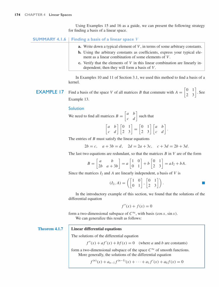
174 CHAPTER 4 Linear Spaces
Using Examples 15 and 16 as a guide, we can present the following strategyfor finding a basis of a linear space.
SUMMARY 4.1.6 Finding a basis of a linear space V
a. Write down a typical element of V , in terms of some arbitrary constants.b. Using the arbitrary constants as coefficients, express your typical ele-
ment as a linear combination of some elements of V .c. Verify that the elements of V in this linear combination are linearly in-
dependent; then they will form a basis of V .
In Examples 10 and 11 of Section 3.1, we used this method to find a basis of akernel.
EXAMPLE 17 Find a basis of the space V of all matrices B that commute with A =[
0 12 3
]. See
Example 13.
Solution
We need to find all matrices B =[
a bc d
]such that
[a bc d
] [0 12 3
]=
[0 12 3
] [a bc d
].
The entries of B must satisfy the linear equations
2b = c, a + 3b = d, 2d = 2a + 3c, c + 3d = 2b + 3d.
The last two equations are redundant, so that the matrices B in V are of the form
B =[
a b2b a + 3b
]= a
[1 00 1
]+ b
[0 12 3
]= aI2 + bA.
Since the matrices I2 and A are linearly independent, a basis of V is
(I2, A) =([
1 00 1
],
[0 12 3
]). !
In the introductory example of this section, we found that the solutions of thedifferential equation
f ′′(x) + f (x) = 0
form a two-dimensional subspace of C∞, with basis (cos x, sin x).We can generalize this result as follows:
Theorem 4.1.7 Linear differential equations
The solutions of the differential equation
f ′′(x) + a f ′(x) + b f (x) = 0 (where a and b are constants)
form a two-dimensional subspace of the space C∞ of smooth functions.More generally, the solutions of the differential equation
f (n)(x) + an−1 f (n−1)(x) + · · · + a1 f ′(x) + a0 f (x) = 0

4.1 Introduction to Linear Spaces 175
Theorem 4.1.7 Linear differential equations (Continued)
(where a0, . . . , an−1 are constants) form an n-dimensional subspace of C∞. Adifferential equation of this form is called an nth-order linear differential equa-tion with constant coefficients.
Second-order linear DEs are frequently used to model oscillatory phenomenain physics. Important examples are damped harmonic motion and LC circuits.
Consider how cumbersome it would be to state the second part of Theorem4.1.7 without using the language of linear algebra. (Try it!) This may convince youthat it can be both natural and useful to apply the language of linear algebra tofunctions. Theorem 4.1.7 will be proven in Section 9.3.
EXAMPLE 18 Find all solutions of the DE
f ′′(x) + f ′(x) − 6 f (x) = 0.
Hint: Find all exponential functions f (x) = ekx that solve the DE.
SolutionAn exponential function f (x) = ekx solves the DE if
f ′′(x) + f ′(x) − 6 f (x) = k2ekx + kekx − 6ekx
= (k2 + k − 6)ekx = (k + 3)(k − 2)ekx = 0.
The solutions are k = 2 and k = −3. Thus, e2x and e−3x are solutions of the DE.(Check this!) Theorem 4.1.7 tells us that the solution space is two-dimensional.Thus, the linearly independent functions e2x , e−3x form a basis of V , and all solu-tions are of the form
f (x) = c1e2x + c2e−3x . !EXAMPLE 19 Let f1, . . . , fn be polynomials. Explain why these polynomials will not span the
space P of all polynomials.
SolutionLet N be the maximum of the degrees of the polynomials f1, . . . , fn . Then all linearcombinations of f1, . . . , fn are in PN , the space of polynomials of degree ≤N . Anypolynomial of higher degree, such as f (x) = x N+1, will not be in the span off1, . . . , fn , proving our claim. !
Example 19 implies that the space P of all polynomials does not have a finitebasis f1, . . . , fn.
Here we are faced with an issue that we did not encounter in Chapter 3, whenstudying Rn and its subspaces (they all have finite bases). This state of affairs callsfor some new terminology.
Definition 4.1.8 Finite dimensional linear spaces
A linear space V is called finite dimensional if it has a (finite) basis f1, . . . , fn , sothat we can define its dimension dim(V ) = n. See Definition 4.1.5. Otherwise,the space is called infinite dimensional.5
As we have just seen, the space P of all polynomials is infinite dimensional (aswas known to Peano in 1888).
5More advanced texts introduce the concept of an infinite basis.

176 CHAPTER 4 Linear Spaces
Take another look at the linear spaces introduced in Examples 1 through 8 ofthis section and see which of them are finite dimensional.
The basic theory of infinite dimensional spaces of functions was establishedby David Hilbert (1862–1943) and his student Erhard Schmidt (1876–1959), in thefirst decade of the twentieth century, based on their work on integral equations. Amore general and axiomatic approach was presented by Stefan Banach (1892–1945)in his 1920 doctoral thesis. These topics (Hilbert spaces, Banach spaces) would bediscussed in a course on functional analysis rather than linear algebra.
EXERCISES 4.1GOAL Find a basis of a linear space and thus determineits dimension. Examine whether a subset of a linear spaceis a subspace.
Which of the subsets of P2 given in Exercises 1 through5 are subspaces of P2 (see Example 16)? Find a basis forthose that are subspaces.
1. p(t): p(0) = 2 2. p(t): p(2) = 0
3. p(t): p′(1) = p(2) (p′ is the derivative.)
4. p(t):∫ 1
0 p(t) dt = 0
5. p(t): p(−t) = −p(t), for all t
Which of the subsets V of R3×3 given in Exercises 6through 11 are subspaces of R3×3?
6. The invertible 3 × 3 matrices
7. The diagonal 3 × 3 matrices
8. The upper triangular 3 × 3 matrices
9. The 3 × 3 matrices whose entries are all greater than orequal to zero
10. The 3 × 3 matrices A such that vector
⎡
⎣123
⎤
⎦ is in the
kernel of A
11. The 3 × 3 matrices in reduced row-echelon form
Let V be the space of all infinite sequences of real num-bers. See Example 5. Which of the subsets of V given inExercises 12 through 15 are subspaces of V?
12. The arithmetic sequences [i.e., sequences of the form(a, a + k, a + 2k, a + 3k, . . .), for some constants aand k]
13. The geometric sequences [i.e., sequences of the form(a, ar, ar2, ar3, . . .), for some constants a and r ]
14. The sequences (x0, x1, . . .) that converge to zero (i.e.,lim
n→∞xn = 0)
15. The square-summable sequences (x0, x1, . . .) (i.e.,
those for which∞∑
i=0
x2i converges)
Find a basis for each of the spaces V in Exercises 16through 36, and determine its dimension.
16. R3×2 17. Rn×m 18. Pn
19. The real linear space C2
20. The space of all matrices A =[
a bc d
]in R2×2 such
that a + d = 0
21. The space of all diagonal 2 × 2 matrices
22. The space of all diagonal n × n matrices
23. The space of all lower triangular 2 × 2 matrices
24. The space of all upper triangular 3 × 3 matrices
25. The space of all polynomials f (t) in P2 such thatf (1) = 0
26. The space of all polynomials f (t) in P3 such thatf (1) = 0 and
∫ 1−1 f (t) dt = 0
27. The space of all 2 × 2 matrices A that commute with
B =[
1 00 2
]
28. The space of all 2 × 2 matrices A that commute with
B =[
1 10 1
]
29. The space of all 2 × 2 matrices A such that
A[
1 11 1
]=
[0 00 0
]
30. The space of all 2 × 2 matrices A such that[
1 23 6
]A =
[0 00 0
]
31. The space of all 2 × 2 matrices S such that[
0 11 0
]S = S
[1 00 −1
]
32. The space of all 2 × 2 matrices S such that[
1 11 1
]S = S
[2 00 0
]

4.1 Introduction to Linear Spaces 177
33. The space of all 2 × 2 matrices S such that[
1 11 1
]S = S
34. The space of all 2 × 2 matrices S such that[
3 24 5
]S = S
35. The space of all 3 × 3 matrices A that commute with
B =
⎡
⎣2 0 00 3 00 0 4
⎤
⎦
36. The space of all 3 × 3 matrices A that commute with
B =
⎡
⎣2 0 00 3 00 0 3
⎤
⎦
37. If B is a diagonal 3 × 3 matrix, what are the possibledimensions of the space V of all 3 × 3 matrices A thatcommute with B? Use Exercises 35 and 36 as a guide.
38. If B is a diagonal 4 × 4 matrix, what are the possibledimensions of the space V of all 4 × 4 matrices A thatcommute with B?
39. What is the dimension of the space of all upper triangu-lar n × n matrices?
40. If c is any vector in Rn , what are the possible dimen-sions of the space V of all n × n matrices A such thatAc = 0?
41. If B is any 3 × 3 matrix, what are the possible dimen-sions of the space V of all 3 × 3 matrices A such thatB A = 0?
42. If B is any n × n matrix, what are the possible dimen-sions of the space V of all n × n matrices A such thatB A = 0?
43. If matrix A represents the reflection about a line L inR2, what is the dimension of the space V of all matri-ces S such that
AS = S[
1 00 −1
]?
Hint: Write S =[v w
], and show that v must be paral-
lel to L , while w must be perpendicular to L .
44. If matrix A represents the orthogonal projection onto aplane V in R3, what is the dimension of the space V ofall matrices S such that
AS = S
⎡
⎣1 0 00 1 00 0 0
⎤
⎦?
See Exercise 43.
45. Find a basis of the space V of all 3 × 3 matrices A thatcommute with
B =
⎡
⎣0 1 00 0 10 0 0
⎤
⎦ ,
and thus determine the dimension of V .
46. In the linear space of infinite sequences, consider thesubspace W of arithmetic sequences. See Exercise 12.Find a basis for W , and thus determine the dimensionof W .
47. A function f (t) from R to R is called even if f (−t) =f (t), for all t in R, and odd if f (−t) = − f (t), forall t . Are the even functions a subspace of F(R, R), thespace of all functions from R to R? What about the oddfunctions? Justify your answers carefully.
48. Find a basis of each of the following linear spaces, andthus determine their dimensions. See Exercise 47.a. f in P4: f is evenb. f in P4: f is odd
49. Let L(Rm , Rn) be the set of all linear transforma-tions from Rm to Rn . Is L(Rm , Rn) a subspace ofF(Rm , Rn), the space of all functions from Rm to Rn?Justify your answer carefully.
50. Find all the solutions of the differential equationf ′′(x) + 8 f ′(x) − 20 f (x) = 0.
51. Find all the solutions of the differential equationf ′′(x) − 7 f ′(x) + 12 f (x) = 0.
52. Make up a second-order linear DE whose solution spaceis spanned by the functions e−x and e−5x .
53. Show that in an n-dimensional linear space we can findat most n linearly independent elements. Hint: Considerthe proof of Theorem 4.1.5.
54. Show that if W is a subspace of an n-dimensional lin-ear space V , then W is finite dimensional as well, anddim(W ) ≤ n. Compare with Exercise 3.2.38a.
55. Show that the space F(R, R) of all functions from R toR is infinite dimensional.
56. Show that the space of infinite sequences of real num-bers is infinite dimensional.
57. We say that a linear space V is finitely generated if itcan be spanned by finitely many elements. Show thata finitely generated space is in fact finite dimensional(and vice versa, of course). Furthermore, if the elementsg1, . . . , gm span V , then dim(V ) ≤ m.
58. In this exercise we will show that the functions cos(x)and sin(x) span the solution space V of the differen-tial equation f ′′(x) = − f (x). See Example 1 of thissection.

178 CHAPTER 4 Linear Spaces
a. Show that if g(x) is in V , then the function(g(x)
)2 +(g′(x)
)2is constant. Hint: Consider the
derivative.b. Show that if g(x) is in V , with g(0) = g′(0) = 0,
then g(x) = 0 for all x .c. If f (x) is in V , then g(x) = f (x) − f (0) cos(x) −
f ′(0) sin(x) is in V as well (why?). Verify thatg(0) = 0 and g′(0) = 0. We can conclude thatg(x) = 0 for all x , so that f (x) = f (0) cos(x) +f ′(0) sin(x). It follows that the functions cos(x) andsin(x) span V , as claimed.
59. Show that if 0 is the neutral element of a linear spaceV , then k0 = 0, for all scalars k.
60. Consider the sequence ( f0, f1, f2, . . .) recursively de-fined by f0 = 0, f1 = 1, and fn = fn−2 + fn−1 forall n = 2, 3, 4, . . . . This is known as the Fibonacci se-quence; for some historical context, see Exercise 48 ofSection 7.3.
In this exercise you are invited to derive a closedformula for fn , expressing fn in terms of n, ratherthan recursively in terms of fn−1 and fn−2. Anotherderivation of this closed formula will be presented inExercise 7.3.48b.
a. Find the terms f0, f1, . . . , f9, f10 of the Fibonaccisequence.
b. In the space V of all infinite sequences of real num-bers (see Example 5), consider the subset W of allsequences (x0, x1, x2, . . .) that satisfy the recursiveequation xn = xn−2 + xn−1 for all n = 2, 3, 4, . . . .Note that the Fibonacci sequence belongs to W .Show that W is a subspace of V , and find a basisof W (write the first five terms x0, . . . , x4 of eachsequence in your basis). Determine the dimensionof W .
c. Find all geometric sequences of the form(1, r, r2, . . .) in W . Can you form a basis of Wconsisting of such sequences? (Be prepared to dealwith irrational numbers.)
d. Write the Fibonacci sequence as a linear combina-tion of geometric sequences. Use your answer tofind a closed formula for fn .6
e. Explain why fn is the integer closest to1√5
(1+
√5
2
)n, for all n = 0, 1, 2, . . . . Use tech-
nology to find f50.7
f. Find limn→∞
fn+1fn
.
4.2 Linear Transformations and Isomorphisms
In this section, we will define the concepts of a linear transformation, image, kernel,rank, and nullity in the context of linear spaces.
Definition 4.2.1 Linear transformations, image, kernel, rank, nullity
Consider two linear spaces V and W . A function T from V to W is called alinear transformation if
T ( f + g) = T ( f ) + T (g) and T (k f ) = kT ( f )
for all elements f and g of V and for all scalars k. These two rules are referredto as the sum rule and the constant-multiple rule, respectively.
For a linear transformation T from V to W , we let
im(T ) = T ( f ) : f in V and
ker(T ) = f in V : T ( f ) = 0.Note that im(T ) is a subspace of target space W and that ker(T ) is a subspace ofdomain V .
6This is known as Binet’s formula, named after the French mathematician Jacques Binet (1786–1856),although the result was known to Leonhard Euler and Daniel Bernoulli more than a century earlier.7The number 1+
√5
2 ≈ 1.618, known as the golden ratio or golden section, is of interest not just tomathematicians, but to painters, musicians, architects, and biologists as well.

4.2 Linear Transformations and Isomorphisms 179
Definition 4.2.1 Linear transformations, image, kernel, rank, nullity (Continued)
If the image of T is finite dimensional, then dim(im T ) is called the rank of T ,and if the kernel of T is finite dimensional, then dim(ker T ) is the nullity of T .
If V is finite dimensional, then the rank-nullity theorem holds. See Theo-rem 3.3.7:
dim(V ) = rank(T ) + nullity(T ) = dim(im T ) + dim(ker T ).
A proof of the rank-nullity theorem is outlined in Exercise 81.
EXAMPLE 1 Consider the transformation D( f ) = f ′ from C∞ to C∞. It follows from the rulesof calculus that D is a linear transformation:
D( f + g) = ( f + g)′ = f ′ + g′ equals D( f ) + D(g) = f ′ + g′ andD(k f ) = (k f )′ = k f ′ equals k D( f ) = k f ′.
Here f and g are smooth functions, and k is a constant.What is the kernel of D? This kernel consists of all smooth functions f such
that D( f ) = f ′ = 0. As you may recall from calculus, these are the constantfunctions f (x) = k. Therefore, the kernel of D is one-dimensional; the functionf (x) = 1 is a basis. The nullity of D is 1.
What about the image of D? The image consists of all smooth functions g suchthat g = D( f ) = f ′ for some function f in C∞ (i.e., all smooth functions g thathave a smooth antiderivative f ). The fundamental theorem of calculus implies thatall smooth functions (in fact, all continuous functions) have an antiderivative. Wecan conclude that
im(D) = C∞. !EXAMPLE 2 Let C[0, 1] be the linear space of all continuous functions from the closed interval
[0, 1] to R. We define the transformation
I ( f ) =∫ 1
0f (x) dx from C[0, 1] to R.
We adopt the simplified notation I ( f ) =∫ 1
0 f . To check that I is linear, we applybasic rules of integration:
I ( f + g) =∫ 1
0( f + g) =
∫ 1
0f +
∫ 1
0g equals I ( f ) + I (g) =
∫ 1
0f +
∫ 1
0g
and
I (k f ) =∫ 1
0(k f ) = k
∫ 1
0f equals k I ( f ) = k
∫ 1
0f.
What is the image of I ? The image of I consists of all real numbers b such that
b = I ( f ) =∫ 1
0f,
for some continuous function f . One of many possible choices for f is the constantfunction f (x) = b. Therefore,
im(I ) = R, and rank(I ) = 1.
We leave it to the reader to think about the kernel of I . !

180 CHAPTER 4 Linear Spaces
EXAMPLE 3 Let V be the space of all infinite sequences of real numbers. Consider thetransformation
T (x0, x1, x2, . . .) = (x1, x2, x3, . . .)
from V to V . (We drop the first term, x0, of the sequence.)
a. Show that T is a linear transformation.b. Find the kernel of T .c. Is the sequence (1, 2, 3, . . .) in the image of T ?d. Find the image of T .
Solutiona. T
((x0, x1, x2, . . .) + (y0, y1, y2, . . .)
)= T (x0 + y0, x1 + y1, x2 + y2, . . .)
= (x1 + y1, x2 + y2, x3 + y3, . . .)
equals
T (x0, x1, x2, . . .) + T (y0, y1, y2, . . .) = (x1, x2, x3, . . .) + (y1, y2, y3, . . .)= (x1 + y1, x2 + y2, x3 + y3, . . .).
We leave it to the reader to verify the constant-multiple rule.b. The kernel consists of everything that is transformed to zero, that is, all
sequences (x0, x1, x2, . . .) such that
T (x0, x1, x2, . . .) = (x1, x2, x3, . . .) = (0, 0, 0, . . .).
This means that entries x1, x2, x3, . . . all have to be zero, while x0 is ar-bitrary. Thus, ker(T ) consists of all sequences of the form (x0, 0, 0, . . .),where x0 is arbitrary. The kernel of T is one-dimensional, with basis(1, 0, 0, 0, . . .). The nullity of T is 1.
c. We need to find a sequence (x0, x1, x2, . . .) such that
T (x0, x1, x2, . . .) = (x1, x2, x3, . . .) = (1, 2, 3, . . .).
It is required that x1 = 1, x2 = 2, x3 = 3, . . . , and we can choose any valuefor x0, for example, x0 = 0. Thus,
(1, 2, 3, . . .) = T (0, 1, 2, 3, . . .)
is indeed in the image of T .d. Mimicking our solution in part (c), we can write any sequence (b0, b1,
b2, . . .) as
(b0, b1, b2, . . .) = T (0, b0, b1, b2, . . .),
so that im(T ) = V . !EXAMPLE 4 Consider the transformation
L([
a bc d
])=
⎡
⎢⎢⎣
abcd
⎤
⎥⎥⎦ from R2×2 to R4.
Note that L is the coordinate transformation L! with respect to the standard basis
! =([
1 00 0
],
[0 10 0
],
[0 01 0
],
[0 00 1
])
of R2×2; see Example 4.1.15. Being a coordinate transformation, L is both linearand invertible; see Theorem 4.1.4.
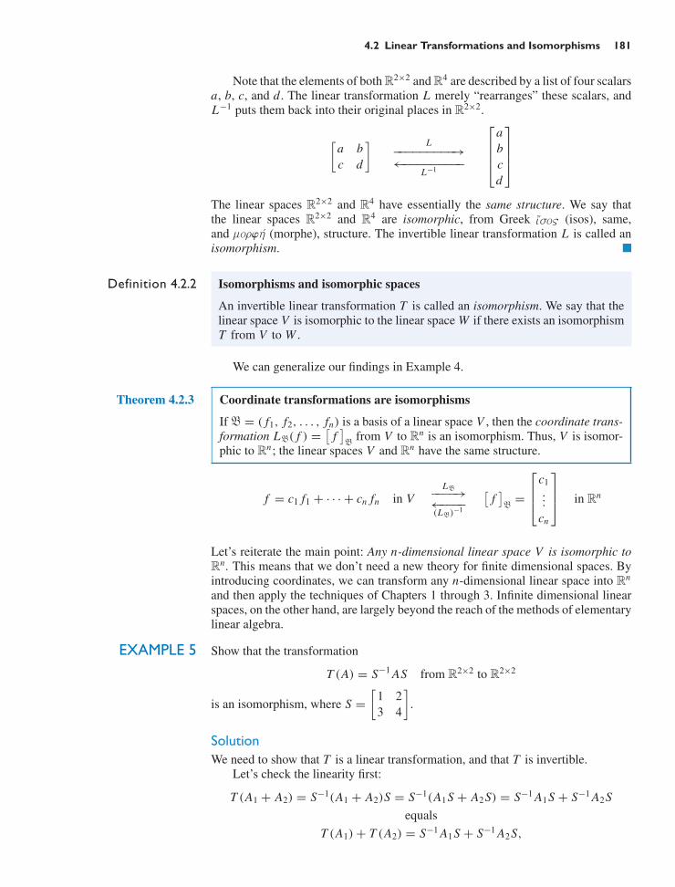
4.2 Linear Transformations and Isomorphisms 181
Note that the elements of both R2×2 and R4 are described by a list of four scalarsa, b, c, and d. The linear transformation L merely “rearranges” these scalars, andL−1 puts them back into their original places in R2×2.
[a bc d
] L−−−−−−−−−→←−−−−−−−−−
L−1
⎡
⎢⎢⎣
abcd
⎤
⎥⎥⎦
The linear spaces R2×2 and R4 have essentially the same structure. We say thatthe linear spaces R2×2 and R4 are isomorphic, from Greek (isos), same,and (morphe), structure. The invertible linear transformation L is called anisomorphism. !
Definition 4.2.2 Isomorphisms and isomorphic spaces
An invertible linear transformation T is called an isomorphism. We say that thelinear space V is isomorphic to the linear space W if there exists an isomorphismT from V to W .
We can generalize our findings in Example 4.
Theorem 4.2.3 Coordinate transformations are isomorphisms
If ! = ( f1, f2, . . . , fn) is a basis of a linear space V , then the coordinate trans-formation L!( f ) =
[f]
!from V to Rn is an isomorphism. Thus, V is isomor-
phic to Rn; the linear spaces V and Rn have the same structure.
f = c1 f1 + · · · + cn fn in VL!−−−−→
←−−−−(L!)−1
[f]
!=
⎡
⎢⎣c1...
cn
⎤
⎥⎦ in Rn
Let’s reiterate the main point: Any n-dimensional linear space V is isomorphic toRn. This means that we don’t need a new theory for finite dimensional spaces. Byintroducing coordinates, we can transform any n-dimensional linear space into Rn
and then apply the techniques of Chapters 1 through 3. Infinite dimensional linearspaces, on the other hand, are largely beyond the reach of the methods of elementarylinear algebra.
EXAMPLE 5 Show that the transformation
T (A) = S−1 AS from R2×2 to R2×2
is an isomorphism, where S =[
1 23 4
].
SolutionWe need to show that T is a linear transformation, and that T is invertible.
Let’s check the linearity first:
T (A1 + A2) = S−1(A1 + A2)S = S−1(A1S + A2S) = S−1 A1S + S−1 A2Sequals
T (A1) + T (A2) = S−1 A1S + S−1 A2S,

182 CHAPTER 4 Linear Spaces
and
T (k A) = S−1(k A)S = k(S−1 AS) equals kT (A) = k(S−1 AS).
The most direct way to show that a function is invertible is to exhibit the inverse.Here we need to solve the equation B = S−1 AS for input A. We find that A =SBS−1, so that T is indeed invertible. The inverse transformation is
T −1(B) = SBS−1. !
Theorem 4.2.4 Properties of isomorphisms
a. A linear transformation T from V to W is an isomorphism if (and onlyif) ker(T ) = 0 and im(T ) = W .
In parts (b) through (d), the linear spaces V and W are assumed to be finitedimensional.
b. The linear space V is isomorphic to W if (and only if) dim(V ) =dim(W ).
c. Suppose T is a linear transformation from V to W with ker(T ) = 0. Ifdim(V ) = dim(W ), then T is an isomorphism.
d. Suppose T is a linear transformation from V to W with im(T ) = W . Ifdim(V ) = dim(W ), then T is an isomorphism.
Proof a. Suppose first that T is an isomorphism. To find the kernel of T , we haveto solve the equation T ( f ) = 0. Applying T −1 on both sides, we find thatf = T −1(0) = 0, so that ker(T ) = 0, as claimed. See Exercise 75. To seethat im(T ) = W , note that any g in V can be written as g = T
(T −1(g)
).
Conversely, suppose that ker(T ) = 0 and im(T ) = W . We have toshow that T is invertible; that is, the equation T ( f ) = g has a uniquesolution f for every g in W (by Definition 2.4.1). There is at least onesolution f , since im(T ) = W . Consider two solutions f1 and f2, so thatT ( f1) = T ( f2) = g. Then
0 = T ( f1) − T ( f2) = T ( f1 − f2),
so that f1 − f2 is in the kernel of T . Since the kernel of T is 0, we musthave f1 − f2 = 0 and f1 = f2, as claimed.
b. First assume that V is isomorphic to W , and let T be an isomorphism fromV to W . Now apply the rank-nullity theorem (Definition 4.2.1) to T :
dim(V ) = dim(ker T ) + dim(im T ) = 0 + dim(W ) = dim(W ), by part (a).
Conversely, suppose that dim(V ) = dim(W ) = n. Then, by Theo-rem 4.2.3, both V and W are isomorphic to Rn . If L1 is an isomorphismfrom V to Rn and L2 is an isomorphism from W to Rn , then L−1
2 L1will be an isomorphism from V to W , by Exercises 76 and 77. Thus, V isisomorphic to W , as claimed.
V
W
L1
o L1L–12
L2
!n

4.2 Linear Transformations and Isomorphisms 183
c. By part (a), it suffices to show that im(T ) = W , or, equivalently, thatdim(im T ) = dim(W ); compare with Exercise 3.3.61. But this claim fol-lows from the rank-nullity theorem:
dim(W ) = dim(V ) = dim(ker T ) + dim(im T ) = dim(im T ).
d. By part (a), it suffices to show that ker(T ) = 0. The proof is analogous topart (c). !
EXAMPLE 6 a. Is the linear transformation
L(
f (x))
=
⎡
⎣f (1)
f (2)
f (3)
⎤
⎦ from P3 to R3 an isomorphism?
b. Is the linear transformation
T(
f (x))
=
⎡
⎣f (1)
f (2)
f (3)
⎤
⎦ from P2 to R3 an isomorphism?
Solutiona. Consider Theorem 4.2.4b. Since dim(P3) = 4 and dim(R3) = 3, the spaces
P3 and R3 fail to be isomorphic, so that L fails to be an isomorphism.b. In this case, the domain and target space have the same dimension,
dim(P2) = dim(R3) = 3.
This fact alone does not guarantee that T is an isomorphism, however. Let’sfind the kernel of T and use Theorem 4.2.4c. The kernel of T consists of allpolynomials f (x) in P2 such that
Is dim(V) = dim(W) ?
Can you write a formulafor the inverse of T ?
Is ker(T) = 0 ?
T isn't an isomorphism T is an isomorphism
yes
no
Is im(T) = W ?
can'ttell
no yes
no
no
yes
yes
Figure 1 Is the linear transformation T from V to W an isomorphism? (V and W are finitedimensional linear spaces.)
184 CHAPTER 4 Linear Spaces
T(
f (x))
=
⎡
⎣f (1)
f (2)
f (3)
⎤
⎦ =
⎡
⎣000
⎤
⎦ ,
that is, f (1) = 0, f (2) = 0, and f (3) = 0. Since a nonzero polynomial inP2 has at most two zeros, the zero polynomial is the only solution, so thatker(T ) = 0. Thus, T is indeed an isomorphism. !
The diagram in Figure 1 can be a useful guide in determining whether a givenlinear transformation T from V to W is an isomorphism. Here we assume that bothV and W are finite dimensional. (We leave it as an exercise for the reader to adaptthe diagram to the case of infinite dimensional spaces.)
EXERCISES 4.2GOAL Examine whether a transformation is linear.Find the image and kernel of a linear transformation. Ex-amine whether a linear transformation is an isomorphism.
Find out which of the transformations in Exercises 1through 50 are linear. For those that are linear, determinewhether they are isomorphisms.
1. T (M) = M + I2 from R2×2 to R2×2
2. T (M) = 7M from R2×2 to R2×2
3. T (M) = (sum of the diagonal entries of M) fromR2×2 to R
4. T (M) = det(M) from R2×2 to R
5. T (M) = M2 from R2×2 to R2×2
6. T (M) = M[
1 23 6
]from R2×2 to R2×2
7. T (M) =[
1 23 4
]M from R2×2 to R2×2
8. T (M) = M[
1 23 4
]M from R2×2 to R2×2
9. T (M) = S−1 M S, where S =[
3 45 6
], from R2×2 to
R2×2
10. T (M) = P M P−1, where P =[
2 35 7
], from R2×2 to
R2×2
11. T (M) = P M Q, where P =[
2 35 7
]and Q =
[3 57 11
], from R2×2 to R2×2
12. T (c) = c[
2 34 5
]from R to R2×2
13. T (M) = M[
1 20 1
]−
[1 20 1
]M from R2×2 to R2×2
14. T (M) =[
2 35 7
]M − M
[2 35 7
]from R2×2 to R2×2
15. T (M) =[
2 00 3
]M − M
[4 00 5
]from R2×2 to R2×2
16. T (M) = M[
2 00 3
]−
[3 00 4
]M from R2×2 to R2×2
17. T (x + iy) = x from C to C18. T (x + iy) = x2 + y2 from C to C19. T (x + iy) = i(x + iy) from C to C20. T (x + iy) = x − iy from C to C21. T (x + iy) = y + i x from C to C22. T
(f (t)
)=
∫ 3−2 f (t) dt from P2 to R
23. T(
f (t))
= f (7) from P2 to R24. T
(f (t)
)= f ′′(t) f (t) from P2 to P2
25. T(
f (t))
= f ′′(t) + 4 f ′(t) from P2 to P2
26. T(
f (t))
= f (−t) from P2 to P2, that is, T (a + bt +ct2) = a − bt + ct2
27. T(
f (t))
= f (2t) from P2 to P2, that is, T (a + bt +ct2) = a + 2bt + 4ct2
28. T(
f (t))
= f (2t) − f (t) from P2 to P2
29. T(
f (t))
= f ′(t) from P2 to P2
30. T(
f (t))
= t(
f ′(t))
from P2 to P2
31. T(
f (t))
=[
f (0) f (1)
f (2) f (3)
]from P2 to R2×2
32. T(
f (t))
= f ′(t) + t2 from P2 to P2
In Exercises 33 through 36, V denotes the space of infinitesequences of real numbers.
33. T (x0, x1, x2, x3, x4, . . .) = (x0, x2, x4, . . .) from V toV (we are dropping every other term)
34. T (x0, x1, x2, . . .) = (0, x0, x1, x2, . . .) from V to V
4.2 Linear Transformations and Isomorphisms 185
35. T(
f (t))
=(
f (0), f ′(0), f ′′(0), f ′′′(0), . . .)
from Pto V , where P denotes the space of all polynomials
36. T(
f (t))
=(
f (0), f (1), f (2), f (3), . . .)
from P toV , where P denotes the space of all polynomials
37. T ( f ) = f + f ′ from C∞ to C∞
38. T ( f ) = f + f ′′ from C∞ to C∞
39. T ( f ) = f ′′ − 5 f ′ + 6 f from C∞ to C∞
40. T ( f ) = f ′′ + 2 f ′ + f from C∞ to C∞
41. T(
f (t))
= f (t) + f ′′(t) + sin(t) from C∞ to C∞
42. T(
f (t))
=[
f (7)
f (11)
]from P2 to R2
43. T(
f (t))
=
⎡
⎣f (5)
f (7)
f (11)
⎤
⎦ from P2 to R3
44. T(
f (t))
=
⎡
⎣f (1)
f ′(2)
f (3)
⎤
⎦ from P2 to R3
45. T(
f (t))
= t(
f (t))
from P to P
46. T(
f (t))
= (t − 1) f (t) from P to P
47. T(
f (t))
=∫ t
0 f (x) dx from P to P
48. T(
f (t))
= f ′(t) from P to P
49. T(
f (t))
= f (t2) from P to P
50. T(
f (t))
= f (t + 2) − f (t)2
from P to P
51. Find the kernel and nullity of the transformation T inExercise 13.
52. Find the kernel and nullity of the transformation T inExercise 6.
53. Find the image, rank, kernel, and nullity of the transfor-mation T in Exercise 25.
54. Find the image, rank, kernel, and nullity of the transfor-mation T in Exercise 22.
55. Find the image and kernel of the transformation T inExercise 33.
56. Find the image, rank, kernel, and nullity of the transfor-mation T in Exercise 30.
57. Find the kernel and nullity of the transformation T inExercise 39.
58. Find the image and kernel of the transformation T inExercise 34.
59. For the transformation T in Exercise 23, find the kernel,nullity, rank, and image, in this order.
60. For the transformation T in Exercise 42, find the kernel,nullity, rank, and image, in this order.
61. Find the image and kernel of the transformation T inExercise 45.
62. Find the image and kernel of the transformation T inExercise 48.
63. Define an isomorphism from P3 to R3, if you can.
64. Define an isomorphism from P3 to R2×2, if you can.
65. We will define a transformation T from Rn×m toF(Rm , Rn); recall that F(Rm , Rn) is the space of allfunctions from Rm to Rn . For a matrix A in Rn×m , thevalue T (A) will be a function from Rm to Rn ; thus, weneed to define
(T (A)
)(v) for a vector v in Rm . We let
(T (A)
)(v) = Av.
a. Show that T is a linear transformation.b. Find the kernel of T .c. Show that the image of T is the space L(Rm , Rn)
of all linear transformations from Rm to Rn . SeeExercise 4.1.19.
d. Find the dimension of L(Rm , Rn).
66. Find the kernel and nullity of the linear transformationT ( f ) = f − f ′ from C∞ to C∞.
67. For which constants k is the linear transformation
T (M) =[
2 30 4
]M − M
[3 00 k
]
an isomorphism from R2×2 to R2×2?
68. For which constants k is the linear transformation
T (M) = M[
5 00 1
]−
[2 00 k
]M
an isomorphism from R2×2 to R2×2?
69. If matrix A is similar to B, is T (M) = AM − M B anisomorphism from R2×2 to R2×2?
70. For which real numbers c0, c1, . . . , cn is the lineartransformation
T(
f (t))
=
⎡
⎢⎢⎢⎣
f (c0)
f (c1)...
f (cn)
⎤
⎥⎥⎥⎦
an isomorphism from Pn to Rn+1?
71. Does there exist a polynomial f (t) of degree ≤4 suchthat f (2) = 3, f (3) = 5, f (5) = 7, f (7) = 11,and f (11) = 2? If so, how many such polynomials arethere? Hint: Use Exercise 70.

186 CHAPTER 4 Linear Spaces
In Exercises 72 through 74, let Zn be the set of all polyno-mials of degree ≤n such that f (0) = 0.
72. Show that Zn is a subspace of Pn , and find the dimen-sion of Zn .
73. Is the linear transformation T(
f (t))
=∫ t
0 f (x) dx anisomorphism from Pn−1 to Zn?
74. Define an isomorphism from Zn to Pn−1 (think calcu-lus!).
75. Show that if T is a linear transformation from V to W ,then T (0V ) = 0W , where 0V and 0W are the neutralelements of V and W , respectively. If T is an isomor-phism, show that T −1(0W ) = 0V .
76. Prove that if T is an isomorphism from V to W , thenT −1 is an isomorphism from W to V . Hint: T −1( f +g) = T −1(T (T −1( f )) + T (T −1(g))). Compare withExercise 2.2.29.
77. If T is a linear transformation from V to W and L isa linear transformation from W to U , is the compositetransformation L T from V to U linear? How can youtell? If T and L are isomorphisms, is L T an isomor-phism as well?
78. Let R+ be the set of positive real numbers. On R+ wedefine the “exotic” operations
x ⊕ y = xy (usual multiplication)
and
k ⊙ x = xk .
a. Show that R+ with these operations is a linearspace; find a basis of this space.
b. Show that T (x) = ln(x) is a linear transformationfrom R+ to R, where R is endowed with the ordi-nary operations. Is T an isomorphism?
79. Is it possible to define “exotic” operations on R2, so thatdim(R2) = 1?
80. Let X be the set of all students in your linear algebraclass. Can you define operations on X that make X intoa real linear space? Explain.
81. In this exercise, we will outline a proof of the rank-nullity theorem: If T is a linear transformation from Vto W , where V is finite dimensional, then
dim(V ) = dim(im T ) + dim(ker T )
= rank(T ) + nullity(T ).
a. Explain why ker(T ) and image (T ) are finite dimen-sional. Hint: Use Exercises 4.1.54 and 4.1.57.
Now consider a basis v1, . . . , vn of ker(T ),where n = nullity(T ), and a basis w1, . . . , wrof im(T ), where r = rank(T ). Consider elementsu1, . . . , ur in V such that T (ui ) = wi for i =1, . . . , r . Our goal is to show that the r +n elementsu1, . . . , ur , v1, . . . , vn form a basis of V ; this willprove our claim.
b. Show that the elements u1, . . . , ur , v1, . . . , vn arelinearly independent. Hint: Consider a relationc1u1 + · · · + cr ur + d1v1 + · · · + dnvn = 0, ap-ply transformation T to both sides, and take it fromthere.
c. Show that the elements u1, . . . , ur , v1, . . . , vn spanV . Hint: Consider an arbitrary element v in V , andwrite T (v) = d1w1 + · · · + drwr . Now show thatthe element v − d1u1 − · · · − dr ur is in the kernelof T , so that v − d1u1 − · · · − dr ur can be writtenas a linear combination of v1, . . . , vn .
82. Prove the following variant of the rank-nullity theorem:If T is a linear transformation from V to W , and ifker T and im T are both finite dimensional, then V isfinite dimensional as well, and dim V = dim(ker T ) +dim(im T ).
83. Consider linear transformations T from V to W andL from W to U . If ker T and ker L are both finite di-mensional, show that ker(L T ) is finite dimensional aswell, and dim
(ker(L T )
)≤ dim(ker T )+dim(ker L).
Hint: Restrict T to ker(L T ) and apply the rank-nullitytheorem, as presented in Exercise 82.
84. Consider linear transformations T from V to W and Lfrom W to U . If ker T and ker L are both finite dimen-sional, and if im T = W , show that ker(L T ) is fi-nite dimensional as well and that dim
(ker(L T )
)=
dim(ker T ) + dim(ker L).
4.3 The Matrix of a Linear Transformation
Next we will examine how we can express a linear transformation in coordinates.
EXAMPLE 1 Consider the linear transformation
T ( f ) = f ′ + f ′′ from P2 to P2,

4.3 The Matrix of a Linear Transformation 187
or, written more explicitly,
T(
f (x))
= f ′(x) + f ′′(x).
Since P2 is isomorphic to R3, this is essentially a linear transformation from R3 toR3, given by a 3 × 3 matrix B. Let’s see how we can find this matrix.
If we let f (x) = a + bx + cx2, then we can write transformation T as
T (a + bx + cx2) = (a + bx + cx2)′ + (a + bx + cx2)′′
= (b + 2cx) + 2c = (b + 2c) + 2cx .
Next let’s write the input f (x) = a + bx + cx2 and the output T(
f (x))
=(b + 2c) + 2cx in coordinates with respect to the standard basis ! = (1, x, x2)of P2:
f (x) = a + bx + cx2 T−−−−−→ T(
f (x))
= (b + 2c) + 2cx
L!
L!
[f (x)
]!
=
⎡
⎣abc
⎤
⎦ −−−−−→[T
(f (x)
)]!
=
⎡
⎣b + 2c
2c0
⎤
⎦ .
Written in !-coordinates, transformation T takes[
f (x)]
!to
[T
(f (x)
)]!
=
⎡
⎣b + 2c
2c0
⎤
⎦ =
⎡
⎣0 1 20 0 20 0 0
⎤
⎦
⎡
⎣abc
⎤
⎦ =
⎡
⎣0 1 20 0 20 0 0
⎤
⎦ [f (x)
]!
.
The matrix
B =
⎡
⎣0 1 20 0 20 0 0
⎤
⎦
is called the !-matrix of transformation T . It describes the transformation T if theinput and output are written in !-coordinates. Let us summarize our work in twodiagrams:
P2T−−−−−→ P2
| |L! | | L!↓ ↓
R3 B−−−−−→ R3,
f T−−−−−→ T ( f )| |
L! | | L!↓ ↓[ f ]!
B−−−−−→ [T ( f )]!.
!
Definition 4.3.1 The !-matrix of a linear transformation
Consider a linear transformation T from V to V , where V is an n-dimensionallinear space. Let ! be a basis of V . Consider the linear transformationL! T L−1
! from Rn to Rn , with standard matrix B, meaning that Bx =L!
(T
(L−1
! (x)))
for all x in Rn . This matrix B is called the !-matrix of transfor-mation T . See the accompanying diagrams Letting f = L−1
! (x) and x =[
f]
!,
we find that[T ( f )
]!
= B[
f]
!, for all f in V .

188 CHAPTER 4 Linear Spaces
Consider the following diagrams.
V T−−−−−→ V| |
L! | | L!↓ ↓Rn B−−−−−→ Rn
f T−−−−−→ T ( f )| |
L! | | L!↓ ↓[ f ]!
B−−−−−→ [T ( f )]!
Compare this with Theorem 3.4.3.We can write B in terms of its columns. Suppose that ! = ( f1, . . . , fi , . . . , fn).
Then
[T ( fi )
]!
= B[
fi]
!= Bei = (i th column of B).
Theorem 4.3.2 The columns of the !-matrix of a linear transformation
Consider a linear transformation T from V to V , and let B be the matrix of Twith respect to a basis ! = ( f1, . . . , fn) of V . Then
B =
⎡
⎣| |[
T ( f1)]
!· · ·
[T ( fn)
]!
| |
⎤
⎦ .
The columns of B are the !-coordinate vectors of the transforms of the basiselements f1, . . ., fn of V .
EXAMPLE 2 Use Theorem 4.3.2 to find the matrix B of the linear transformation T ( f ) = f ′+ f ′′
from P2 to P2 with respect to the standard basis ! = (1, x, x2); see Example 1.
SolutionBy Theorem 4.3.2, we have
B =
⎡
⎣[T (1)
]!
[T (x)
]!
[T (x2)
]!
⎤
⎦ .
Now
T (1) = 1′ + 1′′
= 0
[T (1)
]!
=
⎡
⎣000
⎤
⎦
❳ ❳ ❳ ❳ ❳ ❳ ❳ ❳ ❳ ❳ ❳ ❳ ❳ ❳ ❳ ❳ ❳③
❩❩
❩❩
❩❩❩⑦
T (x) = x ′ + x ′′
= 1
[T (x)
]!
=
⎡
⎣100
⎤
⎦
T (x2) = (x2)′ + (x2)′′
= 2 + 2x
[T (x2)
]!
=
⎡
⎣220
⎤
⎦
B =
⎡
⎣[T (1)
]!
[T (x)
]!
[T (x2)
]!
⎤
⎦ =
⎡
⎣0 1 20 0 20 0 0
⎤
⎦ .

4.3 The Matrix of a Linear Transformation 189
As in Section 3.4, it is suggestive to write the basis elements 1, x , and x2 next to therows of matrix B, while the values T (1) = 0, T (x) = 1, and T (x2) = 2 + 2x arewritten above the columns:
T (1) T (x) T (x2)
B =
⎡
⎣0 1 20 0 20 0 0
⎤
⎦1xx2
.
The last column of B, for example, indicates that T (x2)= 2 · 1 + 2 · x = 2 + 2x . !A problem concerning a linear transformation T can often be done by solving
the corresponding problem for the matrix B of T with respect to some basis !. Wecan use this technique to find the image and kernel of T , to determine whether T isan isomorphism (this is the case if B is invertible), or to solve an equation T ( f ) = gfor f if g is given (this amounts to solving the linear system B
[f]
!=
[g]
!).
EXAMPLE 3 Let V be the span of cos(x) and sin(x) in C∞; note that V consists of all trigonomet-ric functions of the form f (x) = a cos(x) + b sin(x). Consider the transformation
T ( f ) = 3 f + 2 f ′ − f ′′ from V to V .
We are told that T is a linear transformation.
a. Using Theorem 4.3.2, find the matrix B of T with respect to the basis ! =(cos(x), sin(x)
).
b. Is T an isomorphism?
Solutiona. Here
B =
⎡
⎣[T (cos x)
]!
[T (sin x)
]!
⎤
⎦ .
NowT (cos x)= 3 cos(x) − 2 sin(x) + cos(x)= 4 cos(x) − 2 sin(x)
T (sin x)= 3 sin(x) + 2 cos(x) + sin(x)= 2 cos(x) + 4 sin(x).
ThenT (cos x) T (sin x)
B =[
4 2−2 4
]cos(x)sin(x)
.
Matrix B represents a rotation combined with a scaling.b. Matrix B is invertible, since det(B) = ad − bc = 20 = 0. Thus transforma-
tion T is invertible as well, so that T is an isomorphism (we were told thatT is linear). !
EXAMPLE 4 Consider the linear transformation
T (M) =[
0 10 0
]M − M
[0 10 0
]from R2×2 to R2×2.
a. Find the matrix B of T with respect to the standard basis ! of R2×2 .b. Find bases of the image and kernel of B.

190 CHAPTER 4 Linear Spaces
c. Find bases of the image and kernel of T , and thus determine the rank andnullity of transformation T .
Solutiona. For the sake of variety, let us find B by means of a diagram.
[a bc d
]T−−−−→
[0 10 0
] [a bc d
]−
[a bc d
] [0 10 0
]
=[
c d0 0
]−
[0 a0 c
]=
[c d − a0 −c
]
L!
L!
⎡
⎢⎢⎣
abcd
⎤
⎥⎥⎦−−−−→
B
⎡
⎢⎢⎣
cd − a
0−c
⎤
⎥⎥⎦
We see that
B =
⎡
⎢⎢⎣
0 0 1 0−1 0 0 1
0 0 0 00 0 −1 0
⎤
⎥⎥⎦ .
b. Note that columns v2 and v4 of B are redundant, with v2 = 0 and v4 = −v1,or v1 + v4 = 0. Thus, the nonredundant columns
v1 =
⎡
⎢⎢⎣
0−1
00
⎤
⎥⎥⎦ , v3 =
⎡
⎢⎢⎣
100
−1
⎤
⎥⎥⎦ form a basis of im(B),
and⎡
⎢⎢⎣
0100
⎤
⎥⎥⎦ ,
⎡
⎢⎢⎣
1001
⎤
⎥⎥⎦ form a basis of ker(B).
c. We apply L−1! to transform the vectors we found in part (b) back into R2×2,
the domain and target space of transformation T :[
0 −10 0
],
[1 00 −1
]is a basis of im(T ),
and[
0 10 0
], I2 =
[1 00 1
]is a basis of ker(T ).
Thus, rank(T ) = dim(im T ) = 2 and nullity(T ) = dim(ker T ) = 2. !Change of BasisIf " and ! are two bases of a linear space V , what is the relationship between thecoordinate vectors
[f]
"and
[f]
!, for an element f of V ?

4.3 The Matrix of a Linear Transformation 191
Definition 4.3.3 Change of basis matrix
Consider two bases " and ! of an n-dimensional linear space V . Consider thelinear transformation L" L−1
! from Rn to Rn , with standard matrix S, mean-ing that Sx = L"
(L−1
! (x))
for all x in Rn . This invertible matrix S is calledthe change of basis matrix from ! to ", sometimes denoted by S!→". See theaccompanying diagrams. Letting f = L−1
! (x) and x =[
f]
!, we find that
[f]
"= S
[f]
!, for all f in V .
If ! = (b1, . . . , bi , . . . , bn), then[bi
]"
= S[bi
]!
= Sei = (i th column of S),
so that
S!→" =
⎡
⎣| |[
b1]
"· · ·
[bn
]"
| |
⎤
⎦ .
6 6 6 6 6 67
L"
Rn
V S
L! Rn
6 6 6 6 6 6 67
L"
[ f ]"
f S
L!
[ f ]!
What is the relationship between the change of basis matrices S!→" andS"→!? Solving the equation
[f]
"= (S!→")
[f]
!for
[f]
!, we find that[
f]
!= (S!→")−1
[f]
", so that
S"→! = (S!→")−1.
EXAMPLE 5 Let V be the subspace of C∞ spanned by the functions ex and e−x , with the bases" = (ex , e−x) and ! = (ex + e−x , ex − e−x). Find the change of basis matrixS!→".
SolutionBy Definition 4.3.3,
S =[
[ex + e−x
]"
[ex − e−x
]"
].
Now
ex + e−x = 1 · ex + 1 · e−x
[ex + e−x
]"
=[
11
]
ex − e−x = 1 · ex + (−1) · e−x
[ex − e−x
]"
=[
1−1
]
S!→" =[
1 11 −1
]

192 CHAPTER 4 Linear Spaces
It is suggestive to write the functions ex and e−x of basis " next to the rows ofmatrix S!→", while the functions ex + e−x and ex − e−x of basis ! are writtenabove the columns:
ex + e−x ex − e−x
S!→" =[
1 11 −1
]ex
e−x .
The second column of matrix S indicates that ex − e−1 = 1 · ex + (−1) · e−x . !EXAMPLE 6 Let " = (e1, . . . , en) be the standard basis of Rn , and let ! = (b1, . . . , bn) be an
arbitrary basis of Rn . Find the change of basis matrix S!→".
SolutionBy Definition 4.3.3,
S!→" =[[b1
]"
· · ·[bn
]"
].
But note that[x]
"= x for all x in Rn ,
since
x =
⎡
⎢⎣x1...
xn
⎤
⎥⎦ = x1e1 + · · · + xnen;
the components of x are its coordinates with respect to the standard basis. Thus,
S!→" =[
b1 · · · bn
].
Compare this with Definition 3.4.1. !EXAMPLE 7 The equation x1 + x2 + x3 = 0 defines a plane V in R3. In this plane, consider the
two bases
" = (a1, a2)=
⎛
⎝
⎡
⎣01
−1
⎤
⎦ ,
⎡
⎣10
−1
⎤
⎦
⎞
⎠ and ! = (b1, b2)=
⎛
⎝
⎡
⎣12
−3
⎤
⎦ ,
⎡
⎣4
−1−3
⎤
⎦
⎞
⎠ .
a. Find the change of basis matrix S from ! to ".b. Verify that the matrix S in part (a) satisfies the equation
[
b1 b2
]=
[
a1 a2
]S.
Solutiona. By inspection, we find that b1 = 2a1 + a2 and b2 = −a1 + 4a2, so that
b1 b2
S!→" =[
2 −11 4
]a1a2
.

4.3 The Matrix of a Linear Transformation 193
b. We can verify that⎡
⎣ b1 b2
⎤
⎦ =
⎡
⎣1 42 −1
−3 −3
⎤
⎦ =
⎡
⎣0 11 0
−1 −1
⎤
⎦[
2 −11 4
]=
⎡
⎣ a1 a2
⎤
⎦ S.
This equation reflects the fact that the two columns of S are the coordinatevectors of b1 and b2 with respect to the basis " = (a1, a2). We can illustratethis equation with a commutative diagram, where x represents a vector in V :
[x]
"
6 6 6 6 6 6 67
[
a1 a2
]
S x
[
b1 b2
][x]
!
.
Let us remind ourselves where the equation x =[
b1 b2] [
x]
!comes
from: If c1, c2 are the coordinates of x with respect to !, then
x = c1b1 + c2b2 =[
b1 b2
] [c1
c2
]=
[
b1 b2
][
x]
!.
!We can generalize.
Theorem 4.3.4 Change of basis in a subspace of Rn
Consider a subspace V of Rn with two bases " = (a1, . . . , am) and ! =(b1, . . . , bm). Let S be the change of basis matrix from ! to ". Then the fol-lowing equation holds:
⎡
⎣| |
b1 · · · bm
| |
⎤
⎦ =
⎡
⎣| |
a1 · · · am
| |
⎤
⎦ S.
As in Example 7, this equation can be justified by means of a commutativediagram:
[x]
"
6 6 6 6 6 6 67
[
a1 · · · am
]
S x
[
b1 · · · bm
][x]
!
.
Now consider a linear transformation T from V to V , where V is a finite di-mensional linear space. Let " and ! be two bases of V , and let A and B be the"- and the !-matrix of T , respectively. What is the relationship among A, B, andthe change of basis matrix S from ! to "?

194 CHAPTER 4 Linear Spaces
Consider the following diagram.
[f]
"
❩❩
❩❩⑥
❩❩
❩❩⑦
A−−−−−−−−−−−−−−−−−−−−−−→
[T ( f )
]"
L" L"
S fT
−−−−−−−−−→ T ( f ) S
L! L!
[f]
! −−−−−−−−−−−−−−−−−−−−−−→B
[T ( f )
]!
As in Section 3.4, we see that[T ( f )
]"
= AS[
f]
!= SB
[f]
!for all f in V , so
that AS = SB.
Theorem 4.3.5 Change of basis for the matrix of a linear transformation
Let V be a linear space with two given bases " and !. Consider a linear trans-formation T from V to V , and let A and B be the "-matrix and !-matrix of T ,respectively. Let S be the change of basis matrix from ! to ". Then A is similarto B, and
AS = SB or A = SBS−1 or B = S−1 AS.
EXAMPLE 8 As in Example 5, let V be the linear space spanned by the functions ex and e−x ,with the bases " = (ex , e−x) and ! = (ex + e−x , ex − e−x). Consider the lineartransformation D( f ) = f ′ from V to V .
a. Find the "-matrix A of D.b. Use part (a), Theorem 4.3.5, and Example 5 to find the !-matrix B of D.c. Use Theorem 4.3.2 to find the !-matrix B of D in terms of its columns.
Solutiona. Let’s use a diagram. Recall that (e−x)′ = −e−x , by the chain rule.
aex + be−x D−−−−−−−−−→ aex − be−x
[ab
]−−−−−−−−−→
A =[
1 00 −1
][
a−b
]
b. In Example 5 we found the change of basis matrix S =[
1 11 −1
]from !
to ". Now
B = S−1 AS = 12
[1 11 −1
] [1 00 −1
] [1 11 −1
]=
[0 11 0
].
c. Note that D(ex + e−x) = ex − e−x and D(ex − e−x) = ex + e−x . Thus,
D(ex + e−x) D(ex − e−x )
B =[
0 11 0
]ex + e−x
ex − e−x . !

4.3 The Matrix of a Linear Transformation 195
EXERCISES 4.3GOAL Use the concept of coordinates. Find the matrixof a linear transformation. Use this matrix to find the im-age and kernel of a transformation.
1. Are the polynomials f (t) = 7 + 3t + t2, g(t) =9 + 9t + 4t2, and h(t) = 3 + 2t + t2 linearly inde-pendent?
2. Are the matrices[
1 11 1
],
[1 23 4
],
[2 35 7
],
[1 46 8
]
linearly independent?
3. Do the polynomials f (t) = 1 + 2t + 9t2 + t3, g(t) =1 + 7t + 7t3, h(t) = 1 + 8t + t2 + 5t3, and k(t) =1 + 8t + 4t2 + 8t3 form a basis of P3?
4. Consider the polynomials f (t) = t + 1 and g(t) =(t+2)(t+k), where k is an arbitrary constant. For whichvalues of the constant k are the three polynomials f (t),t f (t), and g(t) a basis of P2?
In Exercises 5 through 40, find the matrix of the given lin-ear transformation T with respect to the given basis. Ifno basis is specified, use the standard basis: " = (1, t, t2)for P2,
" =([
1 00 0
],
[0 10 0
],
[0 01 0
],
[0 00 1
])
for R2×2, and " = (1, i) for C. For the space U2×2 of up-per triangular 2 × 2 matrices, use the basis
" =([
1 00 0
],
[0 10 0
],
[0 00 1
])
unless another basis is given. In each case, determinewhether T is an isomorphism. If T isn’t an isomorphism,find bases of the kernel and image of T , and thus deter-mine the rank of T .
5. T (M) =[
1 20 3
]M from U 2×2 to U 2×2
6. T (M) =[
1 20 3
]M from U 2×2 to U 2×2, with respect
to the basis ! =([
1 00 0
],
[0 10 0
],
[0 10 1
])
7. T (M) = M[
1 20 1
]−
[1 20 1
]M from U 2×2 to U 2×2,
with respect to the basis
! =([
1 00 1
],
[0 10 0
],
[1 00 −1
])
8. T (M) = M[
1 20 1
]−
[1 20 1
]M from U 2×2 to U 2×2
9. T (M) =[
1 00 2
]−1
M[
1 00 2
]from U 2×2 to U 2×2
10. T (M) =[
1 20 3
]−1
M[
1 20 3
]from U 2×2 to U 2×2
11. T (M) =[
1 20 3
]−1
M[
1 20 3
]from U 2×2 to U 2×2,
with respect to the basis
! =([
1 −10 0
],
[0 10 1
],
[0 10 0
])
12. T (M) = M[
2 00 3
]from R2×2 to R2×2
13. T (M) =[
1 12 2
]M from R2×2 to R2×2
14. T (M) =[
1 12 2
]M from R2×2 to R2×2, with respect
to the basis
! =([
1 0−1 0
],
[0 10 −1
],
[1 02 0
],
[0 10 2
])
15. T (x + iy) = x − iy from C to C
16. T (x + iy) = x − iy from C to C, with respect to thebasis ! = (1 + i, 1 − i)
17. T (z) = i z from C to C
18. T (z) = (2 + 3i)z from C to C
19. T (z) = (p + iq)z from C to C, where p and q arearbitrary real numbers
20. T ( f ) = f ′ from P2 to P2
21. T ( f ) = f ′ − 3 f from P2 to P2
22. T ( f ) = f ′′ + 4 f ′ from P2 to P2
23. T(
f (t))
= f (3) from P2 to P2
24. T(
f (t))
= f (3) from P2 to P2, with respect to thebasis ! =
(1, t − 3, (t − 3)2)
25. T(
f (t))
= f (−t) from P2 to P2
26. T(
f (t))
= f (2t) from P2 to P2
27. T(
f (t))
= f (2t − 1) from P2 to P2
28. T(
f (t))
= f (2t −1) from P2 to P2, with respect to thebasis ! =
(1, t − 1, (t − 1)2)
29. T(
f (t))
=∫ 2
0 f (t) dt from P2 to P2

196 CHAPTER 4 Linear Spaces
30. T(
f (t))
= f (t + h) − f (t)h
from P2 to P2, where h is
a nonzero constant. Interpret transformation T geomet-rically.
31. T(
f (t))
= f (t + h) − f (t − h)
2hfrom P2 to P2, where
h is a nonzero constant. Interpret transformation T ge-ometrically.
32. T(
f (t))
= f (1)+ f ′(1)(t −1) from P2 to P2. Interprettransformation T geometrically.
33. T(
f (t))
= f (1) + f ′(1)(t − 1) from P2 to P2, withrespect to the basis ! =
(1, t − 1, (t − 1)2)
34. T (M) =[
2 00 5
]M − M
[2 00 5
]from R2×2 to R2×2
35. T (M) =[
2 10 2
]M − M
[2 10 2
]from R2×2 to R2×2
36. T (M) =[
1 11 1
]M − M
[1 11 1
]from R2×2 to R2×2
37. T (M) =[
1 11 1
]M − M
[1 11 1
]from R2×2 to R2×2,
with respect to the basis
! =([
1 1−1 −1
],
[1 −11 −1
],
[1 00 1
],
[0 11 0
])
38. T (M) =[
0 11 0
]M − M
[1 00 −1
]from R2×2 to
R2×2, with respect to the basis
! =([
1 01 0
],
[1 0
−1 0
],
[0 10 1
],
[0 10 −1
])
39. T (M) =[
0 11 0
]M − M
[1 00 −1
]from R2×2 to
R2×2
40. T (M) =[
1 24 3
]M − M
[5 00 −1
]from R2×2 to
R2×2
41. a. Find the change of basis matrix S from the basis !considered in Exercise 6 to the standard basis " ofU 2×2 considered in Exercise 5.
b. Verify the formula SB = AS for the matrices B andA you found in Exercises 6 and 5, respectively.
c. Find the change of basis matrix from " to !.
42. a. Find the change of basis matrix S from the basis !considered in Exercise 7 to the standard basis " ofU 2×2 considered in Exercise 8.
b. Verify the formula SB = AS for the matrices B andA you found in Exercises 7 and 8, respectively.
c. Find the change of basis matrix from " to !.
43. a. Find the change of basis matrix S from the basis !considered in Exercise 11 to the standard basis " ofU 2×2 considered in Exercise 10.
b. Verify the formula SB = AS for the matrices B andA you found in Exercises 11 and 10, respectively.
c. Find the change of basis matrix from " to !.
44. a. Find the change of basis matrix S from the basis !considered in Exercise 14 to the standard basis " ofR2×2 considered in Exercise 13.
b. Verify the formula SB = AS for the matrices B andA you found in Exercises 14 and 13, respectively.
45. a. Find the change of basis matrix S from the basis! considered in Exercise 16 to the standard basis" = (1, i) of C considered in Exercise 15.
b. Verify the formula SB = AS for the matrices B andA you found in Exercises 16 and 15, respectively.
c. Find the change of basis matrix from " to !.
46. a. Find the change of basis matrix S from the basis! considered in Exercise 24 to the standard basis" = (1, t, t2) of P2 considered in Exercise 23.
b. Verify the formula SB = AS for the matrices B andA you found in Exercises 24 and 23, respectively.
c. Find the change of basis matrix from " to !.
47. a. Find the change of basis matrix S from the basis! considered in Exercise 28 to the standard basis" = (1, t, t2) of P2 considered in Exercise 27.
b. Verify the formula SB = AS for the matrices B andA you found in Exercises 28 and 27, respectively.
c. Find the change of basis matrix from " to !.
In Exercises 48 through 53, let V be the space spannedby the two functions cos(t) and sin(t). In each exercise,find the matrix of the given transformation T with respectto the basis cos(t), sin(t), and determine whether T is anisomorphism.
48. T ( f ) = f ′ 49. T ( f ) = f ′′ + 2 f ′ + 3 f
50. T ( f ) = f ′′ +a f ′ +b f , where a and b are arbitrary realnumbers. Find all the values of a and b such that T isan isomorphism.
51. T(
f (t))
= f (t − π/2)
52. T(
f (t))
= f (t − π/4)
53. T(
f (t))
= f (t − θ), where θ is an arbitrary real num-ber. Hint: Use the addition theorems for sine and cosine.
In Exercises 54 through 58, let V be the plane with equa-tion x1 + 2x2 + 3x3 = 0 in R3. In each exercise, find thematrix B of the given transformation T from V to V , with

4.3 The Matrix of a Linear Transformation 197
respect to the basis
⎡
⎣11
−1
⎤
⎦ ,
⎡
⎣5
−41
⎤
⎦. Note that the domain
and target space of T are restricted to the plane V , so thatB will be a 2 × 2 matrix.
54. The orthogonal projection onto the line spanned by
vector
⎡
⎣11
−1
⎤
⎦
55. The orthogonal projection onto the line spanned by
vector
⎡
⎣1
−21
⎤
⎦
56. T (x) =
⎡
⎣123
⎤
⎦ × x . See Theorem A.11 in the Appendix.
57. T (x) =
⎡
⎣−2 −3 1
1 0 −20 1 1
⎤
⎦ x
58. T (x) =
⎛
⎝x ·
⎡
⎣11
−1
⎤
⎦
⎞
⎠
⎡
⎣11
−1
⎤
⎦
59. Consider a linear transformation T from V to V withker(T ) = 0. If V is finite dimensional, then T is anisomorphism, since the matrix of T will be invertible.Show that this is not necessarily the case if V is in-finite dimensional: Give an example of a linear trans-formation T from P to P with ker(T ) = 0 that isnot an isomorphism. (Recall that P is the space of allpolynomials.)
60. In the planeV defined by the equation 2x1 + x2 −2x3 =0, consider the bases
" = (a1, a2) =
⎛
⎝
⎡
⎣122
⎤
⎦ ,
⎡
⎣2
−21
⎤
⎦
⎞
⎠
and
! = (b1, b2) =
⎛
⎝
⎡
⎣122
⎤
⎦ ,
⎡
⎣303
⎤
⎦
⎞
⎠ .
a. Find the change of basis matrix S from ! to ".b. Find the change of basis matrix from " to !.c. Write an equation relating the matrices
[a1 a2
],[
b1 b2], and S = S!→".
61. In R2, consider the bases
" = (a1, a2) =([
12
],
[2
−1
])
and
! = (b1, b2) =([
5−10
],
[10
5
]).
a. Find the change of basis matrix S from ! to ". Inter-pret the transformation defined by S geometrically.
b. Find the change of basis matrix from " to !.c. Write an equation relating the matrices
[a1 a2
],[
b1 b2], and S = S!→".
62. In the planeV defined by the equation x1 − 2x2 + 2x3 =0, consider the basis
" = (a1, a2) =
⎛
⎝
⎡
⎣210
⎤
⎦ ,
⎡
⎣−2
01
⎤
⎦
⎞
⎠ .
a. Construct another basis ! = (b1, b2) of V , such thatneither b1 nor b2 has any zero components.
b. Find the change of basis matrix S from ! to ".c. Find the change of basis matrix from " to !.d. Write an equation relating the matrices
[a1 a2
],[
b1 b2], and S = S!→".
63. In the planeV defined by the equation x1 + 3x2 − 2x3 =0, consider the basis
" = (a1, a2) =
⎛
⎝
⎡
⎣−3
10
⎤
⎦ ,
⎡
⎣−1
11
⎤
⎦
⎞
⎠ .
a. Construct another basis ! = (b1, b2) of V , such thatneither b1 nor b2 has any negative components.
b. Find the change of basis matrix S from ! to ".c. Find the change of basis matrix from " to !.d. Write an equation relating the matrices
[a1 a2
],[
b1 b2], and S = S!→".
64. Let V be the space of all upper triangular 2×2 matrices.Consider the linear transformation
T[
a b0 c
]= aI2 + bQ + cQ2
from V to V , where Q =[
1 20 3
].
a. Find the matrix A of T with respect to the basis
" =([
1 00 0
],
[0 10 0
],
[0 00 1
]).
b. Find bases of the image and kernel of T , and thusdetermine the rank of T .

198 CHAPTER 4 Linear Spaces
65. Let V be the subspace of R2×2 spanned by the matrices
I2 and Q =[
a bc d
], where b = 0.
a. Compute Q2 and find the coordinate vector[Q2]
!,where ! = (I2, Q).
b. Consider the linear transformation T (M) = M Qfrom V to V . Find the !-matrix B of T . For whichmatrices Q is T an isomorphism?
c. If T fails to be an isomorphism, find the image andkernel of T . What is the rank of T in that case?
66. Let V be the linear space of all functions in two vari-ables of the form q(x1, x2) = ax2
1 + bx1x2 + cx22 .
Consider the linear transformation
T ( f ) = x2∂ f∂x1
− x1∂ f∂x2
from V to V .a. Find the matrix ! of T with respect to the basis x2
1 ,x1x2, x2
2 of V .b. Find bases of the kernel and image of T .
67. Let V be the linear space of all functions of the form
f (t) = c1 cos(t) + c2 sin(t) + c3t cos(t) + c4t sin(t).
Consider the linear transformation T from V to V givenby
T ( f ) = f ′′ + f.
a. Find the matrix of T with respect to the basis cos(t),sin(t), t cos(t), t sin(t) of V .
b. Find all solutions f in W of the differential equation
T ( f ) = f ′′ + f = cos(t).
Graph your solution(s). [The differential equationf ′′+ f = cos(t) describes a forced undamped oscil-lator. In this example, we observe the phenomenonof resonance.]
68. Consider the linear space V of all infinite sequences ofreal numbers. We define the subset W of V consisting ofall sequences (x0, x1, x2, . . .) such that xn+2 = xn+1 +6xn for all n ≥ 0.a. Show that W is a subspace of V .b. Determine the dimension of W .c. Does W contain any geometric sequences of the
form (1, c, c2, c3, . . .), for some constant c? Find allsuch sequences in W .
d. Can you find a basis of W consisting of geometricsequences?
e. Consider the sequence in W whose first two termsare x0 = 0, x1 = 1. Find x2, x3, x4. Find a closedformula for the nth term xn of this sequence. Hint:Write this sequence as a linear combination of thesequences you found in part (d).
69. Consider a basis f1, . . . , fn of Pn−1. Let a1, . . . , anbe distinct real numbers. Consider the n × n matrix Mwhose i j th entry is f j (ai ). Show that the matrix M isinvertible. Hint: If the vector
⎡
⎢⎢⎢⎣
c1c2...
cn
⎤
⎥⎥⎥⎦
is in the kernel of M , then the polynomial f = c1 f1 +· · · + cn fn in Pn−1 vanishes at a1, . . . , an ; therefore,f = 0.
70. Let a1, . . . , an be distinct real numbers. Show that thereexist “weights” w1, . . . , wn such that
∫ 1
−1f (t) dt =
n∑
i=1
wi f (ai ),
for all polynomials f (t) in Pn−1. Hint: It suffices toprove the claim for a basis f1, . . . , fn of Pn−1. Exer-cise 69 is helpful.
71. Find the weights w1, w2, w3 in Exercise 70 for a1 =−1,a2 = 0, a3 = 1. Compare this with Simpson’s rule incalculus.
72. In all parts of this problem, let V be the set of all vectorsx in R4 such that x3 = x1 + x2 and x4 = x2 + x3.a. Represent V as the kernel of a matrix M . Find
the rank of M and the dimension of V . Show that
" =
⎛
⎜⎝
⎡
⎢⎣
1011
⎤
⎥⎦ ,
⎡
⎢⎣
0112
⎤
⎥⎦
⎞
⎟⎠ is a basis of V .
b. Find all vectors of the form
⎡
⎢⎢⎣
1rr2
r3
⎤
⎥⎥⎦ that are contained
in V . (Be prepared to deal with irrational numbers.)Can you form a basis ! of V consisting of such vec-tors?
c. Consider the linear transformation T
⎡
⎢⎣
x1x2x3x4
⎤
⎥⎦ =
⎡
⎢⎣
x2x3x4
x3 + x4
⎤
⎥⎦ from R4 to R4. If x is a vector in V ,
show that T (x) is in V as well. Thus, T induces alinear transformation from V to V , which we willdenote by F .
d. Find the matrix A of F with respect to the basis "from part (a). [Note that A will be a 2 × 2 matrix,since dim(V ) = 2.]

Chapter Four Exercises 199
e. Find the matrix B of F with respect to your basis !from part (b).
f. Find the change of basis matrix S = S!→".g. Write an equation relating the matrices A, B, and S,
and check that this equation holds for the matricesyou found in parts (d), (e), and (f).
73. As in Problem 72, let V be the set of all vectors x in R4
such that x3 = x1 +x2 and x4 = x2 +x3. In Problem 72we see that V is a subspace of R4 with dim(V ) = 2.
a. Consider the linear transformation T
⎡
⎢⎣
x1x2x3x4
⎤
⎥⎦ =
⎡
⎢⎣
x4−x3
x2−x1
⎤
⎥⎦ from R4 to R4. Show that T (x) is orthog-
onal to x , for all x in R4. If x is a vector in V , show
that T (x) is in V as well. Thus, T induces a lineartransformation from V to V , which we will denoteby F .
b. Find the matrix A of F with respect to the basis
" =
⎛
⎜⎝
⎡
⎢⎣
1011
⎤
⎥⎦ ,
⎡
⎢⎣
0112
⎤
⎥⎦
⎞
⎟⎠.
c. Find the matrix B of F with respect to the basis
! =
⎛
⎜⎝
⎡
⎢⎣
0112
⎤
⎥⎦ ,
⎡
⎢⎣
2−1
10
⎤
⎥⎦
⎞
⎟⎠.
d. Find the change of basis matrix S = S!→".e. Write an equation relating the matrices A, B, and S,
and check that this equation holds for the matricesyou found in parts (b), (c), and (d).
f. Does there exist a basis # of V such that the #-matrix C of F is diagonal?
Chapter Four Exercises
TRUE OR FALSE?1. The polynomials of degree less than 7 form a seven-
dimensional subspace of the linear space of allpolynomials.
2. The function T ( f ) = 3 f − 4 f ′ from C∞ to C∞ is alinear transformation.
3. The lower triangular 2 × 2 matrices form a subspace ofthe space of all 2 × 2 matrices.
4. The kernel of a linear transformation is a subspace ofthe domain.
5. The space R2×3 is five-dimensional.
6. If f1, . . . , fn is a basis of a linear space V , then anyelement of V can be written as a linear combination off1, . . . , fn .
7. The space P1 is isomorphic to C.
8. If the kernel of a linear transformation T from P4 to P4is 0, then T must be an isomorphism.
9. If W1 and W2 are subspaces of a linear space V , thenthe intersection W1 ∩ W2 must be a subspace of V aswell.
10. If T is a linear transformation from P6 to R2×2, thenthe kernel of T must be three-dimensional.
11. All bases of P3 contain at least one polynomial of de-gree ≤2.
12. If T is an isomorphism, then T −1 must be an isomor-phism as well.
13. The linear transformation T ( f ) = f + f ′′ from C∞ toC∞ is an isomorphism.
14. All linear transformations from P3 to R2×2 are isomor-phisms.
15. If T is a linear transformation from V to V , then theintersection of im(T ) and ker(T ) must be 0.
16. The space of all upper triangular 4 × 4 matrices isisomorphic to the space of all lower triangular 4 × 4matrices.
17. Every polynomial of degree 3 can be expressed as a lin-ear combination of the polynomial (t −3), (t −3)2, and(t − 3)3.
18. If a linear space V can be spanned by 10 elements, thenthe dimension of V must be ≤ 10.
19. The function T (M) = det(M) from R2×2 to R is a lin-ear transformation.
20. There exists a 2 × 2 matrix A such that the space V ofall matrices commuting with A is one-dimensional.
21. The linear transformation T (M) =[
1 23 6
]M from
R2×2 to R2×2 has rank 1.
22. If the matrix of a linear transformation T (with respect
to some basis) is[
3 50 4
], then there must exist a
nonzero element f in the domain of T such thatT ( f ) = 3 f .

200 CHAPTER 4 Linear Spaces
23. The kernel of the linear transformation T(
f (t))
=f (t2) from P to P is 0.
24. If S is any invertible 2 × 2 matrix, then the linear trans-formation T (M) = SM S is an isomorphism from R2×2
to R2×2.
25. There exists a 2 × 2 matrix A such that the space of allmatrices commuting with A is two-dimensional.
26. There exists a basis of R2×2 that consists of four invert-ible matrices.
27. If the image of a linear transformation T from P to Pis all of P , then T must be an isomorphism.
28. If f1, f2, f3 is a basis of a linear space V , then f1,f1 + f2, f1 + f2 + f3 must be a basis of V as well.
29. If a, b, and c are distinct real numbers, then the polyno-mials (x −b)(x −c), (x −a)(x −c), and (x −a)(x −b)must be linearly independent.
30. The linear transformation T(
f (t))
= f (4t − 3) fromP to P is an isomorphism.
31. If W is a subspace of V , and if W is finite dimensional,then V must be finite dimensional as well.
32. There exists a linear transformation from R3×3 to R2×2
whose kernel consists of all lower triangular 3 × 3 ma-trices, while the image consists of all upper triangular2 × 2 matrices.
33. Every two-dimensional subspace of R2×2 contains atleast one invertible matrix.
34. If " = ( f, g) and ! = ( f, f + g) are two bases of alinear space V , then the change of basis matrix from "
to ! is[
1 10 1
].
35. If the matrix of a linear transformation T with respect
to a basis ( f, g) is[
1 23 4
], then the matrix of T with
respect to the basis (g, f ) is[
2 14 3
].
36. The linear transformation T ( f ) = f ′ from Pn to Pnhas rank n, for all positive integers n.
37. If the matrix of a linear transformation T (with respect
to some basis) is[
2 35 7
], then T must be an isomor-
phism.
38. There exists a subspace of R3×4 that is isomorphicto P9.
39. There exist two distinct subspaces W1 and W2 of R2×2
whose union W1 ∪ W2 is a subspace of R2×2 as well.
40. There exists a linear transformation from P to P5 whoseimage is all of P5.
41. If f1, . . . , fn are polynomials such that the degree of fkis k (for k = 1, . . . , n), then f1, . . . , fn must be linearlyindependent.
42. The transformation D( f ) = f ′ from C∞ to C∞ is anisomorphism.
43. If T is a linear transformation from P4 to W withim(T ) = W , then the inequality dim(W ) ≤ 5 musthold.
44. The kernel of the linear transformation
T(
f (t))
=∫ 1
0f (t) dt
from P to R is finite dimensional.
45. If T is a linear transformation from V to V , then f in V : T ( f ) = f must be a subspace of V .
46. If T is a linear transformation from P6 to P6 thattransforms tk into a polynomial of degree k (for k =0, 1, . . . , 6), then T must be an isomorphism.
47. There exist invertible 2 × 2 matrices P and Q such thatthe linear transformation T (M) = P M − M Q is anisomorphism.
48. There exists a linear transformation from P6 to C whosekernel is isomorphic to R2×2.
49. If f1, f2, f3 is a basis of a linear space V , and if f isany element of V , then the elements f1 + f , f2 + f ,f3 + f must form a basis of V as well.
50. There exists a two-dimensional subspace of R2×2
whose nonzero elements are all invertible.
51. The space P11 is isomorphic to R3×4 .
52. If T is a linear transformation from V to W , and if bothim(T ) and ker(T ) are finite dimensional, then W mustbe finite dimensional.
53. If T is a linear transformation from V to R2×2 withker(T ) = 0, then the inequality dim(V ) ≤ 4 musthold.
54. The function
T(
f (t))
= ddt
∫ 3t+4
2f (x) dx
from P5 to P5 is an isomorphism.
55. Any four-dimensional linear space has infinitely manythree-dimensional subspaces.
56. If the matrix of a linear transformation T (with respect
to some basis) is[
3 50 4
], then there must exist a
nonzero element f in the domain of T such thatT ( f ) = 4 f .

Chapter Four Exercises 201
57. If the image of a linear transformation T is infinitedimensional, then the domain of T must be infinitedimensional.
58. There exists a 2 × 2 matrix A such that the space of allmatrices commuting with A is three-dimensional.
59. If A, B, C , and D are noninvertible 2 × 2 matrices,then the matrices AB, AC , and AD must be linearlydependent.
60. There exist two distinct three-dimensional subspacesW1 and W2 of P4 such that the union W1 ∪ W2 is asubspace of P4 as well.
61. If the elements f1, . . . , fn (where f1 = 0) are lin-early dependent, then one element fk can be expresseduniquely as a linear combination of the preceding ele-ments f1, . . . , fk−1.
62. There exists a 3 × 3 matrix P such that the linear trans-formation T (M) = M P − P M from R3×3 to R3×3 isan isomorphism.
63. If f1, f2, f3, f4, f5 are elements of a linear space V ,and if there are exactly two redundant elements inthe list f1, f2, f3, f4, f5, then there must be exactlytwo redundant elements in the list f2, f4, f5, f1, f3as well.
64. There exists a linear transformation T from P6 to P6such that the kernel of T is isomorphic to the imageof T .
65. If T is a linear transformation from V to W , and if bothim(T ) and ker(T ) are finite dimensional, then V mustbe finite dimensional.
66. If the matrix of a linear transformation T (with respect
to some basis) is[
3 50 4
], then there must exist a
nonzero element f in the domain of T such thatT ( f ) = 5 f .
67. Every three-dimensional subspace of R2×2 contains atleast one invertible matrix.

C H A P T E R
5Orthogonality and Least Squares
5.1 Orthogonal Projections and Orthonormal Bases
In Section 2.2, we took a first look at some linear transformations that are impor-tant in geometry: orthogonal projections, reflections, and rotations in particular. Inthis chapter, we will generalize these ideas. In Sections 5.1 and 5.2, we will dis-cuss the orthogonal projection onto a subspace V of Rn . In Section 5.3, we willstudy linear transformations that preserve length, such as reflections and rotations.In Section 5.4, we will present an important application of orthogonal projections:the method of least squares in statistics. Finally, in Section 5.5, we will go a stepfurther and generalize all these ideas from Rn to linear spaces.
First, we will discuss some basic concepts of geometry.
Definition 5.1.1 Orthogonality, length, unit vectors
a. Two vectors v and w in Rn are called perpendicular or orthogonal1 ifv · w = 0.
b. The length (or magnitude or norm) of a vector v in Rn is ∥v∥ =√
v · v.c. A vector u in Rn is called a unit vector if its length is 1, (i.e., ∥u∥ = 1, or
u · u = 1).
If v is a nonzero vector in Rn , then
u = 1∥v∥
v
is a unit vector. See Exercise 25b.A vector x in Rn is said to be orthogonal to a subspace V of Rn if x is orthog-
onal to all the vectors v in V , meaning that x · v = 0 for all vectors v in V .
1The two terms are synonymous: Perpendicular comes from Latin and orthogonal from Greek.
202
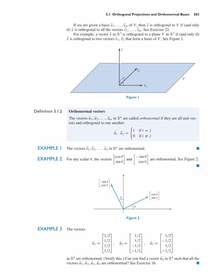
5.1 Orthogonal Projections and Orthonormal Bases 203
If we are given a basis v1, . . . , vm of V , then x is orthogonal to V if (and onlyif) x is orthogonal to all the vectors v1, . . . , vm . See Exercise 22.
For example, a vector x in R3 is orthogonal to a plane V in R3 if (and only if)x is orthogonal to two vectors v1, v2 that form a basis of V . See Figure 1.
v1
v2
x
V
Figure 1
Definition 5.1.2 Orthonormal vectors
The vectors u1, u2, . . . , um in Rn are called orthonormal if they are all unit vec-tors and orthogonal to one another:
ui · u j =
1 if i = j0 if i = j
EXAMPLE 1 The vectors e1, e2, . . . , en in Rn are orthonormal. !EXAMPLE 2 For any scalar θ , the vectors
[cos θ
sin θ
]and
[− sin θ
cos θ
]are orthonormal. See Figure 2.
!
cos−sin
cossin
Figure 2
EXAMPLE 3 The vectors
u1 =
⎡
⎢⎢⎣
1/21/21/21/2
⎤
⎥⎥⎦ , u2 =
⎡
⎢⎢⎣
1/21/2
−1/2−1/2
⎤
⎥⎥⎦ , u3 =
⎡
⎢⎢⎣
1/2−1/2
1/2−1/2
⎤
⎥⎥⎦
in R4 are orthonormal. (Verify this.) Can you find a vector u4 in R4 such that all thevectors u1, u2, u3, u4 are orthonormal? See Exercise 16. !

204 CHAPTER 5 Orthogonality and Least Squares
The following properties of orthonormal vectors are often useful:
Theorem 5.1.3 Properties of orthonormal vectors
a. Orthonormal vectors are linearly independent.b. Orthonormal vectors u1, . . . , un in Rn form a basis of Rn .
Proof a. Consider a relation
c1u1 + c2u2 + · · · + ci ui + · · · + cmum = 0
among the orthonormal vectors u1, u2, . . . , um in Rn . Let us form the dotproduct of each side of this equation with ui :
(c1u1 + c2u2 + · · · + ci ui + · · · + cmum) · ui = 0 · ui = 0.
Because the dot product is distributive (see Theorem A5 in the Appendix),
c1(u1 · ui ) + c2(u2 · ui ) + · · · + ci (ui · ui ) + · · · + cm(um · ui ) = 0.
We know that ui · ui = 1, and all other dot products u j · ui are zero.Therefore, ci = 0. Since this holds for all i = 1, . . . , m, it follows that thevectors u1, . . . , um are linearly independent.
b. This follows from part (a) and Summary 3.3.10. (Any n linearly indepen-dent vectors in Rn form a basis of Rn .) !
Orthogonal ProjectionsIn Section 2.2 we discussed the basic idea behind an orthogonal projection: If x is avector in R2 and L is a line in R2, then we can resolve the vector x into a componentx∥ parallel to L and a component x⊥ perpendicular to L ,
x = x∥ + x⊥,
and this decomposition is unique. The vector x∥ is called the orthogonal projectionof x onto L . See Figure 3.
x
O
Lx⊥ (translated)
xll = projL(x)
Figure 3
Let’s see how we can generalize this idea to any subspace V of Rn .
Theorem 5.1.4 Orthogonal projection
Consider a vector x in Rn and a subspace V of Rn . Then we can write
x = x∥ + x⊥,
where x∥ is in V and x⊥ is perpendicular to V , and this representation is unique.

5.1 Orthogonal Projections and Orthonormal Bases 205
Theorem 5.1.4 Orthogonal projection (Continued)
The vector x∥ is called the orthogonal projection of x onto V , denoted byprojV x . See Figure 4.
The transformation T (x) = projV x = x∥ from Rn to Rn is linear.
x
0V
x⊥
x∥ = projV x
Figure 4
Proof Consider an orthonormal basis u1, . . . , um of V (see Definition 5.1.2).2 If a decom-position x = x∥ + x⊥ (with x∥ in V and x⊥ orthogonal to V ) does exist, then wecan write
x∥ = c1u1 + · · · + ci ui + · · · + cmum,
for some coefficients c1, . . . , ci , . . . , cm yet to be determined (since x∥ is in V ). Weknow that
x⊥ = x − x∥ = x − c1u1 − · · · − ci ui − · · · − cmum
is orthogonal to V , meaning that x − c1u1 − · · · − ci ui − · · · − cmum is orthogonalto all the vectors ui in V :
0 = ui · (x − c1u1 − · · · − ci ui − · · · − cmum)
= ui · x − c1 (ui · u1)︸ ︷︷ ︸0
− · · · − ci (ui · ui )︸ ︷︷ ︸1
− · · · − cm (ui · um)︸ ︷︷ ︸0
= ui · x − ci
See Definition 5.1.2. It follows that ci = ui · x , so that
x∥ = (u1 · x)u1 + · · · + (ui · x)ui + · · · + (um · x)um
and
x⊥ = x − x∥ = x − (u1 · x)u1 − · · · − (ui · x)ui − · · · − (um · x)um .
Note that ui · x⊥ = 0, by construction, so that x⊥ is orthogonal to V , as required.(Recall the remarks preceding Figure 1.)
We leave the verification of the linearity of the transformation T (x) =projV x = x∥ as Exercise 24. !
2In the next section we will introduce an algorithm for constructing an orthonormal basis of anysubspace V of Rn . Here we need to convince ourselves merely that such a basis of V does indeedexist. We will present a proof by induction on m = dim(V ), for a fixed n. See Appendix B.1. Ifdim(V ) = 1, then a unit vector u in V will form an orthonormal basis of V . For the induction stepfrom m − 1 to m, consider a subspace V of Rn with dim(V ) = m, and let u be a unit vector in V .Consider the linear transformation T (x) = x · u from V to R. By the rank-nullity theorem, the kernelof T will be an (m − 1)-dimensional subspace W of V , consisting of all vectors x in V that areorthogonal to u [since T (x) = x · u = 0]. By the induction hypothesis, there exists an orthonormalbasis (u1, . . . , um−1) of W , and (u1, . . . , um−1, u) will be an orthonormal basis of V .

206 CHAPTER 5 Orthogonality and Least Squares
Theorem 5.1.5 Formula for the orthogonal projection
If V is a subspace of Rn with an orthonormal basis u1, . . . , um , then
projV x = x∥ = (u1 · x)u1 + · · · + (um · x)um .
for all x in Rn .
Note that projV x is the sum of all vectors (ui · x)ui , for i = 1, . . . , m, repre-senting the orthogonal projections of x onto the lines spanned by the basis vectorsu1, . . . , um of V . See Definition 2.2.1.
For example, projecting a vector in R3 orthogonally onto the x1–x2-planeamounts to the same as projecting it onto the x1-axis, then onto the x2-axis, andthen adding the resultant vectors. See Figure 5.
x1x2x3
x =
0x20
x1x20
x100
Figure 5
EXAMPLE 4 Consider the subspace V = im(A) of R4, where
A =
⎡
⎢⎢⎣
1 11 −11 −11 1
⎤
⎥⎥⎦ .
Find projV x , for
x =
⎡
⎢⎢⎣
1317
⎤
⎥⎥⎦ .
SolutionSince the two column vectors of A happen to be linearly independent, they form abasis of V . Since they happen to be orthogonal, we can construct an orthonormalbasis of V merely by dividing each of these two vectors by its length (2 for bothvectors):
u1 =
⎡
⎢⎢⎣
1/21/21/21/2
⎤
⎥⎥⎦ , u2 =
⎡
⎢⎢⎣
1/2−1/2−1/2
1/2
⎤
⎥⎥⎦ .

5.1 Orthogonal Projections and Orthonormal Bases 207
Then
projV x = (u1 · x)u1 + (u2 · x)u2 = 6u1 + 2u2 =
⎡
⎢⎢⎣
3333
⎤
⎥⎥⎦ +
⎡
⎢⎢⎣
1−1−1
1
⎤
⎥⎥⎦ =
⎡
⎢⎢⎣
4224
⎤
⎥⎥⎦ .
To check this answer, verify that x − projV x is perpendicular to both u1 and u2. !What happens when we apply Theorem 5.1.5 to the subspace V = Rn of Rn
with orthonormal basis u1, u2, . . . , un? Clearly, projV x = x , for all x in Rn byTheorem 5.1.4. Therefore,
x = (u1 · x)u1 + · · · + (un · x)un,
for all x in Rn .
Theorem 5.1.6 Consider an orthonormal basis u1, . . . , un of Rn . Then
x = (u1 · x)u1 + · · · + (un · x)un,
for all x in Rn .
This means that if you project x onto all the lines spanned by the basis vectorsui and add the resultant vectors, you get the vector x back. Figure 6 illustrates thisin the case n = 2.
x = (u1 · x)u1 + (u2 · x)u2
(u2 · x)u2
(u1 · x)u1u2
u1
O
Figure 6
What is the practical significance of Theorem 5.1.6? Whenever we have a basisv1, . . . , vn of Rn , any vector x in Rn can be expressed uniquely as a linear combi-nation of the vi , by Theorem 3.2.10:
x = c1v1 + c2v2 + · · · + cn vn.
To find the coordinates ci , we generally need to solve a linear system, which mayinvolve a fair amount of computation. However, if we are dealing with an orthonor-mal basis u1, . . . , un , then we can find the ci much more easily, using the formula
ci = ui · x .
EXAMPLE 5 Consider the orthogonal projection T (x) = projV x onto a subspace V of Rn . De-scribe the image and kernel of T .

208 CHAPTER 5 Orthogonality and Least Squares
SolutionBy definition of an orthogonal projection, the image of T is the subspace V , whilethe kernel of T consists of all those vectors x in Rn such that T (x) = projV x =x∥ = 0, meaning that x = x⊥. In other words, the kernel consists of those vectorsx in Rn that are orthogonal to V . This space deserves a name. !
Definition 5.1.7 Orthogonal complement
Consider a subspace V of Rn . The orthogonal complement V ⊥ of V is the set ofthose vectors x in Rn that are orthogonal to all vectors in V :
V ⊥ = x in Rn: v · x = 0, for all v in V .Note that V ⊥ is the kernel of the orthogonal projection onto V .
Take another look at Figures 3 and 4, and identify the kernel of the projectionin each case.
In Figure 7, we sketch the orthogonal complements of a line L and of a planeV in R3. Note that both L⊥ and V ⊥ are subspaces of R3. Furthermore,
dim(L) + dim(L⊥) = 1 + 2 = 3 = dim(R3),
and
dim(V ) + dim(V ⊥) = 2 + 1 = 3 = dim(R3).
We can generalize these observations.
O
L⊥
L
O
V
V⊥
Figure 7
Theorem 5.1.8 Properties of the orthogonal complement
Consider a subspace V of Rn .
a. The orthogonal complement V ⊥ of V is a subspace of Rn .b. The intersection of V and V ⊥ consists of the zero vector: V ∩ V ⊥ = 0.c. dim(V ) + dim(V ⊥) = n.
d. (V ⊥)⊥ = V .
Proof a. If T (x) = projV x , then V ⊥ = ker(T ), a subspace of Rn .b. If a vector x is in V as well as in V ⊥, then x is orthogonal to itself: x · x =
∥x∥2 = 0, so that x must equal 0, as claimed.

5.1 Orthogonal Projections and Orthonormal Bases 209
c. We can apply the rank-nullity theorem to the linear transformationT (x) = projV x :
n = dim(imT ) + dim(ker T ) = dim(V ) + dim(V ⊥).
d. We leave this proof as Exercise 23. !From Pythagoras to Cauchy
EXAMPLE 6 Consider a line L in R3 and a vector x in R3. What can you say about the relation-ship between the lengths of the vectors x and projL x?
SolutionApplying the Pythagorean theorem to the shaded right triangle in Figure 8, we findthat ∥projL x∥ ≤ ∥x∥. The statement is an equality if (and only if) x is on L . !
projLx L
x
O
Figure 8
translated y
x
x + y
O
Figure 9
Does this inequality hold in higher-dimensional cases? We have to examinewhether the Pythagorean theorem holds in Rn .
Theorem 5.1.9 Pythagorean theorem
Consider two vectors x and y in Rn . The equation
∥x + y∥2 = ∥x∥2 + ∥y∥2
holds if (and only if) x and y are orthogonal. See Figure 9.
Proof The verification is straightforward:
∥x + y∥2 = (x + y) · (x + y) = x · x + 2(x · y) + y · y = ∥x∥2 + 2(x · y) + ∥y∥2
= ∥x∥2 + ∥y∥2 if (and only if) x · y = 0. !Now we can generalize Example 6.
Theorem 5.1.10 An inequality for the magnitude of projV (x)
Consider a subspace V of Rn and a vector x in Rn . Then
∥projV x∥ ≤ ∥x∥.The statement is an equality if (and only if) x is in V .
Proof We apply the Pythagorean theorem (see Figure 10):
∥x∥2 = ∥projV x∥2 + ∥x⊥∥2.
It follows that ∥projV x∥ ≤ ∥x∥, as claimed. !

210 CHAPTER 5 Orthogonality and Least Squares
x⊥ (translated)
projV(x) = xll
x
O
Figure 10
For example, let V be a one-dimensional subspace of Rn spanned by a(nonzero) vector y. We introduce the unit vector
u = 1∥y∥
y
in V . See Figure 11.
O
x
u
y
V
Figure 11
We know that
projV x = (x · u)u,
for any x in Rn . Theorem 5.1.10 tells us that
∥x∥ ≥ ∥projV x∥ = ∥(x · u)u∥step 3︷︸︸︷= |x · u| =
∣∣∣∣x ·(
1∥y∥
y)∣∣∣∣ = 1
∥y∥|x · y|.
To justify step 3, note that ∥kv∥ = |k|∥v∥, for all vectors v in Rn and all scalars k.See Exercise 25a. We conclude that
|x · y|∥y∥
≤ ∥x∥.
Multiplying both sides of this inequality by ∥y∥, we find the following useful result:
Theorem 5.1.11 Cauchy–Schwarz inequality3
If x and y are vectors in Rn , then
|x · y| ≤ ∥x∥∥y∥.This statement is an equality if (and only if) x and y are parallel.
3Named after the French mathematician Augustin-Louis Cauchy (1789–1857) and the Germanmathematician Hermann Amandus Schwarz (1843–1921).

5.1 Orthogonal Projections and Orthonormal Bases 211
Consider two nonzero vectors x and y in R3. You may know an expression forthe dot product x · y in terms of the angle θ between the two vectors (see Figure 12):
x · y = ∥x∥∥y∥ cos θ .
x
y
Figure 12
This formula allows us to find the angle between two nonzero vectors x and yin R3:
cos θ = x · y∥x∥∥y∥
or θ = arccosx · y
∥x∥∥y∥.
In Rn , where we have no intuitive notion of an angle between two vectors, we canuse this formula to define the angle:
Definition 5.1.12 Angle between two vectors
Consider two nonzero vectors x and y in Rn . The angle θ between these vectorsis defined as
θ = arccosx · y
∥x∥∥y∥.
Note that θ is between 0 and π , by definition of the inverse cosine function.
We have to make sure that
arccosx · y
∥x∥∥y∥is defined; that is,
x · y∥x∥∥y∥
is between −1 and 1, or, equivalently,∣∣∣∣
x · y∥x∥∥y∥
∣∣∣∣ = |x · y|∥x∥∥y∥
≤ 1.
But this follows from the Cauchy–Schwarz inequality, |x · y| ≤ ∥x∥∥y∥.
EXAMPLE 7 Find the angle between the vectors
x =
⎡
⎢⎢⎣
1000
⎤
⎥⎥⎦ and y =
⎡
⎢⎢⎣
1111
⎤
⎥⎥⎦ .
Solution
θ = arccosx · y
∥x∥∥y∥= arccos
11 · 2
= π
3 !Here is an application to statistics of some concepts introduced in this section.

212 CHAPTER 5 Orthogonality and Least Squares
Correlation (Optional)Consider the meat consumption (in grams per day per person) and incidence ofcolon cancer (per 100,000 women per year) in various industrialized countries.
Country Meat Consumption Cancer Rate
Japan 26 7.5Finland 101 9.8Israel 124 16.4Great Britain 205 23.3United States 284 34.0
Mean 148 18.2
Can we detect a positive or negative correlation4 between meat consumptionand cancer rate? Does a country with high meat consumption have high cancer rates,and vice versa? By high, we mean “above average,” of course. A quick look at thedata shows such a positive correlation: In Great Britain and the United States, bothmeat consumption and cancer rate are above average. In the three other countries,they are below average. This positive correlation becomes more apparent when welist the preceding data as deviations from the mean (above or below the average).
Meat Consumption Cancer RateCountry (Deviation from Mean) (Deviation from Mean)
Japan −122 −10.7Finland −47 −8.4Israel −24 −1.8Great Britain 57 5.1United States 136 15.8
Perhaps even more informative is a scatter plot of the deviation data. SeeFigure 13.
Japan
Finland
Israel
Great Britain
United States
100−100
−10
10
Cancer rate(deviationfrom mean)
Meat consumption(deviation from mean)
Figure 13
4We are using the term “correlation” in a colloquial, qualitative sense. Our goal is to quantify thisterm.
Dan Burns

5.1 Orthogonal Projections and Orthonormal Bases 213
A positive correlation is indicated when most of the data points (in our case, allof them) are located in the first and third quadrant.
To process these data numerically, it is convenient to represent the deviation forboth characteristics (meat consumption and cancer rate) as vectors in R5:
x =
⎡
⎢⎢⎢⎢⎣
−122−47−24
57136
⎤
⎥⎥⎥⎥⎦, y =
⎡
⎢⎢⎢⎢⎣
−10.7−8.4−1.8
5.115.8
⎤
⎥⎥⎥⎥⎦.
We will call these two vectors the deviation vectors of the two characteristics.In the case of a positive correlation, most of the corresponding entries xi , yi
of the deviation vectors have the same sign (both positive or both negative). In ourexample, this is the case for all entries. This means that the product xi yi will bepositive most of the time; hence, the sum of all these products will be positive. Butthis sum is simply the dot product of the two deviation vectors.
Still using the term “correlation” in a colloquial sense, we conclude thefollowing:
Consider two characteristics of a population, with deviation vectors x and y.There is a positive correlation between the two characteristics if (and only if)x · y > 0.
A positive correlation between the characteristics means that the angle θ be-tween the deviation vectors is less than 90. See Figure 14.
Acute angle Right angle Obtuse angle
(a) (b) (c)
x
y
x
y
x
y
Figure 14 (a) Positive correlation: x · y > 0. (b) No correlation: x · y = 0. (c) Negativecorrelation: x · y < 0.
We can use the cosine of the angle θ between x and y as a quantitative measurefor the correlation between the two characteristics.
Definition 5.1.13 Correlation coefficient
The correlation coefficient r between two characteristics of a population is thecosine of the angle θ between the deviation vectors x and y for the two charac-teristics:
r = cos(θ) = x · y∥x∥∥y∥
.

214 CHAPTER 5 Orthogonality and Least Squares
In the case of meat consumption and cancer, we find that
r ≈ 4182.9198.53 · 21.539
≈ 0.9782.
The angle between the two deviation vectors is arccos(r) ≈ 0.21 (radians) ≈12.
Note that the length of the deviation vectors is irrelevant for the correlation: Ifwe had measured the cancer rate per 1,000,000 women (instead of 100,000), thevector y would be 10 times longer, but the correlation would be the same.
The correlation coefficient r is always between −1 and 1; the cases when r = 1(representing a perfect positive correlation) and r = −1 (perfect negative correla-tion) are of particular interest. See Figure 15. In both cases, the data points (xi , yi )will be on the straight line y = mx . See Figure 16.
r = 1 r = −1
(a) (b)
x xy y
Figure 15 (a) y = mx , for positive m. (b) y = mx , for negative m.
y
x
yi = mxir = 1y
x
yi = mxi
r = −1
Figure 16
Note that even a strong positive correlation (an r close to 1) does not necessar-ily imply a causal relationship. Based only on the work we did above, we cannotconclude that high meat consumption causes colon cancer. Take a statistics courseto learn more about these important issues!
EXERCISES 5.1GOAL Apply the basic concepts of geometry in Rn:length, angles, orthogonality. Use the idea of an orthog-onal projection onto a subspace. Find this projection if anorthonormal basis of the subspace is given.
Find the length of each of the vectors v in Exercises 1through 3.
1. v =[
711
]2. v =
⎡
⎣234
⎤
⎦ 3. v =
⎡
⎢⎢⎣
2345
⎤
⎥⎥⎦

5.1 Orthogonal Projections and Orthonormal Bases 215
Find the angle θ between each of the pairs of vectors u andv in Exercises 4 through 6.
4. u =[
11
], v =
[7
11
]5. u =
⎡
⎣123
⎤
⎦, v =
⎡
⎣234
⎤
⎦
6. u =
⎡
⎢⎢⎣
1−1
2−2
⎤
⎥⎥⎦, v =
⎡
⎢⎢⎣
2345
⎤
⎥⎥⎦
For each pair of vectors u, v listed in Exercises 7 through9, determine whether the angle θ between u and v is acute,obtuse, or right.
7. u =[
2−3
], v =
[54
]8. u =
⎡
⎣234
⎤
⎦, v =
⎡
⎣2
−85
⎤
⎦
9. u =
⎡
⎢⎢⎣
1−1
1−1
⎤
⎥⎥⎦, v =
⎡
⎢⎢⎣
3453
⎤
⎥⎥⎦
10. For which value(s) of the constant k are the vectors
u =
⎡
⎣234
⎤
⎦ and v =
⎡
⎣1k1
⎤
⎦
perpendicular?
11. Consider the vectors
u =
⎡
⎢⎢⎢⎣
11...
1
⎤
⎥⎥⎥⎦and v =
⎡
⎢⎢⎢⎣
10...
0
⎤
⎥⎥⎥⎦in Rn .
a. For n = 2, 3, 4, find the angle θ between u and v.For n = 2 and 3, represent the vectors graphically.
b. Find the limit of θ as n approaches infinity.
12. Give an algebraic proof for the triangle inequality
∥v + w∥ ≤ ∥v∥ + ∥w∥.
Draw a sketch. Hint: Expand ∥v+ w∥2 = (v+ w) · (v+w). Then use the Cauchy–Schwarz inequality.
13. Leg traction. The accompanying figure shows how a legmay be stretched by a pulley line for therapeutic pur-poses. We denote by F1 the vertical force of the weight.The string of the pulley line has the same tension ev-erywhere; hence, the forces F2 and F3 have the samemagnitude as F1. Assume that the magnitude of eachforce is 10 pounds. Find the angle θ so that the magni-tude of the force exerted on the leg is 16 pounds. Roundyour answer to the nearest degree. (Adapted from E.Batschelet, Introduction to Mathematics for Life Scien-tists, Springer, 1979.)
F3
F2
F1
14. Leonardo da Vinci and the resolution of forces.Leonardo (1452–1519) asked himself how the weightof a body, supported by two strings of different length,is apportioned between the two strings.
longer string shorter string
weight
D
AEB
Three forces are acting at the point D: the tensions F1and F2 in the strings and the weight W . Leonardo be-lieved that
∥F1∥∥F2∥
= E A
E B.
AEB
W
F2F1
D
Was he right? (Source: Les Manuscrits de Leonard deVinci, published by Ravaisson-Mollien, Paris, 1890.)Hint: Resolve F1 into a horizontal and a vertical com-ponent; do the same for F2. Since the system is at rest,the equation F1 + F2 +W = 0 holds. Express the ratios
∥F1∥∥F2∥
andE A
E B
in terms of α and β, using trigonometric functions, andcompare the results.

216 CHAPTER 5 Orthogonality and Least Squares
15. Consider the vector
v =
⎡
⎢⎢⎣
1234
⎤
⎥⎥⎦ in R4.
Find a basis of the subspace of R4 consisting of all vec-tors perpendicular to v.
16. Consider the vectors
u1 =
⎡
⎢⎢⎣
1/21/21/21/2
⎤
⎥⎥⎦ , u2 =
⎡
⎢⎢⎣
1/21/2
−1/2−1/2
⎤
⎥⎥⎦ , u3 =
⎡
⎢⎢⎣
1/2−1/2
1/2−1/2
⎤
⎥⎥⎦
in R4. Can you find a vector u4 in R4 such that the vec-tors u1, u2, u3, u4 are orthonormal? If so, how manysuch vectors are there?
17. Find a basis for W⊥, where
W = span
⎛
⎜⎜⎝
⎡
⎢⎢⎣
1234
⎤
⎥⎥⎦ ,
⎡
⎢⎢⎣
5678
⎤
⎥⎥⎦
⎞
⎟⎟⎠ .
18. Here is an infinite-dimensional version of Euclideanspace: In the space of all infinite sequences, consider thesubspace ℓ2 of square-summable sequences [i.e., thosesequences (x1, x2, . . .) for which the infinite series x2
1 +x2
2 + · · · converges]. For x and y in ℓ2, we define
∥x∥ =√
x21 + x2
2 + · · ·, x · y = x1 y1 + x2 y2 + · · · .
(Why does the series x1 y1 + x2 y2 + · · · converge?)a. Check that x = (1, 1
2 , 14 , 1
8 , 116 , . . .) is in ℓ2, and
find ∥x∥. Recall the formula for the geometric series:1 + a + a2 + a3 + · · · = 1/(1 − a), if −1 < a < 1.
b. Find the angle between (1, 0, 0, . . .) and(1, 1
2 , 14 , 1
8 , . . .).c. Give an example of a sequence (x1, x2, . . .) that
converges to 0 (i.e., limn→∞
xn = 0) but does notbelong to ℓ2.
d. Let L be the subspace of ℓ2 spanned by(1, 1
2 , 14 , 1
8 , . . .). Find the orthogonal projection of(1, 0, 0, . . .) onto L .
The Hilbert space ℓ2 was initially used mostly inphysics: Werner Heisenberg’s formulation of quantummechanics is in terms of ℓ2. Today, this space is used inmany other applications, including economics. See, forexample, the work of the economist Andreu Mas-Colellof the University of Barcelona.
19. For a line L in R2, draw a sketch to interpret the fol-lowing transformations geometrically:a. T (x) = x − projL xb. T (x) = x − 2projL xc. T (x) = 2projL x − x
20. Refer to Figure 13 of this section. The least-squaresline for these data is the line y = mx that fits the databest, in that the sum of the squares of the vertical dis-tances between the line and the data points is minimal.We want to minimize the sum
(mx1 − y1)2 + (mx2 − y2)
2 + · · · + (mx5 − y5)2.
y = mx(xi, mxi)
mxi
yi
(xi, yi)
xi
mxi − yi
In vector notation, to minimize the sum means to findthe scalar m such that
∥mx − y∥2
is minimal. Arguing geometrically, explain how youcan find m. Use the accompanying sketch, which is notdrawn to scale.
x
y
Find m numerically, and explain the relationship be-tween m and the correlation coefficient r . You may findthe following information helpful:
x · y = 4182.9, ∥x∥ ≈ 198.53, ∥y∥ ≈ 21.539.
To check whether your solution m is reasonable, drawthe line y = mx in Figure 13. (A more thorough dis-cussion of least-squares approximations will follow inSection 5.4.)
21. Find scalars a, b, c, d , e, f , g such that the vectors⎡
⎣adf
⎤
⎦ ,
⎡
⎣b1g
⎤
⎦ ,
⎡
⎣ce
1/2
⎤
⎦
are orthonormal.
22. Consider a basis v1, v2, . . . , vm of a subspace V of Rn .Show that a vector x in Rn is orthogonal to V if (andonly if) x is orthogonal to all the vectors v1, . . . , vm .
23. Prove Theorem 5.1.8d. (V ⊥)⊥ = V for any subspaceV of Rn . Hint: Show that V ⊆ (V ⊥)⊥, by the defini-tion of V ⊥; then show that dim(V ) = dim(V ⊥)⊥, byTheorem 5.1.8c.
24. Complete the proof of Theorem 5.1.4: Orthogonal pro-jections are linear transformations.

5.1 Orthogonal Projections and Orthonormal Bases 217
25. a. Consider a vector v in Rn , and a scalar k. Show that
∥kv∥ = |k|∥v∥.
b. Show that if v is a nonzero vector in Rn , then
u = 1∥v∥
v is a unit vector.
26. Find the orthogonal projection of
⎡
⎣494949
⎤
⎦ onto the sub-
space of R3 spanned by⎡
⎣236
⎤
⎦ and
⎡
⎣3
−62
⎤
⎦ .
27. Find the orthogonal projection of 9e1 onto the subspaceof R4 spanned by
⎡
⎢⎢⎣
2210
⎤
⎥⎥⎦ and
⎡
⎢⎢⎣
−2201
⎤
⎥⎥⎦ .
28. Find the orthogonal projection of⎡
⎢⎢⎣
1000
⎤
⎥⎥⎦
onto the subspace of R4 spanned by⎡
⎢⎢⎣
1111
⎤
⎥⎥⎦ ,
⎡
⎢⎢⎣
11
−1−1
⎤
⎥⎥⎦ ,
⎡
⎢⎢⎣
1−1−1
1
⎤
⎥⎥⎦ .
29. Consider the orthonormal vectors u1, u2, u3, u4, u5 inR10. Find the length of the vector
x = 7u1 − 3u2 + 2u3 + u4 − u5.
30. Consider a subspace V of Rn and a vector x in Rn .Let y = projV x . What is the relationship between thefollowing quantities?
∥y∥2 and y · x
31. Consider the orthonormal vectors u1, u2, . . . , um in Rn ,and an arbitrary vector x in Rn . What is the relationshipbetween the following two quantities?
p = (u1 · x)2 + (u2 · x)2 +· · ·+ (um · x)2 and ∥x∥2
When are the two quantities equal?
32. Consider two vectors v1 and v2 in Rn . Form the matrix
G =[v1 · v1 v1 · v2v2 · v1 v2 · v2
].
For which choices of v1 and v2 is the matrix G invert-ible?
33. Among all the vectors in Rn whose components addup to 1, find the vector of minimal length. In the casen = 2, explain your solution geometrically.
34. Among all the unit vectors in Rn , find the one for whichthe sum of the components is maximal. In the casen = 2, explain your answer geometrically, in termsof the unit circle and the level curves of the functionx1 + x2.
35. Among all the unit vectors u =
⎡
⎣xyz
⎤
⎦ in R3, find the
one for which the sum x + 2y + 3z is minimal.
36. There are three exams in your linear algebra class, andyou theorize that your score in each exam (out of 100)will be numerically equal to the number of hours youstudy for that exam. The three exams count 20%, 30%,and 50%, respectively, toward the final grade. If your(modest) goal is to score 76% in the course, how manyhours a, b, and c should you study for each of the threeexams to minimize quantity a2+b2+c2? This quadraticmodel reflects the fact that it may be four times aspainful to study for 10 hours than for just 5 hours.
37. Consider a plane V in R3 with orthonormal basisu1, u2. Let x be a vector in R3. Find a formula forthe reflection R(x) of x about the plane V .
38. Consider three unit vectors v1, v2, and v3 in Rn . We aretold that v1 · v2 = v1 · v3 = 1/2. What are the possiblevalues of v2 · v3? What could the angle between thevectors v2 and v3 be? Give examples; draw sketches forthe cases n = 2 and n = 3.
39. Can you find a line L in Rn and a vector x in Rn suchthat
x · projL x
is negative? Explain, arguing algebraically.
In Exercises 40 through 46, consider vectors v1, v2, v3 inR4; we are told that vi · v j is the entry ai j of matrix A.
A =
⎡
⎣3 5 115 9 20
11 20 49
⎤
⎦
40. Find ∥v2∥.
41. Find the angle enclosed by vectors v2 and v3.
42. Find ∥v1 + v2∥.
43. Find projv2(v1), expressed as a scalar multiple of v2.
44. Find a nonzero vector v in span(v2, v3) such that v isorthogonal to v3. Express v as a linear combination ofv2 and v3.
45. Find projV (v1), where V = span(v2, v3). Express youranswer as a linear combination of v2 and v3.
46. Find projV (v3), where V = span(v1, v2). Express youranswer as a linear combination of v1 and v2.

218 CHAPTER 5 Orthogonality and Least Squares
5.2 Gram–Schmidt Process and QR Factorization
One of the main themes of this chapter is the study of the orthogonal projectiononto a subspace V of Rn . In Theorem 5.1.5, we gave a formula for this projection,
projV x = (u1 · x)u1 + · · · + (um · x)um,
where u1, . . . , um is an orthonormal basis of V . Now we will show how to constructsuch an orthonormal basis. We will present an algorithm that allows us to convertany basis v1, . . . , vm of a subspace V of Rn into an orthonormal basis u1, . . . , umof V .
Let us first think about low-dimensional cases. If V is a line with basis v1, wecan find an orthonormal basis u1 simply by dividing v1 by its length:
u1 = 1∥v1∥
v1.
When V is a plane with basis v1, v2, we first construct
u1 = 1∥v1∥
v1
as before. See Figure 1.
VV
v2
v1O
v2
Ou1 = v1
1∥v1∥
Figure 1
Now comes the crucial step: We have to find a vector in V orthogonal to u1.(Initially, we will not insist that this vector be a unit vector.) Let’s resolve the vectorv2 into its components parallel and perpendicular to the line L spanned by u1:
v2 = v∥2 + v2
⊥
See Figure 2. Then the vector
v2⊥ = v2 − v
∥2 = v2 − projL(v2) = v2 − (u1 · v2)u1
is orthogonal to u1.
VV
v2
v2ll
v2⊥
v2⊥ = v2 − (u1 · v2)u1
u1 u1O L O
Figure 2

5.2 Gram–Schmidt Process and QR Factorization 219
The last step is straightforward: We divide the vector v2⊥ by its length to get
the second vector u2 of an orthonormal basis (see Figure 3):
u2 = 1
∥v2⊥∥
v2⊥.
VV
O u1O u1
u2 = v2⊥1
∥v2⊥∥
v2⊥
Figure 3
EXAMPLE 1 a. Find an orthonormal basis u1, u2 of the subspace
V = span
⎛
⎜⎜⎝
⎡
⎢⎢⎣
1111
⎤
⎥⎥⎦ ,
⎡
⎢⎢⎣
1991
⎤
⎥⎥⎦
⎞
⎟⎟⎠ of R4, with basis v1 =
⎡
⎢⎢⎣
1111
⎤
⎥⎥⎦, v2 =
⎡
⎢⎢⎣
1991
⎤
⎥⎥⎦.
b. Find the change of basis matrix R from the basis ! = (v1, v2) to the basis" = (u1, u2) you constructed in part a.
Solution
a. Following the three steps illustrated in Figures 1, 2, and 3, we will computefirst u1, then v2
⊥, and finally u2:
u1 = 1∥v1∥
v1 = 12
⎡
⎢⎢⎣
1111
⎤
⎥⎥⎦ =
⎡
⎢⎢⎣
1/21/21/21/2
⎤
⎥⎥⎦ ,
v2⊥ = v2 − v
∥2 = v2 − (u1 · v2)u1 =
⎡
⎢⎢⎣
1991
⎤
⎥⎥⎦ − 10
⎡
⎢⎢⎣
1/21/21/21/2
⎤
⎥⎥⎦ =
⎡
⎢⎢⎣
−444
−4
⎤
⎥⎥⎦ ,
u2 = 1
∥v2⊥∥
v2⊥ = 1
8
⎡
⎢⎢⎣
−444
−4
⎤
⎥⎥⎦ =
⎡
⎢⎢⎣
−1/21/21/2
−1/2
⎤
⎥⎥⎦ .
We have found an orthonormal basis " of V :
u1 =
⎡
⎢⎢⎣
1/21/21/21/2
⎤
⎥⎥⎦ , u2 =
⎡
⎢⎢⎣
−1/21/21/2
−1/2
⎤
⎥⎥⎦ .

220 CHAPTER 5 Orthogonality and Least Squares
b. Recall that the columns of the change of basis matrix R from ! to " arethe coordinate vectors of v1 and v2 with respect to basis " = (u1, u2). SeeDefinition 4.3.3.
A straightforward computation shows that v1 = 2u1 and v2 = 10u1 +8u2, so that
R =[ v1 v2
2 100 8
]u1
u2.
(Later in this section, we will develop more efficient methods for finding theentries of R.)
To express the relationship between the bases " and ! in matrix form,we can use Theorem 4.3.4 and write
[v1 v2
]=
[u1 u2
]R, or
⎡
⎢⎢⎣
1 11 91 91 1
⎤
⎥⎥⎦
︸ ︷︷ ︸M
=
⎡
⎢⎢⎣
1/2 −1/21/2 1/21/2 1/21/2 −1/2
⎤
⎥⎥⎦
︸ ︷︷ ︸Q
[2 100 8
]
︸ ︷︷ ︸R
.
In this context, it is customary to denote the matrices on the right-hand sideby Q and R. Note that we have written the 4 × 2 matrix M with columns v1and v2 as the product of the 4 × 2 matrix Q with orthonormal columns andthe upper triangular 2 × 2 matrix R with positive entries on the diagonal.This is referred to as the QR factorization of matrix M . Matrix Q stores theorthonormal basis u1, u2 we constructed, and matrix R gives the relationshipbetween the “old” basis v1, v2, and the “new” basis u1, u2 of V . !
Now that we know how to find an orthonormal basis of a plane, how wouldwe proceed in the case of a three-dimensional subspace V of Rn with basis v1, v2,v3? We can first find an orthonormal basis u1, u2 of the plane E = span(v1, v2), asillustrated in Example 1. Next we resolve the vector v3 into its components paralleland perpendicular to the plane E :
v3 = v∥3 + v3
⊥,
so that
v3⊥ = v3 − v
∥3 = v3 − projE(v3) = v3 − (u1 · v3)u1 − (u2 · v3)u2.
Finally, we let
u3 = 1
∥v3⊥∥
v3⊥.
See Figure 4.
v3
u1
u2
E
u1
u2
E
u1
u2
E
v3⊥
u3 = v3⊥1
∥v3⊥∥
Figure 4
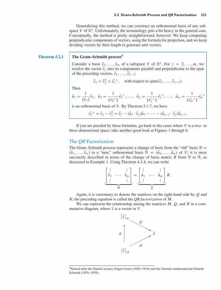
5.2 Gram–Schmidt Process and QR Factorization 221
Generalizing this method, we can construct an orthonormal basis of any sub-space V of Rn . Unfortunately, the terminology gets a bit heavy in the general case.Conceptually, the method is pretty straightforward, however: We keep computingperpendicular components of vectors, using the formula for projection, and we keepdividing vectors by their length to generate unit vectors.
Theorem 5.2.1 The Gram–Schmidt process5
Consider a basis v1, . . . , vm of a subspace V of Rn . For j = 2, . . . , m, weresolve the vector v j into its components parallel and perpendicular to the spanof the preceding vectors, v1, . . . , v j−1:
v j = v∥j + v j
⊥, with respect to span(v1, . . . , v j−1).
Then
u1 = 1∥v1∥
v1, u2 = 1
∥v2⊥∥
v2⊥, . . . , u j = 1
∥v j⊥∥
v j⊥, . . . , um = 1
∥vm⊥∥
vm⊥
is an orthonormal basis of V . By Theorem 5.1.7, we have
v j⊥ = v j − v
∥j = v j − (u1 · v j )u1 − · · · − (u j−1 · v j )u j−1.
If you are puzzled by these formulas, go back to the cases where V is a two- orthree-dimensional space; take another good look at Figures 1 through 4.
The QR FactorizationThe Gram–Schmidt process represents a change of basis from the “old” basis ! =(v1, . . . , vm) to a “new,” orthonormal basis " = (u1, . . . , um) of V ; it is mostsuccinctly described in terms of the change of basis matrix R from ! to ", asdiscussed in Example 1. Using Theorem 4.3.4, we can write
⎡
⎣| |v1 · · · vm
| |
⎤
⎦
︸ ︷︷ ︸M
=
⎡
⎣| |
u1 · · · um
| |
⎤
⎦
︸ ︷︷ ︸Q
R.
Again, it is customary to denote the matrices on the right-hand side by Q andR; the preceding equation is called the QR factorization of M .
We can represent the relationship among the matrices M , Q, and R in a com-mutative diagram, where x is a vector in V .
[x]
"
Q
↑|
R |||
x
M[x]
!
5Named after the Danish actuary Jorgen Gram (1850–1916) and the German mathematician ErhardtSchmidt (1876–1959).

222 CHAPTER 5 Orthogonality and Least Squares
What do the entries of the change of basis matrix R look like? We know that theentries in the j th column of R are the coordinates of v j with respect to the basis" = (u1, . . . , um). Using the equations in Theorem 5.2.1, we can write
v j = v∥j + v j
⊥
=r1 j︷ ︸︸ ︷
(u1 · v j ) u1 + · · · +ri j︷ ︸︸ ︷
(ui · v j ) ui + · · · +r j−1, j︷ ︸︸ ︷
(u j−1 · v j ) u j−1︸ ︷︷ ︸v
∥j
+
r j j︷ ︸︸ ︷∥∥∥v j⊥∥∥∥ u j
︸ ︷︷ ︸v j
⊥
.
It follows that ri j = ui · v j if i < j ; r j j =∥∥∥v j
⊥∥∥∥; and ri j = 0 if i > j . The last
equation implies that R is upper triangular. (The first diagonal entry is r11 = ∥v1∥,since v1 = ∥v1∥u1.)
Theorem 5.2.2 QR factorization
Consider an n × m matrix M with linearly independent columns v1, . . . , vm .Then there exists an n×m matrix Q whose columns u1, . . . , um are orthonormaland an upper triangular matrix R with positive diagonal entries such that
M = Q R.
This representation is unique. Furthermore, r11 = ∥v1∥, r j j =∥∥∥v j
⊥∥∥∥ (for j =
2, . . . , m), and ri j = ui · v j (for i < j).
Take another look at Example 1, where L = V1 = span(v1).The verification of the uniqueness of the Q R factorization is left as Exer-
cise 5.3.51. To find the Q R factorization of a matrix M , we perform the Gram–Schmidt process on the columns of M , constructing R and Q column by column.No extra computations are required: All the information necessary to build R and Qis provided by the Gram–Schmidt process. Q R factorization is an effective way toorganize and record the work performed in the Gram–Schmidt process; it is usefulfor many computational and theoretical purposes.
EXAMPLE 2 Find the Q R factorization of the matrix M =
⎡
⎣2 21 7
−2 −8
⎤
⎦.
SolutionHere
v1 =
⎡
⎣21
−2
⎤
⎦ , and v2 =
⎡
⎣27
−8
⎤
⎦ .
As in Example 1, the Q R factorization of M will have the form
M =[
v1 v2
]=
[u1 u2
]
︸ ︷︷ ︸Q
[∥v1∥ u1 · v2
0∥∥v2
⊥∥∥
]
︸ ︷︷ ︸R
.
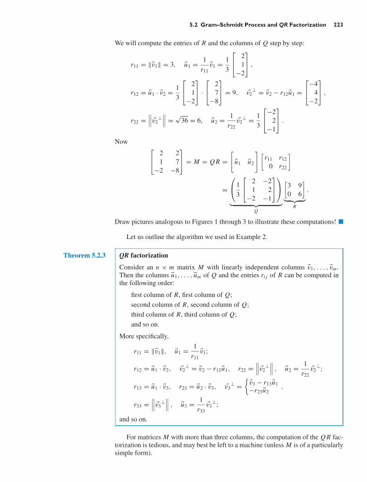
5.2 Gram–Schmidt Process and QR Factorization 223
We will compute the entries of R and the columns of Q step by step:
r11 = ∥v1∥ = 3, u1 = 1r11
v1 = 13
⎡
⎣21
−2
⎤
⎦ ,
r12 = u1 · v2 = 13
⎡
⎣21
−2
⎤
⎦ ·
⎡
⎣27
−8
⎤
⎦ = 9, v2⊥ = v2 − r12u1 =
⎡
⎣−4
4−2
⎤
⎦ ,
r22 =∥∥∥v2
⊥∥∥∥ =
√36 = 6, u2 = 1
r22v2
⊥ = 13
⎡
⎣−2
2−1
⎤
⎦ .
Now⎡
⎣2 21 7
−2 −8
⎤
⎦ = M = Q R =[
u1 u2
] [r11 r12
0 r22
]
=
⎛
⎝13
⎡
⎣2 −21 2
−2 −1
⎤
⎦
⎞
⎠
︸ ︷︷ ︸Q
[3 90 6
]
︸ ︷︷ ︸R
.
Draw pictures analogous to Figures 1 through 3 to illustrate these computations! !Let us outline the algorithm we used in Example 2.
Theorem 5.2.3 QR factorization
Consider an n × m matrix M with linearly independent columns v1, . . . , vm .Then the columns u1, . . . , um of Q and the entries ri j of R can be computed inthe following order:
first column of R, first column of Q;second column of R, second column of Q;third column of R, third column of Q;and so on.
More specifically,
r11 = ∥v1∥, u1 = 1r11
v1;
r12 = u1 · v2, v2⊥ = v2 − r12u1, r22 =
∥∥∥v2⊥∥∥∥ , u2 = 1
r22v2
⊥;
r13 = u1 · v3, r23 = u2 · v3, v3⊥ =
v3 − r13u1−r23u2
,
r33 =∥∥∥v3
⊥∥∥∥ , u3 = 1
r33v3
⊥;
and so on.
For matrices M with more than three columns, the computation of the Q R fac-torization is tedious, and may best be left to a machine (unless M is of a particularlysimple form).

224 CHAPTER 5 Orthogonality and Least Squares
EXERCISES 5.2GOAL Perform the Gram–Schmidt process, and thusfind the Q R factorization of a matrix.
Using paper and pencil, perform the Gram–Schmidt pro-cess on the sequences of vectors given in Exercises 1through 14.
1.
⎡
⎣21
−2
⎤
⎦ 2.
⎡
⎣632
⎤
⎦,
⎡
⎣2
−63
⎤
⎦
3.
⎡
⎣403
⎤
⎦,
⎡
⎣25
0−25
⎤
⎦ 4.
⎡
⎣403
⎤
⎦,
⎡
⎣25
0−25
⎤
⎦,
⎡
⎣0
−20
⎤
⎦
5.
⎡
⎣221
⎤
⎦,
⎡
⎣115
⎤
⎦ 6.
⎡
⎣200
⎤
⎦,
⎡
⎣340
⎤
⎦,
⎡
⎣567
⎤
⎦
7.
⎡
⎣221
⎤
⎦,
⎡
⎣−2
12
⎤
⎦,
⎡
⎣18
00
⎤
⎦ 8.
⎡
⎢⎢⎣
5422
⎤
⎥⎥⎦,
⎡
⎢⎢⎣
367
−2
⎤
⎥⎥⎦
9.
⎡
⎢⎢⎣
1111
⎤
⎥⎥⎦,
⎡
⎢⎢⎣
19
−53
⎤
⎥⎥⎦ 10.
⎡
⎢⎢⎣
1111
⎤
⎥⎥⎦,
⎡
⎢⎢⎣
6464
⎤
⎥⎥⎦
11.
⎡
⎢⎢⎣
4003
⎤
⎥⎥⎦,
⎡
⎢⎢⎣
52
1410
⎤
⎥⎥⎦ 12.
⎡
⎢⎢⎣
2306
⎤
⎥⎥⎦,
⎡
⎢⎢⎣
442
13
⎤
⎥⎥⎦
13.
⎡
⎢⎢⎣
1111
⎤
⎥⎥⎦,
⎡
⎢⎢⎣
1001
⎤
⎥⎥⎦,
⎡
⎢⎢⎣
021
−1
⎤
⎥⎥⎦ 14.
⎡
⎢⎢⎣
1717
⎤
⎥⎥⎦,
⎡
⎢⎢⎣
0727
⎤
⎥⎥⎦,
⎡
⎢⎢⎣
1816
⎤
⎥⎥⎦
Using paper and pencil, find the Q R factorizations of thematrices in Exercises 15 through 28. Compare with Exer-cises 1 through 14.
15.
⎡
⎣21
−2
⎤
⎦ 16.
⎡
⎣6 23 −62 3
⎤
⎦
17.
⎡
⎣4 250 03 −25
⎤
⎦ 18.
⎡
⎣4 25 00 0 −23 −25 0
⎤
⎦
19.
⎡
⎣2 12 11 5
⎤
⎦ 20.
⎡
⎣2 3 50 4 60 0 7
⎤
⎦
21.
⎡
⎣2 −2 182 1 01 2 0
⎤
⎦ 22.
⎡
⎢⎢⎣
5 34 62 72 −2
⎤
⎥⎥⎦
23.
⎡
⎢⎢⎣
1 11 91 −51 3
⎤
⎥⎥⎦ 24.
⎡
⎢⎢⎣
1 61 41 61 4
⎤
⎥⎥⎦
25.
⎡
⎢⎢⎣
4 50 20 143 10
⎤
⎥⎥⎦ 26.
⎡
⎢⎢⎣
2 43 40 26 13
⎤
⎥⎥⎦
27.
⎡
⎢⎢⎣
1 1 01 0 21 0 11 1 −1
⎤
⎥⎥⎦ 28.
⎡
⎢⎢⎣
1 0 17 7 81 2 17 7 6
⎤
⎥⎥⎦
29. Perform the Gram–Schmidt process on the followingbasis of R2:
v1 =[−3
4
], v2 =
[17
].
Illustrate your work with sketches, as in Figures 1through 3 of this section.
30. Consider two linearly independent vectors v1 =[
ab
]
and v2 =[
cd
]in R2. Draw sketches (as in Fig-
ures 1 through 3 of this section) to illustrate the Gram–Schmidt process for v1, v2. You need not perform theprocess algebraically.
31. Perform the Gram–Schmidt process on the followingbasis of R3:
v1 =
⎡
⎣a00
⎤
⎦ , v2 =
⎡
⎣bc0
⎤
⎦ , v3 =
⎡
⎣def
⎤
⎦ .
Here, a, c, and f are positive constants, and the otherconstants are arbitrary. Illustrate your work with asketch, as in Figure 4.
32. Find an orthonormal basis of the plane
x1 + x2 + x3 = 0.
33. Find an orthonormal basis of the kernel of the matrix
A =[
1 1 1 11 −1 −1 1
].
34. Find an orthonormal basis of the kernel of the matrix
A =[
1 1 1 11 2 3 4
].

5.3 Orthogonal Transformations and Orthogonal Matrices 225
35. Find an orthonormal basis of the image of the matrix
A =
⎡
⎣1 2 12 1 12 −2 0
⎤
⎦ .
36. Consider the matrix
M = 12
⎡
⎢⎢⎣
1 1 11 −1 −11 −1 11 1 −1
⎤
⎥⎥⎦
⎡
⎣2 3 50 −4 60 0 7
⎤
⎦ .
Find the Q R factorization of M .
37. Consider the matrix
M = 12
⎡
⎢⎢⎣
1 1 1 11 −1 −1 11 −1 1 −11 1 −1 −1
⎤
⎥⎥⎦
⎡
⎢⎢⎣
3 40 50 00 0
⎤
⎥⎥⎦ .
Find the Q R factorization of M .
38. Find the Q R factorization of
A =
⎡
⎢⎢⎣
0 −3 00 0 02 0 00 0 4
⎤
⎥⎥⎦ .
39. Find an orthonormal basis u1, u2, u3 of R3 such that
span(u1) = span
⎛
⎝
⎡
⎣123
⎤
⎦
⎞
⎠
and
span(u1, u2) = span
⎛
⎝
⎡
⎣123
⎤
⎦ ,
⎡
⎣11
−1
⎤
⎦
⎞
⎠ .
40. Consider an invertible n × n matrix A whose columnsare orthogonal, but not necessarily orthonormal. Whatdoes the Q R factorization of A look like?
41. Consider an invertible upper triangular n × n matrix A.What does the Q R factorization of A look like?
42. The two column vectors v1 and v2 of a 2 × 2 matrix Aare shown in the accompanying figure. Let A = Q R bethe Q R factorization of A. Represent the diagonal en-tries r11 and r22 of R as lengths in the figure. Interpretthe product r11r22 as an area.
v2
v1
43. Consider a block matrix
A =[
A1 A2]
with linearly independent columns. (A1 is an n × m1matrix, and A2 is n × m2.) Suppose you know the Q Rfactorization of A. Explain how this allows you to findthe Q R factorization of A1.
44. Consider an n × m matrix A with rank(A) < m. Is italways possible to write
A = Q R,
where Q is an n × m matrix with orthonormal columnsand R is upper triangular? Explain.
45. Consider an n × m matrix A with rank(A) = m. Is italways possible to write A as
A = QL ,
where Q is an n × m matrix with orthonormal columnsand L is a lower triangular m × m matrix with positivediagonal entries? Explain.
5.3 Orthogonal Transformations and Orthogonal Matrices
In geometry, we are particularly interested in those linear transformations that pre-serve the length of vectors.
Definition 5.3.1 Orthogonal transformations and orthogonal matrices
A linear transformation T from Rn to Rn is called orthogonal if it preserves thelength of vectors:
∥T (x)∥ = ∥x∥, for all x in Rn.
If T (x) = Ax is an orthogonal transformation, we say that A is an orthogo-nal matrix.6
6A list of alternative characterizations of an orthogonal matrix will be presented in Summary 5.3.8.
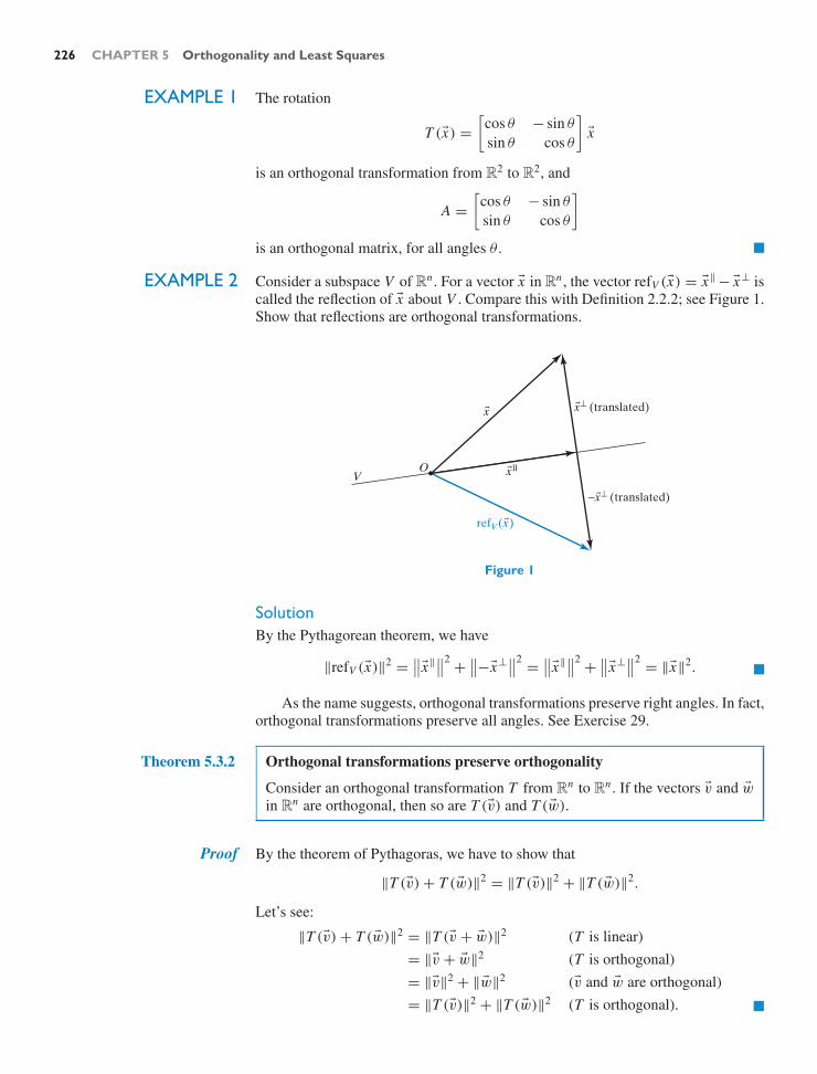
226 CHAPTER 5 Orthogonality and Least Squares
EXAMPLE 1 The rotation
T (x) =[
cos θ − sin θ
sin θ cos θ
]x
is an orthogonal transformation from R2 to R2, and
A =[
cos θ − sin θ
sin θ cos θ
]
is an orthogonal matrix, for all angles θ . !EXAMPLE 2 Consider a subspace V of Rn . For a vector x in Rn , the vector refV (x) = x∥ − x⊥ is
called the reflection of x about V . Compare this with Definition 2.2.2; see Figure 1.Show that reflections are orthogonal transformations.
OV
x
refV(x)
x⊥ (translated)
−x⊥ (translated)
xll
Figure 1
SolutionBy the Pythagorean theorem, we have
∥refV (x)∥2 =∥∥x∥∥∥2 +
∥∥−x⊥∥∥2 =∥∥x∥∥∥2 +
∥∥x⊥∥∥2 = ∥x∥2. !As the name suggests, orthogonal transformations preserve right angles. In fact,
orthogonal transformations preserve all angles. See Exercise 29.
Theorem 5.3.2 Orthogonal transformations preserve orthogonality
Consider an orthogonal transformation T from Rn to Rn . If the vectors v and win Rn are orthogonal, then so are T (v) and T (w).
Proof By the theorem of Pythagoras, we have to show that
∥T (v) + T (w)∥2 = ∥T (v)∥2 + ∥T (w)∥2.
Let’s see:
∥T (v) + T (w)∥2 = ∥T (v + w)∥2 (T is linear)
= ∥v + w∥2 (T is orthogonal)
= ∥v∥2 + ∥w∥2 (v and w are orthogonal)
= ∥T (v)∥2 + ∥T (w)∥2 (T is orthogonal). !

5.3 Orthogonal Transformations and Orthogonal Matrices 227
Theorem 5.3.2 is perhaps better explained with a sketch. See Figure 2.
D1
T
v
w (translated)
D2T(v)
T(w) (translated)
T(v) ! T(w) " T(v ! w)
v ! w
Figure 2
The two shaded triangles are congruent, because corresponding sides are thesame length (since T preserves length). Since D1 is a right triangle, so is D2.
Here is an alternative characterization of orthogonal transformations:
Theorem 5.3.3 Orthogonal transformations and orthonormal bases
a. A linear transformation T from Rn to Rn is orthogonal if (and only if)the vectors T (e1), T (e2), . . . , T (en) form an orthonormal basis of Rn .
b. An n × n matrix A is orthogonal if (and only if) its columns form anorthonormal basis of Rn .
Figure 3 illustrates part (a) for a linear transformation from R2 to R2.
T
e2
e1
T(e1)
T(e2)
Figure 3
Proof We prove part (a); part (b) then follows from Theorem 2.1.2. If T is an orthogonaltransformation, then, by definition, the T (ei ) are unit vectors and, by Theorem 5.3.2,they are orthogonal. Conversely, suppose the T (ei ) form an orthonormal basis.Consider a vectorx = x1e1 + x2e2 + · · · + xnen in Rn . Then

228 CHAPTER 5 Orthogonality and Least Squares
∥T (x)∥2 = ∥x1T (e1) + x2T (e2) + · · · + xnT (en)∥2
= ∥x1T (e1)∥2 + ∥x2T (e2)∥2 + · · · + ∥xnT (en)∥2 (by Pythagoras)= x2
1 + x22 + · · · + x2
n
= ∥x∥2. !Note: A matrix with orthogonal columns need not be an orthogonal matrix. As
an example, consider the matrix A =[
4 −33 4
].
EXAMPLE 3 Show that the matrix A is orthogonal:
A = 12
⎡
⎢⎢⎣
1 −1 −1 −11 −1 1 11 1 −1 11 1 1 −1
⎤
⎥⎥⎦ .
SolutionCheck that the columns of A form an orthonormal basis of R4. !
Here are some algebraic properties of orthogonal matrices.
Theorem 5.3.4 Products and inverses of orthogonal matrices
a. The product AB of two orthogonal n×n matrices A and B is orthogonal.b. The inverse A−1 of an orthogonal n × n matrix A is orthogonal.
Proof In part (a), the linear transformation T (x) = ABx preserves length, because∥T (x)∥ = ∥A(Bx)∥ = ∥Bx∥ = ∥x∥. In part (b), the linear transformationT (x) = A−1 x preserves length, because ∥A−1 x∥ = ∥A(A−1 x)∥ = ∥x∥. Figure 4illustrates property (a). !
x
Bx
ABx
B A
preserveslength
preserveslength
Figure 4
The Transpose of a MatrixEXAMPLE 4 Consider the orthogonal matrix
A = 17
⎡
⎣2 6 33 2 −66 −3 2
⎤
⎦ .

5.3 Orthogonal Transformations and Orthogonal Matrices 229
Form another 3 × 3 matrix B whose i j th entry is the j i th entry of A:
B = 17
⎡
⎣2 3 66 2 −33 −6 2
⎤
⎦ .
Note that the rows of B correspond to the columns of A.Compute B A, and explain the result.
Solution
B A = 149
⎡
⎣2 3 66 2 −33 −6 2
⎤
⎦
⎡
⎣2 6 33 2 −66 −3 2
⎤
⎦ = 149
⎡
⎣49 0 00 49 00 0 49
⎤
⎦ = I3
This result is no coincidence: The i j th entry of B A is the dot product of the i th rowof B and the j th column of A. By definition of B, this is just the dot product of thei th column of A and the j th column of A. Since A is orthogonal, this product is 1if i = j and 0 otherwise. !
Before we can generalize the findings of Example 4, we introduce some newterminology.
Definition 5.3.5 The transpose of a matrix; symmetric and skew-symmetric matrices
Consider an m × n matrix A.The transpose AT of A is the n ×m matrix whose i j th entry is the j i th entry
of A: The roles of rows and columns are reversed.We say that a square matrix A is symmetric if AT = A, and A is called
skew-symmetric if AT = −A.
EXAMPLE 5 If A =[
1 2 39 7 5
], then AT =
⎡
⎣1 92 73 5
⎤
⎦. !
EXAMPLE 6 The symmetric 2 × 2 matrices are those of the form A =[
a bb c
], for example,
A =[
1 22 3
]. The symmetric 2 × 2 matrices form a three-dimensional subspace of
R2×2, with basis[
1 00 0
],[
0 11 0
],[
0 00 1
].
The skew-symmetric 2 × 2 matrices are those of the form A =[
0 b−b 0
],
for example, A =[
0 2−2 0
]. These form a one-dimensional space with basis
[0 1
−1 0
]. !
Note that the transpose of a (column) vector v is a row vector: If
v =
⎡
⎣123
⎤
⎦ , then vT =[
1 2 3].
The transpose gives us a convenient way to express the dot product of two (column)vectors as a matrix product.

230 CHAPTER 5 Orthogonality and Least Squares
Theorem 5.3.6 If v and w are two (column) vectors in Rn , then
v · w = vT w.↑ ↑
Dot Matrixproduct product
Here we are identifying the 1×1 matrix vT w with its sole entry, the scalar v ·w.Purists may prefer to write vT w =
[v · w
].
For example,⎡
⎣123
⎤
⎦ ·
⎡
⎣1
−11
⎤
⎦ =[
1 2 3]⎡
⎣1
−11
⎤
⎦ = 2.
Now we can succinctly state the observation made in Example 4.
Theorem 5.3.7 Consider an n × n matrix A. The matrix A is orthogonal if (and only if) AT A =In or, equivalently, if A−1 = AT .
Proof To justify this fact, write A in terms of its columns:
A =
⎡
⎢⎢⎣
| | |v1 v2 · · · vn
| | |
⎤
⎥⎥⎦ .
Then
AT A =
⎡
⎢⎢⎢⎣
− vT1 −
− vT2 −...
− vTn −
⎤
⎥⎥⎥⎦
⎡
⎢⎢⎣
| | |v1 v2 . . . vn
| | |
⎤
⎥⎥⎦ =
⎡
⎢⎢⎢⎣
v1 · v1 v1 · v2 . . . v1 · vn
v2 · v1 v2 · v2 . . . v2 · vn...
.... . .
...
vn · v1 vn · v2 . . . vn · vn
⎤
⎥⎥⎥⎦.
By Theorem 5.3.3b, this product is In if (and only if) A is orthogonal. !Later in this text, we will frequently work with matrices of the form AT A. It
is helpful to think of AT A as a table displaying the dot products vi · v j among thecolumns of A, as shown above.
We summarize the various characterizations we have found of orthogonalmatrices, and we will add one more characterization, (vi), below.
SUMMARY 5.3.8 Orthogonal matrices
Consider an n × n matrix A. Then the following statements are equivalent:
i. A is an orthogonal matrix.ii. The transformation L(x) = Ax preserves length; that is, ∥Ax∥ = ∥x∥
for all x in Rn .iii. The columns of A form an orthonormal basis of Rn .iv. AT A = In .v. A−1 = AT .
vi. A preserves the dot product, meaning that (Ax) · (Ay) = x · y for all xand y in Rn .

5.3 Orthogonal Transformations and Orthogonal Matrices 231
In Exercise 28, we invite the reader to prove that (vi) is equivalent to the char-acterizations (i) through (v).
Here are some algebraic properties of the transpose.
Theorem 5.3.9 Properties of the transpose
a. (A + B)T = AT + BT for all m × n matrices A and B.b. (k A)T = k AT for all m × n matrices A and for all scalars k.c. (AB)T = BT AT for all m × p matrices A and for all p × n
matrices B.d. rank(AT ) = rank(A) for all matrices A.e. (AT )−1 = (A−1)T for all invertible n × n matrices A.
Proof We leave the proofs of parts (a) and (b) as exercises to the reader. Note that parts(a) and (b) tell us that the function L(A) = AT from Rm×n to Rn×m is a lineartransformation (and, in fact, an isomorphism).
c. Write A in terms of its rows and B in terms of its columns, A =⎡
⎣− w1 −
...− wm −
⎤
⎦ and B =
⎡
⎣| |v1 · · · vn| |
⎤
⎦, so that BT =
⎡
⎣− vT
1 −...
− vTn −
⎤
⎦ and
AT =
⎡
⎣| |
wT1 · · · wT
m| |
⎤
⎦.
Now show that the the i j th entry of (AB)T equals the i j th entry ofBT AT :
(i j th entry of (AB)T )
= ( j i th entry of AB) = w j · vi(i j th entry of BT AT )
= vTi · wT
j = w j · vi .
d. Consider the row space of A (i.e., the span of the rows of A). It is not hardto show that the dimension of this space is rank(A). See Exercises 71–74in Section 3.3. Indeed, we have
rank(AT ) = dimension of the span of the columns of AT
= dimension of the span of the rows of A= rank(A).
e. We know that
AA−1 = In.
Transposing both sides and using part (c), we find that
(AA−1)T = (A−1)T AT = In.
By Theorem 2.4.8, it follows that AT is invertible and
(A−1)T = (AT )−1. !The Matrix of an Orthogonal ProjectionThe transpose allows us to write a formula for the matrix of an orthogonal projec-tion. Consider first the orthogonal projection
projL x = (u1 · x)u1

232 CHAPTER 5 Orthogonality and Least Squares
onto a line L in Rn , where u1 is a unit vector in L . If we view the vector u1 as ann × 1 matrix and the scalar u1 · x as a 1 × 1 matrix, we can write
projL x = u1(u1 · x)
= u1uT1 x
= Mx,
where M = u1uT1 . Note that u1 is an n × 1 matrix and uT
1 is 1 × n, so that M isn × n, as expected.
More generally, consider the projection
projV x = (u1 · x)u1 + · · · + (um · x)um
onto a subspace V of Rn with orthonormal basis u1, . . . , um . We can write
projV x = u1uT1 x + · · · + umuT
m x
=(u1uT
1 + · · · + umuTm
)x
=
⎡
⎢⎣| |
u1 · · · um
| |
⎤
⎥⎦
⎡
⎢⎣− uT
1 −...
− uTm −
⎤
⎥⎦ x .
We have shown the following result:
Theorem 5.3.10 The matrix of an orthogonal projection
Consider a subspace V of Rn with orthonormal basis u1, u2, . . . , um . The matrixP of the orthogonal projection onto V is
P = Q QT , where Q =
⎡
⎣| | |
u1 u2 . . . um
| | |
⎤
⎦ .
Pay attention to the order of the factors (Q QT as opposed to QT Q). Note thatmatrix P is symmetric, since PT = (Q QT )T = (QT )T QT = Q QT = P .
EXAMPLE 7 Find the matrix P of the orthogonal projection onto the subspace of R4 spanned by
u1 = 12
⎡
⎢⎢⎣
1111
⎤
⎥⎥⎦ , u2 = 12
⎡
⎢⎢⎣
1−1−1
1
⎤
⎥⎥⎦ .
SolutionNote that the vectors u1 and u2 are orthonormal. Therefore, the matrix is
P = Q QT = 14
⎡
⎢⎢⎣
1 11 −11 −11 1
⎤
⎥⎥⎦
[1 1 1 11 −1 −1 1
]= 1
2
⎡
⎢⎢⎣
1 0 0 10 1 1 00 1 1 01 0 0 1
⎤
⎥⎥⎦ .
!

5.3 Orthogonal Transformations and Orthogonal Matrices 233
EXERCISES 5.3GOAL Use the various characterizations of orthogonaltransformations and orthogonal matrices. Find the ma-trix of an orthogonal projection. Use the properties of thetranspose.
Which of the matrices in Exercises 1 through 4 are ortho-gonal?
1.[
0.6 0.80.8 0.6
]2.
[−0.8 0.6
0.6 0.8
]
3.13
⎡
⎣2 −2 11 2 22 1 −2
⎤
⎦ 4.17
⎡
⎣2 6 −36 −3 23 2 6
⎤
⎦
If the n × n matrices A and B are orthogonal, which ofthe matrices in Exercises 5 through 11 must be orthogo-nal as well?
5. 3A 6. −B 7. AB 8. A + B
9. B−1 10. B−1 AB 11. AT
If the n × n matrices A and B are symmetric and B is in-vertible, which of the matrices in Exercises 13 through 20must be symmetric as well?
13. 3A 14. −B 15. AB 16. A + B
17. B−1 18. A10
19. 2In + 3A − 4A2 20. AB2 A
If A and B are arbitrary n × n matrices, which of the ma-trices in Exercises 21 through 26 must be symmetric?
21. AT A 22. B BT 23. A − AT
24. AT B A 25. AT BT B A 26. B(A + AT )BT
27. Consider an n × m matrix A, a vector v in Rm , and avector w in Rn . Show that
(Av) · w = v · (AT w).
28. Consider an n × n matrix A. Show that A is an ortho-gonal matrix if (and only if) A preserves the dot prod-uct, meaning that (Ax) · (Ay) = x · y for all x and yin Rn . Hint: In Summary 5.3.8, show that statement (iv)implies (vi), and (vi) implies (ii).
29. Show that an orthogonal transformation L from Rn toRn preserves angles: The angle between two nonzerovectors v and w in Rn equals the angle between L(v)and L(w). Conversely, is any linear transformation thatpreserves angles orthogonal?
30. Consider a linear transformation L from Rm to Rn thatpreserves length. What can you say about the kernel ofL? What is the dimension of the image? What can yousay about the relationship between n and m? If A isthe matrix of L , what can you say about the columnsof A? What is AT A? What about AAT ? Illustrate youranswers with an example where m = 2 and n = 3.
31. Are the rows of an orthogonal matrix A necessarilyorthonormal?
32. a. Consider an n × m matrix A such that AT A = Im .Is it necessarily true that AAT = In? Explain.
b. Consider an n × n matrix A such that AT A = In . Isit necessarily true that AAT = In? Explain.
33. Find all orthogonal 2 × 2 matrices.
34. Find all orthogonal 3 × 3 matrices of the form⎡
⎣a b 0c d 1e f 0
⎤
⎦ .
35. Find an orthogonal transformation T from R3 to R3
such that
T
⎡
⎣2/32/31/3
⎤
⎦ =
⎡
⎣001
⎤
⎦ .
36. Find an orthogonal matrix of the form⎡
⎣2/3 1/
√2 a
2/3 −1/√
2 b1/3 0 c
⎤
⎦ .
37. Is there an orthogonal transformation T from R3 to R3
such that
T
⎡
⎣230
⎤
⎦ =
⎡
⎣302
⎤
⎦ and T
⎡
⎣−3
20
⎤
⎦ =
⎡
⎣2
−30
⎤
⎦ ?
38. a. Give an example of a (nonzero) skew-symmetric3 × 3 matrix A, and compute A2.
b. If an n × n matrix A is skew-symmetric, is matrixA2 necessarily skew-symmetric as well? Or is A2
necessarily symmetric?
39. Consider a line L in Rn , spanned by a unit vector
u =
⎡
⎢⎢⎢⎣
u1u2...
un
⎤
⎥⎥⎥⎦.
Consider the matrix A of the orthogonal projection ontoL . Describe the i j th entry of A, in terms of the compo-nents ui of u.

234 CHAPTER 5 Orthogonality and Least Squares
40. Consider the subspace W of R4 spanned by the vectors
v1 =
⎡
⎢⎢⎣
1111
⎤
⎥⎥⎦ and v2 =
⎡
⎢⎢⎣
19
−53
⎤
⎥⎥⎦ .
Find the matrix of the orthogonal projection onto W .
41. Find the matrix A of the orthogonal projection onto theline in Rn spanned by the vector
⎡
⎢⎢⎢⎣
11...
1
⎤
⎥⎥⎥⎦
⎫⎪⎪⎪⎬
⎪⎪⎪⎭all n components are 1.
42. Let A be the matrix of an orthogonal projection. FindA2 in two ways:a. Geometrically. (Consider what happens when you
apply an orthogonal projection twice.)b. By computation, using the formula given in Theo-
rem 5.3.10.
43. Consider a unit vector u in R3. We define the matrices
A = 2uuT − I3 and B = I3 − 2uuT .
Describe the linear transformations defined by thesematrices geometrically.
44. Consider an n × m matrix A. Find
dim(im(A)
)+ dim
(ker(AT )
),
in terms of m and n.
45. For which n × m matrices A does the equation
dim(ker(A)
)= dim
(ker(AT )
)
hold? Explain.
46. Consider a Q R factorization
M = Q R.
Show that
R = QT M.
47. If A = Q R is a Q R factorization, what is the relation-ship between AT A and RT R?
48. Consider an invertible n × n matrix A. Can you write Aas A = L Q, where L is a lower triangular matrix andQ is orthogonal? Hint: Consider the Q R factorizationof AT .
49. Consider an invertible n × n matrix A. Can you writeA = RQ, where R is an upper triangular matrix and Qis orthogonal?
50. a. Find all n × n matrices that are both orthogonal andupper triangular, with positive diagonal entries.
b. Show that the Q R factorization of an invertible n×nmatrix is unique. Hint: If A = Q1 R1 = Q2 R2, thenthe matrix Q−1
2 Q1 = R2 R−11 is both orthogonal and
upper triangular, with positive diagonal entries.
51. a. Consider the matrix product Q1 = Q2S, whereboth Q1 and Q2 are n × m matrices with orthonor-mal columns. Show that S is an orthogonal matrix.Hint: Compute QT
1 Q1 = (Q2S)T Q2S. Note thatQT
1 Q1 = QT2 Q2 = Im .
b. Show that the Q R factorization of an n × m ma-trix M is unique. Hint: If M = Q1 R1 = Q2 R2,then Q1 = Q2 R2 R−1
1 . Now use part (a) and Exer-cise 50a.
52. Find a basis of the space V of all symmetric 3 × 3 ma-trices, and thus determine the dimension of V .
53. Find a basis of the space V of all skew-symmetric 3×3matrices, and thus determine the dimension of V .
54. Find the dimension of the space of all skew-symmetricn × n matrices.
55. Find the dimension of the space of all symmetric n × nmatrices.
56. Is the transformation L(A) = AT from R2×3 to R3×2
linear? Is L an isomorphism?
57. Is the transformation L(A) = AT from Rm×n to Rn×m
linear? Is L an isomorphism?
58. Find image and kernel of the linear transformationL(A) = 1
2 (A + AT ) from Rn×n to Rn×n . Hint: Thinkabout symmetric and skew-symmetric matrices.
59. Find the image and kernel of the linear transformationL(A) = 1
2 (A − AT ) from Rn×n to Rn×n . Hint: Thinkabout symmetric and skew-symmetric matrices.
60. Find the matrix of the linear transformation L(A) = AT
from R2×2 to R2×2 with respect to the basis[
1 00 0
],
[0 00 1
],
[0 11 0
],
[0 1
−1 0
].
61. Find the matrix of the linear transformation L(A) =A − AT from R2×2 to R2×2 with respect to the basis
[1 00 0
],
[0 00 1
],
[0 11 0
],
[0 1
−1 0
].
62. Consider the matrix
A =
⎡
⎣1 1 −13 2 −52 2 0
⎤
⎦
with LDU-factorization
A =
⎡
⎣1 0 03 1 02 0 1
⎤
⎦
⎡
⎣1 0 00 −1 00 0 2
⎤
⎦
⎡
⎣1 1 −10 1 20 0 1
⎤
⎦ .

5.3 Orthogonal Transformations and Orthogonal Matrices 235
Find the LDU-factorization of AT . See Exercise2.4.90d.
63. Consider a symmetric invertible n × n matrix A whichadmits an LDU-factorization A = L DU . See Exer-cises 90, 93, and 94 of Section 2.4. Recall that thisfactorization is unique. See Exercise 2.4.94. Show thatU = LT . (This is sometimes called the L DLT -factorization of a symmetric matrix A.)
64. This exercise shows one way to define the quaternions,discovered in 1843 by the Irish mathematician Sir W. R.Hamilton (1805–1865). Consider the set H of all 4 × 4matrices M of the form
M =
⎡
⎢⎢⎢⎢⎣
p −q −r −s
q p s −r
r −s p q
s r −q p
⎤
⎥⎥⎥⎥⎦,
where p, q, r, s are arbitrary real numbers. We can writeM more succinctly in partitioned form as
M =[
A −BT
B AT
],
where A and B are rotation–scaling matrices.a. Show that H is closed under addition: If M and N
are in H , then so is M + N .b. Show that H is closed under scalar multiplication:
If M is in H and k is an arbitrary scalar, then k M isin H .
c. Parts (a) and (b) show that H is a subspace of thelinear space R4×4. Find a basis of H , and thus de-termine the dimension of H .
d. Show that H is closed under multiplication: If Mand N are in H , then so is M N .
e. Show that if M is in H , then so is MT .f. For a matrix M in H , compute MT M .g. Which matrices M in H are invertible? If a matrix
M in H is invertible, is M−1 necessarily in H aswell?
h. If M and N are in H , does the equation M N = N Malways hold?
65. Find all orthogonal 2 × 2 matrices A such that all theentries of 10A are integers and such that both entries inthe first column are positive.
66. Find an orthogonal 2 × 2 matrix A such that all the en-tries of 100A are integers while all the entries of 10Afail to be integers.
67. Consider a subspace V of Rn with a basis v1, . . . , vm ;suppose we wish to find a formula for the orthogo-nal projection onto V . Using the methods we havedeveloped thus far, we can proceed in two steps:We use the Gram–Schmidt process to construct anorthonormal basis u1, . . . , um of V , and then we use
Theorem 5.3.10: The matrix of the orthogonal projec-tion is Q QT , where
Q =[
u1 · · · um
].
In this exercise we will see how we can write the ma-trix of the projection directly in terms of the basisv1, . . . , vm and the matrix
A =[v1 · · · vm
].
(This issue will be discussed more thoroughly in Sec-tion 5.4; see Theorem 5.4.7.)
Since projV x is in V , we can write
projV x = c1v1 + · · · + cm vm
for some scalars c1, . . . , cm yet to be determined. Nowx − projV (x) = x − c1v1 − · · ·− cm vm is orthogonal toV , meaning that vi · (x − c1v1 − · · · − cm vm) = 0 fori = 1, . . . , m.a. Use the equation vi · (x − c1v1 − · · · − cm vm) = 0
to show that AT Ac = AT x , where c =
⎡
⎢⎣c1...
cm
⎤
⎥⎦.
b. Conclude that c = (AT A)−1 AT x and projV x =Ac = A(AT A)−1 AT x .
68. The formula A(AT A)−1 AT for the matrix of an or-thogonal projection is derived in Exercise 67. Now con-sider the Q R factorization of A, and express the matrixA(AT A)−1 AT in terms of Q.
69. In R4, consider the subspace W spanned by the vectors⎡
⎢⎣
11
−10
⎤
⎥⎦ and
⎡
⎢⎣
011
−1
⎤
⎥⎦. Find the matrix PW of the ortho-
gonal projection onto W .
70. In all parts of this problem, let V be the subspace of allvectors x in R4 such that x3 = x1+x2 and x4 = x2+x3.See Problems 72 and 73 of Section 4.3.a. Find the matrix PV of the orthogonal projection onto
the subspace V in R4. Hint: Work with one of thebases of V we considered in Problem 4.3.73.
b. What is the relationship between the subspaces Wand V defined in Exercises 69 and 70? Conse-quently, what is the relationship between the matri-ces PW and PV in Exercises 69 and 70?
71. An n ×n matrix A is said to be a Hankel matrix (namedafter the German mathematician Hermann Hankel,1839–1873) if ai j = ai+1, j−1 for all i = 1, . . . , n − 1and all j = 2, . . . , n, meaning that A has constant pos-itive sloping diagonals. For example, a 4 × 4 Hankelmatrix is of the form

236 CHAPTER 5 Orthogonality and Least Squares
A =
⎡
⎢⎣
a b c db c d ec d e fd e f g
⎤
⎥⎦ .
Show that the n × n Hankel matrices form a subspaceof Rn×n . Find the dimension of this space.
72. Consider a vector v in Rn of the form
v =
⎡
⎢⎢⎢⎢⎢⎣
1aa2
...
an−1
⎤
⎥⎥⎥⎥⎥⎦,
where a is any real number. Let P be the matrix ofthe orthogonal projection onto span(v). Describe the en-tries of P in terms of a, and explain why P is a Han-kel matrix. See Exercise 71. As an example, find P for
v =
⎡
⎣124
⎤
⎦.
73. Let n be an even positive integer. In both parts of thisproblem, let V be the subspace of all vectors x in Rn
such that x j+2 = x j + x j+1, for all j = 1, . . . , n − 2.(In Exercise 70 we consider the special case n = 4.)Consider the basis v, w of V with
a =
⎡
⎢⎢⎢⎢⎢⎣
1aa2
...
an−1
⎤
⎥⎥⎥⎥⎥⎦, b =
⎡
⎢⎢⎢⎢⎢⎣
1bb2
...
bn−1
⎤
⎥⎥⎥⎥⎥⎦,
where a = 1 +√
52
and b = 1 −√
52
.
(In Exercise 4.3.72 we consider the case n = 4.)a. Show that a is orthogonal to b.b. Explain why the matrix P of the orthogonal projec-
tion onto V is a Hankel matrix. See Exercises 71 and72.
74. For any integer m, we define the Fibonacci number fmrecursively by f0 = 0, f1 = 1, and f j+2 = f j + f j+1for all integers j .7
a. Find the Fibonacci numbers fm for m = −5, . . . , 5.
b. Based upon your answer in part (a), describe the re-lationship between f−m and fm . (For extra credit,give a formal proof by induction on m.)
Now let n be a positive integer, with n ≥ 2. Let V be thetwo-dimensional subspace of all vectors x in Rn suchthat x j+2 = x j + x j+1, for all j = 1, . . . , n − 2. SeeExercise 73. Note that, by definition, any n consecutiveFibonacci numbers form a vector in V . Consider the ba-sis v, w of V with
v =
⎡
⎢⎢⎢⎢⎢⎣
f0f1...
fn−2fn−1
⎤
⎥⎥⎥⎥⎥⎦=
⎡
⎢⎢⎢⎢⎢⎣
01...
fn−2fn−1
⎤
⎥⎥⎥⎥⎥⎦,
w =
⎡
⎢⎢⎢⎢⎢⎣
f−n+1f−n+2
...
f−1f0
⎤
⎥⎥⎥⎥⎥⎦=
⎡
⎢⎢⎢⎢⎢⎣
fn−1− fn−2
...
10
⎤
⎥⎥⎥⎥⎥⎦.
(In Exercise 4.3.73c, we introduce this basis in the casen = 4.) We are told that ∥v∥2 = ∥w∥2 = fn−1 fn . (Forextra credit, give a proof by induction on n.)c. Find the basis v, w in the case n = 6. Verify the
identity ∥v∥2 = ∥w∥2 = f5 f6. Also, show that v isorthogonal to w.
d. Show that v is orthogonal to w for any even positiveinteger n.
e. For an even positive integer n, let P be the matrix ofthe orthogonal projection onto V . Show that the firstcolumn of P is 1
fnw, while the last column is 1
fnv.
Recall from Exercise 73 that P is a Hankel matrix,and note that a Hankel matrix is determined by itsfirst and last columns. Conclude that
P = 1fn
⎡
⎢⎢⎢⎢⎢⎢⎢⎣
f−n+1 f−n+2 . . . f−1 f0
f−n+2 f−n+3 . . . f0 f1
......
. . ....
...
f−1 f0 . . . fn−3 fn−2
f0 f1 . . . fn−2 fn−1
⎤
⎥⎥⎥⎥⎥⎥⎥⎦
,
meaning that the i j th entry of P is fi+ j−n−1fn
.f. Find the matrix P in the case n = 6.
5.4 Least Squares and Data Fitting
In this section, we will present an important application of the ideas introduced inthis chapter. First, we take another look at orthogonal complements and orthogonalprojections.
7Exercises 69 through 74 are based on research by Prof. Ben Mathes, Colby College.

5.4 Least Squares and Data Fitting 237
Another Characterization of Orthogonal Complements
Consider a subspace V = im(A) of Rn , where A =
⎡
⎣| | |v1 v2 · · · vm
| | |
⎤
⎦. Then
V ⊥ = x in Rn: v · x = 0, for all v in V = x in Rn: vi · x = 0, for i = 1, . . . , m= x in Rn: vT
i x = 0, for i = 1, . . . , m.
In other words, V ⊥ = (imA)⊥ is the kernel of the matrix
AT =
⎡
⎢⎢⎢⎣
− vT1 −
− vT2 −...
− vTm −
⎤
⎥⎥⎥⎦.
Theorem 5.4.1 For any matrix A,
(imA)⊥ = ker(AT ).
Here is a very simple example: Consider the line
V = im
⎡
⎣123
⎤
⎦ .
Then
V ⊥ = ker[1 2 3
]
is the plane with equation x1 + 2x2 + 3x3 = 0. See Figure 1.
0
V⊥ = ker[1 2 3], which isthe plane x1 + 2x2 + 3x3 = 0
the line spanned by
, which is
123
V = im123
Figure 1
The following somewhat technical result will be useful later:
Theorem 5.4.2 a. If A is an n × m matrix, then
ker(A) = ker(AT A).
b. If A is an n × m matrix with ker(A) = 0, then AT A is invertible.

238 CHAPTER 5 Orthogonality and Least Squares
Proof a. Clearly, the kernel of A is contained in the kernel of AT A. Conversely, con-sider a vector x in the kernel of AT A, so that AT Ax = 0. Then Ax is in theimage of A and in the kernel of AT . Since ker(AT ) is the orthogonal com-plement of im(A) by Theorem 5.4.1, the vector Ax is 0 by Theorem 5.1.8b;that is, x is in the kernel of A.
b. Note that AT A is an m × m matrix. By part (a), ker(AT A) = 0, and thesquare matrix AT A is therefore invertible. See Theorem 3.3.10. !
An Alternative Characterization of Orthogonal Projections
Theorem 5.4.3 Consider a vector x in Rn and a subspace V of Rn . Then the orthogonal projec-tion projV x is the vector in V closest to x , in that
∥x − projV x∥ < ∥x − v∥,for all v in V different from projV x .
To justify this fact, apply the Pythagorean theorem to the shaded right trianglein Figure 2.
v
xx − projV x x − v
0projV x
V
(translated)(translated)
Figure 2
Least-Squares ApproximationsConsider an inconsistent linear system Ax = b. The fact that this system is incon-sistent means that the vector b is not in the image of A. See Figure 3.
O im(A)
b
Figure 3
Although this system cannot be solved, we might be interested in finding a goodapproximate solution. We can try to find a vector x∗ such that Ax∗ is “as close aspossible” to b. In other words, we try to minimize the error ∥b − Ax∥.
Definition 5.4.4 Least-squares solution
Consider a linear system
Ax = b,
where A is an n × m matrix. A vector x∗ in Rm is called a least-squares solutionof this system if ∥b − Ax∗∥ ≤ ∥b − Ax∥ for all x in Rm .

5.4 Least Squares and Data Fitting 239
See Figure 4.
Ax
b
(translated)(translated)b − Ax
0Ax*
im(A)
b − Ax*
Figure 4
The term least-squares solution reflects the fact that we are minimizing the sumof the squares of the components of the vector b − Ax .
If the system Ax = b happens to be consistent, then the least-squares solutionsare its exact solutions: The error ∥b − Ax∥ is zero.
How can we find the least-squares solutions of a linear system Ax = b? Con-sider the following string of equivalent statements:
The vector x∗ is a least-squares solutionof the system Ax = b.PQR Definition 5.4.4
∥b − Ax∗∥ ≤ ∥b − Ax∥ for all x in Rm .PQR Theorem 5.4.3
Ax∗ = projV b, where V = im(A).PQR Theorems 5.1.4 and 5.4.1
b − Ax∗ is in V ⊥ = (imA)⊥ = ker(AT ).PQR
AT (b − Ax∗) = 0.PQR
AT Ax∗ = AT b.
Take another look at Figures 2 and 4.
Theorem 5.4.5 The normal equation
The least-squares solutions of the system
Ax = b
are the exact solutions of the (consistent) system
AT Ax = AT b.
The system AT Ax = AT b is called the normal equation of Ax = b.
The case when ker(A) = 0 is of particular importance. Then, the matrix AT Ais invertible (by Theorem 5.4.2b), and we can give a closed formula for the least-squares solution.

240 CHAPTER 5 Orthogonality and Least Squares
Theorem 5.4.6 If ker(A) = 0, then the linear system
Ax = b
has the unique least-squares solution
x∗ = (AT A)−1 AT b.
From a computational point of view, it may be more efficient to solve the nor-mal equation AT Ax = AT b by Gauss–Jordan elimination, rather than by usingTheorem 5.4.6.
EXAMPLE 1 Use Theorem 5.4.6 to find the least-squares solution x∗ of the system
Ax = b, where A =
⎡
⎣1 11 21 3
⎤
⎦ and b =
⎡
⎣006
⎤
⎦ .
What is the geometric relationship between Ax∗ and b?
SolutionWe compute
x∗ = (AT A)−1 AT b =[−4
3
]and Ax∗ =
⎡
⎣−1
25
⎤
⎦ .
Recall that Ax∗ is the orthogonal projection of b onto the image of A. Check that
b − Ax∗ =
⎡
⎣1
−21
⎤
⎦
is indeed perpendicular to the two column vectors of A. See Figure 5. !
b
b − Ax* (translated)
x*
V = im(A)
O
A
Ax* = projV b
Figure 5
If x∗ is a least-squares solution of the system Ax = b, then Ax∗ is the or-thogonal projection of b onto im(A). We can use this fact to find a new formulafor orthogonal projections. Compare this with Theorems 5.1.5 and 5.3.10. Con-sider a subspace V of Rn and a vector b in Rn . Choose a basis v1, . . . , vm ofV , and form the matrix A =
[v1 . . . vm
]. Note that ker(A) = 0, since the
columns of A are linearly independent. The least-squares solution of the systemAx = b is x∗ = (AT A)−1 AT b. Thus, the orthogonal projection of b onto V isprojV b = Ax∗ = A(AT A)−1 AT b.

5.4 Least Squares and Data Fitting 241
Theorem 5.4.7 The matrix of an orthogonal projection
Consider a subspace V of Rn with basis v1, v2, . . . , vm . Let
A =
⎡
⎣| | |v1 v2 . . . vm
| | |
⎤
⎦ .
Then the matrix of the orthogonal projection onto V is
A(AT A)−1 AT .
We are not required to find an orthonormal basis of V here. If the vectorsv1, . . . , vm happen to be orthonormal, then AT A = Im and the formula simplifiesto AAT . See Theorem 5.3.10.
EXAMPLE 2 Find the matrix of the orthogonal projection onto the subspace of R4 spanned bythe vectors
⎡
⎢⎢⎣
1111
⎤
⎥⎥⎦ and
⎡
⎢⎢⎣
1234
⎤
⎥⎥⎦ .
SolutionLet
A =
⎡
⎢⎢⎣
1 11 21 31 4
⎤
⎥⎥⎦ ,
and compute
A(AT A)−1 AT = 110
⎡
⎢⎢⎣
7 4 1 −24 3 2 11 2 3 4
−2 1 4 7
⎤
⎥⎥⎦ .
!
Data FittingScientists are often interested in fitting a function of a certain type to data they havegathered. The functions considered could be linear, polynomial, rational, trigono-metric, or exponential. The equations we have to solve as we fit data are frequentlylinear. See Exercises 31 through 38 of Section 1.1, and Exercises 32 through 35 ofSection 1.2.
EXAMPLE 3 Find a cubic polynomial whose graph passes through the points (1, 3), (−1, 13),(2, 1), (−2, 33).
SolutionWe are looking for a function
f (t) = c0 + c1t + c2t2 + c3t3

242 CHAPTER 5 Orthogonality and Least Squares
such that f (1) = 3, f (−1) = 13, f (2) = 1, f (−2) = 33; that is, we have to solvethe linear system ∣∣∣∣∣∣∣∣∣
c0 + c1 + c2 + c3 = 3c0 − c1 + c2 − c3 = 13c0 + 2c1 + 4c2 + 8c3 = 1c0 − 2c1 + 4c2 − 8c3 = 33
∣∣∣∣∣∣∣∣∣
.
This linear system has the unique solution⎡
⎢⎢⎣
c0
c1
c2
c3
⎤
⎥⎥⎦ =
⎡
⎢⎢⎣
5−4
3−1
⎤
⎥⎥⎦ .
Thus, the cubic polynomial whose graph passes through the four given data pointsis f (t) = 5 − 4t + 3t2 − t3, as shown in Figure 6. !
(1, 3) (2, 1)(−1, 13)
(−2, 33)
f (t)
t
Figure 6
Frequently, a data-fitting problem leads to a linear system with more equationsthan variables. (This happens when the number of data points exceeds the numberof parameters in the function we seek.) Such a system is usually inconsistent, andwe will look for the least-squares solution(s).
EXAMPLE 4 Fit a quadratic function to the four data points (a1, b1) = (−1, 8), (a2, b2) = (0, 8),(a3, b3) = (1, 4), and (a4, b4) = (2, 16).
SolutionWe are looking for a function f (t) = c0 + c1t + c2t2 such that
∣∣∣∣∣∣∣∣∣
f (a1) = b1
f (a2) = b2
f (a3) = b3
f (a4) = b4
∣∣∣∣∣∣∣∣∣
or
∣∣∣∣∣∣∣∣∣
c0 − c1 + c2 = 8c0 = 8c0 + c1 + c2 = 4c0 + 2c1 + 4c2 = 16
∣∣∣∣∣∣∣∣∣
or A
⎡
⎣c0
c1
c2
⎤
⎦ = b,
where
A =
⎡
⎢⎢⎣
1 −1 11 0 01 1 11 2 4
⎤
⎥⎥⎦ and b =
⎡
⎢⎢⎣
884
16
⎤
⎥⎥⎦ .
We have four equations, corresponding to the four data points, but only three un-knowns, the three coefficients of a quadratic polynomial. Check that this system isindeed inconsistent. The least-squares solution is
c∗ =
⎡
⎢⎣c∗
0
c∗1
c∗2
⎤
⎥⎦ = (AT A)−1 AT b =
⎡
⎢⎣5
−1
3
⎤
⎥⎦ .

5.4 Least Squares and Data Fitting 243
The least-squares approximation is f ∗(t) = 5 − t + 3t2, as shown in Figure 7.
(a1, b1)(a2, b2)
(a3, b3)
(a4, b4)f *(t)
t
Figure 7
This quadratic function f ∗(t) fits the data points best, in that the vector
Ac∗ =
⎡
⎢⎢⎢⎢⎣
f ∗(a1)
f ∗(a2)
f ∗(a3)
f ∗(a4)
⎤
⎥⎥⎥⎥⎦
is as close as possible to
b =
⎡
⎢⎢⎢⎢⎣
b1
b2
b3
b4
⎤
⎥⎥⎥⎥⎦.
This means that
∥b − Ac∗∥2 =(b1 − f ∗(a1)
)2 +(b2 − f ∗(a2)
)2
+(b3 − f ∗(a3)
)2 +(b4 − f ∗(a4)
)2
is minimal: The sum of the squares of the vertical distances between graph and datapoints is minimal. See Figure 8. !
(ai, f*(ai))
(ai , bi)
f*(t)bi − f*(ai)
Figure 8
EXAMPLE 5 Find the linear function c0 + c1t that best fits the data points (a1, b1), (a2, b2), . . . ,(an, bn), using least squares. Assume that a1 = a2.
SolutionWe attempt to solve the system
∣∣∣∣∣∣∣∣∣∣
c0 + c1a1 = b1
c0 + c1a2 = b2
......
...
c0 + c1an = bn
∣∣∣∣∣∣∣∣∣∣
,
or⎡
⎢⎢⎢⎣
1 a1
1 a2...
...
1 an
⎤
⎥⎥⎥⎦
[c0
c1
]=
⎡
⎢⎢⎢⎣
b1
b2...
bn
⎤
⎥⎥⎥⎦,
or
A[
c0
c1
]= b.

244 CHAPTER 5 Orthogonality and Least Squares
Note that rank(A) = 2, since a1 = a2.The least-squares solution is
[c∗
0
c∗1
]= (AT A)−1 AT b =
⎛
⎜⎝[
1 · · · 1a1 · · · an
]⎡
⎢⎣1 a1...
...
1 an
⎤
⎥⎦
⎞
⎟⎠
−1[
1 · · · 1a1 · · · an
]⎡
⎢⎣b1...
bn
⎤
⎥⎦
=
⎡
⎣ n∑
i ai∑
i ai∑
i a2i
⎤
⎦−1 ⎡
⎣∑
i bi∑
i ai bi
⎤
⎦ (where∑
i refers to the sum fori = 1, . . . , n)
= 1n(
∑i a2
i ) − (∑
i ai )2
⎡
⎣∑
i a2i −
∑i ai
−∑
i ai n
⎤
⎦
⎡
⎣∑
i bi∑
i ai bi
⎤
⎦ .
We have found that
c∗0 =
(∑i a2
i
) (∑i bi
)−
(∑i ai
) (∑i ai bi
)
n(∑
i a2i
)−
(∑i ai
)2
c∗1 =
n(∑
i ai bi)
−(∑
i ai) (∑
i bi)
n(∑
i a2i
)−
(∑i ai
)2 .
These formulas are well known to statisticians. There is no need to memorize them.!
We conclude this section with an example for multivariate data fitting.
EXAMPLE 6 In the accompanying table, we list the scores of five students on the three examsgiven in a class.
h: m: f :Hour Exam Midterm Exam Final Exam
Gabriel 76 48 43Kyle 92 92 90Faruk 68 82 64Yasmine 86 68 69Alec 54 70 50
Find the function of the form f = c0 +c1h +c2m that best fits these data, usingleast squares. What score f does your formula predict for Marilyn, another student,whose scores in the first two exams were h = 92 and m = 72?
SolutionWe attempt to solve the system
∣∣∣∣∣∣∣∣∣∣∣
c0 + 76c1 + 48c2 = 43c0 + 92c1 + 92c2 = 90c0 + 68c1 + 82c2 = 64c0 + 86c1 + 68c2 = 69c0 + 54c1 + 70c2 = 50
∣∣∣∣∣∣∣∣∣∣∣
.

5.4 Least Squares and Data Fitting 245
The least-squares solution is⎡
⎢⎣c∗
0
c∗1
c∗2
⎤
⎥⎦ = (AT A)−1 AT b ≈
⎡
⎣−42.4
0.6390.799
⎤
⎦ .
The function that gives the best fit is approximately
f = −42.4 + 0.639h + 0.799m.
This formula predicts the score
f = −42.4 + 0.639 · 92 + 0.799 · 72 ≈ 74
for Marilyn. !
EXERCISES 5.4GOAL Use the formula (im A)⊥ = ker(AT ). Apply thecharacterization of projV x as the vector in V “closestto x.” Find the least-squares solutions of a linear systemAx = b using the normal equation AT Ax = AT b.
1. Consider the subspace im(A) of R2, where
A =[
2 43 6
].
Find a basis of ker(AT ), and draw a sketch illustratingthe formula
(im A)⊥ = ker(AT )
in this case.
2. Consider the subspace im(A) of R3, where
A =
⎡
⎣1 11 21 3
⎤
⎦ .
Find a basis of ker(AT ), and draw a sketch illustratingthe formula (im A)⊥ = ker(AT ) in this case.
3. Consider a subspace V of Rn . Let v1, . . . , vp be a ba-sis of V and w1, . . . , wq a basis of V ⊥. Is v1, . . . , vp ,w1, . . . , wq a basis of Rn? Explain.
4. Let A be an n × m matrix. Is the formula
(ker A)⊥ = im(AT )
necessarily true? Explain.
5. Let V be the solution space of the linear system∣∣∣∣x1 + x2 + x3 + x4 = 0
x1 + 2x2 + 5x3 + 4x4 = 0
∣∣∣∣ .
Find a basis of V ⊥.
6. If A is an n × m matrix, is the formula
im(A) = im(AAT )
necessarily true? Explain.
7. Consider a symmetric n × n matrix A. What is the rela-tionship between im(A) and ker(A)?
8. Consider a linear transformation L(x) = Ax from Rn
to Rm , with ker(L) = 0. The pseudoinverse L+ of Lis the transformation from Rm to Rn given by
L+(y) =(the least-squares solution of L(x) = y
).
a. Show that the transformation L+ is linear. Find thematrix A+ of L+, in terms of the matrix A of L .
b. If L is invertible, what is the relationship betweenL+ and L−1?
c. What is L+(L(x)
), for x in Rn?
d. What is L(
L+(y)), for y in Rm?
e. Find L+ for the linear transformation
L(x) =
⎡
⎣1 00 10 0
⎤
⎦ x .
9. Consider the linear system Ax = b, where
A =[
1 32 6
]and b =
[1020
].
a. Draw a sketch showing the following subsets of R2:
• the kernel of A, and (ker A)⊥
• the image of AT
• the solution set S of the system Ax = b
b. What relationship do you observe between ker(A)and im(AT )? Explain.
c. What relationship do you observe between ker(A)and S? Explain.
d. Find the unique vector x0 in the intersection of S and(ker A)⊥. Show x0 on your sketch.
e. What can you say about the length of x0 comparedwith the length of all other vectors in S?

246 CHAPTER 5 Orthogonality and Least Squares
10. Consider a consistent system Ax = b.a. Show that this system has a solution x0 in (ker A)⊥.
Hint: An arbitrary solution x of the system can bewritten as x = xh + x0, where xh is in ker(A) andx0 is in (ker A)⊥.
b. Show that the system Ax = b has only one solutionin (ker A)⊥. Hint: If x0 and x1 are two solutions in(ker A)⊥, think about x1 − x0.
c. If x0 is the solution in (ker A)⊥ and x1 is anothersolution of the system Ax = b, show that ∥x0∥ <∥x1∥. The vector x0 is called the minimal solution ofthe linear system Ax = b.
11. Consider a linear transformation L(x) = Ax from Rn
to Rm , where rank(A) = m. The pseudoinverse L+ ofL is the transformation from Rm to Rn given by
L+(y)=(the minimal solution of the system L(x)= y
).
See Exercise 10.a. Show that the transformation L+ is linear.b. What is L
(L+(y)
), for y in Rm?
c. What is L+(L(x)
), for x in Rn?
d. Determine the image and kernel of L+.e. Find L+ for the linear transformation
L(x) =[
1 0 00 1 0
]x .
12. Using Exercise 10 as a guide, define the term minimalleast-squares solution of a linear system. Explain whythe minimal least-squares solution x∗ of a linear systemAx = b is in (ker A)⊥.
13. Consider a linear transformation L(x) = Ax from Rn
to Rm . The pseudoinverse L+ of L is the transformationfrom Rm to Rn given by
L+(y) =(the minimal least-squares solution
of the system L(x) = y).
See Exercises 8, 11, and 12 for special cases.a. Show that the transformation L+ is linear.b. What is L+(
L(x)), for x in Rn?
c. What is L(
L+(y)), for y in Rm?
d. Determine the image and kernel of L+ [in terms of
im(AT ) and ker(AT )].
e. Find L+ for the linear transformation
L(x) =[
2 0 00 0 0
]x .
14. In the accompanying figure, we show the kernel and theimage of a linear transformation L from R2 to R2, to-gether with some vectors v1, w1, w2, w3. We are toldthat L(v1) = w1. For i = 1, 2, 3, find the vectorsL+(wi ), where L+ is the pseudoinverse of L defined in
Exercise 13. Show your solutions in the figure, and ex-plain how you found them.
im(L)
ker(L)
v1
w2
w1
w3
OO
L
15. Consider an m × n matrix A with ker(A) = 0. Showthat there exists an n × m matrix B such that B A = In .Hint: AT A is invertible.
16. Use the formula (im A)⊥ = ker(AT ) to prove the equa-tion
rank(A) = rank(AT ).
17. Does the equation
rank(A) = rank(AT A)
hold for all n × m matrices A? Explain.
18. Does the equation
rank(AT A) = rank(AAT )
hold for all n × m matrices A? Explain. Hint: Exer-cise 17 is useful.
19. Find the least-squares solution x∗ of the system
Ax = b, where A =
⎡
⎣1 00 10 0
⎤
⎦ and b =
⎡
⎣111
⎤
⎦ .
Use paper and pencil. Draw a sketch showing the vec-tor b, the image of A, the vector Ax∗, and the vectorb − Ax∗.
20. By using paper and pencil, find the least-squares solu-tion x∗ of the system
Ax = b, where A =
⎡
⎣1 11 00 1
⎤
⎦ and b =
⎡
⎣333
⎤
⎦ .
Verify that the vector b − Ax∗ is perpendicular to theimage of A.
21. Find the least-squares solution x∗ of the system
Ax = b, where A =
⎡
⎣6 93 82 10
⎤
⎦ and b =
⎡
⎣0
490
⎤
⎦ .
Determine the error ∥b − Ax∗∥.

5.4 Least Squares and Data Fitting 247
22. Find the least-squares solution x∗ of the system
Ax = b, where A =
⎡
⎣3 25 34 5
⎤
⎦ and b =
⎡
⎣592
⎤
⎦ .
Determine the error ∥b − Ax∗∥.
23. Find the least-squares solution x∗ of the system
Ax = b, where A =
⎡
⎣1 12 81 5
⎤
⎦ and b =
⎡
⎣1
−23
⎤
⎦ .
Explain.
24. Find the least-squares solution x∗ of the system
Ax = b, where A =
⎡
⎣123
⎤
⎦ and b =
⎡
⎣327
⎤
⎦ .
Draw a sketch showing the vector b, the image of A, thevector Ax∗, and the vector b − Ax∗.
25. Find the least-squares solutions x∗ of the systemAx = b, where
A =[
1 32 6
]and b =
[50
].
Use only paper and pencil. Draw a sketch.
26. Find the least-squares solutions x∗ of the systemAx = b, where
A =
⎡
⎣1 2 34 5 67 8 9
⎤
⎦ and b =
⎡
⎣100
⎤
⎦ .
27. Consider an inconsistent linear system Ax = b, whereA is a 3×2 matrix. We are told that the least-squares so-
lution of this system is x∗ =[
711
]. Consider an orthog-
onal 3 × 3 matrix S. Find the least-squares solution(s)of the system S Ax = Sb.
28. Consider an orthonormal basis u1, u2, . . . , un in Rn .Find the least-squares solution(s) of the system
Ax = un,
where
A =
⎡
⎣| | |
u1 u2 · · · un−1| | |
⎤
⎦ .
29. Find the least-squares solution of the system
Ax = b, where A =
⎡
⎣1 1
10−10 00 10−10
⎤
⎦ and
b =
⎡
⎣1
10−10
10−10
⎤
⎦ .
Describe and explain the difficulties you may encounterif you use technology. Then find the solution usingpaper and pencil.
30. Fit a linear function of the form f (t) = c0 + c1t to thedata points (0, 0), (0, 1), (1, 1), using least squares. Useonly paper and pencil. Sketch your solution, and explainwhy it makes sense.
31. Fit a linear function of the form f (t) = c0 + c1t tothe data points (0, 3), (1, 3), (1, 6), using least squares.Sketch the solution.
32. Fit a quadratic polynomial to the data points (0, 27),(1, 0), (2, 0), (3, 0), using least squares. Sketch thesolution.
33. Find the trigonometric function of the form f (t) =c0 + c1 sin(t) + c2 cos(t) that best fits the data points(0, 0), (1, 1), (2, 2), (3, 3), using least squares. Sketchthe solution together with the function g(t) = t .
34. Find the function of the form
f (t) = c0 + c1 sin(t) + c2 cos(t) + c3 sin(2t) + c4 cos(2t)
that best fits the data points (0, 0), (0.5, 0.5), (1, 1),(1.5, 1.5), (2, 2), (2.5, 2.5), (3, 3), using least squares.Sketch the solution, together with the function g(t) = t .
35. Suppose you wish to fit a function of the form
f (t) = c + p sin(t) + q cos(t)
to a given continuous function g(t) on the closed inter-val from 0 to 2π . One approach is to choose n equallyspaced points ai between 0 and 2π [ai = i · (2π/n), fori = 1, . . . , n, say]. We can fit a function
fn(t) = cn + pn sin(t) + qn cos(t)
to the data points(ai , g(ai )
), for i = 1, . . . , n. Now
examine what happens to the coefficients cn , pn , qn offn(t) as n approaches infinity.
a5, g(a5)
fn(t)
g(t)
a1 a2 a3 a4 a5 a6 a7 a8 = 2
ai = i · 2 8( )

248 CHAPTER 5 Orthogonality and Least Squares
To find fn(t), we make an attempt to solve the equations
fn(ai ) = g(ai ), for i = 1, . . . , n,
or∣∣∣∣∣∣∣∣∣
cn + pn sin(a1) + qn cos(a1) = g(a1)cn + pn sin(a2) + qn cos(a2) = g(a2)
......
cn + pn sin(an) + qn cos(an) = g(an)
∣∣∣∣∣∣∣∣∣
,
or
An
⎡
⎣cnpnqn
⎤
⎦ = bn,
where
An =
⎡
⎢⎢⎢⎣
1 sin(a1) cos(a1)
1 sin(a2) cos(a2)...
......
1 sin(an) cos(an)
⎤
⎥⎥⎥⎦, bn =
⎡
⎢⎢⎢⎣
g(a1)
g(a2)...
g(an)
⎤
⎥⎥⎥⎦.
a. Find the entries of the matrix ATn An and the com-
ponents of the vector ATn bn .
b. Find
limn→∞
(2π
nAT
n An
)and lim
n→∞
(2π
nAT
n b)
.
Hint: Interpret the entries of the matrix(2π/n)AT
n An and the components of the vector(2π/n)AT b as Riemann sums. Then the limits arethe corresponding Riemann integrals. Evaluate asmany integrals as you can. Note that
limn→∞
(2π
nAT
n An
)
is a diagonal matrix.c. Find
limn→∞
⎡
⎣cnpnqn
⎤
⎦ = limn→∞
(ATn An)−1 AT
n bn
= limn→∞
[(2π
nAT
n An
)−1 (2π
nAT
n bn
)]
=[
limn→∞
(2π
nAT
n An
)]−1lim
n→∞
(2π
nAT
n bn
).
The resulting vector
⎡
⎣cpq
⎤
⎦ gives you the coefficient
of the desired function
f (t) = limn→∞
fn(t).
Write f (t). The function f (t) is called the firstFourier approximation of g(t). The Fourier ap-proximation satisfies a “continuous” least-squarescondition, an idea we will make more precise in thenext section.
36. Let S(t) be the number of daylight hours on the t th dayof the year 2012 in Rome, Italy. We are given the fol-lowing data for S(t):
Day t S(t)
February 1 32 10March 17 77 12April 30 121 14May 31 152 15
We wish to fit a trigonometric function of the form
f (t) = a + b sin(
2π
366t)
+ c cos(
2π
366t)
to these data. Find the best approximation of this form,using least squares.
How many daylight hours does your model predictfor the longest day of the year 2012? (The actual valueis 15 hours, 13 minutes, 39 seconds.)
37. The accompanying table lists several commercial air-planes, the year they were introduced, and the numberof displays in the cockpit.
Plane Year t Displays d
Douglas DC-3 ’35 35Lockheed Constellation ’46 46Boeing 707 ’59 77Concorde ’69 133
a. Fit a linear function of the form log(d) = c0 + c1tto the data points
(ti , log(di )
), using least squares.
b. Use your answer in part (a) to fit an exponentialfunction d = kat to the data points (ti , di ).
c. The Airbus A320 was introduced in 1988. Based onyour answer in part b, how many displays do youexpect in the cockpit of this plane? (There are 93displays in the cockpit of an Airbus A320. Explain.)
38. In the accompanying table, we list the height h, the gen-der g, and the weight w of some young adults.

5.5 Inner Product Spaces 249
Height h Gender g(in Inches above (1 = “Female,” Weight w
5 Feet) 0 = “Male”) (in Pounds)
2 1 11012 0 1805 1 120
11 1 1606 0 160
Fit a function of the form
w = c0 + c1h + c2g
to these data, using least squares. Before you do thecomputations, think about the signs of c1 and c2. Whatsigns would you expect if these data were representa-tive of the general population? Why? What is the signof c0? What is the practical significance of c0?
39. In the accompanying table, we list the estimated num-ber g of genes and the estimated number z of cell typesfor various organisms.
Number of Number ofOrganism Genes, g Cell Types, z
Humans 600,000 250Annelid worms 200,000 60Jellyfish 60,000 25Sponges 10,000 12Yeasts 2,500 5
a. Fit a function of the form log(z) = c0 + c1 log(g)to the data points
(log(gi ), log(zi )
), using least
squares.b. Use your answer in part (a) to fit a power function
z = kgn to the data points (gi , zi ).c. Using the theory of self-regulatory systems, scien-
tists developed a model that predicts that z is a
square-root function of g (i.e., a = k√
g, for someconstant k). Is your answer in part (b) reasonablyclose to this form?
40. Consider the data in the following table.
a DMean Distance from Period of
the Sun (in RevolutionPlanet Astronomical Units) (in Earth Years)
Mercury 0.387 0.241Earth 1.000 1.000Jupiter 5.203 11.86Uranus 19.19 84.04Pluto 39.53 248.6
Use the methods discussed in Exercise 39 to fit a powerfunction of the form D = kan to these data. Explain,in terms of Kepler’s laws of planetary motion. Explainwhy the constant k is close to 1.
41. In the accompanying table, we list the public debt Dof the United States (in billions of dollars), in variousyears t (as of September 30).
Year 1975 1985 1995 2005D 533 1,823 4,974 7,933
a. Letting t = 0 in 1975, fit a linear function ofthe form log(D) = c0 + c1t to the data points(ti , log(Di )), using least squares. Use the result to fitan exponential function to the data points (ti , Di ).
b. What debt does your formula in part (a) predict for2015?
42. If A is any matrix, show that the linear transforma-tion L(x) = Ax from im(AT ) to im(A) is an isomor-phism. This provides yet another proof of the formularank(A) = rank(AT ).
5.5 Inner Product Spaces
Let’s take a look back at what we have done thus far in this text. In Chapters 1through 3, we studied the basic concepts of linear algebra in the concrete context ofRn . Recall that these concepts are all defined in terms of two operations: additionand scalar multiplication. In Chapter 4, we saw that it can be both natural and use-ful to apply the language of linear algebra to objects other than vectors in Rn , forexample, to functions. We introduced the term linear space (or vector space) for aset that behaves like Rn as far as addition and scalar multiplication are concerned.
In this chapter, a new operation for vectors in Rn takes center stage: the dotproduct. In Sections 5.1 through 5.4, we studied concepts that are defined in termsof the dot product, the most important of them being the length of vectors and

250 CHAPTER 5 Orthogonality and Least Squares
orthogonality of vectors. In this section, we will see that it can be useful to definea product analogous to the dot product in a linear space other than Rn . These gen-eralized dot products are called inner products. Once we have an inner product in alinear space, we can define length and orthogonality in that space just as in Rn , andwe can generalize all the key ideas and theorems of Sections 5.1 through 5.4.
Definition 5.5.1 Inner products and inner product spaces
An inner product in a linear space V is a rule that assigns a real scalar (denotedby ⟨ f, g⟩) to any pair f , g of elements of V , such that the following propertieshold for all f , g, h in V , and all c in R:
a. ⟨ f, g⟩ = ⟨g, f ⟩ (symmetry).b. ⟨ f + h, g⟩ = ⟨ f, g⟩ + ⟨h, g⟩.c. ⟨c f, g⟩ = c⟨ f, g⟩.d. ⟨ f, f ⟩ > 0, for all nonzero f in V (positive definiteness).
A linear space endowed with an inner product is called an inner product space.
Properties (b) and (c) express the fact that T ( f ) = ⟨ f, g⟩ is a linear transfor-mation from V to R, for a fixed g in V .
Compare these rules with those for the dot product in Rn , listed in the Ap-pendix, Theorem A.5. Roughly speaking, an inner product space behaves like Rn
as far as addition, scalar multiplication, and the dot product are concerned.
EXAMPLE 1 Consider the linear space C[a, b] consisting of all continuous functions whose do-main is the closed interval [a, b], where a < b. See Figure 1.
a b
Figure 1
For functions f and g in C[a, b], we define
⟨ f, g⟩ =∫ b
af (t)g(t) dt.
The verification of the first three axioms for an inner product is straightforward. Forexample,
⟨ f, g⟩ =∫ b
af (t)g(t) dt =
∫ b
ag(t) f (t) dt = ⟨g, f ⟩.
The verification of the last axiom requires a bit of calculus. We leave it as Exercise 1.Recall that the Riemann integral
∫ ba f (t)g(t) dt is the limit of the Riemann
sum∑m
i=1 f (tk)g(tk)(t , where the tk can be chosen as equally spaced points onthe interval [a, b]. See Figure 2.

5.5 Inner Product Spaces 251
f (t)
g(t)
… tm = bt0 = a t1 t2
Figure 2
Then
⟨ f, g⟩ =∫ b
af (t)g(t) dt ≈
m∑
k=1
f (tk)g(tk)(t =
⎛
⎜⎜⎜⎝
⎡
⎢⎢⎢⎣
f (t1)f (t2)
...
f (tm)
⎤
⎥⎥⎥⎦·
⎡
⎢⎢⎢⎣
g(t1)g(t2)
...
g(tm)
⎤
⎥⎥⎥⎦
⎞
⎟⎟⎟⎠(t
for large m.This approximation shows that the inner product ⟨ f, g⟩ =
∫ ba f (t)g(t) dt for
functions is a continuous version of the dot product: The more subdivisions youchoose, the better the dot product on the right will approximate the inner product⟨ f, g⟩. !
EXAMPLE 2 Let ℓ2 be the space of all “square-summable” infinite sequences, that is, sequences
x = (x0, x1, x2, . . . , xn, . . .)
such that∑∞
i=0 x2i = x2
0 + x21 + · · · converges. In this space we can define the inner
product
⟨x, y⟩ =∞∑
i=0
xi yi = x0 y0 + x1 y1 + · · · .
(Show that this series converges.) The verification of the axioms is straightforward.Compare this with Exercises 4.1.15 and 5.1.18. !
EXAMPLE 3 The trace of a square matrix is the sum of its diagonal entries. For example,
trace[
1 23 4
]= 1 + 4 = 5.
In Rn×m , the space of all n × m matrices, we can define the inner product
⟨A, B⟩ = trace(AT B).
We will verify the first and fourth axioms.
⟨A, B⟩ = trace(AT B) = trace((AT B)T )
= trace(BT A) = ⟨B, A⟩
To check that ⟨A, A⟩ > 0 for nonzero A, write A in terms of its columns:
A =
⎡
⎣| | |v1 v2 . . . vm
| | |
⎤
⎦ .

252 CHAPTER 5 Orthogonality and Least Squares
Now we have
⟨A, A⟩ = trace(AT A) = trace
⎛
⎜⎜⎜⎝
⎡
⎢⎢⎢⎣
− vT1 −
− vT2 −...
− vTm −
⎤
⎥⎥⎥⎦
⎡
⎣| | |v1 v2 . . . vm
| | |
⎤
⎦
⎞
⎟⎟⎟⎠
= trace
⎛
⎜⎜⎜⎝
⎡
⎢⎢⎢⎣
∥v1∥2 . . . . . .
. . . ∥v2∥2 . . ....
.... . .
...
. . . ∥vm∥2
⎤
⎥⎥⎥⎦
⎞
⎟⎟⎟⎠
= ∥v1∥2 + ∥v2∥2 + · · · + ∥vm∥2.
If A is nonzero, then at least one of the column vectors vi is nonzero, so thatthe sum ∥v1∥2 + ∥v2∥2 + · · · + ∥vm∥2 is positive, as desired. !
We can introduce the basic concepts of geometry for an inner product spaceexactly as we did in Rn for the dot product.
Definition 5.5.2 Norm, orthogonality
The norm (or magnitude) of an element f of an inner product space is
∥ f ∥ =√
⟨ f, f ⟩.Two elements f and g of an inner product space are called orthogonal (or per-pendicular) if
⟨ f, g⟩ = 0.
We can define the distance between two elements of an inner product space asthe norm of their difference:
dist( f, g) = ∥ f − g∥.
Consider a function f in the space C[a, b], with the inner product defined inExample 1. In physics, the quantity ∥ f ∥2 can often be interpreted as energy. Forexample, it describes the acoustic energy of a periodic sound wave f (t) and theelastic potential energy of a uniform string with vertical displacement f (x). SeeFigure 3. The quantity ∥ f ∥2 may also measure thermal or electric energy.
x
Verticaldisplacement at x
a x b
A string attachedat (a, 0) and (b, 0)
Displacement f(x)
Figure 3

5.5 Inner Product Spaces 253
EXAMPLE 4 In the inner product space C[0, 1] with ⟨ f, g⟩ =∫ 1
0 f (t)g(t) dt , find ∥ f ∥ forf (t) = t2.
Solution
∥ f ∥ =√
⟨ f, f ⟩ =
√∫ 1
0t4 dt =
√15 !
EXAMPLE 5 Show that f (t) = sin(t) and g(t) = cos(t) are orthogonal in the inner productspace C[0, 2π] with ⟨ f, g⟩ =
∫ 2π
0 f (t)g(t) dt .
Solution
⟨ f, g⟩ =∫ 2π
0sin(t) cos(t) dt =
[12
sin2(t)]∣∣∣∣
2π
0= 0 !
EXAMPLE 6 Find the distance between f (t) = t and g(t) = 1 in C[0, 1].
Solution
dist⟨ f, g⟩ =
√∫ 1
0(t − 1)2 dt =
√[13(t − 1)3
]∣∣∣∣1
0= 1√
3 !The results and procedures discussed for the dot product generalize to arbitrary
inner product spaces. For example, the Pythagorean theorem holds; the Gram–Schmidt process can be used to construct an orthonormal basis of a (finite di-mensional) inner product space; and the Cauchy–Schwarz inequality tells us that|⟨ f, g⟩| ≤ ∥ f ∥ ∥g∥, for two elements f and g of an inner product space.
Orthogonal ProjectionsIn an inner product space V , consider a finite dimensional subspace W with or-thonormal basis g1, . . . , gm . The orthogonal projection projW f of an element f ofV onto W is defined as the unique element of W such that f −projW f is orthogonalto W . As in the case of the dot product in Rn , the orthogonal projection is given bythe following formula.
Theorem 5.5.3 Orthogonal projection
If g1, . . . , gm is an orthonormal basis of a subspace W of an inner productspace V , then
projW f = ⟨g1, f ⟩g1 + · · · + ⟨gm, f ⟩gm,
for all f in V .
(Verify this by checking that ⟨ f − projW f, gi ⟩ = 0 for i = 1, . . . , m.)We may think of projW f as the element of W closest to f . In other words, if
we choose another element h of W , then the distance between f and h will exceedthe distance between f and projW f .
As an example, consider a subspace W of C[a, b], with the inner product intro-duced in Example 1. Then projW f is the function g in W that is closest to f , in thesense that

254 CHAPTER 5 Orthogonality and Least Squares
dist( f, g) = ∥ f − g∥ =
√∫ b
a
(f (t) − g(t)
)2 dt
is least.The requirement that
∫ b
a
(f (t) − g(t)
)2 dt
be minimal is a continuous least-squares condition, as opposed to the discreteleast-squares conditions we discussed in Section 5.4. We can use the discrete least-squares condition to fit a function g of a certain type to some data points (ak, bk),while the continuous least-squares condition can be used to fit a function g of a cer-tain type to a given function f . (Functions of a certain type are frequently polynomi-als of a certain degree or trigonometric functions of a certain form.) See Figures 4(a)and 4(b).
ak
g(t)
(a1, b1)(ak, bk)
bk − g(ak)
(am, bm)
a t b
f (t)
f (t) − g(t)
g(t)
Figure 4 (a) Discrete least-squares condition: (b) Continuous least-squares condition:∑mk=1 (bk − g(ak ))2
is minimal.∫ b
a ( f (t ) − g(t ))2dt is minimal.
We can think of the continuous least-squares condition as a limiting case of adiscrete least-squares condition by writing
∫ b
a
(f (t) − g(t)
)2 dt = limm→∞
m∑
k=1
(f (tk) − g(tk)
)2(t.
EXAMPLE 7 Find the linear function of the form g(t) = a + bt that best fits the functionf (t) = et over the interval from −1 to 1, in a continuous least-squares sense.
SolutionWe need to find projP1
f . We first find an orthonormal basis of P1 for the given innerproduct; then we will use Theorem 5.5.3. In general, we have to use the Gram–Schmidt process to find an orthonormal basis of an inner product space. Becausethe two functions 1, t in the standard basis of P1 are orthogonal already, or
⟨1, t⟩ =∫ 1
−1t dt = 0,

5.5 Inner Product Spaces 255
we merely need to divide each function by its norm:
∥1∥ =
√∫ 1
−11 dt =
√2 and ∥t∥ =
√∫ 1
−1t2 dt =
√23
.
An orthonormal basis of P1 is
1√2
1 and
√32
t.
Now,
projP1f = 1
2⟨1, f ⟩1 + 3
2⟨t, f ⟩t
= 12(e − e−1) + 3e−1t. (We omit the straightforward computations.)
See Figure 5. !
−1 1
f(t) = et
projP1 f
Figure 5
What follows is one of the major applications of this theory.
Fourier Analysis7
In the space C[−π, π], we introduce an inner product that is a slight modificationof the definition given in Example 1:
⟨ f, g⟩ = 1π
∫ π
−π
f (t)g(t) dt.
The factor 1/π is introduced to facilitate the computations. Convince yourself thatthis is indeed an inner product. Compare with Exercise 7.
More generally, we can consider this inner product in the space of all piece-wise continuous functions defined in the interval [−π, π]. These are functions f (t)that are continuous except for a finite number of jump-discontinuities [i.e., pointsc where the one-sided limits lim
t→c−f (t) and lim
t→c+f (t) both exist, but are not equal].
Also, it is required that f (c) equal one of the two one-sided limits. Let us considerthe piecewise continuous functions with f (c) = lim
t→c−f (t). See Figure 6.
For a positive integer n, consider the subspace Tn of C[−π, π] that is definedas the span of the functions 1, sin(t), cos(t), sin(2t), cos(2t), . . . , sin(nt), cos(nt).The space Tn consists of all functions of the form
7Named after the French mathematician Jean-Baptiste-Joseph Fourier (1768–1830), who developedthe subject in his Theorie analytique de la chaleur (1822), where he investigated the conduction ofheat in very thin sheets of metal. Baron Fourier was also an Egyptologist and governmentadministrator; he accompanied Napoleon on his expedition to Egypt in 1798.

256 CHAPTER 5 Orthogonality and Least Squares
c
f (t)
t
Figure 6 f (t ) has a jump-discontinuity at t = c.
f (t) = a + b1 sin(t) + c1 cos(t) + · · · + bn sin(nt) + cn cos(nt),
called trigonometric polynomials of order ≤n.From calculus, you may recall the Euler identities:
∫ π
−π
sin(pt) cos(mt) dt = 0, for integers p, m
∫ π
−π
sin(pt) sin(mt) dt = 0, for distinct integers p, m
∫ π
−π
cos(pt) cos(mt) dt = 0, for distinct integers p, m.
These equations tell us that the functions 1, sin(t), cos(t), . . . , sin(nt), cos(nt) areorthogonal to one another (and therefore linearly independent).
Another of Euler’s identities tells us that∫ π
−π
sin2(mt) dt =∫ π
−π
cos2(mt) dt = π,
for positive integers m. This means that the functions sin(t), cos(t), . . . , sin(nt),cos(nt) all have norm 1 with respect to the given inner product. This is why wechose the inner product as we did, with the factor 1
π.
The norm of the function f (t) = 1 is
∥ f ∥ =
√1π
∫ π
−π
1 dt =√
2;
therefore,
g(t) = f (t)∥ f (t)∥
= 1√2
is a function of norm 1.
Theorem 5.5.4 An orthonormal basis of Tn
Let Tn be the space of all trigonometric polynomials of order ≤n, with the innerproduct
⟨ f, g⟩ = 1π
∫ π
−π
f (t)g(t) dt.
Then the functions1√2, sin(t), cos(t), sin(2t), cos(2t), . . . , sin(nt), cos(nt)
form an orthonormal basis of Tn .

5.5 Inner Product Spaces 257
For a piecewise continuous function f , we can consider
fn = projTnf.
As discussed after Theorem 5.5.3, fn is the trigonometric polynomial in Tn that bestapproximates f , in the sense that
dist( f, fn) < dist( f, g),
for all other g in Tn .We can use Theorems 5.5.3 and 5.5.4 to find a formula for fn = projTn
f .
Theorem 5.5.5 Fourier coefficients
If f is a piecewise continuous function defined on the interval [−π, π], then itsbest approximation fn in Tn is
fn(t) = projTnf (t)
= a01√2
+ b1 sin(t) + c1 cos(t) + · · · + bn sin(nt) + cn cos(nt),
where
bk = ⟨ f (t), sin(kt)⟩ = 1π
∫ π
−π
f (t) sin(kt) dt
ck = ⟨ f (t), cos(kt)⟩ = 1π
∫ π
−π
f (t) cos(kt) dt
a0 =⟨
f (t),1√2
⟩= 1√
2π
∫ π
−π
f (t) dt.
The bk , the ck , and a0 are called the Fourier coefficients of the function f . Thefunction
fn(t) = a01√2
+ b1 sin(t) + c1 cos(t) + · · · + bn sin(nt) + cn cos(nt)
is called the nth-order Fourier approximation of f .
Note that the constant term, written somewhat awkwardly, is
a01√2
= 12π
∫ π
−π
f (t) dt,
which is the average value of the function f between −π and π . It makes sensethat the best way to approximate f (t) by a constant function is to take the averagevalue of f (t).
The function bk sin(kt) + ck cos(kt) is called the kth harmonic of f (t). Usingelementary trigonometry, we can write the harmonics alternatively as
bk sin(kt) + ck cos(kt) = Ak sin(k(t − δk)
),
where Ak =√
b2k + c2
k is the amplitude of the harmonic and δk is the phase shift.
Figure 7
Consider the sound generated by a vibrating string, such as in a piano or on aviolin. Let f (t) be the air pressure at your eardrum as a function of time t . [Thefunction f (t) is measured as a deviation from the normal atmospheric pressure.] Inthis case, the harmonics have a simple physical interpretation: They correspond tothe various sinusoidal modes at which the string can vibrate. See Figure 7.

258 CHAPTER 5 Orthogonality and Least Squares
The fundamental frequency (corresponding to the vibration shown at the bottomof Figure 7) gives us the first harmonic of f (t), while the overtones (with frequen-cies that are integer multiples of the fundamental frequency) give us the other termsof the harmonic series. The quality of a tone is in part determined by the relativeamplitudes of the harmonics. When you play concert A (440 Hertz) on a piano,the first harmonic is much more prominent than the higher ones, but the same toneplayed on a violin gives prominence to higher harmonics (especially the fifth). SeeFigure 8. Similar considerations apply to wind instruments; they have a vibratingcolumn of air instead of a vibrating string.
The human ear cannot hear tones whose frequencies exceed 20,000 Hertz. Wepick up only finitely many harmonics of a tone. What we hear is the projection off (t) onto a certain Tn .
1 2 3 4 5 6
1 2 3 4 5 6
PianoAk
k
ViolinAk
k
Figure 8
EXAMPLE 8 Find the Fourier coefficients for the function f (t) = t on the interval −π ≤ t ≤ π :
bk = ⟨ f, sin(kt)⟩ = 1π
∫ π
−π
sin(kt)t dt
= 1π
−
[1k
cos(kt)t]∣∣∣∣
π
−π
+ 1k
∫ π
−π
cos(kt) dt
(integration by parts)
=
⎧⎪⎪⎨
⎪⎪⎩
−2k
if k is even
2k
if k is odd
= (−1)k+1 2k.
All ck and a0 are zero, since the integrands are odd functions.The first few Fourier polynomials are
f1 = 2 sin(t),f2 = 2 sin(t) − sin(2t),
f3 = 2 sin(t) − sin(2t) + 23
sin(3t),
f4 = 2 sin(t) − sin(2t) + 23
sin(3t) − 12
sin(4t).
See Figure 9. !
f4
f
f2
Figure 9

5.5 Inner Product Spaces 259
How do the errors ∥ f − fn∥ and ∥ f − fn+1∥ of the nth and the (n +1)st Fourierapproximation compare? We hope that fn+1 will be a better approximation than fn ,or at least no worse:
∥ f − fn+1∥ ≤ ∥ f − fn∥.
This is indeed the case, by definition: fn is a polynomial in Tn+1, since Tn is con-tained in Tn+1, and
∥ f − fn+1∥ ≤ ∥ f − g∥,
for all g in Tn+1, in particular for g = fn . In other words, as n goes to infinity, theerror ∥ f − fn∥ becomes smaller and smaller (or at least not larger). Using somewhatadvanced calculus, we can show that this error approaches zero:
limn→∞
∥ f − fn∥ = 0.
What does this tell us about limn→∞ ∥ fn∥? By the theorem of Pythagoras, wehave
∥ f − fn∥2 + ∥ fn∥2 = ∥ f ∥2.
As n goes to infinity, the first summand, ∥ f − fn∥2, approaches 0, so that
limn→∞
∥ fn∥ = ∥ f ∥.
We have an expansion of fn in terms of an orthonormal basis
fn = a01√2
+ b1 sin(t) + c1 cos(t) + · · · + bn sin(nt) + cn cos(nt),
where the bk , the ck , and a0 are the Fourier coefficients. We can express ∥ fn∥ interms of these Fourier coefficients, using the Pythagorean theorem:
∥ fn∥2 = a20 + b2
1 + c21 + · · · + b2
n + c2n.
Combining the last two “shaded” equations, we get the following identity:
Theorem 5.5.6 a20 + b2
1 + c21 + · · · + b2
n + c2n + · · · = ∥ f ∥2.
The infinite series of the squares of the Fourier coefficients of a piecewise con-tinuous function f converges to ∥ f ∥2.
For the function f (t) studied in Example 8, this means that
4 + 44
+ 49
+ · · · + 4n2
+ · · · = 1π
∫ π
−π
t2 dt = 23π2,
or∞∑
n=1
1n2 = 1 + 1
4+ 1
9+ 1
16+ · · · = π2
6,
an equation discovered by Euler.Theorem 5.5.6 has a physical interpretation when ∥ f ∥2 represents energy. For
example, if f (x) is the displacement of a vibrating string, then b2k + c2
k representsthe energy of the kth harmonic, and Theorem 5.5.6 tells us that the total energy∥ f ∥2 is the sum of the energies of the harmonics.
260 CHAPTER 5 Orthogonality and Least Squares
There is an interesting application of Fourier analysis in quantum mech-anics. In the 1920s, quantum mechanics was presented in two distinct forms:Werner Heisenberg’s matrix mechanics and Erwin Schrodinger’s wave mechanics.Schrodinger (1887–1961) later showed that the two theories are mathematicallyequivalent: They use isomorphic inner product spaces. Heisenberg works with thespace ℓ2 introduced in Example 2, while Schrodinger works with a function spacerelated to C[−π, π]. The isomorphism from Schrodinger’s space to ℓ2 is establishedby taking Fourier coefficients. See Exercise 13.
EXERCISES 5.5GOAL Use the idea of an inner product, and apply thebasic results derived earlier for the dot product in Rn toinner product spaces.
1. In C[a, b], define the product
⟨ f, g⟩ =∫ b
af (t)g(t) dt.
Show that this product satisfies the property
⟨ f, f ⟩ > 0
for all nonzero f .
2. Does the equation
⟨ f, g + h⟩ = ⟨ f, g⟩ + ⟨ f, h⟩
hold for all elements f , g, h of an inner product space?Explain.
3. Consider a matrix S in Rn×n . In Rn , define the product
⟨x, y⟩ = (Sx)T S y.
a. For matrices S is this an inner product?b. For matrices S is ⟨x, y⟩ = x · y (the dot product)?
4. In Rn×m , consider the inner product
⟨A, B⟩ = trace(AT B)
defined in Example 3.a. Find a formula for this inner product in Rn×1 = Rn .b. Find a formula for this inner product in R1×m (i.e.,
the space of row vectors with m components).
5. Is ⟨⟨A, B⟩⟩ = trace(ABT ) an inner product in Rn×m?(The notation ⟨⟨A, B⟩⟩ is chosen to distinguish this prod-uct from the one considered in Example 3 and Exer-cise 4.)
6. a. Consider an n × m matrix P and an m × n matrixQ. Show that
trace(P Q) = trace(Q P).
b. Compare the following two inner products in Rn×m :
⟨A, B⟩ = trace(AT B),
and
⟨⟨A, B⟩⟩ = trace(ABT ).
See Example 3 and Exercises 4 and 5.
7. Consider an inner product ⟨v, w⟩ in a space V , and ascalar k. For which choices of k is
⟨⟨v, w⟩⟩ = k⟨v, w⟩
an inner product?
8. Consider an inner product ⟨v, w⟩ in a space V . Let wbe a fixed element of V . Is the transformation T (v) =⟨v, w⟩ from V to R linear? What is its image? Give ageometric interpretation of its kernel.
9. Recall that a function f (t) from R to R is called
even if f (−t) = f (t), for all t ,
and
odd if f (−t) = − f (t), for all t .
Show that if f (x) is an odd continuous function andg(x) is an even continuous function, then functionsf (x) and g(x) are orthogonal in the space C[−1, 1]with the inner product defined in Example 1.
10. Consider the space P2 with inner product
⟨ f, g⟩ = 12
∫ 1
−1f (t)g(t) dt.
Find an orthonormal basis of the space of all functionsin P2 that are orthogonal to f (t) = t .
11. The angle between two nonzero elements v and w of aninner product space is defined as
"(v,w) = arccos⟨v, w⟩
∥v∥∥w∥.
In the space C[−π,π] with inner product
⟨ f, g⟩ = 1π
∫ π
−πf (t)g(t) dt,
find the angle between f (t) = cos(t) and g(t) =cos(t + δ), where 0 ≤ δ ≤ π . Hint: Use the formulacos(t + δ) = cos(t) cos(δ) − sin(t) sin(δ).

5.5 Inner Product Spaces 261
12. Find all Fourier coefficients of the absolute value func-tion
f (t) = |t |.
13. For a function f in C[−π,π ] (with the inner productdefined on page 255), consider the sequence of all itsFourier coefficients,
(a0, b1, c1, b2, c2, . . . , bn, cn, . . .).
Is this infinite sequence in ℓ2? If so, what is the rela-tionship between
∥ f ∥ (the norm in C[−π,π])
and
∥(a0, b1, c1, b2, c2, . . .)∥ (the norm in ℓ2)?
The inner product space ℓ2 was introduced inExample 2.
14. Which of the following is an inner product in P2?Explain.a. ⟨ f, g⟩ = f (1)g(1) + f (2)g(2)
b. ⟨⟨ f, g⟩⟩ = f (1)g(1) + f (2)g(2) + f (3)g(3)
15. For which values of the constants b, c, and d is the fol-lowing an inner product in R2?
⟨[x1x2
],
[y1y2
]⟩= x1 y1 + bx1 y2 + cx2 y1 + dx2 y2
Hint: Be prepared to complete a square.
16. a. Find an orthonormal basis of the space P1 with in-ner product
⟨ f, g⟩ =∫ 1
0f (t)g(t) dt.
b. Find the linear polynomial g(t) = a + bt that bestapproximates the function f (t) = t2 on the interval[0, 1] in the (continuous) least-squares sense. Drawa sketch.
17. Consider a linear space V . For which linear transforma-tions T from V to Rn is
⟨v, w⟩ = T (v) · T (w)↑
Dot product
an inner product in V ?
18. Consider an orthonormal basis ! of the inner productspace V . For an element f of V , what is the relation-ship between ∥ f ∥ and ∥[ f ]!∥ (the norm in Rn definedby the dot product)?
19. For which 2 × 2 matrices A is
⟨v, w⟩ = vT Aw
an inner product in R2? Hint: Be prepared to completea square.
20. Consider the inner product
⟨v, w⟩ = vT[
1 22 8
]w
in R2. See Exercise 19.
a. Find all vectors in R2 that are perpendicular to[
10
]
with respect to this inner product.b. Find an orthonormal basis of R2 with respect to this
inner product.
21. If ∥v∥ denotes the standard norm in Rn , does the for-mula
⟨v, w⟩ = ∥v + w∥2 − ∥v∥2 − ∥w∥2
define an inner product in Rn?
22. If f (t) is a continuous function, what is the relationshipbetween
∫ 1
0
(f (t)
)2dt and
(∫ 1
0f (t) dt
)2
?
Hint: Use the Cauchy–Schwarz inequality.
23. In the space P1 of the polynomials of degree ≤1, wedefine the inner product
⟨ f, g⟩ = 12
(f (0)g(0) + f (1)g(1)
).
Find an orthonormal basis for this inner product space.
24. Consider the linear space P of all polynomials, with in-ner product
⟨ f, g⟩ =∫ 1
0f (t)g(t) dt.
For three polynomials f , g, and h we are given the fol-lowing inner products:
⟨·⟩ f g h
f 4 0 8g 0 1 3h 8 3 50
For example, ⟨ f, f ⟩ = 4 and ⟨g, h⟩ = ⟨h, g⟩ = 3.a. Find ⟨ f, g + h⟩.b. Find ∥g + h∥.c. Find projE h, where E = span( f, g). Express your
solution as linear combinations of f and g.d. Find an orthonormal basis of span( f, g, h). Express
the functions in your basis as linear combinations off , g, and h.

262 CHAPTER 5 Orthogonality and Least Squares
25. Find the norm ∥x∥ of
x =(
1,12,
13, . . . ,
1n
, . . .
)in ℓ2.
(ℓ2 is defined in Example 2.)
26. Find the Fourier coefficients of the piecewise continu-ous function
f (t) =
−1 if t ≤ 01 if t > 0.
Sketch the graphs of the first few Fourier polynomials.
27. Find the Fourier coefficients of the piecewise continu-ous function
f (t) =
0 if t ≤ 01 if t > 0.
28. Apply Theorem 5.5.6 to your answer in Exercise 26.
29. Apply Theorem 5.5.6 to your answer in Exercise 27.
30. Consider an ellipse E in R2 centered at the origin. Showthat there is an inner product ⟨·, ·⟩ in R2 such that Econsists of all vectors x with ∥x∥ = 1, where the normis taken with respect to the inner product ⟨·, ·⟩.
31. Gaussian integration. In an introductory calculuscourse, you may have seen approximation formulas forintegrals of the form
∫ b
af (t) dt ≈
n∑
i=i
wi f (ai ),
where the ai are equally spaced points on the inter-val (a, b), and the wi are certain “weights” (Riemannsums, trapezoidal sums, and Simpson’s rule). Gauss hasshown that, with the same computational effort, we canget better approximations if we drop the requirementthat the ai be equally spaced. Next, we outline his ap-proach.
Consider the space Pn with the inner product
⟨ f, g⟩ =∫ 1
−1f (t)g(t) dt.
Let f0, f1, . . . , fn be an orthonormal basis of thisspace, with degree( fk) = k. (To construct such a ba-sis, apply the Gram–Schmidt process to the standardbasis 1, t, . . . , tn .) It can be shown that fn has n distinctroots a1, a2, . . . , an on the interval (−1, 1). We can find“weights” w1, w2, . . . , wn such that
∫ 1
−1f (t) dt =
n∑
i=1
wi f (ai ),
for all polynomials of degree less than n. See Exercise4.3.70. In fact, much more is true: This formula holdsfor all polynomials f (t) of degree less than 2n.
You are not asked to prove the foregoing assertionsfor arbitrary n, but work out the case n = 2: Find a1, a2and w1, w2, and show that the formula
∫ 1
−1f (t) dt = w1 f (a1) + w2 f (a2)
holds for all cubic polynomials.
32. In the space C[−1, 1], we introduce the inner product
⟨ f, g⟩ = 12
∫ 1
−1f (t)g(t)dt .
a. Find ⟨tn, tm⟩, where n and m are positive integers.b. Find the norm of f (t) = tn , where n is a positive
integer.c. Applying the Gram–Schmidt process to the standard
basis 1, t, t2, t3 of P3, construct an orthonormalbasis g0(t), . . . , g3(t) of P3 for the given innerproduct.
d. Find the polynomialsg0(t)g0(1)
, . . . ,g3(t)g3(1)
. (Those are
the first few Legendre polynomials, named after thegreat French mathematician Adrien-Marie Legen-dre, 1752–1833. These polynomials have a widerange of applications in math, physics, and engineer-ing. Note that the Legendre polynomials are normal-ized so that their value at 1 is 1.)
e. Find the polynomial g(t) in P3 that best approx-
imates the function f (t) = 11 + t2 on the inter-
val [−1, 1], for the inner product introduced in thisexercise. Draw a sketch.
33. a. Let w(t) be a positive-valued function in C[a, b],where b > a. Verify that the rule ⟨ f, g⟩ =∫ b
a w(t) f (t)g(t)dt defines an inner product onC[a, b].
b. If we chose the weight function w(t) so that∫ ba w(t)dt = 1, what is the norm of the constant
function f (t) = 1 in this inner product space?
34. In the space C[−1, 1], we define the innerproduct ⟨ f, g⟩ =
∫ 1−1
2π
√1 − t2 f (t)g(t) dt =
2π
∫ 1−1
√1 − t2 f (t)g(t) dt . See Exercise 33; here we
let w(t) = 2π
√1 − t2. [This function w(t) is called
a Wigner semicircle distribution, after the Hungarianphysicist and mathematician E. P. Wigner (1902–1995),who won the 1963 Nobel Prize in Physics.] Since thisis not a course in calculus, here are some inner prod-ucts that will turn out to be useful: ⟨1, t2⟩ = 1/4,⟨t, t3⟩ = 1/8, and ⟨t3, t3⟩ = 5/64.a. Find
∫ 1−1 w(t)dt . Sketch a rough graph of the weight
function w(t).b. Find the norm of the constant function f (t) = 1.c. Find ⟨t2, t3⟩; explain. More generally, find ⟨tn, tm⟩
for positive integers n and m whose sum is odd.d. Find ⟨t, t⟩ and ⟨t2, t2⟩. Also, find the norms of the
functions t and t2.

Chapter Five Exercises 263
e. Applying the Gram–Schmidt process to the stan-dard basis 1, t, t2, t3 of P3, construct an orthonor-mal basis g0(t), . . . , g3(t) of P3 for the given innerproduct. [The polynomials g0(t), . . . , g3(t) are thefirst few Chebyshev polynomials of the second kind,named after the Russian mathematician PafnutyChebyshev (1821–1894). They have a wide range ofapplications in math, physics, and engineering.]
f. Find the polynomial g(t) in P3 that best approxi-mates the function f (t) = t4 on the interval [−1, 1],for the inner product introduced in this exercise.
35. In this exercise, we compare the inner products andnorms introduced in Problems 32 and 34. Let’s denotethe two norms by ∥ f ∥32 and ∥ f ∥34, respectively.a. Compute ∥t∥32 and ∥t∥34. Which is larger? Explain
the answer conceptually. Graph the weight func-tions w32(t) = 1
2 and w34(t) = 2π
√1 − t2 on the
same axes. Then graph the functions w32(t)t2 andw34(t)t2 on the same axes.
b. Give an example of a continuous function f (t) suchthat ∥ f ∥34 > ∥ f ∥32.
Chapter Five Exercises
TRUE OR FALSE?
1. If T is a linear transformation from Rn to Rn suchthat T (e1), T (e2), . . . , T (en) are all unit vectors, thenT must be an orthogonal transformation.
2. If A is an invertible matrix, then the equation (AT )−1 =(A−1)T must hold.
3. If matrix A is orthogonal, then matrix A2 must be or-thogonal as well.
4. The equation (AB)T = AT BT holds for all n × n ma-trices A and B.
5. If A and B are symmetric n × n matrices, then A + Bmust be symmetric as well.
6. If matrices A and S are orthogonal, then S−1 AS is or-thogonal as well.
7. All nonzero symmetric matrices are invertible.
8. If A is an n × n matrix such that AAT = In , then Amust be an orthogonal matrix.
9. If u is a unit vector in Rn , and L = span(u), thenprojL (x) = (x · u)x for all vectors x in Rn .
10. If A is a symmetric matrix, then 7A must be symmetricas well.
11. If x and y are two vectors in Rn , then the equation∥x + y∥2 = ∥x∥2 + ∥y∥2 must hold.
12. The equation det(AT ) = det(A) holds for all 2 × 2 ma-trices A.
13. If matrix A is orthogonal, then AT must be orthogonalas well.
14. If A and B are symmetric n ×n matrices, then AB mustbe symmetric as well.
15. If matrices A and B commute, then A must commutewith BT as well.
16. If A is any matrix with ker(A) = 0, then the matrixAAT represents the orthogonal projection onto the im-age of A.
17. If A and B are symmetric n × n matrices, then AB B Amust be symmetric as well.
18. If matrices A and B commute, then matrices AT andBT must commute as well.
19. There exists a subspace V of R5 such that dim(V ) =dim(V ⊥), where V ⊥ denotes the orthogonal comple-ment of V .
20. Every invertible matrix A can be expressed as the prod-uct of an orthogonal matrix and an upper triangularmatrix.
21. The determinant of all orthogonal 2 × 2 matrices is 1.
22. If A is any square matrix, then matrix 12 (A − AT ) is
skew-symmetric.
23. The entries of an orthogonal matrix are all less than orequal to 1.
24. Every nonzero subspace of Rn has an orthonormalbasis.
25.[
3 −44 3
]is an orthogonal matrix.
26. If V is a subspace of Rn and x is a vector in Rn , thenvector projV x must be orthogonal to vector x −projV x .
27. If A and B are orthogonal 2 × 2 matrices, then AB =B A.
28. If A is a symmetric matrix, vector v is in the image of A,and w is in the kernel of A, then the equation v · w = 0must hold.
29. The formula ker(A) = ker(AT A) holds for all matri-ces A.
30. If AT A = AAT for an n × n matrix A, then A must beorthogonal.
31. There exist orthogonal 2×2 matrices A and B such thatA + B is orthogonal as well.
32. If ∥Ax∥ ≤ ∥x∥ for all x in Rn , then A must representthe orthogonal projection onto a subspace V of Rn .

264 CHAPTER 5 Orthogonality and Least Squares
33. If A is an invertible matrix such that A−1 = A, then Amust be orthogonal.
34. If the entries of two vectors v and w in Rn are all posi-tive, then v and w must enclose an acute angle.
35. The formula (ker B)⊥ = im(BT ) holds for all matri-ces B.
36. The matrix AT A is symmetric for all matrices A.
37. If matrix A is similar to B and A is orthogonal, then Bmust be orthogonal as well.
38. The formula im(B) = im(BT B) holds for all squarematrices B.
39. If matrix A is symmetric and matrix S is orthogonal,then matrix S−1 AS must be symmetric.
40. If A is a square matrix such that AT A = AAT , thenker(A) = ker(AT ).
41. Any square matrix can be written as the sum of a sym-metric and a skew-symmetric matrix.
42. If x1, x2, . . . , xn are any real numbers, then theinequality
(n∑
k=1
xk
)2
≤ nn∑
k=1
(x2k )
must hold.
43. If AAT = A2 for a 2 × 2 matrix A, then A must besymmetric.
44. If V is a subspace of Rn and x is a vector in Rn , thenthe inequality x · (projV x) ≥ 0 must hold.
45. If A is an n × n matrix such that ∥Au∥ = 1 for all unitvectors u, then A must be an orthogonal matrix.
46. If A is any symmetric 2 × 2 matrix, then there must ex-ist a real number x such that matrix A − x I2 fails to beinvertible.
47. There exists a basis of R2×2 that consists of orthogonalmatrices.
48. If A =[
1 22 1
], then the matrix Q in the Q R factor-
ization of A is a rotation matrix.
49. There exists a linear transformation L from R3×3 toR2×2 whose kernel is the space of all skew-symmetric3 × 3 matrices.
50. If a 3 × 3 matrix A represents the orthogonal projectiononto a plane V in R3, then there must exist an orthogo-nal 3 × 3 matrix S such that ST AS is diagonal.

C H A P T E R
6Determinants
6.1 Introduction to Determinants
In Chapter 2 we found a criterion for the invertibility of a 2 × 2 matrix: The matrix
A =[
a bc d
]
is invertible if (and only if)
det A = ad − bc = 0,
by Theorem 2.4.9a.You may wonder whether the concept of a determinant can be generalized to
square matrices of arbitrary size. Can we assign a number det A to a square ma-trix A, expressed in terms of the entries of A, such that A is invertible if (and onlyif) det A = 0?
The Determinant of a 3×3 MatrixLet
A =
⎡
⎣a11 a12 a13
a21 a22 a23
a31 a32 a33
⎤
⎦ =
⎡
⎣| | |u v w
| | |
⎤
⎦
(we denote the three column vectors u, v, and w). See Figure 1.The matrix A fails to be invertible if the image of A isn’t all of R3, meaning
that the three column vectors u, v, and w are contained in some plane V. In thiscase, the cross product1 v × w, being perpendicular to V , is perpendicular to vectoru, so that
u · (v × w) = 0.
If A is invertible, on the other hand, then v × w fails to be perpendicular to u, sothat u · (v × w) = 0.
1To review the definition of the cross product, see Definition A.9 in the Appendix.
265

266 CHAPTER 6 Determinants
0
v × w
w
vV
u
Figure 1
Thus, the quantity u · (v × w) has the property we expect from the determinant:It is nonzero if (and only if) matrix
A =[
u v w]
is invertible. This motivates the following definition.
Definition 6.1.1 Determinant of a 3 × 3 matrix, in terms of the columns
If A =[
u v w], then
det A = u · (v × w).
A 3 × 3 matrix A is invertible if (and only if) det A = 0.
Let’s express the determinant det A = u · (v × w) in terms of the entries ofmatrix A:
det A = u·(v × w)
=
⎡
⎣a11
a21
a31
⎤
⎦ ·
⎛
⎝
⎡
⎣a12
a22
a32
⎤
⎦ ×
⎡
⎣a13
a23
a33
⎤
⎦
⎞
⎠ =
⎡
⎣a11
a21
a31
⎤
⎦ ·
⎡
⎣a22a33 − a32a23
a32a13 − a12a33
a12a23 − a22a13
⎤
⎦
= a11(a22a33 − a32a23) + a21(a32a13 − a12a33) + a31(a12a23 − a22a13)
= a11a22a33 − a11a32a23 + a21a32a13 − a21a12a33 + a31a12a23 − a31a22a13.
Here is a memory aid for the determinant of a 3 × 3 matrix.
Theorem 6.1.2 Sarrus’s rule2
To find the determinant of a 3 × 3 matrix A, write the first two columns of A tothe right of A. Then multiply the entries along the six diagonals shown below.
⎡
⎣
− − − + + +
a11 a12 a13
a21 a22 a23
a31 a32 a33
⎤
⎦a11 a12
a21 a22
a31 a32
Add or subtract these diagonal products, as shown in the diagram:
det A = a11a22a33 +a12a23a31 +a13a21a32 −a13a22a31 −a11a23a32 −a12a21a33.
2Stated by Pierre Frederic Sarrus (1798–1861) of Strasbourg, c. 1820.

6.1 Introduction to Determinants 267
EXAMPLE 1 Find the determinant of
A =
⎡
⎣1 2 34 5 67 8 10
⎤
⎦ .
SolutionBy Sarrus’s rule, det A = 1·5·10+2·6·7+3·4·8−3·5·7−1·6·8−2·4·10 = −3.Matrix A is invertible. !
EXAMPLE 2 Find the determinant of the upper triangular matrix
A =
⎡
⎣a b c0 d e0 0 f
⎤
⎦ .
SolutionWe find that det A = ad f , since all other terms in Sarrus’s formula are zero. Thedeterminant of an upper (or lower) triangular 3 × 3 matrix is the product of the di-agonal entries. Thus, a triangular 3 × 3 matrix is invertible if (and only if) all itsdiagonal entries are nonzero. !
EXAMPLE 3 For which values of the scalar λ (lambda) is the matrix
A =
⎡
⎣λ 1 11 λ −11 1 λ
⎤
⎦
invertible?
Solutiondet A = λ3 − 1 + 1 + λ − λ − λ = λ3 − λ
= λ(λ2 − 1) = λ(λ − 1)(λ + 1).
The determinant is 0 if λ = 0, λ = 1, or λ = −1. Matrix A is invertible if λ is anyreal number other than 0, 1, and −1. !
EXAMPLE 4 For three column vectors u, v, w in R3, what is the relationship between the deter-minants of A =
[u v w
]and B =
[u w v
]? Note that matrix B is obtained
by swapping the last two columns of A.
Solutiondet B =det
[u w v
]= u · (w×v) = −u · (v×w) =− det
[u v w
]=− det A.
We have used the fact that the cross product is anticommutative: w×v = −(v × w).See Theorem A.10 in the Appendix. !
It turns out that det B = − det A if B is obtained by swapping any two columnsor any two rows of a 3 × 3 matrix A; we can verify this by direct computation.This is referred to as the alternating property of the determinant on the columnsand on the rows. The 2 × 2 determinant is alternating on the rows and columns aswell (verify this!), and we will see that this property generalizes to determinants ofsquare matrices of any size.

268 CHAPTER 6 Determinants
Linearity Properties of the DeterminantEXAMPLE 5 Is the function F(A) = det A from the linear space R3×3 to R a linear transforma-
tion?
SolutionThe answer is negative. For example, F(I3 + I3) = F(2I3) = 8, while F(I3) +F(I3) = 1 + 1 = 2. !
However, the determinant does have some noteworthy linearity properties.
EXAMPLE 6 Is the function
T
⎡
⎣x1
x2
x3
⎤
⎦ = det
⎡
⎣2 x1 53 x2 64 x3 7
⎤
⎦
from R3 to R a linear transformation? Here we are placing the input variablesx1, x2, x3 in the second column, choosing arbitrary constants for all the otherentries.
SolutionNote that
T
⎡
⎣x1
x2
x3
⎤
⎦ = det
⎡
⎣2 x1 53 x2 64 x3 7
⎤
⎦ = (6 · 4 − 3 · 7)x1 + (2 · 7 − 5 · 4)x2 + (5 · 3 − 2 · 6)x3
= 3x1 − 6x2 + 3x3.
Therefore, T is a linear transformation, by Definition 2.1.1, since the output is alinear combination of the input variables. !
We say that the 3 × 3 determinant is linear in the second column. Likewise, thedeterminant is linear in the two other columns and in all three rows. For example,linearity in the third row means that
L(x) = det
⎡
⎣— v1 —— v2 —— x —
⎤
⎦
is linear on row vectors x with three components, for any two fixed row vectors v1and v2.
Alternatively, we can express the linearity of L by the equations
L(x + y) = L(x) + L(y) and L(kx) = kL(x)
or
det
⎡
⎣— v1 —— v2 —— x + y —
⎤
⎦ = det
⎡
⎣— v1 —— v2 —— x —
⎤
⎦ + det
⎡
⎣— v1 —— v2 —— y —
⎤
⎦ and
det
⎡
⎣— v1 —— v2 —— kx —
⎤
⎦ = k det
⎡
⎣— v1 —— v2 —— x —
⎤
⎦ .

6.1 Introduction to Determinants 269
The Determinant of an n × n MatrixWe may be tempted to define the determinant of an n × n matrix by generalizingSarrus’s rule (see Theorem 6.1.2). For a 4 × 4 matrix, a naive generalization ofSarrus’s rule produces the expression
a11a22a33a44 + · · · + a14a21a32a43 − a14a23a32a41 − · · · − a13a22a31a44.⎡
⎢⎢⎣
− − − − + + + +
a11 a12 a13 a14
a21 a22 a23 a24
a31 a32 a33 a34
a41 a42 a43 a44
⎤
⎥⎥⎦
a11 a12 a13
a21 a22 a23
a31 a32 a33
a41 a42 a43
For example, for the invertible matrix
A =
⎡
⎢⎢⎣
1 0 0 00 1 0 00 0 0 10 0 1 0
⎤
⎥⎥⎦ ,
the expression given by this generalization of Sarrus’s rule is 0. This shows that wecannot define the determinant by generalizing Sarrus’s rule in this way: Recall thatwe want the determinant of an invertible matrix to be nonzero.
We have to look for a more subtle structure in the formula
det A = a11a22a33 + a12a23a31 + a13a21a32 − a13a22a31 − a11a23a32 − a12a21a33
for the determinant of a 3 × 3 matrix. Note that each of the six terms in this ex-pression is a product of three factors involving exactly one entry from each row andeach column of the matrix:
⎡
⎢⎢⎣
a11♠ a12 a13
a21 a22♠ a23
a31 a32 a33♠⎤
⎥⎥⎦
⎡
⎢⎢⎣
a11 a12♠ a13
a21 a22 a23♠a31♠ a32 a33
⎤
⎥⎥⎦
⎡
⎢⎢⎣
a11 a12 a13♠a21♠ a22 a23
a31 a32♠ a33
⎤
⎥⎥⎦
⎡
⎢⎢⎣
a11 a12 a13♠a21 a22♠ a23
a31♠ a32 a33
⎤
⎥⎥⎦
⎡
⎢⎢⎣
a11♠ a12 a13
a21 a22 a23♠a31 a32♠ a33
⎤
⎥⎥⎦
⎡
⎢⎢⎣
a11 a12♠ a13
a21♠ a22 a23
a31 a32 a33♠⎤
⎥⎥⎦ .
For lack of a better word, we call such a choice of a number in each row andcolumn of a square matrix a pattern in the matrix.3 The simplest pattern is thediagonal pattern, where we choose all numbers aii on the main diagonal. For youchess players, a pattern in an 8 × 8 matrix corresponds to placing 8 rooks on achessboard so that none of them can attack another.
How many patterns are there in an n × n matrix? Let us see how we can con-struct a pattern column by column. In the first column we have n choices. For eachof these, we then have n − 1 choices left in the second column. Therefore, we haven(n − 1) choices for the numbers in the first two columns. For each of these, thereare n − 2 choices in the third column, and so on. When we come to the last column,we have no choice, because there is only one row left. We conclude that there aren(n − 1)(n − 2) · · · 3 · 2 · 1 patterns in an n × n matrix. The quantity 1 · 2 · 3 · · ·(n − 2) · (n − 1) · n is written n! (read “n factorial”).
3This theory is usually phrased in the language of permutations. Here we attempt a less technicalpresentation, without sacrificing content.

270 CHAPTER 6 Determinants
For a pattern P in a 3 × 3 matrix, we consider the product of all the entries inthe pattern, denoted prod P . For example, for the pattern P = (a12, a23, a31), wehave prod P = a12a23a31. Then we can write
det A =∑
± prod P,
where the sum is taken over all six patterns P in a 3 × 3 matrix A. Next we need toexamine how the signs of the six summands are chosen.
It turns out that these signs are related to the alternating property of the deter-minant we discussed after Example 4:
det
⎡
⎣0 a12 00 0 a23
a31 0 0
⎤
⎦ = − det
⎡
⎣0 a12 0
a31 0 00 0 a23
⎤
⎦
= det
⎡
⎣a31 0 00 a12 00 0 a23
⎤
⎦ = a31a12a23 = a12a23a31,
since we perform two row swaps to bring the matrix into diagonal form, while
det
⎡
⎣0 0 a13
0 a22 0a31 0 0
⎤
⎦
= − det
⎡
⎣a31 0 00 a22 00 0 a13
⎤
⎦ = −a31a22a13 = −a13a22a31.
There is an equivalent way to predict this sign without actually counting rowswaps. We say that two numbers in a pattern are inverted if one of them is to theright and above the other. Let’s indicate the number of inversions for each of the sixpatterns in a 3 × 3 matrix.
det A = a11a22a33 + a12a23a31 + a13a21a32 − a13a22a31 − a11a23a32 − a12a21a33
⎡
⎢⎢⎣
a11♠ a12 a13
a21 a22♠ a23
a31 a32 a33♠⎤
⎥⎥⎦
⎡
⎢⎢⎣
a11
!!!
a12♠ a13
a21 a22 a23♠a31♠ a32 a33
⎤
⎥⎥⎦
⎡
⎢⎢⎣
a11
!!!
a12 a13♠a21♠ a22 a23
a31 a32♠ a33
⎤
⎥⎥⎦
no inversion 2 inversions 2 inversions⎡
⎢⎢⎣
a11 a12 a13♠a21 a22♠ a23
a31♠ a32 a33
⎤
⎥⎥⎦
⎡
⎢⎢⎣
a11♠ a12 a13
a21 a22 a23♠a31 a32♠ a33
⎤
⎥⎥⎦
⎡
⎢⎢⎣
a11 a12♠ a13
a21♠ a22 a23
a31 a32 a33♠⎤
⎥⎥⎦
3 inversions 1 inversion 1 inversion
We see that the sign of prod P in the formula det A =∑
± prod P depends on thenumber of inversions in P . We get the plus sign if the number of inversions is evenand the minus sign if that number is odd. We can write
det A =∑
(−1)(number of inversions in P)prod P
If we define the signature of a pattern P as sgn P = (−1)(number of inversions in P),then we can write more succinctly
det A =∑
(sgn P)(prod P),
where the sum is taken over all six patterns P in the matrix A.Alternatively, we can describe the signature in terms of row swaps: If we
can bring a pattern P into diagonal form by means of p row swaps, then sgnP = (−1)p. See Theorem 6.2.3b.

6.1 Introduction to Determinants 271
Using these definitions and observations as a guide, we are now ready to definethe determinant of an n × n matrix.
Definition 6.1.3 Patterns, inversions, and determinants4
A pattern in an n × n matrix A is a way to choose n entries of the matrix so thatthere is one chosen entry in each row and in each column of A.
With a pattern P we associate the product of all its entries, denoted prod P .Two entries in a pattern are said to be inverted if one of them is located to
the right and above the other in the matrix.The signature of a pattern P is defined as sgn P = (−1)(number of inversions in P).The determinant of A is defined as
det A =∑
(sgn P)(prod P),
where the sum is taken over all n! patterns P in the matrix A. Thus, we aresumming up the products associated with all patterns with an even number ofinversions, and we are subtracting the products associated with the patterns withan odd number of inversions.
EXAMPLE 7 Apply Definition 6.1.3 to a 2 × 2 matrix, and verify that the result agrees with theformula given in Theorem 2.4.9a.
Solution
There are two patterns in the 2 × 2 matrix A =[
a bc d
]:
[a bc d
] [a bc d
].
No inversions One inversion
Therefore, det A = (−1)0ad + (−1)1bc = ad − bc. !EXAMPLE 8 Find det A for
A =
⎡
⎢⎢⎢⎢⎢⎢⎣
0 2 0 0 0 00 0 0 8 0 00 0 0 0 0 23 0 0 0 0 00 0 0 0 5 00 0 1 0 0 0
⎤
⎥⎥⎥⎥⎥⎥⎦.
4It appears that determinants were first considered by the Japanese mathematician Seki Kowa(1642–1708). Seki may have known that the determinant of an n × n matrix has n! terms and thatrows and columns are interchangeable. See Theorem 6.2.1. The French mathematicianAlexandre-Theophile Vandermonde (1735–1796) was the first to give a coherent and systematicexposition of the theory of determinants. Throughout the 19th century, determinants were consideredthe ultimate tool in linear algebra, used extensively by Cauchy, Jacobi, Kronecker, and others.Recently, determinants have gone somewhat out of fashion, and some people would like to see themeliminated altogether from linear algebra. See, for example, Sheldon Axler’s article “Down withDeterminants” in The American Mathematical Monthly, February 1995, where we read, “This paperwill show how linear algebra can be done better without determinants.” Read it and see what you think.

272 CHAPTER 6 Determinants
SolutionOnly one pattern P makes a nonzero contribution toward the determinant:
⎡
⎢⎢⎢⎢⎢⎢⎢⎢⎢⎢⎢⎣
0 2 0 0 0 0
0 0 0 8 0 0
0 0 0 0 0 23 0 0 0 0 0
0 0 0 0 5 0
0 0 1 0 0 0
⎤
⎥⎥⎥⎥⎥⎥⎥⎥⎥⎥⎥⎦
.
7 inversions
Thus, det A = (sgn P)(prod P) = (−1)72 · 8 · 2 · 3 · 5 · 1 = −480. !EXAMPLE 9 Find det A for
A =
⎡
⎢⎢⎢⎢⎣
6 0 1 0 09 3 2 3 78 0 3 2 90 0 4 0 05 0 5 0 1
⎤
⎥⎥⎥⎥⎦.
SolutionAgain, let’s look for patterns with a nonzero product. We pick the entries columnby column this time. In the second column, we must choose the second component,3. Then, in the fourth column, we must choose the third component, 2. Next, thinkabout the last column, and so on. It turns out that there is only one pattern P with anonzero product.
⎡
⎢⎢⎢⎢⎣
6 0 1 0 09 3 2 3 78 0 3 2 90 0 4 0 05 0 5 0 1
⎤
⎥⎥⎥⎥⎦
1 inversion
det A = (sgn P)(prod P) = (−1)1 6 · 3 · 2 · 4 · 1 = −144. !EXAMPLE 10 Find det A for
A =
⎡
⎢⎢⎢⎢⎣
1 2 3 4 50 2 3 4 50 0 3 4 50 0 0 4 50 0 0 0 5
⎤
⎥⎥⎥⎥⎦.
SolutionNote that A is an upper triangular matrix. To have a nonzero product, a patternmust contain the first component of the first column, then the second component ofthe second column, and so on. Thus, only the diagonal pattern P makes a nonzerocontribution. We conclude that
det A = (sgn P)(prod P) = (−1)01 · 2 · 3 · 4 · 5 = 5! = 120. !

6.1 Introduction to Determinants 273
We can generalize this result:
Theorem 6.1.4 Determinant of a triangular matrix
The determinant of an (upper or lower) triangular matrix is the product of thediagonal entries of the matrix.
In particular, the determinant of a diagonal matrix is the product of its diag-onal entries.
The Determinant of a Block Matrix (optional)EXAMPLE 11 Find det M for
M =
⎡
⎢⎢⎣
a11 a12 b11 b12
a21 a22 b21 b22
0 0 c11 c12
0 0 c21 c22
⎤
⎥⎥⎦ .
SolutionIt is natural to partition the 4 × 4 matrix M into four 2 × 2 blocks, one of which iszero:
M =[
A B0 C
].
Let’s see whether we can express det[
A B0 C
]in terms of det A, det B, and det C .
Let’s find the patterns in M that may have a nonzero product.⎡
⎢⎢⎢⎢⎢⎣
a11♠ a12 b11 b12
a21 a22♠ b21 b22
0 0 c11♠ c12
0 0 c21 c22♠
⎤
⎥⎥⎥⎥⎥⎦,
⎡
⎢⎢⎢⎢⎢⎣
a11♠ a12 b11 b12
a21 a22♠ b21 b22
0 0 c11 c12♠0 0 c21♠ c22
⎤
⎥⎥⎥⎥⎥⎦,
⎡
⎢⎢⎢⎢⎢⎣
a11 a12♠ b11 b12
a21♠ a22 b21 b22
0 0 c11♠ c12
0 0 c21 c22♠
⎤
⎥⎥⎥⎥⎥⎦,
⎡
⎢⎢⎢⎢⎢⎣
a11 a12♠ b11 b12
a21♠ a22 b21 b22
0 0 c11 c12♠0 0 c21♠ c22
⎤
⎥⎥⎥⎥⎥⎦.
Thus
det M = a11a22c11c22 − a11a22c12c21 − a12a21c11c22 + a12a21c12c21
= a11a22(c11c22 − c12c21) − a12a21(c11c22 − c12c21)
= (a11a22 − a12a21)(c11c22 − c12c21) = (det A)(det C).
In summary,
det M = det[
A B0 C
]= (det A)(det C). !
It turns out that the formula we derived in Example 11 holds for block matricesof any size.

274 CHAPTER 6 Determinants
Theorem 6.1.5 Determinant of a block matrix
If M =[
A B0 C
], where A and C are square matrices (not necessarily of the
same size), then
det[
A B0 C
]= (det A)(det C).
Likewise,
det[
A 0B C
]= (det A)(det C).
However, the formula
det[
A BC D
]= (det A)(det D) − (det B)(det C)
does not always hold. See Exercise 48.
Proof Let’s outline a proof for Theorem 6.1.5. As you follow this somewhat technicalpresentation, use Example 11 as a guide.
If PA is a pattern in A and PC is a pattern in C , then their concatenation,PM = (PA, PC), will be a pattern in M , with prod PM = (prod PA)(prod PC)and sgn PM = (sgn PA)(sgn PC), since the number of inversions in PM will bethe sum of those in PA and PC . Conversely, any pattern PM in M with a nonzeroproduct will be of this form, PM = (PA, PC), since the pattern entries cannot betaken from the zero block in matrix M . Now
(det A)(det C) =(
∑
PA
(sgn PA)(prod PA)
)(∑
PC
(sgn PC)(prod PC)
)
=∑
(PA,PC )
(sgn PA)(sgn PC)(prod PA)(prod PC)
=∑
PM
(sgn PM)(prod PM) = det M.
Here is another example illustrating this proof:
M =[
A B0 C
]=
⎡
⎢⎢⎢⎢⎢⎢⎣
1 2 3 0 0 04 5 6 0 0 07 8 7 0 0 06 5 4 3 2 12 3 4 5 6 78 7 6 5 4 3
⎤
⎥⎥⎥⎥⎥⎥⎦.
Here, prod PM = 2 · 4 · 7 · 1 · 5 · 4 = (2 · 4 · 7)(1 · 5 · 4) = (prod PA)(prod PC).There is one inversion in PA and there are two inversions in PC , for a total of threeinversions in PM . Thus, sgn PM = (−1)3 = (−1)1(−1)2 = (sgn PA)(sgn PC). !

6.1 Introduction to Determinants 275
EXAMPLE 12 Find
det
⎡
⎢⎢⎢⎢⎢⎢⎣
1 0 0 0 0 02 7 0 0 0 03 8 6 0 0 04 9 5 2 1 45 8 4 0 2 56 7 3 0 3 6
⎤
⎥⎥⎥⎥⎥⎥⎦.
Solution
det
⎡
⎢⎢⎢⎢⎢⎢⎣
1 0 0 0 0 02 7 0 0 0 03 8 6 0 0 04 9 5 2 1 45 8 4 0 2 56 7 3 0 3 6
⎤
⎥⎥⎥⎥⎥⎥⎦= det
⎡
⎣1 0 02 7 03 8 6
⎤
⎦ det
⎡
⎣2 1 40 2 50 3 6
⎤
⎦
= (1 · 7 · 6)(2 · 2 · 6 − 2 · 5 · 3)
= 42(−6) = −252 !
EXERCISES 6.1Find the determinants of the matrices A in Exercises 1through 10, and find out which of these matrices areinvertible.
1.[
1 23 6
]2.
[2 34 5
]
3.[
3 57 11
]4.
[1 42 8
]
5.
⎡
⎣2 5 70 11 70 0 5
⎤
⎦ 6.
⎡
⎣6 0 05 4 03 2 1
⎤
⎦
7.
⎡
⎣1 1 12 2 23 3 3
⎤
⎦ 8.
⎡
⎣1 2 31 1 13 2 1
⎤
⎦
9.
⎡
⎣0 1 27 8 36 5 4
⎤
⎦ 10.
⎡
⎣1 1 11 2 31 3 6
⎤
⎦
In Exercises 11 through 22, use the determinant to findout for which values of the constant k the given matrix Ais invertible.
11.[
k 23 4
]12.
[1 kk 4
]
13.
⎡
⎣k 3 50 2 60 0 4
⎤
⎦ 14.
⎡
⎣4 0 03 k 02 1 0
⎤
⎦
15.
⎡
⎣0 k 12 3 45 6 7
⎤
⎦ 16.
⎡
⎣1 2 34 k 56 7 8
⎤
⎦
17.
⎡
⎣1 1 11 k −11 k2 1
⎤
⎦ 18.
⎡
⎣0 1 k3 2k 59 7 5
⎤
⎦
19.
⎡
⎣1 1 k1 k kk k k
⎤
⎦ 20.
⎡
⎣1 k 11 k + 1 k + 21 k + 2 2k + 4
⎤
⎦
21.
⎡
⎣k 1 11 k 11 1 k
⎤
⎦ 22.
⎡
⎣cos k 1 − sin k
0 2 0sin k 0 cos k
⎤
⎦
In Exercises 23 through 30, use the determinant to findout for which values of the constant λ the matrix A − λInfails to be invertible.
23.[
1 20 4
]24.
[2 01 0
]
25.[
4 24 6
]26.
[4 22 7
]
27.
⎡
⎣2 0 05 3 07 6 4
⎤
⎦ 28.
⎡
⎣5 7 110 3 130 0 2
⎤
⎦
29.
⎡
⎣3 5 60 4 20 2 7
⎤
⎦ 30.
⎡
⎣4 2 04 6 05 2 3
⎤
⎦

276 CHAPTER 6 Determinants
Find the determinants of the matrices A in Exercises 31through 42.
31.
⎡
⎢⎢⎣
1 9 8 70 2 9 60 0 3 50 0 0 4
⎤
⎥⎥⎦ 32.
⎡
⎢⎢⎣
2 5 7 110 3 5 130 0 5 110 0 0 7
⎤
⎥⎥⎦
33.
⎡
⎢⎢⎣
1 2 3 48 7 6 50 0 2 30 0 7 5
⎤
⎥⎥⎦ 34.
⎡
⎢⎢⎣
4 5 0 03 6 0 02 7 1 41 8 2 3
⎤
⎥⎥⎦
35.
⎡
⎢⎢⎣
2 3 0 24 3 2 16 0 0 37 0 0 4
⎤
⎥⎥⎦ 36.
⎡
⎢⎢⎣
0 0 0 10 0 1 00 1 0 01 0 0 0
⎤
⎥⎥⎦
37.
⎡
⎢⎢⎢⎢⎣
5 4 0 0 06 7 0 0 03 4 5 6 72 1 0 1 22 1 0 0 1
⎤
⎥⎥⎥⎥⎦38.
⎡
⎢⎢⎢⎢⎣
1 2 3 4 53 0 4 5 62 1 2 3 40 0 0 6 50 0 0 5 6
⎤
⎥⎥⎥⎥⎦
39.
⎡
⎢⎢⎢⎢⎣
0 0 0 0 10 0 2 0 00 4 0 0 00 0 0 3 05 0 0 0 0
⎤
⎥⎥⎥⎥⎦40.
⎡
⎢⎢⎢⎢⎣
0 0 3 0 00 0 0 0 20 4 0 0 00 0 0 1 05 0 0 0 0
⎤
⎥⎥⎥⎥⎦
41.
⎡
⎢⎢⎢⎢⎣
0 0 1 0 25 4 3 2 11 3 5 0 72 0 4 0 60 0 3 0 4
⎤
⎥⎥⎥⎥⎦42.
⎡
⎢⎢⎢⎢⎣
0 0 2 3 10 0 0 2 20 9 7 9 30 0 0 0 53 4 5 8 5
⎤
⎥⎥⎥⎥⎦
43. If A is an n ×n matrix, what is the relationship betweendet A and det(−A)?
44. If A is an n × n matrix and k is an arbitrary constant,what is the relationship between det A and det(k A)?
45. If A is a 2 × 2 matrix, what is the relationship betweendet A and det(AT )?
46. If A is an invertible 2×2 matrix, what is the relationshipbetween det A and det(A−1)?
47. Find nonzero numbers a, b, c, d , e, f , g, h such that the
matrix
⎡
⎣a b cd k ef g h
⎤
⎦ is invertible for all real numbers
k, or explain why no such matrix exists.
48. Find 2 × 2 matrices A, B, C , D such that
det[
A BC D
]= (det A)(det D) − (det B)(det C).
49. For two nonparallel vectors v and w in R3, consider thelinear transformation
T (x) = det[v w x
]
from R3 to R. Describe the kernel of T geometrically.What is the image of T ?
50. If u, v, w are three unit vectors in R3, what are the pos-sible values of det
[u v w
]?
51. Explain why any pattern P in a matrix A, other than thediagonal pattern, contains at least one entry below thediagonal and at least one entry above the diagonal.
52. Consider two vectors v and w in R3. Form the matrix
A =[v × w v w
].
Express det A in terms of ∥v × w∥. For which choicesof v and w is A invertible?
53. Find the determinant of the (2n) × (2n) matrix
A =[
0 InIn 0
].
54. Is the determinant of the matrix
A =
⎡
⎢⎢⎢⎢⎣
1 1000 2 3 45 6 7 1000 8
1000 9 8 7 65 4 3 2 10001 2 1000 3 4
⎤
⎥⎥⎥⎥⎦
positive or negative? How can you tell? Do not usetechnology.
55. Does the following matrix have an LU factorization?See Exercises 2.4.90 and 2.4.93.
A =
⎡
⎣7 4 25 3 13 1 4
⎤
⎦
56. Let Mn be the n × n matrix with all 1’s along “the otherdiagonal,” and 0’s everywhere else. For example,
M4 =
⎡
⎢⎢⎣
0 0 0 10 0 1 00 1 0 01 0 0 0
⎤
⎥⎥⎦ .
a. Find det(Mn) for n = 2, 3, 4, 5, 6, 7.b. Find a formula for det(Mn), in terms of n.
57. A square matrix is called a permutation matrix if eachrow and each column contains exactly one entry 1, with
all other entries being 0. Examples are In ,
⎡
⎣0 1 00 0 11 0 0
⎤
⎦,
and the matrices considered in Exercises 53 and 56.What are the possible values of the determinant of apermutation matrix?

6.2 Properties of the Determinant 277
58. a. Find a noninvertible 2 × 2 matrix whose entries arefour distinct prime numbers, or explain why no suchmatrix exists.
b. Find a noninvertible 3 × 3 matrix whose entries arenine distinct prime numbers, or explain why no suchmatrix exists.
59. Consider the function F(A) = F[v w
]= v · w from
R2×2 to R, the dot product of the column vectors of A.a. Is F linear in both columns of A? See Example 6.b. Is F linear in both rows of A?c. Is F alternating on the columns of A? See Exam-
ple 4.
60. Which of the following functions F of A =[
a bc d
]
are linear in both columns? Which are linear in bothrows? Which are alternating on the columns?
a. F(A) = bc b. F(A) = cd c. F(A) = ac
d. F(A) = bc − ad e. F(A) = c
61. Show that the function
F
⎡
⎣a b cd e fg h j
⎤
⎦ = b f g
is linear in all three columns and in all three rows.See Example 6. Is F alternating on the columns? SeeExample 4.
In Exercises 62 through 64, consider a function D fromR2×2 to R that is linear in both columns and alternatingon the columns. See Examples 4 and 6 and the subsequentdiscussions. Assume that D(I2) = 1.
62. Show that D(A) = 0 for any 2 × 2 matrix A whose twocolumns are equal.
63. Show that D[
a b0 d
]= ad . Hint: Write
[bd
]=
[b0
]+
[0d
]and use linearity in the second col-
umn: D[
a b0 d
]= D
[a b0 0
]+ D
[a 00 d
]=
ab D[
1 10 0
]+ . . . . Use Exercise 62.
64. Using Exercises 62 and 63 as a guide, show thatD(A) = ad − bc = det A for all 2 × 2 matrices A.
65. Consider a function D from R3×3 to R that is linearin all three columns and alternating on the columns.Assume that D(I3) = 1. Using Exercises 62 through64 as a guide, show that D(A) = det A for all 3 × 3matrices A.
66. a. Let V be the linear space of all functions F fromR2×2 to R that are linear in both columns. Find abasis of V , and thus determine the dimension of V .
b. Let W be the linear space of all functions D fromR2×2 to R that are linear in both columns and alter-nating on the columns. Find a basis of W , and thusdetermine the dimension of W .
6.2 Properties of the Determinant
The main goal of this section is to show that a square matrix of any size is invertibleif (and only if) its determinant is nonzero. As we work toward this goal, we willdiscuss a number of other remarkable properties of the determinant.
The Determinant of the Transpose5
EXAMPLE 1 Let
A =
⎡
⎢⎢⎢⎢⎣
1 2 3 4 56 7 8 9 87 6 5 4 32 1 2 3 45 6 7 8 9
⎤
⎥⎥⎥⎥⎦.
Express det(AT ) in terms of det A. You need not compute det A.
5If you skipped Chapter 5, read Definition 5.3.5.

278 CHAPTER 6 Determinants
SolutionFor each pattern P in A, we can consider the corresponding (transposed) patternPT in AT ; for example,
A =
⎡
⎢⎢⎢⎢⎢⎢⎣
1 2 34 567 8 9 87 6 5 4 32 12 3 45 6 7 89
⎤
⎥⎥⎥⎥⎥⎥⎦, AT =
⎡
⎢⎢⎢⎢⎣
1 67 2 52 7 6 1638 5 2 74 9 4 3 85 8 34 9
⎤
⎥⎥⎥⎥⎦.
P PT
The two patterns P and PT involve the same numbers, and they contain the samenumber of inversions, but the role of the two numbers in each inversion is reversed.Therefore, the two patterns make the same contributions to the respective determi-nants (sgn P)(prod P) = (sgn PT )(prod PT ). Since these observations apply to allpatterns of A, we can conclude that det(AT ) = det A. !
Since we have not used any special properties of the matrix A in Example 1,we can state more generally:
Theorem 6.2.1 Determinant of the transpose
If A is a square matrix, then
det(AT ) = det A.
This symmetry property will prove very useful. Any property of the determi-nant expressed in terms of the rows holds for the columns as well, and vice versa.
Linearity Properties of the DeterminantIn Section 6.1 we observed that the 3 × 3 determinant is linear in the rows and inthe columns; take another look at Example 6 of Section 6.1. It turns out that theselinearity properties generalize to the determinant of n × n matrices.
Theorem 6.2.2 Linearity of the determinant in the rows and columns
Consider fixed row vectors v1, . . . , vi−1, vi+1, . . . , vn with n components. Thenthe function
T (x) = det
⎡
⎢⎢⎢⎢⎢⎢⎢⎢⎢⎢⎣
— v1 —...
— vi−1 —— x —— vi+1 —
...
— vn —
⎤
⎥⎥⎥⎥⎥⎥⎥⎥⎥⎥⎦
from R1×n to R
is a linear transformation. This property is referred to as linearity of the deter-minant in the i th row. Likewise, the determinant is linear in all the columns.
To prove Theorem 6.2.2, observe that the product prod P associated with apattern P is linear in all the rows and columns, since this product contains exactlyone factor from each row and one from each column. Thus, the determinant itself islinear in all the rows and columns, being a linear combination of pattern products.

6.2 Properties of the Determinant 279
We can express the linearity of the transformation T in Theorem 6.2.2 in termsof the equations T (x + y) = T (x) + T (y) and T (kx) = kT (x), or
det
⎡
⎢⎢⎢⎢⎢⎢⎣
— v1 —...
— x + y —...
— vn —
⎤
⎥⎥⎥⎥⎥⎥⎦= det
⎡
⎢⎢⎢⎢⎢⎢⎣
— v1 —...
— x —...
— vn —
⎤
⎥⎥⎥⎥⎥⎥⎦+
⎡
⎢⎢⎢⎢⎢⎢⎣
— v1 —...
— y —...
— vn —
⎤
⎥⎥⎥⎥⎥⎥⎦and
det
⎡
⎢⎢⎢⎢⎢⎢⎣
— v1 —...
— kx —...
— vn —
⎤
⎥⎥⎥⎥⎥⎥⎦= k det
⎡
⎢⎢⎢⎢⎢⎢⎣
— v1 —...
— x —...
— vn —
⎤
⎥⎥⎥⎥⎥⎥⎦.
In these equations, all rows except the i th are fixed, x and y are arbitrary row vectorswith n components, and k is an arbitrary real number.
Determinants and Gauss–Jordan EliminationConsider a 30×30 matrix A, a rather small matrix by the standards of contemporaryscientific and engineering applications. Then 29 · 30! ≈ 7 · 1033 multiplications arerequired to compute the determinant of A by Definition 6.1.3, using patterns. If asuper computer performs 10 trillion (1013) multiplications a second, it will take overa trillion years to carry out these computations; our universe might long be gone bythen. Clearly, we have to look for more efficient ways to compute the determinant.
To use the language of computer science, is there an algorithm for the determi-nant that runs on polynomial rather than exponential time?
So far in this text, Gauss–Jordan elimination has served us well as a powerfultool for solving numerical problems in linear algebra. If we could understand whathappens to the determinant of a matrix as we row-reduce it, we could use Gauss–Jordan elimination to compute determinants as well. We have to understand howthe three elementary row operations affect the determinant:
a. Row division: dividing a row by a nonzero scalar k,b. Row swap: swapping two rows, andc. Row addition: adding a multiple of a row to another row.
Let’s look at the case of a 2×2 matrix A =[
a bc d
]first, with det A = ad−bc.
a. If B =[
a/k b/kc d
], then det B = a
kd − b
kc = 1
kdet A.
Verify that det B = 1k
det A if B is obtained from A by dividing thesecond row by k.
b. If B =[
c da b
], then det B = cb − da = − det A.
c. If B =[
a + kc b + kdc d
], then det B = (a + kc)d − (b + kd)c = ad +
kcd − bc − kdc = det A. Verify that det B = det A if B is obtained from Aby adding k times the first row to the second row.
Next, we will examine the effect of the elementary row operations on the deter-minant of square matrices of arbitrary size.

280 CHAPTER 6 Determinants
a. Row division: If
A =
⎡
⎢⎢⎢⎢⎢⎢⎣
— v1 —...
— vi —...
— vn —
⎤
⎥⎥⎥⎥⎥⎥⎦and B =
⎡
⎢⎢⎢⎢⎢⎢⎣
— v1 —...
— vi/k —...
— vn —
⎤
⎥⎥⎥⎥⎥⎥⎦,
then det B = (1/k) det A, by linearity in the i th row, Theorem 6.2.2.b. Row swap: Refer to Example 2.
EXAMPLE 2 Consider the matrices
A =
⎡
⎢⎢⎢⎢⎣
1 2 3 4 56 7 8 9 87 6 5 4 32 1 2 3 45 6 7 8 9
⎤
⎥⎥⎥⎥⎦
and B =
⎡
⎢⎢⎢⎢⎣
6 7 8 9 81 2 3 4 57 6 5 4 32 1 2 3 45 6 7 8 9
⎤
⎥⎥⎥⎥⎦.
Note that B is obtained from A by swapping the first two rows. Express det B interms of det A.
SolutionFor each pattern P in A, we can consider the corresponding pattern Pswap in B; forexample,
A =
⎡
⎢⎢⎢⎢⎢⎢⎣
1 2 34 567 8 9 87 6 5 4 32 12 3 45 6 7 89
⎤
⎥⎥⎥⎥⎥⎥⎦and B =
⎡
⎢⎢⎢⎢⎢⎢⎣
67 8 9 81 2 34 57 6 5 4 32 12 3 45 6 7 8 9
⎤
⎥⎥⎥⎥⎥⎥⎦.
P Pswap
These two patterns P and Pswap involve the same numbers, but the number of in-versions in Pswap is one less than in P , since we are losing the inversion formedby the entries in the first two rows of A. Thus, prod Pswap = prod P , butsgn Pswap = −sgn P , so that the two patterns make opposite contributions to therespective determinants. Since these remarks apply to all patterns in A, we can con-clude that
det B = − det A.
(If P is a pattern in A such that the entries in the first two rows do not form an inver-sion, then an additional inversion is created in Pswap; again, sgn Pswap = −sgn P .)
!What if B is obtained from A by swapping any two rows, rather than the first two? Ifwe swap two adjacent rows, then everything works the same way as in Example 2,and det B = − det A. But what if B is obtained from A by swapping two arbitraryrows? Observe that swapping any two rows amounts to an odd number of swaps ofadjacent rows. See Exercise 60. Since the determinant changes its sign with eachswap of adjacent rows, the equation det B = − det A still holds.
EXAMPLE 3 If a matrix A has two equal rows, what can you say about det A?
SolutionSwap the two equal rows and call the resulting matrix B. Since we have swappedtwo equal rows, we have A = B. Now

6.2 Properties of the Determinant 281
det A = det B = − det A,
so that
det A = 0. !c. Row addition: Finally, what happens to the determinant if we add k times the i th
row to the j th row?
A =
⎡
⎢⎢⎢⎢⎢⎢⎢⎣
...
— vi —...
— v j —...
⎤
⎥⎥⎥⎥⎥⎥⎥⎦
−→ B =
⎡
⎢⎢⎢⎢⎢⎢⎢⎣
...
— vi —...
— v j + kvi —...
⎤
⎥⎥⎥⎥⎥⎥⎥⎦
By linearity in the j th row, Theorem 6.2.2, we find that
det B = det
⎡
⎢⎢⎢⎢⎢⎢⎢⎣
...
— vi —...
— v j —...
⎤
⎥⎥⎥⎥⎥⎥⎥⎦
+ k det
⎡
⎢⎢⎢⎢⎢⎢⎢⎣
...
— vi —...
— vi —...
⎤
⎥⎥⎥⎥⎥⎥⎥⎦
= det A,
by Example 3.
Theorem 6.2.3 Elementary row operations and determinants
a. If B is obtained from A by dividing a row of A by a scalar k, then
det B = (1/k) det A.
b. If B is obtained from A by a row swap, then
det B = − det A.
We say that the determinant is alternating on the rows.c. If B is obtained from A by adding a multiple of a row of A to another
row, then
det B = det A.
Analogous results hold for elementary column operations.
Now that we understand how elementary row operations affect determinants,we can analyze the relationship between the determinant of a square matrix A andthat of rref A. Suppose that in the course of Gauss–Jordan elimination we swaprows s times and divide various rows by the scalars k1, k2, . . . , kr . Then
det(rref A) = (−1)s 1k1k2 · · · kr
(det A),
or
det A = (−1)sk1k2 · · · kr det(rref A),
by Theorem 6.2.3.Let us examine the cases when A is invertible and when it is not.

282 CHAPTER 6 Determinants
If A is invertible, then rref A = In , so that det(rref A) = det(In) = 1, and
det A = (−1)sk1k2 · · · kr = 0.
Note that det A fails to be zero since all the scalars ki are nonzero.If A is noninvertible, then the last row of rref A contains all zeros, so that
det(rref A) = 0 (by linearity in the last row). It follows that det A = 0.We have established the following fundamental result.
Theorem 6.2.4 Invertibility and determinant
A square matrix A is invertible if and only if det A = 0.
The foregoing discussion provides us with an efficient method for computingthe determinant, using Gauss–Jordan elimination.
Algorithm 6.2.5 Using Gauss–Jordan elimination to compute the determinanta. Consider an invertible n × n matrix A. Suppose you swap rows s times
as you compute rref A = In , and you divide various rows by the scalarsk1, k2, . . . , kr . Then
det A = (−1)sk1k2 · · · kr .
b. In fact, it is not always sensible to reduce A all the way to rref A. Supposeyou can use elementary row operations to transform A into some matrix Bwhose determinant is easy to compute (B might be a triangular matrix, forexample). Suppose you swap rows s times as you transform A into B, andyou divide various rows by the scalars k1, k2, . . . , kr . Then
det A = (−1)sk1k2 · · · kr det B.
EXAMPLE 4 Find
det
⎡
⎢⎢⎣
0 7 5 31 1 2 11 1 2 −11 1 1 2
⎤
⎥⎥⎦ .
SolutionWe go through the elimination process, keeping a note of all the row swaps and rowdivisions we perform (if any). In view of part b of Algorithm 6.2.5, we realize thatit suffices to reduce A to an upper triangular matrix: There is no need to eliminateentries above the diagonal, or to make the diagonal entries equal to 1.
A =
⎡
⎢⎢⎣
0 7 5 31 1 2 11 1 2 −11 1 1 2
⎤
⎥⎥⎦
−→
⎡
⎢⎢⎣
1 1 2 10 7 5 31 1 2 −11 1 1 2
⎤
⎥⎥⎦ − (I)− (I)
−→
⎡
⎢⎢⎣
1 1 2 10 7 5 30 0 0 −20 0 −1 1
⎤
⎥⎥⎦ −→ B =
⎡
⎢⎢⎣
1 1 2 10 7 5 30 0 −1 10 0 0 −2
⎤
⎥⎥⎦
6.2 Properties of the Determinant 283
We have performed two row swaps, so that det A = (−1)2(det B) = 7(−1)(−2) =14. We have used Theorem 6.1.4: The determinant of the triangular matrix B is theproduct of its diagonal entries. !Determinant of a ProductIf A and B are two n × n matrices, what is the relationship among det A, det B, anddet(AB)? The answer is as simple as could be:
Theorem 6.2.6 Determinants of products and powers
If A and B are n × n matrices and m is a positive integer, then
a. det(AB) = (det A)(det B), and
b. det(Am) = (det A)m .
Proof a. Let’s first consider the case when A is invertible. In Exercise 34 the reader isasked to show that
rref[
A AB]
=[
In B].
Suppose we swap rows s times, and we divide various rows by k1, k2, . . . , kr as weperform this elimination.
Considering the left and right halves of the matrices[
A AB]
and[
In B]
separately, and using Algorithm 6.2.5, we conclude that
det(A) = (−1)sk1k2 · · · kr
and
det(AB) = (−1)sk1k2 · · · kr (det B) = (det A)(det B),
as claimed. If A is not invertible, then neither is AB (think about the image), so that(det A)(det B) = 0(det B) = 0 = det(AB), as claimed.b. We have
det(Am) = det (A · A · · · A)︸ ︷︷ ︸m times
= (det A)(det A) · · · (det A)︸ ︷︷ ︸m times
= (det A)m,
as claimed. !EXAMPLE 5 If matrix A is similar to B, what is the relationship between det A and det B?
SolutionBy Definition 3.4.5, there exists an invertible matrix S such that AS = SB. ByTheorem 6.2.6, we have
(det A)(det S) = (det S)(det B).
Dividing both sides by the nonzero scalar det S, we find that
det A = det B. !

284 CHAPTER 6 Determinants
Theorem 6.2.7 Determinants of similar matrices
If matrix A is similar to B, then det A = det B.
Conversely, if det A = det B, are the matrices A and B necessarily similar? SeeExercise 59.
The Determinant of an InverseIf A is an invertible n × n matrix, what is the relationship between det A anddet(A−1)? By definition of an inverse, the equation In = AA−1 holds. By takingdeterminants of both sides and using Theorem 6.2.6, we find that
1 = det(In) = det(AA−1) = det(A) det(A−1),
so that
det(A−1) = 1det A
.
It turns out that det(A−1) is the reciprocal of det A.
Theorem 6.2.8 Determinant of an inverse
If A is an invertible matrix, then
det(A−1) = 1det A
= (det A)−1.
Minors and Laplace Expansion6 (Optional)Recall the formula
det A = a11a22a33 + a12a23a31 + a13a21a32 − a13a22a31 − a11a23a32 − a12a21a33
for the determinant of a 3 × 3 matrix. See Theorem 6.1.2. Collecting the two termsinvolving a11 and then those involving a21 and a31, we can write
det A = a11(a22a33 − a32a23)
+ a21(a32a13 − a12a33)
+ a31(a12a23 − a22a13).
(Where have we seen this formula before?)Note that computing the determinant this way requires only 9 multiplica-
tions, compared with the 12 for Sarrus’s formula. Let’s analyze the structureof this formula more closely. The terms a22a33 − a32a23, a32a13 − a12a33, anda12a23 − a22a13 are the determinants of submatrices of A, up to the signs. Theexpression a22a33 − a32a23 is the determinant of the matrix we get when we omitthe first row and the first column of A:
⎡
⎣a11 a12 a13
a21 a22 a23
a31 a32 a33
⎤
⎦ .
6Named after the French mathematician Pierre-Simon Marquis de Laplace (1749–1827). Laplace isperhaps best known for his investigation into the stability of the solar system. He was also a prominentmember of the committee that aided in the organization of the metric system.

6.2 Properties of the Determinant 285
Likewise for the other summands:
det A = a11 det
⎡
⎣a11 a12 a13
a21 a22 a23
a31 a32 a33
⎤
⎦ − a21 det
⎡
⎣a11 a12 a13
a21 a22 a13
a31 a32 a33
⎤
⎦
+ a31 det
⎡
⎣a11 a12 a13
a21 a22 a23
a31 a32 a33
⎤
⎦ .
To state these observations more succinctly, we introduce some terminology.
Definition 6.2.9 Minors
For an n × n matrix A, let Ai j be the matrix obtained by omitting the i th rowand the j th column of A. The determinant of the (n − 1) × (n − 1) matrix Ai j iscalled a minor of A.
A =
⎡
⎢⎢⎢⎢⎢⎢⎢⎢⎣
a11 a12 . . . a1 j . . . a1n
a21 a22 . . . a2 j . . . a2n...
......
...
ai1 ai2 . . . ai j . . . ain...
......
...
an1 an2 . . . anj . . . ann
⎤
⎥⎥⎥⎥⎥⎥⎥⎥⎦
,
Ai j =
⎡
⎢⎢⎢⎢⎢⎢⎢⎢⎣
a11 a12 . . . a1 j . . . a1n
a21 a22 . . . a2 j . . . a2n...
......
...
ai1 ai2 . . . ai j . . . ain...
......
...
an1 an2 . . . anj . . . ann
⎤
⎥⎥⎥⎥⎥⎥⎥⎥⎦
We can now represent the determinant of a 3 × 3 matrix more succinctly:
det A = a11 det(A11) − a21 det(A21) + a31 det(A31).
This representation of the determinant is called the Laplace expansion (orcofactor expansion) of det A down the first column. Likewise, we can expand alongthe first row [since det(AT ) = det A]:
det A = a11 det(A11) − a12 det(A12) + a13 det(A13).
In fact, we can expand along any row or down any column. (We can verify thisdirectly or argue in terms of row or column swaps.) For example, the Laplaceexpansion down the second column is
det A = −a12 det(A12) + a22 det(A22) − a32 det(A32),
and the Laplace expansion along the third row is
det A = a31 det(A31) − a32 det(A32) + a33 det(A33).
The rule for the signs is as follows: The summand ai j det(Ai j ) has a negative sign ifthe sum of the two indices, i + j , is odd. The signs follow a checkerboard pattern:

286 CHAPTER 6 Determinants
⎡
⎣+ − +− + −+ − +
⎤
⎦ .
We can generalize the Laplace expansion to n × n matrices.We will focus on the expansion down the j th column of A. The formula for
the expansion along the i th row then follows from the fact that det A = det(AT ),Theorem 6.2.1.
Consider a pattern P in an n × n matrix A. For a fixed j , the pattern P willcontain exactly one entry ai j in the j th column of A. Let Pi j be the pattern in Ai jthat contains the same entries as P , except for the omitted entry ai j . See the examplebelow, where j = 4 and i = 3.
A =
⎡
⎢⎢⎢⎢⎢⎢⎢⎢⎣
1 2 3 1 656 78 2 9 87 6 5 34 32 1 24 3 456 7 5 8 98 7 6 6 5 4
⎤
⎥⎥⎥⎥⎥⎥⎥⎥⎦
← i = 3Ai j =
⎡
⎢⎢⎢⎢⎢⎢⎢⎢⎣
1 2 3 656 78 9 8
2 1 2 3 456 7 8 98 7 6 5 4
⎤
⎥⎥⎥⎥⎥⎥⎥⎥⎦
P j = 4 Pi j
8 inversions 5 inversions
Note that prod P = ai j prod(Pi j ). In Exercise 68 we see that sgn P =(−1)i+ j sgn(Pi j ), so that (sgnP)(prod P) = (−1)i+ j ai j (sgnPi j )(prod Pi j ). Verifythis formula in the example above, where (sgnP)(prod P) = 7! = 5,040. Now wecan compute the determinant of A, collecting the patterns containing a1 j , then thosecontaining a2 j , and so forth, just as we did on page 284 in the case of a 3×3 matrix,with j = 1:
det A =∑
(sgnP)(prod P) =n∑
i=1
∑
P contains ai j
(sgnP)(prod P)
=n∑
i=1
∑
P contains ai j
(−1)i+ j ai j (sgnPi j )(prod Pi j )
=n∑
i=1
(−1)i+ j ai j
∑
P contains ai j
(sgnPi j )(prod Pi j ) =n∑
i=1
(−1)i+ j ai j det(Ai j ).
Theorem 6.2.10 Laplace expansion (or cofactor expansion)
We can compute the determinant of an n × n matrix A by Laplace expansiondown any column or along any row.
Expansion down the j th column:
det A =n∑
i=1
(−1)i+ j ai j det(Ai j ).
Expansion along the i th row:
det A =n∑
j=1
(−1)i+ j ai j det(Ai j ).

6.2 Properties of the Determinant 287
Again, the signs follow a checkerboard pattern:⎡
⎢⎢⎢⎢⎢⎣
+ − + − . . .
− + − + . . .
+ − + − . . .
− + − + . . ....
......
.... . .
⎤
⎥⎥⎥⎥⎥⎦.
EXAMPLE 6 Use Laplace expansion to compute det A for
A =
⎡
⎢⎢⎣
1 0 1 29 1 3 09 2 2 05 0 0 3
⎤
⎥⎥⎦ .
SolutionLooking for rows or columns with as many zeros as possible, we choose the secondcolumn:
det A = −a12 det(A12) + a22 det(A22) − a32 det(A32) + a42 det(A42)
= 1 det
⎡
⎢⎢⎣
1 0 1 29 1 3 09 2 2 05 0 0 3
⎤
⎥⎥⎦ − 2 det
⎡
⎢⎢⎣
1 0 1 29 1 3 09 2 2 05 0 0 3
⎤
⎥⎥⎦
= det
⎡
⎣1 1 29 2 05 0 3
⎤
⎦ − 2 det
⎡
⎣1 1 29 3 05 0 3
⎤
⎦
= 2 det[
9 25 0
]+ 3 det
[1 19 2
]− 2
(2 det
[9 35 0
]+ 3 det
[1 19 3
])
Expand downthe lastcolumn
= −20 − 21 − 2(−30 − 18) = 55. !Computing the determinant using Laplace expansion is a bit more efficient than
using the definition of the determinant, but a lot less efficient than Gauss–Jordanelimination.
The Determinant of a Linear Transformation (Optional)(For those who have studied Chapter 4.)
If T (x) = Ax is a linear transformation from Rn to Rn , then it is natural todefine the determinant of T as the determinant of matrix A:
det T = det A.
This definition makes sense in view of the fact that an n × n matrix is essentiallythe same thing as a linear transformation from Rn to Rn .
If T is a linear transformation from V to V , where V is a finite-dimensionallinear space, then we can introduce coordinates to define the determinant of T . If !is a basis of V and B is the !-matrix of T , then we define

288 CHAPTER 6 Determinants
det T = det B.
We need to think about one issue though. If you pick another basis, ", of V andconsider the "-matrix A of T , will you end up with the same determinant; that is,will det A equal det B?
Fortunately, there is no reason to worry. We know that matrix A is similar toB (by Theorem 4.3.5), so that determinants det A and det B are indeed equal, byTheorem 6.2.7.
Definition 6.2.11 The determinant of a linear transformation
Consider a linear transformation T from V to V , where V is a finite-dimensionallinear space. If ! is a basis of V and B is the !-matrix of T , then we define
det T = det B.
This determinant is independent of the basis ! we choose.
EXAMPLE 7 Let V be the space spanned by functions cos(2x) and sin(2x). Find the determinantof the linear transformation D( f ) = f ′ from V to V .
SolutionThe matrix B of D with respect to the basis cos(2x), sin(2x) is
B =[
0 2−2 0
],
so that
det D = det B = 4. !Determinants: Focus on HistoryMost of the results of this and the preceding section (with the notable exceptionof the product rule, Theorem 6.2.6) were known to Gottfried Wilhelm von Leibniz(1646–1716). In 1678, while studying the solutions of systems of three equationsin three unknowns, he used a method that amounts to expanding the determinantof a 3 × 3 matrix down the third column. Later that year he attempted the samefor 4 × 4 matrices but made a sign error in his computations. In a manuscript of1684, however, Leibniz states the sign rule for determinants in the correct, generalform. His work remained unpublished and was discovered only after 1850, throughcareful examination of his manuscripts.
Meanwhile, the greatest mathematician of ancient Japan, Seki Kowa (1642–1708), came up with remarkably similar results, in his manuscript Kai Fukudai noHo. It appears that he found the correct sign rule for determinants of 4 × 4 matri-ces. However, it is hard to assess his work, as he was an extremely secretive fellow.Florian Cajori, the eminent Swiss historian of mathematics, puts it this way:
Seki was a great teacher who attracted many gifted pupils. Like Pythagoras,he discouraged divulgence of mathematical discoveries made by himself andhis school. For that reason it is difficult to determine with certainty the exactorigin and nature of some of the discoveries attributed to him. He is said tohave left hundreds of manuscripts; the translations of only a few of them stillremain. (Cajori, A History of Mathematics, 1919)
Apparently without detailed knowledge of Leibniz’s work, the Swiss mathe-matician Gabriel Cramer (1704–1752) developed the general theory of determinants(still without the product rule, though) and published his results in the Introduction

6.2 Properties of the Determinant 289
a l’analyse des lignes courbes algebriques (1750). The mathematical communityquickly discovered the power of this new technique, and during the next 100 yearsmany mathematicians made important advances: Bezout, Vandermonde, Laplace,Binet, and Cayley, to name just a few. In 1812, Augustin Louis Cauchy (1789–1857)contributed the product rule. In the 1880s, Karl Weierstrass (1817–1897) offered anaxiomatic definition of the determinant that allows a more elegant exposition of thetheory. See Exercise 55.
EXERCISES 6.2Use Gaussian elimination to find the determinant of thematrices A in Exercises 1 through 10.
1.
⎡
⎣1 1 11 3 32 2 5
⎤
⎦ 2.
⎡
⎣1 2 31 6 8
−2 −4 0
⎤
⎦
3.
⎡
⎢⎢⎣
1 3 2 41 6 4 81 3 0 02 6 4 12
⎤
⎥⎥⎦ 4.
⎡
⎢⎢⎣
1 −1 2 −2−1 2 1 6
2 1 14 10−2 6 10 33
⎤
⎥⎥⎦
5.
⎡
⎢⎢⎣
0 2 3 40 0 0 41 2 3 40 0 3 4
⎤
⎥⎥⎦ 6.
⎡
⎢⎢⎣
1 1 1 11 1 4 41 −1 2 −21 −1 8 −8
⎤
⎥⎥⎦
7.
⎡
⎢⎢⎢⎢⎣
0 0 0 0 10 0 0 1 20 0 1 2 30 1 2 3 41 2 3 4 5
⎤
⎥⎥⎥⎥⎦8.
⎡
⎢⎢⎢⎢⎣
0 0 0 0 21 0 0 0 30 1 0 0 40 0 1 0 50 0 0 1 6
⎤
⎥⎥⎥⎥⎦
9.
⎡
⎢⎢⎢⎢⎣
1 1 1 1 11 2 2 2 21 1 3 3 31 1 1 4 41 1 1 1 5
⎤
⎥⎥⎥⎥⎦10.
⎡
⎢⎢⎢⎢⎣
1 1 1 1 11 2 3 4 51 3 6 10 151 4 10 20 351 5 15 35 70
⎤
⎥⎥⎥⎥⎦
Consider a 4 × 4 matrix A with rows v1, v2, v3, v4.If det(A) = 8, find the determinants in Exercises 11through 16.
11. det
⎡
⎢⎢⎣
v1v2
−9v3v4
⎤
⎥⎥⎦ 12. det
⎡
⎢⎢⎣
v4v2v3v1
⎤
⎥⎥⎦
13. det
⎡
⎢⎢⎣
v2v3v1v4
⎤
⎥⎥⎦ 14. det
⎡
⎢⎢⎣
v1v2 + 9v4
v3v4
⎤
⎥⎥⎦
15. det
⎡
⎢⎢⎣
v1v1 + v2
v1 + v2 + v3v1 + v2 + v3 + v4
⎤
⎥⎥⎦ 16. det
⎡
⎢⎢⎣
6v1 + 2v4v2v3
3v1 + v4
⎤
⎥⎥⎦
Find the determinants of the linear transformations inExercises 17 through 28.
17. T ( f ) = 2 f + 3 f ′ from P2 to P2
18. T(
f (t))
= f (3t − 2) from P2 to P2
19. T(
f (t))
= f (−t) from P2 to P2
20. L(A) = AT from R2×2 to R2×2
21. T(
f (t))
= f (−t) from P3 to P3
22. T(
f (t))
= f (−t) from Pn to Pn
23. L(A) = AT from Rn×n to Rn×n
24. T (z) = (2 + 3i)z from C to C
25. T (M) =[
2 30 4
]M from the space V of upper trian-
gular 2 × 2 matrices to V
26. T (M) =[
1 22 3
]M + M
[1 22 3
]from the space V of
symmetric 2 × 2 matrices to V
27. T ( f ) = a f ′ + b f ′′, where a and b are arbitrary con-stants, from the space V spanned by cos(x) and sin(x)to V
28. T (v) =
⎡
⎣123
⎤
⎦ × v from the plane V given by
x1 + 2x2 + 3x3 = 0 to V
29. Let Pn be the n × n matrix whose entries are all ones,except for zeros directly below the main diagonal; forexample,
P5 =
⎡
⎢⎢⎢⎢⎣
1 1 1 1 10 1 1 1 11 0 1 1 11 1 0 1 11 1 1 0 1
⎤
⎥⎥⎥⎥⎦.
Find the determinant of Pn .
30. Consider two distinct real numbers, a and b. We definethe function
f (t) = det
⎡
⎣1 1 1a b ta2 b2 t2
⎤
⎦ .

290 CHAPTER 6 Determinants
a. Show that f (t) is a quadratic function. What is thecoefficient of t2?
b. Explain why f (a) = f (b) = 0. Conclude thatf (t) = k(t − a)(t − b), for some constant k. Find k,using your work in part (a).
c. For which values of t is the matrix invertible?
31. Vandermonde determinants (introduced by Alexandre-Theophile Vandermonde). Consider distinct real num-bers a0, a1, . . . , an . We define the (n + 1) × (n + 1)matrix
A =
⎡
⎢⎢⎢⎢⎢⎢⎢⎣
1 1 · · · 1a0 a1 · · · an
a20 a2
1 · · · a2n
......
...
an0 an
1 · · · ann
⎤
⎥⎥⎥⎥⎥⎥⎥⎦
.
Vandermonde showed that
det(A) =∏
i> j
(ai − a j ),
the product of all differences (ai − a j ), where iexceeds j .a. Verify this formula in the case of n = 1.b. Suppose the Vandermonde formula holds for n − 1.
You are asked to demonstrate it for n. Consider thefunction
f (t) = det
⎡
⎢⎢⎢⎢⎢⎢⎢⎣
1 1 . . . 1 1a0 a1 . . . an−1 ta2
0 a21 . . . a2
n−1 t2
......
......
an0 an
1 . . . ann−1 tn
⎤
⎥⎥⎥⎥⎥⎥⎥⎦
.
Explain why f (t) is a polynomial of nth degree.Find the coefficient k of tn using Vandermonde’sformula for a0, . . . , an−1. Explain why
f (a0) = f (a1) = · · · = f (an−1) = 0.
Conclude that
f (t) = k(t − a0)(t − a1) · · · (t − an−1)
for the scalar k you found above. Substitute t = anto demonstrate Vandermonde’s formula.
32. Use Exercise 31 to find
det
⎡
⎢⎢⎢⎢⎣
1 1 1 1 11 2 3 4 51 4 9 16 251 8 27 64 1251 16 81 256 625
⎤
⎥⎥⎥⎥⎦.
Do not use technology.
33. For n distinct scalars a1, a2, . . . , an , find
det
⎡
⎢⎢⎢⎢⎣
a1 a2 . . . an
a21 a2
2 . . . a2n
......
...
an1 an
2 . . . ann
⎤
⎥⎥⎥⎥⎦.
34. a. For an invertible n × n matrix A and an arbitraryn × n matrix B, show that
rref[
A AB]
=[
In B].
Hint: The left part of rref[
A AB]
is rref(A) = In .Write rref
[A AB
]=
[In M
]; we have to show
that M = B. To demonstrate this, note that thecolumns of matrix
[B
−In
]
are in the kernel of[
A AB]
and therefore in thekernel of
[In M
].
b. What does the formula
rref[
A AB]
=[
In B]
tell you if B = A−1?
35. Consider two distinct points[
a1a2
]and
[b1b2
]in the
plane. Explain why the solutions[
x1x2
]of the equation
det
⎡
⎣1 1 1x1 a1 b1x2 a2 b2
⎤
⎦ = 0
form a line and why this line goes through the two
points[
a1a2
]and
[b1b2
].
36. Consider three distinct points[
a1a2
],[
b1b2
],[
c1c2
]in the
plane. Describe the set of all points[
x1x2
]satisfying the
equation
det
⎡
⎢⎢⎢⎢⎣
1 1 1 1x1 a1 b1 c1
x2 a2 b2 c2
x21 + x2
2 a21 + a2
2 b21 + b2
2 c21 + c2
2
⎤
⎥⎥⎥⎥⎦= 0.
37. Consider an n × n matrix A such that both A and A−1
have integer entries. What are the possible values ofdet A?
38. If det A = 3 for some n × n matrix, what is det(AT A)?
39. If A is an invertible matrix, what can you say about thesign of det(AT A)?

6.2 Properties of the Determinant 291
40. If A is an orthogonal matrix, what are the possible val-ues of det A?
41. Consider a skew-symmetric n × n matrix A, where nis odd. Show that A is noninvertible, by showing thatdet A = 0.
42. Consider an n × m matrix
A = Q R,
where Q is an n × m matrix with orthonormal columnsand R is an upper triangular m ×m matrix with positivediagonal entries r11, . . . , rmm . Express det(AT A) interms of the scalars rii . What can you say about the signof det(AT A)?
43. Consider two vectors v and w in Rn . Form the matrixA =
[v w
]. Express det(AT A) in terms of ∥v∥, ∥w∥,
and v ·w. What can you say about the sign of the result?
44. The cross product in Rn . Consider the vectors v2,v3, . . . , vn in Rn . The transformation
T (x) = det
⎡
⎢⎣| | | |x v2 v3 · · · vn
| | | |
⎤
⎥⎦
is linear. Therefore, there exists a unique vector u in Rn
such that
T (x) = x · u
for all x in Rn . Compare this with Exercise2.1.43c. This vector u is called the cross product ofv2, v3, . . . , vn , written as
u = v2 × v3 × · · · × vn .
In other words, the cross product is defined by the factthat
x · (v2 × v3 × · · · × vn)
= det
⎡
⎢⎣| | | |x v2 v3 · · · vn
| | | |
⎤
⎥⎦ ,
for all x in Rn . Note that the cross product in Rn isdefined for n − 1 vectors only. (For example, you can-not form the cross product of just two vectors in R4.)Since the i th component of a vector w is ei · w, we canfind the cross product by components as follows:
i th component of v2 × v3 × · · · × vn
= ei · (v2 × · · · × vn)
= det
⎡
⎢⎣| | | |
ei v2 v3 · · · vn
| | | |
⎤
⎥⎦ .
a. When is v2 × v3 × · · · × vn = 0? Give your answerin terms of linear independence.
b. Find e2 × e3 × · · · × en .
c. Show that v2 × v3 × · · ·× vn is orthogonal to all thevectors vi , for i = 2, . . . , n.
d. What is the relationship between v2 × v3 × · · · × vnand v3 × v2 × · · · × vn? (We swap the first two fac-tors.)
e. Express det[v2 × v3 × · · · × vn v2 v3 · · · vn
]in
terms of ∥v2 × v3 × · · · × vn∥.f. How do we know that the cross product of two vec-
tors in R3, as defined here, is the same as the stan-dard cross product in R3? See Definition A.9 of theAppendix.
45. Find the derivative of the function
f (x) = det
⎡
⎢⎢⎢⎢⎣
1 1 2 3 49 0 2 3 49 0 0 3 4x 1 2 9 17 0 0 0 4
⎤
⎥⎥⎥⎥⎦.
46. Given some numbers a, b, c, d , e, and f such that
det
⎡
⎣a 1 db 1 ec 1 f
⎤
⎦ = 7 and det
⎡
⎣a 1 db 2 ec 3 f
⎤
⎦ = 11,
a. Find
det
⎡
⎣a 3 db 3 ec 3 f
⎤
⎦ .
b. Find
det
⎡
⎣a 3 db 5 ec 7 f
⎤
⎦ .
47. Is the function
T[
a bc d
]= ad + bc
linear in the rows and columns of the matrix?
48. Consider the linear transformation
T (x) = det
⎡
⎢⎣| | | |v1 v2 · · · vn−1 x| | | |
⎤
⎥⎦
from Rn to R, where v1, . . . , vn−1, are linearly inde-pendent vectors in Rn . Describe image and kernel ofthis transformation, and determine their dimensions.
49. Give an example of a 3 × 3 matrix A with all nonzeroentries such that det A = 13.

292 CHAPTER 6 Determinants
50. Find the determinant of the matrix
Mn =
⎡
⎢⎢⎢⎢⎢⎣
1 1 1 · · · 11 2 2 · · · 21 2 3 · · · 3...
......
. . ....
1 2 3 · · · n
⎤
⎥⎥⎥⎥⎥⎦
for arbitrary n. (The i j th entry of Mn is the minimumof i and j .)
51. Find the determinant of the (2n) × (2n) matrix
A =[
0 InIn 0
].
52. Consider a 2 × 2 matrix
A =[
a bc d
]
with column vectors
v =[
ac
]and w =
[bd
].
We define the linear transformation
T (x) =[
det[
x w]
det[v x
]]
from R2 to R2.a. Find the standard matrix B of T . (Write the entries
of B in terms of the entries a, b, c, d of A.)b. What is the relationship between the determinants of
A and B?c. Show that B A is a scalar multiple of I2. What about
AB?d. If A is noninvertible (but nonzero), what is the rela-
tionship between the image of A and the kernel ofB? What about the kernel of A and the image of B?
e. If A is invertible, what is the relationship between Band A−1?
53. Consider an invertible 2 × 2 matrix A with integerentries.a. Show that if the entries of A−1 are integers, then
det A = 1 or det A = −1.b. Show the converse: If det A = 1 or det A = −1,
then the entries of A−1 are integers.
54. Let A and B be 2 × 2 matrices with integer entries suchthat A, A + B, A + 2B, A + 3B, and A + 4B are allinvertible matrices whose inverses have integer entries.Show that A + 5B is invertible and that its inverse hasinteger entries. This question was in the William LowellPutnam Mathematical Competition in 1994. Hint: Con-sider the function f (t) =
(det(A+t B)
)2−1. Show thatthis is a polynomial; what can you say about its degree?Find the values f (0), f (1), f (2), f (3), f (4), usingExercise 53. Now you can determine f (t) by using a
familiar result: If a polynomial f (t) of degree ≤m hasmore than m zeros, then f (t) = 0 for all t .
55. For a fixed positive integer n, let D be a function whichassigns to any n × n matrix A a number D(A) such thata. D is linear in the rows (see Theorem 6.2.2),b. D(B) = −D(A) if B is obtained from A by a row
swap, andc. D(In) = 1.Show that D(A) = det(A) for all n × n matrices A.Hint: Consider E = rref A. Think about the relationshipbetween D(A) and D(E), mimicking Algorithm 6.2.5.
The point of this exercise is that det(A) can becharacterized by the three properties a, b, and c; the de-terminant can, in fact, be defined in terms of these prop-erties. Ever since this approach was first presented in the1880s by the German mathematician Karl Weierstrass(1817–1897), this definition has been generally usedin advanced linear algebra courses because it allows amore elegant presentation of the theory of determinants.
56. Use the characterization of the determinant given in Ex-ercise 55 to show that
det(AM) = (det A)(det M).
Hint: For a fixed invertible matrix M , consider the func-tion
D(A) = det(AM)
det M.
Show that this function has the three properties a, b, andc listed in Exercise 55, and therefore D(A) = det A.
57. Consider a linear transformation T from Rm+n to Rm .The matrix A of T can be written in block form asA =
[A1 A2
], where A1 is m × m and A2 is m × n.
Suppose that det(A1) = 0. Show that for every vector xin Rn there exists a unique y in Rm such that
T[
yx
]= 0.
Show that the transformation
x → y
from Rn to Rm is linear, and find its matrix M (in termsof A1 and A2). (This is the linear version of the implicitfunction theorem of multivariable calculus.)
58. Find the matrix M introduced in Exercise 57 for the lin-ear transformation
T (v) =[
1 2 1 23 7 4 3
]v.
You can either follow the approach outlined in Ex-ercise 57 or use Gaussian elimination, expressing theleading variables y1, y2 in terms of the free variablesx1, x2, where

6.2 Properties of the Determinant 293
v =
⎡
⎢⎢⎣
y1y2x1x2
⎤
⎥⎥⎦ .
Note that this procedure amounts to finding the kernelof T , in the familiar way; we just interpret the resultsomewhat differently.
59. If the equation det A = det B holds for two n × nmatrices A and B, is A necessarily similar to B?
60. Consider an n×n matrix A. Show that swapping the i thand j th rows of A (where i < j) amounts to performing2( j − i) − 1 swaps of adjacent rows.
61. Consider n × n matrices A, B, C , and D, where A isinvertible and commutes with C . Show that
det[
A BC D
]= det(AD − C B).
Hint: Consider the product[
In 0−C A
] [A BC D
].
62. Consider n × n matrices A, B , C , and D such that
rank(A) = rank[
A BC D
]= n.
Show thata. D = C A−1 B, and
b. The 2 × 2 matrix[
det(A) det(B)
det(C) det(D)
]is noninvert-
ible. Hint: Consider the product[
In 0−C A−1 In
] [A BC D
].
63. Show that more than n! = 1 · 2 · 3 · · · · · n multipli-cations are required to compute the determinant of ann × n matrix by Laplace expansion (for n > 2).
64. Show that fewer than e · n! algebraic operations (addi-tions and multiplications) are required to compute thedeterminant of an n × n matrix by Laplace expansion.Hint: Let Ln be the number of operations required tocompute the determinant of a “general” n × n matrixby Laplace expansion. Find a formula expressing Ln interms of Ln−1. Use this formula to show, by induction(see Appendix B.1), that
Ln
n!= 1 + 1 + 1
2!+ 1
3!+ · · · + 1
(n − 1)!− 1
n!.
Use the Taylor series of ex , ex =∑∞
n=0xn
n! , to showthat the right-hand side of this equation is less than e.
65. Let Mn be the n × n matrix with 1’s on the main diago-nal and directly above the main diagonal, −1’s directlybelow the main diagonal, and 0’s elsewhere. Forexample,
M4 =
⎡
⎢⎢⎣
1 1 0 0−1 1 1 0
0 −1 1 10 0 −1 1
⎤
⎥⎥⎦ .
Let dn = det(Mn).a. For n ≥ 3, find a formula expressing dn in terms of
dn−1 and dn−2.b. Find d1, d2, d3, d4, and d10.c. For which positive integers n is the matrix Mn
invertible?
66. Let Mn be the matrix with all 1’s along the main diag-onal, directly above the main diagonal, and directly be-low the diagonal, and 0’s everywhere else. For example,
M4 =
⎡
⎢⎢⎣
1 1 0 01 1 1 00 1 1 10 0 1 1
⎤
⎥⎥⎦ .
Let dn = det(Mn).a. Find a formula expressing dn in terms of dn−1 and
dn−2, for positive integers n ≥ 3.b. Find d1, d2, . . . , d8.c. What is the relationship between dn and dn+3? What
about dn and dn+6?d. Find d100.
67. Consider a pattern P in an n × n matrix, and choose anentry ai j in this pattern. Show that the number of inver-sions involving ai j is even if (i + j) is even and odd if(i + j) is odd. Hint: Suppose there are k entries in thepattern to the left and above ai j . Express the number ofinversions involving ai j in terms of k.
68. Using the terminology introduced in the proof of The-orem 6.2.10, show that sgnP = (−1)i+ j sgn(Pi j ). SeeExercise 67.
69. Let G be the set of all integers x that can be written asthe sum of the squares of two integers, x = a2 +b2. Forexample, 13 = 32 + 22 is in G, while 7 fails to be in G.a. List all integers x ≤ 10 that are in G.b. Show that G is closed under multiplication: If x =
a2 + b2 and y = c2 + d2 are in G, then so is their
product xy. Hint: Consider the matrices[
a −bb a
],
[c −dd c
], their product, and their determinants.
c. Given that 2642 = 312+412 and 3218 = 372+432,write 8,501,956 = 2642 · 3218 as the sum ofthe squares of two positive integers. You may usetechnology.
70. Throughout this exercise, consider the Fibonaccisequence f0, f1, f2, . . . recursively defined by f0 = 0,f1 = 1, and fn+2 = fn + fn+1 for all n = 0, 1, 2, . . .

294 CHAPTER 6 Determinants
a. Find the Fibonacci numbers f0, f1, . . . , f8.
b. Consider the matrix A =[
1 11 0
]. Prove by induction
(see Appendix B.1) that An =[
fn+1 fnfn fn−1
]for all
n = 1, 2, . . . .
c. Show that fn+1 fn−1− f 2n = (−1)n . This equation is
known as Cassini’s identity; it was discovered by theItalian/French mathematician and astronomer Gio-vanni Domenico Cassini, 1625–1712.
6.3 Geometrical Interpretations of the Determinant; Cramer’s Rule
We now present several ways to think about the determinant in geometrical terms.Here is a preliminary exercise.
EXAMPLE 1 What are the possible values of the determinant of an orthogonal matrix A?
SolutionWe know that
AT A = In
(by Theorem 5.3.7). Taking the determinants of both sides and using Theorems6.2.1 and 6.2.6, we find that
det(AT A) = det(AT ) det A = (det A)2 = 1.
Therefore, det A is either 1 or −1. !
Theorem 6.3.1 The determinant of an orthogonal matrix is either 1 or −1.
For example,
det[
0.6 −0.80.8 0.6
]= 1,
representing a rotation, and
det[
0.6 0.80.8 −0.6
]= −1,
representing a reflection about a line.
Definition 6.3.2 Rotation matrices
An orthogonal n × n matrix A with det A = 1 is called a rotation matrix, and thelinear transformation T (x) = Ax is called a rotation.
The Determinant as Area and VolumeIn Theorem 2.4.10 we give a geometrical interpretation of the determinant of a 2×2matrix A, based on the formula
det A = det[v1 v2
]= ∥v1∥ sin θ∥v2∥,
where θ is the oriented angle from v1 to v2.Figure 1a illustrates the fact that
|det A| =∣∣det
[v1 v2
]∣∣ = ∥v1∥ |sin θ | ∥v2∥

6.3 Geometrical Interpretations of the Determinant; Cramer’s Rule 295
is the area of the parallelogram spanned by the vectors v1 and v2. In Theorem 2.4.10,we provide a geometrical interpretation of the sign of det A as well; here we willfocus on interpreting the absolute value.
v2
v1
v2 sin θ
Figure 1a
v2
v2⊥
v1
Figure 1b
Alternatively, we can write |det A| in terms of the Gram–Schmidt process, The-orem 5.2.1. Observe that |sin θ | ∥v2∥ =
∥∥v⊥2
∥∥, where v⊥2 denotes the component of
v2 perpendicular to v1. See Figure 1b. Thus
|det A| =∥∥v1
∥∥∥∥v⊥2
∥∥ .
More generally, consider an invertible n × n matrix
A =
⎡
⎣| | |v1 v2 · · · vn
| | |
⎤
⎦ .
By Theorem 5.2.2, we can write A = Q R, where Q is an orthogonal matrix and Ris an upper triangular matrix whose diagonal entries are
r11 = ∥v1∥ and r j j =∥∥v⊥
j
∥∥ , for j ≥ 2.
We conclude that
|det A| = |det Q||det R| =∥∥v1
∥∥∥∥v⊥2
∥∥ · · ·∥∥v⊥
n
∥∥ .
Indeed, |det Q| = 1 by Theorem 6.3.1, and the determinant of R is the product ofits diagonal entries, by Theorem 6.1.4.
Theorem 6.3.3 The determinant in terms of the columns
If A is an n × n matrix with columns v1, v2, . . . , vn , then
| det A| =∥∥v1
∥∥∥∥v⊥2
∥∥ · · ·∥∥v⊥
n
∥∥ ,
where v⊥k is the component of vk perpendicular to span (v1, . . . , vk−1). See
Theorem 5.2.1.
The proof of Theorem 6.3.3 in the case of a noninvertible matrix A is left asExercise 8.
As an example, consider the 3 × 3 matrix
A =
⎡
⎢⎣| | |v1 v2 v3
| | |
⎤
⎥⎦ ,

296 CHAPTER 6 Determinants
with
| det A| =∥∥v1
∥∥∥∥v⊥2
∥∥∥∥v⊥3
∥∥ .
As in Figure 1b,∥∥v1
∥∥ ∥∥v⊥2
∥∥ is the area of the parallelogram defined by v1 and v2.Now consider the parallelepiped defined by v1, v2, and v3 (i.e., the set of all vectorsof the form c1v1 + c2v2 + c3v3, where the ci are between 0 and 1, as shown inFigure 2).
v2
Base
v1
v3
Height
The parallelepipeddefined by v1, v2, and v3
v3⊥
Figure 2
The volume of this parallelepiped is
Volume =
Base area︷ ︸︸ ︷∥v1∥∥v2
⊥∥
Height︷ ︸︸ ︷∥v3
⊥∥ = | det A|
(by Theorem 6.3.3).
Theorem 6.3.4 Volume of a parallelepiped in R3
Consider a 3 × 3 matrix A =[v1 v2 v3
]. Then the volume of the paral-
lelepiped defined by v1, v2, and v3 is | det A|.
For a geometrical interpretation of the sign of det A, see Exercises 19 through 21.Let us generalize these observations to higher dimensions.
Definition 6.3.5 Parallelepipeds in Rn
Consider the vectors v1, v2, . . . , vm in Rn . The m-parallelepiped defined by thevectors v1, . . . , vm is the set of all vectors in Rn of the form c1v1 + c2v2 + · · · +cm vm , where 0 ≤ ci ≤ 1. The m-volume V (v1, . . . , vm) of this m-parallelepipedis defined recursively by V (v1) = ∥v1∥ and
V (v1, . . . , vm) = V (v1, . . . , vm−1)∥∥v⊥
m
∥∥ .
Note that this formula for the m-volume generalizes the formula
(base)(height)
we used to compute the area of a parallelogram (i.e., a 2-parallelepiped) and thevolume of a 3-parallelepiped in R3. Take another look at Figures 1 and 2.

6.3 Geometrical Interpretations of the Determinant; Cramer’s Rule 297
Alternatively, we can write the formula for the m-volume as
V (v1, . . . , vm) =∥∥v1
∥∥ ∥∥v⊥2
∥∥ · · ·∥∥v⊥
m
∥∥ .
Let A be the n × m matrix whose columns are v1, . . . , vm . If the columns of Aare linearly independent, we can consider the Q R factorization A = Q R. Then,AT A = RT QT Q R = RT R, because QT Q = Im (since the columns of Q areorthonormal). Therefore,
det(AT A) = det(RT R) = (det R)2 = (r11r22 · · · rmm)2
=(∥∥v1
∥∥ ∥∥v⊥2
∥∥ · · ·∥∥v⊥
m
∥∥)2 =(V (v1, . . . , vm)
)2.
We can conclude
Theorem 6.3.6 Volume of a parallelepiped in Rn
Consider the vectors v1, v2, . . . , vm in Rn . Then the m-volume of the m-parallelepiped defined by the vectors v1, . . . , vm is
√det(AT A),
where A is the n × m matrix with columns v1, v2, . . . , vm .In particular, if m = n, this volume is
| det A|.Compare this with Theorem 6.3.3.
We leave it to the reader to verify Theorem 6.3.6 for linearly dependent vectorsv1, . . . , vm . See Exercise 15.
As a simple example, consider the 2-volume (i.e., area) of the 2-parallelepiped(i.e., parallelogram) defined by the vectors
v1 =
⎡
⎣111
⎤
⎦ and v2 =
⎡
⎣123
⎤
⎦
in R3. By Theorem 6.3.6, this area is√√√√√det
⎛
⎝[
1 1 11 2 3
]⎡
⎣1 11 21 3
⎤
⎦
⎞
⎠ =
√
det[
3 66 14
]=
√6.
In this special case, we can also determine the area as the norm ∥v1 × v2∥ of thecross product of the two vectors.
The Determinant as Expansion FactorConsider a linear transformation T from R2 to R2. In Chapter 5, we examined howa linear transformation T affects various geometric quantities such as lengths andangles. For example, we observed that a rotation preserves both the length of vectorsand the angle between vectors. Similarly, we can ask how a linear transformation Taffects the area of a region * in the plane. See Figure 3.

298 CHAPTER 6 Determinants
T(Ω)T
Ω
Figure 3
We might be interested in finding the expansion factor, the ratio
area of T (*)
area of *.
The simplest example is the unit square * shown in Figure 4.
T(Ω)Ωe2
e1
T (x) = A x = x a bc d
T (e2) = bd
T (e1) = ac
Figure 4
Since the area of * is 1 here, the expansion factor is simply the area of theparallelogram T (*), which is | det A|, by Theorem 2.4.10.
More generally, let * be the parallelogram defined by v1 and v2, as shown inFigure 5.
T(Ω)
ΩT(x) = A x Av1
Av2
v2
v1
Figure 5
Let B =[v1 v2
]. Then
area of * = | det B|,and
area of T (*) =∣∣det
[Av1 Av2
]∣∣ = | det(AB)| = | det A|| det B|,and the expansion factor is
area of T (*)
area of *= | det A|| det B|
| det B|= | det A|.
It is remarkable that the linear transformation T (x) = Ax expands the area of allparallelograms by the same factor, namely, | det A|.

6.3 Geometrical Interpretations of the Determinant; Cramer’s Rule 299
Theorem 6.3.7 Expansion factor
Consider a linear transformation T (x) = Ax from R2 to R2. Then | det A| is theexpansion factor
area of T (*)
area of *
of T on parallelograms *.Likewise, for a linear transformation T (x) = Ax from Rn to Rn , | det A| is
the expansion factor of T on n-parallelepipeds:
V (Av1, . . . , Avn) = | det A|V (v1, . . . , vn),
for all vectors v1, . . . , vn in Rn .
This interpretation allows us to think about the formulas det(A−1) = 1/ det Aand det(AB) = (det A)(det B) from a geometric point of view. See Figures 6 and 7.
x = A−1y
y = Ax
Figure 6
z = AB x
y = Bxz = Ay
Figure 7
The expansion factor | det(A−1)| is the reciprocal of the expansion factor| det A|:
| det(A−1)| = 1| det A|
.
The expansion factor | det(AB)| of the composite transformation is the productof the expansion factors | det A| and | det B|:
| det(AB)| = | det A|| det B|.

300 CHAPTER 6 Determinants
Using techniques of calculus, you can verify that | det A| gives us the expansionfactor of the transformation T (x) = Ax on any region * in the plane. The approachuses inscribed parallelograms (or even squares) to approximate the area of the re-gion, as shown in Figure 8. Note that the expansion factor of T on each of thesesquares is | det A|. Choosing smaller and smaller squares and applying calculus,you can conclude that the expansion factor of T on * itself is | det A|.
T(x) = AxT(Ω)
a square ST(S) area (T(S))
Ω
area (S)= det (A)
Figure 8
We will conclude this chapter with the discussion of a closed-form solution forthe linear system Ax = b in the case when the coefficient matrix A is invertible.
Cramer’s RuleIf a matrix
A =[
a11 a12
a21 a22
]
is invertible, we can express its inverse in terms of its determinant:
A−1 = 1det(A)
[a22 −a12
−a21 a11
].
This formula can be used to find a closed-formula solution for a linear system∣∣∣∣a11x1 + a12x2 = b1a21x1 + a22x2 = b2
∣∣∣∣
when the coefficient matrix is invertible. We write the system as Ax = b, where
A =[
a11 a12
a21 a22
], x =
[x1
x2
], b =
[b1
b2
].
Then[
x1
x2
]= x = A−1b = 1
det A
[a22 −a12
−a21 a11
] [b1
b2
]
= 1det A
[a22b1 − a12b2
a11b2 − a21b1
].
To write this formula more succinctly, we observe that
a22b1 − a12b2 = det[
b1 a12
b2 a22
]←− replace the first column of A by b.
a11b2 − a21b1 = det[
a11 b1
a21 b2
]←− replace the second column of A by b.

6.3 Geometrical Interpretations of the Determinant; Cramer’s Rule 301
Let Ab,i be the matrix obtained by replacing the i th column of A by b:
Ab,1 =[
b1 a12
b2 a22
], Ab,2 =
[a11 b1
a21 b2
].
The solution of the system Ax = b can now be written as
x1 =det(Ab,1)
det A, x2 =
det(Ab,2)
det A.
EXAMPLE 2 Use the preceding formula to solve the system∣∣∣∣2x1 + 3x2 = 74x1 + 5x2 = 13
∣∣∣∣ .
Solution
x1 =det
[7 3
13 5
]
det[
2 34 5
] = 2, x2 =det
[2 74 13
]
det[
2 34 5
] = 1
!
This method is not particularly helpful for solving numerically given linearsystems; Gauss–Jordan elimination is preferable in this case. However, in manyapplications we have to deal with systems whose coefficients contain parameters.Often we want to know how the solution changes as we change the parameters.The closed-formula solution given before is well suited to deal with questions ofthis kind.
EXAMPLE 3 Solve the system∣∣∣∣(b − 1)x1 + ax2 = 0
−ax1 + (b − 1)x2 = C
∣∣∣∣ ,
where a, b, C are arbitrary positive constants.
Solution
x1 =det
[0 aC b − 1
]
det[
b − 1 a−a b − 1
] = −aC(b − 1)2 + a2
x2 =det
[b − 1 0−a C
]
det[
b − 1 a−a b − 1
] = (b − 1)C(b − 1)2 + a2 !
EXAMPLE 4 Consider the linear system∣∣∣∣ax + by = 1cx + dy = 1
∣∣∣∣ , where d > b > 0 and a > c > 0.
This system always has a unique solution, since the determinant ad − bc is positive
(note that ad > bc). Thus, we can think of the solution vector[
xy
]as a (nonlinear)
function of the vector
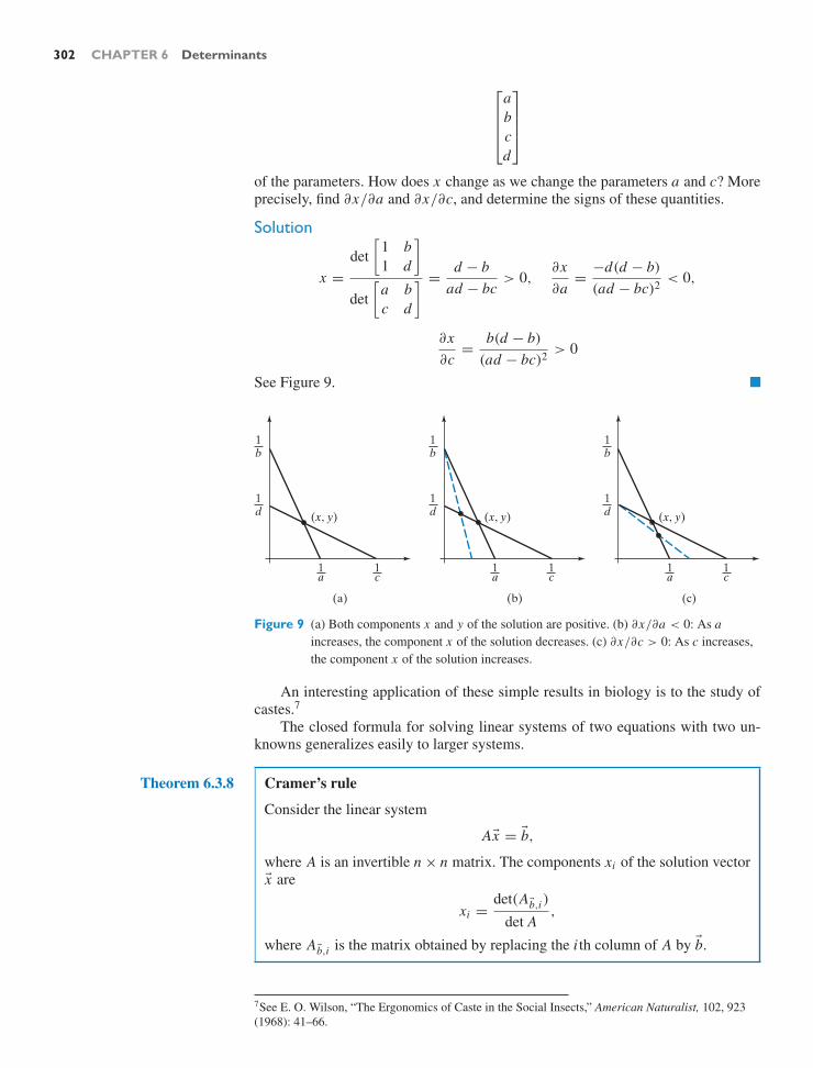
302 CHAPTER 6 Determinants
⎡
⎢⎢⎣
abcd
⎤
⎥⎥⎦
of the parameters. How does x change as we change the parameters a and c? Moreprecisely, find ∂x/∂a and ∂x/∂c, and determine the signs of these quantities.
Solution
x =det
[1 b1 d
]
det[
a bc d
] = d − bad − bc
> 0,∂x∂a
= −d(d − b)
(ad − bc)2 < 0,
∂x∂c
= b(d − b)
(ad − bc)2 > 0
See Figure 9. !
(x, y)
1b
1d
1b
1d
1b
1d (x, y) (x, y)
(a) (b) (c)
1a
1c
1a
1c
1a
1c
Figure 9 (a) Both components x and y of the solution are positive. (b) ∂x/∂a < 0: As aincreases, the component x of the solution decreases. (c) ∂x/∂c > 0: As c increases,the component x of the solution increases.
An interesting application of these simple results in biology is to the study ofcastes.7
The closed formula for solving linear systems of two equations with two un-knowns generalizes easily to larger systems.
Theorem 6.3.8 Cramer’s rule
Consider the linear system
Ax = b,
where A is an invertible n × n matrix. The components xi of the solution vectorx are
xi =det(Ab,i )
det A,
where Ab,i is the matrix obtained by replacing the i th column of A by b.
7See E. O. Wilson, “The Ergonomics of Caste in the Social Insects,” American Naturalist, 102, 923(1968): 41–66.

6.3 Geometrical Interpretations of the Determinant; Cramer’s Rule 303
This result is due to the Swiss mathematician Gabriel Cramer (1704–1752).The rule appeared in an appendix to his 1750 book, Introduction a l’analyse deslignes courbes algebriques.
Proof Write A =[w1 w2 · · · wi · · · wn
]. If x is the solution of the system Ax =
b, then
det (Ab,i ) = det[w1 w2 · · · b · · · wn
]
= det[w1 w2 · · · Ax · · · wn
]
= det[w1 w2 · · · (x1w1 + x2w2 + · · · + xi wi + · · · + xnwn) · · · wn
]
= det[w1 w2 · · · xi wi · · · wn
]
= xi det[w1 w2 · · · wi · · · wn
]
= xi det A.
Note that we have used the linearity of the determinant in the i th column (Theo-rem 6.2.2).
Therefore,
xi =det(Ab,i )
det A. !
Cramer’s rule allows us to find a closed formula for A−1, generalizing the result[
a bc d
]−1
= 1det A
[d −b
−c a
]
for 2 × 2 matrices.Consider an invertible n × n matrix A and write
A−1 =
⎡
⎢⎢⎢⎣
m11 m12 · · · m1 j · · · m1n
m21 m22 · · · m2 j · · · m2n...
......
...
mn1 mn2 · · · mnj · · · mnn
⎤
⎥⎥⎥⎦.
We know that AA−1 = In . Picking out the j th column of A−1, we find that
A
⎡
⎢⎢⎢⎣
m1 j
m2 j...
mnj
⎤
⎥⎥⎥⎦= e j .
By Cramer’s rule, mi j = det(Ae j ,i )/ det A.
Ae j ,i =
⎡
⎢⎢⎢⎢⎢⎢⎢⎢⎣
a11 a12 · · · 0 · · · a1n
a21 a22 · · · 0 · · · a2n...
......
...
a j1 a j2 · · · 1 · · · a jn...
......
...
an1 an2 · · · 0 · · · ann
⎤
⎥⎥⎥⎥⎥⎥⎥⎥⎦← j th row
↑i th column
Now det(Ae j ,i ) = (−1)i+ j det(A ji ) by Laplace expansion down the i th column, sothat

304 CHAPTER 6 Determinants
mi j = (−1)i+ j det(A ji )
det A.
We have shown the following result.
Theorem 6.3.9 Adjoint and inverse of a matrix
Consider an invertible n × n matrix A. The classical adjoint adj(A) is the n × nmatrix whose i j th entry is (−1)i+ j det(A ji ). Then
A−1 = 1det A
adj(A).
For an invertible 2 × 2 matrix A =[
a bc d
], we find
adj(A) =[
d −b−c a
]and A−1 = 1
ad − bc
[d −b
−c a
].
Compare this with Theorem 2.4.9.For an invertible 3 × 3 matrix
A =
⎡
⎣a b cd e fg h k
⎤
⎦ ,
the formula is
A−1 = 1det A
⎡
⎣ek − f h ch − bk b f − cef g − dk ak − cg cd − a fdh − eg bg − ah ae − bd
⎤
⎦ .
We can interpret Cramer’s rule geometrically.
EXAMPLE 5 For the vectors w1, w2, and b shown in Figure 10, consider the linear systemAx = b, where A =
[w1 w2
].
w2
w1
b
Figure 10
Using the terminology introduced in Cramer’s rule, let Ab,2 =[w1 b
]. Note
that det(A) and det(Ab,2) are both positive, according to Theorem 2.4.10. Cramer’srule tells us that
x2 =det(Ab,2)
det Aor det(Ab,2) = x2 det A.
Explain this last equation geometrically, in terms of areas of parallelograms.
SolutionWe can write the system Ax = b as x1w1 + x2w2 = b. The geometrical solution isshown in Figure 11.

6.3 Geometrical Interpretations of the Determinant; Cramer’s Rule 305
w2
w1
x2w2
x1w1
b
Cramer’s rule:
x2 =det w1 b
det w1 w2
Figure 11
Now,
det(Ab,2) = det[w1 b
]= area of the parallelogram defined by w1 and b
= area of the parallelogram8 defined by w1 and x2w2
= x2(area of the parallelogram9 defined by w1 and w2)
= x2 det A,
as claimed. Note that this geometrical proof mimics the algebraic proof of Cramer’srule, Theorem 6.3.8. !
The ambitious and artistically inclined reader is encouraged to draw an anal-ogous figure illustrating Cramer’s rule for a system of three linear equations withthree unknowns.
8The two parallelograms have the same base and the same height.9Again, think about base and height.
EXERCISES 6.3GOAL Interpret the determinant as an area or volumeand as an expansion factor. Use Cramer’s rule.
1. Find the area of the parallelogram defined by[
37
]and
[82
].
2. Find the area of the triangle defined by[
37
]and
[82
].
37
82
3. Find the area of the triangle below.
57
43
101
4. Consider the area A of the triangle with vertices[
a1a2
],
[b1b2
],[
c1c2
]. Express A in terms of
det
⎡
⎣a1 b1 c1a2 b2 c21 1 1
⎤
⎦ .

306 CHAPTER 6 Determinants
5. The tetrahedron defined by three vectors v1, v2, v3 in R3
is the set of all vectors of the form c1v1 + c2v2 + c3v3,where ci ≥ 0 and c1 + c2 + c3 ≤ 1. Explain why thevolume of this tetrahedron is one sixth of the volume ofthe parallelepiped defined by v1, v2, v3.
6. What is the relationship between the volume of thetetrahedron defined by the vectors
⎡
⎣a1a21
⎤
⎦ ,
⎡
⎣b1b21
⎤
⎦ ,
⎡
⎣c1c21
⎤
⎦
and the area of the triangle with vertices[
a1a2
],
[b1b2
],
[c1c2
]?
See Exercises 4 and 5. Explain this relationship geomet-rically. Hint: Consider the top face of the tetrahedron.
7. Find the area of the following region:
55
−77
−5−6
3−4
8. Demonstrate the equation
| det A| =∥∥∥v1
∥∥∥∥∥∥v⊥
2
∥∥∥ · · ·∥∥∥v⊥
n
∥∥∥
for a noninvertible n × n matrix A =[v1 v2 . . . vn
](Theorem 6.3.3).
9. If v1 and v2 are linearly independent vectors in R2,what is the relationship between det
[v1 v2
]and
det[v1 v⊥
2], where v⊥
2 is the component of v2orthogonal to v1?
10. Consider an n × n matrix A =[v1 v2 · · · vn
].
What is the relationship between the product∥v1∥∥v2∥ · · · ∥vn∥ and | det A|? When is | det A| =∥v1∥∥v2∥ · · · ∥vn∥?
11. Consider a linear transformation T (x) = Ax from R2
to R2. Suppose for two vectors v1 and v2 in R2 we haveT (v1) = 3v1 and T (v2) = 4v2. What can you say aboutdet A? Justify your answer carefully.
12. Consider those 4 × 4 matrices whose entries are all 1,−1, or 0. What is the maximal value of the determinantof a matrix of this type? Give an example of a matrixwhose determinant has this maximal value.
13. Find the area (or 2-volume) of the parallelogram (or 2-parallelepiped) defined by the vectors
⎡
⎢⎢⎣
1111
⎤
⎥⎥⎦ and
⎡
⎢⎢⎣
1234
⎤
⎥⎥⎦ .
14. Find the 3-volume of the 3-parallelepiped defined bythe vectors
⎡
⎢⎢⎣
1000
⎤
⎥⎥⎦ ,
⎡
⎢⎢⎣
1111
⎤
⎥⎥⎦ ,
⎡
⎢⎢⎣
1234
⎤
⎥⎥⎦ .
15. Demonstrate Theorem 6.3.6 for linearly dependent vec-tors v1, . . . , vm .
16. True or false? If * is a parallelogram in R3 and T (x) =Ax is a linear transformation from R3 to R3, then
area of T (*) = | det A|(area of *).
17. (For some background on the cross product in Rn , seeExercise 6.2.44.) Consider three linearly independentvectors v1, v2, v3 in R4.a. What is the relationship between V (v1, v2, v3) and
V (v1, v2, v3, v1 × v2 × v3)? See Definition 6.3.5.Exercise 6.2.44c is helpful.
b. Express V (v1, v2, v3, v1 × v2 × v3) in terms of∥v1 × v2 × v3∥.
c. Use parts (a) and (b) to express V (v1, v2, v3) interms of ∥v1 × v2 × v3∥. Is your result still true whenthe vi are linearly dependent?
(Note the analogy to the fact that for two vectors v1 andv2 in R3, ∥v1 × v2∥ is the area of the parallelogram de-fined by v1 and v2.)
18. If T (x) = Ax is an invertible linear transformationfrom R2 to R2, then the image T (*) of the unit circle* is an ellipse. See Exercise 2.2.54.
a. Sketch this ellipse when A =[
p 00 q
], where p
and q are positive. What is its area?b. For an arbitrary invertible transformation T (x) =
Ax , denote the lengths of the semimajor and semi-minor axes of T (*) by a and b, respectively. Whatis the relationship among a, b, and det(A)?
TΩ
T(Ω)
a
b

6.3 Geometrical Interpretations of the Determinant; Cramer’s Rule 307
c. For the transformation T (x) =[
3 11 3
]x , sketch
this ellipse and determine its axes. Hint: Consider
T[
11
]and T
[1
−1
].
19. A basis v1, v2, v3 of R3 is called positively oriented if v1encloses an acute angle with v2 × v3. Illustrate this def-inition with a sketch. Show that the basis is positivelyoriented if (and only if) det
[v1 v2 v3
]is positive.
20. We say that a linear transformation T from R3 to R3
preserves orientation if it transforms any positivelyoriented basis into another positively oriented basis.See Exercise 19. Explain why a linear transformationT (x) = Ax preserves orientation if (and only if) det Ais positive.
21. Arguing geometrically, determine whether the follow-ing orthogonal transformations from R3 to R3 preserveor reverse orientation. See Exercise 20.a. Reflection about a plane b. Reflection about a linec. Reflection about the origin
Use Cramer’s rule to solve the systems in Exercises 22through 24.
22.∣∣∣∣3x + 7y = 14x + 11y = 3
∣∣∣∣ 23.∣∣∣∣
5x1 − 3x2 = 1−6x1 + 7x2 = 0
∣∣∣∣
24.
∣∣∣∣∣∣
2x + 3y = 84y + 5z = 3
6x + 7z = −1
∣∣∣∣∣∣
25. Find the classical adjoint of the matrix
A =
⎡
⎣1 0 10 1 02 0 1
⎤
⎦ ,
and use the result to find A−1.
26. Consider an n×n matrix A with integer entries such thatdet A = 1. Are the entries of A−1 necessarily integers?Explain.
27. Consider two positive numbers a and b. Solve the fol-lowing system:
∣∣∣∣ax − by = 1bx + ay = 0
∣∣∣∣ .
What are the signs of the solutions x and y? How doesx change as b increases?
28. In an economics text,10 we find the following system:
sY + ar = I + GmY − hr = Ms − M.
Solve for Y and r .
29. In an economics text11 we find the following system:⎡
⎢⎢⎢⎢⎣
−R1 R1 −(1 − α)
α 1 − α −(1 − α)2
R2 −R2−(1 − α)2
α
⎤
⎥⎥⎥⎥⎦
⎡
⎣dx1dy1dp
⎤
⎦ =
⎡
⎣00
−R2de2
⎤
⎦ .
Solve for dx1, dy1, and dp. In your answer, you mayrefer to the determinant of the coefficient matrix as D.(You need not compute D.) The quantities R1, R2, andD are positive, and α is between zero and one. If de2is positive, what can you say about the signs of dy1 anddp?
30. Find the classical adjoint of A =
⎡
⎣1 0 02 3 04 5 6
⎤
⎦.
31. Find the classical adjoint of A =
⎡
⎣1 1 11 2 31 6 6
⎤
⎦.
32. Find the classical adjoint of A =
⎡
⎢⎢⎣
0 0 0 10 1 0 00 0 1 01 0 0 0
⎤
⎥⎥⎦.
33. Find the classical adjoint of A =
⎡
⎢⎢⎣
1 0 0 00 2 0 00 0 3 00 0 0 4
⎤
⎥⎥⎦.
34. For an invertible n × n matrix A, find the productA(adjA). What about (adj A)(A)?
35. For an invertible n×n matrix A, what is the relationshipbetween det(A) and det(adj A)?
36. For an invertible n × n matrix A, what is adj(adj A)?
37. For an invertible n×n matrix A, what is the relationshipbetween adj(A) and adj(A−1)?
38. For two invertible n × n matrices A and B, what is therelationship between adj(A), adj(B), and adj(AB)?
39. If A and B are invertible n × n matrices, and if A issimilar to B, is adj(A) necessarily similar to adj(B)?
40. For an invertible n × n matrix A, consider the lineartransformation
T (x) =
⎡
⎢⎢⎢⎣
det(Ax,1)
det(Ax,2)...
det(Ax,n)
⎤
⎥⎥⎥⎦from Rn to Rn .
Express the standard matrix of T in terms of adj(A).10 Simon and Blume, Mathematics for Economists, Norton, 1994.
11 Simon and Blume, op. cit.
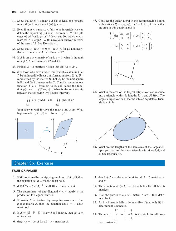
308 CHAPTER 6 Determinants
41. Show that an n × n matrix A has at least one nonzerominor if (and only if) rank(A) ≥ n − 1.
42. Even if an n × n matrix A fails to be invertible, we candefine the adjoint adj(A) as in Theorem 6.3.9. The i j thentry of adj(A) is (−1)i+ j det(A ji ). For which n × nmatrices A is adj(A) = 0? Give your answer in termsof the rank of A. See Exercise 41.
43. Show that A(adjA) = 0 = (adjA)A for all noninvert-ible n × n matrices A. See Exercise 42.
44. If A is an n × n matrix of rank n − 1, what is the rankof adj(A)? See Exercises 42 and 43.
45. Find all 2 × 2 matrices A such that adj(A) = AT .
46. (For those who have studied multivariable calculus.) LetT be an invertible linear transformation from R2 to R2,represented by the matrix M . Let *1 be the unit squarein R2 and *2 its image under T . Consider a continuousfunction f (x, y) from R2 to R, and define the func-tion g(u, v) = f
(T (u, v)
). What is the relationship
between the following two double integrals?∫∫
*2
f (x, y) d A and∫∫
*1
g(u, v) d A
Your answer will involve the matrix M. Hint: Whathappens when f (x, y) = 1, for all x, y?
v
u
Ω1
y
x
Ω2
f
T
g
R
47. Consider the quadrilateral in the accompanying figure,with vertices Pi = (xi , yi ), for i = 1, 2, 3, 4. Show thatthe area of this quadrilateral is
12
(det
[x1 x2y1 y2
]+ det
[x2 x3y2 y3
]
+ det[
x3 x4y3 y4
]+ det
[x4 x1y4 y1
]).
P3 P2
P1
P4
48. What is the area of the largest ellipse you can inscribeinto a triangle with side lengths 3, 4, and 5? Hint: Thelargest ellipse you can inscribe into an equilateral trian-gle is a circle.
49. What are the lengths of the semiaxes of the largest el-lipse you can inscribe into a triangle with sides 3, 4, and5? See Exercise 48.
Chapter Six Exercises
TRUE OR FALSE?
1. If B is obtained be multiplying a column of A by 9, thenthe equation det B = 9 det A must hold.
2. det(A10) = (det A)10 for all 10 × 10 matrices A.
3. The determinant of any diagonal n × n matrix is theproduct of its diagonal entries.
4. If matrix B is obtained by swapping two rows of ann × n matrix A, then the equation det B = − det Amust hold.
5. If A =[
u v w]
is any 3 × 3 matrix, then det A =u · (v × w).
6. det(4A) = 4 det A for all 4 × 4 matrices A.
7. det(A + B) = det A + det B for all 5 × 5 matrices Aand B.
8. The equation det(−A) = det A holds for all 6 × 6matrices.
9. If all the entries of a 7 × 7 matrix A are 7, then det Amust be 77.
10. An 8 × 8 matrix fails to be invertible if (and only if) itsdeterminant is nonzero.
11. The matrix
⎡
⎣k2 1 4k −1 −21 1 1
⎤
⎦ is invertible for all posi-
tive constants k.

Chapter Six Exercises 309
12. det
⎡
⎢⎢⎣
0 1 0 00 0 1 00 0 0 11 0 0 0
⎤
⎥⎥⎦ = 1.
13. Matrix
⎡
⎢⎢⎣
9 100 3 75 4 100 8
100 9 8 76 5 4 100
⎤
⎥⎥⎦ is invertible.
14. If A is an invertible n × n matrix, then det(AT ) mustequal det(A−1).
15. If the determinant of a 4 × 4 matrix A is 4, then its rankmust be 4.
16. There exists a nonzero 4×4 matrix A such that det A =det(4A).
17. If two n×n matrices A and B are similar, then the equa-tion det A = det B must hold.
18. The determinant of all orthogonal matrices is 1.
19. If A is any n × n matrix, then det(AAT ) = det(AT A).
20. There exists an invertible matrix of the form⎡
⎢⎢⎣
a e f jb 0 g 0c 0 h 0d 0 i 0
⎤
⎥⎥⎦.
21. If all the entries of a square matrix are 1 or 0, then det Amust be 1, 0, or −1.
22. If all the entries of a square matrix A are integers anddet A = 1, then the entries of matrix A−1 must be inte-gers as well.
23. If all the columns of a square matrix A are unit vectors,then the determinant of A must be less than or equalto 1.
24. If A is any noninvertible square matrix, then det A =det(rref A).
25. If the determinant of a square matrix is −1, then A mustbe an orthogonal matrix.
26. If all the entries of an invertible matrix A are integers,then the entries of A−1 must be integers as well.
27. There exists a 4 × 4 matrix A whose entries are all 1 or−1, and such that det A = 16.
28. If the determinant of a 2 × 2 matrix A is 4, then theinequality ∥Av∥ ≤ 4∥v∥ must hold for all vectors vin R2.
29. If A =[
u v w]
is a 3 × 3 matrix, then the formuladet(A) = v · (u × w) must hold.
30. There exist invertible 2 × 2 matrices A and B such thatdet(A + B) = det A + det B.
31. There exist real invertible 3 × 3 matrices A and S suchthat S−1 AS = 2A.
32. There exist real invertible 3 × 3 matrices A and S suchthat ST AS = −A.
33. If A is any symmetric matrix, then det A = 1 ordet A=−1.
34. If A is any skew-symmetric 4 × 4 matrix, thendet A = 0.
35. If det A = det B for two n × n matrices A and B, thenA must be similar to B.
36. Suppose A is an n × n matrix and B is obtained fromA by swapping two rows of A. If det B < det A, then Amust be invertible.
37. If an n × n matrix A is invertible, then there must bean (n − 1) × (n − 1) submatrix of A (obtained bydeleting a row and a column of A) that is invertible aswell.
38. If all the entries of matrices A and A−1 are integers,then the equation det A = det(A−1) must hold.
39. If a square matrix A is invertible, then its classical ad-joint adj(A) is invertible as well.
40. There exists a real 3 × 3 matrix A such that A2 = −I3.
41. If all the diagonal entries of an n × n matrix A are oddintegers and all the other entries are even integers, thenA must be an invertible matrix.12
42. If all the diagonal entries of an n × n matrix A are evenintegers and all the other entries are odd integers, thenA must be an invertible matrix.12
43. For every nonzero 2 × 2 matrix A there exists a 2 × 2matrix B such that det(A + B) = det A + det B.
44. If A is a 4×4 matrix whose entries are all 1 or −1, thendet A must be divisible by 8 (i.e., det A = 8k for someinteger k).
45. If A is an invertible n ×n matrix, then A must commutewith its adjoint, adj(A).
46. There exists a real number k such that the matrix⎡
⎢⎢⎣
1 2 3 45 6 k 78 9 8 70 0 6 5
⎤
⎥⎥⎦
is invertible.
47. If A and B are orthogonal n × n matrices such that detA = det B = 1, then matrices A and B must commute.
12 The even integers are 0, ± 2, ± 4, . . ., while the odd integersare ± 1, ± 3, . . . .

C H A P T E R
7Eigenvalues and Eigenvectors
7.1 Diagonalization
Here is an introductory example to motivate the main theme of this chapter.
EXAMPLE 1 Consider the matrices
A =
⎡
⎢⎣
−1 0 0 00 0 0 00 0 1 00 0 0 2
⎤
⎥⎦ and B =
⎡
⎢⎣
1 2 3 45 6 7 89 8 7 65 4 3 2
⎤
⎥⎦ .
Find A5, B5, rank A, rank B, det A, and det B. Find bases of ker A and ker B.
(Partial) SolutionThe parts pertaining to the diagonal matrix A are easy to do, by inspection:
A5 =
⎡
⎢⎢⎣
(−1)5 0 0 00 0 0 00 0 15 00 0 0 25
⎤
⎥⎥⎦ =
⎡
⎢⎣
−1 0 0 00 0 0 00 0 1 00 0 0 32
⎤
⎥⎦ ,
where rank A = 3, the number of nonzero entries on the diagonal; det A = 0, theproduct of the diagonal entries; and a basis of ker A is e2 since the second columnof A is zero.
The corresponding computations for matrix B are doable, of course, but theyare much more tedious. We could compute rref B to find rank B, det B, and ker B,but then we still have to compute B5. !
Example 1 illustrates why we like to work with diagonal matrices wheneverpossible: They are easy to handle.
Let’s put in another plug for diagonal matrices.
310

7.1 Diagonalization 311
Consider the linear transformations
y =
⎡
⎣1 2 34 5 67 8 9
⎤
⎦ x and y =
⎡
⎣1 0 00 2 00 0 3
⎤
⎦ x,
represented by the equations
y1 = x1 +2x2 +3x3y2 = 4x1 +5x2 +6x3y3 = 7x1 +8x2 +9x3
andy1 = x1y2 = 2x2y3 = 3x3,
respectively. If we use arrows to represent the functional dependencies between thevariables, we see a tangled web of dependencies in the case of the first transfor-mation. In the case of the diagonal matrix, however, the web is untangled since thethree equations are uncoupled: We can deal with the three simple equations y1 = x1,y2 = 2x2, and y3 = 3x3 separately:
x1−−−−−−→−−−−−−−→
−−−−−→y1 x1−−−−−→y1
x2 −−−−−−→−−−−−−→−−−−−→y2 x2−−−−−→y2
x3 −−−−−−→−−−
−−−−→
−−−−−→y3 x3−−−−−→y3.
The idea behind diagonalization is to untangle the web of functional dependencieswe see on the left.
When dealing with a linear transformation T (x) = Ax from Rn to Rn , where Afails to be a diagonal matrix, we may be interested in finding a basis of Rn such thatthe matrix of T with respect to that basis is diagonal. In this context, the followingdefinition is useful.
Definition 7.1.1 Diagonalizable matrices
Consider a linear transformation T (x) = Ax from Rn to Rn . Then A (or T )is said to be diagonalizable if the matrix B of T with respect to some basis isdiagonal.
By Theorem 3.4.4 and Definition 3.4.5, matrix A is diagonalizable if (andonly if) A is similar to some diagonal matrix B, meaning that there exists aninvertible matrix S such that S−1 AS = B is diagonal.
To diagonalize a square matrix A means to find an invertible matrix S and adiagonal matrix B such that S−1 AS = B.
In Examples 9 and 10 of Section 3.4, we have seen that the reflection about
a line in R2 is diagonalizable, while the rotation T (x) =[
0 −11 0
]x fails to be
diagonalizable.Consider a linear transformation T (x) = Ax from Rn to Rn and a basis ! =
(v1, . . . , vn) for Rn . In Theorem 3.4.7 we learned that the !-matrix B of T is diag-onal if (and only if) Av1 = λ1v1, . . . , Avn = λn vn for some scalars λ1, . . . , λn . (Inthis context, it is customary to use the Greek letter lambda, λ, to denote the scalars.)
The diagram below reminds us why this result holds; nothing “deep” is goingon here.
Av1 Av2 . . . Avn
B =
⎡
⎢⎢⎣
λ1 0 . . . 00 λ2 . . . 0...
.... . .
...0 0 . . . λn
⎤
⎥⎥⎦
v1v2...vn
We can conclude that an n×n matrix A is diagonalizable if (and only if) there existsa basis v1, . . . , vn of Rn such that Av1 = λ1v1, . . . , Avn = λn vn for some scalarsλ1, . . . , λn .

312 CHAPTER 7 Eigenvalues and Eigenvectors
If we wish to diagonalize a matrix A, we need to find a basis of Rn consistingof vectors v such that
Av = λv, for some scalar λ.
It is sensible to introduce a name for vectors with this property.
Definition 7.1.2 Eigenvectors, eigenvalues, and eigenbases1
Consider a linear transformation T (x) = Ax from Rn to Rn .A nonzero vector v in Rn is called an eigenvector of A (or T ) if
Av = λv
for some scalar λ. This λ is called the eigenvalue associated with eigenvector v.A basis v1, . . . , vn of Rn is called an eigenbasis for A (or T ) if the vectors
v1, . . . , vn are eigenvectors of A, meaning that Av1 = λ1v1, . . . , Avn = λn vnfor some scalars λ1, . . . , λn .
A nonzero vector v in Rn is an eigenvector of A if Av is parallel to v, as shownin Figure 1. See Definition A.3 in the Appendix.
v
Av v
Av
Av = vv
Av = 2v
Av = 0
Av = v = 1v Av = −v = (−1)v Av = 0 = 0v
eigenvalue: 2 eigenvalue: 1 eigenvalue: −1 eigenvalue: 0
Figure 1
If v is an eigenvector of matrix A, with associated eigenvalue λ, then v is an eigen-vector of the matrices A2, A3, . . . as well, with
A2v = λ2v, A3v = λ3v, . . . , Am v = λm v,
for all positive integers m. The proof, by induction on m, is straightforward. Thebase case, A1v = Av = λv = λ1v, is given. As for the induction step, we haveAm+1v = A(Am v) =︸︷︷︸
step 2
A(λm v) = λm(Av) = λmλv = λm+1v. In step 2, we are
using the induction hypothesis, Am v = λm v.The important result below follows from the our work after Definition 7.1.1.
Theorem 7.1.3 Eigenbases and diagonalization
The matrix A is diagonalizable if (and only if) there exists an eigenbasis for A.If v1, . . . , vn is an eigenbasis for A, with Av1 = λ1v1, . . . , Avn = λn vn , thenthe matrices
S =
⎡
⎢⎢⎣
| | |v1 v2 . . . vn
| | |
⎤
⎥⎥⎦ and B =
⎡
⎢⎢⎣
λ1 0 . . . 00 λ2 . . . 0...
.... . .
...0 0 . . . λn
⎤
⎥⎥⎦
will diagonalize A, meaning that S−1 AS = B.
1From German eigen: proper, characteristic. (The words eigen and own have a commonIndo-European root.)

7.1 Diagonalization 313
Theorem 7.1.3 Eigenbases and diagonalization (Continued)
Conversely, if the matrices S and B diagonalize A, then the column vectorsof S will form an eigenbasis for A, and the diagonal entries of B will be theassociated eigenvalues.
Above, we explained Theorem 7.1.3 in terms of a change of basis. Equiva-lently, we can prove the result by using matrix products. Here we will prove justone implication, leaving the other as Exercise 23 to the reader.
Suppose there exists an eigenbasis v1, . . . , vn for A, and define S and B as inTheorem 7.1.3. Then
AS = A
⎡
⎢⎣| | |v1 v2 . . . vn
| | |
⎤
⎥⎦ =
⎡
⎢⎣| | |
Av1 Av2 . . . Avn
| | |
⎤
⎥⎦ =
⎡
⎢⎣| | |
λ1v1 λ2v2 . . . λn vn
| | |
⎤
⎥⎦
=
⎡
⎢⎢⎣
| | |v1 v2 . . . vn
| | |
⎤
⎥⎥⎦
⎡
⎢⎢⎣
λ1 0 . . . 00 λ2 . . . 0...
.... . .
...0 0 . . . λn
⎤
⎥⎥⎦ = SB,
showing that S−1 AS = B, as claimed.
EXAMPLE 2 Find all eigenvectors and eigenvalues of the identity matrix In . Is there an eigenbasisfor In? Is In diagonalizable?
SolutionSince In v = v = 1v for all v in Rn , all nonzero vectors in Rn are eigenvectors ofIn , with associated eigenvalue 1.
Thus, all bases of Rn are eigenbases for In .Clearly, In is diagonalizable; it’s a diagonal matrix already. If S is any invertible
matrix, then S−1 In S = In is diagonal. !EXAMPLE 3 Consider the linear transformation T (x) =
[0.64 0.480.48 0.36
]x . We are told that
T (x) = Ax represents the orthogonal projection onto the line L = span[
43
].
See Example 2 of Section 2.2. Describe the eigenvectors of A geometrically, andfind all eigenvalues of A. Is there an eigenbasis for A? Diagonalize matrix A if youcan.
SolutionWe find the eigenvectors of A by inspection. Can you think of any nonzero vectorsv in R2 such that T (v) = Av is a scalar multiple of v? Clearly, any nonzero vectorv parallel to L will do, with Av = v = 1v, as well as any nonzero vector wperpendicular to L , with Aw = 0 = 0w. The eigenvalues of A are 1 and 0. Notethat the eigenvectors with eigenvalue 0 are the nonzero vectors in the kernel of A.
For example, v =[
43
]is an eigenvector with eigenvalue 1, and w =
[−34
]
is an eigenvector with eigenvalue 0. See Figure 2. Thus, ! = (v, w) will be aneigenbasis for A, and the !-matrix B of T will be the diagonal matrix
T (v) T (w)
B =[
1 00 0
]vw
.
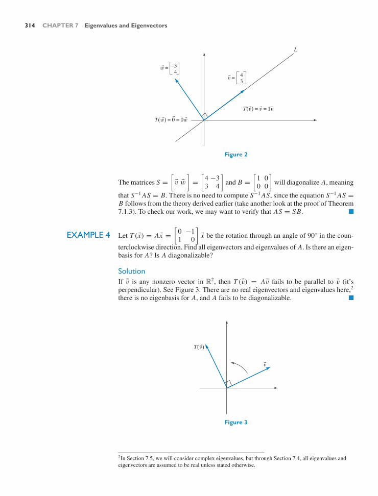
314 CHAPTER 7 Eigenvalues and Eigenvectors
L
w =
T(w) = 0 = 0w
T(v) = v = 1v
−34
v = 43
Figure 2
The matrices S =[
v w
]=
[4 −33 4
]and B =
[1 00 0
]will diagonalize A, meaning
that S−1 AS = B. There is no need to compute S−1 AS, since the equation S−1 AS =B follows from the theory derived earlier (take another look at the proof of Theorem7.1.3). To check our work, we may want to verify that AS = SB. !
EXAMPLE 4 Let T (x) = Ax =[
0 −11 0
]x be the rotation through an angle of 90 in the coun-
terclockwise direction. Find all eigenvectors and eigenvalues of A. Is there an eigen-basis for A? Is A diagonalizable?
SolutionIf v is any nonzero vector in R2, then T (v) = Av fails to be parallel to v (it’sperpendicular). See Figure 3. There are no real eigenvectors and eigenvalues here,2
there is no eigenbasis for A, and A fails to be diagonalizable. !
v
T(v)
Figure 3
2In Section 7.5, we will consider complex eigenvalues, but through Section 7.4, all eigenvalues andeigenvectors are assumed to be real unless stated otherwise.

7.1 Diagonalization 315
EXAMPLE 5 What are the possible real eigenvalues of an orthogonal3 n × n matrix A?
SolutionIf A is an orthogonal matrix, then the linear transformation T (x) = Ax preserveslength, by Definition 5.3.1: We have ∥T (x)∥ = ∥Ax∥ = ∥x∥ for all x in Rn .Consider an eigenvector v of A, with associated eigenvalue λ,
Av = λv.
Then
∥v∥ = ∥Av∥ = ∥λv∥ = |λ|∥v∥,
so that |λ| = 1. We conclude that λ = 1 or λ = −1.
For example, consider the reflection matrix A =[
1 00 −1
], with Ae1 = e1 =
1e1 and Ae2 = −e2 = (−1)e2, so that 1 and −1 are the eigenvalues of A. !
Theorem 7.1.4 The possible real eigenvalues of an orthogonal matrix are 1 and −1.
EXAMPLE 6 For which n × n matrices A is 0 an eigenvalue? Give your answer in terms of thekernel of A and also in terms of the invertibility of A.
SolutionBy definition, 0 is an eigenvalue of A if there exists a nonzero vector v in Rn suchthat Av = 0v = 0, meaning that there exists a nonzero vector in the kernel of A.Thus, 0 is an eigenvalue of A if (and only if) ker A = 0, meaning that A fails tobe invertible. !
Example 6 allows us to update our “Summary on invertible matrices.” Comparethis with Summary 3.3.10.
SUMMARY 7.1.5 Various characterizations of invertible matrices
For an n × n matrix A, the following statements are equivalent.
i. A is invertible.ii. The linear system Ax = b has a unique solution x , for all b in Rn .
iii. rref A = ln .iv. rank A = n.v. im A = Rn .
vi. ker A = 0.vii. The column vectors of A form a basis of Rn .
viii. The column vectors of A span Rn .ix. The column vectors of A are linearly independent.x. det A = 0.
xi. 0 fails to be an eigenvalue of A.
Characterization (x) was given in Theorem 6.2.4.
3Example 5 and Theorem 7.1.4 are for those who have studied Chapter 5.

316 CHAPTER 7 Eigenvalues and Eigenvectors
Dynamical Systems and Eigenvectors (optional)Dynamical systems provide a powerful application of eigenvalues and eigenvectors.We start with a somewhat lighthearted example, but a wealth of relevant exam-ples can be found in applied mathematics, physics, chemistry, biology, engineering,computer science, economics, and the theory of finance. In Section 7.4 we will re-cast the theory of transition matrices in terms of a dynamical system. See Example 9of Section 2.1.
EXAMPLE 7 A stretch of desert in northwestern Mexico is populated mainly by two species ofanimals: coyotes and roadrunners. We wish to model the populations c(t) and r(t)of coyotes and roadrunners t years from now if the current populations c0 and r0are known.4
For this habitat, the following equations model the transformation of this sys-tem from one year to the next, from time t to time (t + 1):
∣∣∣∣c(t + 1) = 0.86c(t) + 0.08r(t)r(t + 1) = −0.12c(t) + 1.14r(t)
∣∣∣∣ .
Why is the coefficient of c(t) in the first equation less than 1, while the coefficientof r(t) in the second equation exceeds 1? What is the practical significance of thesigns of the other two coefficients, 0.08 and −0.12?
The two equations can be written in matrix form, as[
c(t + 1)
r(t + 1)
]=
[0.86c(t) + 0.08r(t)
−0.12c(t) + 1.14r(t)
]=
[0.86 0.08
−0.12 1.14
] [c(t)r(t)
].
The vector
x(t) =[
c(t)r(t)
]
is called the state vector of the system at time t , because it completely describesthis system at time t . If we let
A =[
0.86 0.08−0.12 1.14
],
we can write the preceding matrix equation more succinctly as
x(t + 1) = Ax(t).
The transformation the system undergoes over the period of one year is linear, rep-resented by the matrix A:
x(t)A−→ x(t + 1).
Suppose we know the initial state
x(0) = x0 =[
c0
r0
].
We wish to find x(t), for an arbitrary positive integer t :
x(0)A−→ x(1)
A−→ x(2)A−→ x(3)
A−→ · · · A−→ x(t)A−→ · · · .
4The point of this lighthearted story is to present an introductory example where neither messy datanor a complicated scenario distracts us from the mathematical ideas we wish to develop.

7.1 Diagonalization 317
We can find x(t) by applying the transformation t times to x(0):
x(t) = At x(0) = At x0.
Although it is extremely tedious to find x(t) with paper and pencil for large t , wecan easily compute x(t) using technology. For example, given
x0 =[
100100
],
we find that
x(10) = A10 x0 ≈[
80170
].
To understand the long-term behavior of this system and how it depends on theinitial values, we must go beyond numerical experimentation. It would be useful tohave closed formulas for c(t) and r(t), expressing these quantities as functions oft . We will first do this for certain (carefully chosen) initial state vectors.
Case 1 ! Suppose we have c0 = 100 and r0 = 300. Initially, there are 100 coyotes
and 300 roadrunners, so that x0 =[
100300
]. Then
x(1) = Ax0 =[
0.86 0.08−0.12 1.14
] [100300
]=
[110330
]= 1.1
[100300
]= 1.1x0.
The equation Ax0 = 1.1x0 tells us that x0 is an eigenvector of A with associatedeigenvalue 1.1. See Figure 4. Each population will grow by 10% in the course ofthe next year. According to our remarks after Definition 7.1.2, we have
x(t) = At x0 = (1.1)t x0.
We keep multiplying the state vector by 1.1 each time we multiply with matrix A.
x0 = 100 300
x(1) = 110 330 = 1.1x0
Figure 4
Recall that our goal is to find closed formulas for c(t) and r(t). We have
x(t) =[
c(t)r(t)
]= 1.1t x0 = 1.1t
[100300
],
so that
c(t) = 100(1.1)t and r(t) = 300(1.1)t .
Both populations will grow exponentially, by 10% each year.
Case 2 ! Suppose we have c0 = 200 and r0 = 100. Then
x(1) = Ax0 =[
0.86 0.08−0.12 1.14
] [200100
]=
[18090
]= 0.9x0.
In this case, x0 turns out to be an eigenvector of A with associated eigenvalue 0.9.Both populations decline by 10% in the first year and will therefore decline another10% each subsequent year. Thus,
x(t) = At x0 = 0.9t x0,
so that
c(t) = 200(0.9)t and r(t) = 100(0.9)t .
The initial populations are mismatched: Too many coyotes are chasing too few road-runners, a bad state of affairs for both species.

318 CHAPTER 7 Eigenvalues and Eigenvectors
Case 3 ! Suppose we have c0 = r0 = 1,000. Then
x(1) = Ax0 =[
0.86 0.08−0.12 1.14
] [1,0001,000
]=
[940
1,020
].
Things are not working out as nicely as in the first two cases we considered: Theinitial state vector x0 fails to be an eigenvector of A in this case. Just by computingx(2), x(3), . . . , we could not easily detect a trend that would allow us to generateclosed formulas for c(t) and r(t). We have to look for another approach.
The idea is to work with the eigenbasis
v1 =[
100300
]and v2 =
[200100
]
considered in the first two cases. Any vector in R2 can be written uniquely as alinear combination of the eigenvectors v1 and v2. This holds in particular for theinitial state vector
x0 =[
1,0001,000
]
of the coyote–roadrunner system:
x0 = c1v1 + c2v2.
A straightforward computation shows that the coordinates are c1 = 2 and c2 = 4:
x0 = 2v1 + 4v2.
Recall that At v1 = (1.1)t v1 and At v2 = (0.9)t v2. Therefore,
x(t) = At x0 = At (2v1 + 4v2) = 2At v1 + 4At v2
= 2(1.1)t v1 + 4(0.9)t v2
= 2(1.1)t[
100300
]+ 4(0.9)t
[200100
].
Considering the components of this vector equation, we can now find closed for-mulas for c(t) and r(t):
c(t) = 200(1.1)t + 800(0.9)t
r(t) = 600(1.1)t + 400(0.9)t .
Since the terms involving 0.9t approach zero as t increases, both populations even-tually grow by about 10% a year, and their ratio r(t)/c(t) approaches 600/200 = 3.c(t)
r(t)
x(t) = c(t)r(t)
Figure 5Note that the ratio r(t)/c(t) can be interpreted as the slope of the state vector
x(t), as shown in Figure 5.Alternatively, we can derive the formula
x(t) = 2(1.1)t[
100300
]+ 4(0.9)t
[200100
]
by means of diagonalization. We can use the eigenbasis v1 =[
100300
], v2 =
[200100
]to form the invertible matrix S =
[100 200300 100
]. Then S−1 AS = B =
[1.1 00 0.9
]. See Theorem 7.1.3. Thus, A = SBS−1 and At = (SBS−1)t =

7.1 Diagonalization 319
(SBS−1)(SBS−1) · · · (SBS−1)︸ ︷︷ ︸t times
= SBt S−1. Now x(t) = SBt S−1 x0. We leave it
to the reader to verify that S−1 x0 =[
100 200300 100
]−1 [10001000
]=
[24
]. This is just the
coordinate vector of the initial state vector x0 with respect to the given eigenbasis(by Definition 3.4.1). Thus,
x(t) = SBt S−1 x0 =[
100 200300 100
] [1.1t 0
0 0.9t
] [24
]=
[100 200300 100
] [2(1.1)t
4(0.9)t
]
= 2(1.1)t[
100300
]+ 4(0.9)t
[200100
],
as expected.How can we represent the preceding computations graphically?Figure 6 shows the representation x0 = 2v1 + 4v2 of x0 as the sum of a vector
on L1 = span(v1) and a vector on L2 = span(v2). The formula
x(t) = (1.1)t 2v1 + (0.9)t 4v2
now tells us that the component in L1 grows by 10% each year, while the componentin L2 shrinks by 10%. The component (0.9)t 4v2 in L2 approaches 0, which meansthat the tip of the state vector x(t) approaches the line L1, so that the slope of thestate vector will approach 3, the slope of L1.
To show the evolution of the system more clearly, we can sketch just the end-points of the state vectors x(t). Then the changing state of the system will be tracedout as a sequence of points in the c–r -plane.
It is natural to connect the dots to create the illusion of a continuous trajectory.(Although, of course, we do not know what really happens between times t andt + 1.)
Sometimes we are interested in the state of the system in the past, at times−1, −2, . . . . Note that x(0) = Ax(−1), so that x(−1) = A−1 x0 if A is invertible(as in our example). Likewise, x(−t) = (At )−1 x0, for t = 2, 3, . . . . The trajectory(future and past) for our coyote–roadrunner system is shown in Figure 7.
1000
1000
r
c
x(10)
L1 = span(v1)
x(3)x(2)x(1)x0
2v1
v1 4v2
v2
L2 = span(v2)
Figure 6

320 CHAPTER 7 Eigenvalues and Eigenvectors
1000
1000
L1
L2
t = 10
t = 5
t = −5
t = 0
Past
Future
Present
r
c
Figure 7
To get a sense for the long-term behavior of this system and how it dependson the initial state, we can draw a rough sketch that shows a number of differenttrajectories, representing the various qualitative types of behavior. Such a sketch iscalled a phase portrait of the system. In our example, a phase portrait might showthe trajectory drawn in Figure 7, trajectories moving along the lines L1 and L2, aswell as a trajectory that starts above L1 and one that starts below L2. See Figure 8.
To sketch these trajectories, express the initial state vector x0 as the sum of avector w1 on L1 and a vector w2 on L2. Then see how these two vectors changeover time. If x0 = w1 + w2, then
x(t) = (1.1)t w1 + (0.9)t w2.
We see that the two populations will prosper over the long term if the ratio r0/c0of the initial populations exceeds 1/2; otherwise, both populations will die out.
r
c
L2 = span
L1 = span 100300
200100
Figure 8

7.1 Diagonalization 321
r
c
L1 L2
Figure 9
From a mathematical point of view, it is informative to sketch a phase portraitof this system in the whole c–r -plane, even though the trajectories outside the firstquadrant are meaningless in terms of our population study. See Figure 9. !
Let’s discuss the ideas and techniques developed in Example 7 more sys-tematically. Consider a physical system whose state at any given time t is de-scribed by some quantities x1(t), x2(t), . . . , xn(t). [In Example 7, there were twosuch quantities, the populations c(t) and r(t).] We can represent the quantitiesx1(t), x2(t), . . . , xn(t) by the state vector
x(t) =
⎡
⎢⎢⎢⎣
x1(t)x2(t)
...
xn(t)
⎤
⎥⎥⎥⎦.
Suppose that the state of the system at time t + 1 is determined by the state attime t and that the transformation of the system from time t to time t + 1 is linear,represented by an n × n matrix A:
x(t + 1) = Ax(t).
Then
x(t) = At x0.
Such a system is called a discrete linear dynamical system. (Discrete indicates thatwe model the change of the system from time t to time t + 1, rather than modelingthe continuous rate of change, which would be described by differential equations.)
For an initial state x0, it is often our goal to find closed formulas for x1(t), x2(t),. . . , xn(t) [i.e., formulas expressing xi (t) as a function of t alone, as opposed to arecursive formula, for example, which would merely express xi (t + 1) in terms ofx1(t), x2(t), . . . , xn(t)].
Theorem 7.1.6 Discrete dynamical systems
Consider the dynamical system
x(t + 1) = Ax(t) with x(0) = x0.

322 CHAPTER 7 Eigenvalues and Eigenvectors
Theorem 7.1.6 Discrete dynamical systems (Continued)
Then x(t) = At x0. Suppose we can find an eigenbasis v1, . . . , vn for A, withAv1 = λ1v1, . . . , Avn = λn vn . Find the coordinates c1, . . . , cn of the vector x0with respect to the eigenbasis v1, . . . , vn:
x0 = c1v1 + · · · + cn vn.
Then
x(t) = At x0 = c1 At v1 + · · · + cn At vn = c1λt1v1 + · · · + cnλ
tn vn.
Alternatively, we can derive the formula x(t) = c1λt1v1 + · · · + cnλ
tn vn by
means of diagonalization. See Example 7. If we let
S =
⎡
⎢⎢⎣
| | |v1 v2 . . . vn
| | |
⎤
⎥⎥⎦, B =
⎡
⎢⎢⎣
λ1 0 . . . 00 λ2 . . . 0...
.... . .
...0 0 . . . λn
⎤
⎥⎥⎦, and S−1 x0 =
⎡
⎢⎢⎣
c1c2...
cn
⎤
⎥⎥⎦, then
S−1 AS = B, A = SBS−1, and At = (SBS−1)t = (SBS−1)(SBS−1) · · · (SBS−1)︸ ︷︷ ︸t times
=
SBt S−1, so that
x(t) = At x0 = SBt S−1 x0 =
⎡
⎢⎢⎣
| | |v1 v2 . . . vn
| | |
⎤
⎥⎥⎦
⎡
⎢⎢⎣
λt1 0 . . . 0
0 λt2 . . . 0
......
. . ....
0 0 . . . λtn
⎤
⎥⎥⎦
⎡
⎢⎢⎣
c1c2...
cn
⎤
⎥⎥⎦
=
⎡
⎢⎢⎢⎣
| | |v1 v2 . . . vn
| | |
⎤
⎥⎥⎥⎦
⎡
⎢⎢⎢⎣
c1λt1
c2λt2
...
cnλtn
⎤
⎥⎥⎥⎦= c1λ
t1v1 + c2λ
t2v2 + · · · + cnλ
tn vn.
We are left with two questions: How can we find the eigenvalues and eigenvectors ofan n×n matrix A? When is there an eigenbasis for A, i.e., when is A diagonalizable?These issues are central to linear algebra; they will keep us busy for the rest of thislong chapter.
Definition 7.1.7 Discrete trajectories and phase portraits
Consider a discrete dynamical system
x(t + 1) = Ax(t) with initial value x(0) = x0,
where A is a 2 × 2 matrix. In this case, the state vector x(t) =[
x1(t)x2(t)
]can be
represented geometrically in the x1–x2-plane.The endpoints of state vectors x(0) = x0, x(1) = Ax0, x(2) = A2 x0, . . .
form the (discrete) trajectory of this system, representing its evolution in thefuture. Sometimes we are interested in the past states x(−1) = A−1 x0, x(−2) =(A2)−1 x0, . . . as well. It is suggestive to “connect the dots” to create the illusionof a continuous trajectory. Take another look at Figure 7.
A (discrete) phase portrait of the system x(t+1) = Ax(t) shows trajectoriesfor various initial states, capturing all the qualitatively different scenarios (as inFigure 9).

7.1 Diagonalization 323
L1 L1L1
L2 L2L2
(a) (b) (c)
Figure 10 (a) λ1 > λ2 > 1. (b) λ1 > 1 > λ2 > 0. (c) 1 > λ1 > λ2 > 0.
In Figure 10, we sketch phase portraits for the case when A has two eigenvaluesλ1 > λ2 > 0 with associated eigenvectors v1 and v2. We leave out the special casewhen one of the eigenvalues is 1. Start by sketching the trajectories along the linesL1 = span(v1) and L2 = span(v2). As you sketch the other trajectories
x(t) = c1λt1v1 + c2λ
t2v2,
think about the summands c1λt1v1 and c2λ
t2v2. Note that for a large positive t , the
vector x(t) will be almost parallel to L1, since λt1 will be much larger than λt
2.Likewise, for large negative t the vector x(t) will be almost parallel to L2.
EXERCISES 7.1GOAL Apply the concepts of eigenvalues, eigenvectors,eigenbases, and diagonalization. Use eigenvectors to ana-lyze discrete dynamical systems.
In Exercises 1 through 4, let A be an invertible n × nmatrix and v an eigenvector of A with associated eigen-value λ.
1. Is v an eigenvector of A3? If so, what is the eigenvalue?
2. Is v an eigenvector of A−1? If so, what is the eigen-value?
3. Is v an eigenvector of A + 2In? If so, what is the eigen-value?
4. Is v an eigenvector of 7A? If so, what is the eigenvalue?
5. If a vector v is an eigenvector of both A and B, is vnecessarily an eigenvector of A + B?
6. If a vector v is an eigenvector of both A and B, is vnecessarily an eigenvector of AB?
7. If v is an eigenvector of the n × n matrix A with asso-ciated eigenvalue λ, what can you say about
ker(A − λIn)?
Is the matrix A − λIn invertible?
8. Find all 2 × 2 matrices for which e1 =[
10
]is an eigen-
vector with associated eigenvalue 5.
9. Find all 2 × 2 matrices for which e1 is an eigenvector.
10. Find all 2 × 2 matrices for which[
12
]is an eigenvector
with associated eigenvalue 5.
11. Find all 2 × 2 matrices for which[
23
]is an eigenvector
with associated eigenvalue −1.
12. Consider the matrix A =[
2 03 4
]. Show that 2 and 4
are eigenvalues of A and find all corresponding eigen-vectors. Find an eigenbasis for A and thus diagonal-ize A.
13. Show that 4 is an eigenvalue of A =[
−6 6−15 13
]and
find all corresponding eigenvectors.
14. Find all 4 × 4 matrices for which e2 is an eigenvector.
Arguing geometrically, find all eigenvectors and eigen-values of the linear transformations in Exercises 15through 22. In each case, find an eigenbasis if you can,and thus determine whether the given transformation isdiagonalizable.
15. Reflection about a line L in R2
16. Rotation through an angle of 180 in R2
17. Counterclockwise rotation through an angle of 45 fol-lowed by a scaling by 2 in R2

324 CHAPTER 7 Eigenvalues and Eigenvectors
18. Reflection about a plane V in R3
19. Orthogonal projection onto a line L in R3
20. Rotation about the e3-axis through an angle of 90,counterclockwise as viewed from the positive e3-axisin R3
21. Scaling by 5 in R3
22. The linear transformation with T (v) = v and T (w) =v + w for the vectors v and w in R2 sketched below
v
w
23. Use matrix products to prove the following: IfS−1 AS = B for an invertible matrix S and a diago-nal matrix B, then the column vectors of S will form aneigenbasis for A, and the diagonal entries of B will bethe associated eigenvalues. See Theorem 7.1.3.
In Exercises 24 through 29, consider a dynamical system
x(t + 1) = Ax(t)
with two components. The accompanying sketch showsthe initial state vector x0 and two eigenvectors, v1 and v2,of A (with eigenvalues λ1 and λ2, respectively). For thegiven values of λ1 and λ2, sketch a rough trajectory. Con-sider the future and the past of the system.
v1
v2
x0
24. λ1 = 1.1, λ2 = 0.9 25. λ1 = 1, λ2 = 0.9
26. λ1 = 1.1, λ2 = 1 27. λ1 = 0.9, λ2 = 0.8
28. λ1 = 1.2, λ2 = 1.1 29. λ1 = 0.9, λ2 = 0.9
In Exercises 30 through 32, consider the dynamical system
x(t + 1) =[
1.1 00 λ
]x(t).
Sketch a phase portrait of this system for the given valuesof λ:
30. λ = 1.2 31. λ = 1 32. λ = 0.9
33. Find a 2 × 2 matrix A such that
x(t) =[
2t − 6t
2t + 6t
]
is a trajectory of the dynamical system
x(t + 1) = Ax(t).
34. Suppose v is an eigenvector of the n × n matrix A,with eigenvalue 4. Explain why v is an eigenvector ofA2 + 2A + 3In . What is the associated eigenvalue?
35. Show that similar matrices have the same eigenvalues.Hint: If v is an eigenvector of S−1 AS, then Sv is aneigenvector of A.
36. Find a 2 × 2 matrix A such that[
31
]and
[12
]are eigen-
vectors of A, with eigenvalues 5 and 10, respectively.
37. Consider the matrix
A =[
3 44 −3
].
a. Use the geometric interpretation of this transfor-mation as a reflection combined with a scaling tofind the eigenvalues of A.
b. Find an eigenbasis for A.c. Diagonalize A.
38. We are told that
⎡
⎣1
−1−1
⎤
⎦ is an eigenvector of the matrix
⎡
⎣4 1 1
−5 0 −3−1 −1 2
⎤
⎦; what is the associated eigenvalue?
39. Find a basis of the linear space V of all 2 × 2 matrices
A for which[
01
]is an eigenvector, and thus determine
the dimension of V .
40. Find a basis of the linear space V of all 2×2 matrices A
for which[
1−3
]is an eigenvector, and thus determine
the dimension of V .
41. Find a basis of the linear space V of all 2×2 matrices A
for which both[
11
]and
[12
]are eigenvectors, and thus
determine the dimension of V .
42. Find a basis of the linear space V of all 3 × 3 matrices
A for which both
⎡
⎣100
⎤
⎦ and
⎡
⎣001
⎤
⎦ are eigenvectors, and
thus determine the dimension of V .

7.1 Diagonalization 325
43. Consider the linear space V of all n × n matrices forwhich all the vectors e1, . . . , en are eigenvectors. De-scribe the space V (the matrices in V “have a name”),and determine the dimension of V .
44. For m ≤ n, find the dimension of the space of alln × n matrices A for which all the vectors e1, . . . , emare eigenvectors.
45. If v is any nonzero vector in R2, what is the dimensionof the space V of all 2 × 2 matrices for which v is aneigenvector?
46. If v is an eigenvector of matrix A with associated eigen-value 3, show that v is in the image of matrix A.
47. If v is an eigenvector of matrix A, show that v is in theimage of A or in the kernel of A. Hint: Exercise 46 is ishelpful.
48. If A is a matrix of rank 1, show that any nonzero vectorin the image of A is an eigenvector of A.
49. Give an example of a matrix A of rank 1 that fails to bediagonalizable.
Find an eigenbasis for each of the matrices A in Exercises50 through 54, and thus diagonalize A. Hint: Exercise 48is helpful.
50. A =[
1 32 6
]51. A =
[1 11 1
]52. A =
⎡
⎣1 1 11 1 11 1 1
⎤
⎦
53. A =
⎡
⎣1 2 32 4 63 6 9
⎤
⎦ 54. A =
⎡
⎣1 −1 1
−1 1 −11 −1 1
⎤
⎦
Arguing geometrically, find an eigenbasis for each of thematrices A in Exercises 55 through 63, and thus diagonal-ize A. Use Example 3 as a guide.
55. A =[
0.36 0.480.48 0.64
], representing the orthogonal projec-
tion onto the line L = span[
34
]
56. A =[
0.6 0.80.8 −0.6
], representing the reflection about the
line L = span[
21
]
57. A =[
0.8 −0.6−0.6 −0.8
]58. A =
[0 11 0
]
59. A = 19
⎡
⎣8 2 −22 5 4
−2 4 5
⎤
⎦, representing the orthogonal
projection onto the plane x − 2y + 2z = 0
60. A = 19
⎡
⎣7 4 −44 1 8
−4 8 1
⎤
⎦, representing the reflection
about the plane x − 2y + 2z = 0
61. A = 17
⎡
⎣6 −2 −3
−2 3 −6−3 −6 −2
⎤
⎦, representing the reflection
about a plane E
62. A = 114
⎡
⎣13 −2 −3−2 10 −6−3 −6 5
⎤
⎦, representing the orthogonal
projection onto a plane E
63. A = 114
⎡
⎣1 2 32 4 63 6 9
⎤
⎦
64. In all parts of this problem, let V be the linear space of
all 2 × 2 matrices for which[
12
]is an eigenvector.
a. Find a basis of V and thus determine the dimensionof V .
b. Consider the linear transformation T (A) = A[
12
]
from V to R2. Find a basis of the image of T and abasis of the kernel of T . Determine the rank of T .
c. Consider the linear transformation L(A) = A[
13
]
from V to R2. Find a basis of the image of L and abasis of the kernel of L . Determine the rank of L .
65. Consider an n ×n matrix A. A subspace V of Rn is saidto be A-invariant if Av is in V for all v in V . Describeall the one-dimensional A-invariant subspaces of Rn , interms of the eigenvectors of A.
66. a. Give an example of a 3 × 3 matrix A with as manynonzero entries as possible such that both span(e1)and span(e1, e2) are A-invariant subspaces of R3.See Exercise 65.
b. Consider the linear space V of all 3 × 3 matricesA such that both span (e1) and span (e1, e2) areA-invariant subspaces of R3. Describe the space V(the matrices in V “have a name”), and determinethe dimension of V .
67. Consider the coyotes–roadrunner system discussed inExample 7. Find closed formulas for c(t) and r(t), forthe initial populations c0 = 100, r0 = 800.
68. Two interacting populations of hares and foxes can bemodeled by the recursive equations
h(t + 1) = 4h(t) − 2 f (t)
f (t + 1) = h(t) + f (t).
For each of the initial populations given in parts (a)through (c), find closed formulas for h(t) and f (t).

326 CHAPTER 7 Eigenvalues and Eigenvectors
a. h(0) = f (0) = 100b. h(0) = 200, f (0) = 100c. h(0) = 600, f (0) = 500
69. Two interacting populations of coyotes and roadrunnerscan be modeled by the recursive equations
c(t + 1) = 0.75r(t)r(t + 1) = −1.5c(t) + 2.25r(t).
For each of the initial populations given in parts (a)through (c), find closed formulas for c(t) and r(t).a. c(0) = 100, r(0) = 200b. c(0) = r(0) = 100c. c(0) = 500, r(0) = 700
70. Imagine that you are diabetic and have to pay closeattention to how your body metabolizes glucose. Letg(t) represent the excess glucose concentration in yourblood, usually measured in milligrams of glucose per100 milliliters of blood. (Excess means that we mea-sure how much the glucose concentration deviates fromyour fasting level, i.e., the level your system approachesafter many hours of fasting.) A negative value of g(t)indicates that the glucose concentration is below fast-ing level at time t . Shortly after you eat a heavy meal,the function g(t) will reach a peak, and then it willslowly return to 0. Certain hormones help regulate glu-cose, especially the hormone insulin. Let h(t) repre-sent the excess hormone concentration in your blood.Researchers have developed mathematical models forthe glucose regulatory system. The following is onesuch model, in slightly simplified form (these formulasapply between meals; obviously, the system is disturbedduring and right after a meal):
∣∣∣∣g(t + 1) = ag(t) − bh(t)h(t + 1) = cg(t) + dh(t)
∣∣∣∣ ,
where time t is measured in minutes; a and d are con-stants slightly less than 1; and b and c are small positiveconstants. For your system, the equations might be
∣∣∣∣g(t + 1) = 0.978g(t) − 0.006h(t)h(t + 1) = 0.004g(t) + 0.992h(t)
∣∣∣∣ .
The term −0.006h(t) in the first equation is negative,because insulin helps your body absorb glucose. Theterm 0.004g(t) is positive, because glucose in yourblood stimulates the cells of the pancreas to secrete in-sulin. (For a more thorough discussion of this model,read E. Ackerman et al., “Blood glucose regulationand diabetes,” Chapter 4 in Concepts and Models ofBiomathematics, Marcel Dekker, 1969.)
Consider the coefficient matrix
A =[
0.978 −0.0060.004 0.992
]
of this dynamical system.
a. We are told that[−1
2
]and
[3
−1
]are eigenvectors
of A. Find the associated eigenvalues.b. After you have consumed a heavy meal, the concen-
trations in your blood are g0 = 100 and h0 = 0.Find closed formulas for g(t) and h(t). Sketch thetrajectory. Briefly describe the evolution of this sys-tem in practical terms.
c. For the case discussed in part (b), how long doesit take for the glucose concentration to fall belowfasting level? (This quantity is useful in diagnosingdiabetes: A period of more than four hours may in-dicate mild diabetes.)
71. Three holy men (let’s call them Anselm, Benjamin,and Caspar) put little stock in material things; theironly earthly possession is a small purse with a bit ofgold dust. Each day they get together for the followingbizarre bonding ritual: Each of them takes his purse andgives his gold away to the two others, in equal parts. Forexample, if Anselm has 4 ounces one day, he will give2 ounces each to Benjamin and Caspar.a. If Anselm starts out with 6 ounces, Benjamin with 1
ounce, and Caspar with 2 ounces, find formulas forthe amounts a(t), b(t), and c(t) each will have aftert distributions.
Hint: The vectors
⎡
⎣111
⎤
⎦,
⎡
⎣1
−10
⎤
⎦, and
⎡
⎣10
−1
⎤
⎦ will be
useful.b. Who will have the most gold after one year, that is,
after 365 distributions?
72. Consider the growth of a lilac bush. The state of thislilac bush for several years (at year’s end) is shown inthe accompanying sketch. Let n(t) be the number ofnew branches (grown in the year t) and a(t) the num-ber of old branches. In the sketch, the new branches arerepresented by shorter lines. Each old branch will growtwo new branches in the following year. We assume thatno branches ever die.
year 0
n(0) = 1a(0) = 0
n(1) = 0a(1) = 1
year 1
n(2) = 2a(2) = 1
year 2
n(3) = 2a(3) = 3
year 3
n(4) = 6a(4) = 5
year 4
a. Find the matrix A such that[
n(t + 1)
a(t + 1)
]= A
[n(t)a(t)
].
b. Verify that[
11
]and
[2
−1
]are eigenvectors of A.
Find the associated eigenvalues.c. Find closed formulas for n(t) and a(t).

7.2 Finding the Eigenvalues of a Matrix 327
7.2 Finding the Eigenvalues of a Matrix
In the previous section, we used eigenvalues to diagonalize a matrix A and to ana-lyze the dynamical system
x(t + 1) = Ax(t).
Now we will see how we can actually find those eigenvalues.Consider an n × n matrix A and a scalar λ. By Definition 7.1.2, λ is an eigen-
value of A if there exists a nonzero vector v in Rn such that
Av = λv or Av − λv = 0 or Av − λIn v = 0 or (A − λIn)v = 0.
This means, by definition of the kernel, that
ker(A − λIn) = 0.
(That is, there are other vectors in the kernel besides the zero vector.) This is thecase if (and only if) the matrix A − λIn fails to be invertible (by Theorem 3.1.7c),that is, if det(A − λIn) = 0 (by Theorem 6.2.4).
Theorem 7.2.1 Eigenvalues and determinants; characteristic equation
Consider an n ×n matrix A and a scalar λ. Then λ is an eigenvalue5 of A if (andonly if)
det(A − λIn) = 0.
This is called the characteristic equation (or the secular equation) of matrix A.
Let’s write the observations we made previously as a string of equivalentstatements.
λ is an eigenvalue of A.PRThere exists a nonzero vector v such that
Av = λv or (A − λIn)v = 0.PR
ker(A − λIn) = 0.PRMatrix A − λIn fails to be invertible.PR
det(A − λIn) = 0.
The idea of the characteristic equation is implicit in the work of Jeand’Alembert (1717–1783), in his Traite de Dynamique of 1743. Joseph LouisLagrange (1736–1813) was the first to study the equation systematically (naming itequation seculaire), in his works on gravitational attraction between heavenly bod-ies. Augustin-Louis Cauchy (1789–1857) wrote the equation in its modern form,involving a determinant. It appears that the term eigenvalue (Eigenwert in German)
5Alternatively, the eigenvalues are the solutions of the equation det(λIn − A) = 0. Our formuladet(A − λIn) = 0 is usually more convenient for numerical work.

328 CHAPTER 7 Eigenvalues and Eigenvectors
was first used by David Hilbert in 1904, based perhaps on Helmholtz’s notion of anEigenton in acoustics.
EXAMPLE 1 Find the eigenvalues of the matrix
A =[
1 24 3
].
SolutionBy Theorem 7.2.1, we have to solve the characteristic equation det(A − λI2) = 0.Now
det(A − λI2) = det([
1 24 3
]−
[λ 00 λ
])= det
[1 − λ 2
4 3 − λ
]
= (1 − λ)(3 − λ) − 2 · 4 = λ2 − 4λ − 5 = (λ − 5)(λ + 1) = 0.
The equation det(A − λI2) = (λ − 5)(λ + 1) = 0 holds for λ1 = 5 and λ2 = −1.These two scalars are the eigenvalues of A. In Section 7.3 we will find the corre-sponding eigenvectors. !
EXAMPLE 2 Find the eigenvalues of
A =
⎡
⎣2 3 40 3 40 0 4
⎤
⎦ .
SolutionWe have to solve the characteristic equation det(A − λI3) = 0.
det(A − λI3) = det
⎡
⎣2 − λ 3 4
0 3 − λ 40 0 4 − λ
⎤
⎦step 2︷︸︸︷= (2 − λ)(3 − λ)(4 − λ) = 0
In step 2 we use the fact that the determinant of a triangular matrix is the productof its diagonal entries (Theorem 6.1.4). The solutions of the characteristic equationare 2, 3, and 4; these are the eigenvalues of A. !
Theorem 7.2.2 Eigenvalues of a triangular matrix
The eigenvalues of a triangular matrix are its diagonal entries.
EXAMPLE 3 Find the characteristic equation for an arbitrary 2 × 2 matrix A =[
a bc d
].
Solution
det(A − λI2) = det[
a − λ bc d − λ
]
= (a − λ)(d − λ) − bc = λ2 − (a + d)λ + (ad − bc) = 0
This is a quadratic equation. The constant term of det(A −λI2) is ad − bc = det A,the value of det(A −λI2) at λ = 0. The coefficient of λ is −(a + d), the opposite ofthe sum of the diagonal entries a and d of A. Since this sum is important in manyother contexts as well, we introduce a name for it. !

7.2 Finding the Eigenvalues of a Matrix 329
Definition 7.2.3 Trace
The sum of the diagonal entries of a square matrix A is called the trace of A,denoted by tr A.
Let us highlight the result of Example 3.
Theorem 7.2.4 Characteristic equation of a 2 × 2 matrix A
det(A − λI2) = λ2 − (tr A)λ + det A = 0
For the matrix A =[
1 24 3
], we have tr A = 1+3 = 4 and det A = 3−8 = −5,
so that the characteristic equation is
λ2 − (trA)λ + det A = λ2 − 4λ − 5 = 0,
as we found in Example 1.If A is a 3 × 3 matrix, what does the characteristic equation det(A − λI3) = 0
look like?
det
⎡
⎣a11 − λ a12 a13
a21 a22 − λ a23
a31 a32 a33 − λ
⎤
⎦
= (a11 − λ)(a22 − λ)(a33 − λ) + (a polynomial of degree ≤1)=
(λ2 − (a11 + a22)λ + a11a22
)(a33 − λ) + (a polynomial of degree ≤1)
= −λ3 + (a11 + a22 + a33)λ2 + (a polynomial of degree ≤1)
= −λ3 + (tr A)λ2 + (a polynomial of degree ≤1)= 0,
a cubic equation. Again, the constant term is det A, so that the characteristic equa-tion has the form
det(A − λI3) = −λ3 + (tr A)λ2 − cλ + det A = 0, for some scalar c.
It is possible to give a formula for c, in terms of the entries of A, but this formula iscomplicated, and we will not need it in this introductory text.
Based on the quadratic and cubic cases, we might conjecture that the charac-teristic equation of any n × n matrix A is a polynomial equation of degree n, of theform
det(A − λIn) = (−1)nλn + (−1)n−1(tr A)λn−1 + · · · + det A = 0.
It makes sense to write this equation in terms of −λ rather than λ:
det(A − λIn) = (−λ)n + (tr A)(−λ)n−1 + · · · + det A = 0.
Let us state and then prove that the characteristic equation is indeed of this form.
Theorem 7.2.5 Characteristic polynomial
If A is an n × n matrix, then det(A − λIn) is a polynomial of degree n, of theform
(−λ)n + (tr A)(−λ)n−1 + · · · + det A= (−1)nλn + (−1)n−1(tr A)λn−1 + · · · + det A.
This is called the characteristic polynomial of A, denoted by f A(λ).
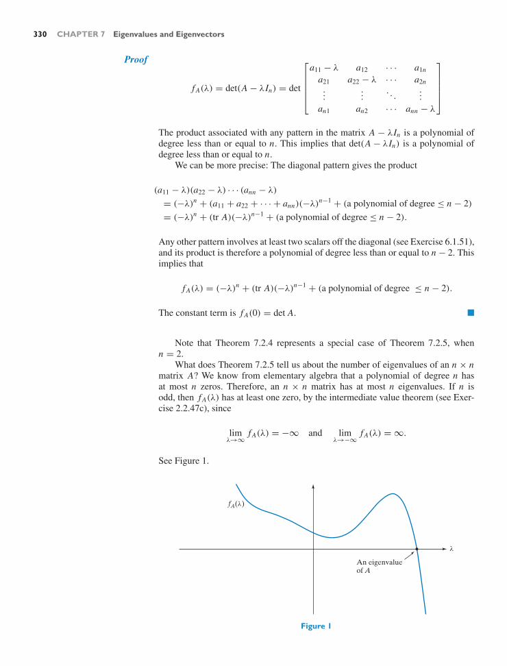
330 CHAPTER 7 Eigenvalues and Eigenvectors
Proof
f A(λ) = det(A − λIn) = det
⎡
⎢⎢⎢⎣
a11 − λ a12 · · · a1n
a21 a22 − λ · · · a2n...
.... . .
...
an1 an2 · · · ann − λ
⎤
⎥⎥⎥⎦
The product associated with any pattern in the matrix A − λIn is a polynomial ofdegree less than or equal to n. This implies that det(A − λIn) is a polynomial ofdegree less than or equal to n.
We can be more precise: The diagonal pattern gives the product
(a11 − λ)(a22 − λ) · · · (ann − λ)
= (−λ)n + (a11 + a22 + · · · + ann)(−λ)n−1 + (a polynomial of degree ≤ n − 2)
= (−λ)n + (tr A)(−λ)n−1 + (a polynomial of degree ≤ n − 2).
Any other pattern involves at least two scalars off the diagonal (see Exercise 6.1.51),and its product is therefore a polynomial of degree less than or equal to n − 2. Thisimplies that
f A(λ) = (−λ)n + (tr A)(−λ)n−1 + (a polynomial of degree ≤ n − 2).
The constant term is f A(0) = det A. !
Note that Theorem 7.2.4 represents a special case of Theorem 7.2.5, whenn = 2.
What does Theorem 7.2.5 tell us about the number of eigenvalues of an n × nmatrix A? We know from elementary algebra that a polynomial of degree n hasat most n zeros. Therefore, an n × n matrix has at most n eigenvalues. If n isodd, then f A(λ) has at least one zero, by the intermediate value theorem (see Exer-cise 2.2.47c), since
limλ→∞
f A(λ) = −∞ and limλ→−∞
f A(λ) = ∞.
See Figure 1.
An eigenvalueof A
fA( )
Figure 1

7.2 Finding the Eigenvalues of a Matrix 331
EXAMPLE 4 Find all eigenvalues of
A =
⎡
⎢⎢⎢⎢⎣
5 4 3 2 10 4 3 2 10 0 5 4 30 0 0 4 30 0 0 0 5
⎤
⎥⎥⎥⎥⎦.
SolutionThe characteristic polynomial is f A(λ) = (5 − λ)3(4 − λ)2, so that the eigenvaluesare 4 and 5. Since 5 is a root of multiplicity 3 of the characteristic polynomial, wesay that the eigenvalue 5 has algebraic multiplicity 3. Likewise, the eigenvalue 4has algebraic multiplicity 2. !
Definition 7.2.6 Algebraic multiplicity of an eigenvalue
We say that an eigenvalue λ0 of a square matrix A has algebraic multiplicity kif λ0 is a root of multiplicity k of the characteristic polynomial f A(λ), meaningthat we can write
f A(λ) = (λ0 − λ)k g(λ)
for some polynomial g(λ) with g(λ0) = 0. We write almu(λ0) = k.
In Example 4, almu(5) = 3 since
f A(λ) = (5↑λ0
−λ)
k↓3 (4 − λ)2︸ ︷︷ ︸
g(λ)
.
EXAMPLE 5 Find the eigenvalues of
A =
⎡
⎣1 1 11 1 11 1 1
⎤
⎦ ,
with their algebraic multiplicities.
SolutionWe leave it to the reader to verify that
f A(λ) = λ2(3 − λ) = (0 − λ)2(3 − λ).
We have two distinct eigenvalues, 0 and 3, with algebraic multiplicities 2 and 1,respectively. We can write, more succinctly, that the eigenvalues are 0, 0, 3. !
Let us summarize.
Theorem 7.2.7 Number of eigenvalues
An n × n matrix has at most n real eigenvalues, even if they are counted withtheir algebraic multiplicities.
If n is odd, then an n × n matrix has at least one real eigenvalue.

332 CHAPTER 7 Eigenvalues and Eigenvectors
If n is even, an n × n matrix A need not have any real eigenvalues. Consider
A =[
0 −11 0
],
with f A(λ) = det[−λ −1
1 −λ
]= λ2 + 1. See Figure 2.
fA( ) = 2 + 1
Figure 2
Recall that the transformation T (x) = Ax is a counterclockwise rotationthrough an angle of 90. Geometrically, it makes sense that A has no real eigen-values: Compare with Example 7.1.4.
EXAMPLE 6 Describe all possible cases for the number of real eigenvalues (with their algebraicmultiplicities) of a 3 × 3 matrix A.
SolutionEither the characteristic polynomial factors completely,
f A(λ) = (λ1 − λ)(λ2 − λ)(λ3 − λ),
or it has a quadratic factor without real zeros:
f A(λ) = (λ1 − λ)p(λ), where p(λ) = 0 for all real λ.
In the first case, the λi could all be distinct, two of them could be equal, or theycould all be equal. This leads to the following possibilities.
No. of Distinct AlgebraicCase Eigenvalues Multiplicities
1 3 1 each2 2 2 and 13 1 34 1 1

7.2 Finding the Eigenvalues of a Matrix 333
Examples for each case follow.
Case 1 ! (see Figure 3)
A =
⎡
⎣1 0 00 2 00 0 3
⎤
⎦ , f A(λ) = (1 − λ)(2 − λ)(3 − λ), Eigenvalues 1, 2, 3
Case 2 ! (see Figure 4)
A =
⎡
⎣1 0 00 1 00 0 2
⎤
⎦ , f A(λ) = (1 − λ)2(2 − λ), Eigenvalues 1, 1, 2
Case 3 ! (see Figure 5)
A = I3, f A(λ) = (1 − λ)3, Eigenvalues 1, 1, 1
Case 4 ! (see Figure 6)
A =
⎡
⎣1 0 00 0 −10 1 0
⎤
⎦ , f A(λ) = (1 − λ)(λ2 + 1), Eigenvalue 1
You can recognize an eigenvalue λ0 whose algebraic multiplicity exceeds 1on the graph of f A(λ) by the fact that f A(λ0) = f ′
A(λ0) = 0 (the derivative iszero, so that the tangent is horizontal). The verification of this observation is left asExercise 37. !
1 2 3
fA( )
Figure 3
1 2
fA( )
Figure 4

334 CHAPTER 7 Eigenvalues and Eigenvectors
1
fA( )
Figure 5
1
fA( )
Figure 6
EXAMPLE 7 Suppose A is a 2 × 2 matrix with eigenvalues λ1 and λ2 (we allow λ1 = λ2 if λ1has algebraic multiplicity 2). Explore the relationship among the sum λ1 + λ2, theproduct λ1λ2, the determinant det A, and the trace tr A. You may want to consider
a numerical example first, such as A =[
1 24 3
], with eigenvalues λ1 = 5 and
λ2 = −1. See Example 1.
Solution
In the case of A =[
1 24 3
], we observe that det A = λ1λ2 = −5 and tr A =
λ1 + λ2 = 4. To see that these results hold in general, write the characteristicpolynomial in two ways, as
f A(λ) = λ2 − (tr A)λ + det A
and as
f A(λ) = (λ1 − λ)(λ2 − λ) = λ2 − (λ1 + λ2)λ + λ1λ2.
Comparing coefficients, we conclude that det A = λ1λ2 and tr A = λ1 + λ2. !It turns out that the observations we made in Example 7 generalize to n × n
matrices.
Theorem 7.2.8 Eigenvalues, determinant, and trace
If an n×n matrix A has the eigenvalues λ1, λ2, . . . , λn , listed with their algebraicmultiplicities, then
det A = λ1λ2 · · · λn, the product of the eigenvalues
and
tr A = λ1 + λ2 + · · · + λn, the sum of the eigenvalues.
We will prove the claim concerning the determinant and leave the case of thetrace as Exercise 21 for the reader.
Since the characteristic polynomial factors completely in this case, we can write
f A(λ) = det(A − λIn) = (λ1 − λ)(λ2 − λ) · · · (λn − λ).

7.2 Finding the Eigenvalues of a Matrix 335
Now
f A(0) = det A = λ1λ2 · · · λn,
as claimed.
Note that the claims of Theorem 7.2.8 are trivial in the case of a triangularmatrix, since the eigenvalues are the diagonal entries in this case.
Finding the Eigenvalues of a Matrix in PracticeTo find the eigenvalues of an n × n matrix A with the method developed in thissection, we have to find the zeros of f A(λ), a polynomial of degree n. For n = 2,this is a trivial matter: We can either factor the polynomial by inspection or use thequadratic formula (this formula was known over 3500 years ago in Mesopotamia,the present-day Iraq). The problem of finding the zeros of a polynomial of higherdegree is nontrivial; it has been of considerable interest throughout the historyof mathematics. In the early 1500s, Italian mathematicians found formulas in thecases n = 3 and n = 4, published in the Ars Magna by Gerolamo Cardano.6 SeeExercise 50 for the case n = 3. During the next 300 years, people tried hard to find ageneral formula to solve the quintic (a polynomial equation of fifth degree). In 1824,the Norwegian mathematician Niels Henrik Abel (1802–1829) showed that no suchgeneral solution is possible, putting an end to the long search. The French mathe-matician Evariste Galois (1811–1832) was the first to give a numerical example ofa quintic that cannot be solved by radicals. (Note the short life spans of these twobrilliant mathematicians. Abel died from tuberculosis, and Galois died in a duel.)
When finding the eigenvalues of a matrix by means of the characteristic poly-nomial, it may be worth trying out a few small integers, such as ± 1 and ± 2. Thematrices considered in introductory linear algebra texts often just happen to havesuch eigenvalues.
In light of the preceding discussion, it is usually impossible to find the exacteigenvalues of a matrix. To find approximations for the eigenvalues, you couldgraph the characteristic polynomial, using technology. The graph may give youan idea of the number of eigenvalues and their approximate values. Numerical ana-lysts tell us that this is not a very efficient way to go about finding the eigenvaluesof large matrices; other techniques are used in practice. See Exercise 7.5.33 for anexample; another approach uses the QR factorization (Theorem 5.2.2). There is a lotof ongoing research in this area. A text in numerical linear algebra7 characterizesthe eigenvalue problem as “the third major problem area in matrix computations,”after linear equations and least squares, dedicating some 200 pages to this topic.
6Cardano (1501–1576) was a Renaissance man with a wide range of interests. In his book Liber deludo aleae, he presents the first systematic computations of probabilities. Trained as a physician, hegave the first clinical description of typhoid fever. In his book Somniorum Synesiorum (Basel, 1562),he explores the meaning of dreams. He was also a leading astrologer of his day, whose predictionswon him access to some of the most powerful people in sixteenth-century Europe. Still, he is bestknown today as the most outstanding mathematician of his time and the author of the Ars Magna. In1570, he was arrested on accusation of heresy; he lost his academic position and the right to publish.
To learn more about this fascinating fellow, read the award-winning biography, Cardano’sCosmos, by Anthony Grafton (Harvard University Press, 2000), focusing on Cardano’s work as anastrologer.
For an English translation of part XI of the Ars Magna (dealing with cubic equations), seeD. J. Struik (editor), A Source Book in Mathematics 1200–1800, Princeton University Press, 1986.7G. H. Golub and C. F. van Loan, Matrix Computations, 3rd ed., Johns Hopkins University Press,1996.

336 CHAPTER 7 Eigenvalues and Eigenvectors
EXERCISES 7.2GOAL Use the characteristic polynomial fA(λ) =det(A − λIn) to find the eigenvalues of a matrix A, withtheir algebraic multiplicities.
For each of the matrices in Exercises 1 through 13, find allreal eigenvalues, with their algebraic multiplicities. Showyour work. Do not use technology.
1.[
1 20 3
]2.
⎡
⎢⎢⎣
2 0 0 02 1 0 02 1 2 02 1 2 1
⎤
⎥⎥⎦
3.[
5 −42 −1
]4.
[0 4
−1 4
]
5.[
11 −156 −7
]6.
[1 23 4
]
7. I3 8.
⎡
⎣−1 −1 −1−1 −1 −1−1 −1 −1
⎤
⎦
9.
⎡
⎣3 −2 51 0 70 0 2
⎤
⎦ 10.
⎡
⎣−3 0 4
0 −1 0−2 7 3
⎤
⎦
11.
⎡
⎣5 1 −52 1 08 2 −7
⎤
⎦ 12.
⎡
⎢⎢⎣
2 −2 0 01 −1 0 00 0 3 −40 0 2 −3
⎤
⎥⎥⎦
13.
⎡
⎣0 1 00 0 11 0 0
⎤
⎦
14. Consider a 4 × 4 matrix A =[
B C0 D
], where B, C ,
and D are 2 × 2 matrices. What is the relationshipamong the eigenvalues of A, B, C , and D?
15. Consider the matrix A =[
1 k1 1
], where k is an arbi-
trary constant. For which values of k does A have twodistinct real eigenvalues? When is there no real eigen-value?
16. Consider the matrix A =[
a bb c
], where a, b, and c
are nonzero constants. For which values of a, b, and cdoes A have two distinct eigenvalues?
17. Consider the matrix A =[
a bb −a
], where a and b are
arbitrary constants. Find all eigenvalues of A. Explainin terms of the geometric interpretation of the lineartransformation T (x) = Ax .
18. Consider the matrix A =[
a bb a
], where a and b are
arbitrary constants. Find all eigenvalues of A.
19. True or false? If the determinant of a 2 × 2 matrix A isnegative, then A has two distinct real eigenvalues.
20. If a 2 × 2 matrix A has two distinct eigenvalues λ1 andλ2, show that A is diagonalizable.
21. Prove the part of Theorem 7.2.8 that concerns the trace:If an n × n matrix A has n eigenvalues λ1, . . . , λn ,listed with their algebraic multiplicities, then tr A =λ1 + · · · + λn .
22. Consider an arbitrary n × n matrix A. What is therelationship between the characteristic polynomials ofA and AT ? What does your answer tell you about theeigenvalues of A and AT ?
23. Suppose matrix A is similar to B. What is the relation-ship between the characteristic polynomials of A andB? What does your answer tell you about the eigenval-ues of A and B?
24. Find all eigenvalues of the positive transition matrix
A =[
0.5 0.250.5 0.75
].
See Definitions 2.1.4 and 2.3.10.
25. Consider a positive transition matrix
A =[
a bc d
],
meaning that a, b, c, and d are positive numbers suchthat a + c = b + d = 1. (The matrix in Exercise 24
has this form.) Verify that[
bc
]and
[1
−1
]are eigenvec-
tors of A. What are the associated eigenvalues? Is theabsolute value of these eigenvalues more or less than 1?Sketch a phase portrait.
26. Based on your answers in Exercises 24 and 25, sketch aphase portrait of the dynamical system
x(t + 1) =[
0.5 0.250.5 0.75
]x(t).
27. a. Based on your answers in Exercises 24 and 25, findclosed formulas for the components of the dynami-cal system
x(t + 1) =[
0.5 0.250.5 0.75
]x(t),
with initial value x0 = e1. Then do the same for theinitial value x0 = e2. Sketch the two trajectories.

7.2 Finding the Eigenvalues of a Matrix 337
b. Consider the matrix
A =[
0.5 0.250.5 0.75
].
Using technology, compute some powers of the ma-trix A, say, A2, A5, A10, . . . . What do you observe?Diagonalize matrix A to prove your conjecture. (Donot use Theorem 2.3.11, which we have not provenyet.)
c. If A =[
a bc d
]is an arbitrary positive transition
matrix, what can you say about the powers At as tgoes to infinity? Your result proves Theorem 2.3.11cfor the special case of a positive transition matrix ofsize 2 × 2.
28. Consider the isolated Swiss town of Andelfingen, in-habited by 1,200 families. Each family takes a weeklyshopping trip to the only grocery store in town, run byMr. and Mrs. Wipf, until the day when a new, fancier(and cheaper) chain store, Migros, opens its doors. Itis not expected that everybody will immediately run tothe new store, but we do anticipate that 20% of thoseshopping at Wipf’s each week switch to Migros thefollowing week. Some people who do switch miss thepersonal service (and the gossip) and switch back: Weexpect that 10% of those shopping at Migros each weekgo to Wipf’s the following week. The state of this town(as far as grocery shopping is concerned) can be repre-sented by the vector
x(t) =[w(t)m(t)
],
where w(t) and m(t) are the numbers of families shop-ping at Wipf’s and at Migros, respectively, t weeks afterMigros opens. Suppose w(0) = 1,200 and m(0) = 0.a. Find a 2 × 2 matrix A such that x(t + 1) = Ax(t).
Verify that A is a positive transition matrix. See Ex-ercise 25.
b. How many families will shop at each store after tweeks? Give closed formulas.
c. The Wipfs expect that they must close down whenthey have less than 250 customers a week. Whendoes that happen?
29. Consider an n × n matrix A such that the sum of theentries in each row is 1. Show that the vector
e =
⎡
⎢⎢⎢⎣
11...
1
⎤
⎥⎥⎥⎦
in Rn is an eigenvector of A. What is the correspondingeigenvalue?
30. In all parts of this problem, consider an n × n matrixA such that all entries are positive and the sum of the
entries in each row is 1 (meaning that AT is a positivetransition matrix).a. Consider an eigenvector v of A with positive com-
ponents. Show that the associated eigenvalue is lessthan or equal to 1. Hint: Consider the largest entryvi of v. What can you say about the i th entry of Av?
b. Now we drop the requirement that the componentsof the eigenvector v be positive. Show that the asso-ciated eigenvalue is less than or equal to 1 in abso-lute value.
c. Show that λ = −1 fails to be an eigenvalue of A, andshow that the eigenvectors with eigenvalue 1 are thevectors of the form
⎡
⎢⎢⎢⎣
cc...c
⎤
⎥⎥⎥⎦,
where c is nonzero.
31. Consider a positive transition matrix A. Explain why 1is an eigenvalue of A. What can you say about the othereigenvalues? Is
e =
⎡
⎢⎢⎢⎣
11...
1
⎤
⎥⎥⎥⎦
necessarily an eigenvector? Hint: Consider Exercises22, 29, and 30.
32. Consider the matrix
A =
⎡
⎣0 1 00 0 1k 3 0
⎤
⎦ ,
where k is an arbitrary constant. For which values of kdoes A have three distinct real eigenvalues? For which kdoes A have two distinct eigenvalues? Hint: Graph thefunction g(λ) = λ3 − 3λ. Find its local maxima andminima.
33. a. Find the characteristic polynomial of the matrix
A =
⎡
⎣0 1 00 0 1a b c
⎤
⎦ .
b. Can you find a 3 × 3 matrix M whose characteristicpolynomial is
−λ3 + 17λ2 − 5λ + π?
34. Suppose a certain 4 × 4 matrix A has two distinct realeigenvalues. What could the algebraic multiplicities ofthese eigenvalues be? Give an example for each possi-ble case and sketch the characteristic polynomial.

338 CHAPTER 7 Eigenvalues and Eigenvectors
35. Give an example of a 4×4 matrix A without real eigen-values.
36. For an arbitrary positive integer n, give a 2n×2n matrixA without real eigenvalues.
37. Consider an eigenvalue λ0 of an n × n matrix A. Weare told that the algebraic multiplicity of λ0 exceeds 1.Show that f ′
A(λ0) = 0 (i.e., the derivative of the char-acteristic polynomial of A vanishes at λ0).
38. If A is a 2 × 2 matrix with tr A = 5 and det A = −14,what are the eigenvalues of A?
39. If A and B are 2 × 2 matrices, show that tr(AB) =tr(B A).
40. If A and B are n × n matrices, show that tr(AB) =tr(B A).
41. If matrix A is similar to B, show that tr B = tr A. Hint:Exercise 40 is helpful.
42. Consider two n×n matrices A and B such that B A = 0.Show that tr
((A + B)2) = tr(A2) + tr(B2). Hint: Exer-
cise 40 is helpful.
43. Do there exist n × n matrices A and B such thatAB − B A = In? Explain. Hint: Exercise 40 is helpful.
44. Do there exist invertible n × n matrices A and B suchthat AB − B A = A? Explain.
45. For which value of the constant k does the matrix A =[−1 k
4 3
]have 5 as an eigenvalue?
46. In all the parts of this problem, consider a matrix A =[a bc d
]with the eigenvalues λ1 and λ2.
a. Show that λ21 + λ2
2 = a2 + d2 + 2bc.b. Show that λ2
1 + λ22 ≤ a2 + b2 + c2 + d2.
c. For which matrices A does the equality λ21 + λ2
2 =a2 + b2 + c2 + d2 hold?
47. For which 2 × 2 matrices A does there exist a nonzero
matrix M such that AM = M D, where D =[
2 00 3
]?
Give your answer in terms of the eigenvalues of A.
48. For which 2×2 matrices A does there exist an invertible
matrix S such that AS = SD, where D =[
2 00 3
]?
Give your answer in terms of the eigenvalues of A.
49. For which 3 × 3 matrices A does there exist a nonzero
matrix M such that AM = M D, where D =⎡
⎣2 0 00 3 00 0 4
⎤
⎦? Give your answer in terms of the eigen-
values of A.
50. In his groundbreaking text Ars Magna (Nuremberg,1545), the Italian mathematician Gerolamo Cardano ex-plains how to solve cubic equations. In Chapter XI, heconsiders the following example:
x3 + 6x = 20.
a. Explain why this equation has exactly one (real)solution. Here, this solution is easy to find by in-spection. The point of the exercise is to show asystematic way to find it.
b. Cardano explains his method as follows (we are us-ing modern notation for the variables): “I take twocubes v3 and u3 whose difference shall be 20, sothat the product vu shall be 2, that is, a third ofthe coefficient of the unknown x . Then, I say thatv − u is the value of the unknown x .” Show thatif v and u are chosen as stated by Cardano, thenx = v − u is indeed the solution of the equationx3 + 6x = 20.
c. Solve the system∣∣∣∣v3 − u3 = 20
vu = 2
∣∣∣∣
to find u and v.d. Consider the equation
x3 + px = q,
where p is positive. Using your work in parts (a),(b), and (c) as a guide, show that the unique solutionof this equation is
x = 3
√q2
+√(q
2
)2+
( p3
)3
− 3
√
−q2
+√(q
2
)2+
( p3
)3.
This solution can also be written as
x = 3
√q2
+√(q
2
)2+
( p3
)3
+ 3
√q2
−√(q
2
)2+
( p3
)3.
What can go wrong when p is negative?e. Consider an arbitrary cubic equation
x3 + ax2 + bx + c = 0.
Show that the substitution x = t − (a/3) allows youto write this equation as
t3 + pt = q.

7.3 Finding the Eigenvectors of a Matrix 339
7.3 Finding the Eigenvectors of a Matrix
Having found an eigenvalue λ of an n × n matrix A, we will now turn our attentionto the corresponding eigenvectors. We have to find the vectors v in Rn such that
Av = λv, or (A − λIn)v = 0.
In other words, we have to find the kernel of the matrix A −λIn . In this context, thefollowing definition is useful.
Definition 7.3.1 Eigenspaces
Consider an eigenvalue λ of an n × n matrix A. Then the kernel of the matrixA − λIn is called the eigenspace associated with λ, denoted by Eλ:
Eλ = ker(A − λIn) = v in Rn : Av = λv.
Note that the eigenvectors with eigenvalue λ are the nonzero vectors in theeigenspace Eλ.
EXAMPLE 1 Let T (x) = Ax be the orthogonal projection onto a plane V in R3. Describe theeigenspaces E1 and E0 geometrically. Is matrix A diagonalizable?
SolutionEigenspace E1 consists of the solutions of the equation Av = 1v = v; those are thevectors on plane V . Thus, E1 = V .
Eigenspace E0 = ker A consists of the solutions of the equation Av = 0v = 0;those are the vectors on the line V ⊥ perpendicular to plane V . See Figure 1.
We can construct an eigenbasis v1, v2, v3 for A by choosing two linearly in-dependent vectors v1, v2 in E1 = V and a nonzero vector v3 in E0 = V ⊥. Thus,
matrix A is diagonalizable; namely, A is similar to B =
⎡
⎣1 0 00 1 00 0 0
⎤
⎦. !
E0: the vectors v such that Av = 0v = 0
V⊥
E1 = V: the vectors v such that Av = 1v = v
Figure 1
To find the eigenvectors associated with a known eigenvalue λ algebraically,we seek a basis of the eigenspace Eλ = ker(A − λIn), a problem we can handle.See Section 3.3.
EXAMPLE 2 Find the eigenspaces of the matrix A =[
1 24 3
]. Diagonalize matrix A if you can.

340 CHAPTER 7 Eigenvalues and Eigenvectors
SolutionIn Example 1 of Section 7.2, we saw that the eigenvalues are 5 and −1. Now
E5 = ker(A − 5I2) = ker[−4 2
4 −2
].
Finding the kernel amounts to finding the relations between the columns. In the caseof a 2 × 2 matrix, this can be done by inspection. Consider the Kyle numbers,
[ 1 2−4 2
4 −2
],
so that
E5 = span[
12
].
Similarly,
E−1 = ker(A + I2) = ker[ 1 −1
2 24 4
]= span
[1
−1
].
We can (and should) check that the vectors we found are indeed eigenvectors of A,with the eigenvalues we claim:
[1 24 3
] [12
]=
[5
10
]= 5
[12
]
and [1 24 3
] [1
−1
]=
[−1
1
]= (−1)
[1
−1
].
√E−1
E5
12
1−1
Figure 2Both eigenspaces are lines, as shown in Figure 2. The vectors
[12
],[
1−1
]form an
eigenbasis for A, so that A is diagonalizable, with S =[
1 12 −1
]and B =
[5 00 −1
].
For peace of mind, we may want to check that AS = SB. !Geometrically, the matrix A represents a scaling by a factor of 5 along the line
spanned by vector[
12
], while the line spanned by
[1
−1
]is flipped over the origin.
EXAMPLE 3 Find the eigenspaces of
A =
⎡
⎣1 1 10 0 10 0 1
⎤
⎦ .
Diagonalize matrix A if you can.
SolutionThe eigenvalues are 1 and 0, the diagonal entries of the upper triangular matrix A,with algebraic multiplicities 2 and 1, respectively. Now
E1 = ker(A − I2) = ker
⎡
⎣
1 0 00 1 10 −1 10 0 0
⎤
⎦ = span
⎡
⎣100
⎤
⎦

7.3 Finding the Eigenvectors of a Matrix 341
and
E0 = ker A = ker
⎡
⎣
−1 1 01 1 10 0 10 0 1
⎤
⎦ = span
⎡
⎣−1
10
⎤
⎦ .
Both eigenspaces are lines in the x1–x2-plane, as shown in Figure 3.
x3
−1
−1
1
1
x2
x1
E0 = span−1
10
E1 = span100
Figure 3
We can find only two linearly independent eigenvectors, one in each of theeigenspaces E0 and E1, so that we are unable to construct an eigenbasis for A.Thus, matrix A fails to be diagonalizable. !
Note that Example 3 is qualitatively different from Example 1, where we stud-ied the orthogonal projection onto a plane in R3. There, too, we had two eigenval-ues, 1 and 0, but one of the eigenspaces, E1, was a plane, while both eigenspaces inExample 3 turn out to be lines.
To discuss these different cases, it is useful to introduce the followingterminology.
Definition 7.3.2 Geometric multiplicity
Consider an eigenvalue λ of an n × n matrix A. The dimension of eigenspaceEλ = ker(A − λIn) is called the geometric multiplicity of eigenvalue λ, denotedgemu(λ). Thus,
gemu(λ) = nullity(A − λIn) = n − rank(A − λIn)
Example 3 shows that the geometric multiplicity of an eigenvalue may be dif-ferent from the algebraic multiplicity (but see Theorem 7.3.6). We have
almu(1) = 2,
but
gemu(1) = dim(E1) = 1.
Based on our findings in Examples 1 through 3, we can now tackle the mainquestions of this chapter.

342 CHAPTER 7 Eigenvalues and Eigenvectors
a. Which square matrices A are diagonalizable; that is, when does there existan eigenbasis for A?
b. If eigenbases exist, how can we find one?
Consider an n × n matrix A. If the sum s of the geometric multiplicities of theeigenvalues is less than n (as in Example 3, where s = 2 and n = 3), then there arenot enough linearly independent eigenvectors to form an eigenbasis. In fact, we canfind no more than s linearly independent eigenvectors.
Conversely, suppose that the geometric multiplicities of the eigenvalues do addup to n, as in Examples 1 and 2. Can we construct an eigenbasis for A by finding abasis of each eigenspace and concatenating8 these bases? This method does work inExamples 1 and 2. Next we will state and prove that this approach works in general.
Theorem 7.3.3 Eigenbases and geometric multiplicities
a. Consider an n × n matrix A. If we find a basis of each eigenspace of Aand concatenate all these bases, then the resulting eigenvectors v1, . . . , vswill be linearly independent. (Note that s is the sum of the geometricmultiplicities of the eigenvalues of A.) This result implies that s ≤ n.
b. Matrix A is diagonalizable if (and only if) the geometric multiplicities ofthe eigenvalues add up to n (meaning that s = n in part a).
Proof a. We will argue indirectly, assuming that the eigenvectors v1, . . . , vs are lin-early dependent. Let vm be the first redundant vector in this list, withvm = c1v1+· · ·+cm−1vm−1. Suppose that Avi = λi vi . There must be at leastone nonzero coefficient ck such that λk = λm , since vm cannot be expressedas a linear combination of vectors vi that are all in the same eigenspace Eλm .Multiplying the equation vm = c1v1 + · · · + ck vk + · · · + cm−1vm−1 byA − λm In from the left, and realizing that (A − λm In)vi = (λi − λm)vi , wefind that
(λm − λm)vm = 0= (λ1 − λm)c1v1 + · · · + (λk − λm)ck︸ ︷︷ ︸
=0
vk + · · · + (λm−1 − λm)cm−1vm−1.
This is a nontrivial relation among vectors v1, . . . , vm−1, contradicting ourassumption that vm is the first redundant vector in the list.
b. This claim follows directly from part a. There exists an eigenbasis if (andonly if) s = n in part a. !
Here is an important special case of Theorem 7.3.3.
Theorem 7.3.4 An n × n matrix with n distinct eigenvalues
If an n ×n matrix A has n distinct eigenvalues, then A is diagonalizable. We canconstruct an eigenbasis by finding an eigenvector for each eigenvalue.
8 The concatenation of two lists (a1, a2, . . . , ap) and (b1, b2, . . . , bq) is the list (a1, a2, . . . , ap,b1, b2, . . . , bq ).

7.3 Finding the Eigenvectors of a Matrix 343
EXAMPLE 4 Is the following matrix A diagonalizable?
A =
⎡
⎢⎢⎢⎢⎢⎢⎣
1 2 3 4 5 60 2 3 4 5 60 0 3 4 5 60 0 0 4 5 60 0 0 0 5 60 0 0 0 0 6
⎤
⎥⎥⎥⎥⎥⎥⎦
SolutionYes, since the 6 × 6 matrix A has six distinct eigenvalues, namely, the diagonalentries 1, 2, 3, 4, 5, 6. !Eigenvalues and SimilarityIf matrix A is similar to B, what is the relationship between the eigenvalues of Aand B? The following theorem shows that this relationship is very close indeed.
Theorem 7.3.5 The eigenvalues of similar matrices
Suppose matrix A is similar to B. Then
a. Matrices A and B have the same characteristic polynomial; that is,f A(λ) = fB(λ).
b. rank A = rank B and nullity A = nullity B.c. Matrices A and B have the same eigenvalues, with the same algebraic
and geometric multiplicities. (However, the eigenvectors need not be thesame.)
d. Matrices A and B have the same determinant and the same trace:det A = det B and tr A = tr B.
Proof a. If B = S−1 AS, then fB(λ) = det(B − λIn) = det(S−1 AS − λIn) =det
(S−1(A − λIn)S
)= (det S)−1 det(A − λIn) det(S) = (det S)−1(det S)
det(A − λIn) = det(A − λIn) = f A(λ) for all scalars λ.b. See Exercises 71 and 72 of Section 3.4. An alternative proof is suggested in
Exercise 34 of this section.c. It follows from part a that matrices A and B have the same eigenvalues, with
the same algebraic multiplicities. See Theorem 7.2.1 and Definition 7.2.6.As for the geometric multiplicity, note that A −λIn is similar to B −λIn forall λ (see Exercise 33), so that nullity(A − λIn) = nullity(B − λIn) for alleigenvalues λ, by part b. See Definition 7.3.2.
d. These equations follow from part a and Theorem 7.2.5: Trace and determi-nant are coefficients of the characteristic polynomial, up to signs. !
EXAMPLE 5 Is the matrix A =[
2 35 7
]similar to B =
[3 28 5
]?
SolutionNo, since tr A = 9 and tr B = 8. See Theorem 7.3.5d. !

344 CHAPTER 7 Eigenvalues and Eigenvectors
Earlier in this section we observed that the algebraic and the geometric mul-tiplicity of an eigenvalue are not necessarily the same. However, the following in-equality always holds.
Theorem 7.3.6 Algebraic versus geometric multiplicity
If λ is an eigenvalue of a square matrix A, then
gemu(λ) ≤ almu(λ).
Proof Suppose λ0 is an eigenvalue of an n × n matrix A, with geometric multiplicity m,meaning that the dimension of eigenspace Eλ0 is m. Let v1, . . . , vm be a basis of Eλ0 ,and consider an invertible n × n matrix S whose first m columns are v1, . . . , vm .(How would you find such an S?) Let B = S−1 AS, a matrix similar to A. Nowcompute Bei , for i = 1, . . . , m, keeping in mind that Sei = vi , and thereforeS−1vi = ei : (ith column of B) = Bei = S−1 ASei = S−1 Avi = S−1(λ0vi ) =λ0(S−1vi ) = λ0ei . This computation shows that the first m columns of B look likethose of λ0 In .
m︷ ︸︸ ︷
B =
⎡
⎢⎢⎢⎢⎢⎢⎢⎢⎢⎢⎣
λ0 0 · · · 0 ∗ · · · ∗0 λ0 · · · 0 ∗ · · · ∗...
.... . .
......
......
0 0 · · · λ0 ∗ · · · ∗0 0 · · · 0 ∗ · · · ∗...
......
......
. . ....
0 0 · · · 0 ∗ · · · ∗
⎤
⎥⎥⎥⎥⎥⎥⎥⎥⎥⎥⎦
=[λ0 Im P
0 Q
]
Since B is similar to A, we have
f A(λ)
step 1︷︸︸︷= fB(λ) = det(B − λIn)
step 3︷︸︸︷= (λ0 − λ)m fQ(λ),
showing that the algebraic multiplicity of eigenvalue λ0 is at least m, as claimed. Instep 1 we use Theorem 7.3.5a, and in step 3 we use Theorem 6.1.5. !
We conclude this section with a summary on diagonalization.
Theorem 7.3.7 Strategy for Diagonalization
Suppose we are asked to determine whether a given n × n matrix A is diago-nalizable. If so, we wish to find an invertible matrix S such that S−1 AS = B isdiagonal.
We can proceed as follows.
a. Find the eigenvalues of A by solving the characteristic equation
f A(λ) = det(A − λIn) = 0.
b. For each eigenvalue λ, find a basis of the eigenspace
Eλ = ker(A − λIn).
c. Matrix A is diagonalizable if (and only if) the dimensions of theeigenspaces add up to n. In this case, we find an eigenbasis v1, . . . , vn

7.3 Finding the Eigenvectors of a Matrix 345
for A by concatenating the bases of the eigenspaces we found in part b.Let
S =
⎡
⎣| | |v1 v2 . . . vn| | |
⎤
⎦ . Then S−1 AS = B =
⎡
⎢⎢⎣
λ1 0 . . . 00 λ2 . . . 0...
.... . .
...0 0 . . . λn
⎤
⎥⎥⎦ ,
where λ j is the eigenvalue associated with v j .
EXERCISES 7.3GOAL For a given eigenvalue, find a basis of theassociated eigenspace. Use the geometric multiplicitiesof the eigenvalues to determine whether a matrix isdiagonalizable.
For each of the matrices A in Exercises 1 through 20, findall (real) eigenvalues. Then find a basis of each eigenspace,and diagonalize A, if you can. Do not use technology.
1.[
7 80 9
]2.
[1 11 1
]
3.[
6 32 7
]4.
[0 −11 2
]
5.[
4 5−2 −2
]6.
[2 34 5
]
7.
⎡
⎣1 0 00 2 00 0 3
⎤
⎦ 8.
⎡
⎣1 1 00 2 20 0 3
⎤
⎦
9.
⎡
⎣1 0 10 1 00 0 0
⎤
⎦ 10.
⎡
⎣1 1 00 1 00 0 0
⎤
⎦
11.
⎡
⎣1 1 11 1 11 1 1
⎤
⎦ 12.
⎡
⎣1 1 00 1 10 0 1
⎤
⎦
13.
⎡
⎣3 0 −2
−7 0 44 0 −3
⎤
⎦ 14.
⎡
⎣1 0 0
−5 0 20 0 1
⎤
⎦
15.
⎡
⎣−1 0 1−3 0 1−4 0 3
⎤
⎦ 16.
⎡
⎣1 1 00 −1 −12 2 0
⎤
⎦
17.
⎡
⎢⎢⎣
0 0 0 00 1 1 00 0 0 00 0 0 1
⎤
⎥⎥⎦ 18.
⎡
⎢⎢⎣
0 0 0 00 1 0 10 0 0 00 0 0 1
⎤
⎥⎥⎦
19. A =
⎡
⎣1 1 10 1 00 1 0
⎤
⎦ 20. A =
⎡
⎣1 0 11 1 11 0 1
⎤
⎦
21. Find a 2 × 2 matrix A for which
E1 = span[
12
]and E2 = span
[23
].
How many such matrices are there?
22. Find all 2 × 2 matrices A for which
E7 = R2.
23. Find all eigenvalues and eigenvectors of A =[
1 10 1
].
Is there an eigenbasis? Interpret your result geometri-cally.
24. Find a 2 × 2 matrix A for which
E1 = span[
21
]
is the only eigenspace.
25. What can you say about the geometric multiplicity ofthe eigenvalues of a matrix of the form
A =
⎡
⎣0 1 00 0 1a b c
⎤
⎦ ,
where a, b, c are arbitrary constants?
26. Show that if a 6 × 6 matrix A has a negative determi-nant, then A has at least one positive eigenvalue. Hint:Sketch the graph of the characteristic polynomial.
27. Consider a 2 × 2 matrix A. Suppose that tr A = 5 anddet A = 6. Find the eigenvalues of A.
28. Consider the matrix
Jn(k) =
⎡
⎢⎢⎢⎢⎢⎢⎢⎣
k 1 0 . . . 0 00 k 1 . . . 0 00 0 k . . . 0 0...
......
. . ....
...
0 0 0 . . . k 10 0 0 . . . 0 k
⎤
⎥⎥⎥⎥⎥⎥⎥⎦
(with all k’s on the diagonal and 1’s directly above),where k is an arbitrary constant. Find the eigenvalue(s)of Jn(k), and determine their algebraic and geometricmultiplicities.

346 CHAPTER 7 Eigenvalues and Eigenvectors
29. Consider a diagonal n × n matrix A with rank A = r <n. Find the algebraic and the geometric multiplicity ofthe eigenvalue 0 of A in terms of r and n.
30. Consider an upper triangular n × n matrix A with aii =0 for i = 1, 2, . . . , m and aii = 0 for i = m + 1, . . . , n.Find the algebraic multiplicity of the eigenvalue 0 of A.Without using Theorem 7.3.6, what can you say aboutthe geometric multiplicity?
31. Suppose there is an eigenbasis for a matrix A. Whatis the relationship between the algebraic and geometricmultiplicities of its eigenvalues?
32. Consider an eigenvalue λ of an n × n matrix A. Weknow that λ is an eigenvalue of AT as well (since A andAT have the same characteristic polynomial). Comparethe geometric multiplicities of λ as an eigenvalue of Aand AT .
33. Show that if matrix A is similar to B, then A − λIn issimilar to B − λIn , for all scalars λ.
34. Suppose that B = S−1 AS for some n×n matrices A, B,and S.a. Show that if x is in ker B, then Sx is in ker A.b. Show that the linear transformation T (x) = Sx
from ker B to ker A is an isomorphism.c. Show that nullity A = nullity B and rank A =
rank B.
35. Is matrix[
1 20 3
]similar to
[3 01 2
]?
36. Is matrix[
0 15 3
]similar to
[1 24 3
]?
37. Consider a symmetric n × n matrix A.a. Show that if v and w are two vectors in Rn , then
Av · w = v · Aw.
b. Show that if v and w are two eigenvectors of A, withdistinct eigenvalues, then w is orthogonal to v.
38. Consider a rotation T (x) = Ax in R3. (That is, A isan orthogonal 3 × 3 matrix with determinant 1.) Showthat T has a nonzero fixed point [i.e., a vector v withT (v) = v]. This result is known as Euler’s theorem,after the great Swiss mathematician Leonhard Euler(1707–1783). Hint: Consider the characteristic polyno-mial f A(λ). Pay attention to the intercepts with bothaxes. Use Theorem 7.1.4.
39. Consider a subspace V of Rn with dim(V ) = m.a. Suppose the n × n matrix A represents the orthog-
onal projection onto V . What can you say about theeigenvalues of A and their algebraic and geometricmultiplicities?
b. Suppose the n × n matrix B represents thereflection about V . What can you say about the
eigenvalues of B and their algebraic and geometricmultiplicities?
For which values of constants a, b, and c are the matricesin Exercises 40 through 50 diagonalizable?
40.[
1 a0 1
]
41.[
1 a0 2
]42.
[1 a0 b
]
43.[
1 1a 1
]44.
[a bb c
]
45.
⎡
⎣1 a b0 2 c0 0 3
⎤
⎦ 46.
⎡
⎣1 a b0 2 c0 0 1
⎤
⎦
47.
⎡
⎣1 a b0 1 c0 0 1
⎤
⎦ 48.
⎡
⎣0 0 01 0 a0 1 0
⎤
⎦
49.
⎡
⎣0 0 a1 0 00 1 0
⎤
⎦ 50.
⎡
⎣0 0 a1 0 30 1 0
⎤
⎦
51. Find the characteristic polynomial of the matrix
A =
⎡
⎣0 0 a1 0 b0 1 c
⎤
⎦, where a, b, and c are arbitrary
constants.
52. Find the characteristic polynomial of the n × n matrix
A =
⎡
⎢⎢⎢⎢⎢⎢⎢⎣
0 0 0 · · · 0 a01 0 0 · · · 0 a10 1 0 · · · 0 a2...
......
. . ....
...
0 0 0 · · · 0 an−20 0 0 · · · 1 an−1
⎤
⎥⎥⎥⎥⎥⎥⎥⎦
.
Note that the i th column of A is ei+1, for i =1, . . . , n −1, while the last column has the arbitrary en-tries a0, . . . , an−1. See Exercise 51 for the special casen = 3.
53. Consider a 5×5 matrix A and a vector v in R5. Supposethe vectors v, Av, A2v are linearly independent, whileA3v = av + bAv + cA2v for some scalars a, b, c. Wecan take the linearly independent vectors v, Av, A2vand expand them to a basis ! = (v, Av, A2v, w4, w5)of R5.a. Consider the matrix B of the linear transformation
T (x) = Ax with respect to the basis !. Write theentries of the first three columns of B. (Note that wedo not know anything about the entries of the lasttwo columns of B.)
b. Explain why f A(λ) = fB(λ) = h(λ)(−λ3 + cλ2 +bλ + a), for some quadratic polynomial h(λ). SeeExercise 51.

7.4 More on Dynamical Systems 347
c. Explain why f A(A)v = 0. Here, f A(A) is thecharacteristic polynomial evaluated at A, that is, iff A(λ) = cnλn + · · · + c1λ + c0, then f A(A) =cn An + · · · + c1 A + c0 In .
54. Consider an n × n matrix A and a vector v in Rn . Formthe vectors v, Av, A2v, A3v, . . . , and let Am v be thefirst redundant vector in this list. Then the m vectorsv, Av, A2v, . . . , Am−1v are linearly independent; notethat m ≤ n. Since Am v is redundant, we can writeAm v = a0v + a1 Av + a2 A2v + · · · + am−1 Am−1vfor some scalars a0, . . . , am−1. Form a basis ! =(v, Av, A2v, . . . , Am−1v, wm+1, . . . , wn) of Rn .a. Consider the matrix B of the linear transformation
T (x) = Ax with respect to the basis !. Write B
in block form, B =[
B11 B12B21 B22
], where B11 is an
m×m matrix. Describe B11 column by column, pay-ing particular attention to the mth column. What canyou say about B21? (Note that we do not know any-thing about the entries of B12 and B22.)
b. Explain why f A(λ) = fB(λ) = fB22(λ) fB11(λ) =(−1)m fB22(λ)(λm − am−1λ
m−1 − · · · − a1λ − a0).See Exercise 52.
c. Explain why f A(A)v = 0. See Exercise 53.
d. Explain why f A(A) = 0.
The equation f A(A) = 0 is referred to as theCayley–Hamilton theorem: A square matrix satisfiesits characteristic polynomial. The English mathemati-cian Arthur Cayley (1821–1895) played a leading rolein the development of the algebra of matrices, andthe Irish mathematician Sir William Rowan Hamilton(1805–1865) is best remembered today for his dis-covery of the quaternions. See Exercises 5.3.64 and7.5.37.
55. Give an example of a 3 × 3 matrix A with nonzero in-teger entries such that 7 is an eigenvalue of A.
56. Give an example of a 3 × 3 matrix A with nonzero in-teger entries such that 1, 2, and 3 are the eigenvaluesof A.
7.4 More on Dynamical Systems
In Section 7.1 we learned how to use eigenbases and diagonalization to analyze thedynamical system
x(t + 1) = Ax(t), or x(t) = At x0.
Take another look at Theorem 7.1.6.Now that we know how to find the eigenvalues and the eigenvectors of a matrix,
let us work two more examples of dynamical systems.
EXAMPLE 1 As in Example 9 of Section 2.1, consider a “mini-Web” with only three pages,labeled 1, 2, and 3. Initially there is an equal number of surfers on each page, mean-ing that the initial distribution vector is
x0 =
⎡
⎣1/31/31/3
⎤
⎦ .
At the blow of a whistle, some surfers will move on to a different page, in a waydescribed by the transition matrix
A =
⎡
⎣0.7 0.1 0.20.2 0.4 0.20.1 0.5 0.6
⎤
⎦ .
For example, the entries of the first column of A tell us that 20% of those whoare initially on Page 1 will move to Page 2, while 10% will move to Page 3 and70% will stay on Page 1. (These are not the rules of transition we considered whendefining PageRank.)

348 CHAPTER 7 Eigenvalues and Eigenvectors
We can represent the rules of transition in a diagram:
20%
20%
3
1
2
20% 50%
10%
10%
After one transition, the distribution of the surfers will be
Ax0 =
⎡
⎣1/34/152/5
⎤
⎦ ≈
⎡
⎣0.3330.2670.4
⎤
⎦ .
If we iterate this transition t times, the final distribution will be At x0.
a. Find a closed formula for At x0, expressing the vector At x0 as a function of t .b. What happens in the long run? Find lim
t→∞At x0 if it exists.
Solutiona. Following the strategy outlined in Theorem 7.1.6, we wish to construct an
eigenbasis for A. Using technology, we find the eigenvalues λ1 = 1, λ2 =0.5, and λ3 = 0.2 of A.
At this point, we know that matrix A is diagonalizable, by Theo-rem 7.3.4.
A straightforward but tedious computation, involving nothing more thanfinding some reduced row-echelon forms, reveals that
E1 = span
⎡
⎣758
⎤
⎦ , E0.5 = span
⎡
⎣10
−1
⎤
⎦ , E0.2 = span
⎡
⎣−1−3
4
⎤
⎦ .
Thus, we have the eigenbasis v1 =
⎡
⎣758
⎤
⎦, v2 =
⎡
⎣10
−1
⎤
⎦, v3 =
⎡
⎣−1−3
4
⎤
⎦.
Next we need to find the coordinates c1, c2, c3 of the initial state vectorx0 with respect to the given eigenbasis v1, v2, v3. It turns out that
x0 = c1v1 + c2v2 + c3v3 = 120
v1 − 245
v2 − 136
v3.
Using the formula derived in Theorem 7.1.6, we have
At x0 = c1λt1v1 + c2λ
t2v2 + c3λ
t3v3
= 120
⎡
⎣758
⎤
⎦ − 245
(0.5)t
⎡
⎣10
−1
⎤
⎦ − 136
(0.2)t
⎡
⎣−1−3
4
⎤
⎦ .
For example, the proportion of surfers on Page 1 after t iterations will be
720
− 245
(0.5)t + 136
(0.2)t .

7.4 More on Dynamical Systems 349
In the long run, as we let t go to infinity, this proportion will approach 720 =
35%, since the other two terms, 245 (0.5)t and 1
36 (0.2)t , decay exponentially.
b. limt→∞
(At x0) = 120
⎡
⎣758
⎤
⎦ =
⎡
⎣35%25%40%
⎤
⎦, since the other two terms go to 0. See
our work at the end of part a. In the long run, the proportions of surfers onthe three pages will approach 35%, 25%, and 40%, respectively. Note thatthis limit is the unique distribution vector that is an eigenvector of A witheigenvalue 1. With the terminology of Theorem 2.3.11, this is the equilib-rium distribution for A,
xequ = 120
⎡
⎣758
⎤
⎦ .
In summary, limt→∞
(At x0) = xequ. !We will now state and prove that the equation lim
t→∞(At x0) = xequ holds in
fact for all diagonalizable regular transition matrices A, regardless of the initialdistribution x0. See Definition 2.3.10 and Theorem 2.3.11.
Theorem 7.4.1 Equilibria for regular transition matrices
Let A be a regular transition matrix of size n × n.
a. There exists exactly one distribution vector x in Rn such that Ax = x ,meaning that x is an eigenvector with eigenvalue 1. This is called theequilibrium distribution for A, denoted xequ. All components of xequ arepositive.
b. If x0 is any distribution vector in Rn , then limt→∞
(At x0) = xequ .
c. limt→∞
At =
⎡
⎣| |
xequ . . . xequ| |
⎤
⎦, the matrix whose columns are all xequ .
Proof In this introductory text, we will prove Theorem 7.4.1 for diagonalizable matricesonly.9 We will prove parts a and b together. Part c follows easily from part b since
limt→∞
At = limt→∞
⎡
⎣| |
At e1 . . . At en| |
⎤
⎦ =
⎡
⎣| |
xequ . . . xequ| |
⎤
⎦. Note that e1, . . . . en are
distribution vectors, so that limt→∞
(At e j ) = xequ by part b.In Exercises 7.2.30, 7.2.31, and 7.3.32, we have seen the following facts con-
cerning the eigenvalues of a positive transition matrix A:
• λ = 1 is an eigenvalue of A with gemu(1) = 1.• If λ = 1 is an eigenvalue of A, then |λ| < 1, so that lim
t→∞λt = 0.
9Here we consider a matrix A that is diagonalizable over R. However, our proof can easily be adaptedto the case of a matrix that is diagonalizable over C, as illustrated in Exercises 7.5.31 and 7.5.32. InSection 7.5, we will see that “most” square matrices are diagonalizable over C.

350 CHAPTER 7 Eigenvalues and Eigenvectors
In Exercise 53, you will be asked to prove the analogous results for the eigenvaluesof a regular transition matrix.
Since A is assumed to be diagonalizable, there exists an eigenbasis v1, . . . , vnfor A, with associated eigenvalues λ1, . . . , λn . We can order the eigenvectors so thatλ1 = 1 and |λ j | < 1 for j = 2, . . . , n. Now we can write
x0 = c1v1 + c2v2 + · · · + cn vn.
Then
At x0 = c1λt1v1 + c2λ
t2v2 + · · · + cnλ
tn vn = c1v1 + c2λ
t2v2 + · · · + cnλ
tn vn
and
limt→∞
(At x0) = limt→∞
(c1v1 + c2λt2v2 + · · · + cnλ
tn vn︸ ︷︷ ︸
0
) = c1v1.
Since At x0 is a distribution vector for all t , so is limt→∞
(At x0) = c1v1, by the sumrule for limits. Also, c1v1 is an eigenvector with eigenvalue 1, so that it is an equi-librium distribution. Since the eigenspace E1 is one-dimensional, this equilibriumdistribution is in fact unique, and we can denote it by xequ . By Exercise 2.3.83, allthe components of xequ are positive. !
We can interpret part b of Theorem 7.4.1 geometrically. Let Dn be the set of alldistribution vectors in Rn , that is, vectors x with components x1, . . . , xn such thatx1 + · · · + xn = 1 and x j ≥ 0 for all j . For example, for n = 3, the set D3 is theportion of the plane x1 + x2 + x3 = 1 in the first octant, the triangle with its verticesat (1,0,0), (0,1,0), and (0,0,1). See Figure 1. We know that a transition matrix Amaps Dn into Dn , by Definition 2.1.4.
For a regular transition matrix A, the equilibrium distribution xequ sits some-where on this set Dn , and all the other trajectories At x0, for any other point x0 onDn , will approach xequ as we let t go to infinity. The phase portrait in Figure 1illustrates the case n = 3.
x equx0
x3
x1
x2
D3
1
1
1
Figure 1

7.4 More on Dynamical Systems 351
Let’s work one more example to show a different approach to dynamicalsystems.
EXAMPLE 2 Consider the positive transition matrix A =[
0.4 0.30.6 0.7
].
a. Use diagonalization to find a closed formula for At . Compute limt→∞
At .
b. Find a closed formula for the dynamical system At
[0.50.5
]and compute
limt→∞
(At
[0.50.5
]).
Solution
a. The characteristic polynomial of A is f A(λ) = λ2 − 1.1λ + 0.1 =(λ − 1)(λ − 0.1), so that the eigenvalues are 1 and 0.1.
Now E1 =ker[
−0.6 0.30.6 −0.3
]= span
[12
]and E0.1 =ker
[0.3 0.30.6 0.6
]=
span[
1−1
]. We can diagonalize A with S =
[1 12 −1
]and B =
[1 00 0.1
].
Then S−1 AS = B and A = SBS−1, so that
At = SBt S−1 = 13
[1 12 −1
] [1 00 (0.1)t
] [1 12 −1
]
= 13
[1 + 2(0.1)t 1 − (0.1)t
2 − 2(0.1)t 2 + (0.1)t
].
Now limt→∞
At = limt→∞
(13
[1 + 2(0.1)t 1 − (0.1)t
2 − 2(0.1)t 2 + (0.1)t
])= 1
3
[1 12 2
].
b. At
[0.50.5
]= 1
6
[1 + 2(0.1)t 1 − (0.1)t
2 − 2(0.1)t 2 + (0.1)t
] [11
]= 1
6
[2 + (0.1)t
4 − (0.1)t
]and
limt→∞
(At
[0.50.5
])= lim
t→∞
(16
[2 + (0.1)t
4 − (0.1)t
])= 1
3
[12
].
!Let us summarize the technique we used in Example 2a.
Theorem 7.4.2 Powers of a diagonalizable matrix
If
S−1 AS = B =
⎡
⎢⎢⎢⎣
λ1 0 . . . 00 λ2 . . . 0...
.... . .
...0 0 . . . λn
⎤
⎥⎥⎥⎦,
then
At = SBt S−1 = S
⎡
⎢⎢⎢⎣
λt1 0 . . . 0
0 λt2 . . . 0
......
. . ....
0 0 . . . λtn
⎤
⎥⎥⎥⎦S−1.
352 CHAPTER 7 Eigenvalues and Eigenvectors
The Eigenvalues of a Linear Transformation(for those who have studied Chapter 4)In the preceding three sections, we developed the theory of eigenvalues and eigen-vectors for n × n matrices, or, equivalently, for linear transformations T (x) = Axfrom Rn to Rn . These concepts can be generalized to linear transformations from Vto V , where V is any linear space. In the case of a finite dimensional space V , wecan generalize the idea of diagonalization as well.
Definition 7.4.3 The eigenvalues of a linear transformation
Consider a linear transformation T from V to V , where V is a linear space. Ascalar λ is called an eigenvalue of T if there exists a nonzero element f of Vsuch that
T ( f ) = λ f.
Such an f is called an eigenfunction if V consists of functions, an eigenma-trix if V consists of matrices, and so on. In theoretical work, the inclusive termeigenvector is often used for f .
Now suppose that V is finite dimensional. Then a basis ! of V consistingof eigenvectors of T is called an eigenbasis for T . We say that transformationT is diagonalizable if the matrix of T with respect to some basis is diagonal.Transformation T is diagonalizable if (and only if) there exists an eigenbasis forT . See Theorem 7.1.3.
EXAMPLE 3 Consider the linear transformation D( f ) = f ′ (the derivative) from C∞ to C∞.Show that all real numbers are eigenvalues of D. Hint: Apply D to exponentialfunctions.
SolutionFollowing the hint, we observe that D(ex) = (ex)′ = ex = 1ex . This shows that ex
is an eigenfunction of D, with associated eigenvalue 1. More generally,
D(ekx ) = (ekx)′ = k(ekx ) (use the chain rule),
showing that ekx is an eigenfunction of D with associated eigenvalue k. Here k canbe any real number, proving our claim. !
EXAMPLE 4 Consider the linear transformation L(A) = AT (the transpose10) from R2×2 toR2×2. Is transformation L diagonalizable? If so, find an eigenbasis for L . Hint:Consider symmetric and skew-symmetric matrices.
SolutionIf A is symmetric, then L(A) = AT = A = 1A, so that A is an eigenmatrix
with eigenvalue 1. The symmetric 2×2 matrices[
a bb c
]form a three-dimensional
space, with basis[
1 00 0
],
[0 11 0
],
[0 00 1
].
We need only one more matrix to form an eigenbasis for L , since R2×2 is four-dimensional.
10 If you have skipped Chapter 5, read Definition 5.3.5 and Examples 5 and 6 following that definition.

7.4 More on Dynamical Systems 353
If A is skew symmetric, then L(A) = AT = −A = (−1)A, so that A is an
eigenmatrix with eigenvalue −1. The skew-symmetric 2 × 2 matrices[
0 a−a 0
]
form a one-dimensional space, with basis[
0 1−1 0
].
We have found enough eigenmatrices to form an eigenbasis for L:[
1 00 0
],
[0 11 0
],
[0 00 1
],
[0 1
−1 0
].
Thus, L is diagonalizable. !EXAMPLE 5 Consider the linear transformation T
(f (x)
)= f (2x − 1) from P2 to P2. Is trans-
formation T diagonalizable? If so, find an eigenbasis ! and the !-matrix B of T .
SolutionHere it would be hard to find eigenvalues and eigenfunctions “by inspection”; weneed a systematic approach. The idea is to find the matrix A of T with respect tosome convenient basis ". Then we can determine whether A is diagonalizable, and,if so, we can find an eigenbasis for A. Finally we can transform this basis back intoP2 to find an eigenbasis ! for T .
We will use a commutative diagram to find the matrix A of T with respect tothe standard basis " = (1, x, x2).
a + bx + cx2 T−−−−−−−−−−−−→
T (a + bx + cx2)= a + b(2x − 1) + c(2x − 1)2
= a − b + c + (2b − 4c)x + 4cx2
L" L"
⎡
⎣abc
⎤
⎦ −−−−−−−−−−−−→A =
⎡
⎣1 −1 10 2 −40 0 4
⎤
⎦
⎡
⎣a − b + c2b − 4c
4c
⎤
⎦
The upper triangular matrix A has the three distinct eigenvalues, 1, 2, and 4, so thatA is diagonalizable, by Theorem 7.3.4. A straightforward computation produces theeigenbasis
⎡
⎣100
⎤
⎦ ,
⎡
⎣−1
10
⎤
⎦ ,
⎡
⎣1
−21
⎤
⎦
for A. Transforming these vectors back into P2, we find the eigenbasis ! for Tconsisting of
1, x − 1, x2 − 2x + 1 = (x − 1)2.
To check our work, we can verify that these are indeed eigenfunctions of T :
T (1) = 1T (x − 1) = (2x − 1) − 1 = 2x − 2 = 2(x − 1)
T((x − 1)2) =
((2x − 1) − 1
)2 = (2x − 2)2 = 4(x − 1)2.√
The !-matrix of T is
B =
⎡
⎣1 0 00 2 00 0 4
⎤
⎦ .

354 CHAPTER 7 Eigenvalues and Eigenvectors
Consider Figure 2, where
S =
⎡
⎣1 −1 10 1 −20 0 1
⎤
⎦
is the change of basis matrix from ! to ". ![
f]
"
❩❩
❩❩⑥
❩❩
❩❩⑦
A−−−−−−−−−−−−−−−−−−−−−−−−−−→[T ( f )
]"
L" L"
S f T−−−−−−−−−−→ T ( f ) S
L$ L$
[f]
! −−−−−−−−−−−−−−−−−−−−−−−−−−→B
[T ( f )
]!
Figure 2
EXAMPLE 6 Let V be the space of all infinite sequences of real numbers. We define the lineartransformation
T (x0, x1, x2, x3, x4, . . . ) = (x1, x2, x3, x4, . . . )
from V to V (we omit the first term, x0). Find all the eigenvalues and eigense-quences of T .
SolutionSince V is infinite dimensional, we cannot use the matrix techniques of Example 5here. We have to go back to the definition of an eigenvalue: For a fixed scalar λ, weare looking for the infinite sequences (x0, x1, x2, x3, . . . ) such that
T (x0, x1, x2, x3, . . . ) = λ(x0, x1, x2, x3, . . . )
or
(x1, x2, x3, . . . ) = λ(x0, x1, x2, x3, . . . )
or
x1 = λx0, x2 = λx1 = λ2x0, x3 = λx2 = λ3x0, . . . .
The solutions are the geometric sequences of the form
(x0, λx0, λ2x0, λ
3x0, . . . ) = x0(1, λ, λ2, λ3, . . . ).
Thus, all real numbers λ are eigenvalues of T , and the eigenspace Eλ is one-dimensional for all λ, with the geometric sequence (1, λ, λ2, λ3, . . . ) as a basis.
For example, when λ = 3, we have
T (1, 3, 9, 27, 81, . . . ) = (3, 9, 27, 81, . . . ) = 3(1, 3, 9, 27, . . . ),
demonstrating that (1, 3, 9, 27, 81, . . . ) is an eigensequence of T with eigenvalue 3.!

7.4 More on Dynamical Systems 355
EXERCISES 7.4For the matrices A in Exercises 1 through 12, find closedformulas for At , where t is an arbitrary positive integer.Follow the strategy outlined in Theorem 7.4.2 and illus-trated in Example 2. In Exercises 9 though 12, feel free touse technology.
1. A =[
1 20 3
]2. A =
[2 01 3
]
3. A =[
1 24 3
]4. A =
[4 −21 1
]
5. A =[
1 23 6
]6. A =
[1 12 2
]
7. A =[
0.5 0.250.5 0.75
]8. A =
[0.8 0.60.2 0.4
]
9. A =
⎡
⎣0 0 01 −1 00 1 1
⎤
⎦ 10. A =
⎡
⎣1 1 10 0 10 0 2
⎤
⎦
11. A =
⎡
⎣1 0 −1
−2 −1 −21 1 3
⎤
⎦ 12. A =
⎡
⎣0.3 0.1 0.30.4 0.6 0.40.3 0.3 0.3
⎤
⎦
For the matrices A and the vectors x0 in Exercises 13through 19, find closed formulas for Atx0, where t is anarbitrary positive integer. Follow the strategy outlined inTheorem 7.1.6 and illustrated in Example 1. In Exercises16 through 19, feel free to use technology.
13. A =[
1 20 3
], x0 =
[32
]
14. A =[
4 −21 1
], x0 =
[43
]
15. A =[
0.5 0.250.5 0.75
], x0 =
[10
]
16. A =
⎡
⎣1 1 00 2 10 0 3
⎤
⎦, x0 =
⎡
⎣002
⎤
⎦
17. A =
⎡
⎣1 0 −1
−2 −1 −21 1 3
⎤
⎦, x0 =
⎡
⎣200
⎤
⎦
18. A =
⎡
⎣2 2 10 0 01 1 2
⎤
⎦, x0 =
⎡
⎣020
⎤
⎦
19. A =
⎡
⎣3 1 22 4 21 1 2
⎤
⎦, x0 =
⎡
⎣541
⎤
⎦
For the matrices A in Exercises 20 through 24, findlim
t→∞At. Feel free to use Theorem 7.4.1.
20. A =[
0.2 10.8 0
]21. A =
[0.5 0.250.5 0.75
]
22. A =[
0.8 0.60.2 0.4
]
23. A =
⎡
⎣0 0.5 0.41 0 0.60 0.5 0
⎤
⎦
24. A =
⎡
⎣0.3 0.1 0.30.4 0.6 0.40.3 0.3 0.3
⎤
⎦
For the matrices A and the vectors x0 in Exercises 25through 29, find lim
t→∞(Atx0). Feel free to use Theorem
7.4.1.
25. A =[
0.3 10.7 0
], x0 =
[0.640.36
]
26. A =[
0.4 0.50.6 0.5
], x0 =
[0.540.46
]
27. A =
⎡
⎣0 0.5 0.41 0 0.60 0.5 0
⎤
⎦, x0 =
⎡
⎣0.30.30.4
⎤
⎦
28. A =
⎡
⎣0.3 0.1 0.30.4 0.6 0.40.3 0.3 0.3
⎤
⎦, x0 =
⎡
⎣0.10.20.7
⎤
⎦
29. A =
⎡
⎣0.5 0.2 0.20.2 0.3 0.50.3 0.5 0.3
⎤
⎦, x0 =
⎡
⎣0.50.20.3
⎤
⎦
30. a. Sketch a phase portrait for the dynamical systemx(t + 1) = Ax(t), where
A =[
2 13 2
].
b. In his paper “On the Measurement of the Circle,”the great Greek mathematician Archimedes (c. 280–210 B.C.) uses the approximation
265153
<√
3 <1351780
to estimate cos(30). He does not explain how he ar-rived at these estimates. Explain how we can obtainthese approximations from the dynamical system inpart a. Hint:
A4 =[
97 56168 97
], A6 =
[1351 7802340 1351
].
c. Without using technology, explain why
1351780
−√
3 < 10−6.
Hint: Consider det(A6).

356 CHAPTER 7 Eigenvalues and Eigenvectors
d. Based on the data in part b, give an underestimate ofthe form p/q of
√3 that is better than the one given
by Archimedes.
31. Let x(t) and y(t) be the annual defense budgets of twoantagonistic nations (expressed in billions of U.S. dol-lars). The change of these budgets is modeled by theequations
x(t + 1) = ax(t) + by(t)y(t + 1) = bx(t) + ay(t),
where a is a constant slightly less than 1, expressing thefact that defense budgets tend to decline when there isno perceived threat. The constant b is a small positivenumber. You may assume that a exceeds b.
Suppose x(0) = 3 and y(0) = 0.5. What will hap-pen in the long term? There are three possible cases,depending on the numerical values of a and b. Sketcha trajectory for each case, and discuss the outcomein practical terms. Include the eigenspaces in all yoursketches.
32. A street magician at Montmartre begins to perform at11:00 P.M. on Saturday night. He starts out with no on-lookers, but he attracts passersby at a rate of 10 perminute. Some get bored and wander off: Of the peo-ple present t minutes after 11:00 P.M., 20% will haveleft a minute later (but everybody stays for at least aminute). Let C(t) be the size of the crowd t minutesafter 11:00 P.M. Find a 2 × 2 matrix A such that
[C(t + 1)
1
]= A
[C(t)
1
].
Find a closed formula for C(t), and graph this function.What is the long-term behavior of C(t)?
33. Three friends, Alberich, Brunnhilde, and Carl, play anumber game together: Each thinks of a (real) numberand announces it to the others. In the first round, eachplayer finds the average of the numbers chosen by thetwo others; that is his or her new score. In the secondround, the corresponding averages of the scores in thefirst round are taken, and so on. Here is an example:
A B C
Initial choiceAfter 1st roundAfter 2nd round
7 11 58 6 97.5 8.5 7
Whoever is ahead after 1,001 rounds wins.a. The state of the game after t rounds can be repre-
sented as a vector:
x(t) =
⎡
⎣a(t)b(t)c(t)
⎤
⎦Alberich’s scoreBrunnhilde’s score.Carl’s score
Find the matrix A such that x(t + 1) = Ax(t).
b. With the initial values mentioned earlier (a0 = 7,b0 = 11, c0 = 5), what is the score after 10 rounds?After 50 rounds? Use technology.
c. Now suppose that Alberich and Brunnhilde initiallypick the numbers 1 and 2, respectively. If Carl picksthe number c0, what is the state of the game after trounds? [Find closed formulas for a(t), b(t), c(t),in terms of c0.] For which choices of c0 does Carlwin the game?
34. In an unfortunate accident involving an Austrian truck,100 kg of a highly toxic substance are spilled into LakeSils, in the Swiss Engadine Valley. The river Inn carriesthe pollutant down to Lake Silvaplana and later to LakeSt. Moritz.
River Inn
Lake Silvaplana
Lake St. Moritz
Lake Sils
This sorry state, t weeks after the accident, can bedescribed by the vector
x(t) =
⎡
⎣x1(t)x2(t)x3(t)
⎤
⎦pollutant in Lake Silspollutant in Lake Silvaplanapollutant in Lake St. Moritz
⎫⎬
⎭ (in kg).
Suppose that
x(t + 1) =
⎡
⎣0.7 0 00.1 0.6 00 0.2 0.8
⎤
⎦ x(t).
a. Explain the significance of the entries of the trans-formation matrix in practical terms.
b. Find closed formulas for the amount of pollutant ineach of the three lakes t weeks after the accident.Graph the three functions against time (on the sameaxes). When does the pollution in Lake Silvaplanareach a maximum?
35. Consider a dynamical system
x(t) =[
x1(t)x2(t)
]
whose transformation from time t to time t + 1 is givenby the following equations:
x1(t + 1) = 0.1x1(t) + 0.2x2(t) + 1
x2(t + 1) = 0.4x1(t) + 0.3x2(t) + 2.
Such a system, with constant terms in the equations, isnot linear, but affine.

7.4 More on Dynamical Systems 357
a. Find a 2 × 2 matrix A and a vector b in R2 such that
x(t + 1) = Ax(t) + b.
b. Introduce a new state vector
y(t) =
⎡
⎣x1(t)x2(t)
1
⎤
⎦ ,
with a “dummy” 1 in the last component. Find a3 × 3 matrix B such that
y(t + 1) = B y(t).
How is B related to the matrix A and the vector b inpart (a)? Can you write B as a block matrix involv-ing A and b?
c. What is the relationship between the eigenvalues ofA and B? What about eigenvectors?
d. For arbitrary values of x1(0) and x2(0), what canyou say about the long-term behavior of x1(t) andx2(t)?
36. A machine contains the grid of wires shown in the ac-companying sketch. At the seven indicated points, thetemperature is kept fixed at the given values (in C).Consider the temperatures T1(t), T2(t), and T3(t) atthe other three mesh points. Because of heat flow alongthe wires, the temperatures Ti (t) changes accordingto the formula
Ti (t + 1) = Ti (t) − 110
∑(Ti (t) − Tadj(t)
),
where the sum is taken over the four adjacent points inthe grid and time is measured in minutes. For example,
T2(t + 1) = T2(t) − 110
(T2(t) − T1(t)
)− 1
10
(T2(t) − 200
)
− 110
(T2(t) − 0
)− 1
10
(T2(t) − T3(t)
).
Note that each of the four terms we subtract representsthe cooling caused by heat flowing along one of thewires. Let
x(t) =
⎡
⎣T1(t)T2(t)T3(t)
⎤
⎦ .
a. Find a 3 ×3 matrix A and a vector b in R3 such that
x(t + 1) = Ax(t) + b.
b. Introduce the state vector
y(t) =
⎡
⎢⎢⎣
T1(t)T2(t)T3(t)
1
⎤
⎥⎥⎦ ,
0
0 400
200
200
0
0
T1
T3T2
with a “dummy” 1 as the last component. Find a4 × 4 matrix B such that
y(t + 1) = B y(t).
(This technique for converting an affine system intoa linear system is introduced in Exercise 35; see alsoExercise 32.)
c. Suppose the initial temperatures are T1(0) =T2(0) = T3(0) = 0. Using technology, find the tem-peratures at the three points at t = 10 and t = 30.What long-term behavior do you expect?
d. Using technology, find numerical approximationsfor the eigenvalues of the matrix B. Find an eigen-vector for the largest eigenvalue. Use the results toconfirm your conjecture in part (c).
37. The color of snapdragons is determined by a pair ofgenes, which we designate by the letters A and a. Thepair of genes is called the flower’s genotype. Geno-type AA produces red flowers, genotype Aa pink ones,and genotype aa white ones. A biologist undertakes abreeding program, starting with a large population offlowers of genotype AA. Each flower is fertilized withpollen from a plant of genotype Aa (taken from anotherpopulation), and one offspring is produced. Since it is amatter of chance which of the genes a parent passes on,we expect half of the flowers in the next generation tobe red (genotype AA) and the other half pink (genotypeAa). All the flowers in this generation are now fertilizedwith pollen from plants of genotype Aa (taken from an-other population), and so on.a. Find closed formulas for the fractions of red, pink,
and white flowers in the t th generation. We knowthat r(0) = 1 and p(0) = w(0) = 0, and we foundthat r(1) = p(1) = 1
2 and w(1) = 0.

358 CHAPTER 7 Eigenvalues and Eigenvectors
b. What is the proportion r(t) : p(t) : w(t) in the longrun?
38. Leonardo of Pisa: The rabbit problem. Leonardo ofPisa (c. 1170–1240), also known as Fibonacci, wasthe first outstanding European mathematician after theancient Greeks. He traveled widely in the Islamicworld and studied Arabic mathematical writing. Hiswork is in the spirit of the Arabic mathematics of hisday. Fibonacci brought the decimal-position system toEurope. In his book Liber abaci (1202),11 Fibonaccidiscusses the following problem:
How many pairs of rabbits can be bred fromone pair in one year? A man has one pair ofrabbits at a certain place entirely surroundedby a wall. We wish to know how many pairscan be bred from it in one year, if the natureof these rabbits is such that they breed everymonth one other pair and begin to breed in thesecond month after their birth. Let the first pairbreed a pair in the first month, then duplicate itand there will be 2 pairs in a month. From thesepairs one, namely, the first, breeds a pair in thesecond month, and thus there are 3 pairs in thesecond month. From these, in one month, twowill become pregnant, so that in the third month2 pairs of rabbits will be born. Thus, there are5 pairs in this month. From these, in the samemonth, 3 will be pregnant, so that in the fourthmonth there will be 8 pairs. From these pairs,5 will breed 5 other pairs, which, added to the8 pairs, gives 13 pairs in the fifth month, fromwhich 5 pairs (which were bred in that samemonth) will not conceive in that month, but theother 8 will be pregnant. Thus, there will be 21pairs in the sixth month. When we add to thesethe 13 pairs that are bred in the seventh month,then there will be in that month 34 pairs [andso on, 55, 89, 144, 233, 377, . . .]. Finally, therewill be 377, and this number of pairs has beenborn from the first-mentioned pair at the givenplace in one year.
Let j (t) be the number of juvenile pairs and a(t)the number of adult pairs after t months. Fibonaccistarts his thought experiment in rabbit breeding withone adult pair, so j (0) = 0 and a(0) = 1. At t = 1, theadult pair will have bred a (juvenile) pair, so a(1) = 1and j (1) = 1. At t = 2, the initial adult pair will havebred another (juvenile) pair, and last month’s juvenilepair will have grown up, so a(2) = 2 and j (2) = 1.a. Find formulas expressing a(t + 1) and j (t + 1) in
terms of a(t) and j (t). Find the matrix A such that
x(t + 1) = Ax(t),
where
x(t) =[
a(t)j (t)
].
b. Find closed formulas for a(t) and j (t). (Note: Youwill have to deal with irrational quantities here.)
c. Find the limit of the ratio a(t)/j (t) as t approachesinfinity. The result is known as the golden section.The golden section of a line segment AB is given bythe point P such that
AB † AP AP PB
A P B
.=
Find all the eigenvalues and “eigenvectors” of the lineartransformations in Exercises 39 through 52.
39. T ( f ) = f ′ − f from C∞ to C∞
40. T ( f ) = 5 f ′ − 3 f from C∞ to C∞
41. L(A) = A + AT from R2×2 to R2×2. Is L diagonaliz-able?
42. L(A) = A − AT from R2×2 to R2×2. Is L diagonaliz-able?
43. T (x + iy) = x − iy from C to C. Is T diagonalizable?
44. T (x0, x1, x2, . . . ) = (x2, x3, . . . ) from the space V ofinfinite sequences into V . (We drop the first two termsof the sequence.)
45. T (x0, x1, x2, . . . ) = (0, x0, x1, x2, . . . ) from the spaceV of infinite sequences into V . (We insert a zero at thebeginning.)
46. T (x0, x1, x2, x3, x4, . . . ) = (x0, x2, x4, . . . ) from thespace V of infinite sequences into V . (We drop everyother term.)
47. T(
f (x))
= f (−x) from P2 to P2. Is T diagonalizable?
48. T(
f (x))
= f (2x) from P2 to P2. Is T diagonalizable?
49. T(
f (x))
= f (3x − 1) from P2 to P2. Is T diagonaliz-able?
50. T(
f (x))
= f (x − 3) from P2 to P2. Is T diagonaliz-able?
51. T ( f ) = f ′ from P to P
52. T(
f (x))
= x(
f ′(x))
from P to P
11 For a translation into modern English, see Laurence E. Sigler,Fibonacci’s Liber Abaci, Springer-Verlag, 2002.

7.4 More on Dynamical Systems 359
53. For a regular transition matrix A, prove the following:a. λ = 1 is an eigenvalue of A with geometric multi-
plicity 1, andb. If λ is any real eigenvalue of A, then −1 < λ ≤ 1.Hint: There exists an odd positive integer m such thatAm is a positive transition matrix, by Exercise 2.3.75.
54. Are the following matrices similar?
A =
⎡
⎢⎢⎣
0 1 0 00 0 0 00 0 0 10 0 0 0
⎤
⎥⎥⎦ , B =
⎡
⎢⎢⎣
0 1 0 00 0 1 00 0 0 00 0 0 0
⎤
⎥⎥⎦
Hint: Compute A2 and B2.
55. Find two 2 × 2 matrices A and B such that AB fails tobe similar to B A. Hint: It can be arranged that AB iszero, but B A isn’t.
56. Show that if A and B are two n × n matrices, then thematrices AB and B A have the same characteristic poly-nomial, and thus the same eigenvalues (matrices ABand B A need not be similar though; see Exercise 55).Hint:
[AB 0B 0
] [In A0 In
]=
[In A0 In
] [0 0B B A
].
57. Consider an m ×n matrix A and an n×m matrix B. Us-ing Exercise 56 as a guide, show that matrices AB andB A have the same nonzero eigenvalues, with the samealgebraic multiplicities. What about eigenvalue 0?
58. Consider a nonzero 3 × 3 matrix A such that A2 = 0.a. Show that the image of A is a subspace of the kernel
of A.b. Find the dimensions of the image and kernel of A.c. Pick a nonzero vector v1 in the image of A, and
write v1 = Av2 for some v2 in R3. Let v3 be a vec-tor in the kernel of A that fails to be a scalar multipleof v1. Show that ! = (v1, v2, v3) is a basis of R3.
d. Find the matrix B of the linear transformationT (x) = Ax with respect to basis !.
59. If A and B are two nonzero 3 × 3 matrices such thatA2 = B2 = 0, is A necessarily similar to B? Hint:Exercise 58 is useful.
60. For the matrix A =
⎡
⎣1 −2 12 −4 23 −6 3
⎤
⎦, find an invertible
matrix S such that S−1 AS =
⎡
⎣0 1 00 0 00 0 0
⎤
⎦. Hint: Exer-
cise 58 is useful.
61. Consider an n × n matrix A such that A2 = 0, withrank A = r . (In Example 58 we consider the case when
n = 3 and r = 1.) Show that A is similar to the blockmatrix
B =
⎡
⎢⎢⎢⎢⎢⎢⎢⎢⎢⎣
J 0 · · · 0 · · · 00 J · · · 0 · · · 0...
.... . .
......
0 0 · · · J · · · 0...
......
. . ....
0 0 · · · 0 · · · 0
⎤
⎥⎥⎥⎥⎥⎥⎥⎥⎥⎦
, where J =[
0 10 0
].
Matrix B has r blocks of the form J along the di-agonal, with all other entries being 0. Hint: Mimicthe approach outlined in Exercise 58. Pick a ba-sis v1, . . . , vr of the image if A, write vi = Awifor i = 1, . . . , r , and expand v1, . . . , vr to a basisv1, . . . , vr , u1, . . . , um of the kernel of A. Show thatv1, w1, v2, w2, . . . , vr , wr , u1, . . . , um is a basis of Rn ,and show that B is the matrix of T (x) = Ax with re-spect to this basis.
62. Consider the linear transformation T ( f ) = f ′′ + a f ′ +b f from C∞ to C∞, where a and b are arbitrary con-stants. What does Theorem 4.1.7 tell you about theeigenvalues of T ? What about the dimension of theeigenspaces of T ?
63. Consider the linear transformation T ( f ) = f ′′ fromC∞ to C∞. For each of the following eigenvalues, finda basis of the associated eigenspace. See Exercise 62.a. λ = 1 b. λ = 0 c. λ = −1 d. λ = −4
64. If A =[
1 20 3
], find a basis of the linear space V
of all 2 × 2 matrices S such that AS = SB, where
B =[
1 00 3
]. Find the dimension of V .
65. If A =[
1 24 3
], find a basis of the linear space V
of all 2 × 2 matrices S such that AS = SB, where
B =[
5 00 −1
]. Find the dimension of V .
66. If A =
⎡
⎣1 1 10 2 10 0 1
⎤
⎦, find a basis of the linear space
V of all 3 × 3 matrices S such that AS = SB, where
B =
⎡
⎣1 0 00 1 00 0 2
⎤
⎦. Find the dimension of V .
67. Consider a 5 × 5 matrix A with two distinct eigenval-ues, λ1 and λ2, with geometric multiplicities 3 and 2,respectively. What is the dimension of the linear spaceof all 5 × 5 matrices S such that AS = SB, where Bis the diagonal matrix with the diagonal entries λ1, λ1,λ1, λ2, λ2?

360 CHAPTER 7 Eigenvalues and Eigenvectors
68. If A is an n × n matrix with n distinct eigenvaluesλ1, . . . , λn , what is the dimension of the linear space ofall n ×n matrices S such that AS = SB, where B is thediagonal matrix with the diagonal entries λ1, . . . , λn?Use Exercises 64 and 65 as a guide.
69. We say that two n × n matrices A and B are simultane-ously diagonalizable if there exists an invertible n × nmatrix S such that S−1 AS and S−1 BS are both diago-nal.a. Are the matrices
A =
⎡
⎣1 0 00 1 00 0 1
⎤
⎦ and B =
⎡
⎣1 2 30 2 30 0 3
⎤
⎦
simultaneously diagonalizable? Explain.b. Show that if A and B are simultaneously diagonal-
izable then AB = B A.
c. Give an example of two n × n matrices such thatAB = B A, but A and B are not simultaneously di-agonalizable.
d. Let D be a diagonal n ×n matrix with n distinct en-tries on the diagonal. Find all n × n matrices B thatcommute with D.
e. Show that if AB = B A and A has n distinct eigen-values, then A and B are simultaneously diagonal-izable. Hint: Part d is useful.
70. Consider an n × n matrix A with m distinct eigen-values λ1, . . . , λm . Show that matrix A is diago-nalizable if (and only if) (A − λ1 In)(A − λ2 In) · · ·(A − λm In) = 0. Hint: If (A − λ1 In)(A − λ2 In) · · ·
(A − λm In) = 0, use Exercise 4.2.83 to show that thesum of the dimensions of the eigenspaces is n.
71. Use the method outlined in Exercise 70 to check
whether the matrix A =
⎡
⎣2 0 1
−1 1 −10 0 1
⎤
⎦ is diagonaliz-
able.
72. Use the method outlined in Exercise 70 to check forwhich values of the constants a, b, and c the matrix
A =
⎡
⎣1 a b0 0 c0 0 1
⎤
⎦ is diagonalizable.
73. Prove the Cayley–Hamilton theorem, f A(A) = 0, fordiagonalizable matrices A. See Exercise 7.3.54.
74. In both parts of this problem, consider the matrix
A =[
1 24 3
],
with eigenvalues λ1 = 5 and λ2 = −1. See Example 1.a. Are the column vectors of the matrices A − λ1 I2
and A − λ2 I2 eigenvectors of A? Explain. Does thiswork for other 2×2 matrices? What about diagonal-izable n × n matrices with two distinct eigenvalues,such as projections or reflections? Hint: Exercise 70is helpful.
b. Are the column vectors of
A −[λ1 00 λ2
]
eigenvectors of A? Explain.
7.5 Complex Eigenvalues
Imagine that you are diabetic and have to pay close attention to how your body me-tabolizes glucose. After you eat a heavy meal, the glucose concentration will reacha peak, and then it will slowly return to the fasting level. Certain hormones helpregulate the glucose metabolism, especially the hormone insulin. Compare withExercise 7.1.70. Let g(t) be the excess glucose concentration in your blood, usuallymeasured in milligrams of glucose per 100 milliliters of blood. (Excess means thatwe measure how much the glucose concentration deviates from the fasting level.) Anegative value of g(t) indicates that the glucose concentration is below fasting levelat time t . Let h(t) be the excess insulin concentration in your blood. Researchershave developed mathematical models for the glucose regulatory system. The fol-lowing is one such model, in slightly simplified (linearized) form.
g(t + 1) = ag(t) − bh(t)h(t + 1) = cg(t) + dh(t)
(These formulas apply between meals; obviously, the system is disturbed duringand right after a meal.)
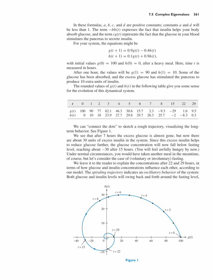
7.5 Complex Eigenvalues 361
In these formulas, a, b, c, and d are positive constants; constants a and d willbe less than 1. The term −bh(t) expresses the fact that insulin helps your bodyabsorb glucose, and the term cg(t) represents the fact that the glucose in your bloodstimulates the pancreas to secrete insulin.
For your system, the equations might be
g(t + 1) = 0.9g(t) − 0.4h(t)h(t + 1) = 0.1g(t) + 0.9h(t),
with initial values g(0) = 100 and h(0) = 0, after a heavy meal. Here, time t ismeasured in hours.
After one hour, the values will be g(1) = 90 and h(1) = 10. Some of theglucose has been absorbed, and the excess glucose has stimulated the pancreas toproduce 10 extra units of insulin.
The rounded values of g(t) and h(t) in the following table give you some sensefor the evolution of this dynamical system.
t 0 1 2 3 4 5 6 7 8 15 22 29
g(t) 100 90 77 62.1 46.3 30.6 15.7 2.3 −9.3 −29 1.6 9.5h(t) 0 10 18 23.9 27.7 29.6 29.7 28.3 25.7 −2 −8.3 0.3
We can “connect the dots” to sketch a rough trajectory, visualizing the long-term behavior. See Figure 1.
We see that after 7 hours the excess glucose is almost gone, but now thereare about 30 units of excess insulin in the system. Since this excess insulin helpsto reduce glucose further, the glucose concentration will now fall below fastinglevel, reaching about −30 after 15 hours. (You will feel awfully hungry by now.)Under normal circumstances, you would have taken another meal in the meantime,of course, but let’s consider the case of (voluntary or involuntary) fasting.
We leave it to the reader to explain the concentrations after 22 and 29 hours, interms of how glucose and insulin concentrations influence each other, according toour model. The spiraling trajectory indicates an oscillatory behavior of the system:Both glucose and insulin levels will swing back and forth around the fasting level,
−40 −20 20 40 60 80 100
−10
10
0
20
30
t = 0
t = 2
t = 4t = 6
h(t)
g(t)
t = 8
t = 15t = 22
t = 29
Figure 1

362 CHAPTER 7 Eigenvalues and Eigenvectors
10 30
−40
−200
20
40
60
80
100
t (hours)
g(t)
h(t)
Figure 2
like a damped pendulum. Both concentrations will approach the fasting level (thusthe name).
Another way to visualize this oscillatory behavior is to graph the functions g(t)and h(t) against time, using the values from our table. See Figure 2.
Next, we try to use the tools developed in the last four sections to analyze thissystem. We can introduce the transformation matrix
A =[
0.9 −0.40.1 0.9
]
and the state vector
x(t) =[
g(t)h(t)
].
Then
x(t + 1) = Ax(t) and thus x(t) = At x(0) = At[
1000
].
To find formulas for g(t) and h(t), we need to know the eigenvalues and eigen-vectors of matrix A. The characteristic polynomial of A is
f A(λ) = λ2 − 1.8λ + 0.85,
so that
λ1,2 = 1.8 ±√
3.24 − 3.42
= 1.8 ±√
−0.162
.
Since the square of a real number cannot be negative, there are no real eigenvalueshere. However, if we allow complex solutions, then we have the eigenvalues
λ1,2 = 1.8 ±√
−0.162
= 1.8 ± i√
0.162
= 0.9 ± 0.2i.
In this section, we will first review some basic facts on complex numbers. Thenwe will examine how the theory of eigenvalues and eigenvectors developed in Sec-tions 7.1 through 7.4 can be adapted to the complex case. In Section 7.6 we willapply this work to dynamical systems. A great many dynamical systems, in physics,chemistry, biology, and economics, show oscillatory behavior; we will see that wecan expect complex eigenvalues in this case.

7.5 Complex Eigenvalues 363
These tools will enable you to find formulas for g(t) and h(t). See Exer-cise 7.6.32.
Complex Numbers: A Brief ReviewLet us review some basic facts about complex numbers. We trust that you have atleast a fleeting acquaintance with complex numbers. Without attempting a formaldefinition, we recall that a complex number can be expressed as
z = a + ib,
where a and b are real numbers.12 Addition of complex numbers is defined in anatural way, by the rule
(a + ib) + (c + id) = (a + c) + i(b + d),
and multiplication is defined by the rule
(a + ib)(c + id) = (ac − bd) + i(ad + bc);
that is, we let i · i = −1 and distribute.If z = a + ib is a complex number, we call a its real part, denoted by Re z
and b its imaginary part, denoted by Im z. A complex number of the form ib (witha = 0) is called imaginary.
The set of all complex numbers is denoted by C. The real numbers, R, form asubset of C (namely, those complex numbers with imaginary part 0).
Complex numbers can be represented as vectors (or points) in the complexplane,13 as shown in Figure 3. This is a graphical representation of the isomorphism
T[
ab
]= a + ib from R2 to C.
−1 1 2 3 Real axis
Imaginaryaxis
3i
2i
i
z = 2 + 3i
Figure 3
iz = −b + ia
z = a + ib
90°
Figure 4
EXAMPLE 1 Consider a nonzero complex number z. What is the geometric relationship betweenz and i z in the complex plane?
12 The letter i for the imaginary unit was introduced by Leonhard Euler, the most prolificmathematician in history. For a fascinating glimpse at the history of the complex numbers, see TobiasDantzig, Number: The Language of Science, Macmillan, 1954. For another intriguing introduction,full of poetry, history, and philosophy, see Barry Mazur, Imagining Numbers (particularly the squareroot of minus fifteen), Farrar, Straus, and Giroux, 2003.13Also called “Argand plane,” after the Swiss mathematician Jean Robert Argand (1768–1822). Therepresentation of complex numbers in the plane was introduced independently by Argand, by Gauss,and by the Norwegian mathematician Caspar Wessel (1745–1818).

364 CHAPTER 7 Eigenvalues and Eigenvectors
Solution
If z = a + ib, then i z = −b + ia. We obtain the vector[−b
a
](representing i z)
by rotating the vector[
ab
](representing z) through an angle of 90 in the counter-
clockwise direction. See Figure 4. !The conjugate of a complex number z = a + ib is defined by
z = a − ib.
(The sign of the imaginary part is reversed.) We say that z and z form a conjugatepair of complex numbers. Geometrically, the conjugate z is the reflection of z aboutthe real axis, as shown in Figure 5.
Sometimes it is useful to describe a complex number in polar coordinates, asshown in Figure 6.
The length r of the vector is called the modulus of z, denoted by |z|. The polarangle θ is called an argument of z; note that the argument is determined only up toa multiple of 2π . (Mathematicians say “modulo 2π .”) For example, for z = −1, wecan choose the argument π , −π , or 3π .
z = a + ib
z = a − ib
Figure 5
z = a + ibr = a2 + b2 = |z|
= arg(z)
Figure 6
EXAMPLE 2 Find the modulus and an argument of z = −2 + 2i .
Solution|z| =
√22 + 22 =
√8. Representing z in the complex plane, we see that 3
4π is anargument of z. See Figure 7. !
If z is a complex number with modulus r and argument θ , we can write z as
z = r(cos θ) + ir(sin θ) = r(cos θ + i sin θ),
as shown in Figure 8.
−2
z 2
r = 8
= 34
Figure 7
z
r r (sin )
r (cos )
Figure 8

7.5 Complex Eigenvalues 365
The representation
z = r(cos θ + i sin θ)
is called the polar form of the complex number z.
EXAMPLE 3 Consider the complex numbers z = cos α + i sin α and w = cos β + i sin β. Findthe polar form of the product zw.
SolutionApply the addition formulas from trigonometry (see Exercise 2.2.32):
zw = (cos α + i sin α)(cos β + i sin β)
= (cos α cos β − sin α sin β) + i(sin α cos β + cos α sin β)
= cos(α + β) + i sin(α + β).
We conclude that the modulus of zw is 1, and α + β is an argument of zw. SeeFigure 9. !
zw
w
z
1
Figure 9
In general, if z = r(cos α + i sin α) and w = s(cos β + i sin β), then
zw = rs(cos(α + β) + i sin(α + β)
).
When we multiply two complex numbers, we multiply the moduli, and we add thearguments:
|zw| = |z||w|arg(zw) = arg z + arg w (modulo 2π).
EXAMPLE 4 Describe the transformation T (z) = (3 + 4i)z from C to C geometrically.
Solution
|T (z)| = |3 + 4i ||z| = 5|z|
arg(T (z)
)= arg(3 + 4i) + arg(z) = arctan
(43
)+ arg(z) ≈ 53 + arg(z)
The transformation T is a rotation combined with a scaling in the complex plane.See Figure 10.
z1
z2
T(z1)
T(z2 )
Figure 10 Rotate through about 53 and stretch the vector by a factorof 5.

366 CHAPTER 7 Eigenvalues and Eigenvectors
Alternatively, we observe that the matrix of the linear transformation T with
respect to the basis 1, i is[
3 −44 3
], representing a rotation combined with a scal-
ing.The polar form is convenient for finding powers of a complex number z: If
z = r(cos θ + i sin θ),
then
z2 = r2(cos(2θ) + i sin(2θ)
),
...zn = rn
(cos(nθ) + i sin(nθ)
),
for any positive integer n. Each time we multiply by z, the modulus is multiplied byr and the argument increases by θ . The preceding formula was found by the Frenchmathematician Abraham de Moivre (1667–1754). !
Theorem 7.5.1 De Moivre’s formula
(cos θ + i sin θ)n = cos(nθ) + i sin(nθ)
EXAMPLE 5 Consider the complex number z = 0.5 + 0.8i . Represent the powers z2, z3, . . . inthe complex plane. What is lim
n→∞zn?
SolutionTo study the powers, write z in polar form:
z = r(cos θ + i sin θ).
Here
r =√
0.52 + 0.82 ≈ 0.943
and
θ = arctan0.80.5
≈ 58.
We have
zn = rn(cos(nθ) + i sin(nθ)).
The vector representation of zn+1 is a little shorter than that of zn (by about5.7%), and zn+1 makes an angle θ ≈ 58 with zn . If we connect the tips of con-secutive vectors, we see a trajectory that spirals in toward the origin, as shown inFigure 11. Note that lim
n→∞zn = 0, since r = |z| < 1. !

7.5 Complex Eigenvalues 367
z2 z
z7
z8
z3
z4z5
z6 1
i
−1
−i
Figure 11
Perhaps the most remarkable property of the complex numbers is expressed inthe fundamental theorem of algebra, first demonstrated by Carl Friedrich Gauss (inhis thesis, at age 22).
Theorem 7.5.2 Fundamental theorem of algebra
Any polynomial p(λ) with complex coefficients splits; that is, it can be writtenas a product of linear factors
p(λ) = k(λ − λ1)(λ − λ2) · · · (λ − λn),
for some complex numbers λ1, λ2, . . . , λn , and k. (The λi need not be distinct.)Therefore, a polynomial p(λ) of degree n has precisely n complex roots if
they are properly counted with their multiplicities.
For example, the polynomial
p(λ) = λ2 + 1,
which does not have any real zeros, splits over C:
p(λ) = (λ + i)(λ − i).
More generally, for a quadratic polynomial
q(λ) = λ2 + bλ + c,
where b and c are real, we can find the complex roots
λ1,2 = −b ±√
b2 − 4c2
and
q(λ) = (λ − λ1)(λ − λ2).

368 CHAPTER 7 Eigenvalues and Eigenvectors
Proving the fundamental theorem of algebra would lead us too far afield. Read anyintroduction to complex analysis or check Gauss’s original proof.14
Complex Eigenvalues and EigenvectorsThe complex numbers share some basic algebraic properties with the real num-bers.15 Mathematicians summarize these properties by saying that both the realnumbers R and the complex numbers C form a field. The rational numbers Q areanother important example of a field; the integers Z, on the other hand, don’t forma field. (Which of the 10 properties listed in the footnote fail to hold in this case?)
Which of the results and techniques derived in this text thus far still apply whenwe work with complex numbers throughout, that is, when we consider complexscalars, vectors with complex components, and matrices with complex entries? Weobserve that everything works the same way except for those geometrical conceptsthat are defined in terms of the dot product (length, angles, orthogonality, and soon, discussed in Chapter 5 and Section 6.3). The dot product in Cn is defined ina way that we will not discuss in this introductory text. The whole body of “corelinear algebra” can be generalized without difficulty, however: echelon form, lineartransformation, kernel, image, linear independence, basis, dimension, coordinates,linear spaces, determinant, eigenvalues, eigenvectors, and diagonalization.
EXAMPLE 6 Diagonalize the rotation-scaling matrix A =[
a −bb a
]“over C.” Here, a and b are
real numbers, and b is nonzero.
SolutionWe will find the eigenvalues of A first:
f A(λ) = det[
a − λ −bb a − λ
]= (a − λ)2 + b2 = 0
when(a − λ)2 = −b2 or a − λ = ± ib or λ = a ± ib.
Now we find the eigenvectors:
Ea+ib = ker[−ib −b
b −ib
]= span
[i1
]
Ea−ib = ker[
ib −bb ib
]= span
[−i
1
].
14C. F. Gauss, Werke, III, 3–56. For an English translation, see D. J. Struik (editor), A Source Book inMathematics 1200–1800, Princeton University Press, 1986.15Here is a list of these properties:
1. Addition is commutative.2. Addition is associative.3. There exists a unique number n such that a + n = a, for all numbers a. This number n is
denoted by 0.4. For each number a there exists a unique number b such that a + b = 0. This number b is denoted
by −a. (Comment: This property says that we can subtract in this number system.)5. Multiplication is commutative.6. Multiplication is associative.7. There is a unique number e such that ea = a, for all numbers a. This number e is denoted by 1.8. For each nonzero number a there exists a unique number b such that ab = 1. This number b is
denoted by a−1. (Comment: This property says that we can divide by a nonzero number.)9. Multiplication distributes over addition: a(b + c) = ab + ac.
10. The numbers 0 and 1 are not equal.

7.5 Complex Eigenvalues 369
Thus,
R−1[
a −bb a
]R =
[a + ib 0
0 a − ib
], where R =
[i −i1 1
]. !
EXAMPLE 7 Let A be a real 2 × 2 matrix with eigenvalues a ± ib (where b = 0). Show that A
is similar (over R) to the matrix[
a −bb a
], representing a rotation combined with
a scaling.
SolutionLet v ± iw be eigenvectors of A with eigenvalues a ± ib. See Exercise 42. Matrix
A is similar to[
a + ib 00 a − ib
]; more precisely,
[a + ib 0
0 a − ib
]= P−1 AP,
where P =[v + iw v − iw
]. By Example 6, matrix
[a −bb a
]
is similar to [a + ib 0
0 a − ib
]
as well, with[
a + ib 00 a − ib
]= R−1
[a −bb a
]R, where R =
[i −i1 1
].
Thus,
P−1 AP = R−1[
a −bb a
]R,
and[
a −bb a
]= R P−1 AP R−1 = S−1 AS,
where S = P R−1 and S−1 = (P R−1)−1 = R P−1.A straightforward computation shows that
S = P R−1 = 12i
[v + iw v − iw
] [1 i
−1 i
]=
[w v
];
note that S has real entries, as claimed. !
Theorem 7.5.3 Complex eigenvalues and rotation-scaling matrices
If A is a real 2 × 2 matrix with eigenvalues a ± ib (where b = 0), and if v + iwis an eigenvector of A with eigenvalue a + ib, then
S−1 AS =[
a −bb a
], where S =
[w v
].

370 CHAPTER 7 Eigenvalues and Eigenvectors
We see that matrix A is similar to a rotation-scaling matrix. Those who have stud-ied Section 5.5 can go a step further: If we introduce the inner product ⟨x, y⟩= (S−1 x) · (S−1 y) in R2 and define the length of vectors and the angle betweenvectors with respect to this inner product, then the transformation T (x) = Ax is arotation combined with a scaling in that inner product space. (Think about it!)
EXAMPLE 8 For A =[
3 −51 −1
], find an invertible 2 × 2 matrix S such that S−1 AS is a rotation-
scaling matrix.
SolutionWe will use the method outlined in Theorem 7.5.3:
f A(λ) = λ2 − 2λ + 2, so that λ1,2 = 2 ±√
4 − 82
= 1 ± i.
Now
E1+i = ker[
2 − i −51 −2 − i
]= span
[−5
−2 + i
],
and[
−5−2 + i
]=
[−5−2
]+ i
[01
], so that w =
[01
], v =
[−5−2
].
Therefore,
S−1 AS =[
1 −11 1
], where S =
[0 −51 −2
]. !
The great advantage of complex eigenvalues is that there are so many of them.By the fundamental theorem of algebra, Theorem 7.5.2, the characteristic polyno-mial always splits:
f A(λ) = (λ1 − λ)(λ2 − λ) · · · (λn − λ).
Theorem 7.5.4 A complex n × n matrix has n complex eigenvalues if they are counted withtheir algebraic multiplicities.
Although a complex n × n matrix may have fewer than n distinct complex
eigenvalues (examples are In or[
0 10 0
]), this is literally a coincidence: Some of
the λi in the factorization of the characteristic polynomial f A(λ) coincide. “Most”complex n × n matrices do have n distinct eigenvalues, so that most complex n × nmatrices are diagonalizable (by Theorem 7.3.4). An example of a matrix that fails
to be diagonalizable over C is[
0 10 0
].
In this text, we focus on diagonalizable matrices and often dismiss others asrare aberrations. Some theorems will be proven in the diagonalizable case only,with the nondiagonalizable case being left as an exercise. Much attention is givento nondiagonalizable matrices in more advanced linear algebra courses.
EXAMPLE 9 Consider an n × n matrix A with complex eigenvalues λ1, λ2, . . . , λn , listed withtheir algebraic multiplicities. What is the relationship between the λi and the deter-minant of A? Compare with Theorem 7.2.8.

7.5 Complex Eigenvalues 371
Solution
f A(λ) = det(A − λIn) = (λ1 − λ)(λ2 − λ) · · · (λn − λ)
f A(0) = det A = λ1λ2 · · · λn
so that
det A = λ1λ2 · · · λn !Can you interpret this result geometrically when A is a 3 × 3 matrix with a real
eigenbasis? Hint: Think about the expansion factor. See Exercise 18.In Example 9, we found that the determinant of a matrix is the product of its
complex eigenvalues. Likewise, the trace is the sum of the eigenvalues. The verifi-cation is left as Exercise 35.
Theorem 7.5.5 Trace, determinant, and eigenvalues
Consider an n×n matrix A with complex eigenvalues λ1, λ2, . . . , λn , listed withtheir algebraic multiplicities. Then
tr A = λ1 + λ2 + · · · + λn
and
det A = λ1λ2 · · · λn.
Note that this result is obvious for a triangular matrix: In this case, the eigen-values are the diagonal entries.
EXERCISES 7.5GOAL Use the basic properties of complex numbers.Write products and powers of complex numbers in polarform. Apply the fundamental theorem of algebra.
1. Write the complex number z = 3 − 3i in polar form.
2. Find all complex numbers z such that z4 = 1. Representyour answers graphically in the complex plane.
3. For an arbitrary positive integer n, find all complexnumbers z such that zn = 1 (in polar form). Representyour answers graphically.
4. Show that if z is a nonzero complex number, then thereare exactly two complex numbers w such that w2 = z.If z is in polar form, describe w in polar form.
5. Show that if z is a nonzero complex number, then thereexist exactly n complex numbers w such that wn = z.If z is in polar form, write w in polar form. Representthe vectors w in the complex plane.
6. If z is a nonzero complex number in polar form, de-scribe 1/z in polar form. What is the relationship be-tween the complex conjugate z and 1/z? Represent thenumbers z, z, and 1/z in the complex plane.
7. Describe the transformation T (z) = (1 − i)z from C toC geometrically.
8. Use de Moivre’s formula to express cos(3θ) and sin(3θ)in terms of cos θ and sin θ .
9. Consider the complex number z = 0.8−0.7i . Representthe powers z2, z3, . . . in the complex plane and explaintheir long-term behavior.
10. Prove the fundamental theorem of algebra for cubicpolynomials with real coefficients.
11. Express the polynomial f (λ) = λ3 − 3λ2 + 7λ − 5 asa product of linear factors over C.
12. Consider a polynomial f (λ) with real coefficients.Show that if a complex number λ0 is a root of f (λ),then so is its complex conjugate, λ0.
For the matrices A listed in Exercises 13 through 17,
find an invertible matrix S such that S−1 AS =[
a −bb a
],
where a and b are real numbers.
13.[
0 −41 0
]14.
[1 −21 −1
]
15.[
0 1−5 4
]16.
[3 1
−2 5
]

372 CHAPTER 7 Eigenvalues and Eigenvectors
17.[
5 4−5 1
]
18. Consider a real 2 × 2 matrix A with two distinct realeigenvalues, λ1 and λ2. Explain the formula det A =λ1λ2 geometrically, thinking of |det A| as an expan-sion factor. Illustrate your explanation with a sketch.Is there a similar geometric interpretation for a 3 × 3matrix?
19. Consider a subspace V of Rn , with dim(V ) = m < n.a. If the n × n matrix A represents the orthogonal pro-
jection onto V , what is tr A? What is det A?b. If the n × n matrix B represents the reflection about
V , what is tr B? What is det B?
Find all complex eigenvalues of the matrices in Exercises20 through 26 (including the real ones, of course). Do notuse technology. Show all your work.
20.[
3 −52 −3
]21.
[11 −156 −7
]
22.[
1 3−4 10
]23.
⎡
⎣0 0 11 0 00 1 0
⎤
⎦
24.
⎡
⎣0 1 00 0 15 −7 3
⎤
⎦ 25.
⎡
⎢⎢⎣
0 0 0 11 0 0 00 1 0 00 0 1 0
⎤
⎥⎥⎦
26.
⎡
⎢⎢⎣
1 −1 1 −11 1 1 10 0 1 10 0 1 1
⎤
⎥⎥⎦
27. Suppose a real 3 × 3 matrix A has only two distincteigenvalues. Suppose that tr A = 1 and det A = 3. Findthe eigenvalues of A with their algebraic multiplicities.
28. Suppose a 3 × 3 matrix A has the real eigenvalue 2 andtwo complex conjugate eigenvalues. Also, suppose thatdet A = 50 and tr A = 8. Find the complex eigenvalues.
29. Consider a matrix of the form
A =
⎡
⎣0 a bc 0 00 d 0
⎤
⎦ ,
where a, b, c, and d are positive real numbers. Sup-pose the matrix A has three distinct real eigenvalues.What can you say about the signs of the eigenvalues?(How many of them are positive, negative, zero?) Is theeigenvalue with the largest absolute value positive ornegative?
30. a. If 2i is an eigenvalue of a real 2 × 2 matrix A, findA2.
b. Give an example of a real 2 × 2 matrix A such thatall the entries of A are nonzero and 2i is an eigen-
value of A. Compute A2 and check that your answeragrees with part a.
31. Consider the regular transition matrix
A = 115
⎡
⎢⎢⎢⎣
4 2 5 1 31 3 4 5 23 5 1 2 42 1 3 4 55 4 2 3 1
⎤
⎥⎥⎥⎦.
Note that the matrix 15A contains each of the integers1, 2, 3, 4, and 5 once in every row and in every column.a. Using technology, compute a high power of A, such
as A20. What do you observe? Make a conjecture forlim
t→∞At . (In part e, you will prove this conjecture.)
b. Use technology to find the complex eigenvalues ofA. Is matrix A diagonalizable over C?
c. Find the equilibrium distribution xequ for A, that is,the unique distribution vector in the eigenspace E1.
d. Without using Theorem 7.4.1 (which was provenonly for matrices that are diagonalizable over R),show that lim
t→∞(At x0) = xequ for any distribution
vector x0. Hint: Adapt the proof of Theorem 7.4.1to the complex case.
e. Find limt→∞
At , proving your conjecture from part a.
32. Consider the dynamical system
x(t + 1) = Ax(t), where A =
⎡
⎣0.4 0.1 0.50.4 0.3 0.10.2 0.6 0.4
⎤
⎦ ,
perhaps modeling the way people surf a mini-Web, asin Exercise 7.4.1.a. Using technology, compute a high power of A, such
as A20. What do you observe? Make a conjecture forlim
t→∞At . (In part e, you will prove this conjecture.)
b. Use technology to find the complex eigenvalues ofA. Is matrix A diagonalizable over C?
c. Find the equilibrium distribution xequ for A, that is,the unique distribution vector in the eigenspace E1.
d. Without using Theorem 7.4.1 (which was provenonly for matrices that are diagonalizable over R),show that lim
t→∞(At x0) = xequ for any distribution
vector x0. Hint: Adapt the proof of Theorem 7.4.l tothe complex case.
e. Find limt→∞
At , proving your conjecture frompart a.
33. The power method for finding eigenvalues. Using tech-nology, generate a random 5 × 5 matrix A with non-negative entries. (Depending on the technology you areusing, the entries could be integers between zero and
7.5 Complex Eigenvalues 373
nine, or numbers between zero and one.) Using tech-nology, compute B = A20 (or another high power ofA). We wish to compare the columns of B. This is hardto do by inspection, particularly because the entries ofB may get rather large.
To get a better hold on B, form the diagonal 5 × 5matrix D whose i th diagonal element is b1i , the i th en-try of the first row of B. Compute C = B D−1.a. How is C obtained from B? Give your answer in
terms of elementary row or column operations.b. Take a look at the columns of the matrix C you get.
What do you observe? What does your answer tellyou about the columns of B = A20?
c. Explain the observations you made in part b. Youmay assume that A has five distinct (complex)eigenvalues and that the eigenvalue with maximalmodulus is real and positive. (We cannot explainhere why this will usually be the case.)
d. Compute AC . What is the significance of the en-tries in the top row of this matrix in terms of theeigenvalues of A? What is the significance of thecolumns of C (or B) in terms of the eigenvectorsof A?
34. Exercise 33 illustrates how you can use the powers ofa matrix to find its dominant eigenvalue (i.e., the eigen-value with maximal modulus), at least when this eigen-value is real. But what about the other eigenvalues?a. Consider an n × n matrix A with n distinct com-
plex eigenvalues λ1, λ2, . . . , λn , where λ1 is real.Suppose you have a good (real) approximation λof λ1 (good in that |λ − λ1| < |λ − λi |, fori = 2, . . . , n). Consider the matrix A − λIn . Whatare its eigenvalues? Which has the smallest modu-lus? Now consider the matrix (A − λIn)−1. Whatare its eigenvalues? Which has the largest modulus?What is the relationship between the eigenvectors ofA and those of (A − λIn)−1? Consider higher andhigher powers of (A − λIn)−1. How does this helpyou to find an eigenvector of A with eigenvalue λ1,and λ1 itself? Use the results of Exercise 33.
b. As an example of part a, consider the matrix
A =
⎡
⎣1 2 34 5 67 8 10
⎤
⎦ .
We wish to find the eigenvectors and eigenvalues ofA without using the corresponding commands onthe computer (which is, after all, a “black box”).First, we find approximations for the eigenvalues bygraphing the characteristic polynomial (use techno-logy). Approximate the three real eigenvalues of Ato the nearest integer. One of the three eigenvaluesof A is negative. Find a good approximation forthis eigenvalue and a corresponding eigenvectorby using the procedure outlined in part a. You
are not asked to do the same for the two othereigenvalues.
35. Demonstrate the formula
tr A = λ1 + λ2 + · · · + λn,
where the λi are the complex eigenvalues of thematrix A, counted with their algebraic multiplicities.Hint: Consider the coefficient of λn−1 in f A(λ) =(λ1 − λ)(λ2 − λ) · · · (λn − λ), and compare the resultwith Theorem 7.2.5.
36. In 1990, the population of the African country Beninwas about 4.6 million people. Its composition by agewas as follows:
Age Bracket 0–15 15–30 30–45 45–60 60–75 75–90Percent of 46.6 25.7 14.7 8.4 3.8 0.8
Population
We represent these data in a state vector whose compo-nents are the populations in the various age brackets, inmillions:
x(0) = 4.6
⎡
⎢⎢⎢⎢⎢⎢⎣
0.4660.2570.1470.0840.0380.008
⎤
⎥⎥⎥⎥⎥⎥⎦≈
⎡
⎢⎢⎢⎢⎢⎢⎣
2.141.180.680.390.170.04
⎤
⎥⎥⎥⎥⎥⎥⎦.
We measure time in increments of 15 years, with t = 0in 1990. For example, x(3) gives the age composition inthe year 2035 (1990 + 3 · 15). If current age-dependentbirth and death rates are extrapolated, we have the fol-lowing model:
x(t + 1) =
⎡
⎢⎢⎢⎢⎢⎢⎣
1.1 1.6 0.6 0 0 00.82 0 0 0 0 00 0.89 0 0 0 00 0 0.81 0 0 00 0 0 0.53 0 00 0 0 0 0.29 0
⎤
⎥⎥⎥⎥⎥⎥⎦x(t)
= Ax(t).
a. Explain the significance of all the entries in the ma-trix A in terms of population dynamics.
b. Find the eigenvalue of A with the largest modu-lus and an associated eigenvector (use technology).What is the significance of these quantities in termsof population dynamics? (For a summary on ma-trix techniques used in the study of age-structuredpopulations, see Dmitrii O. Logofet, Matrices andGraphs: Stability Problems in Mathematical Ecol-ogy, Chapters 2 and 3, CRC Press, 1993.)

374 CHAPTER 7 Eigenvalues and Eigenvectors
37. Consider the set H of all complex 2 × 2 matrices of theform
A =[w −zz w
],
where w and z are arbitrary complex numbers.a. Show that H is closed under addition and multipli-
cation. (That is, show that the sum and the productof two matrices in H are again in H .)
b. Which matrices in H are invertible?c. If a matrix in H is invertible, is the inverse in H as
well?d. Find two matrices A and B in H such that AB =
B A.H is an example of a skew field: It satisfies all
axioms for a field, except for the commutativity ofmultiplication. [The skew field H was introducedby the Irish mathematician Sir William Hamilton(1805–1865); its elements are called the quater-nions. Another way to define the quaternions is dis-cussed in Exercise 5.3.64.]
38. Consider the matrix
C4 =
⎡
⎢⎢⎣
0 0 0 11 0 0 00 1 0 00 0 1 0
⎤
⎥⎥⎦ .
a. Find the powers C24 , C3
4 , C44 , . . . .
b. Find all complex eigenvalues of C4, and construct acomplex eigenbasis.
c. A 4 × 4 matrix M is called circulant if it is of theform
M =
⎡
⎢⎢⎣
a d c bb a d cc b a dd c b a
⎤
⎥⎥⎦ .
Circulant matrices play an important role in statistics.Show that any circulant 4×4 matrix M can be expressedas a linear combination of I4, C4, C2
4 , C34 . Use this rep-
resentation to find an eigenbasis for M . What are theeigenvalues (in terms of a, b, c, d)?
39. Consider the n × n matrix Cn which has ones directlybelow the main diagonal and in the right upper corner,and zeros everywhere else. See Exercise 38 for a dis-cussion of C4.a. Describe the powers of Cn .b. Find all complex eigenvalues of Cn , and construct a
complex eigenbasis.c. Generalize part c of Exercise 38.
40. Consider a cubic equation
x3 + px = q,
where (p/3)3 +(q/2)2 is negative. Show that this equa-tion has three real solutions; write the solutions in theform x j = A cos(θ j ) for j = 1, 2, 3, expressing A andθ j in terms of p and q . How many of the solutions arein the interval (
√−p/3, 2
√−p/3)? Can there be so-
lutions larger than 2√
−p/3? Hint: Cardano’s formuladerived in Exercise 7.2.50 is useful.
41. In his high school final examination (Aarau, Switzer-land, 1896), young Albert Einstein (1879–1955) wasgiven the following problem: In a triangle ABC , let Pbe the center of the inscribed circle. We are told thatAP = 1, B P = 1
2 , and C P = 13 . Find the radius ρ of
the inscribed circle. Einstein worked through this prob-lem as follows:
sin(α
2
)= ρ
sin(
β
2
)= 2ρ
sin(γ
2
)= 3ρ .
(not to scale)
A B
C
α β
γ
ρP
For every triangle the following equation holds:
sin2(α
2
)+ sin2
(β
2
)+ sin2
(γ
2
)
+ 2 sin(α
2
)sin
(β
2
)sin
(γ
2
)= 1.
In our case
14ρ2 + 12ρ3 − 1 = 0.
Now let
ρ = 1x.
At this point we interrupt Einstein’s work and ask youto finish the job. Hint: Exercise 40 is helpful. Find theexact solution (in terms of trigonometric and inversetrigonometric functions), and give a numerical approxi-mation as well. (By the way, Einstein, who was allowedto use a logarithm table, solved the problem correctly.)Source: The Collected Papers of Albert Einstein, Vol. 1,Princeton University Press, 1987.
42. Consider a complex n × m matrix A. The conjugate Ais defined by taking the conjugate of each entry of A.For example, if

7.6 Stability 375
A =[
2 + 3i 52i 9
], then A =
[2 − 3i 5−2i 9
].
a. Show that if A and B are complex n × p and p × mmatrices, respectively, then
AB = A B.
b. Let A be a real n × n matrix and v + iw an eigen-vector of A with eigenvalue p + iq . Show that thevector v− iw is an eigenvector of A with eigenvaluep − iq .
43. Consider two real n × n matrices A and B that are“similar over C”: That is, there is a complex invert-ible n × n matrix S such that B = S−1 AS. Showthat A and B are in fact “similar over R”: That is,there is a real R such that B = R−1 AR. Hint: WriteS = S1 + i S2, where S1 and S2 are real. Consider thefunction f (z) = det(S1 + zS2), where z is a complexvariable. Show that f (z) is a nonzero polynomial. Con-clude that there is a real number x such that f (x) = 0.Show that R = S1 + x S2 does the job.
44. Show that every complex 2 × 2 matrix is similar to anupper triangular 2 × 2 matrix. Can you generalize thisresult to square matrices of larger size? Hint: Argue byinduction.
For which values of the real constant a are the matricesin Exercises 45 through 50 diagonalizable over C?
45.[
1 1a 1
]46.
[0 −aa 0
]47.
⎡
⎣0 0 01 0 a0 1 0
⎤
⎦
48.
⎡
⎣0 0 a1 0 30 1 0
⎤
⎦ 49.
⎡
⎣0 1 00 0 10 1 − a a
⎤
⎦
50.
⎡
⎣−a a −a
−a − 1 a + 1 −a − 10 0 0
⎤
⎦
For Exercises 51 through 55, state whether the given set isa field (with the customary addition and multiplication).
51. The rational numbers Q
52. The integers Z
53. The binary digits (introduced in Exercises 3.1.53 and3.1.54)
54. The rotation-scaling matrices of the form[
p −qq p
],
where p and q are real numbers
55. The set H considered in Exercise 5.3.64
7.6 Stability
In applications, the long-term behavior is often the most important qualitative fea-ture of a dynamical system. We are frequently faced with the following situa-tion: The state 0 represents an equilibrium of the system (in physics, ecology, oreconomics, for example). If the system is disturbed (moved into another state, awayfrom the equilibrium 0) and then left to its own devices, will it always return to theequilibrium state 0?
EXAMPLE 1 Consider a dynamical system x(t + 1) = Ax(t), where A is an n × n matrix.Suppose an initial state vector x0 is given. We are told that A has n distinct complexeigenvalues, λ1, . . . , λn , and that |λi | < 1 for i = 1, . . . , n. What can you say aboutthe long-term behavior of the system, that is, about lim
t→∞x(t)?
SolutionFor each complex eigenvalue λi , we can choose a complex eigenvector vi . Thenthe vi form a complex eigenbasis for A (by Theorem 7.3.4). We can write x0 as acomplex linear combination of the vi :
x0 = c1v1 + · · · + cn vn.
Then
x(t) = At x0 = c1λt1v1 + · · · + cnλ
tn vn.
By Example 5 of Section 7.5,
limt→∞
λti = 0, since |λi | < 1.

376 CHAPTER 7 Eigenvalues and Eigenvectors
Therefore,
limt→∞
x(t) = 0. !For the discussion of the long-term behavior of a dynamical system, the follow-
ing definition is useful:
Definition 7.6.1 Stable equilibrium
Consider a dynamical system
x(t + 1) = Ax(t).
We say that 0 is an (asymptotically) stable equilibrium for this system if
limt→∞
x(t) = limt→∞
(At x0) = 0
for all vectors x0 in Rn .16
Note that the zero state is stable if (and only if)
limt→∞
At = 0
(meaning that all entries of At approach zero). See Exercise 36.Consider the examples shown in Figure 1.
Figure 1(a) Asymptotically stable. Figure 1(b) Not asymptotically stable.
Generalizing Example 1, we have the following result:
Theorem 7.6.2 Stability and eigenvalues
Consider a dynamical system x(t +1) = Ax(t). The zero state is asymptoticallystable if (and only if) the modulus of all the complex eigenvalues of A is lessthan 1.
Example 1 illustrates this fact only when A is diagonalizable (i.e., when thereis a complex eigenbasis for A); recall that this is the case for most matrices A. InExercises 45 through 50 of Section 8.1, we will discuss the nondiagonalizable case.
16In this text, stable will always mean “asymptotically stable.” Several other notions of stability areused in applied mathematics.

7.6 Stability 377
For an illustration of Theorem 7.6.2, see Figure 10 of Section 7.1, where wesketched the phase portraits of 2×2 matrices with two distinct positive eigenvalues.
We will now turn our attention to the phase portraits of 2 × 2 matrices withcomplex eigenvalues p ± iq (where q = 0).
EXAMPLE 2 Consider the dynamical system
x(t + 1) =[
p −qq p
]x(t),
where p and q are real, and q is nonzero. Examine the stability of this system.Sketch phase portraits. Discuss your results in terms of Theorem 7.6.2.
SolutionAs in Theorem 2.2.4, we can write
[p −qq p
]= r
[cos θ − sin θ
sin θ cos θ
],
representing the transformation as a rotation through an angle θ combined with ascaling by r =
√p2 + q2. Then
x(t) =[
p −qq p
]t
x0 = r t[
cos(θ t) − sin(θ t)sin(θ t) cos(θ t)
]x0,
representing a rotation through an angle θ t combined with a scaling by r t .Figure 2 illustrates that the zero state is stable if r =
√p2 + q2 < 1.
(a) (b) (c)Figure 2 (a) r < 1: trajectories spiral inward. (b) r = 1: trajectories are circles. (c) r > 1:
trajectories spiral outward.
Alternatively, we can use Theorem 7.6.2 to examine the stability of the system.
From Example 6 of Section 7.5, we know that the eigenvalues of[
p −qq p
]are
λ1,2 = p ± iq, with |λ1| = |λ2| =√
p2 + q2. By Theorem 7.6.2, the zero state isstable if
√p2 + q2 < 1. !
Let us generalize Example 2. If A is any 2 × 2 matrix with eigenvalues λ1,2 =p± iq, what does the phase portrait of the dynamical system x(t +1) = Ax(t) looklike? Let v+iw be an eigenvector of A with eigenvalue p+iq. From Theorem 7.5.3,
we know that A is similar to the rotation–scaling matrix[
p −qq p
], with

378 CHAPTER 7 Eigenvalues and Eigenvectors
S−1 AS =[
p −qq p
]or A = S
[p −qq p
]S−1, where S =
[w v
].
Using the terminology introduced in Example 2, we find that
x(t) = At x0 = S[
p −qq p
]t
S−1 x0 = r t S[
cos(θ t) − sin(θ t)sin(θ t) cos(θ t)
]S−1 x0.
Theorem 7.6.3 Dynamical systems with complex eigenvalues
Consider the dynamical system x(t +1) = Ax(t), where A is a real 2×2 matrixwith eigenvalues
λ1,2 = p ± iq = r(cos(θ) ± i sin(θ)
), where q = 0.
Let v + iw be an eigenvector of A with eigenvalue p + iq.Then
x(t) = r t S[
cos(θ t) − sin(θ t)sin(θ t) cos(θ t)
]S−1 x0, where S =
[w v
].
Note that S−1 x0 is the coordinate vector of x0 with respect to basis w, v.
EXAMPLE 3 Consider the dynamical system
x(t + 1) =[
3 −51 −1
]x(t) with initial state x0 =
[01
].
Use Theorem 7.6.3 to find a closed formula for x(t), and sketch the trajectory.
SolutionIn Example 8 of Section 7.5, we found the eigenvalues
λ1,2 = 1 ± i.
The polar coordinates of eigenvalue 1 + i are r =√
2 and θ = π4 . Furthermore, we
found that
S =[w v
]=
[0 −51 −2
].
Since
S−1 x0 =[
10
],
Theorem 7.6.3 gives
x(t) = (√
2)t[
0 −51 −2
] ⎡
⎣cos(
π4 t
)− sin
(π4 t
)
sin(
π4 t
)cos
(π4 t
)
⎤
⎦[
10
]
= (√
2)t
⎡
⎣ −5 sin(
π4 t
)
cos(
π4 t
)− 2 sin
(π4 t
)
⎤
⎦ .
We leave it to the reader to work out the details of this computation.Next, let’s think about the trajectory. We will develop the trajectory step by
step:

7.6 Stability 379
• The points⎡
⎣cos(
π4 t
)− sin
(π4 t
)
sin(
π4 t
)cos
(π4 t
)
⎤
⎦[
10
](for t = 0, 1, 2, . . . )
are located on the unit circle, as shown in Figure 3a. Note that at t = 8 the
system returns to its initial position,[
10
]; the period of this system is 8.
• In Exercise 2.2.54, we saw that an invertible linear transformation maps theunit circle into an ellipse. Thus, the points
[0 −51 −2
]⎡
⎣cos(
π4 t
)− sin
(π4 t
)
sin(
π4 t
)cos
(π4 t
)
⎤
⎦[
10
]
are located on an ellipse, as shown in Figure 3b. The two column vectors of
S =[
0 −51 −2
]=
[w v
]
are shown in that figure as well. Again, the period of this system is 8.• The exponential growth factor (
√2)t will produce longer and longer vectors
x(t) = (√
2)t[
0 −51 −2
]⎡
⎣cos(
π4 t
)− sin
(π4 t
)
sin(
π4 t
)cos
(π4 t
)
⎤
⎦[
10
].
t = 4
t = 3t = 2
t = 1
t = 0,8
t = 4
t = 3t = 2
t = 1
t = 0,8
(a) (b)
(c)
1
1
1
1
t = 8
t = 4t = 3t = 2
t = 1 t = 020
20
v
w
−5−2
01
−5−2
01x(t) = ( 2)t
10
cos t4sin t4
−sin t4cos t4
10
cos t4sin t4
−sin t4cos t4
10
cos t4sin t4
−sin t4cos t4
Figure 3

380 CHAPTER 7 Eigenvalues and Eigenvectors
Thus, the trajectory spirals outward, as shown in Figure 3c. (We are usingdifferent scales in Figures 3a, b, and c.) Note that x(8) = (
√2)8 x(0) =
16x(0). !We can generalize our findings in Example 3.
Theorem 7.6.4 Phase portrait of a system with complex eigenvalues
Consider a dynamical system
x(t + 1) = Ax(t),
where A is a real 2 × 2 matrix with eigenvalues λ1,2 = p ± iq (where q = 0).Let
r = |λ1| = |λ2| =√
p2 + q2.
If r = 1, then the points x(t) are located on an ellipse; if r exceeds 1, thenthe trajectory spirals outward; and if r is less than 1, then the trajectory spiralsinward, approaching the origin.
Theorem 7.6.4 provides another illustration of Theorem 7.6.2: The zero state isstable if (and only if) r = |λ1| = |λ2| < 1.
If you have to sketch a trajectory of a system with complex eigenvalues with-out the aid of technology, it helps to compute and plot the first few points x(0),x(1), x(2), . . . , until you see a trend.
EXERCISES 7.6GOAL Use eigenvalues to determine the stability ofa dynamical system. Analyze the dynamical systemx(t + 1) = Ax(t), where A is a real 2 × 2 matrix witheigenvalues p ± iq.
For the matrices A in Exercises 1 through 10, determinewhether the zero state is a stable equilibrium of the dy-namical system x(t + 1) = Ax(t).
1. A =[
0.9 00 0.8
]2. A =
[−1.1 0
0 0.9
]
3. A =[
0.8 0.7−0.7 0.8
]4. A =
[−0.9 −0.4
0.4 −0.9
]
5. A =[
0.5 0.6−0.3 1.4
]6. A =
[−1 3
−1.2 2.6
]
7. A =[
2.4 −2.51 −0.6
]8. A =
[1 −0.2
0.1 0.7
]
9. A =
⎡
⎣0.8 0 −0.6
0 0.7 00.6 0 0.8
⎤
⎦
10. A =
⎡
⎣0.3 0.3 0.30.3 0.3 0.30.3 0.3 0.3
⎤
⎦
Consider the matrices A in Exercises 11 through 16. Forwhich real numbers k is the zero state a stable equilibriumof the dynamical system x(t + 1) = Ax(t)?
11. A =[
k 00 0.9
]12. A =
[0.6 k−k 0.6
]
13. A =[
0.7 k0 −0.9
]14. A =
[k kk k
]
15. A =[
1 k0.01 1
]16. A =
[0.1 k0.3 0.3
]
For the matrices A in Exercises 17 through 24, findreal closed formulas for the trajectory x(t + 1) = Ax(t),
where x(0) =[
01
]. Draw a rough sketch.
17. A =[
0.6 −0.80.8 0.6
]18. A =
[−0.8 0.6−0.8 −0.8
]
19. A =[
2 −33 2
]20. A =
[4 3
−3 4
]
21. A =[
1 5−2 7
]22. A =
[7 −156 −11
]
23. A =[−0.5 1.5−0.6 1.3
]24. A =
[1 −3
1.2 −2.6
]

7.6 Stability 381
Consider an invertible n × n matrix A such that thezero state is a stable equilibrium of the dynamical systemx(t + 1) = Ax(t). What can you say about the stability ofthe systems listed in Exercises 25 through 30?
25. x(t + 1) = A−1 x(t) 26. x(t + 1) = AT x(t)
27. x(t + 1) = −Ax(t) 28. x(t + 1) = (A − 2In)x(t)
29. x(t + 1) = (A + In)x(t) 30. x(t + 1) = A2 x(t)
31. Let A be a real 2 × 2 matrix. Show that the zero state isa stable equilibrium of the dynamical system x(t +1) =Ax(t) if (and only if)
|tr A| − 1 < det A < 1.
32. Let’s revisit the introductory example of Section 7.5:The glucose regulatory system of a certain patient canbe modeled by the equations
g(t + 1) = 0.9g(t) − 0.4h(t)
h(t + 1) = 0.1g(t) + 0.9h(t).
Find closed formulas for g(t) and h(t), and draw thetrajectory. Does your trajectory look like the one onpage 361?
33. Consider a real 2 × 2 matrix A with eigenvalues p ± iqand corresponding eigenvectors v ± iw. Show that if areal vector x0 is written as x0 = c1(v+iw)+c2(v−iw),then c2 = c1.
34. Consider a dynamical system x(t + 1) = Ax(t), whereA is a real n × n matrix.a. If | det A| ≥ 1, what can you say about the stability
of the zero state?b. If | det A| < 1, what can you say about the stability
of the zero state?
35. a. Consider a real n × n matrix with n distinct realeigenvalues λ1, . . . , λn , where |λi | ≤ 1 for all i =1, . . . , n. Let x(t) be a trajectory of the dynamicalsystem x(t+1) = Ax(t). Show that this trajectory isbounded; that is, there is a positive number M suchthat ∥x(t)∥ ≤ M for all positive integers t .
b. Are all trajectories of the dynamical system
x(t + 1) =[
1 10 1
]x(t)
bounded? Explain.
36. Show that the zero state is a stable equilibrium of thedynamical system x(t + 1) = Ax(t) if (and only if )
limt→∞
At = 0
(meaning that all entries of At approach zero).
37. Consider the national income of a country, whichconsists of consumption, investment, and govern-ment expenditures. Here we assume the government
expenditure to be constant, at G0, while the nationalincome Y (t), consumption C(t), and investment I (t)change over time. According to a simple model, wehave
∣∣∣∣∣∣
Y (t) = C(t) + I (t) + G0C(t + 1) = γ Y (t)I (t + 1) = α
(C(t + 1) − C(t)
)
∣∣∣∣∣∣(0 < γ < 1),(α > 0)
where γ is the marginal propensity to consume and αis the acceleration coefficient. (See Paul E. Samuelson,“Interactions between the Multiplier Analysis and thePrinciple of Acceleration,” Review of Economic Statis-tics, May 1939, pp. 75–78.)a. Find the equilibrium solution of these equations,
when Y (t + 1) = Y (t), C(t + 1) = C(t), andI (t + 1) = I (t).
b. Let y(t), c(t), and i(t) be the deviations of Y (t),C(t), and I (t), respectively, from the equilibriumstate you found in part (a). These quantities are re-lated by the equations
∣∣∣∣∣∣
y(t) = c(t) + i(t)c(t + 1) = γ y(t)i(t + 1) = α
(c(t + 1) − c(t)
)
∣∣∣∣∣∣.
(Verify this!) By substituting y(t) into the secondequation, set up equations of the form
∣∣∣∣c(t + 1) = pc(t) + qi(t)i(t + 1) = rc(t) + si(t)
∣∣∣∣ .
c. When α = 5 and γ = 0.2, determine the stability ofthe zero state of this system.
d. When α = 1 (and γ is arbitrary, 0 < γ < 1), deter-mine the stability of the zero state.
e. For each of the four sectors in the α–γ -plane, deter-mine the stability of the zero state.
γ
α
αγ = 1
1
1 2 3 4
IV II III
I
γ = 4α(1 + α)2
Discuss the various cases, in practical terms.
38. Consider an affine transformation
T (x) = Ax + b,
where A is an n×n matrix and b is a vector in Rn . Com-pare this with Exercise 7.4.35. Suppose that 1 is not aneigenvalue of A.a. Find the vector v in Rn such that T (v) = v; this vec-
tor is called the equilibrium state of the dynamicalsystem x(t + 1) = T
(x(t)
).
b. When is the equilibrium v in part (a) stable (mean-ing that lim
t→∞x(t) = v for all trajectories)?

382 CHAPTER 7 Eigenvalues and Eigenvectors
39. Consider the dynamical system
x1(t + 1) = 0.1x1(t) + 0.2x2(t) + 1,
x2(t + 1) = 0.4x1(t) + 0.3x2(t) + 2.
See Exercise 7.4.35. Find the equilibrium state of thissystem and determine its stability. See Exercise 38.Sketch a phase portrait.
40. Consider the matrix
A =
⎡
⎢⎢⎣
p −q −r −sq p s −rr −s p qs r −q p
⎤
⎥⎥⎦ ,
where p, q , r , s are arbitrary real numbers. Comparethis with Exercise 5.3.64.a. Compute AT A.b. For which values of p, q , r , s is A invertible? Find
the inverse if it exists.c. Find the determinant of A.d. Find the complex eigenvalues of A.e. If x is a vector in R4, what is the relationship be-
tween ∥x∥ and ∥Ax∥?f. Consider the numbers
59 = 32 + 32 + 42 + 52
and
37 = 12 + 22 + 42 + 42.
Express the number
2183
as the sum of the squares of four integers:
2183 = a2 + b2 + c2 + d2.
Hint: Part e is useful. Note that 2183 = 59 · 37.g. The French mathematician Joseph-Louis Lagrange
(1736–1813) showed that any prime number can beexpressed as the sum of the squares of four integers.Using this fact and your work in part (f) as a guide,show that any positive integer can be expressed inthis way.
41. Find a 2 × 2 matrix A without real eigenvalues and avector x0 in R2 such that for all positive integers t , thepoint At x0 is located on the ellipse in the accompanyingsketch.
−34
86
42. We quote from a text on computer graphics (M. Beeleret al., “HAKMEM,” MIT Artificial Intelligence ReportAIM-239, 1972):
Here is an elegant way to draw almost circleson a point-plotting display.
CIRCLE ALGORITHM:
NEW X = OLD X - K*OLD Y;NEW Y = OLD Y + K*NEW X.
This makes a very round ellipse centered atthe origin with its size determined by the ini-tial point. The circle algorithm was invented bymistake when I tried to save a register in a dis-play hack!
(In the preceding formula, k is a small number.) Here,a dynamical system is defined in “computer lingo.” Inour terminology, the formulas are
x(t + 1) = x(t) − ky(t),
y(t + 1) = y(t) + kx(t + 1).
a. Find the matrix of this transformation. [Note the en-try x(t + 1) in the second formula.]
b. Explain why the trajectories are ellipses, as claimed.
Chapter Seven Exercises
TRUE OR FALSE?1. If 0 is an eigenvalue of a matrix A, then det A = 0.
2. The eigenvalues of a 2 × 2 matrix A are the solutions ofthe equation λ2 − (trA)λ + (det A) = 0.
3. The eigenvalues of any triangular matrix are its diago-nal entries.
4. The trace of any square matrix is the sum of its diagonalentries.

Chapter Seven Exercises 383
5. The algebraic multiplicity of an eigenvalue cannot ex-ceed its geometric multiplicity.
6. If an n × n matrix A is diagonalizable (over R), thenthere must be a basis of Rn consisting of eigenvectorsof A.
7. If the standard vectors e1, e2, . . . , en are eigenvectorsof an n × n matrix A, then A must be diagonal.
8. If v is an eigenvector of A, then v must be an eigenvec-tor of A3 as well.
9. There exists a diagonalizable 5×5 matrix with only twodistinct eigenvalues (over C).
10. There exists a real 5 × 5 matrix without any realeigenvalues.
11. If matrices A and B have the same eigenvalues (over C),with the same algebraic multiplicities, then matrices Aand B must have the same trace.
12. If a real matrix A has only the eigenvalues 1 and −1,then A must be orthogonal.
13. Any rotation-scaling matrix in R2×2 is diagonalizableover C.
14. If A is a noninvertible n × n matrix, then the geometricmultiplicity of eigenvalue 0 is n − rank(A).
15. If matrix A is diagonalizable, then its transpose AT
must be diagonalizable as well.
16. If A and B are two 3 × 3 matrices such that tr A = tr Band det A = det B, then A and B must have the sameeigenvalues.
17. If 1 is the only eigenvalue of an n × n matrix A, then Amust be In .
18. If A and B are n × n matrices, if α is an eigenvalue ofA, and if β is an eigenvalue of B, then αβ must be aneigenvalue of AB.
19. If 3 is an eigenvalue of an n × n matrix A, then 9 mustbe an eigenvalue of A2.
20. The matrix of any orthogonal projection onto a sub-space V of Rn is diagonalizable.
21. All diagonalizable matrices are invertible.
22. If vector v is an eigenvector of both A and B, then vmust be an eigenvector of A + B.
23. If matrix A2 is diagonalizable, then matrix A must bediagonalizable as well.
24. The determinant of a matrix is the product of its eigen-values (over C), counted with their algebraic multiplic-ities.
25. All lower triangular matrices are diagonalizable(over C).
26. If two n × n matrices A and B are diagonalizable, thenAB must be diagonalizable as well.
27. If an invertible matrix A is diagonalizable, then A−1
must be diagonalizable as well.
28. If det(A) = det(AT ), then matrix A must be symmetric.
29. If matrix A =
⎡
⎣7 a b0 7 c0 0 7
⎤
⎦ is diagonalizable, then a, b,
and c must all be zero.
30. If two n × n matrices A and B are diagonalizable, thenA + B must be diagonalizable as well.
31. If u, v, w are eigenvectors of a 4 × 4 matrix A, withassociated eigenvalues 3, 7, and 11, respectively, thenvectors u, v, w must be linearly independent.
32. If a 4 × 4 matrix A is diagonalizable, then the matrixA + 4I4 must be diagonalizable as well.
33. If an n×n matrix A is diagonalizable, then A must haven distinct eigenvalues.
34. If two 3×3 matrices A and B both have the eigenvalues1, 2, and 3, then A must be similar to B.
35. If v is an eigenvector of A, then v must be an eigenvec-tor of AT as well.
36. All invertible matrices are diagonalizable.
37. If v and w are linearly independent eigenvectors of ma-trix A, then v + w must be an eigenvector of A as well.
38. If a 2×2 matrix R represents a reflection about a line L ,then R must be diagonalizable.
39. If A is a 2×2 matrix such that tr A = 1 and det A = −6,then A must be diagonalizable.
40. If a matrix is diagonalizable, then the algebraic multi-plicity of each of its eigenvalues λ must equal the geo-metric multiplicity of λ.
41. All orthogonal matrices are diagonalizable (over R).
42. If A is an n × n matrix and λ is an eigenvalue of the
block matrix M =[
A A0 A
], then λ must be an eigen-
value of matrix A.
43. If two matrices A and B have the same characteristicpolynomials, then they must be similar.
44. If A is a diagonalizable 4 × 4 matrix with A4 = 0, thenA must be the zero matrix.
45. If an n ×n matrix A is diagonalizable (over R), then ev-ery vector v in Rn can be expressed as a sum of eigen-vectors of A.
46. If vector v is an eigenvector of both A and B, then v isan eigenvector of AB.

384 CHAPTER 7 Eigenvalues and Eigenvectors
47. Similar matrices have the same characteristicpolynomials.
48. If a matrix A has k distinct eigenvalues, thenrank(A) ≥ k.
49. If the rank of a square matrix A is 1, then all the nonzerovectors in the image of A are eigenvectors of A.
50. If the rank of an n × n matrix A is 1, then A must bediagonalizable.
51. If A is a 4 × 4 matrix with A4 = 0, then 0 is the onlyeigenvalue of A.
52. If two n × n matrices A and B are both diagonalizable,then they must commute.
53. If v is an eigenvector of A, then v must be in the kernelof A or in the image of A.
54. All symmetric 2 × 2 matrices are diagonalizable(over R).
55. If A is a 2 × 2 matrix with eigenvalues 3 and 4 and if uis a unit eigenvector of A, then the length of vector Aucannot exceed 4.
56. If u is a nonzero vector in Rn , then u must be an eigen-vector of matrix uuT .
57. If v1, v2, . . . , vn is an eigenbasis for both A and B, thenmatrices A and B must commute.
58. If v is an eigenvector of a 2 × 2 matrix A =[
a bc d
],
then v must be an eigenvector of its classical adjoint
adj(A) =[
d −b−c a
]as well.

C H A P T E R
8Symmetric Matrices and Quadratic Forms
8.1 Symmetric Matrices
In this chapter we will work with real numbers throughout, except for a briefdigression into C in the discussion of Theorem 8.1.3.
Our work in the last chapter dealt with the following central question:
When is a given square matrix A diagonalizable? That is, when is there aneigenbasis for A?
In geometry, we prefer to work with orthonormal bases, which raises the fol-lowing question:
For which matrices is there an orthonormal eigenbasis? Or, equivalently, forwhich matrices A is there an orthogonal matrix S such that S−1 AS = ST AS isdiagonal?
(Recall that S−1 = ST for orthogonal matrices, by Theorem 5.3.7.) We say thatA is orthogonally diagonalizable if there exists an orthogonal matrix S such thatS−1 AS = ST AS is diagonal. Then, the question is:
Which matrices are orthogonally diagonalizable?
Simple examples of orthogonally diagonalizable matrices are diagonal matrices(we can let S = In) and the matrices of orthogonal projections and reflections.
EXAMPLE 1 If A is orthogonally diagonalizable, what is the relationship between AT and A?
SolutionWe have
S−1 AS = D or A = SDS−1 = SDST ,
385

386 CHAPTER 8 Symmetric Matrices and Quadratic Forms
for an orthogonal S and a diagonal D. Then
AT = (SDST )T = SDT ST = SDST = A.
We find that A is symmetric:
AT = A. !Surprisingly, the converse is true as well:
Theorem 8.1.1 Spectral theorem
A matrix A is orthogonally diagonalizable (i.e., there exists an orthogonal Ssuch that S−1 AS = ST AS is diagonal) if and only if A is symmetric (i.e.,AT = A).
We will prove this theorem later in this section, based on two preliminary re-sults, Theorems 8.1.2 and 8.1.3. First, we will illustrate the spectral theorem withan example.
EXAMPLE 2 For the symmetric matrix A =[
4 22 7
], find an orthogonal S such that S−1 AS is
diagonal.
SolutionWe will first find an eigenbasis. The eigenvalues of A are 3 and 8, with correspond-
ing eigenvectors[
2−1
]and
[12
], respectively. See Figure 1.
E8 = span 12
E3 = span 2−1
Figure 1
Note that the two eigenspaces, E3 and E8, are perpendicular. (This is no coin-cidence, as we will see in Theorem 8.1.2.) Therefore, we can find an orthonormaleigenbasis simply by dividing the given eigenvectors by their lengths:
v1 = 1√5
[2
−1
], v2 = 1√
5
[12
].
If we define the orthogonal matrix
S =
⎡
⎣| |v1 v2
| |
⎤
⎦ = 1√5
[2 1
−1 2
],
then S−1 AS will be diagonal; namely, S−1 AS =[
3 00 8
]. !
8.1 Symmetric Matrices 387
The key observation we made in Example 2 generalizes as follows:
Theorem 8.1.2 Consider a symmetric matrix A. If v1 and v2 are eigenvectors of A with distincteigenvalues λ1 and λ2, then v1 · v2 = 0; that is, v2 is orthogonal to v1.
Proof We compute the product
vT1 Av2
in two different ways:
vT1 Av2 = vT
1 (λ2v2) = λ2(v1 · v2)
vT1 Av2 = vT
1 AT v2 = (Av1)T v2 = (λ1v1)
T v2 = λ1(v1 · v2).
Comparing the results, we find
λ1(v1 · v2) = λ2(v1 · v2),
or
(λ1 − λ2)(v1 · v2) = 0.
Since the first factor in this product, λ1 − λ2, is nonzero, the second factor, v1 · v2,must be zero, as claimed. !
Theorem 8.1.2 tells us that the eigenspaces of a symmetric matrix are perpen-dicular to one another. Here is another illustration of this property:
EXAMPLE 3 For the symmetric matrix
A =
⎡
⎣1 1 11 1 11 1 1
⎤
⎦ ,
find an orthogonal S such that S−1 AS is diagonal.
SolutionThe eigenvalues are 0 and 3, with
E0 = span
⎛
⎝
⎡
⎣−1
10
⎤
⎦ ,
⎡
⎣−1
01
⎤
⎦
⎞
⎠ and E3 = span
⎡
⎣111
⎤
⎦ .
Note that the two eigenspaces are indeed perpendicular to one another, in accor-dance with Theorem 8.1.2. See Figure 2.
We can construct an orthonormal eigenbasis for A by picking an orthonormalbasis of each eigenspace (using the Gram–Schmidt process in the case of E0). SeeFigure 3.
In Figure 3, the vectors v1, v2 form an orthonormal basis of E0, and v3 is aunit vector in E3. Then v1, v2, v3 is an orthonormal eigenbasis for A. We can letS =
[v1 v2 v3
]to diagonalize A orthogonally.
If we apply the Gram–Schmidt1 process to the vectors⎡
⎣−1
10
⎤
⎦ ,
⎡
⎣−1
01
⎤
⎦
1Alternatively, we could find a unit vector v1 in E0 and a unit vector v3 in E3, and then let v2 = v3 × v1.
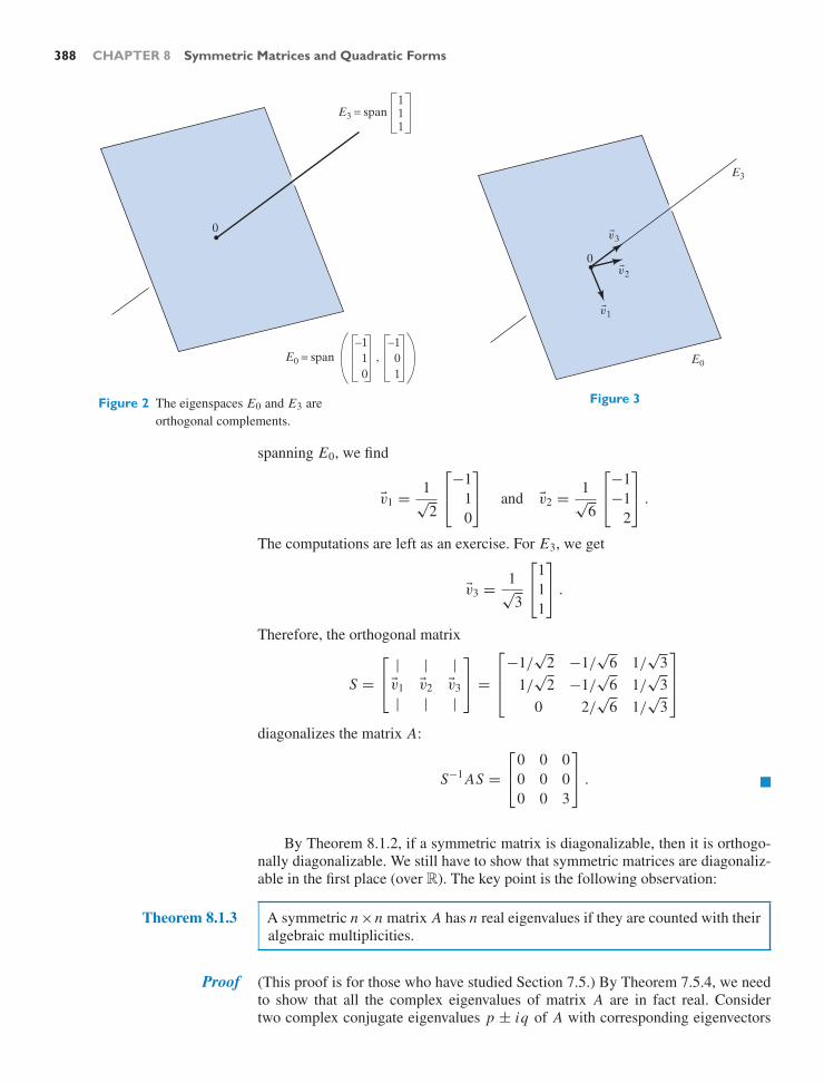
388 CHAPTER 8 Symmetric Matrices and Quadratic Forms
0
E3 = span111
E0 = span ,−1
10
−101
Figure 2 The eigenspaces E0 and E3 areorthogonal complements.
0
E3
E0
v3
v2
v1
Figure 3
spanning E0, we find
v1 = 1√2
⎡
⎣−1
10
⎤
⎦ and v2 = 1√6
⎡
⎣−1−1
2
⎤
⎦ .
The computations are left as an exercise. For E3, we get
v3 = 1√3
⎡
⎣111
⎤
⎦ .
Therefore, the orthogonal matrix
S =
⎡
⎣| | |v1 v2 v3
| | |
⎤
⎦ =
⎡
⎢⎣−1/
√2 −1/
√6 1/
√3
1/√
2 −1/√
6 1/√
30 2/
√6 1/
√3
⎤
⎥⎦
diagonalizes the matrix A:
S−1 AS =
⎡
⎣0 0 00 0 00 0 3
⎤
⎦ . !
By Theorem 8.1.2, if a symmetric matrix is diagonalizable, then it is orthogo-nally diagonalizable. We still have to show that symmetric matrices are diagonaliz-able in the first place (over R). The key point is the following observation:
Theorem 8.1.3 A symmetric n ×n matrix A has n real eigenvalues if they are counted with theiralgebraic multiplicities.
Proof (This proof is for those who have studied Section 7.5.) By Theorem 7.5.4, we needto show that all the complex eigenvalues of matrix A are in fact real. Considertwo complex conjugate eigenvalues p ± iq of A with corresponding eigenvectors

8.1 Symmetric Matrices 389
v ± iw. Compare this with Exercise 7.5.42b. We wish to show that these eigen-values are real; that is, q = 0. Note first that
(v + iw)T (v − iw) = ∥v∥2 + ∥w∥2.
(Verify this.) Now we compute the product
(v + iw)T A(v − iw)
in two different ways:
(v + iw)T A(v − iw) = (v + iw)T (p − iq)(v − iw)
= (p − iq)(∥v∥2 + ∥w∥2)
(v + iw)T A(v − iw) =(
A(v + iw))T
(v − iw) = (p + iq)(v + iw)T (v − iw)
= (p + iq)(∥v∥2 + ∥w∥2).
Comparing the results, we find that p + iq = p − iq, so that q = 0, as claimed.!
The foregoing proof is not very enlightening. A more transparent proof wouldfollow if we were to define the dot product for complex vectors, but to do so wouldlead us too far afield.
We are now ready to prove Theorem 8.1.1: Symmetric matrices are orthogo-nally diagonalizable.
Even though this is not logically necessary, let us first examine the case of asymmetric n × n matrix A with n distinct real eigenvalues. For each eigenvalue,we can choose an eigenvector of length 1. By Theorem 8.1.2, these eigenvectorswill form an orthonormal eigenbasis; that is, the matrix A will be orthogonallydiagonalizable, as claimed.
Proof(of Theorem 8.1.1):
This proof is somewhat technical; it may be skipped in a first reading of this textwithout harm.
We prove by induction on n that a symmetric n × n matrix A is orthogonallydiagonalizable. See Appendix B.
For a 1 × 1 matrix A, we can let S = [1].Now assume that the claim is true for n; we show that it holds for n + 1. Pick a
real eigenvalue λ of A (this is possible by Theorem 8.1.3), and choose an eigenvec-tor v1 of length 1 for λ. We can find an orthonormal basis v1, v2, . . . , vn+1 of Rn+1.(Think about how you could construct such a basis.) Form the orthogonal matrix
P =
⎡
⎣| | |v1 v2 · · · vn+1
| | |
⎤
⎦ ,
and compute
P−1 AP.
The first column of P−1 AP is λe1. (Why?) Also note that P−1 AP = PT AP issymmetric: (PT AP)T = PT AT P = PT AP , because A is symmetric. Combiningthese two statements, we conclude that P−1 AP has the block form
P−1 AP =[λ 00 B
], (I)

390 CHAPTER 8 Symmetric Matrices and Quadratic Forms
where B is a symmetric n×n matrix. By the induction hypothesis, B is orthogonallydiagonalizable; that is, there exists an orthogonal n × n matrix Q such that
Q−1 B Q = D
is a diagonal n × n matrix. Now introduce the orthogonal (n + 1) × (n + 1) matrix
R =[
1 00 Q
].
Then
R−1[λ 00 B
]R =
[1 00 Q−1
] [λ 00 B
] [1 00 Q
]=
[λ 00 D
](II)
is diagonal.Combining equations (I) and (II), we find that
R−1 P−1 AP R =[λ 00 D
](III)
is diagonal. Consider the orthogonal matrix S = P R. (Recall Theorem 5.3.4a:The product of orthogonal matrices is orthogonal.) Note that S−1 = (P R)−1 =R−1 P−1. Therefore, equation (III) can be written
S−1 AS =[λ 00 D
],
proving our claim. !The method outlined in the proof of Theorem 8.1.1 is not a sensible way to find
the matrix S in a numerical example. Rather, we can proceed as in Example 3:
Theorem 8.1.4 Orthogonal diagonalization of a symmetric matrix A
a. Find the eigenvalues of A, and find a basis of each eigenspace.b. Using the Gram–Schmidt process, find an orthonormal basis of each
eigenspace.c. Form an orthonormal eigenbasis v1, v2, . . . , vn for A by concatenating
the orthonormal bases you found in part b, and let
S =
⎡
⎣| | |v1 v2 . . . vn
| | |
⎤
⎦ .
S is orthogonal (by Theorem 8.1.2), and S−1 AS will be diagonal.
We conclude this section with an example of a geometric nature:
EXAMPLE 4 Consider an invertible symmetric 2 × 2 matrix A. Show that the linear transforma-tion T (x) = Ax maps the unit circle into an ellipse, and find the lengths of thesemimajor and the semiminor axes of this ellipse in terms of the eigenvalues of A.Compare this with Exercise 2.2.54.
SolutionThe spectral theorem tells us that there exists an orthonormal eigenbasis v1, v2 forT , with associated real eigenvalues λ1 and λ2. These eigenvalues will be nonzero,

8.1 Symmetric Matrices 391
since A is invertible. Arrange things so that |λ1| ≥ |λ2|. The unit circle in R2
consists of all vectors of the form
v = cos(t)v1 + sin(t)v2.
The image of the unit circle consists of the vectors
T (v) = cos(t)T (v1) + sin(t)T (v2)
= cos(t)λ1v1 + sin(t)λ2v2,
an ellipse whose semimajor axis λ1v1 has the length ∥λ1v1∥ = |λ1|, while the lengthof the semiminor axis is ∥λ2v2∥ = |λ2|. See Figure 4.
v1v2
T
T(v2) = 2v2Unitcircle
T(v1) = 1v1
Figure 4
In the example illustrated in Figure 4, the eigenvalue λ1 is positive, and λ2 isnegative. !
EXERCISES 8.1GOAL Find orthonormal eigenbases for symmetricmatrices. Apply the spectral theorem.
For each of the matrices in Exercises 1 through 6, find anorthonormal eigenbasis. Do not use technology.
1.[
1 00 2
]2.
[1 11 1
]
3.[
6 22 3
]4.
⎡
⎣0 0 10 0 11 1 1
⎤
⎦
5.
⎡
⎣0 1 11 0 11 1 0
⎤
⎦ 6.
⎡
⎣0 2 22 1 02 0 −1
⎤
⎦
For each of the matrices A in Exercises 7 through 11, findan orthogonal matrix S and a diagonal matrix D such thatS−1 AS = D. Do not use technology.
7. A =[
3 22 3
]8. A =
[3 33 −5
]
9. A =
⎡
⎣0 0 30 2 03 0 0
⎤
⎦ 10. A =
⎡
⎣1 −2 2
−2 4 −42 −4 4
⎤
⎦
11. A =
⎡
⎣1 0 10 1 01 0 1
⎤
⎦
12. Let L from R3 to R3 be the reflection about the linespanned by
v =
⎡
⎣102
⎤
⎦ .
a. Find an orthonormal eigenbasis ! for L .b. Find the matrix B of L with respect to !.c. Find the matrix A of L with respect to the standard
basis of R3.
13. Consider a symmetric 3 × 3 matrix A with A2 = I3.Is the linear transformation T (x) = Ax necessarily thereflection about a subspace of R3?

392 CHAPTER 8 Symmetric Matrices and Quadratic Forms
14. In Example 3 of this section, we diagonalized the ma-trix
A =
⎡
⎣1 1 11 1 11 1 1
⎤
⎦
by means of an orthogonal matrix S. Use this result todiagonalize the following matrices orthogonally (find Sand D in each case):
a.
⎡
⎣2 2 22 2 22 2 2
⎤
⎦ b.
⎡
⎣−2 1 1
1 −2 11 1 −2
⎤
⎦
c.
⎡
⎢⎢⎢⎣
0 12
12
12 0 1
212
12 0
⎤
⎥⎥⎥⎦
15. If A is invertible and orthogonally diagonalizable, isA−1 orthogonally diagonalizable as well?
16. a. Find the eigenvalues of the matrix
A =
⎡
⎢⎢⎢⎢⎣
1 1 1 1 11 1 1 1 11 1 1 1 11 1 1 1 11 1 1 1 1
⎤
⎥⎥⎥⎥⎦
with their multiplicities. Note that the algebraicmultiplicity agrees with the geometric multiplicity.(Why?) Hint: What is the kernel of A?
b. Find the eigenvalues of the matrix
B =
⎡
⎢⎢⎢⎢⎣
3 1 1 1 11 3 1 1 11 1 3 1 11 1 1 3 11 1 1 1 3
⎤
⎥⎥⎥⎥⎦
with their multiplicities. Do not use technology.c. Use your result in part b to find det B.
17. Use the approach of Exercise 16 to find the determinantof the n × n matrix B that has p’s on the diagonal andq’s elsewhere:
B =
⎡
⎢⎢⎢⎣
p q · · · qq p · · · q...
.... . .
...
q q · · · p
⎤
⎥⎥⎥⎦.
18. Consider unit vectors v1, . . . , vn in Rn such that the an-gle between vi and v j is 60 for all i = j . Find then-volume of the n-parallelepiped spanned byv1, . . . , vn . Hint: Let A =
[v1 · · · vn
], and think
about the matrix AT A and its determinant. Exercise 17is useful.
19. Consider a linear transformation L from Rm toRn . Show that there exists an orthonormal ba-sis v1, v2, . . . , vm of Rm such that the vectorsL(v1), L(v2), . . . , L(vm) are orthogonal. Note thatsome of the vectors L(vi ) may be zero. Hint: Consideran orthonormal eigenbasis v1, v2, . . . , vm for the sym-metric matrix ATA.
20. Consider a linear transformation T from Rm to Rn ,where m ≤ n. Show that there exist an orthonor-mal basis v1, . . . , vm of Rm and an orthonormal basisw1, . . . , wn of Rn such that T (vi ) is a scalar multipleof wi , for i = 1, . . . , m. Hint: Exercise 19 is helpful.
21. Consider a symmetric 3 × 3 matrix A with eigenval-ues 1, 2, and 3. How many different orthogonal matricesS are there such that S−1 AS is diagonal?
22. Consider the matrix
A =
⎡
⎢⎢⎣
0 2 0 0k 0 2 00 k 0 20 0 k 0
⎤
⎥⎥⎦ ,
where k is a constant.a. Find a value of k such that the matrix A is diagonal-
izable.b. Find a value of k such that A fails to be diagonal-
izable.
23. If an n × n matrix A is both symmetric and orthogo-nal, what can you say about the eigenvalues of A? Whatabout the eigenspaces? Interpret the linear transforma-tion T (x) = Ax geometrically in the cases n = 2 andn = 3.
24. Consider the matrix
A =
⎡
⎢⎢⎣
0 0 0 10 0 1 00 1 0 01 0 0 0
⎤
⎥⎥⎦ .
Find an orthonormal eigenbasis for A.
25. Consider the matrix⎡
⎢⎢⎢⎢⎣
0 0 0 0 10 0 0 1 00 0 1 0 00 1 0 0 01 0 0 0 0
⎤
⎥⎥⎥⎥⎦.
Find an orthogonal 5 × 5 matrix S such that S−1 AS isdiagonal.
26. Let Jn be the n × n matrix with all ones on the “otherdiagonal” and zeros elsewhere. (In Exercises 24 and 25,we studied J4 and J5, respectively.) Find the eigenval-ues of Jn , with their multiplicities.

8.1 Symmetric Matrices 393
27. Diagonalize the n × n matrix⎡
⎢⎢⎢⎢⎢⎢⎢⎣
1 0 0 · · · 0 10 1 0 · · · 1 00 0 1 · · · 0 0...
......
. . ....
...
0 1 0 · · · 1 01 0 0 · · · 0 1
⎤
⎥⎥⎥⎥⎥⎥⎥⎦
.
(All ones along both diagonals, and zeros elsewhere.)
28. Diagonalize the 13 × 13 matrix⎡
⎢⎢⎢⎢⎢⎢⎢⎣
0 0 0 · · · 0 10 0 0 · · · 0 10 0 0 · · · 0 1...
......
. . ....
...
0 0 0 · · · 0 11 1 1 · · · 1 1
⎤
⎥⎥⎥⎥⎥⎥⎥⎦
.
(All ones in the last row and the last column, and zeroselsewhere.)
29. Consider a symmetric matrix A. If the vector v is in theimage of A and w is in the kernel of A, is v necessarilyorthogonal to w? Justify your answer.
30. Consider an orthogonal matrix R whose first column isv. Form the symmetric matrix A = vvT . Find an or-thogonal matrix S and a diagonal matrix D such thatS−1 AS = D. Describe S in terms of R.
31. True or false? If A is a symmetric matrix, thenrank(A) = rank(A2).
32. Consider the n × n matrix with all ones on the main di-agonal and all q’s elsewhere. For which values of q isthis matrix invertible? Hint: Exercise 17 is helpful.
33. For which angle(s) θ can you find three distinct unitvectors in R2 such that the angle between any two ofthem is θ? Draw a sketch.
34. For which angle(s) θ can you find four distinct unit vec-tors in R3 such that the angle between any two of themis θ? Draw a sketch.
35. Consider n + 1 distinct unit vectors in Rn such that theangle between any two of them is θ . Find θ .
36. Consider a symmetric n × n matrix A with A2 = A.Is the linear transformation T (x) = Ax necessarily theorthogonal projection onto a subspace of Rn?
37. If A is any symmetric 2×2 matrix with eigenvalues −2and 3, and u is a unit vector in R2, what are the possi-ble values of ∥Au∥? Explain your answer geometrically,using Example 4 as a guide.
38. If A is any symmetric 2 × 2 matrix with eigenvalues−2 and 3, and u is a unit vector in R2, what are thepossible values of the dot product u · Au? Illustrate
your answer, in terms of the unit circle and its imageunder A.
39. If A is any symmetric 3 × 3 matrix with eigenvalues−2, 3, and 4, and u is a unit vector in R3, what are thepossible values of the dot product u · Au?
40. If A is any symmetric 3×3 matrix with eigenvalues −2,3, and 4, and u is a unit vector in R3, what are the possi-ble values of ∥Au∥? Explain your answer geometrically,in terms of the unit sphere and its image under A.
41. Show that for every symmetric n × n matrix A, thereexists a symmetric n × n matrix B such that B3 = A.
42. Find a symmetric 2 × 2 matrix B such that
B3 = 15
[12 1414 33
].
43. For A =
⎡
⎣2 11 11
11 2 1111 11 2
⎤
⎦, find a nonzero vector v in
R3 such that Av is orthogonal to v.
44. Consider an invertible symmetric n×n matrix A. Whendoes there exist a nonzero vector v in Rn such that Av isorthogonal to v? Give your answer in terms of the signsof the eigenvalues of A.
45. We say that an n × n matrix A is triangulizable if A issimilar to an upper triangular n × n matrix B.a. Give an example of a matrix with real entries that
fails to be triangulizable over R.b. Show that any n × n matrix with complex entries is
triangulizable over C. Hint: Give a proof by induc-tion analogous to the proof of Theorem 8.1.1.
46. a. Consider a complex upper triangular n ×n matrix Uwith zeros on the diagonal. Show that U is nilpotent(i.e., that U n = 0). Compare with Exercises 3.3.78and 3.3.79.
b. Consider a complex n × n matrix A that has zero asits only eigenvalue (with algebraic multiplicity n).Use Exercise 45 to show that A is nilpotent.
47. Let us first introduce two notations.For a complex n × n matrix A, let |A| be the matrixwhose i j th entry is |ai j |.For two real n × n matrices A and B, we write A ≤ Bif ai j ≤ bi j for all entries. Show thata. |AB| ≤ |A||B|, for all complex n × n matrices A
and B, andb. |At | ≤ |A|t , for all complex n × n matrices A and
all positive integers t .
48. Let U ≥ 0 be a real upper triangular n × n matrix withzeros on the diagonal. Show that
(In + U )t ≤ tn(In + U + U 2 + · · · + U n−1)
for all positive integers t . See Exercises 46 and 47.

394 CHAPTER 8 Symmetric Matrices and Quadratic Forms
49. Let R be a complex upper triangular n × n matrix with|rii | < 1 for i = 1, . . . , n. Show that
limt→∞
Rt = 0,
meaning that the modulus of all entries of Rt ap-proaches zero. Hint: We can write |R| ≤ λ(In +U ), forsome positive real number λ < 1 and an upper triangu-lar matrix U ≥ 0 with zeros on the diagonal. Exercises47 and 48 are helpful.
50. a. Let A be a complex n × n matrix such that |λ| < 1for all eigenvalues λ of A. Show that
limt→∞
At = 0,
meaning that the modulus of all entries of At ap-proaches zero.
b. Prove Theorem 7.6.2.
8.2 Quadratic Forms
In this section, we will present an important application of the spectral theorem(Theorem 8.1.1).
In a multivariable calculus text, we find the following problem:
EXAMPLE 1 Consider the function
q(x1, x2) = 8x21 − 4x1x2 + 5x2
2
from R2 to R.Determine whether q(0, 0) = 0 is the global maximum, the global minimum,
or neither.Recall that q(0, 0) is called the global (or absolute) minimum if q(0, 0)
≤ q(x1, x2) for all real numbers x1, x2; the global maximum is defined analogously.
SolutionThere are a number of ways to do this problem, some of which you may have seenin a previous course. Here we present an approach based on matrix techniques. Wewill first develop some theory and then do the example.
Note that we can write
q[
x1
x2
]= 8x2
1 − 4x1x2 + 5x22
=[
x1
x2
]·[
8x1 − 2x2
−2x1 + 5x2
]We “split” the term −4x1x2
equally between the two components.
More succinctly, we can write
q(x) = x · Ax, where A =[
8 −2−2 5
],
orq(x) = x T Ax .
The matrix A is symmetric by construction. By the spectral theorem (Theorem8.1.1), there exists an orthonormal eigenbasis v1, v2 for A. We find
v1 = 1√5
[2
−1
], v2 = 1√
5
[12
],
with associated eigenvalues λ1 = 9 and λ2 = 4. (Verify this.)If we write x =c1v1 +c2v2, we can express the value of the function as follows:
q(x) = x · Ax = (c1v1 + c2v2) · (c1λ1v1 + c2λ2v2) = λ1c21 + λ2c2
2 = 9c21 + 4c2
2.

8.2 Quadratic Forms 395
(Recall that v1 · v1 = 1, v1 · v2 = 0, and v2 · v2 = 1, since v1, v2 is an orthonormalbasis of R2.)
The formula q(x) = 9c21 + 4c2
2 shows that q(x) > 0 for all nonzero x , becauseat least one of the terms 9c2
1 and 4c22 is positive.
Thus, q(0, 0) = 0 is the global minimum of the function.The preceding work shows that the c1–c2-coordinate system defined by an
orthonormal eigenbasis for A is “well adjusted” to the function q. The formula
9c21 + 4c2
2
is easier to work with than the original formula
8x21 − 4x1x2 + 5x2
2 ,
because no term involves c1c2:
q(x1, x2) = 8x21 − 4x1x2 + 5x2
2
= 9c21 + 4c2
2
The two coordinate systems are shown in Figure 1. !
v1
v2
x2
x1
e2
e1
c2
c1
Figure 1
Let us present these ideas in greater generality:
Definition 8.2.1 Quadratic forms
A function q(x1, x2, . . . , xn) from Rn to R is called a quadratic form if it is alinear combination of functions of the form xi x j (where i and j may be equal).A quadratic form can be written as
q(x) = x · Ax = x T Ax,
for a unique symmetric n × n matrix A, called the matrix of q.
The uniqueness of matrix A will be shown in Exercise 52.The set Qn of quadratic forms q(x1, x2, . . . , xn) is a subspace of the linear
space of all functions from Rn to R. In Exercise 42 you will be asked to think aboutthe dimension of this space.
EXAMPLE 2 Consider the quadratic form
q(x1, x2, x3) = 9x21 + 7x2
2 + 3x23 − 2x1x2 + 4x1x3 − 6x2x3.
Find the matrix of q.

396 CHAPTER 8 Symmetric Matrices and Quadratic Forms
SolutionAs in Example 1, we let
aii = (coefficient of x2i )
ai j = a ji = 12 (coefficient of xi x j ), if i = j .
Therefore,
A =
⎡
⎣9 −1 2
−1 7 −32 −3 3
⎤
⎦ .!
The observation we made in Example 1 can now be generalized as follows:
Theorem 8.2.2 Diagonalizing a quadratic form
Consider a quadratic form q(x) = x · Ax , where A is a symmetric n × n ma-trix. Let ! be an orthonormal eigenbasis for A, with associated eigenvaluesλ1, . . . , λn . Then
q(x) = λ1c21 + λ2c2
2 + · · · + λnc2n,
where the ci are the coordinates of x with respect to !.2
Again, note that we have been able to get rid of the mixed terms: No summandinvolves ci c j (with i = j) in the preceding formula. To justify the formula stated inTheorem 8.2.2, we can proceed as in Example 1. We leave the details as an exercise.
When we study a quadratic form q, we are often interested in finding outwhether q(x) > 0 for all nonzero x (as in Example 1). In this context, it is use-ful to introduce the following terminology:
Definition 8.2.3 Definiteness of a quadratic form
Consider a quadratic form q(x) = x · Ax , where A is a symmetric n × n matrix.We say that A is positive definite if q(x) is positive for all nonzero x in Rn ,
and we call A positive semidefinite if q(x) ≥ 0, for all x in Rn .Negative definite and negative semidefinite symmetric matrices are defined
analogously.Finally, we call A indefinite if q takes positive as well as negative values.
EXAMPLE 3 Consider an n × m matrix A. Show that the function q(x) = ∥Ax∥2 is a quadraticform, find its matrix, and determine its definiteness.
SolutionWe can write q(x) = (Ax) · (Ax) = (Ax)T (Ax) = x T AT Ax = x · (AT Ax).This shows that q is a quadratic form, with matrix AT A. This quadratic form ispositive semidefinite, because q(x) = ∥Ax∥2 ≥ 0 for all vectors x in Rm . Note thatq(x) = 0 if and only if x is in the kernel of A. Therefore, the quadratic form ispositive definite if and only if ker(A) = 0. !
2The basic properties of quadratic forms were first derived by the Dutchman Johan de Witt(1625–1672) in his Elementa curvarum linearum. De Witt was one of the leading statesmen of histime, guiding his country through two wars against England. He consolidated his nation’s commercialand naval power. De Witt met an unfortunate end when he was literally torn to pieces by an angrymob. (He should have stayed with math!)

8.2 Quadratic Forms 397
By Theorem 8.2.2, the definiteness of a symmetric matrix A is easy to deter-mine from its eigenvalues:
Theorem 8.2.4 Eigenvalues and definiteness
A symmetric matrix A is positive definite if (and only if) all of its eigenval-ues are positive. The matrix A is positive semidefinite if (and only if) all of itseigenvalues are positive or zero.
These facts follow immediately from the formula
q(x) = λ1c21 + · · · + λnc2
n. See Theorem 8.2.2.
The determinant of a positive definite matrix is positive, since the determinant isthe product of the eigenvalues. The converse is not true, however: Consider a sym-metric 3 × 3 matrix A with one positive and two negative eigenvalues. Then det Ais positive, but q(x) = x · Ax is indefinite. In practice, the following criterion forpositive definiteness is often used (a proof is outlined in Exercise 34):
Theorem 8.2.5 Principal submatrices and definiteness
Consider a symmetric n × n matrix A. For m = 1, . . . , n, let A(m) be the m × mmatrix obtained by omitting all rows and columns of A past the mth. Thesematrices A(m) are called the principal submatrices of A.
The matrix A is positive definite if (and only if) det(A(m)) > 0, for allm = 1, . . . , n.
Consider the matrix
A =
⎡
⎣9 −1 2
−1 7 −32 −3 3
⎤
⎦
from Example 2:
det(A(1)) = det[9]
= 9 > 0
det(A(2)) = det[
9 −1−1 7
]= 62 > 0
det(A(3)) = det(A) = 89 > 0.
We can conclude that A is positive definite.Alternatively, we could find the eigenvalues of A and use Theorem 8.2.4. Using
technology, we find that λ1 ≈ 10.7, λ2 ≈ 7.1, and λ3 ≈ 1.2, confirming our result.
Principal AxesWhen we study a function f (x1, x2, . . . , xn) from Rn to R, we are often interestedin the solutions of the equations
f (x1, x2, . . . , xn) = k,
for a fixed k in R, called the level sets of f (level curves for n = 2, level surfacesfor n = 3).
Here we will think about the level curves of a quadratic form q(x1, x2) of twovariables. For simplicity, we focus on the level curve q(x1, x2) = 1.

398 CHAPTER 8 Symmetric Matrices and Quadratic Forms
Let us first consider the case when there is no mixed term in the formula. Wetrust that you had at least a brief encounter with those level curves in a previouscourse. Let us discuss the two major cases:
Case 1: q(x1, x2) = ax21 + bx2
2 = 1, where b > a > 0. This curve is an ellipse, asshown in Figure 2. The lengths of the semimajor and the semiminor axes are 1/
√a
and 1/√
b, respectively. This ellipse can be parametrized by[
x1
x2
]= cos t
[1/
√a
0
]+ sin t
[0
1/√
b
].
Case 2: q(x1, x2) = ax21 + bx2
2 = 1, where a is positive and b negative. This is a
hyperbola, with x1-intercepts[± 1/
√a
0
], as shown in Figure 3. What are the slopes
of the asymptotes, in terms of a and b?
x2
x1
1/ a0
1/ b0
Figure 2
x2
x11/ a0
Figure 3
Now consider the level curve
q(x) = x · Ax = 1,
where A is an invertible symmetric 2 × 2 matrix. By Theorem 8.2.2, we can writethis equation as
λ1c21 + λ2c2
2 = 1,
where c1, c2 are the coordinates of x with respect to an orthonormal eigenbasis forA, and λ1, λ2 are the associated eigenvalues.
This curve is an ellipse if both eigenvalues are positive and a hyperbola if oneeigenvalue is positive and one negative. (What happens when both eigenvalues arenegative?)
EXAMPLE 4 Sketch the curve
8x21 − 4x1x2 + 5x2
2 = 1.
See Example 1.

8.2 Quadratic Forms 399
SolutionIn Example 1, we found that we can write this equation as
9c21 + 4c2
2 = 1,
where c1, c2 are the coordinates of x with respect to the orthonormal eigenbasis
v1 = 1√5
[2
−1
], v2 = 1√
5
[12
],
for A =[
8 −2−2 5
]. We sketch this ellipse in Figure 4.
The c1- and c2-axes are called the principal axes of the quadratic formq(x1, x2) = 8x2
1 − 4x1x2 + 5x22 . Note that these are the eigenspaces of the ma-
trix
A =[
8 −2−2 5
]
of the quadratic form. !x2
x1
c2
c1
12
13
Figure 4
Definition 8.2.6 Principal axes
Consider a quadratic form q(x) = x · Ax , where A is a symmetric n × n matrixwith n distinct eigenvalues. Then the eigenspaces of A are called the principalaxes of q. (Note that these eigenspaces will be one-dimensional.)
Let’s return to the case of a quadratic form of two variables. We can summarizeour findings as follows:
Theorem 8.2.7 Ellipses and hyperbolas
Consider the curve C in R2 defined by
q(x1, x2) = ax21 + bx1x2 + cx2
2 = 1.
Let λ1 and λ2 be the eigenvalues of the matrix[
a b/2b/2 c
]of q.
If both λ1 and λ2 are positive, then C is an ellipse. If one eigenvalue ispositive and the other is negative, then C is a hyperbola.

400 CHAPTER 8 Symmetric Matrices and Quadratic Forms
EXERCISES 8.2GOAL Apply the concept of a quadratic form. Use anorthonormal eigenbasis for A to analyze the quadraticform q(x) = x · Ax.
For each of the quadratic forms q listed in Exercises 1through 3, find the matrix of q.
1. q(x1, x2) = 6x21 − 7x1x2 + 8x2
2
2. q(x1, x2) = x1x2
3. q(x1, x2, x3) = 3x21 + 4x2
2 + 5x23 + 6x1x3 + 7x2x3
Determine the definiteness of the quadratic forms inExercises 4 through 7.
4. q(x1, x2) = 6x21 + 4x1x2 + 3x2
2
5. q(x1, x2) = x21 + 4x1x2 + x2
2
6. q(x1, x2) = 2x21 + 6x1x2 + 4x2
2
7. q(x1, x2, x3) = 3x22 + 4x1x3
8. If A is a symmetric matrix, what can you say about thedefiniteness of A2? When is A2 positive definite?
9. Recall that a real square matrix A is called skew sym-metric if AT = −A.a. If A is skew symmetric, is A2 skew symmetric as
well? Or is A2 symmetric?b. If A is skew symmetric, what can you say about
the definiteness of A2? What about the eigenvaluesof A2?
c. What can you say about the complex eigenvalues ofa skew-symmetric matrix? Which skew-symmetricmatrices are diagonalizable over R?
10. Consider a quadratic form q(x) = x · Ax on Rn and afixed vector v in Rn . Is the transformation
L(x) = q(x + v) − q(x) − q(v)
linear? If so, what is its matrix?
11. If A is an invertible symmetric matrix, what is the rela-tionship between the definiteness of A and A−1?
12. Show that a quadratic form q(x) = x · Ax of two vari-ables is indefinite if (and only if) det A < 0. Here, A isa symmetric 2 × 2 matrix.
13. Show that the diagonal elements of a positive definitematrix A are positive.
14. Consider a 2 × 2 matrix A =[
a bb c
], where a and
det A are both positive. Without using Theorem 8.2.5,show that A is positive definite. Hint: Show first that cis positive, and thus tr A is positive. Then think aboutthe signs of the eigenvalues.
Sketch the curves defined in Exercises 15 through 20. Ineach case, draw and label the principal axes, label the in-tercepts of the curve with the principal axes, and give theformula of the curve in the coordinate system defined bythe principal axes.
15. 6x21 + 4x1x2 + 3x2
2 = 1 16. x1x2 = 1
17. 3x21 + 4x1x2 = 1 18. 9x2
1 − 4x1x2 + 6x22 = 1
19. x21 + 4x1x2 + 4x2
2 = 1 20. −3x21 + 6x1x2 + 5x2
2 = 1
21. a. Sketch the following three surfaces:
x21 + 4x2
2 + 9x23 = 1
x21 + 4x2
2 − 9x23 = 1
−x21 − 4x2
2 + 9x23 = 1.
Which of these are bounded? Which are connected?Label the points closest to and farthest from the ori-gin (if there are any).
b. Consider the surface
x21 + 2x2
2 + 3x23 + x1x2 + 2x1x3 + 3x2x3 = 1.
Which of the three surfaces in part (a) does this sur-face qualitatively resemble most? Which points onthis surface are closest to the origin? Give a roughapproximation; you may use technology.
22. On the surface
−x21 + x2
2 − x23 + 10x1x3 = 1,
find the two points closest to the origin.
23. Consider an n × n matrix M that is not symmetric, anddefine the function g(x) = x · Mx from Rn to R. Is gnecessarily a quadratic form? If so, find the matrix of g.
24. Consider a quadratic form
q(x) = x · Ax,
where A is a symmetric n × n matrix. Find q(e1). Giveyour answer in terms of the entries of the matrix A.
25. Consider a quadratic form
q(x) = x · Ax,
where A is a symmetric n × n matrix. Let v be a uniteigenvector of A, with associated eigenvalue λ. Findq(v).
26. Consider a quadratic form
q(x) = x · Ax,
where A is a symmetric n × n matrix. True or false? Ifthere exists a nonzero vector v in Rn such that q(v) = 0,then A fails to be invertible.

8.2 Quadratic Forms 401
27. Consider a quadratic form q(x) = x · Ax , where A isa symmetric n × n matrix with eigenvalues λ1 ≥ λ2≥ · · · ≥ λn . Let Sn−1 be the set of all unit vectors inRn . Describe the image of Sn−1 under q , in terms of theeigenvalues of A.
28. Show that any positive definite n × n matrix A can bewritten as A = B BT , where B is an n × n matrix withorthogonal columns. Hint: There exists an orthogonalmatrix S such that S−1 AS = ST AS = D is a diagonalmatrix with positive diagonal entries. Then A = SDST .Now write D as the square of a diagonal matrix.
29. For the matrix A =[
8 −2−2 5
], write A = B BT as
discussed in Exercise 28. See Example 1.
30. Show that any positive definite matrix A can be writtenas A = B2, where B is a positive definite matrix.
31. For the matrix A =[
8 −2−2 5
], write A = B2 as dis-
cussed in Exercise 30. See Example 1.
32. Cholesky factorization for 2×2 matrices. Show that anypositive definite 2 × 2 matrix A can be written uniquelyas A = L LT , where L is a lower triangular 2 × 2 ma-trix with positive entries on the diagonal. Hint: Solvethe equation
[a bb c
]=
[x 0y z
] [x y0 z
].
33. Find the Cholesky factorization (discussed in Exer-cise 32) for
A =[
8 −2−2 5
].
34. A Cholesky factorization of a symmetric matrix A is afactorization of the form A = L LT , where L is lowertriangular with positive diagonal entries.
Show that for a symmetric n × n matrix A, the fol-lowing are equivalent:
(i) A is positive definite.(ii) All principal submatrices A(m) of A are positive
definite. See Theorem 8.2.5.(iii) det(A(m)) > 0 for m = 1, . . . , n.(iv) A has a Cholesky factorization A = L LT .Hint: Show that (i) implies (ii), (ii) implies (iii), (iii)implies (iv), and (iv) implies (i). The hardest step is theimplication from (iii) to (iv): Arguing by induction onn, you may assume that A(n−1) has a Cholesky factor-ization A(n−1) = B BT . Now show that there exist avector x in Rn−1 and a scalar t such that
A =[
A(n−1) v
vT k
]=
[B 0
x T 1
] [BT x0 t
].
Explain why the scalar t is positive. Therefore, we havethe Cholesky factorization
A =[
B 0x T √
t
] [BT x0
√t
].
This reasoning also shows that the Cholesky factor-ization of A is unique. Alternatively, you can use theL DLT factorization of A to show that (iii) implies (iv).See Exercise 5.3.63.
To show that (i) implies (ii), consider a nonzerovector x in Rm , and define
y =
⎡
⎢⎢⎢⎣
x0...
0
⎤
⎥⎥⎥⎦
in Rn (fill in n − m zeros). Then
x T A(m) x = yT Ay > 0.
35. Find the Cholesky factorization of the matrix
A =
⎡
⎣4 −4 8
−4 13 18 1 26
⎤
⎦ .
36. Consider an invertible n × n matrix A. What is the re-lationship between the matrix R in the QR factorizationof A and the matrix L in the Cholesky factorization ofAT A?
37. Consider the quadratic form
q(x1, x2) = ax21 + bx1x2 + cx2
2 .
We define
q11 = ∂2q
∂x21, q12 = q21 = ∂2q
∂x1 ∂x2, q22 = ∂2q
∂x22.
The discriminant D of q is defined as
D = det[
q11 q12q21 q22
]= q11q22 − (q12)
2.
The second derivative test tells us that if D and q11 areboth positive, then q(x1, x2) has a minimum at (0, 0).Justify this fact, using the theory developed in thissection.
38. For which values of the constants p and q is the n × nmatrix
B =
⎡
⎢⎢⎢⎣
p q · · · qq p · · · q...
.... . .
...
q q · · · p
⎤
⎥⎥⎥⎦
positive definite? (B has p’s on the diagonal and q’selsewhere.) Hint: Exercise 8.1.17 is helpful.
39. For which angles θ can you find a basis of Rn such thatthe angle between any two vectors in this basis is θ?

402 CHAPTER 8 Symmetric Matrices and Quadratic Forms
40. Show that for every symmetric n × n matrix A thereexists a constant k such that matrix A + k In is positivedefinite.
41. Find the dimension of the space Q2 of all quadraticforms in two variables.
42. Find the dimension of the space Qn of all quadraticforms in n variables.
43. Consider the transformation T(q(x1, x2)
)= q(x1, 0)
from Q2 to P2. Is T a linear transformation? If so, findthe image, rank, kernel, and nullity of T .
44. Consider the transformation T(q(x1, x2)
)= q(x1, 1)
from Q2 to P2. Is T a linear transformation? Is it anisomorphism?
45. Consider the transformation T(q(x1, x2, x3)
)=
q(x1, 1, 1) from Q3 to P2. Is T a linear transformation?If so, find the image, rank, kernel, and nullity of T .
46. Consider the linear transformation T(q(x1, x2, x3)
)=
q(x1, x2, x1) from Q3 to Q2. Find the image, kernel,rank, and nullity of this transformation.
47. Consider the function T (A)(x) = x T Ax from Rn×n
to Qn . Show that T is a linear transformation. Find theimage, kernel, rank, and nullity of T .
48. Consider the linear transformation T(q(x1, x2)
)=
q(x2, x1) from Q2 to Q2. Find all the eigenvalues andeigenfunctions of T . Is transformation T diagonaliz-able?
49. Consider the linear transformation T(q(x1, x2)
)=
q(x1, 2x2) from Q2 to Q2. Find all the eigenvalues andeigenfunctions of T . Is transformation T diagonaliz-able?
50. Consider the linear transformation
T(q(x1, x2)
)= x1
∂q∂x2
+ x2∂q∂x1
from Q2 to Q2. Find all the eigenvalues and eigenfunc-tions of T . Is transformation T diagonalizable?
51. What are the signs of the determinants of the principalsubmatrices of a negative definite matrix? See Theo-rem 8.2.5.
52. Consider a quadratic form q . If A is a symmetric ma-trix such that q(x) = x T Ax for all x in Rn , show thataii = q(ei ) and ai j = 1
2
(q(ei + e j ) − q(ei ) − q(e j )
)
for i = j .
53. Consider a quadratic form q(x1, . . . , xn) with sym-metric matrix A. For two integers i and j with1 ≤ i < j ≤ n, we define the function
p(x, y) = q
⎛
⎜⎝0, . . . , 0, x︸︷︷︸i th
, 0, . . . , 0, y︸︷︷︸j th
, 0, . . . , 0
⎞
⎟⎠.
a. Show that p is a quadratic form, with matrix[aii ai ja ji a j j
].
b. If q is positive definite, show that p is positive def-inite as well.
c. If q is positive semidefinite, show that p is positivesemidefinite as well.
d. Give an example where q is indefinite, but p ispositive definite.
54. If A is a positive semidefinite matrix with a11 = 0, whatcan you say about the other entries in the first row andin the first column of A? Hint: Exercise 53 is helpful.
55. If A is a positive definite n × n matrix, show that thelargest entry of A must be on the diagonal. Hint: UseExercise 53 to show that ai j < aii or ai j < a j j for all1 ≤ i < j ≤ n.
56. If A is a real symmetric matrix, show that there existsan eigenvalue λ of A with λ ≥ a11. Hint: Exercise 27 ishelpful.
In Exercises 57 through 61, consider a quadratic formq on R3 with symmetric matrix A, with the given prop-erties. In each case, describe the level surface q(x) = 1geometrically.
57. q is positive definite.
58. q is positive semidefinite and rank A = 2.
59. q is positive semidefinite and rank A = 1.
60. q is indefinite and det A > 0.
61. q is indefinite and det A < 0.
62. Consider an indefinite quadratic form q on R3 withsymmetric matrix A. If det A < 0, describe the levelsurface q(x) = 0.
63. Consider a positive definite quadratic form q on Rn
with symmetric matrix A. We know that there exists anorthonormal eigenbasis v1, . . . , vn for A, with associ-ated positive eigenvalues λ1, . . . , λn . Now consider the
orthogonal eigenbasis w1, . . . , wn , where wi = 1√λi
vi .
Show that q(c1w1 + · · · + cnwn
)= c2
1 + · · · + c2n .
64. For the quadratic form q(x1, x2) = 8x21 − 4x1x2 + 5x2
2 ,find an orthogonal basis w1, w2 of R2 such thatq(c1w1 + c2w2) = c2
1 + c22. Use your answer to sketch
the level curve q(x) = 1. Compare with Example 4 andFigure 4 in this section. Exercise 63 is helpful.
65. Show that for every indefinite quadratic form q on R2,there exists an orthogonal basis w1, w2 of R2 such thatq(c1w1 + c2w2) = c2
1 − c22. Hint: Modify the approach
outlined in Exercise 63.
66. For the quadratic form q(x1, x2) = 3x21 −10x1x2+3x2
2 ,find an orthogonal basis w1, w2 of R2 such that

8.3 Singular Values 403
q(c1w1 + c2w2) = c21 − c2
2. Use your answer to sketchthe level curve q(x) = 1. Exercise 65 is helpful.
67. Consider a quadratic form q on Rn with symmetric ma-trix A, with rank A = r . Suppose that A has p positiveeigenvalues, if eigenvalues are counted with their mul-tiplicities. Show that there exists an orthogonal basisw1, . . . , wn of Rn such that q(c1w1 + · · · + cnwn) =c2
1 + · · · + c2p − c2
p+1 − · · · − c2r . Hint: Modify the
approach outlined in Exercises 63 and 65.
68. If q is a quadratic form on Rn with symmetric matrix A,and if L(x) = Rx is a linear transformation from Rm toRn , show that the composite function p(x) = q
(L(x)
)
is a quadratic form on Rm . Express the symmetric ma-trix of p in terms of R and A.
69. If A is a positive definite n ×n matrix, and R is any realn × m matrix, what can you say about the definitenessof the matrix RT AR? For which matrices R is RT ARpositive definite?
70. If A is an indefinite n × n matrix, and R is a real n × mmatrix of rank n, what can you say about the definite-ness of the matrix RT AR?
71. If A is an indefinite n × n matrix, and R is any realn × m matrix, what can you say about the definitenessof the matrix RT AR?
8.3 Singular Values
In Exercise 47 of Section 2.2, we stated the following remarkable fact.
EXAMPLE 1 Show that if L(x) = Ax is a linear transformation from R2 to R2, then there existtwo orthogonal unit vectors v1 and v2 in R2 such that vectors L(v1) and L(v2)are orthogonal as well (although not necessarily unit vectors). See Figure 1. Hint:Consider an orthonormal eigenbasis v1, v2 of the symmetric matrix AT A.
x2
x1
y2
y1
L
L(v1)
L(v2)
v1
v2
Figure 1
SolutionThis statement is clear for some classes of transformations. For example,
• If L is an orthogonal transformation, then any two orthogonal unit vectors v1and v2 will do, by Theorem 5.3.2.
• If L(x) = Ax , where A is symmetric, then we can choose two orthogonal uniteigenvectors, by the spectral theorem, Theorem 8.1.1. See also Example 4 ofSection 8.1.
However, for an arbitrary linear transformation L , the statement isn’t that obvious;think about the case of a shear, for example.
In Exercise 47 of Section 2.2, we suggested a proof based on the intermediatevalue theorem for continuous functions. Here we will present a proof in the spiritof linear algebra that generalizes more easily to higher-dimensional spaces.
Following the hint, we first note that matrix AT A is symmetric, since(AT A)T = AT (AT )T = AT A. The spectral theorem (Theorem 8.1.1) tells us thatthere exists an orthonormal eigenbasis v1, v2 for AT A, with associated eigenvaluesλ1, λ2. We can verify that vectors L(v1) = Av1 and L(v2) = Av2 are orthogonal,as claimed:

404 CHAPTER 8 Symmetric Matrices and Quadratic Forms
(Av1) · (Av2) = (Av1)T Av2 = vT
1 AT Av2 = vT1 (λ2v2) = λ2(v1 · v2) = 0.
It is worth mentioning that v1 and v2 need not be eigenvectors of matrix A. !EXAMPLE 2 Consider the linear transformation L(x) = Ax , where A =
[6 2
−7 6
].
a. Find an orthonormal basis v1, v2 of R2 such that vectors L(v1) and L(v2)are orthogonal.
b. Show that the image of the unit circle under transformation L is an ellipse.Find the lengths of the two semiaxes of this ellipse, in terms of the eigenval-ues of matrix AT A.
Solutiona. Using the ideas of Example 1, we will find an orthonormal eigenbasis for
matrix AT A:
AT A =[
6 −72 6
] [6 2
−7 6
]=
[85 −30
−30 40
].
The characteristic polynomial of AT A is
λ2 − 125λ + 2500 = (λ − 100)(λ − 25),
so that the eigenvalues of AT A are λ1 = 100 and λ2 = 25. Now we can findthe eigenspaces of AT A:
E100 = ker[−15 −30−30 −60
]= span
[2
−1
]
and
E25 = ker[
60 −30−30 15
]= span
[12
].
To find an orthonormal basis, we need to multiply these vectors by the re-ciprocals of their lengths:
v1 = 1√5
[2
−1
], v2 = 1√
5
[12
].
b. The unit circle consists of the vectors of the form x = cos(t)v1 + sin(t)v2,and the image of the unit circle consists of the vectors L(x) = cos(t)L(v1)+sin(t)L(v2). This image is the ellipse whose semimajor and semiminor axesare L(v1) and L(v2), respectively. What are the lengths of these axes?
∥L(v1)∥2 = (Av1) · (Av1) = vT1 AT Av1 = vT
1 (λ1v1) = λ1(v1 · v1) = λ1
Likewise,
∥L(v2)∥2 = λ2.
Thus,
∥L(v1)∥ =√
λ1 =√
100 = 10 and ∥L(v2)∥ =√
λ2 =√
25 = 5.
See Figure 2. We can compute the lengths of vectors L(v1) and L(v2) di-rectly, of course, but the way we did it before is more informative. For ex-ample,
L(v1) = Av1 = 1√5
[6 2
−7 6
] [2
−1
]= 1√
5
[10
−20
],
so that
∥L(v1)∥ =∥∥∥∥
1√5
[10
−20
]∥∥∥∥ = 10. !

8.3 Singular Values 405
v1
v2
Unitcircle
Image ofthe unitcircle:an ellipse
L(x) = Ax
L(v2)
L(v1)
2
1
not toscale
Figure 2
Part b of Example 2 shows that the square roots of the eigenvalues of matrixAT A play an important role in the geometrical interpretation of the transformationL(x) = Ax . In Example 8.2.3 we have seen that the symmetric matrix AT A ispositive semidefinite for any n × m matrix A, meaning that the eigenvalues of AT Aare positive or zero.
Definition 8.3.1 Singular values
The singular values of an n × m matrix A are the square roots of the eigenvaluesof the symmetric m × m matrix AT A, listed with their algebraic multiplicities. Itis customary to denote the singular values by σ1, σ2, . . . , σm and to list them indecreasing order:
σ1 ≥ σ2 ≥ · · · ≥ σm ≥ 0.
The singular values of the matrix A =[
6 2−7 6
]considered in Example 2 are
σ1 =√
λ1 = 10 and σ2 =√
λ2 = 5, since the eigenvalues of AT A are λ1 = 100and λ2 = 25.
We can now generalize our work in Example 2.
Theorem 8.3.2 The image of the unit circle
Let L(x) = Ax be an invertible linear transformation from R2 to R2. The imageof the unit circle under L is an ellipse E . The lengths of the semimajor andsemiminor axes of E are the singular values σ1 and σ2 of A, respectively.
Take another look at Figure 2.We can generalize our findings in Examples 1 and 2 to matrices of arbitrary
size.
Theorem 8.3.3 Let L(x) = Ax be a linear transformation from Rm to Rn . Then there exists anorthonormal basis v1, v2, . . . , vm of Rm such that
a. Vectors L(v1), L(v2), . . . , L(vm) are orthogonal, andb. The lengths of vectors L(v1), L(v2), . . . , L(vm) are the singular values
σ1, σ2, . . . , σm of matrix A.

406 CHAPTER 8 Symmetric Matrices and Quadratic Forms
Theorem 8.3.3 (Continued)
To construct v1, v2, . . . , vm , find an orthonormal eigenbasis for matrix AT A.Make sure that the corresponding eigenvalues λ1, λ2, . . . , λm appear in descend-ing order:
λ1 ≥ λ2 ≥ · · · ≥ λm ≥ 0,
so that λi = σ 2i for i = 1, . . . , m.
The proof is analogous to the special case n = m = 2 considered in Examples 1and 2:
a. L(vi ) · L(v j ) = (Avi ) · (Av j ) = (Avi )T Av j = vT
i AT Av j = vTi (λ j v j ) =
λ j (vi · v j ) = 0 when i = j , andb. ∥L(vi )∥2 = (Avi ) · (Avi ) = vT
i AT Avi = vTi (λi vi ) = λi (vi · vi ) = λi = σ 2
i ,so that ∥L(vi )∥ = σi .
EXAMPLE 3 Consider the linear transformation
L(x) = Ax, where A =[
0 1 11 1 0
].
a. Find the singular values of A.b. Find orthonormal vectors v1, v2, v3 in R3 such that L(v1), L(v2), and L(v3)
are orthogonal.c. Sketch and describe the image of the unit sphere under the transformation L .
Solution
a. AT A =
⎡
⎣0 11 11 0
⎤
⎦[
0 1 11 1 0
]=
⎡
⎣1 1 01 2 10 1 1
⎤
⎦
The eigenvalues of AT A are λ1 = 3, λ2 = 1, λ3 = 0. The singular values ofA are
σ1 =√
λ1 =√
3, σ2 =√
λ2 = 1, σ3 =√
λ3 = 0.
b. Find an orthonormal eigenbasis v1, v2, v3 for AT A (we omit the details):
E3 = span
⎡
⎣121
⎤
⎦ , E1 = span
⎡
⎣10
−1
⎤
⎦ , E0 = ker(AT A) = span
⎡
⎣1
−11
⎤
⎦
v1 = 1√6
⎡
⎣121
⎤
⎦ , v2 = 1√2
⎡
⎣10
−1
⎤
⎦ , v3 = 1√3
⎡
⎣1
−11
⎤
⎦ .
We compute Av1, Av2, Av3 and check orthogonality:
Av1 = 1√6
[33
], Av2 = 1√
2
[−1
1
], Av3 =
[00
].
We can also check that the length of Avi is σi :
∥Av1∥ =√
3 = σ1, ∥Av2∥ = 1 = σ2, ∥Av3∥ = 0 = σ3.
c. The unit sphere in R3 consists of all vectors of the form
x = c1v1 + c2v2 + c3v3, where c21 + c2
2 + c23 = 1.

8.3 Singular Values 407
The image of the unit sphere consists of the vectors
L(x) = c1L(v1) + c2L(v2),
where c21 + c2
2 ≤ 1. [Recall that L(v3) = 0.]The image is the full ellipse shaded in Figure 3. !
v1
v2
L(x) = Ax
Av2
Av1
1
2
v3
Unit spherein !3
Figure 3
Example 3 shows that some of the singular values of a matrix may be zero.Suppose the singular values σ1, . . . , σs of an n × m matrix A are nonzero, whileσs+1, . . . , σm are zero. Choose vectors v1, . . . , vs, vs+1, . . . , vm for A as introducedin Theorem 8.3.3. Note that ∥Avi∥ = σi = 0 and therefore Avi = 0 for i =s + 1, . . . , m. We claim that the vectors Av1, . . . , Avs form a basis of the imageof A. Indeed, these vectors are linearly independent (because they are orthogonaland nonzero), and they span the image, since any vector in the image of A can bewritten as
Ax = A(c1v1 + · · · + cs vs + · · · + cm vm)
= c1 Av1 + · · · + cs Avs .
This shows that s = dim(imA) = rank A.
Theorem 8.3.4 Singular values and rank
If A is an n×m matrix of rank r , then the singular values σ1, . . . , σr are nonzero,while σr+1, . . . , σm are zero.
The Singular Value DecompositionJust as we expressed the Gram–Schmidt process in terms of a matrix decomposition(the Q R-factorization), we will now express Theorem 8.3.3 in terms of a matrixdecomposition.
Consider a linear transformation L(x) = Ax from Rm to Rn , and choose anorthonormal basis v1, . . . , vm of Rm as in Theorem 8.3.3. Let r = rank A. We knowthat the vectors Av1, . . . , Avr are orthogonal and nonzero, with ∥Avi∥ = σi . Weintroduce the unit vectors
u1 = 1σ1
Av1, . . . , ur = 1σr
Avr .

408 CHAPTER 8 Symmetric Matrices and Quadratic Forms
We can expand the sequence u1, . . . , ur to an orthonormal basis u1, . . . , un of Rn .Then we can write
Avi = σi ui for i = 1, . . . , rand
Avi = 0 for i = r + 1, . . . , m.
We can express these equations in matrix form as follows:
A
⎡
⎢⎢⎣
| | | |v1 · · · vr vr+1 · · · vm
| | | |
⎤
⎥⎥⎦
︸ ︷︷ ︸V
=
⎡
⎢⎢⎣
| | | |σ1u1 · · · σr ur 0 · · · 0
| | | |
⎤
⎥⎥⎦
=
⎡
⎢⎢⎣
| | | |u1 · · · ur 0 · · · 0
| | | |
⎤
⎥⎥⎦
⎡
⎢⎢⎢⎢⎣
σ1. . . 0
σr
0 0
⎤
⎥⎥⎥⎥⎦
=
⎡
⎢⎢⎣
| | | |u1 · · · ur ur+1 · · · un
| | | |
⎤
⎥⎥⎦
︸ ︷︷ ︸U
⎡
⎢⎢⎢⎢⎣
σ1. . . 0
σr
0 0
⎤
⎥⎥⎥⎥⎦,
︸ ︷︷ ︸.
or, more succinctly,
AV = U..
Note that V is an orthogonal m × m matrix; U is an orthogonal n × n matrix; and. is an n × m matrix whose first r diagonal entries are σ1, . . . , σr , while all otherentries are zero.
Multiplying the equation AV = U. with V T from the right, we find thatA = U.V T .
Theorem 8.3.5 Singular value decomposition (SVD)
Any n × m matrix A can be written as
A = U.V T ,
where U is an orthogonal n ×n matrix; V is an orthogonal m ×m matrix; and .is an n × m matrix whose first r diagonal entries are the nonzero singular valuesσ1, . . . , σr of A, while all other entries are zero (where r = rank A).
Alternatively, this singular value decomposition can be written as
A = σ1u1vT1 + · · · + σr ur v
Tr ,
where the ui and the vi are the columns of U and V , respectively. See Exer-cise 29.

8.3 Singular Values 409
A singular value decomposition of a 2 × 2 matrix A is presented in Figure 4.
v1
v2
A = U.VT
e1
e2
VT = V−1
orthogonal
1e1
Uorthogonal
Av2 = 2u2
. = 1 00 2
2e2
Av1 = 1u1
Figure 4
Here are two numerical examples.
EXAMPLE 4 Find an SVD for A =[
6 2−7 6
]. Compare with Example 2.
Solution
In Example 2, we found v1 = 1√5
[2
−1
]and v2 = 1√
5
[12
], so that
V = 1√5
[2 1
−1 2
].
The columns u1 and u2 of U are defined as
u1 = 1σ1
Av1 = 1√5
[1
−2
]
u2 = 1σ2
Av2 = 1√5
[21
],
and therefore
U = 1√5
[1 2
−2 1
].
Finally,
. =[σ1 00 σ2
]=
[10 0
0 5
].
You can check that
A = U.V T . !

410 CHAPTER 8 Symmetric Matrices and Quadratic Forms
EXAMPLE 5 Find an SVD for A =[
0 1 11 1 0
]. Compare with Example 3.
SolutionUsing our work in Example 3, we find that
V =
⎡
⎣1/
√6 1/
√2 1/
√3
2/√
6 0 −1/√
31/
√6 −1/
√2 1/
√3
⎤
⎦
U =[
1/√
2 −1/√
21/
√2 1/
√2
],
and
. =[√
3 0 00 1 0
].
Check that A = U.V T . !Consider a singular value decomposition
A = U.V T ,
where
V =
⎡
⎢⎢⎣
| |v1 . . . vm
| |
⎤
⎥⎥⎦ and U =
⎡
⎢⎢⎣
| |u1 . . . un
| |
⎤
⎥⎥⎦ .
We know that
Avi = σi ui for i = 1, . . . , r
and
Avi = 0 for i = r + 1, . . . , m.
These equations tell us that
ker A = span(vr+1, . . . , vm)
and
im A = span(u1, . . . , ur ).
(Fill in the details.) We see that an SVD provides us with orthonormal bases for thekernel and image of A.
Likewise, we have
AT = V .T U T or AT U = V .T .
Reading the last equation column by column, we find that
AT ui = σi vi for i = 1, . . . , r ,
and
AT ui = 0 for i = r + 1, . . . , n.
(Observe that the roles of vectors ui and vi are reversed.)As before, we have
im(AT ) = span(v1, . . . , vr )

8.3 Singular Values 411
andker(AT ) = span(ur+1, . . . , un).
In Figure 5, we make an attempt to visualize these observations. We representeach of the kernels and images simply as a line.
span (v1 , . . . , vr)= im(AT)
Av i = iui if i # rspan (v r + 1 , . . . , vm)= ker(A)
span (u1 , . . . , ur)= im(A)
span (ur + 1 , . . . , un)= ker(AT)
ATui = ivi if i # r
AT
A
Av i = 0 if i $ r
ATui = 0 if i $ r
Figure 5
Note that im(A) and ker(AT ) are orthogonal complements, as observed in The-orem 5.4.1.
We conclude this section with a brief discussion of one of the many applica-tions of the SVD—an application to data compression. We follow the exposition ofGilbert Strang (Linear Algebra and Its Applications, 4th ed., Brooks Cole, 2005).
Suppose a satellite transmits a picture containing 1000 × 1000 pixels. If thecolor of each pixel is digitized, this information can be represented in a 1000×1000matrix A. How can we transmit the essential information contained in this picturewithout sending all 1,000,000 numbers?
Suppose we know an SVD
A = σ1u1vT1 + · · · + σr ur v
Tr .
Even if the rank r of the matrix A is large, most of the singular values willtypically be very small (relative to σ1). If we neglect those, we get a good approxi-mation A ≈ σ1u1v
T1 + · · · + σs us v
Ts , where s is much smaller than r . For example,
if we choose s = 10, we need to transmit only the 20 vectors σ1u1, . . . , σ10u10 andv1, . . . , v10 in R1000, that is, 20,000 numbers.
EXERCISES 8.3GOAL Find the singular values and a singular valuedecomposition of a matrix. Interpret the singular valuesof a 2 × 2 matrix in terms of the image of the unit circle.
1. Find the singular values of A =[
1 00 −2
].
2. Let A be an orthogonal 2 × 2 matrix. Use the image ofthe unit circle to find the singular values of A.
3. Let A be an orthogonal n × n matrix. Find the singularvalues of A algebraically.
4. Find the singular values of A =[
1 10 1
].
5. Find the singular values of A =[
p −qq p
]. Explain
your answer geometrically.
6. Find the singular values of A =[
1 22 4
]. Find a unit
vector v1 such that ∥Av1∥ = σ1. Sketch the image ofthe unit circle.
Find singular value decompositions for the matrices listedin Exercises 7 through 14. Work with paper and pencil.In each case, draw a sketch analogous to Figure 4 in thetext, showing the effect of the transformation on the unitcircle, in three steps.

412 CHAPTER 8 Symmetric Matrices and Quadratic Forms
7.[
1 00 −2
]8.
[p −qq p
]9.
[1 22 4
]
10.[
6 −72 6
](See Example 4.)
11.
⎡
⎣1 00 20 0
⎤
⎦ 12.
⎡
⎣0 11 11 0
⎤
⎦ (See Example 5.)
13.[
6 3−1 2
]14.
[2 30 2
]
15. If A is an invertible 2 × 2 matrix, what is the relation-ship between the singular values of A and A−1? Justifyyour answer in terms of the image of the unit circle.
16. If A is an invertible n×n matrix, what is the relationshipbetween the singular values of A and A−1?
17. Consider an n × m matrix A with rank(A) = m, anda singular value decomposition A = U.V T. Show thatthe least-squares solution of a linear system Ax = b canbe written as
x∗ = b · u1
σ1v1 + · · · + b · um
σmvm .
18. Consider the 4 × 2 matrix
A = 110
⎡
⎢⎢⎣
1 1 1 11 1 −1 −11 −1 1 −11 −1 −1 1
⎤
⎥⎥⎦
⎡
⎢⎢⎣
2 00 10 00 0
⎤
⎥⎥⎦
[3 −44 3
].
Use the result of Exercise 17 to find the least-squaressolution of the linear system
Ax = b, where b =
⎡
⎢⎢⎣
1234
⎤
⎥⎥⎦ .
Work with paper and pencil.
19. Consider an n × m matrix A of rank r , and a singu-lar value decomposition A = U.V T . Explain howyou can express the least-squares solutions of a sys-tem Ax = b as linear combinations of the columnsv1, . . . , vm of V .
20. a. Explain how any square matrix A can be written as
A = QS,
where Q is orthogonal and S is symmetric positivesemidefinite. This is called the polar decompositionof A. Hint: Write A = U.V T = U V T V .V T .
b. Is it possible to write A = S1 Q1, where Q1 is or-thogonal and S1 is symmetric positive semidefinite?
21. Find a polar decomposition A = QS as discussed in
Exercise 20 for A =[
6 2−7 6
]. Draw a sketch showing
S(C) and A(C) = Q(
S(C)), where C is the unit circle
centered at the origin. Compare with Examples 2 and 4and with Figure 4.
22. Consider the standard matrix A representing the lineartransformation
T (x) = v × x from R3 to R3,
where v is a given nonzero vector in R3.a. Use the geometrical interpretation of the cross prod-
uct to find an orthogonal projection T1 onto a plane,a scaling T2, and a rotation T3 about a line such thatT (x) = T3
(T2(T1(x))
), for all x in R3. Describe the
transformations T1, T2, and T3 as precisely as youcan: For T1 give the plane onto which we project,for T2 find the scaling factor, and for T3 give theline about which we rotate and the angle of rotation.All of these answers, except for the angle of rota-tion, will be in terms of the given vector v. Now letA1, A2, and A3 be the standard matrices of thesetransformations T1, T2, and T3, respectively. (Youare not asked to find these matrices.) Explain howyou can use the factorization A = A3 A2 A1 to writea polar decomposition A = QS of A. Express thematrices Q and S in terms of A1, A2, and A3. SeeExercise 20.
b. Find the A3 A2 A1 and QS factorizations discussedin part (a) in the case
v =
⎡
⎣020
⎤
⎦ .
23. Consider an SVD
A = U.V T
of an n ×m matrix A. Show that the columns of U forman orthonormal eigenbasis for AAT . What are the as-sociated eigenvalues? What does your answer tell youabout the relationship between the eigenvalues of AT Aand AAT ? Compare this with Exercise 7.4.57.
24. If A is a symmetric n×n matrix, what is the relationshipbetween the eigenvalues of A and the singular valuesof A?
25. Let A be a 2 × 2 matrix and u a unit vector in R2. Showthat
σ2 ≤ ∥Au∥ ≤ σ1,
where σ1, σ2 are the singular values of A. Illustrate thisinequality with a sketch, and justify it algebraically.
26. Let A be an n × m matrix and v a vector in Rm . Showthat
σm∥v∥ ≤ ∥Av∥ ≤ σ1∥v∥,
where σ1 and σm are the largest and the smallest singu-lar values of A, respectively. Compare this with Exer-cise 25.

Chapter Eight Exercises 413
27. Let λ be a real eigenvalue of an n × n matrix A. Showthat
σn ≤ |λ| ≤ σ1,
where σ1 and σn are the largest and the smallest singularvalues of A, respectively.
28. If A is an n × n matrix, what is the product of its sin-gular values σ1, . . . , σn? State the product in terms ofthe determinant of A. For a 2 × 2 matrix A, explain thisresult in terms of the image of the unit circle.
29. Show that an SVD
A = U.V T
can be written as
A = σ1u1vT1 + · · · + σr ur v
Tr .
30. Find a decomposition
A = σ1u1vT1 + σ2u2v
T2
for A =[
6 2−7 6
]. See Exercise 29 and Example 2.
31. Show that any matrix of rank r can be written as thesum of r matrices of rank 1.
32. Consider an n × m matrix A, an orthogonal n × n ma-trix S, and an orthogonal m ×m matrix R. Compare thesingular values of A with those of S AR.
33. If the singular values of an n × n matrix A are all 1, isA necessarily orthogonal?
34. For which square matrices A is there a singular valuedecomposition A = U.V T with U = V ?
35. Consider a singular value decomposition A = U.V T
of an n × m matrix A with rank A = m. Let v1, . . . , vmbe the columns of V and u1, . . . , un the columns ofU . Without using the results of Chapter 5, compute(AT A)−1 AT ui . Explain the result in terms of least-squares approximations.
36. Consider a singular value decomposition A = U.V T
of an n × m matrix A with rank A = m. Let u1, . . . , unbe the columns of U . Without using the results of Chap-ter 5, compute A(AT A)−1 AT ui . Explain your result interms of Theorem 5.4.7.
Chapter Eight Exercises
TRUE OR FALSE?(Work with real numbers throughout.)
1. The singular values of any diagonal matrix D are theabsolute values of the diagonal entries of D.
2. The equation 2x2 + 5xy + 3y2 = 1 defines an ellipse.
3. All symmetric matrices are diagonalizable.
4. If the matrix[
a bb c
]is positive definite, then a must
be positive.
5. If A is an orthogonal matrix, then there must exist asymmetric invertible matrix S such that S−1 AS is dia-gonal.
6. The singular value of the 2 × 1 matrix[
34
]is 5.
7. The function q(x1, x2) = 3x21 + 4x1x2 + 5x2 is a
quadratic form.
8. The singular values of any matrix A are the eigenvaluesof matrix AT A.
9. If matrix A is positive definite, then all the eigenvaluesof A must be positive.
10. The function q(x) = x T[
1 22 4
]x is a quadratic form.
11. The singular values of any triangular matrix are the ab-solute values of its diagonal entries.
12. If A is any matrix, then matrix ATA is the transposeof AAT .
13. If the singular values of a 2 × 2 matrix A are 3 and 4,then there must exist a unit vector u in R2 such that∥Au∥ = 4.
14. The determinant of a negative definite 4×4 matrix mustbe positive.
15. If A is a symmetric matrix such that Av = 3v andAw = 4w, then the equation v · w = 0 must hold.
16. Matrix
⎡
⎣−2 1 1
1 −2 11 1 −2
⎤
⎦ is negative definite.
17. All skew-symmetric matrices are diagonalizable(over R).
18. If A is any matrix, then matrix AAT is diagonalizable.
19. All positive definite matrices are invertible.
20. Matrix
⎡
⎣3 2 12 3 21 2 3
⎤
⎦ is diagonalizable.
21. If A is an invertible symmetric matrix, then A2 must bepositive definite.
22. If the two columns v and w of a 2 × 2 matrix A are or-thogonal, then the singular values of A must be ∥v∥ and∥w∥.

414 CHAPTER 8 Symmetric Matrices and Quadratic Forms
23. If A and S are invertible n × n matrices, then matricesA and ST AS must be similar.
24. If A is negative definite, then all the diagonal entries ofA must be negative.
25. If the positive definite matrix A is similar to the sym-metric matrix B, then B must be positive definite aswell.
26. If A is a symmetric matrix, then there must exist an or-thogonal matrix S such that S AST is diagonal.
27. If v and w are linearly independent eigenvectors of asymmetric matrix A, then w must be orthogonal to v.
28. For any n×m matrix A there exists an orthogonal m×mmatrix S such that the columns of matrix AS are orthog-onal.
29. If A is a symmetric n ×n matrix such that An = 0, thenA must be the zero matrix.
30. If q(x) is a positive definite quadratic form, then so iskq(x), for any scalar k.
31. If A and B are 2 × 2 matrices, then the singular valuesof matrices AB and B A must be the same.
32. If A is any orthogonal matrix, then matrix A + A−1 isdiagonalizable (over R).
33. The product of two quadratic forms in three variablesmust be a quadratic form as well.
34. The function q(x) = x T[
1 23 4
]x is a quadratic form.
35. If the determinants of all the principal submatrices of asymmetric 3 × 3 matrix A are negative, then A must benegative definite.
36. If A and B are positive definite n × n matrices, thenmatrix A + B must be positive definite as well.
37. If A is a positive definite n×n matrix and x is a nonzerovector in Rn , then the angle between x and Ax must beacute.
38. If the 2×2 matrix A has the singular values 2 and 3 andthe 2 × 2 matrix B has the singular values 4 and 5, thenboth singular values of matrix AB must be ≤15.
39. The equation AT A = AAT holds for all square matri-ces A.
40. For every symmetric n × n matrix A there exists a con-stant k such that A + k In is positive definite.
41. If matrix
⎡
⎣a b cb d ec e f
⎤
⎦ is positive definite, then a f
must exceed c2.
42. If A is positive definite, then all the entries of A mustbe positive or zero.
43. If A is indefinite, then 0 must be an eigenvalue of A.
44. If A is a 2 × 2 matrix with singular values 3 and 5,then there must exist a unit vector u in R2 such that∥Au∥ = 4.
45. If A is skew symmetric, then A2 must be negativesemidefinite.
46. The product of the n singular values of an n × n matrixA must be | det A|.
47. If A =[
1 22 3
], then there exist exactly four orthogo-
nal 2 × 2 matrices S such that S−1 AS is diagonal.
48. The sum of two quadratic forms in three variables mustbe a quadratic form as well.
49. The eigenvalues of a symmetric matrix A must be equalto the singular values of A.
50. Similar matrices must have the same singular values.
51. If A is a symmetric 2 × 2 matrix with eigenvalues 1 and2, then the angle between x and Ax must be less thanπ/6, for all nonzero vectors x in R2.
52. If both singular values of a 2 × 2 matrix A are less than5, then all the entries of A must be less than 5.
53. If A is a positive definite matrix, then the largest entryof A must be on the diagonal.
54. If A and B are real symmetric matrices such that A3 =B3, then A must be equal to B.

C H A P T E R
9Linear Differential Equations
9.1 An Introduction to Continuous Dynamical Systems
There are two fundamentally different ways to model the evolution of a dynamicalsystem over time: the discrete approach and the continuous approach. As a simpleexample, consider a dynamical system with only one component.
EXAMPLE 1 You want to open a savings account and you shop around for the best available inter-est rate. You learn that DiscreetBank pays 7%, compounded annually. Its competi-tor, the Bank of Continuity, offers 6% annual interest, compounded continuously.Everything else being equal, where should you open the account?
SolutionLet us examine what will happen to your investment at the two banks. At Discreet-Bank, the balance grows by 7% each year if no deposits or withdrawals are made.
newbalance = old
balance + interest
↓ ↓ ↓x(t + 1) = x(t) + 0.07x(t)x(t + 1) = 1.07x(t)
This equation describes a discrete linear dynamical system with one component.The balance after t years is
x(t) = (1.07)t x0.
The balance grows exponentially with time.At the Bank of Continuity, by definition of continuous compounding, the bal-
ance x(t) grows at an instantaneous rate of 6% of the current balance:
dxdt
= 6% of balance x(t),
415

416 CHAPTER 9 Linear Differential Equations
ordxdt
= 0.06x .
Here, we use a differential equation to model a continuous linear dynamical sys-tem with one component. We will solve the differential equation in two ways, byseparating variables and by making an educated guess.
Let us try to guess the solution. We think about an easier problem first. Do weknow a function x(t) that is its own derivative: dx/dt = x? You may recall fromcalculus that x(t) = et is such a function. [Some people define x(t) = et in termsof this property.] More generally, the function x(t) = Cet is its own derivative, forany constant C . How can we modify x(t) = Cet to get a function whose derivativeis 0.06 times itself? By the chain rule, x(t) = Ce0.06t will do:
dxdt
= ddt
(Ce0.06t) = 0.06Ce0.06t = 0.06x(t).
Note that x(0) = Ce0 = C ; that is, C is the initial value, x0. We conclude that thebalance after t years is
x(t) = e0.06t x0.
Again, the balance x(t) grows exponentially.Alternatively, we can solve the differential equation dx/dt = 0.06x by sepa-
rating variables. Write
dxx
= 0.06dt
and integrate both sides to get
ln x = 0.06t + k,
for some constant k. Exponentiating gives
x = eln x = e0.06t+k = e0.06t C,
where C = ek .Which bank offers the better deal? We have to compare the exponential func-
tions (1.07)t and e0.06t . Using a calculator (or a Taylor series), we compute
e0.06t = (e0.06)t ≈ (1.0618)t
to see that DiscreetBank offers the better deal. The extra interest from continuouscompounding does not make up for the one-point difference in the nominal interestrate. !
We can generalize.
Theorem 9.1.1 Exponential growth and decay
Consider the linear differential equationdxdt
= kx,
with initial value x0 (k is an arbitrary constant). The solution is
x(t) = ekt x0.
The quantity x will grow or decay exponentially (depending on the sign of k).See Figure 1.

9.1 An Introduction to Continuous Dynamical Systems 417
x
t
x(t) = e0.06t
(a)
x
t
x(t) = e−t
(b)
321
1
0.5
5 010 1 215
Figure 1 (a) x (t ) = ekt with positive k. Exponential growth. (b) x (t ) = ekt with negative k. Exponential decay.
Now consider a dynamical system with state vector x(t) and components x1(t),. . . , xn(t). In Chapter 7, we use the discrete approach to model this dynamical sys-tem: We take a snapshot of the system at times t = 1, 2, 3, . . . , and we describe thetransformation the system undergoes between these snapshots. If x(t + 1) dependslinearly on x(t), we can write
x(t + 1) = Ax(t),
or
x(t) = At x0,
for some n × n matrix A.In the continuous approach, we model the gradual change the system undergoes
as time goes by. Mathematically speaking, we model the (instantaneous) rates ofchange of the components of the state vector x(t), or their derivatives
dx1
dt,
dx2
dt, . . . ,
dxn
dt.
If these rates depend linearly on x1, x2, . . . , xn , then we can write∣∣∣∣∣∣∣∣∣∣∣∣∣∣∣∣
dx1
dt= a11x1 + a12x2 + · · · + a1nxn
dx2
dt= a21x1 + a22x2 + · · · + a2nxn
......
......
dxn
dt= an1x1 + an2x2 + · · · + annxn
∣∣∣∣∣∣∣∣∣∣∣∣∣∣∣∣
,
or, in matrix form,
dxdt
= Ax,
where
A =
⎡
⎢⎢⎢⎣
a11 a12 · · · a1n
a21 a22 · · · a2n...
.... . .
...
an1 an2 · · · ann
⎤
⎥⎥⎥⎦.

418 CHAPTER 9 Linear Differential Equations
The derivative of the parameterized curve x(t) is defined componentwise:
dxdt
=
⎡
⎢⎢⎢⎢⎢⎢⎢⎢⎢⎢⎢⎣
dx1
dtdx2
dt...
dxn
dt
⎤
⎥⎥⎥⎥⎥⎥⎥⎥⎥⎥⎥⎦
.
We summarize these observations:
Theorem 9.1.2 Linear dynamical systems: Discrete versus continuous
A linear dynamical system can be modeled by
x(t + 1) = Bx(t) (discrete model)or
dxdt
= Ax (continuous model).
A and B are n ×n matrices, where n is the number of components of the system.
We will first think about the equation
dxdt
= Ax
from a graphical point of view when A is a 2 × 2 matrix. We are looking for theparametrized curve
x(t) =[
x1(t)x2(t)
]
that represents the evolution of the system from a given initial value x0. Each pointon the curve x(t) will represent the state of the system at a certain moment in time,as shown in Figure 2.
x2Trajectory
x(2)
x1
x(0) = x0
x(1)
Figure 2
x2
x1
x(1)at t = 1dx
dt
Figure 3
It is natural to think of the trajectory x(t) in Figure 2 as the path of a movingparticle in the x1–x2-plane. As you may have seen in a previous course, the velocityvector dx/dt of this moving particle is tangent to the trajectory at each point.1 SeeFigure 3.
1It is sensible to attach the velocity vector dx/dt at the endpoint of the state vector x(t), indicating thepath the particle would take if it were to maintain its direction at time t .

9.1 An Introduction to Continuous Dynamical Systems 419
In other words, to solve the system
dxdt
= Ax
for a given initial state x0, we have to find the trajectory in the x1–x2-plane that startsat x0 and whose velocity vector at each point x is the vector Ax . The existenceand uniqueness of such a trajectory seems intuitively obvious. Our intuition canbe misleading in such matters, however, and it is comforting to know that we canestablish the existence and uniqueness of the trajectory later. See Theorems 9.1.3and 9.2.3 and Exercise 9.3.48.
We can represent Ax graphically as a vector field in the x1–x2-plane: At theendpoint of each vector x , we attach the vector Ax . To get a clearer picture, we oftensketch merely a direction field for Ax , which means that we will not necessarilysketch the vectors Ax to scale. (We care only about their direction.)
To find the trajectory x(t), we follow the vector field (or direction field); that is,we follow the arrows of the field, starting at the point representing the initial statex0. The trajectories are also called the flow lines of the vector field Ax .
To put it differently, imagine a traffic officer standing at each point of the plane,showing us in which direction to go and how fast to move (in other words, definingour velocity). As we follow these directions, we trace out a trajectory.
EXAMPLE 2 Consider the linear system dx/dt = Ax , where A =[
1 24 3
]. In Figure 4, we
sketch a direction field for Ax . Draw rough trajectories for the three given initialvalues.
SolutionSketch the flow lines for the three given points by following the arrows, as shownin Figure 5.
This picture does not tell the whole story about a trajectory x(t). We don’tknow the position x(t) of the moving particle at a specific time t . In other words,we know roughly which curve the particle follows, but we don’t know how fast itmoves along that curve. !
x1
x2
Figure 4
x1
x2
Figure 5
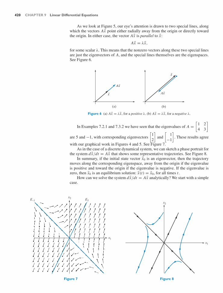
420 CHAPTER 9 Linear Differential Equations
As we look at Figure 5, our eye’s attention is drawn to two special lines, alongwhich the vectors Ax point either radially away from the origin or directly towardthe origin. In either case, the vector Ax is parallel to x :
Ax = λx,
for some scalar λ. This means that the nonzero vectors along these two special linesare just the eigenvectors of A, and the special lines themselves are the eigenspaces.See Figure 6.
Ax
x Ax
x
(b)(a)
Figure 6 (a) Ax = λx , for a positive λ. (b) Ax = λx , for a negative λ.
In Examples 7.2.1 and 7.3.2 we have seen that the eigenvalues of A =[
1 24 3
]
are 5 and −1, with corresponding eigenvectors[
12
]and
[1
−1
]. These results agree
with our graphical work in Figures 4 and 5. See Figure 7.As in the case of a discrete dynamical system, we can sketch a phase portrait for
the system dx/dt = Ax that shows some representative trajectories. See Figure 8.In summary, if the initial state vector x0 is an eigenvector, then the trajectory
moves along the corresponding eigenspace, away from the origin if the eigenvalueis positive and toward the origin if the eigenvalue is negative. If the eigenvalue iszero, then x0 is an equilibrium solution: x(t) = x0, for all times t .
How can we solve the system dx/dt = Ax analytically? We start with a simplecase.
x1
x2E−1 E5
Figure 7
x1
x2
Figure 8

9.1 An Introduction to Continuous Dynamical Systems 421
EXAMPLE 3 Find all solutions of the system
dxdt
=[
2 00 3
]x .
SolutionThe two differential equations
dx1
dt= 2x1
dx2
dt= 3x2
are unrelated, or uncoupled; we can solve them separately, using Theorem 9.1.1:
x1(t) = e2t x1(0)
x2(t) = e3t x2(0).
Thus,
x(t) =[
e2t x1(0)
e3t x2(0)
].
Both components of x(t) grow exponentially, and the second one will grow fasterthan the first. In particular, if one of the components is initially 0, it remains 0 forall future times. In Figure 9, we sketch a rough phase portrait for this system. !
x2
x1
Figure 9
Now let’s do a slightly harder example:
EXAMPLE 4 Find all solutions of the system
dxdt
= Ax, where A =[
1 2−1 4
].
SolutionWe have seen that the eigenvalues and eigenvectors of A tell us a lot about thebehavior of the solutions of the system dx/dt = Ax . The eigenvalues of A are

422 CHAPTER 9 Linear Differential Equations
λ1 = 2 and λ2 = 3, with corresponding eigenvectors v1 =[
21
]and v2 =
[11
].
This means that S−1 AS = B, where S =[
2 11 1
]and B =
[2 00 3
], the matrix
considered in Example 3.We can write the system
dxdt
= Ax
as
dxdt
= SBS−1 x,
or
S−1 dxdt
= BS−1 x,
or (see Exercise 51)
ddt
(S−1 x) = B(S−1 x).
Let us introduce the notation c(t) = S−1 x(t); note that c(t) is the coordinate vectorof x(t) with respect to the eigenbasis v1, v2. Then the system takes the form
dcdt
= Bc,
which is just the equation we solved in Example 3. We found that the solutions areof the form
c(t) =[
e2t c1
e3t c2
],
where c1 and c2 are arbitrary constants. Therefore, the solutions of the originalsystem
dxdt
= Ax
are
x(t) = Sc(t) =[
2 11 1
] [e2t c1
e3t c2
]= c1e2t
[21
]+ c2e3t
[11
].
We can write this formula in more general terms as
x(t) = c1eλ1t v1 + c2eλ2t v2.
Note that c1 and c2 are the coordinates of x(0) with respect to the basis v1, v2, since
x(0) = c1v1 + c2v2.
It is informative to consider a few special trajectories: If c1 = 1 and c2 = 0, thetrajectory
x(t) = e2t[
21
]

9.1 An Introduction to Continuous Dynamical Systems 423
moves along the eigenspace E2 spanned by[
21
], as expected. Likewise, if c1 = 0
and c2 = 1, we have the trajectory
x(t) = e3t[
11
]
moving along the eigenspace E3.
If c2 = 0, then the entries of c2e3t
[11
]will become much larger (in abso-
lute value) than the entries of c1e2t
[21
]as t goes to infinity. The dominant term
c2e3t
[11
], associated with the larger eigenvalue, determines the behavior of the sys-
tem in the distant future. The state vector x(t) is almost parallel to E3 for large t .For large negative t , on the other hand, the state vector is very small and almostparallel to E2.
In Figure 10, we sketch a rough phase portrait for the system dx/dt = Ax .
x1
x2
E3
E2
Figure 10
This is a linear distortion of the phase portrait we sketched in Figure 9. More
precisely, the matrix S =[
2 11 1
]transforms the phase portraits in Figure 9 into
the phase portrait sketched in Figure 10 (transforming e1 into the eigenvector[
21
]
and e2 into[
11
]). !
Our work in Examples 3 and 4 generalizes readily to any n × n matrix A thatis diagonalizable over R (i.e., for which there is an eigenbasis in Rn):
Theorem 9.1.3 Continuous dynamical systems
Consider the system dx/dt = Ax . Suppose there is a real eigenbasis v1, . . . , vnfor A, with associated eigenvalues λ1, . . . , λn . Then the general solution of thesystem is
x(t) = c1eλ1t v1 + · · · + cneλn t vn.

424 CHAPTER 9 Linear Differential Equations
Theorem 9.1.3 Continuous dynamical systems (Continued)
The scalars c1, c2, . . . , cn are the coordinates of x0 with respect to the basisv1, v2, . . . , vn .
We can write the preceding equation in matrix form as
x(t) =
⎡
⎢⎣| | |v1 v2 . . . vn
| | |
⎤
⎥⎦
⎡
⎢⎢⎢⎣
eλ1t 0 · · · 00 eλ2t · · · 0...
.... . .
...
0 0 · · · eλn t
⎤
⎥⎥⎥⎦
⎡
⎢⎢⎢⎣
c1
c2...
cn
⎤
⎥⎥⎥⎦
= S
⎡
⎢⎢⎢⎣
eλ1t 0 · · · 00 eλ2t · · · 0...
.... . .
...
0 0 · · · eλn t
⎤
⎥⎥⎥⎦S−1 x0,
where S =
⎡
⎢⎣| | |v1 v2 · · · vn
| | |
⎤
⎥⎦.
We can think of the general solution as a linear combination of the solutionseλi t vi associated with the eigenvectors vi . Note the analogy between this solutionand the general solution of the discrete dynamical system x(t + 1) = Ax(t),
x(t) = c1λt1v1 + · · · + cnλ
tn vn.
See Theorem 7.1.6.The terms λt
i are replaced by eλi t . We have already observed this fact in a dy-namical system with only one component. See Example 1.
We can state Theorem 9.1.3 in the language of linear spaces. The solutions ofthe system dx/dt = Ax form a subspace of the space F(R, Rn) of all functionsfrom R to Rn . See Exercises 22 and 23. This space is n-dimensional, with basiseλ1t v1, eλ2t v2, . . . , eλn t vn .
EXAMPLE 5 Consider a system dx/dt = Ax , where A is diagonalizable over R. When is the zerostate a stable equilibrium solution? Give your answer in terms of the eigenvaluesof A.
SolutionNote that lim
t→∞eλt = 0 if (and only if) λ is negative. Therefore, we observe stability
if (and only if) all eigenvalues of A are negative. !Consider an invertible 2 × 2 matrix A with two distinct eigenvalues λ1 > λ2.
Then the phase portrait of dx/dt = Ax looks qualitatively like one of the threesketches in Figure 11. We observe stability only in Figure 11c.
Consider a trajectory that does not run along one of the eigenspaces. In allthree cases, the state vector x(t) is almost parallel to the dominant eigenspace Eλ1
for large t . For large negative t , on the other hand, the state vector is almost parallelto Eλ2 . Compare with Figure 7.1.11.

9.1 An Introduction to Continuous Dynamical Systems 425
E 2
E 2 E
2
E 1
E 1
E 1
(a) (b) (c)
Figure 11 (a) λ1 > λ2 > 0. (b) λ1 > 0 > λ2. (c) 0 > λ1 > λ2.
EXERCISES 9.1GOAL Use the concept of a continuous dynamical sys-tem. Solve the differential equation dx/dt = kx. Solvethe system dx/dt = Ax when A is diagonalizable over R,and sketch the phase portrait for 2 × 2 matrices A.
Solve the initial value problems posed in Exercises 1through 5. Graph the solution.
1.dxdt
= 5x with x(0) = 7
2.dxdt
= −0.71x with x(0) = −e
3.d Pdt
= 0.03P with P(0) = 7
4.dydt
= 0.8t with y(0) = −0.8
5.dydt
= 0.8y with y(0) = −0.8
Solve the nonlinear differential equations in Exercises 6through 11 using the method of separation of vari-ables: Write the differential equation dx/dt = f (x) asdx/ f (x) = dt and integrate both sides.
6.dxdt
= 1x
, x(0) = 1
7.dxdt
= x2, x(0) = 1. Describe the behavior of yoursolution as t increases.
8.dxdt
=√
x , x(0) = 4
9.dxdt
= xk (with k = 1), x(0) = 1
10.dxdt
= 1cos(x)
, x(0) = 0
11.dxdt
= 1 + x2, x(0) = 0
12. Find a differential equation of the form dx/dt = kx forwhich x(t) = 3t is a solution.
13. In 1778, a wealthy Pennsylvanian merchant namedJacob DeHaven lent $450,000 to the ContinentalCongress to support the troops at Valley Forge. Theloan was never repaid. Mr. DeHaven’s descendants havetaken the U.S. government to court to collect what theybelieve they are owed. The going interest rate at the timewas 6%. How much were the DeHavens owed in 1990a. if interest is compounded yearly?b. if interest is compounded continuously?Source: Adapted from The New York Times, May 27,1990.
14. The carbon in living matter contains a minute propor-tion of the radioactive isotope C-14. This radiocarbonarises from cosmic-ray bombardment in the upper at-mosphere and enters living systems by exchange pro-cesses. After the death of an organism, exchange stops,and the carbon decays. Therefore, carbon dating enablesus to calculate the time at which an organism died. Letx(t) be the proportion of the original C-14 still presentt years after death. By definition, x(0) = 1 = 100%.We are told that x(t) satisfies the differential equation
dxdt
= − 18270
x .
a. Find a formula for x(t). Determine the half-life ofC-14 (that is, the time it takes for half of the C-14 todecay).
b. The Iceman. In 1991, the body of a man wasfound in melting snow in the Alps of NorthernItaly. A well-known historian in Innsbruck, Austria,determined that the man had lived in the BronzeAge, which started about 2000 B.C. in that region.

426 CHAPTER 9 Linear Differential Equations
Examination of tissue samples performed indepen-dently at Zurich and Oxford revealed that 47% ofthe C-14 present in the body at the time of his deathhad decayed. When did this man die? Is the resultof the carbon dating compatible with the estimate ofthe Austrian historian?
15. Justify the “Rule of 69”: If a quantity grows at a con-stant instantaneous rate of k%, then its doubling time isabout 69/k. Example: In 2008 the population of Mada-gascar was about 20 million, growing at an annual rateof about 3%, with a doubling time of about 69/3 = 23years.
Consider the system
dxd t
=[λ1 00 λ2
]x.
For the values of λ1 and λ2 given in Exercises 16 through19, sketch the trajectories for all nine initial values shownin the following figure. For each of the points, trace outboth the future and the past of the system.
1
1
x2
x1
16. λ1 = 1, λ2 = −1 17. λ1 = 1, λ2 = 2
18. λ1 = −1, λ2 = −2 19. λ1 = 0, λ2 = 1
20. Consider the system dx/dt = Ax with A =[
0 −11 0
].
Sketch a direction field for Ax . Based on your sketch,describe the trajectories geometrically. From yoursketch, can you guess a formula for the solution with
x0 =[
10
]? Verify your guess by substituting into the
equations.
21. Consider the system dx/dt = Ax with A =[
0 10 0
].
Sketch a direction field of Ax . Based on your sketch,describe the trajectories geometrically. Can you find thesolutions analytically?
22. Consider a linear system dx/dt = Ax of arbitrary size.Suppose x1(t) and x2(t) are solutions of the system. Is
the sum x(t) = x1(t) + x2(t) a solution as well? Howdo you know?
23. Consider a linear system dx/dt = Ax of arbitrary size.Suppose x1(t) is a solution of the system and k is anarbitrary constant. Is x(t) = kx1(t) a solution as well?How do you know?
24. Let A be an n × n matrix and k a scalar. Consider thefollowing two systems:
dxdt
= Ax (I)
dcdt
= (A + k In)c. (II)
Show that if x(t) is a solution of system (I), then c(t) =ekt x(t) is a solution of system (II).
25. Let A be an n × n matrix and k a scalar. Consider thefollowing two systems:
dxdt
= Ax (I)
dcdt
= k Ac. (II)
Show that if x(t) is a solution of system (I), then c(t) =x(kt) is a solution of system (II). Compare the vectorfields of the two systems.
In Exercises 26 through 31, solve the system with the giveninitial value.
26.dxdt
=[
1 23 0
]x with x(0) =
[72
]
27.dxdt
=[−4 3
2 −3
]x with x(0) =
[10
]
28.dxdt
=[
4 34 8
]x with x(0) =
[11
]
29.dxdt
=[
1 22 4
]x with x(0) =
[50
]
30.dxdt
=[
1 22 4
]x with x(0) =
[2
−1
]
31.dxdt
=
⎡
⎣2 1 11 3 33 2 2
⎤
⎦ x with x(0) =
⎡
⎣1
−21
⎤
⎦
Sketch rough phase portraits for the dynamical systemsgiven in Exercises 32 through 39.
32.dxdt
=[
1 23 0
]x 33.
dxdt
=[−4 3
2 −3
]x

9.1 An Introduction to Continuous Dynamical Systems 427
34.dxdt
=[
4 34 8
]x 35.
dxdt
=[
1 22 4
]x
36. x(t + 1) =[
0.9 0.2
0.2 1.2
]x(t)
37. x(t + 1) =[
1 0.3
−0.2 1.7
]x(t)
38. x(t + 1) =[
1.1 0.2
−0.4 0.5
]x(t)
39. x(t + 1) =[
0.8 −0.4
0.3 1.6
]x(t)
40. Find a 2×2 matrix A such that the system dx/dt = Axhas
x(t) =[
2e2t + 3e3t
3e2t + 4e3t
]
as one of its solutions.
41. Consider a noninvertible 2 × 2 matrix A with two dis-tinct eigenvalues. (Note that one of the eigenvalues mustbe 0.) Choose two eigenvectors v1 and v2 with eigenval-ues λ1 = 0 and λ2 as shown in the accompanying fig-ure. Suppose λ2 is negative. Sketch a phase portrait forthe system dx/dt = Ax , clearly indicating the shapeand long-term behavior of the trajectories.
x2
x1
v2
v1
42. Consider the interaction of two species of animals in ahabitat. We are told that the change of the populationsx(t) and y(t) can be modeled by the equations
∣∣∣∣∣∣∣∣
dxdt
= 1.4x − 1.2y
dydt
= 0.8x − 1.4y
∣∣∣∣∣∣∣∣,
where time t is measured in years.a. What kind of interaction do we observe (symbiosis,
competition, or predator–prey)?b. Sketch a phase portrait for this system. From the na-
ture of the problem, we are interested only in thefirst quadrant.
c. What will happen in the long term? Does the out-come depend on the initial populations? If so, how?
43. Answer the questions posed in Exercise 42 for the fol-lowing system:
∣∣∣∣∣∣∣∣
dxdt
= 5x − y
dydt
= −2x + 4y
∣∣∣∣∣∣∣∣.
44. Answer the questions posed in Exercise 42 for the fol-lowing system:
∣∣∣∣∣∣∣∣
dxdt
= x + 4y
dydt
= 2x − y
∣∣∣∣∣∣∣∣.
45. Two herds of vicious animals are fighting each otherto the death. During the fight, the populations x(t) andy(t) of the two species can be modeled by the followingsystem:2
∣∣∣∣∣∣∣∣
dxdt
= − 4y
dydt
= − x
∣∣∣∣∣∣∣∣.
a. What is the significance of the constants −4 and−1 in these equations? Which species has the morevicious (or more efficient) fighters?
b. Sketch a phase portrait for this system.c. Who wins the fight (in the sense that some individ-
uals of that species are left while the other herd iseradicated)? How does your answer depend on theinitial populations?
2 This is the simplest in a series of combat models developedby F. W. Lanchester during World War I (F. W. Lanchester,Aircraft in Warfare, the Dawn of the Fourth Arm, Tiptree,Constable and Co., Ltd., 1916).

428 CHAPTER 9 Linear Differential Equations
46. Repeat Exercise 45 for the system
∣∣∣∣∣∣∣∣
dxdt
= − py
dydt
= −qx
∣∣∣∣∣∣∣∣,
where p and q are two positive constants.3
47. The interaction of two populations of animals is mod-eled by the differential equations
∣∣∣∣∣∣∣∣
dxdt
= − x + ky
dydt
= kx − 4y
∣∣∣∣∣∣∣∣,
for some positive constant k.a. What kind of interaction do we observe? What is the
practical significance of the constant k?b. Find the eigenvalues of the coefficient matrix of the
system. What can you say about the signs of theseeigenvalues? How does your answer depend on thevalue of the constant k?
c. For each case you discussed in part (b), sketch arough phase portrait. What does each phase portraittell you about the future of the two populations?
48. Repeat Exercise 47 for the system
∣∣∣∣∣∣∣∣
dxdt
= − x + ky
dydt
= x − 4y
∣∣∣∣∣∣∣∣,
where k is a positive constant.
49. Here is a continuous model of a person’s glucose reg-ulatory system. Compare this with Exercise 7.1.70. Letg(t) and h(t) be the excess glucose and insulin concen-trations in a person’s blood. We are told that
∣∣∣∣∣∣∣∣∣
dgdt
= −g − 0.2h
dhdt
= 0.6g − 0.2h
∣∣∣∣∣∣∣∣∣
,
where time t is measured in hours. After a heavy hol-iday dinner, we measure g(0) = 30 and h(0) = 0.Find closed formulas for g(t) and h(t). Sketch thetrajectory.
50. Consider a linear system dx/dt = Ax , where A is a2 × 2 matrix that is diagonalizable over R. When is thezero state a stable equilibrium solution? Give your an-swer in terms of the determinant and the trace of A.
51. Let x(t) be a differentiable curve in Rn and S an n × nmatrix. Show that
ddt
(Sx) = Sdxdt
.
52. Find all solutions of the system
dxdt
=[λ 10 λ
]x,
where λ is an arbitrary constant. Hint: Exercises 21 and24 are helpful.
Sketch a phase portrait. For which choices of λ isthe zero state a stable equilibrium solution?
53. Solve the initial value problem
dxdt
=[
p −qq p
]x with x0 =
[10
].
Sketch the trajectory for the cases when p is positive,negative, or 0. In which cases does the trajectory ap-proach the origin? Hint: Exercises 20, 24, and 25 arehelpful.
54. Consider a door that opens to only one side (as mostdoors do). A spring mechanism closes the door au-tomatically. The state of the door at a given time t(measured in seconds) is determined by the angular dis-placement θ(t) (measured in radians) and the angularvelocity ω(t) = dθ/dt . Note that θ is always positiveor zero (since the door opens to only one side), but ωcan be positive or negative (depending on whether thedoor is opening or closing).
When the door is moving freely (nobody is pushing orpulling), its movement is subject to the following dif-ferential equations:
∣∣∣∣∣∣∣∣
dθ
dt= ω
dω
dt= − 2θ − 3ω
∣∣∣∣∣∣∣∣
(the definition of ω)
(−2θ reflects the force of thespring, and −3ω models friction).
3 The result is known as Lanchester’s square law.

9.2 The Complex Case: Euler’s Formula 429
a. Sketch a phase portrait for this system.b. Discuss the movement of the door represented by
the qualitatively different trajectories. For whichinitial states does the door slam (i.e., reach θ = 0with velocity ω < 0)?
55. Answer the questions posed in Exercise 54 for thesystem
∣∣∣∣∣∣∣∣∣∣
dθ
dt= ω
dω
dt= − pθ − qω
∣∣∣∣∣∣∣∣∣∣
,
where p and q are positive, and q2 > 4p.
9.2 The Complex Case: Euler’s Formula
Consider a linear system
dxdt
= Ax,
where the n × n matrix A is diagonalizable over C: There exists a complex eigen-basis v1, . . . , vn for A, with associated complex eigenvalues λ1, . . . , λn . You maywonder whether the formula
x(t) = c1eλ1t v1 + · · · + cneλn t vn
(with complex ci ) produces the general complex solution of the system, just as inthe real case (Theorem 9.1.3).
Before we can make sense out of the formula above, we have to think about theidea of a complex-valued function and in particular about the exponential functioneλt for complex λ.
Complex-Valued FunctionsA complex-valued function z = f (t) is a function from R to C (with domain Rand target space C): The input t is real, and the output z is complex. Here are twoexamples:
z = t + i t2
z = cos t + i sin t.
For each t , the output z can be represented as a point in the complex plane. Aswe let t vary, we trace out a trajectory in the complex plane. In Figure 1, we sketchthe trajectories of the two complex-valued functions just defined.
t = −1z = −1 + i
t = 0z = 0
t = 1z = 1 + i
t = /2z = i
t = 0z = 1
t =z = −1
t = 3 /2z = − i
(a) (b)
Figure 1 (a) The trajectory of z = t + i t2. (b) The trajectory of z = cos t + i sin t .

430 CHAPTER 9 Linear Differential Equations
We can write a complex-valued function z(t) in terms of its real and imaginaryparts:
z(t) = x(t) + iy(t).
(Consider the two preceding examples.) If x(t) and y(t) are differentiable real-valued functions, then the derivative of the complex-valued function z(t) is definedby
dzdt
= dxdt
+ idydt
.
For example, if
z(t) = t + i t2,
then
dzdt
= 1 + 2i t.
If
z(t) = cos t + i sin t,
then
dzdt
= − sin t + i cos t.
Please verify that the basic rules of differential calculus (the sum, product, andquotient rules) apply to complex-valued functions. The chain rule holds in the fol-lowing form: If z = f (t) is a differentiable complex-valued function and t = g(s)is a differentiable function from R to R, then
dzds
= dzdt
dtds
.
The derivative dz/dt of a complex-valued function z(t), for a given t , can be visu-alized as a tangent vector to the trajectory at z(t), as shown in Figure 2.
z(t)
z(1)
dzdt at t = 1
Figure 2
Next let’s think about the complex-valued exponential function z = eλt , whereλ is complex and t real. How should the function z = eλt be defined? We can getsome inspiration from the real case: The exponential function x = ekt (for real k)is the unique function such that dx/dt = kx and x(0) = 1. Compare this withTheorem 9.1.1.
We can use this fundamental property of real exponential functions to definethe complex exponential functions:

9.2 The Complex Case: Euler’s Formula 431
Definition 9.2.1 Complex exponential functions
If λ is a complex number, then z = eλt is the unique complex-valued functionsuch that
dzdt
= λz and z(0) = 1.
The existence of such a function, for any λ, will be established later; the proofof uniqueness is left as Exercise 38.
It follows that the unique complex-valued function z(t) withdzdt
= λz and z(0) = z0
isz(t) = eλt z0,
for an arbitrary complex initial value z0.Let us first consider the simplest case, z = eit , where λ = i . We are looking for
a complex-valued function z(t) such that dz/dt = i z and z(0) = 1.From a graphical point of view, we are looking for the trajectory z(t) in the
complex plane that starts at z = 1 and whose tangent vector dz/dt = i z is per-pendicular to z at each point. See Example 1 of Section 7.5. In other words, we arelooking for the flow line of the vector field in Figure 3 starting at z = 1.
The unit circle, with parametrization z(t) = cos t + i sin t , satisfiesdzdt
= − sin t + i cos t = i z(t),
and z(0) = 1. See Figure 4.
z = 1
Figure 3
z(t) = cos(t) + i sin(t)
Figure 4
We have shown the following fundamental result:
Theorem 9.2.2 Euler’s formula
eit = cos t + i sin t

432 CHAPTER 9 Linear Differential Equations
The case t = π leads to the intriguing formula eiπ = −1; this has been calledthe most beautiful formula in all of mathematics.4
Figure 5 Euler’slikeness and his
celebrated formulaare shown on aSwiss postage
stamp.
Euler’s formula can be used to write the polar form of a complex number moresuccinctly:
z = r(cos θ + i sin θ) = reiθ .
Now consider z = eλt , where λ is an arbitrary complex number, λ = p + iq.By manipulating exponentials as if they were real, we find that
eλt = e(p+iq)t = ept eiqt = ept(cos(qt) + i sin(qt)).
We can validate this result by checking that the complex-valued function
z(t) = ept(cos(qt) + i sin(qt))
does indeed satisfy the definition of eλt , namely, dz/dt = λz and z(0) = 1:
dzdt
= pept(cos(qt) + i sin(qt))
+ ept(−q sin(qt) + iq cos(qt))
= (p + iq)ept(cos(qt) + i sin(qt))
= λz.
EXAMPLE 1 Sketch the trajectory of the complex-valued function z(t) = e(0.1+i)t in the complexplane.
Solutionz(t) = e0.1t ei t = e0.1t (cos t + i sin t)
5i
5
Figure 6
The trajectory spirals outward as shown in Figure 6, since the function e0.1t growsexponentially. !
4Benjamin Peirce (1809–1880), a Harvard mathematician, after observing that eiπ = −1, used toturn to his students and say, “Gentlemen, that is surely true, it is absolutely paradoxical, we cannotunderstand it, and we don’t know what it means, but we have proved it, and therefore we know it mustbe the truth.” Do you not now think that we understand not only that the formula is true but also whatit means?

9.2 The Complex Case: Euler’s Formula 433
EXAMPLE 2 For which complex numbers λ is limt→∞
eλt = 0?
SolutionRecall that
eλt = e(p+iq)t = ept(cos(qt) + i sin(qt)),
so that |eλt | = ept . This quantity approaches zero if (and only if) p is negative (i.e.,if ept decays exponentially).
We summarize: limt→∞
eλt = 0 if (and only if) the real part of λ is negative.!
We are now ready to tackle the problem posed at the beginning of this section:Consider a system dx/dt = Ax , where the n×n matrix A has a complex eigenbasisv1, . . . , vn , with eigenvalues λ1, . . . , λn . Find all complex solutions x(t) of thissystem. By a complex solution, we mean a function from R to Cn (that is, t is realand x is in Cn). In other words, the component functions x1(t), . . . , xn(t) of x(t)are complex-valued functions.
As you review our work in the last section, you will find that the approach wetook to the real case applies to the complex case as well, without modifications:
Theorem 9.2.3 Continuous dynamical systems with complex eigenvalues
Consider a linear system
dxdt
= Ax .
Suppose there exists a complex eigenbasis v1, . . . , vn for A, with associatedcomplex eigenvalues λ1, . . . , λn . Then the general complex solution of the sys-tem is
x(t) = c1eλ1t v1 + · · · + cneλn t vn,
where the ci are arbitrary complex numbers.We can write this solution in matrix form, as in Theorem 9.1.3.
We can check that the given curve x(t) satisfies the equation dx/dt = Ax : Wehave
dxdt
= c1λ1eλ1t v1 + · · · + cnλneλn t vn
(by Definition 9.2.1), and
Ax = c1eλ1tλ1v1 + · · · + cneλn tλn vn,
because the vi are eigenvectors. The two answers match.When is the zero state a stable equilibrium solution for the system dx/dt =
Ax? Considering Example 3 and the form of the solution given in Theorem 9.2.3,we can conclude that this is the case if (and only if) the real parts of all eigenvaluesare negative (at least when A is diagonalizable over C). The nondiagonalizable caseis left as Exercise 9.3.48.
Theorem 9.2.4 Stability of a continuous dynamical system
For a system
dxdt
= Ax,
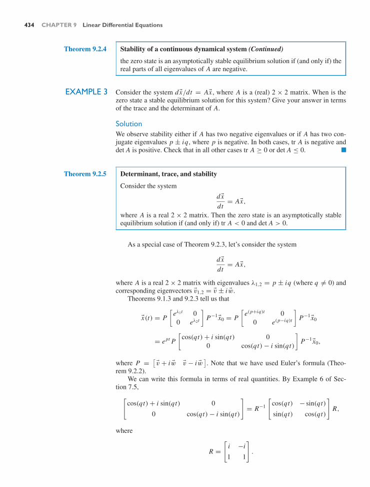
434 CHAPTER 9 Linear Differential Equations
Theorem 9.2.4 Stability of a continuous dynamical system (Continued)
the zero state is an asymptotically stable equilibrium solution if (and only if) thereal parts of all eigenvalues of A are negative.
EXAMPLE 3 Consider the system dx/dt = Ax , where A is a (real) 2 × 2 matrix. When is thezero state a stable equilibrium solution for this system? Give your answer in termsof the trace and the determinant of A.
SolutionWe observe stability either if A has two negative eigenvalues or if A has two con-jugate eigenvalues p ± iq, where p is negative. In both cases, tr A is negative anddet A is positive. Check that in all other cases tr A ≥ 0 or det A ≤ 0. !
Theorem 9.2.5 Determinant, trace, and stability
Consider the system
dxdt
= Ax,
where A is a real 2 × 2 matrix. Then the zero state is an asymptotically stableequilibrium solution if (and only if) tr A < 0 and det A > 0.
As a special case of Theorem 9.2.3, let’s consider the system
dxdt
= Ax,
where A is a real 2 × 2 matrix with eigenvalues λ1,2 = p ± iq (where q = 0) andcorresponding eigenvectors v1,2 = v ± iw.
Theorems 9.1.3 and 9.2.3 tell us that
x(t) = P[
eλ1t 00 eλ2t
]P−1 x0 = P
[e(p+iq)t 0
0 e(p−iq)t
]P−1 x0
= ept P[
cos(qt) + i sin(qt) 00 cos(qt) − i sin(qt)
]P−1 x0,
where P =[v + iw v − iw
]. Note that we have used Euler’s formula (Theo-
rem 9.2.2).We can write this formula in terms of real quantities. By Example 6 of Sec-
tion 7.5,[
cos(qt) + i sin(qt) 0
0 cos(qt) − i sin(qt)
]= R−1
[cos(qt) − sin(qt)
sin(qt) cos(qt)
]R,
where
R =[
i −i
1 1
].
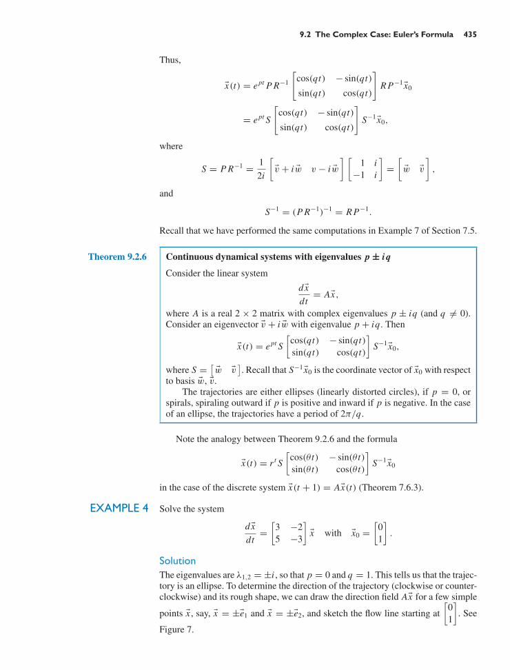
9.2 The Complex Case: Euler’s Formula 435
Thus,
x(t) = ept P R−1
[cos(qt) − sin(qt)
sin(qt) cos(qt)
]R P−1 x0
= ept S
[cos(qt) − sin(qt)
sin(qt) cos(qt)
]S−1 x0,
where
S = P R−1 = 12i
[v + iw v − iw
] [1 i
−1 i
]=
[w v
],
and
S−1 = (P R−1)−1 = R P−1.
Recall that we have performed the same computations in Example 7 of Section 7.5.
Theorem 9.2.6 Continuous dynamical systems with eigenvalues p ± iq
Consider the linear system
dxdt
= Ax,
where A is a real 2 × 2 matrix with complex eigenvalues p ± iq (and q = 0).Consider an eigenvector v + iw with eigenvalue p + iq. Then
x(t) = ept S[
cos(qt) − sin(qt)sin(qt) cos(qt)
]S−1 x0,
where S =[w v
]. Recall that S−1 x0 is the coordinate vector of x0 with respect
to basis w, v.The trajectories are either ellipses (linearly distorted circles), if p = 0, or
spirals, spiraling outward if p is positive and inward if p is negative. In the caseof an ellipse, the trajectories have a period of 2π/q.
Note the analogy between Theorem 9.2.6 and the formula
x(t) = r t S[
cos(θ t) − sin(θ t)sin(θ t) cos(θ t)
]S−1 x0
in the case of the discrete system x(t + 1) = Ax(t) (Theorem 7.6.3).
EXAMPLE 4 Solve the system
dxdt
=[
3 −25 −3
]x with x0 =
[01
].
SolutionThe eigenvalues are λ1,2 = ± i , so that p = 0 and q = 1. This tells us that the trajec-tory is an ellipse. To determine the direction of the trajectory (clockwise or counter-clockwise) and its rough shape, we can draw the direction field Ax for a few simple
points x , say, x = ± e1 and x = ± e2, and sketch the flow line starting at[
01
]. See
Figure 7.

436 CHAPTER 9 Linear Differential Equations
Now let us find a formula for the trajectory:
Ei = ker[
3 − i −25 −3 − i
]= span
[−2
i − 3
]
[−2
i − 3
]=
[−2−3
]
︸ ︷︷ ︸v
+i[
01
]
︸︷︷︸w
.
Therefore,
x(t) = ept S
[cos(qt) − sin(qt)
sin(qt) cos(qt)
]S−1 x0 =
[0 −21 −3
][cos t − sin t
sin t cos t
] [10
]
=[
−2 sin t
cos t − 3 sin t
]= cos t
[01
]+ sin t
[−2−3
].
You can check that
dxdt
= Ax and x(0) =[
01
].
The trajectory is the ellipse shown in Figure 8. !
1
Figure 7
t = 0, 2
t =
23
t =
2t =
3
2
−3 −2 −1
−2
−3
1 2 3
Figure 8
Consider a 2 × 2 matrix A. The various scenarios for the system dx/dt = Axcan be conveniently represented in the tr A–det A plane, where a 2 × 2 matrix A isrepresented by the point (tr A, det A). Recall that the characteristic polynomial is
λ2 − (tr A)λ + det A
and the eigenvalues are
λ1,2 = 12
(tr A ±
√(trA)2 − 4 det A
).
Therefore, the eigenvalues of A are real if (and only if) the point (trA, det A) islocated below or on the parabola
det A =(
tr A2
)2
in the tr A–det A plane. See Figure 9.

9.2 The Complex Case: Euler’s Formula 437
det A
tr A
det A = tr A 2
2
Figure 9
Note that there are five major cases, corresponding to the regions in Figure 9,and some exceptional cases, corresponding to the dividing lines.
What does the phase portrait look like when det A = 0 and tr A = 0?In Figure 10 we take another look at the five major types of phase portraits. Both
in the discrete and in the continuous cases, we sketch the phase portraits producedby various eigenvalues. We include the case of an ellipse, since it is important inapplications.
EXERCISES 9.2GOAL Use the definition of the complex-valued expo-nential function z = eλt . Solve the system
dxd t
= Ax
for a 2 × 2 matrix A with complex eigenvalues p ± iq.
1. Find e2π i .
2. Find e(1/2)π i .
3. Write z = −1 + i in polar form as z = reiθ .
4. Sketch the trajectory of the complex-valued function
z = e3i t .
What is the period?
5. Sketch the trajectory of the complex-valued function
z = e(−0.1−2i)t .
6. Find all complex solutions of the system
dxdt
=[
3 −25 −3
]x
in the form given in Theorem 9.2.3. What solution doyou get if you let c1 = c2 = 1?
7. Determine the stability of the system
dxdt
=[−1 2
3 −4
]x .
8. Consider a system
dxdt
= Ax,
where A is a symmetric matrix. When is the zero state astable equilibrium solution? Give your answer in termsof the definiteness of the matrix A.
9. Consider a system
dxdt
= Ax,
where A is a 2 × 2 matrix with tr A < 0. We are toldthat A has no real eigenvalues. What can you say aboutthe stability of the system?
10. Consider a quadratic form q(x) = x · Ax of two vari-ables, x1 and x2. Consider the system of differentialequations
∣∣∣∣∣∣∣∣
dx1
dt= ∂q
∂x1
dx2
dt= ∂q
∂x2
∣∣∣∣∣∣∣∣,

438 CHAPTER 9 Linear Differential Equations
Discrete Continuous Phase Portrait
λ1 > λ2 > 1 λ1 > λ2 > 0
E 2
E 1
λ1 > 1 > λ2 > 0 λ1 > 0 > λ2
E 2
E 1
1 > λ1 > λ2 > 0 0 > λ1 > λ2
E 2
E 1
λ1,2 = p ± iq
p2 + q2 > 1λ1,2 = p ± iq
p > 0
λ1,2 = p ± iq
p2 + q2 < 1λ1,2 = p ± iq
p < 0
λ1,2 = p ± iq
p2 + q2 = 1
λ1,2 = ± iq
Figure 10 The major types of phase portraits.

9.2 The Complex Case: Euler’s Formula 439
or, more succinctly,
dxdt
= grad q.
a. Show that the system dx/dt = grad q is linear byfinding a matrix B (in terms of the symmetric matrixA) such that grad q = Bx .
b. When q is negative definite, draw a sketch showingpossible level curves of q . On the same sketch, drawa few trajectories of the system dx/dt = grad q .What does your sketch suggest about the stability ofthe system dx/dt = grad q?
c. Do the same as in part b for an indefinite quadraticform.
d. Explain the relationship between the definiteness ofthe form q and the stability of the system dx/dt= grad q .
11. Do parts a and d of Exercise 10 for a quadratic form ofn variables.
12. Determine the stability of the system
dxdt
=
⎡
⎣0 1 00 0 1
−1 −1 −2
⎤
⎦ x .
13. If the system dx/dt = Ax is stable, is dx/dt = A−1 xstable as well? How can you tell?
14. Negative Feedback Loops. Suppose some quantitiesx1(t), x2(t), . . . , xn(t) can be modeled by differentialequations of the form
∣∣∣∣∣∣∣∣∣∣∣∣∣∣∣∣
dx1
dt= −k1x1 − bxn
dx2
dt= x1 − k2x2
.... . .
dxn
dt= xn−1 − kn xn
∣∣∣∣∣∣∣∣∣∣∣∣∣∣∣∣
,
where b is positive and the ki are positive. (The matrixof this system has negative numbers on the diagonal,1’s directly below the diagonal, and a negative num-ber in the top right corner.) We say that the quantitiesx1, . . . , xn describe a (linear) negative feedback loop.a. Describe the significance of the entries in this sys-
tem, in practical terms.b. Is a negative feedback loop with two components
(n = 2) necessarily stable?c. Is a negative feedback loop with three components
necessarily stable?
15. Consider a noninvertible 2 × 2 matrix A with a posi-tive trace. What does the phase portrait of the systemdx/dt = Ax look like?
16. Consider the system
dxdt
=[
0 1a b
]x,
where a and b are arbitrary constants. For which valuesof a and b is the zero state a stable equilibrium solution?
17. Consider the system
dxdt
=[−1 k
k −1
]x,
where k is an arbitrary constant. For which values of kis the zero state a stable equilibrium solution?
18. Consider a diagonalizable 3 × 3 matrix A such that thezero state is a stable equilibrium solution of the systemdx/dt = Ax . What can you say about the determinantand the trace of A?
19. True or False? If the trace and the determinant of a 3×3matrix A are both negative, then the origin is a stableequilibrium solution of the system dx/dt = Ax . Jus-tify your answer.
20. Consider a 2 × 2 matrix A with eigenvalues ± π i . Letv+iw be an eigenvector of A with eigenvalue π i . Solvethe initial value problem
dxdt
= Ax, with x0 = w.
Draw the solution in the accompanying figure. Mark thevectors x(0), x( 1
2 ), x(1), and x(2).
vw
21. Ngozi opens a bank account with an initial balance of1,000 Nigerian naira. Let b(t) be the balance in theaccount at time t ; we are told that b(0) = 1,000. Thebank is paying interest at a continuous rate of 5% peryear. Ngozi makes deposits into the account at a contin-uous rate of s(t) (measured in naira per year). We aretold that s(0) = 1,000 and that s(t) is increasing at acontinuous rate of 7% per year. (Ngozi can save moreas her income goes up over time.)a. Set up a linear system of the form
∣∣∣∣∣∣∣∣
dbdt
= ?b + ?s
dsdt
= ?b + ?s
∣∣∣∣∣∣∣∣.
(Time is measured in years.)b. Find b(t) and s(t).

440 CHAPTER 9 Linear Differential Equations
For each of the linear systems in Exercises 22 through 26,find the matching phase portrait below.
22. x(t + 1) =[
3 0−2.5 0.5
]x(t)
23. x(t + 1) =[−1.5 −1
2 0.5
]x(t)
24.dxdt
=[
3 0−2.5 0.5
]x
25.dxdt
=[−1.5 −1
2 0.5
]x
26.dxdt
=[−2 0
3 1
]x
3
3
2
2
1
1
0
0
−1
−1
−2
−2−3
−3
I
3
3
2
2
1
1
0
0
−1
−1
−2
−2−3
−3
III
3
3
2
2
1
1
0
0
−1
−1
−2
−2−3
−3
V
3
3
2
2
1
1
0
0
−1
−1
−2
−2−3
−3
VII
3
3
2
2
1
1
0
0
−1
−1
−2
−2−3
−3
II
3
3
2
2
1
1
0
0
−1
−1
−2
−2−3
−3
IV
3
3
2
2
1
1
0
0
−1
−1
−2
−2−3
−3
VI
3
3
2
2
1
1
0
0
−1
−1
−2
−2−3
−3
VIII

9.2 The Complex Case: Euler’s Formula 441
Find all real solutions of the systems in Exercises 27through 30.
27.dxdt
=[
0 −33 0
]x 28.
dxdt
=[
0 4−9 0
]x
29.dxdt
=[
2 4−4 2
]x 30.
dxdt
=[−11 15−6 7
]x
Solve the systems in Exercises 31 through 34. Give thesolution in real form. Sketch the solution.
31.dxdt
=[−1 −2
2 −1
]x with x(0) =
[1
−1
]
32.dxdt
=[
0 1−4 0
]x with x(0) =
[10
]
33.dxdt
=[−1 1−2 1
]x with x(0) =
[01
]
34.dxdt
=[
7 10−4 −5
]x with x(0) =
[10
]
35. Prove the product rule for derivatives of complex-valued functions.
36. Consider the following mass-spring system:
x
Equilibrium
Let x(t) be the deviation of the block from theequilibrium position at time t . Consider the velocityv(t) = dx/dt of the block. There are two forces act-ing on the mass: the spring force Fs , which is assumedto be proportional to the displacement x , and the forceF f of friction, which is assumed to be proportional tothe velocity,
Fs = −px and F f = −qv,
where p > 0 and q ≥ 0 (q is 0 if the oscillation is fric-tionless). Therefore, the total force acting on the massis
F = Fs + F f = −px − qv.
By Newton’s second law of motion, we have
F = ma = mdv
dt,
where a represents acceleration and m the mass of theblock. Combining the last two equations, we find that
mdv
dt= −px − qv,
or
dv
dt= − p
mx − q
mv.
Let b = p/m and c = q/m for simplicity. Then thedynamics of this mass-spring system are described bythe system
∣∣∣∣∣∣∣∣
dxdt
= v
dv
dt= −bx − cv
∣∣∣∣∣∣∣∣(b > 0, c ≥ 0).
Sketch a phase portrait for this system in each of thefollowing cases, and describe briefly the significance ofyour trajectories in terms of the movement of the block.Comment on the stability in each case.a. c = 0 (frictionless). Find the period.b. c2 < 4b (underdamped).c. c2 > 4b (overdamped).
37. a. For a differentiable complex-valued function z(t),find the derivative of
1z(t)
.
b. Prove the quotient rule for derivatives of complex-valued functions.
In both parts of this exercise, you may use the prod-uct rule. See Exercise 35.
38. Let z1(t) and z2(t) be two complex-valued solutions ofthe initial value problem
dzdt
= λz, with z(0) = 1,
where λ is a complex number. Suppose that z2(t) = 0for all t .a. Using the quotient rule (Exercise 37), show that the
derivative of
z1(t)z2(t)
is zero. Conclude that z1(t) = z2(t) for all t .b. Show that the initial value problem
dzdt
= λz, with z(0) = 1,
has a unique complex-valued solution z(t). Hint:One solution is given in the text.
39. Solve the system
dxdt
=
⎡
⎣λ 1 00 λ 10 0 λ
⎤
⎦ x .
Compare this with Exercise 9.1.24. When is the zerostate a stable equilibrium solution?
442 CHAPTER 9 Linear Differential Equations
40. An eccentric mathematician is able to gain autocraticpower in a small Alpine country. In her first decree, sheannounces the introduction of a new currency, the Euler,which is measured in complex units. Banks are orderedto pay only imaginary interest on deposits.a. If you invest 1,000 Euler at 5i% interest, com-
pounded annually, how much money do you haveafter 1 year, after 2 years, after t years? Describethe effect of compounding in this case. Sketch a tra-jectory showing the evolution of the balance in thecomplex plane.
b. Do part a in the case when the 5i% interest is com-pounded continuously.
c. Suppose people’s social standing is determined bythe modulus of the balance of their bank account.Under these circumstances, would you choose anaccount with annual compounding or with contin-uous compounding of interest?
Source: This problem is based on an idea of ProfessorD. Mumford, Brown University.
9.3 Linear Differential Operators and Linear Differential Equations
In this final section, we will study an important class of linear transformations fromC∞ to C∞. Here, C∞ denotes the linear space of complex-valued smooth functions(i.e., functions from R to C), which we consider as a linear space over C.
Definition 9.3.1 Linear differential operators and linear differential equations
A transformation T from C∞ to C∞ of the form
T ( f ) = f (n) + an−1 f (n−1) + · · · + a1 f ′ + a0 f
is called an nth-order linear differential operator.5,6 Here f (k) denotes the kthderivative of function f, and the coefficients ak are complex scalars.
If T is an nth-order linear differential operator and g is a smooth function,then the equation
T ( f ) = g or f (n) + an−1 f (n−1) + · · · + a1 f ′ + a0 f = g
is called an nth-order linear differential equation (DE). The DE is called homo-geneous if g = 0 and inhomogeneous otherwise.
Verify that a linear differential operator is indeed a linear transformation.Examples of linear differential operators are
D( f ) = f ′,
T ( f ) = f ′′ − 5 f ′ + 6 f andL( f ) = f ′′′ − 6 f ′′ + 5 f,
of first, second, and third order, respectively.Examples of linear DEs are
f ′′ − f ′ − 6 f = 0 (second order, homogeneous)
and
f ′(t) − 5 f (t) = sin t (first order, inhomogeneous).
Note that solving a homogeneous DE T ( f ) = 0 amounts to finding the kernel of T .
5More precisely, this is a linear differential operator with constant coefficients. More advanced textsconsider the case when the ak are functions.6The term operator is often used for a transformation whose domain and target space consist offunctions.
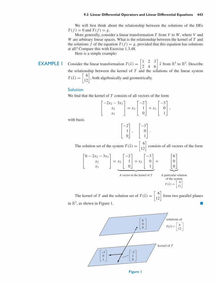
9.3 Linear Differential Operators and Linear Differential Equations 443
We will first think about the relationship between the solutions of the DEsT ( f ) = 0 and T ( f ) = g.
More generally, consider a linear transformation T from V to W , where V andW are arbitrary linear spaces. What is the relationship between the kernel of T andthe solutions f of the equation T ( f ) = g, provided that this equation has solutionsat all? Compare this with Exercise 1.3.48.
Here is a simple example:
EXAMPLE 1 Consider the linear transformation T (x) =[
1 2 32 4 6
]x from R3 to R2. Describe
the relationship between the kernel of T and the solutions of the linear system
T (x) =[
612
], both algebraically and geometrically.
SolutionWe find that the kernel of T consists of all vectors of the form
⎡
⎣−2x2 − 3x3
x2
x3
⎤
⎦ = x2
⎡
⎣−2
10
⎤
⎦ + x3
⎡
⎣−3
01
⎤
⎦ ,
with basis⎡
⎣−2
10
⎤
⎦ ,
⎡
⎣−3
01
⎤
⎦ .
The solution set of the system T (x) =[
612
]consists of all vectors of the form
⎡
⎣6 − 2x2 − 3x3
x2
x3
⎤
⎦ = x2
⎡
⎣−2
10
⎤
⎦ + x3
⎡
⎣−3
01
⎤
⎦
︸ ︷︷ ︸A vector in the kernel of T
+
⎡
⎣600
⎤
⎦
︸︷︷︸A particular solution
of the system
T (x) =[
612
]
The kernel of T and the solution set of T (x) =[
612
]form two parallel planes
in R3, as shown in Figure 1. !
solutions of
T(x) =
kernel of T
−3
10
−2
01
6
00 6
12
Figure 1

444 CHAPTER 9 Linear Differential Equations
These observations generalize as follows:
Theorem 9.3.2 Consider a linear transformation T from V to W , where V and W are arbitrarylinear spaces. Suppose we have a basis f1, f2, . . . , fn of the kernel of T . Con-sider an equation T ( f ) = g with a particular solution f p. Then the solutions fof the equation T ( f ) = g are of the form
f = c1 f1 + c2 f2 + · · · + cn fn + f p,
where the ci are arbitrary constants.
Note that T ( f ) = T (c1 f1 + · · · + cn fn) + T ( f p) = 0 + g = g, so that f isindeed a solution. Verify that all solutions are of this form.
What is the significance of Theorem 9.3.2 for linear differential equations? Atthe end of this section, we will demonstrate the following fundamental result:
Theorem 9.3.3 The kernel of an nth-order linear differential operator is n-dimensional.
Theorem 9.3.2 now provides us with the following strategy for solving lineardifferential equations:
Theorem 9.3.4 Strategy for solving linear differential equations
To solve an nth-order linear DE
T ( f ) = g,
we have to find
a. a basis f1, . . . , fn of ker(T ), andb. a particular solution f p of the DE T ( f ) = g.
Then the solutions f are of the form
f = c1 f1 + · · · + cn fn + f p,
where the ci are arbitrary constants.
EXAMPLE 2 Find all solutions of the DE
f ′′(t) + f (t) = et .
We are told that f p(t) = 12 et is a particular solution (verify this).
SolutionConsider the linear differential operator T ( f ) = f ′′ + f . A basis of the kernel ofT is f1(t) = cos t and f2(t) = sin t . Compare with Example 1 of Section 4.1.
Therefore, the solutions f of the DE f ′′ + f = et are of the form
f (t) = c1 cos t + c2 sin t + 12
et ,
where c1 and c2 are arbitrary constants. !We now present an approach that allows us to find solutions to homogeneous
linear DEs more systematically.

9.3 Linear Differential Operators and Linear Differential Equations 445
The Eigenfunction Approach to Solving Linear DEs
Definition 9.3.5 Eigenfunctions
Consider a linear differential operator T from C∞ to C∞. A smooth function fis called an eigenfunction of T if T ( f ) = λ f for some complex scalar λ; thisscalar λ is called the eigenvalue associated with the eigenfunction f .
EXAMPLE 3 Find all eigenfunctions and eigenvalues of the operator D( f ) = f ′.
SolutionWe have to solve the differential equation
D( f ) = λ f or f ′ = λ f.
For a given λ, the solutions are all exponential functions of the form f (t) = Ceλt .This means that all complex numbers are eigenvalues of D, and the eigenspaceassociated with the eigenvalue λ is one-dimensional, spanned by eλt . Compare thiswith Definition 9.2.1. !
It follows that the exponential functions are eigenfunctions for all linear differ-ential operators: If
T ( f ) = f (n) + an−1 f (n−1) + · · · + a1 f ′ + a0 f,
then
T (eλt) = (λn + an−1λn−1 + · · · + a1λ + a0)eλt .
This observation motivates the following definition:
Definition 9.3.6 Characteristic polynomial
Consider the linear differential operator
T ( f ) = f (n) + an−1 f (n−1) + · · · + a1 f ′ + a0 f.
The characteristic polynomial of T is defined as
pT (λ) = λn + an−1λn−1 + · · · + a1λ + a0.
Theorem 9.3.7 If T is a linear differential operator, then eλt is an eigenfunction of T , withassociated eigenvalue pT (λ), for all λ:
T (eλt ) = pT (λ)eλt .
In particular, if pT (λ) = 0, then eλt is in the kernel of T .
EXAMPLE 4 Find all exponential functions eλt in the kernel of the linear differential operator
T ( f ) = f ′′ + f ′ − 6 f.
SolutionThe characteristic polynomial is pT (λ) = λ2 +λ−6 = (λ+3)(λ−2), with roots 2and −3. Therefore, the functions e2t and e−3t are in the kernel of T . We can checkthis:
T (e2t ) = 4e2t + 2e2t − 6e2t = 0T (e−3t) = 9e−3t − 3e−3t − 6e−3t = 0. !
446 CHAPTER 9 Linear Differential Equations
Since most polynomials of degree n have n distinct complex roots, we can find ndistinct exponential functions eλ1t , . . . , eλn t in the kernel of most nth-order lineardifferential operators. Note that these functions are linearly independent. (They areeigenfunctions of D with distinct eigenvalues; the proof of Theorem 7.3.4 applies.)
Now we can use Theorem 9.3.3.
Theorem 9.3.8 The kernel of a linear differential operator
Consider an nth-order linear differential operator T whose characteristic poly-nomial pT (λ) has n distinct roots λ1, . . . , λn . Then the exponential functions
eλ1t , eλ2t , . . . , eλn t
form a basis of the kernel of T ; that is, they form a basis of the solution space ofthe homogeneous DE
T ( f ) = 0.
See Exercise 38 for the case of an nth-order linear differential operator whosecharacteristic polynomial has fewer than n distinct roots.
EXAMPLE 5 Find all solutions f of the differential equation
f ′′ + 2 f ′ − 3 f = 0.
SolutionThe characteristic polynomial of the operator T ( f ) = f ′′ + 2 f ′ − 3 f is pT (λ) =λ2 + 2λ − 3 = (λ + 3)(λ − 1), with roots 1 and −3. The exponential functions et
and e−3t form a basis of the solution space; that is, the solutions are of the form
f (t) = c1et + c2e−3t . !EXAMPLE 6 Find all solutions f of the differential equation
f ′′ − 6 f ′ + 13 f = 0.
SolutionThe characteristic polynomial is pT (λ) = λ2 − 6λ + 13, with complex roots 3 ± 2i .The exponential functions
e(3+2i)t = e3t(cos(2t) + i sin(2t))
and
e(3−2i)t = e3t(cos(2t) − i sin(2t))
form a basis of the solution space. We may wish to find a basis of the solution spaceconsisting of real-valued functions. The following observation is helpful: If f (t) =g(t) + ih(t) is a solution of the DE T ( f ) = 0, then T ( f ) = T (g) + iT (h) = 0,so that g and h are solutions as well. We can apply this remark to the real and theimaginary parts of the solution e(3+2i)t : The functions
e3t cos(2t) and e3t sin(2t)
are a basis of the solution space (they are clearly linearly independent), and thegeneral solution is
f (t) = c1e3t cos(2t) + c2e3t sin(2t) = e3t(c1 cos(2t) + c2 sin(2t)). !

9.3 Linear Differential Operators and Linear Differential Equations 447
Theorem 9.3.9 Consider a differential equation
T ( f ) = f ′′ + a f ′ + b f = 0,
where the coefficients a and b are real. Suppose the zeros of pT (λ) are p ± iq,with q = 0. Then the solutions of the given DE are
f (t) = ept(c1 cos(qt) + c2 sin(qt)),
where c1 and c2 are arbitrary constants.The special case when a = 0 and b > 0 is important in many applications.
Then p = 0 and q =√
b, so that the solutions of the DE
f ′′ + b f = 0
are
f (t) = c1 cos(√
bt) + c2 sin(√
bt).
Note that the function
f (t) = ept(c1 cos(qt) + c2 sin(qt))
is the product of an exponential and a sinusoidal function. The case when p isnegative comes up frequently in physics, when we model a damped oscillator. SeeFigure 2.
t
f(t) = ept c1 cos(qt) + c2 sin(qt)
Figure 2
What about nonhomogeneous differential equations? Let us discuss an examplethat is particularly important in applications.
EXAMPLE 7 Consider the differential equation
f ′′(t) + f ′(t) − 6 f (t) = 8 cos(2t).
a. Let V be the linear space consisting of all functions of the formc1 cos(2t) + c2 sin(2t). Show that the linear differential operatorT ( f ) = f ′′ + f ′ − 6 f defines an isomorphism from V to V .
b. Part (a) implies that the DE T ( f ) = 8 cos(2t) has a unique particular solu-tion f p(t) in V . Find this solution.
c. Find all solutions of the DE T ( f ) = 8 cos(2t).

448 CHAPTER 9 Linear Differential Equations
Solutiona. Consider the matrix A of T with respect to the basis cos(2t), sin(2t). A
straightforward computation shows that
A =[−10 2−2 −10
],
representing a rotation combined with a scaling. Since A is invertible, Tdefines an isomorphism from V to V .
b. If we work in coordinates with respect to the basis cos(2t), sin(2t), the DE
T ( f ) = 8 cos(2t) takes the form Ax =[
80
], with the solution
x = A−1[
80
]= 1
104
[−10 −2
2 −10
] [80
]=
[−10/13
2/13
].
The particular solution in V is
f p(t) = −1013
cos(2t) + 213
sin(2t).
A more straightforward way to find f p(t) is to set f p(t) = P cos(2t) +Q sin(2t) and substitute this trial solution into the DE to determine P andQ. This approach is referred to as the method of undetermined coefficients.
c. In Example 4, we have seen that the functions f1(t) = e2t and f2(t) = e−3t
form a basis of the kernel of T . By Theorem 9.3.4, the solutions of the DEare of the form
f (t) = c1 f1(t) + c2 f2(t) + f p(t)
= c1e2t + c2e−3t − 1013
cos(2t) + 213
sin(2t). !Let us summarize the methods developed in Example 7:
Theorem 9.3.10 Consider the linear differential equation
f ′′(t) + a f ′(t) + b f (t) = C cos(ωt),
where a, b, C, and ω are real numbers. Suppose that a = 0 or b = ω2. This DEhas a particular solution of the form
f p(t) = P cos(ωt) + Q sin(ωt).
Now use Theorems 9.3.4 and 9.3.8 to find all solutions f of the DE.
What goes wrong when a = 0 and b = ω2?
The Operator Approach to Solving Linear DEsWe will now present an alternative, deeper approach to DEs, which allows us tosolve any linear DE (at least if we can find the zeros of the characteristic poly-nomial). This approach will lead us to a better understanding of the kernel andimage of a linear differential operator; in particular, it will enable us to prove The-orem 9.3.3.
Let us first introduce a more succinct notation for linear differential operators.Recall the notation D f = f ′ for the derivative operator. We let
Dm = D D · · · D︸ ︷︷ ︸m times
;

9.3 Linear Differential Operators and Linear Differential Equations 449
that is,
Dm f = f (m).
Then the operator
T ( f ) = f (n) + an−1 f (n−1) + · · · + a1 f ′ + a0 f
can be written more succinctly as
T = Dn + an−1 Dn−1 + · · · + a1 D + a0,
the characteristic polynomial pT (λ) “evaluated at D.”For example, the operator
T ( f ) = f ′′ + f ′ − 6 f
can be written as
T = D2 + D − 6.
Treating T formally as a polynomial in D, we can write
T = (D + 3) (D − 2).
We can verify that this formula gives us a decomposition of the operator T :((D+3)(D−2)
)f = (D+3)( f ′−2 f ) = f ′′−2 f ′+3 f ′−6 f = (D2+ D−6) f.
This works because D is linear: We have D( f ′ − 2 f ) = f ′′ − 2 f ′.The fundamental theorem of algebra (Theorem 7.5.2) now tells us the
following:
Theorem 9.3.11 An nth-order linear differential operator T can be expressed as the composite ofn first-order linear differential operators:
T = Dn + an−1 Dn−1 + · · · + a1 D + a0
= (D − λ1)(D − λ2) . . . (D − λn),
where the λi are complex numbers.
We can therefore hope to understand all linear differential operators by studyingfirst-order operators.
EXAMPLE 8 Find the kernel of the operator T = D − a, where a is a complex number. Do notuse Theorem 9.3.3.
SolutionWe have to solve the homogeneous differential equation T ( f ) = 0 orf ′(t) − a f (t) = 0 or f ′(t) = a f (t). By definition of an exponential function,the solutions are the functions of the form f (t) = Ceat , where C is an arbitraryconstant. See Definition 9.2.1. !
Theorem 9.3.12 The kernel of the operator
T = D − a
is one dimensional, spanned by
f (t) = eat .

450 CHAPTER 9 Linear Differential Equations
Next we think about the nonhomogeneous equation
(D − a) f = g,
or
f ′(t) − a f (t) = g(t),
where g(t) is a smooth function. It will turn out to be useful to multiply both sidesof this equation with the function e−at :
e−at f ′(t) − ae−at f (t) = e−at g(t).
We recognize the left-hand side of this equation as the derivative of the functione−at f (t), so that we can write
(e−at f (t)
)′ = e−at g(t).
Integrating, we get
e−at f (t) =∫
e−at g(t) dt
and
f (t) = eat∫
e−at g(t) dt,
where∫
e−at g(t) dt denotes the indefinite integral, that is, the family of allantiderivatives of the functions e−at g(t), involving a parameter C .
Theorem 9.3.13 First-order linear differential equations
Consider the differential equation
f ′(t) − a f (t) = g(t),
where g(t) is a smooth function and a a constant.Then
f (t) = eat∫
e−at g(t) dt.
Theorem 9.3.13 shows that the differential equation (D−a) f = g has solutionsf , for any smooth function g; this means that
im(D − a) = C∞.
EXAMPLE 9 Find the solutions f of the DE
f ′ − a f = ceat ,
where c is an arbitrary constant.
SolutionUsing Theorem 9.3.13, we find that
f (t) = eat∫
e−at ceat dt = eat∫
c dt = eat (ct + C),
where C is another arbitrary constant. !

9.3 Linear Differential Operators and Linear Differential Equations 451
Now consider an nth-order DE T ( f ) = g, where
T = Dn + an−1 Dn−1 + · · · + a1 D + a0
= (D − λ1)(D − λ2) · · · (D − λn−1)(D − λn).
We can break this DE down into n first-order DEs:
fD−λn
fn−1
D−λn−1
fn−2 · · · f2D−λ2
f1D−λ1
g.
We can successively solve the first-order DEs:
(D − λ1) f1 = g(D − λ2) f2 = f1
...
(D − λn−1) fn−1 = fn−2
(D − λn) f = fn−1.
In particular, the DE T ( f ) = g does have solutions f .
Theorem 9.3.14 The image of a linear differential operator
The image of all linear differential operators (from C∞ to C∞) is C∞; that is,any linear DE T ( f ) = g has solutions f .
EXAMPLE 10 Find all solutions of the DE
T ( f ) = f ′′ − 2 f ′ + f = 0.
Note that pT (λ) = λ2 − 2λ + 1 = (λ − 1)2 has only one root, 1, so that we cannotuse Theorem 9.3.8.
SolutionWe break the DE down into two first-order DEs, as discussed earlier:
fD−1
f1D−1
0.
The DE (D − 1) f1 = 0 has the general solution f1(t) = c1et , where c1 is anarbitrary constant.
Then the DE (D − 1) f = f1 = c1et has the general solution f (t) = et (c1t +c2), where c2 is another arbitrary constant. See Example 9.
The functions et and tet form a basis of the solution space (i.e., of the kernel ofT ). Note that the kernel is two-dimensional, since we pick up an arbitrary constanteach time we solve a first-order DE. !
Now we can explain why the kernel of an nth-order linear differential operatorT is n-dimensional. Roughly speaking, this is true because the general solution ofthe DE T ( f ) = 0 contains n arbitrary constants. (We pick up one each time wesolve a first-order linear DE.)
Here is a formal proof of Theorem 9.3.3. We will argue by induction on n.Theorem 9.3.12 takes care of the case n = 1. By Theorem 9.3.11, we can write annth-order linear differential operator T as T = (D − λ) L , where L is of ordern −1. Arguing by induction, we assume that the kernel of L is (n −1)-dimensional.Since dim
(ker(D − λ)
)= 1 and imL = C∞, by Theorem 9.3.14, we can conclude
that dim(ker T ) = dim(
ker(D − λ))
+ dim(ker L) = n, by Exercise 4.2.84.
Let’s summarize the main techniques we discussed in this section.

452 CHAPTER 9 Linear Differential Equations
SUMMARY 9.3.15 Strategy for linear differential equations
Suppose you have to solve an nth-order linear differential equation T ( f ) = g.
Step 1 Find n linearly independent solutions of the DE T ( f ) = 0.• Write the characteristic polynomial pT (λ) of T [replacing f (k) by λk].• Find the solutions λ1, λ2, . . . , λn of the equation pT (λ) = 0.• If λ is a solution of the equation pT (λ) = 0, then eλt is a solution of T ( f ) =
0.• If λ is a solution of pT (λ) = 0 with multiplicity m, then eλt , teλt , t2eλt , . . . ,
tm−1eλt are solutions of the DE T ( f ) = 0. See Exercise 38.• If p ± iq are complex solutions of pT (λ) = 0, then ept cos(qt) and
ept sin(qt) are real solutions of the DE T ( f ) = 0.
Step 2 If the DE is inhomogeneous (i.e., if g = 0), find one particular solutionf p of the DE T ( f ) = g.• If g is of the form g(t) = A cos(ωt)+B sin(ωt), look for a particular solution
of the same form, f p(t) = P cos(ωt) + Q sin(ωt).• If g is constant, look for a constant particular solution f p(t) = c.7
• If the DE is of first order, of the form f ′(t) − a f (t) = g(t), use the formulaf (t) = eat
∫e−at g(t) dt .
• If none of the preceding techniques applies, write T = (D − λ1)(D − λ2) · · · (D − λn), and solve the corresponding first-order DEs.
Step 3 The solutions of the DE T ( f ) = g are of the form
f (t) = c1 f1(t) + c2 f2(t) + · · · + cn fn(t) + f p(t),
where f1, f2, . . . , fn are the solutions from step 1 and f p is the solution fromstep 2.
Take another look at Examples 2, 5, 6, 7, 9, and 10.
EXAMPLE 11 Find all solutions of the DE
f ′′′(t) + f ′′(t) − f ′(t) − f (t) = 10.
SolutionWe will follow the approach just outlined.
Step 1• pT (λ) = λ3 + λ2 − λ − 1.
• We recognize λ = 1 as a root, and we can use long division to factor:
pT (λ) = λ3 + λ2 − λ − 1 = (λ − 1)(λ2 + 2λ + 1) = (λ − 1)(λ + 1)2.
• Since λ = 1 is a solution of the equation pT (λ) = 0, we let f1(t) = et .• Since λ = −1 is a solution of pT (λ) = 0 with multiplicity 2, we let f2(t)
= e−t and f3(t) = te−t .
7More generally, it is often helpful to look for a particular solution of the same form as g(t), forexample, a polynomial of a certain degree, or an exponential function Cekt . This technique is exploredmore fully in a course on differential equations.

9.3 Linear Differential Operators and Linear Differential Equations 453
Step 2 Since g(t) = 10 is a constant, we look for a constant solution, f p(t) =c. Plugging into the DE, we find that c = −10. Thus, we can let f p(t) = −10.Step 3 The solutions can be written in the form
f (t) = c1et + c2e−t + c3te−t − 10,
where c1, c2, and c3 are arbitrary constants. !
EXERCISES 9.3GOAL Solve linear differential equations.
Find all real solutions of the differential equations inExercises 1 through 22.
1. f ′(t) − 5 f (t) = 0
2.dxdt
+ 3x = 7
3. f ′(t) + 2 f (t) = e3t
4.dxdt
− 2x = cos(3t)
5. f ′(t) − f (t) = t
6. f ′(t) − 2 f (t) = e2t
7. f ′′(t) + f ′(t) − 12 f (t) = 0
8.d2xdt2 + 3
dxdt
− 10x = 0
9. f ′′(t) − 9 f (t) = 0
10. f ′′(t) + f (t) = 0
11.d2xdt2 − 2
dxdt
+ 2x = 0
12. f ′′(t) − 4 f ′(t) + 13 f (t) = 0
13. f ′′(t) + 2 f ′(t) + f (t) = 0
14. f ′′(t) + 3 f ′(t) = 0
15. f ′′(t) = 0
16. f ′′(t) + 4 f ′(t) + 13 f (t) = cos(t)
17. f ′′(t) + 2 f ′(t) + f (t) = sin(t)
18. f ′′(t) + 3 f ′(t) + 2 f (t) = cos(t)
19.d2xdt2 + 2x = cos(t)
20. f ′′′(t) − 3 f ′′(t) + 2 f ′(t) = 0
21. f ′′′(t) + 2 f ′′(t) − f ′(t) − 2 f (t) = 0
22. f ′′′(t) − f ′′(t) − 4 f ′(t) + 4 f (t) = 0
Solve the initial value problems in Exercises 23 thro-ugh 29.
23. f ′(t) − 5 f (t) = 0, f (0) = 3
24.dxdt
+ 3x = 7, x(0) = 0
25. f ′(t) + 2 f (t) = 0, f (1) = 1
26. f ′′(t) − 9 f (t) = 0, f (0) = 0, f ′(0) = 1
27. f ′′(t) + 9 f (t) = 0, f (0) = 0, f(
π2
)= 1
28. f ′′(t) + f ′(t) − 12 f (t) = 0, f (0) = f ′(0) = 0
29. f ′′(t) + 4 f (t) = sin(t), f (0) = f ′(0) = 0
30. The temperature of a hot cup of coffee can be modeledby the DE
T ′(t) = −k(T (t) − A
).
a. What is the significance of the constants k and A?b. Solve the DE for T (t), in terms of k, A, and the ini-
tial temperature T0.
31. The speed v(t) of a falling object can sometimes bemodeled by
mdv
dt= mg − kv,
ordv
dt+ k
mv = g,
where m is the mass of the body, g the gravitational ac-celeration, and k a constant related to the air resistance.Solve this DE when v(0) = 0. Describe the long-termbehavior of v(t). Sketch a graph.
32. Consider the balance B(t) of a bank account, with ini-tial balance B(0) = B0. We are withdrawing money ata continuous rate r (in euro/year). The interest rate is k(%/year), compounded continuously. Set up a differen-tial equation for B(t), and solve it in terms of B0, r ,

454 CHAPTER 9 Linear Differential Equations
and k. What will happen in the long run? Describeall possible scenarios. Sketch a graph for B(t) in eachcase.
33. Consider a pendulum of length L . Let x(t) be the an-gle the pendulum makes with the vertical (measured inradians). For small angles, the motion is well approxi-mated by the DE
d2xdt2 = − g
Lx,
where g is the acceleration due to gravity (g ≈9.81 m/s2). How long does the pendulum have to beso that it swings from one extreme position to the otherin exactly one second?
x(t)
L
Note: x(t) is negativewhen the pendulum ison the left.
The two extreme positionsof the pendulum.
Historical note: The result of this exercise was consid-ered as a possible definition of the meter. The Frenchcommittee reforming the measures in the 1790s finallyadopted another definition: A meter was set to be the10,000,000th part of the distance from the North Pole tothe Equator, measured along the meridian through Paris.(In 1983 a new definition of the meter was adopted,based on the speed of light.)
34. Consider a wooden block in the shape of a cube whoseedges are 10 cm long. The density of the wood is0.8 g/cm3. The block is submersed in water; a guidingmechanism guarantees that the top and the bottom sur-faces of the block are parallel to the surface of the waterat all times. Let x(t) be the depth of the block in thewater at time t . Assume that x is between 0 and 10 atall times.
x(t)
a. Two forces are acting on the block: its weight andthe buoyancy (the weight of the displaced water).Recall that the density of water is 1 g/cm3. Find for-mulas for these two forces.
b. Set up a differential equation for x(t). Find the solu-tion, assuming that the block is initially completelysubmersed [x(0) = 10] and at rest.
c. How does the period of the oscillation change if youchange the dimensions of the block? (Consider alarger or smaller cube.) What if the wood has a dif-ferent density or if the initial state is different? Whatif you conduct the experiment on the moon?
35. The displacement x(t) of a certain oscillator can bemodeled by the DE
d2xdt2 + 3
dxdt
+ 2x = 0.
a. Find all solutions of this DE.b. Find the solution with initial values x(0) = 1,
x ′(0) = 0. Graph the solution.c. Find the solution with initial values x(0) = 1,
x ′(0) = −3. Graph the solution.d. Describe the qualitative difference of the solutions
in parts (b) and (c), in terms of the motion of theoscillator. How many times will the oscillator gothrough the equilibrium state x = 0 in each case?
36. The displacement x(t) of a certain oscillator can bemodeled by the DE
d2xdt2 + 2
dxdt
+ 101x = 0.
Find all solutions of this DE, and graph a typical solu-tion. How many times will the oscillator go through theequilibrium state x = 0?
37. The displacement x(t) of a certain oscillator can bemodeled by the DE
d2xdt2 + 6
dxdt
+ 9x = 0.
Find the solution x(t) for the initial values x(0) = 0,x ′(0) = 1. Sketch the graph of the solution. How manytimes will the oscillator go through the equilibrium statex = 0 in this case?
38. a. If p(t) is a polynomial and λ a scalar, show that
(D − λ)(
p(t)eλt) = p′(t)eλt .
b. If p(t) is a polynomial of degree less than m, whatis
(D − λ)m(p(t)eλt)?
c. Find a basis of the kernel of the linear differentialoperator (D − λ)m .
d. If λ1, . . . , λr are distinct scalars and m1, . . . , mr arepositive integers, find a basis of the kernel of the lin-ear differential operator
(D − λ1)m1 . . . (D − λr )
mr .

9.3 Linear Differential Operators and Linear Differential Equations 455
39. Find all solutions of the linear DE
f ′′′(t) + 3 f ′′(t) + 3 f ′(t) + f (t) = 0.
Hint: Use Exercise 38.
40. Find all solutions of the linear DE
d3xdt3 + d2x
dt2 − dxdt
− x = 0.
Hint: Use Exercise 38.
41. If T is an nth-order linear differential operator and λ isan arbitrary scalar, is λ necessarily an eigenvalue of T ?If so, what is the dimension of the eigenspace associatedwith λ?
42. Let C∞ be the space of all real-valued smooth func-tions.a. Consider the linear differential operator T = D2
from C∞ to C∞. Find all (real) eigenvalues of T .For each eigenvalue, find a basis of the associatedeigenspace.
b. Let V be the subspace of C∞ consisting ofall periodic functions f (t) with period one [i.e.,f (t + 1) = f (t), for all t]. Consider the linear dif-ferential operator L = D2 from V to V . Find all(real) eigenvalues and eigenfunctions of L .
43. The displacement of a certain forced oscillator can bemodeled by the DE
d2xdt2 + 5
dxdt
+ 6x = cos(t).
a. Find all solutions of this DE.b. Describe the long-term behavior of this oscillator.
44. The displacement of a certain forced oscillator can bemodeled by the DE
d2xdt2 + 4
dxdt
+ 5x = cos(3t).
a. Find all solutions of this DE.b. Describe the long-term behavior of this oscillator.
45. Use Theorem 9.3.13 to solve the initial value problem
dxdt
=[
1 20 1
]x, with x(0) =
[1
−1
].
Hint: Find first x2(t) and then x1(t).
46. Use Theorem 9.3.13 to solve the initial value problem
dxdt
=
⎡
⎣2 3 10 1 20 0 1
⎤
⎦ , with x(0) =
⎡
⎣21
−1
⎤
⎦ .
Hint: Find first x3(t), then x2(t), and finally x1(t).
47. Consider the initial value problem
dxdt
= Ax, with x(0) = x0,
where A is an upper triangular n × n matrix with m dis-tinct diagonal entries λ1, . . . , λm . See the examples inExercises 45 and 46.a. Show that this problem has a unique solution x(t),
whose components xi (t) are of the form
xi (t) = p1(t)eλ1t + · · · + pm(t)eλm t ,
for some polynomials p j (t). Hint: Find first xn(t),then xn−1(t), and so on.
b. Show that the zero state is a stable equilibrium so-lution of this system if (and only if) the real part ofall the λi is negative.
48. Consider an n × n matrix A with m distinct eigenvaluesλ1, . . . , λm .a. Show that the initial value problem
dxdt
= Ax, with x(0) = x0,
has a unique solution x(t).b. Show that the zero state is a stable equilibrium so-
lution of the system
dxdt
= Ax
if and only if the real part of all the λi is negative.Hint: Exercise 47 and Exercise 8.1.45 are helpful.

This page intentionally left blank

A P P E N D I X
AVectors
Here we will provide a concise summary of basic facts on vectors. InSection 1.2, vectors are defined as matrices with only one column:
v =
⎡
⎢⎢⎢⎣
v1
v2...
vn
⎤
⎥⎥⎥⎦. The scalars vi are called the components of the vector.1 The set
of all vectors with n components is denoted by Rn .You may be accustomed to a different notation for vectors. Writing the compo-
nents in a column is the most convenient notation for linear algebra.
Vector Algebra
Definition A.1 Vector addition and scalar multiplication
a. The sum of two vectors v and w in Rn is defined “componentwise”:
v + w =
⎡
⎢⎢⎢⎣
v1
v2...
vn
⎤
⎥⎥⎥⎦+
⎡
⎢⎢⎢⎣
w1
w2...
wn
⎤
⎥⎥⎥⎦=
⎡
⎢⎢⎢⎣
v1 + w1
v2 + w2...
vn + wn
⎤
⎥⎥⎥⎦.
b. The product of a scalar k and a vector v is defined componentwise as well:
kv = k
⎡
⎢⎢⎢⎣
v1
v2...
vn
⎤
⎥⎥⎥⎦=
⎡
⎢⎢⎢⎣
kv1
kv2...
kvn
⎤
⎥⎥⎥⎦.
1In vector and matrix algebra, the term “scalar” is synonymous with (real) number.
457

458 APPENDIX A Vectors
EXAMPLE 1
⎡
⎢⎢⎣
1234
⎤
⎥⎥⎦ +
⎡
⎢⎢⎣
420
−1
⎤
⎥⎥⎦ =
⎡
⎢⎢⎣
5433
⎤
⎥⎥⎦ !
EXAMPLE 2 3
⎡
⎢⎢⎣
120
−1
⎤
⎥⎥⎦ =
⎡
⎢⎢⎣
360
−3
⎤
⎥⎥⎦ !
The negative or opposite of a vector v in Rn is defined as
−v = (−1)v.
The difference v − w of two vectors v and w in Rn is defined componentwise.Alternatively, we can express the difference of two vectors as
v − w = v + (−w).
The vector in Rn that consists of n zeros is called the zero vector in Rn:
0 =
⎡
⎢⎢⎢⎣
00...
0
⎤
⎥⎥⎥⎦.
Theorem A.2 Rules of vector algebra
The following formulas hold for all vectors u, v, w in Rn and for all scalars cand k:
1. (u + v) + w = u + (v + w): Addition is associative.2. v + w = w + v: Addition is commutative.3. v + 0 = v.
4. For each v in Rn , there exists a unique x in Rn such that v + x = 0;namely, x = −v.
5. k(v + w) = kv + kw.6. (c + k)v = cv + kv.7. c(kv) = (ck)v.8. 1v = v.
These rules follow from the corresponding rules for scalars (commutativity,associativity, distributivity); for example:
v + w =
⎡
⎢⎢⎢⎣
v1
v2...
vn
⎤
⎥⎥⎥⎦+
⎡
⎢⎢⎢⎣
w1
w2...
wn
⎤
⎥⎥⎥⎦=
⎡
⎢⎢⎢⎣
v1 + w1
v2 + w2...
vn + wn
⎤
⎥⎥⎥⎦=
⎡
⎢⎢⎢⎣
w1 + v1
w2 + v2...
wn + vn
⎤
⎥⎥⎥⎦
=
⎡
⎢⎢⎢⎣
w1
w2...
wn
⎤
⎥⎥⎥⎦+
⎡
⎢⎢⎢⎣
v1
v2...
vn
⎤
⎥⎥⎥⎦= w + v.

APPENDIX A Vectors 459
Geometrical Representation of Vectors
The standard representation of a vector
x =[
x1
x2
]
in the Cartesian coordinate plane is as an arrow (a directed line segment) connectingthe origin to the point (x1, x2), as shown in Figure 1.
Occasionally, it is helpful to translate (or shift) the vector in the plane (preserv-ing its direction and length), so that it will connect some point (a1, a2) to the point(a1 + x1, a2 + x2). See Figure 2.
(x1, x2)
0
x = x1x2
Figure 1
(x1, x2)
translated x
(a1, a2) x1
(a1 + x1, a2 + x2 )
x2
x
Figure 2
In this text, we consider the standard representation of vectors, unless we ex-plicitly state that the vector has been translated.
A vector in R2 (in standard representation) is uniquely determined by its end-point. Conversely, with each point in the plane we can associate its position vector,which connects the origin to the given point. See Figure 3.
(x1, x2)x1x2
Figure 3 The components of a vector in standard representation are the coordinates of itsendpoint.
We need not clearly distinguish between a vector and its endpoint; we can iden-tify them as long as we consistently use the standard representation of vectors.
For example, we will talk about “the vectors on a line L” when we really meanthe vectors whose endpoints are on the line L (in standard representation). Likewise,we can talk about “the vectors in a region R” in the plane. See Figure 4.
Adding vectors in R2 can be represented by means of a parallelogram, as shownin Figure 5.

460 APPENDIX A Vectors
L
(a) (b)
R
x x
Figure 4 (a) x is a vector on the line L . (b) x is a vector in the region R.
w
(v1 + w1, v2 + w2)translated v
(w1, w2)
(v1, v2)
translated w
v
Figure 5
0
0v
v
3v
v12
−
Figure 6
If k is a positive scalar, then kv is obtained by stretching the vector v by a factorof k, leaving its direction unchanged. If k is negative, then the direction is reversed.See Figure 6.
Definition A.3 We say that two vectors v and w in Rn are parallel if one of them is a scalarmultiple of the other.
EXAMPLE 3 The vectors⎡
⎢⎢⎣
132
−2
⎤
⎥⎥⎦ and
⎡
⎢⎢⎣
396
−6
⎤
⎥⎥⎦
are parallel, since⎡
⎢⎢⎣
396
−6
⎤
⎥⎥⎦ = 3
⎡
⎢⎢⎣
132
−2
⎤
⎥⎥⎦ .
!
EXAMPLE 4 The vectors⎡
⎢⎢⎣
1234
⎤
⎥⎥⎦ and
⎡
⎢⎢⎣
0000
⎤
⎥⎥⎦

APPENDIX A Vectors 461
are parallel, since⎡
⎢⎢⎣
0000
⎤
⎥⎥⎦ = 0
⎡
⎢⎢⎣
1234
⎤
⎥⎥⎦ .
!
Let us briefly review Cartesian coordinates in space: If we choose an origin 0and three mutually perpendicular coordinate axes through 0, we can describe anypoint in space by a triple of numbers, (x1, x2, x3). See Figure 7.
The standard representation of the vector
x =
⎡
⎣x1
x2
x3
⎤
⎦
is the arrow connecting the origin to the point (x1, x2, x3), as shown in Figure 8.
x3
x1
x2
(x1, x2, x3)
(0, x2,0)
0
(0, 0, x3)
(x1, 0, 0 )
Figure 7
x3
x1
x2
x =
x1x2x3
Figure 8
Dot Product, Length, Orthogonality
Definition A.4 Consider two vectors v and w with components v1, v2, . . . , vn and w1,w2, . . . , wn , respectively. Here v and w may be column or row vectors, and theyneed not be of the same type (these conventions are convenient in linear algebra).The dot product of v and w is defined as
v · w = v1w1 + v2w2 + · · · + vnwn.
We can interpret the dot product geometrically: If v and w are two nonzero vec-tors in Rn , then
v · w = ∥v∥ cos θ∥w∥,where θ is the angle enclosed by vectors v and w. See Definition 5.1.12.
Note that the dot product of two vectors is a scalar.

462 APPENDIX A Vectors
EXAMPLE 5
⎡
⎣121
⎤
⎦ ·
⎡
⎣3
−1−1
⎤
⎦ = 1 · 3 + 2 · (−1) + 1 · (−1) = 0 !
EXAMPLE 6[
1 2 3 4]·
⎡
⎢⎢⎣
310
−1
⎤
⎥⎥⎦ = 3 + 2 + 0 − 4 = 1 !
Theorem A.5 Rules for dot products
The following equations hold for all column or row vectors u, v, w with n com-ponents, and for all scalars k:
1. v · w = w · v.2. (u + v) · w = u · w + v · w.3. (kv) · w = k(v · w).4. v · v > 0 for all nonzero v.
The verification of these rules is straightforward. Let us justify Rule 4: Since vis nonzero, at least one of the components vi is nonzero, so that v2
i is positive. Then
v · v = v21 + v2
2 + · · · + v2i + · · · + v2
n
is positive as well.Let us think about the length of a vector. The length of a vector
x =[
x1
x2
]
in R2 is√
x21 + x2
2 by the Pythagorean theorem. See Figure 9.
x =
x1
x2
x1x2
Figure 9This length is often denoted by ∥x∥. Note that we have
x · x =[
x1
x2
]·[
x1
x2
]= x2
1 + x22 = ∥x∥2;
therefore,∥x∥ =
√x · x .
Verify that this formula holds for vectors x in R3 as well.We can use this formula to define the length of a vector in Rn:
Definition A.6 The length (or norm) ∥x∥ of a vector x in Rn is
∥x∥ =√
x · x =√
x21 + x2
2 + · · · + x2n .
EXAMPLE 7 Find ∥x∥ for
x =
⎡
⎢⎢⎣
717
−1
⎤
⎥⎥⎦ .
Solution∥x∥ =
√x · x =
√49 + 1 + 49 + 1 = 10 !
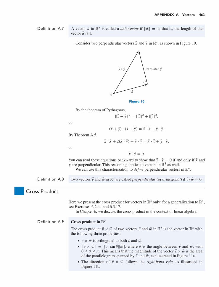
APPENDIX A Vectors 463
Definition A.7 A vector u in Rn is called a unit vector if ∥u∥ = 1; that is, the length of thevector u is 1.
Consider two perpendicular vectors x and y in R2, as shown in Figure 10.
x
translated yx + y
0
Figure 10
By the theorem of Pythagoras,
∥x + y∥2 = ∥x∥2 + ∥y∥2,
or
(x + y) · (x + y) = x · x + y · y.
By Theorem A.5,
x · x + 2(x · y) + y · y = x · x + y · y,
or
x · y = 0.
You can read these equations backward to show that x · y = 0 if and only if x andy are perpendicular. This reasoning applies to vectors in R3 as well.
We can use this characterization to define perpendicular vectors in Rn:
Definition A.8 Two vectors v and w in Rn are called perpendicular (or orthogonal) if v · w = 0.
Cross Product
Here we present the cross product for vectors in R3 only; for a generalization to Rn ,see Exercises 6.2.44 and 6.3.17.
In Chapter 6, we discuss the cross product in the context of linear algebra.
Definition A.9 Cross product in R3
The cross product v × w of two vectors v and w in R3 is the vector in R3 withthe following three properties:
• v × w is orthogonal to both v and w.• ∥v × w∥ = ∥v∥ sin θ∥w∥, where θ is the angle between v and w, with
0 ≤ θ ≤ π . This means that the magnitude of the vector v × w is the areaof the parallelogram spanned by v and w, as illustrated in Figure 11a.
• The direction of v × w follows the right-hand rule, as illustrated inFigure 11b.

464 APPENDIX A Vectors
v
w
(a)
v × w
w
v
(b)
Figure 11 (a) ∥v × w∥ is the shaded area. (b) A right-handed system.
Theorem A.10 Properties of the cross product
The following equations hold for all vectors u, v, w in R3 and for all scalars k.
a. w × v = −(v × w): The cross product is anticommutative.b. (kv) × w = k(v × w) = v × (kw).c. v × (u + w) = v × u + v × w.d. v × w = 0 if (and only if) v is parallel to w.e. v × v = 0.f. e1 × e2 = e3, e2 × e3 = e1, e3 × e1 = e2
(and e2 × e1 = −e3, e3 × e2 = −e1, e1 × e3 = −e2).
Note that the cross product fails to be associative: u × (v × w) = (u × v) × w, ingeneral. For example, (e1 × e1) × e2 = 0, but e1 × (e1 × e2) = −e2.
Properties b and c stated in Theorem A.10 imply that the function T (x) = v× xis a linear transformation from R3 to R3, for any fixed vector v in R3.
The following diagram can serve as a memory aid for property f:
e3
e1 → e2.
We can use the properties stated in Theorem A.10 to express the cross products incomponents.
⎡
⎣v1
v2
v3
⎤
⎦ ×
⎡
⎣w1
w2
w3
⎤
⎦ = (v1e1 + v2e2 + v3e3) × (w1e1 + w2e2 + w3e3)
= (v2w3 − v3w2)e1 + (v3w1 − v1w3)e2 + (v1w2 − v2w1)e3
=
⎡
⎣v2w3 − v3w2
v3w1 − v1w3
v1w2 − v2w1
⎤
⎦

APPENDIX A Vectors 465
Theorem A.11 The cross product in components⎡
⎣v1
v2
v3
⎤
⎦ ×
⎡
⎣w1
w2
w3
⎤
⎦ =
⎡
⎣v2w3 − v3w2
v3w1 − v1w3
v1w2 − v2w1
⎤
⎦
EXAMPLE 8⎡
⎣234
⎤
⎦ ×
⎡
⎣567
⎤
⎦ =
⎡
⎣3 · 7 − 4 · 64 · 5 − 2 · 72 · 6 − 3 · 5
⎤
⎦ =
⎡
⎣−3
6−3
⎤
⎦!

This page intentionally left blank

A P P E N D I X
BTwo Techniques of Proof:
Induction and Contraposition
Here is the principle of induction, succinctly stated (you may have to work an ex-ample or two before fully understanding the wording).
Proof Technique B.1 Principle of mathematical induction
The truth of a sequence of statements P1, P2, . . . , Pn, . . . is established if2
1. P1 is true, and
2. Pn implies Pn+1 for all n = 1, 2, . . . .
Alternatively, we can write property 2 as Pn ⇒ Pn+1, with the arrow “⇒”signifying implication.
For example, if properties 1 and 2 hold, then P5 is true since
P1 ⇒ P2 ⇒ P3 ⇒ P4 ⇒ P5.
First we are using property 1 and then property 2 for n = 1, 2, 3, and 4.The following terminology is useful for proofs by induction:
• P1 is referred to as the base case,• The implication Pn ⇒ Pn+1 is called the induction step,• When proving the implication Pn ⇒ Pn+1, statement Pn is called the
induction hypothesis.
EXAMPLE 1 Let’s consider the Fibonacci sequence f0, f1, f2, . . . , recursively defined by f0 =0,f1 = 1, and fn+2 = fn+ fn+1 for all n = 0, 1, 2, . . . . The first few terms are f0 = 0,f1 = 1, f2 = 1, f3 = 2, f4 = 3, f5 = 5, f6 = 8, f7 = 13, f8 = 21, . . . .
Let’s prove by induction that
f1 + f2 + · · · + fn = fn+2 − 1
for all n = 1, 2, . . . . (Verify this equation for n = 6.)
2“Statement Pn” is written as an equation or a sentence involving an arbitrary positive integer n.
467

468 APPENDIX B Two Techniques of Proof: Induction and Contraposition
Here, the “Statement Pn” in B.1 is the equation f1 + f2 + · · ·+ fn = fn+2 − 1.
1. Base Case: We need to show that P1 is true, meaning that f1 = f3 −1. Thisequation does hold since f1 = 1 and f3 = 2.
2. Induction Step: Then we need to show that Pn implies Pn+1, meaning thatthe equation f1 + f2 + · · · + fn = fn+2 − 1 implies f1 + f2 + · · · + fn+1 =fn+3 − 1; here we are replacing n by n + 1 throughout.Indeed, f1 + f2 + · · · + fn+1 = ( f1 + f2 + · · · + fn) + fn+1 =︸︷︷︸
step2
fn+2 −
1 + fn+1 =︸︷︷︸step3
fn+3 − 1. In step 2, we are using the induction hypothesis,
f1 + f2 + · · · + fn = fn+2 − 1, and step 3, fn+3 = fn+1 + fn+2, followsfrom the definition of the Fibonacci sequence. !
As a broad strategy for a proof by induction, we suggest you proceed systematically,as illustrated in the table below. In the right column, we show the implementationof this strategy in Example 1.
Write down statement Pn f1 + f2 + · · · + fn?= fn+2 − 1
Let n = 1 and write down the basecase P1
f1?= f3 − 1
Verify the base case 1 = 2 − 1√
Write down the induction step, ( f1 + f2 + · · · + fn = fn+2 − 1)
Pn ⇒ Pn+1?⇒ ( f1 + f2 +· · ·+ fn+1 = fn+3 −1)
Do the induction step: Using the f1 + f2 + · · · + fn+1
induction hypothesis Pn , prove Pn+1 = ( f1 + f2 + · · · + fn) + fn+1
= fn+2 − 1 + fn+1 = fn+3 − 1√
Let’s move on to a second important technique of proof.
Proof Technique B.2 Contraposition
The contrapositive of the statement “P implies Q” is “Not Q implies not P ,”
where, P and Q are two statements.
An implication “P implies Q” and its contrapositive “Not Q implies not P” arelogically equivalent: They are either both true or both false.
The technique of “proof by contraposition” takes advantage of the logical equiv-alence of an implication with its contrapositive. Instead of proving an implica-tion, we can prove the contrapositive if that turns out to be easier.
EXAMPLE 2 On a plumber’s service truck we read the boast “If we can’t fix it, it ain’t broken”.The contrapositive of this claim is the logically equivalent (but less catchy) phrase“If it is broken, we can fix it”. (The lesson to be learned from this example: If yourstory is too dull, contrapose it!) !

APPENDIX B Two Techniques of Proof: Induction and Contraposition 469
EXAMPLE 3 Prove the following proposition by contraposition:
If x ≤ y + ε for all positive ε, then x ≤ y.
Here, ε denotes the Greek letter epsilon.Let’s state and then prove the contrapositive:
If x > y, then x > y + ε for some positive ε.
We assume that x > y, and we draw the two numbers x and y on the numberline. What positive number ε can we add to y so that x > y + ε? Clearly, anynumber 0 < ε < x − y will work, for example, ε = x−y
2 . Let’s verify the inequalityx > y + ε algebraically:
y + ε = y + x − y2
= x + y2
<︸︷︷︸step3
x + x2
= x . In step 3 we use the fact that y < x .
!
y xy+εε
ε

This page intentionally left blank

Answers to Odd-Numbered ExercisesCHAPTER 11.1 Answers to more theoretical questions are omitted.
1. (x, y) = (−1, 1) 3. No solutions5. (x, y) = (0, 0) 7. No solutions
9. (x, y, z) = (t, 12 − 2t, t), where t is arbitrary
11. (x, y) = (4, 1) 13. No solutions15. (x, y, z) = (0, 0, 0)
17. (x, y) = (−5a + 2b, 3a − b)
19. a. If k = 7b. If k = 7, there are infinitely many solutions.c. If k = 7, the solutions are (x, y, z) =
(1 − t, 2t − 3, t).21. 11, 13, and 1723. a. Products are competing.
b. P1 = 26, P2 = 4625. a = 400, b = 30027. a. (x, y) = (t, 2t);
b. (x, y) = (t,−3t);c. (x, y) = (0, 0)
31. f (t) = 1 − 5t + 3t2 33. f (t) = 2t2 − 3t + 4
35. f (t) = at2 + (1 − 4a)t + 3a, for arbitrary a37. f (t) = 2e3t − e2t
39. −20 − 2x − 4y + x2 + y2 = 0, the circle centeredat (1, 2) with radius 5
41. If a − 2b + c = 043. a. The intercepts of the line x + y = 1 are (1, 0)
and (0, 1). The intercepts of the line x + t2 y =
t are (t, 0) and (0, 2). The lines intersect ift = 2.
b. x = − tt − 2
, y = 2t − 2t − 2
45. There are many correct answers. Example:∣∣∣∣x −5z = −4
y −3z = −2
∣∣∣∣
49. Twenty $1 bills, eight $5 bills, and four $10 bills.
1.2 Answers to more theoretical questions are omitted.
1.
⎡
⎣xyz
⎤
⎦ =
⎡
⎣10t + 13−8t − 8
t
⎤
⎦
3.
⎡
⎣xyz
⎤
⎦ =
⎡
⎣4 − 2s − 3t
st
⎤
⎦
5.
⎡
⎢⎢⎣
x1x2x3x4
⎤
⎥⎥⎦ =
⎡
⎢⎢⎣
−tt
−tt
⎤
⎥⎥⎦
7.
⎡
⎢⎢⎢⎢⎣
x1x2x3x4x5
⎤
⎥⎥⎥⎥⎦=
⎡
⎢⎢⎢⎢⎣
−2tt000
⎤
⎥⎥⎥⎥⎦
9.
⎡
⎢⎢⎢⎢⎢⎢⎣
x1x2x3x4x5x6
⎤
⎥⎥⎥⎥⎥⎥⎦=
⎡
⎢⎢⎢⎢⎢⎢⎣
t − s − 2rr
−t + s + 1t − 2s + 2
st
⎤
⎥⎥⎥⎥⎥⎥⎦
11.
⎡
⎢⎢⎣
x1x2x3x4
⎤
⎥⎥⎦ =
⎡
⎢⎢⎣
−2t3t + 4
t−2
⎤
⎥⎥⎦
13. No solutions 15.
⎡
⎣xyz
⎤
⎦ =
⎡
⎣421
⎤
⎦
17.
⎡
⎢⎢⎢⎢⎣
x1x2x3x4x5
⎤
⎥⎥⎥⎥⎦=
⎡
⎢⎢⎢⎢⎣
−8221/43408591/86804695/434−459/434
699/434
⎤
⎥⎥⎥⎥⎦
19.
⎡
⎢⎢⎣
0000
⎤
⎥⎥⎦ and
⎡
⎢⎢⎣
1000
⎤
⎥⎥⎦
21. b = 0, c = 1, d = 0, with a being arbitrary
23. 4 types
27. Yes; perform the operations backwards.
29. No; you cannot make the last column zero by ele-mentary row operations.
31. a = 2, b = c = d = 1
33. f (t) = 1 − 5t + 4t2 + 3t3 − 2t4
35. f (t) = −5 + 13t − 10t2 + 3t3
37.
⎡
⎢⎢⎣
−t6t
−9t4t
⎤
⎥⎥⎦, where t is arbitrary.
39.
⎡
⎣x1x2x3
⎤
⎦ =
⎡
⎣500300400
⎤
⎦
41. a. Neither the manufacturing nor the energy sectormakes demands on agriculture.
b. x1 ≈ 18.67, x2 ≈ 22.60, x3 ≈ 3.63
471

472 ANSWERS TO ODD-NUMBERED EXERCISES
43. m1 = 23 m2
45. a ≈ 12.17, b ≈ −1.15, c ≈ 0.18. The longest dayis about 13.3 hours.
47. a. If k is neither 1 nor 2b. If k = 1 c. If k = 2
49. a. x1 = 3x3 − 2x4, x2 = 2x3 − x4, for arbitrary x3and x4
b. Yes, x1 = 1, x2 = 5, x3 = 9, x4 = 13.
51. C = 25
53. xy = 0, the union of the two coordinate axes
55. a(xy − y) + b(y2 − y) = 0, where a = 0 or b = 0
57. a(x2 − x) + b(y2 − y) = 0, where a = 0 or b = 0
59. 25 − 10x − 10y + x2 + y2 = 0, the circle of radius5 centered at (5, 5)
61. No solutions
63. Statistics: $86; Set Theory: $92; Psychology: $55
65. Beginning: 120 liberal, 140 conservative.End: 140 liberal, 120 conservative.
67. Cow: 34/21 liang; sheep: 20/21 liang
69. Swallow: 24/19 liang; sparrow: 32/19 liang
71. A: 265; B: 191; C: 148; D: 129; E: 76
73. Gaussian elimination shows that
Pigeons = −250 + 59 (Swans) + 20(Peacocks) and
Sarasas = 350 − 149 (Swans) − 21(Peacocks).
One solution (the one given by Mahavira) is 15 pi-geons, 28 sarasabirds, 45 swans, and 12 peacocks(spending 9, 20, 35, and 36 panas, respectively).
75. 53 sheep, 42 goats, and 5 hogs
77. Full Half Empty
1st Son p 10 − 2p p2nd Son q 10 − 2q q3rd Son 10 − p − q 2p + 2q − 10 10 − p − q
Here, p and q are integers between 0 and 5 such thatp + q ≥ 5.
1.3 Answers to more theoretical questions are omitted.1. a. No solutions b. One solution
c. Infinitely many solutions
3. Rank is 1.
5. a. x[
13
]+ y
[21
]=
[7
11
]
b. x = 3, y = 2
7. One solution
9.
⎡
⎣1 2 34 5 67 8 9
⎤
⎦
⎡
⎣xyz
⎤
⎦ =
⎡
⎣149
⎤
⎦
11. Undefined
13.[
2965
]15. 70
17. Undefined 19.
⎡
⎣000
⎤
⎦
21.
⎡
⎢⎢⎣
1587081
123
⎤
⎥⎥⎦ 23.
⎡
⎢⎢⎣
1 0 00 1 00 0 10 0 0
⎤
⎥⎥⎦
25. The system Ax = c has infinitely many solutions ornone.
27.
⎡
⎢⎢⎣
1 0 0 00 1 0 00 0 1 00 0 0 1
⎤
⎥⎥⎦29.
⎡
⎢⎣
25 0 00 0 00 0 − 1
9
⎤
⎥⎦
31.
⎡
⎣1 2 10 3 10 0 − 1
9
⎤
⎦, for example
33. Ax = x
35. Aei is the i th column of A.
37. x =
⎡
⎣2 − 2t
t1
⎤
⎦, where t is arbitrary
39.
⎡
⎣1 0 0 ∗0 1 0 ∗0 0 1 ∗
⎤
⎦
41. One solution 43. No solutions47. a. x = 0 is a solution.
b. By part (a) and Theorem 1.3.3c. A(x1 + x2) = Ax1 + Ax2 = 0 + 0 = 0d. A(kx) = k(Ax) = k0 = 0
49. a. Infinitely many solutions or noneb. One solution or nonec. No solutionsd. Infinitely many solutions
51. If m = r and s = p
53. Yes
55. Yes;
⎡
⎣789
⎤
⎦ = −1
⎡
⎣123
⎤
⎦ + 2
⎡
⎣456
⎤
⎦
57.[
711
]=
[39
]+
[42
]
59. c = 9, d = 11
61. For c = 2 and for c = 3
63. Line through the endpoint of v in the direction of w

ANSWERS TO ODD-NUMBERED EXERCISES 473
65. Parallelogram with its vertices at the origin and atthe endpoints of vectors v, w, and v + w
67. Triangle with its vertices at the origin and at the end-points of vectors v and w
69.(
b+c−a2 , c−b+a
2 , b−c+a2
)
CHAPTER 22.1 Answers to more theoretical questions are omitted.
1. Not linear 3. Not linear
5. A =[
7 6 −1311 9 17
]
7. T is linear; A =[v1 v2 · · · vm
]
9. Not invertible
11. The inverse is[
3 −2/3−1 1/3
].
15. A is invertible if a = 0 or b = 0. In this case,
A−1 = 1a2 + b2
[a b
−b a
].
17. Reflection about the origin; this transformation is itsown inverse.
19. Orthogonal projection onto the e1-axis; not inver-tible
21. Rotation through an angle of 90 in the clockwisedirection; invertible
23. Clockwise rotation through an angle of 90, fol-lowed by a scaling by a factor of 2; invertible
25. Scaling by a factor of 2
27. Reflection about the e1-axis
29. Reflection about the origin
31. Reflection about the e2-axis, represented by the
matrix[−1 0
0 1
]
33.
√2
2
[1 −11 1
]35.
[1 22 1
]
37. T (x) = T (v) + k(T (w) − T (v)
)is on the line
segment.
41. y = c1x1 + c2x2; the graph is a plane through theorigin in R3.
43. a. T is linear, represented by the matrix[2 3 4
]
45. Yes; use Theorem 2.1.3.
47. Write w = c1v1 + c2v2; thenT (w) = c1T (v1) + c2T (v2).
51. A =
⎡
⎢⎣
0 0 1/3 01/2 0 1/3 1/21/2 0 0 1/20 1 1/3 0
⎤
⎥⎦, xequ = 113
⎡
⎢⎣
1435
⎤
⎥⎦,
and Page 4 has the highest (naıve) PageRank.
53. B =
⎡
⎢⎣
0.05 0.45 0.05 0.050.45 0.05 0.05 0.850.45 0.45 0.05 0.050.05 0.05 0.85 0.05
⎤
⎥⎦, xequ = 128
⎡
⎢⎣
5977
⎤
⎥⎦
55. B =
⎡
⎢⎢⎣
0.05 0.05 0.316 0.050.45 0.05 0.316 0.450.45 0.05 0.05 0.450.05 0.85 0.316 0.05
⎤
⎥⎥⎦, xequ = 12860
⎡
⎢⎣
323855675
1007
⎤
⎥⎦ ≈
⎡
⎢⎣
0.1130.2990.2360.352
⎤
⎥⎦, and Page 4 has the highest
PageRank.
57. a. 37 SFr2 coins, and 14 SFr5 coins
b. A =[
2 51 1
]
c. Yes. A−1 =
⎡
⎣− 13
53
13 − 2
3
⎤
⎦
59. a.
[59 − 160
90 1
]
b. Yes.
[95 320 1
], F = 9
5 C + 32
61. A =
⎡
⎢⎢⎣
1 4/5 1/8 5/45/4 1 5/32 25/168 32/5 1 10
4/5 16/25 1/10 1
⎤
⎥⎥⎦
63. B =
⎡
⎣1 −40 10 2
⎤
⎦
2.2 Answers to more theoretical questions are omitted.
1. The image consists of the vectors[
31
]and
[24
].
3. The parallelogram in R3 defined by the vectorsT (e1) and T (e2)
5. About 2.5 radians 7. 19
⎡
⎣11
111
⎤
⎦
9. A vertical shear
11. 125
[7 24
24 −7
]13.
[2u2
1 − 1 2u1u22u1u2 2u2
2 − 1
]
15. aii = 2u2i − 1, and ai j = 2ui u j when i = j
17. If b = 0, then let v =[
b1 − a
]and w =
[−b
1 + a
],
for example.
19.
⎡
⎣1 0 00 1 00 0 0
⎤
⎦ 21.
⎡
⎣0 −1 01 0 00 0 1
⎤
⎦

474 ANSWERS TO ODD-NUMBERED EXERCISES
23.
⎡
⎣1 0 00 0 10 1 0
⎤
⎦
25.[
1 −k0 1
]; you shear back.
27. A is a reflection; B is a scaling; C is a projection; Dis a rotation; E is a shear.
31. A =
⎡
⎣−2 0 0
1 0 00 0 0
⎤
⎦
33. Use a parallelogram. 35. Yes
37. a. 1 b. 0
c. −2 ≤ tr A ≤ 2 d. 2
39. a. Projection with scalingb. Shear with scalingc. Reflection with scaling
41. refQ x = −refP x
43.[
cos θ sin θ
− sin θ cos θ
], a clockwise rotation through the
angle θ
45. A−1 = A. The inverse of a reflection is the reflec-tion itself.
47. Write T (x) =[
a bc d
]x . Express f (t) in terms of
a, b, c, d .
49. c = 0 (or c = π2 ), v1 =
[10
], and v2 =
[01
]
51. c = π4 , v1 = 1√
2
[11
], and v2 = 1√
2
[−1
1
]
53. The image is an ellipse with semimajor axes ± 5e1and semiminor axes ± 2e2.
55. The curve C is the image of the unit circle under thetransformation with matrix
[w1 w2
].
2.3 Answers to more theoretical questions are omitted.
1.[
4 63 4
]3. Undefined
5.
⎡
⎣a bc d0 0
⎤
⎦ 7.
⎡
⎣−1 1 0
5 3 4−6 −2 −4
⎤
⎦
9.[
0 00 0
]11. [10] 13. [h]
15.
⎡
⎢⎣1 02 0
19 16
⎤
⎥⎦
17. All matrices of the form[
a 00 b
]
19. All matrices of the form[
a b−b a
]
21. All matrices of the form[
a bb a − b
]
23. All matrices of the form
[a b23 b 5
3 b + a
]
25. All matrices of the form
⎡
⎣a 0 b0 c 0d 0 e
⎤
⎦
29. a. The matrices Dα Dβ and Dβ Dα both representthe counterclockwise rotation through the angleα + β.
b. Dα Dβ = Dβ Dα
=[
cos(α + β) − sin(α + β)
sin(α + β) cos(α + β)
]
31. (i th row of AB) = (i th row of A)B33. An = I2 for even n and An = −I2 for odd n. A
represents the rotation through π .35. An = I2 for even n and An = A for odd n. A repre-
sents the reflection about the line spanned by[
11
].
37. An =
⎡
⎣ 1 0
−n 1
⎤
⎦. A represents a vertical shear.
39. An represents the rotation through nπ/4 in theclockwise direction, so that A8 = I2. Now A1001 =(A8)125 A = A.
41. An = I2 for even n and An = A for odd n. A repre-sents the reflection about a line.
43. A = −I2, for example, or any matrix representing areflection about a line
45. The matrix representing the rotation through 2π/3,
for example, A =[
cos(2π/3) − sin(2π/3)
sin(2π/3) cos(2π/3)
]=
12
[−1 −
√3√
3 −1
]
47. Any projection or reflection matrix with nonzero
entries will do, for example, A =[
0.6 0.80.8 −0.6
].
49. AF =[
1 00 −1
], F A =
[−1 0
0 1
]. We compose a
rotation with a reflection to obtain a reflection.
51. F J = J F =[−1 −1
1 −1
]. Note that F represents
the rotation through π/2 while J represents therotation through π/4 combined with a scaling by√
2. The products F J and J F both represent therotation through 3π/4 combined with a scalingby
√2.

ANSWERS TO ODD-NUMBERED EXERCISES 475
53. C D =[
0 −11 0
]and DC =
[0 1
−1 0
]. We com-
pose two reflections to obtain a rotation.
55. X =[−2s −2t
s t
], where s and t are arbitrary
constants
57. X =[−5 2
3 − 1
]
59. No such matrix X exists.
61. X =
⎡
⎣1 + s −2 + t−2s 1 − 2t
s t
⎤
⎦, where s and t are arbitrary
constants63. No such matrix X exists.
65. X =[
0 t0 0
], where t is an arbitrary constant
67a. [1 1 1]A = [1 1 1]69a. Of the surfers who are on Page 1 initially, 25% will
be on Page 3 after following two consecutive links.69b. The i j th entry of A2 is 0 if there is no path of
length 2 from vertex j to vertex i in the graph ofthe mini-Web, meaning that a surfer cannot get fromPage j to Page i by following two consecutive links.
71. A straightforward computation shows that the onlynonzero entry of A4 is the first component of thethird column. Thus there is no path of length 4 fromPage 3 to Page 1 in the graph of the mini-Web, whilethere is a path of length 4 linking any other twopages. We cannot get from Page 3 to Page 1 by fol-lowing four consecutive links.
73. limm→∞
(Am x) =(
limm→∞
Am)
x =⎡
⎣| |
xequ · · · xequ| |
⎤
⎦ x = (x1 + · · · + xn)︸ ︷︷ ︸components of x
xequ =
xequ
75. The i j th entry of Am+1 = Am A is the dot productof the i th row w or Am with the j th column v of A.Since all components of w and some components ofv are positive (with all components of v being non-negative), this dot product is positive, as claimed.
77. We find A10 ≈
⎡
⎣0.5003 0.4985 0.50000.0996 0.1026 0.09990.4002 0.3989 0.4001
⎤
⎦. This
shows that A is regular and it suggests then xequ =⎡
⎣0.50.10.4
⎤
⎦. To be sure, we verify that A
⎡
⎣0.50.10.4
⎤
⎦ =
⎡
⎣0.50.10.4
⎤
⎦.
79. An extreme example is the identity matrix In . In thiscase, In x = x for all distribution vectors.
81. Am v = 5m v
83. By Definition 2.3.10, there exists a positive integerm such that Am is a positive transition matrix. Notethat Am x = x . Thus, the i th component of x is thedot product of the i th row w of Am with x . Sinceall components of w and some components of x arepositive (with all components of x being nonnega-tive), this dot product is positive, as claimed.
85. There is one and only one such X .
2.4 Answers to more theoretical questions are omitted.
1.[
8 −3−5 2
]3.
⎡
⎣− 12 112 0
⎤
⎦
5. Not invertible 7. Not invertible
9. Not invertible 11.
⎡
⎣1 0 −10 1 00 0 1
⎤
⎦
13.
⎡
⎢⎢⎣
1 0 0 0−2 1 0 0
1 −2 1 00 1 −2 1
⎤
⎥⎥⎦
15.
⎡
⎢⎢⎣
−6 9 −5 19 −1 −5 2
−5 −5 9 −31 2 −3 1
⎤
⎥⎥⎦
17. Not invertible
19. x1 = 3y1 − 2.5y2 + 0.5y3x2 = −3y1 + 4y2 − y3x3 = y1 − 1.5y2 + 0.5y3
21. Not invertible 23. Invertible
25. Invertible 27. Not invertible
29. For all k except k = 1 and k = 2
31. It’s never invertible.
33. If a2 + b2 = 1
35. a. Invertible if a, d , f are all nonzerob. Invertible if all diagonal entries are nonzeroc. Yes; use Theorem 2.4.5.d. Invertible if all diagonal entries are nonzero
37. (cA)−1 = 1c
A−1
39. M is invertible; if mi j = k (where i = j), then thei j th entry of M−1 is −k; all other entries are thesame.
41. The transformations in parts a, c, and d are invert-ible, while the projection in part b is not.
43. Yes; x = B−1(A−1 y)

476 ANSWERS TO ODD-NUMBERED EXERCISES
45. a. 33 = 27 b. n3
c. 123
33 = 64 (seconds)
47. f (x) = x2 is not invertible, but the equationf (x) = 0 has the unique solution x = 0.
51. a. Since rank A < n, all the entries in the last rowof E will be zero. We can let c = en ; the sys-tem Ex = en will be inconsistent. Reversingthe row reduction from A to E , we can trans-form the system Ex = en into an inconsistentsystem Ax = b.
b. We have rank A ≤ m < n. Now use part a.
53. a. λ1 = 2, λ2 = 6
b. We chose λ = 2. A−λI2 =[
1 13 3
], x =
[−1
1
].
c. Check that[
3 13 5
]x = 2x .
55. det A =∥∥∥∥
[20
]∥∥∥∥ sin(π/2)
∥∥∥∥
[02
]∥∥∥∥ = 4, and A−1 =[
1/2 00 1/2
], a scaling by 1/2
57. det A =∥∥∥∥
[cos α
sin α
]∥∥∥∥ sin(−π/2)
∥∥∥∥
[sin α
− cos α
]∥∥∥∥ =
−1, and A−1 = A, a reflection
59. det A =∥∥∥∥
[0.60.8
]∥∥∥∥ sin(π/2)
∥∥∥∥
[−0.8
0.6
]∥∥∥∥ = 1, and
A−1 =[
0.6 0.8−0.8 0.6
], a rotation
61. det A =∥∥∥∥
[1
−1
]∥∥∥∥ sin(π/2)
∥∥∥∥
[11
]∥∥∥∥ = 2, and A−1 =
12
[1 −11 1
], a rotation through π/4 combined with
a scaling by√
2/2
63. det A =∥∥∥∥
[−3
4
]∥∥∥∥ sin(−π/2)
∥∥∥∥
[43
]∥∥∥∥ = −25, and
A−1 = 125
[−3 4
4 3
], a reflection combined with a
scaling by 1/5
65. det A =∥∥∥∥
[11
]∥∥∥∥ sin(π/4)
∥∥∥∥
[01
]∥∥∥∥ = 1, and A−1 =[
1 0−1 1
], a vertical shear
67. False 69. False 71. True
73. True 75. True
77. A = BS−1 79. A = 15
[9 3
−2 16
]
81.
⎧⎪⎪⎪⎪⎪⎪⎪⎨
⎪⎪⎪⎪⎪⎪⎪⎩
matrix of T :
⎡
⎣0 0 1
−1 0 00 −1 0
⎤
⎦
matrix of L:
⎡
⎣0 1 01 0 00 0 1
⎤
⎦
83. Yes; yes; each elementary row operation can be “un-done” by an elementary row operation.
85. a. Use Exercise 84; let S = E1 E2 · · · E p .
b. S =[
1 0−4 1
] [ 12 00 1
]=
[ 12 0
−2 1
]
87.[
k 00 1
],
[1 00 k
],
[1 c0 1
],
[1 0c 1
],
[0 11 0
],
where k is nonzero and c is arbitrary. Cases 3 and 4represent shears, and case 5 is a reflection.
89. Yes; use Theorem 2.3.4.
91. a. y =
⎡
⎢⎢⎣
−3520
⎤
⎥⎥⎦ b. x =
⎡
⎢⎢⎣
1−1
20
⎤
⎥⎥⎦
93. a. Write A =[
A(m) A2A3 A4
], L =
[L(m) 0
L3 L4
],
U =[
U (m) U20 U4
]. Use Theorem 2.3.9.
c. Solve the equation
A =[
A(n−1) v
w k
]=
[L ′ 0x t
] [U ′ y
0 1
]
for x , y, and t .
95. A is invertible if both A11 and A22 are invertible. Inthis case,
A−1 =[
A−111 0
0 A−122
].
97. rank A = rank(A11) + rank(A23)
99. Only A = In
101. (i j th entry of AB) =∑n
k=1 aikbk j ≤s∑n
k=1 bk j ≤ sr
107. g(
f (x))
= x , for all x
f(g(x)
)=
x if x is evenx + 1 if x is odd
The functions f and g are not invertible.
CHAPTER 33.1 Answers to more theoretical questions are omitted.
1. ker A = 0 3. e1, e2
5.
⎡
⎣1
−21
⎤
⎦ 7. ker A = 0

ANSWERS TO ODD-NUMBERED EXERCISES 477
9. ker A = 0 11.
⎡
⎢⎢⎣
−2310
⎤
⎥⎥⎦
13.
⎡
⎢⎢⎢⎢⎢⎢⎣
−210000
⎤
⎥⎥⎥⎥⎥⎥⎦,
⎡
⎢⎢⎢⎢⎢⎢⎣
−30
−2−1
10
⎤
⎥⎥⎥⎥⎥⎥⎦,
⎡
⎢⎢⎢⎢⎢⎢⎣
000001
⎤
⎥⎥⎥⎥⎥⎥⎦
15.[
11
],
[12
]17. All of R2
19. The line spanned by[
1−2
]
21. All of R3
23. kernel is 0, image is all of R2.
25. Same as Exercise 23
27. f (x) = x3 − x
29. f[φ
θ
]=
⎡
⎣sin φ cos θ
sin φ sin θ
cos φ
⎤
⎦
(compare with spherical coordinates)
31. A =
⎡
⎣−2 −3
0 11 0
⎤
⎦
33. T
⎡
⎣xyz
⎤
⎦ = x + 2y + 3z
35. ker T is the plane with normal vector v;im T = R.
37. im A = span(e1, e2); ker A = span(e1);im(A2) = span(e1); ker(A2) = span(e1, e2);A3 = 0 so ker(A3) = R3 and im(A3) = 0
39. a. ker B is contained in ker(AB), but they need notbe equal.
b. im(AB) is contained in im A, but they need notbe equal.
41. a. im A is the line spanned by[
34
], and ker A is the
perpendicular line, spanned by[−4
3
].
b. A2 = A; if v is in im A, then Av = v.c. Orthogonal projection onto the line spanned by[
34
]
43. Suppose A is an n × m matrix of rank r . Let B bethe matrix you get when you omit the first r rowsand the first m columns of rref
[A In
]. (What can
you do when r = n?)
45. There are m − r nonleading variables, which can bechosen freely. The general vector in the kernel canbe written as a linear combination of m − r vectors,with the nonleading variables as coefficients.
47. im T = L2 and ker T = L1
51. ker(AB) = 0
53. a.
⎡
⎢⎢⎢⎢⎢⎢⎢⎢⎣
1111000
⎤
⎥⎥⎥⎥⎥⎥⎥⎥⎦
,
⎡
⎢⎢⎢⎢⎢⎢⎢⎢⎣
0110100
⎤
⎥⎥⎥⎥⎥⎥⎥⎥⎦
,
⎡
⎢⎢⎢⎢⎢⎢⎢⎢⎣
1010010
⎤
⎥⎥⎥⎥⎥⎥⎥⎥⎦
,
⎡
⎢⎢⎢⎢⎢⎢⎢⎢⎣
1100001
⎤
⎥⎥⎥⎥⎥⎥⎥⎥⎦
b. ker H = span(v1, v2, v3, v4), by part a,and im M = span(v1, v2, v3, v4), by Theo-rem 3.1.3. Thus ker H = im(M). H(Mx) = 0,since Mx is in im M = ker H .
3.2 Answers to more theoretical questions are omitted.
1. Not a subspace 3. W is a subspace.
7. Yes 9. Dependent
11. Independent 13. Dependent
15. Dependent 17. Independent
19.
⎡
⎢⎢⎣
2000
⎤
⎥⎥⎦ and
⎡
⎢⎢⎣
3450
⎤
⎥⎥⎦ are redundant.
21. v2 = v1, or, v1 − v2 = 0, so that[
1−1
]is in the
kernel.
23. v1 = 0, so that[
10
]is in the kernel.
25. v3 = v1, or, v1 − v3 = 0, so that
⎡
⎣10
−1
⎤
⎦ is in the
kernel.
27.
⎡
⎣111
⎤
⎦,
⎡
⎣123
⎤
⎦ 29.[
14
],[
25
]
31.
⎡
⎢⎢⎣
1235
⎤
⎥⎥⎦,
⎡
⎢⎢⎣
5678
⎤
⎥⎥⎦ 33.
⎡
⎢⎢⎣
1000
⎤
⎥⎥⎦,
⎡
⎢⎢⎣
0100
⎤
⎥⎥⎦,
⎡
⎢⎢⎣
0010
⎤
⎥⎥⎦
35. Suppose there is a nontrivial relation c1v1 + · · · +ci vi + · · · + cm vm = 0, with ci = 0. We can solvethis equation for vi and thus express vi as a linearcombination of the other vectors in the list.
Conversely, if vi is a linear combination of theother vectors, vi = . . . , then we can subtract vifrom both sides of the equation to obtain a nontri-vial relation (the coefficient of vi will be −1).

478 ANSWERS TO ODD-NUMBERED EXERCISES
37. The vectors T (v1), . . . , T (vm) are not necessarilyindependent.
39. The vectors v1, . . . , vm , v are linearly independent.
41. The columns of B are linearly independent, whilethe columns of A are dependent.
43. The vectors are linearly independent.
45. Yes 47.
⎡
⎢⎢⎣
1 0 00 1 00 0 10 0 0
⎤
⎥⎥⎦
49. L = im
⎡
⎣111
⎤
⎦ = ker[
1 0 −10 1 −1
]
51. a. Consider a relation c1v1 +· · ·+ cp v p +d1w1 +· · · + dq wq = 0. Then c1v1 + · · · + cp v p =−d1w1 − · · · − dq wq is 0, because this vector isboth in V and in W . The claim follows.
b. From part a we know that the vectorsv1, . . . , v p, w1, . . . , wq are linearly indepen-dent. Consider a vector x in V + W . By thedefinition of V + W , we can write x = v + wfor a v in V and a w in W . The v is a linearcombination of the vi , and w is a linear com-bination of the w j . This shows that the vectorsv1, . . . , v p, w1, . . . , wq span V + W .
55.
⎡
⎢⎢⎢⎢⎣
−21000
⎤
⎥⎥⎥⎥⎦,
⎡
⎢⎢⎢⎢⎣
−30100
⎤
⎥⎥⎥⎥⎦,
⎡
⎢⎢⎢⎢⎣
−40010
⎤
⎥⎥⎥⎥⎦,
⎡
⎢⎢⎢⎢⎣
−50001
⎤
⎥⎥⎥⎥⎦
57. For j = 1, 3, 6, and 7, corresponding to the columnsthat do not contain leading 1’s
3.3 Answers to more theoretical questions are omitted.
1. v2 = 3v1; basis of image:[
12
];
basis of kernel:[−3
1
]
3. No redundant vectors; basis of image:[
13
],[
24
];
basis of kernel: ∅
5. v3 = 3v1; basis of image:[
12
],[−2
4
];
basis of kernel:
⎡
⎣−3
01
⎤
⎦
7. v2 = 2v1; basis of image:[
11
],[
34
];
basis of kernel:
⎡
⎣−2
10
⎤
⎦
9. v2 = 2v1; basis of image:
⎡
⎣111
⎤
⎦,
⎡
⎣123
⎤
⎦;
basis of kernel:
⎡
⎣−2
10
⎤
⎦
11. v3 = v1; basis of image:
⎡
⎣100
⎤
⎦,
⎡
⎣011
⎤
⎦;
basis of kernel:
⎡
⎣−1
01
⎤
⎦
13. v2 = 2v1, v3 = 3v1; basis of image:[1];
basis of kernel:
⎡
⎣−2
10
⎤
⎦,
⎡
⎣−3
01
⎤
⎦
15. v3 = 2v1 + 2v2, v4 = 0;
basis of image:
⎡
⎢⎢⎣
1010
⎤
⎥⎥⎦,
⎡
⎢⎢⎣
0101
⎤
⎥⎥⎦;
basis of kernel:
⎡
⎢⎢⎣
−2−2
10
⎤
⎥⎥⎦,
⎡
⎢⎢⎣
0001
⎤
⎥⎥⎦
17. v1 = 0, v3 = 2v2, v5 = 3v2 + 4v4;
basis of image:[
10
],[
01
];
basis of kernel:
⎡
⎢⎢⎢⎢⎣
10000
⎤
⎥⎥⎥⎥⎦,
⎡
⎢⎢⎢⎢⎣
0−2
100
⎤
⎥⎥⎥⎥⎦,
⎡
⎢⎢⎢⎢⎣
0−3
0−4
1
⎤
⎥⎥⎥⎥⎦
19. v3 = 5v1 + 4v2, v4 = 3v1 + 2v2;
basis of image:
⎡
⎢⎢⎣
1000
⎤
⎥⎥⎦,
⎡
⎢⎢⎣
0100
⎤
⎥⎥⎦,
⎡
⎢⎢⎣
0010
⎤
⎥⎥⎦;
basis of kernel:
⎡
⎢⎢⎢⎢⎣
−5−4
100
⎤
⎥⎥⎥⎥⎦,
⎡
⎢⎢⎢⎢⎣
−3−2
010
⎤
⎥⎥⎥⎥⎦
21. rref A =
⎡
⎣1 0 −30 1 40 0 0
⎤
⎦;

ANSWERS TO ODD-NUMBERED EXERCISES 479
basis of image:
⎡
⎣147
⎤
⎦,
⎡
⎣356
⎤
⎦;
basis of kernel:
⎡
⎣3
−41
⎤
⎦
23. rref A =
⎡
⎢⎢⎣
1 0 2 40 1 −3 −10 0 0 00 0 0 0
⎤
⎥⎥⎦;
basis of image:
⎡
⎢⎢⎣
1030
⎤
⎥⎥⎦,
⎡
⎢⎢⎣
014
−1
⎤
⎥⎥⎦;
basis of kernel:
⎡
⎢⎢⎣
−2310
⎤
⎥⎥⎦,
⎡
⎢⎢⎣
−4101
⎤
⎥⎥⎦
25. rref A =
⎡
⎢⎢⎢⎢⎣
1 2 0 5 00 0 1 −1 00 0 0 0 10 0 0 0 00 0 0 0 0
⎤
⎥⎥⎥⎥⎦;
basis of image:
⎡
⎢⎢⎣
1312
⎤
⎥⎥⎦,
⎡
⎢⎢⎣
3949
⎤
⎥⎥⎦,
⎡
⎢⎢⎣
1322
⎤
⎥⎥⎦;
basis of kernel:
⎡
⎢⎢⎢⎢⎣
−21000
⎤
⎥⎥⎥⎥⎦,
⎡
⎢⎢⎢⎢⎣
−50110
⎤
⎥⎥⎥⎥⎦
27. They do. 29.
⎡
⎣−3
20
⎤
⎦,
⎡
⎣−1
02
⎤
⎦
31. A =
⎡
⎢⎢⎣
1 −2 −41 0 00 1 00 0 1
⎤
⎥⎥⎦
33. The dimension of a hyperplane in Rn is n − 1.
35. The dimension is n − 1.
37. A =
⎡
⎢⎢⎣
1 0 0 0 00 1 0 0 00 0 0 0 00 0 0 0 0
⎤
⎥⎥⎦
39. ker C is at least one-dimensional, and ker C is con-tained in ker A.
41. To fit a conic through a given point Pj (x j , y j ), weneed to solve the equation c1 + c2x j + c3 y j +c4x2
j + c5x j y j + c6 y2j = 0, a homoge-
neous linear equation in the six unknownsc1, . . . , c6. Thus, fitting a conic to four given pointsP1(x1, y1), . . . , P4(x4, y4) amounts to solving asystem of four homogeneous linear equations withsix unknowns. This in turn amounts to finding thekernel of a 4×6 matrix A. This kernel is at least two-dimensional. Since every one-dimensional subspaceof ker A defines a unique conic (see Exercise 40),there will be infinitely many such conics.
43. Building on our work in Exercise 41, we observethat fitting a conic through six points amounts tofinding the kernel of a 6 × 6 matrix A. Therewill be no such conic if ker A = 0, one conicif dim(ker A) = 1, and infinitely many conics ifdim(ker A) > 1. To give an example for each case,recall Exercise 1.2.53, where we showed that theunique conic xy = 0 runs through the points (0, 0),(1, 0), (2, 0), (0, 1), (0, 2). Thus, there is no conicthrough the points (0, 0), (1, 0), (2, 0), (0, 1), (0, 2),(1, 1), whereas the only conic through (0, 0), (1, 0),(2, 0), (0, 1), (0, 2), (0, 3) is xy = 0. There are in-finitely many conics through (0, 0), (1, 0), (2, 0),(3, 0), (4, 0), (5, 0).
45. A cubic runs through (0, 0) if c1 = 0. Now the cu-bic runs through the points (1, 0), (2, 0), and (3, 0)as well if
c2 + c4 + c7 = 02c2 + 4c4 + 8c7 = 03c3 + 9c4 + 27c7 = 0.
Gaussian elimination shows that c2 = c4 = c7 =0. Analogously, the cubic runs through the points(0, 1), (0, 2), and (0, 3) if c3 = c6 = c10 = 0. Theclaim follows.
Each such cubic is the union of the x-axis, they-axis, and an arbitrary line in R2.
47. Plugging the points (1, 1) and (2, 2) into the solu-tion xy(c5 +c8x +c9 y) = 0 of Problem 45, we findc5 = 0 and c9 = −c8, so that the solutions are of theform xy(c8x − c8 y) = 0, where c8 = 0. Divisionby c8 produces the unique solution xy(x − y) = 0,the union of the y-axis, the x-axis, and the diagonaly = x .
49. No such cubic exists, since the unique cubic throughthe first 9 points does not pass through (2, 1). SeeExercise 47.
51. Plugging the points (4, 0), (0, 4) and (1, 1) intothe solution xy(c5 + c8x + c9 y) = 0 of Prob-lem 45, we find that c5 + c8 + c9 = 0. Definea = c8 and b = c9. There are infinitely many cu-bics running through the given points, of the formxy(ax + by − a − b) = 0, where a = 0 or b = 0.

480 ANSWERS TO ODD-NUMBERED EXERCISES
Each such cubic is the union of the y-axis, thex-axis, and any line through the point (1, 1).
53. Plugging the points (1, 1), (2, 1), (1, 2), and(3, 2) into the solutions of Problem 44, we find thatc5 = c7 = c8 = c9 = 0, so that the solutionsare of the form c10 y(y − 1)(y − 2) = 0, wherec10 = 0. Division by c10 produces the unique so-lution y(y − 1)(y − 2) = 0, the union of the threehorizontal lines y = 0, y = 1, and y = 2.
55. Plugging the points (1, 1), (2, 1), (1, 2), (2, 2), and(3, 3) into the solutions of Problem 44, we find thatc5 = c8 = c9 = 0 and c7 + c10 = 0, so thatthe solutions are of the form c7x(x − 1)(x − 2) −c7 y(y − 1)(y − 2) = 0, where c7 = 0. Division byc7 produces the unique solution x(x − 1)(x − 2) =y(y − 1)(y − 2), the union of the diagonal y = xwith an ellipse.
57. See Exercises 41 and 56. Since the kernel of the8 × 10 matrix A is at least two-dimensional, andbecause every one-dimensional subspace of ker Adefines a unique cubic (compare with Exercise 40),there will be infinitely many such cubics.
59. There may be no such cubic [as in Exercise 49], ex-actly one [take the 9 points in Exercise 47 and add(−1,−1)], or infinitely many [as in Exercise 51].
63. A basis of V is also a basis of W , by Theorem3.3.4c.
65. dim(V +W )= dim V + dim W , by Exercise 3.2.51.
67. The first p columns of rref A contain leading 1’s be-cause the vi are linearly independent. Now applyTheorem 3.3.5.
71.[
0 1 0 2 0],[
0 0 1 3 0],
[0 0 0 0 1
]
73. a. A and E have the same row space, since ele-mentary row operations leave the row space un-changed.
b. rank A = dim(rowspace(A)
), by part a and Ex-
ercise 72.
77. Suppose rank A = n. The submatrix of A consistingof the n pivot columns of A is invertible, since thepivot columns are linearly independent.
Conversely, if A has an invertible n ×n subma-trix, then the columns of that submatrix span Rn , soim A = Rn and rank A = n.
79. Let m be the smallest number such that Am = 0.By Exercise 78, there are m linearly independentvectors in Rn ; therefore, m ≤ n, and An =Am An−m = 0.
83. a. 3, 4, or 5 b. 0, 1, or 2
85. a. rank(AB) ≤ rank A b. rank(AB) ≤ rank B
3.4 Answers to more theoretical questions are omitted.
1.[x]
!=
[23
]3.
[x]
!=
[01
]
5.[x]
!=
[−4
3
]7.
[x]
!=
[34
]
9. x isn’t in V . 11.[x]
!=
[1/21/2
]
13.[x]
!=
⎡
⎣1
−10
⎤
⎦ 15.[x]
!=
⎡
⎣8
−125
⎤
⎦
17.[x]
!=
⎡
⎣11
−1
⎤
⎦ 19. B =[
1 00 −1
]
21. B =[
7 00 0
]23. B =
[2 00 −1
]
25. B =[−1 −1
4 6
]27. B =
⎡
⎣9 0 00 0 00 0 0
⎤
⎦
29. B =
⎡
⎣0 0 00 1 00 0 2
⎤
⎦ 31. B =
⎡
⎣0 0 10 0 0
−1 0 0
⎤
⎦
33. B =
⎡
⎣0 0 00 1 00 0 0
⎤
⎦ 35. B =
⎡
⎣1 0 0
−2 1 00 0 1
⎤
⎦
37.[
12
],[−2
1
], for example
39.
⎡
⎣123
⎤
⎦,
⎡
⎣−2
10
⎤
⎦,
⎡
⎣−3
01
⎤
⎦, for example
41.
⎡
⎣312
⎤
⎦,
⎡
⎣−1
30
⎤
⎦,
⎡
⎣0
−21
⎤
⎦, for example
43. x =
⎡
⎣4
−32
⎤
⎦
45. If v is any vector in the plane that is not parallelto x , then v, 1
3 (x − 2v) is a basis with the desired
property. For example, v =
⎡
⎣320
⎤
⎦ gives the basis
⎡
⎣320
⎤
⎦ ,13
⎡
⎣−4−4−1
⎤
⎦.
47. A =[
d cb a
]49.
[−1−1
]
53. x =[
4058
]55.
12
[−1 2
1 0
]

ANSWERS TO ODD-NUMBERED EXERCISES 481
57. Consider a basis with two vectors parallel to theplane, and one vector perpendicular.
59. Yes
61.[−9
6
],[
01
], for example
63. Yes 67. B =[
0 bc − ad1 a + d
]
69. If S =[
1 22 1
], then S−1 AS =
[3 00 −1
].
71. a. If Bx = S−1 ASx = 0, then A(Sx) = 0.b. Since we have the p linearly independent vec-
tors Sv1, Sv2, . . . , Sv p in ker A, we know thatdim(ker B) = p ≤ dim(ker A), by Theo-rem 3.3.4a. Reversing the roles of A and B,we find that dim(ker A) ≤ dim(ker B). Thus,nullity A = dim(ker A) = dim(ker B) =nullity B.
73.
⎡
⎣0.36 0.48 0.80.48 0.64 −0.6
−0.8 0.6 0
⎤
⎦
75.[
0 −11 0
]
77. bi j = an+1−i,n+1− j
79. By Theorem 3.4.7, we seek a basis v1, v2 such thatAv1 = v1 and Av2 = −v2. Solving the linear sys-tems Ax = x and Ax = −x [or (A − I2)x = 0 and
(A + I2)x = 0], we find v1 =[
31
]and v2 =
[52
],
for example.
CHAPTER 44.1 Answers to more theoretical questions are omitted.
1. Not a subspace
3. Subspace with basis 1 − t , 2 − t2
5. Subspace with basis t 7. Subspace9. Not a subspace 11. Not a subspace
13. Not a subspace 15. Subspace
17. Matrices with one entry equal to 1 and all other en-tries equal to 0. The dimension is mn.
19. A basis is[
10
],[
i0
],[
01
],[
0i
], so that the dimension
is 4.
21. A basis is[
1 00 0
],[
0 00 1
], so that the dimension
is 2.
23. A basis is[
1 00 0
],[
0 01 0
],[
0 00 1
], so that the
dimension is 3.
25. A basis is 1 − t , 1 − t2, so that the dimension is 2.
27. A basis is[
1 00 0
],[
0 00 1
], so that the dimension
is 2.
29. A basis is[−1 1
0 0
],[
0 0−1 1
], so that the dimen-
sion is 2.
31. A basis is[
1 01 0
],[
0 −10 1
], so that the dimension
is 2.
33. Only the zero matrix has this property, so that thebasis is ∅, and the dimension is 0.
35. A basis is
⎡
⎣1 0 00 0 00 0 0
⎤
⎦,
⎡
⎣0 0 00 1 00 0 0
⎤
⎦,
⎡
⎣0 0 00 0 00 0 1
⎤
⎦, and the dimension is 3.
37. 3, 5, or 9 39.n∑
k=1
k = n(n + 1)
2
41. 0, 3, 6, or 9 43. 2 45. dim(V ) = 3
47. Yes and yes 49. Yes
51. f (x) = ae3x + be4x
4.2 Answers to more theoretical questions are omitted.1. Nonlinear
3. Linear, not an isomorphism
5. Nonlinear 7. Isomorphism9. Isomorphism 11. Isomorphism
13. Linear, not an isomorphism
15. Isomorphism
17. Linear, not an isomorphism
19. Isomorphism 21. Isomorphism23. Linear, not an isomorphism25. Linear, not an isomorphism27. Isomorphism29. Linear, not an isomorphism31. Linear, not an isomorphism33. Linear, not an isomorphism35. Linear, not an isomorphism37. Linear, not an isomorphism39. Linear, not an isomorphism41. Nonlinear 43. Isomorphism45. Linear, not an isomorphism47. Linear, not an isomorphism49. Linear, not an isomorphism
51. ker T consists of all matrices of the form[
a b0 a
],
so that the nullity is 2.

482 ANSWERS TO ODD-NUMBERED EXERCISES
53. The image consists of all linear functions, of theform mt+b, so that the rank is 2. The kernel consistsof the constant functions, so that the nullity is 1.
55. The image consists of all infinite sequences, andthe kernel consists of all sequences of the form(0, x1, 0, x3, 0, x5, . . .).
57. The kernel consists of all functions of the formae2t + be3t , so that the nullity is 2.
59. The kernel has the basis t − 7, (t − 7)2, so that thenullity is 2. The image is all of R, so that the rankis 1.
61. The kernel consists of the zero function alone, andthe image consists of all polynomials g(t) whoseconstant term is zero [that is, g(0) = 0].
63. Impossible, since dim(P3) = dim(R3).65. b. ker T consists of the zero matrix alone.
d. This dimension is mn.67. For all k except k = 2 and k = 469. No; if B = S−1 AS, then T (S) = 0.71. Yes, there is exactly one such polynomial.73. Yes 77. Yes and yes79. Surprisingly, yes83. The transformation T induces a transformation T
from ker(L T ) to ker L , with ker T = ker T .Applying the rank-nullity theorem as stated inExercise 82 to T , we find that dim (ker(L T )) = dim (ker T ) + dim (im T ) ≤ dim (ker T ) +dim (ker L), since im T is a subspace of the kernelof L .
4.3 Answers to more theoretical questions are omitted.
1. Yes 3. Yes
5.
⎡
⎣1 0 00 1 20 0 3
⎤
⎦ 7.
⎡
⎣0 0 00 0 40 0 0
⎤
⎦
9.
⎡
⎣1 0 00 2 00 0 1
⎤
⎦ 11.
⎡
⎣1 0 00 1 00 0 3
⎤
⎦
13.
⎡
⎢⎢⎣
1 0 1 00 1 0 12 0 2 00 2 0 2
⎤
⎥⎥⎦ 15.[
1 00 −1
]
17.[
0 −11 0
]19.
[p −qq p
]
21.
⎡
⎣−3 1 0
0 −3 20 0 −3
⎤
⎦ 23.
⎡
⎣1 3 90 0 00 0 0
⎤
⎦
25.
⎡
⎣1 0 00 −1 00 0 1
⎤
⎦ 27.
⎡
⎣1 −1 10 2 −40 0 4
⎤
⎦
29.
⎡
⎣2 2 8/30 0 00 0 0
⎤
⎦ 31.
⎡
⎣0 1 00 0 20 0 0
⎤
⎦
33.
⎡
⎣1 0 00 1 00 0 0
⎤
⎦ 35.
⎡
⎢⎢⎣
0 0 1 0−1 0 0 1
0 0 0 00 0 −1 0
⎤
⎥⎥⎦
37.
⎡
⎢⎢⎣
−2 0 0 00 2 0 00 0 0 00 0 0 0
⎤
⎥⎥⎦ 39.
⎡
⎢⎢⎣
−1 0 1 00 1 0 11 0 −1 00 1 0 1
⎤
⎥⎥⎦
41. a. S =
⎡
⎣1 0 00 1 10 0 1
⎤
⎦
c. S−1 =
⎡
⎣1 0 00 1 −10 0 1
⎤
⎦
43. a. S =
⎡
⎣1 0 0
−1 1 10 1 0
⎤
⎦
c. S−1 =
⎡
⎣1 0 00 0 11 1 −1
⎤
⎦
45. a. S =[
1 11 −1
]c. S−1 = 1
2
[1 11 −1
]
47. a. S =
⎡
⎣1 −1 10 1 −20 0 1
⎤
⎦
c. S−1 =
⎡
⎣1 1 10 1 20 0 1
⎤
⎦
49.[
2 2−2 2
]51.
[0 −11 0
]
53.[
cos θ − sin θ
sin θ cos θ
]55.
[2/9 −14/9
−1/9 7/9
]
57.[−1 3−1 0
]
59. T(
f (t))
= t · f (t) from P to P , for example
61. a. S =[−3 4
4 3
]b. S−1 = 1
25
[−3 4
4 3
]
63. a. b1 =
⎡
⎣201
⎤
⎦, b2 =
⎡
⎣023
⎤
⎦, for example
b. S =[−1 −1
1 3
]c. S−1 = 1
2
[−3 −1
1 1
]

ANSWERS TO ODD-NUMBERED EXERCISES 483
65. a. P2 =[
a2 + bc b(a + d)
c(a + d) bc + d2
]and
[P2]
!=
[bc − ada + d
]
b. B =[
0 bc − ad1 a + d
]. T is an isomorphism if B
is invertible.c. In this case, im T is spanned by P and ker T is
spanned by (a + d)I2 − P =[
d −b−c a
].
67. a.
⎡
⎢⎢⎣
0 0 0 20 0 −2 00 0 0 00 0 0 0
⎤
⎥⎥⎦ b. f (t) = 12 t sin(t)
73. b. A =[
1 2−1 −1
]c. B =
[0 −11 0
]
d. S =[
0 21 −1
]e. AS = S A f. No
CHAPTER 55.1 Answers to more theoretical questions are omitted.
1.√
170 3.√
54
5. arccos(
20√406
)≈ 0.12 (radians)
7. obtuse 9. acute
11. arccos(
1√n
)→ π
2(as n → ∞)
13. 2 arccos(0.8) ≈ 74
15.
⎡
⎢⎢⎣
−2100
⎤
⎥⎥⎦,
⎡
⎢⎢⎣
−3010
⎤
⎥⎥⎦,
⎡
⎢⎢⎣
−4001
⎤
⎥⎥⎦
17.
⎡
⎢⎢⎣
1−2
10
⎤
⎥⎥⎦,
⎡
⎢⎢⎣
2−3
01
⎤
⎥⎥⎦
19. a. Orthogonal projection onto L⊥
b. Reflection about L⊥
c. Reflection about L
21. For example: b = d = e = g = 0, a = 12
,
c =√
32
, f = −√
32
25. a. ∥kv∥ =√
(kv) · (kv) =√
k2(v · v) =√k2
√v · v = |k| ∥v∥
b. By part a,∣∣∣∣
∣∣∣∣1
∥v∥v
∣∣∣∣
∣∣∣∣ = 1∥v∥
∥v∥ = 1.
27.
⎡
⎢⎢⎣
802
−2
⎤
⎥⎥⎦
29. By Pythagoras, ∥x∥ =√
49 + 9 + 4 + 1 + 1 = 8.
31. p ≤ ∥x∥2. Equality holds if (and only if) x is alinear combination of the vectors ui .
33. The vector whose n components are all 1/n
35. − 1√14
⎡
⎣123
⎤
⎦
37. R(x) = 2(u1 · x)u1 + 2(u2 · x)u2 − x
39. No; if u is a unit vector in L , then x · projL x =x · (u · x)u = (u · x)2 ≥ 0.
41. arccos(20/21) ≈ 0.31 radians
43. 59 v2 45. 25
41 v2 − 141 v3
5.2 Answers to more theoretical questions are omitted.
1.
⎡
⎣2/31/3
−2/3
⎤
⎦ 3.
⎡
⎣4/5
03/5
⎤
⎦,
⎡
⎣3/5
0−4/5
⎤
⎦
5.
⎡
⎣2/32/31/3
⎤
⎦,1√18
⎡
⎣−1−1
4
⎤
⎦
7.
⎡
⎣2/32/31/3
⎤
⎦,
⎡
⎣−2/3
1/32/3
⎤
⎦,
⎡
⎣1/3
−2/32/3
⎤
⎦
9.
⎡
⎢⎢⎣
1/21/21/21/2
⎤
⎥⎥⎦,
⎡
⎢⎢⎣
−1/107/10
−7/101/10
⎤
⎥⎥⎦
11.
⎡
⎢⎢⎣
4/500
3/5
⎤
⎥⎥⎦,
⎡
⎢⎢⎣
−3/152/15
14/154/15
⎤
⎥⎥⎦
13.
⎡
⎢⎢⎣
1/21/21/21/2
⎤
⎥⎥⎦,
⎡
⎢⎢⎣
1/2−1/2−1/2
1/2
⎤
⎥⎥⎦,
⎡
⎢⎢⎣
1/21/2
−1/2−1/2
⎤
⎥⎥⎦
15.
⎡
⎣2/31/3
−2/3
⎤
⎦ [3]
17.
⎡
⎣4/5 3/5
0 03/5 −4/5
⎤
⎦[
5 50 35
]

484 ANSWERS TO ODD-NUMBERED EXERCISES
19.
⎡
⎣2/3 −1/
√18
2/3 −1/√
181/3 4/
√18
⎤
⎦[
3 30
√18
]
21.13
⎡
⎣2 −2 12 1 −21 2 2
⎤
⎦
⎡
⎣3 0 120 3 −120 0 6
⎤
⎦
23.
⎡
⎢⎢⎣
1/2 −1/101/2 7/101/2 −7/101/2 1/10
⎤
⎥⎥⎦
[2 40 10
]
25.
⎡
⎢⎢⎣
4/5 −3/150 2/150 14/15
3/5 4/15
⎤
⎥⎥⎦
[5 100 15
]
27.12
⎡
⎢⎢⎣
1 1 11 −1 11 −1 −11 1 −1
⎤
⎥⎥⎦
⎡
⎣2 1 10 1 −20 0 1
⎤
⎦
29.[−3/5
4/5
],[
4/53/5
]31. e1, e2, e3
33.1√2
⎡
⎢⎢⎣
100
−1
⎤
⎥⎥⎦ ,1√2
⎡
⎢⎢⎣
01
−10
⎤
⎥⎥⎦
35.
⎡
⎣1/32/32/3
⎤
⎦,
⎡
⎣2/31/3
−2/3
⎤
⎦ 37.12
⎡
⎢⎢⎣
1 11 −11 −11 1
⎤
⎥⎥⎦
[3 40 5
]
39.1√14
⎡
⎣123
⎤
⎦,1√3
⎡
⎣11
−1
⎤
⎦,1√42
⎡
⎣5
−41
⎤
⎦
41. Q is diagonal with qii = 1 if aii > 0 and qii = −1if aii < 0. You can get R from A by multiplying thei th row of A with −1 whenever aii is negative.
43. Write the Q R factorization of A in partitioned form
as A =[
A1 A2]
=[
Q1 Q2] [
R1 R20 R4
].
Then A1 = Q1 R1 is the Q R factorization of A1.
45. Yes
5.3 Answers to more theoretical questions are omitted.1. Not orthogonal 3. Orthogonal
5. Not orthogonal 7. Orthogonal
9. Orthogonal 11. Orthogonal13. Symmetric15. Not necessarily symmetric17. Symmetric 19. Symmetric
21. Symmetric23. Not necessarily symmetric25. Symmetric27. (Av) · w = (Av)T w = vT AT w = v · (AT w)
29. "(
L(v), L(w))
= arccosL(v) · L(w)
∥L(v)∥∥L(w)∥=
arccosv · w
∥v∥∥w∥= "(v, w) [The equation
L(v) · L(w) = v · w is shown in Exercise 28.]31. Yes, since AAT = In .33. The first column is a unit vector; we can write it
as v1 =[
cos θ
sin θ
]for some θ . The second col-
umn is a unit vector orthogonal to v1; there are
two choices:[− sin θ
cos θ
]and
[sin θ
− cos θ
]. Solution:
[cos θ − sin θ
sin θ cos θ
]and
[cos θ sin θ
sin θ − cos θ
], for arbi-
trary θ .
35. For example, T (x) = 13
⎡
⎣1 −2 2
−2 1 22 2 1
⎤
⎦ x
37. No, by Theorem 5.3.239. (i j th entry of A) = ui u j
41. All entries of A are1n
.
43. A represents the reflection about the line spanned byu (compare with Example 2), and B represents thereflection about the plane with normal vector u.
45. dim(ker A
)= m − rank A (by Theorem 3.3.7) and
dim(ker(AT )
)= n − rank(AT ) = n − rank A (by
Theorem 5.3.9c). Therefore, the dimensions of thetwo kernels are equal if (and only if) m = n, that is,if A is a square matrix.
47. AT A = (Q R)T Q R = RT QT Q R = RT R
49. By Exercise 5.2.45, we can write AT = QL , whereQ is orthogonal and L is lower triangular. ThenA = (QL)T = LT QT does the job.
51. a. Im = QT1 Q1 = ST QT
2 Q2S = ST S, so that S isorthogonal.
b. R2 R−11 is both orthogonal (by part a) and up-
per triangular, with positive diagonal entries. ByExercise 50a, we have R2 R−1
1 = Im , so thatR2 = R1 and Q1 = Q2, as claimed.
53.
⎡
⎣0 1 0
−1 0 00 0 0
⎤
⎦,
⎡
⎣0 0 10 0 0
−1 0 0
⎤
⎦,
⎡
⎣0 0 00 0 10 −1 0
⎤
⎦;
dimension 3
55.n(n + 1)
257. Yes, and yes

ANSWERS TO ODD-NUMBERED EXERCISES 485
59. The kernel consists of the symmetric n × n matri-ces, and the image consists of the skew-symmetricmatrices.
61.
⎡
⎢⎢⎣
0 0 0 00 0 0 00 0 0 00 0 0 2
⎤
⎥⎥⎦
63. If A = L DU , then AT = U T DLT is the L DUfactorization of AT . Since A = AT the two factor-izations are identical, so that U = LT , as claimed.
65.[
0.6 −0.80.8 0.6
],
[0.8 −0.60.6 0.8
],
[0.6 0.80.8 −0.6
], and
[0.8 0.60.6 −0.8
]
69. PW = 13
⎡
⎢⎣
1 1 −1 01 2 0 −1
−1 0 2 −10 −1 −1 1
⎤
⎥⎦
71. dim V = 2n − 1
73. a. Note that ab = −1. Now a · b =n−1∑k=0
(ab)k =
1 − (ab)n
1 − ab= 0 for even n.
b. By Theorem 5.3.10 and the preceding para-graph, P is a linear combination of the matricesM = aaT and N = bbT . It suffices to show thatM and N are Hankel matrices. Indeed, mi j =ai+ j−2 = mi+1, j−1 and ni j = bi+ j−2 =ni+1, j−1 for all i = 1, . . . , n − 1 and all j = 2,. . . , n.
5.4 Answers to more theoretical questions are omitted.
1. im A = span[
23
]and ker(AT ) = span
[−3
2
]
3. The vectors form a basis of Rn .5. V ⊥ =
(ker A
)⊥ = im(AT ), where
A =[
1 1 1 11 2 5 4
]
Basis of V ⊥:
⎡
⎢⎢⎣
1111
⎤
⎥⎥⎦,
⎡
⎢⎢⎣
1254
⎤
⎥⎥⎦
7. im A =(ker A
)⊥
0
x0 =
im(AT) = (ker A)⊥
ker A
S: parallel to ker A13
9. ∥x0∥ < ∥x∥ for all other vectors x in S11. b. L
(L+(y)
)= y
c. L+(L(x)
)= projV x , where V =
(ker A
)⊥ =im(AT )
d. im(L+) = im(AT ) and ker(L+) = 0
e. L+(y) =
⎡
⎣1 00 10 0
⎤
⎦ y
13. b. L+(L(x)
)= projV x , where V =
(ker A
)⊥ =im(AT )
c. L(
L+(y))
= projW y, where W = im A =(ker(AT )
)⊥
d. im(L+) = im(AT ) and ker(L+) = ker(AT )
e. L+(y) =
⎡
⎢⎣
12 00 00 0
⎤
⎥⎦ y
15. Let B = (AT A)−1 AT .17. Yes; note that ker A = ker(AT A).
19.[
11
]
21. x∗ =[−1
2
], ∥b − Ax∗∥ = 42
23.[
00
]
25.[
1 − 3tt
], for arbitrary t
27.[
711
]29. x∗
1 = x∗2 ≈ 1
2
31. 3 + 1.5t33. approximately 1.5 + 0.1 sin(t) − 1.41 cos(t)
37. a. Try to solve the system
∣∣∣∣∣∣∣
c0 + 35c1 = log(35)c0 + 46c1 = log(46)c0 + 59c1 = log(77)c0 + 69c1 = log(133)
∣∣∣∣∣∣∣.
Least-squares solution[
c∗0
c∗1
]≈
[0.9150.017
]. Use
approximation log(d) = 0.915 + 0.017t .b. Exponentiate the equation in part (a): d =
10log d = 100.915+0.017t ≈ 8.221 · 100.017t ≈8.221 · 1.04t .
c. Predicts 259 displays for the A320; there aremuch fewer since the A320 is highly comput-erized.
39. a. Try to solve the system∣∣∣∣∣∣∣∣∣
c0 + log(600,000)c1 = log(250)c0 + log(200,000)c1 = log(60)c0 + log(60,000)c1 = log(25)c0 + log(10,000)c1 = log(12)c0 + log(2,500)c1 = log(5)
∣∣∣∣∣∣∣∣∣
.

486 ANSWERS TO ODD-NUMBERED EXERCISES
5.5 Answers to more theoretical questions are omitted.3. a. If S is invertible
b. If S is orthogonal
5. Yes 7. For positive k
9. True 11. The angle is δ
13. The two norms are equal, by Theorem 5.5.6.
15. If b = c and b2 < d 17. If ker T = 0
19. The matrices A =[
a bc d
]such that b = c, a > 0,
and b2 < ad .
21. Yes, ⟨v, w⟩ = 2(v · w)
23. 1, 2t − 1
25.
√1 + 1
4+ 1
9+ · · · = π√
6
27. a0 = 1√2
. ck = 0 for all k
bk =
⎧⎨
⎩
2kπ
if k is odd
0 if k is even
29.∑
k odd
1k2 = π2
8
33. b. ∥ f ∥2 = ⟨ f, f ⟩ =∫ b
a w(t)dt = 1, so that∥ f ∥ = 1
35. a. ∥t∥32 =
√12
∫ 1
−1t2dt =
√13
and ∥t∥34 =√
2π
∫ 1
−1
√1 − t2 t2dt =
√2π
· π
8= 1
2
b. For f (t) =√
1 − t2 we have ∥ f ∥32 =√
23
and
∥ f ∥34 =√
34
CHAPTER 66.1 Answers to more theoretical questions are omitted.
1. 0 3. −2 5. 110
7. 0 9. −36 11. k = 3/2
13. k = 0 15. k = 1/2
17. If k is neither 1 nor −1
19. If k is neither 0 nor 1
21. If k is neither 1 nor −2
23. If λ is 1 or 4 25. If λ is 2 or 8
27. If λ is 2, 3, or 4 29. If λ is 3 or 8
31. 24 33. 99 35. 18
37. 55 39. 120 41. 24
43. det(−A) = (−1)n det A
45. They are the same.
49. The kernel is the plane span(v, w) and the imageis R.
51. Let aii be the first diagonal entry that does not be-long to the pattern. The pattern must contain an en-try in the i th row to the right of aii as well as anentry in the i th column below aii .
53. Only one pattern has a nonzero product, and thatproduct is 1. Since there are n2 inversions in thatpattern, we have det A = (−1)n2 = (−1)n .
55. Yes, since the determinants of all principal subma-trices are nonzero. See Exercise 2.4.93.
57. Only one pattern has a nonzero product, and thatproduct is 1. Thus, det A = 1 or det A = −1.
59. a. Yes b. No c. No
61. Fails to be alternating, since F
⎡
⎣0 1 00 0 11 0 0
⎤
⎦ = 1 but
F
⎡
⎣0 0 10 1 01 0 0
⎤
⎦ = 0.
6.2 Answers to more theoretical questions are omitted.1. 6 3. −24 5. −24
7. 1 9. 24 11. −72
13. 8 15. 8 17. 8
19. −1 21. 1
23. (−1)n(n−1)/2. This is 1 if either n or (n − 1) is di-visible by 4, and −1 otherwise.
25. 16 27. a2 + b2
29. det(P1) = 1 and det(Pn) = det(Pn−1), by expan-sion down the first column, so det(Pn) = 1 for all n.
31. a. det[
1 1a0 a1
]= a1 − a0
b. Use Laplace expansion down the last column tosee that f (t) is a polynomial of degree ≤n. Thecoefficient k of tn is
∏n−1≥i> j
(ai − a j ). Now
det A = f (an) = k(an − a0)(an − a1) · · · (an −an−1) =
∏n≥i> j
(ai − a j ), as claimed.
33.n∏
i=1ai ·
∏i> j
(ai −a j ) (use linearity in the columns and
Exercise 31)
35.[
x1x2
]=
[a1a2
]and
[x1x2
]=
[b1b2
]are solutions. The
equation is of the form px1 + qx2 + b = 0; that is,it defines a line.
37. ± 1
39. det(AT A) =(
det A)2
> 0

ANSWERS TO ODD-NUMBERED EXERCISES 487
41. det A = det(AT ) = det(−A) = (−1)n det A =−det A, so det A = 0
43. AT A =[
∥v∥2 v · w
v · w ∥w∥2
],
so det(AT A) = ∥v∥2∥w∥2 − (v·w)2 ≥ 0, by theCauchy–Schwarz inequality. Equality holds only ifv and w are parallel.
45. Expand down the first column: f (x) =−x det(A41) + constant, so f ′(x) = − det(A41) =−24.
47. T is linear in the rows and columns.
49. A =
⎡
⎣1 1 11 2 21 1 14
⎤
⎦, for example. Start with a
triangular matrix with determinant 13, such as⎡
⎣1 1 10 1 10 0 13
⎤
⎦, and add the first row to the second
and to the third to make all entries nonzero.
51. det A = (−1)n
53. a. Note that det(A) det(A−1) = 1, and both factorsare integers.
b. Use the formula for the inverse of a 2×2 matrix(Theorem 2.4.9b).
59. No
61. Take the determinant of both sides of[In 0
−C A
] [A BC D
]=
[A B0 AD − C B
],
and divide by det A.
65. a. dn = dn−1 + dn−2, a Fibonacci sequenceb. d1 = 1, d2 = 2, d3 = 3, d4 = 5, . . . , d10 = 89c. Invertible for all positive integers n
6.3 Answers to more theoretical questions are omitted.
1. 50 3. 13 7. 110
11. | det A| = 12, the expansion factor of T on the par-allelogram defined by v1 and v2
13.√
2015. We need to show that if v1, . . . , vm are linearly
dependent, then (a) V (v1, . . . , vm) = 0 and(b) det(AT A) = 0.a. One of the vi is redundant, so that v⊥
i = 0 andV (v1, . . . , vm) = 0, by Definition 6.3.5.
b. ker A = 0 and ker A ⊆ ker(AT A), sothat ker(AT A) = 0. Thus, AT A fails to beinvertible.
17. a. V (v1, v2, v3, v1 × v2 × v3)= V (v1, v2, v3)∥v1 × v2 × v3∥ because v1 ×v2 × v3 is orthogonal to v1, v2, and v3
b. V (v1, v2, v3, v1 × v2 × v3)=
∣∣det[v1 × v2 × v3 v1 v2 v3
]∣∣= ∥v1 × v2 × v3∥2, by definition of the crossproduct
c. V (v1, v2, v3) = ∥v1 × v2 × v3∥, by parts (a)and (b)
19. det[v1 v2 v3
]= v1 · (v2 × v3) is positive if
(and only if) v1 and v2 × v3 enclose an acute angle.21. a. Reverses b. Preserves c. Reverses
23. x1 =det
[1 −30 7
]
det[
5 −3−6 7
] = 717
;
x2 =det
[5 1
−6 0
]
det[
5 −3−6 7
] = 617
25. adj A =
⎡
⎣1 0 −10 −1 0
−2 0 1
⎤
⎦;
A−1 = 1det A
adj A = −adj A
=
⎡
⎣−1 0 1
0 1 02 0 −1
⎤
⎦
27. x = aa2 + b2 > 0; y = −b
a2 + b2 < 0; x decreases
as b increases.29. dx1 = −D−1 R2(1 − R1)(1 − α)2de2
dy1 = D−1(1 − α)R2(
R1(1 − α) + α)de2 > 0
dp = D−1 R1 R2de2 > 0
31.
⎡
⎣−6 0 1−3 5 −2
4 −5 1
⎤
⎦ 33.
⎡
⎢⎢⎣
24 0 0 00 12 0 00 0 8 00 0 0 6
⎤
⎥⎥⎦
35. det(adj A) = (det A)n−1
37. adj(A−1) = (adj A)−1 = (det A)−1 A
39. Yes. Use Exercises 38: If AS = SB, then(adj S)(adj A) = (adj B)(adj S).
43. A(adj A) = (adj A)A = (det A)In = 0
45.[
a −bb a
]
CHAPTER 77.1 Answers to more theoretical questions are omitted.
1. Yes; the eigenvalue is λ3.
3. Yes; the eigenvalue is λ + 2.
5. Yes

488 ANSWERS TO ODD-NUMBERED EXERCISES
7. ker(A − λIn) = 0 because (A − λIn)v = 0. Thematrix A − λIn fails to be invertible.
9.[
a b0 d
]11.
⎡
⎣a −2−2a3
c −3−2c3
⎤
⎦
13. All vectors of the form[
3t5t
], where t = 0 (solve the
linear system Ax = 4x)
15. The nonzero vectors in L are the eigenvectors witheigenvalue 1, and the nonzero vectors in L⊥ haveeigenvalue −1. Construct an eigenbasis by pickingone of each. This transformation is diagonalizable.
17. There are no eigenvectors and eigenvalues (comparewith Example 4). There is no eigenbasis, and thetransformation fails to be diagonalizable.
19. The nonzero vectors in L are the eigenvectors witheigenvalue 1, and the nonzero vectors in the planeL⊥ have eigenvalue 0. Construct an eigenbasis bypicking one nonzero vector in L and two linearly in-dependent vectors in L⊥. (Compare with Example3). This transformation is diagonalizable.
21. All nonzero vectors in R3 are eigenvectors witheigenvalue 5. Any basis of R3 is an eigenbasis, sothat the transformation is diagonalizable.
25.
27.
29.
31.
33. x(t) = 2t[
11
]+ 6t
[−1
1
]. We need a ma-
trix A with eigenvectors[
11
],
[−1
1
], with as-
sociated eigenvalues 2 and 6, respectively. Let
A[
1 −11 1
]=
[2 −62 6
]and solve for A. We find
A =[
4 −2−2 4
].
35. If λ is an eigenvalue of S−1 AS, with correspondingeigenvector v, then
S−1 ASv = λv,
so
ASv = Sλv = λSv,
and λ is an eigenvalue of A (Sv is an eigenvector).Likewise, if w is an eigenvector of A, then S−1w isan eigenvector of S−1 AS with the same eigenvalue.
37. a. A represents a reflection about a line followedby a scaling by a factor of
√32 + 42 = 5.
Therefore, the eigenvalues are 5 and −5.b. Solving the linear systems Ax = 5x and Ax =
−5x we find the eigenbasis[
21
],[−1
2
].
c. S =[
2 −11 2
], B =
[5 00 −5
]
39. V consists of all lower triangular 2×2 matrices, anddim V = 3.
41. A basis is[
2 −12 −1
],[−1 1−2 2
], and dim V = 2.
43. V consists of all diagonal matrices, so thatdim V = n.
45. dim V = 3
47. Let Av = λv. If λ = 0, then v is in the kernel of A.If λ = 0, then v = A
(1λ v
), so that v is in the image
of A.
49. A =[
0 10 0
]

ANSWERS TO ODD-NUMBERED EXERCISES 489
51. Eigenbasis[
1−1
],
[11
], S =
[1 1
−1 1
], B =
[0 00 2
]
53. To form an eigenbasis for this matrix of rank 1, con-catenate a basis of the kernel with a nonzero vector
in the image, for example,
⎡
⎣−2
10
⎤
⎦ ,
⎡
⎣−3
01
⎤
⎦ ,
⎡
⎣123
⎤
⎦.
The matrices S =
⎡
⎣−2 −3 1
1 0 20 1 3
⎤
⎦ and B =⎡
⎣0 0 00 0 00 0 14
⎤
⎦ diagonalize A.
55. S =[
3 −44 3
], B =
[1 00 0
]
57. Matrix A represents a reflection, with eigenvalues1 and −1. Solve the equation Ax = x to find aneigenvector with eigenvalue 1. For example, S =[
3 1−1 3
]and B =
[1 00 −1
].
59. Pick two linearly independent vectors v1, v2 on theplane and one perpendicular vector v3, for exam-
ple, S =
⎡
⎣| | |v1 v2 v3| | |
⎤
⎦ =
⎡
⎣2 0 11 1 −20 1 2
⎤
⎦ and
B =
⎡
⎣1 0 00 1 00 0 0
⎤
⎦.
61. Pick two linearly independent solutions v1, v2 ofthe equation Ax = x , let v3 = v1 × v2, and
make S =
⎡
⎣| | |v1 v2 v3| | |
⎤
⎦ =
⎡
⎣−2 −3 1
1 0 20 1 3
⎤
⎦ and
B =
⎡
⎣1 0 00 1 00 0 −1
⎤
⎦.
63. Matrix A represents the orthogonal projection onto
span
⎡
⎣123
⎤
⎦. We can let S =
⎡
⎣−2 −3 1
1 0 20 1 3
⎤
⎦ and
B =
⎡
⎣0 0 00 0 00 0 1
⎤
⎦.
65. The subspaces spanned by an eigenvector
67. c(t) = 300(1.1)t − 200(0.9)t
r(t) = 900(1.1)t − 100(0.9)t
69. a. c(t) = 100(1.5)t , r(t) = 200(1.5)t
b. c(t) = 100(0.75)t , r(t) = 100(0.75)t
c. c(t) = 300(0.75)t + 200(1.5)t ,r(t) = 300(0.75)t + 400(1.5)t
71.
⎡
⎣a(t + 1)
b(t + 1)
c(t + 1)
⎤
⎦ = 12
⎡
⎣0 1 11 0 11 1 0
⎤
⎦
︸ ︷︷ ︸A
⎡
⎣a(t)b(t)c(t)
⎤
⎦. The three
given vectors are eigenvectors of A, with eigenval-ues 1, − 1
2 , − 12 , respectively.
a. a(t) = 3 + 3(− 1
2
)t, b(t) = 3 − 2
(− 1
2
)t,
c(t) = 3 −(− 1
2
)t
b. Benjamin will have the most.
7.2 Answers to more theoretical questions are omitted.
1. 1, 3 3. 1, 3 5. None
7. 1, 1, 1 9. 1, 2, 211. −1 13. 1
15. Eigenvalues λ1,2 = 1±√
k. Two distinct real eigen-values if k is positive; none, if k is negative.
17. A represents a reflection followed by a scaling, witha scaling factor of
√a2 + b2. The eigenvalues are
±√
a2 + b2.
19. True [the discriminant (tr A)2 − 4 det A is positive]
21. Write f A(λ) = (λ1 − λ) · · · (λn − λ) to show thatthe coefficient of (−λ)n−1 is λ1 +· · ·+λn . But thatcoefficient is tr A, by Theorem 7.2.5.
23. A and B have the same characteristic polynomialand the same eigenvalues, with the same algebraicmultiplicities.
25. A[
bc
]=
[bc
]and A
[1
−1
]= (a − b)
[1
−1
]. Note
that |a − b| < 1. Phase portrait when a > b:
bc
line spanned by
line spanned by1
−1
27. a. x(t) = 13
[12
]+ 2
3
(14
)t [1
−1
]for x0 = e1
x(t) = 13
[12
]− 1
3
(14
)t [1
−1
]for x0 = e2

490 ANSWERS TO ODD-NUMBERED EXERCISES
e1
e2
b. At =[
At e1 At e2]
approaches13
[1 12 2
], by
part a.
c. At → 1b + c
[b bc c
]
29. Ae = e, so that e is an eigenvector with associatedeigenvalue 1.
31. A and AT have the same eigenvalues, by Exer-cise 22. Since the row sums of AT are 1, we canuse the results of Exercises 29 and 30: 1 is aneigenvalue of A; if λ is an eigenvalue of A, then−1 < λ ≤ 1. e need not be an eigenvector of A;
consider A =[
0.9 0.90.1 0.1
].
33. a. f A(λ) = −λ3 + cλ2 + bλ + a
b. M =
⎡
⎣0 1 00 0 1π −5 17
⎤
⎦
35. A =
⎡
⎢⎢⎣
0 −1 0 01 0 0 00 0 0 −10 0 1 0
⎤
⎥⎥⎦
37. We can write f A(λ) = (λ − λ0)2g(λ). By the prod-
uct rule, f ′A(λ) = 2(λ − λ0)g(λ) + (λ − λ0)
2g′(λ),so that f ′
A(λ0) = 0.
39. It’s a straightforward computation.
41. tr(
S−1(AS))
= tr((AS)S−1) = tr A
43. No, since tr(AB − B A) = 0 and tr(In) = n
45. For k = 3
47. If we write M =[v w
], then it is required that
Av = 2v and Aw = 3w. Thus, a nonzero M withthe given property exists if 2 or 3 is an eigenvalueof A.
49. If 2, 3, or 4 is an eigenvalue of A
7.3 Answers to more theoretical questions are omitted.
1. Eigenbasis:[
10
],[
41
], with eigenvalues 7, 9
3. S =[
3 1−2 1
]and B =
[4 00 9
]
5. No real eigenvalues.
7. Eigenbasis: e1, e2, e3, with eigenvalues 1, 2, 3
9. S =
⎡
⎣1 0 −10 1 00 0 1
⎤
⎦ and B =
⎡
⎣1 0 00 1 00 0 0
⎤
⎦
11. Eigenbasis:
⎡
⎣111
⎤
⎦,
⎡
⎣1
−10
⎤
⎦,
⎡
⎣10
−1
⎤
⎦, with eigenvalues
3, 0, 0
13. S =
⎡
⎣0 1 11 −3 −10 1 2
⎤
⎦ and B =
⎡
⎣0 0 00 1 00 0 −1
⎤
⎦
15. Eigenvectors:
⎡
⎣010
⎤
⎦,
⎡
⎣1
−12
⎤
⎦, with eigenvalues 0, 1;
no eigenbasis
17. Eigenbasis: e2, e4, e1, e3 − e2, with eigenvalues 1,1, 0, 0
19. Eigenvectors
⎡
⎣10
−1
⎤
⎦,
⎡
⎣100
⎤
⎦ with eigenvalues 0, 1.
Matrix A fails to be diagonalizable.
21. We want A[
12
]=
[12
]and A
[23
]= 2
[23
]=
[46
];
that is, A[
1 22 3
]=
[1 42 6
]. The unique solution
is A =[
5 −26 −2
].
23. The only eigenvalue of A is 1, with E1 = span(e1).There is no eigenbasis. A represents a horizontalshear.
25. The geometric multiplicity is always 1.
27. f A(λ) = λ2 − 5λ + 6 = (λ − 2)(λ − 3), so that theeigenvalues are 2, 3.
29. Both multiplicities are n − r .
31. They are the same.
33. If B = S−1 AS, then B − λIn = S−1(A − λIn)S.
35. No (consider the eigenvalues)
37. a. Av · w = (Av)T w = vT AT w = vT Aw =v · Aw
b. Suppose Av = λv and Aw = µw. ThenAv ·w = λ(v ·w) and v · Aw = µ(v ·w). By parta, λ(v ·w) = µ(v ·w), so that (λ−µ)(v ·w) = 0.Since λ = µ, it follows that v · w = 0, asclaimed.
39. a. E1 = V and E0 = V ⊥, so that the geometricmultiplicity of 1 is m and that of 0 is n − m. Thealgebraic multiplicities are the same. See Exer-cise 31.
b. E1 = V and E−1 = V ⊥, so that the multiplicityof 1 is m and that of −1 is n − m.

ANSWERS TO ODD-NUMBERED EXERCISES 491
41. Diagonalizable for all a
43. Diagonalizable for positive a
45. Diagonalizable for all a, b, c
47. Diagonalizable only if a = b = c = 0
49. Never diagonalizable
51. f A(λ) = −λ3 + cλ2 + bλ + a
53. a. B =
⎡
⎢⎢⎢⎢⎣
0 0 a ∗ ∗1 0 b ∗ ∗0 1 c ∗ ∗0 0 0 w x0 0 0 y z
⎤
⎥⎥⎥⎥⎦=
[B1 B20 B3
]
b. Note that A is similar to B. Thus,f A(λ) = fB(λ) = fB3(λ) fB1(λ)
= h(λ)(−λ3 + cλ2 + bλ + a), whereh(λ) = fB3(λ). See Exercise 51.
c. f A(A)v = h(A)(−A3 + cA2 + bA + aI5)v =h(A) (−A3v + cA2v + bAv + av)︸ ︷︷ ︸
0
= 0
55. We want A − 7I3 to be noninvertible. For example,
A =
⎡
⎣8 1 11 8 11 1 8
⎤
⎦.
7.4 Answers to more theoretical questions are omitted.
1. At =[
1 3t − 10 3t
]
3. At = 13
[5t + 2(−1)t 5 − (−1)t
2 · 5t − 2(−1)t 2 · 5t + (−1)t
]
5. At = 7t−1[
1 23 6
]
7. At = 13
[1 + 2(0.25)t 1 − (0.25)t
2 − 2(0.25)t 2 + (0.25)t
]
9. At = 12
⎡
⎣0 0 0
−2(−1)t 2(−1)t 01 + (−1)t 1 − (−1)t 2
⎤
⎦
11. At = 12
⎡
⎣4 − 2t 2 − 2t 4 − 3 · 2t
−4 −2 −42t 2t 3 · 2t
⎤
⎦
13. At x0 =[
1 + 2 · 3t
2 · 3t
]
15. At x0 = 13
[1 + 2(0.25)t
2 − 2(0.25)t
]
17. At x0 =
⎡
⎣4 − 2t
−42t
⎤
⎦
19. At x0 =
⎡
⎣1 + 2t + 3 · 6t
−2t + 5 · 6t
−1 + 2 · 6t
⎤
⎦
21. limt→∞
At = 13
[1 12 2
]
23. limt→∞
At = 122
⎡
⎣7 7 7
10 10 105 5 5
⎤
⎦
25. limt→∞
(At x0) = 117
[107
]
27. limt→∞
(At x0) = 122
⎡
⎣7
105
⎤
⎦
29. limt→∞
(At x0) = 184
⎡
⎣242931
⎤
⎦
33. a. A = 12
⎡
⎣0 1 11 0 11 1 0
⎤
⎦
c. x(t) =(
1 + c0
3
)⎡
⎣111
⎤
⎦ +(
−12
)t⎡
⎣01
−1
⎤
⎦ +
(−1
2
)t c0
3
⎡
⎣−1−1
2
⎤
⎦
Carl wins if he chooses c0 < 1.
35. a. A =[
0.1 0.20.4 0.3
], b =
[12
]
b. B =[
A b0 1
]
c. The eigenvalues of A are 0.5 and −0.1, those ofB are 0.5, −0.1, 1. If v is an eigenvector of A,
then[v
0
]is an eigenvector of B. Furthermore,
[(I2 − A)−1b
1
]=
⎡
⎣241
⎤
⎦ is an eigenvector of B
with eigenvalue 1.
d. Will approach (I2 − A)−1b =[
24
], for any ini-
tial value
37. Let x(t) =
⎡
⎣r(t)p(t)w(t)
⎤
⎦. Then x(t + 1) = Ax(t) where
A =
⎡
⎢⎢⎣
12
14 0
12
12
12
0 14
12
⎤
⎥⎥⎦. Eigenbasis for A:
⎡
⎣121
⎤
⎦,
⎡
⎣10
−1
⎤
⎦,
⎡
⎣1
−21
⎤
⎦, with eigenvalues 1, 12 , 0.
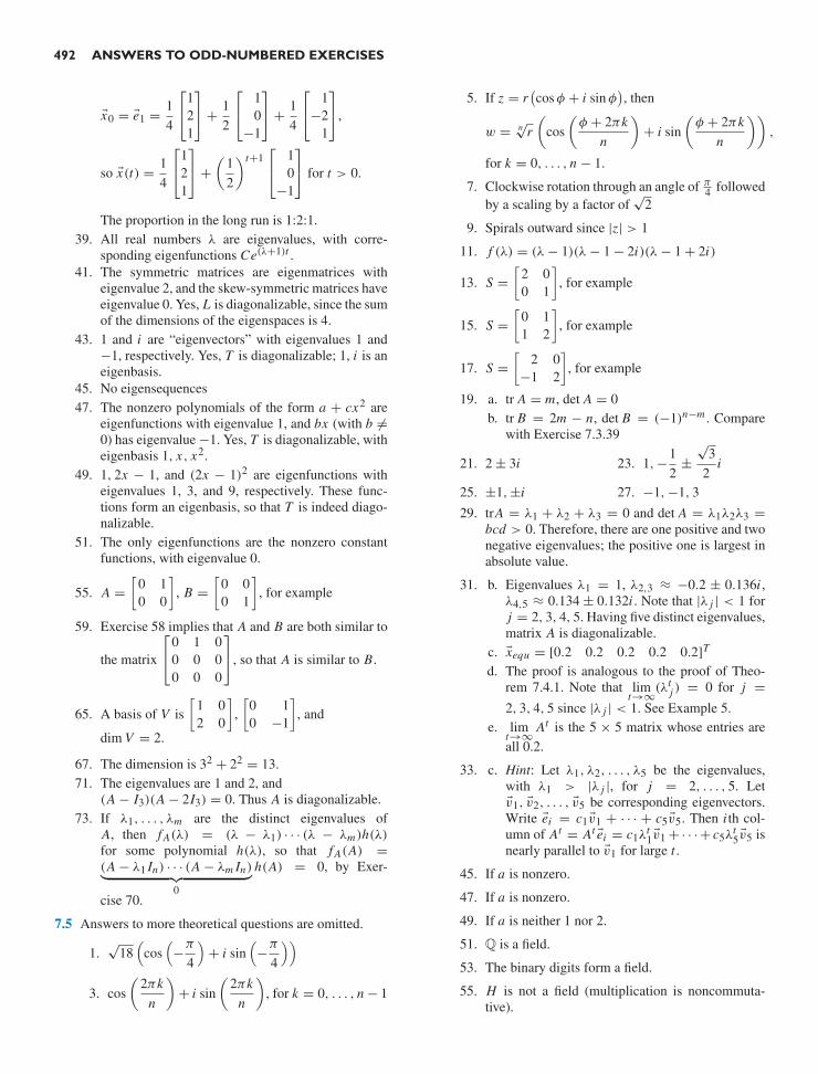
492 ANSWERS TO ODD-NUMBERED EXERCISES
x0 = e1 = 14
⎡
⎣121
⎤
⎦ + 12
⎡
⎣10
−1
⎤
⎦ + 14
⎡
⎣1
−21
⎤
⎦,
so x(t) = 14
⎡
⎣121
⎤
⎦ +(
12
)t+1⎡
⎣10
−1
⎤
⎦ for t > 0.
The proportion in the long run is 1:2:1.39. All real numbers λ are eigenvalues, with corre-
sponding eigenfunctions Ce(λ+1)t .41. The symmetric matrices are eigenmatrices with
eigenvalue 2, and the skew-symmetric matrices haveeigenvalue 0. Yes, L is diagonalizable, since the sumof the dimensions of the eigenspaces is 4.
43. 1 and i are “eigenvectors” with eigenvalues 1 and−1, respectively. Yes, T is diagonalizable; 1, i is aneigenbasis.
45. No eigensequences47. The nonzero polynomials of the form a + cx2 are
eigenfunctions with eigenvalue 1, and bx (with b =0) has eigenvalue −1. Yes, T is diagonalizable, witheigenbasis 1, x, x2.
49. 1, 2x − 1, and (2x − 1)2 are eigenfunctions witheigenvalues 1, 3, and 9, respectively. These func-tions form an eigenbasis, so that T is indeed diago-nalizable.
51. The only eigenfunctions are the nonzero constantfunctions, with eigenvalue 0.
55. A =[
0 10 0
], B =
[0 00 1
], for example
59. Exercise 58 implies that A and B are both similar to
the matrix
⎡
⎣0 1 00 0 00 0 0
⎤
⎦, so that A is similar to B.
65. A basis of V is[
1 02 0
],[
0 10 −1
], and
dim V = 2.
67. The dimension is 32 + 22 = 13.71. The eigenvalues are 1 and 2, and
(A − I3)(A − 2I3) = 0. Thus A is diagonalizable.73. If λ1, . . . , λm are the distinct eigenvalues of
A, then f A(λ) = (λ − λ1) · · · (λ − λm)h(λ)for some polynomial h(λ), so that f A(A) =(A − λ1 In) · · · (A − λm In)︸ ︷︷ ︸
0
h(A) = 0, by Exer-
cise 70.
7.5 Answers to more theoretical questions are omitted.
1.√
18(
cos(−π
4
)+ i sin
(−π
4
))
3. cos(
2πkn
)+ i sin
(2πk
n
), for k = 0, . . . , n − 1
5. If z = r(cos φ + i sin φ
), then
w = n√r(
cos(
φ + 2πkn
)+ i sin
(φ + 2πk
n
)),
for k = 0, . . . , n − 1.
7. Clockwise rotation through an angle of π4 followed
by a scaling by a factor of√
2
9. Spirals outward since |z| > 1
11. f (λ) = (λ − 1)(λ − 1 − 2i)(λ − 1 + 2i)
13. S =[
2 00 1
], for example
15. S =[
0 11 2
], for example
17. S =[
2 0−1 2
], for example
19. a. tr A = m, det A = 0b. tr B = 2m − n, det B = (−1)n−m . Compare
with Exercise 7.3.39
21. 2 ± 3i 23. 1,−12
±√
32
i
25. ± 1, ± i 27. −1,−1, 3
29. trA = λ1 + λ2 + λ3 = 0 and det A = λ1λ2λ3 =bcd > 0. Therefore, there are one positive and twonegative eigenvalues; the positive one is largest inabsolute value.
31. b. Eigenvalues λ1 = 1, λ2,3 ≈ −0.2 ± 0.136i ,λ4,5 ≈ 0.134 ± 0.132i . Note that |λ j | < 1 forj = 2, 3, 4, 5. Having five distinct eigenvalues,matrix A is diagonalizable.
c. xequ = [0.2 0.2 0.2 0.2 0.2]T
d. The proof is analogous to the proof of Theo-rem 7.4.1. Note that lim
t→∞(λt
j ) = 0 for j =2, 3, 4, 5 since |λ j | < 1. See Example 5.
e. limt→∞
At is the 5 × 5 matrix whose entries areall 0.2.
33. c. Hint: Let λ1, λ2, . . . , λ5 be the eigenvalues,with λ1 > |λ j |, for j = 2, . . . , 5. Letv1, v2, . . . , v5 be corresponding eigenvectors.Write ei = c1v1 + · · · + c5v5. Then i th col-umn of At = At ei = c1λ
t1v1 +· · ·+ c5λ
t5v5 is
nearly parallel to v1 for large t .
45. If a is nonzero.
47. If a is nonzero.
49. If a is neither 1 nor 2.
51. Q is a field.
53. The binary digits form a field.
55. H is not a field (multiplication is noncommuta-tive).

ANSWERS TO ODD-NUMBERED EXERCISES 493
7.6 Answers to more theoretical questions are omitted.
1. Stable 3. Not stable
5. Not stable 7. Not stable
9. Not stable 11. For |k| < 1
13. For all k 15. Never stable
17. x(t) =[− sin(φt)
cos(φt)
], where φ = arctan
(43
); a
circle
19. x(t) =√
13t[− sin(φt)
cos(φt)
], where φ = arctan
(32
);
spirals outward
21. x(t) =√
17t[
5 sin(φt)cos(φt) + 3 sin(φt)
], where φ =
arctan(
14
); spirals outward
23. x(t) =(
12
)t[
5 sin(φt)cos(φt) + 3 sin(φt)
], where φ =
arctan(
34
); spirals inward
25. Not stable 27. Stable
29. May or may not be stable; consider A = ± 12 I2.
33. The matrix represents a rotation followed by a scal-ing with a scaling factor of
√0.992 + 0.012 < 1.
Trajectory spirals inward.
35. a. Choose an eigenbasis v1, . . . , vn and write
x0 = c1v1 + · · · + cn vn .
Then
x(t) = c1λt1v1 + · · · + cnλt
n vn
and
∥x(t)∥ ≤ |c1|∥v1∥ + · · · + |cn |∥vn∥ = M
(use the triangle inequality ∥u + w∥≤ ∥u∥ + ∥w∥, and observe that |λt
i | ≤ 1).
b. The trajectory x(t) =[
1 10 1
]t [01
]=
[t1
]
is not bounded. This does not contradict parta, since there is no eigenbasis for the matrix[
1 10 1
].
39.[
24
]is a stable equilibrium.
CHAPTER 88.1 Answers to more theoretical questions are omitted.
1.[
10
],[
01
]
3.1√5
[21
],
1√5
[−1
2
]
5.1√2
⎡
⎣−1
10
⎤
⎦,1√6
⎡
⎣−1−1
2
⎤
⎦,1√3
⎡
⎣111
⎤
⎦
7. S = 1√2
[1 −11 1
], D =
[5 00 1
]
9. S =
⎡
⎣1/
√2 −1/
√2 0
0 0 11/
√2 1/
√2 0
⎤
⎦, D =
⎡
⎣3 0 00 −3 00 0 2
⎤
⎦
11. Same S as in 9, D =
⎡
⎣2 0 00 0 00 0 1
⎤
⎦
13. Yes (reflection about E1)
15. Yes (can use the same orthonormal eigenbasis)
17. Let A be the n × n matrix whose entries are all1. The eigenvalues of A are 0 (with multiplicityn − 1) and n. Now B = q A + (p − q)In , sothat the eigenvalues of B are p − q (with multi-plicity n − 1) and qn + p − q . Therefore, det B =(p − q)n−1(qn + p − q).
21. 48 = 6 · 4 · 2 (note that A has 6 unit eigenvectors)
23. The only possible eigenvalues are 1 and −1 (be-cause A is orthogonal), and the eigenspaces E1and E−1 are orthogonal complements (because Ais symmetric). Hence, A represents the reflectionabout a subspace of Rn .
25. S = 1√2
⎡
⎢⎢⎢⎢⎣
1 1 0 0 00 0 1 1 00 0 0 0
√2
0 0 1 −1 01 −1 0 0 0
⎤
⎥⎥⎥⎥⎦
27. If n is even, we have the eigenbasis e1 − en , e2 −en−1, . . . , en/2 − en/2+1, e1 + en , e2 + en−1, . . . ,en/2 + en/2+1, with associated eigenvalues 0 (n/2times) and 2 (n/2 times).
29. Yes 31. True 33. θ = 23π = 120
35. θ = arccos(− 1n ). Hint: If v0, . . . , vn are such vec-
tors, let A =[v0 · · · vn
]. Then the noninvert-
ible matrix AT A has 1’s on the diagonal and cos θeverywhere else. Now use Exercise 17.
37. In Example 4 we see that the image of the unit circlewill be an ellipse with semimajor axis 3 and semi-minor axis 2. Thus 2 ≤ ∥Au∥ ≤ 3.
39. Let v1, v2, v3 be an orthonormal eigenbasis withassociated eigenvalues −2, 3, and 4, respectively.Consider a unit vector u = c1v1 + c2v2 + c3v3.Then Au = −2c1v1 + 3c2v2 + 4c3v3 and u · Au =−2c2
1 +3c22 +4c2
3 ≤ 4c21 +4c2
2 +4c23 = 4. Likewise,
u · Au = −2c21 + 3c2
2 + 4c23 ≥ −2c2
1 − 2c22 − 2c2
3 =−2. Thus −2 ≤ u · Au ≤ 4.

494 ANSWERS TO ODD-NUMBERED EXERCISES
41. There exist an orthogonal S and a diagonal D suchthat A = SDS−1. Taking cube roots of the diago-nal entries of D, we can write D = D3
0 for somediagonal D0. Now A = SDS−1 = SD3
0 S−1 =(SD0S−1)3 = B3, where B = SD0S−1.
43. Consider the eigenvectors v1 =
⎡
⎣111
⎤
⎦ and v2 =
⎡
⎣1
−10
⎤
⎦, with eigenvalues 24 and −9, respectively.
There must exist a nonzero solution of the formv = av1+bv2. Now v · Av = (av1+bv2)·(24av1−9bv2) = 72a2 − 18b2 = 0 when b = ± 2a. Let
a = 1 and b = 2 to find the solution v =
⎡
⎣3
−11
⎤
⎦.
47. a. i j th entry of |AB| =∣∣∑n
k=1 aikbk j∣∣
≤∑n
k=1 |aik ||bk j |= i j th entry of |A||B|
b. By induction on t , using part a: |At | =|At−1 A| ≤ |At−1||A| ≤ |A|t−1|A| = |A|t
49. Let λ be the maximum of all |rii |, for i = 1, . . . , n.Note that λ < 1. Then |R| ≤ λ(In + U ), where Uis upper triangular with uii = 0 and ui j = |ri j |/λif j > i . Note that U n = 0, by Exercise 46a. Now|Rt | ≤ |R|t ≤ λt (In + U )t ≤ λt tn(In + U + · · · +U n−1). From calculus we know that lim
t→∞λt tn = 0.
8.2 Answers to more theoretical questions are omitted.
1.[
6 −3.5−3.5 8
]
3.
⎡
⎣3 0 30 4 3.53 3.5 5
⎤
⎦
5. Indefinite 7. Indefinite
9. a. A2 is symmetric.b. A2 = −AT A is negative semidefinite, so that its
eigenvalues are ≤0.c. The eigenvalues of A are imaginary (that is, of
the form bi , for a real b). The zero matrix is theonly skew-symmetric matrix that is diagonaliz-able over R.
11. The same (the eigenvalues of A and A−1 have thesame signs).
13. aii = q(ei ) > 0.
15. Ellipse; principal axes spanned by[
21
]and
[−1
2
];
equation 7c21 + 2c2
2 = 1
17. Hyperbola; principal axes spanned by[
21
]and
[−1
2
], equation 4c2
1 − c22 = 1
19. A pair of lines; principal axes spanned by[
2−1
]and
[12
]; equation 5c2
2 = 1
Note that we can write x21 + 4x1x2 + 4x2
2= (x1 + 2x2)
2 = 1, so that x1 + 2x2 = ± 1.
21. a. The first is an ellipsoid, the second a hyper-boloid of one sheet, and the third a hyperboloidof two sheets (see any text in multivariable cal-culus). Only the ellipsoid is bounded, and thefirst two surfaces are connected.
b. The matrix A of this quadratic form has positiveeigenvalues λ1 ≈ 0.56, λ2 ≈ 4.44, and λ3 = 1,with corresponding unit eigenvectors
v1 ≈
⎡
⎣0.860.19
−0.47
⎤
⎦ , v2 ≈
⎡
⎣0.310.540.78
⎤
⎦ ,
v3 ≈
⎡
⎣0.41
−0.820.41
⎤
⎦ .
Since all eigenvalues are positive, the surface isan ellipsoid. The points farthest from the originare
± 1√λ1
v1 ≈ ±
⎡
⎣1.150.26
−0.63
⎤
⎦
and those closest are
± 1√λ2
v2 ≈ ±
⎡
⎣0.150.260.37
⎤
⎦ .
23. Yes; A = 12 (M + MT )
25. q(v) = v · λv = λ
27. The closed interval [λn, λ1]
29. B = 1√5
[6 2
−3 4
]
31. B = 15
[14 −2−2 11
]
33. L = 1√2
[4 0
−1 3
]35. L =
⎡
⎣2 0 0
−2 3 04 3 1
⎤
⎦
39. For 0 < θ < arccos(
− 1n − 1
)
41. 3

ANSWERS TO ODD-NUMBERED EXERCISES 495
43. im T = span(x21 ), rank T = 1,
ker T = span(x1x2, x22 ), nullity T = 2
45. im T = P2, rank T = 3,ker T = span(x2
3 − x22 , x1x3 − x1x2, x2x3 − x2
2 ),nullity T = 3
47. The determinant of the mth principal submatrix ispositive if m is even, and negative if m is odd.
55. Note that det[
aii ai ja ji a j j
]= aii a j j − a2
i j > 0, so
that aii > ai j or a j j > ai j .
57. q(x) = λ1c21 + λ2c2
2 + λ3c23 = 1, with positive λi ,
defines an ellipsoid.
59. q(x) = λ1c21 = 1, with positive λ1, defines a pair of
parallel planes, c1 = ± 1√λ1
.
61. q(x) = λ1c21 + λ2c2
2 + λ3c23 = 1, with λ1 > 0,
λ2 > 0, λ3 < 0 defines a hyperboloid of one sheet.
63. q(c1w1 + · · · + cnwn) = (c1w1 + · · · + cnwn) ·(c1λ1w1 + · · · + cnλnwn) = c2
1λ1∥w1∥2 + · · · +c2
nλn∥wn∥2 = c21 + · · · + c2
n since ∥wi∥2 = 1λi
, by
construction.
65. Adapt the method outlined in Exercise 63. Consideran orthonormal eigenbasis v1, v2 for A with associ-ated eigenvalues λ1 > 0 and λ2 < 0. Now let w1 =v1/
√λ1 and w2 = v2/
√−λ2, so that ∥w1∥2 =
1/λ1 and ∥w2∥2 = −1/λ2. Then q(c1w1+c2w2) =(c1w1+c2w2)·(λ1c1w1+λ2c2w2) = λ1c2
1∥w1∥2+λ2c2
2∥w2∥2 = c21 − c2
2.
67. Adapt the method outlined in Exercises 63and 65. Consider an orthonormal eigenbasisv1, . . . , v p, . . . , vr , . . . , vn for A such that the asso-ciated eigenvalues λ j are positive for j = 1, . . . , p,negative for j = p + 1, . . . , r , and zero for j =r + 1, . . . , n. Let w j = v j/
√|λ j | for j = 1, . . . , r
and w j = v j for j = r + 1, . . . , n.
69. Note that x T RT ARx = (Rx)T A(Rx) ≥ 0 for all xin Rm . Thus RT AR is positive semidefinite. RT ARis positive definite if (and only if) ker R = 0.
71. Anything can happen: The matrix RT AR may bepositive definite, positive semidefinite, negative def-inite, negative semidefinite, or indefinite.
8.3 Answers to more theoretical questions are omitted.1. σ1 = 2, σ2 = 1
3. All singular values are 1 (since AT A = In).
5. σ1 = σ2 =√
p2 + q2
7.[
0 1−1 0
] [2 00 1
] [0 11 0
]
9.1√5
[1 −22 1
] [5 00 0
]1√5
[1 2
−2 1
]
11.
⎡
⎣0 1 01 0 00 0 1
⎤
⎦
⎡
⎣2 00 10 0
⎤
⎦[
0 11 0
]
13. I2
[3√
5 00
√5
]1√5
[2 1
−1 2
]
15. Singular values of A−1 are the reciprocals of thoseof A.
21.[
0.8 0.6−0.6 0.8
] [9 −2
−2 6
]
23. AAT ui =
σ 2i ui for i = 1, . . . , r
0 for i = r + 1, . . . , nThe nonzero eigenvalues of AT A and AAT are thesame.
25. Choose vectors v1 and v2 as in Theorem 8.3.3.Write
u = c1v1 + c2v2.
Note that∥u∥2 = c2
1 + c22 = 1.
NowAu = c1 Av1 + c2 Av2,
so that
∥Au∥2 = c21∥Av1∥2 + c2
2∥Av2∥2
= c21σ 2
1 + c22σ 2
2
≤ (c21 + c2
2)σ 21
= σ 21 .
We conclude that ∥Au∥ ≤ σ1. The proof ofσ2 ≤ ∥Au∥ is analogous.
27. Apply Exercise 26 to a unit eigenvector v with as-sociated eigenvalue λ.
33. No; consider A =[
0 12 0
].
35. (AT A)−1 AT ui =
⎧⎪⎨
⎪⎩
1σi
vi for i = 1, . . . , m
0 for i = m + 1, . . . , n
CHAPTER 99.1 Answers to more theoretical questions are omitted.
1. x(t) = 7e5t 3. P(t) = 7e0.03t
5. y(t) = −0.8e0.8t
7. x(t) = 11−t , has a vertical asymptote at t = 1.
9. x(t) =((1 − k)t + 1
)1/(1−k)
11. x(t) = tan t13. a. About 104 billion dollars
b. About 150 billion dollars15. The solution of the equation ekT/100 = 2 is
T = 100 ln(2)
k≈ 69
k.

496 ANSWERS TO ODD-NUMBERED EXERCISES
17.
19.
21. x(t) =[
1 t0 1
]x0 23. x(t) is a solution.
27. x(t) = 0.2e−6t[
3−2
]+ 0.4e−t
[11
]
29. x(t) = 2[
2−1
]+ e5t
[12
]
31. x(t) = et
⎡
⎣1
−21
⎤
⎦
33.E−1
E−6
35. E5
E0
0
37. E1.1 = span[
31
]and E1.6 = span
[12
]. Looks
roughly like the phase portrait in Figure 10.
39. E1 = span[
2−1
]and E1.4 = span
[2
−3
]. Looks
roughly like the phase portrait in Exercise 35.
41.
0
43. a. Competitionb.
x
y
c. Species 1 “wins” ify(0)
x(0)< 2.
45. b.
x
y
c. Species 1 “wins” ify(0)
x(0)<
12
.
47. a. Symbiosis
b. The eigenvalues are 12 (−5 ±
√9 + 4k2). There
are two negative eigenvalues if k < 2; if k > 2,there is a negative and a positive eigenvalue.
49. g(t) = 45e−0.8t − 15e−0.4t andh(t) = −45e−0.8t + 45e−0.4t
53. x(t) = ept[
cos(qt)sin(qt)
], a spiral if p = 0 and a circle
if p = 0. Approaches the origin if p is negative.55. Eigenvalues λ1,2 = 1
2 (−q ±√
q2 − 4p); botheigenvalues are negative.

ANSWERS TO ODD-NUMBERED EXERCISES 497
trajectory 1
trajectory 2
w
E 1
E 2
door slams
trajectory 3
door slams ifω(0)
θ(0)< λ2.
9.2 Answers to more theoretical questions are omitted.1. 1 3.
√2e3π i/4
5. e−0.1t(cos(2t) − i sin(2t)); spirals inward, in the
clockwise direction
7. Not stable 9. Stable11. a. B = 2A
d. The zero state is a stable equilibrium of the sys-
temdxdt
= grad(q) if (and only if) q is negative
definite (then, the eigenvalues of A and B are allnegative).
13. The eigenvalues of A−1 are the reciprocals of theeigenvalues of A; the real parts have the same sign.
15.E0
0
17. If |k| < 1
19. False; consider A with eigenvalues 1, 2, −4.
21. a.
∣∣∣∣∣∣∣∣
dbdt
= 0.5b + s
dsdt
= 0.07s
∣∣∣∣∣∣∣∣b. b(t) = 50,000e0.07t − 49,000e0.5t
s(t) = 1,000e0.07t
27. x(t) =[
cos(3t) − sin(3t)sin(3t) cos(3t)
] [ab
], where a, b are
arbitrary constants
29. Eigenvalue 2 + 4i with corresponding eigenvector[i
−1
]. Use Theorem 9.2.6, with p = 2, q = 4,
w =[
10
], v =
[0
−1
].
x(t) = e2t[
1 00 −1
] [cos(4t) − sin(4t)sin(4t) cos(4t)
] [ab
]
31. Eigenvalue −1 + 2i with corresponding eigenvec-
tor[
i1
]. x(t) = e−t
[cos(2t) − sin(2t)sin(2t) cos(2t)
] [1
−1
]=
e−t[
cos(2t) + sin(2t)sin(2t) − cos(2t)
]. Spirals inward, in the
counterclockwise direction.
33. Eigenvalue i with corresponding eigenvec-
tor[
11 + i
]. x(t) =
[0 11 1
] [cos tsin t
]=
[sin t
sin t + cos t
]. An ellipse with clockwise ori-
entation.
39. The systemdcdt
=
⎡
⎣0 1 00 0 10 0 0
⎤
⎦ c has the solutions
c(t) =
⎡
⎣k1 + k2t + k3t2/2
k2 + k3tk3
⎤
⎦ ,
where k1, k2, k3 are arbitrary constants. The solu-tions of the given system are x(t) = eλt c(t), by Ex-ercise 9.1.24. The zero state is a stable equilibriumsolution if (and only if) the real part of λ is negative.
9.3 Answers to more theoretical questions are omitted.1. Ce5t
3. 15 e3t + Ce−2t (use Theorem 9.3.13)
5. −1 − t + Cet 7. c1e−4t + c2e3t
9. c1e3t + c2e−3t
11. et(c1 cos t + c2 sin t)
13. e−t (c1 + c2t) (compare with Example 10).15. c1 + c2t17. e−t (c1 + c2t) − 1
2 cos t
19. cos t + c1 cos(√
2t) + c2 sin(√
2t)
21. c1et + c2e−t + c3e−2t 23. 3e5t
25. e−2t+2 27. − sin(3t)
29. 13 sin(t) − 1
6 sin(2t)
31. v(t) = mgk
(1 − e−kt/m)
limt→∞
v(t) = mgk
= terminal velocity
35. a. c1e−t + c2e−2t
b. 2e−t − e−2t
c. −e−t + 2e−2t
d. In part c the oscillator goes through the equi-librium state once; in part b it never reaches it.
37. x(t) = te−3t 39. e−t (c1 + c2t + c3t2)
41. λ is an eigenvalue with dim(Eλ) = n, because Eλ
is the kernel of the nth-order linear differential op-erator T (x) − λx .
43. 110 cos t + 1
10 sin t + c1e−2t + c2e−3t
45. et[
1 − 2t−1
]

This page intentionally left blank

SUBJECT INDEX
AAffine system, 356Algebraic multiplicity of an eigenvalue, 331
and complex eigenvalues, 371and geometric multiplicity, 344
Algorithm, 18Alternating property of determinant, 267, 281Angle, 211
and orthogonal transformations, 226Approximations,
Fourier, 248, 257least-squares, 17, 238
Argument (of a complex number), 364of a product, 365
Associative law for matrix multiplication, 81Asymptotically stable equilibrium, 376
(see stable equilibrium)Augmented matrix, 11
BBase case (for induction), 466Basis, 125, 172
and coordinates, 149and dimension, 135, 172and unique representation, 130finding basis of a linear space, 174of an image, 126, 138, 141of a kernel, 137, 141of Rn , 142standard, 135
Binary digits, 121Block matrices, 81
determinant of, 274inverse of, 96multiplication of, 82
Bounded trajectory, 381
CCarbon dating, 425Cardano’s formula, 335, 338, 374Cartesian coordinates, 10, 147Cassini’s identity, 294Cauchy–Schwarz inequality, 210, 253
and angles, 211and triangle inequality, 215
Cayley–Hamilton Theorem, 347Center of mass, 21Change of basis, 191, 194
Characteristic polynomial, 329and algebraic multiplicity, 331and its derivative, 338of linear differential operator, 445of similar matrices, 343
Chebyshev polynomials, 263Cholesky factorization, 401Circulant matrix, 374Classical adjoint, 304Closed-formula solution
for discrete dynamical system, 321for Fibonacci sequence, 178for inverse, 304for least-squares approximation, 240for linear system, 302
Coefficient matrixof a linear system, 11of a linear transformation, 42
Column of a matrix, 9Column space of a matrix, 114Column vector, 10Commuting matrices, 79Complements, 145Complex eigenvalues, 368
and determinant, 371and rotation–scaling matrices, 369, 377, 435and stable equilibrium, 376and trace, 371
Complex numbers, 168, 363and rotation–scaling, 365in polar form, 365
Complex-valued functions, 429derivative of, 430exponential, 430
Component of a vector, 10Composite functions, 75Computational complexity, 98, 105Concatenation, 342Conics, 23, 144Consistent linear system, 25Continuous least-squares condition, 254Continuous linear dynamical system, 418
stability of, 433with complex eigenbasis, 435with real eigenbasis, 423
Contraction, 60Contraposition, 26, 467Coordinates, 149, 172Coordinate transformation, 172, 181Coordinate vector, 149, 172
499

500 Subject Index
Correlation (coefficient), 213Cramer’s Rule, 302Cross product
and polar (QS) factorization, 412in R3, 56, 463, 465in Rn , 291rules for, 464
Cubic equation (Cardano’s formula), 335, 374Cubic splines, 19Cubics, 144Curve fitting
with conics, 23, 144with cubics, 144
DData compression, 411Data fitting, 241
multivariate, 244De Moivre’s formula, 366Determinant, 94, 271
alternating property of, 267, 281and characteristic polynomial, 329and eigenvalues, 334, 371and Cramer’s rule, 302and elementary row operations, 281and invertibility, 282and Laplace expansion, 284, 286and QR factorization, 295as area, 94, 295as expansion factor, 299as volume, 297is linear in rows and columns, 268, 278of inverse, 284of linear transformation, 288of orthogonal matrix, 294of permutation matrix, 276of product, 283of rotation matrix, 294of similar matrices, 284of 3 × 3 matrix, 266of transpose, 278of triangular matrix, 273of 2 × 2 matrix, 94patterns and, 271Vandermonde, 290Weierstrass definition of, 292
Diagonalizable matrices, 311, 344and eigenbases, 312and powers, 351orthogonally, 385, 390simultaneously, 360
Diagonal matrix, 9
Diagonal of a matrix, 9Dilation, 60Dimension, 135, 172
and isomorphism, 182of image, 138, 179of kernel, 139, 179of orthogonal complement, 208
Direction field, 419Discrete linear dynamical system, 321
and complex eigenvalues, 378, 380and stable equilibrium, 376, 377
Distance, 252Distribution vector, 53Distributive Laws, 81Domain of a function, 44Dominant eigenvector, 423Dot product, 20, 29, 230, 461
and matrix product, 79, 230and product Ax , 29rules for, 462
Dynamical system(see continuous, discrete linear dynamical system)
EEigenbasis, 312
and continuous dynamical system, 423and diagonalization, 312and discrete dynamical system, 321and distinct eigenvalues, 342and geometric multiplicity, 342
Eigenfunction, 352, 445Eigenspaces, 339
and geometric multiplicity, 341and principal axes, 399
Eigenvalue(s), 312algebraic multiplicity of, 331and characteristic polynomial, 329and determinant, 334, 371and positive (semi)definite matrices, 397and QR factorization, 335and singular values, 405and stable equilibrium, 376, 433and trace, 334, 371complex, 368, 380geometric multiplicity of, 341of linear transformation, 352of orthogonal matrix, 315of rotation–scaling matrix, 369of similar matrices, 343of symmetric matrix, 388of triangular matrix, 328power method for finding, 372

Subject Index 501
Eigenvectors, 312and linear independence, 342dominant, 423of symmetric matrix, 387
Elementary matrix, 102Elementary row operations, 16
and determinant, 281and elementary matrices, 102
Ellipse, 75as image of the unit circle, 75, 390, 405as level curve of quadratic form, 399as trajectory, 380, 435
Equilibrium distribution, 52, 84for regular transition matrix, 349Power method for, 87
Equilibrium (state), 376Equivalence Relation, 157Error (in least-squares solution), 238Error-correcting codes, 121Euler identities, 256Euler’s formula, 431Euler’s theorem, 346Exotic operations (in a linear space), 186Expansion factor, 299Exponential functions, 416
complex-valued, 431
FFactorizations,
Cholesky, 401LDLT , 235, 401LDU, 102, 235LLT , 401LU, 102QR, 222, 223, 295, 335QS, 412SDST , 385U.V T , 408
Fibonacci sequence, 178, 236, 293, 466Field, 368Finite dimensional linear space, 175Flow line, 419Fourier analysis, 257Function, 44Fundamental theorem of algebra, 367Fundamental theorem of linear algebra, 139
GGaussian integration, 262Gauss–Jordan elimination, 17
and determinant, 281and inverse, 91
Geometric multiplicity of an eigenvalue, 341and algebraic multiplicity, 344and eigenbases, 342
Golden section, 178, 358Google, 52Gram–Schmidt process, 221
and determinant, 295and orthogonal diagonalization, 390and QR factorization, 222
HHankel matrix, 235Harmonics, 257Hilbert space ℓ2, 216, 251
and quantum mechanics, 260Homogeneous linear system, 36Hyperbola, 399Hyperplane, 144
IIdentity matrix In , 46Identity transformation, 46Image of a function, 110Image of a linear transformation, 114, 178
and rank, 138is a subspace, 114, 178orthogonal complement of, 237written as a kernel, 120
Imageof the unit circle, 75, 390, 405
Imaginary part of a complex number, 363Implicit function theorem, 292Inconsistent linear system, 5, 17, 25
and least-squares, 238Indefinite matrix, 396Induction, 466Infinite dimensional linear space, 175Inner product (space), 250Input-output analysis, 6, 20, 99, 104, 163Intermediate value theorem, 74Intersection of subspaces, 132
dimension of, 145Invariant Subspace, 325Inverse (of a matrix), 89
and Cramer’s rule, 304determinant of, 284of an orthogonal matrix, 230of a product, 92of a transpose, 231of a 2 × 2 matrix, 94of a block matrix, 96
Inversion (in a pattern), 271

502 Subject Index
Invertible function, 88Invertible matrix, 89
and determinant, 282and kernel, 118
Isomorphism, 181and dimension, 182
KKernel, 115, 178
and invertibility, 118and linear independence, 129and rank, 139dimension of, 139is a subspace, 117, 178
Kyle numbers, 140, 340
LLaplace expansion, 284, 286LDLT factorization, 235, 401LDU factorization, 102, 235Leading one, 16Leading variable, 13Least-squares solutions, 17, 216, 238
and normal equation, 239minimal, 246
Left inverse, 132Legendre polynomials, 262Length of a vector, 202, 462
and orthogonal transformations, 225Linear combination, 31, 169
and span, 114Linear dependence, 125Linear differential equation, 174, 442
homogeneous, 442order of, 442solution of, 444, 452solving a first order, 450solving a second order, 447, 448
Linear differential operator, 442characteristic polynomial of, 445eigenfunctions of, 445image of, 451kernel of, 446
Linear independence, 125, 171and dimension, 136and kernel, 129and relations, 128in Rn , 125in a linear space, 171of eigenvectors, 342of orthonormal vectors, 204
Linearity of the determinant, 268, 278
Linear relations, 127Linear space(s), 167
basis of, 172dimension of, 172finding basis of, 174finite dimensional, 175isomorphic, 181
Linear systemclosed-formula solution for, 302consistent, 25homogeneous, 36inconsistent, 5, 25least-squares solutions of, 238matrix form of, 33minimal solution of, 246number of solutions of, 25of differential equations: see continuous linear
dynamical systemunique solution of, 28vector form of, 32with fewer equations than unknowns, 27
Linear transformation, 42, 45, 49, 178image of, 114, 178kernel of, 115, 178matrix of, 42, 45, 48, 153, 187
Lower triangular matrix, 10LU factorization, 102
and principal submatrices, 103
MMain diagonal of a matrix, 9Mass-spring system, 441Mathematical Induction, 466Matrix, 9
(for a composite entry such as “zero matrix”see zero)
Minimal solution of a linear system, 246Minors of a matrix, 285Modulus (of a complex number), 364
of a product, 365Momentum, 21Multiplication (of matrices), 78
and determinant, 283column by column, 78entry by entry, 79is associative, 81is noncommutative, 79of block matrices, 82
NNegative feedback loop, 439Neutral element, 167

Subject Index 503
Nilpotent matrix, 146, 393Norm
of a vector, 202in an inner product space, 252
Normal equation, 239Nullity, 139, 179Null space, 115
OOrthogonal complement, 208
of an image, 237Orthogonally diagonalizable matrix, 385, 390Orthogonal matrix, 225, 230
determinant of, 294eigenvalues of, 315inverse of, 230transpose of, 230
Orthogonal projection, 63, 204, 206,241, 253
and Gram–Schmidt process, 218and reflection, 64as closest vector, 238matrix of, 232, 241
Orthogonal transformation, 225and orthonormal bases, 232preserves dot product, 230preserves right angles, 226
Orthogonal vectors, 202, 252, 463and Pythagorean theorem, 209
Orthonormal bases, 204, 207and Gram–Schmidt process, 218and orthogonal transformations, 227and symmetric matrices, 386
Orthonormal vectors, 203are linearly independent, 204
Oscillator, 198
PPageRank, 52
naıve, 53Parallelepiped, 296Parallel vectors, 460Parametrization (of a curve), 111Partitioned matrices, 82
(see block matrix)Pattern (in a matrix), 271
inversion in, 271signature of, 271
Permutation matrix, 98determinant of, 276
Perpendicular vectors, 202, 252, 463
Phase portrait,of continuous system, 419, 438of discrete system, 320, 438summary, 438
Piecewise continuous function, 255Pivot, 16Polar factorization, 412Polar form (of a complex number), 365
and powers, 366and products, 365with Euler’s formula, 432
Positive (semi)definite matrix, 396and eigenvalues, 397and principal submatrices, 397
Positive transition matrix, 84Positively oriented basis, 307Power method for finding eigenvalues, 372Principal axes, 399Principal submatrices, 103
and positive definite matrices, 397Product Ax , 29
and dot product, 29and matrix multiplication, 78
Projection, 61, 73(see also orthogonal projection)
Proof techniques, 466Pseudo-inverse, 245Pythagorean theorem, 209, 253
QQR factorization, 222
and Cholesky factorization, 401and determinant, 295and eigenvalues, 335is unique, 234
QS factorization, 412Quadratic forms, 395
indefinite, 396negative (semi)definite, 396positive (semi)definite, 396principal axes for, 399
Quaternions, 235, 374, 382form a skew field, 374
RRank (of a matrix), 26, 138
and image, 138and kernel, 139and row space, 146and singular values, 407of similar matrices, 343of transpose, 231

504 Subject Index
Rank-nullity theorem, 139, 179Real part of a complex number, 363Reduced row-echelon form (rref), 15
and determinant, 281and inverse, 89, 91and rank, 26
Redundant vector(s), 125, 171image and, 126, 141kernel and, 141
Reflection, 64Regular transition matrix, 84, 349
Equilibrium for, 349Relations (among vectors), 127Resonance, 198Riemann integral, 248, 250Rotation matrix, 67, 294Rotation–scaling matrix, 68
and complex eigenvalues, 369and complex numbers, 365
Row of a matrix, 9Row space, 146Row vector, 10Rule of 69, 426
SSarrus’s rule, 266Scalar, 12Scalar multiples of matrices, 28Scaling, 60Second derivative test, 401Secular equation, 327Separation of variables, 416, 425Shears, 70Signature of a pattern, 271Similar matrices, 156
and characteristic polynomial,343
Simultaneously diagonalizablematrices, 360
Singular value decomposition(SVD), 408
Singular values, 405and ellipses, 405and rank, 407
Skew field, 374Skew-symmetric matrices, 229, 400
determinant of, 291Smooth function, 170Space of functions, 168Span
in Rn , 114in a linear space, 171
Spectral theorem, 386Spirals, 361, 366, 380, 432, 435, 438Square matrix, 9Square-summable sequences, 216, 251Stable equilibrium, 84, 376
of continuous system, 433of discrete system, 376
Standard basis, 135, 173State vector, 316Subspace
invariant, 325of Rn , 122of a linear space, 170
Sudoku, 81Sum of subspaces, 132
dimension of, 145Sums of matrices, 28Symmetric matrices, 229
are orthogonally diagonalizable, 386have real eigenvalues, 388
TTarget space (of a function), 44Tetrahedron, 101, 162, 306Theorem of Pythagoras, 209, 253Trace, 251, 329
and characteristic polynomial, 329and eigenvalues, 334, 371and inner product, 251of similar matrices, 343
Trajectory, 319, 418bounded, 381
Transition matrix, 53positive, 84regular, 84, 349
Transpose (of a matrix), 229and determinant, 278and inverse, 231and rank, 231of an orthogonal matrix, 230of a product, 231
Triangle inequality, 215Triangular matrices, 10
and determinant, 273and eigenvalues, 328invertible, 98
Triangulizable matrix, 393Trigonometric polynomials, 256
UUnit vector, 202, 463Upper triangular matrix, 10

Subject Index 505
VVandermonde determinant, 290Vector(s), 10
angles between, 211addition, 457column, 10coordinate, 149, 172cross product of, 56, 265, 463distribution, 53dot product of, 461geometric representation of, 459length of, 202, 462orthogonal, 202, 463parallel, 460position, 459redundant, 125row, 10rules of vector algebra, 458scalar multiplication, 457
standard representation of, 10, 459unit, 202, 463velocity, 418vs. points, 11, 459zero, 458
Vector field, 419Vector form of a linear system, 32Vector space, 10, 167
(see linear space)Velocity vector, 418
WWeierstrass definition of determinant, 292Wigner semicircle distribution, 262
ZZero matrix, 10Zero vector, 458

This page intentionally left blank

NAME INDEX
Abel, Niels Henrik, 335Alcuin of York, 24al-Kashi, Jamshid, 24al-Khowarizmi, Mohammed, 1, 18nal-Ma’mun, Caliph, 1Archimedes, 57, 355Argand, Jean Robert, 363n
Banach, Stefan, 176Berlinski, David, 18Bernoulli, Daniel, 178nBezout, Etienne, 289Binet, Jacques, 178, 289Brin, Sergey, 52Burke, Kyle, 140n
Cajori, Florian, 288Cardano, Gerolamo, 335, 338Cassini, Giovanni, 294Cauchy, Augustin-Louis, 210, 271n,
289, 327Cayley, Arthur, 289, 347Chebyshev, Pafnuty, 263Cholesky, Andre-Louis, 401Cramer, Gabriel, 145, 288, 303
d’Alembert, Le Rond, 135, 327Dantzig, Tobias, 363nDe Moivre, Abraham, 366Descartes, Rene, 127n, 147, 168De Witt, Johan, 396n
Einstein, Albert, 374Euler, Leonhard Paul, 24, 145, 256, 259, 346,
363n, 431
Fermat, Pierre de, 147Fibonacci (Leonardo of Pisa), 358Fourier, Jean Baptiste Joseph, 255n
Galois, Evariste, 335Gauss, Carl Friedrich, 17–18, 54, 262,
363n, 368Gram, Jorgen, 221nGrassmann, Hermann Gunther, 135
Hamilton, William Rowan, 235, 347, 374Hamming, Richard W., 121
Hankel, Hermann, 235Harriot, Thomas, 127nHeisenberg, Werner, 216, 260Helmholtz, Hermann von, 328Hilbert, David, 176, 216, 328
Jacobi, Carl Gustav Jacob, 271nJordan, Wilhelm, 17
Kepler, Johannes, 249Kronecker, Leopold, 271n
Lagrange, Joseph Louis, 327, 382Lanchester, Frederick William, 427nLaplace, Pierre-Simon Marquis de,
284n, 289Legendre, Adrien-Marie, 262Leibniz, Gottfried Wilhelm von, 288Leonardo da Vinci, 215Leontief, Wassily, 6, 163
Mahavira, 24Mas-Colell, Andreu, 216Mazur, Barry, 363nMedawar, Peter B., 70Mumford, David, 442
Newton, Isaac, 24
Olbers, Wilhelm, 17
Page, Lawrence, 52Peano, Giuseppe, 167nPeirce, Benjamin, 432nPiazzi, Giuseppe, 17Pythagoras, 209, 259, 288
Riemann, Bernhard, 248, 250, 262Roosevelt, Franklin D., 99n
Samuelson, Paul E., 381Sarrus, Pierre Frederic, 266nSchlafi, Ludwig, 135Schmidt, Erhard, 176, 221nSchrodinger, Erwin, 260Schwarz, Hermann Amandus, 210Seki, Kowa (or Takakazu), 271n, 288Simpson, Thomas, 262Strang, Gilbert, 411
507

508 Name Index
Strassen, Volker, 105Sylvester, James Joseph, 9n
Thompson, d’Arcy, 70
Vandermonde, Alexandre-Theophile, 271n, 289
Weierstrass, Karl, 289, 292Wessel, Caspar, 363nWeyl, Hermann, 135Wigner, Eugene Paul, 262Wilson, Edward O., 302n