Homework 2: Numerical Linear Algebra and Optimization

CME292: Advanced MATLAB for Scientific Computing

Homework #2NLA & Opt

Due: Thursday, April 22, 2014

InstructionsFor this problem set, 2 problems out of 4 are required. You are free to choose the 2 problems you complete.

Before completing problem set, please see HomeworkInstructions on Coursework for general homeworkinstructions, grading policy, and number of required problems per problem set.

Problem 1A matrix A P Rmˆn can be compressed using the low-rank approximation property of the SVD. Theapproximation algorithm is given in Algorithm 1.

Algorithm 1 Low-Rank Approximation using SVD

Input: A P Rmˆn of rank r and approximation rank k (k ď r)Output: Ak P Rmˆn, optimal rank k approximation to A

1: Compute (thin) SVD of A “ UΣVT , where U P Rmˆr, Σ P Rrˆr, V P Rnˆr

2: Ak “ Up:, 1 : kqΣp1 : k, 1 : kqVp:, 1 : kqT

Notice the low-rank approximation, Ak, and the original matrix, A, are the same size. To actually achievecompression, the truncated singular factors, Up:, 1 : kq P Rmˆk, Σp1 : k, 1 : kq P Rkˆk, Vp:, 1 : kq P Rnˆk,should be stored. As Σ is diagonal, the required storage is pm`n`1qk doubles. The original matrix requiresstoring mn doubles. Therefore, the compression is useful only if k ă mn

m`n`1 .

Recall from lecture that the SVD is among the most expensive matrix factorizations in numerical linearalgebra. Many SVD approximations have been developed; a particularly interesting one from [1] is given inAlgorithm 2. This algorithm computes a rank p approximation to the SVD of a matrix. This approximationrank is different than the compression rank from Algorithm 1.

Algorithm 2 Low-Rank Probabilistic SVD Approximation

Input: A P Rmˆn (usually n ! m), approximation rank p, and number of power iterations qOutput: Approximate SVD of A « UΣVT

1: Generate nˆ p Gaussian test matrix Ω

2: Form Y “ pAAT qqAΩ

3: Compute QR factorization of Y: Y “ QR

4: Form B “ QTA

5: Compute SVD of B “ UΣVT

6: Set U “ QU

In this problem, you will use the Singular Value Decomposition (SVD) to compress an image of your choosing.You will be given the function get_rgb.m that accepts the filename of an image and returns the RGB matrices

1

CME292 Homework #2 (NLA & Opt) M. J. Zahr

defining the image, stacked vertically to form a single skinny matrix. Also, the function plot_image_rgb.m

will take stacked RGB matrix and (optionally) a handle to an axes graphics object (default will use gca) andplot the corresponding image (the input to plot_image_rgb.m is the output of get_rgb.m). To “compress”the image, compress the stacked RGB matrix and pass to plot_image_rgb.m. Another possibility involvescompressing the RGB matrices individually. For this assignment, use the stacked version for the compression.

1 function [RGB] = get_rgb(fname)2

3 % Parse filename to determine extension4 if isempty(find(fname=='.',1))5 error('Filename must include extension.');6 else7 ext = fname(find(fname=='.',1,'last')+1:end);8 end9

10 A = double(imread(fname,ext));11 RGB = [A(:,:,1);A(:,:,2);A(:,:,3)];12

13 end

1 function [] = plot_image_rgb(RGB,axHan)2

3 if nargin < 4, axHan=gca; end4

5 m = size(RGB,1)/3; n = size(RGB,2);6 A = zeros(m,n,3);7 A(:,:,1)=RGB(1:m,:);8 A(:,:,2)=RGB(m+1:2*m,:);9 A(:,:,3)=RGB(2*m+1:end,:);

10 image(uint8(A),'Parent',axHan);11

12 end

• Consider an image of mˆ n pixels. The R, G, B matrices will be of dimension mˆ n.

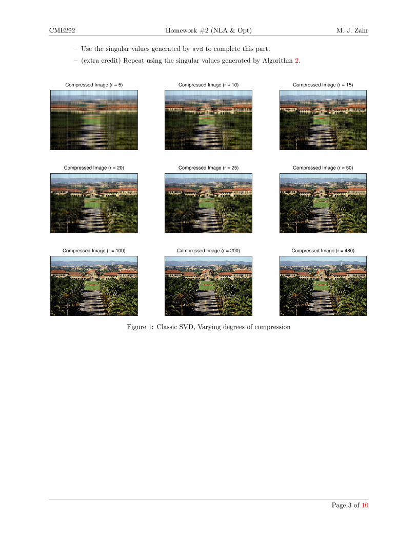
• Compress to ranks r5, 10, 15, 20, 25, 50, 100, 200,minp3m,nqs and visualize resulting images. Your resultshould be similar to Figure 1 for the image of Palm Drive.

– Use svd for the SVD step in Algorithm 1

– (extra credit) Implement the probabilistic SVD algorithm from Algorithm 2 and use this for theSVD step in Algorithm 1. Good values for the approximation rank will depend on the image youchoose to compress. Notice that a rank p approximation to the SVD in Algorithm 2 only admitslow-rank approximations of up to rank p (cannot go up to minp3m,nq). In this case, the ranksr5, 10, 15, 20, 25, 50, 100, 200,minp3m,nqs cannot all be used. Choose any 9 interesting ranks topresent.

• Plot νpkq for k P t1, 2, . . . ,minp3m,nqu for the stacked RGB matrix, where

νpkq “ 1´

řki“1 σ

2i

řminp3m,nqj“1 σ2

j

. (1)

and σi is the ith singular value of the matrix. The result should be similar to Figure 2a for the imageof Palm Drive. This gives an indication of the compressibility of the image. A fast singular value decayimplies the image can be compressed to a small rank with minimal loss in quality.

Problem 1 continued on next page. . . of 10


– Use the singular values generated by svd to complete this part.

– (extra credit) Repeat using the singular values generated by Algorithm 2.

Compressed Image (r = 5) Compressed Image (r = 10) Compressed Image (r = 15)



Figure 1: Classic SVD, Varying degrees of compression

of 10


0 50 100 150 200 250 300 350 400 450 50010

−8

10−7

10−6

10−5

10−4

10−3

10−2

10−1

100

Rank of Approximation

Sin

gula

r V

alu

e D

ecay o

f R

GB

(a) Classic SVD

0 5 10 15 20 25 30 35 40 45 5010

−4

10−3

10−2

10−1

100

Rank of Approximation

Sin

gu

lar

Va

lue

De

ca

y o

f R

GB

(b) Probabilistic SVD (rank 50)

Figure 2: Singular value decay

Problem 2In this problem, you will gain experience with sparse matrices, matrix decompositions, and linear systemsolvers. You will be given a medium-scale sparse matrix in triplet format (row, col, val) as well as aright-hand side vector, b (matrix_medium.mat). For this matrix, complete the following tasks.

(a) Convert sparse triplet (row, col, val) into a matrix A

(b) Determine number of nonzeros in A

(c) Compute approximate minimum degree permutation of A: p = amd(A)

(d) Plot sparsity structure of matrix A

(e) Compute LU decomposition of L*U = A(p,p) and plot sparsity structure of both matrix factors

(f) Determine whether matrix is symmetric positive definite (don’t use eig as it my be very slow). If matrixis SPD,

• compute Cholesky factorization of A(p,p)= R'*R and plot sparsity structure of factor R

• compute incomplete Cholesky factorization of A Ñ Rinc with no fill-in

– ichol or cholinc depending on your version of MATLAB

• Plot the sparsity structure of Rinc. Briefly comment.

(g) Solve linear system of equations A*x = b. Define M = Rinc'*Rinc.

• Using mldivide (backslash); this will be considered the exact solution of A*x = b

• Using the following iterative schemes

– Conjugate Gradient without preconditioning– Preconditioned Conjugate Gradient, preconditioned with M

– MINRES without preconditioning– MINRES, preconditioned with M



• Create a table containing the CPU time and number of iterations required for convergence of eachalgorithm and the relative error in converged solution, where (error = norm(x_backslash - ...

x_iterative)/norm(x_backslash)).

• Create a convergence plot of residual vector norm for each algorithm.

Additionally, you will also be given a large-scale sparse matrix in triplet format (matrix_large.mat). Repeatparts (a), (b), (c), (f), (g), (h) for the large matrix. Generate a spy plot for only the matrix itself (not thefactors as some may be dense). Warning: The large matrix will be fairly CPU intensive. I recommendrunning on corn.

Problem 3In this problem, you will write a nonlinear equation solver using Newton-Raphson method. The Newton-Raphson method solves a nonlinear system iteratively by linearizing about the current iterate and findingthe root of the linear system. To be explicit, consider the nonlinear function R : Rn Ñ Rn. The goal is tosolve Rpxq “ 0, given some starting value x0. The truncated Taylor series of R about point x is

Rpxq “ Rpxq `BR

Bxpxqpx´ xq `Op||x´ x||2q. (2)

Substituting the truncated Taylor series into the equation Rpxq “ 0 we have

x “ x´

„

BR

Bxpxq

´1

Rpxq (3)

Applying (2) iteratively, starting from x0, until some convergence criteria is met is the Newton-Raphsonmethod for solving nonlinear equations. Convergence is only guaranteed if x0 is close to the actual solution.

• The convergence criteria for the nonlinear iterations is an important consideration for algorithmicspeed and reliability. Most convergence criteria are based on the norm of the residual ||Rpxq||. In thisproblem, we consider the nonlinear iterations to be converged if either of the following are satified:

– ||Rpxnq|| ď εrelres||Rpx0q||

– ||Rpxnq|| ď εabsres AND ||xn ´ xn´1|| ď εabs

inc

where εrelres, εabsres , εabs

inc are convergence tolerances. Use the 2-norm for this assignment (norm(x)).

• For many situations in computational science, the computation of the Jacobian matrix BRBx is very

expensive and it is desirable to reduce the number of times it must be computed. Therefore variants ofNewton’s method have considered freezing the Jacobian matrix at some iteration and reusing it untilan iteration fails to reduce the residual. Namely, the Jacobian matrix is only recomputed when

– ||Rpxkq|| ą ε||Rpxk´1q|| for ε P r0, 1s

• As Newton’s method is not guaranteed to converge for an arbitrary starting point, it is good practiceto specify a maximum number of nonlinear iterations. If the nonlinear iterations do not converge, awarning message should be issued. It is up to you to decide whether the final iterate xNmax is anacceptable solution.

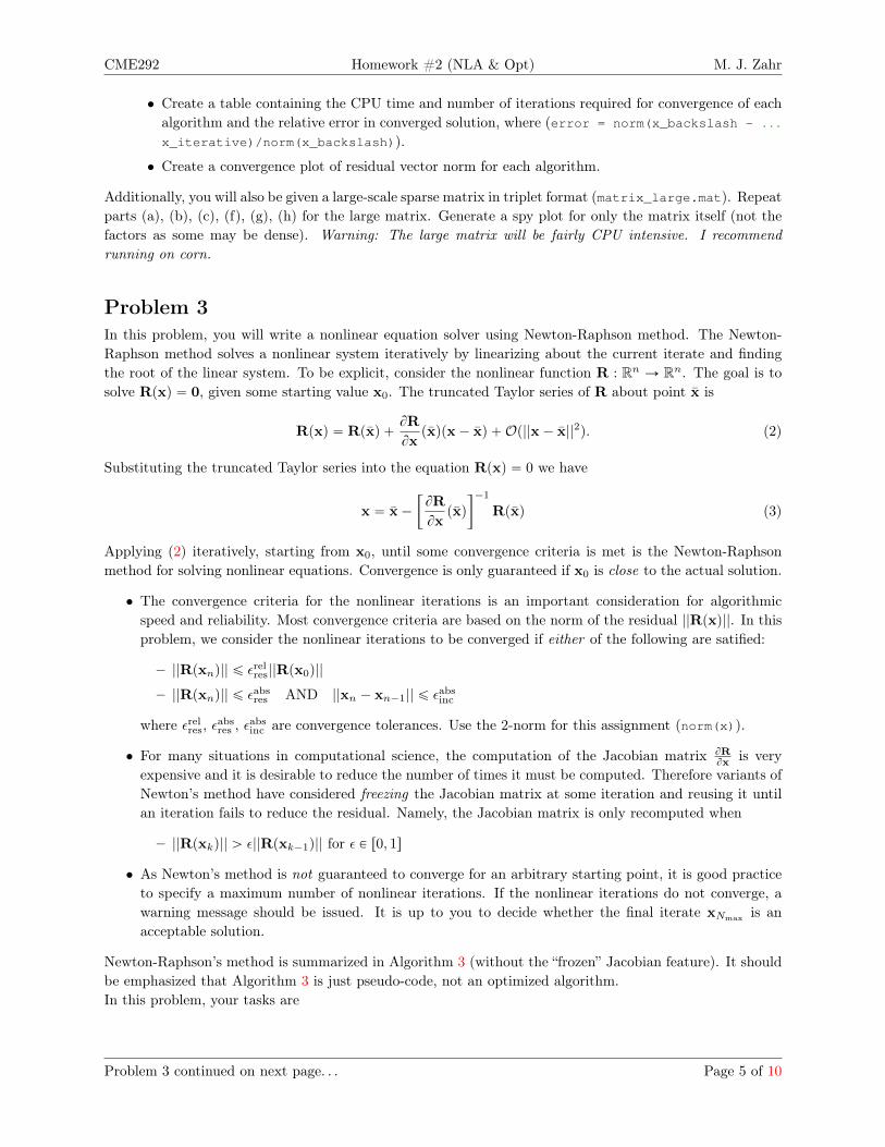
Newton-Raphson’s method is summarized in Algorithm 3 (without the “frozen” Jacobian feature). It shouldbe emphasized that Algorithm 3 is just pseudo-code, not an optimized algorithm.In this problem, your tasks are



Algorithm 3 Newton-Raphson Method

Input: x0 P Rn, εrelres, εabsres , εabs

inc , Nmax

Output: x˚ P Rn such that Rpx˚q « 0

1: for k “ 0, 1, 2, ..., Nmax do2: ∆xk “ ´

BRBx pxkq

´1Rpxkq

3: xk`1 “ xk `∆xk

4: if ||Rpxk`1q|| ď εrelres||Rpx0q|| or (||Rpxk`1q|| ď εabsres AND ||xk`1 ´ xk|| ď εabs

inc ) then5: x˚ “ x

6: return7: end if8: Issue convergence warning9: x˚ “ x

10: end for

(1) Implement Newton-Raphson’s method (Algorithm 3). The input for your Newton-Raphson implemen-tation should be similar to that of fsolve, namely, a function handle, a starting point x0, and varioustolerances. The function handle should accept a vector and return two outputs, the nonlinear functionand Jacobian evaluated at the input vector. Starter code (newton_raphson) has been provided in thecode distribution for this assignment. Feel free to use this as a starting point or start from scratch.

(2) Implement the modified Newton-Raphson method that allows for

• freezing the Jacobian matrix until ||Rpxkq|| ą 0.1||Rpxk´1q||

(3) Make sure you algorithm returns the following output information (I recommend storing it in a structure,but it is not required)

• the number of nonlinear iterations required for convergence, k

• the residual norm at convergence, ||Rpxkq||

• the number of Jacobian computations required

• the residual norm convergence history, i.e. ||Rpxjq|| for j P t0, . . . , ku

(4) The piece of code below will setup a nonlinear system of equations of dimension 122 and define a functionhandle whose first argument is the nonlinear function and the second is the Jacobian. The solution ofthis nonlinear equation will solve an instance of the nonlinear truss problem defined in Problem 4 ofthis assignment. To run this code, the folder nltruss must be on your MATLAB search path. Eithercopy all files in nltruss to your current folder or preferably use addpath('/path/to/nltruss') toadd nltruss to your search path. Starter code provided in nonlinear_study.m.

1 mesh = 'mesh3';2 nel = eval([mesh,'()']);3 [msh,bcs,mat] = setup_problem(0.1*ones(nel,1),mesh);4 func = @(W) staticResidual(W,msh,mat,bcs);

Using the function handle defined above and your Newton-Raphson solver, conduct the following study:

• Solve the nonlinear system using fsolve. Turn the Jacobian option on for a fair comparison withyour Newton-Raphson implementation. Make sure the tolerances, TolX and TolFun, and maximumiterations, MaxIter, correspond to those you use below. Record the number of iterations. Assumethere is one Jacobian evaluation per iteration.



– Plot the mesh and its deformation (the solution of the nonlinear system) usingvisualize_truss_loads(msh,bcs,mat,x,1) where x is the solution of the nonlinear systemof equations (output of fsolve)

• Solve the nonlinear system using your Newton-Raphson implementation with the following varia-tions. For each, record the residual norm history, number of iterations required for convergence,and number of Jacobian evaluations.

– Recompute the Jacobian at every iteration and use backslash to solve the linear system– Repeat the above three tasks, but reuse the Jacobian until ||Rpxkq|| ą 0.1||Rpxk´1q||

• I recommend all tolerances be set to 10´8 and Nmax “ 1000.

(5) Create a table that summarizes the results of the above study, comparing number of nonlinear iterations,residual at convergence, and number of Jacobian evaluations required for each algorithm (3 in total -fsolve and your Newton-Raphson solver with and without recycling the Jacobian).

(6) Create a plot of residual norm versus nonlinear iteration for both Newton-Raphson algorithms (notnecessary for fsolve).

(7) Briefly comment on the results.

Problem 4In this problem, you will gain experience with MATLAB’s optimization functions, in particular fmincon.You will be given a general, nonlinear 2D truss code that will be used to define the optimization problems.Prior knowledge of truss analysis or mechanics is not necessary. A brief exposition of the truss analysisframework is provided below.First, we begin with some terminology and nomenclature. A truss structure will be composed of nv nodesor vertices connected by nel truss elements. Each element e has an initial length Le, cross-sectional area Ae,elastic modulus Ee, density ρe, and deformed length (i.e. after loads applied) `e. A truss element can onlycarry normal forces, not shear or moments. This means the direction of the force within an element mustalign with the element. By definition, the intersection of two truss elements will be a pinned connection(otherwise the members would carry shear/moments). The force carried by element e will be denoted Ne.Each vertex will be subject to forces that are applied externally or transferred from the truss elements. Letf inti P R2 denote the force on vertex i due to the truss elements, usually called the internal force. Also, let

f exti P R2 denote the force on vertex i due to external loads. Finally, ui P R2 denotes the displacement ofvertex i induced by the loads.Boundary conditions for truss elements can either be displacement or force boundary conditions. Forceboundary conditions correspond to external loads, while displacement boundary conditions indicate pre-scribed displacements. Every node must have exactly one boundary condition for each degree of freedom(i.e. the x´ and y´directions).Static equilibrium at the nodes leads to the governing equation

f intpuq “ f ext. (4)

There are several important quantities that will be used in this assignment as objective or constraints.

• Stressσe “ Ee

`eLe

(5)



• Weight

W “

nelÿ

e“1

ρeAe`e (6)

• Compliance

C “nvÿ

i“1

fTi ui (7)

In the truss program you are given, there will be three relevant data structures.

• msh - contains all mesh information

• bcs - contains all boundary condition information

• mat - contains all material information (including area)

The below piece of code demonstrates how to call use the nonlinear truss code. Pay particular attention tothe commands up to solve_truss as this describes how to solve the nonlinear truss problem given a newvector of elemental areas. Additional starter code (optimize_truss.m) has been provided for you in thecode distribution.

% Bridge meshmesh = 'mesh2';

% Determine number of elements in mesh and define vector of areasnel = eval([mesh,'()']);A = ones(nel,1);

% Setup mesh, BCs, and materials[msh,bcs,mat] = setup_problem(A,mesh);

% Solve nonlinear truss equations (and sensitivity equations)[U,dUdA,F,dFdA] = solve_truss(msh,mat,bcs);

% Plot mesh and deformation% Vary last argument to scale deformationvisualize_truss_loads(msh,bcs,mat,U,10);

% Compute deformed lengths and sensitivities[l,dldA] = compute_element_lengths(U,dUdA,msh)

% Compute weight and sensitivities[W,dWdA] = compute_weight(U,dUdA,msh,mat);

% Compute compliance and sensitivities[C,dCdA] = compute_compliance(U,dUdA,F,dFdA);

% Compute element force and sensitivities[N,dNdA] = compute_internal_force(U,dUdA,msh,mat);

% Compute stress and sensitivities[s,dsdA] = compute_stress(U,dUdA,msh,mat);

(1) Solve the following minimization problem

minimizeAPRnel

W pAq

subject to |σepAq| ď σfail

0.01 ď A ď 1,

(8)



for the mesh in Figure 4. Use an initial guess of A “ 0.1. This is accomplished using mesh = ...

'mesh2' in the code provided above. I recommend starting (and debugging) with mesh = 'mesh1' asthe corresponding mesh has fewer elements and is faster to solve/optimize (Figure 3). Also, feel free toplay around with nseg in mesh2.m, which controls the number of spans in the bridge.

• Use fmincon - try active set, interior point, and SQP algorithms

• Use both user-defined gradients (provided in nltruss) and gradients automatically computed withfinite differences ('GradObj', 'GradConstr').

• Comment on differences in optimal solution and timings.

• Plot the deformed truss with optimal areas (visualize_truss_loads.m)

0 1 2 3 4 5 6 7 8

0

1

2

3

4

5

6

Figure 3: Simple Mesh (mesh1)

0 2 4 6 8 10 12 14 16 18−0.5

0

0.5

1

1.5

Figure 4: Truss Bridge Mesh (mesh2)

0 2 4 6 8 10 12 14 16 18

−3

−2

−1

0

1

2

3

4

Figure 5: Truss Bridge - Optimized (Min Weight), Deformed (mesh2)



(2) Solve the following optimization problem

minimizeAPRnel

CpAq

subject to W pAq ďW pA0q

|σepAq| ď σfail

0.01 ď A ď 1,

(9)

where A0 “ 0.1 is the initial guess.

• Use fmincon - any optimization algorithm you choose

• Use user-defined gradients (provided in nltruss) ('GradObj', 'GradConstr').

• Plot the deformed truss with optimal areas (visualize_truss_loads.m)

References[1] N. Halko, P.-G. Martinsson, and J. A. Tropp, “Finding structure with randomness: Probabilistic algo-

rithms for constructing approximate matrix decompositions,” SIAM review, vol. 53, no. 2, pp. 217–288,2011.

of 10

Homework 2: Numerical Linear Algebra and Optimization

Documents

Transcript of Homework 2: Numerical Linear Algebra and Optimization