
High-Throughput Detection of Linear Features: Selected Applications in BiologicalImaging
397
Transcript of High-Throughput Detection of Linear Features: Selected Applications in BiologicalImaging


BIOLOGICAL AND MEDICAL PHYSICS,BIOMEDICAL ENGINEERING

BIOLOGICAL AND MEDICAL PHYSICS,BIOMEDICAL ENGINEERINGThe fields of biological and medical physics and biomedical engineering are broad, multidisciplinaryand dynamic. They lie at the crossroads of frontier research in physics, biology, chemistry, and medicine.The Biological and Medical Physics, Biomedical Engineering Series is intended to be comprehensive,covering a broad range of topics important to the study of the physical, chemical and biological sciences.Its goal is to provide scientists and engineers with textbooks, monographs, and reference works to addressthe growing need for information.
Books in the series emphasize established and emergent areas of science including molecular,membrane, and mathematical biophysics; photosynthetic energy harvesting and conversion; informa-tion processing; physical principles of genetics; sensory communications; automata networks, neuralnetworks, and cellular automata. Equally important will be coverage of applied aspects of biologicaland medical physics and biomedical engineering such as molecular electronic components and devices,biosensors, medicine, imaging, physical principles of renewable energy production, advanced prostheses,and environmental control and engineering.
Editor-in-Chief:Elias Greenbaum, Oak Ridge National Laboratory, Oak Ridge, Tennessee, USA
Editorial Board:Masuo Aizawa, Department of Bioengineering,Tokyo Institute of Technology, Yokohama, Japan
Olaf S. Andersen, Department of Physiology,Biophysics & Molecular Medicine,Cornell University, New York, USA
Robert H. Austin, Department of Physics,Princeton University, Princeton, New Jersey, USA
James Barber, Department of Biochemistry,Imperial College of Science, Technologyand Medicine, London, England
Howard C. Berg, Department of Molecularand Cellular Biology, Harvard University,Cambridge, Massachusetts, USA
Victor Bloomfield, Department of Biochemistry,University of Minnesota, St. Paul,Minnesota, USA
Robert Callender, Department of Biochemistry,Albert Einstein College of Medicine,Bronx, New York, USA
Britton Chance, Department of Biochemistry/Biophysics, University of Pennsylvania,Philadelphia, Pennsylvania, USA
Steven Chu, Lawrence Berkeley NationalLaboratory, Berkeley, California, USA
Louis J. DeFelice, Department of Pharmacology,Vanderbilt University, Nashville, Tennessee, USA
Johann Deisenhofer, Howard Hughes MedicalInstitute, The University of Texas, Dallas, Texas, USA
George Feher, Department of Physics, University ofCalifornia, San Diego, La Jolla, California, USA
Hans Frauenfelder, Los Alamos National Laboratory,Los Alamos, New Mexico, USA
Ivar Giaever, Rensselaer Polytechnic Institute,Troy, NewYork, USA
Sol M. Gruner, Cornell University, Ithaca,New York, USA
For other titles published in this series, go tohttp://www.springer.com/series/3740
Judith Herzfeld, Department of Chemistry,Brandeis University,Waltham, Massachusetts, USAMark S. Humayun, Doheny Eye Institute,Los Angeles, California, USA
Pierre Joliot, Institute de Biologie Physico-Chimique,Fondation Edmond de Rothschild, Paris, France
Lajos Keszthelyi, Institute of Biophysics,Hungarian Academy of Sciences, Szeged, Hungary
Robert S. Knox, Department of Physicsand Astronomy, University of Rochester,Rochester, New York, USA
Aaron Lewis, Department of Applied Physics,Hebrew University, Jerusalem, IsraelStuart M. Lindsay, Department of Physicsand Astronomy, Arizona State University,Tempe, Arizona, USA
David Mauzerall, Rockefeller University,New York, New York, USAEugenie V. Mielczarek, Department of Physicsand Astronomy, George Mason University,Fairfax, Virginia, USAMarkolf Niemz, Medical Faculty Mannheim,University of Heidelberg, Mannheim, GermanyV. Adrian Parsegian, Physical Science Laboratory,National Institutes of Health, Bethesda,Maryland, USALinda S. Powers, University of Arizona,Tucson, Arizona, USA
Earl W. Prohofsky, Department of Physics,Purdue University,West Lafayette, Indiana, USAAndrew Rubin, Department of Biophysics,Moscow State University, Moscow, Russia
Michael Seibert, National Renewable EnergyLaboratory, Golden, Colorado, USA
David Thomas, Department of Biochemistry,University of Minnesota Medical School,Minneapolis, Minnesota, USA

Geoff DoughertyEditor
Medical Image Processing
Techniques and Applications
123

EditorGeoff DoughertyApplied Physics and Medical ImagingCalifornia State University Channel IslandsOne University Drive93012 [email protected]
ISSN 1618-7210ISBN 978-1-4419-9769-2 e-ISBN 978-1-4419-9779-1DOI 10.1007/978-1-4419-9779-1Springer New York Dordrecht Heidelberg London
Library of Congress Control Number: 2011931857
c© Springer Science+Business Media, LLC 2011All rights reserved. This work may not be translated or copied in whole or in part without the writtenpermission of the publisher (Springer Science+Business Media, LLC, 233 Spring Street, New York,NY 10013, USA), except for brief excerpts in connection with reviews or scholarly analysis. Use inconnection with any form of information storage and retrieval, electronic adaptation, computer software,or by similar or dissimilar methodology now known or hereafter developed is forbidden.The use in this publication of trade names, trademarks, service marks, and similar terms, even if they arenot identified as such, is not to be taken as an expression of opinion as to whether or not they are subjectto proprietary rights.
Printed on acid-free paper
Springer is part of Springer Science+Business Media (www.springer.com)

To my mother, Adeline Maud Dougherty,and my father, Harry Dougherty (who leftus on 17th November 2009)


Preface
The field of medical imaging advances so rapidly that all of those working in it,scientists, engineers, physicians, educators, and others, need to frequently updatetheir knowledge to stay abreast of developments. While journals and periodicalsplay a crucial role in this, more extensive, integrative publications that connectfundamental principles and new advances in algorithms and techniques to practicalapplications are essential. Such publications have an extended life and form durablelinks in connecting past procedures to the present, and present procedures to thefuture. This book aims to meet this challenge and provide an enduring bridge in theever expanding field of medical imaging.
This book is designed for end users in the field of medical imaging, whowish to update their skills and understanding with the latest techniques in imageanalysis. The book emphasizes the conceptual framework of image analysis and theeffective use of image processing tools. It is designed to assist cross-disciplinarydialog both at graduate and at specialist levels, between all those involved in themultidisciplinary area of digital image processing, with a bias toward medicalapplications. Its aim is to enable new end users to draw on the expertise of expertsacross the specialization gap.
To accomplish this, the book uses applications in a variety of fields to demon-strate and consolidate both specific and general concepts, and to build intuition,insight, and understanding. It presents a detailed approach to each application whileemphasizing the applicability of techniques to other research areas. Although thechapters are essentially self-contained, they reference other chapters to form anintegrated whole. Each chapter uses a pedagogical approach to ensure conceptuallearning before introducing specific techniques and “tricks of the trade”.
The book is unified by the theme foreshadowed in the title “Medical ImageProcessing: Techniques and Applications.” It consists of a collection of specializedtopics, each presented by a specialist in the field. Each chapter is split intosections and subsections, and begins with an introduction to the topic, method, ortechnology. Emphasis is placed not only on the background theory but also on thepractical aspects of the method, the details necessary to implement the technique,
vii

viii Preface
and limits of applicability. The chapter then introduces selected more advancedapplications of the topic, method, or technology, leading toward recent achievementsand unresolved questions in a manner that can be understood by a reader with nospecialist knowledge in that area.
Chapter 1, by Dougherty, presents a brief overview of medical image processing.He outlines a number of challenges and highlights opportunities for further devel-opment.
A number of image analysis packages exist, both commercial and free, whichmake use of libraries of routines that can be assembled/mobilized/concatenated toautomate an image analysis task. Chapter 2, by Luengo, Malm, and Bengtsson,introduces one such package, DIPimage, which is a toolbox for MatLab thatincorporates a GUI for automatic image display and a convenient drop-down menuof common image analysis functions. The chapter demonstrates how one canquickly develop a solution to automate a common assessment task such as countingcancerous cells in a Pap smear.
Segmentation is one of the key tools in medical image analysis. The main appli-cation of segmentation is in delineating an organ reliably, quickly, and effectively.Chapter 3, by Couprie, Najman and Talbot, presents very recent approaches thatunify popular discrete segmentation methods.
Deformable models are a promising method to handle the difficulties in seg-menting images that are contaminated by noise and sampling artifact. The modelis represented by an initial curve (or surface in three dimensions (3D)) in theimage which evolves under the influence of internal energy, derived from the modelgeometry, and an external force, defined from the image data. Segmentation isthen achieved by minimizing the sum of these energies, which usually results in asmooth contour. In Chapter 4, Alfiansyah presents a review of different deformablemodels and issues related to their implementations. He presents some examples ofthe different models used with noisy medical images.
Over the past two decades, many authors have investigated the use of MRI forthe analysis of body fat and its distribution. However, when performed manually,accurate isolation of fat in MR images can be an arduous task. In order toalleviate this burden, numerous segmentation algorithms have been developed forthe quantification of fat in MR images. These include a number of automated andsemi-automated segmentation algorithms. In Chapter 5, Costello and Kenny discusssome of the techniques and models used in these algorithms, with a particularemphasis on their application and implementation. The potential impact of artifactssuch as intensity inhomogeneities, partial volume effect (PVE), and chemical shiftartifacts on image segmentation are also discussed.
An increasing portion of medical imaging problems concern thin objects, andparticularly vessel filtering, segmentation, and classification. Example applicationsinclude vascular tree analysis in the brain, the heart, or the liver, the detection ofaneurysms, stenoses, and arteriovenous malformations in the brain, and coronaltree analysis in relation to the prevention of myocardial infarction. Thin, vessel-likeobjects are more difficult to process in general than most images features, preciselybecause they are thin. They are prone to disappear when using many common image
Preface ix
analysis operators, particularly in 3D. Chapter 6, by Tankyevych, Talbot, Passat,Musacchio, and Lagneau, introduces the problem of cerebral vessel filtering anddetection in 3D and describes the state of the art from filtering to segmentation, usinglocal orientation, enhancement, local topology, and scale selection. They apply bothlinear and nonlinear operators to atlas creation.
Automated detection of linear structures is a common challenge in manycomputer vision applications. Where such structures occur in medical images, theirmeasurement and interpretation are important steps in certain clinical decision-making tasks. In Chapter 7, Dabbah, Graham, Malik, and Efron discuss some ofthe well-known linear structure detection methods used in medical imaging. Theydescribe a quantitative method for evaluating the performance of these algorithms incomparison with their newly developed method for detecting nerve fibers in imagesobtained using in vivo corneal confocal microscopy (CCM).
Advances in linear feature detection have enabled new applications where thereliable tracing of line-like structures is critical. This includes neurite identificationin images of brain cells, the characterization of blood vessels, the delineation of cellmembranes, and the segmentation of bacteria under high resolution phase contrastmicroscopy. Linear features represent fundamental image analysis primitives. InChapter 8, Domanski, Sun, Lagerstrom, Wang, Bischof, Payne, and Vallottonintroduce the algorithms for linear feature detection, consider the preprocessing andspeed options, and show how such processing can be implemented convenientlyusing a graphical user interface called HCA-Vision. The chapter demonstrates howthird parties can exploit these new capabilities as informed users.
Osteoporosis is a degenerative disease of the bone. The averaging nature of bonemineral density measurement does not take into account the microarchitecturaldeterioration within the bone. In Chapter 9, Haidekker and Dougherty considermethods that allow the degree of microarchitectural deterioration of trabecular boneto be quantified. These have the potential to predict the load-bearing capability ofbone.
In Chapter 10, Adam and Dougherty describe the application of medical imageprocessing to the assessment and treatment of spinal deformity, with a focus on thesurgical treatment of idiopathic scoliosis. The natural history of spinal deformityand current approaches to surgical and nonsurgical treatment are briefly described,followed by an overview of current clinically used imaging modalities. The keymetrics currently used to assess the severity and progression of spinal deformitiesfrom medical images are presented, followed by a discussion of the errors anduncertainties involved in manual measurements. This provides the context for ananalysis of automated and semi-automated image processing approaches to measurespinal curve shape and severity in two and three dimensions.
In Chapter 11, Cree and Jelinek outline the methods for acquiring and pre-processing of retinal images. They show how morphological, wavelet, and fractalmethods can be used to detect lesions and indicate the future directions of researchin this area.
The appearance of the retinal blood vessels is an important diagnostic indicatorfor much systemic pathology. In Chapter 12, Iorga and Dougherty show that the

x Preface
tortuosity of retinal vessels in patients with diabetic retinopathy correlates with thenumber of detected microaneurysms and can be used as an alternative indicator ofthe severity of the disease. The tortuosity of retinal vessels can be readily measuredin a semi-automated fashion and avoids the segmentation problems inherent indetecting microaneurysms.
With the increasing availability of highly resolved isotropic 3D medical imagedatasets, from sources such as MRI, CT, and ultrasound, volumetric image render-ing techniques have increased in importance. Unfortunately, volume rendering iscomputationally demanding, and the ever increasing size of medical image datasetshas meant that direct approaches are unsuitable for interactive clinical use. InChapter 13, Zhang, Peters, and Eagleson describe volumetric visualization pipelinesand provide a comprehensive explanation of novel rendering and classificationalgorithms, anatomical feature and visual enhancement techniques, dynamic mul-timodality rendering and manipulation. They compare their strategies with thosefrom the published literatures and address the advantages and drawbacks of each interms of image quality and speed of interaction.
In Chapter 14, Bones and Wu describe the background motivation for adoptingsparse sampling in MRI and show evidence of the sparse nature of biologicalimage data sets. They briefly present the theory behind parallel MRI reconstruction,compressive sampling, and the application of various forms of prior knowledge toimage reconstruction. They summarize the work of other groups in applying theseconcepts to MRI and then describe their own contributions. They finish with a briefconjecture on the possibilities for future development in the area.
In Chapter 15, Momot, Pope, and Wellard discuss the fundamentals of diffusiontensor imaging (DTI) in avascular tissues and the key elements of digital processingand visualization of the diffusion data. They present examples of the applicationof DTI in two types of avascular tissue: articular cartilage and eye lens. Diffusiontensor maps present a convenient way to visualize the ordered microstructure ofthese tissues. The direction of the principal eigenvector of the diffusion tensorreports on the predominant alignment of collagen fibers in both tissues.

Contents
1 Introduction . . . . . . . . . . . . . . . . . . . . . . . . . . . . . . . . . . . . . . . . . . . . . . . . . . . . . . . . . . . . . . . . . 1Geoff Dougherty
2 Rapid Prototyping of Image Analysis Applications . . . . . . . . . . . . . . . . . . . . . 5Cris L. Luengo Hendriks, Patrik Malm, and Ewert Bengtsson
3 Seeded Segmentation Methods for Medical Image Analysis . . . . . . . . . . . 27Camille Couprie, Laurent Najman, and Hugues Talbot
4 Deformable Models and Level Sets in Image Segmentation . . . . . . . . . . . 59Agung Alfiansyah
5 Fat Segmentation in Magnetic Resonance Images . . . . . . . . . . . . . . . . . . . . . . 89David P. Costello and Patrick A. Kenny
6 Angiographic Image Analysis . . . . . . . . . . . . . . . . . . . . . . . . . . . . . . . . . . . . . . . . . . . . . 115Olena Tankyevych, Hugues Talbot, Nicolas Passat, MarianoMusacchio, and Michel Lagneau
7 Detecting and Analyzing Linear Structures in BiomedicalImages: A Case Study Using Corneal Nerve Fibers . . . . . . . . . . . . . . . . . . . . 145Mohammad A. Dabbah, James Graham, Rayaz A. Malik,and Nathan Efron
8 High-Throughput Detection of Linear Features: SelectedApplications in Biological Imaging . . . . . . . . . . . . . . . . . . . . . . . . . . . . . . . . . . . . . . . 167Luke Domanski, Changming Sun, Ryan Lagerstrom, DadongWang, Leanne Bischof, Matthew Payne, and Pascal Vallotton
9 Medical Imaging in the Diagnosis of Osteoporosis andEstimation of the Individual Bone Fracture Risk . . . . . . . . . . . . . . . . . . . . . . . 193Mark A. Haidekker and Geoff Dougherty
xi

xii Contents
10 Applications of Medical Image Processing in the Diagnosisand Treatment of Spinal Deformity . . . . . . . . . . . . . . . . . . . . . . . . . . . . . . . . . . . . . . 227Clayton Adam and Geoff Dougherty
11 Image Analysis of Retinal Images . . . . . . . . . . . . . . . . . . . . . . . . . . . . . . . . . . . . . . . . 249Michael J. Cree and Herbert F. Jelinek
12 Tortuosity as an Indicator of the Severity of Diabetic Retinopathy . . . 269Michael Iorga and Geoff Dougherty
13 Medical Image Volumetric Visualization: Algorithms,Pipelines, and Surgical Applications . . . . . . . . . . . . . . . . . . . . . . . . . . . . . . . . . . . . . 291Qi Zhang, Terry M. Peters, and Roy Eagleson
14 Sparse Sampling in MRI . . . . . . . . . . . . . . . . . . . . . . . . . . . . . . . . . . . . . . . . . . . . . . . . . . . 319Philip J. Bones and Bing Wu
15 Digital Processing of Diffusion-Tensor Imagesof Avascular Tissues . . . . . . . . . . . . . . . . . . . . . . . . . . . . . . . . . . . . . . . . . . . . . . . . . . . . . . . . 341Konstantin I. Momot, James M. Pope, and R. Mark Wellard
Index . . . . . . . . . . . . . . . . . . . . . . . . . . . . . . . . . . . . . . . . . . . . . . . . . . . . . . . . . . . . . . . . . . . . . . . . . . . . . . . 373

Contributors
Clayton Adam Queensland University of Technology, Brisbane, Australia,[email protected]
Agung Alfiansyah Surya Research and Education Center, Tangerang, Indonesia,[email protected]
Ewert Bengtsson Swedish University of Agricultural Sciences, Uppsala, Sweden
Uppsala University, Uppsala, Sweden, [email protected]
Leanne Bischof CSIRO (Commonwealth Scientific and Industrial ResearchOrganisation), North Ryde, Australia, [email protected]
Philip J. Bones University of Canterbury, Christchurch, New Zealand,[email protected]
David P. Costello Mater Misericordiae University Hospital and University CollageDublin, Ireland, [email protected]
Camille Couprie Universite Paris-Est, Paris, France, [email protected]
Michael J. Cree University of Waikato, Hamilton, New Zealand,[email protected]
Mohammad A. Dabbah The University of Manchester, Manchester, England,[email protected]
Luke Domanski CSIRO (Commonwealth Scientific and Industrial ResearchOrganisation), North Ryde, Australia, [email protected]
Geoff Dougherty California State University Channel Islands, Camarillo, CA,USA, [email protected]
Roy Eagleson The University of Western Ontario, London, ON, Canada,[email protected]
xiii

xiv Contributors
Nathan Efron Institute of Health and Biomedical Innovation, QueenslandUniversity of Technology, Brisbane, Australia, [email protected]
James Graham The University of Manchester, Manchester, England,[email protected]
Mark A. Haidekker University of Georgia, Athens, Georgia,[email protected]
Cris L. Luengo Hendriks Uppsala University, Uppsala, Sweden, [email protected]
Michael Iorga NPHS, Thousand Oaks, CA, USA, [email protected]
Herbert F. Jelinek Charles Stuart University, Albury, Australia,[email protected]
Patrick A. Kenny Mater Misericordiae University Hospital and UniversityCollege Dublin, Ireland, [email protected]
Ryan Lagerstrom CSIRO (Commonwealth Scientific and Industrial ResearchOrganisation), North Ryde, Australia, [email protected]
Michel Lagneau Hopital Louis-Pasteur, Colmar, France,[email protected]
Rayaz A. Malik The University of Manchester, Manchester, England,[email protected]
Patrik Malm Swedish University of Agricultural Sciences, Uppsala, Sweden
Uppsala University, Uppsala, Sweden, [email protected]
Konstantin I. Momot Queensland University of Technology, Brisbane, Australia,[email protected]
Mariano Musacchio Hopital Louis-Pasteur, Colmar, France,mariano [email protected]
Laurent Najman Universite Paris-Est, Paris, France, [email protected]
Nicholas Passat Universite de Strasbourg, Strasbourg, France,[email protected]
Matthew Payne CSIRO (Commonwealth Scientific and Industrial ResearchOrganisation), North Ryde, Australia, [email protected]
Terry M. Peters Robarts Research Institute, University of Western Ontario,London, ON, Canada, [email protected]

Contributors xv
James M. Pope Queensland University of Technology, Brisbane, Australia,[email protected]
Changming Sun CSIRO (Commonwealth Scientific and Industrial ResearchOrganisation), North Ryde, Australia, [email protected]
Hugues Talbot Universite Paris-Est, Paris, France, [email protected]
Olena Tankyevych Universite Paris-Est, Paris, France, [email protected]
Pascal Vallotton CSIRO (Commonwealth Scientific and Industrial ResearchOrganisation), North Ryde, Australia, [email protected]
Dadong Wang CSIRO (Commonwealth Scientific and Industrial Research Organ-isation), North Ryde, Australia, [email protected]
R. Mark Wellard Queensland University of Technology, Brisbane, Australia,[email protected]
Bing Wu Duke University, Durham, NC, USA, [email protected]
Qi Zhang Robarts Research Institute, University of Western Ontario, London, ON,Canada, [email protected]


Chapter 1Introduction
Geoff Dougherty
1.1 Medical Image Processing
Modern three-dimensional (3-D) medical imaging offers the potential and promisefor major advances in science and medicine as higher fidelity images are produced.It has developed into one of the most important fields within scientific imaging dueto the rapid and continuing progress in computerized medical image visualizationand advances in analysis methods and computer-aided diagnosis [1], and is now, forexample, a vital part of the early detection, diagnosis, and treatment of cancer. Thechallenge is to effectively process and analyze the images in order to effectivelyextract, quantify, and interpret this information to gain understanding and insightinto the structure and function of the organs being imaged. The general goal is tounderstand the information and put it to practical use.
A multitude of diagnostic medical imaging systems are used to probe the humanbody. They comprise both microscopic (viz. cellular level) and macroscopic (viz.organ and systems level) modalities. Interpretation of the resulting images requiressophisticated image processing methods that enhance visual interpretation andimage analysis methods that provide automated or semi-automated tissue detection,measurement, and characterization [2–4]. In general, multiple transformations willbe needed in order to extract the data of interest from an image, and a hierarchyin the processing steps will be evident, e.g., enhancement will precede restoration,which will precede analysis, feature extraction, and classification [5]. Often, theseare performed sequentially, but more sophisticated tasks will require feedback ofparameters to preceding steps so that the processing includes a number of iterativeloops.
G. Dougherty (�)California State University Channel Islands, Camarillo, CA, USAe-mail: [email protected]
G. Dougherty (ed.), Medical Image Processing: Techniques and Applications, Biologicaland Medical Physics, Biomedical Engineering, DOI 10.1007/978-1-4419-9779-1 1,© Springer Science+Business Media, LLC 2011
1

2 G. Dougherty
There are a number of specific challenges in medical image processing:
1. Image enhancement and restoration2. Automated and accurate segmentation of features of interest3. Automated and accurate registration and fusion of multimodality images4. Classification of image features, namely characterization and typing of structures5. Quantitative measurement of image features and an interpretation of the
measurements6. Development of integrated systems for the clinical sector
Design, implementation, and validation of complex medical systems require notonly medical expertise but also a strong collaboration between physicians andbiologists on the one hand, and engineers, physicists, and computer scientists onthe other.
Noise, artifacts and weak contrast are the principal causes of poor image qualityand make the interpretation of medical images very difficult. They are responsi-ble for the limited success of conventional or traditional detection and analysisalgorithms. Poor image quality invariably leads to problematic and unreliablefeature extraction, analysis and recognition in many medical applications. Researchefforts are geared towards improving the quality of the images, and finding morerobust techniques to successfully handle images of compromised quality in variousapplications.
1.2 Techniques
The major strength in the application of computers to medical imaging lies in theuse of image processing techniques for quantitative analysis. Medical images areprimarily visual in nature; however, visual analysis by human observers is usuallyassociated with limitations caused by interobserver variations and errors due tofatigue, distractions, and limited experience. While the interpretation of an imageby an expert draws from his/her experience and expertise, there is almost always asubjective element. Computer analysis, if performed with the appropriate care andlogic, can potentially add objective strength to the interpretation of the expert. Thus,it becomes possible to improve the diagnostic accuracy and confidence of even anexpert with many years of experience.
Imaging science has expanded primarily along three distinct but related linesof investigation: segmentation, registration and visualization [6]. Segmentation,particularly in three dimensions, remains the holy grail of imaging science. It isthe important yet elusive capability to accurately recognize and delineate all the in-dividual objects in an image scene. Registration involves finding the transformationthat brings different images of the same object into strict spatial (and/or temporal)congruence. And visualization involves the display, manipulation, and measurementof image data. Important advances in these three areas will be outlined in the variouschapters in this book.

1 Introduction 3
A common theme throughout this book is the differentiation and integrationof images. On the one hand, automatic segmentation and classification of tissuesprovide the required differentiation, and on the other the fusion of complementaryimages provides the integration required to advance our understanding of lifeprocesses and disease. Measurement of both form and function, of the whole imageand at the individual pixel level, and the ways to display and manipulate digitalimages are the keys to extracting the clinical information contained in biomedicalimages. The need for new techniques becomes more pressing as improvements inimaging technologies enable more complex objects to be imaged and simulated.
1.3 Applications
The approach required is primarily that of problem solving. However, the under-standing of the problem can often require a significant amount of preparatory work.The applications chosen for this book are typical of those in medical imaging;they are meant to be exemplary, not exclusive. Indeed, it is hoped that many ofthe solutions presented will be transferable to other problems. Each applicationbegins with a statement of the problem, and includes illustrations with real-lifeimages. Image processing techniques are presented, starting with relatively simplegeneric methods, followed by more sophisticated approaches directed at that specificproblem. The benefits and challenges in the transition from research to clinicalsolution are also addressed.
Biomedical imaging is primarily an applied science, where the principles ofimaging science are applied to diagnose and treat disease, and to gain basic insightsinto the processes of life. The development of such capabilities in the researchlaboratory is a time-honored tradition. The challenge is to make new techniquesavailable outside the specific laboratory that developed them, so that others can useand adapt them to different applications. The ideas, skills and talents of specificdevelopers can then be shared with a wider community and this will hopefullyfacilitate the transition of successful research technique into routine clinical use.
1.4 The Contribution of This Book
Computer hardware and software have developed to the point where large imagescan be analyzed quickly and at moderate cost. Automated processes, includingpattern recognition and computer-assisted diagnosis (CAD), can be effectivelyimplemented on a personal computer. This chapter has outlined some of thesuccesses in the field, and brought attention to some of the remaining problems. Thefollowing chapters will describe in detail some of the techniques and applicationsthat are currently being used by experts in the field.

4 G. Dougherty
Medical imaging is very visual. Although the formalism of the techniquesand algorithms is mathematical, we understand the advantages offered throughvisualization. Therefore, this book offers many images and diagrams. Some are forpedagogical purposes, to assist with the exposition, and others are motivational, toreveal interesting features of particular applications.
The book is a collection of chapters, written by experts in the field of imageanalysis, in a style to build intuition, insight, and understanding. Each chapterrepresents the state-of-the-art wisdom in a particular subfield, the result of ongoing,world-wide collaborative efforts over a period of time. Although the chapters areessentially self-contained they reference other chapters to form an integrated whole.Each chapter employs a pedagogical approach to ensure conceptual learning beforeintroducing specific techniques and “tricks of the trade.” The book aims to addressrecent methodological advances in imaging techniques by demonstrating how theycan be applied to a selection of topical applications. It is hoped that this willempower the reader to experiment with and use the techniques in his/her ownresearch area and beyond.
Chapter 2 describes an intuitive toolbox for MatLab, called DipImage, anddemonstrates how it can be used to count cancerous cells in a Pap smear.
Chapter 3 introduces new approaches that unify discrete segmentation tech-niques, Chapter 4 shows how deformable models can be used with noisy images,and Chapter 5 applies a number of automated and semi-automated segmentationmethods to MRI images.
Automated detection of linear structures is a common challenge in manycomputer vision applications. Chapters 6–8 describe state-of-the-art techniques andapply them to a number of biomedical systems.
Image processing methods are applied to osteoporosis in Chapter 9, to idiopathicscoliosis in Chapter 10, and to retinal pathologies in Chapters 11 and 12.
Novel volume rendering algorithms are discussed in Chapter 13.Sparse sampling algorithms in MRI are presented in Chapter 14, and the visual-
ization of diffusion tensor images of avascular tissues is discussed in Chapter 14.
References
1. Dougherty, G.: Image analysis in medical imaging: recent advances in selected examples.Biomed. Imaging Interv. J. 6(3), e32 (2010)
2. Beutel, J., Kundel, H.L., Van Metter, R.L.: Handbook of Medical Imaging, vol. 1. SPIE,Bellingham, Washington (2000)
3. Rangayyan, R.M.: Biomedical Image Analysis. CRC, Boca Raton, FL (2005)4. Meyer-Base, A.: Pattern Recognition for Medical Imaging. Elsevier Academic, San Diego, CA
(2004)5. Dougherty, G.: Digital Image Processing for Medical Applications. Cambridge University Press,
Cambridge (2009)6. Robb, R.A.: Biomedical Imaging, Visualization and Analysis. Wiley-Liss, New York (2000)

Chapter 2Rapid Prototyping of Image AnalysisApplications
Cris L. Luengo Hendriks, Patrik Malm, and Ewert Bengtsson
2.1 Introduction
When developing a program to automate an image analysis task, one does not startwith a blank slate. Far from it. Many useful algorithms have been described in theliterature, and implemented countless times. When developing an image analysisprogram, experience points the programmer to one or several of these algorithms.The programmer then needs to try out various possible combinations of algorithmsbefore finding a satisfactory solution. Having to implement these algorithms justto see if they work for this one particular application does not make much sense.This is the reason programmers and researches build up libraries of routines thatthey have implemented in the past, and draw on these libraries to be able to quicklystring together a few algorithms and see how they work on the current application.Several image analysis packages exist, both commercial and free, and they can beused as a basis for building up such a library. None of these packages will containall the necessary algorithms, but they should provide at least the most basic ones.This chapter introduces you to one such package, DIPimage, and demonstrates howone can proceed to quickly develop a solution to automate a routine medical task.As an illustrative example we use some of the approaches taken over the years tosolve the long-standing classical medical image analysis problem of assessing a Papsmear. To make best use of this chapter, you should have MATLAB and DIPimagerunning on your computer, and try out the command sequences given.
C.L. Luengo Hendriks (�)Centre for Image Analysis, Swedish University of Agricultural Sciences,Box 337, SE-751 05 Uppsala, Swedene-mail: [email protected]
G. Dougherty (ed.), Medical Image Processing: Techniques and Applications, Biologicaland Medical Physics, Biomedical Engineering, DOI 10.1007/978-1-4419-9779-1 2,© Springer Science+Business Media, LLC 2011
5

6 C.L. Luengo Hendriks et al.
2.2 MATLAB and DIPimage
2.2.1 The Basics
DIPimage is built on MATLAB (The MathWorks, Natick, MA, USA), whichprovides a powerful and intuitive programming language, publication-quality graph-ing, and a very extensive set of algorithms and tools. DIPimage adds to this alarge collection of image processing and analysis algorithms, easy computationwith images, and interactive graphical tools to examine images. It is designed forease of use, using MATLAB’s simple command syntax and several graphical userinterfaces, and is accessible to novices but fast and powerful enough for the mostadvanced research projects. It is available free of charge for academic and othernoncommercial purposes from its website: http://www.diplib.org/.
DIPimage extends the MATLAB language with a new data type. Natively,MATLAB knows about arrays of numbers, characters, structures or cells (the lattercan contain any other data type). With this toolbox installed, images are added to thislist. Even though images can be seen simply as an array of numbers, there are severaladvantages to this new type: indexing works differently than in an array, the toolboxcan alter the way operations are performed depending on the pixel representation,and images can be automatically displayed. This latter point is significant, for itgreatly enhances accessibility to novices and significantly increases the interactivityin the design phase of an image analysis application.
In MATLAB, assigning the value 1 to a variable a is accomplished with:
a = 1;
Additionally, if the semicolon is left off this statement, MATLAB will reply bydisplaying the new value of the variable:
a = 1a =
1
Similarly, when leaving the semicolon off a DIPimage statement that assigns animage into a variable, MATLAB will reply by displaying that image in a figurewindow. For example, the next statement reads in the Pap smear image in file“papsmear.tif”1 and assigns it to variable a.
a = readim(’papsmear.tif’)Displayed in figure 10
Depending on the chosen configuration, the image will be displayed to a newwindow or an existing window. To suppress automatic display, all that is thus neededis to add a semicolon at the end of all statements.
1You can obtain this file from http://www.cb.uu.se/∼cris/Images/papsmear.tif
2 Rapid Prototyping of Image Analysis Applications 7
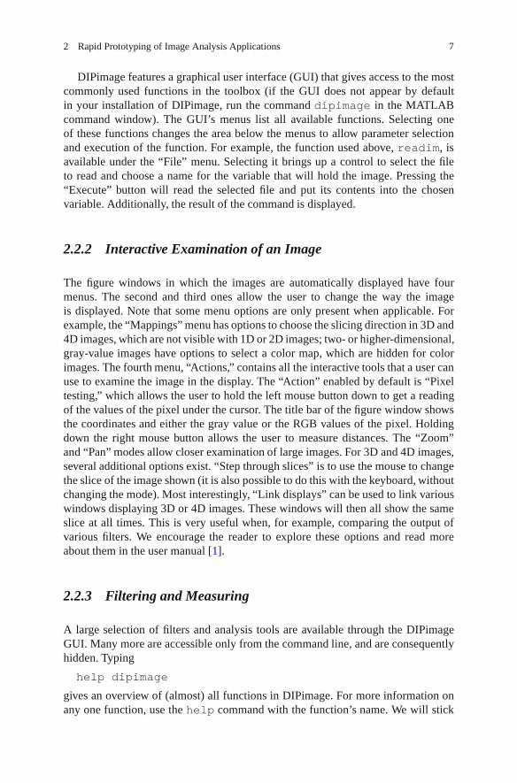
DIPimage features a graphical user interface (GUI) that gives access to the mostcommonly used functions in the toolbox (if the GUI does not appear by defaultin your installation of DIPimage, run the command dipimage in the MATLABcommand window). The GUI’s menus list all available functions. Selecting oneof these functions changes the area below the menus to allow parameter selectionand execution of the function. For example, the function used above, readim, isavailable under the “File” menu. Selecting it brings up a control to select the fileto read and choose a name for the variable that will hold the image. Pressing the“Execute” button will read the selected file and put its contents into the chosenvariable. Additionally, the result of the command is displayed.
2.2.2 Interactive Examination of an Image
The figure windows in which the images are automatically displayed have fourmenus. The second and third ones allow the user to change the way the imageis displayed. Note that some menu options are only present when applicable. Forexample, the “Mappings” menu has options to choose the slicing direction in 3D and4D images, which are not visible with 1D or 2D images; two- or higher-dimensional,gray-value images have options to select a color map, which are hidden for colorimages. The fourth menu, “Actions,” contains all the interactive tools that a user canuse to examine the image in the display. The “Action” enabled by default is “Pixeltesting,” which allows the user to hold the left mouse button down to get a readingof the values of the pixel under the cursor. The title bar of the figure window showsthe coordinates and either the gray value or the RGB values of the pixel. Holdingdown the right mouse button allows the user to measure distances. The “Zoom”and “Pan” modes allow closer examination of large images. For 3D and 4D images,several additional options exist. “Step through slices” is to use the mouse to changethe slice of the image shown (it is also possible to do this with the keyboard, withoutchanging the mode). Most interestingly, “Link displays” can be used to link variouswindows displaying 3D or 4D images. These windows will then all show the sameslice at all times. This is very useful when, for example, comparing the output ofvarious filters. We encourage the reader to explore these options and read moreabout them in the user manual [1].
2.2.3 Filtering and Measuring
A large selection of filters and analysis tools are available through the DIPimageGUI. Many more are accessible only from the command line, and are consequentlyhidden. Typing
help dipimage
gives an overview of (almost) all functions in DIPimage. For more information onany one function, use the help command with the function’s name. We will stick

8 C.L. Luengo Hendriks et al.
0 200 400 600 8000
20
40
60
80
100
120
area (px2)
perim
eter
(px
)
a b
c d
Fig. 2.1 A first look at DIPimage: (a) input image, (b) result of gaussf, (c) result of threshold, and(d) plot of measured area vs. perimeter
to the functions in the GUI for now. Let us assume that we still have the Pap smearimage loaded in variable a. We select the “Gaussian filter” from the “Filters” menu.For the first parameter we select variable a, for the second parameter we enter 2, andfor output image we type b. After clicking “Execute,” we see
b = gaussf(a,2,’best’)Displayed in figure 11
on the command line, and the filtered image is shown in a window (Fig. 2.1b).Typing the above command would have produced the same result, without the needfor the GUI. Because ’best’ is the default value for the third parameter, the sameresult would also have been accomplished typing only
b = gaussf(a,2)

2 Rapid Prototyping of Image Analysis Applications 9
Next we will select the “Threshold” function from the “Segmentation” menu,enter -b for input image and c for output image, and execute the command. Wenow have a binarized image, where the nuclei are marked as objects (red) and therest as background (Fig. 2.1c). If we had left the minus sign out of the input to thethreshold, the output would have been inverted. Finally, we select the “Measure”function from the “Analysis” menu, use c as the first input image, select severalmeasurements by clicking on the “Select. . . ” button (for example: “size,” “center”and “perimeter,” hold the control key down while clicking the options to select morethan one), and execute the command. On the command window we will now seethe result of the measurements. We can generate a plot of surface area (“size”) vs.perimeter (Fig. 2.1d) by typing
figure, plot(msr.size, msr.perimeter,’.’)
Note several small objects are found that are obviously not nuclei. Based onthe size measure these can be discarded. We will see more of this type of logic inSect. 2.4.
2.2.4 Scripting
If you collect a sequence of commands in a plain text file, and save that file with a“.m” extension, you have created a script. This script can be run simply by typingits name (without the extension) at the MATLAB command prompt. For example,if we create a file “analyse.m” with the following content:
a = readim(’papsmear.tif’);b = smooth(a,2);c = threshold(-b);msr = measure(c,[],{’Size’,’Center’,’Perimeter’});figure, plot(msr.size,msr.perimeter,’.’)
then we can execute the whole analysis in this section by just typing
analyse
It is fairly easy to collect a sequence of commands to solve an application insuch a file, execute the script to see how well it works, and modify the scriptincrementally. Because the GUI prints the executed command to the command line,it is possible to copy and paste the command to the script. The script works as botha record of the sequence of commands performed, and a way to reuse solutions.Often, when trying to solve a problem, one will start with the working solution toan old problem. Furthermore, it is easier to write programs that require loops andcomplex logic in a text editor than directly at the command prompt.

10 C.L. Luengo Hendriks et al.
If you are a programmer, then such a script is obvious. However, compared tomany other languages that require a compilation step, the advantage with MATLABis that you can select one or a few commands and execute them independently ofthe rest of the script. You can execute the program line by line, and if the result ofone line is not as expected, modify that line and execute it again, without havingto run the whole script anew. This leads to huge time savings while developingnew algorithms, especially if the input images are large and the analysis takes a lotof time.
2.3 Cervical Cancer and the Pap Smear
Cervical cancer is one of the most common cancers for women, killing abouta quarter million women world-wide every year. In the 1940s, Papanicolaoudiscovered that vaginal smears can be used to detect the disease at an early, curablestage [2]. Such smears have since then commonly been referred to as Pap smears.Screening for cervical cancer has drastically reduced the death rate for this diseasein the parts of the world where it has been applied [3]. Mass screens are possiblebecause obtaining the samples is relatively simple and painless, and the equipmentneeded is inexpensive.
The Pap smear is obtained by collecting cells from the cervix surface (typicallyusing a spatula), and spreading them thinly (by smearing) on a microscope slide(Fig. 2.2). The sample is then stained and analyzed under the microscope by acytotechnologist. This person needs to scan the whole slide looking for abnormalcells, which is a tedious task because a few thousand microscopic fields of viewneed to be scrutinized, looking for the potentially few abnormal cells among the
Fig. 2.2 A Pap smear is obtained by thinly smearing collected cells onto a glass microscope slide

2 Rapid Prototyping of Image Analysis Applications 11
several hundred thousand cells that a slide typically contains. This work is madeeven more difficult due to numerous artifacts: overlapping cells, mucus, blood, etc.The desire to automate the screening has always been great, for all the obviousreasons: trained personnel are expensive, they get tired, their evaluation criteriachange over time, etc. The large number of images to analyze for a single slide,together with the artifacts, has made automation a very difficult problem that hasoccupied numerous image analysis researchers over the decades.
2.4 An Interactive, Partial History of AutomatedCervical Cytology
This section presents an “interactive history,” meaning that the description ofmethods is augmented with bits of code that you, the reader, can try out for yourself.This both makes the descriptions easier to follow, and illustrates the use of DIPimageto quickly and easily implement a method from the literature. This section is only apartial history, meaning that we show the highlights but do not attempt to covereverything; we simplify methods to their essence, and focus only on the imageanalysis techniques, ignoring imaging, classification, etc. For a somewhat moreextensive description of the history of this field see for instance the paper byBengtsson [4].
2.4.1 The 1950s
The first attempt at automation of Pap smear assessment was based on theobservation that cancer cells are typically bigger, with a greater amount of stainedmaterial, than normal cells. Some studies showed that all samples from a patientwith cancer had at least some cells with a diameter greater than 12μm, while nonormal cells were that large. And thus a system, the cytoanalyzer, was developedthat thresholded the image at a fixed level (Fig. 2.3a), and measured the area(counted the pixels) and the integrated optical density (summed gray values) foreach connected component [5]. To replicate this is rather straightforward, and verysimilar to what we did in Sect. 2.2.3:
a = readim(’papsmear.tif’);b = a<128;msr = measure(b,a,{’Size’,’Sum’});As you can see, this only works for very carefully prepared samples. Places
where multiple cytoplasms overlap result in improper segmentation, creating falselarge regions that would be identified as cancerous. Furthermore, the threshold valueof 128 that we selected for this image is not necessarily valid for other images. This

12 C.L. Luengo Hendriks et al.
450 500 550 600 650 700 750 800
4
5
6
7
8x 10⁴
area (px2)in
tegr
ated
opt
ical
den
sity
(un
calib
rate
d)
a b
Fig. 2.3 (a) Segmented Pap-smear image and (b) plot of measured area vs. integrated opticaldensity
requires strong control over the sample preparation and imaging to make sure theintensities across images are constant.
The pixel size in this machine was about 2 μm, meaning that it looked for seg-mented regions with a diameter above 6 pixels. For our image this would be about45 pixels. The resulting data was analyzed as 2D scatter plots and if signals fell inthe appropriate region of the plot the specimen was called abnormal (Fig. 2.3b):
figure, plot(msr.size,msr.sum,’.’)
All the processing was done in hardwired, analog, video processing circuits. Themachine could have worked if the specimens only contained well-preserved, single,free-lying cells. But the true signal was swamped by false signals from small clumpsof cells, blood cells, and other debris [6].
2.4.2 The 1960s
One of the limitations of the cytoanalyzer was the fixed thresholding; it was verysensitive to proper staining and proper system setup. Judith Prewitt (known for herlocal gradient operator) did careful studies of digitized cell images and came upwith the idea of looking at the histogram of the cell image [7]. Although this workwas focused on the identification of red blood cells, the method found applicationin all other kinds of (cell) image analysis, including Pap smear assessment.
Assuming three regions with different intensity (nucleus, cytoplasm, and back-ground), we would expect three peaks in the histogram (Fig. 2.4a). For simpleshapes, we expect fewer pixels on the border between the regions than in the

2 Rapid Prototyping of Image Analysis Applications 13
0 50 100 150 200 2500
500
1000
1500
2000
gray value
freq
uenc
y (n
umbe
r of
pix
els)
a b
Fig. 2.4 (a) Histogram of Pap-smear image, with calculated threshold and (b) segmented image
regions themselves, meaning that there would be two local minima in between thesethree peaks, corresponding to the gray values of the pixels forming the borders.The two gray values corresponding to these two local minima are therefore goodcandidates for thresholding the image, thereby classifying each pixel into one of thethree classes (Fig. 2.4b). Detecting these two local minima requires simplifying thehistogram slightly, for example by a low-pass filter, to remove all the local minimacaused by noise:
a = readim(’papsmear.tif’);h = diphist(a); % obtain a histogramh = gaussf(h,3); % smooth the histogramt = minima(h); % detect the local minimat(h==0) = 0; % mask out the minima at the tailst = find(t) % get coordinates of minimaa < t(1) % threshold the image at the first
local minimum
Basically, this method substitutes the fixed threshold of the cytoanalyzer with asmoothing parameter for the histogram. If this smoothing value is taken too small,we find many more than two local minima; if it is too large, we do not find anyminima. However, the results are less sensitive to the exact value of this parameter,because a whole range of smoothing values allows the detection of the two minima,and the resulting threshold levels are not affected too much by the smoothing. And,of course, it is possible to write a simple algorithm that finds a smoothing value suchthat there are exactly two local minima:
h = diphist(a); % obtain a histogramt = [0,0,0]; % initialize threshold arraywhile length(t)>2 % repeat until we have 2 local
minima

14 C.L. Luengo Hendriks et al.
0 50 100 150 200 2500
2
4
6
8
10
12
14
16
18
gray valuew
eigh
ted
freq
uenc
y
a b
Fig. 2.5 (a) Gradient magnitude of Pap-smear image and (b) differential histogram computedfrom the Pap-smear image and its gradient magnitude
h = gaussf(h,1); % (the code inside the loop isidentical to that used above)
t = minima(h);t(h==0)=0;t = find(t);
end
The loop then repeats the original code, smoothing the histogram more and more,until at most two local minima are found.
2.4.3 The 1970s
In the late 1960s, a group at Toshiba, in Japan, started working on developing a Papsmear screening machine they called CYBEST. They used a differential histogramapproach for the automated thresholding [8, 9]. That is, they computed a histogramweighted by a measure of edge strength; pixels on edges contribute more strongly tothis histogram than pixels in flat areas. Peaks in this histogram indicate gray valuesthat occur often on edges (Fig. 2.5). Though CYBEST used a different schemeto compute edge strength, we will simply use the Gaussian gradient magnitude(gradmag).
a = readim(’papsmear.tif’);b = gradmag(a);h = zeros(255,1); % initialize arrayfor i = 1:255
t = a==i; % t is a binary maskn = sum(t); % n counts number of pixels with value i

2 Rapid Prototyping of Image Analysis Applications 15
if n>0h(i) = sum(b(t))/n; % average gradient at pixels
with value iend
endh = gaussf(h,2); % smooth differential histogram[∼,t] = max(h); % find location of maximuma < t % threshold
A second peak in this histogram gives a threshold to distinguish cytoplasm frombackground, much like in Prewitt’s method.
This group studied which features were useful for analyzing the slides andended up using four features [10]: nuclear area, nuclear density, cytoplasmic area,and nuclear/cytoplasmic ratio. These measures can be easily obtained with themeasure function as shown before. They also realized that nuclear shape andchromatin pattern were useful parameters but were not able to reliably measurethese features automatically, mainly because the automatic focusing was unableto consistently produce images with all the cell nuclei in perfect focus. Nuclearshape was determined as the square of the boundary length divided by thesurface area. Determining the boundary length is even more sensitive to a correctsegmentation than surface area. The measure function can measure the boundarylength (’perimeter’), as well as the shape factor (’p2a’). The shapefactor, computed by perimeter2/(4πarea), is identical to CYBEST’s nuclear shapemeasure, except it is normalized to be 1 for a perfect circle. The chromatin patternmeasure that was proposed by this group and implemented in CYBEST Model 4 issimply the number of blobs within the nuclear region [11]. For example (using thea and t from above):
m = gaussf(a) < t; % detect nucleim = label(m)==3; % pick one nucleusm = (a < mean(a(m))) & m; % detect regions within
nucleusmax(label(m)) % count number of regions
Here, we just used the average gray value within the nucleus as the threshold,and counted the connected components (Fig. 2.6). The procedure used in CYBESTwas more complex, but not well described in the literature.
The CYBEST system was developed in four generations over two decades,and tested extensively, even in full scale clinical trials, but was not commerciallysuccessful.
2.4.4 The 1980s
In the late 1970s and 1980s, several groups in Europe were working on developingsystems similar to CYBEST, all based on the so-called “rare event model,” that is,

16 C.L. Luengo Hendriks et al.
Fig. 2.6 A simple chromatin pattern measure: (a) the nucleus, (b) the nucleus mask, and (c) thehigh-chromatin region mask within that nucleus
looking for the few large, dark, diagnostic cells among the few hundred thousandnormal cells. And these systems had to do this sufficiently fast, while avoiding beingswamped by false alarms due to misclassifications of overlapping cells and smallclumps of various kinds.
As a side effect of the experimentation on feature extraction and classification,carried out as part of this research effort, a new concept emerged. Several groupsworking in the field observed that even “normal” cells on smears from patients withcancer had statistically significant shifts in their features towards the abnormal cells.Even though these shifts were not strong enough to be useful on the individual celllevel, it made it possible to detect abnormal specimens through a statistical analysisof the feature distributions of a small population, a few hundred cells, provided thesefeatures were extracted very accurately. This phenomenon came to be known asMAC, malignancy associated changes [12]. The effect was clearly most prominentin the chromatin pattern in the cell nuclei. The CYBEST group had earlier notedthat it was very difficult to extract features describing the chromatin pattern reliablyin an automated system. A group at the British Colombia Cancer Research Centrein Vancouver took up this idea and developed some very careful cell segmentationand chromatin feature extraction algorithms.
To accurately measure the chromatin pattern, one first needs an accurate de-lineation of the nucleus. Instead of using a single, global threshold to determinethe nuclear boundary, a group in British Colombia used the gradient magnitude toaccurately place the object boundary [13]. They start with a rough segmentation,and selected a band around the boundary of the object in which the real boundarymust be (Fig. 2.7a):
a = readim(’papsmear.tif’);b = gaussf(a,2)<128; % quick-and-dirty thresholdc = b-berosion(b,1); % border pixelsc = bdilation(c,3); % broader region around border

2 Rapid Prototyping of Image Analysis Applications 17
Fig. 2.7 Accurate delineation of the nucleus: (a) boundary regions, (b) gradient magnitude,(c) upper skeleton, and (d) accurate boundaries
Now comes the interesting part: a conditional erosion that is topology preserving(like the binary skeleton), but processes pixels in order of the gray value of thegradient magnitude (Fig. 2.7b), low gray values first. This implies that the skeletonwill lie on the ridges of the gradient magnitude image, rather than on the medialaxis of the binary shape. This operation is identical to the upper skeleton or upperthinning, the gray-value equivalent of the skeleton operation [14], except that thelatter does not prune terminal branches nor isolated pixels (Fig. 2.7c). We can prunethese elements with two additional commands (Fig. 2.7d):
g = gradmag(a);g = closing(g,5); % reducing number of local minima
in gd = dip upperskeleton2d(g*c);
% compute upper skeleton in border region only

18 C.L. Luengo Hendriks et al.
d = bskeleton(d,0,’looseendsaway’);% prune terminal branches
d = d -getsinglepixel(d); % prune isolated pixels
It is interesting to note, the upper skeleton is related to the watershed in thatboth find the ridges of the gray value image. We could have used the functionwatershed to obtain the exact same result.
We now have an accurate delineation of the contour. The following commandscreate seeds from the initial segmentation, and grow them to fill the detectedcontours:
e = b & ∼c;e = bpropagation(e,∼d,0,1,0);Because the pixels comprising the contours are exactly on the object edge, we
need an additional step to assign each of these pixels to either the background orthe foreground. In the paper, the authors suggest two methods based on the grayvalue of the pixel, but do not say which one is better. We will use option 1: comparethe border pixel’s value to the average for all the nuclei and the average for all thebackground, and assign it to whichever class it is closest:
gv nuc = mean(a(e)); % average nuclear gray valuegv bgr = mean(a(∼(d|e))); % average background gray
valuet = a < (gv nuc+gv bgr)/2; % threshold halfway between
the two averagese(d) = t(d); % reassign border pixels only
The other option is to compare each border pixel with background and fore-ground pixels in the neighborhood, and will likely yield a slightly better result formost cells.
A very large group of features were proposed to describe each nucleus. Basedon the outline alone, one can use the mean and maximum radius, sphericity,eccentricity, compactness, elongation, etc., as well as Fourier descriptors [15].Simple statistics of gray values within one nucleus are maximum, minimum, mean,variance, skewness, and kurtosis. Texture features included contour analysis andregion count after thresholding the nucleus into areas of high, medium and lowchromatin content; statistics on the co-occurrence matrix [16] and run lengths [17];and the fractal dimension[18]. The fractal dimension is computed from the fractalarea measured at different resolutions, and gives an indication of how the imagebehavior changes with scale. The fractal area is calculated with:
fs = 1 + abs(dip finitedifference(a,0,’m110’)) + ...abs(dip finitedifference(a,1,’m110’));
m = label(e)==4; % pick one nucleussum(fs(m)) % sum values of fs within nucleus
2 Rapid Prototyping of Image Analysis Applications 19
The function dip finitedifference calculates the difference betweenneighboring pixels, and is equivalent to MATLAB’s functiondiff, except it returnsan image of the same size as the input.
Multivariate statistical methods were finally used to select the best combinationof features to determine whether the cell population was normal or from a slideinfluenced by cancer.
2.4.5 The 1990s
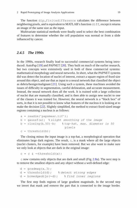
In the 1990s, research finally lead to successful commercial systems being intro-duced: AutoPap [19] and PAPNET [20]. They built on much of the earlier research,but two concepts were extensively used in both of these commercial systems:mathematical morphology and neural networks. In short, what the PAPNET systemsdid was detect the location of nuclei of interest, extract a square region of fixed sizearound this object, and use that as input to a neural network that classified the objectas debris/benign/malignant [21]. Using such a system, these machines avoided theissues of difficulty in segmentation, careful delineation, and accurate measurement.Instead, the neural network does all the work. It is trained with a large collectionof nuclei that are manually classified, and is then able to assign new nuclei to oneof the classes it was trained for. However, the neural network is a “black box” ofsorts, in that it is not possible to know what features of the nucleus it is looking at tomake the decision [22]. Slightly simplified, the method to extract fixed-sized imageregions containing a nucleus is as follows:
a = readim(’papsmear.tif’);b = gaussf(a); % slight smoothing of the imageb = closing(b,50)-b; % top-hat, max. diameter is 50
pixelsc = threshold(b);
The closing minus the input image is a top-hat, a morphological operation thateliminates large dark regions. The result, c, is a mask where all the large objects(nuclei clusters, for example) have been removed. But we also want to make surewe only look at objects that are dark in the original image:
c = c & ∼threshold(a);c now contains only objects that are dark and small (Fig. 2.8a). The next step is
to remove the smallest objects and any object without a well-defined edge:
d = gradmag(a,3);d = threshold(d); % detect strong edgesd = brmedgeobjs(∼d); % find inner regions
The first step finds regions of large gradient magnitude. In the second stepwe invert that mask and remove the part that is connected to the image border.

20 C.L. Luengo Hendriks et al.
Fig. 2.8 Detecting the location of possible nuclei: (a) all dark, small regions, (b) all regionssurrounded by strong edges, and (c) the combination of the two
Fig. 2.9 Extracted regions around potential nuclei. These subimages are the input to a neuralnetwork
The regions that remain are all surrounded by strong edges (Fig. 2.8b). Thecombination of the two partial results,
e = c & d;
contains markers for all the medium-sized objects with a strong edge (Fig. 2.8c).These are the objects we want to pass on to the neural network for classification.We shrink these markers to single-pixel dots and extract an area around each dot(Fig. 2.9):
e = bskeleton(e,0,’looseendsaway’);% reduce each region to a single dot
coords = findcoord(e); %get the coordinates for eachdot
N = size(coords,1); % number of dotsreg = cell(N); % we’ll store the little regions in herefor ii=1:N
x = coords(ii,1);y = coords(ii,2);reg{ii} = a(x-20:x+20,y-20:y+20);
% the indexing cuts a region from the imageendreg = cat(1,reg{:}) % glue regions together for display

2 Rapid Prototyping of Image Analysis Applications 21
That last command just glues all the small regions together for display. Note that,for simplicity, we did not check the coords array to avoid out-of-bounds indexingwhen extracting the regions. One would probably want to exclude regions that fallpartially outside the image.
The PAPNET system recorded the 64 most “malignant looking” regions of theslide for human inspection and verification, in a similar way to what we did just forour single image field.
2.4.6 The 2000s
There was a reduced academic research activity in the field after the commercialdevelopments took over in the 1990s. But there was clearly room for improvements,so some groups continued basic research. This period is marked by the departurefrom the “black box” solutions, and a return to accurate measurements of specificcellular and nuclear features. One particularly active group was located in Brisbane,Australia [23]. They applied several more modern concepts to the Pap smears anddemonstrated that improved results could be achieved. For instance, they took thedynamic contour concept (better known as the “snake,” see Chapter 4) and appliedit to cell segmentation [24]. Their snake algorithm is rather complex, since theyused a method to find the optimal solution to the equation, rather than the iterativeapproach usually associated with snakes, which can get stuck in local minima. Using“normal” snakes, one can refine nuclear boundary thus:
a = readim(’papsmear.tif’)b = bopening(threshold(-a),5); % quick-and-dirty
%segmentationc = label(b); % label the nucleiN = max(c); % number of nucleis = cell(N,1); % this will hold all snakesvf = vfc(gradmag(a)); % this is the snake’s ‘‘external
force’’for ii = 1:N % we compute the snake for each nucleus
separatelyini = im2snake(c==ii); % initial snake given by
segmentations{ii} = snakeminimize(ini,vf,0.1,2,1,0,10);
% move snake so its energy is minimizedsnakedraw(s{ii}) % overlays the snake on the image
end
The snake is initialized by a rough segmentation of the nuclei (Fig. 2.10a),then refined by an iterative energy minimization procedure (snakeminimize,Fig. 2.10b). Note that we used the function vfc to compute the external force, theimage that drives the snake towards the edges of the objects. This VFC (vector field

22 C.L. Luengo Hendriks et al.
Fig. 2.10 (a) Initial snake and (b) final snake in active contour method to accurately delineatenuclei
convolution) approach is a recent improvement to the traditional snake [25]. For thisexample image, the results are rather similar when using the traditional gradient,because the initial snake position is close to its optimal. Also note the large numberof parameters used as input to the function snakeminimize, the function thatmoves the control points of the snake to minimize the snake’s energy function. Thislarge number of parameters (corresponding to the various weights in the energyfunction) indicates a potential problem with this type of approach: many valuesneed to be set correctly for the method to work optimally, and thus this particularprogram is only applicable to images obtained under specific circumstances.
2.5 The Future of Automated Cytology
An interesting observation that can be made from the brief samples of the longhistory of automated cervical cytology that has been presented in this chapter is thatthe focus of the research in the field has been moving around the world about onceevery decade – Eastern USA, Japan, Europe, Western USA/Canada, and Australia(Fig. 2.11) – although there are, of course, outliers to this pattern. This pattern mighthave arisen because of the apparent ease of the problem: when researchers in oneregion have been making strong promises of progress for too long, without beingable to deliver on these promises, it becomes increasingly difficult to obtain moreresearch funds in that region; researchers in a different region in the world are thenable to take the lead.
One significant development that we have not discussed so far is the effortsof producing cleaner specimens that are more easy to analyze than the smears,which can be very uneven in thickness and general presentation of the cells. These

2 Rapid Prototyping of Image Analysis Applications 23
Fig. 2.11 A map of the world showing the location of major Pap smear analysis automationresearch over the decades
efforts led to two commercial liquid cytology systems in the 1990s [26, 27]. Thecompanies behind these sample preparation devices have also developed dedicatedimage analysis systems. These devices work well, but the modified kits for preparingthe specimens are so expensive that most of the economic gain from automationdisappears.
The cost of automation is an important issue. One of the original motivationsfor developing automation was the high cost of visual screening. Still, the firstgeneration automated systems were very complex and expensive machines costingabout as much to operate as visual screening. The need for modified samplepreparation for some systems added to these costs. A third aspect was that thecombined effect of visual and machine screening gives a higher probability ofactually detecting a lesion than either one alone, making it hard in some countries,due to legal liability reasons, to use automation alone even if it is comparable inperformance to visual screening. All of this has made the impact of automation verylimited in the poorer parts of the world, so cervical cancer is still killing a quartermillion women each year. Most of these deaths could be prevented by a globallyfunctioning screening program.
A significant challenge for the future, therefore, is to come up with a screeningsystem that is significantly cheaper than the present generation. How can this beachieved? Looking at the history we can see two approaches.
One is the “rare event” approach. Modern whole-slide scanners are much morerobust, cheaper, and easier to operate than earlier generations of robot microscopes.With software for such systems, a competitive screening system should be possible,perhaps utilizing a somewhat modified specimen preparation approach that givescleaner specimens without the high cost of the present liquid-based preparations.
The alternative approach is to use the MAC concept. The obstacle there is toachieve sufficiently robust imaging to consistently detect the subtle changes ofchromatin texture between normal and malignancy-influenced cells in an automated

24 C.L. Luengo Hendriks et al.
system. A malignancy-influenced cell looks too much like a normal cell when it isslightly out of focus or poorly segmented. Here, modern 3D scanning concepts maymake a significant difference.
So perhaps the next generation systems will be developed in third-world coun-tries, to solve their great need for systems that are better and more economical thanthe systems that have been developed in the richer parts of the world.
2.6 Conclusions
As we have seen, the availability of a toolbox of image analysis routines greatlysimplifies the process of “quickly trying out” an idea. Some of the algorithms thatwe approximated using only two or three lines of code would require many hundredsof lines of code without such a toolbox.
Another benefit to using an environment like MATLAB is the availability ofmany other tools not directly related to images that are very useful in developingnovel algorithms. For example, in this chapter we have created graphs with someof the intermediate results. Being able to graphically see the numbers obtainedis invaluable. In Sect. 2.4.5, we implemented only the first stage of the PAPNETsystem, but with equal ease we could have constructed the rest, using any of theneural network toolboxes that exist for MATLAB.
These two benefits are augmented in the MATLAB/DIPimage environment withan interpreted language, allowing interactive examination of intermediate results,and a high-level syntax, allowing easy expression of mathematical operations.The downside is that certain algorithms can be two orders of magnitude fasterwhen expressed in C than in MATLAB, and algorithms written in MATLAB aremore difficult to deploy. A common approach is to develop the algorithms inMATLAB, and translate them to C, C++, or Java when the experimentation phaseis over. Though it is not always trivial to translate MATLAB code to C, MATLABcode that uses DIPimage has a big advantage: most of the image processing andanalysis routines are implemented in a C library, DIPlib, that can be distributedindependently of the DIPimage toolbox and MATLAB. All these things considered,even having to do the programming a second time in C, one can save largeamounts of time when doing the first development in an environment such as thatdescribed here.
References
1. Luengo Hendriks, C.L., van Vliet, L.J., Rieger, B., van Ginkel, M., Ligteringen, R.: DIPimageUser Manual. Quantitative Imaging Group, Delft University of Technology, Delft, TheNetherlands (1999–2010)

2 Rapid Prototyping of Image Analysis Applications 25
2. Traut, H.F., Papanicolaou, G.N.: Cancer of the uterus: the vaginal smear in its diagnosis. Cal.West. Med. 59(2), 121–122 (1943)
3. Christopherson, W.M., Parker, J.E., Mendez, W.M., Lundin Jr., F.E.: Cervix cancer death ratesand mass cytologic screening. Cancer 26(4), 808–811 (1970)
4. Bengtsson, E.: Fifty years of attempts to automate screening for cervical cancer. Med. ImagingTechnol. 17(3), 203–210 (1999)
5. Tolles, W.E., Bostrom, R.C.: Automatic screening of cytological smears for cancer: theinstrumentation. Ann. N. Y. Acad. Sci. 63, 1211–1218 (1956)
6. Spencer, C.C., Bostrom, R.C.: Performance of the Cytoanalyzer in recent clinical trials. J. Natl.Cancer Inst. 29, 267–276 (1962)
7. Prewitt, J.M.S., Mendelsohn, M.L.: The analysis of cell images. Ann. N. Y. Acad. Sci. 128(3),1035–1053 (1965)
8. Watanabe, S., the CYBEST group: An automated apparatus for cancer prescreening: CYBEST.Comput. Graph. Image Process. 3(4), 350–358 (1974)
9. Tanaka, N., Ikeda, H., Ueno, T., Watanabe, S., Imasato, Y.: Fundamental study of automaticcyto-screening for uterine cancer. II. Segmentation of cells and computer simulation. ActaCytol. 21(1), 79–84 (1977)
10. Tanaka, N., Ikeda, H., Ueno, T., Takahashi, M., Imasato, Y.: Fundamental study of automaticcyto-screening for uterine cancer. I. Feature evaluation for the pattern recognition system. ActaCytol. 21(1), 72–78 (1977)
11. Tanaka, N., Ueno, T., Ikeda, H., Ishikawa, A., Yamauchi, K., Okamoto, Y., Hosoi, S.: CYBESTmodel 4: automated cytologic screening system for uterine cancer utilizing image analysisprocessing. Anal. Quant. Cytol. Histol. 9(5), 449–453 (1987)
12. Burger, G., Jutting, U., Rodenacker, K.: Changes in benign cell populations in cases of cervicalcancer and its precursors. Anal. Quant. Cytol. 3(4), 261–271 (1981)
13. MacAulay, C., Palcic, B.: An edge relocation segmentation algorithm. Anal. Quant. Cytol.Histol. 12(3), 165–171 (1990)
14. Serra, J.: Image Analysis and Mathematical Morphology. Academic, London (1982)15. Kuhl, F.P., Giardina, C.R.: Elliptic Fourier features of a closed contour. Comput. Graph. Image
Process. 18(3), 236–258 (1982)16. Haralick, R.M., Shanmugam, K., Dinstein, I.: Textural features for image classification. IEEE
Trans. Syst. Man Cybern. 3(6), 610–621 (1973)17. Galloway, M.M.: Texture analysis using gray level run lengths. Comput. Graph. Image Process.
4(2), 172–179 (1975)18. MacAulay, C., Palcic, B.: Fractal texture features based on optical density surface area. Use in
image analysis of cervical cells. Anal. Quant. Cytol. Histol. 12(6), 394–398 (1990)19. Lee, J., Nelson, A., Wilbur, D.C., Patten, S.F.: The development of an automated Papanicolaou
smear screening system. Cancer 81, 332–336 (1998)20. DeCresce, R.P., Lifshitz, M.S.: PAPNET cytological screening system. Lab Med. 22, 276–280
(1991)21. Luck, R.L., Scott, R.: Morphological classification system and method. US Patent 5,257,182,
199322. Duda, R.O., Hart, P.E., Stork, D.G.: Pattern Classification, 2nd edn. Wiley, New York (2001)23. Mehnert, A.J.H.: Image Analysis for the Study of Chromatin Distribution in Cell Nuclei. Ph.D.
Thesis, University of Queensland, Brisbane, Australia, 200324. Bamford, P., Lovell, B.: Unsupervised cell nucleus segmentation with active contours. Signal
Process. 71(2), 203–213 (1998)25. Li, B., Acton, S.T.: Active contour external force using vector field convolution for image
segmentation. IEEE Trans. Image Process. 16(8), 2096–2106 (2007)26. Hutchinson, M.L., Cassin, C.M., Ball, H.G.: The efficacy of an automated preparation device
for cervical cytology. Am. J. Clin. Pathol. 96(3), 300–305 (1991)27. Howell, L.P., Davis, R.L., Belk, T.I., Agdigos, R., Lowe, J.: The AutoCyte preparation system
for gynaecologic cytology. Acta Cytol. 42(1), 171–177 (1998)


Chapter 3Seeded Segmentation Methods for MedicalImage Analysis
Camille Couprie, Laurent Najman, and Hugues Talbot
Segmentation is one of the key tools in medical image analysis. The objective ofsegmentation is to provide reliable, fast, and effective organ delineation. Whiletraditionally, particularly in computer vision, segmentation is seen as an early visiontool used for subsequent recognition, in medical imaging the opposite is often true.Recognition can be performed interactively by clinicians or automatically usingrobust techniques, while the objective of segmentation is to precisely delineatecontours and surfaces. This can lead to effective techniques known as “intelligentscissors” in 2D and their equivalent in 3D.
This chapter is divided as follows. Section 3.1 starts off with a more “philosoph-ical” section setting the background for this study. We argue for a segmentationcontext where high-level knowledge, object information, and segmentation methodare all separate.
In Sect. 3.2, we survey in some detail a number of segmentation methods thatare well-suited to image analysis, in particular of medical images. We illustrate this,make some comparisons and some recommendations.
In Sect. 3.3, we introduce very recent methods that unify many popular discretesegmentation methods and we introduce a new technique. In Sect. 3.4, we give someremarks about recent advances in seeded, globally optimal active contour methodsthat are of interest for this study.
In Sect. 3.5, we compare all presented methods qualitatively. We then concludeand give some indications for future work.
H. Talbot (�)Universite Paris-Est, Paris, France
G. Dougherty (ed.), Medical Image Processing: Techniques and Applications, Biologicaland Medical Physics, Biomedical Engineering, DOI 10.1007/978-1-4419-9779-1 3,© Springer Science+Business Media, LLC 2011
27

28 C. Couprie et al.
3.1 The Need for Seed-Driven Segmentation
Segmentation is a fundamental operation in computer vision and image analysis. Itconsists of identifying regions of interests in images that are semantically consistent.Practically, this may mean finding individual white blood cells amongst red bloodcells; identifying tumors in lungs; computing the 4D hyper-surface of a beatingheart, and so on.
Applications of segmentation methods are numerous. Being able to reliably andreadily characterize organs and objects allows practitioners to measure them, countthem and identify them. Many images analysis problems begin by a segmentationstep, and so this step conditions the quality of the end results. Speed and ease of useare essential to clinical practice.
This has been known for quite some time, and so numerous segmentationmethods have been proposed in the literature [57]. However, segmentation is adifficult problem. It usually requires high-level knowledge about the objects understudy. In fact, semantically consistent, high-quality segmentation, in general, isa problem that is indistinguishable from strong Artificial Intelligence and hasprobably no exact or even generally agreeable solution. In medical imaging, expertsoften disagree amongst themselves on the placement of the 2D contours of normalorgans, not to mention lesions. In 3D, obtaining expert opinion is typically difficult,and almost impossible if the object under study is thin, noisy and convoluted, suchas in the case of vascular systems. At any rate, segmentation is, even for humans, adifficult, time-consuming and error-prone procedure.
3.1.1 Image Analysis and Computer Vision
Segmentation can be studied from many angles. In computer vision, the segmen-tation task is often seen as a low-level operation, which consists of separating anarbitrary scene into reasonably alike components (such as regions that are consistentin terms of color, texture and so on). The task of grouping such component intosemantic objects is considered a different task altogether. In contrast, in imageanalysis, segmentation is a high-level task that embeds high-level knowledge aboutthe object.
This methodological difference is due to the application field. In computer vision,the objective of segmentation (and grouping) is to recognize objects in an arbitraryscene, such as persons, walls, doors, sky, etc. This is obviously extremely difficultfor a computer, because of the generality of the context, although humans dogenerally manage it quite well. In contrast, in image analysis, the task is often toprecisely delineate some objects sought in a particular setting known in advance.It might be for instance to find the contours of lungs in an X-ray photograph.
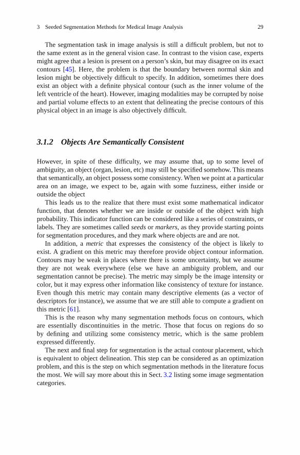
3 Seeded Segmentation Methods for Medical Image Analysis 29
The segmentation task in image analysis is still a difficult problem, but not tothe same extent as in the general vision case. In contrast to the vision case, expertsmight agree that a lesion is present on a person’s skin, but may disagree on its exactcontours [45]. Here, the problem is that the boundary between normal skin andlesion might be objectively difficult to specify. In addition, sometimes there doesexist an object with a definite physical contour (such as the inner volume of theleft ventricle of the heart). However, imaging modalities may be corrupted by noiseand partial volume effects to an extent that delineating the precise contours of thisphysical object in an image is also objectively difficult.
3.1.2 Objects Are Semantically Consistent
However, in spite of these difficulty, we may assume that, up to some level ofambiguity, an object (organ, lesion, etc) may still be specified somehow. This meansthat semantically, an object possess some consistency. When we point at a particulararea on an image, we expect to be, again with some fuzziness, either inside oroutside the object
This leads us to the realize that there must exist some mathematical indicatorfunction, that denotes whether we are inside or outside of the object with highprobability. This indicator function can be considered like a series of constraints, orlabels. They are sometimes called seeds or markers, as they provide starting pointsfor segmentation procedures, and they mark where objects are and are not.
In addition, a metric that expresses the consistency of the object is likely toexist. A gradient on this metric may therefore provide object contour information.Contours may be weak in places where there is some uncertainty, but we assumethey are not weak everywhere (else we have an ambiguity problem, and oursegmentation cannot be precise). The metric may simply be the image intensity orcolor, but it may express other information like consistency of texture for instance.Even though this metric may contain many descriptive elements (as a vector ofdescriptors for instance), we assume that we are still able to compute a gradient onthis metric [61].
This is the reason why many segmentation methods focus on contours, whichare essentially discontinuities in the metric. Those that focus on regions do soby defining and utilizing some consistency metric, which is the same problemexpressed differently.
The next and final step for segmentation is the actual contour placement, whichis equivalent to object delineation. This step can be considered as an optimizationproblem, and this is the step on which segmentation methods in the literature focusthe most. We will say more about this in Sect. 3.2 listing some image segmentationcategories.

30 C. Couprie et al.
3.1.3 A Separation of Powers
In summary, to achieve segmentation in the analysis framework, we need threeingredients: (1) an indicator function that denotes whether we are inside or outsideof the object of interest; (2) a metric from which we may derive contour information,and (3) an optimization method for placing the contour accurately.
To achieve accuracy, we need flexibility and robustness. Some have argued thatit is useful to treat these three steps separately. This was first described in [47])as the morphological method, but is also called by others interactive or seededsegmentation [31]. In this context, this does not mean that user interaction isrequired, only that object identification is provided by some means, and contourextraction separately by a segmentation operator.
The first ingredient, the object identification, or our indicator function, is ofcourse essential and it is frustrating to be obliged to only write here “by somemeans”. Accurate content identification can simplify the requirements on thesegmentation operator greatly. Unfortunately, the means in question for contentsidentification are problem-dependent and sometimes difficult to publish, becausethey are often seen as ad hoc and of limited interest beyond their immediate use inthe problem at hand. Fortunately, some journals accept such publications, such as theJournal of Image Analysis and Stereology and applications journals (e.g. Journal ofMicroscopy, materials, etc). There are also a few recent books on the matter [23,52].Software libraries are also important but not many are freely available for training,although the situation is improving.
Also, whereas in computer vision a fully automated solution is required, in medi-cal imaging a semi-automated method might be sufficient. In biomedical imaging, alarge number of objects are typically measured (such as cells, organelles, etc.), anda fully automated method is often desirable. However, in medical imaging, typicallya relatively small number of patients is being monitored, treated or surveyed, and sohuman-guided segmentation can be sufficient. The objective of the segmentationmethod in this context is to provide reasonable contours quickly, which can beadjusted easily by an operator.
In this variety of contexts, is it possible to define precisely the segmentationproblem? The answer is probably no, at this stage at least in image analysis research.However, it is possible to provide formulations of the problem. While this maysound strange or even suspicious, the reason is that there exists a real need forautomated or semi-automated segmentation procedures for both image analysis andcomputer vision, and so solutions have been proposed. They can still be explained,compared and evaluated.
3.1.4 Desirable Properties of Seeded Segmentation Methods
We come to the first conclusion that to provide reliable and accurate results, wemust rely on a segmentation procedure and not just an operator. Object identification

3 Seeded Segmentation Methods for Medical Image Analysis 31
and constraints analysis will set us in good stead to achieve our results, but not allsegmentation operators are equivalent. We can list here some desirable properties ofinteractive segmentation operators.
• It is useful if the operator can be expressed in an energy or cost optimizationformulation. It is then amenable to existing optimization methods, and this entailsa number of benefits. Lowering the cost or the energy of the formulation can bedone in several ways (e.g. continuous or discrete optimization), which results indifferent characteristics and compromises, say between memory resources andtime. Optimization methods improve all the time through the work of researchers,and so our formulations will benefit too.
• It is desirable if the optimization formulation can provide a solution that is atleast locally optimal, and if possible globally optimal, otherwise noise will almostcertainly corrupt the result.
• The operator should be fast, and provide guaranteed convergence, because it willbe most likely restarted several times, in order to adjust parameters. Together withthis requirement, the ability to segment many objects at once is also desirable,otherwise the operator will need to be restarted as many time as there are objectsin the image. This may not be a big problem if objects do not overlap and ifbounding boxes can be drawn around them, because the operator can then be runonly within the bounding box, but this is not the general case.
• The operator should be bias-free: e.g. with respect to objects size or to thediscretization grid or with respect to initialization.
• The operator should be flexible: it is useful if it can be coupled with topologyinformation for instance, or with multi-scale information.
• It should be generic, not tied to particular data or image types.• It should be easy to use. This in practice means possessing as few parameters as
possible. Of course one can view constraints setting as an enormous parameterlist, but this is the reason why we consider this step as separate.
Such a method certainly does not yet exist to our knowledge, although somemight be considered to come close. We describe some of them in the next section.
3.2 A Review of Segmentation Techniques
Here, we list and detail some segmentation categories that are compatible with theimage analysis viewpoint, although cannot hope to present a complete descriptionof this field.
3.2.1 Pixel Selection
Pixel selection is likely the oldest segmentation method. It consists of selectingpixels solely based on their values and irrespective of their spatial neighborhood.

32 C. Couprie et al.
The simplest pixel selection method is humble thresholding, where we select pixelsthat have a gray-level value greater or smaller than some threshold value. Thisparticular method is of course very crude, but is used frequently nonetheless.Multiple thresholding uses several values instead of a single value; color and multi-spectral thresholding using vectors of values and not just scalars. By definition allhistogram-based methods for finding the parameters of the thresholding, includingthose that optimize a metric to achieve this [54], are pixel selection methods.Statistical methods (e.g. spectral classification methods) that include no spatialregularization fall into this category as well. This is therefore a veritable plethoraof methods that we are including here, and research is still active in this domain.
Of course, thresholding and related methods are usually very fast and easily madeinteractive, which is why they are still used so much. By properly pre-processingnoisy, unevenly illuminated images, or by other transforms, it is surprising howmany problems can be solved by interactive or automated thresholding. However,this is of course not always the case, hence the need for more sophisticated methods.
3.2.2 Contour Tracking
It was realized early on that (1) human vision is sensitive to contours and (2) thereis a duality between simple closed contours and objects. A simple closed contour(or surface) is one that is closed and does not self-intersect. By the Jordan theorem,in the Euclidean space, any such contour or surface delineates a single object offinite extent. There are some classical difficulties with the Jordan theorem in thediscrete setting [52], but they can be solved by selecting proper object/backgroundconnectivities, or by using a suitable graph, for instance, the 6-connected hexagonalgrid or the Khalimsky topology [22, 40].
A contour can be defined locally (it is a frontier separating two objects (oran object and its background in the binary case)), while an object usually cannot(an object can have an arbitrary extent). A gradient (first derivative) or a Laplacian(second derivative) operator can be used to define an object border in many cases,and gradients are less sensitive to illumination conditions than pixel values. As aresult, contour detection through the use of gradient or Laplacian operators becamepopular, and eventually led to the Marr–Hildreth theory [44].
Given this, it is only natural that most segmentation method use contourinformation directly in some ways, and we will revisit this shortly. Early methodsused only this information to detect contours and then tried to combine them in someway. By far the most popular and successful version of this approach is the Cannyedge detector [9]. In his classical paper, Canny proposed a closed-form optimal1D edge detector assuming the presence of additive white Gaussian noise, andsuccessfully proposed a 2D extension involving edge tracking using non-maximasuppression with hysteresis.

3 Seeded Segmentation Methods for Medical Image Analysis 33
One problem with this approach is that there is no optimality condition in 2D,no topology or connectivity constraints and no way to impose markers in the finalresult. All we get is a series of contours, which may or may not be helpful. Findinga suitable combination of detected contours (which can be incomplete) to defineobjects is then a combinatorial problem of high complexity. Finally, this approachextends even less to 3D.
Overall, in practical terms, these contour tracking methods have been supersededby more recent methods and should not be used without good reasons. For instance,more recent minimal-path methods can be applied to contour tracking methods,although they are much more sophisticated in principle [3, 14]. In this class ofmethods belongs also the “intelligent scissors” types. There were many attempts inprevious decades to provide automated delineating tools in various image processingsoftware packages, but a useful contribution was provided relatively recently byMortensen [48]. This method is strictly interactive, in the sense that it is designedfor human interaction and feedback. “Intelligent scissor” methods are useful toclinicians for providing ground truth data for instance. Such methods are still strictly2D. As far as we know, no really satisfying 3D live-wire/intelligent scissor method isin broad use today [5]. However, minimal surfaces methods, which we will describeshortly in Sect. 3.4.3, in some ways do perform this extension to nD [30].
3.2.3 Statistical Methods
The opposite approach to contour detection is to work on the objects, or regionsthemselves. An early and intuitive approach has been to try to divide (the splittingstep) an image into uniform regions, for example using a hierarchical representationof an image in the form of quadtrees (in 2D) and octrees (in 3D). Uniformitycan be defined by statistical parameters and/or tests. Subsequently, a merging stepconsidering neighboring and statistical region information is performed [36]. Initialconsidered statistics were color and intensity, but other region descriptors can beused as well, for instance including texture, motion and so on. In this approach,even though regions statistics are used, they are inevitably derived at the pixel level.The split and merge approach consists of acquiring all the statistics first and basinga decision on them.
A different approach, which is also productive, consists of building a modelfirst. One way is to consider an image as a 2D or 3D graph of pixels, to startfrom a vast over-segmentation at the pixel level, and to evolve cliques of pixels(e.g. sets of one, two or more pixels that are fully-connected, respectively calledunary, binary or higher-level cliques) to fit that model. This is the Markov RandomField (MRF) model, named in this way by comparison to classical one-dimensionalMarkov chains, for which only immediate neighboring relationships matter. Modelsthat can be written using these cliques turn out to corresponds to energies featuring

34 C. Couprie et al.
weighted finite sums with as many terms as there are different kinds of cliques.In [26] Geman and Geman proposed to optimize these sums using Gibbs sampling (aform of Monte-Carlo Markov Chain algorithm) and simulated annealing. This wasfirst used for image restoration, but can be readily applied to segmentation as well.This approach was very successful because it is very flexible. Markers and textureterms can be added in, and many algorithmic improvement were proposed overthe years. However, it remains a relatively costly and slow approach. Even thoughGeman and Geman showed that their simulated annealing strategy converges, it onlydoes so under conditions that make the algorithm extremely slow, and so usuallyonly a non-converged or approximate result is used. More recently, it was realizedthat Graph-Cut (GC) methods were well-suited to optimized some MRF energiesvery efficiently. We will give more details in the corresponding section.
MRFs belong to the larger class of Bayesian methods. Information-theoreticperspectives and formulations, such as following the Minimum Description Lengthprinciple, also exist. These frameworks are also very flexible, allowing for exampleregion competition [69]. However, the corresponding models might be complicatedboth to understand and run, and sometimes possess many parameters that are notobvious to tune. Well-designed methods are guaranteed to converge to at least alocal minimum.
In general, when dealing with regions that have complex content (for instance,textures, or multispectral content), statistical methods can be a very good choicealthough they cannot be recommended for general work, since simpler and fastermethods often are sufficient.
3.2.4 Continuous Optimization Methods
In the late 1980s, it was realized that contour tracking methods were too limited forpractical use. Indeed, getting closed contours around objects were difficult to obtainwith contour tracking. This meant that detecting actual objects was difficult exceptin the simplest cases.
3.2.4.1 Active Contours
Researchers, therefore, proposed to start from already-closed loops, and to makethem evolve in such a way that they would converge towards the true contours ofthe image. Thus were introduced active contours, or snakes [39]. The formulationof snakes takes the following continuous-domain shape:
Esnake =∫ 1
0{Einternal(v(s))+ Edata(v(s))+ Econstraints(v(s))}ds. (3.1)
where v(s) is a parametric representation of the contour.

3 Seeded Segmentation Methods for Medical Image Analysis 35
This model is very flexible. It contains internal terms, image data terms andconstraints terms (see Chapter 4 for more details):
• The first term, the internal energy, contains a curvature term and a “rubber band”energy. The former tends to smooth the resulting contour following a thin plate,while the latter tends to make it shrink around features of interest. Other termssuch as kinetic energy can be added too, which makes it possible for the snake toavoid noisy zones and flat areas.
• The second term, the data energy, attracts the active contours towards points ofinterest in the image: typically, image contours (zones of high gradient), lines ortermination points.
• The last term, the constraint term, is optional, but allows interaction with thesnake by defining zones of attraction and repulsion.
To solve this equation, the Euler–Lagrange of (3.1) is worked out (typically inclosed form), and a gradient descent algorithm is used. All the terms are combinedin a linear combination, allowing them to be balanced according to the needs of theuser. Due to its flexibility, the active contour model was very popular in the literatureas well as in applications. It fits very well into the interactive segmentation paradigmbecause constraints can be added very easily, and it can be quite fast because it uses aso-called Lagrangian framework. The contour itself is discretized at regular intervalpoints and evolves according to (3.1). Convergence towards a local minimum of theenergy is guaranteed, but may require many iterations.
In practice, there are some difficulties: the snake energy is flexible but difficultto tune. Because of the contour evolution, points along the contour tend to spreadout or bunch up, requiring regular and frequent resampling. There can also betopological difficulties, for instance causing the snake to self-intersect. The snakeis also sensitive to its parametrization and to initialization. Finally, even though alocal optimum is guaranteed, in practice, it may not be of good quality due to noisesensitivity.
One major difficulty with snakes is that they can be extended to 3D viatriangulation, but such extensions can be complicated, and topological problemsplaguing snakes in 2D are usually more difficult to avoid in 3D. However, 3D activesurfaces are still widely used, because they make it easy to improve or regularize atriangulated surface obtained by other means. For instance, the brain segmentationsoftware FreeSurfer includes such a method. To distinguish them from other modelswe are going to introduce now, snake-like active contours or surfaces are sometimescalled parametric deformable models.
3.2.4.2 Level Sets
One way to avoid altogether some of the problems brought about by the wayparametric deformable models are discretized, is to embed the contour into a higher-dimensional manifold. This idea gave rise to level sets, proposed by Osher andSethian in 1988 [53]. Remarkably, this is around the same time when active contours

36 C. Couprie et al.
a b
Fig. 3.1 Embedding and evolving a curve as a level set of a higher-dimension function. The zero-level of function ψ is shown in color, representing a 2D contour. To evolve the contour, the wholefunction evolves. Note that topology changes can occur in the contour, while the embedding surfaceshows no such effect
were proposed. However level sets were initially proposed for computational fluiddynamics and numerical simulations. They were applied to imaging somewhatlater [43, 62]. A contour is represented on the surface S of an evolving regularfunction ψ by its zero level-set, which is simply the threshold of the function ψ atzero. By using sufficiently regular embedding functions ψ , namely signed distancetransforms from an initial contour, it was possible to propose effective evolutionequations to solve similar problems to Lagrangian active contours.
The main advantages of the level-sets method were that contour resampling wasno longer necessary, and contour self-intersection (shock solutions) was avoidedbecause level sets were able to change topology easily (see Fig. 3.1b). This meanspractically that it was possible at least in theory to initialize a segmentation by draw-ing a box around a series of object of interest, and the level set could find a contouraround each of them. This was seen as a major benefit by the vision community.The level set Eulerian formulation (where the whole space is discretized) is thoughtto offer better theoretical guarantees than the Lagrangian framework of previousnon-embedded formulations, and the simulation of function evolution is a well-researched topic with many usable and interesting results. Finally, the formulation isdimension independent. Level sets work virtually unchanged in 3D or more, whichis a major benefit.
There are also a number of drawbacks. First, the level set formulation is moreexpensive than earlier active contour formulations. It requires the iterative solvingof PDEs in the whole space, which is expensive. In practice, it is possible to limitthe computation in a narrow band around the contour, but this is still more costlythan if they were limited to the contour itself, and requires the resampling thatwas sought to be avoided. The surface S of function ψ is implicitly representedby the function itself, but it requires more space than the contour. In 3D or more,

3 Seeded Segmentation Methods for Medical Image Analysis 37
this may be prohibitive. Some contour motions are not representable (e.g. contourrotation), but this is a minor problem. More importantly, the fact that level-sets canundergo topology changes is actually a problem in image analysis, where it is usefulto know that a contour initialized somewhere will converge to a single simple closedcontour. In some cases, a contour can split or even disappear completely, leading toundesirable results.
Nonetheless, level-set formulations are even more flexible than active contours,and very complex energies solving equally complex problems have been proposedin the literature. Solving problem involving texture, motion, competing surfacesand so on is relatively easy to formulate in this context [55, 56]. For this reason,they were and remain popular. Complex level-set formulation tend to be sensitive tonoise and can converge to a poor locally optimal solution. On the other hand, morerobust, closer to convex solutions can now be solved via other means. An exampleof relatively simple PDE that can be solved by level sets is the following:
ψt + F|∇ψt | = 0, (3.2)
where F is the so-called speed function. Malladi and Sethian proposed the followingfor F :
F =1− εκ1 + |∇I| + β (∇ψ .∇|∇I|). (3.3)
The first part of the equation is a term driving the embedding function ψtowards contours of the image with some regularity and smoothing controlled bythe curvature κ . The amount of smoothing is controlled by the parameter ε . Thesecond term is a “balloon” force that tends to expand the contour. It is expected thatthe contour initially be placed inside the object of interest, and that this balloon forceshould be reduced or eliminated after some iterations, controlled by the parameter β .We see here that even though this model is relatively simple for a level-set one, italready has a few parameters that are not obvious to set or optimize.
3.2.4.3 Geodesic Active Contours
An interesting attempt to solve some of the problems posed by overly generallevel sets was to go back and simplify the problem, arguing for consistency and ageometric interpretation of the contour obtained. The result was the geodesic activecontour (GAC), proposed by Caselles et al. in 1997 [10]. The level set formulationis the following:
ψt = |∇ψ |div
(g(I)
∇ψ|∇ψ|
). (3.4)
This equation is virtually parameter-free, with only a g function required. Thisfunction is a metric and has a simple interpretation: it defines at point x the cost ofa contour going through x. This metric is expected to be positive definite, and in

38 C. Couprie et al.
most cases is set to be a scalar functional with values in R+. In other words, the
GAC equation finds the solution of:
argminC
∫C
g(s)ds, (3.5)
where C is a closed contour or surface. This is the minimal closed path or minimalclosed surface problem, i.e. finding the closed contour (or surface) with minimumweight defined by g. In addition to simplified understanding and improved consis-tency, (3.4) has the required form for Weickert’s PDE operator splitting [28, 68],allowed PDEs to be solved using separated semi-implicit schemes for improvedefficiency. These advances made GAC a reference method for segmentation, whichis now widely used and implemented in many software packages such as ITK.The GAC is an important interactive segmentation method due to the importanceof initial contour placement, as with all level-sets methods. Constraints such asforbidden or attracting zones can all be set through the control of function g, whichhas an easy interpretation.
As an example, to attract the GAC towards zones of actual image contours, wecould set
g ≡ 11 + |∇I|p , (3.6)
With p = 1 or 2. We see that for this function, g is small (costs little) for zoneswhere the gradient is high. Many other functions, monotonically decreasing forincreasing values for ∇I, can be used instead. One point to note, is that GAC has aso-called shrinking bias, due to the fact that the globally optimal solution for (3.5)is simply the null contour (the energy is then zero). In practice, this can be avoidedwith balloon forces but the model is again non-geometric. Because GAC can onlyfind a local optimum, this is not a serious problem, but this does mean that contoursare biased towards smaller solutions.
3.2.5 Graph-Based Methods
The solution to (3.5) proposed in the previous section was in fact inspired bypreexisting discrete solutions to the same problem. On computers, talking aboutcontinuous-form solutions is a bit of a misnomer. Only the mathematical formula-tion is continuous, the computations and the algorithms are all necessarily discreteto be computable. The idea behind discrete algorithm is to embrace this constraintand embed the discrete nature of numerical images in the formulation itself.
3.2.5.1 Graph Cuts
We consider an image as a graph Γ (V ,E ) composed of n vertices V and m edges E .For instance, a 2D N ×N 4-connected square grid image will have n = N2 vertices

3 Seeded Segmentation Methods for Medical Image Analysis 39
and m = 2×N × (N − 1) edges.1 We assume that both the edges and the verticesare weighted. The vertices will typically hold image pixel values and the edgevalues relate to the gradient between their corresponding adjacent pixels, but this isnot necessary. We assume furthermore that a segmentation of the graph can berepresented as a graph partition, i.e:
V =⋃
Vi∈ΓVi;∀i �= j,Vj ∩Vi = /0. (3.7)
Then E� is the set of edges that are such that their corresponding vertices are indifferent partitions.
E� = {e = {pi, p j} ∈ E, pi ∈Vi; p j ∈Vj, i �= j}. (3.8)
The set E� is called the cut, and the cost of the cut is the sum of the edge weightsthat belong to the cut:
C(E�) = ∑e∈E�
we, (3.9)
where we is the weight of individual edge e. We assume these weights to bepositive. Reinterpreting these weights as capacities, and specifying a set of verticesas connected to a source s and a distinct set connected to a sink t, the celebrated1962 Ford and Fulkerson result [25] is the following:
Theorem 3.1. Let P be a path in Γ from s to t. A flow through that path is a quantitywhich is constrained by the minimum capacity along the path. The edges with thiscapacity are said to be saturated, i.e. the flow that goes through them is equal totheir capacity. For a finite graph, there exists a maximum flow that can go throughthe whole graph Γ. This maximum flow saturates a set of edges Es. This set of edgesdefine a cut between s and t, and this cut has minimal weight.
This theorem is illustrated in Fig. 3.2.In 2D and if Γ is planar, this duality essentially says that the Ford and Fulkerson
minimum cut can be interpreted as a shortest path in a suitable dual graph to Γ [2].In arbitrary dimension, the maxflow – mincut duality allows us to compute discreteminimal hypersurfaces by optimizing a discrete version of (3.4).
There exist many algorithms that can be used to compute the maximum flow ina graph (also called network in this framework), but none with a linear complexity.Augmenting paths algorithms [7] are effective in 2D where the number of verticesis relatively high compared to the number of edges. In 3D and above, where thereverse is true, push-relabel algorithms [27] are more efficient. These algorithmscan only be used when there is one source and one sink. The case where there aremultiple sources or sinks is known to be NP-hard. To compute energies comprisingseveral sources or sinks and leading to multi-label segmentation, approximations
1This particular computation is left as an exercise to the reader.

40 C. Couprie et al.
S
t
S
t
a b
Fig. 3.2 (a) A graph with edge weights interpreted as capacities, shown as varying diameters inthis case. (b) A maximum flow on this graph. We see that the saturated vertices (in black) separates from t , and they form a cut of minimum weight
can be used, such as α-expansions. These can be used to formulate and optimizecomplex discrete energies with MRF interpretations [8, 66], but the solution is onlyapproximate. Under some conditions, the result is not necessarily a local minimumof the energy, but can be guaranteed not to be too far from the globally optimalenergy (within a known factor, often 2).
In the last 10 years, GC methods have become extremely popular due to theirability to solve a large number of problems in computer vision, particularly instereo-vision and image restoration. In image analysis, their ability to form aglobally optimal binary partition with a geometric interpretation is very useful.However, GC do have some drawbacks. They are not easy to parallelize, they arenot very efficient in 3D, they have a so-called shrinking bias, just as GAC andcontinuous maxflow have as well. In addition, they have a grid bias, meaningthat they tend to find contours and surfaces that follow the principal directions ofthe underlying graph. This results in “blocky” artifacts, which may or may not beproblematic.
Due to their relationship with sources and sinks, which can be seen as internaland external markers, as well as their ability to modify the weights in the graph toselect or exclude zones, GC are at least as interactive as the continuous methods ofprevious sections.
3.2.5.2 Random Walkers
In order to correct some of the problems inherent to graph cuts, Grady introducedthe Random Walker (RW) in 2004 [29,32]. We set ourselves in the same frameworkas in the Graph Cuts case with a weighted graph, but we consider from the start

3 Seeded Segmentation Methods for Medical Image Analysis 41
a multilabel problem, and, without loss of generality, we assume that the edgeweights are all normalized between 0 and 1. This way, they represent the probabilitythat a random particle may cross a particular edge to move from a vertex to aneighboring one. Given a set of starting points on this graph for each label, thealgorithm considers the probability for a particle moving freely and randomly onthis weighted graph to reach any arbitrary unlabelled vertex in the graph before anyother coming from the other labels. A vector of probabilities, one for each label, istherefore computed at each unlabeled vertex. The algorithm considers the computedprobabilities at each vertex and assigns the label of the highest probability to thatvertex.
Intuitively, if close to a label starting point the edge weights are close to 1, then itscorresponding “random walker” will indeed walk around freely, and the probabilityto encounter it will be high. So the label is likely to spread unless some other labelsare nearby. Conversely, if somewhere edge weights are low, then the RW will havetrouble crossing these edges. To relate these observations to segmentation, let usassume that edge weights are high within objects and low near edge boundaries.Furthermore, suppose that a label starting point is set within an object of interestwhile some other labels are set outside of it. In this situation, the RW is likely toassign the same label to the entire object and no further, because it spreads quicklywithin the object but is essentially stopped a the boundary. Conversely, the RWspreads the other labels outside the object, which are also stopped at the boundary.Eventually, the whole image is labeled with the object of interest consistentlylabeled with a single value.
This process is similar in some way to classical segmentation procedures likeseeded region growing [1], but has some interesting differentiating properties andcharacteristics. First, even though the RW explanation sounds stochastic, in realitythe probability computations are deterministic. Indeed, there is a strong relationshipbetween random walks on discrete graphs and various physical interpretations. Forinstance, if we equate an edge weight with an electrical resistance with the samevalue, thereby forming a resistance lattice, and if we set a starting label at 1 V andall the other labels to zero volt, then the probability of the RW to reach a particularvertex will be the same as its voltage calculated by the classical Kirchhoff’s laws onthe resistance lattice [24]. The problem of computing these voltages or probabilityis also the same as solving the discrete Dirichlet problem for the Laplace equation,i.e. the equivalent of solving ∇2ϕ = 0 in the continuous domain with some suitableboundary conditions [38]. To solve the discrete version of this equation, discretecalculus can be used [33], which in this case boils down to inverting the graphLaplacian matrix. This is not too costly as it is large but very sparse. Typicallycalculating the RW is less costly and more easily parallelizable than GC, as itexploits the many advances realized in numerical analysis and linear algebra overthe past few decades.
The RW method has some interesting properties with respect to segmentation.It is quite robust to noise and can cope well with weak boundaries (see Fig. 3.3).Remarkably, in spite of the RW being a purely discrete process, it exhibits nogrid bias. This is due to the fact that level lines of the resistance distance (i.e. the
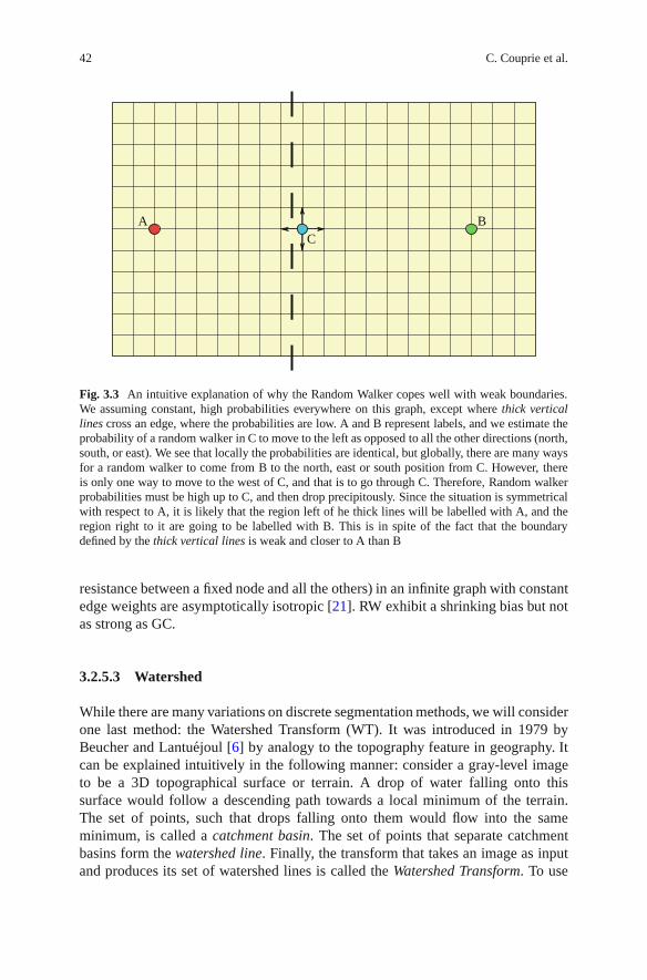
42 C. Couprie et al.
A BC
Fig. 3.3 An intuitive explanation of why the Random Walker copes well with weak boundaries.We assuming constant, high probabilities everywhere on this graph, except where thick verticallines cross an edge, where the probabilities are low. A and B represent labels, and we estimate theprobability of a random walker in C to move to the left as opposed to all the other directions (north,south, or east). We see that locally the probabilities are identical, but globally, there are many waysfor a random walker to come from B to the north, east or south position from C. However, thereis only one way to move to the west of C, and that is to go through C. Therefore, Random walkerprobabilities must be high up to C, and then drop precipitously. Since the situation is symmetricalwith respect to A, it is likely that the region left of he thick lines will be labelled with A, and theregion right to it are going to be labelled with B. This is in spite of the fact that the boundarydefined by the thick vertical lines is weak and closer to A than B
resistance between a fixed node and all the others) in an infinite graph with constantedge weights are asymptotically isotropic [21]. RW exhibit a shrinking bias but notas strong as GC.
3.2.5.3 Watershed
While there are many variations on discrete segmentation methods, we will considerone last method: the Watershed Transform (WT). It was introduced in 1979 byBeucher and Lantuejoul [6] by analogy to the topography feature in geography. Itcan be explained intuitively in the following manner: consider a gray-level imageto be a 3D topographical surface or terrain. A drop of water falling onto thissurface would follow a descending path towards a local minimum of the terrain.The set of points, such that drops falling onto them would flow into the sameminimum, is called a catchment basin. The set of points that separate catchmentbasins form the watershed line. Finally, the transform that takes an image as inputand produces its set of watershed lines is called the Watershed Transform. To use

3 Seeded Segmentation Methods for Medical Image Analysis 43
Fig. 3.4 Watershed segmentation: (a) an MRI image of the heart, (b) its smoothed gradient, (c) thegradient seen as a topographic surface, (d) Watershed of the gradient, and (e) topographical viewof the watershed
this transform in practical segmentation settings, we must reverse the point of viewsomewhat. Assume now that labels are represented by lakes on this terrain and thatby some flooding process, the water level rises evenly. The set of points that aresuch that waters from different lakes meet is also called the watershed line. Nowthis watershed line is more constrained, because there are only as many lines asnecessary to separate all the lakes.
This intuitive presentation is useful but does not explain why the WT is useful forsegmentation. As the “terrain”, it is useful to consider the magnitude of the gradientof the image. On this gradient image, interior objects will have values close to zeroand will be surrounded by zones of high values: the contours of the objects. Theycan therefore be assimilated to catchment basins, and the WT can delineate themwell (see Fig. 3.4).
The WT is a seeded segmentation method, and has many interesting interpreta-tions. If we consider the image again as a graph as in the GC setting, then on thisgraph the set of watershed lines from the WT form a graph cut. The edges of thistree can be weighted with a functional derived from a gradient exactly as in the GCcase. Computing the WT can be performed in many efficient ways [46, 67], but aninteresting one is to consider the Maximum Spanning Forest (MSF) algorithm [19].In this algorithm, the classical graph algorithm for maximum spanning tree (MST)is run on the graph of the image, following for instance Kruskal’s algorithm [41,59],with the following difference: when an edge selected by the MST algorithm isconnected with a seed, then all vertices that are connected with it become also
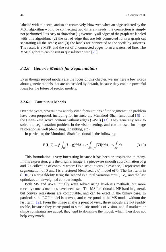
44 C. Couprie et al.
labeled with this seed, and so on recursively. However, when an edge selected by theMST algorithm would be connecting two different seeds, the connection is simplynot performed. It is easy to show that (1) eventually all edges of the graph are labeledwith this algorithm; (2) the set of edge that are left connected form a graph cutseparating all the seeds; and (3) the labels are connected to the seeds by subtrees.The result is a MSF, and the set of unconnected edges form a watershed line. TheMSF algorithm can be run in quasi-linear time [20].
3.2.6 Generic Models for Segmentation
Even though seeded models are the focus of this chapter, we say here a few wordsabout generic models that are not seeded by default, because they contain powerfulideas for the future of seeded models.
3.2.6.1 Continuous Models
Over the years, several now widely cited formulations of the segmentation problemhave been proposed, including for instance the Mumford–Shah functional [49] orthe Chan–Vese active contour without edges (AWE) [13]. They generally seek tosolve the segmentation problem in the vision setting, and can be used for imagerestoration as well (denoising, inpainting, etc).
In particular, the Mumford–Shah functional is the following:
E(f,C) = β∫
Ω(f−g)2dA + α
∫Ω\C
|∇f|2dA + γ∫
Cds. (3.10)
This formulation is very interesting because it has been an inspiration to many.In this expression, g is the original image, f a piecewise smooth approximation of gand C a collection of contours where f is discontinuous. In essence, C represents thesegmentation of ð and f is a restored (denoised, etc) model of ð. The first term in(3.10) is a data fidelity term; the second is a total variation term (TV), and the lastoptimizes an unweighted contour length.
Both MS and AWE initially were solved using level-sets methods, but morerecently convex methods have been used. The MS functional is NP-hard in general,but convex relaxations are computable, and can be exact in the binary case. Inparticular, the ROF model is convex, and correspond to the MS model without thelast term [12]. From the image analysis point of view, these models are not readilyusable, because they correspond to simplistic models of vision, and if markers orshape constraints are added, they tend to dominate the model, which then does nothelp very much.

3 Seeded Segmentation Methods for Medical Image Analysis 45
3.2.6.2 Hierarchical Models
Hierarchies of segmentations are a powerful way to deal with the multi-resolutioninherent to nature. Many images contain objects at different scales. In medicalimaging a vascular network is a typical example. It is very difficult to come upwith a seeded strategy to solve this case. One general idea is to perform manysegmentations at once or in sequence, taking into account various scales. This isnot as easy to do as it sounds, because simply repeating a segmentation procedurewith different parameters will not yield compatible segmentations, in the sense thatcontours are not likely to remain stable as the scale increases or decreases. One wayof dealing with this is to offer a measure to the strength of a particular piece ofcontour, and as the scale increase, remove pieces of contours with weak strengthfirst. This saliency idea was proposed by Najman and Schmitt in [51] in the contextof watershed segmentation, but more work has been done on this idea since, forexample, on ultrametric watershed and connections [50, 63]. A saliency map orultrametric watershed is an interactive segmentation because edge strength can beselected by interactive thresholding for instance, but it is not always obvious how tocombine this with seeded segmentation.
Hierarchical methods do offer some other benefits, such as the ability toefficiently optimize Mumford–Shah-like functionals on a saliency map [35]. Otherfunctionals are also possible, such as optimizing minimum ratio costs [34]. There aresome drawbacks as well, such as decreased speed and extra memory requirement,and again the question of compatibility with other constraints. This is at present avery interesting area of research.
3.2.6.3 Combinations
Many segmentation algorithms can be combined to provide different sets ofcompromises or extensions. For instance, Yuille proposed an interesting modelcombining Bayesian methods with level-sets [69]. An active area of research todayare so-called turbopixels, where a first-level over-segmentation is performed in orderto group pixels into consistent regions of similar size. Then these regions are linkedin a graph and a discrete segmentation is performed over them [42]. This two-level segmentation procedure has some advantages in terms of speed and resourceallocations. Final segmentation can still be precise if the first-order grouping isdone well, and these methods are compatible with seeded segmentation. However,segmentation quality may be poor in the presence of weak edges [64].
3.3 A Unifying Framework for Discrete Seeded Segmentation
In many early segmentation methods, the focus was on the values of the pixelsthemselves, or in graph terms the values of the vertices. Since the advent of GCmethods, it was realized that focusing instead on the edges was useful. In particular,

46 C. Couprie et al.
defining a gradient function on the edges is easy. Let p and q be two vertices inthe graph Γ(V ,E ) of image I, that we have been using so far (see Sect. 3.2.5),then we can set as weight wp,q for the edge linking p and q any value dependingon the discrete gradient Iq − Ip, where Iq represents the value of I at vertex q. Forinstance, we can use wp,q = exp(−β |Iq − Ip|2), with β a positive scalar parameter.This is a monotonically decreasing function of the gradient, recommended byseveral authors. In addition, there are topological advantages, as a cut in such agraph obeys the Jordan property in arbitrary dimension. In addition, there is afundamental difference between regions, formed of uniformly labeled vertices, andcuts formed of edges. In former pixel-based segmentation procedures, the contourswere themselves made of pixels, which created problems [19]. The only significantdrawback is that storing edge weights rather than pixels costs roughly twice as muchmemory in 2D, or three times as much in 3D for the simplest nearest-neighborconnectivity. This extra cost increases with the connectivity, and may be indeedbe a problem in some applications.
3.3.1 Discrete Optimization
Assuming then this simple model of discrete images, the segmentation problem canbe viewed as an optimization problem over cliques of one or two pixels, like in theMRF setting. For instance, classical graph cut can optimize the following problemexactly:
argminx E(x) = ∑u∈V
wu|xu − yu|+ ∑(u,v)∈E
wu,v|xu − xv|, (3.11)
in the case where x is a binary vertex labeling, y a reference binary image that can,for instance, represent seeds, and wu and wu,v positive unary weights and binaryweights respectively. The seeded segmentation case corresponds to an image ycontaining some vertices labelled with 0, others with 1 (the seeds) and unlabelledones as well. The wu for the labelled vertices in y have infinite weights, and theunlabeled one zero. Using the same notation, the Random Walker optimizes thefollowing energy:
argminx E(x) = ∑u∈V
wu(xu − yu)2 + ∑(u,v)∈E
wu,v(xu − xv)2. (3.12)
In this case, the optimal labelling x� is not binary even if y is binary. It expressesthe probability of a vertex belonging to label 0 or label 1. To reach a unique solution,we must threshold the result:
su = 0 if xu <12,su = 1 otherwise. (3.13)
In this case, the binary result s represents the segmentation. There is a strik-ing similarity between (3.11) and (3.12), which leads us to propose a unifyingframework.

3 Seeded Segmentation Methods for Medical Image Analysis 47
Table 3.1 Our generalized scheme for image segmentation includes severalpopular segmentation algorithms as special cases of the parameters p and q.The power watershed are previously unknown in the literature, but may beoptimized efficiently with a MSF calculation
q∖
p 0 Finite ∞1 Collapse to seeds Graph cuts Power watershed q = 12 �2 norm Voronoi Random walker Power watershed q = 2∞ �1 norm Voronoi �1 norm Voronoi Shortest path forest
3.3.2 A Unifying Framework
We propose to optimize the following general discrete energy:
argminx E(x) = ∑u∈V
wpu |xu − yu|q + ∑
(u,v)∈E
wpu,v|xu − xv|q, (3.14)
The p and q terms are integer exponents. In cases where the optimal x� is notbinary, we threshold it in the end as in (3.13). An analysis of the influence of p andq provides us with Table 3.1.
In this table, we find some well-known algorithms, such as previously mentionedGR and RW, in addition to the Shortest Path Forests algorithm [20], that uses forestsof shortest path leading to seeds as segmentation criteria. Most of the other cases arenot interesting (Voronoi diagrams, for instance), but the case q = 1 or 2 and p → ∞is novel and interesting: this is the Power Watershed algorithm [15].
3.3.3 Power Watershed
Among the drawbacks of traditional watershed as described in Sect. 3.2.5.3 are thefollowing: (1) watershed has no energy interpretation and is purely a segmentationalgorithm; (2) watershed segmentations are not unique: for the same seed placementand edge weights, the same definition can provide different results; (3) watershedresults tend to leak in the presence of weak boundaries. We intend to solve all threeproblems.
An analysis of the convergence of (3.14) in the case q = 1 or 2 and p → ∞ led usto the algorithm shown below.
This algorithm is illustrated in Fig. 3.5. We also show some pictorial results inFig. 3.6, where we compare qualitatively the results of PW with the other classicaldiscrete segmentation algorithms, namely GC, RW, SPF and the classical WT in theform of a MSF.
More details on the Power Watershed algorithm can be found in [16]. Weshow the PW algorithm performs very well in terms of quantitative results, thatqualitatively PW is devoid of size bias and grid artifacts, while being only slightly

48 C. Couprie et al.
Algorithm: power watershed algorithm, optimizing p → ∞,q ≥ 1Data: A weighted graph Γ(V ,E ) and a reference image y containing seed
informationResult: A potential function x and a labeling s associating a label to each
vertex.Set x values as unknown except seed values.Sort the edges of E by decreasing order of weight.while any node has an unknown potential do
Find an edge (or a plateau) EMAX in E of maximal weight; denote by S theset of nodes connected by EMAX.if S contains any nodes with known potential then
Find xS minimizing (3.14) (using the input value of q) on the subset Swith the weights in EMAX set to wi j = 1, all other weights set to wi j = 0and the known values of x within S fixed to their known values.Consider all xS values produced by this operation as known.
elseMerge all of the nodes in S into a single node, such that when the valueof x for this merged node becomes known, all merged nodes areassigned the same value of x and considered known.
Set si = 1 if xi ≥ 12 and si = 0 otherwise.
a b c d e f
Fig. 3.5 Illustration of the different steps for Algorithm in the case q = 2. The values on thenodes correspond to x, their color to s. The bold edges represents edges belonging to a MaximumSpanning Forest. (a) A weighted graph with two seeds, all maxima of the weight function areseeded, (b) First step, the edges of maximum weight are added to the forest, (c) After several steps,the next largest edge set belongs to a plateau connected to two labeled trees, (d) Minimize (3.14)on the subset (considering the merged nodes as a unique node) with q = 2 (i.e., solution of theRandom Walker problem), (e) Another plateau connected to three labeled vertices is encountered,and (f) Final solutions x and s obtained after few more steps. The q-cut, which is also an MSF cut,is represented in dashed lines
slower than standard watershed and much faster than either GC or RW, particularlyin 3D. The PW algorithm provides a unique unambiguous result, and an energyinterpretation for watershed, which allows it to be used in wider contexts as a solver,for instance in filtering [17] and surface reconstruction. One chief advantage of PWwith respect with GC for instance, is its ability to compute a globally optimal resultin the presence of multiple labels. When segmenting multiple objects this can beimportant.

3 Seeded Segmentation Methods for Medical Image Analysis 49
Fig. 3.6 Slides of a 3D lung segmentation. The foreground seed used for this image is a smallrectangle in one slice of each lung, and the background seed is the frame of the image (a) GC(b) RW (c) SPF (d) MSF (e) PW
3.4 Globally Optimum Continuous Segmentation Methods
Here, we provide some arguments for globally optimal segmentation in the contextof continuous-domain optimization.
3.4.1 Dealing with Noise and Artifacts
Even assuming we can construct a contents metric as explained in the first section,there are several sources of artifacts in segmentation: (1) weak edges causeuncertainty in the result; (2) noise tends to corrupt boundaries, and for some methodstend to lead to wrong results; (3) method artifacts, such as a size bias or blockinessartifacts can cause undesirable results. Of course all these artifacts are linked andessentially due to the contents metric, reflecting insufficient knowledge about thecontent, but it is precisely to solve this problem that we require segmentation.
Weak edges are a fact of life in medical imaging. Most often in CT for example itis difficult to delineate a lesion because it has a similar radiation absorption profileto surrounding tissues. In this case, it is better to use methods that interpolatecontours and surfaces well. The GAC is very useful in this context because of itsgeometric formulation and shortest path/minimal surface interpretation. In addition,it is straightforward to add simple shape information, such as elliptical or sphericalshape priors.
Many iterative methods do not cope well with noise. One reason might be that theformulation of the corresponding energy is not convex, which implies that it wouldprobably not have a single global optimum. This is unfortunately the case withmost active contours and level set formulations, including the classic formulationof GACs. In addition, these methods make it easy to add terms to the energy andmake it look like it can be optimized. The reality is that in most cases, these methods

50 C. Couprie et al.
get stuck into a poor quality local minimum. If models are complex, tweakingtheir parameters is difficult and error-prone. This is the reason why most recentsegmentation models feature few parameters and tend to propose formulations thatcan be optimized globally.
Finally, all segmentation methods present artifacts. Graph Cuts for instance tendto both produce blocky results (grid bias) and favour small objects (shrinking bias).They can be coped with by augmenting the connectivity of the graph and by metricmanipulation knowing the position of the seeds. However, it is preferable to useformulations that are isotropic in nature, such as continuous-domain ones.
These are some of the reasons that motivate us to mention continuous, isotropic,efficient formulations for finding the global solution to the GAC equation exactly.
3.4.2 Globally Optimal Geodesic Active Contour
In spite of advances in GAC optimization, more efficient ways of solving equa-tion (3.5) do exist. In particular, in 2D, this equation can be solved by a continuous-domain, non point-convex circular shortest path [3]. The solution, called the globallyoptimal geodesic active contour (GOGAC) is globally optimal and extremelyefficient [4], although it can only find a single contour at a time. The GOGACsolution is as flexible as the original GAC, but due to its formulation and algorithm,it is significantly less affected by noise.
This GOGAC has no shrinking bias and no grid bias, however, it tends to favorcircular boundaries due to its polar coordinate equivalence. This may be desirablein some applications, but not in others. This can be avoided by using a differentweighting than the 1/r given in the original article. A flat weighting can be used ifsmall solutions are forbidden for instance.
3.4.3 Maximal Continuous Flows and Total Variation
The GOGAC solution is extremely efficient but does not extend to 3D and higher,but in 2006, Appleton and Talbot proposed a continuous maximum flow (CMF)solution to solve this problem. Their solution, inspired by local solutions for discretegraph cuts, consists of simulating a flow originating from a source s and ending in asink t, and a pressure field, linked by a PDE system forming a propagation equationand constrained by the metric g:
∂�F∂ t
= −∇P
∂P∂ t
= −div�F
‖�F‖ ≤ g. (3.15)

3 Seeded Segmentation Methods for Medical Image Analysis 51
This unusual system, at convergence, produces a scalar field P that acts as anindicator function for the interior of the contour C of (3.5). It solves the closedminimal surface problem exactly and efficiently, and so this represents a betterway to solve it than (3.4). The result in 2D is exactly the same as that obtainedwith GOGAC. This CMF result provides a direct algorithm for solving the problemposed by Iri and Strang in [37, 65]. Interestingly, researchers in image restorationhad proposed over the years solutions to Strang’s dual problem, that of minimizingthe total variation (TV) of a functional. Initial solutions used level-set formula-tions [60], and later ones convex optimization methods [11, 58]. Nonetheless, itis thought that primal maximum flow methods are better suited to segmentationthan TV formulations [18]. Note that CMF are also biased towards small contours,and because they find a global optimum, this is a more serious problem than withstandard GAC. However, there exist ways to remove this shrinking bias for anarbitrary collection of sources and sinks [2], and the bias is less strong in 3D andcan be ignored, as long as small solutions are forbidden, using for instance largeenough inner seeds. CMFs are about as fast as GC, but can be parallelized easily.
3.5 Comparison and Discussion
In the space of a single chapter it is not possible to present a thorough, quantitativeassessment of the most popular segmentation methods. However, in Table 3.2, wepresent a qualitative comparison.
In this table, we have presented all the methods discussed in the chapter. Ascore of 1 indicates a low, undesirable score and the highest score is 5. Thesescores are potentially controversial and represent experience and opinion ratherthan hard fact. We have ranked all methods according to some desirable features.In the following discussion, we present robustness as the ability of a method tocope with noise and weak edges. Flexibility denotes the ability of a method to beused in different contexts: seeded or non-seeded segmentation, and the possibilityto optimize different models, for instance with texture.
Taking the methods in order, we see that (1) Pixel selection uses low resourcesbut is extremely simplistic; (2) Contour tracking has some speed and flexibilityadvantages but is limited to 2D; (3) Split-and-merge methods generally havehigh scores but are not robust and not flexible; (4) MRFs and Bayesian methodsoptimized by simulated annealing feature a lot of flexibility but are very slow; (5)Active contours are fast and flexible but not robust, they find only one object ata time, and cannot be extended easily to 3D; (6) Level sets (LS) are similar insome ways but are quite slow, require lots of resources and are not robust. Theydo extend to 3D readily; (7) GAC are a particular case of LS methods, which arepopular in medical imaging because they are faster and more robust but less flexible.However standard GAC is slow compared to many other methods and still not robustenough; (8) Graph cuts are a very popular recent method, which feature relativelyhigh scores across the board, in particular they are among the most flexible and
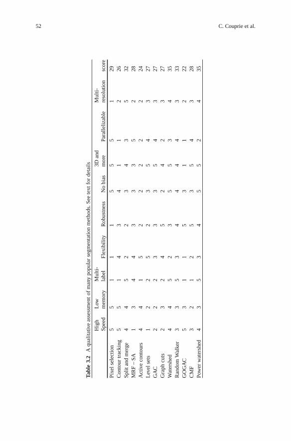
52 C. Couprie et al.
Tab
le3.
2A
qual
itat
ive
asse
ssm
ent
ofm
any
popu
lar
segm
enta
tion
met
hods
.See
text
for
deta
ils
Hig
hL
owM
ulti
-3D
and
Mul
ti-
Spee
dm
emor
yla
bel
Flex
ibil
ity
Rob
ustn
ess
No
bias
mor
ePa
rall
eliz
able
reso
luti
onsc
ore
Pixe
lsel
ecti
on5
51
11
55
51
29C
onto
urtr
acki
ng5
51
43
41
12
26Sp
lita
ndm
erge
44
52
23
43
532
MR
F–
SA1
34
43
33
52
28A
ctiv
eco
ntou
rs4
41
52
22
22
24L
evel
sets
12
25
23
54
327
GA
C2
22
33
35
43
27G
raph
cuts
23
24
52
42
327
Wat
ersh
ed4
45
23
55
34
35R
ando
mW
alke
r3
35
34
44
43
33G
OG
AC
53
11
53
11
222
CM
F3
21
25
35
43
28Po
wer
wat
ersh
ed4
35
34
55
24
35

3 Seeded Segmentation Methods for Medical Image Analysis 53
Fig. 3.7 Segmentation of the lungs in a chest CT image. (a) The CT image. (b) Segmentationusing 3D standard Geodesic Active Contours. The surfaces fail to fill the base of the lung.(c) Segmentation using a discrete maximal flow algorithm. Observe the directional bias due tothe grid. (d) Segmentation from identical input using continuous maximal flows
robust methods. However, they are slow, particularly in 3D, not parallelizable easilyand feature much bias; (9) Watershed is an old method but has definite advantagesfor segmentation: it is fast, bias-free and multi-label (it can segment many objectsat once). However, it is not flexible or very robust. Watershed can be extendedreadily for multi-resolution, and due to its age, many parallel implementations exist,including hardware ones; (10) The Random Walker is a recent method which issimilar in some ways to Watershed, but is significantly more robust. It requires moreresources however.
Among the newer methods presented in this chapter, (11) GOGAC solves GACexactly and quickly in 2D, and so provides a quick robust solution, which is good for2D interactive segmentation of single objects. However, is not flexible in its model;

54 C. Couprie et al.
(12) CMF is probably among the most robust segmentation method in the literaturefor 3D segmentation, but it segments only one object at a time, is not very flexible,and has no grid bias but does feature a shrinking bias. Finally, (13) Power watershedfits in between standard watershed and random walker. It is significantly moreflexible and robust than standard watershed. Its speed is also comparable, but ituses more memory, and is less parallelizable.
The global score is probably even more subject to controversy than the individualones, but it would tend to show that active contour methods should not be triedas a first choice method. For medical imaging, Random Walker and watershed-based methods are probably a good first choice, particularly for ease of use. It iscomforting to realize that more modern methods suitable for 3D medical imaging(GC, RW, PW and CMF) are all very robust.
Many advantages presented in the literature, such as purported sub-pixel accu-racy of segmentation, are not listed here because they are an illusion. The reportedability of some methods to control topology or on the contrary to allow it to changeis not necessarily a drawback or advantage either way, so we do not include itas well.
3.6 Conclusion and Future Work
In conclusion, we argue that seeded or interactive segmentation is useful in medicalimaging. Compared with model-based segmentation, seeded segmentation is morerobust in actual image analysis applications, as opposed to computer vision. Theability to separate seeds/markers, use contour information, and perform contouroptimization are very useful, as these elements generally result in a higher likelihoodof good results. From this point of view, we argue that segmentation is a process andnot merely an operator.
In general, the literature focuses on contour placement optimization at theexpense of the other two components, with some rare exceptions. This is unfor-tunate but understandable with respect to seeds/markers, because they are highlyapplication dependent. The choice of methods for obtaining contour information isalso limited, and this is probably a good area for future research. One conclusionof this study is that contour placement optimization methods are important. Morerecent methods focus on optimization robustness, which is important. For someonenot yet experienced in medical segmentation, simpler, more robust methods shouldbe preferred over complex ones. Among those, power-watershed is a good candidatebecause of its combination of speed, relative robustness, ability to cope withmultiple labels, absence of bias and availability (the code is easily available online).The random walker is also a very good solution, but is not generally and freelyavailable.
We have not surveyed or compared methods that encompass shape constraints.We recognize that this is important in some medical segmentation methods, but thiswould require another study altogether.

3 Seeded Segmentation Methods for Medical Image Analysis 55
Finally, at present there exists a dichotomy between the way discrete andcontinuous-domain work and are presented. In the near future, it is likely we willsee methods unifying both aspects to great advantage.
References
1. Adams, R., Bischof, L.: Seeded region growing. IEEE Trans. Pattern Anal. Mach. Intell. 16(6),641–647 (1994)
2. Appleton, B.: Globally minimal contours and surfaces for image segmentation. Ph.D. thesis,University of Queensland (2004). Http://espace.library.uq.edu.au/eserv/UQ:9759/ba thesis.pdf
3. Appleton, B., Sun, C.: Circular shortest paths by branch and bound. Pattern Recognit. 36(11),2513–2520 (2003)
4. Appleton, B., Talbot, H.: Globally optimal geodesic active contours. J. Math. Imaging Vis. 23,67–86 (2005)
5. Ardon, R., Cohen, L.: Fast constrained surface extraction by minimal paths. Int. J. Comput.Vis. 69(1), 127–136 (2006)
6. Beucher, S., Lantuejoul, C.: Use of watersheds in contour detection. In: International Workshopon Image Processing. CCETT/IRISA, Rennes, France (1979)
7. Boykov, Y., Kolmogorov, V.: An experimental comparison of min-cut/max- flow algorithmsfor energy minimization in vision. PAMI 26(9), 1124–1137 (2004)
8. Boykov, Y., Veksler, O., Zabih, R.: Fast approximate energy minimization via graph cuts. IEEETrans. Pattern Anal. Mach. Intell. 23(11), 1222–1239 (2001)
9. Canny, J.: A computational approach to edge detection. IEEE Trans. Pattern Anal. Mach. Intell.8(6), 679–698 (1986)
10. Caselles, V., Kimmel, R., Sapiro, G.: Geodesic active contours. Int. J. Comput. Vis. 22(1),61–79 (1997)
11. Chambolle, A.: An algorithm for total variation minimization and applications. J. Math.Imaging Vis. 20(1–2), 89–97 (2004)
12. Chan, T., Bresson, X.: Continuous convex relaxation methods for image processing. In:Proceedings of ICIP 2010 (2010). Keynote talk, http://www.icip2010.org/file/Keynote/ICIP
13. Chan, T., Vese, L.: Active contours without edges. IEEE Trans. Image Process. 10(2), 266–277(2001)
14. Cohen, L.D., Kimmel, R.: Global minimum for active contour models: A minimal pathapproach. Int. J. Comput. Vis. 24(1), 57–78 (1997). URL citeseer.nj.nec.com/cohen97global.html
15. Couprie, C., Grady, L., Najman, L., Talbot, H.: Power watersheds: A new image segmentationframework extending graph cuts, random walker and optimal spanning forest. In: Proceedingsof ICCV 2009, pp. 731–738. IEEE, Kyoto, Japan (2009)
16. Couprie, C., Grady, L., Najman, L., Talbot, H.: Power watersheds: A unifying graph-basedoptimization framework. IEEE Transactions on Pattern Analysis and Machine Intelligence,33(7), 1384–1399 (2011)
17. Couprie, C., Grady, L., Talbot, H., Najman, L.: Anisotropic diffusion using power watersheds.In: Proceedings of the International Conference on Image Processing (ICIP), pp. 4153–4156.Honk-Kong (2010)
18. Couprie, C., Grady, L., Talbot, H., Najman, L.: Combinatorial continuous maximum flows.SIAM J. Imaging Sci. (2010). URL http://arxiv.org/abs/1010.2733. In revision
19. Cousty, J., Bertrand, G., Najman, L., Couprie, M.: Watershed cuts: Minimum spanning forestsand the drop of water principle. In: IEEE Transactions on Pattern Analysis and MachineIntelligence, pp. 1362–1374. (2008)

56 C. Couprie et al.
20. Cousty, J., Bertrand, G., Najman, L., Couprie, M.: Watershed cuts: Thinnings, shortest-pathforests and topological watersheds. IEEE Trans. Pattern Anal. Mach. Intell. 32(5), 925–939(2010)
21. Cserti, J.: Application of the lattice Green’s function for calculating the resistance of an infinitenetwork of resistors. Am. J. Phys. 68, 896 (2000)
22. Daragon, X., Couprie, M., Bertrand, G.: Marching chains algorithm for Alexandroff-Khalimsky spaces. In: SPIE Vision Geometry XI, vol. 4794, pp. 51–62 (2002)
23. Dougherty, E., Lotufo, R.: Hands-on Morphological Image Processing. SPIE press, Bellingham(2003)
24. Doyle, P., Snell, J.: Random Walks and Electric Networks. Carus Mathematical Monographs,vol. 22, p. 52. Mathematical Association of America, Washington, DC (1984)
25. Ford, J.L.R., Fulkerson, D.R.: Flows in Networks. Princeton University Press, Princeton, NJ(1962)
26. Geman, S., Geman, D.: Stochastic relaxation, gibbs distributions, and the bayesian restorationof images. PAMI 6, 721–741 (1984)
27. Goldberg, A., Tarjan, R.: A new approach to the maximum-flow problem. J. ACM 35, 921–940(1988)
28. Goldenberg, R., Kimmel, R., Rivlin, E., Rudzsky, M.: Fast geodesic active contours. IEEETrans. Image Process. 10(10), 1467–1475 (2001)
29. Grady, L.: Multilabel random walker image segmentation using prior models. In: ComputerVision and Pattern Recognition, IEEE Computer Society Conference, vol. 1, pp. 763–770(2005). DOI http://doi.ieeecomputersociety.org/10.1109/CVPR.2005.239
30. Grady, L.: Computing exact discrete minimal surfaces: Extending and solving the shortest pathproblem in 3D with application to segmentation. In: Computer Vision and Pattern Recognition,2006 IEEE Computer Society Conference, vol. 1, pp. 69–78. IEEE (2006)
31. Grady, L.: Random walks for image segmentation. IEEE Trans. Pattern Anal. Mach. Intell.28(11), 1768–1783 (2006)
32. Grady, L., Funka-Lea, G.: Multi-label image segmentation for medical applications basedon graph-theoretic electrical potentials. In: Computer Vision and Mathematical Methods inMedical and Biomedical Image Analysis, pp. 230–245. (2004)
33. Grady, L., Polimeni, J.: Discrete Calculus: Applied Analysis on Graphs for ComputationalScience. Springer Publishing Company, Incorporated, New York (2010)
34. Grady, L., Schwartz, E.: Isoperimetric graph partitioning for image segmentation. Pattern Anal.Mach. Intell. IEEE Trans. 28(3), 469–475 (2006)
35. Guigues, L., Cocquerez, J., Le Men, H.: Scale-sets image analysis. Int. J. Comput. Vis. 68(3),289–317 (2006)
36. Horowitz, S., Pavlidis, T.: Picture segmentation by a directed split-and-merge procedure. In:Proceedings of the Second International Joint Conference on Pattern Recognition, vol. 424,p. 433 (1974)
37. Iri, M.: Survey of Mathematical Programming. North-Holland, Amsterdam (1979)38. Kakutani, S.: Markov processes and the Dirichlet problem. In: Proceedings of the Japan
Academy, vol. 21, pp. 227–233 (1945)39. Kass, M., Witkin, A., Terzopoulos, D.: Snakes: Active contour models. Int. J. Comput. Vis. 1,
321–331 (1988)40. Khalimsky, E., Kopperman, R., Meyer, P.: Computer graphics and connected topologies on
finite ordered sets. Topol. Appl. 36(1), 1–17 (1990)41. Kruskal, J.J.: On the shortest spanning subtree of a graph and the travelling salesman problem.
Proc. AMS 7(1) (1956)42. Levinshtein, A., Stere, A., Kutulakos, K., Fleet, D., Dickinson, S., Siddiqi, K.: Turbopixels:
Fast superpixels using geometric flows. Pattern Anal. Mach. Intell. IEEE Trans. 31(12),2290–2297 (2009)
43. Malladi, R., Sethian, J., Vemuri, B.: Shape modelling with front propagation: A level setapproach. IEEE Trans. Pattern Anal. Mach. Intell. 17(2), 158–175 (1995)

3 Seeded Segmentation Methods for Medical Image Analysis 57
44. Marr, D., Hildreth, E.: Theory of edge detection. Proc. R. Soc. Lond. Ser. B Biol. Sci. 207,187–217 (1980)
45. Menzies, S.W., Crotty, K.A., Ingvar, C., McCarthy, W.H.: An Atlas of Surface Microscopy ofPigmented Skin Lesions. McGraw-Hill, Roseville, Australia (1996). ISBN 0 07 470206 8
46. Meyer, F.: Topographic distance and watershed lines. Signal Process. 38(1), 113–125 (1994)47. Meyer, F., Beucher, S.: Morphological segmentation. J. Vis. Commun. Image Represent. 1(1),
21–46 (1990)48. Mortensen, E., Barrett, W.: Interactive segmentation with intelligent scissors. Graph. Models
Image Process. 60(5), 349–384 (1998)49. Mumford, D., Shah, J.: Optimal approximations by piecewise smooth functions and associated
variational problems. Commun. Pure Appl. Math. 42(5), 577–685 (1989)50. Najman, L.: On the equivalence between hierarchical segmentations and ultrametric water-
sheds. Journal of Mathematical Imaging and Vision, 40(3), 231–247 (2011)51. Najman, L., Schmitt, M.: Geodesic saliency of watershed contours and hierarchical segmenta-
tion. Pattern Anal. Mach. Intell. IEEE Trans. 18(12), 1163–1173 (2002)52. Najman, L., Talbot, H. (eds.): Mathematical Morphology: From theory to applications. ISTE-
Wiley, London, UK (2010)53. Osher, S., Sethian, J.: Fronts propagating with curvature-dependent speed: Algorithms based
on Hamilton-Jacobi formulations. J. Comput. Phys. 79(1), 12–49 (1988)54. Otsu, N.: A threshold selection method from gray-level histograms. Automatica 11, 285–296
(1975)55. Paragios, N., Deriche, R.: Geodesic active contours and level sets for the detection and tracking
of moving objects. Pattern Anal. Mach. Intell. IEEE Trans. 22(3), 266–280 (2002)56. Paragios, N., Deriche, R.: Geodesic active regions and level set methods for supervised texture
segmentation. Int. J. Comput. Vis. 46(3), 223–247 (2002)57. Pham, D., Xu, C., Prince, J.: Current methods in medical image segmentation1. Biomed. Eng.
2(1), 315 (2000)58. Pock, T., Cremers, D., Bischof, H., Chambolle, A.: An algorithm for minimizing the Mumford-
Shah functional. In: 12th International Conference on Computer Vision, pp. 1133–1140. IEEE(2009)
59. Prim, R.: Shortest connection networks and some generalizations. Bell Syst. Techn. J. 36(6),1389–1401 (1957)
60. Rudin, L.I., Osher, S., Fatemi, E.: Nonlinear total variation based noise removal algorithms.Phys. D 60(1-4), 259–268 (1992). DOI http://dx.doi.org/10.1016/0167-2789(92)90242-F
61. Sagiv, C., Sochen, N., Zeevi, Y.: Integrated active contours for texture segmentation. ImageProcess. IEEE Trans. 15(6), 1633–1646 (2006)
62. Sethian, J.: Level set methods and fast marching methods. Cambridge University Press,Cambridge (1999). ISBN 0-521-64204-3
63. Soille, P.: Constrained connectivity for hierarchical image partitioning and simplification. IEEETrans. Pattern Anal. Mach. Intell. 30(7), 1132–1145 (2008)
64. Stawiaski, J., Decenciere, E., Bidault, F.: Computing approximate geodesics and minimalsurfaces using watershed and graph cuts. In: Banon, G.J.F., Barrera, J., Braga-Neto, U.d.M.,Hirata, N.S.T. (eds.) Proceedings of the 8th International Symposium on MathematicalMorphology, vol. 1, pp. 349–360. Instituto Nacional de Pesquisas Espaciais (INPE) (2007).URL http://urlib.net/dpi.inpe.br/ismm@80/2007/03.19.13.04
65. Strang, G.: Maximal flow through a domain. Math. Program. 26, 123–143 (1983)66. Veksler, O.: Efficient graph-based energy minimization. Ph.D. thesis, Cornell University (1999)67. Vincent, L., Soille, P.: Watersheds in digital spaces: An efficient algorithm based on immersion
simulations. IEEE Trans. Pattern Anal. Mach. Intell. 13(6), 583–598 (1991)68. Weickert, J., Romeny, B., Viergever, M.: Efficient and reliable schemes for nonlinear diffusion
filtering. Image Process. IEEE Trans. 7(3), 398–410 (2002)69. Zhu, S., Yuille, A.: Region competition: Unifying snakes, region growing, and Bayes/MDL for
multiband image segmentation. Pattern Anal. Mach. Intell. IEEE Trans. 18(9), 884–900 (2002)


Chapter 4Deformable Models and Level Setsin Image Segmentation
Agung Alfiansyah
4.1 Introduction
Segmentation is a partitioning process of an image domain into non-overlappingconnected regions that correspond to significant anatomical structures. Automatedsegmentation of medical images is a difficult task. Images are often noisy andusually contain more than a single anatomical structure with narrow distancesbetween organ boundaries. In addition, the organ boundaries may be diffuse.Although medical image segmentation has been an active field of research forseveral decades, there is no automatic process that can be applied to all imagingmodalities and anatomical structures [1].
In general, segmentation techniques can be classified into two main categories:(a) segmentation methods that allow users to explicitly specify the desired featureand (b) algorithms where the specification is implicit. The first segmentationclass considers the segmentation as a real-time interaction process between theuser and the algorithm. The user is provided with the output and allowed toperform feed-back directly in order to modify the segmentation until he/she getsa satisfactory result. In the extreme case, this framework might degenerate intomanual segmentation with the user forcing his/her desirable results. Some examplesof this approach are the livewire segmentation algorithms [2–5]. These algorithmsproduce a piecewise optimal boundary representation of an object, by viewingthe image as a weighted graph and finding the shortest path between consecutivespecified boundary points of the user. A more recent example of this approach basedon the concept of random walks is described in [6].
The majority of segmentation methods belong to the second category, where thedesired result is specified implicitly. Segmentation algorithms belonging to this cat-egory include: thresholding, various contour-based and region-based segmentation
A. Alfiansyah (�)Surya Research and Education Center Tangerang, Tangerang, Indonesiae-mail: [email protected]
G. Dougherty (ed.), Medical Image Processing: Techniques and Applications, Biologicaland Medical Physics, Biomedical Engineering, DOI 10.1007/978-1-4419-9779-1 4,© Springer Science+Business Media, LLC 2011
59

60 A. Alfiansyah
methods, Markov random fields, active contours, model-based, and deformablemodel methods. As this domain has been studied extensively, there exist manypublished reviews of medical image segmentation [7, 39, 40], with specializedsurveys on deformable models [7,8], vessel extraction [9,10], or brain segmentation[10, 11].
This chapter is organized as follows. In Sect. 4.2, we review the main conceptsof the deformable model and its role in image segmentation. We present severaltypes of deformable models according to how they are represented, followed bya description of their energy definition and possible optimization methods. InSect. 4.3, we compare the performance of these deformable models accordingto properties such as initialization, topological change handling, stability, etc. InSect. 4.4, we discuss several cases of developed applications of medical imagesegmentation and conclude in Sect. 4.5.
4.2 Deformable Models
The basic idea of active contours for image segmentation is to embed an initial con-tour (or surface in the three-dimensional case) into the image, and to subsequentlylet it evolve while being subjected to various constraints. In order to detect objectsin the image, the contour has to stop its evolution on the boundary of the objectof interest. Although the term deformable models first appeared in the work byKass et al. [12] in the late eighties, the idea of deforming a template for extractingimage features dates back much further, with work on spring-loaded templates [13]and on the rubber mask technique [14]. In image processing literature, deformablemodels are also variously known as snakes, active contours or surfaces, balloons,and deformable contours or surfaces. An extensive review of the current research inthis area can be found in [1, 38].
In the following subsection, we present the different types of deformable modelsclassified according to contour representation, and some energy optimizationstrategies.
4.2.1 Point-Based Snake
This classical snake was firstly proposed by Kass et al. [12] and represents thecontour using discrete points. The behavior of this classical snake is usually modeledby a weighted linear combination of: internal energy calculated from the contourthat determines the regularity of the curve; external energy which attracts thecontour towards the significant features in the image; and often an additional userenergy allowing the operator to better interact with the model.
In the first snake-type, one applies the simplest way to represent the model: aset of discrete points as snake elements (C(s)). Using this representation, closed

4 Deformable Models and Level Sets in Image Segmentation 61
contours can be formed by connecting the last “snaxel” (snake element) to the firstone. For segmentation, the snake has to minimize the energy as follows:
E(C(s)) =∫
Ω
⎧⎪⎨⎪⎩Econtour(C(s))︸ ︷︷ ︸
internal energy
+Eimage(C(s))+ Euser(C(s))︸ ︷︷ ︸external energy
⎫⎪⎬⎪⎭ds. (4.1)
Applying discrete-point representation, the internal energy can be approximated byaccommodating the elasticity and rigidity terms:
Econtour(C(s)) = w1(s)Eelasticity(C(s))+ w2(s)Erigidity(C(s))
= w1(s)Cs(s)2 + w2(s)Css(s)2, (4.2)
where the subscripts s and ss denote the first and second derivatives with respectto the curve parameter. The model behavior is controlled by constants w1 and w2,respectively, weighting the curve elasticity and rigidity.
Internal Energy Definition: In the first term in equation (4.2), Cs(s) representsthe elastic energy and makes the snake behave like a membrane. The second termCss(s) represents the contour’s bending energy that makes the model act like athin plate. Decreasing elasticity allows the contour to increase in length, whileincreasing elasticity increases the tension of the model by reducing its length.Decreasing rigidity allows the active contour model to develop corners, whileincreasing rigidity makes the model smoother and less flexible. Setting either ofthe weighting coefficients to zero permits first- and second-order discontinuities,respectively.
This energy equation can then be discretized using the finite differencemethod as:
Eelasticity ≈ (xs − xs−1)2 +(ys − ys−1)
2 . (4.3)
This term will minimize the distance between the points on the snake, causingshrinking during optimization of the energy process in the absence of externalenergy. In a similar way, the rigidity term is discretized as:
Erigidity ≈ (xs+1− xs − xs−1)2 +(ys+1 − ys − ys−1)
2 . (4.4)
The elasticity definition using finite differences discretization scheme is valid forthe condition that the model’s snaxels are evenly spaced [15]. In other cases, acontinuity term can be defined that subtracts the average distance of the snaxels,otherwise the energy value will be larger for points which are further apart.This constraint forces the points to be more evenly spaced, and avoids possiblecontraction of the snake.

62 A. Alfiansyah
External Energy Definition: The external energy term in equation (4.1) representsthe image potential derived from image data and guides the contour in finding thedesired object. Ideally, this energy has a minimum value at the feature subject todetection. However, due to the presence of noise, there is often a convergenceproblem at object concavities. The snake can also integrate the constraint energyto interactively guide itself towards or away from particular features. This energyhelps the contour to overcome the initialization problem or the sensitivity to noise.
Kass [12] proposed a weighted sum of the following energy terms in order todetect image features:
Eext(C(s)) = αline · I(s)+ αedge ·−∇I2 +αterm ·Eterm. (4.5)
The most common image functional in this model is the image intensity function I.The first term will simply attract the contour to lower or higher intensity valuesdepending on the αline value. Large positive values of αline tend to make the snakealign itself with dark regions in the image I(s), whereas large negative values ofαline tend to make the snake align itself with bright regions in the image.
The edge energy that attracts the contour towards high gradient values is squaredto narrow the edge-gradient response. Similarly, large positive values of αedge tendto make the snake align itself with sharp edges in the image whereas large negativevalues of αedge make the snake avoid the edges. Eterm is defined to find terminationof line segments and corners. Kass proposed to use the curvature of iso-contours ina Gaussian smoothed image to attract the contours towards line termination.
4.2.1.1 User Constraint Energy
Constraint energy is applied to interactively guide the snake towards or away fromparticular features. This energy helps the contour to overcome the initializationproblem or the sensitivity to noise.
Constraint energy was first proposed for the classical snake by allowing the userto attach springs between points of the contour and fix their position in the imageplane. Kass define an energy in terms of spring (to attract the snake towards specifiedpoints) and volcano (to repulse the snake from specified points) within the image(Fig. 4.1).
The spring term attracts a contour point towards a spring point in the imageplane, with a given constant, spring constant. The active contour model is attractedor repelled by the spring depending on this spring constant sign and value. Thevolcano term acts as a repulsive force between a point on the image at a inversevalue of the distance from a point on the snake.
Balloon Force: Cohen [16,17] proposed an additional force that pushes the contourin the direction normal to the contour. Since it can either inflate or deflate thecontour, this force is known as a balloon force, defined as:
Fballoon(s) = k�N(s), (4.6)
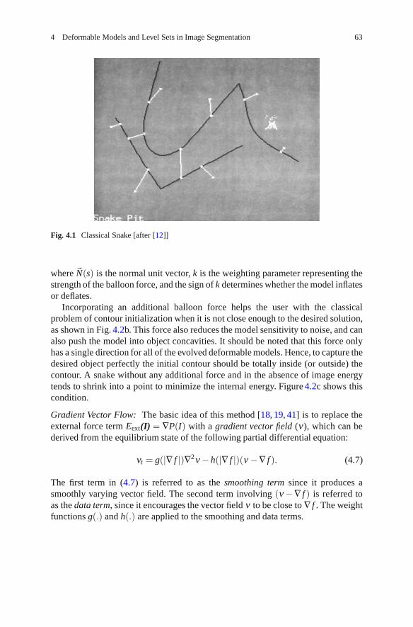
4 Deformable Models and Level Sets in Image Segmentation 63
Fig. 4.1 Classical Snake [after [12]]
where �N(s) is the normal unit vector, k is the weighting parameter representing thestrength of the balloon force, and the sign of k determines whether the model inflatesor deflates.
Incorporating an additional balloon force helps the user with the classicalproblem of contour initialization when it is not close enough to the desired solution,as shown in Fig. 4.2b. This force also reduces the model sensitivity to noise, and canalso push the model into object concavities. It should be noted that this force onlyhas a single direction for all of the evolved deformable models. Hence, to capture thedesired object perfectly the initial contour should be totally inside (or outside) thecontour. A snake without any additional force and in the absence of image energytends to shrink into a point to minimize the internal energy. Figure 4.2c shows thiscondition.
Gradient Vector Flow: The basic idea of this method [18, 19, 41] is to replace theexternal force term Eext(I) = ∇P(I) with a gradient vector field (ν), which can bederived from the equilibrium state of the following partial differential equation:
νt = g(|∇ f |)∇2ν −h(|∇ f |)(ν −∇ f ). (4.7)
The first term in (4.7) is referred to as the smoothing term since it produces asmoothly varying vector field. The second term involving (ν −∇ f ) is referred toas the data term, since it encourages the vector field ν to be close to ∇ f . The weightfunctions g(.) and h(.) are applied to the smoothing and data terms.

64 A. Alfiansyah
Fig. 4.2 Deformable model with additional balloon force
The authors in [5] proposed the following weight functions:
g(∇ f ) = e−|∇ f |
K
h(∇ f ) = 1− e−|∇ f |
K . (4.8)
Using these weight functions, the gradient vector flow field will conform to thedistance map gradient near the relevant features, but will vary smoothly awayfrom them. The constant K determines the extent of the field smoothness and theconformity gradient.
Figure 4.3 Illustrates the Gradient Vector Flow performance when a thin con-cavity or sharp corner is present in the segmented object. The Gradient VectorFlow force is able to attract the snake towards the desired contour and towardsconcave areas. This would not be the case with conventional external energy, sinceno external force attracts the snake towards that part of the image.

4 Deformable Models and Level Sets in Image Segmentation 65
Fig. 4.3 Additional force provided by Gradient Vector Flow for synthetic image segmentation;(a) Initial contour defined as a circle in the image; (b) Vector flow visualization derived from theimage; (c) Segmentation result using Gradient Vector Flow: the snake captures the desired object;(d) Segmentation result without additional force
4.2.1.2 Snake Optimization Method
Image segmentation using an active contour is formulated as a process of energyminimization that evolves the contour. This minimization controls the modeldeformation to reach the desired segmentation result. The term “snake” comes fromthe “slip and slide” movement of the contour during this minimization process.

66 A. Alfiansyah
Fig. 4.4 Local neighborhood in optimization using a greedy algorithm. The energy function isevaluated at vt−1
i and each of the neighbors, using vti−1 and vt−1
i+1 to compute the internal energyterms. The location with lowest energy is chosen as the new position vt
i
Greedy Algorithm
Using greedy algorithms optimization finds the solution incrementally by choosingat each step the direction which is locally the most promising for the final result, i.e.which provides larger energy decrease.
Figure 4.4 illustrates the optimization procedure using a greedy algorithm. Theenergy function at the current point νt−1
i and each of its neighbors is computedunder consideration of adjacent contour points νt
i−1 and νt−1i+1 . The location with
the smallest energy value is chosen as the new position of νti . The previous point
νti−1 has already been updated to the new position in the current iteration over the
contour, while νt−1i+1 will be updated next.
At the first stage of the algorithm, all contour points are sequentially updatedwithin one iteration. At the second stage, the forming of corners is determined byrecalculating the rigidity energy terms with the updated points, and also by adjustingthe weighting rigidity parameter w2 for each contour point accordingly.
Dynamic Programming
Dynamic programming minimization was presented by Amini [20] to solve thevariational problem in energy minimization of active contour models. Dynamicprogramming is different from variational optimizations in the sense that it ensuresa globally optimal solution with respect to the search space and numerical stabilityby moving the contour points on a discrete grid without any derivative numericalapproximations. The optimization process can be viewed as a discrete multi-stagedecision process and is solved by a time-delayed discrete dynamic programmingalgorithm. Dynamic programming bypasses local minima as it embeds the mini-mization problem in a neighborhood-related problem. This is achieved by replacing

4 Deformable Models and Level Sets in Image Segmentation 67
the minimization of the total energy measurement by the minimization of a functionof the form:
E(ν0,ν1,ν2 . . .νn−1) = E1(ν0,ν1,ν2)+ E2(ν1,ν2,ν3)
+E3(ν1,ν2,ν3)+ · · ·+ En−2(νn−1,νn−2,νn−1). (4.9)
S(νi+1,ν1) = minν1
νi−1Si−1(νi,νi−1)+ Eelast(νi−1,νi)+ Erigid(νi−1,νi,νi+1)
+Eext(νi). (4.10)
Apart from the energy matrix corresponding to the optimal value function Si, aposition matrix is also needed so the value of νi minimizing equation (4.10) canbe stored. The optimal contour of minimum energy Emin(s) can be then found byback-tracking from the end position represented in the matrix.
This process is iterated until the active contour finds an energy that does notchange significantly. It consists of a forward pass to determine the minimum energyvalues for each νi and a backward pass to find the minimum energy path in theposition matrix.
Similar to minimization using the greedy algorithm, dynamic programmingallows hard constraints (e.g. minimum distance between snaxels) on the behaviorof the global minimum solution directly and naturally. The other advantage of thismethod comes from the execution time and the required memory. The complexityof this method is O(mn) with O(mn2) memory required, where n is the number ofpoints on the contour and m is the number of potential locations in the search spaceto which every point is allowed to move during one optimization step.
Variational Method
This approach is based on the Euler–Lagrange condition in order to derive adifferential equation that can be solved to minimize the snake energy. For eachiteration, an implicit Euler forward step is performed with respect to the internalenergy, and an explicit Euler step with respect to the external image and constraintsenergy terms.
The basic deformable model (in (4.2)) can be rewritten as:
E(C(s)) =∫
Ω
12
(w1(s)|C′(s)|2 + w2(s)|C′′(s)|2)ds+
∫
Ω
Eext(C(s))ds. (4.11)
Representing the integrand by E(s,C′,C′′), the necessary condition for the variationto locally minimize E(C(s)) must satisfy the following Euler–Lagrange equation:
− (w1(s)C′)′ +(w2(s)C′′)′′ + ∇Eext(C(s)) = 0. (4.12)

68 A. Alfiansyah
The equation can be solved by changing C over time t, then C is a function of thecontour s and time t → C(s,t). When the snake reaches a stable state Ct(s,t) = 0,the solution of (4.12) is obtained. Thus, insertion of this term gives:
∂ Eext
∂ s− (w1(s)C′)′ +(w2(s)C′′)′′ + ∇Eext(C(s)) = 0. (4.13)
If the sum of all external forces and image energy is Eext(s), the equation can besolved numerically by using a finite difference approach and represented implicitlyin matrix multiplication form such as:
F = A.V, (4.14)
where A is a penta-diagonal banded matrix. This expression is correct forsnakes with fixed-point positions at their extremities or closed snakes (i.e.C(0)=C(N −1)).
Generally, we assume that elasticity w1 and rigidity w2 are constant for bothdiscretized space and time during curve evolution, thus:
a1 = e1 =w2
h4 b1 = d1 =(w1
h4 + 4w2
h4
)c =
(2
w1
h4 + 6w2
h4
). (4.15)
To solve (4.14) iteratively, the successive over-relaxation method [21] can beapplied. In the two-dimensional image case, the resulting equations for evaluatingtime t from time t −1 can be solved iteratively after matrix inversion using:
Vt = τ(A+ I)−1 · (Vt−1 + τF(xt−1,yt−1), (4.16)
I is the identity matrix, and τ(A+ I)−1 is also penta-diagonal.This optimization approach does not guarantee a global minimum solution,
and requires estimates of high-order derivatives on the discrete data. Moreover,hard constraints cannot be directly enforced. A desired constraint term like meanor minimum snaxel spacing can only be enforced by increasing the associatedweighting term, which will force more effect on this constraint, but at the cost ofother terms.
4.2.2 Parametric Deformable Models
These deformable models represent the curve or surface in an explicit parametricform during the model deformation. This representation allows for direct interac-tion and gives a compact representation for real-time implementation. Parametric

4 Deformable Models and Level Sets in Image Segmentation 69
deformable models are usually too sensitive to their initial conditions because of thenon-convexity of the energy functional and the contraction force which arises fromthe internal energy term.
B-Spline is often used as a representation of parametric deformable models [42].In this case, the deformable model is split into segments by knot points. Each curvesegment C(t) = {x(t),y(t)} is approximated by a piecewise polynomial function,which is obtained by a linear combination of basis functions βi and a set of controlpoints ν = {xi,y}. In general, however, representations using smooth basis functionsrequire fewer parameters than point-based approaches and thus result in fasteroptimization algorithms [22]. Moreover, such curve models have inherent regularityand hence do not require extra constraints to ensure smoothness [22, 23].
Both point-based and parametric snakes represent the model in an explicit way,hence it is easier to integrate an a priori shape constraint into the deformablemodel. Moreover, the user’s interaction can be accommodated in a straightforwardmanner by allowing the user to specify some points through the desired contourevolution. The inconvenience of this model lies in reduced flexibility in accountingfor topological changes during the evolution, although much effort has been spentto overcome this limitation.
4.2.2.1 Internal Energy Definition
Similar to the discrete point-based snake, internal energy is responsible for ensuringthe smoothness of the contour. Actually, Kass proposed a linear combination ofthe length of the contour and the integral of the square of the curvature along thecontour. Thus, in explicit contour representation, this energy can be defined as:
Econtour = w1
M∫
0
(x′(t)2 + y′(t)2)12 dt + w2
M∫
0
(x′′(t)y′(t)− x′(t)y′′(t)
(x′(t)2 + y′(t)2)32
)2
dt. (4.17)
where the second term represents the curvature at point r(t).
4.2.2.2 Image Energy Definition
The most common image energy applied for the snake is defined as the integral ofthe square of the gradient magnitude along the curve. The main drawback widelyknown in using this energy is the lack of gradient direction. This information can beused to detect edges, since at the boundary image gradient is usually perpendicularto the curve. This direction should be incorporated into the image energy to makethe snake more robust for image segmentation.
Region-based energy. This region-based energy represents the statistical charac-teristics in a region in the contour and provides snake boundary information. This

70 A. Alfiansyah
is indeed very helpful when the contour is far away from the real contour to bedetected. For this purpose we assume two regions in the images (which can beexpanded two more times) with different probability distributions in which eachof these regions has different means and variances. Staib’s [24] formulation todetermine the region likelihood function can be used for this case:
Eregion = −∫
S
log(P(f(s)|s ∈R))dS−∫
S′log(P(f(s)|s ∈R′))dS. (4.18)
Where R and R′ denote the different regions of the curve and S and S′ indicatethe position inside or outside the region, respectively. The energy will be maximumwhen R = S and R′ = S′, and the regional based energy can be reformulated as:
Eregion = −∫
S
log
(P(f(s)|s ∈R)P(f(s)|s ∈R′)
)dS. (4.19)
4.2.2.3 External Constraint Energy Definition
External constraint, proposed by Kass, can be integrated in such a way that the usermight specify a few points which should lie on the contour to be detected. It canbe performed by adding an energy term which is the distance between these givenpoints and the corresponding closest points on the curve.
As mentioned previously, image segmentation finally yields the totality of theenergy minimization process that will place a regular contour at the edge of theobject which we want to detect. Sometimes, we do not require the global optimumsolution, since the initial contour can be provided interactively by the user to obtaina rough initial contour near the edge, even though a robust optimization scheme thatconverges to the minimum solution in an acceptable number of iterations is stronglydesired. Some examples of image segmentation results using a Bspline snake whichintegrate gradient and region based energy are demonstrated in Fig. 4.5.
4.2.3 Geometric Deformable Models (Active Contours)
These models were introduced independently by Caselles [23] and Malladi [25] topropose an efficient solution addressing the primary limitations of the parametricdeformable model using a geometric deformable model (level set). Advantages ofthe implicit contour formulation of the geometric deformable model over parametricformulation include: (1) no parameterization of the contour, (2) topological flex-ibility, (3) good numerical stability, and (4) straightforward extension of the 2Dformulation to higher dimensions.

4 Deformable Models and Level Sets in Image Segmentation 71
Fig. 4.5 B-Spline snake performance with respect to noisy image (i.e. echo cardiogram): (a) Initialcontour by means of manual contouring; (b) Segmentation using only gradient-based energy;anatomical details of the upper part of the heart can be captured since this region has a brightarea, but not in the lower part due to the noises; (c) Region-based energy, noisy problems can besolved but not anatomical details in the upper part; (d) Result using combination of 75% region-based and 25% edge-based energies; the advantage of both energies can be taken and limitationscan be solved, thus enabling a better result
These models are based on curve evolution theory and the level set method[23, 26] proposed by Sethian and Osher [27] to track the surface interface andshape evolution in physical situations. Using this approach, curves and surfaces areevolved using only geometric measures, resulting in an evolution that is independentof parameterization. As in the other types of deformable models, the evolutionis coupled with the image data in such a way that the process recovers objectboundaries. The evolving curves and surfaces can be represented implicitly asa level set of a higher-dimensional function, so the evolution is independent ofparameterization. As a result, topological changes can be handled automatically.
4.2.3.1 Curve Evolution
Let C(t, p) be a kind of closed curves where t parameterizes the family and p thegiven curve, where 0 ≤ p ≤ 1. As a closed curve, we assume that C(0,t) = C(1,t)and similarly for the first derivatives for closed curves. Using this curve definition,the curve shortening flow, in the sense that the Euclidean curve length shrinks as

72 A. Alfiansyah
quickly as possible when the curve evolves, can be obtained from the first variationof the length functional [28]:
∂C∂ p
= κ�N, (4.20)
where κ is the local mean curvature of the contour at a point, and �N is the unit inwardnormal. For the intrinsic property of being closed, the curve under the evolutionof the curve shortening flow will continue to shrink until it vanishes. By adding aconstant ν , which we will refer to as the “inflation term,” the curve tends to growand counteracts the effect of the curvature term when κ is negative [29]:
∂C∂ p
= (ν +κ)�N. (4.21)
A stopping evolution term can be introduced into the above framework by changingthe ordinary Euclidean arc-length function along the curve C to a geodesic arclength, by multiplying with a conformal factor g, where g = g(x,y) is a positivedifferentiable function that is defined based on the given image I (x, y). From thefirst variation of the geodesic curve length function, we obtain a new evolutionequation by combining both the internal property of the contour and the externalimage force:
∂C∂ p
= g(ν + κ)�N −∇g. (4.22)
Equation (4.22) gives us an elegant curve evolution definition for deformable modelformulation applicable for curve evolution analysis. The main problem arises thenin relation to how to represent the contour efficiently in terms of geometric andtopologic stability as well as numerical implementation. One of the most commonmethods for representing the contour in using this scheme is the level set concept.
For a more detailed explanation of curve evolution in terms of image segmen-tation, interested readers are suggested to refer to the works of Casseles [23, 30],Kichenassamy [29], and Yezzi [31].
4.2.3.2 Level Set Concept
Curve evolution analysis using level set method views a curve as the zero level setof a higher-dimensional function φ(x,t). Generally, the level set function satisfies
φ(x,t)
⎧⎨⎩
φ(x,t) < 0 insideΩ(t)φ(x,t) = 0 C(t)φ(x,t) > 0 outsideΩ(t)
,
where the artificial time t denotes the evolution process, C(t) is the evolving curve,and Ω(t) represents the region enclosed by C(t).
Figure 4.6 illustrates an important property of the level set method in handlingthe topological change in the object of interest. The first image shows a closed curve
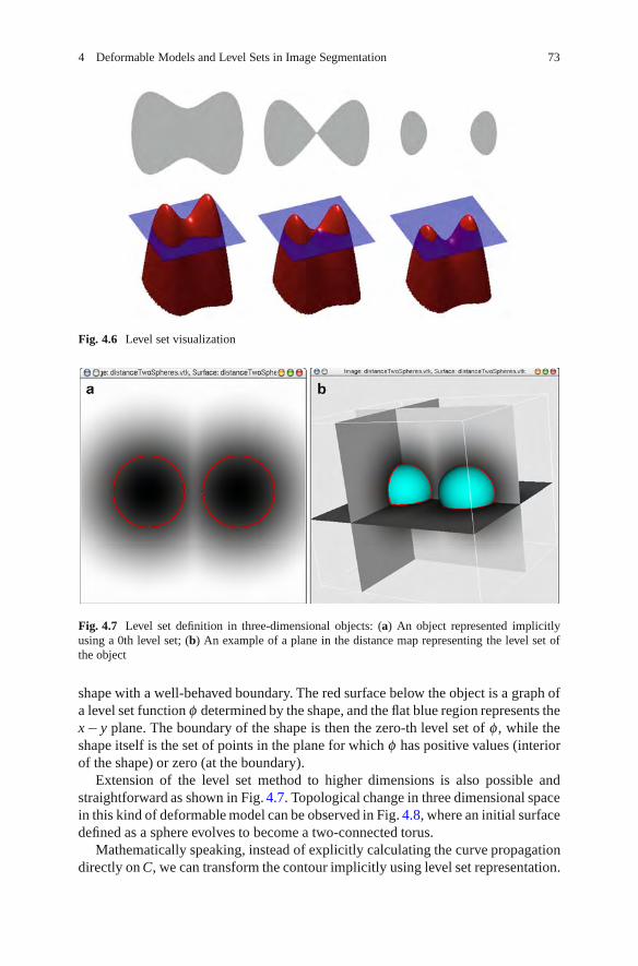
4 Deformable Models and Level Sets in Image Segmentation 73
Fig. 4.6 Level set visualization
Fig. 4.7 Level set definition in three-dimensional objects: (a) An object represented implicitlyusing a 0th level set; (b) An example of a plane in the distance map representing the level set ofthe object
shape with a well-behaved boundary. The red surface below the object is a graph ofa level set function φ determined by the shape, and the flat blue region represents thex− y plane. The boundary of the shape is then the zero-th level set of φ , while theshape itself is the set of points in the plane for which φ has positive values (interiorof the shape) or zero (at the boundary).
Extension of the level set method to higher dimensions is also possible andstraightforward as shown in Fig. 4.7. Topological change in three dimensional spacein this kind of deformable model can be observed in Fig. 4.8, where an initial surfacedefined as a sphere evolves to become a two-connected torus.
Mathematically speaking, instead of explicitly calculating the curve propagationdirectly on C, we can transform the contour implicitly using level set representation.

74 A. Alfiansyah
Fig. 4.8 Level set representation advantage in handling the topological change during segmenta-tion. Initialized using a sphere the method can detect the connected chain as the final result
Thus, contour evolution, which is ∂C∂ p = F�N, can be transformed in level set
representation:∂φ∂ t
= F |∇φ |. (4.23)
It would be very hard to elaborate upon this topology transformation usingparameterized curve representation. One would need to develop an algorithm able todetect the moment the shape split (or merged), and then construct parameterizationsfor the newly obtained curves.
4.2.3.3 Geodesic Active Contour
Slightly different from the other models previously explained, this model doesnot impose any rigidity constraints (i.e. w2 = 0); hence, the minimized energy isformulated as:
E(C) =1∫
0
g(|∇I(C(s))|)ds︸ ︷︷ ︸attraction term
∣∣∣∣∣∣∂C∂ p︸︷︷︸
∣∣∣∣∣∣regularity term
dp. (4.24)
Where g is a monotonically decreasing function, ds is the Euclidian arc-lengthelement and L the Euclidian length of C(t, p).

4 Deformable Models and Level Sets in Image Segmentation 75
Using this formulation, we aim to detect an object in the image by findingthe minimal-length geodesic curve that best takes into account the desired imagecharacteristics. The stated energy in (4.24) can be minimized locally using thesteepest descent optimization method, as demonstrated in [30]. It shows that inorder to deform the contour towards the minimum local solution with respect tothe geodesic curve length in Riemannian space, the curve evolves according to thefollowing equation:
∂C∂ t
= gκ�N − (∇g ·�N)�N. (4.25)
The segmentation result can be achieved in the equilibrium state where ∂C∂ t = 0.
Following the level set method for the curve evolution in (4.25), we obtain the curveevolution using the geodesic active contour in terms of the level set:
∂φ∂ t
= gκ|∇φ |+ ∇g∇φ . (4.26)
Finally, in order to accelerate the convergence and place the model in the correctboundary, we integrate an elastic term in the curve evolution that will pull the modeltowards the desired object [30] and writing the curvature κ explicitly:
∂φ∂ t
= g ·div
(∇φ|∇φ |
)|∇φ |+ ∇g∇φ︸ ︷︷ ︸
elastic term
+ν∇g|∇φ |. (4.27)
The role of this elastic term can be observed in Fig. 4.9 in which the upper-rowactive contour evolves without any elastic term, and hence the converged contourdoes not match the desired contour.
4.2.3.4 Chan–Vese Deformable Model
One limitation of the geodesic active contour lies in its dependence on image energyrepresented by the gradient. In order to stop the curve evolution, we need to defineg(|∇I|) which defines the edges of the object. In practice, discrete gradients arebounded, and so the stopping function is never zero on the edges, and the curvemay pass through the boundary. Moreover, if the image is very noisy, the isotropicsmoothing Gaussian has to be strong, which will smooth the edges as well.
To overcome these problems, Chan and Vese [32–34] proposed stopping processbased on the general Mumford–Shah formulation of image segmentation [15], byminimizing the functional:
EMS( f ,C) = μ .Length(C)+ λ∫
Ω
| f − f0|2dxdy +∫
Ω\C
|∇ f |2dxdy, (4.28)
where f0 : Ω → R is a given image to be segmented, and μ and λ are positiveparameters. The solution image f is formed in smooth regions Ri and sharp

76 A. Alfiansyah
Fig. 4.9 Role of the elastic term in geodesic active contour: In the upper row, the model is evolvedwithout the elastic term; in the lower row, an elastic term is used
boundaries C. A reduced form of this problem consists simply in the restrictionof EMS to piecewise constant functions and finding a partition of Ω such that f in Ωequals a constant.
To minimize the functional energy, Chan and Vese proposed a two-phasesegmentation as follows:
minC,Co,Cb
⎧⎪⎨⎪⎩μ
∫
Ω
δ (φ)|∇φ |dxdy + ν∫
Ω
H(φ)dxdy + λo
∫
inside(C)
| f − co|2H(φ)dxdy+
⎫⎪⎬⎪⎭
+λo
∫
outside(C)
| f − co|2(1−H(φ))dxdy,
where φ is the level set function and H(φ) is the Heaviside function.Generally, the above deformable models implemented by means of the level set
method suffer from a slower speed of convergence than parametric deformable mod-els due to their computational complexity. Application of the Chan-Vese deformablemodel to segmentation on a low signal, noisy image is shown in Fig. 4.10.
4.3 Comparison of Deformable Models
Whereas geometric deformable models often have been presented as an improve-ment (and even superior) to classical snakes [23, 25, 30], one might argue that theyactually are complementary to each other. In a wide range of image segmentation

4 Deformable Models and Level Sets in Image Segmentation 77
Fig. 4.10 Image segmentation using a Chan–Vese deformable model: (a) The original image;note that it has a very weak border; (b) The degraded image with added salt-and-paper noises;(c) A segmentation result represented as a binary mask (the white area is the detected object)
applications there is a trade-off between desirable properties. Instances of suchimportant trade-offs are the level of automation versus control, and topologicalflexibility versus a priori constraints. Other important properties are the role of theinitialization, existence of a unique solution, dependence of the result on parameterchoice and the robustness of the method with respect to noise, and imperfect imagedata.
Table 4.1 summarizes the main properties of a number of deformable model typeswhich have been described in the previous section. We categorize the deformablemodels into three approaches following the previous presentation.
Classical and explicit parametric snakes are well-known in performing well if theinitialization is close to the desired objects. Moreover, since a parameterization is

78 A. Alfiansyah
Table 4.1 Comparison of different types of deformable models. We indicate whetherthe approach satisfies some properties (+) or not (−) or it is partially fulfilled ( ).These properties are topological flexibility (a); steady final state (b); possibility ofsegmenting multiple objects (c); support to a priori knowledge (d); independencefrom initialization (e); absence of ad-hoc parameters (f)
Deformable model type a b c d e f
Discrete Points– Classical model − − − −– Balloon − − − + −– Gradient vector Flow − − − + +
Parametric Snake– B-Spline − − + −
Geometric– Geodesic active contour + + + − +– Vesse–Chan model + + + − +
available, morphological properties can directly be derived from the representation.A drawback is that they are easily trapped by spurious edges representing localminimum solution when the initialization is poor. This problem has been tackled bythe balloon approach, where an additional inflation force pushes the level sets overinsignificant edges. This introduces an additional arbitrary parameter on which theresult strongly depends.
Interestingly, the same difference is present between the classical parametricsnake model and its geodesic version. In the latter approach, one parameter less isrequired, but as a consequence the result depends more strongly on the initialization.
4.4 Applications
4.4.1 Bone Surface Extraction from Ultrasound
In order to extract bone surfaces from ultrasound images by following the expertreasoning from clinicians, bones can be characterized by a strong intensity changefrom a bright pixel group to a global dark area below since the high absorption rateof bones generates an acoustic shadow behind them. Discontinuities are normallynot present on the bone surface; hence the segmentation method should produce asmooth contour.
Considering all of these, an open active contour initialized below the edge inthe acoustic shadow was proposed, going from one side of the image to another,and evolving vertically towards the top of the image until it meets the bone surface.A posterior treatment is then necessary to choose only real bone surface points inthe image. A deformable model with an external balloon force is applied for thissegmentation, but we only take into account the vertical component of the normal

4 Deformable Models and Level Sets in Image Segmentation 79
Fig. 4.11 Snake evolution, initialized with a simple contour at the bottom of image (a) and thenevolved until it reaches convergence
to the curve and the horizontal point positions of the snake are fixed. This approachallows the snake to move in the vertical direction. We also require an open contourwith all points able to freely move vertically, as illustrated in Fig. 4.11.
Then the discretization of the energy minimization scheme gives a stiffnessmatrix A similar to (4.15), except for the elements related to the two-modelextremities. The elements of the matrix A become:
a0 = aN = 2w1
h2 + 3w2
h4 b0 = bN = −(w1
h2 + 3w2
h4
).
A new local energy definition [35] is proposed to accommodate the image intensitychanges and reduce the noise effect during the segmentation process. This regionalenergy can be defined as a difference between mean intensities in the regions above,below, and in the considered location. When this difference is negative, then apenalization value is applied, and the final energy term is defined as the productof this region-based measurement and the gradient term, and Fig. 4.12 illustrates therole of this energy in deformable model evolution.
Since the active contour initialization goes from one side to another in the image,and considering that the real bone contour does not always behave in a similarfashion, we need to perform a posterior point selection in which only points havinga high enough intensity are retained.
A method has been proposed to improve its performance [36] by applying aGradient Vector Flow in the narrow band around the evolved contour. Furthermore,addressing serial ultrasound images, snake initialization for the next slice can beobtained from the retrospective results of previous slices. This Gradient VectorFlow imparts bi-directional force to the evolved contour; in consequence, the modelis capable of moving back when placed above the desired contour. To reduce

80 A. Alfiansyah
Fig. 4.12 Role of the regional energy term in bone surface segmentation. The model on the leftevolves without a regional term, while such a term is applied on the right hand figure
computation time, Gradient Vector Flow and other image energy computations areconfined within a thin narrow band around the evolved curve.
For the purpose of bone surface reconstruction from ultrasound imagery, otherenhancements have been proposed [37] following the presented model. A set ofbone contours is first extracted from a series of free-hand 2D B-Mode localizedimages, using an automatic segmentation method based on snakes with region-basedenergy as previously described. This data point-set is then post-processed to obtain ahomogeneous re-sampling point-grid form. For each ultrasound slice, the algorithmfirst computes an approximation of the bone slice center. Using these central points,it approximates a line corresponding to the central axis of the bone. Then, for eachslice, it: (a) updates the value of the central point as the intersection point of the lineand the corresponding slice plane; (b) casts rays from the center towards the surfaceat regular intervals (spaced by a specific angle); (c) computes the new vertex as theintersection between rays and segments connecting the original points.
Three-dimensional B-Spline is applied to approximate the surface departing fromthese points. The method ensures a smooth surface and helps to overcome theproblem of false positives in segmentation. Model reconstructions from localizedultrasound images using the proposed method are shown in Figure 4.13 and 4.14.
4.4.2 Spinal Cord Segmentation
4.4.2.1 Spinal Cord Measurements
This study has been conducted for quantitative assessment of disease progressionin multiple sclerosis using MRI. For this study we use IR-FSPGR volume data as

4 Deformable Models and Level Sets in Image Segmentation 81
Fig. 4.13 Reconstructed surface of a real radius. Results for different numbers of control points c
Fig. 4.14 Reconstructedradius and ulna. Data scannedfrom a real subject
shown in Fig. 4.15, in which the spinal cord under analysis can be characterized bya bright structure against a dark background (representing CFS), normally with acylindrical topology. Segmentation difficulties can arise due to artifacts, noise, andproximity to other structures such as vertebrae.
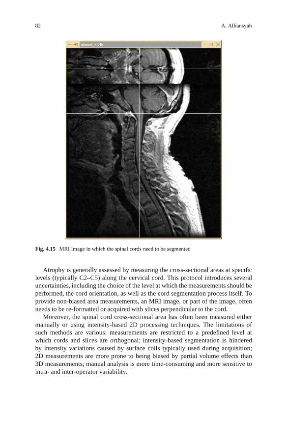
82 A. Alfiansyah
Fig. 4.15 MRI Image in which the spinal cords need to be segmented
Atrophy is generally assessed by measuring the cross-sectional areas at specificlevels (typically C2–C5) along the cervical cord. This protocol introduces severaluncertainties, including the choice of the level at which the measurements should beperformed, the cord orientation, as well as the cord segmentation process itself. Toprovide non-biased area measurements, an MRI image, or part of the image, oftenneeds to be re-formatted or acquired with slices perpendicular to the cord.
Moreover, the spinal cord cross-sectional area has often been measured eithermanually or using intensity-based 2D processing techniques. The limitations ofsuch methods are various: measurements are restricted to a predefined level atwhich cords and slices are orthogonal; intensity-based segmentation is hinderedby intensity variations caused by surface coils typically used during acquisition;2D measurements are more prone to being biased by partial volume effects than3D measurements; manual analysis is more time-consuming and more sensitive tointra- and inter-operator variability.

4 Deformable Models and Level Sets in Image Segmentation 83
Fig. 4.16 Segmentation of an MRI Image using a naive geodesic active contour
4.4.2.2 Segmentation Using Geodesic Active Contour
We propose to apply a geometric deformable model to perform the segmentationwithout any image preprocessing of the data image. The model is initializedby placing a sphere in the spinal cord and letting this sphere evolve until theprocess reaches the convergence. Figure 4.16 shows that the segmentation methodencounters difficulties in extracting the spinal cord at lower levels of vertebrae,due to the proximity of these organs in the image. Using a surface evolution-basedsegmentation method, such as geodesic active contour, the evolved surface passesover the vertebrae border.
We propose an intensity integration approach to solve this organ concurrenceproblem in a specific area, by applying a contrast-based selection to the surfaceof the organ in order to drive the curve evolution bi-directionally according to thatcontrast. Figure 4.17 illustrates the idea of contrast-based selection: suppose that thegray box in the middle is the spinal cord, the two black boxes represent the vertebraeand the red contour is the evolved curve. When the contour is placed in the spinalcord then ∇g and ∇φ have different signs and the contour should be evolved towardsthe spinal cord border. But, when the contour placed in the vertebrae then ∇g and∇φ have the same sign and the contour should be evolved inversely.
Such an approach can be integrated directly into the geodesic active contour’sevolution as:
∂φ∂ t
=[
g ·div
(∇φ|∇φ |
)|∇φ |+ sign(∇g∇φ)(∇g∇φ)+ ν∇g
]‖∇φ‖.

84 A. Alfiansyah
Fig. 4.17 Selective contrast
Fig. 4.18 User interface places the spheres in the spinal cord area (a) and the initialization begins(b and c)
We also enhanced the interactivity of the method, such that the user is allowed toinitialize the method using various spheres in the spinal cord. These spheres canbe provided interactively by means of a user interface in order to browse throughaxial slices and then locate the center of the sphere in that slice. It is not necessaryto place the spheres in the middle of the spinal cord, but they should be situatedentirely inside the spinal cord region in the MRI image.
The curve evolution process of the proposed deformable model for spinalcord segmentation purposes, deviating from the initial curve in Fig. 4.18, prior toreaching the convergence, is visualized in Fig. 4.19.
Applying this type of geometric deformable model, we find that the spinal cordcan be obtained with better quality in a shorter computation time.

4 Deformable Models and Level Sets in Image Segmentation 85
Fig. 4.19 Surface evolution during the segmentation process of spinal cord from the MRI image(the number in the left corner of each image represents the number of elapsed iterations)
4.5 Conclusion
This chapter describes some of the basic concepts of deformable models and theirapplication in different cases of image segmentation. Image segmentation plays acritical role in almost all aspects of image analysis; it has opened a wide range ofchallenging problems oriented towards accurate featuring and geometric extractionof different types of images. The deformable model successfully overcomes thelimitation of classical low-level image processing by providing an elegant andcompact representation of shapes and objects in image analysis.

86 A. Alfiansyah
To gain the best performance of segmentation, the particular deformable modelshould be carefully chosen according to the application context. In general practice,the parametric deformable model runs faster than geometric ones but its typicalshape representation is considerable lower.
References
1. Terzopoulos, D., McInerney, T.: Deformable models in medical image analysis: A survey. Med.Image Anal. 1, 91–108 (1996)
2. Falcao, A., Udupa, J., Samarasekera, S., Sharma, S.: User steered image segmentationparadigm: Livewire and livelane. Graph. Models Image Process. 60(4), 233–260 (1998)
3. Mortensen, E.N.: Interactive segmentation with intelligent scissors. Graph. Models ImageProcess. 60 (5), 349–384 (1998)
4. Falcao, A. et al.: A 3D generalization of user-steered live-wire segmentation. Med. Image Anal.4(4), 389–402. (2000)
5. Schenk, A.M., Guido, P., Peitgen, H.-O.: Efficient semiautomatic segmentation of 3D objects inmedical images. In: Medical Image Computing and Computer-Assisted Intervention, MICCAI2000, vol. 1935, pp. 186–195. (2000)
6. Grady, L., et al. Random Walks for Interactive Organ Segmentation in Two and ThreeDimensions: Implementation and Validation. , 773–780. 2005
7. Pham, D.L., Xu, C., Prince, J.L.: Current methods in medical image segmentation. Annu. Rev.Biomed. Eng. 2(1), 315–337 (2000)
8. McInerney, T., Terzopoulos, D.: Deformable models in medical image analysis: A survey. Med.Image Anal. 1(2), 91–108 (1996)
9. Kirbas, C., Quek, F.: A review of vessel extraction techniques and algorithms. , ACM Comput.Surv. 36(2), 81–121 (2004)
10. Suri, J.S., et al.: Shape recovery algorithms using level sets in 2-D/3-D medical imagery(part-II): a state-of-the-art review. Pattern Anal. Appl. 5(1), 77–89 (2002)
11. Suri, J.S., et al.: A review on MR vascular image processing algorithms: Acquisition andprefiltering: part I. IEEE Trans. Inform. Technol. Biomed. 6(4), 324–337 (2002)
12. Kass, M., Witkin, A., Terzopoulos, D.: Snakes: Active contour models. Int. J. Comput. Vis.321–322 (1998)
13. Fischler, M., Elschlager, R.: The representation and matching of pictorial images. ., IEEETrans.– Comput. 22, 67–92 (1973)
14. Widrow, B.: The “rubber-mask” technique. Pattern Recogn. 5, 175–211 (1973)15. Williams, D., Shah, M.: A fast algorithm for active contours and curvature estimation.
Comput.Vis. Graph. Image Process. Image Underst. 55(1), 14–26 (1992)16. Cohen, L.D.: On active contour models and balloons. , Comput. Vis. Graph. Image Process.
Image Underst. 211–218 (1991)17. Cohen, L.D., Cohen, I.: Finite-element methods for active contour models and balloons for 2D
and 3D images. IEEE Trans. Pattern Anal. Mach. Intell. 1131–1147 (1993)18. Xu, C., Prince, J.L.: Generalized gradient vector flow external forces for active contours. Signal
Process. 71(2), 131–139 (1998)19. Xu, C., Prince, J.L.: Snakes, shapes, and gradient vector flow. IEEE Trans. Image Process. 7(3),
359–369 (1998)20. Amini, A.A., Weymouth, T.E., Jain, R.C.: Using dynamic programming for solving variational
problems in vision. IEEE Trans. Pattern Anal. Mach. Intell. 12(9), 855 (1990)21. Saad, Y.: Iterative methods for sparse linear systems, 2nd edn. s.l. SIAM Publisher,
Philadelphia (2003)

4 Deformable Models and Level Sets in Image Segmentation 87
22. Menet, S., Saint-Mark, P., Medioni, G.: B-snakes: implementation and application to stereo.Image Underst. Workshop. 720–726 (1997)
23. Caselles, V., Kimmel, R., Sapiro, G.: Geodesic active contours. Int. J. Comput. Vis. 22(1),61–79 (1997)
24. Duncan, L.H., Staib, J.S.: Boundary fitting with parametrically deformable models. Trans.Pattern Recogn. Mach. Intell. 14(11), 1061–1075 (1997)
25. Malladi, R., Sethian, J.A., Vemuri, B.C.: Shape modeling with front propagation: A level setapproach. IEEE Trans. Pattern Anal. Mach. Intell. 17(2), 158–175 (1995)
26. Vemuri, B.C., Y., J. Yeand. Image registration via level-set motion: Applications to atlas-basedsegmentation. Medical Image Analysis, 7(1), 1–20 (2003)
27. Osher, S., Sethian, J.A.: Fronts propagating with curvature-dependent speed: algorithms basedon Hamilton-Jacobi formulations. J. Comput. Phys. 79, 12–49 (1988)
28. Tanenbaum, A.: Three snippets of curve evolution theory in computer vision. Math. Comput.Model. 24, 103–119 (1996)
29. Kichenassamy, S., et al.: Conformal curvature flows: From phase transitions to active vision. ,Archive of Rational Mechanics and Analysis 136, 275–301 (1996)
30. Caselles, V., et al.: A geometric model for active contour. Numerische Mathematik 66, 1–31(1993)
31. Yezzi, A., et al.: A geometric snake model for segmentation of medical imagery. IEEE Trans.Med. Imaging, 16, 199–209 (1997)
32. Chan, T.F., Sandberg, B., Vese, L. Active contours without edges for vector valued images. J.Vis. Commun. Image Represent. 11, 130–141 (2000)
33. Chan, T.F., Vese, L.A.: Active contours without edges. IEEE Trans. Image Process. 266–277(2001)
34. Chan, T.F., Vese, L.A.: A Multiphase level set framework for image segmentation using theMumford and Shah model. Int. J. Comput. Vis. 50( 3), 271–293 (2002)
35. Alfiansyah, A., Streichenberger, R., Kilian, P., Bellemare, M.-E., Coulon, O.: Automaticsegmentation of hip bone surface in ultrasound images using an active contour. In: CARS’2006,Computed Assisted Radiology and Surgery, in International Journal of Computer AssistedRadiology and Surgery, 1, supplement 1, 115–116, Osaka Japan, 2006.
36. Alfiansyah, A., Ng, K.H., Lamsudin, R.: Deformable model for serial ultrasound imagessegmentation: application to computer assisted hip athropasty. Singapore: s.n., In: InternationalConference on BioMedical Engineering (2008)
37. Lopez Perez, L., Le Maitre, J., Alfiansyah A., Bellemare, M.-E.: Bone Surface reconstructionusing localized freehand ultrasound imaging. In: Vancouver: 30th Annual International IEEEEMBS Conference, pp. 2964–2967. (2008)
38. Montagnat, J., Delingette, H., Ayache, N.: A review of deformable surfaces: topology,geometry and deformation. Image Vis. Comput. 19, 1023–104037 (2001)
39. Vray, D., et al.: {3D Quantification of Ultrasound Images: Application to Mouse EmbryoImaging In Vivo}. 2002
40. Liu, Y.J. et al.: Computerised prostate boundary estimation in ultrasound images using theradial bas-relief method. , Med. Biol. Eng. Comput. 35, 4450–4454 (1997)
41. Tauber, P., Batatia, H., Ayache, A.: Robust B-Spline Snakes for Ultrasound Images Segmenta-tion. s.l.: IEEE, 2004
42. Liu, F., et al.: Liver segmentation for CT images using GVF snake. Med. Phy. 32(12),3699–3706 (2005)


Chapter 5Fat Segmentation in MagneticResonance Images
David P. Costello and Patrick A. Kenny
5.1 Introduction
Over the past two decades, many authors have investigated the use of magneticresonance imaging (MRI) for the analysis of body fat and body fat distribution.However, accurate isolation of fat in MR images is an arduous task when performedmanually. In order to alleviate this burden, numerous automated and semi-automatedsegmentation algorithms have been developed for the quantification of fat in MRimages. This chapter will discuss some of the techniques and models used in thesealgorithms, with a particular emphasis on their application and implementation.
When segmenting MR images the largest variable in the process is the imageitself. What acquisition parameters give optimal image quality, in terms of signal tonoise ratio (SNR), contrast, uniformity, and boundary definition? An appropriateMRI pulse sequence aims to generate adequate image contrast in the shortestimaging time. MRI can also introduce measurement errors and image artifacts as aresult of the imaging process, which will complicate the segmentation process. Thepotential impact of artifacts such as intensity inhomogeneities and partial volumeeffect (PVE) on image segmentation will be discussed briefly.
Body fat volume and fat distribution provide key risk indicators for a number ofdiseases including non-insulin-dependent diabetes mellitus (NIDDM) and coronaryheart disease (CHD) [1]. Traditionally, anthropometric measurements such as bodymass index (BMI), waist to hip ratio, abdominal circumference, and caliper testshave been used to estimate total body fat and body fat distribution [2–4]. Thesemethods indirectly infer an estimate of body fat based on a known correlation
D.P. Costello (�)Mater Misericordiae University Hospital and University College, Dublin, Irelande-mail: [email protected]
G. Dougherty (ed.), Medical Image Processing: Techniques and Applications, Biologicaland Medical Physics, Biomedical Engineering, DOI 10.1007/978-1-4419-9779-1 5,© Springer Science+Business Media, LLC 2011
89

90 D.P. Costello and P.A. Kenny
with underwater weighing [3]. Obesity is defined in terms of BMI [5], which isexpressed as:
BMI =Weight(kg)Height2 (m2)
. (5.1)
However, BMI is a metric that fails to distinguish fat mass from lean mass. Thisrenders BMI ineffective as a metric for assessing sample groups such as athletes,who because of their increased muscle mass can be categorized as overweight orobese even if their percentage body fat is below normal.
Body fat distribution can be analysed using volumetric images of the body.Both MRI and computed tomography (CT) are sophisticated volumetric imagingtechniques that facilitate delineation of regional fat deposits in the body [6]. It isdifficult to justify whole body CT for fat quantification because of its high radiationdose, especially when MRI exists as a non-ionising alternative [7]. Seidell et al. [8]show a strong correlation between fat volumes measured using both modalities. Asa result of this, radiation dose remains the main reasons for selecting MRI over CTto analyse body fat.
5.2 Imaging Body Fat
Image acquisition is the most important step when quantifying fat with MRI. Goodcontrast, resolution, SNR and homogeneity are required for accurate image segmen-tation. Contrast in MR images depends on proton density, longitudinal relaxationtime (T1) and transverse relaxation time (T 2). As a result of the significantdifference in T1 between fat and soft tissue, T1-weighted (T1w) MR sequences areused to enhance fat contrast. Numerous MRI pulse sequences are used to generatehigh contrast images for fat analysis, including: spin echo (SE), gradient echo (GE),Inversion recovery, three-Point Dixon method and water saturated (WS) balancedsteady-state free precession (WS b-SSFP or TrueFISP) pulse sequences fat [6,8–17].
Both SE and GE sequences are used to image body fat [9–15]. GE sequencesare faster than SE but provide decreased homogeneity, lower SNR and reduced T1contrast. However, in some circumstances short scan times are necessary to reducemotion artifact. Fast-SE1 (FSE) sequences reduce imaging time while maintaininghomogeneity. Barnard et al. [9], compared fast and conventional spin echo pulsesequences and found good correlation between the two. However, when comparedto GE sequences, FSE sequences are relatively slow for whole body imaging [18].Brennan et al. [15], successfully used a T1w GE pulse sequence to demonstrate therelationship between whole body fat and BMI.
A number of authors have used advanced pulse sequences to improve contrastbetween fat and soft tissue. One variation on Gradient echo pulse sequence is ab-SSFP sequence. Both WS [19] and non-WS b-SSFP [6] pulse sequences have
1Fast spin echo techniques acquire between 2 and 16 lines of k-space during each TR.

5 Fat Segmentation in Magnetic Resonance Images 91
Fig. 5.1 (a) Whole body MR scan acquired in 6 stations; (b) the stitched image after postprocessing and (c) stitched image with no post processing
been used to image body fat. Peng et al. [19] proposed using a WS b-SSFP pulsesequence for fat quantification. WS b-SSFP [16, 19] allows for rapid acquisitionof high contrast images containing fat and soft tissue. Peng et al. [19] found thatthis sequence performed better than a WS Fast-SE sequence and simplifies thesegmentation process (see Sect. 5.4.2) [16].
Once a pulse sequence is selected, sequence parameters (e.g. repetition time(TR), echo time (TE), number of signal averages (NSA) and echo train length)should be set to optimize both acquisition time and image contrast. Acquisition timeis a key factor when selecting a pulse sequence, as long scan times increases thelikelihood of motion artifacts. The presence of motion artifact in the visceral cavitycan make it very difficult to quantify fat. Scan time can be reduced by shorteningacquisition time, reducing the NSA and increasing the echo train length. Changingthese factors can also lead to a decrease in image contrast and SNR, which shouldbe investigated prior to scanning large cohorts of patients.
There are a number of other imaging parameters that must also be considered.These include field of view (FOV), scan orientation, matrix size, slice thickness, andslice gap. FOV size affects the severity of inhomogeneities across the image.A larger FOV results in a less homogeneous B–field (magnetic–field) across theimage. Homogeneity is particularly important when acquiring coronal whole bodydata sets. Consequently, it is normal practice to split a whole body scan into anumber of smaller sections, known as stations, to reduce inhomogeneities caused by
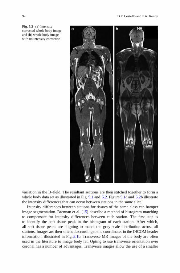
92 D.P. Costello and P.A. Kenny
Fig. 5.2 (a) Intensitycorrected whole body imageand (b) whole body imagewith no intensity correction
variation in the B–field. The resultant sections are then stitched together to form awhole body data set as illustrated in Fig. 5.1 and 5.2. Figure 5.1c and 5.2b illustratethe intensity differences that can occur between stations in the same slice.
Intensity differences between stations for tissues of the same class can hamperimage segmentation. Brennan et al. [15] describe a method of histogram matchingto compensate for intensity differences between each station. The first step isto identify the soft tissue peak in the histogram of each station. After which,all soft tissue peaks are aligning to match the gray-scale distribution across allstations. Images are then stitched according to the coordinates in the DICOM headerinformation, illustrated in Fig. 5.1b. Transverse MR images of the body are oftenused in the literature to image body fat. Opting to use transverse orientation overcoronal has a number of advantages. Transverse images allow the use of a smaller

5 Fat Segmentation in Magnetic Resonance Images 93
FOV, which reduces non-uniformities in the image. Smaller self-contained sectionsalso remove the need for post processing such as image stitching and histogrammatching. Transverse images of the abdomen make it possible to get an estimate ofvisceral fat volume from a small number of sample slices, which reduces scan timesignificantly [20].
Slice thickness and voxel size both influence SNR and PVE. Larger voxelsincreased SNR but increase the incidence of partial volume voxels (PVE is discussedin Sect. 5.3.1). Therefore, it is important to find a balance between SNR and PVEto optimize the segmentation process. Increasing the gap between slices can reduceacquisition time without compromising image quality. A slice gap of 100% will halfacquisition time. Fat volume in the gap can be estimated using interpolation.
5.3 Image Artifacts and Their Impact on Segmentation
5.3.1 Partial Volume Effect
PVE occurs when a single voxel contains a mixture of two or more tissue types,(e.g. at the interface of fat and soft tissue or fat and air), resulting in blurringat boundaries. Figure 5.3 illustrates the effect of the PVE on subcutaneous fat.MR images have limited resolution which increases the probability of the PVEoccurring [21]. Voxels affected by the PVE have an intermediate gray level intensity,which is determined by the proportion of each tissue type contained within thatvoxel [22]. This effect is observed at interfaces between gray and white matter inthe brain and fat and soft tissue throughout the body. The PVE can cause fuzziness(or uncertainty) at the boundaries of two tissues classes [8]. This inhibits the use ofedge detection methods due to ambiguity at the interface of tissue classes leading toa lack of clear edges [8, 23].
Edge-based segmentation methods aim to find borders between regions bylocating edges (or boundaries) within images. MR images have a relatively lowresolution and SNR when compared to other modalities such as CT. PVE and low
Fig. 5.3 (a) T1w GE image containing fat, soft tissue, and background (b) is a profile through plotof the region outlined in red in image (a)

94 D.P. Costello and P.A. Kenny
SNR can result in uncertainty at the boundary of objects in MR images whichlimits the use of edge detection algorithms [8]. Figure 5.3b illustrates the problemencountered by edge detectors when faced with the PVE. Where does fat stop andbackground start? The use of edge detection algorithms can lead to incompletesegmentation of boundaries in MR images. PVE is a three-dimensional phenomenonand can affect large volumes of tissue in a local area. This can affect the performanceof global segmentation techniques, discussed in Sect. 5.4.
5.3.2 Intensity Inhomogeneities
Intensity inhomogeneities can have a significant impact on segmentation andquantitative analysis of MR images. They are caused by non-uniformity in the RFfield (B1), irregularities in the main magnetic field (B0), susceptibility effects ofnormal tissue and receiver coil sensitivity profile [24]. This artifact can cause theappearance of skewed or bimodal fat peaks in the image histogram [25]. As a result,clinical MR images require some processing before segmentation and analysis cantake place. Inhomogeneities in MR images can be modeled as a multiplicative biasfield [23]. The bias field is characterized as a gradual change in intensity withinsegmentation classes across the entire image which cannot be attributed to randomnoise [23]. It can degrade the performance of the intensity–based segmentationalgorithm, as the model assumes spatial invariance between tissues of the same classacross the entire image. An expression for the biased image is given in (5.1).
fbiased = foriginal (x,y)β (x,y)+ n(x,y), (5.2)
where fbiased is the degraded image, forignal is the image without degradation or noiseand n(x,y) is random noise. A number of approaches are investigated in the literaturefor the correction of the bias field (26–30). The impact of intensity inhomogeneitieson thresholding is illustrated in Fig. 5.4.
Siyal et al. [26] and Rajapakse et al. [23] reviewed a number of approachesto reduce the appearance of the intensity inhomogeneities. These approaches canbe split into two categories, retrospective and prospective modeling. Prospectivemodeling uses prior knowledge of the bias field, which can be obtained by imaginga homogeneous phantom. Homogeneous phantoms only provide a good estimate ofthe bias field for objects of similar size to the phantom. When imaging patients,the dimensions of the scanned volume can vary from patient to patient and alsobetween sections of the same patient (e.g. the legs and the torso). The volume of thearea being imaged changes the loading on the receiver coils’ in the MRI scanner,which in turn alters the coils sensitivity profile [27]. To account for this Murakamiet al. [28] performed a calibration scan directly on the patient to estimate the biasfield. Prospective modeling of the bias field can be impractical for studies containinglarge numbers of patients, as imaging time increases due to the need for additionalphantom/patient scans [27].

5 Fat Segmentation in Magnetic Resonance Images 95
Fig. 5.4 (a) Ideal unbiased image (b) Product of the ideal image and bias field, (c) and (d) are thecorresponding thresholded images
Retrospective methods are more practical to implement, as they are based onimage processing and do not require any additional scan time. A number of methodsto retrospectively correct the bias field were used in the literature [27, 29–32]. Inan MR image, the bias field is considered to have a low spatial frequency, whileanatomical structures are likely to consist of higher spatial frequencies. Therefore,it is possible to model the bias field based on the low frequency componentsof the original image [33]. This model can then be used with (5.2) to correctthe inhomogeneity. Guillemaud et al. [34] proposed a method that changes themultiplicative bias field into an additive one, by applying homomorphic filteringto the logarithmic transform of the image data. An extension to this correctionmethod which combines homomorphic filtering and normalized convolution wasalso proposed by Guillemaud et al. [32]. Both of these methods can affect highfrequency components in the image. However, the second approach uses normalizedconvolution to compensate for this.

96 D.P. Costello and P.A. Kenny
Yang et al. [35] proposed the use of overlapping mosaics to segment fat in MRimages affected by intensity inhomogeneities. This segmentation technique is anexample of adaptive thresholding and is discussed further in Sect. 5.4.6.
5.4 Overview of Segmentation Techniques Used to Isolate Fat
Most of the segmentation algorithms discussed in this section are ‘hard segmenta-tion algorithms’, i.e. a definite label is assigned to every voxel in the image (e.g. fator non-fat). Some consideration will be given to soft segmentation algorithms andtheir usefulness in dealing with the PVE. These algorithms take into considerationthe proportion of each tissue type in every voxel.
Once an image has been segmented, the volume of fat (VF) contained within animage is calculated using:
VFat = NFat Voxels ×Vvoxel. (5.3)
where NFat Voxels is the number of voxels classified as fat in the image and Vvoxel
is the volume of a single voxel. The total fat in kilograms can be calculated bymultiplying this value by the density of fat [15].
5.4.1 Thresholding
Thresholding is the simplest forms of image segmentation. It is a real-time segmen-tation technique that is both fast and computationally inexpensive. Thresholdingtransforms a gray-scale image f (i, j), into a binary image g(i, j), based on athreshold value, T . The process is summarized as:
g(i, j) = 1 for f (i, j) > T,
g(i, j) = 0 for f (i, j) ≤ T. (5.4)
In its simplest form thresholding is a manual process in which the user interactivelyselects a threshold value (T ), based on the distribution of gray-levels in the imagehistogram, to create a binary image similar to those shown in Fig. 5.5.
Manual thresholding, like all subjective processes, is open to inter and intra-operator variability. Figure 5.5c, d are examples of alternative segmentation resultsthat were obtained using alternative threshold values.
At the outset, some authors used manual thresholding to quantify fat in MRimage. However, in an effort to reduce subjectivity, Chan et al. [11] set a strictprotocol for threshold selection. The threshold was selected as the minima betweenthe soft tissue and fat peaks in the image histogram. Chan’s method shows goodcorrelation with BMI for a sample group of patients [11]. One drawback of this

5 Fat Segmentation in Magnetic Resonance Images 97
Fig. 5.5 (a) T1-Weighted GE image (b) manually thresholded image (c) over-thresholded(d) under-thresholded (e) image histogram
approach is that MR image histograms can have multiple minima between tissuepeaks as a result of random noise and inhomogeneities. This can cause ambiguitywhen manually selecting a threshold value. Another approach used in the literatureis to preset a threshold for all subjects based on the manual analysis of a group ofhealthy controls [13, 36]. This system of segmentation is very rigid and can requireuser interaction to reclassify mislabelled pixels [13]. One way to avoid variability isto automate the process of thresholding to select an optimum threshold value.
5.4.2 Selecting the Optimum Threshold
Subjectively choosing an image threshold is a relatively simple task. However, theobjective selection of an optimum threshold can be much more complex. Many
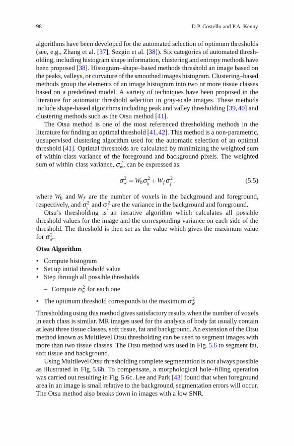
98 D.P. Costello and P.A. Kenny
algorithms have been developed for the automated selection of optimum thresholds(see, e.g., Zhang et al. [37], Sezgin et al. [38]). Six categories of automated thresh-olding, including histogram shape information, clustering and entropy methods havebeen proposed [38]. Histogram–shape–based methods threshold an image based onthe peaks, valleys, or curvature of the smoothed images histogram. Clustering–basedmethods group the elements of an image histogram into two or more tissue classesbased on a predefined model. A variety of techniques have been proposed in theliterature for automatic threshold selection in gray-scale images. These methodsinclude shape-based algorithms including peak and valley thresholding [39,40] andclustering methods such as the Otsu method [41].
The Otsu method is one of the most referenced thresholding methods in theliterature for finding an optimal threshold [41,42]. This method is a non-parametric,unsupervised clustering algorithm used for the automatic selection of an optimalthreshold [41]. Optimal thresholds are calculated by minimizing the weighted sumof within-class variance of the foreground and background pixels. The weightedsum of within-class variance, σ 2
w, can be expressed as:
σ 2w = Wbσ2
b+Wf σ 2
f, (5.5)
where Wb and Wf are the number of voxels in the background and foreground,respectively, and σ2
band σ 2
fare the variance in the background and foreground.
Otsu’s thresholding is an iterative algorithm which calculates all possiblethreshold values for the image and the corresponding variance on each side of thethreshold. The threshold is then set as the value which gives the maximum valuefor σ2
w.
Otsu Algorithm
• Compute histogram• Set up initial threshold value• Step through all possible thresholds
– Compute σ 2w for each one
• The optimum threshold corresponds to the maximum σ 2w
Thresholding using this method gives satisfactory results when the number of voxelsin each class is similar. MR images used for the analysis of body fat usually containat least three tissue classes, soft tissue, fat and background. An extension of the Otsumethod known as Multilevel Otsu thresholding can be used to segment images withmore than two tissue classes. The Otsu method was used in Fig. 5.6 to segment fat,soft tissue and background.
Using Multilevel Otsu thresholding complete segmentation is not always possibleas illustrated in Fig. 5.6b. To compensate, a morphological hole–filling operationwas carried out resulting in Fig. 5.6c. Lee and Park [43] found that when foregroundarea in an image is small relative to the background, segmentation errors will occur.The Otsu method also breaks down in images with a low SNR.

5 Fat Segmentation in Magnetic Resonance Images 99
Fig. 5.6 (a) T1w GE image containing fat and soft tissue, (b) image segmentation using a Multi-Otsu method and (c) segmented image corrected using morphological operator
In MRI, the water signal can sometimes obscure the fat peak in the imagehistogram and make it difficult to use histogram–based global–segmentation tech-niques to locate the optimum threshold. WS sequences such as b-SSFP (or FISP)and T1w FSE can be used to simplify the image segmentation process [19]. Penget al. [19] compared Water-suppressed T1w TSE and WS b-SSFP and found thatSNR and contrast were superior in WS b-SSFP. In later work, Peng et al. [44]introduced a simple automated method to quantify fat in water saturated MRimages. This technique is based on an ideal model of the image histogram andglobal thresholding. Figure 5.7 illustrates the effect of water saturation on the imagehistogram.
Peng’s segmentation model assumes that all voxels beyond the peak fat value(Smax) in Fig. 5.7e are fat and all voxels between 0 and Smax are partial volumefat voxels. On average, partial volume fat voxels are 50% fat [16]. Therefore,the threshold value, Sth, is set to Smax/2. Once a threshold value is calculatedclassification of subcutaneous and visceral fat is completed manually. Using water–saturated MR images removes the obstacle of overlapping peaks from the imagehistogram, which facilitates simple thresholding. Segmentation results shown inFig. 5.7e, f are very different because of the improved contrast in (d), demonstratingthat an optimal imaging protocol can greatly simplify the segmentation process.

100 D.P. Costello and P.A. Kenny
Fig. 5.7 Images and their corresponding intensity histograms obtained using T1W TSE and WSb-SSFP sequences. Both images are acquired from the same anatomic slice of the same subjectwith breath hold. The T1W TSE image (a) is shown to have lower contrast between fat andnonfat. Water and partial-volume fat signal are also in the same gray level range as shown in(b), making automated fat quantification difficult. The WS b-SSFP image (d), however, showsnegligible water signal, leading to fat-only images. The corresponding histogram (e) shows thatsignal from suppressed water, partial-volume fat, and full-volume fat are delineated. This makesit possible to perform automated, yet accurate fat quantification. This material is reproduced withpermission of John Wiley & Sons, Inc. [44] with the addition of images (c) and (f). Image (c) isthe result of OTSU thresholding applied to (a) and (f) is the result of the segmentation techniquedescribed by Peng et al. [44]
5.4.3 Gaussian Mixture Model
When overlapping peaks cannot be avoided the Gaussian mixture model (GMM)can be used to model complex probability density functions (PDF), such as imagehistograms, f (x), as k overlapping Gaussians. This is illustrated in Fig. 5.8 and canbe expressed as:
f (x) =k
∑i=1
piN(x|μi,σ 2
i
), (5.6)
where μi and σi are the mean and standard deviation of the ith Gaussian, respec-tively. pi is the mixing proportion of the constituent Gaussians, N, used to modelthe PDF of the image. It satisfies the conditions:
pi > 0,k
∑i=1
pi = 1. (5.7)

5 Fat Segmentation in Magnetic Resonance Images 101
Fig. 5.8 (a) T1-weighted GE image containing fat and soft tissue, (b) shows the threshold valueT illustrates the threshold location using a red line. Voxels with gray level intensities higher than Tare classified as fat. (c) Image histogram of (a) and its constituent Gaussians estimated using theGMM
Each Gaussian cluster is then modeled using the product of (5.8), the generalequation for a Gaussian distribution and its probability (pi).
N(μi,σi) =1
σi√
2πexp
(− (x− μi)2
2σ 2i
). (5.8)
Figure 5.8c, illustrates an image histogram containing 3 tissue classes and its con-stituent Gaussians calculated using a GMM. One of the most common algorithmsused to calculate pi, μi and σi is the expectation maximization (EM) algorithm [45].
The GMM assumes that the PDF of all constituent tissue types in an imagehistogram are Gaussian and that tissue of the same class is uniform in intensitythroughout the image or region of image to be segmented. When segmenting fat inMR images, k is usually estimated using a priori knowledge as 3 (fat, soft tissue andbackground).
The probability of an event (pixel/voxel) belonging to the ith distribution isgiven by
P(x|Θ) =k
∑i=1
piN(x|μi,σi), (5.9)

102 D.P. Costello and P.A. Kenny
where
Θ = {μi=1, . . . ,μi=k,σi=1, . . . ,σi=k, pi=1, . . . , pi=k}. (5.10)
The EM algorithm is a two-step iterative algorithm consisting of an expectation step(E-step) and a maximization step (M-step). The algorithm can be initialized using k-means clustering or by equal partitioning of the data into k regions or by automatedseed initialization [46]. The expected log likelihood function for the complete data
is calculated using the E-step and is defined by Q(Θ,�
Θ(t)) using the estimated
parameters�
Θ(t).
Q(Θ,�
Θ(t)) ≡ E[logN (X , Y |Θ)|X ,�
Θ(t)]. (5.11)
The function Q(Θ,�
Θ(t)) contains two arguments Θ denotes the parameters that
will be optimized in order to maximize the likelihood and�
Θ(t) corresponds to theestimated values. X is the observed data and remains constant while Y is the missingdata, which is controlled by the underlying distributions.
The second step in the algorithm is the M-step. This step uses the maximizedvalues from (5.11) above to generate a new set of parameters and is given by:
�
Θ(t + 1) = arg maxΘ
Q(Θ,�
Θ(t)). (5.12)
If we have an estimate of the means (μi) and standard deviation (σi) of theconstituent Gaussians we can compute the probability (pi) of a point (gray-level)in the histogram belonging to the kth Gaussian. The maximization step updates theGaussian parameters using (5.13), (5.14) and (5.15).
pnewi =
1k
k
∑i=1
N( i|x, �
Θ(t)). (5.13)
μnewi = ∑k
i=1 xN( i|x, �
Θ(t))
∑ki=1 N( i|x, �
Θ(t)). (5.14)
σnewi =
∑ki=1 N( i|x, �
Θ(t))(xi − μnewi )(xi −μnew
i )T
∑ki=1 N( i|x, �
Θ(t)). (5.15)
The algorithm iterates between (5.11) and (5.12) until convergence is reached.Based on the Gaussian estimated using the EM algorithm an optimized thresholdis calculated that minimizes misclassification error. The threshold for fat is set tothe closest gray-level corresponding to the intersection of the fat and soft tissueGaussians, as illustrated in Fig. 5.8b. Figure 5.13 in Sect. 5.5 is an example of animage which has been segmented successfully using the GMM. Lynch et al. [46]

5 Fat Segmentation in Magnetic Resonance Images 103
Fig. 5.9 Seed point selection voxels in a region of interest. Each of the nearest neighbor voxelsare illustrated using yellow arrows
proposed a novel approach to initialize cluster centers based on histogram analysis.It used the GMM to obtain a more robust segmentation of fat in MR images. Noobjective assessment of this method was carried out.
5.4.4 Region Growing
Region growing is an image segmentation technique that creates regions based somepredefined homogeneity criteria such as texture, gray-level or color. Gray-level isthe characteristic most commonly used when segmenting fat in MR images. Regiongrowing aims to merge voxels or small regions in an image into larger ones basedon a homogeneity criteria. The first step in any region-growing algorithm is theselection of a seed point, as illustrated in Fig. 5.9. This can be a single voxel ora small region of voxels and can be selected manually or automatically. Next, ahomogeneity criterion is set. For example, if the gray-level of the neighboring voxelis between two threshold values, merge the voxel (region) with the seed point. Theseed voxels nearest neighbors are illustrated using the yellow arrows in Fig. 5.9.Each new voxel in the region becomes a growth point and is compared to its nearestneighbors using the same homogeneity criteria. Growth of the region ceases when

104 D.P. Costello and P.A. Kenny
no new growth points can be created within the confines of the homogeneity criteria.Growth or merging of regions will continue iteratively until the stopping criterion isreached.
Region Growing Algorithm
• Select a seed point/points• Define a homogeneity/merging criteria• Join all voxels connected to the seed that follow the homogeneity criteria to form
a region• Stop the algorithm when no adjacent voxels agree with the homogeneity criteria
Figure 5.10 shows an image containing a number of manually selected seed pointsand the resultant segmentation using region growing. Unlike thresholding, regiongrowing can differentiate objects based on their spatial location, which enables theclassification of different fat categories. In Fig. 5.10b, note also that bone marrowadipose tissue and the liver are not classified as fat. Fat classification as distinct fromsegmentation is an important issue and is discussed in detail in Sect. 5.5.
Region growing can be implemented using a number of algorithms, includingregion merging, region splitting and split and merge algorithms [39, 47]. Splitand merge algorithms can be used to automate region growing, removing theneed for subjective seed point selection [48]. Automated seed selection does notalways guarantee complete segmentation due to the unpredictability of seed pointselection and may therefore require manual addition of extra seed points after initialsegmentation. In noisy images, it is possible for holes to appear in the segmentedregions, post processing may be used to reduce these.
Siegel et al. [6] used a region growing technique in its simplest form tosegment fat in transverse MR images of the abdomen. However, region growingis sometimes combined with edge detection to reduce the occurrence of over- andunder-segmentation. In a study by Yan et al. [49], a three-step segmentation processto isolate skeletal structures in CT images was employed. The first step was theapplication of a three-dimensional region-growing algorithm with adaptive localthresholds, which was followed by a series of boundary correction steps. Thisapproach is both accurate and reliable for high contrast, low noise CT images.Subsequently, a similar technique was applied to the segmentation of fat in MRimages by Brennan et al. [15].
Brennan et al. [15], used a four-step automated algorithm for the quantificationof fat in MR images. Their algorithm was based on initialization of fat regionsusing conservative thresholding followed by steps of boundary enhancement, regiongrowing and region refining (post processing). A weak correlation was foundbetween total body fat quantified using MRI and BMI. The authors attributethis to the flawed nature of BMI measurements. A more appropriate measure ofaccuracy would have been comparison with manual delineation of fat by an expertradiologist (the gold standard). Combination of both region growing and edge–basedsegmentation algorithms contradicts work by Rajapakse and Kruggel [23], who statethat the use of region and edge detection schemes are unsuitable in MR images due

5 Fat Segmentation in Magnetic Resonance Images 105
Fig. 5.10 (a) A T1w GE image and the seed points used for region growing and (b) is the resultantsegmentation following region growing, visceral fat is labeled with red, other fat is labeled blueand the liver purple. Each labeled group is quantified separately
to the lack of clearly defined edges. Despite this, the data presented by Brennanet al. were well segmented. Brennan’s method did not classify and label body fat.Further steps are required to develop classification algorithm.
5.4.5 Adaptive Thresholding
Due to intensity inhomogeneities in MR images a single threshold may not besufficient for the entire image. Segmentation using adaptive thresholding can
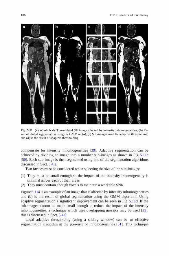
106 D.P. Costello and P.A. Kenny
Fig. 5.11 (a) Whole body T1-weighted GE image affected by intensity inhomogeneities; (b) Re-sult of global segmentation using the GMM on (a); (c) Sub-images used for adaptive thresholding;and (d) is the result of adaptive thresholding
compensate for intensity inhomogeneities [39]. Adaptive segmentation can beachieved by dividing an image into a number sub-images as shown in Fig. 5.11c[50]. Each sub-image is then segmented using one of the segmentation algorithmsdiscussed in Sect. 5.4.2.
Two factors must be considered when selecting the size of the sub-images:
(1) They must be small enough so the impact of the intensity inhomogeneity isminimal across each of their areas
(2) They must contain enough voxels to maintain a workable SNR
Figure 5.11a is an example of an image that is affected by intensity inhomogeneitiesand (b) is the result of global segmentation using the GMM algorithm. Usingadaptive segmentation a significant improvement can be seen in Fig. 5.11d. If thesub-images cannot be made small enough to reduce the impact of the intensityinhomogeneities, a technique which uses overlapping mosaics may be used [35],this is discussed in Sect. 5.4.6.
Local adaptive thresholding (using a sliding window) can be an effectivesegmentation algorithm in the presence of inhomogeneities [51]. This technique

5 Fat Segmentation in Magnetic Resonance Images 107
thresholds individual voxels using the mean or median value of their surroundingn × n neighborhood. MR images acquired for fat analysis can contain largemonotone regions consisting of a single tissue type. In order to achieve meaningfulsegmentation the size of the neighborhood must be large enough to contain morethan one tissue class at any point tin the image. This should be considered whenselecting the neighborhood size.
5.4.6 Segmentation Using Overlapping Mosaics
Yang et al. [35] developed a method to segment fat in MR images using overlappingmosaics. The segmentation technique consists of 3 steps:
(1) Mosaic bias field estimation(2) Adipose tissue segmentation(3) Consistency propagation
Following smoothening (low pass filtering) to remove noise the expression for thebiased image in (5.2) becomes:
f ′biased(x,y) = foriginal(x,y)β (x,y), (5.16)
where f ′biased(x,y) is the image after filtering. Assuming the bias field variesgradually across the entire image, log (β (x,y)) can be approximated by a piecewiselinear function. Yang divides f ′biased(x,y) into a array of overlapping mosaics or sub-images (Tij). Within each of the sub-images Log (β (x,y)) is assumed to be firstorder linear, therefore, ∀(x,y) ∈ Tij:
log f ′biased(x,y) = log( foriginal(x,y))+ aij
(x− x(0)
ij
)+ bij
(y− y(0)
ij
)+ cij, (5.17)
where (x(0)ij ,y(0)
ij ) is the upper left voxel in each sub image. Optimal values for a andb are estimated by maximizing the function:
P = ∑ξ
⎛⎝ ∑
(x,y)∈Tij
δ (log( f ′biased(x,y)))(−aij
(x− x(0)
ij
)−bij
(y− y(0)
ij
)− ξ)⎞⎠
2
,
(5.18)where δ (x) = 1 when x = 0, and ξ is the gray-scale intensity index of the imagehistogram. Cij is not calculated because it affects voxels in the sub–image uniformly,causing a change in position of gray–levels in the image histogram but not the shape.Once the image is corrected, the skewed and bimodal peaks discussed in Sect. 5.3.2appear more distinctive.
When intensity inhomogeneities are corrected, image segmentation is carriedout using a multi-level thresholding technique on each sub-image. Segmentation

108 D.P. Costello and P.A. Kenny
Fig. 5.12 The intermediate processing results of the proposed algorithm applied to a syntheticphantom. (a) The original image with an SNR of 20 dB; (b) the optimum manually segmentedresult by using intensity thresholding; (c) the bias corrected image by using overlappingmosaics; (d) the result of initial segmentation; (e) the final fat distribution after applying inter-mosaic consistency propagation. This material is reproduced with kind permission from SpringerScience+Business Media B.V [35]
is based on an automated thresholding technique that minimises the total variancewithin the three classes, fat soft tissue and background, giving 2 threshold values ξ1
and ξ2 [16].A measure of confidence, λij, of the segmentation result is calculated, as not all
sub images will contain all three tissue classes.
λij =
meanHijξ≥ξ2
(ξ )
meanHijξ<ξ1
(ξ ), (5.19)
Hij(ξ ) is the log transform of the image histogram. λij is likely to be large whenall three tissue classes are present in the sub-image. However, when only one ortwo tissue classes are present λij will be much smaller indicating misclassification.The mosaic tile with the highest value of λij is used as a seed for consistencypropagation. The regions of overlap between the seed tile and its nearest neighborsare compared. If any conflicting segmentation results are present, then the value forξ2 in neighboring tile is changed to that of the seed. This process is propagated toall tiles within the image until segmentation result like those shown in Fig. 5.12 areachieved. Peng et al. [16], compared this technique to the gold standard, manualsegmentation, and found that the mean percentage between the two was 1.5%.

5 Fat Segmentation in Magnetic Resonance Images 109
5.5 Classification of Fat
To appreciate the complexities associated with quantifying fat in medical images, itis important to know what exactly needs to be measured. The most common conflictin the literature is in the terminology used, (i.e. fat or adipose tissue) [52]. Thedifference between fat and adipose tissue is important when quantifying fat in MRimages. Bone marrow in a typical T1w imaging sequence has the same graylevelas body fat. However, bone marrow adipose tissue is not classified as fat because itis connected to haematopoietic activity2 and not to obesity [53, 54]. Classificationis further complicated by the subdivision of fat into three main categories: totalbody fat [15], visceral fat and subcutaneous fat [6]. Whole body fat includes themeasurement of all adipose tissue except bone marrow and adipose tissue containedin the head, hands and feet [52]. A summary of the proposed classification of adiposetissue within the body is given by Shen et al. [52] and is presented in Table 5.1.Examination of body fat distribution involves the analysis of two or more of the fatcategories outlined in Table 5.1.
Global segmentation algorithms such as thresholding require extra steps toclassify fat. This can be achieved manually by drawing a region of interest aroundareas such as the viscera. Figure 5.13 shows the result of manual classification
Table 5.1 Proposed classification of total body adipose tissue as given by Shen et al. [52]
Adipose tissue compartment Definition
Total adipose tissue Sum of adipose tissue, usually excluding bone marrow andadipose tissue in the head, hands, and feet
Subcutaneous adipose tissue The layer found between the dermis and the aponeurosesand fasciae of the muscles. Includes mammary adiposetissue
Superficial subcutaneousadipose tissue
The layer found between the skin and a fascial plane in thelower trunk and gluteal-thigh area
Deep subcutaneous adiposetissue
The layer found between the muscle fascia and a fascialplane in the lower trunk and gluteal-thigh areas
Internal adipose tissue Total adipose tissue minus subcutaneous adipose tissueVisceral adipose tissue Adipose tissue within the chest, abdomen, and pelvisNon-visceral internal adipose
tissueInternal adipose tissue minus visceral adipose tissue
Intramuscular adipose tissue Adipose tissue within a muscle (between fascicles)Perimuscular adipose tissue Adipose tissue inside the muscle fascia (deep fascia),
excluding intramuscular adipose tissueIntermuscular adipose tissue Adipose tissue between musclesParaosseal adipose tissue Adipose tissue in the interface between muscle and bone
(e.g., paravertebral)Other non-visceral adipose
tissueOrbital adipose tissue; aberrant adipose tissue associated
with pathological conditions (e.g., lipoma)
2Hematopoietic activity: pertaining to the formation of blood or blood cells.

110 D.P. Costello and P.A. Kenny
Fig. 5.13 (a) T1w GE image (b) global segmentation using the GMM and (c) classification ofvisceral fat
after global segmentation using the GMM. Region growing allows for classificationbased on spatial location. This is illustrated in Fig. 5.10 where both the liver andvisceral fat are differentiated from fat in the image. Further work is required to fullyautomate classification.
5.6 Conclusions
This chapter reviewed the challenges associated with the quantification of fat inMR images. Accurate segmentation and analysis of fat using MRI is not a trivialmatter. Ideally, MR images acquired for fat analysis should contain three distinct

5 Fat Segmentation in Magnetic Resonance Images 111
tissue classes: fat, soft tissue and air. However, as a result of the many artifactsinherent to MRI this ideal image model is rarely attained. Therefore, considerationmust be given to both the PVE and intensity inhomogeneities when segmenting fatin MR images. It is crucial that fat segmentation is approached with a thoroughunderstanding of these artifacts and the limitations they present. A number oftechniques used to segment fat in the presence of inhomogeneities were outlinedin this chapter.
Image acquisition is the most important step in the quantification and analysis offat using MRI. Before scanning patients, the imaging sequence should be optimizedto achieve a balance between image contrast and acquisition time. Selection of anappropriate imaging sequence, such as the WS–bSSFP can significantly reduce thecomplexity of the segmentation algorithm required.
Fat classification currently requires manual intervention and will remain a signif-icant challenge in the future. Future work in this field will investigate the prospectof fully automating the classification process and the use of soft segmentationalgorithms involving fuzzy sets to overcome the PVE.
References
1. British Nutrition Foundation Obesity Task Force: Obesity: the report of the British NutritionFoundation Task Force, John Wiley & Sons (1999)
2. Sarrıa, A., Moreno, L.A., et al.: Body mass index, triceps skinfold and waist circumferencein screening for adiposity in male children and adolescents. Acta Pædiatrica 90(4), 387–392(2001)
3. Peters, D., et al.: Estimation of body fat and body fat distribution in 11-year-old children usingmagnetic resonance imaging and hydrostatic weighing, skinfolds, and anthropometry. Am. J.Hum. Biol. 6(2), 237–243 (1994)
4. Rush, E.C., et al.: Prediction of percentage body fat from anthropometric measurements:comparison of New Zealand European and Polynesian young women. Am. J. Clin. Nutr. 66(1),2–7 (1997)
5. (WHO), W.H.O. [cited; Available from:www.who.int/dietphysicalactivity/publication/facts/obesity/en/. (2008)
6. Siegel, M.J., et al.: Total and intraabdominal fat distribution in preadolescents and adolescents:measurement with MR imaging. Radiology 242(3), 846–56 (2007)
7. Kullberg, J., et al.: Whole-body adipose tissue analysis: comparison of MRI, CT and dualenergy X-ray absorptiometry. Br. J. Radiol. 82(974), 123–130 (2009)
8. Seidell, J.C., Bakker, C.J., van der Kooy, K.: Imaging techniques for measuring adipose-tissuedistribution–a comparison between computed tomography and 1.5-T magnetic resonance. Am.J. Clin. Nutr. 51(6), 953–957 (1990)
9. Barnard, M.L., et al.: Development of a rapid and efficient magnetic resonance imagingtechnique for analysis of body fat distribution. NMR Biomed. 9(4), 156–64 (1996)
10. Thomas, E.L., et al.: Magnetic resonance imaging of total body fat. J. Appl. Physiol. 85(5),1778–85 (1998)
11. Chan, Y.L., et al.: Body fat estimation in children by magnetic resonance imaging, bioelectricalimpedance, skinfold and body mass index: a pilot study. J Paediatr. Child Health 34(1), 22–28(1998)
12. Kamel, E.G., McNeill, G., Van Wijk, M.C.: Change in intra-abdominal adipose tissue volumeduring weight loss in obese men and women: correlation between magnetic resonance imagingand anthropometric measurements. Int. J. Obes. Relat. Metab. Disord. 24(5), 607–613 (2000)

112 D.P. Costello and P.A. Kenny
13. Ross, R., et al.: Influence of diet and exercise on skeletal muscle and visceral adipose tissue inmen. J. Appl. Physiol. 81(6), 2445–2455 (1996)
14. Terry, J.G., et al.: Evaluation of magnetic resonance imaging for quantification of intraabdom-inal fat in human beings by spin-echo and inversion-recovery protocols. Am. J. Clin. Nutr.62(2), 297–301 (1995)
15. Brennan, D.D., et al.: Rapid automated measurement of body fat distribution from whole-bodyMRI. AJR Am. J. Roentgenol. 185(2), 418–23 (2005)
16. Peng, Q., et al.: Automated method for accurate abdominal fat quantification on water-saturatedmagnetic resonance images. J. Magn. Reson. Imaging. 26(3), 738–46 (2007)
17. Kovanlikaya, A., et al.: Fat quantification using three-point dixon technique: in vitro validation.Acad. Radiol. 12(5), 636–639 (2005)
18. Goyen, M.: In: Goyen, M. (ed.) Real Whole Body MRI Requirements, Indications, Perspec-tives, 1 edn., vol. 1, p. 184. Berlin, Mc Graw Hill (2007)
19. Peng, Q., et al.: Water-saturated three-dimensional balanced steady-state free precession forfast abdominal fat quantification. J. Magn. Reson. Imaging . 21(3), 263–271 (2005)
20. Warren, M., Schreiner, P.J., Terry, J.G.: The relation between visceral fat measurement andtorso level–is one level better than another? The Atherosclerosis Risk in Communities Study,1990–1992. Am. J. Epidemiol. 163(4), 352–358 (2006)
21. Dugas-Phocion, G., et al.: Improved EM-Based tissue segmentation and partial volume effectquantification in multi-sequence brain MRI. In: Lecture Notes in Computer Science, MedicalImage Computing and Computer-Assisted Intervention – MICCAI 2004, vol. 3216, p. 7. (2004)
22. Gonzalez Ballester, M.A., Zisserman, A.P. Brady, M.: Estimation of the partial volume effectin MRI. Med. Image Anal. 6(4), 389–405 (2002)
23. Rajapakse, J.C., Kruggel, F.: Segmentation of MR images with intensity inhomogeneities.Image Vis. Comput. 16(3), 165–180 (1998)
24. Li, X., et al.: Partial volume segmentation of brain magnetic resonance images based onmaximum a posteriori probability. Med. Phys. 32(7), 2337–2345 (2005)
25. Horsfield, M.A., et al.: Incorporating domain knowledge into the fuzzy connectedness frame-work: Application to brain lesion volume estimation in multiple sclerosis. Med. Imaging IEEETrans. 26(12), 1670–1680 (2007)
26. Siyal, M.Y., Yu, L.: An intelligent modified fuzzy c-means based algorithm for bias estimationand segmentation of brain MRI. Pattern Recognit. Lett. 26(13), 2052–2062 (2005)
27. Yun, S., Kyriakos, W.E., et al.: Projection-based estimation and nonuniformity correction ofsensitivity profiles in phased-array surface coils. J. Magn. Reson. Imaging. 25(3), 588–597(2007)
28. Murakami, J.W., Hayes, C.E. Weinberger, E. Intensity correction of phased-array surface coilimages. Magn. Reson. Med. 35(4), 585–590 (1996)
29. Pham, D.L., Prince, J.L.: An adaptive fuzzy C-means algorithm for image segmentation in thepresence of intensity inhomogeneities. Pattern Recognit. Lett. 20(1), 57–68 (1999)
30. Nie, S., Zhang, Y., Li, W., Chen, Z.: A novel segmentation method of MR brain images basedon genetic algorithm. IEEE International Conference on Bioinformatics and Biomed. Eng.729–732 (2007)
31. Wells, W.M., et al.: Adaptive segmentation of MRI data. Med. Imaging IEEE Trans. 15(4),429–442 (1996)
32. Guillemaud, R.: Uniformity correction with homomorphic filtering on region of interest.In: Image Processing, 1998. ICIP 98. Proceedings. 1998 International Conference on (1998)
33. Behrenbruch, C.P., et al.: Image filtering techniques for medical image post-processing: anoverview. Br. J. Radiol. 77(suppl 2), S126–132 (2004)
34. Guillemaud, R., Brady, M.: Estimating the bias field of MR images. Med. Imaging IEEE Trans.16(3), 238–251 (1997)
35. Yang, G.Z., et al.: Automatic MRI adipose tissue mapping using overlapping mosaics.MAGMA 14(1), 39–44 (2002)
36. Leroy-Willig, A., et al.: Body composition determined with MR in patients with Duchennemuscular dystrophy, spinal muscular atrophy, and normal subjects. Magn. Reson. Imaging15(7), 737–44 (1997)

5 Fat Segmentation in Magnetic Resonance Images 113
37. Zhang, Y.J., Gerbrands, J.J.: Comparison of thresholding techniques using synthetic imagesand ultimate measurement accuracy. In: Pattern Recognition, 1992. Vol.III. Conference C:Image, Speech and Signal Analysis, Proceedings., 11th IAPR International Conference on(1992)
38. Mehmet, S., Bulent, S.: Survey over image thresholding techniques and quantitative perfor-mance evaluation. J. Electron. Imaging 13(1), 146–168 (2004)
39. Sonka, M., Hlavac, V., Boyle, R.: In: Hilda, G. (ed.) Image Processing, Analysis, and MachineVision, International Student Edition, 3rd edn., vol. 1. Thomson, Toronto, p. 829. (2008)
40. Nualsawat, H., et al.: FASU: A full automatic segmenting system for ultrasound images. In:Proceedings of the Sixth IEEE Workshop on Applications of Computer Vision. 2002, IEEEComputer Society.
41. Otsu, N.: A threshold selection method from gray-level histograms. Syst. Man Cybern. IEEETrans. 9(1), 62–66 (1979)
42. Sezgin, M., Sankur, B.: Survey over image thresholding techniques and quantitative perfor-mance evaluation. J. Electron. Imaging 13(1), 146–168 (2004)
43. Lee, H., Park, R.H.: Comments on ‘An optimal multiple threshold scheme for image segmen-tation’. Syst. Man Cybern. IEEE Trans. 20(3), 741–742 (1990)
44. Peng, Q., et al.: Automated method for accurate abdominal fat quantification on water-saturatedmagnetic resonance images. J. Magn. Reson. Imaging 26(3), 738–746 (2007)
45. Dempster, A.P., Laird, N.M., R.D. B.: Maximum likelihood from incomplete data via the EMalgorithm. J. R. Stat. Soc. Ser. B (Methodological) 39(1), 1–38 (1977)
46. Lynch, M., et al.: Automatic seed initialization for the expectation-maximization algorithm andits application in 3D medical imaging. J. Med. Eng. Technol. 31(5), 332–340 (2007)
47. Liang, Z.: Tissue classification and segmentation of MR images. Eng. Med. Biol. Mag. IEEE.12(1), 81–85 (1993)
48. Pham, D.L., Xu, C., Prince, J.L.: Current methods in medical image segmentation. Annu. Rev.Biomed. Eng. 2, 315–37 (2000)
49. Yan, K., Engelke, K., Kalender, W.A.: A new accurate and precise 3-D segmentation methodfor skeletal structures in volumetric CT data. Med. Imaging IEEE Trans. 22(5), 586–598 (2003)
50. Wee-Chung Liew, A., Yan, H., Yang, M.: Robust adaptive spot segmentation of DNAmicroarray images. Pattern Recogn. 36(5), 1251–1254 (2003)
51. Dougherty, G.: Digital Image Processing for Medical Applications, 1 edn., vol. 1, p. 447.Cambridge University Press, New York (2009)
52. Shen, W., et al.: Adipose tissue quantification by imaging methods: A proposed classification.Obes. Res. 11(1), 5–16 (2003)
53. Laharrague, P., Casteilla, L.: Bone Marow Adipose Tissue, 1 edn. Nutrition and health.Humana Press, New Jersey (2007)
54. Mantatzis, M., Prassopoulos P.: Total body fat, visceral fat, subcutaneous fat, bone marrowfat? What is important to measure? AJR Am. J. Roentgenol. 189(6), W386 (2007); authorreply W385

Chapter 6Angiographic Image Analysis
Olena Tankyevych, Hugues Talbot, Nicolas Passat, Mariano Musacchio,and Michel Lagneau
6.1 Introduction
The important rise of medical imaging during the twentieth century, mainly inducedby physics breakthroughs related to nuclear magnetic resonance and X-rays has ledto the development of imaging modalities devoted to visualize vascular structures.The analysis of such angiographic images is of great interest for several clinicalapplications. Initially designed to generate 2D data, these imaging modalitiesprogressively led to the acquisition of 3D images, enabling the visualization ofvascular volumes.
However, such 3D data are generally huge, being composed of several millionsof voxels, while the useful –vascular– information generally represents less than5% of the whole volume. In addition to this sparseness, the frequent low signal-to-noise ratio and the potential presence of artifacts make the analysis of suchimages a challenging task. In order to assist radiologists and clinicians, it is thereforenecessary to design software tools enabling them to extract as well as possible therelevant information embedded in 3D angiographic data.
One of the main ways to perform such a task is to develop segmentation methods,i.e., tools which (automatically or interactively) extract the vessels as 3D volumesfrom the angiographic images. A survey of such segmentation methods is proposedin Sect. 6.3. In particular, it sheds light on recent advances devoted to merge differentimage processing methodologies to improve the segmentation accuracy.
Another way to consider computer-aided analysis of 3D angiographic images isto provide human experts with a base of high-level anatomical knowledge which canpossibly be involved in more specific analysis procedures such as vessel labelling.
O. Tankyevych (�)Universite Paris-Est, Laboratoire d’Informatique Gaspard-Monge – UMR CNRS 8049,Paris, Francee-mail: [email protected]
G. Dougherty (ed.), Medical Image Processing: Techniques and Applications, Biologicaland Medical Physics, Biomedical Engineering, DOI 10.1007/978-1-4419-9779-1 6,© Springer Science+Business Media, LLC 2011
115

116 O. Tankyevych et al.
Such knowledge can in particular be embedded in vascular atlases which aredevoted to model qualitative and/or quantitative information related to vessels.A survey of different existing vascular atlases, and ways they can be created ispresented in Sect. 6.4.
The purpose of this chapter is to provide some general background notions on 3Dangiographic image analysis. Due to space limitations, it is impossible to proposean exhaustive overview on vessel segmentation and vascular knowledge modeling.Consequently, Sects. 6.3 and 6.4 propose partial, but hopefully relevant, states ofthe art on these topics. They present some of the most classical and/or recent relatedworks, and some pointers on more complete surveys linked to the main topics ofthis chapter (or to connected research fields, for the sake of completeness). Theyalso present some recent contributions of some of the authors, especially related tovessel segmentation.
6.2 Clinical Context
Vascular pathologies are one of the main causes of morbidity and mortality inthe Western world, and thus constitute an important issue in public health. Thecauses are manifold, from traumatic lesions (due to accidents) to genetic vasculardiseases (such as some arteriovenous malformations), via those linked to obesityand stress (such as atheromatosis and diabetes).
An anomaly affecting vessels can provoke perturbations in organ circulation aswell as in tissues supplied by the involved vascular network. If the lumen of thearteries is shrunk, such as in an atheromatosis disease, blood flow will be affectedand the associated organ will be insufficiently supplied, leading, in the worst cases,to ischemia, and then tissue death. The breaking of a vessel, normal (as in a trauma)or pathological (as in an aneurysm rupture), can cause hemorrhages.
The various angiographic imaging techniques need to determine the nature ofpotential and actual vascular problems, and to accurately identify the affectedvessels, in order to select the most effective treatment. Magnetic resonance an-giography (MRA) was developed during the last decades, and has the advantageof being non-invasive. X-ray angiography, and particularly computed tomographyangiography (CTA), is invasive and irradiating, but remains effective in terms ofimage accuracy.
6.3 Vessel Segmentation
The segmentation of vascular structures from 3D images is a particularly challeng-ing task. Here, the notion of segmentation is considered in a broad sense. Froman image processing point of view, segmentation consists of partitioning an image

6 Angiographic Image Analysis 117
into an object, i.e., a structure of interest, and a background, i.e., the remainderof the image volume. In the context of angiographic imaging, we consider thatvessel segmentation includes (a) methods that detect either whole vessels (i.e., theirlumen and/or walls) or their medial axes and/or (b) methods that perform low-levelprocessing or high-level knowledge extraction (e.g., vein/artery discrimination [100,103] or vessel labelling [14, 42]). We also consider some methods which could beclassified as filtering, since their purpose is to perform vessel enhancement, whichconsists mainly of denoising, but also of vessel reconnection (e.g., in the case ofstenosis, or of signal loss [27, 76]).
As discussed above, the difficulty in performing vessel segmentation is due tothe sparseness of data, and the possible presence of irrelevant signal (other tissues,artifacts or noise). Moreover, anatomical properties of vessels are highly variable insize, appearance, geometry and topology, even more so in pathological cases suchas aneurysms, stenoses, calcifications or arteriovenous malformations.
There exist several kinds of angiographic data, generally well-fitted for visualiz-ing specific vascular structures, and consequently for dealing with specific clinicalissues. The choice of a segmentation method is often linked to the type of imagesunder consideration, the vessel(s) being studied and the clinical purpose. The nextsection discusses the various methodological segmentation strategies.
6.3.1 Survey of Vessel Segmentation Methods
6.3.1.1 General Overview
Several surveys devoted to 3D vascular segmentation have been proposed during thelast decade. The survey proposed in [94] focuses on vessel segmentation from MRAimages,1 and divides them into skeleton methods (with an interest in medial axes)and non-skeleton ones (that aim at detecting whole vascular volumes). Another(globally similar) classification is proposed in [51], which deals more generallywith vessel segmentation from any kind of data independently of their dimensionor acquisition technique. The most recent survey [56] mainly refers to 3D vesselsegmentation from MRA and CTA, and divides its description into (a) the a prioriinformation which can be used for segmentation, (b) the basic tools using thisinformation for detecting vessels, and (c) the methodological frameworks involvingthese tools, as well as a discussion on pre- and post-processing considerations.
In the next section, we introduce the segmentation methods divided into eightmain categories corresponding to the main image processing strategies on which
1Part I of this survey [93] also describes MRA acquisition techniques.

118 O. Tankyevych et al.
they rely: region-growing, differential analysis, model-based filtering, deformablemodels, path finding, vessel tracking, statistical approaches, and mathematicalmorphology.2
6.3.1.2 Region-Growing Methods
Region-growing has been one of the first strategies considered for image segmenta-tion [117], and in particular medical/angiographic ones.Basically, region-growingrelies on two elements: one (or several) seed(s) [1] assumed to belong to thestructure of interest to be segmented, and a propagation criterion, enabling thesegmentation of the object from the seed, by iterative addition of adjacent voxels.
In the case of vessel segmentation, seeds are generally defined interactivelyinside vessels. The seeds can also be detected automatically, especially in the casewhere they constitute the root of a vascular tree [69]. The possible definition ofseveral seeds can straightforwardly lead to an application of region-growing tovessel separation, and in particular, to vein/artery discrimination. In such a case,a set of seeds is defined for arteries and veins, respectively. A competitive region-growing is then performed, based on ad hoc propagation criteria (e.g., a measure ofgray-scale connectedness in [100]).3
The propagation criterion is commonly based on intensity properties, relatedto the high-intensity vascular signal. However, more sophisticated properties canalso be embedded in this segmentation strategy. In particular, it has been proposedto consider a priori knowledge related to the shape and size of the vessels to besegmented [68], or to their topology [78]. The correctness of the orientation ofthe vessels during the segmentation process has also been considered by proposing“wave propagation” strategies [115], which aim to constrain the segmentation frontto remain normal to the vessel axis. It may be noticed that this kind of approach hasbeen further used for vessel tracking methods (discussed later in the section). Theconcept of wave propagation has also led to the development of methods relatedto both deformable models (level-sets) and path-finding approaches, namely, fast-marching methods [61].
Region-growing methods rely on a simple algorithmic framework, which makestheir development and use quite easy and induces a low (generally linear) compu-tational cost. In addition, they guarantee termination which is not systematicallyavailable for other non-monotonic strategies. However, the connectivity hypothesisintrinsically associated with this strategy constitutes a weakness, since the methodmay fail in segmenting vessels in case of vascular signal loss (due to partial volume
2Due to limited space we heave omitted those methods which have resulted led to fewerpublications, such as neural network-based methods [52].3Note that, by duality, region-growing also provides solutions to segmenting vessels by skele-tonization. In such a case, the growing process starts from a seed being a subset of the background(which can then be automatically defined), and generally includes topological constraints in thepropagation criterion [27, 76].
6 Angiographic Image Analysis 119
effect, or flow artifacts, for instance). A contrario, the use of a criterion beingtoo permissive may lead to leakage phenomena, and a final over-segmentation ofvessels [66]. In this context, region-growing methods have often been preferentiallydevoted to the segmentation of large and/or well-contrasted vessels (for whichintensity and connectivity hypotheses are generally reliable).
6.3.1.3 Differential Analysis
Vessels are generally bright structures within a dark background. If an image isviewed as the discrete analog of a function from R
3 to R, vessels then appear asthe maxima of this function. Consequently, it may be possible to detect them byanalyzing the differential properties of the image.
In order to deal with the discrete/continuous issue involved by this strategy, the(discrete) image is convolved with a series of Gaussian derivatives of differentstandard deviations and in different directions, and the responses obtained arecombined into a matrix.
In the case of first derivatives analysis, this matrix, which is the covariancematrix of gradient vectors [2, 8], is called the structure tensor. Except for vesselsegmentation, the first derivatives have also been involved in diffusion filtering,which consists of the propagation of information in the orientations suggested bythese derivatives [60].
In the case of second derivatives analysis, the resulting information is gatheredin the Hessian matrix. The main idea behind eigen analysis of the Hessian matrix isto extract one or more principal directions of the local structure of the image. Thisgives the direction of the minimal curvature, the principal direction in the tubularstructure and a high curvature in the vessel cross-section plane, which makes thefilter more efficient than line filters.
Compared with the image gradient, the Hessian matrix can capture the shapecharacteristics of objects, such as tubes, planes, blob surfaces or noise. In particular,the eigenvalues of the Hessian matrix can be combined into a vesselness function inorder to describe plate-, blob-like and tubular objects [34, 53, 84].
These methods can be performed in multi-scale frameworks in order to detectobjects of different sizes. It has to be noticed that the choice and number of theconsidered scales is particularly important in such methods. If performed at a uniquescale, they do not detect vessels of different sizes, especially those out of the rangeof the considered scale. Conversely, if performed at numerous scales, they canpotentially detect all the vessels but they become computationally quite expensive.
In addition, the robustness of such methods to noise is strongly related to theconsidered scale. For large scales, the blurring effect of Gaussian filtering tendsto remove noise effects and, unfortunately, smaller objects. A contrario, for smallscales, the noise is hardly corrected by this filtering, and the method may biasthe derivative evaluation accuracy, thus requiring the incorporation of assumptionsrelated to noise in the method [113].

120 O. Tankyevych et al.
Despite some weaknesses, which require specific care, derivative-based methodsprovide efficient solutions for detecting vessels, especially in a multi-scale frame-work, and have therefore often been considered for the design of segmentationmethods based on model filtering (see next section) or for the guidance ofdeformable models, for instance.
6.3.1.4 Model-Based Filtering
In general, vessel appearance can be used as a prior for segmentation. In this case,such a prior can describe vessel specific characteristics: photometric (usually beingbrighter than the background) and/or geometric (curvilinear). The most simple areintensity and geometry-based models, which are often combined in deformablemodel methodologies (see next section). We will describe such models in the orderof increasing complexity.
Intensity Models
Intensity models, which are among the simplest ones, strongly depend on theimaging modality. They can integrate brightness, contrast and gradient priors,but also imaging properties, like intensity ranges or intensity variation based onlocation, or even noise distribution [2] (see also Sect. 6.3.1.6 for a discussion ofnoise modeling).
In [111], a cylindrical parametric intensity model is directly fit to the imageintensities through an incremental process based on a Kalman filter for estimatingthe radii of the vessels. While in [79], local neighborhood intensities are consideredin a spherical polar coordinate system in order to capture the common properties forthe different types of vascular points. A natural integration into this kind of modelsis a background description [85, 102].
While simple, intensity models are highly dependent on the nature of the images.Therefore, they have to be tuned for all kinds of circumstances, such as artifacts orother image distortions, as well as to compensate for image variability.
Geometry Models
The assumption that vessels are elongated thin objects, globally similar to tubes hasbeen used for the design of several geometric models, such as generalized cylinders,superellipsoids, Gaussian lines, or bar-like profiles [9, 53, 102].
Based on second-order derivatives (see previous section), several models incor-porating geometrical properties have been developed. In [34], an ideal cylinder isproposed in order to enhance vessels within a measure called vesselness, while in[84] a more general model incorporates elliptical shapes.

6 Angiographic Image Analysis 121
The bifurcation issue has also been considered, for instance in [3] where a bifur-cation models is proposed and optimized based on vessel centerline information.
Geometry models are powerful tools for describing vessels and aiding theirfurther extraction within tracking schemes or by deformation. However, thesemethods assume image regularities that are present in high-quality images, butnot necessarily in noisier ones, nor in pathological cases. Furthermore, they oftenrequire careful parameter tuning, which may change from one data set to the next.They can be used together with the intensity models, often combined in probabilisticand/or statistical approaches contributing to decision-making whether pixel belongto a vascular structure or not.
6.3.1.5 Deformable Models
Deformable models aim at fitting a geometric hypersurface (e.g., a 2D surfacein a 3D image), by moving it and modifying its shape from an initial model,under the guidance of several (generally antagonist) forces: external (“data-driven”)ones, related to the image content, and internal (“model-driven”) ones, devotedto preserve correct geometric properties (e.g., regularity). Such models have beenintensively used in the field of image analysis due to the following advantages:arbitrary shape representation, topological adaptivity, sub-pixel precision, etc.
Among the most classical methods, snakes (often used in 2D in order to segmentvessel cross-sections), have been considered, e.g., in [64], or in [46], where two (1Dand 2D) snakes are used for both segmentation and stenosis quantification.
Level-sets constitute another classical type of deformable model, and rely on anEulerian version of contour evolution with partial derivative equations. The contouris integrated as the zero-level of a higher dimension function (level-set). In [59],an original level-set based scheme deformed an initial boundary estimate toward thevascular structures in the image using a codimension-two regularization force, basedon the vessel centerlines instead of the vessel surface (see Fig. 6.1a). Another level-set based method [62] estimated the background and vessel intensity distributionsbased on the intensity histogram, to more efficiently steer the level-set onto thevessel boundaries.
Several efforts have been conducted to improve deformable models in the quitespecific case of elongated structures. In this context, [104] used flux maximizationas an alternative curvature-based regularization to make surface normals evolveaccording to the gradient vector field. The key idea was to evolve a curve or a surfaceunder constraints by incorporating not only the magnitude but also the direction ofan appropriate vector field.
In [54], local variances are measured with first-order derivatives and are prop-agated according to their strengths and directions, with an optimally oriented fluxreporting more accurate and stable responses and higher robustness to disturbancesfrom adjacent structures in comparison with Hessian-based measures.
The major advantage of deformable model methods is that they are sensitive toweak edges and robust to noisy structures. However, the intensity variation inside

122 O. Tankyevych et al.
Fig. 6.1 Vessel segmentation examples. (a) Brain vessels segmentation based on deformablemodels. (b) Brain arteries segmentation based on path-finding and statistical approaches. (c) Brainarteries segmentation based on vessel tracking. (d) Brain vessels segmentation based on gray-levelhit-or-miss transform. Illustrations from (a) [59], (b) [110], (c) [31], (d) [68]
vascular structures can generate significant intensity gradient with this undesireddiscontinuity stopping the contour evolution at these regions. Due to this localminima, the initial forces should be described with such precision that the finalobject borders are not far from the initial ones. Nonetheless, the evolution of thedeformation can be a costly process. However, integrating vessel features and forcesin powerful optimization schemes helps overcome these problems.

6 Angiographic Image Analysis 123
6.3.1.6 Statistical Approaches
Vessel segmentation based on statistical approaches generally relies on specificassumptions related to the intensity distribution of the vascular/non-vascular signalsin MRA data (only very few statistical methods have been devoted to CTA, see, e.g.,[32], which proposes a particle-filtering strategy for the segmentation of coronaryarteries), and especially physical models of blood flow. If the number and the natureof these distributions is known correctly, it is possible to determine their respectiveparameters (and in particular the mean intensity characterizing the associatedstructures), via a standard Expectation-Maximization (EM) technique [23].
In MRA, two or three distributions are generally considered, for the blood,and the other anatomical structures and the background, respectively. They led,in particular to the definition of Gaussian-Gaussian-uniform [107] and normal-Rayleigh–2×normal [80] mixtures for time-of-flight (TOF) MRA, and Maxwell-Gaussian [19], Maxwell-Gaussian-uniform [17] mixtures for phase-contrast (PC)MRA. In [18], a hybrid model, enables one to choose between these two kinds ofmixtures. Alternatively to these “constrained” mixture choices, [29] has proposeda linear combination of discrete Gaussians with alternate signs, involved in amodified EM, which adaptively deals with both laminar and turbulent (pathological)blood flow [28].
In the primarily considered strategies, the determination of the vascular intensityled to a straightforward segmentation by thresholding of the image (sometimes en-riched by a hierarchical analysis of the image by octree decomposition [107]). Froman algorithmic point of view, segmentation improvements were also performedby considering spatial information (i.e., statistical dependence) between neighborvoxels, by integrating Markov random fields (MRF) [38] in a post-classificationcorrection step [80]. In other works, speed and phase information provided by PC-MRA were fused and involved in a maximum a posteriori-MRF framework toenhance vessel segmentation [17, 18].
Statistical methods globally inherit the strengths and weaknesses of the EMalgorithm. First, they generally require one to establish hypotheses on the signaldistribution. Moreover, they involve several parameters, for instance, weight, meanand standard deviation, of the distributions. The initialization of the segmentationprocess then requires special attention. Indeed, the convergence may depend onthe quality of the initial distribution settings (sometimes automatically determinedbased on heuristic rules [17,107]). As for any optimization strategy, the terminationalso requires one to decide whether the process has correctly converged or not(which is sometimes empirically determined, for instance by a maximal numberof iterations [107]). Finally, since the segmentation process is strongly based onphotometric properties (the results often consist of global or local thresholdings),higher-level knowledge such as geometric assumptions are hardly considered, andrequire post-processing steps based on a statistical framework [80], or, more effi-ciently the collaboration of alternative image processing techniques (see examplesin Sect. 6.3.1).

124 O. Tankyevych et al.
6.3.1.7 Path Finding
Based on extremal intensity and connectedness criteria, the detection of a vesselsegment (or more precisely its medial axis) can be expressed as the determinationof a minimal cost path in a weighted graph modeling voxels, their neighborhoodrelations and their intensity.
Vessel segmentation based on such strategies can rely on standard minimal pathfinding techniques [25] (i.e., on “global” minimization strategies, while methodscategorized in the next Vessel tracking section will rely on “local” (step-by-step)minimization strategies). This is, for instance, the case in [75].
Alternatively to classic path-finding methods, fast-marching strategies [101] havebeen considered. They are both related to the level-sets (see Sect. 6.3.1.5) andminimal path-finding methodologies (they remain, in particular, consistent with thecontinuous formulation of the minimal-path research). In contrast to fully discretepath-finding, they enable the determination of paths with a sub-voxel accuracy [4].
The methods based on path-finding are globally well-suited to the detection ofvessel medial axes, especially in the case of small vessels which justifies theirfrequent use in coronary detection. (For larger vessels, the optimal path may divergefrom the medial axis, leading to eccentric results [57].) However, efforts have alsobeen conducted in developing segmentation methods that extract both vessel axesand vessel walls [7, 57], expressing the whole vascular volume segmentation as theminimization of a path in a space enriched with a supplementary “scale” dimensioncorresponding to the vessel radius.
Despite attempts to segment whole vascular trees [114], such methods generallyremain devoted to the segmentation of vessel segments, thus requiring one tointeractively provide at least an initial and final point [75, 108]. In this case, theymay be robust to noise, and signal decrease (or short signal loss) along the vessel,especially in the case of stenoses. Since these methods are based on monotonicand/or finite algorithmic processes, their termination is guaranteed and their theo-retical algorithmic cost is generally low. However, in practice, the computationalcost may be high, and the provision of initial and final points can potentially enableits reduction by computing paths from both points simultaneously [75].
6.3.1.8 Tracking Methods
By opposition to path-finding methods, tracking methods consist of finding a vessellocally, by progressively determining successive segments composing it. Such anapproach requires one to interactively propose a seed, namely the starting point ofthe tracking process, located in the vessel, and (in most cases) the direction in whichthe vessel has to be tracked.

6 Angiographic Image Analysis 125
This strategy has to be applied step by step, a small segment of the vesselbeing detected at each step. The principal issues to consider in such methodsare the determination of a correct geometry of the detected segment (namely thedetermination of its cross section), the determination of the vessel axis, and theevaluation of the direction of the next segment to be found (i.e., the trajectorymodification), or equivalently, the next point in the vessel. Less frequently, vesseltracking methods, such as the one proposed in [63], directly perform a more globaliterative vascular volume detection, corrected, at each step, by the analysis of theinduced vessel axis, which can in particular be constrained by ad hoc topologicalhypotheses.
The determination of the vessel cross-section at the current point (which enablesin particular its correct repositioning on the vessel axis) can be performed accordingto several strategies. The use of a gradient-based measure is considered in [109](a centerline measure based on the vessel profile then enables one to approximatethe vessel centerline, even in case of non-circularity). The explicit determinationof vessel cross-sections to estimate the vessel axis may however be avoided. Inparticular, it can be done by considering that the medial axis is necessarily locatedon a ridge point [5], which may be detected by second-derivatives criteria. Suchan approach requires a minima the use of cross section information related to thesize of the vessel (in order to determine the correct scale factor) and circularityhypotheses. It can also be performed based on a local optimisation of 3D models[102, 112], which may also lead to the determination of the vessel axis orientation.More classically, the next tracking point may be determined according to the best fitof a sphere modeling the vessel into the image [12, 47, 69].
Despite a few attempts to deal with the case of bifurcations, which can enablethe recursive processing of a whole vascular tree [9, 13, 31], vessel tracking isespecially well-suited to the segmentation of single vessels (see Fig. 6.1c). In thiscase, the termination has to be considered. Some methods require, in particular, theprovision of both a start and an end point [109].
It should be noted that, similarly to the other local approaches (which aimat detecting a part of the vessels, and/or are guided by providing a seed), suchmethods present a generally low algorithmic/computational cost. However, theypresent some drawbacks related to the determination of multiple parameters andto possible error propagation (which characterize such local methods), potentiallyleading to incorrect segmentation if vessel orientation and/or axis is miscalculatedat a given step, for instance due to a bifurcation, non circular section, or a strongaxis curvature.
6.3.1.9 Mathematical Morphology Methods
Mathematical morphology (MM) is a well-established theory of non-linear, order-based image analysis. Fundamental texts on morphology include the books by Serra[86, 87], but more recent and more synthetic texts are also available, including theworks by Soille [89] and by Najman and Talbot [72].

126 O. Tankyevych et al.
Filtering thin objects with morphology can be achieved using appropriatestructuring elements. Typically, thin structuring elements include segments andpaths, combined over families. To account for arbitrary orientation, one can usefamilies of oriented segments and compute a supremum of openings or an infimumof closings as described in [90].
To account for noise or disconnection, families of incomplete segments can beused instead, yielding so-called rank-max openings, which are just as efficient andalso described in the same reference.
Paths are elongated structuring elements, but they are not necessarily locallystraight. Even though the size of families of paths grow exponentially with theirlength, there exists a recursive decomposition that makes the use of such familiestractable [43]. As with segments, it is useful to account for some discontinuitiesusing so-called incomplete paths. As with segments, there exists an efficientimplementation [95]. In fine, path and segment operations are comparable in speed.
In [96], it is shown that path and segment morphological operators significantlyoutperform linear and steerable filters for the segmentation of thin (2D) structures,even in the presence of heavy noise. Paths operators have been extended to 3Din [44], and shown to outperform all other morphological filters for thin objectsegmentation in 3D, both for efficiency and performance.
Connected operators are also the supremum of openings or infimum of closings,but using families of structuring elements that are so large makes little sense.Instead, the concept of connectivity is used [83, 105]. The simplest of those is thearea opening or closing. Informally, the area opening suppresses objects that aresmaller in area than a given size λ . It extends readily to arbitrary lattices, andcorresponds to a supremum of openings with a very large family of structuringelements: all the connected sets that have an area smaller than λ . In the continuum,this family is not countable, but in the discrete case it is still very large. Fortunatelyit is not implemented in this way. A very efficient way to implement this operator isvia the component tree [65, 71, 82].
In [106], a scale-independent elongation criterion was introduced to find vascularstructures, while in [11], component tree was mixed with classification strategies tosegment 3D vessels in an automated fashion.
Other useful connected operators are thinnings rather than openings, as theymake it possible to use more complex criteria for object selection, for instance,using elongation measures, that are not necessarily increasing.
Hit-or-miss transforms repeatedly use pairs of structuring elements (SEs) toselect objects of interest, rather than single SEs. In [10, 68], authors used suchoperators for 3D vessel segmentation, including brain, liver and heart vessels(see Fig. 6.1d).

6 Angiographic Image Analysis 127
6.3.1.10 Hybrid Methods
Despite the huge amount of methodological contributions dedicated to 3D vesselsegmentation, proposed during the last 20 years, the results provided by suchsegmentation methods generally remain less than perfect.
The handling of under-segmentation (especially in the case of small vessels,whose size is close to the image resolution, of signal decrease, or of the partialvolume effect) and over-segmentation (especially in the case of neighboring anatom-ical structures, or of high intensity artifacts), the robustness to image degradations(low signal-to-noise ratio), the ergonomy (automation or easy interaction), the lowcomputational cost, the guarantee of termination and convergence, and the accuracyof the result (for instance, the ability to provide results at a higher resolution thanthe image one) are desirable properties for such methods. Unfortunately, none isgenerally exempt from drawbacks, even in the frequent (and justified) case where themethod is devoted to a quite specific task, vascular structure, and/or image modality.
As nearly all the main strategies of image processing have been –not fullysatisfactorily– investigated to propose solutions to this issue, a reasonable trendduring the last years has consisted of designing hybrid segmentation methodsobtained by crossing methodologies. An alternative way to overcome this issue isto inject more guiding knowledge in the segmentation processes, which justifies –among other reasons– the generation of anatomical vascular models, as discussedin Sect. 6.4. These strategies aim, in particular, at taking advantage of (distinct andcomplementary) advantages of different segmentation techniques.
A synthetic overview of such hybrid methods is now presented.
Principal Strategies
Hybrid vessel segmentation methods present a range of possible solutions forovercoming certain weaknesses of each method and combining their advantages.
One of the most popular hybrid methods is a combination of multi-scaledifferential analysis within vessel detection schemes as in [34, 84] with deformablemodels, such as level-sets [15], B-spline snakes [33], and maximum geometric flow[24, 103].
The deformable method with energy minimizing functionals has also beencombined with statistical region-based information in a multi-scale feature space forautomatic cerebral vessel segmentation [45]. The tracking strategies were reinforcedby gradient flux of circular cross-sections as in [55], while in [35] a multiplehypothesis tracking was used with Gaussian vessel profile and a statistical modelfitting.
In [110], a probabilistic method for axis finding was used within a tracking withminimal path finding strategy together with a possible used guidance (see Fig. 6.1b).This method is especially well-fitted for pathological cases.

128 O. Tankyevych et al.
Multi-scale morphology has been used with Gabor wavelets (providing vesselsize and direction) filters in [92]. The advantage of the Gabor wavelet is thatit is capable of tuning to specific frequencies, allowing estimation of the vesseldimension, while the morphological top-hat filter enhances the contrast betweenvessel structures and background.
6.4 Vessel Modeling
6.4.1 Motivation
6.4.1.1 Context
The availability of accurate knowledge related to anatomical structures is of precioususe in nearly all the fields related to medical image analysis. Knowing where anorgan is located, its shape, dimensions, functions, cellular or chemical composition,and its spatial relations or collaborations with other organs constitutes the basics ofanatomy and medicine.
In the case of vessels, and more generally of vascular trees,4 anatomicalknowledge can be classified into three categories:
• Morphological properties: what is the shape of a vessel (cross-section, trajec-tory), its size (diameter, cross-section area), its orientation, etc.?
• Structural properties: what is the topology of a vascular network (number ofbranches, bifurcations, presence of cycles/anastomoses), its position, its spatialrelations with other organs, etc.?
• Functional properties: what are the vascular territories of an organ (i.e., whatparts of an organ are supplied by a given branch of a vascular network)?
In the field of angiographic image analysis, the question of functional properties,and more specifically the partition of an organ into vascular territories has notbeen intensively considered. In the case of coronaries, the vascular territories aregenerally implicitly provided by the different branches of the coronary tree (theknowledge of such regions is of actual importance for determining the parts ofthe heart being affected by vessel stenoses, and possible subsequent heart attack).Computational modeling of these branches has been carefully studied for severalyears. In the case of cerebral vasculature, the different areas of the brain supplied bythe main branches originated from the Willis polygon have been described long ago
4From a structural (and more especially from a topological) point of view, the terminology of“tree” is generally incorrect for most of vascular networks, despite its frequent use in the literaturedevoted to angiographic imaging. In the sequel of the chapter we will generally distinguish vasculartrees from vascular networks. This distinction will be clarified in the next sections.

6 Angiographic Image Analysis 129
in the medical literature (see, e.g., [70, 97, 98] for recent contributions),5 but theseareas have not yet played a crucial role in angiographic/medical image analysisdespite their potential helpfulness. Similar considerations can be made for the livervascular networks, and in particular the portal network, the branches of which definethe main hepatic anatomical segments [21].
6.4.1.2 Usefulness
The other two kinds of anatomical knowledge, namely, morphological and struc-tural, have been the subject of a several publications related to medical imageanalysis dating back to the end of the 1980s. In particular, the coronary tree andthe (arterial and venous) networks of the brain have been considered.
The first studies, related to the heart, have essentially been devoted to gather andmodel structural information related to the coronary arteries in order to assist theradiologists in their analysis of vessels from CT data, especially for the diagnosisand follow-up of stenoses and their consequences on heart blood supply. Theglobally simple structure of the coronary tree and its (relative) invariance has ledto the design of the first vascular models. Such vascular models will be referred toas atlases6 in the sequel of the chapter. A survey of this first family of (deterministic)atlases is proposed in Sect. 6.4.2.
More recent studies, essentially devoted to the cerebrovasculature, have intendedto gather and model morphological information related to potentially complexvascular networks. It should be noted that, in contrast to vascular structures such ascoronary arteries or hepatic vessels, vascular networks such as the cerebral ones arenot actually tree structures. A vascular tree originates from a single vessel, whichprogressively divides itself (by bifurcations) into branches, leading to an arborescenthierarchy (which, in particular, does not present any cycle). Vascular networks, suchas the cerebral ones, present a more complex organisation. They can originate fromseveral vessels, which divide themselves to refine into smaller branches, but whichcan also join together to give birth to new vessels, or present cyclic structures, asanastomoses. To the complexity induced by the structure of such vascular networks,one must add the complexity induced by the nature of the vessels visualized inthe considered images (both veins and arteries, large and small vessels), from theimage modalities (generally non-injected data, especially in MRA, in the case ofbrain vessels), but also from the anatomical variability of the vessels (from bothmorphological and structural points of view). In this context, the design of no longerdeterministic, but statistical atlases had to be considered. A survey of this second
5The notion of “vascular areas”, which actually does not match the anatomical notion of vascularterritories, was introduced in [78] in order to propose a partition of the cerebral volume to facilitatethe segmentation of vessels from PC-MRA data.6The notion of an atlas has been the subject of a quite intensive research activity during the last15 years, especially in the field of brain imaging. The emergence of computational anatomy [39,50, 99] is, in particular, a direct expression of such research activities.

130 O. Tankyevych et al.
family of atlases is proposed in Sect. 6.4.3. One of the main uses of such statisticalatlases is the guidance of automated vessel segmentation procedures [68], which isa crucial step for several medical image analysis applications.
6.4.2 Deterministic Atlases
The first works on vascular atlases have consisted in developing deterministicmodels of the vessels. By deterministic, we mean that a model is a (representative)example of what can be considered a vascular network. Although being a good(and actually useful) representation of the anatomical truth, such a deterministicatlas is however not necessarily able to take in consideration in an accurate way theinterindividual variability. Broadly speaking, these atlases can be seen as a directtranscription of the models described (both textually and visually) in the anatomyliterature. The pioneering works related to this topic were actually based on thisapproach.
6.4.2.1 Pioneering Works
To the best of our knowledge, the first vascular atlas generated from angiographicdata was developed for the modeling of coronary arteries [26]. This “hand-made”atlas consists of a (piecewise linear) skeleton modeling the main coronary arterysegments and branches, and providing information on topology (e.g., position of thebifurcations), position and trajectory of vessels. Starting from 2D arteriographies of37 patients, vessels were manually segmented from two orthogonal views, fromthe origin of the coronaries to the most distal visible point on each consideredbranch. A total set of approximately 100 points was then regularly sampled oneach segmented tree, leading to a 3D mean positioning of each point. An interactivechoice of the structures to be visualized, and the visualization angle allowed thegeneration of 2D projections of the atlas. In the same period, a second approachwas proposed in [36], relying on a model composed of two orthogonal planesembedding a structural and spatial representation of each one of the left and rightcoronary trees. Based on this pseudo-3D reference, a symbolic description of thearteries was proposed, providing in particular information on branch names andhierarchy, position, (qualitative) orientation, or vascular territories. This descriptionwas made by use of declarative programming with each predicate formalizing agiven information related to a vessel, while some more general rules modeledheuristic information, such as continuity or angular limits at bifurcations.
In contrast to methods such as [36], which rely on bases of semantic knowledge,those which took advantage of the emerging technologies offered by computergraphics at the end of the 1980s (such as [26]), gave rise to related strategies,essentially based on graph modeling and geometric information.

6 Angiographic Image Analysis 131
6.4.2.2 Graph-Based and Geometric Atlases
Among the methods aiming at generating deterministic atlases, one can distinguishthose based on graphs, and those based on geometry. The first ones essentiallyfocus on a symbolic description of the vascular structures (independently from theirembedding in the 3D space, i.e., from their anatomical reality), while the secondones especially aim at defining such models as objects which “match at best” aspatial reality.
One of the main uses of such atlases, is the labeling of coronary branches,i.e., the automatic naming of vessels, in order to assist radiological analysis.The extraction of reliable vascular information from cardiovascular data (generally2D or 3D CT angiography) is of precious use for coronary disease assessment.In this context, it is not only required to segment these vessels (which is a non-trivialtask, subject to strong research efforts by the medical image analysis community[67]), but also to be able to name each branch of the coronary tree, in order tofacilitate the radiological analysis. Such a highly semantic task can not, of course,be carried out without using high-level a priori anatomical knowledge. Based onthese considerations, several vascular atlases have been involved in –and sometimesspecifically designed for– this labeling task [14, 30, 36, 41, 42].
Graph-Based Atlases
The extraction of a graph modeling the structure of a vascular network (i.e.,assigning an edge to each vessel branch, and a node to each junction/bifurcation)has been a purpose frequently considered by the first vessel segmentation methodsdevoted to 3D angiographic data [37, 115]. Note that the main weakness of thesefirst approaches was propagation of segmentation errors in the obtained model.
A solution proposed in [30] relies on the data collected, and validated, in [26].It proposed to define both a symbolic graph-based atlas, which models the treestructure of the coronary arteries, and to couple it with a geometric 3D atlas whichmodels spatial and geometric relationships. Unclassically, the nodes of the graphrepresent vessel segments while the edges model their bifurcations. Each node ofthe graph is then associated with a vessel name, a width, but also a list of pointslocated on the vessel medial axis. This information then intrinsically provides ageometric model of the vessels.
In order to automatically build a graph-model of a vascular tree without depend-ing on possible errors inherited from the segmentation process of real images, analternative consists of generating such a graph from a realistic anatomical phantom.This is the approach proposed in [14] for generating a graph-based atlas of thecoronary arteries. The use of a phantom enables to easily obtain a segmentation(which can be validated a posteriori) and to derive, by a topological post-processing,curvilinear structures enabling to define a graph structure. In [14], such an atlas canbe achieved by storing at each edge/vessel segment information attributes such asits name, length, orientation and diameter.

132 O. Tankyevych et al.
Fig. 6.2 Geometry-based atlases. (a) Atlas of the cerebral vascular (arterial and venous) networks.(b) Atlas of the whole heart and of the coronary arteries. Illustrations from (a) [74] and (b) [58]
Geometry-Based Atlases
The works described above have focused on vascular structures presenting simpleproperties, namely the coronary arteries, out of their anatomical neighboringcontext. In recent works, efforts have been conducted to design vascular atlasesrelated to more complex structures. These contributions rely, in particular, on theuse of geometric models, and specifically surfacic meshes.
In [74], a geometric atlas of the whole cerebral vascular network was proposed(see Fig. 6.2a). This network was quite complex, being composed of veins andarteries of varying sizes (at the resolutions available in 3D CT and MR angiographicdata, namely 0.5 mm), organized in a non-arborescent fashion. The generationprocess, based on the TOF MRA of a healthy patient, was composed of severaliterative steps, the most crucial of which was segmentation (performed manually,for the sake of correctness), medial axes determination and topology correction(also performed interactively), vessel surface generation, quantitative knowledgeextraction and vessel labeling. It led to a quite accurate vascular atlas providinginformation on the type of vessels (arteries or veins), their position in the intracranialvolume, their name, size and topology. Such an atlas, essentially designed with high-level image processing tools, but in a basically manual fashion, however, remainsstrongly related to the only patient involved in the image acquisition process.
In [58], a geometric atlas of the whole heart, made of surfacic meshes cor-responding to different anatomical structures, was proposed (see Fig. 6.2b). Inaddition to the coronary arteries, it also modeled several anatomical structuressuch as the heart chambers and the trunks of the connected vasculature (the modelgeneration of which is beyond the scope of this chapter). The information usedfor generating this vascular atlas consisted of measurements from [26], which

6 Angiographic Image Analysis 133
helped to create a first vascular model. In order to correctly fit this model on itsneighboring cardiac structures, a registration step was carried out.7 The registrationprocess was driven by the medial axes of the main artery segments, interactivelydelineated from 27 3D CT data (which had previously been involved in the meshgeneration of the other anatomical structures). It was based on an incrementalrelaxation of the authorized degrees of freedom, first accepting rigid (translation,rotation) transformation, then scaling, and finally, affine transformation. In contrastto the vascular atlas proposed in [74] for the cerebrovasculature, the one presentedhere, despite the relative simplicity of the modeled vascular tree, was sufficientlyspecific to model spatial relationships with neighboring –non vascular– structures.This is the first (and to our knowledge, the only) vascular atlas offering such aproperty. In contrast to the previous atlas, this one was created (at least partially)thanks to the vascular information provided by 3D CT data of several patients.As stated in the synthetic description of the generation protocol, this required oneto be able to process heterogeneous anatomical knowledge, possibly presentingvariability. In particular, this implies the consideration of tools enabling one to fusethe information related to several patients in a unified result. In the present case,this was done by considering registration. In Sect. 6.4.3, it will be shown that basedon similar registration-based strategies, it is possible to obtain results which areno longer deterministic, but statistical, enabling in particular the modeling of theinterindividual variability.
6.4.3 Statistical Atlases
In the above section, we have considered the vascular atlases which can be qualifiedas deterministic, in the sense that they present a model of vasculature which couldbe seen as the vascular network of a representative patient among the population.In this section, we now focus on non deterministic vascular atlases, and moreespecially on statistical ones, which are intuitively less similar to a hard anatomicalmodel, but which aim at gathering and modeling more completely and efficientlythe characteristics of a whole population of patients.
6.4.3.1 Anatomical Variability Handling
When designing an anatomical model (in the present case, a vascular atlas), twoquestions have to be considered carefully:
1. How to model the invariant information, i.e., the set of characteristics shared bythe whole population?
7The reader interested in registration – which is an issue strongly linked to (vascular) atlasgeneration – may complete the study of this chapter by reading the following surveys [48, 116].

134 O. Tankyevych et al.
2. How to model the interindividual variability, i.e., the set of varying characteristicsamong this population, in a unified framework?
The deterministic atlases described in Sect. 6.4.2 actually provide efficient answersto the first question. However, since they are based on a hard (graph or geometric)model, their ability to handle interindividual variability is not obvious.8
Most of the contributions devoted to deterministic vascular atlas generationpropose various (partial) solutions to this issue. In the preliminary works oncoronary modeling [26], it is mentioned that there exist three variants in the coronarytrees structure: right dominant (10%), balanced anatomic distribution (80%), andleft dominant (10%)9. In [36], such variations are considered by exhaustivelymodeling each induced branch distribution (in this case by integrating them intothe symbolic base of knowledge).
In the case of cerebral vessels, there also exists a strong interindividual variabilityfrom both topological and geometrical points of view [81]. In order to cope with thisissue in the case of the vascular atlas proposed in [74] (and obtained from a singlepatient), a straightforward solution is an exhaustive list of each topological variationdescribed in the anatomy literature [73]. In [41], a more unified solution is proposedfor the modeling and storing of such interindividual topological variations. This isdone by initially considering a classical graph-based modeling (see Sect. 6.4.2.2)enriched by fusing of several anatomical models/graphs into a “vascular catalog”,composed of a graph of all variations, and a discrimination matrix. This matrix helpsto extract these variations as graphs similar to those of [14, 30]. (See also [40] for amore theoretical/methodological contribution related to the same concepts.)
The handling of variability proposed in these contributions is essentially basedon characteristics related to the structure of the vascular networks. This is astraightforward consequence of the modeling strategies which are primarily basedon topological data structures. In particular, the quantitative variations are generallyomitted from these atlases, and the answer of these methods to the second questionactually remains partial.
Some recent contributions try to propose complementary answers to this secondquestion. They are specifically devoted to coping with the issue of modeling thevariability of anatomical characteristics which can be quantified, for instance thesize, orientation, position, or even the shape of the vessels. To this end, they proposeto generate non-deterministic (namely statistical) atlases.
8However, this fact does not represent a crippling drawback, since the relevance of interindividualvariability handling is essentially modulated by the applications requiring the designed atlas. Inparticular, deterministic atlases must not be considered as less (or more) relevant than statisticalones.9Note that the information on coronary arteries gathered in [26] corresponds to a sample of patientswith “normal-sized hearts”. This example illustrates the general necessity to constraint someanatomical hypotheses if we hope to finally obtain a useful model from a finite (and generallyrestricted) set of patients. Such a consideration remains valid when considering statistical models:a classical example is the restriction to either healthy or non-healthy people in the considered poolof patients.

6 Angiographic Image Analysis 135
Fig. 6.3 Atlas for the portal vein entry, in the liver. (a) Sagittal, (b) coronal, and (c) axial slices.Illustration from [68]
6.4.3.2 Recent Works
The methods described hereafter are mainly devoted to design vascular atlases ofvessels or vascular trees/networks from a set of patients/images presenting possibleanatomical variations. In all these contributions, the input data consist of vascularvolumes extracted from angiographic images. Similarly to most of the methods fordeterministic atlas generation, those for statistical atlas generation then strongly relyon vessel segmentation. The following methods have been classified according tothe degree of complexity of the modeled anatomical information.
Shape model
When the vascular structures of interest are sufficiently simple, for instance whenonly a vessel, or a vessel segment has to be modeled, a first (and straightforward)approach for generating vascular atlases can consist in creating shape models. Suchmodels can be defined by computing the mean image of data obtained from thesegmentation of a (learning) image database. This mean image of binary functionscan be seen as a fuzzy function with values in the interval [0,1].
In [69], such a model (which can in particular be involved in subsequentsegmentation procedures [68]) was proposed for a vessel segment, namely theentrance of the portal vein, in the liver. The atlas, built from a database of 15segmented images of the portal vein entry, is illustrated in Fig. 6.3.
Density Atlas
When the vascular structures become more complex, in particular in the casewhere a whole vascular tree/network is considered, a straightforward mean imagegathering each patient vascular information is no longer sufficient to accuratelygenerate a satisfactory vascular atlas. In this more difficult context, it becomesnecessary to develop adequate strategies for fusing several vascular images onto acoherent anatomical reference. Such strategies thus require the use of a registrationprocedure.

136 O. Tankyevych et al.
Fig. 6.4 Atlas of the cerebral arteries. (a) Sagittal, (b) coronal, and (c) axial maximum intensityprojections. Illustration from [20] (with kind permission from Springer Science+Business Media:MICCAI 2003, Tissue-based affine registration of brain images to form a vascular density atlas,volume 2879 of LNCS, 2003, p. 12, D. Cool et al., Fig. 1)
Intuitively, a first and natural way to proceed consists in attempting to register allthe (segmented) vascular networks onto a chosen one, considered as the reference.Such an approach has been developed in [16], where the reference network is firstskeletonized and then processed to provide a distance map (providing the distance tothe closest vessel). The other segmented vascular networks are then registered (byaffine transformation) on this template. The mean and variance images obtainedfrom the distance maps of all the registered images finally provide a kind ofprobabilistic vascular atlas.
If such an approach enables the discrimination between healthy and non-healthypatients (especially in the case of arterio-venous malformations), it is actually notsufficient to accurately model the vessels. This is due, in particular, to the lackof a morphological reference. In order to correct this drawback, it is possible toperform registration no longer to angiographic data, but to associated morphologicalimages. This alternative approach was proposed in [20], where each angiographicdata (in this case, cerebral MRA) was associated with a T2-weighted MRI of thesame patient. An affine registration procedure was then applied between these T2data, leading to morphology-based deformation fields which were then applied ondistance maps similar to the ones previously described, leading to an atlas consistingof a vascular density map. A result for cerebral arteries, obtained from 9 patientsis depicted in Fig. 6.4. Nonetheless, for creating vascular atlases as density fields,a recent strategy was proposed in [88] for cardiovascular CT data. In contrast tothe case of cerebral MRA data, which requires the simultaneous use of MRI data,the considered CTA images contained both morphological (cardiac) structures andangiographic ones. It was then possible to directly perform registration on such data.After (non-rigid) registration of the main vessel centerlines of each image with thechosen reference image and estimation of the closest centerline for each point of theimage, a mean-shift clustering was performed in order to assign each point to oneof the three main vessel clusters. An artery-specific density at each point was thencomputed from a covariance analysis. The result obtained from 85 CTA is depictedin Fig. 6.5.

6 Angiographic Image Analysis 137
Fig. 6.5 3D visualisation of the vascular atlas (here, thresholded density field) for the three maincoronary arteries (centerlines of which, for a given CTA, are depicted in green, red and yellow).Illustration from [88], ( c©2010 IEEE)
Enriched atlas
The statistical atlas generation protocols presented above are essentially devoted to adensity field generation. This density field models information related to a “vascularpresence probability” and possibly a shape, when the interindividual variability issufficiently low.
It may, however, be useful to be able to model more accurate information, relatedfor instance to size and orientation. An approach described in [77] proposed such amethod. It requires as input more information than a simple segmentation, namelya segmented volume (as in [69]), the associated medial axes (as in [16, 20, 88]),but also information on the vessel orientation (it should be noted that all theseinformation elements may be obtained from a segmented volume, by using adequatemethods10). It also requires correct deformation fields in order to register thesedifferent data with an anatomical reference. In order to do so, each angiographicimage (in the current case, cerebral PC-MRA phase image) was associated with amorphological image (namely the associate PC-MRA magnitude image), followinga strategy similar to the one proposed in [20]. Non-rigid registration of thesemorphological images then provided the deformation fields in order to match thesegmentation, medial axes and orientation maps associated with each image onto
10See, e.g., [22] for a robust medial axis computation method.

138 O. Tankyevych et al.
Fig. 6.6 Atlas of the cerebral vascular network. (a) Vascular density, visualized as a maximumintensity projection (sagittal view). (b) Mean vessel diameters, visualized as a maximum intensityprojection (sagittal view). (c) 3D visualisation of a part of the orientation image. Illustrationfrom [77]
the anatomical reference. The mean and variance values for each one of these scalarand vectorial attributes finally led to a vascular density field (as in [16, 20, 88]), butalso to size and orientation intervals at each vascular point of the atlas. Such anatlas, modeling both cerebral veins and arteries, built from 16 patients is partiallyillustrated in Fig. 6.6.
Remaining Challenges
The vascular atlas generation protocols discussed in the previous section provide,in contrast to most of the ones devoted to deterministic atlases, the way tofuse information from a potentially large set of data in a globally automatedfashion. Such automation requirements however induce several conditions relatedto vessel segmentation which can be performed automatically as already discussedin Sect. 6.3.1, but which (at least in the case of vessels) still does not offer perfectresults. However, it should be noted that in the context of atlas generation, asufficient condition for a correct use of automatically segmented data would be theguarantee that they do not present any false positives (the presence of false negativesbeing possibly compensated by the possibly high number of segmented data).
Another crucial issue related to non-deterministic atlas generation is the avail-ability of efficient registration methods. The most recent methods [77, 88] arebased on non-rigid registration techniques, the accuracy of which (in contrast torigid or even affine registration) is probably a sine qua non condition to obtainsatisfactory results. Since such non-rigid registration algorithms have probablyreached a sufficient degree of efficiency for the processing of dense images (such asmorphological cerebral data, for instance), the development of efficient registrationprocedures in the case of sparse – and more especially of angiographic – data seemsto remain, despite a few recent works [6, 16, 49, 91], a globally open question.

6 Angiographic Image Analysis 139
References
1. Adams, R., Bischof, L.: Seeded region growing. IEEE Trans. Pattern Anal. Mach. Intell.16(6), 641–647 (1994)
2. Agam, G., Armato, S. III, Wu, C.: Vessel tree reconstruction in thoracic CT scans withapplication to nodule detection. IEEE Trans. Med. Imaging 24(4), 486–499 (2005)
3. Antiga, L., Steinman, D.A.: Robust and objective decomposition and mapping of bifurcatingvessels. IEEE Trans. Med. Imaging 23(6), 704–713 (2004)
4. Avants, B.B., Williams, J.P.: An adaptive minimal path generation technique for vesseltracking in CTA/CE-MRA volume images. In: Medical Image Computing and Computer-Assisted Intervention – MICCAI 2000. Lecture Notes in Computer Science, vol. 1935,pp. 707–716. Springer, Berlin (2000)
5. Aylward, S.R., Bullitt, E.: Initialization, noise, singularities, and scale in height ridge traversalfor tubular object centerline extraction. IEEE Trans. Med. Imaging 21(2), 61–75 (2002)
6. Aylward, S.R., Jomier, J., Weeks, S., Bullitt, E.: Registration and analysis of vascular images.Int. J. Comput. Vis. 55(2–3), 123–138 (2003)
7. Benmansour, F., Cohen, L.D.: A new interactive method for coronary arteries segmentationbased on tubular anisotropy. In: International Symposium on Biomedical Imaging – ISBI2009, pp. 41–44. IEEE (2009)
8. Bigun, J., Bigun, T., Nilsson, K.: Recognition by symmetry derivatives and the generalizedstructure tensor. IEEE Trans. Pattern Anal. Mach. Intell. 26(12), 1590–1605 (2004)
9. Boldak, C., Rolland, Y., Toumoulin, C.: An improved model-based vessel tracking algorithmwith application to computed tomography angiography. Biocybern. Biomed. Eng. 23(1),41–64 (2003)
10. Bouraoui, B., Ronse, C., Baruthio, J., Passat, N., Germain, P.: 3D segmentation of coronaryarteries based on advanced Mathematical Morphology techniques. Comput. Med. ImagingGraph. 34(5), 377–387 (2010)
11. Caldairou, C., Passat, N., Naegel, B.: Attribute-filtering and knowledge extraction for vesselsegmentation. In: International Symposium on Visual Computing – ISVC 2010, LectureNotes in Computer Science, vol. 6453, pp. 13–22. Springer, Berlin (2010)
12. Carrillo, J.F., Hernandez Hoyos, M., Davila-Serrano, E.E., Orkisz, M.: Recursive tracking ofvascular tree axes in 3D medical images. Int. J. Comput. Assist. Radiol. Surg. 1(6), 331–339(2007)
13. Carrillo, J.F., Orkisz, M., Hernandez Hoyos, M.: Extraction of 3D vascular tree skeletonsbased on the analysis of connected components evolution. In: Computer Analysis of Imagesand Patterns – CAIP 2005, Lecture Notes in Computer Science, vol. 3691, pp. 604–611.Springer, Berlin (2005)
14. Chalopin, C., Finet, G., Magnin, I.E.: Modeling the 3D coronary tree for labeling purposes.Med. Image Anal. 5(4), 301–315 (2001)
15. Chen, J., Amini, A.A.: Quantifying 3-D vascular structures in MRA images using hybrid PDEand geometric deformable models. IEEE Trans. Med. Imaging 23(10), 1251–1262 (2004)
16. Chillet, D., Jomier, J., Cool, D., Aylward, S.: Vascular atlas formation using a vessel-to-image affine registration method. In: Medical Image Computing and Computer-AssistedIntervention – MICCAI 2003. Lecture Notes in Computer Science, vol. 2878, pp. 335–342.Springer, Berlin (2003)
17. Chung, A.C.S., Noble, J.A., Summers, P.: Fusing speed and phase information for vascularsegmentation of phase contrast MR angiograms. Med. Image Anal. 6(2), 109–128 (2002)
18. Chung, A.C.S., Noble, J.A., Summers, P.E.: Vascular segmentation of phase contrast magneticresonance angiograms based on statistical mixture modeling and local phase coherence. IEEETrans. Med. Imaging 23(12), 1490–1507 (2004)
19. Chung, A.C.S., Noble, J.A., Summers, P.E., Brady, M.: 3D vascular segmentation using MRAstatistics and velocity field information in PC-MRA. In: Information Processing in MedicalImaging – IPMI 2001. Lecture Notes in Computer Science, vol. 2082, pp. 461–467. Springer,Berlin (2001)

140 O. Tankyevych et al.
20. Cool, D., Chillet, D., Guyon, J.P., Foskey, M., Aylward, S.: Tissue-based affine registration ofbrain images to form a vascular density atlas. In: Medical Image Computing and Computer-Assisted Intervention – MICCAI 2003. Lecture Notes in Computer Science, vol. 2879,pp. 9–15. Springer, Berlin (2003)
21. Couinaud, C.: Le foie, etudes anatomiques et chirurgicales. Masson, Paris (1957)22. Couprie, M., Coeurjolly, D., Zrour, R.: Discrete bisector function and Euclidean skeleton in
2D and 3D. Image Vis. Comput. 25(10), 1519–1698 (2007)23. Dempster, A.P., Laird, N.M., Rubin, D.B.: Maximum likelihood from incomplete data via the
EM algorithm. J. R. Stat. Soc. Ser. B (Methodological) 39(1), 1–38 (1977)24. Descoteaux, M., Collins, D.L., Siddiqi, K.: A geometric flow for segmenting vasculature in
proton-density weighted MRI. Med. Image Anal. 12(4), 497–513 (2008)25. Dijkstra, E.W.: A note on two problems in connection with graphs. Numerische Mathematik
1, 269–271 (1959)26. Dodge, J.T. Jr., Brown, B.G., Bolson, E.L., Dodge, H.T.: Intrathoracic spatial location of
specified coronary segments on the normal human heart. Circulation 78(5), 1167–1180(1988)
27. Dokladal, P., Lohou, C., Perroton, L., Bertrand, G.: Liver blood vessels extraction by a 3-Dtopological approach. In: Medical Image Computing and Computer-Assisted Intervention –MICCAI 1999. Lecture Notes in Computer Science, vol. 1679, pp. 98–105. Springer, Berlin(1999)
28. El-Baz, A., Farag, A.A., Gimel’farb, G.L., El-Ghar, M.A., Eldiasty, T.: A new adaptiveprobabilistic model of blood vessels for segmenting MRA images. In: Medical ImageComputing and Computer-Assisted Intervention – MICCAI 2006. Lecture Notes in ComputerScience, vol. 4191, pp. 799–806. Springer, Berlin (2006)
29. El-Baz, A., Farag, A.A., Gimel’farb, G.L., Hushek, S.G.: Automatic cerebrovascular seg-mentation by accurate probabilistic modeling of TOF-MRA images. In: Medical ImageComputing and Computer-Assisted Intervention – MICCAI 2005. Lecture Notes in ComputerScience, vol. 3749, pp. 34–42. Springer, Berlin (2005)
30. Ezquerra, N., Capell, S., Klein, L., Duijves, P.: Model-guided labeling of coronary structure.IEEE Trans. Med. Imaging 17(3), 429–441 (1998)
31. Flasque, N., Desvignes, M., Constans, J.M., Revenu, M.: Acquisition, segmentation andtracking of the cerebral vascular tree on 3D magnetic resonance angiography images. Med.Image Anal. 5(3), 173–183 (2001)
32. Florin, C., Paragios, N., Williams, J.: Particle filters, a quasi-Monte-Carlo-solution for seg-mentation of coronaries. In: Medical Image Computing and Computer-Assisted Intervention –MICCAI 2005. Lecture Notes in Computer Science, vol. 3749, pp. 246–253. Springer, Berlin(2005)
33. Frangi, A.F., Niessen, W.J., Hoogeveen, R.M., van Walsum, T., Viergever, M.A.: Model-basedquantitation of 3-D magnetic resonance angiographic images. IEEE Trans. Med. Imaging18(10), 946–956 (1999)
34. Frangi, A.F., Niessen, W.J., Vincken, K.L., Viergever, M.A.: Multiscale vessel enhancementfiltering. In: Medical Image Computing and Computer-Assisted Intervention – MICCAI 1998.Lecture Notes in Computer Science, vol. 1496, pp. 130–137. Springer, Berlin (1998)
35. Friman, O., Hindennach, M., Kuhnel, C., Peitgen, H.O.: Multiple hypothesis templatetracking of small 3D vessel structures. Med. Image Anal. 14(2), 160–171 (2009)
36. Garreau, M., Coatrieux, J.L., Collorec, R., Chardenon, C.: A knowledge-based approach for3-D reconstruction and labeling of vascular networks from biplane angiographic projections.IEEE Trans. Med. Imaging 10(2), 122–131 (1991)
37. Gerig, G., Koller, T., Szekely, G., Brechbuhler, C., Kubler, O.: Symbolic description of3-D structures applied to cerebral vessel tree obtained from MR angiography volume data.In: Information Processing in Medical Imaging – IPMI 1993. Lecture Notes in ComputerScience, vol. 687, pp. 94–111. Springer, Berlin (1993)
38. Graffigne, C., Heitz, F., Perez, P., Preteux, F., Sigelle, M., Zerubia, J.: Hierarchical Markovrandom field models applied to image analysis: A review. In: Neural Morphological and

6 Angiographic Image Analysis 141
Stochastic Methods in Image and Signal Processing, 1995, SPIE Proceedings, vol. 2568,pp. 2–17. SPIE (1995)
39. Guimond, A., Meunier, J., Thirion, J.P.: Average brain models: A convergence study. Comput.Vis. Image Underst. 77(2), 192–210 (2000)
40. Hall, P.: On the addition and comparison of graphs labeled with stochastic variables:Learnable anatomical catalogs. J. Comb. Optim. 5(1), 43–58 (2004)
41. Hall, P., Ngan, M., Andreae, P.: Reconstruction of vascular networks using three-dimensionalmodels. IEEE Trans. Med. Imaging 16(6), 919–930 (1997)
42. Haris, K., Efstratiadis, S.N., Maglaveras, M., Papas, C., Gourassas, J., Louridas, G.: Model-based morphological segmentation and labeling of coronary angiograms. IEEE Trans. Med.Imaging 18(10), 1003–1015 (1999)
43. Heijmans, H., Buckley, M., Talbot, H.: Path openings and closings. J. Math. Imaging Vis. 22,107–119 (2005)
44. Hendriks, C.L.L.: Constrained and dimensionality-independent path openings. IEEE Trans.Image Process. 19(6), 1587–1595 (2010)
45. Hernandez, M., Frangi, A.F.: Non-parametric geodesic active regions: Method and evaluationfor cerebral aneurysms segmentation in 3DRA and CTA. Med. Image Anal. 11(3), 224–241(2007)
46. Hernandez, M., Frangi, A.F., Sapiro, G.: Three-dimensional segmentation of brain aneurysmsin CTA using non-parametric region-based information and implicit deformable models:Method and evaluation. In: Medical Image Computing and Computer-Assisted Intervention –MICCAI 2003. Lecture Notes in Computer Science, vol. 2879, pp. 594–602. Springer, Berlin(2003)
47. Hernandez Hoyos, M., Orłowski, P., Piatkowska-Janko, E., Bogorodzki, P., Orkisz, M.:Vascular centerline extraction in 3D MR angiograms for phase contrast MRI blood flowmeasurement. Int. J. Comput. Assist. Radiol. Surg. 1(1), 51–61 (2006)
48. Holden, M.: A review of geometric transformations for nonrigid body registration. IEEETrans. Med. Imaging 27(1), 111–128 (2008)
49. Jomier, J., Aylward, S.R.: Rigid and deformable vasculature-to-image registration: A hi-erarchical approach. In: Medical Image Computing and Computer-Assisted Intervention –MICCAI 2004. Lecture Notes in Computer Science, vol. 3216, pp. 829–836. Springer, Berlin(2004)
50. Joshi, S., Davis, B., Jomier, M., Gerig, G.: Unbiased diffeomorphic atlas construction forcomputational anatomy. NeuroImage 23(Supplement 1), S151–S160 (2004)
51. Kirbas, C., Quek, F.: A review of vessel extraction techniques and algorithms. ACM Comput.Surv. 36(2), 81–121 (2004)
52. Kobashi, S., Kamiura, N., Hata, Y., Miyawaki, F.: Volume-quantization-based neural networkapproach to 3D MR angiography image segmentation. Image Vis. Comput. 19(4), 185–193(2001)
53. Krissian, K., Malandain, G., Ayache, N., Vaillant, R., Trousset, Y.: Model-based detection oftubular structures in 3D images. Comput. Vis. Image Underst. 80(2), 130–171 (2000)
54. Law, M.W.K. sand Chung, A.C.S.: Weighted local variance-based edge detection and itsapplication to vascular segmentation in magnetic resonance angiography. IEEE Trans. Med.Imaging 26(9), 1224–1241 (2007)
55. Lesage, D., Angelini, E.D., Bloch, I., Funka-Lea, G.: Design and study of flux-based featuresfor 3D vascular tracking. In: International Symposium on Biomedical Imaging – ISBI 2009,pp. 286–289. IEEE (2009)
56. Lesage, D., Angelini, E.D., Bloch, I., Funka-Lea, G.: A review of 3D vessel lumensegmentation techniques: Models, features and extraction schemes. Med. Image Anal. 13(6),819–845 (2009)
57. Li, H., Yezzi, A.J.: Vessels as 4-D curves: Global minimal 4-D paths to extract 3-D tubularsurfaces and centerlines. IEEE Trans. Med. Imaging 26(9), 1213–1223 (2007)
58. Lorenz, C., von Berg, J.: A comprehensive shape model of the heart. Med. Image Anal. 10(4),657–670 (2006)

142 O. Tankyevych et al.
59. Lorigo, L.M., Faugeras, O.D., Grimson, W.E.L., Keriven, R., Kikinis, R., Nabavi, A., Westin,C.F.: CURVES: Curve evolution for vessel segmentation. Med. Image Anal. 5(3), 195–206(2001)
60. Mahadevan, V., Narasimha-Iyer, H., Roysam, B., Tanenbaum, H.L.: Robust model-basedvasculature detection in noisy biomedical images. IEEE Trans. Inform. Technol. Biomed.8(3), 360–376 (2004)
61. Manniesing, R., Niessen, W.J.: Local speed functions in level set based vessel segmentation.In: Medical Image Computing and Computer-Assisted Intervention – MICCAI 2004. LectureNotes in Computer Science, vol. 3216, pp. 475–482. Springer, Berlin (2004)
62. Manniesing, R., Velthuis, B.K., van Leeuwen, M.S., van der Schaaf, I.C., van Laar, P.J.,Niessen, W.J.: Level set based cerebral vasculature segmentation and diameter quantificationin CT angiography. Med. Image Anal. 10(2), 200–214 (2006)
63. Manniesing, R., Viergever, M.A., Niessen, W.J.: Vessel axis tracking using topology con-strained surface evolution. IEEE Trans. Med. Imaging 26(3), 309–316 (2007)
64. McInerney, T., Terzopoulos, D.: Medical image segmentation using topologically adaptablesurfaces. In: Computer Vision, Virtual Reality and Robotics in Medicine and MedicalRobotics and Computer-Assisted Surgery - CVRMed-MRCAS 1997. Lecture Notes inComputer Science, vol. 1205, pp. 23–32. Springer, Berlin (1997)
65. Meijster, A., Wilkinson, H.: A comparison of algorithms for connected set openings andclosings. IEEE Trans. Pattern Anal. Mach. Intell. 24(4), 484–494 (2002)
66. Metz, C., Schaap, M., van der Giessen, A., van Walsum, T., Niessen, W.: Semi-automaticcoronary artery centerline extraction in computed tomography angiography data. In: Interna-tional Symposium on Biomedical Imaging – ISBI 2007, pp. 856–859. IEEE (2007)
67. Metz, C., Schaap, M., van Walsum, T., van der Giessen, A., Weustink, A., Mollet, N.,Krestin, G., Niessen, W.: Editorial: 3D segmentation in the clinic: A grand challengeII- Coronary artery tracking. In: Medical Image Computing and Computer-AssistedIntervention – MICCAI 2008 – Workshop: Grand Challenge Coronary Artery Tracking(2008). http://hdl.handle.net/10380/1399
68. Naegel, B., Passat, N., Ronse, C.: Grey-level hit-or-miss transforms – Part II: Application toangiographic image processing. Pattern Recognit. 40(2), 648–658 (2007)
69. Naegel, B., Ronse, C., Soler, L.: Using grey-scale hit-or-miss transform for segmenting theportal network of the liver. In: International Symposium on Mathematical Morphology –ISMM 2005. Computational Imaging and Vision, vol. 30, pp. 429–440. Springer SBM (2005)
70. Naidich, T.P., Brightbill, T.C.: Vascular territories and watersheds: A zonal frequencyanalysis of the gyral and sulcal extent of cerebral infarcts. Part I: the anatomic template.Neuroradiology 45(8), 536–540 (2003)
71. Najman, L., Couprie, M.: Building the component tree in quasi-linear time. IEEE Trans.Image Process. 15(11), 3531–3539 (2006)
72. Najman, L., Talbot, H. (eds.): Mathematical Morphology: From Theory to Applications.Wiley, London (2010)
73. Nowinski, W., Thirunavuukarasuu, A., Volkau, I., Marchenko, Y., Aminah, B., Puspitasari,F., Runge, V.: A three-dimensional interactive atlas cerebral arterial variants. NeuroInformat-ics 7(4), 255–264 (2009)
74. Nowinski, W., Volkau, I., Marchenko, Y., Thirunavuukarasuu, A., Ng, T., Runge, V.: A 3Dmodel of human cerebrovasculature derived from 3T magnetic resonance angiography.NeuroInformatics 7(1), 23–36 (2009)
75. Olabarriaga, S.D., Breeuwer, M., Niessen, W.J.: Minimum cost path algorithm for coronaryartery central axis tracking in CT images. In: Medical Image Computing and Computer-Assisted Intervention – MICCAI 2003. Lecture Notes in Computer Science, vol. 2879,pp. 687–694. Springer, Berlin (2003)
76. Passat, N., Ronse, C., Baruthio, J., Armspach, J.P., Bosc, M., Foucher, J.: Using multimodalMR data for segmentation and topology recovery of the cerebral superficial venous tree. In:International Symposium on Visual Computing – ISVC 2005. Lecture Notes in ComputerScience, vol. 3804, pp. 60–67. Springer, Berlin (2005)

6 Angiographic Image Analysis 143
77. Passat, N., Ronse, C., Baruthio, J., Armspach, J.P., Maillot, C.: Magnetic resonance angiogra-phy: From anatomical knowledge modeling to vessel segmentation. Med. Image Anal. 10(2),259–274 (2006)
78. Passat, N., Ronse, C., Baruthio, J., Armspach, J.P., Maillot, C., Jahn, C.: Region-growingsegmentation of brain vessels: An atlas-based automatic approach. J. Magn. Reson. Imaging21(6), 715–725 (2005)
79. Qian, X., Brennan, M.P., Dione, D.P., Dobrucki, W.L., Jackowski, M.P., Breuer, C.K., Sinusas,A.J., Papademetris, X.: A non-parametric vessel detection method for complex vascularstructures. Med. Image Anal. 13(1), 49–61 (2009)
80. Sabry Hassouna, M., Farag, A.A., Hushek, S., Moriarty, T.: Cerebrovascular segmentationfrom TOF using stochastic models. Med. Image Anal. 10(1), 2–18 (2006)
81. Salamon, G., Huang, Y.P.: A Radiological Anatomy of the Brain. Springer, Berlin (1976)82. Salembier, P., Garrido, L.: Binary partition tree as an efficient representation for image
processing, segmentation and information retrieval. IEEE Trans. Image Process. 9(4), 561–576 (2000)
83. Salembier, P., Serra, J.: Flat zone filtering, connected operators and filters by reconstruction.IEEE Trans. Image Process. 3(8), 1153–1160 (1995)
84. Sato, Y., Nakajima, S., Atsumi, H., Koller, T., Gerig, G., Yoshida, S., Kikinis, R.: 3D multi-scale line filter for segmentation and visualization of curvilinear structures in medical images.In: Computer Vision, Virtual Reality and Robotics in Medicine and Medical Robotics andComputer-Assisted Surgery – CVRMed-MRCAS 1997. Lecture Notes in Computer Science,vol. 1205, pp. 213–222. Springer, Berlin (1997)
85. Schaap, M., Manniesing, R., Smal, I., van Walsum, T., van der Lugt, A., Niessen, W.:Bayesian tracking of tubular structures and its application to carotid arteries in CTA. In:Medical Image Computing and Computer-Assisted Intervention – MICCAI 2007. LectureNotes in Computer Science, vol. 4792, pp. 562–570. Springer, Berlin (2007)
86. Serra, J.: Image Analysis and Mathematical Morphology. Academic, London, UK (1982)87. Serra, J. (ed.): Image Analysis and Mathematical Morphology. Volume 2: Theoretical
Advances. Academic, London, UK (1988)88. Shahzad, R., Schaap, M., van Walsum, T., Klien, S., Weustink, A.C., van Vliet, L.J.,
Niessen, W.J.: A patient-specific coronary density estimate. In: International Symposium onBiomedical Imaging – ISBI 2010, pp. 9–12. IEEE (2010)
89. Soille, P.: Morphological Image Analysis. Springer, Heidelberg (2003)90. Soille, P., Talbot, H.: Directional morphological filtering. IEEE Trans. Pattern Anal. Mach.
Intell. 23(11), 1313–1329 (2001)91. Suh, J.W., Scheinost, D., Qian, X., Sinusas, A.J., Breuer, C.K., Papademetris, X.: Serial non
rigid vascular registration using weighted normalized mutual information. In: InternationalSymposium on Biomedical Imaging – ISBI 2010, pp. 25–28. IEEE (2010)
92. Sun, K.Q., Sang, N.: Morphological enhancement of vascular angiogram with multiscaledetected by Gabor filters. Electron. Lett. 44(2), 86–87 (2008)
93. Suri, J.S., Liu, K., Reden, L., Laxminarayan, S.: A review on MR vascular image processingalgorithms: Acquisition and prefiltering: Part I. IEEE Trans. Inform. Technol. Biomed. 6(4),324–337 (2002)
94. Suri, J.S., Liu, K., Reden, L., Laxminarayan, S.: A review on MR vascular image processing:Skeleton versus nonskeleton approaches: Part II. IEEE Trans. Inform. Technol. Biomed. 6(4),338–350 (2002)
95. Talbot, H., Appleton, B.: Efficient complete and incomplete paths openings and closings.Image Vis. Comput. 25(4), 416–425 (2007)
96. Tankyevych, O.: Filtering of thin objects, applications to vascular image analysis. Ph.D.thesis, University Paris-Est (2010)
97. Tatu, L., Moulin, T., Bogousslavsky, J., Duvernoy, H.: Arterial territories of the human brain:Brainstem and cerebellum. Neurology 47(5), 1125–1135 (1996)
98. Tatu, L., Moulin, T., Bogousslavsky, J., Duvernoy, H.: Arterial territories of the human brain:Cerebral hemispheres. Neurology 50(6), 1699–1708 (1998)

144 O. Tankyevych et al.
99. Thompson, P.M., Toga, A.W.: A framework for computational anatomy. Comput. Vis. Sci.5(1), 13–34 (2002)
100. Tizon, X., Smedby, O.: Segmentation with gray-scale connectedness can separate arteries andveins in MRA. J. Magn. Reson. Imaging 15(4), 438–445 (2002)
101. Tsitsiklis, J.: Efficient algorithms for globally optimal trajectories. IEEE Trans. Autom.Control 40(9), 1528–1538 (1995)
102. Tyrrell, J.A., di Tomaso, E., Fuja, D., Tong, R., Kozak, K., Jain, R.K., Roysam, B.: Robust3-D modeling of vasculature imagery using superellipsoids. IEEE Trans. Med. Imaging 26(2),223–237 (2007)
103. van Bemmel, C.M., Spreeuwers, L.J., Viergever, M.A., Niessen, W.J.: Level-set-based artery-vein separation in blood pool agent CE-MR angiograms. IEEE Trans. Med. Imaging 22(10),1224–1234 (2003)
104. Vasilevskiy, A., Siddiqi, K.: Flux maximizing geometric flows. IEEE Trans. Pattern Anal.Mach. Intell. 24(12), 1565–1578 (2002)
105. Vincent, L.: Grayscale area openings and closings, their efficient implementation andapplications. In: International Symposium on Mathematical Morphology – ISMM 1993,pp. 22–27. Barcelona, Spain (1993)
106. Wilkinson, M.H.F., Westenberg, M.A.: Shape preserving filament enhancement filtering. In:Medical Image Computing and Computer-Assisted Intervention – MICCAI 2001. LectureNotes in Computer Science, vol. 2208, pp. 770–777. Springer, Berlin (2001)
107. Wilson, D.L., Noble, J.A.: An adaptive segmentation algorithm for time-of-flight MRA data.IEEE Trans. Med. Imaging 18(10), 938–945 (1999)
108. Wink, O., Frangi, A.F., Verdonck, B., Viergever, M.A., Niessen, W.J.: 3D MRA coronary axisdetermination using a minimum cost path approach. Magn. Reson. Med. 47(6), 1169–1175(2002)
109. Wink, O., Niessen, W.J., Viergever, M.A.: Fast delineation and visualization of vessels in 3-Dangiographic images. IEEE Trans. Med. Imaging 19(4), 337–346 (2000)
110. Wong, W.C.K., Chung, A.C.S.: Probabilistic vessel axis tracing and its application to vesselsegmentation with stream surfaces and minimum cost paths. Med. Image Anal. 11(6), 567–587 (2007)
111. Worz, S., Rohr, K.: A new 3D parametric intensity model for accurate segmentation andquantification of human vessels. In: Medical Image Computing and Computer-AssistedIntervention - MICCAI 2004. Lecture Notes in Computer Science, vol. 3216, pp. 491–499.Springer, Berlin (2004)
112. Worz, S., Rohr, K.: Segmentation and quantification of human vessels using a 3-D cylindricalintensity model. IEEE Trans. Image Process.16(8), 1994–2004 (2007)
113. Wyatt, C., Bayram, E., Ge, Y.: Minimum reliable scale selection in 3D. IEEE Trans. PatternAnal. Mach. Intell. 28(3), 481–487 (2006)
114. Yim, P.J., Choyke, P.L., Summers, R.M.: Gray-scale skeletonization of small vessels inmagnetic resonance angiography. IEEE Trans. Med. Imaging 19(6), 568–576 (2000)
115. Zahlten, C., Jurgens, H., Evertsz, C.J.G., Leppek, R., Peitgen, H.O., Klose, K.J.: Portal veinreconstruction based on topology. Eur. J. Radiol. 19(2), 96–100 (1995)
116. Zitova, B., Flusser, J.: Image registration methods: A survey. Image Vis. Comput. 21(11),977–1000 (2003)
117. Zucker, S.W.: Region growing: Childhood and adolescence. Comput. Graph. Image Process.5(3), 382–399 (1976)

Chapter 7Detecting and Analyzing Linear Structuresin Biomedical Images: A Case Study UsingCorneal Nerve Fibers
Mohammad A. Dabbah, James Graham, Rayaz A. Malik,and Nathan Efron
7.1 Introduction
Diabetic peripheral neuropathy (DPN) is one of the most common long-termcomplications of diabetes. The accurate detection and quantification of DPN areimportant for defining at-risk patients, anticipating deterioration, and assessing newtherapies. Current methods of detecting and quantifying DPN, such as neurophysi-ology, lack sensitivity, require expert assessment and focus primarily on large nervefibers. However, the earliest damage to nerve fibers in diabetic neuropathy is tothe small nerve fibers. At present, small nerve fiber damage is currently assessedusing skin/nerve biopsy; both are invasive technique and are not suitable for repeatedinvestigations.
Recent research [1–3] using Corneal Confocal Microscopy (CCM) suggests thatthis noninvasive, and hence reiterative, test might be an ideal surrogate endpoint forhuman diabetic neuropathy. These studies demonstrate that measurements made byCCM accurately quantify corneal nerve fiber morphology. The measurements reflectthe severity of DPN and relate to the extent of intra-epidermal nerve fiber loss seenin skin biopsy. However, the major limitation preventing extension of this techniqueto wider clinical practice is that analysis of the images using interactive imageanalysis is highly labor-intensive and requires considerable expertise to quantifynerve fiber pathology. To be clinically useful as a diagnostic tool, it is essential thatthe measurements be extracted automatically.
The chapter is organized as follows. Section 7.2 provides an overview of somelinear structure detection methods. Section 7.3 focuses on the quantification ofCCM imaging. Section 7.3.1 provides more detail on its relationship with diabeticneuropathy, while Sect. 7.3.2 discusses the characteristics of CCM images and
M.A. Dabbah (�)The University of Manchester, Manchester, Englande-mail: [email protected]
G. Dougherty (ed.), Medical Image Processing: Techniques and Applications, Biologicaland Medical Physics, Biomedical Engineering, DOI 10.1007/978-1-4419-9779-1 7,© Springer Science+Business Media, LLC 2011
145

146 M.A. Dabbah et al.
Sect. 7.3.3 presents the metrics used to quantify the images. The dual-modeldetection algorithm is then presented in Sect. 7.4. The foreground and backgroundmodels are described in Sect. 7.4.1 and the method for estimating local orientation ispresented in Sect. 7.4.2. The final outcome of the dual-model and its postprocessingare discussed in Sects. 7.4.3 and 7.4.4, respectively. Section 7.5 describes themethod and results of the comparative evaluations together with the assessment ofclinical utility. The conclusion is provided in Sect. 7.6.
7.2 Linear Structure Detection Methods
The first critical stage in analysis of CCM images is the detection of nerve fibers.This is challenging as the nerve fibers often show poor contrast in the relativelynoisy images. The literature on this topic is not extensive, although the problemhas a superficial similarity to other, more widely investigated, applications, such asdetection of blood-vessels in retinal images. Ruggeri et al. [4] describe a heuristicmethod that was adapted from retinal analysis. Linear structures occur in a numberof imaging applications, in biomedicine and other fields. Below, we briefly reviewsome that are particularly relevant to this application.
In [5], we conducted a preliminary comparison of methods for contrast en-hancement of nerve fibers, comparing a Gabor wavelet with a well-established linedetector. This method (Line Operator – LinOp), originally developed for detectionof asbestos fibers [6] has also been used in other contexts, such as the detection ofcracks in metal castings [7] and has been shown to be effective in detecting ductsand other linear structures in mammograms [8]. LinOp exploits the linear natureof the structures to enhance their contrast by computing the average intensity ofpixels lying on a line passing through the reference pixel for multiple orientationsand scales. The largest values are chosen to correspond to the line, the strength ofwhich is determined by the difference with the average intensity of the similarlyoriented square neighborhood. In the original LinOp implementation, processingwas conducted at a single scale, but later versions used a multi-scale analysis.
In our comparative study [5], the 2D Gabor filter [9] was used to detect nervefibers in CCM images. The filter is a band-pass filter that consists of a sinusoidalplane wave with a certain orientation and frequency, modulated by a Gaussianenvelope. This spatial domain enhancement is based on the convolution of the imagewith the even-symmetric Gabor filter that is tuned to the local nerve fiber orientation.The comparison indicated that the oriented Gabor response, gave slightly improvedenhancement of nerve fibers over that provided by LinOp.
Inspired by [10, 11], Frangi et al. [12] used a multi-scale decomposition of theHessian matrix (matrix of second order image derivatives) to detect and measureblood vessels in Digital Subtraction Angiography images in 2D and 3D MagneticResonance Angiography images. Local second order structure of the image can

7 Detecting and Analyzing Linear Structures in Biomedical Images: A Case Study... 147
be decomposed by extracting the principal directions using the eigenvalues ofthe Hessian. Unlike Lorenz et al. [10] and Sato et al. [11], Frangi et al. [12]simultaneously used the eigenvalues and eigenvectors of the Hessian to derivea discriminant function that has maximum response for tube-like structures. Themethod uses the norm of the Hessian to distinguish between background andforeground based on the observation that the magnitude of the derivatives (andthus the eigenvalues) is small at background pixels. Several other models based onsecond derivatives have been widely used for linear structure detection in medicalimage analysis [13].
The dual-tree complex wavelet transform (DTCWT) [14] is an extension ofthe discrete wavelet transform (DWT), which provides a sparse representation andcharacterization of structures and texture of the image at multiple resolutions. TheDTCWT utilizes two DWT decompositions (trees) with specifically selected filtersthat give it the properties of approximate shift-invariance and good directionality.The key feature of the DTCWT operation lies in the differences between the filtersin the two trees. DTCWT has been used in extracting and decomposing informationfrom images to obtain rich feature descriptors of key-points [15]. It was also used todetect linear structures in retinal image [16] and mammograms [17].
The Monogenic Signal [18] (a variant of a 2D analytic signal) is an extensionof the analytic signal using quaternionic algebra in an attempt to generalize themethod to enable it to analyze intrinsically 2D signals, for example, structureswithin images. The Monogenic Signal is based on the Riesz transform, which is a2D generalization of the Hilbert transform used in the conventional analytic signal.The Monogenic Signal is defined as the combination of the original signal and theRiesz-transformed one in the algebra of quaternions. It has been used in extractingstructure information (such as edge, ridge, etc.) from images in several medicalimage analysis applications [19, 20].
7.3 Quantification of Nerve Fibers in Corneal ConfocalMicroscopy Imaging
CCM imaging is a new technology based on confocal laser scanning microscopes(CLSM), which captures high-resolution images with depth selectivity from thecornea of the human eye. However, confocal microscopy itself is not new, havingbeen first introduced in 1961 [21] and later adopted as a standard technology in thelate 1980s.
Confocal microscopy provides highly improved image quality over “conven-tional” transmitted-light microscopy due to its highly controlled and limited depthof focus. Images are reconstructed by detecting light from the focal plane in apoint-by-point fashion, with the result that light from out-of-focus parts of thesample does not contribute to image background. Confocal imaging is widely

148 M.A. Dabbah et al.
used for constructing three dimensional images of prepared samples. A number ofinstruments are available that apply the same imaging procedure to the cornea invivo (such as Tomey Confoscan,1 Nidek,2 HRT-III.3)
7.3.1 CCM for Imaging Diabetic Peripheral Neuropathy
Diabetic neuropathy is one of the commonest long-term complications of diabetesand is the main initiating factor for foot ulceration, Charcot’s neuroarthropathy, andlower extremity amputation. As 80% of amputations are preceded by foot ulceration,an effective means of detecting and treating neuropathy would have a major medical,social, and economic impact. The development of new treatments to slow, arrest, orreverse this condition is of paramount importance but is presently limited due todifficulties with end points employed in clinical trials [22].
Recent studies suggest that small unmyelinated c-fibers may be the earliest tobe damaged in diabetic neuropathy [23–25]. The only technique which allows adirect examination of unmyelinated nerve fiber damage are those of sural nervebiopsy with electron microscopy [25, 26], and the skin-punch biopsy [27–29],but both are invasive procedures. However, our previous studies in patients withdiabetic neuropathy have shown that CCM can be used to quantify early smallnerve fiber damage and accurately quantify the severity of diabetic neuropathy[1, 2]. These observations led us to suggest that CCM may be an ideal noninvasivesurrogate marker for detecting small fiber damage in diabetic and other peripheralneuropathies [3]. Moreover, we have shown that corneal nerve damage assessedusing CCM relates to the severity of intra-epidermal nerve fiber loss in foot skinbiopsies [30] and the loss of corneal sensation [31] in diabetic patients. CCM alsodetects early nerve fiber regeneration following pancreas transplantation in diabeticpatients [32]. Recently, we have also shown that CCM detects nerve fiber damagein patients with Fabry disease [33] and idiopathic small fiber neuropathy [34] in thepresence of normal electrophysiology and quantitative sensory testing (QST). CCMoffers considerable potential as a surrogate marker, and hence as an end-point forclinical trials in diabetic neuropathy [35].
7.3.2 CCM Image Characteristics and Noise Artifacts
CCM images are captured at different depths in the cornea by manual focusing ofthe CLSM. Due to different capturing conditions such as saccadic eye movements
1Tomey Corporation, http://www.tomey.com/.2Nidek Inc. http://usa.nidek.com/.3Heidelberg Engineering, Inc. http://www.heidelbergengineering.com/.

7 Detecting and Analyzing Linear Structures in Biomedical Images: A Case Study... 149
Fig. 7.1 CCM images of nerve fibers obtained from the Bowman’s membrane. The images exhibitdifferent varieties of artifacts due to acquisition conditions
in the eye, the degree of physical pressure on the eye, the spherical shape of thecornea, etc. images can suffer a variety of artifacts (Fig. 7.1).
One of the common artifacts seen in CCM images is uneven illumination: lowfrequency intensity variations across the entire CCM image with no correspondenceto the feature of interest of the image (nerve fibers, cells, etc.). These illuminationartifacts are caused by the physical pressure of the CLSM lens on the sphericallyshaped cornea. It is difficult to avoid such artifacts while capturing the images as theacquisition requires constant physical contact through a medium that matches therefractive index of the cornea. These artifacts could not be defined by a certain orien-tation or frequency. This makes it plausible for pass-band directional filters to elimi-nate them from the image. Two-dimensional wavelets are an example of such filters.
Motion artifacts arise from the fact that it is difficult for patients to keep their eyesstill with the microscope lens in contact with the cornea, despite the application ofan anesthetic drop. The result is blurring of the nerve fibers.
The human cornea has a diameter of about 11.5 mm and a thickness of0.5–0.6 mm in the centre and 0.6–0.8 mm at the periphery. It is transparent, hasno blood supply and gets oxygen directly from the atmosphere. It consists offive layers: Epithelium, Bowman’s membrane, Stroma, Descemet’s membrane,and Endothelium. The Bowman’s membrane is 8–12μm thick, helps the corneamaintain its shape and is composed of nerve fibers. It is in this layer that CCMimages are acquired for analysis.

150 M.A. Dabbah et al.
Fig. 7.2 CCM image characteristics. Nerve fibers flow in a predominant direction everywhere inthe image with some minor variation in the direction and size. The size of these nerve fibers canbe attributed to high-frequency components in the Fourier domain as shown in the right-hand sideof the figure
These nerve fibers extend into different depths of the membrane causing themto disappear when they move out of the scanning focal plane. The spherical shapeof the cornea also contributes to this depth-of-field artifact, especially around theperiphery of the field of view.
Nerve fibers in CCM images display different lengths, widths, patterns, andorientations (Fig. 7.2). However, within an image they exhibit a predominant globalorientation with minor variations across the image.
This predominant orientation depends on the part of the cornea the image iscaptured from. Across the cornea, the nerve fibers tend to converge toward thecentre, in front of the pupil. The 2D Fourier Transform of the image in Fig. 7.2 showsthe high frequency components (i.e., edges or nerve fibers) lying in an orientedpattern around the origin. These image characteristic can be used to detect nervefibers and filter out noise.
7.3.3 Quantified Metrics of Nerve Fibers in CCM Images
For quantitative measurement of nerve fibers four main metrics are used: nerve fiberlength (NFL), nerve fiber density (NFD), nerve-branch density (NBD), and nervefiber tortuosity (NFT). The nerve fibers are considered as being the main trunkswhile braches are the secondary fibers which originate from the main nerve fibers(see Fig. 7.2).
NFL is defined as the total length of all nerve fibers visible in the CCM image persquare millimeter. The total length is computed by tracing all the nerve fibers andnerve-branches in the image. This number is then divided by the area of the field-of-view provided by the microscope to produce the NFL [mm/mm2]. According to

7 Detecting and Analyzing Linear Structures in Biomedical Images: A Case Study... 151
Fig. 7.3 An example of aCCM image with a tortuousnerve fiber
ongoing research and previously published data, this metric seems to be the mostsignificant measure in categorizing and analyzing the diabetic neuropathy. The NFDand nerve-branch densities are the number of the major nerves per square millimeterand the number of branches emanating from those major nerve trunks per squaremillimeter of corneal tissue, respectively.
NFT is a metric indicating the degree of curvature or tortuousness of the mainnerve fibers. There have been several attempts to quantify this property in medicalimage analysis such as in retinopathy [36], corneal neuropathy [2], etc. Clinicalresearch [2] has shown that NFT (Fig. 7.3) can differentiate between differingseverities of neuropathy.
7.4 A Dual-Model Detector for Linear Structuresin CCM Images
To quantify the CCM images, the nerve fibers have to be reliably detected. Thequality of captured images is often low due to the imaging effects outlined inSect. 7.3.2 and nerve fibers may appear faint due to either their small size orbeing only partly in the focus plane. Therefore, a nerve fiber contrast enhancementalgorithm is needed to exploit the linear structure of the nerve fibers and distinguishthem from the background noise. All of the methods described in Sect. 7.2 arecapable of providing this enhancement. In the next section, we describe ourapproach, the dual-model [37].

152 M.A. Dabbah et al.
The dual-model consists of a 2D Gabor wavelet (foreground model) and aGaussian envelope (background model), which are applied to the original CCMimages. The detection relies on estimating the correct local and dominant orientationof the nerve fibers. We evaluate our dual-model in comparison with feature detectorsdescribed in Sect. 7.2 that are well established for linear and more general imagefeatures. In addition to the evaluation of the nerve fiber detection responses, wehave also evaluated the clinical utility of the method by a comparison with manualanalysis.
7.4.1 Foreground and Background Adaptive Models
For this purpose, the foreground model MF is an even-symmetric and real-valuedGabor [9,38] wavelet and the background model MB is a two-dimensional Gaussianenvelope, Fig. 7.4.
MF(xθ ,yθ ) =(
cos
(2πλ
xθ + ϕ))
exp
{−1
2
(x2
θσ 2
x+
γ2y2θ
σ 2y
)}(7.1)
MB(xθ ,yθ ) = α exp
{−1
2
(x2
θσ2
x+
γ2y2θ
σ 2y
)}(7.2)
xθ = xcosθ + ysinθ (7.3)
yθ = −xsinθ + ycosθ (7.4)
The x and y axes of the dual-model coordinate frame xθ and yθ are defined by arotation of θ , which is the dominant orientation of the nerve fibers in a particularregion within the image (see Sect. 7.4.2). This dual-model is used to generate thepositive response RP = MF + MB and the negative response RN = MF −MB that areapplied to the original CCM image and can be represented as in (7.5) and (7.6),respectively.
RP(xθ ,yθ ) =[
cos
(2πλ
xθ +ϕ)
+ α]
exp
{−1
2
(x2
θσ2
x+
γ2y2θ
σ 2y
)}(7.5)
RN(xθ ,yθ ) =[
cos
(2πλ
xθ +ϕ)−α
]exp
{−1
2
(x2
θσ2
x+
γ2y2θ
σ 2y
)}(7.6)
The equations of RP and RN assume that the Gaussian envelope of both responsesare identical, that is, they have the same variances σ 2(x,y) and the same aspectratio γ . The magnitude of the Gaussian envelope α defines the threshold in which a

7 Detecting and Analyzing Linear Structures in Biomedical Images: A Case Study... 153
Fig. 7.4 Foreground and background models for the nerve fibers. (a) the two-dimensional Gaborwavelet at a particular orientation and frequency. It represents the foreground model of the nervefibers. (b) the Fourier transforms of (a). (c) the two-dimensional Gaussian envelope that representsthe background model and (d) its Fourier transform
nerve fiber can be distinguished from the background image. The value of α can beset empirically to control sensitivity and accuracy of detection. The wavelength λdefines the frequency band of the information to be detected in the CCM image, andis related to the width of the nerve fibers (see Fig. 7.2). Its value might be computedfor a sub-region within the image that has significant variability of nerve fiber width.However, for simplicity, λ is chosen to be a global estimate of the entire image basedon empirical results.
7.4.2 Local Orientation and Parameter Estimation
In CCM images, the nerve fibers flow in locally constant orientations. In addition,there is a global orientation that dominates the general flow. The orientation field de-scribes the coarse structure of nerve fibers in the CCM images and has been provento be of a fundamental importance in many image analysis applications [39, 40].Using the least mean square algorithm [41], the local orientation θ (i, j) of the blockcentered at pixel (i, j) (7.9), is computed using the following equations [39].

154 M.A. Dabbah et al.
Vx(i, j) = ∑i+ ω2
u=i− ω2
∑ j+ ω2
v= j− ω2
(∂ 2
x (u,v)− ∂ 2y (u,v)
)(7.7)
Vy(i, j) = ∑i+ ω2
u=i− ω2
∑ j+ ω2
v= j− ω2
2∂x(u,v)∂y(u,v) (7.8)
θ(i, j) = π/2 +12
tan−1(
Vy(i, j)Vx(i, j)
)(7.9)
The gradients ∂x(u,v) and ∂y(u,v) are computed at each pixel (u,v) and may varyfrom the simple Sobel operator to the more complex Canny operator dependingon the computational requirements. ω is the width of the block centered at pixel(i, j). The orientation field is then smoothed by convolving the x and y vector fieldcomponents in (7.7) and (7.8), respectively, with a low-pass Gaussian filter. This
smoothed orientation field is calculated by (7.14), where�
Φx(i, j) and�
Φy(i, j) arethe smoothed continuous x and y vector field components.
Φx(i, j) = cos(2θ(i, j)) (7.10)
Φy(i, j) = sin(2θ (i, j)) (7.11)
According to the original algorithm [41], the low-pass 2-dimensional Gaussianfilter G is applied on the block level ω of the orientation field computed earlier in(7.9). The filter has a unit integral and a kernel size of ωΦ ×ωΦ. However, sincethe orientation in CCM images varies at a slow rate, the low-pass filter is appliedglobally to further reduce errors at near-nerve fiber and nonnerve fiber regions. Theestimated orientation is not always correct, hence, the low-pass filter tries to rectifythe error given that the orientation in the local neighborhood varies slowly;
�
Φx(i, j) = ∑ωΦ2
u=−ωΦ2
∑ωΦ2
v=−ωΦ2
G(u,v)Φx(i−u, j− v) (7.12)
�
Φy(i, j) = ∑ωΦ2
u=−ωΦ2
∑ωΦ2
v=−ωΦ2
G(u,v)Φy(i−u, j− v) (7.13)
O(i, j) =12
tan−1
( �
Φy(i, j)�
Φx(i, j)
)(7.14)
The least square estimate produces a stable smooth orientation field in the regionof the nerve fibers. However, when applied on the background of the image, that is,between fibers, the estimate is dominated by noise due to the lack of structure anduniform direction, which is expected and understandable. Figure 7.5 shows a CCMimage and its orientation field estimate.

7 Detecting and Analyzing Linear Structures in Biomedical Images: A Case Study... 155
Fig. 7.5 An illustration of the orientation field (right) of the original CCM image (left). Theorientations on the nerve fibers and their surrounding are similar and follow the predominantorientation in the image, while orientations everywhere else (background) are random and noisy
7.4.3 Separation of Nerve Fiber and Background Responses
The models are applied on the image pixel-wise. During this operation, they areadjusted to suit the local neighborhood characteristics of the reference pixel at f (i, j)by modifying their parameters of the foreground and background separately in (7.5)and (7.6). The dot products of the models and the reference pixel’s neighborhood((7.15) and (7.16)) are then combined to generate the final enhanced value of thisparticular reference pixel g(i, j) (7.17).
Γp(i, j) = 〈 fω(i, j),RP〉 (7.15)
Γn(i, j) = 〈 fω (i, j),RN〉 (7.16)
g(i, j) =Γp(i, j)
1 + exp{−2kΓn(i, j)} (7.17)
The neighborhood area of the reference pixel is defined by the width ω . Thetransition from foreground to background at a particular pixel g(i, j) occurs atΓn = 0. The sharpness of this transition is controlled by k: larger k results in sharpertransition. This in turn enhances the nerve fibers that are oriented in the dominantdirection, and decreases noisy structures that are oriented differently by increasingthe contrast between the foreground and the noisy background, whilst effectivelyreducing noise around the nerve fiber structure as shown in Fig. 7.6.

156 M.A. Dabbah et al.
Fig. 7.6 An illustration of the dual-model enhancement results. The dual-model algorithm wasapplied on the original CCM image on the left resulting in the response image on the right. Eventhe structures of small and faint nerve fibers were enhanced
7.4.4 Postprocessing the Enhanced-Contrast Image
Once the CCM image is enhanced, the detection of the nerve fibers becomes a trivialtask. The response image of the dual-model has a zero value for a background pixeland a value that is greater than zero, up to unity for everything else. This makesglobal thresholding of intensities an effective technique of separating backgroundand foreground.
Changing the threshold value of the dual-model detector α in (7.5) and (7.6) willchange the sensitivity of the detection as shown in Fig. 7.7. A lower threshold valuewill produce sensitive detection even for the very faint nerve fibers. However, thiswill also cause a more noisy response image due to the false positive detected nervefibers that are represented as small fragments. These fragments can then be easilyfiltered out by simple postprocessing techniques as shown in Fig. 7.7.
The values that correspond to foreground pixels, that is, pixels on a nerve fiber,represent a confidence measure. The higher the value the more likely this is a nervefiber pixel. Once the image is thresholded and turned into a binary form, zeros forbackground and ones for foreground, nerve fibers appear as thick ridges flowingacross the image. This is followed by morphological operators to eliminate islands(separate pixels) between nerve fibers and to reduce the number of spurs in thethinned image.
To be able to estimate the center of these ridges, that is, the one-pixel linedetection of nerve fibers, the binary linear structures are thinned using [42]. Theskeletonized image (e.g., Fig. 7.8) provides a straightforward representation for

7 Detecting and Analyzing Linear Structures in Biomedical Images: A Case Study... 157
Fig. 7.7 An illustration of the dual-model enhancement threshold α on the response image. Thefirst column contains the original CCM; the images in the second column are enhanced with arelatively high threshold. The images in the third and the last column are enhanced with the samelow threshold but the images in the last column are also postprocessed to remove small fragmentednerve fibers
Fig. 7.8 After the original CCM image is enhanced to exploit the nerve fiber structures, the imageis thresholded to produce a binary image which is then thinned to a skeleton image as shown in thelast image on the right
defining the image features described in Sect. 7.3.3. NFL is simply the count ofpixels with binary value of one. Fully connected lines of detected pixels that havea length greater than a certain threshold are counted to give the number of majornerve fibers in the CCM image and used to compute the NFD.
At each pixel on the skeleton, we can calculate the crossing number [43], whichdefines the number of neighbors the pixel has on the skeleton. One defines an endpoint, two is a ridge point, and three or more indicate a branch point. This allows usto recognize and count branch points.
158 M.A. Dabbah et al.
7.5 Quantitative Analysis and Evaluation of Linear StructureDetection Methods
7.5.1 Methodology of Evaluation
The performance of the dual-model detector and the other methods described inSect. 7.2 is obtained by validating the extracted nerve fibers in comparison withan expert manual delineation using CCMetrics.4 Only the raw response of eachmethod is taken into account without any further postprocessing operations or shadecorrection methods as shown in Fig. 7.9. Binary images are obtained by a simpleuniform thresholding operation that is followed by a thinning operation to achieve aone-pixel-wide skeleton image.
To be consistent in this comparison of different methods, the detection algorithmdid not include any pixel classifications. Responses from techniques with multi-scale analysis, such as LinOp, Hessian, DTCWT, and Monogenic Signal, wereconsidered by taking the maximum magnitude of all levels.
Three measures have been used to quantify the evaluation: the false-positive(FPR), the true-positive (TPR), and the equal-error rate (EER), which is theaverage of optimal FPR and false-negative rate at minimal difference between both.A receiver operating characteristic (ROC) analysis was conducted by comparing thegenerated skeleton at different threshold intervals of the methods’ responses with themanually delineated ground-truth. A tolerance of ±3.141μm (3 pixels) was allowedin determining coincidence between the ground-truth and the detected nerve fibers.
The peak signal to noise ratio (PSNR) in (7.18) is also used to evaluate theperformance of all methods.
PSNRdB = 20 log
(MAXI√
e
)(7.18)
The PSNR is computed with respect to the mean squared error e, which is themean square difference between the detected nerve fibers and the ground-truthmanual delineation. MAXI is the maximum possible intensity (fixed) and e is themean square error. The practical implementations of the Hessian, the DTCWT, andthe Monogenic Signal were obtained from public domain sources [44–46], whilethe rest were implemented by our research group.
4CCMetrics is a purpose built interactive graphical interface which helps in the analysis undertakenby experts to manually delineate nerve fibers in CCM images.

7 Detecting and Analyzing Linear Structures in Biomedical Images: A Case Study... 159
Fig. 7.9 Example response images for all different detection methods. The responses were takenas a raw output from the detector without any postprocessing and converted to binary images andthen to skeleton images for fair comparison
7.5.2 Database and Experiment Setup
The evaluation has been conducted on a database of 525 CCM images capturedusing the HRT-III5 microscope from 69 subjects (20 controls and 49 diabeticpatients). The pixel size is 1.0417μm and the field of view is 400× 400μm2 of
5Heidelberg Engineering Inc. modified to acquire corneal confocal images.

160 M.A. Dabbah et al.
Fig. 7.10 The receiver operating characteristic (ROC) curves of all five detectors. The dual-modelperformance of detecting nerve fibres has clearly outperformed the other methods
the cornea. For each individual, several fields of view are selected manually in thecentre of the cornea from the Bowman’s layer showing recognizable nerve fibers.
Using the neuropathy disability score (NDS) [47], 48 patients were categorizedinto four groups according to severity of neuropathy (nonneuropathic: 0 ≤ NDS ≤2(n = 26), mild: 3 ≤ NDS ≤ 5(n = 9), moderate: 6 ≤ NDS ≤ 8(n = 10) and severe:9 ≤ NDS ≤ 10(n = 3).
7.5.3 Nerve Fiber Detection Comparison Results
The superior performance of the dual-model is borne out by the ROC curves ofFig. 7.10 in which the dual-model shows improved detection at all operation points.The EER and PSNR values for all the methods are presented in the box-plots inFig. 7.11 and Table 7.1. Each data point in Fig. 7.11 corresponds to the evaluationon one of the 525 CCM images in the database.
The dual-model shows lower EER and higher PSNR than all other methods(Table 7.1). These improvements are statistically significant (p≈0 using threedifferent nonparametric tests). The table also shows that the standard deviationsof both EER and PSNR are low for the dual-model, which indicates a more stableand robust behavior.

7 Detecting and Analyzing Linear Structures in Biomedical Images: A Case Study... 161
Fig. 7.11 The box-plots of the EER (left) and the PSNR (right) are shown for all methods. Thebox-plots indicate the upper and the lower quartiles as well as the median (the bar) of the EER andPSNR values respectively; whiskers show the extent of the rest of the data while crosses indicateoutliers for (a) dual-model, (b) LinOp, (c) 2D Gabor, (d) Hessian, (e) DTCWT, and (f) Monogenic
Table 7.1 A comparison ofmean EER and PSNR andtheir standard deviations forall five detection methods; thedual-model has achieved thelowest EER and the highestPSNR
EER(%) PSNR(dB)
μ σ μ σDual-model 17.79 10.58 19.0774 2.16LinOp 22.65 10.76 18.5132 2.092D Gabor 24.15 10.74 18.8042 2.11Hessian 23.14 11.53 17.9269 2.27DTCWT 34.17 10.43 17.0045 2.23Monogenic 26.50 12.58 18.1084 2.20
The closest performance to the dual-model has been achieved by LinOp, whichhas 4.86% greater EER on average. The performance of the Hessian methods isalso similar with an average EER of 23.14% (Table 7.1). The poorest performanceis obtained with the DTCWT and Monogenic Signal, as these are general-purposemethods. The dual-model has also shown a superior performance in terms ofachieving higher PSNR values for the response images. As shown in the box-plot(Fig. 7.11), the average PSNR of the dual-model is 19.08 dB, while all PSNR groupshave means smaller than the dual-model as indicated by Table 7.1, which shows asummary of the comparison. The closest PSNR is at 18.80 dB.
7.5.4 Evaluation of Clinical Utility
Of the several features listed in Sect. 7.3.3, which may be used to quantify the nervefibers, NFL has been shown to be the most discriminating, and it is that feature that

162 M.A. Dabbah et al.
Fig. 7.12 The scatter plot of the manually and the automatically computed NFL metrics. There isclearly a very strong correlation (r = 0.93)
Table 7.2 A comparison of the manual and the automated analysis;unlike manual analysis, the automated analysis is insensitive to observervariability and can be much quicker
Manual Automated
p-value(×10−8) 0.03 2.03Coefficient of variation 0.34 0.29Observer variability Yes NoProcessing time 5–10 min ≈ 5s
we use to compare automatic detection with expert manual analysis (ground-truth).NFL is measured as the total number of pixels in the nerve fiber skeleton after thepostprocessing of Sect. 7.4.4.
Figure 7.12 shows a scatter plot of manual vs. automatic measurements of NFL.There is clearly a strong correlation (r = 0.93) indicating that the automated systemis successfully identifying the correct nerve fibers. The coefficient of variation cv =σ/μ of the manual analysis is 0.34, reducing for the automated analysis to 0.29,which indicates more reliability and robustness of the results (Table 7.2).
The box-plots in Fig. 7.13 shows NFL measured manually and automatically forthe stratified group of subjects. There is a strong similarity between the manual andthe automated analysis. However, the scale of the NFL has slightly changed from

7 Detecting and Analyzing Linear Structures in Biomedical Images: A Case Study... 163
Fig. 7.13 Boxplots showing the NFL scores for each of the NDS groups calculated manually (left)and automatically (right)
(3.68–33.91) for the manual analysis to (1.22–20.03) for the automated analysis.ANOVA analysis results in a p-value for discrimination among these groups whichis slightly higher for the automated than the manual analysis, though both are highlysignificant (p ≈ 0) (Table 7.2).
7.6 Conclusion
The analysis of CCM images requires the identification of fiber-like structureswith low contrast in noisy images. This is a requirement shared by a number ofimaging applications in biology, medicine, and other fields. A number of methodshave been applied in these applications, and we have compared some of these, andmore generic methods, with a dual-model detection algorithm devised for this study.The comparison used a large set of images with manual ground-truth. In terms ofboth error-rates (pixel misclassification) and signal-to-noise ratio, the dual modelachieved the highest performance. It seems reasonable to propose that this filter islikely to prove equally useful in applications of a similar nature.
The question of the clinical utility of the method was also addressed. Theevaluation has shown that the automatic analysis is consistent with the manualground-truth with a correlation of r = 0.93. Similarity in grouping control andpatient subjects between manual and automated analysis was also achieved with(p ≈ 0). Therefore, we conclude that automated analysis of corneal nerve fibers is amuch quicker and potentially more reliable practical alternative to manual analysisdue to its consistency and immunity to the inter/intra-observer variability. Theseprosperities will help deliver CCM from a research tool to a practical and potentiallylarge scale clinical technique for the assessment of neuropathic severity.

164 M.A. Dabbah et al.
Acknowledgments The authors thank Dr. Mitra Tavakoli and Mr. Ioannis Petropoulos forcapturing the CCM images and providing the manually delineated ground-truth. The authorsalso thank the Juvenile Diabetes Research Foundation (JDRF) for the financial support under thescholar grant 17–2008–1031.
References
1. Malik, R.A., Kallinikos, P., Abbott, C.A., van Schie, C.H.M., Morgan, P., Efron, N., Boulton,A.J.M.: Corneal confocal microscopy: A non-invasive surrogate of nerve fibre damage andrepair in diabetic patients. Diabetologia 46, 683–688 (2003)
2. Kallinikos, P., Berbanu, M., O’Donnell, C., Boulton, A., Efron, N., Malik, R.: Corneal nervetortuosity in diabetic patients with neuropathy. Invest. Ophthalmol. Vis. Sci. 45, 418–422(2004)
3. Hossain, P., Sachdev, A., Malik, R.A.: Early detection of diabetic peripheral neuropathy withcorneal confocal microscopy. Lancet 366, 1340–1343 (2005)
4. Ruggeri, A., Scarpa, F., Grisan, E.: Analysis of corneal images for the recognition of nervestructures. In: IEEE Conference of the Engineering in Medicine and Biology Society (EMBS),pp. 4739–4742, September 2006
5. Dabbah, M.A., Graham, J., Tavakoli, M., Petropoulos, Y., Malik, R.A.: Nerve fibre extractionin confocal corneal microscopy images for human diabetic neuropathy detection using gaborfilters. In: Medical Image Understanding and Analysis (MIUA), pp. 254–258, July 2009
6. Dixon, R.N., Taylor, C.J.: Automated asbestos fibre counting. Mach. Aided Image Anal.178–185 (1979)
7. Bryson, N., Dixon, R.N., Hunter, J.J., Taylor, C.J.: Contextual classification of cracks. ImageVis. Comput. 12, 149–154 (1994)
8. Zwiggelaar, R., Astley, S., Boggis, C., Taylor, C.: Linear structures in mammographic images:Detection and classification. IEEE Trans. Med. Imag. 23, 1077–1086 (2004)
9. Jain, A.K., Farrokhnia, F.: Unsupervised texture segmentation using Gabor filters. PatternRecogn. 24, 1167–1186 (1991)
10. Lorenz, C., Carlsen, I., Buzug, T.: Fassnacht, C., Weese, J.: Multi-scale line segmentation withautomatic estimation of width, contrast and tangential direction in 2D and 3D medical images.In: CVRMed-MRCAS’97, pp. 233–242 (1997)
11. Sato, Y., Nakajima, S., Atsumi, H., Koller, T., Gerig, G., Yoshida, S., Kikinis, R.: 3D multi-scale line filter for segmentation and visualization of curvilinear structures in medical images.In: CVRMed-MRCAS’97, pp. 213–222 (1997)
12. Frangi, A.F., Niessen, W.J., Vincken, K.L., Viergever, M.A.: Multiscale vessel enhancementfiltering. In: Medical Image Computing and Computer-Assisted Interventation (MICCAI),pp. 130–137, July 1998
13. Krissian, K., Malandain, G., Ayache, N., Vaillant, R., Trousset, Y.: Model-based detection oftubular structures in 3D images. Comput. Vis. Image Underst. 80, 130–171 (2000)
14. Kingsbury, N.: Complex wavelets for shift invariant analysis and filtering of signals. Appl.Comput. Harmonic Anal. 10, 234–253 (2001)
15. Kingsbury, N.: Rotation-invariant local feature matching with complex wavelets. In: EuropeanConference on Signal Processing (EUSIPCO), Florence, pp. 4–8, 2006
16. Sadeghzadeh, R., Berks, M., Astley, S., Taylor, C.: Detection of retinal blood vessels usingcomplex wavelet transforms and random forest classification. In: Proceedings of MedicalImage Understanding and Analysis (MIUA), pp. 127–131 (2010)
17. Chen, Z., Berks, M.: Astley, S., Taylor, C., Classification of linear structures in mammogramsusing random forests. In: Digital Mammography, pp. 153–160 (2010)
18. Felsberg, M., Sommer, G.: The Monogenic Signal. IEEE Trans. Signal Process. 49, 3136–3144(2001)

7 Detecting and Analyzing Linear Structures in Biomedical Images: A Case Study... 165
19. Pan, X.B., Brady, M., Highnam, R., Declerck, J.: The use of multi-scale monogenic signal onstructure orientation identification and segmentation. In: Digital Mammography, pp. 601–608(2006)
20. Ali, R., Gooding, M., Christlieb, M., Brady, M.: Advanced phase-based segmentation ofmultiple cells from brightfield microscopy images. In: IEEE International Symposium onBiomedical Imaging: From Nano to Macro (ISBI), pp. 181–184 (2008)
21. Minsky, M.: Microscopy apparatus US Patent 3013467. U. S. P. Office, Ed. US, 196122. Dyck, P., Norell, J., Tritschler, H., Schuette, K., Samigullin, R., Ziegler, D., Bastyr, E.,
Litchy, W., O’Brien, P.: Challenges in design of multicenter trials: end points assessedlongitudinally for change and monotonicity. Diabetes Care 30, 2619–2625 (2007)
23. Umapathi, T., Tan, W., Loke, S., Soon, P., Tavintharan, S., Chan, Y.: Intraepidermal nerve fiberdensity as a marker of early diabetic neuropathy. Muscle Nerve 35, 591–598 (2007)
24. Loseth, S., Stalberg, E., Jorde, R., Mellgren, S.: Early diabetic neuropathy: thermal thresholdsand intraepidermal nerve fibre density in patients with normal nerve conduction studies.J. Neurol. 255, 1197–1202 (2008)
25. Malik, R., Tesfaye, S., Newrick, P., Walker, D., Rajbhandari, S., Siddique, I., Sharma, A.,Boulton, A., King, R., Thomas, P., Ward, J.: Sural nerve pathology in diabetic patients withminimal but progressive neuropathy. Diabetologia 48, 578–585 (2005)
26. Malik, R., Veves, A., Walker, D., Siddique, I., Lye, R., Schady, W., Boulton, A.: Sural nervefibre pathology in diabetic patients with mild neuropathy: relationship to pain, quantitative sen-sory testing and peripheral nerve electrophysiology. Acta Neuropathol. (Berl.) 101, 367–374(2001)
27. Novella, S., Inzucchi, S., Goldstein, J.: The frequency of undiagnosed diabetes and impairedglucose tolerance in patients with idiopathic sensory neuropathy. Muscle Nerve 24, 1229–1231(2001)
28. Singleton, J., Smith, A., Bromberg, M.: Increased prevalence of impaired glucose tolerance inpatients with painful sensory neuropathy. Diabetes Care 24, 1448–1453 (2001)
29. Sumner, C., Sheth, S., Griffin, J., Cornblath, D., Polydefkis, M.: The spectrum of neuropathyin diabetes and impaired glucose tolerance. Neurology 60, 108–111 (2003)
30. Quattrini, C., Tavakoli, M., Jeziorska, M., Kallinikos, P., Tesfaye, S., Finnigan, J., Marshall, A.,Boulton, A.J.M., Efron, N., Malik, R.A.: Surrogate markers of small fiber damage in humandiabetic neuropathy. Diabetes 56, 2148–2154 (2007)
31. Tavakoli, M., Kallinikos, P.A., Efron, N., Boulton, A.J.M., Malik, R.A.: Corneal sensitivity isreduced and relates to the severity of neuropathy in patients with diabetes. Diabetes Care 30,1895–1897 (2007)
32. Mehra, S., Tavakoli, M., Kallinikos, P.A., Efron, N., Boulton, A.J.M., Augustine, T., Malik,R.A.: Corneal confocal microscopy detects early nerve regeneration after pancreas transplan-tation in patients with type 1 diabetes. Diabetes Care 30, 2608–2612 (2007)
33. Tavakoli, M., Marshall, A., Thompson, L., Kenny, M., Waldek, S., Efron, N., Malik, R.A.:Corneal confocal microscopy: A novel noninvasive means to diagnose neuropathy in patientswith Fabry disease. Muscle and Nerve 40, 976–984 (2009)
34. Tavakoli, M., Marshall, A., Pitceathly, R., Fadavi, H., Gow, D., Roberts, M.E., Efron, N.,Boulton, A.J.M., Malik, R.A.: Corneal confocal microscopy: A novel means to detect nervefibre damage in idiopathic small fibre neuropathy. Exp. Neurol. 223, 245–250 (2010)
35. Tavakoli, M., Quattrini, C., Abbott, C., Kallinikos, P., Marshall, A., Finnigan, J., Morgan, P.,Efron, N., Boulton, A.J.M., Malik, R.A.: Corneal confocal microscopy: A novel non-invasivetest to diagnose and stratify the severity of human diabetic neuropathy. Diabetes Care 33,1792–1797 (2010)
36. Dougherty, G., Johnson, M.J., Wiers, M.D.: Measurement of retinal vascular tortuosity and itsapplication to retinal pathologies. Med. Biol. Eng. Comput. 48, 87–95 (2010)
37. Dabbah, M.A., Graham, J., Tavakoli, M., Petropoulos, Y., Malik, R.A.: Dual-model automaticdetection of nerve-fibres in corneal confocal microscopy images. In: The InternationalConference on Medical Image Computing and Computer Assisted Intervention (MICCAI),vol. 6361, pp. 300–307 (2010)

166 M.A. Dabbah et al.
38. Daugman, J.G.: Two-dimensional spectral analysis of cortical receptive field profiles. Vis. Res.20, 847–856 (1980)
39. Rao, A.R.: A taxonomy for texture description and identification. Springer, New York (1990)40. Kass, M., Witkin, A.: Analyzing oriented patterns. Comp. Vis. Graph. Image Process. 37,
362–385 (1987)41. Hong, L., Wan, Y., Jain, A.: Fingerprint image enhancement: algorithm and performance
evaluation. IEEE Trans. Pattern Anal. Mach. Intell. 20, 777–789 (1998)42. Zhang, T.Y., Suen, C.Y.: A fast parallel algorithm for thinning digital patterns. Commun. ACM
27, 236–239 (1984)43. Rutovitz, D.: Pattern recognition. J. R. Stat. Soc. A (General) 129, 504–530 (1966)44. Kingsbury, N.: Dual-tree complex wavelet transform pack. http://www-sigproc.eng.cam.ac.
uk/\∼ngk/. Accessed June 200245. Kovesi, P.: An implementation of Felsberg’s monogenic filters. http://www.csse.uwa.edu.
au1pk/research/matlabfns/. Accessed August 200546. Kroon, D.J., Schrijver, M.: Hessian based Frangi Vesselness filter. http://www.mathworks.co.
uk/. Accessed October 200947. Abbott, C.A., Carrington, A.L., Ashe, H., Bath, S., Every, L.C., Griffiths, J., Hann, A.W.,
Hussein, A., Jackson, N., Johnson, K.E., Ryder, C.H., Torkington, R., Ross, E.R.E.V., Whalley,A.M., Widdows, P., Williamson, S., Boulton, A.J.M.: The North-West diabetes foot care study:Incidence of, and risk factors for, new diabetic foot ulceration in a community-based patientcohort. Diabetic Med. 19, 377–384 (2002)

Chapter 8High-Throughput Detection of Linear Features:Selected Applications in Biological Imaging
Luke Domanski, Changming Sun, Ryan Lagerstrom, Dadong Wang,Leanne Bischof, Matthew Payne, and Pascal Vallotton
8.1 Introduction
Psychovisual experiments support the notion that a considerable amount ofinformation is contained in region boundaries such as edges and linear features[1]. Thus, as long as these elements are preserved, it is possible to simplify imagesdrastically with no apparent loss of content. Linear features also underlie theorganization of many structures of interest in biology, remote sensing, medicine,and engineering. Examples include rivers and their deltas, road networks, thecirculatory system, and textile microstructure (see [2] for a more extensive list andChapters 6, 7, and 11 in this book).
Given that linear features play a central role in image analysis, a major aimis to develop fast and sensitive implementations for identifying them in digitalimages. Section 8.2 describes an efficient approach based on nonmaximum intensitysuppression. The method systematically probes the image intensity along shortsegments in the image. By sampling a few transect directions (typically 8) at eachimage pixel in turn, linear features can be detected very rapidly. Although thealgorithm in its original form is unable to detect linear features in close proximity,small modifications can deal with this issue while sacrificing very little in terms ofspeed. This is described in Sect. 8.2.3.
The output of our linear feature detector sometimes contains artifacts that needtreatment. Thus, one typically removes isolated pixels and attempts to restoreskeleton continuity when the latter is broken. Our approach to these issues ispresented in Sect. 8.2.4.
Linear features can be considered intermediate representations on which to applyfurther computations to obtain morphological information, such as the number of
P. Vallotton (�)CSIRO (Commonwealth Scientific and Industrial Research Organisation), North Ryde, Australiae-mail: [email protected]
G. Dougherty (ed.), Medical Image Processing: Techniques and Applications, Biologicaland Medical Physics, Biomedical Engineering, DOI 10.1007/978-1-4419-9779-1 8,© Springer Science+Business Media, LLC 2011
167

168 L. Domanski et al.
branches, their length, or the number of branching points. Branching structurestypically possess a hierarchical organization, and it is important to capture anddeliver information at each level. This higher order processing is described inSect. 8.2.5.
There is renewed excitement nowadays around computational platforms such asGraphics Programming Units (GPUs) to speed up algorithms. This is particularly thecase for high-throughput applications and for 3D and 4D datasets, where executiontime still represents a major bottleneck. Section 8.3 describes the implementation ofour linear feature detection algorithm on the GPU.
The technology presented in this contribution has been implemented in aWindowsTM package called HCA-Vision. For the user’s benefit, Sect. 8.4 outlinesthe software architecture and the main capabilities of this user-friendly tool(www.hca-vision.com).
Section 8.5 describes several representative applications in biological imaging.The first example demonstrates that even subtle phenotypic changes in the arborsof neurons in culture can be characterized if a sufficient number of neurons areanalyzed. In this type of application, automation is central to reaching statisticalsignificance. The importance of maintaining linear feature continuity is also high-lighted by this example.
We have also used HCA-Vision with success to characterize the phenotype of as-trocytes in response to drug-induced stress. In this application, fluorescently stainedbundles of intermediate filaments were traced rather than neurites. Intermediatefilaments are typical of the many polymers present within the cells, and we expectthis application to grow in importance in the future.
In our final example, we describe how we used our sensitive linear featuredetector to separate closely adjoining bacteria under minimal contrast, thus com-plementing the capability of more mainstream edge detectors.
Section 8.6 concludes this chapter by giving insight into recent developments, aswell as by speculating about future directions.
8.2 Methods
There are many different algorithms suitable for linear feature detection. Goodreviews are provided in [3,4]. Sun and Vallotton {Sun, 2009 #2}developed a fast lin-ear feature detection method using multiple directional nonmaximum suppression(MDNMS). This approach is particularly intuitive and suitable for a nonspecialistaudience. We will summarize the main steps of this algorithm in this section anddescribe its implementations on the GPU in Sect. 8.3.
8.2.1 Linear Feature Detection by MDNMS
Linear features are thin objects across which the image presents an intensitymaximum in the direction of the largest variance, gradient, or surface curvature

8 High-Throughput Detection of Linear Features: Selected Applications... 169
Fig. 8.1 Illustration of linear windows at four different directions. “x” indicates the centre of thelinear windows. The other pixels in the window are shown as small circles. The length of the linearwindow is 7 pixels in this illustration
(i.e., perpendicular to the linear feature). This direction may be obtained by theuse of computationally expensive Hessian-based detectors or by using matched orsteerable filters. Rather than searching for the local direction of linear features,we use 1D nonmaximum suppression (NMS) [5] in multiple directions to identifycandidate pixels on a linear feature.
NMS is the process of removing all pixels whose intensity is not the largestwithin a certain local neighborhood, that is searching for local maxima. The shape ofthis local neighborhood is usually a square or rectangular window. For our purpose,we choose this local neighborhood as an orientated linear window. A number ofapproaches are available to obtain the directional local maximum within a one-dimensional window. For example, a local maximum can be obtained by using basicmorphological operators to check whether a pixel value in the input image is equalto that in the dilated image [6].
Figure 8.1 shows four examples of linear windows at angles equal to 0, 45, 90,and 135◦. Additional directions, such as 22.5, 67.5, 112.5, and 157.5◦ can also beused. NMS is performed successively for each direction at every pixel. The resultis independent of the order of the scanning process. The longer the linear window,the lower the number of candidate pixels detected in an image. The ideal scenariooccurs when the linear window crosses the linear feature at right angles as this willproduce maximum contrast.
The outputs of the directional NMS are binary images, as opposed to grayscaleimages produced by most directional filter methods [3]. This eliminates the need foran arbitrary thresholding step. Linear features are detected by the union of MDNMSresponses, that is we combine the NMS responses at each orientation.
The algorithms for linear feature detection using NMS can be easily extendedfor 3D images by using 3D linear windows. We used either 3 or 9 directions in 3D,although additional directions may be necessary, depending on the data.

170 L. Domanski et al.
Fig. 8.2 Cross sectionthrough a linear feature
8.2.2 Check Intensities Within 1D Window
Bona fide linear features are characterized by an approximately symmetric intensityprofile across the feature, as opposed to edges which show a step-like profile. Thistranslates into approximately equal intensity values around the central pixel on bothsides of the linear window. Figure 8.2 illustrates the parameters that characterise theshape of a profile. Imax is the value of a local directional maximum at the centrepixel of the linear window. Iaverage1 and Iaverage2 are the average intensity values overthe two sides of the local maximum within the local window; and Idiff1 and Idiff2
are the differences between the maximum value and these two average values. For agenuine linear feature, both Idiff1 and Idiff2 should be large. The parameter Idiff1 andIdiff2 can be used to control the sensitivity of the algorithm. Lowering the values ofIdiff1 and Idiff2 increases the number of linear features detected.
8.2.3 Finding Features Next to Each Other
Some images present linear features in close proximity to one another. The NMSprocess will detect only one feature in each linear window. Figure 8.3 shows anexample where four local maxima lie within the linear window. We can extend theNMS process so that multiple local maxima are detected for any particular linearwindow. Once a local maximum is found at the center of a linear window, a secondlocal maximum search is performed within the original window using a smallerwindow size. The use of a smaller window size allows additional local maxima tobe found within the original window. The newly found local maxima are orderedbased on their maximum intensity as shown in Fig. 8.3. To prevent detecting falsepeaks due to noise, we also check that the intensity does not deviate significantlyfrom Imax and that it conforms to the symmetry condition defined in Sect. 8.2.2. Forexample, in Fig. 8.3, Imax3 and Imax4 are two local maxima, but they are not strongenough to be retained.
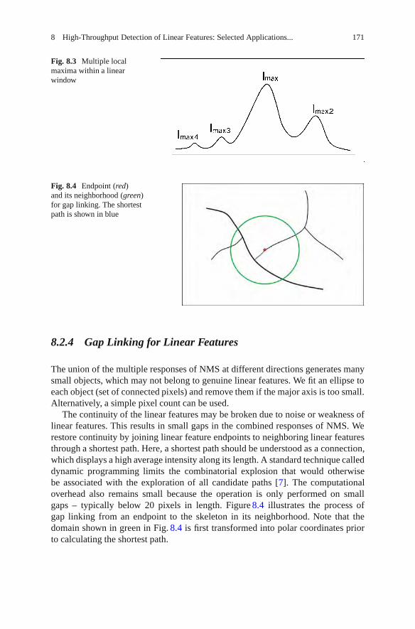
8 High-Throughput Detection of Linear Features: Selected Applications... 171
Fig. 8.3 Multiple localmaxima within a linearwindow
Fig. 8.4 Endpoint (red)and its neighborhood (green)for gap linking. The shortestpath is shown in blue
8.2.4 Gap Linking for Linear Features
The union of the multiple responses of NMS at different directions generates manysmall objects, which may not belong to genuine linear features. We fit an ellipse toeach object (set of connected pixels) and remove them if the major axis is too small.Alternatively, a simple pixel count can be used.
The continuity of the linear features may be broken due to noise or weakness oflinear features. This results in small gaps in the combined responses of NMS. Werestore continuity by joining linear feature endpoints to neighboring linear featuresthrough a shortest path. Here, a shortest path should be understood as a connection,which displays a high average intensity along its length. A standard technique calleddynamic programming limits the combinatorial explosion that would otherwisebe associated with the exploration of all candidate paths [7]. The computationaloverhead also remains small because the operation is only performed on smallgaps – typically below 20 pixels in length. Figure 8.4 illustrates the process ofgap linking from an endpoint to the skeleton in its neighborhood. Note that thedomain shown in green in Fig. 8.4 is first transformed into polar coordinates priorto calculating the shortest path.
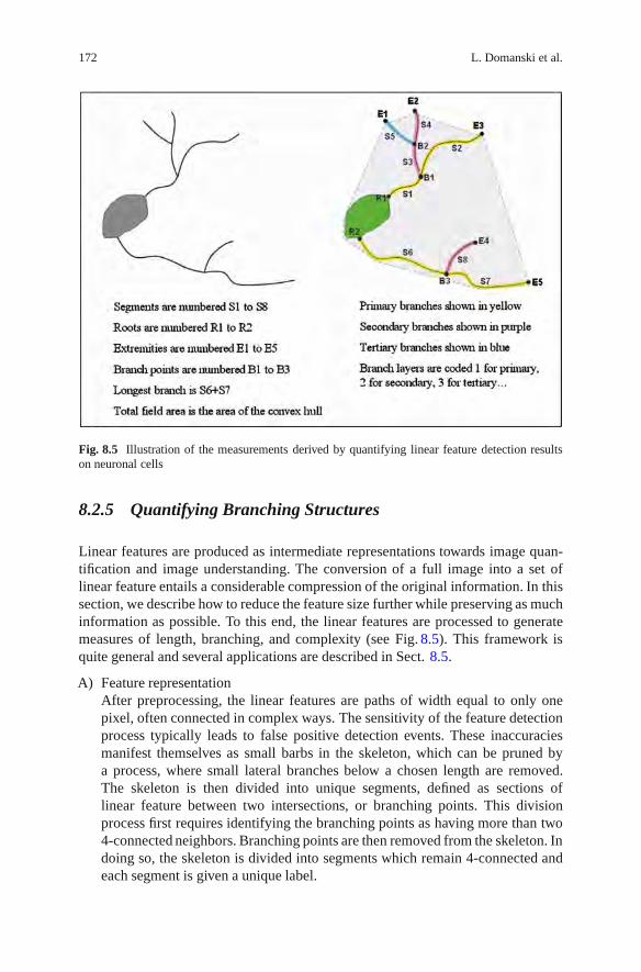
172 L. Domanski et al.
Fig. 8.5 Illustration of the measurements derived by quantifying linear feature detection resultson neuronal cells
8.2.5 Quantifying Branching Structures
Linear features are produced as intermediate representations towards image quan-tification and image understanding. The conversion of a full image into a set oflinear feature entails a considerable compression of the original information. In thissection, we describe how to reduce the feature size further while preserving as muchinformation as possible. To this end, the linear features are processed to generatemeasures of length, branching, and complexity (see Fig. 8.5). This framework isquite general and several applications are described in Sect. 8.5.
A) Feature representationAfter preprocessing, the linear features are paths of width equal to only onepixel, often connected in complex ways. The sensitivity of the feature detectionprocess typically leads to false positive detection events. These inaccuraciesmanifest themselves as small barbs in the skeleton, which can be pruned bya process, where small lateral branches below a chosen length are removed.The skeleton is then divided into unique segments, defined as sections oflinear feature between two intersections, or branching points. This divisionprocess first requires identifying the branching points as having more than two4-connected neighbors. Branching points are then removed from the skeleton. Indoing so, the skeleton is divided into segments which remain 4-connected andeach segment is given a unique label.

8 High-Throughput Detection of Linear Features: Selected Applications... 173
A graph of neighborhood relationships for segments then has to be built. Wefirst morphologically dilate [6] uniquely labeled intersection points with a 3×3structuring element, so that they overlap with the extremities of segments.Segments which overlap a common intersection point are considered neighbors.This information is initially contained in a bivariate histogram of segmentsversus intersection points. A linked list is then created by scanning across eachrow of the histogram and locating nonzero entries in the histogram indicatingneighborhood relationships among segments.When the image corresponds to a structure possessing an organizing centre fromwhich branches are protruding (such as the mitotic organizing centre, the trunkof a tree, or the cell body of a neuron), we identify segments that are in contactwith that organizing centre as “root” segments. To identify them, we first thickenthe labelled centre, so that it overlaps root segments (a thickening is a dilationthat preserves an object’s label [6]). Again, we use a bivariate histogram tostore the overlap information. Nonzero entries correspond to root segments fora particular cell body.
B) Tree growing using the watershed algorithmAt this stage, we must associate all segments with a particular tree. A tree is aconnected network extending from a single root segment. We use the watershedalgorithm to derive the association. Typically, the watershed is performed onan image called the segmentation function, which highlights object boundaries.A set of unique seeds are grown on the segmentation function using a priorityqueue. Seeds are placed in the queue and neighboring pixels are added withpriority given to those with the lowest value in the segmentation function. Pixelsare repeatedly taken from the top of the queue and added to the object definedby the pixel’s neighboring seed.We use the watershed methodology to grow all trees from their root segment.The framework for the watershed in our case is different to that which is used for2D images: we are dealing with graph nodes instead of pixels. The nodes are theindividual segments and our seeds are the root segments as found in the previoussection. Root segments are initially put in the priority queue and neighboringsegments are added with priority given to segments with the highest averagebrightness. The average brightness is calculated over the pixels that form thesegment. Brightness was chosen as priority feature because it is generally foundto be preserved along branches. Other criteria for the prioritization could be usedsuch as the relative orientation of the segments. Segments are repeatedly takenfrom the top of the queue and associated with their neighboring neurite tree untilall segments have been removed from the queue.
C) Measures on segments and treesVarious measurements can be accumulated for each branch during the treegrowing process. These measurements can in turn be aggregated on a per-tree or per-organizing centre basis. It is also common to report measurementson a per-image basis. There are two groups of measurements collected duringthe watershed process: those relating to length, width or brightness and thoserelating to complexity. Fig. 8.5 illustrates these measurements.

174 L. Domanski et al.
Length and width measurements seem particularly important in applications(see Sect. 8.5 for some examples). Before the tree growing process is initiated,the length of each segment is estimated [8]. The average width of each segmentis also computed using the method proposed by Lagerstrom et al. [9]. Theaverage brightness of the segment is computed not only to guide the watershedprocess, but also as a reportable measure in itself. As each segment is removedfrom the queue, we accumulate the length back to the centre for the segment,the longest path back to the centre for the tree and the total length of the tree.In a similar fashion, the average width of the tree, the total area of the tree,the average brightness and integrated intensity of the tree are also accumulated.Once the trees have been grown, the total field area is calculated, defined by thearea of the convex hull of all trees associated with a single organizing centre.
A variety of complexity measures for capturing additional morphologicalmeasures are also collected via the tree growing process. Often trees displaybehaviour where a dominant or primary branch extends from the centre, withsecondary branches projecting from the primary branches, and recursively. Ona per-line basis, we refer to this as branching layer. Root segments are given aprimary branching layer coded as “1.” As segments are removed from the queue,they inherit their parent’s branching layer if they represent a child segmentwith the highest average brightness. The remaining child segments inherit anincremented branching layer. The average branching layer per tree, the numberof branching points per tree and the number of extreme segments (i.e., thosewith no children) are accumulated as the tree is grown.
8.3 Linear Feature Detection on GPUs
While the algorithm presented in Sect. 8.2 is generally considered fast, executiontime can become an issue in the case of large images or those containing complexlinear structures. In this context, complexity refers to both density of linearstructures and their branching rate, as well as the variation of intensity along linearfeatures. In high-throughput biological experiments, where thousands of imagesmay need to be processed in batch during a single experiment, the overall increasein processing time can be significant, thus motivating attempts to improve algorithmperformance further.
In this section, we will look at using many-core processing units and parallelprogramming techniques to help accelerate parts of the linear feature detectionalgorithm described in Sect. 8.2. This problem will serve as an interesting exampleof how these methods can be used to accelerate image processing problems ingeneral. We will utilize Graphics Processing Units (GPUs) as the many-coreprocessors in our discussions and tests. These commodity processing chips are nowa widely available and popular parallel processing platform, with most personal andoffice computers containing one or more of them.

8 High-Throughput Detection of Linear Features: Selected Applications... 175
8.3.1 Overview of GPUs and Execution Models
Originally designed to accelerate the rendering of 3D computer graphics, GPUs arenow used widely as architecture for executing general purpose parallel programs[10]. Modern GPUs consist of hundreds of light-weight processor cores, capable ofexecuting thousands of parallel threads concurrently. GPUs are coupled to dedicatedoff-chip RAM through a high-bandwidth memory interface. Data is transferredbetween this dedicated GPU RAM and a host processor’s memory via an expansioncard bus (usually PCI-Express). GPUs also provide a number of on-chip storagespaces including register files, unmanaged shared memory, and various memorycaches. Accessing these on-chip storage spaces can be orders of magnitude fasterthan accessing GPU RAM which, while being high-bandwidth, can incur significantaccess latencies.
On the NVIDIA GPUs [4] used in our tests, the processors are grouped intoa number of streaming multi-processors (SMs), which can concurrently execute alarge number of assigned threads by switching execution between different groupsof these threads. On-chip storage is arranged such that each SM has its ownprivate register file and shared memory space, which cannot be accessed by threadsexecuting on other SMs.
Threads are logically grouped into n-dimensional blocks whose sizes are cus-tomisable. A regular grid of common sized blocks is used to parameterize threadsover a problem domain. Each thread is assigned unique n-dimensional grid andblock level IDs to distinguish it from other threads. A block is assigned to a singleSM for its lifetime, and its threads can synchronize their execution and share data viaSM shared memory. Each thread in the grid of blocks executes the same program,which is defined by a parallel kernel function. A grid of threads only executes asingle kernel at a time, and on-chip storage does not remain persistent betweenkernel launches.
For example, the process of executing a simple image operation on the GPU thatsubtracts image A from B and places the result in image C can be performed asfollows:
1. Transfer image A and B from host RAM to GPU RAM.2. Assign a single thread to each output pixel by constructing a grid of 2D thread
blocks to cover the image domain.3. Launch a subtraction kernel where each thread reads corresponding pixel values
from image A and B in GPU RAM and writes the subtraction result to image Cin GPU RAM.
4. Transfer image C from GPU RAM to host RAM.
Data transfer between host and GPU can be a performance bottleneck, so it shouldbe avoided where possible. For example, when performing a number of dependentparallel image operations in succession on the GPU, it may not be necessary totransfer the result of each operation back to the host.

176 L. Domanski et al.
Fig. 8.6 Execution times for different stages of linear feature detection for images shown inFig. 8.7. MDNMS, small object removal, and gap filling steps are described in Sects. 8.2.1–8.2.4.Aggregated time taken by short utility operations performed between steps, such as labelling andskeletonization, is represented as “other”
8.3.2 Linear Feature Detection Performance Analysis
Before attempting to parallelize the algorithm on a GPU, one should analyzeperformance issues and determine how different changes might take effect. Forexample, the MDNMS algorithm from Sect. 8.2 is a classic neighborhood filter thatcomputes the value for each pixel in the output image by analyzing only pixelswithin a small neighborhood around the pixel. Although the number of symmetrychecks performed (Sect. 8.2.2) may vary with image content, its performance isprimarily determined by the size of the image, as well as by the size and number oflinear windows used for filtering. Accelerating this portion of the algorithm shouldprovide performance improvement irrespective of the image complexity. However,the number of false objects and feature mask endpoints in the MDNMS output canincrease significantly with input image complexity. This places a higher workloadon the steps that remove small objects and bridge gaps in the resulting featuremasks. The performance of these steps is, therefore, affected more strongly by imagecomplexity than by size.
Figure 8.6 shows the breakdown of linear feature detection processing time fora number of images with varying size and linear structure complexity (Fig. 8.7).In general, we see that MDNMS takes the largest portion of overall executiontime for each image. Gap filling also consumes a large amount time for compleximages (Fig. 8.7, img 2 and img 3) due to an increase in the number of feature maskendpoints produced by the MDNMS step, and the need to perform costly shortestpath calculations for each endpoint (Sect. 8.2.4). Although small object removalperformance also appears to be affected by image complexity, as hypothesizedabove, its execution time is relatively low compared to the other two steps. Thesame remark applies to the utility functions.

8 High-Throughput Detection of Linear Features: Selected Applications... 177
Fig. 8.7 Neurite images used in performance tests. (a) img 1: 1,300× 1,030 pixels. (b) img 2:1,280 × 1,280 pixels. (c) img 3: 1,280 × 1,280 pixels. (d) img 4: 640 × 640 pixels. (e) img 5:694×520 pixels. (f) img 6: 512×512 pixels

178 L. Domanski et al.
Intuitively, one would expect that efforts would be best directed towardsimproving the performance of those steps, which consume the largest percentage oftime, assuming they can be accelerated. Therefore, we will focus our attention onthe implementation of the initial linear feature detection on the GPU.
8.3.3 Parallel MDNMS on GPUs
The MDNMS algorithm with extensions to support symmetry checks and dual localmaxima detection (Sects. 8.2.2 and 8.2.3) consists of four steps for each windoworientation:
1. Detecting primary maxima by NMS with given window size.2. Detecting candidate secondary maxima by NMS with a smaller window size.3. Symmetry check on primary maxima.4. Secondary maxima search and symmetry check in presence of positive primary
detection.
NMS is achieved most simply using a brute force neighborhood filter. In this case,each pixel is compared directly to every pixel within its local linear window todetermine whether it is the maximum in the window. Although it is possible to reusethe max operator observations across nearby pixels to improve performance in aserial context [2], this would not work effectively in a parallel implementation wherenearby pixels can be processed concurrently and where the order of operations is notpredictable. The symmetry checks are performed using similar brute force filters,but carry out different operations on the values within a pixel’s linear window.
In each of these brute force neighborhood filters, the result for a single pixel isnot dependent on the output of other pixels, and can be performed in parallel on theGPU using one thread to calculate each output pixel. Examples of the parallel filterkernels are shown in Listing 8.1 through Listing 8.3. Note that the NMS kernel isexecuted with two different windows sizes to produce the primary and secondary
Listing 8.1 Parallel NMS kernel

8 High-Throughput Detection of Linear Features: Selected Applications... 179
Listing 8.2 Parallel symmetry check kernel
Listing 8.3 Parallel secondary maxima search and symmetry check

180 L. Domanski et al.
maxima images “prim” and “sec.” Each of these parallel kernels can be executedusing a simple 2D grid and block configuration that assigns one thread to each outputpixel.
8.3.4 Combining Steps for Efficiency
In Sect. 8.3.1, we discussed the high latency of GPU RAM accesses (where the inputimage resides) compared to on-chip data access to registers, shared memory or cachememories. Because of these latencies, it is important to minimize transfers to GPURAM where practical. The steps outlined in Sect. 8.3.3 can easily be performedusing separate parallel image filters by executing separate GPU kernel functions foreach step. However, a solution with fewer GPU RAM accesses can be developed ifwe consider the following properties of the filters:
1. NMS: A pixel can be compared with the pixels in its linear window in any orderto determine its suppression status.
2. NMS: Testing a pixel’s suppression status in a given linear window is a subtaskof doing the same for a larger linear window at the same orientation.
3. Symmetry check: Performing a symmetry check on a maxima pixel requires thesame set of values as its primary suppression test
With these properties identified, we can combine the two NMS steps and the primarymaxima symmetry check into a single kernel shown in Listing 8.4. The code in thiskernel visits the first and second halves of a pixel’s linear window separately,allowing it to calculate the average value in each half-window while simultaneouslychecking whether the pixel is a maximum. It also assesses the secondary NMSresult for a pixel at the same time as the primary NMS. This allows everythingexcept the secondary maxima symmetry check to be calculated after reading apixel’s primary linear window values only once from GPU RAM. In contrast, usinga separate kernel for each filter requires these values to be read multiple times fromRAM, since on-chip storage is not persistent between kernel launches. It would alsorequire the values of the primary NMS kernel to be communicated to the primarysymmetry check kernel via GPU RAM. It should be noted that this combination ofsteps might also help speed up the CPU algorithm by reducing overall workloadand memory accesses.
The secondary maxima search and symmetry check around a primary maximumcannot be performed efficiently in the same kernel as the other filters. This isbecause the thread responsible for a pixel requires both the secondary NMS andhalf-window average values calculated by other threads to avoid recalculating them.It is non-trivial to share these values using shared memory, as many threads withdata interdependency relationships will belong to different processing blocks. Thesethreads will not be able to access each other’s shared memory space or synchronizetheir execution. All NMS and half-window averages are, therefore, written to globalmemory by the kernel in Listing 8.4, and a different kernel is utilized to facilitatethe exchange of values and perform the necessary processing.

8 High-Throughput Detection of Linear Features: Selected Applications... 181
Listing 8.4 Parallel kernel calculating primary and secondary NMS, and primary symmetry check

182 L. Domanski et al.
Table 8.1 Speedup of linear feature detection al-gorithm after GPU acceleration. Results indicatehow many times faster the NMS and gap fillingran on the GPU in isolation, as well as how manytimes faster the process ran overall
Speedup on GPU (times ×)
Img NMS Gap filling Overall
1 13.3 4.8 3.02 13.7 8.3 3.33 13.6 8.6 3.34 9.0 8.6 3.35 7.9 3.5 2.76 8.0 6.9 3.0
8.3.5 Results for GPU Linear Feature Detection
We have also sped up the gap closing steps on the GPU, which involved parallelizingpolar image generation and shortest path calculations. Various lower level code andmemory optimisations were applied throughout. For example, loop unrolling hasbeen applied to the NMS kernels [11], while texture fetches, a special kind ofcached [12, 13]. GPU RAM access operation used in computer graphics, have beenused to accelerate polar image generation. Discussion of these topics is beyond thescope of an introductory text. The reader may want to check [14] if his/her curiosityhas been aroused.
Tests were performed on a Geforce GTX 260 GPU (NVIDA Corp., Santa Clara,CA, USA). The host computer consisted of a Xeon E5520 2.3GHz CPU (IntelCorp., Santa Clara, CA, USA) with 3GB of RAM running 32-bit Windows XP(Microsoft Corp., Redmond, WA, USA). Table 8.1 shows the performance of thelinear feature detection algorithm after GPU accelerations for the images displayedin Fig. 8.7. The speedup for NMS is quite high, and is more significant for largerimages (Fig. 8.7, img 1–3). The speedup for gap filling is also significant in the caseof complex images (img 2–4, 6), but reduces for less complex images. These typesof performance inconsistencies are common in parallel programs, where higherworkloads help offset the costs of setup and communication that tend to take aconstant amount of time or do not parallelize well.
Note that the overall speedup of the algorithm is much lower than the speedup ofthe accelerated steps in isolation due to the portion of the process consumed by thesteps that were not accelerated. Since these steps consumed around 21–24% of theoriginal CPU algorithm’s execution time for the test images, the maximum overallspeedup we could hope for by accelerating NMS and gap filling is less than 4.7times. The described GPU algorithms have achieved up to 70% of this theoreticalspeedup. Greater overall speedup will come from accelerating other parts of thealgorithm.

8 High-Throughput Detection of Linear Features: Selected Applications... 183
8.4 HCA-Vision, A Software Platform for Linear FeatureDetection and Analysis
The algorithms detailed in Sects. 8.2 and 8.3 have been integrated in standalonesoftware that rapidly and reproducibly quantifies linear features and their orga-nization. It can be used both for linear feature detection and for more dedicatedmorphological analyses, such as neurite analysis. HCA-Vision was originally aimedfor cell phenotyping and thus also provides functions for cell and nucleus detectionand counting, cell scoring and sub-cellular analysis. It supports batch processingwith a built-in database to store results, a batch result viewer and an ad hoc querybuilder for users to retrieve events of interest (e.g., identify all cells with neuritefield above 50μm2 and projecting in excess of 5 root neurites). Results from HCA-Vision have been shown to be more objective, reliable and reproducible than thosefrom manual or semi-automated approaches [15].
8.4.1 Architecture and Implementation
HCA-Vision has been designed with three layers: the image processing layer writtenin C, a C++ wrapper layer, and the data and image presentation layer, written inC#. It also includes an optional web service for users to remotely view their batchprocessing results.
The GUI provides an assistant to guide the user in the process of choosing opti-mal parameters for the automated segmentation of cells and sub-cellular structures.It delivers quantitative measures and statistics that are biologically relevant, togetherwith result images.
8.4.2 HCA-Vision Features
HCA-Vision enables a range of various activities including the detection of neurons,neurites, astrocytes, and other glial cells, even in the presence of varying backgroundbrightness, variable neurite staining, high cell densities, and high levels of neuriteinterconnections. It delivers quantitative measures and statistics that are biologicallyrelevant, including measurements of neurite features at various levels of branching,neuron “webbiness,” and astrocyte “starriness” and roundness (see Table 8.3 fordefinitions).
To accommodate a wide range of applications, a step-by-step wizard guides theuser through a process that fine-tunes individual parameter required for obtainingbest results. At each step of the process, the user is given a semantic descriptionof each parameter and controls their effect through user-friendly interfaces. As theprocessing has been optimized for speed, intermediate results are immediatelypresented on screen as each parameter is adjusted (Fig. 8.8).

184 L. Domanski et al.
Fig. 8.8 Results produced by HCA-Vision. (a) Original image. (b) Detected neurite segments.(c) Assignment of neurites to neuron bodies. (d) Labelled neurite branching structure
Once parameters are tuned, they can be saved into a profile. The user can loadthe saved profile to process individual images or batch process all images generatedin an experiment. Summaries of batch processing results can be produced using thequery facilities provided.
8.4.3 Linear Feature Detection and Analysis Results
HCA-vision detects linear features and reports their properties such as length, width,area and complexity. For example, with the neurite analysis module, neurites canbe detected and their branching behaviour can be analysed, including the primaryneurites in contact with the cell body and the number of layers of branchingfrom these primary neurites into secondary, tertiary and quaternary branches (seeFig. 8.9).
Users can query and view the batch processing results using the batch resultviewer (Fig. 8.10), including both the result images and measured features.
When HCA-Vision is used with microplates, the batch processing also generatesa plate summary with normalized features for each well. The features extracted fromthe images captured from the same well are averaged to produce the well-basednormalized statistics. A sample plate summary is shown in Table 8.2.

8 High-Throughput Detection of Linear Features: Selected Applications... 185
Fig. 8.9 Batch processing result viewer
8.5 Selected Applications
8.5.1 Neurite Tracing for Drug Discovery and FunctionalGenomics
High Content Screening or Analysis (HCS, respectively HCA) has virtually becomean obligatory step of the Drug Development process. Cells in small transparentwells in a 96-, 384-, or 1,536-microplate format are exposed in a fully automatedmanner to thousands of different candidate compounds (see Table 8.2). They arethen imaged and analysed using computer vision algorithms for evidence of drugaction. In the case of neuronal cells, such evidence includes the growth of neuronalprojections (neurites), but it can also include receptor trafficking, apoptosis, motility,as well as many other assays [16]. Measuring neurite dynamics is a particularlydirect and informative approach but it is also challenging because neurites tend tobe very thin, long, and may present extensive branching behaviour.
Some drugs trigger spectacular effects on neurites (e.g., nocodazole destabilizesmicrotubules thus inducing neurite retraction). More often however, dendriticarbours are altered in subtle ways only. Pharma is generally interested in changesto the length, shape and complexity of neurites. In fact, most of the general imagefeatures described in Sect. 8.2.5 are directly relevant for this particular application.

186 L. Domanski et al.
Fig. 8.10 (a) Original image showing astrocyte nuclei. (b) Nuclei identified by the software aregray coded, with surrogate cellular region boundaries overlaid in white. (c) Original image showingstaining of GFAP fibres of the cytoskeleton. (d) Linear features identified by the software and graycoded as per nuclei, with surrogate cellular region boundaries overlaid in white
Generally, one does not know in advance how the phenotype will be altered.Therefore, it is desirable to apply as wide a spectrum of quantitative features aspossible. Neuronal phenotype may also be altered by mutations, or by changesin the protein expression level elicited, for example, by small inhibitory RNAs.In collaboration with the Group of S.S. Tan and J.M. Gunnersen at the HowardFlorey institute, we have been particularly interested in uncovering the role of theSeizure-related protein type 6 (Sez-6) [15]. From mouse behavioural studies, Sez-6had already been implicated in cognitive processes but it was not clear yet whetherthe cell morphology was affected. In general, the biological variability across cellsprecludes drawing definitive conclusions from observing by eye a limited number ofcells. Indeed, an individual knockout cell (lacking Sez-6) may appear more similar

8 High-Throughput Detection of Linear Features: Selected Applications... 187
Table 8.2 Plate summary showing well-based normalized features
Well number A1 A2 – – – H11 H12
Number of cells 625 425 – – – 899 648Total neurite outgrowth 32,124 19,801 – – – 30,883 11,887Average neurite
outgrowth51.4 46.59 – – – 34.35 18.34
Total neurite area 36,466 23.348 – – – 36,432 14,025Average neurite area 58.35 54.94 – – – 40.52 21.64Total number of
segments3,826 2,110 – – – 4,820 2,119
Average number ofsegments
6.12 4.96 – – – 5.36 3.27
Average longestneurite length
25.68 27.58 – – – 18.97 12.97
Total number of roots 1,213 583 – – – 1,479 571Average number of
roots1.94 1.37 – – – 1.65 0.88
Total number ofextreme neurites
1,353 747 – – – 1,492 615
Average number ofextreme neurites
2.16 1.76 – – – 1.66 0.95
Total number ofbranching points
455 251 – – – 438 101
Average number ofbranching points
0.73 0.59 – – – 0.49 0.16
Average branchinglayers
1.28 1.13 – – – 1.17 0.71
to a wild type cell (possessing Sez-6) than to another knockout cell (Fig. 8.9).It is only when large numbers of cells are systematically analysed that statisticallysignificant differences can be uncovered. In conducting these comparisons, it isextremely important to ensure that the analysis is performed identically on boththe knockout and the wild-type images.
Our results demonstrated clearly that while the neurite field area was not affected,the mutation both increased branching and diminished the mean branch length.The full biological significance of these findings is not yet appreciated but theseexperiments clearly indicate that the geometry of neurite arbours is in large partunder genetic control.
8.5.2 Using Linear Features to Quantify Astrocyte Morphology
In this example, we show how linear feature detection can be used to characterisemorphological changes in the cytoskeleton of astrocytes, as induced by kinaseinhibitors. This was part of a larger study into the role played by astrocytic glutamatetransporters in maintaining brain homeostasis [17].

188 L. Domanski et al.
Fig. 8.11 The sensitivity of our linear feature proved helpful in this bacterial segmentationproblem. By themselves, the detected edges (in gray) would not be sufficient to segment cellssuccessfully. Together with the detected edges, our linear features (in white) form a double barriersystem that enables accurate segmentation
It is often important to make measurements on a per-cell basis rather than ona per-image basis. To achieve this, one needs some way to identify the extent ofeach cell. This is done either directly by acquiring an additional image of a labelledcytoplasmic protein, or indirectly by generating a surrogate for the cell extent. Thesurrogate commonly used in cellular screening requires the capture of an additionalimage of labelled nuclei, the segmentation of those nuclei and the placing of adoughnut or ring around each nucleus. If cells are isolated, the surrogate cell regionwill appear roughly elliptical and the approximation to the actual cell shape tends tobe crude. However, if cells are closely packed (as they often are in screening assays),the surrogate cell regions from neighboring nuclei deform to the midpoint betweenthe two nuclei. This gives rise to regions which are close to the actual cell shapes(Fig. 8.11).
Within these surrogate cell regions, we quantify the features of the linearstructures forming the astrocyte cytoskeleton (see Table 8.3). These measures havebeen used by our collaborators, O’Shea et al. of the Howard Florey Institute, toquantify the changes induced by the Rho-kinase inhibitor HA1077 in primarycultures of mouse astrocytes.
The astrocyte cytoskeleton was labelled using immunocytochemical stainingfor the astrocytic intermediate filament protein GFAP. Nuclei were labelled usingHoechst 33342. Figure 8.11 shows a sample nucleus and cytoskeleton image, alongwith the detected nuclei, the calculated surrogate cell extent and the detected linesin the cytoskeleton. Treatment with HA1077 (100μM) produced rapid (<1h) andpersistent changes in astrocytic morphology. The lineAngleVar feature (variance ofthe orientation angles of the “lines” within the cells) was significantly reduced byHA1077 (to 81± 4% of control, p < 0.05). A low lineAngleVar means that the

8 High-Throughput Detection of Linear Features: Selected Applications... 189
Table 8.3 Features developed specifically to characterize linear structures in theastrocyte cytoskeleton
lineNo Number of lines detected within celllineMean Mean brightness of lines within celllineLength Length of lines within celllineDensity Density of lines within celllineAngle Mean orientation angle of lines Within celllineAngleVar Variance of orientation angle of lines within celllineWidthMean Mean width of lines within celllineWidthMedian Median width of lines within celllineStar “Starriness” measure based on how much linear structure is
removed by an opening of a specific radiuslineWeb “Webbiness” measure based on how much the gaps between
lines are filled in by a closing of specific radius
linear structures within a cell are generally aligned in a particular direction, whereasa high value indicates that the linear structures are randomly oriented. In addition,the lineDensity measure (the density of these “lines” within cells) also decreased (to44±5% of control, p < 0.05), demonstrating a decrease in the cellular area labelledby GFAP.
8.5.3 Separating Adjacent Bacteria Under Phase ContrastMicroscopy
In bacterial cultures, cells tend to come in very close proximity to each other, suchthat the contrast between individual cells is sometimes minute (see Fig. 8.11). Thismakes bacterial counting and measurement of size and shape difficult. We havefound that our linear feature detector was capable of detecting the very weak linearfeatures that separate adjacent bacteria (see Fig. 8.11). By combining this tool with astandard Canny edge detector, a system was put together that permitted counting andsegmenting bacteria with over 97% reliability [18]. We expect this new capability tobe generally useful for microbial studies and we are planning to extend this work toallow tracking of bacterial cells with a comparable reliability. This work is motivatedby the need to understand how bacterial films are able to spread quickly over tissuesurfaces and thus cause infections.
8.6 Perspectives and Conclusions
Our approach to linear feature is both conceptually simple and very fast. It isfairly general – independent of any model assumption about linear features. Thisalso means that the approach is not recommended for very noisy images. In the
190 L. Domanski et al.
rare instances where noise was an issue, we found that it was often possible touse a preliminary processing step to increase the contrast of linear features, forexample, using the technique of anisotropic filtering [19]. Another promising toolto preprocess linear feature images in this manner is afforded by so-called flexiblepath openings, which aim to identify paths along which the intensity remains highon average [20].
There are also instances where the contrast mechanism of the optical instrumentmakes the analysis difficult. This is the case with Differential Interference Contrast(DIC) microscopy. For such images, the Hilbert transform can be used to createimages that are suitable for analysis.
In the case of very noisy images, the potential of more global methods, such as“shortest paths” [7], or even “linear paths” [9], has been explored. While useful,these more complex approaches may also represent warnings that the experimentershould go back to the bench to produce better data. With the availability of EMMCDcamera and the availability of bright and photostable dyes, such as the AlexaTM
dyes, this is often the best course of action.This is an exciting time for image analysis, with a growing number of applica-
tions that can be automated. The samples presented in this chapter only touch thesurface, as illustrated by the content of other exciting chapters in this book.
Acknowledgements The authors would like to thank the following people for allowing us touse their images as sample images: Marjo Gotte, Novartis Institutes for BioMedical Research;Dr. Myles Fennell, Wyeth Research, Princeton, NJ, USA; Dr. Xiaokui Zhang, Helicon Thera-peutics, Inc., USA; Prof. Pat Doherty, Kings College, London, UK; Dr. Jenny Gunnersen, Prof.Seong-Seng Tan, and Dr. Ross O’Shea Howard Florey Institute, Melbourne; Ass. Prof. CynthiaWhitchurch, UTS, Sydney.
References
1. Palmer, S.E.: Vision science. MIT, MA (1999)2. Sun, C., Vallotton, P.: Fast linear feature detection using multiple directional non-maximum
suppression. J. Microsc. 234, 147–57 (2009)3. Kirbas, C., Quek, F.: A review of vessel extraction techniques and algorithms. ACM Comput.
Surv. 36, 81–121 (2004)4. Meijering, E.: Neuron tracing in perspective. Cytometry 77, 693–704 (2010)5. Neubeck, A., Van Gool, L.: Efficient non-maximum suppression. In: Tang, Y.Y., Wang, S.P.,
Lorette, G., Yeung, D.S., Yan, H. (eds.) Proceedings of 18th International Conference onPattern Recognition, vol. 3, pp. 850–855. IEEE Computer Soc, Los Alamitos (2006)
6. Soille, P.: Morphological image analysis, 2nd edn. Springer, Heidelberg (2004)7. Sun, C., Pallottino, S.: Circular shortest path in images. Pattern Recogn. 36, 709–719 (2003)8. Dorst, L., Smeulders, A.W.M.: Length estimators for digitized contours. Comput. Vis. Graph.
Image Process. 40, 311–333 (1987)9. Lagerstrom, R., Sun, C., Vallotton, P.: Boundary extraction of linear features using dual paths
through gradient profiles. Pattern Recogn. Lett. 29, 1753–1757 (2008)10. Owens, J.D., Luebke, D., Govindaraju, N., Harris, M., Kruger, J., Lefohn, A.E., Purcell, T.J.:
A survey of general-purpose computation on graphics hardware. Comput. Graph. Forum 26,80–113 (2007)
11. Harris, M.: Optimizing parallel reduction in CUDA. NVIDIA SDK white paper (2007)

8 High-Throughput Detection of Linear Features: Selected Applications... 191
12. Hakura, Z.S., Gupta, A.: The design and analysis of a cache architecture for texture mapping.In: 24th Annual International Symposium on Computer Architecture, Conference Proceedings,pp. 108–120. Assoc Computing Machinery, New York (1997)
13. Cox, M., Bhandari, N., Shantz, M.. Multi-level texture caching for 3D graphics hardware. In:Proceedings of the 25th Annual International Symposium on Computer Architecture. IEEEComputer Soc, Los Alamitos, pp. 86–97 (1998)
14. Domanski, L.: Linear feature detection on GPUs. In: International Conference on Digital ImageComputing: Techniques and Applications (DICTA), Sydney (2010)
15. Vallotton, P., Lagerstrom, R., Sun, C., Buckley, M., Wang, D., De Silva, M., Tan, S.S.,Gunnersen, J.M.: Automated analysis of neurite branching in cultured cortical neurons usingHCA-Vision. Cytometry A 71, 889–895 (2007)
16. Conrad, C., Gerlich, D.W.: Automated microscopy for high-content RNAi screening. J. CellBiol. 188, 453–461 (2010)
17. Lau, C., O’Shea, R., Broberg, B., Bischof, L., Beart, P.: The Rho kinase inhibitor Fasudilup-regulates astrocytic glutamate transport subsequent to actin remodelling in murine culturedastrocytes. https://nsw.owa.csiro.au/pubmed/21309758. Br. J. Pharmacol. 163, 533–545 (2011)
18. Vallotton, P., Sun, C., Wang, D., Ranganathan, P., Turnbull, L. Whitchurch, C.: Segmentationand tracking of individual Pseudomonas aeruginosa bacteria in dense populations of motilecells. In: Image and Vision Computing New Zealand Wellington, New Zealand (2009)
19. Orkisz, M.M., Bresson, C., Magnin, I.E., Champin, O., Douek, P.C.: Improved vesselvisualization in MR angiography by nonlinear anisotropic filtering. Magn. Reson. Med. 37,914–919 (1997)
20. Heijmans, H., Buckley, M., Talbot, H.: Path-based morphological openings. In: ICIP: 2004International Conference on Image Processing, vol. 1–5, pp. 3085–3088. IEEE, New York(2004)

Chapter 9Medical Imaging in the Diagnosisof Osteoporosis and Estimation of the IndividualBone Fracture Risk
Mark A. Haidekker and Geoff Dougherty
Abstract Osteoporosis is a degenerative disease of the bone. In an advancedstate, bone weakened by osteoporosis may fracture spontaneously with debili-tating consequences. Beginning osteoporosis can be treated with exercise andcalcium/vitamin D supplement, whereas osteoclast-inhibiting drugs are used inadvanced stages. Choosing the proper treatment requires accurate diagnosis of thedegree of osteoporosis. The most commonly used measurement of bone mineralcontent or bone mineral density provides a general orientation, but is insufficientas a predictor for load fractures or spontaneous fractures. There is wide agreementthat the averaging nature of the density measurement does not take into account themicroarchitectural deterioration, and imaging methods that provide a prediction ofthe load-bearing quality of the trabecular network are actively investigated. Studieshave shown that X-ray projection images, computed tomography (CT) images, andmagnetic resonance images (MRI) contain texture information that relates to thetrabecular density and connectivity. In this chapter, image analysis methods arepresented which allow to quantify the degree of microarchitectural deterioration oftrabecular bone and have the potential to predict the load-bearing capability of bone.
9.1 Introduction
Osteoporosis is defined as a skeletal disorder characterized by compromised bonestrength predisposing a person to an increased risk of fracture. Bone strengthprimarily reflects the integration of bone density and bone quality [1].
The official definition of osteoporosis further specify bone density as referringto specify mineral content and bone quality as referring to architecture, turnover,damage accumulation, and mineralization [1]. Bone density peaks at an age between
M.A. Haidekker (�)University of Georgia, Faculty of Engineering, Athens, GA 30602, Georgiae-mail: [email protected]
G. Dougherty (ed.), Medical Image Processing: Techniques and Applications, Biologicaland Medical Physics, Biomedical Engineering, DOI 10.1007/978-1-4419-9779-1 9,© Springer Science+Business Media, LLC 2011
193

194 M.A. Haidekker and G. Dougherty
20 and 30 and declines as people age. Hormonal changes, most notably menopause,accelerate this decline. For the purpose of diagnosis, individual bone density iscommonly compared to an age-matched reference collective. The World HealthOrganization defines osteopenia as a loss of bone density to one standard deviationbelow the age-matched mean (T-score of −1) and osteoporosis as a loss of bonedensity to below 2.5 standard deviations (T-score of −2.5). The major healthconcern is the risk of fracture. The relationship between reduced bone density andthe incidence of fractures is well known [2–5].
Bone loss can be slowed or prevented. A diet rich in calcium and vitamin D,or dietary supplements thereof, reduce the risk of osteopenia and osteoporosis [6].Strength-building exercise stimulates bone formation (see [7] for a critical review).Whereas calcium intake and exercise primarily improve the baseline, patients witha low T-score need to be treated with drugs that reduce bone deterioration, such ascalcitonin or bisphosphonates.
The primary goal of the diagnostic procedures is to assess the degree ofbone loss for a decision on possible treatment. Whereas calcium and vitamin Dsupplementation are widely recommended, the type and vigorousness of a possibleexercise regimen strongly depends on the degree of bone deterioration. The use ofdrugs also depends on the diagnosis. In advanced stages of bone deterioration it is,therefore, crucial to establish the individual fracture risk.
Presently, the diagnostic process most commonly involves the measurement ofbone density (see Sect. 9.2). However, bone deterioration that leads to osteopeniaand osteoporosis is a complex process [2, 8] that affects bone microarchitecture. Infact, early studies show that osteoporosis is associated with a deterioration of thecomplex three-dimensional network of trabeculae, which form the weight-bearingcomponent of spongy bone [9]. There is a discrepancy between the relatively lowbone density gain of around 1% by exercise [10] and the strong reduction of fractureincidence [11]. The benefits of exercise clearly include improved muscular strength,dexterity, and range of motion, thus directly contributing to a lower incidence offalls, accidents, or fracture-causing motions. Conversely, treatment with fluorideshas been shown to strongly increase bone density while not decreasing [12] or evenincreasing fracture incidence [13]. Similarly, observations have been made for drugsthat enhance bone formation. Moreover, bone density has been shown to stronglyoverlap between patients with and without osteoporosis-related fractures. Clearly,bone density alone is not a sufficiently specific predictor of the individual fracturerisk [14].
Bone is heterogeneous and biomechanically complex. Fracture-prone sites, suchas vertebrae, wrist, femoral head, and calcaneus are composed of spongy bone,which is a three-dimensional strut-like network of trabeculae, and the surroundingcortical shell, which is composed of compact bone. Both parts contribute tothe weight-bearing capacity of bone. The loss of bone density reflects both thedeterioration of the cortical shell and thinning of the trabeculae in spongy bone.An early study by Rockoff et al. found that the compact bone of the cortical shellcarried between 45% and 75% of the total mechanical load, and that the weight-bearing contribution of the cortical shell increased with decreasing ash content [15].

9 Medical Imaging in the Diagnosis of Osteoporosis... 195
A more recent study indicated that both vertebral stiffness and vertebral strength isalmost completely attributable to spongy bone, and the cortical shell plays only avery small role in the weight-bearing capacity [16]. Further biomechanical studiessuggested a power–law relationship between apparent bone density ρ and elasticmodulus E and maximum compressive stress σmax in the form of (9.1),
E = ρA =(
Vb
Vt
)A
; σmax = ρB =(
Vb
Vt
)B
(9.1)
where Vb is the apparent bone volume, Vt is the total volume, and A and B areexperimentally-determined constants [17]. Although a case can be made that mi-crostructural deterioration is reflected in a loss of bone density [18], the deteriorationof trabeculae is not isotropic. Rather, deterioration of vertical trabeculae occursmore rapidly than that of horizontal trabeculae [9]. Non-isotropic deterioration mayin part explain differences in failure load at the same bone density [19]. Conse-quently, analysis of bone microstructure remains under active investigation [20].
The focus of recent research has been three-pronged. On the treatment side, sci-entists are striving to understand the cellular mechanisms that determine the balancebetween bone-resorbing cells (osteoclasts) and bone-forming cells (osteoblasts),with the long-term goal to influence this balance in favor of bone formation.On the diagnostic side, researchers are striving to obtain information about thebone microarchitecture, because the combined measurement of bone density andmicrostructural parameters promise to improve the prediction of the fracture loadand therefore the individual fracture risk. Finally, basic research efforts are aimed atunderstanding the complex biomechanical behavior of bone. In all three cases,imaging methods play a central role.
9.2 Bone Imaging Modalities
The clinical modalities for imaging bone include X-ray imaging and the related dualenergy X-ray absorptiometry (DEXA), computed tomography, magnetic resonanceimaging, and ultrasound imaging.
9.2.1 X-Ray Projection Imaging
X-ray imaging provides excellent bone-tissue contrast, with a spatial resolution ofabout 30–40μm. Dual-Energy X-ray Absorptiometry (DEXA) reduces the influenceof soft tissue, such as muscle or marrow, which surrounds the bone. Since X-rayattenuation coefficients are energy-dependent, the X-ray intensity is measured attwo different energies along the same path to eliminate the contribution of the soft

196 M.A. Haidekker and G. Dougherty
tissue. Like conventional X-ray imaging, DEXA is a projection imaging method.It is typically applied to the thoracic or lumbar spine, the femoral neck, or thecalcaneus.
The accuracy of the DEXA method is limited because the X-ray beam ispolychromatic and because the soft tissue may be composed of muscle and adiposetissue, with varying absorption coefficients between individuals. It is possible toobtain the soft tissue composition from the DEXA image [21] to correct for theerror. DEXA is best known for the measurement of bone density. Typical DEXAscanners feature a spatial resolution in the millimeter range, which is not sufficientto image structural details.
9.2.2 Computed Tomography
Computed tomography (CT) is an X-ray based technique that provides cross-sectional images of the X-ray absorption coefficient. Unlike projection imagingmethods, computed tomography provides bone density as a true volumetric valuethat can be calibrated in mg/cm3. Accuracy and reproducibility of bone densitymeasurements can be further increased by introducing a calibration phantom intothe image. With a phantom that provides representative image values of bone IB
and of soft tissue IS, bone density D, calibrated in milligrams of hydroxyapatite permilliliter of bone volume, can be computed from the average image value < I > inthe bone region and the known specific density of bone, ρB, through (9.2):
D =< I > −IS
IB − ISρB (9.2)
The computed tomography method that provides calibrated bone density valuesis often referred to as quantitative CT. It is further possible to use a dual-energyprinciple similar to DEXA to eliminate artifacts caused by soft tissue and bonemarrow [22]. Dual-energy quantitative CT is often regarded as the gold-standardfor the noninvasive measurement of bone density.
Whereas a low spatial resolution, dominantly in the form of a wide slicethickness, is used for bone density measurement, CT can be used to image the bonemicroarchitecture when a high resolution is selected. Slice thicknesses of 1 mm within-plane pixel sizes of 0.2× 0.2mm are possible with many clinical CT scanners.Micro-CT scanners are available that feature isotropic voxel sizes in the micronrange, but these devices can hold only small samples, and are therefore reservedfor biopsies or for in vivo imaging of, for example, the wrist (Fig. 9.1). The interiorof the radius and ulna show a clear texture that can be related to the trabecularmicroarchitecture.

9 Medical Imaging in the Diagnosis of Osteoporosis... 197
Fig. 9.1 Cross-sectional Micro-CT image of a human forearm. The voxel size is 70μm, smallenough to make the trabecular structure visible. Note the presence of reconstruction artifacts (thepseudo-texture that is particularly prominent in the air region surrounding the arm) and beam-hardening artifacts (straight lines extending from bone edges). Note also the low tissue-tissuecontrast that makes tissue structures (blood vessels, muscle, tendons) indiscernible. The scale barrepresents 10 mm
9.2.3 Magnetic Resonance Imaging
Magnetic resonance imaging (MRI) is presently not clinically used for imaging bonebecause of the low water content of bone, which leads to a very weak resonancesignal. Figure 9.2 shows a T1-weighted high-resolution spin-echo image of the wrist,acquired with a conventional clinical 1.5T scanner. Inside the ulna and radius areas,texture becomes apparent that is related to the trabecular architecture, analogousto Fig. 9.1. In-plane resolution is approximately 120μm, with pixels almost twiceas large as in Fig. 9.1. The long T1 relaxation of bone marrow makes spongy boneappear bright in this image, although compact bone itself appears dark. AlthoughMRI is not currently a method of choice for bone densitometry, there is a risingpopularity of MRI methods in research to examine bone microstructure and itschanges in osteoporosis.
9.2.4 Ultrasound Imaging
Ultrasound is widely used for bone densitometry. Sound waves travel much faster inbone than in soft tissue, with the speed of sound being approximately 4,080 m/s incompact bone and 1,600 m/s in muscle tissue [23]. A broadband ultrasound signalis attenuated in tissue in a frequency-dependent manner. Broadband ultrasoundattenuation is commonly measured in transverse transmission mode by computing

198 M.A. Haidekker and G. Dougherty
Fig. 9.2 Cross-sectional magnetic resonance image of a human forearm. Similar to Fig. 9.1, radiusand ulna can easily be recognized. In contrast to the CT image, however, compact bone appearsdark, and the MR image clearly reveals soft tissue features, such as muscle, tendons, and bloodvessels. Spongy bone appears particularly bright because of the long relaxation times of bonemarrow. The inset shows the section inside the white rectangle magnified and inverted to match thehigher image values for bone in CT images. In the spongy area, texture that is related to trabecularstructure is discernible, although it appears more blurred than in the corresponding CT image.Image courtesy of Dr. Kai Haidekker
the ratio of the transmitted spectra with and without the sample. A single value,often referred to as BUA (the broadband ultrasound attenuation value), is obtainedfrom the slope of the attenuation over the frequency. No theoretical relationshipbetween ultrasound attenuation and the mechanical properties of cancellous bonehas been established [24], but both the speed of sound and the BUA value are higherin healthy bone than in osteoporotic bone.
9.3 Quantifying the Microarchitecture of Trabecular Bone
In Sect. 9.1, we discussed the need to estimate the individual fracture risk and therole that bone microstructure plays in that estimation. A very rigorous approachis computerized modeling of the biomechanical behavior of bone under a definedload. For this purpose, the exact three-dimensional microscopic geometry of thetrabeculae and their interface with cortical bone need to be available. It is feasibleto extract the geometry with sufficient precision by micro-CT or microscopy or

9 Medical Imaging in the Diagnosis of Osteoporosis... 199
histology in a slice-by-slice manner [25], yet these methods are normally restrictedto ex vivo samples. Other three-dimensional imaging methods with high resolution,for example, micro-MRI, change the apparent geometry due to the system’s point-spread function. At lower resolution, individual trabeculae cannot be imagedaccurately. In such cases, the image shows a distinct texture that is more orless related to trabecular microarchitecture. Even two-dimensional cross-sectionalslices and projection images can provide such texture information, but otherinfluences (noise, reconstruction artifacts, pseudo-texture) become more dominantas the resolution becomes lower. Below a certain resolution, artifacts dominate,and any texture in the image is unrelated to trabecular microarchitecture, at whichthe image can only be used to measure average bone density. The most importantmethods to quantify image texture and relate it to trabecular microarchitecture arediscussed in this section.
9.3.1 Bone Morphometric Quantities
Morphometric quantities are directly related to the microstructure of the trabecularnetwork. From the segmented three-dimensional bone image, total volume and bonesurface area can be obtained immediately. In the literature [26], these are abbreviatedTV and BS, respectively. Bone volume (BV) is the space occupied by actual bonemineral. BV can be determined by measuring the total volume of the trabeculae aftersegmentation of those voxels that lie above a certain density. These primary indicescan be used in normalized form, that is, relative bone volume BV/TV, relative bonesurface BS/TV, and bone surface–volume-ratio BS/BV, to allow comparison betweenindividuals.
Microstructural analysis of the trabeculae leads to the derived indices of tra-becular thickness (Tb.Th) and trabecular spacing (Tb.Sp). In a simplified model,trabeculae can be interpreted as thin plates of constant thickness and width. In thiscase, the following relationships can be found [27]:
Tb.Th = 2BV/BS
T b.Sp = 2(BV −TV )/BS
Tb.N = BS/2BV (9.3)
Tb.N is the number of trabecular plates. Bone mineral content (BMC) was foundto directly correlate with the normalized bone volume [28],
BMC =(
BVTV
)ρBα (9.4)
where ρB is the specific weight of bone mineral and α is the ash fraction. Valuesfor α range from α = 0 for osteoid to α = 0.7 for fully mineralized bone [28].

200 M.A. Haidekker and G. Dougherty
Ω
r
P
a b
Fig. 9.3 Analysis of the trabecular microstructure. (a): Structures can be quantitatively analyzedby fitting a maximum-radius sphere into the structure Ω so that a point P ∈ Ω is an element of themaximum-radius sphere (adapted from [29]). (b): Scan-line method to quantify the microstructure.Parfitt [26] suggested counting the intersections of the bone structure with a rectangular grid oflines to obtain Tb.N. The method can be extended to obtain the distribution of runs along bone(light gray) and runs along marrow spaces (black)
These values correspond to a dry tissue density of 1.41g/cm3 and 2.31g/cm3,respectively. Furthermore, an experimental relationship of these values to elasticityE and ultimate stress σult was found (9.5) with the constants a, b, c, and ddetermined by nonlinear regression as a = 2.58 ± 0.02, b = 2.74 ± 0.13, c =1.92±0.02, and d = 2.79±0.09 [28].
E ∝ (BV/TV )aαb; σult ∝ (BV/TV )cαd (9.5)
The assumption of homogeneous plates is a very rough approximation, andactual measurements from images provide more accurate estimations. Hilebrandand Ruegsegger proposed an image analysis method where a maximum-size sphereis fitted into the space between the segmented trabeculae [29]. By examining eachpoint P inside the structure (Fig. 9.3a), statistical analysis of the void spaces canbe performed. For each structure, the mean thickness (the arithmetic mean value ofthe local thicknesses taken over all points in the structure), the maximum thickness,average volume, and similar metrics can be found and examined over the entirebone segment, which can then be characterized by statistical methods. This methodis capable of analyzing 3D volumetric data, but by using a circle rather than a sphere,it can be adapted to 2D slices.
An alternative method, known as the run-length method, can produce similarquantitative parameters with relatively low computational effort. Originally, Parfitt[26] suggested to use a rectangular grid of scanlines and count the intersections withtrabecular bone in microscopic images to determine Tb.N. This idea can be extendedto the run-length method (Fig. 9.3b): In an image that contains the segmented bone,

9 Medical Imaging in the Diagnosis of Osteoporosis... 201
linear runs of bone and marrow are measured. The average length of the marrowruns is related to Tb.Sp, and the average length of the bone runs is related to Tb.Th.The number of bone runs relative to the total number of runs provides Tb.N. Withprogressing bone deterioration, where trabeculae become thinner and disconnected,we can expect fewer and longer marrow runs, and shorter bone runs. Typically, runsare calculated at 0◦, 45◦, 90◦, and 135◦, and the resulting run lengths are averagedto obtain a measurement that is widely orientation-independent. Alternatively, runsin different directions can be used to determine orientational preferences. The runlength method is a 2D method.
Two representative examples for the application of the run-length method for thequantification of trabecular microstructure on CT images [30, 31] demonstrate thatthis technique does not require an accurate microscopic representation of trabecularbone. A relationship between morphometric quantities and bone strength has beenestablished [32]. On the other hand, noise and partial-volume effects have a stronginfluence on which voxels are classified as bone. Furthermore, image degradation bythe point-spread function of the device makes the selection of a suitable threshold forthe separation of bone and soft tissue difficult. Even with micro-CT and micro-MRItechniques, the thickness of individual trabeculae is on the order of a single voxel.
Topological quantities, such as the number of struts or the number of holes,are popular in the analysis of the trabecular network. The interconnected trabeculaecan be represented as a graph, and the number of links (i.e., trabecular struts),the number of nodes, the number of holes (i.e., the marrow spaces), and relatedmetrics, such as the Euler characteristic can be determined. The Euler characteristiccan be seen as the number of marrow cavities completely surrounded by bone. Toobtain the topological quantities, the image needs to be segmented into bone andnon-bone areas followed by thinning of the structures (skeletonization, Fig. 9.4).One of the most interesting features of the topological quantities is the invarianceunder affine transformations. Therefore, these quantities should be robust – withinlimitations of the pixel discretization – against changes in scale, rotations, and evenshear and perspective distortions.
Analysis of the skeleton is traditionally a 2D method, but extensions to 3D havebeen reported [33]. In two and three dimensions additional parameters have beendefined. These include the connectivity index by Le et al. [34]; the marrow starvolume by Vesterby et al. [35], which also reflects connectivity; the trabecular bonepattern factor (often abbreviated TBPf ) by Hahn et al. [36], which decreases withbone deterioration; the ridge number density by Laib et al. [37]; and the structuremodel index (SMI) by Hildebrand and Ruegsegger [38], which is designed tocharacterize a 3D shape as being plate-like or rod-like and requires a 3D imageof microscopic resolution.
9.3.2 Texture Analysis
Whereas morphometric analysis is based on the assumption that individual trabec-ulae are resolved in the image (thus, requiring high-resolution images with voxel

202 M.A. Haidekker and G. Dougherty
Fig. 9.4 X-ray image of an excised section of trabecular bone with its skeleton superimposed.Skeletonization is a popular method to quantify the connectivity. Microstructural deterioration ofbone increases the number of branches (links that are connected to the network on only one end),and decreases the number of loops
sizes generally smaller than trabecular width), such an assumption is not needed forthe analysis of the texture in image regions representing trabecular bone. Texturecan be defined as a systematic local variation of the image values [39]. Thisdefinition normally implies the existence of multiple image values (gray values) asopposed to the purely binary values used in the morphometric analysis. Moreover,an assumption must be made that the image texture is related to the microstructureof trabecular bone. This is a reasonable assumption, as can be demonstrated in asimple experiment (Fig. 9.5). Let us consider an imaging device with a non-idealpoint-spread function, for example, X-ray projection imaging where the size of thefocal spot of the X-ray tube and the bone–film distance introduce blur. This processcan be simulated by additive superposition of blurred images of some defined binarystructure. A structure that somewhat resembles the distribution of trabecular boneis shown in Fig. 9.5a. The purely binary image represents trabecular bone (white)and marrow space (black). This image has been generated by a suitable randomgenerator. Six such images, blurred with a second-order Butterworth filter adjustedto a random cutoff frequency of 10±3 pixel−1 were created and added on a pixel-by-pixel basis (Fig. 9.5b). The similarity of the resulting texture to an actual CTimage (Fig. 9.5c) is striking.

9 Medical Imaging in the Diagnosis of Osteoporosis... 203
Fig. 9.5 Demonstration of the relationship between microarchitecture and texture in an imagingsystem with non-ideal point-spread function. (a): A synthetically generated pattern that somewhatresembles segmented and binarized trabeculae in a microscopic image. (b): Six patterns similarto the one shown in (a), blurred and superimposed. (c): Magnified computed tomography slice ofthe trabecular area in a lumbar vertebra. The trabecular area has been slightly contrast-enhanced,leading to saturation of the image values that correspond to cortical bone
Texture can be analyzed in two or three dimensions. Because most imagingmodalities have anisotropic voxel sizes with much lower resolution in the axialdirection than in-plane, texture analysis normally takes place as a two-dimensionaloperation. In 3D imaging modalities (CT and MRI), texture analysis can takeplace slice-by-slice. When an analysis method is extended into three dimensions,a possible voxel anisotropy needs to be taken into account.
The simplest method for texture analysis is the computation of the statisticalmoments of the histogram inside a region of interest. Most notably, the standarddeviation and its normalized equivalent, the coefficient of variation, contain infor-mation about the irregularity of the structure. Healthy bone can be expected to have amore irregular structure with a higher coefficient of variation than osteoporotic bonewith larger and more homogeneous marrow spaces. Both variance and coefficientof variation can be computed locally inside a sliding window. A compact metricis the average local variance (ALV), which shows a similar trend as the globalvariance, i.e., declines with the lower roughness of the texture of osteoporoticbone. Basic statistical moments can also be computed on gradient images [40],and the first moment is sometimes referred to as edgeness. The use of edgeenhancement to emphasize the roughness was applied by Caldwell et al. [41], whoprocessed digitized radiographies of thoracic vertebrae with the Sobel operator anda thresholding algorithm to remove small gradients that are likely caused by noise.A histogram of the gradient values showed two maxima that were related to apreferredly horizontal and vertical orientation of the trabeculae, respectively. Thetwo maxima, relative to the mean gradient, related to the fracture load.
The run length method, introduced in the previous section, can be adapted toanalyze texture in a straightforward manner. The grayscale image (such as Fig. 9.5ccan be binarized with the application of a threshold. Clearly, the application of a

204 M.A. Haidekker and G. Dougherty
threshold leads to a loss of information, and the original microstructure cannot berestored. The binary run length method can be extended by allowing more than twogray level bins. In this case, a two-dimensional histogram N(g, l) of the number ofruns N as a function of the gray value g and the run length l is obtained. The run-length histogram is still relatively complex, and statistical quantities can be extractedthat characterize the histogram. Examples are the short- and long-run emphasis(SRE and LRE), low and high gray value emphasis (LGRE and HGRE), combinedmetrics, such as the long-run low gray-value emphasis (LRLGE), and uniformitymetrics, such as the gray-level and run-length nonuniformities (GNLU and RLNU).Three of these quantitative descriptors are listed in (9.6) as examples, and a completelist can be found in [39].
SRE =G−1
∑g=0
L
∑l=1
P(g, l)l2
LGRE =G−1
∑g=0
L
∑l=1
P(g, l)(g + 1)2
GLNU =L
∑l=1
[G−1
∑g=0
P(g, l)
]2
(9.6)
Here, L is the longest run, G is the number of gray bins, and P(g, l) is the runprobability where P(g, l) = N(g, l)/n with n being the total number of runs. It canbe expected that trabecular rarefaction due to osteoporosis would increase LRE andLRLGE because of the longer intratrabecular runs, and would decrease GLNU asan indicator of the loss of complexity. In fact, Chappard et al. found that X-raybased SRE and GLN showed a high negative correlation with 2D histomorphometricmethods ex vivo. Lespessailles et al. found significant differences in the SRE valuebetween patients with and without osteoporosis-related fractures in a multicenterstudy [42]. In radiography images, Ito et al. [31] reported a significant increase of aparameter termed I-texture with age and with the presence of fractures. The I-textureis the average length of dark runs in a binary run-length histogram and correspondsto intratrabecular spaces. Conversely, the T-texture, the white runs that correspond tothe trabecular area, did not change significantly. This observation can be interpretedas the increase of marrow spaces with otherwise unchanged trabecular width.
Selection of the threshold, or placement of the gray-level bins, have a stronginfluence on the quantitative texture descriptors. Neither projection images nor CTimages allow the application of a defined threshold to separate bone from softtissue and marrow. Depending on the threshold, the runs can be almost arbitrarilyshifted from black to white runs. Bin selection is less critical when a gray-levelrun-length histogram is computed. However, a large number of gray levels leadsto predominantly short runs, whereas a small number of gray levels allows longerruns, but introduces a sensitivity against shifts in image value. Frequently, thebin size b is determined from the maximum and minimum image intensity as

9 Medical Imaging in the Diagnosis of Osteoporosis... 205
b = (Imax − Imin)/G. A few outlier pixels can strongly influence bin placement. Inthe example of Fig. 9.5b, clamping the brightest 0.1% of the pixels reduces SREby 15%, LGRE by 25%, GLNU by 28%, SRLGE by 27%, and LRLGE by 16%.All other descriptors are also affected, albeit to a lesser degree. A more robustmethod to select a threshold or to place bins would be based on the gray-valuehistogram [43]. Histogram-based threshold and bin selection also ensures that thequantitative descriptors are independent of the image intensity. Bone deteriorationleads to lower image values in X-ray and CT images. A change in exposure ora different CT calibration may have a similar effect, although the microstructurehas not been altered. The quantitative descriptors directly reflect the image intensityrather than the microarchitecture. This potential fallacy applies to most other textureanalysis methods as well. Any method can be subjected to a simple test. If all imagevalues are linearly transformed such that I′(x,y) = a · I(x,y)+ b, where a > 0 and bare scalars, any algorithm that produces different descriptors for I′ when a and b aremodified does not reflect pure texture.
Other artifacts that may influence texture descriptors are image noise andpseudotexture, introduced in the image formation process. Noise can be seen asan artifactual texture on the pixel level. By using a low number of gray-value binsand by discarding the shortest runs, the run-length method can be made more robustagainst noise. Pseudo-texture (see, for example, Fig. 9.1) cannot be fully eliminated.In special cases, suitable filters can suppress the pseudo-texture to some extent.The presence of this artifact makes it difficult to compare quantitative parametersobtained with different instruments or reconstruction settings. Lastly, the applicationof a highpass filter is advisable before texture parameters are determined. A highpassfilter removes broad trends in the image values, for example, inhomogeneous X-rayillumination or MR bias field artifacts.
Two other texture analysis methods, based on the co-occurrence matrix [44]and on Law’s texture energy metrics [45], have been successfully applied intexture analysis of trabecular bone. The co-occurrence matrix is the histogram ofprobabilities that an image value i is accompanied by the image value j at thedistance �r. To create the co-occurrence matrix, a copy of the image is shifted by−�r = (Δx,Δy), and the two-dimensional joint histogram is computed. Analogousto the two-dimensional run-length histogram, single-value quantitative descriptorscan be extracted. The most widely used set of quantitative descriptors are knownas Haralick’s texture classification metrics [44]. Haralick proposes 14 differentclassification metrics, such as the energy, entropy, contrast, and correlation. Eachof these metrics can be determined for different�r. Texture analysis is often drivenby a high-dimensional feature vector that is used as the input of some artificial-intelligence decision mechanism. In the analysis of bone, however, single valuesare normally used. The choice of�r is critical. Since the texture features of interestare normally larger than a single pixel, single-pixel offsets reflect predominantlynoise. A thorough analysis of the relevant size of the features is necessary to obtainmeaningful values from the co-occurrence matrix. The influence of the offset �ris shown in Fig. 9.6, where the co-occurrence matrices for Δx = 1 and Δx = 15

206 M.A. Haidekker and G. Dougherty
0 10 20 30 40 500
500
1000
1500
2000
2500
0
10
20
30
40
x (pixels)
Iner
tia(
)
Contrast(- - - -)
a b c
Fig. 9.6 Examples of the gray-level co-occurrence matrix of the image in Fig. 9.5b. A single-pixel offset (a) shows highly correlated pixel values with high-probability co-occurrences arrangedalong the diagonal i = j. With a larger offset (Δx = 15 pixels), a broader distribution of the co-occurrence matrix is seen (b). Analysis of the influence of the offset ((c), inertia and contrast shownas representative metrics) reveals that the values strongly depend on the choice of Δx until Δx � 20
are juxtaposed, and two representative metrics, inertia and contrast, are shown fordifferent Δx. Neighboring pixels are highly correlated for small�r (the diagonal i = jdominates the histogram). The metrics become robust against changes of Δx forΔx � 20, which indicates that the features of interest coincide with this size. In fact,Euclidean distances between local maxima of the image fluctuate between 15 and35. One example study be Lee et al. [46] examines the inverse difference momentIDM (9.7) of the co-occurrence matrix,
IDM(θ ,d) = ∑a,b,a �=b
Pθ ,d(a,b)|a−b|2 (9.7)
where θ and d describe the displacement in polar coordinates, and a and b arethe indices of the co-occurrence matrix. Lee et al. found a negative correlationof IDM in digitized radiographies of the femoral neck with bone strength, andfound that IDM was significantly correlated with bone density, although highpassfiltering and histogram normalization made IDM independent from radiographicdensity. On the other hand, Lee et al. [46] did not find a statistically significantdifference of IDM between cases with and without fractures. One possible reason isthe low resolution of approximately 8 pixels/mm, where the displacement d = 7corresponds to 1 mm and is much larger than the trabecular size. Lespessailleset al. [47] found only a weak and nonsignificant correlation between the energyparameter and bone density. This observation can be interpreted in two ways. First, itshould be expected that microarchitectural organization and density are independentquantities, and a high correlation cannot be expected. On the other hand, it is knownthat microarchitectural deterioration is seen as reduced bone density in large-volumeaverages, and a moderate correlation between the two quantities should be observed.Since Lespessailles et al. used single-pixel distances for r, the energy metric mayhave been dominated by pixel noise rather than actual microstructural information.

9 Medical Imaging in the Diagnosis of Osteoporosis... 207
Unlike run-length classifiers and co-occurrence classifiers, Laws’ energy metrics[45] are local neighborhood values obtained by convolving the image with two outof five one-dimensional convolution kernels to yield a feature vector with up to 25elements. Laws proposes a three-step process where the image is first subjected tobackground removal (for example, a highpass filter step), subsequently convolvedwith the kernel pair, and finally lowpass filtered. The resulting image is referred to asthe energy map. Typically, Laws’ energy maps result in a high-dimensional featurevector per pixel and advertises itself for classification or segmentation with high-dimensional clustering techniques or artificial intelligence methods. In one example[48], classical statistical parameters were obtained from the texture energy maps,and the discrete first-order finite difference convolution kernel that approximates∂ 2/∂x∂y showed some ability to discriminate between cases with and withoutfractures. However, Laws’ texture maps are not in common use for this specialapplication of texture analysis. One possible reason is the fixed scale on which thetexture maps operate. Laws’ convolution kernels are fixed to 5 by 5 pixels, and pixelnoise dominates this scale. Thus, the method suffers from the same problems asthe co-occurrence matrix with short displacements. However, it is conceivable thata combination of multiscale decomposition (such as a wavelet decomposition) withLaws’ texture energy maps provides a more meaningful basis to obtain a quantitativedescription of the texture.
In summary, texture analysis methods in the spatial domain provide, to someextent, information that is related to actual trabecular structure. Therefore, textureanalysis methods have the potential to provide information on bone architecturethat is independent from bone density. However, texture analysis methods aresensitive towards the image formation function (e.g., projection image versustomography), towards the point-spread function, the pixel size relative to trabecularsize, and towards image artifacts, most notably noise.
9.3.3 Frequency-Domain Methods
The Fourier transform decomposes an image into its periodic components. A reg-ular, repeating pattern of texture elements (sometimes referred to as texels), causesdistinct and narrow peaks in the Fourier transform. A comprehensive discussionof the Fourier transform and its application in image analysis can be foundin the pertinent literature [39, 40]. Since the Fourier transform reveals periodiccomponents, i.e., the distances at which a pattern repeats itself, operations acting onthe Fourier-transform of an image are referred to as frequency-domain operationsin contrast to the spatial-domain operations that were covered in the previoussection. The magnitude of the Fourier transform is often referred to as the frequencyspectrum. In two-dimensional images, the frequency spectrum is two-dimensionalwith two orthogonal frequency components u and v. It is possible to analyze thosefrequency components separately and include properties such as texture anisotropy.

208 M.A. Haidekker and G. Dougherty
Alternatively, the spectrum can be reduced to one dimension by averaging allfrequency coefficients at the same spatial frequency ω =
√u2 + v2. Intuitively, the
frequency spectrum can be interpreted as a different representation of the spatial-domain image data that emphasizes a specific property, namely, the periodicity.
Trabecular bone does not exhibit any strict periodicity, because trabeculae areto some extent randomly oriented and have random size. The Fourier transform ofrandom structures does not show distinct peaks. Rather, the frequency componentsdecay more or less monotonically with increasing spatial frequency. This propertyis demonstrated in Fig. 9.7. The Fourier transform images (more precisely, the log-transformed magnitude of the Fourier transform) of a relatively regular texture andan irregular, bone-like structure are shown. Peaks that indicate the periodicity ofthe knit pattern do not exist in the Fourier transform of the bone-like structure.However, the decay behavior of the central maximum contains information aboutthe texture. A fine, highly irregular texture, typically associated with healthybone architecture, would show a broad peak with slow drop-off towards higherfrequencies. Conversely, osteoporotic bone with large intratrabecular spacing wouldshow a narrow peak with a faster drop-off towards higher frequencies.
In the analysis of trabecular bone texture, frequency-domain methods are oftenused to detect self-similar properties. These methods are described in the nextsection. Moreover, a number of single-value metrics can be derived from the Fouriertransform. These include the root mean square variation and the first moment of thepower spectrum (FMP, (9.8)):
FMP =∑u ∑v
√u2 + v2|F(u,v)|2
∑u ∑v |F(u,v)|2 (9.8)
Here, F(u, v) indicates the Fourier coefficients at the spatial frequencies u andv, and the summation takes place over all u,v. The computation of the FMP-valuecan be restricted to angular “wedges” of width Δθ , where the angle-dependent FMP(θi) is computed over all u,v with tan(θi) < v/u ≤ tan(θi + Δθ). In this case, theminimum and maximum value of FMP (θi) provide additional information on theanisotropy of the texture. For example, if the texture has a preferredly horizontal andvertical orientation, FMP(θ) shows very distinct maxima for θ around 0◦,±90◦,and 180 ◦. Conversely, the FMP-index for a randomly oriented texture has lessdistinct maxima, and the coefficient of variation of FMP(θ) is lower. Two recentrepresentative studies describe the use of frequency-domain metrics in radiographicimages of the femur in patients with osteoprosis [49] and osteolysis [50]. Special useof the anisotropy was made in a study by Chappard et al. [51] and Brunet-Imbaultet al. [52].
Frequency-domain methods have two major advantages over spatial-domainmethods for the analysis of bone structure and its texture representation in images.First, frequency-domain methods are less sensitive against background irregularitiesand inhomogeneous intensity distributions. Trend-like background inhomogeneitiesmap to very low spatial frequencies, and the corresponding Fourier coefficients

9 Medical Imaging in the Diagnosis of Osteoporosis... 209
Fig. 9.7 Frequency-domain representation of texture. (a): Photography of a knit texture thatcontains a somewhat regular repeating pattern. The regularity of the pattern is representedby distinct peaks in the Fourier transform (b). The slight off-vertical orientation of the knittexture finds a correspondence of the off-horizontal orientation of the Fourier-transform pattern.(c): Synthetic trabecular pattern from Fig. 9.5. Such a pattern does not have repeated textureelements, and the frequency coefficients decay mostly monotonically with increasing frequencies(d). The decay behavior can be used to characterize any irregular texture
are close to the center of the Fourier spectrum image. By omitting the F(u,v)from any single-value metric computation for small u,v, trends are automaticallyexcluded from the metric. Second, frequency-domain methods are usually lessnoise-sensitive than spatial-domain methods. Many spatial-domain methods act onthe pixel level (examples are Laws’ texture energies or the co-occurrence matrixwith low displacements), and pixel noise directly influences the measured values.In the frequency domain, the energy of the noise is broadly distributed over theentire frequency spectrum. High spatial frequencies, i.e., those frequencies that are

210 M.A. Haidekker and G. Dougherty
above the inverse spatial distance of the image features of interest, can be omittedfrom the computation of any frequency-domain metric, leading to an immediatereduction of the influence of noise. Application of a moderate spatial-domain noisefilter before performing the Fourier transform is none the less advisable, because itreduces aliasing artifacts.
9.3.4 Use of Fractal Dimension Estimators for Texture Analysis
Fractal models enjoy great popularity for modeling the texture in medical images,with the fractal dimension commonly used as a compact descriptor. The fractaldimension D describes how an object occupies space and is related to the complexityof its structure: it gives a numerical measure of the degree of boundary irregularityor surface roughness. In its original mathematical definition, a fractal object iscreated by a set of mapping rules that are applied iteratively on an object. After aninfinite application of the mapping operation, the resulting object is invariant underthe mapping operation and therefore referred to as the attractor of the mappingrules. The attractor is self-similar in the sense that any part, magnified, looks likethe whole. Furthermore, the mapping rules determine the self-similarity dimensionof the attractor, which is strictly less than, or equal to, the Euclidean dimensionE of the embedding space (E = 1 for a line, E = 2 for a surface, and E = 3for a volume). In nature, self-similarity occurs, but contains a certain degree ofrandomness. For this reason, no strict self-similarity dimension exists, and theapparent fractal dimension needs to be estimated by suitable methods. To coverthe details of this comprehensive topic is beyond the scope of this chapter. A highlydetailed overview of the subject with a mathematical focus can be found in [53], thegroundbreaking work by Mandelbrot [54] deals with the aspect of randomness innatural fractal objects, and an in-depth overview of the methodology of estimatingfractal dimensions in images can be found in [39].
Fractal analysis always involves the detection and quantification of self-similarbehavior, i.e., to find a scaling rule under which a magnified part of the imagefeature is similar to the whole. This property can be illustrated with the exampleof the coastline of England. The length of the coastline can be estimated withcalipers. However, as the caliper setting is reduced, the length of the coastlineappears increased, because the caliper now covers more of the smaller detail, suchas bays and headlands. In fact, nonlinear regression of the coastline length l as afunction of the caliper setting s reveals a power law,
l =1sD (9.9)
where D is the apparent fractal dimension. Equation (9.9) implies that the measuredlength exceeds all bounds as s→ 0, which is indeed a property of some mathematicalfractals. In actual images, the scaling law fails when the limits of the resolution

9 Medical Imaging in the Diagnosis of Osteoporosis... 211
a b
Fig. 9.8 Demonstration of the box-counting method to estimate the fractal dimension of binaryimages. The image (a) shows the water body (black) of the Amazon river. Superimposed is asquare mesh of boxes. Every box that contains or touches the river is counted. Next, the mesh isrefined (usually by powers of two), and the number of smaller boxes containing part of the river iscounted again. If self-similar properties exist, the log-transformed number of boxes, plotted overthe log-transformed inverse box size (b), will follow a straight line with slope D
are reached. In practice, the range of scales under which a scaling law similar to(9.9) can be found is even more limited. In the example of the coastline, valuesaround D = 1.2 can be found [39, 53]. This is consistent with the notion of a verycomplex and convoluted line embedded in two-dimensional Euclidean space, where1≤D ≤ 2. A surface, such as a grayscale elevation landscape, is embedded in three-dimensional space, where 2 ≤ D ≤ 3 holds.
A very widespread method to estimate an apparent fractal dimension in binaryimages is the box-counting method, explained in Fig. 9.8. The feature needs to besegmented (the river in the example), and the number of boxes that contain part ofthe feature are counted as a function of the box size. If a power-law similar to (9.9)exists, the counted boxes NB over the inverse scale 1/s lie on a straight line in alog–log plot, and nonlinear regression yields the box-counting dimension DB:
log NB = −DB · logs (9.10)
In a grayscale extension of the box-counting method, the image intensities areinterpreted as heights in an elevation landscape. The surface area is determined,whereby the scale is controlled by averaging neighboring pixel values inside boxesof a grid. Numerous other algorithms for estimating fractal dimension have beendescribed [39, 55, 56]. They are all based on measuring an image characteristic,chosen heuristically, as a function of a scale parameter. Generally, these twoquantities are linearly regressed on a log–log scale, and the fractal dimensionobtained from the resulting slope, although nonparametric estimation techniqueshave also been used [57]. In all fractal estimation methods, the scale range needsto be chosen carefully. For large box sizes, to remain with the example of the

212 M.A. Haidekker and G. Dougherty
Table 9.1 A visual classification scheme for the assessment of the trabecular structure used forthe determination of the degree of osteoporosis and its relationship to fractal properties
FractalWHO Bone Spongiosa dimension ofclassification strength pattern Marrow size feature
1 (Healthy) High Homogeneously densewith granularstructures
Small,homogeneous
Low, Unifractal
2 (Beginningdemineral-ization)
Normal Discrete disseminatedintertrabecular areas
Medium, inho-mogeneous
High,Multifractal
3 (Osteopenia) Low Confluentintratrabecular areas<50% of thecross-sectionalsurface
Large, inhomo-geneous
High,Multifractal
4 (Osteoporosis) Verylow
Confluentintratrabecular areas≥50% of thecross-sectionalsurface
Very large,homogeneous
Low, Multifractal
box-counting method, there is insufficient resolution to measure the feature areaproperly. In the presence of noise, the scaling law at the smallest scales may bedominated by noise, and partial-volume artifacts may result in misclassification ofpixels in the segmented image [58]. Further critique of the method specifically fortrabecular bone stems from the observation that trabeculae, on the microscopicscale, are not fractal [58]. This observation reinforces the notion that the scalerange needs to be carefully considered [59, 60]. In spite of some criticism [58]and the limitations discussed above, estimation methods for the fractal dimensionhave been applied successfully in hundreds of studies (for representative reviews,see [61, 62]).
There has been considerable debate in the literature regarding the change infractal dimension with decalcification. An early study of human calcaneous bone[63] during immobilization for fracture (causing a process similar to osteoporosis)found an increased fractal dimension during immobilization. Likewise, a studyof mandibular alveolar bone reported an increased fractal dimension after decal-cification [64]. On the other hand, a later study showed a reduction in fractaldimension of the ankle with immobilization and age [65], and a CT study ofvertebral trabecular bone reported that osteoporotic patients had a smaller fractaldimension [66]. Furthermore, a study of dental radiographs [67] concluded thatfractal dimension decreased with decalcification. In fact, the majority of studiesagrees that the fractal dimension declines with the progression of the disease.Clearly, changes in fractal dimension need to be interpreted with care. We concludethat global fractal dimension does not change monotonically with decalcification(Table 9.1), but rather that it reflects the homogeneity of the spongiosa pattern of

9 Medical Imaging in the Diagnosis of Osteoporosis... 213
the trabecular bone. Studies with subjects who do not reflect the full range of thispattern can report either an increase (WHO classes 1,2, perhaps 3) or a decrease infractal dimension (from class 2 or 3 to class 4) with osteoporosis.
9.3.4.1 Frequency-Domain Estimation of the Fractal Dimension
Self-similar properties of texture can be quantified in the frequency domain. Themain advantage of frequency-domain methods is the better representation of thestochastic nature of images: Certain characteristics are less robust when appliedto digitized data, especially when these are sparse, and algorithms that implicitlyassume an exactly self-similar fractal model are inappropriate for medical images,because they are fractal only in a statistical sense and because pixel intensity andposition are different physical properties and cannot be expected to scale withthe same ratio. Thus, methods that do not meet the intensity–scale independencyrequirement [68], such as the surface area algorithm, may not be applicable. Incontrast, the Fourier power spectrum method conveniently represents the statisticalnature of real images by describing them in terms of a fractional Brownianmotion model.
Roughness (or is opposite, smoothness) is an important feature of texture, and acommonly used method to estimate the smoothness of a one-dimensional functionis from the decay of the Fourier power spectrum with increasing frequency f . Fora two-dimensional image, the radial Fourier power spectrum should be used. For arough image that adheres to the model of uncorrelated noise, the power spectrumfalls off as 1/ f 2, whereas a smooth image (correlated or Brownian noise) has apower spectrum that decays with 1/ f 4. In a log-log plot of the spectral powerover the frequency, a decay with a straight line of slope β indicates self-similarproperties. Furthermore, β will be 2 and 4 for a rough- and a smooth-textured image,respectively. Similar to the scaling range in spatial-domain methods, the range inwhich a power-law decay of the power spectrum with frequency is found, may belimited. At very low spatial frequencies, corresponding to the bulk features of anobject, the power spectrum may be fairly constant. At very high spatial frequencies,system noise will dominate and the power spectrum will become constant again.The power spectrum has been shown to estimate the fractal dimension of self-affinefractals reliably and accurately [69] and has been used to discriminate textures inconventional radiographs of osteoarthritic knees [70].
The link between power-law spectral decay β and fractal dimension is estab-lished by interpreting the image data as fractional Brownian motion (FBM), becauseFBM shows a statistical scaling behavior. FBM is an extension of the more familiarBrownian motion. It has been shown [57] that the decay exponent of the powerspectrum, β , is related to the fractal dimension of a function modeled by FBMaccording to
D = 1 +12(3E −β ) (9.11)

214 M.A. Haidekker and G. Dougherty
where E is the Euclidean dimension of the embedding space (for a two-dimensionalimage, E = 2 and therefore D = 4−β/2). In a two-dimensional image, the value ofD will be constrained to be between 2 (smooth) and 3 (rough), and for a projectedimage generated by Brownian motion (a special case of FBM), the value of D willbe 2.5.
In practice, images are degraded by noise and blurring within a particularimaging device. Image noise adds to the roughness and results in an overestimateof the fractal dimension, whereas blurring results in an underestimate of the fractaldimension. A very important advantage of the power spectrum method is that itallows for correction of these two effects. The noise power can be obtained byscanning a water phantom under the same conditions, and can then be subtractedfrom the power spectrum of the noisy image. Image blurring can be described by themodulation transfer function (MTF) of the system that typically attenuates higherfrequencies in an image. The effect of system blurring can be eliminated by dividingthe measured power spectrum by the square of the MTF, obtained by scanning a verysmall object approximating a point. With these corrections, accurate estimates ofthe fractal dimension of CT images of trabecular bone have been obtained, enablingvery small difference in texture to be distinguished [71].
9.3.4.2 Lacunarity
Lacunarity (from lacuna, meaning gap or cavity) is a less frequently used metricthat describes the complex intermingling of the shape and distribution of gapswithin an image; specifically, it quantifies the deviation of a geometric shape fromtranslational invariance. Lacunarity was originally developed to describe a propertyof fractals [54, 72] to distinguish between textures of the same fractal dimension.However, lacunarity is not predicated on self-similarity and can be used to describethe spatial distribution of data sets with and without self-similarity [73]. Lacunarityis relatively insensitive to image boundaries, and is robust to the presence of noiseand blurring within the image.
Lacunarity is most frequently computed as a function of a local neighborhood(i.e., moving window) of size r. To compute the lacunarity, we first define a “score”S(r,x,y) for each pixel, which is the sum of the pixel values inside the movingwindow centered on (x,y). The detailed derivation of the lacunarity L(r) can befound in [73]. Simplified, we obtain L(r) as
L(r) =σ 2
S (r)S2(r)
+ 1 =∑N
r=1(S(r)−S(r))2
S2(r)+ 1 (9.12)
where S(r) is the mean value of all S(r) and σ 2S is the variance of S(r).
Equation (9.12) reveals explicitly the relationship between lacunarity and thevariance of the scores: Lacunarity relies on the variance of the scores, standardizedby the square of the mean of the scores. The lacunarity, L(r) of an image at a

9 Medical Imaging in the Diagnosis of Osteoporosis... 215
particular window size r uses all the scores obtained by exhaustively samplingthe image. Thus, in general, as the window size r increases, the lacunarity willdecrease, approaching unity whenever the window size approaches the image size(when there is only one measurement and the variance is consequently zero) – orfor a spatially random (i.e., noisy) pattern, since the variance of the scores will beclose to zero even for small window sizes. The lacunarity defined in (9.12) andits variants (including normalized lacunarity and grayscale lacunarity) are scale-invariant but are not invariant to contrast and brightness transformations, so thathistogram equalization of images is a necessary pre-processing step.
A plot of lacunarity against window size contains significant information aboutthe spatial structure of an image at different scales. In particular, it can distinguishvarying degrees of heterogeneity within an image, and in the case of a homogeneousimage it can identify the size of a characteristic substructure. Hierarchically struc-tured random images can be generated using curdling [54]. Higher lacunarity valuesare obtained when the window sizes are smaller than the scale of randomness, andimages with the same degree of randomness at all levels (viz. self-similar fractals)are close to linear, where the slope is related to the fractal dimension. Specifically,the magnitude of the slope of the lacunarity plot for self-similar fractals is equal toD−E , where D and E are the fractal and Euclidean dimensions, respectively.
One problem with the lacunarity metric defined in (9.12) is that the verticalscaling is related to the image density, with sparse maps having higher lacunaritiesthan dense maps for the same window size. This complicates the comparison ofplots between images of different density. It is possible to formulate a normalizedlacunarity whose decay is a function of clustering only and is independent fromimage density. A normalized lacunarity, NL(r), can be achieved by combining thelacunarity of an image, L(r) with the lacunarity of its complement, cL(r), which canassume values between 0 and 1 [71, 74]:
NL(r) = 2− 1L(r)
+1
cL(r)(9.13)
9.3.4.3 Lacunarity Parameters
Lacunarity plots, i.e., plots of L(r) over r, show how the lacunarity varies withscale. The plots monotonically decay to a value of unity at large scales, unlessthere is considerable periodicity in the image; in which case it can pass throughsome minima (corresponding to the repeat distance) and maxima as it falls to unity.Most real images, as opposed to synthetic images, will show only the monotonicdecay. In image features with strict self-similarity, L(r) results in a straight-lineplot from (0,1) to (1,0). If this line is seen as the neutral model, the deviation ofthe (normalized) lacunarity plots from the straight line, calculated as a percentageof the (normalized) lacunarity value, will emphasize subtle differences that are notconspicuous in the decay curves themselves and is useful in identifying size rangesfor different tonal features [74]. Positive (negative) deviations indicate greater

216 M.A. Haidekker and G. Dougherty
Fig. 9.9 Lacunarity plots for three sample textures, highly correlated noise (Perlin noise, dashedline labeled P), uncorrelated Gaussian noise (black circles, labeled GN), and the texture from aCT cross-section of spongy bone in a healthy lumbar vertebra (black diamonds, labeled S). Fittedcurves (9.14) are shown in gray. The lacunarity for Perlin noise cannot be described by (9.14). ForGaussian noise, α = 1.5 and β = 0.007 was found, and for the spongiosa texture, α = 0.45 andβ = 0.021
(lesser) spatial homogeneity than the underlying scale-invariant neutral (fractal)model. The presence of a prominent maximum would indicate the typical size of astructuring element in the image. Moreover, Lacunarity plots often resemble the plotof a power-law function, and Zaia et al. [75] have fitted non-normalized lacunarityplots from binary images to a function of the form
L(r) =βrα + γ (9.14)
where the parameters α, β , and γ are regression parameters that represent the orderof the convergence of L(r), the magnitude (vertical scaling) of L(r), and the offset(vertical shift) of L(r), respectively. We have explored the fitting to monotonicnormalized lacunarity plots, where the parameter γ can be conveniently set to unity,which is the value that NL(r) approaches at large scales. This simplifies the power-law fit to
NL(r)−1 =βrα (9.15)
Examples for lacunarity plots L(r) are shown in Fig. 9.9. The plots of L(r) andthe curve fits with (9.14) are shown. Highly correlated noise (Perlin noise) cannotbe described by (9.14). Conversely, both the uncorrelated noise and the texture ofspongy bone in a cross-sectional CT slice show a good fit with (9.14) with R2 > 0.99in both cases. The score S(r) rapidly reaches statistical stability for increasing r,and the variance of S over the location of a sliding window becomes very low. Thetexture of trabecular bone has a higher variance with the location of S, and its decaywith increasing window size is slower. It becomes obvious that window sizes withr > 20 do not carry additional information in this example, where a window size was

9 Medical Imaging in the Diagnosis of Osteoporosis... 217
used that coincides with the largest textural variations in the spongy bone image.Since bone density, the fractal dimension, and lacunarity are orthogonal metrics,they can be used for multidimensional clustering to better discriminate betweendegrees of osteoporosis (Table 9.1) [74].
9.3.5 Computer Modeling of Biomechanical Properties
Up to this point, Sect. 9.3 was primarily concerned with the empirical relationshipbetween image properties and bone strength. Most notably X-ray attenuation, whichis directly related to bone density, can be linked to bone strength. The textureanalysis methods introduced in the previous sections aim at extracting informationfrom biomedical images of trabecular bone that are independent from averagedensity and therefore provide additional information. A less empirical approach isthe modeling of bone biomechanical properties with finite-element models (FEM).In finite-element analysis, an inhomogeneous object is subdivided into a largenumber of small geometrical primitives, such as tetrahedrons or cuboids. Eachelement is considered homogeneous with defined mechanical properties (stress–strain relationship). External forces and displacements are applied by neighboringelements. External boundary conditions can be defined. Those include spatialfixation and external forces. The entire system of interconnected finite elementsis solved numerically, and the forces, the shear tensor and the displacement foreach element are known. Finite-element models also allow time-resolved analysis,providing information on motion and the response to time-varying forces.
The use of FEM for skeletal bone became popular in the late 1970s and has beenextensively used to relate skeletal variation to function (for a general overview, see[76]). Since then, literally dozens of studies have been published each year whereFEM were used for the functional understanding of bone, predominantly in thespine. Because of the large volume of available literature, we will focus on spinalvertebrae as one pertinent example. One of the most fundamental questions that canbe approached with finite-element analysis is the contribution of compact bone tothe overall weight-bearing capacity of bone. Studies by Rockoff et al. and Vesterbyet al. indicate a major load-bearing contribution of the cortical shell [15, 77].
Two main approaches exist. A general vertebral model with representativegeometry can be designed and used to study general spine biomechanics. Con-versely, the geometry of individual vertebrae can be extracted from volumetricimages (CT or MRI), approximated by finite elements, and subjected to load anddeformation analysis. Although the second approach holds the promise to improvethe assessment of the individual fracture risk, it has not found its way into medicalpractice, mainly because of the computational effort and because of uncertaintiesabout the influence of the finite-element subdivision, material property assignment,and the exact introduction of external forces [78]. The two representative approachesare shown in Fig. 9.10. The early model by Lavaste et al. [79] was generated fromglobal X-ray based measurements, including the width and height of the vertebral

218 M.A. Haidekker and G. Dougherty
a b
Fig. 9.10 Finite-element approximations of the spine. (a): Early parametric model of a vertebralbody (adapted from [79]). The vertebral body is generated from X-ray measurements, such asheight, width, and curvature. (b): Comprehensive finite-element model of the lumbar spine andthe computed stress magnitude (adapted from [80] with permission to reprint through the CreativeCommons License)
body, the diameter of its waist, and the length of the vertebral processes. As such,it is a semi-individual model that reflects gross measurements combined with ageneralized shape model. Individual vertebral bodies can be combined to form asemi-individualized model of the spine or segments of the spine [79]. The recentmodel by Kuo et al. was segmented from volumetric high-resolution CT images(0.35 mm pixel size), and different material properties were assigned to spongybone, the cortical shell, the endplates, and the intervertebral discs. Such a model mayeasily contain 20,000 elements per vertebra, and it accurately reflects the geometryof an individual spine.
The assignment of material properties is an ongoing question. In many models,including the two examples presented above, the spongiosa is modeled as a homo-geneous material – in the example of Kuo et al., spongy bone is assigned a Young’smodulus of 100 MPa compared to cortical bone with 12,000 MPa. However, spongybone may have a larger local variation of its mechanical strength than the modelallows. General models for spongy bone include hexagonal or cubic stick models[81, 82]. Specific models have been developed for spongy bone, often based onmicro-CT or micro-MRI images that can resolve individual trabeculae [83,84]. Onceagain, the model strongly depends on the accurate representation of the geometryand the local material properties. To determine the load-bearing capacity of an entirevertebra, the spongiosa model needs to be appropriately connected to the corticalshell and the endplates. Furthermore, detailed models of the spongiosa cannotpresently be used in a clinical setting, because whole-body scanners do not providethe necessary microscopic resolution to build a detailed model of the trabeculae.
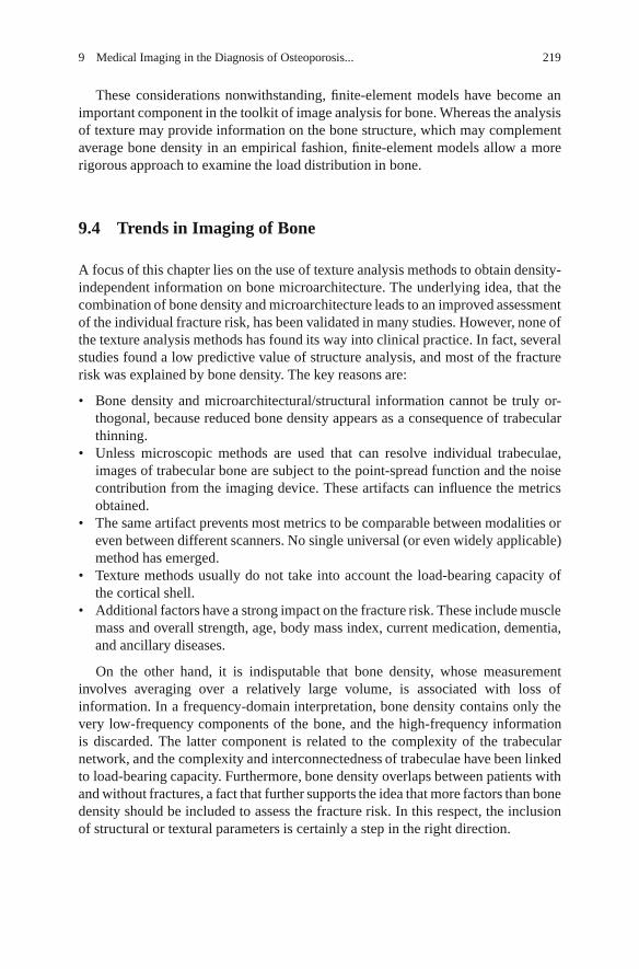
9 Medical Imaging in the Diagnosis of Osteoporosis... 219
These considerations nonwithstanding, finite-element models have become animportant component in the toolkit of image analysis for bone. Whereas the analysisof texture may provide information on the bone structure, which may complementaverage bone density in an empirical fashion, finite-element models allow a morerigorous approach to examine the load distribution in bone.
9.4 Trends in Imaging of Bone
A focus of this chapter lies on the use of texture analysis methods to obtain density-independent information on bone microarchitecture. The underlying idea, that thecombination of bone density and microarchitecture leads to an improved assessmentof the individual fracture risk, has been validated in many studies. However, none ofthe texture analysis methods has found its way into clinical practice. In fact, severalstudies found a low predictive value of structure analysis, and most of the fracturerisk was explained by bone density. The key reasons are:
• Bone density and microarchitectural/structural information cannot be truly or-thogonal, because reduced bone density appears as a consequence of trabecularthinning.
• Unless microscopic methods are used that can resolve individual trabeculae,images of trabecular bone are subject to the point-spread function and the noisecontribution from the imaging device. These artifacts can influence the metricsobtained.
• The same artifact prevents most metrics to be comparable between modalities oreven between different scanners. No single universal (or even widely applicable)method has emerged.
• Texture methods usually do not take into account the load-bearing capacity ofthe cortical shell.
• Additional factors have a strong impact on the fracture risk. These include musclemass and overall strength, age, body mass index, current medication, dementia,and ancillary diseases.
On the other hand, it is indisputable that bone density, whose measurementinvolves averaging over a relatively large volume, is associated with loss ofinformation. In a frequency-domain interpretation, bone density contains only thevery low-frequency components of the bone, and the high-frequency informationis discarded. The latter component is related to the complexity of the trabecularnetwork, and the complexity and interconnectedness of trabeculae have been linkedto load-bearing capacity. Furthermore, bone density overlaps between patients withand without fractures, a fact that further supports the idea that more factors than bonedensity should be included to assess the fracture risk. In this respect, the inclusionof structural or textural parameters is certainly a step in the right direction.
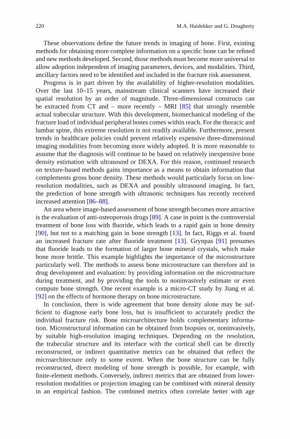
220 M.A. Haidekker and G. Dougherty
These observations define the future trends in imaging of bone. First, existingmethods for obtaining more complete information on a specific bone can be refinedand new methods developed. Second, those methods must become more universal toallow adoption independent of imaging parameters, devices, and modalities. Third,ancillary factors need to be identified and included in the fracture risk assessment.
Progress is in part driven by the availability of higher-resolution modalities.Over the last 10–15 years, mainstream clinical scanners have increased theirspatial resolution by an order of magnitude. Three-dimensional constructs canbe extracted from CT and – more recently – MRI [85] that strongly resembleactual trabecular structure. With this development, biomechanical modeling of thefracture load of individual peripheral bones comes within reach. For the thoracic andlumbar spine, this extreme resolution is not readily available. Furthermore, presenttrends in healthcare policies could prevent relatively expensive three-dimensionalimaging modalities from becoming more widely adopted. It is more reasonable toassume that the diagnosis will continue to be based on relatively inexpensive bonedensity estimation with ultrasound or DEXA. For this reason, continued researchon texture-based methods gains importance as a means to obtain information thatcomplements gross bone density. These methods would particularly focus on low-resolution modalities, such as DEXA and possibly ultrasound imaging. In fact,the prediction of bone strength with ultrasonic techniques has recently receivedincreased attention [86–88].
An area where image-based assessment of bone strength becomes more attractiveis the evaluation of anti-osteoporosis drugs [89]. A case in point is the controversialtreatment of bone loss with fluoride, which leads to a rapid gain in bone density[90], but not to a matching gain in bone strength [13]. In fact, Riggs et al. foundan increased fracture rate after fluoride treatment [13]. Grynpas [91] presumesthat fluoride leads to the formation of larger bone mineral crystals, which makebone more brittle. This example highlights the importance of the microstructureparticularly well. The methods to assess bone microstructure can therefore aid indrug development and evaluation: by providing information on the microstructureduring treatment, and by providing the tools to noninvasively estimate or evencompute bone strength. One recent example is a micro-CT study by Jiang et al.[92] on the effects of hormone therapy on bone microstructure.
In conclusion, there is wide agreement that bone density alone may be suf-ficient to diagnose early bone loss, but is insufficient to accurately predict theindividual fracture risk. Bone microarchitecture holds complementary informa-tion. Microstructural information can be obtained from biopsies or, noninvasively,by suitable high-resolution imaging techniques. Depending on the resolution,the trabecular structure and its interface with the cortical shell can be directlyreconstructed, or indirect quantitative metrics can be obtained that reflect themicroarchitecture only to some extent. When the bone structure can be fullyreconstructed, direct modeling of bone strength is possible, for example, withfinite-element methods. Conversely, indirect metrics that are obtained from lower-resolution modalities or projection imaging can be combined with mineral densityin an empirical fashion. The combined metrics often correlate better with age
9 Medical Imaging in the Diagnosis of Osteoporosis... 221
and existing fractures than density alone. Although it would be desirable tohave assessment methods for the bone microarchitecture in routine, low-resolutionmodalities (e.g., DEXA), no single method has emerged as a routine complementfor bone densitometry. Due to their costs, high-resolution modalities are rarely usedin clinical practice, but could turn out to be promising in drug development.
References
1. Klibanski, A., Adams-Campbell, L., Bassford, T., Blair, S.N., Boden, S.D., Dickersin, K., et al.:Osteoporosis prevention, diagnosis, and therapy. J. Am. Med. Assoc 285(6), 785–795 (2001)
2. Hernandez, C.J., Keaveny, T.M.: A biomechanical perspective on bone quality. Bone 39(6),1173–1181 (2006)
3. Holroyd, C., Cooper, C., Dennison, E.: Epidemiology of osteoporosis. Best Pract. Res. Clin.Endocrinol. Metabol. 22(5), 671–685 (2008)
4. Ritchie, R.O.: How does human bone resist fracture? Ann. New York Acad. Sci. 1192, 72–80(2010)
5. Small, R.E.: Uses and limitations of bone mineral density measurements in the management ofosteoporosis. Medsc. Gen. Med. 7(2), 3 (2005)
6. Gennari, C.: Calcium and vitamin D nutrition and bone disease of the elderly. Publ. HealthNutr. 4, 547–559 (2001)
7. Rittweger, J.: Can exercise prevent osteoporosis? J. Musculosceletal Neuronal Interact. 6(2),162 (2006)
8. Felsenberg, D., Boonen, S.: The bone quality framework: Determinants of bone strength andtheir interrelationships, and implications for osteoporosis management. Clin. Therapeut. 27(1),1–11 (2005)
9. Frost, H.M.: Dynamics of bone remodeling. Bone Biodynamics 315 (1964)10. Wolff, I., Van Croonenborg, J.J., Kemper, H.C.G., Kostense, P.J., Twisk, J.W.R.: The effect
of exercise training programs on bone mass: a meta-analysis of published controlled trials inpre-and postmenopausal women. Osteoporos. Int. 9(1), 1–12 (1999)
11. Karlsson, M.K., Nordqvist, A., Karlsson, C.: Physical activity, muscle function, falls andfractures. Food Nutr. Res. 52 (2008)
12. Meunier, P.J., Sebert, J.L., Reginster, J.Y., Briancon, D., Appelboom, T., Netter, P., et al.:Fluoride salts are no better at preventing new vertebral fractures than calcium-vitamin D inpostmenopausal osteoporosis: the FAVOStudy. Osteoporos. Int. 8(1), 4–12 (1998)
13. Riggs, B.L., Hodgson, S.F., O’Fallon, W.M., Chao, E., Wahner, H.W., Muhs, J.M., et al.: Effectof fluoride treatment on the fracture rate in postmenopausal women with osteoporosis. Obstet.Gynecol. Surv. 45(8), 542 (1990)
14. McCreadie, B.R., Goldstein, S.A.: Biomechanics of fracture: Is bone mineral density sufficientto assess risk? J. Bone Miner. Res. 15(12), 2305–2308 (2000)
15. Rockoff, S.D., Sweet, E., Bleustein, J.: The relative contribution of trabecular and cortical boneto the strength of human lumbar vertebrae. Calcif. Tissue Int. 3(1), 163–175 (1969)
16. Fields, A.J., Eswaran, S.K., Jekir, M.G., Keaveny, T.M.: Role of trabecular microarchitecturein whole-vertebral body biomechanical behavior. J. Bone Miner. Res. 24(9), 1523–1530 (2009)
17. Keaveny, T.M., Morgan, E.F., Niebur, G.L., Yeh, O.C.: Biomechanics of trabecular bone. Annu.Rev. Biomed. Eng. 3(1), 307–333 (2001)
18. Hernandez, C.J.: How can bone turnover modify bone strength independent of bone mass?Bone 42(6), 1014–1020 (2008)
19. Ammann, P., Rizzoli, R.: Bone strength and its determinants. Osteoporos. Int. 14(S3), 13–18(2003)

222 M.A. Haidekker and G. Dougherty
20. Chappard, D., Basle, M.F., Legrand, E., Audran, M.: Trabecular bone microarchitecture:A review. Morphologie 92(299), 162–170 (2008)
21. Svendsen, O.L., Haarbo, J., Hassager, C., Christiansen, C.: Accuracy of measurements of bodycomposition by dual-energy x-ray absorptiometry in vivo. Am. J. Clin. Nutr. 57(5), 605 (1993)
22. Lang, T.F.: Quantitative computed tomography. Radiol. Clin. N. Am. 48(3), 589–600 (2010)23. Bushberg, J., Seibert, J., Leidholdt, Jr. E.M., Boone, J.M.: The essential Physics of medical
imaging. Lippincott Williams & Wilkins, New York (2002)24. Njeh, C.F., Boivin, C.M., Langton, C.M.: The role of ultrasound in the assessment of
osteoporosis: a review. Osteoporos. Int. 7(1), 7–22 (1997)25. Liu, X.S., Sajda, P., Saha, P.K., Wehrli, F.W., Bevill, G., Keaveny, T.M., et al.: Complete
volumetric decomposition of individual trabecular plates and rods and its morphologicalcorrelations with anisotropic elastic moduli in human trabecular bone. J. Bone Miner. Res.23(2), 223–235 (2008)
26. Parfitt, A.M.: Bone histomorphometry: standardization of nomenclature, symbols and units(summary of proposed system). Bone 9(1), 67–69 (1988)
27. Hildebrand, T., Laib, A., Muller, R., Dequeker, J., Ruegsegger, P.: Direct three dimensionalmorphometric analysis of human cancellous bone: microstructural data from Spine, Femur,Iliac Crest, and Calcaneus. J. Bone Miner. Res. 14(7), 1167–1174 (1999)
28. Hernandez, C.J., Beaupre, G.S., Keller, T.S., Carter, D.R.: The influence of bone volumefraction and ash fraction on bone strength and modulus. Bone 29(1), 74–78 (2001)
29. Hildebrand, T., Ruegsegger, P.: A new method for the model-independent assessment ofthickness in three-dimensional images. J. Microsc. 185(1), 67–75 (1997)
30. Cortet, B., Bourel, P., Dubois, P., Boutry, N., Cotten, A., Marchandise, X.: CT scan textureanalysis of the distal radius: influence of age and menopausal status. Rev. Rhum. (Englishedn.) 65(2), 109 (1998)
31. Ito, M., Ohki, M., Hayashi, K., Yamada, M., Uetani, M., Nakamura, T.: Trabecular textureanalysis of CT images in the relationship with spinal fracture. Radiology 194(1), 55 (1995)
32. Thomsen, J.S., Ebbesen, E.N., Mosekilde, L.: Relationships between static histomorphometryand bone strength measurements in human iliac crest bone biopsies. Bone 22(2), 153–163(1998)
33. Saha, P.K., Gomberg, B.R., Wehrli, F.W.: Three-dimensional digital topological characteriza-tion of cancellous bone architecture. Int. J. Imag. Syst. Tech. 11(1), 81–90 (2000)
34. Le, H.M., Holmes, R.E., Shors, E.C., Rosenstein, D.A.: Computerized quantitative analysis ofthe interconnectivity of porous biomaterials. Acta. Stereologica. 11, 267–267 (1992)
35. Vesterby, A., Gundersen, H.J.G., Melsen, F.: Star volume of marrow space and trabeculae ofthe first lumbar vertebra: sampling efficiency and biological variation. Bone 10(1), 7–13 (1989)
36. Hahn, M., Vogel, M., Pompesius-Kempa, M., Delling, G.: Trabecular bone pattern factor–a newparameter for simple quantification of bone microarchitecture. Bone 13(4), 327–330 (1992)
37. Laib, A., Hildebrand, T., Hauselmann, H.J., Ruegsegger, P.: Ridge number density: a newparameter for in vivo bone structure analysis. Bone 21(6), 541–546 (1997)
38. Hildebrand, T., Ruegsegger, P.: Quantification of bone microarchitecture with the structuremodel index. Comput. Meth. Biomech. Biomed. Eng. 1(1), 15–23 (1997)
39. Haidekker, M.A.: Advanced Biomedical Image Analysis. Wiley, Hoboken, NJ (2011)40. Dougherty, G.: Image enhancement in the spatial domain. In: Digital image processing for
medical applications, p. 170–188. Cambridge University Press, New York (2009)41. Caldwell, C.B., Willett, K., Cuncins, A.V., Hearn, T.C.: Characterization of vertebral strength
using digital radiographic analysis of bone structure. Med. Phys. 22, 611 (1995)42. Lespessailles, E., Gadois, C., Kousignian, I., Neveu, J.P., Fardellone, P., Kolta, S., et al.:
Clinical interest of bone texture analysis in osteoporosis: a case control multicenter study.Osteoporos. Int. 19(7), 1019–1028 (2008)
43. Haidekker, M.A., Andresen, R., Evertsz, C.J., Banzer, D., Peitgen, H.O.: Issues of thresholdselection when determining the fractal dimension in HRCT slices of lumbar vertebrae. Br. J.Radiol. 73(865), 69 (2000)

9 Medical Imaging in the Diagnosis of Osteoporosis... 223
44. Haralick, R.M., Shanmugam, K., Dinstein, I.H.: Textural features for image classification.IEEE Trans. Syst. Man. Cybern. Syst. Hum. 3(6), 610–621 (1973)
45. Laws, K.I.: Texture energy measures. Proc DARPA Image Unerstanding Workshop, pp. 47–51(1979)
46. Lee, R.L., Dacre, J.E., Hart, D.J., Spector, T.D.: Femoral neck trabecular patterns predictosteoporotic fractures. Med. Phys. 29, 1391 (2002)
47. Lespessailles, E., Gadois, C., Lemineur, G., Do-Huu, J.P., Benhamou, L.: Bone texture analysison direct digital radiographic images: precision study and relationship with bone mineraldensity at the os calcis. Calcif. Tissue Int. 80(2), 97–102 (2007)
48. Rachidi, M., Marchadier, A., Gadois, C., Lespessailles, E., Chappard, C., Benhamou, C.L.:Laws’ masks descriptors applied to bone texture analysis: an innovative and discriminant toolin osteoporosis. Skeletal. Radiol. 37(6), 541–548 (2008)
49. Vokes, T., Lauderdale, D., Ma, S.L., Chinander, M., Childs, K., Giger, M.: Radiographic textureanalysis of densitometric calcaneal images: Relationship to clinical characteristics and to bonefragility. J. Bone Miner. Res. 25(1), 56–63 (2010)
50. Wilkie, J.R., Giger, M.L., Engh, Sr. C.A., Hopper, Jr. R.H., Martell, J.M.: Radiographic textureanalysis in the characterization of trabecular patterns in periprosthetic osteolysis1. Acad.Radiol. 15(2), 176–185 (2008)
51. Chappard, C., Brunet-Imbault, B., Lemineur, G., Giraudeau, B., Basillais, A., Harba, R., et al.:Anisotropy changes in post-menopausal osteoporosis: characterization by a new index appliedto trabecular bone radiographic images. Osteoporos. Int. 16(10), 1193–1202 (2005)
52. Brunet-Imbault, B., Lemineur, G., Chappard, C., Harba, R., Benhamou, C.L.: A new anisotropyindex on trabecular bone radiographic images using the fast Fourier transform. BMC Med.Imag. 5(1), 4 (2005)
53. Peitgen, H.O., Jurgens, H., Saupe, D.: Chaos and fractals: new frontiers of science. Springer,New York (2004)
54. Mandelbrot, B.B.: The Fractal Geometry of Nature. Freeman, USA (1982)55. Martınez-Lopez, F., Cabrerizo-Vılchez, M., Hidalgo-Alvarez, R.: A study of the different
methods usually employed to compute the fractal dimension1. Phys. Stat. Mech. Appl. 311,411–428 (2002)
56. Saupe, D.: Algorithms for random fractals. In: Peitgen, H.-O., and Saupe, D. (eds.), TheScience of Fractal Images, pp. 71–136. Springer, New York (1988)
57. Stein, M.C.: Nonparametric estimation of fractal dimension, vol. 1001 of Society of Photo-Optical Instrumentation Engineers (SPIE) Conference Series. SPIE (1988)
58. Chung, H.W., Chu, C.C., Underweiser, M., Wehrli, F.W.: On the fractal nature of trabecularstructure. Med. Phys. 21, 1535 (1994)
59. Dubuc, B., Zucker, S., Tricot, C., Quiniou, J., Wehbi, D.: Evaluating the fractal dimension ofsurfaces. Proc. Roy. Soc. Lond. Math. Phys. Sci. 425(1868), 113–127 (1989)
60. Huang, Q., Lorch, J.R., Dubes, R.C.: Can the fractal dimension of images be measured? PatternRecogn. 27(3), 339–349 (1994)
61. Geraets, W.G., Van Der Stelt, P.F.: Fractal properties of bone. Dentomaxillofacial Radiology29(3), 144 (2000)
62. Lopes, R., Betrouni, N.: Fractal and multifractal analysis: A review. Med. Image. Anal. 13(4),634–649 (2009)
63. Lundahl, T., Ohley, W., Kuklinski, W.: Analysis and interpolation of angiographic images byuse of fractals. Computers in Cardiology, p. 355. Linkoping, Sweden (1985)
64. Ruttimann, U.E., Webber, R.L., Hazelrig, J.B.: Fractal dimension from radiographs of periden-tal alveolar bone:: A possible diagnostic indicator of osteoporosis. Oral. Surg. Oral. Med. Oral.Pathol. 74(1), 98–110 (1992)
65. Webber, R., Underhill, T., Horton, R., Dixon, R., Pope, Jr. T.: Predicting osseous changes inankle fractures. IEEE Eng. Med. Biol. Mag. 12(1), 103–110 (2002)
66. Majumdar, S., Weinstein, R.S., Prasad, R.R.: Application of fractal geometry techniques to thestudy of trabecular bone. Med. Phys. 20, 1611 (1993)

224 M.A. Haidekker and G. Dougherty
67. Southard, T.E., Southard, K.A.: Detection of simulated osteoporosis in maxillae usingradiographic texture analysis. IEEE Trans. Biomed. Eng. 43(2), 123–132 (2002)
68. Veenland, J., Grashuis, J., Van der Meer, F., Beckers, A., Gelsema, E.: Estimation of fractaldimension in radiographs. Med. Phys. 23, 585 (1996)
69. Fortin, C., Kumaresan, R., Ohley, W., Hoefer, S.: Fractal dimension in the analysis of medicalimages. IEEE Eng. Med. Biol. Mag. 11(2), 65–71 (2002)
70. Messent, E., Buckland-Wright, J., Blake, G.: Fractal analysis of trabecular bone in kneeosteoarthritis (OA) is a more sensitive marker of disease status than bone mineral density(BMD). Calcif. Tissue Int. 76(6), 419–425 (2005)
71. Dougherty, G., Henebry, G.M.: Fractal signature and lacunarity in the measurement of thetexture of trabecular bone in clinical CT images. Med. Eng. Phys. 23(6), 369–380 (2001)
72. Dong, P.: Test of a new lacunarity estimation method for image texture analysis. Int. J. Rem.Sens. 21(17), 3369–3373 (2000)
73. Plotnick, R.E., Gardner, R.H., Hargrove, W.W., Prestegaard, K., Perlmutter, M.: Lacunarityanalysis: a general technique for the analysis of spatial patterns. Phys. Rev. E 53(5), 5461–5468(1996)
74. Dougherty, G., Henebry, G.M.: Lacunarity analysis of spatial pattern in CT images of vertebraltrabecular bone for assessing osteoporosis. Med. Eng. Phys. 24(2), 129–138 (2002)
75. Zaia, A., Eleonori, R., Maponi, P., Rossi, R., Murri, R.: MR imaging and osteoporosis: Fractallacunarity analysis of trabecular bone. IEEE Trans. Inform. Tech. Biomed. 10(3), 484–489(2006)
76. Panagiotopoulou, O.: Finite element analysis (FEA): applying an engineering method tofunctional morphology in anthropology and human biology. Ann. Hum. Biol. 36(5), 609–623(2009)
77. Vesterby, A., Mosekilde, L., Gundersen, H.J.G., Melsen, F., Holme, K., Sørensen, S.:Biologically meaningful determinants of the in vitro strength of lumbar vertebrae. Bone 12(3),219–224 (1991)
78. Jones, A.C., Wilcox, R.K.: Finite element analysis of the spine: Towards a framework ofverification, validation and sensitivity analysis. Med. Eng. Phys. 30(10), 1287–1304 (2008)
79. Lavaste, F., Skalli, W., Robin, S., Roy-Camille, R., Mazel, C.: Three-dimensional geometricaland mechanical modelling of the lumbar spine. J. Biomech. 25(10), 1153–1164 (1992)
80. Kuo, C.S., Hu, H.T., Lin, R.M., Huang, K.Y., Lin, P.C., Zhong, Z.C., et al.: Biomechanicalanalysis of the lumbar spine on facet joint force and intradiscal pressure-a finite element study.BMC Muscoskel. Disord. 11, 151 (2010)
81. Gibson, L.J.: The mechanical behaviour of cancellous bone. J. Biomech. 18(5), 317–328 (1985)82. Jensen, K.S., Mosekilde, L.: A model of vertebral trabecular bone architecture and its
mechanical properties. Bone 11(6), 417–423 (1990)83. Hollister, S.J., Brennan, J.M., Kikuchi, N.: A homogenization sampling procedure for calcu-
lating trabecular bone effective stiffness and tissue level stress. J. Biomech. 27(4), 433–444(1994)
84. Muller, R., Ruegsegger, P.: Three-dimensional finite element modelling of non-invasivelyassessed trabecular bone structures. Med. Eng. Phys. 17(2), 126–133 (1995)
85. Magland, J., Vasilic, B., Wehrli, F.W.: Fast Low Angle Dual Spin Echo (FLADE): A new robustpulse sequence for structural imaging of trabecular bone. Magn. Reson. Med. 55(3), 465–471(2006)
86. Karjalainen, J.P., Toyras, J., Riekkinen, O., Hakulinen, M., Jurvelin, P.S.: Ultrasoundbackscatter imaging provides frequency-dependent information on structure, composition andmechanical properties of human trabecular bone. Ultrasound Med. Biol. 35(8), 1376–1384(2009)
87. Haıat, G., Padilla, F., Svrcekova, M., Chevalier, Y., Pahr, D., Peyrin, F., et al.: Relationshipbetween ultrasonic parameters and apparent trabecular bone elastic modulus: A numericalapproach. J. Biomech. 42(13), 2033–2039 (2009)

9 Medical Imaging in the Diagnosis of Osteoporosis... 225
88. Hosokawa, A.: Effect of porosity distribution in the propagation direction on ultrasound wavesthrough cancellous bone. IEEE Trans. Ultrason. Ferroelectrics Freq. Contr. 57(6), 1320–1328(2010)
89. Davison, K.S., Kendler, D.L., Ammann, P., Bauer, D.C., Dempster, D.W., Dian, L., et al.:Assessing fracture risk and effects of osteoporosis drugs: bone mineral density and beyond.Am. J. Med. 122(11), 992–997 (2009)
90. Resch, H., Libanati, C., Farley, S., Bettica, P., Schulz, E., Baylink, D.J.: Evidence that fluoridetherapy increases trabecular bone density in a peripheral skeletal site. J. Clin. Endocrinol.Metabol. 76(6), 1622 (1993)
91. Grynpas, M.D.: Fluoride effects on bone crystals. J. Bone Miner. Res. 5(S1), S169–S175(1990)
92. Jiang, Y., Zhao, J., Liao, E.Y., Dai, R.C., Wu, X.P., Genant, H.K.: Application of micro-CTassessment of 3-D bone microstructure in preclinical and clinical studies. J. Bone Miner.Metabol. 23, 122–131 (2005)


Chapter 10Applications of Medical Image Processingin the Diagnosis and Treatmentof Spinal Deformity
Clayton Adam and Geoff Dougherty
10.1 Introduction
Spinal deformities are a group of disorders characterized by abnormal curvatureof the spine. In the healthy spine, natural curves occur in the sagittal plane, witha lordosis (concave curvature) in the lower back (lumbar) region and kyphosis(convex curvature) in the upper back (thoracic) region. In some spinal deformi-ties, these natural curves can be either suppressed or amplified, as in the caseof hypokyphosis (flatback) or hyperkyphosis (exaggerated thoracic curvature or‘hunchback’). However, the most common type of deformity is scoliosis, whichis defined as abnormal lateral (side to side) curvature of the spine accompaniedby axial rotation. Because of the combined sagittal curvature, abnormal lateralcurvature, and axial rotation, scoliosis is a complex three-dimensional deformitywhich cannot be visualised in any single viewing plane (Fig. 10.1).
This chapter describes the application of image processing to the assessmentand treatment of spinal deformity, with a focus on the most common deformity,adolescent idiopathic scoliosis (AIS). We will briefly describe the natural historyof spinal deformity and current approaches to surgical and non-surgical treatmentto give some background to the problem, and present an overview of currentclinically used imaging modalities. We will introduce the key metric currently usedto assess the severity and progression of spinal deformities from medical images,the Cobb angle, and discuss the uncertainties involved in manual Cobb anglemeasurements. An alternative metric, the Ferguson angle, will also be discussed.This provides the context for an examination of semi-automated image processingapproaches for improved measurement of spinal curve shape and severity, includingthe development of discrete and continuum representations of the thoracolumbar
C. Adam (�)Queensland University of Technology, Brisbane, Australiae-mail: [email protected]
G. Dougherty (ed.), Medical Image Processing: Techniques and Applications, Biologicaland Medical Physics, Biomedical Engineering, DOI 10.1007/978-1-4419-9779-1 10,© Springer Science+Business Media, LLC 2011
227

228 C. Adam and G. Dougherty
Fig. 10.1 Three dimensional CT reconstructions of a scoliotic spine showing overall spine andribcage shape (left), sagittal, and coronal close-up views of the vertebral column (right)
spine and tortuosity measures. The newly defined metrics are applied to a dataset ofidiopathic scoliosis patients and assessed by comparison with clinical Cobb anglemeasurements for the same patient group. Finally, areas for future image processingresearch applied to spinal deformity assessment and treatment are discussed.
10.1.1 Adolescent Idiopathic Scoliosis
While scoliosis can occur as a secondary consequence of a primary pathology(such as a leg length inequality or congenital malformation), most (70–80%)scoliosis cases occur during the adolescent growth spurt without known cause.These deformities are classified as AIS, and affect 2–4% of the population.
People with scoliosis often have no symptoms beyond a slight increase in painand reduced lung capacity. However, progressive scoliosis leads to an increasinglysevere cosmetic deformity and can compromise the function of internal organsin severe cases. For these reasons, both conservative (non-surgical) and surgicaltreatments for spinal deformities have been developed. Bracing is a common

10 Applications of Medical Image Processing in the Diagnosis and Treatment... 229
Fig. 10.2 Post-operativeX-rays single rod showinganterior (left) and dual rodposterior (right) implants forscoliosis correction
conservative treatment in which the patient is asked to wear an orthotic brace whichattempts to exert corrective forces on the deformed spine. Surgical approaches toscoliosis correction (Fig. 10.2) involve attachment of implants to the spine to restorea more normal curvature. Successful surgical approaches typically achieve a 60%reduction of the deformity and prevent further progression; however, there are risksof complication and further deformity progression after surgery which mandateongoing imaging to monitor the corrected spine.
10.2 Imaging Modalities Used for Spinal Deformity Assessment
Many spinal deformities are visible just by looking at a patient. However, due todifferences in body fat levels and bone structure between patients, they cannotbe accurately assessed by visual examination of the patient’s appearance. Medicalimaging, therefore, plays a key role both in the monitoring of spinal deformityprogression before treatment, and in assessing treatment outcomes. There are fourmedical imaging modalities relevant to the assessment of spinal deformities.

230 C. Adam and G. Dougherty
Planar and biplanar radiography Plane radiographs (X-rays) are the gold standardfor imaging spinal deformities, and are used in spine clinics worldwide. A relativelynew technology developed in France, the EOS system (EOS imaging, Paris, France),uses bi-planar radiography to simultaneously obtain coronal and sagittal radiographsof standing scoliosis patients with low radiation dose.
Computed Tomography (CT) CT is currently not used routinely for clinical assess-ment of scoliosis due to its greater cost and higher radiation dose than plane X-rays[1, 2]. However, low dose pre-operative CT is clinically indicated in endoscopicor keyhole scoliosis surgery for planning implant placement [3], and advances inscanner technology now allow CT with much lower radiation doses than previouslypossible [4]. In the research context, a number of groups have used CT to assessspinal deformities (in particular vertebral rotation in the axial plane) due to the 3Dinformation provided [5–10].
Magnetic Resonance (MR) MR imaging is sometimes used clinically to detectsoft tissue abnormalities (particularly the presence of syringomyelia in scoliosispatients), but clinical use of MR for spinal deformities is generally limited. Severalresearch studies have used MR to investigate scoliosis [11–15]. MR is a usefulresearch tool because of the absence of ionizing radiation, although the ability ofMR to define bony anatomy is limited and thus image processing of MR datasets isoften labour-intensive.
Back surface topography Various optical surface topography systems have beenused to directly visualise the cosmetic effects of spinal deformity by assessing backshape in 3D [16–24]. Back surface topography does not involve ionising radiation,and so is useful for functional evaluations involving repeated assessments [25].However, the relationship between spinal deformity and back shape is complicatedby factors such as body positioning, trunk rotation, body build and fat folds [26].
10.2.1 Current Clinical Practice: The Cobb Angle
Currently, the accepted measure for clinical assessment of scoliosis is the Cobbangle [27]. The Cobb angle is measured on plane radiographs by drawing a linethrough the superior endplate of the superior end vertebra of a scoliotic curve,and another line through the inferior endplate of the inferior-most vertebra of thesame scoliotic curve, and then measuring the angle between these lines (Fig. 10.3).Clinically, many Cobb measurements are still performed manually using penciland ruler on hardcopy X-ray films, but PACS systems (viz. computer networks)are increasingly used which allow manual Cobb measurements to be performeddigitally by clinicians on the computer screen. As well as being used to assessscoliosis in the coronal plane, the Cobb angle is used on sagittal plane radiographsto assess thoracic kyphosis and lumbar lordosis.

10 Applications of Medical Image Processing in the Diagnosis and Treatment... 231
Fig. 10.3 Schematic view ofa scoliotic deformity showingmeasurement of the Cobbangle
α
Cobb angle
Although widely used for scoliosis assessment for its simplicity, the Cobb anglehas several shortcomings. First, numerous studies have shown that the inter- andintra-observer measurement variabilities associated with the Cobb angle are high.If the vertebral endplates on a plane X-ray appear blurred due to a forward orbackward tilt, considerable inter-observer errors can be introduced in the Cobbmethod as a result of the difficulty in selecting the endplate orientation. Sucherrors are even more pronounced in the presence of contour changes resulting fromosteoporosis [28, 29]. Figure 10.4 shows a summary of Cobb variability studiesperformed between 1982 and 2005, indicating that the 95% confidence interval forthe difference between two measurements by the same observer is around 5–7◦, andfor two measurements by different observers is around 6–8◦. These measurementerrors are large enough to make the difference between a diagnosis of progression(requiring treatment) or stability, and so introduce uncertainty into the assessmentand treatment process.
Second, because of its simplicity, the Cobb angle omits potentially usefulinformation about the shape of a scoliotic spine. Specifically, the Cobb angle cannotdifferentiate between a large scoliotic curve which may span 8 or 9 vertebral levels,and a small scoliotic curve which may only span 2 or 3 vertebral levels but that hasthe same endplate angulation due to its severity (Fig. 10.5).
10.2.2 An Alternative: The Ferguson Angle
Prior to the adoption of the Cobb angle as standard practice by the ScoliosisResearch Society in 1966, a number of other scoliosis measurement techniques

232 C. Adam and G. Dougherty
0
2
4
6
8
10
12
95%
CI f
or in
tra-
obse
rver
var
iabi
lity
(deg
rees
)
Fig. 10.4 Ninety five percent confidence intervals for intra-observer measurement variabilityusing the Cobb angle from previous studies (figure based on [30])
Fig. 10.5 Simplifiedrepresentation of threedifferent scoliotic curves withincreasing radius and agreater number of vertebrallevels in the curve, but thesame Cobb angle α
Cobb angle
had been proposed, including the Ferguson angle [31]. The Ferguson angle requiresidentification of three landmark points, the geometric centres of the upper, apical(i.e. the most laterally deviated) and lower vertebrae in a scoliotic curve (Fig. 10.6).Not only does the Ferguson angle take into account the position of the apicalvertebra, which the Cobb angle does not, it is less influenced by changes in theshape of the vertebrae [32].

10 Applications of Medical Image Processing in the Diagnosis and Treatment... 233
Fig. 10.6 Schematic view ofa scoliotic deformity showingmeasurement of the Fergusonangle (Cobb angle shown forcomparison)
α
Cobb angle
Fergusonangle
The Ferguson angle is slightly more complicated to measure than Cobb due tothe three landmark points (rather than two endplates in the Cobb technique). Therecan be difficulties in identifying the centres of the vertebrae, depending on theirshape. The diagonals of the vertebra, as used in the standard Ferguson method, donot intersect at its geometric centre. The intersection of perpendicular lines drawnthrough the midpoints of the upper and lower endplates of a vertebra, proposed as amore accurate method of obtaining the geometric centre especially with prominentlywedge-shaped vertebrae [32], is also flawed since it assumes that the four cornersof the vertebral body lie on a circle. An alternative, more reliable method offinding the geometric centres has been proposed [33]. It has been shown that theFerguson angle is closely related to the Cobb angle, with the ratio between Cobband Ferguson angles for the same curve being ∼1.35 [34]. Measurement variabilityfor the Ferguson angle appears to be comparable with, or slightly higher than thatof the Cobb angle [32, 34, 35].
10.3 Image Processing Methods
The increasing adoption of digital imaging provides a growing opportunity to (a)develop more detailed metrics for spinal deformity assessment which consider allvertebral levels in a scoliotic curve rather than just the two end vertebrae, (b)implement these metrics quickly and accurately using semi- and fully-automatedimage processing tools, and (c) measure scoliosis curvature using 3D datasets frommodalities such as biplanar radiography, CT and MR. The remainder of this chapterpresents details of image processing applications which are being developed by theauthors in an attempt to avoid the manual measurement variability mentioned above,and also to allow development of new metrics which may in the longer term improvesurgical planning and treatment decision making for spinal deformity patients.

234 C. Adam and G. Dougherty
10.3.1 Previous Studies
Development of medical image processing algorithms for assessment of scoliosishas been sparse to date. Several studies have used algorithms to perform computer-aided measurement of Cobb angle and other standard measures based on digitizedanatomical landmarks manually selected by a user on a computer screen [36–39].Gerard et al. [40] developed a semi-automated algorithm for scoliotic deformitymeasurement using dynamic programming optimisation. An automated algorithmfor measuring vertebral rotation from a CT slices using the inherent symmetry ofthe vertebral cross-section was developed by Adam et al. [10]. Algorithms havealso been developed to process back surface topography images (see Sect. 10.2),including a recent non-rigid registration algorithm [41]. However, as mentioned pre-viously, back shape approaches are limited in their ability to assess the underlyingspinal deformity and so are not widely used clinically.
10.3.2 Discrete and Continuum Functions for Spinal Curvature
A key aspect of developing more detailed metrics for spinal deformity assessmentis measuring all vertebrae in a scoliotic curve, not just the end or apical vertebrae(as in the Cobb and Ferguson methods). Measuring all vertebrae provides a fullerunderstanding of how deformities affect each vertebral level before treatment, andalso captures changes in spinal configuration after surgical treatment which mayoccur over only one or two vertebral levels (such as decompensation at the top ofan implant construct). However, the challenges in measuring all vertebral levels are(a) defining appropriate anatomical landmarks for reliable, semi- or fully-automateddetection from radiographic images, and (b) processing these landmark coordinatesto obtain meaningful measures of deformity shape which will assist in diagnosis andtreatment.
One approach being developed by the authors for use with low dose CT datasetsof AIS patients is to use the edge of the vertebral canal as a robust anatomicallandmark suitable for semi-automated detection. Figure 10.7 shows a transverse CTslice of a scoliosis patient, which demonstrates the clearly defined, high contrast,enclosed inner boundary of the vertebral canal.
Even though individual vertebrae may be substantially tilted relative to thetransverse CT slices, even in large scoliosis curves (Cobb angle ∼60◦), one or moreCT slices will contain an enclosed vertebral canal such as that shown in Fig. 10.7.From these images, a spinal canal tracking algorithm has been developed usingthe ImageJ software (version 1.43u, National Institutes of Health, USA), whichuses ImageJ’s automatic edge tracing command to locate the inner boundary ofthe vertebral canal, and determine the canal centroid coordinates. By applying thisalgorithm for each vertebral level in a scoliosis curve, a series of 17 x,y,z datapointsfor the entire thoracolumbar spine can be generated, and pairs of x,z and y,z datapoints define spinal curvature in the coronal and sagittal planes respectively.
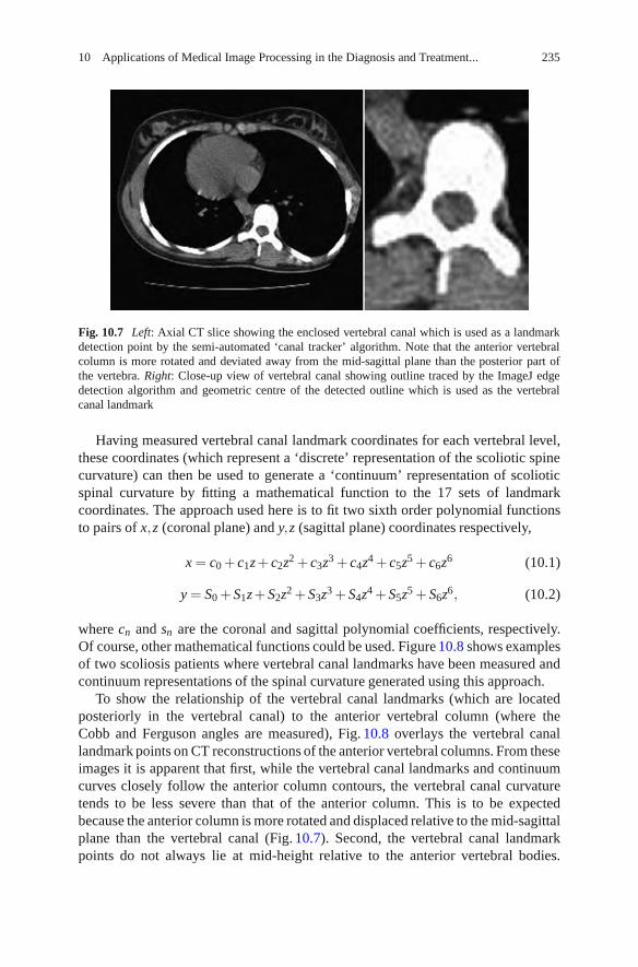
10 Applications of Medical Image Processing in the Diagnosis and Treatment... 235
Fig. 10.7 Left: Axial CT slice showing the enclosed vertebral canal which is used as a landmarkdetection point by the semi-automated ‘canal tracker’ algorithm. Note that the anterior vertebralcolumn is more rotated and deviated away from the mid-sagittal plane than the posterior part ofthe vertebra. Right: Close-up view of vertebral canal showing outline traced by the ImageJ edgedetection algorithm and geometric centre of the detected outline which is used as the vertebralcanal landmark
Having measured vertebral canal landmark coordinates for each vertebral level,these coordinates (which represent a ‘discrete’ representation of the scoliotic spinecurvature) can then be used to generate a ‘continuum’ representation of scolioticspinal curvature by fitting a mathematical function to the 17 sets of landmarkcoordinates. The approach used here is to fit two sixth order polynomial functionsto pairs of x,z (coronal plane) and y,z (sagittal plane) coordinates respectively,
x = c0 + c1z+ c2z2 + c3z3 + c4z4 + c5z5 + c6z6 (10.1)
y = S0 + S1z+ S2z2 + S3z3 + S4z4 + S5z5 + S6z6, (10.2)
where cn and sn are the coronal and sagittal polynomial coefficients, respectively.Of course, other mathematical functions could be used. Figure 10.8 shows examplesof two scoliosis patients where vertebral canal landmarks have been measured andcontinuum representations of the spinal curvature generated using this approach.
To show the relationship of the vertebral canal landmarks (which are locatedposteriorly in the vertebral canal) to the anterior vertebral column (where theCobb and Ferguson angles are measured), Fig. 10.8 overlays the vertebral canallandmark points on CT reconstructions of the anterior vertebral columns. From theseimages it is apparent that first, while the vertebral canal landmarks and continuumcurves closely follow the anterior column contours, the vertebral canal curvaturetends to be less severe than that of the anterior column. This is to be expectedbecause the anterior column is more rotated and displaced relative to the mid-sagittalplane than the vertebral canal (Fig. 10.7). Second, the vertebral canal landmarkpoints do not always lie at mid-height relative to the anterior vertebral bodies.

236 C. Adam and G. Dougherty
Fig. 10.8 Coronal CT reconstructions of two scoliosis patients showing the vertebral canallandmark points (dark blue diamonds) and polynomial fits (pink lines) to the vertebral canallandmark points which provide a continuum mathematical description of the spinal curvature
This can occur firstly because the vertebra may be tilted in the sagittal plane (withthe anterior vertebral body higher than the posterior vertebral canal – see the sagittalCT view in Fig. 10.1), and also because the current implementation of the algorithmis semi-automated, so there may be a choice of several axial CT slices in which anenclosed vertebral canal can be clearly seen by the user, leading to a user variabilityin slice selection. We note, however, that the resulting continuum mathematicalrepresentation is insensitive to variations in the CT slice chosen within a particularvertebrae for spinal canal landmark detection.
Having obtained discrete landmark points and a continuum representation of thespinal curvature, various curve metrics can be extracted. In particular, the inflectionpoints of the coronal plane polynomial can be readily located by finding the zeros ofthe second derivative of the polynomial (i.e. the roots of a fourth order polynomial),
d2xdz2 = 2c2 + 6c3z+ 12c4z2 + 20c5z3 + 30c6z4 = 0, (10.3)
and the angle between the normals to the coronal curve at two neighboring inflectionpoints can then be determined to provide a ‘Cobb-equivalent angle’. This approachis analogous with the clinical definition of the coronal Cobb angle, which is basedon locating the ‘most tilted’ endplates in a scoliotic curve.
In some cases, the coronal polynomial curve has only one inflection point, and inthese cases an alternative approach must be used to generate the ‘Cobb-equivalent’

10 Applications of Medical Image Processing in the Diagnosis and Treatment... 237
metric. Here, we propose that the z-coordinates of the upper and lower end vertebraeof the scoliotic curve as determined clinically are used in this situation. The anglebetween the normals to the coronal curve at these vertebral levels is again a Cobb-equivalent measure, with the disadvantage that a manual selection of levels wasrequired.
The two approaches just presented; (1) Cobb-equivalent angle determined as theangle between inflection points of coronal polynomial, and (2) Cobb-equivalentangle determined as the angle between manually selected vertebral locations ofcoronal polynomial are denoted as the ‘Cobb-equivalent 1’ and ‘Cobb-equivalent 2’angles, respectively.
10.3.3 Tortuosity
The concept of tortuosity, the accumulation of curvature along a curve, has beenused to characterise blood vessels and their risk of aneurysm formation or rupture[33, 42–47]. A variety of possible metrics for tortuosity have been proposed, suchas the distance factor (the relative length increase from a straight line) [48–50] orsinuosity [51], the number of inflection points along the curve [52], the angle changealong segments [53,54], and various line integrals of local curvature values [42,44],which can be computed from second differences of the curve [43].
We have developed two tortuosity metrics [45] which are amenable to automationand can be used as putative scoliosis metrics for measuring the severity of thecondition. Both are inherently three-dimensional, although they can be applied totwo-dimensional projections. (A third possible metric, the integral of the square ofthe derivative of curvature of a spline-fit smoothest path, was found not to be scale-invariant, and subsequently abandoned [55]).
The first metric delivers a scoliotic angle, which can be considered an extensionof the Ferguson angle. It is the accumulated angle turned along the length ofthe section of spine of interest, calculated as the sum of the magnitudes of theangles between straight line segments connecting the consecutive centres of all thevertebrae under consideration (Fig. 10.9). We have previously designated it as M. Itcan be applied to the whole spine, or a designated curve within it.
Figure 10.9 shows that M can be considered an extension of the Ferguson angle(referred to here as the segmental Ferguson angle). For a given scoliotic curve, thesegmental Ferguson angle will be larger than the conventional Ferguson angle andsmaller than the Cobb angle, although in the special (theoretical) case of a circulararc comprising many short segments its value approaches that of the Cobb angle.This special case is shown schematically in Fig. 10.10.
The second metric is based on a continuum function for the spinal curve,based on a unit speed parameterization of the vertebral centres. A piece-wisespline is used to produce a continuous function, which is the ‘smoothest path’connecting the vertebral centres (Fig. 10.11), and it is used to compute a normalized

238 C. Adam and G. Dougherty
α
φ1φ2
φ3
Μ=φ1+φ2+φ3
Cobbangle
SegmentalFerguson angles
Conventional Ferguson angle
φ5
φ1φ2
φ3
φ4
M= |f1|+ |f2|+ |f3|+ |f4|+ |f5 |
Fig. 10.9 Left: Portion of a scoliotic curve showing conventional Cobb and Ferguson angles aswell as the segmental Ferguson angles which are summed to give the coronal tortuosity metric M.Right: Absolute segmental angles are summed in the case of a spinal curve containing both positiveand negative angles
Fig. 10.10 For the specialcase of a circular arc theCobb angle α is twice theFerguson angle φ. As the arcis divided into successivelymore segments, the coronaltortuosity (sum of thesegmental Ferguson anglesM = φ1 +φ2 +φ3 + . . .)approaches the Cobb angle
Cobb angle
f =30°
f1=f2=f3=f4=f5=8.57°M=f1+f2+f3+f4+f5=42.85°
f1
f2
f3
f4
f5
a = 60°

10 Applications of Medical Image Processing in the Diagnosis and Treatment... 239
Fig. 10.11Anterior–posterior (AP)radiograph, illustrating themeasurement of theconventional Cobb andFerguson angles, and showingthe smoothest-pathpiece-wise spline iterativelyfitted to the geometric centresof the vertebrae
root-mean-square (rms) curvature, which we designated K. It is defined in terms ofthe root-mean-square curvature, J, of the smoothest path by
K =√
J.L, (10.4)
where L is the length of the smoothed curve. The ‘normalization’ by√
L ensures thatK is dimensionless (viz. an angle). While M is an accumulated angle using straightline segments between the vertebral centres, K is an accumulated angle using thesmoothest path connecting the centres. With K, the accumulation is not democratic;rather contributions of higher curvature are given more weight than contributionsof lower curvature. (If the curvature is constant, then K is forced to accumulatedemocratically and K = M.)
Both metrics have been shown to be scale invariant and additive, and K is essen-tially insensitive to digitization errors [45] Their usefulness has been demonstratedin discriminating between arteries of different tortuosities in assessing the relativeutility of the arteries for endoluminal repair of aneurysms [33].

240 C. Adam and G. Dougherty
10.4 Assessment of Image Processing Methods
Before adopting an automated method for the assessment of spinal deformities, thereis a need to compare the proposed method with the results from current practice,in particular the Cobb angle which is the clinically accepted measure of scoliosisseverity. Here, we apply the image processing techniques described above to deriveCobb-equivalent and tortuosity metrics in a series of AIS patients. We then comparethe new metrics with existing, clinically measured Cobb angles for the patients inthe series.
10.4.1 Patient Dataset and Image Processing
The patient group comprised 79 AIS patients from the Mater Children’s Hospitalin Brisbane, Australia. Each of the patients in this series underwent thoracoscopic(keyhole) anterior surgery for correction of their deformity, and prior to surgeryeach patient received a single, low-dose, pre-operative CT scan for surgical planningpurposes. Pre-operative CT allows safer screw sizing and positioning in keyholescoliosis surgery procedures [56]. The estimated CT radiation dose for the scanningprotocol used was 3.7 mSv [57].
Following the procedure described in Sect. 10.3.2, vertebral canal landmark co-ordinates were measured for each thoracolumbar vertebrae in each patient in theseries. We note that measurement of spinal deformities from supine CT scans yieldslower values of the Cobb angle than measurements on standing patients. Torellet al. [58] reported a 9◦ reduction in Cobb angle for supine compared to standingpatients, and Yazici et al. [59] showed a reduction in average Cobb angle from 56 to39◦ between standing and supine positions.
10.4.2 Results and Discussion
The patient group comprised of 74 females and 5 males with a mean age of 15.6years (range 9.9–41.2) at the time the CT scan was performed. The mean height was161.5 cm (range 139.5–175) and mean weight was 53.4 kg (range 30.6–84.7). All79 patients had right-sided major scoliotic curves.1 The mean clinically measuredmajor Cobb angle for the group was 51.9◦ (range 38–68◦). The clinical Cobbmeasurements were performed manually at the Mater Children’s Hospital spinalclinic by experienced clinicians, using standing radiographs. Figure 10.12 shows a
1The major curve is defined as the curve with the largest Cobb angle in a scoliotic spine. Typically,adolescent idiopathic scoliosis major curves are convex to the right in the mid-thoracic spine, withsmaller (minor) curves above and below, convex to the left.

10 Applications of Medical Image Processing in the Diagnosis and Treatment... 241
y = 1.13 x -15.52 R² = 0.38
y = 1.04 x -13.72 R² = 0.32
20
40
60
80
100
30 40 50 60 70 80 90 100
Cob
b-eq
uiva
lent
ang
le (
°)
Clinically measured Cobb (°)
Cobb-equivalent 1Cobb-equivalent 2Linear (Cobb-equivalent 1)Linear (Cobb-equivalent 2)
Fig. 10.12 Plot of Cobb-equivalent 1 and Cobb-equivalent 2 angles against clinically measuredcoronal Cobb angle for each patient in the series. Note that for 10 of the 79 patients, there wasonly one inflection point on the polynomial curve so Cobb-equivalent1 could not be determinedfor these ten patients
comparison between the clinically measured (standing) Cobb angle and the Cobb-equivalent 1 and Cobb-equivalent 2 metrics derived from the supine CT scans forthe patient group.
With respect to Fig. 10.12, the relatively low R2 values of 0.38 and 0.32(Cobb-equivalent 1 and Cobb-equivalent 2, respectively) show there are substantialvariations between individual clinical Cobb measurements from standing radio-graphs, and the Cobb-equivalent angles derived from continuum representations ofspine shape on supine CT scans. The 13.7 and 15.5◦ offsets in the linear regressionequations for the two Cobb-equivalent angles are consistent with the magnitude ofchange in Cobb angle between standing and supine postures of 9◦ and 17◦ reportedby Torell et al. [58] and Yazici et al. [59]. The gradients of the regression lines forCobb-equivalent 1 (1.13) and Cobb-equivalent 2 (1.04) in Fig. 10.13 are close tounity as would be expected, but the slightly greater than unity values suggest thateither (1) bigger scoliotic curves are more affected by gravity (i.e. the differencebetween standing and supine Cobb increases with increasing Cobb angle), or (2)there is greater rotation of the anterior vertebral column (where clinical Cobb anglesare measured from endplates) compared to the posterior vertebral canal (where theCobb-equivalent landmarks are measured) in patients with larger deformities. Notethat although not shown in Fig. 10.12, Cobb-equivalent 1 and Cobb-equivalent 2 arehighly correlated with each other (R2 = 0.96).
Figure 10.13 shows the close correlation between two of the new metrics,the coronal tortuosity (segmental Ferguson angle) of the major curve and theCobb-equivalent 2. The coronal tortuosity, M (or segmental Ferguson angle), isstrongly correlated (R2 = 0.906, p < 0.0000001) with the Cobb-equivalent 2 angle.
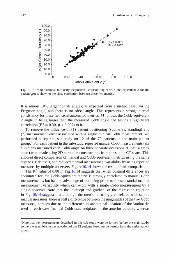
242 C. Adam and G. Dougherty
y = 1.0985xR² = 0.9057
0.0
10.0
20.0
30.0
40.0
50.0
60.0
70.0
80.0
90.0
100.0
0.0 20.0 40.0 60.0 80.0 100.0
Ma
jor
Cor
onal
Tor
tuos
ity (
°)
Cobb-Equivalent 2 (°)
Fig. 10.13 Major coronal tortuosity (segmental Ferguson angle) vs. Cobb-equivalent 2 for thepatient group, showing the close correlation between these two metrics
It is almost 10% larger for all angles, as expected from a metric based on theFerguson angle, and there is no offset angle. This represents a strong internalconsistency for these two semi-automated metrics. M follows the Cobb-equivalent2 angle in being larger than the measured Cobb angle and having a significantcorrelation (R2 = 0.30, p < 0.007) to it.
To remove the influence of (1) patient positioning (supine vs. standing) and(2) measurement error associated with a single clinical Cobb measurement, weperformed a separate sub-study on 12 of the 79 patients in the main patientgroup.2 For each patient in the sub-study, repeated manual Cobb measurements (sixclinicians measured each Cobb angle on three separate occasions at least a weekapart) were made using 2D coronal reconstructions from the supine CT scans. Thisallowed direct comparison of manual and Cobb-equivalent metrics using the samesupine CT datasets, and reduced manual measurement variability by using repeatedmeasures by multiple observers. Figure 10.14 shows the result of this comparison.
The R2 value of 0.88 in Fig. 10.14 suggests that when postural differences areaccounted for, the Cobb-equivalent metric is strongly correlated to manual Cobbmeasurements, but has the advantage of not being prone to the substantial manualmeasurement variability which can occur with a single Cobb measurement by asingle observer. Note that the intercept and gradient of the regression equationin Fig. 10.14 suggest that although the metric is strongly correlated with supinemanual measures, there is still a difference between the magnitudes of the two Cobbmeasures, perhaps due to the difference in anatomical location of the landmarksused in each case (manual Cobb uses endplates in the anterior column, whereas
2Note that the measurements described in this sub-study were performed before the main study,so there was no bias in the selection of the 12 patients based on the results from the entire patientgroup.

10 Applications of Medical Image Processing in the Diagnosis and Treatment... 243
y = 0.8192x + 11.37R² = 0.8812
20
30
40
50
60
20 30 40 50 60
Man
ual C
obb
from
sup
ine
CT
re
cons
truc
tions
(°)
Cobb-equivalent 1 (°)
Fig. 10.14 Comparison of manually measured Cobb and Cobb-equivalent 1 for a subgroup of 12patients, where manual Cobb angles were measured from 2D coronal supine CT reconstructions.Each data point represents the mean of 18 manual measurements (six observers on three occasionseach). Error bars are the standard deviation of the manual measurements
y = 2.6057x + 208.65R² = 0.0642
0
200
400
600
800
0.0 20.0 40.0 60.0 80.0 100.0
Cor
onal
nor
mal
ized
rm
s to
rtuo
sity
, K
Coronal tortuosity, M
Fig. 10.15 Plot of normalized root-mean-square tortuosity, K, against tortuosity, M, both mea-sured in the coronal (AP) plane, for each patient in the series
Cobb-equivalent metric uses vertebral canal). Also the number of patients used inthis sub-study was relatively small, due to the constraints associated with obtainingmultiple repeat Cobb measurements by a group of clinicians.
Figure 10.15 shows the relationship between the two tortuosity-based metrics,K and M (Sect. 10.3.3). Clearly, the correlation is very poor, although both metricshave been shown to correlate well with the ranking of an expert panel when usedwith retinal vessels [47]. However, in this application, the data is very sparse andthere are no ‘data balls’ which can be used to constrain the spline-fitting [45].

244 C. Adam and G. Dougherty
Under these circumstances, the utility of the K metric is questionable. Since itcomputes tortuosity differently, by emphasizing contributions of high curvature, itis not directly comparable to any of the other methods and seems to have limitedapplicability to scoliotic angles.
10.5 Summary
Current clinical approaches to spinal deformity assessment and treatment are basedon manual (printed film or computer screen) measurement of plane radiographs,along with limited use of other modalities such as CT/MRI or back shape analysis.The Cobb angle is currently the standard clinical metric for assessing the severity ofa scoliotic curve. It reduces the 3D curvature to a single angle, measured at theupper and lower vertebral endplates of the curve. The Cobb angle is a key pa-rameter used in surgical decision-making, yet measurement variability studies havedemonstrated that it is a relatively ‘noisy’ measure (Sect. 10.2.1). The alternative,the Ferguson angle, includes lateral deviation at the apex of the deformity but thegeometric centres of the vertebrae are difficult to establish from a plane radiograph(Sect. 10.2.2), especially when the vertebrae are wedge-shaped [32].
Given these uncertainties in manual measurement and the increasing availabilityof digitized medical images, there are emerging opportunities for the developmentof medical image processing techniques to assess spinal deformities. Both discreteand continuum representations of spinal curvature on a vertebral level-by-level basisoffer the potential for better reproducibility and sensitivity so that the progression ofdisease can be followed using automated or semi-automated selection of anatomicallandmarks such as the vertebral canal landmark detection approach demonstratedhere. Image processing approaches also offer the potential to develop new metricswhich use data from all of the vertebrae in a scoliotic curve rather than only two orthree manually selected vertebrae.
One practical issue around the development of new spinal deformity assessmenttechniques is how they compare with existing clinical measures, and for thisreason we included a comparison of several new metrics (Cobb equivalent 1,Cobb equivalent 2 and tortuosity metrics) with manual Cobb measurements fora group of AIS patients. This comparison showed that a single manual Cobbmeasurement by a single observer is subject to significant measurement variability,which results in scatter when comparing manual and Cobb-equivalent measures(Fig. 10.12). However, when a group of manual measurements of the same imageare averaged, there is much closer agreement between manual Cobb and Cobb-equivalent metrics (Fig. 10.14). Further, the Cobb-equivalent 1, Cobb-equivalent 2and coronal tortuosity metrics are all closely correlated. These initial results showthat continuum and discrete representations of entire thoracolumbar spinal curvescan be interrogated to yield simple clinical measures which agree closely withcurrent manual measurements, but more work is required to extend the comparisonto 3D (sagittal and axial planes), and to other clinical measures than the Cobb angle.
10 Applications of Medical Image Processing in the Diagnosis and Treatment... 245
The image processing metrics which we presented here were based on semi-automated landmark detection in the vertebral canal, which is a high-contrastlandmark on transverse CT slices; however, semi-automated detection of theanterior vertebral column would be a valuable direction for future study, as theanterior column in scoliosis tends to be more deformed than the posterior region.
We note again that although CT is not current clinical practice for scoliosisassessment (except in the case of keyhole surgery planning), advances in CTscanner technology have dramatically reduced radiation dose compared to earlierscanners [6], and CT or biplanar radiography (with their associated advantages of3D reconstruction with good bony resolution) may become more common. Oneissue with CT is the relatively large difference in deformity magnitude betweensupine and standing postures (which in itself is a potentially valuable indicator ofspine flexibility). A move toward 3D imaging modalities is likely considering theincreasing realisation of the need to consider scoliosis as a 3D deformity [60].
There is much potential for future development of image processing algorithmsbased on 3D imaging modalities for improved assessment and treatment of spinaldeformities. New metrics can assist in surgical planning by highlighting 3D aspectsof the deformity, by feeding into biomechanical analysis tools (such as finite elementsimulations of scoliosis [61], and by interfacing with existing classification systems[39, 62, 63] to provide automated classification.
References
1. Nash, C.L. Jr., Gregg, E.C., Brown, R.H., et al.: Risks of exposure to X-rays in patientsundergoing long-term treatment for scoliosis. J. Bone Joint Surg Am. 61, 371–374 (1979)
2. Levy, A.R., Goldberg, M.S., Mayo, N.E., et al.: Reducing the lifetime risk of cancer fromspinal radiographs among people with adolescent idiopathic scoliosis. Spine (Phila. Pa. 1976)21, 1540–1547 (1996); discussion 1548
3. Kamimura, M., Kinoshita, T., Itoh, H., et al.: Preoperative CT examination for accurate andsafe anterior spinal instrumentation surgery with endoscopic approach. J. Spinal Disord. Tech.15, 47–51 (2002); discussion 51–42
4. Abul-Kasim, K., Overgaard, A., Maly, P., et al.: Low-dose helical computed tomography (CT)in the perioperative workup of adolescent idiopathic scoliosis. Eur. Radiol. 19, 610–618 (2009)
5. Aaro, S., Dahlborn, M.: Estimation of vertebral rotation and the spinal and rib cage deformityin scoliosis by computer tomography. Spine 6, 460–467 (1981)
6. Ho, E.K., Upadhyay, S.S., Ferris, L., et al.: A comparative study of computed tomographic andplain radiographic methods to measure vertebral rotation in adolescent idiopathic scoliosis.Spine 17, 771–774 (1992)
7. Krismer, M., Sterzinger, W., Haid, C., et al.: Axial rotation measurement of scoliotic vertebraeby means of computed tomography scans. Spine 21, 576–581 (1996)
8. Krismer, M., Chen, A.M., Steinlechner, M., et al.: Measurement of vertebral rotation: acomparison of two methods based on CT scans. J. Spinal Disord. 12, 126–130 (1999)
9. Gocen, S., Havitcioglu, H., Alici, E.: A new method to measure vertebral rotation from CTscans. Eur. Spine J. 8, 261–265 (1999)
10. Adam, C.J., Askin, G.N.: Automatic measurement of vertebral rotation in idiopathic scoliosis.Spine (Phila. Pa. 1976) 31, E80–E83 (2006)

246 C. Adam and G. Dougherty
11. Perie, D., Sales de Gauzy, J., Curnier, D., et al.: Intervertebral disc modeling using a MRImethod: migration of the nucleus zone within scoliotic intervertebral discs. Magn. Reson.Imag. 19, 1245–1248 (2001)
12. Perie, D., Curnier, D., de Gauzy, J.S.: Correlation between nucleus zone migration withinscoliotic intervertebral discs and mechanical properties distribution within scoliotic vertebrae.Magn. Reson. Imag. 21, 949–953 (2003)
13. Violas, P., Estivalezes, E., Briot, J., et al.: Objective quantification of intervertebral disc volumeproperties using MRI in idiopathic scoliosis surgery. Magn. Reson. Imag. 25, 386–391 (2007)
14. Wessberg, P., Danielson, B.I., Willen, J.: Comparison of Cobb angles in idiopathic scoliosis onstanding radiographs and supine axially loaded MRI. Spine (Phila. Pa. 1976) 31, 3039–3044(2006)
15. Adam, C., Izatt, M., Askin, G.: Design and evaluation of an MRI compatible axial compressiondevice for 3D assessment of spinal deformity and flexibility in AIS. Stud. Health Technol.Inform. 158, 38–43 (2010)
16. Willner, S.: Moire topography for the diagnosis and documentation of scoliosis. Acta Orthop.Scand. 50, 295–302 (1979)
17. Stokes, I.A., Moreland, M.S.: Measurement of the shape of the surface of the back in patientswith scoliosis. The standing and forward-bending positions. J. Bone Joint Surg. Am. 69,203–211 (1987)
18. Turner-Smith, A.R., Harris, J.D., Houghton, G.R., et al.: A method for analysis of back shapein scoliosis. J. Biomech. 21, 497–509 (1988)
19. Weisz, I., Jefferson, R.J., Turner-Smith, A.R., et al.: ISIS scanning: a useful assessmenttechnique in the management of scoliosis. Spine (Phila. Pa. 1976) 13, 405–408 (1988)
20. Theologis, T.N., Fairbank, J.C., Turner-Smith, A.R., et al.: Early detection of progression inadolescent idiopathic scoliosis by measurement of changes in back shape with the integratedshape imaging system scanner. Spine 22, 1223–1227 (1997); discussion 1228
21. Hackenberg, L., Hierholzer, E., Potzl, W., et al.: Rasterstereographic back shape analysis inidiopathic scoliosis after posterior correction and fusion. Clin. Biomech. (Bristol, Avon) 18,883–889 (2003)
22. Berryman, F., Pynsent, P., Fairbank, J., et al.: A new system for measuring three-dimensionalback shape in scoliosis. Eur. Spine. J. 17, 663–672 (2008)
23. Shannon, T.M.: Development of an apparatus to evaluate Adolescent Idiopathic Scoliosis bydynamic surface topography. Stud. Health Technol. Inform. 140, 121–127 (2008)
24. Zubovic, A., Davies, N., Berryman, F., et al.: New method of scoliosis deformity assessment:ISIS2 System. Stud. Health Technol. Inform. 140, 157–160 (2008)
25. Drerup, B., Ellger, B., Meyer zu Bentrup, F.M., et al.: Functional raster stereographic images:A new method for biomechanical analysis of skeletal geometry. Orthopade 30, 242–250 (2001)
26. Wong, H.K., Balasubramaniam, P., Rajan, U., et al.: Direct spinal curvature digitization inscoliosis screening – a comparative study with Moire contourgraphy. J. Spinal Disord. 10,185–192 (1997)
27. Cobb, J.R.: Outline for the study of scoliosis. American Academy of Orthopedic SurgeonsInstructional Course Lectures (1948)
28. Genant, H.K., Wu, C.Y., van Kuijk, C., et al.: Vertebral fracture assessment using a semiquan-titative technique. J. Bone Miner Res. 8, 1137–1148 (1993)
29. Polly, D.W., Jr., Kilkelly, F.X., McHale, K.A., et al.: Measurement of lumbar lordosis.Evaluation of intraobserver, interobserver, and technique variability. Spine (Phila. Pa. 1976)21, 1530–1535 (1996); discussion 1535–1536
30. Adam, C.J., Izatt, M.T., Harvey, J.R., et al.: Variability in Cobb angle measurements usingreformatted computerized tomography scans. Spine 30, 1664–1669 (2005)
31. Ferguson, A.B.: Roentgen diagnosis of the extremities and spine, pp. 414–415. Hoeber,New York (1949)
32. Diab, K.M., Sevastik, J.A., Hedlund, R., et al.: Accuracy and applicability of measurement ofthe scoliotic angle at the frontal plane by Cobb’s method, by Ferguson’s method and by a newmethod. Eur. Spine J. 4, 291–295 (1995)

10 Applications of Medical Image Processing in the Diagnosis and Treatment... 247
33. Dougherty, G., Johnson, M.J.: Assessment of scoliosis by direct measurement of the curvatureof the spine. Proc. SPIE 7260, 72603Q (2009). doi:10.1117/12.806655
34. Stokes, I.A., Aronson, D.D., Ronchetti, P.J., et al.: Reexamination of the Cobb and Fergusonangles: Bigger is not always better. J. Spinal Disord. 6, 333–338 (1993)
35. Gupta, M.C., Wijesekera, S., Sossan, A., et al.: Reliability of radiographic parameters inneuromuscular scoliosis. Spine 32, 691–695 (2007)
36. Chockalingam, N., Dangerfield, P.H., Giakas, G., et al.: Computer-assisted Cobb measurementof scoliosis. Eur. Spine J. 11, 353–357 (2002)
37. Cheung, J., Wever, D.J., Veldhuizen, A.G., et al.: The reliability of quantitative analysis ondigital images of the scoliotic spine. Eur. Spine J. 11, 535–542 (2002)
38. Zhang, J., Lou, E., Hill, D.L., et al.: Computer-aided assessment of scoliosis on posteroanteriorradiographs. Med. Biol. Eng. Comput. 48, 185–195 (2010)
39. Stokes, I.A., Aronsson, D.D.: Computer-assisted algorithms improve reliability of Kingclassification and Cobb angle measurement of scoliosis. Spine 31, 665–670 (2006)
40. Gerard, O., Lelong, P., Planells-Rodriguez, M., et al.: Semi-automatic landmark detection indigital X-ray images of the spine. Stud. Health Technol. Inform. 88, 132–135 (2002)
41. Mitchell, H.L., Ang, K.S.: Non-rigid surface shape registration to monitor change in backsurface topography. Stud. Health Technol. Inform. 158, 29–33 (2010)
42. Hart, W.E., Goldbaum, M., Cote, B., et al.: Measurement and classification of retinal vasculartortuosity. Int. J. Med. Inform. 53, 239–252 (1999)
43. Dougherty, G., Varro, J.: A quantitative index for the measurement of the tortuosity of bloodvessels. Med. Eng. Phys. 22, 567–574 (2000)
44. Bullitt, E., Gerig, G., Pizer, S.M., et al.: Measuring tortuosity of the intracerebral vasculaturefrom MRA images. IEEE Trans. Med. Imag. 22, 1163–1171 (2003)
45. Johnson, M.J., Dougherty, G.: Robust measures of three-dimensional vascular tortuosity basedon the minimum curvature of approximating polynomial spline fits to the vessel mid-line. Med.Eng. Phys. 29, 677–690 (2007)
46. Dougherty, G., Johnson, M.J.: Clinical validation of three-dimensional tortuosity metrics basedon the minimum curvature of approximating polynomial splines. Med. Eng. Phys. 30, 190–198(2008)
47. Dougherty, G., Johnson, M.J., Wiers, M.D.: Measurement of retinal vascular tortuosity and itsapplication to retinal pathologies. Med. Biol. Eng. Comput. 48, 87–95 (2010)
48. Capowski, J.J., Kylstra, J.A., Freedman, S.F.: A numeric index based on spatial frequency forthe tortuosity of retinal vessels and its application to plus disease in retinopathy of prematurity.Retina 15, 490–500 (1995)
49. Grisan, E., Foracchia, M., Ruggeri, A.: A novel method for the automatic grading of retinalvessel tortuosity. IEEE Trans. Med. Imag. 27, 310–319 (2008)
50. Wallace, D.K.: Computer-assisted quantification of vascular tortuosity in retinopathy ofprematurity. Trans. Am. Ophthalmol. Soc. 105, 594–615 (2007)
51. Benhamou, S.: How to reliably estimate the tortuosity of an animal’s path: straightness,sinuosity, or fractal dimension? J. Theor. Biol. 229, 209–220 (2004)
52. Smedby, O., Hogman, N., Nilsson, S., et al.: Two-dimensional tortuosity of the superficialfemoral artery in early atherosclerosis. J. Vasc. Res. 30, 181–191 (1993)
53. Kimball, B.P., Bui, S., Dafopoulos, N.: Angiographic features associated with acute coronaryartery occlusion during elective angioplasty. Can. J. Cardiol. 6, 327–332 (1990)
54. Brinkman, A.M., Baker, P.B., Newman, W.P., et al.: Variability of human coronary arterygeometry: an angiographic study of the left anterior descending arteries of 30 autopsy hearts.Ann. Biomed. Eng. 22, 34–44 (1994)
55. Patasius, M., Marozas, V., Lukosevicius, A., et al.: Model based investigation of retinal vesseltortuosity as a function of blood pressure: Preliminary results. Conf. Proc. IEEE Eng. Med.Biol. Soc. 2007, 6460–6463 (2007)
56. Kamimura, M., Kinoshita, T., Itoh, H., et al.: Preoperative CT examination for accurate andsafe anterior spinal instrumentation surgery with endoscopic approach. J. Spinal Disord. Tech.15, 47–51 (2002)

248 C. Adam and G. Dougherty
57. Schick, D.: Computed tomography radiation doses for paediatric scoliosis scans. Internalreport commissioned by QUT/Mater Health Services Paediatric Spine Research Group fromQueensland Health Biomedical Technology Services (2004)
58. Torell, G., Nachemson, A., Haderspeck-Grib, K., et al.: Standing and supine Cobb measures ingirls with idiopathic scoliosis. Spine 10, 425–427 (1985)
59. Yazici, M., Acaroglu, E.R., Alanay, A., et al.: Measurement of vertebral rotation in standingversus supine position in adolescent idiopathic scoliosis. J. Pediatr. Orthop. 21, 252–256 (2001)
60. Krawczynski, A., Kotwicki, T., Szulc, A., et al.: Clinical and radiological assessment ofvertebral rotation in idiopathic scoliosis. Ortop. Traumatol. Rehabil. 8, 602–607 (2006)
61. Little, J.P., Adam, C.J.: The effect of soft tissue properties on spinal flexibility in scoliosis:biomechanical simulation of fulcrum bending. Spine 34, E76–82 (2009)
62. King, H.A., Moe, J.H., Bradford, D.S., et al..: The selection of fusion levels in thoracicidiopathic scoliosis. J. Bone Joint Surg. Am. 65, 1302–1313 (1983)
63. Lenke, L.G., Betz, R.R., Harms, J., et al.: Adolescent idiopathic scoliosis: a new classificationto determine extent of spinal arthrodesis. J. Bone Joint Surg. Am. 83-A, 1169–1181 (2001)
Chapter 11Image Analysis of Retinal Images
Michael J. Cree and Herbert F. Jelinek
11.1 Introduction
The eye is sometimes said to provide a window into the health of a person forit is only in the eye that one can actually see the exposed flesh of the subjectwithout using invasive procedures. That ‘exposed flesh’ is, of course, the retina,the light sensitive layer at the back of the eye. There are a number of diseases,particularly vascular disease, that leave tell-tale markers in the retina. The retina canbe photographed relatively straightforwardly with a fundus camera and now withdirect digital imaging there is much interest in computer analysis of retinal imagesfor identifying and quantifying the effects of diseases such as diabetes.
It is a particularly exciting and interesting field for the image analysis expertbecause of the richness and depth of detail in retinal images and the challenges pre-sented for analysis. There are many distinctive lesions and features for segmentationand quantification ranging from those requiring straightforward implementationsto those presenting formidable challenges that remain largely unsolved. Findingsolutions to these problems present enormous opportunity to positively impact onthe health care of millions of people.
In this chapter, we present a tutorial introduction to some of the image processingtechniques used in analysis of retinal images. Some space is given to the simplerapproaches to image preprocessing and the detection of two major features. Thefirst, the blood vessel network, is ubiquitous to all retinal images and can providea wealth of health and disease information. The second, microaneurysms, is alesion particularly associated with diabetic retinopathy – a disease of the retinaresulting from diabetes. This is polished off with some more recent and sophisticatedtechniques in wavelet and fractal analysis of the vessel network.
M.J. Cree (�)University of Waikato, Hamilton, New Zealande-mail: [email protected]
G. Dougherty (ed.), Medical Image Processing: Techniques and Applications, Biologicaland Medical Physics, Biomedical Engineering, DOI 10.1007/978-1-4419-9779-1 11,© Springer Science+Business Media, LLC 2011
249
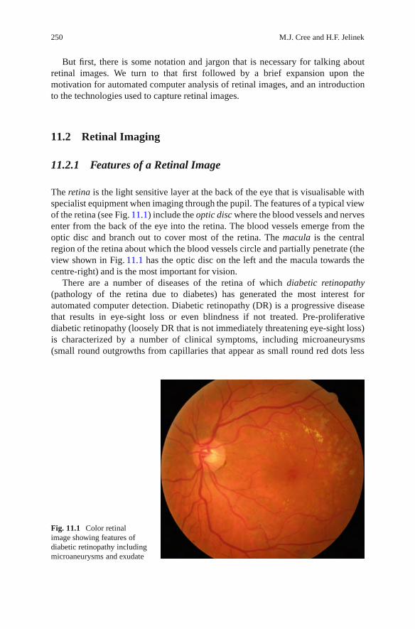
250 M.J. Cree and H.F. Jelinek
But first, there is some notation and jargon that is necessary for talking aboutretinal images. We turn to that first followed by a brief expansion upon themotivation for automated computer analysis of retinal images, and an introductionto the technologies used to capture retinal images.
11.2 Retinal Imaging
11.2.1 Features of a Retinal Image
The retina is the light sensitive layer at the back of the eye that is visualisable withspecialist equipment when imaging through the pupil. The features of a typical viewof the retina (see Fig. 11.1) include the optic disc where the blood vessels and nervesenter from the back of the eye into the retina. The blood vessels emerge from theoptic disc and branch out to cover most of the retina. The macula is the centralregion of the retina about which the blood vessels circle and partially penetrate (theview shown in Fig. 11.1 has the optic disc on the left and the macula towards thecentre-right) and is the most important for vision.
There are a number of diseases of the retina of which diabetic retinopathy(pathology of the retina due to diabetes) has generated the most interest forautomated computer detection. Diabetic retinopathy (DR) is a progressive diseasethat results in eye-sight loss or even blindness if not treated. Pre-proliferativediabetic retinopathy (loosely DR that is not immediately threatening eye-sight loss)is characterized by a number of clinical symptoms, including microaneurysms(small round outgrowths from capillaries that appear as small round red dots less
Fig. 11.1 Color retinalimage showing features ofdiabetic retinopathy includingmicroaneurysms and exudate

11 Image Analysis of Retinal Images 251
than 125 μm in diameter in color retinal images), dot-haemorrhages (which areoften indistinguishable from microaneurysms), exudate (fatty lipid deposits thatappear as yellow irregular patches with sharp edges often organized in clusters)and haemorrhage (clotting of leaked blood into the retinal tissue). These symptomsare more serious if located near the centre of the macular.
Proliferative diabetic retinopathy (PDR) is the more advanced form that posessignificant risk of eye-sight loss. Features that lead to a diagnosis of PDR includeleakage of blood or extensive exudate near the macular, ischaemia, new vesselgrowth and changes in vessel diameter such as narrowing of the arterioles andvenous beading (venules alternately pinching and dilating that look like a stringof sausages). Indeed, there is a reconfiguring of the blood vessel network that wehave more to say about later.
11.2.2 The Reason for Automated Retinal Analysis
Recent data suggest that there are 37 million blind people and 124 million with lowvision, excluding those with uncorrected refractive errors. The main causes of globalblindness are cataract, glaucoma, corneal scaring, age-related macular degeneration,and diabetic retinopathy. The global Vision 2020 initiative is having an impact toreduce avoidable blindness particularly from ocular infections, but more needs tobe done to address cataract, glaucoma, and diabetic retinopathy [14]. Screening isgenerally considered effective if a number of criteria are met including identificationof disease at an early, preferably preclinical, stage and that the disease in its early orlate stage is amenable to treatment. Screening for diabetic retinopathy, for example,and monitoring progression, especially in the early asymptomatic stage has beenshown to be effective in the prevention of vision loss and cost.
Automated screening (for example, by computer analysis of retinal images)allows a greater number of people to be assessed, is more economical and accessiblein rural and remote areas where there is a lack of eye specialists. Automated assess-ment of eye disease as an ophthalmological equivalent to the haematology point-ofcare testing such as blood glucose levels has been subject to intense research overthe past 40 years by many groups with algorithms being proposed for identificationof the optic disc, retinal lesions such as microaneurysms, haemorrhage, cotton woolspots and hard exudates, and retinal blood vessel changes.
Retinal morphology and associated blood vessel pattern can give an indicationof risk of hypertension (high blood pressure), cardiovascular and cerebrovasculardisease as well as diabetes [23, 28, 36]. With the increase in cardiovascular disease,diabetes and an aging population, a greater number of people will need to bescreened yet screening a large number of people is difficult with limited resourcesnecessitating a review of health care services.
Early identification of people at risk of morbidity and mortality due to diversedisease processes allows preventative measures to be commenced with the greatestefficacy. However in many instances preclinical signs are not easily recognized and

252 M.J. Cree and H.F. Jelinek
often appear as signs or symptoms that are not specific for a particular disease.The retina and its blood vessel characteristics however have been shown to be awindow into several disease processes. The identification of increased risk of diseaseprogression is based on several markers in the eye including venous dilatation,vessel tortuosity and the change in the ratio of the arteriolar to venular vesseldiameter especially in proximity to the optic disc. This morphological characteristicallows the application of image analysis and automated classification [23, 28, 36].
11.2.3 Acquisition of Retinal Images
Digital images of the human retina are typically acquired with a digital funduscamera, which is a specialized camera that images the retina via the pupil of the eye.The camera contains an illumination system to illuminate the retina and optics tofocus the image to a 35 mm SLR camera. Modern systems image at high-resolutionand in color with Nikon or Canon digital SLR camera backends. The field of view(FOV) of the retina that is imaged can usually be adjusted from 25◦ to 60◦ (asdetermined from the pupil) in two or three small steps. The smaller FOV has betterdetail but this is at the expense of a reduced view of the retina.
When monochromatic film was commonplace a blue-green filter was sometimesplaced in the optical path of the fundus camera as the greatest contrast in retinalimages occurs in the green wavelengths of light. An image acquired in such amanner is referred to as a red-free image. With color digital imaging it is commonpractice to take the green field of a RGB image as a close approximation to thered-free image.
In fluorescein angiographic imaging, the patient is injected with a sodiumfluorescein drug which is transported in the blood supply to the retina. The funduscamera uses a flash filtered to the blue spectrum (465–490 nm) to activate thefluorescein, which fluoresces back in the green part of the spectrum (520–630 nm).The collected light is filtered with a barrier filter so that only the fluorescencefrom the retina is photographed. Images obtained with fluorescein angiography aremonochromatic and highlight the blood flow in the retina. Since the fluorescein,when injected into the blood stream, takes a few seconds to completely fill the retinalvessels, images taken early in the angiographic sequence show the vasculature fillingwith fluorescein. First the fluorescein streams into the arterioles, and then a couple orso seconds later fills the venules. Over time (minutes) the images fade as fluoresceinis flushed out of the retinal blood supply.
Angiographic retinal images better highlight vascular lesions such as microa-neurysms, ischaemia (absence of blood flow) and oedema (leakage of blood intothe surrounding tissues). The downside of the use of fluorescein is the inherent riskto the patient with about 1 in 200,000 patients suffering anaphylactic shock. Indo-cyanine green (ICG) is sometimes used for imaging the choroidal vasculature butrequires a specially designed fundus camera due to the low intensity fluorescence.
Other imaging technologies such as the scanning laser ophthalmoscope (SLO)and optical coherence tomography (OCT) may be encountered. The SLO scans a

11 Image Analysis of Retinal Images 253
laser point on to the retina and simultaneously collects light reflected back from theretina with a photodiode. The photodiode has no pixels; an image is formed by thescanning of the light source in a raster fashion over the retina in time.
The raster scanning of the SLO has been exploited in some interesting ap-plications, such as forming images on the retina in a form of heads-up display,and projecting images on to the retina to measure retinal distortion. In anotherapplication, in vivo study of cell movement in retinal vessels is made with a singlescan only by fluorescent labelling of the blood cells [18,38]. This is possible becausethe SLO used scans the retina with interlacing, namely it scans the odd lines of theraster first (the odd field) and then scans the intervening even lines (the even field). Inbetween scanning the two fields the leucocyte moves so it appears in two locationsin one image. Matching the two appearances of the leucocyte together enables acalculation of leucocyte speed in the blood stream.
11.3 Preprocessing of Retinal Images
As the photographer does not have complete control over the patient’s eye whichforms a part of the imaging optical system, retinal images often contain artifactsand/or are of poorer quality than desirable. Patients often have tears covering theeye and, particularly the elderly, may have cataract that obscures and blurs the viewof the retina. In addition, patients often do not or cannot hold their eye still duringthe imaging process hence retinal images are often unevenly illuminated with partsof the retinal image brighter or darker than the rest of the image, or, in worst cases,washed out with a substantial or complete loss of contrast.
Not much attention has been given to the blurring effect of cataract and tears,maybe because one can sometimes choose another image out of a sequence thatis better and, in any case, it has a position dependent blurring function that variesfrom image to image, making restoration difficult. Much more problematic is theuneven illumination of the retina, partly because it occurs more often, but also inpart because in its extreme form can obliterate almost all the detail in a substantialpart of the retinal image.
It should be recognized that in addition to the uneven illumination due tofailures in the imaging system, the retina varies in intensity due to its ownnatural appearance. This distinction, though, is not too important for general imageprocessing and pattern recognition of the features of the retina, but must beconsidered in quantitative analysis of illumination such as that occurs, for example,in fluorescence change over time in angiographic sequences [10].
Minor unevenness in illumination occurs in most retinal images and it is usuallyadvantageous to correct for during preprocessing for successful automated detectionof retinal lesions. For example, Chaudhuri et al. [3] described one of the veryfirst attempts at vessel detection in retinal images (the algorithm is described inmore detail in Sect. 11.4.1 below). Recent proposals for vessel detection are oftencompared to the algorithm of Chaudhuri et al. [3] and if they are any good they

254 M.J. Cree and H.F. Jelinek
show substantial improvement. But it has not always been realized that the algorithmproposed by Chaudhuri et al. does not include shade- (or illumination-) correctionas a preprocessing step. Preprocessing with shade-correction (as described below)can substantially improve the [3] algorithm on certain images.
The shading effect due to uneven illumination is a slowly changing function ofthe spatial coordinates, that is, it consists of low frequency content only, thus can beisolated by a low-pass filter. While it is possible to do this with a filter in the Fourierdomain, it is much more common to isolate the illumination changes using a grossmean or median filtering of the image. In the past, the mean filter was sometimespreferred because it was much quicker to compute than the median filter, however,the median filter has better edge preserving properties and typically gives betterresults on retinal images. Now that a very efficient implementation of the medianfilter whose computational efficiency is almost independent of the kernel size iswidely available [27], the median filter should be preferred.
How large the median filter kernel should be is determined by the resolution ofthe retinal image and the size of the objects/lesions that one wishes to segment. Ifthe lesions are small (for example microaneurysms and dot-haemorrhages) then itwould not matter if one underestimated the size of the kernel as long as it is muchbigger than the largest lesion to be detected. On the hand if large lesions such asextensive haemorrhage that cover a large part of the retinal image are to be detectedthen determining the size of the kernel becomes a tough proposition as the lesionsize is on the same scale as the illumination changes. Methods more sophisticatedthan those described here are then needed for shade-correcting the image.
If we take the illumination of the retina by the camera to be L(x,y) where (x,y)labels the pixels in the image, and f (x,y) to be the perfect image of the retina, thenthe camera measures g(x,y) given by
g = Lf , (11.1)
where the multiplication is pixel-wise. It is clear that we should divide the capturedretinal image g by the illumination estimated by gross median filtering to give areasonable approximation f ∗ to the true image f . Of course, the goodness of theapproximation depends on our ability to estimate the illumination and the goodnessof the model expressed by (11.1).
The above, as illustrated in Fig. 11.2, generally works well for preparing colorfundus images for the segmentation of lesions/objects that are smaller than the scaleof illumination change. It may be seen in Fig. 11.2 that the technique is correctingfor more than unevenness in illumination, but also for intrinsic background intensitychanges of the retina, and that is advantageous in many applications.
The illumination expressed in (11.1) is, however, not an appropriate model for theshade-correction of fluorescein angiographic images. This is because the capillarybed of the retina (the capillaries themselves are not resolvable in the typical retinalimage) contributes a background glow due to the fluorescein in the blood. Wherethe retina is densely populated with capillaries the background glow is substantial,and where the retina is absent of capillaries, i.e. the foveal avascular zone, there islittle or no background glow.

11 Image Analysis of Retinal Images 255
Fig. 11.2 Shade-correction of a retinal image. (a) Green plane, (b) background illuminationestimated by median filtering, and (c) shade-correction by dividing green plane by estimatedillumination (contrast adjusted by linear stretch for display purposes)
Applying a gross median filter to an angiographic image does determine the illu-mination change across the image, however, it is not solely due to the illuminationfunction L but includes the background fluorescence B due to the capillary bed. Inthis case the illumination model is better described as
g = L( f + B). (11.2)
Since the contribution due to B is substantial, reducing (11.2) to g ≈ f + I, whereI is the illumination estimated with a gross median filtering of f , thus estimatingf by subtracting I from g usually produces sufficiently good results for detectingsmall lesions. Indeed, this is the approach used by early microaneurysm detectionalgorithms that were designed for use with angiographic images [9, 31].
For the segmentation of large lesions such as extensive haemorrhage or quan-tifying changes in brightness over time (for example, quantifying blood leakageinto surrounding tissues during an angiographic sequence) then more sophisticatedphysics inspired preprocessing approaches are required [10,13]. Some authors havenoted that the global approach to shade-correction described above still leavessome room for improvement when segmenting microaneurysms in regions of poorcontrast. Huang and Yan [19], Fleming et al. [12] and Walter et al. [35] all resort tosome form of locally adaptive shade-correction with contrast enhancement to ekeout slight improvements in microaneurysm detection.
11.4 Lesion Based Detection
We now turn attention to the segmentation of features of interest and lesions inretinal images. In the following pages three general techniques in image processing,namely linear filtering in image space, morphological processing, and waveletsare illustrated by way of application to the detection of retinal blood vessels andmicroaneurysms. Analysis of blood vessels is of particular interest as vascular

256 M.J. Cree and H.F. Jelinek
Fig. 11.3 Cross-section of a blood vessel. The asterisks show the intensity at pixel locations acrossthe vessel and the solid line is the fitted Gaussian function
disease such as diabetes cause visible and measurable changes to the bloodvessel network. Detecting (i.e. segmenting) the blood vessels and measuring bloodvessel parameters provides information on the severity and likely progression ofa variety of diseases. Microaneurysms are a particular vascular disorder in whichsmall pouches grow out of the side of capillaries. They appear in color fundusimages as small round red dots and in fluorescein angiographic images as smallhyperfluorescent round dots. The detected number of microaneurysms is known tocorrelate with the severity and likely progression of diabetic retinopathy.
11.4.1 Matched Filtering for Blood Vessel Segmentation
One of the earliest and reasonably effective proposals for the segmentation of bloodvessels in retinal images [3] is the use of oriented matched-filters for the detectionof long linear structures.
Blood vessels often have a Gaussian like cross-section (see Fig. 11.3) that isfairly consistent along the length of vessel segments. Provided the vessels are nottoo tortuous then they can be approximated as elongated cylinders of Gaussiancross-section between the vessel branch points. Thus, the two-dimensional modelconsisting of an elongated cylinder of Gaussian cross-section should correlate wellwith a vessel segment provided they have both the same orientation. The model ismoved to each possible position in the image and the correlation of the local patch ofimage to the model is calculated to form a correlation image. Peaks in the correlationimage occur at the locations of the blood vessels.

11 Image Analysis of Retinal Images 257
Fig. 11.4 Segmentation of blood vessels by matched-filtering: (a) Inverted shade-corrected greencomponent of the retinal image of Fig. 11.1, (b) vessel model used for matched-filtering, (c) theresult match-filtering with the vertical orientation model, (d) combined matched-filters applied inall orientations, and (e) thresholded to give the blood vessels
A better theoretical formulation can be given to support the argument [3]. Takef (x) to be a signal and F( f ) be its Fourier transform (that is, the spectrum ofthe signal f ). Consider f (x) contaminated by additive Gaussian white noise withspectrum N( f ). The optimal linear filter in the sense of maximising the signalto noise ratio that recovers f in the presence of the noise N is F∗, the complexconjugate of F . That is, if we calculate
f0(x) =∫
H( f )(F( f )+ N( f ))e2π i f x dx (11.3)
then H( f ) = F∗( f ) gives the best approximation of f0(x) as f (x). Equation (11.3)is the correlation of f with itself.
Now if f is a localized patch of retinal image (the generalisation to 2D doesnot change the argument) then correlation of f with the blood vessel signal is theoptimal linear filter for detecting the blood vessel. Of course, this assumes thateverything else in the localized patch of retinal image is Gaussian noise, which iscertainly not true. Let us proceed anyway despite the flawed assumption.
The blood vessel model described above is correlated with a small patch of imageto isolate the blood vessel section. This is repeated over every local region of theimage to form a correlation image. The peaks in the correlation image correspondto the locations of the model in the image. This process is commonly referred to asa matched-filter or as matched-filtering.
Figure 11.4a shows the shade-corrected image of a color retinal image. It isinverted to make the vessels appear bright and a median filter with a kernel size

258 M.J. Cree and H.F. Jelinek
of 5× 5 pixels has been applied to reduce pixel noise. The vessel model in thevertical orientation is shown in Fig. 11.4b. It is correlated with the retinal image toproduce the image shown in Fig. 11.4c. All vertical sections of blood vessels arestrongly emphasized and everything else in the image is suppressed. The model isrotated by a small amount and the matched-filter is applied again to the image. Thisis repeated for all possible orientations of the model, and the maximum response ateach pixel over all the matched-filtered images is taken as the final response for thepixel as shown in Fig. 11.4d. This is then thresholded to give the vessel network, seeFig. 11.4e. A failing of this approach is evident in the example given, namely that ithas false-detected on the exudate at the top-right of the image.
The amount to rotate the model for each application of the matched-filter shouldbe small enough so that all vessel segments are segmented in at least one of thematched-filtered images but not so small that processing time becomes excessive.Chaudhuri et al. used 15◦ angular increments with a kernel size of 32×32 pixels onimages of size 512×480.
11.4.2 Morphological Operators in Retinal Imaging
Morphological operators are based on mathematical set theory and provide a naturalway of analysing images for geometrical structure. The basic operators are thedilation and the erosion. The dilation has the effect of dilating objects so thatclosely located structures become joined and small holes are filled. The erosionhas the effect of eroding objects with sufficiently thin structures eliminated. But itis better than that; the direction, size and even shape, of the erosion or dilation canbe controlled with a mask called the structuring element.
The downside of the basic operators is that while they have extremely usefulproperties they nevertheless do not retain the object size. Dilation, not unsurpris-ingly, causes objects to grow in size and erosion causes them to shrink. Better is acombination of the two operators to form the opening and the closing.
The opening is an erosion followed by a dilation. It has the effect of returningobjects to their near original size (since the dilation reverses somewhat the effectof the erosion) with the destruction of very small objects and thin joins betweenobjects that are smaller than the structuring element (since the dilation cannotdilate structures that have been entirely eliminated by the opening). The closingis a dilation followed by an erosion and has the effect of returning objects to nearoriginal size but with small holes filled and objects that are very close to each otherjoined together.
The general description of gray-scale morphology treats both the image andthe structuring element as gray-scale [17, 30] but in many implementations thestructuring element is taken to be a set of connected pixels. The erosion of imagef (x,y) by structuring element b, written f �b is
( f �b)(x,y) = min(x′,y′)∈b
f (x + x′,y + y′), (11.4)

11 Image Analysis of Retinal Images 259
Fig. 11.5 The tophat operator used to detect microaneurysms. (a) median filtered inverted greenplane of retinal image, (b) the result of the tophat operator with a 6-pixel radius disc structuringelement, and (c) thresholded to segment microaneurysms and, unfortunately, many other spuriousfeatures (contrasts adjusted by linear stretch for display purposes)
and the dilation, written as f ⊕b, is1
( f ⊕b)(x,y) = max(x′,y′)∈b
f (x− x′,y− y′). (11.5)
The closing of f by mask b, written f •b, is
f •b = ( f ⊕b)�b, (11.6)
and the opening is
f ◦b = ( f �b)⊕b. (11.7)
The opening and closing operators are idempotent; repeated application of theoperator does not change the result further.
An opening removes all objects that cannot be enclosed by the structuringelement from the image. Subtracting the opening off the original image, namelycalculating,
m = f − f ◦b (11.8)
eliminates most structure in the image except for objects smaller than the structuringelement. This procedure is referred to as the tophat transform.
As described in Sect. 11.2.1 microaneurysms appear in retinal images as littleround dots (see Fig. 11.5). If the structuring element is chosen to be round andjust bigger than the largest microaneurysm and f is the inverted green plane of aretinal image, then m is an image that contains the microaneurysms. This, with afinal thresholding of m to give a binary image, is the basis of some of the earliestproposals for microaneurysm detection in retinal images [2,24], but, it is not specificenough. Other small objects, bits of background texture, and vessel bits are all
1The reflection of the structuring element in the dilation that is not present in the erosion is intendedas it simplifies the definitions of the opening and closing following.
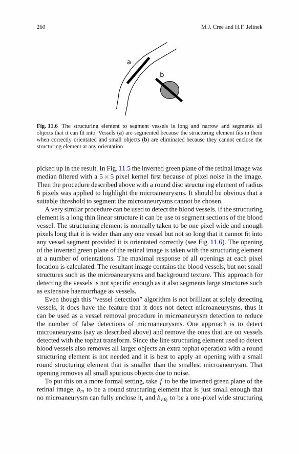
260 M.J. Cree and H.F. Jelinek
Fig. 11.6 The structuring element to segment vessels is long and narrow and segments allobjects that it can fit into. Vessels (a) are segmented because the structuring element fits in themwhen correctly orientated and small objects (b) are eliminated because they cannot enclose thestructuring element at any orientation
picked up in the result. In Fig. 11.5 the inverted green plane of the retinal image wasmedian filtered with a 5× 5 pixel kernel first because of pixel noise in the image.Then the procedure described above with a round disc structuring element of radius6 pixels was applied to highlight the microaneurysms. It should be obvious that asuitable threshold to segment the microaneurysms cannot be chosen.
A very similar procedure can be used to detect the blood vessels. If the structuringelement is a long thin linear structure it can be use to segment sections of the bloodvessel. The structuring element is normally taken to be one pixel wide and enoughpixels long that it is wider than any one vessel but not so long that it cannot fit intoany vessel segment provided it is orientated correctly (see Fig. 11.6). The openingof the inverted green plane of the retinal image is taken with the structuring elementat a number of orientations. The maximal response of all openings at each pixellocation is calculated. The resultant image contains the blood vessels, but not smallstructures such as the microaneurysms and background texture. This approach fordetecting the vessels is not specific enough as it also segments large structures suchas extensive haemorrhage as vessels.
Even though this “vessel detection” algorithm is not brilliant at solely detectingvessels, it does have the feature that it does not detect microaneurysms, thus itcan be used as a vessel removal procedure in microaneurysm detection to reducethe number of false detections of microaneurysms. One approach is to detectmicroaneurysms (say as described above) and remove the ones that are on vesselsdetected with the tophat transform. Since the line structuring element used to detectblood vessels also removes all larger objects an extra tophat operation with a roundstructuring element is not needed and it is best to apply an opening with a smallround structuring element that is smaller than the smallest microaneurysm. Thatopening removes all small spurious objects due to noise.
To put this on a more formal setting, take f to be the inverted green plane of theretinal image, bm to be a round structuring element that is just small enough thatno microaneurysm can fully enclose it, and bv,θi to be a one-pixel wide structuring

11 Image Analysis of Retinal Images 261
element of suitable length to detect vessels when correctly orientated (θi) along thelength of the vessel. The image with the vessels (and other large structures) removedis constructed by tophat transform, viz
f1 = f −maxi
f ◦bv,θi . (11.9)
This image contains the microaneurysms and other small detections. They areremoved with the opening,
m = f1 ◦bm, (11.10)
then m is thresholded to those objects of enough depth to be a microaneurysm.This reduces false-detections of microaneurysms on vessels but false-detections ofsmall bits of texture, retinal-pigment epithelium defects, and so on, still occur soimprovements can yet be made.
Some prefer to use a matched-filter approach to detect the microaneurysms.A good model of microaneurysm intensity is a circularly symmetric Gaussian func-tion. Applying such a model to the image f1 of (11.9) (i.e. the image with vesselsremoved) with a matched-filter then thresholding to isolate the microaneurysmsgives a reasonable result but, yet again, it is not good enough [32].
A small improvement to the above algorithms can be made by using morpho-logical reconstruction [33]. The tophat transform to detect objects does not preservethe segmented objects’ shape precisely; morphological reconstruction addresses thisproblem. First some operator is applied to identify objects of interest. It need notsegment the objects in their entirety; just having one of the brightest pixels withinthe object is sufficient. This image is called the marker and the original imageis the mask. The marker is dilated by one pixel with the limitation that it cannotdilate further than any objects in the mask. Note that this restricted dilation by onepixel, called the geodesic dilation, is different to the dilation described by (11.5)in that it is limited by structures in the mask. The geodesic dilation is repeatedlyapplied until the limit is reached when no more changes occur. This process is calledreconstruction by dilation.
If the marker has a peak that is in the mask then the shape of the peak is returnedfrom the mask in reconstruction by dilation. If the marker has no feature at a peakin the mask then the peak in the mask is eliminated. Morphological reconstructionby dilation better preserves the shapes of the segmented features in the image thandoes an opening or tophat transform. Opening by reconstruction is the process ofreconstructing by dilation an image with its erosion with a structuring element asthe marker. It has a similar effect as the morphological opening but with a muchbetter preservation of the shape of the segmented objects.
As described above microaneurysm detection often proceeds by removing theblood vessels before segmenting the microaneurysms. Tests show that removingthe blood vessels in a retinal image with tophat by reconstruction instead of themorphological tophat transform reduces the false detection of microaneurysms inblood vessels [16]. An extra opening with a disc structuring element smaller than

262 M.J. Cree and H.F. Jelinek
Fig. 11.7 Detection of microaneurysms by way of vessel removal (a) median filtered invertedgreen plane of retinal image, (b) tophat by reconstruction of the image to remove vessels, then(c) opened with a structuring element smaller than microaneurysms to remove small specks, and(d) thresholded to isolate the microaneurysms and overlaid original image
any microaneurysm helps to remove spurious noise. See Fig. 11.7 for an illustrationof the process. The detection of microaneurysms shown in Fig. 11.7c is a prettygood result but there are a couple of false detections, one on the optic disc and oneamongst the patch of exudate, thus there is still room for improvement. There arealso other non-trivial issues, such as how to automatically adapt the threshold foreach image.
Walter and Klein [34] and Walter et al. [35] argue that the diameter opening(and closing) is a better morphological operator to detect microaneurysms. Thediameter opening is the maximum of all openings with structuring elements witha diameter greater than or equal to a required diameter. Here, the diameter of aconnected group of pixels is the maximum distance from any one pixel in the objectto a pixel on the other side of the object. Nevertheless, to improve specificity mostauthors that use morphology or matched filtering or some combination of both tosegment microaneurysms, measure features such as size, shape, and intensity on the

11 Image Analysis of Retinal Images 263
segmented candidate microaneurysms, and apply machine learning techniques torefine the detection of the microaneurysms [8, 9, 26, 31, 35].
The above illustrates an important point in processing complicated medicalimages rich in detail such as retinal images. With basic and well understood imageprocessing operators it is easy to do reasonably well in detecting a certain lesionor feature. But reasonably well is not good enough. One missed lesion that hasserious clinical implications (such as missing indications of proliferative retinopathyin retinal images when it can lead to significant eye-sight loss within a few days orweeks) will not generate trust from the medical profession. On the other hand, falsedetections on far too many images is useless. Getting the first 80% sensitivity andspecificity is easy; improving that to better than 90% sensitivity at 90% specificityis the hard problem.
11.5 Global Analysis of Retinal Vessel Patterns
So far we have discussed segmenting specific lesions (in particular microaneurysms)and features (vasculature) in retinal images. Typically, lesion specific measures suchas number of microaneurysms or localized vessel parameters that are known topredict or correlate with disease are measured. The analysis of vessel properties,in particular, often involves sophisticated fitting of parametric models to the bloodvessels in a local region from which features such as vessel diameter, tortuosity andbranching ratios are measured [15, 37]. Vessel diameters of arterioles and venules,for example, can be used to calculate arterio-venous diameter ratios that predicthypertensive (high blood pressure) disorders [6].
In this section, we take a different tack and examine an approach to measure gen-eral disease condition with global vessel analysis. Proliferative diabetic retinopathy(PDR) – an advanced form of retinopathy due to diabetes with high risk of eye-sightloss if not treated [7] – is characterized by a reconfiguration of the blood vesselsresulting from ischaemia in parts of the retina and new vessel growth that emergesfrom the area of the optic disc or from peripheral vessels [22]. Given that the vesselpattern is noticeably different in PDR than non-proliferative diabetic retinopathy itis tempting to ask whether a global operator applied to the vessel patterns is capableof characterising the changes in the vasculature and, therefore, detect PDR [21].We, therefore, seek such operators.
Traditional and simpler shape analysis features often used in image processing,such as area (a), perimeter (p), and circularity (typically calculated as p2/a) arenot expected to be powerful enough as these features are dependent on a changeof the amount of vasculature whereas the existing vessel network can reconfigurewith minimal change in the amount of vasculature. Jelinek et al. [21] explore globalvessel analysis with wavelet and fractal inspired features to characterise the vesselreconfiguration that occurs in PDR. The vessels are detected with a sophisticatedwavelet based segmentation [29], then reduced by a morphological skeletonisationto a 1-pixel wide skeleton that represents the vessel tracks.

264 M.J. Cree and H.F. Jelinek
The vector gradient of the vessel skeleton image is calculated via analysingwavelets, namely the partial derivatives of the Gaussian, viz,
ψ1(x,y) =∂g(x,y)x
∂x, ψ2(x,y) =
∂ g(x,y)y∂y
, (11.11)
where g(x,y) denotes the two-dimensional Gaussian. Calculating the wavelet trans-form of the skeletonized vessel image f with the two wavelets at displacement band scale a and forming the vector,
Tψ [ f ](b,a) =(
Tψ1 [ f ](b,a)Tψ2 [ f ](b,a)
)(11.12)
where the entries are the two wavelet transforms is an estimate of the vector gradient.This can be efficiently implemented with the fast Fourier transform.
The vector gradient image is analysed on the boundary of the vessels. It has twoorthogonal components, namely orientation and magnitude, which can be analysedseparately. Let us first consider calculating the entropy of the orientations as entropyis a quantitative measure of manifest disorder. If the vessels all tend to be aligned inthe same direction (i.e. order) then the orientation entropy will be low, whereas if thevessels are randomly orientated throughout the image (disorder) then the entropywill be high. The suspicion is that the new vessel growth in PDR may affect thedistribution of vessel orientations and, hence, the orientation of the gradient field.The orientation entropy also has the advantage that it is invariant against rotationsand reflections of the image.
The orientation entropy s is straightforward to calculate and involves forming ahistogram of orientations and calculating
s = −∑i
pi ln pi (11.13)
where i indexes the histogram bins, that is orientations, and pi is the frequency ofoccurrence of orientation i.
One can also analyse the magnitudes of the gradient vector field. A usefulmeasure is the second moment which when applied to Tψ indicates bias in thegradient vector field. A histogram can be formed from the magnitudes then the CWTsecond moment is
m2 = ∑i
i2qi (11.14)
where the i are the centers of the histogram bins and qi is the frequency of occurrenceof the magnitudes in the bin.
There are other features that can be measured on the vessels with a globalapproach. The vessels are shapes and an important parameter of a shape is thecurvature which characterises how the direction of a unit tangent vector varies alongthe shape contour. What is interesting is that the curvature can be measured with a

11 Image Analysis of Retinal Images 265
two-dimensional global Fourier analysis of the image without having to performsophisticated one-dimensional parameterisations of the shape contours [11]. Jelineket al. [21] apply this technique to the skeletonized vessel patterns to estimate a globalmeasure of vessel curvature.
The blood vessels in the retina branch a number of times each time forming avessel tree that is similar in characteristics to the branch it came from. Systemsthat have self-similarity at multiple scales are known as fractals. There are somereports of measuring fractal properties of blood vessel patterns of the retina; mosthave involved manual segmentation of the blood vessel patterns [4,5,25]. Now withreliable automated vessel segmentation, attention is turning to analysing the retinalvasculature as a fractal. As the retinal tree branches it fills the two-dimensionalspace of the image. One way to measure the space-filling is with various fractaldimensions of which the correlation dimension Dc(ε) is a common choice [1]. It isdefined as
Dc = limr→0
logC(r)logr
, (11.15)
where C(r) is the correlation integral given by
C(r) =number of distances less than r
total number of distances. (11.16)
The limit is usually approximated by evaluating the slope of the straight linesegments of a plot of logC(r) against logr. In practice the first and last line segmentsshould be disregarded since at these scales of r little fractal information is broughtfrom the shape. Jelinek et al. [21] make two calculations of correlation dimensionover the skeletonized retinal vessel shapes. The first is the median of the rankedline segment slopes and the second is the global correlation dimension calculatedby adding all slopes except those from the first and last line segments.
Jelinek et al. [21] test the features described on a database of 27 retinal images(16 with PDR; 11 with pathology but not PDR) for the ability to predict PDR.The traditional measures (area, perimeter, and circularity) showed no predictivepower whatsoever when used separately and failed statistical significance at 95%confidence when used in combination to predict PDR. All the wavelet based featureswhen used separately showed predictive power but only the curvature achieved 95%confidence in predicting PDR. Combining features and using linear discriminantanalysis as the classifier correctly classified all images except three.
11.6 Conclusion
Automated analysis of retinal images is an ongoing active field of research. Inthe above some of the simpler and some of the more recent analytical toolsbought to analyse retinal images have been discussed. We have seen that standard

266 M.J. Cree and H.F. Jelinek
image processing techniques that may be found in any good text on general imageprocessing can go a long way to detecting certain features/lesions in retinal imagesand produce seemingly good results, but do not provide the quality of result requiredin clinical practice. Sophisticated image analysis techniques are now being exploredfor the quantification of previously difficult to assess features and to improveexisting methods. The interested reader can find a useful summary and inspirationfor further research in the text by Jelinek and Cree [20].
References
1. Asvestas, P., Matsopoulos, G.K., Nikita, K.S.: Estimation of fractal dimension of images usinga fixed mass appoach. Patt. Recog. Lett. 20, 347–354 (1999)
2. Baudoin, C., Maneschi, F., Quentel, G., Soubrane, G., Hayes, T., Jones, G., Coscas, G., Kohner,E.M.: Quantitative-evaluation of fluorescein angiograms – microaneurysm counts. Diabetes 32,8–13 (1983)
3. Chaudhuri, S., Chatterjee, S., Katz, N.P., Nelson, M., Goldbaum, M.H.: Detection of bloodvessels in retinal images using two-dimensional matched filters. IEEE Trans. Med. Im. 8,263–269 (1989)
4. Cheng, S.C., Huang, Y.M.: A novel approach to diagnose diabetes based on the fractalcharacteristics of retinal images. IEEE Trans. Inf. Technol. Biomed. 7(3), 163–170 (2003)
5. Cheung, N., Donaghue, K.C., Liew, G., Rogers, S.L., Wang, J.J., Lim, S.W., Jenkins, A.J.,Hsu, W., Lee, M.L., Wong, T.Y.: Quantitative assessment of early diabetic retinopathy usingfractal analysis. Diabetes Care 32, 106–110 (2009)
6. Cheung, N., Wong, T.Y., Hodgson, L.: Retinal vascular changes as biomarkers of systemiccardiovasular diseases. In: Jelinek, H.F., Cree, M.J. (eds.) Automated Image Detection ofRetinal Pathology, pp. 185–219. CRC Press, Boca Raton, FL (2010)
7. Coyne, K.S., Margolis, M.K., Kennedy-Matrin, T., Baker, T.M., Klein, R., Paul, M.D., Revicki,D.A.: The impact of diabetic retinopathy: Perspectives from patient focus groups. Fam. Pract.21, 447–453 (2004)
8. Cree, M.J.: Automated microaneurysm detection for screening. In: Jelinek, H.F., Cree, M.J.(eds.) Automated Image Detection of Retinal Pathology, pp. 155–184. CRC Press, Boca Raton,FL (2010)
9. Cree, M.J., Olson, J.A., McHardy, K.C., Sharp, P.F., Forrester, J.V.: A fully automatedcomparative microaneurysm digital detection system. Eye 11, 622–628 (1997)
10. Cree, M.J., Olson, J.A., McHardy, K.C., Sharp, P.F., Forrester, J.V.: The preprocessing of retinalimages for the detection of fluorescein leakage. Phys. Med. Biol. 44, 293–308 (1999)
11. Estrozi, L.F., Rios, L.G., Campos, A.G., Cesar Jr, R.M., d. F. Costa, L.: 1D and 2DFourier-based approaches to numeric curvature estimation and their comparative performanceassessment. Digit. Signal Process. 13, 172–197 (2003)
12. Fleming, A.D., Philip, S., Goatman, K.A., Olson, J.A., Sharp, P.F.: Automated microaneurysmdetection using local contrast normalization and local vessel detection. IEEE Trans. Med. Im.25(9), 1223–1232 (2006)
13. Foracchia, M., Grisan, E., Ruggeri, A.: Luminosity and contrast normalization in retinalimages. Med. Im. Anal. 9, 179–190 (2005)
14. Foster, A., Resnikoff, S.: The impact of Vision 2020 on global blindness. Eye 19(10), 1133–1135 (2005)
15. Fritzsche, K.H., Stewart, C.V., Roysam, B.: Determining retinal vessel widths and detectionof width changes. In: Jelinek, H.F., Cree, M.J. (eds.) Automated Image Detection of RetinalPathology, pp. 269–304. CRC Press, Boca Raton, FL (2010)

11 Image Analysis of Retinal Images 267
16. Gamble, E.: Microaneurysm detection in directly acquired colour digital fundus images.Master’s thesis, University of Waikato, Hamilton, New Zealand (2005)
17. Gonzalez, R.C., Woods, R.E.: Digital Image Processing, 2nd edn. Prentice-Hall, Upper SaddleRiver, NJ (2002)
18. Hossain, P., Liversidge, J., Cree, M.J., Manivannan, A., Vieira, P., Sharp, P.F., Brown, G.C.,Forrester, J.V.: In vivo cell tracking by scanning laser ophthalmoscopy: Quantification ofleukocyte kinetics. Invest. Ophthalmol. Vis. Sci. 39, 1879–1887 (1998)
19. Huang, K., Yan, M.: A local adaptive algorithm for microaneurysms detection in digital fundusimages. In: Proceedings of Computer Vision for Biomedical Image Applications, Lecture Notesin Computer Science, vol. 3765, pp. 103–113 (2005)
20. Jelinek, H.F., Cree, M.J. (eds.): Automated Image Detection of Retinal Pathology. CRC Press,Boca Raton, FL (2010)
21. Jelinek, H.F., Cree, M.J., Leandro, J.J.G., Soares, J.V.B., Cesar Jr, R.M.: Automated segmenta-tion of retinal blood vessels and identification of proliferative diabetic retinopathy. J. Opt. Soc.Am. A 24, 1448–1456 (2007)
22. Kanski, J.: Clinical Ophthalmology: A Systematic Approach. Butterworth-Heinemann, Boston(1989)
23. Klein, R., Klein, B.E., Moss, S.E., Wong, T.Y., Hubbard, L., Cruickshanks, K.J., Palta, M.:The relation of retinal vessel caliber to the incidence and progression of diabetic retinopathy:XIX: The Wisconsin Epidemiologic Study of Diabetic Retinopathy. Arch. Ophthalmol. 122(1),76–83 (2004)
24. Lay, B., Baudoin, C., Klein, J.C.: Automatic detection of microaneurysms in retinopathyfluoro-angiogram. Proc. SPIE 432, 165–173 (1983)
25. Masters, B.R.: Fractal analysis of the vascular tree in the human retina. Annu. Rev. Biomed.Eng. 6, 427–452 (2004)
26. Niemeijer, M., van Ginneken, B., Cree, M.J., Mizutani, A., Quellec, G., Sanchez, C.I.,Zhang, B., Hornero, R., Lamard, M., Muramatsu, C., Wu, X., Cazuguel, G., You, J., Mayo,A., Li, Q., Hatanaka, Y., Cochener, B., Roux, C., Karray, F., Garcia, M., Fujita, H., Abramoff,M.D.: Retinopathy online challenge: Automatic detection of microaneurysms in digital colorfundus photographs. IEEE Trans. Med. Im. 29, 185–195 (2010)
27. Perreault, S., Hebert, P.: Median filtering in constant time. IEEE Trans. Im. Proc. 16(9), 2389–2394 (2007)
28. Sherry, L.M., Wang, J.J., Rochtchina, E., Wong, T., Klein, R., Hubbard, L.D., Mitchell, P.:Reliability of computer-assisted retinal vessel measurement in a population. Clin. Experiment.Ophthalmol. 30, 179–82 (2002)
29. Soares, J.V.B., Leandro, J.J.G., Cesar Jr., R.M., Jelinek, H.F., Cree, M.J.: Retinal vesselsegmentation using the 2-D Gabor wavelet and supervised classification. IEEE Trans. Med.Im. 25, 1214–1222 (2006)
30. Soille, P.: Morphological Image Analysis, 2nd edn. Springer, Berlin, Germany (2004)31. Spencer, T., Olson, J.A., McHardy, K.C., Sharp, P.F., Forrester, J.V.: An image-processing
strategy for the segmentation and quantification of microaneurysms in fluorescein angiogramsof the ocular fundus. Comp. Biomed. Res. 29, 284–302 (1996)
32. Spencer, T., Phillips, R.P., Sharp, P.F., Forrester, J.V.: Automated detection and quantificationof microaneurysms in fluorescein angiograms. Graefes Arch. Clin. Exp. Ophthalmol. 230,36–41 (1992)
33. Vincent, L.: Morphological grayscale reconstruction in image analysis: Applications andefficient algorithms. IEEE Trans. Im. Proc. 2, 176–201 (1993)
34. Walter, T., Klein, J.C.: Automatic detection of microaneurysms in color fundus images of thehuman retina by means of the bounding box closing. In: Proceedings Medical Data Analysis,Lecture Notes in Computer Science, vol. 2526, pp. 210–220 (2002)
35. Walter, T., Massin, P., Erginay, A., Ordonez, R., Jeulin, C., Klein, J.C.: Automatic detection ofmicroaneurysms in color fundus images. Med. Im. Anal. 11, 555–566 (2007)

268 M.J. Cree and H.F. Jelinek
36. Wang, J.J., Mitchell, P., Sherry, L.M., Smith, W., Wong, T.Y., Klein, R., Hubbard, L.D., Leeder,S.R.: Generalized retinal arteriolar narrowing predicts 5-year cardiovascular and cerebro-vascular mortality: Findings from the Blue Mountains Eye Study. Invest. Ophthalmol. Vis.Sci. p. 43 (2002)
37. Witt, N.W., Martinez-Perez, M.E., Parker, K.H., Thom, S.A.M., Hughes, A.D.: Geometricaland topological analysis of vascular branches from fundus retinal images. In: Jelinek, H.F.,Cree, M.J. (eds.) Automated Image Detection of Retinal Pathology, pp. 305–338. CRC Press,Boca Raton, FL (2010)
38. Xu, H., Manivannan, A., Goatman, K.A., Liversidge, J., Sharp, P.F., Forrester, J.V., Crane, I.J.:Improced leukocyte tracking in mouse retinal and choroidal circulation. Exp. Eye Res. 74,403–410 (2002)

Chapter 12Tortuosity as an Indicator of the Severityof Diabetic Retinopathy
Michael Iorga and Geoff Dougherty
12.1 Introduction
The retinal vasculature can be viewed directly and noninvasively, offering a uniqueand accessible window to study the health of the human microvasculature in vivo.The appearance of the retinal blood vessels is an important diagnostic indicator formuch systemic pathology, including diabetes mellitus, hypertension, cardiovascularand cerebrovascular disease, and atherosclerosis [1–3]. There is mounting evidencesupporting the notion that the retinal vasculature may provide a lifetime summarymeasure of genetic and environmental exposure, and may therefore act as a valuablerisk marker for future systemic diseases [4]. Using its characteristics may provideearly identification of people at risk due to diverse disease processes [5].
12.1.1 The Progression of Diabetic Retinopathy
Diabetic retinopathy is the most frequent cause of new cases of blindness amongadults aged 20–74 years [6]. It is a progressive disease, beginning with mildnonproliferative abnormalities, characterized by increased vascular permeability,and progressing through moderate and severe nonproliferative diabetic retinopathy(NPDR) characterized by vascular closure, to proliferative diabetic retinopathy(PDR) with the growth of new blood vessels on the retina and posterior surface ofthe vitreous. Macular edema, marked by retinal thickening from leaky blood vessels,can develop at all stages of retinopathy.
In the early state of the disease, symptoms are mild or nonexistent. The curvatureof a blood vessel influences its local flow hemodynamics and may result in
G. Dougherty (�)California State University Channel Islands, Camarillo, CA 91320, USAe-mail: [email protected]
G. Dougherty (ed.), Medical Image Processing: Techniques and Applications, Biologicaland Medical Physics, Biomedical Engineering, DOI 10.1007/978-1-4419-9779-1 12,© Springer Science+Business Media, LLC 2011
269

270 M. Iorga and G. Dougherty
unfavorable clinical consequences [7–9]. The tortuosity of intracranial arteries, forexample, has been implicated in the risk of aneurysm formation due to the highshear stress weakening the outer walls of the arteries [10]. The process may besimilar in diabetic retinopathy. As the disease develops, increased tortuosity of theretinal blood vessels may result in the weakening of the outer walls and precedethe formation of microaneurysms, which can leak fluid into the retina and causeswelling of the macula.
Microaneurysms are often the first clinical sign of diabetic retinopathy, and areseen as intraretinal deep red spots 10–100μm in diameter. The significance ofmicroaneurysm counts and their close correlation with the severity of the diseaseare well documented [11,12]. Microaneurysm formation and regression are dynamicprocesses [13], where microaneurysms form and then later clot and regress. Morethan 50% of them either form or regress within a 12-month period [14]. Thereis evidence that turnover, as well as absolute counts, is an early indicator ofretinopathy progression [12, 15]. Rupture of microaneurysms gives rise to smallround dot hemorrhages, which are indistinguishable from microaneurysms in colorfundus images. Hemorrhages present a range of size, color, and texture from thedot hemorrhages, through blotch (cluster) hemorrhages to larger boat-shaped orflame-shaped hemorrhages. A pattern recognition approach may well be requiredto reliably detect all the variants.
White lesions comprise exudates, cotton wool spots, and drusen. Hard exudatesare caused when weakened blood vessels in the eye leak lipids onto the retina, whichin turn block it from sensing light. This results in blurred or completely obstructedvision in some areas of the eye. Since exudates are made of lipids, they appear aslight yellow in fundus images. Early automated detection systems used thresholdingof red-free images [16, 17], while a more recent study used a multilayer neural net-work to detect exudates [18]. The appearance of microaneurysms and hard exudatesin the macular area is more serious, and is identified as “Diabetic Maculopathy” soas to highlight the potential sight-threatening nature of this condition.
As the disease advances (preproliferative retinopathy), circulation problemscause the retina to become more ischemic and cotton wool spots to become moreprevalent. In proliferative retinopathy (PDR), new fragile blood vessels can begin togrow in the retina in an attempt to restore the malnourished area and prevent it fromdying. These new blood vessels may leak blood into the vitreous, clouding vision.Other complications of PDR include detachment of the retina due to scar tissueformation and the development of glaucoma, an eye disease resulting in progressivedamage to the optic nerve.
12.2 Automated Detection of Diabetic Retinopathy
Many studies have been initiated worldwide to develop advanced systems forthe automated detection and monitoring of diabetic retinopathy. They compriseimage analysis tools for detecting and measuring common lesions (such as

12 Tortuosity as an Indicator of the Severity of Diabetic Retinopathy 271
microaneurysms, hemorrhages, and exudates) and may include indexing andautomated retrieval techniques applied to image databases. A major issue is how toaccurately and objectively assess results from different studies.
Microaneurysms are among the first signs of the presence of diabetic retinopathyand their numbers correlate well with the severity of the disease in its early stages[12, 13]. Since microaneurysms are extremely small and similarly colored to thebackground, they are very tedious to measure manually. Most publications onautomated microaneurysm detection use monochromatic data from one of the colorplanes of a fundus image, even though full color information is available. (Microa-neurysms are better visualized with fluorescein angiography but it is more invasiveand therefore less practical for screening purposes). The green plane normallycontains the best detail; the red plane, while brighter and sometimes saturated, haspoorer contrast; and the blue plane is dark and of least use. Hemoglobin has anabsorption peak in the green region of the spectrum, so that features containinghemoglobin (e.g., microaneurysms) absorb more green light than surroundingtissues and appear dark, giving the green plane a higher contrast. Red lightpenetrates deeper into the layers of the retina and is primarily reflected in thechoroid, explaining the reddish appearance of fundus images. Because red light hasa lower absorption than green in the tissues of the eye, the red plane has less contrast.Blue light is mostly absorbed by the lens, and then by melanin and hemoglobin, andis the most scattered light, so the blue plane shows very little contrast.
However, the appearance of color retinal images can vary considerably, espe-cially between people of different race [16, 19], so that it may be prudent to useall the color information and to employ some form of color normalization. Forexample, divisive shade correction can be applied to each of the color planes, andthen the individual contrasts normalized to a specific mean and standard deviation[20]. This process retains the overall shape of the color image histogram, but shiftsthe hue (which is often dominated by the ratio of green to red in retinal images) tobe consistent between images.
12.2.1 Automated Detection of Microaneurysms
Over the years, a variety of algorithms have been used to automatically detectmicroaneurysms [21]. For example, a morphological top-hat transformation witha linear structuring element at different orientations was used to distinguishconnected, elongated structures (i.e., the vessels) from unconnected circular ob-jects (i.e., the microaneurysms) [22]. A shade-correction preprocessing step anda matched filtering postprocessing step were then added to the basic detectiontechnique [23–32].1,2,3
1 http:www.ces.clemson.edu/ahoover/stare.2 http://www.isi.uu.nl/Research/Databases/DRIVE/.3 http://messidor.crihan.fr.
272 M. Iorga and G. Dougherty
The Waikato Microaneurysm Detector [26, 27] modified this procedure to workon full-color retinal images. The green plane of the retinal images was used to findall candidate objects. After normalization by subtracting a median filtered versionof the image, noise was removed by median filtering using a small kernel. A top-hattransform was performed by morphological reconstruction [28], using an elongatedstructuring element at different orientations to detect the vasculature. Followingthe removal of the vasculature and a microaneurysm matched filtering step, anadaptive threshold isolated microaneurysm candidates and region-growing on theshade-corrected green plane at the positions of candidates was used to isolate themorphology of the underlying candidate. A number of features based on the color,intensity, and shape of the candidates were extracted [27], and a naıve Bayesianclassifier was used to assign a likelihood to each of the found candidate objectsthat it is a true microaneurysm. Sensitivity can be traded against specificity byvarying a threshold probability that determines whether or not a candidate shouldbe considered a microaneurysm.
A recent study [29], using a variation of this processing method and a k-nearest neighbor (k-NN) classifier, reported a sensitivity of 88.5% for detectingmicroaneurysms. An alternative method [30] used template matching in the waveletdomain to find the microaneurysm candidates. It assumed that microaneurysmsat a particular scale can be modeled with two-dimensional, rotation-symmetricgeneralized Gaussian functions.
12.3 Image Databases
The STARE (see footnote 1) and DRIVE (see footnote 2) [31, 32] databases ofretinal images have been widely used to compare various vessel segmentationalgorithms. A subset of the DRIVE database is being used for an online challenge(the Retinopathy Online Challenge [21]) to compare algorithms used to detectmicroaneurysms.
The Messidor project database (see footnote 3) is the largest database of retinalimages currently available on the Internet. It was established to facilitate studieson computer-assisted diagnoses of diabetic retinopathy, and comprises 1,200 colorfundus images of the posterior pole acquired using a Topcon TRC NW6 camera[Topcon Medical Systems, Inc. (TMS), of Paramus, NJ] with a 45◦ field of view.The 24-bit RGB color images are of various sizes: 1,440× 960, 2,240× 1,488 or2,304×1,536 pixels. Eight hundred of the images were acquired with pupil dilationand 400 without dilation.
Two diagnoses are provided by expert ophthalmologists for each image: theretinopathy grade and the risk of macular edema. The retinopathy grade [0 (normal),1, 2 or 3] is based on the numbers of microaneurysms (MA) and hemorrhages (H),and whether there is neovascularization (NV = 1) or not (NV = 0), using
0: (MA = 0) AND (H = 0)1: (0 < MA ≤ 5) AND (H = 0)
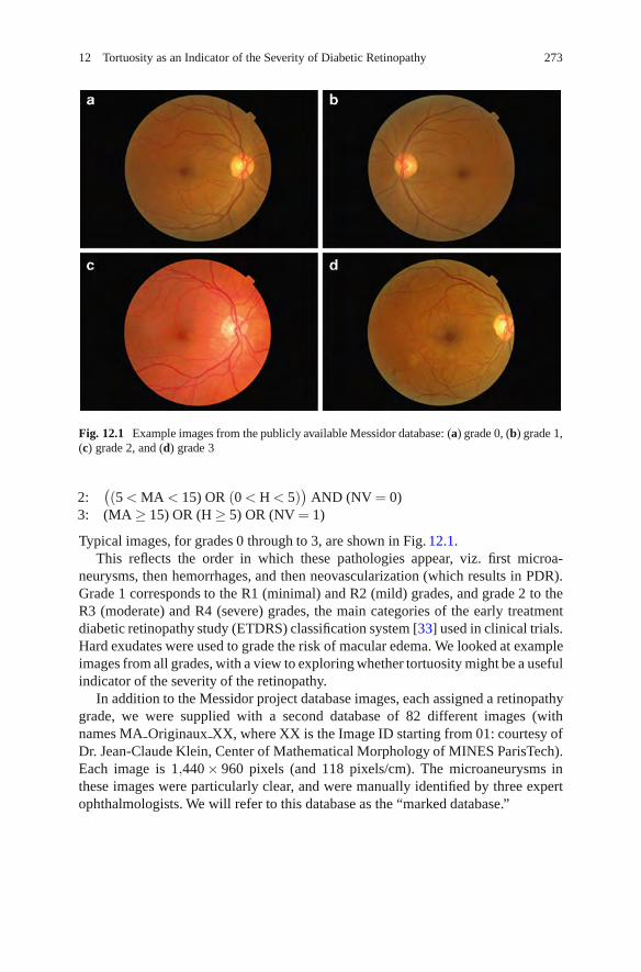
12 Tortuosity as an Indicator of the Severity of Diabetic Retinopathy 273
Fig. 12.1 Example images from the publicly available Messidor database: (a) grade 0, (b) grade 1,(c) grade 2, and (d) grade 3
2:((5 < MA < 15) OR (0 < H < 5)
)AND (NV = 0)
3: (MA ≥ 15) OR (H ≥ 5) OR (NV = 1)
Typical images, for grades 0 through to 3, are shown in Fig. 12.1.This reflects the order in which these pathologies appear, viz. first microa-
neurysms, then hemorrhages, and then neovascularization (which results in PDR).Grade 1 corresponds to the R1 (minimal) and R2 (mild) grades, and grade 2 to theR3 (moderate) and R4 (severe) grades, the main categories of the early treatmentdiabetic retinopathy study (ETDRS) classification system [33] used in clinical trials.Hard exudates were used to grade the risk of macular edema. We looked at exampleimages from all grades, with a view to exploring whether tortuosity might be a usefulindicator of the severity of the retinopathy.
In addition to the Messidor project database images, each assigned a retinopathygrade, we were supplied with a second database of 82 different images (withnames MA Originaux XX, where XX is the Image ID starting from 01: courtesy ofDr. Jean-Claude Klein, Center of Mathematical Morphology of MINES ParisTech).Each image is 1,440× 960 pixels (and 118 pixels/cm). The microaneurysms inthese images were particularly clear, and were manually identified by three expertophthalmologists. We will refer to this database as the “marked database.”

274 M. Iorga and G. Dougherty
12.4 Tortuosity
Normal retinal blood vessels are straight or gently curved, but they become dilatedand tortuous in a number of disease classes, including high blood flow, angiogenesis,and blood vessel congestion [34]. It has been suggested that the severity ofmany retinal diseases, and the progression of retinopathy, could be inferred fromthe tortuosity of the blood vessel network if a consistent quantitative measureof tortuosity could be demonstrated [34]. In clinical practice, ophthalmologistscommonly grade tortuosity using a qualitative scale (e.g., mild, moderate, severe,and extreme) [35], but a reliable quantitative measure would enable the automatedmeasurement of retinal vascular tortuosity and its progression to be more easilydiscerned.
A multiplicity of tortuosity measures are in use, including the relative lengthincrease over a straight vessel [36] or a smoothed curve through the vessel [37],the relative length increase for vessels in a range of spatial frequencies [36, 38],and various measures of integral curvature along the vessels [39–43]. Thosebased on relative length increase only measure vessel elongation and have novalue in measuring morphology or hemodynamic consequences, while those usingintegrated curvature require arbitrary smoothing schemes to smooth the noise in thecoordinates resulting from limited sampling.
12.4.1 Tortuosity Metrics
Two robust metrics have been proposed for quantifying vascular tortuosity in termsof three-dimensional (3-D) curvature [44]. They are additive and scale invariant, andlargely independent of image noise (for signal-to-noise ratios greater than ∼50dB)and the resolution of the imaging system. The metrics were validated using both 2-Dand 3-D clinical vascular systems [45], and are well suited to automated detectionand measurement when used with a vessel tracking algorithm. In a preliminaryapplication to retinal pathologies [46], they correlated strongly with the rankingof tortuosity by an expert panel of ophthalmologists, and were able to distinguishseveral pathologies from normal in a discretionary (i.e., referred) population.
One of these metrics, the mean tortuosity, is equivalent to the accumulatingangle change along the length of a vessel considered to comprise straight-linesegments between closely digitized points along its midline. Figure 12.2 showshow the tortuosity decreases as the length of these segments (viz., the samplinginterval) increases. There are large digitization errors with small sampling intervals,which results in an artificially elevated tortuosity. Large sampling intervals misshigh-frequency changes and underestimate the tortuosity of highly tortuous vessels.A sampling interval of five pixels minimized digitization errors and accuratelytraced the vessels in images corresponding to all retinopathy grades.

12 Tortuosity as an Indicator of the Severity of Diabetic Retinopathy 275
Fig. 12.2 Tortuosity measured using different sampling intervals along two typical vessels
Since tortuosity is additive, it is clear that it is the tortuosity per unit length, ratherthan tortuosity itself, that is the actual metric of interest. Therefore, Fig. 12.2 plotsthe tortuosity divided by the length of the vessel (in pixels).
12.5 Tracing Retinal Vessels
A common approach to tracing linear features (viz., thin objects across whichthe image presents an intensity maximum in the direction of the largest variance,gradient, or surface curvature (i.e., perpendicular to the linear feature)) in animage is to segment the image and perform skeletonization, after some initialpreprocessing. Typically, an image will be hampered by noise (inevitable statisticalfluctuations as well as other irrelevant structures), poor resolution, low contrast,and background gradients (nonuniform illumination). Although prevention is betterthan cure, to some extent these artifacts can be minimized by image processingoperations such as (nonlinear) smoothing [47], deconvolution, shading correction,and morphological filtering [48]. Comparison of images often calls for histogramequalization or histogram matching.
Segmentation is a challenging process in all but the very simplest images. Meth-ods for segmentation can be roughly categorized as region-based and boundary-based approaches. Region-based segmentation is usually implemented by someform of (adaptive) thresholding. However, intensity thresholding, while commonlyused for its simplicity and efficiency, is generally known to be one of the most error-prone segmentation methods. Boundary-based methods include edge-detectingand subsequent linking, boundary tracking, active contours (see Chapter 4), and

276 M. Iorga and G. Dougherty
watershed segmentation. The next step would be to extract the centerlines, for whichvarious skeletonization algorithms have been proposed [48]. The process is verysensitive to noise, and generally results in a number of errors such as spurious gapsand branches (spurs) and ambiguities (especially in 2-D) such as spurious loops andcrossings. Various filling and pruning strategies must then be employed to try torectify these retrospectively.
An alternative approach, which circumvents the problems inherent in segmen-tation and skeletonization, is to obtain the centerlines directly from the grayscaleimages by applying a Hessian [49–52] or Jacobian [53] based analysis of criticalpoints, using matched or steerable filters [54] or by nonmaximum suppression [55,and Chapter 8].
The Hessian is a generalization of the Laplacian operator; it is a square matrixcomprising second-order partial derivatives of the image, and can therefore be usedto locate the center of a ridge-like structure. Specifically, the local principal ridgedirections at any point in an image are given by the eigenvectors of the second-derivative matrix computed from the intensity values around that point.
The Hessian of an intensity image can be obtained at each point by computing
H(x,y) =[
∂2L/∂ x2 ∂2L/∂ x∂y∂2L/∂ x∂y ∂2L/∂ y2
]=
[Lxx LxyLyx Lyy
], (12.1)
where
L(x,y;t) = g(x,y;t)∗ f (x,y) (12.2)
and g(· ; t) is a Gaussian function with variance t, f is an image, (x,y) is a pixellocation, and ∗ represents the convolution operation. The partial derivatives can becomputed by convolving the image f with a derivative-of-Gaussian kernel. Due tothe symmetry of this matrix, the eigenvectors are orthogonal, with the eigenvectorcorresponding to the smaller absolute eigenvalue pointing in the longitudinaldirection of the ridge. The scale-normalized determinant of the Hessian has betterscale selection properties than the more commonly used Laplacian operator [56].The Hessian values can be incorporated into a boundary tracking algorithm andlinked using the so-called live-wire segmentation paradigm [57–59].
12.5.1 NeuronJ
This latter approach is the method of semiautomated tracing employed by NeuronJ[49], a plugin for ImageJ, which was developed to identify and trace neurons withlimited user intervention but which we have used equally effectively to trace thecenterlines of retinal blood vessels. The user selects a starting point and the searchalgorithm finds the optimal paths from that point to all other points in the image(on the basis of their Hessian “vesselness” values), where “optimal” means having aglobally minimal cumulative cost according to a predefined function. The paths can

12 Tortuosity as an Indicator of the Severity of Diabetic Retinopathy 277
Fig. 12.3 Use of a tracing sampling interval of (a) 5 and (b) 10 in tracing a typical segment of avessel
be displayed in real time as the user moves the cursor towards the end of the object ofinterest, until the presented path starts to deviate too much from what is consideredthe optimal tracing by the user. The tracing can then be anchored up to that pointby a single mouse click, after which the algorithm proceeds by presenting optimalpaths from that point. The process is iterated until the entire object has been traced.In cases where the user is not completely satisfied with the paths presented, whichmay sometimes occur in regions with very low contrast, it is possible to switch tomanual delineation.
Before tracing can begin, several parameters must be selected. We choseparameter settings based on test tracings. For our images, we used a samplinginterval of 5 (viz., 1 out of every 5 pixels along the tracings is used). Figure 12.3ashows a tracing with a sampling interval of 5, and Fig. 12.3b uses a sampling intervalof 10. The former produces a smoother and better fit to the vessel, while the latterproduces a more jagged centerline, which would artifactually result in a highertortuosity. However for narrow vessel segments which are straight, or nearly so, alarger sampling interval performs better at finding the centerline. Figure 12.4a showsa nearly straight segment of a vessel using a sampling interval of 5. (Short lines areshown extending from each subsegment for clarity). In Fig. 12.4b, with a samplinginterval of 10, the centerline tracing more closely follows the straight vessel. Thisis a consequence of NeuronJ using integer coordinates (taken as the centers of thepixels); representing lines other than those along the horizontal, vertical or at 45◦to the grid can introduce subpixel errors which are more significant the smaller thesubsegments. (We will return to this point later.)
The tracings are generally smoothed prior to sampling using a moving-averagefilter; we used a smoothing half-length of 5, namely a filter length of 11. We foundthat selecting a smoothing half-length lower than the sampling interval tends toproduce more jagged lines, while a smoothing half-length larger than the samplinginterval makes it difficult to follow sharply bending vessels.

278 M. Iorga and G. Dougherty
Fig. 12.4 Use of a tracing sampling interval of (a) 5 and (b) 10 in tracing a straight segment ofa vessel. To highlight the error on straight lines, each segment has been extrapolated to show theangle it forms with the next
Fig. 12.5 Showing thechoice of tracing atbifurcations (see magnifiedareas) in a particular image(MA Originaux 33)
Typically, there are four long blood vessels which emerge from the optic diskin a retinal image – two arterioles and two venules. We identified the (oxygen-rich) arterioles as the redder vessels (they also tended to have smaller diametersand higher tortuosity than the venules) and traced two of them (an “upper” and a“lower” arteriole) from each image, starting where the vessels leave the optic disk.At a bifurcation, we selected the ongoing branch at the shallower branching angle,which generally corresponded to the thicker, longer branch (Fig. 12.5). The digitizedcoordinates of the vessel centerlines were then exported to an Excel file.
The quantization of the digitized coordinates to integers when tracing in NeuronJis an unwanted limitation. It introduces an error that is particularly noticeable for
12 Tortuosity as an Indicator of the Severity of Diabetic Retinopathy 279
line-like structures or segments. We mitigated this by applying a three-point movingaverage filter to the exported coordinates prior to calculating tortuosities.
NeuronJ is a semiautomated tracing method, as it requires the user to guidethe vessel tracing. However, it has major advantages in that there is no need topreprocess the images (e.g., by histogram equalization) nor is segmentation required(i.e., the tracing can be performed on a grayscale image (usually the green plane ofan RGB color image) directly).
12.5.2 Other Software Packages
Hessian-based detectors are computationally expensive. HCA-vision is a softwareplatform for the automated detection and analysis of linear features based onmultidirectional nonmaximum suppression (MDNMS). HCA-vision has been suc-cessfully applied to a number of applications including neurite tracing for drugdiscovery and functional genomics [60], quantifying astrocyte morphology [61], andseparating adjacent bacteria under phase contrast microscopy [62]. It is discussed indetail in Chapter 8. The software can be downloaded after completing a requestat http://www.hca-vision.com/product download hca vision.html. The large noisecontent in our images precluded us from utilizing the program successfully.
Retinal vessel centerline extraction can also be achieved using multiscalematched filters, with a vessel confidence measure defined as a projection of a vectorformed from a normalized pixel neighborhood on to a normalized ideal vesselprofile [54]. Vessel boundary measures and associated confidences are computedat potential vessel boundaries. A training technique is used to develop a mappingof this vector to a likelihood ratio that measures the “vesselness” at each pixel.Results comparing this vesselness measure to matched filters alone and to measuresbased on the Hessian of intensities have shown substantial improvements bothqualitatively and quantitatively. Binary executables of the code are available athttp://www.sofka.com/LRV.html.
This represents a possible route for fully automated tracing of retinal vessels.A typical tracing is shown in Fig. 12.6. This is a promising result, although itwas difficult to avoid breaks in the tracings without adding spurious vessels. Itmay be possible to achieve a more acceptable result with an optimal choice oftracer sensitivity, and judicious preprocessing of the image to remove backgroundvariation and reduce noise.
12.6 Experimental Results and Discussion
The grades associated with the Messidor project database (and all other databases)are rather coarse. To explore changes in the vessels with the severity of retinopathy,we need a finer grading scheme. The number of detected microaneurysms has been

280 M. Iorga and G. Dougherty
Fig. 12.6 The result of a fully automated tracing of retinal vessels using Sofka’s program onthe same image as in Fig. 12.5. The traced vessels are shown in green, with the bifurcationssubsequently colored red
used as a surrogate for the severity of retinopathy in its early stages [12, 13]. Thisinformation was available in the marked database (of 82 unique images) suppliedby MINES ParisTech.
Figure 12.7 shows that the tortuosity (per cm) increases steadily with the numberof manually identified microaneurysms from images in the marked database. Thecorrelation coefficient (r = 0.4159, n = 46) corresponds to a probability, p, for thenull hypothesis of 0.004.4 This suggests that tortuosity is related to microaneurysmcount, and that the tortuosity increases with the severity of retinopathy.
The number of microaneurysms detected by the Waikato Automated Microa-neurysm Detector did not match the numbers manually counted by experts forimages from the marked database. Despite the normalization of the images prior tosegmentation, the number of microaneurysms detected is still somewhat dependenton the threshold probability used in the Bayes classifier. Useful thresholds normallylie between 10−5 and 10−7 (Cree, private communication). The key is to select athreshold which is high enough to detect all the microaneurysms but small enoughnot to count noise as aneurysm, but this optimum threshold depends on the particularimage. We investigated two methods for finding the optimum value of the threshold.
4http://faculty.vassar.edu/lowry/VassarStats.html.

12 Tortuosity as an Indicator of the Severity of Diabetic Retinopathy 281
Fig. 12.7 The tortuosity/length for 46 vessels from the marked database. The best-fitted line issuperimposed
For both methods, we plotted the number of microaneurysms detected in an im-age for a series of thresholds between 10−5 and 10−7. The higher the threshold, thesmaller the number of aneurysms detected. We considered the optimum thresholdto be a balance between the microaneurysm count changing too fast with thresholdand it hardly changing at all with threshold. In our first method (method 1), weconsidered this be the value where the plot of microaneurysm counts was furthestfrom a straight line connecting the two extreme thresholds (Fig. 12.8). In our secondmethod (method 2), we calculated the local curvature of datapoints (by calculatingthe local tortuosity using five points centered on the datapoint of interest) in the plotof microaneurysm counts vs. threshold, and considered the largest value to indicatethe position of the optimum threshold.
We tested both methods on the marked database, for which we know themicroaneurysm counts (viz., the “gold standard” counts from manual counting bythree experts). Table 12.1 shows the number of microaneurysms in the images,assessed by the various methods. Probability thresholds of 10−5, 10−6, and 10−7
are included, although microaneurysm counts for 100 different thresholds werecomputed. The correlation coefficient for these fixed values with the “gold standard”values varied between 0.4696 and 0.6805, depending on the value of the threshold.Although it is possible to achieve a correlation of 0.6805 with a fixed threshold,it would be highly unlikely that this particular value of the threshold would bechosen a priori. The correlation coefficient for the number of microaneurysms foundby method 1 with the “gold standard” counts was 0.6458, while the correlationcoefficient for the number of microaneurysms found by method 2 with the “goldstandard” counts was higher at 0.7303. (This corresponds to p < 0.001 (n = 82)
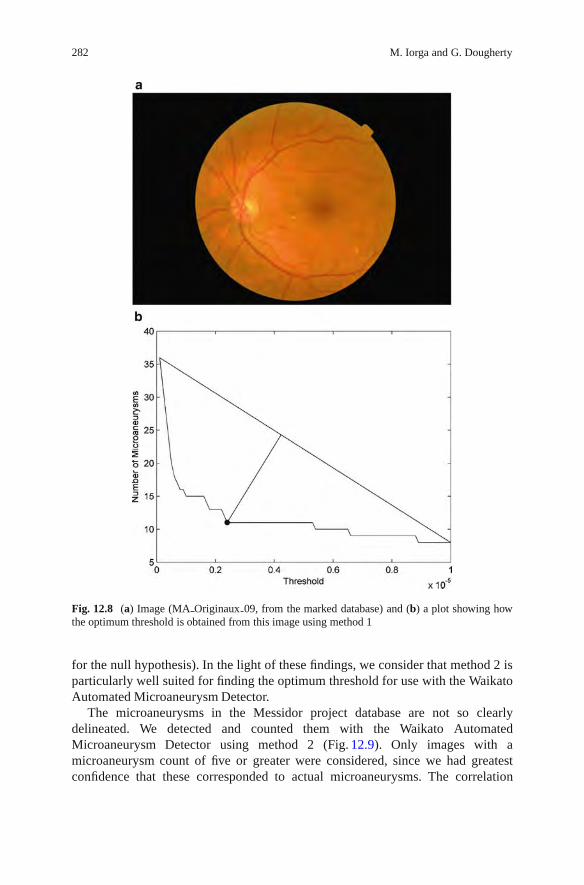
282 M. Iorga and G. Dougherty
Fig. 12.8 (a) Image (MA Originaux 09, from the marked database) and (b) a plot showing howthe optimum threshold is obtained from this image using method 1
for the null hypothesis). In the light of these findings, we consider that method 2 isparticularly well suited for finding the optimum threshold for use with the WaikatoAutomated Microaneurysm Detector.
The microaneurysms in the Messidor project database are not so clearlydelineated. We detected and counted them with the Waikato AutomatedMicroaneurysm Detector using method 2 (Fig. 12.9). Only images with amicroaneurysm count of five or greater were considered, since we had greatestconfidence that these corresponded to actual microaneurysms. The correlation

12 Tortuosity as an Indicator of the Severity of Diabetic Retinopathy 283
Table 12.1 The number of microaneurysms detected for the images of the marked database usingvarious thresholds, and our methods 1 and 2, compared with the actual “gold standard” counts
“Goldstandard” Threshold Threshold Threshold
Image ID counts = 10−5 = 10−6 = 10−7 Method 1 Method 2
1 2 0 1 11 1 22 3 2 3 11 3 43 2 1 1 4 1 24 1 3 4 16 3 45 4 2 4 19 4 46 16 5 17 34 11 167 3 1 6 11 2 78 8 3 7 12 4 79 9 8 15 36 11 1110 19 7 20 39 16 1611 14 4 15 41 11 912 3 2 3 11 3 413 3 2 4 11 4 514 4 0 4 7 1 415 1 3 4 16 3 416 5 2 4 19 4 417 11 3 10 22 10 1118 16 7 17 29 13 1519 7 2 8 21 4 420 0 1 1 7 1 321 2 0 1 4 1 122 3 1 6 11 2 723 6 2 7 11 4 524 7 3 13 25 11 1025 0 1 1 3 1 326 0 0 1 6 0 127 6 3 10 39 8 628 10 8 17 48 14 1429 11 0 3 12 2 330 5 5 13 20 5 1531 2 1 7 21 5 632 8 4 13 36 9 733 7 0 6 13 3 634 5 4 7 33 6 835 3 1 3 15 1 336 0 1 2 43 2 237 1 0 6 34 2 238 18 5 12 24 10 1039 18 1 13 34 8 1440 22 5 17 42 11 1741 7 3 9 25 9 942 17 3 8 31 5 843 10 5 18 57 10 10
(continued)
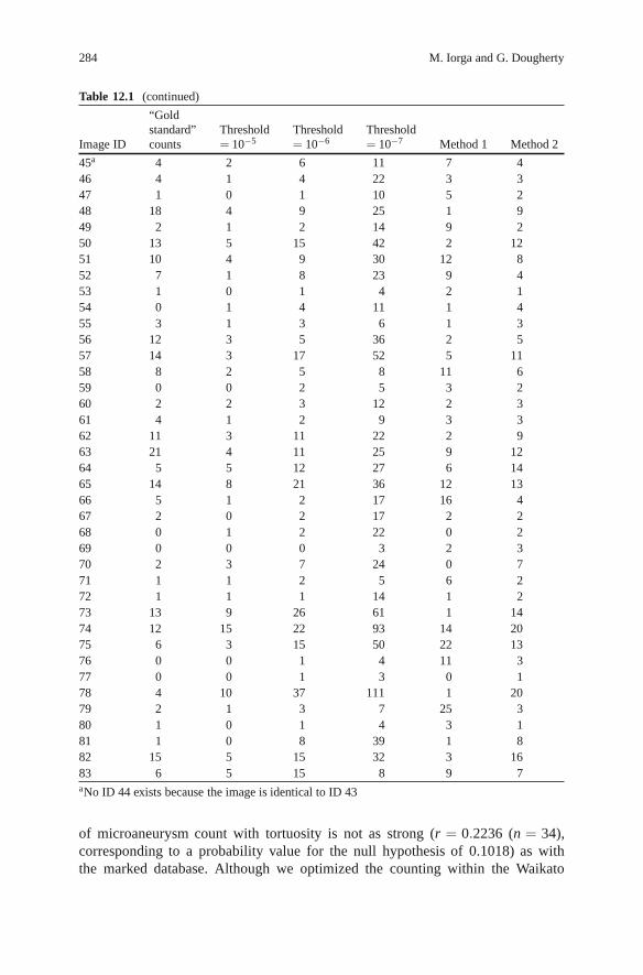
284 M. Iorga and G. Dougherty
Table 12.1 (continued)
“Goldstandard” Threshold Threshold Threshold
Image ID counts = 10−5 = 10−6 = 10−7 Method 1 Method 2
45a 4 2 6 11 7 446 4 1 4 22 3 347 1 0 1 10 5 248 18 4 9 25 1 949 2 1 2 14 9 250 13 5 15 42 2 1251 10 4 9 30 12 852 7 1 8 23 9 453 1 0 1 4 2 154 0 1 4 11 1 455 3 1 3 6 1 356 12 3 5 36 2 557 14 3 17 52 5 1158 8 2 5 8 11 659 0 0 2 5 3 260 2 2 3 12 2 361 4 1 2 9 3 362 11 3 11 22 2 963 21 4 11 25 9 1264 5 5 12 27 6 1465 14 8 21 36 12 1366 5 1 2 17 16 467 2 0 2 17 2 268 0 1 2 22 0 269 0 0 0 3 2 370 2 3 7 24 0 771 1 1 2 5 6 272 1 1 1 14 1 273 13 9 26 61 1 1474 12 15 22 93 14 2075 6 3 15 50 22 1376 0 0 1 4 11 377 0 0 1 3 0 178 4 10 37 111 1 2079 2 1 3 7 25 380 1 0 1 4 3 181 1 0 8 39 1 882 15 5 15 32 3 1683 6 5 15 8 9 7aNo ID 44 exists because the image is identical to ID 43
of microaneurysm count with tortuosity is not as strong (r = 0.2236 (n = 34),corresponding to a probability value for the null hypothesis of 0.1018) as withthe marked database. Although we optimized the counting within the Waikato

12 Tortuosity as an Indicator of the Severity of Diabetic Retinopathy 285
Fig. 12.9 The tortuosity/length for 34 vessels from the Messidor project database. The best-fittedline is superimposed
Fig. 12.10 The tortuosity of the first quintile length compared to the tortuosity of the entire vessel,for 46 vessels from the marked database
Automated Microaneurysm Detector, we do not expect the number of counts tobe completely accurate. Despite this, the level of correlation supports our earlierfinding with the marked database that tortuosity is related to microaneurysm count,and that tortuosity increases with severity of retinopathy.
A complicating factor in the use of vessel tortuosity as an indicator of the severityof retinopathy would be a change in tortuosity along an individual blood vessel. Wemeasured the tortuosity of vessels along the quintiles of their length. Figure 12.10
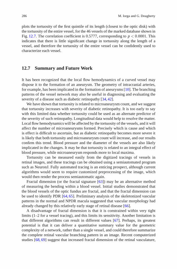
286 M. Iorga and G. Dougherty
plots the tortuosity of the first quintile of its length (closest to the optic disk) withthe tortuosity of the entire vessel, for the 46 vessels of the marked database shown inFig. 12.7. The correlation coefficient is 0.5777, corresponding to p < 0.0001. Thisindicates that there is little significant change in tortuosity along the length of avessel, and therefore the tortuosity of the entire vessel can be confidently used tocharacterize each vessel.
12.7 Summary and Future Work
It has been recognized that the local flow hemodynamics of a curved vessel maydispose it to the formation of an aneurysm. The geometry of intracranial arteries,for example, has been implicated in the formation of aneurysms [10]. The branchingpatterns of the vessel network may also be useful in diagnosing and evaluating theseverity of a disease such as diabetic retinopathy [34, 42].
We have shown that tortuosity is related to microaneurysm count, and we suggestthat tortuosity increases with severity of diabetic retinopathy. It is too early to saywith this limited data whether tortuosity could be used as an alternate predictor ofthe severity of such retinopathy. Longitudinal data would help to resolve the matter.Local flow hemodynamics will be affected by the tortuosity of the vessels, and it willaffect the number of microaneurysms formed. Precisely which is cause and whichis effect is difficult to ascertain, but as diabetic retinopathy becomes more severe itis likely that both tortuosity and microaneurysm count will increase, and our resultsconfirm this trend. Blood pressure and the diameter of the vessels are also likelyimplicated in the changes. It may be that tortuosity is related to an integral effect ofblood pressure, while microaneurysm responds more to local maxima.
Tortuosity can be measured easily from the digitized tracings of vessels inretinal images, and these tracings can be obtained using a semiautomated programsuch as NeuronJ. Fully automated tracing is an enticing prospect, although currentalgorithms would seem to require customized preprocessing of the image, whichwould then render the process semiautomatic again.
Fractal dimension (or the fractal signature [63]) may be an alternative methodof measuring the bending within a blood vessel. Initial studies demonstrated thatthe blood vessels of the optic fundus are fractal, and that the fractal dimension canbe used to identify PDR [64, 65]. Preliminary analysis of the skeletonized vascularpatterns in the normal and NPDR macula suggested that vascular morphology hadalready changed by this relatively early stage of retinal disease [66].
A disadvantage of fractal dimension is that it is constrained within very tightlimits (1–2 for a vessel tracing), and this limits its sensitivity. Another limitation isthat different algorithms can result in different values [67]. Perhaps, its greatestpotential is that it can deliver a quantitative summary value for the geometriccomplexity of a network, rather than a single vessel, and could therefore summarizethe complete retinal vascular branching pattern in an image. Recent computerizedstudies [68, 69] suggest that increased fractal dimension of the retinal vasculature,

12 Tortuosity as an Indicator of the Severity of Diabetic Retinopathy 287
reflecting increased geometric complexity of the retinal vascular branching pattern,is associated with early diabetic retinopathy microvascular damage. Although thedifferences in fractal dimension were small [69], the average fractal dimensionwas higher in participants with retinopathy than in those without retinopathy(median 1.46798 [interquartile range 1.45861–1.47626] compared with 1.46068[1.44835–1.47062], respectively; p < 0.001). After adjustments for age and sex,greater fractal dimension was significantly associated with increased odds ofretinopathy (odds ratio [OR] 4.04 [95%CI 2.21–7.49] comparing highest to lowestquartile of fractal dimension; OR 1.33 for each 0.01 increase in fractal dimension).This association remained with additional adjustments for diabetes duration, bloodsugar, blood pressure, body mass index (BMI), and total cholesterol levels. Furtheradjustment for retinal arteriolar or venular caliber had minimal impact on theassociation (OR 3.92 [95% CI 1.98–7.75]).
Acknowledgments We acknowledge with thanks the help and assistance of Dr. Eric Meijering,Dr. Michal Sofka, and Dr. Michael Cree on issues regarding their respective software. A databaseof retinal images, with the microaneurysms manually identified by experts, was kindly supplied byDr. Jean-Claude Klein of the Center of Mathematical Morphology of MINES, Paris Tech. One of us(G.D.) acknowledges the award of a Fulbright Senior Scholarship, which provided the opportunityto expand work in this area and others.
References
1. Hoover, A., Kouznetsova, V., Goldbaum, M.: Locating blood vessels in retinal images bypiecewise threshold probing of a matched filter response. IEEE Trans. Med. Imaging 19,203–210 (2000)
2. Witt, N., Wong, T.Y., Hughes, A.D., et al.: Abnormalities of retinal vasculature structure andthe risk of mortality from ischemic heart disease and stroke. Hypertension 47, 975–981 (2006)
3. Wong, T.Y., Shankar, A., Klein, R., et al.: Retinal arteriolar narrowing, hypertension andsubsequent risk of diabetes mellitus. Medicine 165, 1060–1065 (2005)
4. Cheung, N., Wong, T.Y., Hodgson, L.: Retinal vascular changes as biomarkers of systemiccardiovascular diseases. In: Jelinek, H.F., Cree, M.J. (eds.) Automated Image Detection ofRetinal Pathology, pp. 185–219, CRC Press, Boca Raton, FL (2010)
5. Wong, T.Y., Mohamed, Q., Klein, R., et al.: Do retinopathy signs in non-diabetic individualspredict the subsequent risk of diabetes? Br. J. Ophthalmol. 90, 301–303 (2006)
6. Fong, D.S., Aiello, L., Gardner, T.W., et al.: Diabetic retinopathy. Diabetes Care 26, 226–229(2003)
7. Dobrin, P.B., Schwarz, T.H., Baker, W.H.: Mechanisms of arterial and aneurismal tortuosity.Surgery 104, 568–571 (1988)
8. Wenn, C.M., Newman, D.L.: Arterial tortuosity. Aust. Phys. Eng. Sci. Med. 13, 67–70 (1990)9. Dougherty, G., Varro, J.: A quantitative index for the measurement of the tortuosity of blood
vessels. Med. Eng. Phys. 222, 567–574 (2000)10. Bor, A.S.E., Velthuis, B.K., Majoie, C.B., et al.: Configuration of intracranial arteries and
development of aneurysms: a follow-up study. Neurology 70, 700–705 (2008)11. Klein, R., Meuer, S.M., Moss, S.E., et al.: Retinal aneurysm counts and 10-year progression of
diabetic retinopathy. Arch. Ophthalmol. 113, 1386–1391 (1995)12. Kohner, E.M., Stratton, I.M., Aldington, S.J., et al.: Microaneurysms in the development of
diabetic retinopathy (UKPDS 42). Diabetologia 42, 1107–1112 (1999)

288 M. Iorga and G. Dougherty
13. Hellstedt, T., Immonen I.: Disappearance and formation rates of microaneurysms in earlydiabetic retinopathy. Br. J. Ophthalmol. 80, 135–139 (1996)
14. Kohner, E.M., Dollery, C.T.: The rate of formation and disappearance of microaneurysms indiabetic retinopathy. Eur. J. Clin. Invest. 1, 167–171 (1970)
15. Goatman, K.A., Cree, M.J., Olson, J.A., et al.: Automated measurement of microaneurysmturnover. Invest. Ophthalmol. Vis. Sci. 44, 5335–5341 (2003)
16. Phillips, R.P., Spencer, T., Ross, P.G., et al.: Quantification of diabetic maculopathy by digitalimaging of the fundus. Eye 5, 130–137 (1991)
17. Phillips, R., Forrester, J., Sharp, P.: Automated detection and quantification of retinal exudates.Graefe’s Arch. Clin. Exp. Ophthalmol. 231, 90–94 (1993)
18. Osareh, A., Shadgar, B., Markham, R.: A computational-intelligence-based approach fordetection of exudates in diabetic retinopathy images. IEEE Trans. Inf. Tech Biomed. 13,535–545 (2009)
19. Preece, S.J., Claridge E. Monte Carlo modeling of the spectral reflectance of the human eye.Phys. Med. Biol. 47, 2863–2877 (2002)
20. Cree, M.J., Gamble, E., Cornforth, D.J.: Colour normalisation to reduce inter-patient and intra-patient variability in microaneurysm detection in colour retinal images. In: APRS Workshop inDigital Imaging (WDIC2005), Brisbane, Australia, pp. 163–168 (2005)
21. Niemeijer, M., van Ginneken, B., Cree, M.J., et al.: Retinopathy online challenge: automaticdetection of microaneurysms in digital color fundus photographs. IEEE Trans. Med. Imaging29, 185–195 (2010)
22. Baudoin, C.E., Lay, B.J., Klein, J.C.: Automatic detection of microaneurysms in diabeticfluorescein angiographies. Revue D’Epidemiologie et de Sante Publique 32, 254–261 (1984)
23. Spencer, T., Olson, J.A., McHardy, K.C., et al.: An image-processing strategy for thesegmentation and quantification in fluorescein angiograms of the ocular fundus. Comput.Biomed. Res. 29, 284–302 (1996)
24. Cree, M.J., Olson, J.A., McHardy, K.C., et al.: A fully automated comparative microaneurysmdigital detection system. Eye 11, 622–628 (1997)
25. Frame, A.J., Undrill, P.E., Cree, M.J., et al.: A comparison of computer based classificationmethods applied to the detection of microaneurysms in ophthalmic fluorescein angiograms.Comput. Biol. Med. 28, 225–238 (1998)
26. Streeter, L., Cree, M.J.: Microaneurysm detection in colour fundus images. In: Proceedings ofthe Image and Vision Computing New Zealand Conference (IVCNZ’03), Palmerston North,New Zealand, pp. 280–285 (2003)
27. Cree, M.J., Gamble, E., Cornforth, D.: Colour normalisation to reduce inter-patient and intra-patient variability in microaneurysm detection in colour retinal images. In: Proceedings ofAPRS Workshop on Digital Image Computing (WDIC2005), Brisbane, Australia, pp. 163–168(2005)
28. Vincent, L.: Morphological grayscale reconstruction in image analysis: applications andefficient algorithms. IEEE Trans. Image Process. 2, 176–201 (1993)
29. Dupas, B., Walter, T., Erginay, A., et al.: Evaluation of automated fundus photograph analysisalgorithms for detecting microaneurysms, haemorrhages and exudates, and of a computer-assisted diagnostic system for grading diabetic retinopathy. Diabetes Metab. 36, 213–220(2010)
30. Quellec, G., Lamard, M., Josselin, P.M., et al.: Optimal wavelet transform for the detection ofmicroaneurysms in retina photographs. IEEE Trans. Med. Imaging 27, 1230–1241 (2008)
31. Niemeijer, M., Staal, J.S., van Ginneken, B., et al.: Comparative study of retinal vesselsegmentation on a new publicly available database. Proc. SPIE 5370–5379 (2004)
32. Staal, J., Abramoff, M., Neimeijer, Mc, et al.: Ridge-based vessel segmentation in color imagesof the retina. IEEE Trans. Med. Imaging 23, 501–509 (2004)
33. Early Treatment Diabetic Retinopathy Study Research Group: Grading diabetic retinopathyfrom stereoscopic color fundus photographs – an extension of the modified Airlie Houseclassification. ETDRS report #10. Ophthalmology 98, 786–806 (1991)

12 Tortuosity as an Indicator of the Severity of Diabetic Retinopathy 289
34. Hart, W.E., Goldbaum, M., Cote, B., et al.: Measurement and classification of retinal vasculartortuosity. Int. J. Med. Inform. 53, 239–252 (1999)
35. Aslam, T., Fleck, B., Patton, N., et al.: Digital image analysis of plus disease in retinopathy ofprematurity. Acta ophthalmol. 87, 368–377 (2009)
36. Capowski, J.J., Kylstra, J.A., Freedman, S.F.: A numeric index based on spatial frequency forthe tortuosity of retinal vessels and its application to plus disease in retinopathy of prematurity.Retina 15, 490–500 (1995)
37. Wallace, D.K.: Computer-assisted quantification of vascular tortuosity in retinopathy ofprematurity. Trans. Am. Ophthalmol. Soc. 105, 594–615 (2007)
38. Owen, C.G., Rudnicka, A.R., Mullen, R., et al.: Measuring retinal vessel tortuosity in 10-year-old children: validation of the computer-assisted image analysis of the retina (CAIAR)program. Invest. Ophthalmol. Vis. Sci. 50, 2004–2010 (2009)
39. Lotmar, W., Freiburghaus, A., Bracker, D.: Measurement of vessel tortuosity on fundusphotographs. Graefe’s Arch. Clin. Exp. Ophthalmol. 211, 49–57 (1979)
40. Smedby, O., Hogman, N., Nilsson, U., et al.: Two-dimensional tortuosity of the superficialfemoral artery in early atherosclerosis. J. Vasc. Res. 30, 181–191 (1993)
41. Saidlear, C.A.: Implementation of a Quantitative Index for 3-D Arterial Tortuosity. M.Sc.thesis, University of Dublin, 2002
42. Bullitt, E., Gerig, G., Pizer, S.M., et al.: Measuring tortuosity of the intracerebral vasculaturefrom MRA images. IEEE Trans. Med. Imaging 22, 1163–1171 (2003)
43. Grisan, E., Foracchia, M., Ruggeri, A.: A novel method for the automatic evaluation of retinalvessel tortuosity. IEEE Trans. Med. Imaging 27, 310–319 (2008)
44. Johnson, M.J., Dougherty, G.: Robust measures of three-dimensional vascular tortuosity basedon the minimum curvature of approximating polynomial spline fits to the vessel mid-line. Med.Eng. Phys. 29, 677–690 (2007)
45. Dougherty, G., Johnson, M.J.: Clinical validation of three-dimensional tortuosity metrics basedon the minimum curvature of approximating polynomial splines. Med. Eng. Phys. 30, 190–198(2008)
46. Dougherty, G., Johnson, M.J., Wiers, M.D.: Measurement of retinal vascular tortuosity and itsapplication to retinal pathologies. Med. Biol. Eng. Comput. 48, 87–95 (2010)
47. Sonka, M., Hlavac, V., Boyle, R.: Image Processing, Analysis, and Machine Vision, 3rd edn.Cengage Learning, Florence, KY (2007)
48. Dougherty G.: Digital Image Processing for Medical Applications. Cambridge UniversityPress, Cambridge (2009) (a) pp. 259–263; (b) pp. 157–159; (c) pp. 296–301; (d) pp. 140–144
49. Meijering, E., Jacob, M., Sarria, J.C.F., et al.: Design and validation of a tool for Neurite tracingand analysis in fluorescence microscopy images. Cytometry A 58, 167–176 (2004)
50. Xiong, G., Zhou, X., Degterev, A., et al.: Automated neurite labeling and analysis influorescence microscopy images. Cytometry A 69, 494–505 (2006)
51. Zhang, Y., Zhou, X., Witt, R.M., et al.: Dendritic spine detection using curvilinear structuredetector and LDA classifier. Neuroimage 36, 346–360 (2007)
52. Fan, J., Zhou, X., Dy, J.G., et al.: An automated pipeline for dendrite spine detection andtracking of 3D optical microscopy neuron images of in vivo mouse models. Neuroinformatics7, 113–130 (2009)
53. Yuan, X., Trachtenberg, J.T., Potter, S.M., et al.: MDL constrained 3-D grayscale skeletoniza-tion algorithm for automated extraction of dendrites and spines from fluorescence confocalimages. Neuroinformatics 7, 213–232 (2009)
54. Sofka, M., Stewart, C.V.: Retinal vessel centerline extraction using multiscale matched filters,confidence and edge measures. IEEE Trans. Med. Imaging 25, 1531–1546 (2006)
55. Sun, C., Vallotton, P.: Fast linear feature detection using multiple directional non-maximumsuppression. J. Microsc. 234, 147–157 (2009)
56. Lindeberg, T.: Feature detection with automatic scale selection. Int. J. Comput. Vis. 30(2),77–116 (1998)
57. Barrett, W.A., Mortensen, E.N.: Interactive live-wire boundary extraction. Med. Image Anal.1, 331–341 (1996)

290 M. Iorga and G. Dougherty
58. Falcao, A.X., Udupa, J.K., Samarasekera, S., et al.: User-steered image segmentationparadigms: live wire and live lane. Graph. Models Image Process. 60, 233–260 (1998)
59. Falcao, A.X., Udupa, J.K., Miyazawa, F.K.: An ultra-fast user-steered image segmentationparadigm: LiveWire on the fly. IEEE Trans. Med. Imaging 19, 55–62 (2000)
60. Vallotton, P., Lagerstrom, R., Sun, C., et al.: Automated analysis of neurite branching incultured cortical neurons using HCA-vision. Cytometry A 71, 889–895 (2007)
61. Conrad, C., Gerlich D.W.: Automated microscopy for high-content RNAi screening. J. CellBiol. 188, 453–461 (2010)
62. Vallotton, P., Sun, C., Wang, D., et al.: Segmentation and tracking of individual Pseudomonasaeruginosa bacteria in dense populations of motile cells. In: Image and Vision Computing NewZealand, Wellington, New Zealand, 2009
63. Dougherty, G., Henebry, G.M.: Fractal signature and lacunarity in the measurement of thetexture of trabecular bone in clinical CT images. Med. Eng. Phys. 23, 369–380 (2001)
64. Family, F., Masters, B.R., Platt, D.: Fractal pattern formation in human retinal vessels. PhysicaD 38, 98–103 (1989)
65. Daxer, A.: The fractal geometry of proliferative diabetic retinopathy: implications for thediagnosis and the process of retinal vasculogenesis. Curr. Eye Res. 12, 1103–1109 (1993)
66. Avakian, A., Kalina, R.E., Sage, E.H., et al.: Fractal analysis of region-based vascular changein the normal and non-proliferative diabetic retina. Curr. Eye Res. 24, 274–280 (2002)
67. Schepers, H.E., Van Beek, J.H.G.M., Bassingthwaighte, J.B.: Four methods to estimate thefractal dimension from self-affine signals. IEEE Eng. Med. Biol. 11, 57–64 (1992)
68. MacGillivray, T.J., Patton, N.: A reliability study of fractal analysis of the skeletonised vascularnetwork using the “box-counting” technique. Conf. Proc. IEEE Eng. Med. Biol. Soc. 1,4445–4448 (2006)
69. Cheung, N., Donaghue, K.C., Liew, G., et al.: Quantitative assessment of early diabeticretinopathy using fractal analysis. Diabetes Care 32, 106–110 (2009)

Chapter 13Medical Image Volumetric Visualization:Algorithms, Pipelines, and Surgical Applications
Qi Zhang, Terry M. Peters, and Roy Eagleson
13.1 Introduction
With the increasing availability of high-resolution datasets of 3D medical images,the development of volumetric image rendering techniques have become an impor-tant complement to classical surface-based rendering. Since volumetric visualiza-tion does not require that surfaces be selected from within the 3D volumes, thefull volume dataset is maintained during the rendering process. These methods arebased on a foundation of projecting rays through volumes, which have a range ofopacity attributes, onto a viewing window. Volume rendering is computationallydemanding, and the ever increasing size of medical image datasets means that brute-force algorithms are not feasible for interactive use.
More recently, further efficiencies have been attained by implementing manyof these algorithms on graphics processing hardwares (GPUs). In this chapter, wedescribe volumetric visualization pipelines, and provide a comprehensive overviewof rendering algorithms that use effective approximate models to compute volumet-ric scenes of medical applications. We review and implement several mainstreammedical image visualization strategies and rendering pipelines, including multipla-nar reformation (MPR), direct and indirect surface rendering (DSR and ISR) withshading, direct volume rendering (DVR), software-based raycasting, 2D and 3Dtexture mapping (3DTM), GPU-based raycasting, maximum intensity projection(MIP), X-ray based rendering, gradient estimation and different interpolationapproaches, voxel classification, and optical composition schemes. We present anoverview of these techniques, and also evaluate their image quality and renderingperformance.
R. Eagleson (�)The University of Western Ontario, London, ON, Canadae-mail: [email protected]
G. Dougherty (ed.), Medical Image Processing: Techniques and Applications, Biologicaland Medical Physics, Biomedical Engineering, DOI 10.1007/978-1-4419-9779-1 13,© Springer Science+Business Media, LLC 2011
291

292 Q. Zhang et al.
Where space permits, we have also added some of our recent research results andnew rendering and classifications algorithms. In particular, these include anatomicalfeature enhancement techniques, dynamic multimodality rendering, and interactivemanipulation. We have implemented a GPU-based medical image manipulation andvisualization system with these volume rendering enhancements. We compare theperformance of our strategies with those obtained by implementation algorithmsfrom the published literature. We also address the advantages and drawbacks ofeach in terms of image quality and speed of interaction.
Fig. 13.1 MPR of 3D cardiac CT image. Top: three arbitrary cross-planes. Bottom: synchronized2D displays of cross-planes

13 Medical Image Volumetric Visualization: Algorithms, Pipelines... 293
13.2 Volumetric Image Visualization Methods
Three principle rendering algorithms have been established for volumetric medicalimage visualization, that is multiplanar reformation (MPR; see Fig. 13.1), surfacerendering (SR), and volume rendering (VR). As illustrated in the following sections,the rendering techniques can be categorized as direct and indirect rendering. Directrendering includes DVR and DSR, while indirect rendering includes ISR. Here, werefer to both DSR and ISR as SR.
13.2.1 Multiplanar Reformation (2D slicing)
MPR is an image processing technique, which extracts 2D slices from a 3D volumeusing arbitrarily positioned orthogonal or oblique planes [1]. Although it is still a2D method, it has the advantages of ease of use, high speed, and no informationloss. The observer can display a structure of interest in any desired plane within thedata set, and 4D MPR can be performed in real time using graphics hardware [2].2D multiplanar reformatting can readily complement 3D volume rendering wherethe 2D slices of MPR can be readily texture-mapped to cut-planes through a 3Dvolume.
13.2.2 Surface-Based Rendering
SR [3] is a common method of displaying 3D images. ISR can be consideredas surface modeling, while DSR is a special case of DVR. ISR requires that thesurfaces of relevant structure boundaries within the volume be identified a prioriby segmentation and representation as a series of surface tiles using isosurfaceextracting such as marching cubes [4] or region growing [5], and can be acceleratedby taking advantage of graphics processing unit (GPU) and geometry shaders[6, 7]. Such models reduce the amount of data to be displayed by several orders ofmagnitude, making it easy to manipulate the surfaces interactively with reasonablefidelity. For DSR, the surfaces are rendered directly from the volume withoutintermediate geometric representations, setting thresholds or using object labels todefine a range of voxel intensities to be viewed. Only those voxels within this range,or which have labels, are selected and rendered with DVR. Surface reconstructioncan also be improved further by employing GPUs [8].
A fully parallel isosurface extraction algorithm was presented by Zhang et al. [9].In addition, a high degree of realism can be achieved with lighting models thatsimulate realistic viewing conditions. Figure 13.2a illustrates an implementation ofISR, while Fig. 13.3b shows the results of DSR for comparison.

294 Q. Zhang et al.
Fig. 13.2 (a) ISR of cardiac structures: myocardium (myo), and the left atrium and aorta (LAA),compared with (b) DSR of an MR cardiac volume and heart phantom
Fig. 13.3 SR applications: (a) image generated with MIP and shaded SR, demonstrating the prox-imal middle cerebral artery mainstem occlusion (arrow) [12]; (b). SR display of the endoluminalCT colonographic data, showing sessile morphology of the lesion (arrow) [13]
SR is often applied to contrast-enhanced CT data for displaying skeletal andvascular structures, and is also usually used in describing vascular disease anddislocations. In the process of detecting acute ischemic stroke, Schellinger and hiscolleagues [10] combined MIP with shaded SR to visualize proximal middle cere-

13 Medical Image Volumetric Visualization: Algorithms, Pipelines... 295
Fig. 13.4 Volume renderingpipeline and correspondingnumerical operations
bral artery mainstem occlusion (Fig. 13.3a). SR has also been exploited to describepolyps within the 3D endoluminal CT colonographic images [11] (Fig. 13.3b).
We note that sometimes it is difficult to justify the accuracy and reliability of theimages generated with shaded SR, that is the shiny surfaces might be misleading,causing the relation between image data and brightness in the resultant imagebecomes more complex, a property which could affect the diagnosis.
13.2.3 Volumetric Rendering
DVR displays the entire 3D dataset by tracing rays through the volume and project-ing onto a 2D image, without computing any intermediate geometry representations[14–16]. This algorithm can be further divided into image-space DVR, such assoftware- [17, 18] and GPU-based raycasting [19], and object-space DVR, such assplatting [20,21], shell rendering [22], TM [23], and cell projection [24]. Shear-warp[25] can be considered as a combination of these two categories. In addition, MIP[26], minimum intensity projection (MinIP), and X-ray projection [27] are alsowidely used methods for displaying 3D medical images. This chapter now focusesits attentions on DVR, and the datasets discussed here are assumed to be representedon cubic and uniform rectilinear grids, such as are provided by standard 3D medicalimaging modalities. Figure 13.4 describes the DVR pipeline with correspondingcomputations, which are described in detail in the next section that is followed bya discussion of traditional DVR algorithms. Figure 13.5 shows an example of ourDVR results applied to an MR cardiac volume.
When compared with SR, the main advantage of DVR is that interior informationis retained, and so provides more information about the spatial relationships ofdifferent structures [14]. In clinical applications, sensitivity and specificity are the

296 Q. Zhang et al.
Fig. 13.5 Volume rendered images of volumetric human cardiac CT data set
major diagnostic criteria that must be considered. Even though DVR generally hashigh sensitivity and specificity for diagnosis [28], it is computationally intensive,so interactive performance is not always feasible. Another disadvantage is that itmay be difficult to interpret the “cloudy” interiors that can result from the ray-tracing process. For detailed observation of specific lesions, slab imaging, wherethick slices are rendered with DVR or MIP, has generally been used in clinicaldiagnosis [29]. In addition, the combination of cross-sectional MPR and DVR cansignificantly increase the interpretation rate of anatomical structures [30]. DVRhas a wide range of clinical applications. For example, to perform renal donorevaluation, Fishman et al. [31] used DVR and MIP to display the renal vein ofCT angiography (CTA) data, as shown in Fig. 13.6, for the DVR generated image,the left gonadal vein (large arrow) is well defined (a), while the locations of therenal vein and gonadal vein (arrow) are inaccurately depicted in the MIP generatedimage (b). Gill et al. [32] used DVR and MinIP to show the central airway andvascular structures of a 60-year-old man who underwent double lung transplantationfor idiopathic pulmonary fibrosis, evaluating posttreatment in a noninvasive manner(Fig. 13.6c,d).
13.3 Volume Rendering Principles
The core component of DVR is to solve the volume rendering integral that describesthe optical model. Different DVR techniques share similar components in therendering pipeline, the main difference being the order in which they are applied,and the manner in which they traverse the volumetric data. Due to the rapiddevelopment of programmable GPUs, many CPU-based algorithms and techniqueshave been or can be implemented on GPUs. In this paper, for the texture-mappingbased DVR, we refer to algorithms that use a fixed graphics pipeline, while forGPU-based raycasting, we refer to DVR implemented on GPUs.
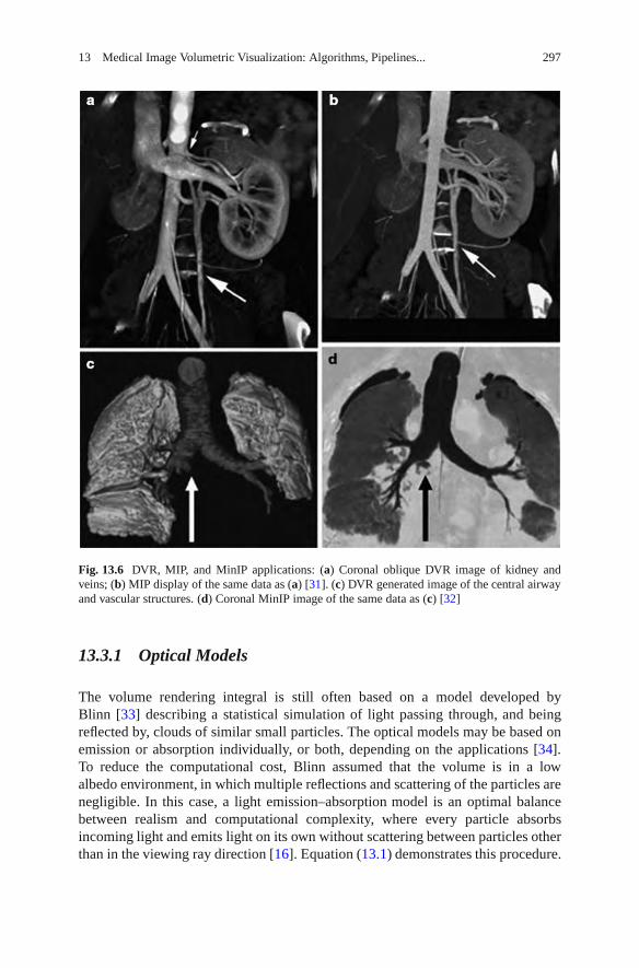
13 Medical Image Volumetric Visualization: Algorithms, Pipelines... 297
Fig. 13.6 DVR, MIP, and MinIP applications: (a) Coronal oblique DVR image of kidney andveins; (b) MIP display of the same data as (a) [31]. (c) DVR generated image of the central airwayand vascular structures. (d) Coronal MinIP image of the same data as (c) [32]
13.3.1 Optical Models
The volume rendering integral is still often based on a model developed byBlinn [33] describing a statistical simulation of light passing through, and beingreflected by, clouds of similar small particles. The optical models may be based onemission or absorption individually, or both, depending on the applications [34].To reduce the computational cost, Blinn assumed that the volume is in a lowalbedo environment, in which multiple reflections and scattering of the particles arenegligible. In this case, a light emission–absorption model is an optimal balancebetween realism and computational complexity, where every particle absorbsincoming light and emits light on its own without scattering between particles otherthan in the viewing ray direction [16]. Equation (13.1) demonstrates this procedure.

298 Q. Zhang et al.
dI(λ)dλ
= c(λ)τ(λ)− I(λ)τ(λ) = c(λ)− I(λ). (13.1)
The solution to this equation is given below, showing the intensity of each pixel.
I(D) = I0T (D)+∫ D
0c(λ)T (λ)dλ,
T (λ ) = exp
(−
∫ λ
0τ(x)dx
), (13.2)
describes the volume transparency. The first term I0 illustrates light coming from thebackground, and D is the extent of the ray over which light is emitted. The last termdemonstrates the behavior of the volume emitting and absorbing incoming light. Thesource term c() indicates the color change, and the extinction coefficient (tau)(D)defines the occlusion of light per unit length due to light scattering or extinction.
13.3.2 Color and Opacity Mapping
13.3.2.1 Voxel Classification
To display 3D medical images with DVR, the scalar values must first be mappedto optical properties such as color and opacity through transfer function (TF),a process referred to as voxel classification. Pre- and postclassification approachesdiffer with respect to the order in which the TF and sampling interpolation areapplied [16, 35]. Pre-classification first maps every scalar value at the grid intocolor and opacity in a pre-processing step, where the color and opacity are assignedat the resampling points. However, for post-classification, we first sample thescalar value by interpolation, and then map the acquired values to colors andopacity through TFs. Both the pre-and post-classification operations introduce highfrequency components via the nonlinear TFs [36–38]. Pre-classification suppressesthis high-frequency information, so the rendered image appears blurry (Fig. 13.7a),while postclassification maintains all the high frequencies, but introduces “striping”artifacts in the final images (Fig. 13.7b).
To address the undersampling problem, Rottger et al. [39, 41] proposed a prein-tegrated classification algorithm for hardware-accelerated tetrahedra projection,which was first introduced by Max et al. [40]. Later, Engel et al. [36] appliedthis classification algorithm for 3D texture-mapping-based volume visualization ofregular-grid volume data. Preintegrated classification separates the DVR integralinto two parts, one for the continuous scalar value, and the other for the TF pa-rameters c(colors) and tau(extinction). This algorithm renders the volume segment-by-segment, instead of point-by-point. In this manner, the Nyquist frequency forreconstructing the continuous signal is not increased by the TF nonlinear properties.Assuming there are n + 1 sampling points along the viewing ray, then the segment

13 Medical Image Volumetric Visualization: Algorithms, Pipelines... 299
Fig. 13.7 DVR of cardiac vessels via different voxel classification algorithms: (a) preclassifica-tion; (b) postclassification; (c) preintegrated classification; (d) post color-attenuated classification
length d equals D = n, where D is the maximum ray length. For the ith segment,the front and back points are sa = s(id) and sb = s((i+1)d). The calculated opacityand color of this segment are then given by (13.3) and (13.4), respectively.
I(D) f b =n
∑i=0
αiCi
i−1
∏j=0
Tj =n
∑i=0
αiCi
i−1
∏j=0
(1−α j) (13.3)
I(D)b f =n
∑i=0
αiCi
n
∏j=i+1
Tj =n
∑i=0
αiCi
n
∏j=i+1
(1−α j). (13.4)
13.3.2.2 Transfer Function
The important step of voxel classification is implemented through a TF adjustment,which plays an important role in DVR. However, TF specification is a complexprocedure and is a major obstacle for the widespread clinical use of DVR [42, 43].In this section, we briefly review the TFs that are of crucial clinical importance. InDVR, the TF was typically used for tissue classification based on local intensities inthe 3D dataset [44]. Multidimensional TF is efficient for multiple spatial featuredetection, for example, Kniss et al. [45] designed such a TF and demonstratedits medical applications, while Higuera et al. [46] built a 2D TF to effectively

300 Q. Zhang et al.
visualize intracranial aneurysm structures. Abellan et al. [47] introduced a 2Dfusion TF to facilitate the visualization of merged multimodal volumetric data, anda 3D TF was designed by Hadwiger et al. [48] to interactively explore featureclasses within the industrial CT volumes, where individual features and featuresize curves can be colored, classified, and quantitatively measured with the helpof TF specifications. Furthermore, Honigmann et al. [49] designed an adaptiveTF for 3D and 4D ultrasound display, and a default TF template was built to fitspecific requirements. Similarly, Rezk-Salama et al. [50] proposed a template-basedreproducible automatic TF design algorithm and applied it to medical diagnosis.Later, to facilitate the TF specification, these authors also introduced semanticmodels for TF parameter assignment, while a similar idea was used by Rautek et al.[51] to add a semantic layer in the TF design. As pointed by Freiman et al. [52],automation is important in TF design.
13.3.3 Composition
During the DVR process, a number of composition schemes are commonly em-ployed, including simulating an X-ray projection (Fig. 13.8a) [53], MIP [54, 55],MinIP, and alpha blending. MIP and MinIP are widely used techniques in 3D CT andMR angiography. The salient features in the image are generally comprised by thevoxels having the maximum (MIP) or minimum (MinIP) intensity along the viewingrays traversing through the object. MIP and MinIP images can be generated rapidlyand can clearly display vessels, tumor, or bones [56], and the image generation hasbeen accelerated by graphics hardware [57,58]. Because no user input is necessary,MIP is a widely used 3D visualization option in radiology.
Local MIP, MinP, or closest vessel projection (CVP) are often used in slabimaging for vascular structure diagnosis [29, 59]. For vascular diagnosis, CVP issuperior to MIP, however the user needs to set an appropriate threshold for thelocal maximum, which is determined by a specific dataset, making the applicationof CVP more difficult than MIP (which is shown in Fig. 13.8b). Alpha blending[17, 34] is a popular optical blending technique, often implemented by summing todiscretize the continuous function (13.2), resulting front-to-back and back-to-frontalpha blending, depending on the compositing order. The front-to-back and back-to-front alpha blending methods represent opposite rendering directions. Figure 13.8cdescribes the DVR result using alpha blending without shading, while Fig. 13.8dshows the result with shading.
13.3.4 Volume Illumination and Illustration
In volume illumination, the normal at every sampling point is calculated byinterpolation using the intensity changes across that voxel. These approximated

13 Medical Image Volumetric Visualization: Algorithms, Pipelines... 301
Fig. 13.8 DVR results of human head with angiographic contrast using different compositingtechniques: (a) X-ray projection; (b) MIP; (c) alpha blending without shading; and (d) alphablending with shading
voxel normals are then used in a Phong or Blinn-Phong model for shadingcomputations, with the results being employed in the DVR composition. Theshading computations may be accelerated using commodity graphics hardware[60]. In addition, the shading model can be used with volumetric shadows tocapture chromatic attenuation for simulating translucent rendering [61], and canbe combined with clipped volumes to increase the visual cues [62]. Figure 13.9illustrates a DVR of MR and CT cardiac data sets with and without illumination,demonstrating that images with shading are visually more pleasing.
Lighting and illumination are important aspects of volumetric visualization.Examples of approaches employed include those by Rheingans and Ebert [63] whoproposed an illumination method similar to volume shading, using nonphotorealisticrendering [64] to enhance physics-based DVR, and Lum and Ma [65] who acceler-ated this algorithm with multitexture-based hardware, and they also introduced apre-integrated lighting with voxel classification-based DVR, resulting in decreasedillumination artifacts [66]. To explore hidden structures and depict their spatialrelations in volumes, Chan et al. [67] introduced a relation-aware visualization

302 Q. Zhang et al.
Fig. 13.9 DVR images of CT pulmonary data showing illumination (right image) compared withno illumination (left image)
pipeline, in which inner structural relationships were defined by a region connectioncalculus and were represented by a relation graph interface. In addition, Rauteket al. [68] gave a comprehensive review on illustrative visualization and envisionedtheir potential medical applications. Such illustrative techniques are sometimesintegrated within commercial systems; however, there have been very few system-atic studies done to verify the perceptual enhancement, nor to validate the clinicalbenefit [69].
13.4 Software-Based Raycasting
Raycasting [14] is a popular technique used to display a 3D dataset in twodimensions, in which the basic idea is to cast a ray from each pixel in the viewingplane into the volume, sampling the ray with a predetermined step in a front-to-backor back-to-front order using trilinear interpolation. In this process, a TF is used tomap the scalar value to RGB color and opacity, which can be performed on everyvoxel in the volume before the sampling step (preclassification), or on the sampledscalar values along the casting ray after sampling, where post-, preintegrated, orpostcolor attenuated classification can be used. Finally, the acquired optical values atthese sampling points along the casting ray are composited using (13.5) or (13.6) toapproximately compute the DVR integral (13.2), obtaining the corresponding finalpixel color on the output image. Figure 13.10 illustrates the raycasting pipeline, andFig. 13.11demonstrates this on four medical images.

13 Medical Image Volumetric Visualization: Algorithms, Pipelines... 303
Fig. 13.10 Raycasting pipeline: sampling, optical mapping, and compositing
Fig. 13.11 Medical images rendered with software-based raycasting: (a) CT skull; (b) MR brain;(c) CT jaw, and (d) MR cerebral blood vessel

304 Q. Zhang et al.
13.4.1 Applications and Improvements
Because of its rendering speed, raycasting has been not often used in clinicalapplications until now. However, it was a significant 3D display method in someapplications ever when graphics hardware accelerated DVR was not commonlyavailable. For example, Sakas et al. [70] used raycasting to display 3D ultrasounddata of a fetus, and Hohne [71] and Tiede et al. [72] employed this algorithm foranatomical visualization. Many of the approaches to improve raycasting techniqueshave focused on schemes to eliminate unnecessary voxels from the computation.
13.5 Splatting Algorithms
Splatting is a popular DVR algorithm which was first proposed by Westhover[73–75] and was improved in terms of quality and speed by the research communityover the years [76, 77]. This technique was developed to accelerate the speed ofDVR at the expense of lower accuracy, and calculates the influence of each voxelin the volume on multiple pixels in the output image. This algorithm representsthe volume as an array of overlapping basis functions called reconstruction kernels,which are commonly rotationally symmetric Gaussian functions with amplitudesscaled by the voxel values. This process is described in Fig. 13.12, and Fig. 13.13presents examples of images rendered with the splatting algorithm.
13.5.1 Performance Analysis
Splatting is efficient because it reorders the DVR integral, making the preintegrationof reconstruction kernels possible, so that each voxel’s contribution to the integral
Fig. 13.12 Splatting pipeline: the optical model is evaluated for each voxel and projected onto theimage plane, leaving a footprint (splat). Then these footprints are composited to create the finalimage

13 Medical Image Volumetric Visualization: Algorithms, Pipelines... 305
Fig. 13.13 Medical images rendered with splatting: (a) CT skull with shading; (b) MR brain withshading [76]; (c) CT jaw, and (d) MR cerebral blood vessel [77]
can be viewed separately. Another major advantage is that only voxels relevant tothe image are projected and rasterized, so empty (transparent) regions can easily beskipped. However, because all of the splats are composited back-to-front directlywithout considering the kernel overlaps, the basic splatting algorithm is plaguedby artifacts known as “color bleeding,” where the colors of hidden objects orbackground appearing in the final image.
13.5.2 Applications and Improvements
Vega-Higuera et al. [78] exploited texture-accelerated splatting to visualize theneurovascular structures surrounded by osseous tissue in CTA data in real time.

306 Q. Zhang et al.
Splatting was also employed by Birkfellner et al. [79] to generate digitally renderedradiographs (DRRs) rapidly in the iterative registration of medical images, and theauthors later exploited graphics hardware to accelerate the splat-based creation ofDRRs [80]. Audigier and his colleagues [81] used splatting with raycasting to guidethe interactive 3D medical image segmentation, providing users with feedback ateach iterative segmentation step. Since basic splatting algorithms suffer from “colorbleeding” artifacts, Westover originally employed an axis-aligned sheet buffer tosolve this problem. However, this technique needs to maintain three stacks of sheetsand introduces “popping” artifacts. To address this issue, Mueller and his colleagues[82] aligned the sheet buffers parallel to the image plane instead of parallel to theaxes, and they later accelerated this image aligned splatting algorithm with modernGPUs [83]. They also proposed a postshaded pipeline for splatting to improve theresultant image [77].
13.6 Shell Rendering
Shell rendering [84] is an efficient software-based hybrid of surface and volumerendering proposed by Udupa and Odhner. The shell rendering algorithm is basedon a compact data structure referred to as a shell, which is a set of nontransparentvoxels near the extracted object boundary with a number of attributes associatedwith each related voxel for visualization. The shell data structure can store the entire3D scene or only the hard (binary) boundary. For a hard boundary, the shell is crispand only contains the voxels on the object surface, and shell rendering degeneratesto SR. For a fuzzy boundary, the shell includes voxels in the vicinity of the extractedsurface, and shell rendering is identified as DVR. Figure 13.14 shows examples ofshell SR and DVR.
13.6.1 Application and Improvements
Lei et al. [85] employed this algorithm to render the segmented structures of vesselsand arteries of contrast-enhanced magnetic resonance angiography (CE-MRA)image. However, the explicit surface extraction creates errors. To address theproblem, Bullitt et al. [86] selectively dilated the segmented object boundaries alongall axes, and visualized the extracted fuzzy shell with raycasting. To acceleratethe shell rendering speed, Falcao and his colleagues [87] added the shear-warpfactorization to the shell data structure, and Botha and Post [88] used a splat-likeelliptical Gaussian to compute the voxel contribution energy to the rendered image.Later, Grevera et al. [89] extended the point-based shell element to a new T-shellelement comprised of triangular primitives for isosurface rendering, referred to asT-Shell rendering.

13 Medical Image Volumetric Visualization: Algorithms, Pipelines... 307
Fig. 13.14 Shell rendering examples. Top row, shell SR [174]: skull CT data (left) and CT data ofa “dry” child’s skull (right). Bottom row, shell DVR [175]: CT skull (left), and MR head (right)
13.7 Texture Mapping
The pioneering work of exploiting texture hardware for DVR was performed byCullip and Neumann [90] and Cabral et al. [91]. When graphics hardware does notsupport trilinear interpolation, 2D texture mapping (2DTM) must be adopted. In thiscase, the volume is decomposed into three stacks of perpendicularly object-alignedpolygons. For the current viewing direction, the stack whose slicing direction(normal) must be within 45 degrees of the current viewing direction is chosenfor rendering. During rasterization, each of the polygon slices is textured with theimage information obtained from the volume via bilinear interpolation. Finally, thetextured slices are alpha-blended in a back-to-front order to produce the final image.

308 Q. Zhang et al.
Fig. 13.15 The working pipeline of 3DTM for 3D head rendering
Fig. 13.16 Medical image rendered with 3DTM: (a) CT skull; (b) MR brain; (c) CT jaw, and (d)MR cerebral blood vessel
Figure 13.15 describes the working pipeline, and Fig. 13.16 illustrates the ren-dering results with this algorithm. 3DTM uploads the volume to the graphicsmemory as a single 3D texture, and a set of polygons perpendicular to the viewingdirection is placed within the volume and textured with the image information bytrilinear interpolation. Compared with 2DTM, there are no orientation limitations

13 Medical Image Volumetric Visualization: Algorithms, Pipelines... 309
for the decomposed polygon slices, making the texture access more flexible. Thecompositing process is similar to 2DTM, in that the set of textured polygon planesare alpha-blended in a back-to-front order.
13.7.1 Performance Analysis
Compared with 3DTM, the main advantage of 2DTM is higher rendering speed andlower hardware requirements, since it uses efficient in-slice bilinear interpolations,instead of expensive trilinear interpolations. However, this algorithm is prone toaliasing artifacts at the edges of the slice polygons, and has to maintain threecopies of the volume in graphics memory. The shift of viewing directions causesthe algorithm to switch from one texture stack to another, resulting in the “popping”artifacts mentioned earlier. In 3DTM, the extracted slices can have arbitraryorientations and only a single copy of the data is required; therefore, there areno artifacts caused by the texture stack switching during the viewing directionchanging process. In addition, the extracted slices are textured with trilinear insteadof bilinear interpolation, so the mapped texture information has a higher accuracy.For orthographic projections, the viewport-aligned slices can be employed toachieve a consistent sampling step, but because the sampling distance cannot beuniform for projective views, “striping” artifacts are introduced. This limitationmay be overcome using spherical rendering primitives [92], albeit with an increasedcomputational cost.
13.7.2 Applications
In the published literature, there are three main types of medical applications forTM-based DVR. The first is multimodal medical image rendering and tissue sepa-ration. Sato et al. [93] designed a multidimensional TF to identify tissue structures inmultimodal medical images generated with 3DTM. A two-level rendering techniquewas integrated with 3DTM by Hauser et al. [94], allowing different renderingtechniques to be selected for different tissues based on segmentation information.Later, Hadwiger et al. [95] improved this 3DTM-based two-level DVR algorithm inthe aspects of image quality and performance, minimizing the number of renderingpasses and the computational cost of each pass, adding dynamic filtering, and usingdepth and stencil buffering to achieve correct compositing of objects created withdifferent rendering techniques.
The second application area is in the display of specific tissues and organs fordiagnosis and therapy. Holmes et al. [96] used 3DTM to achieve a real-time displayof transurethral ultrasound (TUUS) for prostate treatment. This technique was alsoused by Etlik et al. [97] to find bone fractures, and also by Wenger et al. [98] tovisualize diffusion tensor MRI (DTI) data in the brain. Wang et al. [99] exploited

310 Q. Zhang et al.
3DTM to display 3D ultrasound for cardiac ablation guidance, and Sharp et al. [100]employed this technique to visualize the light diffusion in 3D inhomogeneous tissueto provide visual information relating to structures located beneath the skin surface.Lopera et al. [101] used this DVR approach to view a stenosis in arbitrary imageplanes, and employed the rendering results to demonstrate the subsequent arterialbypass.
The third area of application is in dynamic imaging, deformation, and 4D datadisplay. Levin et al. [102] developed a software platform based on TM, which wasused to render multimodality 4D cardiac datasets interactively. A similar techniquewas used by Lehmann et al. [103] to visualize the beating heart in real time, in whicha hierarchical memory structure was employed to improve bandwidth efficiency. Inaddition, Yuan et al. [104] designed a TF for nonlinear mapping density values in thedynamic range medical volumes, while Correa and his colleagues [105] presented a3DTM algorithm that sampled the deformed space instead of the regular grid points,simulating volume deformations caused by clinical manipulations, such as cuts anddissections.
13.7.3 Improvements
13.7.3.1 Shading Inclusion
In 1996, shading was first included into TM approaches by Van Gelder et al. [23].Both diffuse and specular shading models were added to texture-based DVR byRezk-Salama et al. [92] with the use of register combiners and paletted texture.In addition, Kniss et al. [61] proposed a simple shading model that capturedvolumetric light attenuation to produce volumetric shadows and translucency. Theshading model was also used with depth-based volume clipping by Weiskopf and hiscolleagues [62] in a 3DTM pipeline. To decrease shading artifacts, Lum et al. [66]introduced preintegrated lighting into the TM-based DVR, resulting in decreasedlighting artifacts. Recently, Abellan and Tost [106] defined three types of shadingsfor the TM-accelerated volume rendering of dual-modality dataset, that is emissionplus absorption, surface shading, and the mixture of both shadings, with user-selected choice of shading model for a specific imaging modality.
13.7.3.2 Empty Space Skipping
As mentioned earlier, the DVR speed can often be improved if the empty spaces canbe skipped during rendering procedure, for example, Li et al. [107–109] computedtexture hulls of all connected nonempty regions, and they later improved thehull technique with “growing boxes” and an orthogonal binary space partitioningtree. Bethune and Stewart [110] proposed an adaptive slice DVR algorithm based

13 Medical Image Volumetric Visualization: Algorithms, Pipelines... 311
on 3DTM. In this algorithm, the volume was partitioned into transparent andnontransparent regions, axis aligned bounding boxes were used to enclose thenontransparent ones, and an octree was used to encode these boxes for efficientempty space skipping. In addition, Keles et al. [111] exploited the slab silhouettemaps (SSMs) and the early depth test to skip empty spaces along the directionnormal to the texture slice.
13.8 Discussion and Outlook
DVR is an efficient technique to explore complex anatomical structures withinvolumetric medical data. Real-time DVR of clinical datasets needs efficient datastructures, algorithms, parallelization, and hardware acceleration. The progress ofprogrammable GPUs has dramatically accelerated the performance and medicalapplications of volume visualization, and opened a new door for future develop-ments of real-time 3D and 4D rendering techniques. For DVR algorithms such assplatting, shell rendering, and shear-warp, and hardware accelerations have beenproposed and implemented; however, most of these improvements are based onfixed graphics pipelines, and do not take full advantages of the programmablefeatures of GPU. As mentioned previously, even if the TM-based DVR algorithmsmake use of graphics hardware in the volume-rendering pipeline, they differconsiderably from the programmable GPU algorithms, such as raycasting, in that allof the volume rendering computations and corresponding acceleration techniquesare implemented on the GPU fragment shaders. The TM-based DVR algorithmsonly use fixed graphics pipelines that include relative simple texture operations,such as texture extraction, blending, and interpolation.
In addition, to further enhance the visualization environment, DVR algorithmsshould be effectively combined with realistic haptic (i.e., force) feedback andcrucial diagnostic and functional information extracted from medical data using newalgorithms in the research fields such as machine learning and pattern recognition.Furthermore, innovative techniques of robotics, human–computer interaction, andcomputational vision must be developed to facilitate medical image exploration,interpretation, processing, and analysis.
Finally, we note that the current volume visualization algorithms should beintegrated into standard graphical and imaging processing frameworks such as theInsight Segmentation and Registration Toolkit (ITK) [112] and the VisualizationToolKit (VTK) [113], enabling them to be used readily in clinical medical imagingapplications. We also note that even though there have been many efficient andadvanced techniques developed for all parts of the volume rendering pipeline, onlya few simple ones have been developed for clinical visualization. The translation ofthese advances into clinical practice, nevertheless, remains a problem. However, wemust ensure that such challenges are addressed so as not to introduce roadblockswith respect to related technologies as image-guided interventions.

312 Q. Zhang et al.
Acknowledgments The authors thank the following people for allowing us to use their imagesas sample images: Marjo Gotte, Novartis Institutes for BioMedical Research; Dr. Myles Fennell,Wyeth Research, Princeton, NJ, USA; Dr. Xiaokui Zhang, Helicon Therapeutics, Inc., USA;Prof. Pat Doherty, Kings College, London, UK; Dr. Jenny Gunnersen, Prof. Seong-Seng Tan, andDr. Ross O’Shea Howard Florey Institute, Melbourne; Prof. Cynthia Whitchurch, UTS, Sydney.
References
1. Baek, S.Y., Sheafor, D.H., Keogan, M.T., DeLong, D.M., Nelson,R.C.: Two-dimensionalmultiplanar and three-dimensional volume-rendered vascular CT in pancreatic carcinoma:Interobserver agreement and comparison with standard helical techniques. Am. J. Roentgenol.176(6), 1467–1473 (2001)
2. Shekhar, R., Zagrodsky, V.: Cine MPR: interactive multiplanar reformatting of four-dimensional cardiac data using hardware-accelerated texture mapping. IEEE Trans. Inf.Technol. Biomed. 7(4), 384–393 (2003)
3. Tatarchuk, N., Shopf, J., DeCoro, C.: Advanced interactive medical visualization on the GPU.J. Parallel Distrib. Comput. 68(10), 1319–1328 (2008)
4. Buchart, C., Borro, D., Amundarain, A.: GPU local triangulation: an interpolating surfacereconstruction algorithm. Comput. Graph. Forum 27(3), 807–814 (2008)
5. Hadwiger, M., Sigg, C., Scharsach, H., Buhler, K., Gross, M., Realtime ray-casting andadvanced shading of discrete isosurfaces. Comput. Graph. Forum 24(3), 303–312 (2005)
6. Hirano, M., Itoh, T., Shirayama, S.: Numerical visualization by rapid isosurface extractionsusing 3D span spaces, J. Vis. 11(3), 189–196 (2008)
7. Petrik, S., Skala, V.: Technical section: space and time efficient isosurface extraction, Comput.Graph. 32(6), 704–710 (2008)
8. Kim, S., Choi, B., Kim, S., Lee, J.: Three-dimensional imaging for hepatobiliary andpancreatic diseases: emphasis on clinical utility. Indian J. Radiol. Imaging 19, 7–15 (2009)
9. Hadwiger, M., Kniss, J.M., Rezk-salama, C., Weiskopf, D., Engel, K.: Real-Time VolumeGraphics, 1st edn. A. K. Peters, Ltd., Natick (2006)
10. Schellinger, P.D., Richter, G., Kohrmann, M., Dorfler, A.: Noninvasive angiography magneticresonance and computed tomography diagnosis of ischemic cerebrovascular disease. Cere-brovasc. Dis. 24(1), 16–23 (2007)
11. Park, S.H., Choi, E.K., et al.: Linear polyp measurement at CT colonography: 3D endoluminalmeasurement with optimized surface-rendering threshold value and automated measurement.Radiology 246, 157–167 (2008)
12. Schellinger, P.D., Richter, G., Kohrmann, M., Dorfler, A.: Noninvasive angiography magneticresonance and computed tomography in the diagnosis of ischemic cerebrovascular disease.Cerebrovasc. Dis. 24(1), 16–23 (2007)
13. Park, S.H., Choi, E.K., et al.: Linear polyp measurement at CT colonography: 3D endoluminalmeasurement with optimized surface-rendering threshold value and automated measurement.Radiology 246, 157–167 (2008)
14. Drebin, R., Carpenter, L., Hanrahan, P.: Volume rendering. In: Proceedings SIGGRAPH88,pp 65–74 (1988)
15. Johnson, C., Hansen, C.: Visualization Handbook. Academic, Orlando (2004)16. Hadwiger, M., Kniss, J.M., Rezk-salama, C., Weiskopf, D., Engel, K.: Real-Time Volume
Graphics, 1st edn. A. K. Peters, Natick (2006)17. Levoy, M.: Display of surfaces from volume data. IEEE Comput. Graph. Appl. 8(3), 29–37
(1988)18. Hohne, K.H., Bomans, M., Pommert, A., Riemer, M., Schiers, C., Tiede, U.: Wiebecke G: 3D
visualization of tomographic volume data using the generalized voxel model. Vis. Comput.6(1), 28–36 (1990)

13 Medical Image Volumetric Visualization: Algorithms, Pipelines... 313
19. Kruger, J., Westermann, R.: Acceleration techniques for GPU-based volume rendering. In:VIS’03: Proceedings of the 14th IEEE Visualization 2003 (VIS’03), IEEE Comp Society,Washington, DC, pp. 287–292 (2003)
20. Westover, L.: Interactive volume rendering. In; Proc. of the 1989 Chapel Hill Workshop onVolume visualization, ACM, pp. 9–16
21. Westover, L.: Footprint evaluation for volume rendering. In: SIGGRAPH’90: Proceedingsof the 17th Annual Conference on Computer Graphics and Interactive Techniques, ACM,pp. 367–376 (1990)
22. Udupa, J.K., Odhner, D.: Shell rendering. IEEE Comput. Graph. Appl. 13(6), 58–67 (1993)23. Gelder, A.V., Kim, K.: Direct volume rendering with shading via three-dimensional textures.
In: Proc. of the 1996 Symposium on Volume Visualization. IEEE, pp. 23–30 (1996)24. Marroquim, R., Maximo, A., Farias, R.C., Esperanca, C.: Volume and isosurface rendering
with GPU accelerated cell projection. Comput. Graph. Forum 27(1), 24–35 (2008)25. Lacroute, P., Levoy, M.: Fast volume rendering using a shear-warp factorization of the viewing
transformation. Comput. Graph. 28(Annual Conference Series), 451–458 (1994)26. Mroz, L., Hauser, H., Groller, E.: Interactive high-quality maximum intensity projection.
Comput. Graph. Forum 19(3), 341–350 (2000)27. Robb, R.: X-ray computed tomography: from basic principles to applications. Annu. Rev.
Biophys. Bioeng. 11, 177–182 (1982)28. Ahmetoglu, A., Kosucu, P., Kul, S., et al.: MDCT cholangiography with volume rendering
for the assessment of patients with biliary obstruction. Am. J. Roentgenol. 183, 1327–1332(2004)
29. Fishman, E.K., Horton, K.M., Johnson, P.T.: Multidetector CT and three-dimensional CTangiography for suspected vascular trauma of the extremities. Radiographics 28, 653–665(2008)
30. Singh, A.K., Sahani, D.V., Blake, M.A., Joshi, M.C., Wargo, J.A., del Castillo, C.F.:Assessment of pancreatic tumor respectability with multidetector computed tomography:semiautomated console-generated versus dedicated workstation-generated images. Acad.Radiol. 15(8), 1058–1068 (2008)
31. Fishman, E.K., Ney, D.R., et al.: Volume rendering versus maximum intensity projection inCT angiography: what works best, when, and why. Radiographics 26, 905–922 (2006)
32. Gill, R.R., Poh, A.C., Camp, P.C., et al.: MDCT evaluation of central airway and vascularcomplications of lung transplantation. Am. J. Roentgenol. 191, 1046–1056 (2008)
33. Blinn, J.F.: Light reflection functions for simulation of clouds and dusty surfaces. Comput.Graph. 16(3), 21–29 (1982)
34. Max, N.: Optical models for direct volume rendering. IEEE Trans. Vis. Comput. Graph. 1(2),99–108 (1995)
35. Rezk-Salama, C.: Volume Rendering Techniques for General Purpose Graphics Hardware.Ph.D. thesis, University of Siegen, Germany, 2001
36. Engel, K., Kraus, M., Ertl, T.: High-quality pre-integrated volume rendering usinghardware-accelerated pixel shading. In: Eurographics/SIGGRAPH Workshop on GraphicsHardware’01, Annual Conf Series, pp. 9–16. Addison-Wesley, Boston (2001)
37. Kraus, M.: Direct Volume Visualization of Geometrically Unpleasant Meshes. Ph.D. thesis,Universitat Stuttgart, Germany, 2003
38. Kraus, M., Ertl, T.: Pre-integrated volume rendering. In: Hansen, C., Johnson, C. (eds.) TheVisualization Handbook, pp. 211–228. Academic, Englewood Cliffs, NY (2004)
39. Rottger, S., Kraus, M., Ertl, T.: Hardware-accelerated volume and isosurface renderingbased on cell-projection. In: VIS’00: Proc. Conf. on Visualization’00, pp. 109–116. IEEEComputer Society, Los Alamitos (2000)
40. Max, N., Hanrahan, P., Crawfis, R.: Area and volume coherence for efficient visualization of3D scalar functions. SIGGRAPH Comput. Graph. 24(5), 27–33 (1990)
41. Roettger, S., Guthe, S., Weiskopf, D., Ertl, T., Strasser, W.: Smart hardware-acceleratedvolume rendering. In: Proc. of the Symp. on Data Visualisation 2003, pp. 231–238.Eurographics Assoc (2003)

314 Q. Zhang et al.
42. Zhang, Q., Eagleson, R., Peters, T.M.: Rapid voxel classification methodology for interactive3D medical image visualization. In: MICCAI (2), pp. 86–93 (2007)
43. Sato, Y., Westin, C.-F., Bhalerao, A., Nakajima, S., Shiraga, N., Tamura, S., Kikinis, R.:Tissue classification based on 3D local intensity structures volume rendering. IEEE Trans.Vis. Comp. Graph. 6 (2000)
44. Pfister, H., Lorensen, B., Bajaj, C., Kindlmann, G., Schroeder, W., Avila, L.S., Martin,K., Machiraju, R., Lee, J.: The transfer function bake-off. IEEE Comput. Graph. Appl. 21(3),16–22 (2001)
45. Kniss, J., Kindlmann, G.L., Hansen, C.D.: Multidimensional transfer functions for interactivevolume rendering. IEEE Trans. Vis. Comput. Graph. 8(3), 270–285 (2002)
46. Higuera, F.V., Hastreiter, P., Fahlbusch, R., Greiner, G.: High performance volume splattingfor visualization of neurovascular data. In: IEEE Visualization, p. 35 (2005)
47. Abellan, P., Tost, D.: Multimodal volume rendering with 3D textures. Comput. Graph. 32(4),412–419 (2008)
48. Hadwiger, M., Laura, F., Rezk-Salama, C., Hollt, T., Geier, G., Pabel, T.: Interactive volumeexploration for feature detection and quantification in industrial CT data. IEEE Trans. Vis.Comput. Graph. 14(6), 1507–1514 (2008)
49. Petersch, B., Hadwiger, M., Hauser, H., Honigmann, D.: Real time computation and temporalcoherence of opacity transfer functions for direct volume rendering. Comput. Med. ImagingGraph. 29(1), 53–63 (2005)
50. Rezk-Salama, C., Keller, M., Kohlmann, P.: High-level user interfaces for transfer functiondesign with semantics. IEEE Trans. Vis. Comput. Graph. 12(5), 1021–1028 (2006)
51. Rautek, P., Bruckner, S., Groller, E.: Semantic layers for illustrative volume rendering. IEEETrans. Vis. Comput. Graph. 13(6), 1336 (2007)
52. Freiman, M., Joskowicz, L., Lischinski, D., Sosna, J.: A feature-based transfer function forliver visualization. CARS 2(1), 125–126 (2007)
53. Robb, R.: X-ray computed tomography: from basic principles to applications. Annu. Rev.Biophys. Bioeng. 11, 177–182 (1982)
54. Mroz, L., Hauser, H., Groller, E., Interactive high-quality maximum intensity projection.Comput. Graph. Forum 19(3) (2000)
55. Mora, B., Ebert, D.S.: Low-complexity maximum intensity projection. ACM Trans. Graph.24(4), 1392–1416 (2005)
56. Hoang, J.K., Martinez, S., Hurwitz, L.M.: MDCT angiography of thoracic aorta endovascularstent-grafts: pearls and pitfalls, Am. J. Roentgenol. 192, 515–524 (2009)
57. Kiefer, G., Lehmann, H., Weese, J.: Fast maximum intensity projections of large medicaldata sets by exploiting hierarchical memory architectures. IEEE Trans. Inf. Technol. Biomed.10(2), 385–394 (2006)
58. Kye, H., Jeong, D.: Accelerated MIP based on GPU using block clipping and occlusionquery. Comput. Graph. 32(3), 283–292 (2008)
59. Rubin, G.D., Rofsky, N.M.: CT and MR Angiography: Comprehensive Vascular Assessment.Lippincott Williams & Wilkins, Philadelphia (2008)
60. Kautz, J.: Hardware lighting and shading: a survey. Comput. Graph. Forum 23(1), 85–112(2004)
61. Kniss, J., Premoze, S., Hansen, C.D., Shirley, P., McPherson, A.: A model for volumelighting and modeling. IEEE Trans. Vis. Comput. Graph. 9(2), 150–162 (2003)
62. Weiskopf, D., Engel, K., Ertl, T.: Interactive clipping techniques for texture-based volumevisualization and volume shading. IEEE Trans. Vis. Comput. Graph. 9(3), 298–312 (2003)
63. Rheingans, P., Ebert, D.: Volume illustration: nonphotorealistic rendering of volume models.IEEE Trans. Vis. Comput. Graph. 7(3), 253–264 (2001)
64. Winkenbach, G., Salesin, D.H.: Computer-generated pen-and-ink illustration. In:SIGGRAPH’94: Proc. of the 21st Annual Conference on Computer Graphics and InteractiveTechniques, pp. 91–100. ACM, New York (1994)

13 Medical Image Volumetric Visualization: Algorithms, Pipelines... 315
65. Lum, E.B., Ma, K.-L.: Hardware-accelerated parallel nonphotorealistic volume rendering.In: NPAR’02: Proc. of the 2nd International Symposium on Non-Photorealistic Animationand Rendering, pp. 67–ff. ACM, New York (2002)
66. Lum, E.B., Wilson, B., Ma, K.-L.: High-quality lighting for preintegrated volume rendering:In: Deussen, O., Hansen, C.D., Keim, D.A., Saupe, D. (eds.) VisSym, Eurographics, pp.25–34 (2004)
67. Chan, M.-Y., Qu, H., Chung, K.-K., Mak, W.-H., Wu, Y.: Relationaware volume explorationpipeline. IEEE Trans. Vis. Comput. Graph. 14(6), 1683–1690 (2008)
68. Rautek, P., Bruckner, S., Groller, E., Viola, I.: Illustrative visualization: new technology oruseless tautology? SIGGRAPH 42(3), 1–8 (2008)
69. Preim, B., Bartz, D.: Visualization in Medicine: Theory, Algorithms, and Applications(The Morgan Kaufmann Series in Computer Graphics), 1st edn. Morgan Kaufmann, SanFrancisco, CA (2007)
70. Sakas, G., Schreyer, L.-A., Grimm, M.: Preprocessing and volume rendering of 3D ultrasonicdata. IEEE Comput. Graph. Appl. 15(4), 47–54 (1995)
71. KH Hohne, M., Bomans, A., Pommert, M., Riemer, C., Schiers, U., Tiede, G.: Wiebecke, 3Dvisualization of tomographic volume data using generalized voxel model. Vis. Comput. 6(1),28–36 (1990)
72. Tiede, U., Schiemann, T., Hohne, K.H.: Visualizing the visible human. IEEE Comput. Graph.Appl. 16(1), 7–9 (1996)
73. Westover, L.: Interactive volume rendering. In: Proc 1989 Chapel Hill Workshop on VolumeVisualization, pp. 9–16. ACM, New York (1989)
74. Westover, L.: Footprint evaluation for volume rendering. In: SIGGRAPH’90: Proc. of the17th Annual Conference on Computer Graphics and Interactive Techniques, pp. 367–376.ACM, New York (1990)
75. Westover, L.: Splatting: A Parallel, Feed-Forward Volume Rendering Algorithm. PhD Thesis,Univ North Carolina, 1991
76. Lee, R.K., Ihm, I.: On enhancing the speed of splatting using both object- and image-spacecoherence. Graph. Models 62(4), 263–282 (2000)
77. Meißner, M., Huang, J., Bartz, D., Mueller, K., Crawfis, R.: A practical evaluation of popularvolume rendering algorithms. In: VVS’00: Proc. of the 2000 IEEE Symposium on VolumeVisualization, pp. 81–90. ACM, New York (2000)
78. Higuera, F.V., Hastreiter, P., Fahlbusch, R., Greiner, G.: High performance volume splattingfor visualization of neurovascular data. In: IEEE Visualization, p. 35 (2005)
79. Birkfellner, W., et al.: Fast DRR splat rendering using common consumer graphics hardware.Phys. Med. Biol. 50(9), N73–N84 2005
80. Spoerk, J., Bergmann, H., Wanschitz, F., Dong, S., Birkfellner, W., Fast DRR splat renderingusing common consumer graphics hardware. Med. Phys. 34(11), 4302–4308 (2007)
81. Audigier, R., Lotufo, R., Falcao, A.: 3D visualization to assist iterative object definition frommedical images. Comput. Med. Imaging Graph. 4(20), 217–230 (2006)
82. Mueller, K., Shareef, N., Huang, J., Crawfis, R.: High-quality splatting on rectilinear gridswith efficient culling of occluded voxels. IEEE Trans. Vis. Comput. Graph. 5(2), 116–134(1999)
83. Neophytou, N., Mueller, K.: Gpu accelerated image aligned splatting. In: Kaufman, A.E.,Mueller, K., Groller, E., Fellner, D.W., Moller, T., Spencer, S.N. (eds.) Volume Graphics.Eurographics Assoc, pp. 197–205 (2005)
84. Udupa, J.K., Odhner, D.: Shell rendering: IEEE Comput. Graph. Appl. 13(6), 58–67 (1993)85. Lei, T., Udupa, J.K., Saha, P.K., Odhner, D.: Artery-vein separation via MRA – an image
processing approach. IEEE Trans. Med. Imaging 20(8), 689–703 (2001)86. Bullitt, E., Aylward, S.: Volume rendering of segmented image objects. IEEE Trans. Med.
Imaging 21(8), 998–1002 (2002)87. Falcao, A.X., Rocha, L.M., Udupa, J.K.: A comparative analysis of shell rendering and
shear-warp rendering. In: Proc. of SPIE Med. Imaging, vol. 4681, pp. 472–482. San Diego,CA (2002)

316 Q. Zhang et al.
88. Botha, C.P., Post, F.H.: Shellsplatting: interactive rendering of anisotropic volumes. In: Proc.of the Symposium on Data Visualisation 2003, pp. 105–112. Eurographics Association (2003)
89. Grevera, G.J., Udupa, J.K., Odhner, D.: T-shell rendering and manipulation. In: Proc. of SPIEMed. Imaging, vol. 5744, pp. 22–33. San Diego, CA (2005)
90. Cullip, T.J., Neumann, U.: Accelerating Volume Reconstruction with 3D Texture Hardware.Technical report, Univ North Carolina Chapel Hill, 1994
91. Cabral, B., Cam, N., Foran, J.: Accelerated volume rendering and tomographic reconstructionusing texture mapping hardware. In: Proc. of the 1994 Symposium on Volume Visualization,pp. 91–98. ACM, New York (1994)
92. Lamar, E.C., Hamann, B., Joy, K.I.: Multiresolution techniques for interactive texture-basedvolume visualization. IEEE Vis., 355–362 (1999)
93. Sato, Y., Westin, C.-F., Bhalerao, A., Nakajima, S., Shiraga, N., Tamura, S., Kikinis, R.:Tissue classification based on 3D local intensity structures for volume rendering. IEEE Vis.Comput. Graph. 6(2), 160–180 (2000)
94. Hauser, H., Mroz, L., Bischi, G.I., Groller, E.: Two-level volume rendering. IEEE Trans. Vis.Comput. Graph. 7(3), 242–252 (2001)
95. Hadwiger, M., Berger, C., Hauser, H.: High-quality two-level volume rendering of segmenteddata sets on consumer graphics hardware. In: VIS’03: Proceedings of the 14th IEEEVisualization 2003 (VIS’03), p. 40. IEEE Computer Society, Washington, DC (2003)
96. Holmes, D., Davis, B., Bruce, C., Robb, R.: 3D visualization, analysis, and treatment ofthe prostate using trans-urethral ultrasound. Comput. Med. Imaging Graph. 27(5), 339–349(2003)
97. Etlik, O¨., Temizoz, O., Dogan, A., Kayan, M., Arslan, H., Unal, O.: Three-dimensionalvolume rendering imaging in detection of bone fractures. Eur. J. Gen. Med. 1(4), 48–52 (2004)
98. Wenger, A., Keefe, D.F., Zhang, S., Laidlaw, D.H.: Interactive volume rendering of thinthread structures within multivalued scientific data sets. IEEE Trans. Vis. Comput. Graph.10(6), 664–672 (2004)
99. Wang, A., Narayan, G., Kao, D., Liang, D.: An evaluation of using real-time volumetricdisplay of 3D ultrasound data for intracardiac catheter manipulation tasks. Comput. Med.Imaging Graph. 41–45 (2005)
100. Sharp, R., Adams, J., Machiraju, R., Lee, R., Crane, R.: Physics-based subsurface visualiza-tion of human tissue. IEEE Trans. Vis. Comput. Graph. 13(3), 620–629 (2007)
101. Lopera, J.E., et al.: Multidetector CT angiography of infrainguinal arterial bypass.RadioGraphics 28, 529–548 (2008)
102. Levin, D., Aladl, U., Germano, G., Slomka, P.: Techniques for efficient, real-time, 3Dvisualization of multi-modality cardiac data using consumer graphics hardware. Comput.Med. Imaging Graph. 29(6), 463–475 (2005)
103. Lehmann, H., Ecabert, O., Geller, D., Kiefer, G., Weese, J.: Visualizing the beating heart:interactive direct volume rendering of high-resolution CT time series using standard pc hard-ware. In: Proc. of SPIE Med. Imaging, vol. 6141, pp. 614109–1–12. San Diego, CA (2006)
104. Yuan, X., Nguyen, M.X., Chen, B., Porter, D.H., Volvis, H.D.R.: High dynamic range volumevisualization. IEEE Trans. Vis. Comput. Graph. 12(4), 433–445 (2006)
105. Correa, C.D., Silver, D., Chen, M.: Feature aligned volume manipulation for illustration andvisualization. IEEE Trans. Vis. Comput. Graph. 12(5), 1069–1076 (2006)
106. Abellan, P., Tost, D.: Multimodal volume rendering with 3D textures. Comput. Graph. 32(4),412–419 (2008)
107. Li, W., Kaufman, A.: Accelerating volume rendering with texture hulls. In: IEEE/SIGGRAPHSymposium on Volume Visualization and Graphics, pp. 115–122 (2002)
108. Li, W., Kaufman, A.E.: Texture partitioning and packing for accelerating texture-basedvolume rendering. In: Graphics Interface, p. 81–88 (2003)
109. Li, W., Mueller, K., Kaufman, A.: Empty space skipping and occlusion clipping fortexture-based volume rendering. IEEE Vis. 317–324 (2003)
110. Bethune, C., Stewart, A.J.: Adaptive slice geometry for hardware-assisted volume rendering.J. Graph. Tools 10(1), 55–70 (2005)

13 Medical Image Volumetric Visualization: Algorithms, Pipelines... 317
111. Keles, H.Y., Isler, V.: Acceleration of direct volume rendering with programmable graphicshardware. Vis. Comput. 23(1), 15–24 (2007)
112. Ibanez, L., Schroeder, W., Ng, L., Cates, J., the Insight Software Consortium: The ITKSoftware Guide, 2nd edn. updated for itk v2.4 Nov 2005
113. Schroeder, W., Martin, K., Lorensen, B.: The Visualization Toolkit, 3rd edn. Kitware Inc.,Clifton Park, (2004)

Chapter 14Sparse Sampling in MRI
Philip J. Bones and Bing Wu
14.1 Introduction
The significant time necessary to record each resonance echo from the volumebeing imaged in magnetic resonance imaging (MRI) has led to much effort todevelop methods which take fewer measurements. Faster methods mean less timefor the patient in the scanner, increased efficiency in the use of expensive scanningfacilities, improved temporal resolution in studies involving moving organs orflows, and they lessen the probability that patient motion adversely affects thequality of the images. Images like those of the human body possess the propertyof sparsity, that is the property that in some transform space they can be representedmuch more compactly than in image space. The technique of compressed sensing,which aims to exploit sparsity, has therefore been adapted for use in MRI. This,coupled with the use of multiple receiving coils (parallel MRI) and the use ofvarious forms of prior knowledge (e.g., support constraints in space and time), hasresulted in significantly faster image acquisitions with only a modest penalty inthe computational effort required for reconstruction. We describe the backgroundmotivation for adopting sparse sampling and show evidence of the sparse natureof biological image data sets. We briefly present the theory behind parallel MRIreconstruction, compressed sensing and the application of various forms of priorknowledge to image reconstruction. We summarize the work of other groups inapplying these concepts to MRI and our own contributions. We finish with a briefconjecture on the possibilities for future development in the area.
P.J. Bones (�)University of Canterbury, Christchurch, New Zealande-mail: [email protected]
G. Dougherty (ed.), Medical Image Processing: Techniques and Applications, Biologicaland Medical Physics, Biomedical Engineering, DOI 10.1007/978-1-4419-9779-1 14,© Springer Science+Business Media, LLC 2011
319
320 P.J. Bones and B. Wu
14.1.1 Magnetic Resonance Imaging
MRI is the term used to represent the entire set of methods which apply theprinciples first developed for chemistry as nuclear magnetic resonance in such away that the spatial variation of a property within an object is observed. A strongand extremely uniform magnetic field is applied to the object. Under the influenceof the field those atoms in the object which have a magnetic spin property alignin the direction of the magnetic field in one of two orientations such that a smallnet magnetization occurs. The atoms exhibit a resonance at a frequency, which islinearly dependent on the magnetic field strength. The resonance can be excited bymeans of a radiofrequency (RF) pulse at the appropriate frequency and the atomswhich have been excited precess about an axis aligned with the direction of themagnetic field. After excitation, the precessing atoms relax back to equilibrium andin the process generate a small, but measurable, RF field – an “echo.”
By imposing a gradient in magnetic field strength as a linear function of one ofthe Cartesian space coordinates, z say, it is possible to encode that spatial coordinatein the resonance frequencies of the spins. By considerable extension of this basicidea, signal processing of the signals recovered from echoes after a specific sequenceof gradient impositions with respect to the x, y, and z directions, coupled withRF excitations, and echo signal acquisitions, allows the formation of an image ofthe interior of the object. Many excitation and acquisition sequences have beendevised. Because of the relationship between resonance frequency and magneticfield strength, virtually all of them make measurements in spatial frequency space,or “k-space” as the MRI community generally refers to it. Moreover, tissues in thebody can be characterized in terms of the time constants associated with the atomicresonances, known as “T1” and “T2”. The differences between tissue responseshelp to make MRI effective in distinguishing between them. For a good overviewof the basis of MRI, see [1] and for a comprehensive review of MRI sequences andalgorithms, see [2].
While MRI also has applications in biological science and in the study ofmaterials, it is its role in medicine that has led to a whole industry. The size of theannual meeting of the International Society for Magnetic Resonance in Medicine(ISMRM, http://ismrm.org) is testament to the extraordinary interest in the imagingmodality. The reason that MRI has had such a profound effect on the practice ofmodern medicine is because of the exquisite detail that it has achieved in imagesof soft tissues within the human body. In this, it is quite complementary to X-raycomputed tomography, which is particularly good at imaging harder tissues, notablybone. The two imaging modalities thus coexist and many patients are imaged usingboth for some diagnoses. Note that there are no known detrimental effects on thehuman body caused by MRI scanners of the sort in regular use, while the use ofX-ray computed tomography is strictly limited by the dose of ionizing radiation thepatient receives in such a scanner.
The use of MRI is restricted in one specific way: the physical processes involvedin the excitation and reception of MR signals are inherently quite slow. Thus,the time taken to invoke a specific sequence and to measure the signals that are

14 Sparse Sampling in MRI 321
generated is measured in a matter of milliseconds per pulse. Note that this hasnothing to do with the electronics associated with the scanner – faster hardwaredoes not solve the problem. To take a complete set of measurements for, say, a 3Dimaging study of the brain may take many minutes; some acquisition sequencesrequire periods approaching 1 h [2]. As well as reducing the throughput of anexpensive facility, the slowness of acquisition limits how useful MRI is in imagingorgans where motion is intrinsic, most notably the heart and circulatory system; evenwhen these organs are not specifically the target for a particular imaging study, theiractivity may affect the success of imaging nearby or associated organs. The effortsof the authors and of many others involved in MRI research are directed towarddeveloping smarter algorithms to attempt to reconstruct useful images from fewermeasurements and therefore in less time.
14.1.2 Compressed Sensing
The conventional wisdom in signal processing is that the sampling rate for anysignal must be at twice the maximum frequency present in the signal. The SamplingTheorem is variously attributed to Whittaker, Nyquist, Kotelnikov, and Shannonand its conception represents a very significant landmark in the history of signalprocessing. However in the work performed in recent years related to signalcompression, it has become obvious that the total amount of information whichis needed to represent a signal or image to high accuracy is in many cases muchless than that implied by the “Nyquist limit.” This is nowhere more apparent thanin the modern digital camera where quite acceptable images can be stored andrecreated from a small fraction of the data volume that was associated with theoriginal image sampling. The total amount of information acquired, 4 megapixels at24-bit per pixel for example, may often be compressed to several hundred thousandbytes by the JPEG compression method without appreciable loss of image quality.The image property that lies behind this compressibility is “sparsity”: the fact thatunder some transformation many of the data values in the space associated withthe transform can be set to zero and the image reconstructed from the rest of thedata values without appreciable effect. An image which is very sparse (under thattransformation) is one for which the number of nonzero values is relatively low.
The technique of compressed sensing (also known as “compressive sensing”)was introduced to exploit image sparsity [3, 4]. Consider a 2D image with N pixelsrepresented by the vector x and suppose that it can be accurately represented byK � N data values under the linear transformation y = Φx. Rather than measuringthe N pixel values and then performing the transformation, we seek to make just Mmeasurements m, where K ≤ M � N. Thus, m = Ψy, where Ψ is a measurementmatrix of dimension M ×K. While this might be of little direct benefit in the casecited above of a modern digital camera, for which the design of the sensor is moststraightforwardly implemented as a regular 2D array of individual pixel detectors,there are many other applications, notably including MRI, for which making fewer

322 P.J. Bones and B. Wu
Fig. 14.1 Comparing (a) conventional image sensing and compression to (b) compressed sensing.In (a), the image is sampled at the Nyquist sampling rate and stored. Then all of the smallestcoefficients in the image’s wavelet transform are discarded to reduce the storage volume. In (b),the significant coefficients of the wavelet transform are directly estimated from a lesser number ofsamples of the image
measurements does offer an advantage. In the remainder of this chapter, we showhow the exploitation of sparsity by means of compressed sensing methods hasconsiderable potential in speeding up MRI image acquisition.
An illustration of how compressed sensing might work for the general opticalimaging case is shown in Fig. 14.1. Suppose that the well-known cameraman imageis being acquired with a conventional digital camera in Fig. 14.1a and a full set

14 Sparse Sampling in MRI 323
of pixels are being recorded and stored. Applying a linear transform, such asthe discrete wavelet transform (DWT), to the image allows many of the DWTcoefficients to be set to zero, resulting in a compressed form of storage. Thecompressed data set can be used to reconstruct a good likeness of the original image.The compressed sensing (CS) approach is illustrated in Fig. 14.1b: by some processmany fewer samples are made of the original scene and the nonzero coefficients ofthe compressed image are directly estimated. Thus, the waste associated with fulldata measurement followed by compression is avoided in CS.
At the time of writing, the group at Rice University has established a verycomprehensive bibliography of literature related to the theory and application ofcompressed sensing (see http://dsp.rice.edu).
14.1.3 The Role of Prior Knowledge
The term “prior knowledge” is most frequently associated with Bayesian inference,in which a posterior estimate based on gathered measurements is influenced byknowledge of prior distributions for the measurements and for the result. See Gemanand Geman [5] and Hu et al. [6] for a full treatment of Bayesian estimation methods.Here, we use the term in a wider context, however. By prior knowledge is here meantany constraint which can be put on the estimate. For example if the interior of anobject is being imaged that is known to exist within a given boundary, then thatboundary, or possibly a conservative estimate of it, can be incorporated into theimaging process: this is an example of a “support constraint.” In the situation cited,those pixels (or voxels, if 3D images are being considered), which lie outside thesupport region do not need to be estimated, suggesting that incorporating the priorknowledge may make the estimation process easier.
The spatial support constraint represents only one from a rich set of forms ofprior knowledge, which may be applied to imaging problems in general and MRI inparticular. Other examples include:
1. Knowledge that the image is sparse in some sense is itself a form of priorknowledge
2. Knowledge that the object being imaged is approximately piecewise homoge-neous
3. Knowledge that the object has a smooth boundary or boundaries4. Knowledge that changes in time occur smoothly5. Knowledge that only a relatively small portion of the object undergoes changes
with time
Some authors may argue that all of the examples of prior knowledge listed abovemay be able to be labeled as “sparsity,” but here we use a more restricted definition:sparsity is the property that when the image is expressed in terms of some basis,many fewer coefficients are required to accurately represent the image than isimplied by Nyquist sampling.

324 P.J. Bones and B. Wu
14.2 Sparsity in MRI Images
In this section, we explore the properties of MR images, which make them amenableto compressed sensing, show examples of how some common transforms can beused to exploit the sparsity, and introduce a novel nonlinear approach to promotingsparsity.
14.2.1 Characteristics of MR Images (Prior Knowledge)
As mentioned in the introduction, MRI measurements are made in the k-spacedomain. In some cases, the measurements may be at positions constrained by aregular Cartesian grid. Since an inverse Fourier transform is required to generatean image from the sampled k-space data, the regular Cartesian sample positionsallow the straightforward use of the efficient FFT algorithm. However to achievefaster scanning or some signal processing advantages non-Cartesian sampling isfrequently employed. Radial and spiral sampling [2] are quite common, for example.Some sampling strategies involve a higher density of samples near the center ofk-space (i.e., concentrated in the area of lower spatial frequencies). In any case,there is a direct relationship between the extent of the k-space domain within whichmeasurements are distributed and the resolution of the image obtained. Likewise,there is a direct relationship between the field-of-view (FOV) in the spatial domainand the effective spacing of samples in k-space [1].
The main source of noise in MR imaging is due to thermal fluctuations ofelectrolytes in the region being imaged which are detected by the receiver coil orcoils. Electronic noise is inevitably present as well but may usually be of lesserorder. Generally, the SNR increases as the square root of the acquisition time andlinearly with the voxel size. Thus any moves to increase imaging speed and/orimaging resolution inevitably lead to a loss of SNR. Importantly, the noise statisticsof each k-space sample is essentially equal [1]. Since the amplitude of samples nearthe origin of k-space is much greater than near the periphery, the SNR of these centersamples is much better. This consideration often influences the design of a samplingscheme.
In many significant imaging situations, the object is known not to extendthroughout the FOV. For example, in making a 2D axial plane image of the brain,the FOV is usually chosen to be a square or rectangular region that entirely containsthe outline of the head. There is therefore part of the FOV which lies outside thehead and which is therefore known not to contribute a significant signal to themeasurements made. This support constraint is explicit. A support constraint mayalso be implicit: for example if it is known that a transformed version of the imageis known to be nonzero only within an unspecified region which spans some knownproportion of the transformed space.

14 Sparse Sampling in MRI 325
Fig. 14.2 Compressibility of an MR brain slice. The wavelet and DCT approximations of theoriginal MR brain slice shown in (a), using only the 10% highest amplitude and the 5% highestamplitude coefficients of the transforms, are shown in (b) to (e). There appears to be little loss ofinformation under such high levels of image compression
Constraints may also be temporal. While the relatively slow acquisition of MRdata restricts its use in dynamic imaging tasks, the facts that measurements aremade at precise timing instants and that objects under observation move relativelysmoothly allows temporal constraints to be formulated and exploited.
Biological tissues comprise a large number of types. While at a microscopiclevel these tissues are generally inhomogeneous, at the resolution observed by MRtechniques, each tissue type is relatively homogeneous. It is the difference in MRsignal between tissue types which allows such useful anatomical information tobe gleaned. The image as a whole therefore exhibits an approximately piecewisehomogeneity, which can be exploited.
The forms of prior knowledge about the MR images discussed above can all beseen as evidence for expecting the images to be sparse.
14.2.2 Choice of Transform
The term implicit support was introduced in Sect. 14.2.1. This represents theproperty that under some transformation an image can be shown to be nonzeroonly within some unspecified part of the domain. The success of lossy imagecompression schemes based on the DCT and wavelet transforms indicate that theseare useful sparsifying transforms. In Fig. 14.2, we illustrate the degree to which atypical MR image can be compressed by the two transforms. The image in Fig. 14.2ais formed for an axial slice of the brain with the full resolution afforded by the MRIsequence employed (256×256). The other parts of the figure show reconstructionswith only a fraction of the transform coefficients retained. It is clear that undereither of the two transforms a substantial reduction of data volume is possible before
326 P.J. Bones and B. Wu
serious degradation of the image occurs. Note that the compression here is “lossy,”in that there is always some degradation generated by setting small coefficients tozero, but not so much degradation that the image usefulness is seriously impaired.
The discrete cosine transform (DCT) was the transform of choice for manyyears for image compression [7]. It was the basis of the original JPEG standard.The properties of the DCT which make it a useful choice for image compressioninclude:
1. It lends itself to representing small rectangular blocks of pixels2. It can be shown to have a faster fall off in coefficient amplitude as frequency
increases in comparison with the DFT3. It is relatively efficient to compute via the FFT
The DWT has taken over from the DCT in certain regards [8]. The properties of theDWT which make it a useful choice for image compression include:
1. It naturally distributes information over a number of scales and localizes thatinformation in space
2. It offers a wide range of basis function (wavelet families) from which to choose3. It is inherently efficient to compute
The decision between the transforms is unlikely to be critical. The nature ofthe DWT, however, does render it better at representing boundaries in the imagebetween two tissue types where the image function exhibits a step change. Withthe DCT, such a boundary necessarily injects some energy in high frequencycomponents and adversely affects the sparsity in the transformed representation.The DWT with an appropriate choice of wavelet may perform better in this regard.
14.2.3 Use of Data Ordering
A quite distinctly different approach for increasing sparsity has recently beenproposed. In 2008, Adluru and DiBella [9] and Wu et al. [10] independentlyproposed performing a sorting operation on the signal or image as part of thereconstruction process. The principle is presented in Fig. 14.3 for a 2D axial brainimage. In Fig. 14.3a, the situation is shown whereby the image is transformed bythe 2D DCT and then a compression occurs by setting all coefficients less thana given threshold to zero. The resulting reconstruction is similar to the original,but noticeably smoother due to the loss of some small amplitude high frequencycomponents. In Fig. 14.3b, the image pixels are sorted from largest amplitude inthe lower right to highest amplitude in the upper left to make the resulting functionmonotonic and the mapping required to do this is retained (denoted “R”). The sametransformation and recovery operation after thresholding as in (a) is performed anda re-sorting (denoted “R−1”) is performed. Because the compression retains muchof the shape of the image after sorting, the result has much higher fidelity than in
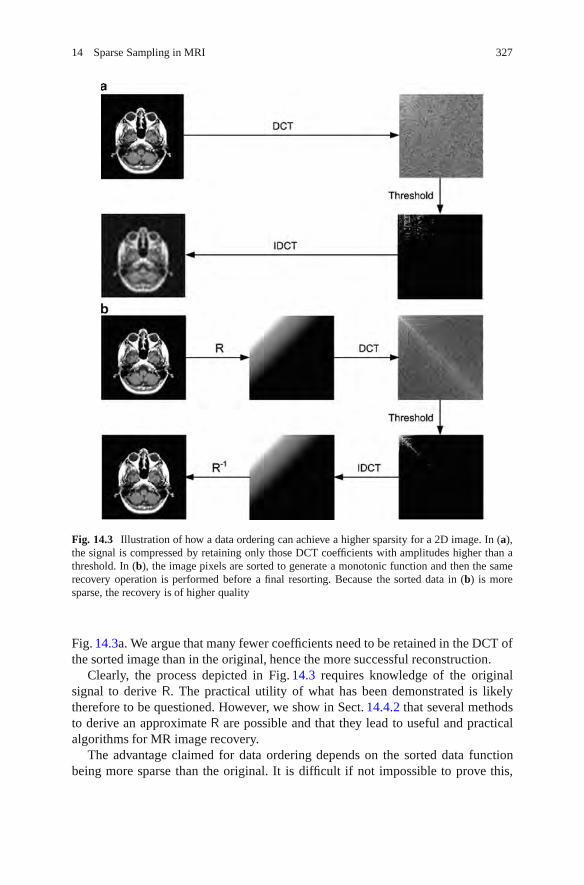
14 Sparse Sampling in MRI 327
Fig. 14.3 Illustration of how a data ordering can achieve a higher sparsity for a 2D image. In (a),the signal is compressed by retaining only those DCT coefficients with amplitudes higher than athreshold. In (b), the image pixels are sorted to generate a monotonic function and then the samerecovery operation is performed before a final resorting. Because the sorted data in (b) is moresparse, the recovery is of higher quality
Fig. 14.3a. We argue that many fewer coefficients need to be retained in the DCT ofthe sorted image than in the original, hence the more successful reconstruction.
Clearly, the process depicted in Fig. 14.3 requires knowledge of the originalsignal to derive R. The practical utility of what has been demonstrated is likelytherefore to be questioned. However, we show in Sect. 14.4.2 that several methodsto derive an approximate R are possible and that they lead to useful and practicalalgorithms for MR image recovery.
The advantage claimed for data ordering depends on the sorted data functionbeing more sparse than the original. It is difficult if not impossible to prove this,

328 P.J. Bones and B. Wu
Fig. 14.4 Examples whichshow the higher sparsity thatdata ordering can achieve for2D images: (a) a set of 5original images; (b) thenumber of DCT coefficientsneeded to achieve areconstruction of each imagewith a relative mean squareerror (RMSE) ≤ 1%; (c) theimage after a data orderingoperation; and (d) the numberof DCT coefficients needed toachieve a reconstruction ofthe ordered image withRMSE≤ 1%
but experiments indicate that in virtually all cases it is true. In Fig. 14.4, we showa set of 2D example images; three are typical brain axial slices (128× 128 pixels)while the others are popular test images (200×200 pixels). A data sorting operationwas performed on each image such that the highest intensity pixel was positioned inthe top left corner and the lowest intensity pixel in the bottom right corner. A simplealgorithm arranged the others in a type of raster which achieved the “wedge” imagesshown in column (c). Clearly, other algorithms for arranging the sorted pixels arepossible. To the right of each image in columns (b) and (d) is the number of DCT
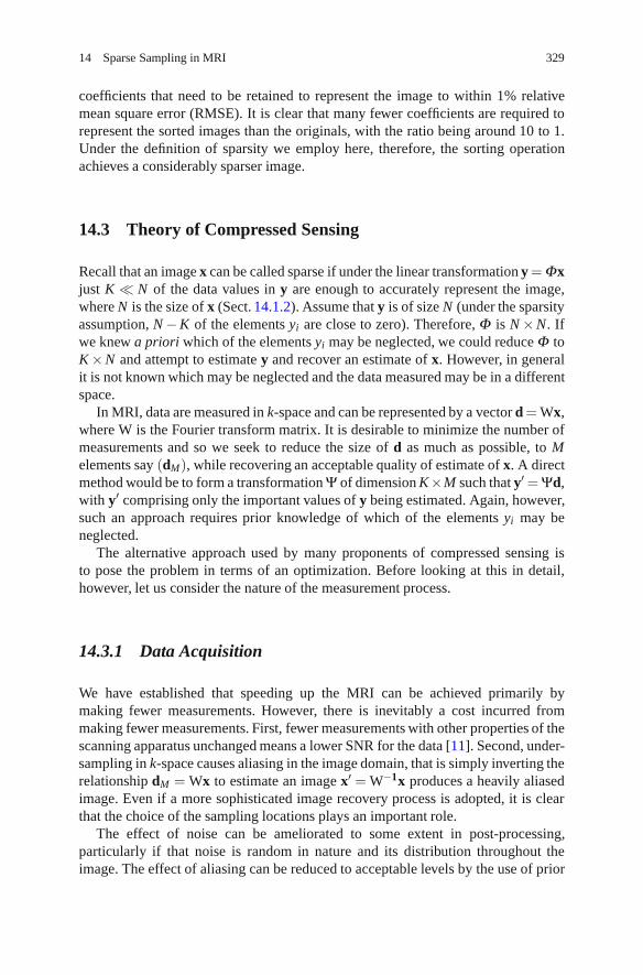
14 Sparse Sampling in MRI 329
coefficients that need to be retained to represent the image to within 1% relativemean square error (RMSE). It is clear that many fewer coefficients are required torepresent the sorted images than the originals, with the ratio being around 10 to 1.Under the definition of sparsity we employ here, therefore, the sorting operationachieves a considerably sparser image.
14.3 Theory of Compressed Sensing
Recall that an image x can be called sparse if under the linear transformation y = Φxjust K � N of the data values in y are enough to accurately represent the image,where N is the size of x (Sect. 14.1.2). Assume that y is of size N (under the sparsityassumption, N −K of the elements yi are close to zero). Therefore, Φ is N ×N. Ifwe knew a priori which of the elements yi may be neglected, we could reduce Φ toK ×N and attempt to estimate y and recover an estimate of x. However, in generalit is not known which may be neglected and the data measured may be in a differentspace.
In MRI, data are measured in k-space and can be represented by a vector d = Wx,where W is the Fourier transform matrix. It is desirable to minimize the number ofmeasurements and so we seek to reduce the size of d as much as possible, to Melements say (dM), while recovering an acceptable quality of estimate of x. A directmethod would be to form a transformation Ψ of dimension K×M such that y′ = Ψd,with y′ comprising only the important values of y being estimated. Again, however,such an approach requires prior knowledge of which of the elements yi may beneglected.
The alternative approach used by many proponents of compressed sensing isto pose the problem in terms of an optimization. Before looking at this in detail,however, let us consider the nature of the measurement process.
14.3.1 Data Acquisition
We have established that speeding up the MRI can be achieved primarily bymaking fewer measurements. However, there is inevitably a cost incurred frommaking fewer measurements. First, fewer measurements with other properties of thescanning apparatus unchanged means a lower SNR for the data [11]. Second, under-sampling in k-space causes aliasing in the image domain, that is simply inverting therelationship dM = Wx to estimate an image x′ = W−1x produces a heavily aliasedimage. Even if a more sophisticated image recovery process is adopted, it is clearthat the choice of the sampling locations plays an important role.
The effect of noise can be ameliorated to some extent in post-processing,particularly if that noise is random in nature and its distribution throughout theimage. The effect of aliasing can be reduced to acceptable levels by the use of prior

330 P.J. Bones and B. Wu
Fig. 14.5 The transform point spread functions (TPSFs) corresponding to one 2D DWT coeffi-cient with random and regular sampling patterns. (a) Original 128× 128 axial image; (b) TPSFfor random k-space sampling; (c) TPSF for regular k-space sampling (showing clear aliasing); (d)low-resolution image formed from 1/16 k-space data; (e) TPSF for random k-space sampling withdata ordering; and (f) TPSF for regular k-space sampling with data ordering
information. However, the pattern of undersampling plays a particularly importantrole. In CS, random sampling patterns are often employed [3, 12]. In Fig. 14.5, weillustrate the important roles that both random sampling patterns and data orderingcan play. Figure 14.5a is the original 128 × 128 axial brain image formed froma fully sampled k-space dataset. Two subsets of the k-space samples were takenby a random pattern and a regular pattern. A DWT was formed (Debauchies-4wavelets) in each case and one coefficient was chosen to be estimated from theundersampled k-space data. Figure 14.5b, c shows the estimates in the DWT domainfor random and regular undersampling patterns, respectively. Lustig, Donoho, andPauly [13] refer to this type of plot as the “transform point spread function” (TPSF).In Fig. 14.5b, the coefficient is estimated with relatively little aliasing, whereas inFig. 14.5c the process generates several aliases for the coefficient. Many authorswho have written on CS describe this as an “incoherence” property [3, 12, 13].
The remainder of Fig. 14.5 illustrates what happens when data ordering isintroduced into the process, with the ordering based on the low-resolution re-construction shown in Fig. 14.5d (formed from the center 1/16 of the k-spacedata). Figure 14.5e, f shows the TPSF for random and regular undersamplingpatterns, respectively, with data ordering and reordering included. In this case, littledifference is seen between random and regular k-space undersampling patterns, withrelatively minor aliasing occurring in both cases. We believe this indicates that thedata ordering itself introduces the incoherence property. In Sect. 14.4.2 below, werelate our experience with a number of different sampling strategies.

14 Sparse Sampling in MRI 331
14.3.2 Signal Recovery
Assuming that we have chosen a sampling strategy for the k-space data and atransform Φ under which the true image is expected to be sparse, we seek a solutionx′ as close as possible to x, which is constrained in two ways:
1. The solution is consistent with the data dM
2. The solution is sparse under the transformation Φ
Condition 1 can be achieved in principle at least by minimizing the power ofthe error between the measurements and the values at those measurement points,which are predicted by the imaging model for the current image estimate, that is byminimizing the squared norm ||dM −WMx′||2. Such squared norm minimizationshave formed the backbone of image recovery for many years [14].
Condition 2 above implies a minimization of the quantity ||Φx′||0, that is thenumber of nonzero elements in Φx′. However, this minimization is computationallyintractable [4, 15]. It turns out that a minimization of the quantity ||Φx′||1, thatis the first norm of the transformed image estimate, can achieve Condition 2remarkably well [4,16]. The l1 norm applied here has the effect of pushing negligiblecoefficients toward zero while retaining larger components accurately. This is incontrast with a squared norm which tends to penalize large coefficients.
As explained in the previous section, the random sampling patterns which offeradvantages in CS do generate noise-like artifacts. Therefore in our experience, it isalso useful to apply a further constraint:
3. The solution is piecewise smooth
Minimizing the total variation (TV), that is the sum of the magnitudes of differencesbetween each pixel and its immediate neighbors, has been shown to be effective atmeeting Condition 3. We denote the total variation for image vector y, TV(y).
The minimization problem can now be posed: Find an estimate for the requiredimage x′ by minimizing
||dM −WMx′||2 +λ ||Φx′||1 + β TV(x′)
where λ and β are positive constants used to control the relative importance ofthe constraints being placed on the solution. A method such as conjugate gradientminimization is suitable to solve the problem. We have employed the SparseMRIpackage provided by [13] as part of the very comprehensive resource on compressedsensing provided by Rice University (see http://dsp.rice.edu).
14.4 Progress in Sparse Sampling for MRI
In this section, we briefly review the progress made to date in applying the principlesof sparse sampling to MRI. We first review the important developments that haveappeared in the literature. We believe that the biggest single contribution came

332 P.J. Bones and B. Wu
from Lustig, Donoho, and Pauly [13]. This group has continued to make valuablecontributions. Our own contributions, in the form of two new algorithms forapplying sparse sampling in MRI, are then presented.
14.4.1 Review of Results from the Literature
Prior to the introduction of compressed sensing, exploiting signal sparseness byutilizing the l1 norm constraint started in mid-1980s when Santosa, Symes, andRaggio [17] utilized an l1 norm to recover a sparse series of spikes from the aliasedrepresentation that resulted from sub-Nyquist sampling in the Fourier domain.A similar experiment was implemented by Donoho [18] using soft thresholding,where the individuals in a sparse series of spikes were recovered sequentially inthe order of the descending magnitude: the strongest component was first recoveredand its aliasing effects were then removed to reduce the overall aliasing artifactsto allow the next strongest component to be recovered, and so on. These simplenumerical experiments in fact have the same nature as the application of the moderncompressed sensing technique in contrast-enhanced magnetic resonance angiogra-phy (CE-MRA). In CE-MRA, the contrast-enhanced regions to be recovered can beusefully approximated as isolated regions residing within a 2D plane, and hence theuse of simple l1 norm suffices in recovering the contrast-enhanced angiogram.
Another application of the l1 norm before compressed sensing is in the use ofTV filter [19], which imposes a l1 norm in gradient magnitude images (GMI), orthe gradient of the image. As discussed previously, l1 norm promotes the strongcomponents while penalizing weak components. In the operations on the GMI,the TV operator suppresses small gradient coefficients, whereas it preserves largegradient coefficients. The former are considered as noise to be removed, whereasthe latter are considered to be part of the image features (edges) that need to beretained; hence, TV can serve as an edge-preserving denoising tool. TV itself canbe employed as a powerful constraint for recovering images from undersampleddata sets. In [20], TV is employed to recover MR images from undersampledradial trajectory measurements; Sidky and Pan [21] investigated the use of TV inrecovering computed tomography images from limited number of projection angles.
The formal introduction of compressed sensing into MRI methods was madeby Lustig, Donoho, and Pauly in 2007 [13]. Their key contribution is the explicituse of a different transform domain for appropriate application of the l1 norm.Both the sparse set of spikes and the TV filter mentioned previously are specialinstances of the general transform-based compressed sensing setup. The authorsidentified the use of DWT and DCT as suitable transform bases for applicationin MR images, as evidenced by their sparse representation under DWT and DCT.A reconstruction framework was given, which converts the CS formulation into aconvex optimization problem and hence allows for computational efficiency. Theauthors also spelt out that a key requirement in data measurement for successfulcompressed sensing recovery is to achieve incoherent aliasing. In MRI, such a

14 Sparse Sampling in MRI 333
requirement can be satisfied by employing a pseudorandom data acquisition patternon Cartesian k-space grid. The idea of compressed sensing has received muchattention thereafter and has been extended to the use of non-Cartesian trajectoriessuch as radial [20] and spiral [22].
Another place where a high level of sparseness exists is the temporal domainof dynamic MRI. Not only does each individual temporal frame have inherentsparseness under the appropriate transform, and hence allows undersampling usingcompressed sensing, there also exists a high level of redundancy in the time domaindue to the generally slow object variation over time. Such redundancy can beexploited in terms of its sparseness under appropriate transform to allow under-sampling in the temporal domain. In fact, this idea has been well exploited prior tothe use of compressed sensing: Fourier-encoding the overlaps using the temporaldimension (UNFOLD) [23], k-t broad-use linear acquisition speed-up technique(k-t BLAST) [24] and k-t focal underdetermined system solver (k-t FOCUSS, [25])are all good examples of this. They all include an additional temporal frequencydimension in addition to the spatial frequency dimensions of the data set, andutilize the sparseness in the resulting spatial–temporal frequency domain. In fact, k-tFOCUSS was later shown to be a general implementation of compressed sensing byinherently utilizing the l1 norm constraint. In [26], compressed sensing is explicitlyapplied in the additional temporal dimension to in MR cardiac imaging, and it wasshown to outperform the k-t BLAST method.
In general, the application of compressed sensing to MRI is a recently emergedand fast developing area. The use of the l1 norm in the appropriate domain, whichis the core of compressed sensing, can be used as a general regularization constraintin many cases. One good example is in the conjoint use of parallel imaging, whichnormally faces the penalty of reduced SNR with reduced sampling density. The l1norm regularization intrinsically suppresses noise and hence offers complementarycharacteristics to those of parallel imaging [27].
14.4.2 Results from Our Work
Our own work in applying sparse sampling in MRI has led to the development of twonew algorithms: Prior estimate-based compressed sensing (PECS) and sensitivityencoding with compressed sensing (SENSECS). PECS has been demonstrated inboth brain imaging, that is imaging of a static structure, and in contrast-enhancedangiography, that is dynamic imaging as part of a pilot study on normal volunteers[28, 29]. SENSECS has been demonstrated in brain imaging [27]. We brieflysummarize the work in the remainder of this section.
14.4.2.1 PECS
The success of compressed sensing is determined by the sparsity of the underlyingsignal. In our experience to date, the sparsest representation of a typical MRI

334 P.J. Bones and B. Wu
a
b
c
Fig. 14.6 Presentation of an argument for the approximate ordering process incorporating priorknowledge into PECS recovery. Figure (b) depicts the computation of an approximate data orderfrom a low-resolution version of the signal. Figure (a) depicts the use of that sampling orderon the original signal. Figure (c) depicts the effect of sorting on the discrepancies between theoriginal signal and the prior knowledge. After transformation, the large amplitude coefficientsretain information about the sorting prior, while the smaller coefficients are mainly associatedwith the discrepancies between the original and low-resolution signals
anatomical image is obtained by ordering the set of pixel (or voxel) amplitudesas described in Sect. 14.2.3. Assume that a set of undersampled k-space data havebeen collected with a particular MRI sequence with the purpose of forming a high-resolution image. In addition, a prior estimate is available of the image, for examplea low-resolution image. In PECS, the prior estimate of the image is first used toderive a data ordering, R′; compressed sensing is used to recover an image fromthe measured k-space data, incorporating the approximate ordering (to promotesparsity) and a TV minimization (to promote piecewise smoothness in the resultingimage). The process is illustrated in Fig. 14.6 for the case of a 1D signal. Recall fromSect. 14.2.3 that ordering the amplitudes of a signal into a monotonic function allowsthat signal to be represented by fewer coefficients under an appropriate transform(DCT or DWT, say). In this case the approximate ordering, R′, is derived from alow resolution (low pass filtered) version of the signal. When R′ is applied to thehigh resolution data, the result is a highly noisy signal which only approximatesin form to a monotonic function. Under the transform the largest coefficients
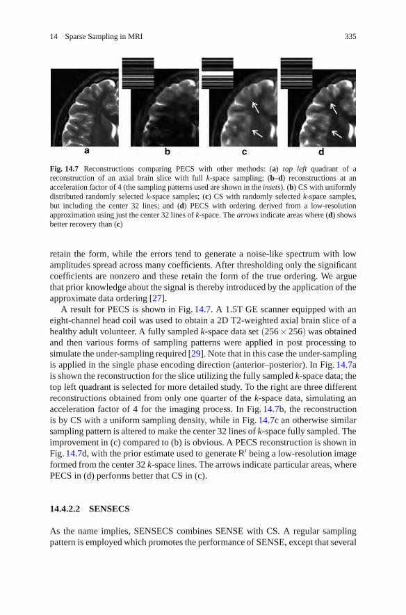
14 Sparse Sampling in MRI 335
Fig. 14.7 Reconstructions comparing PECS with other methods: (a) top left quadrant of areconstruction of an axial brain slice with full k-space sampling; (b–d) reconstructions at anacceleration factor of 4 (the sampling patterns used are shown in the insets). (b) CS with uniformlydistributed randomly selected k-space samples; (c) CS with randomly selected k-space samples,but including the center 32 lines; and (d) PECS with ordering derived from a low-resolutionapproximation using just the center 32 lines of k-space. The arrows indicate areas where (d) showsbetter recovery than (c)
retain the form, while the errors tend to generate a noise-like spectrum with lowamplitudes spread across many coefficients. After thresholding only the significantcoefficients are nonzero and these retain the form of the true ordering. We arguethat prior knowledge about the signal is thereby introduced by the application of theapproximate data ordering [27].
A result for PECS is shown in Fig. 14.7. A 1.5T GE scanner equipped with aneight-channel head coil was used to obtain a 2D T2-weighted axial brain slice of ahealthy adult volunteer. A fully sampled k-space data set (256×256) was obtainedand then various forms of sampling patterns were applied in post processing tosimulate the under-sampling required [29]. Note that in this case the under-samplingis applied in the single phase encoding direction (anterior–posterior). In Fig. 14.7ais shown the reconstruction for the slice utilizing the fully sampled k-space data; thetop left quadrant is selected for more detailed study. To the right are three differentreconstructions obtained from only one quarter of the k-space data, simulating anacceleration factor of 4 for the imaging process. In Fig. 14.7b, the reconstructionis by CS with a uniform sampling density, while in Fig. 14.7c an otherwise similarsampling pattern is altered to make the center 32 lines of k-space fully sampled. Theimprovement in (c) compared to (b) is obvious. A PECS reconstruction is shown inFig. 14.7d, with the prior estimate used to generate R′ being a low-resolution imageformed from the center 32 k-space lines. The arrows indicate particular areas, wherePECS in (d) performs better that CS in (c).
14.4.2.2 SENSECS
As the name implies, SENSECS combines SENSE with CS. A regular samplingpattern is employed which promotes the performance of SENSE, except that several

336 P.J. Bones and B. Wu
Fig. 14.8 Reconstructions comparing SENSECS with other methods at high acceleration factors(shown in the top left of the reconstructions): (a) reconstruction of an axial brain slice with fullk-space sampling; in the lower section of the figure, the left column is SENSE, the center columnis CS, and the right column is SENSECS. Note that the SENSECS reconstructions use the SENSEreconstructions to derive the data sorting order
additional lines are sampled at the center of k-space. SENSE is applied to achievean intermediate reconstruction [11]. Because of the high acceleration factor beingused, the image is likely to be quite noisy. The noise is in part at least due to theimperfect knowledge available of the sensitivities of the individual receiver coils.An approximate sorting order R′ is derived from the intermediate SENSE-derivedimage. Then PECS is performed with the same set of k-space data and using R′.
Again, a single set of results is shown for the new algorithm in Fig. 14.8. Thesame set of data as described above in this section was used and the fully sampledk-space data was again undersampled in postprocessing [29]. High accelerationfactors of 5.8 and 6.5 were simulated. In Fig. 14.8a is shown the reconstruction forthe slice utilizing the fully sampled k-space data; the top left quadrant is selected for

14 Sparse Sampling in MRI 337
Fig. 14.9 The application of PECS to CE-MRA is illustrated. Samples in k-space samples areacquired progressively by means of different randomly selected subsets (top row). A combinationof a set of the acquisitions is used to achieve a “reference” image which is sorted to derive R.PECS is applied to each of the (high acceleration factor) subsets using R. The result (bottom right)is a sequence of relatively high time resolution images. The arrow indicates a region in one of theoutput frames, which does not show an artifact which appears in the reference image
more detailed study. In each of the two lower rows are three different reconstructionsobtained from a fraction of the k-space data, simulating the acceleration factorsindicated. In the left column are shown the SENSE reconstructions, which areclearly noisy and unlikely to be diagnostically useful. CS reconstructions are shownin the center column; in this case, the sampling pattern employed was designedspecifically for CS. The results are superior to the SENSE reconstructions, butsomewhat blurred in appearance. SENSECS reconstructions are shown in the rightcolumn; they show better fidelity than the other reconstructions and diagnosticallyuseful results up to at least an acceleration factor of 6.5. Note that the imagesobtained by SENSE were used to derive the sorting order here.
14.4.2.3 PECS Applied to CE-MRA
The PECS method has been extended to enable it to be applied to CE-MRA.There is a strong desire in CE-MRA to increase the temporal resolution, that isto increase the acceleration factor in image acquisition and reconstruction. Thealgorithm is depicted in Fig. 14.9. Note that the depiction is for 3D imaging, sothe sampling patterns depicted correspond to the two phase encoding directions.In the first acquisition, a small number of k-space samples (corresponding toa high acceleration factor) are acquired at pseudo-random locations; a secondacquisition takes the same number of samples, again randomly distributed, but ata different subset of k-space locations; the acquisitions proceed in this manner until

338 P.J. Bones and B. Wu
all of k-space is filled, then the sequence is repeated. To improve sparsity, datafor a “background” image can be collected before the contrast agent is injected,and those sample values subtracted from the corresponding samples collected asthe contrast agent moves through the vessels. Combining the data from severalcontiguous acquisitions allows a fully sampled “reference” image to be made (afterbackground subtraction), but it has low temporal resolution and may suffer fromartifacts caused by the dynamically changing nature of the volume being imaged.It is adequate, however, to generate an approximate sorting order R. That orderingis used in applying PECS to individual acquisition frames (again after backgroundsubtraction) to achieve a high frame rate sequence of reconstructions. The arrows inthe sample images lower right highlight how features, which appear in the relativelyartifact filled reference image. Results with the method have been encouraging upto acceleration factors of 12 (for an eight-channel receiver coil system) [29].
14.5 Prospects for Future Developments
We have presented some preliminary and very encouraging results for incorporatinga data ordering step in the recovery of MR images by compressed sensing. Thereremains considerable scope for putting this nonlinear processing on a firm theoret-ical footing. Candes and others have provided such rigor to the basic compressedsensing recovery of certain classes of image [3, 4], but no such attention has toour knowledge been directed at the data ordering and its use in incorporating priorknowledge.
We have demonstrated the exploitation of several forms of sparsity above.Briefly, this includes the sparsity achieved by ordering the image into a monotonicfunction, the use of a compressive transform such as DCT or DWT, and thesubtraction of the contribution to signal from static structures in dynamic CE-MRA.Other authors have likewise exploited piecewise homogeneity. Given that CS isrelatively new as a practical method in signal processing, it seems likely thatother transforms may be available, or as yet undiscovered, which may allow moregains to be made. Our work and the work of many others in the area of applyingsparse sampling in MRI suggests that it has a bright future and we should see themanufacturers of MRI scanning systems incorporating some of the algorithms basedon sparse sampling soon.
References
1. McRobbie, D.W., Moore, E.A., Graves, M.J: MRI from Picture to Proton. CambridgeUniversity Press, Cambridge (2003)
2. Bernstein, M.A., King, K.F., Zhou, X.J.: Handbook of MRI Pulse Sequences. ElsevierAcademic, Amsterdam (2004)

14 Sparse Sampling in MRI 339
3. Candes, E., Romberg, J., Tao, T.: Robust uncertainty principles: exact signal reconstructionfrom highly incomplete frequency information. IEEE Trans. Inf. Theory 52, 489–509 (2006)
4. Baraniuk, B.: Compressive sensing. IEEE Signal Process. Mag. 24, 118–121 (2007)5. Geman, S., Geman, D.: Stochastic relaxation, Gibbs distributions, and the Bayesian restoration
of images. IEEE Trans. Pat. Anal. Mach. Intel. 6, 721–741 (1983)6. Hu, X., Johnson, V., Wong, W.H., Chen, C-T.: Bayesian image processing in magnetic
resonance imaging. Magn. Res. Imaging 9, 611–620 (1991)7. Strang, G.: The discrete cosine transform. SIAM Rev. 41, 135–147 (1999)8. Velho, L., Frery, A., Gomes, J.: Image Processing for Computer Graphics and Vision, Ch. 9:
Multiscale Analysis and Wavelets. Springer, London (2008)9. Adluru, G., DiBella, E.V.R.: Reordering for improved constrained reconstruction from under-
sampled k-space data. Int. J. Biomed. Imaging 2008, 341684 (2008)10. Wu, B., Millane, R.P., Watts, R., Bones P.J.: Applying compressed sensing in parallel MRI. In:
Proc. 16th Ann. Meet. ISMRM, Toronto, p. 1480 (2008)11. Pruessmann, K.P., Weiger, M., Scheidegger, M.B., Boesiger, P.: SENSE: sensitivity encoding
for fast MRI. Magn. Reson. Med. 42, 952–962 (1999)12. Donoho, D.L.: Compressed sensing. IEEE Trans. Inf. Theory 52, 1289–1306 (2006)13. Lustig, M., Donoho, D., Pauly, J.M.: Sparse MRI: the application of compressed sensing for
rapid MR imaging. Magn. Reson. Med. 58, 1182–1195 (2007)14. Jain, A.K.: Fundamentals of Digital Image Processing. Prentice-Hall, Englewood Cliffs,
NJ (1989)15. Candes, E., Romberg, J.: Sparsity and incoherence in compressive sampling. Inverse Probl. 23,
969–985 (2007)16. Candes, E., Wakin, M.B.: An introduction to comprehensive sampling. IEEE Signal Process.
Mag. 25, 21–30 (2008)17. Santosa, F., Symes, W.W., Raggio, G.: Inversion of band-limited reflection seismograms using
stacking velocities as constraints. Inverse Probl. 3, 477–499 (1987)18. Donoho, D.L.: De-noising by soft-thresholding. IEEE Trans. Inf. Theory 41, 614–627 (1995)19. Rudin, L.I., Osher, S., Fatemi, E.: Nonlinear total variation based noise removal algorithms.
Physica D 60, 259–268 (1992)20. Block, K.T., Uecker, M., Frahm, J.: Undersampled radial MRI with multiple coils. Iterative
image reconstruction using a total variation constraint. Magn. Reson. Med. 57, 1086–1098(2007)
21. Sidky, E.Y., Pan, X.: Image reconstruction in circular cone-beam computed tomography byconstrained, total-variation minimization. Phys. Med. Biol. 53, 47–77 (2008)
22. Seeger, M., Nickisch, H., Pohmann, R., Scholkopf, B.: Optimization of k-space trajectories forcompressed sensing by Bayesian experimental design. Magn. Reson. Med. 63, 116–126 (2010)
23. Madore, B., Glover, G.H., Pelc, N.J.: Unaliasing by fourier-encoding the overlaps using thetemporal dimension (UNFOLD), applied to cardiac imaging and fMRI. Magn. Reson. Med.42, 813–828 (1999)
24. Taso, J., Boesiger, P., Pruessmann, K.P.: k-t BLAST and k-t SENSE: dynamic MRI with highframe rate exploiting spatiotemporal correlations. Magn. Reson. Med. 50, 1031–1042 (2003)
25. Jung, H., Sung, K., Nayak, K.S., Kim, E.Y., Ye, J.C.: k-t FOCUSS: a general compressedsensing framework for high resolution dynamic MRI. Magn. Reson. Med. 61, 103–116 (2009)
26. Gamper, U., Boesiger, P., Kozerke, S.: Compressed sensing in dynamic MRI. Magn. Reson.Med. 50, 1031–1042 (2003)
27. Wu, B., Millane, R.P., Watts, R., Bones, P.J.: Prior estimate-based compressed sensing inparallel MRI. Magn. Reson. Med. 65, 83–95 (2011)
28. Wu, B., Bones, P.J., Millane, R.P., Watts, R.: Prior estimated based compressed sensing incontrast enhanced MRA. In: Proc. 18th Ann. Meet., ISMRM, Stockholm (2010)
29. Wu, B.: Exploiting Data Sparsity in Parallel Magnetic Resonance Imaging. PhD thesis,University of Canterbury, Christchurch, New Zealand, 2009

Chapter 15Digital Processing of Diffusion-Tensor Imagesof Avascular Tissues
Konstantin I. Momot, James M. Pope, and R. Mark Wellard
15.1 Introduction
Diffusion is the process that leads to the mixing of substances as a result ofspontaneous and random thermal motion of individual atoms and molecules. It wasfirst detected by the English botanist Robert Brown in 1827, and the phenomenonbecame known as ‘Brownian motion’. More specifically, the motion observed byBrown was translational diffusion – thermal motion resulting in random variationsof the position of a molecule. This type of motion was given a correct theoreticalinterpretation in 1905 by Albert Einstein, who derived the relationship betweentemperature, the viscosity of the medium, the size of the diffusing molecule, and itsdiffusion coefficient [1]. It is translational diffusion that is indirectly observed in MRdiffusion-tensor imaging (DTI). The relationship obtained by Einstein provides thephysical basis for using translational diffusion to probe the microscopic environmentsurrounding the molecule.
In living systems, translational diffusion is vital for the transport of water andmetabolites both into and around cells. In the presence of a concentration gradient,diffusion results in the mixing of substances: The molecules of a compoundon average tend to move from areas of high concentration into areas of lowconcentration, resulting in a net transport of the compound in the direction of thegradient. A classic example of this is the spontaneous mixing of a dyestuff into astationary solvent.
Diffusive mass transport can serve as the basis for the measurement of moleculardiffusion: a concentration gradient is artificially created, and its equilibrationwith time observed (Fig. 15.1). This method of measuring diffusion is not alwaysphysically relevant because a concentration gradient is neither required for diffusion
K.I. Momot (�)Queensland University of Technology, Brisbane, Australiae-mail: [email protected]
G. Dougherty (ed.), Medical Image Processing: Techniques and Applications, Biologicaland Medical Physics, Biomedical Engineering, DOI 10.1007/978-1-4419-9779-1 15,© Springer Science+Business Media, LLC 2011
341

342 K.I. Momot et al.
Fig. 15.1 Diffusion in thepresence of a concentrationgradient C(x, t) gives rise to anet flux or flow of particlesJ(x, t) from high to lowconcentration
nor always present. The majority of DTI applications are based on the diffusionof water, whose concentration is essentially uniform in extracellular and intracel-lular microenvironments of living organisms. Diffusion of molecules of the samesubstance in the absence of a concentration gradient is known as ‘self-diffusion’.It is self-diffusion that is observed in DTI. Self-diffusion can be measured bythe technique of Pulsed Field Gradient Nuclear Magnetic Resonance (PFG-NMR),which is exquisitely sensitive to the microstructural environment of nuclear spins.(Other examples of applications of magnetic resonance to tissues can be seen inChapters 5, 9, and 10.) In recent years, PFG-NMR has been increasingly combinedwith magnetic resonance imaging (MRI) to study diffusion of water protons inbiological tissues for diagnosis of stroke and multiple sclerosis, for white matterfiber tracking in the brain, muscle fiber tracking, and other applications.
While no concentration gradient is necessary for DTI, the notion of a concen-tration gradient is instructive for understanding how DTI works. In an isotropicmedium such as bulk water, the process of diffusion is itself isotropic and can bedescribed by a scalar diffusion coefficient D. If we were to “label” a subset ofmolecules, the flux of the labeled molecules would be governed by Fick’s first lawof diffusion:
J(r,t) = −D ∇C(r,t) ≡−D
(i∂C∂x
+ j∂C∂ y
+ k∂C∂ z
). (15.1)
Here, C(r,t) is the spatial concentration profile of the labeled molecules; D isthe diffusion coefficient; and J is the flux of particles, defined as the amount ofsubstance that flows through a unit area per unit time. The meaning of (15.1) isthat in isotropic media the flux occurs strictly in the direction of the concentrationgradient. Combining (15.1) with the conservation of mass and the assumption that Dis independent of concentration yields Fick’s second law of diffusion or the diffusionequation:
∂ C(r,t)∂ t
= D ∇2C(r,t) ≡ D
(∂ 2C∂x2 +
∂ 2C∂y2 +
∂ 2C∂ z2
). (15.2)

15 Digital Processing of Diffusion-Tensor Images of Avascular Tissues 343
Diffusion in biological tissues is substantially different from isotropic diffusion.Tissues are intrinsically heterogeneous: there are barriers to free diffusion ofwater molecules arising from the presence of macromolecules, organelles, cellmembranes, and larger scale structures. As a result, diffusion of water moleculesin many tissues is both restricted and anisotropic.
Restricted diffusion results in measurements of the diffusion coefficient givingresults that are dependent on the timescale of the diffusion interval Δ over whichthe measurement is performed. This is known as an ‘apparent diffusion coefficient’(ADC). Besides Δ, the ADC is dependent on the nature and the length scale of theobstructions and is generally smaller than the self-diffusion coefficient of bulk water(D0 = 2.3 ·10−9 m2 s−1 at 25◦C). For example, the ADC of water confined betweenparallel, semipermeable barriers approximately equals D0 at Δ << d2/D0, where dis the separation between the barriers, but decreases to D0/(1+1/P) at Δ >> d2/D0
(where P is the permeability of the barriers) [2].Anisotropic diffusion means that the diffusing molecules encounter less restric-
tion in some directions than others. Diffusion can be anisotropic when the tissuepossesses some form of global alignment. Two well-known examples of anisotropictissues are the white matter of the brain and the heart muscle. In muscles, the globalalignment arises from the elongated form of the muscle cells forming muscle fibers.In white matter, the anisotropy arises from the fact that nerve fiber tracts followspecific pathways. In both these cases, the cellular structures preferentially restrictthe diffusion of water in the direction perpendicular to the fibers. Diffusion is alsoanisotropic in the two tissues that are the focus of this chapter: articular cartilage(AC) and the eye lens. In AC, the anisotropic restrictions to diffusion are imposedby the aligned collagen fibers that form the biomacromolecular “scaffold” of thetissue. In the crystalline eye lens, the restrictions are imposed by the fiber cells.
To take account of anisotropic diffusion, a common approach is to re-write thediffusion equation in terms of a diffusion tensor:
J(r,t) = −D ·∇C(r,t), (15.3)
where the diffusion tensor D is represented by a symmetric and real 3×3 matrix:
D =
⎛⎝ Dxx Dxy Dxz
Dxy Dyy Dyz
Dxz Dyz Dzz
⎞⎠ . (15.4)
In the anisotropic case, Fick’s second law becomes:
∂C∂ t
= ∇ ·D ·∇C ≡(
∂∂x
∂∂y
∂∂ z
)⎛⎝ Dxx Dxy Dxz
Dxy Dyy Dyz
Dxz Dyz Dzz
⎞⎠⎛⎝ ∂/∂ x
∂/∂ y∂/∂ z
⎞⎠C. (15.5)
Note that while the diagonal elements of the diffusion tensor (DT) scaleconcentration gradients and fluxes that are in the same direction, the off-diagonal

344 K.I. Momot et al.
Fig. 15.2 Diffusion ellipsoid as a visual representation of the diffusion tensor. The straight linesradiating from the center of the ellipsoid illustrate two possible choices of the diffusion samplingdirections, as discussed in Sects. 15.2.2 and 15.2.5
elements couple fluxes and concentration gradients in orthogonal directions. Thisis because in the anisotropic case the distribution of diffusional displacementsof molecules tends to follow the geometry of the restricting barriers. This is thephysical basis for using DTI to measure the microscopic morphology of the tissue.In Sects. 15.2.4 and 15.4, we discuss applications of DTI to the eye lens and AC,respectively, as examples.
A convenient way of representing the DT is the diffusion ellipsoid, whichis illustrated in Fig. 15.2. The shape of the ellipsoid represents the directionalasymmetry of the average displacements of the diffusing molecules. The directionsof the principal axes of the ellipsoid characterize the orientation of the DT, whichin turn represents the spatial anisotropy of the restricting barriers imposed by thetissue.
In the isotropic case, the DT is a diagonal matrix:
D =
⎛⎜⎜⎝
D 0 0
0 D 0
0 0 D
⎞⎟⎟⎠ , (15.6)
where D is the isotropic diffusion coefficient. In this case, (15.5) reverts to (15.2),and the ellipsoid in Fig. 15.2 becomes a sphere.

15 Digital Processing of Diffusion-Tensor Images of Avascular Tissues 345
15.2 Acquisition of DT Images
15.2.1 Fundamentals of DTI
DT images can be obtained using Nuclear Magnetic Resonance (NMR). NMRmeasures the frequency of precession of nuclear spins such as that of the proton(1H), which in a magnetic field B0, is given by the Larmor equation:
ω0 = γB0. (15.7)
The key to achieving spatial resolution in MRI is the application of time-dependentmagnetic field gradients that are superimposed on the (ideally uniform) staticmagnetic field B0. In practice, the gradients are applied via a set of dedicated3-axis gradient coils, each of which is capable of applying a gradient in one ofthe orthogonal directions (x, y, and z). Thus, in the presence of a magnetic fieldgradient g,
g =(
∂Bz
∂x,
∂ Bz
∂y,
∂Bz
∂ z
)(15.8)
the magnetic field strength, and hence the precession frequency become positiondependent. The strength of the magnetic field experienced by a spin at position r isgiven by:
B = B0 + g · r (15.9)
The corresponding Larmor precession frequency is changed by the contributionfrom the gradient:
ω(r) =∂φ(r)
∂ t= γ(B0 + g · r). (15.10)
The precession frequency ω is the rate of change of the phase, φ, of a spin – thatis, its precession angle in the transverse plane (Fig. 15.3). Therefore, the time-dependent phase φ is the integral of the precession frequency over time. In MRI, weswitch gradients on and off in different directions to provide spatial resolution, sothe gradients are time dependent and the phase of a spin is given by:
φ(r,t) =t∫
0
ω(r,t ′)dt ′ = γB0t + γt∫
0
g(t ′) · rdt ′. (15.11)
We observe the phase relative to the reference frequency given by (15.7). Forexample if the gradient is applied in the x direction in the form of a rectangular pulseof amplitude gx and duration δ the additional phase produced by the gradients is

346 K.I. Momot et al.
Fig. 15.3 The effect of a magnetic field gradient on precession of spins. A constant magnetic fieldgradient g (illustrated by the blue ramp) applied in some arbitrary direction changes the magneticfield at position r from B0 to a new value B = B0 +g ·r. The gradient perturbs the precession of thespins, giving rise to an additional position-dependent phase φ′, which may be positive or negativedepending on whether the magnetic field produced by the gradient coils strengthens or weakensthe static magnetic field B0
φ′(r,t) = γδ∫
0
gx(t ′)xdt ′ = γδgxx = 2πkxx, (15.12)
where the “spatial frequency” kx = γδgx/2π is also known as the “k value”. It playsan important role in the description of spatial encoding in MRI and can be thoughtof as the frequency of spatial harmonic functions used to encode the image.
In MRI to achieve spatial resolution in the plane of the selected slice (x,y), weapply gradients in both x and y directions sequentially. The NMR signal is thensampled for a range of values of the corresponding spatial frequencies kx and ky.
For one of these gradients (gx, say), this is achieved by keeping the amplitudefixed and incrementing the time t at which the signal is recorded (the process called‘frequency encoding’).
In the case of the orthogonal gradient (gy), the amplitude of the gradient isstepped through an appropriate series of values. For this gradient, the appropriatespatial frequency can be written:
ky = γδ∫
0
gy(t ′)dt ′ = γδgy/2π. (15.13)
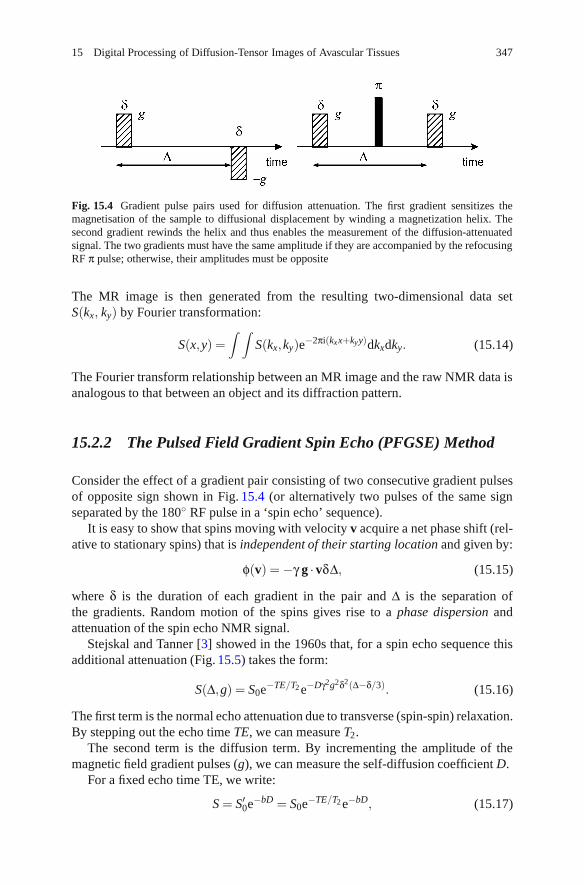
15 Digital Processing of Diffusion-Tensor Images of Avascular Tissues 347
Fig. 15.4 Gradient pulse pairs used for diffusion attenuation. The first gradient sensitizes themagnetisation of the sample to diffusional displacement by winding a magnetization helix. Thesecond gradient rewinds the helix and thus enables the measurement of the diffusion-attenuatedsignal. The two gradients must have the same amplitude if they are accompanied by the refocusingRF π pulse; otherwise, their amplitudes must be opposite
The MR image is then generated from the resulting two-dimensional data setS(kx, ky) by Fourier transformation:
S(x,y) =∫ ∫
S(kx,ky)e−2πi(kxx+kyy)dkxdky. (15.14)
The Fourier transform relationship between an MR image and the raw NMR data isanalogous to that between an object and its diffraction pattern.
15.2.2 The Pulsed Field Gradient Spin Echo (PFGSE) Method
Consider the effect of a gradient pair consisting of two consecutive gradient pulsesof opposite sign shown in Fig. 15.4 (or alternatively two pulses of the same signseparated by the 180◦ RF pulse in a ‘spin echo’ sequence).
It is easy to show that spins moving with velocity v acquire a net phase shift (rel-ative to stationary spins) that is independent of their starting location and given by:
φ(v) = −γ g ·vδΔ, (15.15)
where δ is the duration of each gradient in the pair and Δ is the separation ofthe gradients. Random motion of the spins gives rise to a phase dispersion andattenuation of the spin echo NMR signal.
Stejskal and Tanner [3] showed in the 1960s that, for a spin echo sequence thisadditional attenuation (Fig. 15.5) takes the form:
S(Δ,g) = S0e−TE/T2 e−Dγ2g2δ2(Δ−δ/3). (15.16)
The first term is the normal echo attenuation due to transverse (spin-spin) relaxation.By stepping out the echo time TE, we can measure T2.
The second term is the diffusion term. By incrementing the amplitude of themagnetic field gradient pulses (g), we can measure the self-diffusion coefficient D.
For a fixed echo time TE, we write:
S = S′0e−bD = S0e−TE/T2 e−bD, (15.17)

348 K.I. Momot et al.
Fig. 15.5 A pulsed fieldgradient spin echo (PGSE)sequence showing the effectsof diffusive attenuation onspin echo amplitude
where
b = γ2g2δ2(
Δ− δ3
). (15.18)
The ADC is then given by:
ADC = −ln
(SS′0
)/b (15.19)
For the case of anisotropic diffusion described by a diffusion tensor D, theexpression for the echo attenuation in a PFG spin echo experiment becomes:
S(Δ,g) = S′0e−γ2g·D·gδ2(Δ−δ/3), (15.20)
where g = (gx,gy,gz) is the gradient vector, and the scalar product g ·D ·g is definedanalogously to (15.5).
Overall, if diffusion is anisotropic, the echo attenuation will have an orientationdependence with respect to the measuring gradient g. Gradients along the x, y, and zdirections sample, respectively, the diagonal elements Dxx, Dyy, and Dzz of the DT.In order to sample the off-diagonal elements, we must apply gradients in obliquedirections – that is combinations of gx and gy or gy and gz, etc. Because the DTis symmetric, there are just 6 independent elements. To fully determine the DTtherefore requires a minimum of 7 separate measurements – for example:
⎛⎝gx
gy
gz
⎞⎠=
⎛⎝0
00
⎞⎠ ,
⎛⎝ g
00
⎞⎠ ,
⎛⎝0
g0
⎞⎠ ,
⎛⎝0
0g
⎞⎠ ,
1√2
⎛⎝g
g0
⎞⎠ ,
1√2
⎛⎝g
0g
⎞⎠ ,
1√2
⎛⎝0
gg
⎞⎠ .
(15.21)

15 Digital Processing of Diffusion-Tensor Images of Avascular Tissues 349
Fig. 15.6 Spin echodiffusion imaging pulsesequence. “RF” denotes theRF pulses and acquisition.Gradient pulses: S, sliceselection; P, encoding in thePhase direction; R, encodingin the Read direction; D,diffusion gradients
This choice of diffusion gradient directions is illustrated in Fig. 15.2a. We shallrefer to a data set measured with this set of gradients as the minimal diffusion-tensor dataset. As seen below, this is neither the only nor the best choice of DTIgradient directions. Other gradient combinations exist that achieve optimal signal-to-noise ratio (SNR) in the resulting DT images and/or optimal gradient amplifierefficiency (see Sect. 15.2.5). The first measurement with all gradients off is requiredto determine S′0.
15.2.3 Diffusion Imaging Sequences
Diffusion gradients can readily be incorporated in a conventional spin echo MRIsequence as follows (Fig. 15.6).
The sequence is repeated for the appropriate different combinations of gradientsgx, gy, and gz to yield a set of 7 different diffusion weighted images. These are thenused to calculate the elements of the DT, pixel by pixel, to yield 6 images represent-ing the three diagonal elements and 3 off-diagonal elements of the DT. (Because ofthe symmetry of the DT, the off-diagonal elements are duplicated in the 3× 3 DTimage). Once obtained the DT must be diagonalized to obtain the eigenvalues andeigenvectors. For more details, see, for example Basser and Jones [4].
For a given DTI imaging sequence and available MRI hardware, the effects ofT2 relaxation can be minimized by making more efficient use of available gradientpower to maximize b values and reduce the minimum echo time TE. For example by

350 K.I. Momot et al.
ensuring that gradients are applied simultaneously along two axes at the maximumamplitude for each individual axis, the resultant gradient amplitude is increasedby a factor of
√2, while by employing all three basic gradients in an icosahedral
arrangement it is possible to increase the maximum amplitude by Fibonacci’s goldenratio: (1 +
√5)/2 (see e.g. [5] and references therein). This choice of diffusion
gradient directions is illustrated in Fig. 15.2b.For clinical applications of DTI, patient motion can be a serious problem because
even relatively small bulk motions can obscure the effects of water diffusion onthe NMR signal. In such applications, it is common to employ spin echo singleshot echo planar imaging (SS-EPI) sequences that incorporate diffusion weightingin order to acquire an entire DWI data set in a fraction of a second (albeit atsomewhat reduced spatial resolution when compared with more conventional spinecho imaging sequences). Such SS-EPI sequences also have the added advantage ofa relatively high SNR per unit scanning time, allowing a complete DTI data set tobe acquired in 1–2 min. Further improvements in acquisition time and/or SNR canbe achieved by combining such sequences with parallel imaging techniques and/orpartial Fourier encoding of k-space (see e.g. [6] and references therein).
15.2.4 Example: Anisotropic Diffusion of Water in the Eye Lens
We have used the PFGSE method to measure the components of the DT for water(H2O) in human eye lenses [7]. In this case, we were measuring diffusion on atimescale of ∼20ms corresponding to diffusion lengths � =
√2Dt ∼= 10μm with
D = 2.3 · 10−9m2s−1 for bulk water at 20◦C and t = 20ms. This is comparable tothe cell dimensions. Since the cells are fiber-like in shape (i.e., long and thin) withdiameter ∼8μm, we might expect to observe diffusion anisotropy on this timescale.
Note that four of the off-diagonal elements in the (undiagonalized) DT are almostzero. This implies that in this example diagonalization (see Figs. 15.7 and 15.8)involves a simple rotation of axes about the normal to the image plane.
If we assume cylindrical symmetry for the cell fibers within a voxel, then ε = 0and in the principal axes frame we can describe the diffusion in terms of a 2× 2tensor:
D′ ≡(
D⊥ 00 D//
). (15.22)
What is more if we choose the image plane to correspond to the center of symmetryof the lens, we only require one angle θ to describe the orientation of the principalaxis of the DT with respect to the gradients gx and gz, say. Consequently, we onlyrequire four images to calculate D//, D⊥ and θ, corresponding to gradients of 0, gx,gz, and 1√
2(gx + gz).
The next problem is how to display the data, since even in this case of cylindricalsymmetry and a 2× 2 DT, we have 3 parameters to display for each pixel! The

15 Digital Processing of Diffusion-Tensor Images of Avascular Tissues 351
Fig. 15.7 Diffusion tensor images of human eye lenses in vitro from a 29-year-old donor(left column) and an 86-year-old donor (right column) [7]. Top row images are of the raw(undiagonalized) diffusion tensor; those in the bottom row are after diagonalization
method we have developed using MatLab is to display for each pixel a pair oforthogonal lines whose lengths are proportional to D// and D⊥, respectively, withthe direction of the larger component defining the angle θ, viz (Fig. 15.8).
More generally, if the DT does not display cylindrical symmetry, there are 6parameters to define per pixel (three eigenvalues and three Euler angles defining thedirections of the eigenvectors relative to the laboratory frame). In such cases, it maybe necessary to map the principal eigenvalues, the orientations of the eigenvectors,the fractional anisotropy (FA), and the mean eigenvalues (see below) as separatediffusion maps or images in order to visualize the full DT.
15.2.5 Data Acquisition
In situations where time is limited by the need to minimize motion artifacts orto achieve adequate patient throughput, it may be practical only to acquire datafor the minimum number of diffusion gradient combinations required to definethe DT. In other cases, it may be necessary to employ signal averaging to reduce

352 K.I. Momot et al.
Fig. 15.8 2D diffusion tensor images of a human eye lens from a 29-year-old donor: (a) axesof the principal components D// and D⊥ of the diagonalized diffusion tensor with respect to thedirections of the diffusion gradients; (b) quiver plot showing both principal components on thesame scale; (c) and (d) plots of D// and D⊥, respectively
‘sorting bias’ (see below) and/or to acquire data for additional gradient directionsto improve precision in measuring the eigenvalues and eigenvectors of the DTand derived parameters such as the FA. Even for the case where the number ofgradient directions is restricted to the minimum value [6], significant improvementsin precision of DTI-derived parameters can be achieved by appropriate choice ofthose directions [8].
Several authors have investigated optimum strategies for measuring diffusionparameters in anisotropic systems using MRI [4, 5, 8–13]. Jones et al. [9] derivedexpressions for the optimum diffusion weighting (b values) and the optimum ratioof the number of signal acquisitions acquired with high diffusion weighting (NH)to the number (NL) with low or minimum diffusion weighting, for which b∼0.(Note that for an imaging sequence b = 0 is generally not strictly achievable dueto the influence of the imaging gradients, which produce some diffusive attenuationof the signal.) If the effects of transverse relaxation (T2) are ignored, they foundb = 1.09× 3/Tr(D) and NH = 11.3 · NL, where Tr(D) = Dxx + Dyy + Dzz is thetrace of the DT and b here refers to the difference in diffusion weighting betweenhigh and low values (assuming the latter is non-zero). This result applies providedthat the diffusion is not too anisotropic (so that diffusive attenuation is similar inall directions). It compares with the situation of minimum overall imaging timein which each of the 7 combinations of gradient magnitude and direction is appliedonly once, for which clearly NH = 6NL and according to Jones et al. [9] the optimumb = 1.05 ·3/Tr(D). However, these results must be modified to take account of the

15 Digital Processing of Diffusion-Tensor Images of Avascular Tissues 353
effects of T2 relaxation, which results in additional signal attenuation since it isnecessary to operate with a finite echo time TE to allow sufficient time to apply thegradients. For example, in the case of white matter in the human brain, for whichT2∼80ms, Jones et al. [9] find that it is necessary to reduce both the b value and theratio NH/NL to ∼77% of the asymptotic (long T2) values quoted above.
Chang et al. [14] used a first order perturbation method to derive analyticalexpressions for estimating the variance of diffusion eigenvalues and eigenvectorsas well as DTI derived quantities such as the trace and FA of the DT, for a givenexperimental design and over a useful range of SNRs. They also validated theirresults using Monte Carlo simulations.
A number of authors have compared the merits of applying diffusion gradientsin more than the minimum six directions. Some reports [10, 12] have suggestedthere may be no advantage in using more than the minimum number of samplingdirections provided that the selected orientations point to the vertices of anicosahedron [11]. However, a more recent Monte Carlo analysis [5] supports earliersuggestions [13,15] that ∼20–30 unique and evenly distributed sampling directionsare required for robust estimation of mean diffusivity, FA and DT orientation.Batchelor et al. [11] conclude that ‘the recommended choice of (gradient) directionsfor a DT-MRI experiment is . . . the icosahedral set of directions with the highestnumber of directions achievable in the available time.’
The use of multiple sets of magnetic field gradient directions is of particularimportance for applications involving fiber tracking in the brain. Fiber tracking or‘Tractography’ is used to infer axonal connectivity in the white matter of the brain[16–19]. It relies on the fact that the myelin sheaths surrounding neuronal fibersin the white matter restrict water diffusion perpendicular to the direction of thefiber bundles, while diffusion parallel to the nerve fibers is relatively unrestricted.Consequently, the eigenvectors corresponding to the largest eigenvalues reflect the(average) fiber direction within a voxel. By analyzing the directions of the principaleigenvectors in adjacent voxels, it is possible to trace the fiber tracts and inferconnectivity between different regions of the brain. The situation becomes morecomplicated if two or more fiber bundles with significantly different directionsintersect or cross within a voxel due to partial volume effects. (Typical voxeldimensions in DTI∼1–3mm are much larger than the individual white matter tracts∼1–10μm). Behrens et al. [20] estimate that one-third of white matter voxels inthe human brain fall into this category. In such cases, the use of a single DTwill yield a principal diffusion eigenvector that represents a weighted average ofthe individual fiber directions and as such will not correspond to the directionof any of the individual fiber bundles. This problem can be at least partiallyalleviated by acquiring data for multiple gradient directions using high angularresolution diffusion imaging (HARDI) and employing spherical tomographic in-version methods [21] or constrained spherical deconvolution (CSD) techniques [22]to model the resulting DWI data in terms of a set of spherical harmonics ratherthan a single DT. HARDI techniques employ stronger diffusion weighting gradients(b-values ≥ 3,000s/mm2) compared with those ∼1,000s/mm2 more routinelyemployed in clinical DTI. Recently, Tournier et al. [23] using such methods have
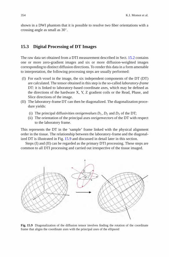
354 K.I. Momot et al.
shown in a DWI phantom that it is possible to resolve two fiber orientations with acrossing angle as small as 30◦.
15.3 Digital Processing of DT Images
The raw data set obtained from a DTI measurement described in Sect. 15.2 containsone or more zero-gradient images and six or more diffusion-weighted imagescorresponding to distinct diffusion directions. To render this data in a form amenableto interpretation, the following processing steps are usually performed:
(I) For each voxel in the image, the six independent components of the DT (DT)are calculated. The tensor obtained in this step is the so-called laboratory-frameDT: it is linked to laboratory-based coordinate axes, which may be defined asthe directions of the hardware X, Y, Z gradient coils or the Read, Phase, andSlice directions of the image.
(II) The laboratory-frame DT can then be diagonalized. The diagonalization proce-dure yields:
(i) The principal diffusivities oreigenvalues D1, D2 and D3 of the DT;(ii) The orientation of the principal axes oreigenvectors of the DT with respect
to the laboratory frame.
This represents the DT in the ‘sample’ frame linked with the physical alignmentorder in the tissue. The relationship between the laboratory-frame and the diagonal-ized DT is illustrated in Fig. 15.9 and discussed in detail later in this section.
Steps (I) and (II) can be regarded as the primary DTI processing. These steps arecommon to all DTI processing and carried out irrespective of the tissue imaged.
Fig. 15.9 Diagonalization of the diffusion tensor involves finding the rotation of the coordinateframe that aligns the coordinate axes with the principal axes of the ellipsoid

15 Digital Processing of Diffusion-Tensor Images of Avascular Tissues 355
(III) In “secondary” processing, the DT image obtained in step (II) is representedas a voxel-by-voxel map of one or more of the following parameters:
Direction of the principal eigenvector.Angle between the principal eigenvector and a specified axis.Principal eigenvalue (maximum diffusivity).Mean eigenvalue (mean diffusivity).Fractional anisotropy.The nonaxial anisotropy parameters of the DT.
The user must decide what DT parameters best enable visualization of the imageacquired.
(IV) In “tertiary” processing, the information from individual voxels is translatedinto “global” characteristics describing the image as a whole. An exampleof such analysis is the nerve fiber tracking used in DTI of the brain or thespinal cord. The voxels of the image are grouped into tracts such that theprincipal eigenvectors of the voxels within a tract form continuous “flow lines”representing a large bundle of axons.
Unlike the primary DTI processing, the secondary and tertiary processing is organ-or tissue dependent. The choice of the processing approaches and the DT metricsis determined by the morphology of the tissue and the information sought aboutthe tissue. In avascular tissues, the objective is to characterize the overall alignmentorder in the tissue rather than identify individual fibers. (The latter is not possiblebecause of the huge number of fibers within a single voxel.) Examples of secondaryprocessing of DT images of cartilage will be presented in Sect. 15.4.
In the following, we provide an overview of the basic principles and themathematics underlying DT image processing. The processing techniques aredescribed without reference to a specific platform and are generally applicable.
15.3.1 Primary DTI Processing: Calculationof the Laboratory-Frame DT
In Sect. 15.2, the signal intensity was represented as a function of the diffusiongradient as shown in (15.20). This representation provides an intuitive and visualexplanation of the diffusive attenuation of the signal in DT images. In practice, it ismore convenient to base DTI processing on the so-called B matrix. Equation(15.20)can be rewritten as follows (15.24):
ln
[S(g)S0
]= −
3
∑i=1
3
∑j=1
bijDij ≡−b : D, (15.23)

356 K.I. Momot et al.
where the indices i, j take the values of x, y, or z. The B matrix, b, is a 3× 3 realsymmetric matrix. In the spin-echo experiment, its values are given by
bij = γ2gig jδ2(Δ− δ/3), (15.24)
where gi, g j are the components of the diffusion gradient vector g. The B matrix isan extension of the quantity b introduced in (15.18) to multiple gradient directions.
There are two main advantages to using the B matrix rather than the gradientvectors for processing of DT images. First, the functional form of the signalattenuation is dependent on the DTI pulse sequence used. Equation(15.20) appliesto the basic spin-echo pulse-sequence with rectangular diffusion gradients. Theattenuation expression is different if a different pulse sequence or nonrectangulardiffusion gradients are used [25]. Calculation of the attenuation factor can bedifficult and time-consuming for the general pulse sequence [26]. Fortunately, theattenuation equation is amenable to algorithmic, software-based calculation. Whenthe attenuation factor is kept in the simple and general form given by (15.23), anypulse sequence-specific factors can be incorporated into the B matrix as part of thealgorithm. The software of most modern MRI spectrometers is capable of automaticcalculation of the B matrix for any pulse sequence installed on the spectrometer,eliminating the need for the operator to perform this time-consuming calculationmanually.
The second advantage of using the B matrix is that it facilitates accounting forcontribution to the diffusive attenuation due to the imaging gradients. This sourceusually leads to much smaller attenuation than the diffusion gradients. However,it can be important when an accurate DT is sought or when imaging at high spatialresolution. As with diffusion-gradient attenuation factors, the spectrometer softwarecan automatically build all the pulse sequence-specific corrections to the diffusionattenuation factor into the B matrix. Once the B matrix for each diffusion gradientis known, the calculation of the DT can be performed in a way that is independentof the measurement method. Automatic calculation of the B matrix means that DTIprocessing is greatly simplified from the operator’s point of view.
Equation (15.23) yields the signal attenuation for a known B matrix and a knownDT. In DTI measurements, where the DT is not known a priori, the inverse problemmust be solved: the DT needs to be determined from a set of NG ≥ 7 measurementsof the signal intensity. In this inverse problem, the inputs are NG distinct 3× 3 Bmatrices (one B matrix for each diffusion gradient vector) and the correspondingNG measured signal values. The DT is the output. In DT imaging, this problemis solved for each voxel in the image, yielding a separate DT for each voxel (seeFig. 15.10).
In practice, two typical scenarios are encountered:
(1) The diffusion gradient directions correspond to the “pure” elements of thelaboratory-frame DT: Dxx, Dxy, . . . , as shown in (15.21) and Fig. 15.2a.

15 Digital Processing of Diffusion-Tensor Images of Avascular Tissues 357
Fig. 15.10 Schematicillustration of a DTI dataset.Each voxel in the image ischaracterized by a uniquediffusion tensor: threeeigenvalues (the principaldiffusivities) and threemutually perpendiculareigenvectors. In thisillustration, the lengths of theeigenvectors are proportionalto the correspondingeigenvalues
In this scenario, the diagonal elements of the laboratory-frame DT are simply thediffusivities along the respective gradient directions:
Dii = −1b
ln
(Sii
S0
)i = x,y,z. (15.25)
The off-diagonal elements are given by [27]:
Dxy = − 12b
(ln
Sxx
S0+ ln
Syy
S0
)+
1b
lnSxy
S0,etc. (15.26)
Equations (15.25) and (15.26) are applicable only in the special case when thegradient directions are given by (15.21). This special case is very instructive forbeginners because it visually and simply illustrates the meaning of the diagonal andthe off-diagonal elements of the DT.
(2) The second scenario is a data set containing more than the minimal number ofdiffusion gradient directions, as illustrated in Fig. 15.2b.
In this case, the signal corresponding to each direction depends on a combinationof several (potentially all) elements of the DT. The DT is determined using least-squares fitting of (15.23) to all the measured signal values simultaneously:
(i) Create a vector of length NG containing the signal values from the NG
measurements: s = (S1 . . . SNG).(ii) For each n = 1 . . . NG, calculate yn = −ln(Sn);
(iii) Set up the linearized least-squares fit equation:
yn = A +3
∑i=1
3
∑j=1
(bij)nDij. (15.27)

358 K.I. Momot et al.
Because the matrix D in (15.27) is symmetric (Dij ≡ Dji), the LSF involves 7parameters: 6 independent elements of the symmetric DT and the 7th is theamplitude of the nonattenuated signal.
(iv) Find the set of Dij that minimizes the sum of the squared differences betweensn and yn. This can be done using the standard linear LSF procedure [28] ormathematical software packages such as Mathematica or Matlab. The elementsDij comprise the reconstructed laboratory-frame DT.
The LSF-based approach of scenario (2) is generally applicable: it can be usedwith an arbitrary pattern of the gradient directions (including the optimal-samplingpatterns discussed in Sect. 15.2) as well as the minimal 6 + 1 dataset. The zero-gradient measurement S0 is crucially important in both scenarios. However, in theLSF-based approach, the zero-gradient measurements do not have a special status:the least-squares fitting procedure treats them on par with diffusion-attenuatedpoints. Nevertheless, the importance of the zero-gradient measurements can berecognized by assigning a greater LSF weight to them than to diffusion-attenuatedmeasurements.
As discussed earlier, one advantage of the LSF-based approach is that it allowsthe diffusive attenuation due to imaging gradients to be accounted for easily. Itsother advantage is that, when redundant measurements are available (i.e., when morethan the minimal set of 6 + 1 measurements was made), it enables an estimation ofthe standard errors of the DT elements. This can be done as part of the LSF and doesnot require additional computation time. In the absence of redundant measurements,the seven parameters can always be adjusted to fit the 7 “minimal” measurementsexactly; therefore, this advantage is realized only when redundant measurements areavailable.
15.3.2 Diagonalization of the DT
The laboratory-frame DT is difficult to interpret directly because its off-diagonalelements lack a straightforward physical meaning. The off-diagonal elements can benegative; therefore, they are not simply the diffusivities along the directions givenby (15.21) (any diffusivity must be positive).
To enable a physical interpretation, the laboratory-frame DT is usually subjectedto diagonalization. In the first approximation, diagonalization can be visualized asa 3D rigid-body rotation that aligns the laboratory-frame coordinate axes with theprincipal axes of the DT ellipsoid, as shown in Fig. 15.9. Such a rotation is describedby the Euler angles α, β, γ, which relate the orientation of the principal axes ofthe DT to the laboratory axes. The lengths of the principal axes correspond to theprincipal diffusivities (also known as the DT eigenvalues). The directions of theprincipal axes relative in the laboratory frame are known as the DT eigenvectors.DT eigenvectors tend to represent the alignment order in the tissue and thereforeprovide a means of visualizing the tissue microstructure.

15 Digital Processing of Diffusion-Tensor Images of Avascular Tissues 359
Diagonalization may also involve improper rotations - rotations combined withpermutations of the coordinate axes or inversion of the signs of the axes. Thisis because there is no physical distinction between the positive and the negativedirection of DT eigenvectors. In general, diagonalization is represented by a unitarytransformation:
D′ = U(α,β,γ)DU+ (α,β,γ), (15.28)
where U is a unitary matrix, defined as a matrix whose Hermitian conjugate equalsits inverse: UU+ = 1. Rotational transformations illustrated in Fig. 15.9 are a subsetof unitary transformations.
In general, a given DT can be diagonalized by more than one matrix U. U can befound using the standard algorithms such as Jacobi diagonalization [28]. Packagessuch as Mathematica or Matlab contain built-in diagonalization functions that canbe used for this purpose.
A general property of unitary transformations is that they conserve the sum of thediagonal elements (the trace of the matrix). Therefore, the trace of the DT remainsunchanged under a transformation given by (15.28). This means that the meandiffusivity can be found from the laboratory-frame DT without diagonalization:
Dav =13(D1 + D2 + D3) =
13(Dxx + Dyy + Dzz). (15.29)
In the experimental setting, the measured signal inevitably contains a contributionfrom random noise, which can distort the elements of the DT. In the limit of strongnoise, the distortion can be sufficiently large to make some of the diagonal elementsor the eigenvalues of the DT negative. In this case, the measurement should beconsidered unreliable and the DT in the given voxel discarded. Alternatively, theDT can be calculated using an algorithm that enforces its positive-definiteness [29].
15.3.3 Gradient Calibration Factors
Another important factor from the experimental standpoint is the need for gradientcalibration factors. On many NMR spectrometers, diffusion gradient amplitudes areset as percentages of the maximum amplitude; however, the absolute amplitudecorresponding to “100%” may differ between the x, y, and z gradient coils. In thiscase, it is useful to introduce unitless calibration factors relating the actual and thenominal amplitude of each gradient:
greal =
⎛⎜⎝
grealx
grealy
grealz
⎞⎟⎠= C ·gnom =
⎛⎜⎝
Cx 0 0
0 Cy 0
0 0 Cz
⎞⎟⎠ ·
⎛⎜⎝
gnomx
gnomy
gnomz
⎞⎟⎠ . (15.30)

360 K.I. Momot et al.
The gradient calibration matrix, C, can be incorporated into the B matrix: in thecoordinate system of the hardware gradients, the actual and the nominal matricesare related as breal = C · bnom ·C, where bnom is calculated from the uncalibratedgradient values. It is important to note that C is not a unitary matrix – rather, it is arescaling matrix that scales different bij’s by the appropriate factors.
In a different coordinate system (say, the RPS coordinates), the B matrix can berecalibrated according to
b′real = (UCU+) · (UbnomU+) · (UCU+) = C′ ·b′nom ·C′, (15.31)
where the ′ refers to the RPS coordinates.An alternative approach is to make use of an isotropic region of the sample,
for example the saline surrounding the anisotropic tissue. In an isotropic region,the diffusion attenuation should depend only on the b value (i.e., the trace of theB matrix) and not on the direction of the diffusion gradient. By comparing theattenuation factors of (15.17) corresponding to different gradient directions, onecan empirically introduce scalar calibration factors for each gradient direction. Thisapproach is often more robust than that given by (15.31).
15.3.4 Sorting Bias
Each eigenvalue of the DT is associated with a 3D vector that represents thecharacteristic direction corresponding to that diffusivity, as illustrated in Fig. 15.10.The greatest eigenvalue and the corresponding eigenvector are referred to as theprincipal eigenvalue and the principal eigenvector. The second largest diffusivity isreferred to as the secondary eigenvalue (secondary eigenvector).
In the experimental context identifying the correct order of the eigenvalues isnot completely straightforward because of the presence of noise in the images.Noise leads to the so-called sorting bias, which can be understood as follows.Suppose that two voxels, A and B, contain physically identical tissue and aretherefore characterized by an identical underlying DT, DTrue, with eigenvaluesD1
True ≥ D2True ≥ D3
True. The apparent DT is a combination of the underlying DTand a contribution due to noise:
D1A = Dtrue1A + ΔD1A D1B = Dtrue
1B + ΔD1B
D2A = Dtrue2A + ΔD2A D2B = Dtrue
2B + ΔD2B
D3A = Dtrue3A + ΔD3A D3B = Dtrue
3B + ΔD3B (15.32)
where ΔD1A . . . ΔD3B are contributions from noise. Therefore, although the under-lying DT in the two voxels is the same, the experimentally measured tensors invoxels A and B usually differ due to the random nature of the noise contribution.Suppose that, in a particular instance, ΔD1A and ΔD2B are negative, while ΔD1B and

15 Digital Processing of Diffusion-Tensor Images of Avascular Tissues 361
ΔD2A are positive. If the noise is sufficiently large, or the DT anisotropy small, theorder of the eigenvalues in voxel A may be reversed: D1A < D2A but D1B > D2B. Ifthe sorting of the eigenvalues is based only on the magnitude of the diffusivity, thenthe eigenvalues and the eigenvectors in voxel A will be assigned incorrectly: D2A
will be taken as the principal eigenvalue and D1A as the secondary eigenvalue. Thissorting bias has two main consequences:
(1) It results in an overestimation of the principal eigenvalue and underestimationof the secondary eigenvalue. This happens because the diffusivity-based sortingfails to take into account the possibility of negative ΔD1A, which introduces aninherent bias into the distribution of the eigenvalues;
(2) In the example above, the direction of the principal DT eigenvector in voxel Awill be off by 90◦ because the eigenvalues are misidentified. Therefore, sortingbias also introduces disjoint voxels in an eigenvector map.
The basic principles of techniques that minimize sorting bias can be understoodbased on the following idea. If the morphology of the tissue varies slowly fromone voxel to another, then it can be assumed that the corresponding eigenvectorsin neighboring voxels should have similar directions. Conversely, in the biasedexample described above, the apparent principal eigenvectors in voxels A andB would be nearly perpendicular. Therefore, in order to minimize sorting bias,the eigenvalues and eigenvectors need to be treated as pairs, and the sortingof eigenvalues needs to take into account the directions of the correspondingeigenvectors. A number of approaches exist that alleviate (but do not completelyeliminate) sorting bias [30].
15.3.5 Fractional Anisotropy
For a prolate DT (D1 > D2 ≈ D3), the FA is defined as
FA =
√32
√(D1 − D)2 +(D2 − D)2 +(D3 − D)2√
D21 + D2
2 + D23
=1√2
√(D1 −D2)2 +(D2 −D3)2 +(D3 −D1)2√
D21 + D2
2 + D23
. (15.33)
This definition is appropriate for diffusion between long fibers (such as in AC) orwithiners (e.g., within nerve fiber tracts). In the case of extreme anisotropy, the FAgiven by (15.33) equals 1, while in the perfectly isotropic case FA = 0.
For an oblate DT (D1 ≈ D2 > D3), the appropriate definition of the FA is
FA =
√23
√(D1 − D)2 +(D2 − D)2 +(D3 − D)2√
D21 + D2
2 + D23
. (15.34)

362 K.I. Momot et al.
The FA given by (15.34) can be used for diffusion between confining planes (e.g.,diffusion of water molecules in the aqueous domain of lamellar lipid bilayers) andalso has the range between 1 (extreme anisotropy) and 0 (isotropic limit).
The value of FA represents the amount of restriction imposed on diffusionaldisplacement of water molecules by the solid component of the tissue (e.g., collagenfibers or cell walls). The value of FA depends on both the relative volume fractionoccupied by the solid domain and the degree of alignment of the fibers or cells.FA is therefore a useful morphological metric of the tissue. Specific examples ofthe relationship between FA and the morphology of the tissue are presented inSect. 15.4.
The theoretical value of the FA defined according to (15.33) and (15.34) in theisotropic case is zero. In practice, the presence of noise in MR signal leads to apositive FA even when the underlying eigenvalues of the true DT are equal. Theorigin of this is fundamentally the same as the origin of sorting bias discussed above.If D1A
true = D2Atrue = D3A
true, the measured eigenvalues D1A, D2A and D3A wouldalmost always be different due to the presence of noise, as shown in (15.32). Bycombining (15.32) and (15.33), it is easily seen that the measured FA in this casegiven by
FAnoise =
√32
ΔDD
. (15.35)
Equation(15.35) represents a “noise” FA that is observed in isotropic parts of thesample such as water or saline surrounding the anisotropic tissue. Its magnitudedepends on the conditions of the measurement but typically lies in the range0.01–0.1 [31–33]. Nonzero FA due to noise is also observed in Monte Carlosimulations of the DT, where it is inversely proportional to the square root of theensemble size [28,34]. Noise FA should be taken as a baseline when interpreting thevalues of FA in tissue. In the limit of low noise (ΔD/D << 1), the experimentallymeasured FA is the sum of the “true” underlying FA (FAtrue) and the noisecontribution given by (15.35):
FA = FAtrue + FAnoise (15.36)
15.3.6 Other Anisotropy Metrics
The FA definitions of (15.33) and (15.34) are usually used to characterize axiallysymmetric tensors (when two of the eigenvalues are equal or nearly equal to eachother). In the asymmetric case, the following model-free parameters can be appliedto characterize the DT anisotropy:
η =13
[D1 − (D2 + D3)
2
](15.37)

15 Digital Processing of Diffusion-Tensor Images of Avascular Tissues 363
ε =D2 −D3
2. (15.38)
In the case of axial symmetry, ε = 0.
15.4 Applications of DTI to Articular Cartilage
In Sect. 15.2.4, we discussed two ways of presenting DT images of the eye lens:maps of individual DT elements and eigenvector maps. In this section, we focus onanother avascular tissue, articular cartilage (AC) [31–33]. We discuss several typesof DTI parameter maps used by us for visualizing the DT in this tissue. Differenttypes of parameter maps emphasize different aspects of the DT, and the choiceof the type of map to be used is determined by what characteristics of the tissuemicrostructure need to be gleaned from the images.
15.4.1 Bovine AC
Figure 15.11 shows a spin echo MR image from a sample of bovine patellarAC (with bone attached) recorded at a magnetic field strength B0 of 16.4 T. Thesample, immersed in Fomblin� oil (which gives no 1HNMR signal), was orientedwith the normal to the articular surface at 55◦ to the static magnetic field to: (1)optimize the SNR, and (2) suppress the characteristic banding seen in conventionalMR images of AC to ensure relatively uniform signal intensity throughout thecartilage [31]. Diffusion-weighted images were acquired with the minimal set ofdiffusion gradients using a spin-echo pulse sequence with the following acquisitionparameters: echo time, 18 ms; repetition time 700 ms; average b value 1,550smm−2;2 ms diffusion gradients; 12 ms diffusion interval; 10×12.8mm field of view; 50μmin-plane resolution and 400μm slice thickness. Two images were acquired withoutdiffusion gradients, one of which is shown in Fig. 15.11. Total acquisition time was14 h 38 m.
The magnitude of the FA is shown in Fig. 15.12a with black representing thesmallest FA. The direction of the principal diffusion eigenvector within the voxels isincorporated into the map in Fig. 15.12b using color. Figure 15.13 shows the averageFA as a function of distance from the articular surface.
In Fig. 15.14, the principal eigenvectors are scaled by their eigenvalue to enablevisualization of how the collagen fibers ‘direct’ the diffusion of water perpendicularto the supporting bone in the radial zone. The fibers are less ordered in thetransitional zone and align parallel to the articular surface in the superficial zone.This figure shows the eigenvectors from two contiguous slices.

364 K.I. Momot et al.
Fig. 15.11 A raw SE image of an excised sample of bovine articular cartilage at 16.4 T
15.4.2 Human AC
The image in Fig. 15.15 was recorded at 7 T from a sample of human right lateraltibia, obtained from a 57-year-old male undergoing complete knee replacement.This region was the only remaining cartilage in the joint and was describedby the surgeon as being in poor condition. Acquisition parameters: echo time,13.3 ms; repetition time 2,000 ms; 2 ms diffusion gradient duration; 8 ms diffusioninterval; average b value 1,075mm−2; 20×20mm field of view, with a 156μm in-plane isotropic voxel dimension and 2 mm slice thickness. Total acquisition timewas 19 h.

15 Digital Processing of Diffusion-Tensor Images of Avascular Tissues 365
Fig. 15.12 (a) Fractional anisotropy map of the sample shown in Fig. 15.11. Black corresponds toFA = 0; white to FA = 0.15. (b) Directional FA map of the same sample. The colors denote thedirection of the principal DT eigenvector: Read, Phase, and Slice gradient directions are shown inred, green, and blue, respectively. Color intensity reflects the magnitude of the FA
Fig. 15.13 The average fractional anisotropy in the same sample plotted as a function of distancefrom the articular surface

366 K.I. Momot et al.
Fig. 15.14 A quiver plot showing the directions of the principal DT eigenvectors in the samecartilage sample

15 Digital Processing of Diffusion-Tensor Images of Avascular Tissues 367
Fig. 15.15 MR image of human cartilage recorded at 7 T in vitro
Fig. 15.16 The conventional (a) and the directional (b) FA maps of the same human cartilagesample. In (b), the principal eigenvector direction is represented by colors: red, left-right (Read);blue, up-down (Phase); and Green, in-out (Slice)
Figure 15.16 shows the conventional (a) and the directional (b) FA maps for thehuman cartilage sample shown in Fig. 15.15. The color coding in the directionalmap is identical to Fig. 15.12b.

368 K.I. Momot et al.
Fig. 15.17 The average FAplotted against depth from thearticular surface
The profile of average FA (± std dev) as a function of distance from the articularsurface for the human cartilage sample is shown in Fig. 15.17. The FA is withinthe expected range for cartilage of (0.04–0.28) [34], except for the region near thesupporting bone, where calcification is likely to contribute to an increase in theobserved FA.
Figure 15.18 shows a ‘quiver’ plot for a single slice of the same human cartilagesample in which the principal eigenvector is represented by a line, proportional inlength to the principal eigenvalue.
In addition to DTI processing with the Matlab or Mathematica software packagesutilized by us, DTI data can be processed using proprietary software from thescanner manufacturers if available, or transformed data to a common format, suchas DICOM, Analyse or NIFTI and processed using one of the readily availableshareware diffusion processing packages.
Acknowledgments This research was supported under Australian Research Council’s DiscoveryProjects funding scheme (project number DP0880346). We thank the University of Queenslandnode of the National Instrumentation Facility for access to the 16.4 T microMRI spectrometerand Dr Gary Cowin for assistance with data acquisition. We thank Mr Garth Brooks and MrsStacey Manson (Teys Bros Pty. Ltd., Beenleigh, Australia) for providing samples of bovine patellarcartilage. We thank Prof Ross Crawford for providing human cartilage samples and Mrs Sally deVisser for acquiring the DTI data sets used to generate Figs. 15.15–15.18.

15 Digital Processing of Diffusion-Tensor Images of Avascular Tissues 369
Fig. 15.18 Quiver plot showing the principal DT eigenvector for each voxel in the sample
References
1. Einstein, A.: Zur allgemeinen molekularen Theorie der Warme. Annalen der Physik 14(S1),154–163 (2005)
2. Tanner, J.E.: Transient diffusion in a system partitioned by permeable barriers. Application toNMR measurements with a pulsed field gradient. J. Chem. Phys. 69(4), 1748–1754 (1978)
3. Stejskal, E.O., Tanner, J.E.: Spin diffusion measurements: Spin echoes in the presence of atime-dependent field gradient. J. Chem. Phys. 42, 288–292 (1965)
4. Basser, P.J., Jones, D.K.: Diffusion-tensor MRI: theory, experimental design and data analysis –a technical review. NMR Biomed. 15(7–8), 456–467 (2002)
5. Jones, D.K.: The effect of gradient sampling schemes on measures derived from diffusiontensor MRI: A Monte Carlo study. Magn. Reson. Med. 51(4), 807–815 (2004)

370 K.I. Momot et al.
6. Mukherjee, P., Chung, S.W., Berman, J.I., Hess, C.P., Henry, R.G.: Diffusion tensor MRimaging and fiber tractography: Technical considerations. Am. J. Neuroradiol. 29(5), 843–852(2008)
7. Moffat, B.A., Pope, J.M.: Anisotropic water transport in the human eye lens studied bydiffusion tensor NMR micro-imaging. Exp. Eye. Res. 74(6), 677–687 (2002)
8. Papadakis, N.G., Xing, D., Huang, C.L.H., Hall, L.D., Carpenter, T.A.: A comparative study ofacquisition schemes for diffusion tensor imaging using MRI. J. Magn. Reson. 137(1), 67–82(1999)
9. Jones, D.K., Horsfield, M.A., Simmons, A.: Optimal strategies for measuring diffusion inanisotropic systems by magnetic resonance imaging. Magn. Reson. Med. 42(3), 515–525(1999)
10. Batchelor, P.G.: Optimisation of Direction Schemes for Diffusion Tensor Imaging. St Malo,France (2002)
11. Batchelor, P.G., Atkinson, D., Hill, D.L.G., Calamante, F., Connelly, A.: Anisotropic noisepropagation in diffusion tensor MRI sampling schemes. Magn. Reson. Med. 49(6), 1143–1151(2003)
12. Hasan, K.M., Parker, D.L., Alexander, A.L.: Comparison of gradient encoding schemes fordiffusion-tensor MRI. J. Magn. Reson. Imaging. 13(5), 769–780 (2001)
13. Papadakis, N.G., Xing, D., Houston, G.C., Smith, J.M., Smith, M.I., James, M.F., Parsons,A.A., Huang, C.L.H., Hall, L.D., Carpenter, T.A.: A study of rotationally invariant andsymmetric indices of diffusion anisotropy. Magn. Reson. Imaging. 17(6), 881–892 (1999)
14. Chang, L.C., Koay, C.G., Pierpaoli, C., Basser, P.J.: Variance of estimated DTI-derivedparameters via first-order perturbation methods. Magn. Reson. Med. 57(1), 141–149(2007)
15. Skare, S., Hedehus, M., Moseley, M.E., Li, T.Q.: Condition number as a measure of noiseperformance of diffusion tensor data acquisition schemes with MRI. J. Magn. Reson. 147(2),340–352 (2000)
16. Poupon, C., Mangin, J.F., Clark, C.A., Frouin, V., Regis, J., Le Bihan, D., Bloch, I.: Towardsinference of human brain connectivity from MR diffusion tensor data. Med. Image. Anal. 5(1),1–15 (2001)
17. Basser, P.J., Pajevic, S., Pierpaoli, C., Duda, J., Aldroubi, A.: In vivo fiber tractography usingDT-MRI data. Magn. Reson. Med. 44(4), 625–632 (2000)
18. Conturo, T.E., Lori, N.F., Cull, T.S., Akbudak, E., Snyder, A.Z., Shimony, J.S.,McKinstry, R.C., Burton, H., Raichle, M.E.: Tracking neuronal fiber pathways in the livinghuman brain. Proc. Natl. Acad. Sci. USA 96(18), 10422–10427 (1999)
19. Mori, S., van Zijl, P.C.M.: Fiber tracking: principles and strategies - a technical review. NMRBiomed. 15(7–8), 468–480 (2002)
20. Behrens, T.E.J., Berg, H.J., Jbabdi, S., Rushworth, M.F.S., Woolrich, M.W.: Probabilisticdiffusion tractography with multiple fibre orientations: What can we gain? Neuroimage 34(1),144–155 (2007)
21. Tuch, D.S.: Q-Ball imaging. Magn. Reson. Med. 52(6), 1358–1372 (2004)22. Tournier, J.D., Calamante, F., Connelly, A.: Robust determination of the fibre orientation distri-
bution in diffusion MRI: Non-negativity constrained super-resolved spherical deconvolution.Neuroimage 35(4), 1459–1472 (2007)
23. Tournier, J.D., Yeh, C.H., Calamante, F., Cho, K.H., Connelly, A., Lin, C.P.: Resolving crossingfibres using constrained spherical deconvolution: Validation using diffusion-weighted imagingphantom data. Neuroimage 42(2), 617–625 (2008)
24. Basser, P.J., Mattiello, J., LeBihan, D.: Estimation of the effective self-diffusion tensor fromthe NMR spin-echo. J. Magn. Reson. B 103(3), 247–254 (1994)
25. Momot, K.I., Kuchel, P.W.: PFG NMR diffusion experiments for complex systems. ConceptsMagn. Reson. 28A, 249–269 (2006)
26. Momot, K.I., Kuchel, P.W.: Convection-compensating diffusion experiments with phase-sensitive double-quantum filtering. J. Magn. Reson. 174(2), 229–236 (2005)
15 Digital Processing of Diffusion-Tensor Images of Avascular Tissues 371
27. Coremans, J., Luypaert, R., Verhelle, F., Stadnik, T., Osteaux, M.: A method for myelinfiber orientation mapping using diffusion-weighted MR-images. Magn. Reson. Imaging 12(3),443–454 (1994)
28. Press, W.H., Teukolsky, S.A., Vetterling, W.T., Flannery, B.P.: Numerical Recipes in Fortran.Cambridge University Press, New York (1992)
29. Lenglet, C., Campbell, J.S.W., Descoteaux, M., Haro, G., Savadjiev, P., Wassermann, D.,Anwander, A., Deriche, R., Pike, G.B., Sapiro, G., Siddiqi, K., Thompson, P.M.: Mathematicalmethods for diffusion MRI processing. Neuroimage 45(1), S111–S122 (2009)
30. Basser, P.J., Pajevic, S.: Statistical artifacts in diffusion tensor MRI (DT-MRI) caused bybackground noise. Magn. Reson. Med. 44(1), 41–50 (2000)
31. Meder, R., de Visser, S.K., Bowden, J.C., Bostrom, T., Pope, J.M.: Diffusion tensor imagingof articular cartilage as a measure of tissue microstructure. Osteoarthr. Cartilage. 14, 875–881(2006)
32. de Visser, S.K., Crawford, R.W., Pope, J.M.: Structural adaptations in compressed articularcartilage measured by diffusion tensor imaging. Osteoarthr. Cartilage. 16(1), 83–89 (2008)
33. de Visser, S.K., Bowden, J.C., Wentrup-Byrne, E., Rintoul, L., Bostrom, T., Pope, J.M.,Momot, K.I.: Anisotropy of collagen fibre alignment in bovine cartilage: Comparison ofpolarised light microscopy and spatially-resolved diffusion-tensor measurements. Osteoarthr.Cartilage. 16(6), 689–697 (2008)
34. Momot, K.I.: Diffusion tensor of water in model articular cartilage. Eur. Biophys. J. 40(1),81–91 (2011)

Index
AAbellan, P., 300, 310Active contours. See Deformable modelsAdam, C.J., 227, 234Adaptive thresholding. See SegmentationAdluru, G., 326Adolescent idiopathic scoliosis (AIS),
227–229, 234, 240, 244Alfiansyah, A., 59Aliasing, 210, 309, 329, 330, 332Amini, A.A., 66Anatomical landmark, 234, 244Angiography
computed tomography angiography (CTA),116, 117, 122, 131, 136, 137, 296,305
contrast-enhanced MRA (CE-MRA), 306,332, 337–338
digital subtraction angiography (DSA), 146fluorescein, 252, 254, 256, 271magnetic resonance angiography (MRA),
116, 117, 122, 129, 136, 146phase contrast MRA (PC-MRA), 122, 128,
137time-of-flight MRA (TOF MRA), 122, 132
ANOVA, 163Apparent diffusion coefficient (ADC). See
DiffusionArtifacts, 2, 11, 40, 47, 49–50, 82, 89, 91,
93–96, 111, 115, 117, 119, 120, 126,148–150, 196, 197, 199, 205, 207,210, 212, 219, 275, 298, 301, 305,306, 309, 310, 331, 332, 337, 338,351
Artificial intelligence, 28, 205, 207Astrocyte cytoskeleton, 187–189
Attractor. See Fractal dimensionAudigier, R., 306Average local variance (ALV), 203Axial. See Spinal curvature
BBack surface topography, 230, 234Barnard, M.L., 90Basser, P.J., 349Batchelor, P.G., 353Bayesian classification, 272Behrens, T.E.J., 353Bengtsson, E., 5, 11Bethune, C., 310Beucher, S., 42Bias field, 94, 95, 107, 205Bifurcation, 121, 124, 128–131, 278, 280Birkfellner, W., 306Bischof, L., 167Blinn, J.F., 296B matrix, 355, 356, 360Body mass index (BMI), 89, 90, 96, 104, 219,
287Bone
connectivity, 197morphometry, 199–201
Bones, P.J., 319Botha, C.P., 306Branch point. See Skeleton, branch pointBrennan, D.D., 90, 92, 104, 105Brownian noise. See TextureBrunet-Imbault, B., 208Bullitt, E., 306Butterworth filter. See Filter, Butterworth
G. Dougherty (ed.), Medical Image Processing: Techniques and Applications, Biologicaland Medical Physics, Biomedical Engineering, DOI 10.1007/978-1-4419-9779-1,© Springer Science+Business Media, LLC 2011
373

374 Index
CCabral, B., 307Caldwell, C.B., 203Candes, E., 338Canny edge detector, 32, 189Canny, J., 32Cardiovascular disease, 251Cartilage, 343, 355, 363, 364, 366–368Caselles, V., 37, 71, 72CCMetrics (software), 158Cervical cancer
automated cytology, 22–24malignancy associated change (MAC), 16,
23Chang, L.C., 353Chan, M,-Y., 301Chan, T.F., 75, 76Chan, Y.L., 96Chappard, C.B., 204, 208Chaudhuri, S., 253, 254, 258Classification, Bayesian, 272Closing, 17, 19, 125, 182, 189, 258, 259, 262Cobb angle, 227, 228, 230–234, 236–238,
240–244Cobb-equivalent angle, 236, 237, 241, 242Cohen, L.D., 62Collagen fibers, 343, 362, 363Color bleeding, 305, 306Component tree, 125Compressed sampling. See Sampling, sparse
samplingCompressionJPEG, 321, 326
lossless, 321lossy, 325, 326
Computed tomography (CT)micro CT, 196–198, 201, 218, 220quantitative CT, 196
Computer vision, 4, 27–30, 40, 54, 185Conditional erosion, 17Confocal microscopy, 147Connected components4-connected, 172 (AU: Exact term not found.Found as 4-connected segments)8-connected, (AU: Not found)
linked list, 173Contour, 18, 21, 22, 27–30, 32–38, 40, 43–46,
49–54, 59–76, 78, 80, 81, 83, 121,122, 231, 235, 264, 265, 275
Contour tracking. See SegmentationContrast agent, 338Cornea, 147–150, 160Corneal confocal microscopy (CCM),
145–160, 163
Coronal. See Spinal curvatureCorrea, C.D., 310Correlation
coefficient, 280, 281, 286dimension, 265image, 256, 257integral, 265
Costello, D.P., 89Couprie, C., 27Cree, M.J., 249, 266Cullip, T.J., 307Curvature, 35, 37, 62, 70, 72, 75, 98, 119,
121, 124, 151, 168, 218, 227, 229,233–237, 239, 244, 264, 265, 269,274, 275, 281
CYBEST, 14–16
DDabbah, M.A., 145Data ordering, 326–330, 334, 335, 338Deformable models
active contours, 35, 60–62, 65–67, 71–76,80, 81, 83–85
balloon force, 62–64, 80Chan–Vese model, 75–77
constraint energy, 62–65, 71edge energy, 62elasticity, 61, 68energy minimization, 65, 66, 71, 80external energy, 60–62, 64geodesic active contours (GAC), 74–76, 80,
83–85gradient vector flow, 63–65, 80, 81greedy snake algorithm, 21 (AU: Found
only as snake algorithm in text)image energy, 63, 68, 70, 75, 81internal energy, 60, 61, 63, 66, 67, 69, 70level sets, 59–86, 118, 121, 127live wire, 59parametric deformable model, 35, 68–71,
76, 86rigidity, 61, 66, 68, 74shrinking bias, 38, 40, 42, 50, 51, 54snakes, 60–70, 76–81, 121, 127snaxel, 61, 67, 68speed function, 37spring term, 62variational method, 67–68vector field convolution (VFC), 21–22volcano term, 62
Dephasing, (AU: Not found)Diabetes, 116, 145, 148, 249–251, 256, 263,
269

Index 375
Diabetic peripheral neuropathy (DPN), 145,148
c-fibers, 148Diabetic retinopathy
non-proliferative, 263, 269proliferative, 251, 263–265, 269, 270, 273,
286Diagonalization, 350, 351, 354, 358–359DiBella, E.V.R., 326DICOM, 92, 368Diffusion
anisotropic, 343, 348, 350–351apparent diffusion coefficient (ADC), 343,
348coefficient, 341–344ellipsoid, 344
Fick’s laws, 342, 343tensor, 4, 343, 344, 348–363, 365, 366, 369weighting, 350, 352, 353
Diffusion filtering, 119Diffusion tensor imaging (DTI), 309, 341,
342, 344–347, 349, 350, 352–358,363–368
gradient calibration, 359–360Dilation, geodesic, 261DipImage (software), 4–11, 24Directional filters, 149, 169Direction field regularization, (AU: Not found)Disorder. See EntropyDomanski, L, 167Donoho, D.L., 330, 332Dougherty, G., 1, 193, 227, 269DRIVE database, 272Dual energy X-ray absorptiometry (DEXA),
195, 196, 220, 221Dual-model detector
background model, 152–153foreground model, 152–153
Dynamic imaging, 310, 325, 333Dynamic programming, 66–67, 171, 234
EEagleson, R., 291Early treatment diabetic retinopathy study,
(ETDRS), 273Ebert, D., 301Edgeness, 203Efron, N., 145Elastic modulus, 195Engel, K., 298Entropy, orientation, 264Equal error rate (EER), 158, 160, 161
Erosion, conditional, 17Etlik, O., 309Euler
angles, 351, 358number, 201
Expectation maximization (EM) algorithm,101, 102, 122
FFalcao, A.X., 306False positive rate (FPR), 158Feature extraction, 1, 2, 16, 60Ferguson angle, 227, 231–233, 235, 239, 244
segmental Ferguson angle, 237, 238, 241,242
Fibonacci’s golden ratio, 350Fick’s laws. See Diffusion, Fick’s lawsFilter
adaptive, (AU: Not found)Butterworth, 202Gaussian, 8, 119, 154
matched, 169, 256–258, 261, 262, 272,276, 279
median, 254, 255, 257, 259, 260, 262, 272moving-average, 277, 279
Finite element model, 217Fishman, E.K., 296Fleming, A.D., 255Ford, J.L.R., 39Fourier space, (AU: Not found)Fourier transform
frequency spectrum, 207, 208power spectrum, 208
Fractal, 18, 210–217, 249, 263, 265, 286, 287Fractal dimension
attractor, 210box-counting, 211, 212self-similarity, 210, 214, 215
Fractional anisotropy (FA), 351–353, 355,361–365, 367, 368
Fractional Brownian motion. See TextureFractional Brownian noise. See Noise,
fractional BrownianFracture risk, 193–221Frangi, A.F, 146Frangi, A.F., 147Freiman, M., 300Frequency encoding. See Magnetic resonance
imaging, frequency encodingFulkerson, D.R., 39Fundus camera, 249, 252Fuzzy boundary, 306

376 Index
GGabor wavelet, 127, 146, 152, 153Gap linking, 171Gaussian distribution, 101Gaussian filter. See Filter, GaussianGaussian mixture model. See SegmentationGelder, A.V., 310Geman, D., 34, 323Geman, S., 34, 323Geodesic dilation, 261Gerard, O., 234Gill, R.R., 296Gradient, 12, 14, 16, 17, 19, 22, 29, 32, 35,
38, 39, 43, 46, 62–65, 69, 70, 75,80, 81, 90, 119–122, 124, 127, 154,168, 203, 241, 242, 264, 275, 291,320, 331, 332, 341–350, 352–360,363–365
Grady, L., 40Graham, J., 145Graphics Programming Units (GPUs), 168,
174–182, 291–293, 295, 296, 306,311
Gray-scale morphology, 96, 169, 203, 211,215, 258, 276, 279
Grevera, G.J., 306Grynpas, M.D., 220Guillemaud, R., 95Gunnersen, J.M., 186
HHadwiger, M., 300, 309Hahn, M., 201Haidekker, M.A., 193Haralick, R.M., 205Hauser, H., 309HCA-Vision (software), 168, 183–185,
279Hessian matrix, 119, 146High content analysis (HCA), 185Higuera, F.V., 299, 305Hilbert transform, 147, 190Hildebrand, T., 200, 201Hit-or-miss transform, 125, 126Hohne, K.H., 304Holmes, D., 309Homomorphic filtering, 95Honigmann, D., 300Huang, K., 255Hu, X., 323Hypertension, 251, 269
IIllumination, 32, 149, 205, 252–255, 275,
300–302Image energy, 63, 68, 70, 75, 81ImageJ (software), 234, 235, 276Insight Segmentation and Registration Toolkit,
ITK (Software), 311Iorga, M., 269Iri, M., 51Ito, M., 204
JJelinek, H.F., 249, 263, 265, 266Jiang, Y., 220Jones, D.K., 349, 352, 353JPEG compression. See Compression, JPEG
KKass, M., 60, 62, 70, 71Keles, H.Y., 311Kenny, P.A., 89Khalimsky, E., 32Khalimsky topology, 32Kichenassamy, S., 72Klein, J.C., 262k-nearest neighbor (k-NN), 272Kniss, J., 299, 310Kruggel, F., 104k-space. See Fourier spaceKuo, C.S., 218
LLacunarity
lacunarity plot, 215–216normalized lacunarity, 215, 216
Lagerstrom, R., 167, 174Lagneau, M., 115Laib, A., 201Lantuejoul, C., 42Laplacian operator, 32, 41, 276Larmor equation, 345Lavaste, F., 217Least mean square algorithm, 153Lee, H., 98Lee, R.L., 206Le, H.M., 201Lehmann, H., 310Lei, T., 306Lespessailles, E., 204, 206

Index 377
Levin, D., 310Likelihood, 54, 70, 91, 102, 272, 279Linear structures
multiple directional non-maximumsuppression (MDNMS), 168–169,176, 178, 279
non-maximum suppression (NMS),169–171, 182
Linear windows, 169, 170, 178, 180Line Operator (LinOp), 146, 158, 161Linked list. See Connected componentsLi, W., 310Local orientation, 146, 153–155Lopera, J.E., 310Lorenz, C., 147Luengo Hendriks, C.L., 5Lum, E.B., 301, 310Lustig, M., 330, 332Lynch, M., 102
MMagnetic resonance imaging (MRI)
diffusion tensor images, 309, 341–368echo time (TE), 91frequency encoding, 346gradient echo (GE), 90inversion recovery, 90longitudinal relaxation time (T1), 90, 320pulsed field gradient spin echo (PFGSE),
347–349pulse sequences, 90, 91repetition time (TR), 91spin echo (SE), 90, 349, 363transverse relaxation time (T2), 90, 320
Ma, K.-L., 301Malignancy associated change (MAC). See
Cervical cancerMalik, R.A., 145Malladi, R., 37, 71Malm, P., 5Mandelbrot,B.B., 210Marker, 20, 29, 33, 34, 40, 44, 54, 148, 252,
261Markov random field, 33, 60, 122Marr–Hildreth theory, 32Mask, 16, 19, 60, 176, 258, 261Matched filter. See Filter, matchedMatLab (software), 6–10, 19, 351, 359, 368Maximal continuous flow, 50–51Max, N., 298Medial axis, 17, 117, 123, 124, 131–133, 137,
138Median filter. See Filter, median
Messidor database, 272, 273, 279, 282, 285Microaneurysms, 249–251, 254–256, 259–263,
270–273, 279–285Microarchitecture, 194–196, 198–221Model-based filtering
deformable models, 121–122geometry models, 120–121intensity models, 120
Modulation transfer function (MTF), 214Moments. See TextureMomot, K.I., 341Monogenic signal, 147, 158, 161Monte Carlo methods, 353, 362Morphology, gray-scale, 96, 169, 203, 211,
215, 258, 276, 279Mortensen, E., 33Mosaics. See SegmentationMoving-average filter. See Filter, moving-
averageMueller,K., 306Mueller, K., 306Multiple sclerosis. See Spinal cord
segmentationMurakami, J.W., 94Musacchio, M., 115
NNajman, L., 27, 45, 125Nerve fibers
nerve branch density, 150–151nerve fiber density, 150–151nerve fiber length, 150, 157, 161–162neurites, 177, 185
Neumann, U., 307NeuronJ (software), 276–279, 286Neuropathy disability score (NDS), 160Noise
additive, 32, 257fractional Brownian, 213reduction, 210white, 32, 257
Nuclear magnetic resonance (NMR), 115, 320,345–347, 350, 359
OOdhner, D., 306Opacity, 291, 298–300, 302Opening, 125, 258–262Orientation entropy, 264Orientation field, 153–155O’Shea, R., 188Osher, S., 35, 71

378 Index
Osteopenia, 194, 212Osteoporosis, 193–221, 231Otsu method. See Segmentation
PPACS systems, 230Pan, X., 332Papanicolaou, G.N., 10Pap smear. See Cervical cancerParfitt, A.M., 200Park, R.H., 98Partial volume effect (PVE), 29, 82, 93–94,
118–119, 126, 201, 353Passat, N., 115Pauly, J.M., 330, 332Payne, M., 167Peng, Q., 91, 99, 100, 108Peters, T.M., 291Phase contrast microscopy, 189, 279Phase dispersion, 347Pipeline, 291–311Polynomials, 69, 235–237Pope, J.M., 341Post, F.H., 306Precession. See Larmor equationPredictive power, 265Prewitt, J.M.S., 12Probability density function (PDF), 100–101Pseudo-texture. See Texture
QQuaternions, 147Quiver plot, 352, 366, 368, 369
RRaggio, G., 332Rajapakse, J.C., 94, 104Rare event model, 15–16, 23Rautek, P., 300, 302Raycasting, 295, 296, 302–304, 306Receiver operating characteristic (ROC), 158,
160Reconstruction, 48, 81, 147, 199, 205, 220,
235, 236, 261, 272, 293, 298, 304,321, 323, 325–327, 332, 335–338
Rendering. See Three-dimensionalvisualization
Rezk-Salama, C., 300, 310RGB color, 7, 252, 272, 279, 302Rheingans, P., 301Riesz transform, 147
Riggs, B.L., 220Rockoff, S.D., 194, 217Rottger, S., 298Roughness. See TextureRuegsegger, P., 200, 201Ruggeri, A., 146
SSagittal. See Spinal curvatureSakas, G., 304SamplingNyquist, 298, 321, 323, 332
sparse sampling, 319–338Santosa, F., 332Sato, Y., 147Sato,Y., 309Schmitt, M., 45Scoliosis, 228–237, 240, 245Scoliotic angle. See TortuositySecond-derivative operator, 32Seeds. See SegmentationSegmentation
active contours, 34–35adaptive thresholding, 105–107automated, 89
Bayesian methods, 34, 45, 51bias-free, 31, 53confidence, 108continuous, 34–38, 44, 49–51contour tracking, 32–33convergence, 35, 47, 83, 84, 102deformable models (see Deformable
models)differential analysis, 119–120discrete optimization, 46edge-based, 93–94, 104
Gaussian mixture model, 100–103graph-cuts, 38–40hierarchical, 45hybrid methods, 126–127indicator function, 29, 30, 51intensity, 82, 94live wire, 59, 276mosaics, 107–108optimization methods, 34–38optimum threshold, 97–100
Otsu method, 98–99path finding, 123pixel selection, 31–32power watershed, 47–49random walker, 40–42region growing, 103–105, 118–119seed-driven, 28–31

Index 379
semi-automated, 89snakes, 21, 34, 35, 60, 68, 69, 76, 77, 81,
121statistical methods, 33–34, 122–123thresholding, 96–97watershed, 42–45, 47
Seidell, J.C., 90Sensitivity, 35, 62, 63, 94, 153, 156, 170, 172,
188, 204, 244, 263, 272, 279, 286,295, 333, 336
Serra, J., 125Sethian, J.A., 35, 37, 71Shading effect, 254Shape factor, 15Sharp,R., 310Shen, W., 109Sidky, E.Y., 332Siegel, M.J., 104Signal-to-noise ratio (SNR), 89–92, 94, 98–99,
106, 115, 127, 158, 163, 257, 274,324, 329, 333, 349, 350, 353, 363
peak signal-to-noise ratio (PSNR), 158,160, 161
Siyal, M.Y., 94Skeleton
branch point, 157end point, 157, 171pruning, 17, 172, 276ridge point, 157
Smoothest path, 237, 239Smoothness. See TextureSobel operator, 154, 203Soille, P., 125Sorting bias, 352, 360–362SparseMRI (software), 331Sparsity. See Sampling, sparse samplingSpatial frequency space. See Fourier spaceSpatial resolution, 195, 196, 220, 345, 346,
350, 356Specificity, 133, 262, 263, 272, 295Spinal cord segmentation, 81–85Spinal curvature
axial, 135, 235, 236continuum, 234–237coronal, 135, 234–237discrete, 234–237sagittal, 135, 234–236
Spinal deformity. See ScoliosisSplatting, 295, 304–306, 311Staib, J.S., 70STARE database, 272Stejskal, E.O., 347Stewart, A.J., 310Strang, G., 51
Structure tensor, 119Structuring element, 125, 173, 216, 258–262,
271–272Sun, C., 167, 168Surface extraction, 80–81, 306Symes, W.W., 332Symmetry, 146, 152, 170, 176, 178–180, 234,
261, 272, 276, 304, 343, 348–351,356, 358, 362, 363
TTalbot, H., 27, 115, 125Tankyevych, O., 115Tanner, J.E., 347Tan, S.S., 186Texture
contour analysis, 18co-occurrence matrix, 18, 205–207, 209fractional Brownian motion, 213
Haralick, 205Laws’ texture, 207, 209
mapping, 210, 298, 307–311moments, 203pseudo-texture, 199, 205radial Fourier power spectrum, 213run lengths, 18, 203–205, 207
Three-dimensional visualizationmaximum intensity projection (MIP), 291,
293, 295, 296multiplanar reformation, 292, 293surface rendering, 292–295volume rendering, 292, 293, 295–302
Thresholding. See SegmentationTiede, U., 304Top-hat, 19, 127, 259–261, 271, 272Topology, 17, 31–33, 35–37, 46, 54, 60, 70–74,
77, 82, 117, 118, 121, 124, 128,130–132, 134, 201
Torell, G., 240, 241Tortuosity
curvature, 237, 239, 274metrics, 237, 239, 274–275scoliotic angle, 237
Tost, D., 310Total variation, 44, 50–51, 199, 331, 332, 334Tournier, J.D., 354Tractography, 353Transfer function, 298–300, 302, 309, 310Tree growing
child segments, 174root segments, 173, 174
True-positive rate (TPR), 158T-score, 194

380 Index
UUdupa, J.K., 306Ultrasound, 80–81, 197–198, 220, 300, 304,
310Uneven illumination. See Shading effect
VVallotton, P., 167, 168Vascular atlases
density, 135–137deterministic, 129–135, 138enriched, 137–138geometry-based, 132–133graph-based, 130–131statistical, 129, 133–139
Vector gradient, 63–65, 81, 119, 121, 264, 348,356
Vese, L.A., 75, 76Vessel curvature, 264–265, 269–270Vessel modeling, 128–139, 257–258Vesselness, 119, 120, 276, 279Vessel segmentation, 116–127, 129, 131, 135,
138, 256–258, 260, 265, 272, 277Vesterby, A., 201, 217Visualization ToolKit, VTK (Software), 311
WWaikato Aneurysm Detector, 272, 280, 282,
284–285
Walter, T., 255, 262Wang, A., 309Wang, D., 167Watershed. See SegmentationWatershed transform, 42, 43, 47Wavelet transform, 264, 325
discrete wavelet transform (DWT), 147,323, 326, 330, 332, 334, 338
dual-tree complex wavelet transform, 147,158, 161
Weiskopf, D., 310Wellard, R.M., 341Wenger, A., 309Westover, L., 304, 306Wu, B., 319, 326
YYang, G.Z., 96, 107Yan, K., 104Yan, M., 255Yazici, M., 240, 241Yezzi, A., 72Young’s modulus, 218Yuan, X., 310Yuille, A., 45
ZZaia, A., 216Zhang, Q., 291, 293