numerical linear algebra - Cambridge University Press

NUMERICAL LINEAR ALGEBRA

W. Kahan

Table of Contents

The Solution of Linear Equations 0. Introduction. 1. The Time Needed to Solve Linear Equations. 2. The Time Needed to Solve a Linear System with a

Band Matrix. 3. Iterative Methods for Solving Linear Systems. 4. Errors in the Solution of Linear Systems. 5. Pivoting and Equilibration.

The Solution of the Symmetric Eigenproblem * 6. The General Eigenproblem and the QR Method. 7. Iterative Methods for Symmetric Eigenproblems. 8. The Reduction to Tri-diagonal form. 9. Eigenvalues of a Tri-diagonal Matrix.

10. Eigenvectors of a Tri-diagonal Matrix. 11. Errors in the Solution of an Eigenproblem.

0. Introduction. The primordial problems of linear algebra are the solution of a system of linear equations

Ax = b> (i.e., E.a..x = b.) ,

and the solution of the eigenvalue problem

A-k = Xk-k

for the eigenvalues X, and corresponding eigenvectors x, of a given matrix A . The numerical solution of these problems without the aid of an electronic computer is a project not to be undertaken lightly. For example, using a mechanical desk-calculator to solve five linear equations in five unknowns (and check them) takes me nearly an hour, and to calculate five eigenvalues and eigenvectors of a five-by-five matrix costs me at least an afternoon of drudgery. But any of today1s electronic computers are capable of performing both calculations in less than a second.

T~ Sections 6 to 11 will appear in this Bulletin at a later date.

757

Downloaded from https://www.cambridge.org/core. 22 Jan 2022 at 19:02:38, subject to the Cambridge Core terms of use.

https://www.cambridge.org/core

What is the current state of the art of solving numerical problems in linear algebra with the aid of electronic computers? That question is the theme of part of this paper. The rest of the paper touches upon two or three of the collateral mathematical problems which have captured my attention for the past several years. These problems spring from the widespread desire to give the computer all its instructions in advance. When the computer is engrossed in its computation at the rate of perhaps a million arithmetic operations per second, human supervision is at best superficial. One dare not interrupt the machine too frequently with requests "WHAT ARE YOU DOING NOW?" and with afterthoughts and countermands, lest the machine be dragged back to the pace at which a human can plod through a morass of numerical data. Instead, it is more profitable to launch the computer on its phrenetic way while we calmly embrace mathematical (not necessarily computational) techniques like error-analysis to predict and appraise the machine's work. Besides, the mathematical problems of prediction and appraisal are interesting in their own right.

758



1. The Time Needed to Solve Linear Equations, On our computer (an IBM 709^-11 at the University of Toronto) the solution of 100 linear equations in 100 unknowns can be calculated in about 7 seconds; during this time the computer executes about 5000 divisions, 330000 multiplications and additions, and a comparable amount of extra arithmetic with small integers which ensures that the aforementioned operations are performed in their correct order. This calculation costs about a dollar. To calculate the inverse of the coefficient matrix costs about three times as much. If the coefficients are complex instead of real, the cost is roughly quadrupled. If the same problem were taken to any other appropriate electronic computer on this continent, the time taken could differ by a factor between 1/10 and 1000 (i.e. 1 second to 2 hours for 100 equations) depending upon the speed of the particular machine used. These quotations do not include the time required to produce the equations' coefficients in storage, nor the time required (a few seconds) to print the answers on paper.

For the next five years it will be economically practical to solve general systems of 1000 or so linear equations, but not 10000. One limitation is the need to store the equations' coefficients somewhere easily accessible to the computer1s arithmetic units. A general system of N equations

2 has an NxN coefficient matrix containing N elements. When N=100 , these 10000 elements fit with ease into current storage units. When N=1000 , finding the space for a million elements requires today some attention to technical details; tomorrowTs storage units will handle a million elements easily.

o

But when N=10000 space is needed for 10 elements, and current storage units with that capacity are unable to share their information with the computer at speeds commensurate with its arithmetic units.

o

Besides, to produce, collect, and check those 10 elements is a formidable undertaking.

Today, the solution of 1000 equations is not a simple task, even on a large computer like ours. Our computer's immediate access store, to which reference can be made in a fraction of the time required for one multiplication, has a capacity of 215=32768 words, of which about 10000 would be needed for program. The remaining space is just

759



about enough for 10 or 20 rows of the matrix. The rest of the matrix, 980 rows, has to be kept in bulk storage units, like magnetic tapes or disks, to which access takes at least as long as several multiplications. Now, most of the time spent in solving a linear system is spent thus:

Select an element from the matrix, multiply by another, subtract the product from a third, which is then replaced by the difference.

It is clear that careful organization is required to prevent storage-access from consuming far more time than the arithmetic. Such organization is possible; for a good example see Barron and Swinnerton-Dyer (I960). The main idea is to transfer each row of the matrix in turn from slow storage to fast storage and back in such a way that, while in fast storage, each row partakes in-as many arithmetic operations with neighbouring rows as possible. Further time is saved by the simultaneous execution of input, output and calculation; while one row is being transferred from slow to fast storage, another is being transferred back, and arithmetic operations are being performed upon a third row. In this way, 1000 linear equations could be solved on our machine in a morning, not much longer than would be needed for the arithmetic operations alone (and in much less time than would likely be needed to collect the data or to interpret the answer).

Let us count up those arithmetic operations. The methods most widely used for solving linear equations are elimination methods patterned after that described by Gauss (1826). Here is an outline:

Given the augmented matrix {A,b_} of the system

N E a±jXj = b± , i-1,2,...,N ,

J ~~ -*-

we select a variable, say xT , and eliminate it

from all the equations but one. This can be done, for example, by selecting a suitable equation, say

the I , and subtracting (the I equation, times

a.T/aTT) from (the i equation ) for all i 7* I . th th

After the I equation and J variable have been

760



set aside, one has just (N-l) linear equations in (N-l) unknowns left.

This simple process is repeated until there remains only one equation in one unknown; this can be solved easily. The solution is substituted back into the equation previously set aside and that one is solved. This process of back substitution is repeated until, at the end, xT is obtained from

th the I equation after the substitution of the

computed values of the other N-l variables.

Gaussian elimination requires i-N3(l + I N " 1 - | N " 2 ) additions or subtractions,

and 1 ^ -1 -2 -NJ(1 + 3N - N ) multiplications or divisions. 3

In the 140 years since this method appeared in print, many other methods, some of them very different, have been proposed. All methods satisfy the following new theorem of Klyuyev and Kokovkin-Shcherbak (1965):

Any algorithm which uses only rational arithmetic operations to solve a general system of N linear equations requires at least as many additions and subtractions, and at least as many multiplications and divisions as does Gaussian elimination.

One consequence of this theorem is obtained by setting N=10000; to solve 10000 linear equations would take more than two months for the arithmetic alone on our machine. The time might come down to a day or so when machines 100 times faster than ours are produced, but such machines are just now being developed, and are most unlikely to be in widespread use within the next five years. The main impediment seems to be storage access time. (For more details, see IPIP (1965).)

In the meantime, there are several good reasons to want to solve systems of as many as 10000 equations. For example, the study of many physical processes (radiation, diffusion, elasticity,...) revolves about the solution of partial differential equations. A powerful technique for solving these differential equations is to

761



approximate them by difference equations over a lattice erected to approximate the continuum. The finer the lattice (i.e. the more points there are in the lattice), the better the approximation. In a 20x20x20 cubic lattice there are 8000 points. To each point corresponds an unknown and a difference equation. Fortunately, these equations have special properties which free us from the limitation given by Klyuyev and Kokovkin-Shcherbak. (For details about partial difference equations, see Smith (1965) or Forsythe and Wasow (i960).)

2. The Time Needed to Solve a Linear System with a Band Matrix. The systems of linear equations which arise from the discretization of boundary value problems frequently have matrices {a..} with

the following "band property":

a. . = 0 if i-j| M

A Band-Matrix,

Although N equals the number of lattice points in the discretization, and can therefore be quite large whenever a fine lattice is needed for high accuracy, the half-bandwidth M is usually much smaller than N . For a boundary value problem in 6 dimensions M is usually very near the number of points in one or two (6-1) dimensional sections of the lattice, and hence the quotient

M/N 1-1/6

is frequently between 1 and 3 . With care, the matrix corresponding to k coupled boundary value problems over the same lattice can often be put in a band form for which the quotient above lies between k and 3k .

The advantage of a band structure derives from the fact that it is preserved by the row-operations involved in Gaussian elimination. This is obvious

762



when we select, for I = 1,2,..., N in turn, the

I equation to eliminate the I unknown from all subsequent equations. It is true also when any other row-selection rule is used, provided the width of that part of the band above the main diagonal is allowed to increase by M . Consequently, far less time and space are needed to solve band-systems than to solve general systems. The following table summarizes the dependence of time and space requirements upon the parameters M and N . For the sake of simplicity, constants of proportionality have been omitted, and terms of the order of 1/M and 1/N or smaller are ignored.

Type of Storage required Time required for Matrix (Total) arithmetic alone

Band MN M2N

Full N2 N3

Incidentally, there is no need to find space for all MN elements of the band-matrix in the immediate-access store. Instead, it suffices to store the rows of the matrix in slow bulk storage

2 (tape or disk) and find space for 2M elements (in some cases fewer) in the immediate access store,

rec th

Then as the I row of the matrix is transferred

from slow to fast storage, a transformed (I-M) row can be transferred from fast to slow.

The economies that result from band structure permit the solution of two dimensional boundary value problems with thousands of points, and one dimensional problems with tens of thousands of points, to be carried out in times measured in minutes. (For more details about the solution of band systems, see Cayless (1961), Fox (1957) pp. 150-155, Walsh's ch. 22 in Fox (1962), or Varga (1962) pp. 194-201.)

3. Iterative Methods for Solving Linear Systems. Iterative methods for solving linear systems, due originally to Gauss (1823), Liouville (1837) and Jacobi (1845), embody an approach which is very different from that behind the direct methods like Gaussian elimination. The difference can be characterized as follows:

763



Direct methods apply to the equation Ax. = b. a finite sequence of transformations at whose termination the equations have a new form, say U:x = c_ , which can be solved by an obvious and finite calculation. For example, in Gaussian elimination U is an upper triangular matrix which, with £ , can be shown to satisfy

{U-,£} = iT-'-PUjb}

where P is a permutation of the identity and L is a lower triangular matrix with diagonal elements all equal to 1 ; and the obvious calculation that solves Ux = c_ is back substitution. In the absence of rounding errors, the computed solution is exact. (For more details see Faddeev and Faddeeva (1964) ch. II, Householder (1964) ch. 5, or Fox (1964) ch. 3-5.)

On the other hand, an iterative method for solving Ax = b_ begins with a first approximation z_n , to which a sequence of transformations are

applied to produce a sequence of iterates

z, , z_p , z~ , . . . which are supposed to converge

toward the desired solution x_ • -n practice the sequence is terminated as soon as some member z,

of the sequence is judged to be close enough to x_ •

An example of an iterative method is the Liouvilie-Neumann series which is produced by what numerical analysts call nJacobiTs Method":

Suppose Ax = b_ can be transformed conveniently into the form

x. = Bx_ + c_

where the matrix B is small in some sense. To be more precise, we shall assume that ||B || = 8 < 1 . (The symbol ||. ..|| represents a matrix norm about which more will be said later.) We begin with a first approximation z_n , for which 0_ will do if

nothing better is known, and iterate thus:

764



z. k + 1 = Bz^ + £ f o r k = 0 , 1 , 2 , . . . ,

= (I+B+B2+ . . . +Bk)c + B k + 1 z r

= x + B k + 1 ( z , 0 - x ) •

Hence, the error is bounded by

l | z k -x!<S k | l z 0 -x | l .

The practicality of this scheme depends upon three considerations :

i) The smaller is 3 , the fewer are the iterations required to effect a given factor of reduction in the error bound. Therefore, small values of & are desired for rapid convergence.

ii) The better is z_0 , the fewer are the

iterations required to bring the error bound below a given tolerance. Therefore, good initial approximations are desired for early termination of the iteration.

iii) If each matrix-vector multiplication Bz_,

is cheap enough that we can afford a large number of them, then the two previous considerations will carry less weight.

The last consideration is quite important in many applications. For example, if the NxN matrix B is "sparse", which means that most of BTs elements are zeros, then the number of arithmetic operations required to compute Bz, may well be a

p small multiple of N instead of N . Such sparse matrices are frequently encountered during the study of trusswork bridges, electric networks, economists1

input-output models, and boundary value problems. In the case of some large two-dimensional boundary value problems, and most three dimensional ones, it may be more economical to exploit the sparseness of the matrix than to exploit its band properties.

Despite a sparse matrix and a fast computer, the simple iteration described above is usually too slow to be practical. This fact has spurred the

765



^generalization and improvement of iterative methods in a vast diversity of ways.

One generalization begins with the iteration

-k+1 = -k + Ck-k

where

Zk = b - Azk

is z, ts "residual" in the equation Ax. = b_ .

(The Jacob! iteration is obtained formally by

letting C ~ be ATs diagonal.) For simplicity

suppose C, = YkC a with scalars y, and the matrix

C to be chosen later in accordance with the subsequent analysis. We find that

z^ = x + Pk(CA)(z_0-x)

where P, (w) is a k degree polynomial defined

by the recurrence

PQ(w) = 1 , Pk+1(w) = (l-ykw)Pk(w) .

To simplify the exposition now I shall assume that CA!s elementary divisors are all linear; otherwise what follows would be complicated by the appearance of some derivatives of P^Cw) • The

matrix CA can be decomposed into its idempotent elements E(x) defined by

(CA)n = z XnE(x) for all n X

where the summation is taken over the values of the eigenvalues X of CA . (Cf. Dunford and Schwartz (1958) pp. 558-9.) Then

Pk(CA) = Z Pk(X)'E(A) , A

whence comes the following theorem:

A necessary and sufficient condition that z, -> x as k •> 00 3 no matter how zn —k — * —0

766



be chosen, is that ïV(*) "* 0 f° r every

eigenvalue X of CA .

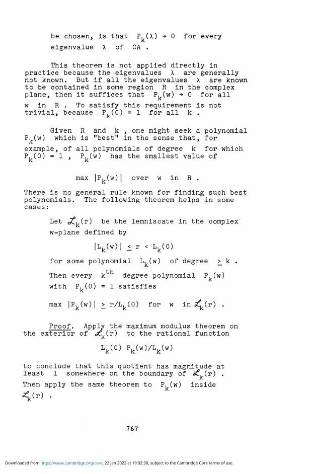
This theorem is not applied directly in practice because the eigenvalues X are generally not known. But if all the eigenvalues X are known to be contained in some region R in the complex plane, then it suffices that p

k(w) ~* ° for all

w in R . To satisfy this requirement is not trivial, because ^(O) = ! f°r a 1 1 k •

Given R and k , one might seek a polynomial Pk(w) which is "best" in the sense that, for

example, of all polynomials of degree k for which P,(0) = 1 , pi<-(

w) h a s the smallest value of

max |P, (w) | over w in R

There is no general rule known for finding such best polynomials. The following theorem helps in some cases :

Let <j£,(r) be the lemniscate in the complex

w-plane defined by

|Lk(w)| £ r < Lk(0)

for some polynomial L,(w) of degree >_ k .

Then every k degree polynomial P^Cw)

with Pk(0) = 1 satisfies

max |Pk(w)| _> r/Lk(0) for w in ( r ) .

Proof. Apply the maximum modulus theorem on the exterior of <^f(^) to the rational function

Lk(0) Pk(w)/Lk(w)

to conclude that this quotient has magnitude at least 1 somewhere on the boundary of <>£ (r) .

Then apply the same theorem to P^Cw) inside

4(r)

767



The simplest application of this theorem is to the circle

|Lk(w)| = |(l-w)k| 1 Bk ,

which shows that, if A = I-B and we know only that ||B|| == 6 < 1 (so that all eigenvalues X of A must satisfy 11-X | <_ 3 < 1) , then the simple

Jacobi iteration described above is the best that can be done.

Having chosen a polynomial *V(W) > the

numbers y . are defined as the reciprocals of the

zeros of Pk^w^ ' This relation amounts to an

inconvenient restriction on the sequence of polynomials P.(w) for j < k , and is also a

source of possible numerical instability. To illustrate this point, suppose all the eigenvalues X of CA lie in an interval on the real axis, say 0 < a o < _ X < _ a . The following theorem of

Markoff is applicable:

Of all k degree polynomials pk(

z) with

P,(0) = 1 , the one for which

max |P,(z)| on ag <_ % <_ a

is smallest is just the Tchebycheff polynomial

where

Tk(L(z))/Tk(L(0))

T,(cos 0) = cos k Q and

L(z) = (am + a0 - 2z)/(am - a0) .

Proof. If |Pk(z)| <_ l/Tk(L(0)) on ao £ z £ a m 9 then the difference

Tk(L(z)) - Tk(L(0))Pk(z) has at least one zero

between each pair of adjacent extrema of T,(L(z))

on the interval, and another at z = 0 , making k+1 zeros altogether.

Now, the zeros \."" of T,(L(z)) include

768



some numbers quite near ao > which may be very small

in cases of slow convergence. But then the term Y-tCr. , when its turn comes in the iteration, can be

so large and so much magnify the effects of rounding errors that the convergence of the iteration is jeopardized (Young (1956)).

Fortunately, the Tchebycheff polynomials satisfy a three-term recurrence

Tk+1(L(z)) = 2L(z)Tk(L(z)) - T^1(L(z))

which can be implemented conveniently and is numerically stable. A suitable form for the iteration is

^k+i • k + Vïk + 6k^k - s*-i> •

and an appropriate choice of y , , 6, , and

zk = x + Tk(L(CA))(zQ - x)/Tk(

L(°))

for all k >_ 0 . One great convenience of this

iteration is that the polynomial ^(w) that

appears in the relation

zk = x + Pk(CA) (z_Q - x)

is the "best" such polynomial for each k , so that there is no need to choose a degree k in advance. This convenience persists whenever the sequence of polynomials P, (w) are orthogonal polynomials

2 which minimize some weighted mean value of |P(w)| over an interval of interest, because these polynomials also satisfy a three-term recurrence. For details see Stiefel (1958) and Faddeev and Faddeeva (1964) ch. 9.

A very different approach to iterative methods can be illustrated by the Jacobi method once again. We note that, since

*k+i - 2-= B ( ^ k - 1 > >

769



where 6 = ||B|| < 1 . In other words, each iteration

reduces the norm of the error by a factor 3 < 1 .

More generally, given a norm for the error ||z, - x|| or for the residual ||b_ - A^J| , one seeks

a direction £, and distance \, such that the

norm associated with

is smaller than for z, . In Gauss-Seidel

iterations the direction g. is one of the

coordinate directions; in gradient iterations the direction g, is that in which the norm is

decreasing most quickly. For further discussion see Householder (1964) sec. 4.2-3. I shall elaborate upon only one such method, called "the method of conjugate gradients".

Suppose A is symmetric and positive definite^

and let us use || r» || = (r,Trk) as a norm for the

residual r, = b_ - Az, . Then each iteration step

Sk+i = ^k + y<A + 6 k ( ^k " S t - i >

looks formally just like the iteration that was used above to construct the Tchebycheff polynomials, but now the constants -y, and 6, must be chosen to

minimize IK,.-J I i-n that step. This choice of "y,

and 6, has the stronger property that no other

choice of v Q, 6Q, \-., 6-,, ... , Y, , 6, could yield

a smaller value for IIUV+TJI • I n particular,

ÎIM = 2. > the iteration converges in a finite number

of steps. An excellent exposition of this powerful

technique is given by Stiefel (1953) and (1958).

Another approach to iterative methods is embodied in the relaxation methods. The basic idea

770



here is to adjust some unknown Xj to satisfy

("relax") the I equation I. a^. x. = b. ,

even though in doing so some other equation may be dissatisfied. The next step is to relax some other equation, and so on. Gauss (1823) claimed that this iteration could be performed successfully

"... while half asleep, or while thinking about other things".

Since his time the method has been systematized and generalized and improved by orders of magnitude, especially where its applications to discretized boundary value problems are concerned. The best survey of this development is currently to be found in Vargafs book (1962). Nowadays some of the most active research into iterative methods is being conducted upon those variants of relaxation known as Alternating Direction Methods; see for example Douglas and Gunn (1965)* Gunn (1965)* Murray and Lynn (1965), and Kellog and Spanier (1965).

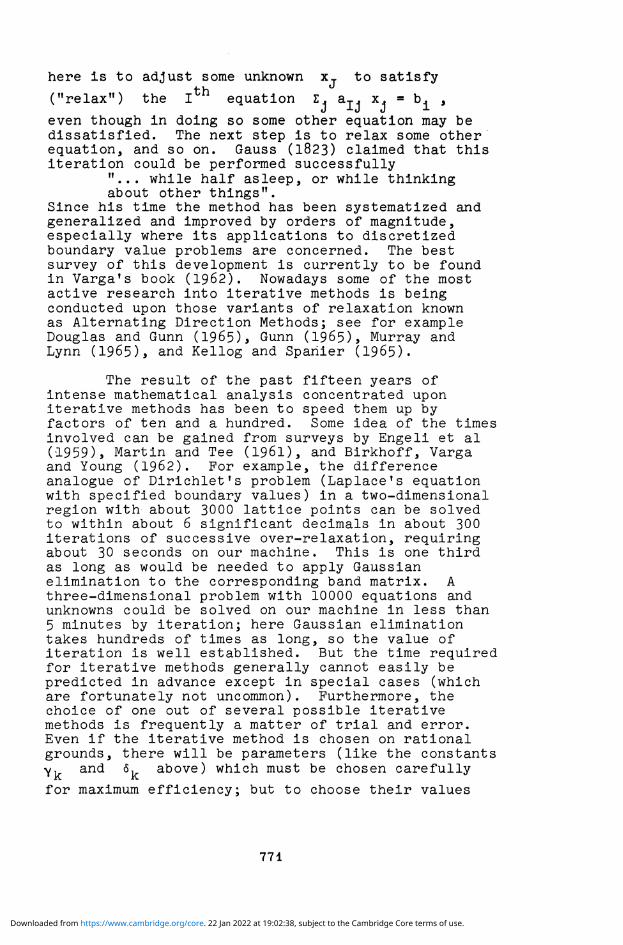
The result of the past fifteen years of intense mathematical analysis concentrated upon iterative methods has been to speed them up by factors of ten and a hundred. Some idea of the times involved can be gained from surveys by Engeli et al (1959), Martin and Tee (1961), and Birkhoff, Varga and Young (1962). For example, the difference analogue of Dirichlet?s problem (Laplace's equation with specified boundary values) in a two-dimensional region with about 3000 lattice points can be solved to within about 6 significant decimals in about 300 iterations of successive over-relaxation, requiring about 30 seconds on our machine. This is one third as long as would be needed to apply Gaussian elimination to the corresponding band matrix. A three-dimensional problem with 10000 equations and unknowns could be solved on our machine in less than 5 minutes by iteration; here Gaussian elimination takes hundreds of times as long, so the value of iteration is well established. But the time required for iterative methods generally cannot easily be predicted in advance except in special cases (which are fortunately not uncommon). Furthermore, the choice of one out of several possible iterative methods is frequently a matter of trial and error. Even if the iterative method is chosen on rational grounds, there will be parameters (like the constants Y k and 6, above) which must be chosen carefully

for maximum efficiency; but to choose their values

771



will frequently require information that is harder to obtain than the solution being sought in the first place, (A welcome exception is the method of conjugate gradients.) Evidently there is plenty of room for more research, and especially for the consolidation of available knowledge.

4. Errors in the Solution of Linear Systems. It is possible in principle to perform a variant of Gaussian elimination using integer arithmetic throughout in such a way that no rounding errors are committed (see Aitken's method described by Fox (1964) on pp. 8 2 - 8 6 ) . But the integers can grow quite long, as much as N times as long as they were to begin with in the given NxN matrix A. Whenever N is large, one is easily persuaded to acquiesce when the computer rounds its arithmetic operations to some finite number of significant digits specified in advance. Consequently, it comes as no surprise when the calculated value z of the solution of

Ax = b

exhibits a small residual

r = b_ - A^ .

How small must r be to be negligible? The following example shows that this question can have a surprising answer.

Example 1.

A _ / . 2 1 6 1 . l 4 4 l \ / . l44o\ v _ / . 9 9 1 1 \ A " U.2969 -8648/ > 5 . " (.8642/ > £ ~ (- .4870/ •

Then the residual is

r = b - Az = (--0000000l\ e x a c t l y . r D_ - AZ_ - ^ .00000001/ e x a c t ±y >

no other vector z_ specified to 4 dec. can have a smaller residual r unless r = 0_ . But z_ does not contain a single correct digit I The"correctft

solution is

Linear systems with this kind of pathological behaviour are often called "ill-conditioned". Precisely what does "ill-conditioned" mean?

772



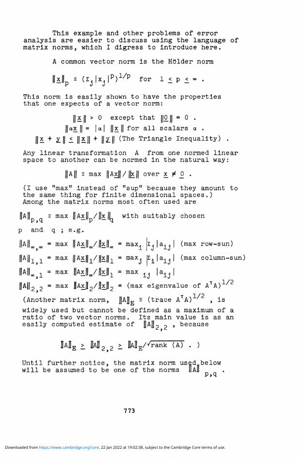
This example and other problems of error analysis are easier to discuss using the language of matrix norms, which I digress to introduce here.

A common vector norm is the Holder norm

||x||p = (Zjlxjl?)1^ for 1 I P < - .

This norm i s e a s i l y shown t o have t h e p r o p e r t i e s t h a t one e x p e c t s of a v e c t o r norm:

| | x | | > 0 excep t t h a t ||0J| = 0 .

||a2L|| = I a I I I ^ L I I f o r a 1 1 s c a l a r s a .

||2L + Z.|| £ | | £ | | + ||JL|| (The T r i a n g l e I n e q u a l i t y ) .

Any l i n e a r t r a n s f o r m a t i o n A from one normed l i n e a r space t o a n o t h e r can be normed i n t h e n a t u r a l way:

||A|| = max ||AxJ|/| |x|| over x + _0 .

(I use "max" instead of "sup" because they amount to the same thing for finite dimensional spaces,) Among the matrix norms most often used are

||A|| = max ||Ax|| / | | x |L w i th s u i t a b l y chosen

p and q ; e . g .

oo oo = max llAxllyHxJI^ = maX l | ^ | a i J | (max row-sun)

, _ = max | |Ax|J,/ | |x |L = max. | z . | a - . | (max column-sun)

IIAIL,I =max iML/yii =max ij iaiji ||A||2 2 = max ||AxII2/||xJ|2 = (max e i g e n v a l u e of A T A ) 1 / 2

T 1/2 (Another m a t r i x norm, J|AjJE = ( t r a c e A A) ' , i s

widely used but cannot be defined as a maximum of a ratio of two vector norms. Its main value is as an easily computed estimate of |JAJJ2 2 , because

Ul\E L M2$2 > W E / ^ r a n k (A) . )

U n t i l f u r t h e r n o t i c e , t h e m a t r i x norm used below w i l l be assumed t o be one of t h e norms IIAII

773



= 1

Finally, the notion of a dual linear functional should be mentioned.. If the row-vector

£T is regarded as a linear operator from a normed vector space to the space of complex numbers normed as usual, then

Bz.T||a max lz.Tï.|/||x|l over 2L * £ •

e-g- Blip = max lzTx|/||x||p = ||ï||q where p"1 + q"1

And the Hahn-Banach theorem guarantees that to each

x ^ 0 corresponds a dual functional £T such that

Z\ = IIJLT|| 11*11 = 1 •

(For more details, see Householder (1964) or any text on normed linear spaces; e.g. Day (1962), Kantorovich and Akilov (1964).)

Now it is possible to discuss the meaning of "ill-condition". To each matrix A , regarded as a linear operator from one normed space to another, can be assigned its condition number K(A) associated with the norms and defined thus:

K(A) -= S2L M/l W l l HI

over a l l x ï 0_ and £ ï jO

In other words, if the vectors Ax, and Ab are regarded as errors correlated by A(x + AxJ = b_ + Ab , where x_ a n d 5. satisfy A c = b_ , then

1/K(A) £ (i|Axtl/||x|l)/(llAb||/||b||) <K(A) .

This means that a small change Ab_ in b_ causes a change Ax in x_ which has, relatively speaking, a norm that can be K(A) times as big. When K(A) is very large, we say that "A is ill-conditioned" .

It is easy to prove that when A is a square matrix,

K(A) - |A| HA"1! .

The matrix A of the numerical example is very ill-conditioned indeed;

774



/ -86480000. Il*4l0000.>

\i2969OOOO. -21610000. A" - UonEnnnnn o-i£-innnrj J and

K(A) * 2 x 108 .

If we apply the inequality, associating r with Ajb and z_ - x with Ax , we verify that

(fl£ - xJl/fl^l)/(|IlJ|/IlbJ|) * (l/2)/(l(T8) < K(A) .

Had K(A) been known in advance, the example would not have come as a surprise.

Another important property of the condition number is given by the following:

THEOREM: A differs from a singular matrix by no more in norm than |]A||/K(A) , (Gastinel)

i.e., given A , ||A||/K(A) = min ||AA|| over all

singular (A + AA) .

Proof . Of c o u r s e , i f (A + AA) i s s i n g u l a r , t h e n t h e r e i s some x ^ 0_ f o r which (A + AA) x. = Q.

T h e r e f o r e || AA|| >_ ||AAX)| / ||x ||

• rai/M = I I A X I I / I I A - 1 AXII i I/HA"1)! = ||A||/K(A) .

To find a AA which achieves the inequality we

consider that vector £ f o r which

II A " 1 d = II A " 1 ! ! ||Z|J ¥ 0 . T -1

Then let w be dual to A £

i.e. wT A"1 Z = JJwTj| jJA"1 2|| - 1 ,

and set AA = - £ wT . We have (A + AA) A~ £ = 0 , so A + AA is singular.

And

|AA[| = max JJ^ wTxJJ/j|x|| o v e r 2L ^ H = BjJ max |wTx|/ i ixii

775


file:///i2969OOOO


- l id I*TI MMI/lK^Jl = i/IJA-1! = ||A||/K(A) .

Let us return to the example again. If the elements of A have been rounded to 4 decimal places, then the uncertainty introduced by the rounding is 10000 times larger than the difference between A and the nearest singular matrix! Under these circumstances it is reasonable to ask whether the system Ax_ = b_ deserves to have a solution.

The pathological behaviour of ill-conditioned matrices seems to have preyed upon the minds of the early analysts of the error committed during Gaussian elimination. Certainly the conclusions of von Neumann and Goldstine (19^7, 1951 ) are incredibly pessimistic; for example they concluded that on a machine like ours there were substantial risks taken in the numerical inversion of matrices of orders much larger than 20, although their error-analysis was correct in other respects. (Their trouble arises from an attempt to compute

A" from the formula

A - 1 = ( A ^ r 1 AT ,

an attempt which we know now to have been ill-conceived. )

A more nearly modern error-analysis was provided by Turing (1948) in a paper whose last few paragraphs foreshadowed much of what was to come, but his paper lay unnoticed for several years until Wilkinson (I960) began to publish the papers which have since become a model of modern error-analysis.

WilkinsonTs main result about Gaussian elimination can be summarized thus:

Provided Gaussian elimination is carried out in a reasonable way (about which more later), the computed approximation z_ to the solution of

Ax = b_

will satisfy instead an equation of the form

(A + AA) z = b

776



where, although AA is not independent of b and z, , AA satisfies an inequality of the form

||AA||< c gN NP 3 " S ||A||

where N is the order of A ,

3~s represents "1 unit in the last place" -s -8 e.g. e =10 on an 8 dec. digit machine,

c is a modest positive constant, usually less than 10,

p is a small positive constant always smaller than 3.

gN is the pivot-ratio, about which more later.

The constants c and p depend upon the details of the arithmetic and the norm; they will not be discussed here. (See Wilkinson (1963) and references cited therein.)

In short, JJAAjl is comparable to rounding errors in JJAJJ ; and if the data in A is already uncertain by more than a few hundred units in the last place carried then the perturbation AA attributable to the process of elimination will be quite negligible by comparison. Indeed, in many cases the perturbation AA will amount to less than one unit in the last place of each element of A !

So, a small residual

r = b_ - Az_ = AA z

is just what might be expected from Gaussian elimination. But the error z, - x. is another matter;

£ - x =-A AA z_ , where JJ AA|) <_ e |}AJ[ , say .

T h e r e f o r e \\z - x|l 1 IIA"1 II I|AA|| || z j |

< K ( A ) e 11 M

- 1 - K(A) e , l ^"

where K(A) is Afs condition number,

e = c gN Np B~S and is very small,

and we assume that K(A) e < 1 .

777



In other words, although the residual r is always small, the error £ - x. may be very large if A is ill-conditioned; but this error will be no worse than

c gN N^ units in its if A were in error by about

last place to begin with.

The constant gN has an interesting history

It is connected with the rate of growth of the "pivots" in the Gaussian elimination scheme. The

pivot is the coefficient a-j-j by which the I

equation is divided during the elimination of x, .

This term "pivot" will be easier to explain after the following example has been considered:

Example 2.

A =

-10 -1

1

1

,-1

.1 2 x.

À A. 0 -2

h { -2 0.9999999998 . „ «. , -2

2 1.0000000002 0.9999999998/ xQ

1.0000000002 1 x.

Clearly, A is not ill-conditioned at all. But suppose we apply Gaussian elimination to solve the equation Ax_ = b_ . Our first step could be to

eliminate x, from equations 2 and 3 by subtracting

suitable multiples of equation 1 from them. The reduced matrix should be

x __1

2 x

0

0

lu"10 -1

-4999999999

5000000001

13 1

5000000001

-^999999999/

"1

778



But if we have a calculator whose capacity is limited to 8 decimal digits then the best we could do would be to approximate the reduced matrix by

-10 -1

-5 x 10-

22. l

5 x 10:

5 x 10* -5 x 10'

ul bf.

but this is precisely the reduced matrix we should have obtained without rounding errors if A had originally been

A + AA =

-10 _2 -1

0

0

In other words, the data in Afs lower right hand 2 x 2 submatrix has fallen off the right hand end of our calculator's 8-digit register, and been lost. The result is tantamount to distorting our original data by the amount of the loss, and in this example the distortion is a disaster.

These disasters occur whenever abnormally large numbers are added to the moderate sized numbers comprising our data. To avoid such disasters it is customary to choose the variable Xj to be

eliminated, and/or the row I with which it is to be eliminated from all other rows, in such a way that the pivot a IJ is the largest available element a

in its row, or column, or both. Since the typical ij

computation replaces a ij by

ij = a ij " aiJ aIj/aIJ for all (i,j) Ï (I,J)

max we see that max.^a1..! <_ 2

so that no abnormally large numbers should appear. ij1 ij

In the example above we might choose

pivot to obtain the reduced matrix

l21 as the

779



1

•1.0000000

2

1.0000000

2

°2 b'

(working to 8 significant digits) .

This reduced matrix is what would have resulted if no rounding errors had been committed during the reduction of

A + AA =

-1

1

1

which differs negligibly from the given matrix A .

Wilkinson's error bound, quoted above, assumes that each pivot aTT is the largest in its row or

else in its column of the reduced matrix, and then gN is the ratio of the largest of the pivots to

the largest element in A . We can see that, since the largest elements of each reduced matrix never exceed twice those of the previous one,

% ± 2 N-l

This bound is achieved for X = 1 by the matrix

Example 3:

Ax •

1 0 -1 1 -1 -1

0 0 0 0 1 0

-1 -1 -1 1

-1 -1 -1

0 1 0 1 0 1

1 0 1 -1 1 1 -1 -1 X

a±J = -1 if i > j ,

a ± ± = 1 if i < N ,

a±1 • 0 if i < j < N,

a.j, = 1 if i < N, and

N x N

= X

780



if each pivot is chosen on the diagonal as one of the largest elements in its column, and the columns are chosen in their natural order 1,2,3, ..., N during the^elimination. But when we repeat the computation with X = 2 and sufficiently large N , an apparent disaster occurs -because the value of X = 2 gets lost off the right-hand side of our computing register. On a binary machine like our 7094 (using truncated 27-bit arithmetic), X = 2 is replaced by X = 1 if N > 28 . An example like this was used by Wilkinson (1961, p. 327) as part of the justification for his recommendation that one use both row and column interchanges when selecting pivot aTT to ensure that it is one of the largest

elements in the reduced matrix. This pivot-selection strategy is called "complete pivoting" to distinguish it from "partial pivoting" in which either row exchanges or column exchanges, but not both, are used.

The other justification for complete pivoting was Wilkinson1s proof of a remarkable bound for the ratio gN of the largest pivot to the largest

element of A :

gN < iX.Z1^1'2.*1'3 ... N 1 / ( N - 1 } ) 1 / 2 < 2N** 1 O « N ,

which is certainly far smaller than 2

(This bound is worth a small digression. It is known to be unachievable for N > 2 ; and the bound

% £N

has been conjectured for complete pivoting when A is real. The conjectured bound is achieved whenever A is a Hadamard matrix, and L. Tornheim has shown that the conjecture is valid when N s 3 • He has also shown that when A is complex the larger bound

g3 £ 16/3372

can be achieved.)

Despite the theoretical advantages of complete pivoting over partial pivoting, the former is used much less often than the latter, mainly because

781



interchanging both rows and columns is far more of a nuisance than interchanging, say, rows alone. Moreover, it is easy to monitor the size of the pivots used during a partial pivoting computation, and stop the calculation if the pivots grow too large; then another program can be called in to recompute a more accurate solution with the aid of complete pivoting. Such is the strategy in use on our comDUter at Toronto, and the results of using this strategy support the conviction that intolerable pivot-growth is a phenomenon that happens only to numerical analysts who are looking for that phenomenon.

Despite the confidence with which the computed vector z_ , produced by Gaussian elimination or some other comparable method, can be expected to have a residual

r = b_ - Az_

which is scarcely larger than the rounding errors committed during the calculation of r_ ,

i . e . Dr | | - lib - AzJI ~ N6-S(||b|| + ||A|| | |Z| |) ,

an important problem remains. How large is the error z_ - x. with which z_ approximates the "true solution" x. of Ax = b_ ? This question is meaningful even if A and b_ are not known precisely; we can interpret z_ to be the solution of a perturbed system

(A + AA) z, = ;b + Ab_

i n which |] AA JJ and ||Ab_|| a r e bounded i n some g i v e n way, and hence so i s v_ = AAz_ - Ab_ . A p r e c i s e answer t o t h e q u e s t i o n i s

x - z = K-\ , || z - x | | < || A"1!! | | r | | ,

but here we must know || A" || in order to complete

the answer. If we try to compute A~ , we shall instead obtain some approximation, say Z , and once again we shall have to ask the question

How large is the error Z - A" ?

This question can be answered fairly easily if Z is accurate enough, as shall now be shown.

782



Each column z. of Z = {z.-,,z_p> ... > Zvr)

can be regarded as an approximation to the corresponding column X- °f

A = A = I X_n y X_P * * * * * ~Kf *

the solution of AX = I . A reasonable way to solve the last equation is to use Gaussian elimination, in which case each column z_. will be computed

separately and will satisfy

(A + A±A) z_. = (the i t h column of I)

where ||A.A|| <_ e || A || for some small e which

depends upon the details of the program in a way discussed by Wilkinson (1961).

Now let R be the residual

R = I - AZ .

It is not necessary to compute R ; we can write

R = I-A {z^z^, ... 3 z_N> = {A1Az_1,A2Az_2, ..., A ^ ^ } ,

i n which each column A.Az_. of R i s bounded i n

norm by

KAzJ < cflAfllzJ . Therefore

P = llHJI i n | |A|| |jZ||

where r\/e depends upon N and the norms; usually

n/e 1 N 1 / 2 .

Since e can be predicted in advance, so can n ; and it is possible to check whether

n IIAJUJZJI < 1 ,

in which case p < 1 and the following argument is valid:

783



H A- fl Jlzll+H A-^-zj^nzii^ IIA-^-CI-AZ)!! =!IZ/|+||A-:LR||

£l|z|M|Ai|p ;

llA^llillZll/d-p) .

Then I IA" 1 -ZIU lU""1!! p £ ||z||p/(l-p) .

The last inequality says that, neglecting modest factors which depend upon N , the relative

error || A~1-Z||/||z || is at worst about K(A) times as large as the relative errors committed during each arithmetic operation of ZTs computation. In other words, if A is known precisely then one must carry at least l°g-iQ K(A) more decimal guard

digits during the computation of A~ than one wants to have correct in the approximation Z , and one can verify the accuracy of Z at the end of the computation by computing n ||A || ||Z || .

If the method by which an approximation Z

to A~ was computed is not known, there is no way to check the accuracy of Z better than to compute R and p directly, and this calculation is not very attractive for two reasons. First, the computation of either residual

R = I-AZ or I-ZA

costs almost as much time as the computation of an -1 3

approximate A ; both computations cost about N multiplications and additions. Second, if K(A) is large then ||l-AZ|| and || I-ZA || can be very different, and there is no way to tell in advance which residual will give the least pessimistic over-estimate of the error in Z .

(p=||l-AZ|J = ||A(I-ZA)A""1|| <_ K(A)||I-ZA|| etc.)

Both residuals can be pessimistic by a factor like

K(A) . Finally, although a better approximation to

A" than Z is the matrix

Z1 = Z + Z(I-AZ) = Z + (I-ZA)Z

(because [[I-AZj = |[(I-AZ)2[| <_ ||l-AZ||2 ) ,

784



the computation of Z., is in most cases more costly

and less accurate than a direct computation of an

approximate A" using Gaussian elimination with double precision arithmetic. For example, on our 7094 it takes less than twice as long to invert A to double precision (carrying 16 dec.) than to do the same job in single precision (8 d e c ) , and the double precision computation has almost 8 more correct digits in its answer. But Z., has at most

twice as many correct digits as Z . Therefore, if Z comes from a single precision Gaussian elimination program, it will have about 8-log K(A) correct digits. Z, will have 16-2 log K(A) digits at best. The double precision elimination will produce about 16-log K(A) correct digits. Thus does engineering technique overtake mathematical ingenuity !

The solution of Ax_ = b_ for a single vector x_ is not normally performed by first computing

A" and then x = A" b_ for four reasons. First, the vector Zb_ , where Z is an approximation to

A~ , is frequently much less accurate than the approximation z_ given directly by Gaussian elimination. Second, the direct computation of the vector £ by elimination costs about 1/3 as much time as the computation of the matrix Z . Third, if one wants only to compute a vector z_ which makes r = b_ - Az_ negligible compared with the uncertainties in b_ and A , then Gaussian elimination is a satisfactory way to do the job despite the possible ill-condition of A , whereas b_ - A(Zb_) = Rb_ can be appreciably larger than negligible. Fourth, Gaussian elimination can be applied when A is a band matrix without requiring the vast storage that would otherwise be needed for

A" . The only disadvantage that can be occasioned

by the lack of an estimate Z of A~ is that there is no other way to get a rigorous error-bound for z - x . This disadvantage can be partially overcome by an iterative method known as re-substitution.

To solve Ax_ = b_ by re-substitution, we first apply any direct method, say Gaussian elimination, to obtain an approximation z_ to x •

785



This vector z will be in error by e_ = x - z_ , and

Ae_ = A(x-z) = b - A^ = r ,

which can be computed. (It is necessary to compute r carefully lest it consist of nothing but the rounding errors left when ID and A_z nearly cancel. Double precision accumulation of products is appropriate here.) Clearly, the error e_ satisfies an equation similar to xTs except that r replaces b_ . Therefore, we can approximate e_ by f , say, obtained by repeating part of the previous calculation. If enough intermediate results have been saved during the computation of z_ , one obtains f_ by repeating upon r the operations that transformed b_ into z_ . The cost of f_ in time and storage is usually negligible.

Now z_! = z_ + f_ is a better approximation to x than was £ , provided _z was good enough to begin with. We shall see that this is so in the case of Gaussian elimination as follows:

(A + A-j A) z. = b , where || A ^ || <_ e||A || .

r = b_ - A;z , say exactly for simplicity.

Il£ll = llA3_Az.ll <. s||A|| |(z.|| ,

and this inequality is not normally a wild overestimate.

(A + A2A) f = r , ||A2A|| <_ e||A|| .

r = b_ - Az/ = r - Af = A2Af , so

ll£'ll 1 e | |A| | Hill < £ | |A|| ||(A + AgA)-1!! | |£ | |

1 e K ( A ) l l l l l l /^1 - e K(A)) i f e K(A) < 1 .

And if e K(A) << 1 then ||rf|| can be expected to be much smaller than || r || . If z_! is renamed z_ , the process can be continued. We have left out several details here; the point is that the process of re-substitution generally converges to an approximation z_ which is correct to nearly full single precision, provided the matrix A is jfarther from a singular matrix than a few hundred units in its last place. The problem is to know when to stop.

786


llA3_Az.ll


The word "convergence" is well-defined mathematically in several contexts. But the empirical meaning of "convergence" is more subtle. For example, suppose we consider the sequence ZpZp, . . ., z_ , ... of successive approximations to

x_ produced by the re-substitution iteration, and suppose that z = z ,-, = z , 0 = . . . . We should ^ -m -m+1 -m+2 conclude that the sequence has converged. And if z n - z is a good deal smaller than —m-1 —m ° z n - z ., j we should incline to the belief that —m-2 —m-1 '

the convergence of the sequence is not accidental; there is every reason to expect z to be the J ^ -m correct answer x_ except for roundoff in the last place. But a surprise is possible if A is exceptionally ill-conditioned:

Example 4. Here is an example of a 2x2 system with

= /.8647 .5766) = /.2885 ) A 1.4322 .2822/ a n a - (.1442/ *

We shall use Gaussian elimination to compute a first approximation z_ to the solution x of Ax = b_ . Then r = b_ - Az, is computed exactly, and the solution e_ of Ae = r is approximated by £ , obtained again by Gaussian elimination. z_T = z. + f. , and rT = b_ - Az_T .

We shall try to calculate x correctly to 3 sig. figTs. It seems reasonable to carry one guard digit at first, since we can repeat the calculation with more figures later if that is not enough. We shall truncate all calculations to 4 sig. figfs., just like our 7094 (except that it truncates to about 8 sig. figTs.). Intermediate results enclosed in parentheses are obtained by definition rather than by means of an arithmetic operation.

787



Comment

1st pivotal .4327/.8647=

.4998xEl Is

E2-E1'

E3/.lxl0~3

.5766xZ2 E1-E3* E4/.8647

row is . .4998

. . .

. . .

Our first approximat

Equ'n no.

. . El E2

El'

E3 Z2

E3' E4 Zl

ion is z

Coef. of x.

.8647

.4322

(.4322)

( 0 )

( 0 )

( 0 ) (.8647) ( 1 )

• h

Coef. Right hand of x2

.5766

.2882

.2881

.lxlO"3

( 1 )

(.5766) ( 0 ) ( 0 )

333l\ • .000/

side b

.2885

.1442

.1441

.lxlO"3

1.000

.5766 -.2881 -.3331

Next we compute r precision:

Residual of El ...

Residual of E2 ...

= b - Az exactly using double

Rl

R2

-.6843x10

-.3418x10

-4

-4

We get f_ by repeating upon r the operation which transformed b into z .

.4988XR1 R2-R1'

R3/.lxlO-3 .

.5766xF2

R1-R3'

R4/.8647

Rl'

R3 F2

R3' R4

Fl

-.3420x10

.2xl0"7

.2000x10

-4

.1153x10

-.1837x10

-.2124x10

-3

-3

-3

-3

z = /-3331) - (1.000/

f = -.2124 .2000 x l0~ 3

z ' = z + f = M 3 3 3 1 2 l | | x±u , z_ zti_ (1#o002000/ *

Clearly z_! i s so close to z_ t ha t e i t h e r i s an acceptable 3-f igure approximation t o x . But, j u s t in case t he r e i s some doubt, we compute

= b - AzT = - . 0 0 0 0 0 0 0 8 7 7 2 , > , 0 0 0 0 0 0 0 2 0 7 2

788



which is reassuringly smaller than r_ .

Is x = (î'Joo) t o 3 s i g' f ig ? s ? No> 1= / _ 1

The only clue to ATs ill-condition is the cancellation in E3 . If there were time and space available, an example could be constructed of sufficiently high dimensionality that severe cancellation would not occur to warn of the disaster. Presumably this kind of disaster is rare in practice, because none has yet been reported elsewhere. Indeed, a prominent figure in the world of error-analysis has said

"Anyone unlucky enough to encounter this sort of calamity has probably already been run over by a truck."

But being run over by a truck can hardly go unnoticed.

Despite the risks, re-substitution is the most reasonable and efficient way to check and improve the accuracy of an approximation z_ when the matrices A and b_ are known more precisely than to within the uncertainties AA and Ab_ in the perturbed equation

(A + AA) z, = b + Ab

satisfied by the product z_ of Gaussian elimination. For fuller detail, see Wilkinson (1963) pp. 121-126. But if A and b_ are intrinsically uncertain in, say, their fourth decimal place, and if Gaussian Elimination has been carried out with about 6 to 8 sig. figTs and with a reasonable pivotal strategy, then re-substitution may well be pointless, since the errors committed during the elimination will be negligible compared with intrinsic uncertainties.

5. Pivoting and Equilibration. How reliable are the sizes of the pivots as indications of a matrixfs ill-condition? Is it true that a matrix is ill-conditioned if and only if some of its pivots are small? Most people who are experienced with hand calculations would answer "yes" to the last question unless they have tried to test their belief on problems of high dimensionality with the aid of an electronic computer. When the dimensionality of a

789



problem becomes large (say > 30), much of our experience and Intuition with small dimensionality (say <. 5) becomes misleading. The following examples are designed to correct misleading impressions.

MIS-STATEMENT NO. 1. The determinant of A is the product of the pivots encountered during Gaussian elimination (to within a * sign); and since a singular matrix has determinant zero, and det A is a continuous function of A , an ill-conditioned (nearly singular) matrix must have a small determinant and hence must have at least one small pivot.

The flaw in this argument is the same as that which

says that, since |x| is a continuous function of

x no matter how large N may be, |x| / must be small when x is small. The trouble is that two "small" numbers can still be relatively very different. A matrix counterexample is

Example

A =

5. f

1 0 0 •

fi

- 1 1 0

- 1 - 1

1 •

• • •

. . .

• •

1

- 1 - 1 - 1

•

- 1 1

a ± J = 0 i f i > J ,

a1(J - - 1 i f i < j ,

& i l = 1 .

NxN

Here det A = 1 , and every pivot can be 1

A can be made singular by subtracting 2 1-N

all a il Therefore, when N is large A

but

from differs

negligibly from a singular matrix, and must be ill-conditioned. The ill-condition of A is not "caused" by a large number of nearly equal elements, as some observers have suggested, because |if all -lTs in A are replaced by +lfs then A becomes the well conditioned inverse of

1 - 1 0 0 1-1 0 0 1

0 0 0

1 -1 0 1

790



The foregoing examples indicate that Gaussian elimination is a poor way to determine the rank of a matrix because a few rounding errors may suffice to cause none of the pivots to be small despite a theorem which says that, in the absence of rounding errors, the rank of a matrix is the same as the number of non-zero pivots generated during Gaussian elimination with both row and column pivotal interchanges to select maximal pivots.

Most other methods for determining rank fare no better in the face of roundoff. For example, the Schmidt orthogonalization procedure can be described in terms of an orthogonal projection of ATs n-th column a upon the space spanned by the previous

n-1 columns a-,, . . . , a __-, (see Householder (1964)

pp. 6-8 and 134-7). The columns can be interchanged, if necessary, in order at each stage to maximize the distance from a to the space of a., ..... a -, . —n ^ — l* 5 —n-1 If this is done, the rank r of A will become evident when a ,-,, a + ?, •••* and aN all have

distance zero from the space spanned by a-, , a,p, ...,

and a . However, if A is merely nearly singular,

there is no guarantee that any of the distances mentioned above will be anywhere near as small as the distance between A and the nearest singular matrix. Difficulties arise whenever || Av|| << |JA|| [|v|| for some vector v whose components v. can be

ordered in such a way that they steadily decrease in magnitude to a point where the smallest component is negligible compared with the largest. The following example illustrates the phenomenon:

i-1 for i,j = 1,2,

a.. = 0 if i > J

a.. = s-

i-1 . « . a. . = -cs if l ij

2 2 Here N is large (N > 30) and s + c = 1 .

Since A is upper triangular, the n column of 1 is distant a from the space spanned by the

previous columns. Also, this example has been so chosen that no column interchanges are needed to maximize the distance, since a , a^,,, ... , and

aN are all equally distant from the space spanned

791



by a,, a2, ... j ân i • T h e smallest distance

N-l ann l s aNN = s * H o w m u c h s m a H e r > t h a n a„N

is the distance || AA || between A and the nearest singular matrix A + AA ?

By examining the vector Av , where

v. := c(l+c) " •"" except v„ = 1 ,

we can show that

||AA||/aNN = 0 ( l / ( l + c ) N " 1 ) as N - « .

- 0 ( l / ( l + / l - a N N2 / N ) N ) .

For fixed aNN = a > 0 , the righthand side tends to

zero like

l/[a exp/-2 (N - 1/3 log a) log a ] as N -> °° .

-N For fixed N , it is like 2 as a ™ •> 0 . In

other words, A can be closer to singular than a. by orders of magnitude if N is large.

No simple method is known for computing the rank of a matrix in the face of roundoff. An effective but complicated method has been given by Golub and Kahan (1965).

MIS-STATEMENT NO. 2. The reason for pivotal interchanges is to prevent incorrect answers caused by the use of an inaccurate small pivot.

This statement seems reasonable in the light of the 2x2 example at the end of section 4 of this paper,, where cancellation in E3 produced a tiny pivot .0001 whose value consisted almost entirely of rounding error. And the computed answer was quite wrong. Post hoc ergo propter hoc.

However, the pivot 2x10"" in example 2 is quite accurate, yet any answer gained by its use is likely to be wrong.

Now, what can one mean by the accuracy of a pivot? The meaning would be clear if the object of

792



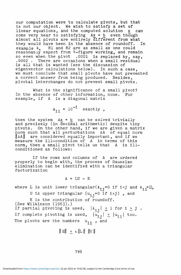
our computation were to calculate pivots, but that is not our object. We wish to satisfy a set of linear equations, and the computed solution £ can come very near to satisfying Ax_ = b_ even though almost all pivots are entirely different from what they would have been in the absence of roundoff. In example 4, Rl and R2 are as small as one could reasonably expect from 4-figure working, and remain so even when the pivot .0001 is replaced by, say, .0002 . There are occasions when a small residual is all that is wanted (see the discussion of eigenvector calculations below). In such a case, we must conclude that small pivots have not prevented a correct answer from being produced. Besides, pivotal interchanges do not prevent small pivots.

What is the significance of a small pivot? In the absence of other information, none. For example, if A is a diagonal matrix

a.. = 10"1 exactly ,

then the system Ax = b_ can be solved trivially and precisely (in decimal arithmetic) despite tiny pivots. On the other hand, if we are given a matrix norm such that all perturbations AA of equal norm || A A || are considered equally important, and if we measure the ill-condition of A in terms of this norm, then a small pivot tells us that A is ill-conditioned as follows:

If the rows and columns of A are ordered •properly to begin with, the process of Gaussian elimination can be identified with a triangular factorization

A = LU - E

where L is unit lower triangular(l. . = 0 if i<j and £..,=1),

U is upper triangular (u..=0 if i>j) , and

E is the contribution of roundoff. (See Wilkinson (1963).) If partial pivoting is used, |&. .| £ 1 for i >_ j .

If complete pivoting is used, |u. . | <_ |u..| too.

The pivots are the numbers u.. , and

II E|| 1 e ||L || ||U ||

793



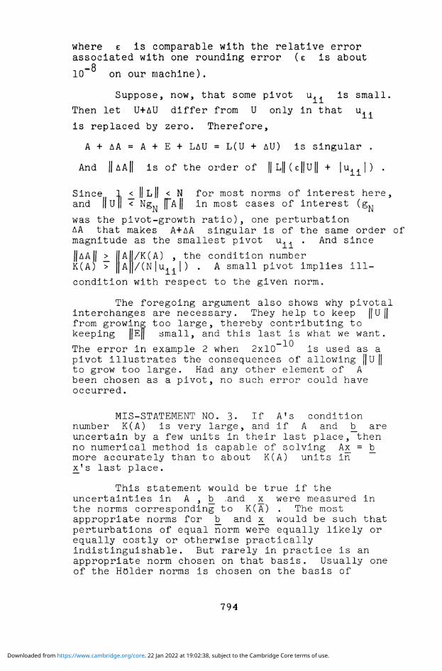
where e is comparable with the relative error associated with one rounding error (e is about —8

10"" on our machine).

Suppose, now, that some pivot u.. is small.

Then let U+AU differ from U only in that u..

is replaced by zero. Therefore,

A + A A = A + E + LAU = L(U + AU) is singular .

And || A A || is of the order of || L|| ( e||u|| + I ^ J ) .

Since 1 <_ || L || < N for most norms of interest here, and |f TU II < Ng„ [f"A || in most cases of interest (g„

was the pivot-growth ratio), one perturbation AA that makes A+AA singular is of the same order of magnitude as the smallest pivot u.. . And since || A A || > K(A) >

/K(A) , the condition number /(N|u..|) . A small pivot implies ill-

condition with respect to the given norm.

The foregoing argument also shows why pivotal interchanges are necessary. They help to keep ||U|| from growing too large, thereby contributing to keeping ||E|| small, and this last is what we want.

The error in example 2 when 2x10" is used as a pivot illustrates the consequences of allowing ||u|| to grow too large. Had any other element of A been chosen as a pivot, no such error could have occurred.

MIS-STATEMENT NO. 3. If ATs condition number K(A) is very large, and if A and b_ are uncertain by a few units in their last place, then no numerical method is capable of solving Ax_ = b_ more accurately than to about K(A) units in x_!s last place.

This statement would be true if the uncertainties in A , b_ .and x^ were measured in the norms corresponding to K(A) . The most appropriate norms for b_ and x_ would be such that perturbations of equal norm were equally likely or equally costly or otherwise practically indistinguishable. But rarely in practice is an appropriate norm chosen on that basis. Usually one of the Holder norms is chosen on the basis of

794



convenience, and such norms can be terribly inappropriate.

Example 6.

Let A = -1 10 " 10 " and b =

— 8 with a relative uncertainty of 10" in each

element. In other words, A + AA is acceptable in

place of A provided | Aa.. . | <_ 10" | a.. . | . If any

of the aforementioned Holder norms are used, the

condition number of A is at least 10 because

there exists a AÂ with || AÂ || <_ 10"10 ||Â|| such

that Â+AA is singular. Therefore, when Gaussian elimination carried out with eight sig. fig. arithmetic gives no useful answer, one is not surprised. "The system is ill-conditioned." However, the true solution is

x =

_7 with a relative error smaller than 10 in each

component no matter how A and b_ are perturbed,

provided only that no element of A or b is

changed by more than 10 of itself. This system is well conditioned! But not in the usual Holder norm.

Example 6 can be obtained from example 2 by a diagonal transformation;

I = DAD with D = diag (105 , 10"5 , 10~5) .

This transformation does no more than shift a decimal point 10 places left or right. If Gaussian elimination is applied simultaneously to the

matrices A and A , then the results in both cases will be identical down to the rounding errors except for the 10 place shifts of decimal point.

But example 2 teaches us not to use 2x10" as a

795



pivot, whereas the most natural pivot in example 6 is the corresponding element 2. Any other pivot would be far better.

This is where equilibration comes in. Equilibration consists of diagonal transformations intended to scale each row and column of A in such a way that, when Gaussian elimination is applied to the equilibrated system of equations, the results are nearly as accurate as possible. In other words, the system

Ax = b

is replaced by

(RAC) £ = (Rb)

where R and C are diagonal matrices. Then Gaussian elimination (or any other method) is applied to the array {RAC, RM to produce an approximation to 2. anc* hence to x. = Z. •

How should R and C be chosen? No one has published a foolproof method. The closest anyone has come is in a paper by F.L. Bauer (1963) in which the R and C which minimize K(RAC) are described in terms of an eigenvalue and eigenvectors of certain

matrices constructed from A and A*" . But no way is known to construct R and C without first

knowing A"

There is some doubt whether R and C should be chosen to minimize K(RAC) . The next example illustrates the problem; the reader should write out the matrices involved in extenso for N = 6 to follow the argument.

Let A be the NxN matrix defined in A

example 3, and le t

ri 1. o^-N 01-N 01-Nv -, R = diag (h 9 h , . . . y 2 , 2 , 2 ) a n d

C = diag ( 1 , 2 , . . . , 2N~3 2N~2 , 1) .

-1 T -1

We observe that A1 = (RA^C) , so k± and A±

are both well-conditioned matrices with elements no larger than 1.

796



Let u = (0, 0, 0, ... , 0, 1) T and note that

A. = A, + u uT .

Therefore, by a simple computation,

A2~X = A1"

1 - (1 + 2X~N) A ^ 1 u uT A ^ 1 .

Now recall that when row-pivoting alone is used with Ap , the result can be an error tantamount to

replacing Ap by A.. , and if no other errors are

committed then one will compute A ~ instead of

Ap" . Note that, when the usual Holder-norms are

used,

||A1-A2||/||A1| | = 0(1) and || A ^ - A , , " 1 1 | = 0(1) .

Next observe that either complete or partial pivoting can be used with RApC ; the result is to

make an error which replaces RApC by RA-.C . But now

IIRA1C - RA2CI1/HRA1C|| = 0(2"N) and

|| ( R A ^ T 1 - (RA2C)-1||/||(RA2C)-

1|| = 0 (2"N) .

In other words, despite some hocus-pocus with shifted binary points, the error made in applying Gaussian elimination to RApC is the same

as that made with Ap , except for a change of

scale. But the former error looks negligible and

affects (R'A9C)~ negligibly, whereas the same d _1

errors look disastrous in A2 and A2 . And nowhere is there any ill-conditioned matrix, nor do any of the matrices look poorly scaled by the usual criteria!

The moral of the story is that the choice of R and C should reflect the norms by which the errors are being appraised. But no one knows yet precisely how to effect such a choice.

797



REFERENCES

D.W. Barron and H.P.F. Swinnerton-Dyer, Solution of Simultaneous Linear Equations Using a Magnetic-Tape Store. The Computer Journal, Vol. 3, (I960) pp. 28-33.

F.L. Bauer, Optimally Scaled Matrices. Numerische Math., Vol. 5, (1963) pp. 73-87.

G. Birkhoff, R.S. Varga, and D. Young, Alternating Direction Implicit Methods. Advances in Computers, Vol. 3, Academic Press (1962).

E. Bodewig, Matrix Calculus, 2nd ed. North Holland (1959). (A catalogue of methods and tricks, with historical asides.)

M.A. Cayless, Solution of Systems of Ordinary and Partial Differential Equations by Quasi-Diagonal Matrices. The Computer Journal, Vol. 4, (1961) pp. 54-61.

M.M. Day, Normed Linear Spaces* Springer (1962).

J. Douglas and J.E. Gunn, A General Formulation of Alternating Direction Methods, part I. Numerische Math. Vol. 6, (1965) pp. 428-453.

Dunford and Schwartz, Linear Operators, part I: General Theory. Interscience (1958).

M. Engeli et. al., Refined Iterative Methods for Computation of the Solution and the Eigenvalues of Self-Adjoint Boundary Value Problems. Mitteilung Nr. 8 aus dem Inst, fur angew. Math, an dur E.T.H., Zurich! Birkhauser (1959).

D.K. Faddeev and V.N. Faddeeva, Computational Methods of Linear Algebra, translated from the Russian by R.C. Williams. W.H. Freeman (1964). (This text is a useful catalogue, but weak on error-analysis. A new augmented Russian edition has appeared.)

G.E. Forsythe and W.R. Wasow, Finite Difference Methods for Partial Differential Equations. Wiley (I960). (A detailed text.)

L. Fox, The Numerical Solution of Two-Point Boundary Problems in Ordinary Differential Equations. Oxford Univ. Press (1957).

798



L. Fox, Numerical Solution of Ordinary and Partial Differential Equations. Pergamon Press (1962) (Ed.). (Based on a Summer School held in Oxford, Aug.-Sept. 1961.)

L. Fox, An Introduction to Numerical Linear Algebra. Oxford Univ. Press (1964). (This is an excellent introduction.)

C F . Gauss, Letter to Gerling, 26 Dec. 1823. Werke Vol. 9, (1823) pp. 278-281. A translation by G.E. Forsythe appears in MTAC Vol. 5 (1950), pp. 255-258.

C F . Gauss, Supplementum ... . Werke, Gôttingen, Vol. 4, (1826) pp. 55-93.

G. Golub and W. Kahan, Calculating the Singular Values and Pseudo-Inverse of a Matrix. J. SIAM Numer. Anal. (B), Vol. 2, (1965) pp. 205-224.

J.E. Gunn, The Solution of Elliptic Difference Equations by Semi-Explicit Iterative Techniques. J. SIAM Numer. Anal. Ser. B, Vol. 2, (1965) pp. 24-45.

A.S. Householder, The Theory of Matrices in Numerical Analysis. Blaisdell (1964). (An elegant but terse treatment, including material on matrix norms which is otherwise hard to find in Numerical Analysis texts.)

IFIP: Proceedings of the Congress of the International Federation for Information Processing, held in New York City, May 24-29, 1965. Spartan Books (1965).

C.G.J. Jacobi, Uber eine neue Auflftsumgsart ... . Astr. Nachr.Vol. 22, No. 523, (1845) pp. 297-306. (Reprinted in his Werke Vol. 3, p. 467.)

L.V. Kantorovich and G.P. Akilov, Functional Analysis in Normed Spaces, translated from the Russian by D.E. Brown. Pergamon (1964).

R.B. Kellog and J. Spanier, On Optimal Alternating Direction Parameters for Singular Matrices. Math, of Comp., Vol. 19, (1965) pp. 448-451.

799



V.V. Klyuyev and N.I. Kokovkin-Shcherbak, On the Minimization of the Number of Arithmetic Operations for the Solution of Linear Algebraic Systems of Equations. Journal of Computational Math, and Math. Phys., Vol. 5, (1965) pp. 21-33 (Russian). A translation, by G.J. Tee, is available as Tech. Repft CS24 from the Computer Sci. Dep't of Stanford University. (My copy has mistakes in it which I have not yet sorted out.)

J. Liouville, Sur le développement des fonctions en series ... . II, J. Math, pures appl. (1), Vol. 2, (1837) pp. 16-37.

D.W. Martin and G.J. Tee, Iterative Methods for Linear Equations with Symmetric Positive Definite Matrix. The Computer Journal Vol. 4, (1961) pp. 242-254. (An excellent survey.)

W.A. Murray and M.S. Lynn, A Computer-Oriented Description of the Peaceman-Rachford ADI Method. The Computer Journal, Vol. 8, (1965) pp. 166-175.

J. von Neumann and H.H. Goldstine, Numerical Inverting of Matrices of High Order. Bull. Amer. Math. Soc, Vol. 53, (1947) pp. 1021-1099.

J. von Neumann and H.H. Goldstine, ".... part II" Proc. Amer. Math. Soc, Vol. 2, (1951) pp. 188-202.

L.B. Rail, Error in-Digital Computation. Two volumes (1965) Wiley. (Contains a valuable bibliography.)

G.D. Smith, Numerical Solution of Partial Differential Equations. Oxford Univ. Press (1965). (This is an introductory text.)

E.L. Stiefel, Some Special Methods of Relaxation Technique appearing in Simultaneous Linear Equations and the Determination of Eigenvalues. National Bureau of Standards Applied Math. Series No. 29 (1953). (A subsequent article by J.B. Rosser in this same book contains more details about conjugate gradient methods.)

E.L. Stiefel, Kernel Polynomials in Linear Algebra and their Applications. in Further Contributions ..., National Bureau of Standards Applied Math., Series No. 49 (1958).

800



33. A.M. Turing, Rounding-off Errors in Matrix Processes. Quart. J. Mech. Appl. Math. 1, (1948) pp. 287-308.

34. R.S. Varga, Matrix Iterative Analysis. Prentice Hall (1962). (An important treatise on those iterative methods most widely used to solve large boundary-value problems.)

35. J.H. Wilkinson, Rounding Errors in Algebraic Processes, in Information Processing, (i960) pp. 44-53. Proceedings of a UNESCO conference held in Paris in 1959.

36. J.H. Wilkinson, Error Analysis of Direct Methods of Matrix Inversion. J. Assoc. Computing Machinery, Vol. 8 (1961) pp. 281-330.

37. J.H. Wilkinson, Rounding Errors in Algebraic Processes. National Physical Lab. Note on Applied Science No. 32(1963), Her Majesty's Stationery Office.

University of Toronto

801



numerical linear algebra - Cambridge University Press

Documents

Transcript of numerical linear algebra - Cambridge University Press