Lecture Notes in Earth Sciences E&tors: S Bhattacharj1, Brooklyn G M. Friedman, Brooklyn and Troy H. J. Neugebauer, Bonn A. Sedacher, Tueblngen and Yale

77

Christian Goltz

Fractal and Chaotic Properties of Earthquakes

Springer

Author

Dr. Christian Goltz Klel University, Institute of Geophysics Leibnizstraf3e 15, D-24118 Klel, Germany E-mail: goltz @physlk. uni-kiel, de

"For all Lecture Notes in Earth Sciences published till now please see final pages of the book"

Cataloging-ln-Pubhcatlon data applied for

Die Deutsche Bib l io thek - CIP-Einhei tsaufnahme

Gol tz , Chris t ian: Fractal and chaotic proper t ies o f ear thquakes / Chris t ian Goltz. - Berl in ; He ide lberg ; N e w York ; Barce lona ; Budapes t ; H o n g K o n g ; London ; Mi lan ; Paris ; S ingapore ; Tokyo : Springer, 1998

(Lecture notes in earth sciences ; 77) ISBN 3-540-64893-3

ISSN 0930-0317 ISBN 3-540-64893-3 Sprmger-Verlag Berlin Heidelberg New York

This work is subject to copyright. All rights are reserved, whether the whole or part of the material is concerned, specifically the rights of translation, reprinting, re-use of illustrations, recatation, broadcasting, reproduction on microfilms or in any other way, and storage in data banks. Duplication of thas publication or parts thereof is permitted only under the provisions of the German Copyright Law of September 9. 1965, m its current version, and permission for use must always be obtained from Springer-Verlag. Violations are liable for prosecution under the German Copyright Law.

© Sprmger-Verlag Berhn Heidelberg 1997 Printed in Germany

Typesetting Camera ready by author SPIN" 10677150 32/3142-543210 - Pnnted on acid-free paper

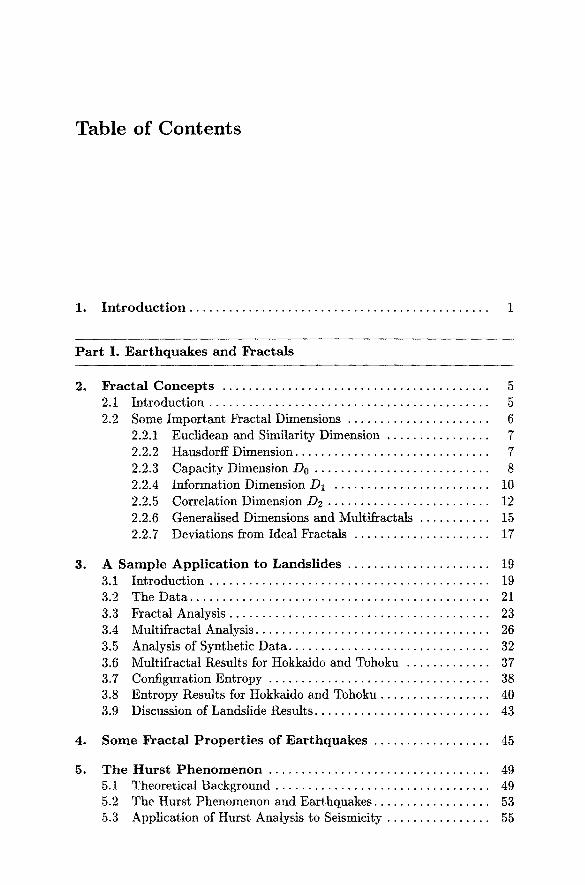
Table of Contents

1. I n t r o d u c t i o n . . . . . . . . . . . . . . . . . . . . . . . . . . . . . . . . . . . . . . . . . . . . . . 1

P a r t I. E a r t h q u a k e s and Fracta ls

. Fracta l C o n c e p t s . . . . . . . . . . . . . . . . . . . . . . . . . . . . . . . . . . . . . . . . .

2.1 In t roduc t i on . . . . . . . . . . . . . . . . . . . . . . . . . . . . . . . . . . . . . . . . . . .

2.2 Some I m p o r t a n t Fracta l Dimensions . . . . . . . . . . . . . . . . . . . . . .

5

5

6 2.2.1 Eucl idean and Similari ty Dimens ion . . . . . . . . . . . . . . . . 7

2.2.2 Hansdorff Dimens ion . . . . . . . . . . . . . . . . . . . . . . . . . . . . . . 7

2.2.3 Capac i ty Dimens ion Do . . . . . . . . . . . . . . . . . . . . . . . . . . . 8

2.2.4 In fo rmat ion Dimension D1 . . . . . . . . . . . . . . . . . . . . . . . . 10

2.2.5 Corre la t ion Dimens ion D2 . . . . . . . . . . . . . . . . . . . . . . . . . 12

2.2.6 General ised Dimensions and Mult i f ractals . . . . . . . . . . . 15

2.2.7 Deviat ions from Ideal Fractals . . . . . . . . . . . . . . . . . . . . . 17

3. A S a m p l e A p p l i c a t i o n t o L a n d s l i d e s . . . . . . . . . . . . . . . . . . . . . .

4o

5.

19

3.1 In t roduc t i on . . . . . . . . . . . . . . . . . . . . . . . . . . . . . . . . . . . . . . . . . . . 19 3.2 The D a t a . . . . . . . . . . . . . . . . . . . . . . . . . . . . . . . . . . . . . . . . . . . . . . 21

3.3 Frac ta l Analysis . . . . . . . . . . . . . . . . . . . . . . . . . . . . . . . . . . . . . . . . 23

3.4 Mul t i f rac ta l Analysis . . . . . . . . . . . . . . . . . . . . . . . . . . . . . . . . . . . . 26

3.5 Analysis of Synthet ic D a t a . . . . . . . . . . . . . . . . . . . . . . . . . . . . . . . 32

3.6 Mul t i f rac ta l Results for Hokkaido and Tohoku . . . . . . . . . . . . . 37 3.7 Conf igura t ion En t ropy . . . . . . . . . . . . . . . . . . . . . . . . . . . . . . . . . . 38 3.8 En t ropy Resul ts for Hokkaido and Tohoku . . . . . . . . . . . . . . . . . 40

3.9 Discussion of Landsl ide Results . . . . . . . . . . . . . . . . . . . . . . . . . . . 43

S o m e F r a c t a I P r o p e r t i e s o f E a r t h q u a k e s . . . . . . . . . . . . . . . . . . 45

T h e H u r s t P h e n o m e n o n . . . . . . . . . . . . . . . . . . . . . . . . . . . . . . . . . . 49 5.1 Theoret ica l Background . . . . . . . . . . . . . . . . . . . . . . . . . . . . . . . . . 49 5.2 The Hurs t P h e n o m e n o n and Ear thquakes . . . . . . . . . . . . . . . . . . 53 5.3 Appl ica t ion of Hurs t Analysis to Seismicity . . . . . . . . . . . . . . . . 55

VI Table of Contents

.

.

.

M u l t i f r a c t a l S p e c t r a as P r e c u r s o r s . . . . . . . . . . . . . . . . . . . . . . . . 61

6.1 Mul t i f rac ta l Ear thquake Precursors . . . . . . . . . . . . . . . . . . . . . . . 61

6.2 Mul t i f rac ta l Phase Transi t ions . . . . . . . . . . . . . . . . . . . . . . . . . . . 66

F r a c t a l P r e c u r s o r y B e h a v i o u r . . . . . . . . . . . . . . . . . . . . . . . . . . . . . 71

7.1 The Da ta . . . . . . . . . . . . . . . . . . . . . . . . . . . . . . . . . . . . . . . . . . . . . . 71 7.2 Overall Proper t ies . . . . . . . . . . . . . . . . . . . . . . . . . . . . . . . . . . . . . . 72

7.2.1 Mult i f rac ta l Spec t rum . . . . . . . . . . . . . . . . . . . . . . . . . . . . 74

7.2.2 H O T Analysis . . . . . . . . . . . . . . . . . . . . . . . . . . . . . . . . . . . 78

7.2.3 Conf igura t ion En t ropy . . . . . . . . . . . . . . . . . . . . . . . . . . . . 80

7.3 Tempora l Var ia t ion of Propert ies . . . . . . . . . . . . . . . . . . . . . . . . . 80

7.3.1 Tempora l Mult i f racta l . . . . . . . . . . . . . . . . . . . . . . . . . . . . 82

7.3.2 Tempora l Configurat ion Ent ropy . . . . . . . . . . . . . . . . . . . 88

F r a c t a l P r o p e r t i e s o f A f t e r s h o c k s . . . . . . . . . . . . . . . . . . . . . . . . . 93

8.1 Mult i f rac ta l Proper t ies . . . . . . . . . . . . . . . . . . . . . . . . . . . . . . . . . . 95

8.2 Conf igura t ion En t ropy . . . . . . . . . . . . . . . . . . . . . . . . . . . . . . . . . . 99

8.3 (An)Isotropic Fracta l Propert ies . . . . . . . . . . . . . . . . . . . . . . . . . . 100

8.4 Overall and Aftershock Seismicity . . . . . . . . . . . . . . . . . . . . . . . . 101

P a r t I I . E a r t h q u a k e s a n d C h a o s

.

9.1

9.2

9.3

C h a o s . . . . . . . . . . . . . . . . . . . . . . . . . . . . . . . . . . . . . . . . . . . . . . . . . . . . 107

Nonl inear Time Series Analysis . . . . . . . . . . . . . . . . . . . . . . . . . . . 109

Analysis of Known Dynamics . . . . . . . . . . . . . . . . . . . . . . . . . . . . 113

9.2.1 Quasi-periodic Dynamics . . . . . . . . . . . . . . . . . . . . . . . . . . 113

9.2.2 Inf in i te-dimensional Dynamics (Noise) . . . . . . . . . . . . . . 118

9.2.3 Low-dimensional Chaotic Dynamics . . . . . . . . . . . . . . . . . 123

Analysis of Ear thquake Da ta . . . . . . . . . . . . . . . . . . . . . . . . . . . . . 128 9.3.1 R a d o n . . . . . . . . . . . . . . . . . . . . . . . . . . . . . . . . . . . . . . . . . . 128 9.3.2 St ra in . . . . . . . . . . . . . . . . . . . . . . . . . . . . . . . . . . . . . . . . . . . 134

9.3.3 Inter-arr ival Times . . . . . . . . . . . . . . . . . . . . . . . . . . . . . . . 141 9.3.4 Moni tor ing Seismicity in Phase Space . . . . . . . . . . . . . . . 151

A. A M o d i f i e d B o x - C o u n t i n g A l g o r i t h m . . . . . . . . . . . . . . . . . . . . . 159

B. F r a c t a l C l u s t e r A n a l y s i s . . . . . . . . . . . . . . . . . . . . . . . . . . . . . . . . . . 163

A c k n o w l e d g e m e n t s . . . . . . . . . . . . . . . . . . . . . . . . . . . . . . . . . . . . . . . . . . . 165

R e f e r e n c e s . . . . . . . . . . . . . . . . . . . . . . . . . . . . . . . . . . . . . . . . . . . . . . . . . . . . 167

I n d e x . . . . . . . . . . . . . . . . . . . . . . . . . . . . . . . . . . . . . . . . . . . . . . . . . . . . . . . . . 177

List of Figures

2.1 M o u n t a i n or rock? A n example for scale- invar iance . . . . . . . . . . . . . 6

2.2 T h e Hausdor f f d imens ion . . . . . . . . . . . . . . . . . . . . . . . . . . . . . . . . . . . . 8 2.3 T h e Box-coun t ing d imens ion . . . . . . . . . . . . . . . . . . . . . . . . . . . . . . . . . 9

2.4 T h e i n fo rma t ion d imens ion . . . . . . . . . . . . . . . . . . . . . . . . . . . . . . . . . . 12

2.5 T h e co r re l a t ion d imens ion . . . . . . . . . . . . . . . . . . . . . . . . . . . . . . . . . . . 14 2.6 Typ i ca l Dq a n d f ( a ) - a curve and the i r re la t ion . . . . . . . . . . . . . . . 16

3.1 Geograph ica l l oca t ion of landsl ide regions considered a n d the i r

d i s t r i bu t ions of landsl ides . . . . . . . . . . . . . . . . . . . . . . . . . . . . . . . . . . . . 21 3.2 Pe r spec t ive th ree -d imens iona l views of the p r o b a b i l i t y dens i ty dis-

t r i b u t i o n of landsl ides . . . . . . . . . . . . . . . . . . . . . . . . . . . . . . . . . . . . . . . 22 3.3 P l o t of log(1/N(r)) versus l o g r for lands l ide sets . . . . . . . . . . . . . . . 25 3.4 Theore t i ca l mu l t i f r ac t a l s p e c t r u m of the two-d imens iona l De Wi j s

f r ac ta l . . . . . . . . . . . . . . . . . . . . . . . . . . . . . . . . . . . . . . . . . . . . . . . . . . . . 28 3.5 log(C(q,r) 1/(q-1)) versus l o g r p lo ts wi th the bes t nonl inear fits

for q = 15, 0, - 1 5 for the Tohoku lands l ide d i s t r i bu t ion . . . . . . . . . 31

3.6 Three ar t i f ic ia l monof rac ta l s w i th ind is t inguishab le p rope r t i e s . . . . 33 3.7 M u l t i f r a c t a l s p e c t r a of ar t i f ic ia l monof rac ta l s . . . . . . . . . . . . . . . . . . . 34 3.8 Mul t i f r a c t a l po in t d i s t r i bu t i on accord ing to t he De Wi j s mode l for

p = 0.25 . . . . . . . . . . . . . . . . . . . . . . . . . . . . . . . . . . . . . . . . . . . . . . . . . 36 3.9 Mul t i f r a c t a l s p e c t r a for the d a t a shown in Fig. 3.8 and a no the r

r a n d o m set of t he same size . . . . . . . . . . . . . . . . . . . . . . . . . . . . . . . . . . 37 3.10 Mul t i f r a c t a l s p e c t r a for lands l ide d a t a . . . . . . . . . . . . . . . . . . . . . . . . . 38 3.11 Conf igura t ion en t ropy curves for the Tohoku subse ts . . . . . . . . . . . . 41 3.12 Conf igura t ion en t ropy curves for syn the t ic sets . . . . . . . . . . . . . . . . . 42

5.1 S t r a in re lease f rom shallow large ea r thquakes . . . . . . . . . . . . . . . . . . 53 5.2 Cumula t i ve ea r thquake energy for Mexico . . . . . . . . . . . . . . . . . . . . . 54

5.3 U p p e r and lower bounds of the range of a f rac ta l profile . . . . . . . . . 55 5.4 A f rac ta l e levat ion profile and i ts Hurs t range . . . . . . . . . . . . . . . . . . 56 5.5 Hurs t p lo t for a f rac ta l profile . . . . . . . . . . . . . . . . . . . . . . . . . . . . . . . . 57 5.6 R a n g e image a n d rose p lo t of an i so t ropic field . . . . . . . . . . . . . . . . . 58 5.7 R a n g e image a n d rose p lo t of an an iso t rop ic field . . . . . . . . . . . . . . . 59

6.1 Schemat ic i l l u s t r a t ion of mu l t i f r ac t a l p recursory behav iou r . . . . . . . 63

VIII List of Figures

6.2 6.3

6.4 6.5

6.6

6.7

7.1

7.2

10-daily frequency of earthquakes in California . . . . . . . . . . . . . . . . . 64 Ahnost monofractal and definitely muttifractal Dq curve for seis- micaUy quiet and active intervals . . . . . . . . . . . . . . . . . . . . . . . . . . . . . 65 3-daily frequency of earthquakes in Eastern Japan . . . . . . . . . . . . . . 65 Almost monofractal and extreme multifractal Dq curve for seis- mically quiet and active intervals . . . . . . . . . . . . . . . . . . . . . . . . . . . . . 66 Example of an f(a) spectrum obtained from a singular probability distribution . . . . . . . . . . . . . . . . . . . . . . . . . . . . . . . . . . . . . . . . . . . . . . . . 68 f (a) spectrum obtained for the Henon map . . . . . . . . . . . . . . . . . . . . 69

Epicentral distribution of the catalogue selected for the search of possible precursory fractal behaviour . . . . . . . . . . . . . . . . . . . . . . . . . . 72 Perspective three-dimensional views of the epicentre distribution and the earthquake size distribution in an area selected for analysis of possible precursory fractal behaviour . . . . . . . . . . . . . . . . . . . . . . . 75

7.3 Spectrum of generalised dimensions and multifractal f ( a ) - a curve for the epicentre distribution of the catalogue selected for analysis of possible precursory behaviour . . . . . . . . . . . . . . . . . . . . . . 77

7.4 Spectrum of generalised dimensions and multifractal f (a) - a curve for the temporal distribution of earthquakes selected for analysis of possible precursory behaviour . . . . . . . . . . . . . . . . . . . . . . 78

7.5 HOT table and rose plot of H for epicentre distribution . . . . . . . . . 79 7.6 HOT table and rose plot of H for rupture area distribution . . . . . . 79 7.7 Configuration Entropy curve for the epicentre distribution selected

for analysis of possible precursory behaviour . . . . . . . . . . . . . . . . . . . 80 7.8 Magnitude (m > = 3.0) versus time diagram for the data set se-

lected for analysis of precursory fractal behaviour . . . . . . . . . . . . . . . 81 7.9 Magnitude vs. event number and daily frequency of earthquakes

for the area selected for analysis of precursory fractal behaviour . . 83 7.10 Temporal variation of Dq for q = -2 , 0, 1, 2 for the epicentre distri-

bution selected for analysis of possible fractal precursory behaviour 84 7.11 Temporal variation of c~,~n and O~rna~ for the epicentre distribu-

tion selected for analysis of fractal precursory behaviour . . . . . . . . . 85 7.12 Temporal variation of f(ami,~) and f(O~rnax ) for the epicentre dis-

tr ibution selected for analysis of possible fractal precursory be- haviour . . . . . . . . . . . . . . . . . . . . . . . . . . . . . . . . . . . . . . . . . . . . . . . . . . . 86

7.13 Temporal variation of A and A ~ for the epicentre distribution selected for analysis of possible fractal precursory behaviour . . . . . 86

7.14 Temporal variation of Dq for q -= -2 , 0, 1, 2 for the temporal dis- tr ibution of earthquakes selected for analysis of possible fractal precursory behaviour . . . . . . . . . . . . . . . . . . . . . . . . . . . . . . . . . . . . . . . . 87

7.15 Temporal variation of ami,~ and f(am~n) for the temporal dis- tr ibution of earthquakes selected for analysis of possible fractal precursory behaviour . . . . . . . . . . . . . . . . . . . . . . . . . . . . . . . . . . . . . . . . 88

List of Figures IX

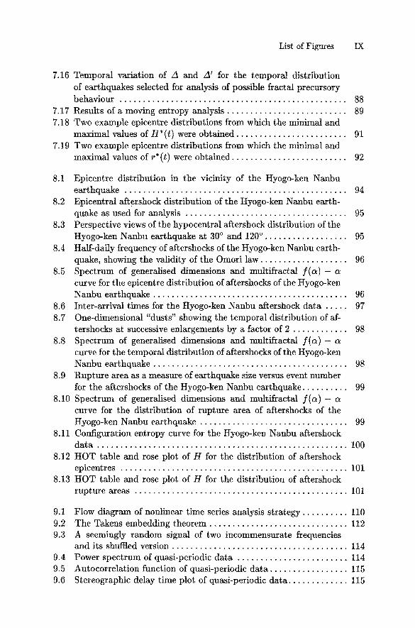
7.16 Temporal variation of A and A ~ for the temporal distribution of earthquakes selected for analysis of possible fractal precursory behaviour . . . . . . . . . . . . . . . . . . . . . . . . . . . . . . . . . . . . . . . . . . . . . . . . . 88

7.17 Results of a moving entropy analysis . . . . . . . . . . . . . . . . . . . . . . . . . . 89 7.18 Two example epicentre distributions from which the minimal and

maximal values of H* (t) were obtained . . . . . . . . . . . . . . . . . . . . . . . . 91 7.19 Two example epicentre distributions from which the minimal and

maximal values of r*(t) were obtained . . . . . . . . . . . . . . . . . . . . . . . . . 92

8.1 Epicentre distribution in the vicinity of the Hyogo-ken Nanbu earthquake . . . . . . . . . . . . . . . . . . . . . . . . . . . . . . . . . . . . . . . . . . . . . . . . 94

8.2 Epicentral aftershock distribution of the Hyogo-ken Nanbu earth- quake as used for analysis . . . . . . . . . . . . . . . . . . . . . . . . . . . . . . . . . . . 95

8.3 Perspective views of the hypocentral aftershock distribution of the Hyogo-ken Nanbu earthquake at 30 ° and 120 ° .................. 95

8.4 Half-daily frequency of aftershocks of the Hyogo-ken Nanbu earth- quake, showing the validity of the Omori law ................... 96

8.5 Spectrum of generalised dimensions and multifractal f ( a ) - a

curve for the epicentre distribution of aftershocks of the Hyogo-ken Nanbu earthquake . . . . . . . . . . . . . . . . . . . . . . . . . . . . . . . . . . . . . . . . . . 96

8.6 Inter-arrival times for the Hyogo-ken Nanbu aftershock data . . . . . 97 8.7 One-dimensional "dusts" showing the temporal distribution of af-

tershocks at successive enlargements by a factor of 2 . . . . . . . . . . . . 98 8.8 Spectrum of generalised dimensions and multifractal f ( a ) - a

curve for the temporal distribution of aftershocks of the Hyogo-ken Nanbu earthquake . . . . . . . . . . . . . . . . . . . . . . . . . . . . . . . . . . . . . . . . . . 98

8.9 Rupture area as a measure of earthquake size versus event number for the aftershocks of the Hyogo-ken Nanbu earthquake . . . . . . . . . . 99

8.10 Spectrum of generalised dimensions and multifractal / ( a ) - a curve for the distribution of rupture area of aftershocks of the Hyogo-ken Nanbu earthquake . . . . . . . . . . . . . . . . . . . . . . . . . . . . . . . . 99

8.11 Configuration entropy curve for the Hyogo-ken Nanbu aftershock da ta . . . . . . . . . . . . . . . . . . . . . . . . . . . . . . . . . . . . . . . . . . . . . . . . . . . . . . 100

8.12 H O T table and rose plot of H for the distribution of aftershock epicentres . . . . . . . . . . . . . . . . . . . . . . . . . . . . . . . . . . . . . . . . . . . . . . . . . 101

8.13 H O T table and rose plot of H for the distribution of aftershock rupture areas . . . . . . . . . . . . . . . . . . . . . . . . . . . . . . . . . . . . . . . . . . . . . . 101

9.1 Flow diagram of nonlinear t ime series analysis s t rategy . . . . . . . . . . 110 9.2 The Takeus embedding theorem . . . . . . . . . . . . . . . . . . . . . . . . . . . . . . 112 9.3 A seemingly random signal of two incommensurate frequencies

and its shuffled version . . . . . . . . . . . . . . . . . . . . . . . . . . . . . . . . . . . . . . 114 9.4 Power spectrum of quasi-periodic data . . . . . . . . . . . . . . . . . . . . . . . . 114 9.5 Autocorrelation function of quasi-periodic data . . . . . . . . . . . . . . . . . 115 9.6 Stereographic delay t ime plot of quasi-periodic da ta . . . . . . . . . . . . . 115

X List of Figures

9.7 Return map of quasi-periodic data . . . . . . . . . . . . . . . . . . . . . . . . . . . . 116 9.8 Phase space plot of shuffled quasi-periodic data . . . . . . . . . . . . . . . . 116 9.9 D2(d) for embedding dimensions of 1 to 10 for quasi-periodic data 117 9.10 D2(d) for embedding dimensions of 1 to 10 for shuffled quasi-

periodic data . . . . . . . . . . . . . . . . . . . . . . . . . . . . . . . . . . . . . . . . . . . . . . 117 9.11 A data set of 2000 Ganssian random points . . . . . . . . . . . . . . . . . . . . 119 9.12 Stereographic phase space plot of Gaussian noise . . . . . . . . . . . . . . . 119 9.13 Return map of Gaussian noise . . . . . . . . . . . . . . . . . . . . . . . . . . . . . . . . 120 9.14 Probability histogram of Gaussian noise . . . . . . . . . . . . . . . . . . . . . . . 120 9.15 IFS-clumpiness test of Gaussian noise . . . . . . . . . . . . . . . . . . . . . . . . . 121 9.16 Autocorrelation function for Gaussian noise . . . . . . . . . . . . . . . . . . . . 121 9.17 Power spectrum for Gaussian noise . . . . . . . . . . . . . . . . . . . . . . . . . . . 121 9.18 Hurst plot for integrated Gaussian noise . . . . . . . . . . . . . . . . . . . . . . . 122 9.19 D2(d) for d -- 1 to 10 for Gaussian noise . . . . . . . . . . . . . . . . . . . . . . . 122 9.20 D2(d) for d = 1 to 10 for "randomised Gaussian noise" . . . . . . . . . . 122 9.21 A chaotic signal from the Lorenz system and its shuffled version. . 124 9.22 Stereographic phase space plot of chaotic Lorenz data . . . . . . . . . . . 124 9.23 Return map for chaotic Lorenz data . . . . . . . . . . . . . . . . . . . . . . . . . . 125 9.24 Probability distribution of chaotic Lorenz data . . . . . . . . . . . . . . . . . 125 9.25 IFS-clumpiness test for chaotic Lorenz data . . . . . . . . . . . . . . . . . . . . 126 9.26 Power spectrum of chaotic Lorenz data . . . . . . . . . . . . . . . . . . . . . . . . 126 9.27 D2(d) for d = 1 to 10 for chaotic Lorenz data . . . . . . . . . . . . . . . . . . 127 9.28 D2(d) for d = 1 to 10 for shuffled chaotic Lorenz data . . . . . . . . . . . 127 9.29 Location of radon site KSM . . . . . . . . . . . . . . . . . . . . . . . . . . . . . . . . . . 129 9.30 Observed hourly radon gas concentration at KSM . . . . . . . . . . . . . . 130 9.31 Power spectrum of radon observation at site KSM . . . . . . . . . . . . . . 130 9.32 6th order polynomial fit to radon data to remove slow trend . . . . . 131 9.33 Radon residual after a maximum-entropy analysis . . . . . . . . . . . . . . 131 9.34 Power spectrum of non-harmonic residual of radon data . . . . . . . . . 132 9.35 IFS clumpiness test of non-harmonic residual of radon data . . . . . . 132 9.36 Autocorrelation function of non-harmonic residual of radon data . 133 9.37 D2(d) as obtained for delay-time embedding of non-harmonic

radon residual . . . . . . . . . . . . . . . . . . . . . . . . . . . . . . . . . . . . . . . . . . . . . . 133 9.38 D2(d) as obtained for delay-time embedding of radon fluctuation . 133 9.39 Location and details of strain observation vault at Yamasaki fault

(from Watanabe (1991)) . . . . . . . . . . . . . . . . . . . . . . . . . . . . . . . . . . . . . 134 9.40 Daily strain fluctuation at the Yamasaki fault for 1975 to 1987 . . . 136 9.41 Hourly strain fluctuation at the Yamasaki fault for 1984 to 1985.. 136 9.42 Three-dimensional delay time embedding of daily strain fluctua-

tions revealing no discernible structure . . . . . . . . . . . . . . . . . . . . . . . . 137 9.43 Logarithmic power spectrum of hourly strain fluctuations . . . . . . . . 137 9.44 Logarithmic histogram of hourly strain fluctuations . . . . . . . . . . . . . 138 9.45 IFS-clumpiness test of hourly strain fluctuations . . . . . . . . . . . . . . . . 138 9.46 Autocorrelation function of hourly strain fluctuations . . . . . . . . . . . 139

List of Figures XI

9.47 D2(d) for embeddings of daily strain fluctuations . . . . . . . . . . . . . . . 139 9.48 D2(d) for embeddings of hourly strain fluctuations . . . . . . . . . . . . . . 140 9.49 D2(d) for embeddings of scrambled hourly strain fluctuations . . . . 140 9.50 First 15 000 values of the fluctuation of earthquake inter-arrival

t imes . . . . . . . . . . . . . . . . . . . . . . . . . . . . . . . . . . . . . . . . . . . . . . . . . . . . . 141 9.51 Power spect rum of earthquake inter-arrival t ime fluctuation . . . . . . 142 9.52 Hurst plot of integrated earthquake inter-arrival times . . . . . . . . . . 143 9.53 Probabil i ty distribution of earthquake inter-arrival t ime fluctuation143 9.54 IFS-clumpiness test for earthquake inter-arrival t ime f luc tua t ion . . 144 9.55 Symmetric wavelet t ransform of earthquake inter-arrival t ime fluc-

tuat ion . . . . . . . . . . . . . . . . . . . . . . . . . . . . . . . . . . . . . . . . . . . . . . . . . . . . 144 9.56 Stereog:raphic view of two-dimensional embedding of inter-arrival

t ime fluctuation . . . . . . . . . . . . . . . . . . . . . . . . . . . . . . . . . . . . . . . . . . . . 145 9.57 A re turn map of earthquake inter-arrival t ime fluctuation . . . . . . . . 145 9.58 Autocorrelat ion function for earthquake inter-arrival t ime fluctu-

ation . . . . . . . . . . . . . . . . . . . . . . . . . . . . . . . . . . . . . . . . . . . . . . . . . . . . . . 146 9.59 D2(d) for embedding dimensions of 1 to 10 for earthquake inter-

arrival t ime fluctuations . . . . . . . . . . . . . . . . . . . . . . . . . . . . . . . . . . . . . 147 9.60 Surrogate earthquake inter-arrival t ime fluctuation data sets: Phase

randonfised and shuffled in the t ime domain . . . . . . . . . . . . . . . . . . . 149 9.61 D2(d) for embedding dimensions of 1 to 10 for phase randomised

earthquake inter-arrival t ime fluctuations . . . . . . . . . . . . . . . . . . . . . . 150 9.62 D2(d) for embedding dimensions of 1 to 10 for shuffled earthquake

inter-arrival t ime fluctuations . . . . . . . . . . . . . . . . . . . . . . . . . . . . . . . . 150 9.63 Da ta used for monitoring in phase space . . . . . . . . . . . . . . . . . . . . . . . 152 9.64 Earthquake inter-arrival times and first derivative . . . . . . . . . . . . . . 153 9.65 Gaussian inter-arrival times and first derivative . . . . . . . . . . . . . . . . . 153 9.66 Poisson inter-arrival times and first derivative . . . . . . . . . . . . . . . . . . 154 9.67 Two dimensional phase space embedding of earthquake inter-

arrival da ta . . . . . . . . . . . . . . . . . . . . . . . . . . . . . . . . . . . . . . . . . . . . . . . . 154 9.68 Two dimensional phase space embedding of Gauss data . . . . . . . . . 155 9.69 Two dimensional phase space embedding of Poisson da ta . . . . . . . . 155 9.70 Correlation versus embedding dimension for several t ime series . . . 156 9.71 At t rac tor dimension versus t ime . . . . . . . . . . . . . . . . . . . . . . . . . . . . . . 157 9.72 Magnitude versus t ime . . . . . . . . . . . . . . . . . . . . . . . . . . . . . . . . . . . . . . 157

List of Tables

3.1

7.1

Results of entropy analyses of the da ta sets T1 to T4 together with the correlation dimensions of the sets . . . . . . . . . . . . . . . . . . . . . 40

Listing of earthquakes of m > = 4.5 in the area selected for analysis of possible precursory fractal behaviour . . . . . . . . . . . . . . . . . . . . . . . 82

8.1 Summary of the anisotropy analysis of the epicentre distribution and rupture size distribution . . . . . . . . . . . . . . . . . . . . . . . . . . . . . . . . . 102

8.2 Some significant differences between fractal parameters of overall and aftershock seismicity . . . . . . . . . . . . . . . . . . . . . . . . . . . . . . . . . . . . 103

1. Introduct ion

Earthquake prediction research has been carried out for over t00 years now. There has been no success in the sense of a reproducible prediction of the time, location and magnitude of earthquakes (e.g. [Gel97]). The discussion whether earthquakes are predictable at all has gained some impetus during the last few years (e.g. [~r97, GJKM97, Wys97]). At the same time there has been a great development in the fields of fractal geometry (e.g. [Kor92, HS93]) and nonlinear dynamics (e.g. fABST93]), especially in numerical analysis. Fractality of real-world earthquake statistics has by now been established beyond doubt (e.g. [Wak90]) and is in agreement with modern models of seismicity (e.g. [Tur97]). While there is no proof of deterministic chaos in real earthquake data, nobody questions nonlinearity of the earthquake process (e.g. [Mei94]) and slider block models have been shown to exhibit chaotic behaviour (e.g. [HT92]).

Have inappropriate (Euclidean, linear) methods of analysis been used so that possibly existing earthquake precursors simply couldn't be detected? Or is it that individual earthquakes are inherently unpredictable due to their chaotic dynamics or high "complexity"? Both issues will be addressed in a theoretical as well as empirical fashion in this book.

Part I discusses the application of fractat concepts to seismicity, while Part II applies ideas from nonlinear analysis. Emphasis is on numerical analysis of real-world data with theoretical background and models introduced where applicable to show the motivation behind the analyses and to aid in the interpretation of the results.

Part I begins with the introduction of fractal fundamentals and discusses the various fractal dimensions including multifractals. Special attention is given to deviations from ideal scaling behaviour and to practical aspects of the numerical determination of fractal properties.

A comprehensive sample application to landslides in Chapter 3 may be read on its own. It deepens the understanding of multifractals and addresses further problems in numerical analysis. Configuration entropy analysis as a promising complementary tool to fractal methods is also applied. Implications of the confirmation of landslides as' a multifractal process are discussed.

Chapter 4 summarises the various fractal properties of earthquakes which have been established or rediscovered during the past years.

2 1. Introduction

A fascinating "fractal" property of many natural systems is the Hurst phenomenon which characterises persistence or antipersistence of processes, i.e. their long time memory. This phenomenon is discussed in connection with seismicity in Chapter 5. Hurst analysis is used to describe anisotropy in scaling properties of earthquake fields.

Chapter 6 sheds some light on the relationship between multifractal spec- tra and phase transitions and what precursory qualities these spectra might have and why.

In Chapter 7 the whole toolbox of fractal analysis is applied to seismicity in a region containing the Kobe earthquake of January 1995. After deter- mination of the overall properties of the earthquake catalogue the temporal variation of fractal properties is obtained to check for fractal precursors. A comparison of overall and aftershock seismicity concludes Part I.

Part II first introduces some principles of nonlinear time series analysis. Analysis of three synthetic time series from different classes of dynamics (quasi-periodic, infinite-dimensional and low-dimensional chaotic) illustrates the methods and shows what may be obtained. Next, nonlinear analysis is applied to radon emission and strain, two prominent earthquake-related real- world time series and to earthquake inter-arrival times directly derived from an earthquake catalogue. Finally, "complexity" of earthquake dynamics is discussed by monitoring the variation of apparent attractor dimension with time.