Learning and Using Taxonomies for Visual and OlfactoryClassification

Thesis by

Greg Griffin

In Partial Fulfillment of the Requirements

for the Degree of

Doctor of Philosophy

California Institute of Technology

Pasadena, California

2013

(Defended April 12, 2013)

ii

c© 2013

Greg Griffin

All Rights Reserved

iii

FOR LESLIE

iv

v

Acknowledgements

First and foremost I would like to thank my advisor, Dr. Pietro Perona. I simply could not have

asked for a kinder advisor or a better learning experience. Without his patient support and imag-

ination none of this would have even started. Dr. Nate Lewis and Dr. Richard Flagan have also

been extremely gracious in sharing their projects with me. Pietro and Rick have been a constant

source of encouragement and brain-storming, and Nate and his students Marc Woodka and Edgardo

Garcia-Berrios not only provided extremely sensitive sensors but gave me copious help in an area

of research I knew very little about. Finally I would like to give my heartfelt thanks to Dr. James

House who has been such an excellent teacher and friend.

My lab-mates have also been extremely generous, and even though none of them ever read this

sort of thing I would like to thank them here. Alex Holub, Ron Appel, Kristen Branson, Claudo

Fanti, Anelia Angelova, Merrielle Spain, Thomas Fuchs, Ryan Gomes, David Hall and many others

made being here that much more fun and interesting, each in their own way. I especially want to

single out fellow grad students Marco Andreetto, Ruxandra Paun and Nadine Dabbey as important

friends who made day-to-day life particularly enjoyable.

Mom and Dad cannot ever be thanked enough: they and my sister Kathy have been everything

to me. I have come to think of three extraordinary people as myextended family here at Caltech:

Zachary Abbott, Catherine Beni and Andy Kositsky. I have relied heavily on their laughter and love.

Most of all I want to thank Leslie Johnson, soon to be my wife, to whom this thesis is dedicated.

vi

Her tolerance and understanding, insight and unfailing sweetness at even the roughest of times fill

me with gratitude, wonder and the deepest abiding Love.

And Hien. Where do I even begin?

vii

Abstract

Humans are able of distinguishing more than 5000 visual categories[10] even in complex environ-

ments using a variety of different visual systems all working in tandem[74]. We seem to be capable

of distinguishing thousands of different odors as well [66,93, 107]. In the machine learning com-

munity, many commonly used multi-class classifiers do not scale well to such large numbers of

categories. This thesis demonstrates a novel method of automatically creating application-specific

taxonomies to aid in scaling classification algorithms to more than 100 categories using both visual

and olfactory data. The visual data consists of images collected online and pollen slides scanned

under a microscope. The olfactory data was acquired by constructing a small portable sniffing appa-

ratus which draws air over 10 carbon black polymer compositesensors. We investigate performance

when classifying 256 visual categories, 8 or more species ofpollen and 130 olfactory categories

sampled from common household items and a standardized scratch-and-sniff test. Taxonomies

are employed in a divide-and-conquer classification framework which improves classification time

while allowing the end user to trade performance for specificity as needed. Before classification can

even take place, the pollen counter and electronic nose mustfilter out a high volume of background

“clutter” to detect the categories of interest. In the case of pollen this is done with an efficient cas-

cade of classifiers that rule out most non-pollen before invoking slower multi-class classifiers. In the

case of the electronic nose, much of the extraneous noise encountered in outdoor environments can

be filtered using a sniffing strategy which preferentially samples the sensor response at frequencies

viii

that are relatively immune to background contributions from ambient water vapor. This combina-

tion of efficient background rejection with scalable classification algorithms is tested in detail for

three separate projects: 1) the Caltech-256 Image Dataset,2) the Caltech Automated Pollen Identi-

fication and Counting System (CAPICS) and 3) the Caltech Electronic Nose, a portable electronic

nose specially designed for outdoor use.

ix

Contents

Acknowledgements v

Abstract vii

1 Introduction 1

2 The Caltech-256 5

2.1 Introduction . . . . . . . . . . . . . . . . . . . . . . . . . . . . . . . . . . . .. . 5

2.2 Collection Procedure . . . . . . . . . . . . . . . . . . . . . . . . . . . . .. . . . 7

2.2.1 Image Relevance . . . . . . . . . . . . . . . . . . . . . . . . . . . . . . . 10

2.2.2 Categories . . . . . . . . . . . . . . . . . . . . . . . . . . . . . . . . . . 11

2.2.3 Taxonomy . . . . . . . . . . . . . . . . . . . . . . . . . . . . . . . . . . 11

2.2.4 Background . . . . . . . . . . . . . . . . . . . . . . . . . . . . . . . . . . 13

2.3 Benchmarks . . . . . . . . . . . . . . . . . . . . . . . . . . . . . . . . . . . . . .14

2.3.1 Performance . . . . . . . . . . . . . . . . . . . . . . . . . . . . . . . . . 16

2.3.2 Localization and Segmentation . . . . . . . . . . . . . . . . . . .. . . . . 17

2.3.3 Generality . . . . . . . . . . . . . . . . . . . . . . . . . . . . . . . . . . . 18

2.3.4 Background . . . . . . . . . . . . . . . . . . . . . . . . . . . . . . . . . . 18

2.4 Results . . . . . . . . . . . . . . . . . . . . . . . . . . . . . . . . . . . . . . . . .19

2.4.1 Size Classifier . . . . . . . . . . . . . . . . . . . . . . . . . . . . . . . . 19

x

2.4.2 Correlation Classifier . . . . . . . . . . . . . . . . . . . . . . . . . .. . . 22

2.4.3 Spatial Pyramid Matching . . . . . . . . . . . . . . . . . . . . . . . .. . 22

2.4.4 Generality . . . . . . . . . . . . . . . . . . . . . . . . . . . . . . . . . . . 23

2.4.5 Background . . . . . . . . . . . . . . . . . . . . . . . . . . . . . . . . . . 25

2.5 Conclusion . . . . . . . . . . . . . . . . . . . . . . . . . . . . . . . . . . . . . .28

3 Visual Hierarchies 31

3.1 Introduction . . . . . . . . . . . . . . . . . . . . . . . . . . . . . . . . . . . .. . 31

3.2 Experimental Setup . . . . . . . . . . . . . . . . . . . . . . . . . . . . . . .. . . 33

3.2.1 Training and Testing Data . . . . . . . . . . . . . . . . . . . . . . . .. . 33

3.2.2 Spatial Pyramid Matching . . . . . . . . . . . . . . . . . . . . . . . .. . 34

3.2.3 Measuring Performance . . . . . . . . . . . . . . . . . . . . . . . . . .. 36

3.2.4 Hierarchical Approach . . . . . . . . . . . . . . . . . . . . . . . . . .. . 37

3.3 Building Taxonomies . . . . . . . . . . . . . . . . . . . . . . . . . . . . . .. . . 40

3.4 Top-Down Classification Algorithm . . . . . . . . . . . . . . . . . .. . . . . . . 40

3.5 Results . . . . . . . . . . . . . . . . . . . . . . . . . . . . . . . . . . . . . . . . .42

3.6 Conclusions . . . . . . . . . . . . . . . . . . . . . . . . . . . . . . . . . . . . .. 44

4 Pollen Counting 47

4.1 Introduction . . . . . . . . . . . . . . . . . . . . . . . . . . . . . . . . . . . .. . 47

4.2 Data Collection Method . . . . . . . . . . . . . . . . . . . . . . . . . . . .. . . . 49

4.3 Classification Algorithm . . . . . . . . . . . . . . . . . . . . . . . . . .. . . . . 51

4.4 Comparison To Humans . . . . . . . . . . . . . . . . . . . . . . . . . . . . . .. 54

4.5 Comparison To Experts . . . . . . . . . . . . . . . . . . . . . . . . . . . . .. . . 57

4.6 Conclusions . . . . . . . . . . . . . . . . . . . . . . . . . . . . . . . . . . . . .. 58

xi

5 Machine Olfaction: Introduction 61

6 Machine Olfaction: Methods 65

6.1 Instrument . . . . . . . . . . . . . . . . . . . . . . . . . . . . . . . . . . . . . .. 65

6.2 Sampling and Measurements . . . . . . . . . . . . . . . . . . . . . . . . .. . . . 65

6.3 Datasets and Environment . . . . . . . . . . . . . . . . . . . . . . . . . .. . . . 68

7 Machine Olfaction: Results 73

7.1 Classification Performance vs. Subsniff Frequency . . . .. . . . . . . . . . . . . 74

7.2 Effects of Different Numbers of Sensors on Classification Performance . . . . . . . 76

7.3 Feature Performance . . . . . . . . . . . . . . . . . . . . . . . . . . . . . .. . . 76

7.4 Feature Consistency . . . . . . . . . . . . . . . . . . . . . . . . . . . . . .. . . . 78

7.5 Top-Down Category Recognition . . . . . . . . . . . . . . . . . . . . .. . . . . . 79

8 Machine Olfaction: Discussion 83

A Olfactory Datasets 85

Bibliography 87

xii

xiii

List of Figures

1.1 A rough illustration of machine vision (red) and olfaction (green) tasks lying in and

between the regimes of classification and detection. While early problems in vision

tended to cluster along either axis, more recent datasets have driven progress further

towards the top right. The three projects discussed in this paper are the Caltech-

256, the Caltech Electronic Nose and the Caltech Automated Pollen Identification

and Counting System (CAPICS). Each is an attempt to take small steps towards the

ultimate goal of a system that can robustly detect and classify thousands of categories

in the “real world” (upper right). . . . . . . . . . . . . . . . . . . . . . .. . . . . . 2

2.1 Examples of a 1, 2 and 3 rating for images downloaded usingthe keyworddice. . . . 6

2.2 Summary of Caltech image datasets. There are actually 102 and 257 categories if the

clutter categories in each set are included. . . . . . . . . . . . . . . . . . . . .. . . 7

2.3 Distribution of image sizes as measured by√width · height, and aspect ratios as

measured bywidth/height. Some common image sizes and aspect ratios that are

overrepresented are labeled above the histograms. Overallin Caltech-256 the mean

image size is 351 pixels while the mean aspect ratio is 1.17. .. . . . . . . . . . . . 8

xiv

2.4 Histogram showing number of images per category. Caltech-101’s largest categories

faces-easy(435),motorbikes(798),airplanes(800) are shared with Caltech-256. An

additional large categoryt-shirt (358) has been added. Theclutter categories for

Caltech-101 (467) and 256 (827) are identified with arrows. This figure should be

viewed in color. . . . . . . . . . . . . . . . . . . . . . . . . . . . . . . . . . . . . . 9

2.5 Precision of images returned by Google. This is defined asthe total number of images

ratedgooddivided by the total number of images downloaded (averaged over many

categories). As more images are download, it becomes progressively more difficult to

gather large numbers of images per object category. For example, to gather 40 good

images per category it is necessary to collect 120 images anddiscard 2/3 of them. To

gather 160 good images, expect to collect about 640 images and discard 3/4 of them. 10

2.6 A taxonomy of Caltech-256 categories created by hand. Atthe top level these are

divided into animate and inanimate objects. Green categories contain images that

were borrowed from Caltech-101. A category is colored red ifit overlaps with some

other category (such asdogandgreyhound). . . . . . . . . . . . . . . . . . . . . . . 12

2.7 Examples ofclutter generated by cropping the photographs of Stephen Shore [103,

104]. . . . . . . . . . . . . . . . . . . . . . . . . . . . . . . . . . . . . . . . . . . 13

2.8 Performance of all 256 object categories using a typicalpyramid match kernel [67] in

a multi-class setting withNtrain = 30. This performance corresponds to the diagonal

entries of the confusion matrix, here sorted from largest tosmallest. The ten best

performing categories are shown in blue at the top left. The ten worst performing

categories are shown in red at the bottom left. Vertical dashed lines indicate the mean

performance. . . . . . . . . . . . . . . . . . . . . . . . . . . . . . . . . . . . . . . 15

xv

2.9 The mean of all images in five randomly chosen categories,as compared to the mean

clutter image. Four categories show some degree of concentration towards the center

while refrigerator andclutter do not. . . . . . . . . . . . . . . . . . . . . . . . . . 17

2.10 The256 × 256 matrixM for the correlation classifier described in subsection 2.4.2.

This is the mean of 10 separate confusion matrices generatedfor Ntrain = 30. A log

scale is used to make it easier to see off-diagonal elements.For clarity we isolate the

diagonal and row 82galaxyand describe their meaning in Fig. 2.11. . . . . . . . . . 20

2.11 A more detailed look at the confusion matrixM from figure 2.10. Top: row 82 shows

which categories were most likely to be confused withgalaxy. These are:galaxy,

saturn, fireworks, cometandmars(in order of greatest to least confusion). Bottom:

the largest diagonal elements represent the categories that are easiest to classify with

the correlation algorithm. These are:self-propelled-lawn-mower, motorbikes-101,

trilobite-101, guitar-pickandsaturn. All of these categories tend to have objects that

are located consistently between images. . . . . . . . . . . . . . . .. . . . . . . . 21

2.12 Performance as a function ofNtrain for Caltech-101 and Caltech-256 using the 3

algorithms discussed in the text. The spatial pyramid matching algorithm is that of

Lazebnik, Schmid and Ponce [67]. We compare our own implementation with their

published results, as well as the SVM-KNN approach of Zhang,Berg, Maire and

Malik [120]. . . . . . . . . . . . . . . . . . . . . . . . . . . . . . . . . . . . . . . 23

xvi

2.13 Selected rows and columns of the256×256 confusion matrixM for spatial pyramid

matching [67] andNtrain = 30. Matrix elements containing 0.0 have been left blank.

The first 6 categories are chosen because they are likely to beconfounded with the

last 6 categories. The main diagonal shows the performance for just these 12 cate-

gories. The diagonals of the other 2 quadrants show whether the algorithm can detect

categories which are similar but not exact. . . . . . . . . . . . . . .. . . . . . . . 24

2.14 ROC curve for three different interest classifiers described in section 2.4.5. These

classifiers are designed to focus the attention of the multi-category detectors bench-

marked in Figure 2.12. BecauseDetector Bis roughly 200 times faster thanA or

C, it represents the best tradeoff between performance and speed. This detector can

accurately detect 38.2% of the interesting (non-clutter) images with a 0.1% rate of

false detections. In other words, 1 in 1000 of the images classified asinteresting

will instead contain clutter (solid red line). If a 1 in 100 rate of false detections is

acceptable, the accuracy increases to 58.6% (dashed red line). . . . . . . . . . . . . 27

2.15 In general the Caltech-256 images are more difficult to classify than the Caltech-

101 images. Here we plot performance of the two datasets overa random mix of

Ncategories from each dataset. Even when the number of categories remains the same,

the Caltech-256 performance is lower. For example atNcategories = 100 the perfor-

mance is∼ 60% lower. . . . . . . . . . . . . . . . . . . . . . . . . . . . . . . . . . 28

xvii

3.1 A typical one-vs-all multi-class classifier (top) exhaustively tests each image against

every possible visual category requiringNcat decisions per image. This method does

not scale well to hundreds or thousands of categories. Our hierarchical approach uses

the training data to construct a taxonomy of categories which corresponds to a tree

of classifiers (bottom). In principle each image can now be classified with as few as

log2 Ncat decisions. The above example illustrates this for an unlabeled test image

andNcat = 8. The tree we actually employ has slightly more flexibility asshown in

Fig. 3.4 . . . . . . . . . . . . . . . . . . . . . . . . . . . . . . . . . . . . . . . . . 33

3.2 Performance comparison between Caltech-101 and Caltech-256 datasets using the

spatial pyramid matching algorithm of Lazebnik et al. [67].The performance of our

implementation is almost identical to that reported by the original authors; any per-

formance difference may be attributed to a denser grid used to sample SIFT features.

This illustrates a standard non-hierarchical approach where authors mainly present

the number of training examples and the classification performance, without also

plotting classification speed. . . . . . . . . . . . . . . . . . . . . . . . .. . . . . . 35

3.3 In general the Caltech-256 [55] images are more difficultto classify than the Caltech-

101 images. Here we fixNtrain = 30 and plot performance of the two datasets over a

random mix ofNcat categories chosen from each dataset. The solid region represents

a range of performance values for 10 randomized subsets. Even when the number of

categories remains the same, the Caltech-256 performance is lower. For example at

Ncat = 100 the performance is∼ 60% lower (dashed red line). . . . . . . . . . . . . 36

xviii

3.4 A simple hierarchical cascade of classifiers (limited totwo levels and four categories

for simplicity of illustration). We call A, B, C and D four sets of categories as illus-

trated in Fig 3.5. Each white square represents a binarybranch classifier. Test images

are fed into the top node of the tree where a classifier assignsthem to either the set A

∪ B or the set C∪ D (white square at the center-top). Depending on the classification,

the image is further classified into either A or B, or C or D. Test images ultimately

terminate in one of the 7 red octagonal nodes where a conventional multi-classnode

classifiermakes the final decision. For a two-levelℓ = 2 tree, images terminate in

one of the 4 lower octagonal nodes. Ifℓ = 0 then all images terminate in the top

octagonal node, which is equivalent to conventional non-hierarchical classification.

The tree is not necessarily perfectly balanced: A, B, C and D may have different

cardinality. Each branch or node classifier is trained exclusively on images extracted

from the sets that the classifier is discriminating. See Sec.3.4 for details. . . . . . . 38

3.5 Top-down grouping as described in Sec. 3.3. Our underlying assumption is that cate-

gories that are easily confused should be grouped together in order to build the branch

classifiers in Fig 3.4. First we estimate a confusion matrix using the training set and

a leave-one-out procedure. Shown here is the confusion matrix for Ntrain = 10, with

diagonal elements removed to make the off-diagonal terms easier to see. . . . . . . 39

xix

3.6 Taxonomy discovered automatically by the computer, using only a limited subset of

Caltech-256 training images and their labels. Aside from these labels there is no

other human supervision; branch membership is not hand-tuned in any way. The

taxonomy is created by first generating a confusion matrix for Ntrain = 10 and recur-

sively dividing it by spectral clustering. Branches and their categories are determined

solely on the basis of the confusion between categories, which in turn is based on the

feature-matching procedure of spatial pyramid matching. To compare this with some

recognizably human categories we color code all the insects(red), birds (yellow),

land mammals (green) and aquatic mammals (blue). Notice that the computer’s hier-

archy usually begins with a split that puts all the plant and animal categories together

in one branch. This split is found automatically with such consistency that in a third

of all randomized training setsnot a single category of living thingends up on the

opposite branch. . . . . . . . . . . . . . . . . . . . . . . . . . . . . . . . . . . . .41

3.7 The taxonomy from Fig.3.6 is reproduced here to illustrate how classification per-

formance can be traded for classification speed. NodeA represents an ordinary non-

hierarchical one-vs-all classifier implemented using an SVM. This is accurate but

slow because of the large combined set of support vectors inNcats = 256 individual

binary classifiers. A the other extreme, each test image passes through a series of

inexpensive binary branch classifiers until it reaches 1 of the 256 leaves, collectively

labeledC above. A compromise solution B invokes a finite set of branch classifiers

prior to final multi-class classification in one of 7 terminalnodes. . . . . . . . . . . 43

xx

3.8 Comparison of three different methods for generating taxonomies. For each taxon-

omy we vary the number of branch comparisons prior to final classification, as illus-

trated in Fig. 3.4. This results in a tradeoff between performance and speed as one

moves between two extremesA andC. Randomly generated hierarchies result in poor

cascade performance. Of the three methods, taxonomies based on Spectral Cluster-

ing yield marginally better performance. All three curves measure performance vs.

speed forNcat = 256 andNtrain = 10. . . . . . . . . . . . . . . . . . . . . . . . . 44

3.9 Cascade performance / speed trade-off as a function ofNtrain. Values ofNtrain = 10

andNtrain = 50 result in a 5-fold and 20-fold speed increase (respectively) for a fixed

10% performance drop. . . . . . . . . . . . . . . . . . . . . . . . . . . . . . . . .. 45

4.1 Dr. James House stands next to a modern-day Burkard pollen sampler located on the

roof of Keck Laboratory at Caltech (left). The basic techniques used to collect pollen

date back to the work of J. M. Hirst in the early 1950’s (right). . . . . . . . . . . . . 48

4.2 The shape, brightness distribution and texture are eachdiscriminative for different

types of pollen. The first feature encodes shape as the Fourier transform of the outer

radius, with values representing the mean radius, eccentricity and higher moments.

The second feature computes the ratio of several different quartiles of the brightness

distribution in a way that is invariant to absolute brightness. Finally, SIFT features

extracted on a 32x32 grid are matched against training examples using the spatial

pyramid matching algorithm of Lazebnik et al. [67]. The firsttwo features can be

computed far more efficiently than the third. . . . . . . . . . . . . .. . . . . . . . . 51

xxi

4.3 Pollen is classified using a cascade of progressively more expensive classification

stages. The size of each yellow diamond represents the complexity of the classifier

stage, with successive stages passing fewer and fewer candidates to the slower, more

refined classifiers downstream. . . . . . . . . . . . . . . . . . . . . . . . .. . . . 52

4.4 In a Mechanical Turk experiment, test subjects are askedto classify the pollen on the

right side using a randomized set of training examples provided on the left. . . . . . 54

4.5 Test subjects do not see the expert classification (red) or the computer classification

(green). While the computer “misclassified” this particular birch sample as oak, the

true ground-truth classification could actually be either,as demonstrated by visually

similar instances circled in each class. . . . . . . . . . . . . . . . .. . . . . . . . . 55

4.6 Mechanical Turk test subjects and the automated system make similar classification

mistakes. Overall performance is 60.3% averaged over all test subjects, 70.9% av-

eraged over the 8 most reliable test subjects, and 80.2% for the automated count.

Confusion matrices may vary significantly among individualtest subjects, as shown

by 9 individual confusion matrices for the 9 test subjects with the largest number of

classifications. . . . . . . . . . . . . . . . . . . . . . . . . . . . . . . . . . . . .. 56

4.7 Pollen counts aggregated over 15 days are plotted against one another to show the de-

gree of agreement between experts and the automated system.As the counts increase

in each plot (bottom-left to top-right) the sampling error decreases. Thus an ideal,

unbiased pair of counts should converge towards a line of slope m=1. In each column

the pair with the best agreement (i.e. slope closest to 1) arelabelled in green. For

3 out of 8 species the experts actually showed better agreement with the automated

system than they did with one another. . . . . . . . . . . . . . . . . . . .. . . . . . 57

xxii

4.8 Daily automated pollen counts for 2012. The total count is broken down into color

bands showing the contribution from individual species. Integrated counts for the

year are displayed in the legend. The system can count a month’s worth of pollen

in 1 day when scanning the slide as an expert would, utilizingless than .1% of the

total collecting area. It is thus nearly fast enough to scan the entire slide which would

drastically reduce the sampling error and bias. We continueto optimize the code

towards this eventual goal. . . . . . . . . . . . . . . . . . . . . . . . . . . .. . . . 59

6.1 A fan draws air from 1 of 4 ordorant chambers or an empty reference chamber, de-

pending on the state of the computer-controlled solenoid valve. The valve control

signal can then be compared to the resistances changes recorded from an arrays of 10

individual sensors as shown in Fig. 2. . . . . . . . . . . . . . . . . . . .. . . . . . 66

xxiii

6.2 (a) A sniff consisted of 7 individual subsniffss1...s7 of sensor data taken as the valve

switched between a single odorant and reference air. From this data a7× 4 = 28 size

featurem was generated representing the measured power in each of the7 subsniffs

i over 4 fundamental harmonicsj. For comparison purposes a simple amplitude fea-

ture differenced the top and bottom 5% quartiles of∆RR

in each subsniff. (b) As the

switching frequencyf increased by powers of 2 so did the number of pulses, so that

the time periodT was constant for all but the first subsniff. (c) To illustratehowm

was measured we show the harmonic decomposition of justs4, highlighted in (a).

The corresponding measurementsm4j were the integrated spectral power for each

of 4 harmonics. Higher-order harmonics suffered from attenuation due to the lim-

ited time-constant of the sensors but had the advantage of being less susceptible to

slow signal drift. Fitting a1/fnnoise spectrum to the average indoor and outdoor fre-

quency response of our sensors in the absence of any odorantsillustrates why higher-

frequency switching and higher-order harmonics may be especially advantageous in

outdoors environments. . . . . . . . . . . . . . . . . . . . . . . . . . . . . . .. . . 70

6.3 Visual representation of the harmonic decomposition featurem for 2 wines, 2 lemon

parts and 2 teas from the Common Household Odors Dataset. Each odorant was

sampled 4 times on 2 different days in 2 separate environments. Each box represents

one complete 400 s sniff reduced to a 280-dimensional feature vector. Within each

box, the 10 rows (y axis) show the response of different sensor over 28 frequencies

(x axis) corresponding to 7 subsniffs and 4 harmonics. For visual clarity, the columns

are sorted by frequency and rows are sorted so that adjacent sensors are maximally

correlated. . . . . . . . . . . . . . . . . . . . . . . . . . . . . . . . . . . . . . . . .71

xxiv

7.1 Classification performance for the University of Pittsburgh Smell Identification Test

(UPSIT) and the Common Household Odors Dataset (CHOD) for different sniff sub-

sets using 4 and 16 categories for training and testing. For control purposes data

were also acquired with empty odorant chambers. Compared with using the entire

sniff (top), the high-frequency subsniffs (2nd row) outperformed the low-frequency

subsniffs (bottom) especially forNcat = 16. The dotted lines show the expected

performance for random guessing. . . . . . . . . . . . . . . . . . . . . . .. . . . . 75

7.2 Classification error for all three datasets taken indoors and outdoors while varying the

number of sensors and the number of categories used for training and testing. Each

dotted colored line represents the mean performance over randomized subsets of 2,

4, 6 and 8 sensors out of the available 10. To illustrate this behavior for a single value

of Ncat, gray vertical lines were used to mark the error averaged over randomized

sets of 16 odor categories for the indoor and outdoor datasets. When the number of

sensors increased from 4 to 10, the indoor error (left line) decreased by< 2% for

the CHOD and UPSIT while the outdoor error (right line) decreased by 4-7%. The

Control error is also important because deviations from random chance when no odor

categories are present may suggest sensitivity to environmental factors such as water

vapor. The indoor error for both 4 and 10 sensors remained consistent with 93.75%

random chance while the outdoor error increased from 85.9% to 91.7% . . . . . . . 77

7.3 Classification error using features based on sensor response amplitude and harmonic

decomposition. For comparison, the UPSIT testing error[32] for human test subjects

10-59 years of age (who performed better than our instrument) and 70-79 years of age

(who performed roughly the same) are also shown. The combined Indoor/Outdoor

dataset used data taken indoors and outdoors as separate training and testing sets. . . 78

xxv

7.4 The confusion matrix for the Indoor Common Household Odor Dataset was used to

automatically generate a top-down hierarchy of odor categories. Branches in the tree

represent splits in the confusion matrix that minimized theintercluster confusion. As

the depth of the tree increased with successive splits, the categories in each branch be-

came more and more difficult for the electronic nose to distinguish. The color of each

branch node represents the classification performance whendetermining whether an

odorant belongs to that branch. This procedure helps characterize the instrument

by showing which odor categories and super-categories werereadily detectable and

which were not. The highlighted categories show the relationships discovered be-

tween the wine, lemon and tea categories, whose features areshown in Fig. 6.3. The

occurrence of wine and citrus categories in the same top-level branch indicated that

these odor categories were harder to distinguish from one another than from tea. . . 81

xxvi

1

Chapter 1

Introduction

My first project in the Caltech Vision Lab was to collect the Caltech-256 Image Dataset[55] with the

help of paid workers and other lab members. It was collected using the same methods used to create

the Caltech-101[69] years earlier. Starting with images downloaded from the Google and Picsearch

search engines with a query such as “airplane”, annotators removed those images that did not fit the

visual category. This followup to the Caltech-101 not only increased the number of available cate-

gories to 256 but also increased the total image count from∼ 9000 to 30000. Individual categories

were better represented1 with larger variation in pose and background environment. An additional

clutter category based on the photographs of Stephen Shore [103, 104] was added to represent the

appearance of images possessing no distinct visual category. The Caltech-256 was successful in the

sense that it challenged the computer vision community to scale image classification algorithms to

a larger number and variety of categories than were previously available2. One the other hand, the

classification of static images is in many ways a synthetic task which does not address the very real

problem of actuallyfinding instances of visual categories in the world we observe. Despite attempts

to include images with varying degrees of clutter one is still merely classifying photographs with

all the inherent biases that photography implies.

Face detection[112, 44] and pedestrian detection[27] algorithms tackle a different class of the

1at least 80 images per categories instead of 312as of April 20013 the Caltech-256 has been cited in 497 papersaccording to Google Scholar

2

Figure 1.1: A rough illustration of machine vision (red) andolfaction (green) tasks lying in andbetween the regimes of classification and detection. While early problems in vision tended to clusteralong either axis, more recent datasets have driven progress further towards the top right. Thethree projects discussed in this paper are the Caltech-256,the Caltech Electronic Nose and theCaltech Automated Pollen Identification and Counting System (CAPICS). Each is an attempt to takesmall steps towards the ultimate goal of a system that can robustly detect and classify thousands ofcategories in the “real world” (upper right).

computer vision problem:visual object detection. Applications typically focus on finding one

or several specific visual categories “in the wild” without attempting to classify the full range

of observable objects. By comparison, humans are able to distinguish more than 5000 visual

categories[10] in complex environments using a variety of different recognition systems all working

in tandem[74].

Fig. 1.1 is a schematic representation of visual and olfactory tasks lying along a continuum

between detection and classification. The x-axis represents the specificity of the task as the number

3

of categories that can be classified. The y-axis represents the detection difficulty as the degree of

background clutter, that is, how much “haystack” there is for each “needle” that the automated

system is trying to detect.

Since the release of the Caltech-256 in 2007, image datasetswith over a thousand categories

have emerged such as SUN[17], LabelMe[109] and Imagenet[21]. At least some subset of each of

these datasets is annotated so that the visual objects are not only labelled but localized. These and

other datasets are helping to push machine vision algorithms closer to the ideal of a system that could

accurately detectandclassify thousands of object categories in a variety of visual environments[65,

64, 71, 92, 18, 72]. Though it is a much younger field, machine olfaction is also beginning to

confront some of these same challenges.

This thesis is a collection of 4 papers3 which each represent small steps towards the top-right of

Fig. 1.1. Chapter 2 discusses the collection methodology for the Caltech-256 and the challenges it

presents. This includes spatial pyramid matching [67] classification performance, as well as exper-

iments using the new clutter category to create a fast foreground/background “objectness” detector

to be used in conjunction with multi-class classifiers. Chapter 3 presents a novel method for cre-

ating detailed taxonomies of visual categories using a classifier’s inter-category confusion. To take

advantage of such taxonomies we experiment with a simple learning framework that combines an

initial decision-tree stage with a final multi-class classification stage to obtain some of the advan-

tages of each. The resulting 5 to 20-fold increase in classification speed suggests that taxonomies

may be employed in a divide-and-conquer classification strategy to scale existing computer vision

algorithms to larger numbers of categories than might otherwise be computationally feasible.

Chapter 4 describes The Caltech Automated Pollen Identification and Counting System (CAPICS).

While the pollen classification task involves fewer object categories than the Caltech-256, the detec-

3two of these are in preparation at time of defense

4

tor burden is much higher since the microscope slides contain 1,000 to 10,000 unwanted particles

for each particle of pollen. To achieve acceptable speed andperformance our system uses a seg-

mentation stage coupled to a cascade of detectors followed by a final multi-class classification stage.

Initial results and potential applications are discussed.

Finally Chapters 5 through 8 apply some of these same principles to machine olfaction. Our

dataset consists of 90 odorants in our Caltech Common Household Odors Dataset (CHOD) and

40 additional scratch-and-sniff odorants from the University of Pittsburgh Smell Identification Test

(UPSIT). The problem of rejecting clutter ie. large outdoorbackground systematics is handled using

a sniffing strategy that captures the full spectral responseof the sensors while rejecting relatively

slow changes in water vapor density and temperature. We build a taxonomy of odorants and discuss

its applications when scaling machine olfaction to such a large number of real-world odor categories.

5

Chapter 2

The Caltech-256

We introduce a challenging set of 256 object categories containing a total of 30607 images. The

original Caltech-101 [69] was collected by choosing a set ofobject categories, downloading exam-

ples from Google Images and then manually screening out all images that did not fit the category.

Caltech-256 is collected in a similar manner with several improvement: a) the number of categories

is more than doubled, b) the minimum number of images in any category is increased from 31 to 80,

c) artifacts due to image rotation are avoided and d) a new andlarger clutter category is introduced

for testing background rejection. We suggest several testing paradigms to measure classification

performance, then benchmark the dataset using two simple metrics as well as a state-of-the-art spa-

tial pyramid matching [67] algorithm. Finally we use the clutter category to train an interest detector

which rejects uninformative background regions.

2.1 Introduction

Recent years have seen an explosion of work in the area of object recognition [69, 67, 120, 77, 42,

2]. Several datasets have emerged as standards for the community, including the Coil [86], MIT-

CSAIL [108] PASCAL VOC [14], Caltech-6 and Caltech-101 [69]and Graz [87] datasets. These

datasets have become progressively more challenging as existing algorithms consistently saturated

6

1. good2. bad

3. not applicable

Figure 2.1: Examples of a 1, 2 and 3 rating for images downloaded using the keyworddice.

performance. The Coil set contains objects placed on a blackbackground with no clutter. The

Caltech-6. consists of 3738 images of cars, motorcycles, airplanes, faces and leaves. The Caltech-

101 is similar in spirit to the Caltech-6 but has many more object categories, as well as hand-

clicked silhouettes of each object. The MIT-CSAIL databasecontains more than 77,000 objects

labeled within 23,000 images that are shown in a variety of environments. The number of labeled

objects, object categories and region categories increases over time thanks to a publicly available

LabelMe [98] annotation tool. The PASCAL VOC 2006 database contains 5,304 images where

10 categories are fully annotated. Finally, the Graz set contains three object categories in difficult

viewing conditions. These and other standardized sets of categories allow users to compare the

performance of their algorithms in a consistent manner.

Here we introduce the Caltech-256. Each category has a minimum of 80 images (compared to

the Caltech-101 where some classes have as few as31 images). In addition we do not left-right

align the object categories as was done with the Caltech-101, resulting in a more formidable set of

categories.

Because Caltech-256 images are harvested from two popular online image databases, they rep-

resent a diverse set of lighting conditions, poses, backgrounds, image sizes and camera systematics.

7

The categories were hand-picked by the authors to representa wide variety of natural and artificial

objects in various settings. The organization is simple andthe images are ready to use, without the

need for cropping or other processing. In most cases the object of interest is prominent with a small

or medium degree of background clutter.

Dataset Released Categories Images Images Per CategoryTotal Min Med Mean Max

Caltech-101 2003 102 9144 31 59 90 800Caltech-256 2006 257 30607 80 100 119 827

Figure 2.2: Summary of Caltech image datasets. There are actually 102 and 257 categories if theclutter categories in each set are included.

In Section 2.2 we describe the collection procedures for thedataset. In Section 2.3 we give

paradigms for testing recognition algorithms, including the use of the backgroundclutter class.

Example experiments are provided in Section 2.4. Finally inSection 2.5 we conclude with a

general discussion of advantages and disadvantages of the set.

2.2 Collection Procedure

The object categories were assembled in a similar manner to the Caltech-101. A small group of

vision dataset users were asked to supply the names of roughly 300 object categories. Images from

each category were downloaded from both Google and PicSearch using scripts . We required that

the minimum size in either aspect be 100 with no upper range. Typically this procedure resulted in

about400 − 600 images from each category. Duplicates were removed by detecting images which

contained over15 similar SIFT descriptors [76].

The images obtained were of varying quality. We asked 4 different subjects to rate these images

using the following criteria:

1. Good: A clear example of the visual category

8

0 200 400 600 800 1000 12000

500

1000

1500

640x480

800x6001024x768

sqrt(width*height)

Imag

esImage Size and Aspect Ratio

0 0.5 1 1.5 2 2.5 3 3.5 40

1000

2000

3000

4000

5000

width/height

Imag

es

2/3 3/4

1

4/3

3/2

Figure 2.3: Distribution of image sizes as measured by√width · height, and aspect ratios as mea-

sured bywidth/height. Some common image sizes and aspect ratios that are overrepresented arelabeled above the histograms. Overall in Caltech-256 the mean image size is 351 pixels while themean aspect ratio is 1.17.

2. Bad: A confusing, occluded, cluttered or artistic example

3. Not Applicable: Not an example of the object category

Sorters were instructed to label the imagebad if either: (1) the image was very cluttered, (2)

the image was a line drawing, (3) the image was an abstract artistic representation, or (4) the object

within the image occupied only a small fraction of the image.If the image contained no examples

of the visual category it was labelednot applicable. Examples of each of the 3 ratings are shown in

Fig. 2.1.

The final set of images included in Caltech-256 are the ones that passed our size and duplicate

checks and were also ratedgood. Out of 304 original categories 48 had less than 80good images

and were dropped, leaving 256 categories. Fig. 2.3 shows thedistribution of the sizes of these final

9

0 100 200 300 400 500 600 700 8000

20

40

60

80

100

120

140

Images

Cat

egor

ies

Distribution of Category Sizes

Caltech256Caltech101

Figure 2.4: Histogram showing number of images per category. Caltech-101’s largest categoriesfaces-easy(435), motorbikes(798), airplanes (800) are shared with Caltech-256. An additionallarge categoryt-shirt (358) has been added. Theclutter categories for Caltech-101 (467) and 256(827) are identified with arrows. This figure should be viewedin color.

images.

In Caltech-101, categories such asminarethad a large number of images that were artificially

rotated, resulting in large black borders around the image.This rotation created artifacts which

certain recognition systems exploited resulting in deceptively high performance. This made such

categories artificially easy to identify. We have not introduced such artifacts into this set and col-

lecting an entirely newminaretcategory which was not artificially rotated.

In addition we did not consistently right-left align the object categories as was done in Caltech-

101. For exampleairplanesmay be facing in either the left or right direction now. This gives a

better idea of what categorization performance would be like under realistic conditions, unlike that

Caltech-101airplaneswhich are all facing right.

10

0 100 200 300 400 5000

5

10

15

20

25

30

35

40

Google Precision Recall Curve

Images Downloaded

Pre

cisi

on (

%)

Figure 2.5: Precision of images returned by Google. This is defined as the total number of imagesratedgood divided by the total number of images downloaded (averaged over many categories).As more images are download, it becomes progressively more difficult to gather large numbers ofimages per object category. For example, to gather 40 good images per category it is necessary tocollect 120 images and discard 2/3 of them. To gather 160 goodimages, expect to collect about 640images and discard 3/4 of them.

2.2.1 Image Relevance

We compiled statistics on the downloaded images to examine the typical yield ofgood images.

Fig. 2.5 summarizes the results for images returned by Google. As expected, the relevance of the

images decreases as more images are returned. Some categories return more pertinent results than

others. In particular, certain categories contain dual semantic meanings. For example the category

pawnyields both the chess piece and also images of pawn shops. Thecategoryeggis too ambiguous,

because it yields images of whole eggs, egg yolks, Faberge Eggs, etc. which are not in the same

visual category. These ambiguities were often removed witha more specific keyword search, such

asfried-egg.

When using Google images alone, 25.6% of the images downloaded were found to begood. To

11

increase the precision of image downloading we augmented the Google search with PicSearch.

Since both search engines return largely non-overlapping sets of images, the overall precision

for the initial set of downloaded images increased, as both returned a high fraction of good images

initially. Now 44.4% of the images were usable. The true overall precision was slightly lower as

there was some overlap between the Google and PicSearch images. A total of 9104good images

were gathered from PicSearch and 20677 from Google, out of a total of 92652 downloaded images.

Thus the overall sorting efficiency was 32.1%.

2.2.2 Categories

The category numbering provides some insight into which categories are similar to an existing cate-

gory. CategoriesC1...C250 are relatively independent of one another, whereas categoriesC251...C256

are closely related to other categories. These areairplane-101, car-side-101, faces-easy-101, grey-

hound, tennis-shoeandtoad, which are closely related tofighter-jet, car-tire, people, dog, sneaker

andfrog respectively. We felt these 6 category pairs would be the most likely to be confounded with

one another, so it would be best to remove one of each pair fromthe confusion matrix, at least for

the standard benchmarking procedure1.

2.2.3 Taxonomy

Fig. 2.6 shows a taxonomy of the final categories, grouped by animate and inanimate and other

finer distinctions. This taxonomy was compiled by the authors and is somewhat arbitrary; other

equally valid hierarchies can be constructed. The largest 30 categories from Caltech-101 (shown in

green) were included in Caltech-256, with additional images added as needed to boost the number

1While horseshoe-crabmay seem to be a specific case ofcrab, the images themselves involve two entirely differentsub-phylum of Arthropoda, which have clear differences in morphology. We find these easy to tell apart whereasfrogand toad differences can be more subtle (none of our sorters were herpetologists). Likewise we feel thatknife andswiss-army-knifeare not confounding, even though they share some characteristics such as blades.

12

Figure 2.6: A taxonomy of Caltech-256 categories created byhand. At the top level these aredivided into animate and inanimate objects. Green categories contain images that were borrowedfrom Caltech-101. A category is colored red if it overlaps with some other category (such asdogandgreyhound).

13

Figure 2.7: Examples ofcluttergenerated by cropping the photographs of Stephen Shore [103, 104].

of images in each category to at least 80. Animate objects - 69categories in all - tend to be more

cluttered than the inanimate objects, and harder to identify. A total of 12 categories are marked in

red to denote a possible relation with some other visual category.

2.2.4 Background

CategoryC257 is clutter2. For several reasons (see subsection 2.3.4) it is useful to have such a

background category, but the exact nature of this category will vary from set to set. Different

backgrounds may be appropriate for different applications, and the statistics of a given background

category can effect the performance of the classifier [55].

For instance Caltech-6 contains a background set which consists of random pictures taken

2For purposes here we will use the termsbackgroundandclutter interchangeably to indicate the absence or near-absence of any objects categories

14

around Caltech. The image statistics are no doubt biased by their specific choice of location. The

Caltech-101 contains a set of background images obtained bytyping the keyword “things” into

Google. This can turn up a wide variety of objects not in Caltech-101. However these images may

or may not contain objects of interest that the user would wish to classify.

Here we choose a different approach. Thecluttercategory in Caltech-256 is derived by cropping

947 images from the pictures of photographer Stephen Shore [103, 104]. Images were cropped such

that the final image sizes in the clutter category are representative of the distribution of images sizes

found in all the other categories (figure 2.3). Those croppedimages which contained Caltech-256

categories (such as people and cars) were manually removed,with a total of 827clutter images

remaining. Examples are shown in Fig. 2.7.

We feel that this is an improvement over our previous cluttercategories, since the images contain

clutter in a variety of indoor and outdoor scenes. However itis still far from perfect. For example

some visual categories such as grass, brick and clouds appear to be over-represented.

2.3 Benchmarks

Previous datasets suffered from non-standard testing and training paradigms, making direct com-

parisons of certain algorithms difficult. For instance, results reported by Grauman [52] and Berg [9]

were not directly comparable as Berg used only 15 training while Grauman used 30 training ex-

amples3. Some authors used the same number of test examples for each category, while other did

not. This can be confusing if the results are not normalized in a consistent way. For consistent

comparisons between different classification algorithms,it is useful to adopt standardized training

and testing procedures

3It should be noted that Grauman achieved results surpassingthose of Berg in experiments conducted later.

15

0 10 20 30 40 50 60 70 80 90 100

car−side−101: 252 faces−easy−101: 253airplanes−101: 251 motorbikes−101: 145leopards−101: 129 self−propelled−lawn−mower: 182tower−pisa: 225 trilobite−101: 230watch−101: 240 desk−globe: 053ketch−101: 123 hibiscus: 103sunflower−101: 204 brain−101: 020zebra: 250 mars: 137saturn: 177 galaxy: 082bonsai−101: 015 guitar−pick: 094sheet−music: 184 menorah−101: 140revolver−101: 172 fireworks: 073teepee: 214 fire−truck: 072license−plate: 130 rainbow: 170homer−simpson: 104 grand−piano−101: 091photocopier: 161 tennis−court: 217cartman: 032 lightning: 133buddha−101: 022 hawksbill−101: 100ewer−101: 066 chandelier−101: 036golden−gate−bridge: 086 vcr: 237harp: 098 hourglass: 110backpack: 003 french−horn: 077touring−bike: 224 yarmulke: 248coffee−mug: 041 grapes: 092tombstone: 222 comet: 044video−projector: 238 hamburger: 095laptop−101: 127 washing−machine: 239waterfall: 241 boom−box: 016breadmaker: 021 telephone−box: 215eyeglasses: 067 cereal−box: 035diamond−ring: 054 stained−glass: 200binoculars: 012 computer−monitor: 046pci−card: 157 treadmill: 227tennis−shoes: 255 helicopter−101: 102chess−board: 037 palm−tree: 154hot−tub: 109 microwave: 142paper−shredder: 156 school−bus: 178rotary−phone: 174 human−skeleton: 112lightbulb: 131 umbrella−101: 235eiffel−tower: 062 frying−pan: 081mountain−bike: 146 elephant−101: 064porcupine: 164 top−hat: 223cd: 033 skyscraper: 187beer−mug: 010 harpsichord: 099tomato: 221 tripod: 231t−shirt: 232 american−flag: 002baseball−glove: 005 starfish−101: 201theodolite: 219 head−phones: 101roulette−wheel: 175 frisbee: 079hot−air−balloon: 107 covered−wagon: 050saddle: 176 megaphone: 139football−helmet: 076 tweezer: 234pez−dispenser: 160 spaghetti: 196teapot: 212 killer−whale: 124picnic−table: 162 sextant: 183steering−wheel: 202 coin: 043swiss−army−knife: 208 elk: 065wine−bottle: 246 skunk: 186house−fly: 111 teddy−bear: 213kangaroo−101: 121 pyramid: 167ipod: 117 billiards: 011fire−extinguisher: 070 mattress: 138segway: 181 llama−101: 134ak47: 001 toad: 256snowmobile: 192 toaster: 220triceratops: 228 chopsticks: 039refrigerator: 171 scorpion−101: 179electric−guitar−101: 063 iris: 118fern: 068 minaret: 143palm−pilot: 153 bathtub: 008microscope: 141 stirrups: 203tennis−racket: 218 ostrich: 151gorilla: 090 cowboy−hat: 051calculator: 027 doorknob: 058car−tire: 031 jesus−christ: 119welding−mask: 243 bulldozer: 023gas−pump: 083 harmonica: 097cormorant: 049 sneaker: 191soccer−ball: 193 penguin: 158giraffe: 084 mandolin: 136necktie: 149 octopus: 150tambourine: 211 butterfly: 024light−house: 132 raccoon: 168owl: 152 hummingbird: 113bowling−pin: 018 cake: 026computer−keyboard: 045 joy−stick: 120sushi: 206 blimp: 014tricycle: 229 bowling−ball: 017floppy−disk: 075 minotaur: 144lathe: 128 cactus: 025speed−boat: 197 xylophone: 247radio−telescope: 169 wheelbarrow: 244crab−101: 052 computer−mouse: 047hammock: 096 boxing−glove: 019duck: 060 ibis−101: 114superman: 205 swan: 207baseball−bat: 004 tennis−ball: 216watermelon: 242 chimp: 038ice−cream−cone: 115 birdbath: 013cockroach: 040 horseshoe−crab: 106pram: 165 bear: 009cannon: 029 spider: 198centipede: 034 fried−egg: 078mussels: 148 smokestack: 188windmill: 245 basketball−hoop: 006fighter−jet: 069 screwdriver: 180sword: 209 fire−hydrant: 071playing−card: 163 unicorn: 236dice: 055 mushroom: 147paperclip: 155 socks: 194greyhound: 254 dolphin−101: 057camel: 028 tuning−fork: 233flashlight: 074 grasshopper: 093coffin: 042 bat: 007goat: 085 golf−ball: 088goose: 089 frog: 080traffic−light: 226 goldfish: 087canoe: 030 dumb−bell: 061iguana: 116 snail: 189kayak: 122 mailbox: 135people: 159 drinking−straw: 059horse: 105 spoon: 199conch: 048 knife: 125snake: 190 syringe: 210yo−yo: 249 dog: 056praying−mantis: 166 hot−dog: 108soda−can: 195 ladder: 126rifle: 173 skateboard: 185

Performance By Category

Performance (%)

←

Wor

se P

erfo

rman

ce

B

ette

r P

erfo

rman

ce

→

Figure 2.8: Performance of all 256 object categories using atypical pyramid match kernel [67]in a multi-class setting withNtrain = 30. This performance corresponds to the diagonal entries ofthe confusion matrix, here sorted from largest to smallest.The ten best performing categories areshown in blue at the top left. The ten worst performing categories are shown in red at the bottomleft. Vertical dashed lines indicate the mean performance.

16

2.3.1 Performance

First we selectNtrain andNtest images from each class to train and test the classifier. Specifically

Ntrain = 5, 10, 15, 20, 25, 30, 40 andNtest = 25.

Each test image is assigned to a particular class by the classifier. Performance of each classC can

be measured by determining the fraction of test examples forclassC which are correctly classified

as belonging to classC. The cumulative performance is calculated by counting the total number

of correctly classified test imagesNtest within each ofNclass classes. It is of course important to

weight each class equally in this metric. The easiest way to guarantee this is to use the same number

of test images for each class. Finally, better statistics are obtained by averaging the above procedure

multiple times (ideally at least 10 times) to reduce uncertainty.

The exactly value ofNtest is not important. For Caltech-101 values higher thanNtrain = 30

are impossible since some categories contain only 31 images. However Caltech-256 has at least 80

images in all categories. Even a training set size ofNtrain = 75 leavesNtest ≥ 5 available for

testing in all categories.

The confusion matrixMij illustrates classification performance. It is a table whereeach ele-

menti, j stores the fraction of the test images from categoryCi that were classified as belonging to

Cj. Note that perfect classification would result in a table with ones along the main diagonal. Even

if such a classification method existed, this ideal performance would not be reached for several rea-

sons. Images in most categories contain instances of other categories, which is a built-in source of

confusion. Also our sorting procedure is never prefect; there are bound to be some small fraction of

incorrectly classified images in a dataset of this size.

Since the last 6 categories are redundant with existing categories, andclutter indicates the ab-

sence of any category, one might argue that only categoriesC1...C250 are appropriate for generating

performance benchmarks. Another justification for removing these last 6 categories when measur-

17

242.watermelon 171.refrigerator 093.grasshopper

162.picnic−table 014.blimp 257.clutter

Figure 2.9: The mean of all images in five randomly chosen categories, as compared to the meanclutter image. Four categories show some degree of concentration towards the center whilerefrig-erator andclutter do not.

ing overall performance is that they are among the easiest toidentify. Thus removing them makes

the detection task more challenging4.

However for better clarity and consistency, we suggest thatauthors remove only theclutter

category,generate a 256x256 confusion matrixwith the remaining categories, and report their per-

formance results directly from the diagonal of this matrix5. Is also useful for authors to post the

confusion matrix itself - not just the mean of the diagonal.

2.3.2 Localization and Segmentation

Both Caltech-101 and the Caltech-256 contain categories inwhich the object may tend to be cen-

tered (Fig. 2.9). Thus, neither set is appropriate for localization experiments, in which the algorithm

must not only identify what object is present in the image butalso where the object is.

Furthermore we have not manually annotated the images in Caltech-256 so there is presently no

4As shown in figure 2.13, categoriesC251, C252 andC253 each yield performance above90%5The difference in performance between the 250x250 and 256x256 matrix is typically less than a percent

18

ground truth for testing segmentation algorithms.

2.3.3 Generality

Why not remove the last 6 categories from the dataset altogether? Closely related categories can

provide useful information that is not captured by the standard performance metric. Is a certain

greyhoundclassifier also good at identifyingdog, or does it only detect specific breeds? Does a

sneakerdetector also detect images fromtennis-shoe, a word which means essentially the same

thing? If it does not, one might worry that the algorithm is over-training on specific features of the

dataset which do not generalize to visual categories in the real world.

For this reason we plot rows 251..256 of the confusion matrixalong with the categories which

are most similar to these, and discuss the results in section2.3.3.

2.3.4 Background

Consider the example of a Mars rover that moves around in its environment while taking pictures.

Raw performance only tells us the accuracy with which objects are identified. Just as important

is the ability to identify where there is an object of interest and where there is only uninteresting

background. The rover cannot begin to understand its environment if background is constantly

misidentified as an object.

The rover example also illustrates how the meaning of the word backgroundis strongly depen-

dent on the environment and the application. Our choice of background images for Caltech-256, as

described in 2.2.4, is meant to reflect a variety of common (terrestrial) environments.

Here we generate an ROC curve that tests the ability of the classification algorithm to identify

regions of interest. An ROC curve shows the ratio of false positives to true positives. In single-

category detection the meaning of true positive and false positive is unambiguous. Imagine that a

19

search window of varied size scans across an image employingsome sort of bird classifier. Each

true positive marks a successful detection of a bird inside the scan window while each false positive

indicates an erroneous detection.

What do positive and negative mean in the context of multi-class classification? Consider a two-

step process in which each search window is evaluated by a cascade [112] of two classifiers. The

first classifier is aninterestdetector that decides whether a given window contains a object category

or background. Background regions are discarded to save time, while all other images are passed to

the second classifier. This more expensive multi-class classifier now attempts to identify which of

the remaining 256 object categories best matches the regionas described in 2.3.1.

Our ROC curve measures the performance of severalinterestclassifiers. A false positive is any

clutter image which is misclassified as containing an object of interest. Likewise true positive refers

to an object of interest that is correctly identified. Here “object of interest” means any classification

besidesclutter.

2.4 Results

In this section we describe two simple classification algorithms as well as the more sophisticated

spatial pyramid matching algorithm of Lazebnik, Schmid andPonce [67]. Performance, generality

and background rejection benchmarks are presented as examples for discussion.

2.4.1 Size Classifier

Our first classifier used only the width and height of each image as features. During the training

phase, the width and height of all256 ·Ntrain images are stored in a 2-dimensional space. Each test

image is classified in a KNN fashion by voting among the 10 nearest neighbors to each image. The

1-norm Manhattan distance yields slightly better performance than the 2-norm Euclidean distance.

20

50 100 150 200 250

50

100

150

200

250 0.002

0.004

0.006

0.0080.01

0.02

0.04

0.06

0.080.1

0.2

0.4

0.6

0.81

Figure 2.10: The256 × 256 matrixM for the correlation classifier described in subsection 2.4.2.This is the mean of 10 separate confusion matrices generatedfor Ntrain = 30. A log scale is usedto make it easier to see off-diagonal elements. For clarity we isolate the diagonal and row 82galaxyand describe their meaning in Fig. 2.11.

As shown in Fig. 2.12, this algorithm identifies the correct category for an image3.7± 0.6% of the

time whenNtrain = 30.

Although identifying the correct object category 3.7% of the time seems like paltry performance,

we note that baseline (random guessing) would result in a performance of less than .25%. This

illustrates a danger inherent in many recognition datasets: the algorithm can learn on ancillary

features of the dataset instead of features intrinsic to theobject categories. Such an algorithm will

fail to identify categories if the images come from another dataset with different statistics.

21

0 50 100 150 200 2500

0.05

0.1

0.15

0.2

0.25

0.3

0.35Row 82: "galaxy"

082.galaxy

177.saturn

073.fireworks 044.comet 137.mars

0 50 100 150 200 2500

0.1

0.2

0.3

0.4

0.5

0.6

0.7

0.8Diagonal

182.self−propelled−lawn−mower 145.motorbikes−101

230.trilobite−101 094.guitar−pick 177.saturn

Figure 2.11: A more detailed look at the confusion matrixM from figure 2.10. Top: row 82shows which categories were most likely to be confused withgalaxy. These are:galaxy, saturn,fireworks, cometandmars (in order of greatest to least confusion). Bottom: the largest diagonalelements represent the categories that are easiest to classify with the correlation algorithm. Theseare:self-propelled-lawn-mower, motorbikes-101, trilobite-101, guitar-pickandsaturn. All of thesecategories tend to have objects that are located consistently between images.

22

2.4.2 Correlation Classifier

The next classifier we employed was a correlation based classifier. All images were resized to

Ndim×Ndim, desaturated and normalized to have unit variance. The nearest neighbor was computed

in theNdim2-dimensional space of pixel intensities. This is equivalent to finding the training image

that correlates best with the test image, since

< (X − Y )2 >=< X2 > + < Y 2 > −2 < XY >= −2 < XY >

for imagesX,Y with unit variance. Again we use the 1-norm instead of the 2-norm because it is

faster to compute and yields better classification performance.

Performance of7.6 ± 0.7% atNtrain = 30 is computed by taking the mean of the diagonal of

the confusion matrix in Fig. 2.10.

2.4.3 Spatial Pyramid Matching

As a final test we re-implement the spatial pyramid matching algorithm of Lazebnik, Schmid and

Ponce [67] as faithfully as possible. In this procedure an SVM kernel is generating from matching

scores between a set of training images. Their published Caltech-101 performance atNtrain = 30

was64.6 ± 0.8%. Our own performance is practically the same.

As shown in Fig. 2.12, performance on Caltech-256 is roughlyhalf the performance achieved

on Caltech-101. For example atNtrain = 30 our Caltech-256 and Caltech-101 performance are

67.6 ± 1.4% and34.1 ± 0.2% respectively.

23

0 5 10 15 20 25 30 35 400

10

20

30

40

50

60

70

Ntrain

Per

form

ance

(%

)

Caltech−101 / Caltech−256 Performance

Caltech−101

SPM

SVM−KNN [3]

SPM [2]

Caltech−256

SPM

Correlation

Size

Figure 2.12: Performance as a function ofNtrain for Caltech-101 and Caltech-256 using the 3 algo-rithms discussed in the text. The spatial pyramid matching algorithm is that of Lazebnik, Schmidand Ponce [67]. We compare our own implementation with theirpublished results, as well as theSVM-KNN approach of Zhang, Berg, Maire and Malik [120].

2.4.4 Generality

Fig. 2.13 shows the confusion between six categories and their six confounding categories. We

define thegeneralityas the mean of the off-quadrant diagonals divided by the meanof the main

diagonal. In this case, forNtrain = 30, the generality isg = 0.145.

What doesg signify? Consider two extreme cases. Ifg = 0.0 then their is absolutely no

confusion between any of the similar categories, includingtennis-shoeandsneaker. This would

be suspicious since it means the categorization algorithm is splitting hairs, ie. finding significant

differences where none should exist. Perhaps the classifieris training on some inconsequential

artifact of the dataset. At the other extremeg = 1.0 suggests that the two confounding sets of

24

12.5

0.5

0.5

5.0

0.5

25.0

0.5

0.5

0.5

1.0

0.5

2.0

5.0

2.0

1.0

5.5

0.5

0.5

1.5

3.5

0.5

2.5

0.5

1.0

24.5

22.0

0.5

0.5

8.5

10.5

1.0

94.5

1.0 100.0

0.5

98.5

0.5

0.5

1.0

2.0

0.5

10.5

1.0

1.0

15.0

0.5

50.0

1.5

0.5

3.5

30.5

069 031 159 056 191 080 251 252 253 254 255 256

069.fighter−jet

031.car−tire

159.people

056.dog

191.sneaker

080.frog

251.airplanes−101

252.car−side−101

253.faces−easy−101

254.greyhound

255.tennis−shoes

256.toad0 %

10 %

20 %

30 %

40 %

50 %

60 %

70 %

80 %

90 %

100 %

Figure 2.13: Selected rows and columns of the256 × 256 confusion matrixM for spatial pyramidmatching [67] andNtrain = 30. Matrix elements containing 0.0 have been left blank. The first 6categories are chosen because they are likely to be confounded with the last 6 categories. The maindiagonal shows the performance for just these 12 categories. The diagonals of the other 2 quadrantsshow whether the algorithm can detect categories which are similar but not exact.

six categories were completely indistinguishable. Such a classifier is not discriminating enough to

differentiate betweenairplanesand the more specific categoryfighter-jet, or betweenpeopleand

their faces. In other words, the classifier generalizes so well about similar object classes that it may

be considered too sloppy for some applications.

In practice the desired value ofg depends on the needs of the customer. Lower values ofg

denote fine discrimination between similar categories or sub-categories. This would be particularly

desirable in situations that require the exact identification of a particular species of mammal. A

more inclusive classifier tends toward higher value ofg. Such a classifier would presumably be

better at identifying a mammal it has never seen before, based on general features shared by a large

class of mammals.

25

As shown in Figure 2.13, a spatial pyramid matching classifier does indeed confusetennis-shoes

andsneakersthe most. This is a reassuring sanity check. To a lesser extent the object categories

frog/toad, dog/greyhound, fighter-jet/airplanesandpeople/faces-easyare also confused.

Confusion betweencar-tire andcar-side is entirely absent. This seems surprising since tires

are such a conspicuous feature of cars when viewed from the side. However the tires pictured in

car-tire tend to be much larger in scale than those found incar-side. One reasonable hypothesis is

that the classifier has limited scale-invariance: objects or pieces of objects are no longer recognized

if their size changes by an order of magnitude. This characteristic of the classifier may or may not

be important, depending on the application. Another hypothesis is that the classifier relies not just

on the presence of individual parts, but on their relationship to one another.

In short, generality defines a trade-off between classifier precision and robustness. Our metric

for generatingg is admittedly crude because it uses only six pairs of similarcategories. Nonetheless

generating a confusion matrix like the one shown in Figure 2.13 can provide a useful sanity check,

while exposing features of a particular classifier that are not apparent from the raw performance

benchmark.

2.4.5 Background

Returning to the example of a Mars rover, suppose that the rover’s camera is used to scan across

the surface of the planet. Because there may be only one interesting object in103-105 images, the

interest detector must have a low rate of false detections inorder to be effective. As illustrated

in figure 2.14 this is a challenging problem, particularly when the detector must accommodate

hundreds of different object categories that are all consideredinteresting.

In the spirit of the attentional cascade [112] we train interest classifiers to discover which regions

are worthy of detailed classification and which are not. These detectors are summarized below. As

26

before the classifier is an SVM with a spatial pyramid matching kernel [67]. The margin threshold

is adjusted in order to trace out a full ROC curve6.

Interest Ntrain Speed Description

Detector C1...C256 C257 (images/sec)

A 30 512 24 Modified 257-category classifier

B 2 512 4600 Fast two-category classifier

C 30 30 25 Ordinary 257-category classifier

First let us considerInterest Detector C. This is the same detector that was employed for rec-

ognizing object categories in section 2.4.3. The only differences is that 257 categories are used

instead of 256. Performance is poor because only 30clutter images are used during training. In

other words,clutter is treated exactly like any other category.

Interest Detector Acorrects the above problem by using 512 training images fromthe clutter

category. Performance improves because their is now a balance between the number of positive

and negative examples. However the detector is still slow because it is a attempts to recognize 257

different object categories in every single image or cameraregion. This is wasteful if we expect

the vast majority of regions to contain irrelevant clutter which is not worth classifying. In fact this

detector only classifies about 25 images per second on a 3 GHz Pentium-based PC.

Interest Detector Btrains on 512clutter images and 512 images taken from the other 256 object

categories. These two groups of images are assigned to the categoriesuninterestingandinteresting,

respectively. ThisB classifier is extremely fast because it combines all theinterestingimages into

a single category instead of treating them as 256 separate categories. On a typical 3GHz Pentium

processor this classifier can evaluate 4600 images (or scan regions) per second.

It may seem counter-intuitive to group two images from each categoryC1...C256 into a huge

6When measuring speed, training time is ignored because it isa one-time expense

27

0.1 1.0 10 1000

10

20

30

40

50

60

70

80

90

100

False Positives (%)

Tru

e P

ositi

ves

(%)

ROC

Interest Detector A

Interest Detector B

Interest Detector C

Figure 2.14: ROC curve for three different interest classifiers described in section 2.4.5. Theseclassifiers are designed to focus the attention of the multi-category detectors benchmarked in Fig-ure 2.12. BecauseDetector Bis roughly 200 times faster thanA or C, it represents the best tradeoffbetween performance and speed. This detector can accurately detect 38.2% of the interesting (non-clutter) images with a 0.1% rate of false detections. In other words, 1 in 1000 of the images classi-fied asinterestingwill instead contain clutter (solid red line). If a 1 in 100 rate of false detections isacceptable, the accuracy increases to 58.6% (dashed red line).

meta-category, as is done with Interest Detector B. What exactly is the classifier training on? What

makes an imageinteresting? What if we have merely created a classifier that detects the photo-

graphic style of Stephen Shore? For these reasons any classifier which implements attention should

be verified on a variety of background images, not just those in C257. For example the Caltech-6

provides 550 background images with very different statistics.

28

4 6 8 10 20 40 60 80 100 200

10

20

30

40

50

60

70

80

90

100Performance as a Function of the Number of Categories

Per

form

ance

(%

)

Ncategories

Caltech−101Caltech−256

Figure 2.15: In general the Caltech-256 images are more difficult to classify than the Caltech-101images. Here we plot performance of the two datasets over a random mix ofNcategories from eachdataset. Even when the number of categories remains the same, the Caltech-256 performance islower. For example atNcategories = 100 the performance is∼ 60% lower.

2.5 Conclusion

Thanks to rapid advances in the vision community over the last few years, performance over60% on

the Caltech-101 has become commonplace. Here we present a new Caltech-256 image dataset, the

largest set of object categories available to our knowledge. Our intent is to provide a freely available

set of visual categories that does a better job of challenging today’s state-of-the-art classification

algorithms.

For example, spatial pyramid matching [67] withNtrain = 30 achieves performance of67.6%

on the Caltech-101 as compared to34.1% on Caltech-256. The standard practice among authors in

the vision community is to benchmark raw classification performance as a function of training exam-

29

ples. As classification performance continues to improve, however, new benchmarks will be needed

to reflect the performance of algorithms under realistic conditions. Beyond raw performance, we

argue that a successful algorithm should also be able to

• Generalize beyond a specific set of images or categories

• Identify which images or image regions are worth classifying

In order to evaluate these characteristics we test two new benchmarks in the context of Caltech-

256. No doubt there are other equally relevant benchmarks that we have not considered. We invite

researchers to devise suitable benchmarks and share them with the community at large.

If you would like to share performance results as well as yourconfusion matrix, please send

them to caltech256@vision.caltech.edu. We will try to keepour comparison of performance as

up-to-date as possible. For more details seehttp://www.vision.caltech.edu/Image_

Datasets/Caltech256.

30

31

Chapter 3

Visual Hierarchies

The computational complexity of current visual categorization algorithms scales linearly at best

with the number of categories. The goal of classifying simultaneouslyNcat = 104 − 105 visual

categories requires sub-linear classification costs. We explore algorithms for automatically building

classification trees which can have, in principle,logNcat complexity. We find that a greedy algo-

rithm that recursively splits the set of categories into thetwo minimally confused subsets achieves

5-20 fold speedups at a small cost in classification performance. Our approach is independent of the

specific classification algorithm used. A welcome by-product of our algorithm is a very reasonable

taxonomy of the Caltech-256 dataset.

3.1 Introduction

Much progress has been made during the past 10 years in approaching the problem of visual recog-

nition. The literature shows a quick growth in the scope of automatic classification experiments:

from learning and recognizing one category at a time until year 2000 [15, 112] to a handful around

year 2003 [114, 43, 68] to∼ 100 in 2006 [53, 52, 37, 77, 101, 120, 53]. While some algorithms are

remarkably fast [44, 112, 52] the cost of classification is still at best linear in the number of cate-

gories; in most cases it is in fact quadratic since one-vs-one discriminative classification is used in

32

most approaches. There is one exception: cost is logarithmic in the number of models for Lowe [76].

However Lowe’s algorithm was developed to recognize specific objects rather than categories. Its

speed hinges on the observation that local features are highly distinctive, so that one may index

image features directly into a database of models which is organized like a tree [8]. In the more

general case of visual category recognition, local features are not very distinctive, hence one cannot

take advantage of this insight.

Humans can recognize between 104 and 105 object categories [10] and this is a worthwhile and

practical goal for machines as well. It is therefore important to understand how to scale classification

costs sub-linearly with respect to the number of categoriesto be recognized. It is quite intuitive that

this is possible: when we see a dog we are not for a moment considering the possibility that it

might be classified as either a jet-liner or an ice cream cone.It is reasonable to assume that, once

an appropriate hierarchical taxonomy is developed for the categories in our visual world, we may

be able to recognize objects by descending the branches of this taxonomy and avoid considering

irrelevant possibilities. Thus, tree-like algorithms appear to be a possibility worth considering,

although formulations need to be found that are more ‘holistic’ than Beis and Lowe’s feature-based

indexing [8].

Here we explore one such formulation. We start by considering the confusion matrix that arises

in one-vs-all discriminative classification of object categories. We postulate that the structure of this

matrix may reveal which categories are more strongly related. In Sec. 3.3 we flesh out this heuristic

and to produce taxonomies. In Sec. 3.4 we propose a mechanismfor automatically splitting large

sets of categories into cleanly separated subsets, an operation which may be repeated obtaining a

tree-like hierarchy of classifiers. We explore experimentally the implications of this strategy, both

in terms of classification quality and in terms of computational cost. We conclude with a discussion

in Sec. 3.5.

33

Class 1 vs others Class 2 vs others

Decision:Class 6

1,3,6,8vs

2,4,5,7

1,6 vs 3,8

2,7 vs 4,5

1 vs 6

3 vs 8

2 vs 7

4 vs 5

Class 3 vs othersClass 4 vs othersClass 5 vs others Class 6 vs othersClass 7 vs othersClass 8 vs others

Decision:Class 6

Figure 3.1: A typical one-vs-all multi-class classifier (top) exhaustively tests each image againstevery possible visual category requiringNcat decisions per image. This method does not scale wellto hundreds or thousands of categories. Our hierarchical approach uses the training data to constructa taxonomy of categories which corresponds to a tree of classifiers (bottom). In principle each imagecan now be classified with as few aslog2Ncat decisions. The above example illustrates this for anunlabeled test image andNcat = 8. The tree we actually employ has slightly more flexibility asshown in Fig. 3.4

3.2 Experimental Setup

The goal of our experiment is to compare classification performance and computational costs when

a given classification algorithm is used in the conventionalone-vs-many configuration vs our pro-

posed hierarchical cascade (see Fig. 3.1).

3.2.1 Training and Testing Data

The choice of the image classifier is somewhat arbitrary for the purposes of this study. We decided

to use the popular spatial pyramid matching technique of Lazebnik et al. [67] because of its high

34

performance and ease of implementation. We summarize our implementation in Sec.3.2.2. Our

implementation performs as reported by the original authors on Caltech-101. As expected, typical

performance on Caltech-256 [55] is lower than on Caltech-101 [69] (see Fig. 3.2). This is due to

two factors: the larger number of categories and the more challenging nature of the pictures them-

selves. For example some of the Caltech-101 pictures are left-right aligned whereas the Caltech-256

pictures are not. On average a random subset ofNcat categories from the Caltech-256 is harder to

classify than a random subset of the same number of categories from the Caltech-101 (see Fig. 3.3).

Other authors have achieved higher performance on the Caltech-256 than we report here, for

example, by using a linear combination of multiple kernels [111]. Our goal here is not to achieve

the best possible performance but to illustrate how a typical algorithm can be accelerated using a

hierarchical set of classifiers.

The Caltech-256 image set is used for testing and training. We remove theclutter category from

Caltech-256 leaving a total ofNcat = 256 categories.

3.2.2 Spatial Pyramid Matching

First each image is desaturated, removing all color information. For each of these black-and-white

images, SIFT features [76] are extracted along a uniform 72x72 grid using software that is publicly

available [84]. An M-word feature vocabulary is formed by fitting a Gaussian mixture model to

10,000 features chosen at random from the training set. Thismodel maps each 128-dimensional

SIFT feature vector to a scalar integerm = 1..M whereM = 200 is the total number of Gaussians.

The choice of clustering algorithm does not seem to affect the results significantly, but the choice of

M does. The original authors [67] find that 200 visual words are adequate.

At this stage every image has been reduced to a 72x72 matrix ofvisual words. This representa-

tion is reduced still further by histogramming over a coarse4x4 spatial grid. The resulting 4x4xM

35

5 10 15 20 25 300

10

20

30

40

50

60

70

Ntrain

Per

form

ance

(%

)

Caltech−101Caltech−101(Lazebnik et al.)Caltech−256

Figure 3.2: Performance comparison between Caltech-101 and Caltech-256 datasets using the spa-tial pyramid matching algorithm of Lazebnik et al. [67]. Theperformance of our implementationis almost identical to that reported by the original authors; any performance difference may be at-tributed to a denser grid used to sample SIFT features. This illustrates a standard non-hierarchicalapproach where authors mainly present the number of training examples and the classification per-formance, without also plotting classification speed.

histogram counts the number of times each word 1..M appears in each of the 16 spatial bins. Unlike

a bag-of-words approach [53], coarse-grained position information is retained as the features are

counted.

The matching kernel proposed by Lazebnik et al. finds the intersection between each pair of

4x4xM histograms by counting the number of common elements in any two bins. Matches in nearby

bins are weighed more strongly than matches in far-away bins, resulting in a single match score for

each word. The scores for each word are then summed to get the final overall score. We follow

this same procedure resulting in a kernel K that satisfies Mercer’s condition [53] and is suitable for

36

4 6 8 10 20 40 60 80 100 200

10

20

30

40

50

60

70

80

90

100P

erfo

rman

ce (

%)

Ncat

Caltech−101Caltech−256

Figure 3.3: In general the Caltech-256 [55] images are more difficult to classify than the Caltech-101 images. Here we fixNtrain = 30 and plot performance of the two datasets over a random mix ofNcat categories chosen from each dataset. The solid region represents a range of performance valuesfor 10 randomized subsets. Even when the number of categories remains the same, the Caltech-256performance is lower. For example atNcat = 100 the performance is∼ 60% lower (dashed redline).

training an SVM.

3.2.3 Measuring Performance

Classification performance is measured as a function of the number of training examples. First we

select a random but disjoint set ofNtrain andNtest training and testing images from each class. All

categories are sampled equally, ie.Ntrain andNtest do not vary from class to class.

Like Lazebnik et al. [67] we use a standard multi-class method consisting of a Support Vec-

tor Machine (SVM) trained on the spatial pyramid matching kernel in a one-vs-all classification

37

scheme. The training kernel has dimensionsNcat · Ntrain along each side. Once the classifier has

been trained, each test image is assigned to exactly one visual category by selecting the one-vs-all

classifier which maximizes the margin.

The confusion matrixCij counts the fraction of test examples from classi which were classified

as belonging to classj. Correct classifications lie along the diagonalCii so that the cumulative

performance is the mean of the diagonal elements. To reduce uncertainty we average the matrix

obtained over 10 experiments using different randomized training and testing sets. By inspecting

the off-diagonal elements of the confusion matrix it is clear that some categories are more difficult

to discriminate than other categories. Upon this observation we build a heuristic that creates an

efficient hierarchy of classifiers.

3.2.4 Hierarchical Approach

Our hierarchical classification architecture is shown in Fig. 3.4. The principle behind the archi-

tecture is simple: rather than a single one-vs-all classifier, we achieve classification by recursively

splitting the set of possible labels into two roughly equal subsets. This divide-and-conquer strategy

is familiar to anyone who has played the game of 20 questions.

This method is faster because the binarybranchclassifiers are less complex than the one-vs-all

nodeclassifiers. For example the 1-vs-N node classifier at the topof Fig. 3.1 actually consists of

N=8 separate binary classifiers, each with its own setSi of support vectors. During classification

each test image must now be compared with the union of training images

Snode =N⋃i=1

Si

Unless the setsSi happen to be the same (which is highly unlikely) the size ofSnode will increase

38

A U B vs

C U D

A vs B C vs D

D

C U DA U B

A U B U

C U D

CBA

N est Images

Figure 3.4: A simple hierarchical cascade of classifiers (limited to two levels and four categoriesfor simplicity of illustration). We call A, B, C and D four sets of categories as illustrated in Fig 3.5.Each white square represents a binarybranch classifier. Test images are fed into the top node ofthe tree where a classifier assigns them to either the set A∪ B or the set C∪ D (white square at thecenter-top). Depending on the classification, the image is further classified into either A or B, orC or D. Test images ultimately terminate in one of the 7 red octagonal nodes where a conventionalmulti-classnode classifiermakes the final decision. For a two-levelℓ = 2 tree, images terminatein one of the 4 lower octagonal nodes. Ifℓ = 0 then all images terminate in the top octagonalnode, which is equivalent to conventional non-hierarchical classification. The tree is not necessarilyperfectly balanced: A, B, C and D may have different cardinality. Each branch or node classifieris trained exclusively on images extracted from the sets that the classifier is discriminating. SeeSec. 3.4 for details.

with N.

Our procedure works as follows. In the first stage of classification, each test image reaches its

terminal node via a series ofℓ inexpensive branch comparisons. By the time the test image arrives

at its terminal node there are only∼ Ncat/2ℓ categories left to consider instead ofNcat. The greater

the number of levelsℓ in the hierarchy, the fewer categories there are to considerat the expensive

final stage - with correspondingly fewer support vectors overall.

The main decision to be taken in building such a hierarchicalclassification tree is how to choose

39

Figure 3.5: Top-down grouping as described in Sec. 3.3. Our underlying assumption is that cate-gories that are easily confused should be grouped together in order to build the branch classifiers inFig 3.4. First we estimate a confusion matrix using the training set and a leave-one-out procedure.Shown here is the confusion matrix forNtrain = 10, with diagonal elements removed to make theoff-diagonal terms easier to see.

the sets into which each branch divides the remaining categories. The key intuition which guides

our architecture is that decisions between categories thatare more easily confused should be taken

later in the decision tree, i.e. at the lower nodes where fewer categories are involved. With this in

mind we start the training phase by constructing a confusionmatrix C′

ij from the training set alone

using a leave-one-out validation procedure. This matrix (see Fig. 3.5) is used to estimate the affinity

between categories. This should be distinguished from the standard confusion matrixCij which

measures the confusion between categories during thetestingphase.

40

3.3 Building Taxonomies

Next, we compare two different methods for generating taxonomies automatically based on the

confusion matrixC′

ij .

The first method splits the confusion matrix into two groups using Self-Tuning Spectral Clus-

tering [119]. This is a variant of the Spectral Clustering algorithm which automatically chooses

an appropriate scale for analysis. Because our cascade is a binary tree we always choose two for

the number of clusters. Fig. 3.4 shows only the first two levels of splits while Fig. 3.6 repeats the

process until the leaves of the tree contain individual categories.

The second method builds the tree from the bottom-up. At eachstep the two groups of cate-

gories with the largest mutual confusion are joined while their confusion matrix rows/columns are

averaged. This greedy process continues until there is onlya single super-group containing all 256

categories. Finally, we generate a random hierarchy as a control.

3.4 Top-Down Classification Algorithm

Once a taxonomy of classes is discovered, we now seek to exploit this taxonomy for efficient top-

down classification. The problem of multi-stage classification has been studied in many different

contexts [5, 40, 73, 70]. For example, Viola and Jones [113] use an attentional cascade to quickly

exclude areas of their image that are unlikely to contain a face. Instead of using a tree, however,

they use a linear cascade of classifiers that are progressively more complex and computationally in-

tensive. Fleuret and German [44] demonstrate a hierarchy ofincreasingly discriminative classifiers

which detect faces while also estimating pose.

Our strategy is illustrated in Fig. 3.4 and described in its caption. We represent the taxonomy of

categories as a binary tree, taking the two largest branchesat the root of the tree and calling these

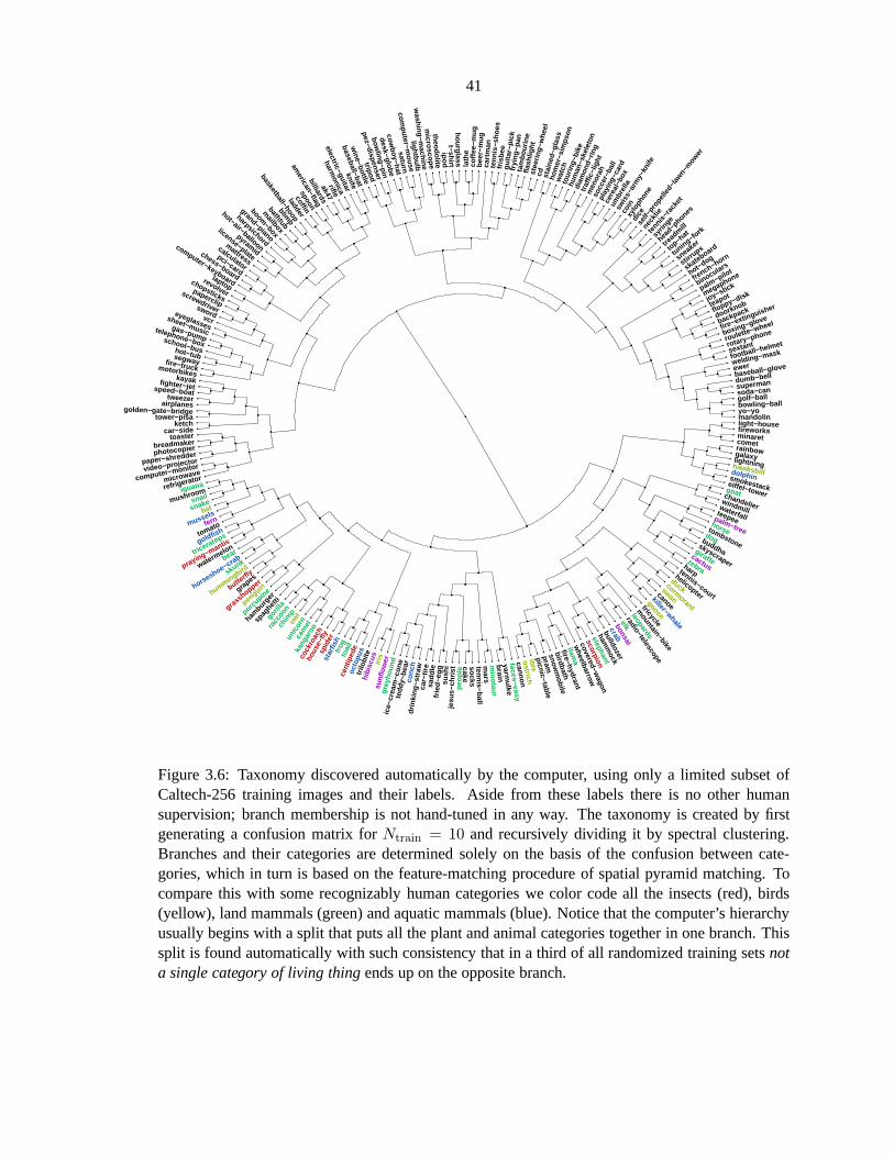
41

faces−easy

hom

er−s

imps

on

sta

ined

−gla

ss

car

tman

ketch car−side

refrigerator

tril

obite

s

unflo

wer

tennis−ball

brain yarm

ulke

lightning

comet minaret fireworks light−house

palm−pilot

lightbulb

cowboy−hat

desk−globe

bowling−pin

pez−dispenser

tripod

wine−bottle

laptop revolver

vcr eyeglasses

sheet−music

fire−truck motorbikes

golden−gate−bridge tower−pisa

toaster

paper−shredder

video−projector

computer−monitor

microwave

hib

iscu

s

iris

mars

minotaur

helicopter

tennis−court

horse

waterfall

windmill

chandelier

goat

eiffel−tower

smokestack

dolphin

hawksbill

galaxy rainbow

binoculars

french−horn

hea

d−ph

ones

syr

inge

ten

nis−r

acke

t

nec

ktie

sel

f−pr

opel

led−

lawn−

mow

er

men

orah

tra

ffic−

light

dia

mon

d−rin

g

hum

an−s

kele

ton

tou

ring−

bike

wat

ch

fris

bee

t

enni

s−sh

oes

bee

r−m

ug

hourglass t−shirt

ipod theodolite

microscope

washing−m

achine

computer−m

ouse

saturn

calculator

pci−card

chess−board

computer−keyboard

school−bus hot−tub segway

kayak

tweezer airplanes

breadmaker

photocopier

por

cupin

e

ham

burg

er

spa

ghet

ti u

nico

rn

coc

kroa

ch

hou

se−f

ly

spi

der

sta

rfish

f

rog

t

oad

c

entip

ede

o

ctop

us

frie

d−eg

g

sus

hi

jes

us−c

hris

t p

eopl

e cake

socks

leopards

mountain−bike

tricycle

cormorant

duck

tombstone

palm−tree

teepee

hot−dog s

neaker

tuning−fork

top−

hat

trea

dmill

soc

cer−

ball

fry

ing−

pan

gui

tar−

pick

cof

fee−

mug

l

athe

electric−guitar

american−flag

spoon

coffin

ladder harpsichord

hot−air−balloon

pyramid

license−plate

mattress

chopsticks paperclip

screwdriver sword

gas−pump telephone−box

fighter−jet speed−boat

bear

hummingbird

grass

hopper

pen

guin

gor

illa

rac

coon

c

him

p

owl

cam

el

kan

garo

o

car

−tire

s

addl

e

wheelbarrow

bulldozer

crab bonsai

goose

killer−whale

canoe

swan

harp

zebra

cactus

buddha

dog

welding−mask football−helmet sextant rotary−phone

roulette−wheel boxing−glove

fire−extinguisher

backpack doorknob

floppy−disk

teapot

joy−stick

megaphone

ska

teboard

stirr

ups

coi

n

sw

iss−

arm

y−kn

ife

um

brel

la

cer

eal−

box

pla

ying

−car

d

cd

s

teer

ing−

whe

el

fla

shlig

ht

tam

bour

ine

baseball−bat

knife

harmonica

rifle

ak47

billiards

basketball−hoop

blimp

bathtub

mailbox

boom−box

grand−piano

fern

tomato

goldfish

triceratops

praying−mantis

watermelon

horseshoe−crab

sku

nk

butte

rfly

grapes

gre

yhou

nd

con

ch

drin

king

−str

aw

pram

snowm

obile birdbath

covered−wagon

scorpion elephant

hamm

ock elk

radio−telescope

giraffe

skyscraper

dumb−bell baseball−glove ewer

dice

xylo

phon

e

bat

mussels

ice

−cre

am−c

one

t

eddy

−bea

r cannon

ostrich ibis picnic−table

fire−hydrant llam

a

mandolin yo−yo bowling−ball golf−ball soda−can superman

iguana

mushroom

snail

snake

Figure 3.6: Taxonomy discovered automatically by the computer, using only a limited subset ofCaltech-256 training images and their labels. Aside from these labels there is no other humansupervision; branch membership is not hand-tuned in any way. The taxonomy is created by firstgenerating a confusion matrix forNtrain = 10 and recursively dividing it by spectral clustering.Branches and their categories are determined solely on the basis of the confusion between cate-gories, which in turn is based on the feature-matching procedure of spatial pyramid matching. Tocompare this with some recognizably human categories we color code all the insects (red), birds(yellow), land mammals (green) and aquatic mammals (blue).Notice that the computer’s hierarchyusually begins with a split that puts all the plant and animalcategories together in one branch. Thissplit is found automatically with such consistency that in athird of all randomized training setsnota single category of living thingends up on the opposite branch.

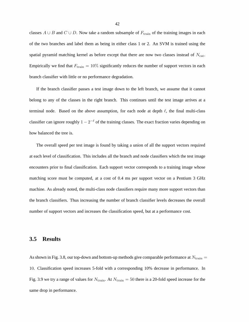
42

classesA ∪ B andC ∪D. Now take a random subsample ofFtrain of the training images in each

of the two branches and label them as being in either class 1 or2. An SVM is trained using the

spatial pyramid matching kernel as before except that thereare now two classes instead ofNcat.

Empirically we find thatFtrain = 10% significantly reduces the number of support vectors in each

branch classifier with little or no performance degradation.

If the branch classifier passes a test image down to the left branch, we assume that it cannot

belong to any of the classes in the right branch. This continues until the test image arrives at a

terminal node. Based on the above assumption, for each node at depthℓ, the final multi-class

classifier can ignore roughly1− 2−ℓ of the training classes. The exact fraction varies depending on

how balanced the tree is.

The overall speed per test image is found by taking a union of all the support vectors required

at each level of classification. This includes all the branchand node classifiers which the test image

encounters prior to final classification. Each support vector corresponds to a training image whose

matching score must be computed, at a cost of 0.4 ms per support vector on a Pentium 3 GHz

machine. As already noted, the multi-class node classifiersrequire many more support vectors than

the branch classifiers. Thus increasing the number of branchclassifier levels decreases the overall

number of support vectors and increases the classification speed, but at a performance cost.

3.5 Results

As shown in Fig. 3.8, our top-down and bottom-up methods givecomparable performance atNtrain =

10. Classification speed increases 5-fold with a corresponding 10% decrease in performance. In

Fig. 3.9 we try a range of values forNtrain. At Ntrain = 50 there is a 20-fold speed increase for the

same drop in performance.

43

A

B

C

Figure 3.7: The taxonomy from Fig.3.6 is reproduced here to illustrate how classification perfor-mance can be traded for classification speed. NodeA represents an ordinary non-hierarchical one-vs-all classifier implemented using an SVM. This is accuratebut slow because of the large combinedset of support vectors inNcats = 256 individual binary classifiers. A the other extreme, each testimage passes through a series of inexpensive binary branch classifiers until it reaches 1 of the 256leaves, collectively labeledC above. A compromise solution B invokes a finite set of branch classi-fiers prior to final multi-class classification in one of 7 terminal nodes.

44

0 1 2 3 4 5 6 7 8 9 100

5

10

15

20

25

Speed (images/s)

Per

form

ance

(%

cla

ssifi

ed c

orre

ctly

)

A

B

C

top−downbottom−uprandom

Figure 3.8: Comparison of three different methods for generating taxonomies. For each taxonomywe vary the number of branch comparisons prior to final classification, as illustrated in Fig. 3.4.This results in a tradeoff between performance and speed as one moves between two extremesAandC. Randomly generated hierarchies result in poor cascade performance. Of the three methods,taxonomies based on Spectral Clustering yield marginally better performance. All three curvesmeasure performance vs. speed forNcat = 256 andNtrain = 10.

3.6 Conclusions

Learning hierarchical relationships between categories of objects is an essential part of how humans

understand and analyze the world around them. Someone playing the game of “20 Questions” must

make use of some preconceived hierarchy in order to guess theunknown object using the fewest

number of queries. Computers face the same dilemma: withoutsome knowledge of the taxonomy

of visual categories, classifying thousands of categoriesis reduced to blind guessing. This becomes

45

.2 .3 .4 .5 .6 .7 .8 .9 1 2 3 4 5 6 7 8 9100.0

5.0

10.0

15.0

20.0

25.0

30.0

35.0

40.0

Speed (images/s)

Per

form

ance

(%

cla

ssifi

ed c

orre

ctly

)

Ntrain

504030201510

Figure 3.9: Cascade performance / speed trade-off as a function ofNtrain. Values ofNtrain = 10 andNtrain = 50 result in a 5-fold and 20-fold speed increase (respectively) for a fixed 10% performancedrop.

prohibitively inefficient as computation time scales linearly with the number of categories.

To break this linear bottleneck, we attack two separate problems. How can computers automat-

ically generate useful taxonomies, and how can these be applied to the task of classification? The

first problem is critical. Taxonomies built by hand have beenapplied to the task of visual classi-

fication [122] for a small number of categories, but this method does not scale well. It would be

tedious - if not impossible - for a human operator to generatedetailed visual taxonomies for the

computer, updating them for each new environment that the computer might encounter. Another

46

problem for this approach is consistency: any two operatorsare likely to construct entirely different

trees. A more consistent approach is to use an existing taxonomy such as WordNet [41] and apply it

to the task of visual classification [80]. One caveat is that lexical relationships may not be optimal

for certain visual classification tasks. The wordlemonrefers to an unreliablecar, but the visual

categories lemon and car are not at all similar.

Our experiments suggest that plausible taxonomies of object categories can be created automat-

ically using a classifier (in this case, spatial pyramid matching) coupled to a learning phase which

estimates inter-category confusion. The only input used for this process is a set of training images

and their labels. The taxonomies such the one shown in Fig. 3.6 seem to consistently discover

broader categories which are naturally recognizable to humans, such as the distinction between

animate and inanimate objects.

How should we compare one hierarchy to another? It is difficult to quantify such a comparison

without a specific goal in mind. To this end we benchmark a cascade of classifiers based on our

hierarchy and demonstrate significant speed improvements.In particular, top-down and bottom-up

recursive clustering processes both result in better performance than a a randomly generated control

tree.

47

Chapter 4

Pollen Counting

4.1 Introduction

Airborne pollen has been linked to a number of respiratory conditions ranging from common al-

lergies to potentially life-threatening asthma attacks. Considering that one in five people in the

United States are affected by at least one of these conditions, we know surprisingly little about the

concentration and identity of the pollen in the air we breathe each day. This is largely due to the

fact that a nation-wide or even regional daily manual pollencounting effort would be extremely

labor-intensive, requiring an army of trained professionals. Efforts to understand the complex links

between climate change, air quality and human health would be greatly facilitated by an efficient,

unbiased system for identifying airborne pollen concentrations on a mass scale [51, 62, 102].

Over the last decade there have been several efforts aimed atcreating such a system. Most

modern-day instruments that are used to sample airborne pollen trace their origins to the pollen col-

lection techniques pioneered by J. M. Hirst in the 1950’s[58, 54]. While basic sampling techniques

have changed relatively little, the optical hardware and computer algorithms employed to count the

pollen vary from project to project. Ronneberger et al. [96,95, 97] use a confocal microscope to

construct 3-D pollen surfaces which are reduced to a set of gradients statistics designed to be invari-

ant to translation, rotation and local deformations. A nearest neighbor algorithm is then used for

48

Figure 4.1: Dr. James House stands next to a modern-day Burkard pollen sampler located on theroof of Keck Laboratory at Caltech (left). The basic techniques used to collect pollen date back tothe work of J. M. Hirst in the early 1950’s (right).

classification. While the system is accurate it requires theuse of a confocal microscope. Unfortu-

nately such microscopes are more costly and less common thantraditional compound microscopes.

Systems developed in New Zealand [4, 3] and Germany [57] use more conventional hardware that

may ultimately prove more suitable for wide-scale deployment. In particular the Pollen Monitor

BAA500 created by the German team seems poised for broad deployment thanks in part to strong

national funding and a large 25-member team of scientists and engineers working on the project.

It is not yet clear what the exact price of the device would be,whether it can be purchased and

deployed outside of Germany, and whether it can be easily re-programmed to recognize pollen in

other countries.

Rather than building and deploying a single monolithic device designed and maintained by a

dedicated team of engineers, our 3-member team has focused instead on a more bottom-up ap-

49

proach. Our goal has been to design and deploy a system that uses off-the-shelf, inexpensive

hardware in conjunction with flexible state-of-the-art classification software to 1) count pollen, 2)

maintain a reliable stream of daily counts over the course ofmany years and 3)apply the result-

ing datasets to actual research projects in climate scienceand epidemiology. The process needs

to be scalable. Relatively inexpensive pollen samplers canbe purchased from companies such as

Burkard Agronomic Instruments1. The optical requirements are likewise modest - a compound mi-

croscope with a computer-controlled stage - and the microscopy software is open-source. Arguably

the primary limiting factor for most research groups that would undertake their own local pollen

counting effort is the difficulty of creating a software package to robustly segment and classify a

variety of pollen species, especially in the presence of high volumes of soot and other background

clutter. If this were freely available, more researchers atdifferent locations would be enabled to

collect and count their own pollen and, potentially, pool their data with others for the use of the

entire community.

4.2 Data Collection Method

The basic principles used to prepare and acquire pollen fromour Burkard pollen sampler are very

similar to those used by Hirst in 1952. A pump draws air through a narrow inlet at a fixed flow rate

while a servo-controlled drum turns exactly once per week. As pollen accumulates along a piece

of sticky tape mounted on the outside circumference of the drum, the exact location of each pollen

grain along the direction of travel encodes the date when thepollen was deposited. The drum is

removed at the end of 1 week and the tape strip is transferred to microscope slides for observation

and, in our case, digitization.

The slide preparation techniques currently used by Dr. James House have been refined over

1www.burkardscientific.com/agronomics/sporewatch.htm

50

many years. This methodology turns out to be important because poorly-prepared slides suffer from

a variety of problems, such as:

Condition Result

Pollen clumping and overlapping Complicates segmentation of individual pollengrains

Soot, insect parts and other clutter Puts an excessive burden on the automated clutterrejection algorithms

Formation of air bubbles during slidepreparation

Can occlude or mimic pollen

Variable tape thickness Complicates microscope focusingNon-uniform distribution of coverslipmounting fluid

Optical reflections and chromatic aberration

Redistribution of pollen as coverslip isapplied

Counting biases in selectively sampled slides, un-certainty and bias in the position and thus the timeat which pollen is deposited

Through a process of trial and error, the best results have been found using Mowiol coverslip so-

lution containing 2.5% 1,4-diazobicyclo-[2.2.2]-octaneheated to room temperature. Further details

of the mounting process will be presented in a forthcoming paper [59].

For each week of data collected, the resulting 7 slides - one for each day - are placed on a

computer-controlled stage and scanned with a PC runningµManager, a complete open-source mi-

croscopy software package2. A QImaging Retiga-4000R 2048x2048 CCD camera3 is mounted to

a conventional compound microscope with an 100x objective.Scripts written in Beanshell (a sim-

plified Java-like environment) control the exact pattern used to scan the slides. At each point in the

scan, the program calculates a single synthetic image usingastackof 18 individual images acquired

over a range of focus settings4. This image contains all planes of maximum sharpness from the indi-

vidual images. In addition to providing more flexibility in the data analysis, this process of scanning

and analyzing stacks was found to be faster than the microscope’s built-in focusing procedure.

Our standard observation script views each slide in much thesame way as a human operator2developed by Ron Vale’s laboratory at UCSF. For more information see http://valelab.ucsf.edu/ MM/MMwiki3http://www.qimaging.com/products/cameras/scientific/retiga 4000r.php4using a MATLAB program written by Xavier Burgos-Artizzu in Pietro Perona’s Vision Lab at Caltech

51

Grass

y

Cypress Pine

Olive Birch

ShapeHarmonics

BrightnessDistribution

TextureSpatial Pyramid

Feature Matching

Figure 4.2: The shape, brightness distribution and textureare each discriminative for different typesof pollen. The first feature encodes shape as the Fourier transform of the outer radius, with valuesrepresenting the mean radius, eccentricity and higher moments. The second feature computes theratio of several different quartiles of the brightness distribution in a way that is invariant to absolutebrightness. Finally, SIFT features extracted on a 32x32 grid are matched against training examplesusing the spatial pyramid matching algorithm of Lazebnik etal. [67]. The first two features can becomputed far more efficiently than the third.

would, scanning a single horizontal row across the entire slide. Because the 762 x 762µm2 field

of view of the camera is roughly half that of the field seen through the viewfinder, two rows are

actually scanned for a total of 126 images per slide covering73mm2.

4.3 Classification Algorithm

On a typical slide, background particulates i.e. “clutter”outnumbers pollen by∼ O(103 − 104).

In the spirit of the Viola and Jones face detection algorithm[112] we apply a cascade of classifiers

designed to quickly weed out the more obvious instances of clutter. More complex classifiers down-

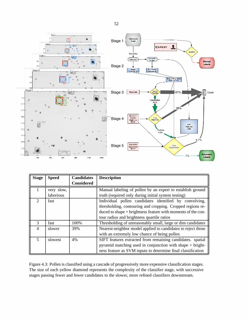
52

Manual

Labels

Thresholds

NN-based

Shape+

Brightness

Model

Clutter

SVM+SPM

Appearance

Model

Automatic

Labels

Shape

Features (6)

Cropped

PollenContours

LabelGUI

Stage 2

Stage 3

Stage 4

Stage 5

Convolve

Shape+Brightness

Features (12)

SIFT

Features

(128)

Candidates39 %

Finalists4.2%

Expert

Brightness

Features (6)

Stage 1Microscope

Image

61%

35%

.1%

4.1%

Coarse

Rejection

Fine

Rejection

Final

Classification

Stage Speed CandidatesConsidered

Description

1 very slow,laborious

Manual labeling of pollen by an expert to establish groundtruth (required only during initial system testing)

2 fast Individual pollen candidates identified by convolving,thresholding, contouring and cropping. Cropped regions re-duced to shape + brightness feature with moments of the con-tour radius and brightness quartile ratios

3 fast 100% Thresholding of unreasonably small, large or dim candidates4 slower 39% Nearest-neighbor model applied to candidates to reject those

with an extremely low chance of being pollen5 slowest 4% SIFT features extracted from remaining candidates. spatial

pyramid matching used in conjunction with shape + bright-ness feature as SVM inputs to determine final classification

Figure 4.3: Pollen is classified using a cascade of progressively more expensive classification stages.The size of each yellow diamond represents the complexity ofthe classifier stage, with successivestages passing fewer and fewer candidates to the slower, more refined classifiers downstream.

53

stream can thus ignore the bulk of the test data and concentrate on the difficult and ambiguous cases.

The process begins by convolving and thresholding the imageto find contours representing the

outer perimeter of each distinct particle. Since two or moreparticles may clump together to produce

a single contour, a separate heuristic allows contours thatare pinched in the middle to iteratively

separate into two loops. Cropping a region around each of theresulting contours typically gives

hundreds of possible cropped pollen candidates for each slide.

The features we extract from these cropped images are shown in Fig. 4.2. The figure illus-

trates how shape, brightness and texture can each be useful for visual classification of pollen type

depending on the species that are present.

The shape feature is constructed by converting each contourto polar coordinates(r, θ) and tak-

ing the Fourier transform of r. The resulting feature vectorreturns the radius, eccentricity, and

progressively higher-order moments of r. Moments higher than 6 are added together into a sin-

gle measure ofroughnesswhich is particularly useful for differentiating pollen from background

particulates such as dust and soot. The brightness feature encodes only the brightness distribu-

tion, not the absolute brightness. This is necessary because the brightness of the microscope light

source and the software camera calibration can vary over thecourse of many months. We construct

center-weighted and unweighted brightness histograms andcalculate ratios of 3 different brightness

quartiles for each. The overall result is a combined shape + brightness feature vector of length

n=12. As shown in Fig. 4.3, using this inexpensive feature toexclude very unlikely candidates

means that the relatively expensive SIFT feature grid need only be computed for a fraction (∼4%)

of the candidate regions. This increases the final classification speeds by more than an order of

magnitude.

At the moment, the time required to classify 126 images i.e. aday’s worth of data is 35 minutes

using a MATLAB program running on a 6-core Intel Zeon 3.33GHzprocessor. Preprocessing a

54

Figure 4.4: In a Mechanical Turk experiment, test subjects are asked to classify the pollen on theright side using a randomized set of training examples provided on the left.

day’s worth of image stacks into synthetic images takes another 10 minutes. Thus a month’s worth

of data (almost 4000 images) can be analyzed in just under 1 day.

4.4 Comparison To Humans

In 2009 we ran an experiment to compare machine performance with human performance using the

Amazon Mechanical Turk5. The advantage of using this resource is that experiments can be imple-

mented quickly and efficiently at minimal expense. One majordisadvantage is that no information

is available concerning the test subjects themselves. While it is hard to draw broad conclusions

without knowing something about the test demographic, we can at least try to selectively average

the results of our 28 test subjects to get a rough idea what therange of performance might be for

untrained non-specialists.

5https://www.mturk.com/mturk/

55

Figure 4.5: Test subjects do not see the expert classification (red) or the computer classification(green). While the computer “misclassified” this particular birch sample as oak, the true ground-truth classification could actually be either, as demonstrated by visually similar instances circled ineach class.

To keep the interface as straightforward as possible we implemented a simplified version of our

pollen classification task6. Fig. 4.4 shows what the test subject sees. On the left are randomized

examples of 9 different species of pollen drawn from the sametraining set used by the computer.

On the right a crop box is drawn around a single pollen gain whose ground truth label is known7.

The test subject is asked to identify the pollen type using the available training data. Fig. 4.5 shows

what the test subject does not see: the ground truth (red) andcomputer (green) labels. This illustrate

an inherent ambiguity in the pollen identification task: classifying the pollen as either birch or oak

would be understandable given the training set that is visible. Neither the computer nor the test

subjects are given other information that an expert would need to further refine their guess, such as

the date when the pollen was acquired.

6with the help of Merrielle Spain in Pietro Perona’s Vision Lab at Caltech7to the extent that a pollen expert was able to visually identify them. A gold standard test such as DNA extraction is

not available for our labelled training data, since it wouldbe prohivitively expensive to implement.

56

79%

56%

47%

98%

94%

99%

88%

Ground Truth

alde

r

ash

birc

h

clut

ter

cypr

ess

pine

wal

nut

Computer

80.2%80.2%80.2%80.2%80.2%80.2%80.2%80.2%80.2%80.2%80.2%80.2%

37%

55%

43%

91%

74%

85%

37%

Ground Truth

Cla

ssifi

catio

n

alde

r

ash

birc

h

clut

ter

cypr

ess

pine

wal

nut

People

60.3%60.3%60.3%60.3%60.3%60.3%60.3%60.3%60.3%60.3%60.3%60.3%

alder

ash

birch

clutter

cypress

pine

walnut

62%

88%

36%

92%

81%

89%

48%

Ground Truth

alde

r

ash

birc

h

clut

ter

cypr

ess

pine

wal

nut

People: best 8 of 28 (25%)

70.9%70.9%70.9%70.9%70.9%70.9%70.9%70.9%70.9%70.9%70.9%70.9%

36%

15%

50%

100%

50%

88%

15%

Cla

ssifi

catio

n

alde

r

ash

birc

h

clut

ter

cypr

ess

pine

wal

nut

Subject #1 : 78 samples

50.6%50.6%50.6%50.6%50.6%50.6%50.6%50.6%50.6%50.6%50.6%50.6%

alder

ash

birch

clutter

cypress

pine

walnut

20%

36%

22%

70%

92%

75%

14%

alde

r

ash

birc

h

clut

ter

cypr

ess

pine

wal

nut

Subject #2 : 75 samples

47.2%47.2%47.2%47.2%47.2%47.2%47.2%47.2%47.2%47.2%47.2%47.2%

alder

ash

birch

clutter

cypress

pine

walnut

8%

11%

85%

89%

86%

83%

62%

alde

r

ash

birc

h

clut

ter

cypr

ess

pine

wal

nut

Subject #3 : 73 samples

60.6%60.6%60.6%60.6%60.6%60.6%60.6%60.6%60.6%60.6%60.6%60.6%

alder

ash

birch

clutter

cypress

pine

walnut

11%

79%

27%

89%

75%

100%

9%

Cla

ssifi

catio

n

alde

r

ash

birc

h

clut

ter

cypr

ess

pine

wal

nut

Subject #4 : 72 samples

55.7%55.7%55.7%55.7%55.7%55.7%55.7%55.7%55.7%55.7%55.7%55.7%

alder

ash

birch

clutter

cypress

pine

walnut

100%

91%

30%

90%

83%

78%

18%

alde

r

ash

birc

h

clut

ter

cypr

ess

pine

wal

nut

Subject #5 : 70 samples

70.0%70.0%70.0%70.0%70.0%70.0%70.0%70.0%70.0%70.0%70.0%70.0%

alder

ash

birch

clutter

cypress

pine

walnut

27%

50%

45%

82%

50%

67%

73%

alde

r

ash

birc

h

clut

ter

cypr

ess

pine

wal

nut

Subject #6 : 63 samples

56.3%56.3%56.3%56.3%56.3%56.3%56.3%56.3%56.3%56.3%56.3%56.3%

alder

ash

birch

clutter

cypress

pine

walnut

33%

60%

40%

100%

75%

89%

75%

Ground Truth

Cla

ssifi

catio

n

alde

r

ash

birc

h

clut

ter

cypr

ess

pine

wal

nut

Subject #7 : 34 samples

67.5%67.5%67.5%67.5%67.5%67.5%67.5%67.5%67.5%67.5%67.5%67.5%

alder

ash

birch

clutter

cypress

pine

walnut

100%

60%

40%

100%

67%

100%

0%

Ground Truth

alde

r

ash

birc

h

clut

ter

cypr

ess

pine

wal

nut

Subject #8 : 32 samples

66.7%66.7%66.7%66.7%66.7%66.7%66.7%66.7%66.7%66.7%66.7%66.7%

alder

ash

birch

clutter

cypress

pine

walnut

50%

100%

0%

100%

50%

50%

67%

Ground Truth

alde

r

ash

birc

h

clut

ter

cypr

ess

pine

wal

nut

Subject #9 : 25 samples

59.5%59.5%59.5%59.5%59.5%59.5%59.5%59.5%59.5%59.5%59.5%59.5%

alder

ash

birch

clutter

cypress

pine

walnut

Figure 4.6: Mechanical Turk test subjects and the automatedsystem make similar classificationmistakes. Overall performance is 60.3% averaged over all test subjects, 70.9% averaged over the8 most reliable test subjects, and 80.2% for the automated count. Confusion matrices may varysignificantly among individual test subjects, as shown by 9 individual confusion matrices for the 9test subjects with the largest number of classifications.

Results are shown in Fig. 4.6. Overall performance is 60.3% averaged over all test subjects

and 70.9% averaged over the 8 individual test subjects foundto be most accurate. For comparison

the computer classified 80.2% of the examples correctly. Theconfusion matrices show that the

computer can outperform non-experts when classifying pre-segmented pollen grains, and that the

patterns of mistakes made by the computer closely resemble those of the test subjects. Both found

Alder, Ash and Birch to be the most difficult to classify and Pine and clutter ie. non-pollen to be the

easiest.

57

0 10 200

10

20

Expert #1

alderC

ompu

ter

0 100200Expert #1

ash

0 25 50Expert #1

birch

Best

0 100 200Expert #1

cypress

0 25 50Expert #1

grass

Best

0 200 400Expert #1

oak

0 50 100Expert #1

olive

0 100 200Expert #1

pine

0 25 500

25

50

Expert #2

Com

pute

r

0 250 500Expert #2

0 25 50Expert #2

0 100 200Expert #2

0 25 50Expert #2

0 250 500Expert #2

Best

0 200 400Expert #2

0 100 200Expert #2

0 25 500

25

50

Expert #1

Exp

ert #

2 Best

0 250 500Expert #1

Best

0 20 40Expert #1

0 50 100Expert #1

Best

0 20 40Expert #1

0 250 500Expert #1

0 100 200Expert #1

Best

0 100 200Expert #1

Best

Figure 4.7: Pollen counts aggregated over 15 days are plotted against one another to show thedegree of agreement between experts and the automated system. As the counts increase in eachplot (bottom-left to top-right) the sampling error decreases. Thus an ideal, unbiased pair of countsshould converge towards a line of slope m=1. In each column the pair with the best agreement (i.e.slope closest to 1) are labelled in green. For 3 out of 8 species the experts actually showed betteragreement with the automated system than they did with one another.

4.5 Comparison To Experts

The test described in the previous section examines only theperformance of classification stages 3,

4 and 5 of the algorithm in Fig. 4.3. This does not include the performance of stage 2 where the

candidates themselves are located and segmented. We now proceed to a second experiment which

is a better end-to-end test of the entire algorithm. The testcompares computer performance with

that of two certified pollen identification experts. For eachday’s data, the experts are presented with

the same set of 126 microscope images that the computer uses.Like the computer, the experts place

bounding boxes around each pollen grain and classify them8. Individual slides typically have very

small pollen counts for most species with correspondingly large sampling errors. To compensate for

8using a MATLAB GUI interface originally written by Marc’aurelio Ranzato in Pietro Perona’s Vision Lab at Caltech

58

this we aggregate the automated counts for each species over15 days spread throughout the first half

of 2012. These days were chosen to coincide with relatively large counts for a variety of species.

The automated counts were then plotted against the counts for the two pollen counters “Expert #1”

and “Expert #2”. Preliminary results are shown in Fig. 4.7. There is currently only a limited subset

of data for which 3 separate counts are available. We hope to expand this subset in order to reduce

the sampling error, especially for Alder, Birch and Grass which are under-represented.

4.6 Conclusions

The final product of our automated counting system is an estimate of the daily pollen count for the

entire year, shown in Fig. 4.8. Results are still preliminary pending final publication [59]. While we

are still in the process of improving the learning model and evaluating final classification accuracy,

our initial results are promising. The automated system observes several well-established yearly

patterns such as the Cypress bloom in early February followed by a Pine bloom later in the month.

Likewise sporadic blooms of Oak throughout March, April andMay have been recorded at our site

every year since manual counting began in 2003.

Beyond just reproducing manual pollen counts, automated counts hold the promise of recording

new types of pollen data that would otherwise be prohibitively difficult to obtain. For example, the

ability to accurately locate each individual pollen sampleon a slide brings with it the possibility

of recording minute daily changes in the pollen count causedby diurnal cycles or local whether

conditions. Pollen experts typically scan only a small fraction of the total pollen available on each

slide, whereas the automated system is fast enough to scan the entire slide. This promises to revolu-

tionize antiquated manual counting techniques plagued by sampling biases and unnecessarily high

counting variance.

Manual counts also limit our ability to understand how pollen counts vary from one location

59

Jan Feb Mar Apr May Jun Jul Aug Sep Oct Nov Dec0

10

20

30

40

50

60

70

80

90

100

Month

Tot

al C

ount

Automatic Pollen Counts for 2012

oak : 1467 cypress : 1026 pine : 947 birch : 528 grass : 463 ash : 232 olive : 185 alder : 72 poplar : 50 chinelm : 49

Figure 4.8: Daily automated pollen counts for 2012. The total count is broken down into color bandsshowing the contribution from individual species. Integrated counts for the year are displayed in thelegend. The system can count a month’s worth of pollen in 1 daywhen scanning the slide as anexpert would, utilizing less than .1% of the total collecting area. It is thus nearly fast enough toscan the entire slide which would drastically reduce the sampling error and bias. We continue tooptimize the code towards this eventual goal.

to another. The speed of automatic counting would enable researchers to collect and compare data

from tens, hundreds or even thousands of different sites. Inshort, the speed, temporal resolution

and minimal counting biases offered by an automated pollen counting system promise to provide

new tools heretofore unavailable to climate scientists andepidemiologists in their research.

60

61

Chapter 5

Machine Olfaction: Introduction

Electronic noses have been used successfully in a wide variety of applications[94, 115] ranging from

safety[25, 47, 117, 50] and detection of explosives[1, 61, 45] to medical diagnosis[24, 46, 110, 19,

82], food quality assessment[121, 49, 13, 6] and discrimination of beverages like coffee[88, 89],

tea[116, 35, 78] and wine[23, 78, 91, 100]. These applications typically involve a limited variety of

odor categories with tens or even hundreds of training examples available for each odorant.

Human text subjects, on the other hand, are capable of distinguishing thousands of different

odors[66, 93, 107] and can recognize new odors with only a fewtraining examples[20, 16]. How

we organize individual odor categories into broader classes - and how many classes are required

- is still a matter of active debate in the psychophysics community. One recent study of 881 per-

fume materials found that human test subjects group the vastmajority of these odors into 17 dis-

tinct classes[118]. Another comprehensive study of 146-dimensional odorant responses obtained

by Dravnieks[34] showed that most of the variability in the responses can be explained using only

6-10 parameters[63].

Results such as these suggest that the bulk of the variability in human odor perception can be

represented in a relatively low-dimensional space. What isless clear is whether this low dimen-

sionality is an intrinsic quality of the odorants themselves or a feature of our olfactory perception.

Measuring a large variety of odorants electronically provides an opportunity to compare how ma-

62

chines and humans organize their olfactory environment. One way to represent this is to construct a

taxonomy of odor categories and super-categories with closely related categories residing in nearby

branches of the tree.

Over the last 10 years hierarchical organization tools haveproven increasingly useful in the field

of computer vision as image classification techniques have been scaled to larger image datasets. Ex-

amples include PASCAL[38], Caltech-101[69], Caltech-256[55] and, more recently, the SUN[17]

LabelMe[109] and Imagenet[21] datasets with over a thousand categories each. These datasets are

challenging not just because they include a larger number ofcategories but because the objects

themselves are photographed in a variety of poses and lighting conditions with varying degrees of

background clutter.

While it is possible to borrow taxonomies such as WordNet[106] and apply them to machine

classification tasks, lexical relationships are at best an imperfect approximation of visual or ol-

factory relationships. It is therefore useful to automatically discover taxonomies that are directly

relevant to the specific task at hand. One straightforward greedy approach involves clustering the

confusion-matrix created with a conventional one-vs-all multi-class classifier. This results in a top-

down arrangement of classifiers where simple, inexpensive decisions are made first in order to re-

duce the available solution space. Such an approach yields faster terrain recognition for autonomous

navigation[7] as well as more computationally efficient classification of images containing hundreds

of visual categories[56]. One way to improve overall classification accuracy is to identify categories

which cannot be excluded early and include them on multiple hierarchy branches[81]. Binder et al.

show that taxonomy-based classification can improve both speed and accuracy at the same time[11].

In addition to larger more challenging datasets and hierarchical classification approaches that

scale well, machine vision has benefitted from discriminative features like SIFT and GLOH that

are relatively invariant to changes in illumination, viewpoint and pose[83]. Such features are not

63

dissimilar from those extracted from astronomical data by switching between fixed locations on

the sky[33, 26]. The resulting measurements can reject slowly-varying atmospheric contamination

while retaining extremely faint cosmological signals thatareO(106) times smaller.

Motivated by this approach, we construct a portable apparatus capable of sniffing at a range

of frequencies to explore how well a small array of 10 sensorscan classify hundreds of odors

in indoor and outdoor environments. We evaluate this swept-frequency approach by sampling 90

common household odors as well as 40 odors in the University of Pittsburgh Smell Identification

Test. Reference data with no odorants is also gathered in order to model and remove any systematic

errors that remain after feature extraction.

The sensors themselves are carbon black-polymer compositethin-film chemiresistors. Using

controlled concentrations of analytes under laboratory conditions, these sensors have been shown

to exhibit steady-state and time-dependent resistance profiles that are highly sensitive to inorganic

gasses as well as organic vapors[12] and can be used for classifying both[105, 79]. A challenge

when operating outdoors is that variability in water vapor concentrations masks the response of other

analytes. Our approach focuses on extracting features thatare insensitive to background analytes

whose concentrations changes more slowly than the sniffing frequency. This strategy exploits the

linearity of the sensor response and the slowly-varying nature of ambient changes in temperature

and humidity.

From an instrument design perspective, we would like to discover how the choice of sniffing fre-

quencies, number of sensors and feature reduction method all contribute to the final indoor/outdoor

classification performance. Next we construct a top-down classification framework which aggre-

gates odor categories that cannot be easily distinguished from one another. Such a framework

quantitatively addresses questions like: what sorts of odor groupings can be readily classified by the

instrument, and with what specificity?

64

65

Chapter 6

Machine Olfaction: Methods

6.1 Instrument

The odorants to be tested were contained in four sample chambers, while one empty chamber served

as a reference (Fig.6.1). The instrument drew air through a small sensor chamber while controlling

the source of the air via a manifold mixing solenoid valve[85, 48, 75] A small fan drew the air

through a computer-controlled valve with five inlets. No flowmeters, gas cylinders, air dryers or

other filters were used, with the instrument being as simple and portable as possible to facilitate the

acquisition of data in both indoor and outdoor environments. The sensor chamber, sample chambers,

solenoid valve, computer and electronics were light enoughto carry, and all electronic components

ran on battery power.

6.2 Sampling and Measurements

Ideally the sniffing frequencies would be high enough to reject unwanted environmental noise but

low enough that the time-constant of the sensors did not attenuate the signal. A range of usable

frequencies between1/64 and 1 Hz was satisfactory for this purpose.

To implement the sniffing scheme, the computer first chose a single odor, and 7 frequencies

were sampled in 7.5 min. During this span of time, 400 s were spent switching between a single

66

Figure 6.1: A fan draws air from 1 of 4 ordorant chambers or an empty reference chamber, depend-ing on the state of the computer-controlled solenoid valve.The valve control signal can then becompared to the resistances changes recorded from an arraysof 10 individual sensors as shown inFig. 2.

odorant and the reference chamber, while the remaining 50 s were spent purging the chamber with

reference air. This complete sampling pattern is designated herein as a “sniff”, and each of the 7

individual frequency modulations as “subsniffs”.

Each sniff was repeated 4 times for each of 4 odorants, for a total of 2 h per “run”. Within

each run, the odorants were randomly selected and were presented to the sensors in random order.

To avoid residual odors, each run started with a 1-hour period during which the sensor chamber

was purged with reference air, the odorant chambers were replaced, and the tubing that led to the

chambers was washed and then dried.

67

The resistance of each sensor was sampled at 50 Hz while the valve modulated the incoming

odor streams. The relative differential resistance change∆RR

was then calculated by dividing each

resistance valueR(t) by the mean resistance in a 4 min window centered att. From this time-

series data, each individual sniff was reduced to a feature vector of measurements that represented

the band power of the sensor resistance integrated over subsniffs i = 1..7 and frequency bands

j = 1..4. Fig. 6.2c illustrates this filtering fori=4. In this subsniff, the valve switched 4 times, at

a frequency of1/8 Hz, between odorant and the reference. Integration of each portion of the Fourier

transform of the signal

Si(f) =

∫si(t)e

−2πiftdt

weighted by four different window functions resulted in7× 4 = 28 measurements

mij =

∫ fmax

0

Hij(f)df , Hij(f) = Si(f)Wij(f)

wherefmax

= 25 Hz is the Nyquist frequency. The modulation of the odorant in the ith subsniff

can be thought of as the product of a single 64 s pulse and progressively faster square waves of

frequencyfi = 2 i−7 Hz. Thus the first window functionj = 1 in each subsniff was centered

aroundf1 = 1/64, while window functions forj = 2..4 were centered at the odd harmonicsfi, 3fi

and5fi, for which the square-wave modulation had maximal power. Repetition of this procedure

for each sensork = 1..10 gave a final featuremijk of size7×4×10 = 280, which was normalized

to unit length.

For comparison, a second featuremi of size7× 10 = 70 was generated by simply differencing

the top and bottom 5% quartiles of∆RR

within each subsniff. This type of amplitude estimate is

comparable to the so-called sensorial odor perception (SOP) feature commonly used in machine

olfaction experiments [22], and is similar tomi1k in that it ignores harmonics with frequencies

68

higher than1/64 Hz within each subsniff.

6.3 Datasets and Environment

Three separate datasets were used for training and testing.The University of Pittsburgh Smell

Identification Test (UPSIT)consists of 40 micro-encapsulated odorants chosen to be relatively rec-

ognizable and to span known odor classes [31, 32]. The test isadministered as a booklet of 4-item

multiple choice questions with an accompanying scratch-and-sniff patch for each question. It is an

especially useful standard because of the wealth of psychophysical data that has been gathered on a

variety of test subjects since the UPSIT was introduced in 1984 [30, 29, 28, 36].

To sample realistic real-world odors, we developed aCommon Household Odors Dataset (CHOD)

that contained 90 common foods products and household items. Items were chosen to be as diverse

as possible while remaining readily available. Odor categories for both the CHOD and UPSIT are

listed in the appendix. Of these, 78 were sampled indoors, 40were sampled outdoors, and 32 were

sampled in both locations

A Control Datasetwas acquired in the same manner as the other two sets, but withempty

odorant chambers. The purpose of this data set was to model and remove environmental components

that were not associated with an odor class. In this sense thecontrol data set is analogous to the

clutter category present in some image datasets. To capture as much environmental variation as

possible, control data were taken on a semi-weekly basis over the entire 80-day period during which

the other 2 datasets were acquired. Half of the control data were used for modeling while the other

half were used for verification purposes.

These 3 data sets collectively contained 250 h of data that spanned 130 odor categories and 2

environments. The first 130 h of data were acquired over a 40-day period in a typical laboratory

environment, with temperatures of 22.0-25.0◦C and 36-52% humidity. Over the subsequent 40 days,

69

the remaining 120 h of data were collected on a rooftop and balcony, with temperatures ranging

from 10.1-24.7◦C and 29-81% humidity. On a 2 h time scale, the average change in temperature

and humidity was0.11◦C and0.4% in the laboratory and0.61◦C and1.9% outdoors. Thus the

environmental variation outdoors was roughly∼ 5 times greater than indoors.

70

ref

odorant

0

10

20

x 10−4

∆ R

/ R

s7

s6

s5

s4

s3

s2

s1

1 2 3 4 5 6

10−4

minutes

∆ R

/ R

mi1

mi2

mi3

mi4 amplitude

si fi Ti Ni Ttot

s1 1/64 Hz 64 s 1 64 ss2 1/32 32 1 32s3 1/16 16 2 32s4 1/8 8 4 32s5 1/4 4 8 32s6 1/2 2 16 32s7 1 1 32 32

−20 0 20−5

0

5

10

15x 10

−4

∆ R

/ R

sec

s4

−20 0 20sec

h41

−20 0 20sec

h42

−20 0 20sec

h43

−20 0 20sec

h44

0.01 0.10 1.00

10−6

10−5

10−4

10−3

f1

f4

3f4

5f4

Hz

∆ R

/ R

Outdoor NoiseIndoor NoiseS

4H

41H

42H

43H

44

Figure 6.2: (a) A sniff consisted of 7 individual subsniffss1...s7 of sensor data taken as the valveswitched between a single odorant and reference air. From this data a7 × 4 = 28 size featuremwas generated representing the measured power in each of the7 subsniffsi over 4 fundamentalharmonicsj. For comparison purposes a simple amplitude feature differenced the top and bottom5% quartiles of∆R

Rin each subsniff. (b) As the switching frequencyf increased by powers of 2

so did the number of pulses, so that the time periodT was constant for all but the first subsniff.(c) To illustrate howm was measured we show the harmonic decomposition of justs4, highlightedin (a). The corresponding measurementsm4j were the integrated spectral power for each of 4harmonics. Higher-order harmonics suffered from attenuation due to the limited time-constant ofthe sensors but had the advantage of being less susceptible to slow signal drift. Fitting a1/fnnoisespectrum to the average indoor and outdoor frequency response of our sensors in the absence of anyodorants illustrates why higher-frequency switching and higher-order harmonics may be especiallyadvantageous in outdoors environments.

71

10/10

wine : Cabernet SauvignonIndoor

10/04

wine : Chardonnay

11/07

lemon : juice

10/03

lemon : slice

10/11

tea : English Breakfast

10/08

tea : Irish Breakfast

1 2 3 4

12/24

Outdoor

12/26

12/14

12/26

12/19

12/08

1 2 3 4

Figure 6.3: Visual representation of the harmonic decomposition featurem for 2 wines, 2 lemonparts and 2 teas from the Common Household Odors Dataset. Each odorant was sampled 4 times on2 different days in 2 separate environments. Each box represents one complete 400 s sniff reducedto a 280-dimensional feature vector. Within each box, the 10rows (y axis) show the response ofdifferent sensor over 28 frequencies (x axis) corresponding to 7 subsniffs and 4 harmonics. Forvisual clarity, the columns are sorted by frequency and rowsare sorted so that adjacent sensors aremaximally correlated.

72

73

Chapter 7

Machine Olfaction: Results

Four experiments were performed to evaluate the effect of sniffing frequency, sensor array size, fea-

ture type and sensor stability on the classification performance over a broad range of odor categories.

In each experiment 4 presentations per odor category were separated into randomly selected sets, to

produce training and testing sets of 2 sniffs each. Each sniff was reduced to a feature vectorm and

a SVM1 was used for final classification. Feature vectorsmik were also generated for comparison

purposes. Both features were pre-processed by normalizingthem to unit length and projecting out

the first two principle components of the control data, whichtogether accounted for 83% of the

feature variability when no odorants were present. The performance was averaged over randomized

data subsets ofNcat= 2, 4, ... odor categories up to the maximum number of categories in theset.

The classification error naturally increased withNcat as the task became more challenging and the

probability of randomly guessing the correct odorant decreased.

Fig. 6.3 shows features that were extracted for 6 specific odorants in 3 broader odor categories:

wine, lemon and tea. Different teas were easily distinguishable from wine and lemon, but were

less distinguishable from one another. A fifth experiment evaluated quantitatively the intuition

that certain odor categories can be more readily differentiated than others, and incorporated this

hypothesis into a learning framework. In addition to randomcategory groupings, this test clustered

1specifically the LIBLINEAR package of[60, 39]

74

odorants to examine the classification performance for top-down category groupings.

7.1 Classification Performance vs. Subsniff Frequency

Two fundamental limiting factors in the experiments were the time required to prepare the odorant

chambers as well as the time required to sample the contents of the chambers. In many real-world

applications, an unnecessarily long sampling procedure limits the usefulness of machine olfaction.

A reduction in the duration of a sniff is thus highly worthwhile if such a time reduction does not

significantly impact the classification accuracy.

A complete sniff was divided into 4 overlapping 200 s time segments. Each segment covered

a different range of modulation frequencies, from 1 -1/8 Hz for the fastest segment to1/16- 1/64 Hz

for the slowest segment. Fig. 7.1 compares classification results using features constructed from

each time segment as well as the entire 400 s sniff, in both indoor and outdoor environments. Av-

eraging the CHOD and UPSIT results in both environments, theoverall performance forNcat = 4

decreased by 5.6%, 5.1%, 8.3% and 24.4%, respectively, whenthe 200 s data were collected using a

progressively slower range of modulations frequencies. For Ncat= 16, a more significant decrease

in performance, of 9.5%, 10.6%, 17.2% and 41.2% respectively, was observed. The low-frequency

subsniffs therefore contributed relatively little to classification performance.

This behavior is consistent with the observation that the mean spectrum of background noise in

the control data was skewed towards lower frequencies (Fig.6.2c). Although this noise spectrum

depended partially on the type of sensor used, this behaviorwas also symptomatic of the slow linear

drifts in both temperature and humidity that were observed throughout the tests. Other sensors

that are sensitive to such drifts may also benefit from rapid switching, provided that the switching

frequency does not far exceed the cutoff imposed by the sensor time constants. In our experiments,

these time constants ranged from .1 s for the fastest sensor to 1 s for the slowest responding sensor.

75

0255075

Performance (%)

Ncat

= 160 25 50 75 100

1−7

4−7

3−6

2−5

1−3

Performance (%)

Ncat

= 4

Sub

−sn

iffs

400 s

200 s

200 s

200 s

200 sCHOD Indoor

CHOD Outdoor

UPSIT Indoor

UPSIT Outdoor

Control Indoor

Control Outdoor

random

Figure 7.1: Classification performance for the University of Pittsburgh Smell Identification Test(UPSIT) and the Common Household Odors Dataset (CHOD) for different sniff subsets using 4and 16 categories for training and testing. For control purposes data were also acquired with emptyodorant chambers. Compared with using the entire sniff (top), the high-frequency subsniffs (2ndrow) outperformed the low-frequency subsniffs (bottom) especially forNcat = 16. The dotted linesshow the expected performance for random guessing.

76

7.2 Effects of Different Numbers of Sensors on Classification Perfor-

mance

Another important design consideration is the number and variety of sensors required for a given

classification task. The second test measured the classification error as the number of sensors grad-

ually increased from 2 up to the full array of 10.

As shown in Fig. 7.2, the marginal utility of including additional sensors depended on the dif-

ficulty of the task. Consistently, the performance in outdoor conditions, or with a large number

of odor categories, showed the most improvement as additional sensors were added to the array.

However, the control data classification error consistently increased as sensors were added to the

array, with the errors becoming increasingly close to the level expected for random chance. When

averaged over all values of Ncat, when 10 sensors were used the Outdoor Control error was 17%

less than what would be expected from random chance, as compared to 58% less than expected

from random chance when only 2 of the available sensors were used. The positive detection of

distinct odor categories where no such categories were actually present suggests either overfitting

or a sensitivity to extraneous environmental factors such as water vapor. The use of additional sen-

sors therefore was important for background rejection in outdoor environments even when only a

marginal reduction in classification error was obtained forthe other datasets.

7.3 Feature Performance

For each individual sensor, the feature extraction processconverted 400 s, i.e. 20,000 samples, of

time-stream data per sniff into a compact arraymij of 28 values that represented the total spectral

response over multiple harmonics of the sniffing frequency.An even smaller featuremi measured

only the amplitude of the sensor response within each of the 7subsniffs. The third test compared the

77

2 4 8 16 32 64

10

20

30

40

50

60

70

80

90

100

Ncats

Err

or (

%)

Indoor

2 4 8 16 32 64N

cats

Outdoor

CHOD

10 sensors

8 sensors

6 sensors

4 sensors

2 sensors

UPSIT

10 sensors

8 sensors

6 sensors

4 sensors

2 sensors

Control

10 sensors

8 sensors

6 sensors

4 sensors

2 sensors

random

Figure 7.2: Classification error for all three datasets taken indoors and outdoors while varying thenumber of sensors and the number of categories used for training and testing. Each dotted coloredline represents the mean performance over randomized subsets of 2, 4, 6 and 8 sensors out of theavailable 10. To illustrate this behavior for a single valueof Ncat, gray vertical lines were usedto mark the error averaged over randomized sets of 16 odor categories for the indoor and outdoordatasets. When the number of sensors increased from 4 to 10, the indoor error (left line) decreasedby < 2% for the CHOD and UPSIT while the outdoor error (right line)decreased by 4-7%. TheControl error is also important because deviations from random chance when no odor categoriesare present may suggest sensitivity to environmental factors such as water vapor. The indoor errorfor both 4 and 10 sensors remained consistent with 93.75% random chance while the outdoor errorincreased from 85.9% to 91.7%

classification accuracy for both features, to determine whether measurement of the spectral response

of the sensor over a broad range of harmonics yielded any compelling enhancement in classification

performance.

ForNcat= 4, using the spectral response featurem, the CHOD and UPSIT classification errors

were 8.7% and 26.2%, respectively, indoors and were 27.6% and 32.2%, respectively, outdoors.

When the amplitude-based featurem was used, these errors increased to 27.3% and 31.9%, respec-

tively, indoors and 36.8% and 51.3%, respectively, outdoors. As shown in Fig. 7.3, the amplitude-

based feature continued to underperform the spectral response feature across all values ofNcat.

Spurious classifications were more apparent in the absence of odorants, with detection rates on the

78

2 4 8 16 32 64

10

20

30

40

50

60

70

80

90

100

Err

or (

%)

Ncats

Indoor

2 4 8 16 32 64N

cats

Outdoor

2 4 8 16 32 64N

cats

Indoor / Outdoor

Harmonic

CHOD

UPSIT

Control

Amplitude

CHOD

UPSIT

Control

UPSIT subjects

age 70−79

UPSIT subjects

age 10−59

random

Figure 7.3: Classification error using features based on sensor response amplitude and harmonicdecomposition. For comparison, the UPSIT testing error[32] for human test subjects 10-59 years ofage (who performed better than our instrument) and 70-79 years of age (who performed roughly thesame) are also shown. The combined Indoor/Outdoor dataset used data taken indoors and outdoorsas separate training and testing sets.

Control Dataset being 30-75% higher than random chance.

Relative to human performance on the UPSIT, the electronic nose performance of 26-32% in-

doors was comparable to test subjects 70-79 yrs of age. Subjects 10-59 yrs of age outperformed

the electronic nose, with only 4-18% error, whereas subjects over 80 yrs show mean error rates in

excess of 36% [32].

7.4 Feature Consistency

To evaluate whether the spectral response features were sufficiently reproducible to be used for

classification across different environments and over timescales of several months, the rightmost

plot of Fig. 7.3 displays a classifier trained on data taken indoors between October 3 and November

18 and test data taken outdoors between November 19 and December 26. For comparison, the data

taken in the center plot used the outdoor datasets for both training and testing. The classification

79

errors for the Indoor/Outdoor CHOD were 8-14 % higher than for the Outdoor CHOD, while those

for the UPSIT were 3-25 % higher than the Outdoor CHOD.

These data alone do not allow evaluation of the relative contribution of the change in envi-

ronment vs sensor degradation to the observed increase in classification error. However similar

polymer-carbon sensor arrays have been shown to exhibit response changes of less than 10% over

15-18 months [99]. The data therefore can be taken to primarily reflect the magnitude of the classi-

fication error produced when training data acquired an indoor laboratory environment are used for

testing in an uncontrolled outdoor environment. This type of experiment is analogous to the visual

classification task of using images taken under controlled lighting conditions in a relatively clutter-

free environment to classify object categories in more complex outdoor scenes that have variable

lighting, occlusion etc.

Compared with the amplitude response feature (dotted lines), the full spectral response of the

sensor provided a feature that was significantly more accurate and more robust for classification

across indoor and outdoor environments. In the majority of our tests, for example, the CHOD

classification error dropped by more than 30% when using the spectral response feature in place of

the amplitude response feature.

7.5 Top-Down Category Recognition

The data discussed above were averaged over randomized subsets ofNcat categories, as is appro-

priate when the categories experienced during testing are not known in advance. Such a procedure

does not, however, reveal how the classification performance changes from category to category, or

specifically how a given category classification may be refined.

The odor categories in the CHOD can be broadly divided into four main groups: food items,

beverages, vegetation and miscellaneous household items.Finer distinctions are possible within

80

each category, such as food items that are cheeses or fruits,but such distinctions are inherently

arbitrary and vary significantly according to personal bias. Even a taxonomy such as WordNet

[106], which groups words by meaning, may or may not be relevant to the olfactory classification

task. The fact that coffee and tea are both in the “beverages”category, for example, does not provide

any real insight into whether coffee and tea will emit similar odors.

A more experimentally meaningful taxonomy can be created using the inter-category confusion

produced during classification. This quantity was represented as a matrixCij that described how

often a member of categoryi was classified as belonging to categoryj. Hence, the diagonal ele-

ments recorded the rate of correct classifications for each category while the off-diagonal elements

indicated misclassifications. Hierarchically clusteringthis matrix resulted in a taxonomy in which

successive branches represented increasingly difficult classification tasks. As this process continues,

the categories that are most often confused would ideally end up as adjacent leaves on the tree.

Following our work with the Caltech-256 Image Dataset[56],we created a taxonomy of odor

categories by recursively clustering the olfactory confusion matrix via self-tuning spectral clustering[90].

Fig. 7.4 displays the results for the Indoor CHOD. Two training examples per category were ran-

domly selected and assigned positive or negative labels depending on whether the category belonged

to the branch, to thereby generate a binary classifier to evaluate the membership in each branch of

the tree. The remaining examples were then used to evaluate the performance of each classifier.

With branch nodes color-coded by performance, the taxonomyrevealed which individual cat-

egories and super-categories were detectable by the instrument for a given performance threshold.

The clustering process is prone to errors in part because of uncertainty in the individual elements

of the confusion matrix. Some odorants, such as individual flowers and cheeses, were practically

undetectable with our instrument, making it impossible to establish taxonomic relationships with

any certainty. Other odorants, especially those with low individual detection rates, showed rela-

81

beverage:milk:regular

food:condiments:toasted sesame oil household:bathroom:rubbing alcohol beverage:alcoholic:other:vanilla extract household:bathroom:mint mouthwash

food:other:flavoring:Equal food:other:flavoring:sugar

food:other:flavoring:salt household:bathroom:aspirin

vegetation:herbs:lavender vegetation:other:pine

food:other:tuna

food:fruit:rosids:citrus:lemon:juice

beverage:coffee:expresso:Lavazzi

beverage:alcoholic:wine:Moscato beverage:alcoholic:wine:White Zinfandel

beverage:alcoholic:wine:Chardonnay

food:spices:rosids:mustard beverage:juice:apple

beverage:coffee:dry:Lavazzi

food:vinegar:distilled

food:other:rice

food:fruit:rosids:berries:strawberry food:fruit:rosids:other:grape

vegetation:flower:Achillae Milefolium household:other:moist cardboard

food:fruit:rosids:citrus:mango

food:fruit:rosids:citrus:lemon:slice food:fruit:rosids:other:apple

food:cheese:cottage food:fruit:rosids:citrus:lemon:peel

beverage:juice:orange gatorade

beverage:alcoholic:wine:Cabernet Sauvignon household:bathroom:hydrogen peroxide

food:spices:rosids:allspice

vegetation:flower:Agerastum Houstonianum

food:vinegar:apple cider

food:fruit:asterids:kiwi beverage:coffee:expresso:TJHBD

food:fruit:rosids:other:melon food:fruit:other:pineapple

vegetation:other:grass food:condiments:French’s yellow mustard

vegetation:flower:Rosa Rosideae food:fruit:rosids:berries:rasberries

beverage:tea:English Breakfast food:cheese:cheddar food:fruit:other:banana

food:condiments:peanut butter food:spices:asterids:cayenne pepper food:spices:magnoliids:bay leaves

food:cheese:provolone beverage:milk:vanilla soy

food:condiments:soy sauce food:vinegar:red wine

vegetation:herbs:cilantro food:cheese:swiss

beverage:tea:Genmai Cha beverage:tea:Irish Breakfast food:spices:asterids:red pepper

food:fruit:magnoliids:avocado food:other:vanilla cookie fragrance oil

vegetation:herbs:rosemary food:fruit:asterids:tomato

vegetation:herbs:parsley food:vinegar:rice

vegetation:herbs:mint beverage:tea:Russian Caravan

food:spices:asterids:chili powder food:spices:rosids:clove

0 20 40 60 80 100 %

Figure 7.4: The confusion matrix for the Indoor Common Household Odor Dataset was used to au-tomatically generate a top-down hierarchy of odor categories. Branches in the tree represent splitsin the confusion matrix that minimized the intercluster confusion. As the depth of the tree increasedwith successive splits, the categories in each branch became more and more difficult for the elec-tronic nose to distinguish. The color of each branch node represents the classification performancewhen determining whether an odorant belongs to that branch.This procedure helps characterizethe instrument by showing which odor categories and super-categories were readily detectable andwhich were not. The highlighted categories show the relationships discovered between the wine,lemon and tea categories, whose features are shown in Fig. 6.3. The occurrence of wine and citruscategories in the same top-level branch indicated that these odor categories were harder to distin-guish from one another than from tea.

tively high inter-category confusion; for example, all of the spices except mustard were located on

a single sub-branch that could be detected with 42% accuracy, even though the individual spice

categories in that branch all had detection rates below 5%. Thus, while it is possible to make refined

guesses for some categories, other “undetectable” categories were detectable only when pooled into

meaningful super-categories. The construction of a top-down classification taxonomy for a given

instrument provided the flexibility to exchange the classifier performance for specificity depending

on the odor categories and application requirements.

82

83

Chapter 8

Machine Olfaction: Discussion

Several design parameters for an electronic nose were explored, with the goal of optimizing the

performance while minimizing the environmental sensitivity. The spectral response profiles of a set

of 10 carbon black-polymer composite thin film resistors were directly measured using a portable

apparatus that switched between reference air and odorantsover a range of frequencies. Com-

pared to a feature based only on the fractional change in sensor resistance, the spectral feature gave

significantly better classification performance while remaining relatively invariant to water vapor

fluctuations and other environmental systematics.

After acquiring two 400 s sniffs of every odorant in a set of 90common household odor cate-

gories, the instrument was presented with unlabeled odorants each of which it also sniffed twice.

The features extracted from these sniffs were used to selectthe most likely category label out ofNcat

options. Given Ncat = 4 possible choices and an indoor training set, the correct label was found 91%

of the time indoors and 72% of the time outdoors (compared to 25% for random guessing). Fig. 7.3

shows how the classification error increased with Ncat as thetask became more difficult. The in-

strument’s score on the UPSIT was roughly comparable to scores obtained from elderly humans.

Sampling 130 different odor categories in both indoor and outdoor environments required 250

hours of data acquisition and roughly an equal amount of timepurging, cleaning and preparing

the sample chambers. Fortunately, high-frequency subsniffs in the 1 -1/8 Hz range provided 50%

84

better olfactory classification performance than an equal time-segment of relatively low-frequency

subsniffs, in the1/16- 1/64 Hz range. By focusing on higher frequencies, the sniff time could be cut in

half with only a marginal (5-10%) decrease in overall performance.

Judging from progress in the fields of machine vision and olfactory psychophysics, it is reason-

able to expect that the number and variety of odorants used inelectronic nose experiments will only

increase with time. Hierarchical classification frameworks scale well to large numbers of categories

and provide error rates for specific categories as well as forsuper-categories. Such an approach has

many potential advantages, including the ability to predict category performance at different levels

of specificity. The identification of easily-confused categories, groupings, and sub-groupings may

furthermore reveal instrumental “blind spots” that can then be addressed by the use of complemen-

tary sensor technologies as well as by different sniffing techniques or feature extraction algorithms.

85

Appendix A

Olfactory Datasets

UPSIT Categories: pizza, bubble gum, menthol, cherry, motor oil, mint, banana, clove, leather,

coconut, onion, fruit punch, licorice, cheddar cheese, cinnamon, gasoline, strawberry, cedar, choco-

late, ginger, lilac, turpentine, peach, root beer, dill pickle, pineapple, lime, orange, wintergreen,

watermelon, paint thinner, grass, smoke, pine, grape, lemon, soap, natural gas, rose, peanut

CHOD Categories: allspice, alcohol, apple, apple juice, aspirin avocado, banana, basil, bay

leaves, beer (Guinness Extra Stout), bleach (regular, chorine-free and lavender), cardboard, cayenne

pepper, cheese (cheddar, provolone, swiss), chili powder,chlorinated water, chocolate (milk and

dark), cilantro, cinnamon, cloves, coffee (Lavazzi, Trader Joe’s house blend dark), expresso (Lavazzi,

Trader Joe’s house blend dark), cottage cheese, Equal, flowers (Rosa Rosideae, Agerastum Hous-

tonianum, Achillae Millefolium), gasoline, Gatorade (orange), grapes, grass, honeydew mellon,

hydrogen peroxide, kiwi fruit, lavender, lemon (slice, peel only, pulp only), lime (slice, peel only,

pulp only), mango, mellon, milk (2%), mint, mouth rinse, mustard (powder and French’s yellow),

orange juice, paint thinner, parsley, peanut butter, pine,pineapple, raspberries, red pepper, rice,

rosemary, salt, soy milk (regular and vanilla), soy sauce, strawberry, sugar, tea (Cha Genmail, En-

glish Breakfast, Irish Breakfast, Russian Caravan), toasted sesame oil, tomato, tuna, vanilla cookie

fragrance oil, vanilla extract, vinegar (apple, distilled, red wine, rice), windex (regular and vinegar),

wine (Cabernet Sauvignon, Chardonnay, Moscato, White Zinfandel)

86

87

Bibliography

[1] K. J. Albert, M. L. Myrick, S. B. Brown, D. L. James, F. P. Milanovich, and D. R. Walt. Field-

deployable sniffer for 2, 4-dinitrotoluene detection.Environmental Science & Technology,

35(15):3193–3200, 2001.

[2] T. L. B. Alexander Berg and J. Malik. Shape Matching and Object Recognition using Low

Distortion Correspondences. Technical report, 2004.

[3] G. Allen. An automated pollen recognition system. Master’s thesis, Massey University, 2008.

[4] G. Allen, B. Hodgson, S. Marsland, G. Arnold, R. Flemmer,J. Flenley, and D. Fountain.

Automatic recognition of light microscope pollen images. Technical report, 2006.

[5] Y. Amit, D. Geman, and X. Fan. A Coarse-to-Fine Strategy for Multiclass Shape Detec-

tion. IEEE Transactions on Pattern Analysis and Machine Intelligence (PAMI), 26(12):1606–

1621, 2004.

[6] S. Ampuero and J. Bosset. The electronic nose applied to dairy products: a review.Sensors

and Actuators B: Chemical, 94(1):1–12, 2003.

[7] A. Angelova, L. Matthies, D. Helmick, and P. Perona. Learning slip behavior using automatic

mechanical supervision. InIEEE International Conference on Robotics and Automation

(ICRA), pages 1741–1748. IEEE, 2007.

88

[8] J. S. Beis and D. G. Lowe. Shape Indexing Using Approximate Nearest-Neighbour Search in

High-Dimensional Spaces. InIEEE Computer Society Conference on Computer Vision and

Pattern Recognition (CVPR), pages 1000–1006, 1997.

[9] A. C. Berg, T. L. Berg, and J. Malik. Shape Matching and Object Recognition Using Low

Distortion Correspondences.IEEE Conference on Computer Vision and Pattern Recognition

(CVPR), 1:26–33, 2005.

[10] I. Biederman. Recognition-by-components: A theory ofhuman image understanding.Psy-

chological Review, 94(2):115–117, 1987.

[11] A. Binder, K.-R. Muller, and M. Kawanabe. On Taxonomies for Multi-class Image Catego-

rization. International Journal of Computer Vision, 99(3):281–301, Jan. 2011.

[12] S. M. Briglin and N. S. Lewis. Characterization of the temporal response profile of car-

bon black-polymer composite detectors to volatile organicvapors. The Journal of Physical

Chemistry B, 107(40):11031–11042, 2003.

[13] K. Brudzewski, S. Osowski, and T. Markiewicz. Classification of milk by means of an elec-

tronic nose and SVM neural network.Sensors and Actuators B: Chemical, 98(2-3):8–8, Mar.

2004.

[14] F. d. Buc, I. Dagan, and J. Quinonero. The PASCAL Visual Object Classes Challenge 2005

Results (VOC 2005). 2:72, 2006.

[15] M. C. Burl and P. Perona. Recognition of Planar Object Classes. InIEEE Computer Society

Conference on Computer Vision and Pattern Recognition (CVPR), pages 223–230, 1996.

[16] W. S. Cain, R. de Wijk, C. Lulejian, F. Schiet, and L.-C. See. Odor identification: perceptual

and semantic dimensions.Chemical Senses, 23(3):309–326, 1998.

89

[17] M. J. Choi, J. J. Lim, A. Torralba, and A. S. Willsky. Exploiting hierarchical context on

a large database of object categories.IEEE Conference on Computer Vision and Pattern

Recognition (CVPR), pages 129–136, 2010.

[18] C. Cusano and R. Schettini. Automatic annotation of outdoor photographs. In F. H. Imai and

F. Xiao, editors,IS&T/SPIE Electronic Imaging, pages 78760D–78760D–9. SPIE, Jan. 2011.

[19] A. D’Amico, C. Di Natale, R. Paolesse, A. Macagnano, E. Martinelli, G. Pennazza, M. San-

tonico, M. Bernabei, C. Roscioni, and G. Galluccio. Olfactory systems for medical applica-

tions. Sensors and Actuators B: Chemical, 130(1):458–465, 2008.

[20] R. G. Davis. Acquisition of verbal associations to olfactory stimuli of varying familiarity

and to abstract visual stimuli.Journal of Experimental Psychology, Human Learning and

Memory, 104(2):134, 1975.

[21] J. Deng, W. Dong, R. Socher, L.-J. Li, K. Li, and L. Fei-Fei. ImageNet: A Large-Scale

Hierarchical Image Database. InIEEE Computer Society Conference on Computer Vision

and Pattern Recognition Workshops (CVPRW), pages 248–255. IEEE, 2009.

[22] T. Dewettinck, K. Van Hege, and W. Verstraete. The electronic nose as a rapid sensor for

volatile compounds in treated domestic wastewater.Water Research, 35(10):2475–2483,

July 2001.

[23] C. Di Natale, F. A. Davide, A. D’Amico, P. Nelli, S. Groppelli, and G. Sberveglieri. An

electronic nose for the recognition of the vineyard of a red wine. Sensors and Actuators B:

Chemical, 33(1):83–88, 1996.

90

[24] C. Di Natale, A. Mantini, A. Macagnano, D. Antuzzi, R. Paolesse, and A. D’Amico.

Electronic nose analysis of urine samples containing blood. Physiological Measurement,

20(4):377, 1999.

[25] C. Di Natale, R. Paolesse, and A. D’Amico. Metalloporphyrins based artificial olfactory

receptors.Sensors and Actuators B: Chemical, 121(1):9–9, Jan. 2007.

[26] R. H. Dicke. The Measurement of Thermal Radiation at Microwave Frequencies.Review of

Scientific Instruments, 17(7):268–275, 1946.

[27] P. Dollar, C. Wojek, B. Schiele, and P. Perona. Pedestrian detection: An evaluation of the

state of the art.IEEE Transactions on Pattern Analysis and Machine Intelligence (PAMI),

34(4):743–761, 2012.

[28] R. L. Doty. Studies of Human Olfaction from the University of Pennsylvania Smell and Taste

Center.Chemical Senses, 22(5):565–586, 1997.

[29] R. L. Doty, S. Applebaum, H. Zusho, and R. G. Settle. Sex differences in odor identification

ability: a cross-cultural analysis.Neuropsychologia, 23(5):667–672, 1985.

[30] R. L. Doty, P. Shaman, S. Applebaum, R. Giberson, L. Siksorski, and L. Rosenberg. Smell

identification ability: changes with age.Science, 226(4681):1441–1443, 1984.

[31] R. L. Doty, P. Shaman, and M. Dann. Development of the University of Pennsylvania Smell

Identification Test: a standardized microencapsulated test of olfactory function.Physiology

& Behavior, 32(3):489–502, Mar. 1984.

[32] R. L. Doty, P. Shaman, C. P. Kimmelman, and M. S. Dann. University of Pennsylvania Smell

Identification Test: a rapid quantitative olfactory function test for the clinic.The Laryngo-

scope, 1984.

91

[33] M. Dragovan, J. E. Ruhl, G. Novak, S. Platt, B. Crone, R. Pernic, and J. Peterson. Anisotropy

in the microwave sky at intermediate angular scales.The Astrophysical Journal, 427:L67–

L70, 1994.

[34] A. Dravnieks. Atlas of odor character profiles.ASTM data series, ed ASTM Committee E-18

on Sensory Evaluation of Materials and Products Section E-180412 on Odor Profiling, page

354, 1992.

[35] R. Dutta, E. L. Hines, J. W. Gardner, K. R. Kashwan, and M.Bhuyan. Tea quality prediction

using a tin oxide-based electronic nose: an artificial intelligence approach.Sensors and

Actuators B: Chemical, 94(2):228–237, Sept. 2003.

[36] A. Eibenstein, A. B. Fioretti, C. Lena, N. Rosati, G. Amabile, and M. Fusetti. Modern

psychophysical tests to assess olfactory function.Neurological Sciences, 26(3):147–155,

July 2005.

[37] M. Everingham, L. V. Gool, C. Williams, and A. Zisserman. The PASCAL Visual Object

Classes Challenge Results (VOC 2005).Available from www. pascal-network. org, 2005.

[38] M. Everingham, A. Zisserman, C. Williams, and L. Van Gool. The PASCAL Visual Object

Classes Challenge 2006 Results (VOC 2006).Available from www. pascal-network. org,

2006.

[39] R.-E. Fan, K.-W. Chang, C.-J. Hsieh, X.-R. Wang, and C.-J. Lin. LIBLINEAR: A library for

large linear classification.The Journal of Machine Learning Research, 9:1871–1874, 2008.

[40] X. Fan. Efficient Multiclass Object Detection by a Hierarchy of Classifiers. InIEEE Com-

puter Society Conference on Computer Vision and Pattern Recognition (CVPR), pages 716–

723, 2005.

92

[41] C. Fellbaum, editor. WordNet: An Electronic Lexical Database (Language, Speech, and

Communication). The MIT Press, May 1998.

[42] R. Fergus.Visual Object Category Recognition. PhD thesis, University of Oxford, 2005.

[43] R. Fergus, P. Perona, and A. Zisserman. Object Class Recognition by Unsupervised Scale-

Invariant Learning. InIEEE Computer Society Conference on Computer Vision and Pattern

Recognition (CVPR), pages 264–271, 2003.

[44] F. Fleuret and D. Geman. Coarse-to-Fine Face Detection. International Journal of Computer

Vision, 41(1/2):85–107, 2001.

[45] J. W. Gardner. Review of conventional electronic noses and their possibleapplication to

the detection of explosives. Electronic Noses & Sensors for the Detection of Explosives.

Springer, 2004.

[46] J. W. Gardner, H. W. Shin, and E. L. Hines. An electronic nose system to diagnose illness.

Sensors and Actuators B: Chemical, 70(1):19–24, 2000.

[47] J. W. Gardner, H. W. Shin, E. L. Hines, and C. S. Dow. An electronic nose system for

monitoring the quality of potable water.Sensors and Actuators B: Chemical, 69(3):336–341,

Oct. 2000.

[48] J. W. Gardner, H. V. Shurmer, and T. T. Tan. Application of an electronic nose to the discrim-

ination of coffees.Sensors and Actuators B: Chemical, 6(1):71–75, 1992.

[49] M. Ghasemi-Varnamkhasti, S. S. Mohtasebi, M. Siadat, and S. Balasubramanian. Meat Qual-

ity Assessment by Electronic Nose (Machine Olfaction Technology). Sensors, 9(8):6058–

6083, Aug. 2009.

93

[50] P. Gostelow, S. A. Parsons, and R. M. Stuetz. Odour measurements for sewage treatment

works. Water Research, 35(3):579–597, 2001.

[51] R. W. Graham and E. C. Grimm. Effects of global climate change on the patterns of terrestrial

biological communities.Trends in Ecology & Evolution, 5(9):289–292, Sept. 1990.

[52] K. Grauman and T. Darrell. The Pyramid Match Kernel: Discriminative Classification with

Sets of Image Features. InIEEE International Conference on Computer Vision (ICCV), pages

1458–1465, 2005.

[53] K. Grauman and T. Darrell. Unsupervised Learning of Categories from Sets of Partially

Matching Image Features. InIEEE Computer Society Conference on Computer Vision and

Pattern Recognition (CVPR), pages 19–25, 2006.

[54] P. H. Gregory and J. M. Hirst. The summer air-spora at Rothamsted in 1952.Journal of

General Microbiology, 1957.

[55] G. Griffin, A. Holub, P. Moreels, and P. Perona. Caltech-256 Object Category Dataset. Tech-

nical report, 2007.

[56] G. Griffin and P. Perona. Learning and using taxonomies for fast visual categorization.IEEE

Conference on Computer Vision and Pattern Recognition (CVPR), pages 1–8, 2008.

[57] U. Heimann, J. Haus, and D. Zuehlke. Fully Automated Pollen Analysis and Counting: The

Pollen Monitor BAA500. InSENSOR+TEST Conference 2009, 2009.

[58] J. M. Hirst. An automatic volumetric spore trap.Annals of Applied Biology, 39(2):257–265,

1952.

[59] J. House, G. Griffin, and R. Flagan. Automated Pollen Identification and Counting System

(APICS). In Preparation.

94

[60] C.-J. Hsieh, K.-W. Chang, C.-J. Lin, S. S. Keerthi, and S. Sundararajan. A dual coordinate de-

scent method for large-scale linear SVM. InInternational Conference on Machine Learning

(ICML), pages 408–415. ACM, 2008.

[61] J. Kauer, J. White, T. Turner, and B. Talamo. Principlesof Odor Recognition by the Olfactory

System Applied to Detection of Low-Concentration Explosives. Technical report, Boston,

MA, Jan. 2003.

[62] P. L. Kinney. Climate Change, Air Quality, and Human Health. American Journal of Pre-

ventive Medicine, 35(5):459–467, Nov. 2008.

[63] A. A. A. Koulakov, B. E. B. Kolterman, A. G. A. Enikolopov, and D. D. Rinberg. In search

of the structure of human olfactory space.Frontiers in Systems Neuroscience, 5:65–65, Jan.

2011.

[64] A. Krizhevsky, I. Sutskever, and G. Hinton. Imagenet classification with deep convolutional

neural networks.Advances in Neural Information Processing Systems, pages 1106–1114,

2012.

[65] K. Lai, L. Bo, X. Ren, and D. Fox. Detection-based objectlabeling in 3d scenes. InIEEE In-

ternational Conference on Robotics and Automation (ICRA), pages 1330–1337. IEEE, 2012.

[66] D. Lancet. Vertebrate olfactory reception.Annual Review of Neuroscience, 9(1):329–355,

1986.

[67] S. Lazebnik, C. Schmid, and J. Ponce. Beyond Bags of Features: Spatial Pyramid Match-

ing for Recognizing Natural Scene Categories. InIEEE Computer Society Conference on

Computer Vision and Pattern Recognition (CVPR), pages 2169–2178, 2006.

95

[68] B. Leibe and B. Schiele. Scale-Invariant Object Categorization Using a Scale-Adaptive

Mean-Shift Search.DAGM-Symposium, pages 145–153, 2004.

[69] F. F. Li, R. Fergus, and P. Perona. Learning Generative Visual Models from Few Train-

ing Examples: An Incremental Bayesian Approach Tested on 101 Object Categories. In

IEEE Computer Society Conference on Computer Vision and Pattern Recognition Workshops

(CVPRW), page 178, 2004.

[70] T. Li, S. Zhu, and M. Ogihara. Hierarchical document classification using automatically

generated hierarchy.Journal of Intelligent Information Systems, 29(2):211–230, Oct. 2007.

[71] X. Li and Y. Guo. An Object Co-occurrence Assisted Hierarchical Model for Scene Under-

standing. InThe British Machine Vision Conference (BMVC), 2012.

[72] X.-x. Li, D.-W. Sun, P. LU, X.-j. Wang, and Y.-x. Zhong. Simultaneous image classification

and annotation based on probabilistic model.The Journal of China Universities of Posts and

Telecommunications, 19(2):107–115, 2012.

[73] T.-Y. Liu, Y. Yang, H. Wan, H.-J. Zeng, Z. Chen, and W.-Y.Ma. Support vector machines

classification with a very large-scale taxonomy.SIGKDD Explorations, 7(1):36–43, 2005.

[74] N. K. Logothetis and D. L. Sheinberg. Visual object recognition. Annual Review of Neuro-

science, 19(1):577–621, 1996.

[75] T. Lorig, D. Elmes, D. Zald, and J. Pardo. A computer-controlled olfactometer for fMRI

and electrophysiological studies of olfaction.Behavior Research Methods, Instruments and

Computers, 31(2):370–375, May 1999.

[76] D. G. Lowe. Distinctive Image Features from Scale-Invariant Keypoints.International Jour-

nal of Computer Vision, 60(2):91–110, 2004.

96

[77] J. M. Lowe and D. G. Multiclass Object Recognition with Sparse, Localized Features. In

IEEE Computer Society Conference on Computer Vision and Pattern Recognition (CVPR),

pages 11–18, Apr. 2006.

[78] J. Lozano, J. P. Santos, and M. C. Horrillo. Classification of white wine aromas with an

electronic nose.Talanta, 67(3):610–616, 2005.

[79] S. Maldonado, E. Garcıa-Berrıos, M. D. Woodka, B. S. Brunschwig, and N. S. Lewis. De-

tection of organic vapors and NH3 (g) using thin-film carbon black-metallophthalocyanine

composite chemiresistors.Sensors and Actuators B: Chemical, 134(2):521–531, 2008.

[80] M. Marszałek and C. Schmid. Semantic Hierarchies for Visual Object Recognition. InIEEE

Computer Society Conference on Computer Vision and PatternRecognition (CVPR), June

2007.

[81] M. Marszałek and C. Schmid. Constructing Category Hierarchies for Visual Recognition. In

Computer Vision–ECCV 2008, pages 479–491. Springer Berlin Heidelberg, Berlin, Heidel-

berg, 2008.

[82] K. Matsumura, M. Opiekun, H. Oka, A. Vachani, S. M. Albelda, K. Yamazaki, and G. K.

Beauchamp. Urinary Volatile Compounds as Biomarkers for Lung Cancer: A Proof of Princi-

ple Study Using Odor Signatures in Mouse Models of Lung Cancer. PLoS ONE, 5(1):e8819,

Jan. 2010.

[83] K. Mikolajczyk and C. Schmid. A performance evaluationof local descriptors.IEEE Trans-

actions on Pattern Analysis and Machine Intelligence (PAMI), 27(10):1615–1630, Oct. 2005.

97

[84] K. Mikolajczyk, T. Tuytelaars, C. Schmid, A. Zisserman, J. Matas, F. Schaffalitzky, T. Kadir,

and L. Van Gool. A Comparison of Affine Region Detectors.International Journal of Com-

puter Vision, 2005.

[85] T. Nakamoto, K. Fukunishi, and T. Moriizumi. Identification capability of odor sensor using

quartz-resonator array and neural-network pattern recognition. Sensors and Actuators B:

Chemical, 1990.

[86] S. Nene, S. Nayar, and H. Murase. Columbia Object Image Library: COIL. Technical report,

1996.

[87] A. Opelt and A. Pinz. Object localization with boostingand weak supervision for generic

object recognition. InProceedings of the 14th Scandinavian Conference on Image Analysis

(SCIA), 2005.

[88] M. Pardo, G. Faglia, G. Sberveglieri, and L. Quercia. Rediscovering Measurement in the

Age of Informatics . InIEEE Instrumentation and Measurement Technology Conference.

Rediscovering Measurement in the Age of Informatics (IMTC), pages 123–127. IEEE, 2001.

[89] M. Pardo and G. Sberveglieri. Coffee analysis with an electronic nose.IEEE Transactions

on Instrumentation and Measurement, 51(6):1334–1339, 2002.

[90] P. Perona and L. Zelnik-Manor. Self-tuning spectral clustering. Advances in Neural Infor-

mation Processing Systems, 17:1601–1608, 2004.

[91] J. A. Ragazzo-Sanchez, P. Chalier, D. Chevalier, M. Calderon-Santoyo, and C. Ghommidh.

Identification of different alcoholic beverages by electronic nose coupled to GC.Sensors and

Actuators B: Chemical, 134(1):43–48, 2008.

98

[92] S. Ramenahalli, S. Mihalas, and E. Niebur. Figure-ground classification based on spectral

properties of boundary image patches. In2012 46th Annual Conference on Information

Sciences and Systems (CISS), pages 1–4. IEEE, 2012.

[93] R. R. Reed. How does the nose know?Cell, 60(1):1–2, Jan. 1990.

[94] F. Rock, N. Barsan, and U. Weimar. Electronic nose: current status and future trends.Chem-

ical Reviews, 108(2):705, 2008.

[95] O. Ronneberger, H. Burkhardt, and E. Schultz. General-purpose object recognition in 3D

volume data sets using gray-scale invariants-classification of airborne pollen-grains recorded

with a confocal laser scanning microscope. InInternational Conference on Pattern Recogni-

tion (ICPR), pages 290–295. IEEE, 2002.

[96] O. Ronneberger, E. Schultz, and H. Burkhardt. Automated pollen recognition using 3D

volume images from fluorescence microscopy.Aerobiologia, 18(2):107–115, 2002.

[97] O. Ronneberger, Q. Wang, and H. Burkhardt. 3D invariants with high robustness to local

deformations for automated pollen recognition.Pattern Recognition, pages 425–435, 2007.

[98] B. C. Russell, A. Torralba, K. P. Murphy, and W. T. Freeman. LabelMe: a Database and

Web-Based Tool for Image Annotation.MIT AI Lab Memo AIM-2005-025, 2005.

[99] M. A. Ryan, K. S. Manatt, S. Gluck, A. V. Shevade, A. K. Kisor, H. Zhou, L. M. Lara, and

M. L. Homer. The JPL electronic nose: Monitoring air in the U.S. Lab on the International

Space Station.IEEE Sensors. Proceedings, pages 1242–1247, Nov. 2010.

[100] J. P. Santos, J. M. Cabellos, T. Arroyo, and M. C. Horrillo. Portable Electronic Nose to

Discriminate Artificial Aged Wine from BarrelAged Wine. InAmerican Institute of Physics,

page 171, 2011.

99

[101] T. Serre, L. Wolf, and T. Poggio. Object Recognition with Features Inspired by Visual Cortex.

In IEEE Computer Society Conference on Computer Vision and Pattern Recognition (CVPR),

pages 994–1000, 2005.

[102] K. M. Shea, R. T. Truckner, R. W. Weber, and D. B. Peden. Climate change and allergic

disease.Journal of Allergy and Clinical Immunology, 122(3):443–453, Sept. 2008.

[103] S. Shore.Uncommon Places: The Complete Works. Aperture, 2004.

[104] S. Shore.American Surfaces. Phaidon Press, 2005.

[105] B. C. Sisk and N. S. Lewis. Estimation of chemical and physical characteristics of analyte

vapors through analysis of the response data of arrays of polymer-carbon black composite

vapor detectors.Sensors and Actuators B: Chemical, 96(1):268–282, 2003.

[106] M. M. Stark and R. F. Riesenfeld. Wordnet: An electronic lexical database. InEurographics

Workshop On Rendering, 1998.

[107] S. L. Sullivan, K. J. Ressler, and L. B. Buck. Spatial patterning and information coding in

the olfactory system.Current Opionion in Genetics and Development, 5(4):516–523, 1995.

[108] A. Torralba, K. P. Murphy, and W. T. Freeman. Sharing features: efficient boosting proce-

dures for multiclass object detection. InIEEE Computer Society Conference on Computer

Vision and Pattern Recognition (CVPR), pages 762–769, Washington, DC, June 2004.

[109] A. Torralba, B. C. Russell, and J. Yuen. LabelMe: Online Image Annotation and Applica-

tions. Proceedings of the IEEE, 98(8):1467–1484, Aug. 2010.

[110] A. P. F. Turner and N. Magan. Innovation: Electronic noses and disease diagnostics.Nature

Reviews Microbiology, 2(2):161–166, Feb. 2004.

100

[111] M. Varma and D. Ray. Learning The Discriminative Power-Invariance Trade-Off. InIEEE

International Conference on Computer Vision (ICCV), Oct. 2007.

[112] P. Viola and M. Jones. Rapid object detection using a boosted cascade of simple features.

Technical report, 2001.

[113] P. A. Viola and M. J. Jones. Robust Real-Time Face Detection. International Journal of

Computer Vision, 57(2):137–154, 2004.

[114] M. Weber, M. Welling, and P. Perona. Unsupervised Learning of Models for Recognition. In

IEEE European Conference on Computer Vision (ECCV), pages 18–32, 2000.

[115] A. D. Wilson and M. Baietto. Applications and advancesin electronic-nose technologies.

Sensors, 9(7):5099–5148, 2009.

[116] H. Yu and J. Wang. Discrimination of LongJing green-tea grade by electronic nose.Sensors

and Actuators B: Chemical, 122(1):134–140, 2007.

[117] S. Zampolli, I. Elmi, F. Ahmed, M. Passini, G. C. Cardinali, S. Nicoletti, and L. Dori. An

electronic nose based on solid state sensor arrays for low-cost indoor air quality monitoring

applications.Sensors and Actuators B: Chemical, 101(1):39–46, 2004.

[118] M. Zarzo and D. T. Stanton. Identification of latent variables in a semantic odor profile

database using principal component analysis.Chemical Senses, 31(8):713–724, 2006.

[119] L. Zelnik-Manor and P. Perona. Self-Tuning Spectral Clustering. Conference on Neural

Information Processing Systems (NIPS), 2004.

[120] H. Zhang, A. C. Berg, M. Maire, and J. Malik. SVM-KNN: Discriminative Nearest Neighbor

Classification for Visual Category Recognition. InIEEE Computer Society Conference on

Computer Vision and Pattern Recognition (CVPR), pages 2126–2136, 2006.

101

[121] Q. Zhang, S. Zhang, C. Xie, D. Zeng, C. Fan, D. Li, and Z. Bai. Characterization of Chinese

vinegars by electronic nose.Sensors and Actuators B: Chemical, 119(2):538–546, Dec. 2006.

[122] A. Zweig and D. Weinshall. Exploiting Object Hierarchy: Combining Models from Different

Category Levels.IEEE International Conference on Computer Vision (ICCV), pages 1–8, 14.