Lagrangian conditional statistics, acceleration and local relative motion in numerically simulated...
24
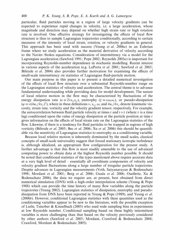
J. Fluid Mech. (2007), vol. 582, pp. 399–422. c 2007 Cambridge University Press doi:10.1017/S0022112007006064 Printed in the United Kingdom 399 Lagrangian conditional statistics, acceleration and local relative motion in numerically simulated isotropic turbulence P. K. YEUNG 1 , S. B. POPE 2 , E. A. KURTH 1 AND A. G. LAMORGESE† 2 1 School of Aerospace Engineering, Georgia Institute of Technology, Atlanta, GA 30332, USA 2 Sibley School of Mechanical and Aerospace Engineering, Cornell University, Ithaca, NY 14853, USA (Received 30 June 2006 and in revised form 19 March 2007) Lagrangian statistics of fluid-particle velocity and acceleration conditioned on fluctuations of dissipation, enstrophy and pseudo-dissipation representing different characteristics of local relative motion are extracted from a direct numerical simulation database of stationary (forced) homogeneous isotropic turbulence. The grid resolution in the simulations is up to 2048 3 , and the Taylor-scale Reynolds number ranges from about 40 to 650, where characteristics of small-scale intermittency in the Eulerian flow field are well developed. A key joint statistic of the conditioning variables is the dissipation–enstrophy cross-correlation, which is asymmetric, but becomes less so at high Reynolds number. Conditional velocity autocorrelations are consistent with rapid changes in the velocity of fluid particles moving in regions of large velocity gradients. Examination of statistics conditioned upon enstrophy, especially in a local coordinate frame moving with the vorticity vector, and of the centripetal acceleration suggests the presence of vortex-trapping effects which persist for several Kolmogorov time scales. Further results on acceleration statistics and joint velocity–acceleration autocorrelations are also presented to help characterize in detail the properties of a joint stochastic process of velocity, acceleration and the pseudo-dissipation. Together with recent work on Eulerian conditional acceleration and Reynolds-number dependence of basic Lagrangian quantities, the present results are directly useful for the development of a new stochastic model formulated to account for intermittency and Reynolds-number effects as described in detail in a companion paper. 1. Introduction The Lagrangian approach of following the motions of infinitesimal fluid elements has long been recognized (Taylor 1921; Monin & Yaglom 1975) as central in descriptions of turbulent transport and dispersion. It is clear that the spatial structure of the turbulence plays an important role: namely, the large-scale motions determine integral time scales and particle displacement, whereas local relative motion in the form of turbulent straining and rotation determines changes of fluid-particle velocity with time and between different particles which diffuse relative to each other. In † Present address: CTR/Stanford University, Bldg 500, Stanford, CA 94305, USA.
-
Upload
independent -
Category
Documents
-
view
1 -
download
0
Transcript of Lagrangian conditional statistics, acceleration and local relative motion in numerically simulated...
J. Fluid Mech. (2007), vol. 582, pp. 399–422. c© 2007 Cambridge University Press
doi:10.1017/S0022112007006064 Printed in the United Kingdom
399
Lagrangian conditional statistics, accelerationand local relative motion in numerically
simulated isotropic turbulence
P. K. YEUNG1, S. B. POPE2, E. A. KURTH 1
AND A. G. LAMORGESE†2
1School of Aerospace Engineering, Georgia Institute of Technology, Atlanta, GA 30332, USA2Sibley School of Mechanical and Aerospace Engineering,
Cornell University, Ithaca, NY 14853, USA
(Received 30 June 2006 and in revised form 19 March 2007)
Lagrangian statistics of fluid-particle velocity and acceleration conditioned onfluctuations of dissipation, enstrophy and pseudo-dissipation representing differentcharacteristics of local relative motion are extracted from a direct numericalsimulation database of stationary (forced) homogeneous isotropic turbulence. The gridresolution in the simulations is up to 20483, and the Taylor-scale Reynolds numberranges from about 40 to 650, where characteristics of small-scale intermittency inthe Eulerian flow field are well developed. A key joint statistic of the conditioningvariables is the dissipation–enstrophy cross-correlation, which is asymmetric, butbecomes less so at high Reynolds number. Conditional velocity autocorrelations areconsistent with rapid changes in the velocity of fluid particles moving in regionsof large velocity gradients. Examination of statistics conditioned upon enstrophy,especially in a local coordinate frame moving with the vorticity vector, and of thecentripetal acceleration suggests the presence of vortex-trapping effects which persistfor several Kolmogorov time scales. Further results on acceleration statistics andjoint velocity–acceleration autocorrelations are also presented to help characterize indetail the properties of a joint stochastic process of velocity, acceleration and thepseudo-dissipation. Together with recent work on Eulerian conditional accelerationand Reynolds-number dependence of basic Lagrangian quantities, the present resultsare directly useful for the development of a new stochastic model formulated toaccount for intermittency and Reynolds-number effects as described in detail in acompanion paper.
1. IntroductionThe Lagrangian approach of following the motions of infinitesimal fluid elements
has long been recognized (Taylor 1921; Monin & Yaglom 1975) as central indescriptions of turbulent transport and dispersion. It is clear that the spatial structureof the turbulence plays an important role: namely, the large-scale motions determineintegral time scales and particle displacement, whereas local relative motion in theform of turbulent straining and rotation determines changes of fluid-particle velocitywith time and between different particles which diffuse relative to each other. In
† Present address: CTR/Stanford University, Bldg 500, Stanford, CA 94305, USA.
400 P. K. Yeung, S. B. Pope, E. A. Kurth and A. G. Lamorgese
particular, fluid particles moving in a region of large velocity gradients can beexpected to experience rapid changes in velocity, i.e. a large acceleration, whosemagnitude and direction may depend on whether high strain rate or high rotationrate is involved. One effective strategy for investigating the effects of local flowstructure is thus to sample Lagrangian trajectories conditionally, according to certainmeasures of the intensity of local strain, rotation, or velocity gradients in general.This approach has been used with success (Yeung et al. 2006a) in an Eulerianframe where we study acceleration as the material derivative of velocity accordingto the Navier–Stokes equations. Consideration of intermittency via a model for theLagrangian acceleration (Sawford 1991; Pope 2002; Reynolds 2003a) is important forincorporating Reynolds-number dependence in stochastic modelling. Recent interestin various aspects of the acceleration (e.g. LaPorta et al. 2001; Sawford et al. 2003;Biferale et al. 2004) also provides further motivation for examining the effects ofsmall-scale intermittency on statistics of Lagrangian fluid-particle motion.
Our main purpose in this paper is to present a detailed numerical investigationof the effects of local flow structure over a substantial Reynolds-number range onthe Lagrangian statistics of velocity and acceleration. The central theme is to advancefundamental understanding while providing data for model development. The natureof local relative motion in the flow may be characterized by fluctuations of theenergy dissipation rate (ε ≡ 2νsij sij ), enstrophy (ζ ≡ νωiωi), or pseudo-dissipation(ϕ ≡ ν(∂ui/∂xj )
2), where in these definitions ν, sij , ωi and ∂ui/∂xj denote kinematic vis-cosity, strain rate, vorticity and the velocity gradient tensor, respectively. For example,the autocorrelation between fluid particle velocity at times t and t+τ (where τ is a timelag) conditioned upon the value of energy dissipation at the particle position at time t
gives information on the effects of local strain rate on the Lagrangian statistics of theflow. Likewise, if there is a tendency for fluid particles to be trapped in regions of highvorticity (Biferale et al. 2005; Bec et al. 2006; Xu et al. 2006) this should be quantifi-able via the sensitivity of Lagrangian statistics to enstrophy as a conditioning variable.
Because local relative motion is inherently dominated by the small scales, classicalconcepts of small-scale universality suggest that forced stationary isotropic turbulenceis, although idealized, an appropriate flow configuration for the present study. Afurther advantage is that this flow is most readily amenable to the use of advancedcomputing power to obtain data at the highest Reynolds number possible. It shouldbe noted that conditional statistics of the types mentioned above require accurate dataat a very high level of detail – essentially all coordinate components of velocity andvelocity gradient fluctuations along a large number of irregular particle trajectories.Despite advances in Lagrangian measurements (Voth, Satyanarayan & Bodenschatz1998; Mordant et al. 2001; Berg et al. 2006; Guala et al. 2006; Ouellette, Xu &Bodenschatz 2006), the data we require are, at present, best obtained from directnumerical simulation (DNS) with a high-order interpolation scheme (Yeung & Pope1988) which can provide the time history of many flow variables along the particletrajectories (Yeung 2002). Lagrangian statistics of dissipation, enstrophy and pseudo-dissipation from DNS have been reported in Yeung & Pope (1989), and Yeung et al.(2006b). However, conditional Lagrangian statistics with these quantities used as theconditioning variables appear to be new to the literature, with the possible exceptionof Luthi, Tsinober & Kinzelbach (2005) who used wide sampling bins in experimentsat low Reynolds number. Conditional sampling based on these highly intermittentvariables is more challenging than that based on the velocity previously consideredby other authors (Sawford et al. 2003; Mordant, Crawford & Bodenschatz 2004;Crawford, Mordant & Bodenschatz 2005).
Lagrangian conditional statistics 401
N 64 128 256 512 1024 2048Rλ 43 86 140 235 393 648ν 0.025 0.0071 0.0028 0.0011 0.000437 0.0001732〈ε〉 1.31 1.17 1.17 1.20 1.26 1.10L1/η 24 52 98 201 450 732TL/τη 5.4 8.6 13.1 19.8 31.1 43.8kmaxη 1.77 1.41 1.41 1.40 1.37 1.44T/TL 32.3 36.3 15.5 10.7 10.0 6.0t/τη 0.0432 0.0328 0.0191 0.0166 0.0101 0.00066h/τη 0.217 0.193 0.184 0.198 0.215 0.243
Table 1. Major parameters of the numerical simulation database.
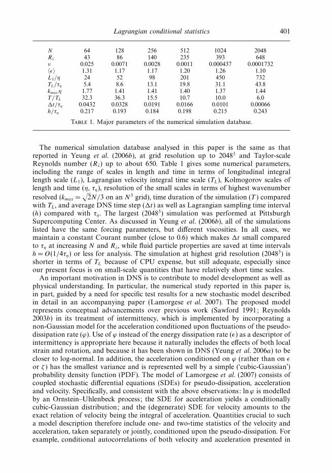
The numerical simulation database analysed in this paper is the same as thatreported in Yeung et al. (2006b), at grid resolution up to 20483 and Taylor-scaleReynolds number (Rλ) up to about 650. Table 1 gives some numerical parameters,including the range of scales in length and time in terms of longitudinal integrallength scale (L1), Lagrangian velocity integral time scale (TL), Kolmogorov scales oflength and time (η, τη), resolution of the small scales in terms of highest wavenumber
resolved (kmax =√
2N/3 on an N3 grid), time duration of the simulation (T ) comparedwith TL, and average DNS time step (t) as well as Lagrangian sampling time interval(h) compared with τη. The largest (20483) simulation was performed at PittsburghSupercomputing Center. As discussed in Yeung et al. (2006b), all of the simulationslisted have the same forcing parameters, but different viscosities. In all cases, wemaintain a constant Courant number (close to 0.6) which makes t small comparedto τη at increasing N and Rλ, while fluid particle properties are saved at time intervalsh = O(1/4τη) or less for analysis. The simulation at highest grid resolution (20483) isshorter in terms of TL because of CPU expense, but still adequate, especially sinceour present focus is on small-scale quantities that have relatively short time scales.
An important motivation in DNS is to contribute to model development as well asphysical understanding. In particular, the numerical study reported in this paper is,in part, guided by a need for specific test results for a new stochastic model describedin detail in an accompanying paper (Lamorgese et al. 2007). The proposed modelrepresents conceptual advancements over previous work (Sawford 1991; Reynolds2003b) in its treatment of intermittency, which is implemented by incorporating anon-Gaussian model for the acceleration conditioned upon fluctuations of the pseudo-dissipation rate (ϕ). Use of ϕ instead of the energy dissipation rate (ε) as a descriptor ofintermittency is appropriate here because it naturally includes the effects of both localstrain and rotation, and because it has been shown in DNS (Yeung et al. 2006a) to becloser to log-normal. In addition, the acceleration conditioned on ϕ (rather than on ε
or ζ ) has the smallest variance and is represented well by a simple (‘cubic-Gaussian’)probability density function (PDF). The model of Lamorgese et al. (2007) consists ofcoupled stochastic differential equations (SDEs) for pseudo-dissipation, accelerationand velocity. Specifically, and consistent with the above observations: lnϕ is modelledby an Ornstein–Uhlenbeck process; the SDE for acceleration yields a conditionallycubic-Gaussian distribution; and the (degenerate) SDE for velocity amounts to theexact relation of velocity being the integral of acceleration. Quantities crucial to sucha model description therefore include one- and two-time statistics of the velocity andacceleration, taken separately or jointly, conditioned upon the pseudo-dissipation. Forexample, conditional autocorrelations of both velocity and acceleration presented in
402 P. K. Yeung, S. B. Pope, E. A. Kurth and A. G. Lamorgese
this paper have been used for model development and testing by Lamorgese et al.(2007). Likewise, conditional and unconditional structure functions of the velocity arereported in Lamorgese et al. (2007) and used to show that the new model achievesbetter agreement with DNS over previous work by Reynolds (2003b) which assumeda conditionally Gaussian acceleration given the energy dissipation rate.
In § 2, we give a brief summary of the numerical methods used to perform thesimulation and analyse the data, including specific issues that arise in the processingof auto- and cross-correlation functions conditioned on either ε, ζ or ϕ. Currentresults on the autocorrelations of these three conditioning variables have been givenin Yeung et al. (2006b), together with basic information on the velocity structurefunction and frequency spectrum interpreted in terms of classical Kolmogorov scaling.Some additional background results on the joint statistics of these variables are firstgiven in § 3. Results on conditional statistics are given in §§ 4–6, for velocity andacceleration considered separately, and then jointly as a pair of random variables. In§ 4, we observe that, when the Reynolds number is low, the velocity autocorrelationconditioned on high enstrophy has some special features which can be interpretedas evidence of fluid particles trapped in regions of high vorticity (Biferale et al.2005). A decomposition of the velocity vector in local coordinate axes parallel andperpendicular to the vorticity vector is used to help explain this effect, which becomesweaker at high Reynolds number. In § 5, we present acceleration–dissipation cross-correlations followed by acceleration autocorrelations conditioned on the dissipationvariables. In § 6, we present both unconditional and conditional versions of the cross-correlation between velocity and acceleration. We conclude this paper in § 7 with asummary of the DNS results and and their role in stochastic modelling.
2. Numerical approachThe basic elements of our numerical simulation approach are as described in several
previous publications (e.g. Yeung 2001; Yeung et al. 2006b): namely, the well-knownFourier pseudo-spectral approach of Rogallo (1981) coupled with the particle-trackingalgorithm of Yeung & Pope (1988). Stochastic forcing at the large scales (Eswaran& Pope 1988) is used to maintain a statistically stationary state and allow higherReynolds numbers to be sustained on a given grid. Cubic spline interpolation, which isfourth-order accurate and twice-differentiable, is used to calculate velocity and velocitygradients (hence the quantities ε, ζ , ϕ) along the trajectories of a large number of fluidparticles with randomly distributed initial positions. The smoothness properties ofcubic splines also facilitate the calculation of acceleration by a simple finite differencein time from velocity time series saved at intervals (h) of order 1/4 of a Kolmogorovtime-scale (τη) or less apart. Theoretical arguments based on intermittency (Yakhot& Sreenivasan 2005) have suggested that accurate results for acceleration statistics(especially the higher-order moments) may require the small scales to be resolvedto a degree beyond prevailing practices in DNS. However, in Yeung et al. (2006a)we show that these effects are weaker for statistics of acceleration conditioned uponfluctuations of ε, ζ or ϕ since the conditional variables are inherently less intermittent.
Knowledge of conditional averages in turbulence is valuable because they providea quantifiable measure of the statistical coupling between fluctuations in one flowvariable and another, and because they are needed as unclosed terms in PDFmodelling where a Lagrangian viewpoint is frequently adopted (Pope 1985). However,most available DNS data on conditional statistics in the literature (e.g. Kronenburg& Bilger 1997; Vedula, Yeung & Fox 2001) are Eulerian, with all variables involved
Lagrangian conditional statistics 403
taken at the same grid points. In the Lagrangian frame, we have a choice of whether totake the conditioning variable at, say, the beginning or the end of a time interval fromt to t +τ . However, conditioning on the ‘present’ (time t) is more natural for stochasticmodelling aimed at predicting the future (time t + τ ). With superscript + denotingLagrangian quantities and u+(t) being a component of the fluid particle velocity, wecan define the conditional velocity autocorrelation given a random variable Z+(t)(which may be ε, ζ or ϕ) as
ρu(τ |Z) ≡ 〈u+(t)u+(t + τ )|Z+(t) = Z〉〈(u+(t))2|Z+(t) = Z〉 , (2.1)
where Z is the corresponding sample-space variable for Z+(t). Because of stationarity,both the numerator and denominator above can be averaged over time t withinthe entire period of the simulation. Computation of the numerator requires bothconditional sampling for each particle over the distribution of Z+(t) divided intosuitable histogram bins, and the averaging over many intervals of size τ within afinite overall simulation period (T ). From (2.1), it can be seen that ρu(τ |Z) equalsunity at τ = 0 (as for its unconditional counterpart), but (because of the normalizationchosen) is not strictly bounded between −1 and 1. A negative τ corresponds toconditioning on Z+(t + τ ) at the end of the interval [t, t + τ ]. In most instances, wechoose histogram bins for Z+(t) (which may be ε, ζ or ϕ) based on their logarithms,which are approximately Gaussian (Yeung et al. 2006a).
Conditioning on enstrophy (in the manner of (2.1)) provides information on theLagrangian history of fluid particles moving in regions of high vorticity, whichis relevant to the issue of fluid particles trapped in vortical regions in turbulentflow (Biferale et al. 2005). Clearly, the statistics of velocity components along andperpendicular to the axis of a strong vortex are expected to differ. To characterizethese effects, it is useful to project the velocity vector onto a system of local coordinateaxes consisting of a unit vector along the direction of local vorticity, and two unitvectors which rotate in the orthogonal plane according to the local rotation-ratetensor. Specifically, let ξ (t), p(t), q(t) be mutually orthogonal unit vectors, withξ (t) = ω(t)/|ω(t)|. We allow p(t) and q(t) to rotate according to the fluctuating rate-of-rotation tensor R(t), but require them to remain orthogonal to ξ (t) (and to eachother). These conditions are met if we let p(t) and q(t) evolve by the pair of (identical)equations
d pdt
= R p − ξ ( p · dξ/dt),dqdt
= R q − ξ (q · dξ/dt). (2.2)
From these equations it can be readily shown that if ξ (t), p(t), q(t) are initiallyorthogonal, then the time derivatives of dot products between any two of themvanish; thus they should remain mutually orthogonal at all times. Initial conditionsare generated by using a Craya decomposition: e.g. let e(1) be the unit vector alongthe x1-axis in a fixed coordinate system, then defining
p(0) =(ξ (0) × e(1)
)/∣∣ξ (0) × e(1)∣∣, q(0) = (ξ (0) × p(0))/|ξ (0) × p(0)|. (2.3)
For numerical integration from time level tn to tn+1 = tn + h we use a second-orderpredictor–corrector scheme similar to that for time advancement in the DNS code,with the time derivative dξ/dt computed from the Lagrangian time series of vorticityusing second-order central differences. In practice, the interval h can only be as smallas the time interval at which we collect Lagrangian time series in the simulations:usually this is about 1/4 of τη, which may not be small enough to capture rapid
404 P. K. Yeung, S. B. Pope, E. A. Kurth and A. G. Lamorgese
variations of the change of vorticity vector orientation. To correct for discretizationerrors due to the finiteness of h we enforce orthogonality at each time level using theprojection tensor based on ξ (tn+1): i.e. the numerical solution p to (2.2) at time tn+1 isconverted to pi(tn+1) = Pij (ξ (tn+1))pj , where Pij (ξ ) = δij −ξiξj . The effectiveness of thiscorrection procedure has been checked by forming the PDF of ξ · p before and afterthe correction at each time step, and by comparing results with a 643 simulation inwhich we used a value of h as small as 1/16 of τη. We refer to the velocity componentalong the vorticity vector as u‖ whereas the two components along p(t) and q(t) arestatistically equivalent and referred to as u⊥.
Lagrangian properties of each of the variables ε, ζ and ϕ taken separately provideimportant background information for interpreting velocity and acceleration statisticsconditioned on these quantities. Results on ε, ζ and ϕ taken separately have beenpresented in Yeung et al. (2006b). These variables are found to have approximatelyexponential autocorrelations with integral time scales which decrease with respect toTL but increase relative to τη as the Reynolds number increases. In contrast to resultsby Yeung & Pope (1989), at high Reynolds number, dissipation and enstrophy arefound to have similar time scales whereas the logarithms of ε, ζ and ϕ all have longertime scales that appear to follow TL. The results also suggest that modelling as adiffusion process with Gaussian statistics is more appropriate for ln ϕ than for ln ε.
In this paper, we include cross-correlations between pairs of random variables. Asa generic definition for two Lagrangian variables X and Y of mean values µX , µY
and variances Var(X), Var(Y ), we write
ρXY (τ ) ≡ 〈(X+(t) − µX)((Y +(t + τ ) − µY )〉{Var(X)Var(Y )}1/2
, (2.4)
where the denominator is averaged over the entire time record of each simulation.The variable X+(t) is considered to be leading in time if τ > 0, but lagging if τ < 0.Although stationarity requires ρXY (−τ ) = ρYX(τ ), this relation does not carry over tothe conditional cross-correlation given another variable Z at time t , i.e. in generalρXY (−τ |Z) (defined by replacing τ by −τ in Eq. 2.4) is not the same as ρYX(τ |Z). Atτ = 0, the single-time correlation coefficient is recovered, which is also written simplyas ρ(X, Y ).
3. Dissipation–enstrophy cross-correlationsAlthough in most studies in the literature (e.g. Yeung & Pope 1989; Chen,
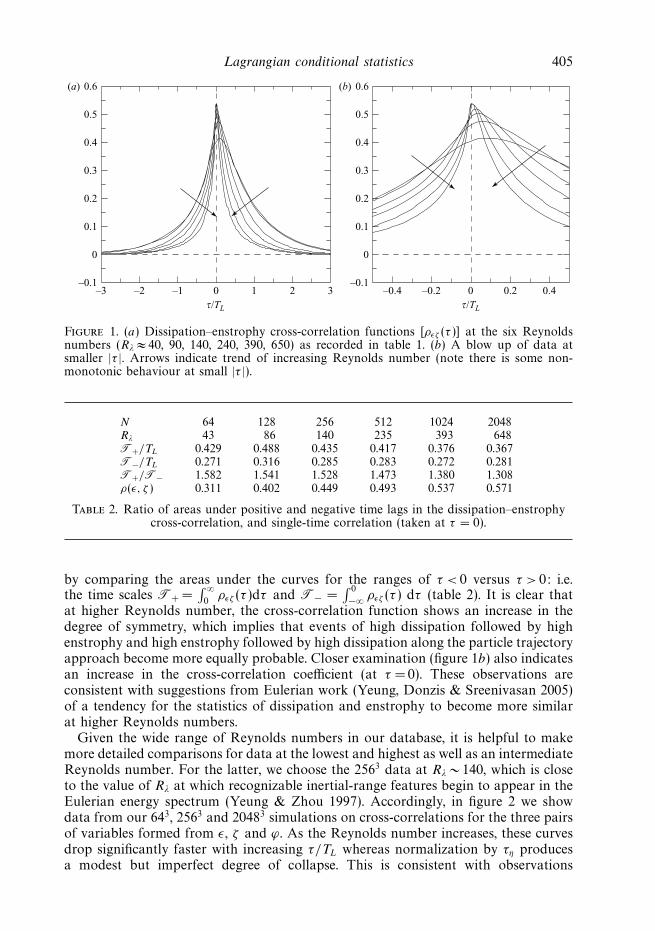
Sreenivasan & Nelkin 1997; Zhou & Antonia 2000) enstrophy is found to be moreintermittent than the dissipation, there is considerable interest in whether theirstatistics may scale similarly at high Reynolds number (Sreenivasan & Antonia1997; Nelkin 1999). From a Lagrangian perspective, diagnostics useful for this issueinclude the autocorrelations of these quantities (Yeung et al. 2006b), and their cross-correlations (Yeung & Pope 1989), shown in figure 1 for six simulations withRλ ≈ 40 − 650 (as in table 1) and time lag normalized by TL. Because both of thesevariables evolve on time scales shorter than TL, as the Reynolds number increases allsix curves shown become narrower under this scaling. A more significant observationis the asymmetry of stronger correlation for τ > 0. Physically, this suggests fluidparticles are more likely to experience high dissipation followed by high enstrophyversus high enstrophy followed by high dissipation. Alternatively, this also suggestsevents of high enstrophy are more intermittent and last for shorter periods of timethan those of high dissipation. The degree of asymmetry in figure 1 can be quantified
Lagrangian conditional statistics 405
τ/TL
0.6(a) (b)
0.5
0.4
0.3
0.2
0.1
0
–0.1–3 –2 –1 0 1 2 3
τ/TL
0.6
0.5
0.4
0.3
0.2
0.1
0
–0.1–0.4 –0.2 0 0.2 0.4
Figure 1. (a) Dissipation–enstrophy cross-correlation functions [ρεζ (τ )] at the six Reynoldsnumbers (Rλ ≈ 40, 90, 140, 240, 390, 650) as recorded in table 1. (b) A blow up of data atsmaller |τ |. Arrows indicate trend of increasing Reynolds number (note there is some non-monotonic behaviour at small |τ |).
N 64 128 256 512 1024 2048Rλ 43 86 140 235 393 648T+/TL 0.429 0.488 0.435 0.417 0.376 0.367T−/TL 0.271 0.316 0.285 0.283 0.272 0.281T+/T− 1.582 1.541 1.528 1.473 1.380 1.308ρ(ε, ζ ) 0.311 0.402 0.449 0.493 0.537 0.571
Table 2. Ratio of areas under positive and negative time lags in the dissipation–enstrophycross-correlation, and single-time correlation (taken at τ = 0).
by comparing the areas under the curves for the ranges of τ < 0 versus τ > 0: i.e.the time scales T+ =
∫ ∞0
ρεζ (τ )dτ and T− =∫ 0
−∞ ρεζ (τ ) dτ (table 2). It is clear thatat higher Reynolds number, the cross-correlation function shows an increase in thedegree of symmetry, which implies that events of high dissipation followed by highenstrophy and high enstrophy followed by high dissipation along the particle trajectoryapproach become more equally probable. Closer examination (figure 1b) also indicatesan increase in the cross-correlation coefficient (at τ =0). These observations areconsistent with suggestions from Eulerian work (Yeung, Donzis & Sreenivasan 2005)of a tendency for the statistics of dissipation and enstrophy to become more similarat higher Reynolds numbers.
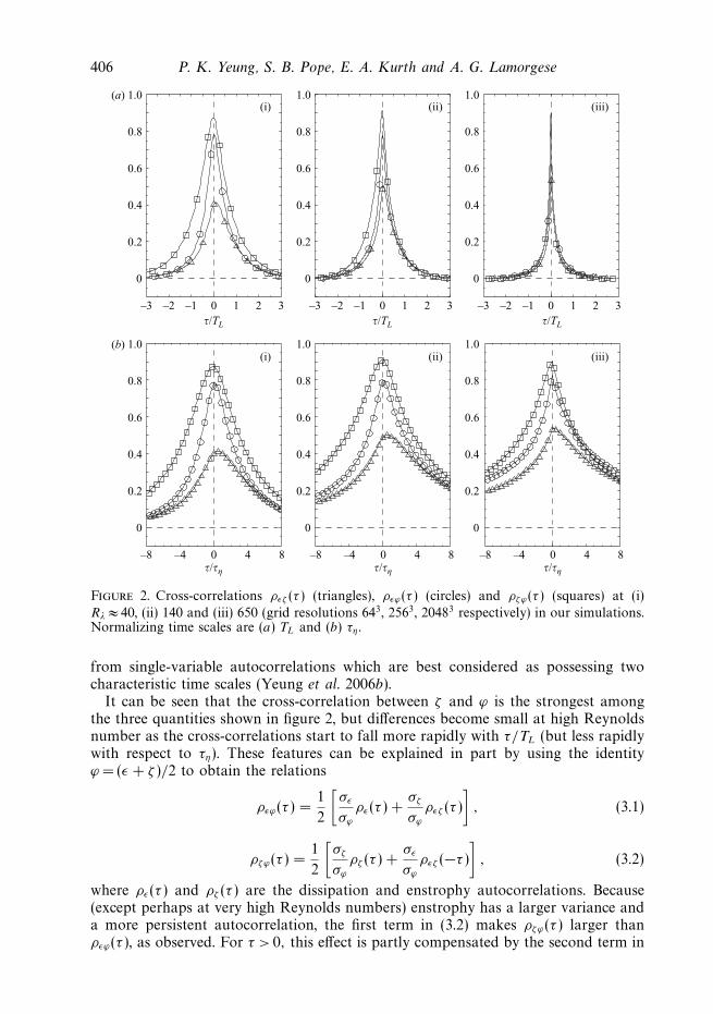
Given the wide range of Reynolds numbers in our database, it is helpful to makemore detailed comparisons for data at the lowest and highest as well as an intermediateReynolds number. For the latter, we choose the 2563 data at Rλ ∼ 140, which is closeto the value of Rλ at which recognizable inertial-range features begin to appear in theEulerian energy spectrum (Yeung & Zhou 1997). Accordingly, in figure 2 we showdata from our 643, 2563 and 20483 simulations on cross-correlations for the three pairsof variables formed from ε, ζ and ϕ. As the Reynolds number increases, these curvesdrop significantly faster with increasing τ/TL whereas normalization by τη producesa modest but imperfect degree of collapse. This is consistent with observations
406 P. K. Yeung, S. B. Pope, E. A. Kurth and A. G. Lamorgese
1.0(a)(i) (ii) (iii)
(i) (ii) (iii)(b)
0.8
0.6
0.4
0.2
0
–3 –2 –1 0 1 2 3
1.0
0.8
0.6
0.4
0.2
0
–3 –2 –1 0 1 2 3
1.0
0.8
0.6
0.4
0.2
0
–3 –2 –1 0 1 2 3
1.0
0.8
0.6
0.4
0.2
0
–8 –4 0 4 8
1.0
0.8
0.6
0.4
0.2
0
1.0
0.8
0.6
0.4
0.2
0
τ/τη
–8 –4 0 4 8τ/τη
–8 –4 0 4 8τ/τη
τ/TL τ/TL τ/TL
Figure 2. Cross-correlations ρεζ (τ ) (triangles), ρεϕ(τ ) (circles) and ρζϕ(τ ) (squares) at (i)
Rλ ≈ 40, (ii) 140 and (iii) 650 (grid resolutions 643, 2563, 20483 respectively) in our simulations.Normalizing time scales are (a) TL and (b) τη .
from single-variable autocorrelations which are best considered as possessing twocharacteristic time scales (Yeung et al. 2006b).
It can be seen that the cross-correlation between ζ and ϕ is the strongest amongthe three quantities shown in figure 2, but differences become small at high Reynoldsnumber as the cross-correlations start to fall more rapidly with τ/TL (but less rapidlywith respect to τη). These features can be explained in part by using the identityϕ =(ε + ζ )/2 to obtain the relations
ρεϕ(τ ) =1
2
[σε
σϕ
ρε(τ ) +σζ
σϕ
ρεζ (τ )
], (3.1)
ρζϕ(τ ) =1
2
[σζ
σϕ
ρζ (τ ) +σε
σϕ
ρεζ (−τ )
], (3.2)
where ρε(τ ) and ρζ (τ ) are the dissipation and enstrophy autocorrelations. Because(except perhaps at very high Reynolds numbers) enstrophy has a larger variance anda more persistent autocorrelation, the first term in (3.2) makes ρζϕ(τ ) larger thanρεϕ(τ ), as observed. For τ > 0, this effect is partly compensated by the second term in
Lagrangian conditional statistics 407
1.0
(a)
(i) (ii) (iii)
0.8
0.6
0.4
0.2
0
0 1 2 3
1.0
0.8
0.6
0.4
0.2
0
0 1 2 3
1.0
0.8
0.6
0.4
0.2
0
0 1 2 3
1.0
(b)
(i) (ii) (iii)
0.8
0.6
0.4
0.2
0
0 1 2 3
1.0
0.8
0.6
0.4
0.2
0
0 1 2 3
1.0
0.8
0.6
0.4
0.2
0
0 1 2 3τ/TL τ/TL τ/TL
ε ζ �
ε ζ �
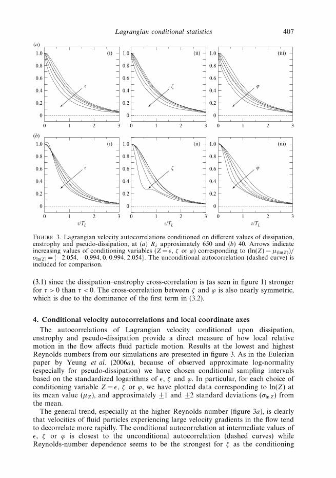
Figure 3. Lagrangian velocity autocorrelations conditioned on different values of dissipation,enstrophy and pseudo-dissipation, at (a) Rλ approximately 650 and (b) 40. Arrows indicateincreasing values of conditioning variables (Z = ε, ζ or ϕ) corresponding to (ln(Z) − µ(ln(Z))/σln(Z) = {−2.054, −0.994, 0, 0.994, 2.054}. The unconditional autocorrelation (dashed curve) isincluded for comparison.
(3.1) since the dissipation–enstrophy cross-correlation is (as seen in figure 1) strongerfor τ > 0 than τ < 0. The cross-correlation between ζ and ϕ is also nearly symmetric,which is due to the dominance of the first term in (3.2).
4. Conditional velocity autocorrelations and local coordinate axesThe autocorrelations of Lagrangian velocity conditioned upon dissipation,
enstrophy and pseudo-dissipation provide a direct measure of how local relativemotion in the flow affects fluid particle motion. Results at the lowest and highestReynolds numbers from our simulations are presented in figure 3. As in the Eulerianpaper by Yeung et al. (2006a), because of observed approximate log-normality(especially for pseudo-dissipation) we have chosen conditional sampling intervalsbased on the standardized logarithms of ε, ζ and ϕ. In particular, for each choice ofconditioning variable Z = ε, ζ or ϕ, we have plotted data corresponding to ln(Z) atits mean value (µZ), and approximately ±1 and ±2 standard deviations (σln Z) fromthe mean.
The general trend, especially at the higher Reynolds number (figure 3a), is clearlythat velocities of fluid particles experiencing large velocity gradients in the flow tendto decorrelate more rapidly. The conditional autocorrelation at intermediate values ofε, ζ or ϕ is closest to the unconditional autocorrelation (dashed curves) whileReynolds-number dependence seems to be the strongest for ζ as the conditioning
408 P. K. Yeung, S. B. Pope, E. A. Kurth and A. G. Lamorgese
1.0
0.8
0.6
0.4
0.2
0
0 1 2 3τ/TL/�
�
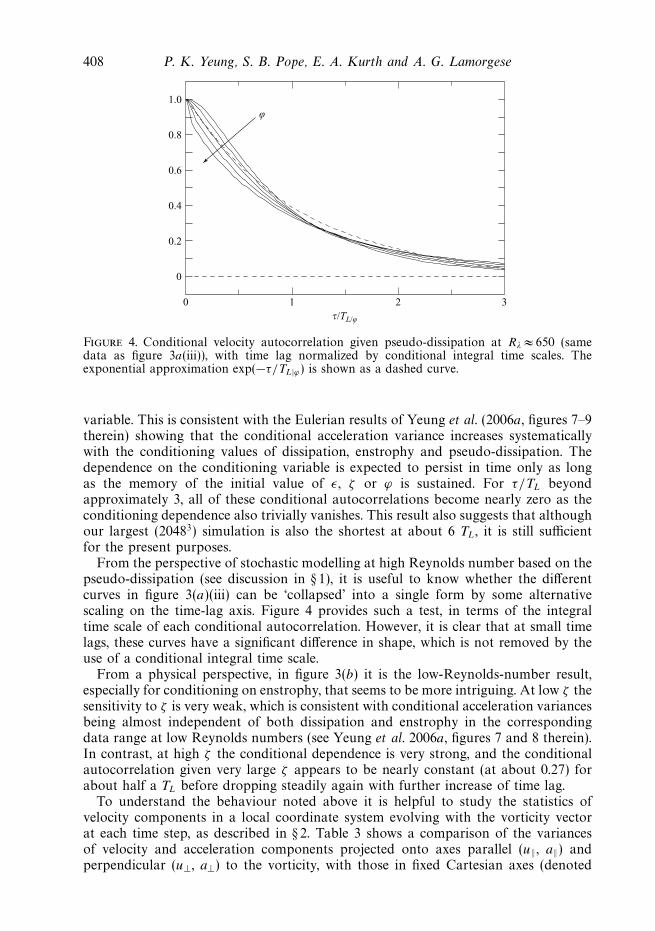
Figure 4. Conditional velocity autocorrelation given pseudo-dissipation at Rλ ≈ 650 (samedata as figure 3a(iii)), with time lag normalized by conditional integral time scales. Theexponential approximation exp(−τ/TL|ϕ) is shown as a dashed curve.
variable. This is consistent with the Eulerian results of Yeung et al. (2006a, figures 7–9therein) showing that the conditional acceleration variance increases systematicallywith the conditioning values of dissipation, enstrophy and pseudo-dissipation. Thedependence on the conditioning variable is expected to persist in time only as longas the memory of the initial value of ε, ζ or ϕ is sustained. For τ/TL beyondapproximately 3, all of these conditional autocorrelations become nearly zero as theconditioning dependence also trivially vanishes. This result also suggests that althoughour largest (20483) simulation is also the shortest at about 6 TL, it is still sufficientfor the present purposes.
From the perspective of stochastic modelling at high Reynolds number based on thepseudo-dissipation (see discussion in § 1), it is useful to know whether the differentcurves in figure 3(a)(iii) can be ‘collapsed’ into a single form by some alternativescaling on the time-lag axis. Figure 4 provides such a test, in terms of the integraltime scale of each conditional autocorrelation. However, it is clear that at small timelags, these curves have a significant difference in shape, which is not removed by theuse of a conditional integral time scale.
From a physical perspective, in figure 3(b) it is the low-Reynolds-number result,especially for conditioning on enstrophy, that seems to be more intriguing. At low ζ thesensitivity to ζ is very weak, which is consistent with conditional acceleration variancesbeing almost independent of both dissipation and enstrophy in the correspondingdata range at low Reynolds numbers (see Yeung et al. 2006a, figures 7 and 8 therein).In contrast, at high ζ the conditional dependence is very strong, and the conditionalautocorrelation given very large ζ appears to be nearly constant (at about 0.27) forabout half a TL before dropping steadily again with further increase of time lag.
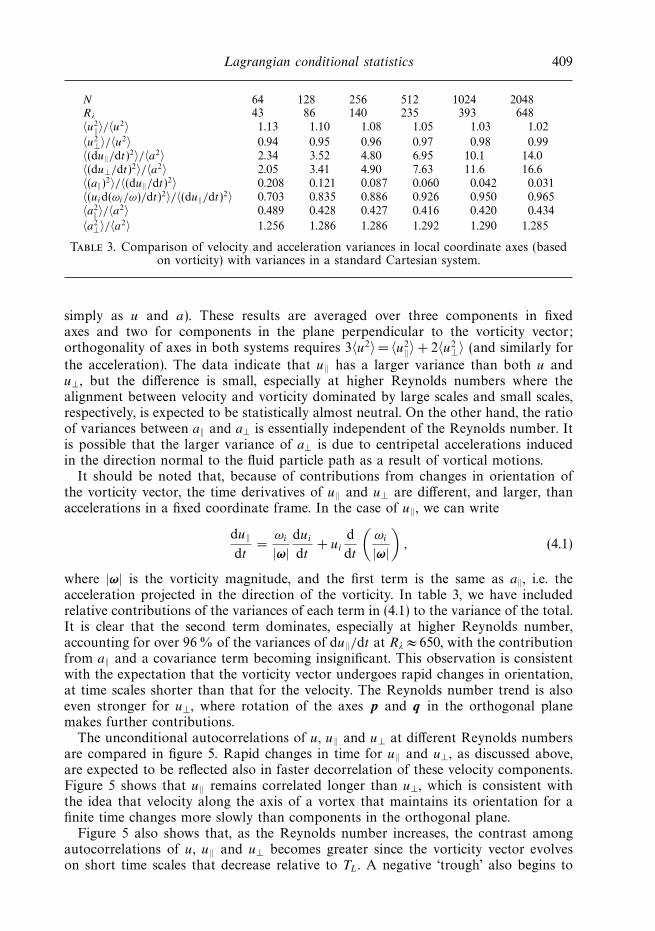
To understand the behaviour noted above it is helpful to study the statistics ofvelocity components in a local coordinate system evolving with the vorticity vectorat each time step, as described in § 2. Table 3 shows a comparison of the variancesof velocity and acceleration components projected onto axes parallel (u‖, a‖) andperpendicular (u⊥, a⊥) to the vorticity, with those in fixed Cartesian axes (denoted
Lagrangian conditional statistics 409
N 64 128 256 512 1024 2048Rλ 43 86 140 235 393 648〈u2
‖〉/〈u2〉 1.13 1.10 1.08 1.05 1.03 1.02
〈u2⊥〉/〈u2〉 0.94 0.95 0.96 0.97 0.98 0.99
〈(du‖/dt)2〉/〈a2〉 2.34 3.52 4.80 6.95 10.1 14.0〈(du⊥/dt)2〉/〈a2〉 2.05 3.41 4.90 7.63 11.6 16.6〈(a‖)
2〉/〈(du‖/dt)2〉 0.208 0.121 0.087 0.060 0.042 0.031〈(uid(ωi/ω)/dt)2〉/〈(du‖/dt)2〉 0.703 0.835 0.886 0.926 0.950 0.965〈a2
‖〉/〈a2〉 0.489 0.428 0.427 0.416 0.420 0.434
〈a2⊥〉/〈a2〉 1.256 1.286 1.286 1.292 1.290 1.285
Table 3. Comparison of velocity and acceleration variances in local coordinate axes (basedon vorticity) with variances in a standard Cartesian system.
simply as u and a). These results are averaged over three components in fixedaxes and two for components in the plane perpendicular to the vorticity vector;orthogonality of axes in both systems requires 3〈u2〉 = 〈u2
‖〉 + 2〈u2⊥〉 (and similarly for
the acceleration). The data indicate that u‖ has a larger variance than both u andu⊥, but the difference is small, especially at higher Reynolds numbers where thealignment between velocity and vorticity dominated by large scales and small scales,respectively, is expected to be statistically almost neutral. On the other hand, the ratioof variances between a‖ and a⊥ is essentially independent of the Reynolds number. Itis possible that the larger variance of a⊥ is due to centripetal accelerations inducedin the direction normal to the fluid particle path as a result of vortical motions.
It should be noted that, because of contributions from changes in orientation ofthe vorticity vector, the time derivatives of u‖ and u⊥ are different, and larger, thanaccelerations in a fixed coordinate frame. In the case of u‖, we can write
du‖
dt=
ωi
|ω|dui
dt+ ui
d
dt
(ωi
|ω|
), (4.1)
where |ω| is the vorticity magnitude, and the first term is the same as a‖, i.e. theacceleration projected in the direction of the vorticity. In table 3, we have includedrelative contributions of the variances of each term in (4.1) to the variance of the total.It is clear that the second term dominates, especially at higher Reynolds number,accounting for over 96 % of the variances of du‖/dt at Rλ ≈ 650, with the contributionfrom a‖ and a covariance term becoming insignificant. This observation is consistentwith the expectation that the vorticity vector undergoes rapid changes in orientation,at time scales shorter than that for the velocity. The Reynolds number trend is alsoeven stronger for u⊥, where rotation of the axes p and q in the orthogonal planemakes further contributions.
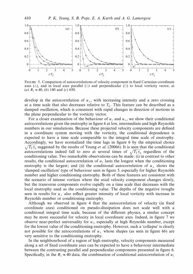
The unconditional autocorrelations of u, u‖ and u⊥ at different Reynolds numbersare compared in figure 5. Rapid changes in time for u‖ and u⊥, as discussed above,are expected to be reflected also in faster decorrelation of these velocity components.Figure 5 shows that u‖ remains correlated longer than u⊥, which is consistent withthe idea that velocity along the axis of a vortex that maintains its orientation for afinite time changes more slowly than components in the orthogonal plane.
Figure 5 also shows that, as the Reynolds number increases, the contrast amongautocorrelations of u, u‖ and u⊥ becomes greater since the vorticity vector evolveson short time scales that decrease relative to TL. A negative ‘trough’ also begins to
410 P. K. Yeung, S. B. Pope, E. A. Kurth and A. G. Lamorgese
1.0(a) (b) (c)
0.8
0.6
0.4
0.2
0
0 1 2 543 0 1 2 543 0 1 2 543
1.0
0.8
0.6
0.4
0.2
0
1.0
0.8
0.6
0.4
0.2
0
τ/TL τ/TL τ/TL
Figure 5. Comparison of autocorrelations of velocity component in fixed Cartesian coordinateaxes (�), and in local axes parallel (�) and perpendicular (�) to local vorticity vector, at(a) Rλ ≈ 40, (b) 140 and (c) 650.
develop in the autocorrelation of u⊥, with increasing intensity and a zero crossingat a time scale that also decreases relative to TL. This feature can be described as adamped oscillation, which is consistent with rapid changes in direction of motions inthe plane perpendicular to the vorticity vector.
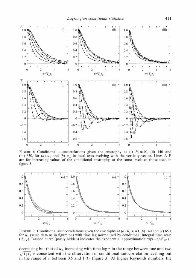
For a closer examination of the behaviour of u‖ and u⊥, we show their conditionalautocorrelations given the enstrophy in figure 6 at low, intermediate and high Reynoldsnumbers in our simulations. Because these projected velocity components are definedin a coordinate system moving with the vorticity, the conditional dependence isexpected to have a time scale comparable to the integral time scale of enstrophy.Accordingly, we have normalized the time lags in figure 6 by the empirical choice√
TLτη suggested by the results of Yeung et al. (2006b). It is seen that the conditionalautocorrelations indeed fall to zero at several times of
√TLτη regardless of the
conditioning value. Two remarkable observations can be made: (i) in contrast to otherresults, the conditional autocorrelation of u‖ lasts the longest when the conditioningenstrophy is the largest; and (ii) the conditional autocorrelation of u⊥ shows the‘damped oscillation’ type of behaviour seen in figure 5, especially for higher Reynoldsnumber and higher conditioning enstrophy. Both of these features are consistent withthe scenario of intense vortices where the axial velocity component changes slowly,but the transverse components evolve rapidly on a time scale that decreases with thelocal enstrophy used as the conditioning value. The depths of the negative troughsseen in results for u⊥ also reflect greater intensity of local vorticity with increase inReynolds number or conditioning enstrophy.
Although we observed in figure 4 that the autocorrelation of velocity (in fixedcoordinate axes) conditioned on pseudo-dissipation does not scale well with aconditional integral time scale, because of the different physics, a similar conceptmay be more successful for velocity in local coordinate axes. Indeed, in figure 7 weobserve near-perfect universality for u‖, especially at high Reynolds number, exceptfor the lowest value of the conditioning enstrophy. However, such a ‘collapse’ is clearlynot possible for the autocorrelations of u⊥ whose shapes (as seen in figure 6b) arevery sensitive to the conditioning enstrophy.
In the neighbourhood of a region of high enstrophy, velocity components measuredalong a set of fixed coordinate axes can be expected to have a behaviour intermediatebetween the contrasting parallel and perpendicular components presented in figure 6.Specifically, in the Rλ ≈ 40 data, the combination of conditional autocorrelation of u‖
Lagrangian conditional statistics 411
E
ED
D
ED
ED
E
E
EE
E
D
D
DD DA
AA
AA
A
AA A A A
AA
AA
A
AA A A ACBBB
B
B
BDDD
DD
DE
E
EB
DD
EB
BE
E E CCC
C
C
C
CC
BB
B
B
B
BB
B B
D
DD
D
D
D
CC
C
C
C
CC C
EE
E
E
EDE
DE DEAAA
A
A
AA
AA
BBB
B
B
B
BB
B
CCC
C
C
C
CC
EEA C
CC
C
CC C
BD
DDD
D
DD D D
A
A
A
A
A
A A
B
B
B
B
BBE E
E
EEE E E
EE
EE
EE
EE
AAD
DD
DD
D
D
DD D DBB
A
A
A
AA
BC
BB
B
B
CC
CC
C CC
CC
C
EE
E
E
CE
CD
AB
BB
B
B BB BB B
CC
CC
C
C
C
C C
DE
EE
EE
E
EE
E
E
E
DD
DD
DD
D
DD
AA
A
AE CEEA A
1.0(a)
(i) (ii) (iii)
(i) (ii) (iii)(b)
0.8
0.6
0.4
0.2
0
0 2 4 6
AB
1.0
0.8
0.6
0.4
0.2
0
0 2 4 6A
B
1.0
0.8
0.6
0.4
0.2
0
0 2 4 6A
AB
C
BD
AB
1.0
0.8
0.6
0.4
0.2
–0.2
–0.4
–0.6
–0.2
–0.4
–0.6
–0.2
–0.4
–0.6
0
0 2 4 6
AB
1.0
0.8
0.6
0.4
0.2
0
0 2 4 6
AB
1.0
0.8
0.6
0.4
0.2
0
0 2 4 6
τ/√TLτη τ/√TLτη τ/√TLτη
Figure 6. Conditional autocorrelations given the enstrophy at (i) Rλ ≈ 40, (ii) 140 and(iii) 650, for (a) u‖ and (b) u⊥ in local axes evolving with the vorticity vector. Lines A–Eare for increasing values of the conditional enstrophy, at the same levels as those used infigure 3.
1.0
0.8
0.6
0.4
0.2
0
0 2 4 6
1.0(a) (b) (c)
0.8
0.6
0.4
0.2
0
0 2 4 6
1.0
0.8
0.6
0.4
0.2
0
0 2 4 6s/T || |ζ s/T || |ζ s/T || |ζ
Figure 7. Conditional autocorrelations given the enstrophy at (a) Rλ ≈ 40, (b) 140 and (c) 650,for u‖ (same data as in figure 6a) with time lag normalized by conditional integral time scale(T‖|ζ ). Dashed curve (partly hidden) indicates the exponential approximation exp(−τ/T‖|ζ ).
decreasing but that of u⊥ increasing with time lag τ in the range between one and two√TLτη is consistent with the observation of conditional autocorrelation levelling out
in the range of τ between 0.5 and 1 TL (figure 3). At higher Reynolds numbers, the
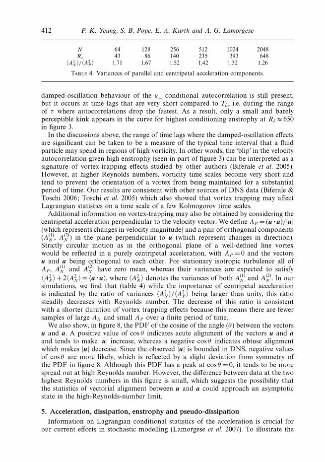
412 P. K. Yeung, S. B. Pope, E. A. Kurth and A. G. Lamorgese
N 64 128 256 512 1024 2048Rλ 43 86 140 235 393 648
〈A2N 〉/〈A2
P 〉 1.71 1.67 1.52 1.42 1.32 1.26
Table 4. Variances of parallel and centripetal acceleration components.
damped-oscillation behaviour of the u⊥ conditional autocorrelation is still present,but it occurs at time lags that are very short compared to TL, i.e. during the rangeof τ where autocorrelations drop the fastest. As a result, only a small and barelyperceptible kink appears in the curve for highest conditioning enstrophy at Rλ ≈ 650in figure 3.
In the discussions above, the range of time lags where the damped-oscillation effectsare significant can be taken to be a measure of the typical time interval that a fluidparticle may spend in regions of high vorticity. In other words, the ‘blip’ in the velocityautocorrelation given high enstrophy (seen in part of figure 3) can be interpreted as asignature of vortex-trapping effects studied by other authors (Biferale et al. 2005).However, at higher Reynolds numbers, vorticity time scales become very short andtend to prevent the orientation of a vortex from being maintained for a substantialperiod of time. Our results are consistent with other sources of DNS data (Biferale &Toschi 2006; Toschi et al. 2005) which also showed that vortex trapping may affectLagrangian statistics on a time scale of a few Kolmogorov time scales.
Additional information on vortex-trapping may also be obtained by considering thecentripetal acceleration perpendicular to the velocity vector. We define AP = (u · a)/|u|(which represents changes in velocity magnitude) and a pair of orthogonal components(A(1)
N , A(2)N ) in the plane perpendicular to u (which represent changes in direction).
Strictly circular motion as in the orthogonal plane of a well-defined line vortexwould be reflected in a purely centripetal acceleration, with AP = 0 and the vectorsu and a being orthogonal to each other. For stationary isotropic turbulence all ofAP , A
(1)N and A
(2)N have zero mean, whereas their variances are expected to satisfy
〈A2P 〉 +2〈A2
N〉 = 〈a · a〉, where 〈A2N〉 denotes the variances of both A
(1)N and A
(2)N . In our
simulations, we find that (table 4) while the importance of centripetal accelerationis indicated by the ratio of variances 〈A2
N〉/〈A2P 〉 being larger than unity, this ratio
steadily decreases with Reynolds number. The decrease of this ratio is consistentwith a shorter duration of vortex trapping effects because this means there are fewersamples of large AN and small AP over a finite period of time.
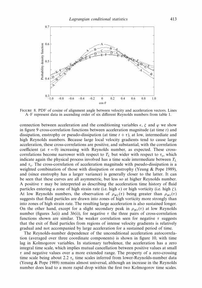
We also show, in figure 8, the PDF of the cosine of the angle (θ) between the vectorsu and a. A positive value of cos θ indicates acute alignment of the vectors u and aand tends to make |u| increase, whereas a negative cos θ indicates obtuse alignmentwhich makes |u| decrease. Since the observed |u| is bounded in DNS, negative valuesof cos θ are more likely, which is reflected by a slight deviation from symmetry ofthe PDF in figure 8. Although this PDF has a peak at cos θ =0, it tends to be morespread out at high Reynolds number. However, the difference between data at the twohighest Reynolds numbers in this figure is small, which suggests the possibility thatthe statistics of vectorial alignment between u and a could approach an asymptoticstate in the high-Reynolds-number limit.
5. Acceleration, dissipation, enstrophy and pseudo-dissipationInformation on Lagrangian conditional statistics of the acceleration is crucial for
our current efforts in stochastic modelling (Lamorgese et al. 2007). To illustrate the
Lagrangian conditional statistics 413
cos θ
A
A
B
DC
C
C C
C
C
E
E
EE E
E
ECA
A
A
A
A
A
F
F
FF F
F
BD
D
D DD
D
B
B B
B
B
B
0.7
0.6
0.5
0.4
0.3–1.0 –0.8 –0.6 –0.4 –0.2 0 0.2 0.4 0.6 0.8 1.0
Pro
babi
lity
den
sity
fun
ctio
n
Figure 8. PDF of cosine of alignment angle between velocity and acceleration vectors. LinesA–F represent data in ascending order of six different Reynolds numbers from table 1.
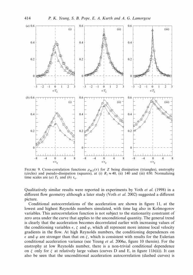
connection between acceleration and the conditioning variables ε, ζ and ϕ we showin figure 9 cross-correlation functions between acceleration magnitude (at time t) anddissipation, enstrophy or pseudo-dissipation (at time t + τ ), at low, intermediate andhigh Reynolds numbers. Because large local velocity gradients tend to cause largeacceleration, these cross-correlations are positive, and substantial, with the correlationcoefficient (at τ = 0) increasing with Reynolds number, as expected. These cross-correlations become narrower with respect to TL but wider with respect to τη, whichindicate again the physical process involved has a time scale intermediate between TL
and τη. The cross-correlation of acceleration magnitude with pseudo-dissipation is aweighted combination of those with dissipation or enstrophy (Yeung & Pope 1989),and (since enstrophy has a larger variance) is generally closer to the latter. It canbe seen that these curves are all asymmetric, but less so at higher Reynolds number.A positive τ may be interpreted as describing the acceleration time history of fluidparticles entering a zone of high strain rate (i.e. high ε) or high vorticity (i.e. high ζ ).At low Reynolds numbers, the observation of ρ|a|ζ (τ ) being greater than ρ|a|ε(τ )suggests that fluid particles are drawn into zones of high vorticity more strongly thaninto zones of high strain rate. The resulting large acceleration is also sustained longer.On the other hand, except for a slight secondary peak in ρ|a|ε(τ ) at low Reynoldsnumber (figures 3a(i) and 3b(i)), for negative τ the three pairs of cross-correlationfunctions shown are similar. The weaker correlation seen for negative τ suggeststhat the exit of fluid particles from regions of intense velocity gradients is relativelygradual and not accompanied by large acceleration for a sustained period of time.
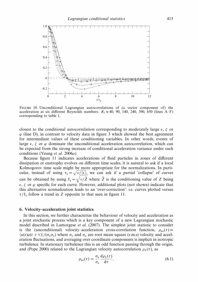
The Reynolds-number dependence of the unconditional acceleration autocorrela-tion (averaged over three coordinate components) is shown in figure 10, with timelag in Kolmogorov variables. In stationary turbulence, the acceleration has a zerointegral time scale, which implies mutual cancellation between positive values at smallτ and negative values over a more extended range. The property of a zero-crossingtime scale being about 2.2 τη time scales inferred from lower-Reynolds-number data(Yeung & Pope 1989) remains almost universal, although an increase in the Reynoldsnumber does lead to a more rapid drop within the first two Kolmogorov time scales.
414 P. K. Yeung, S. B. Pope, E. A. Kurth and A. G. Lamorgese
0.6(a)(i) (ii) (iii)
(i) (ii) (iii)
0.4
0.2
0
–3 –2 –1 0 1 2 3
0.6
0.4
0.2
0
–3 –2 –1 0 1 2 3
0.6
0.4
0.2
0
0.6(b)
0.4
0.2
0
–8 –4 0 4 8
0.6
0.4
0.2
0
0.6
0.4
0.2
0
–3 –2 –1 0 1 2 3τ/TL τ/TL τ/TL
τ/τη τ/τη τ/τη
–8 –4 0 4 8 –8 –4 0 4 8
Figure 9. Cross-correlation functions ρ|a|Z(τ ) for Z being dissipation (triangles), enstrophy(circles) and pseudo-dissipation (squares), at (i) Rλ ≈ 40, (ii) 140 and (iii) 650. Normalizingtime scales are (a) TL and (b) τη .
Qualitatively similar results were reported in experiments by Voth et al. (1998) in adifferent flow geometry although a later study (Voth et al. 2002) suggested a differentpicture.
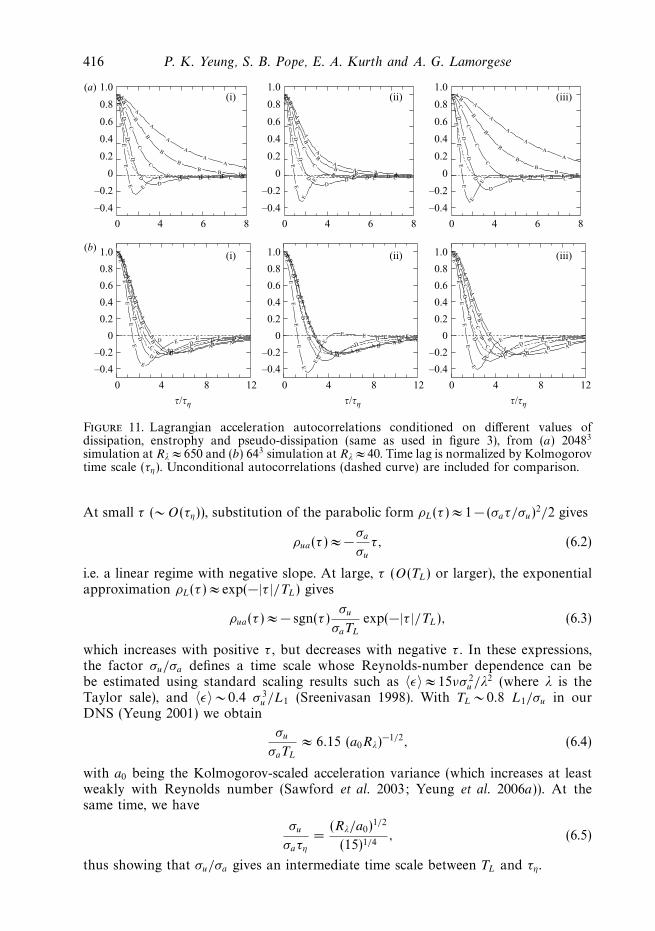
Conditional autocorrelations of the acceleration are shown in figure 11, at thelowest and highest Reynolds numbers simulated, with time lag also in Kolmogorovvariables. This autocorrelation function is not subject to the stationarity constraint ofzero area under the curve that applies to the unconditional quantity. The general trendis clearly that the acceleration becomes decorrelated earlier with increasing values ofthe conditioning variables ε, ζ and ϕ, which all represent more intense local velocitygradients in the flow. At high Reynolds numbers, the conditioning dependences onε and ϕ are stronger than that on ζ , which is consistent with results for the Eulerianconditional acceleration variance (see Yeung et al. 2006a, figure 10 therein). For theenstrophy at low Reynolds number, there is a non-trivial conditional dependenceon ζ only for ζ at relatively large values (curves D and E, in figure 11b(ii)). It canalso be seen that the unconditional acceleration autocorrelation (dashed curves) is
Lagrangian conditional statistics 415
1.0
0.8
0.6
0.4
0.2
0
–0.2
0 2 4 6 8 10 12τ/τη
D
D
D
D
D D D D DD
A
A
A
A
A
AA
A A
AB
B
B
B
BB B B
B
C
C
C
C
C C C C C
EE
E
E
E E E E E
FF
F
FF F F F F
Figure 10. Unconditional Lagrangian autocorrelations of (a vector component of) theacceleration at six different Reynolds numbers: Rλ ≈ 40, 90, 140, 240, 390, 650 (lines A–F)corresponding to table 1.
closest to the conditional autocorrelation corresponding to moderately large ε, ζ orϕ (line D), in contrast to velocity data in figure 3 which showed the best agreementfor intermediate values of these conditioning variables. In other words, events oflarge ε, ζ or ϕ dominate the unconditional acceleration autocorrelation, which canbe expected from the strong increase of conditional acceleration variance under suchconditions (Yeung et al. 2006a).
Because figure 11 indicates accelerations of fluid particles in zones of differentdissipation or enstrophy evolves on different time scales, it is natural to ask if a localKolmogorov time scale might be more appropriate for the normalizations. In parti-cular, instead of using τη =
√ν/〈ε〉, we can ask if a partial ‘collapse’ of curves
can be obtained by using τη =
√ν/Z where Z is the conditioning value of Z being
ε, ζ or ϕ specific for each curve. However, additional plots (not shown) indicate thatthis alternative normalization leads to an ‘over-correction’: i.e. curves plotted versusτ/τη follow a trend in Z opposite to that seen in figure 11.
6. Velocity–acceleration joint statisticsIn this section, we further characterize the behaviour of velocity and acceleration as
a joint stochastic process which is a key component of a new Lagrangian stochasticmodel described in Lamorgese et al. (2007). The simplest joint statistic to consideris the (unconditional) velocity–acceleration cross-correlation function, ρua(τ ) ≡〈u(t)a(t + τ )〉/(σuσa) where σu and σa are root mean square (r.m.s) velocity and accel-eration fluctuations, and averaging over coordinate components is implicit in isotropicturbulence. In stationary turbulence this is an odd function passing through the origin,and (Pope 2000) related to the Lagrangian velocity autocorrelation ρL(τ ), as
ρua(τ ) =σu
σa
dρL(τ )
dτ. (6.1)
416 P. K. Yeung, S. B. Pope, E. A. Kurth and A. G. Lamorgese
1.0(a)(i) (ii) (iii)
(i) (ii) (iii)(b)
0.8
0.6
0.4
0.2
0
–0.2
–0.4
0 4 6 8
1.0
0.8
0.6
0.4
0.2
0
–0.2
–0.4
0 4 6 8
1.0
0.8
0.6
0.4
0.2
0
–0.2
–0.4
0 4 6 8
1.0
0.8
0.6
0.4
0.2
0
–0.2
–0.4
1.0
0.8
0.6
0.4
0.2
0
–0.2
–0.4
1.0
0.8
0.6
0.4
0.2
0
–0.2
–0.4
0 4 8 12 0 4 8 12 0 4 8 12
A
A
A
A
A
AA
A
B
B
B
B
B
BB B
CC
C
C
CCCC
DD
D
DDDDD
DD
D
EE
DEE
EE
E
E
E EEEE
A
A
A
A
AA A A
BB
B
B
BB B B
CC
C
C
C CCC
D
DD DD
D
DD
D
EE
EE
E
E
EEEE
DE
A
A
A
A
A
AA
B
B
B
B
B
BB B
C
C
C
C
C CCC
D
DD DD
DD
DD
EE
EE
E
E
EEEE
A
AA
A
A
A AA
A
BB
BB
B
B BB
B
CC
CC
C C
CC
C
DD
D DD
DD
D
DD
D
EE
DE
EE
E
E
E
E EE
E
E
A
AA
AA A
AA
A
BB
BB
B
B BB
B
CC
CC
CC
C
C
C
D
DD
D
DDD
DD
EE
EE
E
EE EEEE
E
DE
A
A
A
A
A
A
A AA
B
BB
B
B
BB
B
B
CC
CC
CC
C
C
C
D
D
D
DD
D
DD
D
EE
EE
E
E E E EEE
E
τ/τη τ/τη τ/τη
Figure 11. Lagrangian acceleration autocorrelations conditioned on different values ofdissipation, enstrophy and pseudo-dissipation (same as used in figure 3), from (a) 20483
simulation at Rλ ≈ 650 and (b) 643 simulation at Rλ ≈ 40. Time lag is normalized by Kolmogorovtime scale (τη). Unconditional autocorrelations (dashed curve) are included for comparison.
At small τ (∼ O(τη)), substitution of the parabolic form ρL(τ ) ≈ 1− (σaτ/σu)2/2 gives
ρua(τ ) ≈ −σa
σu
τ, (6.2)
i.e. a linear regime with negative slope. At large, τ (O(TL) or larger), the exponentialapproximation ρL(τ ) ≈ exp(−|τ |/TL) gives
ρua(τ ) ≈ − sgn(τ )σu
σaTL
exp(−|τ |/TL), (6.3)
which increases with positive τ , but decreases with negative τ . In these expressions,the factor σu/σa defines a time scale whose Reynolds-number dependence can bebe estimated using standard scaling results such as 〈ε〉 ≈ 15νσ 2
u /λ2 (where λ is theTaylor sale), and 〈ε〉 ∼ 0.4 σ 3
u /L1 (Sreenivasan 1998). With TL ∼ 0.8 L1/σu in ourDNS (Yeung 2001) we obtain
σu
σaTL
≈ 6.15 (a0Rλ)−1/2, (6.4)
with a0 being the Kolmogorov-scaled acceleration variance (which increases at leastweakly with Reynolds number (Sawford et al. 2003; Yeung et al. 2006a)). At thesame time, we have
σu
σaτη
=(Rλ/a0)
1/2
(15)1/4, (6.5)
thus showing that σu/σa gives an intermediate time scale between TL and τη.
Lagrangian conditional statistics 417
0.4
(a) (b)
0.2
0
–0.2
–0.4
–2 0 2τ/TL
0.4
0.2
0
–0.2
–0.4
–8 –4 0 4 8τ/TLτη
A
AA
A
A
A
AA
A
A
A
A
A
A
B
B
B
B
BB B
B
B
B
B
BB
B
CC
C
C
CC
C
C
C
CC
CD
DD
D
D
DD
D
DCD
D
E
E
E
E
E
EE
EEEF
F
F
F
FF
FF
FF
–––––
Figure 12. Unconditional Lagrangian velocity–acceleration autocorrelations at differentReynolds numbers (lines A–F, for Rλ ≈ 40, 90, 140, 240, 390, 650), with time lag undertwo different normalizations.
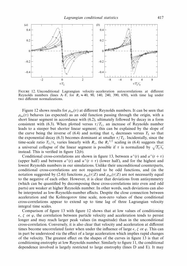
Figure 12 shows results for ρua(τ ) at different Reynolds numbers. It can be seen thatρua(τ ) behaves (as expected) as an odd function passing through the origin, with ashort linear segment in accordance with (6.2), ultimately followed by decay in a formconsistent with (6.3). When plotted versus τ/TL, an increase of Reynolds numberleads to a steeper but shorter linear segment; this can be explained by the slope ofthe curve being the inverse of (6.4) and noting that τη decreases versus TL so thatthe exponential decay (6.3) becomes dominant at smaller τ/TL. Incidentally, since thetime-scale ratio TL/τη varies linearly with Rλ, the Rλ
1/2 scaling in (6.4) suggests that
a universal collapse of the linear segment is possible if τ is normalized by√
TLτη
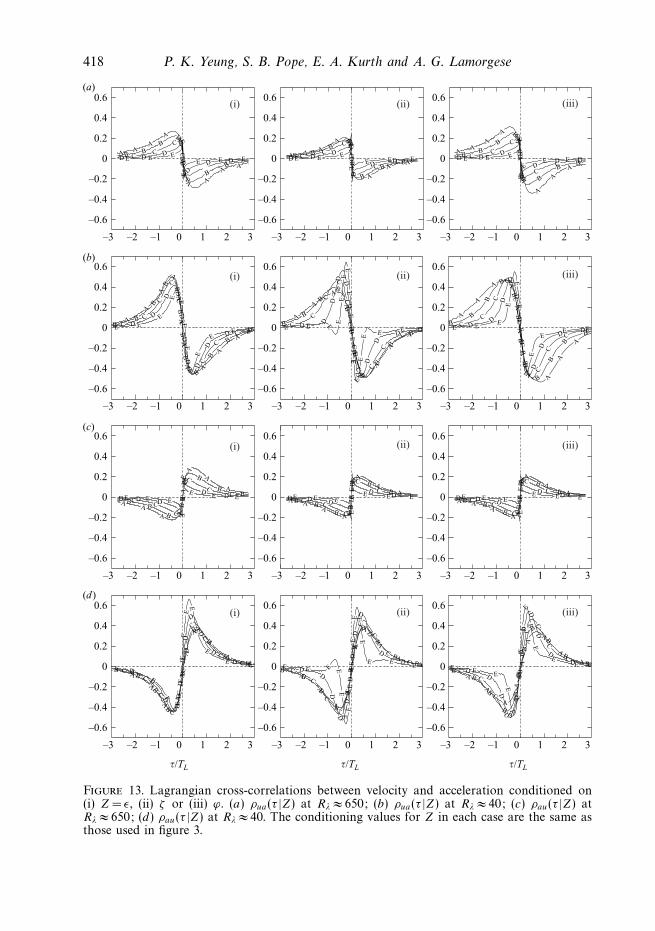
instead. This is verified in figure 12(b).Conditional cross-correlations are shown in figure 13, between u+(t) and a+(t + τ )
(upper half) and between a+(t) and u+(t + τ ) (lower half), and for the highest andlowest Reynolds numbers in our simulations. Unlike their unconditional counterparts,conditional cross-correlations are not required to be odd functions, and (in thenotation suggested by (2.4)) functions ρua(τ |Z) and ρau(τ |Z) are not necessarily equalto the negative of each other. However, it is clear that deviations from antisymmetry(which can be quantified by decomposing these cross-correlations into even and oddparts) are weaker at higher Reynolds number. In other words, such deviations can alsobe interpreted as low-Reynolds-number effects. Despite the close connection betweenacceleration and the Kolmogorov time scale, non-zero values of these conditionalcross-correlations appear to extend up to time lag of three Lagrangian velocityintegral time scales.
Comparison of figure 13 with figure 12 shows that at low values of conditioningε, ζ or ϕ, the correlation between particle velocity and acceleration tends to persistlonger and may reach larger peak values (in magnitude) than in the unconditionalcross-correlation. Conversely, it is also clear that velocity and acceleration at differenttimes become uncorrelated faster when under the influence of large ε, ζ or ϕ. This canin part be understood via the effect of a large acceleration which implies rapid changesof the velocity. The greatest effect on the shapes of the curves in figure 13 is that ofconditioning enstrophy at low Reynolds number. Similarly to figure 11, the conditionaldependence involved is largely restricted to large enstrophy (lines D and E). It may
418 P. K. Yeung, S. B. Pope, E. A. Kurth and A. G. Lamorgese
0.6(a)
(b)
(c)
(d)
0.4
0.2
0
–0.2
–0.4
–0.6
–3 –2 –1 0 1 2 3
0.6
0.4
0.2
0
–0.2
–0.4
–0.6
–3 –2 –1 0 1 2 3
0.6
0.4
0.2
0
–0.2
–0.4
–0.6
–3 –2 –1 0 1 2 3
0.6
0.4
0.2
0
–0.2
–0.4
–0.6
–3 –2 –1 0 1 2 3
0.6
0.4
0.2
0
–0.2
–0.4
–0.6
–3 –2 –1 0 1 2 3
0.6
0.4
0.2
0
–0.2
–0.4
–0.6
–3 –2 –1 0 1 2 3
0.6
0.4
0.2
0
–0.2
–0.4
–0.6
–3 –2 –1 0 1 2 3
0.6
0.4
0.2
0
–0.2
–0.4
–0.6
–3 –2 –1 0 1 2 3
0.6
0.4
0.2
0
–0.2
–0.4
–0.6
–3 –2 –1 0 1 2 3
0.6
0.4
0.2
0
–0.2
–0.4
–0.6
–3 –2 –1 0 1 2 3
0.6
0.4
0.2
0
–0.2
–0.4
–0.6
–3 –2 –1 0 1 2 3
0.6
0.4
0.2
0
–0.2
–0.4
–0.6
–3 –2 –1 0 1 2 3
A AA
A AA A
AA
A A AA A
A
AA
AA
A
A
A
A
AA
A
A
AB BB
B
B
BB
B
B BB
B
B
BB
BB
B
B
BB
BB
B
CC
C
C
C
CC
CC
C
CC
CC
C
CC C
CC
D DD
DD D D D
D D
DD D
D
DD D
D
D
D
D
DD
D
D
E E E
E
E E E E E
EEE E E E E E E
EE E
EE
E
E
EE
A
A
A
A
AA
BB
B
B BB
BB
B
B
B
BB
B
B
B
BB
BB
B
CC
C
C
CC
DD
D
DD
E EE
E EE
AA
A
A
A
A
A
A
AA
A
A
BA
B
BB
B
B
BB
BB
B
B
B
BA
A
A AA
AA
A
A
A
A
AA
CC C
C
CC
CC
C
CC
C
C
C
C
CC
C CC
CC
C
C
CC
C
C
DD
D
D
DD
D D
DD D
DD
D
DD
DD
D
D
DD
D
DD
DD
D
D
D
D
EE
E
EE E E E E
EE
EE
EE
E
EE
E
E E E EE
E
EE
E
E
E
E EE
E
E
D D D
D
D
DD
D
AA
A
AA
AAA
BB
B
BB
B
BB
CC
C
C
CC
C
E E E
EE
E
EE E D D D
DD
D
D
D
AA
AA
A
A
AA B BB
BB
BB
C C
CC
C
C
C
E
EE
E
EE E E D D D
DD
D
D
D
A AA
A
AA
A
AB
BB
BB
BB
CC
CC
C
CC
E EE E E
E
EE
E
E
E
BB
B
B
B
CC
C
C
C
D
DEE
D
D
E
EDE
DED
D
D
D
DD
D
D
DD
DD
D
D
D
DD
D
DD
DD
D
D
D
DD
DD
E
E
E
EE
E
EE E
EE
EE E
E
EEE E E
E
EE
EE
E
E
EE
EE
E
EEE
E
E
A
A
A AB
B
B
B
BC
CC
C
C
CC
C
C
C
C
AA
A
A
AB
BB
A
A
B
B
B
A
A
AC
C
C
CC
CC
C
C
CC
CC
C
C
CC
B
B
B
BB
BB
B
B
BB
B
B
B
BB
A
A
A
AA
A
A
A
AA
A
A
A
A
CBA
(i) (ii)
(ii)
(ii)
(ii) (iii)
(iii)
(iii)
(iii)
(i)
(i)
(i)
τ/TL τ/TL τ/TL
Figure 13. Lagrangian cross-correlations between velocity and acceleration conditioned on(i) Z = ε, (ii) ζ or (iii) ϕ. (a) ρua(τ |Z) at Rλ ≈ 650; (b) ρua(τ |Z) at Rλ ≈ 40; (c) ρau(τ |Z) atRλ ≈ 650; (d) ρau(τ |Z) at Rλ ≈ 40. The conditioning values for Z in each case are the same asthose used in figure 3.
Lagrangian conditional statistics 419
be recognized the conditional cross-correlations shown here are at a level of detailbeyond what most current stochastic models (to our knowledge) can predict. Neverthe-less, the data presented will be potentially useful for future developments in modelling.
7. Conclusions and discussionIn this paper, we have used direct numerical simulation (DNS) data in forced,
stationary isotropic turbulence, at Taylor-scale Reynolds numbers in the range 40–650and grid resolution 643 to 20483, to study the effects of spatial intermittency onLagrangian fluid particle motion including the properties of velocity and acceleration.A primary emphasis is on the behaviour of Lagrangian statistics conditioned onfluctuations of dissipation (ε), enstrophy (ζ ) and pseudo-dissipation (ϕ), as extensionsof studies of Eulerian conditional statistics of the acceleration (Yeung et al. 2006a) andthe Reynolds-number dependence of basic Lagrangian quantities (Yeung et al. 2006b).Besides advancing physical understanding, this work also provides data required totest new developments in stochastic modelling incorporating effects of intermittency(Reynolds et al. 2005; Lamorgese et al. 2007). The Lagrangian conditional statisticspresented here are new and involve a degree of detail currently possible only in DNS.
The Lagrangian cross-correlation (in time) between dissipation and enstrophy hasan asymmetric form which suggests there is a preferential tendency for fluid particlesto experience high dissipation followed by high enstrophy instead of the converse,although this effect becomes weaker at high Reynolds numbers. Conditional auto-correlations of velocity given ε, ζ or ϕ, show clearly that (as expected) the velocitiesof fluid particles moving in regions of large velocity gradients tend to decorrelaterapidly, in accordance with a large conditional acceleration variance (Yeung et al.2006a). However, at low Reynolds number, the conditional autocorrelation givenhigh enstrophy has some distinctive features (figure 3b(ii)) which we have examinedclosely by considering velocity components u‖ and u⊥ in a system of local coordinateaxes parallel and perpendicular to the vorticity vector. Both u‖ and u⊥ evolve anddecorrelate rapidly as a result of rapid changes in the vorticity vector orientation,with the autocorrelation of the latter taking on (especially at high Reynolds number)a negative trough typical of systems with damped oscillations. Results for conditionaland unconditional autocorrelations of u‖ and u⊥ suggest that the ‘blip’ in figure 3 is asignature of vortex-trapping effects which other authors (e.g. Biferale et al. 2005) havereported to have a time scale of several Kolmogorov time scales. Additional informa-tion is also presented in terms of centripetal acceleration projected along the directionof the velocity vector. At higher Reynolds number, since the vorticity then evolves onshorter time scales, a strong vortex in the flow is probably not well sustained in time.
Results on the cross-correlations between acceleration magnitude (|a|) and thevariables ε, ζ and ϕ suggest that fluid particles are drawn into zones of high vorticitywith a larger acceleration compared with zones of high strain rate, although thecontrast becomes weaker at high Reynolds number. At high Reynolds numbers,conditional acceleration autocorrelations show a very strong dependence on theconditioning variables, especially for dissipation and pseudo-dissipation (figure 11a).Although the conditional acceleration evolves on a time scale that decreases with theintensity of local velocity gradients, normalization by a local Kolmogorov time scalebased on the conditioning variables does not produce a close ‘collapse’ of the data.
For a further characterization of the conditional joint distribution of velocityand acceleration, we have also presented cross-correlations between the velocity andacceleration. The unconditional cross-correlation is shown to be characterized by a
420 P. K. Yeung, S. B. Pope, E. A. Kurth and A. G. Lamorgese
short linear segment followed by an exponential decay related to the shape of thevelocity autocorrelation. The conditional cross-correlation departs from antisymmetryprimarily at low Reynolds number, where high conditioning enstrophy again leads toqualitatively different results.
In summary, we have presented here new results from numerical simulations up to20483 grid resolution on the conditional statistics of Lagrangian fluid-particle motion,where several features associated with low Reynolds number have been identified.While contrasts between conditioning on dissipation and on enstrophy give usefulinformation on the physics of intermittency effects, pseudo-dissipation is (as suggestedby Yeung et al. 2006a) the best conditioning variable for use in modelling. The bodyof data presented here, as well as the underlying simulation database, is expected to beuseful in the development of Lagrangian stochastic models, such as the conditionallycubic Gaussian model for velocity, acceleration and pseudo-dissipation, developed byLamorgese et al. (2007).
We gratefully knowledge support from the National Science Foundation (NSF),via Grants CTS-0328314 (P.K.Y.) and CTS-0328329 (S.B.P.). The computations weremade possible by large resource allocations at Pittsburgh Supercomputing Center(PSC, for the 20483 Lagrangian simulation) and San Diego Supercomputer Center(SDSC), which are both supported by NSF.
REFERENCES
Bec, J., Biferale, L., Cencini, M., Lanotte, A. & Toschi, F. 2006 Effect of vortex filaments on thevelocity of tracers and heavy particles in turbulence. Phys. Fluids 18, 081702.
Berg, J., Luthi, B., Mann, J. & Ott, S. 2006 Backwards and forwards relative dispersion inturbulent flow: an experimental investigation. Phys. Rev. E 74, 016304.
Biferale, L. & Toschi, F. 2006 Joint statistics of acceleration and vorticity in fully developedturbulence. J. Turbulence 6 (10), 1–8.
Biferale, L., Boffetta, G., Celani, A., Devenish, B. J., Lanotte, A. & Toschi, F. 2004 Multifractalstatistics of Lagrangian velocity and acceleration in turbulence. Phys. Rev. Lett. 93, 064502.
Biferale, L., Boffetta, G., Celani, A., Lanotte, A. & Toschi, F. 2005 Particle trapping in three-dimensional fully developed turbulence. Phys. Fluids 17, 021701.
Chen, S., Sreenivasan, K. R. & Nelkin, M. 1997 Inertial range scalings of dissipation and enstrophyin isotropic turbulence. Phys. Rev. Lett. 79, 1253–1256.
Chevillard, L., Roux, S. G., Leveque, E., Mordant, N., Pinton, J. F. & Arneo, A. 2003 Lagrangianvelocity statistics in turbulent flows: effects of dissipation. Phys. Rev. Lett. 91, 214502.
Crawford, A. M., Mordant, N. & Bodenschatz, E. 2005 Joint statistics of the Lagrangianacceleration and velocity in fully developed turbulence. Phys. Rev. Lett. 94, 024501.
Eswaran, V. & Pope, S. B. 1988 An examination of forcing in direct numerical simulations ofturbulence. Computers Fluids 16, 257–278.
Guala, M., Liberzon, A., Kinzelbach, W. & Tsinober, A. 2006 Stretching and tilting of materiallines in turbulence: the effect of strain and vorticity. Phys. Rev. E 73, 036303.
Kronenburg, A. & Bilger, R. W. 1997 Modelling of differential diffusion effects in nonpremixednonreacting turbulent flow. Phys. Fluids 9, 1435–1447.
LaPorta A., Voth, G. A., Crawford, A. M., Alexander, J. & Bodenschatz, E. 2001 Fluid particleaccelerations in fully developed turbulence. Nature 409, 1017.
Lamorgese, A. G., Pope, S. B., Yeung, P. K. & Sawford, B. L. 2007 A conditionally cubic-Gaussian stochastic Lagrangian model for acceleration in isotropic turbulence. J. Fluid Mech.582, 423–448.
Luthi, B., Tsinober, A. & Kinzelbach, W. 2005 Lagrangian measurement of vorticity dynamics inturbulent flow. J. Fluid Mech. 528, 87–118.
Monin, A. S. & Yaglom, A. M. 1975 Statistical Fluid Mechanics, vol. 2. MIT Press, Cambridge, MA.
Lagrangian conditional statistics 421
Mordant, N., Metz, P., Michel, O. & Pinton, J.-F. 2001 Measurement of Lagrangian velocity infully developed turbulence. Phys. Rev. Lett. 87, 214501.
Mordant, N., Crawford, A. M. & Bodenschatz, E. 2004 Experimental Lagrangian accelerationprobability density function measurement. Physica D 193, 245–251.
Nelkin, M. 1999 Energy and dissipation must have the same scaling exponent in the high Reynoldsnumber limit of fluid turbulence. Phys. Fluids 11, 2202–2204.
Ouellette, N. T., Xu, H. T. & Bodenschatz, E. 2006 A quantitative study of three-dimensionalLagrangian particle tracking algorithms. Exps. Fluids 40, 301–313.
Pope, S. B. 1985 PDF methods for turbulent reactive flows. Prog. Energy Combust. Sci. 11, 119–192.
Pope, S. B. 2000 Turbulent Flows. Cambridge University Press.
Pope, S. B. 2002 A stochastic Lagrangian model for acceleration in turbulent flows. Phys. Fluids 14,2360–2375.
Pope, S. B. & Chen, Y. L. 1990 The velocity-dissipation probability density function model forturbulent flows. Phys. Fluids A 2, 1437–1449.
Reynolds, A. M. 2003a On the application of non-extensive statistics to Lagrangian turbulence.Phys. Fluids 15, L1.
Reynolds, A. M. 2003b Superstatistical mechanics of tracer particle motions in turbulence. Phys.Rev. Lett. 91, 084503.
Reynolds, A. M., Mordant, N., Crawford, A. M. & Bodenschatz, E. 2005 On the distributionof Lagrangian accelerations in turbulent flows. New J. Phys. 7, art. 58.
Rogallo, R. S. 1981 Numerical experiments in homogeneous turbulence. NASA T.M 81315.
Sawford, B. L. 1991 Reynolds number effects in Lagrangian stochastic models of turbulentdispersion. Phys. Fluids A 3, 1577–1586.
Sawford, B. L. 2001 Turbulent relative dispersion. Annu. Rev. Fluid Mech. 33, 289–317.
Sawford, B. L., Yeung, P. K., Borgas, M. S., Vedula, P., Crawford, A. M., LaPorta, A. &
Bodenschatz, E. 2003 Acceleration variance and conditional variance statistics in turbulence.Phys. Fluids 15, 3478–3489.
Sreenivasan, K. R. 1998 An update on the dissipation range in homogeneous turbulence. Phys.Fluids 10, 528–529.
Sreenivasan, K. R. & Antonia, R. A. 1997 The phenomenology of small-scale turbulence. Annu.Rev. Fluid Mech. 29, 435–472.
Taylor, G. I. 1921 Diffusion by continuous movements. Proc. Lond. Math. Soc. Ser. 2 20, 196–211.
Toschi, F., Biferale, L., Boffetta, G., Celani, A., Devenish, B. J. & Lanotte, A. 2005. Accelerationand vortex filaments in turbulence. J. Turbulence 6 (15), 1–10.
Vedula, P., Yeung, P. K. & Fox, R. O. 2001 Dynamics of scalar dissipation in isotropic turbulence:a numerical and modelling study. J. Fluid Mech. 433, 29–60.
Voth, G. A., Satyanarayan, K. & Bodenschatz, E. 1998 Lagrangian acceleration measurements atlarge Reynolds number. Phys. Fluids 10, 2268–2280.
Voth, G. A., LaPorta, A., Crawford, A. M., Alexander, J. & Bodenschatz, E. 2002 Measurementof particle accelerations in fully developed turbulence. J. Fluid Mech. 469, 121–160.
Xu, H. T., Ouellette, N., Bourgoin, M. & Bodenschatz, E. 2006 Lagrangian velocity structurefunctions in high Reynolds number turbulence. Phys. Rev. Lett. 96, 024503.
Yakhot, V. & Sreenivasan, K. R. 2005 Anomalous scaling of structure functions and dynamicconstraints in turbulence simulations. J. Stat. Phys. 121, 823–841.
Yeung, P. K. 1997 One- and two-particle Lagrangian acceleration correlations in numericallysimulated homogeneous turbulence. Phys. Fluids 9, 2981–2990.
Yeung, P. K. 2001 Lagrangian characteristics of turbulence and scalar transport in direct numericalsimulations. J. Fluid Mech. 427, 241–274.
Yeung, P. K. 2002 Lagrangian investigations of turbulence. Annu. Rev. Fluid Mech. 34, 115–142.
Yeung, P. K. & Pope, S. B. 1988 An algorithm for tracking fluid particles in numerical simulationsof homogeneous turbulence. J. Comput. Phys. 79, 373–416.
Yeung, P. K. & Pope, S. B. 1989 Lagrangian statistics from direct numerical simulations of isotropicturbulence. J. Fluid Mech. 207, 531–586.
Yeung, P. K. & Zhou, Y. 1997 On the universality of the Kolmogorov constant in numericalsimulations of turbulence. Phys. Rev. E 56, 1746–1752.
422 P. K. Yeung, S. B. Pope, E. A. Kurth and A. G. Lamorgese
Yeung, P. K., Donzis, D. A. & Sreenivasan, K. R. 2005 High Reynolds number simulation ofturbulent mixing. Phys. Fluids 17, 081703.
Yeung, P. K., Pope, S. B., Lamorgese, A. G. & Donzis, D. A. 2006a Acceleration and dissipationstatistics of numerically simulations of isotropic turbulence. Phys. Fluids 18, 065103.
Yeung, P. K., Pope, S. B. & Sawford, B. L. 2006b Reynolds number dependence of Lagrangianstatistics in large numerical simulations of isotropic turbulence. J. Turbulence 7(58), 1–12.
Zhou, T. & Antonia, R. A. 2000 Reynolds number dependence of the small-scale structure of gridturbulence. J. Fluid Mech. 406, 81–107.