l l

J

)

J

J

• Strathmore UNIVERSITY

~

STUDY OF THE MACROECONOMIC DETERMINANTS OF THE PRICES OF

RESIDENTIAL REAL ESTATE IN KENYA.

Mulekyo, Tracy Mbeneka,

083179.

Submitted in partial fulfillment ofthe requirements for the Degree ofBacb:elor of

Business Science in Finance at Strathmore University . .. · .

Strathmore Institute of Mathematical Sciences,

Strathmore University.

Nairobi, Kenya. ·

January, 2019

This Research Project is available for Library use on the understanding that it is copyright

. material and that no quotation from the Research Project may be published without proper

acknowledgement.

1

-1

l

1

I 1

J

l

DECLARATION

I declare that this work has not been previously submitted and approved for the award of a

degree by this or any other University. To the best of my knowledge and belief, the Research

Proposal contains no material previously published or written by another person except where

due reference is made in the Research Proposal itself

©No part ofthis Research Proposal may be reproduced without the permission ofthe author

and Strathmore University

.. M\J~!\6 ... .TM\:':\. ... f':1RJ.f.:.~f.}91 . [Name ofCandidate]

..... .. . . ... ·~· · ·········· · ·········· · ···· · · ·· · ··· [Signature] : ·, .. ,. :.: .. 23./QJ/J.?.i~L .................... [Date]

This Research Proposal has been submitted for examination with my approval . as the

Supervisor. · ' ·

...... .JS .~. flf.'"?:-: ... ~.~ ·~· ··· · · ····· · ·· · ···· ·· [Name of Supervisor] ~ t .

· · · ·· ·· ··· · ··~~ .. .... ....... ........ .. ......... [Signature]

..... .... .. .. 23.(.~ ... /km-1-. ....... ..... ..... ... [Date] ..

Strathmore Institute of Mathematical Sciences

Strathmore University

2

-1

-1

J

j

Table of Contents

DECLARATION .................................................................................................................... 2

CHAPTER ONE: INTRODUCTION ................................................................................................. 4 -1.1. Introduction of the study .... ....................... ..................................................................................... 4 1.2. Background of the Study ................................................................................................................ 5 1.3. Statement of the Problem .............................................. .......................... .... ............ ....... ............... 6 1.4. Objective of Study .......................................................................................................................... 6 1.5. Value of Study ................................................................................................................................. 6

CHAPTER TWO: LITERATURE REVIEW ................................................................................ , ........ 7 2.1. Introduction .................................................................................................................................... 7 2.2. Macroeconomic Determinants of Residential Real Estate Prices ................................. : ................. 7 2.3. Review of Theories ................................................................................................... : ..................... 9 2.4. Empirical Studies .................... .. ....... .... ... ....... .................. ..................................................... -.. ....... 10 2.5. Summary of Literature Review ......................................... ....... .......... ........ ................................... 12

CHAPTER THREE: RESEARCH METHODOLOGY ........................................................................... 13 3.1. .3.2 . . 3.3.

. 3.4. . 3.5 ..

3.6 ..

Introduction ... ..... ..... ... .... .......... ...................... ......... ... ......... ..... .. ... ............... .... ............................ 13 · Research Design ........................................................................................... _ ........ _ ............ :-... , ....... . 13

Population· ............... .... ............................ ... ........................ .... .. ... ...... ....... .................. ..... :;· .... _ ....... : 13 Sample Design ............................................................................................................ :-._.: ... .. .... -.. : .. 13 Data Collection ................................................................................... : ..... -........ .. ............ , . .' .. , ... · .... :'13 Qata.Analysis ....................................................................................................... ; ........... _ ............. 13 ·. . . .

CHAPTER FOUR: DATA ANALYSIS, RESULTS AND DISCUSSION ........................... ; ...... ~: ..... : ........ 1i 4,1. lntroduction ................................................................................................................ : ........... , ..... i7 4.2. Descriptive Statistics .................................................................................................. : .................. 17 · 4.3. Correlation .......................... .. ............................ .. ........................................ ..... : ........ ....... : ............ 18 4.4. Diagnostic Checks .......................................... .. ... ........... .... ..... ... .... .............. ... ...................... ........ 18 4.5. VAR and Variance Decomposition .................................................................................... _ .......... .. 20 4.6. Impulse Response Functions ........................................................................................ .... ............ 24 4.7. - Conclusion ........... ................................................................................................................ : ........ 28 ·

CHAPTER FIVE: SUMMARY AND RECOMMENDATIONS ............................................................. 29 5.1. Summary ................................................................................................................................... ; ... 29 5.2. Policy Recommendations ............................................................................................................. 29 5.3. Limitations of the Study ............................................................................................ _: ...... .. ........... 30

References: .............................................................................................................................. 31-

3

l l

! .

_]

j

CHAPTER ONE: lNTRODUCTION

1. Introduction of the study.

According to Brueggeman and Fisher (2005) and Pagourtzi, Assimakopoulous, Hatzichristos

and French (2003) real estate refers to land and anything fixed , immovable or permanently

attached to it such as buildings and fences. Real estate markets are mainly characterized by the

fact that they are heterogenous. There are no purchases in this market that are similar; every

purchase, be it aparcel of land or developed property is unique and often, information on these

transactions is not easily accessible or available to the public. The market is also characterized

by large transaction costs and amounts in general. (Ridker, & Henning. 1969.) The buying

process is not standardized because the pricing process is heavily based on negotiation.

Housing has a significant role in sustaining economy growth in a country. The level of housing

provision is one of the key performance indicators (KPis) of development (Ireri, 2010). ln

. Kenya, specifically in major urban centres like Nairobi, supply of housing does not meet the .

increasing demand, as a result of poor planning among other factors (UN- HABITAT, 2008)~

.· The Ministry of Land, Housing and Urban Development in 2013 estimated the annual demand

for housing in Nairobi County at over 250,000 units yet the annual supply was a mere 30,000

. units niostly contributed by the private sector and not the government (Hassanali, 2012).

House prices are a significant indicator of the real estate market because prices are driven by

the demand in the market. Demand on the other hand is determined by a number of macro and

micro economic factors in an economy. Thus to fully understand the changes and developments

in a real estate market, it is important to fully understand the forces behind price fluctuations.

Higher property prices also tend to stimulate the economic activity through wealth effects,

thereby encouraging investment and consumption spending.

Real estate markets are heterogenous, with a series of geographical and sectoral submarkets

that lack a central trading market. Every property is usually unique and information on the

market transactions is often not available. The pricing process is usually negotiated and the

market is characterized by large transaction costs. The prices of an existing property should

theoretically be equal to discounted present value of the expected stream of future income

(rents), which depend on expected growth in income, anticipated real interest rates, taxes and

other structural factors . The price should equilibrate demand and supply in a well-functioning

market. The fundamental equilibrium price is the price at which the stock of existing real estate

equals the replacement cost (Hilbers et al 2001). Therefore in theory a growth in prices

4

-I

l

J

indicates growth in demand and hence a growth in the market. Several factors drive the demand

of the real estate market.

In this study, we seek to detennine which factors are driving the cost of housing in Kenya and

measure the factors to determine their effect on the price.

2. Background ofthe Study

Studies to determine what drives house prices in urban areas have been conducted widely

across the world such as the Hou (2010) and the Terrones & Otrok (2004). In Kenya, similar

studies have been conducted in this sector with the most relative one to this study being by

Julius (2012) that sought to establish the determinants of residential real estate prices in

Nairobi. Generally, we can state that in Nairobi's real estate market, there are few concentrated

studies that seek to explain what further lies behind the price points of the housing and this

study seeks to fill in the research gap by determining not only the factors that affect housing

but also the quantitative effect each of these factors have on the price.

Price theory says the- interaction between the forces of demand and supply in a .market ' '

determine the pr~ce , of a. house. A mismatch in the supply and demand can have extreme

consequeripes. -~en there is a low demand for housing and an oversupply of properties, the ·

prices ofhouses tend to fall. Decreasing housing prices have a negative effect on banks and .

fmancial institutions. Banks will lose money if people default from their mortgage payments

(Tracy & Wright, 2012). These banks' losses lead to lower bank lending and lower investment

which negatively affect the whole economy. When the demand for houses is higher than the

supply (which is the case for houses in Nairobi), the prices rise and this leads to a shortage of

affordable homes (Baran off, 20 16) and consequently an overpricing problem.

5

-l

l

!

!•

!

J

_j

J. '·

l

3. Statement of the Problem

Macroeconomic variables are systematic variables and a s such though their impact on the

market as a whole have they have a direct influence on market risk (Radcliffe, 1998). These

variables include economic output, unemployment level, level of money supply, inflation,

savings and investment. The macroeconomic factors are real GDP, the inflation rate, the

interest rate, the exchange rate, and the level of the stock market (Khalid et al., 20 12). These

factors give us insight on purchasing power, the question the paper seek to solve is what drives

property prices in Kenya and intends to get the solution by determining if these factors affect

property prices, and if they do, how each of these factors individually interact with prices.

4. Objective of Study

The general objective of this study was to investigate the effects of Macroeconomic variables

on real estate prices in Kenya. The specific objectives of the study are:

i. . To determine the effect of rate of interest on real estate prices iri Kenya;

ii. To investigate the effect of inflation on real estate prices in Kenya ·

111. To establish the effect of level of money supply on real estate prices in Kenya

5. Value of Study

The main expectation of this study is that individual homeowners and aspiring homeowners

looking to sell or purchase apartments in the country will be able to determine the

characteristics that cause influence house pricing and thus make well-informed decisions.

This study will expectedly add to the existing knowledge in the real estate field which will be

beneficial to other researchers in this field as well as other academicians. It may also act as a

foundation for continued research not only on this topic but on the industry in general.

Hence it makes a supplementary addition to similar studies conducted on the literature on

detenninants of residential real estate prices.

6

l I

1

. l

_)

_j

CHAPTER TWO: LITERATURE REVIEW

1. Introduction

This chapter brings up the relevant literature relating to residential real estate pricing. First, a

recapitalization of the macroeconomic determinants of house prices, then a review of the

theories that guide this study is made to give the research a firm theoretical base. Lastly, the

empirical studies done in this area are also reviewed.

2. Macroeconomic Determinants ofResidential Real Estate Prices

The prices of houses are a good indicator of the size of the real estate market. House prices are

a good indicator of the size of a real estate market. Several factors affect residential real estate

prices and according to (Mak, Choy, & Ho, 2012) the main ones are interest rates, GDP, level

of money supply in the market, and the market inflation rate.

Interest Rates.

Interest rates have a major impaCt on real estate markets. Changes in interest rates .can greatly

influence a person's ability to purchase ?->house. ·When interest rates go down, mortgages are

more affordable hence more people are able to purchase a house which drives the prices of

houses up and . the converse is true. When interest rates go up, mortgages become more . .

expensive thus lowering demand and prices of real estate. The heavy influence of interest rates

on an individual's purchasing power for residential properties is large and hence many people

wrongly assume that mortgage rate is the only deciding factor in real estate valuation .

Gross Domestic Product (GDP).

This measure is a good indicator ofthehealth of an economy. GOP is a monetary measure of

all goods and services produced in a period of time, typically one year. When it is divided by

the total population, one obtains the per capita measure which shows the people's standards of

living. A low GDP indicates a lowered purchasing power and subsequently an overall low

demand on real estate, which will lower the prices of houses in the market and the ·exact

opposite is true. Therefore, we can generally state that the state of the economy and real estate

prices are positively correlated. However, the cyclical nature of the economy may have

differentiated effects on varied types of real estate. For example, an hotel investment would

expectedly be more affected by downward economic movement than an investment in an office

building. Hotels are more sensitive to current economic activity since they employ the short­

term lease business model; customers will avoid paying their lease when the economy is doing

7

-I ··-l

I. .

I 1

J

I

!

_i

J

J ..

badly as opposed to offices which have longer term leases and thus current changes in the

economy will not affect the lease. (Case et al, 2005).

Level of money supply

Money supply may be defined as a measure of the circulation of money in the economy.

Increase in money supply increases inflation risk and this has a negative effect on the real estate

market. Abnom1al growth in money supply leads to an inflated environment and affects

investments because of increased discount rates (Liow, Ibrahim & Huang, 2005). In the period

· between the years 1980 and 1990, there was a bubble in the Japanese real estate market which

was largely contributed to by the level of fmancial liberalization which caused a rapid,

unmanageable expansion of credit. (Allen and Gale, 2000)

Inflation rate

Inflation may be described as a continued increase in prices of goods and services in an

economy. Inflation rates affect the purchasing power of money and play a significant role in . .

real estate irivestment decisions. Inflation can be measured by changes in the Consumer Price

Index (CPI); the CPl measures retail prices of goods and services bought iri households (Liow,

Ibrahirn and Huang, 2005): A study by Tsatsaronis and Zhu (2004) noted that.most houses in . .

. developed nations are affected by inflation and that a higher inflation had a negative effect on

house prices ..

Other Factors: Microeconomic Factors

Comparable prices in the location.

According to a representative in Hass Consult, the prices of neighbouring house also play a

large part when it comes to determining what the cost of a house will be in the area. The area

where the house is located also plays a big role in determining its price. This may be driven by

the cost of acquiring land in that area.

Amenities of individual houses.

Factors such as the availability of a swimming pool, a sauna or steam room; a gym, a generator,

security, an elevator, and a borehole just to name a few will influence the price point of a house.

Other amenities to be taken into consideration will be the number of parking spaces, the size

of the house in square footage, the number of bedrooms and bathrooms in the house, the age

of house, the materials used for the finish of the house, the availability or lack thereof of interior

furnishing, and lastly the general appearance of the home.

8

l -·1

1

I

J

.1

_j

J

Timing of the purchase of the house.

The off-plan price of a house tends to be about 30%- 35% cheaper than the price of a house

post-completion. [Property 24. (20 18, June 29) The pros and cons of buying a property off­

plan. Retrieved from: https://www.property24.com]. This is because at the beginning of the

project, the developers need capital investors and thus an off-plan buyer will only be charged

VAT whereas after the project is completed, the buyers of the home will have to pay an

additional transfer duty.

Despite the fact that rental income from letting office spaces in Westlands did not do well last

year seeing as the rent dropped by 2.5% [Muli F. (2017; September 25). Allure of living in

Westlands crashes. Retrieved from: https://businesstoday.co.ke], the residential market in

Westlands has maintained an upbeat performance. Accordfug to data collected during the third

quarter of 201 7, purchasing of an apartment remains the best investment alternative since the

yield from the rent is 7. 7% and the overall return is 27. 7<}'Q gross . . ·

The study also indicated that three-bedroomed apartments ~eJh~ optimal investment to make

given the heightened demand for them by the middle ' class. _Hass Consult Pricing Index

indicates that one to three-bedroomed apartments are highly associated with middle-class

earners who account for approximately 56% of the total purchases made in the market. Also,

apartments make up an average of 40% of all properties that are available for sale in the market.

[Hass House Price Index. (2017. Quarter 4) Retrieved from: http://hassconsult.co.ke]

According to Cytonn, the rent for this area ranges between KES 40,000 toKES 150,000 for a

typical apartment with average selling prices ofKES 12 million-KES 25 million depending on

the aforementioned factors that influence pricing. [Mbugua, W. (2018, June 29). Ideal areas to

live in Nairobi; For different incomes. Retrieved from: https://www.cytonn.com/blog]

3. Review ofTheories

User Cost Model

This model says that the cost of owning a house in a given period oftime is known as the user

cost which comprises the cost of not investing in any other asset or opportunity cost, all out of

pocket expenses comprising maintenance as well as mortgage repayments and any valuation

changes that may occur such as depreciation. If living in one own's house is cheaper than

renting a house elsewhere, then homeowners will prefer to buy houses for subsistence rather

than to make business renting their houses. (Rosen, 1979).

9

-·1

-1

_j

J

J

Efficient Market Hypothesis

According to Fama, efficiency of a market means that at any time, information signals sent out

in a market will cause investment prices move to reflect the signals almost immediately and

thus the market constantly regulates itself to mirror the current state of the economy. The real

estate sector is considered generally safe and in this instance, under this theory, it means that

investors believe that the prices of real estate in the economy actually reflect all the information

available.

Agency Theory

In the Agency theory, thereare two parties, one the principal, who engages an agent, to perform

a task on their behalf. In this case, the principal is the prospective homeowner who hires a

broker to find them a home. (Rottke, 2001). If there is any hidden information, hidden action

and hidden intentions from any of the parties then there is an agency problem due to

information asymmetry · The problem may result in overpricing which may cause people to

reach for legal aid as it.is unfair.

Hedonic Model of Pricing .

A Hedonic pricing model is used to identify price factors of a certain good, in this case, a house,

and it does so under the assumption that the price is determined by internal characteristics of

the good and the external factors affecting it. (Lancaster, 1966). The price of a house is

determined by intrinsic characteristics of the property itself such as its size with regards to

square footage and thus the number of bedrooms and bathrooms it has, its appearance and any ·

other additional amenities it may come with such as a swimming pool or a tennis court. (Rosen,

197 4 ). The price is also affected by extrinsic factors such as its location: primarily, the

proximity of the house to amenities, both public and private, such as schools, hospitals, and

shopping centres or malls; (Casetti, E. 2004. Applications of the Expansion Method.)

4. Empirical Studies

Mak, Choy, & Ho,(2012) studied the determinants ofReal Estate Investments in China specific

to regions. Their paper utilized a reduced- form equilibrium model to investigate the possible

sources of real estate investments differentials among the region of study in the country.

Specifically, empirical results suggested that demographics, economic and planning factors are

the major determinants that cause real estate investments to vary among Chinese regions. The

10

l l

I l

J.

J

.1

relatively small coefficient estimate of real interest rates indicated that it has a significant but

modest impact. Based on the coefficient estimates, the paper finally suggested that the Chinese

government should focus on several policy parameters in order to achieve a more balanced

state of real estate investments across Chinese regions.

Lieser & Groh, (20 11 ), examined the determinants of commercial real estate investments for

47 countries from 2007 to 2009. They explored how different socio-economic, demographic

and institutional characteristics affect commercial real estate investment activity through both

cross- sectional and time series analysis, running augmented random effect panel regressions.

Their results showed that economic growth, rapid urbanization, and compelling demographics

attract real estate investments and also confirmed that lack of transparency in the legal

framework, administrative burdens of doing real estate business, socio-cultural challenges arid

political instabilities of countries reduce real estate allocations.

Mikhed (2009) investigated whether rapidly decreasing U.S. house prices have been justified

by fundamental factors such as personal income, population, house rent, stock market wealth, . . .

bt1ilding costs, and mortgage rate. They frrst conductedthe standard unit root and co integration

tests with aggregate data. Nationwide analysis potentially suffers from problems bf the low

: powe~ of stationarity tests and the ignorance Of dependence among regi?nal hou·~~ markets.

Therefore, they also employed panel data stationarity tests which are robu~t to cross-seqtional

dependence. Contrary to previous panel studies of the U.S. housing market, they considered

several, not just one, fundamental factors. Their results confirmed that panel data unit root tests

have greater power as compared with univariate tests. However, the overall conclusions are the

same for both methodologies. The house price does not align with the fundamentals in sub­

samples prior to 1996 and from 1997 to 2006. It appears that the real estate prices take long

swings from their fundamental value and it can take decades before they revert to it. The most

recentcorrection (a collapsed bubble) occurred around 2006.

Posedel & Vizek (2009) studied house price developments in six European countries: Croatia,

Estonia, Poland, Ireland, Spain and the United Kingdom. The main goal was to explore the

factors -driving the rise of house prices in transition countries. Because house price increases in

. the last two decades were not peculiar to transition countries, the analysis was extended to three

EU-15 countries that have recorded house price rises. The similarities and differences between

the two groups of countries in terms of house price determinants can thus be explored. In the

first part of the empirical analysis V AR was employed to detect how GDP, housing loans,

interest rates and construction contribute to real house price variance. In the second part of the

analysis multiple regression models were estimated. The results of both methods suggested that

11

l -1

J

the driving forces behind house price inflation in both groups of countries were very similar

and encompass the combined influence of house price persistence, income and interest rates.

Julius, (2012) studied the determinants of Residential Real Estate Prices in Nairobi. Her

objective was to evaluate factors that have been affecting the real estate market since there was

little empirical study prior to this. In particular she evaluated how interest rates, level of money

supply, rate of inflation, employment rate and population growth affected house prices. Using

secondary data collected from the Central Bank of Kenya, Kenya National Bureau of Statistics

and the Hass Consulting Ltd., a multivariate regression was done using SPSS to establish the

relationships. The study found out that employment growth and the level of money supply

information can give economists and financial analysts a better understanding of the real estate

market and its influence on teal estate prices. An increase in interest rates reduces residential

real estate prices.

5. Summary of Literature Review

In conclusion, there is wide literature to support residential real estate pricing. The hedonic

model though widely u-sed suffers a few setbacks due to the ideal assumptions on which it

operates and the likelihoodofmisspeciflcations. The prospect, agency and game theories each

try to explain real estate priciJ1g from different aspects and provide a good basis for empirical

study. Empirical studies have also been undertaken on the determinants of house prices

globally. Locally no comprehensive research has bee'n done to cover the whole nation. There

is evidence that the real estate market is enlarging not only in Nairobi but also in other parts of

the country. Hence there is need to extend the research.

12

..

l l

J

J

CHAPTER THREE: RESEARCH METHODOLOGY

1. Introduction

This chapter describes the methodology used to conduct the research and analyze the data

collected.

2. Research Design

The study takes the form of a descriptive design as it seeks to establish a relationship between

certain: existing phenomena from the information collected on the variables under study.

Population

The target population for the study are the regions in which Hass Consult has carried out

residential real estate projects in; these areas represent the scope of interest.

Sample Design

The Housing .Propertyindex (HPI) is a composite index assimilated by Hass Consult Limited · ' '

and represe~ted .the dat~ . scope · for this study

Data Collection

The data used iri the study was collected from The Central Bank of Kenya (interest rates), The

Kenya National Bureau of Statistics (housing and population trends), and Hass Consult Limited

(residential real estate prices).

Data Analysis

A simple vector autoregressive (V AR) model was run to analyze the way real estate prices

react to each of the independent macroeconomic variables as listed in its simple form below:

Yt = AlYt-1 + Et

Such that Yt represents the Housing Price Index (HPI) and AIYt-1 is a combination of the .

vectors of the 'x' variables and Et is the error term. The explanatory variables in this regression

were:

1. Central Bank Rate (CBR)

2. Foreign Exchange Rate (FOREX)

3. Annual change in the national Gross Domestic Product (GDP)

4. Level ofMoney Supply (Ml)

13

l l

l l

1

1

1

)

_)

I

5. Level of Inflation (INF)

NB: The USD is not only the world's major reserve currency but Kenya's reserve currency as

well. This is why when considering the foreign exchange rate, we use the historical data of the

Kenyan shilling versus the US Dollar rate.

This simple V AR is then further expounded as follows:

(y,,) [a" ap l (YII-1) ( e1,) Y21 == a~1 a~ Y21-1 + t 21

These equations prove that all the variables are related to each other and thus can further be

generally specified as:

Y It= a11Y1t-1 + a12Y2t-l + Ett

Y2t = a21Ytt-I + a22Y2t-I + E2t

The regression in the study applied a vector autoregressive model of order 1, denoted V AR( 1 ),

as follows:

Xt,I =at + .<l>iiXt-I,I + <l>I2Xt-1,2 +<l>13Xt-I,3 + <l>t4Xt-I,4 + Et,t

Xt,2 = a2 + <I>itXt~l,l + <I>22Xt-1,2 + <I>23Xt-1,3 + <I>i4Xt-1,4 + Et,2

Xt3 = a3 +<l>3tXt-I 1 + <l>32Xt-12+ <l>33Xt-t3+ <l>34Xt-t4+ Et3 ' . ' ' ' . _, ' '

Xt,4 = a4 + <l>4tXt-I,I + <l>4~t-I,2 + <l>43Xt-I,3 + <l>44Xt-I,4 + Et,4

Xt,5 = as + <l>5tXt-I,I + <l>5~t-I,2 + <l>53Xt-I,3 + <l>54Xt-I,4 + Et,5

Where the variables were specified as follows:

1. Xt,1-DCBR

2. Xt,2- DLOGFOREX

3. Xt,3-DLOGGDP

4. Xt,4-DLOGMl

5. Xt,5- DINFLATION

14

.- .· .

l l

L

J

Unit Root Test

Throughout this study, unit root test is conducted to test whether the series in the group (or it

is first or second difference) are stationarity, for the purpose to prevent obtaining any spurious

and invalid results .

. Hypothesis statements:

HO: There is a unit root test (Non-stationary).

H1:There is no unit root test (Stationary).

Decision rule: Reject null hypothesis if p-value is less than the significance level. Otherwise,

do not rejectnull hypothesis.

Unit root test is employed to examine whether there are stationary or non- stationary trend of

time series data for all variables

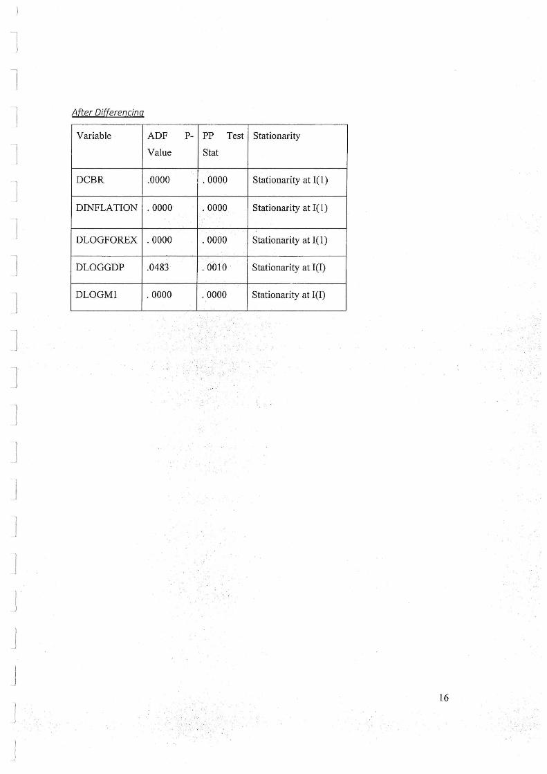
Both Augmented Dickey-Fuller (ADF) and Phillips-Perron (PP) tests under the category of . . .

uni~ ro'ottest will be run to determine whether there is stationary or non-stationary in thiirstudy . . · ., . .

Therefore, following test results above, the 'D' used as the prefix of the variable titles is to .

• signify that each of the variables have been differenced to ensure that they were stationary for · .. . _,: . . '• . . . .

... estimation ofV AR purposes. Other variables were logged in order to get their perc~ntage forms

and enable comparisons to be drawn.

Unit Test Results

Before Differencing

Variable ADF

Value

CBR .1027

INFLATION .1124

LOG .4140

FOREX

LOGGDP .1408

LOGMl .2471

P- pp Test Stationarity

Stat

.1027 Non-Stationary

.1415 Non-Stationary

.5417 Non-Stationary

.4194 Non-Stationary

.3566 Non-Stationary

15

l I

l

I I

1

1

J

l

After Differencing

Variable

DCBR

DINFLATION

DLOGFOREX

DLOGGDP

DLOGMl

ADF

Value

.0000

. 0000

. 0000

.0483

. 0000

P- pp Test Stationarity

Stat

. 0000 Stationarity at I( 1)

. 0000 Stationarity at I( 1)

. 0000 Stationarity at I(l)

. 0010 . Stationarity at I(I)

. 0000 Stationarity at I(I)

16

l -l

I I

J

J

CHAPTER FOUR: DATA ANALYSIS, RESULTS AND DISCUSSION

1. Introduction

The data in this chapter was analyzed using E-Views 10.0 and was used to interpret how

inflation rates, GDP, money supply, interest and location of real estate affect real estate prices,

using multivariate regression and descriptive models. The flrst part, the descriptive statistics,

enable us to make statistical conclusions about the data trends and the latter, the inferential

statistics help us to determine the relationship between the dependent and independent

variables.

2. · Descriptive Statistics

The research finding on the descriptive statistic in the data collected.

Table 4.2.1: Descriptive Statistics

Date: 01/11/19 Time: 01 :16 Sample: 1 120

CBR INFLATION LOGFOREX LOGGDP . LOGM1

Mean 9.322333 10.17198 4.329199 5.889573 6.104321 Median 8.500000 10.68716 4.330272 5.875610 6.115085

· Maximum 21.65000 19.71573 4.603469 6.094377 6.646852 Minimum 5.750000 2.001324 4.127618 . 5.651127 5.312565 Std. Dev. 3.179816 5.008021 0.093431 0.118660 0.409847 Skewness 1.875912 -0.017212 0.231027 -0.132020 -0.383744 Kurtosis 6.144437 1.612583 3.205499 1.972287 1.875412

Jarque-Bera 119.8183 9.630552 1.278619 5.629561 9.268691 Probability 0.000000 0.008105 0.527657 0.059918 0.009712

Sum 1118.680 1220.638 519.5039 706.7488 732.5185

Findings show that there was mean of9.32 for CBR, 5.88 for LOGGDP, 6.104 for LOGM1 ·

and 10.17 for INFLATION. On standard deviation CBR had 3 .179, LOGGDP had 0.118,

LOGMI had 0.4098 while INFLATION had 5.008. The Consumer Price Index which was used

to calculate inflation had the highest standard deviation hence the highest variation from the

mean.

17

-1

"l

l 1

J

J

3. Correlation

Table 4.3.1.Correlation Tests before Differencing CBR INFLATION LOGFOREX LOGGDP LOGM1

CBR 1 0.219655854 0.188603532 0.273049906 0.247565754 INFLATION 0.219655854 1 0.150749087 0.313070181 0.339088318 LOGFOREX 0.188603532 0.150749087 1 0.338242387 0.378453598

LOGGDP 0.273049906 0.313070181 0.338242387 1 0.982995184 LOGM1 0.247565754 0.339088318 0.378453598 0.982995184 1

The table above shows correlation tests before the data was differenced (when the data was

non-stationary). We are able to observe that theLevelofMoney Supply and the GDP growth

are highly positively correlated, almost at 1 (.9829).

Table 4.3.2. Correlation Tests after Dtfferencing DCBR DINFLATION DLOGFOREX DLOGGDP DLOGM1

DCBR 1 -0.022926996 -0.089957329 -0.332985838 -0.030933789 DINFLATION -0.022926996 1 -0.055224201 -0.057512937 ·0.022552037 DLOGFOREX -0.089957329 -0.055224201 1 -0.033904052 0.092089712

DLOGGDP -0.332985838 -0.057512937 -0.033904052 1 0.036786648 DLOGM1 -0.030933789 -0.022552037 0.092089712 0.036786648 1

The table above shows correlation tests afterthe data w~s differenced; here the data was all

stationary. All the data here is weakly correlatedwith each other as opposed to the previous

case.

We are able to see the data shifted to become negatively correlated in the second table as

compared to the first one.

4. Diagnostic Checks

Autocorrelation

8 reusch-Godfrey Serial Correlation LM Test:

F-statistic Obs~R-squared

0.095013 0.246388

Prob. F(2,43) Prob. Chi-Square(2)

0.9096 0.8841

Do not reject HO since the p-value for the Breusch-Godfrey Serial Correlation LM test is 0.8841

which is greater than a.=0.05. Therefore, there is no. imtocorrelation problem.

18

l l 1

.,

J

Normality

Series: Residuals Sample 200201 201504

Mean 1.23e-15 Median 0.000326 Maximum Minimum 0.019096

Std. Dev. -0.019505 Skewness

n .nnR?1:'1

Jarque~Bera 0.360028

Do not rejecfRO smce the p-value for the JB statistic is 0.835259 which is greater than a.=0.05.

Therefore, the errorterm is normally distributed in this model.

Heteroskedasticity

H eteroskedasticity Test ARCH

F-statistic · 0.323724 Prob. F(1,53) 0.57.18 Obs•Rcsquared . 0.333901 Prob . Chi -Square(1) 0.5634 .. .

Do not reject HO since the p-value for the ARCH test is 0.5634 which is greater than a.=0.05.

· Therefore, there is no heteroscedasticity problem.

19

l l 1

l

j

j

5. VAR and Variance Decomposition

Before estimating the VAR and subsequently running the Variance Decomposition, we must

first detennine the order of the V AR. Ordering means placing the variables in the decreasing

order of exogeneity.

VAR Granger Causality Test Results

VAR Granger Causality/Block Exogeneity Wald Tests Date: 01/17/19 Time: 14:13 Sample: 1 120 Included observations: 117

Dependent variable: DCBR

Excluded

DINFLATION DLOGFOREX

DLOGGDP DLOGM1

All

Chi-sq

0.945120 0.441593 0.543652 0.094723

2.254146

Dependent variable: DINFLATION

Excluded Chi-sq

DCBR 0.612215 DLOGFOREX 0.266195

DLOGGDP . 0.607964 DLOGM1 5.511467

All 7.653373

Dependent variable: DLOGFOREX

Excluded Chi-sq

DCBR 3.214694 DINFLATION 0.287635 DLOGGDP 0.929621 DLOGM1 2.078071

All 5.931854

Dependent variable: DLOGGDP

Excluded Chi-sq

DCBR 2.976471 DINFLATION 1.819018 DLOGFOREX 5.655858

DLOGM1 1.577529

All 10.21709

Dependent variable: DLOGM1

Excluded Chi-sq

DCBR 3.652163 DINFLATION 0.805910 DLOGFOREX 2.894428

DLOGGDP 2.309406

All 7.530195

df

2 2 2 2

8

df

' 2 2 2 • 2

8

df

2 2 2 2

8

df

2 2 2 2

8

df

2 2 2 2

8

Pro b.

0.6234 0.8019 0,7620 0.9537

0.9722

Pro b.

0.73.63 0.8754 .0.7379 0.0636

·. 0.4680 :

· .Prob.

0.2004 0.8660 0.6283 0.3538

0.6549

Pro b.

0.2258 0.4027 0.0591 0.4544 .

0.2501

'Prob.

0.1610 . 0.6683 .0.2352 0.3152

0.4807

For every test result; the variable that is not listed as dependent is considered to be independent,

i.e. the excluded variables. The above test included two lags.

20

-l

l l

I I I

l '

! .

l

J

l i

The test:

NULL: The independent variable (lag 1 & lag 2) cannot cause the dependent variable

ALT: They cause the dependent variable

The decision rule :

IF P VALUE> 5PC WE CANNOT REJECT NULL: WE ACCEPT NULL

IF P VALUE <5PC WE REJECT NULL AND ACCEPT AL T

Thus for all test results, none of the independent variables cause the dependent variable: this

implies exogeneity.

Also the order of the variables will be as follows:

1. Dcbr- 97.22%

2. Dlogforex- 65.49%

3. Dlogml- 48.07%

4. Dinflation- 46.80%

5. Dloggdp- 25 .01%

21

~~

I

'1

.I

.I

j

J

.1

VAR Test Results

Vector Autoregression Estimates Date: 01/17/19 Time: 14:42 Sample (adjusted}: 4 120 Included observations: 117 after adjustments Standard errors in ( ) & !-statistics in ( 1

DCBR DLOGFOREX DLOGM1 DINFLATION DLOGGDP

DCBR(-1) 0.035976 -0.003082 -0.003650 0.042548 0.000536 (0.105571 (0.001731 (0.001981 (0.105901 (0.000421

[ 0.34080 [·1.77802 (·1 .84228 ( 0.40178 [ 1.27638

DCBR(-2) -0.112578 -0.000215 -0.000787 -0.073491 0.000454 (0.105531 (0.001731 (0.001981 (0.105861 (0.000421

[·1.06680 (·0.12429 (~0.39712 (·0.69422 ( 1.08239

DLOGFOREX(-1) -0.204605 0.279182 -0.153905 2.884853 0.054322 (5.770681 (0.094751 (0.108321 (5.788901 (0.022961

(-0.03546 ( 2.94641 (-1.42087 [ 0.49834 [ 2.36631

DLOGFOREX(-2) 3.820352 -0.240976 0.138800 0.029028 ·0.008420 (5.864731 (0.098301 (0.110081 (5.883251 (0.023331

( 0.65141 (·2.50240 [ 1.26087 [ 0.00493 (·0.36088

DLOGM1(-1) -1.549405 -0.098182 . -0.318757 8.366079 0.005916 (5.104281 (0.083811 (0.'095811 (5.120401 (0.020311

[-0.30355 [-1 .17146 [-3.32700 [ 1.63387 [ 0.29135

DLOGM1(·2) -0.732686 0.035917 -0.061208 -5.556652 0.025383 (5.098891 (0.083721 (0.095711 (5.114981 (0.020281

(·0.14370 ( 0.42899 [·0.63953 [· 1.08635 ( 1.25137

DINFLA TION( ·1) 0.074232 -0.000829 ·3.10E-05 0.381865 -0.000508 (0.096281 (0.001581 co.oo18H (0.096581 (0.000381

( 0.77101 (·0.52443 [-0.0171 [ 3.95377 [·1 .32657

DINFLATION(-2) 0.025675 0.000136 -0.001481 0.000993 9.76E-05 (0.095171 (0.001561 (0.001791 (0.0954 71 (0.000381

[ 0.26979 ( 0.08692 [·0.82933 . . [ 0.01040 [ 0.25775

DLOGGDP(-1) -5.844390 . ,0.396015 -0.706165 10.50556 0.763971 (26.52471 (0.435531 (0.497881 (26.60851 (0.105521

[-0.22034 . [-0.90927 [-1.41835 [ 0.39482 [ 7.24015

DLOGGDP(~2) -10.53232 0.349439 o.G.!o2os -20.00859 -0.197261 (25.87731 (0.424901 (0.485731 (25.95901 (0.102941

[-D.40701 [ 0.82240 . [ 1.31~04 [-0.77078 [·1 .91622

c 0.087326 -0.0001()3 0:01'5766 0.008393 0.001012 (0.184471

[ 0.47338 (0.003031

[·0.03411 (0.003461

[ 4.55305 (0.185061

[ 0.04535 (0.000731

[ 1.37904

A-squared 0.031377 0.161186 0.162882 0.184539 0.425003 Adj. A-squared -0.060002 0.082053 0.083909 0.107609 0.370758 Sum SQ . resids 247.3891 0.066699 0:087161 . 248.9536 0.003915 S.E. equation 1.527698 0.025085 0.028675 1.532520 0.006077 F-statistic 0.343374 2.036891 2.062492 2.398781 7.834888 Log likelihood -209.8199 270.9641 255.3109 -210.1887 436.8326 Akaike AIC 3.774700 -4.443831 -4.176255 3.781004 -7.279190 Schwarz SC 4.034391 -4.184140 -3.916564 4.040695 -7.019498 Mean dependent 0.004017 -0.001002 0.011265 0.012037 0.003214 S.D. dependent 1.483830 0.026182 0.029960 1.622290 0.007661

Determinant resid covariance (dof adj.) 8.46E-11 Determinant resid covariance 5.16E-11 Log likelihood Akaike information criterion

555.6065 -8.557376

Schwarz criterion -7.258918 Number of coefficients 55

V AR estimates are interpreted similar to OLS estimates and thus must be considered while

applying the ceteris paribus effect Judging by the t-statistics (values in square brackets on the

third rows), they exhibit that most of the variables, be it in the first or second lags, weakly

influence their own selves and thus are weakly endogenous. This is to mean, none of the

differenced variables have a strong influence on the other values that are being regressed

against them in the vector autoregression:

Next, we interpret the values in the first row, with a specific focus on the first realizations (-1).

Ensuring ceteris paribus holds, the first realization of the differenced value of the CBR (DCBR)

is associated with 3.5976% increase in the differenced value ofCBR. Holding the same line of

reasoning constant: DLOGFOREX(-1) causes a 27.9182% increase in DLOGFOREX,

22

l -,

l

I J

DLOGM1(-1) causes a 31.8757% decrease in DLOGMl given that the sign is negative,

DINFLATION(-1) causes a 38.1865% increase in DINFLATION, DLOGGDP(-1) causes a

76.3971% increase inDLOGGDP.

Variance Decomposition Results

Variance Decom~osition of DCBR: Period .E. DCBR DLOGFOR DLOGM1 DINFLATION DLOGGDP

1 1.527698 100.0000 0.000000 0.000000 0.000000 0.000000 2 1.534283 99.31142 0.004208 0.077214 0.562855 0.044300 3 1.548970 98.29836 0.425613 0.076272 0.932808 0.266950 4 1.551297 98.02598 0.435744 0.091479 0.985012 0.461786 5 1.552105 97.92448 0.496401 0.095674 0.991395 0.492055 6 1.552279 97.90275 0.515404 0.095916 0.993605 0.492323 7 1.552287 97.90183 0.515711 0.095977 0.994106 0.492377 8 1.552301 97.90002 0.517390 0.096042 0.994146 0.492404 9 1.552303 97.89985 0.517433 0.096048 0.994157 0.492509

10 1.552304 97.89970 0.517553 0.096048 0.994162 0.492533

Variance Decom~osition of DLOGFOREX: Period .E. . DCBR DLOGFOR DLOGM1 DINFLATION DLOGGDP

1 0.025085 0.631030 99.36897 0.000000 0.000000 0.000000 2 0.026664 2.964153 94.75400 1.425791 0.182592 0.673462 3 0.027049 3.122200 94.46584 1.517626 0.238982 0.655348 4 0.027333 3.117407 94.26920 1.540807 0.236792 0.835795 5 0.027361 3.157082 94.07958 1.546331 0.239946 0.977061 6 0.027390 3.150524 94.08048 1.543929 0.242336 0.982734 7 0.027394 3.152233 94.07675 1.543534 0.243082 0.984398 8 0.027395 3.152184 94.07584 1.543505 0.243082 0.985387 9 0.027395 3.152148 94.07591 1.543501 0.243073 0.985369

10 0.027395 3.152206 94.07570 1.543498 0.243072 0.985527

Variance [)ecom~osition: of DLOGM1: . Period · .E. · . . DCBR . . DLOGFOR DLOGM1 DINFLATION DLOGGDP

1 0.028675 0.152826 0.657736 99.18944 0.000000 0.000000 2 . 0.030982 1:231957 2.485957 94.69271 0.003245 1.586129 3 0.031309 . 1.240624 3.181194 93.06941 0.437688 2.071082 4 0.031348 1.243684 3.197549 92.94210 0.494851 2.121814 5 0.031370. 1:244068 3.193168 92.87386 0.517506 2.1 71398 6 0.031372 . . 1.244530 . 3.200176 92.85869 0.519328 2.177276 7 . 0.031373 .. 1.244806 3.200581 92.85469 0.520139 2.179789 8 0.031374 1.244789 3.201568 92.85350 0.520298 2.179845 9 0.031374 1.244795 3.201685 92.85333 0.520351 2.179841

10 0.031374 1.244795 " 3.201725 92.85328 0.520357 2.179840

Varian·ce Decom~osition of DINFLATION: Period .E. . DCBR . . . DLOGFOR DLOGM1 DINFLATION DLOGGDP

1 1.532520 0.488508 0.103172 0.297020 99.11130 0.000000 2 1.664440 0.423042 0.256564 3.062808 96.13596 0.121630 3 1.691914 0.851906 0.258683 3.770505 94.75251 0.366399 4 1.694930 0.866118 0.302500 3.760964 94.59532 0.475093 5 1.696782 0.864593 0.339548 3. 774829 94.44300 0.578031 6 1.697215 0.864774 0.358926 3.772939 94.40820 0.595157 7 1.697304 0.864684. 0.359782 3.774235 94.40248 0.598815 8 1.697323 0.864694 0.360343 3.774346 94.40107 0.599548 9 1.697329 0.864728 0.360383 3.774428 94.40059 0.599876

10 1.697330 0.864731 0.360439' 3.774424 94.40047 0.599941

Variance Decom~osition of DLOGGDP: · Period .E. . DCBR DLOGFOR DLOGM1 DINFLATION DLOGGDP

1 0.006077 14.93561 0.464370 1.665839 0.271961 82.66222 2 0.007652 11.25322 2.287474 1.950263 1.938939 82.57010 3 0.008049 10.20338 3.813601 2.603836 2.892524 80.48666 4 0.008096 10.14164 3.877853 2.763692 3.157511 80.05930 5 0.008102 10.13693 3.877657 2.800194 3.202554 79.98266 6 0.008102 . 10.13660 3.878934 2.802318 3.209356 79.97280 7 0.008103 10.13634 3.879881 2.802257 3.210902 79.97062 8 0.008103 10.13621 3.880709 2.802222 3.211286 79.96957 9 0.008103 10.13621 3.880712 2.802223 3.211376 79.96948

10 0.008103 10.13620 . 3.880753 2.802228 3.211391 79.96943

Cholesky Ordering: DCBR DLOGFOREX DLOGM1 DINFLATION DLOGGDP

The rows indicate the percentage ofthe Forecast Error Variance of the variable in thetit1e for

every variance decomposition. We may further divide the time periods into short run (period

1- period 5) and long run (period 6- period 1 0).

For example, in the short run, looking at Year 1, 100% of forecast error variance in DCBR is

explained by the variable itself therefore other variables in the model do not have a strong

influence on DCBR (they have strong exogenous impact). This is seen to continue with time

23

l -1

l

J

.l

even into the long run where the impact of the other variables on DCBR is negligible as it is

less than zero.

6. Impulse Response Functions

Response to Cholesky One S.D. (d. f. adjusted) Innovations

Response of DLOGFOREX to DCBR

.000 +-------f----..0.."""'==~------1

--001

-.002

-.003

-.004

10

Response of DINFLATION to DCBR

.oo~========~~~========~ . ·i

-.02 .

·.--04

--of .-.06

-.10

10

Response of DLOGM1 to DCBR

.000 -~==========;;;z::::=:==::::::=;;;;::::======1

-.001

-.002

· -003

2 3 6 ,8 10

Response ol DLOGGDP to DCBR

.0000 -1-----'-+--'----=====--------1

·.0005

·.0010

-.0015

-.0020

3 4 10

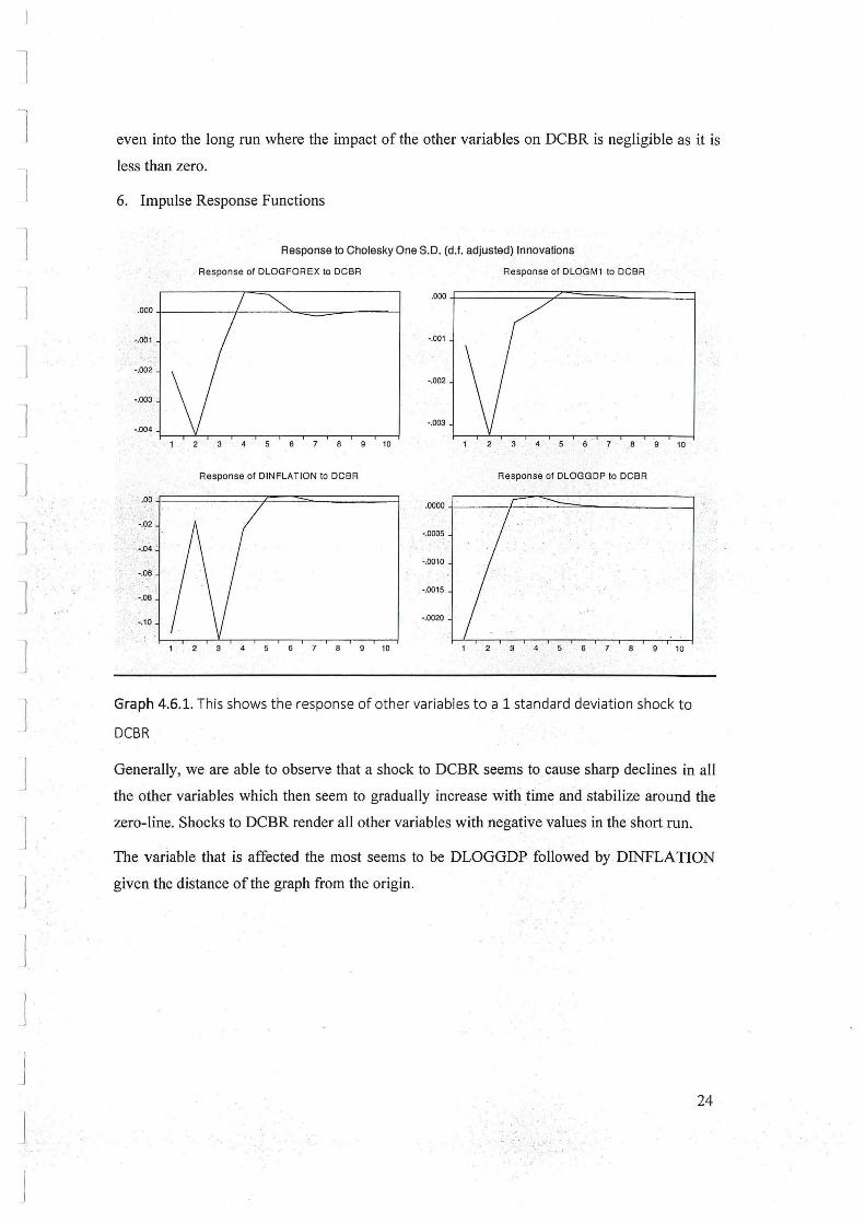
Graph 4.6.1. This shows the response of other variables to a 1 standard deviation shock to

DCBR

Generally, we are able to observe that a shock to DCBR seems to cause sharp declines in all

the other variables which then seem to gradually increase with time and stabilize around the

zero-line. Shocks to DCBR render all other variables with negative values in the short run.

The variable that is affected the most seems to be DLOGGDP followed by DINFLA TION

given the distance ofthe graph from the origin.

24

·· ...

l -~

1

J

_I

Response to Cholesky One S.D. (d .f. adjusted) Innovations

Response of DCBR to DLOGFOREX Response of DLOGM1 to DLOGFOREX

.10

.002 .08

.001 .06

.000 .04

-.001 .02

-.002 .00

-.003 -.02

-.004

10 1 2 3 4 5 6 7 8 9 10

Response of DINFLATION to DLOGFOREX Response of DLOGGDP to DLOGFOREX

.06

.0008 .04

.02 .0004

.oo \ 7~ I

-.02 . ,ooqq ·1 ! \, ___..- I

-.04

• -.000~ 1-;+-.,---,.--,..,-r--r--.--..--.-----.---,---1 ·g ·11r 3 6 7 8 10

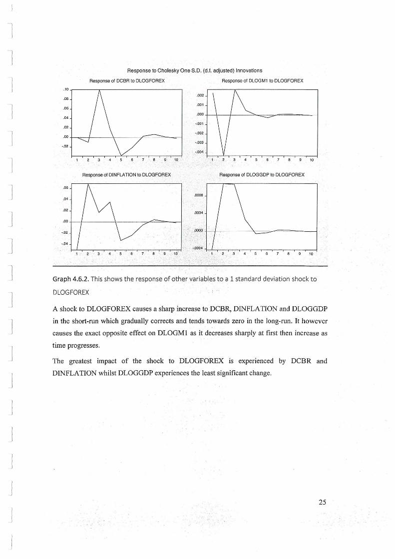
Graph 4.6.2. This shows the response of other variables to a 1 standard deviation shock to

DLOGFOREX

A shock to DLOGFOREX causes a sharp increase to DCBR, DINFLA TION and DLOGGDP

in the short-run which gradually corrects and tends towards zero in the long-run. It however

causes the exact opposite effect on DLOGMl as it decreases sharply at first then increase as

time progresses.

The greatest impact of the shock to DLOGFOREX is experienced by DCBR and

DINFLA TION whilst DLOGGDP experiences the least significant change.

25

l -·1

l

_I

Response to Cholesky One S.D. (d. I. adjusted) Innovations

Response of DCBR to DLOGM1 Response of DLOGFOREX to DLOGM1

=Mr .000

·.001 ·.02

·.03 I I I I ·.002

· .04 .j II ·.003

4 5 6 7 8 9 10 2 8 ·10

Response of Q~NFLATION to DLOGM1 Response of DLOGGDP to DLOGM1

.2 .0006

.1 .0004

;_ .o· , . .0002

. : .1•

'·"' ·;·, .oopo 2 3 5 6 7 8 9 10 . 6 l 8 · 9 10

Graph4.6.3. This shows the response of other variables to a 1 standard deviation shock to

DLOGMl

A shock to DLOGMl causes a sharp decrease in the short-run to DCBR and DLOGFOREX

with a relatively smaller impact as compared to the impact the shock has on DINFLA TION

with regards to magnitude.

The impact of the shock is experienced in its least form by DLOGGDP but has a gradual

reducing effect.

26

l l

I

J

Response to CholeskyOne S.D. (d. f. adjusted) Innovations

Response of DCBR to DINFLATION Response of DLOGFOREX to DINFLATION

.0000 ...-...-------------=------, .10

-.0002

.08 -.0004

.06 -.0006

.04 -.0008

.02 -.0010

.00 7 8 ·g 10 5 3 . 4 8 10

Response of DLOGM1 to DINFLATION Response of DLOGGDP to DINFLATION

.0000 -t--""--t---------=======---j -.0002

-.0005

-.0004

-.0010 -.0006

-.0015 -.0008

-.0020 : -.0010r-~,_~,---~-,---,---,---,---,---,---~ 1 -- 2 4 · ·5 6 7 ·a· g ·- 10 ' 3 . 5· 5 ·7 - a g· · 10

. .

Graph 4.6.4. This shows the response of other vari~bles to a 1 standard deviation shock to

DINFLATION

A shock to DINFLA TION seems to only have a great impact to DCBR, i.e. a sharp increase

as the other graphs show a thousand times less impact and appear to be reducing in the short

term.

27

~I

l

J J

Response to Cholesky One S.D. (d. f. adjusted) Innovations

Response of DCBR to DLOGGDP

.oo I \ r - - -, -.01

-.02

I \ I I -.03

-.04

-.o5 I \ I -.06

-.07 .~ I 2

1 \<1 I ·•· I

1 5 6 7 8 9 10

Response of DLOGM1 to DLOGGDP

.002

.001

.000 ·+--.----f--------===-------j

-.001

-.!J02

.. - ~.00.3 .

· •· : · 1 ·2 ' · 3 :<. 4 5 .. s· ·. i 8 · ." ;· g· fo

-<.;

Response of DLOGFORE X to DLOGGDP

.001

.000

-.001

-.002

5 g· 10

Response of DINFLATION to DLOGGDP

.04

.00 t--'----t----------=====~

-.04

-.08

5 . 6 .. 7 8 . :' 9 ',' .10

Graph 4.6.5. This shows the response of other variables to a 1 standard deviation shock to

DLOGGDP.

A shock to DLOGGDP, similarly to shocks to inflation seem to majorly affect DCBR by

ca11sing a .sharp decrease. Overall this decreasing effect is the same for DLOGFOREX and

DLOGMI whereas as for DINFLATION, the effect shows a slight increase, the opposite.

7. Conclusion

In a nutshell, this study has analyzed the dynamics data with a series of time series

econometrics test. In the beginning, the descriptive statistics of each variable is being reviewed.

Besides that, Unit Root Test which consists of ADF and PP test, V AR test, diagnostic checking

and variance decomposition have been conducted in this chapter. Overall, all the empirical

results from the. methodologies used in this study have been interpreted and showed in figure,

diagram and table form. The clear and precise interpretation of the results have be~n showed

on the below of each of the test in this chapter.

28

l l

I.

I

I

J

J

CHAPTER FIVE: SUMMARY AND RECOMMENDATIONS

1. Summary

Chapter One gave a brief introduction to the topic and set the context for the study by briefly

introducing concepts that would be used throughout the paper. Chapter 2 explains the

relationship between HPI and macroeconomic variables has been explained based on literature

from previous researchers; theoretical models such as supply and demand theory and

purchasing power parity theory are discussed as part of the literature published to determine

. between housing price index determinants in Kenya.

Next, this chapter 3 discusses all the methodologies and statistical test that will be

implementing in this study. It has clearly defined and elaborated the ideas for each of the

methodology. Firstly, Unit Root Test that consists of ADF and PP tests is carried out to test

whether there are stationary or non-stationary trend of time series data for all variables. It is

necessary to check the order of integration of the level variables for an appropriate

econometrics method in order to avoid obtaining any spurious and invalid results. Diagnostic

. testing has been conducted in order to ensure no econometric problems in the model.

· In the chapter 4, a series of test have been conducted and the results we , obtain are clearly

explained. Initially, this study has overviews the descriptive . statistics of aU the measured

variable and controlled variables. The results from both ADF and PP tests reveal that all

' variables in the dataset are non-stationary at level. After the first difference of both ADF test

·and PP test, all the variables are stationary at the first difference. After running the V AR test,

it was seen that none of the differenced variables had a strong influence on the other values

that are being regressed against them. The variance decomposition test showed that the

variables in the model do not have a strong influence (small percentage) on each other when it

comes to predictability of values in future time periods. Lastly, the impulse response functions

showed for how long a shock on each of the variables affects the other variables and clearly

showed us the impact in both the short and long run.

2. Policy Recommendations

It is vital for investors to understand which macroeconomic variables are bringing the utmost

effect to house price. The research aimed to delineate how macroeconomic variables affect real

estate prices in Kenya. From the results, we may postulate that Ministry of Transport,

Infrastructure, Housing and Urban Development should avail lower-price, good quality homes

to Kenyans in need. This is already underway, through partnership with the United Nations for

29

l "l

_j

J

Project Services (UNOPS) and will see one million Kenyans are housed in the National

Housing Project in the first phase.

The Central Bank of Kenya should apply controls to regulate the money supply levels so as to

reduce extreme price fluctuations thus ensuring stability of not only prices, but exchange and

interest rates as well. This is in turn will ensure the purchasing power of the shilling does not

depreciate and thus foreign direct investment will be encouraged which will boost economic

growth.

3. Limitations ofthe Study

The data collected was secondary from sources including previous literature documented from

the study of the aforementioned topic, the Central Bank of Kenya data, the Kenya National

Bureau of Statistics website and lastly, Hass Consult Limited. The data represented in the study

was true and obtained from reliable sources but may have been prone to unreliability, say

because it was intended for other uses.

30

l l

l .l

j

J

j

References:

Arnold, M. A. (1992). The principal-agent relationship in real estate brokerage services.

Journal of the American Real Estate and Urban Economics Association, (20), 89-106.

Blanchard, Olivier (2000). Macroeconomics, 2nd ed. Englewood Cliffs, N.J: Prentice Hall.

Baumol, W. J. & Blinder, A.S. (2011). Economics: Principles and policies, New YorK:

Cengage Learning.

Brasinton, D.M. & Sarama, R.E. (2008). Deed types, house prices and mortgage interest rates,

Real Estate Economics, 36(3) 587-610.

Brueggeman, W., & Fisher, J. (2005). Real estate finance and investments, (5th Ed.) New York:

Me Graw Hill.

Bruggerman, W. and Fisher, J. (2008) Real estate finance and investments, 11Ed New York:

MC Graw- Hill. . . .,

Burnside; C, Eichenbaum, M. & Rebelo, S. (20 11 ). Understanding booms and busts in housing

markets: NBER Wo~king Pap~r i6734 (Cambridge, Massachusetts: National Bureau of

.. Economic Research). . . . .

Case, K., Shiller, R. 8l_ Quigley, M. (2005). Comparing wealth effects: The stock market versus ·

the housing market. Advances in M::tcroeconomics 5(1).

Central Bank of Kenya (2013). Monthly economic review from

www.centrabank.go.ke/index.php/monthly-economic-review.

Egert, B. & Miha1jek,D. (2007). Determinants of house prices in central and eastern Europe.

CESIFO Working Paper Series, 2152 (6), 1-31

Gallagher, M. (20 11 ). The effect of inflation of housing prices from

http:/ /homeguides.sfgate.com/effect-inflation-housing-prices-2161.html

Hass Consult Ltd (2013). Base figures- Sales and letting monthly changes.

Hilbers, P., Loi, Q., & Zacho, L. (2011). Real estate market developments and financial. sector

soundness. IMF, working paper 01/129, Washington.

Julius .. S.M. (2012). Determinants of residential real estate prices in Nairobi.

Unpublished MBA Project, University ofNairobi.

Jumbale, D.K (2012). The Relationship between house prices and real estate financing in

Kenya. Unpublished MBA Project, University ofNairobi.

31

-l

-1

1

I I l

j

_j

_j

Kagendo, D. (20 11). The Determinants of real estate property prices: The case of Kiarnbu

municipality in Kenya (Unpublished MBA project). University ofNairobi.

Khalid, Z., Iqtidar, A. S., Muhammad, M., K., Mehboob, A., (2012) Macroeconomic factors

determining FDI impact on Pakistan's growth, South Asian journal of global business research,

1 (1), 79-95.

KNBS (2013). Leading Economic Indicators from www.knbs.or.ke/economicindicators.php

Kahneman, D. & Tversy A. (1979). Prospect Theory: An analysis of decision under risk

from http://www.princeton.edu/-kahneman/docs/Publications/prospect_theory.pdf

Knight Frank & Citi Private Bank (2012). The Wealth Report 2011

http://www .knightfrank.com/resources/pdf-documents/20 11 thewea1threport. pdf Knight Frank

(20 12). Quarter 4 General market update from

http://my.knightfrank.co.ke/researchl?regionid

. Lancast~r, k. J. (1966). A new approach to consumer theory, Journal of politicaJeconomy, 7 4,

132:..157.' .· . . .

·. Lieser, K. : & Groh, A.P. (2011). The Determinants of international commercial r.eal estate

investments.

· Liow, K.H., Ibrahim, M.F. & Huang, Q. (2006). Macroeconomic risk influences in the property

stock market. Journal of property investment and finance, 24( 4 ).

Lu, S. (2012). An empirical study on relationship between real estate enterprise EBusiness

Model and its performance. Advances in Intelligent and Soft Computing, 165 187- 194.

Mak, S., Choy, L. & Ho, W. (2012). Region- specific estimates of the determinants of real

estate investments in China. Urban studies, 49(4) 741-755.

Markowitz, H. M. (1959), Portfolio selection: Efficient diversification of investments, John

Wiley & Sons, NewYork.

Markowitz, H (1952) Portfolio Selection: Efficient diversification of investment. New York:

John Wiley and Sons

Mikhed, V. & Zemak, P. (2009). Do house prices reflect fundamentals? Aggregate and panel

data evidence.

Mu, L. & Ma, J. 2007. Game theory of price decision in real estate industry.

32

l -1

l International journal of nonlinear science, 3(2) 155-160.

Muli, J. (2011). The relationship between property prices and mottgage lending in Kenya.

Unpublished MBA Project, University ofNairobi.

Mugenda, 0. M., & Mugenda, A. G. (2003). Research methods: Quantitative and qualitative

approaches. African centre for technology studies. Nairobi.

Muthee, K. M. (2012). Relationship between economic growth and real estate prices in

Kenya. Unpublished MBA Project, University ofNairobi.

Ngechu, A.J. (2004) Elements of education and science research methods. Masona publishers.

Omboi, B. M. (20 11 ). Factors influencing real estate property prices: A survey of real estates

in Meru municipality, Kenya. Journal of economics and sustainable development, 2(4), 1-21.

Otwoma, F.B.K. (20 13). The effect of interest rates on property prices in the Kenyan real estate

market. Unpublished MBA Project, University ofNairobi.

Posedel, P & Vizek, M. (2008). House price determinants in transition and EU- 15 countries.

Post- Communist Economies, 21(3) 327-343.

Rosen, H.S. (1979). "Housmg decisions and the U .S. income tax: An enometric analysis".

Journal of Public Economics, 1-24 .

Rosen, S. (1974). Hedonic prices and implicit markets: Product differentiation m pure

competition, Journal of Political Economy, 82(1) 35-55.

Rottke, N. (200 1 ). International real estate fund vehicles using opportunistic strategies: An

agency theory based analysis. Working Paper Series # 06-002. Real Estate Management

Institute (REMI)

Ruitha, J. (2010). Emerging opportunities in the housing industry in Kenya.

The national housing corporation

Stadelmann D. (20 1 0) Which factors capitalize into house prices? A Bayesian averaging

approach. Journal of housing economics, 19(3) 180-204

Terrones, M., & Otrok, C. (2004). The global house price boom. International monetary fund,

pp.71-89.

Tsatsaronis, K., & Zhu, H. (2004). What drives housing price dynamics: cross country

evidence.

33

"l -1

l

_I

J

_l

_I

J

Bis quarterly review, 3, 65-78.

UN HABITAT (2013). from http://www.unhabitat.org/stats/

Yuanbin, H. (2006). A game the01y analysis on developer, local government and consumers in

Real Estate Market. Journal of Beijing technology and business university: Social Science, Vol

5.

World Bank (2011). Turning the tide in turbulent times: Making the most of Kenya's

demographic change and rapid urbanization. © Washington, .· · DC.

https://openknowledge.worldbank.org/handle/1 0986/13002 License: CC BY 3.0 Unported."

34