Kuroshio Meanders in the East China Sea

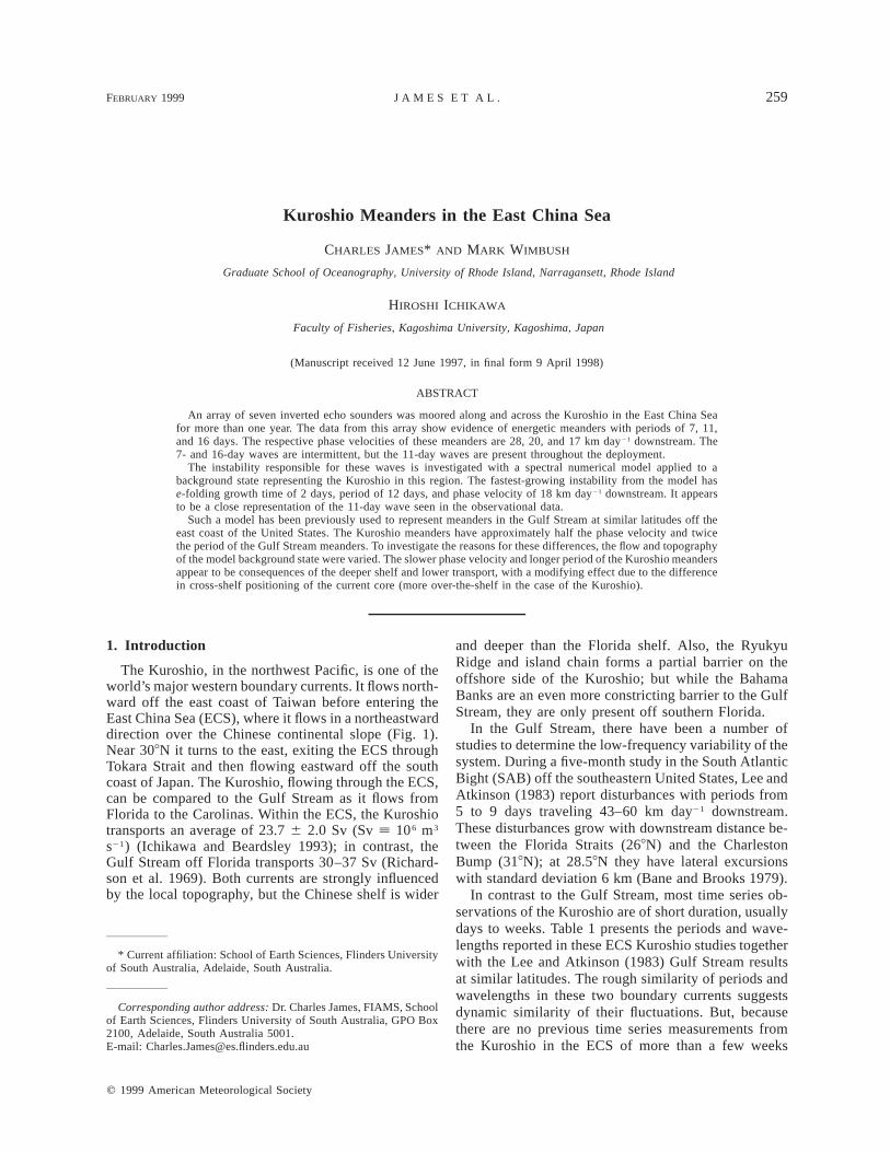
FEBRUARY 1999 259J A M E S E T A L .

q 1999 American Meteorological Society

Kuroshio Meanders in the East China Sea

CHARLES JAMES* AND MARK WIMBUSH

Graduate School of Oceanography, University of Rhode Island, Narragansett, Rhode Island

HIROSHI ICHIKAWA

Faculty of Fisheries, Kagoshima University, Kagoshima, Japan

(Manuscript received 12 June 1997, in final form 9 April 1998)

ABSTRACT

An array of seven inverted echo sounders was moored along and across the Kuroshio in the East China Seafor more than one year. The data from this array show evidence of energetic meanders with periods of 7, 11,and 16 days. The respective phase velocities of these meanders are 28, 20, and 17 km day21 downstream. The7- and 16-day waves are intermittent, but the 11-day waves are present throughout the deployment.

The instability responsible for these waves is investigated with a spectral numerical model applied to abackground state representing the Kuroshio in this region. The fastest-growing instability from the model hase-folding growth time of 2 days, period of 12 days, and phase velocity of 18 km day21 downstream. It appearsto be a close representation of the 11-day wave seen in the observational data.

Such a model has been previously used to represent meanders in the Gulf Stream at similar latitudes off theeast coast of the United States. The Kuroshio meanders have approximately half the phase velocity and twicethe period of the Gulf Stream meanders. To investigate the reasons for these differences, the flow and topographyof the model background state were varied. The slower phase velocity and longer period of the Kuroshio meandersappear to be consequences of the deeper shelf and lower transport, with a modifying effect due to the differencein cross-shelf positioning of the current core (more over-the-shelf in the case of the Kuroshio).

1. Introduction

The Kuroshio, in the northwest Pacific, is one of theworld’s major western boundary currents. It flows north-ward off the east coast of Taiwan before entering theEast China Sea (ECS), where it flows in a northeastwarddirection over the Chinese continental slope (Fig. 1).Near 308N it turns to the east, exiting the ECS throughTokara Strait and then flowing eastward off the southcoast of Japan. The Kuroshio, flowing through the ECS,can be compared to the Gulf Stream as it flows fromFlorida to the Carolinas. Within the ECS, the Kuroshiotransports an average of 23.7 6 2.0 Sv (Sv [ 106 m3

s21) (Ichikawa and Beardsley 1993); in contrast, theGulf Stream off Florida transports 30–37 Sv (Richard-son et al. 1969). Both currents are strongly influencedby the local topography, but the Chinese shelf is wider

* Current affiliation: School of Earth Sciences, Flinders Universityof South Australia, Adelaide, South Australia.

Corresponding author address: Dr. Charles James, FIAMS, Schoolof Earth Sciences, Flinders University of South Australia, GPO Box2100, Adelaide, South Australia 5001.E-mail: [email protected]

and deeper than the Florida shelf. Also, the RyukyuRidge and island chain forms a partial barrier on theoffshore side of the Kuroshio; but while the BahamaBanks are an even more constricting barrier to the GulfStream, they are only present off southern Florida.

In the Gulf Stream, there have been a number ofstudies to determine the low-frequency variability of thesystem. During a five-month study in the South AtlanticBight (SAB) off the southeastern United States, Lee andAtkinson (1983) report disturbances with periods from5 to 9 days traveling 43–60 km day21 downstream.These disturbances grow with downstream distance be-tween the Florida Straits (268N) and the CharlestonBump (318N); at 28.58N they have lateral excursionswith standard deviation 6 km (Bane and Brooks 1979).

In contrast to the Gulf Stream, most time series ob-servations of the Kuroshio are of short duration, usuallydays to weeks. Table 1 presents the periods and wave-lengths reported in these ECS Kuroshio studies togetherwith the Lee and Atkinson (1983) Gulf Stream resultsat similar latitudes. The rough similarity of periods andwavelengths in these two boundary currents suggestsdynamic similarity of their fluctuations. But, becausethere are no previous time series measurements fromthe Kuroshio in the ECS of more than a few weeks

260 VOLUME 29J O U R N A L O F P H Y S I C A L O C E A N O G R A P H Y

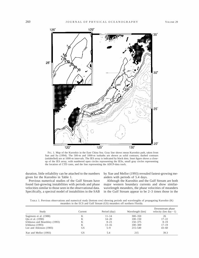
FIG. 1. Map of the Kuroshio in the East China Sea. Gray line shows mean Kuroshio path, taken fromSun and Su (1994). The 500-m and 1000-m isobaths are shown as solid contours; dashed contours(unlabelled) are at 1000-m intervals. The IES array is indicated by black dots. Inset figure shows a close-up of the IES array, with numbered open circles representing the IESs, small gray circles representingthe location of CTD casts, and the line representing the ADCP-data track.

TABLE 1. Previous observations and numerical study (bottom row) showing periods and wavelengths of propagating Kuroshio (K)meanders in the ECS and Gulf Stream (GS) meanders off northern Florida.

Study Current Period (day) Wavelength (km)Downstream phase

velocity (km day21)

Sugimoto et al. (1988)Qiu et al. (1990)Ichikawa and Beardsley (1993)Ichikawa (1993)Lee and Atkinson (1983)

KKKKGS

11–1414–20

8–2313–16

5–9

300–350100–150150–375100–300215–540

2617–22

8–1917–1943–60

Xue and Mellor (1993) GS 5.4 215 39.3

duration, little reliability can be attached to the numbersgiven for the Kuroshio in Table 1.

Previous numerical studies of the Gulf Stream havefound fast-growing instabilities with periods and phasevelocities similar to those seen in the observational data.Specifically, a spectral model of instabilities in the SAB

by Xue and Mellor (1993) revealed fastest-growing me-anders with periods of 5.4 days.

Although the Kuroshio and the Gulf Stream are bothmajor western boundary currents and show similar-wavelength meanders, the phase velocities of meandersin the Gulf Stream appear to be 2–3 times those in the


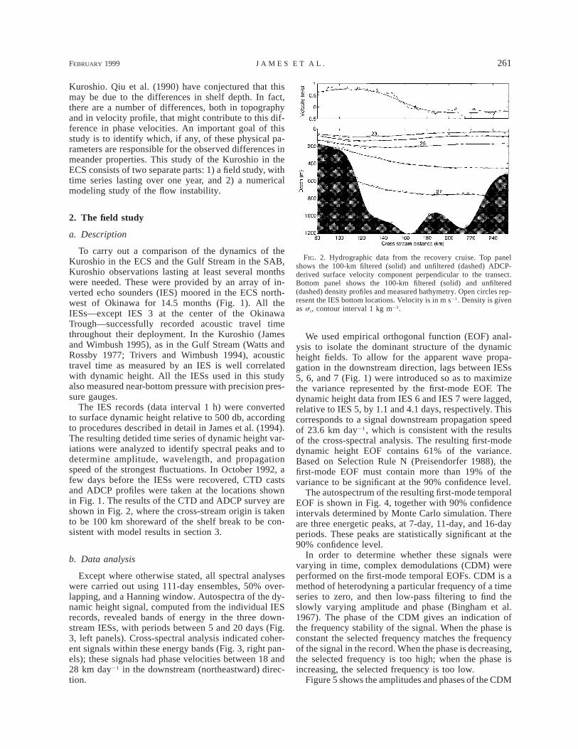
FIG. 2. Hydrographic data from the recovery cruise. Top panelshows the 100-km filtered (solid) and unfiltered (dashed) ADCP-derived surface velocity component perpendicular to the transect.Bottom panel shows the 100-km filtered (solid) and unfiltered(dashed) density profiles and measured bathymetry. Open circles rep-resent the IES bottom locations. Velocity is in m s21. Density is givenas st, contour interval 1 kg m23.

Kuroshio. Qiu et al. (1990) have conjectured that thismay be due to the differences in shelf depth. In fact,there are a number of differences, both in topographyand in velocity profile, that might contribute to this dif-ference in phase velocities. An important goal of thisstudy is to identify which, if any, of these physical pa-rameters are responsible for the observed differences inmeander properties. This study of the Kuroshio in theECS consists of two separate parts: 1) a field study, withtime series lasting over one year, and 2) a numericalmodeling study of the flow instability.

2. The field study

a. Description

To carry out a comparison of the dynamics of theKuroshio in the ECS and the Gulf Stream in the SAB,Kuroshio observations lasting at least several monthswere needed. These were provided by an array of in-verted echo sounders (IES) moored in the ECS north-west of Okinawa for 14.5 months (Fig. 1). All theIESs—except IES 3 at the center of the OkinawaTrough—successfully recorded acoustic travel timethroughout their deployment. In the Kuroshio (Jamesand Wimbush 1995), as in the Gulf Stream (Watts andRossby 1977; Trivers and Wimbush 1994), acoustictravel time as measured by an IES is well correlatedwith dynamic height. All the IESs used in this studyalso measured near-bottom pressure with precision pres-sure gauges.

The IES records (data interval 1 h) were convertedto surface dynamic height relative to 500 db, accordingto procedures described in detail in James et al. (1994).The resulting detided time series of dynamic height var-iations were analyzed to identify spectral peaks and todetermine amplitude, wavelength, and propagationspeed of the strongest fluctuations. In October 1992, afew days before the IESs were recovered, CTD castsand ADCP profiles were taken at the locations shownin Fig. 1. The results of the CTD and ADCP survey areshown in Fig. 2, where the cross-stream origin is takento be 100 km shoreward of the shelf break to be con-sistent with model results in section 3.

b. Data analysis

Except where otherwise stated, all spectral analyseswere carried out using 111-day ensembles, 50% over-lapping, and a Hanning window. Autospectra of the dy-namic height signal, computed from the individual IESrecords, revealed bands of energy in the three down-stream IESs, with periods between 5 and 20 days (Fig.3, left panels). Cross-spectral analysis indicated coher-ent signals within these energy bands (Fig. 3, right pan-els); these signals had phase velocities between 18 and28 km day21 in the downstream (northeastward) direc-tion.

We used empirical orthogonal function (EOF) anal-ysis to isolate the dominant structure of the dynamicheight fields. To allow for the apparent wave propa-gation in the downstream direction, lags between IESs5, 6, and 7 (Fig. 1) were introduced so as to maximizethe variance represented by the first-mode EOF. Thedynamic height data from IES 6 and IES 7 were lagged,relative to IES 5, by 1.1 and 4.1 days, respectively. Thiscorresponds to a signal downstream propagation speedof 23.6 km day21, which is consistent with the resultsof the cross-spectral analysis. The resulting first-modedynamic height EOF contains 61% of the variance.Based on Selection Rule N (Preisendorfer 1988), thefirst-mode EOF must contain more than 19% of thevariance to be significant at the 90% confidence level.

The autospectrum of the resulting first-mode temporalEOF is shown in Fig. 4, together with 90% confidenceintervals determined by Monte Carlo simulation. Thereare three energetic peaks, at 7-day, 11-day, and 16-dayperiods. These peaks are statistically significant at the90% confidence level.

In order to determine whether these signals werevarying in time, complex demodulations (CDM) wereperformed on the first-mode temporal EOFs. CDM is amethod of heterodyning a particular frequency of a timeseries to zero, and then low-pass filtering to find theslowly varying amplitude and phase (Bingham et al.1967). The phase of the CDM gives an indication ofthe frequency stability of the signal. When the phase isconstant the selected frequency matches the frequencyof the signal in the record. When the phase is decreasing,the selected frequency is too high; when the phase isincreasing, the selected frequency is too low.

Figure 5 shows the amplitudes and phases of the CDM


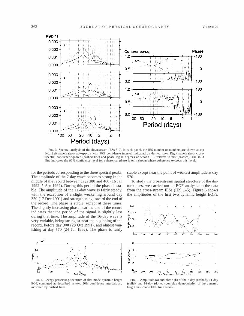
FIG. 3. Spectral analysis of the downstream IESs 5–7. In each panel, the IES number or numbers are shown at topleft. Left panels show autospectra with 90% confidence interval indicated by dashed lines. Right panels show cross-spectra: coherence-squared (dashed line) and phase lag in degrees of second IES relative to first (crosses). The solidline indicates the 90% confidence level for coherence; phase is only shown where coherence exceeds this level.

FIG. 5. Amplitude (a) and phase (b) of the 7-day (dashed), 11-day(solid), and 16-day (dotted) complex demodulation of the dynamicheight first-mode EOF time series.

FIG. 4. Energy-preserving spectrum of first-mode dynamic heightEOF, computed as described in text; 90% confidence intervals areindicated by dashed lines.

for the periods corresponding to the three spectral peaks.The amplitude of the 7-day wave becomes strong in themiddle of the record between days 380 and 460 (16 Jan1992–5 Apr 1992). During this period the phase is sta-ble. The amplitude of the 11-day wave is fairly steady,with the exception of a slight weakening around day350 (17 Dec 1991) and strengthening toward the end ofthe record. The phase is stable, except at these times.The slightly increasing phase near the end of the recordindicates that the period of the signal is slightly lessduring that time. The amplitude of the 16-day wave isvery variable, being strongest near the beginning of therecord, before day 300 (28 Oct 1991), and almost van-ishing at day 570 (24 Jul 1992). The phase is fairly

stable except near the point of weakest amplitude at day570.

To study the cross-stream spatial structure of the dis-turbances, we carried out an EOF analysis on the datafrom the cross-stream IESs (IES 1–5). Figure 6 showsthe amplitudes of the first two dynamic height EOFs,


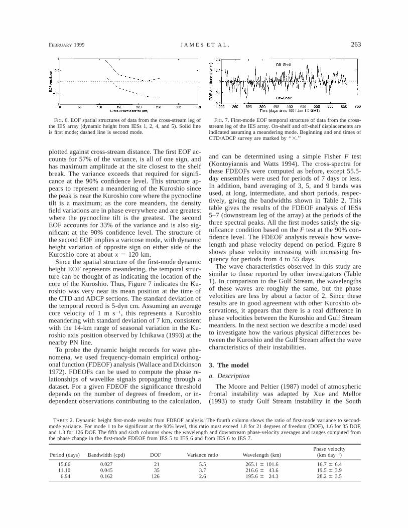
FIG. 6. EOF spatial structures of data from the cross-stream leg ofthe IES array (dynamic height from IESs 1, 2, 4, and 5). Solid lineis first mode; dashed line is second mode.

FIG. 7. First-mode EOF temporal structure of data from the cross-stream leg of the IES array. On-shelf and off-shelf displacements areindicated assuming a meandering mode. Beginning and end times ofCTD/ADCP survey are marked by ‘‘3.’’

TABLE 2. Dynamic height first-mode results from FDEOF analysis. The fourth column shows the ratio of first-mode variance to second-mode variance. For mode 1 to be significant at the 90% level, this ratio must exceed 1.8 for 21 degrees of freedom (DOF), 1.6 for 35 DOF,and 1.3 for 126 DOF. The fifth and sixth columns show the wavelength and downstream phase-velocity averages and ranges computed fromthe phase change in the first-mode FDEOF from IES 5 to IES 6 and from IES 6 to IES 7.

Period (days) Bandwidth (cpd) DOF Variance ratio Wavelength (km)Phase velocity

(km day21)

15.8611.106.94

0.0270.0450.162

2135

126

5.53.72.6

265.1 6 101.6216.6 6 43.6195.6 6 24.3

16.7 6 6.419.5 6 3.928.2 6 3.5

plotted against cross-stream distance. The first EOF ac-counts for 57% of the variance, is all of one sign, andhas maximum amplitude at the site closest to the shelfbreak. The variance exceeds that required for signifi-cance at the 90% confidence level. This structure ap-pears to represent a meandering of the Kuroshio sincethe peak is near the Kuroshio core where the pycnoclinetilt is a maximum; as the core meanders, the densityfield variations are in phase everywhere and are greatestwhere the pycnocline tilt is the greatest. The secondEOF accounts for 33% of the variance and is also sig-nificant at the 90% confidence level. The structure ofthe second EOF implies a varicose mode, with dynamicheight variation of opposite sign on either side of theKuroshio core at about x 5 120 km.

Since the spatial structure of the first-mode dynamicheight EOF represents meandering, the temporal struc-ture can be thought of as indicating the location of thecore of the Kuroshio. Thus, Figure 7 indicates the Ku-roshio was very near its mean position at the time ofthe CTD and ADCP sections. The standard deviation ofthe temporal record is 5-dyn cm. Assuming an averagecore velocity of 1 m s21, this represents a Kuroshiomeandering with standard deviation of 7 km, consistentwith the 14-km range of seasonal variation in the Ku-roshio axis position observed by Ichikawa (1993) at thenearby PN line.

To probe the dynamic height records for wave phe-nomena, we used frequency-domain empirical orthog-onal function (FDEOF) analysis (Wallace and Dickinson1972). FDEOFs can be used to compute the phase re-lationships of wavelike signals propagating through adataset. For a given FDEOF the significance thresholddepends on the number of degrees of freedom, or in-dependent observations contributing to the calculation,

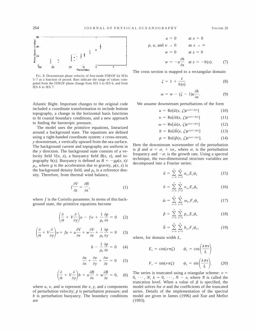
and can be determined using a simple Fisher F test(Kontoyiannis and Watts 1994). The cross-spectra forthese FDEOFs were computed as before, except 55.5-day ensembles were used for periods of 7 days or less.In addition, band averaging of 3, 5, and 9 bands wasused, at long, intermediate, and short periods, respec-tively, giving the bandwidths shown in Table 2. Thistable gives the results of the FDEOF analysis of IESs5–7 (downstream leg of the array) at the periods of thethree spectral peaks. All the first modes satisfy the sig-nificance condition based on the F test at the 90% con-fidence level. The FDEOF analysis reveals how wave-length and phase velocity depend on period. Figure 8shows phase velocity increasing with increasing fre-quency for periods from 4 to 55 days.

The wave characteristics observed in this study aresimilar to those reported by other investigators (Table1). In comparison to the Gulf Stream, the wavelengthsof these waves are roughly the same, but the phasevelocities are less by about a factor of 2. Since theseresults are in good agreement with other Kuroshio ob-servations, it appears that there is a real difference inphase velocities between the Kuroshio and Gulf Streammeanders. In the next section we describe a model usedto investigate how the various physical differences be-tween the Kuroshio and the Gulf Stream affect the wavecharacteristics of their instabilities.

3. The model

a. Description

The Moore and Peltier (1987) model of atmosphericfrontal instability was adapted by Xue and Mellor(1993) to study Gulf Stream instability in the South


FIG. 8. Downstream phase velocity of first-mode FDEOF for IESs5–7 as a function of period. Bars indicate the range of values com-puted from the FDEOF phase change from IES 5 to IES 6, and fromIES 6 to IES 7.

Atlantic Bight. Important changes to the original codeincluded a coordinate transformation to include bottomtopography, a change in the horizontal basis functionsto fit coastal boundary conditions, and a new approachto finding the barotropic pressure.

The model uses the primitive equations, linearizedaround a background state. The equations are definedusing a right-handed coordinate system: x cross-stream,y downstream, z vertically upward from the sea surface.The background current and topography are uniform inthe y direction. The background state consists of a ve-locity field V(x, z), a buoyancy field B(x, z), and to-pography h(x). Buoyancy is defined as B 5 2gr(x, z)/r0, where g is the acceleration due to gravity, r(x, z) isthe background density field, and r0 is a reference den-sity. Therefore, from thermal wind balance,

]V ]Bf 5 , (1)

]z ]x

where f is the Coriolis parameter. In terms of this back-ground state, the primitive equations become

] ] 1 ]p1 V u 2 f y 1 5 0 (2)1 2]t ]y r ]x0

] ] ]V ]V 1 ]p1 V y 1 fu 1 u 1 w 1 5 0 (3)1 2]t ]y ]x ]z r ]y0

1 ]pb 2 5 0 (4)

r ]z0

]u ]y ]w1 1 5 0 (5)

]x ]y ]z

] ] ]B ]B1 V b 1 u 1 w 5 0, (6)1 2]t ]y ]x ]z

where u, y , and w represent the x, y, and z componentsof perturbation velocity; p is perturbation pressure; andb is perturbation buoyancy. The boundary conditionsare

u 5 0 at x 5 0

p, u, and y → 0 as x → `

w 5 0 at z 5 0

]hw 5 2u at z 5 2h(x). (7)

]x

The cross section is mapped to a rectangular domain:

zz 5 1 1 (8)

h(x)

]hv 5 w 2 (z 2 1)u . (9)

]x

We assume downstream perturbations of the formi(st1by)u 5 Re[u(x, z)e ] (10)i(st1by)y 5 Re[iy(x, z)e ] (11)i(st1by)v 5 Re[v(x, z)e ] (12)i(st1by)b 5 Re[ib(x, z)e ] (13)i(st1by)p 5 Re[ip(x, z)e ]. (14)

Here the downstream wavenumber of the perturbationis b and s 5 sr 1 isi, where sr is the perturbationfrequency and 2si is the growth rate. Using a spectraltechnique, the two-dimensional structure variables aredecomposed into a Fourier series:

` `

u 5 u E c (15)O O ln n ln50 l50

` `

y 5 y E f (16)O O ln n ln50 l50

` `

v 5 v F f (17)O O ln n ln50 l50

` `

p 5 p E f (18)O O ln n ln50 l50

` `

b 5 b F f , (19)O O ln n ln50 l50

where, for domain width L,

lpxE 5 cos(npz) f 5 cosn l 1 2L

lpxF 5 sin(npz) c 5 sin . (20)n l 1 2L

The series is truncated using a triangular scheme: n 50, · · · , N; l 5 0, · · · , N 2 n, where N is called thetruncation level. When a value of b is specified, themodel solves for s and the coefficients of the truncatedseries. Details of the implementation of the spectralmodel are given in James (1996) and Xue and Mellor(1993).


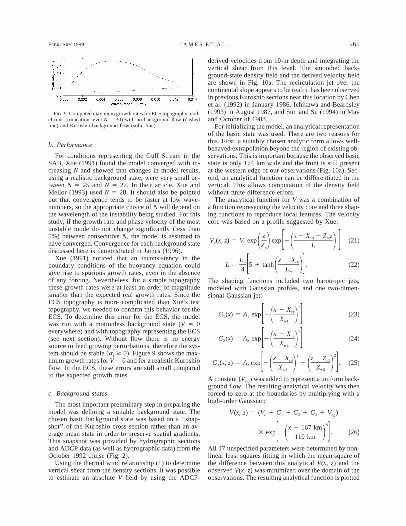
FIG. 9. Computed maximum growth rates for ECS topography mod-el runs (truncation level N 5 30) with no background flow (dashedline) and Kuroshio background flow (solid line).

b. Performance

For conditions representing the Gulf Stream in theSAB, Xue (1991) found the model converged with in-creasing N and showed that changes in model results,using a realistic background state, were very small be-tween N 5 25 and N 5 27. In their article, Xue andMellor (1993) used N 5 28. It should also be pointedout that convergence tends to be faster at low wave-numbers, so the appropriate choice of N will depend onthe wavelength of the instability being studied. For thisstudy, if the growth rate and phase velocity of the mostunstable mode do not change significantly (less than5%) between consecutive N, the model is assumed tohave converged. Convergence for each background statediscussed here is demonstrated in James (1996).

Xue (1991) noticed that an inconsistency in theboundary conditions of the buoyancy equation couldgive rise to spurious growth rates, even in the absenceof any forcing. Nevertheless, for a simple topographythese growth rates were at least an order of magnitudesmaller than the expected real growth rates. Since theECS topography is more complicated than Xue’s testtopography, we needed to confirm this behavior for theECS. To determine this error for the ECS, the modelwas run with a motionless background state (V 5 0everywhere) and with topography representing the ECS(see next section). Without flow there is no energysource to feed growing perturbations, therefore the sys-tem should be stable (si $ 0). Figure 9 shows the max-imum growth rates for V 5 0 and for a realistic Kuroshioflow. In the ECS, these errors are still small comparedto the expected growth rates.

c. Background states

The most important preliminary step in preparing themodel was defining a suitable background state. Thechosen basic background state was based on a ‘‘snap-shot’’ of the Kuroshio cross section rather than an av-erage mean state in order to preserve spatial gradients.This snapshot was provided by hydrographic sectionsand ADCP data (as well as hydrographic data) from theOctober 1992 cruise (Fig. 2).

Using the thermal wind relationship (1) to determinevertical shear from the density sections, it was possibleto estimate an absolute V field by using the ADCP-

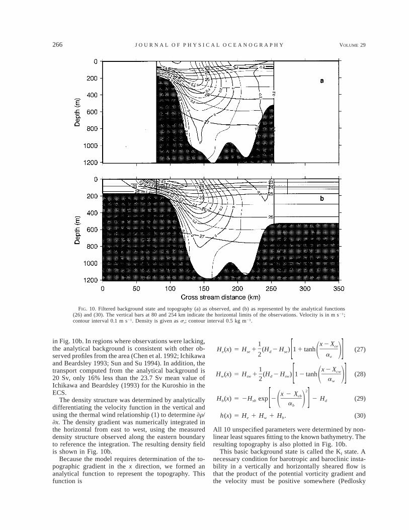
derived velocities from 10-m depth and integrating thevertical shear from this level. The smoothed back-ground-state density field and the derived velocity fieldare shown in Fig. 10a. The recirculation jet over thecontinental slope appears to be real; it has been observedin previous Kuroshio sections near this location by Chenet al. (1992) in January 1986, Ichikawa and Beardsley(1993) in August 1987, and Sun and Su (1994) in Mayand October of 1988.

For initializing the model, an analytical representationof the basic state was used. There are two reasons forthis. First, a suitably chosen analytic form allows well-behaved extrapolation beyond the region of existing ob-servations. This is important because the observed basicstate is only 174 km wide and the front is still presentat the western edge of our observations (Fig. 10a). Sec-ond, an analytical function can be differentiated in thevertical. This allows computation of the density fieldwithout finite difference errors.

The analytical function for V was a combination ofa function representing the velocity core and three shap-ing functions to reproduce local features. The velocitycore was based on a profile suggested by Xue:

2z x 2 X 2 Z zc0 mV (x, z) 5 V exp exp 2 (21)c 0 1 2 1 2[ ]Z Le

L x 2 Xw c0L 5 5 1 tanh . (22)1 2[ ]4 Lw

The shaping functions included two barotropic jets,modeled with Gaussian profiles, and one two-dimen-sional Gaussian jet:

2x 2 Xc1G (x) 5 A exp 2 (23)1 1 1 2[ ]Xw1

2x 2 Xc2G (x) 5 A exp 2 (24)2 2 1 2[ ]Xw2

2 2x 2 X z 2 Zc3 c3G (x, z) 5 A exp 2 2 . (25)3 3 1 2 1 2[ ]X Zw3 w3

A constant (Vbg) was added to represent a uniform back-ground flow. The resulting analytical velocity was thenforced to zero at the boundaries by multiplying with ahigh-order Gaussian:

V(x, z) 5 (V 1 G 1 G 1 G 1 V )c 1 2 3 bg

8x 2 167 km3 exp 2 . (26)1 2[ ]110 km

All 17 unspecified parameters were determined by non-linear least squares fitting in which the mean square ofthe difference between this analytical V(x, z) and theobserved V(x, z) was minimized over the domain of theobservations. The resulting analytical function is plotted


FIG. 10. Filtered background state and topography (a) as observed, and (b) as represented by the analytical functions(26) and (30). The vertical bars at 80 and 254 km indicate the horizontal limits of the observations. Velocity is in m s21;contour interval 0.1 m s21. Density is given as st; contour interval 0.5 kg m23.

in Fig. 10b. In regions where observations were lacking,the analytical background is consistent with other ob-served profiles from the area (Chen et al. 1992; Ichikawaand Beardsley 1993; Sun and Su 1994). In addition, thetransport computed from the analytical background is20 Sv, only 16% less than the 23.7 Sv mean value ofIchikawa and Beardsley (1993) for the Kuroshio in theECS.

The density structure was determined by analyticallydifferentiating the velocity function in the vertical andusing the thermal wind relationship (1) to determine ]r/]x. The density gradient was numerically integrated inthe horizontal from east to west, using the measureddensity structure observed along the eastern boundaryto reference the integration. The resulting density fieldis shown in Fig. 10b.

Because the model requires determination of the to-pographic gradient in the x direction, we formed ananalytical function to represent the topography. Thisfunction is

1 x 2 XceH (x) 5 H 1 (H 2 H ) 1 1 tanh (27)e se d se 1 2[ ]2 ae

1 x 2 XcwH (x) 5 H 1 (H 2 H ) 1 2 tanh (28)w sw d sw 1 2[ ]2 aw

2x 2 XcbH (x) 5 2H exp 2 2 H (29)b sb d1 2[ ]ab

h(x) 5 H 1 H 1 H . (30)e w b

All 10 unspecified parameters were determined by non-linear least squares fitting to the known bathymetry. Theresulting topography is also plotted in Fig. 10b.

This basic background state is called the KI state. Anecessary condition for barotropic and baroclinic insta-bility in a vertically and horizontally sheared flow isthat the product of the potential vorticity gradient andthe velocity must be positive somewhere (Pedlosky


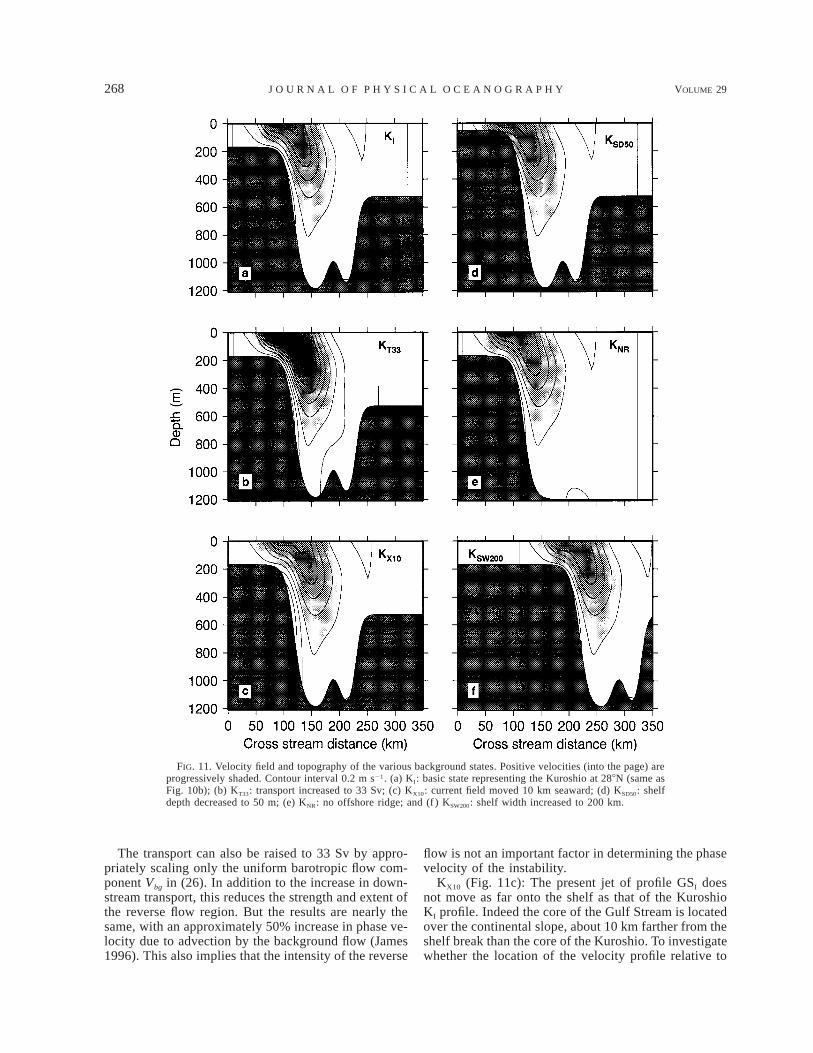
1964). Based on this condition, the KI basic state hasbeen shown to be potentially unstable to both barotropicand baroclinic instabilities (James 1996), and thereforesuitable for study using this model. A somewhat similarbasic state for the Gulf Stream south of the CharlestonBump, used by Xue and Mellor (1993), is designatedGSI (but called I1 by Xue and Mellor 1993). In additionto the basic KI state, established from the observationalKuroshio data, we consider several variations on thisstate in order to investigate the influence of variousfeatures of the flow and topography on the instabilityproperties. In each of these variations, just one featureof the KI state is altered. In four of the variations, aparameter is altered to make a particular feature of thebackground state resemble the Gulf Stream GSI state:the shelf depth is reduced from 167 to 50 m in the KSD50

state; the velocity field is scaled up to raise the transportfrom 20 to 33 Sv in the KT33 state; the entire velocityfield is shifted 10 km in the offshelf direction in theKX10 state; the offshore Ryukyu Ridge is eliminated inthe KNR state. In one other background-state variation,the shelf width is increased from 100 to 200 km. Thesevarious Kuroshio background states are shown in Fig.11.

4. Model results and discussion

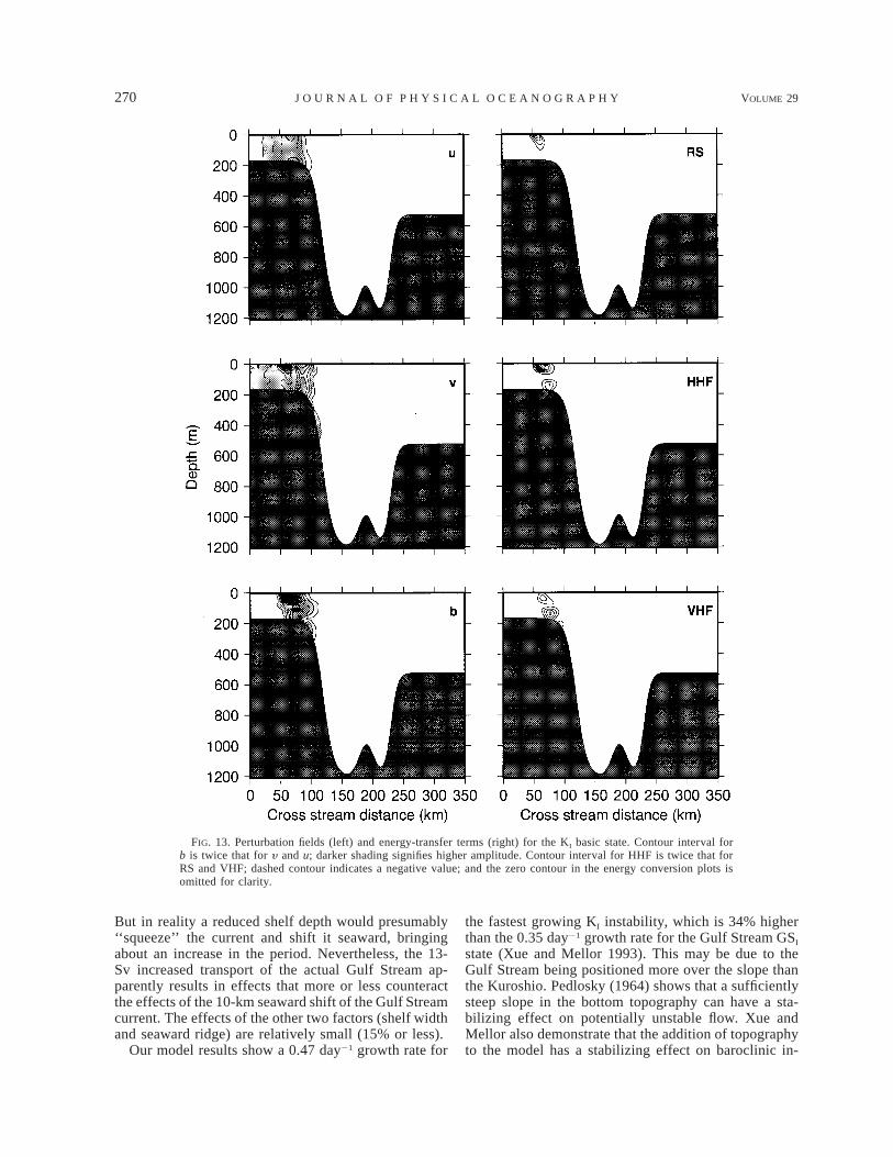
The characteristics of model instability modes werecalculated for a range of wavenumbers correspondingto wavelengths between 105 and 1257 km. In each case,the described wave properties are those of the modewith the fastest growth rate at its fastest-growth wave-number. In particular, the model is used to give us thewavelength (2p/b), period (2p/|sr|), downstream phasevelocity (2sr/b), and growth rate (2si) of this insta-bility. The model also provides the spatial structures ofthe velocity (u, y , w) and buoyancy (b) perturbationfields and of the energy-transfer terms. There are threeenergy-transfer terms: mean-to-eddy kinetic energy, orReynolds stress (RS); mean-to-eddy potential energy, orhorizontal heat flux (HHF); and eddy potential energyto eddy kinetic energy, or vertical heat flux (VHF). Xueand Mellor (1993) define these terms and discuss theirsignificance.

a. The Kuroshio basic background state

For the Kuroshio basic state (Fig. 11a), the modelpredicts a peak growth rate at a period of 12 days, closeto the energetic 11-day peak in the observed EOF spec-trum (Fig. 4). The model-predicted wavelength is 209km, consistent with the observed 217 6 44 km. Thephase velocities are also close: 18 and 20 6 4 km day21,respectively. This agreement is encouraging and sug-gests that the model is reproducing a realistic instabilityat this period.

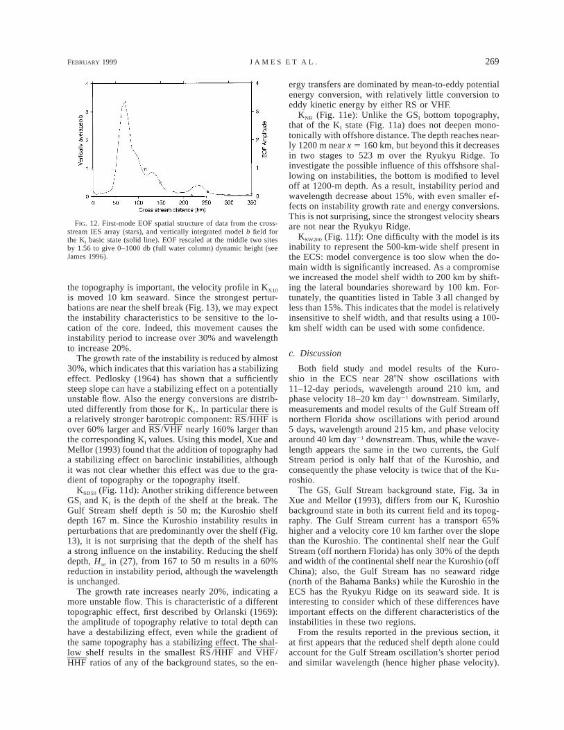
A separate confirmation comes from the results of theEOF analysis illustrated in Fig. 12. The IES records

may be interpreted as representing full-water-columndynamic height variations,

pb g 12 dp, (31)E r B 1 b00

where pb is pressure near the sea floor. Since b K B,these variations are proportional to

pb

b dp. (32)E0

Hence fluctuations in the IES record should be propor-tional to fluctuations in the vertically integrated b field.Figure 12 shows both the first-mode EOF spatial func-tion from our IES measurements and the vertically in-tegrated b field from the model of the Kuroshio basicbackground state. Note that the first-mode EOF is thesame as that in Fig. 6 but rescaled to give full-water-column (rather than 0–500 db) dynamic height, as inEq. (32). The agreement in shape between these twofunctions in Fig. 12 suggests that the model is repro-ducing the observed instability. Spatial structures of theperturbation fields and energy-transfer terms are shownin Fig. 13. It is clear that all of these perturbations (u,y , b) and energy transfers (RS, HHF, VHF) are strongestover the outer shelf, about 30–40 km from the shelfbreak.

Our observed spectrum (Fig. 4) shows additionalpeaks at 16 and 7 day periods. Possible explanations ofthese will be discussed in section 4c after we have con-sidered, in the next section, the effects of background-state variations on the resulting instability.

b. Background-state variations

The model was run for the various alternate back-ground states described at the end of section 3c. Theresults are summarized in Table 3 and are discussedindividually below. Profile GSI refers to the Gulf Streamprofile from Xue and Mellor (1993).

KT33 (Fig. 11b): The higher transport of profile GSI

is associated with higher-current velocity, and we wouldlike to determine if the resulting increased advectioncould account for the observed increase in phase ve-locity. Raising the transport from 20 to 33 Sv by scalingthe velocity profile—that is, multiplying V(x, z) obtainedfrom (26) by 1.7—results in a 40% reduction in insta-bility period and a 14% reduction in wavelength. Thedownstream phase velocity increases by 50% or 9 kmd21 5 10 cm s21, the same as the increase in surfacecurrent velocity at the point x 5 51 km (Figs. 11a,b),which is where the disturbance is concentrated (Fig. 13).This, together with the smallness of the change in wave-length, suggests that advection is principally responsiblefor the increased phase velocity. The growth rate of theinstability is also very high. This is presumably due tothe increased velocity shear resulting in a more unstablebackground state.


FIG. 11. Velocity field and topography of the various background states. Positive velocities (into the page) areprogressively shaded. Contour interval 0.2 m s21. (a) KI: basic state representing the Kuroshio at 288N (same asFig. 10b); (b) KT33: transport increased to 33 Sv; (c) KX10: current field moved 10 km seaward; (d) KSD50: shelfdepth decreased to 50 m; (e) KNR: no offshore ridge; and (f ) KSW200: shelf width increased to 200 km.

The transport can also be raised to 33 Sv by appro-priately scaling only the uniform barotropic flow com-ponent Vbg in (26). In addition to the increase in down-stream transport, this reduces the strength and extent ofthe reverse flow region. But the results are nearly thesame, with an approximately 50% increase in phase ve-locity due to advection by the background flow (James1996). This also implies that the intensity of the reverse

flow is not an important factor in determining the phasevelocity of the instability.

KX10 (Fig. 11c): The present jet of profile GSI doesnot move as far onto the shelf as that of the KuroshioKI profile. Indeed the core of the Gulf Stream is locatedover the continental slope, about 10 km farther from theshelf break than the core of the Kuroshio. To investigatewhether the location of the velocity profile relative to


FIG. 12. First-mode EOF spatial structure of data from the cross-stream IES array (stars), and vertically integrated model b field forthe KI basic state (solid line). EOF rescaled at the middle two sitesby 1.56 to give 0–1000 db (full water column) dynamic height (seeJames 1996).

the topography is important, the velocity profile in KX10

is moved 10 km seaward. Since the strongest pertur-bations are near the shelf break (Fig. 13), we may expectthe instability characteristics to be sensitive to the lo-cation of the core. Indeed, this movement causes theinstability period to increase over 30% and wavelengthto increase 20%.

The growth rate of the instability is reduced by almost30%, which indicates that this variation has a stabilizingeffect. Pedlosky (1964) has shown that a sufficientlysteep slope can have a stabilizing effect on a potentiallyunstable flow. Also the energy conversions are distrib-uted differently from those for KI. In particular there isa relatively stronger barotropic component: RS/HHF isover 60% larger and RS/VHF nearly 160% larger thanthe corresponding KI values. Using this model, Xue andMellor (1993) found that the addition of topography hada stabilizing effect on baroclinic instabilities, althoughit was not clear whether this effect was due to the gra-dient of topography or the topography itself.

KSD50 (Fig. 11d): Another striking difference betweenGSI and KI is the depth of the shelf at the break. TheGulf Stream shelf depth is 50 m; the Kuroshio shelfdepth 167 m. Since the Kuroshio instability results inperturbations that are predominantly over the shelf (Fig.13), it is not surprising that the depth of the shelf hasa strong influence on the instability. Reducing the shelfdepth, Hse in (27), from 167 to 50 m results in a 60%reduction in instability period, although the wavelengthis unchanged.

The growth rate increases nearly 20%, indicating amore unstable flow. This is characteristic of a differenttopographic effect, first described by Orlanski (1969):the amplitude of topography relative to total depth canhave a destabilizing effect, even while the gradient ofthe same topography has a stabilizing effect. The shal-low shelf results in the smallest RS/HHF and VHF/HHF ratios of any of the background states, so the en-

ergy transfers are dominated by mean-to-eddy potentialenergy conversion, with relatively little conversion toeddy kinetic energy by either RS or VHF.

KNR (Fig. 11e): Unlike the GSI bottom topography,that of the KI state (Fig. 11a) does not deepen mono-tonically with offshore distance. The depth reaches near-ly 1200 m near x 5 160 km, but beyond this it decreasesin two stages to 523 m over the Ryukyu Ridge. Toinvestigate the possible influence of this offshsore shal-lowing on instabilities, the bottom is modified to leveloff at 1200-m depth. As a result, instability period andwavelength decrease about 15%, with even smaller ef-fects on instability growth rate and energy conversions.This is not surprising, since the strongest velocity shearsare not near the Ryukyu Ridge.

KSW200 (Fig. 11f): One difficulty with the model is itsinability to represent the 500-km-wide shelf present inthe ECS: model convergence is too slow when the do-main width is significantly increased. As a compromisewe increased the model shelf width to 200 km by shift-ing the lateral boundaries shoreward by 100 km. For-tunately, the quantities listed in Table 3 all changed byless than 15%. This indicates that the model is relativelyinsensitive to shelf width, and that results using a 100-km shelf width can be used with some confidence.

c. Discussion

Both field study and model results of the Kuro-shio in the ECS near 288N show oscillations with11–12-day periods, wavelength around 210 km, andphase velocity 18–20 km day21 downstream. Similarly,measurements and model results of the Gulf Stream offnorthern Florida show oscillations with period around5 days, wavelength around 215 km, and phase velocityaround 40 km day21 downstream. Thus, while the wave-length appears the same in the two currents, the GulfStream period is only half that of the Kuroshio, andconsequently the phase velocity is twice that of the Ku-roshio.

The GSI Gulf Stream background state, Fig. 3a inXue and Mellor (1993), differs from our KI Kuroshiobackground state in both its current field and its topog-raphy. The Gulf Stream current has a transport 65%higher and a velocity core 10 km farther over the slopethan the Kuroshio. The continental shelf near the GulfStream (off northern Florida) has only 30% of the depthand width of the continental shelf near the Kuroshio (offChina); also, the Gulf Stream has no seaward ridge(north of the Bahama Banks) while the Kuroshio in theECS has the Ryukyu Ridge on its seaward side. It isinteresting to consider which of these differences haveimportant effects on the different characteristics of theinstabilities in these two regions.

From the results reported in the previous section, itat first appears that the reduced shelf depth alone couldaccount for the Gulf Stream oscillation’s shorter periodand similar wavelength (hence higher phase velocity).


FIG. 13. Perturbation fields (left) and energy-transfer terms (right) for the KI basic state. Contour interval forb is twice that for y and u; darker shading signifies higher amplitude. Contour interval for HHF is twice that forRS and VHF; dashed contour indicates a negative value; and the zero contour in the energy conversion plots isomitted for clarity.

But in reality a reduced shelf depth would presumably‘‘squeeze’’ the current and shift it seaward, bringingabout an increase in the period. Nevertheless, the 13-Sv increased transport of the actual Gulf Stream ap-parently results in effects that more or less counteractthe effects of the 10-km seaward shift of the Gulf Streamcurrent. The effects of the other two factors (shelf widthand seaward ridge) are relatively small (15% or less).

Our model results show a 0.47 day21 growth rate for

the fastest growing KI instability, which is 34% higherthan the 0.35 day21 growth rate for the Gulf Stream GSI

state (Xue and Mellor 1993). This may be due to theGulf Stream being positioned more over the slope thanthe Kuroshio. Pedlosky (1964) shows that a sufficientlysteep slope in the bottom topography can have a sta-bilizing effect on potentially unstable flow. Xue andMellor also demonstrate that the addition of topographyto the model has a stabilizing effect on baroclinic in-


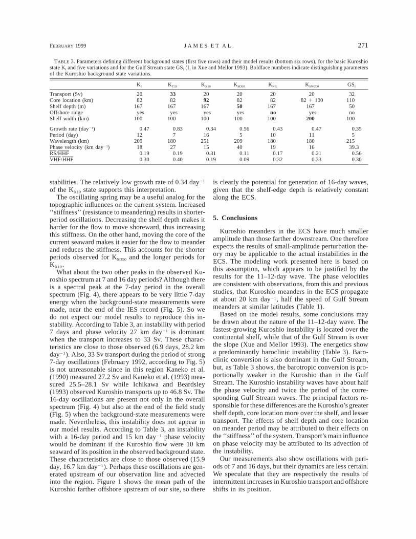
TABLE 3. Parameters defining different background states (first five rows) and their model results (bottom six rows), for the basic Kuroshiostate KI and five variations and for the Gulf Stream state GSI (I1 in Xue and Mellor 1993). Boldface numbers indicate distinguishing parametersof the Kuroshio background state variations.

KI KT33 KX10 KSD50 KNR KSW200 GSI

Transport (Sv)Core location (km)Shelf depth (m)Offshore ridgeShelf width (km)

2082

167yes

100

3382

167yes

100

2092

167yes

100

208250yes

100

2082

167no

100

2082 1 100

167yes

200

3211050no

100

Growth rate (day21)Period (day)Wavelength (km)

0.4712

209

0.837

180

0.3416

251

0.565

209

0.4310

180

0.4711

180

0.355

215Phase velocity (km day21)RS/HHFVHF/HHF

180.190.30

270.190.40

150.310.19

400.110.09

190.170.32

160.210.33

39.30.560.30

stabilities. The relatively low growth rate of 0.34 day21

of the KX10 state supports this interpretation.The oscillating spring may be a useful analog for the

topographic influences on the current system. Increased‘‘stiffness’’ (resistance to meandering) results in shorter-period oscillations. Decreasing the shelf depth makes itharder for the flow to move shoreward, thus increasingthis stiffness. On the other hand, moving the core of thecurrent seaward makes it easier for the flow to meanderand reduces the stiffness. This accounts for the shorterperiods observed for KSD50 and the longer periods forKX10.

What about the two other peaks in the observed Ku-roshio spectrum at 7 and 16 day periods? Although thereis a spectral peak at the 7-day period in the overallspectrum (Fig. 4), there appears to be very little 7-dayenergy when the background-state measurements weremade, near the end of the IES record (Fig. 5). So wedo not expect our model results to reproduce this in-stability. According to Table 3, an instability with period7 days and phase velocity 27 km day21 is dominantwhen the transport increases to 33 Sv. These charac-teristics are close to those observed (6.9 days, 28.2 kmday21). Also, 33 Sv transport during the period of strong7-day oscillations (February 1992, according to Fig. 5)is not unreasonable since in this region Kaneko et al.(1990) measured 27.2 Sv and Kaneko et al. (1993) mea-sured 25.5–28.1 Sv while Ichikawa and Beardsley(1993) observed Kuroshio transports up to 46.8 Sv. The16-day oscillations are present not only in the overallspectrum (Fig. 4) but also at the end of the field study(Fig. 5) when the background-state measurements weremade. Nevertheless, this instability does not appear inour model results. According to Table 3, an instabilitywith a 16-day period and 15 km day21 phase velocitywould be dominant if the Kuroshio flow were 10 kmseaward of its position in the observed background state.These characteristics are close to those observed (15.9day, 16.7 km day21). Perhaps these oscillations are gen-erated upstream of our observation line and advectedinto the region. Figure 1 shows the mean path of theKuroshio farther offshore upstream of our site, so there

is clearly the potential for generation of 16-day waves,given that the shelf-edge depth is relatively constantalong the ECS.

5. Conclusions

Kuroshio meanders in the ECS have much smalleramplitude than those farther downstream. One thereforeexpects the results of small-amplitude perturbation the-ory may be applicable to the actual instabilities in theECS. The modeling work presented here is based onthis assumption, which appears to be justified by theresults for the 11–12-day wave. The phase velocitiesare consistent with observations, from this and previousstudies, that Kuroshio meanders in the ECS propagateat about 20 km day21, half the speed of Gulf Streammeanders at similar latitudes (Table 1).

Based on the model results, some conclusions maybe drawn about the nature of the 11–12-day wave. Thefastest-growing Kuroshio instability is located over thecontinental shelf, while that of the Gulf Stream is overthe slope (Xue and Mellor 1993). The energetics showa predominantly baroclinic instability (Table 3). Baro-clinic conversion is also dominant in the Gulf Stream,but, as Table 3 shows, the barotropic conversion is pro-portionally weaker in the Kuroshio than in the GulfStream. The Kuroshio instability waves have about halfthe phase velocity and twice the period of the corre-sponding Gulf Stream waves. The principal factors re-sponsible for these differences are the Kuroshio’s greatershelf depth, core location more over the shelf, and lessertransport. The effects of shelf depth and core locationon meander period may be attributed to their effects onthe ‘‘stiffness’’ of the system. Transport’s main influenceon phase velocity may be attributed to its advection ofthe instability.

Our measurements also show oscillations with peri-ods of 7 and 16 days, but their dynamics are less certain.We speculate that they are respectively the results ofintermittent increases in Kuroshio transport and offshoreshifts in its position.


Acknowledgments. The efforts of the captains andcrews of the T/V Keiten-maru and T/V Kagoshima-maru were essential to the success of the cruises. Mi-chael Mulroney was responsible for the preparation, de-ployment, and recovery of the IES’s. Shiro Imawaki andToru Yamashiro helped much during the 1991 cruise forthe deployment of the instruments. Professors MasaakiChaen and Akio Maeda of Kagoshima University en-couraged this study. Huijie Xue generously gave us thecomputer code for her model and much helpful advice.The model was run using the resources of the CornellTheory Center, which receives major funding from theNational Science Foundation and New York State withadditional support from the Advanced Research ProjectsAgency, the National Center for Research Resources atthe National Institutes of Health, IBM Corporation, andmembers of the Corporate Research Institute. The workof Charles James and Mark Wimbush was supported bythe National Science Foundation (NSF) and the Officeof Naval Research (ONR) through NSF Grant OCE-9018581 and ONR Grant N00014-94-10023. The par-ticipation of Hiroshi Ichikawa was covered by the Min-istry of Education, Science, and Culture, Japan. The dataanalysis and model work was carried out as part ofJames’s dissertation.

REFERENCES

Bane, J. M., and D. A. Brooks, 1979: Gulf Stream meanders alongthe continental margin from the Florida Straits to Cape Hatteras.Geophys. Res. Lett., 6, 280–282.

Bingham, C., M. Godfrey, and J. Tukey, 1967: Modern techniquesof power spectrum estimation. IEEE Trans. Audio Electroa-coust., AU-15, 56–66.

Chen, C., R. C. Beardsley, and R. Limeburner, 1992: The structureof the Kuroshio southwest of Kyushu: velocity, transport andpotential vorticity fields. Deep-Sea Res., 39, 245–268.

Ichikawa, H., 1993: Short period variations of the Kuroshio volumetransport in the East China Sea. Umi to Sora, 69, 135–148., and R. C. Beardsley, 1993: Temporal and spatial variability ofvolume transport of the Kuroshio in the East China Sea. Deep-Sea Res., 40, 583–605.

James, C., 1996: Kuroshio instabilities in the East China Sea—Ob-servations, modeling, and comparison with the Gulf Stream.Ph.D. thesis, University of Rhode Island, 150 pp., and M. Wimbush, 1995: Inferring dynamic height variations

from acoustic travel time in the Pacific Ocean. J. Oceanogr., 51,553–569., , and H. Ichikawa, 1994: East China Sea, Kuroshio 1991–92 data report, Graduate School of Oceanography Tech. Rep.94-3, 22 pp. [Available from Graduate School of Oceanography,University of Rhode Island, Narragansett, RI 02882.]

Kaneko, A., W. Koterayama, H. Honji, S. Mizuno, K. Kawatate, andR. Gordon, 1990: Cross-stream survey of the upper 400 m ofthe Kuroshio by an ADCP on a towed fish. Deep-Sea Res., 37,875–889., N. Gohda, W. Koterayama, M. Nakamura, S. Mizuno, and H.Furukawa, 1993: Towed ADCP fish with depth and roll con-trollable wings and its application to the Kuroshio observation.J. Oceanogr., 49, 383–395.

Kontoyiannis, H., and D. R. Watts, 1994: Observations on the var-iability of the Gulf Stream path between 748W and 708W. J.Phys. Oceanogr., 24, 1999–2013.

Lee, T. N., and L. P. Atkinson, 1983: Low-frequency current andtemperature variability from Gulf Stream frontal eddies and at-mospheric forcing along the southeast U.S. outer continentalshelf. J. Geophys. Res., 88, 4541–4567.

Moore, G. W. K., and W. R. Peltier, 1987: Cyclogenesis in frontalzones. J. Atmos. Sci., 44, 384–409.

Orlanski, I., 1969: The influence of bottom topography on the stabilityof jets in a baroclinic fluid. J. Atmos. Sci., 26, 1216–1232.

Pedlosky, J., 1964: The stability of currents in the atmosphere andthe ocean: Part I. J. Atmos. Sci., 21, 201–219.

Preisendorfer, R. W., 1988: Principal Component Analysis in Mete-orology and Oceanography. Elsevier, 425 pp.

Qiu, B., T. Toda, and N. Imasato, 1990: On Kuroshio front fluctuationsin the East China Sea using satellite and in situ observationaldata. J. Geophys. Res., 95, 18 191–18 203.

Richardson, W. S., W. J. Schmitz, and P. N. Niiler, 1969: The velocitystructure of the Florida Current from the Straits of Florida toCape Fear. Deep-Sea Res., 16 (Suppl.), 225–231.

Sugimoto, Y., S. Kimura, and K. Miyaji, 1988: Meander of the Ku-roshio front and current variability in the East China Sea. J.Oceanogr. Soc. Japan, 44, 125–135.

Sun, X.-P., and Y.-F. Su, 1994: On the variation of Kuroshio in EastChina Sea. Oceanology of China Seas, D. Zhou, Y.-B. Liang,and C. K. Tseng, Eds., Vol. 1, Kluwer Academic, 49–58.

Trivers, G., and M. Wimbush, 1994: Using acoustic travel time todetermine dynamic height variations in the North Atlantic Ocean.J. Atmos. Oceanic Technol., 11, 1309–1316.

Wallace, J. M., and R. E. Dickinson, 1972: Empirical orthogonalrepresentation of time series in the frequency domain. Part I:Theoretical considerations. J. Appl. Meteor., 11, 887–892.

Watts, D. R., and H. T. Rossby, 1977: Measuring dynamic heightswith inverted echo sounders: Results from MODE. J. Phys.Oceanogr., 7, 345–358.

Xue, H., 1991: Numerical studies of Gulf Stream meanders in theSouth Atlantic Bight. Ph.D. thesis, Princeton University, 188 pp., and G. Mellor, 1993: Instability of the Gulf Stream front in theSouth Atlantic Bight. J. Phys. Oceanogr., 23, 2326–2350.

Kuroshio Meanders in the East China Sea

Documents

Transcript of Kuroshio Meanders in the East China Sea