arX

iv:1

203.

2367

v2 [

mat

h.N

A]

21

Oct

201

2

Junction between a plate and a rod of comparable

thickness in nonlinear elasticity. Part II

D. Blanchard1, G. Griso2

1 Universite de Rouen, France. DECEASED on February 11th, 20121.2 Laboratoire J.-L. Lions–CNRS, Boıte courrier 187, Universite Pierre et Marie Curie,

4 place Jussieu, 75005 Paris, France, Email: griso@ann.jussieu.fr

Abstract

We analyze the asymptotic behavior of a junction problem between a plateand a perpendicular rod made of a nonlinear elastic material. The two parts ofthis multi-structure have small thicknesses of the same order δ. We use the de-composition techniques obtained for the large deformations and the displacementsin order to derive the limit energy as δ tends to 0.

KEY WORDS: nonlinear elasticity, junctions, straight rod, plate.

Mathematics Subject Classification (2000): 74B20, 74K10, 74K30.

1 Introduction

In a former paper [12] we derive the limit energy of the junction problem betweena plate and a rod under an assumption that couples their respective thicknesses δ andε to the order of the Lame’s coefficients of the materials in the plate and in the rod.This assumption precludes the case where the thicknesses have the same order and thestructure is made of the same material (see equation 1.1 in the introduction of [12]).The aim of the present paper is to analyze this specific case for a total energy of orderδ5. As in [12], the structure is clamped on a part of the lateral boundary of the plateand it is free on the rest of its boundary.

The main difference here is the behavior in the rod in which, for this level of energy(which is higher than the maximum allowed in [12]), the stretching-compression is oforder δ while the bending is of order δ1/2. The most important consequence is that in thelimit model for the rod the stretching-compression is actually given by the bending in therod (through a nonlinear relation) and by the bending in the plate at the junction point

1We were just finishing this paper when suddenly two days later my friend the Professor DominiqueBlanchard died. We worked seven years together, our collaboration was very successful for both.

1

(see (6.15) and (6.16)). The bending and torsion models in the rod are the standardlinear ones. In the plate the limit model is the Von Karman system in which the actionof the rod is modelized by a punctual force at the junction.

Let us emphasize that in order to obtain sharp estimates on the deformations in thejunction area, see Lemma 4.2, we use the decomposition techniques in thin domains(see [12],[24], [8], [7]). In order to scale the applied forces which induce a total energyenergy of order δ5, from Lemma 4.2 and [7], we derive a nonlinear Korn’s inequality forthe rod (as far as the plate is concerned this type of inequality is already established in[12]). The nonlinear character of these Korn’s inequalities prompt us to adopt smallnessassumptions on some components of the forces. Then, we are in a position to studythe asymptotic behavior of the Green-St Venant’s strain tensors in the two parts of thestructure. At last this allows us to characterize the limit of the rescaled infimum of the 3denergy as the minimum of a functional over a set of limit admissible displacements whichincludes the nonlinear relation between the stretching-compression and the bending inthe rod.

In Section 2 we introduce a few general notations. Section 3 gives a few recalls onthe decomposition technique of the deformations in thin structures. In Section 4, wederive first estimates on the terms of the decomposition of a deformation in the rodand sharp estimates in the junction area. In the same section we also obtain Korn’sinequality in the rod. In Section 5 we introduce the elastic energy and the assumptionson the applied forces in order to obtain a total elastic energy of order δ5. In Section6 we analyze the asymptotic behavior of the Green-St-Venant’s strain tensors in theplate and in the rod. In Section 7 we prove the main result of the paper namely thecharacterization of the limit of the rescaled infimum of the 3d energy.

As general references on the theory of elasticity we refer to [2] and [14]. The readeris referred to [1], [32], [22] for an introduction of rods models and to [17], [16], [13], [19],[31] for plate models. As far as junction problems in multi-structures we refer to [15],[16], [28], [29], [30], [3], [26], [27], [23], [20], [21], [4], [5], [6], [25], [10], [11]. For thedecomposition method in thin structures we refer to [22], [23], [24], [25], [7], [8], [9], [11].

2 Notations.

Let us introduce a few notations and definitions concerning the geometry of the plateand the rod. Let ω be a bounded domain in R

2 with lipschitzian boundary included inthe plane (O; e1, e2) and such that O ∈ ω. The plate is the domain

Ωδ = ω×]− δ, δ[.

Let γ0 be an open subset of ∂ω which is made of a finite number of connected components(whose closure are disjoint). The corresponding lateral part of the boundary of Ωδ is

Γ0,δ = γ0×]− δ, δ[.

2

The rod is defined by

Bδ = Dδ×]− δ, L[, Dδ = D(O, δ), D = D(O, 1)

where δ > 0 and where Dr = D(O, r) is the disc of radius r and center the origin O.We assume that D ⊂⊂ ω. The whole structure is denoted

Sδ = Ωδ ∪Bδ

while the junction isCδ = Ωδ ∩ Bδ = Dδ×]− δ, δ[.

We denote Id the identity map of R3. The set of admissible deformations of the structureis

Dδ =v ∈ H1(Sδ;R

3) | v = Id on Γ0,δ

.

The Euclidian norm in Rk (k ≥ 1) will be denoted | · | and the Frobenius norm of a

square matrix will be denoted ||| · |||.

3 Some recalls.

To any vector F ∈ R3 we associate the antisymmetric matrix AF defined by

∀x ∈ R3, AF x = F ∧ x. (3.1)

From now on, in order to simplify the notations, for any open set O ⊂ R3 and any field

u ∈ H1(O;R3), we set

Gs(u,O) = ||∇u+ (∇u)T ||L2(O;R3×3)

andd(u,O) = ||dist(∇u, SO(3))||L2(O).

3.1 Recalls on the decompositions of the plate-displacement.

We know (see [23] or [24]) that any displacement u ∈ H1(Ωδ;R3) of the plate is decom-

posed asu(x) = U(x1, x2) + x3R(x1, x2) ∧ e3 + u(x), x ∈ Ωδ (3.2)

where U is defined by

U(x1, x2) =1

2δ

∫ δ

−δ

u(x1, x2, x3)dx3 for a.e. x3 ∈ ω

and where R is also defined via an average involving the displacement u (see [23] or[24]). The fields U and R belong to H1(ω;R3) and u belongs to H1(Ωδ;R

3). The sum

3

of the two first terms Ue(x) = U(x1, x2) + x3R(x1, x2) ∧ e3 is called the elementarydisplacement associated to u.

The following Theorem is proved in [23] for the displacements in H1(Ωδ;R3) and in [24]

for the displacements in W 1,p(Ωδ;R3) (1 < p < +∞).

Theorem 3.1. Let u ∈ H1(Ωδ;R3), there exists an elementary displacement Ue(x) =

U(x1, x2) + x3R(x1, x2) ∧ e3 and a warping u satisfying (3.2) such that

||u||L2(Ωδ ;R3) ≤ CδGs(u,Ωδ), ||∇u||L2(Ωδ ;R3) ≤ CGs(u,Ωδ),∥∥∥ ∂R∂xα

∥∥∥L2(ω;R3)

≤ C

δ3/2Gs(u,Ωδ),

∥∥∥ ∂U∂xα

−R ∧ eα

∥∥∥L2(ω;R3)

≤ C

δ1/2Gs(u,Ωδ),

||∇u−AR||L2(ω;R9) ≤ CGs(u,Ωδ),

(3.3)

where the constant C does not depend on δ.

The warping u satisfies the following relations

∫ δ

−δ

u(x1, x2, x3)dx3 = 0,

∫ δ

−δ

x3uα(x1, x2, x3)dx3 = 0 for a.e. (x1, x2) ∈ ω.

(3.4)If a deformation v belongs to Dδ then the displacement u = v− Id is equal to 0 on Γ0,δ.In this case the the fields U , R and the warping u satisfy

U = R = 0 on γ0, u = 0 on Γ0,δ. (3.5)

Then, from (3.3), for any deformation v ∈ Dδ the corresponding displacement u = v−Idverifies the following estimates (see also [23]):

||R||H1(ω;R3) + ||U3||H1(ω) ≤C

δ3/2Gs(u,Ωδ),

||R3||L2(ω) + ||Uα||H1(ω) ≤C

δ1/2Gs(u,Ωδ).

(3.6)

The constants depend only on ω. From the above estimates we deduce the followingKorn’s type inequalities for the displacement u

||uα||L2(Ωδ) ≤ C0Gs(u,Ωδ), ||u3||L2(Ωδ) ≤C0

δGs(u,Ωδ),

||u− U||L2(Ωδ;R3) ≤C

δGs(u,Ωδ), ||∇u||L2(Ωδ;R9) ≤

C

δGs(u,Ωδ).

(3.7)

Due to Theorem 3.3 established in [8], the displacement u = v − Id is also decomposedas

u(x) = U(x1, x2) + x3(R(x1, x2)− I3)e3 + u(x), x ∈ Ωδ (3.8)

4

where R ∈ H1(ω;R3×3), u ∈ H1(Ωδ;R3) and we have the following estimates

||u||L2(Ωδ ;R3) ≤ Cδd(v,Ωδ) ||∇u||L2(Ωδ;R9) ≤ Cd(v,Ωδ)∥∥∥ ∂R∂xα

∥∥∥L2(ω;R9)

≤ C

δ3/2d(v,Ωδ)

∥∥∥ ∂U∂xα

− (R− I3)eα

∥∥∥L2(ω;R3)

≤ C

δ1/2d(v,Ωδ)

∥∥∇v −R∥∥L2(Ωδ;R9)

≤ Cd(v,Ωδ)

(3.9)

where the constant C does not depend on δ. The following boundary conditions aresatisfied

U = 0, R = I3 on γ0, u = 0 on Γ0,δ. (3.10)

Due to (3.9) and the above boundary conditions we obtain

||R− I3||H1(ω;R9) + ||U||H1(ω;R3) ≤C

δ3/2d(v,Ωδ). (3.11)

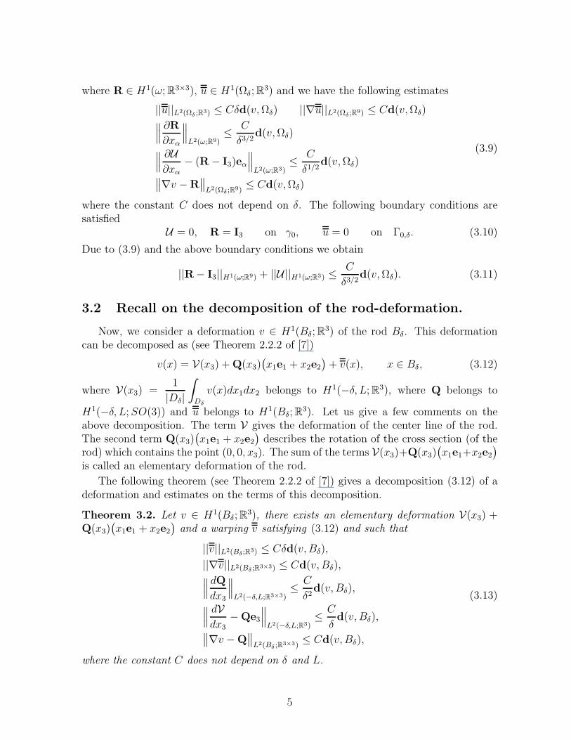
3.2 Recall on the decomposition of the rod-deformation.

Now, we consider a deformation v ∈ H1(Bδ;R3) of the rod Bδ. This deformation

can be decomposed as (see Theorem 2.2.2 of [7])

v(x) = V(x3) +Q(x3)(x1e1 + x2e2

)+ v(x), x ∈ Bδ, (3.12)

where V(x3) =1

|Dδ|

∫

Dδ

v(x)dx1dx2 belongs to H1(−δ, L;R3), where Q belongs to

H1(−δ, L;SO(3)) and u belongs to H1(Bδ;R3). Let us give a few comments on the

above decomposition. The term V gives the deformation of the center line of the rod.The second term Q(x3)

(x1e1 + x2e2

)describes the rotation of the cross section (of the

rod) which contains the point (0, 0, x3). The sum of the terms V(x3)+Q(x3)(x1e1+x2e2

)

is called an elementary deformation of the rod.

The following theorem (see Theorem 2.2.2 of [7]) gives a decomposition (3.12) of adeformation and estimates on the terms of this decomposition.

Theorem 3.2. Let v ∈ H1(Bδ;R3), there exists an elementary deformation V(x3) +

Q(x3)(x1e1 + x2e2

)and a warping v satisfying (3.12) and such that

||v||L2(Bδ;R3) ≤ Cδd(v, Bδ),

||∇v||L2(Bδ;R3×3) ≤ Cd(v, Bδ),∥∥∥ dQdx3

∥∥∥L2(−δ,L;R3×3)

≤ C

δ2d(v, Bδ),

∥∥∥ dVdx3

−Qe3

∥∥∥L2(−δ,L;R3)

≤ C

δd(v, Bδ),

∥∥∇v −Q∥∥L2(Bδ ;R3×3)

≤ Cd(v, Bδ),

(3.13)

where the constant C does not depend on δ and L.

5

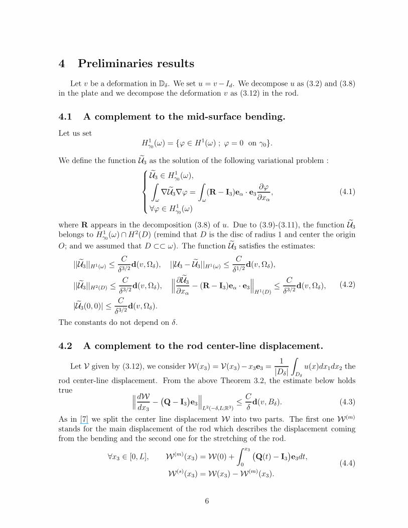
4 Preliminaries results

Let v be a deformation in Dδ. We set u = v− Id. We decompose u as (3.2) and (3.8)in the plate and we decompose the deformation v as (3.12) in the rod.

4.1 A complement to the mid-surface bending.

Let us setH1

γ0(ω) = ϕ ∈ H1(ω) ; ϕ = 0 on γ0.

We define the function U3 as the solution of the following variational problem :

U3 ∈ H1γ0(ω),∫

ω

∇U3∇ϕ =

∫

ω

(R− I3)eα · e3∂ϕ

∂xα,

∀ϕ ∈ H1γ0(ω)

(4.1)

where R appears in the decomposition (3.8) of u. Due to (3.9)-(3.11), the function U3

belongs to H1γ0(ω)∩H2(D) (remind that D is the disc of radius 1 and center the origin

O; and we assumed that D ⊂⊂ ω). The function U3 satisfies the estimates:

||U3||H1(ω) ≤C

δ3/2d(v,Ωδ), ||U3 − U3||H1(ω) ≤

C

δ1/2d(v,Ωδ),

||U3||H2(D) ≤C

δ3/2d(v,Ωδ),

∥∥∥∂U3

∂xα− (R− I3)eα · e3

∥∥∥H1(D)

≤ C

δ3/2d(v,Ωδ),

|U3(0, 0)| ≤C

δ3/2d(v,Ωδ).

(4.2)

The constants do not depend on δ.

4.2 A complement to the rod center-line displacement.

Let V given by (3.12), we consider W(x3) = V(x3)−x3e3 =1

|Dδ|

∫

Dδ

u(x)dx1dx2 the

rod center-line displacement. From the above Theorem 3.2, the estimate below holdstrue ∥∥∥dW

dx3−

(Q− I3

)e3

∥∥∥L2(−δ,L;R3)

≤ C

δd(v, Bδ). (4.3)

As in [7] we split the center line displacement W into two parts. The first one W(m)

stands for the main displacement of the rod which describes the displacement comingfrom the bending and the second one for the stretching of the rod.

∀x3 ∈ [0, L], W(m)(x3) = W(0) +

∫ x3

0

(Q(t)− I3

)e3dt,

W(s)(x3) = W(x3)−W(m)(x3).

(4.4)

6

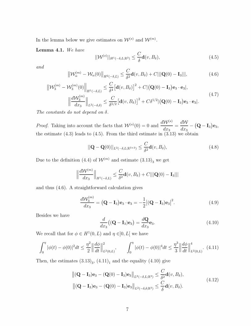
In the lemma below we give estimates on W(s) and W(m).

Lemma 4.1. We have

||W(s)||H1(−δ,L;R3) ≤C

δd(v, Bδ), (4.5)

and ∥∥W(m)α −Wα(0)

∥∥H2(−δ,L)

≤ C

δ2d(v, Bδ) + C|||Q(0)− I3|||, (4.6)

∥∥W(m)3 −W(m)

3 (0)∥∥∥H1(−δ,L)

≤ C

δ4[d(v, Bδ)

]2+ C|

(Q(0)− I3

)e3 · e3|,

∥∥∥dW(m)3

dx3

∥∥∥L2(−δ,δ)

≤ C

δ5/2[d(v, Bδ)

]2+ Cδ1/2|

(Q(0)− I3

)e3 · e3|.

(4.7)

The constants do not depend on δ.

Proof. Taking into account the facts that W(s)(0) = 0 anddW(s)

dx3=dWdx3

−(Q− I3

)e3,

the estimate (4.3) leads to (4.5). From the third estimate in (3.13) we obtain

||Q−Q(0)||L2(−δ,L;R3×3) ≤C

δ2d(v, Bδ), (4.8)

Due to the definition (4.4) of W(m) and estimate (3.13)3 we get

∥∥∥dW(m)

dx3

∥∥∥H1(−δ,L)

≤ C

δ2d(v, Bδ) + C|||Q(0)− I3|||

and thus (4.6). A straightforward calculation gives

dW(m)3

dx3=

(Q− I3

)e3 · e3 = −1

2

∣∣(Q− I3)e3∣∣2. (4.9)

Besides we haved

dx3

((Q− I3)e3

)=dQ

dx3e3. (4.10)

We recall that for φ ∈ H1(0, L) and η ∈]0, L[ we have

∫ η

0

|φ(t)− φ(0)|2dt ≤ η2

2

∥∥∥dφdt

∥∥∥2

L2(0,L),

∫ η

0

|φ(t)− φ(0)|4dt ≤ η3

3

∥∥∥dφdt

∥∥∥4

L2(0,L). (4.11)

Then, the estimates (3.13)3, (4.11)1 and the equality (4.10) give

∥∥(Q− I3)e3 − (Q(0)− I3)e3∥∥L2(−δ,L;R3)

≤ C

δ2d(v, Bδ),

∥∥(Q− I3)e3 − (Q(0)− I3)e3∥∥L2(−δ,δ;R3)

≤ C

δd(v, Bδ).

(4.12)

7

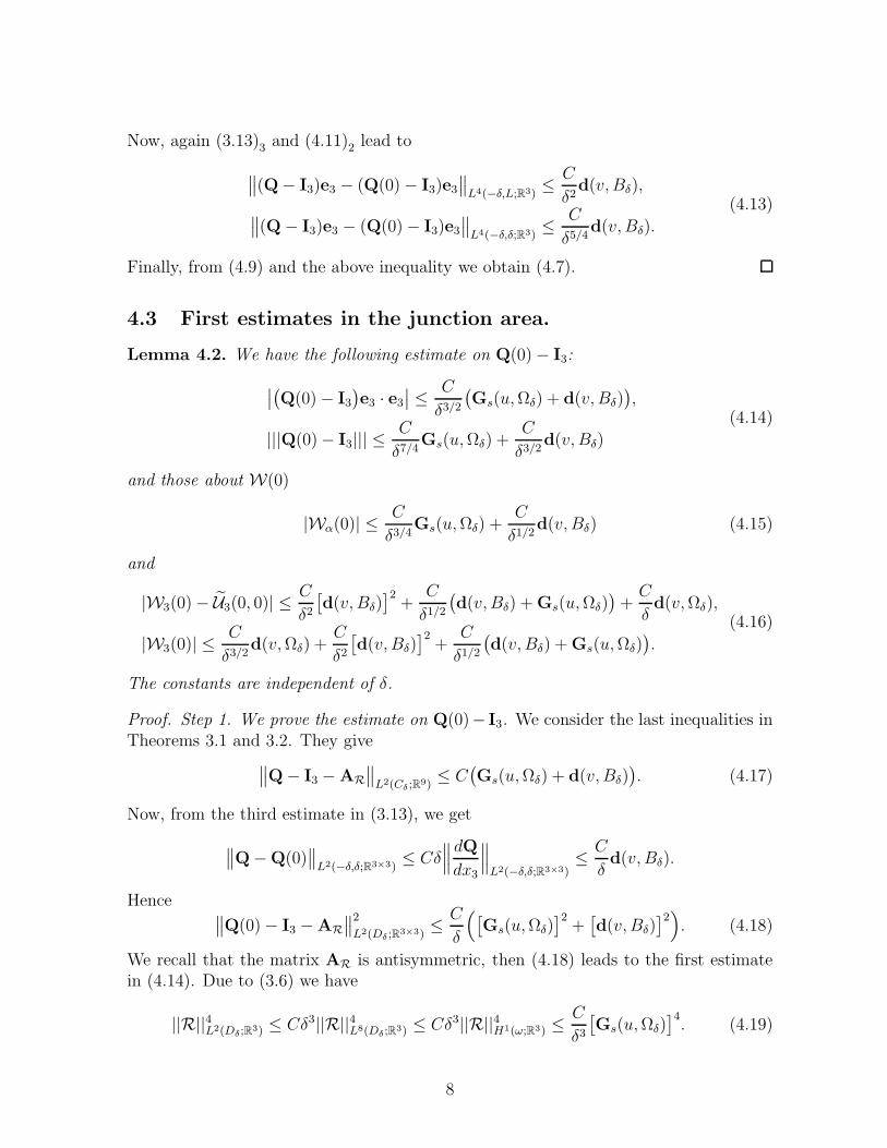
Now, again (3.13)3 and (4.11)2 lead to

∥∥(Q− I3)e3 − (Q(0)− I3)e3∥∥L4(−δ,L;R3)

≤ C

δ2d(v, Bδ),

∥∥(Q− I3)e3 − (Q(0)− I3)e3∥∥L4(−δ,δ;R3)

≤ C

δ5/4d(v, Bδ).

(4.13)

Finally, from (4.9) and the above inequality we obtain (4.7).

4.3 First estimates in the junction area.

Lemma 4.2. We have the following estimate on Q(0)− I3:

∣∣(Q(0)− I3)e3 · e3

∣∣ ≤ C

δ3/2(Gs(u,Ωδ) + d(v, Bδ)

),

|||Q(0)− I3||| ≤C

δ7/4Gs(u,Ωδ) +

C

δ3/2d(v, Bδ)

(4.14)

and those about W(0)

|Wα(0)| ≤C

δ3/4Gs(u,Ωδ) +

C

δ1/2d(v, Bδ) (4.15)

and

|W3(0)− U3(0, 0)| ≤C

δ2[d(v, Bδ)

]2+

C

δ1/2(d(v, Bδ) +Gs(u,Ωδ)

)+C

δd(v,Ωδ),

|W3(0)| ≤C

δ3/2d(v,Ωδ) +

C

δ2[d(v, Bδ)

]2+

C

δ1/2(d(v, Bδ) +Gs(u,Ωδ)

).

(4.16)

The constants are independent of δ.

Proof. Step 1. We prove the estimate on Q(0)− I3. We consider the last inequalities inTheorems 3.1 and 3.2. They give

∥∥Q− I3 −AR

∥∥L2(Cδ ;R9)

≤ C(Gs(u,Ωδ) + d(v, Bδ)

). (4.17)

Now, from the third estimate in (3.13), we get

∥∥Q−Q(0)∥∥L2(−δ,δ;R3×3)

≤ Cδ∥∥∥dQdx3

∥∥∥L2(−δ,δ;R3×3)

≤ C

δd(v, Bδ).

Hence ∥∥Q(0)− I3 −AR

∥∥2

L2(Dδ;R3×3)≤ C

δ

([Gs(u,Ωδ)

]2+[d(v, Bδ)

]2). (4.18)

We recall that the matrix AR is antisymmetric, then (4.18) leads to the first estimatein (4.14). Due to (3.6) we have

||R||4L2(Dδ;R3) ≤ Cδ3||R||4L8(Dδ;R3) ≤ Cδ3||R||4H1(ω;R3) ≤C

δ3[Gs(u,Ωδ)

]4. (4.19)

8

Then, using the above estimate and (4.18) we deduce the second estimate in (4.14).

Step 2. We prove the estimate (4.15) on Wα(0).

The two decompositions of u = v − Id ((3.2) and (3.12)) give, for a.e. x ∈ Cδ

U(x1, x2) + x3R(x1, x2) ∧ e3 + u(x)

=W(x3) + (Q(x3)− I3)(x1e1 + x2e2) + v(x).(4.20)

Taking the averages on the cylinder Cδ of the terms in this equality (4.20) give

MDδ

(U)=

1

|Dδ|

∫

Dδ

U(x1, x2)dx1dx2 = MIδ

(W

)=

1

2δ

∫ δ

−δ

W(x3)dx3. (4.21)

Besides, proceeding as for R in (4.19) and from (3.6) we have

||Uα||L2(Dδ) ≤ Cδ1/4Gs(u,Ωδ).

From this estimate we get

|MIδ

(Wα

)| = |MDδ

(Uα

)| ≤ C

δ3/4Gs(u,Ωδ). (4.22)

We set yα(x3) = Wα(x3)− x3(Q(0)− I3)e3 · eα. The estimates (4.3) and (4.12) lead to

∥∥∥dyαdx3

∥∥∥L2(−δ,δ)

≤ C

δd(v, Bδ)

which in turn implies ∥∥yα − yα(0)∥∥L2(−δ,δ)

≤ Cd(v, Bδ).

Taking the average, it yields

|MIδ

(Wα

)−Wα(0)| ≤

C

δ1/2d(v, Bδ). (4.23)

Finally, from (4.22) and (4.23) we obtain (4.15).

Step 3. We prove the estimate on W3(0). Using (4.2) we deduce that

||U3 − U3||L2(Dδ) ≤ Cδ1/2||U3 − U3||L4(ω)

≤ Cδ1/2||U3 − U3||H1(ω) ≤ Cd(v,Ωδ).(4.24)

Then we replace U3 with U3 and W3 with W(m)3 in (4.21). Taking into account (4.5) we

obtain

|MDδ

(U3

)−MIδ

(W(m)

3

)| ≤ C

δd(v,Ωδ) +

C

δ1/2d(v, Bδ). (4.25)

We carry on by comparing MDδ

(U3

)with U3(0, 0). Let us set

rα =1

πδ2

∫

Dδ

(R(x1, x2)− I3

)eα · e3 dx1dx2

9

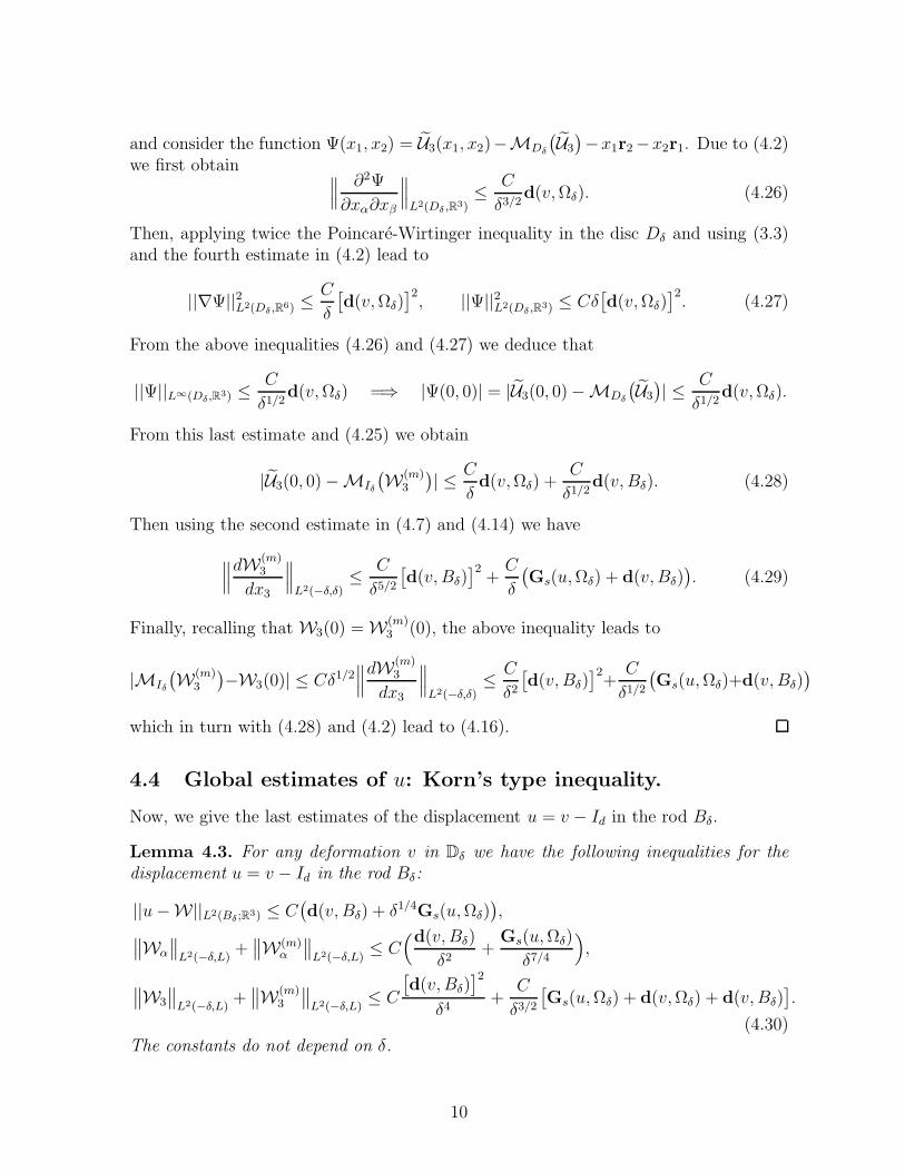
and consider the function Ψ(x1, x2) = U3(x1, x2)−MDδ

(U3

)−x1r2−x2r1. Due to (4.2)

we first obtain ∥∥∥ ∂2Ψ

∂xα∂xβ

∥∥∥L2(Dδ ,R3)

≤ C

δ3/2d(v,Ωδ). (4.26)

Then, applying twice the Poincare-Wirtinger inequality in the disc Dδ and using (3.3)and the fourth estimate in (4.2) lead to

||∇Ψ||2L2(Dδ ,R6) ≤C

δ

[d(v,Ωδ)

]2, ||Ψ||2L2(Dδ,R3) ≤ Cδ

[d(v,Ωδ)

]2. (4.27)

From the above inequalities (4.26) and (4.27) we deduce that

||Ψ||L∞(Dδ,R3) ≤C

δ1/2d(v,Ωδ) =⇒ |Ψ(0, 0)| = |U3(0, 0)−MDδ

(U3

)| ≤ C

δ1/2d(v,Ωδ).

From this last estimate and (4.25) we obtain

|U3(0, 0)−MIδ

(W(m)

3

)| ≤ C

δd(v,Ωδ) +

C

δ1/2d(v, Bδ). (4.28)

Then using the second estimate in (4.7) and (4.14) we have

∥∥∥dW(m)3

dx3

∥∥∥L2(−δ,δ)

≤ C

δ5/2[d(v, Bδ)

]2+C

δ

(Gs(u,Ωδ) + d(v, Bδ)

). (4.29)

Finally, recalling that W3(0) = W(m)3 (0), the above inequality leads to

|MIδ

(W(m)

3

)−W3(0)| ≤ Cδ1/2

∥∥∥dW(m)3

dx3

∥∥∥L2(−δ,δ)

≤ C

δ2[d(v, Bδ)

]2+C

δ1/2(Gs(u,Ωδ)+d(v, Bδ)

)

which in turn with (4.28) and (4.2) lead to (4.16).

4.4 Global estimates of u: Korn’s type inequality.

Now, we give the last estimates of the displacement u = v − Id in the rod Bδ.

Lemma 4.3. For any deformation v in Dδ we have the following inequalities for the

displacement u = v − Id in the rod Bδ:

||u−W||L2(Bδ;R3) ≤ C(d(v, Bδ) + δ1/4Gs(u,Ωδ)

),

∥∥Wα

∥∥L2(−δ,L)

+∥∥W(m)

α

∥∥L2(−δ,L)

≤ C(d(v, Bδ)

δ2+

Gs(u,Ωδ)

δ7/4

),

∥∥W3

∥∥L2(−δ,L)

+∥∥W(m)

3

∥∥L2(−δ,L)

≤ C

[d(v, Bδ)

]2

δ4+

C

δ3/2[Gs(u,Ωδ) + d(v,Ωδ) + d(v, Bδ)

].

(4.30)The constants do not depend on δ.

10

Proof. From (4.8) and (4.14) we get

∥∥Q− I3∥∥L2(−δ,L;R3×3)

≤ C(d(v, Bδ)

δ2+

Gs(u,Ωδ)

δ7/4

). (4.31)

Then, from (3.13) and the above inequality we deduce that

||u−W||L2(Bδ;R3) ≤ C(d(v, Bδ) + δ1/4Gs(u,Ωδ)

). (4.32)

From (4.6) again (4.14) and (4.15) we obtain

∥∥W(m)α

∥∥H1(−δ,L)

≤ C

δ2d(v, Bδ) +

C

δ7/4Gs(u,Ωδ). (4.33)

Then since W = W(m) +W(s), (4.5) and (4.33) give the second estimate in (4.30).

From (4.7) and (4.14) we deduce that

∥∥∥dW(m)3

dx3

∥∥∥L2(−δ,L)

≤ C

δ4[d(v, Bδ)

]2+

C

δ3/2[Gs(u,Ωδ) + d(v, Bδ)

].

which in turn using (4.16) lead to

∥∥W(m)3

∥∥L2(−δ,L)

≤ C

δ4[d(v, Bδ)

]2+

C

δ3/2[Gs(u,Ωδ) + d(v,Ωδ) + d(v, Bδ)

]

and then due to (4.5) we get the last estimate in (4.30).

Corollary 4.4. For any deformation v in Dδ we have the following Korn’s type inequal-

ity for the displacement u = v − Id in the rod Bδ:

∥∥∇u∥∥L2(Bδ ;R3×3)

≤ C

δd(v, Bδ) +

C

δ3/4Gs(u,Ωδ),

||uα||L2(Bδ) ≤C

δd(v, Bδ) +

C

δ3/4Gs(u,Ωδ),

||u3||L2(Bδ) ≤ C

[d(v, Bδ)

]2

δ3+

C

δ1/2[Gs(u,Ωδ) + d(v,Ωδ) + d(v, Bδ)

].

(4.34)

The constants do not depend on δ.

Proof. From (3.13) and (4.31) we obtain

∥∥∇u∥∥L2(Bδ ;R3×3)

≤ C

δd(v, Bδ) +

C

δ3/4Gs(u,Ωδ). (4.35)

The second and third inequalities are immediate consequences of Lemma 4.3.

11

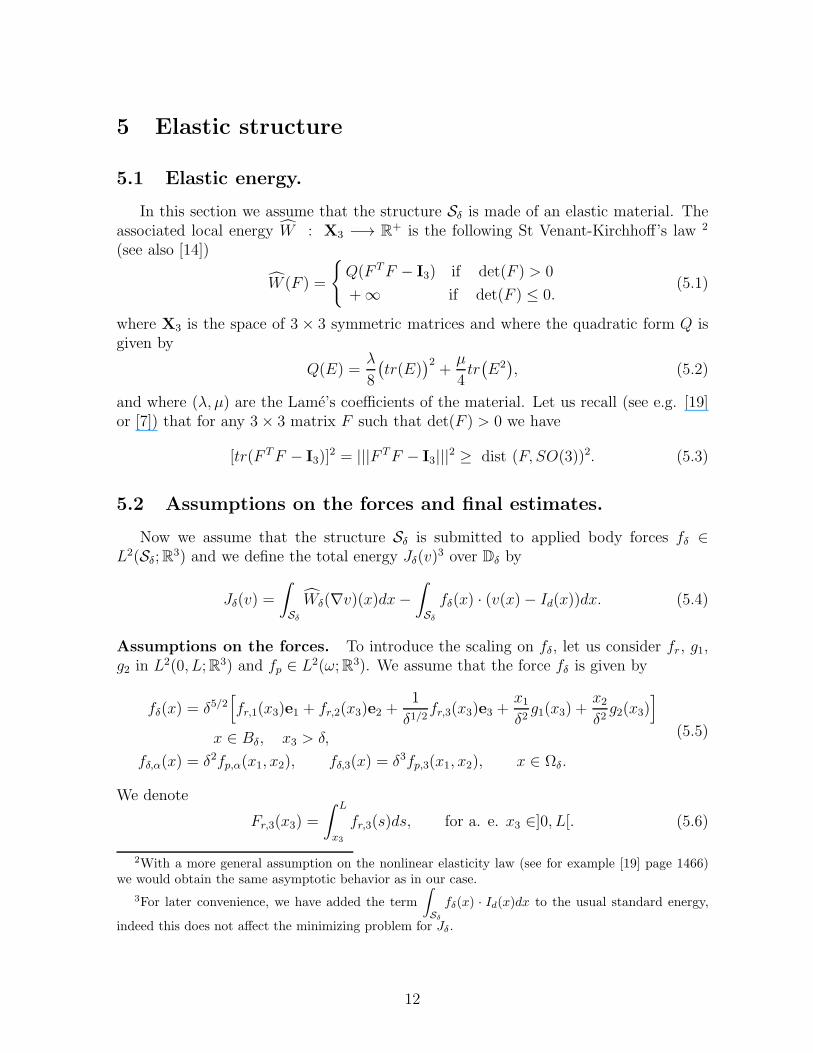
5 Elastic structure

5.1 Elastic energy.

In this section we assume that the structure Sδ is made of an elastic material. Theassociated local energy W : X3 −→ R

+ is the following St Venant-Kirchhoff’s law 2

(see also [14])

W (F ) =

Q(F TF − I3) if det(F ) > 0

+∞ if det(F ) ≤ 0.(5.1)

where X3 is the space of 3 × 3 symmetric matrices and where the quadratic form Q isgiven by

Q(E) =λ

8

(tr(E)

)2+µ

4tr(E2

), (5.2)

and where (λ, µ) are the Lame’s coefficients of the material. Let us recall (see e.g. [19]or [7]) that for any 3× 3 matrix F such that det(F ) > 0 we have

[tr(F TF − I3)]2 = |||F TF − I3|||2 ≥ dist (F, SO(3))2. (5.3)

5.2 Assumptions on the forces and final estimates.

Now we assume that the structure Sδ is submitted to applied body forces fδ ∈L2(Sδ;R

3) and we define the total energy Jδ(v)3 over Dδ by

Jδ(v) =

∫

Sδ

Wδ(∇v)(x)dx−∫

Sδ

fδ(x) · (v(x)− Id(x))dx. (5.4)

Assumptions on the forces. To introduce the scaling on fδ, let us consider fr, g1,g2 in L2(0, L;R3) and fp ∈ L2(ω;R3). We assume that the force fδ is given by

fδ(x) = δ5/2[fr,1(x3)e1 + fr,2(x3)e2 +

1

δ1/2fr,3(x3)e3 +

x1δ2g1(x3) +

x2δ2g2(x3)

]

x ∈ Bδ, x3 > δ,

fδ,α(x) = δ2fp,α(x1, x2), fδ,3(x) = δ3fp,3(x1, x2), x ∈ Ωδ.

(5.5)

We denote

Fr,3(x3) =

∫ L

x3

fr,3(s)ds, for a. e. x3 ∈]0, L[. (5.6)

2With a more general assumption on the nonlinear elasticity law (see for example [19] page 1466)we would obtain the same asymptotic behavior as in our case.

3For later convenience, we have added the term

∫

Sδ

fδ(x) · Id(x)dx to the usual standard energy,

indeed this does not affect the minimizing problem for Jδ.

12

Theorem 5.1. There exist two constants C0 and C1, which depend only on ω, L and

µ, such that if

||fp||L2(Ω;R3) ≤ C0 (5.7)

and if eitherCase 1: for a. e. x3 ∈]0, L[, Fr,3(x3) ≥ 0,

or

Case 2: ||fr,3||L2(0,L) ≤ C1

(5.8)

then for δ small enough and for any v ∈ Dδ satisfying Jδ(v) ≤ 0 we have

d(v, Bδ) + d(v,Ωδ) ≤ Cδ5/2 (5.9)

where the constant does not depend on δ.

Proof. From (3.7) and the assumptions (5.5) on the body forces, we obtain on the onehand for any v ∈ Dδ and with u = v − Id

∣∣∣∫

Ωδ

fδ(x) · u(x)dx∣∣∣ ≤ Cδ5/2||fp||L2(ω;R3)Gs(u,Ωδ). (5.10)

As far as the term involving the forces in the rod are concerned we first have

∫

Bδ

fδ(x) · u(x)dx = πδ9/2∫ L

δ

fr,α(x3)Wα(x3)dx3 + πδ4∫ L

δ

fr,3(x3)W3(x3)dx3

+

∫

Bδ

fδ(x) · (u(x)−W(x3))dx.

Then, using Lemma 4.3 and (5.5) we first get

∣∣∣∫ L

δ

fr,α(x3)Wα(x3)dx3

∣∣∣ ≤ C

δ2

2∑

α=1

||fr,α||L2(0,L)

(d(v, Bδ) + δ1/4Gs(u,Ωδ)

),

∣∣∣∫

Bδ

fδ(x) ·(u(x)−W(x3)

)dx

∣∣∣ ≤ Cδ5/2(||g1||L2(0,L;R3) + ||g2||L2(0,L;R3)

)

(d(v, Bδ) + δ1/4Gs(u,Ωδ)

)

(5.11)

Now we estimate

∫ L

δ

fr,3W3(x3)dx3. From (4.5) we first obtain

∣∣∣∫ L

δ

fr,3(x3)W(s)3 (x3)dx3

∣∣∣ ≤ C

δ||fr,3||L2(0,L)d(v, Bδ). (5.12)

Then we have

∫ L

δ

fr,3(x3)W(m)3 (x3)dx3 = Fr,3(δ)W(m)

3 (δ) +

∫ L

δ

Fr,3(x3)dW(m)

3

dx3(x3)dx3. (5.13)

13

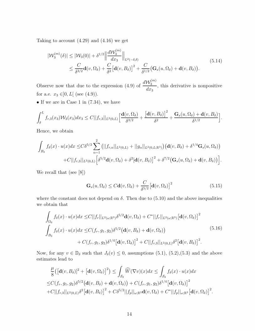
Taking to account (4.29) and (4.16) we get

|W(m)3 (δ)| ≤ |W3(0)|+ δ1/2

∥∥∥dW(m)3

dx3

∥∥∥L2(−δ,δ)

≤ C

δ3/2d(v,Ωδ) +

C

δ2[d(v, Bδ)

]2+

C

δ1/2(Gs(u,Ωδ) + d(v, Bδ)

).

(5.14)

Observe now that due to the expression (4.9) ofdW(m)

3

dx3, this derivative is nonpositive

for a.e. x3 ∈]0, L[ (see (4.9)).

• If we are in Case 1 in (7.34), we have

∫ L

δ

fr,3(x3)W3(x3)dx3 ≤ C||fr,3||L2(0,L)

[d(v,Ωδ)

δ3/2+

[d(v, Bδ)

]2

δ2+

Gs(u,Ωδ) + d(v, Bδ)

δ1/2

].

Hence, we obtain

∫

Bδ

fδ(x) · u(x)dx ≤Cδ5/22∑

α=1

(||fr,α||L2(0,L) + ||gα||L2(0,L;R3)

)(d(v, Bδ) + δ1/4Gs(u,Ωδ)

)

+C||fr,3||L2(0,L)

[δ5/2d(v,Ωδ) + δ2[d(v, Bδ)

]2+ δ7/2

(Gs(u,Ωδ) + d(v, Bδ)

)].

We recall that (see [8])

Gs(u,Ωδ) ≤ Cd(v,Ωδ) +C

δ5/2[d(v,Ωδ)

]2(5.15)

where the constant does not depend on δ. Then due to (5.10) and the above inequalitieswe obtain that

∫

Ωδ

fδ(x) · u(x)dx ≤C||fr||L2(ω;R3)δ5/2d(v,Ωδ) + C∗||fr||L2(ω;R3)

[d(v,Ωδ)

]2

∫

Bδ

fδ(x) · u(x)dx ≤C(fr, g1, g2)δ5/2(d(v, Bδ) + d(v,Ωδ)

)

+ C(fr, g1, g2)δ1/4

[d(v,Ωδ)

]2+ C||fr,3||L2(0,L)δ

2[d(v, Bδ)

]2.

(5.16)

Now, for any v ∈ Dδ such that Jδ(v) ≤ 0, assumptions (5.1), (5.2),(5.3) and the aboveestimates lead to

µ

8

([d(v, Bδ)]

2 +[d(v,Ωδ)

]2) ≤∫

Sδ

W (∇v)(x)dx ≤∫

Sδ

fδ(x) · u(x)dx

≤C(fr, g1, g2)δ5/2(d(v, Bδ) + d(v,Ωδ)

)+ C(fr, g1, g2)δ

1/4[d(v,Ωδ)

]2

+C||fr,3||L2(0,L)δ2[d(v, Bδ)

]2+ Cδ5/2||fp||ω;R3d(v,Ωδ) + C∗||fp||ω;R3

[d(v,Ωδ)

]2.

14

wich in turn gives(µ8− C||fr,3||L2(0,L)δ

2)[

d(v, Bδ)]2 +

(µ8− C∗||fp||ω;R3 − C(fr, g1, g2)δ

1/4)[

d(v,Ωδ)]2

≤C(fr, g1, g2)δ5/2(d(v, Bδ) + d(v,Ωδ)

)+ Cδ5/2||fp||ω;R3d(v,Ωδ).

Indeed the two quantities C||fr,3||L2(0,L)δ2 and C(fr, g1, g2)δ

1/4 tend to 0 as δ tends to0, then, under the condition C∗||fp||L2(ω;R3) ≤ µ/32 and for δ small enough we obtain

d(v, Bδ) + d(v,Ωδ) ≤ Cδ5/2.

The constant does not depend on δ.

• If we are in Case 2 in (7.34), from (4.30) we immediately have

∫ L

δ

fr,3(x3)W3(x3)dx3 ≤ C||fr,3||L2(0,L)

[[d(v, Bδ)]2

δ4+

Gs(u,Ωδ) + d(v,Ωδ) + d(v, Bδ)

δ3/2

].

Then, proceeding as in Case 1 leads to

∫

Bδ

fδ(x) · u(x)dx ≤Cδ5/22∑

α=1

(||fr,α||L2(0,L) + ||gα||L2(0,L;R3)

)(d(v, Bδ) + δ1/4Gs(u,Ωδ)

)

+ C||fr,3||L2(0,L)

[[d(v, Bδ)

]2+ δ5/2

(Gs(u,Ωδ) + d(v,Ωδ) + d(v, Bδ)

)].

(5.17)Then for δ small enough, we get

µ

8

([d(v, Bδ)]

2 +[d(v,Ωδ)

]2) ≤∫

Sδ

W (∇v)(x)dx ≤∫

Sδ

fδ(x) · u(x)dx

≤ Cδ5/2C(f, g)(d(v, Bδ) + d(v,Ωδ)

)+ C∗∗||fr,3||L2(0,L)

[[d(v, Bδ)

]2+[d(v,Ωδ)

]2]

+ Cδ5/2||fp||ω;R3d(v,Ωδ) + C∗||fp||ω;R3

[d(v,Ωδ)

]2.

Hence, under the conditions C∗||fp||L2(ω;R3) ≤ µ/32 and C∗∗||fr,3||L2(0,L) ≤ µ/32 wededuce that

d(v, Bδ) + d(v,Ωδ) ≤ Cδ5/2.

In the both cases, we finally obtain (5.9)

As a consequence of Theorem 5.1 and estimates (5.16)-(5.17), we deduce that for δsmall enough and for any v ∈ Dδ satisfying Jδ(v) ≤ 0 we have (u = v − Id)

∫

Sδ

fδ · u ≤ Cδ5,

∫

Sδ

Wδ(∇v)(x)dx ≤ Cδ5. (5.18)

From (5.18) we also obtain for any v ∈ Dδ such that Jδ(v) ≤ 0

cδ5 ≤ Jδ(v) (5.19)

15

where c is a nonpositive constant which does not depend on δ. We set

mδ = infv∈Dδ

Jδ(v).

As a consequence of (5.19) we have

c ≤ mδ

δ5≤ 0. (5.20)

In general, a minimizer of Jδ does not exist on Dδ.

6 Asymptotic behavior of a sequence of deforma-

tions of the whole structure Sδ.In this subsection and the following one, we consider a sequence of deformations (vδ)

belonging to Dδ and satisfying

d(vδ, Bδ) + d(vδ,Ωδ) ≤ Cδ5/2 (6.1)

where the constant does not depend on δ. Setting uδ = vδ − Id, then, due to (6.1) and(5.15) we obtain that

Gs(uδ,Ωδ) ≤ Cδ5/2. (6.2)

For any open subset O ⊂ R2 and for any field ψ ∈ H1(O;R3), we denote

γαβ(ψ) =1

2

(∂ψα

∂xβ+∂ψβ

∂xα

), (α, β) ∈ 1, 2. (6.3)

6.1 The rescaling operators

Before rescaling the domains, we introduce the reference domain Ω for the plate andthe one B for the rod

Ω = ω×]− 1, 1[, B = D×]0, L[= D(O, 1)×]0, L[.

As usual when dealing with thin structures, we rescale Ωδ and Bδ using -for the plate-the operator

Πδ(w)(x1, x2, X3) = w(x1, x2, δX3) for any (x1, x2, X3) ∈ Ω

defined for e.g. w ∈ L2(Ωδ) for which Πδ(w) ∈ L2(Ω) and using -for the rod- the operator

Pδ(w)(X1, X2, x3) = w(δX1, δX2, x3) for any (X1, X2, x3) ∈ B

defined for e.g. w ∈ L2(Bδ) for which Pδ(w) ∈ L2(B).

16

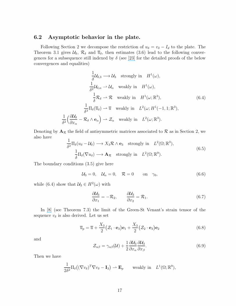
6.2 Asymptotic behavior in the plate.

Following Section 2 we decompose the restriction of uδ = vδ − Id to the plate. TheTheorem 3.1 gives Uδ, Rδ and uδ, then estimates (3.6) lead to the following conver-gences for a subsequence still indexed by δ (see [23] for the detailed proofs of the belowconvergences and equalities)

1

δUδ,3 −→ U3 strongly in H1(ω),

1

δ2Uδ,α Uα weakly in H1(ω),

1

δRδ R weakly in H1(ω;R3),

1

δ3Πδ(uδ) u weakly in L2(ω;H1(−1, 1;R3),

1

δ2

(∂Uδ

∂xα−Rδ ∧ eα

) Zα weakly in L2(ω;R3).

(6.4)

Denoting by AR the field of antisymmetric matrices associated to R as in Section 2, wealso have

1

δ2Πδ(uδ − Uδ) −→ X3R ∧ e3 strongly in L2(Ω;R3),

1

δΠδ(∇uδ) −→ AR strongly in L2(Ω;R9).

(6.5)

The boundary conditions (3.5) give here

U3 = 0, Uα = 0, R = 0 on γ0, (6.6)

while (6.4) show that U3 ∈ H2(ω) with

∂U3

∂x1= −R2,

∂U3

∂x2= R1. (6.7)

In [8] (see Theorem 7.3) the limit of the Green-St Venant’s strain tensor of thesequence vδ is also derived. Let us set

up = u+X3

2

(Z1 · e3

)e1 +

X3

2

(Z2 · e3

)e2 (6.8)

and

Zαβ = γαβ(U) +1

2

∂U3

∂xα

∂U3

∂xβ. (6.9)

Then we have

1

2δ2Πδ

((∇vδ)T∇vδ − I3

) Ep weakly in L1(Ω;R9),

17

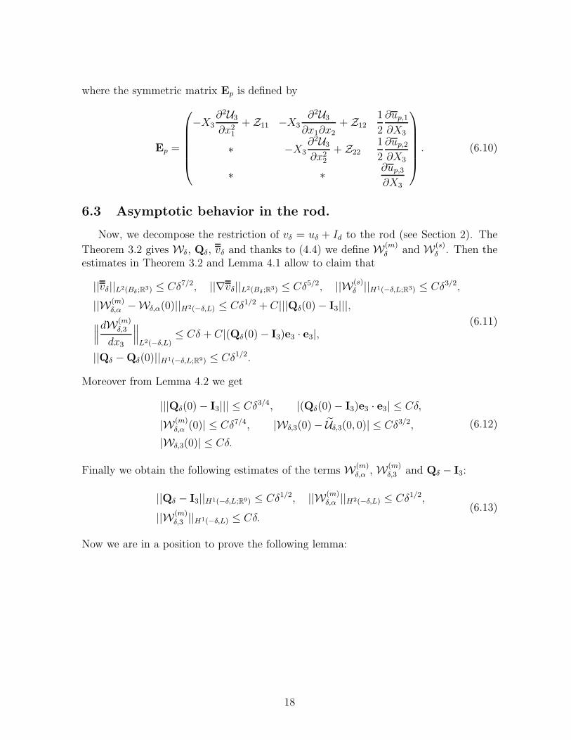
where the symmetric matrix Ep is defined by

Ep =

−X3∂2U3

∂x21+ Z11 −X3

∂2U3

∂x1∂x2+ Z12

1

2

∂up,1∂X3

∗ −X3∂2U3

∂x22+ Z22

1

2

∂up,2∂X3

∗ ∗ ∂up,3∂X3

. (6.10)

6.3 Asymptotic behavior in the rod.

Now, we decompose the restriction of vδ = uδ + Id to the rod (see Section 2). The

Theorem 3.2 gives Wδ, Qδ, vδ and thanks to (4.4) we define W(m)δ and W(s)

δ . Then theestimates in Theorem 3.2 and Lemma 4.1 allow to claim that

||vδ||L2(Bδ ;R3) ≤ Cδ7/2, ||∇vδ||L2(Bδ ;R3) ≤ Cδ5/2, ||W(s)δ ||H1(−δ,L;R3) ≤ Cδ3/2,

||W(m)δ,α −Wδ,α(0)||H2(−δ,L) ≤ Cδ1/2 + C|||Qδ(0)− I3|||,

∥∥∥dW(m)

δ,3

dx3

∥∥∥L2(−δ,L)

≤ Cδ + C|(Qδ(0)− I3)e3 · e3|,

||Qδ −Qδ(0)||H1(−δ,L;R9) ≤ Cδ1/2.

(6.11)

Moreover from Lemma 4.2 we get

|||Qδ(0)− I3||| ≤ Cδ3/4, |(Qδ(0)− I3)e3 · e3| ≤ Cδ,

|W(m)δ,α (0)| ≤ Cδ7/4, |Wδ,3(0)− Uδ,3(0, 0)| ≤ Cδ3/2,

|Wδ,3(0)| ≤ Cδ.

(6.12)

Finally we obtain the following estimates of the terms W(m)δ,α , W(m)

δ,3 and Qδ − I3:

||Qδ − I3||H1(−δ,L;R9) ≤ Cδ1/2, ||W(m)δ,α ||H2(−δ,L) ≤ Cδ1/2,

||W(m)δ,3 ||H1(−δ,L) ≤ Cδ.

(6.13)

Now we are in a position to prove the following lemma:

18

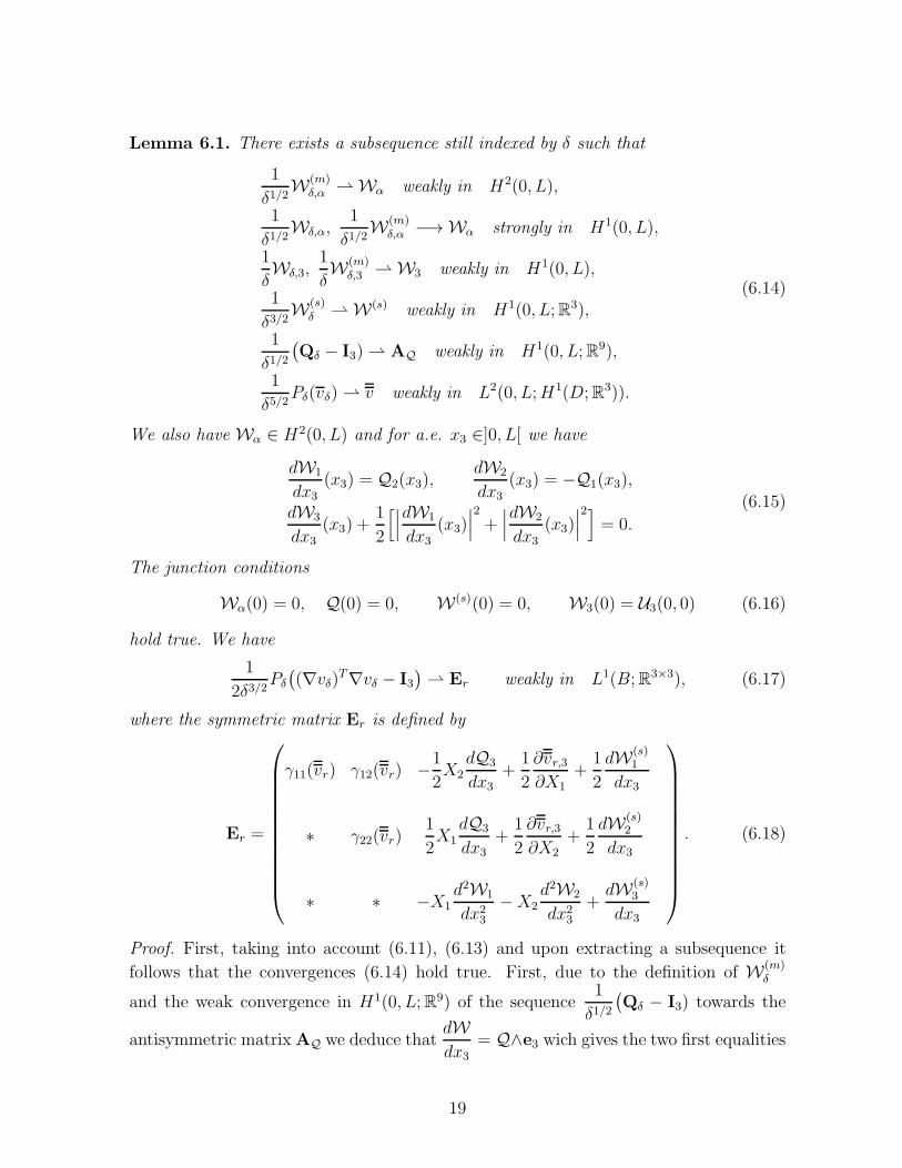
Lemma 6.1. There exists a subsequence still indexed by δ such that

1

δ1/2W(m)

δ,α Wα weakly in H2(0, L),

1

δ1/2Wδ,α,

1

δ1/2W(m)

δ,α −→ Wα strongly in H1(0, L),

1

δWδ,3,

1

δW(m)

δ,3 W3 weakly in H1(0, L),

1

δ3/2W(s)

δ W(s) weakly in H1(0, L;R3),

1

δ1/2(Qδ − I3) AQ weakly in H1(0, L;R9),

1

δ5/2Pδ(vδ) v weakly in L2(0, L;H1(D;R3)).

(6.14)

We also have Wα ∈ H2(0, L) and for a.e. x3 ∈]0, L[ we have

dW1

dx3(x3) = Q2(x3),

dW2

dx3(x3) = −Q1(x3),

dW3

dx3(x3) +

1

2

[∣∣∣dW1

dx3(x3)

∣∣∣2

+∣∣∣dW2

dx3(x3)

∣∣∣2]

= 0.

(6.15)

The junction conditions

Wα(0) = 0, Q(0) = 0, W(s)(0) = 0, W3(0) = U3(0, 0) (6.16)

hold true. We have

1

2δ3/2Pδ

((∇vδ)T∇vδ − I3

) Er weakly in L1(B;R3×3), (6.17)

where the symmetric matrix Er is defined by

Er =

γ11(vr) γ12(vr) −1

2X2

dQ3

dx3+

1

2

∂vr,3∂X1

+1

2

dW(s)1

dx3

∗ γ22(vr)1

2X1

dQ3

dx3+

1

2

∂vr,3∂X2

+1

2

dW(s)2

dx3

∗ ∗ −X1d2W1

dx23−X2

d2W2

dx23+dW(s)

3

dx3

. (6.18)

Proof. First, taking into account (6.11), (6.13) and upon extracting a subsequence it

follows that the convergences (6.14) hold true. First, due to the definition of W(m)δ

and the weak convergence in H1(0, L;R9) of the sequence1

δ1/2(Qδ − I3) towards the

antisymmetric matrixAQ we deduce thatdWdx3

= Q∧e3 wich gives the two first equalities

19

in (6.15). Then, the strong convergence in L∞(0, L;R3) of the sequence1

δ1/2(Qδ − I3)e3

towards Q∧e3, hence1

δ|(Qδ−I3)e3|2 convergences towards |Q∧e3|2 =

∣∣∣dW1

dx3

∣∣∣2

+∣∣∣dW2

dx3

∣∣∣2

strongly in L∞(0, L). Finally using equality (4.9) we obtain the last equality in (6.15).The junction conditions on Q and Wα are immediate consequences of (6.12) and theconvergences (6.14).

In order to obtain the junction condition between the bending in the plate and the

stretching in the rod note first that the sequence1

δUδ,3 converges strongly in H1(ω) to

U3 because of (4.2) and the first convergence in (6.4). Besides this sequence is uniformlybounded in H2(D), hence it converges strongly to the same limit U3 in C

0(D). Moreover

the weak convergence of the sequence1

δW(m)

δ,3 in H1(0, L), implies the convergence of

1

δW(m)

δ,3 (0) =1

δWδ,3(0) to W3(0). Using the third estimate in (6.12) gives the last

condition in (6.16).

Once the convergences (6.14) are established, the limit of the rescaled Green-StVenant strain tensor of the sequence vδ is analyzed in [7] (see Subsection 3.3) and itgives (6.18).

7 Asymptotic behavior of the sequencemδ

δ5.

The goal of this section is to establish Theorem 7.2. Let us first introduce a fewnotations. We set

D0 =(U ,W,Q3) ∈ H1(ω;R3)×H1(0, L;R3)×H1(0, L) |

U3 ∈ H2(ω), Wα ∈ H2(0, L), U = 0,∂U3

∂xα= 0 on γ0,

dW3

dx3+

1

2

[∣∣∣dW1

dx3

∣∣∣2

+∣∣∣dW2

dx3

∣∣∣2]

= 0 in ]0, L[,

W3(0) = U3(0, 0), Wα(0) =dWα

dx3(0) = Q3(0) = 0

(7.1)

Let us notice that D0 is a closed subset of H1(ω;R3)×H1(0, L;R3)×H1(0, L).

We introduce below the ”limit” elastic energies for the plate and the rod whoseexpressions are well known for such structures4

4E, ν are the Young modulus and the Poisson’s ratio of the plate and the rod.

20

Jp(U) =E

3(1− ν2)

∫

ω

[(1− ν)

2∑

α,β=1

∣∣∣ ∂2U3

∂xα∂xβ

∣∣∣2

+ ν(∆U3

)2]

+E

(1− ν2)

∫

ω

[(1− ν)

2∑

α,β=1

∣∣Zαβ

∣∣2 + ν(Z11 + Z22

)2],

Jr(W1,W2,Q3) =Eπ

8

∫ L

0

[∣∣∣d2W1

dx23

∣∣∣2

+∣∣∣d

2W2

dx23

∣∣∣2]

+µπ

8

∫ L

0

∣∣∣dQ3

dx3

∣∣∣2

(7.2)

where Zαβ is given by

Zαβ = γαβ(U) +1

2

∂U3

∂xα

∂U3

∂xβ.

The total energy of the plate-rod structure is given by the functional J defined over D0

J (U ,W,Q3) = Jp(U) + Jr(W1,W2,Q3)− L(U ,W,Q3) (7.3)

with

L(U ,W,Q3) = 2

∫

ω

fp · U + π

∫ L

0

fr · Wdx3 +π

2

∫ L

0

gα ·(Q ∧ eα

)dx3 (7.4)

where

Q = −dW2

dx3e1 +

dW1

dx3e2 +Q3e3.

Below we prove the existence of at least a minimizer of J .

Lemma 7.1. There exist two constants C∗p , C

∗r such that, if (fp,1, fp,2) satisfies

||fp,1||2L2(ω) + ||fp,2||2L2(ω) < C∗p (7.5)

and if fr,3 satisfies

||fr,3||L2(0,L) < C∗r (7.6)

then the minimization problem

min(U ,W ,Q3)∈D0

J (U ,W,Q3) (7.7)

admits at least a solution.

Proof. Due to the boundary conditions on U3 in D0, we immediately have

||U3||2H2(ω) ≤ CJp(U). (7.8)

21

Then we get2∑

α,β=1

||γα,β(U)||2L2(ω) ≤ CJp(U) + C∥∥∇U3

∥∥4

L4(ω;R2)

≤ CJp(U) + C[Jp(U)]2.(7.9)

Thanks to the 2D Korn’s inequality we obtain

||U1||2H1(ω) + ||U2||2H1(ω) ≤ CJp(U) + Cp[Jp(U)]2. (7.10)

Again, due to the boundary conditions on Wα and Q3 in D0, we immediately have

||W1||2H2(0,L) + ||W2||2H2(0,L) + ||Q3||2H1(0,L) ≤ CJr(W1,W2,Q3). (7.11)

Then, due to the definition of D0 and (7.11) we get

∥∥∥dW3

dx3

∥∥∥2

L2(0,L)≤ C

∥∥∥dW1

dx3

∥∥∥4

L4(0,L)+∥∥∥dW2

dx3

∥∥∥4

L4(0,L)

≤ C[Jr(W1,W2,Q3)]

2. (7.12)

From the above inequality and (7.8) we obtain

∥∥W3

∥∥2

L2(0,L)≤ C|W3(0)|2 + C

∥∥∥dW3

dx3

∥∥∥2

L2(0,L)

≤ CJp(U) + Cr[Jr(W1,W2,Q3)]2.

(7.13)

Since J (0, 0, 0) = 0, let us consider a minimizing sequence (U (N),W(N),Q(N)3 ) ∈ D0

satisfying J (U (N),W(N),Q(N)3 ) ≤ 0

m = inf(U ,W ,Q3)∈D0

J (U ,W,Q3) = limN→+∞

J (U (N),W(N),Q(N)3 )

where m ∈ [−∞, 0].

With the help of (7.8)-(7.13) we get

Jp(U (N)) + Jr(W(N)1 W(N)

2 ,Q(N)3 ) ≤ C||fp,3||

√Jp(U (N))

+ 2(||fp,1||2L2(ω) + ||fp,2||2L2(ω)

)1/2(C√

Jp(U (N)) +√CpJp(U (N))

)

+ C2∑

α=1

(||fr,α||L2(0,L) + ||gα||L2(0,L;R3)

)√Jr(W(N)

1 W(N)2 ,Q(N)

3 )

+ π||fr,3||L2(0,L)

(C

√Jr(W(N)

1 W(N)2 ,Q(N)

3 ) +√CrJr(W(N)

1 W(N)2 ,Q(N)

3 ))

(7.14)

Choosing C∗p =

1

2Cpand C∗

r =1

π√Cr

, if the applied forces satisfy (7.5) and (7.6) then

the following estimates hold true

||U (N)3 ||H2(ω) + ||U (N)

1 ||H1(ω) + ||U (N)2 ||H1(ω) + ||W(N)

1 ||H2(0,L)

+||W(N)2 ||H2(0,L) + ||Q(N)

3 ||H1(0,L) + ||W(N)3 ||H1(0,L) ≤ C

(7.15)

22

where the constant C does not depend on N .

As a consequence, there exists (U (∗),W(∗),Q(∗)3 ) ∈ H1(ω;R3)×H1(0, L;R3)×H1(0, L)

such that for a subsequence

U (N)3 U (∗)

3 weakly in H2(ω) and strongly in W 1,4(ω),

U (N)α U (∗)

α weakly in H1(ω),

W(N)α W(∗)

α weakly in H2(0, L) and strongly in W 1,4(0, L),

Q(N)3 Q(∗)

3 weakly in H1(0, L),

W(N)3 W(∗)

3 weakly in H1(0, L).

Notice that we also get the following convergences:

Z(N)αβ Z(∗)

αβ = γαβ(U (∗)) +1

2

∂U (∗)3

∂xα

∂U (∗)3

∂xβweakly in L2(ω).

The above convergences show that (U (∗),W(∗),Q(∗)3 ) ∈ D0. Finally, since J is weakly

sequentially continuous in

H1(ω;R2)×H2(ω)× L2(ω;R3)×H2(0, L;R2)×H1(0, L;R2)

with respect to(U1,U2,U3,Z11,Z12,Z22,W1,W2,W3,Q3)

The above weak and strong converges imply that

J (U (∗),W(∗),Q(∗)3 ) = m = min

(U ,W ,Q3)∈D0

J (U ,W,Q3)

which ends the proof of the lemma.

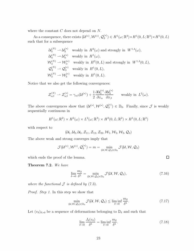
Theorem 7.2. We have

limδ→0

mδ

δ5= min

(U ,W ,Q3)∈D0

J (U ,W,Q3), (7.16)

where the functional J is defined by (7.3).

Proof. Step 1. In this step we show that

min(U ,W ,Q3)∈D0

J (U ,W,Q3) ≤ lim infδ→0

mδ

δ5. (7.17)

Let (vδ)δ>0 be a sequence of deformations belonging to Dδ and such that

limδ→0

Jδ(vδ)

δ5= lim inf

δ→0

mδ

δ5. (7.18)

23

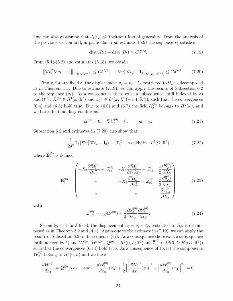
One can always assume that Jδ(vδ) ≤ 0 without loss of generality. From the analysis ofthe previous section and, in particular from estimate (5.9) the sequence vδ satisfies

d(vδ,Ωδ) + d(vδ, Bδ) ≤ Cδ5/2. (7.19)

From (5.1)-(5.2) and estimates (5.18), we obtain

∥∥∇vTδ ∇vδ − I3∥∥L2(Ωδ;R3×3)

≤ Cδ5/2,∥∥∇vTδ ∇vδ − I3

∥∥L2(Bδ;R3×3)

≤ Cδ5/2. (7.20)

Firstly, for any fixed δ, the displacement uδ = vδ−Id, restricted to Ωδ, is decomposedas in Theorem 3.1. Due to estimate (7.19), we can apply the results of Subsection 6.2to the sequence (vδ). As a consequence there exist a subsequence (still indexed by δ)and U (0), R(0) ∈ H1(ω;R3) and u(0)p ∈ L2(ω;H1(−1, 1;R3)), such that the convergences

(6.4) and (6.5) hold true. Due to (6.6) and (6.7) the field U (0)3 belongs to H2(ω), and

we have the boundary conditions

U (0) = 0, ∇U (0)3 = 0, on γ0. (7.21)

Subsection 6.2 and estimates in (7.20) also show that

1

2δ2Πδ

(∇vTδ ∇vδ − I3

) E(0)

p weakly in L2(Ω;R9) (7.22)

where E(0)p is defined

E(0)p =

−X3∂2U (0)

3

∂x21+ Z(0)

11 −X3∂2U (0)

3

∂x1∂x2+ Z(0)

12

1

2

∂u(0)p,1

∂X3

∗ −X3∂2U (0)

3

∂x22+ Z(0)

22

1

2

∂u(0)p,2

∂X3

∗ ∗∂u

(0)p,3

∂X3

(7.23)

with

Z(0)αβ = γαβ(U (0)) +

1

2

∂U (0)3

∂xα

∂U (0)3

∂xβ. (7.24)

Secondly, still for δ fixed, the displacement uδ = vδ − Id, restricted to Bδ, is decom-posed as in Theorem 3.2 and (4.4). Again due to the estimate in (7.19), we can apply theresults of Subsection 6.3 to the sequence (vδ). As a consequence there exist a subsequence

(still indexed by δ) andW(0), W(s,0), Q(0) ∈ H1(0, L;R3) and v(0)r ∈ L2(0, L;H1(D;R3))

such that the convergences (6.14) hold true. As a consequence of (6.15) the components

W(0)α belong to H2(0, L) and we have

dW(0)

dx3= Q(0) ∧ e3 and

dW(0)3

dx3(x3) +

1

2

[∣∣∣dW(0)1

dx3(x3)

∣∣∣2

+∣∣∣dW

(0)2

dx3(x3)

∣∣∣2]

= 0.

24

The junction conditions (6.16) give

Q(0)(0) = 0, W(0)α (0) = 0, W(s,0)(0) = 0, W(0)

3 (0) = U (0)3 (0, 0). (7.25)

As a first consequence, the triplet (U (0),W(0),Q(0)3 ) belongs to D0.

Subsection 6.3 and the second estimate (7.20) also show that

1

2δ3/2Pδ

((∇vδ)T∇vδ − I3

) E(0)

r weakly in L2(B;R3×3), (7.26)

where the symmetric matrix E(0)r is defined by

E(0)r =

γ11(v(0)r ) γ12(v

(0)r ) −1

2X2

dQ(0)3

dx3+

1

2

∂v(0)r,3

∂X1+

1

2

dW(s,0)1

dx3

∗ γ22(v(0)r )

1

2X1

dQ(0)3

dx3+

1

2

∂v(0)r,3

∂X2+

1

2

dW(s,0)2

dx3

∗ ∗ −X1d2W(0)

1

dx23−X2

d2W(0)2

dx23+dW(s,0)

3

dx3

. (7.27)

In order to bound from below the quantity lim infδ→0

Jδ(vδ)

δ5, using the assumptions on the

forces (5.5) and the convergences (6.4) and (6.14) we first have

limδ→0

1

δ5

∫

Sδ

fδ · (vδ − Id) = L(U (0),W(0),Q(0)3 ) (7.28)

where L(U ,W,Q3) is given by (7.4) for any triplet in D0.

As far as the elastic energy is concerned, we write

1

δ5

∫

Sδ

Wδ

(∇vδ

)=

1

δ5

∫

Ωδ

Wδ

(∇vδ

)+

1

δ5

∫

Bδ\Cδ

Wδ

(∇vδ

)

=

∫

Ω

Q(Πδ

[ 1

δ2((∇vδ)T∇vδ − I3

])+

∫

B

Q(χB\D×]0,δ[Pδ

[ 1

δ3/2((∇vδ)T∇vδ − I3

])

From the weak convergences of the Green-St Venant’s tensors in (7.22), (7.26) andequality (7.28), we obtain

lim infδ→0

Jδ(vδ)

δ5≥

∫

Ω

Q(E(0)

p

)+

∫

B

Q(E(0)

r

)−L(U (0),W(0),Q(0)

3 ) (7.29)

where E(0)p and E

(0)r are given by (7.23) and (7.50).

The next step in the derivation of the limit energy consists in minimizing

∫ 1

−1

Q(E(0)

p

)dX3

(resp.

∫

D

Q(E(0)

r

)dX1dX2) with respect to u(0)p ( resp. v

(0)r ).

25

First the expressions of Q and of E(0)p under a few calculations show that

∫ 1

−1

Q(E(0)

p

)dX3 ≥

E

3(1− ν2)

[(1− ν)

2∑

α,β=1

∣∣∣ ∂2U (0)

3

∂xα∂xβ

∣∣∣2

+ ν(∆U (0)

3

)2]

+E

(1− ν2)

[(1− ν)

2∑

α,β=1

∣∣Z(0)αβ

∣∣2 + ν(Z(0)

11 + Z(0)22

)2](7.30)

the expression in the right hand side of (7.30) is obtained through replacing u(0)p by

u(0)p (·, ·, X3) =

ν

1− ν

[(X23

2− 1

6

)∆U (0)

3 −X3

(Z(0)

11 + Z(0)22

)]e3. (7.31)

Following [7] (see equation (4.56) and (4.57)), choosing W(s,0)3 = 0 and v

(0)r such that

v(0)

r,1 = −ν[X2

2 −X21

2

d2W(0)1

dx23−X1X2

d2W(0)2

dx23

],

v(0)

r,2 = −ν[X2

1 −X22

2

d2W(0)2

dx23−X1X2

d2W(0)1

dx23

],

v(0)

r,3 = −X1dW(s,0)

1

dx3−X2

dW(s,0)2

dx3,

(7.32)

permit to obtain

∫

D

Q(E(0)

r

)dX1dX2 ≥

Eπ

8

[∣∣∣d2W(0)

1

dx23

∣∣∣2

+∣∣∣d

2W(0)2

dx23

∣∣∣2]

+µπ

8

∣∣∣dQ(0)3

dx3

∣∣∣2

. (7.33)

In view of (7.29), (7.30) and (7.33), the proof of(7.17) is achieved.

Step 2. In this step we show that

lim supδ→0

mδ

δ5≤ min

(U ,W ,Q3)∈D0

J (U ,W,Q3).

Let (U (1),W(1),Q(1)3 ) ∈ D0 such that

min(U ,W ,Q3)∈D0

J (U ,W,Q3) = J (U (1),W(1),Q(1)3 ).

We consider a sequence(U (n),W(n),Q(n)

3

)n≥2

of elements belonging to D0 such that

• U (n)α ∈ W 2,∞(ω) ∩H1

γ0(ω) and

∇U (n)α = 0 in D1/n, (α, β) ∈ 1, 22,

U (n)α −→ U (1)

α strongly in H1(ω),(7.34)

26

• U (n)3 ∈ W 3,∞(ω) ∩H2

γ0(ω) and

∂2U (n)3

∂xα∂xβ= 0 in D1/n, (α, β) ∈ 1, 22,

U (n)3 −→ U (1)

3 strongly in H2(ω),

(7.35)

• W(n)α ∈ W 3,∞(−1/n, L) with W(n)

α = 0 in [−1/n, 1/n] and

W(n)α −→ W(1)

α strongly in H2(0, L), (7.36)

• Q(n)3 ∈ W 1,∞(−1/n, L) with Q(n)

3 = 0 in [−1/n, 1/n] and

Q(n)3 −→ Q(1)

3 strongly in H1(0, L), (7.37)

We define W(n)3 ∈ W 2,∞(−1/n, L) by

W(n)3 = U (n)

3 (0, 0) anddW(n)

3

dx3+

1

2

[∣∣∣dW(n)1

dx3

∣∣∣2

+∣∣∣dW

(n)2

dx3

∣∣∣2]

= 0 in ]− 1/n, L[.

Obviously we haveW(n)

3 −→ W(1)3 strongly in H1(0, L). (7.38)

In order to define an admissible deformation of the whole structure, we introduce

both fields u(1)p ∈ L2(ω;H1(−1, 1;R3)) obtained through replacing U (0) by U (1) in (7.24)-

(7.31) and v(1)

r,α ∈ L2(0, L;H1(D)) obtained through replacing W(0) and Q(0)3 by U (1) and

Q(0)3 in (7.32) and taking v

(1)

r,3 = 0.

Then, we consider two sequences of warpings u(n)p , v(n)r such that

• u(n)p ∈ W 1,∞(Ω;R3) with u(n)p = 0 on ∂ω×] − 1, 1[, u(n)p = 0 in the cylinderD(O, 1/n)×]− 1, 1[ and

u(n)p −→ u(1)p strongly in L2(ω;H1(−1, 1;R3)),

• v(n)r ∈ W 1,∞(]− 1/n, L[×D;R3) with v(n)r = 0 in the cylinder D×]− 1/n, 1/n[ and

v(n)r −→ v

(1)

r strongly in L2(0, L;H1(D;R3)).

For n fixed, let us consider the sequence of deformations of the plate Ωδ. We set

v(n)δ,1 (x) = x1 + δ2

[U (n)1 (x1, x2)−

x3δ

∂U (n)3

∂x1(x1, x2) + δu

(n)p,1(x1, x2,

x3δ

)],

v(n)δ,2 (x) = x2 + δ2

[U (n)2 (x1, x2)−

x3δ

∂U (n)3

∂x2(x1, x2) + δu

(n)p,2(x1, x2,

x3δ

)],

v(n)δ,3 (x) = x3 + δ

[U (n)3 (x1, x2) + δ2u

(n)p,3(x1, x2,

x3δ

)].

(7.39)

27

If δ is small enough (in order to have δ ≤ 1/n) the expression of v(n)δ in the cylinder Cδ

is given by

v(n)δ,1 (x) = x1 + δ2

[U (n)1 (0, 0)− x3

δ

∂U (n)3

∂x1(0, 0)

],

v(n)δ,2 (x) = x2 + δ2

[U (n)2 (0, 0)− x3

δ

∂U (n)3

∂x2(0, 0)

],

v(n)δ,3 (x) = x3 + δ

[U (n)3 (0, 0) + x1

∂U (n)3

∂x1(0, 0) + x2

∂U (n)3

∂x2(0, 0)

].

(7.40)

We denote

Q(n) = −dW(n)2

dx3e1 +

dW(n)1

dx3e2 +Q(n)

3 e3, R(n) =∂U (n)

3

∂x2(0, 0)e1 −

∂U (n)3

∂x1(0, 0)e2.

The field Q(n) belongs to W 1,∞(−1/n, L;R3). Let R(n)δ be the matrix field defined by

R(n)δ (0) = I3,

dR(n)δ

dx3= A

F(n)δ

R(n)δ in [−1/n, L] (7.41)

where F(n)δ = δ1/2

dQ(n)

dx3+ δR(n) (see (3.1)) and let W(n)

δ be defined in [−1/n, L] by

W(n)δ (x3) =

∫ x3

0

(R

(n)δ (t)−I3

)e3dt+δ

2U (n)1 (0, 0)e1+δ

2U (n)2 (0, 0)e2+δU (n)

3 (0, 0)e3. (7.42)

We have R(n)δ ∈ W 1,∞(−1/n, L;SO(3)), W(n)

δ ∈ W 2,∞(−1/n, L;R3) and the follow-ing strong convergences (as δ tends towards 0)

R(n)δ −→ I3 strongly in W 1,∞(−1/n, L;SO(3)),

1

δ1/2dR

(n)δ

dx3−→ A

dQ(n)

dx3

strongly in L∞(−1/n, L;R9),

1

δ1/2(R

(n)δ − I3

)−→ AQ(n) strongly in W 1,∞(−1/n, L;R9),

1

δ

(R

(n)δ − I3

)e3 · e3 −→ −1

2||AQ(n)e3||22 strongly in L∞(−1/n, L),

1

δ1/2W(n)

δ,α −→ W(n)α strongly in W 1,∞(−1/n, L),

1

δW(n)

δ,3 −→ W(n)3 strongly in W 1,∞(−1/n, L).

(7.43)

By definition, Q(n) is equal to 0 in [−1/n, 1/n], hence we have

∀x3 ∈ [−1/n, 1/n], R(n)δ (x3) = exp

(δAR(n)x3

).

28

Now, we consider the fields R(n)

δ ∈ W 1,∞(−δ, L;SO(3)) and W (n)

δ ∈ W 2,∞(−δ, L;R3)defined by

R(n)

δ (x3) = exp(δAR(n)x3

)in [−δ, L],

W(n)

δ (x3) =

∫ x3

0

(R

(n)

δ (t)− I3)e3dt+W(n)

δ (0) in [−δ, L].(7.44)

We introduce a last displacement v(n)δ belonging to W 1,∞(Bδ;R

3) (for δ ≤ 1/n)

v(n)δ (x) =

δ2(U (n)1 (0, 0)− x3

δ

∂U (n)3

∂x1(0, 0)

)

δ2(U (n)2 (0, 0)− x3

δ

∂U (n)3

∂x2(0, 0)

)

δ(U (n)3 (0, 0) + x1

∂U (n)3

∂x1(0, 0) + x2

∂U (n)3

∂x2(0, 0)

)

−W(n)

δ (x3)−(R

(n)

δ (x3)− I3)(x1e1 + x2e2).

We have||∇v(n)δ ||L∞(Bδ ;R9) ≤ C(n)δ2.

Now, we are in a position to define the deformation v(n)δ in the rod Bδ. We set

v(n)δ (x) = x+W(n)

δ (x3) +(R

(n)δ (x3)− I3)(x1e1 + x2e2) + δ5/2v

(n)r

(x1δ,x2δ, x3

)+ v

(n)δ (x).

(7.45)

In the cylinder Cδ, the above expression of v(n)δ matches the one given by (7.40) if δ is

small enough ( δ ≤ 1/n).

By construction the deformation v(n)δ belongs to Dδ and satisfies

||∇v(n)δ − I3||L∞(Sδ ;R9) ≤ C(n)δ1/2.

Hence, for a.e. x ∈ Sδ we have det(∇v(n)δ (x)

)> 0. Then we have

mδ ≤ Jδ(v(n)δ ). (7.46)

The expression (7.39) of the displacement v(n)δ − Id in the plate is similar to the

decomposition (3.2) given in Section 2. Hence the results of Subsection 6.2 and theregularity of the terms U (n) and u(n) lead to

1

2δ2Πδ

((∇v(n)δ )T∇v(n)δ − I3

)−→ E(n)

p strongly in L∞(Ω;R9), (7.47)

29

where the symmetric matrix E(n)p is defined by

E(n)p =

−X3∂2U (n)

3

∂x21+ Z(n)

11 −X3∂2U (n)

3

∂x1∂x2+ Z(n)

12

1

2

∂u(n)p,1

∂X3

∗ −X3∂2U (n)

3

∂x22+ Z(n)

22

1

2

∂u(n)p,2

∂X3

∗ ∗∂u

(n)p,3

∂X3

Remark that here u(n)p = u(n) (see (6.8) and where the Z(n)αβ ’s are obtained through

replacing U by U (n) in (6.9).

Now, in the rod Bδ we have the following strong convergence in L∞(B;R9) (as δ tendstowards 0):

1

δ3/2Pδ

(∇v(n)δ −R

(n)δ

)−→ dR(n)

dx3(X1e1 +X2e2) +

γ11(v(n)r ) γ12(v

(n)r )

1

2

∂v(n)r,3

∂X1

∗ γ22(v(n)r )

1

2

∂v(n)r,3

∂X2

∗ ∗ 0

.

(7.48)Then we obtain

1

2δ3/2Pδ

((∇v(n)δ )T∇v(n)δ − I3

)−→ E(n)

r strongly in L∞(0;R9), (7.49)

where the symmetric matrix E(n)r is defined by

E(n)r =

γ11(v(n)r ) γ12(v

(n)r ) −1

2X2

dQ(n)3

dx3+

1

2

∂v(n)r,3

∂X1

∗ γ22(v(n)r )

1

2X1

dQ(n)3

dx3+

1

2

∂v(n)r,3

∂X2

∗ ∗ −X1d2W(n)

1

dx23−X2

d2W(n)2

dx23

. (7.50)

Before passing to the limit, notice that

∣∣∣ 1δ5

∫

Sδ

Wδ(∇v(n)δ )(x)dx−∫

Ω

Q(Πδ

((∇v(n)δ )T∇v(n)δ − I3

))−

∫

B

Q(Pδ

((∇v(n)δ )T∇v(n)δ − I3

))∣∣∣

≤ C

δ5

∫

Cδ

|||((∇v(n)δ )T∇v(n)δ − I3

)|||2,

30

then from the expression (7.40) of v(n)δ in Cδ and the strong convergences (7.47)-(7.49)

we get

limδ→0

1

δ5

∫

Sδ

Wδ(∇v(n)δ )(x)dx =

∫

Ω

Q(E(n)p ) +

∫

B

Q(E(n)r ).

From the expressions of v(n)δ in the plate and in the rod, from the convergences (7.43)

and taking to account the expressions of the applied forces (5.5) we get

limδ→0

1

δ5

∫

Sδ

fδ · (v(n)δ − Id) = L(U (n),W(n),Q(n)3 ).

Then, from the above limits and (7.46) we finally get

lim supδ→0

mδ

δ5≤ lim

δ→0

Jδ(v(n)δ )

δ5=

∫

Ω

Q(E(n)

p

)+

∫

B

Q(E(n)

r

)− L(U (n),W(n),Q(n)

3 ). (7.51)

Now, n goes to infinity, due to the definitions of the warpings u(1)p and v

(1)

r and thestrong convergences (7.34)-(7.35)-(7.36)-(7.37)-(7.38) that give

lim supδ→0

mδ

δ5≤

∫

Ω

Q(E(1)

p

)+

∫

B

Q(E(1)

r

)−L(U (1),W(1),Q(1)

3 ) = J (U (1),W(1),Q(1)3 ).

This conclude the proof of the theorem.

Remark 7.3. Let us point out that Theorem 7.2 shows that for any minimizing sequence

(vδ)δ>0 as in Step 1, the convergence of the rescaled Green-St Venant’s strain tensor in

(7.22) is a strong convergence in L2(Ω;R3×3) and the convergence (7.26) is a strong

convergence in L2(B;R3×3).

References

[1] S. S. Antman. The theory of rods, in Handbuch der Physik, Band VIa/2, S. Flugge& C. Truesdell eds., Springer-Verlag, Berlin, (1972), 641–703.

[2] S. S. Antman. Nonlinear Problems of Elasticity, Applied Mathematical Sciences107, Springer-Verlag, New York (1995).

[3] M. Aufranc. Junctions between three-dimensional and two-dimensional non-linearly elastic structures. Asymptotic Anal. 4 (1991), 4, 319–338.

[4] D. Blanchard, A. Gaudiello, G. Griso. Junction of a periodic family of elastic rodswith a 3d plate. I. J. Math. Pures Appl. (9) 88 (2007), no 1, 149-190.

[5] D. Blanchard, A. Gaudiello, G. Griso. Junction of a periodic family of elastic rodswith a thin plate. II. J. Math. Pures Appl. (9) 88 (2007), no 2, 1-33.

31

[6] D. Blanchard, G. Griso. Microscopic effects in the homogenization of the junctionof rods and a thin plate. Asymptot. Anal. 56 (2008), no 1, 1-36.

[7] D. Blanchard, G. Griso. Decomposition of deformations of thin rods. Applicationto nonlinear elasticity, Ana. Appl. 7 (1) (2009) 21-71.

[8] D. Blanchard, G. Griso. Decomposition of the deformations of a thin shell. Asymp-totic behavior of the Green-St Venant’s strain tensor. J. of Elasticity, 101 (2),179-205 (2010).

[9] Blanchard D., Griso G.: A simplified model for elastic thin shells. Asymptot.Anal. 76(1), 1-33 (2012)

[10] D. Blanchard, G. Griso. Modeling of rod-structures in nonlinear elasticity. C. R.Math. Acad. Sci. Paris 348 (2010), 19-20, 1137–1141.

[11] Blanchard D., Griso G.: Asymptotic Behavior of Structures Made of StraightRods. J. Elast. 108(1), 85-118 (2012)

[12] D. Blanchard, G. Griso: Asymptotic behavior of a structure made by a plate anda straight rod (hal-00611655, arXiv : 1107.5283).

[13] P.G. Ciarlet and P. Rabier. Les equations de Von Karman. Lectures Notes inMathematics. (Springer Verlag 1980).

[14] P.G. Ciarlet. Mathematical Elasticity, Vol. I, North-Holland, Amsterdam (1988).

[15] P.G. Ciarlet, H. Le Dret and R. Nzengwa. Junctions between three dimensionaland two dimensional linearly elastic structures. J. Math. Pures Appl. 68 (1989),261–295.

[16] P.G. Ciarlet. Plates and Junctions in Elastic Multi-Structures: An AsymptoticAnalysis (Masson, Paris, 1990).

[17] P.G. Ciarlet. Mathematical Elasticity, Vol. II: Theory of plates, North-Holland,Amsterdam (1997).

[18] G. Friesecke, R. D. James and S. Muller. A theorem on geometric rigidity andthe derivation of nonlinear plate theory from the three-dimensional elasticity.Communications on Pure and Applied Mathematics, Vol. LV, 1461-1506 (2002).

[19] G. Friesecke, R. D. James and S. Muller. A hierarchy of plates models derivedfrom nonlinear elasticity by Γ-convergence, Arch. Rat. Mech. Anal. 180 (2006)183-236.

[20] A. Gaudiello, R. Monneau, J. Mossino, F. Murat, A. Sili. Junction of elastic platesand beams. ESAIM Control Optim. Calc. Var. 13 (2007), no. 3, 419–457.

32

[21] A. Gaudiello, E. Zappale. A Model of Joined Beams as Limit of a 2D Plate. J.Elast. (2011) 103, 205-233.

[22] G. Griso. Asymptotic behavior of rods by the unfolding method. Math. Meth.Appl. Sci. 2004; 27: 2081-2110.

[23] G. Griso. Asymptotic behavior of structures made of plates. Analysis and Appli-cations 3 (2005), 4, 325-356.

[24] G. Griso. Decomposition of displacements of thin structures. J. Math. Pures Appl.89 (2008), 199-233.

[25] G. Griso. Asymptotic behavior of structures made of curved rods. Analysis andApplications, 6 (2008), 1, 11-22.

[26] I. Gruais. Modelisation de la jonction entre une plaque et une poutre en elasticitelinearisee. RAIRO: Model. Math. Anal. Numer. 27 (1993) 77-105.

[27] I. Gruais. Modeling of the junction between a plate and a rod in nonlinear elas-ticity. Asymptotic Anal. 7 (1993) 179-194.

[28] H. Le Dret. Modeling of the junction between two rods, J. Math. Pures Appl. 68(1989), 365–397.

[29] H. Le Dret. Modeling of a folded plate, Comput. Mech., 5 (1990), 401-416.

[30] H. Le Dret. Problemes Variationnels dans les Multi-domaines: Modelisation desJonctions et Applications. Masson, Paris (1991).

[31] M. G. Mora, L. Scardia. Convergence of equilibria of thin elastic plates underphysical growth conditions for the energy density. Journal of Differential Equa-tions, Volume 252, Issue 1 (2012), 35-55.

[32] L. Trabucho and J.M. Viano. Mathematical Modelling of Rods, Handbook ofNumerical Analysis 4. North-Holland, Amsterdam (1996).

33