JU

NE

, 2014

M.S

c. in E

lectrical a

nd

Electro

nics E

ng

ineerin

g

Ali A

. H. K

AR

AH

BA

SH

UNIVERSITY OF GAZİANTEP

GRADUATE SCHOOL OF

NATURAL & APPLIED SCIENCES

A COMPRESSIVE SENSING BASED ON WATERMARKING SCHEME FOR

SPARSE IMAGE

M. Sc. THESIS

IN

ELECTRICAL AND ELECTRONICS ENGINEERING

BY

ALI A. H. KARAH BASH

JUNE 2014

a compressive sensing based on watermarking scheme for sparse image

M.Sc. Thesis

In

Electrical and Electronics Engineering

University of Gaziantep

Supervisor

Assist. Prof. Dr. Sema Koç KAYHAN

By

Ali A. H. KARAH BASH

june 2014

II

© 2014 [Ali A. H. KARAH BASH]

III

IV

I hereby declare that all information in this document has been obtained and

presented in accordance with academic rules and ethical conduct. I also declare

that, as required by these rules and conduct, I have fully cited and referenced all

material and results that are not original to this work.

Ali A. H. KARAH BASH

V

ABSTRACT

A COMPRESSIVE SENSING BASED ON WATERMARKING

SCHEME FOR SPARSE IMAGE

Ali A. H. KARAH BASH

M.Sc. Thesis in Electrical and Electronics Eng.

Supervisor: Assist. Prof. Dr. Sema Koç KAYHAN

June 2014

85 pages

The traditional Nyquist Shannon theorem explains that the number of samples which are

needed for recovering a signal must be at least twice the maximum frequency in the

bandwidth of a signal. This approach is used in all applications of the signal processing.

This problem is solved by using a new sampling method developed called Compressive

Sampling or Compressive Sensing (CS), where it is used to recover signals or images

from far fewer measurements or samples than the traditional theorem. CS theory

depends on Sparsity principle, thereby the signals or images must be sparse. However,

most of the natural signals or images are not sparse. Therefore, there are some

transformation methods used to alter these signals or images into sparse like Discrete

Cosine Transform (DCT), Discrete Wavelet Transform (DWT) and Discrete Fourier

Transform (DFT).

In this thesis, we integrate the watermarking technology and compressive sensing theory

to protect the watermarking image in the compressive sensing measurements. The

watermarking image is embedded into the compressive measurement vectors. The

measurement vectors are sparse in a suitable basis. The resulting watermarked

measurements recover by using both the Orthogonal Matching Pursuit (OMP) and

Orthogonal Matching Pursuit With Partially Known Support (OMP-PKS) reconstruction

algorithms. Then the decoder procedure utilizes to extract the watermarking image. In

experimental study, the results obtained by comparing between the OMP and OMP-PKS

algorithms to clarify the performance of them. The results show that the OMP-PKS

algorithm achieves performance superior to that of the OMP reconstruction algorithm.

Key Words: Watermarking image, CS, OMP and OMP-PKS algorithms.

VI

ÖZET

SEYREK İMGELERİN SIKIŞTIRMALI ÖRNEKLEME YÖNTEMİ

İLE DAMGALANMASI

Ali A. H. KARAH BASH

Yüksek Lisans Tezi, Elektrik-Elektronik Müh. Bölümü

Tez Yöneticisi: Yrd. Doç. Dr. Sema Koç KAYHAN

Haziran 2014

85 sayfa

Nyquist Shannon teorimine göre bir işaretin geri kazanımı için örnekleme sayısı en az

işaretin maksimum frekansının iki katı olmalıdır. İşaret ile ilgili pek çok alanda bu

yaklaşım kullanılmaktadır. Bu yaklaşımda çok fazla örnek kullanılmaktadır. Örnekleme

sayısını azaltmak için sıkıştırmalı örnrkleme algoritmaları (CS) geliştirilmiştir. Bu

algoritma ile çok az sayıda örnek kullanarak sinyalin geri kazanımı mümkün olmaktadır.

CS teorisi seyreklik prensibine dayandığı için örneklenecek olan işaretin veya imgenin

de seyrek olması gerekir.

Fakat pek çok doğal imge veya işaret seyrek yapıda değildir. Bu nedenle bu sinyalleri

seyrek olarak ifade edebilmek için Ayrık Kosinüs Dönüşümü (DCT), Fourier Dönüşümü

(DFT) veya Dalgacık Dönüşümü (DWT) gibi dönüşüm methodları kullanılmaktadır.

Sıkıştırmalı örnekleme ve işaretin geri kazanımı sırasında bağımsız ölçüm matrisi

kullanılmaktadır..

Bu tezde, sıkıştırmalı örnekleme ölçümlerindeki damgalama imgesini korumak için CS

tabanlı bir damgalama algoritması geliştirilmiştir. Öncelikle damgalama imgesi CS

vektörlerine gömülür. Örnekleme vektörünün de seyreltilmiş olması gerekmektedir.

Sonuçta elde edilen damgalama ölçümleri farklı dik eşleştirme algoritmaları

((Orthogonal Matching Pursuit, OMP), (Orthogonal matching pursuit with partially

known support OMP-PKS)) kullanılarak geri kazanılmaktadır. Damgalama imgesini

çıkarmak için kod çözme algoritması kullanılmaktadır.

Deneysel çalışmalarda OMP ve OMP-PKS algoritmalarının sonucu karşılaştırılmış ve

OMP-PKS algoritmasının OMP ye göre daha iyi sonuç verdiği görülmüştür.

Anahtar Kelimeler: Damgalama imgesi, CS, OMP ve OMP-PKS algoritmaları.

VII

To My Parents

VIII

ACKNOWLEDGMENTS

I thank Allah who helped and guided me to complete this work. Also, I would like to

express my deep thankfulness and sincere gratitude to my advisor Assist. Prof. Dr.

Sema Koç Kayhan for her direction, suggestion and encouragement. This work would

not be possible without her precious support and advice.

I would like to thank the government of Turkey represented by Ministry of Turks

Abroad and Related Communities (Yurtdışı Türkler ve Akraba Topluluklar Bakanlığı)

for granting me the scholarship to study in the Turkey and supporting me financially

during my study in Gaziantep University.

In addition, I present a private thanks to my parents for encouraging and supporting me

in this work and throughout my study. It is my pleasure to thank the people who

supported me to make this thesis possible. I would also like to thank my friend Hasan

Alpegamberli for his support and help throughout this work. I would like to thank Mr.

Taha Al-Meryem, who introduced me into the field of Linear algebra and gave me a lot

of guidance and teaching.

IX

TABLE OF CONTENTS

Page

ABSTRACT ...................................................................................................................... V

ÖZET............................................................................................................................... VI

ACKNOWLEDGMENTS ............................................................................................ VIII

CONTENTS .................................................................................................................... IX

LIST OF TABLES ............................................................................................................ X

LIST OF FIGURES ........................................................................................................ XI

LIST OF SYMBOLS .................................................................................................... XIV

LIST OF ABBREVIATIONS ........................................................................................ XV

CHAPTER 1: INTRODUCTION ...................................................................................... I

CHAPTER 2: OVERVIEW ............................................................................................... 8

2.1 Compressive Sensing CS ....................................................................................... 8

2.1.1 Overview of Compressive Sensing CS ......................................................... 8

2.1.2 Applications of CS ...................................................................................... 11

2.2 Overview of Reconstruction Algorithms ............................................................. 15

2.2.1 L1 minimization algorithm ......................................................................... 15

2.2.2 Orthogonal matching pursuit OMP ............................................................. 17

2.2.3 Orthogonal matching pursuit with partially known support OMP-PKS ..... 22

2.3 Watermarking image ............................................................................................ 25

2.3.1 Overview of Watermarking Image.............................................................. 25

2.3.2 Watermarking properties ............................................................................. 26

2.3.3 Application of the digital watermarking ..................................................... 27

CHAPTER 3: METHODOLOGY ................................................................................... 30

3.1 Compressive Sensing CS ..................................................................................... 30

3.2 The reconstruction algorithms ............................................................................. 33

3.2.1 L1 minimization algorithm ......................................................................... 33

3.2.2 Orthogonal matching pursuit OMP ............................................................. 33

3.2.3 Orthogonal matching pursuit with partially known support OMP-PKS ..... 34

3.3 Digital Watermarking .......................................................................................... 37

3.3.1 The encoder algorithm ................................................................................ 38

3.3.2 The reconstruction algorithms..................................................................... 39

3.3.3 The decoder algorithm ................................................................................ 40

3.4 Proposed Flowchart .............................................................................................. 44

CHAPTER 4: RESULTS AND DISCUSSION ............................................................... 47

CHAPTER 5: CONCLUSION AND SUGGESTIONS FOR FUTURE WORKS .......... 61

REFERENCES ................................................................................................................. 62

X

LIST OF TABLES

Page

Table 2.1. Orthogonal Matching Pursuit OMP algorithm. .............................................. 18

Table 2.2. Orthogonal Matching Pursuit with partially known support

OMP-PKS algorithm. ....................................................................................................... 24

Table 3.1. OMP-PKS and OMP algorithms in the first decoder method ......................... 41

Table 3.2. OMP-PKS and OMP algorithms in the second decoder method .................... 43

Table 4.1. PSNR and its execution time with different measurement rates M/N by

using the three reconstruction algorithms with the first and second decoder methods. ... 59

Table 4.2. PSNR and its execution time with different Sparsity rates K/N by using

the three reconstruction algorithms with the first and second decoder methods. ............ 60

XI

LIST OF FIGURES

Page

Figure 1.1. Basic block diagram of CS technique. ............................................................ 2

Figure 1.2. Traditional data acquisition approach [3]. ....................................................... 3

Figure 1.3. CS data acquisition approach [3]. .................................................................... 3

Figure 1.4. A scheme of the general watermarking encoder and decoder. ........................ 7

Figure 1.5. A scheme of CS watermarking procedure. ..................................................... 7

Figure 2.1. Block diagram of Compressive Imaging Camera [22]. ................................. 12

Figure 3.1. Compressive acquisition and reconstruction [80].......................................... 32

Figure 3.2. Wavelet decomposition by filter bank analysis. HP and LP are high

pass filter and low pass filter, respectively [64]. .............................................................. 35

Figure 3.3. The octave-tree discrete wavelet transform: (a) the original image and

(b) the wavelet transformed image. Sub-bands inside the blue, green and red windows

are the first, the second and the third level sub-bands, respectively [65]. ....................... 35

Figure 3.4. Wavelet transform and its block processing: (a) wavelet transformed

image, (b) wavelet sub-bands rearranging and (c) wavelet blocks [65]. ......................... 36

XII

Figure 3.5. The coefficients of LL3 sub-band, that are in the first four columns at

the red region.................................................................................................................... 37

Figure 3.6. Watermarking image embedding structure [10]. ........................................... 38

Figure 3.7. The proposed flowchart. ................................................................................ 46

Figure 4.1. (a) Original Lena image and (b) Watermarking image. ................................ 47

Figure 4.2. (a) Random Gaussian distribution of the sensing matrix Φ. (b) Random

Gaussian distribution of ΦQ matrices. ............................................................................. 48

Figure 4.3. The quality of the reconstructed image with the extracted

watermarking image in varying M/N rates using L1-min in the first decoder method. ... 49

Figure 4.4. The quality of the reconstructed image with the extracted

watermarking image in varying M/N rates using L1-min in the second decoder

method. ............................................................................................................................. 49

Figure 4.5. The quality of the reconstructed image with the extracted watermarking

image in varying M/N rates using the OMP algorithm in the first decoder method. ....... 50

Figure 4.6. The quality of the reconstructed image with the extracted

watermarking image in varying M/N rates using the OMP algorithm in the second

decoder method. ............................................................................................................... 50

Figure 4.7. The quality of the reconstructed image with the

extracted watermarking image in varying M/N rates using the OMP-PKS

algorithm in the first decoder method ........................................................................... 51

XIII

Figure 4.8. The quality of the reconstructed image with the extracted

watermarking image in varying M/N rates using the OMP-PKS algorithm in the second

decoder method. ............................................................................................................... 51

Figure 4.9. (a) Residual values with different M/N in the first decoder method.............. 52

Figure 4.9. (b) Residual values with varying M/N in the second decoder method.

(c) MSE values with varying M/N in the first decoder method. ...................................... 53

Figure 4.9. (d) MSE values with different M/N in the second decoder method.

(e) PSNR values with varying M/N in the first decoder method...................................... 54

Figure 4.9. (f) PSNR values with different M/N in second decoder method. .................. 55

Figure 4.10. Performance of the L1-min, OMP and OMP-PKS algorithms in varying

K/N values, (a) Residual with different K/N values in the first decoder method.

(b) Residual with different K/N values in the second decoder method. ........................... 56

Figure 4.10. Performance of the L1-min, OMP and OMP-PKS algorithms in varying

K/N values, (c) MSE with different K/N values in the first decoder method.

(d) MSE with different K/N values in the second decoder method.................................. 57

Figure 4.10. Performance of the L1-min, OMP and OMP-PKS algorithms in varying

K/N values, (e) PSNR with different K/N values in the first decoder method.

(f) PSNR with different K/N values in the second decoder method. ………………….58

XIV

LIST OF SYMBOLS

x Signal or image which is usually sparse or compressible.

y Observation or Measurement vector.

R Real numbers space.

N Rows of the vector x.

M Rows of the measurement vector y.

K Sparsity (number of nonzero entries of the vector x).

Φ Projection or sensing matrix of size M × N.

Ψ Spatial domain in size N x N.

𝑖𝑡ℎ column of the matrix Φ.

I Active set.

Inactive set.

t Iteration counter.

𝑟 Residual vector at iteration t.

Restricted Isometry Constant.

Incoherence between two columns of the measurement matrix Φ.

Transform Domain components.

V Watermarking image.

Watermarked compressive sensed measurement.

L Number of bits in the watermarking image.

D Random matrix by M x L.

Measurement vector combines x and V.

H Measurement matrix combines Φ and D.

T Index of known support part of a sparse image.

Q Random matrix with M x N.

XV

LIST OF ABBREVIATIONS

CS Compressed Sensing.

L1-min L1 minimization algorithm.

OMP Orthogonal Matching Pursuit.

MP Matching pursuit.

OMP-PKS Orthogonal Matching Pursuit with partially known support.

LP Linear programing.

BP Basis pursuit.

TOMP Tree based Orthogonal matching pursuit.

RIP Restricted Isometry Property.

UUP Uniform uncertainty principle.

NP Nondeterministic polynomial time.

SBS Sequential basis selection.

FSR Forward Stepwise Regression.

CMP Complementary Matching Pursuit.

OCMP Orthogonal Complementary Matching Pursuit.

GOMP Generalized Orthogonal Matching Pursuit.

STOMP Stage-Wise Orthogonal Matching Pursuit.

ROMP Regularized Orthogonal Matching Pursuit.

MR Magnetic Resonance.

DWT Discrete Wavelet Transform.

TV min Total Variation Minimization.

DCT Discrete Cosine Transform.

DFT Discrete Fourier Transform.

SPC Single Pixel Camera.

XVI

DMD Digital Micro mirror Device.

CRSI Curvelet Based Recovery By Sparsity Promoting Inversion.

GPRs Ground Penetrating Radars.

AIC Analog to Information Conversion.

ADC Analog to Digital Converter.

DIVX Digital Video Disk Players.

DVD Digital Video Disks.

LARS Least Angle Regression.

LASSO Least Absolute Shrinkage and Selection Operator.

PSNR Peak Signal to Noise Ratio.

MSE Mean Square Error.

1

CHAPTER 1

INTRODUCTION

Data transmission in the signal processing field is often executed in the digital domain,

because this process occupies lower bandwidth compared to the analog domain. So the

analog to digital converter is used for converting the band limited signal to a digital

signal to implement the sampling operation at a particular sampling rate. The uniformly

spaced samples result from sampling the signal. These uniformly spaced samples are

used for recovering the signal back to the origin by the Nyquist Shannon theorem. The

condition of the Nyquist Shannon theorem in the signal recovering case is that the

number of samples must be at least twice the maximum frequency of the interested

signal, i.e. the perfect recovery encloses when the sampling rate is twice the maximum

frequency of the original signal. The resulting particular rate and sampling the signal are

called Nyquist rate.

Regrettably, in the signal processing applications field, there are far too many samples

when using the Nyquist Shannon theorem in the data sampling. Therefore, the amount of

data at the transmitter increases, which in turn leads to increased cost of the building

devices that are able to acquire the samples at the Nyquist rate. The data compression is

the best method to cope this problem. Data compression finds a brief representation of a

signal that is capable of reaching the target rate with a reasonable distortion. The

transform coding is a known technique used in the data compression, which is dependent

on a basis that supplies sparse approximation of the signal.

The disadvantage of the transform coding technique is sampling the data at Nyquist rate

before compressing it; this increases cost of acquiring the sampled devices at Nyquist

rate. To cope this case, there is a new technique developed known Compressive

Sampling or Compressive Sensing CS [1]. The CS technique is used to recover the

original signal from far too few samples or measurements which lead to decrease cost

2

of acquiring the sampled devices [2]. Figure 1.1 shows the basic block diagram of CS

technique, which x is the input signal with N length and y represents an M

measurement vector; this has been arrived at by computing the correlation between x and

measurement or projection matrix Φ , mathematically y is given as follows:

=<x, >. Where i=1, 2…. M. (1.1)

where M << N and is the recovered signal from M measurements. The

compressive sensing immediately acquires the compressed signal samples at a lower

sampling rate instead of first data sampling, which acquires the compressed signal

samples at a higher rate, then the sampling of data compresses, i.e. the data compression

and sensing are achieved together. The input signal x is sparse or sparse in Ψ domain, in

this case:

=<Ψ , >. Where i =1, 2…. M. (1.2)

Figure 1.1. Basic block diagram of CS technique.

To perfectly recover the band limited signal by using the Nyquist Shannon theorem as

depicted in Figure 1.2, a certain number of samples equal to the Nyquist rate are needed.

When the sampling rate is less than the Nyquist rate, the original signal cannot be

recovered by traditional recovery approaches. In contrast, in the compressive sensing as

shown in Figure 1.3 though the samples are far too less than the samples that are needed

in the conventional process, the original signal can be recovered.

Sensing/ Projection

Φ

Reconstruction

M

Transmission

y=Φx

x ��

3

Figure 1.2. Traditional data acquisition approach [3].

Figure 1.3. CS data acquisition approach [3].

4

The compressive sensing is different from the classical Nyquist paradigm which

provides a sparse solution for underdetermined linear systems and is capable of

recovering the signals from fewer samples than the Nyquist sampling rate. CS solves the

problem of a limited number of samples that happens in different applications like data

capturing devices and imaging techniques. In each case, CS provides a hopeful solution.

The compressive sensing CS takes advantage of the Sparsity of signals in some

transform domains and the incoherency of these measurements with the original domain

is also taken.

In addition, CS deals with the compression and sampling in one step by computing the

minimum samples. These samples have maximum information about the signal. Thus,

the procedure described above minimizes the requirements to acquire and store a large

number of samples because of their minimal values. There are many approaches that are

reconstructed the sparse image like the optimization and the greedy methods. In this

thesis, three reconstruction algorithms are explained, L1 minimization, orthogonal

matching pursuit OMP and orthogonal matching pursuit with partially known support

OMP-PKS, which are employed to reconstruct the measurement vectors resulting from

the CS.

L1 minimization L1-min is one of the most famous reconstruction methods, which is

used in the signal processing and optimization communities in the last years or so. L1-

min is an efficient approach utilized in the CS theory, which reconstructs the sparse

solution to a certain underdetermined linear equation system [1]. Let x is an

unknown signal, a measurement vector y is generated by using the linear

projection of y, where y = Φx, if the sensing matrix Φ is a full rank and over complete,

i.e., M N, an L1-min algorithm solves the following convex optimization problem:

(F1): min 1l

x subject to y = Φx. (1.3)

where F1 formula represents a linear inverse problem, y is the number of measurements

and is smaller than the number of unknowns x. The CS approach displays x as efficient

sparse and measurement matrix Φ as incoherent in basis under which x is sparse. This

Sparsity property of F1 is shown in the major applications as image processing, data

5

compression, sensor, recent computer vision and networks. The formula of F1 represents

a Linear Programing LP problem shown in the basis pursuit BP [4]. The OMP is an

iterative greedy algorithm, which is used in the sparse signal or sparse image

reconstruction. In each iteration, OMP selects columns from the measurement matrix Φ

which has best correlation with the residual r of the signal. Then the OMP produces a

new approximation signal by projecting the signals onto the selected columns of

measurement matrix Φ. This approach extends for the trivial greedy algorithm, which is

successful in an orthonormal system. Also the OMP algorithm is simple and has fast

implementation [5].

Let S be an arbitrary K-sparse signal in , y is a measurement vector, Φ is an M

× N measurement matrix and N measurements of the signal are observed in an M-

dimensional measurement vector y = ΦS. The columns of the measurement matrix Φ are

denoted as { , . . . , }. As mentioned earlier, it is natural to think of signal recovery

as a problem dual to sparse approximation. Since S has only K nonzero coefficients, the

measurement vector y = ΦS represents a linear combination of K columns from Φ, and y

has K non-zero coefficients over the measurement matrix Φ. This idea allows

transporting the sparse results from approximation to signal recovery problem. In

particular, sparse approximation approaches are used for signal reconstruction. To match

the ideal signal S, it is required to compute which columns of Φ combine with the

measurement vector y. The algorithm idea is to choose columns in a greedy fashion. In

each iteration, the column of Φ is selected; this has the strongest correlation with the

remaining part of y. Then we subtract off its contribution to y and iterate on the residual.

After K iteration, the algorithm will have identified the correct set of columns.

The OMP-PKS is a greedy algorithm used for image reconstruction from the

measurement vectors and it is developed from the traditional OMP algorithm [6]. OMP-

PKS provides a priori information about the coefficients of the sparse signal, that some

coefficients are more important than the others. These important coefficients are selected

as non-zero coefficients. The characteristic of OMP-PKS is the same as OMP, where the

requirement of restricted isometry property RIP is not severed as BP [7]. OMP-PKS

needs low measurement rates in the signal recovery. The OMP-PKS is different from

6

Tree based Orthogonal matching pursuit TOMP, where in the OMP-PKS the next basis

selection is not dependent on the previously selected bases. But in the TOMP, the basis

selections are compared with and selected a next good group of the related atoms in

wavelet tree [8]. In the OMP-PKS, the partially known support ideas are required to

enhance a performance of the reconstruction. The partially known support PKS

provides priori information about the selected columns of the measurement matrix Φ.

The PKS modifies OMP-PKS algorithm initialization because the columns of Φ are

contributed with the measurement vector y before staring the iteration.

In the digital management, illegal manner can easily be used in contents of multimedia.

Therefore, the easy distribution of multimedia data on the Internet needs some protection

techniques to protect these data from unauthorized use. The digital watermarking is used

for protection of the digital images [9]. Digital Watermarking is a visible or invisible

identification code which is always embedded in the host media. In any digital

watermarking technique, there are two main components: watermark embedding and

watermark detection. Digital watermarking provides the embedding process to insert the

data known as watermark into the contents of a multimedia involving as text documents,

images, audio or video streams. The watermark is detected later by using the extraction

algorithms. Figure 1.4 shows the watermarking scheme which consists of three parts:

1-The watermark.

2-The encoder (insertion algorithm).

3-The decoder (extraction or detection algorithm).

In this thesis, the watermarking algorithm has been used to insert the watermarking

image into the compressive sensed measurement vector y as shown in the Figure 1.5

[10]. The measurement vectors are sparse in suitable basis. The resulting watermarked

compressive sensed measurements are recovered by using the three reconstruction

algorithms L1-min, OMP and OMP-PKS. Then the extraction algorithm is used to

extract the watermarking image.

7

Figure 1.4. A scheme of the general watermarking encoder and decoder.

Figure 1.5. A scheme of CS watermarking procedure.

x Original image

N x N

Sensing

Matrix M x N

Measurement

Vector M x N +

Watermark

image

Reconstruction

Algorithms

Reconstructed

watermarked

image N x N

Watermark

Detector

Recovered

image

Watermark

Image

Watermark

Image

Encoder

Decoder

Watermarked Image

Original Image

8

CHAPTER 2

OVERVIEW

2.1 Compressive Sensing CS

In this part, the overview of Compressive Sensing CS is displayed. Accordingly, some

CS applications are explained.

2.1.1 Overview of Compressive Sensing CS

Compressive Sensing CS, also called Compressive Sampling, is an emerging area in

information theory and signal processing that is attracting a lot of attention recently [11].

The motivation of using the compressive sensing is coming from the fact that the CS

combines the sampling and the compression at the same time. In traditional recovery

algorithms, to fully reconstruct a signal, it is sampled at a rate equal or greater than the

Nyquist sampling rate. In different applications such as imaging, sensor networks,

astronomy, high-speed analog-to-digital compression and biological systems, the signals

are sparse in a certain basis.

The compressive sensing is used to reconstruct the high dimensional signals exactly by

using much smaller measurements. Generally, the signals are represented by vectors in

many applications like images or other objects. In the linear algebra theorem, many

equations are unknown, thus the unique signal recovering from an incomplete set of

linear vectors is not possible. As mentioned earlier, many signals are often sparse or

compressible in some basis, these signals are represented as real world images or audio

signals, and can accurately recover from incomplete linear measurements. However, the

signal itself is sparse and non-trivial; thereby the compressed measurements are used to

reconstruct this signal. The CS is utilized to recover the sparse signals from compressed

measurements by efficiently and effectively decoding algorithms. One popular decoding

algorithm is the Basis Pursuit algorithm [4].

9

The CS idea didn't come from anywhere, where the theoretical foundation of CS is

dealing with high dimensional geometry and associated with the geometric functional

analysis field. For example, Garnaev studied how many and what linear measurements

are required to reconstruct vectors of CS by using the basic decoding method. By

knowing the measurement matrix Φ, all solutions of x are in the underdetermined

systems and are laid in an affine space parallel to the null space of Φ. Then Garnaev‟s

problem clearly becomes a high dimensional geometrical problem, which is about how

to select the null space so the affine space‟s intersection with the L1 ball has minimal

radius [12]. Their pantheistic results depend on randomly choosing of the linear

measurements and are optimized in order of a number of measurements, which is within

a multiplicative factor of what the minimization compressive sensing supplies.

The deep probabilistic technique [13] is the generic chaining technique. This technique

controls the upper of a random processes; these are used as an important technical tool in

verifying that a certain measurement matrix ensembles satisfy the condition for

recovering the sparse signals [14]. Compressive sensing has effects on the coding

theory, such as in the error correlation problem over the real number field. The error

correlation problem is considered a traditional problem in the coding theory. In the

communications, the signals are sent from a sender to a receiver, these signals are

corrupted by errors. Thus, these problems are taken into consideration when designing a

system to correct the errors by using the decoding algorithms. The errors occur in a few

places, so the sparse recovery reconstructs the signal by using the corrupted encoding

data [7].

The error correlation problem happens in the real field, while the classical theory of

coding supposes data in a finite field. In many practical applications, the encoding data

happens in continuous real systems. The error correlation problem is formulated by

exploiting the close relationship between the coding theory and CS. Let v is M

dimensional input vector, the „plaintext‟ that we hope to transmit depends on a remote

receiver. N dimensional coded text is transmitted namely „cipher text‟ where z = βv, β is

M × N coding matrix. In case of no noise, if β has a full rank, the input vector v can

recover from z. But in case of noise, z has been corrupted by sparse noises, the input

10

vector v recovers from the corrupted receiving code z′ = βv + e, where e is the

sparse error vector.

To understand that in CS setting, let Φ is a matrix that has a null space in range of β,

then Φ applies to both sides of the equation z′ = βv + e to get Φz′ = Φe. Set y = βz′, the

problem is reconstructing the sparse vector e from the linear measurement y. The error

vector e is reconstructed by the actual measurement Φx, if Φ is a full rank, the input

signal v can recover. The starting point in the CS is an N dimensional signal vector that

has a sparse representation in particular basis, assume x is N dimensional vector

with K non-zero entries, K N. Here, assume K can be up to a constant fraction of N,

since this case is of great practical interest [7].

Compressive sensing has a recent study to receive a great amount of interested signals in

the mathematics and signal processing application. The CS theory has been developed

over the past few years. The recent researches show the major breakthrough explained

under some sensible assumptions. By using the linear programming LP, the results could

be practically feasible [15]. The method basically constrained L1-min has

experimentally been known to implement well to find sparse solutions and shown in the

literature as Basis Pursuit [4]. The compressive sensing area is closely connected to a

related area of coding [7], high-dimensional geometry [16], the sparse approximation

theory [17], data streaming algorithms [18] and random sampling [19]. Moreover, the

compressive sensing applications are emerging in compressive imaging, medical

imaging, sensor networks and analog-to-digital conversion [2].

CS is used in the sparse signal with a high dimensional space, CS connected both the

sampling and the compression. Then the sparse signal exactly recovered from a fewer

measurements that are a much less from it is a full dimension by sparse prior of the

signal. Also, CS image is reconstructed by using the orthogonal matching pursuit OMP

and the Matching Pursuit MP. The CS images must have a sparse representation in

multi-wavelet transform domain. The Gaussian and Bernoulli matrices are used as

measurement matrix [20]. The previous work compared between the CS and classical

sampling. The CS directly sensed the data at a low sampling rate in a compressed form.

The classical sampling theory focused on an infinite length and continuous time signal.

11

But the mathematical theory of CS focused on measuring a finite dimensional vectors in

and signal sampling at specific points in time [21].

2.1.2 Applications of CS

There are many applications for CS approach, we will review some of them as the

following:

1-CS in Cameras

The block diagram of CS in Cameras is shown in Figure 2.1. Compressive sensing has a

wide history in the compressive imaging systems and cameras. CS reduces the power

consumption, computational complexity and storage space without losing the spatial

resolution. With the single pixel camera appearance SPC by Rice University, the

imaging systems altered significantly. The camera is based on a single photon detector

adaptable with the image at wavelengths, which were impossible with conventional

CCD and CMOS images [22]. The CS used to reconstruct an N x N sparse image by

fewer than measurements. In single pixel camera SPC, each mirror in Digital Micro

mirror Device DMD array implements two of the following tasks: either reflect light

towards the sensor or reflect light away from it. Thus the light delivered at the sensor

(photo diode) end is a weighted average of many pixels; this combination provides a

single pixel.

When N measurements are taken with random selection of pixels, SPC acquires a

recognizable picture similar to N pixel picture. The single pixel camera SPC is used in

the color images (hyper spectral camera) in combination with Bayer color filter [23].

The SPC captures the data, when it is used for background subtraction for automatic

detection and tracking of objects. In a sequence of video frames, the foreground objects

separate from the background. But it is more expensive in the wavelengths than the

visible light. Compressive sensing solves the problem of vision applications. The natural

images are sparsely represented in wavelet domains [24]. In CS, the random projections

of a scene are taken to an incoherent set of a tested function and reconstructed by

solving the convex optimization problem or Orthogonal Matching Pursuit algorithm. CS

measurements also decrease the packet drop over the communication channel. In the

12

recent works, the design of Tera hertz imaging systems is proposed. In these systems,

image acquisition time is relatively connected with the speed of the THz detector. The

proposed systems remove the need for Tera hertz beam and have a faster scanning of

object [25].

Figure 2.1. Block diagram of Compressive Imaging Camera [22].

2- Medical Imaging

In the medical imaging, the compressive sensing has an active pursue in the different

applications such as the Magnetic Resonance Imaging MRI. MRI images are used in the

different applications like angiograms. The MR images have Sparsity properties in

Fourier domain or wavelet basis domain. The MRI is time consuming because of the

data collection processes, which depend on physical and physiological constraints, but

the CS technique improves the image quality by reducing the number of the collected

measurements and uses their implicit Sparsity later. The MRI has wide research area in

the CS community, and there are some CS algorithms, particularly designed for this

purpose [26].

Low cost, fast, sensitive

Optical detection

Compressed, encoded Image

data sent via RF for

reconstruction Image encoded by DMD and

random basis

Xmtr

DMD

Rcvr

13

3-Seismic Imaging

The seismic images are not sparse or compressible images. However, by using the

transform domains e.g. the curvelet basis, the seismic images can be altered to

compressible images [27]. Seismic data has a high dimensional and incomplete

properties. In the seismology detection techniques, the collection of massive data

volume requires, which is represented at five directions: one for a time, two for sources

and two for receivers. These numbers of sources and receivers must be reduced, because

they have high measurements and computational cost. At the same time, the number of

samples is also reduced. The sampling technique needs a fewer number of samples. At

the same time, the image quality must be saved. CS treats with this problem by

implementing the sampling and the encoding techniques at one step by reducing their

dimensions. This randomized sub sampling is useful because the linear encoding does

not require high resolution information. The reconstruction theory of CS has been

developed like Curvelet Based Recovery by using the Sparsity Promoting Inversion

CRSI [28].

4-Biological Applications

The CS approach is used in biological applications, because it has efficient and

inexpensive sensing. The idea of group testing is closely related with CS. It was used for

the first time in World War II to test soldiers for syphilis [29]. Because testing for

syphilis antigen in the blood is costly, instead of testing the blood of each soldier alone,

the used method was grouped of the blood samples had been taken from the soldiers and

these samples were tested together. The recent works used the CS in comparative DNA

microarray [30]. Classical microarray bio-sensors are only beneficial for discovering the

limited number of microorganisms. The DNA microarrays are described by millions of

probe spots to check a large number of goals in a single experiment. In classical

microarrays, the single spot is described by a large number of copies of the probes

designed to capture single goal and hence its combined data of a single data spot. CS

provides alternative design for the compressed microarrays [30], whose each spot has

copies of various probe sets to reduce the total number of measurements and still

efficiently recovery implemented for them.

14

5-Compressive Radar

The CS theory is used in the Radar system design by removing the need for of pulse

compression matched filters at the receiver, and decreasing the analog to digital

conversion bandwidth from Nyquist rate to information rate. CS is used to simplify the

hardware design [31]. Also, CS provides a better resolution through traditional Radars,

the resolution can be restricted by time-frequency uncertainty approaches [32].

The resolution of any signal is improved by using the following serial approach:

transmitting an incoherent deterministic signals, eliminating the matched filter and

recovering a received signal using Sparsity constraints. CS is used to increase the

resolution of a wide angle synthetic aperture Radar [33]. The CS techniques are used in

the following applications: mono-static, bi-static and multi-static Radar. The CS image

is used in the sonar and ground Penetrating Radars GPRs application [34]. Also, the CS

enters in the detection of human motion identification through the wall imaging.

6-Analog-to-Information Converters

In the communication systems, high bandwidth RF signals are used at a rate enough to

sampling these signals. The information contained in the signals is much smaller than

the bandwidth of these signals in different applications. This problem is solved by the

CS approach, which converts the Analog signal to Digital by Analog to Information

Conversion AIC approach. In the Analog to Digital converter ADC, the random non

uniform sampling approach is used in the bandwidth limited to present the hardware

devices [35]. AIC approach uses random samples in wideband signals for which random

non uniform sampling fails.

The AIC establishes three basic components: demodulation, filtering and uniform

sampling [36]. The random demodulator is described by using the limitation to discrete

multi-tone signals and incurred high computational load [37]. In the AIC, the random

filtering is used and it needs less storage and computation for measurement and recovery

[38]. The modulated wideband converter is described in the recent works; it has three

basic components: low pass filtering, uniform sampling at low rate and multiplication of

analog signal with bank of periodic waveforms [39].

15

2.2 Overview of Reconstruction Algorithms

2.2.1 L1 minimization algorithm

L1 minimization is an optimization method used in the signal or image reconstruction by

the underdetermined systems in a long history. L1 minimization is heard of many

statistical and numerical analysis algorithms. These algorithms are utilized for

compression, approximation and statistical estimation. Sometimes, L1 minimization

norm is used as Sparsity promoting function that is found in the convolution of seismic

traces and reflection seismology. The L1 minimization has accurate results and begun to

emerge in the early stages [40]. The statistical application of L1-minimization algorithm

began in the mid-1990‟s with the introduction of the least square absolute shrinkage and

selection operator LASSO and related formulations [41]. The iterative soft-threshold,

also known as Basis Pursuit [42] is used in the compression applications to decode the

sparsest signal from high complete frames.

In addition, L1 minimization algorithm is used by the signal processing groups for the

sparse signal analysis [43]. The basic theory of CS consists of two components:

recoverability and stability. The recoverability has a basic question: what types of the

measurement matrices and reconstruction procedures include an exact recovery of all K-

sparse signals (where have K-nonzero), and how many measurements are sufficient to

guarantee such a recovery? The stability and robustness exist in the reconstruction

methods when the measurements are noisy and / or Sparsity. The new researches

explained that the certain matrices can guarantee reconstruction by using the L1

minimization when the Sparsity K up to order of √ [7].

These researches show that the standard normal random matrix Φ is recovered

by a high probability for Sparsity K up to order of M, where M = (K) log (K/N), which is

the best recoverability order available [14]. In practice, almost all cases take the

measurements as noisy or take the signal Sparsity as inexact or both. The signal is

represented as the inexact Sparsity case if this signal has a small number of coefficients

in the magnitude. The subject of CS stability studies the CS approach accuracy in the

signal reconstruction. This stability is taken by L1 minimization algorithm:

16

min {1

x :2

Ax b }. (2.1)

where b = A , is approximately K sparse and only has K significant components,

assume (K) is a best K term approximation of and obtaining by setting N K ,

where N is insignificant components of setting to zero. Let be the optimal solution

for L1 minimization algorithm. The stability results of L1 minimization can be seen in

following two types of error bounds:

2

ˆx x C 1

ˆ ˆ( )x x K . (2.2)

2

ˆx x C 1

ˆ ˆ( )x x K . (2.3)

The Sparsity level K is order of M, where M= log (K / N) and it depends on the type of

measurement matrices which are in use, C is a constant and can vary from one case to

another, then C is established by some works [14, 44]. The stability result case in L1

minimization method (2.1) extends in the work [44] as:

2

ˆx x C( 1

ˆ ˆ( )x x K ), (2.4)

where represents the exactly K-sparse and = (K), the stability results in the previous

equations (2.3), (2.4) reduce the exact recoverability, whose = , also γ = 0 required

in the equation (2.4). The stability results in the equation (2.4) imply recoverability if it

is combined with pertinent random matrix properties. The more recent work explains the

stability results establishment by using L1 minimization algorithm and some greedy

algorithms [45]. Today, the CS approach has recoverability with unknown stability. The

CS recoverability and stability results are primarily based on analyzing properties for

measurement matrix Φ, and Φ matrix must satisfy the Restricted Isometry Property RIP.

RIP is an analytic tool which is most widely used in measurement matrix Φ satisfying.

The RIP is firstly introduced for the CS recoverability analysis [7], but an earlier usage

is found in [46]. Donoho explains the stable reconstruction of L1 minimization under

three conditions: namely conditions CS1-CS3 on measurement matrix Φ. These

conditions do not use RIP properties directly; CS1 condition is used in the minimum

17

singular values of a sub-matrices that are represented as M x K, with K < M / log (N)

for some > 0, Φ is uniformly bounded under from zero. Thus, the stability

results depend on a matrix Φ [4].

Another work studies another analysis tool; it includes the combinatorial and geometric

properties of the polytypic fashion by using Φ columns. But RIP approach uses

sufficient conditions for the recoverability [47]. The stability results in (2.2) and (2.4)

are coming from the polytypic approach, which used a necessary and sufficient

condition. The last approach leads to tighter recoverability constants. The minimum L1-

norm criterion is used to produce accurate results and many researchers indicate that.

The minimum L1-norm is used to recover a sparse spike from its partial spectrum

information and this result is mathematically proven. Also the L1-norm minimization

method is used to reconstruct the sparse signals in ultrasonic nondestructive evaluation

application area [43].

David Donoho explains the theoretical explanation to why the minimization L1- norm is

used to reconstruct sparse signal [46]. Also, another work makes great contributions in

the same area [48]. Other researchers are putting their results in the accurate image

recovery from highly incomplete frequency information. They suggest the Uniform

Uncertainty Principle UUP concepts together with the restricted isometry constant to

support their work [15]. Team of Digital Signal Processing DSP at Rice University

mentioned the signal pixel camera recovery, and they understood the sparse signal

reconstruction by the CS theory experimentally.

2.2.2 Orthogonal matching pursuit OMP

In the communication and signal processing systems, the data compression approach is

considered a crucial process because of the limitation on the amount of the data. One of

compression methods expands the information over a complete signal space, which

searches about the sparse representation with a small number of nonzero. Also the

compression method tries to find a sparse solution of linear systems, which is a

nondeterministic polynomial time NP hard problem [49]. The greedy algorithms are

considered as a simpler solution; it needs a sequential selection of basis vectors form set

18

a of the over complete vectors called a dictionary. These algorithms are known as

Sequential Basis Selection SBS algorithms. One type of SBS algorithms is the Matching

pursuit MP. It is used in a signal and image reconstruction [50]. There are some usages

of MP algorithm in the practice shown in the video coding [51].

Orthogonal Matching Pursuit OMP is a greedy algorithm developed from the MP. It is

widely used for sparse signals recovery from compressed measurements. It is an

alternative method used to find the target vector x from the measurement vector y as

shown in Table 2.1. OMP algorithm takes many steps from MP and makes some

essentially modification for these steps. These modifications are represented by using a

least square formulation to obtain the best approximation for the measurement vector y

over the selected columns. The column indices kept by the OMP algorithm at a set

known as the active set I. Thus, the selected columns are called active columns as

explained in Table 2.1. The OMP approach just like MP begins from all zero solution,

then initializes the residual to measurement vector y. In each iteration, columns of

sensing matrix Φ are selected. These Φ columns must have a good correlation with the

residual vector r. Then index of the selected column is added into the active set I.

The active entries are the active set I. In the next step, the active entries of the solution

vector x are found by solving the least square problem over the active columns. The final

solution of OMP algorithm is represented by the orthogonalization step. In this step, the

OMP algorithm is faster and columns of measurement matrix Φ are selected one time

more than the traditional MP algorithm. Therefore, the MP approach requires a number

of iterations more than the OMP approach to reach the final solution. In each iteration,

the OMP algorithm has a higher computational cost than the MP algorithm iteration. The

reason for that is the orthogonalization step, which provides the least square problem

solution in the OMP algorithm.

Table 2.1. Orthogonal Matching Pursuit OMP algorithm.

Inputs

Initialization: measurements y

Sensing matrix Φ

19

Sparsity K.

Iteration count k = 0

Residual vector 𝑟 = y

Estimated support set = Φ.

Procedure

While k < K

k = k + 1.

= 𝑟 |⟨𝑟 , ⟩|.

= ∪ { }.

= 𝑟 𝑖 2kIy x .

𝑟 = y − .

End

Output

= x:supp(x)=I

arg mink

2y x

OMP algorithm has a high probability to reconstruct K sparse signal which contains K

nonzero entries, and the vector y with the matrix Φ are used at most K iterations [5]. The

OMP approach finds an efficiently sparse solution of the underdetermined linear systems

by using a small Sparsity K. The Sparsity K of any vector is indicated by nonzero entries

number in the same vector. The Forward Stepwise Regression FSR algorithm is the

same as the OMP algorithm in the statistical literature [52]. The OMP algorithm is used

to solve a linear equation, which reconstructs the sparse signal. The algorithm is genius

to solve the percent damage in few numbers of element cases. The OMP approach

chooses the damaged entries one by one. This method is used to cope with the noise and

error case through the reduction model. Another researcher uses the Complementary

Matching Pursuit (CMP) algorithm for a sparse approximation. The CMP method is the

same as MP method, but it takes the row space of a sensing matrix in the

implementation. The CMP has a similar sub-optimality problem just like the MP method

20

[53]. The Orthogonal Complementary Matching Pursuit (OCMP) algorithm is used to

solve this problem which tries to eliminate the sub-optimality by updating elements of

the selected atoms at each iteration.

The OCMP approach is a developed case of CMP approach, where it uses the same

OMP procedure, but the residual errors that result from using OCMP are not orthogonal

to the selected atoms up to competent iteration. In the OMP approach, the residual

energy increases through the first iteration, while in the OCMP approach, the

convergence speed increases in the next iteration and it improves the Sparsity of the

solution vector. The OMP algorithm has a low cost in different applications. Therefore,

it is used instead of the linear programing LP algorithm. The Generalized Orthogonal

Matching Pursuit (GOMP) is derived from the OMP [54]; this is proposed to generalize

the OMP through various N indices identified per iteration. The GOMP approach is

finished with a few numbers of iteration than the OMP, and exactly recovers K sparse

signals.

A number of studies about the insertion of some modifications to OMP approach are

available; these modifications improve the computational efficiency and recovery

performance of OMP. These studies propose a method, where in each iteration more

than one indices are identified. This method is called Stage-Wise Orthogonal Matching

Pursuit STOMP, which selects a correlation magnitude surpass the deliberately designed

threshold. The benefit of that is shown when comparing it with L1-min technique, where

it is faster than the L1-min [55].

There is another method which is different from the OMP approach and known as

Regularized Orthogonal Matching Pursuit (ROMP) [45]. This method shrinks the

candidate through choosing a subset which satisfies the predefined regularization rule.

Also, the ROMP approach provides an accurate reconstruction of K sparse signal. In

general, the MP method is more powerful than the OMP method. But the OMP method

has a better computationally efficient and an easy implementation. The OMP method has

an additional benefit where it seeks the sparsest solution, and it stops after number of

selected Φ columns. Thereby the OMP is used for the sparse signal reconstruction.

21

The OMP is proposed as simplicity and fastness for a high-dimensional sparse signal

reconstruction, which has simply realized the reconstruction process in the practice [56].

The performance of OMP approach has proved its ability to reconstruct the sparse

signals with high probability; where the OMP starts by finding column of measurement

matrix Φ, then this step is repeated by correlating columns of the measurement matrix Φ

with the signal residual r, which is implemented by subtracting the partial estimation of

the signal from the original measurement vector [5].

The classical signal representation methods use the orthogonal bases to represent the

signals. These methods decompose the arbitrary signal into a linear expansion of the

waveforms, which choose a bigger and a redundant family of functions known as

dictionaries. These dictionaries are recovered by using a frame structure [57]. The MP

and OMP approaches are used to reconstruct these dictionaries [4]. The MP algorithm is

used to represent the sparse signal by selecting a dictionary atom, which is adapted with

the approximation part of a signal at each iteration. The MP approach does not have a

linear expansion of the selected atoms; it is used in the signal approximation, while the

OMP algorithm is used to increase a set of coefficients. These coefficients result from a

linear expansion that reduces the distance of a signal to minimize residual of the new

approximation [58].

Some researchers suggest another approach to show the performance of OMP in the

exact support reconstruction through certain restricted isometry property RIP

assumptions [4]. Authors proposed [59] the optimized orthogonal matching pursuit with

the OMP approach. These algorithms are introduced by using the optimization and the

orthogonal projections. The optimization approach selects the atoms with a minimum

number of approximation error, while the orthogonal projection takes the OMP

properties. That the data vector and the dictionary atoms are projected onto orthogonal

subspace spanned of the active atoms. Also the orthogonal projection selects the

normalized projection atoms which have the largest inner product with the residual data.

In each iteration, the amount of the active atoms is increased by one.

22

2.2.3 Orthogonal Matching Pursuit with Partially Known Support OMP-PKS

By prior information, the noise tolerance may be increased. The wavelet tree structure

has a public knowledge in the model of a sparse signal [60]. This model is used in the

recovering methods that have three benefits: reduction in the number of measurements,

increase in robustness and the faster iterative signal recovery from incomplete and

inaccurate samples. OMP-PKS is a greedy algorithm which is used in the sparse signal

or image reconstruction [6, 61, 62]. The OMP-PKS algorithm is developed from the

traditional OMP algorithm [5]. The OMP-PKS approach has a partially known support

property exploited in the sparse signal or image reconstruction.

The partially known support PKS part provides a priori information to determine

whether any sub-band in the sparse signal is more important than the other sub-bands.

The important sub-bands are selected as non-zero elements. The OMP-PKS algorithm,

similar to the OMP satisfies the Restricted Isometry Property (RIP) and the requirement

of RIP is not as sharp as BP [1]. The OMP-PKS approach has fast implementation and it

requires very low measurement rates. OMP-PKS algorithm is different from the Tree-

based Orthogonal Matching Pursuit (TOMP) algorithm [8], which does not use the

previously selected bases in the next basis selection. But the TOMP selects a best next

wavelet sub-tree and set of atoms in the wavelet tree.

In the last years, the recent works have used the basic concepts of the CS and modified

them to include the partially known support PKS idea in sparse or compressible signal

reconstructions. One of these works modified three greedy methods to combine the

partially known support idea with the reconstruction approaches. The activity and

performance of using the prior data are studied. Then the result has showed a high

performance of the modified greedy methods, which need a few number of samples for

the approximated reconstruction [6]. In other works the priori information idea is

exploited to minimize the number of samples in a sparse image or signal recovery,

which uses the known subspace model or known graphical model ideas for the signals

then mixes these models with the recovering methods to implement an exact few

samples reconstruction [63]. In the OMP-PKS algorithm, the portion of a signal is priori

23

known and tries to evaluate the unknown support part which is a sparser signal than the

original [62].

As in the recent works, the CS framework has been modified to give prior knowledge

supports, which are used to improve result of reconstruction a fewer measurements [61].

The modified compressive sensing demonstrates the measurements whose support

include a smallest number of new samples as shown in the equation (2.5), which

modified the Basis Pursuit (BP) algorithm [62] to explain the sparse signal by supposing

the uncorrupted measurements. This method has been expanded to prove the stability

results from using the corrupted measurements and compressible signals [61]. OMP-

PKS algorithm solves the following optimization program:

0 1

min c

nT

x R

x

Subject to 2

y x . (2.5)

A recent work proposed a robust reconstruction approach that used the compressed

signal ensemble from one compressed signal. The compressed signal is represented as

sub samples for t times to generate the ensemble of t compressed signals [64]. The

OMP-PKS is implemented to each ensemble signals to recover t noisy outputs, whose t

is a noisy output averaged for denoising. A new CS recovery approach has been

designed. This approach used the known support ideas to recover the sparse image. The

performance of this new method compared with the basis pursuit denoising methods

[64].

The sparse recovery problem with the noiseless measurements is studied [62]; the

portion of the signal support is known. This known part may have some errors. The prior

knowledge provides the known support portion. In the Magnetic Resonance (MR)

image, the Discrete Wavelet Transform (DWT) is used to convert this image into a

sparse image. After that, the image has the fewest black background known as detail part

and other most coefficients are nonzero. These coefficients are obtained as

approximation coefficients, and then the indices of these coefficients are called known

support part [65].

24

All nonzero elements of the sparse signal in the Sparsity basis can be altered through

time. Then the new coefficients will be nonzero. So the Sparsity size becomes equal or

larger than the original signal. Therefore, the reconstruction of this signal by few

measurements becomes not exact [66]. Table 2.2 explains the OMP-PKS algorithm,

which shows and explains the Partially Known Support (PKS) part, where Φ is the

measurement matrix, y is the measurement vector, z is the PKS part with indices

{ , ,…….., }.

Table 2.2. Orthogonal Matching Pursuit with Partially Known Support (OMP-PKS)

algorithm.

Input

Φ = [ ].

y: measurement vector.

The Sparsity level K.

z = { , ,…….., }.

Procedure

Selection without correlation test.

1- Select every basis of the known part.

t = |z|.

= z.

=[ ].

2- Solve the least square problem to obtain the new reconstructed

signal, .

= 𝑟 𝑖 2ty z

3- Calculate the new approximation , and find the residual 𝑟 , which

is the projection of y on the space spanned by .

=

𝑟 = y-

25

2.3 Watermarking image

2.3.1 Overview of Watermarking Image

Digital watermarking has embedding data process in a certain digital signal. The digital

image is known as a cover or host image. The digital watermarking innovation traces

back to 1954. Some of works in the watermarking technique got a patent by describing

an approach for music signal identification through inaudible codes embedding [67].

The digital watermarking interest began in the early/mid-nineties, and then started to

grow significantly. Digital watermarking techniques were used fundamentally in the

intellectual property rights protection in the digital work [68]. Different embedding

algorithms were developed for inserting variety information into still images, videos,

texts, audio and digital circuits [69, 70].

Digital watermarking became a very important research field with a promising future, as

evident in a number of workshops, in different conferences and journals about the

watermarking research. The digital watermarking is considered as an open topic, and far

from being a mature technology. Digital watermarking technologies could not handle

some problems in the Digital Rights Management field. The digital watermarking is

exploited by some companies in different applications such as broadcast monitoring,

audience metering, or audio and video watermarking. Some companies merged the

watermarking capabilities to their video surveillance solutions like GeoVision [71],

MediaSec [72] and TRedess [72]. The recent researches exploited the digital

watermarking and fingerprinting techniques in many experiments [73]. Few works make

reference to combine the watermarking and compressive sensing systems. One of these

works is an innovated method to protect copyright information with the compressive

Output

The reconstructed signal

The set containing K indexes of non-zero element in ,

= { , ,……., }

26

sensing. In that work, the relationship between the coefficients is carefully taken. A few

numbers of transmitting coefficients are able to recover the image. The secret data are

inserted into the image before reconstructing it by using the reconstruction approaches

[74]. Another watermark insertion technique explained that the watermarked image is

detected in some degree at the receiver with keeping the robustness. This method is used

to protect a copyright of the original multimedia contents. In addition, the watermarked

image quality must be reasonable with the compressive sensing [75].

The digital watermarking method with the CS approach takes three process steps:

compression of the compressive sensing process, compressive sensing reconstruction

process and compressive sensing extraction. The watermarking image is embedded by

utilizing the embedded procedure between compression of the compressive sensing

process and the compressive sensing reconstruction process. The proposed method has

robustness in the performance [76]. Another work proposes the watermarking image

procedure in the compressive sensing, which is used the random selection measurements

from image blocks to insert the watermark [77].

The image reconstruction approach requires a set of watermarked measurements that are

implemented by the total variation minimization TV min method. The reconstructed

image has a high quality, and the extracted watermarking image from the reconstructed

image has a high accuracy. Another researcher analyzed the performance of the

watermark extraction method through the CS. The watermark image is generated by

using the pseudo random sequence. Then it is inserted into coefficients of the Discrete

Cosine Transform (DCT) image. The watermarked image is reconstructed by using a

good quality CS reconstruction method with a small number of samples. These samples

are generated from the low frequency DCT coefficients [78].

2.3.2 Watermarking properties

The watermarking systems have many important properties. Some of these properties

are often conflicted and often forced to accept some trade-offs between these properties;

they depend on the watermarking system applications. The first property is the

effectiveness and it is a very important property. This property ensures the successful

27

detection of a message from the watermarked image. The second property is the image

fidelity. The watermarking approach is used to add a message into a host image, so it

inevitably affects the image quality. Therefore, the degradation of the image quality

must be kept to a minimum value, so no obvious difference is observed in the image

fidelity. The third property is the payload size. In the watermark embedding algorithm,

the watermarked image carries a message; this message size is very important in many

systems, which require a relatively large payload to be embedded in a covered work.

Other applications need a single bit to be embedded. In the watermarking systems, the

false positive rate is also very important. There are a number of digital works which

have a watermark embedding, but in the fact there is no watermark embedding.

Therefore, this case should be kept low in the watermarking systems. Lastly, robustness

has been widely used in the most watermarking systems. The watermarked works are

altered during their lifetime in many situations: either by the transmission case over a

lossy channel or by several malicious attacks, which try to eliminate the watermark or

make it undetectable. The robust watermark must be capable of resisting the additive

Gaussian noise, compression, printing and scanning, rotation, scaling, cropping and

many other operations.

2.3.3 Application of the digital watermarking

In this section, some digital watermarking applications are explained as follows:

1-Signatures

The owner of the content is identified by the watermark. This information helps the user

obtain legal rights to copy or publish a data from the contact owner. It may be also used

to settle the ownership disputes.

2-Fingerprinting

The watermark is utilized to identify the content buyers. This may help in tracing the

source of illegal copies, which are executed in the Digital Video Disk Players (DVDP),

whose watermark is put in each of it, then it identifies the player in each movie that is

played.

28

3-Broadcast and publication monitoring

As in the previous case, the watermark identifies the owner of content, while here

automated system is applied to detect the watermark as in the computer networks,

monitor, television, radio broadcasts and any other distribution channels to save track of

when and where the content is shown. The Music-Code system prepares broadcast

monitoring of an audio, VEIL-II and MediaTrax are preparing broadcast monitoring of a

video. European project known VIVA began to develop the watermark technology for a

broadcast monitoring.

4-Authentication

The watermark encodes information needed to show that the content is authentic. It is

designed in a way that any content change either destroys the watermark, or does a

mismatch between the content and the watermark, which is easily uncovered. If the

watermark matches the content, the user of the content can be sure that it has not been

altered since the watermark is inserted.

5-Copy control

The watermark provides information about the usage rules and copying where the

content owner hopes to enforce. These are simple rules like “this content may not be

copied”, or “this content may be copied, but no next copies may be made from that copy.

The devices which are able to copy that content require a law or a patent license to check

for, and abide by these watermarks. Also, the devices that can play the content may be

checked for the watermarks and compared with other clues, e.g., whether the content is

on a recordable storage device to identify illegal copies and refuse to play them. This is

the application that is currently envisaged for Digital Video Disks (DVD).

6-Secret communication

The secret information is transmitted from a person or computer to another by using the

embedding algorithm, and along the way no one will know that this information is being

sent. This represents the traditional application of steganography. Simmons works are

motivated by the Strategic Arms Reduction Treaty verification. Electronic detectors

29

provide transmitting the status (loaded or unloaded) of a nuclear missile silo, but not the

position of that silo. It applies the digital signature schemes that are intended to explain

the integrity of such a status message, misused as a”subliminal channel” to pass a long

espionage information [79].

Many general domains and shareware programs are available to provide the

watermarking for the secret communication. Some related works suggest that the

availability of the technology casts serious suspicion on the effectiveness of government

limitation on encryption, since these limitations cannot be implemented to

steganography [57]. The watermark has some major applications which are currently

being explained or used. However, many others which appeared in a full implication of

this technology are realized.

30

CHAPTER 3

METHODOLOGY

In this work the watermarking algorithm is utilized to protect the watermarking image in

the compressive sensing CS. The watermarking algorithm uses the encoder and decoder

procedures to insert and extract the watermarking image. The watermarking image

inserts into the measurement vectors that result from applying the CS approach for the

sparse image. The resulting watermarked measurement vectors are reconstructed by

using three reconstruction algorithms: L1 minimization (L1-min), Orthogonal Matching

Pursuit (OMP) and Orthogonal Matching Pursuit with Partially Known Support (OMP-

PKS). After reconstructing the watermarked measurement vectors, a best decoder

procedure is applied to extract the watermarking image again.

In this chapter, firstly CS has been considered and accordingly a basic explanation of CS

has been given. Then the proposed reconstruction approaches have been discussed.

Finally, efficient watermarking encoder and decoder methods, and the proposed

flowchart considering all the used algorithms with the procedures have been discussed,

respectively.

3.1 Compressive Sensing CS

CS [1, 2] handles the signals or the images that are sparse in a certain transform domain.

It means that the signals have a brief representation in a suitable basis. In general, a

signal which has K sparse can be exhibited by M measurements, where K << M << N, N

is the number of columns in the measurement matrix Φ, expressed as samples in the

Shannon-Nyquist theorem. If x is a discrete signal with length N, then the signal x can be

shown in basis vectors as:

1

N

i iix f f

(3.1)

31

where is the transform domain components, represents as a basis vector by N x N

transform matrix, columns are orthonormal basis. Although, the dimension of the

signal reduces, the needed data must be enough for reconstructing the signal to be

similar to the original signal. The sensing matrix has an incoherence

characteristic together with the basis matrix Ψ. The coherence defines as a measurement

of the largest correlation between two columns in the measurement matrix or between

two matrices as shown below:

( , Ψ) =√ ,k j . (3.2)

where N represents the length of the signal, and are taken as column and row

vectors of and Ψ matrices respectively. The coherence can be appeared in the range:

1 ( , Ψ) N. (3.3)

When the columns and the rows are correlated with a high value, which leads to reduce

the coherence, then the low coherence between and Ψ mean that the number of

measurements is needed to reconstruct the signal will be reduced. These numbers are

estimated by using the following equation:

M O (K) log (N / K). (3.4)

where O is a constant. When the number of measurements is small compared with the

signal length as shown in Figure 3.1, the measurement matrix is called underdetermined

matrix because the number of rows are less than the number of columns in the

measurement matrix. This means the number of equations are less than the number of

unknown variables. Therefore, there are some dependent variables together with the free

variables in the underdetermined matrix systems. The measurement matrix is used to

compute the measurement vector y as shown below:

= . (3.5)

From (3.1) and (3.5) produce the linear equation system which contains M equation

together with N unknowns, M << N, as follows:

32

y = x = Ψ f = f. (3.6)

To get the optimal solution, the underdetermined system has been used with many

(infinite) solutions. The equation (3.5) is underdetermined when K M N, if the

matrix satisfies the Restricted Isometry Property (RIP), can be reconstructed exactly

by a suitable reconstruction algorithm. Candès and Tao [7] introduce RIP as follows:

Definition: A matrix satisfies RIP of order K if there exists a (0, 1) such that:

2 2 2

2 2 2(1 ) (1 )K Kx x x . (3.7)

If satisfies the RIP of order 2K with √ – 1, the K sparse vector x given in

equation (3.6) can be reconstructed as explained in the Figure 3.1 by using the

reconstruction approaches.

Figure 3.1. Compressive acquisition and reconstruction [80].

Signal Acquisition

Measurement

vector y 𝑹𝐌𝐱𝟏

Measurement

Matrix

Φ 𝑹𝑴𝒙𝑵

Signal of

Interest

q 𝑹𝑵𝒙𝟏

Representation

Matrix Ψ 𝑹𝑵𝒙𝑵

K sparse

vector

x 𝑹𝑵𝒙𝟏

Signal Reconstruction

Compressive sampling

Signal of

Interest

q 𝑹𝑵𝒙𝟏

Measurement

vector y 𝑹𝐌𝐱𝟏 Measurement

Matrix Φ 𝑹𝑴𝒙𝑵

K sparse

vector

x 𝑹𝑵𝒙𝟏

=

=

X

X

= X

33

3.2 The reconstruction algorithms

Three reconstruction algorithms L1-min, OMP and OMP-PKS, are used to reconstruct

the sparse image.

3.2.1 L1 minimization algorithm

The L1 norm minimization is an optimization linear programing (LP) algorithm, that

solves the underdetermined systems shown in equation (3.6), where is estimated by

applying pseudo-inverse of the measurement matrix Φ into the measurement vector y as

explained below:

1

minx lx x . Subject to Φx = y and Φx – y = 0. (3.8)

Then is exactly recovered. The L1 minimization gives the same results as L0

minimization in a different case of practical interest. L1 minimization method also

approximately recovers the compressible signals. The L1 minimization is also known as

a convex optimization program. This convex optimization program is often called Basis

Pursuit BP [4]. In compressive sensing, the measurement number M is smaller than the

signal length N, M N. In this situation, the equation (3.5) is ill posed not immediately

solved. If the signal x has K sparse (where the relationship between K and M defined in

equation (3.4)) which means the cardinality of the signal is smaller or equal to K, the

sparse signal x can be reconstructed from K measurements by solving L1 minimization

problem as shown in equation (3.8)

3.2.2 Orthogonal Matching Pursuit (OMP)

The OMP is a greedy algorithm developed from the matching pursuit MP [51, 58]. It is

used in the image reconstruction by estimating over number of iterations. The OMP

approach similar to MP begins from all zero solution, then initializes the residual r into

the measurement vector y. In each iteration, columns of sensing matrix Φ are selected.

These Φ columns must have a best correlation with the residual vectors r. Then index of

the selected columns is added into the active set. The active entries correspond as the

active set λ as shown in Tables 3.1 and 3.2 (part two). In the next step, the active entries

34

of the solution vector x are found by solving the least square problem over the active

columns:

r =y – Φx . (3.9)

(λ)= 𝑟 𝑖 2

2y x . (3.10)

where is a minimum error value, is a sub-matrix formed by the active columns,

(λ) is a sub-vector formed by the active entries of the vector x. The equation (3.10) is

solved by finding the projection of vector y onto the space spanned by the active

columns, and that needs a good knowledge of the linear algebra techniques. Also (λ)

solving is achieved by the following equation:

(λ)=

y. (3.11)

The equation (3.11) is a linear system with unique solutions and known as normal

equation. By using the equation (3.9), the new residual vector is computed. This is the

same as the MP algorithm. All steps are repeated until the current residual norm

becomes a very small value approximation to . The vector y will span by a set of active

columns in OMP termination. In each iteration, the residual vector r in OMP approach

is always orthogonal to all active columns. In the next iteration, the correlation of the

active columns will be zero. Therefore, the columns are not selected twice. The active

set and iteration counter are growing together.

3.2.3 Orthogonal Matching Pursuit with Partially Known Support (OMP-PKS)

The OMP-PKS is a greedy algorithm which is used in the image reconstruction from the

measurement vectors y and it is derived from the traditional OMP algorithm [64, 65].

OMP-PKS uses the sparse image that has some coefficients more important than the

other coefficients. The OMP-PKS approach provides a successful reconstruction to the

measurement vector y as defined in equations (3.5) and (3.6), where the M dimensions of

y is a very small; that means it has a very low measurement rate M/N.

The sparse image is generated by using the discrete wavelet transformation DWT [64].

35

The wavelet transformation in the image shown in the Figure 3.2 is realized by the filter

banks.

Figure 3.2. Wavelet decomposition by filter bank analysis. HP and LP are high pass

filter and low pass filter, respectively [64].

By using the Discrete Wavelet Transformation (DWT), the image decomposes into four

sub-bands: approximation sub-band LL, vertical sub-band HL, horizontal sub-band LH

and diagonal sub-band HH. The HL, LH and HH sub-bands are called detail sub-band.

In this thesis, the DWT has been applied as the octave-tree wavelet transform as

depicted in the Figure 3.3, which displays the original and wavelet transformed images.

The second level and the third level sub-bands are constructed from the approximation

sub-band LL by applying the filter bank analysis. The LL sub-band takes the first and

the second levels of DWT.

Figure 3.3. The octave-tree discrete wavelet transform: (a) the original image and (b) the

wavelet transformed image. Sub-bands inside the blue, green and red windows are the

first, the second and the third level sub-bands, respectively [65].

LL

(b) (a)

Image

H

HL

LH

LL

HP

LP

2

2

2

2

2

HP

LP 2

HP

LP

36

The LL3 sub-band has been explained in the red region of the Figure 3.4.a; its

coefficients have been selected as non-zero elements without testing for correlation. The

other colors in the Figure 3.4.a show the detail parts of different DWT levels. The LL3 is

a very important sub-band, because it contains most of the energy in the image, this

means it has the highest frequencies (large value coefficients). All LL3 sub-band

components are used as known support part in the OMP-PKS algorithm. The detail parts

are at variance with LL3 part, where the detail parts have lower frequencies (small value

coefficients).

Figure 3.4.b shows the rearranging of DWT coefficients, where the LL3 sub-band takes

location at the beginning of each row, then it follows by the detail sub-bands of a

different DWT levels respectively. The Figure 3.5 depicts the rearranged coefficients

that LL3 sub-band takes location in the first four columns. All coefficients of LL3 sub-

band are nonzero. Therefore, LL3 sub-band has been used as known support part in this

thesis. The sparse image in wavelet domain is divided into blocks along its row as

depicted in Figure 3.4.c. These rows in the resulting image are represented as sparse

vectors in this thesis. The image can be a sparser image by using the wavelet shrinkage

threshold approach [42]. The wavelet shrinkage threshold is used for making most of the

coefficients in the detail sub-bands equal to zero, and the other less number of remaining

components are nonzero.

Figure 3.4. Wavelet transform and its block processing: (a) wavelet transformed image,

(b) wavelet sub-bands rearranging and (c) wavelet blocks [65].

(a) (b) (c)

37

Figure 3.5. The coefficients of LL3 sub-band, that are in the first four columns at the red

region.

3.3 Digital Watermarking

The watermarking algorithm has been used for information protection [78, 81]. In the

communication systems, if there are some important data wanted to be protected, this

data is added into the host image before transmitting it. The watermarking algorithm

used in this thesis is the same as with the algorithm in [10, 82], but for the

reconstruction, we use OMP and OMP-PKS approaches instead of L1 minimization. The

watermarking process includes three algorithms: encoder, reconstruction and decoder

algorithms:

38

3.3.1 The encoder algorithm

In the encoder process as explained in the Figure 3.6, a watermark V embeds into the

compressive sensed measurements of a sparse signal x . The watermarking image is

represented as V {–α, +α , L is the number of bits in the watermarking image. The

measurement vector is symbolized as , where :

= Φx + DV. (3.12)

where D is a random matrix with M x L, where L M N, and must be known prior to

the insertion and extraction procedures. Φ is a measurement matrix. The

watermarked measurements may be changed by parasitical or by channel defects and the

decoder receives:

= Φx + DV. (3.13)

That reorders as:

V

xy H

V

, such that |H D . (3.14)

Figure 3.6. Watermarking image embedding structure [10].

Φ 𝐷

x

=

V

+

39

3.3.2 The reconstruction algorithms

The three reconstruction algorithms are used to reconstruct the watermarked

compressive sensed measurements , the first algorithm is L1 norm minimization

algorithm as in [10, 82], which is reconstructed exactly by solving the following

equation:

2

y x . (3.15)

The second reconstruction algorithm is OMP, explained in Table 3.1. Part two and Table

3.2. Part two. The OMP estimates the magnitude of the nonzero coefficients in x by

solving the least square error between the orthogonal projection of the recovered x and

measurement vector y. The watermarked compressive sensed measurement in

equation (3.14) includes both K-sparse x and L bit watermarking image V.

2

argminxx y x .

Then It is changed as:

= 𝑟 𝑖 . (3.16)

Where: ,x x

Z Zv V

and |H D .

The third reconstruction algorithm is OMP-PKS, which is successfully reconstructed .

Let T is a set that includes indexes of the LL3 sub-band coefficients as explained in the

Figure 3.5, which is represented the known support part that all components in it are

nonzero.

T = (index of known port), T= { , ,…, }. (3.17)

The procedure of OMP-PKS algorithm is divided into two parts detailed in the Table 3.1

and Table 3.2, the first part uses the partially known support PKS that provides a priori

knowledge to compute the important sub-bands in the sparse image. The second part

shows the OMP algorithm.

40

3.3.3 The decoder algorithm

The decoder procedure is used for the watermarking image extraction. After

reconstructing the watermarked compressive sensing measurements , the

watermarking extraction is used to extract the watermarking image as in [10]. The

decoder procedure utilizes two methods to detect the watermarking image. In the first

method, the watermarking image is extracted from the reconstructed watermarked

measurement vectors, i.e. it is reconstructed by using the L1-min, OMP and OMP-PKS

algorithms. When the L1-min uses as reconstruction algorithm, the watermarking and

recovered images are represented as:

1

minx V

l

x x

V V

.

= sgn ( ). (3.18)

= 𝑖 1l

x Subject to 2

( )Vl

y DV x . (3.19)

where is the extracted watermark image and is the recovered image. The

watermarking image is extracted from the reconstructed watermarked compressive

sensed vectors which use the OMP in the reconstruction as shown in Table 3.1. Part two

where:

= 𝑟 𝑖 2Vy HZ .

x

Zv

.

= α *sgn ( ).

where is the extracted watermark image and is the recovered image after solving the

least square error problem of the equation (3.19). Also, the watermarking image is

extracted as in Table 3.1 from the reconstructed watermarked measurements that use the

41

OMP-PKS as reconstruction algorithm. The OMP-PKS algorithm has indexes of the

known support part coefficients as defined in the following equation:

= ( (3.20)

Table 3.1. OMP-PKS and OMP algorithms in the first decoder method

Inputs: H = [Φ | D]: measurement (sensing) matrix.

: watermarked measurement vector by Mx1.

λ0= {} index set of support of x.

V: watermarked image, V {– , + }L.

L is the number of bits.

T: known support part.

K: Sparsity rate.

Procedure

Part one

Initialize: 𝑡 =|T|, iteration

T = (index of known support part, T= { , ,…, }.

Λ = T.

x

ZV

.

H = [ , , , …,

],

= ( .

= HZ .

r = − ( y). Or

r = –

Part two

While

t << K.

t=t+1.

= [ ] | < 𝑟 > |.

= ∪ .

={ ∪ }.

= 𝑟 𝑖 2t

y H Z .

=< >.

𝑟 = y – .

42

End

Outputs: = 𝑟 𝑖 2tVy H Z .

x

ZV

.

= *sgn ( ).

2

argmin ( )x Vx y DV x

= { }, n = 1, 2,.…, K.

In the second decoder method, the new matrix Q is created, where Q is a

random matrix, and D matrix represents a null space of the matrix Q. Then the matrix Q

will eliminate the matrix D, QD = 0. The important point in this system is that the

matrices QD must satisfy the RIP of order 2K. Then in the equation (3.12) is

expressed as follows:

=Q (Φx + DV) = QΦx, QDV = 0. (3.21)

The reconstructed watermarked compressive sensed vector by using L1 norm

minimization is expressed in the following equation:

= 𝑖 1l

x Subject to 2l

y Q x . (3.22)

where is the recovered image, then the watermarking image is extracted by using the

following equation:

= ( D ( Φ ). (3.23)

After finding , the equation (3.18) is used for computing the finally watermarking

image extraction. By using the OMP algorithm, shown in Table 3.2 (part two) and OMP-

PKS algorithm, shown in Table 3.2 (part one) are used to reconstruct the watermarked

measurements, then the exact watermarking image extraction and recovered image are

shown as:

43

= 𝑟 𝑖 2

y x , = ( D ( – Φ ).

After is computed, the decoder uses the equation (3.18) to extract the watermarking

image.

Table 3.2. OMP-PKS and OMP algorithms in the second decoder method

Inputs: Φ: measurement (sensing) matrix by MxN.

: watermarked measurement vector by Mx1.

= QΦx: measurement vector by Mx1.

λ0= {} index set of support of x.

V: watermarked image, V {– , + }L.

L is the number of bits.

T: known support part.

K: Sparsity rate.

Procedure

Part one

Initialize: 𝑡 =|T|, iteration.

T = (index of known support part), T= { , , …, }.

Λ = T.

Φ = [ , , , …,

].

= ( .

= < >.

r = – ( ). O

r = – .

Part two

While

t << K.

t = t+1.

= [ ] | < 𝑟 > |.

= ∪ .

={ ∪ }.

= 𝑖 ||y – x||2.

=< >.

𝑟 = y – .

End

Outputs: = 𝑟 𝑖 || y – Φ x ||2.

= ( D ( – Φ ).

= *sgn ( ).

44

= { }, n = 1, 2,.…, K.

3.4 Proposed Flowchart

In this section, we display a proposed flowchart to integrate all the previously explained

algorithms (encoder method, reconstruction algorithms and decoder method) and all

procedures of this thesis. This flowchart is depicted as follows:

Compute the number of rows and columns of Lena image, where M is the

number of rows and N is the number of columns.

Convert the Lena image x into sparse image by using DWT with db1 as a

mother wavelet.

Using the Shrinkage Thresholding method to make x a much sparser

image.

Create x as blocks, where LL3 takes the first four columns in each row, then it

flows by the detailed parts LH,HL and HH.

Generate the sensing matrix ϕ with M x N.

Convert V into the binary image, then takes it at form {-α α}.

Compute the measurement vector y, where y= ϕx.

Select the original Lena x and watermarking V images.

t is the number of iteration, t = 0.

START

45

Encoder procedure

Using the encoder procedure to insert the binary image V into the

measurement vector y, then the result called the watermarked

measurement vector , where = y + DV.

Image Reconstruction

There are three reconstruction algorithms are used.

t = t+1. Compute the number of nonzero

coefficients K in the sparse

image x.

Select

reconstruction

algorithm.

Compute the number of nonzero

coefficients K in the sparse

image x.

L1 min

reconstruction

algorithm.

t = t+1.

OMP reconstruction

algorithm

OMP-PKS

reconstruction

algorithm

Is

t = K ? Is

t = K ? No No

Yes Yes

46

Figure 3.7. The proposed flowchart.

Decoder procedure

There are two decoder procedures are used to extract the image V from the

watermarked measurement vector after reconstruction.

Select

a decoder

algorithm.

END

First decoder method Second decoder method

Extracted

watermark

image

Recover Lena

image Extracted

watermark

image

Recover Lena

image

Rearrange the sparse image

blocks back to original case

Take the inverse DWT (IDWT)

for the image

Final

recovered

Lena image

47

CHAPTER 4

RESULTS AND DISCUSSION

This chapter discusses and displays all experimental results in this thesis. These results

are implemented by using a PC with processor Intel (R) Core (TM) i5-2430M, CPU

2.40GHz, and 6 GB of RAM. All algorithms and programs are executed using 46 bits

R2013a Matlab program. The original Lena and the watermarking image have 256x256

and 64x64 sizes respectively as depicted in Figure 4.1. The DWT is used to convert the

original image into a sparse image by the octave transformation. The Daubechies 1 (db1)

is used as a mother wavelet. In addition, the shrinkage hard thresholding is also used to

make the image much sparser.

After DWT implementation for the original image, the resulting image is divided into

256 blocks and each block consists of 1x256 row vector. These vectors are used as

sparse vectors in this thesis. The measurement matrix Φ has been created by random

Gaussian distribution as shown in Figure 4.2.a, which is satisfying RIP in order K with

an interval which varies between -0.252 to 0.246. There are two other matrices D and Q

generated also by using a random Gaussian. The details has been used of D and Q

matrices are explained in the previous chapter (Methodology). The matrix Q has been

used to eliminate the matrix D in the watermarking extraction procedure, where DQ =0.

The important point is ΦQ which must satisfy RIP as shown in Figure 4.2.b through an

interval which varies between -0.226 to 0.265.

Figure 4.1. (a) Original Lena image and (b) Watermarking image.

a b

48

Figure 4.2. (a) Random Gaussian distribution of the sensing matrix Φ. (b) Random

Gaussian distribution of ΦQ matrices.

The watermarking image is embedded into the compressive sensing measurements by

using the encoder procedure. The resulting watermarked measurements are

reconstructed by using three reconstruction algorithms L1-min, OMP and OMP-PKS.

The L1-min algorithm reconstructs the watermarked measurements. The performance of

L1 algorithm has been tested by using a wide interval of the measurement rates M/N that

are taken between 0.234 to 0.840 and the peak signal to noise ratio PSNR computes in

each value of M/N with its execution time as shown in Table 4.1.

The Figure 4.3 shows the reconstructed Lena image by L1-min and the extracted

watermarking image in the first decoder method, where the exact reconstruction of Lena

image and the accuracy extraction of watermarking image obtain when M/N= 0.762 with

maximum PSNR= 29.885. Other high M/N values give the same PSNR and same quality

of the resulting images. But in the second decoder method, the reconstructed image by

L1-min and the extracted watermarking image do not have a good quality in the

maximum measurement rate M/N= 0.840 with maximum PSNR =29.885. Therefore, the

L1-min algorithm does not have a good performance compared to the other two

reconstruction algorithms in the second decoder approach.

a

Random generated values by Gaussian

distribution

Fre

qu

ency

Fre

quen

cy

Random generated values by Gaussian

distribution

b

49

Figure 4.3. The quality of the reconstructed image with the extracted watermarking

image in varying M/N rates using L1-min in the first decoder method.

Figure 4.4. The quality of the reconstructed image with the extracted watermarking

image in varying M/N rates using L1-min in the second decoder method.

In the case of the OMP approach for reconstruction the watermarked measurements in

the first decoder method, the reconstructed image and extracted watermark image have a

better quality in case M/N= 0.547 with maximum PSNR= 29.885 as depicted in Figure

4.5. But in the second decoder method, in case M/N= 0.840 the maximum PSNR=

29.885, the extracted watermarking image does not have a good quality as shown in

Figure 4.6.

M/N: 0.234 0.254 0.313 0.332 0.352 0.742 0.762 0.840

PSNR:10.415 10.422 12.78 13.062 14.074 29.885 29.885 29.885

M/N: 0.234 0.254 0.313 0.332 0.352 0.723 0.742 0.840

PSNR:10.415 10.422 12.78 13.062 14.074 29.885 29.885 29.885

50

Figure 4.5. The quality of the reconstructed image with the extracted watermarking

image in varying M/N rates using the OMP algorithm in the first decoder method.

Figure 4.6. The quality of the reconstructed image with the extracted watermarking

image in varying M/N rates using the OMP algorithm in the second decoder method.

The OMP-PKS algorithm is also used to reconstruct the watermarked measurements. In

the first decoder approach, the reconstructed image by OMP-PKS and the extracted

watermarking image have a good quality in small values of the measurement rate M/N

compared with the other previous reconstruction approaches, where M/N= 0.313 the

maximum PSNR becomes 37.991 and the higher M/N values get the same PSNR as

shown in Figure 4.7. In the second decoder method, the extracted watermark image has

also a high quality when M/N=0.313 with maximum PSNR value 37.991 as depicted in

Figure 4.8.

M/N: 0.234 0.254 0.273 0.332 0.352 0.527 0.547 0.840

PSNR: 8.136 7.978 8.264 9.77 10.363 29.885 29.885 29.885

M/N:0.234 0.254 0.273 0.332 0.352 0.703 0.723 0.840

PSNR:29.776 29.782 29.796 29.853 29.856 29.884 29.884 29.884

51

Figure 4.7. The quality of the reconstructed image with the extracted watermarking

image in varying M/N rates using the OMP-PKS algorithm in the first decoder method.

Figure 4.8. The quality of the reconstructed image with the extracted watermarking

image in varying M/N rates using the OMP-PKS algorithm in the second decoder

method.

The Table 4.1 shows the different values of measurement rates M/N and in each of M/N

the PSNR value is computed with its execution time at sec. The Figure 4.9 shows a

various values of mean square error MSE, residual r and PSNR with different

measurement rates M/N at both of the two decoder methods. This figure also shows the

three reconstruction algorithms L1-min, OMP and OMP-PKS together to explain the

performance of these algorithms. The OMP-PKS uses a small measurement rate M/N to

produce a high efficiency and a better quality of the reconstructed image together with

M/N: 0.234 0.254 0.313 0.332 0.352 0.371 0.391 0.840

PSNR:37.47 37.694 37.991 37.991 37.991 37.991 37.991 37.991

M/N: 0.234 0.254 0.313 0.332 0.352 0.371 0.820 0.840

PSNR:14.739 20.044 37.991 37.991 37.991 37.991 37.991 37.991

52

the extracted watermark image by using both the first and the second decoder

algorithms. Also the OMP-PKS algorithm has a high PSNR value in varying M/N rates

than the other approaches. Therefore, the OMP-PKS algorithm has a high efficiency and

better performance in the sparse image reconstruction than the other two reconstruction

algorithms.

Figure 4.9. (a) Residual values with different M/N in the first decoder method.

Res

idual

val

ues

Measurement rates M/N

a

53

Figure 4.9. (b) Residual values with varying M/N in the second decoder method. (c)

MSE values with varying M/N in the first decoder method.

MS

E v

alues

Measurement rates M/N

c

Measurement rates M/N b

Res

idual

val

ues

54

Figure 4.9. (d) MSE values with different M/N in the second decoder method. (e) PSNR

values with varying M/N in the first decoder method.

Measurement rates M/N

MS

E v

alues

d

PS

NR

val

ues

Measurement rates M/N

e

55

Figure 4.9. (f) PSNR values with different M/N in second decoder method.

In addition, the nonzero coefficients K in the sparse image are taken as varying K values

to study the performance of the reconstruction algorithms. When the Sparsity rates K/N

take on various values ranging from 21.508 to 45.648, then in each Sparsity rate K/N the

PSNR is evaluated. Thus, there are different sets of the PSNR values according to the

three different reconstruction methods. The Table 4.2 shows the varying K/N rates with

different PSNR values and the execution time. Then both the first and the second

decoder methods are utilized to extract the watermarking image after each reconstruction

for the watermarked measurement vectors by using each of the three reconstruction

approaches. Also the residual r, MSE and the PSNR values are evaluated by taking

varying rates of K/N as depicted in Figure 4.10 to explain performance of the

reconstruction algorithms. All results show high performance and faster implementation

of the OMP-PKS algorithm than the other reconstruction algorithms.

PS

NR

val

ues

Measurement rates M/N

f

56

Figure 4.10. Performance of the L1-min, OMP and OMP-PKS algorithms in varying

K/N values, (a) Residual with different K/N values in the first decoder method. (b)

Residual with different K/N values in the second decoder method.

Res

idual

val

ues

Different Sparsity rates K/N

b

Res

idual

val

ues

Different Sparsity rates K/N

a

57

Figure 4.10. Performance of the L1-min, OMP and OMP-PKS algorithms in varying

K/N values, (c) MSE with different K/N values in the first decoder method. (d) MSE

with different K/N values in the second decoder method.

Different Sparsity rates K/N

MS

E v

alues

c

Res

idual

val

ues

d

Different Sparsity rates K/N

58

Figure 4.10. Performance of the L1-min, OMP and OMP-PKS algorithms in varying

K/N values, (e) PSNR with different K/N values in the first decoder method. (f) PSNR

with different K/N values in the second decoder method.

e

Res

idual

val

ues

Different Sparsity rates K/N

Res

idual

val

ues

Different Sparsity rates K/N

f

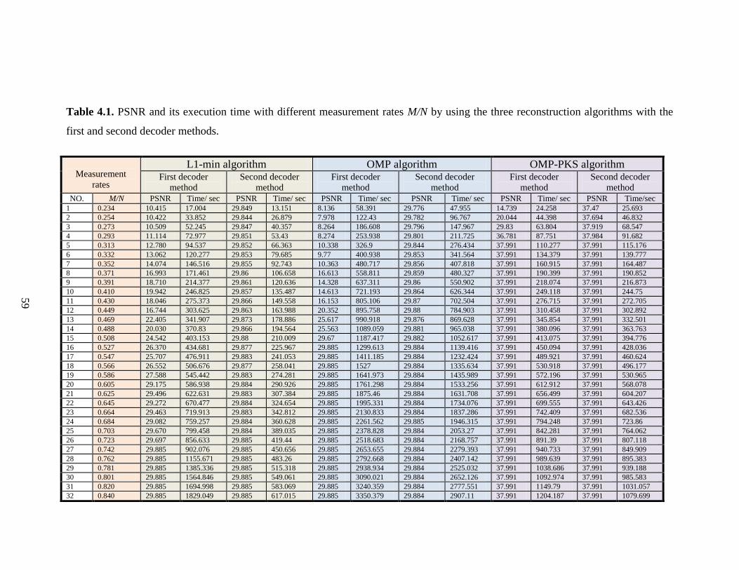
59

Table 4.1. PSNR and its execution time with different measurement rates M/N by using the three reconstruction algorithms with the

first and second decoder methods.

Measurement

rates

L1-min algorithm OMP algorithm OMP-PKS algorithm First decoder

method

Second decoder

method

First decoder

method

Second decoder

method

First decoder

method

Second decoder

method

NO. M/N PSNR Time/ sec PSNR Time/ sec PSNR Time/ sec PSNR Time/ sec PSNR Time/ sec PSNR Time/sec 1 0.234 10.415 17.004 29.849 13.151 8.136 58.391 29.776 47.955 14.739 24.258 37.47 25.693

2 0.254 10.422 33.852 29.844 26.879 7.978 122.43 29.782 96.767 20.044 44.398 37.694 46.832

3 0.273 10.509 52.245 29.847 40.357 8.264 186.608 29.796 147.967 29.83 63.804 37.919 68.547

4 0.293 11.114 72.977 29.851 53.43 8.274 253.938 29.801 211.725 36.781 87.751 37.984 91.682

5 0.313 12.780 94.537 29.852 66.363 10.338 326.9 29.844 276.434 37.991 110.277 37.991 115.176

6 0.332 13.062 120.277 29.853 79.685 9.77 400.938 29.853 341.564 37.991 134.379 37.991 139.777

7 0.352 14.074 146.516 29.855 92.743 10.363 480.717 29.856 407.818 37.991 160.915 37.991 164.487

8 0.371 16.993 171.461 29.86 106.658 16.613 558.811 29.859 480.327 37.991 190.399 37.991 190.852

9 0.391 18.710 214.377 29.861 120.636 14.328 637.311 29.86 550.902 37.991 218.074 37.991 216.873

10 0.410 19.942 246.825 29.857 135.487 14.613 721.193 29.864 626.344 37.991 249.118 37.991 244.75

11 0.430 18.046 275.373 29.866 149.558 16.153 805.106 29.87 702.504 37.991 276.715 37.991 272.705

12 0.449 16.744 303.625 29.863 163.988 20.352 895.758 29.88 784.903 37.991 310.458 37.991 302.892

13 0.469 22.405 341.907 29.873 178.886 25.617 990.918 29.876 869.628 37.991 345.854 37.991 332.501

14 0.488 20.030 370.83 29.866 194.564 25.563 1089.059 29.881 965.038 37.991 380.096 37.991 363.763

15 0.508 24.542 403.153 29.88 210.009 29.67 1187.417 29.882 1052.617 37.991 413.075 37.991 394.776

16 0.527 26.370 434.681 29.877 225.967 29.885 1299.613 29.884 1139.416 37.991 450.094 37.991 428.036

17 0.547 25.707 476.911 29.883 241.053 29.885 1411.185 29.884 1232.424 37.991 489.921 37.991 460.624

18 0.566 26.552 506.676 29.877 258.041 29.885 1527 29.884 1335.634 37.991 530.918 37.991 496.177

19 0.586 27.588 545.442 29.883 274.281 29.885 1641.973 29.884 1435.989 37.991 572.196 37.991 530.965

20 0.605 29.175 586.938 29.884 290.926 29.885 1761.298 29.884 1533.256 37.991 612.912 37.991 568.078

21 0.625 29.496 622.631 29.883 307.384 29.885 1875.46 29.884 1631.708 37.991 656.499 37.991 604.207

22 0.645 29.272 670.477 29.884 324.654 29.885 1995.331 29.884 1734.076 37.991 699.555 37.991 643.426

23 0.664 29.463 719.913 29.883 342.812 29.885 2130.833 29.884 1837.286 37.991 742.409 37.991 682.536

24 0.684 29.082 759.257 29.884 360.628 29.885 2261.562 29.885 1946.315 37.991 794.248 37.991 723.86

25 0.703 29.670 799.458 29.884 389.035 29.885 2378.828 29.884 2053.27 37.991 842.281 37.991 764.062

26 0.723 29.697 856.633 29.885 419.44 29.885 2518.683 29.884 2168.757 37.991 891.39 37.991 807.118

27 0.742 29.885 902.076 29.885 450.656 29.885 2653.655 29.884 2279.393 37.991 940.733 37.991 849.909

28 0.762 29.885 1155.671 29.885 483.26 29.885 2792.668 29.884 2407.142 37.991 989.639 37.991 895.383

29 0.781 29.885 1385.336 29.885 515.318 29.885 2938.934 29.884 2525.032 37.991 1038.686 37.991 939.188

30 0.801 29.885 1564.846 29.885 549.061 29.885 3090.021 29.884 2652.126 37.991 1092.974 37.991 985.583

31 0.820 29.885 1694.998 29.885 583.069 29.885 3240.359 29.884 2777.551 37.991 1149.79 37.991 1031.057

32 0.840 29.885 1829.049 29.885 617.015 29.885 3350.379 29.884 2907.11 37.991 1204.187 37.991 1079.699

59

60

Table 4.2. PSNR and its execution time with different Sparsity rates K/N by using the three reconstruction algorithms with the first

and second decoder methods.

Sparsity rates L1-min algorithm OMP algorithm OMPPKS algorithm

First decoder

method

Second decoder

method

First decoder method Second decoder

method

First decoder

method

Second decoder

method NO. K/N PSNR Time/ sec PSNR Time/ sec PSNR Time/ sec PSNR Time/ sec PSNR Time/ sec PSNR Time/ sec

1 21.508 27.847 30.857 29.083 23.634 32.263 109.341 30.047 94.646 33.083 52.12 33.083 23.946

2 21.992 25.696 72.338 29.219 48.828 32.817 215.422 30.185 187.607 33.219 74.381 33.219 45.303

3 22.445 25.743 111.432 29.345 72.915 32.726 319.272 30.313 280.474 33.345 99.185 33.345 66.456

4 22.988 26.857 140.604 29.494 97.625 32.65 425.337 30.457 375.182 33.494 120.573 33.494 87.875

5 23.496 27.222 192.568 29.631 122.383 32.963 531.87 30.589 480.233 33.631 142.117 33.631 109.638

6 24.137 27.129 230.226 29.803 147.577 32.149 639.62 30.753 576.548 33.803 165.174 33.803 130.994

7 24.676 26.849 272.081 29.945 171.773 32.902 743.594 30.882 675.516 33.945 187.591 33.945 152.538

8 25.352 27.195 312.236 30.121 196.374 32.484 845.135 31.054 773.203 34.121 210.711 34.121 174.269

9 26.043 27.705 351.205 30.299 221.989 32.813 951.887 31.208 872.81 34.299 233.471 34.299 195.875

10 26.789 27.524 390.814 30.49 246.809 32.986 1056.049 31.413 969.531 34.49 255.81 34.49 218.152

11 27.398 27.179 426.959 30.644 272.191 33.364 1159.181 31.569 1064.676 34.644 278.009 34.644 239.664

12 28.207 27.033 475.117 30.841 297.962 32.757 1266.323 31.748 1156.482 34.845 298.992 34.845 261.114

13 28.984 28.716 512.12 30.033 323.686 32.596 1372.076 31.931 1248.133 35.036 328.008 35.036 283.469

14 29.82 27.721 542.337 30.239 349.411 32.814 1475.567 31.123 1340.517 35.239 350.94 35.239 305.06

15 30.617 24.995 589.294 30.43 374.699 32.504 1582.1 32.307 1431.59 35.43 378.256 35.43 327.072

16 31.691 25.729 630.026 30.68 400.314 32.413 1698.289 32.547 1523.069 35.684 403.06 35.684 349.692

17 32.652 27.097 681.553 30.904 426.086 33.168 1820.594 32.758 1614.454 35.909 426.741 35.909 372.078

18 33.598 26.426 726.465 31.124 452.512 32.574 1929.28 32.97 1705.512 36.128 449.688 36.128 394.589

19 34.551 25.922 773.406 31.33 479.079 31.998 2039.089 32.162 1796.445 36.344 474.711 36.344 417.739

20 35.688 27.398 816.884 31.589 505.474 31.933 2157.665 33.383 1887.004 36.598 497.113 36.598 440.422

21 36.848 27.251 866.71 31.837 532.447 31.119 2279.112 33.641 1978.779 36.854 521.324 36.854 463.37

22 38.047 25.471 900.188 32.101 558.874 31.879 2392.728 33.853 2069.852 37.114 543.585 37.114 485.756

23 39.352 26.251 943.556 32.372 587.172 31.968 2510.633 34.11 2162.221 37.392 569.872 37.392 508.454

24 40.762 27.551 988.329 32.655 614.909 31.58 2628.196 34.358 2252.53 37.688 594.754 37.688 532.088

25 42.23 25.731 1035.285 32.973 643.582 30.951 2746.366 34.639 2344.804 38.224 619.979 38.666 554.911

26 43.887 27.703 1096.749 33.299 671.553 31.102 2866.456 34.937 2435.909 38.224 642.521 38.666 578.062

27 45.648 27.274 1150.18 33.623 700.008 30.571 2981.71 34.937 2527.107 38.224 666.701 38.666 601.54

60

61

CHAPTER 5

CONCLUSION AND SUGGESTIONS FOR FUTURE WORKS

Compressive Sensing CS is a very active area of research. It is efficient and accurate for

acquiring and processing the huge data. It takes to recover the signals or the images from

a few non-adaptive linear measurements. There are a different reconstruction algorithms

which are used to reconstruct the sparse image such as the optimization and greedy

methods.

In this thesis, we combine between the watermarking techniques and the CS theory,

where the watermarking image is embedded into the measurement vectors of CS and the

watermarked compressive sensing measurements resulted. The watermarked

compressive sensing measurements are reconstructed by using the orthogonal matching

pursuit OMP and orthogonal matching pursuit with partially known support OMP-PKS

algorithms.

The OMP-PKS algorithm has a priori knowledge about some coefficients of the sparse

image. All these coefficients are nonzero and considered more important than the other

coefficients in the sparse signal. These nonzero coefficients are considered the partially

known support PKS. The reconstructed image by the OMP and OMP-PKS consists of

the original and watermarking images. Then the decoder procedure has been used to

extract the watermarking image from the reconstructed watermarked CS image. The

results compare the performance of the OMP and OMP-PKS algorithms. Experimental

results prove that OMP-PKS algorithm improves the performance, thereby requiring a

fewer samples than the OMP to reconstruct the signal.

As for the future work, we recommend to study the mathematical proof of the OMP-

PKS. As well as, using the field-programmable gate array FPGA to implement this work

as hardware.

62

REFERENCES

[1] Baraniuk, R. (2007). Compressive sensing, IEEE signal processing magazine,

24.

[2] Candès, E.J. and M.B. Wakin. (2008). An introduction to compressive sampling,

Signal Processing Magazine, IEEE, 25, 21-30.

[3] Takeva-Velkova, V. (2010). Optimization algorithms in compressive sensing

(CS) sparse magnetic resonance imaging (MRI), MSC thesis University of

Ontario Institute of Technology, June

[4] Chen, S.S., D.L. Donoho, and M.A. Saunders. (1998). Atomic decomposition by

basis pursuit, SIAM journal on scientific computing, 20, 33-61.

[5] Tropp, J.A. and A.C. Gilbert. (2007). Signal recovery from random

measurements via orthogonal matching pursuit, Information Theory, IEEE

Transactions on, 53, 4655-4666.

[6] Carrillo, R.E., L.F. Polania, and K.E. Barner. (2010). Iterative algorithms for

compressed sensing with partially known support. in Acoustics Speech and

Signal Processing (ICASSP), 2010 IEEE International Conference on, 3654-

3657.

[7] Candes, E.J. and T. Tao. (2005). Decoding by linear programming, Information

Theory, IEEE Transactions on, 51, 4203-4215.

[8] La, C. and M.N. Do. (2006). Tree-based orthogonal matching pursuit algorithm

for signal reconstruction. In Image Processing, 2006 IEEE International

Conference on, 1277-1280.

[9] Barni, M. and F. Bartolini. (2004). Watermarking systems engineering: enabling

digital assets security and other applications. CRC Press.

[10] Yamaç, M., Ç. Dikici, and B. Sankur. (2013). Robust Watermarking Of

Compressive Sensed Measurements Under Impulsive And Gaussian Attacks, In

SPARS,Lausanne.

63

[11] Donoho, D.L. (2006). Compressed sensing, Information Theory, IEEE

Transactions on, 52, 1289-1306.

[12] Garnaev, A.Y. and E.D. Gluskin. (1984). The widths of a Euclidean ball. In

Dokl. Akad. Nauk SSSR, 277, 1048-1052.

[13] Bourgain, J. (1989). Bounded orthogonal systems and the Λ (p)-set problem,

Acta Mathematica, 162, 227-245.

[14] Candes, E.J. and T. Tao. (2006). Near-optimal signal recovery from random

projections: Universal encoding strategies?, Information Theory, IEEE

Transactions on, 52, 5406-5425.

[15] Candès, E.J., J. Romberg, and T. Tao. (2006). Robust uncertainty principles:

Exact signal reconstruction from highly incomplete frequency information,

Information Theory, IEEE Transactions on, 52, 489-509.

[16] Donoho, D.L. (2006). High-dimensional centrally symmetric polytopes with

neighborliness proportional to dimension, Discrete & Computational Geometry,

35, 617-652.

[17] Donoho, D.L. (2006). For most large underdetermined systems of linear

equations the minimal, Communications on pure and applied mathematics, 59,

797-829.

[18] Cormode, G. and S. Muthukrishnan. (2006). Combinatorial algorithms for

compressed sensing. In Structural Information and Communication Complexity.

Springer.

[19] Gilbert, A.C., et al. (2002). Near-optimal sparse Fourier representations via

sampling, In Proceedings of the thiry-fourth annual ACM symposium on Theory

of computing, 152-161.

[20] Yang, F., S. Wang, and C. Deng. (2010). Compressive sensing of image

reconstruction using multi-wavelet transforms. In Intelligent Computing and

Intelligent Systems (ICIS), 2010 IEEE International Conference on, 1, 702-705.

[21] Dias, U., M. Rane, and S. Bandewar. (2012). Survey of Compressive Sensing,

International Journal of Scientific & Engineering Research, 3.

64

[22] Wakin, M.B., et al. (2006). An architecture for compressive imaging. In Image

Processing, 2006 IEEE International Conference on, 1273-1276.

[23] Nagesh, P. and B. Li. (2009). Compressive imaging of color images. In

Acoustics, Speech and Signal Processing, 2009. ICASSP 2009. IEEE

International Conference on, 1261-1264.

[24] Piccardi, M. (2004). Background subtraction techniques: a review. In Systems,

man and cybernetics, 2004 IEEE international conference on, 4, 3099-3104.

[25] Chan, W.L., et al. (2008). A single-pixel terahertz imaging system based on

compressed sensing, Applied Physics Letters, 93, 121105.

[26] Jung, H., et al. (2009). k‐t FOCUSS: A general compressed sensing framework

for high resolution dynamic MRI, Magnetic Resonance in Medicine, 61, 103-

116.

[27] Herrmann, F.J. and G. Hennenfent. (2008). Non‐parametric seismic data

recovery with curvelet frames, Geophysical Journal International, 173, 233-248.

[28] Hennenfent, G. and F.J. Herrmann. (2008). Simply denoise: wavefield

reconstruction via jittered undersampling, Geophysics, 73, V19-V28.

[29] Du, D. and F. Hwang. (1993). Combinatorial group testing and its applications.

World Scientific.

[30] Mohtashemi, M., et al. (2010). Sparse sensing DNA microarray-based biosensor:

Is it feasible? In Sensors Applications Symposium (SAS), 2010 IEEE, 127-130.

[31] Baraniuk, R. and P. Steeghs. (2007). Compressive radar imaging. In Radar

Conference, 2007 IEEE, 128-133.

[32] Herman, M.A. and T. Strohmer. (2009). High-resolution radar via compressed

sensing, Signal Processing, IEEE Transactions on, 57, 2275-2284.

[33] Moses, R.L., L.C. Potter, and M. Cetin. (2004). Wide-angle SAR imaging. In

Defense and Security, 164-175.

[34] Qu, L. and T. Yang. (2012). Investigation of air/ground reflection and antenna

beamwidth for compressive sensing SFCW GPR migration imaging, Geoscience

and Remote Sensing, IEEE Transactions on, 50, 3143-3149.

[35] Walden, R.H. (1999). Analog-to-digital converter survey and analysis, IEEE

Journal on selected areas in communications, 17, 539-550.

65

[36] Laska, J.N., et al. (2007). Theory and implementation of an analog-to-

information converter using random demodulation. In Circuits and Systems,

2007. ISCAS 2007. IEEE International Symposium on, 1959-1962.

[37] Kirolos, S., et al. (2006). Analog-to-information conversion via random

demodulation. In Design, Applications, Integration and Software, 2006 IEEE

Dallas/CAS Workshop on, 71-74.

[38] Tropp, J.A., et al. (2006). Random filters for compressive sampling and

reconstruction. In Acoustics, Speech and Signal Processing, 2006. ICASSP 2006

Proceedings. 2006 IEEE International Conference on, 3, III-III.

[39] Mishali, M. and Y.C. Eldar. (2010). From theory to practice: Sub-Nyquist

sampling of sparse wideband analog signals, Selected Topics in Signal

Processing, IEEE Journal of, 4, 375-391.

[40] Donoho, D.L. and B.F. Logan. (1992). Signal recovery and the large sieve, SIAM

Journal on Applied Mathematics, 52, 577-591.

[41] Tibshirani, R. (1996). Regression shrinkage and selection via the lasso, Journal

of the Royal Statistical Society. Series B (Methodological), 267-288.

[42] Donoho, D.L. (1995). De-noising by soft-thresholding, Information Theory,

IEEE Transactions on, 41, 613-627.

[43] O'Brien, M.S., A.N. Sinclair, and S.M. Kramer. (1994). Recovery of a sparse

spike time series by l 1 norm deconvolution, Signal Processing, IEEE

Transactions on, 42, 3353-3365.

[44] Candes, E.J., J.K. Romberg, and T. Tao. (2006). Stable signal recovery from

incomplete and inaccurate measurements, Communications on pure and applied

mathematics, 59, 1207-1223.

[45] Needell, D. and R. Vershynin. (2010). Signal recovery from incomplete and

inaccurate measurements via regularized orthogonal matching pursuit, Selected

Topics in Signal Processing, IEEE Journal of, 4, 310-316.

[46] Donoho, D.L. and M. Elad. (2003). Optimally sparse representation in general

(nonorthogonal) dictionaries via ℓ1 minimization, Proceedings of the National

Academy of Sciences, 100, 2197-2202.

66

[47] Donoho, D. and J. Tanner. (2009). Counting faces of randomly projected

polytopes when the projection radically lowers dimension, Journal of the

American Mathematical Society, 22, 1-53.

[48] Fuchs, J.-J. (2004). On sparse representations in arbitrary redundant bases,

Information Theory, IEEE Transactions on, 50, 1341-1344.

[49] Natarajan, B.K. (1995). Sparse approximate solutions to linear systems, SIAM

journal on computing, 24, 227-234.

[50] Gribonval, R., et al. (1996). Analysis of sound signals with high resolution

matching pursuit. In Time-Frequency and Time-Scale Analysis, 1996.,

Proceedings of the IEEE-SP International Symposium on, 125-128.

[51] Banham, M.R. and J.C. Brailean. (1997). A selective update approach to

matching pursuits video coding, Circuits and Systems for Video Technology,

IEEE Transactions on, 7, 119-129.

[52] Hastie, T., et al. (2009). The elements of statistical learning. 2: Springer.

[53] Rath, G. and C. Guillemot. (2009). Sparse approximation with an orthogonal

complementary matching pursuit algorithm. In Acoustics, Speech and Signal

Processing, 2009. ICASSP 2009. IEEE International Conference on, 3325-3328.

[54] Wang, J., S. Kwon, and B. Shim. (2012). Generalized orthogonal matching

pursuit, Signal Processing, IEEE Transactions on, 60, 6202-6216.

[55] Donoho, D.L., et al. (2012). Sparse solution of underdetermined systems of

linear equations by stagewise orthogonal matching pursuit, Information Theory,

IEEE Transactions on, 58, 1094-1121.

[56] Needell, D., J. Tropp, and R. Vershynin. (2008). Greedy signal recovery review.

In Signals, Systems and Computers, 2008 42nd Asilomar Conference on, 1048-

1050.

[57] Rebollo-Neira, L. (2001). Frames in two dimensions arising from wavelet

transforms, Proceedings of the Royal Society of London. Series A: Mathematical,

Physical and Engineering Sciences, 457, 2079-2091.

[58] Mallat, S.G. and Z. Zhang. (1993). Matching pursuits with time-frequency

dictionaries, Signal Processing, IEEE Transactions on, 41, 3397-3415.

67

[59] Rebollo-Neira, L. and D. Lowe. (2002). Optimized orthogonal matching pursuit

approach, Signal Processing Letters, IEEE, 9, 137-140.

[60] Needell, D. and J.A. Tropp. (2009). CoSaMP: Iterative signal recovery from

incomplete and inaccurate samples, Applied and Computational Harmonic

Analysis, 26, 301-321.

[61] Jacques, L. (2010). A short note on compressed sensing with partially known

signal support, Signal Processing, 90, 3308-3312.

[62] Vaswani, N. and W. Lu. (2010). Modified-CS: Modifying compressive sensing

for problems with partially known support, Signal Processing, IEEE

Transactions on, 58, 4595-4607.

[63] Duarte, M.F., et al. (2009). Recovery of compressible signals in unions of

subspaces. In Information Sciences and Systems, 2009. CISS 2009. 43rd Annual

Conference on, 175-180.

[64] Sermwuthisarn, P., et al. (2012). Impulsive noise rejection method for

compressed measurement signal in compressed sensing, EURASIP Journal on

Advances in Signal Processing, 2012, 1-23.

[65] Sermwuthisarn, P., et al. (2012). Robust reconstruction algorithm for compressed

sensing in Gaussian noise environment using orthogonal matching pursuit with

partially known support and random subsampling, EURASIP Journal on

Advances in Signal Processing, 2012, 1-21.

[66] Cevher, V., et al. (2008). Compressive sensing for background subtraction. In

Computer Vision–ECCV 2008. Springer.

[67] Cox, I.J. and M.L. Miller. (2002). The first 50 years of electronic watermarking,

EURASIP Journal on Applied Signal Processing, 2002, 126-132.

[68] Swanson, M.D., B. Zhu, and A.H. Tewfik. (1996). Robust data hiding for

images. In Digital Signal Processing Workshop Proceedings, 1996., IEEE, 37-

40.

[69] Hernandez, J.R., M. Amado, and F. Perez-Gonzalez. (2000). DCT-domain

watermarking techniques for still images: Detector performance analysis and a

new structure, Image Processing, IEEE Transactions on, 9, 55-68.

68

[70] Hartung, F. and B. Girod. (1998). Watermarking of uncompressed and

compressed video, Signal processing, 66, 283-301.

[71] http://www.geovision.com.tw.

[72] http://www.mediasec.com.

[73] Kirstein, M., Beyond traditional DRM: Moving to digital watermarking and

fingerprinting in media monetization. 2006, January.

[74] Huang, H.-C., et al. (2012). Watermarking for compressive sampling

applications. In Intelligent Information Hiding and Multimedia Signal

Processing (IIH-MSP), 2012 Eighth International Conference on, 223-226.

[75] Huang, H.-C., et al. (2011). Tabu search based multi-watermarks embedding

algorithm with multiple description coding, Information Sciences, 181, 3379-

3396.

[76] Kundur, D. and D. Hatzinakos. (1997). A robust digital image watermarking

method using wavelet-based fusion. In International Conference on Image

Processing, 3, 544-547.

[77] Orovic, I. and S. Stankovic. (2013). Combined compressive sampling and image

watermarking. In ELMAR, 2013 55th International Symposium, 41-44.

[78] Orović, I., A. Draganić, and S. Stanković. (2013). Compressive Sensing as a

Watermarking Attack, 21st Telecommunications Forum TELFOR

2013, Novembar.

[79] Simmons, G.J. (1984). The prisoners‟ problem and the subliminal channel. In

Advances in Cryptology, 51-67.

[80] Qaisar, S., et al. (2013). Compressive sensing: From theory to applications, a

survey, Communications and Networks, Journal of, 15, 443-456.

[81] Tiesheng, F., et al. (2013). A Digital Image Watermarking Method Based on the

Theory of Compressed Sensing, International Journal of Automation and

Control Engineering, 2.

[82] M. Yamac, C. Dikici, and B. Sankur. (2013). Watermarking of Compressive

Sensed Measurements, in SPARS,Lausanne.

69