JOURNAL OF SOUND AND VIBRATION Limit cycles, bifurcations, and accuracy of the milling process

JOURNAL OFSOUND ANDVIBRATION

www.elsevier.com/locate/jsvi

Journal of Sound and Vibration 277 (2004) 31–48

Limit cycles, bifurcations, and accuracy of the milling process

B.P. Manna,*, P.V. Baylyb, M.A. Daviesc, J.E. Halleyd

aDepartment of Mechanical and Aerospace Engineering, University of Florida, P.O. Box 116300,

Gainesville, FL 32611, USAbDepartment of Mechanical Engineering, Washington University, St. Louis, MO, USA

cDepartment of Mechanical Engineering, University of North Carolina, Charlotte, NC, USAdTech Manufacturing, Wright City, MO, USA

Received 14 October 2002; accepted 19 August 2003

Abstract

Time finite element analysis (TFEA) is used to determine the accuracy, stability, and limit cycle behaviorof the milling process. Predictions are compared to traditional Euler simulation and experiments. TheTFEA method forms an approximate solution by dividing the time in the cut into a finite number ofelements. The approximate solution is then matched with the exact solution for free vibration to obtain adiscrete linear map. Stability is then determined from the characteristic multipliers of the map. Map fixedpoints correspond to stable periodic solutions which are used to evaluate surface location error.Bifurcations and limit cycle behavior are predicted from a non-linear TFEA formulation. Experimentalcutting tests are used to confirm theoretical predictions.r 2003 Elsevier Ltd. All rights reserved.

1. Introduction

Relative vibrations between a cutting tool and workpiece result in a machining process withsurface location errors and time-varying chip loads. Since cutting forces are approximatelyproportional to the uncut chip area [1–4], chip load variations cause dynamic cutting forces whichmay excite the structural modes of a machine–tool system resulting in unstable vibrations knownas chatter. Unless avoided, chatter vibrations may cause large dynamic loads on the machinespindle and table structure, damage to the cutting tool, and a poor surface finish [1,5]. Therefore,it is desirable to avoid chatter vibrations. Even in the absence of chatter, the accurate placement ofa machined surface is complicated by vibrations and surface location errors result when themachined surface does not lie ‘‘exactly’’ at the commanded location.

ARTICLE IN PRESS

*Corresponding author. Tel.: +1-352-392-4550; fax: +1-352-392-1071.

E-mail address: [email protected] (B.P. Mann).

0022-460X/$ - see front matter r 2003 Elsevier Ltd. All rights reserved.

doi:10.1016/j.jsv.2003.08.040

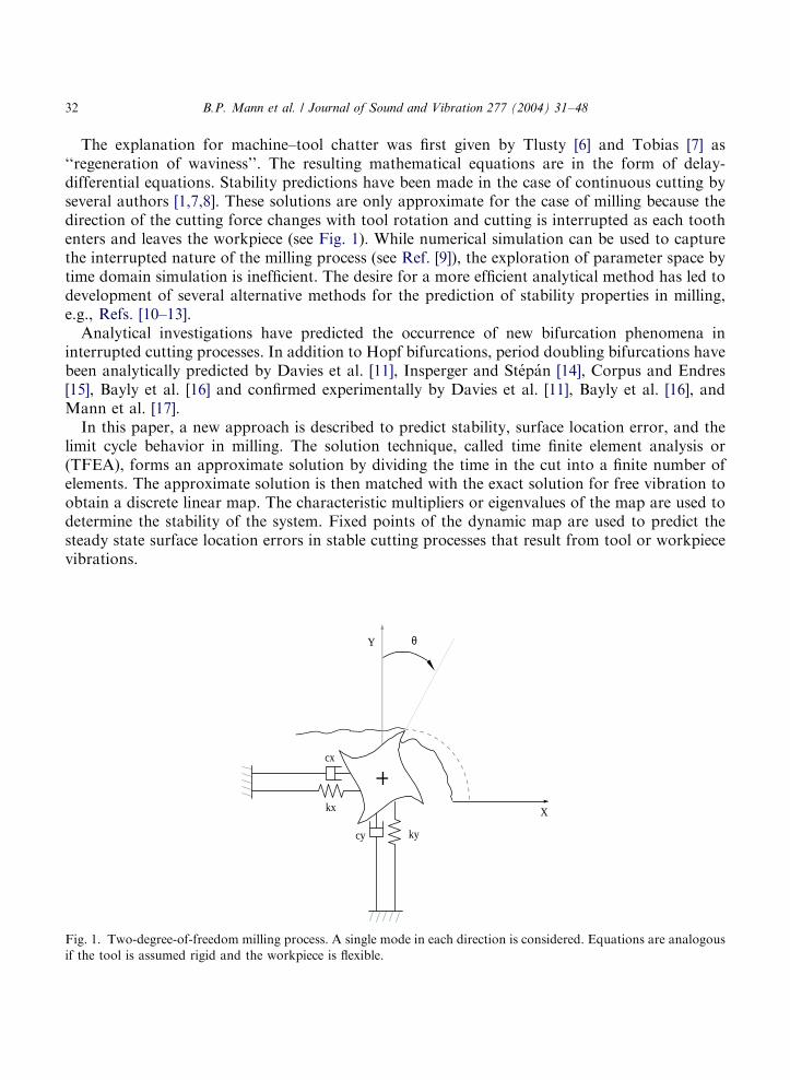
The explanation for machine–tool chatter was first given by Tlusty [6] and Tobias [7] as‘‘regeneration of waviness’’. The resulting mathematical equations are in the form of delay-differential equations. Stability predictions have been made in the case of continuous cutting byseveral authors [1,7,8]. These solutions are only approximate for the case of milling because thedirection of the cutting force changes with tool rotation and cutting is interrupted as each toothenters and leaves the workpiece (see Fig. 1). While numerical simulation can be used to capturethe interrupted nature of the milling process (see Ref. [9]), the exploration of parameter space bytime domain simulation is inefficient. The desire for a more efficient analytical method has led todevelopment of several alternative methods for the prediction of stability properties in milling,e.g., Refs. [10–13].Analytical investigations have predicted the occurrence of new bifurcation phenomena in

interrupted cutting processes. In addition to Hopf bifurcations, period doubling bifurcations havebeen analytically predicted by Davies et al. [11], Insperger and St!ep!an [14], Corpus and Endres[15], Bayly et al. [16] and confirmed experimentally by Davies et al. [11], Bayly et al. [16], andMann et al. [17].In this paper, a new approach is described to predict stability, surface location error, and the

limit cycle behavior in milling. The solution technique, called time finite element analysis or(TFEA), forms an approximate solution by dividing the time in the cut into a finite number ofelements. The approximate solution is then matched with the exact solution for free vibration toobtain a discrete linear map. The characteristic multipliers or eigenvalues of the map are used todetermine the stability of the system. Fixed points of the dynamic map are used to predict thesteady state surface location errors in stable cutting processes that result from tool or workpiecevibrations.

ARTICLE IN PRESS

X

Y θ

kycy

kx

cx

Fig. 1. Two-degree-of-freedom milling process. A single mode in each direction is considered. Equations are analogous

if the tool is assumed rigid and the workpiece is flexible.

B.P. Mann et al. / Journal of Sound and Vibration 277 (2004) 31–4832

For an unstable cutting process, relative vibrations build until the tool jumps out of the cut.When the tool continues to reenter and jump out of the cut, the result is a limit cycle. A recursivemapping process, called non-linear TFEA, is introduced here to capture the non-linearity of thetool jumping out of the cut.The stability, accuracy, and limit cycle predictions from the TFEA method are compared

to experimental cutting tests and Euler simulation. Strong agreement is obtained betweenthe both numerical methods and experiments. In addition, the computation times requiredfor TFEA predictions is shown to be significantly less than computational times for Eulersimulation.

2. Mechanical model

A schematic diagram of a two-degree-of-freedom milling process is shown in Fig. 1. Acompliant tool or structure with a single mode of vibration in two uncoupled and orthogonaldirections will result in the following equation of motion:

mx 0

0 my

" #.xðtÞ

.yðtÞ

" #þ

cx 0

0 cy

" #’xðtÞ

’yðtÞ

" #þ

kx 0

0 ky

" #xðtÞ

yðtÞ

" #¼

FxðtÞ

FyðtÞ

" #; ð1Þ

where the terms mx;y; cx;y; kx;y; and Fx;y are the modal mass, damping, spring stiffness, and cuttingforces in the flexible directions of the system. The x and y cutting force components on the pthtooth are given by

FxpðtÞ ¼ gpðtÞ½FtpðtÞ cos ypðtÞ þ FnpðtÞ sin ypðtÞ; ð2Þ

FypðtÞ ¼ gpðtÞ½FtpðtÞ sin ypðtÞ FnpðtÞ cos ypðtÞ; ð3Þ

where gpðtÞ acts as a switching function, it is equal to one if the pth tooth is active and zero if it isnot cutting [10,12]. The tangential and normal cutting force components, FtpðtÞ and FnpðtÞ;respectively, are considered to be the product of linearized cutting coefficients Kt and Kn; thenominal depth of cut b; and the instantaneous chip width wpðtÞ:

FtpðtÞ ¼ KtbwpðtÞ; FnpðtÞ ¼ KnbwpðtÞ; ð4; 5Þ

where wpðtÞ depends upon the feed per tooth, h; the cutter rotation angle ypðtÞ; and regeneration inthe compliant structure directions:

wpðtÞ ¼ h sin ypðtÞ þ ½xðtÞ xðt tÞsin ypðtÞ þ ½yðtÞ yðt tÞcos ypðtÞ: ð6Þ

Here, h sin ypðtÞ is the circular tool path approximation [1,5], t ¼ 60=NO ½s is the tooth passperiod, O is the spindle speed given in r.p.m. and N is the total number of cutting teeth. Theangular position of the pth tooth for a cutter with evenly spaced teeth is ypðtÞ ¼ ð2pO=60Þt þp2p=N:

ARTICLE IN PRESS

B.P. Mann et al. / Journal of Sound and Vibration 277 (2004) 31–48 33

The total cutting force equations are found by summing the forces on each cutting tooth andsubstituting Eqs. (4)–(6) into Eqs. (2) and (3):

Fx

Fy

" #¼XN

p¼1

gpðtÞb hKtsc Kns2

Kts2 Knsc

" #

þKtsc Kns2 Ktc

2 Knsc

Kts2 Knsc Ktsc Knc2

" #xðtÞ xðt tÞ

yðtÞ yðt tÞ

" #!; ð7Þ

where s ¼ sin ypðtÞ and c ¼ cos ypðtÞ: A more compact form for the equation of motion and isrealized by defining the substitutions

KcðtÞ ¼XN

p¼1

gpðtÞKtsc Kns2 Ktc

2 Knsc

Kts2 Knsc Ktsc Knc2

" #; ð8Þ

f 0ðtÞ ¼XN

p¼1

gpðtÞhKtsc Kns2

Kts2 Knsc

" #; ð9Þ

and rewriting Eq. (1) as

M .XðtÞ þ C ’XðtÞ þ KXðtÞ ¼ KcðtÞb½XðtÞ Xðt tÞ þ f 0ðtÞb; ð10Þ

where XðtÞ ¼ ½xðtÞ yðtÞ? is the two-element position vector and M;C; and K are the 2 2 mass,damping, and stiffness matrices of Eq. (1). When the structure is only compliant in a singledirection, Eq. (10) can be modified by eliminating the corresponding rows and columns of theopposing direction. For instance, a structure compliant only in the x direction would have thefollowing equation of motion:

mx .xðtÞ þ cx ’xðtÞ þ kxxðtÞ ¼ KsxðtÞb½xðtÞ xðt tÞ f0xðtÞb; ð11Þ

where the x direction terms of KcðyðtÞÞ and f 0ðyðtÞÞ have now been written as

KsxðtÞ ¼XN

p¼1

gpðtÞ½Kt cos ypðtÞ þ Kn sin ypðtÞsin ypðtÞ; ð12Þ

f0xðtÞ ¼XN

p¼1

gpðtÞ½Kt cos ypðtÞ þ Kn sin ypðtÞh sin ypðtÞ: ð13Þ

The terms KsxðtÞ and f0xðtÞ provide a periodic forcing term which would result in a periodicsolution in the absence of the perturbations given by the time-delayed relative displacement termsof Eq. (11). Perturbation growth reflects the loss of stability, while perturbation decaycharacterizes an asymptotically stable cutting process.

3. TFEA

The dynamic behavior of the milling process is dependent upon a time-delay differentialequation which does not have a closed form solution. Therefore, an approximate solution is

ARTICLE IN PRESS


sought to understand the behavior of the system. One such approximation technique usedfor dynamic systems is TFEA [18]. This method was first applied to an interrupted turningprocess by Halley [19] and Bayly et al. [20]. The authors matched an approximation for thecutting motion obtained using a single finite element to the exact solution for free vibrationto obtain a discrete linear map. The characteristic multipliers or eigenvalues of the map wereused to determine the stability of the system. Comparisons with experimental tests showedstrong agreement for small fractions of the spindle period in the cut ðrÞ: However,diminished correlations were shown for larger values of r: This was corrected in Baylyet al. [16] by dividing the time in the cut into multiple finite elements in time. The multipleelement turning solution was adapted to model single-degree-of-freedom (SDOF) millingsystems in Mann et al. [17] and multiple degree of freedom systems (MDOF) inBayly et al. [21]. The analysis presented in this article extends the previous stability SDOFwork of Mann et al. [17] to the prediction of surface location error and the limit cycle behaviorassociated with the non-linearity of the tool exiting the cut during chatter vibrations. Theformulation of the dynamic map for the MDOF system (Eq. (10)) closely follows thediscretization procedure outlined in Bayly et al. [21], but has been presented here forcompleteness.

3.1. Free vibration

When the tool is not in contact with the workpiece, the system is governed by the equation forfree vibration

M .XðtÞ þ C ’XðtÞ þ KXðtÞ ¼ 0: ð14Þ

This equation can be rearranged into state-space form

’XðtÞ.XðtÞ

" #¼

0 I

M1K M1C

" #XðtÞ’XðtÞ

" #; ð15Þ

where the 2 2 state matrix in Eq. (15) will be denoted by G: If we let t ¼ tc as the tool leaves thematerial and tf be the duration of free vibration, a state transition matrix ðU ¼ eGtf Þ can beobtained that relates the state of the tool at the beginning of free vibration to the state of the toolat the end of free vibrations.This equation is true for every period, such that for all n:

XðntÞ’XðntÞ

" #¼ U

Xððn 1Þtþ tcÞ’Xððn 1Þtþ tcÞ

" #: ð16Þ

3.2. Vibration during cutting

When the tool is in the cut, its motion is governed by a time-delayed differential equation. Sincethis equation does not have a closed form solution, an approximate solution for the tooldisplacement is assumed for the jth element of the nth tooth passage as a linear combination of

ARTICLE IN PRESS


polynomials (see Ref. [22])

XðtÞ ¼X4i¼1

anjifiðsjðtÞÞ: ð17Þ

Here, sjðtÞ ¼ t ntPj1

k¼1 tk is the ‘‘local’’ time within the jth element of the nth period, thelength of the kth element is tk and the trial functions fiðsjðtÞÞ are the cubic Hermite polynomials.On the jth element these functions are

f1ðsjÞ ¼ 1 3sj

tj

2

þ2sj

tj

3

; ð18aÞ

f2ðsjÞ ¼ tj

sj

tj

2

sj

tj

2

þsj

tj

3" #

; ð18bÞ

f3ðsjÞ ¼ 3sj

tj

2

2sj

tj

3

; ð18cÞ

f4ðsjÞ ¼ tj sj

tj

2

þsj

tj

3" #

: ð18dÞ

These functions are particularly useful because they allow the coefficients of the assumed solutionto be found by matching the initial and final velocities for each element.Substitution of the assumed solution (Eq. (17)) into the equation of motion (Eq. (11)) leads to a

non-zero error. The error from the assumed solution is ‘‘weighted’’ by multiplying by a set of testfunctions and setting the integral of the weighted error to zero to obtain two equations perelement [16,19,20,22,23]. The test functions are chosen to be the simplest possible functions:c1ðsjÞ ¼ 1 (constant) and c2ðsjÞ ¼ sj=tj 1=2 (linear). The integral is taken over the time for eachelement, tj ¼ tc=E; thereby dividing the time in the cut tc into E elements. The resulting twoequations areZ tj

0

MX4i¼1

anji.fiðsjÞcpðsjÞ

!þ C

X4i¼1

anji’fiðsjÞcpðsjÞ

!"

þ ðK bKcðsjÞÞX4i¼1

anjifiðsjÞcpðsjÞ

!

þ bKcðsjÞX4i¼1

an1ji fiðsjÞcpðsjÞ

! bf 0ðsjÞcpðsjÞ

#dsj ¼ 0; p ¼ 1; 2: ð19Þ

Here p is used to identify the test function and the terms KcðsjÞ and f 0ðsjÞ have been used in placeof the previously defined KcðtÞ and f 0ðtÞ to explicitly show dependence on the local time.The displacement and velocity at tool entry into the cut are specified by the coefficients

of the first two basis functions on the first element: an11 and an

12: The relationship betweenthe initial and final conditions during free vibration can be rewritten in terms of the

ARTICLE IN PRESS


coefficients as

a11

a12

!n

¼ UaE3

aE4

!n1

; ð20Þ

where E is the total number of finite elements in the cut. For the remainder of the elements, acontinuity constraint is imposed to set the position and velocity at the end of one element areequal to the position and velocity at the beginning of the next element.Eqs. (19) and (20) can be arranged into a global matrix relating the coefficients of the assumed

solution in terms of the coefficients of the previous tooth passage. The following expression is forthe case when the number of elements is E ¼ 3:

I 0 0 0

N11 N1

2 0 0

0 N21 N2

2 0

0 0 N31 N3

2

266664

377775

a11

a12

a21

a22

a31

a32

a33

a34

2666666666666664

3777777777777775

n

¼

0 0 0 F

P11 P1

2 0 0

0 P21 P2

2 0

0 0 P31 P3

2

266664

377775

a11

a12

a21

a22

a31

a32

a33

a34

2666666666666664

3777777777777775

n1

þ

0

0

C1

C2

C1

C2

C1

C2

2666666666666664

3777777777777775

; ð21Þ

where the sub-matrices and elements of the sub-matrices for the jth element are

N j1 ¼

Nj11 N

j12

Nj21 N

j22

" #; N j

2 ¼N

j13 N

j14

Nj23 N

j24

" #; ð22Þ

Pj1 ¼

Pj11 P

j12

Pj21 P

j22

" #; P

j2 ¼

Pj13 P

j14

Pj23 P

j24

" #; ð23Þ

Njpi ¼

Z tj

0

½M .fiðsjÞ þ C ’fiðsjÞ þ ðK bKcðsjÞÞfiðsjÞcpðsjÞ dsj; ð24Þ

Pj

pi ¼Z tj

0

bKcðsjÞfiðsjÞcpðsjÞ dsj; ð25Þ

Cjp ¼

Z tj

0

bf 0ðsjÞcp dsj: ð26Þ

Eq. (21) describes a discrete dynamical system, or map, that can be written as

Aan ¼ Ban1 þ C ; ð27Þ

or

an ¼ Qan1 þ D: ð28Þ

ARTICLE IN PRESS


3.3. Stability prediction from dynamic map characteristic multipliers

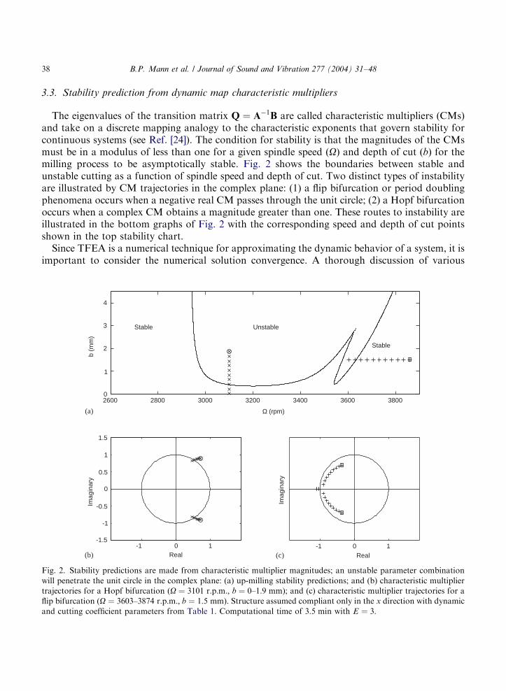
The eigenvalues of the transition matrix Q ¼ A1B are called characteristic multipliers (CMs)and take on a discrete mapping analogy to the characteristic exponents that govern stability forcontinuous systems (see Ref. [24]). The condition for stability is that the magnitudes of the CMsmust be in a modulus of less than one for a given spindle speed ðOÞ and depth of cut ðbÞ for themilling process to be asymptotically stable. Fig. 2 shows the boundaries between stable andunstable cutting as a function of spindle speed and depth of cut. Two distinct types of instabilityare illustrated by CM trajectories in the complex plane: (1) a flip bifurcation or period doublingphenomena occurs when a negative real CM passes through the unit circle; (2) a Hopf bifurcationoccurs when a complex CM obtains a magnitude greater than one. These routes to instability areillustrated in the bottom graphs of Fig. 2 with the corresponding speed and depth of cut pointsshown in the top stability chart.Since TFEA is a numerical technique for approximating the dynamic behavior of a system, it is

important to consider the numerical solution convergence. A thorough discussion of various

ARTICLE IN PRESS

2600 2800 3000 3200 3400 3600 38000

1

2

3

4

Unstable

Stable

Stable

Ω (rpm)

b (m

m)

-1 0 1-1.5

-1

-0.5

0

0.5

1

1.5

Imag

inar

y

Real-1 0 1

Real

Imag

inar

y

(a)

(b) (c)

Fig. 2. Stability predictions are made from characteristic multiplier magnitudes; an unstable parameter combination

will penetrate the unit circle in the complex plane: (a) up-milling stability predictions; and (b) characteristic multiplier

trajectories for a Hopf bifurcation (O ¼ 3101 r:p:m:; b ¼ 0–1:9 mm); and (c) characteristic multiplier trajectories for a

flip bifurcation (O ¼ 3603–3874 r:p:m:; b ¼ 1:5 mm). Structure assumed compliant only in the x direction with dynamic

and cutting coefficient parameters from Table 1. Computational time of 3:5 min with E ¼ 3:


problem formulations, choice of trial functions, and numerical convergence was demonstrated inPeters et al. [22,25]. Bayly et al. [16] demonstrated convergence for interrupted cutting by simplyincreasing the number of temporal finite elements until stability boundaries no longer changed.For the figures presented in this article, the solution convergence was checked and the number ofelements ðEÞ will be included in the figure captions.

3.4. Surface location error from map fixed points

A surface location error results when the machined surface does not lie ‘‘exactly’’ at thecommanded location. Several sources of error such as tool or workpiece vibrations, imperfectspindle motions, thermal errors, controller errors, and friction in the machine drives all contributeto the total error [1,4]. The goal of this section is to present a prediction method for thecontribution of tool or workpiece vibrations to steady state error. This is achieved by formulatinga solution that accounts for changing process parameters such as spindle speed and depth of cut toillustrate their effects on the surface location error.The TFEA method discretizes the continuous system equations to form the dynamic map

shown in Eq. (28). The coefficient vector an identifies the velocity and displacement at thebeginning and end of each element. Surface location error is given by the displacement coefficientvalue when the cutting tooth is normal to the surface. This occurs at cutter tooth entry into the cutfor up-milling and cutter exit for down-milling.Stable milling processes have periodic cutting forces and periodic solutions. The steady state

coefficients are found from the fixed points ðan Þ of the dynamic map:

an ¼ an1 ¼ an : ð29Þ

Substitution of Eq. (29) into Eq. (28) gives the fixed point map solution or steady state coefficientvector

an ¼ ðIQÞ1D: ð30Þ

Since Q and D can be computed exactly for each spindle speed and depth of cut, the fixed pointdisplacement solution can be found and used to specify surface location error as a function ofmachining process parameters.

3.5. Non-linear TFEA for limit cycle prediction

Unstable cutting processes produce large cutting forces as relative vibrations between thecutting tool and workpiece build. Both cutting forces and vibrations continue to grow until thetool jumps out of the cut. As the tool jumps out of the cut, the cutting forces become zero and freevibrations occur until the tool reenters the cut. This leads to a limit cycle when the tool continuesto re-enter and jump out of the cut. Since the non-linearity associated with the tool jumping out ofthe cut is not accounted for in the fixed point solution, a modified solution method called non-linear TFEA is presented in this section to predict the milling process limit cycle behavior. Thishighlights the important aspect that surface location error predictions should only be used forstable cutting processes.

ARTICLE IN PRESS


The non-linear TFEA procedure iterates the dynamic map (Eq. (28)) to obtain the currentcoefficient vector ðanÞ from the previous tooth passage coefficients ðan1Þ: During each toothpassage, the radial chip width ðwpÞ is checked at the beginning and end of each element withEq. (6), where XðtÞ is equal to the displacement coefficients of an: If a negative wp occurs in the jthelement, the tool has jumped out of the cut. The cutting forces are then set to zero by changingKcðsjÞ and f 0ðsjÞ to zero in Eqs. (24)–(26) and updating the rows of the global matrix (Eq. (21))corresponding to the j þ 1 element. In addition, the effect of the tool jumping out of the cut iscaptured in the following revolution by correcting the feed in Eq. (26) to form a new D:

4. Euler simulation

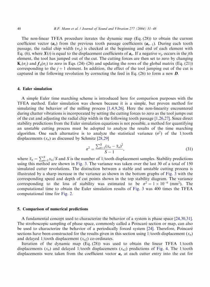
A simple Euler time marching scheme is introduced here for comparison purposes with theTFEA method. Euler simulation was chosen because it is a simple, but proven method forsimulating the behavior of the milling process [1,4,9,26]. Here the non-linearity encounteredduring chatter vibrations is incorporated by setting the cutting forces to zero as the tool jumps outof the cut and adjusting the radial chip width in the following tooth passage [1,26,27]. Since directstability predictions from the Euler simulation equations is not possible, a method for quantifyingan unstable cutting process must be adopted to analyze the results of the time marchingalgorithm. One such alternative is to analyze the statistical variance ðs2Þ of the 1/toothdisplacements ðxnÞ as discussed by Schmitz [28,29]

s2 ¼PS

n¼1ðxn %xnÞ2

S 1; ð31Þ

where %xn ¼PS

n¼1xn=S and S is the number of 1/tooth displacement samples. Stability predictionsusing this method are shown in Fig. 3. The variance was taken over the last 30 of a total of 150simulated cutter revolutions. The distinction between a stable and unstable cutting process isillustrated by a sharp increase in the variance as shown in the bottom graphs of Fig. 3 with thecorresponding speed and depth of cut points shown in the top stability diagram. The variancecorresponding to the loss of stability was estimated to be s2 ¼ 1 106 ðmm2Þ: Thecomputational time to obtain the Euler simulation results of Fig. 3 was 400 times the TFEAcomputational time for Fig. 2.

5. Comparison of numerical predictions

A fundamental concept used to characterize the behavior of a system is phase space [24,30,31].The stroboscopic sampling of phase space, commonly called a Poincar!e section or map, can alsobe used to characterize the behavior of a periodically forced system [24]. Therefore, Poincar!esections have been constructed for the results given in this section using 1/tooth displacement ðxnÞand delayed 1/tooth displacement ðxn2Þ co-ordinates.Iteration of the dynamic map (Eq. (28)) was used to obtain the linear TFEA 1/tooth

displacements ðxnÞ and delayed 1/tooth displacements ðxn2Þ predictions of Fig. 4. The 1/toothdisplacements were taken from the coefficient vector an at each cutter entry into the cut for

ARTICLE IN PRESS


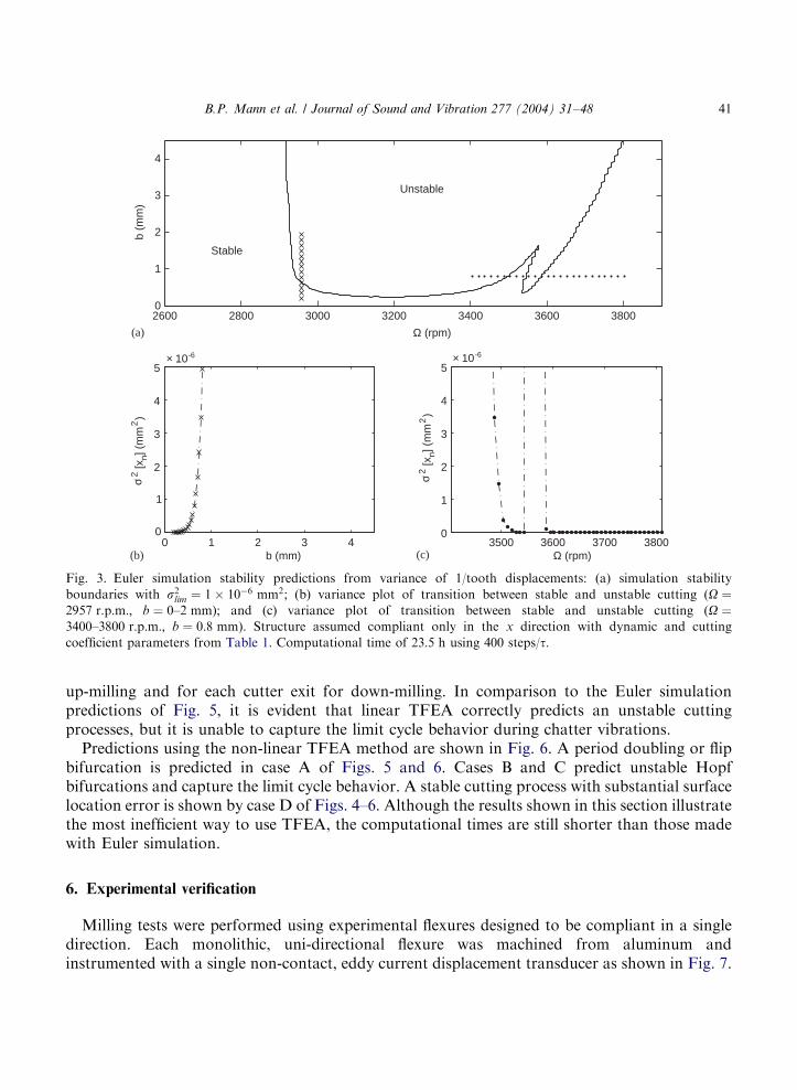
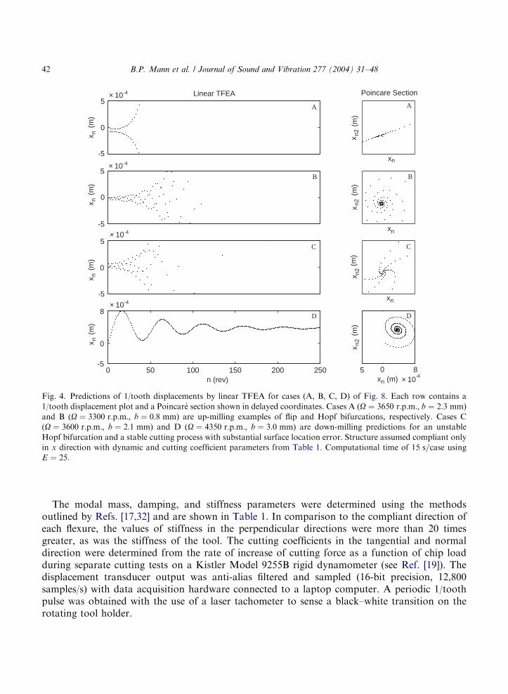
up-milling and for each cutter exit for down-milling. In comparison to the Euler simulationpredictions of Fig. 5, it is evident that linear TFEA correctly predicts an unstable cuttingprocesses, but it is unable to capture the limit cycle behavior during chatter vibrations.Predictions using the non-linear TFEA method are shown in Fig. 6. A period doubling or flip

bifurcation is predicted in case A of Figs. 5 and 6. Cases B and C predict unstable Hopfbifurcations and capture the limit cycle behavior. A stable cutting process with substantial surfacelocation error is shown by case D of Figs. 4–6. Although the results shown in this section illustratethe most inefficient way to use TFEA, the computational times are still shorter than those madewith Euler simulation.

6. Experimental verification

Milling tests were performed using experimental flexures designed to be compliant in a singledirection. Each monolithic, uni-directional flexure was machined from aluminum andinstrumented with a single non-contact, eddy current displacement transducer as shown in Fig. 7.

ARTICLE IN PRESS

2600 2800 3000 3200 3400 3600 38000

1

2

3

4

Ω (rpm)

b (m

m)

0 1 2 3 40

1

2

3

4

5× 10 -6

b (mm)

2 [xn]

(m

m2)

3500 3600 3700 38000

1

2

3

4

5× 10 -6

Ω (rpm)

σ

2 [xn]

(m

m2)

σ

Stable

Unstable

(a)

(b) (c)

Fig. 3. Euler simulation stability predictions from variance of 1/tooth displacements: (a) simulation stability

boundaries with s2lim ¼ 1 106 mm2; (b) variance plot of transition between stable and unstable cutting (O ¼2957 r:p:m:; b ¼ 0–2 mm); and (c) variance plot of transition between stable and unstable cutting (O ¼3400–3800 r:p:m:; b ¼ 0:8 mm). Structure assumed compliant only in the x direction with dynamic and cutting

coefficient parameters from Table 1. Computational time of 23:5 h using 400 steps/t:


The modal mass, damping, and stiffness parameters were determined using the methodsoutlined by Refs. [17,32] and are shown in Table 1. In comparison to the compliant direction ofeach flexure, the values of stiffness in the perpendicular directions were more than 20 timesgreater, as was the stiffness of the tool. The cutting coefficients in the tangential and normaldirection were determined from the rate of increase of cutting force as a function of chip loadduring separate cutting tests on a Kistler Model 9255B rigid dynamometer (see Ref. [19]). Thedisplacement transducer output was anti-alias filtered and sampled (16-bit precision, 12,800samples/s) with data acquisition hardware connected to a laptop computer. A periodic 1/toothpulse was obtained with the use of a laser tachometer to sense a black–white transition on therotating tool holder.

ARTICLE IN PRESS

-5

0

5× 10 -4

× 10 -4

× 10 -4

× 10 -4

x n (

m)

x n (

m)

x n (

m)

x n (

m)

Linear TFEA

x n2

(m)

Poincare Section

xn

-5

0

5

xn2

(m

)

xn

-5

0

5

x n2 (

m)

xn

0 50 100 150 200 250-5

0

8

n (rev)5 0 8

× 10-4

x n2

(m

)

xn (m)

A

B

C

D

A

B

C

D

Fig. 4. Predictions of 1/tooth displacements by linear TFEA for cases (A, B, C, D) of Fig. 8. Each row contains a

1/tooth displacement plot and a Poincar!e section shown in delayed coordinates. Cases A (O ¼ 3650 r:p:m:; b ¼ 2:3 mm)and B (O ¼ 3300 r:p:m:; b ¼ 0:8 mm) are up-milling examples of flip and Hopf bifurcations, respectively. Cases C

(O ¼ 3600 r:p:m:; b ¼ 2:1 mm) and D (O ¼ 4350 r:p:m:; b ¼ 3:0 mm) are down-milling predictions for an unstable

Hopf bifurcation and a stable cutting process with substantial surface location error. Structure assumed compliant only

in x direction with dynamic and cutting coefficient parameters from Table 1. Computational time of 15 s=case usingE ¼ 25:


6.1. Bifurcation and limit cycle tests

When the flexible direction of the structure coincided with the tool feed direction, the compliantx-direction model of equation (11) was used. Aluminum (7075-T6) test specimens of width6:35 mm and length 100 mm were mounted on the flexure and milled with a single flute 0.750-inchð19:050 mmÞ diameter end mill. Specimens were up-milled and down-milled at a constant feed of0:2032 mm=rev and a fraction of the spindle period in the cut r ¼ 0:162:Raw displacement measurements and 1/tooth samples for the compliant x direction flexure are

shown in cases (A, B, C, D) of Fig. 8. Tests were declared stable if the 1/tooth-sampled positionapproached a steady constant value. Unstable behavior, described as period doubling or a flipbifurcation [3,17,20], is predicted when the dominant CM of the TFEA model is negative andreal with a magnitude greater than one. Experimental evidence confirms the Euler simulation and

ARTICLE IN PRESS

-5

0

5× 10 -4

x n (

m)

Euler Simulations

x n2

(m

)

Poincare Sections

xn

-5

0

5× 10 -4

x n (

m)

x n2

(m)

xn

-5

0

5× 10 -4

x n (

m)

x n2 (

m)

xn

0 50 100 150 200 250 300 350 400-5

0

8× 10 -4

x n (

m)

n (rev)5 0 8

× 10 -4

x n2

(m)

xn (m)

A

B B

C C

D D

A

Fig. 5. Predictions of 1/tooth displacements obtained by Euler simulation for cases (A, B, C, D) of Fig. 8. Each row

contains a 1/tooth displacement plot and a Poincar!e section shown in delayed coordinates. Cases A (O ¼ 3650 r:p:m:;b ¼ 2:3 mm) and B (O ¼ 3300 r:p:m:; b ¼ 0:8 mm) are up-milling examples of flip and Hopf bifurcations, respectively.

Cases C (O ¼ 3600 r:p:m:; b ¼ 2:1 mm) and D (O ¼ 4350 r:p:m:; b ¼ 3:0 mm) are down-milling predictions for an

unstable Hopf bifurcation and a stable cutting process with substantial surface location error. Structure assumed

compliant only in the x direction with dynamic and cutting coefficient parameters from Table 1. Computational time of

45 s=case using 400 steps/t:


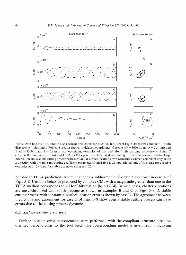
non-linear TFEA predictions where chatter is a subharmonic of order 2 as shown in case A ofFigs. 5–8. Unstable behavior predicted by complex CMs with a magnitude greater than one in theTFEA method corresponds to a Hopf bifurcation [8,16,17,24]. In such cases, chatter vibrationsare unsynchronized with tooth passage as shown in examples B and C of Figs. 5–8. A stablecutting process with substantial surface location error is shown by case D. The agreement betweenpredictions and experiment for case D of Figs. 5–8 show even a stable cutting process can haveerrors due to the cutting process dynamics.

6.2. Surface location error tests

Surface location error measurements were performed with the compliant structure directionoriented perpendicular to the tool feed. The corresponding model is given from modifying

ARTICLE IN PRESS

-5

0

5× 10

-4

× 10 -4

× 10 -4

× 10 -4

x n (

m)

x n (

m)

x n (

m)

x n (

m)

Nonlinear TFEA

xn2

(m

)

Poincare Section

xn

-5

0

5

xn2

(m

)

xn

-5

0

5

xn2

(m

)

xn

0 50 100 150 200 250 300 350 400-5

0

8

n (rev)5 0 8

× 10 -4

x n2

(m)

xn (m)

A

B

C

D

A

B

C

D

Fig. 6. Non-linear TFEA 1/tooth displacement predictions for cases (A, B, C, D) of Fig. 8. Each row contains a 1/tooth

displacement plot and a Poincar!e section shown in delayed coordinates. Cases A (O ¼ 3650 r:p:m:; b ¼ 2:3 mm) andB (O ¼ 3300 r:p:m:; b ¼ 0:8 mm) are up-milling examples of flip and Hopf bifurcations, respectively. Point C

(O ¼ 3600 r:p:m:; b ¼ 2:1 mm) and D (O ¼ 4350 r:p:m:; b ¼ 3:0 mm) down-milling predictions for an unstable Hopf

bifurcation and a stable cutting process with substantial surface location error. Structure assumed compliant only in the

x direction with dynamic and cutting coefficient parameters from Table 1. Computational time of 30 s=case for unstableexamples and 15 s=case for stable examples using E ¼ 25:


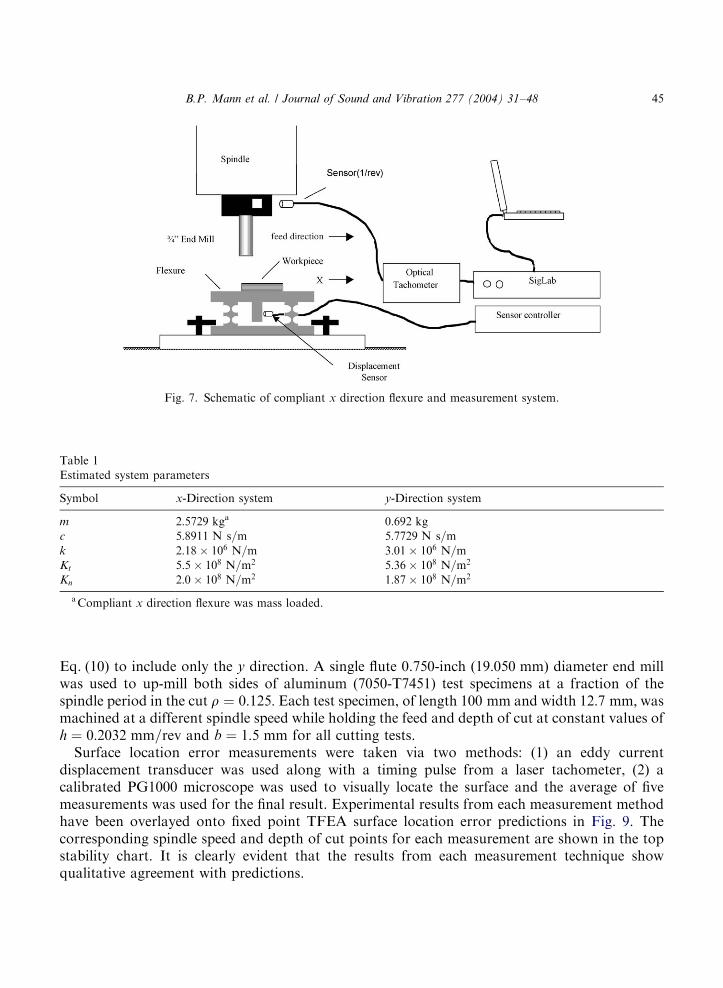
Eq. (10) to include only the y direction. A single flute 0.750-inch ð19:050 mmÞ diameter end millwas used to up-mill both sides of aluminum (7050-T7451) test specimens at a fraction of thespindle period in the cut r ¼ 0:125: Each test specimen, of length 100 mm and width 12:7 mm; wasmachined at a different spindle speed while holding the feed and depth of cut at constant values ofh ¼ 0:2032 mm=rev and b ¼ 1:5 mm for all cutting tests.Surface location error measurements were taken via two methods: (1) an eddy current

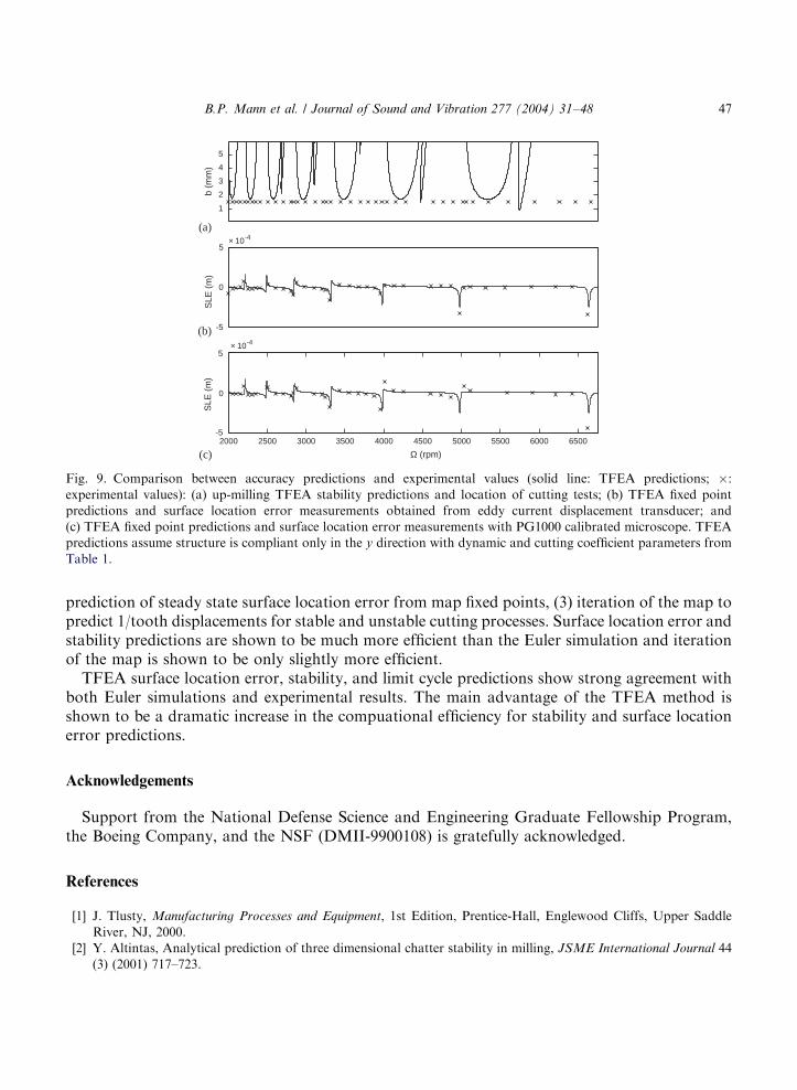
displacement transducer was used along with a timing pulse from a laser tachometer, (2) acalibrated PG1000 microscope was used to visually locate the surface and the average of fivemeasurements was used for the final result. Experimental results from each measurement methodhave been overlayed onto fixed point TFEA surface location error predictions in Fig. 9. Thecorresponding spindle speed and depth of cut points for each measurement are shown in the topstability chart. It is clearly evident that the results from each measurement technique showqualitative agreement with predictions.

ARTICLE IN PRESS

Fig. 7. Schematic of compliant x direction flexure and measurement system.

Table 1

Estimated system parameters

Symbol x-Direction system y-Direction system

m 2:5729 kga 0:692 kgc 5:8911 N s=m 5:7729 N s=mk 2:18 106 N=m 3:01 106 N=mKt 5:5 108 N=m2 5:36 108 N=m2

Kn 2:0 108 N=m2 1:87 108 N=m2

aCompliant x direction flexure was mass loaded.


7. Summary and conclusions

Time finite element analysis is used to analyze the accuracy, stability, and limit cycle behavior ofmilling. Results are compared to Euler simulation which obtains the acceleration, velocity, anddisplacement at each time step. Displacement information corresponding to when the cuttingteeth are normal to the workpiece surface can be used to predict surface location error. Sincedirect stability predictions from the time-marching equations is not possible, an additionaltechnique has been applied to quantify an unstable cutting process. Here we used the variance ofsimulation 1/tooth displacements to find the transition between stable and unstable cutting.The TFEA method forms an approximate solution by dividing the time in the cut into a finite

number of elements. The approximate solution is then matched with the exact solution for freevibration to obtain a discrete linear map. The formulated dynamic map is then used in threedifferent ways: (1) stability prediction from the magnitude of map characteristic multipliers, (2)

ARTICLE IN PRESS

-5

0

5× 10 -4

x(t)

(m)

x n(m

)

x n2

(m)

xn

-5

0

5× 10 -4

x(t)

(m)

x n(m

)

xn2

(m)

xn

-5

0

5× 10 -4

x(t)

(m)

x n(m

)

x n2(m

)

xn

0 2 4 -5

0

8× 10 -4

x(t)

(m)

time (s)0 200 400

x n(m

)

n (rev) 5 0 8

× 10 -4

5

0

8× 10 -4

x n2

(m)

xn (m)

Poincare SectionContinuous Sample 1/tooth Passage

A

B

C

D D

C

B

A

D

C

B

A

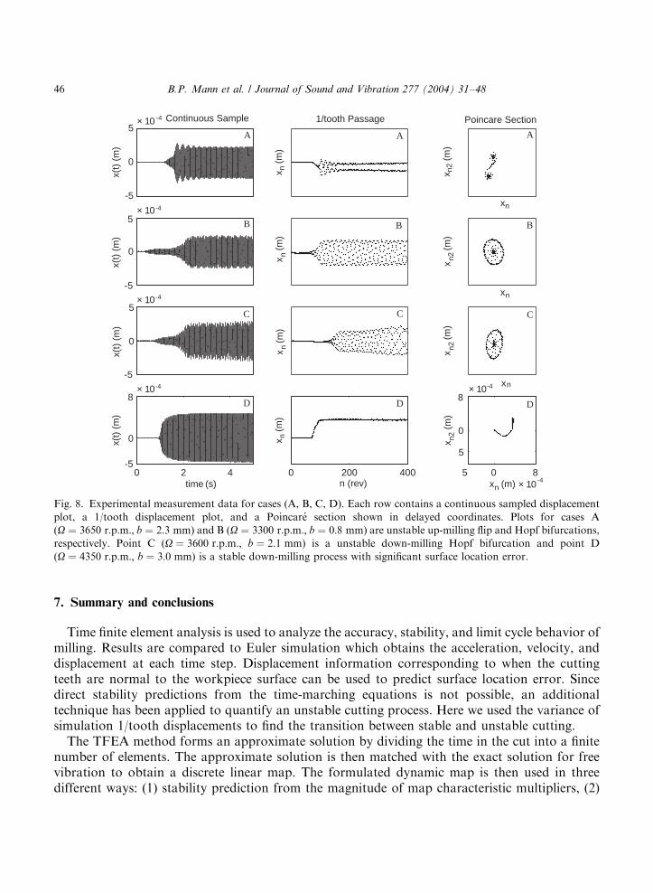
Fig. 8. Experimental measurement data for cases (A, B, C, D). Each row contains a continuous sampled displacement

plot, a 1/tooth displacement plot, and a Poincar!e section shown in delayed coordinates. Plots for cases A

(O ¼ 3650 r:p:m:; b ¼ 2:3 mm) and B (O ¼ 3300 r:p:m:; b ¼ 0:8 mm) are unstable up-milling flip and Hopf bifurcations,respectively. Point C (O ¼ 3600 r:p:m:; b ¼ 2:1 mm) is a unstable down-milling Hopf bifurcation and point D

(O ¼ 4350 r:p:m:; b ¼ 3:0 mm) is a stable down-milling process with significant surface location error.


prediction of steady state surface location error from map fixed points, (3) iteration of the map topredict 1/tooth displacements for stable and unstable cutting processes. Surface location error andstability predictions are shown to be much more efficient than the Euler simulation and iterationof the map is shown to be only slightly more efficient.TFEA surface location error, stability, and limit cycle predictions show strong agreement with

both Euler simulations and experimental results. The main advantage of the TFEA method isshown to be a dramatic increase in the compuational efficiency for stability and surface locationerror predictions.

Acknowledgements

Support from the National Defense Science and Engineering Graduate Fellowship Program,the Boeing Company, and the NSF (DMII-9900108) is gratefully acknowledged.

References

[1] J. Tlusty, Manufacturing Processes and Equipment, 1st Edition, Prentice-Hall, Englewood Cliffs, Upper Saddle

River, NJ, 2000.

[2] Y. Altintas, Analytical prediction of three dimensional chatter stability in milling, JSME International Journal 44

(3) (2001) 717–723.

ARTICLE IN PRESS

1

2

3

4

5

b (m

m)

-5

0

5× 10-4

× 10-4

SLE

(m

)

2000 2500 3000 3500 4000 4500 5000 5500 6000 6500-5

0

5

Ω (rpm)

SLE

(m

)

(a)

(b)

(c)

Fig. 9. Comparison between accuracy predictions and experimental values (solid line: TFEA predictions; :experimental values): (a) up-milling TFEA stability predictions and location of cutting tests; (b) TFEA fixed point

predictions and surface location error measurements obtained from eddy current displacement transducer; and

(c) TFEA fixed point predictions and surface location error measurements with PG1000 calibrated microscope. TFEA

predictions assume structure is compliant only in the y direction with dynamic and cutting coefficient parameters from

Table 1.


[3] M.A. Davies, J.R. Pratt, B. Dutterer, T.J. Burns, Stability prediction for low radial immersion milling, Journal of

Manufacturing Science and Engineering 124 (2) (2002) 217–225.

[4] T. Schmitz, J. Ziegert, Examination of surface location error due to phasing of cutter vibrations, Precision

Engineering 23 (1999) 51–62.

[5] Y. Altintas, Manufacturing Automation, 1st Edition, Cambridge University Press, New York, NY, 2000.

[6] J. Tlusty, A. Polacek, C. Danek, J. Spacek, Selbsterregte schwingungen an werkzeugmaschinen, VEB Verlag

Technik, Berlin, 1962.

[7] S.A. Tobias, Machine Tool Vibration, Blackie, London, 1965.

[8] G. St!ep!an, T. Kalm!ar-Nagy, Nonlinear regenerative machine tool vibration, Proceedings of the 1997 ASME

Design Engineering Technical Conference, Sacramento, CA, no. DETC97/VIB-4021 (CD-ROM), p. n/a, 1997.

[9] S. Smith, J. Tlusty, An overview of the modeling and simulation of the milling process, Journal of Engineering for

Industry 113 (1991) 169–175.

[10] Y. Altintas, E. Budak, Analytical prediction of stability lobes in milling, CIRP Annals 44 (1) (1995) 357–362.

[11] M.A. Davies, J.R. Pratt, B. Dutterer, T.J. Burns, Stability prediction for low radial immersion milling, Journal of

Manufacturing Science and Engineering 124 (2) (2002) 217–225.

[12] I. Minis, R. Yanushevsky, A new theoretical approach for prediction of machine tool chatter in milling, Journal of

Engineering for Industry 115 (1993) 1–8.

[13] T. Insperger, G. St!ep!an, Stability of the milling process, Periodica Polytechnica 44 (1) (2000) 47–57.

[14] T. Insperger, G. St!ep!an, Stability of high-speed milling, Proceedings of Symposium of Nonlinear Dynamics and

Stochastic Mechanics, no. AMD-241, Orlando, FL, 2000, pp. 119–123.

[15] W.T. Corpus, W.J. Endres, A high order solution for the added stability lobes in intermittent machining,

Proceeding of the Symposium on Machining Processes, no. MED-11, 2000, pp. 871–878.

[16] P.V. Bayly, J.E. Halley, B.P. Mann, M.A. Davies, Stability of interrupted cutting by temporal finite element

analysis, September 2001.

[17] B.P. Mann, T. Insperger, P.V. Bayly, G. St!ep!an, Stability of up-milling and down-milling, Part 2: experimental

verification, International Journal of Machine Tools and Manufacture 43 (2003) 35–40.

[18] L. Meirovitch, Elements of Vibration Analysis, 2nd Edition, McGraw-Hill, New York, 1986.

[19] J.E. Halley, Stability of Low Radial Immersion Milling, Master’s Thesis, Washington University, Saint Louis, 1999.

[20] P.V. Bayly, B.P. Mann, M.A. Davies, J.R. Pratt, Stability analysis of interrupted cutting with finite time in the cut,

Proceedings of ASME Design Engineering Technical Conference, Manufacturing in Engineering Division, Orlando,

FL, MED-11 (2000) 989–994.

[21] P.V. Bayly, B.P. Mann, T.L. Schmitz, D.A. Peters, G. St!ep!an, T. Insperger, Effects of radial immersion and

cutting direction on chatter instability in endmilling, Proceedings of ASME International Mechanical Engineering

Conference and Exposition, New Orleans, LA, no. IMECE2002-34116, New Orleans, LA, ASME, 2002.

[22] D.A. Peters, A.P. Idzapanah, Hp-version finite elements for the space–time domain, Computational Mechanics 3

(1988) 73–78.

[23] Y. Jaluria, Computational Heat Transfer, 1st Edition, Hemisphere Publishing Corporation, Washington, 1986.

[24] L.N. Virgin, Introduction to Experimental Nonlinear Dynamics, Cambridge University Press, Cambridge, UK, 2000.

[25] L.J. Hou, D.A. Peters, Application of triangular space–time finite elements to problems of wave propagation,

Journal of Sound and Vibration 173 (5) (1994) 611–632.

[26] D. Montgomery, Y. Altintas, Mechanism of cutting force and surface generation in 20 dynamic milling, Journal of

Engineering for Industry 113 (1991) 160–168.

[27] J. Tlusty, F. Ismail, Basic non-linearity in machining chatter, Annals of the CIRP 30 (1981) 21–25.

[28] T.L. Schmitz, Chatter recognition by a statistical evaluation of the synchronously sampled audio signal,

Proceedings of the 2001 India–USA Symposium on Emerging Trends in Vibration and Noise Engineering, Columbus,

OH, December 10–14, 2001.

[29] T.L. Schmitz, K. Medicus, B. Dutterer, Exploring once-per-revolution audio signal variance as a chatter indicator,

Machining Science and Technology 6 (2) (2002) 215–233.

[30] S.H. Strogatz, Nonlinear Dynamics and Chaos, 1st Edition, Perseus Books, Reading, MA, 1994.

[31] E. Kreyszig, Advanced Engineering Mathematics, 8th Edition, Wiley, New York, NY, 1999.

[32] D.J. Inman, Engineering Vibration, 2nd Edition, Prentice-Hall, Upper Saddle River, NJ, 2001.

ARTICLE IN PRESS


JOURNAL OF SOUND AND VIBRATION Limit cycles, bifurcations, and accuracy of the milling process

Documents

Transcript of JOURNAL OF SOUND AND VIBRATION Limit cycles, bifurcations, and accuracy of the milling process