Journal of Experimental B And Agricultural Scien
131
Journal of Expe And Agricul Volum Production and H (http://w erimental Biology ltural Sciences me 8 || Issue II || April, 202 Hosting by Horizon Publisher India www.horizonpublisherindia.in) All rights reserved. JEBAS y 20 ISSN:2320-8694 a[HPI]
-
Upload
khangminh22 -
Category
Documents
-
view
0 -
download
0
Transcript of Journal of Experimental B And Agricultural Scien
Journal of Experimental BiologyAnd Agricultural Sciences
Volume 8
Production and Hosting by Horizon Publisher India[HPI](http://www.horizonpublisherindia.in)
Journal of Experimental BiologyAnd Agricultural Sciences
Volume 8 || Issue II || April, 2020
Production and Hosting by Horizon Publisher India[HPI](http://www.horizonpublisherindia.in)
All rights reserved.
JEBAS
Journal of Experimental Biology
, 2020
ISSN:2320-8694
Production and Hosting by Horizon Publisher India[HPI]
JEBAS
ISSN No. 2320 – 8694
Peer Reviewed - open access journal
Common Creative License - NC 4.0
Volume No – 8 Issue No – II April, 2020 Journal of Experimental Biology and Agricultural Sciences (JEBAS) is an online platform for the advancement and rapid dissemination of scientific knowledge generated by the highly motivated researchers in the field of biological agricultural, veterinary and animal sciences. JEBAS publishes high-quality original research and critical up-to-date review articles covering all the aspects of biological sciences. Every year, it publishes six issues.
JEBAS has been accepted by UGC CARE, INDEX COPERNICUS INTERNATIONAL (Poland), AGRICOLA (USA),CAS (ACS, USA),CABI – Full Text (UK), EBSCO, AGORA (FAO-UN), OARE (UNEP), International Committee of Medical Journal Editors (ICMJE), National Library of Australia, SHERPA – ROMEO; J gate, EIJASR, DRIJ, and Indian Science Abstracts (ISA, NISCAIR) like well reputed indexing agencies.
[HORIZON PUBLISHER INDIA [HPI] http://www.horizonpublisherindia.in/]
JEBAS
Editorial Board Editorial Board
Editor-in-Chief
Prof Y. Norma-Rashid
(University of Malaya, Kuala Lumpur)
Co-Editor-in-Chief
Dr. Kuldeep Dhama, M.V.Sc., Ph.D.
NAAS Associate, Principal Scientist, IVRI, Izatnagar India - 243 122
Managing - Editor
Kamal K Chaudhary, Ph.D. (India)
Dr. Anusheel Varshney
University of Salford United Kingdom
Technical Editors
Dr. Gary Straquadine
Vice Chancellor – USU Eastern Campus, Utah State University Eastern,
2581 West 5200 South, Rexburg, Idaho, 83440
Email: [email protected]
Hafiz M. N. Iqbal (Ph.D.)
Research Professor,
Tecnologico de Monterrey,School of Engineering and Sciences,
Campus Monterrey,Ave. Eugenio Garza Sada 2501,
Monterrey, N. L., CP 64849, Mexico
Tel.: +52 (81) 8358-2000Ext.5561-115
E-mail: [email protected]; [email protected]
Prof. Dr. Mirza Barjees Baig Professor of Extension (Natural Resource Management),
Department of Agricultural Extension and Rural Society,
College of Food and Agriculture Sciences,
King Saud University, P.O. Box 2460, Riyadh 11451
Kingdom of Saudi Arabia
Email: [email protected]
Dr. B L Yadav Head – Botany, MLV Govt. College, Bhilwara, India E mail: [email protected] Dr. K L Meena Associate Professor – Botany, MLV Govt.
College, Bhilwara, India
E mail: [email protected]
JEBAS
Dr. Yashpal S. Malik
ICAR – National FellowIndian Veterinary Research Institute (IVRI)
Izatnagar 243 122, Bareilly, Uttar Pradesh, India
Professor Dr. Muhammad Mukhtar
Professor of Biotechnology/Biochemistry
American University of Ras Al KhaimahRas Al Khaimah, United Arab Emirates
Abdulrasoul M. Alomran Prof. of Soil and Water Sciences
Editor in Chief of JSSAS
College of Food and Agricultural Sciences
King Saud UniversityRiyadh, Saudi Arabia
E-mail: [email protected]
Associate Editors
Dr. Sunil K. Joshi Laboratory Head, Cellular Immunology Investigator, Frank Reidy Research Center of Bioelectrics, College of Health Sciences, Old Dominion
University, 4211 Monarch Way, IRP-2, Suite # 300, Norfolk, VA 23508 USA Email: [email protected]
Dr.Vincenzo Tufarelli Department of Emergency and Organ Transplantation (DETO), Section of Veterinary Science and Animal
Production, University of Bari ‘Aldo Moro’, s.p. Casamassima km 3, 70010 Valenzano, Italy Email: [email protected]
Dr. Md. Moin Ansari
Associate Professor-cum-Senior Scientist
Division of Surgery and Radiology
Faculty of Veterinary Sciences and Animal Husbandry
Shuhama, Srinagar-190006, J&K, India
Prof. Viliana Vasileva, PhD
89 "General Vladimir Vazov" Str.
Institute of Forage Crops
5800 Pleven, BULGARIA
E-mail: [email protected]
Han Bao
MSU-DOE Plant Research Laboratory
Michigan State University
Plant Biology Laboratories
612 Wilson Road, Room 222
East Lansing, MI 48824
JEBAS
Assistant Editors
Dr. Oadi Najim Ismail Matny
Assistant Professor – Plant pathology
Department of Plant Protection
College Of Agriculture Science
University Of Baghdad, Iraq
E-mail: [email protected], [email protected] Najim Ismail OadiMatny
Dr Ayman EL Sabagh
Assistant professor, agronomy department, faculty of agriculture
[Details]kafresheikh university, Egypt
E-mail: [email protected]
Dr. Masnat Al Hiary
Director of the Socio- economic Studies Directorate
Socio-economic Researcher
National Center for Agricultural Research and Extension (NCARE)
P.O.Box 639 Baqa'a 19381 Jordan
Safar Hussein Abdullah Al-Kahtani (Ph.D.)
King Saud University-College of Food and Agriculture Sciences,
Department of the Agricultural Economics
P.O.Box: 2460 Riyadh 11451, KSA
email: [email protected]
Dr Ruchi Tiwari
Assistant Professor (Sr Scale)
Department of Veterinary Microbiology and Immunology,
College of Veterinary Sciences,
UP Pandit Deen Dayal Upadhayay Pashu Chikitsa Vigyan Vishwavidyalay Evum Go-Anusandhan Sansthan (DUVASU),
Mathura, Uttar Pradesh, 281 001, India
Email: [email protected]
Dr. ANIL KUMAR (Ph.D.)
Asstt. Professor (Soil Science)
Farm Science Centre (KVK)
Booh, Tarn Taran, Punjab (India) – 143 412
Email: [email protected]
Akansha Mishra
Postdoctoral Associate, Ob/Gyn lab
Baylor College of Medicine
1102 Bates Ave, Houston Tx 77030
Email: [email protected]; [email protected]
JEBAS
Table of contents
ENTOMOPATHOGENIC NEMATODES AS AN ALTERNATIVE BIOLOGICAL CONTROL AGENTS AGAINST INSECT FOES OF CROPS DOI: 10.18006/2020.8(2).71.75
76—83
EXPLOITING MILLETS IN THE SEARCH OF FOOD SECURITY : A MINI REVIEW DOI: 10.18006/2020.8(2).84.89
84—89
STANDARD HETEROSIS ANALYSIS IN MAIZE HYBRIDS UNDER WATER LOGGING CONDITION DOI: 10.18006/2020.8(2).90.97
90—97
ENERGY USE EFFICIENCY AND GREEN HOUSE GAS EMISSIONS FROM INTEGRATED CROP-LIVESTOCK SYSTEMS IN SEMI-ARID ECOSYSTEM OF DECCAN PLATEAU IN SOUTHERN INDIA DOI: 10.18006/2020.8(2).98.110
98—110
CHARACTER ASSOCIATION AND PATH ANALYSIS FOR SEED VIGOR TRAITS IN SESAME (Sesamum indicum L.) DOI: 10.18006/2020.8(2).111.114
111—114
BIPLOT ANALYSIS FOR SPOT BLOTCH AND YIELD TRAIT USING WAMI PANEL OF SPRING WHEAT DOI: 10.18006/2020.8(2).115.124
115—124
STRIPE RUST RESISTANCE IN WHEAT GERMPLASM OF NORTH-WESTERN HIMALAYAN HILLS DOI: 10.18006/2020.8(2).125.133
125—133
TOXIC EFFECTS OF VARIOUS ARSENIC CONCENTRATIONS ON GERMINATION AND SEEDLINGS GROWTH OF WHEAT (Triticum aestivum L.) DOI: 10.18006/2020.8(2).134.139
134—139
AGRO—MORPHOLOGICAL CHARACTERIZATION OF AFRICAN RICE ACCESSIONS (Oryza glaberrima) IN RAINFED AND IRRIGATED CULTURAL CONDITIONS DOI: 10.18006/2020.8(2).140.147
140—147
GENETIC CHARACTERIZATION OF LOCAL RICE (Oryza sativa L.) GENOTYPES AT MORPHOLOGICAL AND MOLECULAR LEVEL USING SSR MARKERS DOI: 10.18006/2020.8(2).148.156
148—156
IDENTIFICATION OF SUPERIOR THREE WAY-CROSS F1S, ITS LINE×TESTER HYBRIDS AND DONORS FOR MAJOR QUANTITATIVE TRAITS IN Lilium×formolongi DOI: 10.18006/2020.8(2).157.165
157—165
LARVICIDAL ACTIVITY OF TWO RUTACEAE SPECIES AGAINST THE VECTORS OF DENGUE AND FILARIAL FEVER DOI: 10.18006/2020.8(2).166.175
166—175
EFFECT OF CRUDE OIL POLLUTION ON SOIL AND AQUATIC BACTERIA AND FUNGI DOI: 10.18006/2020.8(2).176.184
176—184
DIFFERENTIAL RESPONSES OF CERTAIN ETHIOPIAN GROUNDNUT (Arachis hypogaea L.) VARIETIES VARYING IN DROUGHT TOLERANCE, TO TERMINAL DROUGHT STRESS DOI: 10.18006/2020.8(2).185.192
185—192
IMPACT OF FEED SUBSIDY REMOVAL ON THE ECONOMIC SUCCESS OF SMALL RUMINANT FARMING IN NORTHERN BADIA OF JORDAN DOI: 10.18006/2020.8(2).193.200
193—200
Journal of Experimental Biology and Agricultural Sciences
http://www.jebas.org
ISSN No. 2320 – 8694
Journal of Experimental Biology and Agricultural Sciences, April - 2020; Volume – 8(2) page 76 – 83
ENTOMOPATHOGENIC NEMATODES AS AN ALTERNATIVE BIOLOGICAL
CONTROL AGENTS AGAINST INSECT FOES OF CROPS
Amit Ahuja1*, K.Elango2, Rajendra Kumar3, Ajay Singh Sindhu1, Sachin Gangwar1
1Division of Nematology, ICAR-Indian Agriculture Research Institute, New Delhi, India, 110012
2Agricultural Entomology, Tamil Nadu Agricultural University, Coimbatore, Tamil Nadu, India, 641 003
3Agricultural Entomology, Swami Keshwanand Rajasthan Agricultural University, Bikaner, Rajasthan, India, 334006
Received – January 25, 2020; Revision – March 18, 2020; Accepted – March 28, 2020 Available Online – April 25, 2020
DOI: http://dx.doi.org/10.18006/2020.8(2).76.83
ABSTRACT
Entomopathogenic nematodes belonging to the genus Steinernema, Heterorhabditis and
Neosteinernema are the natural killers of insects belonging to different orders. These nematodes are
suitable biocontrol agents as they do not possess a threat to the environment and safer to human health.
Commercially entomopathogenic nematodes are exploited against insect pests of various economically
valuable crops. Upon application in the field, these nematodes face many biotic and abiotic stresses
which results in inconsistent efficacy in pest management. Traditionally artificial selection and
hybridization techniques were adopted to improve traits related to penetration and infectivity to insect
host and storage stability in the formulation. Artificially improved traits tend to losses in the external
environment once the selection pressure removed. Genomics assisted breeding provides an alternative
way for stable trait improvements in entomopathogenic nematodes which last for a longer period and
exhibit maximum efficacy in the field against targeted insect pests. Understating their lifecycles and
complex mechanisms of host’s infectivity exhibited by nematode-bacterial partners would further
enhance our knowledge to improve their efficacy against insect pests. In the future, there is a huge scope
of developing stable commercial formulations of entomopathogenic nematodes as a suitable biological
control agent.
* Corresponding author
KEYWORDS
Biological control
Entomopathogenic nematode
Steinernema
Heterorhabditis
Insects pest
E-mail: [email protected] (Amit Ahuja)
Peer review under responsibility of Journal of Experimental Biology and
Agricultural Sciences.
All the articles published by Journal of Experimental
Biology and Agricultural Sciences are licensed under a
Creative Commons Attribution-NonCommercial 4.0
International License Based on a work at www.jebas.org.
Production and Hosting by Horizon Publisher India [HPI]
(http://www.horizonpublisherindia.in/).
All rights reserved.
Journal of Experimental Biology and Agricultural Sciences
http://www.jebas.org
Entomopathogenic Nematodes as an Alternative Biological Control Agents Against Insect Foes of Crops 77
1 Introduction
The vices of erratic and over uses of insecticides are contaminating
the aquatic and terrestrial ecosystem, posing a serious threat to
biodiversity and developing resistance in insects. As an alternative,
the uses of entomopathogenic nematodes are increasing as a
suitable biological control agent against insect pests of
economically valuable crops (Gaugler, 2018). The
entomopathogenic nematodes belong to the genus Heterorhabditis
Poinar (1975), Steinernema Travassos (1927),
and Neosteinernema Nguyen & Smart (1994) (Rhabditida:
Nematoda) can kill a wide variety of insects. Among these three
genus, the former two are highly exploited against insects as a
biocontrol agent. The genus Heterorhabditis is associated with the
bacteria Photorhabdus and genus Steinernema is associated with
the bacteria Xenorhabdus (Leite et al., 2019). These nematodes
perform ambushingor cruising activities (Ruan et al., 2018) to
locate it hosts, and regurgitate its mutualistic bacteria once they
reach inside the insect’s midgut (Labaude & Griffin, 2018). The
bacteria secrets multiple toxins and kill the insect by septicemia
and coverts the host’s tissue content into a nutrient-rich medium
for the growth and development of its own and its nematode
partner (Mbata et al., 2019). These nematodes don’t cause harmful
effects to the environment, not allow resurgence and resistance
development in insects, hence they are a suitable alternative to
synthetic insecticides (Askary et al., 2018). The entomopathogenic
nematodes are globally present in every continent except
Antarctica (Griffin et al., 1990).
Once the infective juveniles reach inside the midgut of insects, it
just takes two to three days to kill and entire lifecycles complete in
between 10-15 days (Li et al., 2019). Various researches have done
in the past also exhibited the suitability of these nematode’s
applications via traditional equipment. These nematodes also found
compatible with the range of pesticides upon application in the
field (Chavan et al., 2018). These nematodes are commercially
produced and exploited against insects in many countries such as
European nations and USA, yet their share in the pest management
market is hardly 1 percent (Smart, 1995). These nematodes are
produced on its hosts via in vivo or in vitro techniques on solid or
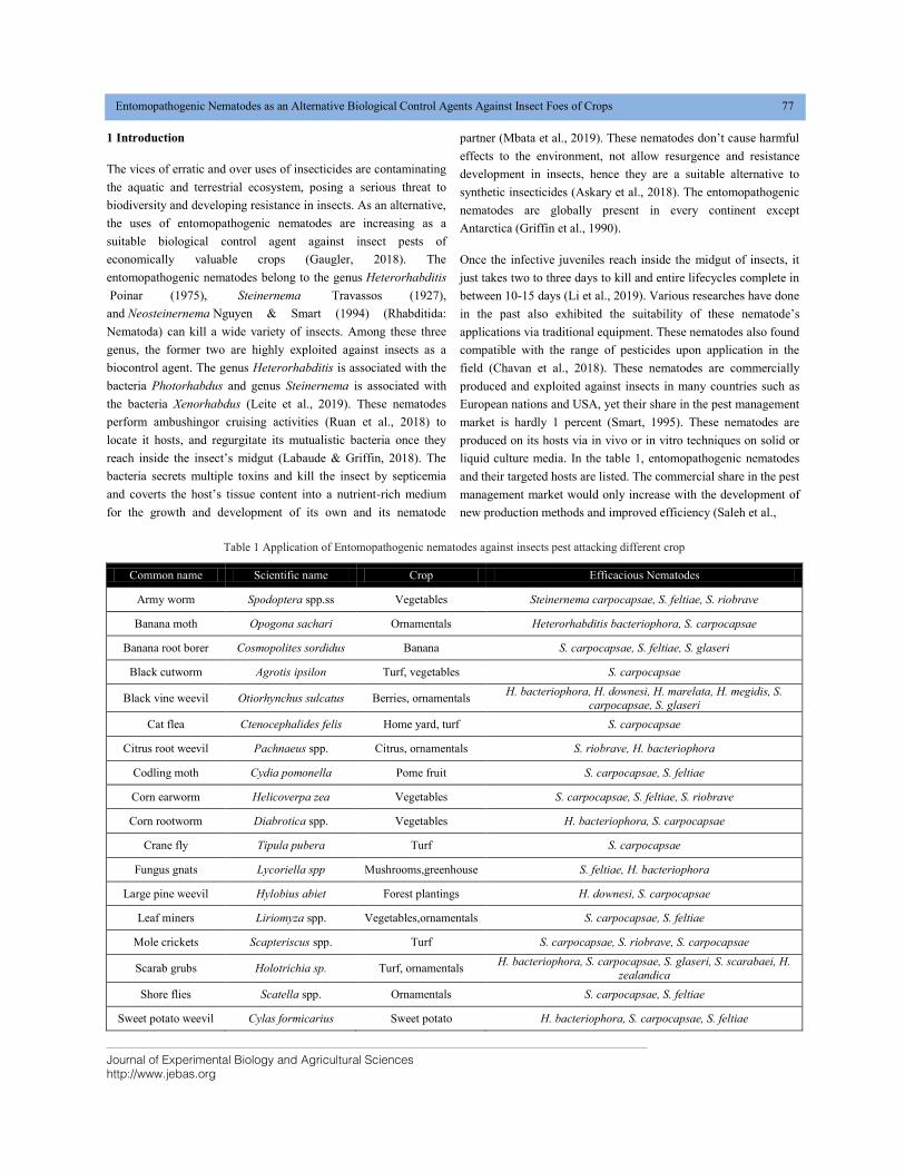
liquid culture media. In the table 1, entomopathogenic nematodes
and their targeted hosts are listed. The commercial share in the pest
management market would only increase with the development of
new production methods and improved efficiency (Saleh et al.,
Table 1 Application of Entomopathogenic nematodes against insects pest attacking different crop
Common name Scientific name Crop Efficacious Nematodes
Army worm Spodoptera spp.ss Vegetables Steinernema carpocapsae, S. feltiae, S. riobrave
Banana moth Opogona sachari Ornamentals Heterorhabditis bacteriophora, S. carpocapsae
Banana root borer Cosmopolites sordidus Banana S. carpocapsae, S. feltiae, S. glaseri
Black cutworm Agrotis ipsilon Turf, vegetables S. carpocapsae
Black vine weevil Otiorhynchus sulcatus Berries, ornamentals H. bacteriophora, H. downesi, H. marelata, H. megidis, S.
carpocapsae, S. glaseri
Cat flea Ctenocephalides felis Home yard, turf S. carpocapsae
Citrus root weevil Pachnaeus spp. Citrus, ornamentals S. riobrave, H. bacteriophora
Codling moth Cydia pomonella Pome fruit S. carpocapsae, S. feltiae
Corn earworm Helicoverpa zea Vegetables S. carpocapsae, S. feltiae, S. riobrave
Corn rootworm Diabrotica spp. Vegetables H. bacteriophora, S. carpocapsae
Crane fly Tipula pubera Turf S. carpocapsae
Fungus gnats Lycoriella spp Mushrooms,greenhouse S. feltiae, H. bacteriophora
Large pine weevil Hylobius abiet Forest plantings H. downesi, S. carpocapsae
Leaf miners Liriomyza spp. Vegetables,ornamentals S. carpocapsae, S. feltiae
Mole crickets Scapteriscus spp. Turf S. carpocapsae, S. riobrave, S. carpocapsae
Scarab grubs Holotrichia sp. Turf, ornamentals H. bacteriophora, S. carpocapsae, S. glaseri, S. scarabaei, H.
zealandica
Shore flies Scatella spp. Ornamentals S. carpocapsae, S. feltiae
Sweet potato weevil Cylas formicarius Sweet potato H. bacteriophora, S. carpocapsae, S. feltiae
Journal of Experimental Biology and Agricultural Sciences
http://www.jebas.org
78 Ahuja et al.
2020). These nematodes face the biotic and abiotic pressures in the
field (Dzięgielewska & Skwiercz, 2018), which hinder its
maximum efficacy. Because there are certain traits like tolerance to
cold and heat, sensation to ultraviolet light, desiccation, and
persistence determines its fitness in the field (Abd-Elgawad, 2019).
Traditionally artificial selection and hybridization methods had
been applied in trait improvement (Lu et al., 2016). But there is a
huge possibility of losing a novel improved trait once the selection
pressure is removed. Nowadays genomic sequence information of
entomopathogenic nematodes assisted with molecular breeding
tool paving a way for the trait improvements (Sumaya, 2018). The
traits improved via molecular methods would last permanently or
for a longer period as compare to artificial selection and
hybridization (Abd-Elgawad, 2019). Once the traits related to
storage stability and host-seeking behavior would be improved,
then the cost of commercial production would reduce to a certain
level. Entomopathogenic nematodes kill effectively the insect
belonging to most thwarting orders like Coleoptera, Lepidoptera,
Hemiptera, Diptera, and Orthoptera (Belien, 2018) etc. There is a
huge scope lying with the uses of these nematodes against insects
in future when the eco-safety and human health is the main
concern. The aim of this review is to highlight the potential of
entomopathogenic nematodes as an effective biological control
agent against the insect-pests of crops. The inclusion of these
nematodes in integrated pest management schemes can negate the
dependence on excess uses of synthetic pesticides.
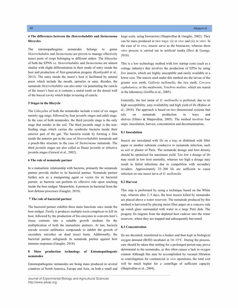
2 Life cycle of EPNs
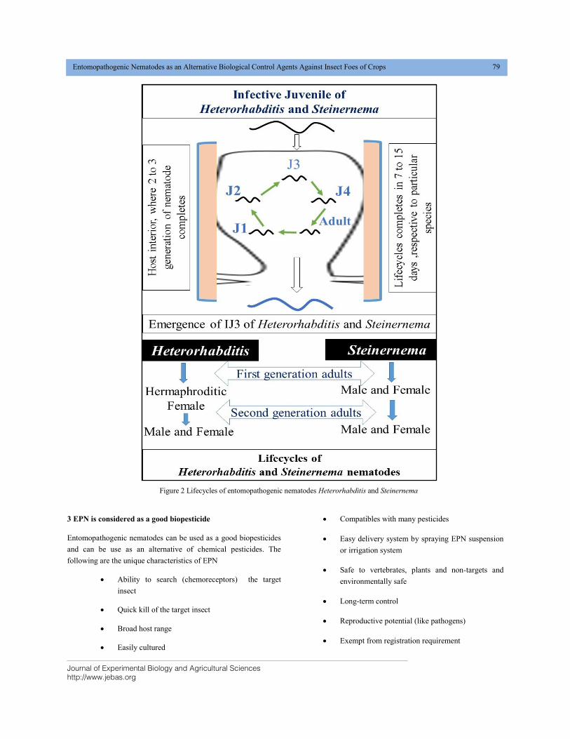
Both entomopathogenic nematodes exhibit a similar type of life
cycle and mode of infection with slight differences in their
formation first generation progeny. Steinernema undergoes
continuous two sexual generations with males and females
separately each time (Gauraha et al., 2018). While in
Heterorhabditis, the first generation coverts to hermaphroditic
female (Zioni et al., 1992). The entomopathogenic nematodes
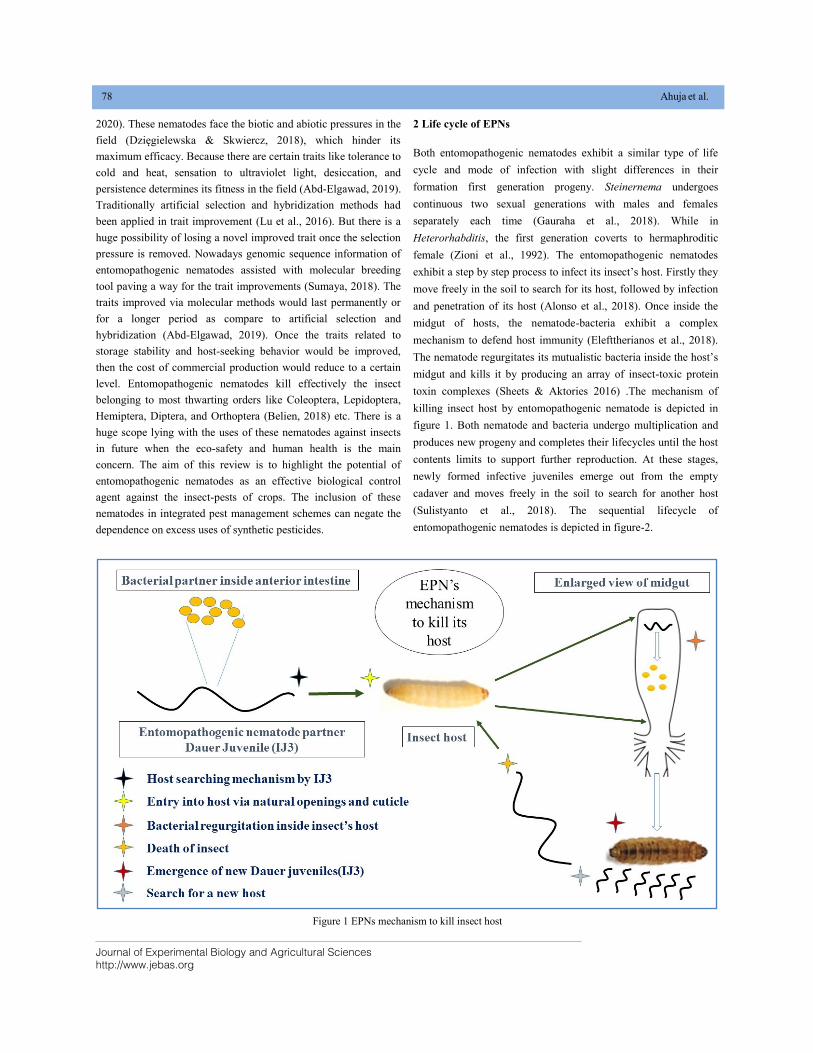
exhibit a step by step process to infect its insect’s host. Firstly they
move freely in the soil to search for its host, followed by infection
and penetration of its host (Alonso et al., 2018). Once inside the
midgut of hosts, the nematode-bacteria exhibit a complex
mechanism to defend host immunity (Elefttherianos et al., 2018).
The nematode regurgitates its mutualistic bacteria inside the host’s
midgut and kills it by producing an array of insect-toxic protein
toxin complexes (Sheets & Aktories 2016) .The mechanism of
killing insect host by entomopathogenic nematode is depicted in
figure 1. Both nematode and bacteria undergo multiplication and
produces new progeny and completes their lifecycles until the host
contents limits to support further reproduction. At these stages,
newly formed infective juveniles emerge out from the empty
cadaver and moves freely in the soil to search for another host
(Sulistyanto et al., 2018). The sequential lifecycle of
entomopathogenic nematodes is depicted in figure-2.
Figure 1 EPNs mechanism to kill insect host
Journal of Experimental Biology and Agricultural Sciences
http://www.jebas.org
Entomopathogenic Nematodes as an Alternative Biological Control Agents Against Insect Foes of Crops 79
3 EPN is considered as a good biopesticide
Entomopathogenic nematodes can be used as a good biopesticides
and can be use as an alternative of chemical pesticides. The
following are the unique characteristics of EPN
Ability to search (chemoreceptors) the target
insect
Quick kill of the target insect
Broad host range
Easily cultured
Compatibles with many pesticides
Easy delivery system by spraying EPN suspension
or irrigation system
Safe to vertebrates, plants and non-targets and
environmentally safe
Long-term control
Reproductive potential (like pathogens)
Exempt from registration requirement
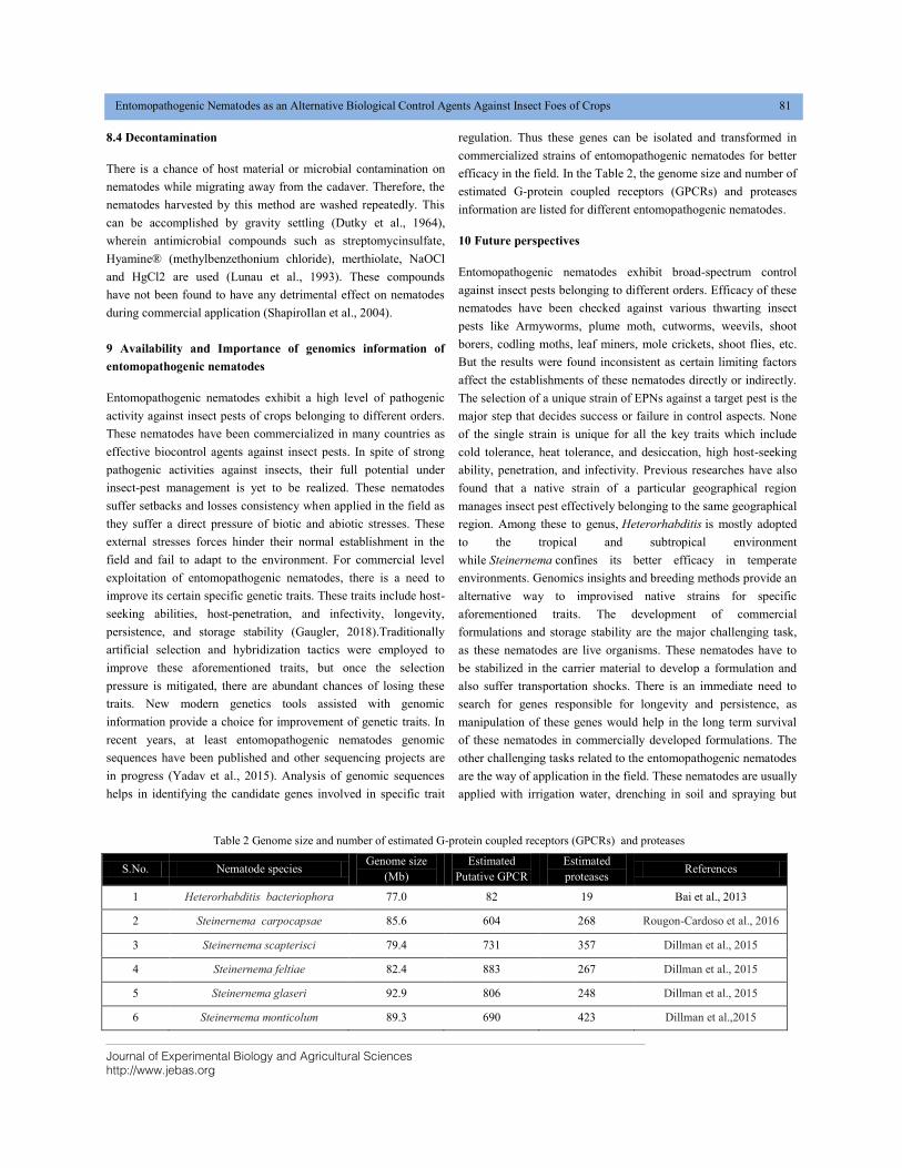
Figure 2 Lifecycles of entomopathogenic nematodes Heterorhabditis and Steinernema
Journal of Experimental Biology and Agricultural Sciences
http://www.jebas.org
80 Ahuja et al.
4 The differences between the Heterorhabditis and Steinernema
lifecycles
The entomopathogenic nematodes belongs to genus
Heterorhabditis and Steinernema are proven to manage effectively
insect pests of crops belonging to different orders. The lifecycles
of both the EPNS i.e. Heterorhabditis and Steinernema are utmost
similar with slight differentiation in their mode of entry inside the
host and production of first-generation progeny (Kooliyottil et al.,
2013). The entry inside the insect’s host is facilitated by natural
pores which include the mouth, spiracles or anus. Besides, the
nematode Heterorhabditis can also enter via penetrating the cuticle
of the insect’s host as it contains a mural tooth on the dorsal wall
of the buccal cavity which helps in tearing of cuticle.
5 Stages in the lifecycle
The Lifecycles of both the nematodes include a total of six stages
namely egg stage, followed by four juvenile stages and adult stage.
In the case of both nematodes, the third juvenile stage is the only
stage that resides in the soil. The third juvenile stage is the non-
feeding stage which carries the symbiotic bacteria inside their
anterior part of the gut. The bacteria reside by forming a film
inside the anterior gut in the case of Heterorhabditis nematode and
a pouch-like structure in the case of Steinernema nematode. The
third juvenile stages are also called as Dauer juvenile or infective
juvenile stages (Grewal et al., 2002).
6 The role of nematode partner
In a mutualistic relationship with bacteria, primarily the nematode
partner provide shelter to its bacterial partner. Nematode partner
further acts as a transporting agent or vector for its bacterial
partner, as bacteria can perform its effective role upon reaching
inside the host midgut. Meanwhile, it protects its bacterial from the
host defense processes (Gaugler, 2018).
7 The role of bacterial partner
The bacterial partner exhibits three main functions once inside the
host midgut. Firstly it produces multiple toxin complexes to kill its
host, followed by the production of bio-enzymes to converts host’s
tissue contents into a suitable growth medium for the
multiplication of both the mutualistic partners. At last, bacteria
encode several antibiotics compounds to inhibit the growth of
secondary microbes on dead insect hosts. Additionally, the
bacterial partner safeguards its nematode partner against host
immune responses (Gaugler, 2018).
8 Mass production technology of Entomopathogenic
nematodes
Entomopathogenic nematodes are being mass produced in several
countries of North America, Europe and Asia, on both a small and
large scale, using bioreactors (ShapiroIlan & Gaugler, 2002). They
can be mass produced in two ways: (i) in vivo and (ii) in vitro. In
the case of in vivo, insects serve as the bioreactor, whereas thein
vitro process is carried out in artificial media (Devi & George,
2018).
This is a low technology method with low startup costs (such as a
cottage industry) that involves the production of EPNs by using
live insects, which are highly susceptible and easily available at a
lower cost. The insects used under this method are the larvae of the
greater wax moth, Galleria mellonella, the rice moth, Corcyra
cephalonica, or the mealworm, Tenebrio molitor, which are reared
in the laboratory (Griffin et al., 2005).
Generally, the last instar of G. mellonella is preferred, due to its
high susceptibility, easy availability and high yield of IJs (Rahoo et
al., 2018). The approach is based on two dimensional systems that
rely on nematode production in trays and
shelves (Ehlers & ShapiroIlan, 2005). The method involves four
steps: inoculation, harvest, concentration and decontamination.
8.1 Inoculation
Insects are inoculated with IJs on a tray or dishlined with filter
paper or another substrate conducive to nematode infection, such
as soil or plaster of Paris. The nematode dosage and host density
should be optimized for maximum yield. Too low a dosage of IJs
may result in low host mortality, whereas too high a dosage may
result in failed infections due to competition with secondary
invaders. Approximately 25–200 IJs are sufficient to cause
infection on one insect larva of G. mellonella.
8.2 Harvest
This step is performed by using a technique based on the White
trap, wherein after 2–5 days, the host insects killed by nematodes
are placed above a water reservoir. The nematode produced by this
method is harvested by placing moist filter paper on a concave side
up watch glass surrounded with water in a large Petri dish. The
progeny IJs migrate from the depleted host cadaver into the water
reservoir, where they are trapped and subsequently harvested.
8.3 Concentration
IJs are decanted, transferred to a beaker and then kept in biological
oxygen demand (BOD) incubator at 10–15°C. During the process,
care should be taken that settling for a prolonged period may prove
detrimental to the nematodes, as this often causes a lack in oxygen
content Although this may be accomplished by vacuum filtration
or centrifugation for commercial in vivo operations, the total cost
will be much higher for a centrifuge of sufficient capacity
(ShapiroIlan et al., 2004).
Journal of Experimental Biology and Agricultural Sciences
http://www.jebas.org
Entomopathogenic Nematodes as an Alternative Biological Control Agents Against Insect Foes of Crops 81
8.4 Decontamination
There is a chance of host material or microbial contamination on
nematodes while migrating away from the cadaver. Therefore, the
nematodes harvested by this method are washed repeatedly. This
can be accomplished by gravity settling (Dutky et al., 1964),
wherein antimicrobial compounds such as streptomycinsulfate,
Hyamine® (methylbenzethonium chloride), merthiolate, NaOCl
and HgCl2 are used (Lunau et al., 1993). These compounds
have not been found to have any detrimental effect on nematodes
during commercial application (ShapiroIlan et al., 2004).
9 Availability and Importance of genomics information of
entomopathogenic nematodes
Entomopathogenic nematodes exhibit a high level of pathogenic
activity against insect pests of crops belonging to different orders.
These nematodes have been commercialized in many countries as
effective biocontrol agents against insect pests. In spite of strong
pathogenic activities against insects, their full potential under
insect-pest management is yet to be realized. These nematodes
suffer setbacks and losses consistency when applied in the field as
they suffer a direct pressure of biotic and abiotic stresses. These
external stresses forces hinder their normal establishment in the
field and fail to adapt to the environment. For commercial level
exploitation of entomopathogenic nematodes, there is a need to
improve its certain specific genetic traits. These traits include host-
seeking abilities, host-penetration, and infectivity, longevity,
persistence, and storage stability (Gaugler, 2018).Traditionally
artificial selection and hybridization tactics were employed to
improve these aforementioned traits, but once the selection
pressure is mitigated, there are abundant chances of losing these
traits. New modern genetics tools assisted with genomic
information provide a choice for improvement of genetic traits. In
recent years, at least entomopathogenic nematodes genomic
sequences have been published and other sequencing projects are
in progress (Yadav et al., 2015). Analysis of genomic sequences
helps in identifying the candidate genes involved in specific trait
regulation. Thus these genes can be isolated and transformed in
commercialized strains of entomopathogenic nematodes for better
efficacy in the field. In the Table 2, the genome size and number of
estimated G-protein coupled receptors (GPCRs) and proteases
information are listed for different entomopathogenic nematodes.
10 Future perspectives
Entomopathogenic nematodes exhibit broad-spectrum control
against insect pests belonging to different orders. Efficacy of these
nematodes have been checked against various thwarting insect
pests like Armyworms, plume moth, cutworms, weevils, shoot
borers, codling moths, leaf miners, mole crickets, shoot flies, etc.
But the results were found inconsistent as certain limiting factors
affect the establishments of these nematodes directly or indirectly.
The selection of a unique strain of EPNs against a target pest is the
major step that decides success or failure in control aspects. None
of the single strain is unique for all the key traits which include
cold tolerance, heat tolerance, and desiccation, high host-seeking
ability, penetration, and infectivity. Previous researches have also
found that a native strain of a particular geographical region
manages insect pest effectively belonging to the same geographical
region. Among these to genus, Heterorhabditis is mostly adopted
to the tropical and subtropical environment
while Steinernema confines its better efficacy in temperate
environments. Genomics insights and breeding methods provide an
alternative way to improvised native strains for specific
aforementioned traits. The development of commercial
formulations and storage stability are the major challenging task,
as these nematodes are live organisms. These nematodes have to
be stabilized in the carrier material to develop a formulation and
also suffer transportation shocks. There is an immediate need to
search for genes responsible for longevity and persistence, as
manipulation of these genes would help in the long term survival
of these nematodes in commercially developed formulations. The
other challenging tasks related to the entomopathogenic nematodes
are the way of application in the field. These nematodes are usually
applied with irrigation water, drenching in soil and spraying but
Table 2 Genome size and number of estimated G-protein coupled receptors (GPCRs) and proteases
S.No. Nematode species Genome size
(Mb)
Estimated
Putative GPCR
Estimated
proteases References
1 Heterorhabditis bacteriophora 77.0 82 19 Bai et al., 2013
2 Steinernema carpocapsae 85.6 604 268 Rougon-Cardoso et al., 2016
3 Steinernema scapterisci 79.4 731 357 Dillman et al., 2015
4 Steinernema feltiae 82.4 883 267 Dillman et al., 2015
5 Steinernema glaseri 92.9 806 248 Dillman et al., 2015
6 Steinernema monticolum 89.3 690 423 Dillman et al.,2015
Journal of Experimental Biology and Agricultural Sciences
http://www.jebas.org
82 Ahuja et al.
the efficacy does not found the same in all the cases. In the
changing scenario where the uses of synthetic pesticides are
neglected, the scope of utility of entomopathogenic nematodes in
insect pest's management would be promoted. In the coming
future, enormous scientific studies and researches are required to
understand the complex biology of these nematodes to maximize
its utility under integrated pest management schemes.
Conclusion
The entomopathogenic nematodes are very effective against the
insect-pests dwelling in the soil environment as these nematodes
naturally thrive well in soil. These nematodes have the great
potential to be used as a biocontrol agent in crop protection
schemes. But the consistency of these nematodes in the field is the
major challenge as these nematodes face environmental extremes
once applied as formulation against a target insect-pests. In the
past, many commercial formulations have been made and applied
to control the insect-pests of economically valuable crops. But a
broad spectrum utility of these nematodes can be achieved by trait
improvements. Genomics assisted with breeding is an effective
methodology to improve traits related to infectivity, persistence
and storage stability of entomopathogenic nematodes. Genomics
help in the identification of genes and their interaction mechanisms
involved in traits regulation. The novel genes specific for a
particular trait can be isolated from a donor strain and transformed
in native strains of entomopathogenic nematodes for their
maximum efficiency. A better understanding of the complex
mechanism of entomopathogenic nematodes involved in
mutualism with bacterial partner and pathogenicity to insects will
enable us to enhance the utilization of these nematodes for
biological control of insect pests.
Conflict Of Interest
Authors would hereby like to declare that there is no conflict of
interests that could possibly arise.
References
Abd-Elgawad MM (2019) Towards optimization of
entomopathogenic nematodes for more service in the biological
control of insect pests. Egyptian Journal of Biological Pest Control
29: 77. DOI: https://doi.org/10.1186/s41938-019-0181-1.
Alonso V, Nasrolahi S, Dillman AR (2018) Host-specific
activation of entomopathogenic nematode infective
juveniles. Insects 9: 59. doi:10.3390/insects9020059.
Askary TH, Ahmad MJ, Wani AR, Mohiddin S, Sofi MA (2018)
Behavioural Ecology of Entomopathogenic Nematodes,
Steinernema and Heterorhabditis for Insect Biocontrol. Sustainable
Agriculture Reviews 31: 425-441.
Bai X, Adams BJ, Ciche TA, Clifton S, Gaugler R, Kim KS,
Spieth J, Sternberg PW, Wilson RK, Grewal PS (2013) A lover
and a fighter: the genome sequence of an entomopathogenic
nematode Heterorhabditis bacteriophora. PloS One 8.7: e69618.
Belien T (2018) Entomopathogenic nematodes as biocontrol agents
of insect pests in orchards. CAB Rev 13: 1-11.
Chavan SN, Somasekhar N, Katti G (2018) Compatibility of
entomopathogenic nematode Heterorhabditis indica (Nematoda:
Heterorhabditidae) with agrochemicals used in the rice
ecosystem. Journal of Entomology and Zoology Studies 6 : 527-
532.
Devi G, George J (2018) Formulation of Insecticidal
Nematode. Annual Research & Review in Biology 7: 1-10.
Dillman AR, Macchietto M, Porter CF, Rogers A, Williams B,
Antoshechkin I, Lee MM, Goodwin Z, Lu X, Lewis EE, Goodrich-
Blair H, Stock SP, Adams BJ, Sternberg PW, Ali Mortazavi A
(2015) Comparative genomics of Steinernema reveals deeply
conserved gene regulatory networks. Genome Biology 16: 200.
https://doi.org/10.1186/s13059-015-0746-6.
Dutky SR, Thompson JV, Cantwell GE (1964) A technique for the
mass propagation of the DD-136 nematode. Journal of Insect
Pathology. 6:417–422.
Dzięgielewska M, Skwiercz A (2018) The influence of selected
abiotic factors on the occurrence of entomopathogenic nematodes
(Steinernematidae, HeterorHabditidae) in soil. Polish Journal of
Soil Science 51 :11-15.
Ehlers RU, Shapiro-Ilan DI (2005) Mass production of
entomopathogenic nematodes as biocontrol Agents. CAB
International 5:65–78.
Eleftherianos I, Yadav S, Kenney E, Cooper D, Ozakman,Y,
Patrnogic J (2018) Role of endosymbionts in insect–parasitic
nematode interactions. Trends in Parasitology 34: 430-444.
Gaugler R (2018) Entomopathogenic nematodes in biological
control. CRC press publication.
Gauraha R, Ganguli J, Deole S (2018) Entomopathogenic
nematodes and their efficiency in different host. Journal of Plant
Development Sciences 10 : 367-373.
Grewal PS, Wang X, Taylor RAJ (2002) Dauer juvenile longevity
and stress tolerance in natural populations of entomopathogenic
Journal of Experimental Biology and Agricultural Sciences
http://www.jebas.org
Entomopathogenic Nematodes as an Alternative Biological Control Agents Against Insect Foes of Crops 83
nematodes: is there a relationship? International Journal for
Parasitology32 : 717-725.
Griffin CT, Boemare NE, Lewis EE (2005) Biology and Behavior.
In: Grewal PS, Ehlers RU, Shapiro-IIan DI (Eds.) Nematodes as
Biocontrol agents, CAB international, Wallingford, UK, Pp. 47-64.
Griffin CT, Downes MJ, Block W (1990) Tests of Antarctic soils
for insect parasitic nematodes. Antarctic Science 2 : 221-222.
Kooliyottil R, Upadhyay D, Inman F, Mandjiny S, Holmes L
(2013) A comparative analysis of entomoparasitic nematodes
Heterorhabditis bacteriophora and Steinernema carpocapsae. Open
Journal of Animal Sciences 3: 324-326.
Labaude S, Griffin CT (2018) Transmission success of
entomopathogenic nematodes used in pest control. Insects 9: 72.
Leite LG, de Almeida JEM, Chacon-Orozco JG, Delgado CY (2019)
Entomopathogenic Nematodes. In: Natural Enemies of Insect Pests
in Neotropical Agroecosystems. Springer Cham pp: 213-221.
Li C, Zhou X, Lewis EE, Yu Y, Wang C (2019) Study on host-seeking
behavior and chemotaxis of entomopathogenic nematodes using Pluronic
F-127 gel. Journal of Invertebrate Pathology 161: 54-60.
Lu D, Baiocchi T, Dillman AR (2016) Genomics of
entomopathogenic nematodes and implications for pest
control. Trends in Parasitology32: 588-598.
Lunau S, Stoessel S, Schmidt-Peisker AJ, Ehlers RU (1993)
Establishment of monoxenic inocula for scaling up in vitro cultures
of the entomopathogenic nematodes Steinernema spp. and
Heterorhabditis spp. Nematologica 39: 385-399.
Mbata GN, Shapiro-Ilan DI, Alborn HT, Strand MR (2019)
Preferential infectivity of entomopathogenic nematodes in an
envenomed host. International journal for Parasitology 49: 737-745.
Nguyen KB, Smart GC (1994) Neosteinernemalongicurvicauda n.
gen., n. sp. (Rhabditida: Steinernematidae), a Parasite of the
Termite Reticuldermesflavipes (Koller). Journal of
Nematology 26: 162.
Poinar GO (1975) Description and biology of a new insect parasitic
rhabditoid, Heterorhabditis bacteriophora n. gen., n. sp.(Rhabditida;
Heterorhabditidae n. fam.). Nematologica 21: 463-470.
Rahoo AM, Mukhtar T, Abro SI, Bughio BA, Rahoo RK (2018)
Comparing the productivity of five entomopathogenic nematodes
in Galleria mellonella. Pakistan Journal of Zoology 50:2
Rougon-Cardoso A, Flores-Ponce M, Ramos-Aboites HE,
Martínez-Guerrero CE, Hao YJ, Cunha L, Chavarría-Hernández N
(2016) The genome, transcriptome, and proteome of the nematode
Steinernema carpocapsae: evolutionary signatures of a pathogenic
lifestyle. Scientific Reports 6:37-53.
Ruan WB, Shapiro-Ilan D, Lewis EE, Kaplan F, Alborn H, Gu
XH, Schliekelman, P (2018) Movement patterns in
entomopathogenic nematodes: Continuous vs. temporal. Journal of
Invertebrate Pathology 151: 137-143.
Saleh MM, Metwally HM, Abonaem M (2020)
Commercialization of Biopesticides Based on Entomopathogenic
Nematodes. In: Cottage Industry of Biocontrol Agents and Their
Applications, Springer Cham Pp: 253-275.
Shapiro-Ilan DI, Gaugler R (2002) Production technology for
entomopathogenic nematodes and their bacterial symbionts. Journal
of Industrial Microbiology and Biotechnology 28: 137–146.
Shapiro-Ilan DI, Gaugler R, Lewis EE (2004) In vivo production
of entomopathogenic nematodes. International Journal of
Nematology 14:13–18.
Sheets J, Aktories K (2016) Insecticidal toxin complexes from
Photorhabdus luminescens. In: The Molecular Biology of
Photorhabdus Bacteria, Springer Cham Pp: 3-23
Smart GC (1995) Entomopathogenic nematodes for the biological
control of insects. Journal of Nematology 27:529.
Sulistyanto D, Ehlers RU, Simamora BH (2018) Bioinsecticide
Entomopathogenic Nematodes as Biological Control Agent for
Sustainable Agriculture. Journal of Tropical Agricultural
Science 41:12-20.
Sumaya NHN (2018) Genetic improvement of oxidative stress
tolerance and longevity of the entomopathogenic nematode
Heterorhabditis bacteriophora. Doctoral thesis submitted to the
university of Christian-Albrechts Universität Kiel.
Travassos L (1927) Sobre O genera Oxystomatium.
BoletimBiologico (Sau Paulo) 5: 20–21
Yadav S, Sharma HK, Siddiqui AU, Sharma SK (2015) In vitro
mass production of Steinernema carpocapsae on different artificial
media. Indian Journal of Nematology 45: 123–124.
Zioni S, Glazer I, Segal D (1992) Life cycle and reproductive
potential of the nematode Heterorhabditis bacteriophora strain
HP88. Journal of Nematology 24: 352.
Journal of Experimental Biology and Agricultural Sciences
http://www.jebas.org
ISSN No. 2320 – 8694
Journal of Experimental Biology and Agricultural Sciences, April - 2020; Volume – 8(2) page 84 – 89
EXPLOITING MILLETS IN THE SEARCH OF FOOD SECURITY : A MINI REVIEW
Inderpreet Dhaliwal1, Prashant Kaushik*,2,3
1Department of Plant Breeding and Genetics, Punjab Agricultural University, 141004 Ludhiana, India
2Instituto de Conservación y Mejora de la Agrodiversidad Valenciana, UniversitatPolitècnica de València, 46022 Valencia, Spain
3Nagano University, 1088 Komaki, Ueda, 386-0031 Nagano, Japan
Received – January 05, 2020; Revision – April 01, 2020; Accepted – April 11, 2020 Available Online – April 25, 2020
DOI: http://dx.doi.org/10.18006/2020.8(2).84.89
ABSTRACT
Climate change is negatively influencing agricultural production, and there is an urgent need for a
rational and cost-effective technique like crop diversification to develop resilience into agrarian
systems. For diversifying against the monoculture of conventional staples, the proposed crops shall
have essential nutritional advantages and also higher income perks for the farmers. Millets are the
better options for the crop diversification. In India, millets are traditionally cultivated from pre-
historic occasions. Millets because of their higher resistance against biotic and abiotic stresses, they
are sustainable towards the climate. Nutritionally, millets are gluten-free and are with a micro-
nutrients profile better than of conventional cereals like rice and wheat. But, millets have faced lots
of neglect within the Indian subcontinent because the population is obtaining much more conscious
from the challenges of food security and climate change. New methods for millet processing are
essential to revert the dietary habits in favour of millet-based diets along with more economical
initiatives for the farmers taking up the millet cultivation. In this review article, author have
discussed the three millets namely foxtail millet, proso millet and finger millet with the hope of
popularizing their cultivation in the Indian subcontinent. We hope that the information provided in
this review will help in the better understanding of the minor millets.
* Corresponding author
KEYWORDS
Finger millet
Food security
Foxtail millet
Millets
Proso millet
E-mail: [email protected] (Prashant Kaushik)
Peer review under responsibility of Journal of Experimental Biology and
Agricultural Sciences.
All the articles published by Journal of Experimental
Biology and Agricultural Sciences are licensed under a
Creative Commons Attribution-NonCommercial 4.0
International License Based on a work at www.jebas.org.
Production and Hosting by Horizon Publisher India [HPI]
(http://www.horizonpublisherindia.in/).
All rights reserved.
Journal of Experimental Biology and Agricultural Sciences
http://www.jebas.org
Exploiting Millets in the Search of Food Security:A Mini Review 85
1 Introduction
The world population is continuously rising; this step rise causes a
lot of pressure in terms of food security and deciding the means to
feed the rising population (Dyson, 1996; Roy et al., 2006).
Tackling the hidden hunger as a result of the deficiencies of macro
and micronutrients is a notable challenge. However, a number of
approaches, such as crop biofortification and yield improvement,
were tried to overcome the hunger issue. But this problem still
persists (Sharma et al., 2019; Saini et al., 2020;). Furthermore, the
challenges imposed by climate change and global warming are also
increasing. Climate change will affect the world population and
agriculture productivity by threatening the overall ecosystem
(DeFries et al., 2019; Kellogg, 2019). Also, the agriculture sector
is among the primary producers of greenhouse gases like methane.
Cereal crop production is contributing to a significant amount of
global warming; additionally, cereals are deficient in important
micronutrients (Soares et al., 2019). The cereal crops like wheat,
rice and maize have a very high global warming potential (releases
around 4 tons CO2 eq/ha) whereas the carbon footprints of minor
millets are far less (Singh et al., 2019; Adegbeye et al., 2020).
Moreover, millets cultivation is recommended to reduce the world
carbon footprint along with sustaining the food production (Jaiswal
& Agrawal, 2020).
Millets cultivation is vital for developing countries like India.
Besides, more than 90% of the global millets produce comes from
the developing world (Taylor, 2019). Pearl millet is the most
widely grown millet. In contrast, millets like foxtail millet, finger
millet, little millet, barnyard millet, proso millet, and Kodo millet
are also cultivated in India but to a lesser extent (Alavi et al.,
2019). The cultivation of millet is undergoing from as far as 5000
year ago for Little millet (Panicum sumatrense) in South Asia and
Kodo millet (Paspalumscrobiculatum) was cultivated for 3700
years before present (Tadele, 2016). India is the leading millet
producing country followed by Niger and China. Efforts are being
executed to increase the demand of millets in India (the Smart
Food campaign) and the world, especially because they provide
cheap and high nutrient options like high fibre content,
magnesium, calcium, iron, potassium, phosphorus and Niacin
(Vitamin B3)(Rao et al., 2018) (Table 1). Millets are gluten-free
and are rich sources of protein and also do not get destroyed easily,
thus providing food security. Most of the millets grown in India are
of short duration, taking 3-4 months from sowing to harvesting. In
the metros and cities, these crops are sold at a premium (Saleh et
al., 2013).
Millets are C4 plants they can work out photosynthesis more
efficiently. Millets are rich in nutrients and are also gluten-free can
be consumed by the people who are allergic to cereals (Thakur &
Tiwari, 2019). Moreover, millets are easily digestible and possess
numerous health benefits like anticancer, antidiabetic and
anticholesterol. Furthermore, millets-based diet is recommended
for the patients facing diabetes and even for patients with chronic
diseases like cancer (Kam et al., 2016). Several mineral elements
like iron, zinc and copper, etc. which are essential for human
health and well-being are present in high quantities in the millets
(Stein, 2010). Moreover, finger millet is known to possess ten
times higher content of calcium than rice or wheat. Early maturing
varieties of millets can be a good alternative for sustaining crop
production under irrigated and also under the stress conditions
(Council, 1996). Millets have a better storability than most of the
cereals (Taylor & Emmambux, 2008). In this review, author have
gathered information regarding the millets in a hope to improve the
cultivation of millets in the Indian subcontinent.
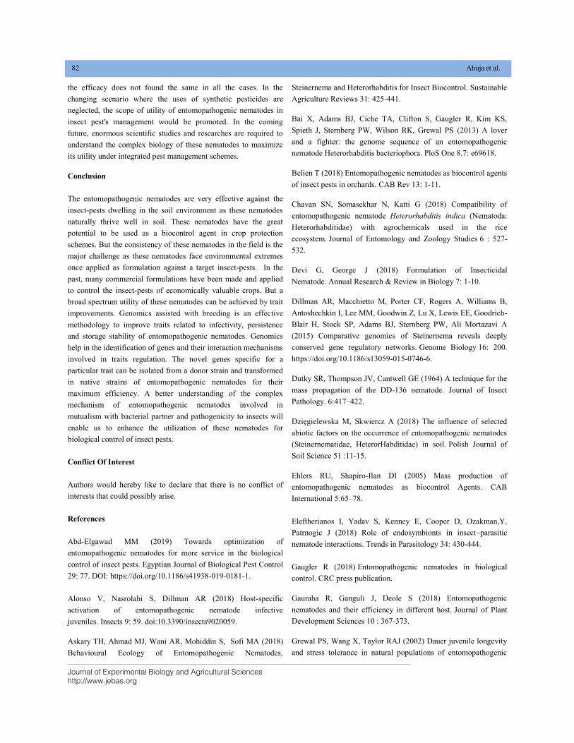
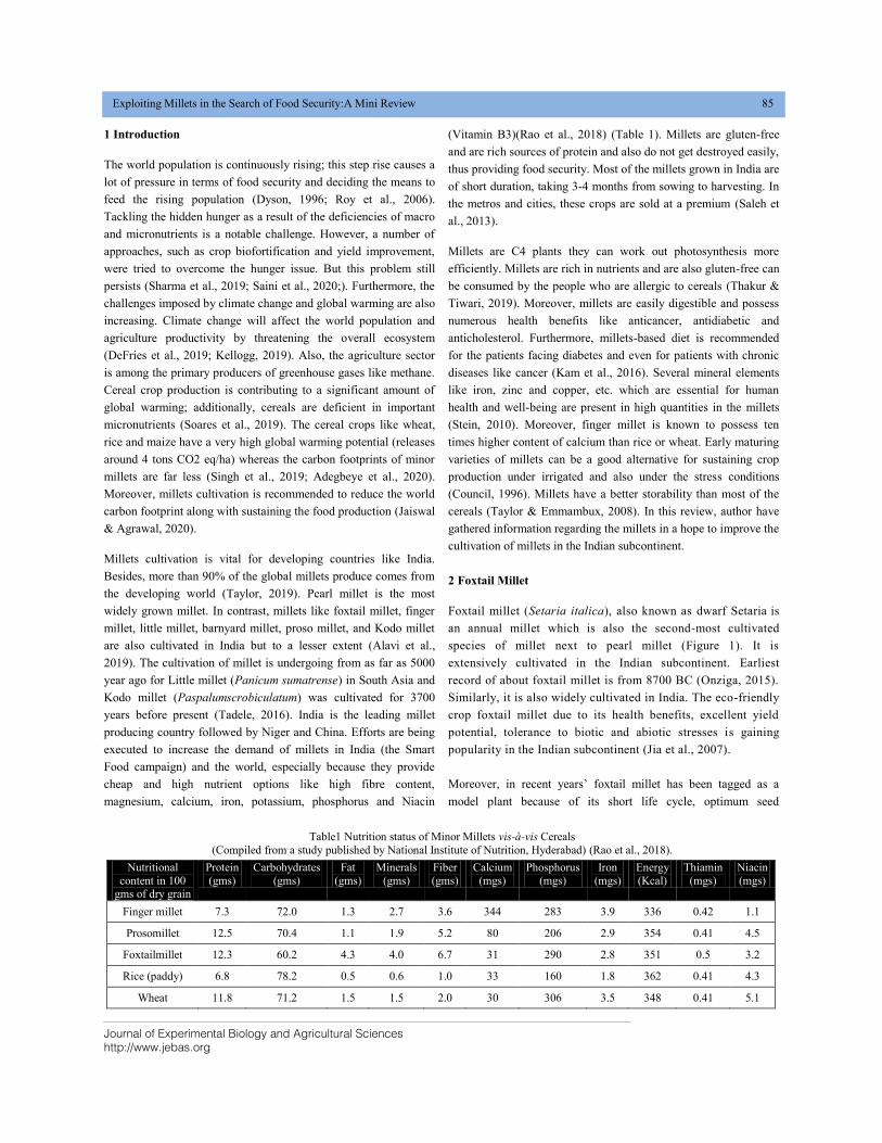
2 Foxtail Millet
Foxtail millet (Setaria italica), also known as dwarf Setaria is
an annual millet which is also the second-most cultivated
species of millet next to pearl millet (Figure 1). It is
extensively cultivated in the Indian subcontinent. Earliest
record of about foxtail millet is from 8700 BC (Onziga, 2015).
Similarly, it is also widely cultivated in India. The eco-friendly
crop foxtail millet due to its health benefits, excellent yield
potential, tolerance to biotic and abiotic stresses is gaining
popularity in the Indian subcontinent (Jia et al., 2007).
Moreover, in recent years’ foxtail millet has been tagged as a
model plant because of its short life cycle, optimum seed
Table1 Nutrition status of Minor Millets vis-à-vis Cereals
(Compiled from a study published by National Institute of Nutrition, Hyderabad) (Rao et al., 2018).
Nutritional
content in 100 gms of dry grain
Protein
(gms)
Carbohydrates
(gms)
Fat
(gms)
Minerals
(gms)
Fiber
(gms)
Calcium
(mgs)
Phosphorus
(mgs)
Iron
(mgs)
Energy
(Kcal)
Thiamin
(mgs)
Niacin
(mgs)
Finger millet 7.3 72.0 1.3 2.7 3.6 344 283 3.9 336 0.42 1.1
Prosomillet 12.5 70.4 1.1 1.9 5.2 80 206 2.9 354 0.41 4.5
Foxtailmillet 12.3 60.2 4.3 4.0 6.7 31 290 2.8 351 0.5 3.2
Rice (paddy) 6.8 78.2 0.5 0.6 1.0 33 160 1.8 362 0.41 4.3
Wheat 11.8 71.2 1.5 1.5 2.0 30 306 3.5 348 0.41 5.1
Journal of Experimental Biology and Agricultural Sciences
http://www.jebas.org
86 Dhaliwal & Kaushik
production, and small genome size (around 400 Mb)
(Zhang et al., 2012). Also, foxtail millet is a C4 plant
and is used to provide valuable information regarding
the C4 photosynthesis (Doust et al., 2009).
Botanically, foxtail millet produces leafy stems with
height upto 200 cm. Foxtail produces a seed head with
a hairy panicle of 5-30 cm long. The seeds are small
approximately 2mm in diameter with a seed colour
that varies from greenish to whitish. In the Indian
subcontinent, its cultivation stretches in arid and semi-
arid regions. It is planted in late spring and usually has
a crop duration of 65-70 days for hay production and
75-90 days as a grain crop. The grain yield typically
varies between 800–900 kg/ha(Austin, 2006).
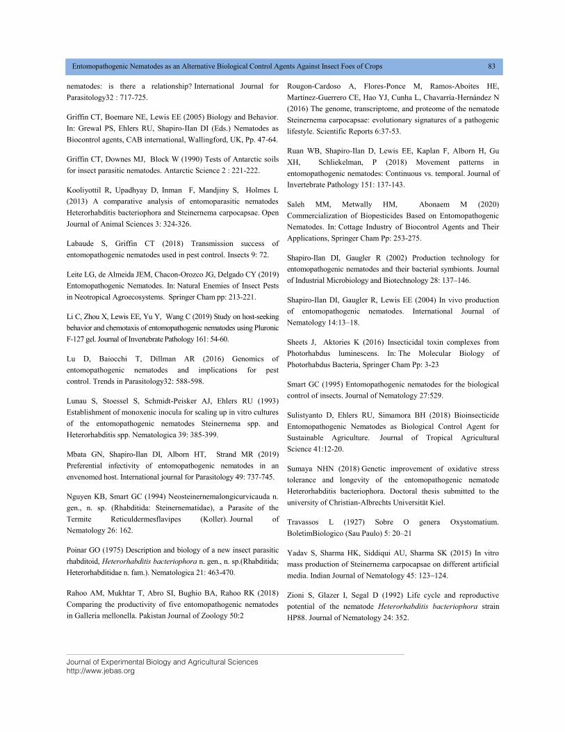
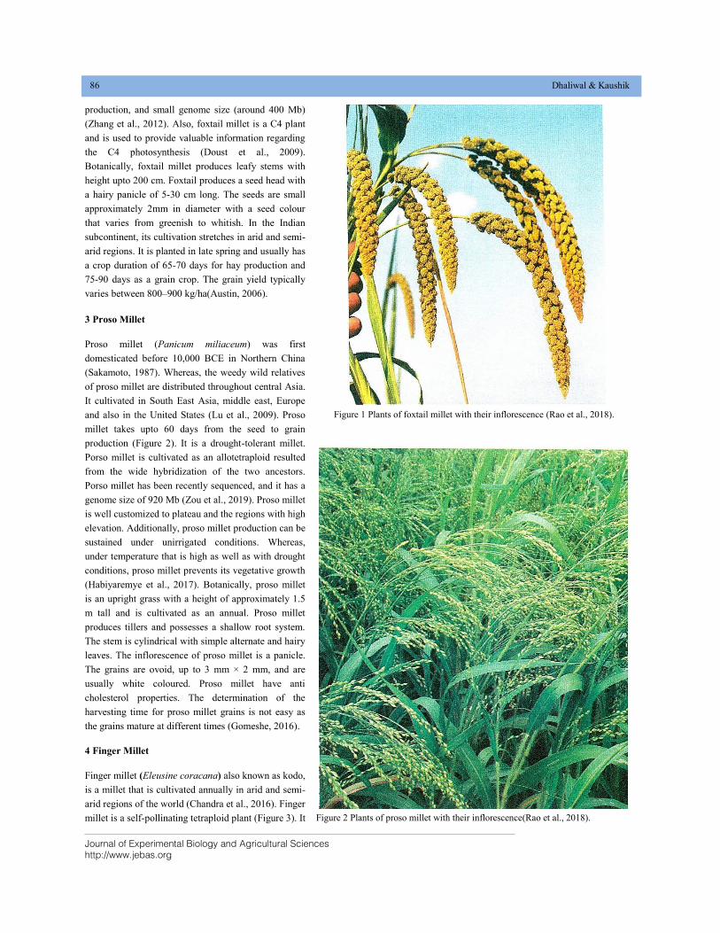
3 Proso Millet
Proso millet (Panicum miliaceum) was first
domesticated before 10,000 BCE in Northern China
(Sakamoto, 1987). Whereas, the weedy wild relatives
of proso millet are distributed throughout central Asia.
It cultivated in South East Asia, middle east, Europe
and also in the United States (Lu et al., 2009). Proso
millet takes upto 60 days from the seed to grain
production (Figure 2). It is a drought-tolerant millet.
Porso millet is cultivated as an allotetraploid resulted
from the wide hybridization of the two ancestors.
Porso millet has been recently sequenced, and it has a
genome size of 920 Mb (Zou et al., 2019). Proso millet
is well customized to plateau and the regions with high
elevation. Additionally, proso millet production can be
sustained under unirrigated conditions. Whereas,
under temperature that is high as well as with drought
conditions, proso millet prevents its vegetative growth
(Habiyaremye et al., 2017). Botanically, proso millet
is an upright grass with a height of approximately 1.5
m tall and is cultivated as an annual. Proso millet
produces tillers and possesses a shallow root system.
The stem is cylindrical with simple alternate and hairy
leaves. The inflorescence of proso millet is a panicle.
The grains are ovoid, up to 3 mm × 2 mm, and are
usually white coloured. Proso millet have anti
cholesterol properties. The determination of the
harvesting time for proso millet grains is not easy as
the grains mature at different times (Gomeshe, 2016).
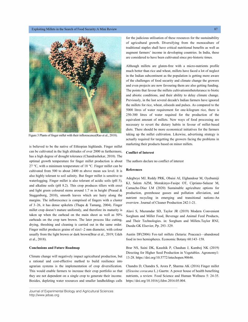
4 Finger Millet
Finger millet (Eleusine coracana) also known as kodo,
is a millet that is cultivated annually in arid and semi-
arid regions of the world (Chandra et al., 2016). Finger
millet is a self-pollinating tetraploid plant (Figure 3). It
Figure 1 Plants of foxtail millet with their inflorescence (Rao et al., 2018).
Figure 2 Plants of proso millet with their inflorescence(Rao et al., 2018).
Journal of Experimental Biology and Agricultural Sciences
http://www.jebas.org
Exploiting Millets in the Search of Food Security:A Mini Review 87
is believed to be the native of Ethiopian highlands. Finger millet
can be cultivated in the high altitudes of over 2000 m furthermore,
has a high degree of drought tolerance (Chandrashekar, 2010). The
optimal growth temperature for finger millet production is about
27 °C, with a minimum temperature of 18 °C. Finger millet can be
cultivated from 500 to about 2400 m above mean sea level. It is
also highly tolerant to soil salinity. But finger millet is sensitive to
waterlogging. Finger millet is also tolerant of acidic soils (pH 5),
and alkaline soils (pH 8.2). This crop produces tillers with erect
and light green coloured stems around 1.7 m in height (Prasad &
Staggenborg, 2010), smooth leaves which are hairy along the
margins. The inflorescence is comprised of fingers with a cluster
of 3–26, it has dense spikelets (Thapa & Tamang, 2004). Finger
millet crop doesn’t mature uniformly, and therefore its maturity is
taken up when the earhead on the main shoot as well as 50%
earheads on the crop turn brown. The later process like cutting,
drying, threshing and cleaning is carried out in the same order.
Finger millet produces grains of size1–2 mm diameter, with colour
usually from the light brown or dark brown(Brar et al., 2019; Udeh
et al., 2018).
Conclusions and Future Roadmap
Climate change will negatively impact agricultural production, but
a rational and cost-effective method to build resilience into
agrarian systems is the implementation of crop diversification.
This would enable farmers to increase their crop portfolio so that
they are not dependent on a single crop to generate their income.
Besides, depleting water resources and smaller landholdings calls
for the judicious utilisation of these resources for the sustainability
of agricultural growth. Diversifying from the monoculture of
traditional staples shall have critical nutritional benefits as well as
augment farmers’ income in developing countries. In India, these
are considered to have been cultivated since pre-historic times.
Although millets are gluten-free with a micro-nutrients profile
much better than rice and wheat, millets have faced a lot of neglect
in the Indian subcontinent as the population is getting more aware
of the challenges of food security and climate change the growers
and even projects are now favouring them are also getting funding.
The points that favour the millets cultivationisthetolerance to biotic
and abiotic conditions, and their ability to delay climate change.
Previously, in the last several decade's Indian farmers have ignored
the millets for rice, wheat, oilseeds and pulses. As compared to the
5000 litres of water requirement for one-kilogram rice, there is
250-300 litres of water required for the production of the
equivalent amount of millets. New ways of food processing are
necessary to revert the dietary habits in favour of millet-based
diets. There should be more economical initiatives for the farmers
taking up the millet cultivation. Likewise, advertising strategy is
actually required for targetting the growers facing the problems in
marketing their products based on minor millets.
Conflict of Interest
The authors declare no conflict of interest
References
Adegbeye MJ, Reddy PRK, Obaisi AI, Elghandour M, Oyebamiji
KJ, Salem AZM, Morakinyo-Fasipe OT, Cipriano-Salazar M,
Camacho-Díaz LM (2020) Sustainable agriculture options for
production, greenhouse gasses and pollution alleviation, and
nutrient recycling in emerging and transitional nations-An
overview. Journal of Cleaner Production 242:1-21.
Alavi S, Mazumdar SD, Taylor JR (2019) Modern Convenient
Sorghum and Millet Food, Beverage and Animal Feed Products,
and Their Technologies. in: Sorghum and Millets.Taylor RNJ,
Duodu GK Elsevier, Pp. 293–329.
Austin DF(2006) Fox-tail millets (Setaria: Poaceae)—abandoned
food in two hemispheres. Economic Botany 60:143–158.
Brar NS, Saini DK, Kaushik P, Chauhan J, Kamboj NK (2019)
Directing for Higher Seed Production in Vegetables. Agronomy1:
13-28. https://doi.org/10.5772/intechopen.90646.
Chandra D, Chandra S, Arora P, Sharma AK (2016) Finger millet
(Eleusine coracana L.) Gaertn: A power house of health benefiting
nutrients, a review. Food Science and Human Wellness 5: 24-35.
https://doi.org/10.1016/j.fshw.2016.05.004.
Figure 3 Plants of finger millet with their inflorescence(Rao et al., 2018).
Journal of Experimental Biology and Agricultural Sciences
http://www.jebas.org
88 Dhaliwal & Kaushik
Chandrashekar A(2010)Finger Millet: Eleusinecoracana.In: Taylor
SL (Ed.), Advances in Food and Nutrition Research. Academic
Press, Pp. 215–262. https://doi.org/10.1016/S1043-4526(10)59006-5
Council NR(1996) Lost crops of Africa: volume I: grains. National
Academies Press.
DeFries RS, Edenhofer O, Halliday AN, Heal GM, Lenton T,
Puma M, Rising J, Rockström J, Ruane A, Schellnhuber HJ (2019)
The missing economic risks in assessments of climate change
impacts. Available on
http://www.lse.ac.uk/GranthamInstitute/publication/the-missing-
economic-risks-in-assessments-of-climate-change-impacts/ access
on 17 October, 2019.
Doust AN, Kellogg EA, Devos KM, Bennetzen JL (2009) Foxtail
millet: a sequence-driven grass model system. Plant Physiology
149: 137–141.
Dyson T(1996) Population and food: global trends and future
prospects. Routledge.
Gomeshe SS (2016) Proso millet, Panicum miliaceum (L.): Genetic
improvement and research needs. In: Patil JV (Ed.) Millets and
Sorghum: Biology and Genetic Improvement, John Wiley & Sons
Ltd Pp.150–179. DOI: https://doi.org/10.1002/9781119130765.ch5.
Habiyaremye C, Matanguihan JB, D’Alpoim Guedes J, Ganjyal
GM, Whiteman MR, Kidwell KK, Murphy KM(2017) Proso Millet
(Panicum miliaceum L.) and Its Potential for Cultivation in the
Pacific Northwest, U.S.: A Review. Frontiers in Plant Science 7:1-
11. https://doi.org/10.3389/fpls.2016.01961
Jaiswal B, Agrawal M, (2020) Carbon Footprints of Agriculture
Sector, in: Carbon Footprints. Springer, pp. 81–99. DOI:
10.1007/978-981-13-7916-1_4.
Jia XP, Shi YS, SongYC, Wang GY, Wang TY, Li
Y(2007)Development of EST-SSR in foxtail millet (Setariaitalica).
Genetic Resources and Crop Evolution 54: 233–236.
Kam J, Puranik S, Yadav R, Manwaring HR, Pierre S, Srivastava
RK, Yadav RS(2016) Dietary interventions for type 2 diabetes:
How millet comes to help. Frontiers in Plant Science 7: 1-9.
https://doi.org/10.3389/fpls.2016.01454.
Kellogg WW(2019) Climate change and society: consequences of
increasing atmospheric carbon dioxide. Routledge. 85-101.Available
on https://www.routledge.com/Climate-Change-And-Society-
Consequences-Of-Increasing-Atmospheric-
Carbon/Kellogg/p/book/9780367018870 Access on 17 October, 2019.
Lu H, Zhang J, Liu K, Wu N, Li Y, Zhou K, Ye M, ZhangT, Zhang
H, Yang X (2009) Earliest domestication of common millet
(Panicum miliaceum) in East Asia extended to 10,000 years ago.
Proceedings of the National Academy of Sciences 106: 7367–7372.
Onziga DI (2015) Characterizing the genetic diversity of finger
millet in Uganda. PhD Thesis submitted to the Makerere
University, Kampala, Uganda Pp. 55-91.
Prasad PVV, Staggenborg S (2010) Growth and Production of
Sorghum and Millets. Encyclopedia of Life Support Systems,
Publisher: EOLSS Publishers, Oxford, U.K. Pp.3-9.
Rao BD, Bhat BV, Tonapi VA (2018)Nutricereals for Nutritional
Security. Director, Indian Institute of Millets, Research,
Hyderabad, Pp. 78:86. Available on
http://www.millets.res.in/technologies/Bulletin-Millets_chapke.pdf
access on 17 October, 2019.
Roy RN, FinckA, Blair GJ, Tandon HLS(2006) Plant nutrition for
food security. A guide for integrated nutrient management 16: 368.
Saini DK, Devi P, Kaushik P (2020) Advances in Genomic
Interventions for Wheat Biofortification: A Review. Agronomy 10:
62-75. https://doi.org/10.3390/agronomy10010062.
Sakamoto S(1987) Origin and dispersal of common millet and
foxtail millet. Japan Agricultural Research Quarterly 21: 84–89.
Saleh AS, Zhang Q, Chen J, Shen Q (2013) Millet grains: nutritional
quality, processing, and potential health benefits. Comprehensive
reviews in food science and food safety 12: 281–295.
Sharma V, Saini DK, Kumar A, Kaushik P (2019) A Review of
Important QTLs for Biofortification Traits in Rice. Preprints 12:1-
16. DOI: 10.20944/preprints201912.0158.v1
Singh H, Sethi S, Kaushik P, Fulford A(2019) Grafting vegetables
for mitigating environmental stresses under climate change: a
review. Journal of Water and Climate Change 29:1-14.
Soares JC, Santos CS, Carvalho SM, Pintado MM, Vasconcelos MW
(2019)Preserving the nutritional quality of crop plants under a
changing climate: importance and strategies. Plant and Soil 443: 1–26.
Stein AJ (2010) Global impacts of human mineral malnutrition.
Plant and soil 335:133–154.
Tadele Z (2016) Drought Adaptation in Millets. In: Shanker A,
Shanker C (Eds.) Abiotic and Biotic Stress in Plants - Recent
Advances and Future Perspectives, Intechopen Publication.
https://doi.org/10.5772/61929.
Taylor JR (2019) Sorghum and Millets: Taxonomy, History,
Distribution, and Production. in: Sorghum and Millets.
Elsevier, Pp. 1–21.
Journal of Experimental Biology and Agricultural Sciences
http://www.jebas.org
Exploiting Millets in the Search of Food Security:A Mini Review 89
Taylor JR, Emmambux MN (2008) Gluten-free foods and
beverages from millets, in: Gluten-Free Cereal Products and
Beverages. Elsevier, pp. 119–V.
Thakur M, Tiwari P (2019) Millets: The undtapped and
underutilized nutritional functional foods. Plant Archives
19:875–883.
Thapa S, Tamang JP(2004) Product characterization of kodo ko
jaanr: fermented finger millet beverage of the Himalayas. Food
microbiology 21: 617–622.doi: 10.1016/j.fm.2004.01.004.
Udeh HO, Duodu KG, Jideani AI(2018) Effect of malting period
on physicochemical properties, minerals, and phytic acid of finger
millet (Eleusinecoracana) flour varieties. Food Science &
Nutrition 6: 1858–1869.https://doi.org/10.1002/fsn3.696.
Zhang G, Liu X, Quan Z, Cheng S, Xu X, Pan S, Xie M, Zeng P,
Yue Z, Wang W (2012) Genome sequence of foxtail millet
(Setariaitalica) provides insights into grass evolution and biofuel
potential. Nature biotechnology 30: 549-554.doi: 10.1038/nbt.2195.
Zou C, Li L, Miki D, Li D, Tang Q, Xiao L, Rajput S, Deng P,
Peng L, Jia W, Huang R, Zhang M, Sun Y, Hu J, Fu X, Schnable
PS, Chang Y, Li F, ZhangH, Feng B, Zhu X, Liu R, SchnableJC,
Zhu JK, Zhang H (2019) The genome of broomcorn millet. Nature
Communications 10:1–11. https://doi.org/10.1038/s41467-019-
08409-5.
Journal of Experimental Biology and Agricultural Sciences
http://www.jebas.org
ISSN No. 2320 – 8694
Journal of Experimental Biology and Agricultural Sciences, April - 2020; Volume – 8(2) page 90 – 97
STANDARD HETEROSIS ANALYSIS IN MAIZE HYBRIDS UNDER WATER
LOGGING CONDITION
Gayatri Kumawat*, Jai Prakash Shahi, Munnesh Kumar, Ashok Singamsetti, Manish Kumar
Choudhary, Kumari Shikha
Department of Genetics and Plant breeding, Institute of Agriculture Science, Banaras Hindu University, Varanasi-221005, India
Received – February 18, 2020; Revision – March 03, 2020; Accepted –March 26, 2020
Available Online – April 25, 2020
DOI: http://dx.doi.org/10.18006/2020.8(2).90.97
ABSTRACT
Maize is one of the important food and forage crops with abundant natural diversity. Determination of
heterosis in CIMMYT maize hybrids under water logging condition is necessary for their commercial
exploitation. The synthetics and composites have contributed to maize production in India in the initial
stages of maize improvement programme, of late, hybrids are playing a vital role due to their high
yielding potential. Breeding of water logging tolerant maize varieties will likely boosts maize
production beyond the present level. Data derived from current study were complied to determine
standard heterosis and identify high yielding hybrids. Among the tested 55 maize hybrids, the maize
hybrids, namely, ZH17506, ZH17496 and VH11128 produced high heterosis which indicating that these
hybrids are available for commercial cultivation. Maize hybrids that perform better than the checks
could be used for release as hybrid variety after re-evaluation in multi-location trials.
* Corresponding author
KEYWORDS
Maize
Water logging condition
Standard heterosis and hybrids
E-mail: [email protected] (Gayatri Kumawat)
Peer review under responsibility of Journal of Experimental Biology and
Agricultural Sciences.
All the articles published by Journal of Experimental
Biology and Agricultural Sciences are licensed under a
Creative Commons Attribution-NonCommercial 4.0
International License Based on a work at www.jebas.org.
Production and Hosting by Horizon Publisher India [HPI]
(http://www.horizonpublisherindia.in/).
All rights reserved.
Journal of Experimental Biology and Agricultural Sciences
http://www.jebas.org
Standard Heterosis Analysis in Maize Hybrids under Water Logging Condition 91
1 Introduction
Maize (Zea mays L.) is one of the most important field crops
cultivated in India to ensure food security. Maize contributes the
greatest share of production and consumption together with other
major cereal crops, such as wheat, rice and Sorghum. Among the
cereal crops, maize ranks third in area coverage and total annual
production and productivity in India (Economic Survey 2015-16,
MoA and FW, GOI). Globally maize covers an area of 178 million
hectares with a production of 978.1 million tonnes (USDA, 2014-
15) and Indian maize occupies an area of 9.2 million hectares with
a production of 22.99 million tonnes (Indiastat.com, 2014-15) and
productivity of 2583 kg ha-1. Initially synthetic and composite
have contributed to maize production in India but now heterosis
breeding play a key role due to their high yielding potential.
Generally, heterosis is an important trait used by breeders to
evaluate the performance of offspring in relation to their parents. It
estimates the enhanced performance of hybrids as compared to
their parents. Often, the superiority of F1 is estimated over the
average of the two parents, or the mid parent or standard check
(Shushay, 2014). Heterosis played an important role in maize
breeding and selection of heterosis is dependent on level of
dominance and differences in gene frequency. The manifestation
of heterosis depends on genetic divergence of the two parental
varieties (Hallauer & Miranda, 1988). Heterosis is manifested as
an increase in vigor, size, growth rate, yield or other
characteristics. But in some cases, the hybrid may be inferior to the
weaker parent, which is also considered as heterosis. That means
heterosis can be positive or negative (Ram Reddy et al., 2015;
Shah et al., 2016). The interpretation of heterosis depends on the
nature of trait under study and the way it is measured.
The low grain yield can be attributed to a number of constraints
which include biotic stress and abiotic stress. Unlike wetland crops,
maize plants do not have a gaseous exchange system between above-
ground plant parts and inundated roots under water lodging
conditions. Therefore, excess soil moisture will results in anoxic soil
condition for maize crop. Therefore, breeding of water logging
tolerant maize varieties will likely boosts maize production beyond
the present level (Kaur et al., 2019). Progress in different discipline
of plant breeding for increased resistance for biotic and abiotic stress
depends predominantly on the extent of heterosis present in
germplasm. So the present investigation conducted to exploit
standard heterosis to select best water logging resistance hybrid.
2 Materials and Methods
2.1 Estimation of mean performance and heterosis
This experimental study was carried out during crop season Kharif
2017 in alpha lattice design with two replications at the Agriculture
Research Farm of Banaras Hindu University, Varanasi, UP, India. The
experiment genotypes comprised of 55 maize genotypes in which two
standard checks (900MG from Monsanto and P3502 from Pioneer)
and 53 maize hybrids were obtained from CIMMYT (International
Maize and Wheat Improvement Center, Mexico) germplasm under the
project- ―Climate Resilient Maize for Asia (CRMA)‖. Each hybrid was
planted in a single row of 3 meters in length with a spacing of row to
row 60cm and plant to plant 25 cm. Water logging stress was imposed
at V6-V7 growth stage/ knee height stage of crop growth (35 days after
sowing). Draining out of excess water was done on seventh day (Zaidi
et al., 2016). The crop was raised as per the recommended agronomic
package of practices. The observations were recorded for fifteen
characters viz. pre harvest data like-number of nodes bearing brace
roots, number of surface roots, days to 50 percent anthesis, days to 50
percent silking, plant height (cm), ear height (cm) and post harvest data
like-ears per plot, grain weight (t/h), plant population, ear length (cm),
ear diameter (cm), number of kernel rows per ear, number of kernels
per row, 100 seed weight (g) and yield per plant (g). The statistical
analysis of data based on the mean value of recorded observations on
five random plant basis was done.
Standard heterosis was estimated for grain yield per plant as deviation
of F1 hybrid from the check included in the trial. It is expressed as
percentage superiority over standard check. Standard heterosis was
calculated for those traits that showed statistically significant
differences among genotypes as suggested by Falconer & Mackay
(1996). These were computed as percentage increase or decrease of the
cross performances over best standard check as follows.
Standard heterosis (SH) = F1− Check
Check ˟100
Where, F1 = mean value of F1 ; SH = mean value over replication
of the local commercial check
2.2 Test of significance
The significance of heterosis was tested by using‗t‘ test as suggested by
Snedecor & Cochran (1989) and Paschal & Wilcox (1975).
SE (d) = 2MSE
r
t = F1− standard Check
SE (d)
Where, SE (d) is standard error of the difference; MSE is error mean
square and r is number of replications and calculated t value was
compared against the tabulated t-value at degree of freedom for error.
3 Results and Discussion
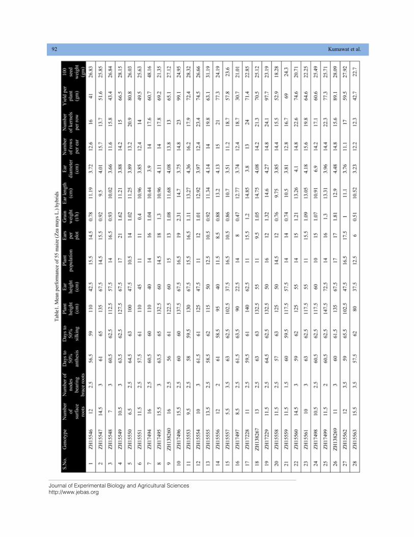
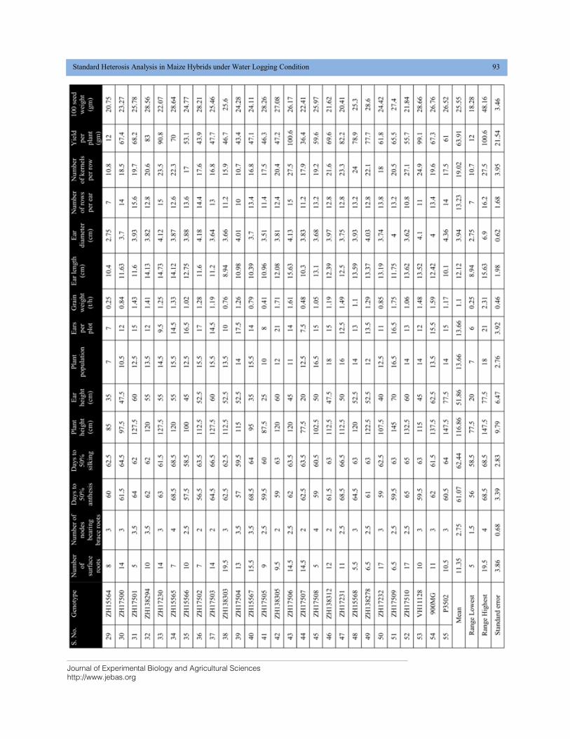
3.1 Mean performance of genotypes
The mean performances of the genotypes (the 53 hybrid progenies
and two standard checks) across site are given in Table 1. Yield
Journal of Experimental Biology and Agricultural Sciences
http://www.jebas.org
92 Kumawat et al.
Journal of Experimental Biology and Agricultural Sciences
http://www.jebas.org
Standard Heterosis Analysis in Maize Hybrids under Water Logging Condition 93
Journal of Experimental Biology and Agricultural Sciences
http://www.jebas.org
94 Kumawat et al.
per plant was recorded with a range of 12.00 g (ZH15564) to
100.00 g (ZH15506). Among the tested hybrids, ZH15506
yielded higher than 900MG check (67.3g). The presence of
crosses having mean values better than the standard checks
indicate the possibility of obtaining good hybrid (s) for future
use in breeding program or for commercial use general mean was
observed 63.9g. Number of surface roots ranged from 5
(ZH17501, ZH17508) to 19.5 (ZH138303) with general mean
11.34 surface root per plant. Number of nodes bearing brace
roots were recorded with a class from 1.50 (ZH15559) to 4.10
(ZH15560) with an average mean of 2.75.
The number of days to 50 % anthesis and days to 50% silking
classified from 56.00 (ZH138260) to 68.50for (ZH15565) and
57.40 (ZH15547) to 68.5 (ZH15565) coupled with a general mean
of 61.07 and 62.30 days respectively among 55 maize genotypes
studied. Most of the crosses showed longest number of days to
anthesis and silking. This shows that it might be because of late
crosses in these genotypes. Late maturing hybrids are important in
the breeding programs for development of high yielding hybrids in
areas that receive sufficient rain fall (Hosana et al., 2015). Further
evaluation and recommendation of this group of materials should
be based on agro-ecological suitability.
At maturity, plant height and ear height mean value of different
genotypes arranged from 77.50 cm (ZH17507) to 147.50 cm
(ZH17499, P3502) and from 20.00cm (ZH17507) to 77.50 cm
(P3502) with an average mean of 116.8 cm and 51.86 cm
respectively. In line with these finding, Hosana et al. (2015)
reported higher grain yield from taller plants; this could be
attributed to high photosynthetic products accumulation during
long period for grain filling.
Plant population ranged from 7.00 (ZH15564) to 18.00
(ZH138312) with an average mean of 13.60. Ear per plots ranged
from 6.00 (ZH17497) to 21.00(ZH15563) with an average mean
of 13.66. Grain weight (weighing the total ears in a plot and later
converted in to tones per hectors) was varied from 0.24
(ZH15564) to 2.30 ton per hectare (ZH17496). Ear length and
ear diameter was recorded with a range of ranged from 8.90 cm
(ZH15561) to 15.60 cm (ZH17232) and 2.70 cm (ZH15564) to
6.90 cm (ZH17498) with an average mean of 12.12cm and 3.90
cm respectively. The number of kernel rows per ear ranged from
7.00 to 16.20 with the mean 13.20. The lowest rows were found
in ZH15564 whereas the highest was found in ZH15553. The
number of kernels per row for 55 maize genotypes varied from
10.70 (ZH15504) to 27.50 (ZH17506) with a general mean
19.01. Wait for 100 grains for all 55 genotypes ranged from
18.27 g in ZH15558 to 48.15g in ZH17494 genotype. The
observed mean was 25.5 g. The genotypes showing high mean
value for post harvest yield attributing traits under water logging
condition can be exploited further for high soil moisture
resistance genotype development (Zaidi et al., 2010; Shushay,
2014;).
3.2 Standard heterosis
The estimates of standard heterosis over the standard check
900MG were computed for grain yield and yield related traits and
presented in Table 2. As the mean value of yield per plant higher
for 900MG check than P3502 check, so 900MG check exploit as
standard check in this experiment. Three hybrids showed positive
and significant heterosis to 900 MG standard check for grain yield
per plant. Standard heterosis for grain yield per plant ranged from -
82.17 (ZH 15564) to 49.48% (ZH17506). ZH17496 and VH11128
(47.25%) exhibited positive standard heterosis to the standard
check. Positive heterosis for this trait indicates increased yield
advantage over the existing standard check. Maize hybrids that
perform better than the checks could be used for release as hybrid
variety after verification.
Standard heterosis for days to 50% anthesis and silking ranged
from -9.68 to 10.48% and -4.88 to 11.38% to 900MG
respectively. Three hybrids showed positive and significant
heterosis for these traits to check indicating that these hybrids
were late maturing as compared to the checks. Heterosis in the
negative direction for these traits indicates earliness of the
crosses over the standard checks so negative heterosis is
desirable for them. Significant negative heterosis for days to
tasseling was observed in ZH15546, ZH138260, ZH15558,
ZH17502 and ZH17504 crosses. Earlier Amiruzzaman et al.
(2013) and Bello & Olawuyi (2015) reported negative heterosis
for these traits in maize.
Standard heterosis for surface and brace roots showed three
and two genotypes positively significant respectively. The
positive heterosis in these traits indicates desirable hybrids
with more water logging resistance. Positively significant
genotypes for plant height and ear height indicated desirable
hybrids with more photosynthetic efficiency. Similarly post
harvest data (yield data) indicates viz- ear length, ear diameter,
number of rows per ear, number of kernels per row and 100
seed weight showed positive significant heterosis for those
hybrids which can be used for commercialization of hybrids
(Singh & Jha 2007; Ulaganathan et al., 2015).
Conclusion
Three hybrids (ZH17506, ZH17496 and VH11128) showed
positive and significant heterosis to 900 MG standard check for
grain yield per plant. Maize hybrids that perform better than the
checks could be used for release as hybrid variety after re-
evaluation in multi-location trials.
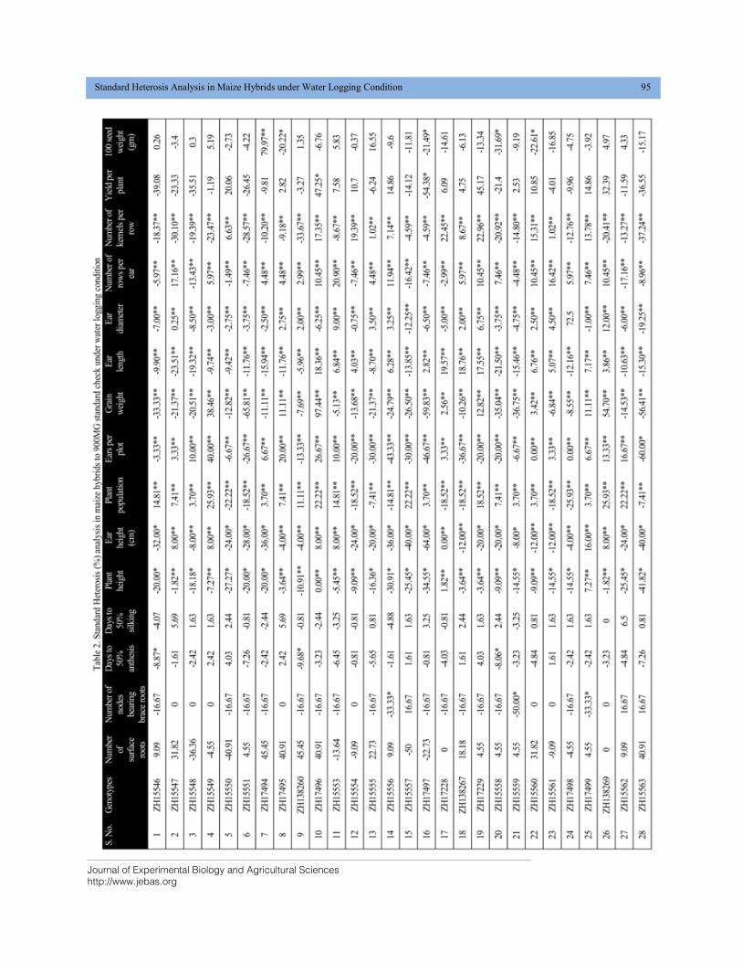
Journal of Experimental Biology and Agricultural Sciences
http://www.jebas.org
Standard Heterosis Analysis in Maize Hybrids under Water Logging Condition 95
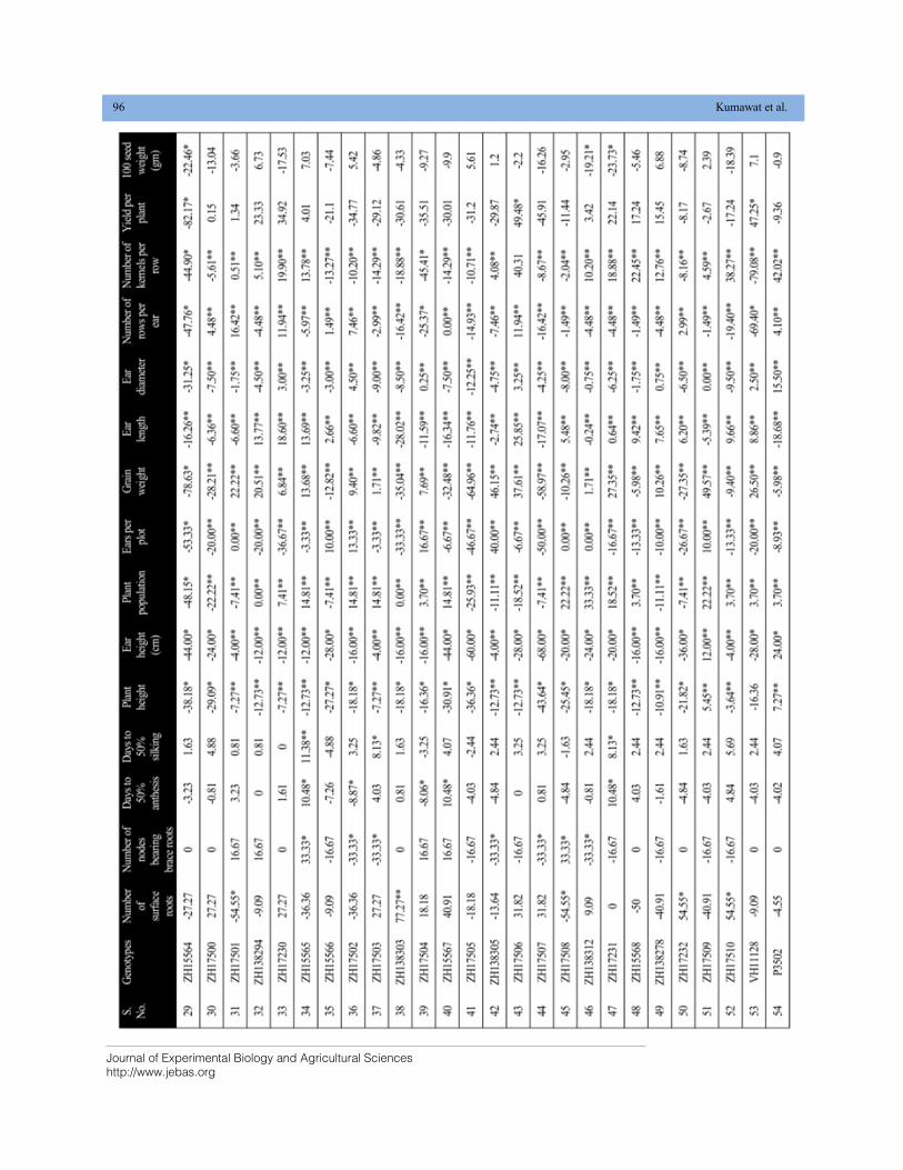
Journal of Experimental Biology and Agricultural Sciences
http://www.jebas.org
96 Kumawat et al.
Journal of Experimental Biology and Agricultural Sciences
http://www.jebas.org
Standard Heterosis Analysis in Maize Hybrids under Water Logging Condition 97
Acknowledgements
We would like to express our sincere appreciation to the CIMMYT
Hyderabad and Institute of Agriculture Sciences Banaras Hindu
University.
Conflict of Interest
Authors would hereby like to declare that there is no conflict of
interests that could possibly arise.
References
Amiruzzaman M, Islam MA, Hasan L, Kadir M, Rohman MM
(2013) Heterosis and combining ability in a diallel among elite
inbred lines of maize (Zea mays L.). Emirates Journal of Food and
Agriculture 25: 132-137.
Bello OB, Olawuyi OJ (2015) Gene action, heterosis, correlation
and regression estimates in developing hybrid cultivars in
maize. Tropical Agriculture 92: 102-117.
Economic Survey (2016). Economic Survey 2015-16 Retrieved
from idiabudget.nic.in/es2015-16/ estat1.pdf access on 18
September, 2019.
Falconer DS, Mackay TFC (1996) Introduction to Quantitative
Genetics, 4th edn. Longman, London.
Hallauer AR, Miranda JB (1988) Quantitative genetics in maize
breeding. Iowa State Univ. Press, Ames. Quantitative genetics in
maize breeding. 2nd ed. Iowa State Univ. Press, Ames.
Hosana GC, Alamerew S, Tadesse B, Menamo T (2015) Test cross
performance and combining ability of maize (Zea mays L.) inbred
lines at Bako, Western Ethiopia. Global Journal (USA) 15: 24.
Indiastat Agriculture production (2014) Indiastat Agriculture
production 201315 available on http://www.indiastat.com access
on 18 September, 2019.
Kaur G, Zurweller B, Motavalli PP, Nelson KA (2019) Screening
Corn Hybrids for Soil Waterlogging Tolerance at an Early Growth
Stage. Agriculture 9: 33.
Paschal EH, Wilcox JR (1975) Heterosis and combining ability in
exotic soybean germplasm. Crop Science 15: 344-349.
Ram Reddy V, Farzana zabeen, Sudarshan MR (2015) Heterosis
studies in diallel crosses of maize for yield and yield attributing
traits in maize over locations. International Journal of Agricultural,
Environment and Biotechnology 8: 271-283.
Shah RT, Prasad K, Kumar P (2016) Maize—A potential source of
human nutrition and health: A review. Cogent Food and
Agriculture 2: 1166995.
Shushay WA (2014) Standard heterosis of maize (Zea mays L.)
inbred lines for grain yield and yield related traits in central Rift
Valley of Ethiopia. Journal of Biology, Agriculture and Healthcare
4: 31-37.
Singh SP, Jha PB (2007) Heterotic potential of winter maize
hybrids for yield attributing traits under variable moisture
condition. Journal of Applied Bioscience 33: 1-7.
Snedecor, GW, Cochran, WG (1989) Statistical Methods. 8th
ed.
Lowa State University press. Ames. IA.
Ulaganathan V, Vinoth R, Baghyalakshmi K, Chimili SR,
Gurusamy A (2015) Standard heterosis for grain yield and other
agronomic characters in maize (Zea mays L.) under normal and
moisture stress conditions. An International Quarterly Journal of
Life Science 10: 1251-1253.
USDA (2014) World Agricultural Production. 2013-2014.
Available on www.usda.gov access on 19 September, 2019.
Zaidi PH, Maniselvan P, Srivastava A, Yadav P, Singh RP (2010)
Genetic analysis of water-logging tolerance in tropical maize (Zea
mays L.). Maydica 55: 17-26.
Zaidi PH, Vinayan MT, Seetharam K (2016) Phenotyping for
abiotic stress tolerance in maize: Waterlogging stress. A field
manual. CIMMYT: Hyderabad, India.
Journal of Experimental Biology and Agricultural Sciences
http://www.jebas.org
ISSN No. 2320 – 8694
Journal of Experimental Biology and Agricultural Sciences, April - 2020; Volume – 8(2) page 98 – 110
ENERGY USE EFFICIENCY AND GREEN HOUSE GAS EMISSIONS FROM
INTEGRATED CROP-LIVESTOCK SYSTEMS IN SEMI-ARID ECOSYSTEM OF
DECCAN PLATEAU IN SOUTHERN INDIA
Md. Latheef Pasha1, G Kiran Reddy2,*, S Sridevi3, M Govardhan4, Md. Ali Baba5, B. Rani6
1Senior Scientist (Agronomy), AICRP-IFS, Hyderabad – 500030
2Scientist (Soil Science), AICRP-IFS, Hyderabad – 500030
3Principal, Agricultural Polytechnic, Tornala
4Principle Scientist & Head, AICRP-IFS, Hyderabad – 500030
5Scientist (Agricultural Economics), AICERP-IFS, Hyderabad – 500030
6SRF, AICRP-IFS, Hyderabad – 500030
Received – January 19, 2020; Revision –March 20, 2020; Accepted – March 28, 2020 Available Online – April 25, 2020
DOI: http://dx.doi.org/10.18006/2020.8(2).98.110
ABSTRACT
Integrated crop-livestock system is the default in vogue farming system followed in semi arid Deccan
plateau in Southern India. Energy flow and environmental impact plays an anchor role for the sustainability
of any farming system. The objective of the present study is to know the energy use and greenhouse gas
(GHG) emission in the integrated crop-livestock systems in study area. Primarily data was collected from
36 farmers by bench mark survey questionnaire. The study area includes 54.53 ha of cultivated land, 177
dairy cattle, 466 sheep and 129 poultry birds. Total input energy required for crop production and livestock
management was 1598441.0 and 6168311.9 MJ respectively, output energy generated was 9063909.8 and
408331.0 MJ respectively. Even livestock enterprise have shown negative energy balance (-5759980.9 MJ),
overall system has shown positive energy balance of 1705487.9 MJ as crop enterprise offset the ill energy
efficiency of livestock enterprise. Rice emits highest amount of CO2eq (3099.4 kg CO2eq ha-1
) among crops
in study, around 50% is contributed by submergence (continuous flooding). Total GHG emission from the
study area was 532215.3 kg CO2eq. Out of which, 26.1% and 73.9% of the emissions were emitted by crop
(138637.3 kg CO2eq) and livestock enterprise (393578.0 kg CO2eq). Both the cases crop enterprise has
greater advantage over the livestock enterprise. The key policy implication from the current study was
integrated crop-livestock system will sustain in long run, as less energy use and higher GHG emissions of
livestock enterprise will be nullified by the crop enterprise.
* Corresponding author
KEYWORDS
Integrated crop-livestock
system
Greenhouse gas (GHG)
emission
Energy use
Sustainability
Input energy
Positive energy balance
E-mail: [email protected] (G Kiran Reddy)
Peer review under responsibility of Journal of Experimental Biology and
Agricultural Sciences.
All the articles published by Journal of Experimental
Biology and Agricultural Sciences are licensed under a
Creative Commons Attribution-NonCommercial 4.0
International License Based on a work at www.jebas.org.
Production and Hosting by Horizon Publisher India [HPI]
(http://www.horizonpublisherindia.in/).
All rights reserved.
Journal of Experimental Biology and Agricultural Sciences
http://www.jebas.org
Energy use efficiency and green house gas emissions from integrated crop-livestock systems 99
1 Introduction
Agriculture is the base for livelihood of 66% of the Indian
population and it contributes 20% of national gross domestic
products. It is the source for national food security (ICAR, 2015).
In 1970’s, with advent of green revolution in India, one side it
increased the food grain production. It directly or indirectly
increased the livestock population, as the energy availability
increased. Other side fertilizer and other external inputs usage
increased manifold resulted in deterioration of soil health, thereby
paradism shift in energy use and GHG’s (green house emissions)
emissions over a period. Agriculture requires large energy and
potent source of GHG as stated by Hoffman et al. (2018).
Nearly 85% of the Indian farmers fall under the category of small
and marginal farmers with acreage less than 1 ha. Initial
investment capacity of the Indian farmers is very low. Investment
should not impair the crop productivity. So, the cost of cultivation
should be kept low. In addition to economic analysis, energy
analysis which indicates the inputs to be minimized and energy use
has to be increased. Farming uses the energy in different capacities
e.g. machinery, human power, seed, diesel, animal power,
irrigation etc. An agricultural production system is to be efficient,
if it produces more output (output energy) with minimum input
energy (especially non reneweable inputs). This makes the
agricultural production system viable in environmental and
economic terms (Sefeedpari et al., 2012). It is very useful to
analyse crops in terms of energy. This should be done without
impairing the yield of the crops.
Livestock and land utilization are the critical factors for the GHG
emissions. Farming contributes around 10-12% of the GHG
globally (IPCC, 2007). The share in India context is a bit higher
side at 18% (INCCA, 2010). Farming is in third line after energy
and industry sector in GHG emissions in India. In Indian
agriculture system, farmers cultivate versatile crops and maintain
livestock for the livelihood and nutrition security to family. Mixed
crop-livestock farming is age old practice, which provides food for
more than half of the world’s population (Ghahramani & Bowran,
2018). So, such farming systems environmental impact assessment
is also an important factor. Most part of GHG from farming in
India is contributed by the livestock (Steinfeld et al., 2006). From
global food security point of view livestock plays a very critical
role, as it is meeting the 17% of global energy and 33% of protein
requirement (Rosegrant et al., 2002). Animal protein demand is
increasing day by day globally in general and semi arid deccan
plateau in Southern India in particular. Increased per capita income
is also playing a pivotal role for the increasing consumption and
demand for animal products in this part of world. In addition,
increase in animal population also has other benefits like, provides
organic matter, which is wealth for poor farmers etc.
In regarding the Deccan plateau in Southern India, livestock – crop
integration system is a principle farming pattern adapted by bulk of
the cultivators. India is also one of the leading producers of rice
and milk. Wide variety of crops like rice, maize, groundnut, cotton,
sorghum, vegetables etc. are grown. More or less all farm families
will maintain livestock (either dairy, sheep, poultry etc.).
Highly scarce information is available regarding the impact of
different farming systems on energy use and GHG emissions in the
Deccan plateau of Southern India. An attempt was made to
evaluate the energy sequestered in integrated crop-livestock
farming system, the energy sequestration of different crops,
livestocks and GHG emission from livestock and crop
management in Southern Deccan plateau region of India.
2 Materials and Methods
2.1 Description of study area
The survey was conducted under All India Coordinated Research
Project on Integrated Farming System, as part of On Farm
Research in Medak district of Telangana State in Southern India.
The area of surveyed includes two blocks of Medak district i.e.
Yeldurthy and Toopran covering three villages in each block.
Three representative villages from each block i.e. six villages for
each district were selected randomly. From each village six farm
households were chosen at a random keeping in mind that at least
four households should represent each farming system. Yeldurthy
and Toopran blocks were the typical blocks of Medak districts,
which are located 100 kms east of capital city Hyderabad
(Telangana State). Study area is situated in the central part of
Telangana State. Its coordinates are 17o 27’ 0” – 18
o 19’ N latitude,
17o 27’ 0” – 18
o 19’ E longitude 442m. Study area comes under
Southern plateau and hill zone agroclimatic zone of India. The
mean annual rainfall was 861 mm, the mean temperature of the
study area was 26.8○C. Climatic condition of the region is tropical.
Before commencement of the study, the strong research
methodology was developed to investigate the targeted farmers
via. statistical and scientific methods through prepared
questionnaire. Overall 36 farmers were surveyed in the year 2017-
18 for a period of one year from June, 2017 to May, 2018. Farmers
in the study area grow crops like rice, maize, fodder sorghum,
tomato, okra, cotton groundnut there acreages are 37.74, 14.04,
0.25, 0.9, 0.3, 1.0, 0.2 ha respectively. With regard to livestock,
total of 177 dairy cattle, 466 sheep and 129 poultry were
maintained by 36 farm families in total. All the farmers were
following integrated livestock and crop farming system in different
proportions. Geographic and meteorological features of the
surveyed villages were similar to other villages, where the
integrated livestock-crop farming systems were practiced in this
part of world.
Journal of Experimental Biology and Agricultural Sciences
http://www.jebas.org
100 Latheef Pasha et al.
2.2 Collection of data
The data regards to the complete production of crops and live
stocks were assessed from the targeted farmers by detail interview
with individual farmer with the help of bench mark survey
questionnaire in the study area. General information of farmer such
as holding size, farm land details, farm machinery and equipment,
crop wise input used like seed, fertilizers, human labour, bullock
labour, chemical, oils used. Production of various farm out puts
(rice, maize, tomato and fodder etc) and disposal of produce
livestock details like number of animals, fodder, concentrates,
mineral mixture, livestock products were reported in detail to
calculate the energy balance and GHG emissions.
2.3 Calculations of energy balance and GHG emissions
Various inputs were used for the production of crops and
maintenance of livestock, outputs that were generated by using the
inputs and their energy equivalents are presented in table 1
(ubiquitous environmental sources of energy i.e. radiation, wind
etc. was not taken into account). Energy equivalents present in the
table 1 were used to calculate the input and output energy values
i.e., the input energy which was utilized to produce the output
energy. Input energy classified into direct (labour, fuel and
electricity) and indirect energy (fertilizers, chemicals, machinery,
irrigation, manures and seed), renewable (labour, organic manures
and seed) and non renewable energy (fuel, fertilizers, chemicals,
machinery and water). Output energy like the energy embodied in
the crops, livestock products and byproducts were considered.
Different values generated from the input and output energy were
used to calculate the energy use efficiency, energy productivity,
specific energy, net energy, land use efficiency, non renewable
energy ratio, direct energy, indirect energy, renewable energy and
non renewable energy (standard formulas are given in table 2).
Land use efficiency is the amount of energy generated in a given
unit of land. The ratio between total output and input energy is the
energy use efficiency. Net energy is the difference between the
total output energy generated minus total input energy supplied to
produce the crop. Energy productivity is the quantity of crop
produced by the supply of given amount of energy. Non renewable
energy ratio is the same as energy use efficiency except it
considers only non renewable energy used for the crop production.
GHG emissions were in principle calculated with default
emission factors, as cited by many authors. In present study
different factors that contribute to the GHG emissions were
machinery, diesel, N, P, K chemical fertilizers, FYM, electricity,
chemicals, rice under submergence, production of milk, FYM,
mutton, eggs and poultry. Default factors per unit for the above
said factors were used to calculate the GHG emissions (Table 3).
The present study accounts only for farm management (within
the farm gate) do not account for outside the farm gate.
Calculation was done up to the farm gate only.
3 Results and Discussion
3.1 Energy use analysis
The data collected from the surveyed area covering 36 farmers
with total acreage of 54.43 ha under crops (occupied by rice,
maize, fodder sorghum, tomato, okra, cotton and groundnut),
177 dairy cattle, 466 sheep and 129 poultry birds; these data
helps in characterizing the energy use by 36 farmers of the
study area in crops and livestock. Input quantities used for
production of crops are presented in table 4, input and output
energies for crop production are presented in table 5. In
production of crops, input energy per unit area crop production
varied considerably among crops. The input energies for the
production of rice, maize, fodder sorghum, tomato, okra,
cotton, groundnut were 1171215.0, 347730.5, 6096.8, 24959.7,
9561.7, 32629.3, 7247.5 MJ respectively. Total input energy
for the crop production in the study area was 1598441.0 MJ.
Input energies required to calculate for individual crops per ha
to produce the output were 31007.2, 24767.1, 24387.3,
27733.0, 31872.3, 32629.3, 36237.7 MJ for rice, maize, fodder
sorghum, tomato, okra, cotton, groundnut respectively. Highest
input energy required for the production of groundnut while the
least one was observed in the fodder sorghum per ha area.
The output energy i.e. economic and byproducts energy varies
with crops, presented in table 5 (in lower panal). The variation
in yield depends on the genetic potential of crop and
management practices. The output energy calculated for both
economic and byproducts, the values for rice, maize, fodder
sorghum, tomato, okra, cotton, groundnut were 6122882.0,
2702090.0, 59850.0, 58634.8, 23458.0, 75725.0, 21270.0 MJ
respectively. Mean values of the output energy in MJ ha-1
(table 5) were calculated as rice (162288.5), maize (192456.6),
fodder sorghum (239400), Tomato (65149.8), okra (78193.3),
cotton (75725.0) and groundnut (106350). Sartori et al. (2005)
observed in the maize conservation farming, it requires input
energy of 46900 MJ ha-1
and it generated 161980.0 MJ ha-1
output energy. The overall output energy for the study area for
crop enterprise was 9063909.8 MJ. Output energies produced
by the crops were higher than the energy consumed for
production (Table 5). The crop enterprise has produced a
positive energy of 7465468.8 MJ compared to consumed
energy in the study area. Similarly, Tsatsarellis (1991)
calculated the energy use in cotton and reported that cotton
crop in total sequestrated energy of 82600.0 MJ ha-1
.
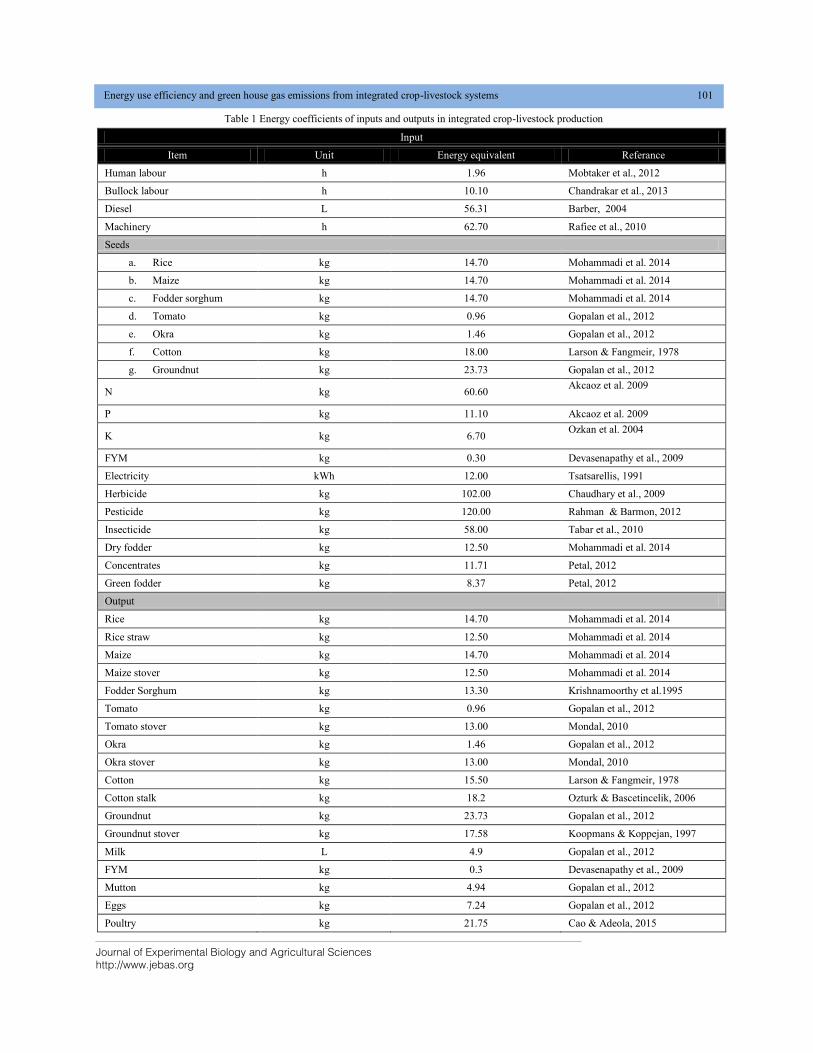
Journal of Experimental Biology and Agricultural Sciences
http://www.jebas.org
Energy use efficiency and green house gas emissions from integrated crop-livestock systems 101
Table 1 Energy coefficients of inputs and outputs in integrated crop-livestock production
Input
Item Unit Energy equivalent Referance
Human labour h 1.96 Mobtaker et al., 2012
Bullock labour h 10.10 Chandrakar et al., 2013
Diesel L 56.31 Barber, 2004
Machinery h 62.70 Rafiee et al., 2010
Seeds
a. Rice kg 14.70 Mohammadi et al. 2014
b. Maize kg 14.70 Mohammadi et al. 2014
c. Fodder sorghum kg 14.70 Mohammadi et al. 2014
d. Tomato kg 0.96 Gopalan et al., 2012
e. Okra kg 1.46 Gopalan et al., 2012
f. Cotton kg 18.00 Larson & Fangmeir, 1978
g. Groundnut kg 23.73 Gopalan et al., 2012
N kg 60.60 Akcaoz et al. 2009
P kg 11.10 Akcaoz et al. 2009
K kg 6.70 Ozkan et al. 2004
FYM kg 0.30 Devasenapathy et al., 2009
Electricity kWh 12.00 Tsatsarellis, 1991
Herbicide kg 102.00 Chaudhary et al., 2009
Pesticide kg 120.00 Rahman & Barmon, 2012
Insecticide kg 58.00 Tabar et al., 2010
Dry fodder kg 12.50 Mohammadi et al. 2014
Concentrates kg 11.71 Petal, 2012
Green fodder kg 8.37 Petal, 2012
Output
Rice kg 14.70 Mohammadi et al. 2014
Rice straw kg 12.50 Mohammadi et al. 2014
Maize kg 14.70 Mohammadi et al. 2014
Maize stover kg 12.50 Mohammadi et al. 2014
Fodder Sorghum kg 13.30 Krishnamoorthy et al.1995
Tomato kg 0.96 Gopalan et al., 2012
Tomato stover kg 13.00 Mondal, 2010
Okra kg 1.46 Gopalan et al., 2012
Okra stover kg 13.00 Mondal, 2010
Cotton kg 15.50 Larson & Fangmeir, 1978
Cotton stalk kg 18.2 Ozturk & Bascetincelik, 2006
Groundnut kg 23.73 Gopalan et al., 2012
Groundnut stover kg 17.58 Koopmans & Koppejan, 1997
Milk L 4.9 Gopalan et al., 2012
FYM kg 0.3 Devasenapathy et al., 2009
Mutton kg 4.94 Gopalan et al., 2012
Eggs kg 7.24 Gopalan et al., 2012
Poultry kg 21.75 Cao & Adeola, 2015
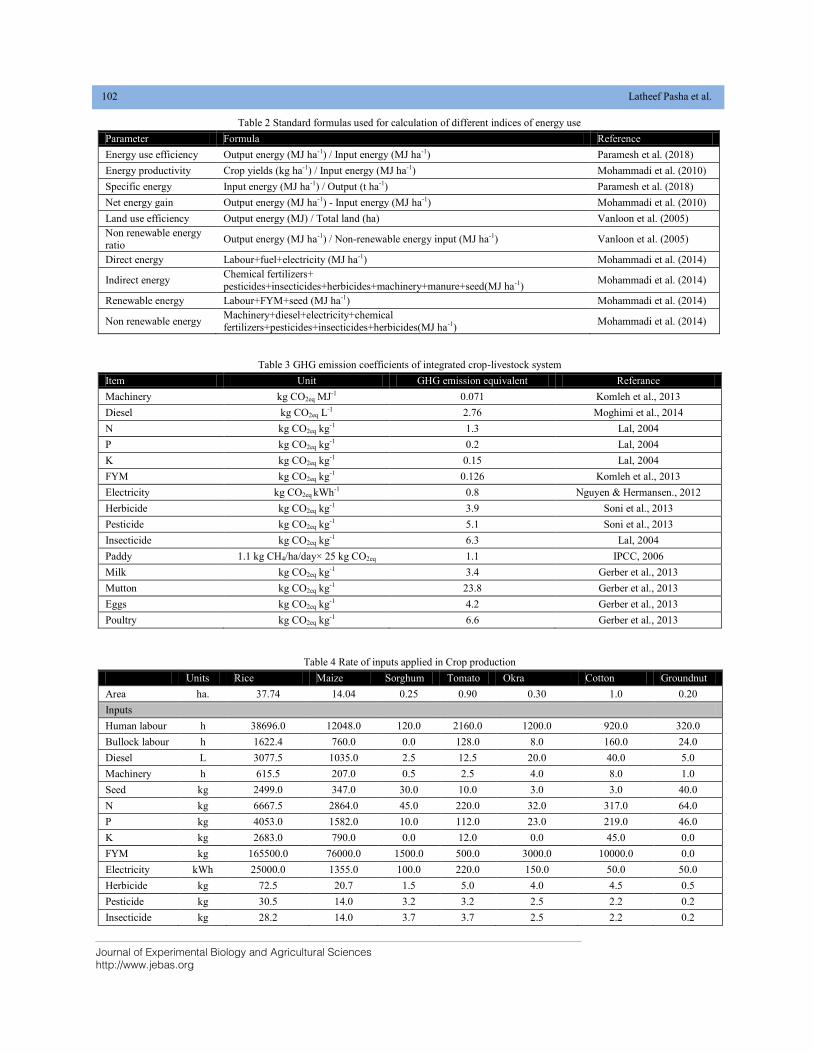
Journal of Experimental Biology and Agricultural Sciences
http://www.jebas.org
102 Latheef Pasha et al.
Table 2 Standard formulas used for calculation of different indices of energy use
Parameter Formula Reference
Energy use efficiency Output energy (MJ ha-1) / Input energy (MJ ha-1) Paramesh et al. (2018)
Energy productivity Crop yields (kg ha-1) / Input energy (MJ ha-1) Mohammadi et al. (2010)
Specific energy Input energy (MJ ha-1) / Output (t ha-1) Paramesh et al. (2018)
Net energy gain Output energy (MJ ha-1) - Input energy (MJ ha-1) Mohammadi et al. (2010)
Land use efficiency Output energy (MJ) / Total land (ha) Vanloon et al. (2005)
Non renewable energy
ratio Output energy (MJ ha-1) / Non-renewable energy input (MJ ha-1) Vanloon et al. (2005)
Direct energy Labour+fuel+electricity (MJ ha-1) Mohammadi et al. (2014)
Indirect energy Chemical fertilizers+
pesticides+insecticides+herbicides+machinery+manure+seed(MJ ha-1) Mohammadi et al. (2014)
Renewable energy Labour+FYM+seed (MJ ha-1) Mohammadi et al. (2014)
Non renewable energy Machinery+diesel+electricity+chemical
fertilizers+pesticides+insecticides+herbicides(MJ ha-1) Mohammadi et al. (2014)
Table 3 GHG emission coefficients of integrated crop-livestock system
Item Unit GHG emission equivalent Referance
Machinery kg CO2eq MJ-1 0.071 Komleh et al., 2013
Diesel kg CO2eq L-1 2.76 Moghimi et al., 2014
N kg CO2eq kg-1 1.3 Lal, 2004
P kg CO2eq kg-1 0.2 Lal, 2004
K kg CO2eq kg-1 0.15 Lal, 2004
FYM kg CO2eq kg-1 0.126 Komleh et al., 2013
Electricity kg CO2eq kWh-1 0.8 Nguyen & Hermansen., 2012
Herbicide kg CO2eq kg-1 3.9 Soni et al., 2013
Pesticide kg CO2eq kg-1 5.1 Soni et al., 2013
Insecticide kg CO2eq kg-1 6.3 Lal, 2004
Paddy 1.1 kg CH4/ha/day× 25 kg CO2eq 1.1 IPCC, 2006
Milk kg CO2eq kg-1 3.4 Gerber et al., 2013
Mutton kg CO2eq kg-1 23.8 Gerber et al., 2013
Eggs kg CO2eq kg-1 4.2 Gerber et al., 2013
Poultry kg CO2eq kg-1 6.6 Gerber et al., 2013
Table 4 Rate of inputs applied in Crop production
Units Rice Maize Sorghum Tomato Okra Cotton Groundnut
Area ha. 37.74 14.04 0.25 0.90 0.30 1.0 0.20
Inputs
Human labour h 38696.0 12048.0 120.0 2160.0 1200.0 920.0 320.0
Bullock labour h 1622.4 760.0 0.0 128.0 8.0 160.0 24.0
Diesel L 3077.5 1035.0 2.5 12.5 20.0 40.0 5.0
Machinery h 615.5 207.0 0.5 2.5 4.0 8.0 1.0
Seed kg 2499.0 347.0 30.0 10.0 3.0 3.0 40.0
N kg 6667.5 2864.0 45.0 220.0 32.0 317.0 64.0
P kg 4053.0 1582.0 10.0 112.0 23.0 219.0 46.0
K kg 2683.0 790.0 0.0 12.0 0.0 45.0 0.0
FYM kg 165500.0 76000.0 1500.0 500.0 3000.0 10000.0 0.0
Electricity kWh 25000.0 1355.0 100.0 220.0 150.0 50.0 50.0
Herbicide kg 72.5 20.7 1.5 5.0 4.0 4.5 0.5
Pesticide kg 30.5 14.0 3.2 3.2 2.5 2.2 0.2
Insecticide kg 28.2 14.0 3.7 3.7 2.5 2.2 0.2
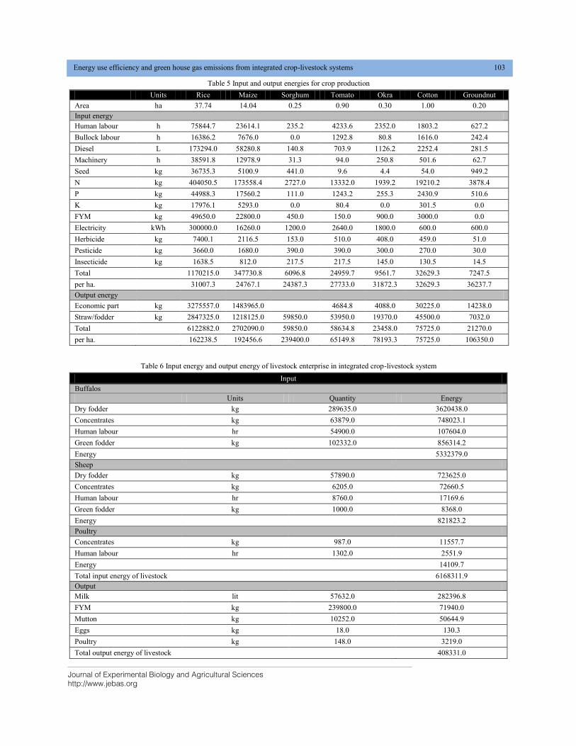
Journal of Experimental Biology and Agricultural Sciences
http://www.jebas.org
Energy use efficiency and green house gas emissions from integrated crop-livestock systems 103
Table 5 Input and output energies for crop production
Units Rice Maize Sorghum Tomato Okra Cotton Groundnut
Area ha 37.74 14.04 0.25 0.90 0.30 1.00 0.20
Input energy
Human labour h 75844.7 23614.1 235.2 4233.6 2352.0 1803.2 627.2
Bullock labour h 16386.2 7676.0 0.0 1292.8 80.8 1616.0 242.4
Diesel L 173294.0 58280.8 140.8 703.9 1126.2 2252.4 281.5
Machinery h 38591.8 12978.9 31.3 94.0 250.8 501.6 62.7
Seed kg 36735.3 5100.9 441.0 9.6 4.4 54.0 949.2
N kg 404050.5 173558.4 2727.0 13332.0 1939.2 19210.2 3878.4
P kg 44988.3 17560.2 111.0 1243.2 255.3 2430.9 510.6
K kg 17976.1 5293.0 0.0 80.4 0.0 301.5 0.0
FYM kg 49650.0 22800.0 450.0 150.0 900.0 3000.0 0.0
Electricity kWh 300000.0 16260.0 1200.0 2640.0 1800.0 600.0 600.0
Herbicide kg 7400.1 2116.5 153.0 510.0 408.0 459.0 51.0
Pesticide kg 3660.0 1680.0 390.0 390.0 300.0 270.0 30.0
Insecticide kg 1638.5 812.0 217.5 217.5 145.0 130.5 14.5
Total 1170215.0 347730.8 6096.8 24959.7 9561.7 32629.3 7247.5
per ha. 31007.3 24767.1 24387.3 27733.0 31872.3 32629.3 36237.7
Output energy
Economic part kg 3275557.0 1483965.0 4684.8 4088.0 30225.0 14238.0
Straw/fodder kg 2847325.0 1218125.0 59850.0 53950.0 19370.0 45500.0 7032.0
Total 6122882.0 2702090.0 59850.0 58634.8 23458.0 75725.0 21270.0
per ha. 162238.5 192456.6 239400.0 65149.8 78193.3 75725.0 106350.0
Table 6 Input energy and output energy of livestock enterprise in integrated crop-livestock system
Input
Buffalos
Units Quantity Energy
Dry fodder kg 289635.0 3620438.0
Concentrates kg 63879.0 748023.1
Human labour hr 54900.0 107604.0
Green fodder kg 102332.0 856314.2
Energy 5332379.0
Sheep
Dry fodder kg 57890.0 723625.0
Concentrates kg 6205.0 72660.5
Human labour hr 8760.0 17169.6
Green fodder kg 1000.0 8368.0
Energy 821823.2
Poultry
Concentrates kg 987.0 11557.7
Human labour hr 1302.0 2551.9
Energy 14109.7
Total input energy of livestock 6168311.9
Output
Milk lit 57632.0 282396.8
FYM kg 239800.0 71940.0
Mutton kg 10252.0 50644.9
Eggs kg 18.0 130.3
Poultry kg 148.0 3219.0
Total output energy of livestock 408331.0
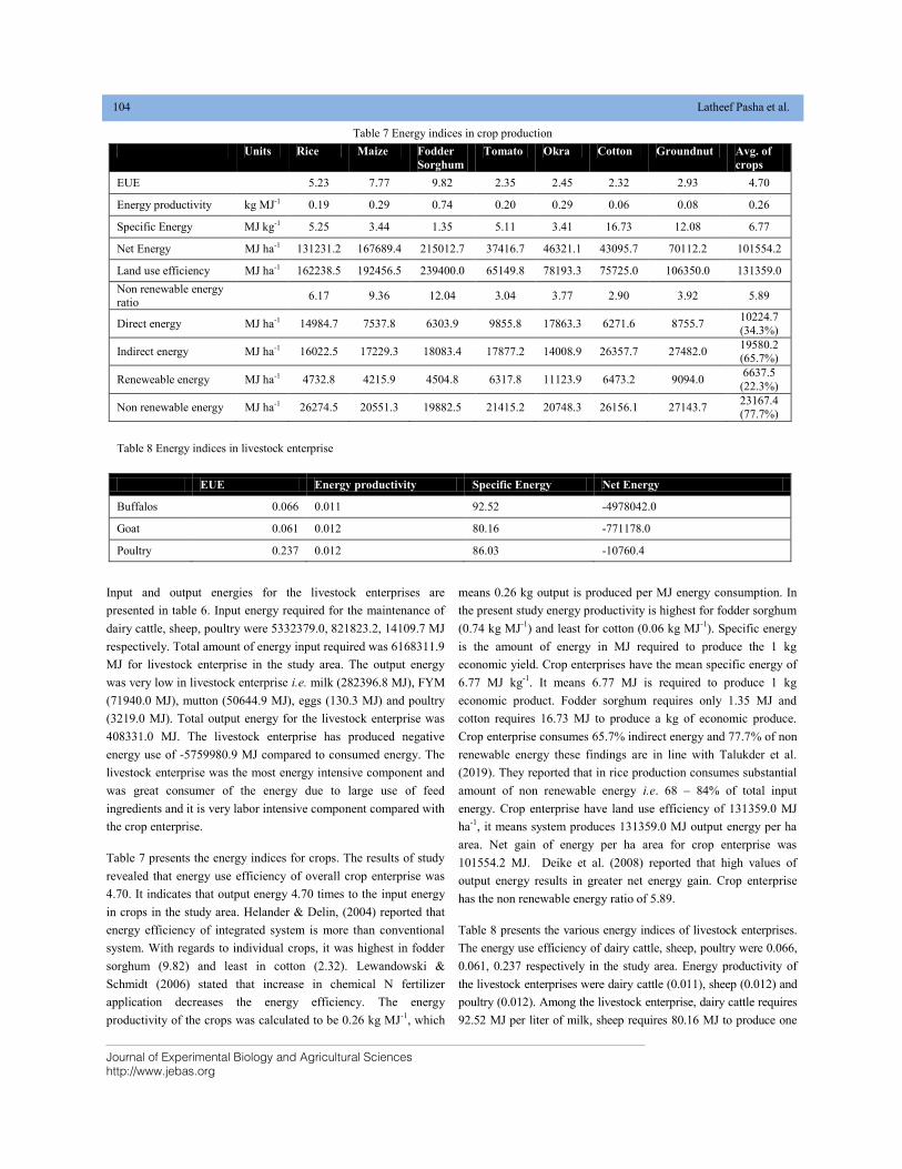
Journal of Experimental Biology and Agricultural Sciences
http://www.jebas.org
104 Latheef Pasha et al.
Input and output energies for the livestock enterprises are
presented in table 6. Input energy required for the maintenance of
dairy cattle, sheep, poultry were 5332379.0, 821823.2, 14109.7 MJ
respectively. Total amount of energy input required was 6168311.9
MJ for livestock enterprise in the study area. The output energy
was very low in livestock enterprise i.e. milk (282396.8 MJ), FYM
(71940.0 MJ), mutton (50644.9 MJ), eggs (130.3 MJ) and poultry
(3219.0 MJ). Total output energy for the livestock enterprise was
408331.0 MJ. The livestock enterprise has produced negative
energy use of -5759980.9 MJ compared to consumed energy. The
livestock enterprise was the most energy intensive component and
was great consumer of the energy due to large use of feed
ingredients and it is very labor intensive component compared with
the crop enterprise.
Table 7 presents the energy indices for crops. The results of study
revealed that energy use efficiency of overall crop enterprise was
4.70. It indicates that output energy 4.70 times to the input energy
in crops in the study area. Helander & Delin, (2004) reported that
energy efficiency of integrated system is more than conventional
system. With regards to individual crops, it was highest in fodder
sorghum (9.82) and least in cotton (2.32). Lewandowski &
Schmidt (2006) stated that increase in chemical N fertilizer
application decreases the energy efficiency. The energy
productivity of the crops was calculated to be 0.26 kg MJ-1
, which
means 0.26 kg output is produced per MJ energy consumption. In
the present study energy productivity is highest for fodder sorghum
(0.74 kg MJ-1
) and least for cotton (0.06 kg MJ-1
). Specific energy
is the amount of energy in MJ required to produce the 1 kg
economic yield. Crop enterprises have the mean specific energy of
6.77 MJ kg-1
. It means 6.77 MJ is required to produce 1 kg
economic product. Fodder sorghum requires only 1.35 MJ and
cotton requires 16.73 MJ to produce a kg of economic produce.
Crop enterprise consumes 65.7% indirect energy and 77.7% of non
renewable energy these findings are in line with Talukder et al.
(2019). They reported that in rice production consumes substantial
amount of non renewable energy i.e. 68 – 84% of total input
energy. Crop enterprise have land use efficiency of 131359.0 MJ
ha-1
, it means system produces 131359.0 MJ output energy per ha
area. Net gain of energy per ha area for crop enterprise was
101554.2 MJ. Deike et al. (2008) reported that high values of
output energy results in greater net energy gain. Crop enterprise
has the non renewable energy ratio of 5.89.
Table 8 presents the various energy indices of livestock enterprises.
The energy use efficiency of dairy cattle, sheep, poultry were 0.066,
0.061, 0.237 respectively in the study area. Energy productivity of
the livestock enterprises were dairy cattle (0.011), sheep (0.012) and
poultry (0.012). Among the livestock enterprise, dairy cattle requires
92.52 MJ per liter of milk, sheep requires 80.16 MJ to produce one
Table 7 Energy indices in crop production
Units Rice Maize Fodder
Sorghum
Tomato Okra Cotton Groundnut Avg. of
crops
EUE 5.23 7.77 9.82 2.35 2.45 2.32 2.93 4.70
Energy productivity kg MJ-1 0.19 0.29 0.74 0.20 0.29 0.06 0.08 0.26
Specific Energy MJ kg-1 5.25 3.44 1.35 5.11 3.41 16.73 12.08 6.77
Net Energy MJ ha-1 131231.2 167689.4 215012.7 37416.7 46321.1 43095.7 70112.2 101554.2
Land use efficiency MJ ha-1 162238.5 192456.5 239400.0 65149.8 78193.3 75725.0 106350.0 131359.0
Non renewable energy ratio
6.17 9.36 12.04 3.04 3.77 2.90 3.92 5.89
Direct energy MJ ha-1 14984.7 7537.8 6303.9 9855.8 17863.3 6271.6 8755.7 10224.7
(34.3%)
Indirect energy MJ ha-1 16022.5 17229.3 18083.4 17877.2 14008.9 26357.7 27482.0 19580.2 (65.7%)
Reneweable energy MJ ha-1 4732.8 4215.9 4504.8 6317.8 11123.9 6473.2 9094.0 6637.5
(22.3%)
Non renewable energy MJ ha-1 26274.5 20551.3 19882.5 21415.2 20748.3 26156.1 27143.7 23167.4 (77.7%)
Table 8 Energy indices in livestock enterprise
EUE Energy productivity Specific Energy Net Energy
Buffalos 0.066 0.011 92.52 -4978042.0
Goat 0.061 0.012 80.16 -771178.0
Poultry 0.237 0.012 86.03 -10760.4

Journal of Experimental Biology and Agricultural Sciences
http://www.jebas.org
Energy use efficiency and green house gas emissions from integrated crop-livestock systems 105
kg of mutton and poultry requires 86.03 MJ to produce one kg of
poultry meat. All the three enterprises in the livestock have a
negative energy gain. Pahlavan et al. (2011) stated that low energy
efficiency in system is due to higher input energy.
Table 5 and 6 presents the results accounts for the energy
performance of study area i.e. crop production and livestock
respectively. Table 6 shows clearly that livestock enterprises
consumes substantially higher energy and in return produces the
very little output energy, which can potentially cause a serious
impact on sustainability in long run. In this regard Moore (2010)
stated that, increase the energy productivity of the system to attain
the sustainability of production. It was quiet opposite in case of the
crop enterprise, it consumes little energy and produces much
higher output energy. As the farmers of the study area practices
integrated livestock and crops, the total input energy for the study
area (all 36 farmers) was 7766752.9 MJ and output energy was
9472240.8 MJ. When the total system is considered, it is
environmentally sustainable in long run, as system as positive
energy of 1705487.9 MJ. This is made possible by the energy use
saving in the crop enterprise; totally offset the livestock negative
energy use. Livestock enterprise is a good revenue generation
sector to farmers, it is recommended to go for integrated livestock-
crops for the energy sustainability. Malcolm et al. (2015), also
reported integration helps in lowering the energy use. According to
Moraine et al. (2017) integration of crop-livestock farming systems
promises a greater sustainability.
3.2 Greenhouse gas emissions
The data collected from the surveyed area, covering 36 farmers,
where integrated livestock-crops were followed and converted into
kg CO2eq by using the emission coefficients for crops and live
stocks. GHG emissions regarding the crop production was
presented in table 9. GHG emissions were highest in rice crop
(116969.6 kg CO2eq) it occupies an area of 37.74 ha of land, with
mean of 3099.4 kg CO2eq ha-1
. Mohammadi et al. (2014) also
reported that compared to all crops under study rice has produced
highest GHG emissions. Maize occupies an area of 14.04 ha and
had potential to emit GHG of 17929.9 kg CO2eq with an average of
1277.1 kg CO2eq ha-1
, followed by cotton (1916.8 kg CO2eq), okra
(643.8 kg CO2eq), tomato (643.6 kg CO2eq), fodder sorghum (382.5
kg CO2eq) and groundnut (151.0 kg CO2eq). Total GHG emissions
from the crops were 138637.3 kg CO2eq in total of 54.43 ha. If we
consider GHG emissions for specific area of ha it ranges between
715.4 kg CO2eq ha-1
(tomato) to 3099.4 kg CO2eq ha-1
(rice). Similar
study was conducted by Tongwane et al. (2016) noticed that
tomato crop management has produced 1650 kg CO2eq ha-1
. Bos et
al. (2014) reported that GHG emission in crop production ranged
from 45 kg CO2eq Mg-1
(sugar beet) to 520 kg CO2eq Mg-1
(pea).
Figure 1 presents the contribution of different parameters to GHG
emissions for 1 ha crop production and figure was quite helpful to
Table 9 Amount of GHG emissions from crop and livestock enterprises
GHG (kg CO2eq) in surveyed area GHG (kg CO2eq)/ha
Crops
Rice 116969.6 3099.4
Maize 17929.9 1277.1
Fodder sorghum 382.5 1529.9
Tomato 643.6 715.1
Okra 643.8 2145.9
Cotton 1916.8 1916.8
Groundnut 151.1 755.4
Crops total 138637.3
Livestock
Milk 195948.8
FYM 30214.8
Mutton 166362.0
Eggs 75.6
Poultry 976.8
Livestock total 393578.0
Overall total 532215.3
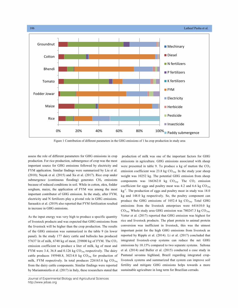
Journal of Experimental Biology and Agricultural Sciences
http://www.jebas.org
106 Latheef Pasha et al.
assess the role of different parameters for GHG emissions in crop
production. For rice production, submergence of crop was the most
important source for GHG emissions followed by electricity and
FYM application. Similar findings were summarized by Liu et al.
(2010); Nayak et al. (2015) and Xu et al. (2017). Rice crop under
submergence (continuous flooding) generates CH4 emissions
because of reduced conditions in soil. While in cotton, okra, fodder
sorghum, maize, the application of FYM was among the most
important contributor of GHG emission. In the study, after FYM,
electricity and N fertilizers play a pivotal role in GHG emissions.
Sarauskis et al. (2019) also reported that FYM fertilization resulted
in increase in GHG emissions.
As the input energy was very high to produce a specific quantity
of livestock products and was expected that GHG emissions from
the livestock will be higher than the crop production. The results
of the GHG emission was summarized in the table 9 (in lower
panal). In the study 177 dairy cattle and bullocks has produced
57637 lit of milk, 6740 kg of meat, 239800 kg of FYM. The CO2
emission coefficient to produce a liter of milk, kg of meat and
FYM were 3.4, 36.8 and 0.126 kg CO2eq respectively. The dairy
cattle produces 195948.8, 30214.8 kg CO2eq for production of
milk, FYM respectively. In total produces 226163.6 kg CO2eq
from the dairy cattle components. Similar findings were reported
by Mariantonietla et al. (2017) in Italy, these researchers stated that
production of milk was one of the important factors for GHG
emissions in agriculture. GHG emissions associated with sheep
were presented in table 9. To produce a kg of mutton the CO2
emission coefficient was 23.8 kg CO2eq. In the study year sheep
weight was 10252 kg. The potential GHG emission from sheep
components was 166362.0 kg CO2eq. The CO2 emission
coefficient for eggs and poultry meat was 4.2 and 6.6 kg CO2eq
kg-1
. The production of eggs and poultry meat in study was 18.0
kg and 148.0 kg respectively. So, the poultry component can
produce the GHG emissions of 1052.4 kg CO2eq. Total GHG
emissions from the livestock enterprises were 641610.0 kg
CO2eq. Whole study area GHG emission was 780247.3 kg CO2eq.
Vetter et al. (2017) reported that GHG emission was highest for
rice and livestock products. The plant protein to animal protein
conversion was inefficient in livestock, this was the utmost
important point for the high GHG emissions from livestock as
reported by Ripple et al. (2014). Li et al. (2017) concluded that
integrated livestock-crop systems can reduce the net GHG
emissions by 10.15% compared to two separate systems. Saltona
et al. (2014) and Buller et al. (2015) conducted a case study in
Pantanal savanna highland, Brazil regarding integrated crop-
livestock systems and summarized that system can improve soil
fertility and mitigate GHG emissions helps towards a more
sustainable agriculture in long term for Brazilian cerrado.
Figure 1 Contribution of different parameters in the GHG emissions of 1 ha crop production in study area
0% 20% 40% 60% 80% 100%
Rice
Maize
Fodder Jowar
Tomato
Bhendi
Cotton
GroundnutMechinary
Diesel
N fertilizers
P fertilizers
K fertilizers
FYM
Electricity
Herbicide
Pesticide
Insecticide
Paddy submergence
Journal of Experimental Biology and Agricultural Sciences
http://www.jebas.org
Energy use efficiency and green house gas emissions from integrated crop-livestock systems 107
Conclusion
The principal aim of the current study was to assess the energy use
and GHG emissions from integrated crop-livestock systems in
semi arid Deccan plateau of Southern India and their sustainability
in long run. Policy makers are very keen at popularizing the
integrated crop-livestock system, assessing energy dynamics and
environmental impact of the system helps in its sustainability in
future. The information regarding inputs and outputs were
collected from 36 farmers, integrated crop-livestock was evaluated
in terms of energy use and GHG emissions. Among enterprises,
crop enterprise in the system was highly efficient in energy while
livestock enterprise was very highly inefficient. The results
indicate that crop enterprise consumed 1598441.0 MJ of energy
and generated 9063909.8 MJ. Crop enterprise has a positive
energy balance of 7465468.8 MJ. Energy use efficiency of 4.7
and it consumed indirect (65.7%), non renewable energy
(77.7%) greater than direct (34.3%) and renewable energy
(22.3%). Regards to livestock enterprise, it consumed
6168311.9 MJ of energy and produced 408331.0 MJ. This
enterprise has a negative energy balance of -5759980.9 MJ.
Overall, the net energy balance of integrated crop-livestock
system was 1705487.9. It implies, negative energy balance in
livestock enterprise is neutralized by positive energy balance of
the crop enterprises. On a whole integrated crop-livestock
system can sustain in long run due to positive energy balance
the system. Livestock enterprise alone sustainability is big
issue in future.
Comparison between energy input and emitted CO2 in the study
area showed that there was a direct relationship between energy
input and CO2 emissions. In GHG emission analysis in crop
enterprise emissions ranged between 3099.4 kg CO2eq ha-1
(rice) to 715.4 kg CO2eq ha-1
(tomato). Among the crops rice
has emitted greater kg CO2eq ha-1
per specific area and 50% of
emissions were caused by submergence of rice crop. Total
GHG emissions form crop enterprise was 138637.3 kg CO2eq.
Livestock enterprise production system emitted 641610.0 kg
CO2eq, it was much higher compared to crop enterprises in
study area. To whole system has produced 780247.3 kg CO2eq.
Livestock production represents the one of the prime source of
income for small and marginal farmers and was the protein
supplement in this part of India. This study clearly insight that
integrating livestock with crop production is best possible option to
increase the energy use and to reduce GHG emissions that helps in
environmental sustainability. Hope, all the farmers will convert to
integrated crop-livestock and policy makers should encourage the
system, so that farming will be sustained both in energy use and
environmental impact.
Conflict of interest
Not have any conflict of interest with any one of co authors and
others.
References
Akcaoz H, Ozcatalbas O, Kizilay H (2009) Analysis of energy use
for pomegranate production in Turkey. Journal of Food,
Agriculture and Environment 7: 475-80.
Barber A (2004) Seven Case Study Farms: Total Energy & Carbon
Indicators for New Zealand Arable & Outdoor Vegetable
Production. AgriLINK New Zealand Ltd, Pukekohe. Available on
http://www.agrilink.co.nz/Files/Arable_Vegetable_Energy_Use_M
ain_Report.pdf access on 21 October, 2019.
Bos JFFP, Haan JD, Sukkel W, Schils RLM (2014) Energy use and
greenhouse gas emissions in organic and conventional farming
systems in the Netherlands. NJAS-Wageningen Journal of Life
Sciences 68: 61-70. DOI:
http://dx.doi.org/10.1016/j.njas.2013.12.003.
Buller LS, Bergier I, Ortega E, Moraes A, Bayma-Silva G, Zanetti
MR (2015) Soil improvement and mitigation of greenhouse gas
emissions for integrated crop–livestock systems: Case study
assessment in the Pantanal savanna highland, Brazil. Agricultural
Systems 137: 206-219. DOI:
http://dx.doi.org/10.1016/j.agsy.2014.11.004.
Cao MH, Adeola O (2015) Energy value of poultry by product
meal and animal-vegetable oil blend for broiler chickens by the
regression method. Poultry Science 95: 268–275. DOI:
http://dx.doi.org/10.3382/ps/pev317.
Chandrakar SK, Soni DL, Yadav DK, Sahu LK (2013)
Experimental study on animal powered mechanical device for
home lighting system. International Journal of Environmental
Engineering and Management 4: 471-482.
Chaudhary VP, Gangwar B, Pandey DK, Gangwar KS (2009)
Energy auditing of diversified rice- wheat cropping systems in
Indo-gangetic plains. Energy 34: 1091-1096. DOI:
https://doi.org/10.1016/j.energy.2009.04.017.
Deike S, Pallutt B, Christen O (2008) Investigations on the energy
efficiency of organic and integrated farming with specific
emphasis on pesticide use intensity. European Journal of
Agronomy 28: 461-470. doi:10.1016/j.eja.2007.11.009
Devasenapathy P, Senthilkumar G, Shanmugam PM (2009)
Energy management in crop production. Indian Journal of
Agronomy 54: 80-89.
Journal of Experimental Biology and Agricultural Sciences
http://www.jebas.org
108 Latheef Pasha et al.
Gerber PJ, Steinfeld H, Henderson B, Mottet A, Opio C, Dijkman
J, Falcucci A, Tempio G (2013) Tackling climate change through
livestock-A global assessment of emissions and mitigation
opportunities. Food and Agriculture Organization of the United
Nations (FAO), Rome.
Ghahramani A, Bowran D (2018) Transformative and systemic
climate change adaptations in mixed crop livestock farming
systems. Agricultural Systems 164: 236–251. DOI:
https://doi.org/10.1016/j.agsy.2018.04.011.
Gopalan C, Sastri BVR, Balasubramanian SC (2012) Nutritive
value of Indian foods. National institute of nutrition, ICMR,
Hyderabad.
Helander CA, Delin K (2004) Evaluation of farming systems
according to valuation indices developed within a European
network on integrated and ecological arable farming systems.
European Journal of Agronomy 21: 53-67. doi:10.1016/S1161-
0301(03)00089-3.
Hoffman E, Cavigelli MA, Camargo G, Ryan M, Ackroyd VJ,
Richard TL, Mirsky S (2018) Energy use and greenhouse gas
emissions in organic and conventional grain crop production:
Accounting for nutrient inflows. Agricultural systems 162: 89-96.
https://doi.org/10.1016/j.agsy.2018.01.021.
ICAR (2015) VISION 2020—Indian Council of Agricultural
Research. ICAR, New Delhi, India.
INCCA (2010) India : Greenhouse Gas Emissions 2007. Indian
Network for Climate Change Assessment, Ministry of
Environment and Forests, Government of India.
IPCC (2006) Guidelines for national greenhouse gas inventories.
In: Eggleston HS, Buendia L, Miwa K, Ngara T, Tanabe K (Eds),
Prepared by the national greenhouse gas inventories programme.
2006. Japan: IGES available on
http://www.ipccnggip.iges.or.jp/public/2006gl/index.htm access on
20 October,2019.
Intergovernmental Panel on Climate Change - IPCC (2007)
Climate Change 2007: Impacts, Adaptation and Vulnerability.
Summary for policy makers. Available on
http://www.ipcc.cg/SPM13apr07.pdf access on 20 October,2019.
Komleh SHP, Omid M, Heidari MD (2013) On the study of energy
use and GHG (greenhouse gas) emissions in greenhouse cucumber
production in Yazd province. Energy 59: 63-71. DOI:
https://doi.org/10.1016/j.energy.2013.07.037.
Koopmans A, Koppejan J (1997) Agricultural and forest residues-
generation, utilization and availability. In: Regional consultation
on modern applications of biomassenergy 1997 held at,
Kualampur, Malaysia: FAO on 6–10January1997.
Krishnamoorthy U, Solled H, Steingass H, Menke KH (1995)
Energy and protein evaluation of tropical feed stuffs for whole
tract and ruminal digestion by chemical analyses and rumen
inoculum studies in vitro. Animal Feed Science and Technology
52: 177-188.
Lal R (2004) Carbon emission from farm operations. Environment
International 30: 981-990. DOI:
https://doi.org/10.1016/j.envint.2004.03.005.
Larson DL, Fangmeir DD (1978) Energy in irrigated crop
production. Transactions of the American Society of Agricultural
Engineers 21:1075-1080.
Lewandowski I, Schmidt U (2006) Nitrogen, energy and land use
efficiency of miscanthus, reed canary grass and triticale as
determined by the boundary line approach. Agriculture, Ecosystem
& Environment 112: 335-346.
Li Z, Sui P, Wang X, Yang X, Long P, Cui J, Yan L, Chen Y
(2017) Comparison of net GHG emissions between separated
system and crop-swine integrated system in the North China Plain.
Journal of Cleaner Production 149: 653-664. DOI:
http://dx.doi.org/10.1016/j.jclepro.2017.02.113.
Liu S, Qin Y, Zou J, Liu Q (2010) Effects of water regime during
rice-growing season on annual direct N2O emission in a paddy
rice-winter wheat rotation system in southeast China. Science of
the Total Environment 408: 906-913.
Malcolm GM, Camargo GGT, Ishler VA, Richard TL, Karsten HD
(2015) Energy and greenhouse gas analysis of northeast US dairy
cropping systems. Agricultural, Ecosystem & Environment 199:
407-417.
Mariantonietta F, Alessia S, Francesco C, Giustina P (2017) GHG
and Cattle Farming: Co-Assessing the Emissions and Economic
Performances in Italy. Journal of Cleaner Production 172: 3704-
3712. doi: 10.1016/j.jclepro.2017.07.167.
Mobtaker HG, Akram A, Keyhani A, Mohammadi A (2012)
Optimization of energy required for alfalfa production using data
envelopment analysis approach. Energy Sustainable Development
16: 242-248. DOI: https://doi.org/10.1016/j.esd.2012.02.001.
Moghimi MR, Pooya M, Mohammadi A (2014) Study on energy
balance, energy forms and greenhouse gas emission for wheat
production in Gorve city, Kordestan province of Iran. European
Journal of Experimental Biology 4: 234-239.
Journal of Experimental Biology and Agricultural Sciences
http://www.jebas.org
Energy use efficiency and green house gas emissions from integrated crop-livestock systems 109
Mohammadi A, Rafiee S, Jafari A, Keyhani A, Avval SHM,
Nonhebel S (2014) Energy use efficiency and greenhouse gas
emissions of farming systems in North Iran. Renewable and
Sustainable Energy Reviews 30: 724-733.
Mohammadi A, Rafiee S, Mohtasebi SS, Rafiee H (2010) Energy
inputs-yield relationship and cost analysis of kiwifruit production
in Iran. Renewable Energy 35: 1071-1075.
Mondal AH (2010) Implications of renewable energy technologies
in the Bangladesh power sector: long-term planning strategies.
ZEF. Ph D Thesis. ISBN: 978-3-940124-25-8
Moore SR (2010) Energy efficiency in small-scale bio intensive
organic onion production in Pennsylvania, USA. Renewable
Agriculture and Food System 25: 181-188.
Moraine M, Melaca P, Ryschawya J, Durua M, Theronda O (2017)
A participatory method for the design and integrated assessment of
crop-livestock systems in farmer’s groups. Ecological Indicators
72: 340–351.
Nayak D, Saetnan E, Cheng K, Wang W, Koslowski F, Cheng Y,
Zhu WY, Wang J, Liu J, Moran D, Yan X, Cardenas L, Newbold J,
Pan G, Lu Y, Smith P (2015) Management opportunities to
mitigate greenhouse gas emissions from Chinese agriculture.
Agricultural Ecosystems and Environment 209: 108-124.
Nguyen TLT, Hermansen JE (2012) System expansion for
handling co-products in LCA of sugarcane bio-energy systems:
GHG consequences of using molasses for ethanol production.
Applied Energy 89: 254-261.
Ozkan B, Akcaoz H, Fert C (2004) Energy input-output analysis in
Turkish agriculture. Renewable Energy 29: 39-51.
Ozturk HH, Bascetincelik A (2006) Energy exploitation of
agricultural biomass potential in Turkey. Energy Exploration &
Explotation 24: 313-330.
Pahlavan R, Omid M, Akram A (2011) Energy use efficiency in
greenhouse tomato production in Iran. Energy 36: 6714-6719.
DOI: https://doi.org/10.1016/j.energy.2011. 10.038.
Paramesh V, Arunachalam V, Nikkhah A, Das B, Ghnimi S (2018)
Optimization of energy consumption and environmental impacts of
arecanut production through coupled data envelopment analysis
and life cycle assessment. Journal of Cleaner Production 203: 1-11.
DOI: https://doi.org/10.1016/j.jclepro.2018.08.263.
Petal A (2012) Nutritive value of commonly available feeds and
fodders in India. Animal nutrition group, National Dairy
Development Board, Anand.
Rafiee S, Avval SHM, Mohammadi A (2010) Modelling and
sensitivity analysis of energy inputs for apple production in Iran.
Energy 35: 3301-3306. DOI:
https://doi.org/10.1016/j.energy.2010.04.015.
Rahman S, Barmon BK (2012) Energy productivity and efficiency
of the ‘gher’ (prawn-fish-rice) farming system in Bangladesh.
Energy 43: 293-300. DOI:
https://doi:10.1016/j.energy.2012.04.027.
Ripple WJ, Smith P, Haberl H, Montzka SA, McAlpine C,
Boucher DH (2014) Ruminants, climate change and climate policy.
Nature Climate Change 4: 2-5.
Rosegrant MW, Cai X, Cline SA (2002) Global water outlook to
2025: Averting and impending crisis. International Water
Management Institute (IWMI), 2020 Vision for Food, Agriculture,
and the Environment, International Food Policy Research Institute
(IFPRI). Washington, D.C, Colombo, Sri Lanka.
Saltona JC, Mercantea FM, Tomazi M, Zanatta JA, Concenc G,
Silva WM, Retorea M (2014) Integrated crop-livestock system in
tropical Brazil: Toward a sustainable production system.
Agriculture, Ecosystems and Environment 190: 70-79. DOI:
http://dx.doi.org/10.1016/j.agee.2013.09.023.
Sarauskis E, Masilionyte L, Juknevicius D, Buragiene S,
Kriauciuniene Z (2019) Energy use efficiency, GHG emissions and
cost-effectiveness of organic and sustainable fertilization. Energy
172: 1151-1160.
Sartori L, Basso B, Bertocco M, Oliviero G (2005). Energy Use
and Economic Evaluation of a Three Year Crop Rotation for
Conservation and Organic Farming in NE Italy. Biosystems
Engineering 91: 245–256.
Sefeedpari P, Rafiee S, Komleh SHP, Ghahderijani M (2012) A
source-wise andoperation-wise energy use analysis for corn silage
production, a case study of Tehranprovince, Iran. International
Journal of Sustainable Built Environment 1: 158-166.
Soni P, Taewichit C, Salokhe VM (2013) Energy consumption and
CO2 emissions in rainfed agricultural production systems of
Northeast Thailand. Agricultural systems 116: 25-36.
Steinfeld H, Gerber P, Wassenaar T, Castel V, Rosales M, Haan
CD (2006) Livestock’s Long Shadow: Environmental Issues and
Options. Food and Agriculture Organization of the United Nations
(FAO).
Tabar BI, Keyhani A, Rafiee S (2010) Energy balance in Iran’s
agronomy (1990-2006). Renewable Sustainable Energy Reviews
14: 849-855.
Journal of Experimental Biology and Agricultural Sciences
http://www.jebas.org
110 Latheef Pasha et al.
Talukdera B, Vanloonb GW, Hipel KW (2019) Energy efficiency
of agricultural systems in the southwest coastal zone of
Bangladesh. Ecological Indicators 98: 641-648. DOI:
https://doi.org/10.1016/j.ecolind.2018.11.030.
Tongwane M, Mdlambuzi T, Moeletsi M, Tsubo M, Mliswa V,
Grootboom L (2016) Greenhouse gas emissions from different
crop production and management practices in South Africa.
Environmental Development 19: 23-35. DOI:
http://dx.doi.org/10.1016/j.envdev.2016.06.004.
Tsatsarellis CA (1991) Energy requirements for cotton production
in Central Greece. Journal of Agricultural Engineering Research.
50: 239-246.
Vanloon GW, Patil SG, Hugar LB (2005) Agricultural
Sustainability: Strategies for Assessment. SAGE.
Vetter SH, Sapkota TB, Hillier J, Stirling CM, Macdiarmid JI,
Aleksandrowicz ., Green R, Joy EJM, Dangour AD, Smith P
(2017) Greenhouse gas emissions from agricultural food
production to supply Indian diets: Implications for climate change
mitigation. Agriculture, ecosystems and environment. 237: 234-
241. DOI: http://dx.doi.org/10.1016/j.agee.2016.12.024.
Xu G, Liu X, Wang Q, Yu X, Hang Y (2017) Integrated rice-duck
farming mitigates the global warming potential in rice season.
Science of the Total Environment 575: 58-66. DOI:
http://dx.doi.org/10.1016/j.scitotenv.2016.09.233.
Journal of Experimental Biology and Agricultural Sciences
http://www.jebas.org
ISSN No. 2320 – 8694
Journal of Experimental Biology and Agricultural Sciences, April - 2020; Volume – 8(2) page 111 – 114
CHARACTER ASSOCIATION AND PATH ANALYSIS FOR SEED VIGOR TRAITS
IN SESAME (Sesamum indicum L.)
Manjeet, Mahavir, Anu, Vivek K. Singh*, P.K. Verma
Department of Genetics and Plant Breeding, CCS Haryana Agricultural University, Hisar, Haryana (India)-125 004
Received – February 05, 2020; Revision – March 06, 2020; Accepted – March 28, 2020 Available Online – April 25, 2020
DOI: http://dx.doi.org/10.18006/2020.8(2).111.114
ABSTRACT
The present investigation was conducted using 24 genotypes of sesame for correlation and path analysis
among seven seed quality characters which revealed that standard germination showed a significant and
positive correlation with shoot length, root length, seedling length, seed vigor index-I and seed vigor
index-II, which indicated that by increasing these attributes, standard germination will be increased, thus
these parameters are suggestive of good plant stand and ultimately seed yield. Path coefficient analysis
suggested that seed vigor index-I, shoot length and seedling length are major components of standard
germination which could increase the seed yield.
* Corresponding author
KEYWORDS
Sesame
Genotype
Correlation
Path analysis
E-mail: [email protected] (Vivek K. Singh)
Peer review under responsibility of Journal of Experimental Biology and
Agricultural Sciences.
All the articles published by Journal of Experimental
Biology and Agricultural Sciences are licensed under a
Creative Commons Attribution-NonCommercial 4.0
International License Based on a work at www.jebas.org.
Production and Hosting by Horizon Publisher India [HPI]
(http://www.horizonpublisherindia.in/).
All rights reserved.
Journal of Experimental Biology and Agricultural Sciences
http://www.jebas.org
Character Association and Path Analysis for Seed Vigor Traits in Sesame (Sesamum indicum L.) 112
1 Introduction
Crop yields and quality would be greatly affected without a steady
supply of high-quality seed (Douglas, 2019). Seed is a basic input in
agriculture and quality seed plays an important role in the sustainable
agronomic and horticultural crops production (Shubha et al., 2017).
Seed quality describes the potential performance of a seed lot.
Trueness to variety is depended on the various important aspects of
seed quality among these some common are, the presence of inert
matter, other crops seeds, noxious weed seed, freedom from disease
and insect infestations (Bishaw et al., 2007). High-quality seed lots
should meet minimum standards for each of these characteristics.
Achieving and maintaining high seed quality is the prerequisite for
any seed certification programs (Gebeyehu et al., 2019). Germination
potential and vigor are at their highest potential when the seed
reaches physiological maturity. Due to high seed moisture, most
crops are not ready to be harvested at that time (Rao et al., 2017).
Seed vigor is the potential of seeds for rapid and uniform emergence
and development of normal seedlings under various environmental
conditions (Marcos Filho, 2015). Although vigor testing is not
required for labeling of seed, many seed producers use vigor tests as
a quality control to ensure that the seed produced is of high quality.
Seed vigor is influenced by many factors, such as maturity level at
harvest, age of the seed, mechanical injuries, disease infection,
storage environment and genetic constitutions of the seeds (Khare &
Bhale, 2016). Correlation coefficient analysis is very important in
plant breeding experiment because it computes the degree of genetic
and non-genetic association between two or more traits and to help in
concurrent selection when more than one trait is desired (Laidig et
al., 2017). Although, correlation coefficient analysis among the
different traits does not considers the cause and effect relationships
between dependent and independent characters. Path analysis
provides a measure of relative significance of each independent
variable to prediction of changes in the dependent one. A path
coefficient is a standardized partial regression coefficient which
measures the direct effect of one trait upon other and allows the
partition of correlation coefficient into direct and indirect effects
(Yakubu, 2010; Mecha et al., 2017). Path coefficients show direct
influence of independent variable upon dependent variable (Jiang et
al., 2017). In plant breeding programme, path coefficient analysis has
been used by geneticist and crop breeders to aid in identifying traits
that are useful as selection criteria to improve seed germination and
seed vigor traits (Sunday et al., 2007; Rahman et al., 2012).
Therefore, the present study was planned to study the association
between different seed quality traits which influences the seed vigor
and germination per cent.
2 Materials and methods
The experimental material comprised of 24 diverse genotypes of
sesame procured from Oilseeds Section, Department of Genetics
and Plant Breeding, CCS Haryana Agricultural University, Hisar.
Seed quality parameters viz., standard germination (%), shoot
length (cm), root length (cm), seedling length (cm), seedling dry
weight (mg), seed vigor index-I & seed vigor index-II were
estimated and recorded in the seed quality testing laboratory of the
Department of Seed Science and Technology from the harvested
seeds of selected plants. For the estimation of standard germination
(%), 3 replications with 100 seeds per replication for each
genotype were placed on sufficiently moistened rolled germination
papers in petri dishes (top of the paper method of standard
germination testing) at 25°C temperature with 90-95% relative
humidity in the seed germinator. Final count for germination was
recorded on 6th
day (as per International Seed Testing Association,
2009). At the time of final seedling evaluation, seeds were
classified as normal seedling, abnormal seedling, fresh un-
germinated seeds and dead seed. Normal seedlings including fresh
un-germinated seeds were expressed as per cent germination.
Shoot length (cm) and root length (cm) were estimated using 30
seedlings selected randomly from the normal seedlings in each
replication for all genotypes at the time of final count of standard
germination and average shoot and root length for each genotype
were measured. Seedling length (cm) was calculated using the
same seedlings which used for calculating shoot and root lengths
for all the genotypes and average seedling length was measured as
Seedling length = Root length + Shoot length. Seedling dry weight
(mg) was measured using the same 30 normal seedlings that were
taken for measuring the root and shoot length and these seedlings
were kept further in hot air oven at 80°C for 24 hours and average
dry weight per seedling was recorded in milligram. From the
observations of standard germination test, the seed vigor index-I
and seed vigor index-II were calculated according to the method
suggested by Abdul-Baki & Anderson (1973) using the following
formulae viz., Seed vigor index-I = Standard Germination (%) X
Seedling length (cm) and Seed vigor index-II = Standard
Germination (%) X Seedling dry weight (mg). The correlation
coefficients among all possible character combinations at
phenotypic ‘r (p)’ and genotypic ‘r (g)’ level were estimated by
employing the formulae given by Al- Jibouri et al. (1958). The
path coefficient analysis was performed as per the formula given
by Wright (1921) and adopted by Dewey & Lu (1959).
3 Results and Discussion
Genotypic correlation coefficients have higher magnitude than
their corresponding phenotypic correlation coefficients, which
revealing a good amount of strong inherent association between
different attributes. Similar findings were also reported by Garg et
al. (2017) in green gram. Standard germination (%) showed
significantly positive correlation at both genotypic and phenotypic
level with shoot length (cm), root length (cm), seedling length
(cm), seed vigor index-I and seed vigor index-II. These parameters
were indicative of good plant stand in the field and ultimately seed
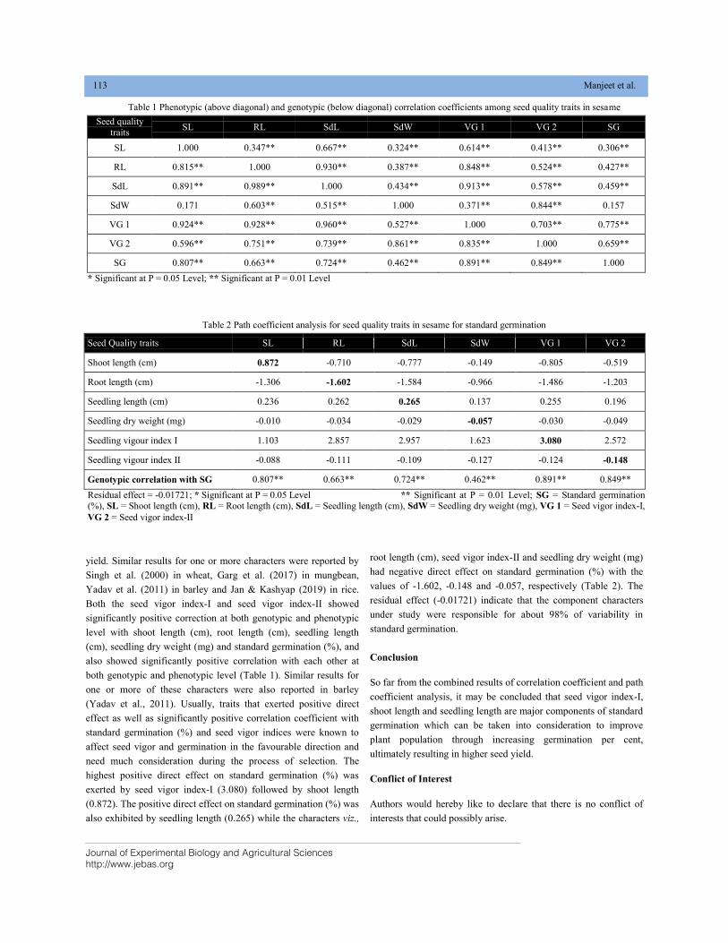
Journal of Experimental Biology and Agricultural Sciences
http://www.jebas.org
113 Manjeet et al.
yield. Similar results for one or more characters were reported by
Singh et al. (2000) in wheat, Garg et al. (2017) in mungbean,
Yadav et al. (2011) in barley and Jan & Kashyap (2019) in rice.
Both the seed vigor index-I and seed vigor index-II showed
significantly positive correction at both genotypic and phenotypic
level with shoot length (cm), root length (cm), seedling length
(cm), seedling dry weight (mg) and standard germination (%), and
also showed significantly positive correlation with each other at
both genotypic and phenotypic level (Table 1). Similar results for
one or more of these characters were also reported in barley
(Yadav et al., 2011). Usually, traits that exerted positive direct
effect as well as significantly positive correlation coefficient with
standard germination (%) and seed vigor indices were known to
affect seed vigor and germination in the favourable direction and
need much consideration during the process of selection. The
highest positive direct effect on standard germination (%) was
exerted by seed vigor index-I (3.080) followed by shoot length
(0.872). The positive direct effect on standard germination (%) was
also exhibited by seedling length (0.265) while the characters viz.,
root length (cm), seed vigor index-II and seedling dry weight (mg)
had negative direct effect on standard germination (%) with the
values of -1.602, -0.148 and -0.057, respectively (Table 2). The
residual effect (-0.01721) indicate that the component characters
under study were responsible for about 98% of variability in
standard germination.
Conclusion
So far from the combined results of correlation coefficient and path
coefficient analysis, it may be concluded that seed vigor index-I,
shoot length and seedling length are major components of standard
germination which can be taken into consideration to improve
plant population through increasing germination per cent,
ultimately resulting in higher seed yield.
Conflict of Interest
Authors would hereby like to declare that there is no conflict of
interests that could possibly arise.
Table 1 Phenotypic (above diagonal) and genotypic (below diagonal) correlation coefficients among seed quality traits in sesame
Seed quality
traits SL RL SdL SdW VG 1 VG 2 SG
SL 1.000 0.347** 0.667** 0.324** 0.614** 0.413** 0.306**
RL 0.815** 1.000 0.930** 0.387** 0.848** 0.524** 0.427**
SdL 0.891** 0.989** 1.000 0.434** 0.913** 0.578** 0.459**
SdW 0.171 0.603** 0.515** 1.000 0.371** 0.844** 0.157
VG 1 0.924** 0.928** 0.960** 0.527** 1.000 0.703** 0.775**
VG 2 0.596** 0.751** 0.739** 0.861** 0.835** 1.000 0.659**
SG 0.807** 0.663** 0.724** 0.462** 0.891** 0.849** 1.000
* Significant at P = 0.05 Level; ** Significant at P = 0.01 Level
Table 2 Path coefficient analysis for seed quality traits in sesame for standard germination
Seed Quality traits SL RL SdL SdW VG 1 VG 2
Shoot length (cm) 0.872 -0.710 -0.777 -0.149 -0.805 -0.519
Root length (cm) -1.306 -1.602 -1.584 -0.966 -1.486 -1.203
Seedling length (cm) 0.236 0.262 0.265 0.137 0.255 0.196
Seedling dry weight (mg) -0.010 -0.034 -0.029 -0.057 -0.030 -0.049
Seedling vigour index I 1.103 2.857 2.957 1.623 3.080 2.572
Seedling vigour index II -0.088 -0.111 -0.109 -0.127 -0.124 -0.148
Genotypic correlation with SG 0.807** 0.663** 0.724** 0.462** 0.891** 0.849**
Residual effect = -0.01721; * Significant at P = 0.05 Level ** Significant at P = 0.01 Level; SG = Standard germination
(%), SL = Shoot length (cm), RL = Root length (cm), SdL = Seedling length (cm), SdW = Seedling dry weight (mg), VG 1 = Seed vigor index-I,
VG 2 = Seed vigor index-II
Journal of Experimental Biology and Agricultural Sciences
http://www.jebas.org
Character Association and Path Analysis for Seed Vigor Traits in Sesame (Sesamum indicum L.) 114
References
Abdul-Baki AA, Anderson JD (1973) Vigor determination in
soybean seed by multiple criteria 1. Crop Science 13: 630-633.
Al-Jibouri HA, Miller PA, Robinson HF (1958) Genetic and
environmental variances and co-variances in an upland cotton
cross of interspecific origin. Agronomy Journal 50: 633-636.
Bishaw Z, Niane AA, Gan Y (2007) Quality seed production.
In: Springer, Dordrecht, Lentil, Pp. 349-383.
Dewey DI, Lu KH (1959) A correlation and path-coefficient
analysis of components of crested wheatgrass seed production.
Agronomy Journal 51: 515-518.
Douglas JE (2019) Successful seed programs: A planning and
management guide. CRC Press.
Garg GK, Verma PK, Kesh H, Kumar A (2017) Genetic
variability, character association and genetic divergence for seed
quality traits in mungbean [Vigna radiata (L.) Wilczek]. Indian
Journal of Agriculture Research 51: 521-528.
Gebeyehu S, Kangile J, Mwakatobe E (2019) Assessment of seed
quality along the rice seed value chain in Tanzania. Development
in Practice 29: 854-866.
ISTA (2009) International rules for seed testing. Seed Science and
Technology 27: 1-334.
Jan N, Kashyap SC (2019) Correlation and path analysis in rice
(Oryza sativa L.) for seed and seed vigor traits. Journal of
Pharmacognosy & Phytochemistry 8: 222-226.
Jiang S, Zhou F, Yang Q, Yang L (2017) Correlation and path
coefficient analyses of the morphological characteristics and body
weight of Penaeus monodon (Crustacea, Decapoda,
Penaeidae). Insights in Aquaculture and Biotechnology 1: 2.
Khare D, Bhale MS (2016) Seed technology. Scientific Publishers,
Jodhpur, India.
Laidig F, Piepho HP, Rentel D, Drobek T, Meyer U (2017)
Breeding progress, genotypic and environmental variation and
correlation of quality traits in malting barley in German official
variety trials between 1983 and 2015. Theoretical and Applied
Genetics 130: 2411-2429.
Marcos Filho J (2015) Seed vigor testing: an overview of the past,
present and future perspective. Scientia Agricola 72: 363-374.
Mecha B, Alamerew S, Assefa A, Assefa E, Dutamo D (2017)
Correlation and path coefficient studies of yield and yield
associated traits in bread wheat (Triticum aestivum L.)
genotypes. Advances in Plants & Agriculture Research 6: 00226.
Rahman MM, Syed MA, Adil M, Ahmad H, Rashid MM (2012)
Genetic variability, correlation and path coefficient analysis of
some physiological traits of transplanted Aman rice (Oryza sativa
L.). Middle East Journal of Scientific Research 11: 563-566.
Rao NK, Dulloo ME and Engels JM (2017) A review of factors
that influence the production of quality seed for long-term
conservation in genebanks. Genetic Resources and Crop
Evolution 64: 1061-1074.
Shubha K, Mukherjee A, Kumari M, Tiwari K, Meena VS (2017)
Bio-stimulants: an approach towards the sustainable vegetable
production. In: agriculturally important microbes for sustainable
agriculture, Springer, Singapore, Pp. 259-277.
Singh AK, Prakash V, Sastry EVD (2000) Effect of salinity stress
on seed germination and seeding growth of wheat. Agricultural
Science Digest 20: 96-98.
Sunday OF, Ayodele AM, Babatunde KO and Oluwole AM (2007)
Genotypic and phenotypic variability for seed vigour traits and
seed yield in West African rice (Oryza sativa L.)
genotypes. Journal of American Science 3: 34-41.
Wright S (1921) Correlation and causation. Journal of Agricultural
Research 20: 557-585.
Yadav INDAL, Soni SK, Jain R, Vimal SC, Yadav VK (2011)
Character Association and Path Analysis of Vigor Index with some
Important Seed Vigor Contributing Traits in Barley (H. vulgare
L.). Environment and Ecology 29: 1866-1870.
Yakubu A (2010) Path coefficient and path Analysis of body
weight and biometric traits of Yankasa lambs. Slovak Journal of
Animal Science 43: 17-25.
Journal of Experimental Biology and Agricultural Sciences
http://www.jebas.org
ISSN No. 2320 – 8694
Journal of Experimental Biology and Agricultural Sciences, April - 2020; Volume – 8(2) page 115 – 124
BIPLOT ANALYSIS FOR SPOT BLOTCH AND YIELD TRAIT USING WAMI
PANEL OF SPRING WHEAT
Ram Narayan Ahirwar1, Vinod Kumar Mishra1*, Dwijesh Chandra Mishra2, Neeraj Budhlakoti2,
Shweta Singh3, Ramesh Chand4
1Department of Genetics and Plant Breeding, Institute of Agricultural Sciences, Banaras Hindu University, Varanasi-221 005, India
2ICAR- Indian Agricultural Statistical Research Institute, New Delhi-110012, India
3Department of Botany, Institute of Science, Banaras Hindu University, Varanasi-221 005, India
4Department of Mycology and Plant Pathology, Institute of Agricultural Sciences, Banaras Hindu University, Varanasi-221 005, India
Received – February 17, 2020; Revision – April 03, 2020; Accepted – April 19, 2020 Available Online – April 25, 2020
DOI: http://dx.doi.org/10.18006/2020.8(2).115.124
ABSTRACT
Wheat (Triticum aestivum L.) is a staple food worldwide. Spot Blotch (SB) has been a major disease for
cultivation of wheat in Eastern Gangatic Plain (EGP). The goal of this study was to evaluate genetically
diverse, advanced elite lines of wheat association mapping initiative (WAMI) population to identify useful
genetic diversity and other related traits for spot blotch resistance present in WAMI panel for wheat
improvement. A panel of 289 elite lines of WAMI population were assessed for spot blotch resistance, days
to heading and plot yield for three consecutive years (2012-13, 2013-14 & 2014-15). The significant
differences among genotype, year and genotype × year for area under disease progress curve (AUDPC),
days to heading and plot yield were exhibited. The negative correlation between days to heading and spot
blotch AUDPC was observed whereas, AUDPC and days to heading was significantly and negatively
correlated with plot yield. Based on GGE biplot, the first two principal components explained 100%, 100%
and 84.5% of the total variation for AUDPC, days to heading and plot yield respectively. Germplasms
9122, 9049 and 9239 were showed most resistant under study. The highest mean value for plot yield was
observed for the panel 9061, 9070, 9203, 9216, 9118 and 9227 which were found relatively more stable for
grain yield. These genotypes could be used in wheat improvement programmes for developing superior
genotypes for yield and spot blotch resistance contributing to food security in south Asia.
* Corresponding author
KEYWORDS
Wheat
Spot blotch
AUDPC
Eastern Gangetic Plains and
GGE biplot
E-mail: [email protected] (Vinod Kumar Mishra)
Peer review under responsibility of Journal of Experimental Biology and
Agricultural Sciences.
All the articles published by Journal of Experimental
Biology and Agricultural Sciences are licensed under a
Creative Commons Attribution-NonCommercial 4.0
International License Based on a work at www.jebas.org.
Production and Hosting by Horizon Publisher India [HPI]
(http://www.horizonpublisherindia.in/).
All rights reserved.
Journal of Experimental Biology and Agricultural Sciences
http://www.jebas.org
Biplot Analysis for Spot Blotch and Yield Trait Using WAMI Panel of Spring Wheat 116
1 Introduction
Wheat is most important and widely cultivated cereal crop
throughout the world and remains a vital source for human food
(FAOSTAT, 2016), contributes substantially to human daily
calories and food security (Braun et al., 2010). Gradually and
consistently wheat demand has been always increasing in the
developing world. The world population expected to increase over
9 billion by 2050, the demand of wheat consumption will be
increase by 60% compared with 2010. To fulfill this demand,
global annual yield of wheat must increase from the current 1% per
year (2001–2010) to 1.6% per year (2011–2050) (Giraldo et al.,
2019). Biotic and abiotic stresses are major constraints leading to
more impacts in productivity of wheat. Among biotic stresses, spot
blotch has emerged as major challenge in the eastern parts of India;
some reports indicated that this disease also spread into the cooler
traditional rice-wheat production areas (Chand et al., 2003).
Spot blotch is a fungal disease caused by pathogen Bipolaris
sorokiniana and it is considered as most important and destructive
disease in the region having warm and humid climate of the world,
restraining wheat production in the areas such as eastern India,
South East and Latin America, the tarai of Nepal, China and Africa
(Raemakers 1988; Saari 1998). Due to wide spread losses, this
disease is considered as the most significant disease of wheat in
north-eastern plain zone (NEPZ) of India encompassing eastern
Utter Pradesh, Bihar, West Bengal and Orissa (Saari 1998; Joshi et
al.,2007b). Due to losses caused by this disease, wheat breeders
rank this disease as number one disease in NEPZ of India (Saari,
1998; Joshi & Chand, 2002). Disease severity is affected by crop
management, soil fertility, planting density, the development stage
of the plant and the weather conditions experienced by the host
during later part of life cycle (Joshi et al., 2007b). Particularly in
grain filling stage, this disease becomes more severe (Joshi &
Chand, 2002) and in Indian subcontinent, the crop losses have been
reported to be in range of 15-25% (Dubin & Van Ginkel, 1991),
but level of losses can be much higher in individual fields. Reports
from several countries indicated that average yield loss due to spot
blotch is estimated to be 15–20% but can reach 40–70% in
susceptible genotypes (Fernandez et al., 2014).
Many effort has been done to control spot blotch disease but only
integrated approach is considered most effective component (Joshi
& Chand, 2002; Duveiller, 2003). However, in some instances,
only resistant varieties prove to be controlling this disease. Wheat
variety that possess high yield, early maturity along with resistance
to spot blotch disease could be best in NEPZ. However, a negative
correlation between spot blotch susceptibility and early maturity
was observed by many researchers (Dubin et al., 1998; Shrestha et
al., 1998). The primary focus of disease control relies on genetic
resistance that involves race non-specific mechanism. Use of
resistant cultivars is the best way to control this disease (Bai &
Shaner, 1994; Chaurasia et al., 1999). Although in recent years,
significant effort has been made by wheat breeding programs
targeting Indian gangetic plains, most cultivars grown in the
subcontinent still harbor relatively low level of resistance to foliar
blight (Joshi et al.,2004b).
Keeping in view of increasing threat of spot blotch disease and
more heat stress to the wheat crop, there is necessity to identify
and develop genetically improved germplasm incorporating
earliness, tolerance and resistance to spot blotch for EGP of south
Asia. In this study, an attempt has been made to identify the
germplasms belong to south Asia which are tolerant to spot blotch
disease by analyzing the genotype x environment interaction in
WAMI panel of wheat.
2 Materials and methods
The experimental materials comprised of 289 genetically diverse,
high-yielding, advanced elite lines of wheat association mapping
initiative (WAMI) population of wheat obtained from Matthew
Reynolds, CIMMYT Mexico.
2.1 Experimental design and trait evaluation
The WAMI population was evaluated at agricultural research farm
of Banaras Hindu University, Varanasi, India (25˚18' N lat., 83˚03'
E long. and 75 m amsl.) for three consecutive years i.e., 2012-13,
2013-14 and 2014-15. The mean temperatures (November-April)
during 2012-13, 2013-14 and 2014-15 was 26.12˚C, 25.41˚C and
23.21˚C respectively and mean annual rainfall was 737.7, 932.7
and 1009.4mm respectively. The experiment field was followed by
rice-wheat cropping system and conducted under irrigated
conditions. The sowing of crop was done from 1th to 10
th December
during three consecutive rabi season. The experiment was laid out
in alpha lattice design with two replications and each genotype was
sown in two rows of two meters long plot under irrigated
conditions maintaining row-to-row distance 20 cm and plant to-
plant 5 cm. The genotypes were allocated randomly to each
replication using Fisher and Yates Random Table (Panse &
Sukhatme, 1985). Recommended fertilizer dose (120 kg N: 60 kg
P2O5: 40 kg K2O in per ha) were applied in field. Full amount of
K2O and P2O5 were supplied as single dose at sowing, while
Nitrogen was given in three split doses: 60 kg per ha at sowing, 30
kg at the time of the first irrigation (21 days after sowing–DAS)
and remaining 30 kg at the time of the second irrigation (45 DAS).
Data was recorded for spot blotch severity, days to heading, plot
yield (grain yield of 50 spikes) and 1000 grain weight.
2.2 Inoculation of pathogen and disease assessment
For creating artificial epiphytotic conditions, the most aggressive
isolate of B. sorokiniana (NABM MAT1; NCBIJN128877, BHU,
Varanasi, India) obtained from the department of mycology and
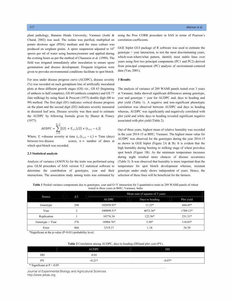
Journal of Experimental Biology and Agricultural Sciences
http://www.jebas.org
117 Ahirwar et al.
plant pathology, Banaras Hindu University, Varanasi (Joshi &
Chand, 2002) was used. The isolate was purified, multiplied on
potato dextrose agar (PDA) medium and the mass culture was
produced on sorghum grains. A spore suspension adjusted to 104
spores per ml of water using haemocytometer and applied during
the evening hours as per the method of Chaurasia et al. (1999). The
field was irrigated immediately after inoculation to ensure spore
germination and disease development. Frequent irrigation were
given to provoke environmental conditions facilitate to spot blotch.
For area under disease progress curve (AUDPC), disease severity
(%) was recorded on each germplasm line of artificially inoculated
plots at three different growth stages (GS) viz., GS 63 (beginning
of anthesis to half complete), GS 69 (anthesis complete) and GS 77
(late milking) by using Saari & Prescott (1975) double digit (00 to
99) method. The first digit (D1) indicates vertical disease progress
on the plant and the second digit (D2) indicates severity measured
in diseased leaf area. Disease severity was then used to estimate
the AUDPC by following formula given by Shaner & Finney
(1977).
𝐴𝑈𝐷𝑃𝐶 = 𝑌𝑖 + 𝑌𝑖+1 /2 × 𝑡𝑖+1 − 𝑡𝑖
𝑛−1
𝑖=0
Where, 𝑌𝑖 =disease severity at time 𝑡𝑖 , 𝑡𝑖+1 − 𝑡𝑖 = Time (days)
between two disease scores, 𝑛 = number of dates at
which spot blotch was recorded.
2.3 Statistical analysis
Analysis of variance (ANOVA) for the traits was performed using
proc GLM procedure of SAS version 9.2 statistical software to
determine the contribution of genotypes, year and their
interactions. The association study among traits was estimated by
using the Proc CORR procedure in SAS in terms of Pearson‟s
correlation coefficients.
GGE biplot GUI package of R software was used to estimate the
genotype × year interaction, to test the most discriminating years,
which-won-where/what pattern, identify most stable lines over
years using first two principal components (PC1 and PC2) derived
from principal component (PC) analysis of environment-centered
data (Yan, 2001).
3 Results
The analysis of variance of 289 WAMI panels tested over 3 years
at Varanasi, India showed significant differences among genotype,
year and genotype × year for AUDPC and, days to heading and
plot yield (Table 1). A negative and non-significant phenotypic
correlation was observed between AUDPC and days to heading
whereas, AUDPC was significantly and negatively correlated with
plot yield and while days to heading revealed significant negative
associated with plot yield (Table 2).
Out of three years, highest mean of relative humidity was recorded
in the year 2014-15 at BHU, Varanasi. The highest mean value for
AUDPC was observed for the genotypes during the year 2014-15
as shown in GGE biplot (Figure 2A & B). It is evident that the
high humidity during booting to milking stage of wheat provokes
spot botch (Figure 1B). As the minimum temperature increases
during night resulted more chances of disease occurrence
(Table 3). It was observed that humidity is more important than the
temperature for spot blotch development whereas, resistant
genotype under study shows independent of years. Hence, the
selection of these lines will be beneficial for the farmers.
Table 1 Pooled variance components due to genotypes, year and G×Y interaction for 3 quantitative traits in 289 WAMI panels of wheat
tested in three years at BHU, Varanasi, India
Source d.f. Mean sum of squares of 3 years
AUDPC Days to heading Plot yield
Genotype 288 102858.93* 11.25* 444.45*
Year 2 549899.51* 4072.36* 1709.12*
Replication 1 10776.34 122.56* 231.31*
Genotype × Year 576 18904.76* 3.50* 118.03*
Error 866 3319.37 1.18 34.39
*Significant at the p-value (P<0.01) probability level.
Table 2 Correlation among AUDPC, days to heading (DH)and plot yield (PY).
AUDPC DH
DH -0.01
PY -0.21* -0.07*
* Significant at P < 0.05.
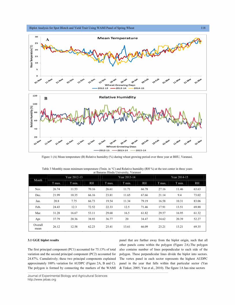
Journal of Experimental Biology and Agricultural Sciences
http://www.jebas.org
Biplot Analysis for Spot Blotch and Yield Trait Using WAMI Panel of Spring Wheat 118
3.1 GGE biplot results
The first principal component (PC1) accounted for 75.13% of total
variation and the second principal component (PC2) accounted for
24.87%. Cumulatively; these two principal components explained
approximately 100% variation for AUDPC (Figure 2A, B and C).
The polygon is formed by connecting the markers of the WAMI
panel that are further away from the biplot origin, such that all
other panels come within the polygon (Figure 2A).The polygon
also contains number of lines perpendicular to each side of the
polygon. These perpendicular lines divide the biplot into sectors.
The vertex panel in each sector represents the highest AUDPC
panel in the year that falls within that particular sector (Yan
& Tinker, 2005; Yan et al., 2010). The figure 1A has nine sectors
Figure 1 (A) Mean temperature (B) Relative humidity (%) during wheat growing period over three year at BHU, Varanasi.
Table 3 Monthly mean minimum temperature (Tmin. in °C) and Relative humidity (RH %) at the test center in three years
at Banaras Hindu University, Varanasi
Month Year 2012-13 Year 2013-14 Year 2014-15
T max. T min. RH T max. T min. RH T max. T min. RH
Nov. 26.74 11.53 70.16 26.61 11.71 66.78 27.16 11.46 63.63
Dec. 21.99 10.35 66.16 23.81 11.65 67.66 21.14 9.4 73.02
Jan. 20.8 7.75 66.73 19.54 11.34 79.19 16.58 10.31 83.06
Feb. 24.43 12.3 72.52 22.33 12.5 71.46 17.91 13.51 69.88
Mar. 31.28 16.67 53.11 29.68 16.5 61.82 29.57 16.95 61.32
Apr. 37.79 20.36 38.93 36.77 20 34.47 34.62 20.39 52.27
Overall
mean 26.12 12.58 62.23 25.41 13.61 66.09 23.21 13.21 69.35
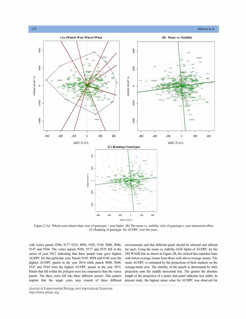
Journal of Experimental Biology and Agricultural Sciences
http://www.jebas.org
119 Ahirwar et al.
with vertex panels 9296, 9177 9235, 9094, 9105, 9148, 9040, 9046,
9147 and 9104. The vertex panels 9296, 9177 and 9235 fell in the
sector of year 2013 indicating that these panels were gave highest
AUDPC for that particular year. Panels 9105, 9094 and 9148 were the
highest AUDPC panels in the year 2014 while panels 9040, 9046,
9147 and 9104 were the highest AUDPC panels in the year 2015.
Panels that fell within the polygon were less responsive than the vertex
panels. The three years fell into three different sectors. This pattern
implies that the target years may consist of three different
environments and that different panel should be selected and utilized
for each. Using the mean vs. stability GGE biplot of AUDPC for the
289 WAMI line as shown in Figure 2B, the vertical line separates lines
with below-average means from those with above-average means. The
mean AUDPC is estimated by the projections of their markers on the
average-tester axis. The stability of the panels is determined by their
projection onto the middle horizontal line. The greater the absolute
length of the projection of a panel, that panel indicates less stable. In
present study, the highest mean value for AUDPC was observed for
(A) sWhich Won Where/What (B) Mean vs. Stability
(C) Ranking Genotypes
Figure 2 (A) „Which-won-where/what view of genotype × year biplot (B) The mean vs. stability view of genotype x year interaction effect
(C) Ranking of genotype for AUDPC over the years.
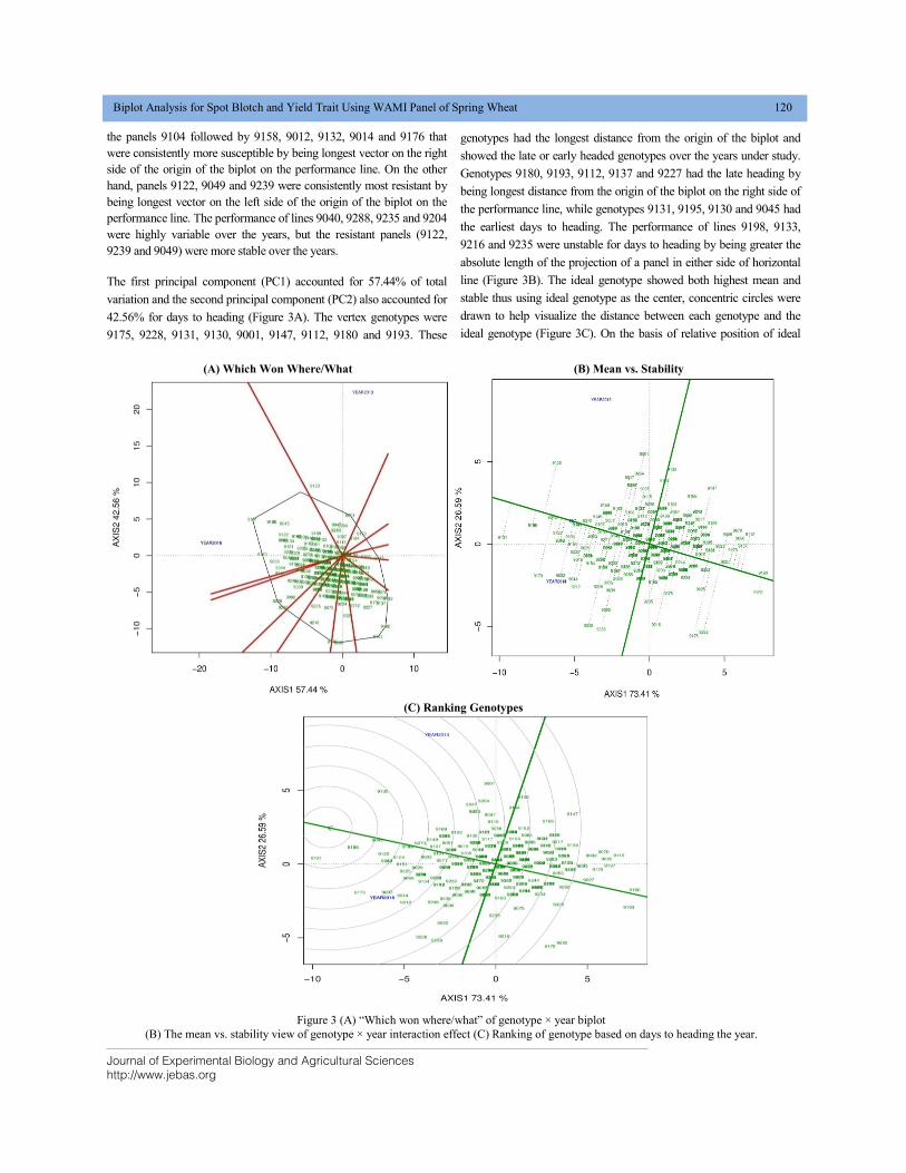
Journal of Experimental Biology and Agricultural Sciences
http://www.jebas.org
Biplot Analysis for Spot Blotch and Yield Trait Using WAMI Panel of Spring Wheat 120
the panels 9104 followed by 9158, 9012, 9132, 9014 and 9176 that
were consistently more susceptible by being longest vector on the right
side of the origin of the biplot on the performance line. On the other
hand, panels 9122, 9049 and 9239 were consistently most resistant by
being longest vector on the left side of the origin of the biplot on the
performance line. The performance of lines 9040, 9288, 9235 and 9204
were highly variable over the years, but the resistant panels (9122,
9239 and 9049) were more stable over the years.
The first principal component (PC1) accounted for 57.44% of total
variation and the second principal component (PC2) also accounted for
42.56% for days to heading (Figure 3A). The vertex genotypes were
9175, 9228, 9131, 9130, 9001, 9147, 9112, 9180 and 9193. These
genotypes had the longest distance from the origin of the biplot and
showed the late or early headed genotypes over the years under study.
Genotypes 9180, 9193, 9112, 9137 and 9227 had the late heading by
being longest distance from the origin of the biplot on the right side of
the performance line, while genotypes 9131, 9195, 9130 and 9045 had
the earliest days to heading. The performance of lines 9198, 9133,
9216 and 9235 were unstable for days to heading by being greater the
absolute length of the projection of a panel in either side of horizontal
line (Figure 3B). The ideal genotype showed both highest mean and
stable thus using ideal genotype as the center, concentric circles were
drawn to help visualize the distance between each genotype and the
ideal genotype (Figure 3C). On the basis of relative position of ideal
(A) Which Won Where/What (B) Mean vs. Stability
(C) Ranking Genotypes
Figure 3 (A) “Which won where/what” of genotype × year biplot
(B) The mean vs. stability view of genotype × year interaction effect (C) Ranking of genotype based on days to heading the year.
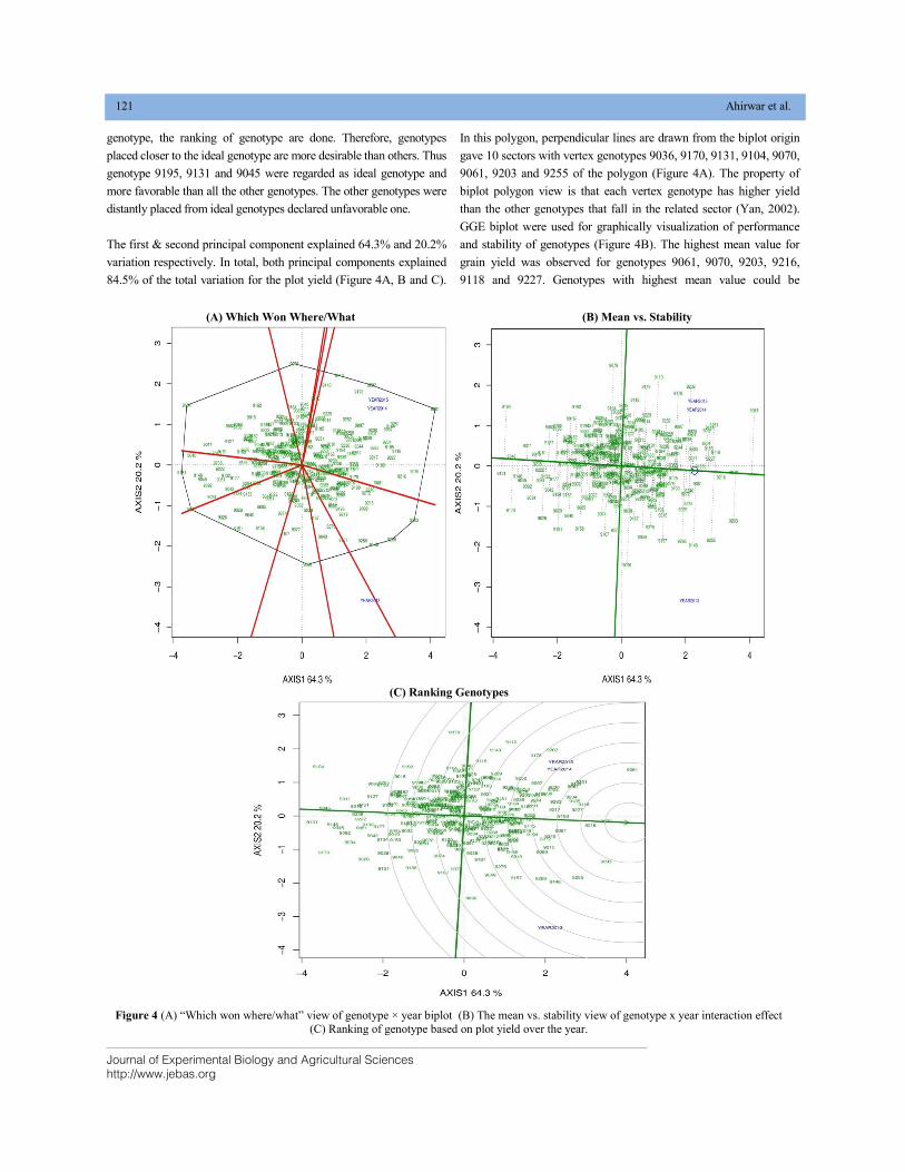
Journal of Experimental Biology and Agricultural Sciences
http://www.jebas.org
121 Ahirwar et al.
genotype, the ranking of genotype are done. Therefore, genotypes
placed closer to the ideal genotype are more desirable than others. Thus
genotype 9195, 9131 and 9045 were regarded as ideal genotype and
more favorable than all the other genotypes. The other genotypes were
distantly placed from ideal genotypes declared unfavorable one.
The first & second principal component explained 64.3% and 20.2%
variation respectively. In total, both principal components explained
84.5% of the total variation for the plot yield (Figure 4A, B and C).
In this polygon, perpendicular lines are drawn from the biplot origin
gave 10 sectors with vertex genotypes 9036, 9170, 9131, 9104, 9070,
9061, 9203 and 9255 of the polygon (Figure 4A). The property of
biplot polygon view is that each vertex genotype has higher yield
than the other genotypes that fall in the related sector (Yan, 2002).
GGE biplot were used for graphically visualization of performance
and stability of genotypes (Figure 4B). The highest mean value for
grain yield was observed for genotypes 9061, 9070, 9203, 9216,
9118 and 9227. Genotypes with highest mean value could be
(A) Which Won Where/What (B) Mean vs. Stability
(C) Ranking Genotypes
Figure 4 (A) “Which won where/what” view of genotype × year biplot (B) The mean vs. stability view of genotype x year interaction effect
(C) Ranking of genotype based on plot yield over the year.
Journal of Experimental Biology and Agricultural Sciences
http://www.jebas.org
Biplot Analysis for Spot Blotch and Yield Trait Using WAMI Panel of Spring Wheat 122
selected, whereas the rest were discarded. The ideal genotypes
identified were 9070 followed 9216, 9227, 9118, 9183 and 9183 for
plot yield (Figure 4C).
4 Discussion and Conclusion
Spot blotch caused by a fungus B. sorokiniana is an important
disease in wheat production. It has become more devastating
disease in the warmer areas of the world particularly the Indian
subcontinent characterized by prevalent warm and humid
conditions (Aggarwal et al., 2010). Further, the wide spread
use of conservation tillage practices may also be favorable for
spot blotch incidence in the south east Asia (Duveiller &
Sharma, 2009). It has been reported that this pathogen spread
into the cooler traditional rice-wheat production areas (Chand
et al., 2003). The extensively adopted rice-wheat cropping
system facilitates suitable environment for the survival and
multiplication of foliar blight pathogens in south Asia. It is
generally believed that the level of resistance in high-yielding
wheat genotypes is still unsatisfactory and needs to be
improved significantly in warmer humid regions of south Asia
(Sharma & Duveiller, 2006; Joshi et al., 2007a). Consequently,
an integrated approach, with host resistance as a major
component, is generally considered best for controlling the
disease (Hetzler et al., 1991; Mehta et al., 1992). The
resistance to spot blotch in prominent cultivars has been slow
due to quantitative nature of resistance which has a large
influence of environment (Joshi et al., 2004a; Kumar et al.,
2009). This is one of the reasons why selection of spot blotch
resistant plants in breeding programmes becomes complicated.
The agricultural research farm of Banaras Hindu University,
Varanasi testing center used in this study fall under EGP
having characteristics of warm-humid weather particularly at
reproductive stage of the crop which provokes spot blotch
disease.
Result of current study indicate significant differences among
genotype, year and genotype × year for AUDPC percent, days
to heading and plot yield exhibit considerable phenotypic
variations. The negative correlation among earliness and spot
blotch susceptibility was found (Dubin et al., 1998; Mahto,
2001; Rosyara et al., 2009) while AUDPC and days to heading
was significantly and negatively correlated with plot yield. The
similar results of Saxesena et al. (2017) also showed by
developing recombinant inbred line population from cross of
two parents YS#58 × YS#24 for spot blotch resistance. The
value of plant genetic resources are realized only when each
and every germplasm line is characterized for relevant traits to
reveal new gene combinations for their use in crop
improvement (Upadhyaya et al., 2010). Further, an association
study on agro-morphological traits with spot blotch resistance
will provide a roadmap in making selection strategy.
According to Heidari et al., 2016, GGE biplot facilitated visual
comparison and informative methods to detect genotypes
stability and in the preferential genotypes recommendations. This
approach provides an easy and comprehensive analysis of
genotype by years‟ interaction such that not only it allows
effective evaluation of genotypes but also a comprehensive
understanding of the target environment (year) (Yan & Tinker,
2005). Genotypes showed variation for spot blotch score and
morpho-agronomic traits. Current study identified superior lines
for specific traits with resistance to spot blotch disease that are
likely to serve as new potential sources of variation in wheat
improvement programme. For AUDPC, the first two principal
components explained 100% (PC1=75.13% and PC2=24.87%) of
the total variation of the year-centered data implying complex
interaction between genotypes and year. The stability analysis of
wheat genotypes is explained by performance line passing
through the origin of the biplot showed that the germplasm 9122,
9049 and 9239 was farthest to the left of the biplot origin and
near to performance line indicating lower AUDPC mean. The
more stable a genotype will be more near to the performance line
as reported earlier by Yan et al., 2000 hence, these lines could be
considered stable for spot blotch resistance across the years.
Identification of genotypes with stable resistance for disease is
an important component that ensures selection of appropriate
sources of resistance for breeding programmes (Sharma et al.,
2012; Singh et al., 2015). Using the ideal environment (year) as
the centre, concentric circles were drawn to help visualize the
distance between each environment and the ideal environment
(Yan et al., 2000; Yan & Rajcan, 2002).
The variation in plot yield was mainly affected by genotype and
genotype × year interactions. The PC1 vs PC2 of genotypes and
environments (years) explained 84.5% of the total variance.
When a genotype is near to performance line and environment on
the right side of origin of biplot, this indicates that the genotype
is specifically adapted to that environment (Kumar et al., 2016).
The highest mean value for plot yield was observed for the panel
9061, 9070, 9203 and 9216 which were found relatively more
stable while 2014 was most discriminating year for plot yield. In
breeding, an ideal genotype is regarded as the one that has the
highest mean yield and is stable across environments (Yan &
Kang, 2003). Results of this study implied that genotypes
possessing good spot blotch resistance, high yield potential and
adaptation under spot blotch conducive environment could be
used in wheat improvement programs for developing superior
genotypes for yield and spot blotch resistance contributing to
food security in south Asia.
Acknowledgements
Authors gratefully acknowledge Matthew P. Reynolds, CIMMYT,
Mexico, for providing WAMI population.
Journal of Experimental Biology and Agricultural Sciences
http://www.jebas.org
123 Ahirwar et al.
Conflict of interest
There is no conflict of interest to declare.
References
Aggarwal R, Singh VB, Shukla R, Gurjar MS, Gupta S, Sharma
TR. (2010) URP-based DNA fingerprinting of Bipolaris
sorokiniana isolates causing spot blotch of wheat. Journal of
Phytopathology 158: 210–216.
Bai G, Shaner G (1994) Scab of Wheat: prospects for control.
Plant Disease 78: 760-766.
Braun HJ, Atlin G, Payne T (2010) Multi-location testing as a tool to
identify plant response to global climate change. In: Reynolds M.P, ed,
Climate change and crop production. CABI, London, UK. pp. 115-138.
Chand R, Pandey SP, Singh HV, Kumar S, Joshi AK (2003)
Variability and its probable cause in the natural populations of spot
blotch pathogen Bipolaris sorokinianaof wheat (T. aestivum L.) in
India. Journal of Plant Diseases and Protection 110: 27-35.
Chaurasia S, Joshi AK, Dhari R, Chand R (1999) Resistance to
foliar blight of wheat; a search. Genetic Resources and Crop
Evolution 46: 469-475.
Dubin HJ, Arun B, Begum SN, Bhatta M, Dhari R, Goel LB, Joshi
AK, Khanna BM, Malaker PK, Pokhrel DR, Rahman MM, Saha
NK, Shaheed MA, Sharma RC, Singh AK, Singh RM, Singh RV,
Vergas M, Verma PC (1998) Results of the south Asia regional
Helminthosporium leaf blight and yield experiment, 1993–94. In:
Duveiller E, Dubin HJ, Reeves J, McNab A (Eds.),
Helminthosporium Blights of Wheat: Spot Blotch and Tan Spot,
CIMMYT, Mexico, D.F. Pp. 182–187.
Dubin HJ, Van Ginkel M (1991) The status of wheat diseases and
disease research inwarmer areas. In: Saunders DA (Ed.), Wheat for the
Nontraditional Warmer Areas. CIMMYT, Mexico, D.F, pp. 125-145.
Duveiller E (2003) Controlling foliar blight of wheat in rice-wheat
system of Asia. Plant Disease 88: 52-56.
Duveiller E, Sharma RC (2009) Genetic improvement and crop
management strategies to minimize yield losses in warm
nontraditional wheat growing areas due to spot blotch pathogen
Cochliobolus sativus. Journal of Plant Pathology157: 521-534.
FAOSTAT (2016) FAOSTAT. Food Agric. Organ. United Nations.
Fernandez MR, Fox SL, Hucl P, Singh AK (2014) Leaf spotting
reaction of spring common durum and spelt wheat and Kamut
under organic management in western. Canadian Journal of Plant
Science 94: 929-935.
Giraldo P, Benavente E, Manzano-Agugliaro F, Gimenez E (2019)
Worldwide Research Trends on Wheat and Barley: A Bibliometric
Comparative Analysis. Agronomy 9: 352.
Heidari Shadi, Azizinezhad Reza, Haghparast Reza (2016) Yield
stability analysis in advanced durum wheat genotypes by using
AMMI and GGE biplot models under diverse environment. Indian
Journal of Genetics 76 : 274-283.
Hetzler J, Eyal Z, Mehta YR, Campos LA (1991) Interaction
between spot blotch (Cochliobolus sativus) and wheat cultivars. In:
Saunders DA, Hettel G, eds. Wheat for Nontraditional Warm
Areas. Mexico, DF: CIMMYT, 146-64.
Joshi AK, Chand R (2002) Variation and inheritance of leaf angle,
and its association with spot blotch (Bipolaris sorokiniana)
severity in wheat (Triticum aestivum). Euphytica 124: 283-291.
Joshi AK, Chand R, Kumar S, Singh RP (2004b) Leaf tip necrosis:
a phenotypic marker associated with resistance to spot blotch
disease in wheat. Crop Science 44:792–796.
Joshi AK, Ferrara O, Crossa G, Singh J, Alvarado J, Bhatta G,
Duveiller MR, Sharma E, Pandit RC, Das SY, Chand R (2007a)
Associations of environments in South Asia based on spot blotch
disease of wheat caused by Cochliobolus sativus. Crop Science 47:
1071-1081.
Joshi AK, Kumar S, Chand R, Ortiz-Ferrara G (2004a) Inheritance
of resistance to spot blotch caused by Bipolaris sorokiniana in
spring wheat. Plant Breeding 123: 213-219.
Joshi AK, Mishra B, Chatrath R, Ortiz-Ferrara G, Singh RP
(2007b) Wheat improvement in India: present status, emerging
challenges and future prospects. Euphytica 157: 431-446.
Kumar U, Joshi AK, Kumar S, Chand R, Roder MS (2009)
Mapping of resistance to spot blotch disease caused by Bipolaris
sorokiniana in spring wheat. Theoretical and Applied Genetics
118: 783-792.
Kumar V, Kharub AS, Verma RPS, Verma A (2016) AMMI, GGE
biplot and regression analysis to comprehend the G x E interaction
in multi environment barley trials. Indian Journal of Genetics 76 :
202-204.
Mahto BN (2001) Effect of Helminthosporium leaf blight on yield
components and determination of resistance in selected wheat
varieties. Annals of Agricultural Sciences 22: 177-181.
Mehta YR, Riede CR, Campos LAC, Cooli MM (1992) Integrated
management of major wheat diseases in Brazil: an example for
southern cone region of Latin America. Crop Protection 11: 517-524.
Journal of Experimental Biology and Agricultural Sciences
http://www.jebas.org
Biplot Analysis for Spot Blotch and Yield Trait Using WAMI Panel of Spring Wheat 124
Panse VG, Sukhatme PV (1985) Statistical method for agricultural
workers, 4th edition, New Delhi.
Raemaekers RH (1988) Bipoloris sorokiniana disease complex on
wheat and source of resistance in Zambia. In: Klatt AR (Eds.)
wheat production constraints in tropical environment, Mexico.
D.F. CIMMYT. 175-185.
Rosyara UR, Khadka K, Subedi S, Sharma RC, Duveiller E (2009)
Field resistance to spot blotch is not associated with undesirable
physio-morphological traits in three spring wheat populations.
Journal of Plant Pathology 91 : 113-122.
Saari EE (1998) Leaf blight diseases and associated soil borne
fungal pathogens of wheat in north and south East Asia. In:
Duveiller E, Dubin HJ, Reeves J, Mc Nab A (Eds)
Helminthosporium Blights of wheat: Spot Blotch and Tan Spot
CIMMYT, Mexico, D.F. Pp. 37-51.
Saari EE, Prescott JM (1975) A scale for appraising the foliar
intensity of wheat diseases. Plant Disease Report 59: 377- 380.
Saxesenaa RR, Mishra VK, Chand R, Chowdhury A, Kumar B,
Prateek Madha, Joshi AK (2017) Pooling together spot blotch
resistance, high yield with earliness in wheat for eastern Gangetic
Plains of South Asia. Field Crops Research 214: 291-300.
Shaner G, Finney R (1977) The effect of nitrogen fertilization on
the expression of slow mildewing in knox wheat. Phytopathology
67: 1051-1056.
Sharma M, Babu TK, Gaur PM, Ghosh R, Rameshwar T, Chaudhary
RG, Upadhyay JP, Gupta O, Saxena DR, Kaur L, Dubey SC,
Anandani VP, Harer PN, Pande S (2012) Identification and multi-
environment validation of resistance to Fusarium oxysporum f. sp.
ciceris in chickpea. Field Crops Research 135: 82-88.
Sharma RC, Duveiller E (2006) Spot blotch continues to cause
substantial grain yield reductions under resource-limited farming
conditions. Journal of Phytopathology 154: 482-488.
Shrestha KK, Timila RD, Mahto BN, Bimb HP (1998) Disease
incidence and disease loss due to foliar blight of wheat in Nepal.
In: Duveiller E, Dubin HJ, Reeves J, McNab A (Eds.),
Helminthosporium Blights of Wheat: Spot Blotch and Tan Spot.
CIMMYT, Mexico, D.F, pp. 67-72.
Singh PK, Zhang Y, Xinyao H, Singh RP, Chand R, Mishra VK,
Malaker PK, Reza MA, Rahman MM, Islam R, Chowdhury AK,
Bhattacharya PM, Kalappanavar I K, Crossa J, Joshi AK (2015)
Development and characterization of the 4th CSISA-spot blotch
nursery of bread wheat. European Journal of Plant Pathology 143:
595-605.
Upadhyaya D, Sharma S, Ramulu B, Bhattacharjee R, Gowda
CLL, Reddy VGG, Singh S (2010) Variation for qualitative and
quantitative traits and identification of trait-specific sources in new
sorghum germplasm. Crop and Pasture Science 61: 609-618
Yan W (2001) GGE biplot: a windows application for graphical
analysis of multi-environment trial data and other types of two-
way data. Agronomy Journal 93: 1111-1118.
Yan W, (2002) Singular-value partitioning in biplot analysis of
multi environment trial data. Agronomy 94: 90-996.
Yan W, Fregeau-Reid J, Pageau D, Martin R, Mitchell-Fetch J,
Etienne M, Sparry E (2010) Identifying essential test locations for
oat breeding in Eastern Canada. Crop Science 50: 505-515.
Yan W, Hunt LA, Sheng QL, Szlavnics Z (2000) Cultivar
evaluation and mega environment investigation based on the GGE
biplot. Crop Science 40: 597-605.
Yan W, Kang MS (2003) GGE biplot analysis: A graphical tool for
breeders, geneticists, and agronomists (pp. 63-88). Boca Raton,
FL: CRC Press.
Yan W, Rajcan I (2002) Biplot analysis of test sites and trait
relations of soybean in Ontario. Crop Science 42: 11-20.
Yan W, Tinker NA (2005) An integrated biplot analysis system for
displaying, interpreting, and exploring genotype-by environment
interactions. Crop Science 45: 1004-1016.
k Journal of Experimental Biology and Agricultural Sciences
http://www.jebas.org
ISSN No. 2320 – 8694
Journal of Experimental Biology and Agricultural Sciences, April - 2020; Volume – 8(2) page 125 – 133
STRIPE RUST RESISTANCE IN WHEAT GERMPLASM OF NORTH-WESTERN HIMALAYAN HILLS
B.R. Raghu1*, O.P. Gangwar2, S.C. Bhardwaj2, K.K. Mishra1
1Vivekananda Parvatiya Krishi Anusandhan Sansthan (VPKAS), Indian Council of Agricultural Research (ICAR), Almora, India. 2Indian Institute of Wheat and Barley Research (IIW&BR), Indian Council of Agricultural Research (ICAR), Shimla, India.
Received – March 09, 2020; Revision – April 11, 2020; Accepted – April 19, 2020 Available Online – April 25, 2020
DOI: http://dx.doi.org/10.18006/2020.8(2).125.133
ABSTRACT
Stripe rust of wheat is one of the major biotic stresses occurring in cooler regions of wheat production
worldwide. In the present study, about 464 wheat germplasm collected from cooler areas of northern
hills, India, were characterized for stripe rust resistance both at seedling and adult-plant stages. Initially,
these genotypes were evaluated in the field at two locations, Hawalbagh and Dalang-Maidan during
three continuous cropping seasons. Under field conditions, 22 genotypes showed a consistent expression
of high field resistance (ACI<5.0), 349 expressed partial field resistance (ACI 5.0-60.0), and 93 were
highly susceptible (ACI>60.0). In next season, the high field resistant genotypes were subjected to both
seedling and an adult-plant stage resistance test against four virulent Pst pathotypes (78S84, 46S119,
110S119 and 238S119) under glasshouse conditions at ICAR-IIWBR, Shimla and Hawalbagh,
Uttarakhand, respectively. Among 22 high resistance genotypes, 14 genotypes possessed all-stage
resistance against all 4 Pst pathotypes and 4 genotypes were resistant to only two pathotypes (78S84 and
46S119) both at seedling and adult plant stages. Further, 349 partially field resistant genotypes were
evaluated for adult-plant stage resistance under artificially inoculated conditions, out of which 18
genotypes were found to have adult-plant stage resistance. Seedling resistance reported in the current
study is effective against newly emerged Pst pathotypes 110S119 and 238S119 and previously reported
predominant pathotypes 78S84 and 46S119 in India. The stripe rust resistance genotypes identified in
the current study may serve as potential donors of stripe rust resistance to wheat breeding programmes
in India and elsewhere.
* Corresponding author
KEYWORDS
Germplasm
Pathotypes
Resistance
Stripe-rust
Wheat
E-mail: [email protected], [email protected] (Dr Raghu B R)
Peer review under responsibility of Journal of Experimental Biology and Agricultural Sciences.
All the articles published by Journal of Experimental Biology and Agricultural Sciences are licensed under a Creative Commons Attribution-NonCommercial 4.0 International License Based on a work at www.jebas.org.
Production and Hosting by Horizon Publisher India [HPI] (http://www.horizonpublisherindia.in/). All rights reserved.
Journal of Experimental Biology and Agricultural Sciences http://www.jebas.org
Stripe rust resistance in wheat germplasm of North-western Himalayan Hills 126
1 Introduction
Yellow or stripe rust of wheat, caused by Puccinia striiformis
Westend. f. sp. tritici Erikss. (Pst) is one of the most
economically important fungal disease of global spread (Chen et
al., 2014). In India, stripe rust is a major biotic stress observed in
cooler areas of the country and causing considerable yield loss
during epidemic years (Hodson, 2011; Sharma & Saharan, 2011;
Prashar et al., 2015; Khan et al., 2016). Under conducive weather
conditions, stripe rust can cause yield loss up to 100%, but
usually damage remains in the range of 10-70% depending upon
crop stage, disease severity, and susceptibility of cultivar
(Gangwar et al., 2019). Yield losses in wheat due to stripe rust
are usually ascribed to reduction of kernel numbers per spike,
shriveled grains, and reduced test weight due to decreased
photosynthesis (Gangwar et al., 2019). Emergence of new
pathotypes and subsequent breakdown of resistance is a major
challenge in stripe rust management. In 1996, pathotype 46S119
which was virulent on widely used Pst resistance gene i. e. Yr9
was reported, followed by 78S84 having combined virulence on
Yr9 and Yr27 was identified in 2001 (Prashar et al., 2007;
Bhardwaj et al., 2019). Both pathotypes have predominantly
distributed and responsible for most of the stripe rust epidemics
in major-wheat growing regions of India (Prashar et al., 2015).
Besides, 3 new Pst pathotypes viz., 110S119, 238S119 and
110S84 with additional virulence on Riebesel47/51,
SuwonXOmar, Yr11, Yr14, and Yr24 were reported during 2013-
14 (Gangwar et al., 2016; Gangwar et al., 2019). Thus, search for
resistance to new Pst pathotypes in addition to existing virulent
pathotypes is need of the hour.
Although, multiple applications of fungicides can save the crop
from stripe rust, but development and deployment of resistant
varieties is the most efficient and environmentally sustainable
means of reducing the loss due to stripe rust (Chen, 2005). In
India, as an emergent tool for managing wheat rusts under high
disease incidence, the fungicides propiconazole 25% EC (tilt),
tebuconazole 25% EC (folicur) and triadimefon 25% EC
(Bayleton) are usually recommended at the rate of 0.1 percent
(Bhardwaj et al., 2016). But use of resistant cultivars has
remained preferable, economically viable, ecologically safe
and effective method for managing wheat rusts epidemics. A
rigorous screening of germplasm against the available
population of rust pathogens leads to the identification of rust
resistance sources. A dynamic rust resistance breeding
programme should always think ahead of the pathogen through
identification of sources of resistance to any new pathotype in
addition to the prevalent ones. Current study related to
identification of seedling and adult-plant resistance sources
among the wheat germplasm collected from Northern hills are
reported in the present communication.
2 Materials and Methods
2.1 Wheat genotypes
The plant materials consisted of 464 germplasm accessions of
cultivated bread wheat collected from Northern hills, India.
2.2 Stripe rust pathogen
Four highly virulent pathotypes (pts.) of wheat stripe rust
(Puccinia striformis f. sp. Tritici) namely, 78S84, 46S119,
110S119 and 238S119 were used in the present study.
2.3 Experimental setup
The schematic diagram of experimental layout and flow of
germplasm in different years and locations is presented in Figure 1.
2.4 Evaluation of wheat germplasm to stripe rust under
natural field conditions
Screening of 464 wheat germplasm to stripe rust was carried out at
two locations, Hawalbagh (29036’N, 79040’E; 1250 m asl),
Uttarakhand and Dalang Maidan (32021’N, 77014’E; 2347 m asl),
Himachal Pradesh, India. These locations are considered as hot
spots for stripe rust development. At these locations, stripe rust
appears every year in severe form on susceptible varieties. At
Hawalbagh, the wheat germplasm was evaluated in three regular
cropping seasons (November to May) during 2013-2016. Whereas,
at Dalang Maidan, the germplasm were evaluated in off-seasons
(May to August) for two years (2014 and 2015).
At both locations, the experiment was laid out in an augmented
design consisting of 16 blocks. In each block, susceptible check
(Agra Local) was repeated after every 29 test genotypes. Seeds of
each genotype were sown by dibbling in two rows with 30 cm
inter-row spacing and100 cm row length. The stripe rust infector’s,
a homogeneous mixture of highly susceptible wheat lines such as
NI5439, Avocet and Agra Local were used as stripe rust spreader
in the field. Infector rows were settled surround the experimental
plot to increase inocula load.
The infection types (IT) and disease severity data were recorded
using modified Cobb scale (Peterson et al., 1948) from boot to
milk stages. The infection types were recorded as 0= no visible
infection (immune); R= necrotic areas with or without uredia
(resistant); MR= necrotic areas with small uredia (moderately
resistant); MS=medium size uredia with no necrosis but some
chlorosis (moderately susceptible); S= large sized uredia with no
necrosis and chlorosis (susceptible); X= variable sized uredia with
necrosis or chlorosis and fully susceptible (intermediate). Stripe
rust severity was assessed as percentage of leaf area infected using
modified Cobb scale. The response value of 0.0, 0.2, 0.4, 0.8 and
1.0 were assigned for 0, R, MR, MS and S, respectively.
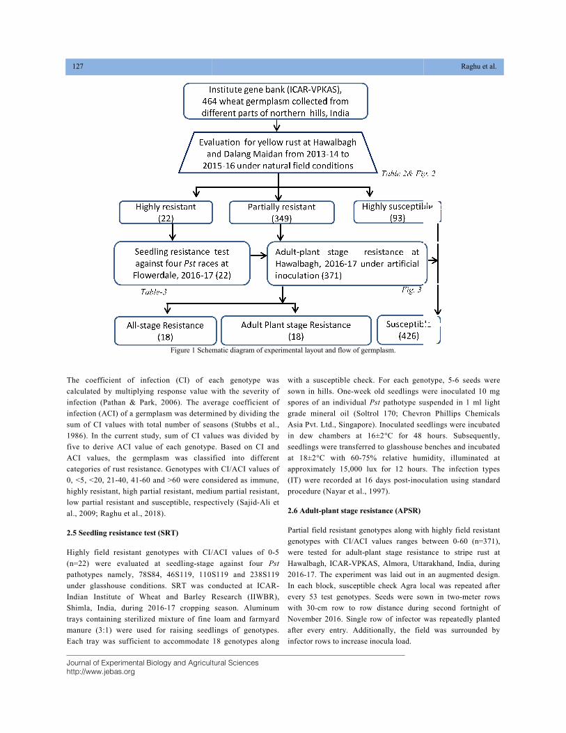
Journal of Experimental Biology and Agriculturhttp://www.jebas.org
127
The coefficient of infection (CI) of each genotype was
calculated by multiplying response value with the severity of
infection (Pathan & Park, 2006). The average coefficient of
infection (ACI) of a germplasm was determined by dividing the
sum of CI values with total number of seasons (Stubbs
1986). In the current study, sum of CI values was divided by
five to derive ACI value of each genotype. Based on CI and
ACI values, the germplasm was classified into different
categories of rust resistance. Genotypes with CI/ACI values of
0, <5, <20, 21-40, 41-60 and >60 were considered as immune,
highly resistant, high partial resistant, medium partial resistant,
low partial resistant and susceptible, respectively (Sajid
al., 2009; Raghu et al., 2018).
2.5 Seedling resistance test (SRT)
Highly field resistant genotypes with CI/ACI values of 0
(n=22) were evaluated at seedling-stage against four
pathotypes namely, 78S84, 46S119, 110S119 and 238S119
under glasshouse conditions. SRT was conducted at ICAR
Indian Institute of Wheat and Barley Research (IIWBR),
Shimla, India, during 2016-17 cropping season. Aluminum
trays containing sterilized mixture of fine loam and farmyard
manure (3:1) were used for raising seedlings of genotypes.
Each tray was sufficient to accommodate 18 genotypes along
Figure 1 Schematic diagram of experimental layout and flow of germplasm.
Journal of Experimental Biology and Agricultural Sciences
coefficient of infection (CI) of each genotype was
calculated by multiplying response value with the severity of
infection (Pathan & Park, 2006). The average coefficient of
infection (ACI) of a germplasm was determined by dividing the
total number of seasons (Stubbs et al.,
1986). In the current study, sum of CI values was divided by
five to derive ACI value of each genotype. Based on CI and
ACI values, the germplasm was classified into different
s with CI/ACI values of
60 and >60 were considered as immune,
highly resistant, high partial resistant, medium partial resistant,
low partial resistant and susceptible, respectively (Sajid-Ali et
Highly field resistant genotypes with CI/ACI values of 0-5
stage against four Pst
78S84, 46S119, 110S119 and 238S119
under glasshouse conditions. SRT was conducted at ICAR-
Indian Institute of Wheat and Barley Research (IIWBR),
17 cropping season. Aluminum
trays containing sterilized mixture of fine loam and farmyard
manure (3:1) were used for raising seedlings of genotypes.
to accommodate 18 genotypes along
with a susceptible check. For each genotype, 5
sown in hills. One-week old seedlings were inoculated 10 mg
spores of an individual Pst pathotype suspended in 1 ml light
grade mineral oil (Soltrol 170; Chevron
Asia Pvt. Ltd., Singapore). Inoculated seedlings were incubated
in dew chambers at 16±2°C for 48 hours. Subsequently,
seedlings were transferred to glasshouse benches and incubated
at 18±2°C with 60-75% relative humidity, illuminated at
approximately 15,000 lux for 12 hours. The infection types
(IT) were recorded at 16 days post-inoculation using standard
procedure (Nayar et al., 1997).
2.6 Adult-plant stage resistance (APSR)
Partial field resistant genotypes along with highly field res
genotypes with CI/ACI values ranges between 0
were tested for adult-plant stage resistance to stripe rust at
Hawalbagh, ICAR-VPKAS, Almora, Uttarakhand, India, during
2016-17. The experiment was laid out in
In each block, susceptible check Agra local was repeated after
every 53 test genotypes. Seeds were sown in two
with 30-cm row to row distance during second fortnight of
November 2016. Single row of infector was repeatedly pl
after every entry. Additionally, the field was surrounded by
infector rows to increase inocula load.
Figure 1 Schematic diagram of experimental layout and flow of germplasm.
Raghu et al.
with a susceptible check. For each genotype, 5-6 seeds were
week old seedlings were inoculated 10 mg
pathotype suspended in 1 ml light
grade mineral oil (Soltrol 170; Chevron Phillips Chemicals
Asia Pvt. Ltd., Singapore). Inoculated seedlings were incubated
in dew chambers at 16±2°C for 48 hours. Subsequently,
seedlings were transferred to glasshouse benches and incubated
75% relative humidity, illuminated at
approximately 15,000 lux for 12 hours. The infection types
inoculation using standard
Partial field resistant genotypes along with highly field resistant
genotypes with CI/ACI values ranges between 0-60 (n=371),
plant stage resistance to stripe rust at
VPKAS, Almora, Uttarakhand, India, during
17. The experiment was laid out in an augmented design.
In each block, susceptible check Agra local was repeated after
53 test genotypes. Seeds were sown in two-meter rows
cm row to row distance during second fortnight of
November 2016. Single row of infector was repeatedly planted
after every entry. Additionally, the field was surrounded by
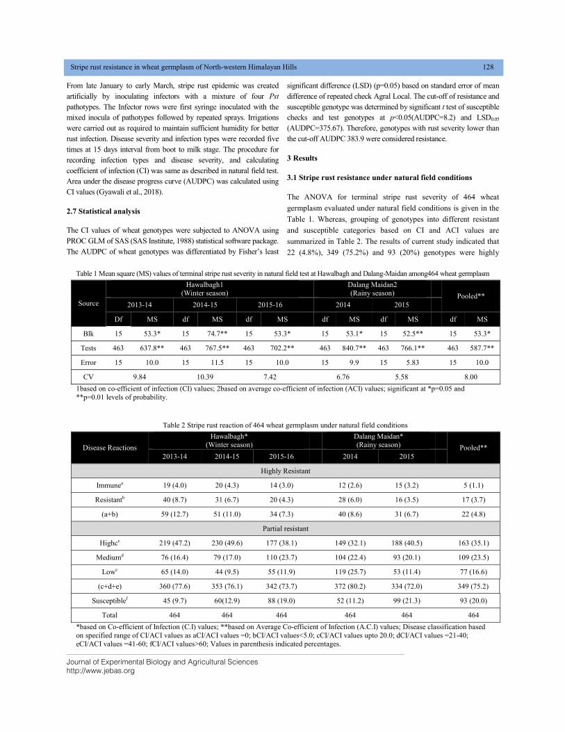
Journal of Experimental Biology and Agricultural Sciences http://www.jebas.org
Stripe rust resistance in wheat germplasm of North-western Himalayan Hills 128
From late January to early March, stripe rust epidemic was created artificially by inoculating infectors with a mixture of four Pst pathotypes. The Infector rows were first syringe inoculated with the mixed inocula of pathotypes followed by repeated sprays. Irrigations were carried out as required to maintain sufficient humidity for better rust infection. Disease severity and infection types were recorded five times at 15 days interval from boot to milk stage. The procedure for recording infection types and disease severity, and calculating coefficient of infection (CI) was same as described in natural field test. Area under the disease progress curve (AUDPC) was calculated using CI values (Gyawali et al., 2018).
2.7 Statistical analysis
The CI values of wheat genotypes were subjected to ANOVA using PROC GLM of SAS (SAS Institute, 1988) statistical software package. The AUDPC of wheat genotypes was differentiated by Fisher’s least
significant difference (LSD) (p=0.05) based on standard error of mean difference of repeated check Agral Local. The cut-off of resistance and susceptible genotype was determined by significant t test of susceptible checks and test genotypes at p<0.05(AUDPC=8.2) and LSD0.05
(AUDPC=375.67). Therefore, genotypes with rust severity lower than the cut-off AUDPC 383.9 were considered resistance.
3 Results
3.1 Stripe rust resistance under natural field conditions
The ANOVA for terminal stripe rust severity of 464 wheat
germplasm evaluated under natural field conditions is given in the
Table 1. Whereas, grouping of genotypes into different resistant
and susceptible categories based on CI and ACI values are
summarized in Table 2. The results of current study indicated that
22 (4.8%), 349 (75.2%) and 93 (20%) genotypes were highly
Table 1 Mean square (MS) values of terminal stripe rust severity in natural field test at Hawalbagh and Dalang-Maidan among464 wheat germplasm
Source
Hawalbagh1 (Winter season)
Dalang Maidan2 (Rainy season)
Pooled**
2013-14 2014-15 2015-16 2014 2015
Df MS df MS df MS df MS df MS df MS
Blk 15 53.3* 15 74.7** 15 53.3* 15 53.1* 15 52.5** 15 53.3*
Tests 463 637.8** 463 767.5** 463 702.2** 463 840.7** 463 766.1** 463 587.7**
Error 15 10.0 15 11.5 15 10.0 15 9.9 15 5.83 15 10.0
CV 9.84 10.39 7.42 6.76 5.58 8.00
1based on co-efficient of infection (CI) values; 2based on average co-efficient of infection (ACI) values; significant at *p=0.05 and **p=0.01 levels of probability.
Table 2 Stripe rust reaction of 464 wheat germplasm under natural field conditions
Disease Reactions
Hawalbagh* (Winter season)
Dalang Maidan* (Rainy season)
Pooled**
2013-14 2014-15 2015-16 2014 2015
Highly Resistant
Immunea 19 (4.0) 20 (4.3) 14 (3.0) 12 (2.6) 15 (3.2) 5 (1.1)
Resistantb 40 (8.7) 31 (6.7) 20 (4.3) 28 (6.0) 16 (3.5) 17 (3.7)
(a+b) 59 (12.7) 51 (11.0) 34 (7.3) 40 (8.6) 31 (6.7) 22 (4.8)
Partial resistant
Highcc 219 (47.2) 230 (49.6) 177 (38.1) 149 (32.1) 188 (40.5) 163 (35.1)
Mediumd 76 (16.4) 79 (17.0) 110 (23.7) 104 (22.4) 93 (20.1) 109 (23.5)
Lowe 65 (14.0) 44 (9.5) 55 (11.9) 119 (25.7) 53 (11.4) 77 (16.6)
(c+d+e) 360 (77.6) 353 (76.1) 342 (73.7) 372 (80.2) 334 (72.0) 349 (75.2)
Susceptiblef 45 (9.7) 60(12.9) 88 (19.0) 52 (11.2) 99 (21.3) 93 (20.0)
Total 464 464 464 464 464 464
*based on Co-efficient of Infection (C.I) values; **based on Average Co-efficient of Infection (A.C.I) values; Disease classification based on specified range of CI/ACI values as aCI/ACI values =0; bCI/ACI values<5.0; cCI/ACI values upto 20.0; dCI/ACI values =21-40; eCI/ACI values =41-60; fCI/ACI values>60; Values in parenthesis indicated percentages.
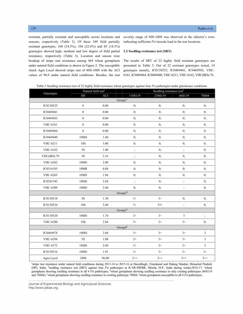
Journal of Experimental Biology and Agricultural Sciences http://www.jebas.org
129 Raghu et al.
resistant, partially resistant and susceptible across locations and
seasons, respectively (Table 2). Of these 349 field partially
resistant genotypes, 160 (34.5%), 104 (22.4%) and 85 (18.3%)
genotypes showed high, medium and low degree of field partial
resistance, respectively (Table 3). Location and season wise
breakup of stripe rust resistance among 464 wheat germplasm
under natural field conditions is shown in Figure 2. The susceptible
check Agra Local showed stripe rust of 80S-100S with the ACI
values of 96.0 under natural field conditions. Besides, the rust
severity range of 80S-100S was observed in the infector’s rows
indicating sufficient Pst inocula load in the test locations.
3.2 Seedling resistance test (SRT)
The results of SRT of 22 highly field resistant genotypes are
presented in Table 3. Out of 22 resistant genotypes tested, 14
genotypes namely, IC0138525, IC0469441, IC0469503, VHC-
6161, IC0469464, IC0469440, VHC-6211, VHC-6162, VHC(BD)-79,
Table 3 Seedling resistance test of 22 highly field resistance wheat genotypes against four Pst pathotypes under glasshouse conditions
Genotypes Natural field testa Seedling resistance testb
HS ACI 110S119 238S119 46S119 78S84
Group1c
IC0138525 0 0.00 0; 0; 0; 0;
IC0469441 0 0.00 0; 0; 0; 0;
IC0469503 0 0.00 0; 0; 0; 0;
VHC-6161 0 0.00 0; 0; 0; 0;
IC0469464 0 0.00 0; 0; 0; 0;
IC0469440 10MS 1.60 0; 0; 0; 0;
VHC-6211 10S 3.00 0; 0; 0; 0;
VHC-6162 5S 1.80 ; 0; ; 0;
VHC(BD)-79 5S 2.16 ; 0; 0; 0;
VHC-6202 10MS 2.00 0; 0; 0; 0;
IC0316103 10MR 0.88 0; 0; 0; 0;
VHC-6265 10MS 1.96 0; 0; 0; 0;
IC0281542 10MS 2.68 ; 0; ; 0;
VHC-6209 10MS 2.40 0; 0; ; 0;
Group2d
IC0138518 5S 1.30 3+ 3+ 0; 0;
IC0138524 10S 3.60 3+ 33+ ; 0;
Group3e
IC0138520 10MS 1.76 3+ 3+ 3 ;
VHC-6290 10S 2.84 3+ 3+ 3+ 0;
Group4f
IC0469478 10MS 2.60 3+ 3+ 3+ 3
VHC-6294 5S 1.08 3+ 3+ 3+ 3
VHC-6372 10MS 2.80 3+ 3+ 3+ 3
IC0138516 10MS 1.91 3+ 3+ 3+ 3+
Agra Local 100S 96.00 3++ 3++ 3++ 3++
astripe rust resistance under natural field conditions during 2013-14 to 2015-16 at Hawalbagh, Uttarakand and Dalang Maidan, Himachal Pradesh (HP), India; bseedling resistance test (SRT) against four Pst pathotypes at ICAR-IIWBR, Shimla, H.P., India during winter,2016-17; cwheat germplasm showing seedling resistance to all 4 Pst pathotypes; dwheat germplasm showing seedling resistance to only existing pathotypes (46S119 and 78S84); ewheat germplasm showing seedling resistance to existing pathotype 78S84; fwheat germplasm susceptible to all 4 Pst pathotypes;
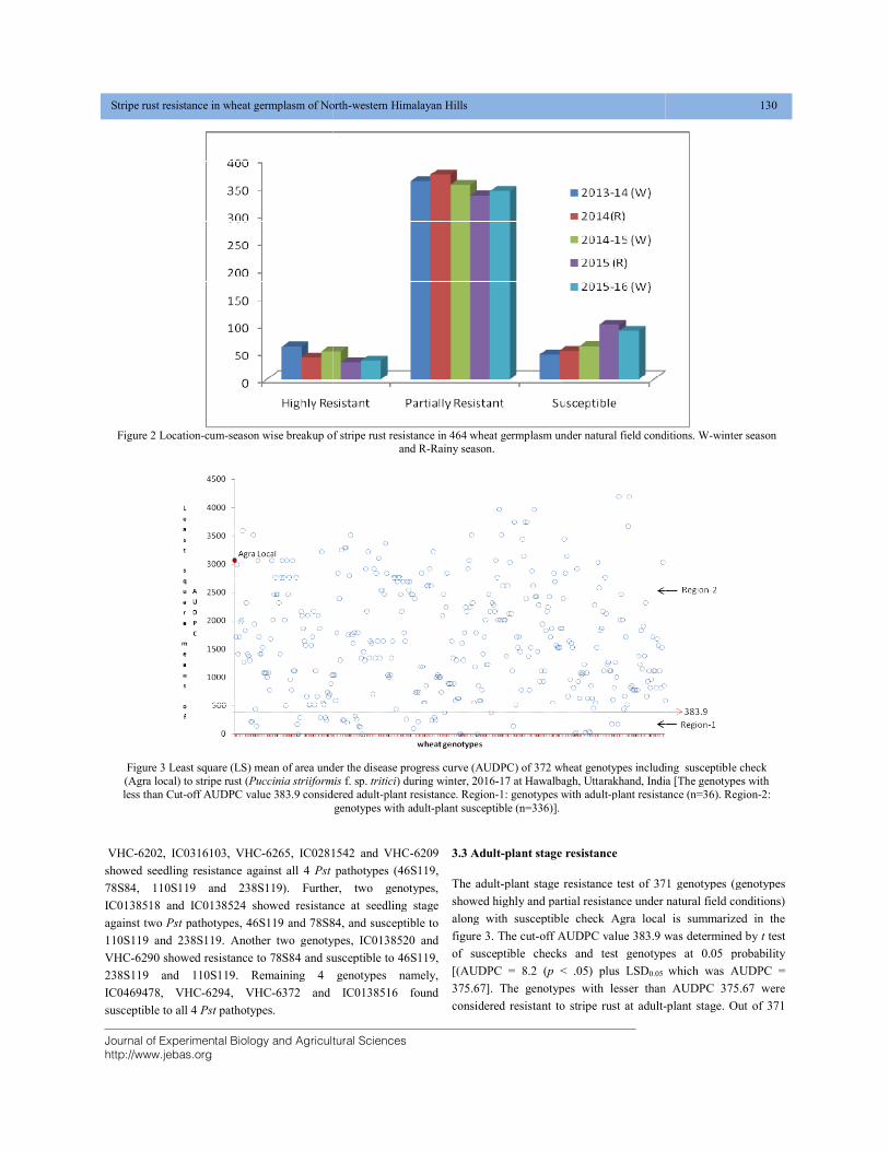
Journal of Experimental Biology and Agriculturhttp://www.jebas.org
Stripe rust resistance in wheat germplasm of North
Figure 2 Location-cum-season wise breakup of
Figure 3 Least square (LS) mean of area under the disease progress curve (AUDPC) of 372 wheat genotypes including susceptibl(Agra local) to stripe rust (Puccinia striiformisless than Cut-off AUDPC value 383.9 considered adult
VHC-6202, IC0316103, VHC-6265, IC0281542 and VHC
showed seedling resistance against all 4 Pst
78S84, 110S119 and 238S119). Further, two genotypes,
IC0138518 and IC0138524 showed resistance at seedling stage
against two Pst pathotypes, 46S119 and 78S84, and susceptible to
110S119 and 238S119. Another two genotypes, IC0138520 and
VHC-6290 showed resistance to 78S84 and susceptible to 46S119,
238S119 and 110S119. Remaining 4 genotypes namely,
IC0469478, VHC-6294, VHC-6372 and IC0138516 found
susceptible to all 4 Pst pathotypes.
Journal of Experimental Biology and Agricultural Sciences
Stripe rust resistance in wheat germplasm of North-western Himalayan Hills
season wise breakup of stripe rust resistance in 464 wheat germplasm under natural field conditions. Wand R-Rainy season.
Figure 3 Least square (LS) mean of area under the disease progress curve (AUDPC) of 372 wheat genotypes including susceptiblPuccinia striiformis f. sp. tritici) during winter, 2016-17 at Hawalbagh, Uttarakhand, India [The genotypes with
off AUDPC value 383.9 considered adult-plant resistance. Region-1: genotypes with adult-plant resistance (genotypes with adult-plant susceptible (n=336)].
6265, IC0281542 and VHC-6209
pathotypes (46S119,
78S84, 110S119 and 238S119). Further, two genotypes,
138524 showed resistance at seedling stage
pathotypes, 46S119 and 78S84, and susceptible to
110S119 and 238S119. Another two genotypes, IC0138520 and
6290 showed resistance to 78S84 and susceptible to 46S119,
ing 4 genotypes namely,
6372 and IC0138516 found
3.3 Adult-plant stage resistance
The adult-plant stage resistance test of 371 genotypes (genotypes
showed highly and partial resistance under natural field conditions)
along with susceptible check Agra local is summarized in the
figure 3. The cut-off AUDPC value 383.9 was determined by
of susceptible checks and test genotypes at 0.05 probability
[(AUDPC = 8.2 (p < .05) plus LSD0.05
375.67]. The genotypes with lesser than AUDPC 375.67 were
considered resistant to stripe rust at adult-
130
natural field conditions. W-winter season
Figure 3 Least square (LS) mean of area under the disease progress curve (AUDPC) of 372 wheat genotypes including susceptible check
17 at Hawalbagh, Uttarakhand, India [The genotypes with plant resistance (n=36). Region-2:
plant stage resistance test of 371 genotypes (genotypes
showed highly and partial resistance under natural field conditions)
along with susceptible check Agra local is summarized in the
off AUDPC value 383.9 was determined by t test
of susceptible checks and test genotypes at 0.05 probability
0.05 which was AUDPC =
375.67]. The genotypes with lesser than AUDPC 375.67 were
-plant stage. Out of 371
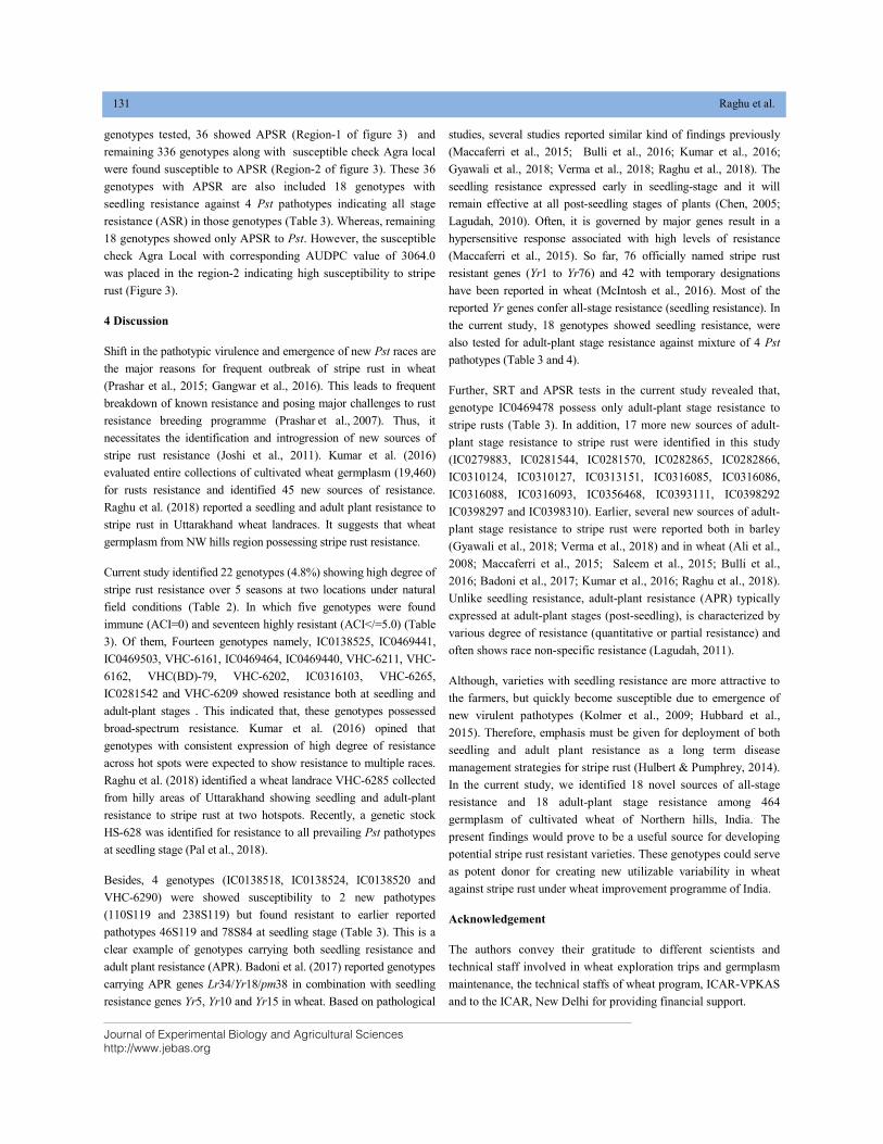
Journal of Experimental Biology and Agricultural Sciences http://www.jebas.org
131 Raghu et al.
genotypes tested, 36 showed APSR (Region-1 of figure 3) and
remaining 336 genotypes along with susceptible check Agra local
were found susceptible to APSR (Region-2 of figure 3). These 36
genotypes with APSR are also included 18 genotypes with
seedling resistance against 4 Pst pathotypes indicating all stage
resistance (ASR) in those genotypes (Table 3). Whereas, remaining
18 genotypes showed only APSR to Pst. However, the susceptible
check Agra Local with corresponding AUDPC value of 3064.0
was placed in the region-2 indicating high susceptibility to stripe
rust (Figure 3).
4 Discussion
Shift in the pathotypic virulence and emergence of new Pst races are
the major reasons for frequent outbreak of stripe rust in wheat
(Prashar et al., 2015; Gangwar et al., 2016). This leads to frequent
breakdown of known resistance and posing major challenges to rust
resistance breeding programme (Prashar et al., 2007). Thus, it
necessitates the identification and introgression of new sources of
stripe rust resistance (Joshi et al., 2011). Kumar et al. (2016)
evaluated entire collections of cultivated wheat germplasm (19,460)
for rusts resistance and identified 45 new sources of resistance.
Raghu et al. (2018) reported a seedling and adult plant resistance to
stripe rust in Uttarakhand wheat landraces. It suggests that wheat
germplasm from NW hills region possessing stripe rust resistance.
Current study identified 22 genotypes (4.8%) showing high degree of
stripe rust resistance over 5 seasons at two locations under natural
field conditions (Table 2). In which five genotypes were found
immune (ACI=0) and seventeen highly resistant (ACI</=5.0) (Table
3). Of them, Fourteen genotypes namely, IC0138525, IC0469441,
IC0469503, VHC-6161, IC0469464, IC0469440, VHC-6211, VHC-
6162, VHC(BD)-79, VHC-6202, IC0316103, VHC-6265,
IC0281542 and VHC-6209 showed resistance both at seedling and
adult-plant stages . This indicated that, these genotypes possessed
broad-spectrum resistance. Kumar et al. (2016) opined that
genotypes with consistent expression of high degree of resistance
across hot spots were expected to show resistance to multiple races.
Raghu et al. (2018) identified a wheat landrace VHC-6285 collected
from hilly areas of Uttarakhand showing seedling and adult-plant
resistance to stripe rust at two hotspots. Recently, a genetic stock
HS-628 was identified for resistance to all prevailing Pst pathotypes
at seedling stage (Pal et al., 2018).
Besides, 4 genotypes (IC0138518, IC0138524, IC0138520 and
VHC-6290) were showed susceptibility to 2 new pathotypes
(110S119 and 238S119) but found resistant to earlier reported
pathotypes 46S119 and 78S84 at seedling stage (Table 3). This is a
clear example of genotypes carrying both seedling resistance and
adult plant resistance (APR). Badoni et al. (2017) reported genotypes
carrying APR genes Lr34/Yr18/pm38 in combination with seedling
resistance genes Yr5, Yr10 and Yr15 in wheat. Based on pathological
studies, several studies reported similar kind of findings previously
(Maccaferri et al., 2015; Bulli et al., 2016; Kumar et al., 2016;
Gyawali et al., 2018; Verma et al., 2018; Raghu et al., 2018). The
seedling resistance expressed early in seedling-stage and it will
remain effective at all post-seedling stages of plants (Chen, 2005;
Lagudah, 2010). Often, it is governed by major genes result in a
hypersensitive response associated with high levels of resistance
(Maccaferri et al., 2015). So far, 76 officially named stripe rust
resistant genes (Yr1 to Yr76) and 42 with temporary designations
have been reported in wheat (McIntosh et al., 2016). Most of the
reported Yr genes confer all-stage resistance (seedling resistance). In
the current study, 18 genotypes showed seedling resistance, were
also tested for adult-plant stage resistance against mixture of 4 Pst
pathotypes (Table 3 and 4).
Further, SRT and APSR tests in the current study revealed that,
genotype IC0469478 possess only adult-plant stage resistance to
stripe rusts (Table 3). In addition, 17 more new sources of adult-
plant stage resistance to stripe rust were identified in this study
(IC0279883, IC0281544, IC0281570, IC0282865, IC0282866,
IC0310124, IC0310127, IC0313151, IC0316085, IC0316086,
IC0316088, IC0316093, IC0356468, IC0393111, IC0398292
IC0398297 and IC0398310). Earlier, several new sources of adult-
plant stage resistance to stripe rust were reported both in barley
(Gyawali et al., 2018; Verma et al., 2018) and in wheat (Ali et al.,
2008; Maccaferri et al., 2015; Saleem et al., 2015; Bulli et al.,
2016; Badoni et al., 2017; Kumar et al., 2016; Raghu et al., 2018).
Unlike seedling resistance, adult-plant resistance (APR) typically
expressed at adult-plant stages (post-seedling), is characterized by
various degree of resistance (quantitative or partial resistance) and
often shows race non-specific resistance (Lagudah, 2011).
Although, varieties with seedling resistance are more attractive to
the farmers, but quickly become susceptible due to emergence of
new virulent pathotypes (Kolmer et al., 2009; Hubbard et al.,
2015). Therefore, emphasis must be given for deployment of both
seedling and adult plant resistance as a long term disease
management strategies for stripe rust (Hulbert & Pumphrey, 2014).
In the current study, we identified 18 novel sources of all-stage
resistance and 18 adult-plant stage resistance among 464
germplasm of cultivated wheat of Northern hills, India. The
present findings would prove to be a useful source for developing
potential stripe rust resistant varieties. These genotypes could serve
as potent donor for creating new utilizable variability in wheat
against stripe rust under wheat improvement programme of India.
Acknowledgement
The authors convey their gratitude to different scientists and
technical staff involved in wheat exploration trips and germplasm
maintenance, the technical staffs of wheat program, ICAR-VPKAS
and to the ICAR, New Delhi for providing financial support.
Journal of Experimental Biology and Agricultural Sciences http://www.jebas.org
Stripe rust resistance in wheat germplasm of North-western Himalayan Hills 132
Conflict of Interest
Authors would hereby like to declare that there is no conflict of
interests that could possibly arise.
References
Ali S, Shah SJA, Maqbool K (2008) Field-Based Assessment of
Partial Resistance to Yellow Rust in Wheat Germplasm. Journal of
Agriculture & Rural Development 6(1): 99-106.
Badoni S, Chaudhary, R, Shekhar R, Badoni S, Ahmad E,
Gangwar RP, Tiwari KN, Rawat RS, Deepshikha, Jaiswal JP
(2017) Unveiling sources of stripe rust resistance in diverse wheat
(Triticum Aestivum L.) germplasm using narrow down
methodology: a proof of concept. Journal of Crop Science and
Biotechnology 20: 393-403.
Bhardwaj SC, Prasad P, Gangwar OP, Khan H, Kumar S (2016)
Wheat rust research - then and now. Indian Journal of Agricultural
Science 86: 1231 – 1244.
Bhardwaj SC, Singh GP, Gangwar OP, Prasad P, Kumar S (2019)
Status of Wheat Rust Research and Progress in Rust Management-
Indian Context. Agronomy 9: 892-905.
Bulli P, Zhang J, Chao S, Chen X, Pumphrey M (2016) Genetic
architecture of resistance to stripe rust in a global winter wheat
germplasm collection. G3 Genes Genomes Genetics 5: 2237-2253.
Chen W, Wellings C, Chen X, Kang Z, Liu T (2014) Wheat stripe
(yellow) rust caused by Puccinia striiformis f. sp. tritici.
Molecular Plant Pathology 15(5):433–446.
Chen XM (2005) Epidemiology and control of stripe rust
(Puccinia striiformis f. sp tritici) on wheat. Canadian Journal of
plant Pathology 27: 314–337.
Gangwar OP, Kumar S, Bhardwaj SC, Kashyap PL, Prasad P
(2019) Characterization of three new Yr9-virulences and
identification of sources of resistance among recently developed
Indian bread wheat germplasm. Journal of Plant Pathology 101:
955-963.
Gangwar OP, Subodh K, Pramod P, Bhardwaj SC, Hanif K,
Verma H (2016) Virulence pattern and emergence of new
pathotypes in Puccinia striiformis tritici during 2011-15 in India.
Indian Phytopathology 69: 178-185.
Gyawali S, Singh RP, Kumar S, Bhardwaj SC, Gangwar OP,
Selvakumar R, Shekhawat PS, Rehman S, Sharma-Poudyal D
(2018) Seedling and adult-plant stage resistance of a world
collection of barley genotypes to stripe rust Journal of
Phytopathology 166: 18-27.
Hodson DP (2011) Shifting boundaries: challenges for rust
monitoring. Euphytica 179: 93–104.
Hubbard A, Lewis CM, Yoshida K, Ramirez-Gonzalez RH, de
Vallavieille-Pope C, Thomas J, Kamoun S, Bayles R, Uauy C,
Saunders DGO (2015) Field pathogenomics reveals the emergence
of a diverse wheat yellow rust population. Genome Biology 16: 23.
Hulbert SH, Pumphrey MO (2014) A time for more booms and
fewer busts? Unraveling cereal–rust interactions. Molecular Plant-
Microbe Interactions 27: 207–214.
Joshi AK, Azab M, Mosaad M, Moselhy M, Osmanzai M,
Gelalcha S ( 2011) Delivering rust resistant wheat to farmers: A
step towards increased food security. Euphytica 179: 187-196.
Khan H, Gangwar OP, Prasad P, Bhardwaj SC (2016) Mehtaensis
Newsletter 36: (1) 1-2.
Kolmer J, Chen X, Jin Y (2009) Diseases which challenge global
wheat production-The wheat rusts. In: Carver BE (Ed) Wheat,
Science and Trade, Wiley-Blackwell, Ames, IA Pp. 89–124.
Kumar S, Sunil A, Tyagi R K, Jagdish K, Vikas V K, Sherry R J,
Kalyani S, Radhamani J, Parimalan R, Sivaswamy M, Sandhya T,
Mamata Y, Jyotisna K, Deepali, Sandeep S, Indoo B, Madhu M,
Bains NS, Chowdhury AK, Saha BC, Bhattacharya PM, Jyoti K,
Singh M C, Gangwar O P, Prasad P, Bharadwaj S C, Robin G,
Sharma JB, Sandeep, Kumar G M, Saharan MS, Manas B, Anirban
R, Prasad T V, Sharma R K, Dutta M, Indu S, Bansal KC (2016)
Evaluation of 19460 wheat accessions conserved in the Indain
national Genebank to identify new sources of resistance to rust and
spot blotch diseases. pLoS ONE, 12: 167-702.
Lagudah ES (2010) Molecular genetics of race non-specific rust
resistance in wheat.. In: Borlaug Global Rust Initiative,
Proceeding of Technical Workshop held on May 30-31, 2010 at St.
Petersburg, Russia, Pp. 183-196.
Lagudah, ES (2011) Molecular genetics of race non-specific rust
resistance in wheat. Euphytica 179: 81–91.
Maccaferri MJ, Zhang PB, Abate Z, Chao S, Cantu D, Bossolini E,
Chen X, Pumphrey M, Dubcovsky J (2015) A genome wide
association study of resistance to stripe rust (Puccinia striiformis f.
sp. tritici) in a worldwide collection of hexaploid spring wheat
(Triticum aestivum L.). G3 Genes Genomes Genetics 5: 449–465.
McIntosh RA, Dubcovsky J, Rogers WJ, Morris C, Appels R,
Xia XC (2016) Catalogue of Gene Symbols for Wheat.
In: Grain Genes. Available on
http://www.shigen.nig.ac.jp/wheat/komugi/genes/symbolClass
List.jsp. Accessed June 2017.
Journal of Experimental Biology and Agricultural Sciences http://www.jebas.org
133 Raghu et al.
Nayar SK, Prashar M, Bhardwaj SC (1997) Manual of current
techniques in wheat rust. Research bulletin 2, Regional Station,
Flowerdale, Shimla, Himachal Pradesh, India: Directorate of
Wheat Research Pp. 1–32.
Pal D, Bhardwaj SC, Hanif K, Patial M (2018) HS628-a potential
genetic stock for resistance to new virulent pathotypes of black,
brown and yellow rusts of wheat (Triticum aestivum L.). Wheat
and Barley Research 10: 132-135.
Pathan AK, Park RF (2006) Evaluation of seedling and adult
plant resistance to leaf rust in European wheat cultivars.
Euphytica 149: 327-342.
Peterson RF, Champbell AB, Hannah AE (1948) A diagrammatic
scale for estimating rust intensity of leaves and stem of cereals.
Canadian Journal of Research 26: 496-500.
Prashar M, Bhardwaj SC, Jain SK, Datta D (2007) Pathotypic
evolution in Puccinia striiformis in India during 1995-2004.
Australian Journal of Agricultural Research 58: 602-604.
Prashar M, Bhardwaj SC, Jain SK, Gangwar OP (2015) Virulence
diversity in Puccinia striiformis f. sp. tritci causing yellow rust on
wheat (Triticum aestivum) in India. Indian Journal of
Phytopathology 68: 129-133.
Raghu BR, Gangwar OP, Bhardwaj SC, Jain SK (2018) seedling
and adult plant resistance to stripe rust in Uttarakhand landraces of
wheat. Applied Biological Research 20: 291-301.
Sajid Ali, Jawad S, Shah A, Rahman H (2009) Multi-location
variability in Pakistan for partial resistance in wheat to Puccinia
striiformis f. sp. Tritici. Phytopathologia Mediterranea 48: 269-279.
Saleem K, Arshad HMI, Shokat S, Atta BM (2015). Appraisal of
wheat germplasm for adult plant resistance against stripe rust.
Journal of Plant Protection Research 55: 405-414.
SAS Institute (1988). Users guide: Statistics, 6th edn. Cary,
NC: SAS Inst.
Sharma I, Saharan MS (2011) Status of wheat disease in India with a
special reference to stripe rust. Research in Plant Diseases 26: 156.
Stubbs RW, Prescott JM, Saari EE, Dubin HJ (1986) Cereal
Diseases Methodology Manual. CIMMYT, Mexico.
Verma RPS, Selvakumar R, Gangwar OP, Shekhawat PS, Bhardwaj
SC, Rehman S, Sharma-Poudyal D, Gyawali S (2018) Identification of
additional sources of resistance to Puccinia striiformis f. sp. hordei
(PSH) in a collection of barley genotypes adapted to the high input
condition. Journal of Phytopathology 1: 1-10.
Journal of Experimental Biology and Agricultural Sciences
http://www.jebas.org
ISSN No. 2320 – 8694
Journal of Experimental Biology and Agricultural Sciences, April - 2020; Volume – 8(2) page 134 – 139
TOXIC EFFECTS OF VARIOUS ARSENIC CONCENTRATIONS ON GERMINATION
AND SEEDLINGS GROWTH OF WHEAT (Triticum aestivum L.)
Rakesh Sil Sarma*, Pravin Prakash, Savita Jangde
Department of Plant Physiology, Institute of Agricultural Sciences, Banaras Hindu University, Varanasi, India
Received – February 27, 2020; Revision – April 09, 2020; Accepted – April 17, 2020
Available Online – April 25, 2020
DOI: http://dx.doi.org/10.18006/2020.8(2).134.139
ABSTRACT
The present study was conducted to assess the effect of different arsenic concentrations on various
germination and growth parameters of wheat. For this, wheat seeds of variety HUW-234 were expose
with five arsenic (AsV) concentrations viz., 50 µM, 100 µM, 150 µM, 200 µM and 250 µM, while
treatment without AsV considered as control (AsV 0). Various growth parameters such as germination
percentage, germination index, shoot length, root length, seedling vigour index, dry matter has been
recorded at 3 days of germination. Results of study revealed that the germination percentage,
germination index, Shoot length, root length, dry matter and SVI significantly reduced at the increasing
the arsenic (AsV) concentrations. Results of study suggested that arsenic have harmful effects on seed
germination and establishment in wheat crops which restricts plant growth and development.
* Corresponding author
KEYWORDS
Wheat
Arsenic
Germination
Seeds
Growth
E-mail: [email protected] (Rakesh Sil Sarma)
Peer review under responsibility of Journal of Experimental Biology and
Agricultural Sciences.
All the articles published by Journal of Experimental
Biology and Agricultural Sciences are licensed under a
Creative Commons Attribution-NonCommercial 4.0
International License Based on a work at www.jebas.org.
Production and Hosting by Horizon Publisher India [HPI]
(http://www.horizonpublisherindia.in/).
All rights reserved.
Journal of Experimental Biology and Agricultural Sciences
http://www.jebas.org
Toxic effects of various arsenic concentrations on germination and seedlings growth of wheat 135
1 Introduction
Wheat (Triticum aestivum L.) is one of the significant crops, grown as
second most important staple food crop of the world. Wheat
accounting nearly 30% of global cereal production and covers an area
of 218.5 million hectares with an average productivity of 3.26 tonnes
ha-1
(FAOSTAT, 2019). In Indian, wheat production stood at record
99.70 million tonnes in 2017-18 cropping year while it crossed 100
million tonnes in the year 2018-19 (Ministry of agriculture, and farmer
welfare, 2018-19). Among major wheat growing countries, China
(134.34 million tonnes) ranked first in the wheat production, followed
by India (98.51 milliontonnes), Russia (85.86 milliontonnes), and the
United States (47.37 million tonnes) (FAOSTAT, 2019). In India,
Uttar Pradesh ranked first in wheat production and productivity. The
state produces up to 300.01 lakh tonnes of wheat followed by Punjab
(164.72 lakh tonnes), Haryana (116.30 lakh tonnes), Madhya Pradesh
(76.27 lakh tonnes), and Rajasthan (72.14 lakh tonnes) (Ministry of
agriculture and farmer welfare 2018-19). World Bank estimates the
demand for wheat in developing countries will increase 60% by 2050.
(FAOSTAT, 2019). Wheat growers around the world need to increase
their productivity for betterment of upcoming food demand and
overwhelming increasing global populations.
More than 200 types of minerals was reported in the Earth’s crust, it’s
maximum percentage (60%) are found in the form of arsenate, 20% are
in the form of sulphides and rest 20% are mainly found at the form of
arsenides, sodium silicates, metal oxides (Onishi.1969). Arsenic
mainly exist in several oxidation states such as As(-III), As(0), As(III),
or As(V) (Panda et al.,2010). Plants can uptake arsenic mainly in
inorganic form with the help of several transporter proteins (Neidhardt
et al., 2015). The principle driving force for arsenic uptake in plant
roots is a concentration gradient between source and sink. According to
Lei et al. (2012) that As (V) uses various Pi channels for its entry into
the plant root cell. Arsenic contaminations disturb physio-chemical
properties of soils and leads to severe loss of crop yields (Rahman et
al., 2007). Arsenic exists in the environment in two forms mainly
inorganic and organic, with arsenate [As(V)] and arsenite [As(III)]
being the most prevalent inorganic and most toxic forms of arsenic
(Duxbury et al., 2003). Arsenate being a phosphate analogy interferes
with phosphate metabolism (phosphorylation and ATP synthesis) in
plants while As(III) binds to sulfhydryl groups of proteins affecting
their structures and/or catalytic functions (Zhao et al., 2010). Several
studies report that arsenic toxicities in plants increased production of
reactive oxygen species (ROS) that leads to membrane damage,
leakage, non-specific oxidation of proteins and membrane lipids and
also causes DNA injury (Srivastava et al., 2011). The mechanism of
As(III) allows As(III) to act as a cross-linking agent by binding up to
three monothiol molecules, and disbalance functions of GSH and
alternatively destroyed several antioxidant systems like SOD, APX,
Glutathione, GPX etc in plant metabolic system (Kitchin & Wallace,
2006). Inappropriate arsenic concentrations can be harmful to wheat
seedling at early developmental stages. Seed germination and seedling
growth were not much affected at low concentration but at higher
concentrations it inhibit both seed germination and seedling growth (5-
20 mg/kg soil). Physiological and biochemical activities of wheat
seedlings were also changed under arsenic stress. Seed germination,
biomass, root length and shoot height decreased, and as accumulation
increased on early seedlings of several wheat varieties as
concentrations increased (Liu et al., 2005). Wheat growers around the
world need to increase their productivity, while the prices of wheat and
other cereal grains decrease. In addition, with the expectation that
prices for fertilizers and chemicals will continue to rise in the future,
wheat producers must substantially improve their production efficiency
to stay competitive. Arsenic in wheat grains was mainly found as
inorganic form. Inorganic arsenic, a class I carcinogen, is more toxicant
than other metalloids. So, it will result in health risk for wheat
consumers. So understanding the mechanisms of arsenic metabolism in
wheat is essential to fulfil the demand of future growing populations.
Current study was conducted to access the effect of arsenic
concentration on seed germination and seedling growth.
2 Materials and Methods
In the present study, 6 different concentrations of arsenic (AsV)
viz., 0, 50, 100, 150, 200 and 250 µM was used to access the
effect of As on wheat seed germination and seedling growth.
Each treatment contained 5 healthy and uniform sized seed in
each petriplates. In experiment, three petri plates per
combination will be arranged in randomized block design and
experiments were repeated three times in a BOD chamber. Data
were recorded each after 3 days intervals of experimental setup.
Thereafter, germination percentage, germination index, shoot
length, root length, dry matter and seedling vigour index was
observed and analyzed.
2.1 Germination percentage (%)
Numbers of germinated seeds were recorded after 48 hours of seed
germination. Germination percentage was calculated as per the
Association of official seed analysis (1983).
Germination percentage = (No of seed germinated/ total
number of seed sown) × 100.
2.2 Germination Index (GI):
Germination index of wheat seed were calculated by the formula
given by Ranal & Santana (2006).
GI= (4×N1) + (3×N2) + · · · +
Where N1, N2 ...N4 is the number of germinated seeds on the first,
second and subsequent days until 3rd day and the multipliers (e.g.
4, 3 ...etc.) are weights given to the days of the germination
2.3 Seedling vigor index (SVI):
Seedling vigor index was measured in 7 day old seedlings and it was
calculated by the formula given by Goodi, & sharifzadeh, (2006).
SVI= germination % × Dry wt. of 7 days old seedling.
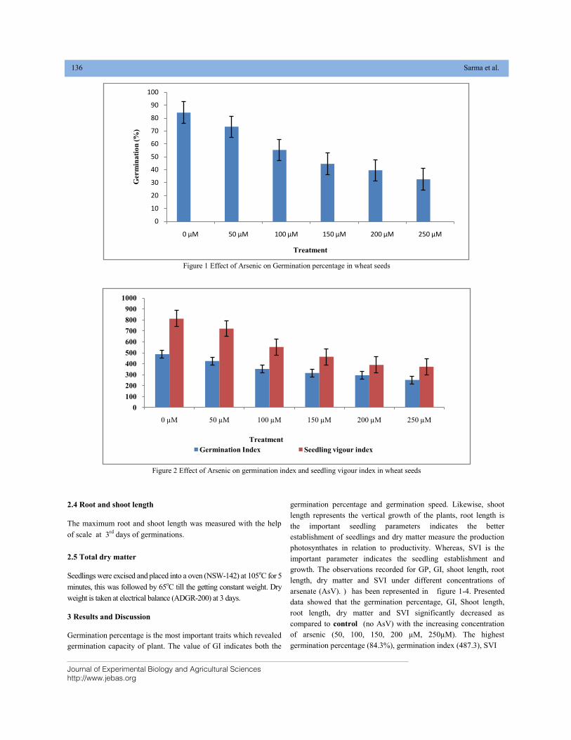
Journal of Experimental Biology and Agricultural Sciences
http://www.jebas.org
136 Sarma et al.
2.4 Root and shoot length
The maximum root and shoot length was measured with the help
of scale at 3rd
days of germinations.
2.5 Total dry matter
Seedlings were excised and placed into a oven (NSW-142) at 105oC for 5
minutes, this was followed by 65oC till the getting constant weight. Dry
weight is taken at electrical balance (ADGR-200) at 3 days.
3 Results and Discussion
Germination percentage is the most important traits which revealed
germination capacity of plant. The value of GI indicates both the
germination percentage and germination speed. Likewise, shoot
length represents the vertical growth of the plants, root length is
the important seedling parameters indicates the better
establishment of seedlings and dry matter measure the production
photosynthates in relation to productivity. Whereas, SVI is the
important parameter indicates the seedling establishment and
growth. The observations recorded for GP, GI, shoot length, root
length, dry matter and SVI under different concentrations of
arsenate (AsV). ) has been represented in figure 1-4. Presented
data showed that the germination percentage, GI, Shoot length,
root length, dry matter and SVI significantly decreased as
compared to control (no AsV) with the increasing concentration
of arsenic (50, 100, 150, 200 µM, 250µM). The highest
germination percentage (84.3%), germination index (487.3), SVI
Figure 1 Effect of Arsenic on Germination percentage in wheat seeds
Figure 2 Effect of Arsenic on germination index and seedling vigour index in wheat seeds
0
10
20
30
40
50
60
70
80
90
100
0 µM 50 µM 100 µM 150 µM 200 µM 250 µM
Ger
min
ati
on
(%
)
Treatment
0
100
200
300
400
500
600
700
800
900
1000
0 µM 50 µM 100 µM 150 µM 200 µM 250 µM
Germination Index Seedling vigour index
Treatment
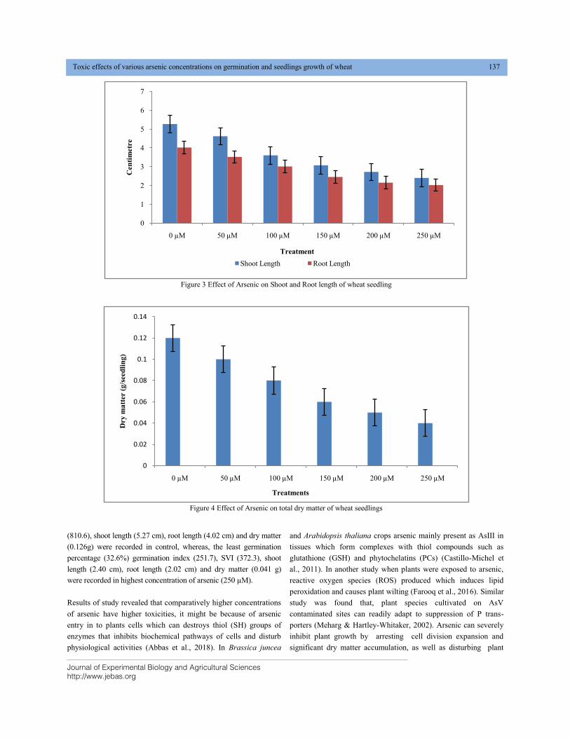
Journal of Experimental Biology and Agricultural Sciences
http://www.jebas.org
Toxic effects of various arsenic concentrations on germination and seedlings growth of wheat 137
(810.6), shoot length (5.27 cm), root length (4.02 cm) and dry matter
(0.126g) were recorded in control, whereas, the least germination
percentage (32.6%) germination index (251.7), SVI (372.3), shoot
length (2.40 cm), root length (2.02 cm) and dry matter (0.041 g)
were recorded in highest concentration of arsenic (250 µM).
Results of study revealed that comparatively higher concentrations
of arsenic have higher toxicities, it might be because of arsenic
entry in to plants cells which can destroys thiol (SH) groups of
enzymes that inhibits biochemical pathways of cells and disturb
physiological activities (Abbas et al., 2018). In Brassica juncea
and Arabidopsis thaliana crops arsenic mainly present as AsIII in
tissues which form complexes with thiol compounds such as
glutathione (GSH) and phytochelatins (PCs) (Castillo-Michel et
al., 2011). In another study when plants were exposed to arsenic,
reactive oxygen species (ROS) produced which induces lipid
peroxidation and causes plant wilting (Farooq et al., 2016). Similar
study was found that, plant species cultivated on AsV
contaminated sites can readily adapt to suppression of P trans-
porters (Meharg & Hartley-Whitaker, 2002). Arsenic can severely
inhibit plant growth by arresting cell division expansion and
significant dry matter accumulation, as well as disturbing plant
Figure 3 Effect of Arsenic on Shoot and Root length of wheat seedling
Figure 4 Effect of Arsenic on total dry matter of wheat seedlings
0
1
2
3
4
5
6
7
0 µM 50 µM 100 µM 150 µM 200 µM 250 µM
Cen
tim
etr
e
Treatment
Shoot Length Root Length
0
0.02
0.04
0.06
0.08
0.1
0.12
0.14
0 µM 50 µM 100 µM 150 µM 200 µM 250 µM
Dry
ma
tter (
g/s
eed
lin
g)
Treatments
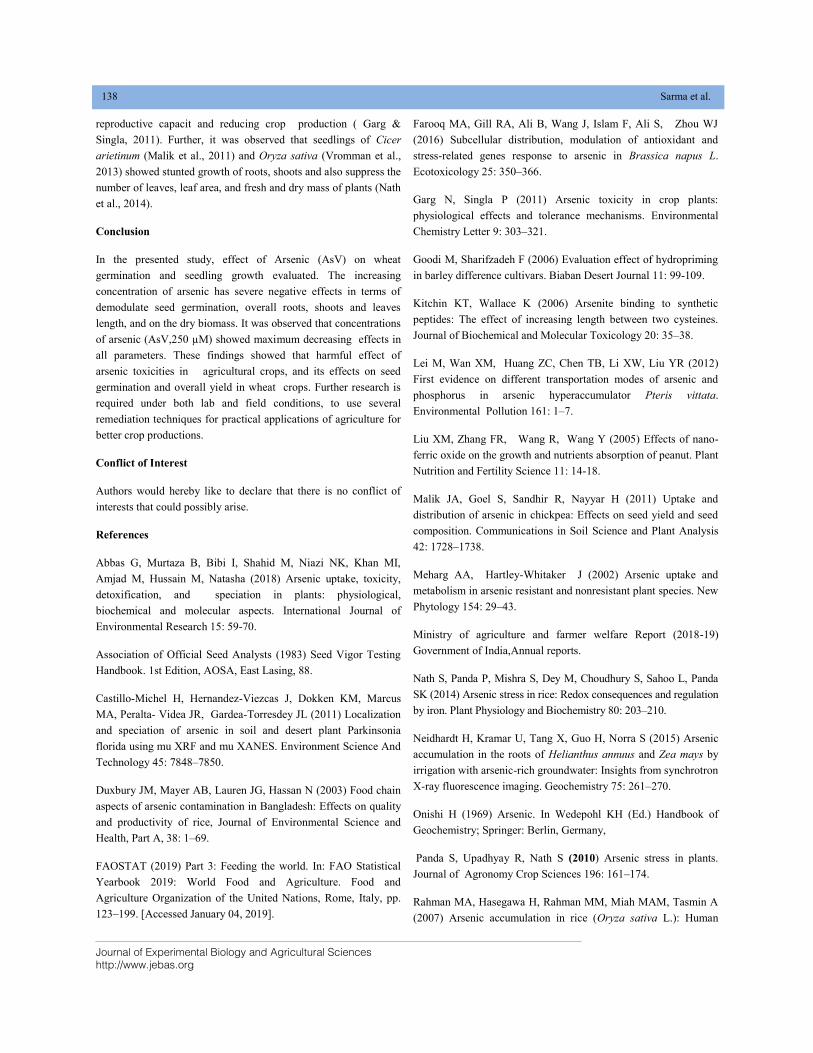
Journal of Experimental Biology and Agricultural Sciences
http://www.jebas.org
138 Sarma et al.
reproductive capacit and reducing crop production ( Garg &
Singla, 2011). Further, it was observed that seedlings of Cicer
arietinum (Malik et al., 2011) and Oryza sativa (Vromman et al.,
2013) showed stunted growth of roots, shoots and also suppress the
number of leaves, leaf area, and fresh and dry mass of plants (Nath
et al., 2014).
Conclusion
In the presented study, effect of Arsenic (AsV) on wheat
germination and seedling growth evaluated. The increasing
concentration of arsenic has severe negative effects in terms of
demodulate seed germination, overall roots, shoots and leaves
length, and on the dry biomass. It was observed that concentrations
of arsenic (AsV,250 µM) showed maximum decreasing effects in
all parameters. These findings showed that harmful effect of
arsenic toxicities in agricultural crops, and its effects on seed
germination and overall yield in wheat crops. Further research is
required under both lab and field conditions, to use several
remediation techniques for practical applications of agriculture for
better crop productions.
Conflict of Interest
Authors would hereby like to declare that there is no conflict of
interests that could possibly arise.
References
Abbas G, Murtaza B, Bibi I, Shahid M, Niazi NK, Khan MI,
Amjad M, Hussain M, Natasha (2018) Arsenic uptake, toxicity,
detoxification, and speciation in plants: physiological,
biochemical and molecular aspects. International Journal of
Environmental Research 15: 59-70.
Association of Official Seed Analysts (1983) Seed Vigor Testing
Handbook. 1st Edition, AOSA, East Lasing, 88.
Castillo-Michel H, Hernandez-Viezcas J, Dokken KM, Marcus
MA, Peralta- Videa JR, Gardea-Torresdey JL (2011) Localization
and speciation of arsenic in soil and desert plant Parkinsonia
florida using mu XRF and mu XANES. Environment Science And
Technology 45: 7848–7850.
Duxbury JM, Mayer AB, Lauren JG, Hassan N (2003) Food chain
aspects of arsenic contamination in Bangladesh: Effects on quality
and productivity of rice, Journal of Environmental Science and
Health, Part A, 38: 1–69.
FAOSTAT (2019) Part 3: Feeding the world. In: FAO Statistical
Yearbook 2019: World Food and Agriculture. Food and
Agriculture Organization of the United Nations, Rome, Italy, pp.
123–199. [Accessed January 04, 2019].
Farooq MA, Gill RA, Ali B, Wang J, Islam F, Ali S, Zhou WJ
(2016) Subcellular distribution, modulation of antioxidant and
stress-related genes response to arsenic in Brassica napus L.
Ecotoxicology 25: 350–366.
Garg N, Singla P (2011) Arsenic toxicity in crop plants:
physiological effects and tolerance mechanisms. Environmental
Chemistry Letter 9: 303–321.
Goodi M, Sharifzadeh F (2006) Evaluation effect of hydropriming
in barley difference cultivars. Biaban Desert Journal 11: 99-109.
Kitchin KT, Wallace K (2006) Arsenite binding to synthetic
peptides: The effect of increasing length between two cysteines.
Journal of Biochemical and Molecular Toxicology 20: 35–38.
Lei M, Wan XM, Huang ZC, Chen TB, Li XW, Liu YR (2012)
First evidence on different transportation modes of arsenic and
phosphorus in arsenic hyperaccumulator Pteris vittata.
Environmental Pollution 161: 1–7.
Liu XM, Zhang FR, Wang R, Wang Y (2005) Effects of nano-
ferric oxide on the growth and nutrients absorption of peanut. Plant
Nutrition and Fertility Science 11: 14-18.
Malik JA, Goel S, Sandhir R, Nayyar H (2011) Uptake and
distribution of arsenic in chickpea: Effects on seed yield and seed
composition. Communications in Soil Science and Plant Analysis
42: 1728–1738.
Meharg AA, Hartley-Whitaker J (2002) Arsenic uptake and
metabolism in arsenic resistant and nonresistant plant species. New
Phytology 154: 29–43.
Ministry of agriculture and farmer welfare Report (2018-19)
Government of India,Annual reports.
Nath S, Panda P, Mishra S, Dey M, Choudhury S, Sahoo L, Panda
SK (2014) Arsenic stress in rice: Redox consequences and regulation
by iron. Plant Physiology and Biochemistry 80: 203–210.
Neidhardt H, Kramar U, Tang X, Guo H, Norra S (2015) Arsenic
accumulation in the roots of Helianthus annuus and Zea mays by
irrigation with arsenic-rich groundwater: Insights from synchrotron
X-ray fluorescence imaging. Geochemistry 75: 261–270.
Onishi H (1969) Arsenic. In Wedepohl KH (Ed.) Handbook of
Geochemistry; Springer: Berlin, Germany,
Panda S, Upadhyay R, Nath S (2010) Arsenic stress in plants.
Journal of Agronomy Crop Sciences 196: 161–174.
Rahman MA, Hasegawa H, Rahman MM, Miah MAM, Tasmin A
(2007) Arsenic accumulation in rice (Oryza sativa L.): Human
Journal of Experimental Biology and Agricultural Sciences
http://www.jebas.org
Toxic effects of various arsenic concentrations on germination and seedlings growth of wheat 139
exposure through food chain. Ecotoxicology and Environmental
safety 69: 317–324.
Ranal MA, Santana DG (2006) How and why to measure the
germination process? Brazil journal of Botany 29: 1-11.
Srivastava S, Suprasanna P, D’Souza SF (2011) Redox state and
energetic equilibrium determine the magnitude of stress in Hydrilla
verticillata upon exposure to arsenate. Protoplasma 48:805–815.
Vromman D, Lutts S, Lefèvre I, Somer L, De Vreese O, Šlejkovec
Z, Quinet M (2013) Effects of simultaneous arsenic and iron
toxicities on rice (Oryza sativa L.) development, yield-related
parameters and As and Fe accumulation in relation to As
speciation in the grains. Plant and Soil 371: 199–217.
Zhao FJ, McGrath SP, Meharg AA (2010) Arsenic as a food chain
contaminant: mechanisms of plant uptake and metabolism and
mitigation strategies. Plant Biology 61:535–559.
Journal of Experimental Biology and Agricultural Sciences
http://www.jebas.org
ISSN No. 2320 – 8694
Journal of Experimental Biology and Agricultural Sciences, April - 2020; Volume – 8(2) page 140 – 147
AGRO-MORPHOLOGICAL CHARACTERIZATION OF AFRICAN RICE ACCESSIONS
(Oryza glaberrima) IN RAINFED AND IRRIGATED CULTURAL CONDITIONS
Claude GNACADJA*,1,2, Balbine FAGLA AMOUSSOU2, Saïdou SALL6, Baboucar MANNEH5,
Benjamin TOULOU3, Florentin AMETONOU5, Jean MOREIRA3, Paulin AZOKPOTA1,2, Moussa SIE4
1Laboratory of Molecular Biology and Food Formulation; Nutrition, Food and Technologies Sciences School, Faculty of Agricultural Sciences, Abomey Calavi University, Benin
2Laboratory of Food Sciences; Nutrition, Food and Technologies Sciences School, Faculty of Agricultural Sciences, Abomey Calavi University, Benin
3Africa Rice Center (Africa Rice), Benin
4Africa Rice Center (Africa Rice), Madagascar
5Africa Rice Center (Africa Rice), Senegal
6Training and Research Unit in Agricultural Sciences, Aquaculture and Food Technologies, GASTON BERGER University, Saint-Louis, Senegal
Received – June 24, 2019; Revision – September 14, 2019; Accepted – April 14, 2020 Available Online – April 25, 2020
DOI: http://dx.doi.org/10.18006/2020.8(2).140.147
ABSTRACT
African rice is used for its resistance to diseases and stresses, to improve Asian species. Unfortunately,
its culture is greatly neglected in favor of Asian varieties and because of this only many African rice
varieties is literally on the way of extinction. Due to its potential, it is important to preserve this
agricultural resource. This work aims primarily at doing agro-morphological characterization of African
rice accessions in the perspective to identify the useful varieties of Oryza glaberrima for future
exploitation. This study was carried out at the Africa Rice Center sites in Republic of Benin and
Senegal, for this 235 African rice accessions including two controls (CG14, NERICA4) have been
observed during rainfed (Benin) and irrigated (Senegal) culture using “Augmented design in randomized
complete block” method. Result of study revealed that all accessions completed their life cycle; among
the tested accessions, 22 were reported as O. sativa and interspecific accessions while reset 213
accessions were phenotypically identified as O.glaberrima. The discriminate variables of PCA (based
on the 9 main parameters) of 213 O.glaberrima accessions, leaded to a dendrogram with two clusters:
cluster I (114 accessions) is characterized by the precocity of their cycle: it can be used as an important
* Corresponding author
KEYWORDS
Wheat
Arsenic
Germination
Seeds
Growth
E-mail: [email protected] (Claude GNACADJA)
Peer review under responsibility of Journal of Experimental Biology and
Agricultural Sciences.
All the articles published by Journal of Experimental
Biology and Agricultural Sciences are licensed under a
Creative Commons Attribution-NonCommercial 4.0
International License Based on a work at www.jebas.org.
Production and Hosting by Horizon Publisher India [HPI]
(http://www.horizonpublisherindia.in/).
All rights reserved.
Journal of Experimental Biology and Agricultural Sciences
http://www.jebas.org
Agro-morphological characterization of African rice accessions 141
1 Introduction
The rice (Oryza spp) is a basic food that provides 27% of the
energy intake in population of third world countries (FAO, 2004).
It is an important agricultural product for food in West
Africa, where 40% of needs are insured by the international market
(Mendez del Viflar & Bauer, 2013). Two species Oryza sativa
(Asian rice) and Oryza glaberrima Steud (African rice) are mainly
cultivated in Africa (Anonymous, 1991; Anonymous, 2002). The
African species is composed of several varieties used for a long
time in varietal improvement systems because of their potential for
resistance to diseases and drought (Africa Rice, 2010).
The introduction and rapid adoption of Asian rice varieties has,
on one hand, led to an increase in rice production resulting in a
positive impact on producer’s income (Obilana & Okumu,
2005 ), and on the other hand, abandonment of African rice.
However, the success of Asian and improved varieties does not
fully satisfy breeder’s ambitions and the expectations of
producers and consumers. There is still an unfavorable
difference between improvement varieties and their parent O.
glaberrima either in the form of resistance, tolerance to
cultural constraints (biotic and abiotic), or organoleptic and
nutritional quality (Futakuchi & Sié, 2009; Africa Rice, 2010).
These observations challenges breeders to improve the abilities
of native varieties (interspecific) being created and tested under
various growing conditions (rainfed, lowland, irrigated, etc.) so
that they can better adapted, more productive and accepted by
consumers. The use of parents such as the O. glaberrima was
therefore indispensable, since they constitute the very basis of
the creation of interspecific varieties.
Domestication, gene flow and natural introgression are interspecies
phenomena that can affect over time the diversity of rice species.
In West Africa, due to its abandonment, very few studies have
focused on characterization of the African rice in varied growing
conditions. This study would make it possible to better evaluate,
with a wide range of agro-morphological indicators, the agronomic
potentials of the African rice. This work, in context of a research
project about the valorization of African rice, aims mainly to
identify the successful accessions of African rice useful for varietal
improvement systems, through a hierarchical classification based
on agronomic descriptors. The results will not only complete the
list of characterized African rice varieties, but also ensure the use
of its diversity for the development of new rice varieties.
2 Materiel and Methods
2.1 Test sites
Two sites namely “the Africa Rice station of Cotonou (Benin)” for
rainfed test (between October and January) and “the Africa Rice
station of Sahel (Ndiaye, Saint Louis, Senegal)”, for irrigated test
(between September and December) were exploited for testing.
2.2 Materials
It consists of 235 accessions of African rice collected in the
villages of Danyi in Togo (in August and December 2008) and
two controls (CG 14, NERICA4) having all been subjected to the
germination test.
2.3 Experimental Setup
The setup used for the implementation of the two tests is built
according to the method "Augmented Design in Randomized
Complete Block" described by Nokoe (2001). This test has been
used because of the high number of accessions while the quantity
of seed is very limited (about 5g). The method consists in
designing a device in which only the controls are repeated in each
block (Sharma, 1988), to be used for the estimation of the
experimental error and the block effect. 24 blocks of 10 entries and
two witnesses, totaling 12 entries per block were designed. Each
elementary plot has a density of 42 plants 20cm apart between the
lines and on the lines. The elementary plots (1.68 m2 of area) are
separated by a path of 30cm.
2.4 Agronomic Practices
2.4.1 For rainfed crops (Benin)
Sowing was carried out in a line by a direct method at the rate of 2
seeds per plant, with a separation (after two weeks) at one plant.
Only basic fertilizer NPK (10-18-18) is applied at the rate of 100
kg / ha at seeding. Irrigation was carried out with a watering
system and weeding was carried out manually.
2.4.2 For irrigated crops (Senegal)
The seeds were pre-germinated at artificial incubator at 30°C for
48 hours. Seedlings were transfer in to pots in greenhouse
conditions. Nine (09) days after sowing, the pots were removed
from the greenhouse and exposed to natural conditions for
trait for variety selection. Cluster II (99 accessions including CG14 and NERICA4) is characterized by
the strong production yield. These results allow us to have a collection of O. glaberrima accessions in
order to study not only its genetic diversity but also to evaluate more potential of these varieties for
exploiting their genetic and nutritional advantage for the development of new varieties.
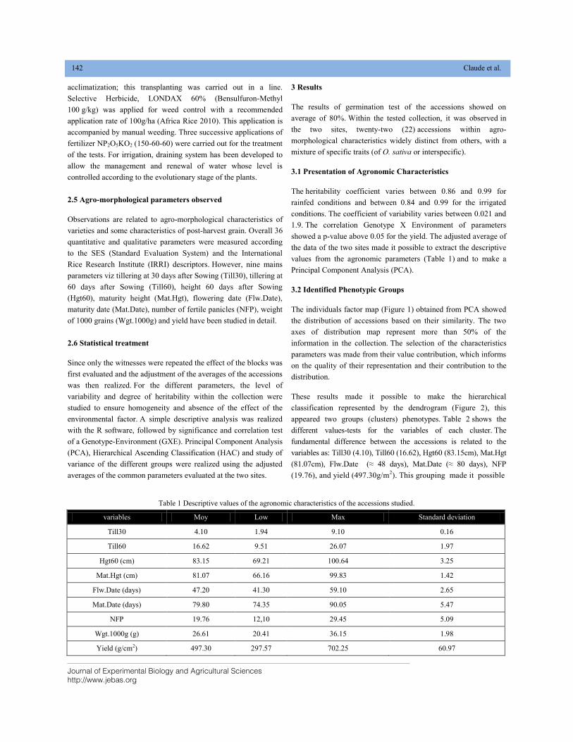
Journal of Experimental Biology and Agricultural Sciences
http://www.jebas.org
142 Claude et al.
acclimatization; this transplanting was carried out in a line.
Selective Herbicide, LONDAX 60% (Bensulfuron-Methyl
100 g/kg) was applied for weed control with a recommended
application rate of 100g/ha (Africa Rice 2010). This application is
accompanied by manual weeding. Three successive applications of
fertilizer NP2O5KO2 (150-60-60) were carried out for the treatment
of the tests. For irrigation, draining system has been developed to
allow the management and renewal of water whose level is
controlled according to the evolutionary stage of the plants.
2.5 Agro-morphological parameters observed
Observations are related to agro-morphological characteristics of
varieties and some characteristics of post-harvest grain. Overall 36
quantitative and qualitative parameters were measured according
to the SES (Standard Evaluation System) and the International
Rice Research Institute (IRRI) descriptors. However, nine mains
parameters viz tillering at 30 days after Sowing (Till30), tillering at
60 days after Sowing (Till60), height 60 days after Sowing
(Hgt60), maturity height (Mat.Hgt), flowering date (Flw.Date),
maturity date (Mat.Date), number of fertile panicles (NFP), weight
of 1000 grains (Wgt.1000g) and yield have been studied in detail.
2.6 Statistical treatment
Since only the witnesses were repeated the effect of the blocks was
first evaluated and the adjustment of the averages of the accessions
was then realized. For the different parameters, the level of
variability and degree of heritability within the collection were
studied to ensure homogeneity and absence of the effect of the
environmental factor. A simple descriptive analysis was realized
with the R software, followed by significance and correlation test
of a Genotype-Environment (GXE). Principal Component Analysis
(PCA), Hierarchical Ascending Classification (HAC) and study of
variance of the different groups were realized using the adjusted
averages of the common parameters evaluated at the two sites.
3 Results
The results of germination test of the accessions showed on
average of 80%. Within the tested collection, it was observed in
the two sites, twenty-two (22) accessions within agro-
morphological characteristics widely distinct from others, with a
mixture of specific traits (of O. sativa or interspecific).
3.1 Presentation of Agronomic Characteristics
The heritability coefficient varies between 0.86 and 0.99 for
rainfed conditions and between 0.84 and 0.99 for the irrigated
conditions. The coefficient of variability varies between 0.021 and
1.9. The correlation Genotype X Environment of parameters
showed a p-value above 0.05 for the yield. The adjusted average of
the data of the two sites made it possible to extract the descriptive
values from the agronomic parameters (Table 1) and to make a
Principal Component Analysis (PCA).
3.2 Identified Phenotypic Groups
The individuals factor map (Figure 1) obtained from PCA showed
the distribution of accessions based on their similarity. The two
axes of distribution map represent more than 50% of the
information in the collection. The selection of the characteristics
parameters was made from their value contribution, which informs
on the quality of their representation and their contribution to the
distribution.
These results made it possible to make the hierarchical
classification represented by the dendrogram (Figure 2), this
appeared two groups (clusters) phenotypes. Table 2 shows the
different values-tests for the variables of each cluster. The
fundamental difference between the accessions is related to the
variables as: Till30 (4.10), Till60 (16.62), Hgt60 (83.15cm), Mat.Hgt
(81.07cm), Flw.Date (≈ 48 days), Mat.Date (≈ 80 days), NFP
(19.76), and yield (497.30g/m2). This grouping made it possible
Table 1 Descriptive values of the agronomic characteristics of the accessions studied.
variables Moy Low Max Standard deviation
Till30 4.10 1.94 9.10 0.16
Till60 16.62 9.51 26.07 1.97
Hgt60 (cm) 83.15 69.21 100.64 3.25
Mat.Hgt (cm) 81.07 66.16 99.83 1.42
Flw.Date (days) 47.20 41.30 59.10 2.65
Mat.Date (days) 79.80 74.35 90.05 5.47
NFP 19.76 12,10 29.45 5.09
Wgt.1000g (g) 26.61 20.41 36.15 1.98
Yield (g/cm2) 497.30 297.57 702.25 60.97
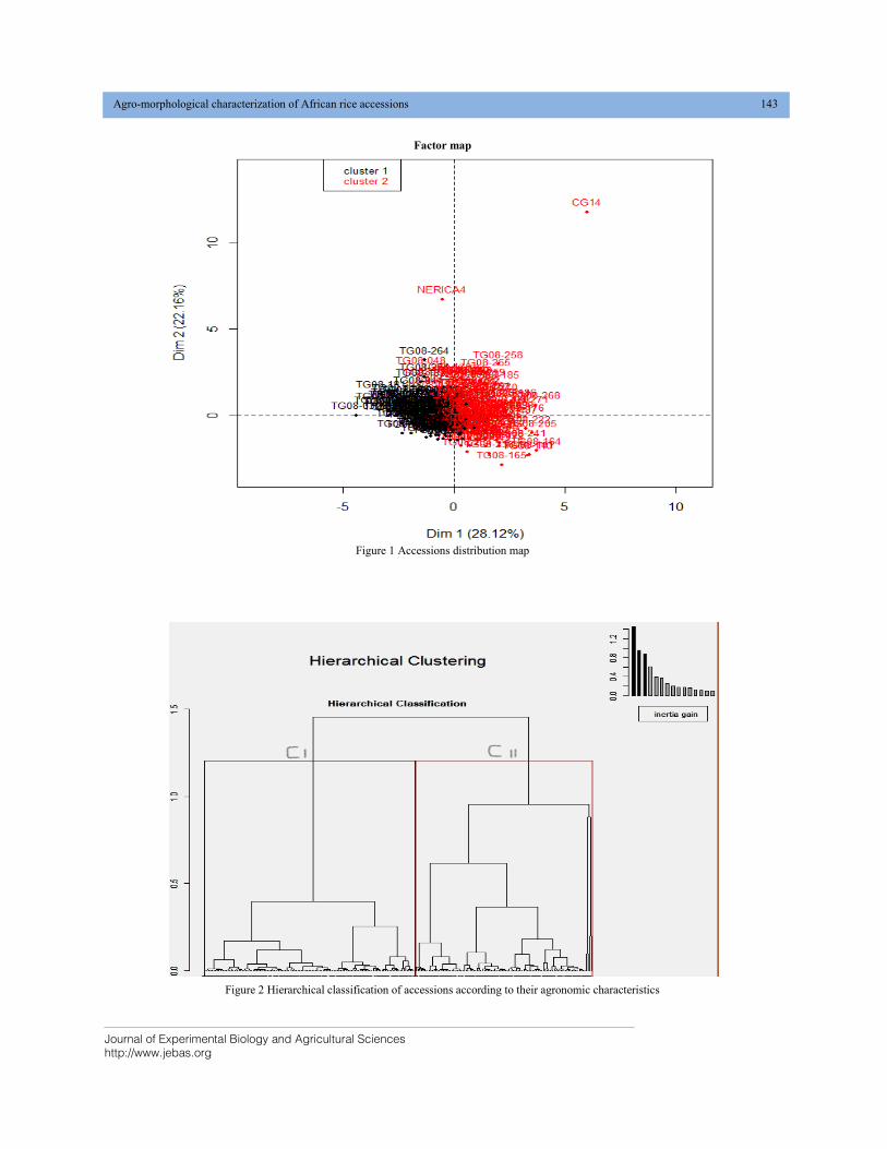
Journal of Experimental Biology and Agricultural Sciences
http://www.jebas.org
Agro-morphological characterization of African rice accessions 143
Factor map
Figure 1 Accessions distribution map
Figure 2 Hierarchical classification of accessions according to their agronomic characteristics
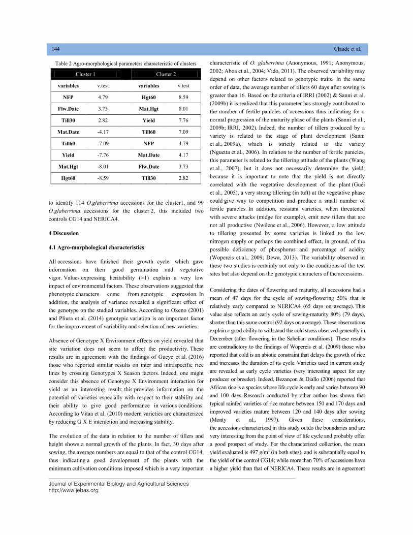
Journal of Experimental Biology and Agricultural Sciences
http://www.jebas.org
144 Claude et al.
to identify 114 O.glaberrima accessions for the cluster1, and 99
O.glaberrima accessions for the cluster 2, this included two
controls CG14 and NERICA4.
4 Discussion
4.1 Agro-morphological characteristics
All accessions have finished their growth cycle: which gave
information on their good germination and vegetative
vigor. Values expressing heritability (≈1) explain a very low
impact of environmental factors. These observations suggested that
phenotypic characters come from genotypic expression. In
addition, the analysis of variance revealed a significant effect of
the genotype on the studied variables. According to Okeno (2001)
and Pliura et al. (2014) genotypic variation is an important factor
for the improvement of variability and selection of new varieties.
Absence of Genotype X Environment effects on yield revealed that
site variation does not seem to affect the productivity. These
results are in agreement with the findings of Gueye et al. (2016)
those who reported similar results on inter and intraspecific rice
lines by crossing Genotypes X Season factors. Indeed, one might
consider this absence of Genotype X Environment interaction for
yield as an interesting result; this provides information on the
potential of varieties especially with respect to their stability and
their ability to give good performance in various conditions.
According to Vitaa et al. (2010) modern varieties are characterized
by reducing G X E interaction and increasing stability.
The evolution of the data in relation to the number of tillers and
height shows a normal growth of the plants. In fact, 30 days after
sowing, the average numbers are equal to that of the control CG14,
thus indicating a good development of the plants with the
minimum cultivation conditions imposed which is a very important
characteristic of O. glaberrima (Anonymous, 1991; Anonymous,
2002; Aboa et al., 2004; Vido, 2011). The observed variability may
depend on other factors related to genotypic traits. In the same
order of data, the average number of tillers 60 days after sowing is
greater than 16. Based on the criteria of IRRI (2002) & Sanni et al.
(2009b) it is realized that this parameter has strongly contributed to
the number of fertile panicles of accessions thus indicating for a
normal progression of the maturity phase of the plants (Sanni et al.,
2009b; IRRI, 2002). Indeed, the number of tillers produced by a
variety is related to the stage of plant development (Sanni
et al., 2009a), which is strictly related to the variety
(Nguetta et al., 2006). In relation to the number of fertile panicles,
this parameter is related to the tillering attitude of the plants (Wang
et al., 2007), but it does not necessarily determine the yield,
because it is important to note that the yield is not directly
correlated with the vegetative development of the plant (Guéi
et al., 2005), a very strong tillering (in tuft) at the vegetative phase
could give way to competition and produce a small number of
fertile panicles. In addition, resistant varieties, when threatened
with severe attacks (midge for example), emit new tillers that are
not all productive (Nwilene et al., 2006). However, a low attitude
to tillering presented by some varieties is linked to the low
nitrogen supply or perhaps the combined effect, in ground, of the
possible deficiency of phosphorus and percentage of acidity
(Wopereis et al., 2009; Dewa, 2013). The variability observed in
these two studies is certainly not only to the conditions of the test
sites but also depend on the genotypic characters of the accessions.
Considering the dates of flowering and maturity, all accessions had a
mean of 47 days for the cycle of sowing-flowering 50% that is
relatively early compared to NERICA4 (65 days on average). This
value also reflects an early cycle of sowing-maturity 80% (79 days),
shorter than this same control (92 days on average). These observations
explain a good ability to withstand the cold stress observed generally in
December (after flowering in the Sahelian conditions). These results
are contradictory to the findings of Wopereis et al. (2009) those who
reported that cold is an abiotic constraint that delays the growth of rice
and increases the duration of its cycle. Varieties used in current study
are revealed as early cycle varieties (very interesting aspect for any
producer or breeder). Indeed, Bezançon & Diallo (2006) reported that
African rice is a species whose life cycle is early and varies between 90
and 100 days. Research conducted by other author has shown that
typical rainfed varieties of rice mature between 150 and 170 days and
improved varieties mature between 120 and 140 days after sowing
(Monty et al., 1997). Given these considerations,
the accessions characterized in this study outdo the boundaries and are
very interesting from the point of view of life cycle and probably offer
a good prospect of study. For the characterized collection, the mean
yield evaluated is 497 g/m2 (in both sites), and is substantially equal to
the yield of the control CG14; while more than 70% of accessions have
a higher yield than that of NERICA4. These results are in agreement
Table 2 Agro-morphological parameters characteristic of clusters
Cluster 1
Cluster 2
variables v.test
variables v.test
NFP 4.79
Hgt60 8.59
Flw.Date 3.73
Mat.Hgt 8.01
Till30 2.82 Yield 7.76
Mat.Date -4.17
Till60 7.09
Till60 -7.09
NFP 4.79
Yield -7.76 Mat.Date 4.17
Mat.Hgt -8.01
Flw.Date 3.73
Hgt60 -8.59
TIll30 2.82
Journal of Experimental Biology and Agricultural Sciences
http://www.jebas.org
Agro-morphological characterization of African rice accessions 145
with the assertions of Linares (2002) who estimates the productivity of
African rice varieties (O. glaberrima) and reported lower yield. These
observations explain a relative control of chattering, lodging incidence
and pests; these factors being controlled by fillets, bird hunters and
border plants during agronomic test. In fact, lodging incidence and
chattering are the factors of the low yield potential of African rice
(Futakuchi & Sié, 2009). Similar results were observed by Africa Rice
(2010) and Aboa et al. (2004), those who suggested that water lodging
and chattering are the major limiting factors for O.
glaberrima varieties. The exsertion panicle also contributes to the
reduction of damage. Indeed, a good exsertion of the panicle is a
characteristic of weak attack of blast on the neck of the panicle and a
good maturation of the spikelets (Jacquot, 1974). This character
obviously favored the absence of damage due to blast and maturation
of grain that improved yields. This study revealed that there are
still accessions of African rice that can have strong yield potential.
4.2 Phenotypic groups identified
The classification of the accessions showed two groups (cluster1
and cluster2). The fundamental difference was reported between
the studied accessions. Studied nine characteristics are well
discriminating the selected African rice collection. Previous
studies conducted on agronomic characteristics revealed that
height of plant and tillering ability are essential characteristics
which can discriminate rice populations (Ogunbayo
et al., 2007; Ojo et al., 2009; Moukoumbi et al., 2011). Current
study identified two clusters, among these, cluster I have 114
accessions while cluster II have 99 accession of African rice, this
cluster also have two controls CG14 and NERICA4. The values-
test (v-test) obtained made it possible to distinguish the variables
that strongly characterize the accessions of each
cluster. Indeed, cluster 1 groups more than half of the accessions,
and the two clusters are strongly characterized by tillering 60
days after sowing (Till60), height of plant (at 60 days after
sowing and at maturity) and yield. For these variables, the
accessions of cluster 1 have their averages relatively lower than
the average of the entire collection; on the other hand, the
accessions of cluster 2 are characterized by their average values
above the average of the entire collection. Concerning the
variable « precocious of the cycle », which is an interesting and
exploitable trait for the varietal selection, the accessions of the
cluster 1 are revealed very early, with sowing-flowering and
sowing-maturity cycles very short compared to the average of the
collection. Results of current study are contradictory to the
findings of Montcho et al. (2017) those who reported that O.
sativa has a shorter life cycle than O. glaberrima. According to
Takeshi (2007), the vegetative cycle is an important factor that
can be used as a control parameter for climatic factors and
pests. The cycle time of a rice variety is strongly related to its
photoperiod sensitivity and depends mainly on the duration of its
basic vegetative phase (Dingkuhn & Asch, 1999).
Conclusion
The results of this study reveal that the collection is composed
of O. glaberrima accessions grouping according to agronomic
performance in two clusters. The characteristics of the hierarchical
groups show that these varieties present an appreciable agronomic
performance with the capacity to develop under several constraints
associated with several ecosystems such as the rainfed and the irrigated
cultural condition. Globally, the accessions of cluster 1 seem to be the
most interesting, owing to their good performance in different
conditions (sites and seasons) and their precocious cycle. It is favorable
materials for further study because these genotypes have good
environmental adaptation, higher productivity, high and stable yields.
This collection constitutes a reservoir of interesting genes, which
explains its use in variety improvement programs. These results give
an opening on the study of the nutritional values in order to reveal over
assets for the valorization of the African rice O. glaberrima.
Acknowledgment
Authors are thankful to competent authorities of Africa Rice,
HAAGRIM Project which is funded by the European Union
Conflict of interest
There is no conflict of interest for the publication of this article.
References
Aboa K, Tamaka K, Dantsey-Barry H (2004) Multiplication and
characterization of rice ecotypes. Activity Report, Lomé, ITRA, Pp.3.
AfricaRice (2010) New Breeding Directions at AfricaRice:
Beyond NERICA. Cotonou, Benin: Pp.24.
Anonymous (1991) Memento of the agronomist. Paris, Ministry of
Cooperation and Development, Pp.687-716 (1635 p).
Anonymous (2002) Memento de l'agrronome, Ministry of Foreign
Affairs - CIRAD -GRET; Pp.799 - 811 (1687 p).
Bezançon G, Diallo S (2006) Oryza glaberrima Steud. [Internet]
Protabase sheet. In: Brink M, Belay G (Eds). PROTA (Plant
Resources of Tropical Africa/Plant Resources of Tropical Africa),
Wageningen, the Netherlands, available on
http://database.prota.org/recherche.htm. Access on June 2014.
Dewa KMK (2013) Agro-morphological characterization of
African rice accessions (Oryza glaberrima steud.) Collected on the
Danyi plateau in Togo. Memory of DEA School of Agronomy
University of Lome Order no.: 023 / SAGE / 13.
Dingkuhn M, Asch F (1999) Phenological responses of Oryza
sativa, O. glaberrima and inter-specific rice cultivars are described
in West Africa. Euphytica 110: 109-126.
Journal of Experimental Biology and Agricultural Sciences
http://www.jebas.org
146 Claude et al.
FAO (2004) Food and Agriculture Organization of the United
Nations. International Year of Rice. Rice is life.
Futakuchi K, Sie M (2009) Better Exploitation of African Rice
(Oryza glaberrima Steud) in Varietal Development for
Resource-Poor Farmers in West and Central
Africa. Agricultural Journal 4: 96 - 102.
Guei GR, Sanni KA, Abamu FS, Fawole I (2005) Genetic diversity
of rice (Oryza sativa L.) Landraces from Ivory Coast. African
Agronomy 5: 17-28.
Gueye T, Saliou N, Abdoulaye D (2016) Evaluation of intra and
inter specific rice lines in irrigated conditions in
Senegal. International Journal of Biological and Chemical
Sciences 10 : 232-241.
IRRI (2002) Standard Evaluation System (SES), International Rice
Research Institute, Pp.65.
Jacquot M (1974) Gene systems controlling a short plant size for
varietal improvement of rainfed rice. Tropical Agronomy,
vol. XXIX, Pp.911-6.
Linares OF (2002) African rice (Oryza glaberrima): History and
future potential. Proceedings of the National Academy of
Sciences, USA, 99:16360-16365.
Mendez Del Villar P, Bauer JM (2013) Rice in West Africa:
dynamics, policies and perspectives. Cahier d’ Agriculture 22:
336-44. doi: 10.1684 / a9r.2013.0657.
Montcho D, Gbenou P, Missihoun AA, Futakuchi K, Ahanhanzo
C, Agbangla C (2017) Comparative study of two rice cultivars
(Oryza glaberrima and O. sativa) under different cultural
conditions. Journal of Experimental Biology and Agricultural
Sciences 5: 45-53.
Monty PJ, Dingkhun M, Aluko G, Mande S (1997)
"Interspecific Oryza sativa L. x O. glaberrima steud, Progenies
in upland rice improvement". Euphytica 92: 237-246.
Moukoumbi YD, Sié M, Vodouhe R, N'dri B, Toulou B,
Ogunbayo SA, Ahanchede A (2011) Assessing phenotypic
diversity of interspecific rice varieties using agromorphological
characterization. Journal of Plant Breeding and Crop Science 3:
74-86.
Nguetta ASP, Guéi RG, Diatta S (2006) Contribution to the
identification of successful varieties of rainfed rice (Oryza sp.)
in the subequatorial region of Congo Brazzaville. Africa
Science 02: 352-364.
Nokoe S (2001) Augmented block Design (ABD): The choice for
large scale farmer participatory on-farm trials, Available on
http://www.unu.edu/enu/plec access on August 2014.
Nwilene FE, Nwanze KF, Okhidievbie O (2006) African Rice Gall
Midge: Biology, Ecology and Control. Field Guide and Technical
Manual. Africa Rice Center WARDA, Pp.20.
Obilana AB, Okumu BN (2005) Evaluation Study Report for
Interspecific Hybridization between African and Asian Rice
Species. African rice center (WARDA) Cotonou, Benin; Available
on http // www.warda.org / publications / UNDP% 20 Report /
UNDP% 20 Report. Pdf access on September 2016
Ogunbayo SA, Ojo DK, Popoola AR, Ariyo OJ, Sié M
(2007) Genetic comparison of landrace rice accessions by
morphological and technical RAPDs. Asian Journal of Plant
Sciences 6: 653-666.
Ojo DK, Ogunbayo SA, Sanni AK, Guei RG (2009) The
Determination of Diversity and Relationships of the Sorrows
(Oryza sativa L ) accessions by comparative analysis of
morphological and RAPD data Pp.12.
Okeno JA (2001) Genotypic variation in morphological traits of
barley as affected by nitrogen supply. In: Horst WJ (Ed.) Nutrition
-Food Security and Sustainability of Agro-Ecosystems. Kluwer
Academic Publishers, Pp.64-65.
Pliura A, Suchockas V, Sarsekova D, Gudynaita V
(2014) Genotypic variation and heritability of growth and adaptive
traits, and adaptation of young poplar hybrids at northern margins
of natural distribution of Populusnigra in Europe. Biomass and
Bioenergy, 70: 513-529.
Sanni KA, Ariyo OJ, Ojo DK, Gregorio G, Somado EA, Sanchez I,
Sie M, Futakuchi K, Ogunbayo SA, Guei RG, Wopereis MCS
(2009b) Additives and Multiplicative Interactions Analysis of
Grain Yield Performances in Rice Genotypes across
Environments. Asian Journal of Plant Science 8: 48-53.
Sanni KA, Ojo DK, Adebisi MA, Somado EA, Ariyo OJ, Sie M,
Akintayo I, Tia DD, Ogunbayo SA, Cisse B, Sikirou M, Adekoya
MA (2009a) Potential of interspecific NERICA Rice
varieties (Oryza glaberrima x Oryza sativa). International Journal
of Botany 5: 112-115.
Sharma JR (1998) Statistical and Biometrical Techniques in Plant
Breeding. New Age International (P) Limited Publishers, New
Delhi, Pp. 432 .
Takeshi I (2007) Adaptation of flowering time by natural and
artificial selection in Arabiodopsis and rice. Journal of
Experimental Botany 58:3097-3097.
Journal of Experimental Biology and Agricultural Sciences
http://www.jebas.org
Agro-morphological characterization of African rice accessions 147
Vido AA (2011) African rice (Oryza glaberrima Steudel), an
aspect of the rural history of the Gold Coast or the extension of the
area of "rice civilization" (XVII-XVIII centuries). Ivorian Journal
of History 19:41 - 60.
Vitaa PD, Mastrangeloa AM, Matteua L, Mazzucotellib E, Virzì N,
Palumboc M, Stortod ML, Rizzab F, Cattivelli L (2010) Genetic
improvement effects on yield stability in durum wheat genotypes
grown in Italy. Field Crops Research, 119: 68-77.
Wang F, Cheng F, Zhang GP (2007) Difference in Grain Yield and
Quality among Rice Tillers in Genotypes Differing in Tillering
Capacity. Rice Science 14: 135-140. DOI:
http://dx.doi.org/10.1016/S1672- 6308(07)60019-5.
Wopereis MCS, Defoer T, Idinoba P, Diack S Dugué MJ (2009)
Curriculum for Participatory Learning and Action Research
(PLAR) for Integrated Rice Management (IRM) in Inland Valleys
of Sub-Saharan Africa. Technical Manual African Rice, Pp.128.
Journal of Experimental Biology and Agricultural Sciences
http://www.jebas.org
ISSN No. 2320 – 8694
Journal of Experimental Biology and Agricultural Sciences, April - 2020; Volume – 8(2) page 148 – 156
GENETIC CHARACTERIZATION OF LOCAL RICE (Oryza sativa L.) GENOTYPES
AT MORPHOLOGICAL AND MOLECULAR LEVEL USING SSR MARKERS
Pooja Pathak, S. K. Singh, Mounika Korada*, Sonali Habde, D. K. Singh, Amrutlal Khaire,
Prasanta Kumar Majhi
Department of Genetics and Plant Breeding, Institute of Agricultural Sciences, Banaras Hindu University, Varanasi-221005, India.
Received – March 07, 2020; Revision – April 12, 2020; Accepted – April 21, 2020 Available Online – April 25, 2020
DOI: http://dx.doi.org/10.18006/2020.8(2).148.156
ABSTRACT
Current study was conducted to estimate the genetic diversity of 29 local rice cultivars including 3
checks at both morphological and molecular level during Kharif 2017 in an augmented design.
Significant results obtained from ANOVA of 29 genotypes for 16 quantitative traits; Mahalanobis’ D2
grouped the total genotypes into 6 clusters. Highest inter-cluster distance was found between clusters III
and VI indicating the genotypes in these clusters are most diverse. The SSR banding pattern revealed a
total of 65 alleles from 21 polymorphic markers across 29 rice genotypes with an average of 3.09
alleles. The polymorphism information content (PIC) values ranged from 0.701 (RM 277) to 0.346
(RM237) with a mean value of 0.571 showing the marker RM277 as best based on the above study. The
dendrogram analysis revealed all the 29 genotypes were grouped into two main clusters i.e. cluster I and
cluster II with dissimilarity coefficient 0.36. Both the clusters were further divided into two groups each
of which are further divide into two sub-groups each. Based on the genetic distances and the
dissimilarity coefficient obtained from both morphological and molecular analysis, genotypes like
Bahubali, Golden 105, Pusa 1121, HUR-1301, RK-2 Lal kasturi and Pan 815 can be selected and used
as parents due to their greater diversity. Knowledge of genetic diversity available within a population at
both morphological and molecular level helps the breeder to formulate a successful hybridization
programme and gain good results.
* Corresponding author
KEYWORDS
Genetic Diversity
Mahalanobis
Molecular markers
Rice
SSR
E-mail: [email protected] (Mounika Korada)
Peer review under responsibility of Journal of Experimental Biology and
Agricultural Sciences.
All the articles published by Journal of Experimental
Biology and Agricultural Sciences are licensed under a
Creative Commons Attribution-NonCommercial 4.0
International License Based on a work at www.jebas.org.
Production and Hosting by Horizon Publisher India [HPI]
(http://www.horizonpublisherindia.in/).
All rights reserved.
Journal of Experimental Biology and Agricultural Sciences
http://www.jebas.org
Genetic Characterization of Local Rice Genotypes 149
1 Introduction
Rice (Oryza sativa L.) is an annual grass of the family Poaceae
(graminae) with chromosome number 2n=24. Rice is being consumed
by more than half of the world’s population and serves as a major
source of carbohydrates. Having more amounts of carbohydrate, it
provides instant energy, and is a staple food that is consumed by the
majority of India’s population. Rice grain contains about 75-80%
starch, 12% water and 7% protein (Hossain et al., 2015). It is also an
important source of vitamins like thiamine, riboflavin and niacin and
minerals like magnesium, phosphorus and calcium. It is enormously
diverse both in the way it is cultivated and its usage by the humans.
Having the smallest genome of all cultivated cereals, being diploid and
self pollinating, it is the most extensively studied species among
cereals (Pooja et al., 2019). Among very few options for increasing
yield potential of rice, improvement of the genetic potential of the crop
cultivars is one of the best options. Rice has endowed with rich natural
genetic diversity and there is tremendous scope to exploit diversity for
improvement of the genetic base.
To encounter the existing food requirements, genetic diversity is a
natural source for rice breeding (Reig-Valiente et al., 2016). The higher
level of genetic variation present in a population, the more valuable
resource, is used for enlarging the genetic base of the breeding program
(Nachimuthu et al., 2015). This would help in development of
transgressive segregants which will perform better than both the
parents. In addition, Haritha et al., 2016 postulated that genetic
diversity obtained precious information for both basic studies and
practical applications.
Mahalanobis’s D2 statistic is a powerful tool in measuring the degree of
divergence between biological populations at genetic level and
provides a quantitative measure of association between geographic and
genetic diversity based on generalized distance. For the assessment of
genetic diversity, microsatellite or simple sequence repeat (SSR)
markers are considered as most amenable, as they are multi- allelic in
nature, highly informative, highly reproducible, have co-dominant
inheritance and provide extensive genomic coverage (McCouch et al.,
2002). SSR markers are able to detect great level of allelic diversity
and they have been extensively used to identify genetic variation
among rice subspecies. Keeping this in view, the present experiment
was conducted using 29 local rice genotypes to characterize the
morphological and molecular genetic diversity.
2 Materials and Methods
2.1 Plant material:
A total of twenty nine local rice genotypes including 3 checks were
grown in an augmented block design with three blocks having repeated
checks during Kharif 2017. The list of genotypes used in this
experiment is presented in table 1.
2.2 Morphological observations:
Data was recorded on sixteen quantitative traits viz. days to first
flowering, days to 50% flowering, tillers per plant, panicle length, plant
height (cm), fertile spikelets, sterile spikelets, total grains per panicle,
kernel length(cm), kernel breadth(cm), L/B ratio,1000 grain weight(g),
plot yield(kg/ha), grain yield (kg/ha), biomass(kg/ha) and Harvest
Index. The data for days to first flowering, days to 50% flowering and
plot yield was collected on plot basis whereas for other yield and yield
attributing traits, data was recorded on five randomly selected plants of
each genotype in the respective block.
2.3 Molecular analysis:
DNA was extracted following CTAB extraction method according to
Doyle & Doyle, (1987) with few modifications and the DNA quality
was estimated using Biophotometer plus. 21 simple sequence repeat
(SSR) markers were used for molecular analysis. The details of SSRs
used are listed in table 2 along with the forward and reverse sequence.
Table 1 List of rice (Oryza sativa L.) genotypes used in the present study
1.Kalanamak-3119 11. Red long 21. Sambha Red
2.RK-2 Lal Kasturi 12. Vishnu Bhog black 22. HUR-97PB-1-S
3. Damni 13.Lal Basmati 23.Govind Bhog
4.Golden G.R.32 White 14. Golden 105 24.Kalanamak-11
5.Vijay 15. Tulsi Manjari 25. Red Mahsuri
6.BHULC-13 16.Kudrat 5 26. HUR-1301
7. Divya 17. NDR 118 27. HUR-3022
8. Bahubali 18.RK-8 Gold 28. BPT5204
9. Pan 815 19.Kudrat 5-17 29.Pusa 1121
10.Red Basmati 20. BHULC-5
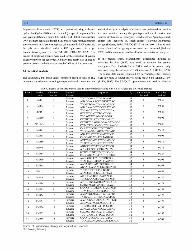
Journal of Experimental Biology and Agricultural Sciences
http://www.jebas.org
150 Pathak et al.
Polymerase chain reaction (PCR) was performed using a thermal
cycler (SureCycler 8800) in vitro to amplify a specific segment of the
total genomic DNA to a billion fold (Mullis et al., 1986). The amplified
DNA products generated through SSR primers were resolved through
electrophoresis in 2.5 per cent agarose gel prepared in TAE buffer and
the gels were visualized under a UV light source in a gel
documentation system (Gel DocTM XR+, BIO-RAD, USA). The
images of amplified products were used for the evaluation of genetic
diversity between the genotypes. A binary data matrix was utilized to
generate genetic similarity data among the 29 lines of rice genotypes.
2.4 Statistical analysis
The quantitative trait mean values computed based on data on five
randomly tagged plants in each genotype and checks were used for
statistical analysis. Analysis of variance was performed to partition
the total variation among the genotypes and check entries into
sources attributable to ‘genotypes+ checks entries, ‘genotype check
entries’ and ‘genotype vs. check entries’ following Augmented
design (Federer, 1956) WINDOSTAT version 9.0. Adjusted trait
mean of each of the genotype accession was estimated (Federer,
1956) and the same were used for all subsequent statistical analysis.
In the present study, Mahalanobis’ generalized distance as
described by Rao (1952) was used to estimate the genetic
divergence. Data Analysis for the SSRs used in the present study
was done using the software NTSYSpc version 2.02 (Rohlf, 1998).
The binary data matrix generated by polymorphic SSR markers
were subjected to further analysis using NTSYS-pc version 2.11W
(Rohlf, 1997). The SIMQUAL programme was used to calculate
Table 2 Details of the SSR primers used in the present study along with No. of Alleles and PIC value obtained
S.No. Marker name
Chromosome no.
Forward/ Reverse
Sequence Ta No. of alleles obtained
PIC value obtained
1 RM431 1 Forward
Reverse
TCCTGCGAACTGAAGAGTTC
AGAGCAAAACCCTGGTTCAC
55
55 3 0.567
2 RM433 1 Forward Reverse
TGCGCTGAACTAAACACAGC AGACAAACCTGGCCATTCAC
52 52
3 0.585
3 RM5 1 Forward
Reverse
TGCAACTTCTAGCTGCTCGA
GCATCCGATCTTGATGGG
52
51 3 0.588
4 RM259 1 Forward Reverse
TGGAGTTTGAGAGGAGGG CTTGTTGCATGGTGCCATGT
50 52
3 0.591
5 RM11943 1 Forward
Reverse
CTTGTTCGAGGACGAAGATAGGG
CCAGTTTACCAGGGTCGAAACC
57
57 3 0.527
6 RM237 1 Forward Reverse
CAAATCCCGACTGCTGTCC TGGGAAGAGAGCACTACAGC
53 54
2 0.346
7 RM514 3 Forward
Reverse
AGATTCATCTCCCATTCCCC
CACGAGCATATTATAGTGG
52
50 4 0.693
8 RM489 3 Forward Reverse
ACTTGAGACGATCGGACACC TCACCCATGGATGTTGTCAG
54 52
3 0.532
9 RM60 3 Forward
Reverse
AGTCCCATGTTCCACTTCCG
ATGGCTACTGCCTGTACTAC
54
52 3 0.586
10 RM334 5 Forward Reverse
GTTCAGTGTTCAGTGCCACC CACGAGCATATTACTAGTGG
54 52
3 0.527
11 RM510 6 Forward
Reverse
AACCGGATTAGTTTCTCGCC
TGAGGACGACGAGCAGATTC
52
54 3 0.501
12 RM455 7 Forward Reverse
AACAACCCACCACCTGTCTC AGAAGGAAAAGGGCTCGATC
54 52
3 0.563
13 RM11 7 Forward
Reverse
TCTCCTCTTCCCCCGATC
ATAGCGGGCGAGGCTTAG
53
53 4 0.652
14 RM44 8 Forward
Reverse
ACGGCAATCCGAACAACC
TCGGGAAAACCTACCCTACC
53
54 3 0.580
15 RM284 8 Forward
Reverse
ATCTCTGATACTCCATCCATCC
CCTGTACGTTGATCCGAAGC
53
54 3 0.574
16 RM215 9 Forward
Reverse
CAAAATGGAGCAGCAAGAGC
TGAGCACCTCCTTCTCTGTAG
52
54 3 0.559
17 RM474 10 Forward
Reverse
AAGATGTACGGGTGGCATTC
TATGAGCTGGTGAGCAATGG
52
52 3 0.576
18 RM171 10 Forward
Reverse
AACGCGAGGACACGTACTTAC
ACGAGATACGTACGCCTTTG
54
52 3 0.576
19 RM536 11 Forward
Reverse
TCTCTCCTCTTGTTTGGCTC
ACACACCAACACGACCACAC
52
54 3 0.589
20 RM552 11 Forward
Reverse
CGCAGTTGTGGATTTCAGTG
TGCTCAACGTTTGACTGTCC
52
52 3 0.585
21 RM277 12 Forward
Reverse
CAAATCCCGACTGCTGTCC
TGGGAAGAGAGAGCACTACAGC
51
52 4 0.701
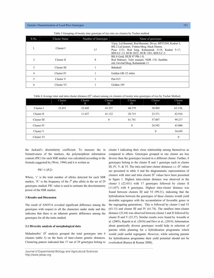
Journal of Experimental Biology and Agricultural Sciences
http://www.jebas.org
Genetic Characterization of Local Rice Genotypes 151
the Jackard’s dissimilarity coefficient. To measure the in
formativeness of the markers, the polymorphism information
content (PIC) for each SSR marker was calculated according to the
formula suggested by (Weir, 1996) and it is written as
PIC=1-(Pi2)
Where, ‘i’ is the total number of alleles detected for each SSR
marker, ‘Pi’ is the frequency of the ith
plus allele in the set of 29
genotypes studied. PIC value is used to estimate the discriminatory
power of the SSR marker.
3 Results and Discussion
The result of ANOVA revealed significant difference among the
genotypes with respect to all the characters under study and this
indicates that there is an inherent genetic difference among the
genotypes for all the traits studied.
3.1 Diversity analysis of morphological data
Mahalanobis’ D2 analysis grouped the total genotypes into 6
clusters (table 3) on the basis of inter-cluster genetic distances.
Clustering pattern indicated that 17 out of 29 genotypes belong to
cluster I indicating their close relationship among themselves as
compared to others. Genotypes grouped in one cluster are less
diverse than the genotypes located in a different cluster. Further, 8
genotypes belong to the cluster II and 1 genotype each in cluster
III, IV, V, & VI. The intra and inter cluster distances i.e. D2 values
are presented in table 4 and the diagrammatic representation of
clusters with inter and intra cluster D2 values have been presented
in figure 1. Highest intra-cluster distance was observed in the
cluster I (22.431) with 17 genotypes followed by cluster II
(11.657) with 8 genotypes. Highest inter-cluster distance was
found between clusters III and VI (99.21), indicating that the
hybridization between the genotypes of these clusters would yield
desirable segregates with the accumulation of favorable genes in
the segregating generations. This is followed by cluster I and VI
(63.13) and cluster III and IV (61.74). The smallest inter-cluster
distance (22.44) was observed between cluster I and II followed by
cluster II and V (23.37). Similar results were found by Awasthi et
al. (2005), Rajesh et al. (2010) and Devi et al., (2019). Information
about genetically diverse genotypes would help in selection of
parents while planning for a hybridization programme which
would yield useful segregants. However, while selecting parents
for hybridization programme their yield potential should not be
overlooked (Ramya & Kumar 2008).
Table 3 Grouping of twenty nine genotype of rice into six clusters by Tocher method
S.No. Cluster Name Number of Genotypes Name of genotypes
1. Cluster I
17
Vijay, Lal Basmati, Red Basmati, Divya, BPT5204, Kudrat 5,
RK-2 Lal kasturi, Vishnu bhog, black Damni, Pusa 1121, Red long, Kalanamak 3119, Kudrat 5-17,
BHULC-13, HUR-3022, HUR 1301, BHULC-5
2 Cluster II 8 RK-8 Gold, HUR 97 PB-1-S, Red Mahsuri, Tulsi manjari, NDR 118, Sambha
red, Govind bhog, Kalanamak-11
3 Cluster III 1 Bahubali
4 Cluster IV 1 Golden GR-32 white
5 Cluster V 1 Pan 815
6 Cluster VI 1 Golden 105
Table 4 Average inter and intra cluster distance (D2 values) among six clusters of twenty nine genotypes of rice by Tocher Method.
Cluster
I Cluster
II Cluster
III Cluster
IV Cluster
V Cluster
VI
Cluster I 22.431 22.445 43.537 40.379 38.969 63.138,
Cluster II 11.657 41.122 28.715 23.371 42.910
Cluster III 0 61.741 57.887 99.217
Cluster IV 0 24.592 43.000
Cluster V 0 34.659
Cluster VI 0
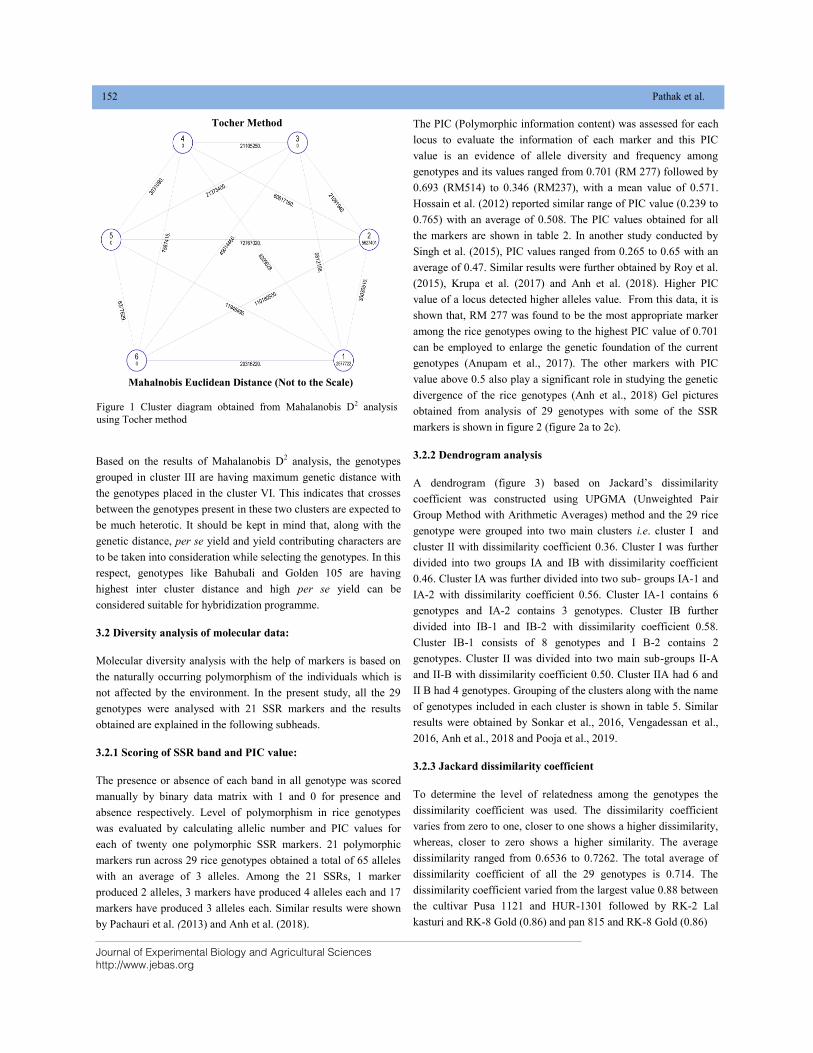
Journal of Experimental Biology and Agricultural Sciences
http://www.jebas.org
152 Pathak et al.
Based on the results of Mahalanobis D2 analysis, the genotypes
grouped in cluster III are having maximum genetic distance with
the genotypes placed in the cluster VI. This indicates that crosses
between the genotypes present in these two clusters are expected to
be much heterotic. It should be kept in mind that, along with the
genetic distance, per se yield and yield contributing characters are
to be taken into consideration while selecting the genotypes. In this
respect, genotypes like Bahubali and Golden 105 are having
highest inter cluster distance and high per se yield can be
considered suitable for hybridization programme.
3.2 Diversity analysis of molecular data:
Molecular diversity analysis with the help of markers is based on
the naturally occurring polymorphism of the individuals which is
not affected by the environment. In the present study, all the 29
genotypes were analysed with 21 SSR markers and the results
obtained are explained in the following subheads.
3.2.1 Scoring of SSR band and PIC value:
The presence or absence of each band in all genotype was scored
manually by binary data matrix with 1 and 0 for presence and
absence respectively. Level of polymorphism in rice genotypes
was evaluated by calculating allelic number and PIC values for
each of twenty one polymorphic SSR markers. 21 polymorphic
markers run across 29 rice genotypes obtained a total of 65 alleles
with an average of 3 alleles. Among the 21 SSRs, 1 marker
produced 2 alleles, 3 markers have produced 4 alleles each and 17
markers have produced 3 alleles each. Similar results were shown
by Pachauri et al. (2013) and Anh et al. (2018).
The PIC (Polymorphic information content) was assessed for each
locus to evaluate the information of each marker and this PIC
value is an evidence of allele diversity and frequency among
genotypes and its values ranged from 0.701 (RM 277) followed by
0.693 (RM514) to 0.346 (RM237), with a mean value of 0.571.
Hossain et al. (2012) reported similar range of PIC value (0.239 to
0.765) with an average of 0.508. The PIC values obtained for all
the markers are shown in table 2. In another study conducted by
Singh et al. (2015), PIC values ranged from 0.265 to 0.65 with an
average of 0.47. Similar results were further obtained by Roy et al.
(2015), Krupa et al. (2017) and Anh et al. (2018). Higher PIC
value of a locus detected higher alleles value. From this data, it is
shown that, RM 277 was found to be the most appropriate marker
among the rice genotypes owing to the highest PIC value of 0.701
can be employed to enlarge the genetic foundation of the current
genotypes (Anupam et al., 2017). The other markers with PIC
value above 0.5 also play a significant role in studying the genetic
divergence of the rice genotypes (Anh et al., 2018) Gel pictures
obtained from analysis of 29 genotypes with some of the SSR
markers is shown in figure 2 (figure 2a to 2c).
3.2.2 Dendrogram analysis
A dendrogram (figure 3) based on Jackard’s dissimilarity
coefficient was constructed using UPGMA (Unweighted Pair
Group Method with Arithmetic Averages) method and the 29 rice
genotype were grouped into two main clusters i.e. cluster I and
cluster II with dissimilarity coefficient 0.36. Cluster I was further
divided into two groups IA and IB with dissimilarity coefficient
0.46. Cluster IA was further divided into two sub- groups IA-1 and
IA-2 with dissimilarity coefficient 0.56. Cluster IA-1 contains 6
genotypes and IA-2 contains 3 genotypes. Cluster IB further
divided into IB-1 and IB-2 with dissimilarity coefficient 0.58.
Cluster IB-1 consists of 8 genotypes and I B-2 contains 2
genotypes. Cluster II was divided into two main sub-groups II-A
and II-B with dissimilarity coefficient 0.50. Cluster IIA had 6 and
II B had 4 genotypes. Grouping of the clusters along with the name
of genotypes included in each cluster is shown in table 5. Similar
results were obtained by Sonkar et al., 2016, Vengadessan et al.,
2016, Anh et al., 2018 and Pooja et al., 2019.
3.2.3 Jackard dissimilarity coefficient
To determine the level of relatedness among the genotypes the
dissimilarity coefficient was used. The dissimilarity coefficient
varies from zero to one, closer to one shows a higher dissimilarity,
whereas, closer to zero shows a higher similarity. The average
dissimilarity ranged from 0.6536 to 0.7262. The total average of
dissimilarity coefficient of all the 29 genotypes is 0.714. The
dissimilarity coefficient varied from the largest value 0.88 between
the cultivar Pusa 1121 and HUR-1301 followed by RK-2 Lal
kasturi and RK-8 Gold (0.86) and pan 815 and RK-8 Gold (0.86)
Tocher Method
Mahalnobis Euclidean Distance (Not to the Scale)
Figure 1 Cluster diagram obtained from Mahalanobis D2 analysis
using Tocher method
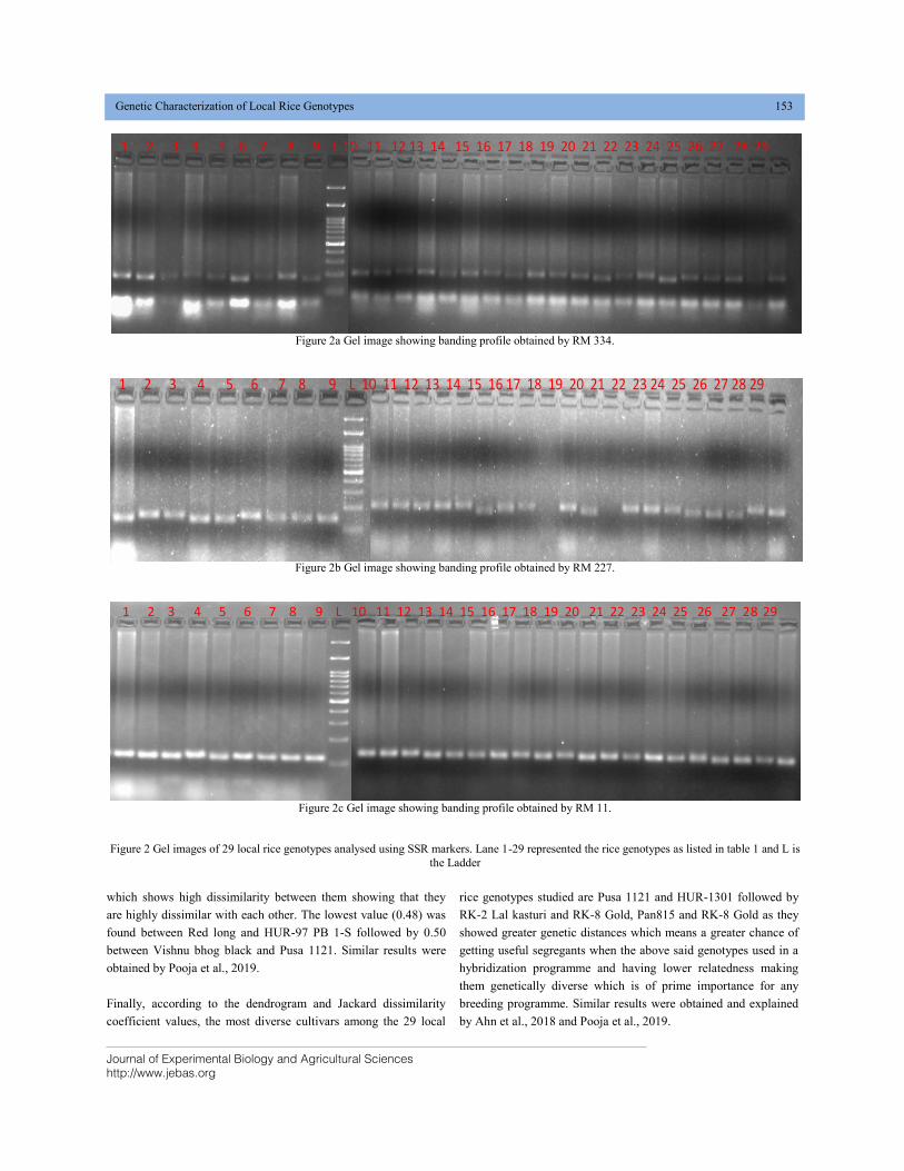
Journal of Experimental Biology and Agricultural Sciences
http://www.jebas.org
Genetic Characterization of Local Rice Genotypes 153
which shows high dissimilarity between them showing that they
are highly dissimilar with each other. The lowest value (0.48) was
found between Red long and HUR-97 PB 1-S followed by 0.50
between Vishnu bhog black and Pusa 1121. Similar results were
obtained by Pooja et al., 2019.
Finally, according to the dendrogram and Jackard dissimilarity
coefficient values, the most diverse cultivars among the 29 local
rice genotypes studied are Pusa 1121 and HUR-1301 followed by
RK-2 Lal kasturi and RK-8 Gold, Pan815 and RK-8 Gold as they
showed greater genetic distances which means a greater chance of
getting useful segregants when the above said genotypes used in a
hybridization programme and having lower relatedness making
them genetically diverse which is of prime importance for any
breeding programme. Similar results were obtained and explained
by Ahn et al., 2018 and Pooja et al., 2019.
Figure 2a Gel image showing banding profile obtained by RM 334.
Figure 2b Gel image showing banding profile obtained by RM 227.
Figure 2c Gel image showing banding profile obtained by RM 11.
Figure 2 Gel images of 29 local rice genotypes analysed using SSR markers. Lane 1-29 represented the rice genotypes as listed in table 1 and L is
the Ladder
1 2 3 4 5 6 7 8 9 L 10 11 12 13 14 15 16 17 18 19 20 21 22 23 24 25 26 27 28 29
1 2 3 4 5 6 7 8 9 L 10 11 12 13 14 15 16 17 18 19 20 21 22 23 24 25 26 27 28 29
1 2 3 4 5 6 7 8 9 L 10 11 12 13 14 15 16 17 18 19 20 21 22 23 24 25 26 27 28 29
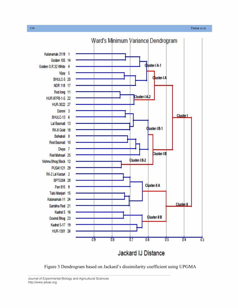
Journal of Experimental Biology and Agricultural Sciences
http://www.jebas.org
154 Pathak et al.
Figure 3 Dendrogram based on Jackard’s dissimilarity coefficient using UPGMA
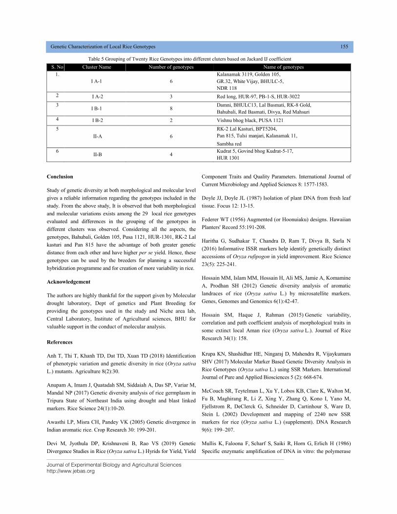
Journal of Experimental Biology and Agricultural Sciences
http://www.jebas.org
Genetic Characterization of Local Rice Genotypes 155
Conclusion
Study of genetic diversity at both morphological and molecular level
gives a reliable information regarding the genotypes included in the
study. From the above study, It is observed that both morphological
and molecular variations exists among the 29 local rice genotypes
evaluated and differences in the grouping of the genotypes in
different clusters was observed. Considering all the aspects, the
genotypes, Bahubali, Golden 105, Pusa 1121, HUR-1301, RK-2 Lal
kasturi and Pan 815 have the advantage of both greater genetic
distance from each other and have higher per se yield. Hence, these
genotypes can be used by the breeders for planning a successful
hybridization programme and for creation of more variability in rice.
Acknowledgement
The authors are highly thankful for the support given by Molecular
drought laboratory, Dept of genetics and Plant Breeding for
providing the genotypes used in the study and Niche area lab,
Central Laboratory, Institute of Agricultural sciences, BHU for
valuable support in the conduct of molecular analysis.
References
Anh T, Thi T, Khanh TD, Dat TD, Xuan TD (2018) Identification
of phenotypic variation and genetic diversity in rice (Oryza sativa
L.) mutants. Agriculture 8(2):30.
Anupam A, Imam J, Quatadah SM, Siddaiah A, Das SP, Variar M,
Mandal NP (2017) Genetic diversity analysis of rice germplasm in
Tripura State of Northeast India using drought and blast linked
markers. Rice Science 24(1):10-20.
Awasthi LP, Misra CH, Pandey VK (2005) Genetic divergence in
Indian aromatic rice. Crop Research 30: 199-201.
Devi M, Jyothula DP, Krishnaveni B, Rao VS (2019) Genetic
Divergence Studies in Rice (Oryza sativa L.) Hyrids for Yield, Yield
Component Traits and Quality Parameters. International Journal of
Current Microbiology and Applied Sciences 8: 1577-1583.
Doyle JJ, Doyle JL (1987) Isolation of plant DNA from fresh leaf
tissue. Focus 12: 13-15.
Federer WT (1956) Augmented (or Hoonuiaku) designs. Hawaiian
Planters' Record 55:191-208.
Haritha G, Sudhakar T, Chandra D, Ram T, Divya B, Sarla N
(2016) Informative ISSR markers help identify genetically distinct
accessions of Oryza rufipogon in yield improvement. Rice Science
23(5): 225-241.
Hossain MM, Islam MM, Hossain H, Ali MS, Jamie A, Komamine
A, Prodhan SH (2012) Genetic diversity analysis of aromatic
landraces of rice (Oryza sativa L.) by microsatellite markers.
Genes, Genomes and Genomics 6(1):42-47.
Hossain SM, Haque J, Rahman (2015) Genetic variability,
correlation and path coefficient analysis of morphological traits in
some extinct local Aman rice (Oryza sativa L.). Journal of Rice
Research 34(1): 158.
Krupa KN, Shashidhar HE, Ningaraj D, Mahendra R, Vijaykumara
SHV (2017) Molecular Marker Based Genetic Diversity Analysis in
Rice Genotypes (Oryza sativa L.) using SSR Markers. International
Journal of Pure and Applied Biosciences 5 (2): 668-674.
McCouch SR, Teytelman L, Xu Y, Lobos KB, Clare K, Walton M,
Fu B, Maghirang R, Li Z, Xing Y, Zhang Q, Kono I, Yano M,
Fjellstrom R, DeClerck G, Schneider D, Cartinhour S, Ware D,
Stein L (2002) Development and mapping of 2240 new SSR
markers for rice (Oryza sativa L.) (supplement). DNA Research
9(6): 199–207.
Mullis K, Faloona F, Scharf S, Saiki R, Horn G, Erlich H (1986)
Specific enzymatic amplification of DNA in vitro: the polymerase
Table 5 Grouping of Twenty Rice Genotypes into different cluters based on Jackard IJ coefficient
S. No Cluster Name Number of genotypes Name of genotypes
1.
I A-1 6
Kalanamak 3119, Golden 105,
GR.32, White Vijay, BHULC-5,
NDR 118
2 I A-2 3 Red long, HUR-97, PB-1-S, HUR-3022
3 I B-1 8
Damni, BHULC13, Lal Basmati, RK-8 Gold,
Bahubali, Red Basmati, Divya, Red Mahsuri
4 I B-2 2 Vishnu bhog black, PUSA 1121
5
II-A 6
RK-2 Lal Kasturi, BPT5204,
Pan 815, Tulsi manjari, Kalanamak 11,
Sambha red
6 II-B 4
Kudrat 5, Govind bhog Kudrat-5-17,
HUR 1301
Journal of Experimental Biology and Agricultural Sciences
http://www.jebas.org
156 Pathak et al.
chain reaction. In Cold Spring Harbour Symposia on Quantitative
Biology 51: 263-73.
Nachimuthu VV, Muthurajan R, Duraialaguraja S, Sivakami R,
Pandian BA, Ponniah G, Gunasekaran K, Swaminathan M, Suji
KK, Sabariappan R (2015) Analysis of population structure and
genetic diversity in rice germplasm using SSR markers: an
initiative towards association mapping of agronomic traits in Oryza
sativa. Rice 18(1):30.
Pachauri V, Taneja N, Vikram P, Singh NN, Singh S (2013)
Molecular and morphological characterization of Indian farmers
rice varieties (Oryza sativa L.). Australian Journal of Crop
Sciences 7 : 923-932.
Pooja S, Singh SK, Sonali H, Singh DK, Prudhvi RV, Amrutlal K
(2019) Studies on genetic diversity in rice (Oryza sativa L.) using
SSR markers. Journal of Pharmacognosy and Phytochemistry 8 :
922-928.
Rajesh T, Paramsivam, Thirumeni S (2010) Evaluated genetic
divergence of land races of rice. Electronic Journal of Plant
Breeding 1(2): 199-204.
Ramya K, Kumar S (2008) Genetic divergence in rice. Crop
Improvement 35 : 119-121.
Rao RC (1952) Advanced statistical methods in biometric
research. New York: John Wiley and Sons, 390p.
Reig-Valiente JL, Viruel J, Sales E, Marqués L, Terol J, Gut M,
Derdak S, Talón M, Domingo C (2016) Genetic diversity and
population structure of rice varieties cultivated in temperate
regions. Rice 9 :58.
Rohlf FJ (1997) NTSYS-pc Version. 2.02i Numerical Taxonomy
and Multivariate Analysis System. Applied Biostatistics Inc.,
Exeter Software, Setauket, New York.
Rohlf FJ (1998) NTSYS-pc: Numerical Taxonomy and
Multivariate Analysis System, Version 2.02i, Exeter Software,
New York.
Roy S, Banerjee A, Mawkhlieng B, Misra AK, Pattanayak A,
Harish GD, Singh SK, Ngachan SV, Bansal KC (2015) Genetic
diversity and population structure in aromatic and quality rice
(Oryza sativa L.) landraces from North-Eastern India. PloS one
10(6): e0129607.
Singh AK, Singh PK, Arya M, Singh NK, Singh US (2015)
Molecular screening of Blast resistance genes in rice using SSR
markers. The Plant Pathology Journal 31(1):12.
Sonkar S, Singh SK, Vennela PR, Singh DK (2016) Molecular
marker based genetic diversity analysis in rice (Oryza sativa L.)
using SSR markers. International Journal of Agriculture,
Environment and Biotechnology 9(1):45-51.
Vengadessan V, Ramapriya S, Selvarajeswari S (2016) Morpho-
molecular diversity analysis of traditional and improved cultivars
in rice. International Journal of Multidisciplinary Education and
Research 1(4): 59-65.
Weir BS (1996) Genetic data analysis II: Methods for discrete
population genetic data. Sinauer Associates Inc, Sunderland,
MA, USA.
148-156_Galley Proof_14_Volume_8_Issue_2_JEBAS2020000505.docx
Journal of Experimental Biology and Agricultural Sciences
http://www.jebas.org
ISSN No. 2320 – 8694
Journal of Experimental Biology and Agricultural Sciences, April - 2020; Volume – 8(2) page 157 – 165
IDENTIFICATION OF SUPERIOR THREE WAY-CROSS F1S, ITS LINE×TESTER
HYBRIDS AND DONORS FOR MAJOR QUANTITATIVE
TRAITS IN Lilium×formolongi
Rameshwar Rai1, Amarsanaa Badarch1, Jong-Hwa Kim1, 2*
1Department of Horticulture, Kangwon National University, Chuncheon 24341, Korea
2Oriental Bio-herb Research Institute, Kangwon National University, Chuncheon 24341, Korea
Received – March 01, 2020; Revision – April 17, 2020; Accepted – April 24, 2020 Available Online – April 25, 2020
DOI: http://dx.doi.org/10.18006/2020.8(2).157.165
ABSTRACT
This experiment was carried out to identify superior parents [three way-cross F1s and donors
(cultivars/breeding line)], and their Line×Tester hybrids (hereafter L×T hybrids) for major quantitative
traits in Lilium×formolongi. The experiment was designed in line×tester mating design taking 5 three
way-cross F1s as lines, 3CVs/breeding lines as testers and their 15 L×T hybrids in a Randomized
Complete Block Design (RCBD) with 3 replications. The analysis of variance (ANOVA) for L×T
analysis revealed a highly significant difference for all the studied quantitative traits revealing the
presence of genetic variability among the genotypes under investigation. The estimated GCA effects
revealed three way-cross F1s; (Stu× W) × AF1-6 (L2) and (AF×Ad) × HU-3(L1) found to be superior as
they possessed significant GCA effects for 7 and 4 quantitative traits respectively. Likewise, Julius-19
(T1) and 12-1-2(T3) can be used as effective donors as both of them possessed significant GCA effects
for 6 quantitative traits. The L×T hybrids, [57-7 (Aug×AugE)×BT] ×12-1-2 i.e. L4×T3 and [60.1
(AF×Ad) × Gel] × Julius-19 i.e.L5×T1 has possessed significant SCA effects for 5 traits and [(Stu×
W) × AF1-6]×Julius-19 i.e.L2×T1, [(Stu× W) × AF1-6]×WT-5 i.e.L2×T2 and [(Stu× W) × AugE-
2]×WT-5 i.e.L3×T2 had revealed significant SCA effects for 4 traits. These hybrids can be considered
as promising hybrids. The estimation of gene action divulged that bud length and the attitude of the
floral axis shown the prevailing of additive gene action while the rest of the traits had predominantly
exhibited non-additive gene action.
* Corresponding author
KEYWORDS
Three way-cross F1s
L×T hybrids
ANOVA for L×T analysis
Randomized Complete Block
Design (RCBD)
Quantitative traits
Lilium×formolongi
E-mail: [email protected], [email protected] (Jong-Hwa Kim)
ORCID: https://orcid.org/0000-0002-9300-6465
Peer review under responsibility of Journal of Experimental Biology and
Agricultural Sciences.
All the articles published by Journal of Experimental
Biology and Agricultural Sciences are licensed under a
Creative Commons Attribution-NonCommercial 4.0
International License Based on a work at www.jebas.org.
Production and Hosting by Horizon Publisher India [HPI]
(http://www.horizonpublisherindia.in/).
All rights reserved.
Journal of Experimental Biology and Agricultural Sciences
http://www.jebas.org
Identification of superior three way-cross F1s for major quantitative traits in Lilium×formolongi 158
1 Introduction
Lily (Lilium L., 2n=2x=24) is one of the most important
ornamental bulbous crops which belongs to the family Liliaceae,
includes 110 species (McRae,1998), 7 sections and more than
10000 documented cultivars (Mathews, 2007; Bakhshaie et
al.,2016) which increases year by year. It is a perennial herb that
possesses scaly bulb, unbranched stem, and smooth/pubescent,
usually bright green, sometimes tinged purple or brown and
generally covered with leaves. The native Lilium species are
spread over the Northern Hemisphere and centered mainly in
Asia, North America, and Europe (Van Tuyl & Arens, 2011).
Lilies are economically most important bulbous crops mostly
used for cut flower, potted plants, some species used as edible
bulbs or medicinal use in Eastern Asia (Bakhshaie et al., 2016).
According to Lucidos et al. (2013) due to its multi aspects viz.
diversity of flower color, flower shape, long and multi flowering
stem and having long post-harvest shelf life; lilies are highly
demanded for its cut flowers in recent international flower trade.
The Lilium×formolongi hort is an interspecific hybrid obtained
through crossing of two Lilium species i.e. L. formosanum and L.
longiflorum.It is popular in East Asia (especially Korea, China and
Japan) as commercial cut flower in flower market (Ho et al., 2006;
Grassotti & Gimelli, 2011; Rai et al., 2018).
The single cross F1s lack population buffering and possess only
individual buffering so it was therefore apprehended that single
cross may not perform as stable as double cross and three way-
cross hybrids (Allard & Bradshaw, 1964). As three way-cross
have both populations and individual buffering; three way-cross
hybrids are intermediate between single and double cross hybrids
concerning uniformity, yield, stability and the relative simplicity
of selecting and testing (Weatherspoon,1970;
Schnell,1975). Keeping this point in mind, current study used
three way-cross hybrids as mother lines.
The Line×Tester mating design is one of the helpful tools
available to the breeder for quantitative plant breeding analysis.
Basically it is the extension of top cross where only one tester
used while more than one tester are used in L×T mating design.
(Nduwumuremyi et al., 2013). It involves hybridization between
lines (f) and wide based testers (m) in one to one fashion for
generating f×m=fm hybrids (Sharma, 2006). Furthermore, it
provides GCA of both lines and testers and SCA of each cross
(Sharma, 2006). At last it is very useful for estimating various
types of gene actions important for the expression of quantitative
traits (Rashid et al., 2007).
The Lilium×formolongi is used for cut flower production mainly
as seed propagation, seeds used to sown during December-
February (upon the availability of labor) usually flowered during
July-August (Goo et al., 2003; Xuan et al., 2005). As populations
derived from the seed propagation are not uniform in plant
height, flowering time and flower shape (Roh, 2002) and the
stability of novel cut flower traits is a major concern for
commercial-scale production (Ho et al., 2006) in this experiment
clonal lines (scaled) of parental material was used to maintain
the heterozygous genotypes for the seed production of a
homogenous population. In this way identification of appropriate
mother lines i.e. three way-cross F1s and its proper donor (tester)
and their promising L×T hybrids for major quantitative traits are
the major concern of this experiment.
2 Materials and Methods
2.1. Plant material, generation of crosses and field experiment
layout
The series of experiments plant material preparation, generation of
crosses according to Line×Tester mating design and the final step
of experiment were carried out in the backside school field, main
gate field and experimental farm of KNU at Chuncheon,
Kangwon-Do, South Korea respectively during the season of 2016
to 2018. The seeds of three-way cross F1s and donor cultivar and
breeding lines were obtained from KNU, Department of
Horticulture, Floricultural breeding lab in 2016 winter for the
preparation of seedlings. During the summer season of 2016 based
on morphological observation of major growth and flowering traits
lines of five promising three-way cross F1s and three clonal lines
of broad-based donor cultivar and breeding, lines have been
selected for the purpose to be used as lines and testers respectively.
The details of parental materials (Lines and testers) are given in
Table 1. In the succeeding year, 15 L×T hybrids have been
prepared to hybridize those 5 three-way cross F1s and three donors
in the Line×Tester method. The seedlings of altogether 23
genotypes (5lines, 3testers, and 15 L×T hybrids) has been prepared
during the January to April in 2018 following the method as
described by Rai et al. (2018) inside plastic house and have been
transplanted in the main field in the last week of April. The field
experiment has been carried out in RCBD plot design with
maintaining 3 replications. The land preparation, fertilizers and
insecticides application, as well as other intercultural operations,
has been carried out following the Rai et al. (2019).
2.2 Measurement of quantitative traits
The measurement of major quantitative traits has been done
during the main flowering season i.e. from last week of June to
the first week of August; taking samples of 12 reliable plants
from each replication. The generation of crosses preparation
procedure and measurement of morphological traits have been
adopted from Rai et al. (2018).
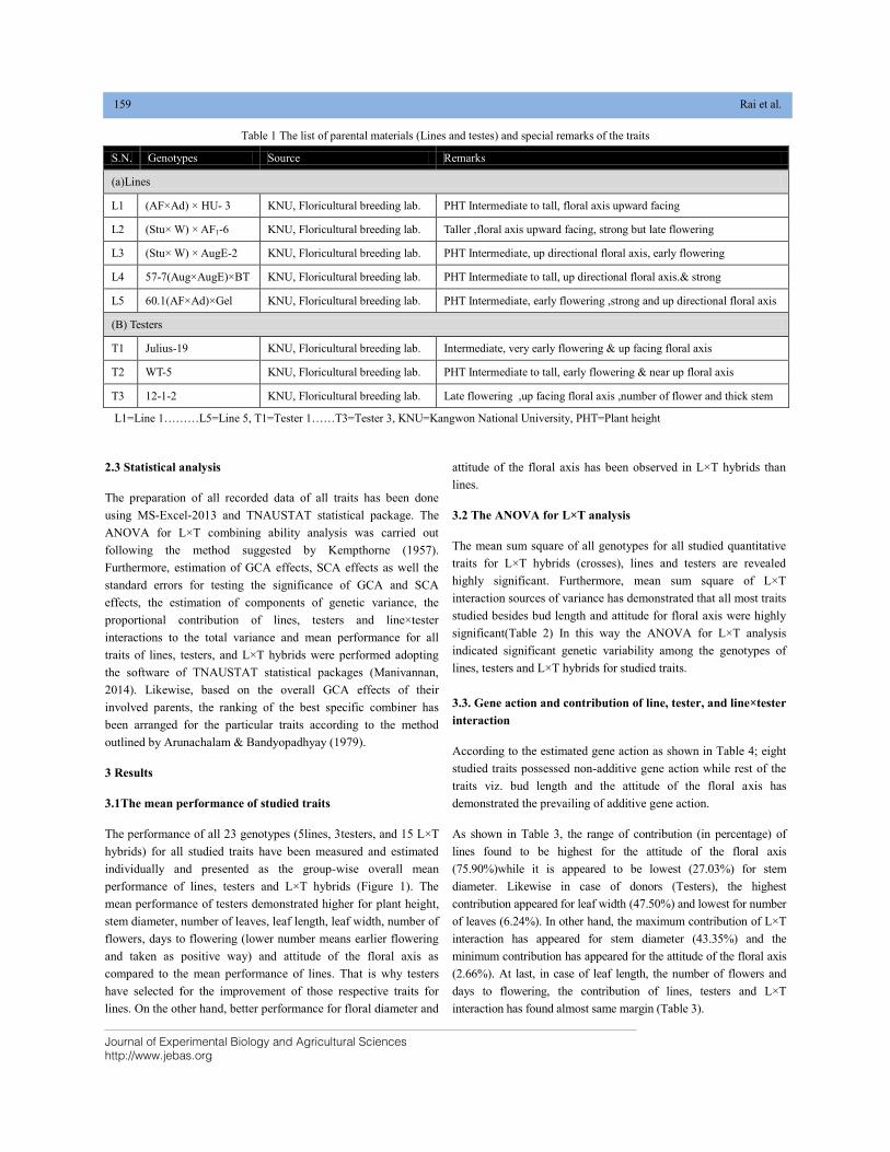
Journal of Experimental Biology and Agricultural Sciences
http://www.jebas.org
159 Rai et al.
2.3 Statistical analysis
The preparation of all recorded data of all traits has been done
using MS-Excel-2013 and TNAUSTAT statistical package. The
ANOVA for L×T combining ability analysis was carried out
following the method suggested by Kempthorne (1957).
Furthermore, estimation of GCA effects, SCA effects as well the
standard errors for testing the significance of GCA and SCA
effects, the estimation of components of genetic variance, the
proportional contribution of lines, testers and line×tester
interactions to the total variance and mean performance for all
traits of lines, testers, and L×T hybrids were performed adopting
the software of TNAUSTAT statistical packages (Manivannan,
2014). Likewise, based on the overall GCA effects of their
involved parents, the ranking of the best specific combiner has
been arranged for the particular traits according to the method
outlined by Arunachalam & Bandyopadhyay (1979).
3 Results
3.1The mean performance of studied traits
The performance of all 23 genotypes (5lines, 3testers, and 15 L×T
hybrids) for all studied traits have been measured and estimated
individually and presented as the group-wise overall mean
performance of lines, testers and L×T hybrids (Figure 1). The
mean performance of testers demonstrated higher for plant height,
stem diameter, number of leaves, leaf length, leaf width, number of
flowers, days to flowering (lower number means earlier flowering
and taken as positive way) and attitude of the floral axis as
compared to the mean performance of lines. That is why testers
have selected for the improvement of those respective traits for
lines. On the other hand, better performance for floral diameter and
attitude of the floral axis has been observed in L×T hybrids than
lines.
3.2 The ANOVA for L×T analysis
The mean sum square of all genotypes for all studied quantitative
traits for L×T hybrids (crosses), lines and testers are revealed
highly significant. Furthermore, mean sum square of L×T
interaction sources of variance has demonstrated that all most traits
studied besides bud length and attitude for floral axis were highly
significant(Table 2) In this way the ANOVA for L×T analysis
indicated significant genetic variability among the genotypes of
lines, testers and L×T hybrids for studied traits.
3.3. Gene action and contribution of line, tester, and line×tester
interaction
According to the estimated gene action as shown in Table 4; eight
studied traits possessed non-additive gene action while rest of the
traits viz. bud length and the attitude of the floral axis has
demonstrated the prevailing of additive gene action.
As shown in Table 3, the range of contribution (in percentage) of
lines found to be highest for the attitude of the floral axis
(75.90%)while it is appeared to be lowest (27.03%) for stem
diameter. Likewise in case of donors (Testers), the highest
contribution appeared for leaf width (47.50%) and lowest for number
of leaves (6.24%). In other hand, the maximum contribution of L×T
interaction has appeared for stem diameter (43.35%) and the
minimum contribution has appeared for the attitude of the floral axis
(2.66%). At last, in case of leaf length, the number of flowers and
days to flowering, the contribution of lines, testers and L×T
interaction has found almost same margin (Table 3).
Table 1 The list of parental materials (Lines and testes) and special remarks of the traits
S.N. Genotypes Source Remarks
(a)Lines
L1 (AF×Ad) × HU- 3 KNU, Floricultural breeding lab. PHT Intermediate to tall, floral axis upward facing
L2 (Stu× W) × AF1-6 KNU, Floricultural breeding lab. Taller ,floral axis upward facing, strong but late flowering
L3 (Stu× W) × AugE-2 KNU, Floricultural breeding lab. PHT Intermediate, up directional floral axis, early flowering
L4 57-7(Aug×AugE)×BT KNU, Floricultural breeding lab. PHT Intermediate to tall, up directional floral axis.& strong
L5 60.1(AF×Ad)×Gel KNU, Floricultural breeding lab. PHT Intermediate, early flowering ,strong and up directional floral axis
(B) Testers
T1 Julius-19 KNU, Floricultural breeding lab. Intermediate, very early flowering & up facing floral axis
T2 WT-5 KNU, Floricultural breeding lab. PHT Intermediate to tall, early flowering & near up floral axis
T3 12-1-2 KNU, Floricultural breeding lab. Late flowering ,up facing floral axis ,number of flower and thick stem
L1=Line 1………L5=Line 5, T1=Tester 1……T3=Tester 3, KNU=Kangwon National University, PHT=Plant height
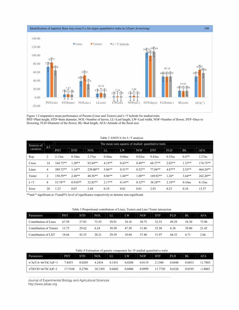
Journal of Experimental Biology and Agricultural Sciences
http://www.jebas.org
Identification of superior three way-cross F1s for major quantitative traits in Lilium×formolongi 160
Figure 1 Comparative mean performance of Parents (Lines and Testers) and L×T hybrids for studied traits
PHT=Plant height, STD=Stem diameter, NOL=Number of leaves, LL=Leaf length, LW=Leaf width, NOF=Number of flower, DTF=Days to flowering, FLD=Diameter of the flower, BL=Bud length, AFA=Attitude of the floral axis
Table 2 ANOVA for L×T analysis
Sources of
variation d.f.
The mean sum squares of studied quantitative traits
PHT STD NOL LL LW NOF DTF FLD BL AFA
Rep. 2 2.13ns 0.10ns 2.37ns 0.44ns 0.00ns 0.02ns 9.43ns 0.52ns 0.47* 2.27ns
Cross 14 164.73** 1.20** 92.84** 4.19** 0.43** 0.49** 68.37** 2.82** 1.33** 174.75**
Lines 4 389.72** 1.14** 239.00** 5.86** 0.51** 0.52** 77.84** 4.87** 2.53** 464.24**
Tester 2 158.59** 2.48** 40.56** 8.96** 1.44** 1.08** 169.92** 1.26* 3.64** 262.20**
L×T 8 53.78** 0.910** 32.82** 2.17** 0.14** 0.32** 38.24** 2.18** 0.16ns 8.15ns
Error 28 1.23 0.07 2.44 0.19 0.01 0.01 2.93 0.23 0.10 13.57
**and * significant at 1%and5% level of significance respectively.ns denotes non-significant.
Table 3 Proportional contribution of Lines, Testers and Line×Tester interaction
Parameters PHT STD NOL LL LW NOF DTF FLD BL AFA
Contribution of Lines 67.59 27.03 73.55 39.91 34.16 30.75 32.53 49.29 54.30 75.90
Contribution of Testers 13.75 29.62 6.24 30.50 47.50 31.86 35.50 6.38 39.00 21.43
Contribution of LXT 18.66 43.35 20.21 29.59 18.04 37.40 31.97 44.32 6.71 2.66
Table 4 Estimation of genetic component for 10 studied quantitative traits
Parameters PHT STD NOL LL LW NOF DTF FLD BL AFA
σ2A(VA=4σ2GCA)F=1 7.8453 0.0205 4.2434 0.1431 0.0208 0.0119 2.1300 0.0448 0.0833 11.7803
σ2D(VD=4σ2SCA)F=1 17.5168 0.2786 10.1305 0.6602 0.0406 0.0999 11.7720 0.6526 0.0195 -1.8065
72.81
7.00
38.95
9.012.21 2.64
106.31
49.60
16.03
49.75
82.77
7.47
52.25
10.35
2.34 3.80
99.27
49.16
14.92
65.4264.28
6.48
31.76
9.212.39 2.23
108.84
49.95
15.80
58.08
-20.00
0.00
20.00
40.00
60.00
80.00
100.00
120.00
140.00
PHT(cm) STD(mm) NOL(no.) LL(cm) LW(cm) NOF(no.) DTF(days) FLD(mm.) BL(cm) AFA(°)
Lines Testers L×T hybrids
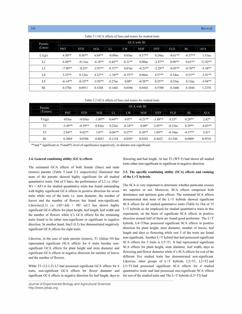
Journal of Experimental Biology and Agricultural Sciences
http://www.jebas.org
161 Rai et al.
3.4, General combining ability (GCA) effects
The estimated GCA effects of both female (lines) and male
(testers) parents (Table 5.1and 5.2 respectively) illustrated that
none of the parents showed highly significant for all studied
quantitative traits. Out of 5 lines, the performance of L2 i.e. (Stu×
W) × AF1-6 for studied quantitative traits has found outstanding
with highly significant GCA effects in positive direction for seven
traits while rest of the traits i.e. stem diameter, the number of
leaves and the number of flowers has found non-significant.
Likewise,(L1) i.e. (AF×Ad) × HU sel.3 has shown highly
significant GCA effects for plant height, leaf length, leaf width and
the number of flowers while it’s GCA effects for the remaining
traits found to be either non-significant or significant in negative
direction. In another hand, line3 (L3) has demonstrated negatively
significant GCA effects for eight traits.
Likewise, in the case of male parents (testers), T1 (Julius-19) has
represented significant GCA effects for 6 traits besides non-
significant GCA effects for plant height and stem diameter and
significant GCA effects in negative direction for number of leaves
and the number of flowers.
While T3 (12-1-2) L3 had possessed significant GCA effects for 6
traits, non-significant GCA effects for flower diameter and
significant GCA effects in negative direction for leaf length, days to
flowering and bud length. At last T2 (WT-5) had shown all studied
traits either non-significant or significant in negative direction.
3.5. The specific combining ability (SCA) effects and ranking
of the L×T hybrids
The SCA is very important to determine whether particular crosses
are superior or not. Moreover, SCA effects comprised both
dominance and epistasis gene effects. The estimated SCA effects
demonstrated that none of the L×T hybrids showed significant
SCA effects for all studied quantitative traits (Table 6). Out of 15
L×T hybrids so far employed for studied quantitative traits in this
experiment, on the basis of significant SCA effects in positive
direction around half of them are found good performer. The L×T
hybrids, L4×T3has possessed significant SCA effects in positive
direction for plant height, stem diameter, number of leaves, leaf
length and days to flowering while rest 5 of the traits are found
non-significant. Another L×T hybrid that had possessed significant
SCA effects for 5 traits is L5×T1. It had represented significant
SCA effects for plant height, stem diameter, leaf width, days to
flowering and flower diameter while it’s SCA effects for rest of the
different five studied traits has demonstrated non-significant.
Likewise, other groups of L×T hybrids, L2×T1, L2×T2 and
L3×T2 had possessed significant SCA effects for 4 studied
quantitative traits and had possessed non-significant SCA effects
for rest of the studied traits and The L×T hybrids (L3×T3) had
Table 5.1 GCA effects of lines and testers for studied traits
Parents
(Lines)
GCA with SE
PHT STD NOL LL LW NOF DTF FLD BL AFA
L1(gi) 4.30** 0.56** 6.84** -0.09ns 0.03ns 0.37** 0.24ns -0.61** -0.37** 1.51ns
L2 6.49** -0.11ns -4.18** 0.44** 0.31** 0.00ns -2.87** 0.98** 0.61** 11.92**
L3 -7.98** -0.25* -2.93** 0.72** 0.07ns -0.23** -2.29** -0.85** -0.70** -5.58**
L4 3.33** 0.12ns 4.22** -1.34** -0.35** 0.06ns 4.57** 0.24ns 0.33** -3.91**
L5 -6.14** -0.32** -3.95** 0.27ns 0.08* -0.20** 0.35** 0.23ns 0.13ns -3.94**
SE 0.3704 0.0911 0.5204 0.1464 0.0396 0.0443 0.5709 0.1606 0.1044 1.2278
Table 5.2 GCA effects of lines and testers for studied traits
Parents
(Testers)
GCA with SE
PHT STD NOL LL LW NOF DTF FLD BL AFA
T1(gj) 055ns -0.03ns -1.89** 0.64** 0.07* -0.21** -3.88** 0.33* 0.28** 2.42*
T2 -3.49** -0.39** 0.82ns 0.22ns -0.34** -0.09* 2.05** -0.15ns 0.29** -4.83**
T3 2.94** 0.42** 1.07* -0.86** 0.27** 0.30** 1.84** -0.18ns -0.57** 2.41*
SE 0.2869 0.0706 0.4031 0.1134 0.0307 0.0343 0.4422 0.1244 0.0809 0.9510
**and * significant at 1%and5% level of significance respectively. ns denotes non-significant.
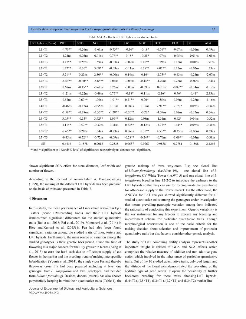
Journal of Experimental Biology and Agricultural Sciences
http://www.jebas.org
Identification of superior three way-cross F1s for major quantitative traits in Lilium×formolongi 162
shown significant SCA effect for stem diameter, leaf width and
number of flower.
According to the method of Arunachalam & Bandyopadhyay
(1979), the ranking of the different L×T hybrids has been prepared
on the basis of traits and presented in Table 7.
4 Discussion
In this study, the mean performance of Lines (three way-cross F1s),
Testers (donor CVs/breeding lines) and their L×T hybrids
demonstrated significant differences for the studied quantitative
traits (Rai et al., 2018; Rai et al., 2019). Montazeri et al. (2014) in
Rice and Kumari et al. (2015) in Pea had also been found
significant variation among the studied traits of lines, testers and
L×T hybrids. Furthermore, the main source of variation among the
studied genotypes is their genetic background. Since the time of
flowering is a major concern for the Lily grower in Korea (Kang et
al., 2013) to earn the hard cash due to off-season supply of cut
flower in the market and the breeding trend of making interspecific
hybridization (Younis et al., 2014), the single cross F1s and thereby
three-way cross F1s had been prepared including at least one
genotype from L. longiflorum and two genotypes had included
from Lilium×formolongi. Besides, donors (testers) has also chosen
purposefully keeping in mind their quantitative traits (Table 1), the
genetic makeup of three way-cross F1s; one clonal line
of Lilium×formolongi (i.e.Julius-19), one clonal line of L.
longiflorum CV White Tower (i.e.WT-5) and one clonal line of L.
longiflorum breeding line 12-2-2 to introduce the earliness to the
L×T hybrids so that they can use for forcing inside the greenhouse
for off-season supply to the flower market. On the other hand, the
ANOVA for L×T analysis showed significantly different for all
studied quantitative traits among the genotypes under investigation
that means prevailing genotypic variation among them indicated
the rationality of conducting this experiment. Genetic variability is
the key instrument for any breeder to execute any breeding and
improvement scheme for particular quantitative traits. Though
morphological observation is one of the basic criteria for the
making decision about selection and improvement of particular
quantitative traits but also have to consider other genetic analysis.
The study of L×T combining ability analysis represents another
important insight is related to GCA and SCA effects which
comprises the relative measure of additive and non-additive gene
action which involved in the inheritance of particular quantitative
traits. Out of the 10 studied quantitative traits, only bud length and
the attitude of the floral axis demonstrated the prevailing of the
additive type of gene action. It opens the possibility of further
backcross breeding for these traits choosing L×T hybrids;
(L4×T3), (L5×T1), (L2×T1), (L2×T2) and (L3×T2) mother line
Table 6 SCA effects of L×T hybrids for studied traits
L×T hybrids(Cross) PHT STD NOL LL LW NOF DTF FLD BL AFA
L1×T1 -4.70** -0.26ns -1.61ns -0.73** -0.16* -0.19* -0.76** -0.07ns -0.01ns 0.49ns
L1×T2 1.24ns -0.03ns 0.01ns 0.76** 0.18* -0.21* 1.97ns -0.05ns 0.01ns -1.01ns
L1×T3 3.47** 0.29ns 1.59ns -0.03ns -0.02ns 0.40** 1.79ns 0.12ns 0.00ns 051ns
L2×T1 1.37** 0.36* 3.08** -0.03ns -0.11ns 0.28** 4.02** 0.15ns -0.02ns 1.33ns
L2×T2 5.21** 0.23ns 2.80** -0.00ns 0.14ns 0.16* -2.75** -0.43ns -0.24ns -2.67ns
L2×T3 -6.59** -0.60** -5.88** 0.04ns -0.03ns -0.44** -1.27ns 0.28ns 0.26ns 1.34ns
L3×T1 0.68ns -0.45** -0.61ns 0.26ns -0.03ns -0.09ns 0.61ns -0.82** -0.14ns -1.17ns
L3×T2 -1.21ns -0.22ns -0.49ns 0.75** -0.18* -0.11ns -2.16* 0.76* 0.41* 2.33ns
L3×T3 0.52ns 0.67** 1.09ns -1.01** 0.21** 0.20* 1.55ns 0.06ns -0.26ns -1.16ns
L4×T1 -0.46ns -0.17ns -0.55ns 0.19ns 0.08ns 0.12ns 2.91** -0.70* 0.09ns -0.34ns
L4×T2 -2.59** -0.18ns -3.36** -1.28** -0.20** -0.20* -1.59ns 0.08ns -0.12ns 0.66ns
L4×T3 3.05** 0.35* 3.92** 1.09** 0.12ns 0.08ns -1.31ns 0.62* 0.04ns -0.32ns
L5×T1 3.11** 0.52** -0.32ns 0.31ns 0.22** -0.12ns -3.77** 1.44** 0.09ns -0.31ns
L5×T2 -2.65** 0.20ns 1.04ns -0.23ns 0.06ns 0.36** 4.53** -0.35ns -0.06ns 0.69ns
L5×T3 -0.45ns -0.72** -0.72ns -0.09ns -0.28** -0.24** -0.76ns -1.09** -0.03ns -0.38ns
SE 0.6416 0.1578 0.9013 0.2535 0.0687 0.0767 0.9888 0.2781 0.1808 2.1266
**and * significant at 1%and5% level of significance respectively.ns denotes non-significant.
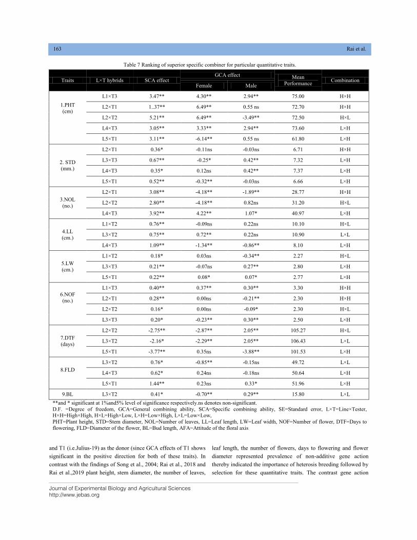
Journal of Experimental Biology and Agricultural Sciences
http://www.jebas.org
163 Rai et al.
and T1 (i.e.Julius-19) as the donor (since GCA effects of T1 shows
significant in the positive direction for both of these traits). In
contrast with the findings of Song et al., 2004; Rai et al., 2018 and
Rai et al.,2019 plant height, stem diameter, the number of leaves,
leaf length, the number of flowers, days to flowering and flower
diameter represented prevalence of non-additive gene action
thereby indicated the importance of heterosis breeding followed by
selection for these quantitative traits. The contrast gene action
Table 7 Ranking of superior specific combiner for particular quantitative traits.
Traits L×T hybrids SCA effect GCA effect Mean
Performance Combination
Female Male
1.PHT
(cm)
L1×T3 3.47** 4.30** 2.94** 75.00 H×H
L2×T1 1..37** 6.49** 0.55 ns 72.70 H×H
L2×T2 5.21** 6.49** -3.49** 72.50 H×L
L4×T3 3.05** 3.33** 2.94** 73.60 L×H
L5×T1 3.11** -6.14** 0.55 ns 61.80 L×H
2. STD
(mm.)
L2×T1 0.36* -0.11ns -0.03ns 6.71 H×H
L3×T3 0.67** -0.25* 0.42** 7.32 L×H
L4×T3 0.35* 0.12ns 0.42** 7.37 L×H
L5×T1 0.52** -0.32** -0.03ns 6.66 L×H
3.NOL
(no.)
L2×T1 3.08** -4.18** -1.89** 28.77 H×H
L2×T2 2.80** -4.18** 0.82ns 31.20 H×L
L4×T3 3.92** 4.22** 1.07* 40.97 L×H
4.LL
(cm.)
L1×T2 0.76** -0.09ns 0.22ns 10.10 H×L
L3×T2 0.75** 0.72** 0.22ns 10.90 L×L
L4×T3 1.09** -1.34** -0.86** 8.10 L×H
5.LW
(cm.)
L1×T2 0.18* 0.03ns -0.34** 2.27 H×L
L3×T3 0.21** -0.07ns 0.27** 2.80 L×H
L5×T1 0.22** 0.08* 0.07* 2.77 L×H
6.NOF (no.)
L1×T3 0.40** 0.37** 0.30** 3.30 H×H
L2×T1 0.28** 0.00ns -0.21** 2.30 H×H
L2×T2 0.16* 0.00ns -0.09* 2.30 H×L
L3×T3 0.20* -0.23** 0.30** 2.50 L×H
7.DTF
(days)
L2×T2 -2.75** -2.87** 2.05** 105.27 H×L
L3×T2 -2.16* -2.29** 2.05** 106.43 L×L
L5×T1 -3.77** 0.35ns -3.88** 101.53 L×H
8.FLD
L3×T2 0.76* -0.85** -0.15ns 49.72 L×L
L4×T3 0.62* 0.24ns -0.18ns 50.64 L×H
L5×T1 1.44** 0.23ns 0.33* 51.96 L×H
9.BL L3×T2 0.41* -0.70** 0.29** 15.80 L×L
**and * significant at 1%and5% level of significance respectively.ns denotes non-significant.
D.F. =Degree of freedom, GCA=General combining ability, SCA=Specific combining ability, SE=Standard error, L×T=Line×Tester, H×H=High×High, H×L=High×Low, L×H=Low×High, L×L=Low×Low,
PHT=Plant height, STD=Stem diameter, NOL=Number of leaves, LL=Leaf length, LW=Leaf width, NOF=Number of flower, DTF=Days to
flowering, FLD=Diameter of the flower, BL=Bud length, AFA=Attitude of the floral axis
Journal of Experimental Biology and Agricultural Sciences
http://www.jebas.org
Identification of superior three way-cross F1s for major quantitative traits in Lilium×formolongi 164
estimation for particular quantitative traits is normal primarily that
depends upon the pedigree of the selected lines and testers.
Furthermore, Song et al. (2004) have employed Single cross F1s in
their diallel analysis while Rai et al. (2018) and Rai et al. (2019)
have used Single cross F1s and Double-cross F1s as mother lines in
their lines×tester analysis.
The most important insight for the selection of particular cross
combinations (hybrids) depending upon the choice of particular
traits is their SCA effects. The SCA effects represent both the
dominance and epispastic effects of a hybrid. In this experiment
out of 15 L×T hybrids none of the hybrids demonstrated
significant value in a positive direction for all studied quantitative
traits. Though SCA effects reflect that L×T hybrids ( L4×T3),
(L5×T1), (L2×T1), (L2×T2), (L3×T2) and (L3×T3) can be used
for the further selection process. The previous results of
Narasimhamurthy & Gowda, (2013) in Tomato, Kumari et al.
(2015) in Pea, Rai et al. (2018) and Rai et al. (2019) in Lilium×
formolongi has been so far reported that the high specific combiner
is the outcomes of the all three types of combination of general
combiner parents viz. high×high, low×low and high ×low that
means not always comes only from the high×high general
combiner parents. There are another evidence that according to the
Sharma et al. (2013), in the majority of the cases, those crosses
exhibiting high SCA effects in a positive direction, were found to
have both or one of the parent as good general combiner for the
studied traits exhibiting non-additive gene action in the genetic
control. Those parents having high GCA effects in positive
direction but sometimes produced low SCA effect is the clear
evidence of the lack of complementation of the parental genes.
Likewise those parents having low GCA effects produced hybrids
with high SCA effects is the clear evidence of complementary gene
action for some traits (Kumari et al., 2015).
Conclusions
The significant variability prevailing in the lines (three way-cross
F1s), testers (donor CVs/breeding line) and their L×T hybrids for
studied quantitative traits has provided the significance of this
experiment. The three way-cross F1s; (Stu× W) × AF1-6 (L2) and
(AF×Ad) × HU-3(L1) can be used as mother lines for seed
production inside the plastic house. For this; Julius-19(T1) and 12-
1-2(T3) can be used as effective donors. Furthermore, L×T
hybrids; (L4×T3), (L5×T1), (L2×T1), (L2×T2) and (L3×T2) can
be used as promising hybrids and some lines of this genotypes can
select and either register as a new cultivar or can be employed for
further breeding program.
Acknowledgements
This work was carried out with a grant of a Golden Seed Project,
the Ministry of Agriculture, Food and Rural Affairs, Republic of
Korea (Project No.213007-05-4-SBN10), a grant from the
Germplasm Reservation Center Program, Rural Development
Administration, Republic of Korea (Project PJ015202012020)
Conflict of interest
All the authors declare that there is no conflict of interest about the
contents of the article.
References
Allard RW, Bradshaw AD (1964) Implications of genotype-
environmental interactions in applied plant breeding. Crop Science
4:503-508.
Arunachalam V, Bandyopadyya A (1979) Are "multiple cross
multiple pollen hybrids "an answer for productive population in
Brassica compestris var. brown sarson ?1. Methods for studying
'mueromphs'. Theoretical and Applied Genetics 54:203-207.
Bakhshaie M, Khosravi S, Azad P, Bagheri H , Van Tuyl JM
(2016) Biotechnological advances in Lilium. Plant Cell Reports
35:1799-1826.
Goo DH, Lim JH, Rhee HK, Cho HR, Kim YJ, Chung HY, Kim
KW (2003) Lily Culture.No.133 Rural Development
Administration, Suwon, Korea (in Korean).
Grassotti A, Gimelli F (2011) Bulb and cut flower production in the
genus Lilium: current status and the future. Acta Horticulture 900.
Ho CW, Jian WT, Lai HC (2006) Plant regeneration via somatic
embryogenesis from suspension cell cultures of Lilium ×
formolongi Hort.using a bioreactor system. In vitro Cellular and
Developmental Biology-Plant 42:240-246.
Kang YI, Joung HY, Goo DH, Choi YJ, Choi MP, An HR, Ko JY,
Choi KJ, Lee KH, Hong KW (2013) A Survey on Cut Flower
Cultivar Trends and Horticultural Status of Lilies (Lilium Hybrids)
in South Korea. Hort Technology 23:629-634.
Kempthorne O (1957) An Introduction to Genetic Statistics. Johan
wiley and sons Inc. New York, U.S.A.
Kumari J, Dikshit HK, Singh B, Singh D (2015) Combining ability
and character association of agronomic and biochemical traits in
pea (Pisum sativum L.). Scientia Horticulturae 181:26-33.
Lucidos JGB, Kwang R, Younis A, Kim CK, Hwang YJ, Son BG,
Lim KB (2013) Different day and night temperatures responses in
Lilium hansonii in relation to growth and flower development.
Horticulture, Environment, and Biotechnology 54:405-41.
Manivannan N (2014) TNAUSTAT-Statistical Package. Retrieved
from https://sites.google/site/tnaustat access on 19December, 2019.
Journal of Experimental Biology and Agricultural Sciences
http://www.jebas.org
165 Rai et al.
Matthews V (2007) The International Lily Register and Checklist.
RHS London, Fourth Edition.
McRae E (1998) Lily species. In: Lilies Timber Press,Portland,
Ore. USA, pp.319-330.
Montazeri Z, Jelodar NB, Bagheri N (2014) Genetic Dissection of
Some Important Agronomic Traits in Rice Using Line × Tester
Method. International Journal of Advanced Biological and
Biomedical Research 2:181-191.
Narasimhamurthy YK, Gowda PHR (2013) Line x Tester analysis
in Tomato (Solanum lycopersicum L.): Identification of superior
parents for fruit quality and yield-attributing traits. International
Journal of Plant Breeding 7:50-54.
Nduwumuremyi A,Tongoona P, Habimana S (2013) Mating
designs: helpful tool for quantitative plant breeding analysis.
Journal of Plant Breeding and Genetics 1:117-129.
Rai R, Shrestha J, Kim JH (2018). Combining Ability and Gene
Action Analysis of Quantitative Traits in Lilium× formolongi.
Journal of Agricultural, Life and Environmental Sciences
30:131-143.
Rai R, Shrestha J, Kim JH (2019) Line xTester analysis in Liliumx
formolongi: Identification of superior parents for growth and
flowering traits. SAARC Journal of Agriculture 17:175-187.
Rashid M, Cheema AA, Ashraf M (2007) Line x tester analysis in
basmati rice. Pakistan Journal of Botany 39: 2035-2042.
Roh MS (2002) New Production Technologies of Lilium -
Prospects and Limitations. Korean Journal of Horticultural Science
and Technology 20:174-190.
Schnell FW (1975) Type of variety and average performance on
hybrid maize. Zeitschrift fuer Pflanzenzuechtung 74:177-188.
Sharma BB, Sharma VK, Dhakar MK, Punetha S (2013)
Combining ability and gene action studies for horticultural traits in
garden pea: A review. African Journal of Agricultural Research
8:4718-4725.
Sharma JR (2006) Statistical and Biometrical techniques in Pland
breeding (First ed.) New Age International ,New Delhi, India.
Song CY, Park SC, Lee JS, Kim YA, Kim JH (2004) Correlation
and combining ability of plant growth and flowering in F1 hybrids
by diallel cross in Lilium formolongi and L. formosanum. Korean
Journal of Horticultural Science and Technology 22:107-113.
Van Tuyl JM, Arens P (2011) Lilium:Breeding History of the
modern cultivar assortment. Acta Horticulturae 900:223-230.
Weatherspoon JH (1970) Comparative Yields of Single, Three-
Way, and Double Crosses of Maize. Crop science 10:157-159.
Xuan Y, Davaasuren YE, Kyung HY, Kim JH (2005) Recovery
of quantitative cut flower characters in backcross generation of
Lilium formolongi. Korean Journal of Flower Research Society
13:268-272.
Younis A, Hwang YJ, Lim KB (2014) Classical vs. modern
genetic and breeding approaches for lily (Lilium) crop
improvement: a review. Flower Research Journal 22:39-47.
Journal of Experimental Biology and Agricultural Sciences
http://www.jebas.org
ISSN No. 2320 – 8694
Journal of Experimental Biology and Agricultural Sciences, April - 2020; Volume – 8(2) page 166 – 175
LARVICIDAL ACTIVITY OF TWO RUTACEAE SPECIES AGAINST THE VECTORS
OF DENGUE AND FILARIAL FEVER
Grace Marin1, Subramanian Arivoli2, Samuel Tennyson3*
1Department of Zoology, Scott Christian College, Nagercoil 629 003, Tamil Nadu, India
2Department of Zoology, Thiruvalluvar University, Vellore 632 115, Tamil Nadu, India
3Department of Zoology, Madras Christian College, Chennai 600 059, Tamil Nadu, India
Received – January 22, 2020; Revision – March 12, 2020; Accepted – April 03, 2020 Available Online – April 25, 2020
DOI: http://dx.doi.org/10.18006/2020.8(2).166.175
ABSTRACT
Mosquito control strategies have been primarily dependent on the use of synthetic chemical insecticides
but its long-term stability and its tendency to bioaccumulate have fostered many environmental and
human health concerns resulting in increase of resistance to chemical insecticides and rebounding
vectorial capacity by mosquitoes. Botanical insecticides serve as suitable alternatives to synthetic ones
as they are relatively effective, and are safe to environment, human, and animal life. In the present
study, Citrus sinensis and Murraya koenigii leaf powders were tested separately on the third instar
larvae of Aedes aegypti and Culex quinquefasciatus at concentrations of 0.2, 0.4, 0.6, 0.8 and 1.0%.
Larval mortality was assessed after 24, 48, 72 and 96 hours and their respective LC50 values for C.
sinensis were 0.69, 0.54, 0.48 and 0.36% for A. aegypti; and 0.61, 0.53, 0.44 and 0.34% for C.
quinquefasciatus. For, M. koenigii, it was 1.05, 0.73, 0.38 and 0.24%; and 0.54, 0.50, 0.32 and 0.22%
for C. sinensis respectively. Amongst tested two botanicals, C. sinensis was found to be more active
against C. quinquefasciatus in dose and time dependent manner and the impact of phytochemicals on
expression of C. quinquefasciatus protein analysed by SDS-PAGE revealed that the phytochemicals
from C. sinensis suppressed the expression of certain proteins present in C. quinquefasciatus. Hence,
this study confirms and recommends that use of C. sinensis and M. koenigii safe and eco-friendly and
could use as an alternative to synthetic pesticides in vector control.
* Corresponding author
KEYWORDS
Citrus sinensis
Murraya koenigii
Aedes aegypti
Culex quinquefasciatus
Larvicidal
E-mail: [email protected] (Samuel Tennyson)
Peer review under responsibility of Journal of Experimental Biology and
Agricultural Sciences.
All the articles published by Journal of Experimental
Biology and Agricultural Sciences are licensed under a
Creative Commons Attribution-NonCommercial 4.0
International License Based on a work at www.jebas.org.
Production and Hosting by Horizon Publisher India [HPI]
(http://www.horizonpublisherindia.in/).
All rights reserved.
Journal of Experimental Biology and Agricultural Sciences
http://www.jebas.org
Larvicidal activity of two Rutaceae species against the vectors of dengue and filarial fever 167
1 Introduction
Insect transmitted disease remains a major source of illness and
death worldwide of which vector-borne diseases are responsible
for 17% of the global burden of parasitic and infectious diseases
(WHO, 2014). Mosquitoes are tremendous public health pests
because of their predominance as marketers of potentially deadly
pathogens of human beings and the annoyance of skin reactions
caused by their bites. Most of the mosquito control programmes
target the larval stage in their breeding sites with larvicides
(Elimam et al., 2009). Most of the mosquito control techniques
have depended on the use of artificial chemical insecticides
(Hemingway et al., 2006). However, the unfriendly effect of most
of these synthetic chemical insecticides leads the insect pest
managers of the world to comb for alternative ways of countering
this disease causing insect (Ileke & Ogungbite, 2015). Also, the
long-term stability of many of these chemical insecticides and their
tendency to bioaccumulate in non-target organisms have fostered
many environmental and human health concerns such as the threats
faced due to resulting in increase of resistance to chemical
insecticides and rebounding vectorial capacity by mosquitoes
(Senthilkumar et al., 2008). Botanical insecticides may serve as
suitable alternatives to synthetic ones in future, as they are
relatively effective, and safe to environment, human, and animal
life (Pitasawat et al., 2007; Borah et al., 2010). Research from all
over the world have documented the effect of various
phytochemical compounds against a wide range of mosquito
species (Samuel et al., 2016; Pathak et al., 2018; Huang et al.,
2019; Kaushik et al., 2019; Samuel et al., 2019; Nathan, 2020).
The Rutaceae family comprises of 150 genera and 1,600 species of
trees, shrubs, and climbers distributed throughout the temperate and
tropical regions of the world (Pollio et al., 2008). The important
genera of this family are Citrus, Fortunella, Murraya, Ptelea, Ruta
and Zanthoxylum (Siddique et al., 2012). Most of the Rutaceae plants
are aromatic whose leaves, fruits or cotyledon in seeds contain a
complex mixture of volatile aroma compounds (Aziz et al., 2010);
which are used in perfumery, gastronomy and traditional medicine.
In addition, various researchers have reported the presence of various
secondary metabolites viz., alkaloids, coumarins, flavonoids,
limonoids, and volatile oils from family Rutaceae, these metabolites
are associated to different biological activities such as antimicrobial
(Ali et al., 2008), antidiarrhoeal (Mandal et al., 2010),
anticholinesterasic (Cardoso-Lopes et al., 2010), antileishmanial
(Andres et al., 2011), antiprotozoal (Severino et al., 2009),
antioxidant (Wansi et al., 2006), and mosquito larvicidal (Rajkumar
& Jebanesan, 2008; Arivoli & Samuel, 2011; Arivoli et al., 2015)
properties. Consequently, this study was conducted to determine the
larvicidal efficacy of C. sinensis and M. koenigii leaves as an
alternative to synthetic insecticides for the management of A. aegypti
and C. quinquefasciatus.
2 Materials and Methods
2.1 Plant collection and preparation of phytopowders
Mature and healthy leaves of C. sinensis and M. koenigii were
collected from Nagercoil, Kanyakumari district, Tamil Nadu, India
and identified taxonomically and confirmed at the Department of
Botany and Research Centre, Nagercoil, Kanyakumari district,
Tamil Nadu, India. In the laboratory, dechlorinated water was used
to wash the leaves and thereafter these leaves were shade dried.
Leaves of each plant (1Kg) was then powdered by an electric
blender and was stored in air tight sterilized amber coloured bottles
for bioassay.
2.2 Phytochemical screening
The active phytochemical compounds in C. sinensis and M.
Koenigii leaf powders were qualitatively determined using
methods described by Harborne (1998) for alkaloids, glycosides,
steroids, phenolics and carbohydrates, Van Burden & Robinson
(1981) for tannins and proteins, Obadoni & Ochuko (2001) for
saponins, Boham & Kocipai (1974) for flavonoids, and Okwu &
Okwu (2004) for vitamins.
2.3 Fourier Transform Infrared Spectroscopy (FTIR)
FTIR is the most powerful tool for identifying functional groups
present in plant extracts. Dried methanol extract powder (10mg) of
each plant was encapsulated in 100mg of KBr pellet, in order to
prepare translucent sample discs. The powdered samples were
loaded in FTIR spectroscope (Shimadzu, Japan), with a scan range
from 400 to 4000cm1 (Visveshwari et al., 2017).
2.4 Sodium Dodecyl sulphate – PolyAcrylamide Gel Electrophoresis
(SDS - PAGE) analysis
SDS-PAGE is the most widely used analytical method to resolve
separate components of a protein mixture. It is almost obligatory to
assess the purity of a protein through an electrophoretic method.
SDS-PAGE simultaneously exploits differences in molecular size
to resolve proteins differing by as little as 1% in their
electrophoretic mobility through the gel matrix. The technique is
also a powerful tool for estimating the molecular weights of
proteins. The molecular weight of the protein was estimated using
a high molecular weight protein calibration kit (Merck, Bangalore,
India) as markers. The molecular mass markers (expressed in Da)
used were myosin (205,000), β-galactosidase (11,600),
phosphorylase b (97,400), bovine serum albumin (66,000),
ovalbumin (43,000), carbonic anhydrase (29,000), soyabean
trypsin inhibitor (20,100) and lysozyme (14,300).
Total protein was extracted by using acetone- TCA (Trichloro Acetic
Acid) precipitation technique of Damerval et al. (1986) and the
Journal of Experimental Biology and Agricultural Sciences
http://www.jebas.org
168 Marin et al.
estimation of protein was executed according to the methodology of
Lowry et al. (1951). Every sample (0.5g) with a buffer (2mL)
containing Tris (hydroxymethyl) aminomethane (Tris)-Glycine (pH
8.3) (50mM), sucrose (0.5M), EDTA (50mM), potassium chloride
(0.1M), PMSF (2mM) and 0.1% (v/v) 2-mercaptoethanol was
homogenized at 4°C in a chilled pestle and mortar. The homogenate
was centrifuged at 14000 rpm for 10 minutes in a refrigerated
centrifuge. The concentration of protein in supernatant samples were
assessed according to the technique of Bradford (1976) and gels
prepared as per the protocol adopted by Laemmli (1970). A
separating gel (12.0%) was used for resolving the polypeptides
which comprised of Tris- HCl (375mM), pH 8.8, 0.1% (w/v) SDS,
0.05% (w/v) ammonium persulfate and 0.4µLmL-1
TEMED. For a
stacking gel (4%) used to concentrate (stack) the polypeptides, it
comprised of Tris-HCl (125mM), pH 6.8, 0.1% (w/v) SDS, 0.05%
(w/v) ammonium persulfate and 0.5µLmL-1
TEMED. The
electrophoresis running buffer was made of Tris (25mM), glycine
(192mM), SDS (0.1%) with pH 8.3, and was accomplished for 4
hours at 35mA. The gels were stained for two hours with Coomassie
Brilliant Blue R-250 (Sigma) (0.25%) in 50% (v/v) methanol and
(v/v) acetic acid (10%) and then destained with methanol and acetic
acid until a clear background was obtained.
2.5 Vector mosquitoes
Insecticide free A. aegypti eggs and C. quinquefasciatus egg rafts
were obtained from Entomology Research Institute, Loyola
College, Chennai, Tamil Nadu, India. Cyclic generations of the
above mentioned vector mosquitoes were maintained separately in
two feet mosquito cages with a mean room temperature of 27±2°C
and a relative humidity of 70-80% inside an insectary and the
adults were fed on 10% glucose solution in water. Ovitraps were
placed inside the mosquito cages for the female mosquitoes to
oviposit eggs and the laid eggs were then transferred to the larval
rearing chamber and were maintained in enamel larval trays. The
larvae fed with larval food (dog biscuits and yeast in the ratio 3:1)
on becoming pupae were transferred to plastic bowls kept inside
another mosquito cage for emergence of adults.
2.6 Larvicidal bioassay
According to the guidelines of World Health Organization (WHO,
2005) with minor modifications, bioassays were performed on
twenty five F1 generation of laboratory colonized third instar
larvae of the above mentioned vector species at test concentrations
of (w/v) 0.2, 0.4, 0.6, 0.8 and 1.0% by introducing them into glass
beakers (250mL) containing 200mL of distilled water and test
concentration. One per cent stock solution for each plant powder
was prepared by dissolving 1g of each leaf powder in 100mL
distilled water, from which the above mentioned concentrations
were arrived. Third instar larvae formed the choice as the research
sample, compared to first and second instar since they possessed a
larger body size and are more adaptive to the environment; while
fourth instar transforms to a pupa in approximately 48 hours
(Marin et al., 2020). Control (distilled water) was run
simultaneously and maintained separately. Bioassays were
performed with five replicates for each concentration per trial with
a total of three trials. Larval mortality was observed 24, 48, 72 and
96 hours after treatment and moribund larvae were recorded dead
when they displayed no signs of movement when probed by a
needle at their respiratory siphon.
2.7 Statistical analysis
Data was subjected to statistical analysis with significance set at
95% confidence in IBM SPSS Statistics v22 (SPSS, 2010). Per
cent larval mortality was calculated and corrections for control
mortality (5-20%) if required was carried according to Abbott’s
formula (Abbott, 1925) and then larval mortality were subjected to
probit analysis. Analysis of variance (ANOVA) of larval mortality
was performed to measure differences between treated bioassays
and controls and at which doses in particular and the differences
were considered significant at P≤0.001 level.
1 – n in T after treatment x 100
n in C after treatment
Where, n is the number of larvae, T: treated and C: control.
3 Results
The qualitative phytochemical analysis of C. sinensis and M.
koenigii leaves are presented in Table 1. The FTIR spectrum of C.
sinensis showed the presence of alcohol, alkenes, aromatic amines,
phenyl, ether, methylene, 1° and 2° amines and aliphatic chloro
compound. The major band was observed at 3308cm-1
due to O-H
stretching vibrations of alcohol group (Figure 1). M. koenigii
Table 1 Phytochemical composition of Citrus sinensis and Murraya koenigii leaves
Plant species Phytocompounds
Alkaloids Carbohydrates Flavonoids Glycosides Phenols Proteins Saponins Steroids Tannins
Citrus sinensis + + + + + + + + + + + + + + + + + + + + + + +++++ + + + + + + + ++
Murraya koenigii + + + + + + + + + + + + + + + + + + + + + + + + + + + + + - + + +
+++++ Above 80%; ++++ 50-75%; +++ Below 50%; ++ Below 25%; and – Nil
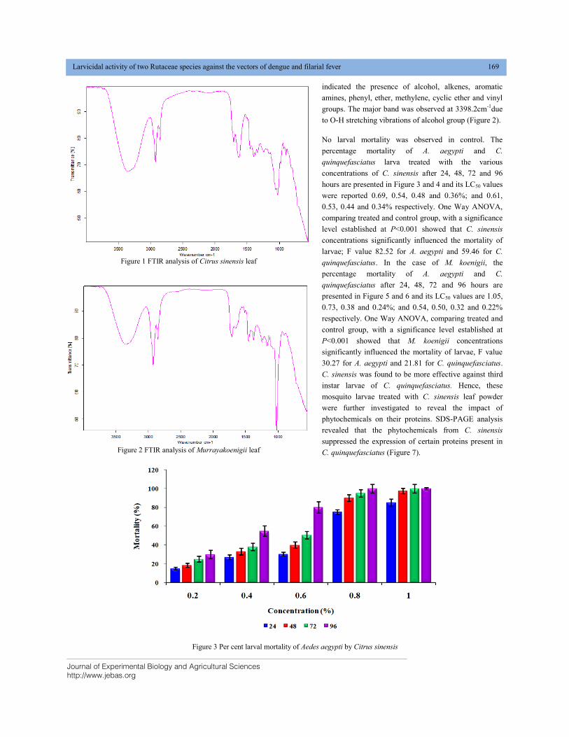
Journal of Experimental Biology and Agricultural Sciences
http://www.jebas.org
Larvicidal activity of two Rutaceae species against the vectors of dengue and filarial fever 169
indicated the presence of alcohol, alkenes, aromatic
amines, phenyl, ether, methylene, cyclic ether and vinyl
groups. The major band was observed at 3398.2cm-1
due
to O-H stretching vibrations of alcohol group (Figure 2).
No larval mortality was observed in control. The
percentage mortality of A. aegypti and C.
quinquefasciatus larva treated with the various
concentrations of C. sinensis after 24, 48, 72 and 96
hours are presented in Figure 3 and 4 and its LC50 values
were reported 0.69, 0.54, 0.48 and 0.36%; and 0.61,
0.53, 0.44 and 0.34% respectively. One Way ANOVA,
comparing treated and control group, with a significance
level established at P<0.001 showed that C. sinensis
concentrations significantly influenced the mortality of
larvae; F value 82.52 for A. aegypti and 59.46 for C.
quinquefasciatus. In the case of M. koenigii, the
percentage mortality of A. aegypti and C.
quinquefasciatus after 24, 48, 72 and 96 hours are
presented in Figure 5 and 6 and its LC50 values are 1.05,
0.73, 0.38 and 0.24%; and 0.54, 0.50, 0.32 and 0.22%
respectively. One Way ANOVA, comparing treated and
control group, with a significance level established at
P<0.001 showed that M. koenigii concentrations
significantly influenced the mortality of larvae, F value
30.27 for A. aegypti and 21.81 for C. quinquefasciatus.
C. sinensis was found to be more effective against third
instar larvae of C. quinquefasciatus. Hence, these
mosquito larvae treated with C. sinensis leaf powder
were further investigated to reveal the impact of
phytochemicals on their proteins. SDS-PAGE analysis
revealed that the phytochemicals from C. sinensis
suppressed the expression of certain proteins present in
C. quinquefasciatus (Figure 7).
Figure 1 FTIR analysis of Citrus sinensis leaf
Figure 2 FTIR analysis of Murrayakoenigii leaf
Figure 3 Per cent larval mortality of Aedes aegypti by Citrus sinensis
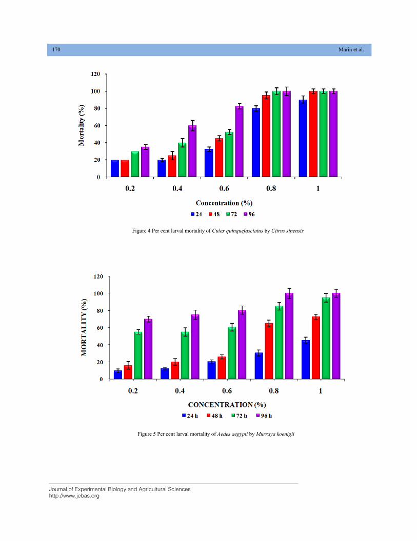
Journal of Experimental Biology and Agricultural Sciences
http://www.jebas.org
170 Marin et al.
Figure 4 Per cent larval mortality of Culex quinquefasciatus by Citrus sinensis
Figure 5 Per cent larval mortality of Aedes aegypti by Murraya koenigii
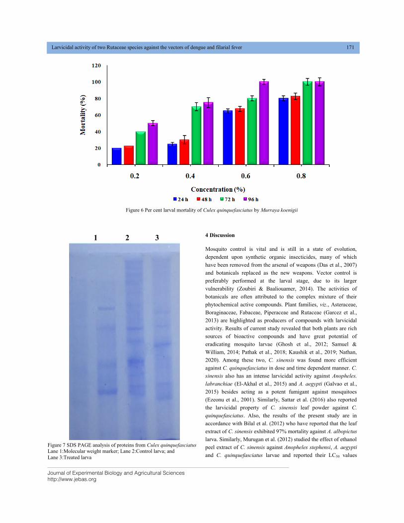
Journal of Experimental Biology and Agricultural Sciences
http://www.jebas.org
Larvicidal activity of two Rutaceae species against the vectors of dengue and filarial fever 171
4 Discussion
Mosquito control is vital and is still in a state of evolution,
dependent upon synthetic organic insecticides, many of which
have been removed from the arsenal of weapons (Das et al., 2007)
and botanicals replaced as the new weapons. Vector control is
preferably performed at the larval stage, due to its larger
vulnerability (Zoubiri & Baaliouamer, 2014). The activities of
botanicals are often attributed to the complex mixture of their
phytochemical active compounds. Plant families, viz., Asteraceae,
Boraginaceae, Fabaceae, Piperaceae and Rutaceae (Garcez et al.,
2013) are highlighted as producers of compounds with larvicidal
activity. Results of current study revealed that both plants are rich
sources of bioactive compounds and have great potential of
eradicating mosquito larvae (Ghosh et al., 2012; Samuel &
William, 2014; Pathak et al., 2018; Kaushik et al., 2019; Nathan,
2020). Among these two, C. sinensis was found more efficient
against C. quinquefasciatus in dose and time dependent manner. C.
sinensis also has an intense larvicidal activity against Anopheles.
labranchiae (El-Akhal et al., 2015) and A. aegypti (Galvao et al.,
2015) besides acting as a potent fumigant against mosquitoes
(Ezeonu et al., 2001). Similarly, Sattar et al. (2016) also reported
the larvicidal property of C. sinensis leaf powder against C.
quinquefasciatus. Also, the results of the present study are in
accordance with Bilal et al. (2012) who have reported that the leaf
extract of C. sinensis exhibited 97% mortality against A. albopictus
larva. Similarly, Murugan et al. (2012) studied the effect of ethanol
peel extract of C. sinensis against Anopheles stephensi, A. aegypti
and C. quinquefasciatus larvae and reported their LC50 values
1 2 3
Figure 7 SDS PAGE analysis of proteins from Culex quinquefasciatus
Lane 1:Molecular weight marker; Lane 2:Control larva; and
Lane 3:Treated larva
Figure 6 Per cent larval mortality of Culex quinquefasciatus by Murraya koenigii
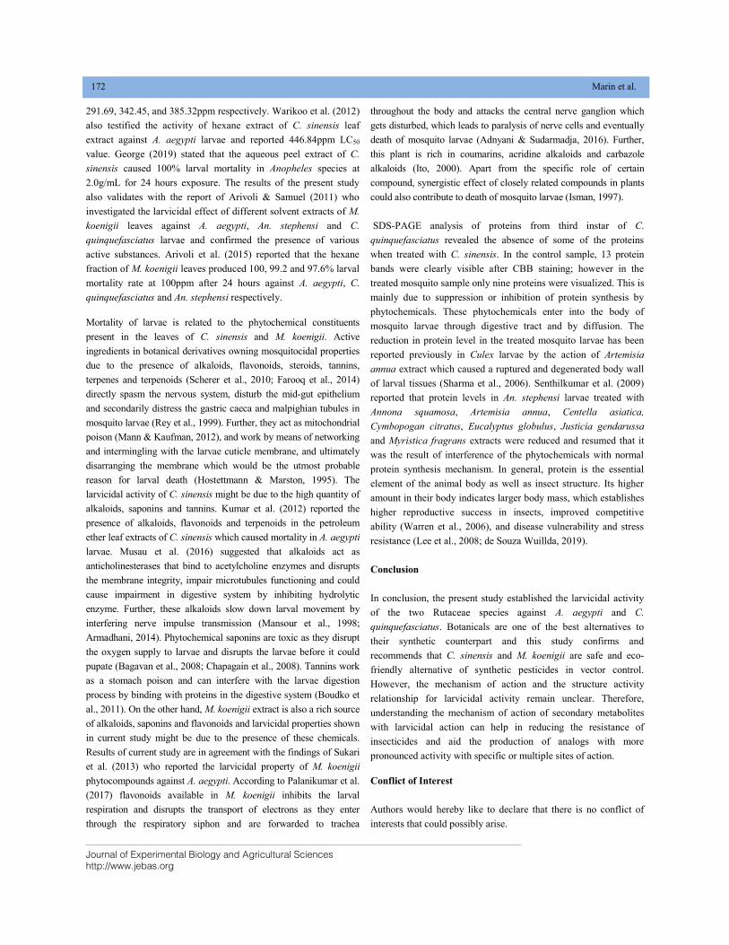
Journal of Experimental Biology and Agricultural Sciences
http://www.jebas.org
172 Marin et al.
291.69, 342.45, and 385.32ppm respectively. Warikoo et al. (2012)
also testified the activity of hexane extract of C. sinensis leaf
extract against A. aegypti larvae and reported 446.84ppm LC50
value. George (2019) stated that the aqueous peel extract of C.
sinensis caused 100% larval mortality in Anopheles species at
2.0g/mL for 24 hours exposure. The results of the present study
also validates with the report of Arivoli & Samuel (2011) who
investigated the larvicidal effect of different solvent extracts of M.
koenigii leaves against A. aegypti, An. stephensi and C.
quinquefasciatus larvae and confirmed the presence of various
active substances. Arivoli et al. (2015) reported that the hexane
fraction of M. koenigii leaves produced 100, 99.2 and 97.6% larval
mortality rate at 100ppm after 24 hours against A. aegypti, C.
quinquefasciatus and An. stephensi respectively.
Mortality of larvae is related to the phytochemical constituents
present in the leaves of C. sinensis and M. koenigii. Active
ingredients in botanical derivatives owning mosquitocidal properties
due to the presence of alkaloids, flavonoids, steroids, tannins,
terpenes and terpenoids (Scherer et al., 2010; Farooq et al., 2014)
directly spasm the nervous system, disturb the mid-gut epithelium
and secondarily distress the gastric caeca and malpighian tubules in
mosquito larvae (Rey et al., 1999). Further, they act as mitochondrial
poison (Mann & Kaufman, 2012), and work by means of networking
and intermingling with the larvae cuticle membrane, and ultimately
disarranging the membrane which would be the utmost probable
reason for larval death (Hostettmann & Marston, 1995). The
larvicidal activity of C. sinensis might be due to the high quantity of
alkaloids, saponins and tannins. Kumar et al. (2012) reported the
presence of alkaloids, flavonoids and terpenoids in the petroleum
ether leaf extracts of C. sinensis which caused mortality in A. aegypti
larvae. Musau et al. (2016) suggested that alkaloids act as
anticholinesterases that bind to acetylcholine enzymes and disrupts
the membrane integrity, impair microtubules functioning and could
cause impairment in digestive system by inhibiting hydrolytic
enzyme. Further, these alkaloids slow down larval movement by
interfering nerve impulse transmission (Mansour et al., 1998;
Armadhani, 2014). Phytochemical saponins are toxic as they disrupt
the oxygen supply to larvae and disrupts the larvae before it could
pupate (Bagavan et al., 2008; Chapagain et al., 2008). Tannins work
as a stomach poison and can interfere with the larvae digestion
process by binding with proteins in the digestive system (Boudko et
al., 2011). On the other hand, M. koenigii extract is also a rich source
of alkaloids, saponins and flavonoids and larvicidal properties shown
in current study might be due to the presence of these chemicals.
Results of current study are in agreement with the findings of Sukari
et al. (2013) who reported the larvicidal property of M. koenigii
phytocompounds against A. aegypti. According to Palanikumar et al.
(2017) flavonoids available in M. koenigii inhibits the larval
respiration and disrupts the transport of electrons as they enter
through the respiratory siphon and are forwarded to trachea
throughout the body and attacks the central nerve ganglion which
gets disturbed, which leads to paralysis of nerve cells and eventually
death of mosquito larvae (Adnyani & Sudarmadja, 2016). Further,
this plant is rich in coumarins, acridine alkaloids and carbazole
alkaloids (Ito, 2000). Apart from the specific role of certain
compound, synergistic effect of closely related compounds in plants
could also contribute to death of mosquito larvae (Isman, 1997).
SDS-PAGE analysis of proteins from third instar of C.
quinquefasciatus revealed the absence of some of the proteins
when treated with C. sinensis. In the control sample, 13 protein
bands were clearly visible after CBB staining; however in the
treated mosquito sample only nine proteins were visualized. This is
mainly due to suppression or inhibition of protein synthesis by
phytochemicals. These phytochemicals enter into the body of
mosquito larvae through digestive tract and by diffusion. The
reduction in protein level in the treated mosquito larvae has been
reported previously in Culex larvae by the action of Artemisia
annua extract which caused a ruptured and degenerated body wall
of larval tissues (Sharma et al., 2006). Senthilkumar et al. (2009)
reported that protein levels in An. stephensi larvae treated with
Annona squamosa, Artemisia annua, Centella asiatica,
Cymbopogan citratus, Eucalyptus globulus, Justicia gendarussa
and Myristica fragrans extracts were reduced and resumed that it
was the result of interference of the phytochemicals with normal
protein synthesis mechanism. In general, protein is the essential
element of the animal body as well as insect structure. Its higher
amount in their body indicates larger body mass, which establishes
higher reproductive success in insects, improved competitive
ability (Warren et al., 2006), and disease vulnerability and stress
resistance (Lee et al., 2008; de Souza Wuillda, 2019).
Conclusion
In conclusion, the present study established the larvicidal activity
of the two Rutaceae species against A. aegypti and C.
quinquefasciatus. Botanicals are one of the best alternatives to
their synthetic counterpart and this study confirms and
recommends that C. sinensis and M. koenigii are safe and eco-
friendly alternative of synthetic pesticides in vector control.
However, the mechanism of action and the structure activity
relationship for larvicidal activity remain unclear. Therefore,
understanding the mechanism of action of secondary metabolites
with larvicidal action can help in reducing the resistance of
insecticides and aid the production of analogs with more
pronounced activity with specific or multiple sites of action.
Conflict of Interest
Authors would hereby like to declare that there is no conflict of
interests that could possibly arise.
Journal of Experimental Biology and Agricultural Sciences
http://www.jebas.org
Larvicidal activity of two Rutaceae species against the vectors of dengue and filarial fever 173
References
Abbott WS (1925) A method of computing the effectiveness of an
insecticide. Journal of Economic Entomology 18: 265-267.
Adnyani IGAP, Sudarmadja IM (2016) Pengaruh Konsentrasi
Ekstrak Etanol Daun Pepaya (Carica papaya L) terhadap
Kematian Larva Nyamuk Aedes aegypti. E-Jurnal Medika 5: 1-5.
Ali MS, Fatima S, Pervez MK (2008) Haplotin: A new
furanoquinoline from Haplophyllum acutifolium (Rutaceae).
Journal of the Chemical Society of Pakistan 30: 775-779.
Andres CCA, Barrera CED, Falla GDS, Murcia DG, Suarez CLE
(2011) Seco-limonoids and quinoline alkaloids from Raputia
heptaphylla and their antileishmanial activity. Chemical and
Pharmaceutical Bulletin 59: 855-859.
Arivoli S, Raveen R, Samuel T (2015) Larvicidal activity of
Murraya koenigii (L.) Spreng (Rutaceae) hexane leaf extract
isolated fractions against Aedes aegypti Linnaeus, Anopheles
stephensi Liston and Culex quinquefasciatus Say (Diptera:
Culicidae). Journal of Mosquito Research 5: 1-8.
Arivoli S, Samuel T (2011) Studies on the mosquitocidal activity
of Murraya koenigii (L.) Spreng (Rutaceae) leaf extracts against
Aedes aegypti, Anopheles stephensi and Culex quinquefasciatus
(Diptera: Culicidae). Asian Journal of Experimental Biological
Science 2: 721-730.
Armadhani (2014) Keefektifan Ekstrak Etanol Daun Petai Cina
(Leucaenaglauca, Benth) sebagai Larvasida Alamiterhadap
Kematian Larva Nyamuk Ae. aegypti Instar III. NaskahPublikasi.
Semarang: Universitas Negeri Semarang.
Aziz SSSA, Sukari MA, Kitajima M, Aimi N, Ahpandi NJ (2010)
Coumarins from Murraya paniculata (Rutaceae). Malaysian
Journal of Analytical Sciences 14: 1-5.
Bagavan A, Rahuman AA, Kamaraj C, Geetha K (2008) Larvicidal
activity of saponins from Achyranthes aspera against Aedes
aegypti and Culex quinquefasciatus (Diptera: Culicidae).
Parasitology Research 103: 223-229.
Bilal H, Akram W, Ali-Hassan S (2012) Larvicidal activity of
Citrus limonoids against Aedes albopictus larvae. Journal of
Arthropod-Borne Diseases 6: 104-111.
Boham A Kocipai AC (1974) Flavonoids and condensed tannins
from leaves of Hawaiia vaccinum vaticulatum and V. calyscinium.
Pacific Science 48: 458-463.
Borah R, Kalita MC, Kar A, Talukdar AK (2010) Medicinal plants
and their applications. African Journal of Biotechnology 9: 25-27.
Boudko DY, Moroz LL, Harvey WR, Linser PJ (2011)
Alkalinization by chloride bicarbonate pathway in larval mosquito
midgut. Proceedings of the National Academy of Sciences of the
United States of America 26: 15355-15359.
Bradford MM (1976) A rapid and sensitive method for the quantitation
of microgram quantities of protein utilizing the principle of protein-dye
binding. Analytical Biochemistry 72: 248-254.
Cardoso-Lopes EM, Maier JA, Da Silva MR, Regasini LO, Simote
SY, Lopes NP, Pirani JR, Bolzni VS, Young MCM (2010) Alkaloids
from stems of Esenbeckia leiocarpa Engl. (Rutaceae) as potential
treatment for Alzheimer disease. Molecules 15: 9205-9213.
Chapagain B, Saharan V, Wiesman Z (2008) Larvicidal activity of
saponins from Balanites aegyptiaca callus against Aedes aegypti
mosquito. Bioresource Technology 99: 1165-1168.
Damerval C, De Vienne C, Zivy M, Thiellement H (1986) The
technical improvements in two-dimensional electrophoresis
increase the level of genetic variation detected in wheat seedling
proteins. Electrophoresis 7: 52-54.
Das NG, Goswami D, Rabha B (2007) Preliminary evaluation of
mosquito larvicidal efficacy of plant extracts. Journal of Vector
Borne Disease 44: 145-148.
de Souza Wuillda ACJ, Martins RCC, Costa FN (2019) Larvicidal
activity of secondary plant metabolites in Aedes aegypti control:
An overview of the previous 6 years. Natural Product
Communications 1: 1-11.
El-Akhal F, Lalamia AEO, Guemmouh R (2015) Larvicidal
activity of essential oils of Citrus sinensis and Citrus aurantium
(Rutaceae) cultivated in Morocco against the malaria vector
Anopheles labranchiae (Diptera: Culicidae). Asian Pacific Journal
of Tropical Disease 5: 458-462.
Elimam AM, Elmalik KH, Ali FS (2009) Efficacy of leaves extract
of Calotropis procera Ait. (Asclepiadaceae) in controlling
Anopheles arabiensis and Culex quinquefasciatus mosquitoes.
Saudi Journal of Biological Sciences 16: 95-100.
Ezeonu FC, Chidume GI, Udedi SC (2001) Insecticidal properties of
volatile extracts of orange peels. Bioresource Technology 76: 273-274.
Farooq U, Waseem B, Muzaffar R, Tripathi J, Tharani M, Sharma
MA (2014) Comparative study of phytochemical investigation of
Xanthium strumarium medicinal plant. International Journal of
Research in Pharmacy and Chemistry 4: 96-100.
Galvão JG, Silva VF, Ferreira SG, França FRM, Santos DA,
Freitas LS, Alves PB, Araújo AAS, Cavalcanti SCH, Nunes RS
(2015) Cyclodextrin inclusion complexes containing Citrus
sinensis (L.) Osbeck essential oil: An alternative to control Aedes
aegypti larvae. Thermochimica Acta 608: 14-19.
Garcez WS, Garcez FR, Silva L, Sarmento UC (2013) Substâncias
de origem vegetal com atividadelarvicida contra Aedes aegypti.
Revista Virtual de Química 5: 363-393.
Journal of Experimental Biology and Agricultural Sciences
http://www.jebas.org
174 Marin et al.
George UI (2019) Environmental control of malaria: Can Citrus
sinensis peel be a potent larvicide for household vector control?
GSC Biological and Pharmaceutical Sciences 09(03): 085-090.
Ghosh A, Chowdhury N, Chandra G (2012) Plant extracts as
potential mosquito larvicides. Indian Journal of Medical Research
135(5): 581-598.
Harborne JB (1998) Phytochemical methods, a guide to modern
techniques of plant analysis, 3rd
Edition. Chapman and Hill Ltd.,
London, 279.
Hemingway J, Beaty BJ, Rowland M, Scott TW, Sharp BL (2006)
The innovative vector control consortium: Improved control of
mosquito-borne diseases. Trends in Parasitology 22: 308-312.
Hostettmann K, Marston A (1995) Saponins (Chemistry and
Pharmacology of Natural Products). University Press, Cambridge, 132.
Huang HT, Lin CC, Kuo TC, Chen SJ, Huang RN (2019)
Phytochemical composition and larvicidal activity of essential oils
from herbal plants. Planta 250: 59-68.
Ileke KD, Ogungbite OC (2015) Alstonia boonei De Wild oil extract in
the management of mosquito (Anopheles gambiae), a vector of malaria
disease. Journal of Coastal Life Medicine 3: 557-563.
Isman MB (1997) Neem and other botanical insecticides: Barriers
to commercialization. Phytoparasitica 25: 339-344.
Ito C (2000) Studies on medicinal resources of rutaceous plants
and development to pharmaceutical chemistry. Natural Medicine
54: 117-122.
Kaushik S, Sharma NR, Thomas TG, Sharma AK, Bansal A (2019)
Indigenous plants and their larvicidal potential against Indian
mosquito vectors: A review. Journal of Communicable Diseases
51: 59-72.
Kumar S, Ray A, Kaur J, Samal R, Wahab N, Warikoo R (2012)
Efficacy of the ethanolic leaf extracts of citrus plant, Citrus sinensis as
larvicidal and irritant agent against dengue vector Aedes aegypti L.
Asian Pacific Journal of Tropical Biomedicine 3: 152-155.
Laemmli UK (1970) Cleavage of structural proteins during the
assembly of the head of bacteriophage T4. Nature 227: 680-685.
Lee KP, Simpson SJ, Wilson K (2008) Dietary protein-quality
influences melanization and immune function in an insect.
Functional Ecology 22: 1052-1061.
Lowry OH, Rosebrough NJ, Farr AL, Randall RJ (1951) Protein
measurement with the Folin phenol reagent. Journal of Biological
Chemistry 193: 265-275.
Mandal S, Nayak A, Kar M, Banerjee SK, Das A, Upadhyay SN,
Singh RK, Banerji A, Banerji J (2010) Antidiarrhoeal activity of
carbazole alkaloids from Murraya koenigii Spreng (Rutaceae)
seeds. Fitoterapia 81: 72-74.
Mann RS, Kaufman PE (2012) Natural product pesticides: their
development, delivery and use against insect vectors. Mini-
Reviews in Organic Chemistry 9: 185-202.
Mansour SA, Messeha SS, Mohamed SM (1998) Botanical
biocides: Mosquitocidal activity of certain Nigella sativa
constituents. Journal of Union Arab Biology 10: 45-63.
Marin G, Arivoli S, Samuel T (2020) Synergistic larvicidal action
of Citrus limon (L.) Osbeck (Rutaceae) and Bacillus thuringiensis
Berliner 1915 (Bacillaceae) against the dengue vector Aedes
aegypti Linnaeus 1762 (Diptera: Culicidae). GSC Biological and
Pharmaceutical Sciences 10: 25-33.
Murugan K, Kumar PM, Kovendan K, Amerasan D, Subrmaniam
J, Hwang JS (2012) Larvicidal, pupicidal, repellent and adulticidal
activity of Citrus sinensis orange peel extract against Anopheles
stephensi, Aedes aegypti and Culex quinquefasciatus (Diptera:
Culicidae). Parasitology Research 111: 1757-1769.
Musau JK, Mbaria JM, Nguta JM, Mathiu M, Kiama SG (2016)
Phytochemical composition and larvicidal properties of plants used
for mosquito control in Kwale County, Kenya. International
Journal of Mosquito Research 3: 12-17.
Nathan SS (2020) A review of resistance mechanisms of synthetic
insecticides and botanicals, phytochemicals, and essential oils as
alternative larvicidal agents against mosquitoes. Frontiers in
Physiology 10: 1591.
Obadoni BO Ochuko PO (2001) Studies and comparative efficacy
of the crude extracts of some homostatic plants in Edo and Delta
states of Nigeria. Global Journal of Pure and Applied Science 8b:
203-208.
Okwu DE, Okwu ME (2004) Phytochemicals and vitamins content
of indigenous plant species of south eastern Nigeria. Journal of
Sustainable Agriculture and Environment 6: 30-37.
Palanikumar M, Pravin Y, Navaneethan M, Mahendren S, Mohanraj
RS, Dhanakkodi B (2017) Callistemon citrinus (Myrtaceae)
methanolic leaf extract: a potent mosquitocidal agent for controlling
dengue vector mosquito Aedes aegypti (Diptera: Culicidae). Journal of
Entomology and Zoology Studies 5: 1051-1059.
Pathak M, Kumar R, Singh MK, Maurya O, Bharati KA (2018) A
review on traditional larvicidal plants. Mintage Journal of
Pharmaceutical & Medical Sciences 7: 1-9
Journal of Experimental Biology and Agricultural Sciences
http://www.jebas.org
Larvicidal activity of two Rutaceae species against the vectors of dengue and filarial fever 175
Pitasawat B, Champakaew D, Choochote W, Jitpakdi A, Chaithong
U, Kanjanapothi D, Rattanachanpichai E, Tippawangkosol P,
Riyong D, Tuetun B, Chaiyasit D (2007) Aromatic plant-derived
essential oil: an alternative larvicide for mosquito control.
Fitoterapia 78: 205-210.
Pollio A, De Natale A, Appetiti E, Aliotta G, Touwaide A (2008)
Continuity and change in the Mediterranean medical tradition:
Ruta spp. (Rutaceae) in Hippocratic medicine and present
practices. Journal of Ethnopharmacology 116: 469-482.
Rajkumar S, Jebanesan A (2008) Bioactivity of flavonoid
compounds from Poncirus trifoliata L. (Family: Rutaceae) against
the dengue vector, Aedes aegypti L. (Diptera: Culicidae).
Parasitology Research 104: 19-25.
Rey D, Pautou MP, Meyran JC (1999) Histopathological effects of
tannic acid on the midgut epithelium of some aquatic Diptera
larvae. Journal of Invertebrate Pathology 73: 173-181.
Samuel T, Arivoli S, William J (2016) Phytonanopesticides for
vector control: A review. Journal of Applied Zoological
Researches 27: 1-11.
Samuel T, Kalarani A, Vinodha V, Arivoli S, Selvakumar S, Meeran
M, Syedalifathima A (2019) Repellent property of plants against
mosquitoes in field conditions by traditional method. International
Journal of Zoology and Applied Biosciences 4: 258-263.
Samuel T, William SJ (2014) Potentiality of botanicals in
sustainable control of mosquitoes (Diptera: Culicidae). In:
Achieving Sustainable Development: Our Vision and Mission, Ed.
William, SJ, Loyola College, Chennai, Tamil Nadu, India 204-227.
Sattar M, Iqbal MN, Ashraf A, Ali S, Shahzad MI, Alam S, Ali T,
Sheikh R (2016) Larvicidal efficacy of Citrus sinensis extracts
against Culex quinquefasciatus. PSM Microbiology 1: 56-61.
Scherer R, Wagner R, Meireles MAA, Godoy HT, Duarte MCT,
Filho JT (2010) Biological activity and chemical composition of
hydrodistilled and supercritical extracts of Xanthium strumarium
L. leaves. Journal of Essential Oil Research 22: 424-429.
Senthilkumar A, Kannathasan K, Venkatesalu V (2008) Chemical
constituents and larvicidal property of the essential oil of Blumea
mollis (D. Don) Merr. against Culex quinquefasciatus. Parasitology
Research 103: 959-962.
Senthilkumar N, Varma P, Gurusubramanian G (2009) Larvicidal and
adulticidal activities of some medicinal plants against the malarial vector,
Anopheles stephensi Liston. Parasitology Research 104: 237-244.
Severino VG, Cazal CM, Forim MR, da Silva MF, Rodrigues-Filho E,
Fernandes JB, Vieira PC (2009) Isolation of secondary metabolites from
Hortia oreadica (Rutaceae) leaves through high-speed counter-current
chromatography. Journal of Chromatography A 1216: 4275-4281.
Sharma P, Mohan L, Srivastava CN (2006) Phytoextract-induced
developmental deformities in malaria vector. Bioresource
Technology 97: 1599-1604.
Siddique S, Javed S, Nawaz S, Perveen Z, Khan RA, Khanum R,
Shahzad K (2012) Volatile components and antimicrobial activity
of Citrus sinensis var. mosammi leaves oil. Journal of Medicinal
Plants Research 6: 2184-2187.
SPSS (2010) IBM SPSS Statistics for Windows, Version 22.0.
Armonk, NY: IBM Corp.
Sukari MA, Noor HSM, Bakar NHA, Ee GCL, Ismail IS, Rahmani
M, Abdul AB (2013) Larvicidal carbazole alkaloids from Murraya
koenigii against dengue fever mosquito Aedes aegypti Linnaeus.
Asian Journal of Chemistry 25: 7719-7721.
Van Burden TP, Robinson WC (1981) Formation of complexes
between protein and tannin acid. Journal of Agricultural Food
Chemistry 1: 77.
Visveshwari M, Subbaiyan B, Thangapandian V (2017)
Phytochemical analysis, antibacterial activity, FTIR and GCMS
analysis of Ceropegia juncea Roxb. International Journal of
Pharmacognosy and Phytochemical Research 9: 914-920.
Wansi JD, Wandji J, Meva'a ML, Waffo KAF, Ranjit R, Khan SN,
Asma A, Iqbal CM, Lallemand MC, Tillequin F, Tanee FZ (2006)
Alpha-glucosidase inhibitory and antioxidant acridone alkaloids
from the stem bark of Oriciopsis glaberrima Engl. (Rutaceae).
Chemical and Pharmaceutical Bulletin 54(3): 292-296.
Warikoo R, Ray A, Sandhu JK, Samal S, Wahab N, Kumar S
(2012) Larvicidal and irritant activities of hexane leaf extracts of
Citrus sinensis against dengue vector Aedes aegypti L. Asian
Pacific Journal of Tropical Biomedicine 2: 152-155.
Warren M, McGeoch MA, Nicolson SW, Chown SL (2006) Body
size patterns in Drosophila inhabiting a mesocosm: interactive
effects of spatial variation in temperature and abundance.
Oecologia 149: 245-255.
WHO (2005) Guidelines for laboratory and field testing of mosquito
larvicides. WHO, Geneva, WHO/CDS/WHOPES/GCDPP/13.
WHO (2014) A global brief on vector-borne diseases.
WHO/DCO/WHD/2014.1
Zoubiri S, Baaliouamer A (2014) Potentiality of plants as
source of insecticide principles. Journal of Saudi Chemical
Society 18: 925-938.
Journal of Experimental Biology and Agricultural Sciences
http://www.jebas.org
ISSN No. 2320 – 8694
Journal of Experimental Biology and Agricultural Sciences, April - 2020; Volume – 8(2) page 176 – 184
EFFECT OF CRUDE OIL POLLUTION ON SOIL AND AQUATIC
BACTERIA AND FUNGI
Eze Chibuzor Nwadibe*, Eze Emmanuel Aniebonam, Okobo Uchenna Jude
Department of Microbiology, University of Nigeria, Nsukka
Received – February 25, 2020; Revision – March 31, 2020; Accepted – April 14, 2020
Available Online – April 25, 2020
DOI: http://dx.doi.org/10.18006/2020.8(2).176.184
ABSTRACT
Crude oil and its derivatives are among the most potent contaminants of the environment, affecting both
the biotic and abiotic components of the ecosystem. The present study was undertaken to evaluate the
effects of crude oil contamination on terrestrial and aquatic microorganisms. Eight different
concentrations of crude oil (Bonny light) were used to contaminate soil and water samples obtained
from pristine environments. Both the control and polluted samples were organized in triplicates and the
studies carried out by plate count procedures using nutrient agar and sabouraud dextrose agar for
bacteria and fungi respectively. Effect of the crude oil on bacterial and fungal counts was significantly
(P<0.05) inhibitory and dose-dependent with 15.0% and 20.0% levels of pollution having the highest
impact on the microbial counts. In the control soil samples, bacterial numbers varied between 2.32x10⁹
to 2.80x10⁹
cfu/g while their numbers varied between 2.00x10⁸ to 2.77x10
9 cfu/g in the test samples.
For the fungi, numbers varied from 1.02x10⁷ to 1.39x10
7 cfu/g in the control soil while it was reported
1.60x10⁵ to 1.18x10
7 cfu/g for the test samples. Results showed that both bacteria and fungi were
significantly affected by crude oil contamination, among tested microorganisms marine microorganisms
demonstrated some tolerance against crude oil contamination.
* Corresponding author
KEYWORDS
Crude oil
Pollution
Ecosystem
Microorganisms
Soil
Water
E-mail: [email protected] (Eze Chibuzor Nwadibe)
Peer review under responsibility of Journal of Experimental Biology and
Agricultural Sciences.
All the articles published by Journal of Experimental
Biology and Agricultural Sciences are licensed under a
Creative Commons Attribution-NonCommercial 4.0
International License Based on a work at www.jebas.org.
Production and Hosting by Horizon Publisher India [HPI]
(http://www.horizonpublisherindia.in/).
All rights reserved.
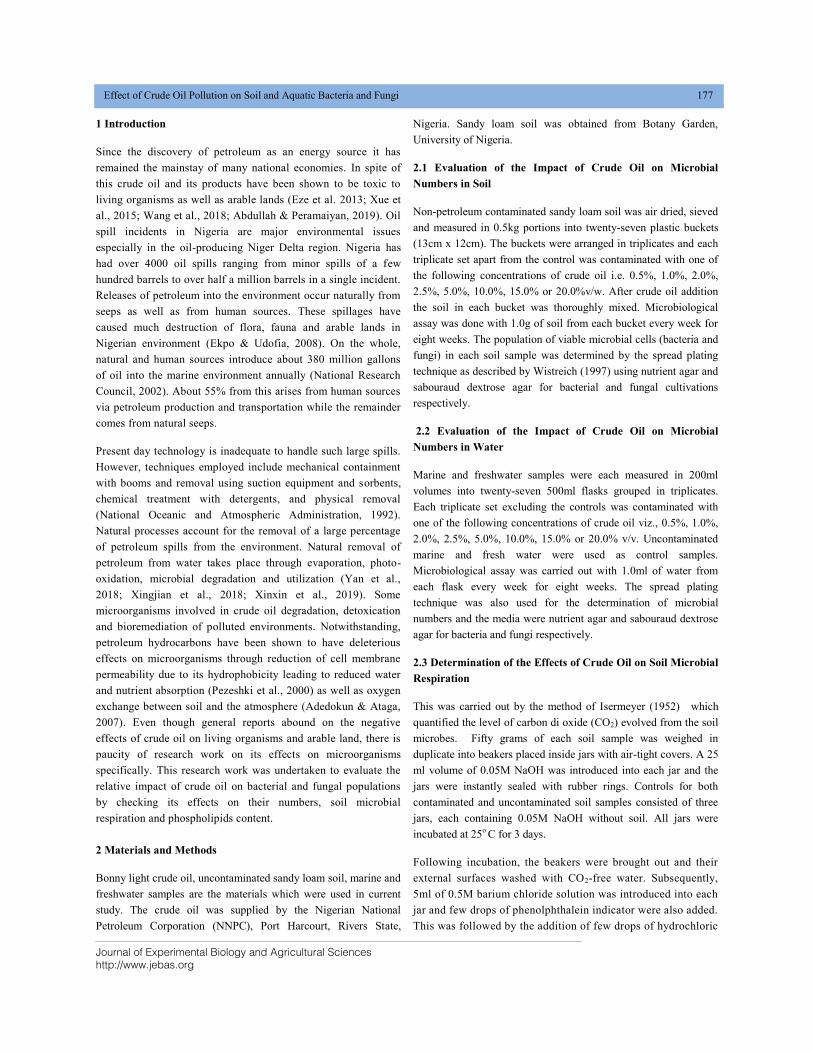
Journal of Experimental Biology and Agricultural Sciences
http://www.jebas.org
Effect of Crude Oil Pollution on Soil and Aquatic Bacteria and Fungi 177
1 Introduction
Since the discovery of petroleum as an energy source it has
remained the mainstay of many national economies. In spite of
this crude oil and its products have been shown to be toxic to
living organisms as well as arable lands (Eze et al. 2013; Xue et
al., 2015; Wang et al., 2018; Abdullah & Peramaiyan, 2019). Oil
spill incidents in Nigeria are major environmental issues
especially in the oil-producing Niger Delta region. Nigeria has
had over 4000 oil spills ranging from minor spills of a few
hundred barrels to over half a million barrels in a single incident.
Releases of petroleum into the environment occur naturally from
seeps as well as from human sources. These spillages have
caused much destruction of flora, fauna and arable lands in
Nigerian environment (Ekpo & Udofia, 2008). On the whole,
natural and human sources introduce about 380 million gallons
of oil into the marine environment annually (National Research
Council, 2002). About 55% from this arises from human sources
via petroleum production and transportation while the remainder
comes from natural seeps.
Present day technology is inadequate to handle such large spills.
However, techniques employed include mechanical containment
with booms and removal using suction equipment and sorbents,
chemical treatment with detergents, and physical removal
(National Oceanic and Atmospheric Administration, 1992).
Natural processes account for the removal of a large percentage
of petroleum spills from the environment. Natural removal of
petroleum from water takes place through evaporation, photo-
oxidation, microbial degradation and utilization (Yan et al.,
2018; Xingjian et al., 2018; Xinxin et al., 2019). Some
microorganisms involved in crude oil degradation, detoxication
and bioremediation of polluted environments. Notwithstanding,
petroleum hydrocarbons have been shown to have deleterious
effects on microorganisms through reduction of cell membrane
permeability due to its hydrophobicity leading to reduced water
and nutrient absorption (Pezeshki et al., 2000) as well as oxygen
exchange between soil and the atmosphere (Adedokun & Ataga,
2007). Even though general reports abound on the negative
effects of crude oil on living organisms and arable land, there is
paucity of research work on its effects on microorganisms
specifically. This research work was undertaken to evaluate the
relative impact of crude oil on bacterial and fungal populations
by checking its effects on their numbers, soil microbial
respiration and phospholipids content.
2 Materials and Methods
Bonny light crude oil, uncontaminated sandy loam soil, marine and
freshwater samples are the materials which were used in current
study. The crude oil was supplied by the Nigerian National
Petroleum Corporation (NNPC), Port Harcourt, Rivers State,
Nigeria. Sandy loam soil was obtained from Botany Garden,
University of Nigeria.
2.1 Evaluation of the Impact of Crude Oil on Microbial
Numbers in Soil
Non-petroleum contaminated sandy loam soil was air dried, sieved
and measured in 0.5kg portions into twenty-seven plastic buckets
(13cm x 12cm). The buckets were arranged in triplicates and each
triplicate set apart from the control was contaminated with one of
the following concentrations of crude oil i.e. 0.5%, 1.0%, 2.0%,
2.5%, 5.0%, 10.0%, 15.0% or 20.0%v/w. After crude oil addition
the soil in each bucket was thoroughly mixed. Microbiological
assay was done with 1.0g of soil from each bucket every week for
eight weeks. The population of viable microbial cells (bacteria and
fungi) in each soil sample was determined by the spread plating
technique as described by Wistreich (1997) using nutrient agar and
sabouraud dextrose agar for bacterial and fungal cultivations
respectively.
2.2 Evaluation of the Impact of Crude Oil on Microbial
Numbers in Water
Marine and freshwater samples were each measured in 200ml
volumes into twenty-seven 500ml flasks grouped in triplicates.
Each triplicate set excluding the controls was contaminated with
one of the following concentrations of crude oil viz., 0.5%, 1.0%,
2.0%, 2.5%, 5.0%, 10.0%, 15.0% or 20.0% v/v. Uncontaminated
marine and fresh water were used as control samples.
Microbiological assay was carried out with 1.0ml of water from
each flask every week for eight weeks. The spread plating
technique was also used for the determination of microbial
numbers and the media were nutrient agar and sabouraud dextrose
agar for bacteria and fungi respectively.
2.3 Determination of the Effects of Crude Oil on Soil Microbial
Respiration
This was carried out by the method of Isermeyer (1952)
which
quantified the level of carbon di oxide (CO2) evolved from the soil
microbes. Fifty grams of each soil sample was weighed in
duplicate into beakers placed inside jars with air-tight covers. A 25
ml volume of 0.05M NaOH was introduced into each jar and the
jars were instantly sealed with rubber rings. Controls for both
contaminated and uncontaminated soil samples consisted of three
jars, each containing 0.05M NaOH without soil. All jars were
incubated at 25o C for 3 days.
Following incubation, the beakers were brought out and their
external surfaces washed with CO2-free water. Subsequently,
5ml of 0.5M barium chloride solution was introduced into each
jar and few drops of phenolphthalein indicator were also added.
This was followed by the addition of few drops of hydrochloric
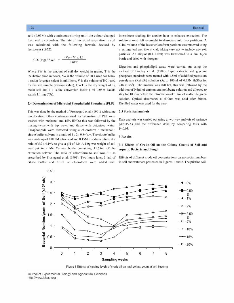
Journal of Experimental Biology and Agricultural Sciences
http://www.jebas.org
178 Eze et al.
acid (0.05M) with continuous stirring until the colour changed
from red to colourless. The rate of microbial respiration in soil
was calculated with the following formula devised by
Isermeyer (1952):
CO2 (mg) / SW/t = (Vo – V) x 1.1
DWT
Where SW is the amount of soil dry weight in grams, T is the
incubation time in hours, Vo is the volume of HCl used for blank
titration (average value) in milliliters. V is the volume of HCl used
for the soil sample (average value), DWT is the dry weight of 1g
moist soil and 1.1 is the conversion factor (1ml 0.05M NaOH
equals 1.1 mg CO2).
2.4 Determination of Microbial Phospholipid Phosphate (PLP)
This was done by the method of Frostegard et al. (1991) with some
modification. Glass containers used for estimation of PLP were
washed with methanol and 15% HNO3; this was followed by the
rinsing twice with tap water and thrice with deionized water.
Phospholipids were extracted using a chloroform : methanol :
citrate buffer solvent in a ratio of 1 : 2 : 0.8v/v/v. The citrate buffer
was made up of 0.015M citric acid and 0.15M trisodium citrate at a
ratio of 5.9 : 4.1v/v to give a pH of 4.0. A 1.0g wet weight of soil
was put in a Mc Cartney bottle containing 11.65ml of the
extraction solvent. The ratio of chloroform to soil was 3:1 as
prescribed by Frostegard et al. (1991). Two hours later, 3.1ml of
citrate buffer and 3.1ml of chloroform were added with
intermittent shaking for another hour to enhance extraction. The
solutions were left overnight to dissociate into two partitions. A
6.4ml volume of the lower chloroform partition was removed using
a syringe and put into a vial, taking care not to include any soil
particles. An aliquot (0.1-1.0ml) was transferred to a 5ml bijou
bottle and dried with nitrogen.
Digestion and phospholipid assay were carried out using the
method of Findlay et al. (1989). Lipid extracts and glycerol
phosphate standards were treated with 1.8ml of acidified potassium
persulphate (K2S3O8) solution (5g to 100ml of 0.35N H2S04) for
24h at 95oC. The mixture was still hot, this was followed by the
addition of 0.4ml of ammonium molybdate solution and allowed to
stay for 10 min before the introduction of 1.8ml of malachite green
solution. Optical absorbance at 610nm was read after 30min.
Distilled water was used for the zero.
2.5 Statistical analysis
Data analysis was carried out using a two-way analysis of variance
(ANOVA) and the difference done by comparing tests with
P<0.05.
3 Results
3.1 Effects of Crude Oil on the Colony Counts of Soil and
Aquatic Bacteria and Fungi
Effects of different crude oil concentrations on microbial numbers
in soil and water are presented in Figures 1 and 2. The pristine soil
Figure 1 Effects of varying levels of crude oil on total colony count of soil bacteria
0
0.5
1
1.5
2
2.5
3
3.5
0 1 2 3 4 5 6 7 8
Bacte
rial
Nu
mb
er/
gra
m o
f S
oil
(x10
9 cfu
)
Sampling weeks
Fig.7: Effects of varying levels of crude oil on total colony count of soil bacteria
0%
0.50%1%
2%
2.50%5%
10%
15%
20%
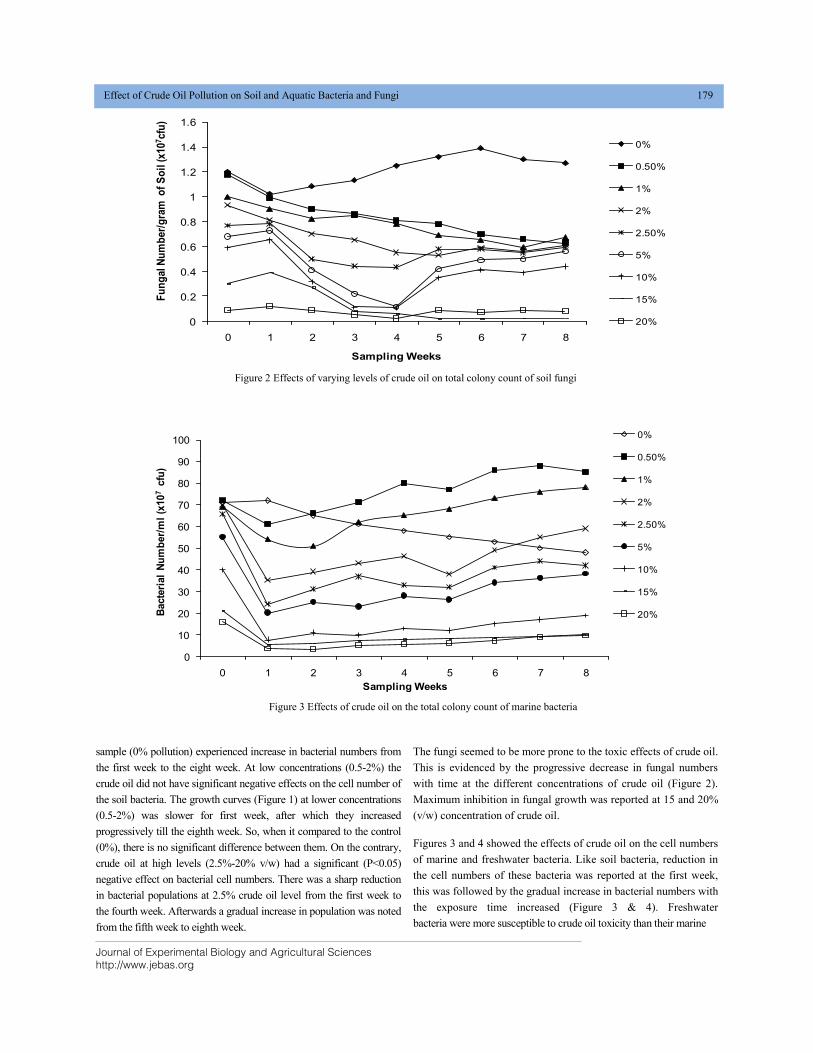
Journal of Experimental Biology and Agricultural Sciences
http://www.jebas.org
Effect of Crude Oil Pollution on Soil and Aquatic Bacteria and Fungi 179
sample (0% pollution) experienced increase in bacterial numbers from
the first week to the eight week. At low concentrations (0.5-2%) the
crude oil did not have significant negative effects on the cell number of
the soil bacteria. The growth curves (Figure 1) at lower concentrations
(0.5-2%) was slower for first week, after which they increased
progressively till the eighth week. So, when it compared to the control
(0%), there is no significant difference between them. On the contrary,
crude oil at high levels (2.5%-20% v/w) had a significant (P<0.05)
negative effect on bacterial cell numbers. There was a sharp reduction
in bacterial populations at 2.5% crude oil level from the first week to
the fourth week. Afterwards a gradual increase in population was noted
from the fifth week to eighth week.
The fungi seemed to be more prone to the toxic effects of crude oil.
This is evidenced by the progressive decrease in fungal numbers
with time at the different concentrations of crude oil (Figure 2).
Maximum inhibition in fungal growth was reported at 15 and 20%
(v/w) concentration of crude oil.
Figures 3 and 4 showed the effects of crude oil on the cell numbers
of marine and freshwater bacteria. Like soil bacteria, reduction in
the cell numbers of these bacteria was reported at the first week,
this was followed by the gradual increase in bacterial numbers with
the exposure time increased (Figure 3 & 4). Freshwater
bacteria were more susceptible to crude oil toxicity than their marine
Figure 2 Effects of varying levels of crude oil on total colony count of soil fungi
Figure 3 Effects of crude oil on the total colony count of marine bacteria
0
0.2
0.4
0.6
0.8
1
1.2
1.4
1.6
0 1 2 3 4 5 6 7 8
Fu
ng
al N
um
ber/
gra
m o
f S
oil
(x10
7cfu
)
Sampling Weeks
Fig. 8: Effects of varying levels of crude oil on total colony count of
soil fungi
0%
0.50%
1%
2%
2.50%
5%
10%
15%
20%
0
10
20
30
40
50
60
70
80
90
100
0 1 2 3 4 5 6 7 8
Bacte
rial
Nu
mb
er/
ml
(x10
7cfu
)
Sampling Weeks
Fig. 4: Effects of Crude oil on the Total Colony Count of Marine Bacteria
0%
0.50%
1%
2%
2.50%
5%
10%
15%
20%
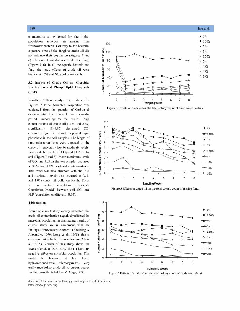
Journal of Experimental Biology and Agricultural Sciences
http://www.jebas.org
180 Eze et al.
counterparts as evidenced by the higher
population recorded in marine than
freshwater bacteria. Contrary to the bacteria,
exposure time of the fungi to crude oil did
not enhance their population (Figures 5 and
6). The same trend also occurred in the fungi
(Figure 5, 6). In all the aquatic bacteria and
fungi the toxic effects of crude oil were
highest at 15% and 20% pollution levels.
3.2 Impact of Crude Oil on Microbial
Respiration and Phospholipid Phosphate
(PLP)
Results of these analyses are shown in
Figures 7 to 9. Microbial respiration was
evaluated from the quantity of Carbon di
oxide emitted from the soil over a specific
period. According to the results, high
concentrations of crude oil (15% and 20%)
significantly (P<0.05) decreased CO2
emission (Figure 7) as well as phospholipid
phosphate in the soil samples. The length of
time microorganisms were exposed to the
crude oil (especially low to moderate levels)
increased the levels of CO2 and PLP in the
soil (Figure 7 and 8). Mean maximum levels
of CO2 and PLP in the test samples occurred
at 0.5% and 1.0% crude oil contaminations.
This trend was also observed with the PLP
and maximum levels also occurred at 0.5%
and 1.0% crude oil pollution levels. There
was a positive correlation (Pearson’s
Correlation Model) between soil CO2 and
PLP (correlation coefficient= 0.74).
4 Discussion
Result of current study clearly indicated that
crude oil contamination negatively affected the
microbial population, in this manner results of
current study are in agreement with the
findings of previous researchers (Boethling &
Alexander, 1979; Long et al., 1995), this is
only manifest at high oil concentrations (Ma et
al., 2015). Results of this study show low
levels of crude oil (0.5- 2.0%) did not have any
negative effect on microbial population. This
might be because at low levels
hydrocarbonoclastic microorganisms very
easily metabolize crude oil as carbon source
for their growth (Adedokun & Ataga, 2007).
Figure 4 Effects of crude oil on the total colony count of fresh water bacteria
Figure 5 Effects of crude oil on the total colony count of marine fungi
Figure 6 Effects of crude oil on the total colony count of fresh water fungi
0
20
40
60
80
100
120
0 1 2 3 4 5 6 7 8B
acte
ria
l N
um
ber/m
l (x
10
7cfu
)Sampling Weeks
Fig.11: Effects of crude oil on the total colony count of fresh water
bacteria
0%
0.50%
1%
2%
2.50%
5%
10%
15%
20%
0
1
2
3
4
5
6
7
8
9
10
0 1 2 3 4 5 6 7 8
Fu
ng
al N
um
bers/m
l (x
10
6cfu
)
Sampling Weeks
Fig.12: Effects of crude oil on the total colony count of marine fungi
0%
0.50%
1%
2%
2.50%
5%
10%
15%
20%
0
2
4
6
8
10
12
0 1 2 3 4 5 6 7 8
Fu
ng
al N
um
bers
/ml
(x10
5cfu
)
Sampling Weeks
Fig. 13: Effects of crude oil on the total colony count of fresh water
fungi
0%
0.50%
1%
2%
2.50%
5%
10%
15%
20%
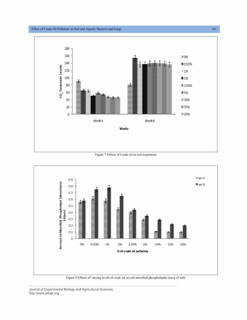
Journal of Experimental Biology and Agricultural Sciences
http://www.jebas.org
Effect of Crude Oil Pollution on Soil and Aquatic Bacteria and Fungi 181
Figure 7 Effects of Crude oil on soil respiration
Figure 8 Effects of varying levels of crude oil on soil microbial phospholipids (nm/g of soil)
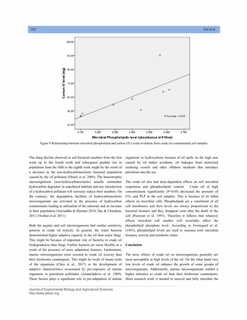
Journal of Experimental Biology and Agricultural Sciences
http://www.jebas.org
182 Eze et al.
The sharp decline observed in soil bacterial numbers from the first
week up to the fourth week and subsequent gradual rise in
population from the fifth to the eighth week might be the result of
a decrease in the non-hydrocarbonoclastic bacterial population
caused by the oil pollutant (Ebueli et al. 2005). The heterotrophic
microorganisms (non-hydrocarbonoclastic) usually outnumber
hydrocarbon degraders in unpolluted habitats and any introduction
of a hydrocarbon pollutant will seriously reduce their numbers. On
the contrary, the degradation facilities of hydrocarbonoclastic
microorganisms are activated in the presence of hydrocarbon
contaminants leading to utilization of the substrate and an increase
in their population (Aniruddha & Hermen 2010; Das & Chandran,
2011; Owabor et al. 2011).
Both the aquatic and soil microorganisms had similar sensitivity
patterns to crude oil toxicity. In general, the water bacteria
demonstrated higher adaptive capacity to the oil than water fungi.
This might be because of important role of bacteria in crude oil
biodegradation than fungi. Further bacteria are more flexible as a
result of the presence of more adaptation features. Furthermore,
marine microorganisms more resisted to crude oil toxicity than
their freshwater counterparts. This might be result of innate traits
of the organisms (Chen et al., 2017) or the development of
adaptive characteristics occasioned by pre-exposure of marine
organisms to petroleum pollutants (Amanchukwu et al. 1989).
These factors plays a significant role in pre-adaptation of marine
organisms to hydrocarbons because of oil spills on the high seas
caused by oil tanker accidents, oil leakages from motorized
seafaring vessels and other offshore incidents that introduce
petroleum into the sea.
The crude oil also had dose-dependent effects on soil microbial
respiration and phosphoslipids content. Crude oil at high
concentrations significantly (P<0.05) decreased the amounts of
CO2 and PLP in the soil samples. This is because of its lethal
effects on microbial cells. Phospholipids are a constituent of all
cell membranes and their levels are always proportional to the
bacterial biomass and they disappear soon after the death of the
cell (Peterson et al. 1991). Therefore it follows that whatever
affects microbial cell number will invariably affect the
phospholipid phosphate level. According to Frostegard et al.
(1991), phospholipid levels are used to measure total microbial
biomass, activity and metabolic status.
Conclusion
The toxic effects of crude oil on microorganisms generally are
more perceptible at high levels of the oil. On the other hand very
low levels of crude oil enhance the growth of some groups of
microorganisms. Additionally, marine microorganisms exhibit a
higher tolerance to crude oil than their freshwater counterparts.
More research work is needed to unravel and fully elucidate the
Figure 9 Relationship between microbial phospholipid and carbon (IV) oxide evolution from crude oil-contaminated soil samples.
Journal of Experimental Biology and Agricultural Sciences
http://www.jebas.org
Effect of Crude Oil Pollution on Soil and Aquatic Bacteria and Fungi 183
reasons for the discrepancy between the reactions of marine and
freshwater microorganisms to crude oil pollution.
Acknowledgement
The authors wish to acknowledge the support given by the
Department of Microbiology, University of Nigeria, Nsukka
through the provision of laboratory space and other facilities used
for the work.
Conflict of Interest
Authors would hereby like to declare that there is no conflict of
interests that could possibly arise.
References
Abdullah MA, Peramaiyan R (2019) Petroleum hydrocarbon and
living organisms. In: Muharrem I, Olcay KI (Eds.), Hydrocarbon
Pollution and Effects on the Environment. IntechOpen.
Doi:10.5772/intechopen.86948.
Adedokun OM, Ataga AE (2007) Effects of amendments and
bioaugmentation of soil polluted with crude oil, automotive
gasoline oil and spent engine oil on the growth of cowpea(Vigna
unguiculata). Scientific Research and Essays 2: 147-149.
Amanchukwu SC, Obafemi A, Okpokwasili GC (1989)
Hydrocarbon degradation and utilization by a palm wine yeast
isolate. FEMS Microbiology Letters 57: 151-154.
Aniruddha S, Hermen S (2010) Enhanced biodegradation of oil
products by some microbl isolates supplemented with heavy
metals. International Journal of Botany 6: 441-448.
Boethling RS, Alexander M (1979) Effect of concentration of
organic chemicals on their biodegradation by natural microbial
communities. Applied and Environmental Microbiology 37: 1211-
1216.
Chen W, Li J, Sun X, Min J, Hu X (2017) High efficiency
degradation of alkanes and crude oil by salt-tolerant bacterium
Dietzia species CN-3. International Biodeterioration and
Biodegradation 118: 110-118. Doi: 10.1016/j.ibiod.2017.01.029.
Das N, Chandran P (2011) Microbial degradation of petroleum
hydrocarbon contaminants. Biotechnological Research
International 2011. Article ID 941810, 13 Pages.
http://dx.doi.org/10.4061/2011/941810.
Ebuehi OAT, Abibo IB, Shekwolo PD, Sigismund KI, Adoki A,
Okoro IC (2005) Remediation of crude oil contaminated soil by
enhanced natural attenuation technique. Journal of Applied Science
and Environmental Management 9: 103-106.
Ekpo MA, Udofia US (2008) Rate of biodegradation of crude oil
by microorganisms isolated from sludge environment. African
Journal of Biotechnology 3: 4495-4499.
Eze CN, Maduka JN, Ogbonna JC, Eze EA (2013) Effects of
Bonny light crude oil contamination on the germination, shoot
growth and rhizobacterial flora of Vigna unguiculata and Arachis
hypogea grown in sandy loam soil. Scientific Research and Essays
8: 99-107.
Findlay RH, King GM, Watling L (1989) Efficacy of
phospholipids analysis in determining microbial biomass in
sediments. Applied Environmental Microbiology 55: 2888-2893.
Frostegard A, Tunlid A, Bath E (1991) Microbial biomass
measured as total lipid phosphate in soils of different organic
content. Journal of Microbiological Methods 13 : 151-163.
Isermeyer H (1952) Eine eifache Methode zur Bestimmung der
Bodenatmung und dem Karbonate im Boden. Zeitschrift für
Pflanzenernährung und Bodenkunde 56 : 26-38.
Long SC, Aelion CM, Dobbins DC, Ptaender FK (1995) A
comparison of microbial community characteristics among
petroleum-contaminated and uncontaminated sub-surface soil
samples. Journal of Microbial Ecology 30: 297-307.
Ma YL, Lu W, Wan LL, Luo L (2015) Elucidation of fluoranthene
degradative characteristics in a newly isolated Achromobacter
xylosoxidans DN OO2. Applied Biochemistry and Biotechnology
175: 1294-1305. Doi:10.1007/s12010-014-1347-7
National Oceanic and Atmospheric Administration (1992) Oil Spill
Case Histories, 1967-1991: Summaries of Significant US and
International spills. NOAA Report NO HMRAD 92-111.
National Research Council (2002) Oil in the sea 111: Inputs, Fates
and Effects. Washington D C: National Academy Press.
Owabor CN, Onwuemene OC, Enaburekhan I (2011)
Bioremediation of polycyclic aromatic hydrocarbon contaminated
aqueous soil matrix: Effect of co-contamination. Journal of
Applied Science and Environmental Management 15: 583-588.
Petersen SO, Henriksen K, Blackburu TH, King GM (1991) A
comparison of phospholipids and chloroform fumigation analyses
for biomass in soil, potentials and limitations. FEMS Microbial
Ecology 85: 257-268.
Pezeshki SR, Hester MW, Lin Q, Nyman JA (2000) The effects of
oil spill and clean-up on dominant US Gulf coast marsh
macrophytes: A review. Environmental Pollution 108: 129-139.
Journal of Experimental Biology and Agricultural Sciences
http://www.jebas.org
184 Eze et al.
Wistreich GA (1997) Microbiology Laboratory: Fundamentals and
Applications. Prentice-Hall Inc. New Jersey, USA. Pp. 144-186,
194-259.
Wang Y, Liang J, Wang J, Gao S (2018) Combining stable carbon
isotope analysis and petroleum fingerprinting to evaluate
petroleum contamination in the Yanchang oilfield located on loess
plateau in China. Environmental Science and Pollution Research
25: 2830-2841.
Xingjian X, Wenming L, Shuhua T, Wei W, Qige Q, Pan J, Xinmei G,
Fengjiao, Haiyan L, Hongwen Y (2018). Petroleum hydrocarbon-
degrading bacteria for the remediation of oil pollution under aerobic
conditions : A perspective analysis. Frontiers in Microbiology 03
December 2018|https://doi.org/10.3389/fmicb.2018.02885.
Xinxin L, Ville AO, Kari S, Aki S (2019) Meat and bone
meal as a novel biostimulation agent in hydrocarbon
contaminated soils. Chemosphere 225: 574-578:
Doi:10.1016/j.chemosphere.2019.03.053.
Xue J, Yu Y, Bai Y, Wang L,Wu Y (2015) Marine oil-degrading
microorganisms and biodegradation process of petroleum
hydrocarbon in marine environments: a review. Current
Microbiology 71 : 220-228.
Yan S, Anna-Lea R, Martin R, Aki S (2018) Requirement of
ecological replication with independent parallel analysis of each
replicate plot to support soil remediation. International
Biodeterioration and Biodegradation 133: 133-141.
Doi:10.1016/j.ibiod.2018.06.006.
Journal of Experimental Biology and Agricultural Sciences
http://www.jebas.org
ISSN No. 2320 – 8694
Journal of Experimental Biology and Agricultural Sciences, April - 2020; Volume – 8(2) page 185 – 192
DIFFERENTIAL RESPONSES OF CERTAIN ETHIOPIAN GROUNDNUT
(Arachis hypogaea L.) VARIETIES VARYING IN DROUGHT TOLERANCE,
TO TERMINAL DROUGHT STRESS
P.R. Jeyaramraja1,*, Woldesenbet Fantahun2
1Department of Biology, College of Natural Sciences, Arba Minch University, Post Box No. 21, Arba Minch, Gamo Zone, Federal Democratic Republic of Ethiopia.
2Ethiopian Biotechnology Institute, Addis Ababa, Federal Democratic Republic of Ethiopia.
Received – February 05, 2020; Revision – March 21, 2020; Accepted – April 15, 2020
Available Online – April 25, 2020
DOI: http://dx.doi.org/10.18006/2020.8(2).185.192
ABSTRACT
Responses of drought tolerant (DT) and drought susceptible (DS) Ethiopian groundnut varieties to
terminal drought stress were compared to determine the traits behind drought tolerance. Drought (D)
induced from 91 to 105 days after sowing (DAS) reduced leaf RWC (relative water content, %), leaf
area (cm2 plant
-1), Chl (chlorophyll, mg g
-1 fresh weight), RDM (root dry mass, g plant
-1), ADM (above-
ground dry mass, g plant-1
), TDM (total dry mass, g plant-1
) and plant height (cm); however, D increased
SLM (specific leaf mass, g m-2
). High leaf RWC in DS types reinstated the hypothesis that capacity to
save leaf water is not a method of drought tolerance. Although there were insignificant Chl differences
between DT and DS types, dry matter accumulation (RDM and ADM) was higher in DT types, which is
attributed to higher SLM in DT types. SLM had significant positive relationship with RDM. An increase
in plant height without increase in leaf area explains drought susceptibility in DS types. Resumption of
irrigation on 106 DAS resulted in an increase in leaf RWC; however, this accompanied no resurrection
response in terms of studied physiological and growth parameters and thus, it was not possible to restore
pod yield after D impaired groundnut growth. Certain parameters were higher in DT types, positively
correlated with DRI (drought response index) and primarily decided by the genotype; such parameters
were concluded to be the traits behind drought tolerance.
* Corresponding author
KEYWORDS
Drought susceptibility
Drought tolerance
Peanut
Specific leaf mass
Water stress
E-mail: [email protected] (P.R. Jeyaramraja)
Peer review under responsibility of Journal of Experimental Biology and
Agricultural Sciences.
All the articles published by Journal of Experimental
Biology and Agricultural Sciences are licensed under a
Creative Commons Attribution-NonCommercial 4.0
International License Based on a work at www.jebas.org.
Production and Hosting by Horizon Publisher India [HPI]
(http://www.horizonpublisherindia.in/).
All rights reserved.
Journal of Experimental Biology and Agricultural Sciences
http://www.jebas.org
Groundnut responses to terminal drought stress 186
1 Introduction
Groundnut (Arachis hypogaea L.) is a significant crop plant
utilized to produce foodstuff and cooking oil. Being a rain-fed crop
(Nagaveni & Khan, 2019), it generally undergoes D under field
conditions that brings about reductions in crop yield. Besides, D is
a predisposing factor for aflatoxin production in groundnut
(Waliyar et al., 2003). D is a devastating physical stress and more
challenging to the attempts of breeders (Tuberosa & Salvi, 2006).
Breeding drought tolerance in groundnuts cultivars would reduce
yield losses due to D in rain-fed growing areas (Kakeeto et al.,
2020). Breeding works to develop drought tolerance have been
hampered in the past by its quantitative genetic base and by low
understanding of the physiological base of productivity under D
(Passioura, 2002). Hence, improvement of the current knowledge
of reactions of crops to D and the methods contained in drought
tolerance have turn out to be main goals of research and
investment, with the crucial objective of producing crops with
better WUE and reduced yield loss due to D (Somerville &
Briscoe, 2001; Zhang et al., 2004).
Plants notice and react quickly to little changes in water status
through a series of physiological, cellular, and molecular
events (Chaves et al., 2009). D can activate a range of plant
reactions, which comprise reduction in leaf RWC and water
potential (Lawlor & Cornic, 2002), decrease in stomatal
aperture and net photosynthetic rate. Photosynthesis is an
important metabolism which is altered by D via reduced
diffusion of CO2 to chloroplast and metabolic limitations
(Pinheiro & Chaves, 2011). Important assessments on crop
reactions at large (Yordanov et al., 2000), and groundnut
especially (Reddy et al., 2003), to D give additional knowledge
on physiological features accompanying D. Nevertheless, there
is even now no complete standard system for assessing drought
tolerance, particularly since the physiological method is not all
the time sufficient for selection on account of negative
relationships between physiological attributes contained in
drought adaptation (Turner et al., 2001). As a result, crop
development plans have been unable to completely use current
physiological data.
Responses of model plants namely, Arabidopsis and
Craterostigma to D have been broadly studied (Yamaguchi-
Shinozaki et al., 1995; Shinozaki & Yamaguchi-Shinozaki,
1996). Evaluation of the regulatory mechanisms of carbon
assimilation in peanut due to forthcoming alterations in
climate, including D, is inadequate (Clifford et al., 2000). Even
though remarkable developments have been achieved regarding
the type of actions happening in crops exposed to D,
explanation of the metabolic regulation is even now absent
(Rolland et al., 2006; Shinozaki & Yamaguchi-Shinozaki,
2007). Jeyaramraja & Thushara (2013) postulated a series of
physiological reactions in peanut exposed to D. However,
holistic studies in groundnut on the relationships among
physiological, growth and yield parameters and their changes
due to terminal D under natural field conditions are limited. As
groundnut is mostly grown as rain-fed crop, it faces D during
terminal stages of crop growth (Hampannavar & Khan, 2019),
which results in reductions in yield and quality. Hence, it is
essential to produce crops that bear D. Knowledge of drought
tolerance mechanisms in legumes innately adjusted to D, such
as groundnut, is essential in identifying markers for drought
tolerance which in turn, can aid in plant breeding programmes.
Nevertheless, little literature is available in groundnut on the
physiological and growth parameters especially during the
terminal stages of crop growth which is prone to D under field
conditions i.e., from 90 to 110 DAS. Hence, the present study
has been taken up.
Bacharou Falke et al. (2019) stated that investigation of
groundnut genotypes response to drought stress could
contribute to improving drought tolerance and productivity.
Hence, in the present investigation, responses of DT and DS
groundnut varieties during terminal stages of growth (90 to 110
DAS) was studied. This study was planned to investigate the
consequence of D on certain physiological and growth
parameters in Ethiopian groundnut varieties differing in
drought tolerance, because it is assumed to be helpful in
identifying traits behind tolerance/susceptibility to D.
2 Materials and Methods
The experiment was conducted inside “Natural Beauty
Initiative Centre”, Main Campus, Arba Minch University,
Ethiopia during April to September 2014.
2.1 Plant Material
Pods of six groundnut varieties were collected from Werer
Agricultural Research Centre during April 2014. Pod and seed
characteristics of these varieties were published (Jeyaramraja
& Fantahun, 2014). These varieties were categorized into DT
(ROBA, Werer 962, NC-4x) and DS (FAYO, Tole 2, Werer
964) types based on DRI values (Table 4) obtained from two
growing seasons (Jeyaramraja & Fantahun, 2016).
2.2 Experimental Design
The experimental design was Randomized Block Design
(RBD) with three replications. There were 6 experimental plots
for each variety (3 for C and 3 for D) and since totally 6
varieties were used in this study; there were totally 36 plots (18
for C and 18 for D). A buffer zone of 2 m was left between C
and D plots to avoid diffusion of water through soil layers
during D induction period from C to D plots.
Journal of Experimental Biology and Agricultural Sciences
http://www.jebas.org
187 Jeyaramraja & Fantahun
2.3 Experimental Layout
After ploughing the field three times into a fine tilth, experimental
layout was made. Each plot had 4 numbers of 5 m ridges. Distance
between two adjacent ridges was 60 cm. Inter-row spacing
between plants was 30 cm while intra-row spacing between plants
was 10 cm. Each plot was surrounded by bunds. Each plot had a
length of 5 m and width of 3 m. Hence, the size of one plot was 15
m2. The size of total experimental layout was 600 m
2.
2.4 Cultivation practices of groundnut
The soil was loamy. Sowing was done manually on both sides of
ridges at ~4 cm depth. Sound, mature and good quality kernels
were only selected for sowing. Kernels were subjected to treatment
with Mancozeb (4g kg-1
kernels) to guard the juvenile seedlings
from root-rot and collar-rot infection. Compost (2 t ha-1
) was
applied as basal dressing and incorporated well into the soil.
Carbaryl 10 per cent DP was applied in soil at the time of seeding
against ants/earwigs/termites.
2.5 Induction of D under field conditions
When groundnut is grown under field conditions as rain-fed crop, it
does not experience D at all developmental stages. Jogloy et al.
(1996) reported that groundnut generally experiences D during
pegging and pod development and then may have sufficient quantity
of water. This would cause severe decrease in yield, and the degree
of decrease would rely on groundnut varieties (Kambiranda et al.,
2011). Hence in the present study, D was induced by withholding
irrigation in the field 91 DAS for a period of 15 days, i.e., up to 105
DAS, so that, simulated D could mimic the effects of naturally
occurring D in the field. Rainout shelter which can cover the whole
D plots was kept ready from 91 DAS to 105 DAS, so that, in the
event of rainfall, the D plots could be covered immediately.
2.6 Irrigation Schedule
On the day of sowing seeds and 1 DAS, the field was irrigated.
Then, irrigation was usually given once a week (i.e., 8 DAS, 15
DAS, 22 DAS and so on) based on soil water measured at four
places (2 in C plots; 2 in D plots) with the help of a tensiometer.
When water potential of top soil reaches -0.25 to -0.50 bars,
irrigation was provided. Irrigation was skipped if rainfall
replenished soil water. For C plots, irrigation continued until a
week before harvest maturity of each variety. For D plots, the
irrigation was skipped two times i.e., at 92 DAS and 99 DAS to
induce D. It has to be noted that there was no rainfall in the field
from 91 DAS to 105 DAS i.e., during the D induction period and
hence, rainout shelter was not used to protect the D plots from rain.
From 106 DAS, water supply was resumed for D plots and was
continued until a week before harvest maturity of each variety.
2.7 Physiological and growth parameters
From each variety that is under C (or) D conditions, one plant was
chosen randomly from each plot for analysis of below-given
parameters which were measured 5 times (i.e., 90 DAS, 95 DAS,
100 DAS, 105 DAS & 110 DAS).
2.7.1 Plant water status
RWC was measured in the third leaf from the top of the main shoot
as said by Clavel et al. (2006) employing the equation: RWC =
[(FM – DM)/(TM – DM)] × 100, where FM was fresh leaf mass,
TM was turgid mass after 4-h rehydration of the leaf in distilled
water at room temperature under dark conditions, and DM was dry
mass after drying at 85°C for 24 h.
2.7.2 Pigment estimation
Chl was determined spectrophotometrically as per the method of
Sadasivam & Manickam (1996) in the second leaf from the top of
main shoot.
2.7.3 Growth parameters
RDM, ADM & TDM were determined in line with Clavel et al.
(2005). Plants were cautiously isolated from the soil and the roots
were cleaned with water. Afterwards, RDM and ADM were
determined after drying at 80°C for 2 days. TDM is the sum of
ADM and RDM. Leaf area was determined by a non-destructive
method employing allometric model (Kathirvelan & Kalaiselvan,
2007). In the third leaf from the top of main shoot, SLM was
obtained (Clavel et al., 2005), which is the ratio of leaf dry mass
per unit leaf area. Plant height was determined with a ruler from
the ground to top of the main axis.
2.8 Statistical analysis
Three factor ANOVA was carried out for the analysis of
physiological and growth parameters wherein Factor A is varieties
(6), Factor B is treatments (2 - C and D) and Factor C is DAS (5 –
90 DAS, 95 DAS, 100 DAS, 105 DAS and 110 DAS). Critical
difference (CD) values were computed at 0.05 and 0.01 levels to
find out whether statistically significant differences existed within
varieties, treatments, and/ DAS. Interactions between the factors
were also studied. Correlation coefficients among various
physiological and growth parameters were studied to find out
relationships among them.
3 Results and Discussion
To compare the effects of C and D on moisture content of groundnut
leaves, RWC was used in the present investigation because it is
thought to be a helpful integrator of crop water balance than leaf
water potential (Wright & Nageswara Rao, 1994). Significant
Journal of Experimental Biology and Agricultural Sciences
http://www.jebas.org
Groundnut responses to terminal drought stress 188
variations were found among the groundnut varieties in terms of
studied physiological and growth parameters except leaf area plant-1
and Chl (Table 1). The fact that DS types had high leaf RWC in this
work is of interest. DT Phaseolus vulgaris frequently open their
stomata under harsh D (Costa França et al., 2000). DS cultivar had at
all times high RWC mainly up to 35 days of D on two-week-old
groundnut seedlings (Clavel et al., 2005). Above quoted earlier
works and the present study reconfirmed the hypothesis proposed by
Jeyaramraja & Thushara (2013) that capacity to save water in
groundnut leaf is not a method of drought tolerance. Vadez (2014)
also said that water saving mechanisms should not be considered as
mechanisms of drought tolerance.
Although leaf RWC was higher in DS types (Table 1), Chl was the
same in both DT and DS types. Kicheva et al. (1994) stated that
reduction in rate of photosynthesis could happen owing to
reduction in Chl under harsh D. Hence, same contents of Chl
observed in this work must lead to same rates of photosynthesis in
DT and DS types and so, same rates of dry matter production.
However, RDM and ADM were higher in DT types. The reason
for higher dry matter production in DT types is attributed to higher
SLM values in DT types. It is imperative to note here that the DT
types had 1.23-fold more SLM as compared to DS types.
Like leaf RWC, plant height was also higher in DS types. Leaf RWC
showed positive correlation with plant height irrespective of DAS (r
= 0.38, p<0.05, n = 36). It must be noted here that leaf area did not
vary between DT and DS types (Table 1); hence, just an increase in
plant height without increase in leaf area would not help DS types to
be productive, which thus resulted in insignificant correlation
between these traits with r value of -0.067. Reduction in plant height
with almost unchanged total biomass accumulation but with
increased grain yield/harvest index was achieved in certain breeding
experiments (Cattivelli et al., 1994; Slafer et al., 1994).
Drought is significantly (p<0.01) reduced leaf RWC, leaf area plant-
1, Chl, RDM, ADM, TDM and plant height (Table 1). SLM was
significantly (p<0.01) increased due to D. The RWC reduction in
plants under D could be related with reduction in crop vigour (Lopez
et al., 2002; Halder & Burrage, 2003). Stomatal regulation of water
loss has been identified (Chaves, 1991) as an initial reaction for
conditioning the leaf water status of field crops, but it rigorously
reduces carbon uptake and biomass production and hence, there was
reduction in RDM, ADM and TDM in the present study.
Although DS types had significantly high leaf RWC than DT types
under C conditions, the leaf RWC of DT types was almost equal to
that of DS types under D conditions (Table 1). As compared to C, D
caused 4.8 % reduction in leaf RWC in DS types whereas in DT
types, it caused only 3 % reduction. Both under C and D conditions,
DT types had significantly higher RDM than DS types. Higher RDM
values in DT types may be attributed to deeper root system for soil
moisture capture which is a successful method of attaining
reproductive success under D (Kirkegaard et al., 2007). High dry
matter production in DT cultivars under field conditions is caused by
more capability to keep up transpiration, which is aided by deep
roots (Blum, 2009). In a study in groundnut profuse root system in
the deep soil was related to better yield under D and it was deduced
that greater, lengthy and denser roots at deep soil was accountable
for more water absorption (Jongrungklang et al., 2012). Although
insignificant difference was found between DT and DS types
regarding ADM and TDM under C conditions, DT types maintained
significantly higher ADM and TDM than DS types under D
conditions. D caused just 9.6 % ADM reduction in DT types while in
DS types, it caused a tremendous reduction of 19.7 % (Table 1).
Because the plants in C and D plots were approaching maturity and
in addition, the plants in D plots suffer D from 91 DAS, leaf RWC
was found to decline significantly and progressively from 90 to
105 DAS (Table 2). However, due to resumption of irrigation on
106 DAS, leaf RWC could significantly (p<0.05) increase on 110
DAS in D plots. Although significant decrease in leaf area plant-1
was observed from 90 DAS, the decrease was irregular (Table 2).
Besides, due to resumption of irrigation on 106 DAS, leaf area
plant-1
could not increase significantly on 110 DAS in D plots. Chl
was also found to decrease significantly from 90 to 105 DAS;
however, Chl could not increase significantly on 110 DAS in D
plots. RDM, ADM and TDM were on the decreasing trend
significantly from 90 to 105 DAS. No resurrection response was
found on 110 DAS in terms of RDM, ADM and TDM in D plots.
Although statistically insignificant, SLM was found to increase
from 90 DAS. Plant height had increased significantly from 90 to
105 DAS and there was statistically insignificant increase in plant
height on 110 DAS in D plots.
As D was induced from 91 DAS, there were no significant
differences between C and D plots on 90 DAS with respect to the
studied physiological and growth parameters (Table 2). Leaf RWC
was found to decrease both in C and D plots as the DAS increased.
Reduction of leaf RWC in C plots was since the groundnut
varieties were approaching maturity while in D plots, the reduction
in leaf RWC was due to both reasons namely, D and approaching
maturity. It is imperative to note here that the reduction of leaf
RWC in D plots was more pronounced than in C plots until 105
DAS. Due to resumption of irrigation on 106 DAS, the leaf RWC
could significantly revive on 110 DAS in D plots. RDM, ADM and
TDM did not change significantly in C plots as DAS increased;
however, these parameters decreased significantly in D plots until
105 DAS. No resurrection response in terms of RDM, ADM and
TDM was observed on 110 DAS in D plots due to resumption of
irrigation on 106 DAS. Plant height significantly increased in C
plots with an increase in DAS; however, in D plots, there was no
such increase in plant height (Table 2).
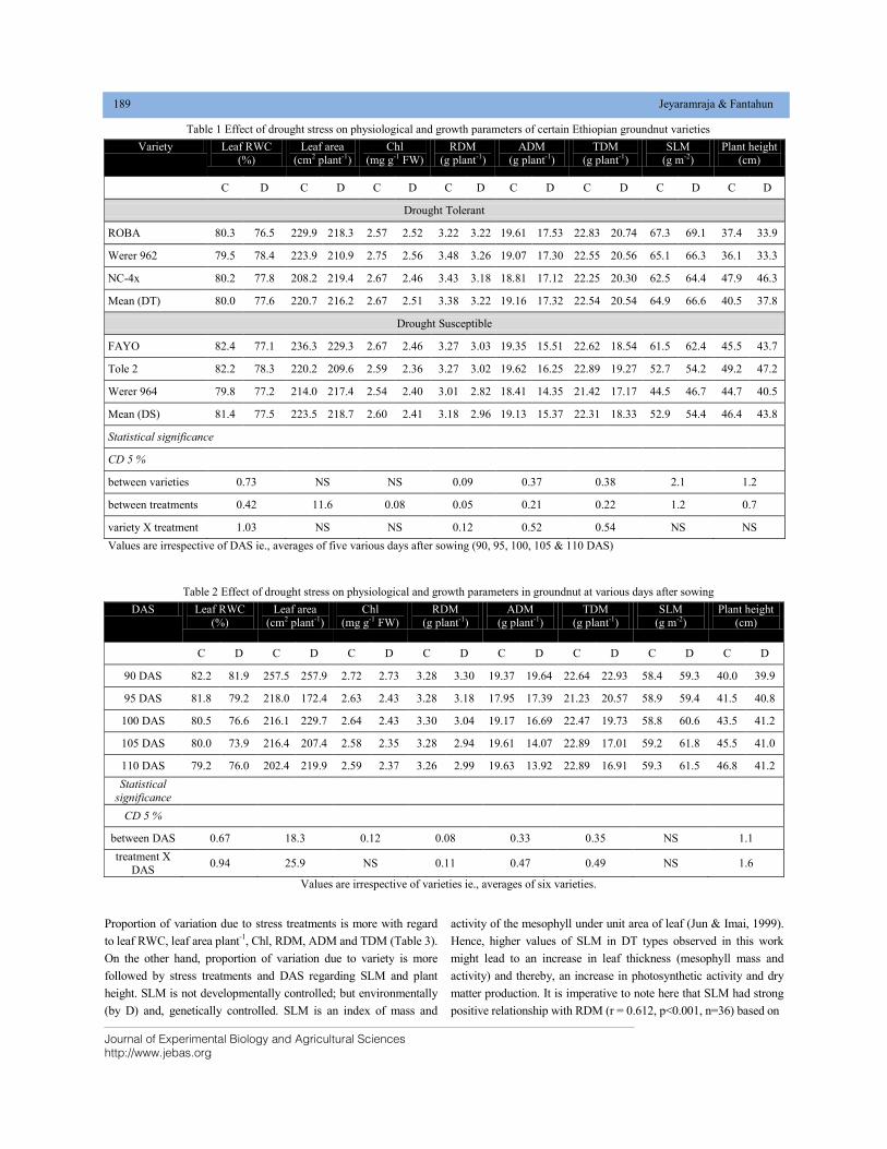
Journal of Experimental Biology and Agricultural Sciences
http://www.jebas.org
189 Jeyaramraja & Fantahun
Proportion of variation due to stress treatments is more with regard
to leaf RWC, leaf area plant-1
, Chl, RDM, ADM and TDM (Table 3).
On the other hand, proportion of variation due to variety is more
followed by stress treatments and DAS regarding SLM and plant
height. SLM is not developmentally controlled; but environmentally
(by D) and, genetically controlled. SLM is an index of mass and
activity of the mesophyll under unit area of leaf (Jun & Imai, 1999).
Hence, higher values of SLM in DT types observed in this work
might lead to an increase in leaf thickness (mesophyll mass and
activity) and thereby, an increase in photosynthetic activity and dry
matter production. It is imperative to note here that SLM had strong
positive relationship with RDM (r = 0.612, p<0.001, n=36) based on
Table 1 Effect of drought stress on physiological and growth parameters of certain Ethiopian groundnut varieties
Variety Leaf RWC
(%)
Leaf area
(cm2 plant-1)
Chl
(mg g-1 FW)
RDM
(g plant-1)
ADM
(g plant-1)
TDM
(g plant-1)
SLM
(g m-2)
Plant height
(cm)
C D C D C D C D C D C D C D C D
Drought Tolerant
ROBA 80.3 76.5 229.9 218.3 2.57 2.52 3.22 3.22 19.61 17.53 22.83 20.74 67.3 69.1 37.4 33.9
Werer 962 79.5 78.4 223.9 210.9 2.75 2.56 3.48 3.26 19.07 17.30 22.55 20.56 65.1 66.3 36.1 33.3
NC-4x 80.2 77.8 208.2 219.4 2.67 2.46 3.43 3.18 18.81 17.12 22.25 20.30 62.5 64.4 47.9 46.3
Mean (DT) 80.0 77.6 220.7 216.2 2.67 2.51 3.38 3.22 19.16 17.32 22.54 20.54 64.9 66.6 40.5 37.8
Drought Susceptible
FAYO 82.4 77.1 236.3 229.3 2.67 2.46 3.27 3.03 19.35 15.51 22.62 18.54 61.5 62.4 45.5 43.7
Tole 2 82.2 78.3 220.2 209.6 2.59 2.36 3.27 3.02 19.62 16.25 22.89 19.27 52.7 54.2 49.2 47.2
Werer 964 79.8 77.2 214.0 217.4 2.54 2.40 3.01 2.82 18.41 14.35 21.42 17.17 44.5 46.7 44.7 40.5
Mean (DS) 81.4 77.5 223.5 218.7 2.60 2.41 3.18 2.96 19.13 15.37 22.31 18.33 52.9 54.4 46.4 43.8
Statistical significance
CD 5 %
between varieties 0.73 NS NS 0.09 0.37 0.38 2.1 1.2
between treatments 0.42 11.6 0.08 0.05 0.21 0.22 1.2 0.7
variety X treatment 1.03 NS NS 0.12 0.52 0.54 NS NS
Values are irrespective of DAS ie., averages of five various days after sowing (90, 95, 100, 105 & 110 DAS)
Table 2 Effect of drought stress on physiological and growth parameters in groundnut at various days after sowing
DAS Leaf RWC
(%)
Leaf area
(cm2 plant-1)
Chl
(mg g-1 FW)
RDM
(g plant-1)
ADM
(g plant-1)
TDM
(g plant-1)
SLM
(g m-2)
Plant height
(cm)
C D C D C D C D C D C D C D C D
90 DAS 82.2 81.9 257.5 257.9 2.72 2.73 3.28 3.30 19.37 19.64 22.64 22.93 58.4 59.3 40.0 39.9
95 DAS 81.8 79.2 218.0 172.4 2.63 2.43 3.28 3.18 17.95 17.39 21.23 20.57 58.9 59.4 41.5 40.8
100 DAS 80.5 76.6 216.1 229.7 2.64 2.43 3.30 3.04 19.17 16.69 22.47 19.73 58.8 60.6 43.5 41.2
105 DAS 80.0 73.9 216.4 207.4 2.58 2.35 3.28 2.94 19.61 14.07 22.89 17.01 59.2 61.8 45.5 41.0
110 DAS 79.2 76.0 202.4 219.9 2.59 2.37 3.26 2.99 19.63 13.92 22.89 16.91 59.3 61.5 46.8 41.2
Statistical
significance
CD 5 %
between DAS 0.67 18.3 0.12 0.08 0.33 0.35 NS 1.1
treatment X
DAS 0.94 25.9 NS 0.11 0.47 0.49 NS 1.6
Values are irrespective of varieties ie., averages of six varieties.
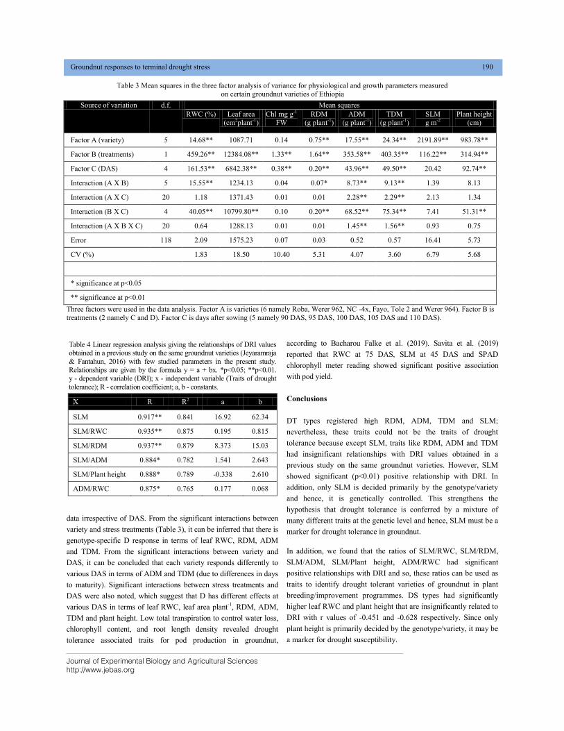
Journal of Experimental Biology and Agricultural Sciences
http://www.jebas.org
Groundnut responses to terminal drought stress 190
data irrespective of DAS. From the significant interactions between
variety and stress treatments (Table 3), it can be inferred that there is
genotype-specific D response in terms of leaf RWC, RDM, ADM
and TDM. From the significant interactions between variety and
DAS, it can be concluded that each variety responds differently to
various DAS in terms of ADM and TDM (due to differences in days
to maturity). Significant interactions between stress treatments and
DAS were also noted, which suggest that D has different effects at
various DAS in terms of leaf RWC, leaf area plant-1
, RDM, ADM,
TDM and plant height. Low total transpiration to control water loss,
chlorophyll content, and root length density revealed drought
tolerance associated traits for pod production in groundnut,
according to Bacharou Falke et al. (2019). Savita et al. (2019)
reported that RWC at 75 DAS, SLM at 45 DAS and SPAD
chlorophyll meter reading showed significant positive association
with pod yield.
Conclusions
DT types registered high RDM, ADM, TDM and SLM;
nevertheless, these traits could not be the traits of drought
tolerance because except SLM, traits like RDM, ADM and TDM
had insignificant relationships with DRI values obtained in a
previous study on the same groundnut varieties. However, SLM
showed significant (p<0.01) positive relationship with DRI. In
addition, only SLM is decided primarily by the genotype/variety
and hence, it is genetically controlled. This strengthens the
hypothesis that drought tolerance is conferred by a mixture of
many different traits at the genetic level and hence, SLM must be a
marker for drought tolerance in groundnut.
In addition, we found that the ratios of SLM/RWC, SLM/RDM,
SLM/ADM, SLM/Plant height, ADM/RWC had significant
positive relationships with DRI and so, these ratios can be used as
traits to identify drought tolerant varieties of groundnut in plant
breeding/improvement programmes. DS types had significantly
higher leaf RWC and plant height that are insignificantly related to
DRI with r values of -0.451 and -0.628 respectively. Since only
plant height is primarily decided by the genotype/variety, it may be
a marker for drought susceptibility.
Table 3 Mean squares in the three factor analysis of variance for physiological and growth parameters measured
on certain groundnut varieties of Ethiopia
Source of variation d.f. Mean squares
RWC (%) Leaf area
(cm2plant-1)
Chl mg g-1
FW
RDM
(g plant-1)
ADM
(g plant-1)
TDM
(g plant-1)
SLM
g m-2
Plant height
(cm)
Factor A (variety) 5 14.68** 1087.71 0.14 0.75** 17.55** 24.34** 2191.89** 983.78**
Factor B (treatments) 1 459.26** 12384.08** 1.33** 1.64** 353.58** 403.35** 116.22** 314.94**
Factor C (DAS) 4 161.53** 6842.38** 0.38** 0.20** 43.96** 49.50** 20.42 92.74**
Interaction (A X B) 5 15.55** 1234.13 0.04 0.07* 8.73** 9.13** 1.39 8.13
Interaction (A X C) 20 1.18 1371.43 0.01 0.01 2.28** 2.29** 2.13 1.34
Interaction (B X C) 4 40.05** 10799.80** 0.10 0.20** 68.52** 75.34** 7.41 51.31**
Interaction (A X B X C) 20 0.64 1288.13 0.01 0.01 1.45** 1.56** 0.93 0.75
Error 118 2.09 1575.23 0.07 0.03 0.52 0.57 16.41 5.73
CV (%)
1.83 18.50 10.40 5.31 4.07 3.60 6.79 5.68
* significance at p<0.05
** significance at p<0.01
Three factors were used in the data analysis. Factor A is varieties (6 namely Roba, Werer 962, NC -4x, Fayo, Tole 2 and Werer 964). Factor B is
treatments (2 namely C and D). Factor C is days after sowing (5 namely 90 DAS, 95 DAS, 100 DAS, 105 DAS and 110 DAS).
Table 4 Linear regression analysis giving the relationships of DRI values obtained in a previous study on the same groundnut varieties (Jeyaramraja
& Fantahun, 2016) with few studied parameters in the present study.
Relationships are given by the formula y = a + bx. *p<0.05; **p<0.01. y - dependent variable (DRI); x - independent variable (Traits of drought
tolerance); R - correlation coefficient; a, b - constants.
X R R2 a b
SLM 0.917** 0.841 16.92 62.34
SLM/RWC 0.935** 0.875 0.195 0.815
SLM/RDM 0.937** 0.879 8.373 15.03
SLM/ADM 0.884* 0.782 1.541 2.643
SLM/Plant height 0.888* 0.789 -0.338 2.610
ADM/RWC 0.875* 0.765 0.177 0.068
Journal of Experimental Biology and Agricultural Sciences
http://www.jebas.org
191 Jeyaramraja & Fantahun
Abbreviations
ADM – aboveground dry mass; C – control, irrigated plants; CD –
critical difference; Chl – chlorophyll; D – drought; DAS – days
after sowing; DRI – drought response index; DS – drought-
susceptible; DT – drought-tolerant; RDM – root dry mass; RWC –
leaf relative water content; SLM – specific leaf mass; TDM – total
dry mass
Acknowledgements
Financial support for this whole study by Arba Minch University
(GOV /AMU /TH14 /CNS /BIOL /01 /06) is gratefully
acknowledged. The authors thank Werer Agricultural Research
Centre for providing the groundnut seeds.
Conflict of interest
Both the authors declare that there is no conflict of interest.
References
Bacharou Falke A, Hamidou F, Halilou O, Harou A (2019)
Assessment of groundnut elite lines under drought conditions and
selection of tolerance associated traits. Advances in Agriculture
Article ID 3034278, DOI: https://doi.org/10.1155/2019/3034278.
Blum A (2009) Effective use of water (EUW) and not water-use
efficiency (WUE) is the target of crop yield improvement under
drought stress. Field Crops Research 112: 119-123.
Cattivelli L, Delogu G, Terzi V, Stanca AM (1994) Progress in
barley breeding. In: Slafer GA (Ed). Genetic Improvement of Field
Crops, New York: Marcel Dekker Inc Pp. 95-181.
Chaves MM (1991) Effects of water deficits on C assimilation.
Journal of Experimental Botany 42: 1-16.
Chaves MM, Flexas J, Pinheiro C (2009) Photosynthesis under
drought and salt stress: regulation mechanisms from whole plant to
cell. Annals of Botany 103: 551-560.
Clavel D, Diouf C, Khalfaoui JL, Braconnier S (2006) Genotypes
variations in fluorescence parameters among closely related
groundnut (Arachis hypogaea L.) lines and their potential for
drought screening programs. Field Crops Research 96: 296-306.
Clavel D, Drame NK, Roy-Macauley H, Braconnier S, Laffray D
(2005) Analysis of early responses to drought associated with field
drought adaptation in four Sahelian groundnut (Arachis hypogaea
L.) cultivars. Environmental and Experimental Botany 54: 219-230.
Clifford SC, Stronach IM, Black CR, Singleton-Jones PR, Azam-
Ali SN, Crout NMJ (2000) Effects of elevated CO2, drought and
temperature on the water relations and gas exchange of groundnut
(Arachis hypogaea) stands grown in controlled environment
glasshouses. Physiologia Plantarum 110: 78-88.
Costa Franca MG, Pham Thi AT, Pimentel C, Pereyra Rossiello
RO, Zuily-Fodil Y, Laffray D (2000) Differences in growth and
water relation among Phaseolus vulgaris cultivars in response to
induced drought stress. Environmental and Experimental Botany
43: 227–337.
Halder KP, Burrage SW (2003) Drought stress effects on water
relations of rice grown in nutrient film technique. Pakistan Journal
of Biological Sciences 6: 441-444.
Hampannavar MR, Khan H (2019) Association study of
morphological and physiological traits with yield in groundnut
genotypes under terminal drought condition. International Journal
of Current Microbiology and Applied Sciences 8: 668-678.
Jeyaramraja PR, Fantahun W (2014) Characterization of yield
Components in certain groundnut (Arachis hypogaea L.) varieties
of Ethiopia. Journal of Experimental Biology and Agricultural
Sciences 2: 592–596.
Jeyaramraja PR, Fantahun W (2016) Influence of drought at pod-
filling stage on yield and yield components of groundnut (Arachis
hypogaea L.) varieties of Ethiopia. Tropical Agriculture (Trinidad)
93: 235-244.
Jeyaramraja PR, Thushara SS (2013) Sequence of physiological
responses in groundnut (Arachis hypogaea L.) subjected to soil
moisture deficit. Photosynthetica 51: 395-403.
Jogloy S, Patanothai A, Toomsan S, Isleib TG (1996) Breeding
peanut to fit into Thai cropping systems. In Proceedings of the
Peanut Collaborative Research Support Program-International
Research Symposium and Workshop, Two Jima Quality Inn,
Arlington, Virginia, USA. 25-31 March 1996. Pp. 353-362.
Jongrungklang N, Toomsan B, Vorasoot N, Jogloy S, Boote KJ,
Hoogenboom G, Patanothai A (2012) Classification of root
distribution patterns and their contributions to yield in peanut
genotypes under mid-season drought stress. Field Crops Research
127: 181–190.
Jun H, Imai K (1999) Cultivar differences of photosynthesis and
respiration in peanut leaves. Bulletin of the Faculty of Agriculture,
Meiji University 119: 21-25.
Kakeeto R, Melis R, Biruma M, Sibiya J (2020) Gene action
governing the inheritance of drought tolerance and selected
agronomic traits in Ugandan groundnut (Arachis hypogaea L.)
lines under drought environment. Euphytica 216: 1.
Journal of Experimental Biology and Agricultural Sciences
http://www.jebas.org
Groundnut responses to terminal drought stress 192
Kambiranda DM, Vasanthaiah HKN, Katam R, Ananga A, Basha SM,
Naik K (2011) Impact of Drought Stress on Peanut (Arachis hypogaea
L.) Productivity and Food Safety. In Vasanthaiah HKN, Kambiranda
DM (Eds). Plants and Environment, InTech Pp. 249-272.
Kathirvelan P, Kalaiselvan P (2007) Groundnut (Arachis hypogaea
L.) leaf area estimation using allometric model. Research Journal
of Agriculture and Biological Sciences 3: 59-61.
Kicheva ML, Tsonev TD, Popova LP (1994) Stomatal and
nonstomatal limitation of photosynthesis in two wheat cultivars
subjected to water stress. Photosynthetica 30: 107- 116.
Kirkegaard JA, Lilley JM, Howe GN, Graham JM (2007) Impact
of subsoil water use on wheat yield. Australian Journal of
Agricultural Research 58: 303–315.
Lawlor DW, Cornic G (2002) Photosynthetic carbon assimilation
and associated metabolism in relation to water deficits in higher
plants. Plant, Cell & Environment 25: 275-294.
Lopez CML, Takahashi H, Yamazaki S (2002) Plant water relations of
Kidney bean plants treated with NaCl and foliarly applied glycine
betaine. Journal of Agronomy and Crop Science 188: 73-80.
Nagaveni K, Khan H (2019) Genetic variability studies in terminal
drought tolerant groundnut (Arachis hypogaea L.). Journal of
Pharmacognosy and Phytochemistry 8: 747-750.
Passioura JB (2002) Environmental biology and crop
improvement. Functional Plant Biology 29: 537-546.
Pinheiro C, Chaves MM (2011) Photosynthesis and drought: can
we make metabolic connections from available data? Journal of
Experimental Botany 62: 869-882.
Reddy TY, Reddy VR, Anbumozhi V (2003) Physiological responses
of groundnut (Arachis hypogea L.) to drought stress and its
amelioration: a critical review. Plant Growth Regulation 41: 75-88.
Rolland F, Baena-Gonzalez E, Sheen J (2006) Sugar sensing and
signaling in plants: conserved and novel mechanisms. Annual
Review of Plant Biology 57: 675-709.
Sadasivam S, Manickam A (1996) Biochemical Methods: 2nd
Edition. New Age Int Limited Publishers, Tamil Nadu Agricultural
University, Coimbatore.
Savita SK, Kenchangoudar PV, Mamata SK, Rajashree B, Nadaf
HL, Deshpande SK (2019) Studies on variability and genetic
association of drought and yield related traits in advance breeding
lines of groundnut (Arachis hypogaea L.). Journal of
Pharmacognosy and Phytochemistry 8: 2145-2148.
Shinozaki K, Yamaguchi-Shinozaki K (1996) Molecular responses
to drought and cold stress. Current Opinion in Biotechnology 7:
161-167.
Shinozaki K, Yamaguchi-Shinozaki K (2007) Gene networks
involved in drought stress response and tolerance. Journal of
Experimental Botany 58: 221-227.
Slafer GA, Satorre EH, Andrade H (1994) Increases in grain yield
in bread wheat from breeding and associated physiological
changes. In Slafer GA (Ed). Genetic Improvement of Field Crops,
Marcel Dekker Inc., New York Pp. 1-67.
Somerville C, Briscoe J (2001) Genetic engineering and water.
Science 292: 2217.
Tuberosa R, Salvi S (2006) Genomics-based approaches to
improve drought tolerance of crops. Trends in Plant Science 11:
405-412.
Turner NC, Wright GC, Siddique KHM (2001) Adaptation of grain
legume (pulses) to water-limited environments. Advances in
Agronomy 71: 193-231.
Vadez V (2014) Root hydraulics:The forgotten side of roots in
drought adaptation. Field Crops Research 165: 15–24.
Waliyar F, Reddy SV, Subramaniam K, Reddy TY, Krama D,
Craufurd PQ, Wheeler TR (2003) Importance of mycotoxins in
food and feed in India. Aspects of Applied Biology 68: 1–8.
Wright GC, Nageswara Rao RC (1994) Groundnut Water
Relations. In Smartt JT (Ed). The Groundnut Crop, Springer,
Dordrecht Pp. 281- 335.
Yamaguchi-Shinozaki K, Urao T, Shinozaki K (1995) Regulation
of genes that are induced by drought stress in Arabidopsis
thaliana. Journal of Plant Research 108: 127-136.
Yordanov I, Velikova V, Tsonev T (2000) Plant Responses to
drought, acclimation, and stress tolerance. Photosynthetica 38:
171-186.
Zhang JZ, Creelman RA, Zhu JK (2004) From laboratory to field.
Using information from Arabidopsis to engineer salt, cold, and
drought tolerance in crops. Plant Physiology 135: 615-621.
Journal of Experimental Biology and Agricultural Sciences
http://www.jebas.org
ISSN No. 2320 – 8694
Journal of Experimental Biology and Agricultural Sciences, April - 2020; Volume – 8(2) page 193 – 200
IMPACT OF FEED SUBSIDY REMOVAL ON THE ECONOMIC SUCCESS OF
SMALL RUMINANT FARMING IN NORTHERN BADIA OF JORDAN
Ja’far Mansur Al-Khaza’leh*
Faculty of Agricultural Technology, Al-Balqa Applied University, P.O. Box 19117, Al-Salt, Jordan
Received – February 12, 2020; Revision – March 15, 2020; Accepted – March 28, 2020
Available Online – April 25, 2020
DOI: http://dx.doi.org/10.18006/2020.8(2).193.200
ABSTRACT
The small ruminant sector contributes substantially to food security and the livelihoods of farmers in
Jordan. Subsidy on feed for the livestock sector is considered to be an important policy for maintaining
feed prices low, thus improving the livelihood of the households. This study aimed to evaluate the effect
of feed subsidy removal on the economic success of small ruminant production in two production
systems in northern Badia of Jordan. Data was collected by questionnaire survey administered to 120
small ruminant farmers. Gross margin (GM1 and GM2) and net benefit (NB) were used to measure the
economic success of small ruminant production. GM1 constitutes cash revenue of sheep and goats,
while GM2 additionally includes in-kind benefits (meat and milk consumption). NB comprises cash
revenue, in-kind benefits and intangible benefits (insurance and finance). The feed price was
significantly affected by feed subsidy removal (p<0.05). Feed subsidy removal negatively (p<0.05)
affected all the parameters of the economic success of small ruminant production. GM1, GM2 and NB
per farm with subsidized feed prices were significantly (p<0.05) higher than farms without subsidized
feed prices in both production systems. A 36 % of farms with feed subsidy had a negative NB compared
to 54% of farms without feed subsidy. Findings of current study revealed that under conditions of forage
shortage in rangelands and high feed prices, feed subsidy removal has a negative impact on the
parameters of the economic success of small ruminant production and can threaten the income and
livelihoods of farmers. Keeping subsidies on the feed aimed at livestock keepers is a good policy to
alleviate the detrimental impact on households.
* Corresponding author
KEYWORDS
In-kind benefits
Intangible benefits
Gross margin
Net benefit
Economic success
E-mail: [email protected] (Ja’far Mansur Al-Khaza’leh)
Peer review under responsibility of Journal of Experimental Biology and
Agricultural Sciences.
All the articles published by Journal of Experimental
Biology and Agricultural Sciences are licensed under a
Creative Commons Attribution-NonCommercial 4.0
International License Based on a work at www.jebas.org.
Production and Hosting by Horizon Publisher India [HPI]
(http://www.horizonpublisherindia.in/).
All rights reserved.
Journal of Experimental Biology and Agricultural Sciences
http://www.jebas.org
Impact of feed subsidy removal on the economic success of small ruminant farming in northern Badia of Jordan 194
1 Introduction
In Jordan, sheep and goats play a considerable role in the
economy, food security and livelihoods of farmers of rural areas
(Al-Atiyat & Tabbaa, 2009; Al-Atiyat, 2014). Small ruminants are
well adapted to the arid and semi-arid conditions of the country
representing the highest proportion of livestock biomass, with an
estimated population of about 3,063,120 head of sheep and
772,670 head of goats in 2017 (Department of Statistics, 2017).
Small ruminants are raised under different production systems
(Abu-Zanat et al., 2005; Alrousan, 2009). Two major production
systems which used in the country are: transhumant production
system (pastoral) which is the prevalent production system and the
sedentary production system (agro-pastoral), which is practiced in
the villages and peri-urban parts of the country.
A sufficient provision of feed is necessary for livestock to ensure
their production and health status. The scarcity of water resources,
shortage of rangeland and feed are major constraints for small
ruminant production in Jordan (Al-Karaki & Al-Momani 2011; Al-
Khaza’leh et al., 2015a). In Jordan, pastures with low nutritional
quality and poor biomass are inadequate for feeding small ruminant
animals (Obeidat et al., 2014). Therefore, animals are supplemented
with concentrates which are a shortage and costly in order to meet
their nutrient needs (Alshdaifat & Obeidat, 2019). Moreover, the
total yield of rained and irrigated barley production as a major
concentrates in Jordan was 394,277 tons in 2016 (Ministry of
Agriculture, 2016) which is not enough to feed livestock. Therefore,
the Jordanian government depends on importing feedstuff from other
countries, which in turn has a significant impact on Jordan's GDP
(Ministry of Industry Trade and Supply, 2018).
Price subsidy on feed is a prevalent policy in many developing
countries like Jordan. The price of feed in Jordan for the livestock
sector had been subsidized by the government for many years.
Nevertheless, the subsidy on feed is one of the most existing volatile
agro-economic policies in Jordan impacting its budgetary. The feed
subsidy is an important instrument for the livelihood of farmers.
Taking into account that feed price in Jordan is the greatest variable
expenses in the sheep and goat industry, stopping feed subsidy could
have a considerable effect on livestock production, incomes,
expenses, profitability, the economic performance of small ruminants
and thus on the sustainability of sheep and goat farming. The
economic consequences of feed subsidy removal on sheep and goat
farming were not adequately investigated in Jordan and hence there
is a need for in-depth analysis including cost-benefits to determine
the impact of subsidy removal on sustaining small ruminant
production. In the light of this background, the objectives of the
present study were to evaluate the economic performance of small
ruminants and to analyze the impact of feed subsidy lifting on the
economic success of small ruminant production in two production
systems of Jordan.
2 Materials and Methods
2.1 The study area and production systems
The study was carried out in the northern Badia of Jordan east of
the Mafarq governorate. The term "Badia" refers to desert or arid
region, dwelled by Bedouins or Badu. The northern Badia
constituted 36% of the total area of Jordanian Badia (km2=71,474
which constitutes 80% of the total area of Jordan). The study area
is characterized by transhumant production system (pastoral, the
herders practice two major patterns of seasonal mobility: toward
east ‘‘al tashreeg’’ to benefit from grazing on the vegetation during
late winter and early spring and back toward west ‘‘al taghreeb’’
after that) and sedentary production system (agro-pastoral). The
northern Badia has arid climate and it has been affected frequently
by drought cycles, receiving a total annual rainfall of about 116
mm. Therefore, water and pasture biomass availability in the study
area are low.
Sheep and goats are the predominant animal species representing the
major small ruminant production systems in the northern Badia.
According to secondary data obtained from the study region's
agricultural offices in 2017, the livestock population in the study area
is estimated to be about 366,940 head of sheep, 61,210 head of goats,
3,020 head of cattle, 1,130 head of camels. The same secondary data
showed that in 2017, the total population of sheep and goats keepers
was 3,150. For the same year, the small ruminant population in the
study area constituted 12% sheep and 7.9% goats of the total
population of sheep and goats in Jordan, respectively.
2.2 Sampling and data collection
For this study, a list of all small ruminant keepers and their
livestock holdings in each village within administrative unit of
the study area was obtained from local officials of the Ministry
of Agriculture. Farmers, who kept at least 10 adult animals in the
flocks, were identified from the list of farmers and systematic
random sampling at the third name was used to select 120
farmers for the interview by the assistance of key informant. In
general, 5 farmers were replaced by the next one during
conducting the actual questionnaire survey. Accordingly, a
sample of 62 farms was assigned for transhumant production
system and 58 farms for sedentary production system. Data were
collected between December 2017 and March 2018 using a
structured questionnaire format. Suitability of questionnaire
survey to the farmers in the study area regarding the language
and the logical flow was assured before conducting the actual
questionnaire survey.
Journal of Experimental Biology and Agricultural Sciences
http://www.jebas.org
195 Al-Khaza’leh
.
The questionnaires captured information regarding socio-economic
variables, livestock holdings, animal productivity, input and output
parameters and annual production costs and revenues generation in
the last 12 months. In addition to the survey method, secondary
data on the number of small ruminants and small ruminant keepers,
water and feed prices were obtained from water and agricultural
offices of the study area. Moreover, climate data including amount
of rainfall and temperature in the study area were acquired from
Meteorological Department of Jordan.
2.3 Economic performance of small ruminant production
The major variable costs (VC) from small ruminant production
comprised purchased feedstuff cost, stubble grazing cost, water cost,
veterinary cost, hired labor cost and transportation cost. Stubble
grazing cost included fees for rented land for grazing. Hired labor
cost included the wage payment given for either the continuous or
seasonal herders. Transportation costs comprised costs for water,
feed and animal transport. The annual costs of housing and
machinery were not considered in the study due to depreciation and
simplicity of material used in animal housing.Veterinary costs
included expenses on medications and vaccinations.
In the present study, the cash revenues (CR) from small ruminant
production included the sale of animals, milk and dairy products. For
home consumption, the unit price of each product was estimated
based on the farm gate price. In-kind benefits (IK) comprised the
values of meat and milk consumption. The monetary values of
manure, wool and hair were negligible and not considered in the
calculations because most of farmers in the study area did not market
or use them. Intangible socio-economic benefits of goat production
included financial (F) and insurance (I).The financial benefit of flock
per household was valued as follows: (number of animals owned X
respective market price of animals) X interest rate of the finance
(3.6%, based on Central Bank of Jordan monthly reviews
2016/2017). The insurance value of flock per household was
estimated as follows: (average monetary values of the flock per
household) X the insurance factor (3.6%, based on Central Bank of
Jordan monthly reviews 2016/2017).
The economic parameters (in JD farm−1
year−1
) were valued by
using the following equations:
GM1 = CR – VC (1)
GM2 = (CR+IK) – VC (2)
NB = (CR+ IK+F+I) – (VC) (3)
Where: GM is the gross margin, NB is the net benefit. Other
acronyms are previously defined. All economic parameters are
given in JD (Jordanian Dinar) whereby 1 JD equivalent to 1.4 US
dollars in the year 2017.
2.4 The policy of feed subsidy
The government allocates the subsidy in the rate of 10 to 15 kg per
head per month for sheep and goat owners who have a
certificate/fodder card (indicates the share of subsidized feed based
on the livestock holdings). All the farmers interviewed had the
fodder card and received the benefit from fodder subsidies. The
value of subsidy was calculated as the difference between the
actual selling price of feed to farmers and the international market
price. In the present study, the subsidized price for barley and
wheat bran was 175 JD/ ton and 77 JD/ ton, respectively, while the
unsubsidized market price for barley and wheat bran used for
calculations was 235 JD/ ton and 140 JD/ ton, respectively, in
2017. Thus, the percentage of the subsidized price for barley and
wheat bran was 25% and 45%, respectively, below the
international market price. The average percentage difference of
barley and wheat bran was added for unsubsidized feed and used
for calculation.
2.5 Statistical analysis
Households' socio-economic characteristics and flock ownership
were descriptively summarized by their frequencies, means and
percentages. Chi-square test for proportions of categorical
variables and the t-test for continuous variables were applied after
checking the normal distribution of residuals to compare the two
production systems. The variable costs, revenues and economic
efficiency parameters were not normally distributed. Hence, the
Wilcoxon-Mann-Whitney test (Bergmann et al., 2000) was
employed to detect significant differences in the mean values of
variables between subsidized and unsubsidized feed and among
transhumant and sedentary systems. The analyses were performed
using SAS version 9.3 (SAS Institute, 2012). For providing overall
ranking of purposes of keeping small ruminants, indices were
calculated and ranks were based on the first five choices of priority
characteristics in order of importance by respondent (i.e. 5=
highest importance, 1= lowest importance) and were calculated as
: index = sum of [5 for rank 1+ 4 for rank 2+3 for rank 3+ 2 for
rank 4 + 1 for rank 5 for specific purpose] divided by the sum [5
for rank 1+ 4 for rank 2+3 for rank 3+ 2 for rank 4 + 1 for rank 5]
for all purposes of keeping small ruminants.
3 Results
3.1 Household characteristics
Small ruminant owners indicated that all households were male-
headed, with average age of 49 years, average household size of 10
members, and average experience of 36 years in livestock
husbandry. The majority of the respondents (77.6%) in the
sedentary system depend on family labor for herding and caring
animals while the transhumant systems (45.2%) had more either
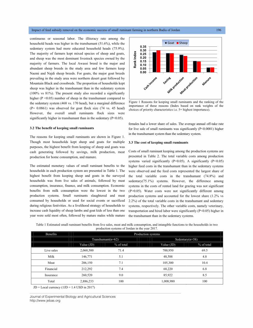
Journal of Experimental Biology and Agricultural Sciences
http://www.jebas.org
Impact of feed subsidy removal on the economic success of small ruminant farming in northern Badia of Jordan 196
continuous or seasonal labor. The illiteracy rate among the
household heads was higher in the transhumant (51.6%), while the
sedentary system had more educated household heads (75.9%).
The majority of farmers kept mixed species of sheep and goats,
and sheep was the most dominant livestock species owned by the
majority of farmers. The local Awassi breed is the major and
abundant sheep breeds in the study area and few farmers keep
Naemi and Najdi sheep breeds. For goats, the major goat breeds
prevailing in the study area were northern desert goat followed by
Mountain Black and crossbreds. The proportion of households kept
sheep was higher in the transhumant than in the sedentary system
(100% vs 81%). The present study also recorded a significantly
higher (P <0.05) number of sheep in the transhumant compared to
the sedentary system (468 vs. 170 head), but a marginal difference
(P= 0.0861) was observed for goat flock size (74 vs. 45 head)
However, the overall small ruminants flock sizes were
significantly higher in transhumant than in the sedentary (P<0.05).
3.2 The benefit of keeping small ruminants
The reasons for keeping small ruminants are shown in Figure 1.
Though most households kept sheep and goats for multiple
purposes, the highest benefit from keeping of sheep and goats was
cash generating followed by savings, milk production, meat
production for home consumption, and manure.
The estimated monetary values of small ruminant benefits to the
households in each production system are presented in Table 1. The
highest benefit from keeping sheep and goats in the surveyed
households was from live sales of animals, followed by meat
consumption, insurance, finance, and milk consumption. Economic
benefits from milk consumption were the lowest in the two
production systems. Small ruminants slaughtered and meat
consumed by households or used for social events or sacrificed
during religious festivities. As a livelihood strategy of households to
increase cash liquidity of sheep lambs and goat kids of less than one
year were sold most often, followed by mature males while mature
females had a lower share of sales. The average annual off-take rate
for live sale of small ruminants was significantly (P<0.0001) higher
in the transhumant system than the sedentary system.
3.3 The cost of keeping small ruminants
Costs of small ruminant keeping among the production systems are
presented in Table 2. The total variable costs among production
systems varied significantly (P<0.05). A significantly (P<0.05)
higher feed costs in the transhumant than in the sedentary systems
were observed and the feed costs represented the largest share of
the total variable costs in the transhumant (74.8%) and
sedentary(75.1%) systems. However, the difference among
systems in the costs of rented land for grazing was not significant
(P>0.05). Water costs were not significantly different among
production systems and accounted for the lowest share (1.2% vs
2.2%) of the total variable costs in the transhumant and sedentary
systems, respectively. The other variable costs, namely veterinary,
transportation and hired labor were significantly (P<0.05) higher in
the transhumant than in the sedentary systems.
Figure 1 Reasons for keeping small ruminants and the ranking of the
importance of these reasons (Index based on rank weights of the
choices of priority characteristics i.e. 5= highest importance).
0.000.050.100.150.200.250.300.35
Ran
k In
de
x
Goat Sheep
Table 1 Estimated small ruminant benefits from live sales, meat and milk consumption, and intangible functions to the households in two
production systems of Jordan in the year 2017.
Benefits Production systems
Transhumant(n=62) Sedentary(n=58)
Value (JD) % of total Value (JD) % of total
Live sales 2,060,500 71.4 700,950 69.5
Milk 146,771 5.1 48,588 4.8
Meat 206,150 7.1 105,300 10.4
Financial 212,292 7.4 68,220 6.8
Insurance 260,520 9.0 85,922 8.5
Total 2,886,233 100 1,008,980 100
JD = Local currency (1JD = 1.4 USD in 2017)
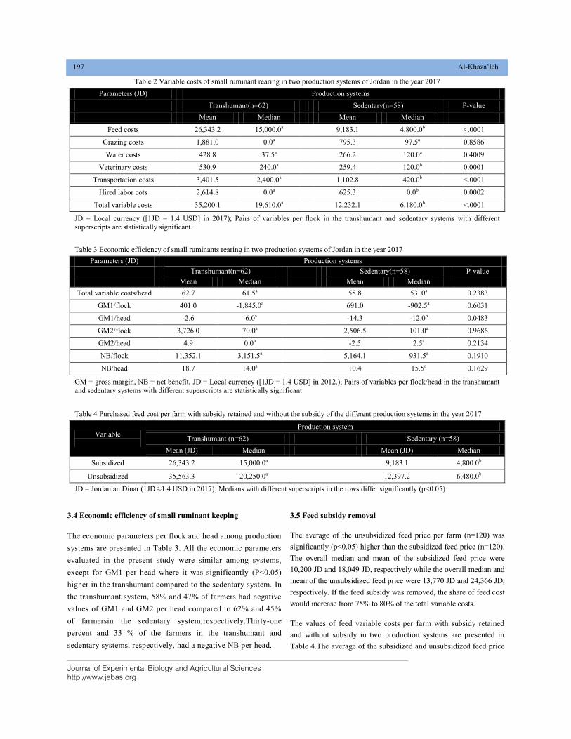
Journal of Experimental Biology and Agricultural Sciences
http://www.jebas.org
197 Al-Khaza’leh
.
3.4 Economic efficiency of small ruminant keeping
The economic parameters per flock and head among production
systems are presented in Table 3. All the economic parameters
evaluated in the present study were similar among systems,
except for GM1 per head where it was significantly (P<0.05)
higher in the transhumant compared to the sedentary system. In
the transhumant system, 58% and 47% of farmers had negative
values of GM1 and GM2 per head compared to 62% and 45%
of farmersin the sedentary system,respectively.Thirty-one
percent and 33 % of the farmers in the transhumant and
sedentary systems, respectively, had a negative NB per head.
3.5 Feed subsidy removal
The average of the unsubsidized feed price per farm (n=120) was
significantly (p<0.05) higher than the subsidized feed price (n=120).
The overall median and mean of the subsidized feed price were
10,200 JD and 18,049 JD, respectively while the overall median and
mean of the unsubsidized feed price were 13,770 JD and 24,366 JD,
respectively. If the feed subsidy was removed, the share of feed cost
would increase from 75% to 80% of the total variable costs.
The values of feed variable costs per farm with subsidy retained
and without subsidy in two production systems are presented in
Table 4.The average of the subsidized and unsubsidized feed price
Table 2 Variable costs of small ruminant rearing in two production systems of Jordan in the year 2017
Parameters (JD) Production systems
Transhumant(n=62) Sedentary(n=58) P-value
Mean Median Mean Median
Feed costs 26,343.2 15,000.0a 9,183.1 4,800.0b <.0001
Grazing costs 1,881.0 0.0a 795.3 97.5a 0.8586
Water costs 428.8 37.5a 266.2 120.0a 0.4009
Veterinary costs 530.9 240.0a 259.4 120.0b 0.0001
Transportation costs 3,401.5 2,400.0a 1,102.8 420.0b <.0001
Hired labor cots 2,614.8 0.0a 625.3 0.0b 0.0002
Total variable costs 35,200.1 19,610.0a 12,232.1 6,180.0b <.0001
JD = Local currency ([1JD = 1.4 USD] in 2017); Pairs of variables per flock in the transhumant and sedentary systems with different
superscripts are statistically significant.
Table 3 Economic efficiency of small ruminants rearing in two production systems of Jordan in the year 2017
Parameters (JD) Production systems
Transhumant(n=62) Sedentary(n=58) P-value
Mean Median Mean Median
Total variable costs/head 62.7 61.5a 58.8 53. 0a 0.2383
GM1/flock 401.0 -1,845.0a 691.0 -902.5a 0.6031
GM1/head -2.6 -6.0a -14.3 -12.0b 0.0483
GM2/flock 3,726.0 70.0a 2,506.5 101.0a 0.9686
GM2/head 4.9 0.0a -2.5 2.5a 0.2134
NB/flock 11,352.1 3,151.5a 5,164.1 931.5a 0.1910
NB/head 18.7 14.0a 10.4 15.5a 0.1629
GM = gross margin, NB = net benefit, JD = Local currency ([1JD = 1.4 USD] in 2012.); Pairs of variables per flock/head in the transhumant
and sedentary systems with different superscripts are statistically significant
Table 4 Purchased feed cost per farm with subsidy retained and without the subsidy of the different production systems in the year 2017
Variable
Production system
Transhumant (n=62) Sedentary (n=58)
Mean (JD) Median Mean (JD) Median
Subsidized 26,343.2 15,000.0a 9,183.1 4,800.0b
Unsubsidized 35,563.3 20,250.0a 12,397.2 6,480.0b
JD = Jordanian Dinar (1JD ≈1.4 USD in 2017); Medians with different superscripts in the rows differ significantly (p<0.05)
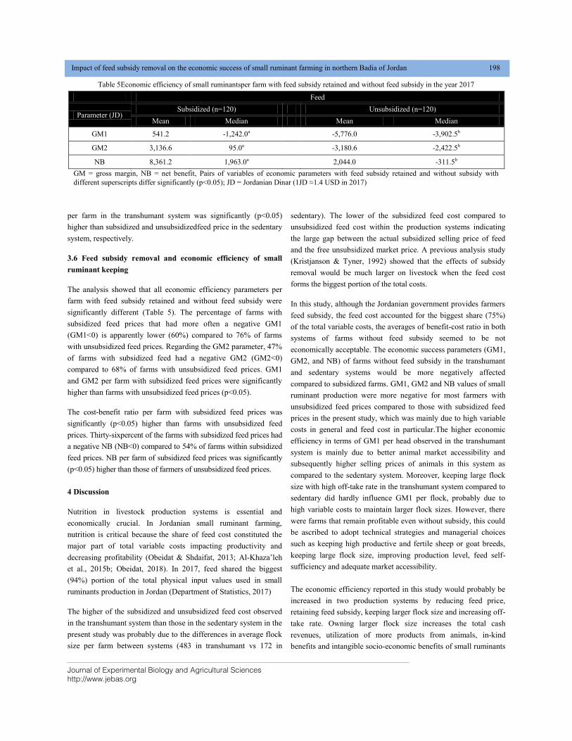
Journal of Experimental Biology and Agricultural Sciences
http://www.jebas.org
Impact of feed subsidy removal on the economic success of small ruminant farming in northern Badia of Jordan 198
per farm in the transhumant system was significantly (p<0.05)
higher than subsidized and unsubsidizedfeed price in the sedentary
system, respectively.
3.6 Feed subsidy removal and economic efficiency of small
ruminant keeping
The analysis showed that all economic efficiency parameters per
farm with feed subsidy retained and without feed subsidy were
significantly different (Table 5). The percentage of farms with
subsidized feed prices that had more often a negative GM1
(GM1>0) is apparently lower (60%) compared to 76% of farms
with unsubsidized feed prices. Regarding the GM2 parameter, 47%
of farms with subsidized feed had a negative GM2 (GM2>0)
compared to 68% of farms with unsubsidized feed prices. GM1
and GM2 per farm with subsidized feed prices were significantly
higher than farms with unsubsidized feed prices (p<0.05).
The cost-benefit ratio per farm with subsidized feed prices was
significantly (p<0.05) higher than farms with unsubsidized feed
prices. Thirty-sixpercent of the farms with subsidized feed prices had
a negative NB (NB>0) compared to 54% of farms within subsidized
feed prices. NB per farm of subsidized feed prices was significantly
(p<0.05) higher than those of farmers of unsubsidized feed prices.
4 Discussion
Nutrition in livestock production systems is essential and
economically crucial. In Jordanian small ruminant farming,
nutrition is critical because the share of feed cost constituted the
major part of total variable costs impacting productivity and
decreasing profitability (Obeidat & Shdaifat, 2013; Al-Khaza’leh
et al., 2015b; Obeidat, 2018). In 2017, feed shared the biggest
(94%) portion of the total physical input values used in small
ruminants production in Jordan (Department of Statistics, 2017)
The higher of the subsidized and unsubsidized feed cost observed
in the transhumant system than those in the sedentary system in the
present study was probably due to the differences in average flock
size per farm between systems (483 in transhumant vs 172 in
sedentary). The lower of the subsidized feed cost compared to
unsubsidized feed cost within the production systems indicating
the large gap between the actual subsidized selling price of feed
and the free unsubsidized market price. A previous analysis study
(Kristjanson & Tyner, 1992) showed that the effects of subsidy
removal would be much larger on livestock when the feed cost
forms the biggest portion of the total costs.
In this study, although the Jordanian government provides farmers
feed subsidy, the feed cost accounted for the biggest share (75%)
of the total variable costs, the averages of benefit-cost ratio in both
systems of farms without feed subsidy seemed to be not
economically acceptable. The economic success parameters (GM1,
GM2, and NB) of farms without feed subsidy in the transhumant
and sedentary systems would be more negatively affected
compared to subsidized farms. GM1, GM2 and NB values of small
ruminant production were more negative for most farmers with
unsubsidized feed prices compared to those with subsidized feed
prices in the present study, which was mainly due to high variable
costs in general and feed cost in particular.The higher economic
efficiency in terms of GM1 per head observed in the transhumant
system is mainly due to better animal market accessibility and
subsequently higher selling prices of animals in this system as
compared to the sedentary system. Moreover, keeping large flock
size with high off-take rate in the transhumant system compared to
sedentary did hardly influence GM1 per flock, probably due to
high variable costs to maintain larger flock sizes. However, there
were farms that remain profitable even without subsidy, this could
be ascribed to adopt technical strategies and managerial choices
such as keeping high productive and fertile sheep or goat breeds,
keeping large flock size, improving production level, feed self-
sufficiency and adequate market accessibility.
The economic efficiency reported in this study would probably be
increased in two production systems by reducing feed price,
retaining feed subsidy, keeping larger flock size and increasing off-
take rate. Owning larger flock size increases the total cash
revenues, utilization of more products from animals, in-kind
benefits and intangible socio-economic benefits of small ruminants
Table 5Economic efficiency of small ruminantsper farm with feed subsidy retained and without feed subsidy in the year 2017
Feed
Parameter (JD) Subsidized (n=120) Unsubsidized (n=120)
Mean Median Mean Median
GM1 541.2 -1,242.0a -5,776.0 -3,902.5b
GM2 3,136.6 95.0a -3,180.6 -2,422.5b
NB 8,361.2 1,963.0a 2,044.0 -311.5b
GM = gross margin, NB = net benefit, Pairs of variables of economic parameters with feed subsidy retained and without subsidy with
different superscripts differ significantly (p<0.05); JD = Jordanian Dinar (1JD ≈1.4 USD in 2017)
Journal of Experimental Biology and Agricultural Sciences
http://www.jebas.org
199 Al-Khaza’leh
.
and in turn the economic success and food security of households.
If feed subsidy is fully removed, the negative economic
implications are expected to be aggravated in the future in both
production systems especially during seasons when the vegetation
on the rangeland at minimum. A previous study (Abu Zanat &
Tabbaa, 2004) showed that drought and removal feed subsidies
negatively impacted the small ruminant production. In 1996, the
Jordanian government suddenly removed the subsidy on livestock
feed, causing the price of feed to jump from 85 USD to around 130
USD per ton (Al-Tabini et al., 2012). Increasing feed price is
usually opposed by farmers and should be usually evaluated by the
government prior to an increase in feed pricing. However, the
government sometimes reduce the percentage of subsidized price
for feed and justifies that to the manipulation in having actual
livestock holdings by farmers (having fake holdings) e.g. due to
the exporting the livestock to neighbour countries, slaughtering the
animals during the religious festival (Eid Aldha), normal occasions
and mortalities during the year.
Different coping strategies have been suggested by farmers to
reduce risks related tothe problem of feed subsidy removal. These
include reducing the quantity of feed supplied, using low quality
fodders, changing ration composition or reducing the flock size. In
1996, when the Jordanian government removed the subsidy on
livestock feed, the livestock owners in the Badia region adapted to
that situation by reducing the flock size by selling some animals to
increase cash liquidity in order to feed the rest of the flock which
in turn the family income affected adversely (Al-Tabini et al.,
2012). Similarly, Jetter (2008) reported that, as a consequence of
feed subsidy removal, many farmers in the Northern Badia of
Jordan sold off their whole flock or reduced their flock sizes to
feed the rest of the flocks. The reduction in the number of livestock
was closely linked to feeding subsidy removal. During the period
of time from 1996 to 1999, the goat and sheep population
apparently decreased as a consequence of feed subsidy lifting and
drought then started to rise after retaining the subsidy. This caused
a further drop in the market price of animals due to the oversupply
in the market and a substantial rise in production costs, and
consequently a decrease in the profitability of livestock production.
Moreover, due to high feed cost as a result of feed subsidy removal
and shortage of rangeland, farmers reduced the share of feed
assigned for each head, which had a negative impact on health,
reproductive efficiency and productivity of livestock (Jetter, 2008).
Furthermore, nutritional qualities and composition of animal feed
rations could also be affected. The ingredients used in producing a
well-balanced and high energy ration will be replaced with other
low-quality ingredients, and in turn, lower feed conversion
efficiency. It is most profitable for farmers to continue to offer a
feed with low-cost ingredients which have a negative impact on
livestock health and production due to malnutrition.
Conclusions
This study revealed that under prevailing conditions of forage and
rangeland shortage in Jordan, the impact of fully feed subsidy
elimination for the livestock sector would aggravate the problem
due to fact that feed cost constitutes 75% of the total variable costs
and dynamic increase in the market prices of feeds. All the
parameters of the economic efficiency of small ruminant
production were found to be different between farms with subsidy
retained and without feed subsidy among production systems.
Hence, removing the subsidies is likely to exacerbate the
inefficiency in the small ruminant production by accentuating feed
inadequacy. However, the variation in feed purchasing and the
consequent variation in animal productivity after the variation of
feed market price should be considered in analysis of farm
efficiency. Technical strategies and managerial choices such as
keeping high productive sheep or goat breeds, increasing flock
size, improving production level, better market accessibility and
feed self-sufficiency are required to sustain small ruminant
production without feed subsidy.
Acknowledgments
Funding the research (107039/2017) by Deanship of Scientific
Research at Al-Balqa Applied University is greatly appreciated.
All contributions provided by the northern Badia people in data
collection are gratefully acknowledged.
Conflict of interest
The authors declare that they have no conflict of interest.
References
Abu-Zanat MM, Migdady HA, Tabbaa MJ (2005) Production
systems of small ruminants in middle Badia of Jordan.Dirasat:
Agricultural Sciences 32:205-214.
Abu Zanat MMW, Tabbaa M (2004) Effect of drought on feed
resources and performance ofsmall ruminants in the Northern
Badia of Jordan. Dirasat: Agricultural Sciences32:347-354.
Al-Atiyat RM (2014) Role of small-scale dairy sector in food
security and poverty alleviation. Food, Agriculture and
Environment12:427-433.
Al-Atiyat RM, Tabbaa MJ (2009) Role of livestock in poverty
alleviation and food security: A review study. In: Proceeding
of Jordan Society of Scientific Research, Amman, Jordan.
Al-Karaki GN, Al-Momani N (2011) Evaluation of Some Barley
Cultivars for Green Fodder Production and Water Use Efficiency
under Hydroponic Conditions. Jordan Journal of Agricultural
Sciences 7:448-457.
Journal of Experimental Biology and Agricultural Sciences
http://www.jebas.org
Impact of feed subsidy removal on the economic success of small ruminant farming in northern Badia of Jordan 200
Al-Khaza’leh J, Reiber C, Al Baqain R, Valle Zárate A (2015a)
Drinking water sources, availability, quality, access and utilization
for goats in the Karak Governorate, Jordan. Tropical Animal
Health and Production 47:163-169.
Al-Khaza’leh J, Reiber C, Al Baqain R, Valle Zárate A (2015b) A
comparative economic analysis of goat production systems in Jordan
with an emphasis on water use. Livestock Research for Rural
Development 27 (5), http://www.lrrd.org/lrrd27/5/khaz27081.html,
accessed on 01 February 2020.
Alrousan L (2009) Goat production in Jordan. Proc. the 24th Ann.
Goat Field Day, Langston Uni., Oklahoma, USA, pp. 33-40.
Alshdaifat SN, Obeidat BS (2019) The impact of feeding corn
dried distillers grains with solubles on milk yield and composition
in lactating Awassi ewes and digestibility and N partitioning in
Awassi ewe lambs. Italian Journal of Animal Science 18:522-529.
Al-Tabini R, Al-Khalidi K, Al-Shudiefat M (2012)Livestock,
medicinal plants and rangeland viability in Jordan’s Badia, through
the lens of traditional and local knowledge. Pastoralism: Research,
Policy and Practice 2: 1-16.
Bergmann R, Ludbrook J, Spooren WPJM (2000) Different
outcomes of the Wilcoxon-Mann-Whitney test from different
statistics packages. The American Statistician 54: 72-77.
Central Bank of Jordan (2017) Publication and statistics, statistical
database, interest rate structure for 2016/2017. Amman. Jordan.
Department of Statistics (2017) Statistics by sector, agriculture,
surveys, livestock for 2016-2017.http://www.dos.gov.jo, accessed
on 01 March 2019.
Jetter C (2008) An assessment of subsidy removal effects on and
future sustainability for livestocksector of in the Northern
Jordanian Badi. Independent Study Project (ISP) Collection. Paper
7.2019.https://digitalcollections.sit.edu/isp_collection/7/, accessed
on 01 October.
Kristjanson P, Tyner WE (1992) Impacts of feed ingredient
subsidy removal and concurrent trade liberalization in Tunisia.
Agricultural Economics 7: 331-339.
Ministry of Agriculture (2016) Statistical annual report 2016,
Amman, Jordan.
Ministry of Industry Trade and Supply (2018) Annual report 2018,
Amman, Jordan.
Obeidat BS (2018) Influence of corn-dried distiller’s grain with
solubles on growth performance and blood metabolites of Awassi
lambs offered a concentrate diet. Italian Journal of Animal
Science17:636-642.
Obeidat BS, Awawdeh MS, Kridli RT, Al-Tamimi HJ, Ballou MA,
Obeidat MD, Abu Ishmais MA, Al-Lataifeh FA, Subih HS (2014)
Feeding corn silage improves nursing performance of Awassi ewes
when used as a source of forage. Animal Feed Science and
Technology 192:24-28.
Obeidat B, Shdaifat M (2013) Partial substitution of barley grain
with ProsopisJuliflora pods in lactating Awassi ewes’ diets: effect
on intake, digestibility, and nursing performance. Small Ruminant
Research 111:50-55.
SAS Institute (2012) Base SAS® 9.3 Procedures Guide: Statistical
Procedures, Second Edition. SAS Institute Inc, Cary, NC, USA.