Jostle heuristics for the 2D-irregular shapes bin ... - CORE

This is a repository copy of Jostle heuristics for the 2D-irregular shapes bin packing problems with free rotation.

White Rose Research Online URL for this paper:http://eprints.whiterose.ac.uk/134688/

Version: Accepted Version

Article:

Abeysooriya, RP, Bennell, JA orcid.org/0000-0002-5338-2247 and Martinez-Sykora, A (2018) Jostle heuristics for the 2D-irregular shapes bin packing problems with free rotation.International Journal of Production Economics, 195. pp. 12-26. ISSN 0925-5273

https://doi.org/10.1016/j.ijpe.2017.09.014

© 2017 Elsevier B.V. This is an author produced version of a paper published in International Journal of Production Economics. Uploaded in accordance with the publisher's self-archiving policy. This manuscript version is made available under the Creative Commons CC-BY-NC-ND 4.0 license http://creativecommons.org/licenses/by-nc-nd/4.0/

[email protected]://eprints.whiterose.ac.uk/

Reuse

This article is distributed under the terms of the Creative Commons Attribution-NonCommercial-NoDerivs (CC BY-NC-ND) licence. This licence only allows you to download this work and share it with others as long as you credit the authors, but you can’t change the article in any way or use it commercially. More information and the full terms of the licence here: https://creativecommons.org/licenses/

Takedown

If you consider content in White Rose Research Online to be in breach of UK law, please notify us by emailing [email protected] including the URL of the record and the reason for the withdrawal request.

mailto:[email protected]

https://eprints.whiterose.ac.uk/

Jostle heuristics for the 2D-irregular shapes bin packing

problems with free rotation

Ranga P. Abeysooriya, Julia A. Bennell, Antonio Martinez-Sykora

Southampton Business School, University of Southampton, UK

Abstract

The paper investigates the two-dimensional irregular packing problem with

multiple homogeneous bins (2DIBPP). The literature on irregular shaped

packing problems is dominated by the single stock sheet strip packing prob-

lem. However, in reality manufacturers are cutting orders over a multi-stock

sheets. Despite its greater relevance, there are only a few papers that tackle

this problem in the literature. A multi-stock sheet problem has two decision

components; the allocation of pieces to stock sheets and the layout design for

each stock sheet. In this paper, we propose a heuristic method that addresses

both the allocation and placement problems together based on the Jostle al-

gorithm. Jostle was first applied to strip packing. In order to apply Jostle

to the bin packing problem we modify the placement heuristic. In addition

we improve the search capability by introducing a diversification mechanism

into the approach. Furthermore, the paper presents alternative strategies for

handling rotation of pieces, which includes a restricted set of angles and un-

restricted rotation. Very few authors permit unrestricted rotation of pieces,

despite this being a feature of many problems where the material is homoge-

neous. Finally, we investigate alternative placement criteria and show that

International Journal of Production Economics

the most commonly applied bottom left criteria does not perform as well as

other options. The paper evaluates performance of each algorithm using dif-

ferent sets of instances considering convex and non-convex shapes. Findings

of this study reveal that the proposed algorithms can be applied to different

variants of the problem and generate significantly better results.

Keywords:

Cutting and packing, heuristics, Irregular shapes, bin packing

1. Introduction

The paper addresses the Two-Dimensional Bin Packing Problem where

the pieces may be any simple polygon; we denote it as the 2DIBPP. The prob-

lem arises in many industries where there is a requirement for irregular shape

pieces to be cut from multiple fixed dimension stock sheets such as metal,

wood, paper and plastic. Despite the many real-life applications, the problem

has received relatively little attention in the literature when compared to the

rectangle bin packing problem or the irregular shape strip packing problem.

Moreover, most data instances for irregular packing problems restrict the

orientation of the pieces to one, two or four angles of orientation. However,

many types of material are homogeneous and pieces can be cut in any orien-

tation. Specifically, the paper describes a heuristic solution method for the

2DIBPP where the stock sheets are homogeneous and a feasible solution is

found when all the pieces are packed within the bins with no overlap between

pieces. The objective is to minimize the total number of bins needed to cut

all of the pieces.

Our approach draws on the literature for irregular strip packing and ap-

2

plies these concepts to bin packing. Further the paper describes new features

that significantly enhance the performance of the algorithm and make it more

generally applicable. The components of our approach include: a single-pass

constructive algorithm (CA) that constructs the bins, placement decisions

that allow either a finite set of rotation angles or free rotation of the pieces,

and an improvement heuristic. The CA is based on TOPOS, which was orig-

inally proposed by Oliveira et al. (2000) and later improved by Bennell and

Song (2010). Since the problem definition allows pieces to take any angle of

orientation, we develop placement rules that permit pieces to rotate either

by a pre-defined finite set of orientations or any angle in the range of 0 to

360 degrees. Finally, the improvement heuristic uses the principles of the

Jostle approach proposed by Dowsland et al. (1998) for strip packing. The

combination of Jostle and the CA means that the approach solves both the

placement and allocation problems together rather than considering them as

two independent problems. Further improvements are made to the Jostle

heuristic to enhance its ability to search the solution space including a kick

to diversify away from local optima and a merge and split mechanism to

retain profitable combinations of pieces.

The contribution of this paper is as follows. We are one of the few pa-

pers to consider multiple bins for packing irregular shapes, and the first to

include the free rotation of the pieces. Hence, the contribution is to propose

and solve a more general and more realistic problem for many industries.

Second, we introduce a new method for identifying promising rotations for

the pieces in the case when any angle is permitted. This is important because

free rotation implies an infinite neigbourhood, which can be sampled from

3

but not exhaustively search. The final contribution is the development of

an efficient heuristic adapted from the Jostle approach that is competitive

across all nesting benchmark data sets. In addition, we introduce a diversifi-

cation mechanism from local search to improve the performance of the Jostle

approach.

The paper is organised as follows. Section 2 provides an overview of the

published work on irregular packing with multiple stock sheets. In Section 3,

we define the problem while introducing some notations used in the paper.

Section 4 introduces our packing procedure. This includes the proposed CA

and describes how we handle finite rotation, free rotation and hole-filling.

Section 5 describes the implementation of the Jostle heuristic for the bin

packing problem and considers its performance as a local search procedure.

In the same section, we propose an iterated Jostle approach and describe

three variants. We present the experimental design and the computational

results in Section 6. This includes results of experiments we use to improve

the performance of the algorithms and the results we achieved for existing

benchmark problems. Section 7, discusses our conclusions from the research.

2. Literature Review

In this section we provide a brief overview of the literature. Note that

there is very little literature on this specific problem, while there is exten-

sive literature on the rectangle bin packing problem and the irregular strip

packing problem. Here we select the papers most relevant to our study.

Irregular shape packing problems hold additional challenges associated

with dealing with complex geometry that can make solution generation com-

4

putationally time consuming. Only recently the research field has sufficiency

matured, along with greater computer processing power, to make considering

multiple stock sheets a fruitful proposition over solving each stock sheet sep-

arately. Hence, literature explicitly covering the 2DIBPP is limited. Lopez-

Camacho et al. (2014), Lopez-Camacho et al. (2013a), Lopez-Camacho et al.

(2013b) and Terashima-Marin et al. (2008) all describe a hyper-heuristic ap-

proach based on a genetic algorithm for the 2DBPP for regular and irregular

shapes. They describe several selection heuristics to solve the allocation of

pieces to bins including variants of first fit, best fit, filler and Djang & Finch

(DJD). For the latter, the position of the pieces in the allocated bin is deter-

mined by the Bottom-Left (BL) algorithm developed by Jakobs (1996) or an

improved bottom left (BLLT) version proposed by Liu and Teng (1999) or a

variant of the constructive approach presented by Hifi and M’Hallah (2003).

Song and Bennell (2014) solve the irregular shape cutting stock problem.

Cutting stock problems are slightly different to bin packing problems. While

both pack multiple stock sheets, the cutting stock problem has many copies

of each piece, hence the piece set is weakly heterogeneous. As a result, mul-

tiple copies of a particular layout can be cut to meet demand. They propose

a column generation procedure, where the master problem determines how

many copies of each layout, and the sub-problem is solved heuristically to

generate a bin layout. They investigated three solution approaches; column

generation, adapted column generation that permits fewer patterns, and a

sequential heuristic procedure to compare the quality of packing solutions.

These papers, as with the majority of the existing literature on irregular

packing, have achieved efficient solutions with restricted rotation of the ir-

5

regular pieces e.g. Bennell and Song (2010), Burke et al. (2007), while only

a few papers (Martinez-Sykora et al., 2015; Rocha, 2014; Han et al., 2013;

Stoyan et al., 2012) have considered unrestricted rotation of irregular pieces.

To our knowledge, Han et al. (2013) and Martinez-Sykora et al. (2015) are

the only papers that considered unrestricted rotation with multiple identi-

cal stock sheets. Both these papers consider an application of cutting glass

where pieces are convex and require guillotine cuts. The guillotine cuts may

be at any angle relative to the edge of the stock sheet. This constraint has

a dominating influences over the algorithm design and strongly influence the

rotation angle of the pieces.

The main body of literature on packing irregular shapes addresses the

strip packing problem, known as nesting problems. Bennell and Oliveira

(2009) provide a tutorial in nesting problems and describe the different types

of solution strategies adopted by researchers. A review of these approaches

is beyond the scope of the paper. Here we highlight the work of Oliveira

et al. (2000) and Dowsland et al. (1998) as these form part of our approach.

Oliveira et al. (2000) TOPOS approach constructs a layout from a given

permutation of pieces. Each piece added to the partial solution is placed

according to a range of criteria. A key innovation in this paper is that the

partial solution does not have a fixed origin on the stock sheet, hence pieces

could be added at any point on the perimeter of the partial layout provided

it does not exceed the width of the stock sheet. They were an early adopter

of the nofit polygon and used this to identify a finite set of placement posi-

tions that optimised their criteria. Dowsland et al. (1998) also use the nofit

polygon to identify feasible positions in their Jostle algorithm. Essentially

6

the algorithm involves repeated applications of a CA. A key innovation is

using the co-ordinates of the current layout to determine the next packing

sequence of pieces starting with the last piece. This simulates the jostling of

pieces from left to right and back again.

3. Problem Description

In this section we give a more formal description of the problem.

Let P = {p1, . . . , pn} be a set of n polygons to be packed into identical

rectangular bins. We denote the bins as rectangular objects with fixed width

W and fixed length L. A feasible solution of the 2DIBPP is described by a set

of bins B = {b1, . . . , bN} where N is the number of bins required to pack the

given n irregular polygons. We denote Pj ⊆ P as the set of packed pieces in

each bin bj and nj denotes the number of placed pieces in bin bj. Each packed

piece pi, has an orientation angle oi ∈ [0, 360o) and a position in its allocated

bin (xi, yi), which is the position of the piece origin. We consider the origin

of each piece as the bottom-left corner point of the enclosing rectangle for a

given angle of rotation and the bottom left corner of the first bin is the bin

origin.

The objective is to minimize the number of bins utilized, N . However,

this measure is not very sensitive and many competing solutions will have

the same value of N for a given problem instance. As a result, we use the

following two measurements to evaluate the bin packing solutions.

1. Fractional number of binsK = N−1+R∗ where R∗ is the proportion of

the least utilised bin used to pack pieces after applying either a vertical

7

or horizontal cut. This assumes that offcuts can be kept and used later.

See Han et al. (2013).

2. F =∑N

j=1U2

j

Nwhere Uj is the utilization of each bin bj, proposed by

Lopez-Camacho et al. (2013a). The utilization of each bin Uj is defined

as the total area of pieces inside the bin bj divided by the area of the

bin (LW ).

Both measures reward solutions that highly utilise bins while trying to

empty one weakest bin, which supports the search in reducing the number

of bins.

4. Packing procedure

In this section we describe all the components of our approach that sup-

port the construction of a single layout. Our packing procedure is a CA

within which we need to identify the candidate placement positions and the

orientation of the piece. We also discuss the selection criteria that will chose

between placement candidates.

A solution method of 2DIBPP addresses two main decision problems: as-

signing pieces to bins and placing those pieces in the bin. The majority of

the cutting and packing literature that considers 2D irregular pieces focuses

on strip packing where there is a single stock sheet. In this case the main

decision is where to place the piece on the strip with the aim of minimising

length. Our approach follows the strip packing approach while imposing the

division between bins therefore making the bin allocation implicit within the

placement decisions. The proposed method always leads to a feasible place-

ment of the next piece by addressing the allocation and placement decisions

8

together.

Our approach seeks to simulate the jostling of pieces. Dowsland et al.

(1998) used this principle to reduce the packing length of the layout for the

irregular shape strip packing problem by moving the pieces from one end of

the strip to the other as in a shaking motion. They called the algorithm

Jostle and suggest it was inspired by the natural human behaviour to shake

a container to encourage objects to pack together as tightly as possible. The

basic idea is to begin with an initial random ordering of the pieces and apply

a constructive heuristic following a placement policy of left most position

packing from the outside edges of the strip towards the centre. Once all the

pieces are packed, Jostle proceeds to take the pieces in order of largest to

smallest x-co-ordinate and pack at the opposite end the stock sheet using a

right most policy and filling holes where possible. The next iteration takes

the packing order from smallest to largest x-coordinate and again packs with

a left most policy, and so on simulating the jostling of pieces from one end

of the stock sheet to the other. Note that packing from left to right and

then right to left is called a Jostle cycle. At the time of publishing, the

approach generated the best results on the benchmark data sets. Since this

work, researchers have developed more effective methods for handling the

geometry and utilise more powerful computers. In this paper, we apply the

principles of Jostle to the homogeneous multiple bin packing problem.

In order to adapt Jostle to the bin packing problem, we first define a very

long packing strip of width W and length n×L. This strip represents n bins

joined together. We then define bin spaces by assigning a set of barrier lines

at fixed intervals of length L along the strip. The bottom left corner of bin

9

i ∈ {1, . . . , n} is placed at (L × (i − 1), 0). We can directly apply Jostle to

the strip with the additional constraint that pieces may not be placed across

a barrier. Along with the usual containment and overlap constraints, this

ensures pieces are always placed entirely within the bins.

Dowsland et al. (1998) imposed a grid of feasible placement positions

over the strip, which formed a search grid for finding the position of the

next piece to be packed. Restricting the placement positions by a grid over

constrains the solution space and good solutions can be lost. More recent

work in irregular packing has developed effective placement policies based

on the nofit polygon (e.g. Bennell and Song (2010)). As a result we design

several new placement policies and incorporate them within Jostle.

4.1. Construction algorithm

In this section we introduce the single-pass CA, which is made up of the

packing order of pieces and the placement policy. The packing order is a ran-

domly generated sequence for the first layout construction and subsequently

is decided by Jostle. The placement policy sets the criteria to compare the

candidate placement positions and orientations of the next piece to be placed,

where any candidate position must be feasible with respect to overlap and

containment in a bin.

Any solution approach to a packing problem involving irregular shapes

requires computational tools for handling the geometry. Specifically, search

heuristics need an efficient test for identifying feasible placement positions

of pieces. Our tool set is based on the nofit polygon (NFP) and inner fit

polygon (IFP) obtained using the approach of Bennell and Song (2008). Since

pieces are permitted to be placed in any orientation, there are infinitely

10

many possible NFPs, hence it is necessary to generate these online as they

are needed. In order to place a piece, the algorithm must generate multiple

NFPs, one for each of the placed piece with the next piece to be placed.

Our investigation shows that it is significantly more efficient to sequentially

merge all the placed pieces into a single polygon and then generate a single,

albeit large and complex, NFP. This is the approach of Oliveira et al. (2000),

called TOPOS, which was later improved by Bennell and Song (2010).

The proposed constructive algorithm represents the existing partial so-

lution as an array of polygons mj where each mj is the polygon generated

by merging the set of pieces packed within the region bj (equivalent to a

bin). Unlike Oliveira et al. (2000), we fix the position of the partial solution

within the bin. As in Bennell and Song (2010), the algorithm retains any

enclosed gaps between the pieces when a piece is merged with the existing

partial solution. These gaps form holes in the merged polygon, which are

made available for placement of subsequent pieces provided the area of the

hole is greater than the area of smallest unpacked piece. Let Hk : h1, .., hq be

the set of holes generated after placing the kth piece. Figure 4.1, provides

an example of two regions, which represent bins and contain a number of

packed pieces. The groups of packed pieces are merged into two polygons

m1 and m2, which contain usable holes h1 and h2. Note, holes that are too

small are ignored. The spaces outside of mj are denoted by Sj.

11

Figure 4.1: Partial solution

4.1.1. Generating candidate placement positions

In this section we describe our approach for identifying the feasible can-

didate positions for the next piece, pi, including its orientation. pi may be

12

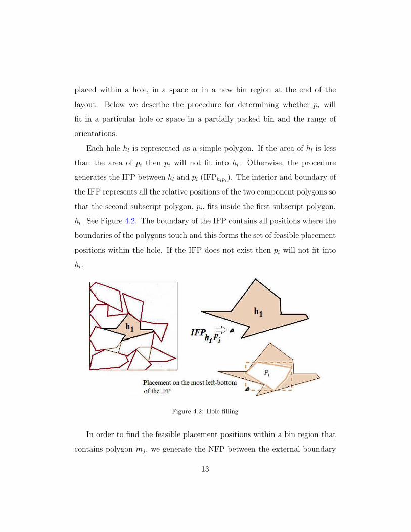
placed within a hole, in a space or in a new bin region at the end of the

layout. Below we describe the procedure for determining whether pi will

fit in a particular hole or space in a partially packed bin and the range of

orientations.

Each hole hl is represented as a simple polygon. If the area of hl is less

than the area of pi then pi will not fit into hl. Otherwise, the procedure

generates the IFP between hl and pi (IFPhlpi). The interior and boundary of

the IFP represents all the relative positions of the two component polygons so

that the second subscript polygon, pi, fits inside the first subscript polygon,

hl. See Figure 4.2. The boundary of the IFP contains all positions where the

boundaries of the polygons touch and this forms the set of feasible placement

positions within the hole. If the IFP does not exist then pi will not fit into

hl.

Figure 4.2: Hole-filling

In order to find the feasible placement positions within a bin region that

contains polygon mj, we generate the NFP between the external boundary

13

of mj and pi, NFPmjpi and the IFP between the bin region bj and pi, IFPbjpi .

The exterior and boundary of the NFP represents all relative positions of

the two component polygons where they do not overlap. The intersection

of the IFPbjpi and the complement of NFPmjpi provides all the positions of

pi such that it is contained within bj and not overlapping mj, assuming bj

and mj have a fixed position. We only consider the boundary segment of

the NFPmjpi that intersects with IFPbjpi as the feasible set, which is all the

feasible touching positions between mj and pi. See Figure 4.3 for an example

of this evaluation.

Figure 4.3: Feasible placement for a new piece

14

4.1.2. Placement orientation of a piece

The above discussion assumes pi is in a given orientation. In this pa-

per, we consider two scenarios with respect to rotating pieces. First, we

allow pieces to rotate by a pre-assigned set of angles, which we define as

the finite rotation approach. This is the most common case in the litera-

ture where the rotation angles of pieces are restricted to oi = 0o, 180o or

α = 0o, 90o, 180o, 270o. Second we consider rotating pieces freely.

In the case of finite rotation angles, we simply consider pi in each of

the four orientations. For each orientation we generate the set of feasible

placement positions, as described in 4.1.1, and select the best according to

the placement policy criteria, described in the next section.

For free rotation there are an infinite set of possible orientations, where

only a subset of these can be evaluated. In order to reduce these to a finite

set of candidate orientations, we devise a mechanism to identify a subset of

promising angles according to the arrangement of the pieces in the current

partial solution. We describe the approach assuming pi can be placed in a

region that contains a merged polygon mj.

Our approach begins by placing pi on the packing layout in a temporary

position and orientation using the finite rotation placement approach, where

the best orientation is selected. As discussed in the previous section, the

position will be touching the boundary of mj. Each touching point or edge

defines two new angles of orientation. These are illustrated in figure 4.4.

15

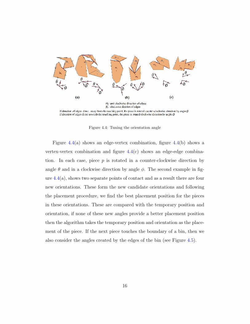
Figure 4.4: Tuning the orientation angle

Figure 4.4(a) shows an edge-vertex combination, figure 4.4(b) shows a

vertex-vertex combination and figure 4.4(c) shows an edge-edge combina-

tion. In each case, piece p is rotated in a counter-clockwise direction by

angle θ and in a clockwise direction by angle φ. The second example in fig-

ure 4.4(a), shows two separate points of contact and as a result there are four

new orientations. These form the new candidate orientations and following

the placement procedure, we find the best placement position for the pieces

in these orientations. These are compared with the temporary position and

orientation, if none of these new angles provide a better placement position

then the algorithm takes the temporary position and orientation as the place-

ment of the piece. If the next piece touches the boundary of a bin, then we

also consider the angles created by the edges of the bin (see Figure 4.5).

16

Figure 4.5: Angle tuning at the edges of bins

4.2. Placement policy

The above procedures provide a set of feasible placement positions and

orientations for piece pi. The placement policy sets the criteria that deter-

mines which position is chosen. Note that for some of the placement rules,

we can often avoid the computational cost of assessing all positions by con-

trolling the order in which they are assessed. In the following we describe

the placement rules in the context of packing from the left hand end of the

strip extending towards the right. However, Jostle also packs from right to

left, in which case simply swap left and right in the following explanation.

We evaluate three well known placement rules; bottom left placement,

minimum length placement and maximum utilization placement, to deter-

mine the position of each piece. However, these rules are dominated by first

trying to fill holes in the layout.

17

The first step when placing pi is to sort all the holes in Hk in order of left

most x-coordinate. These holes are evaluated in that order using the hole

filling procedure. If pi fits in a given hole, it is placed and no further holes

are considered. If pi does not fit within any hole, the algorithm attempts

to find a feasible placement position in each of the bin regions bj starting

with the left most. Using the procedure described in Section 4.1 for finding

placement positions and orientation in a partially packed bin, the candidate

positions are found for each bin region bj in order. The placement policies

are as follows:

• Bottom-left (BL) prioritizes placing the reference point of the piece in

the leftmost feasible position on the stock sheet breaking ties by select-

ing the bottom-most of the left most positions. This is a well-known

single pass placement rule applied in many cutting and packing papers

(Dowsland et al., 1998; Blazewicz et al., 1993; Albano and Sapuppo,

1980). By applying this rule when hole filling fails, once a feasible

position is found in region bj the search can stop. If more than one

orientation of pi gives the same BL position, select the orientation that

minimises the width of the bounding box of the piece. If there is still a

tie, select the orientation randomly. Apply the same tie breaker rules

for placing pi in a new bin.

• Minimum Length (ML) placement rule selects the position that mini-

mize the length from the origin of the bin to the right-most x-coordinate

of pi. The piece is orientated to minimise the right-most x-coordinate.

In case of ties, we select the bottom-left placement position.

18

• Maximum Utilization (MU) placement rule selects the position that

provides the maximum area utilisation in the earliest bin. We assume

the occupied area of a region bj is the area of the convex hull of mj.

Let the area of the convex hull of mj be CHarea(mj), the area of pi

be area(pi) and the area of the convex hull of the new merged polygon

after pi is placed in a certain position be CHarea (mj + pi). Then the

utilisation of the placement position (Utp) is calculated as follows.

Utp =CHarea(mj) + area(pi)

CHarea(mj + pi)

Given the set of feasible placement positions on the boundary of the

NFP, we select each feasible vertex of the NFP as a candidate place-

ment position. This is illustrated in Figure 4.6. Placement positions

are evaluated bin by bin starting at the left most bin. If a feasible

placement is found in a bin then no further bins are considered. Ties

are broken by selecting the bottom left position and minimum length

orientation.

19

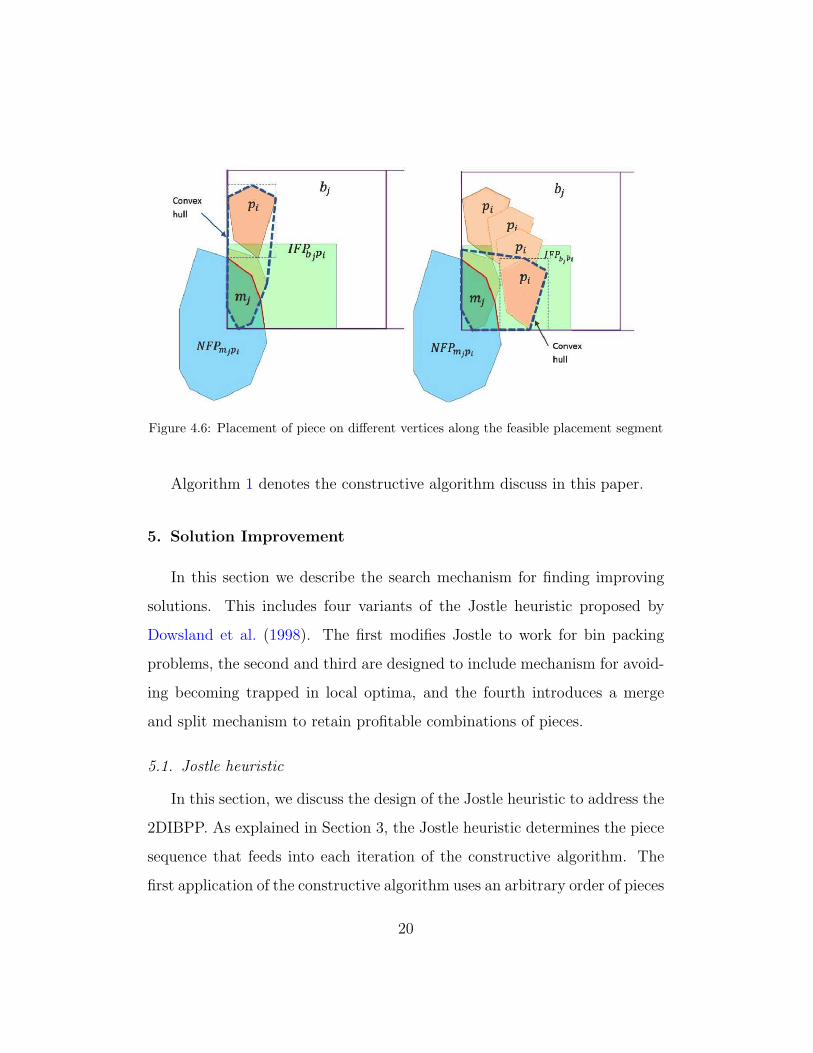
Figure 4.6: Placement of piece on different vertices along the feasible placement segment

Algorithm 1 denotes the constructive algorithm discuss in this paper.

5. Solution Improvement

In this section we describe the search mechanism for finding improving

solutions. This includes four variants of the Jostle heuristic proposed by

Dowsland et al. (1998). The first modifies Jostle to work for bin packing

problems, the second and third are designed to include mechanism for avoid-

ing becoming trapped in local optima, and the fourth introduces a merge

and split mechanism to retain profitable combinations of pieces.

5.1. Jostle heuristic

In this section, we discuss the design of the Jostle heuristic to address the

2DIBPP. As explained in Section 3, the Jostle heuristic determines the piece

sequence that feeds into each iteration of the constructive algorithm. The

first application of the constructive algorithm uses an arbitrary order of pieces

20

Algorithm 1: Constructive AlgorithmInput : P0, Placement rule

Output: P ∗: A feasible packing of all pieces in N Bins1 Set α = 0, π

2, π, 3π

2, N = 1;

2 for i = 1 : n do

3 for l = 1, 2, .., q do

4 if Area(pi) ≤ Area(hl) then

5 Find feasible placement in hole hl by rotating the existing pi by each α angle;6 if there exist any feasible points for placement then

7 Place pi with corresponding α following the Placement rule;8 Update Hi−1 → Hi and update q;9 Sort all the holes in Hi in order of left most x-coordinate;

10 End For Loop l;

11 else

12 move to the next hole in the list Hi−1;13 end

14 else

15 move to the next hole in the list Hi−1;16 end

17 end

18 if No feasible placement by Hole-filling then

19 for j = 1, 2, .... do20 if Area(pi) ≤ Area(bj)−Area(mj) then

21 Find feasible placement path by rotating the existing pi by each α angle;22 Find the best orientation angle;23 Derive new angles by angle tuning mechanism;24 Find feasible placement path by rotating pi by each new angle;25 if there exist any feasible points found for placement by α angles or tuning

angles then

26 Evaluate best placement position and angle for pi following thePlacement rule;

27 Merge pi to mj ;28 Capture any hole created (≥ smallest piece area);29 Update Hi−1 → Hi and update q;30 If there are any new hole, sort holes Hi by left most x-coordinate;31 If (j > N) N = j;32 Break the For loop j;

33 else

34 move to the next bin j;35 end

36 else

37 move to the next bin j;38 end

39 end

40 end

41 end

and packs the pieces from left to right along the strip. After generating a

complete solution, all the pieces are re-ordered according to the piece with the

right-most x-coordinates continuing to the left-most. Following this order,

21

pieces are packed starting at the right-most position of the strip building the

packing layout from right to left. Jostle continues to oscillate from packing

left to right then right to left until the termination criterion is met.

Jostle is analogous to a local search where the search occurs over the se-

quence of the pieces and each Jostle iteration generates a neighbour sequence.

The constructive algorithm takes a sequence of pieces and creates a layout.

The layout is converted back to a sequence according to the x-coordinate

order. Hence, the new layout defines a new sequence of pieces, this is a

neighbour solution based on the arrangement of pieces of the previous pack-

ing layout. Each iteration generates only one neighbour, which is always

accepted. The optimisation arises from the neighbour generation. Instead

of applying a fixed rule to the sequence i.e. swap or insert, the constructive

algorithm changes the sequence by optimising the packing arising from the

current piece sequence. Each complete solution is evaluated according to

K and F defined in Section 3. At the end of the search, the best solution

according to these measures is kept.

Since the constructive algorithm includes filling of holes and multiple

alternative orientation, the piece sequence and placement positions change

between iterations. However, our experiments show that the search can con-

verge and get stuck in local optima. In order to overcome this we incorporate

the diversification ideas from iterated local search to escape from local op-

tima. The new variant is called Iterated Jostle.

5.2. Iterated Jostling

The Iterated Jostle algorithm combines the basic Jostle procedure and a

kick intended to move the solution to a new area of the solution space and

22

escape local optima. This feature is motivated by our observation that the

Jostle heuristic becomes trapped in local optima after running several Jostle

cycles. This is more commonly found for data sets that are small and have

similar size pieces. We perform a kick from the best local optimum found so

far and consider that we are at a local optima after cmax Jostle cycles with

no improvement. We investigate two kick strategies, described below. Note

that in cutting and packing, a small change in the permutations can lead to

a significant change in the layout of the pieces once it has been decoded by

the constructive algorithm. In the case of the first kick strategy, we check

that the move does not produce an identical permutation, which can occur

when there are multiple pieces of the same type.

1-piece insert move:. We perform a single insert move as follows:

1. Select two random positions along the permutation of pieces,

2. Select the piece that corresponds to the highest position selected in step

1,

3. Remove the selected piece from the permutation and insert it in front

of the piece in the other position selected in step 1,

4. Order the remaining pieces following the existing permutation.

Bin-swapping move:. This strategy changes the order of pieces by effec-

tively swapping two bins as follows:

1. Select the bin with the lowest utilization and let sub-sequence A be

the pieces in that bin in x-co-ordinate order,

2. Select another bin randomly and let sub-sequence B be the pieces in

that bin in x-coordinate order,

23

3. Swap sub-sequence A and sub-sequence B in the permutation,

4. Obtain the new permutation of pieces.

Algorithm 2 describes the iterated Jostle procedure (IJS). Let t be the

Jostle cycle, PLt be the permutation of pieces to be packed from left to right

in cycle t, PRt be the permutation of pieces to be packed from right to left in

cycle t and P0 be the initial random permutation. P ∗ stores the permutation

of pieces from the solution with smallest objective function value found so far,

K∗, and D∗ be the direction of packing. The variable c counts the number

of consecutive Jostle iterations with no improvement in solution quality (K).

The termination criteria is the maximum total number of Jostle cycles that

the algorithm will run, Tmax.

5.3. Iterated Jostling with join and release of pieces

This final version of Iterated Jostle draws on the ideas of Adamowicz

and Albano (1972), which was more recently applied by Elkeran (2013).

They combine pieces that fit together well reducing the overall number of

pieces. In our approach we allow two pieces to be combined into one merged

piece for some of the Jostle iterations. The algorithm scans the arrangement

of pieces in each bin and attempts to join adjacent pieces in their current

position. If the combined piece is convex with no holes then they are merged

for the following Jostle iterations. Each scan only permits pairwise merging.

However, scans in later iterations may join a piece to a merged piece resulting

in three or more original pieces joining together. Pieces are joined after each

Jostle iteration until a kick is performed, at which time they are separated

again. The type of kick alternates between 1-piece insert and bin-swapping.

The following steps outline the IJS with join and release procedure.

24

Algorithm 2: IJSInput : P0, Placement rule, kick type, cmax, Tmax

Output: P ∗, K∗, D∗ = L(left) or R(right)1 Set t = 1;2 P ∗ = PL

t = P0;3 Set D∗ = L;4 Set K∗ = a suitably large value;5 Initialize c = 0;6 while t ≤ Tmax do

7 Generate solution layout from PLt ;

8 Evaluate the solution and find KLt ;

9 Derive PRt from solution;

10 Generate solution layout from PRt ;

11 Evaluate the solution and find KRt ;

12 if KLt < KR

t then

13 if KLt < K∗ then

14 Set K∗ = KLt , P

∗ = PLt , D

∗ = L;15 Reset c = 0;

16 else

17 c = c+ 1;18 end

19 else

20 if KRt < K∗ then

21 Set K∗ = KRt , P

∗ = PRt , D∗ = R;

22 Reset c = 0;

23 else

24 c = c+ 1;25 end

26 end

27 if c > cmax then

28 Apply kick to P ∗ and obtain PD∗t ;

29 Generate solution layout from PD∗t ;

30 Derive PLt from solution;

31 end

32 t = t+ 1;

33 end

34 return P ∗, K∗, D∗;

25

1. From a given initial permutation, apply Jostle until the kick criteria is

met.

2. Apply a kick alternating between bin-swap and 1-piece insert,

3. Jostle for one iteration

4. Execute pairwise joining of pieces

5. If stop criteria met, then stop else

6. If kick criteria met, release all joined pieces and go to step 2, else

7. go to step 3

6. Experimental Design and Results

In this section we provide details of our experiments and a discussion of

the results. All the algorithms are coded in C++11 and use version 1.58.0

of the Boost computational geometry library to implement some of the geo-

metric operations. The tests are performed by 2.6 GHz processor and 4 GB

of RAM to execute the program.

6.1. Data instances

Our experiments utilise two sets of benchmark instances: the nesting

instances used by a wide variety of authors for the irregular strip packing

problem and instances proposed by Lopez-Camacho et al. (2013) that are

jigsaw puzzle instances as they have known optimal solutions of 100% utilisa-

tion of the stock sheet. Both are available from the ESICUP (EURO Special

Interest Group on Cutting and Packing) web site http://paginas.fe.up.

pt/~esicup/datasets.

26

http://paginas.fe.up.pt/~esicup/datasets

http://paginas.fe.up.pt/~esicup/datasets

The nesting instances contain 23 irregular strip packing data sets and

contain both convex and non-convex pieces. As these are strip packing in-

stances we need to define bin sizes for each data set. For each instance we

define three different bin sizes based on the maximum dimension of the en-

closing rectangles of each piece in their original orientation denoted as dmax.

The bin sizes are: small bin (1.1dmax for length and width), medium bin

(1.5dmax for length and width) and large bin (2dmax for length and width).

These bin sizes were proposed by Martinez-Sykora et al. (2017).

The jigsaw puzzle (JP) instances contain two sets, which we denote as

JP1 and JP2. JP1 has a collection of 540 instances in which all the pieces

are convex. These instances are divided in 18 classes with 30 problems and

each class carries a different number of pieces. The second set, JP2, has 480

instances (16 classes with 30 problems in each class) in which some of the

pieces have concavities.

6.2. Experimental results

Our solution strategy includes a number of alternative approaches in

terms of the placement policy in the constructive heuristic, the permitted

orientations and the kick strategies in Jostle. Table 6.1 and Table 6.2 provide

a summary and the notation for the alternative approaches. Any variant that

includes a random input is repeated for 10 trials and we report the average

across the trials. We conduct the following set of computational experiments

and compare the performance of each approach.

27

Table 6.1: Notation of Algorithms: placement rule and rotationNotation Placement Rule Piece orientationBL4 Bottom-Left Restricted (0, π

2, π, 3π

2)

BL∞ Bottom-Left UnrestrictedML4 Minimum-Length Restricted (0, π

2, π, 3π

2)

ML∞ Minimum-Length UnrestrictedMU4 Maximum Utilization Restricted (0, π

2, π, 3π

2)

MU∞ Maximum Utilization Unrestricted

Table 6.2: Notation of Algorithms: algorithm and kick typeNotation Description Kick-move strategy

JS Jostling -IJS1 Iterated Jostling 1-piece insert moveIJS2 Iterated Jostling Bin swapping moveIJS3 Iterated Jostling 1-piece insert move , Bin swapping move , Join and Release of pieces

6.2.1. Test 01: Jostling search vs. random order of pieces

These experiments compare the performance of the two rotation criteria,

finite set of angles and free rotation, and the alternative placement policies,

BL4, BL∞, ML4, ML∞, MU4, and MU∞, in terms of quality of packing

and computational time. These experiments use the nesting instances. A

CA trial is made up of 500 random permutations of pieces, each packed us-

ing a constructive heuristic. The best layout is recorded from each trial. In

addition, we evaluate the Jostle heuristic and compare with packing random

permutations of pieces using the CA. These experiments intend to investi-

gate whether the Jostle heuristic provides a good search mechanism that

improves on random trials. Each trial of the basic Jostle heuristic executes

250 Jostle cycles (which generates 500 layouts). Table 6.3 details the results

and considers measure K and F . Note we wish to minimise K and maximise

F .

28

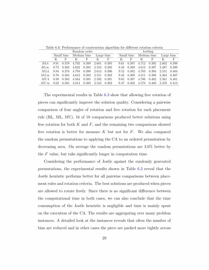
Table 6.3: Performance of construction algorithm for different rotation criteriaRandom order Jostling

Small bins Medium bins Large bins Small bins Medium bins Large binsK F K F K F K F K F K F

BL4 9.91 0.379 4.792 0.389 2.601 0.395 9.61 0.387 4.712 0.392 2.602 0.398BL∞ 9.73 0.383 4.632 0.394 2.555 0.392 9.48 0.389 4.612 0.397 2.487 0.399ML4 9.94 0.378 4.794 0.390 2.613 0.396 9.52 0.382 4.703 0.394 2.551 0.404ML∞ 9.76 0.384 4.612 0.393 2.551 0.392 9.42 0.389 4.511 0.398 2.464 0.407MU4 9.89 0.383 4.944 0.385 2.592 0.391 9.65 0.387 4.786 0.402 2.561 0.401MU∞ 9.62 0.385 4.614 0.393 2.524 0.392 9.47 0.402 4.573 0.408 2.470 0.413

The experimental results in Table 6.3 show that allowing free rotation of

pieces can significantly improve the solution quality. Considering a pairwise

comparison of four angles of rotation and free rotation for each placement

rule (BL, ML, MU), 16 of 18 comparisons produced better solutions using

free rotation for both K and F , and the remaining two comparisons showed

free rotation is better for measure K but not for F . We also compared

the random permutations to applying the CA to an ordered permutation by

decreasing area. On average the random permutations are 3.6% better by

the F value, but take significantly longer in computation time.

Considering the performance of Jostle against the randomly generated

permutations, the experimental results shown in Table 6.3 reveal that the

Jostle heuristic performs better for all pairwise comparisons between place-

ment rules and rotation criteria. The best solutions are produced when pieces

are allowed to rotate freely. Since there is no significant difference between

the computational time in both cases, we can also conclude that the time

consumption of the Jostle heuristic is negligible and time is mainly spent

on the execution of the CA. The results are aggregating over many problem

instances. A detailed look at the instances reveals that often the number of

bins are reduced and in other cases the piece are packed more tightly across

29

the same number of bins. We also observed that Jostle struggles to diversify

from the first local optima, so the improvements are local with respect to the

initial solution. With this in mind, we conclude that Jostle can perform as

an optimisation procedure with more intelligence than a random search.

The final observation from these results concerns the placement rule. For

random permutations BL performs the best once on measure F , ML performs

the best twice and MU performs the best three times. For Jostle the result is

more consistent where ML performs the best for each measure of K and MU

performs the best for each measure of F . This result is intuitive since K aims

to minimise length to provide a greater residual in the last bin, while F is

based on utilisation. It is interesting to note the BL is consistently adopted

in the literature, but in our investigation it is consistently inferior.

6.2.2. Test 02: IJS vs JS

These experiements compare the performance of the four Jostle strategies;

JS, IJS1, IJS2 and IJS3, where the latter three strategies us a kick. Table 6.2

provides details of these strategies. Ten random permutations are used as

initial permutations for each variant and each trial runs for 500 Jostle cycles.

After initial experiments with a range of values for cmax, we set cmax = 4, 6, 6

Jostle cycles for IJS1, IJS2 and IJS3 respectively.

The alternative strategies arose through the observation that JS tends

to get stuck in local optima. This occurs more frequently with small data

sets and with shapes that are less irregular. As an example, Figure 6.1(a)

illustrates solution F values received at each iteration for a certain trial for

Fu data instance using JS. In this case the Jostle heuristic has taken 9-12

cycles to reach a better F value (i.e. F = 0.488). When Jostling continues,

30

the solution rarely reaches F = 0.488 and the best value is recorded at 143rd

cycle. After 176th cycle, the Jostling has reached a steady state generating

the same set of solutions repetitively. Figure 6.1(b) demonstrates the benefit

of using a kick. Here IJS1 is run on the same data. Introducing a kick has

avoided the repetitive cycle and produced better solutions (i.e. F > 0.499)

within fewer iterations.

31

Figure 6.1: JS and IJS1 iterations

32

Figure 6.2: Fu instance packed in the largest bin type (2dmax) using IJS1-MU∞ method,F = 0.509, run time is 8 seconds for 500 iterations

Table 6.4: Performance results JS, IJS1, IJS2 and IJS3 for nesting data instancesJS IJS1 IJS2 IJS3

F T (sec) F T (sec) F T (sec) F T (sec)Small bin BL4 0.384 304.4 0.394 322.4 0.388 310.7 0.394 319.4

BL∞ 0.389 502.7 0.408 528.5 0.394 512.1 0.404 534.8ML4 0.386 278.6 0.393 313.4 0.390 285.8 0.397 320.5ML∞ 0.389 509.1 0.419 526.6 0.392 533.4 0.402 575.3MU4 0.388 281.4 0.393 294.0 0.389 286.4 0.403 335.0MU∞ 0.407 504.9 0.437 518.6 0.427 534.4 0.433 540.5

Avg. 0.391 0.408 0.397 0.406

Medium bin BL4 0.392 287.5 0.403 298.4 0.409 298.1 0.407 315.9BL∞ 0.398 484.7 0.409 506.1 0.403 496.3 0.404 505.4ML4 0.394 269.5 0.409 301.8 0.400 281.2 0.402 306.2ML∞ 0.398 476.6 0.422 515.9 0.418 488.7 0.414 530.6MU4 0.404 267.4 0.418 281.2 0.410 272.0 0.409 306.8MU∞ 0.408 487.9 0.436 499.0 0.415 503.4 0.429 510.1

Avg. 0.399 0.416 0.409 0.410

Large bin BL4 0.398 248.9 0.403 266.5 0.402 255.6 0.410 280.7BL∞ 0.400 421.6 0.404 450.1 0.402 430.7 0.415 485.3ML4 0.404 239.4 0.422 259.7 0.400 249.4 0.410 272.6ML∞ 0.408 426.3 0.425 451.3 0.409 441.6 0.415 477.6MU4 0.402 240.4 0.425 253.9 0.404 247.1 0.410 268.9MU∞ 0.414 426.8 0.431 453.9 0.413 436.8 0.407 480.7

Avg. 0.404 0.418 0.405 0.411

33

Table 6.5: Performance results of IJS1, IJS2 and IJS3 vs JS for JP1 and JP2 instancesF values JS IJS1 IJS2 IJS3

F T (sec) F T (sec) F T (sec) F T (sec)JP1 BL4 0.589 76.5 0.652 81.2 0.648 76.3 0.700 76.2

BL∞ 0.527 148.5 0.564 161.4 0.579 167.4 0.594 153.8ML4 0.508 72.7 0.625 79.6 0.647 80.8 0.693 75.8ML∞ 0.522 150.3 0.634 161.9 0.564 152.0 0.590 162.4MU4 0.566 72.1 0.691 78.1 0.678 79.6 0.732 74.9MU∞ 0.552 159.7 0.677 163.8 0.639 166.7 0.644 161.2

Avg. 0.544 0.641 0.626 0.659

JP2 BL4 0.572 56.3 0.652 59.3 0.682 62.3 0.725 63.8BL∞ 0.506 98.4 0.522 101.2 0.532 102.4 0.547 103.3ML4 0.549 55.7 0.677 61.3 0.697 61.2 0.714 61.5ML∞ 0.505 98.1 0.632 103.4 0.607 104.6 0.516 100.1MU4 0.617 54.9 0.701 62.1 0.680 59.2 0.747 58.3MU∞ 0.584 97.8 0.655 107.8 0.626 112.5 0.613 101.5

Avg. 0.556 0.640 0.637 0.644

In Table 6.4 we present the average results obtained by JS and the three

IJS procedures for the 23 nesting instances. For all placement criteria and

angles of rotation, the three IJS algorithms produce better results when

compared with JS. For nesting data instances, IJS1 provides the best results

for all bin sizes when averaging over all placement/rotation variants and

for each individual result apart from medium bins BL4 where IJS2 is best.

Focusing just on the IJS algorithms, there are 18 variants (3 placement rules

x 2 angles of rotation x 3 IJS algorithms). Out of those 18 methods, IJS1-

MU∞ produces the best results irrespective of the bin sizes.

In Table 6.5 we present the average results obtained by JS and the three

IJS procedures for the 540 JP1 and 480 JP2 instances. Again the IJS ap-

proaches are clearly better than the values of JS. On average IJS3 performed

better for both JP1 and JP2 instances. However, in this case IJS3-MU4

has produced the best results. For this data the optimal solution can only

be found at the zero rotation angle, hence it is intuitive that restricting the

34

rotation is beneficial.

6.2.3. Test 03: Comparing with benchmark results in literature

In this case we compare our results with the work of Lopez-Camacho

et al. (2013a) and Martinez-Sykora et al. (2017). Since these algorithms are

run on different computing platforms, it is not possible to run for the same

amount of time. Hence we retain our termination criteria of 500 Jostle cycles

and report the average result and computational time for the ten random

trials.

Referring to the previous tables 6.4 and 6.5 we can compare these results

with the results from the literature. Martinez-Sykora et al. (2017) report a

best value of F = 0.723 with computational time 161 seconds for JP1 and

F = 0.729 with computational time 123 seconds for JP2. In both cases our

algorithm (IJS3-MU4) provides better results, specifically F = 0.732 with

computational time 74.9 seconds for JP1 and F = 0.747 with computational

time 58.3 seconds for JP2. Also our approach has achieved better results for

11 out of 18 groups of instances for JP1. In the case of JP2 instances our

method has achieved better results for 11 out of 16 groups of instances. A

detailed description of these results are provided in table A.1 and A.2. The

only other existing results for this data is by Lopez-Camacho et al. (2013a),

who only report results for JP1. They achieve F = 0.690 with computational

time 50 seconds. We revised the termination of our algorithm to 50 seconds

and achieved the improved result of F = 0.703.

For the nesting instances we consider the average over all the instances for

each bin size. The only benchmark results are from Martinez-Sykora et al.

(2017). For small bins they achieve F = 0.434 with computation time of 1721

35

seconds, for medium bins they achieve F = 0.452 with computation time of

3172 seconds and for large bins they achieve F = 0.403 with computation

time of 762 seconds. IJS1-MU∞ performs better for small and large bins

and takes less time for all three bin types. The overall results of Martinez-

Sykora et al. (2017) demonstrate that their algorithm has lower performance

when average number of pieces per bin is higher. However in our case, we

achieve significantly better results for large bins in most of our approaches;

i.e. IJS1, IJS2 and IJS3. Even for small and medium sized bins, we achieved

better or close results with no significant drop in average F values, with less

computational time than Martinez-Sykora et al. (2017). Table A.3, A.4 and

A.5 present the results we achieved for each data instance using the IJS1

approach.

7. Concluding Remarks

In this paper we address a new solution method to solve the two dimen-

sional irregular shapes bin packing problem which has received little attention

in literature despite clear industry relevance. We modify the existing use of

the Jostle procedure of Dowsland et al. (1998) applied to strip packing and

convert the heuristic for the homogeneous bin packing problem. Further we

introduced a diversification strategy into Jostle that significantly improved

the results. The proposed heuristic supports the use of restricted rotation

and unrestricted rotation of pieces.

The findings of the study are as follows. Jostle is a promising packing

heuristic that can be applied to bin packing problems. It is demonstrated to

be a low cost search strategy that self governs the neighbourhood structure

36

that modifies the solution. The designed algorithms have been shown to

improve on the results in the literature with lower computation time and does

not require the use of expensive Mixed Integer Program software, making it

attractive to small companies.

We have introduced a new way of dealing with free rotation of pieces.

We have demonstrated the value of free rotation for nesting instances and

justified the results of restricted rotation for the jigsaw puzzle instances.

We have designed and tested a number of placement policies and shown

that despite the extensive use of bottom-left (BL) this does not produce the

best results when compared with minimizing length or maximising utilisa-

tion.

References

M. Adamowicz and A. Albano. A two-stage solution of the cutting stock problem.

Information Processing, 71:1086–1091, 1972.

A. Albano and G. Sapuppo. Optimal Allocation of Two-Dimensional Irregular

Shapes Using Heuristic Search Methods. IEEE Transactions on Systems, Man

and Cybernetics, 10(5):242–248, 1980. ISSN 0018-9472.

J. A. Bennell and J. F. Oliveira. A Tutorial in Irregular shape Packing Problems.

The Journal of the Operational Research Society, 60:s93–s105, 2009. ISSN 0160-

5682.

J. A. Bennell and X. Song. A comprehensive and robust procedure for obtaining

the nofit polygon using minkowski sums. Computers & Operations Research, 35

(1):267–281, 2008. ISSN 0305-0548.

J. A. Bennell and X. Song. A beam search implementation for the irregular shape

packing problem. Journal of Heuristics, 16(2):167–188, 2010. ISSN 1381-1231,

1572-9397.

37

J. Blazewicz, P. Hawryluk, and R. Walkowiak. Using a tabu search approach for

solving the two-dimensional irregular cutting problem. Annals of Operations

Research, 41(4):313–325, 1993. ISSN 0254-5330, 1572-9338.

E. K. Burke, R. S. R. Hellier, G. Kendall, and G. Whitwell. Complete and robust

no-fit polygon generation for the irregular stock cutting problem. European

Journal of Operational Research, 179(1):27–49, 2007. ISSN 0377-2217.

K. A. Dowsland, W. B. Dowsland, and J. A. Bennell. Jostling for position: local

improvement for irregular cutting patterns. Journal of the Operational Research

Society, 49(6):647–658, 1998. ISSN 0160-5682.

Ahmed Elkeran. A new approach for sheet nesting problem using guided cuckoo

search and pairwise clustering. European Journal of Operational Research, 231

(3):757–769, 2013. 00020.

W. Han, J. A. Bennell, X. Zhao, and X. Song. Construction heuristics for two-

dimensional irregular shape bin packing with guillotine constraints. European


M. Hifi and R. M’Hallah. A hybrid algorithm for the two-dimensional layout

problem: the cases of regular and irregular shapes. International Transactions

in Operational Research, 10(3):195–216, 2003. ISSN 1475-3995.

S. Jakobs. On genetic algorithms for the packing of polygons. European Journal

of Operational Research, 88(1):165–181, 1996. ISSN 0377-2217.

D. Liu and H. Teng. An improved BL-algorithm for genetic algorithm of the

orthogonal packing of rectangles1. European Journal of Operational Research,

112(2):413–420, 1999. ISSN 0377-2217.

E. Lopez-Camacho, G. Ochoa, H. Terashima-Marin, and E. K. Burke. An effec-

tive heuristic for the two-dimensional irregular bin packing problem. Annals of

Operations Research, 206(1):241–264, 2013a. ISSN 0254-5330.

E. Lopez-Camacho, H. Terashima-Marin, G. Ochoa, and S. E. Conant-Pablos.

Understanding the structure of bin packing problems through principal compo-

nent analysis. International Journal of Production Economics, 145(1):488–499,

2013b. ISSN 0925-5273.

38

E. Lopez-Camacho, H. Terashima-Marin, P. Ross, and G. Ochoa. A unified hyper-

heuristic framework for solving bin packing problems. Expert Systems with

Applications, 41(15):6876–6889, 2014. ISSN 0957-4174.

A. Martinez-Sykora, R. Alvarez-Valdes, J. A. Bennell, R. Ruiz, and J. M. Tamarit.

Matheuristics for the irregular bin packing problem with free rotations. European


A. Martinez-Sykora, R. Alvarez-Valdes, J. Bennell, and J. M. Tamarit. Construc-

tive procedures to solve 2-dimensional bin packing problems with irregular pieces

and guillotine cuts. Omega, 52:15–32, 2015. ISSN 0305-0483.

J. F. Oliveira, A. M. Gomes, and J. S. Ferreira. TOPOS A new constructive

algorithm for nesting problems. OR-Spektrum, 22(2):263–284, 2000. ISSN 0171-

6468, 1436-6304.

P. Rocha. Circle Covering Representation for Nesting Problems with Continuous

Rotations. In Boje Edward, editor, Proceedings of 19th World Congress The

International Federation of Automatic Control, pages 5235–5240, 2014.

X. Song and J. A. Bennell. Column generation and sequential heuristic procedure

for solving an irregular shape cutting stock problem. Journal of the Operational

Research Society, 65(7):1037–1052, 2014.

Y. G. Stoyan, M. V. Zlotnik, and A. M. Chugay. Solving an optimization pack-

ing problem of circles and non-convex polygons with rotations into a multiply

connected region. Journal of the Operational Research Society, 63(3):379–391,

2012. ISSN 0160-5682.

H. Terashima-Marin, P. Ross, C. J. Farias-Zarate, E. Lopez-Camacho, and

M. Valenzuela-Rendon. Generalized hyper-heuristics for solving 2D Regular

and Irregular Packing Problems. Annals of Operations Research, 179(1):369–

392, 2008. ISSN 0254-5330, 1572-9338.

39

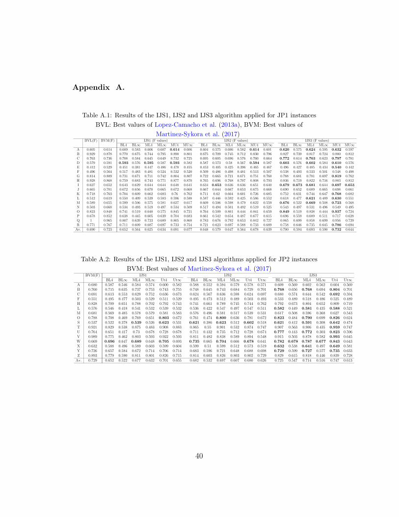
Appendix A.

Table A.1: Results of the IJS1, IJS2 and IJS3 algorithm applied for JP1 instances

BVL: Best values of Lopez-Camacho et al. (2013a), BVM: Best values of

Martinez-Sykora et al. (2017)BVL(F) BVM(F) IJS1 (F values) IJS2 (F values) IJS3 (F values)

BL4 BL∞ ML4 ML∞ MU4 MU∞ BL4 BL∞ ML4 ML∞ MU4 MU∞ BL4 BL∞ ML4 ML∞ MU4 MU∞A 0.605 0.614 0.609 0.583 0.606 0.607 0.614 0.606 0.604 0.575 0.606 0.582 0.614 0.601 0.620 0.575 0.624 0.595 0.632 0.597B 0.929 0.878 0.770 0.675 0.744 0.795 0.890 0.801 0.675 0.709 0.745 0.712 0.830 0.796 0.827 0.739 0.817 0.724 0.880 0.812C 0.763 0.736 0.708 0.584 0.645 0.649 0.732 0.725 0.695 0.605 0.696 0.576 0.760 0.664 0.772 0.614 0.763 0.623 0.797 0.701D 0.579 0.591 0.593 0.576 0.595 0.587 0.593 0.582 0.587 0.573 0.58 0.567 0.594 0.587 0.603 0.576 0.602 0.584 0.610 0.576E 0.412 0.529 0.451 0.381 0.447 0.486 0.478 0.455 0.453 0.405 0.425 0.396 0.465 0.467 0.496 0.427 0.485 0.434 0.540 0.442F 0.496 0.564 0.517 0.483 0.481 0.524 0.532 0.520 0.509 0.486 0.498 0.481 0.513 0.507 0.538 0.493 0.533 0.501 0.548 0.498G 0.814 0.809 0.731 0.671 0.711 0.742 0.804 0.807 0.722 0.665 0.721 0.671 0.751 0.760 0.788 0.681 0.781 0.697 0.819 0.762H 0.928 0.868 0.759 0.683 0.743 0.771 0.877 0.870 0.765 0.696 0.768 0.707 0.808 0.793 0.836 0.719 0.822 0.716 0.883 0.812I 0.627 0.652 0.643 0.629 0.644 0.644 0.648 0.641 0.634 0.653 0.636 0.636 0.651 0.640 0.679 0.673 0.681 0.644 0.697 0.653

J 0.665 0.701 0.672 0.656 0.670 0.665 0.672 0.668 0.667 0.644 0.667 0.653 0.675 0.668 0.690 0.652 0.689 0.665 0.698 0.661K 0.718 0.763 0.704 0.609 0.662 0.683 0.76 0.762 0.711 0.62 0.664 0.601 0.726 0.685 0.752 0.631 0.744 0.647 0.768 0.682L 0.512 0.619 0.550 0.409 0.539 0.583 0.596 0.588 0.587 0.446 0.592 0.425 0.586 0.552 0.618 0.477 0.621 0.489 0.630 0.551M 0.589 0.655 0.599 0.506 0.575 0.581 0.627 0.617 0.609 0.506 0.598 0.479 0.622 0.559 0.676 0.522 0.669 0.508 0.723 0.568N 0.503 0.668 0.534 0.493 0.519 0.497 0.534 0.509 0.517 0.494 0.501 0.492 0.519 0.525 0.543 0.497 0.531 0.496 0.549 0.495O 0.823 0.848 0.741 0.519 0.648 0.575 0.845 0.721 0.764 0.509 0.801 0.444 0.841 0.659 0.849 0.519 0.838 0.444 0.937 0.724P 0.678 0.852 0.638 0.445 0.605 0.639 0.704 0.683 0.661 0.542 0.654 0.487 0.677 0.615 0.696 0.559 0.689 0.511 0.717 0.628Q 1 0.965 0.807 0.639 0.723 0.689 0.805 0.868 0.783 0.676 0.792 0.653 0.842 0.727 0.865 0.699 0.858 0.699 0.956 0.729R 0.771 0.767 0.711 0.609 0.687 0.697 0.733 0.754 0.721 0.623 0.697 0.588 0.733 0.689 0.758 0.646 0.735 0.645 0.786 0.694Av. 0.690 0.723 0.652 0.564 0.625 0.634 0.691 0.677 0.648 0.579 0.647 0.564 0.678 0.639 0.700 0.594 0.693 0.590 0.732 0.644

Table A.2: Results of the IJS1, IJS2 and IJS3 algorithms applied for JP2 instances

BVM: Best values of Martinez-Sykora et al. (2017)BVM(F) IJS1 IJS2 IJS3

BL4 BL∞ ML4 ML∞ Ut4 Ut∞ BL4 BL∞ ML4 ML∞ Ut4 Ut∞ BL4 BL∞ ML4 ML∞ Ut4 Ut∞A 0.680 0.587 0.546 0.584 0.574 0.600 0.582 0.588 0.552 0.594 0.579 0.578 0.571 0.609 0.569 0.602 0.562 0.604 0.569B 0.760 0.715 0.635 0.737 0.753 0.743 0.755 0.748 0.645 0.743 0.684 0.729 0.701 0.768 0.656 0.768 0.694 0.804 0.701C 0.691 0.613 0.553 0.629 0.752 0.636 0.673 0.624 0.567 0.636 0.598 0.624 0.697 0.680 0.574 0.644 0.542 0.692 0.594F 0.551 0.495 0.477 0.503 0.529 0.511 0.529 0.495 0.473 0.512 0.489 0.503 0.493 0.533 0.489 0.518 0.486 0.525 0.489H 0.828 0.709 0.651 0.788 0.702 0.792 0.743 0.741 0.661 0.789 0.745 0.744 0.762 0.792 0.673 0.804 0.652 0.809 0.719L 0.576 0.546 0.418 0.541 0.532 0.539 0.532 0.536 0.422 0.547 0.497 0.547 0.511 0.582 0.449 0.581 0.435 0.588 0.521M 0.681 0.569 0.485 0.578 0.579 0.581 0.583 0.576 0.496 0.581 0.517 0.539 0.531 0.617 0.508 0.596 0.368 0.627 0.543O 0.788 0.708 0.469 0.769 0.651 0.803 0.672 0.761 0.474 0.800 0.636 0.781 0.672 0.823 0.484 0.790 0.699 0.826 0.624S 0.537 0.522 0.378 0.539 0.526 0.623 0.531 0.621 0.386 0.623 0.512 0.602 0.518 0.621 0.412 0.591 0.308 0.642 0.474T 0.921 0.829 0.538 0.875 0.483 0.908 0.883 0.865 0.55 0.901 0.532 0.874 0.747 0.907 0.563 0.906 0.435 0.959 0.747U 0.764 0.651 0.417 0.73 0.678 0.728 0.678 0.711 0.432 0.735 0.712 0.728 0.674 0.777 0.443 0.772 0.303 0.823 0.596V 0.989 0.775 0.462 0.803 0.593 0.922 0.593 0.811 0.482 0.838 0.589 0.894 0.548 0.915 0.503 0.878 0.582 0.993 0.645W 0.669 0.696 0.647 0.689 0.648 0.705 0.693 0.735 0.665 0.704 0.666 0.678 0.641 0.782 0.678 0.787 0.677 0.843 0.643X 0.632 0.588 0.496 0.589 0.603 0.599 0.604 0.599 0.51 0.599 0.512 0.573 0.519 0.632 0.538 0.641 0.497 0.649 0.581Y 0.726 0.657 0.584 0.672 0.714 0.706 0.714 0.683 0.596 0.721 0.648 0.688 0.698 0.729 0.599 0.727 0.577 0.735 0.633Z 0.893 0.779 0.590 0.811 0.801 0.826 0.715 0.814 0.603 0.826 0.803 0.802 0.729 0.829 0.615 0.818 0.446 0.839 0.728Av. 0.729 0.652 0.522 0.677 0.632 0.701 0.655 0.682 0.532 0.697 0.607 0.680 0.626 0.725 0.547 0.714 0.516 0.747 0.613

40

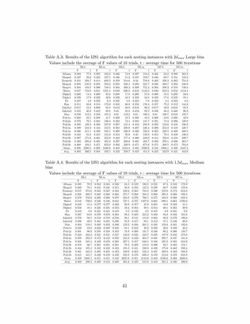
Table A.3: Results of the IJS1 algorithm for each nesting instances with 2dmax Large bins

Values include the average of F values of 10 trials, t : average time for 500 iterationsBL4 BL∞ ML4 ML∞ MU4 MU∞

F t F t F t F t F t F tAlbano 0.383 77.8 0.395 162.2 0.402 74.8 0.387 154.2 0.404 83.2 0.388 163.3Shape2 0.437 56.2 0.424 107.5 0.446 51.2 0.447 103.7 0.440 60.7 0.451 110.3Trousers 0.451 294.7 0.414 683.5 0.459 314.6 0.44 718.8 0.462 358.3 0.462 754.3Shape0 0.294 245.9 0.294 504.2 0.294 248.4 0.294 521.7 0.294 263.7 0.294 548.9Shape1 0.304 416.5 0.306 740.4 0.304 408.3 0.308 751.4 0.304 408.3 0.318 748.4Shirts 0.647 710.9 0.651 1221.4 0.649 626.8 0.652 1143.2 0.646 618.3 0.652 1118.4Dighe2 0.260 14.4 0.260 35.2 0.260 17.0 0.260 37.6 0.260 16.5 0.260 34.6Dighe1 0.329 17.9 0.329 33.6 0.329 18.2 0.329 34.6 0.329 17.6 0.329 35.1Fu 0.487 4.9 0.502 6.3 0.502 5.0 0.505 7.0 0.503 4.4 0.505 8.2Han 0.311 83.6 0.314 172.6 0.316 86.8 0.356 176.4 0.357 79.2 0.412 144.3

Jakobs1 0.617 52.4 0.609 92.4 0.613 50.9 0.616 98.3 0.617 48.9 0.616 92.4Jakobs2 0.455 46.0 0.452 89.8 0.45 45.8 0.454 92.2 0.456 48.4 0.448 96.8Mao 0.256 113.4 0.256 191.3 0.61 119.2 0.61 188.3 0.61 106.7 0.610 176.7

Poly1a 0.368 22.5 0.368 41.7 0.368 23.2 0.368 43.5 0.368 24.6 0.368 42.0Poly2a 0.376 79.5 0.384 126.3 0.382 72.4 0.384 131.7 0.381 74.3 0.386 128.8Poly3a 0.395 149.3 0.389 247.0 0.387 131.4 0.416 258.9 0.392 133.6 0.416 246.8Poly4a 0.399 243.3 0.416 412.5 0.394 238.6 0.407 426.4 0.399 254.9 0.418 420.7Poly5a 0.406 311.1 0.409 526.5 0.399 336.9 0.408 556.9 0.405 328.5 0.408 589.5Poly2b 0.443 81.8 0.455 131.0 0.454 76.6 0.45 132.9 0.454 79.4 0.459 126.3Poly3b 0.387 171.6 0.401 252.9 0.403 177.4 0.399 249.9 0.414 156.8 0.418 239.7Poly4b 0.402 295.8 0.405 491.2 0.397 286.8 0.401 484.7 0.393 276.1 0.406 465.7Poly5b 0.468 433.1 0.471 652.9 0.492 428.9 0.471 671.6 0.471 408.5 0.473 701.6Swim 0.398 2206.5 0.393 3430.0 0.404 2134.8 0.404 3396.6 0.416 1988.1 0.408 3447.3Avg. 0.403 266.5 0.404 450.1 0.422 259.7 0.425 451.3 0.425 253.9 0.431 453.9

Table A.4: Results of the IJS1 algorithm for each nesting instances with 1.5dmax Mediumbins





41

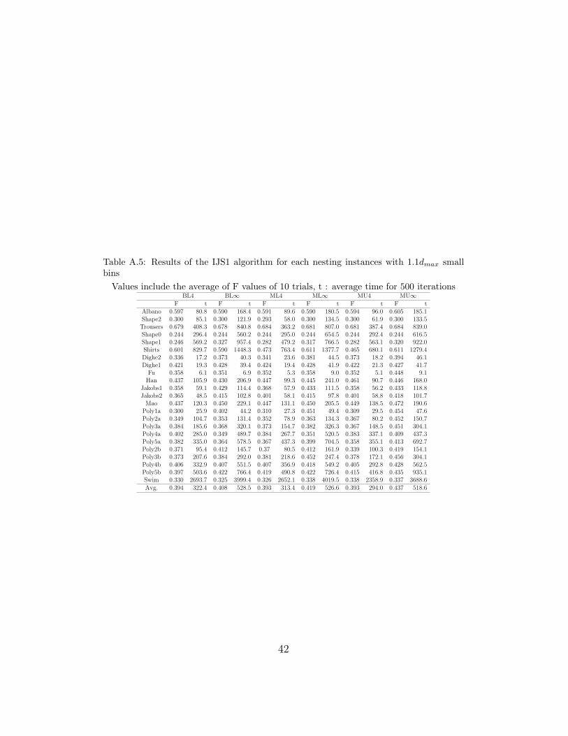
Table A.5: Results of the IJS1 algorithm for each nesting instances with 1.1dmax smallbins





42

Jostle heuristics for the 2D-irregular shapes bin ... - CORE

Documents

Transcript of Jostle heuristics for the 2D-irregular shapes bin ... - CORE