ISSN 2351–6275

KAUNAS UNIVERSITY OF TECHNOLOGY KTU PANEVEZYS FACULTY OF TECHNOLOGIES AND BUSINESS

MILITARY UNIVERSITY OF TECHNOLOGY INTELLIGENT TRANSPORT SYSTEMS

TALLINN UNIVERSITY OF TECHNOLOGY RIGA TECHNICAL UNIVERSITY

INTELLIGENT TECHNOLOGIES IN LOGISTICS AND MECHATRONICS SYSTEMS

ITELMS'2014

PROCEEDINGS OF THE 9TH INTERNATIONAL CONFERENCE

DEDICATED TO PANEVEZYS TOWN AS LITHUANIA CULTURE CAPITAL

EDITED BY Z. BAZARAS AND V. KLEIZA

May 22–23 , 2014 Panevezys, Lithuania

CONFERENCE IS ORGANIZED BY Kaunas University of Technology, Panevezys Faculty of Technologies and Business, Lithuania Military University of Technology, Poland Intelligent Transport Systems, Poland Tallinn University of Technology, Estonia Riga Technical University, Latvia The proceedings of the 9th International Conference INTELLIGENT TECHNOLOGIES IN LOGISTICS AND MECHATRONICS SYSTEMS contain selected papers. All papers were reviewed. The style and language of authors were not corrected. Only minor editorial corrections have been carried out by the Publisher. All rights preserved. No part of this publication may be reproduced, stored in retrieval system, or transmitted in any form or by any means, electronic, photocopying, recording or otherwise, without the permission of the Publisher.

© Kaunas University of Technology, 2014

3

CONFERENCE SCIENTIFIC COMMITTEE CHAIRMAN Prof. Z. Bazaras, Kaunas University of Technology, Lithuania SCIENTIFIC SECRETARY Prof. V. Kleiza, Kaunas University of Technology, Lithuania MEMBERS Prof. J. Bareisis, Kaunas University of Technology, Lithuania Prof. P. T. Castro, Porto University, Portugal Prof. J. Furch, Brno University of Defence, Czech Republic Dr. V. Hutsaylyuk, Military University of Technology, Poland Prof. I. Karabegovic, Bosnia and Herzegovina Prof. A. Levchenkov, Riga Technical University, Latvia Dr. M. Litwin, Intelligent Transport Systems, Poland Prof. V. Ostasevicius, Kaunas University of Technology, Lithuania Dr. O. Purvinis, Kaunas University of Technology, Lithuania Prof. L. Ribickis, Riga Technical University, Latvia Prof. M. Sitarz, Silezian Technical University, TRANSMEC, Poland Prof. A. Sladkowsky, Silezian Technical University, Poland Prof. D. Sprecic, Bosnia and Herzegovina Dr. Ch. Tatkeu, Transport Electronics and Signal Processing Laboratory, France Prof. V. Tilipalov, Kaliningrad State Technical University, Russia Prof. B. Timofeev, St. Petersburg State Polytechnic Institute, Russia Dr. D. Vaiciulis, Kaunas University of Technology, Lithuania Dr. D. Vinnikov, Tallinn University of Technology, Estonia LOCAL ORGANIZING COMMITTEE R. Bukenas V. Narbutas Dr. A. Tautkus 9th International Conference INTELLIGENT TECHNOLOGIES IN LOGISTICS AND MECHATRONICS SYSTEMS Dedicated to Panevezys town as Lithuania culture capital Klaipedos str. 3, Panevezys LT-35209, Lithuania http://ktu.edu/en/content/conferences-2014

4

PREFACE

The first (2006) and second International Workshops “Intelligent Technologies in Logistics and Mechatronics Systems ITELMS” were held at Riga Technical University. The 3rd international workshop ITELMS'2008 was held at Kaunas University of Technology Panevezys Institute on 22 – 23 May, 2008. The international conferences ITELMS'2009 – ITELMS'2014 traditionally takes place at Kaunas University of Technology Panevezys Institute.

The aims of the Conference are to share the latest topical information on the issues of intelligent technologies in logistics and mechatronics Systems. The papers in the Proceedings presented the following areas: • Intelligent Logistics Systems • Multi Criteria Decision Making • Composites in Infrastructures • Automotive Transport • Intelligent applications of solid state physics • Intelligent Mechatronics Systems • Mechanisms of Transport Means and their Diagnostics • Railway Transport • Transport Technologies • Modern Building Technologies • Sensors and Sensing Phenomena

In the invitations to Conference, sent year before the Conference starts, the instructions how to prepare reports and manuscripts provided as well as the deadlines for the reports are indicated.

A primary goal of Conference is to present the highest quality research results. A key element in attiring goal is the evolution and selection procedure developed by the Conference Scientific Committee.

All papers presented in Conference and published in Proceedings undergo this procedure. Instruction for submitting proposals, including requirements and deadlines, are published in “Call for Papers” in the http://ktu.edu/en/content/conferences-2014. Paper proposals must contain sufficient information for a trough review. All submissions to determine topic areas are directed to appropriate Topic Coordinators. The Topic Coordinators review the submissions much them to the expertise according to the interests and forward them to selected reviewers. At least two reviewers examine each submission in details.

Selection of papers for the Conference is highly competitive, so authors should assure their submissions to meet all Conference Scientific Committee’s requirements and to be of the highest possible quality.

All Conference participants prepare manuscripts according to the requirements that make our Proceedings to be valuable recourse of new information which allows evaluating investigations of the scientists from different countries.

Prof. Z. Bazaras Prof. V. Kleiza

5

Contents GENERAL PROGRAMME SCHEDULE .................................................................................................................... 8 A. Ahrens, S. Lochmann MIMO-BICM Multimode Transmission Schemes with iterative Detection .................................................................. 11 A. Ahrens, J. Zascerinska, N. Andreeva Intelligent Technologies in Engineering: Focus on Use of Web 3.0 Technologies for Research Promotion .................................................................................................................................................................. 17 R. Baltusnikiene, S. Susinskas, D. Aviza The Multicriteria Decision Support System of the Residential House Walls and Ground Typical Constructions ............................................................................................................................................................. 28 A. Bartnicki, K. Cieslik, S. Konopka, M. J. Lopatka The Conception of an Anthropomorphic Manipulator with Hydrostatic Drive System ................................................. 36 Z. Bazaras, B. Timofeev, N. Vasileva, J. Igakojyte-Bazariene Research Guidelines of the Nuclear Power Systems in XXI Century ........................................................................... 46 P. Bulovas, S. Susinskas

Influence of the Quantities of Plastifying Concrete Additive on Concrete Properties ................................................... 48 A. Cepauskas, S. Susinskas Panel – Frame Construction House Tightness Research .............................................................................................. 54 M. Chausov, A. Pylypenko, V. Berezin, V. Hutsaylyuk, L. Sniezek, J. Torzewski Property of the Monotonic Deformation of Aluminum Alloy 2024-T3 under Conditions of Complex Loading ..................................................................................................................................................................... 57 A. Dabrowska, S. Konopka, P. Krogul, M. J. Lopatka Influence of Hydraulic Lines on Manipulator Movement Accuracy ............................................................................. 64 J. Daunoravicius, S. Susinskas Sandwich Panels with Different Fillings Rational Selection Research ......................................................................... 73 A. Demeniene, D. Striukiene, E. Zacharoviene, R. Laurikietyte, P. Vaiciulis The Analysis of Accident Rate in the Baltic States (2008–2013) ................................................................................. 76 A. Demeniene, D. Striukiene, E. Zacharoviene, A. Valackiene, R. Laurikietyte, P. Vaiciulis The Impact of Psychological and Psychosocial Factors on Accident Rate .................................................................... 80 N. Dobrzinskij Research into Dependence of Failure Flow Parameter of Diesel Internal-Combustion Engine on Climatic Conditions in Afghanistan ............................................................................................................................ 85 A. Dragunas, S. Susinskas Construction Quality Control...................................................................................................................................... 92 J. Furch Advanced Maintenance Systems of Military Vehicles ................................................................................................. 96 A. Garskienė, J. Kaupiene, D. Aviza, N. Partaukas Industrial Flooring and Industrial Flooring Installations ............................................................................................ 104 E. Girkontas, V. Lukosevicius, Z. Bazaras Modelling and Research of Bus Equipped with Dynamic Stability Control System.................................................... 109 J. Glos, V. Kumbar Monitoring of Chemical Elements during Lifetime of Engine Oil .............................................................................. 114

6

A. Potapovs, M. Gorobetz, A. Levchenkov Application of Statistical Hypothesis Testing of Adaptive Algorithms for Smooth and Precise Train Braking System ........................................................................................................................................................ 118 R. Jackuviene, R. Karpavicius, V. Kleiza The Reversing Engineering Method for Modification Law of Motion of the Spatial Cam (LEAN implementation) ....................................................................................................................................................... 126 M. B. Jaskolowski, S. Konopka, M. J. Lopatka, A. Rubiec The Research Ability to Work on Slopes Articulated Machines ................................................................................. 131 I. Joneliukstiene, S. Susinskas Research of Soil Shear Resistance versus Clay Amount in it ..................................................................................... 137 R. Kampf, M. Vochozka, P. Lejskova, T. Cmiral Dependencies of Personal Vehicle Sales on the Financial Support of their Sales ........................................................ 141 S. Karlapavicius, A. Stasiskis, J. Kaupiene, L. Pelenyte-Vysniauskiene Energy-Efficient Buildings ....................................................................................................................................... 151 V. Kleiza, J. Tilindis The Optimization of the Overall Learning Dependent Manual Assembly Efficiency .................................................. 159 K. Klimavicius, S. Susinskas Composite Rods Reinforced Concrete Structures ...................................................................................................... 162 S. Konopka, M. J. Lopatka, T. Muszynski, M. Przybysz Problem of Kinematic Discrepancy in Hydrostatic Drive Systems Used in Unmanned Ground Vehicles ................................................................................................................................................................... 165 S. Konopka, M. J. Lopatka, A. Rubiec, K. Spadlo Tractive Force Distribution for High Mobility Platforms with Multi Axis Drive Systems .......................................... 173 P. Krogul, M. J. Lopatka, T. Muszynski, M. Przybysz Studies on Resistant Ackerman’s Steering System for Tracked Muskeg Vehicle........................................................ 180 P. O. Maruschak, I. V. Konovalenko, I. M. Danyliuk, S. V. Panin, I. V. Vlasov Form Control of Individual Surface Corrosion Pits in Main Gas Pipe Steel ............................................................... 189 I. Navardauskaite, S. Susinskas Influence of Quantity of Clay in Moraine Soils on Their Cone Resistance ................................................................. 193 V. Neumann Analysis of External Load of Tracked Vehicle Transmissions ................................................................................... 198 A. Pincevicius, V. Jonevicius, S. Bekesiene Decisions of the Applied Tasks of External Ballistics ............................................................................................... 206 T. Poska, S. Susinskas, J. Valickas Influence of Installation of Different Types of Bored Piles to the Ground .................................................................. 211 E. Shatkovskis, V. Zagadskij, A. Jukna, J. Stupakova Ripples Formation on the Silicon Solar Cells Surface by Laser Irradiation ................................................................ 217 T. Slezak, L. Sniezek, K. Grzelak Influence of the Usage of the High-Energy Joining Technology on the Properties of Welds in High Strength Steel........................................................................................................................................................... 221 V. Slivinskas, S. Susinskas, D. Aviza Multiple Criteria Analysis of Floor Installation for Logistics Centre .......................................................................... 227 L. Sniezek, I. Szachogluchowicz, V. Hutsaylyuk Research of Property Fatigue Advanced Al/Ti Laminate ........................................................................................... 232

7

O. Stopka, L. Bartuska, I. Kubasakova Selecting the Most Suitable Region in the Selected Country for the Placement of the Bi-Modal Freight Village Using the WSA Method ............................................................................................................................... 238 G. Stuglys, S. Susinskas, D. Aviza Installation Technology for Bored Piles Foundations ................................................................................................ 244 S. Susinskas, V. Zdanys Impact of the Thermal Insulation Layer of Three-Layer Wall Panels on Energy Consumption of a Building ................................................................................................................................................................... 249 J. Tamuliene, L. Baliulyte Theoretical Study of Fragmentation of Co6O7 Nanoparticle....................................................................................... 257 J. Tamuliene, J. Sarlauskas, S. Bekesiene, V. Kleiza Investigation of Stability of N-(2,4,6-trinitrophenyl)-1H-1,2,4-triazol-3-amine .......................................................... 260 P. Taraba, K. Pitrova Corporate Governance Model in the Czech Republic ................................................................................................ 263 G. Zylius, V. Vaitkus, P. Lengvenis Driving Style Analysis using Spectral Features of Accelerometer Signals ................................................................. 267 Authors Index .......................................................................................................................................................... 274

8

GENERAL PROGRAMME SCHEDULE

International Conference Intelligent Technologies in Logistics and Mechatronics Systems (ITELMS'2014)

22–23 May 2014, Panevezys, Lithuania

THURSDAY, MAY 22 12:00 REGISTRATION, WELCOME, RECEPTION (Klaipedos Str. 3, Panevezys)

OPENING OF THE CONFERENCE

14:00 Z. Bazaras (Conference Chairman) Greetings from Dean of the Faculty D. Zostautiene

(Conference hall, Klaipedos Str. 3, Panevezys) The conference hall is well provided for PowerPoint Viewer 2007 presentations

Moderators: V. Kleiza, O. Purvinis

14:15 G. Zylius, V. Vaitkus, P. Lengvenis Driving Style Analysis using Spectral Features of Accelerometer Signals

14:30 M. Chausov, A. Pylypenko, V. Berezin, V. Hutsaylyuk, L. Sniezek, J. Torzewski Property of the Monotonic Deformation of Aluminum Alloy 2024-T3 under Conditions of Complex Loading

14:45 N. Dobrzinskij Research into Dependence of Failure Flow Parameter of Diesel Internal-Combustion Engine on Climatic Conditions in Afghanistan

15:00 E. Shatkovskis, V. Zagadskij, A. Jukna, J. Stupakova Ripple formation on silicon solar cell surface by laser irradiation

15:10 A. Pincevicius, V. Jonevicius, S. Bekesiene Decisions of the applied tasks of external ballistics

15:20 T. Koppel, M. Ahonen Second hand exposure to the radiofrequency electromagnetic fields from wireless networking in office and classroom environments

15:30 J. Tamuliene L. Baliulyte Theoretical Study of Fragmentation of Co6O7 Nanoparticle

15:40 V. Kleiza, J. Tilindis The Optimization of the Overall Learning Dependent Manual Assembly Efficiency

15:50 P. O. Maruschak, I. V. Konovalenk, I. M. Danyliuk, S. V. Panin, I. V. Vlasov Form Control of Individual Surface Corrosion Pits in Main Gas Pipe Steel

16:00 J. Furch Advanced Maintenance Systems of Military Vehicles

16:10 J. Stodola, P. Stodola Reliability Analysis and Testing of Special Technique

9

16:20 T. Slezak, L. Sniezek, K. Grzelak Influence of the usage of the high-energy joining technology on the properties of welds in high strength steel

16:30 J. Glos, V. Kumbar Monitoring of Chemical Elements During Lifetime of Engine Oil

16:40 COFFEE BREAK

16:50 Z. Bazaras, B. Timofeev, N. Vasileva, J. Ilgakojyte-Bazariene Research Guidelines of the Nuclear Power Systems in XXI Century

17:00 J. Kaupiene, L Pelenyte-Vysniauskiene, N. Partaukas Traffic Flows Influence on Air Pollution in the City of Panevezys

17:10 P. Taraba, K. Pitrova Corporate Governance Model in the Czech Republic

17:20 P.O. Maruschak, I.V. Konovalenko, I.M. Danyliuk, S.V. Panin, I.V. Vlasov

Form Control of Individual Surface Corrosion Pits in Main Gas Pipe Steel

17:30 O. Stopka, L. Bartuska, I. Kubasakova Selecting the Most Suitable Region in the Selected Country for the Placement of the Bi-Modal Freight Village using the WSA Method

17:40 M. Gorobetz, A. Potapovs, A. Levchenkov Application of Statistical Hypothesis Testing of Adaptive Algorithms for Smooth and Precise Train Braking System

17:50 R. Kampf, M. Vochozka, P. Lejskova, T. Cmiral Dependencies of Personal Vehicle Sales on the Financial Support of their Sales

18:00 P. Krogul, M. J. Lopatka, T. Muszynski M. Przybysz Studies on Resistant Acerman’s Steering System for Tracked Muskeg Vehicle

18:10 T. Slezak, L. Sniezek, K. Grzelak Influence of the Usage of The High-Energy Joining Technology on the Properties of Welds in High Strength Steel

18:20 J. Tamuliene, J. Sarlauskas, S. Bekesiene, V. Kleiza Influence of Substitution on Stability and Electronic Structure of N-(2,4,6-trinitrophenyl)-1H-1,2,4-triazol-3-amine

18:30 P. Krogul A. Dabrowska, S. Konopka, M. J. Lopatka Hydraulic Lines Effect on Control Precision of Robot Manipulator

18:40 V. Neumann Analysis of External Load of Tracked Vehicle Transmissions

19:50 DISCUSSION

FRIDAY, MAY 23 (Conference hall, Klaipedos Str. 3, Panevezys)

Moderators: O. Purvinis, V. Kleiza 10:00 S. Susinskas, V. Zdanys

Impact of the Thermal Insulation Layer of Three-Layer Wall Panels on Energy Consumption of a Building

10:10 Garskiene, J. Kaupiene, D. Aviza, N. Partaukas Industrial Flooring and Industrial Flooring Installations

10:20 I. Joneliukstiene, S. Susinskas Research of Soil Shear Resistance Versus Clay Amount in it

10:30 I. Navardauskaite, S. Susinskas Influence of Quantity of Clay in Moraine Soils on their Cone Resistance

10

10:40 A. Cepauskas, S. Susinskas Panel - Frame Construction House Tightness Research

10:50 J. Daunoravicius, S. Susinskas Sandwich Panels with Different Fillings Rational Selection Research

11:00 P. Bulovas, S. Susinskas

Influence of the Quantities of Plastifying Concrete Additive on Concrete Properties

11:10 A. Dragunas, S. Susinskas Construction Quality Control

11:20 S. Karlapavicius, A. Stasiskis, J. Kaupiene Energy-Efficient Buildings

11:30 G. Stuglys, S. Susinskas Installation Technology for Bored Piles Foundations

11:40 T. Poska, S. Susinskas Influence of Installation of Different Types of Bored Piles to the Ground

11:50 K. Klimavicius, S. Susinskas Composite Rods Reinforced Concrete Structures

12:00 V. Slivinskas, S. Susinskas Multiple Criteria Analysis of Floor Installation for Logistics Centre

12:10 R. Baltusnikiene, S. Susinskas The Multicriteria Decision Support System of the Residential House Walls and Ground Typical Constructions

12:20 A. Dabrowska, S. Konopka, P. Krogul, M. J. Łopatka Influence of Hydraulic Lines on Manipulator Movement Accuracy

12:30 A. Bartnicki, K. Cieslik S. Konopka, M. J. Lopatka The Conception of an Anthropomorphic Manipulator with Hydrostatic Drive System

12:40 E. Girkontas, V. Lukosevicius, Z. Bazaras Modelling and Research of Bus Equipped with Dynamic Stability Control System

12:50 M. B. Jaskołowski, S. Konopka, M. J. Lopatka, A. Rubiec The Research Ability to Work on Slopes Articulated Machines

13:00 S. Konopka, M. J. Lopatka, T. Muszynski, M. Przybysz Problem of Kinematic Discrepancy in Hydrostatic Drive Systems Used in Unmanned Ground Vehicles

13:10 S. Konopka, M. J. Lopatka, A. Rubiec, K. Spadlo Tractive Force Distribution for High Mobility Platforms with Multi Axis Drive Systems

13:20 L. Sniezek, I. Szachogluchowicz, V. Hutsaylyuk Research of Property Fatigue Advanced Al/Ti Laminate

13:30 A. Demeniene, R. Laurikietyte, D. Striukiene, E. Zacharoviene, P. Vaiciulis The Analysis of Accident Rate in the Baltic States (2008−2013)

13:40 A. Ahrens, S. Lochmann MIMO-BICM Multimode Transmission Schemes with Iterative Detection

13:50 A. Ahrens, J. Zascerinska, N. Andreeva Intelligent Technologies in Engineering: Focus on Use of Web 3.0 Technologies for Research Promotion

14:00 A. Demeniene, D. Striukiene, E. Zacharoviene, A. Valackiene, R. Laurikietyte, P. Vaiciulis The Impact Of Psychological And Psychosocial Factors On Accident Rate

14:10 R. Jackuviene, R. Karpavicius, V. Kleiza The Reversing Engineering Method for Modification Law of Motion of the Spatial Cam (LEAN implementation)

14:20 DISCUSSION

11

Proceedings of 9th International Conference ITELMS’2014 MIMO-BICM Multimode Transmission Schemes with iterative Detection A. Ahrens, S. Lochmann Hochschule Wismar, University of Applied Sciences - Technology, Business and Design, Philipp-Müller-Straße 14, 23952 Wismar, Germany, E-mail: andreas.ahrens@hs-wismar.de, steffen.lochmann@hs-wismar.de Abstract In this contribution a coherent (2×2) (multiple input multiple output) MIMO transmission with iterative detection over a measured multimode fiber channel at 1325 nm operating wavelength is studied. For the channel measurements a fibre length of 1.4 km was chosen. Extrinsic information transfer (EXIT) charts are used for analyzing and optimizing the convergence behaviour of the iterative demapping and decoding. Our results show that in order to achieve the best bit-error rate, not necessarily all MIMO layers have to be activated. KEYWORDS: Multiple-Input Multiple-Output (MIMO) Transmission, Optical Fibre Transmission, Multimode fiber (MMF), Iterative Detection. 1. Introduction

Intelligent technologies and electrical engineering are inter-connected. MIMO (multiple-input multiple-output) transmission is becoming a foundational basis for reliable data transmission and is aimed at enhancing channel capacity. It is as revolutionary as the intelligent technologies´ support behind the smart grid in the electric as well as mechatronic industry.

The concept of MIMO (multiple input multiple output) transmission has been investigated since decades now for both, twisted-pair copper cable transmission, suffering from crosstalk between neighboring wire pairs [1], as well as for multi-antenna radio systems, where signal interference occurs on the radio interface [2, 3]. In the recent past the concept of MIMO transmission over multimode fibers has attracted increasing interest in the optical fiber transmission community, targeting at increased fiber capacity [4-6].

Bit-interleaved coded modulation (BICM) was designed for bandwidth efficient transmission over fading channels, offering an improved link adaptation capability and an increased design freedom. Wireless MIMO bit-interleaved coded modulation (BICM) transmission schemes for both non-frequency and frequency selective MIMO channels have attracted a lot of attention and reached a state of maturity [3, 7]. By contrast, MIMO-aided and BICM-assisted optical systems require substantial further research [5, 6]. That is why in addition to bit loading algorithms in this contribution the benefits of channel coding are also investigated.

Since the “design-space” is large, a two-stage optimization technique is considered. Firstly, the uncoded MIMO scheme is analyzed, investigating the allocation of both the number of bits per modulated symbol and the number of activated MIMO layers at a fixed data rate. Secondly, the optimized uncoded system is extended by incorporating bit-interleaved coded modulation using iterative detection (BICM-ID), whereby both the uncoded as well as the coded systems are required to support the same user data rate within the same bandwidth.

The novel contribution of this paper is that we jointly optimize the number of activated MIMO layers and the number of bits per symbol combined with powerful error correcting codes under the constraint of a given fixed data throughput and integrity. The performance improvements are exemplarily studied by computer simulations at a measured 1.4 km multimode MIMO fiber channel at 1325 nm operating wavelength.

The remaining part of this contribution is organized as follows: Section 2 introduces our system model and the proposed uncoded solutions. In section 3 the channel encoded MIMO system is introduced. The associated performance results are presented and interpreted in section 4. Finally, section 5 provides our concluding remarks. 2. MIMO System Model

In order to form the optical MIMO channel, different sources of light have to be launched into the fiber. At the receiver side, different spatial filters can be used. In this work, the spatial filters were produced by depositing a metal layer at fiber end-faces and subsequent ion milling. Details on the optical MIMO configuration, which has been determined by channel measurements, are given in [6]. For the investigated optical MIMO channel an eccentricity δ of 10 μm and a mask diameter r of 15 μm were chosen. The arising electrical (2×2) MIMO channel is highlighted in Fig. 2.

The measured MIMO channel impulse responses at 1325 nm operating wavelength are depicted in Fig. 3 and illustrate the activation of different mode groups according to the transmitter side light launch conditions (Fig. 1). The individual mode groups are clearly separated since no chromatic dispersion is imminent at the wavelength of 1325 nm. The block-oriented system for frequency selective channels is modeled by:

u = H c + w (1)

12

In (1), the transmitted signal vector c is mapped by the channel matrix H Honto the received vector u.

Fig. 1. Forming the optical (2×2) MIMO channel (left: light launch positions at the transmitter side with a given

eccentricity δ, right: spatial configuration at the receiver side as a function of the mask diameter r)

The vector of the additive, white Gaussian noise (AWGN) is defined by w. Details on the transmission model

are given in [6] with reference to the results in [7, 8].

Fig. 2. Electrical MIMO system model (example: n = 2)

Singular-value decomposition (SVD) has been established as an efficient concept to compensate the

interferences between the different data streams transmitted over a dispersive channel: SVD is able to transfer the whole system into independent, non-interfering layers exhibiting unequal gains per layer as highlighted in Fig. 4.

Fig. 3. Measured electrical MIMO impulse responses with respect to the pulse frequency fT = 1 / Ts = 5.12 GHz at

1325 nm operating wavelength

The singular-value decomposition (SVD) of the system matrix H results in: H = S V DH, where S and DH are

unitary matrices and V is a real-valued diagonal matrix of the positive square roots of the eigenvalues of the matrix H H H sorted in descending order. The MIMO data vector c is now multiplied by the matrix D before transmission. In turn, the receiver multiplies the received vector u by the matrix S H. In doing so, neither the transmit power budget nor the noise power characteristic is changed. The overall transmission relationship is defined as:

13

( ) wcVwcDHSy ~H +=+= (2)

The unequal gains per layer at the time k, i. e., the diagonal element k1ξ and k2ξ of the matrix V, are defined by the positive square roots of the eigenvalues of the matrix H H H.

In this contribution, coherent transmission and detection is assumed together with the modulation format QAM (quadrature amplitude modulation) per MIMO transmission mode. By taking the different layer-specific weighting introduced by the positive square roots of the eigenvalues of the matrix H H H, into account (Fig. 4), bit- and power loading per layer can be used to balance the bit-error probabilities and thus optimize the performance of the whole transmission system.

Fig. 4. SVD-based layer-specific transmission model

Given a fixed transmission bit rate, the optimization target is a minimum BER: therefore the bit loading to the

different transmission modes is optimized according to the options shown in Tab. 1.

Table 1 Parameters for bitloading: Investigated QAM trans-mission modes for fixed transmission bit rate

Throughput Layer 1 Layer 2 4 bit/s/Hz 4 bit/s/Hz

16 4

0 4

2 bit/s/Hz 2 bit/s/Hz

4 2

0 2

3. Channel Encoded MIMO System

The channel encoded transmitter structure is depicted in Fig. 5. The encoder employs a half-rate non-systematic, non-recursive convolutional (NSNRC) code using the generator polynomials (7.5) in octal notation. The uncoded information is organized in blocks of Ni bits, consisting of at least 3000 bits, depending on the specific QAM constellation used. Each data block i is encoded and results in the block b consisting of Nb = 2 Ni + 4 encoded bits, including 2 termination bits. The encoded bits are interleaved using a random interleaver and stored in the vector b~ . The encoded and interleaved bits are then mapped to the MIMO layers. The task of the multiplexer and buffer block of Fig. 5 is to divide the vector of encoded and interleaved information bits, i. e. b~ , into subvectors according to the chosen transmission mode (Tab. 1). The individual binary data vectors are then mapped to the QAM symbols c1 k and c2 k according to the specific mapper used (Fig. 5).

Fig. 5. The channel-encoded MIMO transmitter structure

The iterative demodulator structure is shown in Fig. 6. When using the iteration index v, the first iteration of

v = 1 commences with the soft-demapper delivering the Nb log-likelihood ratios (LLRs) ( ) ( )bL v ~12

= of the encoded and

interleaved information bits, whose de-interleaved version ( ) ( )bL va

11,= represents the input of the convolutional decoder as

depicted in Fig. 6. This channel decoder provides the estimates ( ) ( )iL v 11

= of the original uncoded information bits as well as the LLRs of the Nb NSNRC-encoded bits in the form of

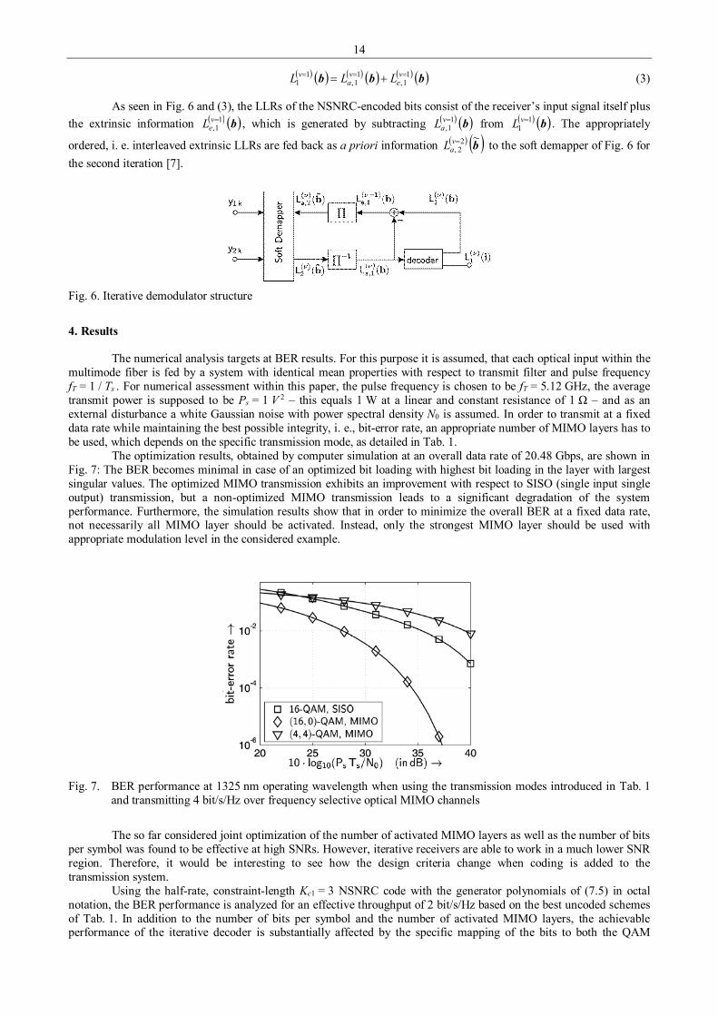
14

( ) ( ) ( ) ( ) ( ) ( )bbb 11,

11,

11

=== += ve

va

v LLL (3)

As seen in Fig. 6 and (3), the LLRs of the NSNRC-encoded bits consist of the receiver’s input signal itself plus the extrinsic information ( ) ( )b1

1,=v

eL , which is generated by subtracting ( ) ( )b11,=v

aL from ( ) ( )b11

=vL . The appropriately

ordered, i. e. interleaved extrinsic LLRs are fed back as a priori information ( ) ( )b~22,

=vaL to the soft demapper of Fig. 6 for

the second iteration [7].

Fig. 6. Iterative demodulator structure

4. Results

The numerical analysis targets at BER results. For this purpose it is assumed, that each optical input within the multimode fiber is fed by a system with identical mean properties with respect to transmit filter and pulse frequency fT = 1 / Ts . For numerical assessment within this paper, the pulse frequency is chosen to be fT = 5.12 GHz, the average transmit power is supposed to be Ps = 1 V 2 – this equals 1 W at a linear and constant resistance of 1 Ω – and as an external disturbance a white Gaussian noise with power spectral density N0 is assumed. In order to transmit at a fixed data rate while maintaining the best possible integrity, i. e., bit-error rate, an appropriate number of MIMO layers has to be used, which depends on the specific transmission mode, as detailed in Tab. 1.

The optimization results, obtained by computer simulation at an overall data rate of 20.48 Gbps, are shown in Fig. 7: The BER becomes minimal in case of an optimized bit loading with highest bit loading in the layer with largest singular values. The optimized MIMO transmission exhibits an improvement with respect to SISO (single input single output) transmission, but a non-optimized MIMO transmission leads to a significant degradation of the system performance. Furthermore, the simulation results show that in order to minimize the overall BER at a fixed data rate, not necessarily all MIMO layer should be activated. Instead, only the strongest MIMO layer should be used with appropriate modulation level in the considered example.

Fig. 7. BER performance at 1325 nm operating wavelength when using the transmission modes introduced in Tab. 1

and transmitting 4 bit/s/Hz over frequency selective optical MIMO channels

The so far considered joint optimization of the number of activated MIMO layers as well as the number of bits

per symbol was found to be effective at high SNRs. However, iterative receivers are able to work in a much lower SNR region. Therefore, it would be interesting to see how the design criteria change when coding is added to the transmission system.

Using the half-rate, constraint-length Kc1 = 3 NSNRC code with the generator polynomials of (7.5) in octal notation, the BER performance is analyzed for an effective throughput of 2 bit/s/Hz based on the best uncoded schemes of Tab. 1. In addition to the number of bits per symbol and the number of activated MIMO layers, the achievable performance of the iterative decoder is substantially affected by the specific mapping of the bits to both the QAM

15

symbols as well as to the MIMO layers. Here, the maximum iteration gain can only be guaranteed, if anti-Gray mapping is used on all activated MIMO layers [7, 9].

Furthermore, observed by comparing the extrinsic information transfer (EXIT) chart results of Fig. 8, the overall performance is strongly influenced by the allocation of the number of bits to the MIMO layers.

Fig. 8. EXIT chart for an effective user-data throughput of 2 bit/s/Hz and the different QAM constellations at

10 log10 (Ps Ts / N0) = 18 dB (1325 nm operating wavelength and anti-Gray mapping on all activated MIMO layers)

In order to guarantee an open EXIT tunnel and therefore an efficient information exchange between the soft

demapper transfer characteristic and the decoder transfer characteristic at a given signal-to-noise ratio, not necessarily all MIMO should be activated. In the considered example only the strongest MIMO layer should be used with appropriate modulation level. Activating all MIMO layers the information exchange between the soft demapper and the decoder stops relatively early, resulting in a reduced BER performance.

The BER performance is finally presented in Fig. 9 based on the best uncoded schemes of Tab. 1 and confirms the EXIT chart results. The information word length is 3000 bits and a random interleaver is applied. 5. Conclusions

Coherent MIMO transmission over measured multimode optical fibers has been investigated targeting at minimized BER while keeping the transmission bit-rate constant. The results show that MIMO transmission based on SVD is a promising approach, in particular when the bit loading is optimized.

Fig. 9. BERs assuming anti-Gray mapping scheme on the activated MIMO layer for an effective user-data throughput

of 2 bit/s/Hz (1325 nm operating wavelength)

In that case significant BER improvements can be achieved compared to a conventional SISO system. The

proposed MIMO-BICM scheme includes an adaptation of the transmit parameters. EXIT charts are used for analysing and optimizing the convergence behaviour of iterative demapping and decoding. Here, the choice of the number of bits

16

per symbol and the number of MIMO layers combined with powerful error correcting codes substantially affects the performance of a MIMO system, suggesting that not all MIMO layers have to be activated in order to achieve the best BERs. References 1. Ahrens A., Lange C. Iteratively Detected MIMO-OFDM Twisted-Pair Transmission Schemes, Communications in

Computer and Information Science, Berlin, Heidelberg: Springer, 2009, vol. 48, pp. 281-293. 2. Foschini G. J. Layered Space-Time Architecture for Wireless Communication in a Fading Environment when using

Multiple Antennas, Bell Labs Technical Journal, vol. 1, no. 2, 1996, pp. 41-59. 3. Kühn V. Wireless Communications over MIMO Channels - Applications to CDMA and Multiple Antenna Systems.

Chichester: Wiley, 2006. 4. Singer A. C., Shanbhag N. R., Bae H. M. Electronic Dispersion Compensation- An Overview of Optical

Communications Systems, IEEE Signal Processing Magazine, vol. 25, no. 6, 2008, pp. 110 - 130. 5. Bülow H., Al-Hashimi H., Schmauss B. Coherent Multi-mode-Fiber MIMO Transmission with Spatial

Constellation Modulation, European Conference and Exhibition on Optical Communication (ECOC), Geneva, Switzerland, 18.-22. September 2011.

6. Pankow J., Aust S., Lochmann S., Ahrens A. Modu-lation-Mode Assignment in SVD-assisted Optical MIMO Multimode Fiber Links, 15th International Conference on Optical Network Design and Modeling (ONDM), Bologna, Italy, 8.-10. February 2011.

7. Ahrens A., Benavente-Peces C. Modulation-Mode Assignment in Iteratively Detected and SVD-assisted Broadband MIMO Systems, Communications in Computer and Information Science, Berlin, Heidelberg: Springer, 2011, vol. 130, pp. 307-319.

8. Raleigh G. G., Cioffi J. M. Spatio-Temporal Coding for Wireless Communication. IEEE Transactions on Communications, vol. 46, no. 3, 1998, pp. 357-366.

9. Chindapol J. A., Ritcey A. Design, Analysis, and Perfor-mance Evaluation for BICM-ID with square QAM Constellations in Rayleigh Fading Channels. IEEE Journal on Selected Areas in Communications, vol. 19, no. 5, 2001, pp. 944-957.

17

Proceedings of 9th International Conference ITELMS’2014 Intelligent Technologies in Engineering: Focus on Use of Web 3.0 Technologies for Research Promotion A. Ahrens*, J. Zascerinska**, N. Andreeva*** *Hochschule Wismar, University of Applied Sciences - Technology, Business and Design, Philipp-Müller-Straße 14, 23952 Wismar, Germany, E-mail: andreas.ahrens@hs-wismar.de **Centre for Education and Innovation Research, Kurzemes prospekts 114, Riga LV-1069, Latvia, E-mail: ceir2012@gmail.com ***Immanuel Kant Baltic Federal University, Nevskogo str. 14a, 236041 Kaliningrad, Russia, E-mail: andreeva_natalia@list.ru Abstract Engineers contribute to the emergence and development of intelligent technologies which allow solving social challenges. However, little attention has been paid to the analysis of engineering students’ attitude to use of such an intelligent technology as Web 3.0 in university studies. The aim of the paper is to analyse engineering students’ attitude to use of Web 3.0 technologies in university studies underpinning elaboration of a hypothesis on use of Web 3.0 technologies for promotion of engineering students’ research. The meaning of the key concepts of university studies, Web 3.0 technologies and attitude is studied. Moreover, the study demonstrates how the key concepts are related to the idea of intelligent technologies and shows how the steps of the process are related: students’ attitude to use of Web 3.0 technologies in university studies → empirical study within a multicultural environment → conclusion. The results of the present research show that engineering students’ attitude to use of Web 3.0 technologies in university studies is positive. A hypothesis on use of Web 3.0 technologies in university studies for promotion of engineering students’ research has been proposed. Directions of further research have been identified. KEYWORDS: intelligent technologies, engineering, Web 3.0 technologies, university studies, research, attitude. 1. Introduction

Intelligent technologies in engineering perform a two-fold role. On the one hand, by solving social challenges, engineers contribute to the emergence and development of intelligent technologies. On the other hand, use of intelligent technologies in engineering that is based on research facilitates the engineers’ success in innovative management with a variety of problematic situations in all the life dimensions such as medicine, education, logistics, building, transportation and others. However, little attention has been paid to the analysis of engineering students’ attitude to use of such an intelligent technology as Web 3.0 in university studies.

The aim of the paper is to analyse engineering students’ attitude to use of Web 3.0 technologies in university studies underpinning elaboration of a hypothesis on use of Web 3.0 technologies in university studies for promotion of engineering students’ research. The meaning of the key concepts of university studies, Web 3.0 technologies and attitude is studied. Moreover, the study demonstrates how the key concepts are related to the idea of intelligent technologies and shows how the steps of the process are related: students’ attitude to use of Web 3.0 technologies in university studies → empirical study within a multicultural environment → conclusion.

Methodological background of the present research is based on the System-Constructivist Theory. The System-Constructivist Theory is introduced as the New or Social Constructivism Pedagogical Theory. The System-Constructivist Theory is formed by • Parsons’s System Theory [38] on any activity as a system, • Luhmann’s Theory [28] on communication as a system, • the Theory of Symbolic Interactionalism [34], • the Theory of Subjectivism [20].

The System-Constructivist Theory implies the dialectical principle of the unity of opposites that contributes to the understanding of the relationship between external (social, social interaction, teaching, etc) and internal (individual, cognitive activity, learning, etc) perspectives as the synthesis of external and internal perspectives [5]. In comparison, the Constructivism Theory focuses on learning and, consequently, the internal perspective, the Social Constructivist theory – on teaching and, consequently, external perspective as well as on the balance between teaching and learning and, consequently, the balance between the external and internal perspectives [5].

The System-Constructivist Theory and, consequently, the System-Constructivist Approach to learning introduced by Reich [39] emphasizes that human being’s point of view depends on the subjective aspect: • everyone has his/her own system of external and internal perspectives [2] that is a complex open system [41], and • experience plays the central role in the knowledge construction process [30].

18

It should be noted that the terms experience and competence are used synonymously in the present manuscript as both terms are similarly structured: experience [43] as well as competence [16] include knowledge, skills and attitudes as highlighted in Fig. 1.

Fig. 1. Elements of experience as well as competence

Hence, engineers’ attitude is identifies as part of their experience as well as competence. The elements of experience as well as competence, namely knowledge, skills and attitude, are inter-related.

Engineers’ negative attitude fails to promote their research expressed by the increase in the level of their knowledge and skills as well as experience and competence, in general. In contrast, engineers’ positive attitude ensures the promotion of their research revealed by the enrichment of the level of their knowledge and skills as well as experience and competence, in general. Therein, the subjective aspect of human being’s point of view is applicable to the present research on use of Web 3.0 technologies in university studies for promotion of engineering students’ research.

The novel contribution of this paper is expressed in the hypothesis on use of Web 3.0 technologies in university studies for promotion of engineering students’ research.

Our target population to generalize the educational model of engineering students’ attitude to use of Web 3.0 technologies in university studies for promotion of engineering students’ research in formal higher education.

The remaining part of this paper is organized as follows: the next section introduces theoretical framework on students’ attitude to use of Web 3.0 technologies in university studies for promotion of engineering students’ research. The associated results of an empirical study will be presented in the following section. Finally, some concluding remarks are provided followed by a short outlook on interesting topics for further work. 2. Theoretical Framework

Engineering constantly develops. The enrichment of engineering is ensured via research as shown in Fig. 2. In its turn, research is part of university education as depicted in Fig. 3. It should be noted that university education proceeds in university studies as demonstrated in Fig. 4. In the present manuscript, the terms university studies, tertiary studies, educational process, teaching and

learning process are used synonymously.

Fig. 2. The relationship between engineering and research

Fig. 3. The relationship between research and university education

Fig. 4. The relationship between university education and university studies

Experience as well as competence

Attitude

Skills

Knowledge

Engineering

Research

Research

University education

University education

University studies

19

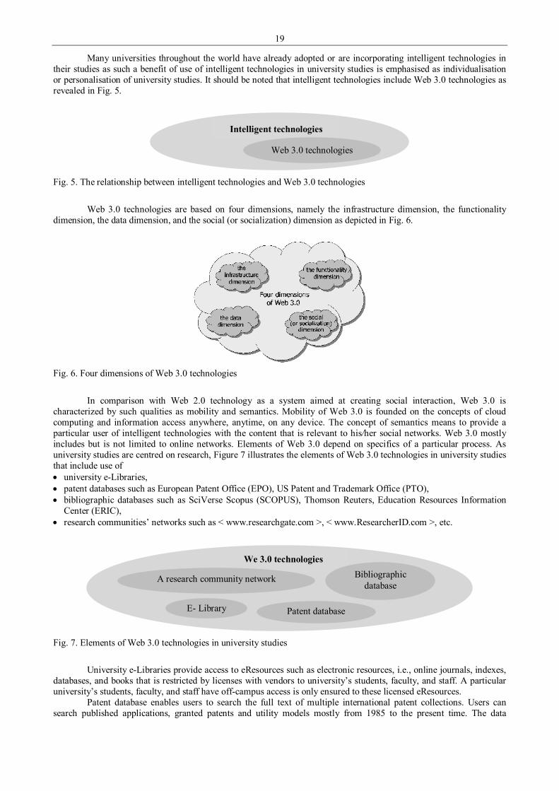
Many universities throughout the world have already adopted or are incorporating intelligent technologies in their studies as such a benefit of use of intelligent technologies in university studies is emphasised as individualisation or personalisation of university studies. It should be noted that intelligent technologies include Web 3.0 technologies as revealed in Fig. 5.

Fig. 5. The relationship between intelligent technologies and Web 3.0 technologies

Web 3.0 technologies are based on four dimensions, namely the infrastructure dimension, the functionality

dimension, the data dimension, and the social (or socialization) dimension as depicted in Fig. 6.

Fig. 6. Four dimensions of Web 3.0 technologies

In comparison with Web 2.0 technology as a system aimed at creating social interaction, Web 3.0 is

characterized by such qualities as mobility and semantics. Mobility of Web 3.0 is founded on the concepts of cloud computing and information access anywhere, anytime, on any device. The concept of semantics means to provide a particular user of intelligent technologies with the content that is relevant to his/her social networks. Web 3.0 mostly includes but is not limited to online networks. Elements of Web 3.0 depend on specifics of a particular process. As university studies are centred on research, Figure 7 illustrates the elements of Web 3.0 technologies in university studies that include use of • university e-Libraries, • patent databases such as European Patent Office (EPO), US Patent and Trademark Office (PTO), • bibliographic databases such as SciVerse Scopus (SCOPUS), Thomson Reuters, Education Resources Information

Center (ERIC), • research communities’ networks such as < www.researchgate.com >, < www.ResearcherID.com >, etc.

Fig. 7. Elements of Web 3.0 technologies in university studies

University e-Libraries provide access to eResources such as electronic resources, i.e., online journals, indexes,

databases, and books that is restricted by licenses with vendors to university’s students, faculty, and staff. A particular university’s students, faculty, and staff have off-campus access is only ensured to these licensed eResources.

Patent database enables users to search the full text of multiple international patent collections. Users can search published applications, granted patents and utility models mostly from 1985 to the present time. The data

Intelligent technologies

Web 3.0 technologies

We 3.0 technologies

Bibliographic database

Patent database

A research community network

E- Library

20

available includes full text patents, English machine translations and full document images. These collections are periodically updated to include additional years of coverage.

A bibliographic database is a database of bibliographic records, an organized digital collection of references to published literature, including journal and newspaper articles, conference proceedings, reports, government and legal publications, patents, books, etc. In contrast to library catalogue entries, a large proportion of the bibliographic records in bibliographic databases describe articles, conference papers, etc., rather than complete monographs, and they generally contain very rich subject descriptions in the form of keywords, subject classification terms, or abstracts [18]. A bibliographic database may be general in scope or cover a specific academic discipline. A significant number of bibliographic databases are still proprietary, available by licensing agreement from vendors, or directly from the indexing and abstracting services that create them [40]. Many bibliographic databases evolve into digital libraries, providing the full-text of the indexed contents. Others converge with non-bibliographic scholarly databases to create more complete disciplinary search engine systems, such as Chemical Abstracts or Entrez.

Research community networks in the present contribution mean use of web-based tools to discover and use research and scholarly information about people and resources [8]. Research community networking tools serve as knowledge management systems for the research enterprise. Research community networking tools connect institution-level/enterprise systems, national research networks, publicly available research data (e.g., grants and publications), and restricted/proprietary data by harvesting information from disparate sources into compiled expertise profiles for faculty, investigators, scholars, clinicians, community partners, and facilities. Research community networks are designed for such target groups as [4]: • investigators o to discover potential collaborators, o more rapidly and competitively to form teams, o to identify targeted grant opportunities and o to create digital vitae,

• administrators o to work with better data for institutional business intelligence, o to better assess performance for annual reviews, o to recruit new faculty and attract students,

• researchers o to study networks of science teams to improve research effectiveness.

Research community networks [4] include four technology components such as • a controlled vocabulary (eg., the VIVO Ontology) for data interoperability, • an architecture for data integration and sharing (Linked Open Data), • applications for collaboration, funding, business intelligence, or administration and • rich faculty profile data of publications, grants, classes, affiliations, interests, etc.

Further on, repositories of profile data need to talk to institutional systems like faculty directories [4]. Research community networks’ tools facilitate the development of new collaborations and team science to

address new or existing research challenges through the rapid discovery and recommendation of researchers, expertise, and resources [7, 17].

Research community networks’ tools differ from search engines such as Google in that they access information in databases and other data not limited to web pages. They also differ from social networking systems such as LinkedIn or Facebook in that they represent a compendium of data ingested from authoritative and verifiable sources rather than predominantly individually asserted information, making research community networks’ tools more reliable [19]. Yet, research community networks’ tools have sufficient flexibility to allow for profile editing. Research community networks’ tools also provide resources to bolster human connector systems: they can make non-intuitive matches, they do not depend on serendipity, and they do not have a propensity to return only to previously identified collaborations/collaborators [10]. Research community networks’ tools also generally have associated analytical capabilities that enable evaluation of collaboration and cross-disciplinary research/scholarly activity, especially over time.

Importantly, data harvested into robust research community networks’ tools is accessible for broad repurposing, especially if available as linked open data (RDF triples). Thus, research community networks’ tools enhance research support activities by providing • data for customized, • up-to-date web pages, • CV/biosketch generation, and • data tables for grant proposals.

A short description of a research community network such as ResearchGate gives a short overview of functions of a research community network: ResearchGate is a social networking site for scientists and researchers to share papers, ask and answer questions, and find collaborators [27]. The site has been described as a mashup of “Facebook, Twitter and LinkedIn” that includes “profile pages, comments, groups, job listings, and ‘like’ and ‘follow’ buttons” [27]. Members are encouraged to share raw data and failed experiment results as well as successes, in order to avoid repeating their peers’ scientific research mistakes [14]. Microsoft co-founder Bill Gates is among the company's investors [26]. ResearchGate announced in 2013 that the site had two million members.

21

Research community networks demonstrate such opportunities as [4] • support to innovative team building approaches, • provision of richer data for comparative institutional studies and • potential for national networks of collaborative research.

Research community networks reveal the existence of such threats as [4] • some desired data are private (eg., award amounts) or restricted (eg., FERPA), • negotiation between research and administrative efforts is required, and • efforts threaten established networks of research influence.

For success of research community networks, such issues are to be considered as [4] • leveraging existing institutional efforts for research networking and annual faculty review, • understanding institutional culture and policy for faculty information sharing, • making the technology investments to develop the required new capabilities, and • identifying sources of available high quality profile data (institutional, corporate, federal, Linked Open Data cloud), • use of existing research or administrative initiatives and workflows that manage profile data, • overcome of institutional cultures that may not prevent data use for research networking, and • bringing together (typically) multiple initiatives that manage faculty profile data in a sustainable institutional

strategy. Hence, research within university studies is promoted by use of Web 3.0 technologies as a kind of intelligent

technologies. In its turn, use of Web 3.0 technologies in university studies is measured via engineering students’ attitude.

Attitude has been defined by a number of researchers. Palmer and Holt define attitude as an individual’s positive or negative feelings about performing the target behavior [37]. This implies that learners’ positive or negative feelings about their use of Web 3.0 technologies in university studies would directly influence their behavior to use Web 3.0 technologies in university studies. Consequently, attitude comprises positive as well as negative feelings as shown in Fig. 8.

Fig. 8. Feelings of attitude

Another definition of attitude that is of the interest of the contribution’s authors is attitude identified as a

combination of evaluative judgements about a phenomenon [12]. Analysis of these definitions of attitude carried out by the contribution’s authors and complementing the

attitude definition formulated by Crites, Fabrigar, Petty [12] with the word individual leads to such a newly determined definition of student’s attitude as an individual combination of evaluative judgements about a phenomenon. As well as, in comparison to attitude’s positive or negative feelings determined by Palmer and Holt [37], the contribution’s authors differentiate attitude into positive, neutral or negative as illustrated in Fig. 9.

Fig. 9. Differentiation of attitude

Understanding students’ attitudes towards Web 3.0 technologies in university studies can help to determine the

extent to which students utilize Web 3.0 technologies in university studies [36]. Attitude differentiation is considered as levels of attitude shown in Tab. 1. A positive attitude is associated with the evidence of motivated behaviour, while a negative change is linked to

a less motivated behavior [6, 35]. The nature of attitude is rooted in emotions. Thus, emotions and attitude are inter-related as depicted in Fig. 10. However, emotions refer to psychology, and attitude – to pedagogy. Therein, psychological processes provide

the basis for pedagogical developments.

Attitude

Negative feelings Positive feelings

Attitude Negative

Neutral

Positive

22

Table 1 Attitude as a criterion of application of Web 3.0 technologies in university studies and levels of attitude

Criterion

Levels Level 1 Level 2 Level 3

low optimal high 1 2 3

Students’ attitude to use of Web 3.0 technologies in university studies Negative Neutral Positive

Fig. 10. The relationship between attitude and emotions

Emotions defined as nerve impulses ensure this faster reaction to a problem situation as emotions encourage for

acting by use of an immediate plan of action [24]. The main thing is that emotional processes and states have their own special positive development in man [25]. Therein, it is widely believed that men and women differ in their emotional responding [33]. The positive development of emotional processes and states must be especially emphasized in as much as the classical conceptions of human emotions as "rudiments" coming from Darwin, consider their transformation in man as their involution, which generates a false ideal of education, leading to the requirement to "subordinate feelings to cold reason" [25]. Consequently, the relationship between human emotions and age has to be further analysed. Emotions are not only feelings, but also other elements, such as expressions in the face or the voice, physiological changes, and changes in action tendencies or action readiness [13]. Emotions fulfill the functions of internal signals, internal in the sense that they do not appear directly as psychic reflection of objective activity itself [25]. The special feature of emotions identified by Leont’ev [25] is that they reflect relationships between motives (needs) and success, or the possibility of success, of realizing the action of the subject that responds to particular motives. Therein, emotions do not reflect those relationships but reveal a direct sensory reflection of emotions, about experiencing [25].

Further on, emotions are relevant to the social activity and not to individual actions or operations that realize it [25]. As a result emotions are not subordinated to activity but appear to be its result and the “mechanism” of its movement [25]. For the cultural dimension of the process of use of Web 3.0 technologies in university studies, it is important that the experience and expression of emotions is dependent on learned convictions or rules and, to the extent that cultures differ in the way they talk about and conceptualize emotions, how they are experienced and expressed will differ in different cultures as well [11]. Consequently, taking into consideration the discipline culture, as emotional practitioners, students can make the process of application of Web 3.0 technologies in university studies exciting or dull [21]. Moreover, students’ interactions can be crucial in developing students’ academic self-concept and enhancing their motivation and achievement [23]. Thereby, on the one hand, emotion reflects the culture trait of a person [22], and, on the other hand, the emotions are social constructions [3].

Analysis of the inter-relationship between attitude and emotions contributes to the identification of attitude’s indicators and constructs presented in Tab. 2.

Table 2 Attitude’s indicators and constructs

Criterion Indicators Constructs Students’ evaluative judgements

on Web 3.0 technologies in university studies

Verbal expression A word, sentence, etc Non-verbal expression Face expression, body language, mimicry, etc

Cultural expression Cultural habits

Such constructs of verbal expression as a word or sentence may express a positive or negative meaning. For example, “excellent” is considered as a construct that demonstrates a positive attitude, “moderate” – neutral, and “bad” – negative.

Regarding non-verbal expression, smiling face means positive attitude, a neutral voice tone – neutral attitude, crossing one's arms – negative attitude.

Such constructs of cultural expression as applauding demonstrates positive attitude, listening without a comment – neutral, and turning one’s back to a colleague – negative. 3. Empirical Study

The present part of the contribution demonstrates • the design of the empirical research,

Attitude Emotions

23

• survey results, and • findings of the present empirical study.

The design of the present empirical research comprised the purpose and question, sample and methodology of the present empirical study as demonstrated in Fig. 11.

Fig. 11. Elements of the design of the present empirical research

The guiding question of the empirical study was as follows: what is engineering students’ attitude to use of

Web 3.0 technologies in university studies? The purpose of the empirical study was to analyse engineering students’ attitude to use of Web 3.0

technologies in university studies underpinning elaboration of a hypothesis on use of Web 3.0 technologies in university studies for promotion of engineering students’ research.

The present empirical study involved 23 engineering students of Baltic Summer School Technical Informatics and Information Technology held at Vilnius Gediminas Technical University, Vilnius, Lithuania, July 20 – August 4, 2013. The respondents of Baltic Summer School Technical Informatics and Information Technology held at Vilnius Gediminas Technical University, Vilnius, Lithuania, July 20 – August 4, 2013 involved four female and 19 male students. The age of the respondents differentiated from 22 to 35. All 23 students had got Bachelor Degree in different fields of engineering and computing. Working experience of the students was different, too. The students represented the cultures of Lithuania, Russia, Poland, Pakistan, France, Estonia, Serbia, Czech Republic, Finland, Ireland, Germany, Mexico, Georgia and Ethiopia. Therefore, the sample is multicultural as the respondents with different cultural backgrounds and diverse educational approaches were chosen. Students’ different cultural and educational experience emphasized the significance of each student’s contribution to the analysis of their attitude to use of Web 3.0 technologies in university studies. Thus, the groups’ socio-cultural context (age, cultural and educational experience, mother tongue, etc.) is heterogeneous.

The interpretive paradigm was used in the empirical study. The interpretive paradigm aims to understand other cultures, from the inside through the use of ethnographic methods such as informal interviewing and participant observation, etc [42]. Interpretive research paradigm that corresponds to the nature of humanistic pedagogy [29] was used in the present empirical study. The interpretive paradigm creates an environment for the development of any individual and helps them to develop their potential [29]. The core of this paradigm is human experience, people’s mutual everyday interaction that tends to understand the subjectivity of human experience [29]. The paradigm is aimed at understanding people’s activity, how a certain activity is exposed in a certain environment, time, conditions, i.e., how it is exposed in a certain socio-cultural context [29]. Thus, the interpretive paradigm is oriented towards one’s conscious activity, and it is future-oriented [29]. Interpretive paradigm is characterized by the researcher’s practical interest in the research question [9]. Researcher is the interpreter.

Explorative research was used in the empirical study [31]. Explorative research is aimed at developing hypotheses, which can be tested for generality in following empirical studies [31]. The explorative methodology proceeds as demonstrated in Fig. 12 [1]: • from exploration in Phase 1; • through analysis in Phase 2; • to hypothesis development in Phase 3.

Phase 1 Exploration is aimed at data collection. Phase 2 Analysis focuses on data processing, analysis and data interpretation. Phase 3 Hypothesis Development ensures analysis of results of the empirical study and elaboration of conclusions and hypotheses for further research.

In order to analyse the students’ feedback regarding their attitude to use of Web 3.0 technologies in university studies, the informal structured interviews were based on the following question: Do you use Web 3.0 technologies in university studies? Only verbal expression of engineering students’ attitude to use of Web 3.0 technologies in university studies was taken into consideration. The evaluation scale of five levels for the question was given, namely, strongly disagree “1”, disagree “2”, neither disagree nor agree “3”, agree “4”, and strongly agree “5”. The evaluation scale was transformed into the level system as illustrated in Tab. 3.

The engineering students’ results of the question (students’ attitude to use of Web 3.0 technologies in university studies) in the informal structured interviews are shown in Fig. 13.

Design of the empirical

research Question

Methodology

Purpose

Sample

24

Fig. 12. Methodology of the explorative research

Table 3

Indicator and levels of students’ attitude to use of Web 3.0 technologies in university studies

Indicator

Levels Level 1 Level 2 Level 3 Level 4 Level 5 very low low average optimal high

1 2 3 4 5 Verbal expression Strongly disagree

Very negative

Disagree

Negative

Neither disagree nor agree

Neither negative nor positive

Agree

Positive

Strongly agree

Very positive

Fig. 13. The engineering students’ results of the question (students’ attitude to use of Web 3.0 technologies in

university studies)

The engineering students’ results of the question (students’ attitude to use of Web 3.0 technologies in

university studies) reveal that • one engineering student’s evaluation of his/her attitude to use of Web 3.0 technologies in university studies refers to

the low level, • three engineering students’ evaluation of their attitude to use of Web 3.0 technologies in university studies refers to

the average level, • three engineering students’ evaluation of their attitude to use of Web 3.0 technologies in university studies refers to

the optimal level, • 16 engineering students’ evaluation of their attitude to use of Web 3.0 technologies in university studies refers to the

high level.

25

The results of the question (students’ attitude to use of Web 3.0 technologies in university studies) show that the majority of engineering students’ evaluate their attitude to use of Web 3.0 technologies in university studies to be of the high level.

The data were processed applying Excel software. Frequencies of the engineering students’ answers were determined in order to reveal students’ attitude to use of

Web 3.0 technologies in university studies as shown in Tab. 4.

Table 4 Frequency of the students’ answers

Question Level Number of answers Percentage

Do you use Web 3.0 technologies in university studies?

Very low 0 0% Low 1 4%

Average 3 13% Optimal 3 13%

High 16 70%

The frequencies of engineering students’ answers to the question (students’ attitude to use of Web 3.0 technologies in university studies) show that the majority of engineering students’ evaluate their attitude to use of Web 3.0 technologies in university studies to be of the high level (70%).

Further on, the mean results determine the high level of engineering students’ attitude to use of Web 3.0 technologies in university studies (4.5) as shown in Tab. 5.

Table 5 Mean results

Question Level Number of answers Mean

Do you use Web 3.0 technologies in university studies?

Very low 0

4.5 Low 1

Average 3 Optimal 3

High 16

The findings of the empirical study allow concluding that engineering students demonstrated the high level of attitude to use of Web 3.0 technologies in university studies (4.5). The summarizing content analysis [32] of the data reveals that the engineering students’ attitude to use of Web 3.0 technologies in university studies is homogeneous. 4. Conclusions

The theoretical findings on the inter-relationship between the relationship between students’ attitude, intelligent technologies, Web 3.0 technologies, university studies in the present research allow determining such criterion of use of Web 3.0 technologies in university studies as students’ attitude.

The findings of the present empirical study allow drawing conclusions that engineering students’ attitude to use of Web 3.0 technologies in university studies is positive. Students’ positive attitude to use of Web 3.0 technologies in university studies is considered as a favourable opportunity for the increase of the level of students’ knowledge and skills as well as experience and competence, in general.

Further on, validity and reliability of the research results have been provided by involving other researchers into several stages of the conducted research. External validity has been revealed by international co-operation as following: • working out the present contribution in co-operation with international colleagues and • assessment of the present research by international colleagues on the basis of co-operation between universities, • participation in workshops given by the international colleagues, • presentations of the research at international conferences and • use of individual consultations given by the Western researchers.

Therein, the researchers’ positive external evaluation of the research of the present contribution validates the findings of the present research.

The following hypothesis has been formulated: students’ positive attitude to use of Web 3.0 technologies in university studies promotes students’ research expressed by the increase of the level of students’ knowledge and skills as well as experience and competence in general if • a favourable blended educational (blended teaching, blended peer-learning and blended learning) environment

focused on research via use of Web 3.0 technologies is organized within university education, • students are externally motivated to use of Web 3.0 technologies in university studies by

26

o asking students to consider the preconceptions about subject-related topics that they bring to the distance learning [15],

o educators’ adapting teaching styles [35] to the student while use of Web 3.0 technologies in university studies, o showing students the relevance of the learning topics to their everyday lives [35],

• students as well as educators are provided with technical support in use of Web 3.0 technologies in university studies,

• educators are ensured training courses focused on use of Web 3.0 technologies in university studies. The present research has limitations. The inter-connections between students’ attitude, emotions, intelligent

technologies, Web 3.0 technologies, university education, university studies, engineering and research have been set. Another limitation is the empirical study conducted by involving only the engineering students. Therein, the results of the study cannot be representative for the whole area. Nevertheless, the results of the research, namely indicators, constructs and levels of students’ attitude to use of Web 3.0 technologies in university studies, may be used as a basis of analysis of students’ attitude to use of Web 3.0 technologies in university studies in other institutions. If the results of other institutions had been available for analysis, different results could have been attained. There is a possibility to continue the study.

Further research tends to analyse students’ attitude to use of Web 3.0 technologies in university studies on the basis of the methodological background different from the methodological background of the present contribution, namely the System-Constructivist Theory introduced as the New or Social Constructivism Pedagogical Theory. Future research intends to re-shape applications of Web 3.0 technologies in university studies. Students’ extrinsic motivation centred on a positive attitude to use of Web 3.0 technologies in university studies has to be further investigated. The relationship between human emotions and age has to be further analyzed, too. Teaching methods of use of Web 3.0 technologies in university studies that increase students’ positive attitude to use of Web 3.0 technologies in university studies are of great interest for a scientific discussion. Efficiency of use of Web 3.0 technologies in university studies could be analysed in future. The search for relevant methods, tools and techniques for evaluation of students’ attitude to use of Web 3.0 technologies in university studies is proposed. Further research tends to implement empirical studies in other students’ groups. Further empirical studies could be focused on the analysis of other indicators of attitude, namely, non-verbal and cultural expression. Constructs of students’ attitude to use of Web 3.0 technologies in university studies are to be further polished. A comparative study of students’ groups of other university’s programmes is to be proposed. Particularly, a study of student teachers’ attitude to use of Web 3.0 technologies in university studies is to be ensured as teachers have a two-fold role: • in society, teachers are the agents of change and, • in education and training, teachers are the key actors for the development of learners’ use of mobile technologies in

distance learning. A comparative research as well as studies of other countries could be carried out, too.

References 1. Ahrens A., Bassus O., Zaščerinska J. Engineering Students’ Direct Experience in Entrepreneurship. Proceedings

of 6th ICEBE International Conference on Engineeirng and Business Education Innovation, Entrepreneurship and Sustainability, Windhoek, Namibia, 7 - 10 October 2013, Germany: University of Wismar, 2013, pp. 93-100.

2. Ahrens A., Zaščerinska J. Social Dimension of Web 2.0 in Student Teacher Professional Development. In: Zogla (Ed), Proceedings of Association for Teacher Education in Europe Spring Conference 2010: Teacher of the 21st Century: Quality Education for Quality Teaching, 7-8 May 2010, Riga, Latvia: University of Latvia, 2010, p. 179-186.

3. Averill J. R. A constructivist view of emotion. In Emotion: Theory, research and experience, edited by Plutchik, R. & Kellerman, H. 1, 305-339. New York: Academic Press, 1980, p. 305-339.

4. Barnett W., Jardines J. Technology now: Research Networking. The Clinical and Translational Science Award (CTSA) Research Networking Affinity Group, March 2012.

5. Bassus O., Zaščerinska J. Innovation and Higher Education. Verlag: Mensch & Buch, 2012, 178 p. 6. Berg A. Factors related to observed attitude change toward learning chemistry among university students.

Chemistry Education Research and Practice, 2005, 6 (1), p. 1-18. 7. Carey J. Faculty of 1000 and VIVO: Invisible colleges and team science. Issues in Science and Technology

Librarianship Number 65 Spring 2011. DOI: 10.5062/F4F769GT. 8. Clinical and Translational Science Award (CTSA) Research Networking Affinity Group. Clinical and Translational

Science Award (CTSA) Research Networking Evaluation Guide, 2012. 9. Cohen L., Manion L. & Morrsion K. Research Methods in Education. London and New York: Routledge/Falmer

Taylor & Francis Group, 2003, 414 p. 10. Contractor N. S., Monge P. R. Managing knowledge networks. Management Communication Quarterly 16 (2):

November 2002, p. 249–58. doi:10.1177/089331802237238. 11. Cornelius R. R. The science of emotion: Research and tradition in the psychology of emotion. New York: Prentice

Hall, 1996. 12. Crites S., Fabrigar L. R. & Petty R. E. Measuring the affective and cognitive properties of attitudes: Conceptual

and methodological issues. Personality and Social Psychology Bulletin (20) 1994, p. 619-634. 13. De Vierville J. P. Emotion. Electronic library of Waikato University, 1999.

27

14. Dolan K. A. How Ijad Madisch Aims To Disrupt Science Research With A Social Network. Lists. Forbes, 2012. 15. Etkina E. and Mestre J. P. Implications of Learning Research for Teaching Science to Non-Science Majors.

SENCER Backgrounder PRESENTED AT at SSI 2004. 16. European Commission Directorate-General for Education and Culture. Implementation of “Education and Training

2010” Work Programme. Working Group B “Key Competences” Key Competences for Lifelong Learning, a European Reference Framework, November 2004, 15 p.

17. Fazel-Zarandi M., Devlin H. J, Huang Y. and Contractor N. Expert recommendation based on social drivers, social network analysis, and semantic data representation. 2nd International Workshop on Information Heterogeneity and Fusion in Recommender Systems. ACM, Chicago, IL, 2011, p. 41-48.

18. Feather J., Sturges P. (Eds.). International Encyclopedia of Information and Library Science (Second ed.). London: Routledge. 2003, 127 p.

19. Gewin V. Collaboration: Social networking seeks critical mass. Nature 468 (7326): 15 December 2010, p. 993–994. doi:10.1038/nj7326-993a.

20. Groeben N. Handeln, Tun, Verhalten als Einheiten einer verstehend-erklärenden Psychologie. Tübingen: Francke, 1986, 477 p.

21. Hargreaves A. The emotional practice of teaching. Teaching and Teacher Education 14, 1998, pp. 835-854. 22. Harré R. The social construction of emotion. New York: Basil Blackwell, 1986. 23. Komarraju M., Musulkin S. & Bhattacharya G. Role of Student-Faculty Interactions in Developing College

Students’ Academic Self‐Concept, Motivation, and Achievement. Journal of College Student Development, 2010, p. 332-342.

24. Kriumane L. Mūzikas skolotāja emocionālās kompetences pilnveide augstskolas studiju procesā. Unpublished doctoral dissertation, Riga, Latvia: University of Latvia (in Latvian), 2013, p. 52.

25. Leont’ev A. N. Activity, Consciousness, and Personality. Prentice-Hall, 1978, 12 p. 26. Levy A. Bill Gates Joins $35 Million Funding in Startup ResearchGate. Bloomberg, 4 June 2013. 27. Lin T. Cracking Open the Scientific Process. The New York Times, 16 January 2012. 28. Luhmann N. Erkenntnis als Konstruktion. Bern: Benteli, 1988, 14 p. 29. Lūka I. Development of Students’ ESP Competence and Educator’s Professional Activity in Tertiary Level

Tourism Studies. Proceedings of ATEE Spring University Conference Teacher of the 21st Century: Quality Education for Quality Teaching, Riga, Latvia: University of Latvia, 2008, p. 689-697.

30. Maslo E. Transformative Learning Space for Life-Long Foreign Languages Learning. In: D. Cunningham, D. Markus, J. Valdmanis ... [u.c.] (Eds). International Nordic-Baltic Region Conference of FIPLV Innovations in Language Teaching and Learning in the Multicultural Context 15-16 June, 2007, (pp. 38-46). - Rīga: SIA "Izglītības soļi".

31. Mayring P. On Generalization in Qualitatively Oriented Research. Forum Qualitative Sozialforschung / Forum: Qualitative Social Research, 8(3), Art. 26, 2007, p. 1-8.

32. Mayring P. Qualitative Content Analysis. In U. Flick, E. Von Kardoff and I. Steinke (Eds). A Companion to Qualitative Research, Glasgow, UK: SAGE, 2004, p. 266-269.

33. McRae K., Ochsner K. N., Mauss I. B., Gabrieli J. J. D. and Gross J. J. Gender Differences in Emotion Regulation: An fMRI Study of Cognitive Reappraisal. Group Processes Intergroup Relations 2008; 11; p. 143-162.

34. Mead, G. H. Geist, Identitat, und Gesselschaft. Frankfurt. A. M, 1973, 298 p. 35. Movahedzadeh F. Improving Students’ Attitude Toward Science Through Blended Learning. An International

Journal Science Education and Civic Engagement 3:2 Summer 2011. < http://seceij.net/seceij/summer11/ movahedzadeh_im.html >.

36. Ong C. H. & Lai J. Y. Gender differences in perceptions and relationships among dominants of elearning acceptance. Computers in Human Behavior, 22(5), 2006, pp. 816-829.

37. Palmer S. A. & Holt D. M. Students' perceptions of the value of the elements of an online learning environment: Looking back in moving forward. Interactive Learning Environments Volume 18, Issue 2, 2010, pp. 135-151.

38. Parsons T. Theorie sozialer Systeme. Opladen: Westdeutscher Verlag, 1976, p. 9-30. 39. Reich K. Systemisch-konstruktivistische Pädagogik. Weinheim u.a. (Beltz), 2005, 299p. 40. Reitz J. M. Bibliographic database. Dictionary for Library and Information Science. Westport, Connecticut:

Libraries Unlimited. , 2004, 70 p. 41. Rudzinska I. The Quality of Aim Setting and Achieved Results in English for Specific Purposes-Study Course in

Lecturers and Students’ Opinion. Proceedings of the ATEE Spring University Conference Teacher of the 21st Century: Quality Education for Quality Teaching, Riga: University of Latvia, Latvia, 2008, p. 366-373.

42. Taylor P. C. & Medina M. N. D. Educational Research Paradigms: From Positivism to Multiparadigmatic. The Journal of Meaning-Centered Education. 1, Article 2, 2013.

43. Zaščerinska J. Development of Students’ Communicative Competence within English for Academic Purposes Studies. Verlag: Mensch & Buch, 2013, 202 p.

28

Proceedings of 9th International Conference ITELMS’2014 The Multicriteria Decision Support System of the Residential House Walls and Ground Typical Constructions R. Baltusnikiene, S. Susinskas, D. Aviza Kaunas University of Technology, Daukanto str. 12, 35212, Panevezys, Lithuania, E-mail: stk@ktu.lt Abstract The article presents the multicriteria decision support system of the residential house walls and floor typical constructions. According to the normative requirements for building design, the specific calculations of walls and floor typical constructions for individual cities of Lithuania, the database of these constructions and the decision support system are made. The change of the revised value and the comparative value of market of evaluative commercial offers are determined according to the results of multicriteria analysis. The obtained data of the variant design is offered to integrate to the systems of “AutoCAD”, energy performance certification of building and others. KEYWORDS: Web-based negotiation support system, multiple criteria analysis, method, walls, floor, decision support systems, single family residential building. 1. The analysis of alternatyves and the identificatio of most efficient ones

According to the methods of multicriteria analysis of complex proportional assessment and determination of efficiency degree and market value the decision support system of the residential house walls and floor typical constructions selection is build up. The databases of the walls and floor are presented in the system. The typical constructions are presented in Tab. 1 and 2.

Then we can solve the problem of the objectives pursued and required monetary resources for these objectives, that is the most rational constructions efficiency and price ratio combination is identified after analysis of all possible options. This we can make by the methods of the variant design, the multicriteria analysis, the determination of efficiency degree and market value and by the decision support systems which are made on the basis of them.

Table 1 Typical walls constructions

Code Type of typical walls constructions SN-1 Plaster + Min. wool + blocks of Fibo SN-2 Plaster + Min. wool + blocks of silicate SN-3 Plaster + Min. wool + blocks of ceramic SN-4 Plaster + Min. wool + blocks of porous concrete SN-5 Plaster + EPS70 + blocks of Fibo SN-6 Plaster + EPS70 + blocks of silicate SN-7 Plaster + EPS70 + blocks of ceramic SN-8 Plaster + EPS70 + blocks of porous concrete SN-9 Decoration brick + TSL 30 mm + Min. wool + blocks of Fibo

SN-10 Decoration brick + TSL 30 mm + Min. wool + blocks of silicate SN-11 Decoration brick + TSL 30 mm + Min. wool + blocks of ceramic SN-12 Decoration brick + TSL 30 mm + Min. wool + blocks of porous concrete SN-13 Decoration brick + EPS50 + blocks of Fibo SN-14 Decoration brick + EPS50 + blocks of silicate SN-15 Decoration brick + EPS50 + blocks of ceramic SN-16 Decoration brick + EPS50 + blocks of porous concrete

Analyzed two types of the masonry walls constructions: two-layer and three-layer masonry (Fig. 1). Typical floors constructions are illustrated in the Fig. 2. Analyzed two types of floor on soil constructions: dry and wet operating mode (Fig. 2).

29

a

b

Fig. 1. Two-layer (a) and three-layer (b) masonry constructions [3, 5, 21]

Table 2

Typical floors constructions

Code Type of typical floors constructions GR-1 Background + min. wool + linoleum GR -2 Background + min. wool + cork GR -3 Background + min. wool + laminate GR -4 Background + min. wool + parquet GR -5 Background + min. wool + wooden board GR -6 Background + min. wool + tiles GR -7 Background + EPS 80 + linoleum GR -8 Background + EPS 80 + cork GR -9 Background + EPS 80 + laminate GR -10 Background + EPS 80 + parqet GR -11 Background + EPS 80 + wooden board GR -12 Background + EPS 80 + tiles GR -13 Background + Ecowool + linoleum GR -14 Background + Ecowool + cork GR -15 Background + Ecowool + laminate GR -16 Background + Ecowool + parqet GR -17 Background + Ecowool + wooden board GR -18 Background + Ecowool + tiles GR -19 Background + XPS 50 + linoleum GR -20 Background + XPS 50 + cork GR -21 Background + XPS 50 + laminate GR -22 Background + XPS 50 + parqet GR -23 Background + XPS 50 + wooden board GR -24 Background + XPS 50 + tiles

a

b

Fig. 2. The dry (a) and wet (b) operating mode floor on soil constructions [3, 17, 21]

In accordance of the quantitative and qualitative information of the database of typical walls and floor

constructions information the decision-making matrix is forming (Tab. 3 and 5). The specific calculations are performed in according to the examined criteria and the significance of criteria for every individual Lithuanian cities (Vilnius, Panevezys, Siauliai, Kaunas and Klaipeda). The significance of commercial offers, the degree of efficiency and the comparative market value are performed also (Tab. 4 and 6).

30

Table 3 Fragment the finding out of real estate alternatives and making of a comparative table

of floors constructions [3, 8, 9, 11, 13, 14, 16, 18, 20 and 22]

Nr. Examined criteria

The measure-

ment units of criteria

*

The signify-cance of criteria

GR-1 GR-2 GR-3 GR-4 GR-5 GR-6 GR-7 GR-8 GR-9 GR-10 GR-11 GR-12 GR-13 GR-14

1

Topcoat’s resistance to wear, scratching

class + 0.0436 4 3 1 3 4 5 4 3 1 3 4 5 4 3

2 The performance of topcoat

scores + 0.034 0.9 0.8 1 0.8 0.8 1 0.9 0.8 1 0.8 0.8 1 0.9 0.8

3 Healthiness scores + 0.09 0.9 1 0.8 1 1 0.9 0.9 1 0.8 1 1 0.9 0.9 1 4 Aestheticity scores + 0.045 0.8 0.9 0.8 1 1 0.9 0.8 0.9 0.8 1 1 0.9 0.8 0.9

5 Resistivity of topcoat’s deck m2K/W + 0.0032 0.1057 0.1472 0.20570.2057 0.35 0.1057 0.02 0.0615 0.12 0.12 0.35 0.02 0.1057 0.1472

6

Thermal transmis. coeffic. of thermal insulation

W/m²K - 0.196 0.041 0.041 0.041 0.041 0.041 0.041 0.038 0.038 0.038 0.038 0.038 0.038 0.041 0.041

7 The thickness of thermal insulation

m - 0.0014 0.13 0.13 0.12 0.12 0.12 0.13 0.11 0.11 0.1 0.1 0.09 0.11 0.13 0.13

8

Long-term water absorption, (Wlp)

% - 0.0072 23 23 23 23 23 23 3 3 3 3 3 3 16 16

9 Flammability classification Euroclass - 0.013 1 1 1 1 1 1 3 3 3 3 3 3 2 2

10 The compressive strength, (σm)

kPa + 0.0015 20 20 20 20 20 20 80 80 80 80 80 80 8.8 8.8

11 Density kg/m3 + 0.006 105 105 105 105 105 105 17 17 17 17 17 17 50 50

12 Junction resistivity m2K/W + 0.018 4.05 4.05 4.05 4.05 4.05 4.05 4.05 4.05 4.05 4.05 4.05 4.05 4.05 4.05

13 Junction 1 m2 price LT/m2 - 0.3115 128.66 167.01 137.48160.36 169.12 176.82126.23 164.61135.12 158 166.3 174.38 146.84 185.24

14 1 m2 installation time

human hour - 0.1976 2.39 2.25 2.55 3.22 3.26 4.41 2.39 2.25 2.55 3.22 3.26 4.41 2.8 2.66

15

Calc. thermal transmission coeffic. of floor on ground, Ufg

w/(m2·K) - 0.005 0.18 0.18 0.18 0.18 0.18 0.18 0.18 0.18 0.18 0.18 0.18 0.18 0.18 0.18

16 Internal specific heat loss, Hpi

W/K - 0.005 24.14 24.14 24.14 24.14 24.14 24.14 24.14 24.14 24.14 24.14 24.14 24.14 24.14 24.14

17 External specific heat loss, Hpe

W/K - 0.005 6.91 6.91 6.91 6.91 6.91 6.91 6.91 6.91 6.91 6.91 6.91 6.91 6.91 6.91

18 Calc. heat flow average, Фfg

W - 0.005 349.84 349.84 349.84349.84 349.84 349.84349.84 349.84349.84349.84 349.84349.84 349.84 349.84

19 Calc. loss through the floor, Qfg yearsm

kWh2 ⋅

- 0.005 15.39 15.39 15.39 15.39 15.39 15.39 15.39 15.39 15.39 15.39 15.39 15.39 15.39 15.39

20

Totals included financial losses through the floor

yearsmLt

2 ⋅ - 0.007 2.92 2.92 2.92 2.92 2.92 2.92 2.92 2.92 2.92 2.92 2.92 2.92 2.92 2.92

31

Table 4 Fragment the results of multi-criteria analysis of typical floors structures

Nr. Examined criteria

The measure-ment units of

criteria *

The signifi-cance

of criteria

GR-1 GR-2 GR-3 GR-4 GR-5 GR-6 GR-7 GR-8 GR-9 GR-10 GR-11 GR-12

1 Topcoat’s resistance to wear, scratching

class + 0.0436 0.0022 0.0016 0.0005 0.0016 0.0022 0.0027 0.0022 0.0016 0.0005 0.0016 0.0022 0.0027

2 The performance of topcoat

scores + 0.0340 0.0014 0.0013 0.0016 0.0013 0.0013 0.0016 0.0014 0.0013 0.0016 0.0013 0.0013 0.0016

3 Healthiness scores + 0.0900 0.0036 0.0040 0.0032 0.0040 0.0040 0.0036 0.0036 0.0040 0.0032 0.0040 0.0040 0.0036 4 Aestheticity scores + 0.0450 0.0017 0.0019 0.0017 0.0021 0.0021 0.0019 0.0017 0.0019 0.0017 0.0021 0.0021 0.0019

5 Resistivity of topcoat’s deck m2K/W + 0.0032 0.0001 0.0001 0.0002 0.0002 0.0003 0.0001 0.0000 0.0001 0.0001 0.0001 0.0003 0.0000

6

Thermal transmis. coeff.of thermal insulation

W/m²K - 0.1960 0.0086 0.0086 0.0086 0.0086 0.0086 0.0086 0.0080 0.0080 0.0080 0.0080 0.0080 0.0080

7 The thickness of thermal insulation

m - 0.0014 0.0001 0.0001 0.0001 0.0001 0.0001 0.0001 0.0001 0.0001 0.0001 0.0001 0.0000 0.0001

8 Long-term water absorp-tion, (Wlp)

% - 0.0072 0.0006 0.0006 0.0006 0.0006 0.0006 0.0006 0.0001 0.0001 0.0001 0.0001 0.0001 0.0001

9 Flammability classification Euroclass - 0.0130 0.0002 0.0002 0.0002 0.0002 0.0002 0.0002 0.0007 0.0007 0.0007 0.0007 0.0007 0.0007

10 The compressive strength, (σm)

kPa + 0.0015 0.0000 0.0000 0.0000 0.0000 0.0000 0.0000 0.0001 0.0001 0.0001 0.0001 0.0001 0.0001

11 Density kg/m3 + 0.0060 0.0005 0.0005 0.0005 0.0005 0.0005 0.0005 0.0001 0.0001 0.0001 0.0001 0.0001 0.0001

12 Junction resistivity m2K/W + 0.0180 0.0008 0.0008 0.0008 0.0008 0.0008 0.0008 0.0008 0.0008 0.0008 0.0008 0.0008 0.0008

13 Junction 1m2 price LT/m2 - 0.3115 0.0101 0.0131 0.0108 0.0126 0.0132 0.0138 0.0099 0.0129 0.0106 0.0124 0.0130 0.0137

14 1m2 installation time human hour - 0.1976 0.0063 0.0059 0.0067 0.0085 0.0086 0.0116 0.0063 0.0059 0.0067 0.0085 0.0086 0.0116

15

Calc. thermal transmission coefficient of floor on ground, Ufg

w/(m2K) - 0.0050 0.0002 0.0002 0.0002 0.0002 0.0002 0.0002 0.0002 0.0002 0.0002 0.0002 0.0002 0.0002

16 Internal specific heat loss, Hpi W/K - 0.0050 0.0002 0.0002 0.0002 0.0002 0.0002 0.0002 0.0002 0.0002 0.0002 0.0002 0.0002 0.0002

17 External specific heat loss, Hpe

W/K - 0.0050 0.0002 0.0002 0.0002 0.0002 0.0002 0.0002 0.0002 0.0002 0.0002 0.0002 0.0002 0.0002

18 Calc. heat flow average, Фfg W - 0.0050 0.0002 0.0002 0.0002 0.0002 0.0002 0.0002 0.0002 0.0002 0.0002 0.0002 0.0002 0.0002

19 Calc. loss through the floor, Qfg yearsm

kWh2 ⋅

- 0.0050 0.0002 0.0002 0.0002 0.0002 0.0002 0.0002 0.0002 0.0002 0.0002 0.0002 0.0002 0.0002

20 Totals included financial losses through the floor yearsm

Lt2 ⋅

- 0.0070 0.0003 0.0003 0.0003 0.0003 0.0003 0.0003 0.0003 0.0003 0.0003 0.0003 0.0003 0.0003

The sum of maximizing normalized evaluations indicators, S+j

0.0103 0.0102 0.0085 0.0105 0.0112 0.0112 0.0099 0.0099 0.0081 0.0101 0.0109 0.0108

The sum of minimizing normalized evaluations indicators, S+j

0.0272 0.0298 0.0283 0.0319 0.0326 0.0362 0.0264 0.029 0.0275 0.0311 0.0317 0.0355

The significance of commercial offer, Qj 0.0465 0.0433 0.0433 0.0414 0.0414 0.0384 0.0472 0.0439 0.044 0.0418 0.042 0.0386 The efficiency degree of commercial offer, Nj 99% 92% 92% 88% 88% 81% 100% 93% 93% 89% 89% 82% The priority of commercial offers 2 6 7 13 14 21 1 5 4 12 11 20 Price of construction, Lt/m2 128.66 167.01 137.48 160.36 169.12 176.82 126.23 164.61 135.12 158.00 166.30 174.38 Comparative price, Lt/m2 128.66 167.01 137.48 159.66 168.38 163.14 126.23 164.61 135.12 158.00 166.30 162.70

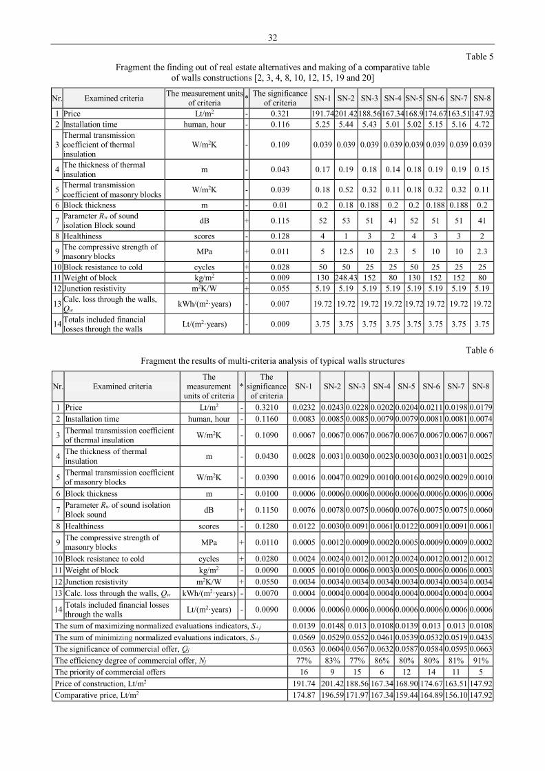
32

Table 5 Fragment the finding out of real estate alternatives and making of a comparative table

of walls constructions [2, 3, 4, 8, 10, 12, 15, 19 and 20]

Nr. Examined criteria The measurement units of criteria * The significance

of criteria SN-1 SN-2 SN-3 SN-4 SN-5 SN-6 SN-7 SN-8

1 Price Lt/m2 - 0.321 191.74201.42188.56167.34168.9174.67163.51147.922 Installation time human, hour - 0.116 5.25 5.44 5.43 5.01 5.02 5.15 5.16 4.72

3 Thermal transmission coefficient of thermal insulation

W/m2K - 0.109 0.039 0.039 0.039 0.039 0.039 0.039 0.039 0.039

4 The thickness of thermal insulation m - 0.043 0.17 0.19 0.18 0.14 0.18 0.19 0.19 0.15

5 Thermal transmission coefficient of masonry blocks W/m2K - 0.039 0.18 0.52 0.32 0.11 0.18 0.32 0.32 0.11

6 Block thickness m - 0.01 0.2 0.18 0.188 0.2 0.2 0.188 0.188 0.2

7 Parameter Rw of sound isolation Block sound dB + 0.115 52 53 51 41 52 51 51 41

8 Healthiness scores - 0.128 4 1 3 2 4 3 3 2

9 The compressive strength of masonry blocks MPa + 0.011 5 12.5 10 2.3 5 10 10 2.3

10 Block resistance to cold cycles + 0.028 50 50 25 25 50 25 25 25 11 Weight of block kg/m2 - 0.009 130 248.43 152 80 130 152 152 80 12 Junction resistivity m2K/W + 0.055 5.19 5.19 5.19 5.19 5.19 5.19 5.19 5.19

13 Calc. loss through the walls, Qw kWh/(m2·years) - 0.007 19.72 19.72 19.72 19.72 19.72 19.72 19.72 19.72

14 Totals included financial losses through the walls Lt/(m2·years) - 0.009 3.75 3.75 3.75 3.75 3.75 3.75 3.75 3.75

Table 6

Fragment the results of multi-criteria analysis of typical walls structures

Nr. Examined criteria The

measurement units of criteria

* The

significance of criteria

SN-1 SN-2 SN-3 SN-4 SN-5 SN-6 SN-7 SN-8

1 Price Lt/m2 - 0.3210 0.0232 0.0243 0.0228 0.0202 0.0204 0.0211 0.0198 0.0179 2 Installation time human, hour - 0.1160 0.0083 0.0085 0.0085 0.0079 0.0079 0.0081 0.0081 0.0074

3 Thermal transmission coefficient of thermal insulation W/m2K - 0.1090 0.0067 0.0067 0.0067 0.0067 0.0067 0.0067 0.0067 0.0067

4 The thickness of thermal insulation m - 0.0430 0.0028 0.0031 0.0030 0.0023 0.0030 0.0031 0.0031 0.0025

5 Thermal transmission coefficient of masonry blocks W/m2K - 0.0390 0.0016 0.0047 0.0029 0.0010 0.0016 0.0029 0.0029 0.0010

6 Block thickness m - 0.0100 0.0006 0.0006 0.0006 0.0006 0.0006 0.0006 0.0006 0.0006

7 Parameter Rw of sound isolation Block sound dB + 0.1150 0.0076 0.0078 0.0075 0.0060 0.0076 0.0075 0.0075 0.0060

8 Healthiness scores - 0.1280 0.0122 0.0030 0.0091 0.0061 0.0122 0.0091 0.0091 0.0061

9 The compressive strength of masonry blocks MPa + 0.0110 0.0005 0.0012 0.0009 0.0002 0.0005 0.0009 0.0009 0.0002

10 Block resistance to cold cycles + 0.0280 0.0024 0.0024 0.0012 0.0012 0.0024 0.0012 0.0012 0.0012 11 Weight of block kg/m2 - 0.0090 0.0005 0.0010 0.0006 0.0003 0.0005 0.0006 0.0006 0.0003 12 Junction resistivity m2K/W + 0.0550 0.0034 0.0034 0.0034 0.0034 0.0034 0.0034 0.0034 0.0034 13 Calc. loss through the walls, Qw kWh/(m2·years) - 0.0070 0.0004 0.0004 0.0004 0.0004 0.0004 0.0004 0.0004 0.0004

14 Totals included financial losses through the walls Lt/(m2·years) - 0.0090 0.0006 0.0006 0.0006 0.0006 0.0006 0.0006 0.0006 0.0006

The sum of maximizing normalized evaluations indicators, S+j 0.0139 0.0148 0.013 0.0108 0.0139 0.013 0.013 0.0108 The sum of minimizing normalized evaluations indicators, S+j 0.0569 0.0529 0.0552 0.0461 0.0539 0.0532 0.0519 0.0435 The significance of commercial offer, Qj 0.0563 0.0604 0.0567 0.0632 0.0587 0.0584 0.0595 0.0663 The efficiency degree of commercial offer, Nj 77% 83% 77% 86% 80% 80% 81% 91% The priority of commercial offers 16 9 15 6 12 14 11 5 Price of construction, Lt/m2 191.74 201.42 188.56 167.34 168.90 174.67 163.51 147.92 Comparative price, Lt/m2 174.87 196.59 171.97 167.34 159.44 164.89 156.10 147.92

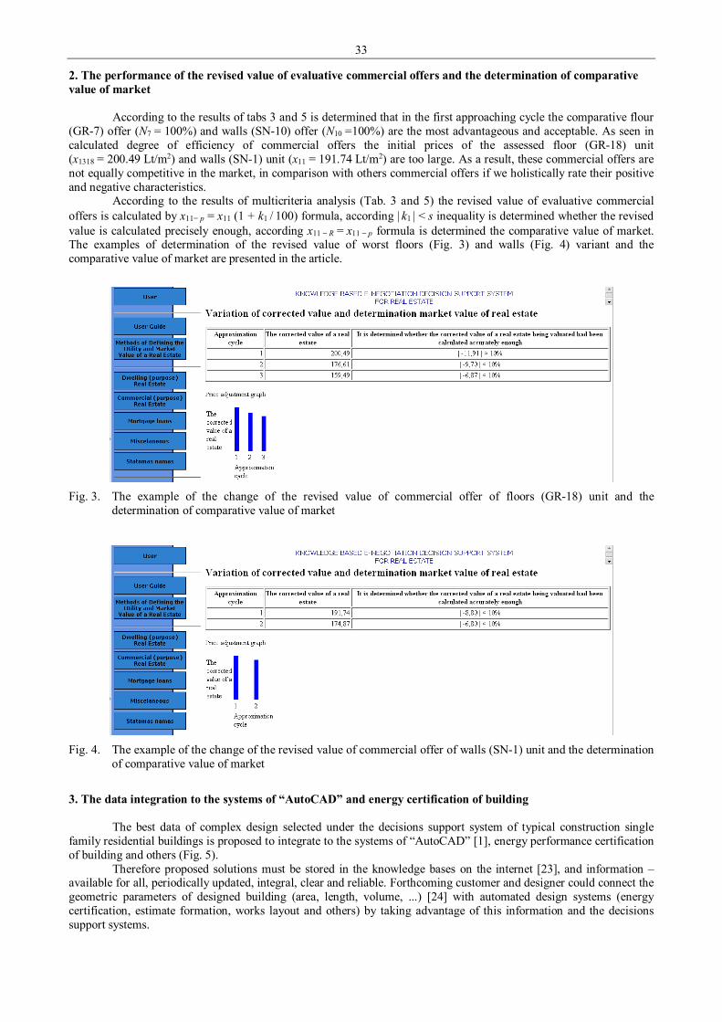
33

2. The performance of the revised value of evaluative commercial offers and the determination of comparative value of market

According to the results of tabs 3 and 5 is determined that in the first approaching cycle the comparative flour (GR-7) offer (N7 = 100%) and walls (SN-10) offer (N10 =100%) are the most advantageous and acceptable. As seen in calculated degree of efficiency of commercial offers the initial prices of the assessed floor (GR-18) unit (x1318 = 200.49 Lt/m2) and walls (SN-1) unit (x11 = 191.74 Lt/m2) are too large. As a result, these commercial offers are not equally competitive in the market, in comparison with others commercial offers if we holistically rate their positive and negative characteristics.

According to the results of multicriteria analysis (Tab. 3 and 5) the revised value of evaluative commercial offers is calculated by x11− p = x11 (1 + k1 / 100) formula, according | k1 | < s inequality is determined whether the revised value is calculated precisely enough, according x11 − R = x11 − p formula is determined the comparative value of market. The examples of determination of the revised value of worst floors (Fig. 3) and walls (Fig. 4) variant and the comparative value of market are presented in the article.

Fig. 3. The example of the change of the revised value of commercial offer of floors (GR-18) unit and the

determination of comparative value of market

Fig. 4. The example of the change of the revised value of commercial offer of walls (SN-1) unit and the determination

of comparative value of market

3. The data integration to the systems of “AutoCAD” and energy certification of building

The best data of complex design selected under the decisions support system of typical construction single family residential buildings is proposed to integrate to the systems of “AutoCAD” [1], energy performance certification of building and others (Fig. 5).

Therefore proposed solutions must be stored in the knowledge bases on the internet [23], and information – available for all, periodically updated, integral, clear and reliable. Forthcoming customer and designer could connect the geometric parameters of designed building (area, length, volume, ...) [24] with automated design systems (energy certification, estimate formation, works layout and others) by taking advantage of this information and the decisions support systems.

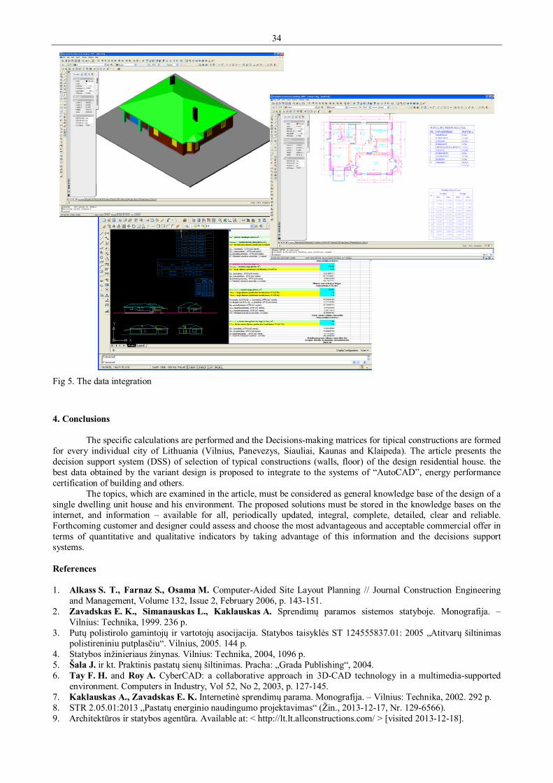
34

Fig 5. The data integration

4. Conclusions

The specific calculations are performed and the Decisions-making matrices for tipical constructions are formed for every individual city of Lithuania (Vilnius, Panevezys, Siauliai, Kaunas and Klaipeda). The article presents the decision support system (DSS) of selection of typical constructions (walls, floor) of the design residential house. the best data obtained by the variant design is proposed to integrate to the systems of “AutoCAD”, energy performance certification of building and others.

The topics, which are examined in the article, must be considered as general knowledge base of the design of a single dwelling unit house and his environment. The proposed solutions must be stored in the knowledge bases on the internet, and information – available for all, periodically updated, integral, complete, detailed, clear and reliable. Forthcoming customer and designer could assess and choose the most advantageous and acceptable commercial offer in terms of quantitative and qualitative indicators by taking advantage of this information and the decisions support systems. References 1. Alkass S. T., Farnaz S., Osama M. Computer-Aided Site Layout Planning // Journal Construction Engineering

and Management, Volume 132, Issue 2, February 2006, p. 143-151. 2. Zavadskas E. K., Simanauskas L., Kaklauskas A. Sprendimų paramos sistemos statyboje. Monografija. –

Vilnius: Technika, 1999. 236 p. 3. Putų polistirolo gamintojų ir vartotojų asocijacija. Statybos taisyklės ST 124555837.01: 2005 „Atitvarų šiltinimas

polistireniniu putplasčiu“. Vilnius, 2005. 144 p. 4. Statybos inžinieriaus žinynas. Vilnius: Technika, 2004, 1096 p. 5. Šala J. ir kt. Praktinis pastatų sienų šiltinimas. Pracha: „Grada Publishing“, 2004. 6. Tay F. H. and Roy A. CyberCAD: a collaborative approach in 3D-CAD technology in a multimedia-supported

environment. Computers in Industry, Vol 52, No 2, 2003, p. 127-145. 7. Kaklauskas A., Zavadskas E. K. Internetinė sprendimų parama. Monografija. – Vilnius: Technika, 2002. 292 p. 8. STR 2.05.01:2013 „Pastatų energinio naudingumo projektavimas“ (Žin., 2013-12-17, Nr. 129-6566). 9. Architektūros ir statybos agentūra. Available at: < http://lt.lt.allconstructions.com/ > [visited 2013-12-18].

35

10. Baltijos polistirenas. Available at: < http://www.balpol.lt > [visited 2013-10-21]. 11. Building & Construction Home: Europe Home. Available at: < http://building.dow.com > [visited 2013-10-21]. 12. Fasadų apdailos medžiagos, grindų dangos. Available at: < http://www.dasfa.lt/products.php?pid=6&sid=152&

id=246 > [visited 2014-01-18]. 13. Grindų ant grunto įrengimo kainos. Available at: < http://www.manonamai.lt > [visited 2013-11-26]. 14. Grindų dangos. Available at: < http://www.solum.lt > [visited 2014-01-10]. 15. Išorės sienų apšiltinimo sistemos. Available at: < http://lt.lt.allconstructions.com/portal/categories > [visited

2013-12-17]. 16. Kamštinė danga grindims. Available at: < http://www.ferimpex.lt/index.php?p=kams&s=grin&m=wica4000%20 >

[visited 2014-01-10]. 17. Konstrukcijų pavyzdžiai. Available at: < http://www.rockwool.lt/ > [visited 2013-02-29]. 18. Konstruktyvinės detalės. Ekovata. Available at: < http://www.ekovata.lt/lt/l > [visited 2013-10-21]. 19. Polistireninio putplasčio plokšių „TERMOPORAS” panaudojimas pastatuose. Available at:

< http://www.baltukme.lt/files/Termoporas.pdf > [visited 2013-12-17]. 20. Sąmatų skaičiavimo programa. Available at: < http://www.ses.lt/index.php?page_id=4&news_id=10 > [visited

2013-11-02]. 21. Statybinė izoliacija. Available at: < http://www.paroc.lt/ > [visited 2013-01-29]. 22. Statybinių darbų kainų skaičiuoklė. Danstema. Available at: < http://www.danstema.lt/skaiciuokle.php > [visited

2012-11-25]. 23. Šakys V. Informacinių technologijų vadovas. Kaunas: Šviesa, 2005. 288 p. 24. Tay F. H. and Roy A. CyberCAD: a collaborative approach in 3D-CAD technology in a multimedia-supported

environment. Computers in Industry, Vol 52, No 2, 2003, p. 127-145.

36

Proceedings of 9th International Conference ITELMS’2014 The Conception of an Anthropomorphic Manipulator with Hydrostatic Drive System A. Bartnicki*, K. Cieslik**, S. Konopka***, M. J. Lopatka**** *Military University of Technology, gen. S. Kaliskiego str, 2, 00-908 Warsaw, Poland, E-mail: abartnicki@wat.edu.pl **Military University of Technology, gen. S. Kaliskiego str, 2, 00-908 Warsaw, Poland, E-mail: kcieslik@wat.edu.pl ***Military University of Technology, gen. S. Kaliskiego str, 2, 00-908 Warsaw, Poland, E-mail: skonopka@wat.edu.pl ****Military University of Technology, gen. S. Kaliskiego str, 2, 00-908 Warsaw, Poland, E-mail: mlopatka@wat.edu.pl Abstract In this article the conception of construction anthropomorphic manipulator with hydrostatic drive system is shown. Made a revision of this type of construction determining used kinematics chains in it, ways of forcing to move particular elements and used drive systems. Formulated kinematics structure of manipulator being imitation of human hand, and determined a way of initiate movement of elements from which assembled a manipulator. Examined and presented series of load cases on manipulator’s construction, which allowed to determinate which elements are the most encumbered. Determined the radius in which manipulator can be useful and presented requirements which should be matched by potential carrier of manipulator construction. KEYWORDS: anthropomorphic manipulator, hydrostatic drive, steering. 1. Introduction

In the end of 20th century began making projects of devices, which would be as much as possible exact as human arm. Tried to achieve manipulability on human upper limb’s level. Moreover designed steering system had to ensure intuitiveness and simplicity of working with manipulator. To achieve it used so-called copying systems, with which operator was equipped. Advantage of such solution, besides steering simplicity, is lack of need long term operators’ training. Constructions which are reaching mobility on human arm level and making use of mentioned steering type has been called as anthropomorphic manipulators [1-5].

To increase functionality and working possibilities of such type of devices, their sizes were significantly bigger than human arm. By this devices had bigger range of work space and capability. It simplified in significant degree moving and transporting of particular shipment without the need of moving closer to object. Nowadays such type of constructions found more and more usage in industrial, medicine, and military. It proves that there is an increase in requirement and interest in functionality and anthropomorphic manipulators’ possibilities, which proves their equity to design and construct such devices. 2. Constructional and kinematics solutions of anthropomorphic manipulators

In the market there are many anthropomorphic manipulators are accessible. Most of them uses electric drive system [6, 7].They find their usage in medicine and light industrial sector, where masses of lifted object which do not exceed 100 kg. Besides it, environment (surrounding) do not expose it for humidity and significant pollution.

Hydrostatic drive system significantly increases working possibilities of manipulators. Connected with themb (possibilities) are lifting capacity, range and working radius. Besides it, this drive system is immune to overloads. That is why further analysis of manipulator constructions concerned only manipulators with hydrostatic drive system

First from discussed constructions was designed by Kraft company and it is called “Predator” (Fig. 1).

Fig. 1. Manipulator “Predator” [8]

Manipulator is based on open kinematics chains with six degrees of latitude. It has 2 m range and it has ability

to lift object which weights 93 kg. Maximum weight to lift for this manipulator equals 230 kg. Its construction contains four elements. Their movement is forced by both linear servomotors (lifting whole manipulator and movement of

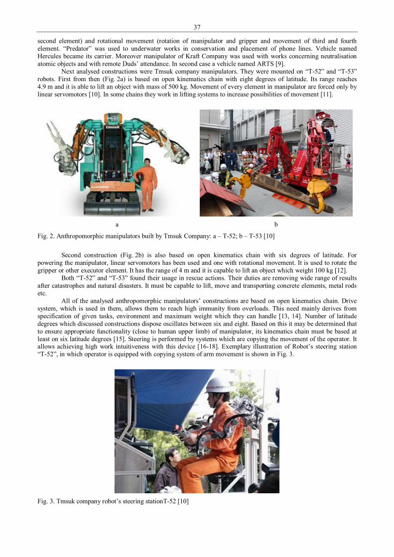
37

second element) and rotational movement (rotation of manipulator and gripper and movement of third and fourth element. “Predator” was used to underwater works in conservation and placement of phone lines. Vehicle named Hercules became its carrier. Moreover manipulator of Kraft Company was used with works concerning neutralisation atomic objects and with remote Duds’ attendance. In second case a vehicle named ARTS [9].

Next analysed constructions were Tmsuk company manipulators. They were mounted on “T-52” and “T-53” robots. First from then (Fig. 2a) is based on open kinematics chain with eight degrees of latitude. Its range reaches 4.9 m and it is able to lift an object with mass of 500 kg. Movement of every element in manipulator are forced only by linear servomotors [10]. In some chains they work in lifting systems to increase possibilities of movement [11].

a

b

Fig. 2. Anthropomorphic manipulators built by Tmsuk Company: a – T-52; b – T-53 [10]

Second construction (Fig. 2b) is also based on open kinematics chain with six degrees of latitude. For

powering the manipulator, linear servomotors has been used and one with rotational movement. It is used to rotate the gripper or other executor element. It has the range of 4 m and it is capable to lift an object which weight 100 kg [12].

Both “T-52” and “T-53” found their usage in rescue actions. Their duties are removing wide range of results after catastrophes and natural disasters. It must be capable to lift, move and transporting concrete elements, metal rods etc.

All of the analysed anthropomorphic manipulators’ constructions are based on open kinematics chain. Drive system, which is used in them, allows them to reach high immunity from overloads. This need mainly derives from specification of given tasks, environment and maximum weight which they can handle [13, 14]. Number of latitude degrees which discussed constructions dispose oscillates between six and eight. Based on this it may be determined that to ensure appropriate functionality (close to human upper limb) of manipulator, its kinematics chain must be based at least on six latitude degrees [15]. Steering is performed by systems which are copying the movement of the operator. It allows achieving high work intuitiveness with this device [16-18]. Exemplary illustration of Robot’s steering station “T-52”, in which operator is equipped with copying system of arm movement is shown in Fig. 3.

Fig. 3. Tmsuk company robot’s steering stationT-52 [10]

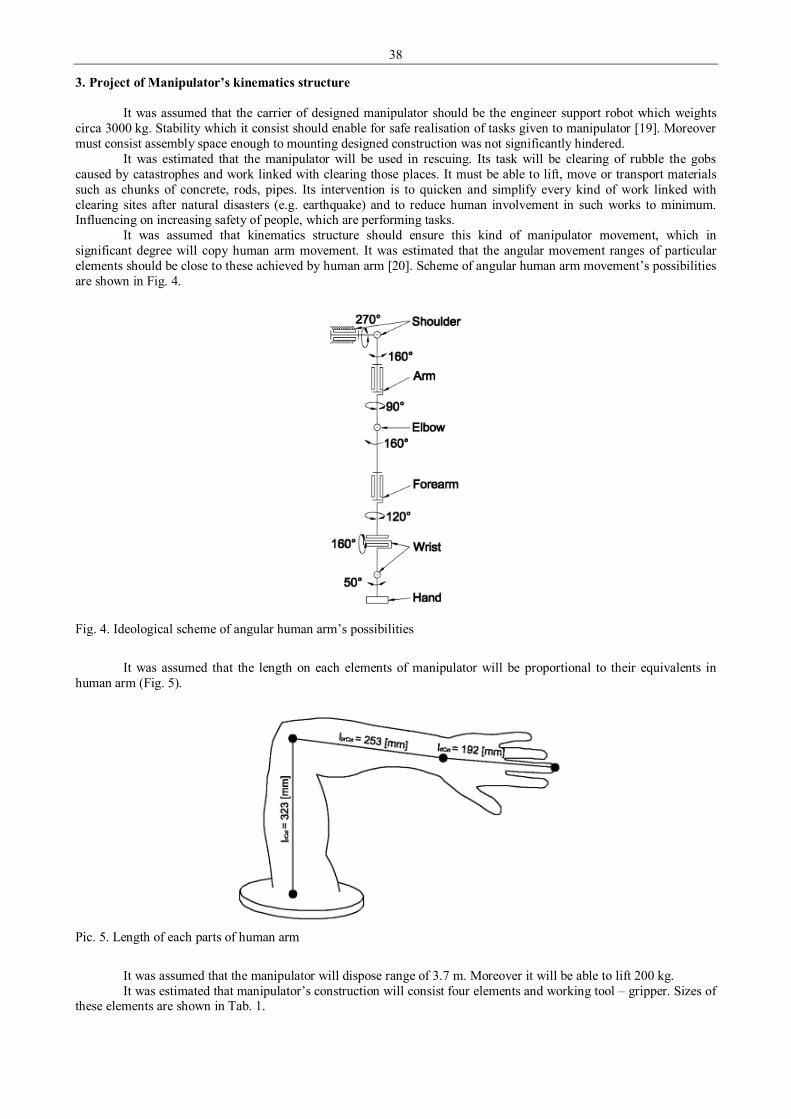
38

3. Project of Manipulator’s kinematics structure

It was assumed that the carrier of designed manipulator should be the engineer support robot which weights circa 3000 kg. Stability which it consist should enable for safe realisation of tasks given to manipulator [19]. Moreover must consist assembly space enough to mounting designed construction was not significantly hindered.

It was estimated that the manipulator will be used in rescuing. Its task will be clearing of rubble the gobs caused by catastrophes and work linked with clearing those places. It must be able to lift, move or transport materials such as chunks of concrete, rods, pipes. Its intervention is to quicken and simplify every kind of work linked with clearing sites after natural disasters (e.g. earthquake) and to reduce human involvement in such works to minimum. Influencing on increasing safety of people, which are performing tasks.

It was assumed that kinematics structure should ensure this kind of manipulator movement, which in significant degree will copy human arm movement. It was estimated that the angular movement ranges of particular elements should be close to these achieved by human arm [20]. Scheme of angular human arm movement’s possibilities are shown in Fig. 4.

Fig. 4. Ideological scheme of angular human arm’s possibilities

It was assumed that the length on each elements of manipulator will be proportional to their equivalents in

human arm (Fig. 5).

Pic. 5. Length of each parts of human arm

It was assumed that the manipulator will dispose range of 3.7 m. Moreover it will be able to lift 200 kg. It was estimated that manipulator’s construction will consist four elements and working tool – gripper. Sizes of

these elements are shown in Tab. 1.

39

Table 1 Sizes of manipulator’s elements

Name of element Assumed size[mm] 1 Element 1 1500 2 Element 2 1200 3 Element 3 300 4 Element 4 300 5 Gripper 400

Main elements composed into manipulator’s construction are shown in Fig. 6.

Fig. 6. Basic components of manipulator’s construction: 1 – mounting plate; 2 – attachment of first element; 3 – first

element; 4 – second element; 5 – third element; 6 – fourth element; 7 – working tool

Based on kinematics structures occurring in analysed anthropomorphic manipulators and angular human arm

movement’s possibilities formulated a kinematics scheme of designed anthropomorphic manipulator.

a

b

Fig. 7. Manipulator’s kinematics scheme: a – side layout; b – layout from above; 1, 2, 3 – possible placement of manipulator

In relation to human arm, designed kinematics scheme (Fig. 7) consists one latitude degree less. Rotation

possibility has been reduced for arm and forearm (Fig. 4) to one place which is gripper’s joint (Fig. 7). Moreover increased range of movement of certain elements. It is to enable proper density of construction after disassembling for transport. 4. Rotation’s mechanism of anthropomorphic manipulator

Based on estimated assumptions formulated two kinds of constructional solutions of anthropomorphic manipulator. Their main difference is the way of rotating of whole construction. First solution assumes that the rotation will be realised by servomotor with rotational movement (Fig. 8).

40

Fig. 8. Construction’s conception of anthropomorphic manipulator number 1

Second solution assumes that to rotate the manipulator two linear servomotors will be applied (Fig. 9). This

kind of solution is used in excavator-loader units to rotate excavator equipment for 180º.

Fig. 9. Construction’s conception of anthropomorphic manipulator number 2

Advantage of first solution is achieving dense construction and constant momentum value while rotating the

manipulator. Based on initial calculations concerning rotational momentum’s value which has to create by servomotor determined its specification according to catalogue [21]. On this base determined that the fundamental defect of this solution is the weight of the servomotor (reaches 200 kg) and its size (height circa. 600 mm).

Second rotation solution characterise with lower weight (circa 90 kg) and simplicity of performed elements of construction. It has been estimated as a result of initial design of manipulator rotation mechanism.

It was assumed that the second conception will be used (Fig. 9). As a condition for outclassing first solution was because their significant weight difference 5. Manipulator hydrostatic system

To ensure estimated kinematics assumptions between its elements which are forcing the movement has been implemented into it, to allow for reaching assumed angles. These elements are hydraulic servomotors with reciprocating or rotational movement. Placement of those hydraulic servomotors in anthropomorphic manipulator is shown in Fig. 10.

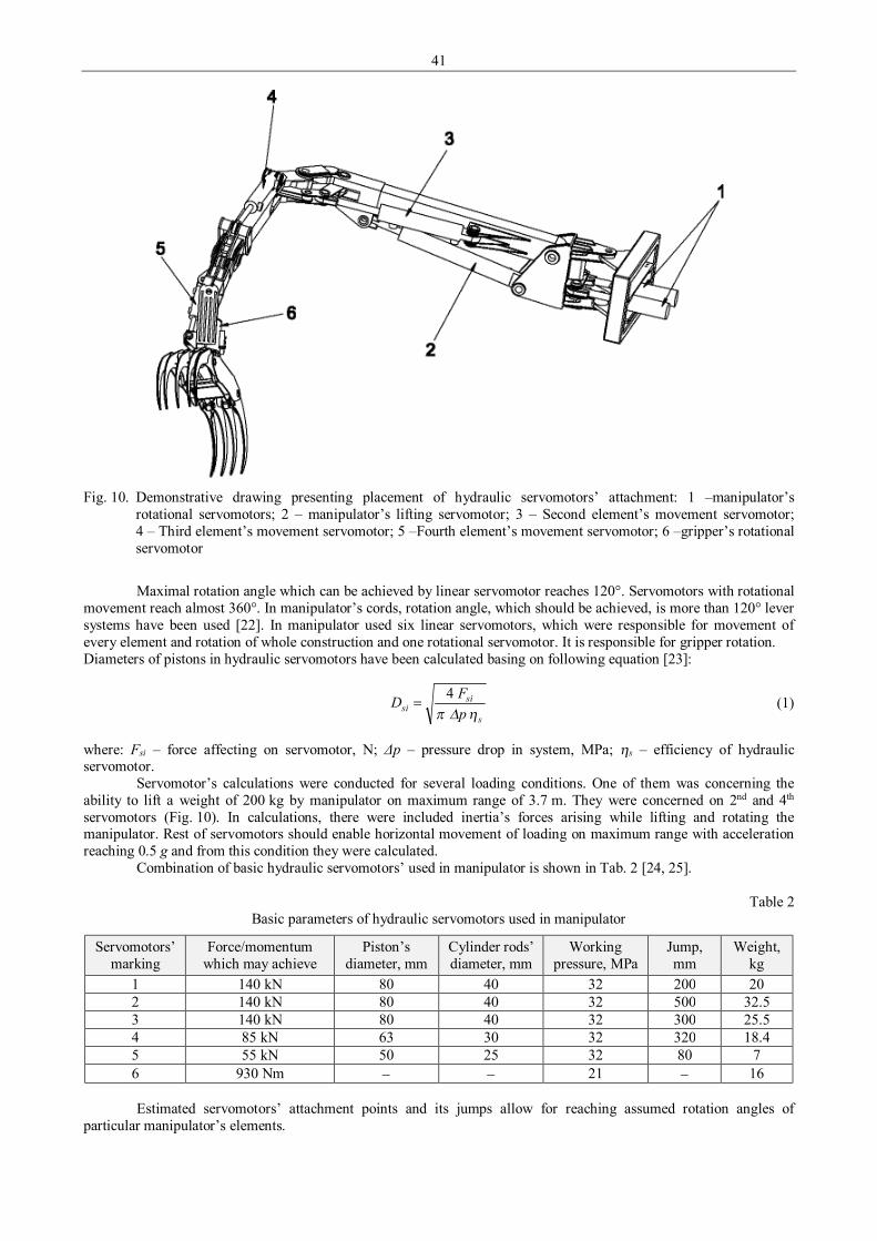
41

Fig. 10. Demonstrative drawing presenting placement of hydraulic servomotors’ attachment: 1 –manipulator’s

rotational servomotors; 2 – manipulator’s lifting servomotor; 3 – Second element’s movement servomotor; 4 – Third element’s movement servomotor; 5 –Fourth element’s movement servomotor; 6 –gripper’s rotational servomotor

Maximal rotation angle which can be achieved by linear servomotor reaches 120°. Servomotors with rotational

movement reach almost 360°. In manipulator’s cords, rotation angle, which should be achieved, is more than 120° lever systems have been used [22]. In manipulator used six linear servomotors, which were responsible for movement of every element and rotation of whole construction and one rotational servomotor. It is responsible for gripper rotation. Diameters of pistons in hydraulic servomotors have been calculated basing on following equation [23]:

s

sisi p

FDη∆π

4= (1)

where: Fsi – force affecting on servomotor, N; Δp – pressure drop in system, MPa; ηs – efficiency of hydraulic servomotor.

Servomotor’s calculations were conducted for several loading conditions. One of them was concerning the ability to lift a weight of 200 kg by manipulator on maximum range of 3.7 m. They were concerned on 2nd and 4th servomotors (Fig. 10). In calculations, there were included inertia’s forces arising while lifting and rotating the manipulator. Rest of servomotors should enable horizontal movement of loading on maximum range with acceleration reaching 0.5 g and from this condition they were calculated.

Combination of basic hydraulic servomotors’ used in manipulator is shown in Tab. 2 [24, 25].

Table 2 Basic parameters of hydraulic servomotors used in manipulator

Servomotors’ marking

Force/momentum which may achieve

Piston’s diameter, mm

Cylinder rods’ diameter, mm

Working pressure, MPa

Jump, mm

Weight, kg

1 140 kN 80 40 32 200 20 2 140 kN 80 40 32 500 32.5 3 140 kN 80 40 32 300 25.5 4 85 kN 63 30 32 320 18.4 5 55 kN 50 25 32 80 7 6 930 Nm − − 21 − 16

Estimated servomotors’ attachment points and its jumps allow for reaching assumed rotation angles of

particular manipulator’s elements.

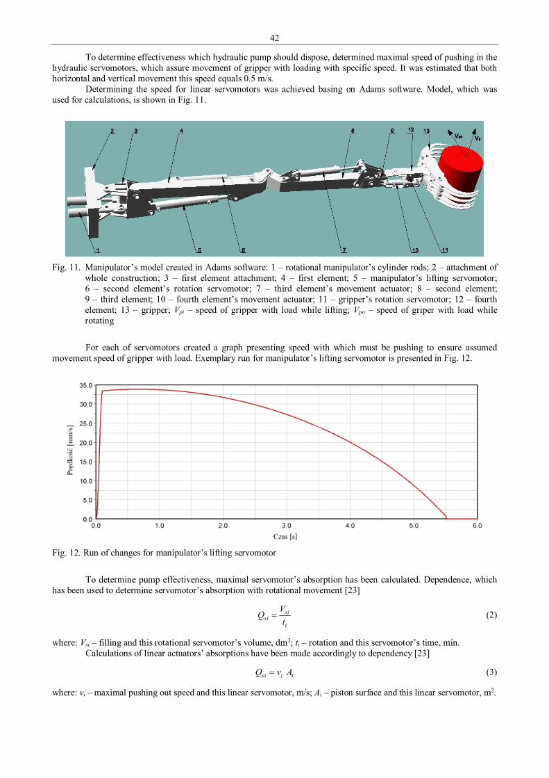
42

To determine effectiveness which hydraulic pump should dispose, determined maximal speed of pushing in the hydraulic servomotors, which assure movement of gripper with loading with specific speed. It was estimated that both horizontal and vertical movement this speed equals 0.5 m/s.

Determining the speed for linear servomotors was achieved basing on Adams software. Model, which was used for calculations, is shown in Fig. 11.

Fig. 11. Manipulator’s model created in Adams software: 1 – rotational manipulator’s cylinder rods; 2 – attachment of

whole construction; 3 – first element attachment; 4 – first element; 5 – manipulator’s lifting servomotor; 6 – second element’s rotation servomotor; 7 – third element’s movement actuator; 8 – second element; 9 – third element; 10 – fourth element’s movement actuator; 11 – gripper’s rotation servomotor; 12 – fourth element; 13 – gripper; Vpi – speed of gripper with load while lifting; Vpo – speed of griper with load while rotating

For each of servomotors created a graph presenting speed with which must be pushing to ensure assumed

movement speed of gripper with load. Exemplary run for manipulator’s lifting servomotor is presented in Fig. 12.

Fig. 12. Run of changes for manipulator’s lifting servomotor

To determine pump effectiveness, maximal servomotor’s absorption has been calculated. Dependence, which

has been used to determine servomotor’s absorption with rotational movement [23]

i

sisi t

VQ = (2)

where: Vsi – filling and this rotational servomotor’s volume, dm3; ti – rotation and this servomotor’s time, min. Calculations of linear actuators’ absorptions have been made accordingly to dependency [23]

iisi AvQ = (3)

where: vi – maximal pushing out speed and this linear servomotor, m/s; Ai – piston surface and this linear servomotor, m2.

43

To determine hydraulic pump’s effectiveness, assumed that while working with manipulator it is possible to simultaneously usage of four actuators working with maximal speeds. To them belong rotational and manipulator lifting servomotors, movement of second element and rotation of the gripper.

After conducting necessary calculations determined the effectiveness with which hydraulic pump should dispose. Its basic parameters are shown in Tab. 3 [26].

Table 3 Basic parameters of hydraulic pump

Pump indication A2FO Series 6 Size 45 Name of

parameter Effectiveness,

dm3/min Working pressure, MPa Rotational speed, obr/min Weight,

kg Nominal Maximal Nominal Maximal Value 102 32 37 2000 3750 13.5

It was assumed that in hydraulic system will be implementer proportional divider, with seven sections, four-

way three-positioned with electro-hydraulical control. It will ensure the sufficient accuracy of pushing out speed control, and this will have its influence on reaching high accuracy of manipulator’s movement [27-30]. 6. Manipulator structure’s durability

It has been assumed that manipulator will be used from thin-walled closed profile. To estimate characteristic geometric values, conducted a series of durability calculations and considered many load cases.

It has been assumed that the manipulator should be a construction with high durability and relatively light. That is why it has been assumed that it will be build from iron 15HGM [31].

Dependencies allowing for estimating sizes of transverse the most loaded element’s section depend on character of load working on construction. Equation allowing calculating maximal bending stresses is presented in following way [32]

gg

gmaxg k

WM

≤=σ (4)

where: Mg – maximal bending momentum, Nm; Wg – bending durability value, m3; kg – admissible value of bending stresses for adopted material, MPa.

For thin-walled profile with measurement of 140×110×4 mm has been conducted analysis of manipulator construction’s exertion to check its durability. To achieve it module MES from CATIA software has been used. On Fig. 13 and 14 presented some of results.

Fig. 13. Analysis of manipulator construction’s exertion on maximal range with load derived from weight

44

Fig. 14. Analysis of manipulator construction’s exertion for second element rotation for 90° with load derived from

weight

In presented analyses of manipulator construction’s exertion, burden derives from maximal weight of load,

which is capable to lift. In first case (Fig. 13) bending dominates. Maximal value of stresses reached 238 MPa. Its concentration occurs in placement of first and second elements’ attachment. In second case (pic. 13) turning linked with bending dominate. The biggest stresses reach 273 MPa, and its concentration occurs in first element. Values of admissible stresses for adopted iron equal: for bending 468 MPa, while for turning 288 MPa. In both first and second presented analyses they were not exceeded. 7. Conclusions

Manipulator construction’s conception is based on open kinetic chain with six latitude degrees. An implemented solution gives manipulability on human limb level. Moreover combined with upper limb copying steering system, the operator is able to achieve very precise manipulator’s movement. By this work with it becomes intuitive and there is no need for long specialisation trainings for operators.

Elements from which manipulator is built are anatomic imitations of their equivalents in human upper limb. Their lengths were proportionally enlarged. Anatomic analogy of human arm for manipulator’s construction affects on simplicity in anticipation of its reaction while working by operator. These significantly simplifies and quicken it, it is very important in area of application for which it has been designed.

Material adopted for manipulator’s construction affects on minimization of its weight. Moreover great influence on it has limitation of servomotors’ number with rotational movement to one, and in places where it was necessary to achieve rotational angles higher than 120°, linear actuators working in lifting systems were implemented. The usage area of designed manipulator is helping the rescue teams with removing results of natural disasters. Related with it are tasks with clearing out rubble and arranging terrains touched with them. Manipulator’s construction ensures enabling to simply, intuitive and precise performance of tasks related to it. References 1. Chiang Ming-Hsun, Chang Fan-Ren. Anthropomorphic Design of the Human-Like Walking Robot. Journal of

bionic engineering, January 2013 2. Paik Jamie K., Shin Bu Hyun, Bang Young-Bong. Development of an Anthropomorphic Robotic Arm and Hand

for Interactive Humanoids. Journal of bionic engineering, January 2012 3. Roa Maximo A., Argus Max J., Leidner Daniel. Power Grasp Planning for Anthropomorphic Robot Hands. IEEE

International Conference on Robotics and Automation, St Paul, May 14-18, 2012 4. Tondu Bertrand. Kinematic Modelling of Anthropomorphic Robot Upper Limb with Human-like Hands. 14th

International Conference on Advanced Robotics Location: Munich, Germany, JUN 22-26, 2009 5. Binaud Nicolas, Cardou Philippe, Caro Stephane. The kinematic sensitivity of robotic manipulators to joint

clearances. ASME Internationl Design Engineering Technical Conferences Computers and Information in Engineering, Montreal, Canada, August 15-18, 2010

6. Podsękowski L. Roboty medyczne budowa i zastosowanie. WNT, Warszawa 2010. 7. Morecki A., Knapczyk J., Kędzior K. Teoria mechanizmów i manipulatorów. WNT, Warszawa2002. 8. Broszura informacyjna produktu Predator firmy Kraft. 9. Online: < www. krafttelerobotics.com >.

45

10. Online: < www.tmsuk.co.jp >. 11. Crane III C. D., Duffy J. Kinematic analysis of robot manipulators, Wydawnictwo Uniwersytetu Cambridge,

Nowy Jork 2008. 12. Broszura informacyjna produktu T-53 firmy Tmsuk. 13. Jezierski E. Dynamika robotów. WNT, Warszawa 2006. 14. Kozłowski K., Dutkiewicz P., Wróblewski W. Modelowanie i sterowanie robotów, Wydawnictwo Naukowe

PWN, Warszawa 2003. 15. Morecki A., Knapczyk J. Podstawy robotyki teoria i elementy manipulatorów i robotów. WNT, Warszawa 1999. 16. Konopka S., Krogul P., Łopatka M. J. Simulation Research of Hydrostatic Power System Control of Engineer

Robot Manipulator, Proceedings of 8th International Conference Intelligent Technologies in Logistics and Mechatronics Systems ITELMS ‘2013, pp. 126-135, Panevėžys, Lithuania, May 23-24, 2013.

17. Dąbrowska A., Typiak R. Universal Robotic Control Station for a Grouping of Unmanned Egineering Machines, Proceedings of 8th International Conference Intelligent Technologies in Logistics and Mechatronics Systems ITELMS ‘2013, pp. 71-75, Panevėžys, Lithuania, May 23-24, 2013.

18. Kim D., Kim J., Lee K., Park C., Song J., Kang D. Excavator tele-operation system using a human arm, Automation in Construction 18, vol. 18, pp. 173-182, 2009.

19. Bartnicki A., Jaskółowski M., Łopatka M. J., Muszyński T. The Researches of Stability Evaluation Articulated Loader while Working on Slopes, Proceedings of 8th International Conference Intelligent Technologies in Logistics and Mechatronics Systems ITELMS ‘2013, pp. 126-135, Panevėžys, Lithuania, May 44-49, 2013.

20. Biryukova E. V., Roby-Brami A., Frolov A. A., Mokhtari M. Kinematics of human arm reconstructed from spatial tracking system recordings. Journal of Biomechanics 33 (2000) 985-995.

21. Online: < www.helac.com >. 22. Miller S. Układy kinematyczne. Podstawy projektowania. WNT, Warszawa 1988. 23. Stryczek S. Napęd hydrostatyczny. Tom I. WNT Warszawa 2005. 24. Katalog liniowych siłowników hydraulicznych firmy Hydro. 25. Katalog siłowników hydraulicznych o ruchu obrotowym firmy Helac. 26. Katalog pomp hydraulicznych firmy Bosch Rexroth. 27. Kuczmarski F. Badania gąsienicowych koparek hydraulicznych z osprzętem podsiębiernym pod kątem możliwości

zwiększenia dokładności wykonywania prac ziemnych, rozprawa doktorska, Wojskowa Akademia Techniczna, Warszawa 1983.

28. Typiak A. M. Zwiększenie dokładności pracy koparek jednonaczyniowych metodą ciągłej kontroli położenia osprzętu roboczego, rozprawa doktorska, Wojskowa Akademia Techniczna, Warszawa 1999.

29. Budny E., Chłosta M., Gutkowski W. Load-independent control of hydraulic excavator, Automation in Construction 12, 10 stron, 2003.

30. Budny E., Chłosta M., Gutkowski W. Sensitivity of the optimum bucket trajectory in controlled excavation, Automation and Robotics in Construction XVI, 1999.

31. Praca zbiorowa: Poradnik mechanika, WNT, Warszawa, 2000. 32. Niezgodziński M. T. Wzory wykresy i tablice wytrzymałościowe, WNT, Warszawa, 2004.

46

Proceedings of 9th International Conference ITELMS’2014 Research Guidelines of the Nuclear Power Systems in XXI Century Z. Bazaras*, B. Timofeev**, N. Vasileva**, J. Igakojyte-Bazariene* *Kaunas University of Technology, Kestucio 27, 44312, Kaunas, Lithuania, E-mail: Zilvinas.Bazaras@ktu.lt **Central Research Institute of Structural Materials “Prometey”, 49 Shpalernaya str., St. Petersburg, Russia, E-mail: mail@crism.ru Abstract In connection with an electric power increasing demand in the world in 21-st century one of the main development direction of the nuclear power systems is transition from water-moderated reactors to metal-liquid nuclear reactors which are used lead or lead-bismuth alloy as the heat-carrier. Development of the new nuclear energy technology based on the fast reactors with the closed nuclear fuel cycle will increase natural uranium and spent nuclear fuel usage efficiency. Subject to the program fulfilment, since 2020-2025 the role of fast reactors in maintenance of consumers of energy should increase essentially. KEYWORDS: water-moderated reactors, fast reactors with the lead heat-carrier, sheet from pearlitic low-alloyed steel. 1. Introduction

In recent years there is an omnipresent and continuous growth of the electric power demand on a world scale [1]. Nowadays this is one of the cardinal problems which society is necessary to face with. In addition to grows both manufacture and electrical energy consumption. 2. Rezults and analysis

Both that and another plays a key role in steady development of the national economy. The electric power is an economic and social development of the world population engine. Its production per head in some way can be the economic development indicator. Russia is already on the 11-th place in the world (2740 kWh) by electric power manufacture per head, a little exceeding average world parameter which is 2140 kWh. Electric power manufacture per head in various countries is presented in Table 1.

Table 1 Electric power manufacture per head in various countries, kWh

Country USA Finland Switzerland Japan Germany UK France Czech Republic Russia Ukraine

Per head kWh 33540 25090 36310 34340 35750 36310 23560 5170 2740 770

In accordance with the welfare growth electric energy deficiency will be one of the biggest problems for the significant part of the world population. First of all it is predicted organic fuel deficiency and also with necessity of thermal stations electric capacities replacement which have exhausted its resources. Nuclear engineering development is also necessary in connection with the growing of the organic fuel cost which is used for thermal power stations and on the other hand it has got a difficult ecological situation during these kinds of fuel usage. Thus, the main sources for the electric power generation at present are the coal and natural gas burning thermal stations and nuclear power stations. In addition to nuclear resources can be used considerably longer. Besides in nuclear power engineering carbon dioxide is not let out in the atmosphere. In spite of the fact that nuclear power units create radioactive wastes which cause a problem with the reprocessing and burial of the nuclear wastes they are more viable for the electric power manufacturing during at least the nearest 50-100 years. Only the nuclear power engineering as it is cheaper has practically inexhaustible resources.

In spite of the difficult development (for the half a century of civil nuclear power there were three large failures: at nuclear power station "Three Mile Island" in the USA in 1979, at the "Chernobyl" nuclear power station in the USSR in 1986, at nuclear power station "Fukushima" in Japan in 2011, it is inevitably develops. Unconditional advantage is behind water-cooled power engineering which is continuously improved by way of safety increase during longer operation time. In 2013 from 433 operating power blocks majority were reactors with pressurized water PWR (271) and boiling water BWR (83). British cooled by carbon dioxide reactors (reactor Magnox – older design and AGR – newer design) in 30 pieces and Russian light-water reactors with graphite moderator type RBMK and EGP in 15 pieces. And only one power unit BN-600 with liquid-metal sodium coolant already operating more than 30 years.

In February, 2010 the federal goal-oriented program «New generation nuclear energy technologies for the years 2010-2015 and future prospects up to 2020» has been accepted. The purpose of the program is new nuclear

47

technologies on the base of the fast reactors with the closed nuclear fuel cycle development that will increase efficiency of the natural uranium and spent fuel usage. On the assumption of the program execution, since 2020-2025 fast reactors role in supply of electrical customers should appreciably increase. However now there is one operating fast reactor BN-600 on the Beloyarsk nuclear power station though more powerful reactor this type is under construction and new sodium nuclear reactor BN-1200 is projected in Russia. Besides at the present time in Russia there is a project of new generation fast neutron reactors with heavy liquid-metal heat-carrier, double-loop cooling system and overcritical steam conditions called BREST. In connection with the ample quantity of constructive decisions which are new in this field the first project will be research and demonstrative reactor installation with the capacity of 300 МW called BREST-OD-300.

This reactor is used high-boiling, radiation-resistant and low-activated lead heat-carrier, which is chemically passive in water and air that allows low pressure heat-sink cooling and excludes fires, chemical and thermal explosions during circuit depressurization, leaks of the steam generator and heat-carrier overheating.

The reactor is pool-type, i.e. there is no reactor vessel in construction – it is shaft made of heat-insulating concrete covered with the metal liner, filled in with the lead heat-carrier where placed an active zone, a steam generator, a pump and other supporting systems.

According to the base project metal liner should be made of steel type 09Mn2Si cladding with austenitic steel called EP302. Sheet thickness of steel type 09Mn2Si is 32 mm, in load carrying places is 52 mm (horizontal sheets), cladding layer thickness of the steel type EP302 is 7 mm. On account of construction complexity, high manufacturing cost of cladding steel there have been carried out some preliminary tests of samples from steel type 09Mn2SiA-A in the lead heat-carrier flow at the special test stand in CRISM “Prometey”. On the base of the results it was offered to replace the cladding steel with sheets from steel type 09Mn2SiA-A.

After Fukushima failure world community was divided in two groups by meaning about nuclear energy usage: 1. The countries against nuclear power engineering: Japan, Germany, Switzerland, Italy, Austria, Holland, Poland,

Spain, New Zealand, Sweden (10 countries); 2. The countries for active nuclear power station construction: China, India, Iran, Russia, Turkey, Belarus

(6 countries). Russia in 2012 is ready to begin Severskoy NPP construction in Tomsk region. By "Romir" data to 2008 when

the project has been started, 73% of region population was against construction. Experts consider that there is no necessity in NPP construction – there are a lot of hydroelectric power stations in Siberia which provide region on 50%. It will be entered into operation large Boguchanskaja hydroelectric power station; it is restored Sayano-Shushenskaja hydroelectric power station which will on total power since 2014. Thermal power stations on the coal are under development. The NPP in Tomsk region at prospects of an expenditure of the electric power for 20 years not only unnecessary, but also is economic detriment. The gain of the power consumption in region was 0.1% per annum, and now is only 3%. By 2030 it will probably be a renewed energy source - a sun, a wind and so on. 2. Conclusions

Nowadays it is possible to approve, that nuclear fuel has an important role in a power balance of the country though in long-term outlook it is not excluded that renewed energy sources will be dominate. So far in stationary nuclear power engineering thermal-neutron reactors with light-water moderator and the heat-carrier of the first and second generations are dominate and such type nuclear power station of III and III+ generations will be under construction during several decades. References 1. Albitzkaya E. Review: Nuclear power systems development. Nuclear technology abroad, 2013, p. 3-16. 2. Pioro I., Kirillov P. Current state of the power generation of the nuclear power station in the world. Nuclear

technology abroad. 2013, №12, p. 3-11. 3. Kagramanjan V. Economic risk estimation caused by fast neutron reactor delay. Nuclear engineering. 2013, vol.

114, № 2, p. 67-76.

48

Proceedings of 9th International Conference ITELMS’2014 Influence of the Quantities of Plastifying Concrete Additive on Concrete Properties P. Bulovas*, S. Susinskas**

*Kaunas University of Technology, S. Daukanto str. 12, 35212, Panevezys, Lithuania, E-mail: bulovas.paulius@gmail.com **Kaunas University of Technology, S. Daukanto str. 12, 35212, Panevezys, Lithuania, E-mail: saulius.susinskas@ktu.lt Abstract Concrete is material obtained by mixing binding substance, coarse and fine aggregates, water and additives which acquires its desired properties during the hardening process. The main properties of concrete are determined by the quality and properties of raw materials used to produce concrete, W/C ratio and the uniformness of the mix compaction. The compressive strength of concrete is among the main concrete properties. The article analyses the influence of plastifying additive on concrete properties and selects optimal quantity of the additive. Investigations of concrete properties with different quantities of plastifying additive have shown that the increase of the quantity of plastifying additive up to 0.8% increases the compressive strength and slump of samples and reduces water absorption. The increase of the quantity of plastifying additive up to 1.2% reduces the compressive strength and slump of samples and increases water absorption. KEYWORDS: concrete, limestone cement, coarse and fine aggregates, compressive strength, plastifying additive. 1. Introduction

Concrete mix is a composite multicomponent polydispersed system obtained by mixing the mixture of cement, aggregates and additives with water. This system consists of smaller or larger particles of cement, particles of fine and coarse aggregate, suitable additives, water and entrained air.

Concrete is one of the oldest substances used in construction. It has been used for buildings, structures and articles of various purposes since the invention of Portland cement in the mid-17th century. Currently, one of the most important tasks of concrete industry and, consequently, of construction industry is to reduce the emissions of carbon dioxide to the environment. Thus, one of the methods to reduce CO2 emissions is to increase production and use of cements where a certain portion of clinker is replaced with mineral additives, such as limestone, pozzolan, slag, etc.

The research has shown that the effect of crushed clinker particles on limestone particles is similar to that of a “lubricant” and thus they ensure a more even distribution of cementitious particles and a more even and thicker structure of hardening cement carcass, in particular in cases with lower W/C ratios [1].

It is states that, in order for cement (without additives) to fully hydrate, W/C ratio must be at least 0.38, lower W/C ratios do not ensure full hydration of cement and some cement particles remain as micro-aggregates. It has been determined that limestone additives facilitate the dispersion of silica particles with a tendency to agglomerate and improve their distribution in cement and, thus, silica additive is an additional cementitious substance essential for the production of strong high-density concrete, as it enhances strength properties during later hardening stage [9].

It was found that limestone additive in cement clinker reduces water demand in the preparation of cement paste of normal thickness. It was determined that the replacement of 15% of cement clinker with limestone reduces water demand by 2% in comparison with initial clinker and when the replaced portion is increased to 35%, water demand is reduced by 3% [7].

Also, it was determined that limestone had double impact on strength properties. Large quantities (35%) significantly (by approx. 40%) reduced concrete`s compressive strength after 28 days in comparison with initial cement clinker, while small quantities (5%) insignificantly (by approx. 5%) increased concrete`s compressive strength. It has been found that the replacement of 5-10% of clinker with limestone increased compressive strength after 2 and 7 days in comparison with initial samples without limestone additives [7].

Concrete additives in modern construction industry were investigated [2]. Results have shown that the simplest and most effective way to modify the properties of concrete mix and to improve quality is the use of chemical additives. They become as important as binding substances, aggregates and water in concrete mix. The use of additives is the most effective way to get concrete of better quality. High strength, frost-resistance, water impermeability and the durability of concrete are ensured by using modern additives in concrete mixes.

Studies show that, in the contrary to, for example, pozzolanic Portland cements, all most popular SPs are suitable for limestone Portland cements; SPs allow to reduce water demand necessary for the preparation of concrete, i.e. they eliminate the deterioration of concrete performance due to increased W/C ratio in case of limestone Portland cement. Researchers have determined that in production of particularly dense strong concretes with low W/C ratio (0.25-0.30) where SPs are necessary, the impact of limestone additive (certain quantities, mostly up to 15-20%) on the strength properties of concrete is negligible in comparison with concrete made of cement without additives. The

49

researchers claim that the strength of such concrete in later hardening stages may be only slightly lower (7-10%) but such concrete is characterised by smaller isolated pores and, consequently, by lower permeability and a more even structure and, as a result, by a better performance [2, 8].

The use of plasticizer C-3 in concrete production was investigated [11]. The study examined the quantity of plasticizer additive which must be added to get concrete mix with as low water content as possible but with higher strength and density. Concrete properties may be adjusted by lowering water and cement ratio using a plasticizer. The study found that the use of plasticizer in concrete mix reduced water demand by 20%. The introduction of superplasticizer increased concrete slump characteristics from 2-4 cm to 20 cm without changing water content in the mix. During the investigation, the quantity of plasticizer did not exceed 0.4-0.8% from concrete weight.

Both limestone and slag Portland cement are produced in Lithuania; therefore, in order to promote wider use of these types, it is important to know their specific properties as well as the particularities of the influence of widely used concrete additives such as superplasticizers, retarders, accelerators, etc. on their properties. As is well known, these chemical additives can essentially modify concrete properties. Under Lithuanian conditions, the most rational solution is to promote usage of limestone Portland cement because limestone is a local raw material for cement production and the cheapest additive.

Two types of cement, coarse and fine aggregates, a plastifying additive and water were used to produce concrete samples. CEM II/A-LL 42.5N cement is used during the warm season. Mortars and concretes made from this cement do not stratify, have high plasticity and do not exude water and, therefore, they are suitable for long-term use. CEM I 42.5N is the purest type of cement because other cements contain large portion of additives while this one only contains up to 5%.

The fine aggregate is sand. In the study, sand of fraction 0/4 was used, i.e. dried sand, the granulometric and quality parameters of which make it suitable for the production of dry construction mixtures. This sand complies with the standard from LST EN 12620:2003 group.

The coarse aggregate is gravel from fraction 4/16. It is the most widely used gravel in concrete production. Water used for the preparation of concrete mix and watering of concrete must be clean, without harmful

impurities which could impede normal hardening of concrete, i.e. drinking water complying with the standard from LST EN 1008:2003 group.

The plastifying additive is polymer-based superplasticizer of the new generation. 8 series of samples were produced for the study. The series differed in the quantities of plastifying additive and water in concrete. Their compositions are presented in Tab. 1. 2. Research and Testing

Research methods, composition of raw materials and test mixes together with analysis of the research is presented in the following part. 2.1. Research Methods

Concrete mixes have been mechanically mixed in the laboratory. After forming 10×10×10cm samples in moulds smeared with oil, they have been compacted on vibro-table. After 24 hours, the samples were removed from moulds and kept in water at 20°C temperature until the testing.

After 7 days of hardening in the water, the strength properties of concrete cubes were determined. Concrete compressive strength was determined in accordance with LST EN 12390-3:2009 standard.

Ultrasonic Pulse Velocity was determined as per the requirements of LST EN 12504-4:2004 standard. The slump of concrete mix was determined in accordance with LST EN 12350-2.

2.2. Composition of raw materials and test mixes

The composition of different series of concrete with plastyfying additive is presented in Tab. 1. The series differed in the quantities of plastifying additive and water in concrete.

Table 1 The composition of concrete with plastifying additive

Series Cement, kg Sand, kg Gravel, kg Water, kg Plasticizer, kg W/C 0L 45.5 70.0 119.0 18 0 0.4

0.4L 45.5 70.0 119.0 16.2 0.182 0.36 0.8L 45.5 70.0 119.0 12.6 0.364 0.28 1.2L 45.5 70.0 119.0 9 0.546 0.2 0N 45.5 70.0 119.0 1.62 0 0.36

0.4N 45.5 70.0 119.0 14.4 0.182 0.32 0.8N 45.5 70.0 119.0 14.4 0.364 0.32 1.2N 45.5 70.0 119.0 12.6 0.546 0.28

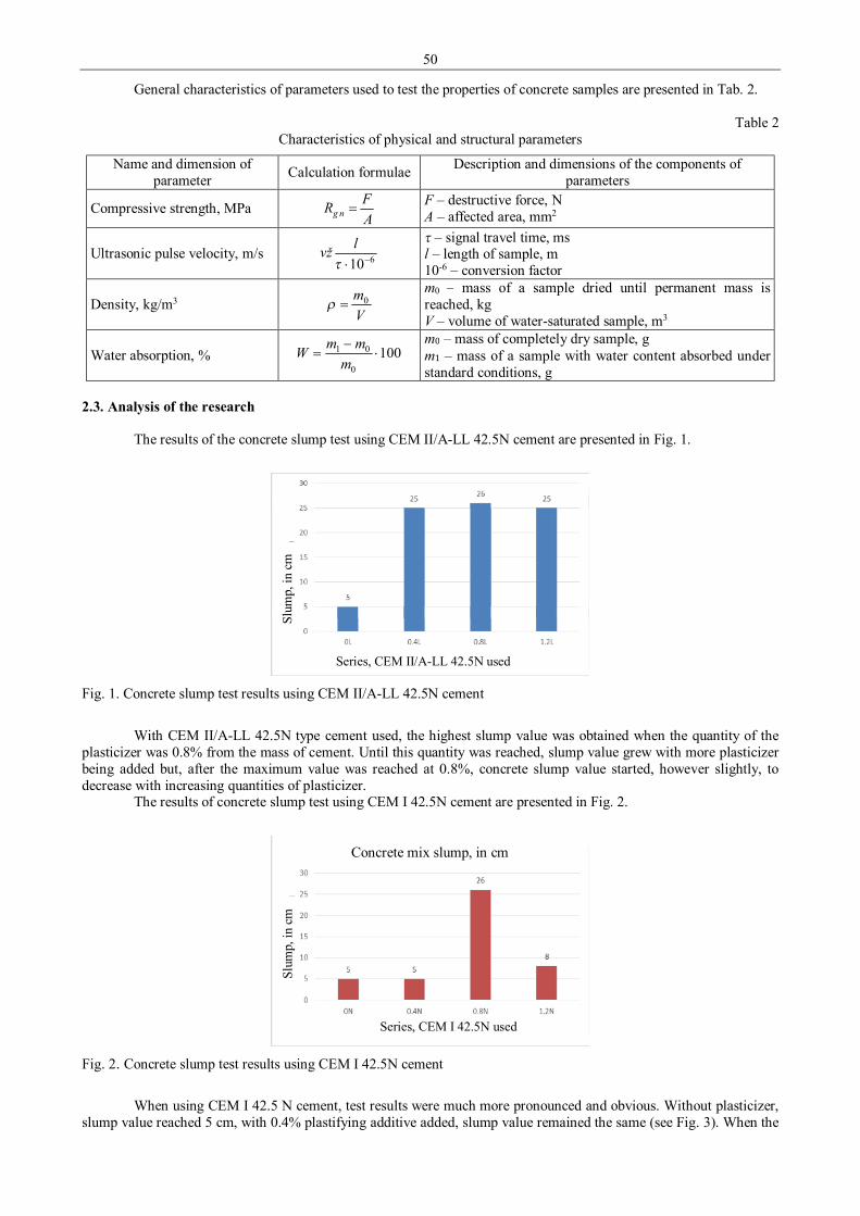
50

General characteristics of parameters used to test the properties of concrete samples are presented in Tab. 2.

Table 2 Characteristics of physical and structural parameters

Name and dimension of parameter Calculation formulae Description and dimensions of the components of

parameters

Compressive strength, MPa AFR ng = F – destructive force, N

A – affected area, mm2

Ultrasonic pulse velocity, m/s 610−⋅τlvž

τ – signal travel time, ms l – length of sample, m 10-6 – conversion factor

Density, kg/m3 Vm0=ρ

m0 – mass of a sample dried until permanent mass is reached, kg V – volume of water-saturated sample, m3

Water absorption, % 1000

01 ⋅−

=m

mmW m0 – mass of completely dry sample, g m1 – mass of a sample with water content absorbed under standard conditions, g

2.3. Analysis of the research

The results of the concrete slump test using CEM II/A-LL 42.5N cement are presented in Fig. 1.

Fig. 1. Concrete slump test results using CEM II/A-LL 42.5N cement

With CEM II/A-LL 42.5N type cement used, the highest slump value was obtained when the quantity of the

plasticizer was 0.8% from the mass of cement. Until this quantity was reached, slump value grew with more plasticizer being added but, after the maximum value was reached at 0.8%, concrete slump value started, however slightly, to decrease with increasing quantities of plasticizer.

The results of concrete slump test using CEM I 42.5N cement are presented in Fig. 2.

Fig. 2. Concrete slump test results using CEM I 42.5N cement

When using CEM I 42.5 N cement, test results were much more pronounced and obvious. Without plasticizer,

slump value reached 5 cm, with 0.4% plastifying additive added, slump value remained the same (see Fig. 3). When the

Slum

p, in

cm

Series, CEM II/A-LL 42.5N used

Slum

p, in

cm

Series, CEM I 42.5N used

Concrete mix slump, in cm

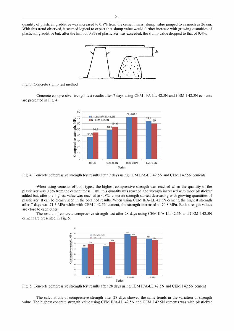
51

quantity of plastifying additive was increased to 0.8% from the cement mass, slump value jumped to as much as 26 cm. With this trend observed, it seemed logical to expect that slump value would further increase with growing quantities of plasticizing additive but, after the limit of 0.8% of plasticizer was exceeded, the slump value dropped to that of 0.4%.

Fig. 3. Concrete slump test method

Concrete compressive strength test results after 7 days using CEM II/A-LL 42.5N and CEM I 42.5N cements

are presented in Fig. 4.

Fig. 4. Concrete compressive strength test results after 7 days using CEM II/A-LL 42.5N and CEM I 42.5N cements

When using cements of both types, the highest compressive strength was reached when the quantity of the

plasticizer was 0.8% from the cement mass. Until this quantity was reached, the strength increased with more plasticizer added but, after the highest value was reached at 0.8%, concrete strength started decreasing with growing quantities of plasticizer. It can be clearly seen in the obtained results. When using CEM II/A-LL 42.5N cement, the highest strength after 7 days was 71.3 MPa while with CEM I 42.5N cement, the strength increased to 70.8 MPa. Both strength values are close to each other.

The results of concrete compressive strength test after 28 days using CEM II/A-LL 42.5N and CEM I 42.5N cement are presented in Fig. 5.

Fig. 5. Concrete compressive strength test results after 28 days using CEM II/A-LL 42.5N and CEM I 42.5N cement

The calculations of compressive strength after 28 days showed the same trends in the variation of strength

value. The highest concrete strength value using CEM II/A-LL 42.5N and CEM I 42.5N cements was with plasticizer

Com

pres

sive

stre

ngth

, MPa

Series

Com

pres

sive

stre

ngth

, MPa

Series

52

quantity of 0.8% and afterwards strength value started decreasing when more plasticizer was added. Compressive strength with CEM II/A-LL 42.5N cement was 71.3 MPa after 7 days and increased to 78.3 MPa after 28 days. With CEM I 42.5N cement, compressive strength increased from 70.8 MPa to 74.4 MPa.

The results obtained when investigating the kinetics of water absorption in the samples formed using CEM II/A-LL 42.5N are presented in Fig. 6.

Fig. 6. Water absorption kinetics of CEM II / A-LL 42.5 N

When analyzing the curves of water absorption kinetics, it was clear that the water absorption of concrete with

CEM II/A-LL 42.5N cement rapidly increased during the first 2 days of soaking rising from 0 to approx. 3–4.5%. Further increase of water absorption was already much slower and, after 4 days, the samples reached maximum water content and practically did not absorb any more water. The graph also shows that the higher the quantity of plastifying additive was, the lower the water absorption was.

The results obtained when investigating the kinetics of water absorption in the samples formed using CEM I 42.5N are presented in Fig. 7.

Fig. 7. Water absorption kinetics of CEM I 42.5 N

Fig. 8. Water absorption in concretes with different cements after 72 hours

Wat

er a

bsor

ptio

n af

ter 7

2 hr

s., %

Series

Wat

er a

bsor

ptio

n, %

Days Day 1 Day 2 Day 3 Day 6 Day 7

Wat

er a

bsor

ptio

n, %

Day 1 Day 2 Day 3 Day 6 Day 7

Days

53

Having investigated water absorption kinetics of samples when CEM I 42.5N cement was used to prepare them, the obtained results were similar to the results of samples prepared with CEM II/A-LL 42.5N cement. Water absorption rapidly increased during the first 2 days rising from 0 to 1.97–2.86%. During the following days, water absorption further increased and reached 3.04% in the samples that were prepared without plastifying additive.

Water absorption of concretes with different cements after 72 hours is presented in Fig. 8. When using CEM II/A-LL 42.5N cement, the highest water absorption value (3.12%) was obtained when no

plastifying additive was used. With the quantity of plasticizer being increased, water absorption decreased. Water absorption value was the lowest (1.69%) when 0.8% of plasticizer was added. When further increasing the quantity of plasticizer to 1.2%, water absorption started growing again and rose to 1.82%. The other cement gave different results. The highest water absorption value of samples made with CEM I 42.5N cement was also measured when no plastifying additive was used in the samples. With plasticizer added and its quantities increased, water absorption of samples decreased, dropping from 2.91% to 1.96%. 3. Conclusions

In order to obtain concrete with good properties, various additives are added to accelerate or slow down the binding of concrete mix, to make it more plastic, to accelerate hardening and to increase strength and water impermeability.

It has been found that the strength properties of concrete samples depend on the quantity of plastifying additive when hardening the samples in water. The comparison of two sorts of cement with equal quantities of plastifying additive has shown that the highest value was reached when using limestone Portland cement and 0.8% of plastifying additive.

Research has shown that polymer-based plastifying additive reduces water absorption in concrete when its quantity is 0.8%. With the said quantity of plasticizer, water absorption of concrete with CEM II/A-LL 42.5N cement was reduced by ~43% while water absorption of concrete with CEM I 42.5N cement was reduced by ~31%. References 1. Allahverdi A., Salem S. 2010. Simultaneous influences of microsilica and limestone powder on properties of

Portland cement paste. Ceramics – Silikaty 54(1), p. 65–71. 2. Bonavetti V., Donza H., Menendez G., Cabrera O., Irassar E. F. 2003. Limestone filler cement in low W/C

concrete: A rational use of energy. Cement and Concrete Research, 33, p. 865–871. 3. Nehdi M. 2003. Why some carbonate fillers cause rapid increases of viscosity in dispersed cement-based materials.

Cement and Concrete Research, 30, p.1663–1669. 4. Yahia A., Tanimura M., Shimoyama Y. 2005. Rheological properties of highly flowable mortar containing

limestone filler-effect of powder content and W/C ratio. Cement and Concrete Research, 35, p. 532–539. 5. Petit J. Y., Wirquin E. 2010. Effect of limestone filler content and superplasticizer dosage on rheological

parameters of highly flowable mortar under light pressure conditions. Cement and Concrete Research, 40, p. 235–240.

6. Nedhi M., Mindess S., Aitcin P. 1996. Optimization of high strength limestone filler cement mortars. Cement and Concrete Research, 26, p. 883–893.

7. Voglis N., Kakali G., Chaniotakis E., Taivilis S. 2005. Portland-limestone cements. Their properties and hydration compared to those of other composite cements, Cement and Concrete Composites, 27, p. 191–196.

8. Bentz D. P., Conway J. T. 2001. Computer modelling of the replacement of “coarse” cement particles by inert fillers in low W/C ratio concretes, 31, p. 503–506.

9. Taylor H. F. W. 1997. Cement Chemistry, second ed. Thomas Telford, London. 10. Naujokaitis A. 2007. Statybinės medžiagos, betonai. Vilnius, Technika, p. 13–25. 11. Калашников В. И. и др. 2006. Класификационнaя оценка цементов в присyтствии сyперластификаторов для

высокопрочныx бетонов. С. 39–42. 12. Nagrockienė D., Žurauskienė R. ir kt. 2010. Medžiagų mokslas, laboratorinių darbų metodikos nurodymai.

Vilnius, Technika, p. 49-63.

54

Proceedings of 9th International Conference ITELMS’2014 Panel – Frame Construction House Tightness Research A. Cepauskas*, S. Susinskas** *Kaunas University of Technology, S. Daukanto str. 12, 35212, Panevezys, Lithuania, E-mail: andriusps9@gmail.com **Kaunas University of Technology, S. Daukanto str. 12, 35212, Panevezys, Lithuania, E-mail: s.susinskas@ktu.lt Summary In this case study work I research panel – frame construction house tightness. I also review laws in wich requirements for buildings tightness are regulated and describe work equipment model as well as a shortened work course with given results. This study also reviews which specifications are necessary for good house tightness. All building parameters which are needed in order to accomplish tightness research are also described. This work consists of 4 chapters: introduction, measurements (all needed data and calculations are shown), conclusion and information sources list. KEYWORDS: panel frame construction buildings, tightness research. 1. Introduction

When technologies nowadays changes so fast there are a lot of possibilities to create something better than its precursor. This leads to easier life for all human beings. Various inventions cover all areas – building industry is no exception. One of the most important things to every of us is our living place, our home. While number of people on earth is growing rapidly the main goal of scientist and inventors is to find alternative resources for ones who are lacking. Modern buildings are built using newest design and installation technologies and materials.

In this case study I will research one of the most trending building industry sectors – panel frame construction buildings. We will test tightness of house which was build by Lithuanian company by demand and requirements of a client. We will also review data of this research.

A house is tight only if you can inflate air in it by using special equipment and generate a higher pressure then it is outside the house. In other word it means that fresh air can't get in through various cracks and walls because it would be a waste of heat. Hot air can't get into colder layers of house insulation because it would result in condensate generation which would lead to wet insulation material. If a building is not tight it is very affected by a direct wind. It is closely related to internal (steam isolation layer) ant windward (wind isolation and decoration) layers tightness, however it should transmit steam. In order to get better tightness it's needed to connect sheets with a respective bonding tape for outdoor and indoor works depending on what kind of sheets is needed to be connected.

In order to build a warm and tight house you need to pay attention not to insulation materials itself (however, it is also really important), but to internal tightness layer because it is most important.

There are a lot of various technologies and counting models to determine main buildings guardrails operational parameters, but to determine air tightness of a building you need special equipment and measurement which are discussed in LST EN 13829:2002. All main requirements for buildings air tightness are regulated in STR 2.05.01:2013 “Buildings energetic efficiency projection”. 2. Measurement

In order to perform air tightness test you need to know several important parameters, such as: 1. Outside climate parameters (speed of wind, air temperature); 2. Building internal temperature; 3. Building parameters that are needed in order to calculate its capacity (length, height, width);

When all needed measurements are done, blowing doors system Mineapolis BlowerDoor Modell 4 is being installed in a certain place of the building where outside borders with inside. Tightness test was done in two ways: first one, extracting air from building when pressures difference is to 50 Pa, the second method is done by blowing air into building when pressures difference is to 50 Pa.

Building information: 1. Premises capacity of 203 cube meters; 2. House has built in air ventilation system; Environment parameters: 1. Inside temperature: 23 °C; 2. Outside temperature: 17 °C; 3. Barometer pressure: 101.33 kPa.

Negative pressure averages: Δp01+ 0.2 Pa, Δp01- -0.6 Pa, Δp02+ 0.2 Pa, Δp02- -0.2 Pa. Over pressure averages: Δp01+ 0.1 Pa, Δp01- -0.7 Pa, Δp02+ 0.8 Pa, Δp02- -0.4 Pa.

55

Table 1 Negative pressure measurement data

Used ring, ABCDE Building pressure, Pa

Equipment pressure, Pa All air flow, m3/h Measurement bias,

% Δp01 -0.5 - - -

B -71 81 724 -1.50 B -66 72 686 -1.47 B -61 66 653 -0.35 B -56 58 613 -0.12 B -50 50 573 1.76 B -46 44 536 0.97 B -40 38 496 3.15 B -36 31 448 1.73 C -31 328 383 -2.88 C -25 255 336 -1.38

Δp02 -0.1 - - -

Table 2 Negative pressure measurement results

Correlation r = 0.997 Range Air flow rate cenv 30 max 36 min 26

Air leakage rate cL 31 max 36 min 26 Air flow exponent n 0.74 max 0.79 min 0.70

Table 3 Overpressure measurement data

Used ring, ABCDE Building pressure, Pa

Equipment pressure, Pa All air flow, m3/h Measurement bias,

% Δp01 -0.4 - - -

B 71 91 768 -1.11 B 67 93 777 4.17 B 61 72 684 -2.11 B 55 62 635 -2.15 B 49 56 602 0.18 B 44 49 566 0.82 B 39 40 511 -0.59 B 34 34 470 1.15 B 30 27 424 0.85 C 25 316 376 -0.74

Δp02 0.2 - - -

Table 4 Overpressure measurement results

Correlation r = 0.997 Range Air flow rate cenv 39 max 46 min 33

Air leakage rate cL 39 max 46 min 33 Air flow exponent n 0.70 max 0.75 min 0.66

Table 5 Overall results

V50 , m3/h Indeterminacy, % n50 , h-1 Indeterminacy, % w50 , m3/ m2h Indeterminacy, %

Nagative pressure 562 +/-7% 2.8 +/-7% 6.7 +/-7% Overpressure 615 +/-7% 3.0 +/-7% 7.3 +/-7%

Pressure average 589 +/-7% 2.9 +/-7% 7.0 +/-7%

56

Fig. 1. Tightness test air leak curve

3. Conclusions 1. Based on requirements from STR 2.05.01:2013 “Buildings energetic efficiency projection” measurements results is

n50 = 2.9. Building does not meet requirements that were given. 2. Air infiltration sources were found using thermal imaging cameras. It was caused by bad tightness and other

building actions. 3. The owner of the building was recommended to fix shortages that were found in order to make building tightness

and overall quality better. References 1. Available at. Am. [previewed 2014.04.02]: < http://www.am.lt/VI/index.php#r/313 >. 2. Available at. Energinis sertifikavimas. [previewed 2014.04.08]: < http://energinissertifikavimas.lt/pastatu-

sandarumo-testas-49?gclid=COWGv7v53b0CFRCWtAodmyMAlQ >. 3. Available at. Skydmedis. [previewed 2014.04.03]: < http://skydmedis.lt/LT/51/Konstrukcija.htm >. 4. Available at.Termas. [ previewed 2014.04.08]: < http://www.termas.lt/lt/pastat-diagnostika/sandarumo-testas >. 5. Pastatų energinio naudingumo projektavimas. STR 2.05.01:2013. Žin., 2013, Nr. 129-6566.

57

Proceedings of 9th International Conference ITELMS’2014 Property of the Monotonic Deformation of Aluminum Alloy 2024-T3 under Conditions of Complex Loading M. Chausov*, A. Pylypenko**, V. Berezin***, V. Hutsaylyuk****, L. Sniezek*****, J. Torzewski******

*National University of Life and Environmental Sciences of Ukraine, Geroiiv Oborony 12, 03041Kyiv, E-mail: Mich@nubip.edu.ua **National University of Life and Environmental Sciences of Ukraine, Geroiiv Oborony 12, 03041Kyiv, E-mail: andriy3pl@gmail.com ***National University of Life and Environmental Sciences of Ukraine, Geroiiv Oborony 12, 03041Kyiv, E-mail: valikb@yandex.ua ****Military University of Technology, Gen. S. Kaliskiego Str. 2, 00-908, Warsaw, Poland, E-mail: vhutsaylyuk@wat.edu.pl *****Military University of Technology, Gen. S. Kaliskiego Str. 2, 00-908, Warsaw, Poland, E-mail: lsniezek@wat.edu.pl ******Military University of Technology, Gen. S. Kaliskiego Str. 2, 00-908, Warsaw, Poland, E-mail: jtorzewski@wat.edu.pl Abstract This publication presents results of a research conducted on influence of force impulse loadings on the fracture kinetics in aluminum sheets made from 2024-T3 alloy, with the assistance of a complete diagrams method. It incorporates a full description of experimental research device for realization of a complex loading and analysis of research results in changes of mechanical properties in a deformation range (0...9%) in dependence from intensity of impulse loading. Aluminum alloy realises wide spectrum of its capabilities in connection to structure change under a complex loading from increase in general plasticity to practically instant fracture. KEYWORDS: aluminium alloy 2024-T3, impulse loading, dynamic non-equilibrium processes, additional impulse forces, complex static loading. 1. Introduction

Under the conditions of real exploitation engineering constructions may be subjected to action of different types of loads. Practically always object is subjected to actions of a few types of loads and to make prognosis for the resource of exploitation and strength reserve, it becomes very important to account their common actions.

Today, in the designs for the engineering construction for the basis accept one or two types of mostly character construction loads. This is due to difficulties in designs and lengthy analytical and numerical models of loading process. Considering all parameters in the process of loading – is a complex task, which not always can be realised on the basis of classical methods of a fracture mechanics.

Otherwise, critical situations and construction fracture mostly happen when construction material has been subjected to influence of additional, often one-time loading. This leads to following; material of the construction that is in the state of relative equilibrium, transforms into state of non-equilibrium.

The change of material mechanical properties in this condition can be characterised most adequately on the basis of mechanics of chaos.

In accordance with theory of non-equilibrium state and self-organization, processed by the school of I. Prigozhina [1-3], we may assume, that under external parameters on a mechanical system (material) by non linear parameters, it would adapt to the new state by the way of creation of the new arranged structure (state of material). This structure is a result of non-equilibrium phase transmissions, which in its turn are consequence of the change of leading parameters (loading). It is understood that mechanical properties of such structure will be different.

Especially importance, it has for the constructions that are design for static loading and in the process of exploitation can be additionally loaded with the force impulse.

Additional impulse loading depending on the value, velocity of realization, level of fatigue of main material, may lead to instant fracture of the material as well to some increase in plasticity of the material. Which does positively reflects on the general resource of the construction.

The research of a problem requires processing of methods as well development of adequate experimental equipment for application and realization of shock changes of additional loading in the process of the main one. In the publications [4], authors propose universal experimental device for the research of such phenomena and worked out general methodology for conducting of research for wide spectrum of materials.

58

Within the frame of the joint project with a Department of Material Resistance and Construction in Civil Engineering at the National University of Life and Environmental Sciences of Ukraine has been carried out a number of researches for studying changes in mechanical properties of aluminum alloy 2024-T3 under the conditions of complex loading.

The choice for the given material is stipulated by the frequent application in aviation construction for the highly responsible element of the plane construction. In addition material constantly is found under the influence of different kinds of loads, among which it is guaranteed, that at least once impulse force jumps will show up.

The goal of the research is evaluation of influence of changes in mechanical characteristics of given material under the influence of additional impulse loadings, under the conditions of static tensile, as one of the main types of loading of the main construction. 2. Materials and methods of mechanical research

The research was conducted on aluminum alloy 2024-T3, that was plated on both sides in the state of delivery; chemical content and mechanical properties of which are presented in the Table 1.

Table 1 Chemical content and mechanical properties of aluminum alloy 2024-T3

Chemical structure, % Cu Mg Mn Fe Zn

3.82-4.04 1.75-1.77 0.56 0.08-0.18 0.16 Mechanical properties in direct roller (LT)

Rm , MPa R02 , MPa A, % 459 - 466 339 – 345 21.5 – 24.7

Flat specimens were cut out from the sheet of aluminum in the direction of the rolling. Specimens were

measuring in working width of 10 mm and thickness of 3 mm (Fig. 1). A two series of specimens, each consisting of 20 pieces were researched.

The research of influence of additional impulse load was realized by using hydraulic machine ZD-100Pu, with experimental device proposed in [2-4]; general view of which is shown on Fig. 2.

Fig. 1. Specimen for the research

Fig. 2. Installation for a research of dynamic non-equilibrium processes: 1 – specimen; 2 – brittle specimens satellite;

3 – dynamometer rod; 4 – saddles

59

Additional impulse was realized on the elastic as well on non-elastic areas of deformation diagram in the range of ε =0…9%.

The processes of deformation and fracture of the material under shock changes in the mode of loading were researched as integral part of a mechanical system, statically not defined construction from three parallel elements (Fig. 2).

A central element of the system – grips with a spherical rests, dynamometer, strain gage and specimen of a researched material. Two symmetrical side elements 2, 3 rods with own stain-gauge dynamometers. Under the certain load of the whole system a brittle specimens-satellites failure and additional impulse load of the main sample is realized.

For realization of simultaneous fracture of brittle specimens saddles 4 were wedged out by four bolts with traverse under controlled effort.

The properties of the loading system determine velocity of material deformation under dynamic relocation of stresses, caused by the failure of specimens-satellites. Because of the inertia of a massive traverse, it was practically possible in the area of momentary increase in deformation velocity to instantly slow down process of deformation of plastic material.

As a result of such procedure, shock changes the energy balance in process of high velocity material deformation and a significant part of the energy that is released in the process of specimen-satellites failure, dissipates into researched material, causing substantial structure changes which accompaniment by “anomaly” of weakening on all stages of deformation.

Above mentioned effects of plastic material deformation appear only under applying to the mechanical system additional conditions. Those conditions in general view under testing of a standard specimen may be formulated as following [5]: 1. The number of stages in the process of shock changes in the loading mode has to be not less than three:

• on the first stage, deformation velocity drastically increases; • on the second stage, drastically slowing down; • on the third, again repeating increase.

All three stages of complex loading mode must be conducted continuously, without outside breaks in loading process.

2. Output impulses of influence on the system are set in the range of 100 – 1500 N·s during 0.02 s. 3. At the time of the testing, loading on the specimen should be transferred through spherical rests without a rigid

attachment. The test-device was equipped with computer assisted measurement system for parameters registration with the

frequency up to 2400 measurements per second and ability to record onto hard drive. Specimens fracture under the conditions of static tensile after a complex loading were carried out on servo-

hydraulic testing machine Instron 8501. Operation of the machine was performed by deformation with record of appropriate level of deformation and load onto computer’s hard drive. To measure deformation dynamical extensometrs with base measurement of 12.5 mm was used. Deformation velocity ε was estimated at10 mm/s.

Control specimen series in the amount of 20 pieces were tested in two stages. Stage one was carried out by deforming to maximum levels of deformation received at complex loading. The deformation velocity ε was at 1 mm/s.

Then specimens were unloaded and repeatedly were loaded until failure was recorded. In this case deformation velocity increased to level of ε =10 mm/s. 3. Results and discussions

To analyze the results of the research we needed to systematize received results. As criteria it has been selected values additional loading impulse and maximal value of material deformation

on the stage of additional loading. Since fracture of the two brittle specimen satellites was coming practically simultaneously (the difference in time and value of the impulse less than 1%) therefore for the analysis it has been accepted maximal value of one impulse (Fig. 3).

As it is shown on Fig. 3, all additional loading impulses practically are the same; the average impulse value located on the level of 110…116 kN for all specimens except one, which reaches practically 130 kN.

Additional impulse forces were performed in three deformation areas: 0…2 ε%; 3.5…5.5 ε%; 8.5…9 ε%. So, they were reaching into elastic and non-elastic areas of the fracture diagram (Fig. 4).

Since in the first and second group clearly visible significant density of impulse loadings, then for the further benefit of the analysis let us limit to selected specimens which are character to each of the groups. Again, in the each group we will analyze specimens in the order of increase of previous deformation value level under which additional impulse loading was performed. According to this specimens in the groups are located as follows, Fig. 5.

By analyzing fracture diagrams in groups it is important to notice that results obtained from the specimens under a complex loading were compared to the results of control group under static load (Fig. 6).

On the first stage of loading by realizing a scheme of complex loading a character mark is clear non-linear elasticity of the diagram area. On all graphs is clearly visible decrease and increase of elasticity. In all of this, at the moment of addition impulse force application, it’s not always able to register a jump of stress (Fig 6; a, b). Evidently, a

60

break that is registered on the graph (blue line with darkened circles) it is a second part of the impulse which is physically recorded by the measuring system. A velocity of fracture processes continuity physically exceeds speed of registration and recording system; therefore we obtain such result.

Fig. 3. Relation of additional impulse force to deformation

Fig. 4. Areas of overlaying of addition impulse force load on the diagram of static tensile of aluminum alloy 2024-Т3

I II III

Fig. 5. Distribution of specimens in groups by the level of previous plastic deformation of aluminum alloy 2024-T3 under complex loading

Second particularity found in following, that on the same area (Fig. 6, a-d) a graph reaches peak elasticity

stress, not a significantly greater than in comparative to ordinary static loading. This also, may be testifying that in a material a certain structural changes happen connected with change in active surface (volume) of material, capable of resistance to failure.

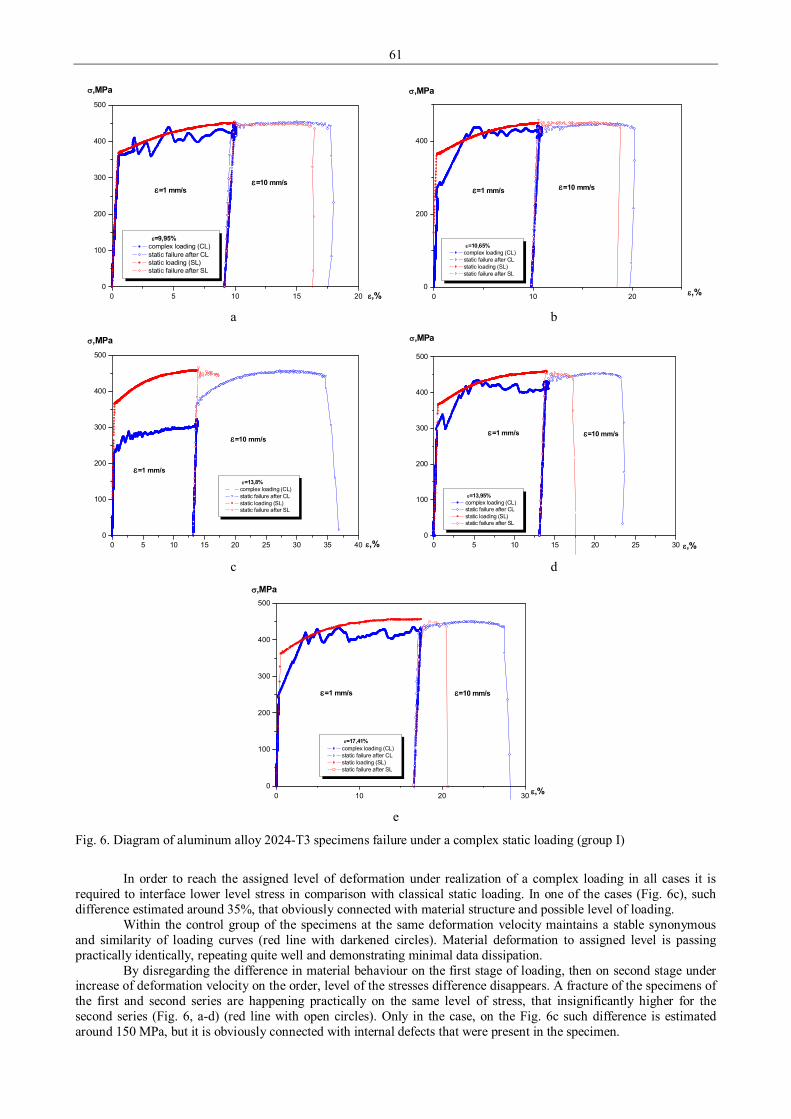
61

0 5 10 15 200

100

200

300

400

500

ε=10 mm/sε=1 mm/s

ε=9,95% complex loading (CL) static failure after CL static loading (SL) static failure after SL

σ,MPa

ε,%

0 10 200

200

400

ε=10,65% complex loading (CL) static failure after CL static loading (SL) static failure after SL

ε=1 mm/s ε=10 mm/s

σ,MPa

ε,%

а b

0 5 10 15 20 25 30 35 400

100

200

300

400

500

ε=13,8% complex loading (CL) static failure after CL static loading (SL) static failure after SL

ε=10 mm/s

ε=1 mm/s

σ,MPa

ε,%

0 5 10 15 20 25 300

100

200

300

400

500

ε=13,95% complex loading (CL) static failure after CL static loading (SL) static failure after SL

ε=1 mm/s ε=10 mm/s

σ,MPa

ε,%

с d

0 10 20 300

100

200

300

400

500

ε=17,41% complex loading (CL) static failure after CL static loading (SL) static failure after SL

ε=10 mm/sε=1 mm/s

σ,MPa

ε,%

e

Fig. 6. Diagram of aluminum alloy 2024-T3 specimens failure under a complex static loading (group I)

In order to reach the assigned level of deformation under realization of a complex loading in all cases it is

required to interface lower level stress in comparison with classical static loading. In one of the cases (Fig. 6c), such difference estimated around 35%, that obviously connected with material structure and possible level of loading.

Within the control group of the specimens at the same deformation velocity maintains a stable synonymous and similarity of loading curves (red line with darkened circles). Material deformation to assigned level is passing practically identically, repeating quite well and demonstrating minimal data dissipation.

By disregarding the difference in material behaviour on the first stage of loading, then on second stage under increase of deformation velocity on the order, level of the stresses difference disappears. A fracture of the specimens of the first and second series are happening practically on the same level of stress, that insignificantly higher for the second series (Fig. 6, a-d) (red line with open circles). Only in the case, on the Fig. 6c such difference is estimated around 150 MPa, but it is obviously connected with internal defects that were present in the specimen.

62

A more significantly differ areas of repeated static load in case of both specimen series in lengthwise. By comparing their prolonging it was notices that the material after a complex loading has much longer area of plasticity. Its length in respect to length at ordinary static loading changes from 0,3 to 3,1 times (Fig. 6; a, b, c, d). On the Fig. 6c, plasticity area almost five times greater from controlled. By excluding from the analysis this specimen, it is possible to affirm, that under complex loading the additional impulse force leads to increase of material plasticity under the room temperature. The mechanism of these phenomena apparent connected with material structure changes and perhaps requires additional research including a fractographic.

Simultaneously such material behaviour without a doubt is influenced by additional load impulse value, time and place of its application and deformation velocity. On the basis of this we may suppose, that in the case of additional impulse force (additional energy) system “specimen-equipment” by the account of internal reconstruction attempting to adapt to the new energy level, and creating at that time separate clusters with a new quality mechanical properties.

Such reconstruction is happening not in a whole volume of the material, but in separate sub-volumes in the direction of implementation of the force (energy impulses).

These affirmations in full scale relate to specimens from the second group (Fig. 7). On the first stage of loading none of the core differences were observed, besides that under a complex loading stress do not exceed suitable level under a static deformation (Fig. 7, a and d). In the case that is shown on the Fig. 7b with a maximal level of deformation covered with static deformation of second specimen series.

0 5 10 15 200

100

200

300

400

500

ε=6,72% complex loading (CL) static failure after CL static loading (SL) static failure after SL

ε=10 mm/sε=1 mm/s

σ,MPa

ε,%

0 5 10 15 200

100

200

300

400

500

ε=1 mm/sε=10 mm/s

ε=13,69%

complex loading (CL) static failure after CL staic loading SL static failure after SL

σ,MPa

ε,%

а b

0 5 10 15 20 250

100

200

300

400

500

ε=16,02% complex loading (CL) static failure after CL static loading (SL) static failure after SL

ε=10 mm/sε=1 mm/s

σ,MPa

ε,%

0 5 10 15 20 25 300

100

200

300

400

500

ε=17,72% complex loading (CL) static failure after CL static loading (SL) static failure after SL

ε=10 mm/sε=1 mm/s

σ,MPa

ε,%

с d

Fig. 7. Diagram of aluminum alloy 2024-T3 specimens failure under a complex static loading (group II)

The difference on the second stage of loading, within the border of the given group consists in that some of the

specimens on Fig. 7 a, c, d; under a repeated static loading practically failed by becoming brittle. The first series of specimens, after a complex loading was demonstrating a growth in plasticity in tens of times.

A specimen on the Fig. 7b is a single one in this group that did fracture similarly to the first group. When compared with corresponding graph from first group (Fig. 6d) let note that practically under a same impulses of additional loading and comparable levels of deformation, we receive somewhat smaller area of plasticity. However, growth order is maintained the same: 1.1 times in this case against 2 in the first group. Here it is obvious influences a level of deformation under which additional force impulse is realized.

All considerations that pertain to the research of structure and assumptions noted earlier for the explanation of the mechanism of this phenomenon are still maintaining its validity.

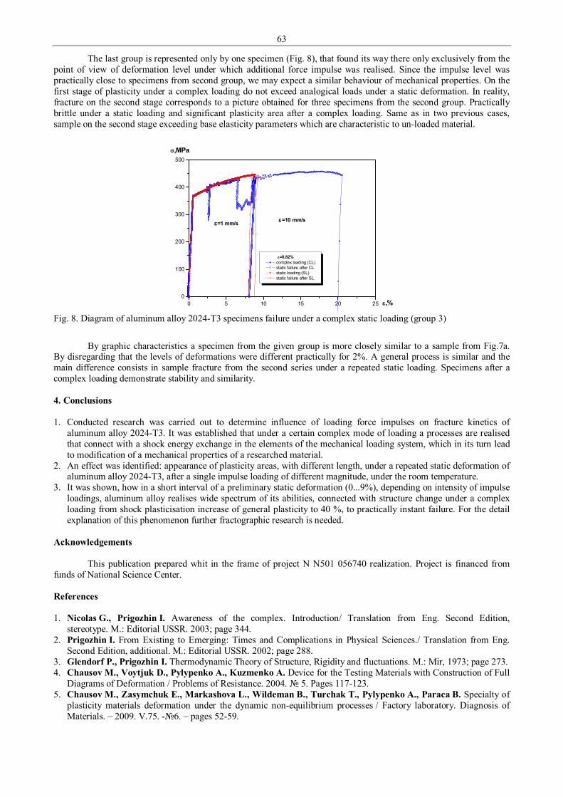
63

The last group is represented only by one specimen (Fig. 8), that found its way there only exclusively from the point of view of deformation level under which additional force impulse was realised. Since the impulse level was practically close to specimens from second group, we may expect a similar behaviour of mechanical properties. On the first stage of plasticity under a complex loading do not exceed analogical loads under a static deformation. In reality, fracture on the second stage corresponds to a picture obtained for three specimens from the second group. Practically brittle under a static loading and significant plasticity area after a complex loading. Same as in two previous cases, sample on the second stage exceeding base elasticity parameters which are characteristic to un-loaded material.

0 5 10 15 20 250

100

200

300

400

500

ε=8,82% complex loading (CL) static failure after CL static loading (SL) static failure after SL

ε=10 mm/sε=1 mm/s

σ,MPa

ε,%

Fig. 8. Diagram of aluminum alloy 2024-T3 specimens failure under a complex static loading (group 3)

By graphic characteristics a specimen from the given group is more closely similar to a sample from Fig.7a.

By disregarding that the levels of deformations were different practically for 2%. A general process is similar and the main difference consists in sample fracture from the second series under a repeated static loading. Specimens after a complex loading demonstrate stability and similarity. 4. Conclusions 1. Conducted research was carried out to determine influence of loading force impulses on fracture kinetics of

aluminum alloy 2024-T3. It was established that under a certain complex mode of loading a processes are realised that connect with a shock energy exchange in the elements of the mechanical loading system, which in its turn lead to modification of a mechanical properties of a researched material.

2. An effect was identified: appearance of plasticity areas, with different length, under a repeated static deformation of aluminum alloy 2024-T3, after a single impulse loading of different magnitude, under the room temperature.

3. It was shown, how in a short interval of a preliminary static deformation (0...9%), depending on intensity of impulse loadings, aluminum alloy realises wide spectrum of its abilities, connected with structure change under a complex loading from shock plasticisation increase of general plasticity to 40 %, to practically instant failure. For the detail explanation of this phenomenon further fractographic research is needed.

Acknowledgements

This publication prepared whit in the frame of project N N501 056740 realization. Project is financed from funds of National Science Center. References 1. Nicolas G., Prigozhin I. Awareness of the complex. Introduction/ Translation from Eng. Second Edition,

stereotype. M.: Editorial USSR. 2003; page 344. 2. Prigozhin I. From Existing to Emerging: Times and Complications in Physical Sciences./ Translation from Eng.

Second Edition, additional. M.: Editorial USSR. 2002; page 288. 3. Glendorf P., Prigozhin I. Thermodynamic Theory of Structure, Rigidity and fluctuations. M.: Mir, 1973; page 273. 4. Chausov M., Voytjuk D., Pylypenko A., Kuzmenko A. Device for the Testing Materials with Construction of Full

Diagrams of Deformation / Problems of Resistance. 2004. № 5. Pages 117-123. 5. Chausov M., Zasymchuk E., Markashova L., Wildeman B., Turchak T., Pylypenko A., Paraca B. Specialty of

plasticity materials deformation under the dynamic non-equilibrium processes / Factory laboratory. Diagnosis of Materials. – 2009. V.75. -№6. – pages 52-59.

64

Proceedings of 9th International Conference ITELMS’2014 Influence of Hydraulic Lines on Manipulator Movement Accuracy A. Dabrowska*, S. Konopka**, P. Krogul***, M. J. Lopatka**** *Military University of Technology, Kaliskiego 2, 00-908 Warsaw, Poland, adabrowska@wat.edu.pl **Military University of Technology, Kaliskiego 2, 00-908 Warsaw, Poland, skonopka@wat.edu.pl ***Military University of Technology, Kaliskiego 2, 00-908 Warsaw, Poland, pkrogul@wat.edu.pl ****Military University of Technology, Kaliskiego 2, 00-908 Warsaw, Poland, mlopatka@wat.edu.pl Abstract In the article was shown how the elasticity of hydraulic lines and the compressibility of a working medium affects the trajectory of the manipulator tool of an engineering robot. The study was done for a serial kinematic structure manipulator with two degrees of freedom. The methodology consisted of moving the manipulator tool along vertical and horizontal trajectories. The analysis of the required data was done based upon set geometrical reference parameters. KEY WORDS: manipulator, simulations, hydraulic, kinematics, dynamics. 1. Introduction

There exist a wide variety of different kinds of equipment for engineer robot manipulators. They differ from each other mainly by the range of functions and which drive unit is used. Particularly, manipulators of heavy engineer robots are characterized by a wide functionality. Most often they exceed operative range of 3 meters and have lifting capacity of above 100 kilograms. Bearing this in mind, the most commonly used drive for these devices is a hydrostatic drive unit. Components used in its construction may significantly affect the precision of the control of the engineer robot manipulator. This stems primarily from the nonlinearity and dynamics of the work of hydraulic control elements [1], but also from the elasticity of hydraulic lines and the compressibility of the working medium. Literature [2] shows how the length of elastic lines which link the control element and hydraulic receiver affects the eigen frequency, which directly stems from the elasticity of lines and the compressibility of the working medium. Unfortunately, there is lack of information as to how this affects the trajectory of manipulator tool.

The limitation in the control effectiveness also stems from the used manipulator control system. Most commonly it is a system based upon individual control of a particular hydraulic actuator by the appropriate over steering of joysticks [3, 4]. Such system is characterized by a low control intuitivity because of this it is hard to realize the established manipulator tool trajectory. In order to increase the control effectiveness, dedicated control systems [5-8] are built. Bearing this in mind, a concept of a control system where the manipulator tool copies horizontal and vertical motions of the operator’s hand was adopted in this article (Fig. 1).

The lack of explicit data on the topic of the impact of the elasticity of hydraulic lines and the compressibility of the working medium on the trajectory of manipulator tool limits the use of the proposed control system. Bearing this in mind, for the purposes of this article there have been performed simulation tests which accounted for the impact of the elasticity of hydraulic lines and the compressibility of the working medium on the trajectory of manipulator tool. The impact of any possible changes in the construction of the drive unit on the trajectory of the manipulator tool, namely the change of elastic lines to stiff lines, has also been taken into the account.

Fig. 1. The idea for an intuitive control system

65

2. The methodology of the simulation tests

The methodology of the simulation tests is in the accordance with the article [1]. It consists of mowing the manipulator tool along the 8 set trajectories (Figure 2), which stem from the assumed control system.

Fig. 2. The examined trajectories chart

The assessment of trajectories of manipulator tool in relation to set trajectories was done on the basis of 6

geometrical reference parameters (Fig. 3): • ymax (+) – the maximum positive deviation along the vertical direction of the manipulator tool trajectory, • ymax (−) – the maximum negative deviation along the vertical direction of the manipulator tool trajectory, • yk – the deviation along the vertical direction of the end of the manipulator tool trajectory from the set trajectory, • yAVE – the average arithmetic value of the manipulator tool trajectory, • yRMS – the average root mean square value of the manipulator tool trajectory, • r – the deviation of the manipulator tool trajectory

r = ymax(+) − ymax(−)

Fig. 3. The geometrical reference parameters chart

3. The structural model of the manipulator

In this article an open kinematic chain manipulator with two degrees of freedom was analyzed. The manipulator model is shown in the Figure 4, while his geometrical measurements are shown in the Table 2.

The program of the conference is intended to be published on Web page of KTU. The authors are requested to submit the manuscript (not exceeding six pages), summary and the presentation title (in English, up to 600 characters) before April 15, 2011 by E-mail as an attached file.

Main points in the construction of the manipulator model and his drive unit are: • individual elements were examined as uniform, non-deformable rod elements of set both mass and mass moment of

inertia, • actuators were examined as non-deformable elements of masses reduced to a point of their attachment,

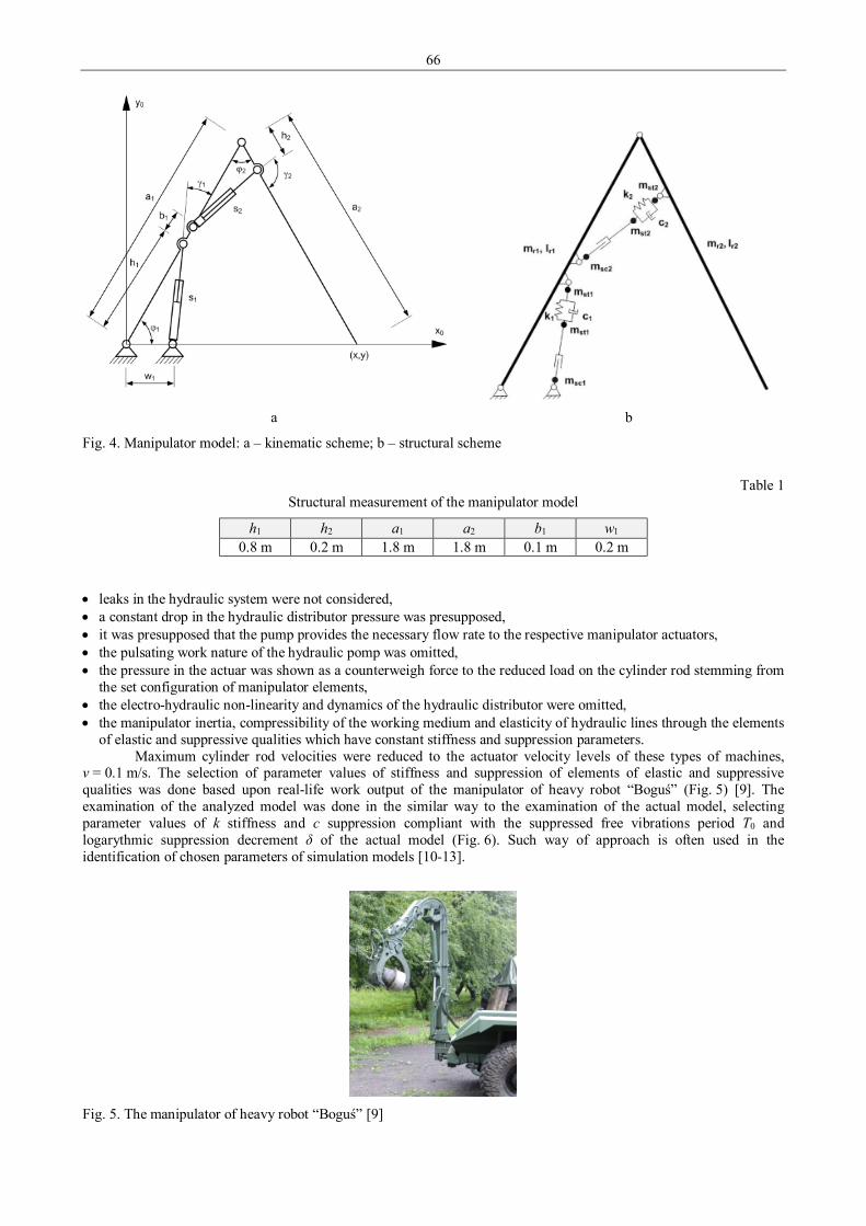
66

a

b

Fig. 4. Manipulator model: a – kinematic scheme; b – structural scheme

Table 1

Structural measurement of the manipulator model

h1 h2 a1 a2 b1 w1 0.8 m 0.2 m 1.8 m 1.8 m 0.1 m 0.2 m

• leaks in the hydraulic system were not considered, • a constant drop in the hydraulic distributor pressure was presupposed, • it was presupposed that the pump provides the necessary flow rate to the respective manipulator actuators, • the pulsating work nature of the hydraulic pomp was omitted, • the pressure in the actuar was shown as a counterweigh force to the reduced load on the cylinder rod stemming from

the set configuration of manipulator elements, • the electro-hydraulic non-linearity and dynamics of the hydraulic distributor were omitted, • the manipulator inertia, compressibility of the working medium and elasticity of hydraulic lines through the elements

of elastic and suppressive qualities which have constant stiffness and suppression parameters. Maximum cylinder rod velocities were reduced to the actuator velocity levels of these types of machines,

v = 0.1 m/s. The selection of parameter values of stiffness and suppression of elements of elastic and suppressive qualities was done based upon real-life work output of the manipulator of heavy robot “Boguś” (Fig. 5) [9]. The examination of the analyzed model was done in the similar way to the examination of the actual model, selecting parameter values of k stiffness and c suppression compliant with the suppressed free vibrations period T0 and logarythmic suppression decrement δ of the actual model (Fig. 6). Such way of approach is often used in the identification of chosen parameters of simulation models [10-13].

Fig. 5. The manipulator of heavy robot “Boguś” [9]

67

The value T0 = 0.8 s was taken directly from the pressure progression in the manipulator arm actuator of the “Boguś”, and the value of δ = 1.197 based upon the dependency relation of

2

1lnAA

=δ (1)

The δ, which was set in his way, allows for the calculation of zero-dimensional suppression rate ξ, which based upon the dependency relation of

0ω

ξh

= (2)

where: 0T

h δ= – suppression rate;

00

2Tπω = – eigenfrequency.

For such obtained values the zero-dimensional suppression rate δ was set on the level of ξ = 0.2. The work shown on the Fig. 5 was done by a manipulator in the maximum outreach with the grapple load of 180 kg in a sudden stop in the vertical position parallel to the surface. Keeping this mind, the examination of the set structural model was done in MSC Adams software designed for simulating compound mechanical systems. Based upon values of T0 and ξ, values of k1,2 = 12000 kN/m and c1,2 = 100 kNs/m were picked. The examined manipulator of the robot “Boguś”, for which T0 = 0.8 and ξ = 0.2, is equipped only with elastic lines linking the distributor with actuators (Fig. 5). By shortening the length of cables and substituting them with stiff lines, the change in the design approach was adopted, coupled with the change in values to T0 = 0.8-0.4 s and ξ = 0.4-0.2. For the examined manipulator, lower values from the set of values were accepted to be k1,2 = 40000 kN/m and c1,2 = 180 kNs/m.

Fig. 6. The progress of pressure in the grapple actuator in the manipulator arm of the robot “Boguś” in a sudden stop

in the vertical position parallel to the surface

4. The control signal

The signal controlling the manipulator tool was set upon set trajectories (Fig. 1). It was set on the basis of equation of motion of the manipulator tip stemming from the imposing of motions of its particular elements for the purposes of inverse kinematics [1]. The task was examined for the dyadic flat mechanism, which is the manipulator in question. On the basis of the depicted scheme (Fig. 7) dependencies were set which took into the account the grid references of point A(x, y) in the angle function φ2 .

Using the law of cosines

( )2212

22

12 cos2 ϕπ −−+= aaaac (3)

and taking into the account

222 yxc += and ( ) 22 coscos ϕϕπ −=− (4)

68

Fig. 7. The scheme for the setting of coordinate dependencies of the point A(x, y) in the angle function φ2

so after transformations

Taa

aayx=

−−+=

21

22

21

22

2 2cosϕ (5)

based on the above equation and tasking in to the account the dependency on the trigonometric identity the angle φ2 equals to

T

T 2

21arctg −−

=ϕ (6)

defining the angle φ1 was done under the condition of

ba 111 ϕϕϕ −= (7)

where

xy

a arctg1 =ϕ (8)

and φ1b was defined taking into the account the law of cosines

2222

1sinsin

yx

ab

+=

ϕϕ (9)

then, after necessary transformations

2

22

2222

1sin

sintgϕ

ϕϕayx

ab

−+

−= (10)

and substituting

2212

22

122 cos2 ϕaaaayx ++=+ (11)

the φ1b was defined as

221

221 cos

sinarctgϕ

ϕϕaa

ab +

= (12)

and so the angle φ1 equals to

221

221 cos

sinarctgarctgϕ

ϕϕaa

axy

+−

−= (13)

69

Defined in this way φ1 and φ2 dependencies were differentiated in relation to the x or y variable in dependency to the examined vertical or horizontal trajectory. Variable definitions were made in the accordance with the scheme on the Fig. 4a. Based on these dependencies, deployment speeds of individual actuators were assigned in dependency on φ1 and φ2 angles with accordance to the dependency of

−= 1111 2

cos γπϕ hs && and

−= 2222 2

cos γπϕ hs && (14)

Discretization of the above equations is done in the accordance with

−= 1111 2

cos γπϕ∆∆ hs and

−= 2222 2

cos γπϕ∆∆ hs (15)

and was inserted into the simulation program in order to simulate them. Next, it was defined that the nominal flow rate generated by the QN pump is equal to the sum of strains exerting the force on the particular actuators Q1 and Q2

QN = Q1 + Q2 (16)

Proportional division of the flow rate for the examined actuators was also taken into the account. It was done under the dependency of

22

11

2

1

FsFs

QQ

∆∆

= (17)

After appropriate transformation of dependencies (16) and (17) control signals for the individual actuators were set. This was done in the form of their speed

111

221

1 FFsFsQv N

+

=

∆∆

and

222

112

1 FFsFsQv N

+

=

∆∆

(18)

where: F1 and F2 – surface are of the piston of the actuator 1 and 2. 5. The results of the simulations tests

On the basis of the performed simulation tests, trajectory profiles of the vertical and horizontal coordinates of manipulator tool have been generated. Sample profiles generated in the MSC Adams software for the trajectories 3 and 6 are shown in the Fig. 8 and 9, where I describes the manipulator tool trajectory with elastic lines and II with stiff lines. Trajectory 3 of the horizontal trajectories is the hardest to realize together with the trajectory 6 from the vertical ones. This stems from the charts for the examined geometrical parameters.

Fig. 8. The profile of manipulator tool trajectory where: I-for elastic lines, II-for stiff lines

70

Fig. 9. The profile of manipulator tool trajectory where: I-for elastic lines, II-for stiff lines

On the basis of the parameter yAVE it can be said that, manipulator tool trajectory values are below required

horizontal trajectory values, while the opposite is true for the vertical trajectories. However, after examining the parameter yrms it was noted, that the structural changes of introducing stiff lines in the majority of cases noticeably improve the control precision. This is confirmed by the charts in the Fig. 10-15. It is also worth noting that in the case of vertical trajectories the structural changes do not improve significantly the control precision. In fact, they may even worsen it (parameters yrms and yAVE, for trajectory 6).

Fig. 10. The comparison of the influence of changing the stiffness of hydraulic lines in the functioning of examined

manipulator tool trajectories based on the ymax(+) parameter: I – for elastic lines; II – for stiff lines

Fig. 11. The comparison of the influence of changing the stiffness of hydraulic lines in the functioning of examined

manipulator tool trajectories based on the ymax(−) parameter: I – for elastic lines; II – for stiff lines

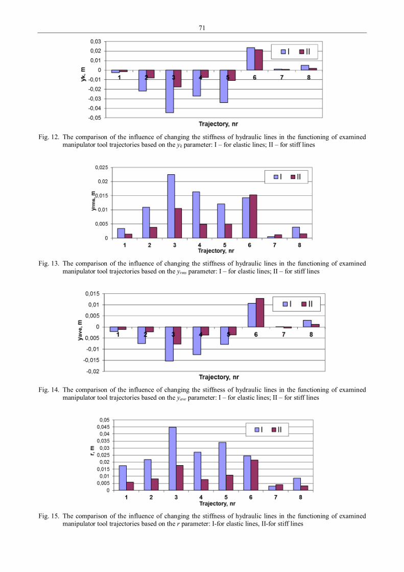
71

Fig. 12. The comparison of the influence of changing the stiffness of hydraulic lines in the functioning of examined

manipulator tool trajectories based on the yk parameter: I – for elastic lines; II – for stiff lines

Fig. 13. The comparison of the influence of changing the stiffness of hydraulic lines in the functioning of examined

manipulator tool trajectories based on the yrms parameter: I – for elastic lines; II – for stiff lines

Fig. 14. The comparison of the influence of changing the stiffness of hydraulic lines in the functioning of examined

manipulator tool trajectories based on the yave parameter: I – for elastic lines; II – for stiff lines

Fig. 15. The comparison of the influence of changing the stiffness of hydraulic lines in the functioning of examined

manipulator tool trajectories based on the r parameter: I-for elastic lines, II-for stiff lines

72

6. Conclusion

Based upon the received simulation tests results it was concluded, that the manipulator tool trajectory deviation, which stems from the stiffness of the hydraulic lines, is couple of centimeters. Maximal manipulator tool trajectory deviation values reach 4.5 centimeters. Adopting the structural changes which influence the stiffness and the suppression of hydraulic lines and the compressibility of the working medium may decrease twofold the manipulator tool trajectory deviation from the required norm, and therefore increase the control precision. To sum up, in the majority of cases the influence of the lines stiffness on the manipulator tool trajectory control precision is not significant and it could be disregarded. However, not taking into the account the examined phenomenon as early as in the design phase, can severely hamper the effectiveness of the realization of the tasks which require high precision, like for example the process of pipe welding. References 1. Konopka S., Krogul P., Łopatka M. J. Simulation Research of Hydrostatic Power System Control of Engineer

Robot Manipulator, Proceedings of 8th International Conference Intelligent Technologies in Logistics and Mechatronics Systems ITELMS‘2013, pp. 126-135, Panevėžys, Lithuania, May 23-24, 2013.

2. Bartnicki A. Badanie właściwości I kształtowanie sterowania hydrostatycznymi układami napędowymi z kompensacją obciążenia, Ph.D. Thesis, Military University of Technology, Warsaw, 2004.

3. Dąbrowska A., Typiak R. Universal Robotic Control Station for a Grouping of Unmanned Egineering Machines, Proceedings of 8th International Conference Intelligent Technologies in Logistics and Mechatronics Systems ITELMS ‘2013, pp. 71-75, Panevėžys, Lithuania, May 23-24, 2013.

4. Zareinia K., Maddahi Y., Sepehri N., Olson T., Mueller W. Unilateral control of teleoperated hydraulic manipulators for live-line maintenance: Comperative study, International Journal of Robotics & Automation, volume 29, pp. 162-174, 2014.

5. Kim D., Kim J., Lee K., Park C., Song J., Kang D. Excavator tele-operation system using a human arm, Automation in Construction 18, vol. 18, pp. 173-182, 2009.

6. Bartnicki A., Sprawka P., Rubiec A. Remote Control system for Rescue Robot, XIV Konferencja automatyzacji i Eksploatacji systemów Sterowania i Łączności ASMOR 2013, Jastrzębia Góra 2013.

7. Pratumsuwan P., Hutamarn S., Po-Ngaen W. A development of tele-controller for hydraulic excavator, Proceedings of the 2012 7th IEEE Conference on Industrial Electronics and Applications, pp. 2123-2126, 2012.

8. Raush G., Freire F., Khamashta M. Hydraulic robot arm controlled by visual servoing, Precision Agriculture’13, pp. 365-371, 2013.

9. Research Project nr. 0012/R/T00/2008/06: Bezzałogowy pojazd do wykonywania zadań w strefach zagrożeni, WAT, Warsaw, 2011.

10. Konopka S., Krogul P., Łopatka M. J., Muszyński T. Symulacyjna analiza stateczności maszyn przegubowych na przykładzie ładowarki kołowej Ł34, Przegląd Mechaniczny, nr 11/2013, str. 13, Warszawa 2013.

11. Bartnicki A., Jaskółowski M., Łopatka M. J., Muszyński T. The Researches of Stability Evaluation Articulated Loader while Working on Slopes, Proceedings of 8th International Conference Intelligent Technologies in Logistics and Mechatronics Systems ITELMS ‘2013, pp. 126-135, Panevėžys, Lithuania, May 44-49, 2013.

12. Bartnicki A., Łopatka M. J., Muszyński T., Rubiec A. Stiffness Evaluation of Fire Rescue Robot Suspension with Hydropneumatic components, XIV Konferencja automatyzacji i Eksploatacji systemów Sterowania i Łączności ASMOR 2013, Jastrzębia Góra 2013.

13. Konopka S., Łopatka M. J. Podstawy konstrukcji maszyn z CAD, część 4 modelowanie ruchu maszyn, WAT, Warsaw, 2005.

73

Proceedings of 9th International Conference ITELMS’2014 Sandwich Panels with Different Fillings Rational Selection Research J. Daunoravicius*, S. Susinskas** *Kaunas University of Technology, S. Daukanto str. 12, 35212, Panevezys, Lithuania, E-mail: justinas19900211@gmail.com **Kaunas University of Technology, S. Daukanto str. 12, 35212, Panevezys, Lithuania, E-mail: s.susinskas@ktu.lt Summary In order to find out most rational sandwich panels filling, we examined basic technical characteristics while applying methodology analysis and market research techniques. The main object of the research – sandwich panels fillings. While applying methodology analysis and market research techniques we identify most important technical characteristics, draw respective diagrams and select most rational filling. KEYWORDS: sandwich panels, fillings, technical characteristics, rationality. 1. Introduction

Nowadays industry is growing faster and faster, in order to build buildings faster and cheaper various alternative building materials gets more popularity. Most of industrial buildings concrete constructions are replaced with newer and more effective constructions. One of the most important constructions is a wall. In order to build wall cheaper and faster builders use sandwich panels. In process of this research we established which sandwich panels filling is most effective, calculated heat transference coefficients and compared fillings types by price and weight. 2. Process

Using formulas:

dec

dRλ

= (1)

R

U 1= (2)

there: R – heat resistance; d – panel thickness; λdec – determined heat resistance coefficient; U – heat transference coefficient, heat transference coefficients of 80, 100, 120, 140, 160, 200 mm thickness sandwich panels with polystyrene foam, mineral wool and polyurethane fillings is calculated. Results are show in Table 1 and Fig. 1.

Table 1 Sandwich panels with different fillings heat transference coefficient calculation

d, mm Polystyrene foam Mineral wool Polyurethane λdec, W/m·K U, W/m2·K λdec, W/m·K U, W/m2·K λdec, W/m·K U, W/m2·K

80 0.0035 0.43 0.0041 0.51 0.0021 0.26 100 0.0035 0.35 0.0041 0.41 0.0021 0.21 120 0.0035 0.28 0.0041 0.34 0.0021 0.17 140 0.0035 0.25 0.0041 0.30 0.0021 0.13 160 0.0035 0.21 0.0041 0.26 0.0021 0.11 200 0.0035 0.17 0.0041 0.21 0.0021 0.10

Market analysis method shows us different sandwich panels fillings square meter price dependence of its

thickness (as shown in Fig. 2). Interesting fact – as manufacturer says concrete wall panels which characteristics is similar to 140 mm. thickness sandwich panel costs around 260 LT per one square meter and it is 2.7 times more than cheapest sandwich panel.

In building sites many employers not understand importancy of sandwitch panel weight. There are many situations when it is not possible to lift a sandwich panel with a crane so workers may need to do it manually, using diesel or scissor lifters. In that case it is important to choose panels with filling which has least load for a one square meter. In Fig. 3 you can see results of analysis how different types of fillings affect panels weight depending on its thickness.

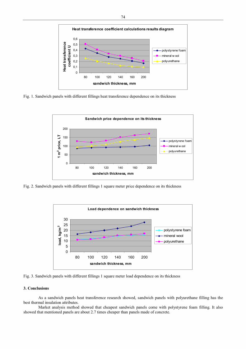
74

Heat transference coefficient calculations results diagram

0

0,1

0,2

0,3

0,4

0,5

0,6

80 100 120 140 160 200

sandwich thickness, mm

Heat

tran

sfer

ence

co

effic

ient

U

polystyrene foam

mineral w ool

polyurethane

Fig. 1. Sandwich panels with different fillings heat transference dependence on its thickness

Sandwich price dependence on its thickness

0

50

100

150

200

80 100 120 140 160 200

sandwich thickness, mm

1 m

2 pri

ce, L

T

polystyrene foam

mineral w ool

polyurethane

Fig. 2. Sandwich panels with different fillings 1 square meter price dependence on its thickness

Load dependence on sandwich thickness

05

1015202530

80 100 120 140 160 200sandwich thickness, mm

load

, kg/

m2

polystyrene foammineral woolpolyurethane

Fig. 3. Sandwich panels with different fillings 1 square meter load dependence on its thickness

3. Conclusions

As a sandwich panels heat transference research showed, sandwich panels with polyurethane filling has the best thermal insulation attributes.

Market analysis method showed that cheapest sandwich panels come with polystyrene foam filling. It also showed that mentioned panels are about 2.7 times cheaper than panels made of concrete.

75

According to a manufacturer date we compared sandwich panel’s fillings load per 1 square meter. This comparison showed us that sandwich panels with mineral wool filling has much bigger load than 2 other fillings, in that case it is wise not to choose sandwich panels with mineral wool filling.

According to results we came to conclusion that it is best to use sandwich panels with polystyrene foam fillings, but only wool filling is fireproof so it is only one that could be used to build firewalls. References 1. Kizinievič O., Žurauskienė R. Inovatyvios polimerinės statybinės medžiagos ir dirbiniai. – Vilnius: Technika,

2012, 104 p. 2. Metalplast sistema product catalogue, 2012. 3. Ruuki sandwitch panels catalogue, 2013. 4. Daugiasluoksnės plokštės internetu [interactive]. Available at: < http://www.b-a.lt/c1759/Daugiasluoksnes-plokstes-

sendwich-plokstes- > [previewed 2014-03-22]. 5. PU sandwitch panels [interactive]. Available at: < http://plytacmb.pl/en/2-pu-sandwich-panels > [previewed 2014-

03-24].

76

Proceedings of 9th International Conference ITELMS’2014 The Analysis of Accident Rate in the Baltic States (2008–2013) A. Demeniene*, D. Striukiene**, E. Zacharoviene***, R. Laurikietyte****, P. Vaiciulis***** *Kaunas University of Technology Panevezys Faculty of Technologies and Business, Nemuno str. 33, 37164, Panevėžys, Lithuania, E-mail: alina.demeniene@ktu.lt **Kaunas University of Technology Panevezys Faculty of Technologies and Business, Nemuno str. 33, 37164, Panevėžys, Lithuania, E-mail: danguole.striukiene@ktu.lt ***Kaunas University of Technology Panevezys Faculty of Technologies and Business, Nemuno str. 33, 37164, Panevėžys, Lithuania, E-mail: elvyra.zacharoviene@ktu.lt ****Kaunas University of Technology Panevezys Faculty of Technologies and Business, Nemuno str. 33, 37164, Panevėžys, Lithuania, E-mail: rita.laurikietyte@ktu.lt *****Vilnius Gediminas Technical University Faculty of Transport Engineering, J. Basanaviciaus str. 28, 03224, Vilnius, Lithuania, E-mail: pauliusvaiciulis@outlook.com Abstract The object of the article is accident rate in the Baltic States. The aim of the article is to assess the situation of accident rate in the Baltic States over the period of 2008−2013. KEYWORDS: transport, accident rate. 1. Introduction

The speed of today’s life inevitably increases traffic density, the number of cars and other vehicles. Traffic density determines the number of road accidents, the injured and road deaths. The problems of traffic safety and accident rate are the object of research of many fields of science. The article is focused mainly on the complex analysis of accident rate in the Baltic States. Complex attitude towards the analysed phenomenon allows covering socio-dynamic tendencies of traffic safety and helps design the methods of managing accident rate by assessing the injury accidents preconditioning factors, specifying territorial regions and outlining the traffic safety implementation strategy.

A favourable geographical and geopolitical position of the Baltic States allows successful integration into the European transport network and the transport services market. Therefore, the issues of traffic safety become a priority area in analyzing social phenomena within the European Union membership.

The tasks of the analysis: 1. To present the analysis of secondary statistic data over the described period. 2. To reveal the main reasons of accidents. 3. To describe the situation of the implementation and improvement of safety measures on roads by highlighting the

impact of these measures on the accident rate indices. Methods used: analysis of scientific literature; analysis of legal documents; analysis of secondary statistical

data. 2. Results and discusion

Every day we hear about road accidents, road deaths and the injured. Traffic safety is one of the oldest and the most important problems. The article presents the analysis of accident rate on Lithuanian, Latvian and Estonian roads in 2008-2013. Indices used for the analysis: the number of accidents, the number of the injured, and the number of road deaths. The information has been taken from available statistic data of the Baltic States and the European Union (Lithuanian Traffic Police Service; Statistics Estonia, Statistics Latvia, 2014).

Over the period of 2008−2012, on the Baltic roads 48,179 injury accidents were recorded, in which 53,535 people were injured and 3,377 road users were killed (European Commission Directorate General Energy and Transport, 2014).

Fig. 1 shows that over the analysed period (2008−2012), the biggest number of traffic accidents occurred in Latvia (46%). Fig. 2 shows that from 2008 until 2012, the number of accidents per one million of the population in Latvia decreased from 4,059 to 1,642. If compared to 2009−2012, the number of accidents from 2009 until 2012(13) increased from 1,461 to 1,642.

In Lithuania and Estonia the number of accidents from 2008 until 2012 decreased approximately by 20%. The reasons of accidents can be highly diverse. The most common factors of reasons of traffic accidents: road

user (human factor); vehicle; road; the surrounding environment (Gužys, 2004), the public (Pečeliūnas, Pikūnas, 2005). Other researchers analyse criminalistic characteristics of traffic accidents on roads and assess their importance to accident prevention (Novikovienė, 2009). Dainauskas, Bražukienė (2013) name the factors that determine accident rate

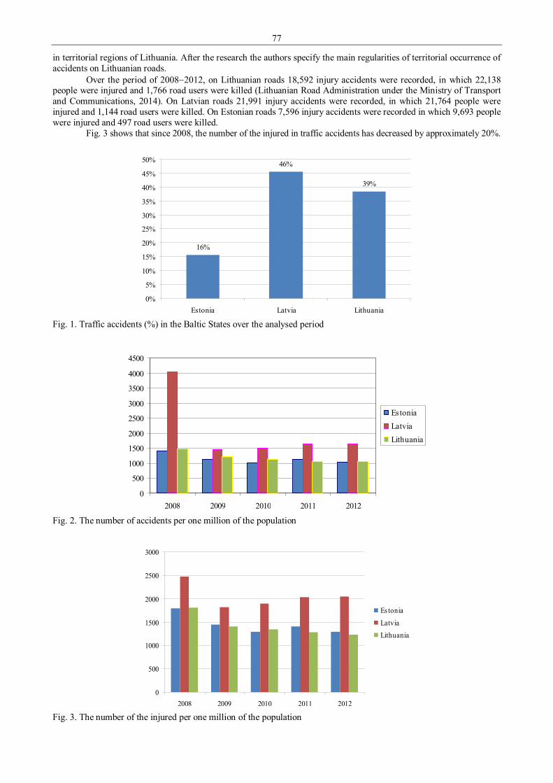
77

in territorial regions of Lithuania. After the research the authors specify the main regularities of territorial occurrence of accidents on Lithuanian roads.

Over the period of 2008−2012, on Lithuanian roads 18,592 injury accidents were recorded, in which 22,138 people were injured and 1,766 road users were killed (Lithuanian Road Administration under the Ministry of Transport and Communications, 2014). On Latvian roads 21,991 injury accidents were recorded, in which 21,764 people were injured and 1,144 road users were killed. On Estonian roads 7,596 injury accidents were recorded in which 9,693 people were injured and 497 road users were killed.

Fig. 3 shows that since 2008, the number of the injured in traffic accidents has decreased by approximately 20%.

16%

46%

39%

0%

5%

10%

15%

20%

25%

30%

35%

40%

45%

50%

Estonia Latvia Lithuania Fig. 1. Traffic accidents (%) in the Baltic States over the analysed period

0

500

1000

1500

2000

2500

3000

3500

4000

4500

2008 2009 2010 2011 2012

EstoniaLatviaLithuania

Fig. 2. The number of accidents per one million of the population

0

500

1000

1500

2000

2500

3000

2008 2009 2010 2011 2012

Es tonia

LatviaLithuania

Fig. 3. The number of the injured per one million of the population

78

0

20

40

60

80

100

120

140

160

2008 2009 2010 2011 2012 2013

EstoniaLatviaLithuaniaEU average

Fig. 4. The number of deaths per one million of the population

From 2008 until 2013, in Lithuania the number of deaths on roads decreased from 155 to 85 (Fig. 4). However,

since 2008, by the biggest number of deaths on roads our country shares the leading position with Latvia. It means that Lithuania and Latvia are the countries of increased risk, although total accident rate (by other indices) in Lithuania has decreased. Comparing statistical data of all the European Union countries, the European Union has an average of 52 road deaths per one million of the population (Fig. 4). Thus compared to the European Union average (52 deaths per one million of the population), the number of road deaths in Lithuania and Latvia remains high. According to the data of the European Commission, Lithuanian drivers are the most dangerous ones in Europe. The growing accident rate and the number of deaths have reached the limit that cannot be tolerated any longer. The problem of road traffic safety can be solved only when it is addressed at all levels of government and through a variety of legal, administrative, engineering and educational measures. 3. Conclusions

Following the analysis of scientific literature, the notion of accident rate has been conceptualized. Accident rate is the process involving not only external reasons; it is also conditioned by internal human motives.

The analysis of secondary statistic data of accident rate in the Baltic States has revealed an interrelation between the traffic density and the growth of accident rate. Congested traffic and intensive movement of transport flows create favourable conditions for accidents; therefore, the probability of encountering a traffic accident in an intensive transport flow is higher.

The analysis of statistical data of the accident rate indices of 2008−2013 has revealed that the number of traffic accidents on roads is decreasing and the situation of accident rate in the Baltic States has stabilized. References 1. European Commission. Available at: < http://ec.europa.eu/transport/road_safety/index_en.htm >, < http://ec.europa.eu/

transport/road_safety/pdf/observatory/historical_evol_popul.pdf >, < http://ec.europa.eu/transport/road_safety/pdf/ com_20072010_en.pdf > [viewed on 10-04-2014].

2. Lithuanian Traffic Police Service. Available at: < http://www.lkpt.lt > [viewed on 10-04-2014]. 3. DELFI news. Available at: < http://www.delfi.lt/auto/patarimai/lietuva-jau-nebe-paskutine-pagal-zuvusiuju-keliuose-

skaiciu.d?id=64411440#ixzz32nzsIFYR > [viewed on 10-04-2014]. 4. Statistics Lithuania. Available at: < http://db1.stat.gov.lt/statbank/selecttable/omrade0.asp?SubjectCode=S7&

PLanguage=0&ShowNews=OFF > [viewed on 10-04-2014]. 5. Statistics Estonia. Available at: < http://www.stat.ee/34300 > [viewed on 10-04-2014]. 6. Statistics Latvia. Available at: < http://www.csb.gov.lv/ > [viewed on 10-04-2014]. 7. Gužys A. Eismo problemos ir žmogiškas faktorius. Lietuvos keliai, 2004, 2: 57–61. 8. Pikūnas A., Pečeliūnas R. Saugaus kelių eismo problemos Lietuvoje. XIII pasaulio lietuvių mokslo ir kūrybos

simpoziumas. Tezių rinkinys. – Vilnius: Lietuvos Respublikos švietimo ir mokslo ministerija, Lietuvos mokslų akademija, Lietuvos mokslininkų sąjunga, 2005.

9. Tumas V., Čigrin V. Kelių eismo saugumo užtikrinimo ypatumai. Visuomenės saugumas ir viešoji tvarka. – Kaunas: Mykolo Riomerio universitetas, 2010. 4: 268–275.

10. Lithuanian Road Administrtion under the Ministry of Transport and Communications of the Republic of Lithuania. Available at: < http://www.lakd.lt/lt.php/lietuvos_keliai/29 > [viewed on 10-04-2014].

79

11. Ministry of Transport and Communications of the Republic of Lithuania. Available at: < http://www.transp.lt/lt/ > [viewed on 10-04-2014].

12. Dainauskas S., Bražukienė I. Lietuvos automobilių kelių avaringumo teritorinė analizė. Geografija. 2013. T. 49. Nr. 1.,p. 82–92

13. Novikovienė L. Eismo įvykių kriminalistinė charakteristika ir jos reikšmė eismo įvykių prevencijai. Current Issues of Business and Law, 2009, Vol. 4.

80

Proceedings of 9th International Conference ITELMS’2014 The Impact of Psychological and Psychosocial Factors on Accident Rate A. Demeniene*, D. Striukiene**, E. Zacharoviene***, A. Valackiene****, R. Laurikietyte*****, P. Vaiciulis****** *Kaunas University of Technology Panevezys Faculty of Technologies and Business, Nemuno str. 33, 37164, Panevėžys, Lithuania, E-mail: alina.demeniene@ktu.lt **Kaunas University of Technology Panevezys Faculty of Technologies and Business, Nemuno str. 33, 37164, Panevėžys, Lithuania, E-mail: danguole.striukiene@ktu.lt ***Kaunas University of Technology Panevezys Faculty of Technologies and Business, Nemuno str. 33, 37164, Panevėžys, Lithuania, E-mail: elvyra.zacharoviene@ktu.lt ****Kaunas University of Technology Panevezys Faculty of Technologies and Business, Nemuno str. 33, 37164, Panevėžys, Lithuania, E-mail: astas.valackiene@ktu.lt *****Kaunas University of Technology Panevezys Faculty of Technologies and Business, Nemuno str. 33, 37164, Panevėžys, Lithuania, E-mail: rita.laurikietyte@ktu.lt ******Vilnius Gediminas Technical University Faculty of Transport Engineering, J. Basanaviciaus str. 28, 03224, Vilnius, Lithuania, E-mail: pauliusvaiciulis@outlook.com Abstract The object of the article is the impact of psychological and psychosocial factors on accident rate. The aim of the analysis is to assess the impact of psychological and psychosocial factors on accident rate. KEYWORDS: lunar cycle, lunar days, insurance events, weekdays, seasons. 1. Introduction

Since ancient times, people have been interested in lunar impact on the earth and humans. Ancient philosophers asserted that the moon had a negative impact on human mind. In the long run, the philosophers‘ views were replaced by scientifically-based truths. More and more scientific research is being carried out in order to assess the effect of the lunar cycle on human body. The effect is caused by strong gravitational lunar impact on the earth surface. Today‘s science seeks to prove the influence of the moon to reasonability of human actions, decision making and personal safety. In many scientific articles this topic becomes the object of analysis. In most publications, two phases of the lunar cycle are being studied – new moon and full moon, both affecting humans. In new moon and full moon, the following physical parameters of the earth change: humidity, atmospheric pressure, temperature, and electric and magnetic fields. Even the slightest variation of these parameters influences a human body. The matters in question are analysed further through science projects.

The tasks of the analysis: • to look into scientific research that discloses an interaction field of the accident rate and the lunar cycle; • to present the analysis of secondary statistical data of insurance events to justify interaction between the accident rate

and the lunar cycle. 2. Results and discusion

In order to prove the importance of the topic in question, it is worth mentioning that in 2005, California Council on Science and Technology financed the project “The Effects of the Lunar Cycle on Rates of Fatal Car Accidents” [1]. Scientists of this country carried out a research using the method of experiment and analysed situations of car accidents and emergencies over five years taking into consideration lunar impact on human behaviour. The project report introduces the facts obtained during the experiment, which justify hypothetical assumptions about the interaction of the lunar cycle and human behaviour on roads.

Research of this type has also been carried out by Swiss scientists. They present the obtained objective facts, which show that the work of human brain changes depending on the lunar cycle [2]. The research disclosed that psychosocial and natural factors are truly interrelated: the phase of the new moon strongly affects human mind. It can be noticed that a person has distorted perception of reality; he can be easily controlled from the outside and affected adversely [3].

It was found out that in full moon, the earth and the moon are in an opposing position because in respect of the sun, the moon is at a distance of 180 degrees and is completely illuminated. In this situation, both of them affect the earth in an adversative manner, which causes huge stress. It was found out that in this phase, people suffer from misbalance and rush, make reckless actions and their behaviour becomes unpredictable. Loss of self-control causes a lot of conflicts, injuries, accidents, violence and crimes [3].

81

According to the information of the insurance company BTA [4], accident rate is also influenced by the lunar cycle. They say that “when the moon is on the wane, accident rate on roads exceeds the average by 4 percent, while in full moon, the number of car accidents increases by 2 percent. The safest is gibbous moon when accident rate decreases by 7 percent” [4].

Having analyzed one of the biggest Lithuanian insurance company‘s (ERGO Insurance SE Lithuanian Subsidiary) data on fatal car accidents over the period of 2008-2013, the following results were obtained by the lunar cycle:

Fig. 1. Accident rate by the lunar cycle

Based on the report of the insurance company ERGO (ERGO Insurance SE Lithuanian Subsidiary), it can be

stated that when the moon is on the wane, the number of car accidents is the biggest and these accidents are caused by young drivers aged 18-35. It should be noted that in gibbous moon, this age group of drivers causes more insurance events too. Full moon affects elderly and old drivers the most.

The period from one full moon until the other lasts 29.53 days. The 30th lunar day does not exist each month. It is useful to study on which lunar days the biggest number of car accidents occur.

Fig. 2. Accident rate by lunar days

The most dangerous is the 22nd lunar day, i.e. the day when the moon is on the wane. The 16th and 27th days

should also be noted. Quite dangerous are the 13th (gibbous moon), 24th and the 26th days. The information that we have obtained contradicts the information of the research carried out in Latvia, which states that the most dangerous lunar days are the 7th, 14th and 18th [5].

Very often people say that full moon affects human mind and behaviour, provokes inappropriate actions. This is testified by the sad statistics of crime [6]. Based on our analysis, accident rate is influenced by full moon, and from Fig. 2 we can see that the 16th day is exceptional. However, the conclusions of the project “The Effects of the Lunar

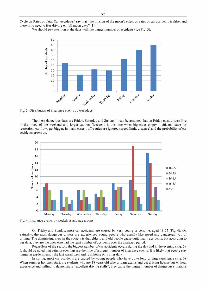
82

Cycle on Rates of Fatal Car Accidents” say that “the illusion of the moon's effect on rates of car accidents is false, and there is no need to fear driving on full moon days” [1].

We should pay attention at the days with the biggest number of accidents (see Fig. 3).

Fig. 3. Distribution of insurance events by weekdays

The most dangerous days are Friday, Saturday and Sunday. It can be assumed that on Friday most drivers live

in the mood of the weekend and forget caution. Weekend is the time when big cities empty – citizens leave for recreation, car flows get bigger, in many cases traffic rules are ignored (speed limit, distance) and the probability of car accidents grows up.

Fig. 4. Insurance events by weekdays and age groups

On Friday and Sunday, most car accidents are caused by very young drivers, i.e. aged 18-25 (Fig. 4). On

Saturday, the most dangerous drivers are experienced young people who usually like speed and dangerous way of driving. The dominating view in the society is that elderly and old people cause quite many accidents, but according to our data, they are the ones who had the least number of accidents over the analyzed period.

Regardless of the season, the biggest number of car accidents occurs during the day and in the evening (Fig. 5). It should be noted that autumn evenings are the time of a bigger number of insurance events. It is likely that people stay longer in gardens, enjoy the last warm days and rush home only after dark.

In spring, most car accidents are caused by young people who have quite long driving experience (Fig. 6). When summer holidays start, the students who are 18 years old take driving exams and get driving license but without experience and willing to demonstrate “excellent driving skills”, they cause the biggest number of dangerous situations

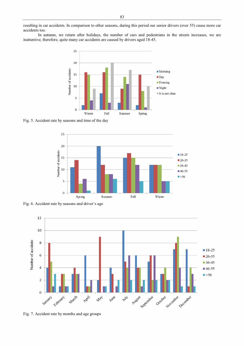
83

resulting in car accidents. In comparison to other seasons, during this period our senior drivers (over 55) cause more car accidents too.

In autumn, we return after holidays, the number of cars and pedestrians in the streets increases, we are inattentive, therefore, quite many car accidents are caused by drivers aged 18-45.

Fig. 5. Accident rate by seasons and time of the day

Fig. 6. Accident rate by seasons and driver‘s age

Fig. 7. Accident rate by months and age groups

84

Most car accidents occur in July, which substantiates the data presented in Fig. 6; and the participants of these events are young inexperienced drivers aged 18-25.

In November and December, when sleet begins, the roads get covered with ice and snow and the number of accidents among young inexperienced driver’s increases. However, November is also unfavourable for experienced drivers because snow and ice influence their driving skills too.

January and July are unfavourable for inexperienced drivers. 3. Conclusions 1. Based on the presented analysis of the secondary statistic data of insurance events, which justifies an interaction

between the accident rate and the lunar cycle, it can be stated that when the moon is on the wane, i.e. on the 22nd, 27th, 24th and 26th lunar days and in gibbous moon, i.e. on the 13th and 14th lunar days, the drivers aged 18-25 and 26-36 should be very careful. In full moon, all drivers should drive with particular caution.

2. Accident rate also depends on the day of the week: Friday, Saturday and Sunday are dangerous days for drivers. On these days, the drivers aged 26-35 should drive with particular caution.

3. Psychosocial factors such as seasons also influence accident rate: in summer, July is an exceptional month for inexperienced drivers. It is advisable for inexperienced drivers to observe traffic rules very closely. At the start of winter, when all drivers need to change their driving manner, the drivers aged 18-45 should drive with particular caution.

References 1. Gaby V. Lion. The Effects of the Lunar Cycle on Rates of Fatal Car Accidents. 2005. Available at:

< http://www.usc.edu/CSSF/History/2005/Projects/S0318.pdf/ > [viewed on 08-04-2014]. 2. Феномен влияния фаз Луны на психику человека действительно существует. Available at:

< http://www.health-ua.org/news/15617.html > [viewed on 09-04-2014]. 3. Фазы луны. Available at: < http://www.e-reading.ws/chapter.php/96892/26/Boreev_-_Pifagor_(Tom_2).html >

[viewed on 05-04-2014]. 4. Avarijų skaičius keliuose priklauso ir nuo mėnulio fazės. Available at: < http://auto.lrytas.lt/naujienos/avariju-

skaicius-keliuose-priklauso-ir-nuo-menulio-fazes.htm#.U6BChyiXeQJ > [viewed on 07-04-2014]. 5. Банькис K. Уникальное исследование в Латвии! Available at: < http://www.astroabc.com/sakums/raksti/

494/Aktuali/Unikalnoe-issledovanie-v-Latvii/ > [viewed on 07-04-2014]. 6. Bryner J. 'Supermoon' Lunacy: Does the Moon Make Us Crazy? Available at: < http://www.livescience.com/

13323-supermoon-lunacy-full-moon-myths.html > [viewed on 07-04-2014]. 7. Skvernelis S. Kas kaltas – policija ar mėnulio fazės? Available at: < http://www.15min.lt/naujiena/ziniosgyvai/

nuomones/saulius-skvernelis-kas-kaltas-policija-ar-menulio-fazes-18-372606#ixzz34u4263TI > [viewed on 08-04-2014].

85

Proceedings of 9th International Conference ITELMS’2014 Research into Dependence of Failure Flow Parameter of Diesel Internal-Combustion Engine on Climatic Conditions in Afghanistan N. Dobrzinskij The General Jonas Žemaitis Military Academy of Lithuania, Silo Str. 5A, LT-10322 Vilnius, Lithuania, E-mail: Nikolaj.Dobrzinskij@gmail.com Abstract Implementing their international commitments in Afghanistan, representatives of different countries pursue their missions under severe physical and geographical conditions. Different machinery and equipment is constantly used for implementation of tasks. Reliability of internal-combustion engines is dependent upon many factors such as internal features of an engine and external conditions of their operation. Engines are subject to effect of many factors that determine occurrence of engine failures and failures. Climatic conditions represent one of the factors of operating load on internal-combustion engines which is directly dependent on the climate zone. Consequently, assessment of the reliability of machinery and equipment, and particularly internal-combustion engines, should begin with the analysis of climatic factors that affect their operating condition. KEY WORDS: engine failures, environmental interaction. 1. Introduction

Automotive engine reliability represents an important feature of engine performance while determining use of a vehicle in an ever globalizing world. Cars are often adapted to be capable of driving on different roads and to operate under various conditions. For this reason, when designing and producing land motor vehicles automotive manufacturers focus not only on their design and comfort level but also on their operating reliability. Given the currently prevailing worldwide trend to develop automotive road systems with rigid pavements, automotive manufacturers tend to develop cars intended for operation on this type of roads. However, in some cases a need emerges for vehicles operable off-road under complicated climatic conditions, for example, for the purpose of exploratory works or to be used on international missions. For the purpose of tasks completion different vehicles are often used effectiveness of which depends on their reliability. As the need for such vehicles is limited, there is a lack of their research, and furthermore, findings and results of not all studies are reported and published, all of which leads to the lack of recommendations on vehicle operation under difficult conditions.

Internal combustion engines (hereinafter – ICE) used in cars are also mainly designed for operation under normal conditions, and the need to adapt series engine for use in vehicles operating under difficult conditions is often accompanied with different problems. Problems are often caused by engine operation in locations with complicated climatic and geographic conditions – mountains, desserts, rapid rivers, increased air dustiness, diurnal temperature variation, and solar radiation.

Assurance of reliability of the internal-combustion engines (ICEs) should never be based on approximate knowledge of average conditions; it requires for precise data on real operating conditions.

Surrounding environment includes all the environmental conditions under which production, operation and storage of equipment takes place [1].

First of all it includes climatic factors. Given the effect of the external factors on equipment, climatic factors are grouped as follows: mechanical, climatic and other environmental external factors that are dependent on the geographic location, season and time of a day, etc., biological, radiation, external factors of electromagnetic fields, factors that affect specific environment externally, thermal.

In respect of ICE operation, the climatic factor is assumed to be one of the most significant factors leading to destabilization of engine’s outside: the climatic factor includes heat and cold that are characterized by °C or °K, relative humidity, precipitation, dust and sand, solar radiation (insolation), and biological environment effect of a specific form.

Research material. The article analyzes performance of thirty five diesel engines operating under difficult conditions: sixteen

vehicles Toyota Land Cruiser 100 (LC) with diesel engines 1HD-FTE, and thirteen high-mobility multipurpose wheeled vehicles M998A2 (HMMWV) with diesel engines GM6.5L with diesel engines OM366 LA. All the vehicles were used under conditions of mountainous desert from the very beginning, i.e., starting with summer of 2005 till December 31, 2011.

The article offers statistical information on engine delectability. Data processing was accomplished using digital engineering techniques and numerical modelling enabling prediction of engine reliability while taking into account its operating conditions.

86

The objective of this research paper was to comprehensively study and examine the failure flow parameter1 of ICEs operating under difficult of the climatic and other environmental factors conditions in Afghanistan region.

Research was carried out in mountainous dessert of Afghanistan having difficult climatic conditions. To collect precise and accurate data, vehicles used by the Provincial Reconstruction Team (hereinafter – PRT) situated in Ghowr province (Afghanistan) were selected for the research. Their operation course, failures, and repairs can be tracked and captured more precisely than those of civilians as their data are recorded in data logs. This research paper used descriptive and analytical methods that involved practically obtained primary research findings from the analysis of machinery operation in Ghowr Province of Afghanistan over period of many years. Actual reliability indicators of diesel engines used in vehicles operating in Ghowr province of Afghanistan do not exactly satisfy modern requirements as their operating conditions differ from those that they have been initially designed and produced for. Actual use of automotive resources depends on intended tasks and season of the year. In summertime, daily mileage of a car varies from 0 to 40 km with the engine running for 10 motor hours per day, whereas in winter these are by half lower. In the case of more complicated tasks, the engine runtime increases significantly.

The following are the main factors determining engine operating conditions in the region under investigation: layout and profile of roads, their altitude above sea level, climatic and geographic conditions, airborne concentration of abrasive substances, patterns of use of vehicles, engine oils and car fluids used, fuel used in Afghanistan (having different properties than normal diesel fuel), and rotation of drivers each half-year. The factors mentioned herein have influence on engine operation and its costs. 2. Geographical location, the characteristics of climatic and other environmental factors of Afghanistan

Afghanistan is located in Central Asia and has borderlines with Tadzhikistan, Uzbekistan, Turkmenistan, Iran, Pakistan and China. Afghanistan lies in the North-Eastern part of Iran Mountain range with high sierras and valleys between mountains. Engine operating conditions represent a significant factor for analysis of vehicles performance under difficult conditions that include low air temperatures, in case of deep snow coverage – frequent snowstorms and snowbanks on roads; regions with hot dessert climate, poorly developed network of roads and driveways, lack of afforestation and water, increased air dustiness, considerable diurnal temperature variation; mountainous terrains with thin air and lower atmospheric pressure; highly variable terrain profiles and considerable diurnal temperature variations; off-roads and scales of road aggravation. Difficult engine operating conditions are also considered to include regions with high humidity levels.

Each of the above-mentioned factors of engine operating conditions has an influence (mostly negative) on operation of automotive engine. The altitude (elevation) of the road location above sea level and violent variations thereof is a fundamental factor determining ICE loading regimes. Difficult combinations of driveways at mountainous locations comprised of downhills and uphills different in size with variable high-intensity road winding and small turning radiuses determine uneven rolling resistance of a vehicle. Another subtype of operating loads involves the climatic factor with parameters such as temperature, air impurities, air humidity, solar radiation (the latter is not attributed to the difficult operating conditions however it is directly linked to the temperatures of air and Earth’s surface). This subtype is also considered to include the geographical factor – atmospheric pressure, which directly takes part in shaping the process of engine operation in the cylinders of the engine [2, 3]. The third factor accountable for reduced engine reliability and determining its parametric failures is the wear of engine parts. Operating (characteristics of fuel and engine oil and their quality, quality of spare parts, etc.) and biological factors (rodents, funguses, vegetation, etc.) might also be distinguished. Highlands and their variable terrains have a negative influence on vehicles and operation of their engines: efficiency decreases, fuel consumption increases, fuel injectors get clogged, slag and cinder form, more intensive wear of engine occurs, if they are not specifically adapted for exploitation in high-alpine regions, service life of individual components and assemblies is significantly reduced.

Estimation of climatic and other natural factors influencing exterior of vehicles operated in Ghor province of Afghanistan, and their diurnal variations, used meteorogical data recorded by the Air Traffic Control Centre of the Provincial Reconstruction Team of Ghor province using weather data recording equipment Vaisala TacMet Tactical Meteorological Observation System MAWS 201M, and processed using software MIDAS IV Tacmet. This equipment is used to detect and record meteorological data at one minute intervals 24h a day. The structural scheme design of the weather station of the Chagcharan Air Traffic Control Centre in Ghor Province (2005–2011) has relative humidity sensor, wind direction sensor, precipitation amount, type and intensity measuring, air temperature sensor, wind speed sensor, visibility sensor, surface temperature sensor, solar radiation meter.

Eight meteorological stations were selected out of all those 47 stations operative since 1996 in Afghanistan: such a choice was based on the need to have a clear climate characteristic for its every representative region located from the lowest to the highest above sea level, and from the coldest to the warmest areas of the country. In the Pamir Mountains, continuously operating meteorological stations were absent. Gathered and summarized meteorological data of Afghanistan provinces show climate of this region to have an exceptional characteristic.

Presents deployment of meteorological stations in Afghanistan, and statistical data on air temperature and pressure, of solar radiation, the relative humidity of air and average annual precipitation ranges, wind speed, number of

1 ICE failure flow parameter is defined as a frequency rate of engine failures which is calculated by subdividing the average number of failures over the period of observation to the engine run kilometres over the same time period.

87

sand storms, biological environment effect of a specific form (microbial, fungal, viral effects, and effect from rodents and insects), by different regions of Afghanistan was detailed and presented in article [4].

The error of approximation of statistical data of all the climatic and weather factors under investigation is below 10%, and determination coefficients are in range of R2 = 0.90 ÷ 0.98, which serves as the evidence of the suitability of mathematical expression.

Air is a mixture of gases full of different impurities. In Asia, impurities of air usually occur in result of sand storms or human activities. In the effect of wind or air flows, particles of surface of the Earth are raised to air making it a polydisperse aerosol mixture – that’s the way a temporally high concentration of dust and sand occurs in air. Research findings of foreign scientists show that dust and sand concentration highly varies during sand storm, and may achieve values of 10.4 g/m3 [1], 0.5 – 10.6 g/m3 [5] size of particles may vary from 0.01 to 1000 µkm [6, 7].

Moving vehicles also cause impurities in air. In Ghowr province, traffic determines occurrence of dust emissions from under the wheels of the moving vehicles. The minimum airborne dust concentrations measured in November, 2009, ranged from 58.28 μg/m3 in the environment of military base, to 18181.82 μg/m3 in the centre of the column of automotive vehicles [8].

To estimate the crystalline structure of the road dust, the X-ray diffraction (XRD) was undertaken in cooperation with E. Krugly, L. Kliučininkas, T. Prasauskas, D. Martuzevičius, scientists of the Faculty of Chemistry of Kaunas University of Technology, and M. Kireitseu and A. Zerrathu, scientists of the Hamburg University. The quantitative analysis showed that road dust samples collected in Ghor province of Afghanistan contained the following minerals: Calcite, Quartz, Albite, Muscovite, Potassium-Feldspar, and Nimite. Major portion of dust is comprised of quartz, compounds of aluminium, and particles of different mountain minerals. Dust with the diameter of 2 μm prevails.

To determine the concentration of salts (potentially causing corrosion of metals) in collected road dust samples, the analysis of concentration of water-soluble sulphates and chlorides as well as of pH value was conducted. The analysis revealed rather high concentrations of water-soluble SO4

-2 and Cl-1 in samples collected in Ghor province of Afghanistan, thus road dust containing these salts when in contact with engine can speed-up processes of corrosion.

The biological factor was examined, too. Samples were collected from automotive fuel filters from the medium of the layer situated between the fuel and the water. Assay showed that in Afghanistan, fungi occur everywhere where compounds of carbon and hydrogen are present under favorable conditions: elevated air temperatures, humidity, surfaces contaminated with dust. In summary of collected information on biological factors, the conclusion is made that under conditions of Afghanistan, the influence of biological factors is insignificant and emerges mainly during downtimes of vehicles caused by various other reasons due to vehicles standing idle. In other words, the biological factor influences engine preservation.

Assessment of climatic factors revealed that maximum value of the adversity of the climatic factor for engine operation belongs to the cold season, and is followed by relative humidity in the second place by significance, whereas the third place is shared between monthly mean air temperature, solar energy irradiation and mean air temperature variation amplitude, with minor error, then closely followed by the scattered solar energy irradiation; wind speed, air pressure, and average air temperature during three hottest months of the warm season were found to be less important. Other factors – duration of the warm season, fluctuations in air temperature through 0 ºC, time period of mist coverage – do not determine adversity of the climate to ICE operation in the region, and such factors as amount of precipitation and time period of precipitation and wind direction have no influence on engine performance at all. 3. Mathematical model of weather technical severity in Afghanistan region

Climatic factors and atmospheric phenomena make substantial effect on reliability of machinery ICEs: different precipitation, sand storms, dust mist, low and high air temperatures and air pressure, wind speed, solar radiation, humidity of air, etc. However, there are some climatic factors and atmospheric phenomena that have no significant effect on ICEs. These include composition and form of clouds, dates of initial frosts, wind direction, etc. Taking into consideration climatic factors and atmospheric phenomena mentioned in part 2, a summary of substantial climatic factors to be considered was made that will be further used to develop a mathematical model and determine complex climatic situation of Afghanistan region. For the mathematical modelling of complex effect of Afghanistan climate to achieve a high level of precision, it is necessary to make mathematical models of climate and weather technical severity under adverse ICE operation conditions for cold and hot mountainous regions, individually [9].

It is wise to characterize intensity effect of climatic factors’ combination on features of materials as a technical severity of a climate – this term was first used by G. Bodman in respect of humans [9]:

( ) ( ) ( ) ( ) ( ) ( ) ( ) ( )[ ]hlarmww ttbtntvtAtPttTtQfSN ,,,,,,,,, ϕ= (1)

where Nw – common indicator of technical severity for cold weather; Sw – common indicator of technical severity for hot weather; Q – total solar radiation; T – air temperature; t – time of factors being in effect; φ – relative humidity of air; P– atmospheric air pressure; Am – average non-periodical amplitude of air temperature fluctuations; ν – average wind speed; nar – atmospheric phenomena having effect on reliability of ICE; thl – time of exposure to low and high temperatures per year; b – effect of biological factor.

88

Analytical expression of equation (1), where climatic characteristics are practically not dependent on each other (what allows using the probability theory [9]), and significant parameter – engine indefectibility over time period t, under effect of main climatic factors, will be as follows:

( ) ( )[ ] ( )[ ] ( )[ ] ( )[ ] ( )[ ] ( )[ ] ( )[ ] ( )[ ]tqtqtqtqtqtqtqtqtP bhlnarATQ

i

ic m−−−−−−−=−= ∑ 11111111

1ϕ (2)

where qi(t) – probability of engine failure due to the effect of the i–th climatic factor over time period (t); qQ(t) – probability of failure due to solar radiation; qT(t) – probability of failure due to air temperature effect on materials; qAm(t) – probability of failure due to the amplitude of average air temperature fluctuations; qφ(t) – probability of failure due to the effect of relative humidity of air; qnar(t) – probability of failure due to the atmospheric phenomena affecting engine’s reliability; qhl(t) – probability of failure due to the exposure time of high and low temperatures per year; qb(t) – probability of failure due to the effect of biological factor per year.

In result of concretization of climate’s dependence (1) on the arid mountainous Afghanistan region by using climate loading, probability reliability equation (2) and analysis results of climate factors ranking offered by Koh P. I., Common indicator of technical severity of hot arid weather in Afghanistan offers a general monthly evaluation of hot weather in Afghanistan for a period of one year. Equation for hot arid weather evaluation of duration of high temperature exposure and average monthly values are being changed [10, 11]:

( ) ( ) ( ) ( ) ( ) ( )hthh

hhhmxabsmxvpw tnvAQTTKS 009.01012.0108.0103.010075.01105.212.055.0 7 ++

+−+⋅++= −

ϕ (3)

where Kp – coefficient of atmospheric air pressure effect on technical climate severity; Tmxv – average value of the highest temperatures over three warmest months, in °C; Tmxabs – average value of air absolute temperature maximum over three warmest months, in °C; Ah – average non-periodical amplitude of air temperature fluctuations per day over three warmest months, in °C; Qh – average total solar radiation over three warmest months; νh – average wind speed over three warmest months, in m/s; φh – average relative humidity of air over three warmest months, in unit shares; nth – average number of days with sand storms and mists per month over three warmest months; th – duration of exposure to positive air temperature, expressed in months.

In formula (2), reliability indicators serve to take into consideration a comprehensive effect of climate load on materials and engine. Analysis of this formula shows that effect of climatic factors – such as high air temperature, extensive fluctuations of air temperature amplitude per day, low relative humidity of air, and sand storms – on ICE will always be a negative one.

The obvious effect of main climatic factors of Afghanistan continental climate in winter on materials and engine reliability is always negative. The more intense influence of each factor, the more extensive their total negative effect is. Analogous to mathematical expression of hot climate technical severity, cold climate technical severity can be expressed as follows [9]:

( )( )( )( )( )( )( )ctmccccmabsmvidpw t.n..v.A.Q.T.T.KN 2201014012601070100750101501250750 +++++++= ϕ (4)

where Kp – coefficient of atmospheric air pressure effect on technical climate severity; Tmvid. – average value of the lowest air temperatures over three coldest months, in °C; Tmabs – average value of air absolute temperature minimum over three coldest months, in °C; Ac – average non-periodical amplitude of air temperature fluctuations per day over three coldest months, in °C; νc – average wind speed over three coldest months, in m/s; φc – average relative humidity of air over three coldest months, in unit shares; ntm – average number of days with snow storms and mists per month over three coldest months; tc – duration of exposure to negative air temperatures, expressed in months.

Duration of exposure to negative air temperatures, expressed in months, was not included in the formula due to its constant value.

Methodology of rating analysis depends on the experience of the expert; each rating is attributed its position after taking into consideration a score of climate technical severity [9]. Analysis of the effect of hot arid climate’s characteristics on ICE reliability might be laid down in the following variation row depending on the significance level of this effect: solar radiation, high air temperatures, and high fluctuations in daily temperature, low relative humidity of air, sand and dust storms. It is worth to mention individually the influence of mountains on climatic factors and ICEs operated in Afghanistan.

Mathematical models of technical severity for hot and cold arid climates might be made based on the analysis of climatic conditions ratings which shows that the major effect on technical severity of a climate and weather comes from solar radiation, high air temperatures, extensive amplitudes of daily temperature fluctuations, low relative humidity of air, sand and dust storms. In both cases, compatibility degree of the periodic rating correlation R2 according shows also good compatibility of these evaluations. The error of approximation of statistical data of all the climatic and weather factors under investigation is below 10%, and determination coefficients are in range of R2 = 0.90 ÷ 0.98, which serves as the evidence of the suitability of mathematical expression.

Technical severity of hot and cold climate in Afghanistan offers only a dotted evaluation of climatic factors’ effect over three coldest or hottest months, consequently technical severity of the climate proves to be a general

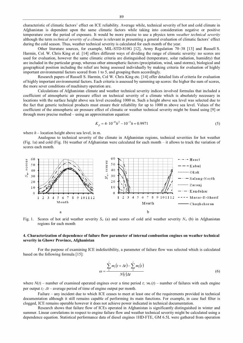
89

characteristic of climatic factors’ effect on ICE reliability. Average while, technical severity of hot and cold climate in Afghanistan is dependent upon the same climatic factors while taking into consideration negative or positive temperature over the period of exposure. It would be more precise to use a physics term weather technical severity although the term technical severity of a climate is relevant in presenting a general evaluation of climatic factors’ effect during the cold season. Thus, weather technical severity is calculated for each month of the year.

Other literature sources, for example, MIL-STD-810G [12], Army Regulation 70–38 [13] and Russell S. Harmin, Col. W. Chris King et al. [14] offers different ways of dividing the range of climatic severity: no scores are used for evaluation, however the same climatic criteria are distinguished (temperature, solar radiation, humidity) that are included in the particular group, whereas other atmospheric factors (precipitation, wind, sand storms), biological and geographical position including the relief are being assessed individually by making criteria for evaluation of highly important environmental factors scored from 1 to 5, and grouping them accordingly.

Research papers of Russell S. Harmin, Col W. Chris King etc. [14] offer detailed lists of criteria for evaluation of highly important environmental factors. Each criteria is assessed by summing up scores: the higher the sum of scores, the more sever conditions of machinery operation are.

Calculations of Afghanistan climate and weather technical severity indices involved formulas that included a coefficient of atmospheric air pressure effect on technical severity of a climate which is absolutely necessary in locations with the surface height above sea level exceeding 1000 m. Such a height above sea level was selected due to the fact that generic technical products must ensure their reliability for up to 1000 m above sea level. Values of the coefficient of the atmospheric air pressure effect of climatic or weather technical severity might be found using [9] or through more precise method – using an approximation equation:

9971010104 328 .hhK p +−⋅= −− (5)

where h – location height above sea level, in m. Analogous to technical severity of the climate in Afghanistan regions, technical severities for hot weather

(Fig. 1a) and cold (Fig. 1b) weather of Afghanistan were calculated for each month – it allows to track the variation of scores each month.

a

b

Fig. 1. Scores of hot arid weather severity Sw (a) and scores of cold arid weather severity Nw (b) in Afghanistan regions for each month

4. Characterization of dependence of failure flow parameter of internal combustion engines on weather technical severity in Ghowr Province, Afghanistan

For the purpose of examining ICE indefectibility, a parameter of failure flow was selected which is calculated based on the following formula [15]:

( ) ( )

( ) ttN

tmttmi i

ii

∆

∆ω

∑ ∑−+= 1 1 (6)

where N(t) – number of examined operated engines over a time period t; mi (t) – number of failures with each engine per output t; Δt – average period of time of engine output per month.

Failure – any incident due to which ICE ceases to meet at least one of the requirements provided in technical documentation although it still remains capable of performing its main functions. For example, in case fuel filter is clogged, ICE remains operable however it does not achieve power indicated in technical documentation.

Research shows that failure flow of ICEs operated in Afghanistan is significantly distinguished in winter and summer. Linear correlations in respect to engine failure flow and weather technical severity might be calculated using a dependence equation. Statistical performance data of diesel engines 1HD-FTE, GM 6.5L were gathered from operation

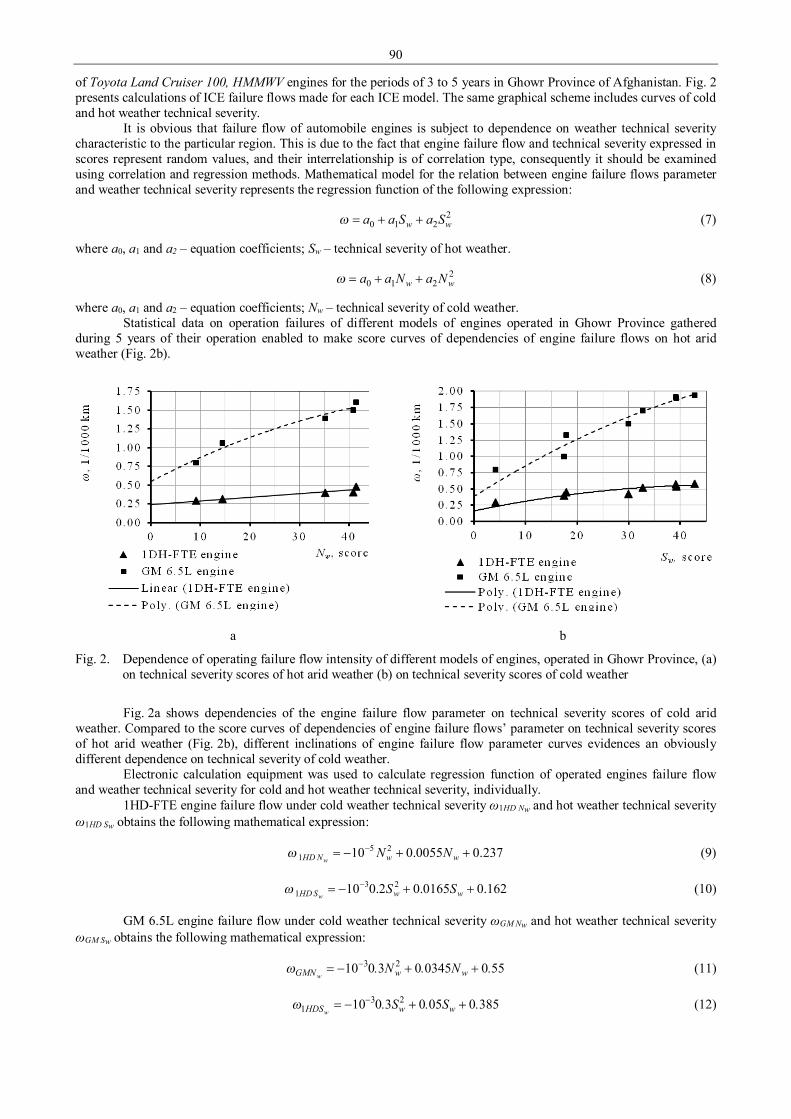
90

of Toyota Land Cruiser 100, HMMWV engines for the periods of 3 to 5 years in Ghowr Province of Afghanistan. Fig. 2 presents calculations of ICE failure flows made for each ICE model. The same graphical scheme includes curves of cold and hot weather technical severity.

It is obvious that failure flow of automobile engines is subject to dependence on weather technical severity characteristic to the particular region. This is due to the fact that engine failure flow and technical severity expressed in scores represent random values, and their interrelationship is of correlation type, consequently it should be examined using correlation and regression methods. Mathematical model for the relation between engine failure flows parameter and weather technical severity represents the regression function of the following expression:

2210 ww SaSaa ++=ω (7)

where a0, a1 and a2 – equation coefficients; Sw – technical severity of hot weather.

2210 ww NaNaa ++=ω (8)

where a0, a1 and a2 – equation coefficients; Nw – technical severity of cold weather. Statistical data on operation failures of different models of engines operated in Ghowr Province gathered

during 5 years of their operation enabled to make score curves of dependencies of engine failure flows on hot arid weather (Fig. 2b).

a

b

Fig. 2. Dependence of operating failure flow intensity of different models of engines, operated in Ghowr Province, (a) on technical severity scores of hot arid weather (b) on technical severity scores of cold weather

Fig. 2a shows dependencies of the engine failure flow parameter on technical severity scores of cold arid

weather. Compared to the score curves of dependencies of engine failure flows’ parameter on technical severity scores of hot arid weather (Fig. 2b), different inclinations of engine failure flow parameter curves evidences an obviously different dependence on technical severity of cold weather.

Electronic calculation equipment was used to calculate regression function of operated engines failure flow and weather technical severity for cold and hot weather technical severity, individually.

1HD-FTE engine failure flow under cold weather technical severity ω1HD Nw and hot weather technical severity ω1HD Sw obtains the following mathematical expression:

237.00055.010 251 ++−= −

wwNHD NNw

ω (9)

162.00165.02.010 231 ++−= −

wwSHD SSw

ω (10)

GM 6.5L engine failure flow under cold weather technical severity ωGM Nw and hot weather technical severity ωGM Sw obtains the following mathematical expression:

550034503010 23 .N.N. wwGMN w++−= −ω (11)

38500503010 231 .S.S. wwHDSw

++−= −ω (12)

91

The error of approximation of engine failure flow parameters under investigation is below 10 %, and determination coefficients are in range of R2 = 0.90 ÷ 0.98, which serves as the evidence of the suitability of mathematical expression.

Analysis of engine failure flow parameters of different models of engines operated in Ghowr Province suggests engines to have different dependencies on weather technical severities based on perpendicular angles of engine failure flow parameter curves. 5. Conclusions 1. Geographical position of Afghanistan determines climate in Afghanistan regions which is characterized as an

extremely arid continental climate with high amplitude of air temperature fluctuations. According to indices of technical severity of a climate, many Afghanistan regions are prevailed by the extremely hot arid severe climate. Based on current studies of climate and weather technical severity in Afghanistan regions, climatic factors are assumed to represent one of the ICE operational loading sub-types dependent on climate zone. Climatic and weather severity is furthermore increased by Afghanistan mountains.

2. The higher the score of climatic and weather technical severity, the higher parameter of engine failure flow in automobiles operated in Ghowr Province, Afghanistan, is. Here offered mathematical model of relation between engine failure flow parameters and weather technical severity delivers sufficiently precise results.

3. The failure flow parameter for Toyota Land Cruiser 100 with diesel engine 1HD-FTE and that for M998A2 with diesel engine GM6.5L, both operated under difficult conditions, has been investigated. ICE failure flow parameter was found to vary depending on the type of engine: for 1HD-FTE – 0.3 to 0.6 failure/1000 km; for GM6.5L – 0.7 to 2.0 failures/1000 km; ICE failures were found to be less frequent in autumn and spring. The fluctuation amplitude of failure flow parameter amounted for two times depending on the season.

4. Differently structured internal combustion engines offer different capabilities of their adaptation for operation under difficult conditions: diesel engines 1HD-FTE of Toyota Land Cruiser 100 offer twice better capabilities of their adaptation for operation under difficult conditions when compared to diesel engines GM6.5L of M998A2.

References 1. Авдуевский В. С., Кузнецов В. А. и др. Надежность и эффективность в технике. Справочник 10 т.

Справочные данные по условиям эксплуатации и характеристикам надежности. – Москва: Машиностроение, 1990, 336 с.

2. Кадыров С., Hиколaeнко А., Хватов В. Надежность автотракторных дизелей в условиях Среднеазиатского региона. – Ташкент: Фан, 1990, 92 с.

3. Махалдиани В. O двигателях для горных автомобилей и тракторов. – Тбилиси: Мецниереба, 1968, 270 с. 4. Dobrzinskij N. Research of the Climatic and Environmental Factors of Afghanistan Region Having Effect on

Diesel Engine Reliability. Monograph. Deterioration, Dependability, Diagnostics. University of Defence Brno. Brno. 2011. p. 189-202.

5. Graveris H. A. Desert Environmental Handbook, US Army Yuma Proving Ground Yuma, Arizona, 1977, 97 p. 6. Blackford P. A., McPhilimy H. S. Sand and dust considerations in the design of military equipment. Technical

Report ELT-TR-72-7, U.S. Army Engineer Topographic Laboratories Fort Belvoir, Virginia, 1972, 18 p. 7. Луканин В. Н., Шатров М. Г. Двигатели внутреннего сгорания. – Москва: Высшая школа, 2007, 479 с. 8. Dobrzhinsky N., Krugly E., Kliucininkas L., Prasauskas T., Kireitseu M., Zerrath A., Martuzevicius D.

Characterization of Desert Road Dust Aerosol from Provinces of Afghanistan and Iraq. Aerosol and Air Quality Research. Taiwan Association for Aerosol Research, Aerosol and Air Quality Research, Vol. 12, No. 6, December 2012, p. 1209-1216.

9. Кох П. И. Климат и надежность машин. – Москва: Машиностроение, 1981, 175 с. 10. Марченкo А. П. Двигуни внутрішнього згоряння: Серія підручників у 6 томах. Т.6. Надійність ДВЗ. За

редакцією проф. засл. діяча науки України А.Ф. Шеховцова. – Харків: Видавн. центр НТУ “ХПІ”, 2004, 425 с.

11. Шеховцов А. Ф. Конструктивные отличия и особенности технической эксплуатации ДВС в условиях стран Азии, Африки и Латинской Америки. Основы климатической принадлежности ДВС. – Ч. І. – К.: УМКВО, 1988. - 230 с.

12. MIL-STD-810G. Environmental Engineering Considerations and Laboratory Tests, Department of Defense Test Method Standard, 31 October 2008, 804 p.

13. Research, Development, Test and Evaluation of materiel for Extreme Climatic Conditions, Army Regulation 70–38 Headquarters Department of the Army, Washington, DC, 15 September 1979, p. 31.

14. Russell S. H., King W. C., Palka E. J., Gilewith D. A. Characterizing Extreme Environments For Army Testing, US Army Research Laboratory, NC, 2005, 8 p.

15. Mickūnaitis V. Transporto priemonių kokybės valdymas. – Vilnius: Technika, 2006, 176 p.

92

Proceedings of 9th International Conference ITELMS’2014 Construction Quality Control A. Dragunas*, S. Susinskas** *Kaunas University of Technology, S. Daukantas str. 12, 35212, Panevezys, E-mail: arturasdragunas3@gmail.com **Kaunas University of Technology, S. Daukantas str. 12, 35212, Panevezys, E-mail: s.susinskas@ktu.lt Summary Construction products entering the market: materials, products, construction supplies and building equipment, which are tested and certified in accordance with applicable standards. EU standardization system has not yet fully formed. It is constantly being improved and standards approximately every five years are being reviewed, if necessary they are being updated. They are combined with new demands of material development, production, testing and technical progress. Construction organizations which pursue to survive in competitive struggle must ensure the quality. For this purpose the companies are implementing Quality management systems. KEYWORDS: construction, quality, control, standardization. 1. Introduction

Lithuanian construction companies give priority to the quality of products. This factor also affects the increase and improving of construction services and quality requirements because the customers’ needs grow together with competition increase. Therefore the value of the quality is becoming more important and it has a greater contribution.

When Lithuania integrated into EU, the internal market surveillance system was adapted to the EU market surveillance system in order to eliminate the trade technical barriers and to allow the free movement of products in the establishing EU single market. The bigger quality requirements have also been influenced by large European companies, which have entered into Lithuanian market and Lithuanian companies must now compete with them as well.

The object of this study is the construction quality management in the companies. The aim of this study is to find out whether the Lithuanian construction companies have to follow the quality

management requirements. For the study execution the following tasks were set:

• To analyze the quality standards. • To analyze the quality requirements. 2. Quality management principles

In recent years many positive achievements of the management theory and practice quality were used for developing of the new ISO 9000:2000 standard version. This is vividly reflected in the quality management principles, which are formulated in the new version of the standards and which should be followed in developing of the Quality management system. Quality management principles’ application provides not only direct benefit, but also contributes to the risk management. Quality management should be incorporated into the organization's management. To make it easier to achieve quality objectives eight management principles have been applied: 1. Principle – Customer Focus. 2. Principle – Leadership (active managers’ activity). The harmonious operation of the quality system can not be

created without the active operation and support from the management. 3. Principle – Involvement of Employees. Employees at all levels are the essence of an organization and its most

valuable resources, therefore employees’ involvement in quality improvement activities enables their abilities to be used for the organization’s benefit.

4. Principle – Process approach. Any activity or production, which transforms inputs into outputs, must be assessed as a process. Almost all product production or service activity is the process.

5. Principle – System Approach to Management. It is necessary to understand the interdependencies of the processes occurring in the system, to create methods by which the processes are combined and connected. The model of process consolidation into the Quality management system is show in Fig. 1.

6. Principle – Continuous Improvement. Under the implementation of this principle the quality improvement activity at all levels of the organization must be harmonized with the organization's strategic targets and the relevant tasks for process improvement must be formulated.

7. Principle – Factual Approach to Decision Making. Effective organizational management decisions and actions must be based on data and information analysis. It is necessary to ensure that data and information should be reliable and available and appropriately processed. Only reliable methods must be applied for data and information collection and processing.

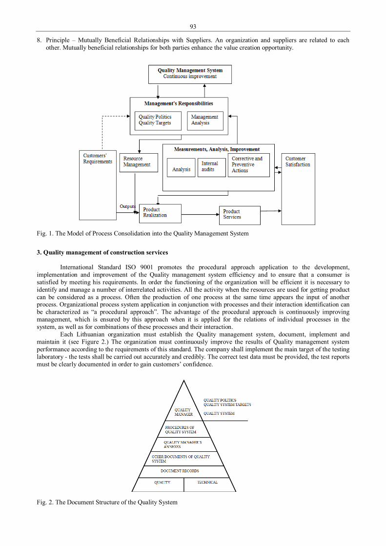
93

8. Principle – Mutually Beneficial Relationships with Suppliers. An organization and suppliers are related to each other. Mutually beneficial relationships for both parties enhance the value creation opportunity.

Fig. 1. The Model of Process Consolidation into the Quality Management System

3. Quality management of construction services

International Standard ISO 9001 promotes the procedural approach application to the development, implementation and improvement of the Quality management system efficiency and to ensure that a consumer is satisfied by meeting his requirements. In order the functioning of the organization will be efficient it is necessary to identify and manage a number of interrelated activities. All the activity when the resources are used for getting product can be considered as a process. Often the production of one process at the same time appears the input of another process. Organizational process system application in conjunction with processes and their interaction identification can be characterized as “a procedural approach”. The advantage of the procedural approach is continuously improving management, which is ensured by this approach when it is applied for the relations of individual processes in the system, as well as for combinations of these processes and their interaction.

Each Lithuanian organization must establish the Quality management system, document, implement and maintain it (see Figure 2.) The organization must continuously improve the results of Quality management system performance according to the requirements of this standard. The company shall implement the main target of the testing laboratory - the tests shall be carried out accurately and credibly. The correct test data must be provided, the test reports must be clearly documented in order to gain customers’ confidence.

Fig. 2. The Document Structure of the Quality System

94

Organizations have: • To implement the required processes of Quality management system and determine their application in the

organization; • To define the sequence of processes and their importance; • To define the criteria and methods, which ensure operation and management of the most necessary processes; • To ensure that the necessary resources and information for process operation and monitoring will be obtained; • To monitor, analyze these processes; • To implement the planned results and continually improve the necessary actions of the processes.

An organization has to manage processes such as ISO 9001 international standard requirements. When an organization chooses the external process that affects product conformity with requirements, it must ensure the management of such process. The processes management in the Quality management system must be identified. 4. Quality control of construction products

For product quality control there is developed the system for Brigade Leaders, Construction Work Managers, Construction Managers, Project Managers, Technical Director and Director of Construction.

Brigade Leader has to organize a brigade work according to issued work tasks. He promptly checks the quality of works performed and makes records in the product quality accounting sheet. If the deviations appear Brigade Leader takes steps to defect correction, delivers the performed works (along with the product quality accounting sheet) to Construction Work Manager. If the quality of works performed is out of control and the records in the product quality accounting sheet have not been made, Construction Work Manager reduces the output coefficient.

Construction Work Manager shall prepare and deliver to Brigade Leader work tasks, write down the product quality accounting sheet, check the records in the product quality sheet made by Brigade Leader, often check the quality of performed works, and if there are any deviations, he shall organize their correction, make records in the product quality accounting sheet and deliver the filled product quality accounting sheets to Construction or Project Manager. In the absence of documentation, the works are not accepted and wage is reduced.

Construction or Project Manager accepts works performed at divisions, if there are any deviations he requests to correct them, makes the record in the product quality accounting sheet, accepts works done by subcontractors and checks work quality. In case of deviations Manager requests to correct them and issues the product quality accounting sheet for the works performed by subcontractors. Every month the completed work quality accounting sheets together with acts of performed works are provided to Production department. Every month Construction Manager receives the acts of performed works at divisions and by subcontractors together with quality accounting sheets labeled with information about the quality of works. In case of the absence of such documentation Construction Manager reduces the wage. Construction Manager together with Quality Manager and Technologist optionally check the quality documentation which is being recorded at construction site, as well as quality of work, the compliance with safety and procedure requirements. When violations are identified the wage is being reduced.

Technical Director controls that the work quality accounting sheets of unfinished works are filled and provided to him at the end of a month. Technical Director reduces the wages for Construction Work Managers if the documentation was not filled or provided.

Construction Manager control that the work quality accounting sheets labeled with information about the quality of works are delivered from divisions and subcontractors. If the documentation was not filled or provided Construction Director reduces the wages for Construction or Project Managers. Construction Manager together with Quality Manager and Technologist optionally check the quality documentation which is being recorded at construction site, as well as quality of work, the compliance with safety and procedure requirements.

All the construction links must be interested in the quality of performed work and they all must participate in quality control: Brigade Leaders, Construction Work Managers, Construction or Project Managers. Work of every construction link is evaluated according to prepared assessment matrix of quality indicators. The wages of appropriate link employees depend on assessment results.

The target of such scheme is to create an efficient, multilevel, motivation based construction work quality control. 5. Conclusions

Quality control issues are being summarized by the international ISO standards. The worldwide standard of ISO 9001:2000 is generic. This is not a product standard; it is applicable to any manufacturing or service industry. In the period of intense market it is necessary to have a Quality management system to ensure sustainable work of construction companies.

According to production and construction service purpose there can be indicated the production suitability for consumers’, customers’ and other interested parties’ needs. Quality management is very important for improving the quality of materials and services. Quality management ensures the customer's long-term confidence in the contractor, the contractor's good name and the recognition in the construction market.

95

Based on the material reviewed and experts’ opinions it can be stated that the quality is managed at all stages of product development. Quality basis is the compliance with applicable rules and standards, and using the basic principles of construction management: good and timely planning, implementation, control and analysis.

Enterprises, which carry out construction works not only in Lithuania, but also abroad must follow the quality standards addressed in this study in order to remain competitive not only in domestic, but also in foreign construction markets. Quality management system development will enhance customer’s demands satisfaction, achieve consistency and improve internal processes. This is especially important for extremely complex objects implementation, which is related to the safety of people, the implementation of complex industrial and public facilities and residential construction objects. References 1. Kokybės vadyba (Quality Management) [interactive]. Web access: < http://www.dnvba.com/lt/

Sertifikavimas/Vadybos-sistemu-sertifikavimas/Kokybe/Pages/ISO-9001.aspx > [viewed on 2014.04.01]. 2. Informacinis verslo konsultanto žinynas (Business Information Consultant Guide) [interactive]. Web access:

< http://www.pakruojovic.lt/ > [viewed on 2014.04.01]. 3. LST EN ISO 9000:2007. Kokybės vadybos sistemos. Pagrindai ir aiškinamasis žodynas (ISO 9000:2005). Vilnius,

2007. (LST EN ISO 9000:2007. Quality Management Systems. Basics and Explanatory Dictionary (ISO 9000:2005). Vilnius, 2007).

4. Barczyk C. C. Visuotinės kokybės vadyba. (Total Quality Management). Vilnius, 1999. 5. Kokybės vadybos standartai (Quality Management Standards) [interactive]. Web access: < http://moodle.vgtu.lt/

pluginfile.php/63851/mod_resource/content/1/KVS_05.pdf > [viewed on 2014.04.01].

96

Proceedings of 9th International Conference ITELMS’2014 Advanced Maintenance Systems of Military Vehicles J. Furch University of Defence, Kounicova 65, 662 10 Brno, Czech Republic, jan.furch@unob.cz Abstract In this article the author describes particular maintenance systems used in the past, some of which are used also at present. The basic maintenance systems include maintenance after use, preventive maintenance with predetermined intervals, and conditioned-based preventive maintenance - predictive maintenance. The current trend in the field of vehicle maintenance tends to continous monitoring of their actual status. By the help of a vehicle monitoring in use, it is possible based on current operating parameters to determinate the technical condition of the vehicle parts. Ideally to prevent the failure or damage of groups of vehicle. Tracking of vehicles in use can be effected through the telemetry. Telemetry is a technology that allows remote measurement and reporting of information. KEYWORDS: preventive maintenance, proactive maintenance, predictive maintenance, telemaintenance, on-board diagnostics. 1. Introduction

Quality and reliability control and the choice of optimal maintenance methods cannot be realised at present without properly functioning technical diagnostics. Thanks to the use of technical diagnostics, the maintenance itself has reached a new level which in a sense may be labelled as a completely new, generation different maintenance system.

Technical literature provides a number of definitions of “maintenance”, more or less influenced by their authors or by the force of a norm upon which they are based. For the purpose of this article, the following definition according to [1] is used: “Maintenance is a combination of all technical, administrative, and managerial activities during a life cycle of an item aimed at maintaining the item in condition, or returning it to condition, in which it can perform a required function”. 2. Development of maintenance approaches

A vehicle is either in usable or unusable condition. Our aim is to maintain the vehicle in usable condition, which means to prevent its failures and limiting condition. This aim shall be achieved upon the lowest vehicle life cycle costs possible while keeping inherent reliability of the vehicle for the whole operating time. This is manifested in particular maintenance systems since the 1930’s until the present, which is shown in Figure 1. In general, maintenance system approaches may be divided as follows: 1. Corrective maintenance system. 2. Preventive maintenance system – schedule based. 3. Preventive maintenance system – condition based:

a) Predictive maintenance system. b) Proactive maintenance system.

Fig. 1. Development of maintenance approaches since the 1930’s [3]

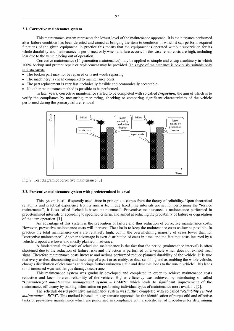
97

2.1. Corrective maintenance system

This maintenance system represents the lowest level of the maintenance approach. It is maintenance performed after failure condition has been detected and aimed at bringing the item to condition in which it can perform required functions of the given equipment. In practice this means that the equipment is operated without supervision for its whole durability and maintenance is performed only when a failure occurs. In this case repair costs are high, including loss due to the vehicle being out of operation.

Corrective maintenance (1st generation maintenance) may be applied to simple and cheap machinery in which 100% backup and prompt repair or replacement may be provided. This type of maintenance is obviously suitable only in these cases: • The broken part may not be repaired or is not worth repairing. • The machinery is cheap compared to maintenance costs. • The part replacement is very fast, technically feasible and economically acceptable. • No other maintenance method is possible to be performed.

In later years, corrective maintenance started to be completed with so called Inspection, the aim of which is to verify the compliance by measuring, monitoring, checking or comparing significant characteristics of the vehicle performed during the primary failure removal.

Cos

ts

Time

repair costs repair costs

losses caused by production

dropout

failure failure losses

caused by production

dropout

Fig. 2. Cost diagram of corrective maintenance [3]

2.2. Preventive maintenance system with predetermined interval

This system is still frequently used since in principle it comes from the theory of reliability. Upon theoretical reliability and practical experience from a similar technique fixed time intervals are set for performing the “service maintenance”, it is so called “schedule-based maintenance“. Preventive maintenance is maintenance performed in predetermined intervals or according to specified criteria, and aimed at reducing the probability of failure or degradation of the item operation. [1].

An advantage of this system is the prevention of failure and thus reduction of corrective maintenance costs. However, preventive maintenance costs will increase. The aim is to keep the maintenance costs as low as possible. In practice the total maintenance costs are relatively high, but in the overwhelming majority of cases lower than for “corrective maintenance”. Another advantage is even distribution of costs in time, and the fact that costs incurred by a vehicle dropout are lower and mostly planned in advance.

A fundamental drawback of scheduled maintenance is the fact that the period (maintenance interval) is often shortened due to the reduction of failure risks and the action is performed on a vehicle which does not exhibit wear signs. Therefore maintenance costs increase and actions performed reduce planned durability of the vehicle. It is true that every useless dismounting and mounting of a part or assembly, or disassembling and assembling the whole vehicle, changes distribution of clearances and brings further unknown static and dynamic loads to the run-in vehicle. This leads to its increased wear and fatigue damage occurrence.

This maintenance system was gradually developed and completed in order to achieve maintenance costs reduction and keep inherent reliability of the vehicle. Higher efficiency was achieved by introducing so called “Computerized maintenance management system – CMMS” which leads to significant improvement of the maintenance efficiency by making information on performing individual types of maintenance more available [2].

The schedule-based preventive maintenance system was further completed with so called “Reliability centred maintenance – RCM”. This method is based on a systematic approach for the identification of purposeful and effective tasks of preventive maintenance which are performed in compliance with a specific set of procedures for determining

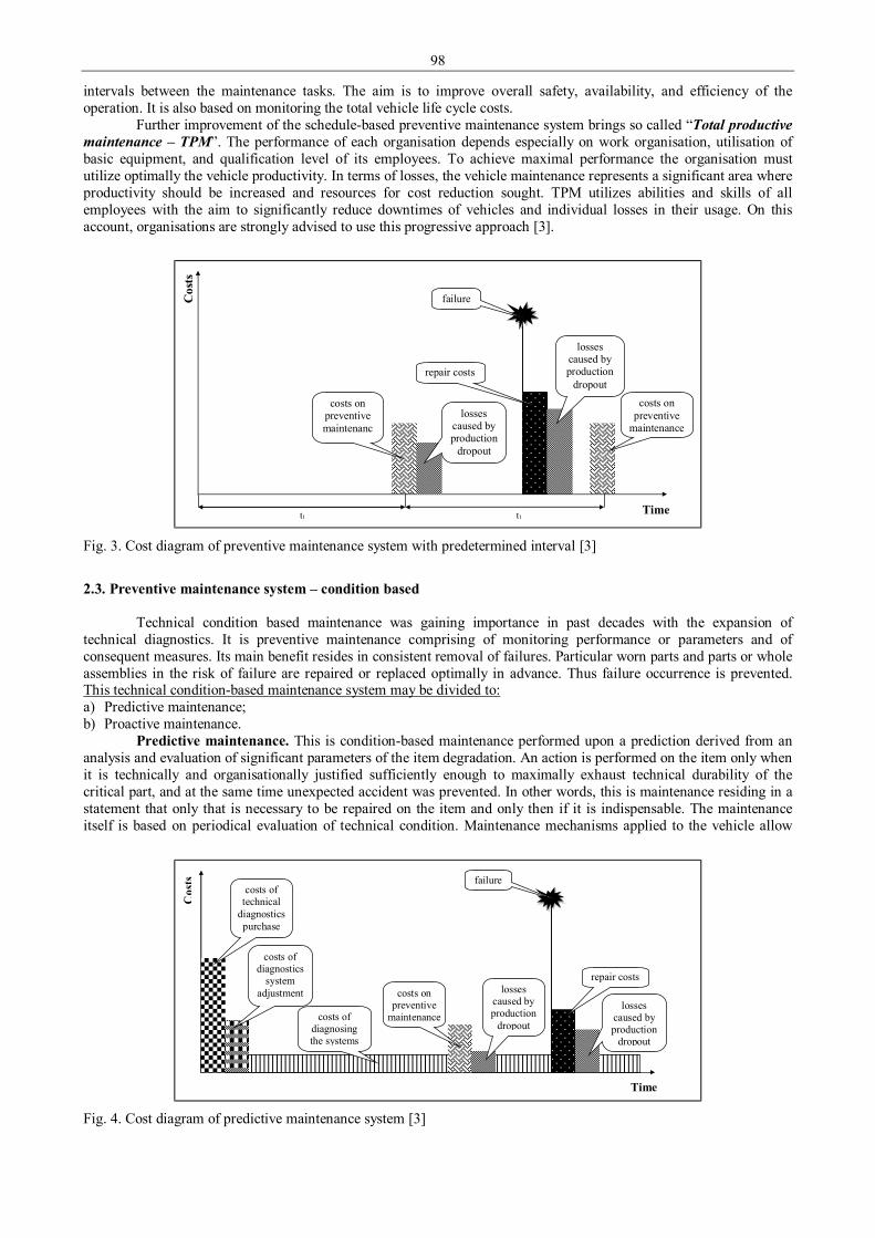
98

intervals between the maintenance tasks. The aim is to improve overall safety, availability, and efficiency of the operation. It is also based on monitoring the total vehicle life cycle costs.

Further improvement of the schedule-based preventive maintenance system brings so called “Total productive maintenance – TPM”. The performance of each organisation depends especially on work organisation, utilisation of basic equipment, and qualification level of its employees. To achieve maximal performance the organisation must utilize optimally the vehicle productivity. In terms of losses, the vehicle maintenance represents a significant area where productivity should be increased and resources for cost reduction sought. TPM utilizes abilities and skills of all employees with the aim to significantly reduce downtimes of vehicles and individual losses in their usage. On this account, organisations are strongly advised to use this progressive approach [3].

t1 t1

repair costs

costs on preventive maintenanc

e

losses caused by production

dropout

failure

costs on preventive

maintenance

Time

Cos

ts

losses caused by production

dropout

Fig. 3. Cost diagram of preventive maintenance system with predetermined interval [3]

2.3. Preventive maintenance system – condition based

Technical condition based maintenance was gaining importance in past decades with the expansion of technical diagnostics. It is preventive maintenance comprising of monitoring performance or parameters and of consequent measures. Its main benefit resides in consistent removal of failures. Particular worn parts and parts or whole assemblies in the risk of failure are repaired or replaced optimally in advance. Thus failure occurrence is prevented. This technical condition-based maintenance system may be divided to: a) Predictive maintenance; b) Proactive maintenance.

Predictive maintenance. This is condition-based maintenance performed upon a prediction derived from an analysis and evaluation of significant parameters of the item degradation. An action is performed on the item only when it is technically and organisationally justified sufficiently enough to maximally exhaust technical durability of the critical part, and at the same time unexpected accident was prevented. In other words, this is maintenance residing in a statement that only that is necessary to be repaired on the item and only then if it is indispensable. The maintenance itself is based on periodical evaluation of technical condition. Maintenance mechanisms applied to the vehicle allow

repair costs costs on

preventive maintenance

losses caused by production

dropout

failure

Time

Cos

ts

costs of technical

diagnostics purchase

costs of diagnostics

system adjustment losses

caused by production

dropout costs of

diagnosing the systems

Fig. 4. Cost diagram of predictive maintenance system [3]

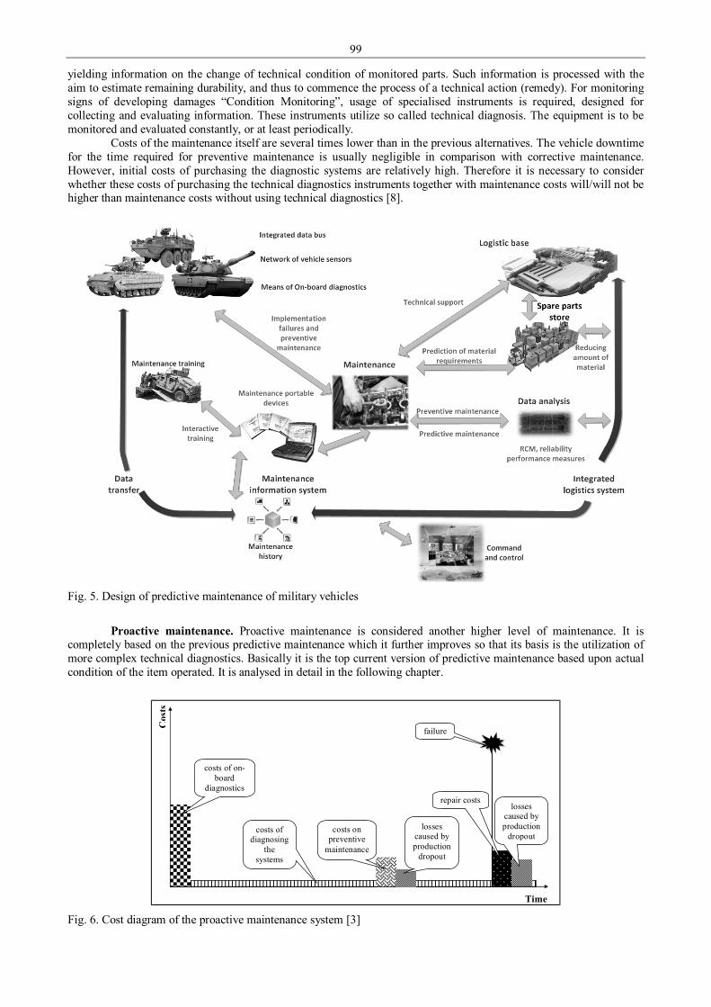
99

yielding information on the change of technical condition of monitored parts. Such information is processed with the aim to estimate remaining durability, and thus to commence the process of a technical action (remedy). For monitoring signs of developing damages “Condition Monitoring”, usage of specialised instruments is required, designed for collecting and evaluating information. These instruments utilize so called technical diagnosis. The equipment is to be monitored and evaluated constantly, or at least periodically.

Costs of the maintenance itself are several times lower than in the previous alternatives. The vehicle downtime for the time required for preventive maintenance is usually negligible in comparison with corrective maintenance. However, initial costs of purchasing the diagnostic systems are relatively high. Therefore it is necessary to consider whether these costs of purchasing the technical diagnostics instruments together with maintenance costs will/will not be higher than maintenance costs without using technical diagnostics [8].

Fig. 5. Design of predictive maintenance of military vehicles

Proactive maintenance. Proactive maintenance is considered another higher level of maintenance. It is

completely based on the previous predictive maintenance which it further improves so that its basis is the utilization of more complex technical diagnostics. Basically it is the top current version of predictive maintenance based upon actual condition of the item operated. It is analysed in detail in the following chapter.

repair costs

costs on preventive

maintenance

losses caused by production

dropout

Time

costs of on-board

diagnostics

losses caused by production

dropout

costs of diagnosing

the systems

Cos

ts

failure

Fig. 6. Cost diagram of the proactive maintenance system [3]

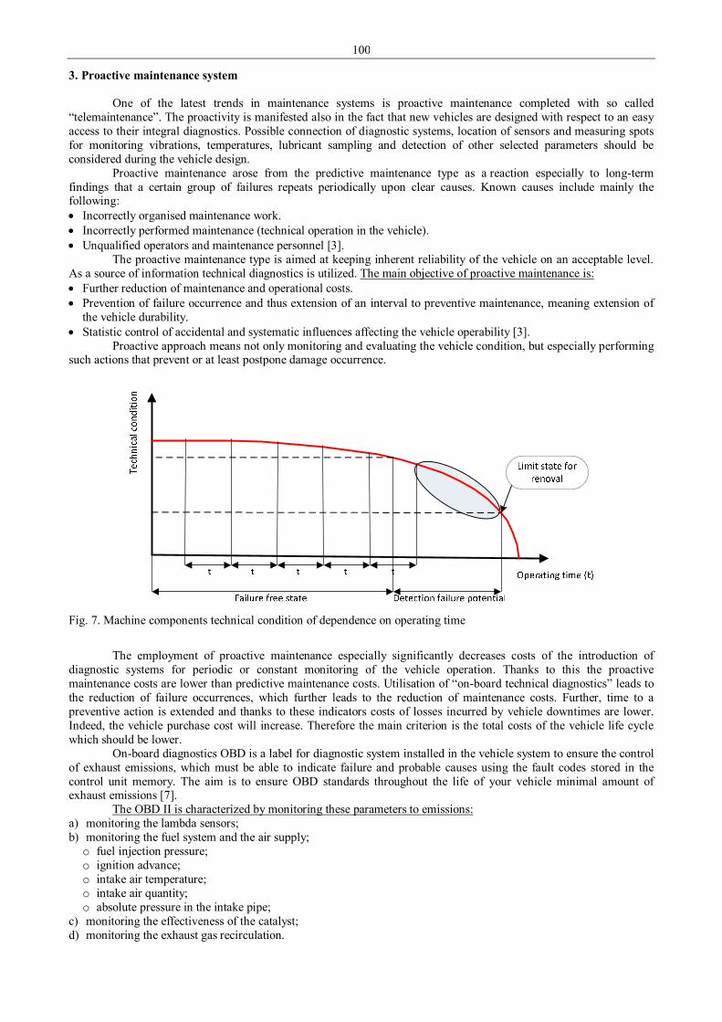
100

3. Proactive maintenance system

One of the latest trends in maintenance systems is proactive maintenance completed with so called “telemaintenance”. The proactivity is manifested also in the fact that new vehicles are designed with respect to an easy access to their integral diagnostics. Possible connection of diagnostic systems, location of sensors and measuring spots for monitoring vibrations, temperatures, lubricant sampling and detection of other selected parameters should be considered during the vehicle design.

Proactive maintenance arose from the predictive maintenance type as a reaction especially to long-term findings that a certain group of failures repeats periodically upon clear causes. Known causes include mainly the following: • Incorrectly organised maintenance work. • Incorrectly performed maintenance (technical operation in the vehicle). • Unqualified operators and maintenance personnel [3].

The proactive maintenance type is aimed at keeping inherent reliability of the vehicle on an acceptable level. As a source of information technical diagnostics is utilized. The main objective of proactive maintenance is: • Further reduction of maintenance and operational costs. • Prevention of failure occurrence and thus extension of an interval to preventive maintenance, meaning extension of

the vehicle durability. • Statistic control of accidental and systematic influences affecting the vehicle operability [3].

Proactive approach means not only monitoring and evaluating the vehicle condition, but especially performing such actions that prevent or at least postpone damage occurrence.

Fig. 7. Machine components technical condition of dependence on operating time

The employment of proactive maintenance especially significantly decreases costs of the introduction of

diagnostic systems for periodic or constant monitoring of the vehicle operation. Thanks to this the proactive maintenance costs are lower than predictive maintenance costs. Utilisation of “on-board technical diagnostics” leads to the reduction of failure occurrences, which further leads to the reduction of maintenance costs. Further, time to a preventive action is extended and thanks to these indicators costs of losses incurred by vehicle downtimes are lower. Indeed, the vehicle purchase cost will increase. Therefore the main criterion is the total costs of the vehicle life cycle which should be lower.

On-board diagnostics OBD is a label for diagnostic system installed in the vehicle system to ensure the control of exhaust emissions, which must be able to indicate failure and probable causes using the fault codes stored in the control unit memory. The aim is to ensure OBD standards throughout the life of your vehicle minimal amount of exhaust emissions [7].

The OBD II is characterized by monitoring these parameters to emissions: a) monitoring the lambda sensors; b) monitoring the fuel system and the air supply; o fuel injection pressure; o ignition advance; o intake air temperature; o intake air quantity; o absolute pressure in the intake pipe;

c) monitoring the effectiveness of the catalyst; d) monitoring the exhaust gas recirculation.

101

Other parameters monitored: e) standardized output operational data; o vehicle speed; o engine speed; o coolant temperature and oil etc.; o engine oil pressure;

f) monitoring of braking systems (ABS, ASR, ESP, etc.); g) monitoring of safety systems - airbags and anti-theft; h) monitoring of transmission (mostly automatic); i) condition of brake pads; j) condition of brake fluid; k) condition of the spark plugs; l) monitoring of active chassis – control wheels, suspension settings etc.; m) condition of accumulator battery and wiring; n) monitoring of engine oil quality.

The OBD system must be equipped with control lamp errors - MIL (Malfunction Indicator Light). Detecting the state and quality of the engine oil is one of the newest ways using internal sensors. These are

mounted directly on the engine. The measured data are transmitted using the CAN bus of the vehicle and then evaluated using the OBD II [9].

Sensors detect oil quality: • amount of oil; • temperature of oil; • index TBN (Total Base Number) – measuring ability to neutralize acids – affects the oxidation and corrosion,

oiliness and viscosity; • dynamic viscosity of oil – η; • specific density of oil – ρ; • for diesel engines soot content in oil; • water content in the oil; • electrolytic conductivity – G, measures the concentration of salts and acids; • permittivity – εr .

Fig. 8. Oil quality sensors [6]

Fig. 9. Function principle of tuning fork sensor [6]

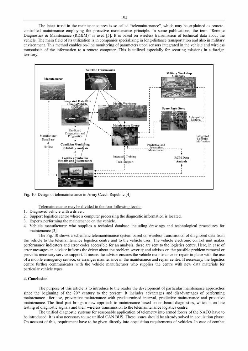
102

The latest trend in the maintenance area is so called “telemaintenance”, which may be explained as remote-controlled maintenance employing the proactive maintenance principle. In some publications, the term “Remote Diagnostics & Maintenance (RD&M)” is used [5]. It is based on wireless transmission of technical data about the vehicle. The main field of its utilization is in companies specializing in long-distance transportation and also in military environment. This method enables on-line monitoring of parameters upon sensors integrated in the vehicle and wireless transmissin of the information to a remote computer. This is utilized especially for securing missions in a foreign territory.

Manufacturer Data Base

&Hotline Predictive and

Preventive Maintenance

On-BoardDiagnostics and

Prognostics Integrated Logistics

Information

Integrated Data BUSCombatVehicle

Interactiv Training&

Tech. Support

Anticipatory Material

RCM Data Analysis

Condition Monitoring Reliability Analysis

Spare Parts StoreMobile Workshop

Manufacturer

Military Workshop Company

Maintenance Group

Satellite Transmission

Logistics Centre forRepairs and Maintenance

Fig. 10. Design of telemaintenance in Army Czech Republic [4]

Telemaintenance may be divided to the four following levels:

1. Diagnosed vehicle with a driver. 2. Support logistics centre where a computer processing the diagnostic information is located. 3. Experts performing the maintenance on the vehicle. 4. Vehicle manufacturer who supplies a technical database including drawings and technological procedures for

maintenance [3]. The Fig. 10 shows a schematic telemaintenance system based on wireless transmission of diagnosed data from

the vehicle to the telemaintenance logistics centre and to the vehicle user. The vehicle electronic control unit makes performance indicators and error codes accessible for an analysis, these are sent to the logistics centre. Here, in case of error messages an advisor informs the driver about the problem severity and advises on the possible problem removal or provides necessary service support. It means the advisor ensures the vehicle maintenance or repair in place with the use of a mobile emergency service, or arranges maintenance in the maintenance and repair centre. If necessary, the logistics centre further communicates with the vehicle manufacturer who supplies the centre with new data materials for particular vehicle types. 4. Conclusion

The purpose of this article is to introduce to the reader the development of particular maintenance approaches since the beginning of the 20th century to the present. It includes advantages and disadvantages of performing maintenance after use, preventive maintenance with predetermined interval, predictive maintenance and proactive maintenance. The final part brings a new approach to maintenance based on on-board diagnostics, which is on-line testing of diagnostic signals and their wireless transmission to the telemaintenance logistics centre.

The unified diagnostic systems for reasonable application of telemetry into armed forces of the NATO have to be introduced. It is also necessary to use unified CAN BUS. These issues should be already solved in acquisition phase. On account of this, requirement have to be given directly into acquisition requirements of vehicles. In case of combat

103

vehicles, the special equipment such as turret, weapon station, vehicle´s filtration system and other cannot be omitted. With regard to previous experiences, I would consider to unify all those components and systems into common control unit including single OBD connector for data transmission for subsequent analysis.

Using telemetry, which can be described as the wireless data transmission into logistic centres, with which is possible to analyse obtained data about technical state of vehicles in real time. The vehicle maintenance can be executed on the basis of comparison of obtained data and data recommended. These workshops should have possibility to contact crew of vehicle in order to give them advice about solution of the problem. In case of execution of more extensive repair, this workshop assumes the role of technical support.

Implementation of maintenance system based on telemetry enables cost reduction of proper realization of maintenance, on the other hand their purchase cause higher acquisition costs of vehicles and related portable wireless devices. Except the lower maintenance expenses, this access bring also the complete overview of general operation of all in this way equipped vehicles. Most evolved armed forces of the NATO (USA, Great Britain and Germany) are already occupying themselves by solution of projects connected with telemetry.

Presented work has been prepared with the support of the Ministry of Defence of the Czech Republic, Partial Project for Institutional Development, K-202, Department of Combat and Special Vehicles, University of Defence, Brno. References 1. ČSN EN 13306, Maintenance terminology. 2. Levitt J. Complete Guide to Preventive and Predictive Maintenance. New York: Industrial Press, 2003. 210 p.

ISBN 0-8311-3154-3. 3. Furch J. New Trends in a Vehicle Maintenance System. Advances in Military Technology, 2010, vol. 5, no. 2, p.

1-9. ISSN 1802-2308. 4. Furch J. Prognostics and Health Management in Military. In. Transport means 2011, 2011, no. 1, p. 5-8. ISSN

1822-296X. 5. You S., Krage M. and Jalics L. Overview of Remote Diagnosis and Maintenance for Automotive Systems. USA.

SAE International. 2005-01-1428. 2005-04-14. 6. Andreas B. Multiparametric Oil Condition Sensor based on the Tuning Fork Technology for Automotive

Applications. Berlin: Hella, 2005, p. 15. 7. Leitner B. Autoregressive models in modelling and simulation of transport means working conditions. In: Transport

means 2010, 2010 no. 1, p. 21 – 24. ISSN 1822-296X. 8. Chovanec A. Analysing and Modelling Off-Road Vehicle Availability. In. Transport means2011, 2011, no. 1,

p. 54-57. ISSN 1822-296X. 9. Glos J. Modern Methods of Tribological Diagnostics. In. Transport means2011, 2011, no. 1, p. 26-29.

ISSN 1822-296X.

104

Proceedings of 9th International Conference ITELMS’2014 Industrial Flooring and Industrial Flooring Installations A. Garskiene, J. Kaupiene, D. Aviza, N. Partaukas Kaunas University of Technology, Daukanto str. 12, 44556, Panevezys, Lithuania Abstract The floor of industrial buildings is mostly burdened. The consist of a a concrete and the methods of the casting can have a influence for it's strength, resistance, wear, density, cold, sedentary and water. Concrete can withstand heavy loads, but if the concrete floor is provided to be cast in the places for which are held the high requirements, the floor should be equipped with a stronger upper layer. KEYWORDS: concrete, industrial flooring, hander, cast floor, polymer flooring, resistant. 1. Introduction

The floor – is one of the main elements of the building and it is the most congested part of the building. It constantly has a very high load associated with abrasive and mechanical abrasion, thermal, chemical and dynamical effects. Modern industrial floors should be resistant to the effects of these types of aesthetic appearance: easy to maintain, non-flammable, non-slip, odorless and not too much strain on the building structure. Irregularities should be repaired easily and quickly. One of the most important decisions, for repair or construction of any building, is choosing the appropriate flooring materials. The term “floor molding” reflects only one of the polymeric materials stacking technology. Floor molding – is an industrial coating made of polymeric materials epoxy, polyurethane, and other methyl methacrylic polymeric binders.

Often, self-leveling cement coating type is called a cast floor. Self-leveling cement is not the final layer, but is used to level the floor before the other coatings (mostly commercial linoleum, carpet) floor.

Fig. 1. Concrete floor structure

2. The main features of industrial floor

Monolithic. Unlike other floor coverings, floor molding has no joints. Cast on the floor do not reproduce bacteria and micro-organisms. It is very important for medical institutions and organizations involved in food production. Polymer flooring is completely hermetically sealed and when the floor is washed, humidity do not percolate, it extends the life of the floor. Also floor molding is widely used in industrial premises, where are chemically active fluids, acid and alkali oil spill.

Durability. Correctly handled properly selected libations floor, epoxy and polyurethane cast floor life of up to 20 years or more. Without the proper type of polymer coating selection, an important factor is technically correct a concrete foundation and implicit cast flooring technology compliance for each production process.

There is no dust. Polymer flooring is one of the few seamless flooring types that completely avoids the concrete foundation of dust. There is no longer any area of human activity, which sees “Dustability” would be allowed, and do not interfere with the work process. Warehouse terminals, garages, industrial premises and personnel, medical institutions, kindergartens, schools, catering companies, research institutes and sports facilities. These are just a few objects that are equipped with molding and coloring polymer coating.

105

High chemical resistance. In today's building materials market, there was a limited floor coverings that may be rendered resistant to solvents, acids, alkalis, petroleum products and other chemically active mixtures. One of them is acid-resistant tiles and epoxy molding floor. Epoxy floor molding is the optimal solution when it comes to the ground with a high chemical resistance. Compared to tiles, epoxy molding floor costs less, there is a seamless, flexible and allows to perform a work.

High resistance to abrasion. Floor molding is a very high resistance to abrasion, which is due to the abrasive effects of continuous floor. First of all, it is a grain of sand, are placed on the floor of the transport machinery, car wheels and the people of footwear. Tests showed that the molding floor can be used for a period of time: a weak wear categories – up to 140 years, the average wear categories – up to 80 years old, wearing a strong category – up to 50 years old (cast polymer coatings data).

Resistance to shock and vibration loads. Polymer industrial flooring is resistant to heavy objects falling, machine tools and other equipment vibration. The most striking example is a modern printing house, there are all of the above listed types of loads - the molding floor keeps these challenges successfully.

Aesthetics. Floor molding is widely applied not only in industrial plants, garages and warehouse complexes, but also sports facilities, offices, medical and educational institutions, entertainment venues. Polymer coatings can be produced in a very wide range of colors. Coatings can be decorated with colored particles, different colors flooring can be installed in the same room. The floor is completely flat, and it gives them an extra decorative features. Laid in epoxy and polyurethane molding floor is completely harmless. These floors are allowed to use medical and scientific institutions, food production facilities and kindergartens.

Fire safety. Molding epoxy and polyurethane coatings are widely used in the risk of explosion-related industrial facilities such as oil refineries, chemical testing laboratory and others. The polymer molding floor is allowed to lay public and residential buildings and structures on the fire escape exit zones. 3. Industrial flooring technology

Concrete floors are cast using ready-mix concrete. The floor surface, depending on your needs, can be smooth or rough. The technology allows levels to cover large areas and offer customers a wide range of colors. Its thickness is chosen according to the floor structure, ranging from 80 to 300 mm.

Mineral and waterproofing powder only used for concreting the new floor. Epoxy resin and an abrasion resistant layer repaired the floor and do strengthen the existing floor. Epoxy and polyurethane industrial compounds resistant to abrasion and impact, petrol, oil and chemistry effects.

The floor below the level of the ground water level or exposed to weather and moisture released during the production, lactic acid, chlorides, oil products, it is advisable to cover for waterproofing with mineral based.

The most common mineral-based protection in garages, garages and underground parking lots used in these types of structures:

Construction materials, which are based on a specific substrate (quartz, granite, etc.) provide monolithic coating and strength. They are resistant to studded tires, detergents destructive effects. These floors can be used for several decades.

Cast floor – monolithic protective coating made of epoxy, polyurethane and mixtures combined basis. This homogeneous 1.5 mm thick membrane coated on the surface of the mineral.

A Thin mixture of paint – a thin polymer coating, covered for 2-3 steps. Monolithic and good performance make the floor reliable protection of low and moderate load conditions.

Concrete floors with a chemical hardener. Chemical concrete hardener binds particles, curing the floor surface and reduce dustiness. All of the concrete during the curing compounds are characterized by three main features: 1. Surface hardening. 2. Surface protection from dust. 3. Surface insulation.

These properties are the chemical reactions taking place between the silicate, Portland cement, calcium hydroxide (free lime) within the pores of the concrete. The flooring is characterized by durability, resistance to higher loads, moisture and grease. Floor surface over time is becoming increasingly shine. This technology is often used in the restoration of old floors, in order to improve their performance, such as reducing wear and dustiness, increase resistance to liquid penetration.

The materials used for mineral floors are made of cement-based with specific additives in quantities depending on surface mechanical properties and resistance to chemical attack. Mineral surface is divided by coating technology into: 1. Dry powder which is applied to a freshly concrete. 2. Special thin mixture, which is laid on the existing concrete floor.

What type of mineral surface will be used in a particular case depends on the expected exploitating conditions on the floor and highlight the desired properties: resistance to abrasion, chemicals or a hose. All mineral coating provide protection from these factors, but the individual characteristics of the individual materials are developed further.

106

Fig. 2. Concrete floor with a chemical hardener

Parking lots, located outdoors, industrial flooring, continuously or periodically exposed to wet and chemically

active environment, used mineral dry shake, giving a deep impact on concrete waterproofing by crystallisation. This shake is applied over freshly placed concrete floors, with the same technology as the coating powder which confers resistance to abrasion, and can be of different colors. Using sprinkles with crystalline waterproofing materials solved several problems. This is a harmless substance permanently impairments concrete, protecting it from water or aggressive chemicals intrusion from any direction. Although the concrete reaches its design strength, the floor becomes a waterproof full-depth (crystals formed by 30 cm), but during the operation the floor after moisture (due to increased groundwater pressure caused microcracks, etc.). Waterproofing effect further increases and resulting microcracks sealed.

Sustained long-term concrete protection against the harmful warming and harmful effects of most chemical environments: 1. Increases the mechanical strength of concrete. 2. Due to the special, abrasion resistance enhancing additive obtained surface hardness, sufficient for light and

medium-duty floor. Rub against the disc greater level will depend on how the surface roughness is obtained. On the technology

used to rub the top layer of flooring is gaining greater strength and resistance to abrasion than the lower layers of concrete. It also provides in depth waterproofing and resistance to chemicals (petroleum products, lubricants, winter on the road surface watered chlorides).

Mineral shake and shake with metallic accessories are placed on freshly placed concrete floors blend. The production of this mixture, do not use plasticizers lignosulfonates containing more than 5% sugar . However, the mixture can be any fiber reinforced base. Additional preparation of the shake before using them is not required. They are evenly disseminated on the floor surface of the concrete mixture, compacted with vibrating beams, after 1.5-3 hours of its laying has been completed. This period of time depends on the ambient temperature and can be longer. Sprinkles possible to spread manually, but it is more practical to use a special mechanical dispenser, which ensures uniform dispersion of the shake. The required amount of the shake can be built in two portions, pour half of the required output, the surface smoothed grater, wait until the powder is wet from a mixture of water and other content will be milled. It is important to lay sprinkles before curing concrete mixture, otherwise the shake-layer can detach from the concrete.

Once on the surface can already walk, shake continue working with mechanical apparatus. Hand working can only be floor or sides of the small area. It creates matte and glossy surfaces.

Abrasion-resistant mineral-based layer can be applied over existing concrete floor. The flooring used in repairing the old concrete floor, or to increase the existing floor abrasion resistance (e.g., changes in operating conditions). The minimum thickness of the coating layer is 12 mm, compressive strength after 28 days – 60 MPa, resistance to frost – F100. Due to these characteristics, the coating can be applied both outside and inside. Before concreting low-abrasion layer properly prepared base: Remove dirt, the floor covered whit the adhesive. The substrate is divided into sections, echoing the thermal and expansion joints. The laid mixture thickened vibrating beams. The layer is leveled and then compacted surface compactor. When the coating reaches the initial strength, the surface is processed mechanically or by hand.

Polymer flooring. Seamless cast polymer flooring can be made of epoxy, polyurethane and methacrylate (also known as acrylic) basis. Before pouring the floor, you need to check the moisture content of concrete, which cannot exceed 5% total weight. Water vapor migration during construction shall be reduced to a minimum. It is necessary to determine the strength of the concrete compressive strength and tensile strength. Concrete compressive strength must be greater than 20 N/mm2 and tension – more than 2 N/mm2. The surface should be smooth and should not be on the cement milk, dust, grease, oil stains and similar substances that interfere with adhesion of the coating.

If it is not possible to wait for 28 days until the concrete base to reach the required residual moisture level, the floor is laid epoxy damp proof membrane.

Epoxy coating – durable and resistant to aggressive environmental conditions. Epoxy flooring laid on existing concrete floors, repairing them or to provide additional protection for concrete from aggressive substances. Epoxy coatings are characterized by good mechanical properties: abrasion resistance, chemical resistance, floor provides an

107

aesthetic appearance. Before application of this type of coating, the surface is prepared, concrete well cleaned, repaired defects. Substrate moisture content does not exceed 4%.This material is used in industrial premises, car parks and other long-term effects of experiencing mechanical surfaces. Perhaps the most important advantage of epoxy coating – working with them fast and cheap, but the quality and aesthetic appearance of the material does not yield expensive ceramic or stone tiles. Waterproof epoxy coating performs the function of waterproofing.

Epoxy coatings can withstand great load, you can choose a few shades or special colored chips to simulate textured surfaces.

Epoxy resins for floor coverings installed, can be classified in various ways: 1. Viscous and low viscosity. 2. One Component, two component, and the multiple. 3. With organic solvents, solvent, diluted with water.

However, the main characteristic that defines whether a coating for the surface pore impregnation or coating on the surface to be awarded – is the viscosity. Low viscosity resins soaked concrete floor. Soggy concrete obtained betonpolimeris has better strength properties, superior resistance to abrasion and chemicals. Using these resins on the floor and does not coat epoxy-resin has absorbed all of the pores. This method is used to reduce the dustiness of the old concrete floor, or the surface before applying the epoxy coating. The epoxy coating on the surface of a clean repaired and is applied with a brush or a broom.

The increased viscosity of the resin used in the new coating. Depending on the properties of the resin, the coating applied by roller or brush. Usually applied in two layers: the first layer for couples impregnation (absorption reduction). When was particularly porous, it is advisable to use a low viscosity epoxy impregnating resin.

In order to improve the strength properties of the epoxy coating, the resin can be placed in quartz aggregates. Their fraction 0.3-0.6 mm, it is possible to select different tones. Fillings can be deposited onto a freshly coated epoxy coating. When the temperature is 20 °C, epoxy film encrust within 45 minutes and fully dries in 24 hours.

The floor surface is smooth, without any seams. Polymer flooring has the strength, excellent aesthetic and performance. The rooms, which are subject to extreme cleanliness and hygiene standards, equipped with a special polyurethane flooring, which among other properties characterized by a high resistance to chemical and thermal effects. Polymer flooring usually serves about 25 years.

Fig. 3. Polymer flooring

4. Cast floor price comparison

After the calculations, is compared five different floor coverings. Comparing flooring price, the cost of materials, labor wage rates revealed that the most expensive covering is No. 1 – flooring installation using solid mineral aggregates, and the cheapest is No.3 – self-leveling two-component epoxy floor coating installation.

Table 1 Flooringo no. and description

Flooring no Description

1. Flooring installation using solid mineral aggregates (KORODUR coating thickness of 12 mm) K8 = 1.03 2. Concrete coating installation with hard fillers (HE 65 NEODUR coating thickness of 3 mm) 3. Self-leveling two-component epoxy floor coating installation (on a prepared base) with two layers (3.0 mm) 4. Two layers of molded polyurethane flooring installation (on a prepared base) 5. Concrete flooring coating a thin layer of polyurethane enamel (on a prepared base)

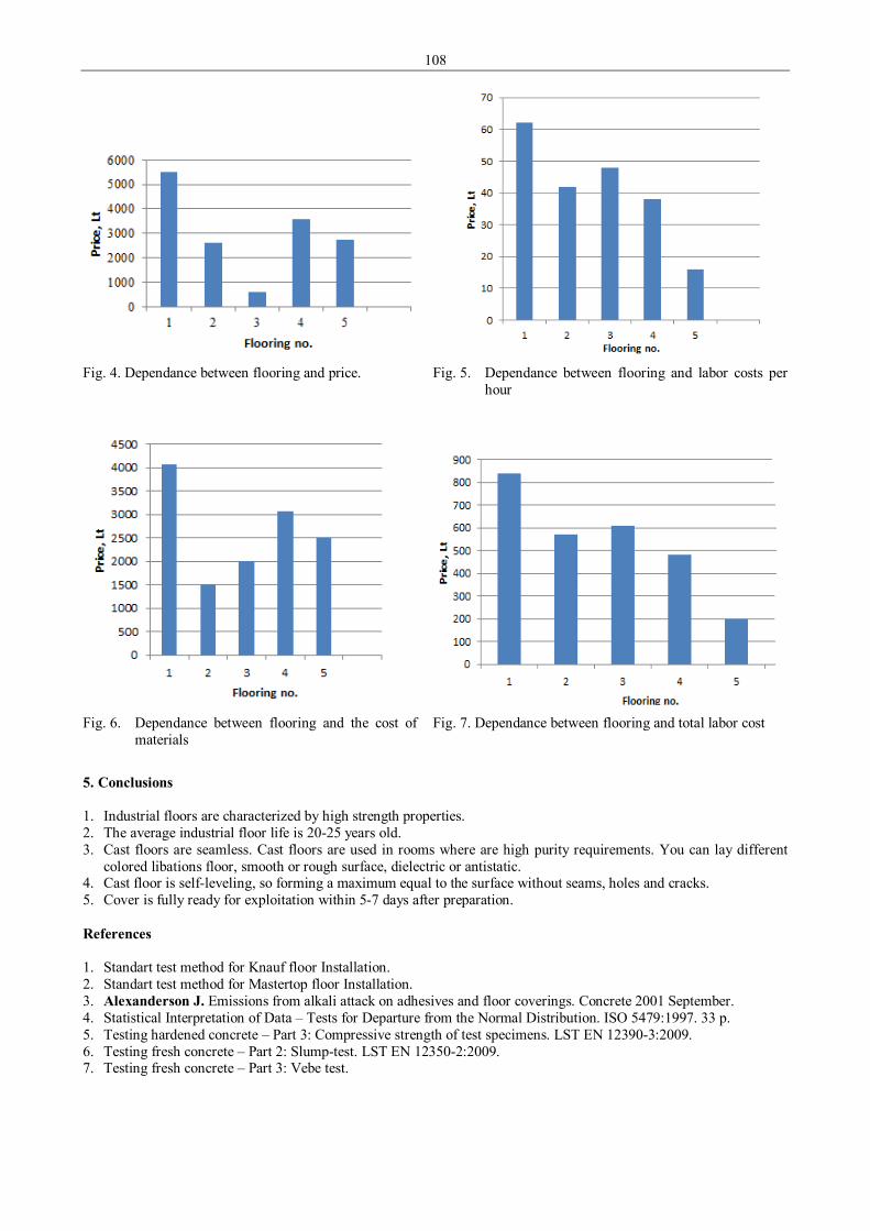
108

Fig. 4. Dependance between flooring and price. Fig. 5. Dependance between flooring and labor costs per

hour

Fig. 6. Dependance between flooring and the cost of

materials Fig. 7. Dependance between flooring and total labor cost

5. Conclusions 1. Industrial floors are characterized by high strength properties. 2. The average industrial floor life is 20-25 years old. 3. Cast floors are seamless. Cast floors are used in rooms where are high purity requirements. You can lay different

colored libations floor, smooth or rough surface, dielectric or antistatic. 4. Cast floor is self-leveling, so forming a maximum equal to the surface without seams, holes and cracks. 5. Cover is fully ready for exploitation within 5-7 days after preparation. References 1. Standart test method for Knauf floor Installation. 2. Standart test method for Mastertop floor Installation. 3. Alexanderson J. Emissions from alkali attack on adhesives and floor coverings. Concrete 2001 September. 4. Statistical Interpretation of Data – Tests for Departure from the Normal Distribution. ISO 5479:1997. 33 p. 5. Testing hardened concrete – Part 3: Compressive strength of test specimens. LST EN 12390-3:2009. 6. Testing fresh concrete – Part 2: Slump-test. LST EN 12350-2:2009. 7. Testing fresh concrete – Part 3: Vebe test.

109

Proceedings of 9th International Conference ITELMS’2014 Modelling and Research of Bus Equipped with Dynamic Stability Control System E. Girkontas*, V. Lukosevicius**, Z. Bazaras*** *Kaunas University of Technology, Kestucio str. 27, LT-43124, Kaunas, Lithuania, E-mail: evaldas.girkontas@stud.ktu.lt **Kaunas University of Technology, Kestucio str. 27, LT-44354, Kaunas, Lithuania, E-mail: vaidas.lukosevicius@ktu.lt ***Kaunas University of Technology, Kestucio str. 27, LT-44354, Kaunas, Lithuania, E-mail: zilvinas.bazaras@ktu.lt Abstract The paper presents a simulation research of lateral stability of virtual bus model, which is equipped with dynamic stability control. Simulations performed by using Adams/Car and Adams/Mechatronics on virtual 3D road. Dynamic stability control system focuses on bus’s yaw stability, but also reduce roll angle. Two types of maneuvers were held: single line change and double line change, on different road friction conditions. In case payload is very important factor for heavy transport, two different payload conditions were analyzed- empty and fully loaded bus model. Simulation data were used to estimate influence of dynamic stability control for bus’s lateral stability and rollover prevention. KEYWORDS: bus, dynamic stability control, ESP, lateral stability, rollover prevention. 1. Introduction

Directional stability is one of the most important subjects of active safety for all kinds of vehicles. Dynamic stability control system is a vehicle control system, whose objective is to maintain lateral stability during maneuvers. There are three main yaw control system types: active torque distribution, steer-by-wire and differential braking. Last one most widely used today in automotive. This system is based on ABS (anti-lock braking system) and uses the vehicle’s brakes to create a yaw moment. A counter-clockwise yaw moment is generated, when brakes pressures are increased at the left wheels. Manufacturers have used a variety of different names for this type of system, as ESP (electronic stability program) or ESC (electronic stability control) [1].

Bus crashes where its instability is an issue can be divided into two main types: rollover crashes and loss of directional control crashes. Loss of directional control crashes generally occurs when one or more axle groups loose directional control. This usually occurs under turning where the road surface friction is low. Rollover crashes occur when the resultant force at the center of gravity of the vehicle falls outside the vehicle track. This resultant force is the combination of the lateral force, usually from a turning maneuver, and the vertical force as result of gravity. This assumes that the sideways friction between the tires and the road surface is sufficient to equal the lateral force. If it is not, sliding and loss of directional control rather than rollover will occur [2].

Computer simulation models are used in almost every research and product development process in automotive industry. 2. Bus model

Bus model was created in Adams/Car and dynamic stability control system’s signals were created by Adams/Mechatronics. Using Adams/Car was constructed multi-body dynamic bus model, which consists of these main parts: bus frame, front and rear suspension, engine, transmission, braking, steering and tire subsystems.

Fig.1 Modeled bus model in MSC Adams/Car

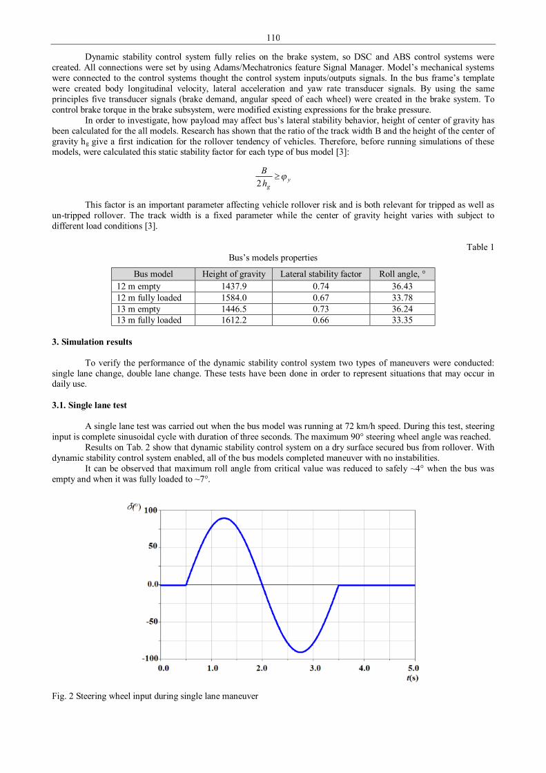
110

Dynamic stability control system fully relies on the brake system, so DSC and ABS control systems were created. All connections were set by using Adams/Mechatronics feature Signal Manager. Model’s mechanical systems were connected to the control systems thought the control system inputs/outputs signals. In the bus frame’s template were created body longitudinal velocity, lateral acceleration and yaw rate transducer signals. By using the same principles five transducer signals (brake demand, angular speed of each wheel) were created in the brake system. To control brake torque in the brake subsystem, were modified existing expressions for the brake pressure.

In order to investigate, how payload may affect bus’s lateral stability behavior, height of center of gravity has been calculated for the all models. Research has shown that the ratio of the track width B and the height of the center of gravity hg give a first indication for the rollover tendency of vehicles. Therefore, before running simulations of these models, were calculated this static stability factor for each type of bus model [3]:

ygh

B ϕ≥2

This factor is an important parameter affecting vehicle rollover risk and is both relevant for tripped as well as un-tripped rollover. The track width is a fixed parameter while the center of gravity height varies with subject to different load conditions [3].

Table 1 Bus’s models properties

Bus model Height of gravity Lateral stability factor Roll angle, ° 12 m empty 1437.9 0.74 36.43 12 m fully loaded 1584.0 0.67 33.78 13 m empty 1446.5 0.73 36.24 13 m fully loaded 1612.2 0.66 33.35

3. Simulation results

To verify the performance of the dynamic stability control system two types of maneuvers were conducted: single lane change, double lane change. These tests have been done in order to represent situations that may occur in daily use. 3.1. Single lane test

A single lane test was carried out when the bus model was running at 72 km/h speed. During this test, steering input is complete sinusoidal cycle with duration of three seconds. The maximum 90° steering wheel angle was reached.

Results on Tab. 2 show that dynamic stability control system on a dry surface secured bus from rollover. With dynamic stability control system enabled, all of the bus models completed maneuver with no instabilities.

It can be observed that maximum roll angle from critical value was reduced to safely ~4° when the bus was empty and when it was fully loaded to ~7°.

Fig. 2 Steering wheel input during single lane maneuver

111

Table 2 Roll angles during single lane maneuver

Bus model μ = 0.2 μ = 0.5 μ = 0.8 12 m empty (DCS off) 1.92 4.22 82.13 12 m empty (DCS on) 1.91 3.67 4.23 12 m fully loaded (DCS off) 3.35 6.72 84.26 12 m fully loaded (DCS on) 3.35 6.17 7.23 13 m empty (DCS off) 2.12 4.61 83.77 13 m empty (DCS on) 2.06 4.04 4.81 13 m fully loaded (DCS off) 3.41 6.76 84.47 13 m fully loaded (DCS on) 3.41 6.18 7.31

Table 3

Yaw rate during single lane maneuver

Bus model μ = 0.2 μ = 0.5 μ = 0.8 12 m empty (DCS off) 7.71 15.59 22.92 12 m empty (DCS on) 7.58 11.07 11.40 12 m fully loaded (DCS off) 77.25 17.12 19.02 12 m fully loaded (DCS on) 10.17 10.11 11.85 13 m empty (DCS off) 66.18 16.15 24.08 13 m empty (DCS on) 9.13 11.44 11.77 13 m fully loaded (DCS off) 77.74 15.77 19.18 13 m fully loaded (DCS on) 9.78 10.83 12.00

When test was carried out on dry surface, dynamic stability control system reduced yaw rate by 100% and by

40% on wet road. That is mean that this existing stability control system may aid in preventing a bus from spinning out, and reduces the potential risk for the vehicle to have a collision with a sidewalk or with other road infrastructure.

However the are some problems on icy surfaces (µ = 0.2). As we see, when the test was performed with 12 m empty bus, there are only minor yaw rate changes. The system detected that there were yaw rate and lateral acceleration gain, activated brakes, but the surface had too low friction. Therefore, it was hard to keep trajectory, when bus axles do not have enough grip. 3.2 Double lane change

This maneuver is widely used all around the world to evaluate the handling and safety of vehicle. Bus’s models velocity were 48 km/h before the entry lane. When lane was changed, here bus traveled for about 30 m straight, and then it returned to the original lane within the 30 m gate.

Fig. 3 Steering input during double lane change maneuver

112

Results show that during this test, no rollover was detected and dynamic stability control system reduced bus body roll only negligible. At dry surface, the range of roll angle of empty bus with activated stability control was observed to be between 6.4° and 7.3°. The maximum roll angle was reached when 13 m fully loaded bus on dry surface was tested. When this bus model was tested with dynamic stability control system enable, the body roll angle was reduced for about 20%.

Table 4 Roll angles during double lane maneuver

Bus model μ = 0.2 μ = 0.5 μ = 0.8 12 m empty (DCS off) 1.73 4.50 5.95 12 m empty (DCS on) 1.73 4.11 6.36 12 m fully loaded (DCS off) 3.45 7.17 12.06 12 m fully loaded (DCS on) 3.33 6.59 10.85 13 m empty (DCS off) 1.95 4.88 7.28 13 m empty (DCS on) 1.93 4.42 7.16 13 m fully loaded (DCS off) 3.43 7.30 15.13 13 m fully loaded (DCS on) 3.32 6.96 12.34

Table 5

Yaw rate during double lane maneuver

Bus model μ = 0.2 μ = 0.5 μ = 0.8 12 m empty (DCS off) 6.92 18.00 21.74 12 m empty (DCS on) 6.93 14.53 19.87 12 m fully loaded (DCS off) 11.55 16.01 22.73 12 m fully loaded (DCS on) 10.45 13.97 21.61 13 m empty (DCS off) 7.66 17.67 21.60 13 m empty (DCS on) 7.60 14.01 18.70 13 m fully loaded (DCS off) 11.56 16.26 26.79 13 m fully loaded (DCS on) 10.45 15.10 23.27

Yaw rate was mostly reduced when bus models were tested on wet surface. Maximum efficiency was reached,

when 13m empty bus model was tested. In this case, yaw rate was reduced by 26%. Like on the single lane change maneuver, there were also minor yaw rate changes on icy surface. 4. Performance criteria

From Single Lane change maneuver data YRR criteria can be calculated. This criterion is developed to evaluate the ability of dynamic stability control in mitigation loss of control crashes. NHTSA claims that DSC equipped vehicle has less than five percent chance to get into a loss control accident if the vehicle meets the required performance limits: • 0.75 s after completion of steering input, the yaw rate of the bus has to be less or equal to 40% of the first local peak; • 1.5 s after completion of steering input, the yaw rate of the bus has to be less or equal to 15% of the first local peak [4].

Table 6

Bus model μ ( )75.00+tψ& , m/s2 ( )5.10+tψ& , m/s2 pikψ& , m/s2 ( )75.00+tYRR , % ( )5.10+tYRR , %

12 m empty 0.2 0.72 0.47 7.57 9.5 6.10 12 m empty 0.5 0.09 0.76 8.08 1.1 9.38 12 m empty 0.8 0.46 1.15 8.84 5.2 13.0 12 m full 0.2 0.82 2.27 10.16 8.1 22.3 12 m full 0.5 2.44 0.04 9.40 25.9 0.50 12 m full 0.8 1.49 0.26 9.55 15.6 2.70 13 m empty 0.2 4.62 3.67 9.09 50.8 40.4 13 m empty 0.5 0.13 0.67 8.81 1.5 7.60 13 m empty 0.8 0.02 0.67 8.72 0.3 7.70 13 m full 0.2 1.93 1.50 9.77 19.8 15.4 13 m full 0.5 1.61 0.01 9.68 16.6 0.10 13 m full 0.8 1.02 0.26 9.00 11.3 2.90

113

As we see from the table, 12 m empty, 13 m empty and 13 m fully loaded bus models do not meet these criteria, when they were tested on icy surfaces. Therefore, this dynamic stability control system was not very reliably in these conditions. However, on other conditions this system worked perfectly and with its intervention achieved acceptable lateral stability. 5. Conclusion

Dynamic stability control system intervention has increase the stability of the bus model in which it is installed. Results showed that this system might prevent rollovers crashes of buses on dry surfaces. However, this type of system has defects because on low friction road’s surface has not been reduced roll angle and yaw rate. Moreover, three bus models with this dynamic stability control system do not meet YRR performance criteria. Acknowledgement

This work has been supported by the European Social Fund within the project “Development and application of innovative research methods and solutions for traffic structures, vehicles and their flows”, project code VP1-3.1-ŠMM-08-K-01-020. References 1. Rajesh Rajamani. Vehicle Dynamics and Control. New York: Springer, 2006.485p. 2. Queensland Department of Transport and Main Roads. Benefits of Heavy Vehicle Stability Safety Technologies.

Report. Queensland: 2011. Acces on the internet: < www.tmr.qld.gov.au/ >. 3. Liebemann E. K., Meder K., Schuh J., Nenninger G. Safety and Performance Enhancement: The Bosch

Electronic Stability Control. Paper: 05-0471, 2004 4. NHTSA. Test Track Lateral Stability Performance of Motorcoaches Equipped With Electronic Stability Control

Systems. Report: DOT HS 811633, 2013.

114

Proceedings of 9th International Conference ITELMS’2014 Monitoring of Chemical Elements during Lifetime of Engine Oil J. Glos*, V. Kumbar** *University of Defence Brno, Kounicova str. 65, 662 10, Brno, Czech Republic, E-mail: josef.glos@unob.cz **Mendel University in Brno, Zemedelska str. 1, 613 00, Brno, Czech Republic, E-mail: vojtech.kumbar@mendelu.cz Abstract The article deals with monitoring of chemical elements during lifetime of commercially distributed automobile engine oil. The passenger car with petrol engine was used to the observed. Lifetime of automobile engine oil has been stated by car producer in interval 15,000 km. The samples of automobile engine oil have been taken in suitable intervals – 1,500 km. The spectrometer Spectroil Q100 has been used to monitoring of chemical elements in automobile engine oil. Increase contents of metals and decrease contents of additives were especially observed. The results were modelled using mathematical models with given the values of coefficient correlation R. The models can uses to prediction of condition of engine oil in same or similar petrol engine aggregates. KEY WORDS: chemical elements, metals, engine oil, lifetime, spectrometry. 1. Introduction

The effective tool to monitoring engine condition is analysing of engine oil. With increasing number of taken samples of engine oil increase the accuracy of analyses. The main emphasis is placed to the sampling apparatus – extraction injection, containers, etc. Selection of sampling point and interval of sampling is very important too. This problematic is describes in publication [12]. Extended lifetime of engine oils and downsizing volume of cylinders (with increasing power) are a new trend in these times. The lifetime extension is tempting for customer but for tribotechnic there are the problems. There are no problems for kinematic viscosity, density, and shear stress of engine oils but in used engine oils there are many of metal particles and other contaminants, which pile up in engine oil during lifetime. It can cause malfunction of the engine or even crash the entire system. All of the friction places are made from several metals. The most of them there are treated iron containing other metals, aluminum and copper components, some portion coated with a surface layer of another metal in order to increase the surface hardness and improve sliding properties, improved corrosion protection, etc. Therefore, we must also interested in other metals (except iron only), such as aluminum, copper, chromium, lead, tin, nickel, silver, etc. [3, 4]. The other chemical elements, which we must monitoring in engine oil, these are chemical elements contained in oil additives. These are detergents, dispersants, friction modifiers, viscosity modifiers, anti-freeze agents, antioxidants, substances affecting the freezing point, anti-abrasion additives, lubricating ingredients and some others. In most cases these are the elements molybdenum, phosphorus, boron, calcium, zinc, magnesium, etc. Similar theses have been stated in publications [7, 8, 11]. 2. Materials and methods

The passenger car Renault Scenic I with gasoline engine has been used. This car have gasoline engine with 1,600 cm3 cylinders capacity and the power 79 kW. The year of made is 1999. Commercially available automotive engine oil Castrol Magnatec 10W-40 (ACEA A3/B3) has been used. The lifetime interval of this engine oil is 15,000 km (according to the manufacturer's recommendations). The samples of used engine oil have been always taken after 1/10 of lifetime interval of engine oil – thus means 1,500 km. The season was spring and summer. The exact intervals of samples taken are reported in Tab. 1.

Table 1 Intervals of collect samples of engine used oil

Number of sample Date of sample taken Raid of oil, km Raid of car, km 1 3. 3. 2012 0 171,790 2 4. 3. 2012 20 171,810 3 16. 3. 2012 1,737 173,527 4 28. 3. 2012 3,097 174,887 5 7. 4. 2012 4,462 176,252 6 23. 4. 2012 6,053 177,843 7 9. 5. 2012 7,550 179,340 8 28. 5. 2012 9,104 180,894 9 13. 6. 2012 11,027 182,817 10 27. 6. 2012 12,079 183,869 11 12. 7. 2012 13,815 185,605 12 25. 7. 2012 15,108 186,898

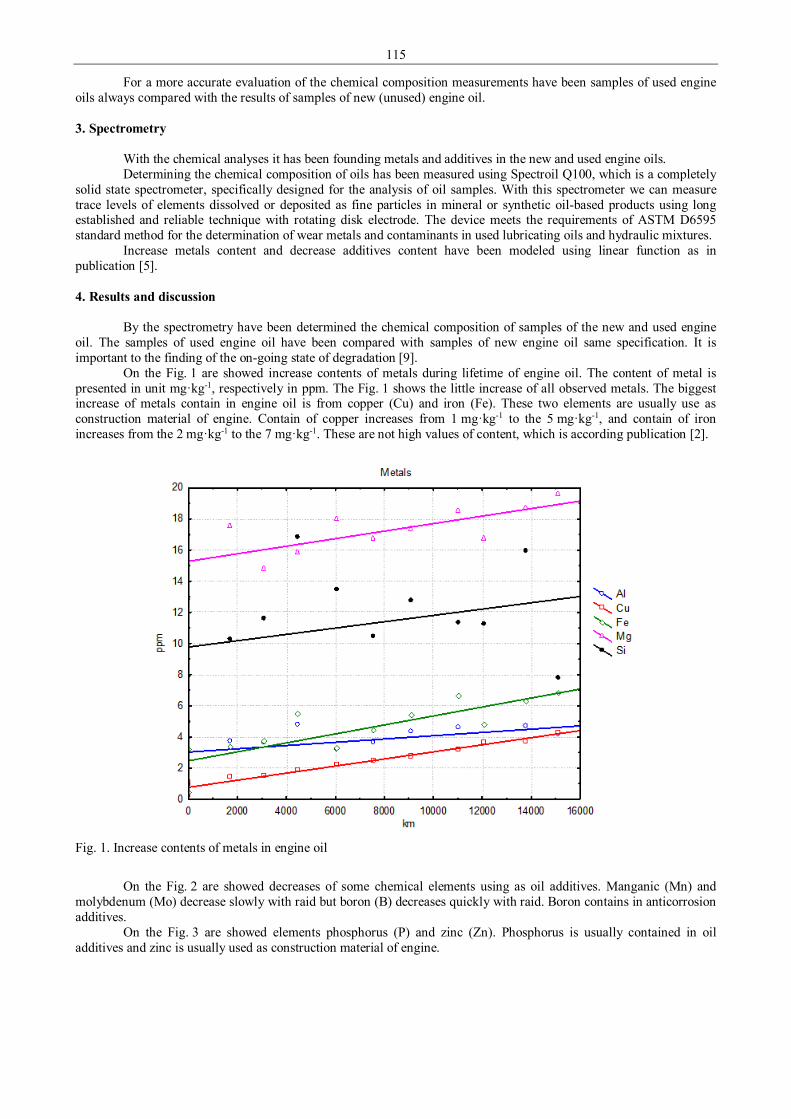
115

For a more accurate evaluation of the chemical composition measurements have been samples of used engine oils always compared with the results of samples of new (unused) engine oil. 3. Spectrometry

With the chemical analyses it has been founding metals and additives in the new and used engine oils. Determining the chemical composition of oils has been measured using Spectroil Q100, which is a completely

solid state spectrometer, specifically designed for the analysis of oil samples. With this spectrometer we can measure trace levels of elements dissolved or deposited as fine particles in mineral or synthetic oil-based products using long established and reliable technique with rotating disk electrode. The device meets the requirements of ASTM D6595 standard method for the determination of wear metals and contaminants in used lubricating oils and hydraulic mixtures.

Increase metals content and decrease additives content have been modeled using linear function as in publication [5]. 4. Results and discussion

By the spectrometry have been determined the chemical composition of samples of the new and used engine oil. The samples of used engine oil have been compared with samples of new engine oil same specification. It is important to the finding of the on-going state of degradation [9].

On the Fig. 1 are showed increase contents of metals during lifetime of engine oil. The content of metal is presented in unit mg·kg-1, respectively in ppm. The Fig. 1 shows the little increase of all observed metals. The biggest increase of metals contain in engine oil is from copper (Cu) and iron (Fe). These two elements are usually use as construction material of engine. Contain of copper increases from 1 mg·kg-1 to the 5 mg·kg-1, and contain of iron increases from the 2 mg·kg-1 to the 7 mg·kg-1. These are not high values of content, which is according publication [2].

Fig. 1. Increase contents of metals in engine oil

On the Fig. 2 are showed decreases of some chemical elements using as oil additives. Manganic (Mn) and

molybdenum (Mo) decrease slowly with raid but boron (B) decreases quickly with raid. Boron contains in anticorrosion additives.

On the Fig. 3 are showed elements phosphorus (P) and zinc (Zn). Phosphorus is usually contained in oil additives and zinc is usually used as construction material of engine.

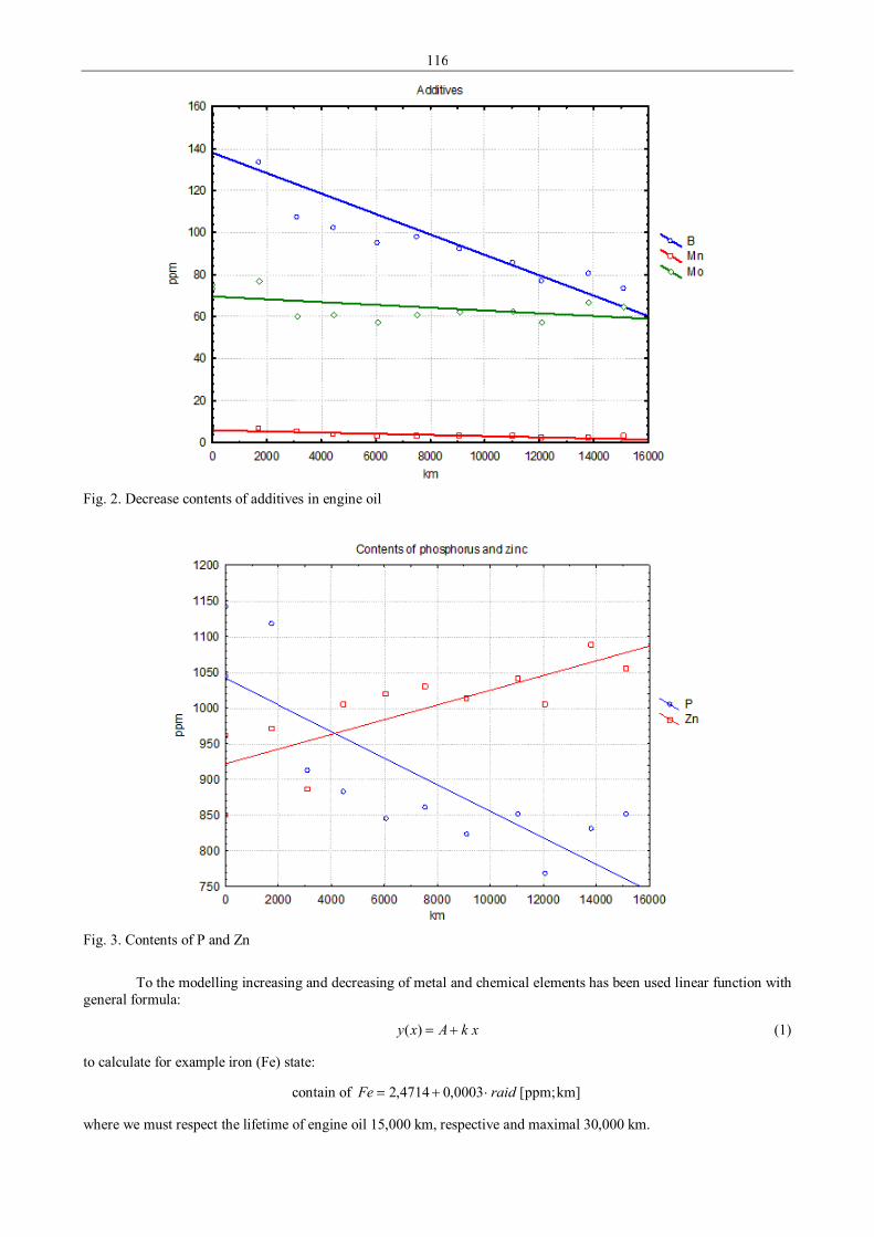
116

Fig. 2. Decrease contents of additives in engine oil

Fig. 3. Contents of P and Zn

To the modelling increasing and decreasing of metal and chemical elements has been used linear function with

general formula:

xkAxy +=)( (1)

to calculate for example iron (Fe) state:

contain of ]kmppm;[0003,04714,2 raidFe ⋅+=

where we must respect the lifetime of engine oil 15,000 km, respective and maximal 30,000 km.

117

Correlation coefficients R achieve high values from the 0.79 to the 0.98. Similar values of correlation coefficient achieve authors in publications [1, 10].

In the Tab. 2 are showed constant values A and k for all of used chemical elements.

Table 2 Intervals of collect samples of engine used oil

Chemical elements Constant A Constant k Chemical elements Constant A Constant k Al 3.0318 0.0001 B 138.0036 –0.0049 Cu 0.7738 0.0002 Mn 5.8424 –0.0003 Fe 2.4714 0.0003 Mo 69.5518 –0.0007 Mg 15.2793 0.0002 P 1041.6257 –0.0186 Si 9.7779 0.0002 Zn 922.0322 0.0103

5. Conclusions

In this part of the paper we can state that use method (spectrometry) is as one of the basic oil analyses very suitable. The suitability rises when the samples of used engine oil are compared with the sample of new (unused) engine oil with same specification. Using spectrometry we have determined chemical composition of all samples of engine oil. We have also quantified individual chemical elements in the new and used engine oil. With graphs we can see increasing trends polluting elements (metals) and decreasing trends of oil additives (detergents, dispersants, friction modifiers, viscosity modifiers, anti-freeze agents, antioxidants, substances affecting the freezing point, anti-abrasion additives, lubricating additives and some other). All trends have been modelled using linear function. Linear function is basic mathematical model, which we can use. But linear function is very accurate, if we use it properly. Coefficients of correlation R have achieved high values – from the 0.79 to the 0.98. Created mathematical models can be used to prediction changes in lifetime of engine oil fill in same or similar petrol engine. References 1. Božiková M., Hlaváč P. Thermophysical and rheologic properties of biooil samples. Journal of Central European

Agriculture, 14, 3. 2013, p. 279 – 290. ISSN 1332-9049. 2. Černý J. Vlastnosti motorových olejů. 10. Otěrové kovy v oleji. AutoExpert, 11, 12. 2006, p. 34 – 36. ISSN 1211-

2380. 3. Furch J. New Trends in a Vehicle Maintenance System. Advances in Military Technology, 2010, vol. 5, no. 2,

p. 111 – 119. ISSN 1802-2308. 4. Kumbár V., Dostál P. Oils degradation in agricultural machinery. Acta Univ. Agric. et Silvic. Mendel. Brun., 61, 5.

2013, p. 1297–1303. ISSN 1211-8516. 5. Kumbár V., Polcar A., Čupera J. Rheological profi les of blends of the new and used motor oils. Acta Univ. Agric.

et Silvic. Mendel. Brun., 61, 1. 2013, p. 115–122. ISSN 1211-8516. 6. Mang T., Dresel W. Lubricants and Lubrication. Weinheim: Wiley, 2001, 759 p. ISBN 978-3-527-31497-3. 7. Meng F., Huang W. The impact of alkaline additives on the performance of lubricating oil. In International

Conference on Chemical, Material and Metallurgical Engineering, ICCMME 2011. P. 396 – 398. ISBN 978-303785308-5.

8. Mihalčová J. Tribotechnical Diagnosis in Aircraft Engine Practice – 2013. In: Applied Mechanics and Materials. Vol. 308 (2013), p. 57 – 62. - ISBN 978-303785656-7 - ISSN 1660-9336

9. Moritani H., Kawai H. Low-temperature degradation of lubricant oil for gasoline engine. Japanese Journal of Tribology, 51, 2. 2006, p. 207 – 217. ISSN 1045-7828.

10. Trávníček P., Krčálová E., Vitěz T. Rheopectic behavior of rendered fat. Polish Journal of Environmental Studies, 22, 5. 2013, p. 1499 – 1504. ISSN 1230-1485.

11. Valach M., Mareček J., Hlaváčová Z., Trávníček P., Glos J. Determination of impurities in biofuels with using a particle size analyzer. Acta Univ. Agric. et Silvic. Mendel. Brun., 61, 3. 2013 p. 813 – 817. ISSN 1211-8516.

12. Vališ D., Žák L., Glos J., Walek A. Contribution to mathematical modelling of oil field data. Applied Mechanics and Materials 332. 2013, p. 455 – 462. ISSN 1660-9336.

118

Proceedings of 9th International Conference ITELMS’2014 Application of Statistical Hypothesis Testing of Adaptive Algorithms for Smooth and Precise Train Braking System A. Potapovs*, M. Gorobetz**, A. Levchenkov*** *Institute of Industrial Electronics and Electrical Engineering, Riga Technical University, 1, Kalku Street, LV-1658, Riga, Latvia, E-mail: Andrejs.Potapovs@rtu.lv **Institute of Industrial Electronics and Electrical Engineering, Riga Technical University, 1, Kalku Street, LV-1658, Riga, Latvia, E-mail: mihails.gorobecs@rtu.lv ***Institute of Industrial Electronics and Electrical Engineering, Riga Technical University, 1, Kalku Street, LV-1658, Riga, Latvia, E-mail: anatolijs.levcenkovs@rtu.lv Abstract This article considers the structure and operation principles of a new adaptive system of starting and accurate braking of railway transport. This system is based on the application of embedded intelligent device, the existed braking equipment of the railway transport, auxiliary mechanical parts as well as adaptive searching algorithms playing a significant role in the effectiveness of the proposed system. The article contains definitions of the functions of the main blocks of the systems under consideration and their mathematical descriptions. Additionally the algorithm of system operation is described. The prototype of the proposed device was tested, the obtained results, advantages and further development opportunities were considered. KEYWORDS: adaptive systems, intelligent control, railway transport. 1. Introduction

Nowadays, the railway transport plays the significant role in passengers and cargo transportations all over the world. Despite of the various advantages, this transportation type has known problems. Mainly these problems are connected with safety during the exploitation and crashes that become causes of human victims and high material losses. Various solutions are continuously developed for new modern railway safety systems for existing railways, but unfortunately none of them may solve the problem completely and propose the solution for the specific problem.

There are some systems which provide solutions for automatic routing and braking tasks: • KLUB-U (Complex Locomotives Safety Unit); • ETCS (European Train Control System); • Ansaldo STS «TCSS» (Train Control and Signalling System); • Knorr Bremse «LEADER» (Locomotive Engineer Assist Display&Event Recorder) and others.

However, all these systems have some disadvantages such as: • They does not provide uninterruptible data exchange between trains; • Needs special additional input of train parameters before working.

Therefore, the adaptive smooth and precise train braking system is proposed to propose the solution for the specific task of crash prevention, target braking and human factor reduction. 2. Purpose and tasks

The main purpose of research is development of adaptive control algorithms for embedded intelligent devices to improve and automate transport control processes increasing safety level, reliability and reducing the unpredictable human factor.

To achieve this goal the adaptive braking control system is proposed. The main feature of the proposed system is a self-learning and adaptation to train parameters and environmental conditions with a special input, therefore providing reduction of the human factor.

The following tasks are defined: • To describe the main elements of the adaptive system of the railway transport starting and accurate braking. • To define functions realized by the basic elements of the system. • To develop mathematical model and function for evaluation of adaptive algorithms. • To perform Statistical Hypothesis Testing to evaluate the workability of different adaptive algorithms in various conditions. 3. Basic elements and functions of the new adaptive system of railway transport soft and accurate braking

As it was mentioned above the task of the adaptive system of starting and accurate braking of railway transport is to improve safety without any cardinal changes in the existing control system of the trains decreasing in parallel the impact of human factor on the process of railway transport routing.

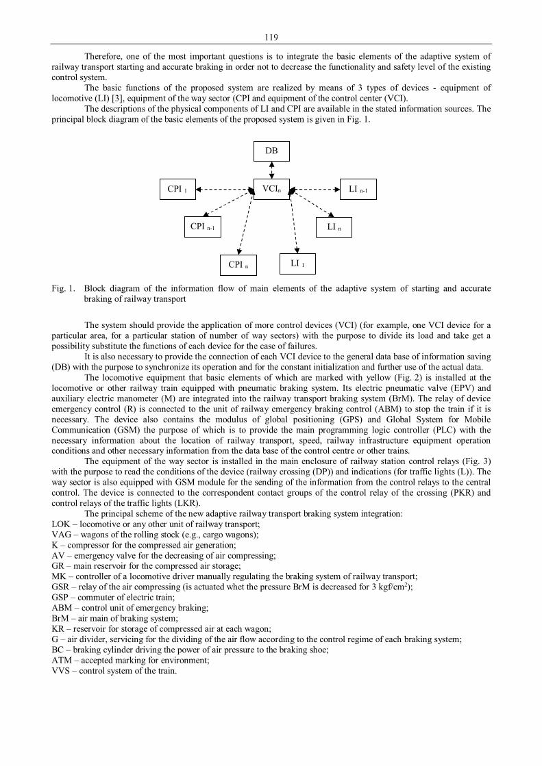
119

Therefore, one of the most important questions is to integrate the basic elements of the adaptive system of railway transport starting and accurate braking in order not to decrease the functionality and safety level of the existing control system.

The basic functions of the proposed system are realized by means of 3 types of devices - equipment of locomotive (LI) [3], equipment of the way sector (CPI and equipment of the control center (VCI).

The descriptions of the physical components of LI and CPI are available in the stated information sources. The principal block diagram of the basic elements of the proposed system is given in Fig. 1.

Fig. 1. Block diagram of the information flow of main elements of the adaptive system of starting and accurate

braking of railway transport

The system should provide the application of more control devices (VCI) (for example, one VCI device for a

particular area, for a particular station of number of way sectors) with the purpose to divide its load and take get a possibility substitute the functions of each device for the case of failures.

It is also necessary to provide the connection of each VCI device to the general data base of information saving (DB) with the purpose to synchronize its operation and for the constant initialization and further use of the actual data.

The locomotive equipment that basic elements of which are marked with yellow (Fig. 2) is installed at the locomotive or other railway train equipped with pneumatic braking system. Its electric pneumatic valve (EPV) and auxiliary electric manometer (M) are integrated into the railway transport braking system (BrM). The relay of device emergency control (R) is connected to the unit of railway emergency braking control (ABM) to stop the train if it is necessary. The device also contains the modulus of global positioning (GPS) and Global System for Mobile Communication (GSM) the purpose of which is to provide the main programming logic controller (PLC) with the necessary information about the location of railway transport, speed, railway infrastructure equipment operation conditions and other necessary information from the data base of the control centre or other trains.

The equipment of the way sector is installed in the main enclosure of railway station control relays (Fig. 3) with the purpose to read the conditions of the device (railway crossing (DP)) and indications (for traffic lights (L)). The way sector is also equipped with GSM module for the sending of the information from the control relays to the central control. The device is connected to the correspondent contact groups of the control relay of the crossing (PKR) and control relays of the traffic lights (LKR).

The principal scheme of the new adaptive railway transport braking system integration: LOK – locomotive or any other unit of railway transport; VAG – wagons of the rolling stock (e.g., cargo wagons); K – compressor for the compressed air generation; AV – emergency valve for the decreasing of air compressing; GR – main reservoir for the compressed air storage; MK – controller of a locomotive driver manually regulating the braking system of railway transport; GSR – relay of the air compressing (is actuated whet the pressure BrM is decreased for 3 kgf/cm2); GSP – commuter of electric train; ABM – control unit of emergency braking; BrM – air main of braking system; KR – reservoir for storage of compressed air at each wagon; G – air divider, servicing for the dividing of the air flow according to the control regime of each braking system; BC – braking cylinder driving the power of air pressure to the braking shoe; ATM – accepted marking for environment; VVS – control system of the train.

VCIn CPI 1

CPI n-1

LI 1 CPI n

LI n-1

LI n

DB

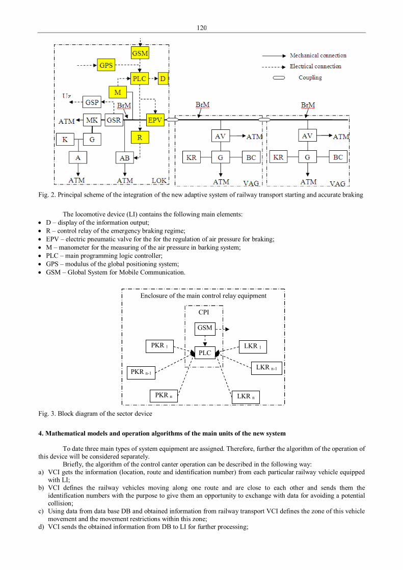
120

Fig. 2. Principal scheme of the integration of the new adaptive system of railway transport starting and accurate braking

The locomotive device (LI) contains the following main elements:

• D – display of the information output; • R – control relay of the emergency braking regime; • EPV – electric pneumatic valve for the for the regulation of air pressure for braking; • M – manometer for the measuring of the air pressure in barking system; • PLC – main programming logic controller; • GPS – modulus of the global positioning system; • GSM – Global System for Mobile Communication.

Fig. 3. Block diagram of the sector device

4. Mathematical models and operation algorithms of the main units of the new system

To date three main types of system equipment are assigned. Therefore, further the algorithm of the operation of this device will be considered separately.

Briefly, the algorithm of the control canter operation can be described in the following way: a) VCI gets the information (location, route and identification number) from each particular railway vehicle equipped

with LI; b) VCI defines the railway vehicles moving along one route and are close to each other and sends them the

identification numbers with the purpose to give them an opportunity to exchange with data for avoiding a potential collision;

c) Using data from data base DB and obtained information from railway transport VCI defines the zone of this vehicle movement and the movement restrictions within this zone;

d) VCI sends the obtained information from DB to LI for further processing;

Enclosure of the main control relay equipment

CPI

PLC

GSM

PKR n-1

PKR 1

PKR n

LKR 1

LKR n-1

LKR n

121

e) In the case if, there is a station in the zone LI obtains the identification number of this station for communication with the CPI of the station and information about the readiness of the route, for the information of the traffic lights situated on this route and any possible restrictions.

The following functions are in the basis of operation algorithm of the distance sector: • Main PLC of CPI onto its input contacts obtains the signals about the conditions of the crossing, prepared routes and

traffic lights; • CPI sends the obtained information to VCI input into data base and control in the real time; • On demand CPI sends the obtained information from a railway vehicle LI; • CPI realizes possible diagnostics of the emergency regimes and in necessity VCI as well as LI send the emergency

signal. The special attention will be turned to the description of the locomotive operation algorithm. First of all let us describe the basic functions completed by the devices:

• Processing of the information obtained from VCI; • According to the obtained identification number a communication takes place with CPI of the station or LI of railway

transport; • Determination of the necessity to realize the working braking because of possible collision or some restrictions on

the route; • Approximate determining of emergency braking distance of railway transport using the available data; • Realization of the working braking process; • Realization of the emergency braking process.

The algorithm of the emergency braking operation of railway transport applying LI is described according to [3]. For the realization of soft working braking process an adaptive searching algorithm is applied as well as special learning algorithm. The purpose f the learning algorithm is to define the effectiveness of the train braking system in the cases when the working braking is applied. The analogue of this value in the calculations of railway transport braking is marked as and called as a braking factor. This factor means the development of total power of braking of the rolling stock over the whole weight of the rolling stock.

But the application of this value is complicated due to the necessity in its calculation (formula 1) of input information that practically impossible to obtain.

PQ

knmknmp +

+= 222111ν (1)

where m1 – number of wagons; n1 – number of wagons axes; k1 – specific power of pressing of cargo wagons braking shoe; m2 – number of locomotives; n2 – number of locomotive axes; k2 – specific power of pressing of locomotives braking shoe; Q – total mass of wagons, t; P – mass of locomotive, t.

Therefore it is necessary to introduce a factor of efficiency of a new braking system (BSef), that according to the available parameters processing describes the condition of the whole rolling stock or of one unit of the braking system (the effectiveness of braking under different conditions).

The learning algorithm determines BSef (2) at the moments when the braking is realized by driver manually. Manometer M installed on LI fixes the decreasing of air pressure in the braking main BrM. If a working braking step is fixed then the changing of speed and acceleration of of the realised braking are

also fixed. There parameters are enough to calculate the approximate value of BSef factor.

( )bref aVPfBS ;; ∆∆= (2)

where ∆P – changing of the air pressure in the braking main realizing one braking step; ∆V – changing of the railway transport speed realizing one braking step; abr – average braking acceleration of railway transport realizing one braking step.

For higher effectiveness of the system operation the calculation of this factor is required at each step of working braking as well as at each speed of movement, description of the way profile and at fixing the outside conditions; in opposite cases the factor is accepted as low as possible within this or that zone. With possible changes of the rolling stock (e.g. changing number of wagon, etc.) the calculation of factor BSef is repeated.

The application of this factor is foreseen during the working of the adaptive searching algorithm, completing the theoretical curves of the railway transport movement during the automatic adaptive and soft braking. The introduction of BSef factor allows to improve the effectiveness and safety of braking process. The curves can be similar to those in Fig. 4.

Fig. 4. demonstrates the theoretical curves of the speed and braking acceleration (red color line) of a cargo train model and the same curves resulted in the system's operation time realizing the soft and accurate braking before the stop point (blue color line). In accordance with higher BSef (the defined higher railway transport braking system effectiveness), the higher realized theoretical braking acceleration is preset and opposite.

This value can be accordingly accurately defined while testing the prototype of the system device.

122

Fig. 4. Dependence of the model movement parameters on time

In compliance with the made before analysis of the searching algorithm [4] the basis of the adaptive searching

algorithm operation is the application of adaptive searching together with the integrated testing and working steps modifying them.

The quality evaluation function of the adaptation algorithm is defined as a set of separate criteria. Main criteria are following: • M – error detecting of the average wagon mass; • N – error detecting number of wagons; • K – error detecting of brake pads pressing force.

Therefore, the quality function is following, where each criteria should be minimized

→−=

→−=

→−=

=

min||

min||

min||

_

_

_

fkk

fvagvag

fvagvag

kkK

nnN

mmM

Q (3)

where mvag_f – actual mass of a wagon; nvag_f – actual number of wagons; kk_f – actual brake pads pressing force. Normalized quality function is presented as a weighted sum function such as:

min'''' 321 →++= KNMQ ααα (4)

where α1 – weight of mass detection criterion; α2 – weight of number of wagons detection criterion; α3 – weight of

pressing force detection criterion; minmax

max

MMMMM

−−

=' – normalized value of mass detection criterion;

minmax

max

NNNNN

−−

=' – normalized value of number of wagons detection criterion; minmax

max

KKKKK

−−

=' – normalized value

of pressing force detection criterion. In addition 1321 =++ ααα . 5. Mathematical formulation and development of adaptive search algorithm

In this chapter, the generic mathematical definition of the adaptive search algorithm is described and the modified algorithm is proposed. All these algorithms potentially may be used in proposed Adaptive Smooth and Precise Braking system.

Target function of each adaptive algorithm is following:

min)()( 2_2_1_2_1

2

1

→−= ∑=

=fakttt

tt

ttteortt SSXΦ (5)

123

where t1 – braking start time moment; t2 – time moment of achievement of nominal braking force value; St1_t2_teor = VKM(nvag , mvag , kk) – simulated braking distance at time t; St1_t2_fakt – actual braking distance at time t; X = {x1 = nvag ; x2 = mvag ; x3 = kk} – searching parameters of the target function.

In this case the optimization task is defined for the algorithm:

**)()(min3

ΦΦΦ ==∈

XXRX

(6)

which is defined in 3 dimensional space with following restrictions:

≤≤

≤≤

≤≤

k_maxk_min

vag_maxvag_min

vag_maxvag_min

kxkmxm

nxnR

3

2

13 : (7)

In the research the following adaptive algorithms are selected: Algorithm 1 – Scan through method; Algorithm 2 – The best trial method; Algorithm 3 – Random search method with a constant radius and random search direction; Algorithm 4 – Combination of the best trial method with scanning in the end; Algorithm 5 – Gauss-Seidel method; Algorithm 6 – Repeating random search method; Algorithm 7 – Monte-Carlo method; Algorithm 8 – Genetic Algorithm.

In this paper the Algorithm 4 is described as proposed by the authors for the specific task. Main steps of this algorithm are following:

Step 1 – Initial values X 0 of search parameters are set, as well as initial length of a search step λ 0 is defined and iteration counter is set as r = 0.

Step 2 – M' = M 0 / λ' random vectors riΨ , i ∈ [1, M'] are generated and trial points 1+r

iX , i ∈ [1, M'] are found.

Step 3 – Value of function ( )1+riXΦ is calculated in trial points ( )1+r

iX , i ∈ [1, M'] and minimal value is

selected ( ) ( )[ ]

( )1

,1

11 min +

∈

++ == riMi

rk

r XXX ΦΦΦ .

Step 4 – If ( ) ( )rr XX ΦΦ <+1 , then r = r + 1 and algorithm returns to the step 2. Otherwise, go to step 5. Step 5 – The end condition is checked (for example, minimal error value is reached). If ending condition is

satisfied then it is assumed that final values of search parameters are X * ≈ X r + 1 and algorithm ends. Otherwise r = r + 1, λ r = α λ r and go to step 6. Here α ∈ (0, 1) – step reduction coefficient briefly selected.

Step 6 – If M' > (2 λ) 3, the all combinations are generated and the minimal value is checked there ( ) ( )

[ ]( )1

,1

11 min +

∈

++ == riMi

rk

r XXX ΦΦΦ .

6. Testing of the developed adaptive braking algorithm and results summary

To perform tests of various working conditions the different combinations of following parameters are defined: • mvag_fakt – actual mass of wagon, t; • nvag_fakt – actual number of wagons; • kk_fakt – brake pads pressing force, kN; • Vvilciena – actual speed of train, km/h.

Each parameter is conditionally divided into three groups – low value, average value and high value (see Fig. 5). During the combining of parameters, following exceptions are defined: • If 3.8 kN ≤ kk , then mvag ≥ 60 t; • If 2.3 kN ≤ kk , then mvag ≥ 35 t.

Fig. 5. Input data for computer experiment

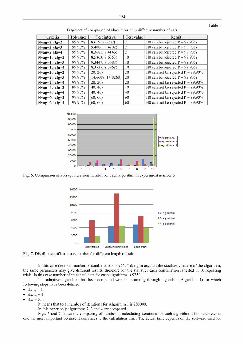
124

Table 1 Fragment of comparing of algorithms with different number of cars

Criteria Tolerance Test interval Test value Result Nvag=2 alg=2 99.90% (8.619; 8.6707) 2 H0 can be rejected P = 99.90% Nvag=2 alg=3 99.90% (9.4086; 9.4282) 2 H0 can be rejected P = 99.90% Nvag=2 alg=4 99.90% (8.3681; 8.4146) 2 H0 can be rejected P = 99.90% Nvag=10 alg=2 99.90% (8.5863; 8.6353) 10 H0 can be rejected P = 99.90% Nvag=10 alg=3 99.90% (9.3447; 9.3688) 10 H0 can be rejected P = 99.90% Nvag=10 alg=4 99.90% (8.3535; 8.3968) 10 H0 can be rejected P = 99.90% Nvag=20 alg=2 99.90% (20; 20) 20 H0 can not be rejected P = 99.90% Nvag=20 alg=3 99.90% (14.6608; 14.8268) 20 H0 can be rejected P = 99.90% Nvag=20 alg=4 99.90% (20; 20) 20 H0 can not be rejected P = 99.90% Nvag=40 alg=2 99.90% (40; 40) 40 H0 can not be rejected P = 99.90% Nvag=40 alg=4 99.90% (40; 40) 40 H0 can not be rejected P = 99.90% Nvag=60 alg=2 99.90% (60; 60) 60 H0 can not be rejected P = 99.90% Nvag=60 alg=4 99.90% (60; 60) 60 H0 can not be rejected P = 99.90%

Fig. 6. Comparison of average iterations number for each algorithm in experiment number 5

Fig. 7. Distribution of iterations number for different length of train

In this case the total number of combinations is 925. Taking in account the stochastic nature of the algorithm,

the same parameters may give different results, therefore for the statistics each combination is tested in 10 repeating trials. In this case number of statistical data for each algorithms is 9250.

The adaptive algorithms has been compared with the scanning through algorithm (Algorithm 1) for which following steps have been defined: • Δnvag = 1; • Δmvag = 1; • Δkk = 0.1.

It means that total number of iterations for Algorithm 1 is 280000. In this paper only algorithms 2, 3 and 4 are compared. Figs. 6 and 7 shows the comparing of number of calculating iterations for each algorithm. This parameter is

one the most important because it correlates to the calculation time. The actual time depends on the software used for

125

algorithm implementation and the hardware of the whole adaptive system realization, such as CPU clock rate, RAM size etc. 7. Conclusions

The practical experimental results of this research allow to conclude that: 1. In 99% cases the adaptive search algorithms may find the solution and perform the adaptation of new system faster

that usual scanning through method. 2. For short rolling stocks (up to 10 wagons) in 99% cases the selected adaptive algorithms could not find the precise

parameters of rolling stock, i.e. mass of wagon, number of wagons and pressing force, but in any case the average quadratic error in calculating of braking curve is less than 10−23;

3. Comparing two the most efficient (from selected) algorithms, the combined algorithm (Algorithm 4) is better in average 1.2 times than the best trial method (Algorithm 2) for smaller values of train parameters;

4. Otherwise, the best trial method is in average 1.1 times more efficient for higher values of train parameters. Acknowledgement

The research leading to these results has received funding from the ARTEMIS Joint Undertaking under grant agreement n°295373 and from Latvian Academy of Science and Ministry of Education and Science. References 1. Wang J. F., Wang H. H., & Lin Z. Research on a new type of train control system used at 350km/h. WIT

Transactions on the Built Environment, 127, - pp 51-60. 2. Gorobecs M., Greivulis J., Ļevčenkovs A., Balckars P., Ribickis L. Train Emergency Braking Device. 2009.

Patent Nr. LV13978. 3. Potapovs A., Gorobetz M., Levchenkov A. Intelligent electronic embedded systems for the protection of railway

transport from accidents. Proceedings of 7th International Conference (ITELMS’2012), Lithuania, Kaunas, 2012. – pp 141-146.

4. Гребенюк П. Т., Долганова А. Н., Скворцова А. И. Тяговые расчеты. Справочник, 1987. – 273 с. 5. Levchenkov А., Gorobetz М., Ribickis L., Balckars P. Generating of Multi-Criteria Alternatives for Decision-

Making in Electric Light Rail Control // In China-USA Business review, December 2009, - pp. 49-55. 6. Patent Nr. LV14384. Train anti-collision device using satellite navigation. A. Levchenkov, M. Gorobetz, I. Rankis,

P. Balckars, L. Ribickis, A. Potapovs, 2011.

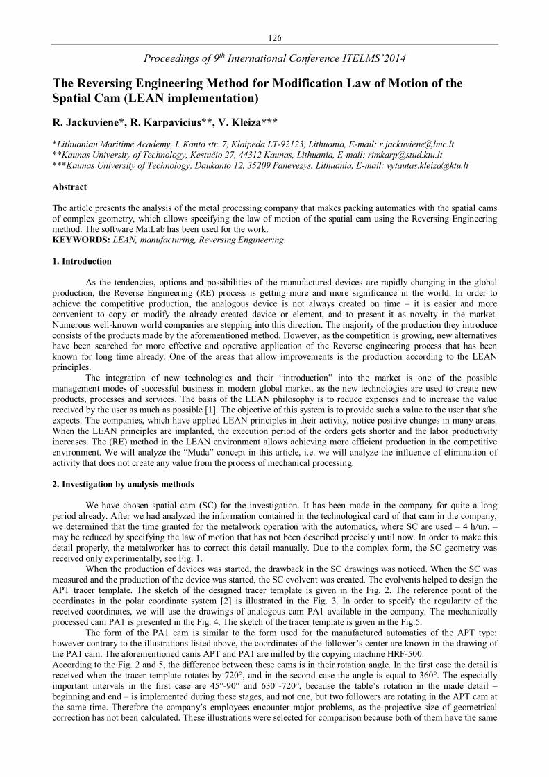
126

Proceedings of 9th International Conference ITELMS’2014 The Reversing Engineering Method for Modification Law of Motion of the Spatial Cam (LEAN implementation) R. Jackuviene*, R. Karpavicius**, V. Kleiza*** *Lithuanian Maritime Academy, I. Kanto str. 7, Klaipeda LT-92123, Lithuania, E-mail: r.jackuviene@lmc.lt **Kaunas University of Technology, Kestučio 27, 44312 Kaunas, Lithuania, E-mail: rimkarp@stud.ktu.lt ***Kaunas University of Technology, Daukanto 12, 35209 Panevezys, Lithuania, E-mail: vytautas.kleiza@ktu.lt Abstract The article presents the analysis of the metal processing company that makes packing automatics with the spatial cams of complex geometry, which allows specifying the law of motion of the spatial cam using the Reversing Engineering method. The software MatLab has been used for the work. KEYWORDS: LEAN, manufacturing, Reversing Engineering. 1. Introduction

As the tendencies, options and possibilities of the manufactured devices are rapidly changing in the global production, the Reverse Engineering (RE) process is getting more and more significance in the world. In order to achieve the competitive production, the analogous device is not always created on time – it is easier and more convenient to copy or modify the already created device or element, and to present it as novelty in the market. Numerous well-known world companies are stepping into this direction. The majority of the production they introduce consists of the products made by the aforementioned method. However, as the competition is growing, new alternatives have been searched for more effective and operative application of the Reverse engineering process that has been known for long time already. One of the areas that allow improvements is the production according to the LEAN principles.

The integration of new technologies and their “introduction” into the market is one of the possible management modes of successful business in modern global market, as the new technologies are used to create new products, processes and services. The basis of the LEAN philosophy is to reduce expenses and to increase the value received by the user as much as possible [1]. The objective of this system is to provide such a value to the user that s/he expects. The companies, which have applied LEAN principles in their activity, notice positive changes in many areas. When the LEAN principles are implanted, the execution period of the orders gets shorter and the labor productivity increases. The (RE) method in the LEAN environment allows achieving more efficient production in the competitive environment. We will analyze the “Muda” concept in this article, i.e. we will analyze the influence of elimination of activity that does not create any value from the process of mechanical processing. 2. Investigation by analysis methods

We have chosen spatial cam (SC) for the investigation. It has been made in the company for quite a long period already. After we had analyzed the information contained in the technological card of that cam in the company, we determined that the time granted for the metalwork operation with the automatics, where SC are used – 4 h/un. – may be reduced by specifying the law of motion that has not been described precisely until now. In order to make this detail properly, the metalworker has to correct this detail manually. Due to the complex form, the SC geometry was received only experimentally, see Fig. 1.

When the production of devices was started, the drawback in the SC drawings was noticed. When the SC was measured and the production of the device was started, the SC evolvent was created. The evolvents helped to design the APT tracer template. The sketch of the designed tracer template is given in the Fig. 2. The reference point of the coordinates in the polar coordinate system [2] is illustrated in the Fig. 3. In order to specify the regularity of the received coordinates, we will use the drawings of analogous cam PA1 available in the company. The mechanically processed cam PA1 is presented in the Fig. 4. The sketch of the tracer template is given in the Fig.5.

The form of the PA1 cam is similar to the form used for the manufactured automatics of the APT type; however contrary to the illustrations listed above, the coordinates of the follower’s center are known in the drawing of the PA1 cam. The aforementioned cams APT and PA1 are milled by the copying machine HRF-500. According to the Fig. 2 and 5, the difference between these cams is in their rotation angle. In the first case the detail is received when the tracer template rotates by 720°, and in the second case the angle is equal to 360°. The especially important intervals in the first case are 45°-90° and 630°-720°, because the table’s rotation in the made detail – beginning and end – is implemented during these stages, and not one, but two followers are rotating in the APT cam at the same time. Therefore the company’s employees encounter major problems, as the projective size of geometrical correction has not been calculated. These illustrations were selected for comparison because both of them have the same

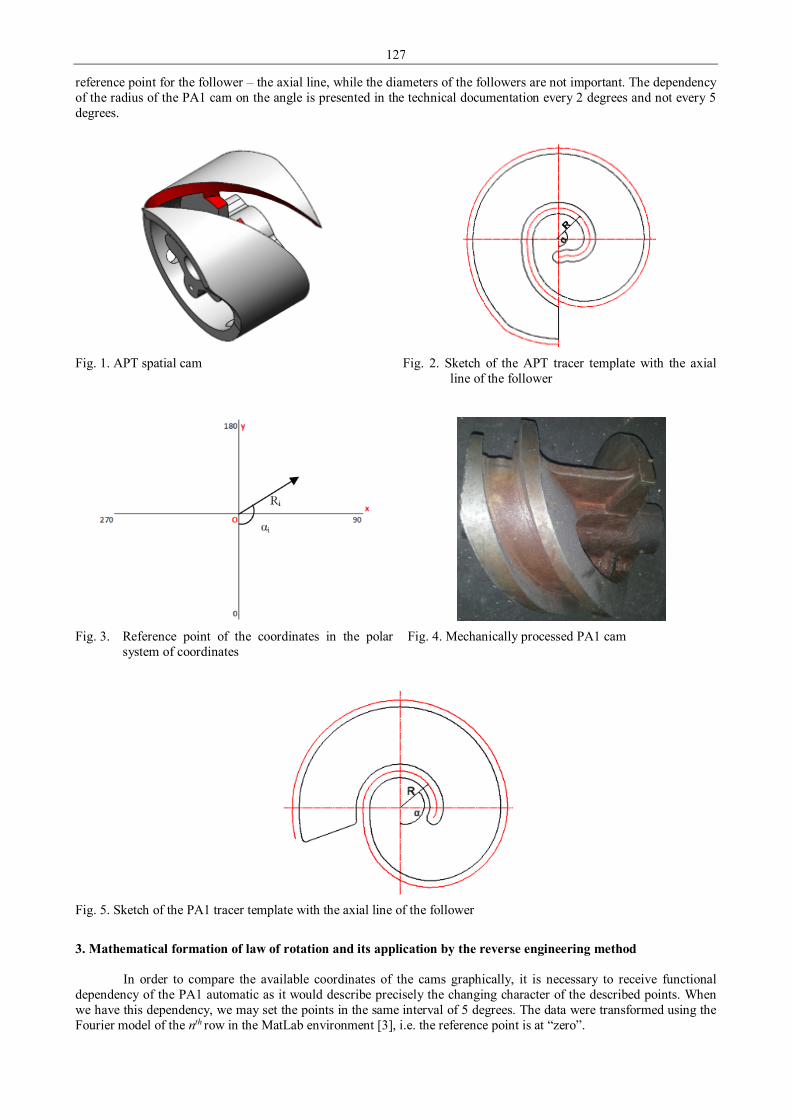
127

reference point for the follower – the axial line, while the diameters of the followers are not important. The dependency of the radius of the PA1 cam on the angle is presented in the technical documentation every 2 degrees and not every 5 degrees.

Fig. 1. APT spatial cam Fig. 2. Sketch of the APT tracer template with the axial

line of the follower

Fig. 3. Reference point of the coordinates in the polar

system of coordinates Fig. 4. Mechanically processed PA1 cam

Fig. 5. Sketch of the PA1 tracer template with the axial line of the follower

3. Mathematical formation of law of rotation and its application by the reverse engineering method

In order to compare the available coordinates of the cams graphically, it is necessary to receive functional dependency of the PA1 automatic as it would describe precisely the changing character of the described points. When we have this dependency, we may set the points in the same interval of 5 degrees. The data were transformed using the Fourier model of the nth row in the MatLab environment [3], i.e. the reference point is at “zero”.

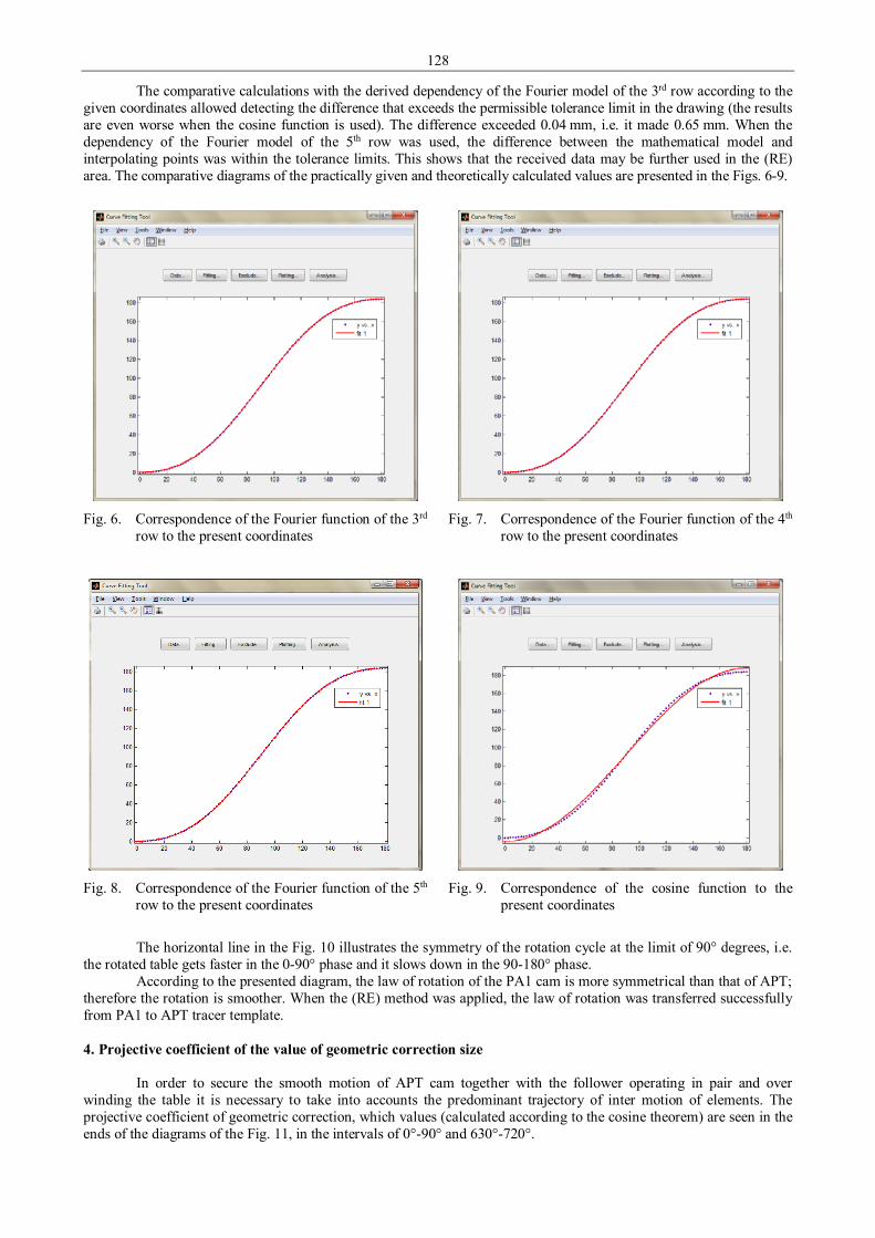
128

The comparative calculations with the derived dependency of the Fourier model of the 3rd row according to the given coordinates allowed detecting the difference that exceeds the permissible tolerance limit in the drawing (the results are even worse when the cosine function is used). The difference exceeded 0.04 mm, i.e. it made 0.65 mm. When the dependency of the Fourier model of the 5th row was used, the difference between the mathematical model and interpolating points was within the tolerance limits. This shows that the received data may be further used in the (RE) area. The comparative diagrams of the practically given and theoretically calculated values are presented in the Figs. 6-9.

Fig. 6. Correspondence of the Fourier function of the 3rd

row to the present coordinates Fig. 7. Correspondence of the Fourier function of the 4th

row to the present coordinates

Fig. 8. Correspondence of the Fourier function of the 5th

row to the present coordinates Fig. 9. Correspondence of the cosine function to the

present coordinates

The horizontal line in the Fig. 10 illustrates the symmetry of the rotation cycle at the limit of 90° degrees, i.e.

the rotated table gets faster in the 0-90° phase and it slows down in the 90-180° phase. According to the presented diagram, the law of rotation of the PA1 cam is more symmetrical than that of APT;

therefore the rotation is smoother. When the (RE) method was applied, the law of rotation was transferred successfully from PA1 to APT tracer template. 4. Projective coefficient of the value of geometric correction size

In order to secure the smooth motion of APT cam together with the follower operating in pair and over winding the table it is necessary to take into accounts the predominant trajectory of inter motion of elements. The projective coefficient of geometric correction, which values (calculated according to the cosine theorem) are seen in the ends of the diagrams of the Fig. 11, in the intervals of 0°-90° and 630°-720°.

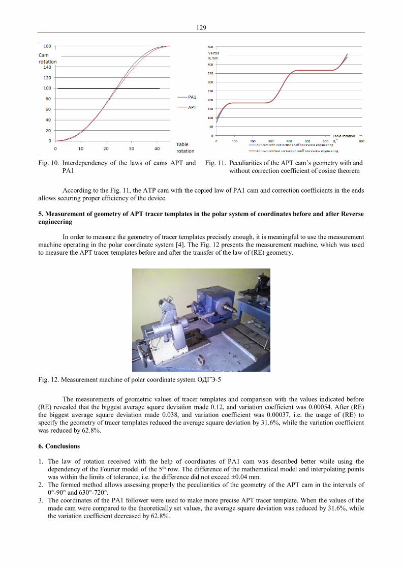
129

Fig. 10. Interdependency of the laws of cams APT and

PA1 Fig. 11. Peculiarities of the APT cam’s geometry with and

without correction coefficient of cosine theorem

According to the Fig. 11, the ATP cam with the copied law of PA1 cam and correction coefficients in the ends

allows securing proper efficiency of the device. 5. Measurement of geometry of APT tracer templates in the polar system of coordinates before and after Reverse engineering

In order to measure the geometry of tracer templates precisely enough, it is meaningful to use the measurement machine operating in the polar coordinate system [4]. The Fig. 12 presents the measurement machine, which was used to measure the APT tracer templates before and after the transfer of the law of (RE) geometry.

Fig. 12. Measurement machine of polar coordinate system ОДГЭ-5

The measurements of geometric values of tracer templates and comparison with the values indicated before

(RE) revealed that the biggest average square deviation made 0.12, and variation coefficient was 0.00054. After (RE) the biggest average square deviation made 0.038, and variation coefficient was 0.00037, i.e. the usage of (RE) to specify the geometry of tracer templates reduced the average square deviation by 31.6%, while the variation coefficient was reduced by 62.8%. 6. Conclusions 1. The law of rotation received with the help of coordinates of PA1 cam was described better while using the

dependency of the Fourier model of the 5th row. The difference of the mathematical model and interpolating points was within the limits of tolerance, i.e. the difference did not exceed ±0.04 mm.

2. The formed method allows assessing properly the peculiarities of the geometry of the APT cam in the intervals of 0°-90° and 630°-720°.

3. The coordinates of the PA1 follower were used to make more precise APT tracer template. When the values of the made cam were compared to the theoretically set values, the average square deviation was reduced by 31.6%, while the variation coefficient decreased by 62.8%.

130

References 1. Šateikienė D., Pancerovas D. Just-initime sistemos įdiegimo galimybės laivų statyboje. Klaipėdos universitetas,

Jūrų technikos fakultetas. ISSN 1648-8776 Jaunųjų mokslininkų darbai. Nr. 2 (31). 2011 p. 182 – 188. 2. Xianqing Lei, Chunyang Zhang, Yujun Xue, Jishun Li. Roundness error evaluation algorithm based on polar

coordinate transform. Measurement, Volume 44, Issue 2, February 2011, Pages 345-350. 3. Cintra R. J., Bayer F. M., Tablada C. J. Low-complexity 8-point DCT approximations based on integer functions.

Signal Processing, Volume 99, June 2014, p. 201-214. 4. Maresca P., Gómez E., Caja J., Barajas C., Berzal M. Use of coordinate measuring machines and digital optical

machines for the geometric characterization of circumference arcs using the minimum zone method. Measurement, Volume 43, Issue 6, July 2010, p. 822-836.

131

Proceedings of 9th International Conference ITELMS’2014 The Research Ability to Work on Slopes Articulated Machines M. B. Jaskolowski*, S. Konopka**, M. J. Lopatka***, A. Rubiec**** *Military University of Technology, gen. S. Kaliskiego str., 2, 00-908 Warsaw, Poland, E-mail: mjaskolowski@wat.edu.pl **Military University of Technology, gen. S. Kaliskiego str., 2, 00-908 Warsaw, Poland, E-mail: skonopka@wat.edu.pl ***Military University of Technology, gen. S. Kaliskiego str., 2, 00-908 Warsaw, Poland, E-mail: mlopatka@wat.edu.pl ****Military University of Technology, gen. S. Kaliskiego str., 2, 00-908 Warsaw, Poland, E-mail: arubiec@wat.edu.pl Abstract The article presents the results of simulation research of the static stability engineering machines with articulated steering system. The aim of the study is to compare the stability of three most common engineering machines on account of their ability to work on slopes. The analysis includes the following articulated machines: scraper, dump truck and loader. The article describes simplified assumptions and conditions for the construction of simulation models of selected articulated machines. In addition, the article describes the methodology for the research of static stability. Stimulation researches were conducted in multibody modeling program MSC.Adams. The results obtained are presented in form of radar graphs and summary table. The machine with articulated steering system characterized by a maximum permissible tilt terrain was specified which is the most advantageous ability to work on slopes. KEYWORDS: stability, articulated machines, MSC.Adams. 1. Introduction

In implementation of earthmoving machines with articulated steering system are extensively used. The main representatives of this type of machinery include scrapers, articulated haulers and wheel articulated loaders. Articulated drivetrains of these machines consisting of a turning joint and axial bearing or a swinging axle provide high maneuverability, low resistance of turning, high ability to copy terrain and move in rough terrain. In contrast, an important problem is their stability; especially the lateral stability of machines being in turn, which directly defines their ability to work on slopes. Their restrictions result directly from the displacement of the local center of gravity and the edge of tipping during turning maneuver (Fig. 1).

a

b

Fig. 1. Scheme of the articulated loader with local centers of gravity and tipping edges: a – machine with frame in the upright position; b – machine with frame in the maximum turn left position; GL – center of gravity cargo; GF – center of gravity front part, GR – center of gravity of the rear part

Now in the available literature one can find many methods to determine the stability of articulated loaders [1,

4, 6, 7 and 11]. In contrast, descriptions of methods of determining the stability of other machines with articulated steer system are not available or commercially sensitive. Because of this fact is not possible to use any of the known methods directly to compare the stability of articulated machines, method of simulation research of stability should be developed which would allow fast and safe assessment of the ability of articulated machines to work on slopes, which allows determining their stability. 2. Simulation model

In order to perform comparisons and determine which of the analyzed articulated machines has the highest ability to work on slopes simulation models using modeling program multibody MSC.Adams were made. The following

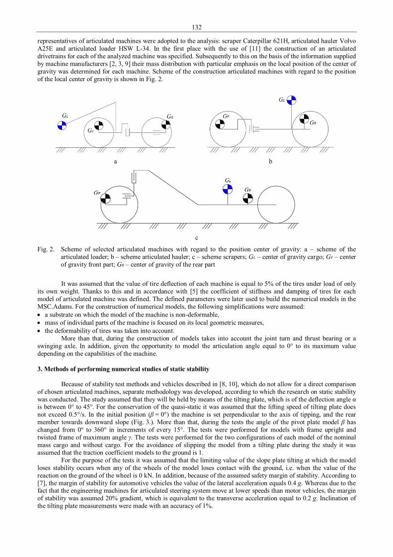
132

representatives of articulated machines were adopted to the analysis: scraper Caterpillar 621H, articulated hauler Volvo A25E and articulated loader HSW L-34. In the first place with the use of [11] the construction of an articulated drivetrains for each of the analyzed machine was specified. Subsequently to this on the basis of the information supplied by machine manufacturers [2, 3, 9] their mass distribution with particular emphasis on the local position of the center of gravity was determined for each machine. Scheme of the construction articulated machines with regard to the position of the local center of gravity is shown in Fig. 2.

a

b

c

Fig. 2. Scheme of selected articulated machines with regard to the position center of gravity: a – scheme of the articulated loader; b – scheme articulated hauler; c – scheme scrapers; GL – center of gravity cargo; GF – center of gravity front part; GR – center of gravity of the rear part

It was assumed that the value of tire deflection of each machine is equal to 5% of the tires under load of only

its own weight. Thanks to this and in accordance with [5] the coefficient of stiffness and damping of tires for each model of articulated machine was defined. The defined parameters were later used to build the numerical models in the MSC.Adams. For the construction of numerical models, the following simplifications were assumed: • a substrate on which the model of the machine is non-deformable, • mass of individual parts of the machine is focused on its local geometric measures, • the deformability of tires was taken into account.

More than that, during the construction of models takes into account the joint turn and thrust bearing or a swinging axle. In addition, given the opportunity to model the articulation angle equal to 0° to its maximum value depending on the capabilities of the machine. 3. Methods of performing numerical studies of static stability

Because of stability test methods and vehicles described in [8, 10], which do not allow for a direct comparison of chosen articulated machines, separate methodology was developed, according to which the research on static stability was conducted. The study assumed that they will be held by means of the tilting plate, which is of the deflection angle α is between 0° to 45°. For the conservation of the quasi-static it was assumed that the lifting speed of tilting plate does not exceed 0.5°/s. In the initial position (β = 0°) the machine is set perpendicular to the axis of tipping, and the rear member towards downward slope (Fig. 3.). More than that, during the tests the angle of the pivot plate model β has changed from 0° to 360° in increments of every 15°. The tests were performed for models with frame upright and twisted frame of maximum angle γ. The tests were performed for the two configurations of each model of the nominal mass cargo and without cargo. For the avoidance of slipping the model from a tilting plate during the study it was assumed that the traction coefficient models to the ground is 1.

For the purpose of the tests it was assumed that the limiting value of the slope plate tilting at which the model loses stability occurs when any of the wheels of the model loses contact with the ground, i.e. when the value of the reaction on the ground of the wheel is 0 kN. In addition, because of the assumed safety margin of stability. According to [7], the margin of stability for automotive vehicles the value of the lateral acceleration equals 0.4 g. Whereas due to the fact that the engineering machines for articulated steering system move at lower speeds than motor vehicles, the margin of stability was assumed 20% gradient, which is equivalent to the transverse acceleration equal to 0.2 g. Inclination of the tilting plate measurements were made with an accuracy of 1%.

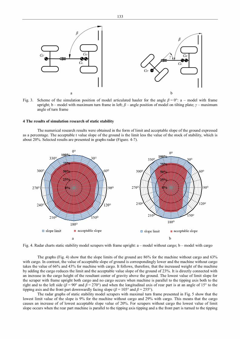
133

a

b

Fig. 3. Scheme of the simulation position of model articulated hauler for the angle β = 0°: a – model with frame upright; b – model with maximum turn frame in left; β – angle position of model on tilting plate; γ – maximum angle of turn frame

4 The results of simulation research of static stability

The numerical research results were obtained in the form of limit and acceptable slope of the ground expressed as a percentage. The acceptable t value slope of the ground is the limit less the value of the stock of stability, which is about 20%. Selected results are presented in graphs radar (Figure. 4-7).

a

b

Fig. 4. Radar charts static stability model scrapers with frame upright: a – model without cargo; b – model with cargo

The graphs (Fig. 4) show that the slope limits of the ground are 86% for the machine without cargo and 63%

with cargo. In contrast, the value of acceptable slope of ground is correspondingly lower and the machine without cargo takes the value of 66% and 43% for machine with cargo. It follows, therefore, that the increased weight of the machine by adding the cargo reduces the limit and the acceptable value slope of the ground of 23%. It is directly connected with an increase in the cargo height of the resultant center of gravity above the ground. The lowest value of limit slope for the scraper with frame upright both cargo and no cargo occurs when machine is parallel to the tipping axis both to the right and to the left side (β = 90° and β = 270°) and when the longitudinal axis of rear part is at an angle of 15° to the tipping axis and the front part downwardly facing slope (β = 105° and β = 255°).

The radar graphs of static stability model scrapers with maximal turn frame presented in Fig. 5 show that the lowest limit value of the slope is 9% for the machine without cargo and 29% with cargo. This means that the cargo causes an increase of of lowest acceptable slope value of 20%. For scrapers without cargo the lowest value of limit slope occurs when the rear part machine is parallel to the tipping axis tipping and a the front part is turned to the tipping

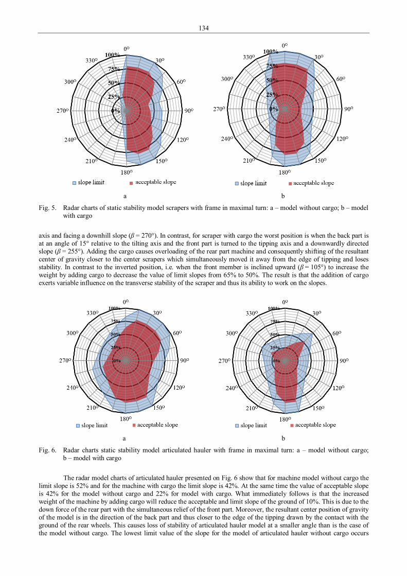
134

a

b

Fig. 5. Radar charts of static stability model scrapers with frame in maximal turn: a – model without cargo; b – model with cargo

axis and facing a downhill slope (β = 270°). In contrast, for scraper with cargo the worst position is when the back part is at an angle of 15° relative to the tilting axis and the front part is turned to the tipping axis and a downwardly directed slope (β = 255°). Adding the cargo causes overloading of the rear part machine and consequently shifting of the resultant center of gravity closer to the center scrapers which simultaneously moved it away from the edge of tipping and loses stability. In contrast to the inverted position, i.e. when the front member is inclined upward (β = 105°) to increase the weight by adding cargo to decrease the value of limit slopes from 65% to 50%. The result is that the addition of cargo exerts variable influence on the transverse stability of the scraper and thus its ability to work on the slopes.

a

b

Fig. 6. Radar charts static stability model articulated hauler with frame in maximal turn: a – model without cargo; b – model with cargo

The radar model charts of articulated hauler presented on Fig. 6 show that for machine model without cargo the

limit slope is 52% and for the machine with cargo the limit slope is 42%. At the same time the value of acceptable slope is 42% for the model without cargo and 22% for model with cargo. What immediately follows is that the increased weight of the machine by adding cargo will reduce the acceptable and limit slope of the ground of 10%. This is due to the down force of the rear part with the simultaneous relief of the front part. Moreover, the resultant center position of gravity of the model is in the direction of the back part and thus closer to the edge of the tipping drawn by the contact with the ground of the rear wheels. This causes loss of stability of articulated hauler model at a smaller angle than is the case of the model without cargo. The lowest limit value of the slope for the model of articulated hauler without cargo occurs

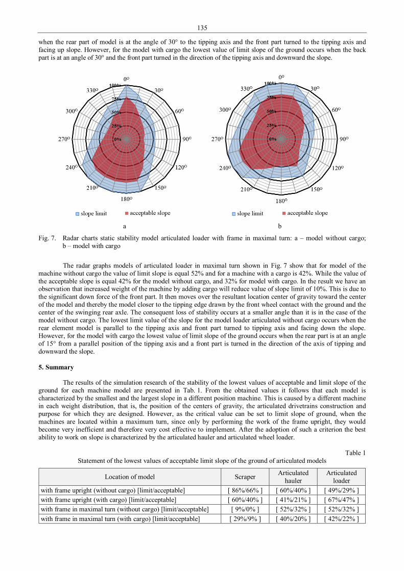
135

when the rear part of model is at the angle of 30° to the tipping axis and the front part turned to the tipping axis and facing up slope. However, for the model with cargo the lowest value of limit slope of the ground occurs when the back part is at an angle of 30° and the front part turned in the direction of the tipping axis and downward the slope.

a

b

Fig. 7. Radar charts static stability model articulated loader with frame in maximal turn: a – model without cargo; b – model with cargo

The radar graphs models of articulated loader in maximal turn shown in Fig. 7 show that for model of the

machine without cargo the value of limit slope is equal 52% and for a machine with a cargo is 42%. While the value of the acceptable slope is equal 42% for the model without cargo, and 32% for model with cargo. In the result we have an observation that increased weight of the machine by adding cargo will reduce value of slope limit of 10%. This is due to the significant down force of the front part. It then moves over the resultant location center of gravity toward the center of the model and thereby the model closer to the tipping edge drawn by the front wheel contact with the ground and the center of the swinging rear axle. The consequent loss of stability occurs at a smaller angle than it is in the case of the model without cargo. The lowest limit value of the slope for the model loader articulated without cargo occurs when the rear element model is parallel to the tipping axis and front part turned to tipping axis and facing down the slope. However, for the model with cargo the lowest value of limit slope of the ground occurs when the rear part is at an angle of 15° from a parallel position of the tipping axis and a front part is turned in the direction of the axis of tipping and downward the slope. 5. Summary

The results of the simulation research of the stability of the lowest values of acceptable and limit slope of the ground for each machine model are presented in Tab. 1. From the obtained values it follows that each model is characterized by the smallest and the largest slope in a different position machine. This is caused by a different machine in each weight distribution, that is, the position of the centers of gravity, the articulated drivetrains construction and purpose for which they are designed. However, as the critical value can be set to limit slope of ground, when the machines are located within a maximum turn, since only by performing the work of the frame upright, they would become very inefficient and therefore very cost effective to implement. After the adoption of such a criterion the best ability to work on slope is characterized by the articulated hauler and articulated wheel loader.

Table 1 Statement of the lowest values of acceptable limit slope of the ground of articulated models

Location of model Scraper Articulated hauler

Articulated loader

with frame upright (without cargo) [limit/acceptable] [ 86%/66% ] [ 60%/40% ] [ 49%/29% ] with frame upright (with cargo) [limit/acceptable] [ 60%/40% ] [ 41%/21% ] [ 67%/47% ] with frame in maximal turn (without cargo) [limit/acceptable] [ 9%/0% ] [ 52%/32% ] [ 52%/32% ] with frame in maximal turn (with cargo) [limit/acceptable] [ 29%/9% ] [ 40%/20% ] [ 42%/22% ]

136

In conclusion the method for evaluating stability of articulated machines and their ability to work on slopes presented in the article is simple and allows for a quick comparison of the several machines. However, with the use of the program MSC.Adams one should remember about the appropriate choice of parameters associated with the selected model and giving relevant bonds which would be conditioned both by the laws of physics as well as kinematics drivetrains. Shortly speaking, the use of programs for modeling type multibody MSC.Adams requires the use of knowledge and experience. References 1. Bartnicki A., Jaskółowski M. B., Łopatka M. J, Muszyński T. The researches of stability evaluation articulated

loader while working on slopes. Proceedings of 8th International Conference ITELMS’2013. 2. Brochure VOLVO Articulated hauler A25E. Sweden 2008. 3. Brochure Caterpillar Wheel Tractor-Scraper 621H. 2012. 4. Dudziński P., Pieczonka K., Sworobowicz G. Aktywny układ do poprawy stateczności pojazdów przemysłowych

na podwoziu kołowym, Problemy maszyn roboczych, Z. 14, 1999, pp. 9-19. 5. Konopka S. Borkowski W. Prochowski L. Dynamika maszyn roboczych. Warszawa, Wydawnictwa Naukowo-

Techniczne, 1996. 6. Konopka S., Krogul P., Łopatka M. J., Muszyński T. Symulacyjna analiza stateczności maszyn przegubowych

na przykładzie ładowarki kołowej Ł34. Przegląd Mechaniczny, nr 11/2013, str. 13, Warszawa 2013. 7. Kozicka A,. Łopatka M. Muszyński T. Testy i kryteria oceny stateczności poprzecznej terenowych przegubowych

maszyn transportowo-przeładunkowych. Logistyka. Nr. 3, 2007. 8. Li X. F., Wang G. Q., Yao Z. W., Yang Y. H. Research on lateral stability and rollover of articulated wheel loader.

Mathematical and computer modelling of dynamical systems. Vol. 20 pp. 248-263. 2014. 9. Ładowarka hydrauliczna Ł – 34. Instrukcja obsługi. Kombinat przemysłowy Huta Stalowa Wola, 37-450 Stalowa

Wola. AGPOL - ZW - 01 - 266/87. 10. Ma W. H., Peng H. Worst-case maneuvers for the roll-over and jackknife of articulated vehicles. 11. Proceedings of the 1998 American coltrol conference. Pp. 2263-2267.1998. 12. Siwulski T. Modelowanie stateczności dynamicznej pojazdów przemysłowych z podatnymi elementami jezdnymi.

Wrocław 2006. 13. Tyro G. Maszyny ciągnikowe do robót ziemnych. WNT, Warszawa 1986.

137

Proceedings of 9th International Conference ITELMS’2014 Research of Soil Shear Resistance versus Clay Amount in it I. Joneliukstiene*, S. Susinskas** *Kaunas University of Technology, Aukstaiciu str. 74-20, 36116, Panevezys, Lithuania, E-mail: irma.kraujalyte@gmail.com **Kaunas University of Technology, Daukanto str. 12, 44556, Panevezys, Lithuania, E-mail: saulius.susinskas@ktu.lt Abstract This paper gives the information about the main properties of soils. The most important is shearing strength which shows the strength of soil. Also there are given some formulas to calculate tangential stresses by normal stresses, cohesive, angle of internal friction and their effective values. There are described methods how to determine shear strength values of soils in laboratory. The paper shows the relationship of cone strength qc and other values of soil. KEYWORDS: soil, sand, clay, shear strength, CPT test. 1. Introduction

The soil can be used by two ways: as a base for foundation of buildings and structures and as a building material for various engineering structures (for example, dams, embankments etc.). By the origin, there are two types of soils – natural and man-made. Natural soils (granular sedimentary rocks) formed during the natural processes. Man-made soils are formed due to human activity (industrial, mining, building or economical).

In Lithuania the widely spread type of soil is moraine clay (till). Clay till can be very heterogeneous and varying in composition and stiffness. At the same profile, there can be several layers of different origin and composition deposited on top of each other. Properties of the clays include plasticity, shrinkage under loss of water and under drying in air, fineness of grain, color after drying, hardness and cohesion. On the basis of such qualities clays are variously divided into classes or groups [3]. 2. Mechanical properties of soils

There are two very important properties of soils – compressibility and shear strength. The soil starts to compress when the base doesn’t create deformations of shear, and when the capacity is decreasing. In this phase, we can determine the modulus of elasticity E and the value of transverse deformation. Increasing the load on the soil begins unquenchable shear deformation and at a certain load the amount of available soil limits bearing capacity. In this phase, the main property of soil is shear strength which is described by the cohesion c and the angle of internal friction φ [1].

The mechanical properties of soil are determined in laboratory and field, in natural situation of stratification, carrying out the tests which are regulated by normative documents. The soil can be deformed due to many reasons, for example some of fine soils shrink when the moisture is decreasing, and when the volume of pores is decreasing the density of soil is increasing. 3. Shear strength

Shear strength is the main parameter of soils strength. Soil shear strength is described due to Coulomb’s and Mohr’s theory by the cohesion c and the internal friction angle φ. They are called value of soil strength. In certain points of plane tangential stresses become the same as the shear strength. In these points the soil deformation of shear starts. Starts formation of slip plane, some part of the soil will begin to slide, causing the collapse of building base. Coulomb in 1776 suggested that the resistance to shear degradation in the plane can be expressed by the equation [2]: c+⋅= ϕστ tg (1)

where τ – tangential stresses in disintegration of the plane, which are valuated as shear strength; σ – normal stresses in disintegration of the plane; φ – angle of internal friction; c – cohesion.

Friction in disintegration of the plane is evaluated by tangent of angle of internal friction. The cohesive due to parts of soils resists for shear when the normal stresses are equal to 0. In real soils disintegration of the plane isn’t between two inflexible surfaces. The surface of this plane deforms, causing the changes of capacity across the plane.

The first equation of Coulomb was adjusted to convey shear of real soils:

''tg' c+⋅= ϕστ (2)

138

where τ – tangential stresses in disintegration of the plane; σ' – effective normal stresses in disintegration of the plane; φ' – effective angle of internal friction; c' – effective cohesion.

In fine-grained soils – clay and silt – drained conditions rejected pore water pressure, and the shear strength is described by the following equation [2]:

''tg' c+⋅= ϕστ (3)

Undrained shear strength conditions of saturated clay and silt will ensure the cohesion between particles and the angle of internal friction is assumed to be equal to 0. Then:

uc=τ (4)

where cu – undrained cohesion. In cohesive soils value of the shear strength depends on soil moisture, porosity, plasticity and consistence. Fine

and mixed soils are classed to medium strength (Tab. 1). The values of shear strength are determined by laboratory tests. According to field studies of shear strength

parameters shall be determined using the empirical relationship by indirect tests.

Table 1 Combinations of cohesion and angle of internal friction

φ', ° c', kPa 0–5 85–70

5–10 70–55 10–15 55–40 15–20 40–30 20–25 30–20

Values of shear strength in laboratory can be determined by:

• direct shear device; • simply shear device; • ring shear device; • triaxial device.

Shearing plane is formed in direct shear device. The device is made by two carriages where the shearing plane forms. Values of shearing strength are determined by shearing stresses in normal stresses. There should be done more than two tests.

The point of simply shear device test is that vertical force affects the sample and creates normal stresses, and horizontal displacements make tangential stresses. During the test shear deformation can be determined by vertical and horizontal displacements.

Using the ring shear device we can determine values of shearing strength by the ring on turning moment. Natural conditions of soils could be simulated by triaxial device (Fig. 1) [1]. The most important normal stresses

σ1 and radials to σ3 and pore pressure u affect the sample of soil in device. There can be done three types of tests: • unconsolidated – undrained test (UU); • consolidated – undrained test (CU); • consolidated – drained test (CD).

a

b

Fig. 1. Triaxial apparatus: a – view; b – scheme: 1 – load cell (can be above or below); 2 – air outlet; 3 – displacement meter; 4 – piston; 5 – cap; 6 – sample; 7 – membrane; 8 – pedestal; 9 – pressure pump chamber; 10 – chamber walls; 11 – channels; 12, 13 – twinning pressure gauge; 14 – pore pressure pump

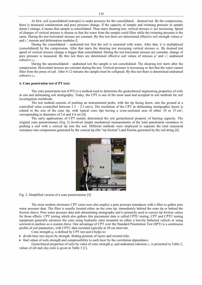
139

At first, soil (consolidated isotropic) is under pressure for the consolidated – drained test. By the compression, there is measured condensation and pore pressure change. If the capacity of sample and twinning pressure in sample doesn’t change, it means that sample is consolidated. Then starts shearing test, vertical stresses σ1 are increasing. Speed of changes of vertical stresses is chosen so that the water from the sample could filter while the twinning pressure is the same. During the test horizontal stresses are constant. By this test there are determined effective soil strength values φ' and c', tension and deformation modulus E.

During the consolidated – undrained test first the soil is saturated with water. After that, it is multiplexed (consolidated) by the compression. After that starts the shearing test increasing vertical stresses σ1. By drained test speed of vertical stresses change is bigger than consolidated. During the test horizontal stresses are constant, change of pore pressure is measured. By this test there are determined effective soil values of stresses φ' and c', undrained cohesive cu.

During the unconsolidated – undrained test the sample is not consolidated. The shearing test starts after the compression. Horizontal stresses are constant during the test. Vertical pressure is increasing so fast that the water cannot filter from the pores of soil. After 8-12 minutes the sample must be collapsed. By this test there is determined undrained cohesive cu. 4. Cone penetration test (CPT test)

The cone penetration test (CPT) is a method used to determine the geotechnical engineering properties of soils in situ and delineating soil stratigraphy. Today, the CPT is one of the most used and accepted in soil methods for soil investigation worldwide.

The test method consists of pushing an instrumented probe, with the tip facing down, into the ground at a controlled value (controlled between 1.5 – 2.5 cm/s). The resolution of the CPT in delineating stratigraphic layers is related to the size of the cone tip, with typical cone tips having a cross-sectional area of either 10 or 15 cm2, corresponding to diameters of 3.6 and 4.4 cm [4].

The early applications of CPT mainly determined the soil geotechnical property of bearing capacity. The original cone penetrometers (Fig. 2) involved simple mechanical measurements of the total penetration resistance to pushing a tool with a conical tip into the soil. Different methods were employed to separate the total measured resistance into components generated by the conical tip (the “tip friction”) and friction generated by the rod string [4].

Fig. 2. Simplified version of a cone penetrometer [4]

The most modern electronic CPT cones now also employ a pore pressure transducer with a filter to gather pore

water pressure data. The filter is usually located either on the cone tip, immediately behind the cone tip or behind the friction sleeve. Pore water pressure data aids determining stratigraphy and is primarily used to correct tip friction values for those effects. CPT testing which also gathers this piezometer data is called CPTU testing. CPT and CPTU testing equipment generally advances the cone using hydraulic rams mounted on either a heavily ballasted vehicle or using screwed-in anchors as a counter-force. One advantage of CPT over the Standard Penetration Test (SPT) is a continuous profile of soil parameters, with CPTU data recorded typically at 20 cm intervals.

Cone strength qc is defined by CPT test and it helps to: • divide base into layers by strength, finding position of layers and oriental title; • find values of soils strength and compressibility to each layer by the correlation dependence.

Geotechnical properties of soils by value of cone strength qc and undrained cohesion cu is presented in Table 2, values of silt and clay soils is given in Table 3 [1].

140

Table 2 Geotechnical properties of soils

Strength Coarse soil (sand) Fine soil (dust and clay)

qc, MPa density qc, MPa cu, kPa consistence Extra weak <0.25 <12.5 Extra soft Very weak <2.5 Very loose 0.25 – 0.5 12.5 – 25.0 Very soft

Weak 2.5 – 5.0 Loose 0.5 – 1.5 25.0 – 75.0 Soft Medium strength 5.0 – 10.0 Medium density 1.5 – 2.5 75.0 – 125.0 Firm

Strong 10.0 – 20.0 Dense 2.5 – 4.0 125.0 – 200.0 Stiff Very strong 20.0 – 40.0 Very dense 4.0 – 6.0 200.0 – 300.0 Very stiff Extra strong >40.0 Extra dense >300.0 Hard

Table 3 Shear strength values of silt and clay soils

qc, MPa Shear strength values of silt and clay soils cohesion c', kPa angle of internal friction ϕ'

0.5 18 16 1.0 24 17 1.5 30 18 2.0 36 19 2.5 41 20 3.0 47 22 3.5 53 23 4.0 58 24 4.5 64 25 5.0 70 26 5.5 76 27 6.0 82 28

3. Conclusions

For buildings of range it is very important to know composition of base on which is going to build building or structure. If the base is clay till, we should remember that it is heterogeneous and varying in composition and stiffness. For that reason it is necessary to determine compressibility and shear strength of soil. Coulomb is suggested some formulas which are used to find tangential stress of soil.

Shear strength is determined in laboratory using direct shearing device, simply shearing device, ring shearing device and triaxial device. It is done cone penetration test (CPT) to find other geotechnical engineering properties and to delineating soil stratigraphy. Cone strength is determined by CPT test and it helps to divide base into layers by strength, finding position of layers and oriental title; to find values of soils strength and compressibility to each layer by the correlation relationships. References 1. Sližytė D., Medzvieckas J., Mackevičius R. Pamatai ir pagrindai. – Vilnius: Technika, 2012. 248 p. 2. Prušinskienė S. Smėlio gruntų ypatumai ir jų tyrimo metodai. – Vilnius: Technika, 2012. 182 p. 3. Larson R. Investigations and load tests in clay till. Linkoping. 2001. 169 p. 4. Mayne P. W. Cone penetration testing state-of- practice. NCHRP Project 20-05, Topic 37-14. February 2007.

141

Proceedings of 9th International Conference ITELMS’2014 Dependencies of Personal Vehicle Sales on the Financial Support of their Sales R. Kampf*, M. Vochozka*, P. Lejskova**, T. Cmiral** *Institute of Technology and Business in České Budějovice, Okružní 517/10, 370 01 České Budějovice, Czech Republic. E-mail: kampf@mail.vstecb.cz, vochozka@mail.vstecb.cz **University of Pardubice, Jan Perner Transport Faculty, Department of Transport Management, Marketing and Logistics; E-mail: pavla.lejskova@upce.cz Abstract The article describes the dependence of the sales of BMW vehicles in the Czech Republic on the financial support of those sales. The current state of sales support of selected BMW models in the Czech Republic is described as is the level of dependence of those sales on the scale of support which is analyzed using regression models. In addition, the future development of sales of selected BMW vehicles is given. The article was written as the partial outcome of research carried out in 2012. KEYWORDS: sales support, communication mix, regression analysis, dependence. 1. Introduction

The aim of the research project was to describe the various means of sales support and their use and to analyze the dependence of personal vehicle sales in the Czech Republic on the level of financial support given for the sales by the producer.

The aim of the article (which is the partial outcome of the research project) is to compile regression models of dependence of sales of selected vehicles on the level of financial sales support on the basis of the analysis of data obtained between 2007 – 2011, and to use these models (after testing their quality) to predict future sales for 2012 – 2014.

The article consists of two parts. Firstly, the theoretical part in which sales support, including the theoretical description of regression and correlation analyses, the use of correlation coefficients and significance tests are characterized. Secondly, the practical (application) part in which regression models will be compiled and used to predict future sales of selected personal vehicles in the Czech Republic over the next three years (the sales of BMW vehicles will be given as a practical example). 2. Sales support

Sales support includes a wide range of tools: coupons, games, competitions, lotteries, premiums and gifts, samples, fairs and sales exhibitions, small exhibitions, presentations, rebates, low interest loans, entertainment events, discounts for returning older version of a product, trading stamps and countertrade. It can be defined for example as: • Sales support is characterized as a set of marketing activities which directly support the behaviour of a consumer and

increase the effectiveness of trade interlinks [1]. • Sales support is understood as short term incentives meant to support the purchase or sale of a product or service.

Advertising and personal sales usually work together with another communication tool, sales support. While advertising and personal sales give reason to the purchase of a product or service, sales support is the incentive for immediate purchase. It is basically a relationship between being informed and accepting a call to act [2].

Sales support is an ever growing tool in marketing communications. The volume of financial means invested into sales support is slowly beginning to exceed the value of investments into advertising. Changes to the cost structure of marketing communication to the disadvantage of media advertising and to the advantage of sales support are very distinct, e.g.: • In Belgium in 1981, 43% of the budget for marketing communications was invested into advertising but by 1992

already 72% went into sales support [3]. • Kotler and Armstrong present the opinion that an average American company in the consumer goods sector

nowadays spends 74% of all marketing costs on various forms of sales support [4]. • In Great Britain £8 billion on average is spent on advertising annually, £9 billion is spent on sales support [5].

Nowadays the trend is towards creating the maximum experience whereby all the senses are involved, in particular in retail communications in shops. It is a set of communication activities Point of Purchase – or POP.

As a marketing communication tool it is uniquely effective because it gives the message of the brand exactly at the right moment – when the consumer is in the shop and is actively engaged (mentally and physically) in the process of buying products [6].

142

The current market is defined as a brand market. Therefore it is clear that POP communication too, must happen on the level of brand presentation and emphasis. One of the basic rules of the communication segment of sales support is: Sales support = support of sales of branded goods.

Sales support tools differ according to what they want to achieve: • Price discounts or free samples aim to make the customer immediately buy and try a product. • Benefit programs aim to “attach” a customer to certain products and build their loyalty to the brand.

The main aim of all sales support activities is to trigger the positive reaction of consumers. Sales support can also be divided according to who it targets and who is the initiator of the sales support

activities – it can be the producer as well as the retailer (seller). The target groups can be divided into three basic units: distributors, sellers and customers. The producer can support all three target groups. The seller targets their customers – the means to their profits.

P. Kotler divides support as follows [4]: • Sales support for consumers. • Sales support for sellers. • Sales support for traders (distributors). 3. Theoretical basis of regression analysis

Regression analysis is a set of statistical methods and procedures the purpose of which is to find a mathematical function which expresses the character of described dependence as best as possible. Such a function is called a regression function [7].

The main task of regression analysis is to estimate the parameters of the hypothetical regression function and to compile this function. Partial tasks of regression analysis are [7]: • To formulate conceptions about the character of regression analysis. • To formulate assumptions about the gross impact of unconsidered statistical codes. • To estimate the empirical regression function. • To evaluate the quality of the empirical regression function.

Types of regression analysis: • Simple (pair) regression – dependence of two variables. • Multiple regressions – more than two variables enter the analysis.

Regression functions can have various forms: • Linear models. • Non-linear models which can be transformed into linear models. • Non-linear models which simply cannot be transformed into linear models. 3.1. Determining parameters of the linear regression function

A simple linear regression model is a model whereby the graph of the regression function is a straight line in the form of

xbbY 10 += (1)

Estimates of the parameters b0 and b1 are mostly done using the method of the least squares. It is quite a simple procedure with relatively good estimate:

n

xby

xxn

yxxyxb

n

i

n

iii

n

ii

n

ii

n

iii

n

ii

n

ii

n

ii ∑ ∑

∑∑

∑∑∑∑= =

==

====−

=

−

−= 1 1

1

2

11

2

111

2

1

2

0

. (2)

2

11

2

1111

.

−

−=

∑∑

∑∑∑

==

===

n

ii

n

ii

n

ii

n

ii

n

iii

xxn

yxyxnb (3)

where y is the dependent variable; x is the independent variable and n is the number of observations. 3.2. Quality of regression function and intensity of dependence

In researching the dependence in the simple regression function the determination index has an essential role. The index determines what part of the variability of researched values can be explained by a given regression model.

143

The determination coefficient takes values from the interval 0, 1. The smaller the unexplained part of the dispersion variance is the better the regression function expresses the dependence of the random variable y on the values of xi, this means the “closer” the points (xi, yi), i = 1, 2, …, n are to the straight line Y = b0 b1 x, the closer the determination index is to 1.

The determination index expresses the proportion of the explained part of the dispersion variance to the overall dispersion and it is given by the relation:

y

T

SSI =2 (4)

where ST is the explained sum of residual squares which characterize the part of the total variability which can be explained by the regression model. The total sum of residual squares is explained by Sy [8]:

( ) ( )

( ) ( )

( ) TyiiR

iiiiiT

iiiy

SSYySny

yxbybyYS

ny

yyyS

−=−=

−+=−=

−=−=

∑

∑ ∑ ∑ ∑

∑ ∑ ∑

2

2

102

222

(5)

3.3. Multiple regressions [9]

This is regression when the dependent variable is influenced by several independent variables. The general equation can be written as:

εββββ +++++= pp xxxy ...22110 (6)

The parameter ɛ describes a random component. The estimated regression function can be written as:

pp xbxbxbbY ++++= ...22110 (7)

or in a more easily interpreted form as:

pxxxyxxxxyxxxxyx xbxbxbbYpppp 121312321 ....2....1....0 ...

−++++= (8)

The parameters b are called partial regression coefficients and indicate an estimate of how the explained (dependent) variable y would change on average in case of a unit change of the independent variable before a point if all other variables after the point remain constant.

In the case of sales of BMW vehicles in the Czech Republic it is a dependence on two explanatory (independent) variables – the amount of sales support and the life-cycle phase of the product, e.g. the age of the sold BMW vehicle. Thus we will deal with multiple regressions, in which the variable y depends on two independent variables x1, x2.

εβββ +++= 22110 xxy or 2.1.0 1221xbxbbY xyxxyx ++=

(9)

Estimates 1221 ..0 ,, xyxxyx bbb are obtained by solving the equations:

∑∑ ∑∑∑ ∑ ∑∑∑ ∑ ∑

++=

++=

++=

22.21.202

21.21.101

2.1.0

1221

1221

1221

ixyxiixyxiii

iixyxixyxiii

ixyxixyxi

xbxxbxbyx

xxbxbxbyx

xbxbnby

(10)

To obtain the coefficients b it is necessary to install and solve the formed set of equations. This calculation is mostly solved by sophisticated computer systems. 3.4. Coefficient of multiple correlations [9]

A multiple correlation coefficient measures the tightness of the dependent variable y on all explanatory variables x1, x2. Its calculation can determine the quality of the compiled regression model. It takes only values <0, 1> and is calculated using the formula:

144

2

22

.21

22121121 1

2

xx

yxxxyxyxyxxxy r

rrrrrr

−

+−= (11)

This means it is necessary to calculate the pair correlation coefficients for the dependencies between individual variables, according to the formula for the simple correlation coefficient:

( )[ ] ( )[ ]∑ ∑∑ ∑

∑ ∑ ∑−⋅−

−=

22

22

21

21

212112

iiii

iiii

xxnxxn

xxxxnr (12)

It is also possible to calculate the partial correlation coefficients that determine the tightness of the dependence between the response variable y and one of the explanatory variables while excluding the influence on the other explanatory variables. For simple and partial correlation coefficients, the values range from <-1, 1>, which indicate a linear relationship (direct or indirect): • In case of a positive correlation the values of both variables increase at the same time. • In case of a negative correlation the value of one variable increases and the value of the other variable decreases. • In the absence of a linear relationship r = 0.

In the case of dependent variables y and x1 the partial correlation coefficient is calculated as follows:

( )( )22.

212

212121

11 xxyx

xxyxyxxyx

rr

rrrr

−−

−= (13)

For other partial dependencies of other variables it is only needed to enter other relevant simple correlation coefficients. 3.5. Hypotheses tests [9]

A high correlation coefficient does not necessarily indicate dependence between variables. It is therefore necessary to test the result of the calculation. 3.5.1. Individual t-test

This is used for testing simple and partial correlation coefficients. The hypothesis H0: 0

21. =jxxyβ , i.e. that dependence does not exist is tested against the hypothesis

H1: 021. >xxyβ , i.e. that dependence exists. The value of test criteria is calculated as:

2

.

.

1

2

ji

ji

xyx

xyx

r

nrT

−

−= (14)

In the selection of the two-dimensional normal distribution, the distribution of n-p-1 has degrees of freedom, where p is the number of explanatory variables. If the calculated value of the test criterion falls into the critical area, we reject the null hypothesis and consider the existence of a linear relationship on the selected significance level to be proven. 3.5.2. F-test

This is used for testing multidimensional correlation coefficients. Again, the hypotheses H0: 0

21. =jxxyβ and H1: 0

21. >xxyβ are tested.

The value of test criterion has the form:

pr

pnrF

xxy

xxy

)1(

)1(2.

2.

21

21

−

−−= (15)

This time we choose from critical values of F-distribution with p and n-p degrees of freedom. Then we reject the hypothesis H0, if the value of the test criterion is greater than the quantile F1−α[p; (n − p − 1)].

145

3.6. Summary of the chapter

Regression analysis will be used to evaluate the data describing the sales of selected BMW vehicles and the provided amount of financial support. The evaluation of the data will lead to obtaining regression coefficients and then the formation of a regression function. To evaluate the regression model and the individual dependencies, correlation coefficients will be used. To confirm or deny the possible dependencies, the following analysis will use an individual t-test, or a total F-test. The last step in the analysis of the data will be the prediction of the future value of sales of selected BMW vehicles for 2012-2014. The prediction will be based on the formed regression function.

The following table gives an overview of BMW vehicle models:

Table 1 Overview of current BMW models (source: author)

Model Description BMW 1 Smaller medium size vehicle in three-or five-door hatchback versions, coupe or convertible.

Entry model to the brand. BMW 3 Medium size in sedan, station wagon, coupe and convertible versions. The world's best-

selling BMW, but not in the Czech Republic. BMW 5 Mid – luxury – sedan and station wagon versions. Best selling BMW in the Czech Republic. BMW 5 GT Model of a new class of vehicles - large comfortable five-door hatchback. BMW 6 Class GT (Gran Turismo) - emphasis on dynamics, in coupe and convertible versions. In the

summer a new model Grand Coupe is coming to the market. BMW 7 Luxurious class in basic sedan form with possibility of extended wheelbase version.

Flagship of the brand. BMW X1 Entry model into so called X series of BMW, follows on from the 3 series. BMW X3 Smaller SAV (Sport Activity Vehicle), established this segment. BMW X5 Larger SAV, it was for a long time the best selling BMW in the Czech Republic. BMW X6 SAC (Sport Activity Coupé) based on X5 with more sporty character. BMW Z4 Roadster with hard foldable roof. BMW M3, M5, M6, X5 M and X6 M

Modified versions of serial BMW vehicles with the strongest engines produced by the sport division of the brand.

4. Regression models

Regression models will be compiled separately for each of the BMW models. The work is aimed at assessing the dependence of quarterly sales of BMW vehicles on the financial support the manufacturer provides to the car dealers. In these regression models the following variables will appear: the explained variable y – indicates the sales of a physical vehicle; the explanatory variable x1 – the average amount of financial support, supplemented by additional explanatory variable x2 – the age of a physical vehicle model, meaning since its launch on the market. This latter variable was chosen because of the great influence of the life cycle of the product on its sales.

To compile regression models, the best selling models of BMW series 1, 5, X3 and X5 were selected for this research. A detailed example of the practical application of the regression model, including a detailed calculation for the BMW X3 is carried out. 4.1. Regression model of the dependence of sales of BMW X3 on financial support

BMW X3 is the best selling model in the SAV range. The average price of this vehicle is around CZK 1.1 million. The yellow colour in the table indicates the launch of a new generation of the vehicle, which is why the age of the vehicle changes to 1.

Table 2 Variables entering the regression model for BMW X3 (source: BMW Vertriebs GmbH ČR + author)

Quarter Sales – number of sold vehicles in quarter – y

Age of vehicle – number of quarters on the market – x1

Average amount of support in thousands CZK – x2

2007

I.Q 102 13 10.5 II.Q 88 14 10.5 III.Q 90 15 24.5 IV.Q 111 16 24.0

2008

I.Q 74 17 24.4 II.Q 84 18 24.4 III.Q 60 19 10.5 IV.Q 53 20 51.0

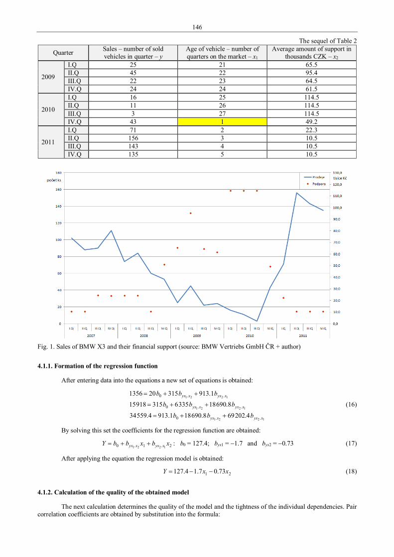
146

The sequel of Table 2

Quarter Sales – number of sold vehicles in quarter – y

Age of vehicle – number of quarters on the market – x1

Average amount of support in thousands CZK – x2

2009

I.Q 25 21 65.5 II.Q 45 22 95.4 III.Q 22 23 64.5 IV.Q 24 24 61.5

2010

I.Q 16 25 114.5 II.Q 11 26 114.5 III.Q 3 27 114.5 IV.Q 43 1 49.2

2011

I.Q 71 2 22.3 II.Q 156 3 10.5 III.Q 143 4 10.5 IV.Q 135 5 10.5

Fig. 1. Sales of BMW X3 and their financial support (source: BMW Vertriebs GmbH ČR + author)

4.1.1. Formation of the regression function

After entering data into the equations a new set of equations is obtained:

1221

1221

1221

..0

..0

..0

4.202698.690181.9134.55934

8.69018335631591815

1.913315203561

xyxxyx

xyxxyx

xyxxyx

bbb

bbbbbb

++=

++=

++=

(16)

By solving this set the coefficients for the regression function are obtained:

2.1.0 1221xbxbbY xyxxyx ++= : b0 = 127.4; byx1 = −1.7 and byx2 = −0.73 (17)

After applying the equation the regression model is obtained:

21 73.07.14.127 xxY −−= (18)

4.1.2. Calculation of the quality of the obtained model

The next calculation determines the quality of the model and the tightness of the individual dependencies. Pair correlation coefficients are obtained by substitution into the formula:

147

( )[ ] ( )[ ]∑ ∑∑ ∑

∑ ∑ ∑−⋅−

−=

22

22

21

21

212112

iiii

iiii

xxnxxn

xxxxnr (19)

829.0

738.0

701.0

2

1

21

−=

−=

=

yx

yx

xx

r

rr

These values are used for the calculation of individual partial correlation coefficients by substitution into the formula:

( )( )22.

212

212121

11 xxyx

xxyxyxxyx

rr

rrrr

−−

−= (20)

647.0

393.0

12

21

.

.

−=

−=

xyx

xyx

r

r

The calculations indicate that in both cases there is an indirect dependence. So even in the case of higher sales support, the sales of the vehicles will decrease.

The last calculation refers to the total correlation coefficient which determines the quality of the regression function. It is calculated using the formula

2

22

.21

22121121 1

2

xx

yxxxyxyxyxxxy r

rrrrrr

−

+−= (21)

857.021. =xxyr

This value is relatively high which means a well selected regression model. 4.1.3. Testing the correctness of the statements

In order to verify the correctness of all previous statements it is necessary to test the results again. 4.2. Testing of partial correlation coefficients - t-test

The test criterion has the form

2

.

.

1

2

ji

ji

xyx

xyx

r

nrt

−

−= (22)

By which results are obtained:

812.1)393.0(1

220393.02. 21

=−−

−−=

xyxT and 602.3

)647.0(1

220647.02. 12

=−−

−−=

xyxT (23)

In the quantile tables of Student's t-distribution of probability and 17 degrees of freedom a critical value t1−α/2, n−p−1 = 2.110 was found on the level of significance α = 5%.

In the case of dependence between the age of the vehicle and its saleability it fell under the critical value and in this case the hypothesis H0 must be accepted; the dependence does not exist. It is contrary to the dependence between sales and sales support for the vehicle where T > t which proves indirect dependence. 4.3. Testing of the total multiple correlation coefficient – F-test

The test criterion has the form

113.512)857.01(

)1220(857.0)1(

)1(2

2

2.

2.

21

21 =−

−−=

−

−−=

prpnr

Fxxy

xxy (24)

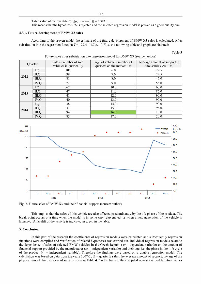
148

Table value of the quantile F1−α[p; (n − p − 1)] = 3.592. This means that the hypothesis H0 is rejected and the selected regression model is proven as a good quality one.

4.3.1. Future development of BMW X3 sales

According to the proven model the estimate of the future development of BMW X3 sales is calculated. After substitution into the regression function Y = 127.4 − 1.7 x1 −0.73 x2 the following table and graph are obtained:

Table 3 Future sales after substitution into regression model for BMW X3 (source: author)

Quarter Sales – number of sold vehicles in quarter – y

Age of vehicle – number of quarters on the market – x1

Average amount of support in thousands CZK – x2

2012

I.Q 101 6.0 22.5 II.Q 99 7.0 22.5 III.Q 81 8.0 45.0 IV.Q 72 9.0 55.0

2013

I.Q 67 10.0 60.0 II.Q 47 11.0 85.0 III.Q 41 12.0 90.0 IV.Q 40 13.0 90.0

2014

I.Q 38 14.0 90.0 II.Q 33 15.0 95.0 III.Q 94 16.0 10.0 IV.Q 85 17.0 20.0

Fig. 2. Future sales of BMW X3 and their financial support (source: author)

This implies that the sales of this vehicle are also affected predominantly by the life phase of the product. The

break point occurs at a time when the model is in some way rejuvenated, or when a new generation of the vehicle is launched. A facelift of the vehicle is indicated in green in the table. 5. Conclusion

In this part of the research the coefficients of regression models were calculated and subsequently regression functions were compiled and verification of related hypotheses was carried out. Individual regression models relate to the dependence of sales of selected BMW vehicles in the Czech Republic (y – dependent variable) on the amount of financial support provided by the manufacturer (x2 – independent variable) and their age, i.e. the phase in the life cycle of the product (x1 – independent variable). Therefore the findings were based on a double regression model. The calculation was based on data from the years 2007-2011 – quarterly sales, the average amount of support, the age of the physical model. An overview of sales is given in Table 4. On the basis of the compiled regression models future values

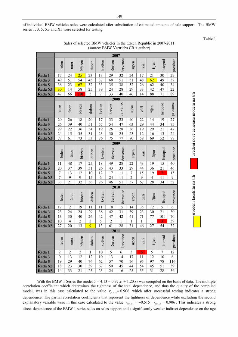
149

of individual BMW vehicles sales were calculated after substitution of estimated amounts of sale support. The BMW series 1, 3, 5, X3 and X5 were selected for testing.

Table 4 Sales of selected BMW vehicles in the Czech Republic in 2007-2011

(source: BMW Vertriebs ČR + author)

2007

lede

n

únor

břez

en

dube

n

květ

en

červ

en

červ

enec

srpe

n

září

říjen

listo

pad

pros

inec

Řada 1 17 24 25 23 13 29 32 24 17 21 30 29 Řada 3 49 51 54 45 37 68 51 51 48 62 49 37 Řada 5 36 23 67 32 33 35 38 52 26 62 40 34 Řada X3 30 14 58 25 39 24 28 29 33 42 47 22 Řada X5 47 66 110 5 7 33 40 46 14 88 71 89 2008

lede

n

únor

břez

en

dube

n

květ

en

červ

en

červ

enec

srpe

n

září

říjen

listo

pad

pros

inec

Řada 1 20 26 18 20 17 33 23 40 22 14 19 27 Řada 3 26 39 40 51 57 54 47 63 29 44 34 75 Řada 5 29 22 36 34 19 26 28 36 19 29 21 47 Řada X3 24 15 35 31 23 30 25 23 12 16 13 24 Řada X5 77 61 73 53 76 75 77 80 58 69 52 77 2009

lede

n

únor

břez

en

dube

n

květ

en

červ

en

červ

enec

srpe

n

září

říjen

listo

pad

pros

inec

Řada 1 11 48 17 25 18 49 28 22 43 19 15 40 Řada 3 20 37 39 31 26 43 33 29 44 36 21 46 Řada 5 7 13 12 10 12 17 11 7 15 19 7 15 Řada X3 7 9 9 15 6 24 11 2 9 4 11 9 Řada X5 33 21 32 36 26 46 51 57 67 28 34 52 2010

lede

n

únor

břez

en

dube

n

květ

en

červ

en

červ

enec

srpe

n

září

říjen

listo

pad

pros

inec

Řada 1 17 2 19 11 11 18 15 14 35 12 5 6 Řada 3 23 24 24 29 38 42 31 39 23 30 21 30 Řada 5 13 30 40 26 42 47 42 41 71 77 101 70 Řada X3 10 4 2 3 6 2 1 1 1 1 3 39 Řada X5 27 20 13 9 13 61 28 31 46 27 54 32 2011

lede

n

únor

břez

en

dube

n

květ

en

červ

en

červ

enec

srpe

n

září

říjen

listo

pad

pros

inec

Řada 1 2 2 2 1 10 5 6 3 6 5 7 12 Řada 3 0 13 12 12 10 13 14 17 11 12 10 6 Řada 5 19 29 40 76 62 57 70 76 95 97 78 116 Řada X3 18 23 30 39 67 50 45 44 54 45 51 39 Řada X5 14 33 21 25 23 24 16 25 35 31 28 56

uved

ení f

acel

iftu

na tr

h uv

edení n

ové

gene

race

mod

elu

na tr

h

With the BMW 1 Series the model Y = 4.13 − 0.97 x1 + 1.20 x2 was compiled on the basis of data. The multiple correlation coefficient which determines the tightness of the total dependence, and thus the quality of the compiled model, was in this case calculated to the value 906.0

21. =xxyr which after successful testing indicates a strong dependence. The partial correlation coefficients that represent the tightness of dependence while excluding the second explanatory variable were in this case calculated to the value 515.0

21. −=xyxr ; 906.012 . =xyxr . This indicates a strong

direct dependence of the BMW 1 series sales on sales support and a significantly weaker indirect dependence on the age

150

of the vehicle. Future sales of the Series 1 depend especially on sales support but it is also partly affected by the phase of the life cycle of the vehicle.

The regression function model for the BMW 3 Series is somewhat different: Y = 227.11 − 5.9 x1 − 0.343 x2 . The multiple correlation coefficient was in this case calculated to the value 901.0

21. =xxyr which after successful testing again indicates a strong dependence. The partial correlation coefficients were then in this case calculated as

716.021. −=xyxr ; 194.0

12 . −=xyxr . This time it indicates a strong indirect dependence on the age of the vehicle and a significantly weaker indirect dependence on the amount of sales support which, after testing at a level of significance of 5% was identified as insignificant. Future sales of this vehicle therefore depend on the age of the model.

The regression function model for the BMW 5 Series has the form: Y = 205.24 − 5.8 x1 + 0.06 x2 and is very similar to the model for the Series 3. The multiple correlation coefficient 728.0

21. =xxyr after successful testing again indicates a relatively strong dependence, albeit weaker than the dependence for the BMW Series 3. The partial correlation coefficients were in this case calculated to the value 707.0

21. −=xyxr ; 054.012 . =xyxr . This again indicates a

strong indirect dependence of BMW 5 Series sales on the age of the vehicle and a significantly weaker indirect dependence on the amount of sales support, which after testing at a level of significance of 5% again was identified as insignificant. Future sales of this vehicle therefore depend only on the age of the model.

The regression model for the BMW X3 series has the form: Y = 127.4 − 1.7 x1 − 0.73 x2 and at first glance there is a noticeable difference. However, the multiple correlation coefficient 857.0

21. =xxyr indicated a strong dependence which was confirmed by testing. The partial correlation coefficients in this case were calculated to the value 393.0

21. −=xyxr ; 647.012 . −=xyxr . Here a weak indirect dependence of BMW X3 sales on the age of the vehicle

was found and a significantly stronger indirect dependence on the amount of sales support. After testing at a significance level of 5% the dependence of sales on the age of the vehicle was found to be insignificant. Future sales of this vehicle therefore only depend on the sales support, the dependence is this time indirect.

The regression function for the BMW X5 series has the form: Y = 172.5 + 0.3 x1 − 0.73 x2 . The multiple correlation coefficient 358.0

21. =xxyr indicates a weak dependence, which is eventually excluded by subsequent testing at a significance level of 5%. Therefore, future sales of this vehicle can not be reliably predicted.

The results of the analysis indicate that there are differences between the various types of vehicles. It is therefore not possible to unequivocally say if the development of BMW vehicles sales depends on the level of sales support directly, indirectly, or not at all. At the same time it follows on from the above that it is necessary to approach individual types of vehicles differently when creating marketing strategies. References 1. Tellis G. J. Reklama a podpora prodeje. Praha: Grada, 2000. ISBN 80-7169-997-7. 4. Kotler P. Marketing management. Praha: Grada, 2001. ISBN 80-247-0016-6. 5. De Pelsmacker P., Geuens M. and Van Den Bergh J. Marketingová komunikace. Praha: Grada, 2003.

ISBN 80-247-0254-1. 6. Kotler P. and Armstrong G. Marketing. Praha: Grada, 2004. ISBN 80-247-0513-3. 7. Smith P. Moderní marketing. Brno: Computer Press, 2000. ISBN 80-7226-252-1. 8. Liljenwall R. and Maskulka J. Mocná zbraň marketingu: reklama P-O-P. Hradec Králové: Libor Palata, 2001.

ISBN 0-970-7099-0-0. 9. Pojkarová K. Ekonometrie a prognostika v dopravě. Pardubice: University of Pardubice, 2006. ISBN 80-719-4868-3. 10. Kubanová J. Statistické metody pro ekonomickou a technickou praxi. 2. vyd. Bratislava: STATIS, 2004.

ISBN 80-85659-37-9. 11. Hindls R. et al. Statistika pro ekonomy. 8. vyd. Praha: Professional, 2007. ISBN 978-80-86946-43-6. 12. BMW Group: Annual Report 2011 [online]. München – Germany: BMW Group, 2012. Available at:

< http://annual-report2011.bmwgroup.com/bmwgroup/annual/2011/gb/English/pdf/report2011.pdf > [cit. 2012-05-07]. 13. Cmíral T. Analýza závislosti prodeje vozidel BMW v ČR na podpoře prodeje. Pardubice, 2012. Diploma Thesis.

University of Pardubice. Supervisor: doc. Ing. Rudolf Kampf, PhD. 14. Kampf R., Faměra J. Řízení složitosti nejen v logistických procesech. In LOGI 2011 – Conference Proceeding.

Brno: Tribun EU, 2011, p. 200-207. ISBN 978-80-263-0094-6. 15. Kampf R., Gašparík J., Kudláčková N. Application of different forms of transport in relation to the process of

transport user value creation. Periodica Polytechnica, Budapest: Budapest University of Technology and Economics, 2012, vol. 40, n. 2, p. 71-75. ISSN 0303-7800.

16. Kampf R., Ližbetin J., Ližbetinová L. Requirements of a Transport System User. COMMUNICATIONS, Žilina: University of Zilina, 2012, vol. 14, n. 4, p. 106-108. ISSN 1335-4205

17. Kampf R.; Roudná J. Slept analysis of logistics center operating in Czech Republic, LOGI, Scientific Journal on Transport and Logistics, 1(1), 2010: 79-85.

18. Vancura M., Bartuska L. City logistics as a tool for the greening of transport. In: Nová železniční technika Journal, Brno: KPM Consult, a.s., 2014. Vol. 22, n. 1, p. 22-26. ISSN 1210-3942.

151

Proceedings of 9th International Conference ITELMS’2014 Energy-Efficient Buildings S. Karlapavicius, A. Stasiskis, J. Kaupiene, L. Pelenyte-Vysniauskiene Kaunas University of Technology, Panevezys Faculty of Technology & Business Abstract Many agree that increasing energy use and pollution is one of the largest twenty-first century problems of humanity. In the European Union about 40% energy use buildings. Energy efficiency is one of the European Union and Lithuania's strategic policies. Even more important for end-user is efficient use of energy. High-energy efficiency potential is not only in building design, but also in their heating systems. Lithuania seeks that since 2016 all newly constructed buildings meet the requirements of Class A, and since 2021 – A + + class, which means nearly zero-energy buildings. According to the Directive 2010/31/EC, which Lithuania has undertaken to implement the Member States shall ensure that, from 2020 December 31, all newly constructed buildings are nearly zero-energy buildings, and after 2018 December 31 shall ensure that their buildings are nearly zero-energy buildings. KEYWORDS: energy efficiency, building energy efficiency class, heat losses. 1. Introduction

Energy-efficient buildings are designed in such a way that they use less energy. Buildings are energy-efficient when high-quality construction and insulation materials are used, reducing heat loss and increasing the air tightness of the building. Basic assumptions that ensure building energy efficiency are professional design and level of craftsmanship during the construction work. It is also important to reduce the impact of thermal bridges.

Energy saving is an important part of Lithuania and the European Union's energy policy. Sustainable energy resource efficiency is one of the most important ways to increase energy security, reduce energy use on the environment and encourage the development of new industries, modern energy-efficient technologies and products.

Energy efficiency it is the ability to get the most benefit from each unit of energy: the rational use of energy, use of energy-efficient technologies and renewable energy resources. By that is achieved a higher quality, higher level of comfort, create more work spaces, increase productivity, save money, reduce pollution. Energy saving and thoughtful use creates so-called win-win solutions – this raise the economy, protect the environment, enhance national security, reduce dependence of imported fuel suppliers. Efficient energy consumption in the building is a complex result of various instruments instalation.

Energy-efficient buildings are classified into four categories: low-energy, passive, zero-energy and energy-self-sufficient buildings. Passive buildings are the optimal choice when considering the whole building life cycle. 2. Energy-efficient buildings

Low energy house. Generically said, a low-energy house is any type of house that uses less energy than a regular house but more than a passive house. Energy performance of a low-energy house is about half lower than the minimum requirement. A cost of low-energy house is higher by 5 percent than a cost of conventional house.

There is no global definition for low energy house because national standards vary considerably among countries. For example, in Germany a “low-energy house” has an energy consumption limit of 50 kWh/m2/year for space heating.

Fig. 1. Difference between old and passive house

152

Passive house. A passive house is a building in which a comfortable room temperature of about 20 °C can be achieved without conventional heating and cooling systems. Such buildings are called “passive”, because the predominant part of their heat requiremen is supplied from “passive” sources, e.g., sun exposure and waste heat of persons and technical devices. The heat still required can be delivered to rooms by the controlled ventilation system with heat recovery.

The annual heat demand for passive house is very low - in the middle of Europe about 15 kWh/m2/year. The need for total primary energy use should not exceed 120 kWh/m2/ year, including heating and cooling, domestic hot water, and household electricity.

The basic features that distinguish passive house construction: compact form and good insulation; southern orientation andshade considerations; good air tightness of building envelope; passive preheating of fresh air; highly efficient heat recovery from exhaust air; using an air-to-air heat exchanger; hot water supply using renewable energy sources; using energy-saving household appliances.

The design of passive houses is a holistic process of planning and realization. It can be used for designing new buildings or for energy renovation of existing buildings.

Fig. 2. Conventional house vs. passive house

Chart 1. Total Costs and Savings in Passive House

Zero- energy buildings. Beyond low-energy buildings are those that use, on average over the course of a year,

no imported energy – zero-energy buildings – or even those that generate a surplus - energy-plus houses – both of which have been and are being successfully built.

This can be achieved by a mixture of energy conservation technologies and the use of renewable energy sources. However, in the absence of recognized standards, the mix between these – and consequently the energy-use profile and environmental impact of the building – can vary significantly.

At one end of the spectrum are buildings with an ultra-low space heating requirement that therefore require low levels of imported energy, even in winter, approaching the concept of an autonomous building.

At the opposite end of the spectrum are buildings where few attempts are made to reduce the space heating requirement and which therefore use high levels of imported energy in winter. While this can be balanced by high levels

153

of renewable energy generation throughout the year, it imposes greater demands on the traditional national energy infrastructure during the peak winter season.

Fig. 3. Zero- energy house

Energy-self-sufficient buildings. An energy-self-sufficient building is completely independent of external

power supply. This type of huose house produces more energy from renewable energy sources, over the course of a year, than it imports from external sources. This is achieved using a combination of microgeneration technology and low-energy building techniques, such as: passive solar building design, insulation and careful site selection and placement. A reduction of modern conveniences can also contribute to energy savings, however many energy-self-sufficient houses are almost indistinguishable from a traditional home, preferring instead to use highly energy-efficient appliances, fixtures, etc., throughout the house. 3. Renewable energy resources using in the energy-efficient buildings

Small-scale wind turbines. In the city on the roof of an apartment house or near the house would be unacceptable and very difficult to install a large wind power plant, which could cover the electricity needs for all house residents. Maximum small-scale wind turbines power, weight and dimensions should be such that they would be safe in operation and maximum wind speeds of its installation location. They can provide a small amount of electrical farmhouses needed light, radios, small household electronics. Simple construction provides durability and resistance to environmental stress. Turbines power is from 200 W up to 1 kW. In a world can be made hundreds of different types of wind turbines, which are very different in their parameters and price. Choosing the wind turbine, which will be constructed on the house roof, should be evaluated and emitted acoustic noise. The horizontal axis of turbine is usually technically more efficient because of the same rotor swept area they produce more electricity. To choose successfully small-scale wind turbine, you need to examine its parameters and power curves, because where is quite expensive and less energy producing turbines. Some small-scale wind turbines has a large nominal wind speed (14-17 m/s), which practically does not blow in Lithuanian conditions. You also need to evaluate that wind energy resources in Lithuania are very unequally distributed. For this reason, the same wind turbines nominal power in seaside annually produce about 5-7 times more power than the eastern Lithuania, where the average annual wind speed is about twice smaller. Also can be used home wind power plant, one of their biggest advantages – the ability to exploit the volatile winds or gusts arising over the roofs of buildings.

154

Fig. 4. Small-scale wind turbines

Small-scale PV system. Lithuanian regions where the average annual wind speed of 10 m above the ground

surface is smaller than 3.5-4 m/s, wind power is not sufficiently productive. In such areas, and the whole territory of Lithuania in apartment buildings can be fitted into an electrical outlet built small-scale PV systems to reduce house electrical costs. The small-scale PV system installation is possible for the following reasons: 1. For state support of small-scale PV systems installation through the buing tarriff (from 1.63 to 1.51 EUR/kWh,

depending on the installed solar electric power). 2. For sufficient solar energy resources and and fairly balanced distribution in Lithuanian territory (from 1050 kWh/m2

on a horizontal plane per year in the south-west to north-east 950 kWh/m2). 3. Apartment house has a lot of free space on itself’s roof, which can be used for electricity and / or heat producing.

Fig. 5. Small-scale PV system

Lithuania is committed to support PV systems installation through buying tariff incentive of up to 50 MW of

solar power plants with an installed general power. Compared with other countries, it is a small contribution to the cost of electricity would increase by only 0.5 cents/kWh (rate 45 cents/kWh). Czech Republic, where solar energy resources are very similar (1,000 in 1100 kWh/m2 per year in the horizontal plane), and it is adopted by a similar mechanism to support PV systems , just over one year of 2009, total installed solar power capacity amounted to 0.411 GW (411 MW). Less than Lithuania, Belgium, with the same levels of solar energy through the year 2009, installed solar power plants with a total capacity of 292 MW.

Solar collectors for water heating. Solar energy is used successfully for water heating solar panels in Lithuania, where is possible. But our country has very little spread. It is a mature, well-developed and economically efficient water heating technology, which is having more and better perspectives for development in our country due to more expensive fossil fuels and electricity. There are two types of solar collectors: flat plate and evacuated tube. The latter is a bit more expensive, but some experts considered effective. Solar collector’s thermal efficiency is up to 80-90%. Installation of providing services in Lithuania is steadily increasing.

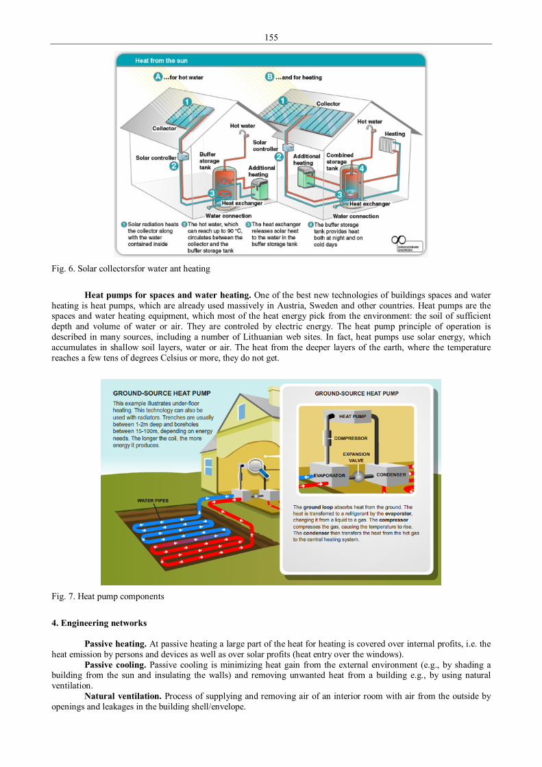
155

Fig. 6. Solar collectorsfor water ant heating

Heat pumps for spaces and water heating. One of the best new technologies of buildings spaces and water

heating is heat pumps, which are already used massively in Austria, Sweden and other countries. Heat pumps are the spaces and water heating equipment, which most of the heat energy pick from the environment: the soil of sufficient depth and volume of water or air. They are controled by electric energy. The heat pump principle of operation is described in many sources, including a number of Lithuanian web sites. In fact, heat pumps use solar energy, which accumulates in shallow soil layers, water or air. The heat from the deeper layers of the earth, where the temperature reaches a few tens of degrees Celsius or more, they do not get.

Fig. 7. Heat pump components

4. Engineering networks

Passive heating. At passive heating a large part of the heat for heating is covered over internal profits, i.e. the heat emission by persons and devices as well as over solar profits (heat entry over the windows).

Passive cooling. Passive cooling is minimizing heat gain from the external environment (e.g., by shading a building from the sun and insulating the walls) and removing unwanted heat from a building e.g., by using natural ventilation.

Natural ventilation. Process of supplying and removing air of an interior room with air from the outside by openings and leakages in the building shell/envelope.

156

There are two principles of natural ventilation: wind driven ventilation and stack ventilation. Stack ventilation is generated by a difference in the density of warm interior air and the cold air from outside. Both ventilation systems are depending on the weather and so they are uncontrollable, mostly too low or much too strong. Modern, energy efficient buildings are working with “controlled mechanical ventilation” (by fans) – the antonym for “natural ventilation”.

Controlled ventilation with heat recovery. Ventilation is a necessary procedure of replacing the used up interior air by air from outside. Through a duct – system, the air from outside is being drawn in by electrically propelled fans (direct current motors). It is filtered, and led to a heat transducer, optionally warmed up and then led into the individual areas (e.g. living room, sleep area, classroom, and work spaces). Used up air is drawn off in the kitchen, bath-room, toilets and led by the way of a second duct system to the heat transducer and blown outside. The amount of air needed per person amounts to approx. 20-30 m 3/h. A controlled ventilation system with heat recovery is necessary for all energy-efficient buildings. The efficiency for high-efficient heat recovery systems is over 90%.

Air tightness of buildings. Airtight building is a building in which no air can get in or out through any kind of leakage. The air tightness of a building is a useful knowledge when trying to increase energy efficiency. If the building envelope is not airtight enough, significant amounts of energy may be lost due to exfiltrating air, or damage to structural elements may occur due to condensation. To ensure the necessary air-change rates, it has to be ventilated manually (by opening the windows) or by an air ventilation system. 5. Examples

New building. Residential houses Mėta 2, 4, 5, 6 and 7 (Santariskiu str. 77, 79, 81, 83, 85, Vilnius): • Building energy efficiency class: B; • Total energy consumption 88.81 kWh/m2.

By building the residential houses “Mėta” was intended to compare the efficiency of different heating methods in the similar type buildings, customers‘attitude to the modern heating systems and their administration features. “Mėta” buildings 2, 4, 7 are equipped with “Viesmann” boilers with solar cells for prepairing hot water. Buildings 5 and 6 are equipped with “Siebel Eltron” geothermal heating system. Compared to the same building with central heating system “Mėta” houses with solar collectors the average bills for heating in 2012-2013 winter season were about 30% smaller, and with geothermal heating – around 45% smaller.

Fig. 8. Residential houses “Mėta”

Passive house. Social services building of full house community (Panaros str., Merkinė, Varėnos district):

• Building energy efficiency class: A+; • Total energy consumption: 34.58 kWh/m2; • Energy consumption for heating: 9.04 kWh/m2.

In the full house community social service building there are established living rooms, doctors‘offices, administrative and utility areas. The project was initiated and actively supported by the National Passive House Association which developes the passive house idea in Lithuania. This is the first building in Lithuania which was sertified by Passive House Institute in Darmstadt. While planning and building this house it was aimed to create a healthy premises microclimate. It was guaranteed by recuperator installed in the system. The geothermal system “Stiebel Eltron” was used for heating system. The solar collectors are used to prepare hot water.

157

Fig. 9. Social services building of full house community

Building after renovation. Hotel Dzūkija in Druskininkai (V.Kudirkos str. 45, Druskininkai):

• Building energy efficiency class: B; • Total energy consumption after renovation: 98.46 kWh/m2; • Total energy consumption before renovation: 300 kWh/m2.

In the center of the resort the hotel, surrounded by nature, suites it with interior as well. To ensure comfort for SPA guests and aiming to lower operating and maintenance costs there were implemented various innovative engineering and architectural solutions. TENKO Baltic installed a German manufacturer BEKA Heinz und Kühlmatten GmbH capillary tubes floor and ceiling heating and cooling system. Its warm can be compared with sun, campfire or stove heat. For this reason the temperature inside can be 2-3 °C lower without any influence to comfort, also in comparison with convective or air heating it allows to save around 12-18% of energy.

Fig. 10. Hotel Dzūkija in Druskininkai

Old house, which needs renovation. Apartment house (J. Tiškevičiaus g. 6, Vilnius):

• Building energy efficiency class: G; • Energy consumption for heating: 351.96 kWh/m2.

The house was built in 1963. Building and it`s partitions need insulation, change heating system, windows. Just insulation of the building could save up to 60% on heating costs.

Fig. 11. Apartment house (J. Tiškevičiaus g. 6, Vilnius)

158

050

100150200250300350400

Passivehouse

New building Renovatedbuilding

Beforerenovation

Old building

Chart 2. Heat consumption per year in vary buildings

Table 1

Energy consumption and heat losses

Building type Energy consumption for heating, kWh/m2

Energy consumption for hot water, kWh/m2

Heat losses through partitions, kWh/m2

Heat losses for ventilation, kWh/m2

Passive houses 34.58 0 10 5 New buildings 88.81 15 35 24

Renovated buildings 98.46 15 70 35 Old buildings 351.96 15 160 50

6. Conclusions 1. Prediction of energy – efficient building heating cost and comparison of the corresponding period of heating degree-

day number of the base temperature at 20 °C, is only qualitative and not applicable to engineering and economic calculations.

2. Dependence between the multi-annual home heating costs for heating and base temperature of vary degrees thermal performance of apartment houses and base temperature. Base temperature for buildings with heat consumption for heating and cooling is 40 kWh/m2 per year, to be considered +8 °C at a cost of 75 kWh / m 2 per year - +10 °C, and the energy- building that are not efficient with a heat input greater than 150 kWh / m2 per year, +20 °C.

3. Renovated old building consumes 3 times less energy than the same old building. 4. Lithuanian territory occupies 65 000 km2, the fact of the sun through the year we get 6.54 kWh × 1013 solar energy

per year. 5. Europe has about 80-85% flat solar panels, because they are cheaper. 6. Passive house consumes 2-3 times less energy than current buildings are constructed corresponding to the current

building regulations. References 1. Badescu V., Staicovici M. D. Renewable energy for passive house heating: Model of the active solar heating

system, 2006 -13 p. 2. Milutienė E. Efektyvaus energijos vartojimo pastatuose vadovas - Kaunas, 2008 -98 p. 3. Hassoun A., Dincer I. Development of power system designs for a net zero energy house, 2014 -10 p. 4. Directive on the energy performance of buildings (EPBD) 2002/91/EC. 5. Pastato energinis naudingumas. Terminų žodynas anglų ir lietuvių kalba. Access via internet: < http://www.intense-

energy.eu/uploads/tx_triedownloads/INTENSE_Glossary_EN-LT_final.pdf > [viewed 2014-03-15]. 6. Energijai neimlaus namo koncepcijos Šiaurės Europos šalyse. Access via internet:

< http://northpass.ivl.se/download/18.13f10919137472a032180009290/1350484455863/NorthPass_WP6_D16-Country-specific-information-packets-in+Lithuanian+(2).pdf > [viewed 2014-03-15].

159

Proceedings of 9th International Conference ITELMS’2014 The Optimization of the Overall Learning Dependent Manual Assembly Efficiency V. Kleiza*, J. Tilindis** *Kaunas University of Technology, S. Daukanto st. 12, 35212, Panevezys, Lithuania, E-mail: vytautas.kleiza@ktu.edu **Kaunas University of Technology, S. Daukanto st. 12, 35212, Panevezys, Lithuania, E-mail: justinas.tilindis@ktu.edu Abstract Optimization in the variety of fields of scope usually provides better results on the outcome. Optimization enables to reach higher levels with the same or even less effort. Operational efficiency maximization is one of the major targets of the production engineering, but the variety of factors (for instance learning) prevent from achieving this goal. This paper presents a mathematical optimization problem formulation of the overall equipment efficiency of the learning dependent manual assembly. The paper proposes method to integrate learning time into the overall equipment expression. Further investigation shows a possibility to minimize the time spent for learning, thus increasing time dedicated for the value-adding assembly and, finally, increasing overall equipment efficiency. KEYWORDS: efficiency, manual assembly, process optimization, operating time. 1. Introduction

To define production performance key performance indicators (KPI) are used. These indicators define major aspects of production performance including quality, operational performance, sickness, time waste, efficiency loses, production breakages and etc. Efficiency is based on variety of factors such as: • Customer demand fluctuations; • Order size; • Production organization; • Production planning and control; • Technology level; • Personnel motivation and etc.

Some of the factors come from outside and therefore cannot be affected, but other factors directly affect the efficiency. Since the group of various factors, parameters, properties, decisions and etc. define the overall efficiency, so obviously exist an optimal set of these parameters to reach the highest possible efficiency and in order to reach it, first of all the optimal set of parameters should be derived.

Current trends in manufacturing show decreasing production order quantities and increasing product variety [1, 2]. As a result, some companies produce enormous variety of different products and the customer demand is fluctuating and changing rapidly for each product and also the demand of particular products sharply differs from each other: from one piece per year, to several hundred per month. This leads to several types of manufacturing layouts: from assembly line to singular prototype production. What is more, these products constantly are changing. Each month from two to three hundred new different products are being introduced to production, thus replacing or supplementing current production set. In the automated assembly this increases setup time, but on manual assembly not only setup time is increased, but also increases the learning time for the operators to learn the manual task or operation. Learning effect is known for decades [3, 4] and initially was based for production improvement prediction, but current trends in manufacturing leads to application of learning curves (LC) for operation time prediction at the beginning of the production cycle [5]. Currently, many researchers focus on a variety of issues due to learning-forgetting effects. Several authors address planning improvement using learning curves.

Many researchers report benefit of the LC application in the production. Learning curve application based on limited production data was used for better allocation of labor resources [6]. Other study [7] reported the LC application to be an effective tool for the production planning and scheduling of work assignments. Rigorous research of the shoe manufacturing company [8, 9] gave results that learning curve application not only gains appropriate work balance but even leads to optimal production schedules. Some other authors [10, 11] addressed the production optimization by using learning models. Both works created analytical production planning algorithms with implemented LC and performed empirical calculation based on particular companies. Reported results confirmed, that impact of the learning effects increases as the order quantity decreases and number of operations increases. Also comparisons with traditional models showed, that LC based planning methods are adequate and realistic and provide more accurate results in the production planning and, finally, decrease the production costs.

Even many authors report the benefit of LC application still there is lack of research that directly connects time spent for learning with key performance indicators (i.e. efficiency). Often the learning time is inevitable, but also the learning time does not create value, but is rather waste of operating time [12] and it should be not only calculated but

160

also minimized for the production improvement. The idea of this paper is to incorporate the learning time into the general efficiency calculation technique and propose the possible optimization problem for the optimal parameter calculation which could be a background for the further production efficiency research an improvement via LC application. 2. Overall equipment efficiency

Overall equipment efficiency (OEE) is common LEAN to calculate the overall performance of the production system. Even it is dedicated for the equipment efficiency calculation it could be used for any production unit i.e. assembly line, job-shop, work cell and etc. This tool plays very important role in the production system, because it helps to identify the ratio, of how much time it is spent in order to produce value, which will be sold to the customer. The OEE could be calculated according to simple formula [12]:

eff eff effOEE A P Q= (1)

where Aeff is availability effectiveness; Peff – performance effectiveness; Qeff – quality effectiveness. Each component of OEE is calculated as follows:

eff OP PLA T T= (2)

where TOP – plant operating time; TPL – planned production time;

( )eff ICT OP OPP T T Q= (3)

where TICT – ideal cycle time of the operation; QOP – overall quantity produced during operating time;

( )eff OP D OPQ Q Q Q= − (4)

where QD – number of defective products produced during operating time. If we supplement (1) equation with the (2), (3) and (4) equation, the OEE equation gets form of

OP

DOP

OP

ICT

PL

OP

QQQ

TT

TTOEE −

××= (5)

Now, the major problem arises of learning factor introduction into the (5) equation. Some of the work is already done in the research [13] where learning time was included into the performance component as the ideal cycle time:

zD

z

OP

z

PL

OP

OP

OP

QQQ

TT

TTOEE

−××= (6)

where zT – ideal cycle time with included learning time. However, learning time appears to be waste and equation (6) cannot be used for the efficiency optimization, so

the formula will be improved. Obviously, learning reduces operator speed and there is the major reasons causing the reduced speed of the operation [12]: • Rough Running; • Under Nameplate Capacity; • Under Design Capacity; • Equipment Wear; • Operator Inefficiency.

If the operator has to learn the task, he/she loses the speed, loses the efficiency and reduces performance so the learning time should be included into the equation (5) as follows in form of the objective function:

( )OP

DOP

LAICT

ICT

PL

OPL Q

QQTTT

TTTTF −

×++

×= (7)

where TL – integrated learning time; TA – other time waste during total operating time. This time TA appears due to other factors such as rough running equipment wear, operator inefficiency and cannot be calculated in the analytical form. Also need to be emphasized operating time is:

LAICTOP TTTT ++= (8)

Further, the optimization problem is stated. However:

161

( )

=

ICTL TL

TL TFTF

,,minmax

βα (9)

Therefore, final optimization problem becomes find:

( )ICTL TT ,,min βα (10)

subject to

0,0,0 >>> ICTTβα (11)

where α and β – parameters of the learning curve ( ) αβ −= xxy . 3. Conclusions

Since the learning does not create a value, but only reduces the speed of the manual operation it should be not only calculated but minimized. To perform the minimization procedure, the learning time was introduced into the general overall equipment efficiency calculation formula as the constituting part of the performance component. Further modeling shows that efficiency can be maximized (optimized) while reducing (optimizing) learning time spent to learn the particular task. Therefore initial efficiency optimization problem turns into the learning time minimization problem and minimal learning time, will result the maximal overall efficiency. Further research should be addressed to the empirical calculations of the proposed optimization problem and further learning time reductions. References 1. Holweg M. The genealogy of LEAN production // Journal of Operational Management, 2006 Vol. 25(2), p. 420-

437. 2. Piller F. T. Mass Customization: Reflections on the State of the Concept // The International Journal of Flexible

Manufacturing Systems, 2004 Vol. 16, p. 313–334. 3. Wright T. P. Factors affecting the cost of airplanes // Journal of the Aeronautical Sciences, 1936 Vol. 3(4), p. 122-

128. 4. Yelle L. E. The learning curve: historical review and comprehensive survey // Decision Science, 1979 Vol. 10 (2),

p. 302-328. 5. Anzanello M. J., Fogliatto F. S. Learning curve models and applications: Literature review and research directions

// Int. Journal of Industrial Ergonomics International, 2011 Vol. 41, p. 573-583. 6. Smunt T. L, Watts C. A. Improving operations planning with learning curves: overcoming the pitfalls of ‘messy’

shop floor data // Journal of Operational Management, 2003 Vol. 21(1), p. 93-107. 7. Gabel T., Riedmiller M. Distributed policy search reinforcement learning for job-shop scheduling tasks // Int.

Journal of Production Research, 2012 Vol. 50(1), p. 41-61. 8. Anzanello M. J., Fogliatto F. S. Learning curve modelling of work assignment in mass customized assembly lines

// Int. Journal of Production Research, 2007 Vol. 45(13), p. 2919-2938. 9. Anzanello M. J., Fogliatto F. S. Scheduling learning dependent jobs in customised assembly lines // Int. Journal of

Production Research, 2010 Vol. 48(22), p. 6683-6699. 10. Cohen Y., Vitner G., Sarin S. C. Optimal allocation of work in assembly lines for lots with homogenous learning //

European Journal of Operational Research, 2006 Vol. 168(3), p. 922-931. 11. Neidigh R. O., Harrison T. P. Optimising lot sizing and order scheduling with non-linear production rates // Int.

Journal of Production Research, 2010 Vol. 48(8), p. 2279-2295. 12. Vorne Industries. The Fast Guide to OEE. Visual Factory and Production Monitoring Systems, information on:

< http://www.vorne.com/pdf/fast-guide-to-oee.pdf >. 13. Tilindis J., Kleiza V. Mathematical Modeling of Production Operations and Processes for Product Design and

Manufacturing // Applied Mechanics and Materials, 2014 Vol. 510, p. 243-247.

162

Proceedings of 9th International Conference ITELMS’2014 Composite Rods Reinforced Concrete Structures K. Klimavicius*, S. Susinskas** *KTU Panevezys faculty of Technology and Business, S. Daukanto str. 12, 35212, Panevezys, Lithuania, E-mail: karolis.klimavicius@ktu.lt **KTU Panevezys faculty of Technology and Business, S. Daukanto str. 12, 35212, Panevezys, Lithuania, E-mail: saulius.susinskas@ktu.lt Abstract Increasingly, the use of composite materials in construction driven by several key aspects: the material corrosion resistance, excellent mechanical properties and easy processing. To reduce composite products price is improving manufacturing technology. Therefore, the current polymeric materials have become common traditional building materials: steel, wood, concrete – alternative. Building construction in the field of composite materials is generally used for: 1) rods as reinforcement concrete structures; 2) the outer leaf fixtures operated by strengthening structures; 3) as building profiles. New materials in the actual construction of buildings are inevitably linked with some risk. While the world has gained a significant composite rod reinforced structures design, construction and operation experience, but due to the high composite reinforcement diversity and specific mechanical properties of the composite beams reinforced structures design remains quite a challenge. KEYWORDS: composite rods, composite products, reinforced concrete, reinforced structures. 1. Introduction

Worldwide decline of natural resources in all industries performed innovative and the searches for optimal solutions to these resources are used more efficiently. Construction industry focuses on innovative design solutions, in order to ensure a higher structures safety, reliability and durability.

Composite materials used in the construction industry started relatively recently. Composite fiber reinforced polymers first begin to use the military, aerospace and automotive industries. In recent decades, they are increasingly being used for building new and strengthening for existing buildings and their structures. Composites and steel rods comparable densities are shown in Table 1.

Table 1 Composite rods densities of fiber volume fraction 3mkg75.05.0 −=fiV

Fiber Matrix Carbon fiber Aramid fiber Fiberglass Steel

Polyester resin 1430 – 1650 1310 – 1430 1750 – 2170 7850 Epoxy resin 1440 – 1670 1320 – 1450 1760 – 2180

Vinyl ester resin 1440 – 1630 1300 – 1410 1730 - 2150

Table above shows that the composite reinforcement is 4-6 times lighter than steel, so that polymer rod density is much lower. For this properties of composite reinforcement easier to transport and use on the construction site. Also it is suitable for optimizing the design and reducing mass. 1. Testing procedure for Fiber-Reinforced Polymers (FRPs) for reinforcing or strengthening concrete structures is

described in the American standard ACI 440.3R-04 [1]. In the majority of tests compact specimens are applied for tension or compression.

2. Composite reinforcement properties and interactions with concrete in details are described in [2, 3]. Reinforced concrete structures commonly used for tensile composite reinforcement stress – strain diagram is

shown in Fig. 1. The same figure shows that the strength of steel reinforcement up to 7 times lower than the composite, however, limit the deformation of the decay time higher. And the valve is different behavior in tension. Reinforced concrete structures used steel rods have a clear plastic stage. Under the influence of tensile stresses are elastically deformed to yield (plain steel) or the relative yield strength (strong steel) and then break down plastic. Composite rods to the disintegration deform elastically and degrade the fragile (Fig. 2). As mentioned above, the steel plasticity is an important determinant of plastic conventional reinforced concrete elements decay nature at the ultimate limit state. Fragile composite reinforcement decomposition – one of its biggest flaws, causing sudden stairways and reinforced polymer bars concrete elements of disintegration.

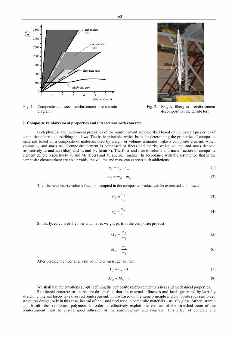
163

Fig. 1. Composite and steel reinforcement stress-strain

diagram Fig. 2. Fragile fiberglass reinforcement

decomposition the tensile test

2. Composite reinforcement properties and interactions with concrete

Both physical and mechanical properties of the reinforcement are described based on the overall properties of composite materials describing the laws. The basic principle, which basis for determining the properties of composite materials based on a composite of materials used by weight or volume estimates. Take a composite element, which volume vc and mass mc . Composite element is composed of fibers and matrix, which volume and mass denoted respectively vfi and mfi (fiber) and vm and mm (matrix). The fiber and matrix volume and mass fraction of composite element denote respectively Vfi and Mfi (fiber) and Vm and Mm (matrix). In accordance with the assumption that in the composite element there are no air voids, the volume and mass can express such addictions:

mfif vvv += (1)

mfif mmm += (2)

The fiber and matrix volume fraction occupied in the composite product can be expressed as follows:

f

fifi v

vV = (3)

f

mm v

vV = (4)

Similarly, calculated the fiber and matrix weight parts in the composite product:

f

fifi m

mM = (5)

f

mm m

mM = (6)

After placing the fiber and resin volume or mass, get an item:

1=+ mfi VV (7)

1=+ mfi MM (8)

We shall use the equations (1)-(8) defining the composite reinforcement physical and mechanical properties. Reinforced concrete structures are designed so that the external influences and loads generated by laterally

stretching internal forces take over rod reinforcement. In this based on the same principle and composite rods reinforced structures design, only in this case, instead of the usual steel used in composite materials – usually glass, carbon, aramid and basalt fiber reinforced polymers. In order to effectively exploit the element of the stretched zone of the reinforcement must be ensure good adhesion of the reinforcement and concrete. This effect of concrete and

164

reinforcement contact surface place takes stress transfer. Joints between sections and cracks can be seen in the reverse process – loaded transmit tensile reinforcement stresses in concrete. In both cases, the stress transfer from concrete reinforcement (and vice versa) is one of the most important feature of reinforced concrete structures , from which compliance depends on both the strength (anchorage area, splices) and eligibility (elements of deflections, cracking) limit state requirements.

Fig. 3. Reinforcement and concrete bonding concept

Bonding called reinforcement and concrete interaction phenomena which the resulting concrete reinforcement

stresses transmitted, and vice versa. Bonding quality is determined by the important design characteristics as reinforcement anchoring splices length, slit width, the distance between the slits and the general structural deformation. Bonding phenomenon can be observed clearly by removing the reinforcement in concrete array, as shown in Figure 3. From the array of concrete pulled the reinforcement rod whose diameter is φ , and anchor length – l. 3. Conclusions

The composite reinforced concrete structures advantages occur only through two different mechanical and physical properties with materials – concrete and reinforcement – bonding. In the tensile zone of concrete effectively transmit stresses reinforcement; it is necessary to ensure a reliable these substances bonding, which is defined as the average force per contact of concrete and steel surface area of the unit. Analysis of concrete and reinforcement bonding mechanic can three main interaction components: 1. Chemical bonding or adhesion. When reinforcement rod is in concrete, adhesion occurs between the cement matrix

and the reinforcement surface. In construction this is not a reliable adhesion component, because chemical bonding is destroyed in the case of very small values of the scroll.

2. The friction force begins to act after the break chemical bonds between reinforcement and concrete. The bond component is running until the reinforcement rod completely removed or decomposes. The friction force depends on the surface of the reinforcement roughness and the lateral pressure of the concrete.

3. Mechanical anchoring is formed between reinforcement wales and concrete. It is the effective of bonding component. When reinforcement ribbed, adhesion plays about 10%; of friction forces – 15-20%; machinable anchorage – 70-75% all the bonding force.

References 1. ACI 440.3R-04 Guide Test Methods for Fiber-Reinforced Polymers (FRPs) for Reinforcing or Strengthening

Concrete Structures. 2004. Michigan: American Concrete Institute. 40 p. ISBN 9780870311628. 2. LST EN 1992-1-1:2005. Eurokodas 2. Gelžbetoninių konstrukcijų projektavimas. 1-1 dalis. Bendrosios ir pastatų

taisyklės. (Eurocode 2: Design of concrete structures - Part 1-1: General rules and rules for buildings). – Vilnius, 2007. 232 p.

3. Kaklauskas G. D. ir kt. Vadovėlis. Kompozitais armuotos betoninės konstrukcijos. (Composites reinforced concrete structures). – Vilnius: Technika, 2012. 298 p.

165

Proceedings of 9th International Conference ITELMS’2014 Problem of Kinematic Discrepancy in Hydrostatic Drive Systems Used in Unmanned Ground Vehicles S. Konopka*, M. J. Lopatka**, T. Muszynski***, M. Przybysz**** *Military Univercity of Technology, Kaliskiego 2, 00-908 Warsaw, Poland, skonopka@wat.edu.pl **Military Univercity of Technology, Kaliskiego 2, 00-908 Warsaw, Poland, mlopatka@wat.edu.pl ***Military Univercity of Technology, Kaliskiego 2, 00-908 Warsaw, Poland, tmuszynski@wat.edu.pl ****Military Univercity of Technology, Kaliskiego 2, 00-908 Warsaw, Poland, mprzybysz@wat.edu.pl Abstract In this paper the problem of kinematic discrepancy of hydrostatic drive systems in high mobility vehicles and its influence on occurrence of disadvantageous effect of circulating power was presented. Moreover, the results of research concerning kinematic discrepancy of hydrostatic drive system carried out on a physical object were described and an analysis of the ability of kinematic discrepancy compensation was presented. KEYWORDS: kinematic discrepancy, unmanned ground vehicles, hydrostatic drive system. 1. Introduction

Tasks given for unmanned ground vehicles while rescue actions and military mission realisation entail high requirements in their mobility and manoeuvres. These requirements include, inter alia, their ability to move on significant terrain inequalities(20-30 cm), hills with 40% angle (22%), sites with low deadweight CI = 150 kPa, overcoming typical terrain obstacles such as; debris landfills, logs, ditches [1, 2]. One of the main systems in vehicles having basic influence on whether the vehicle will match given requirements is drive system. Taking into consideration unmanned ground vehicles specific area of movement and accessible solutions it can be said that above requirements are possible to match with using hydrostatic drive system [3-9]. Main advantages are in continuously variable regulation of movement speed and ability of achieving crawl speed required while overcoming obstacles and precise manoeuvring. Furthermore hydrostatic drive systems allow reaching high driving force values and secures drive system from overloads. Applying discussed system gives also ability to elastic positioning of hydraulic components on the vehicle which is highly recommended for possibility to ensure high jump of wheels suspension in vehicle which enhances ability to overcome the terrain obstacles [10]. Described advantages cause that hydrostatic drive systems are commonly used in work machines and vehicles with higher standards about drive systems.

Movement of the vehicle in difficult terrain and terrain inequalities requires from drive system reaching effective drive force in every wheel which is achieved, in these kinds of vehicles, by individual propulsion on every wheel regardless of load. One of the solutions for achieving this effect in hydrostatic drive systems is applying flow dividers which guarantees same performance for every hydraulic engines. It secures system from loss of driving force caused by reduced ground traction or loss of contact with ground in any wheel. 2. Kinematic discrepancy in drive systems

Driving the unmanned wheeled land vehicles through big terrain inequalities or with various dynamic driving wheels radius values, which can be caused by unequal burden of them or different pressure in tires (Fig. 1). Causes that wheels should rotate with different speed according to pattern:

di

kii r

v=ω (1)

where ωi – rotational speed of particular wheels; vki – progressive speeds of drive wheels axis; rdi – dynamic radius of drive wheels.

This phenomenon is called kinematic discrepancy and it is characterised by kinematic discrepancy degree. Kinematic discrepancy degree Δ of the system is caused by Rotational wheel speed ratio ω', ω'' (moving without skidding), to rotational speed of wheel which is rotating with higher speed, taken into consideration in exact moment of time [11-14]:

( )ωωωω

∆′′′

′′−′=

,max (2)

where ω' and ω'' – rotational speeds of discussed vehicle wheels.

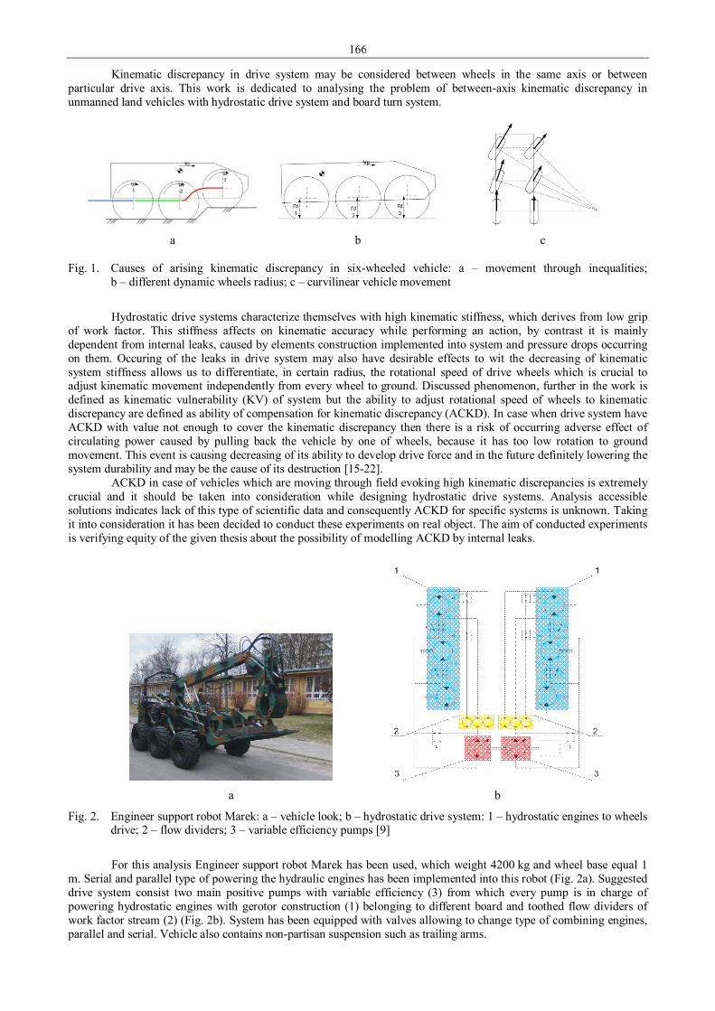
166

Kinematic discrepancy in drive system may be considered between wheels in the same axis or between particular drive axis. This work is dedicated to analysing the problem of between-axis kinematic discrepancy in unmanned land vehicles with hydrostatic drive system and board turn system.

a

b

c

Fig. 1. Causes of arising kinematic discrepancy in six-wheeled vehicle: a – movement through inequalities; b – different dynamic wheels radius; c – curvilinear vehicle movement

Hydrostatic drive systems characterize themselves with high kinematic stiffness, which derives from low grip

of work factor. This stiffness affects on kinematic accuracy while performing an action, by contrast it is mainly dependent from internal leaks, caused by elements construction implemented into system and pressure drops occurring on them. Occuring of the leaks in drive system may also have desirable effects to wit the decreasing of kinematic system stiffness allows us to differentiate, in certain radius, the rotational speed of drive wheels which is crucial to adjust kinematic movement independently from every wheel to ground. Discussed phenomenon, further in the work is defined as kinematic vulnerability (KV) of system but the ability to adjust rotational speed of wheels to kinematic discrepancy are defined as ability of compensation for kinematic discrepancy (ACKD). In case when drive system have ACKD with value not enough to cover the kinematic discrepancy then there is a risk of occurring adverse effect of circulating power caused by pulling back the vehicle by one of wheels, because it has too low rotation to ground movement. This event is causing decreasing of its ability to develop drive force and in the future definitely lowering the system durability and may be the cause of its destruction [15-22].

ACKD in case of vehicles which are moving through field evoking high kinematic discrepancies is extremely crucial and it should be taken into consideration while designing hydrostatic drive systems. Analysis accessible solutions indicates lack of this type of scientific data and consequently ACKD for specific systems is unknown. Taking it into consideration it has been decided to conduct these experiments on real object. The aim of conducted experiments is verifying equity of the given thesis about the possibility of modelling ACKD by internal leaks.

a

b

Fig. 2. Engineer support robot Marek: a – vehicle look; b – hydrostatic drive system: 1 – hydrostatic engines to wheels drive; 2 – flow dividers; 3 – variable efficiency pumps [9]

For this analysis Engineer support robot Marek has been used, which weight 4200 kg and wheel base equal 1

m. Serial and parallel type of powering the hydraulic engines has been implemented into this robot (Fig. 2a). Suggested drive system consist two main positive pumps with variable efficiency (3) from which every pump is in charge of powering hydrostatic engines with gerotor construction (1) belonging to different board and toothed flow dividers of work factor stream (2) (Fig. 2b). System has been equipped with valves allowing to change type of combining engines, parallel and serial. Vehicle also contains non-partisan suspension such as trailing arms.

167

3. Research methods 3.1. Measuring track

Capability research about ACKD consisted performing a run by vehicle trough selected obstacles forward and backward. While deciding which obstacles should be at the field, it has been decided to recreate actual conditions which would be in real terrain where unmanned land vehicles had to overcome and simultaneously causing high values of kinematic discrepancy. To this end, in department of construction machinery MTA (Military Technical Academy) research track has been constructed which contained following obstacles: ditch, earth shaft and hillside.

Research of kinematic discrepancy of drive system occurring when overcoming road ditches will be performed on specially prepared excavation with length of 5 m, asymmetrical height of edges equal 70 and 50 cm, width of the bottom equal 40 cm and slopes with inclinations equal 50% (Fig. 3).

Fig. 3. Transverse section of ditch

Research of kinematic discrepancy of drive system occurring while overcoming the embankment was defined

by overcoming the earth shaft with section shown on Fig. 4b and height equal 80 cm – it has been made without condensation.

a

b

Fig. 4. Embankment: a – demonstrative picture; b – embankment profile

Research of the kinematic discrepancy of drive system occurring while overcoming a hillside with inclinations

equal 18° with elevation length and height (Fig. 5), which has been made without condensation.

Fig. 5. Transverse section of hillside with inclinations equal 18°

To decrease measurement mistake and to record distinct repetition of measurement every manoeuvre has been

repeated five times. While overcoming the obstacle maintained run speed equal circa 0.5 m/s. Research has been conducted for parallel configuration of powering hydraulic engines with usage of flow dividers.

While research values which were recorded were rotational speed of drive wheels belonging to one board and pressure on particular hydraulic engines’ powering lines for drive these wheels. In this way it has been possible to record differencing pressure drops in hydraulic engines and results of different wheels’ rotational speeds.

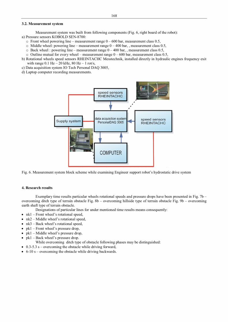
168

3.2. Measurement system

Measurement system was built from following components (Fig. 6, right board of the robot): a) Pressure sensors KOBOLD SEN-8700: o Front wheel powering line – measurement range 0 – 600 bar, measurement class 0.5, o Middle wheel: powering line – measurement range 0 – 400 bar, , measurement class 0.5, o Back wheel : powering line – measurement range 0 – 400 bar, , measurement class 0.5, o Outline mutual for every wheel – measurement range 0 – 600 bar, measurement class 0.5,

b) Rotational wheels speed sensors RHEINTACHC Messtechnik, installed directly in hydraulic engines frequency exit with range 0.1 Hz – 20 kHz, 80 Hz – 1 rot/s,

c) Data acquisition system IO Tech Personal DAQ 3005, d) Laptop computer recording measurements.

Fig. 6. Measurement system block scheme while examining Engineer support robot’s hydrostatic drive system

4. Research results

Exemplary time results particular wheels rotational speeds and pressure drops have been presented in Fig. 7b – overcoming ditch type of terrain obstacle Fig. 8b – overcoming hillside type of terrain obstacle Fig. 9b – overcoming earth shaft type of terrain obstacle.

Designations of particular lines for under mentioned time results means consequently: • nk1 – Front wheel’s rotational speed, • nk2 – Middle wheel’s rotational speed, • nk3 – Back wheel’s rotational speed, • pk1 – Front wheel’s pressure drop, • pk1 – Middle wheel’s pressure drop, • pk1 – Back wheel’s pressure drop.

While overcoming ditch type of obstacle following phases may be distinguished: • 0.3-5.3 s – overcoming the obstacle while driving forward, • 6-10 s – overcoming the obstacle while driving backwards.

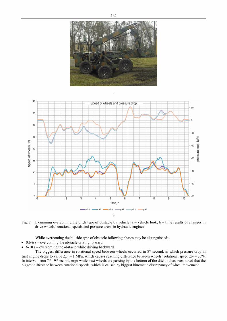
169

a

b

Fig. 7. Examining overcoming the ditch type of obstacle by vehicle: a – vehicle look; b – time results of changes in drive wheels’ rotational speeds and pressure drops in hydraulic engines

While overcoming the hillside type of obstacle following phases may be distinguished:

• 0.6-6 s – overcoming the obstacle driving forward, • 6-10 s – overcoming the obstacle while driving backward.

The biggest difference in rotational speed between wheels occurred in 8th second, in which pressure drop in first engine drops to value ∆p1 = 1 MPa, which causes reaching difference between wheels’ rotational speed ∆n = 35%. In interval from 7th - 9th second, ergo while next wheels are passing by the bottom of the ditch, it has been noted that the biggest difference between rotational speeds, which is caused by biggest kinematic discrepancy of wheel movement.

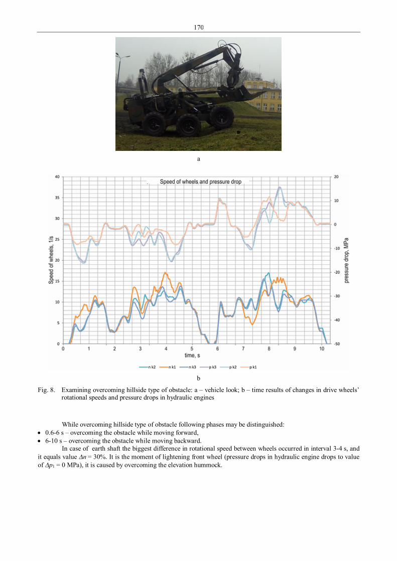
170

a

b

Fig. 8. Examining overcoming hillside type of obstacle: a – vehicle look; b – time results of changes in drive wheels’ rotational speeds and pressure drops in hydraulic engines

While overcoming hillside type of obstacle following phases may be distinguished: • 0.6-6 s – overcoming the obstacle while moving forward, • 6-10 s – overcoming the obstacle while moving backward.

In case of earth shaft the biggest difference in rotational speed between wheels occurred in interval 3-4 s, and it equals value ∆n = 30%. It is the moment of lightening front wheel (pressure drops in hydraulic engine drops to value of ∆p1 = 0 MPa), it is caused by overcoming the elevation hummock.

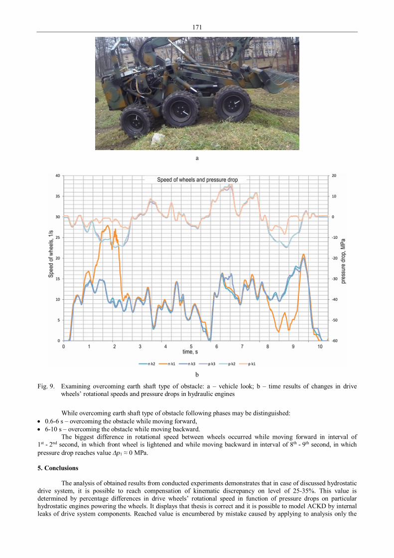
171

a

b

Fig. 9. Examining overcoming earth shaft type of obstacle: a – vehicle look; b – time results of changes in drive wheels’ rotational speeds and pressure drops in hydraulic engines

While overcoming earth shaft type of obstacle following phases may be distinguished:

• 0.6-6 s – overcoming the obstacle while moving forward, • 6-10 s – overcoming the obstacle while moving backward.

The biggest difference in rotational speed between wheels occurred while moving forward in interval of 1st - 2nd second, in which front wheel is lightened and while moving backward in interval of 8th - 9th second, in which pressure drop reaches value ∆p1 ≈ 0 MPa. 5. Conclusions

The analysis of obtained results from conducted experiments demonstrates that in case of discussed hydrostatic drive system, it is possible to reach compensation of kinematic discrepancy on level of 25-35%. This value is determined by percentage differences in drive wheels’ rotational speed in function of pressure drops on particular hydrostatic engines powering the wheels. It displays that thesis is correct and it is possible to model ACKD by internal leaks of drive system components. Reached value is encumbered by mistake caused by applying to analysis only the

172

values of drive wheels’ rotational speeds and pressure drops in hydraulic engines. To enhance the accuracy of the conducted experiment’s results in further stages of this study it is recommended additionally hydraulic cord’s stiffness, because this have great influence on received results character, what in presented runs is visible in form of oscillation. To enhance the accuracy of the experiment’s results it is necessary to extend measurement system with additional flow sensors, which will allow to record efficiency values delivered to every hydraulic engine, and consequently referring this value to wheels’ rotational speeds. It will allow obtaining data about real volumetric loss value in hydraulic engines and flowing divider. References 1. Sprawka P. The methods of evaluation the mobility of off - road vehicles. Solid State Phenomena Vol. 180, Trans

Tech Publications, Switzerland 2011. 2. Łopatka M. J. Praca zbiorowa, Inżynieryjny Robot Wsparcia IOD/EOD – usuwania ładunków niebezpiecznych,

Sprawozdanie z projektu rozwojowego Nr OR00001205/PBR, Warszawa 2011. 3. Bartnicki A., Łopatka J., Muszyński T. Szacowanie oporów skrętu burtowego wieloosiowych platform kołowych,

Logitrans 2010. 4. Budny E. Napęd i sterowanie układów hydraulicznych w maszynach roboczych. ITE, Radom 2001. 5. Bartnicki A., Sprawka P. Zastosowanie hydrostatycznych układów napędowych we współczesnych maszynach i

pojazdach lądowych. LOGITRANS, Szczyrk 2008. 6. Comellas M., Pijuan J., Potau X., Nogue´s M., Roca J. Active bogies, chassis levelling and transmission

efficiency for avehicle operating in rough terrain. Journal of KONES Powertrain and Transport, nr 4. 2007. 7. Comellas M., Pijuan J., Potau X., Nogue´s M., Roca J. Analysis of a hydrostatic transmission driveline for its use

in off-road multiple axle vehicles. Journal of Terramechanics, nr 49. 2012. 8. Stryczek S. Napęd hydrostatyczny. Tom I. Wydawnictwa Naukowo - Techniczne, Warszawa 2005. 9. Bartnicki A., Muszyński T. Koncepcja układu napędowego dla bezzałogowej platformy lądowej o skręcie

burtowym. Międzynarodowa Konferencja Naukowo-Techniczna Napędy i Sterowania Hydrauliczne i Pneumatyczne. Wroclaw 2010.

10. Łopatka M. J., Muszyński T., Rubiec A. Load Analysis of skid steer drive systems, 18th International Conference of Methods and Models in Automation and Robotics MMAR 2013.

11. Studziński K. Teoria I sterowanie. Samochód. WKŁ, Warszawa 1980. 12. Konopka S., Łopatka M. J., Przybysz M. Kinematic Discrepancy of Hydrostatic Drive of Unmanned Ground

Vehicle, ITELMS ‘2013, May 23-24, 2013, Panevėžys, Lithuania. 13. Wong J. Y. Theory of ground vehicle, ISBN: 978-0-470-17038-0, August 2008. 14. Konopka S., Sprawka P., Muszyński T., Spadło K. Investigating resistance of turn six-wheel skid-steer vehicle,

ITELMS ‘2013, Panevėžys, Lithuania, May 23-24, 2013. 15. Li X., Yin X., Zhang Y., Yuan S. Turning resistance coefficient model for skid-steer wheeled vehicles, Automotive

Engineering 2012. 16. Mi H., Yuan H., Wang Q., Zhao J. Algorithm Research and Realization of the Turning Control System for Heavy

Transportation Vehicle, Chinese journal of mechanical engineering, Vol. 25, No. 3, 2012. 17. Cao F., Zhou Z. Y., Xu L. Y., Zhang M. Study on Hydro-mechanical Differential Dynamic Turning Process of

Tracked Vehicle, Second International Conference on Intelligent Computation Technology and Automation 2009. 18. Haggag S., Alstrom D., Cetinkunt S., Egelja A. Modeling, Control, and Validation of an Electro-Hydraulic Steer-

by-Wire System for Articulated Vehicle Applications, IEEE/ASME TRANSACTIONS ON MECHATRONICS, VOL. 10, NO. 6, DECEMBER 2005.

19. Łopatka M. J. Influence of Power Steering System of Directional Stability of Articulated Wheel Loader, ITELMS ‘2013, Panevėžys, Lithuania, May 23-24, 2013.

20. Bartnicki A., Dąbrowska A., Łopatka M. J., Muszyński T. Experimental Research on Directional stability of articulated Tractors, XIV Konferencja automatyzacji i Eksploatacji systemów Sterowania i Łączności ASMOR 2013, Jastrzębia Góra 2013.

21. Bartnicki A., Łopatka M. J., Muszyński T., Jaskółowski M. The Researches of Stability Evaluation Articulated Loader while Working on Slopes, ITELMS ‘2013, Panevėžys, Lithuania, May 23-24, 2013.

22. Konopka S., Krogul P., Łopatka M. J. Simulation Research of Hydrostatic Power System Control of Engineer Robot Manipulator, ITELMS ‘2013, Panevėžys, Lithuania, May 23-24, 2013.

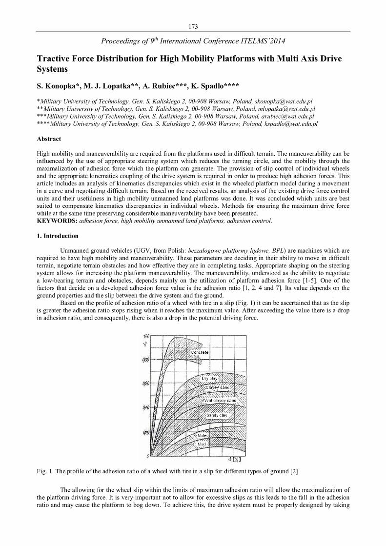
173

Proceedings of 9th International Conference ITELMS’2014 Tractive Force Distribution for High Mobility Platforms with Multi Axis Drive Systems S. Konopka*, M. J. Lopatka**, A. Rubiec***, K. Spadlo**** *Military University of Technology, Gen. S. Kaliskiego 2, 00-908 Warsaw, Poland, skonopka@wat.edu.pl **Military University of Technology, Gen. S. Kaliskiego 2, 00-908 Warsaw, Poland, mlopatka@wat.edu.pl ***Military University of Technology, Gen. S. Kaliskiego 2, 00-908 Warsaw, Poland, arubiec@wat.edu.pl ****Military University of Technology, Gen. S. Kaliskiego 2, 00-908 Warsaw, Poland, kspadlo@wat.edu.pl Abstract High mobility and maneuverability are required from the platforms used in difficult terrain. The maneuverability can be influenced by the use of appropriate steering system which reduces the turning circle, and the mobility through the maximalization of adhesion force which the platform can generate. The provision of slip control of individual wheels and the appropriate kinematics coupling of the drive system is required in order to produce high adhesion forces. This article includes an analysis of kinematics discrepancies which exist in the wheeled platform model during a movement in a curve and negotiating difficult terrain. Based on the received results, an analysis of the existing drive force control units and their usefulness in high mobility unmanned land platforms was done. It was concluded which units are best suited to compensate kinematics discrepancies in individual wheels. Methods for ensuring the maximum drive force while at the same time preserving considerable maneuverability have been presented. KEYWORDS: adhesion force, high mobility unmanned land platforms, adhesion control. 1. Introduction

Unmanned ground vehicles (UGV, from Polish: bezzałogowe platformy lądowe, BPL) are machines which are required to have high mobility and maneuverability. These parameters are deciding in their ability to move in difficult terrain, negotiate terrain obstacles and how effective they are in completing tasks. Appropriate shaping on the steering system allows for increasing the platform maneuverability. The maneuverability, understood as the ability to negotiate a low-bearing terrain and obstacles, depends mainly on the utilization of platform adhesion force [1-5]. One of the factors that decide on a developed adhesion force value is the adhesion ratio [1, 2, 4 and 7]. Its value depends on the ground properties and the slip between the drive system and the ground.

Based on the profile of adhesion ratio of a wheel with tire in a slip (Fig. 1) it can be ascertained that as the slip is greater the adhesion ratio stops rising when it reaches the maximum value. After exceeding the value there is a drop in adhesion ratio, and consequently, there is also a drop in the potential driving force.

Fig. 1. The profile of the adhesion ratio of a wheel with tire in a slip for different types of ground [2]

The allowing for the wheel slip within the limits of maximum adhesion ratio will allow the maximalization of

the platform driving force. It is very important not to allow for excessive slips as this leads to the fall in the adhesion ratio and may cause the platform to bog down. To achieve this, the drive system must be properly designed by taking

174

into the account the desired kinematics discrepancy which stems from the function of the steering system [1, 2, 4, 6, 7 and 8] and is created during the negotiation of terrain obstacles.

Based on the literature analysis it was determined, that the steering system which maneuverability is the greatest is the side steering system [1, 2, 3, 4, 7 and 8]. In the side steering system the turn is done by differentiating the speed of individual sides of the vehicle. An extreme case may be doing the turn maneuver when the turn radius is zero, and in which wheels on both sides of the platform are moving in the opposite directions. This system is widely used in UGVs and for this reason it was chosen as the representative system for further analysis. 2. Defining kinematics discrepancies during the movement of the platform

For the purpose of evaluating of the desired kinematics discrepancy appearing in steering system, a simulation test of the movement of a 6x6 wheeled platform. Its simulation model was created using the MSC Adams software (Fig. 2b). On the basis of the performed analysis the values of kinematics discrepancy appearing during the turn maneuver and negotiating obstacles were determined.

Because of the requirements faced by the UGV and dimensions, for the purposes of the simulation tests the ability of moving along the curve of radius of R = 5 m and R = 1 m and the ability for negotiating terrain obstacles: a log and vertical wall were adopted as its representative characteristics. The aim of the test was to ascertain the rotation rate of individual wheels in a dependence of the terrain upon which the platform is maneuvering.

a

b

Fig. 2. Platform model: a – geometrical dimensions; b – generated model in the MSC Adams software. Where: 1 – model of the wheel; 2 – suspension elements; 3 – the center of mass of the vehicle

a

a

Fig. 3. Model of the wheel: a – physical model; b – model made in the MSC Adams software. Where: rsw – uninhibited radius of the wheel; rd – dynamic radius of the the wheel; Q – the wheel load

In the constructed model the type of the drive system was not taken into the account and it was assumed, that

each of the individual wheels can spin without going into a slip. The platform speed was applied in the center of its mass. In the model, the following assumptions were made: • the surface is non-deformable, • all of the sprung mass is centered in its geometrical center, • the un-sprung mass was assumed to consist of cylinders in the center of the wheels, • the platform is moving at the speed of 0.6 m/s, • during the negotiation of obstacles and the movement in a curve, the linear velocity of the center of the platform is

maintained,

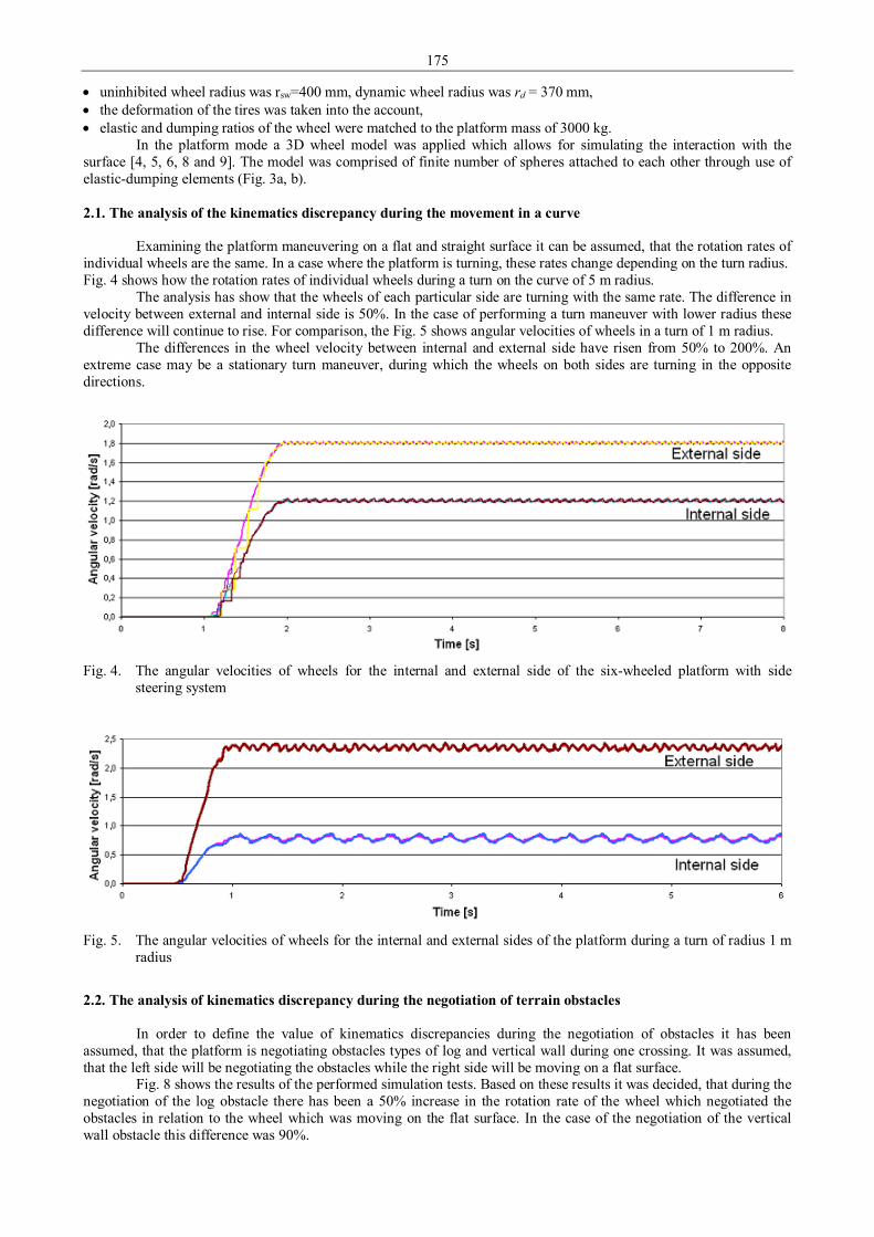
175

• uninhibited wheel radius was rsw=400 mm, dynamic wheel radius was rd = 370 mm, • the deformation of the tires was taken into the account, • elastic and dumping ratios of the wheel were matched to the platform mass of 3000 kg.

In the platform mode a 3D wheel model was applied which allows for simulating the interaction with the surface [4, 5, 6, 8 and 9]. The model was comprised of finite number of spheres attached to each other through use of elastic-dumping elements (Fig. 3a, b). 2.1. The analysis of the kinematics discrepancy during the movement in a curve

Examining the platform maneuvering on a flat and straight surface it can be assumed, that the rotation rates of individual wheels are the same. In a case where the platform is turning, these rates change depending on the turn radius. Fig. 4 shows how the rotation rates of individual wheels during a turn on the curve of 5 m radius.

The analysis has show that the wheels of each particular side are turning with the same rate. The difference in velocity between external and internal side is 50%. In the case of performing a turn maneuver with lower radius these difference will continue to rise. For comparison, the Fig. 5 shows angular velocities of wheels in a turn of 1 m radius.

The differences in the wheel velocity between internal and external side have risen from 50% to 200%. An extreme case may be a stationary turn maneuver, during which the wheels on both sides are turning in the opposite directions.

Fig. 4. The angular velocities of wheels for the internal and external side of the six-wheeled platform with side

steering system

Fig. 5. The angular velocities of wheels for the internal and external sides of the platform during a turn of radius 1 m

radius

2.2. The analysis of kinematics discrepancy during the negotiation of terrain obstacles

In order to define the value of kinematics discrepancies during the negotiation of obstacles it has been assumed, that the platform is negotiating obstacles types of log and vertical wall during one crossing. It was assumed, that the left side will be negotiating the obstacles while the right side will be moving on a flat surface.

Fig. 8 shows the results of the performed simulation tests. Based on these results it was decided, that during the negotiation of the log obstacle there has been a 50% increase in the rotation rate of the wheel which negotiated the obstacles in relation to the wheel which was moving on the flat surface. In the case of the negotiation of the vertical wall obstacle this difference was 90%.

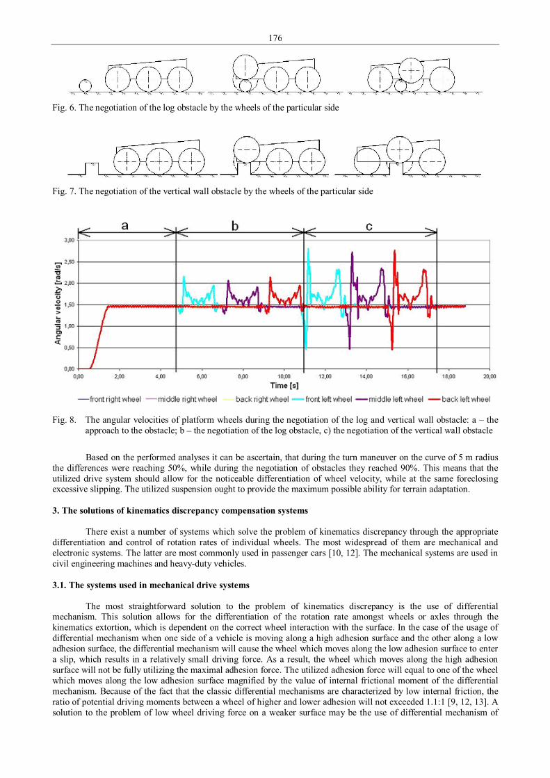
176

Fig. 6. The negotiation of the log obstacle by the wheels of the particular side

Fig. 7. The negotiation of the vertical wall obstacle by the wheels of the particular side

Fig. 8. The angular velocities of platform wheels during the negotiation of the log and vertical wall obstacle: a – the

approach to the obstacle; b – the negotiation of the log obstacle, c) the negotiation of the vertical wall obstacle

Based on the performed analyses it can be ascertain, that during the turn maneuver on the curve of 5 m radius

the differences were reaching 50%, while during the negotiation of obstacles they reached 90%. This means that the utilized drive system should allow for the noticeable differentiation of wheel velocity, while at the same foreclosing excessive slipping. The utilized suspension ought to provide the maximum possible ability for terrain adaptation. 3. The solutions of kinematics discrepancy compensation systems

There exist a number of systems which solve the problem of kinematics discrepancy through the appropriate differentiation and control of rotation rates of individual wheels. The most widespread of them are mechanical and electronic systems. The latter are most commonly used in passenger cars [10, 12]. The mechanical systems are used in civil engineering machines and heavy-duty vehicles. 3.1. The systems used in mechanical drive systems

The most straightforward solution to the problem of kinematics discrepancy is the use of differential mechanism. This solution allows for the differentiation of the rotation rate amongst wheels or axles through the kinematics extortion, which is dependent on the correct wheel interaction with the surface. In the case of the usage of differential mechanism when one side of a vehicle is moving along a high adhesion surface and the other along a low adhesion surface, the differential mechanism will cause the wheel which moves along the low adhesion surface to enter a slip, which results in a relatively small driving force. As a result, the wheel which moves along the high adhesion surface will not be fully utilizing the maximal adhesion force. The utilized adhesion force will equal to one of the wheel which moves along the low adhesion surface magnified by the value of internal frictional moment of the differential mechanism. Because of the fact that the classic differential mechanisms are characterized by low internal friction, the ratio of potential driving moments between a wheel of higher and lower adhesion will not exceeded 1.1:1 [9, 12, 13]. A solution to the problem of low wheel driving force on a weaker surface may be the use of differential mechanism of

177

higher internal friction. In the case of such mechanisms (e.g. Torsen – Fig. 9) the driving moment ratio could even amount to 7:1.

a

b

Fig. 9. The Torsen type differential mechanism of higher internal friction with worm gear: a – the view of the model [12]: 1 – casing, 2 – The set of reduction torques, 3 – output shaft; b – the view of a real-life model [13]

However, the ratio is usually reduced to 2.5:1 because of the need for the adequate steering of the platform

[12, 13]. Higher friction moment of the internal differential mechanism limits the potential for the kinematics extortion of speed differential when one of the wheels do not has the necessary adhesion value during the movement in a curve and the negotiating of terrain obstacles. This can lead to unnecessary slips and the loss of control over the platform. Moreover, the usage of differential mechanism of the higher internal fiction do not solves the driving unit problem when one of the wheels losses the contact with a surface. In such case, the maximal driving moment which can be produced by the wheel which has a contact with a surface stems only from the internal friction resistance of the differential mechanism. Most commonly the resistance value is so low, that the produced driving moment is not able to propel the vehicle.

In the mechanical drive system of personal cars, systems based on conventional differential mechanisms (with low internal friction) and electronic speed control systems of individual wheels are used. They are based on the use of the car’s brake system and the control of engine power. In the case of vehicles with a mechanical drive system, this system is know as the ASR (Acceleration Slip Regulation), the TCS (Traction control system) or the TC (Traction Control) depending on the manufacturer. These systems are used with success in vehicles a one axle or multi axis drives. Fig. 10 shows a scheme example of the ASR system.

Fig. 10. Scheme example of the ASR system [14]

These systems are based on the principle speed comparison of individual wheels [1, 3, 5, 7]. The advantage of

electronic systems is the possibility of exposing the wheel, which is on the low adhesion surface or has lost the contact with the surface, to any braking moment.

The control system allows for retaining the velocity excess on the level which ensures a 10-30% slip, which in turn allows for obtaining the maximum adhesion ratio values on concrete and asphalt surfaces [1]. This optimal wheel slip value for these surfaces comes from the fact, that the personal cars are most commonly driven on hard-surfaced roads. The control of the rotation rate of individual wheels can be done through the use of the braking system or lowering the fuel input to the engine.

Existing electronic traction control systems used in the mechanical drive systems are based on the set algorithm which analyzes the rotation rate of the individual wheels, turn angle of the steering wheel and the wheel load; when it detect a slip it take an appropriate action to reduce the rotation rate of the wheel. Usually they are used in vehicles, which are being driven on flat ground or slightly uneven surfaces. For this reason the existing electronic

178

systems are of no use in the case of UGVs, where every wheel is characterized by significant vertical movements stemming e.g. from the negotiation of terrain obstacles.

The electronic systems used in personal cars as well as the differential mechanisms with increased internal friction require the use of expanded drive systems with a drive axle. This significantly limits the clearance and the possibility for a vertical move of the wheel, which in turn limits the ability for obstacle negotiation. The risk of collision of the drive system with the surface or the obstacle is also increased. The need for connecting the wheels with drive axles and propeller shafts also limits the freedom in the shaping of the platform structures. A solution to this problem could be the use of a hydrostatic system in which the power is transmitted hydrostatically through the use of hydrostatic installation which allows for freedom in the shaping of the platform drive system. 3.2. Systems used in hydrostatic drive systems

In the drive systems of unmanned land platforms there is used a serial (Fig. 11) or parallel (Fig. 12) connection of power receivers (e.g. hydrostatic engines).

The serial connection of hydrostatic engines causes a high synchronization of their rotation rates, which in the case of maneuvering in a low-bearing terrain is the desired effect. In the case of the obstacle negotiation or the movement in a curve this synchronization may cause the appearance of excessive slips and even the phenomenon of the circulating power. An alternative for the serial connection is a parallel connection.

Fig. 11. The schematic diagram of serial connection of hydrostatic engines: M1-4 – the rotation moment which loads

hydrostatic engines; Mp – the rotation moment which loads the hydraulic pump; n1-4 – the rotation rate of hydrostatic engines; np – the rotation moment of hydraulic pump

Fig. 12. The schematic diagram of parallel connection of hydrostatic engines: M1-4 – the rotation moment which loads

hydrostatic engines; Mp – the rotation moment which loads the hydraulic pump; n1-4 – the rotation rate of hydrostatic engines; np – the rotation moment of hydraulic pump

This type of connection allows for differentiation of velocities or particular receivers depending on kinematics

extortions which depend on the wheel-surface interaction. In the parallel connection the pressure of the working medium depends on at least one loaded receiver. In the event of losing the drive by one of the wheels, the pressure in the system will fall to the value stemming from the load receiver load of the wheel which has the lowest adhesion ratio. In this situation, all of the remaining engines will be able to produce a torque which will equal to the toque of the wheel having the lowest driving force. The solution to this problem could be the use of additional elements which will regulate the flow of liquids to individual engines (Fig. 13).

Fig. 13. The schematic diagram of parallel connection of hydrostatic engines with flow choking elements: M1-4 – the

rotation moment which loads hydrostatic engines; Mp – the rotation moment which loads the hydraulic pump; n1-4 – the rotation rate of hydrostatic engines; np – the rotation moment of hydraulic pump

179

The use of additional elements in the system will cause the losses pressure in the system to rise and overall efficiency of the system to fall. The solution for the problem of the fall of the system’s efficiency may be the use of the external control system of individual wheel velocities.

Similar to the mechanical systems, there is a possibility of the use of braking system, which would allow for the differentiation of rotational rate of individual wheels while at the same time not allowing for overall fall in the efficiency of the hydrostatic system. The schematic diagram of a hydrostatic system connected to the braking system is shown on the Fig. 14.

Fig. 14. The schematic diagram of parallel connection of hydrostatic engines with individual engine braking elements:

symbol descriptions are in Fig. 11

4. Summary

The provision for maximal adhesion forces for each of the wheels becomes a priority when dealing with high mobility unmanned land platforms. The usage of systems allowing for the maximal use of adhesion force through the control of wheel slip and prevention of its undesired increase is advised.

The performed analyses have shown that there is a lack of ready solutions which would be suitable in high mobility platforms. The required maneuverability and the ability for negotiation of obstacles limit the use of mechanical drive systems with expanded drive axle. Existing electronics systems are not suitable for use in platforms designed for difficult terrain because of their limited range of usage in personal cars. The use of hydrostatic drive system with an external slip control system will allow for effortless adjustments of kinematics discrepancy appearing during the movement in a curve as well as the negotiation of terrain obstacles by the platforms. References 1. Prochowski L. Mechanika ruchu. Wydawnictwa Komunikacji i Łączności. Warszawa 2008. 2. Przychodzień T. Stan Aktualny i współczesne kierunki rozwoju maszyn fortyfikacyjno – drogowych. Wojskowa

Akademia Techniczna. Warszawa 2001. 3. Li Z., Xiong L., Zhuoping Y. A research on Anti-slip regulation for 4WD electric vehicle with in-wheel Motors.

2nd International Conference on Computer Science and Electronics Engineering (ICCSEE 2013). 4. Łopatka M. J., Muszynski T., Rubiec A. Loads analysis of skid steer robot drive system. 18th International

Conference on Methods and Models in Automation and Robotics. Międzyzdroje 2013. 5. Qian-nan W., Ziai L., Wang J. Study on acceleration slip regulation torque distribution control strategy for four

in-wheel-motors electric vehicle steering. 25th Chinese Control and Decision Conference 2013. 6. Tyro G. Maszyny ciągnikowe do robót ziemnych, WNT, Warszawa 1986. 7. Konopka S., Krogul P., Łopatka M. J., Muszyński T. Symulacyjna analiza stateczności maszyn przegubowych

na przykładzie ładowarki kołowej Ł34, Przegląd Mechaniczny, nr 11/2013, str. 13, Warszawa 2013. 8. Konopka S., Sprawka P., Muszyński T., Spadło K. Investigating resistance of turn six-wheel skid-steer vehicle.

Proceedings of 8th International Conference ITELMS’2013. 9. Platteau R., Guidoni S., Sacchettini P., Jesson R. Traction and handling safety synergy of combined Torsen

differential and electronic traction control. Autotech 95 Birmingham 1995. 10. Dychato R., Szosland A. Algorytm działania elektronicznego urządzenia stabilizacji toru jazdy. Archiwum

motoryzacji, nr 2/2008. 11. Mingxin K., Liang L., Honzghhi L., Song L., Zongqi H. Coordinated vehicle traction control based on engine

torque and brake pressure under complicated road conditions. Taylor & Francis 2013. 12. Studziński K. Samochód – teoria, konstrukcja, obliczanie. Wydawnictwa Komunikacji i Łączności. Warszawa

1980. 13. Konopka S., Łopatka M. J., Przybysz M. Kinematic discrepancy of hydrostatic drive of Unmanned Ground

Vehicle. Proceedings of 8th International Conference ITELMS’2013.

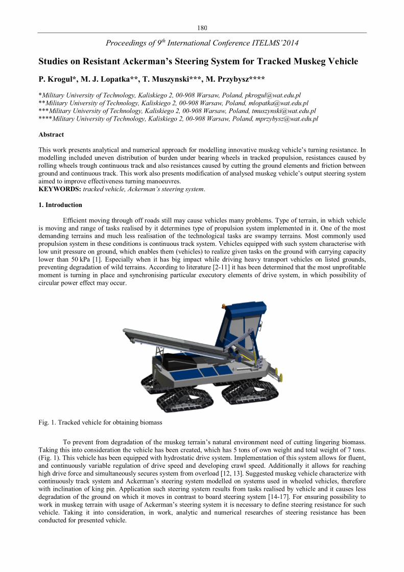
180

Proceedings of 9th International Conference ITELMS’2014 Studies on Resistant Ackerman’s Steering System for Tracked Muskeg Vehicle P. Krogul*, M. J. Lopatka**, T. Muszynski***, M. Przybysz**** *Military University of Technology, Kaliskiego 2, 00-908 Warsaw, Poland, pkrogul@wat.edu.pl **Military University of Technology, Kaliskiego 2, 00-908 Warsaw, Poland, mlopatka@wat.edu.pl ***Military University of Technology, Kaliskiego 2, 00-908 Warsaw, Poland, tmuszynski@wat.edu.pl ****Military University of Technology, Kaliskiego 2, 00-908 Warsaw, Poland, mprzybysz@wat.edu.pl Abstract This work presents analytical and numerical approach for modelling innovative muskeg vehicle’s turning resistance. In modelling included uneven distribution of burden under bearing wheels in tracked propulsion, resistances caused by rolling wheels trough continuous track and also resistances caused by cutting the ground elements and friction between ground and continuous track. This work also presents modification of analysed muskeg vehicle’s output steering system aimed to improve effectiveness turning manoeuvres. KEYWORDS: tracked vehicle, Ackerman’s steering system. 1. Introduction

Efficient moving through off roads still may cause vehicles many problems. Type of terrain, in which vehicle is moving and range of tasks realised by it determines type of propulsion system implemented in it. One of the most demanding terrains and much less realisation of the technological tasks are swampy terrains. Most commonly used propulsion system in these conditions is continuous track system. Vehicles equipped with such system characterise with low unit pressure on ground, which enables them (vehicles) to realize given tasks on the ground with carrying capacity lower than 50 kPa [1]. Especially when it has big impact while driving heavy transport vehicles on listed grounds, preventing degradation of wild terrains. According to literature [2-11] it has been determined that the most unprofitable moment is turning in place and synchronising particular executory elements of drive system, in which possibility of circular power effect may occur.

Fig. 1. Tracked vehicle for obtaining biomass

To prevent from degradation of the muskeg terrain’s natural environment need of cutting lingering biomass.

Taking this into consideration the vehicle has been created, which has 5 tons of own weight and total weight of 7 tons. (Fig. 1). This vehicle has been equipped with hydrostatic drive system. Implementation of this system allows for fluent, and continuously variable regulation of drive speed and developing crawl speed. Additionally it allows for reaching high drive force and simultaneously secures system from overload [12, 13]. Suggested muskeg vehicle characterize with continuously track system and Ackerman’s steering system modelled on systems used in wheeled vehicles, therefore with inclination of king pin. Application such steering system results from tasks realised by vehicle and it causes less degradation of the ground on which it moves in contrast to board steering system [14-17]. For ensuring possibility to work in muskeg terrain with usage of Ackerman’s steering system it is necessary to define steering resistance for such vehicle. Taking it into consideration, in work, analytic and numerical researches of steering resistance has been conducted for presented vehicle.

181

2. Innovative muskeg vehicle’s Ackerman steering system’s construction

This work contains analyse of Ackerman’s steering system (Fig. 2) with hydrostatic drive. Turn in analysed vehicle is realised with usage of hydraulic actuators and control shafts (1), connected with carrying chassis of continuous track (CCCT) (2). Rotation of continuous track is realised around king pin. (3). In researched vehicle applied innovative continuous track’s solution. It’s construction contains four caterpillar strips (4), transverse carrying profiles (5) connecting caterpillar strips, yoke (6) allowing for rotation of carrying chassis, carrying wheels (7) placed rotationally in chassis and drive wheel (8) placed in yoke.

a

b

Fig. 2. Continuous track system: a – continuous tracks; b – single caterpillar track; 1 – hydraulic actuator and control shafts; 2 – carrying chassis of continuous track (CCCT); 3 – King pin’s axis; 4 – caterpillar carrying strips.; 5 – transverse profiles; 6 – yoke; 7 – carrying drive wheels; 8 – drive wheel

3. Analytic researches steering resistances in muskeg vehicle

Firstly for accepted steering system’s construction, analytic researches of its resistance have been conducted. In these researches included: • transverse ground cutting, • rolling resistances of carrying wheels through continuously track, • transverse friction between caterpillar track and ground.

In analytic researches steering resistances falling on one continuous track. That is why for equations accepted weight force falling on one caterpillar track which equals 20 kN. Total value of steering momentum Mskr is a sum of momentum derived from carrying wheels’ rolling resistance Mf and momentum from adhesion continuous track and ground and transverse ground cutting Mμ + τ , which can be presented as a equation:

Mskr = Mf + Mµ + τ (1)

where Mf – rolling resistance momentum; Mμ + τ – momentum derived from adhesion and transverse ground cutting. A momentum from carrying wheels’ rolling resistance Mf (Fig. 3) derives from wheels’ pressure on ground G

and rolling resistance’s rate f and radius r actions of rolling resistance’s force in relation to point of caterpillar track rotation which is presented in equation:

∑∑==

+=m

jjyjj

n

iiyiif rfGrfGM

11 (2)

where G – wheel’s pressure on caterpillar track; f – rate of rolling resistances; r – radiuses of actions of rolling resistance’s force in relation to point of caterpillar track rotation; m and n – amount of carrying wheels in the same row (m = n = 6).

In view of that in discussed case resultant middle point of caterpillar rotation results in internal axis of carrying wheels accepted an assumption that the radius ry j = 0. Placement of wheels’ pressure on caterpillar track assumed to analytic equations is presented on Fig. 5, however values of particular pressures are presented in Tab. 1.

Fig. 3. Scheme to assign constituent momentum of steering resistance derived from carrying wheels’ rolling resistance’s force

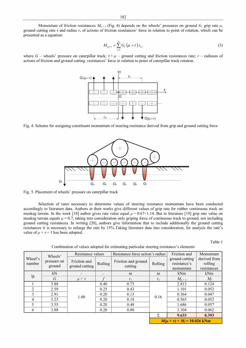
182

Momentum of friction resistances Mμ + τ (Fig. 4) depends on the wheels’ pressures on ground G, grip rate μ, ground cutting rate τ and radius rx of actions of friction resistances’ force in relation to point of rotation, which can be presented as a equation:

( )∑=

+ +=n

iixi rGM

1τµτµ (3)

where G – wheels’ pressure on caterpillar track; τ + μ – ground cutting and friction resistances rate; r – radiuses of actions of friction and ground cutting resistances’ force in relation to point of caterpillar track rotation.

Fig. 4. Scheme for assigning constituent momentum of steering resistance derived from grip and ground cutting force

Fig. 5. Placement of wheels’ pressure on caterpillar track

Selection of rates necessary to determine values of steering resistance momentum have been conducted

accordingly to literature data. Authors in their works give different values of grip rate for rubber continuous track on muskeg terrain. In the work [18] author gives rate value equal μ = 0.67÷1.14. But in literature [19] grip rate value on muskeg terrain equals μ = 0.7, taking into consideration only griping force of continuous track to ground, not including ground cutting resistances. In writing [20], authors give information that to include additionally the ground cutting resistances it is necessary to enlarge the rate by 15%.Taking literature data into consideration, for analysis the rate’s value of μ + τ = 1 has been adopted.

Table 1 Combination of values adopted for estimating particular steering resistance’s elements

Wheel’s number

Wheels’ pressure on

ground

Resistance values Resistance force action’s radius Friction and ground cutting

resistance’s momentum

Momentum derived from

rolling resistances

Friction and ground cutting Rolling Friction and ground

cutting Rolling

lp kN – – m m kNm kNm G μ + τ f rx ry Mμ + τ Mf

1 3.88

1.00

0.40 0.73

0.16

2.813 0.124 2 2.59 0.25 0.43 1.101 0.052 3 2.91 0.20 0.13 0.364 0.047 4 3.23 0.20 0.18 0.565 0.052 5 3.55 0.20 0.48 1.686 0.057 6 3.88 0.20 0.80 3.104 0.062 Σ 9.633 0.393 M(μ + τ) + Mf = 10.026 kNm

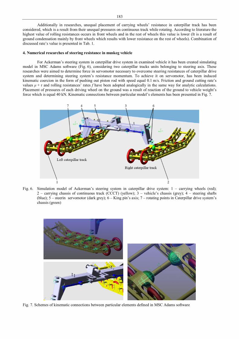
183

Additionally in researches, unequal placement of carrying wheels’ resistance in caterpillar track has been considered, which is a result from their unequal pressures on continuous track while rotating. According to literature the highest value of rolling resistances occurs in front wheels and in the rest of wheels this value is lower (It is a result of ground condensation mainly by front wheels which results with lower resistance on the rest of wheels). Combination of discussed rate’s value is presented in Tab. 1. 4. Numerical researches of steering resistance in muskeg vehicle

For Ackerman’s steering system in caterpillar drive system in examined vehicle it has been created simulating model in MSC Adams software (Fig. 6), considering two caterpillar tracks units belonging to steering axis. These researches were aimed to determine force in servomotor necessary to overcome steering resistances of caterpillar drive system and determining steering system’s resistance momentum. To achieve it on servomotor, has been induced kinematic coercion in the form of pushing out piston rod with speed equal 0.1 m/s. Friction and ground cutting rate’s values μ + τ and rolling resistances’ rates f have been adopted analogically in the same way for analytic calculations. Placement of pressures of each driving wheel on the ground was a result of reaction of the ground to vehicle weight’s force which is equal 40 kN. Kinematic connections between particular model’s elements has been presented in Fig. 7.

Fig. 6. Simulation model of Ackerman’s steering system in caterpillar drive system: 1 – carrying wheels (red);

2 – carrying chassis of continuous track (CCCT) (yellow); 3 – vehicle’s chassis (grey); 4 – steering shafts (blue); 5 – steerin servomotor (dark grey); 6 – King pin’s axis; 7 – rotating points in Caterpillar drive system’s chassis (green)

Fig. 7. Schemes of kinematic connections between particular elements defined in MSC Adams software

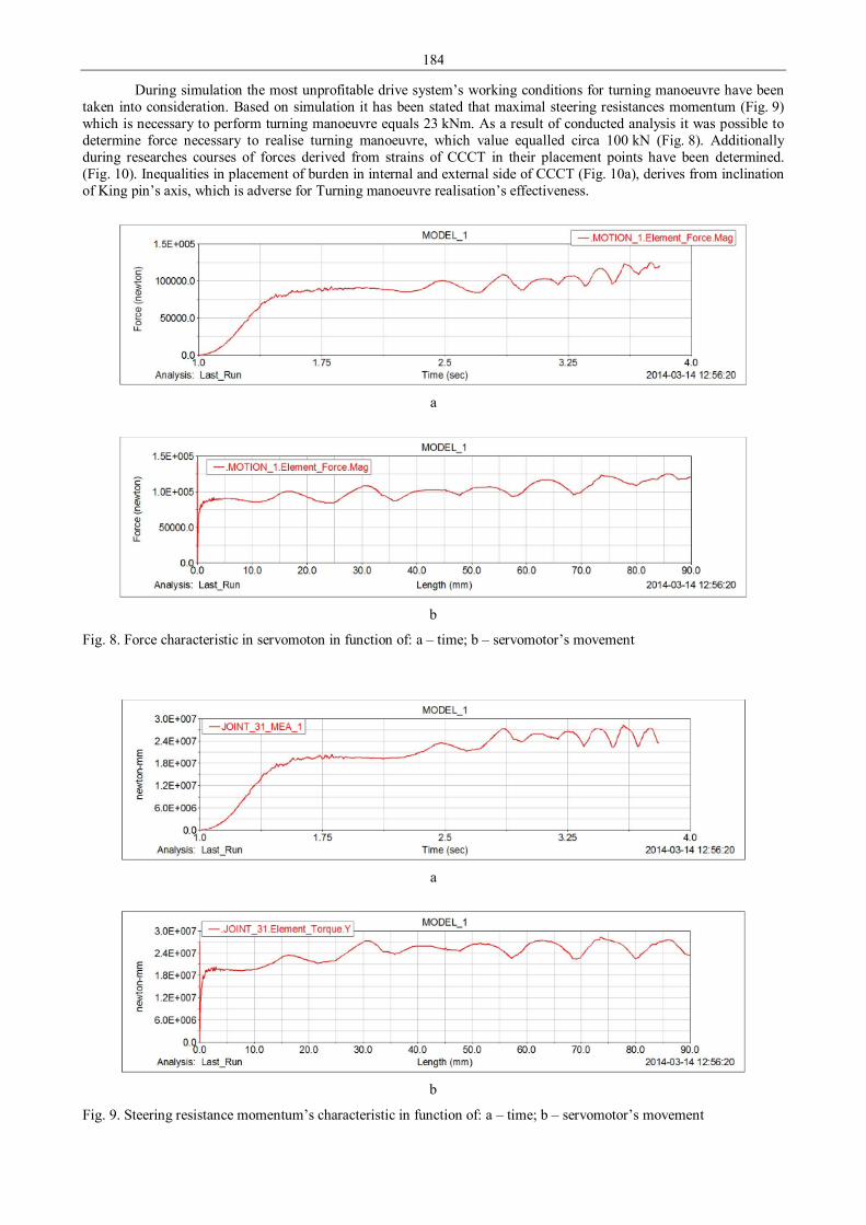
184

During simulation the most unprofitable drive system’s working conditions for turning manoeuvre have been taken into consideration. Based on simulation it has been stated that maximal steering resistances momentum (Fig. 9) which is necessary to perform turning manoeuvre equals 23 kNm. As a result of conducted analysis it was possible to determine force necessary to realise turning manoeuvre, which value equalled circa 100 kN (Fig. 8). Additionally during researches courses of forces derived from strains of CCCT in their placement points have been determined. (Fig. 10). Inequalities in placement of burden in internal and external side of CCCT (Fig. 10a), derives from inclination of King pin’s axis, which is adverse for Turning manoeuvre realisation’s effectiveness.

a

b

Fig. 8. Force characteristic in servomoton in function of: a – time; b – servomotor’s movement

a

b

Fig. 9. Steering resistance momentum’s characteristic in function of: a – time; b – servomotor’s movement

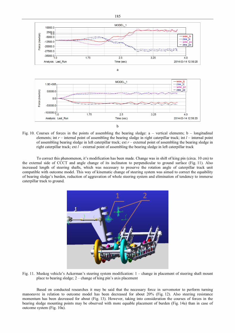
185

a

b

Fig. 10. Courses of forces in the points of assembling the bearing sledge: a – vertical elements; b – longitudinal elements; int r – internal point of assembling the bearing sledge in right caterpillar track; int l – internal point of assembling bearing sledge in left caterpillar track; ext r – external point of assembling the bearing sledge in right caterpillar track; ext l – external point of assembling the bearing sledge in left caterpillar track

To correct this phenomenon, it’s modification has been made. Change was in shift of king pin (circa. 10 cm) to

the external side of CCCT and angle change of its inclinaton to perpendicular to ground surface (Fig. 11). Also increased length of steering shafts, which was necessary to preserve the rotation angle of caterpillar track unit compatible with outcome model. This way of kinematic change of steering system was aimed to correct the equability of bearing sledge’s burden, reduction of aggravation of whole steering system and elimination of tendency to immerse caterpillar track to ground.

Fig. 11. Muskeg vehicle’s Ackerman’s steering system modification: 1 – change in placement of steering shaft mount

place to bearing sledge; 2 – change of king pin’s axis placement

Based on conducted researches it may be said that the necessary force in servomotor to perform turning

manoeuvre in relation to outcome model has been decreased for about 20% (Fig. 12). Also steering resistance momentum has been decreased for about (Fig. 13). However, taking into consideration the courses of forces in the bearing sledge mounting points may be observed with more equable placement of burden (Fig. 14a) than in case of outcome system (Fig. 10a).

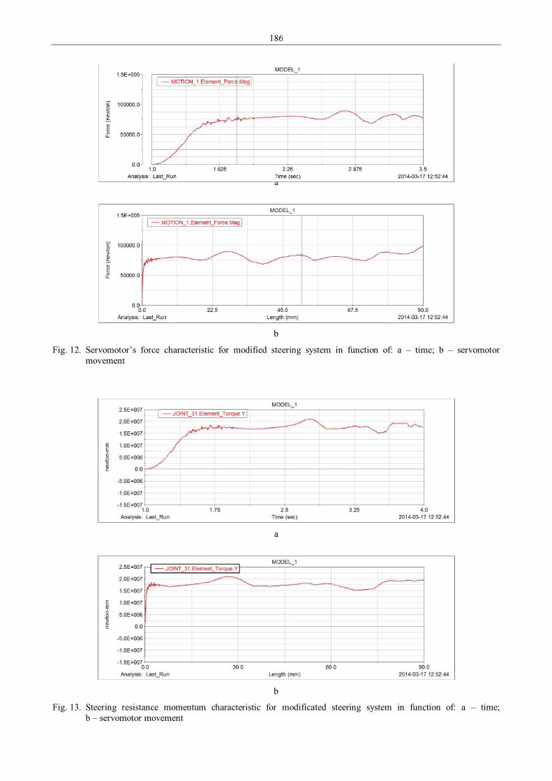
186

a

b

Fig. 12. Servomotor’s force characteristic for modified steering system in function of: a – time; b – servomotor movement

a

b

Fig. 13. Steering resistance momentum characteristic for modificated steering system in function of: a – time; b – servomotor movement

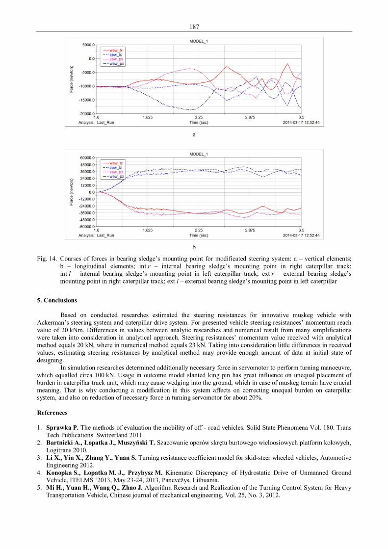
187

a

b

Fig. 14. Courses of forces in bearing sledge’s mounting point for modificated steering system: a – vertical elements; b – longitudinal elements; int r – internal bearing sledge’s mounting point in right caterpillar track; int l – internal bearing sledge’s mounting point in left caterpillar track; ext r – external bearing sledge’s mounting point in right caterpillar track; ext l – external bearing sledge’s mounting point in left caterpillar

5. Conclusions

Based on conducted researches estimated the steering resistances for innovative muskeg vehicle with Ackerman’s steering system and caterpillar drive system. For presented vehicle steering resistances’ momentum reach value of 20 kNm. Differences in values between analytic researches and numerical result from many simplifications were taken into consideration in analytical approach. Steering resistances’ momentum value received with analytical method equals 20 kN, where in numerical method equals 23 kN. Taking into consideration little differences in received values, estimating steering resistances by analytical method may provide enough amount of data at initial state of designing.

In simulation researches determined additionally necessary force in servomotor to perform turning manoeuvre, which equalled circa 100 kN. Usage in outcome model slanted king pin has great influence on unequal placement of burden in caterpillar track unit, which may cause wedging into the ground, which in case of muskeg terrain have crucial meaning. That is why conducting a modification in this system affects on correcting unequal burden on caterpillar system, and also on reduction of necessary force in turning servomotor for about 20%. References 1. Sprawka P. The methods of evaluation the mobility of off - road vehicles. Solid State Phenomena Vol. 180. Trans

Tech Publications. Switzerland 2011. 2. Bartnicki A., Łopatka J., Muszyński T. Szacowanie oporów skrętu burtowego wieloosiowych platform kołowych,

Logitrans 2010. 3. Li X., Yin X., Zhang Y., Yuan S. Turning resistance coefficient model for skid-steer wheeled vehicles, Automotive

Engineering 2012. 4. Konopka S., Łopatka M. J., Przybysz M. Kinematic Discrepancy of Hydrostatic Drive of Unmanned Ground

Vehicle, ITELMS ‘2013, May 23-24, 2013, Panevėžys, Lithuania. 5. Mi H., Yuan H., Wang Q., Zhao J. Algorithm Research and Realization of the Turning Control System for Heavy

Transportation Vehicle, Chinese journal of mechanical engineering, Vol. 25, No. 3, 2012.

188

6. Bartnicki A., Muszyński T. Koncepcja układu napędowego dla bezzałogowej platformy lądowej o skręcie burtowym. Międzynarodowa Konferencja Naukowo-Techniczna Napędy i Sterowania Hydrauliczne i Pneumatyczne. Wroclaw 2010.

7. Cao F., Zhou Z. Y., Xu L. Y., Zhang M. Study on Hydro-mechanical Differential Dynamic Turning Process of Tracked Vehicle, Second International Conference on Intelligent Computation Technology and Automation 2009.

8. Haggag S., Alstrom D., Cetinkunt S., Egelja A. Modeling, Control, and Validation of an Electro-Hydraulic Steer-by-Wire System for Articulated Vehicle Applications, IEEE/ASME TRANSACTIONS ON MECHATRONICS, VOL. 10, NO. 6, DECEMBER 2005.

9. Łopatka M. J. Influence of Power Steering System of Directional Stability of Articulated Wheel Loader, ITELMS ‘2013, Panevėžys, Lithuania, May 23-24, 2013.

10. Bartnicki A., Dąbrowska A., Łopatka M. J., Muszyński T. Experimental Research on Directional stability of articulated Tractors, XIV Konferencja automatyzacji i Eksploatacji systemów Sterowania i Łączności ASMOR 2013, Jastrzębia Góra 2013.

11. Bartnicki A., Łopatka M., J., Muszyński T., Jaskółowski M. The Researches of Stability Evaluation Articulated Loader while Working on Slopes, ITELMS ‘2013, Panevėžys, Lithuania, May 23-24, 2013.

12. Konopka S., Krogul P., Łopatka M. J. Simulation Research of Hydrostatic Power System Control of Engineer Robot Manipulator, ITELMS ‘2013, Panevėžys, Lithuania, May 23-24, 2013.

13. Zhou Z. L., Cao F. Y., Xu L. Y. Dynamic Simulation of Hydro-mechanical Differential Turning Hydraulic System of Tracked Vehicle, Conference: 13th International Manufacturing Conference in China, Dalian, SEP 21-23, 2009.

14. Konopka S., Sprawka P., Muszyński T., Spadło K. Investigating resistance of turn six-wheel skid-steer vehicle, ITELMS ‘2013, Panevėžys, Lithuania, May 23-24, 2013.

15. Cheli F., Leo E., Sabbioni E. A semi-physical model of a hydraulic power steering system for vehicle dynamics simulations, 8th Conference Biennial Conference on Engineering Systems Design and Analysis Location: Turin, ITALY Date: JUL 04-07, 2006.

16. Mi H., Yuan H., Wang Q. Investigation on the Improvement of Turning Ability for Heavy Transportation Vehicle, 6th Conference IEEE Conference on Industrial Electronics and Applications (ICIEA), Beijing, 21-23 jun, 201.

17. Łopatka M. J., Muszyński T., Rubiec A. Load Analysis of skid steer drive systems, 18th International Conference of Methods and Models in Automation and Robotics MMAR 2013.

18. Wong J. Y. Theory of ground vehicle, ISBN: 978-0-470-17038-0, August 2008. 19. Скотников в. а.: проходимость машин, Дальнаука, 2012. 20. Brach I., Walczewski R. Koparki jednonaczyniowe, WNT 1975.

189

Proceedings of 9th International Conference ITELMS’2014 Form Control of Individual Surface Corrosion Pits in Main Gas Pipe Steel P. O. Maruschak*, I. V. Konovalenko*, I. M. Danyliuk*, S. V. Panin**, I. V. Vlasov** *Ternopil Ivan Pul’uj National Technical University, Ruska 56 str., 46001, Ternopil, Ukraine, E-mail: laboratory22b@gmail.com **Institute of Strength Physics and Materials Science SB RAS, Akademicheskii avenue 2/4, 634021, Tomsk, Russia Abstract A optic-digital method of the quantitative evaluation of parameters of the pitting-like defect subjected to the complex loading is developed, which allows analyzing the distribution of strain and shape variation of the object analyzed. KEYWORDS: self-similar structures, cyclic deformations, strain, sensor, corrosion pits. 1. Introduction

In-service surface defects decrease the service life of materials and structures significantly. The authors of previous works substantiated the form and methodology for determining the evaluation parameters of the structural condition using the surface deformation relief parameters of structural elements and specimens-witnesses for aircrafts [1]. The theoretical aspects of self-organization of the fatigue sensor surface during a long-term operation are updated and extended, theoretical approaches to its fixation on the surface are substantiated.

The works by Syzrantsev V. N. substantiate the use of the integral state givers (giver sensors) for heavily loaded structures of travelling cranes [2]. The giver calibration method is proposed, which allows increasing the accuracy of evaluation of heavily loaded structure condition. A number of recommendations are developed regarding the installation of givers, and the correlation connection is established between the damage parameters of the author-developed original givers and the loading amplitude of a structure.

The works by Е. Е. Zasimchuk and others [3] propose to use monocrystals and coatings as giver sensors during diagnostics of the material surface condition subjected to various loading schemes. The main regularities in the kinetics of accumulation of the scattered and localized multiple defects are found, as well as the peculiarities of the relief formation at various stages of the material damage. The use of a number of well-known parameters and algorithms for the giver sensors of damage is substantiated.

The group of М. Satton [4] develops the approaches to identification of the non-uniform deformation zones of structural materials (steel, aluminum alloys) and composites with a construction of surface strain maps (surface strain mapping) under conditions of cyclic loading.

During previous investigations, the authors of the project determined a number of fundamental regularities in the self-organization of the material surface as a response to the external force effect under static, cyclic and impact loading, which allowed proposing the original (protected by the patents of Ukraine) technical solutions regarding the identification of the material and structural damage. However, the difference in structures of various materials and random nature of the deformation response of materials to the force effect necessitates updating the existing approaches to the optical and digital control and development of the new ones [5]. It is important to establish the physical regularities in damage accumulation, which have a universal nature, and propose such parameters that would depict adequately the physical processes of structural and mechanical changes.

The purpose of this work is to develop an algorithm of the optical and digital approach to the analysis of fatigue damage in the vicinity of a circular stress concentrator similar in shape to the corrosion pitting. 2. Research technique

Specimens from steel 17G1S were loaded in cyclic tension Δσ = 250 MPa on the servohydraulic test setup Biss UTM 150. In the course of fatigue tests, the surface analyzed was photographed with the Canon D550 camera to failure. A camera with a source of light was fixed to a specimen with a crack to record images of the specimen surface. The first digital image of the surface of the specimen with a crack was recorded without loading. The rest of images after certain periods of cyclic loading were recorded during the specimen loading and saved in the computer. The accumulated specimen surface images were processed in the computer using a special algorithm.

The total cyclic life of the specimen (N = 1.43·106 cycles) can be conventionally divided into two diagnostic periods: • preliminary cyclic deformation – during this period no structural-mechanical and optical-digital changes are detected

on the specimen surface, N1 = 1.03·106 cycles; • identification of a fatigue crack and defectometry control – at this stage, changes in the surface condition were

recorded, as well as nucleation and propagation of a fatigue crack, N2 ≤ 40·103 cycles.

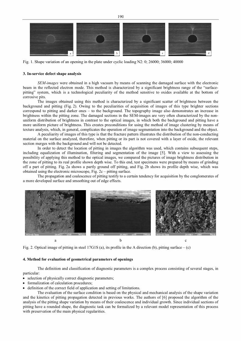
190

Fig. 1. Shape variation of an opening in the plate under cyclic loading N2: 0; 26000; 36000; 40000

3. In-service defect shape analysis

SЕМ-images were obtained in a high vacuum by means of scanning the damaged surface with the electronic beam in the reflected electron mode. This method is characterized by a significant brightness range of the “surface-pitting” system, which is a technological peculiarity of the method sensitive to oxides available at the bottom of corrosive pits.

The images obtained using this method is characterized by a significant scatter of brightness between the background and pitting (Fig. 2). Owing to the peculiarities of acquisition of images of this type brighter sections correspond to pitting and darker ones – to the background. The topography image also demonstrates an increase in brightness within the pitting zone. The damaged sections in the SЕМ-images are very often characterized by the non-uniform distribution of brightness in contrast to the optical images, in which both the background and pitting have a more uniform picture of brightness. This creates preconditions for using the method of image clustering by means of texture analysis, which, in general, complicates the operation of image segmentation into the background and the object.

A peculiarity of images of this type is that the fracture pattern illustrates the distribution of the non-conducting material on the surface analyzed, therefore, when pitting or its part is not covered with a layer of oxide, the relevant section merges with the background and will not be detected.

In order to detect the location of pitting in images the algorithm was used, which contains subsequent steps, including equalization of illumination, filtering and segmentation of the image [5]. With a view to assessing the possibility of applying this method to the optical images, we compared the pictures of image brightness distribution in the zone of pitting to its real profile shown depth wise. To this end, test specimens were prepared by means of grinding off a part of pitting. Fig. 2а shows a partly ground off pitting, and Fig. 2b shows its profile depth wise, which was obtained using the electronic microscope, Fig. 2с – pitting surface.

The propagation and coalescence of pitting testify to a certain tendency for acquisition by the conglomerates of a more developed surface and smoothing out of edge effects.

a

b

c

Fig. 2. Optical image of pitting in steel 17G1S (а), its profile in the A direction (b), pitting surface – (с)

4. Method for evaluation of geometrical parameters of openings

The definition and classification of diagnostic parameters is a complex process consisting of several stages, in particular: • selection of physically correct diagnostic parameters; • formalization of calculation procedures; • definition of the correct field of application and setting of limitations.

The evaluation of the surface condition is based on the physical and mechanical analysis of the shape variation and the kinetics of pitting propagation detected in previous works. The authors of [6] proposed the algorithm of the analysis of the pitting shape variation by means of their coalescence and individual growth. Since individual sections of pitting have a rounded shape, the diagnostic task can be formalized by a relevant model representation of this process with preservation of the main physical regularities.

191

The cyclic growth of cracks caused redistribution of the stress-strain state in the plate, moreover, a distortion of the shape of opening due to a change in the roundness coefficient was recorded. In order to determine a degree of approximation of the corrosive spot shape to roundness, the coordinates of the center of mass Ci (xci , yci) were calculated for each object:

1

/if

ci m im

x x f=

= ∑ and 1

/if

ci m im

y y f=

= ∑ (1)

Next, the roundness coefficient Kci was calculated for the detected objects – a percentage of object pixels that get into the circle with diameter di, the centre of which is merged with the center of mass Ci (Fig. 4а):

1( , )

100%

if

m im

cii

g r dK

f== ⋅

∑uur

( )

>

≤=

2/ if ,0

2/ if ,1,

im

imim

dr

drdrg (2)

where ( , )m ig r duur

is the indicatory function used in the evaluation of chances for the m-th pixel of the object to get into

the equivalent circle with diameter di ; mruur

is the radius-vector directed from the center of the equivalent circle Ci (xci , yci) to the m-th pixel of the object with coordinates xm, ym .

a

b

c

d

Fig. 3. Digital images of the opening for various points of the optical and digital analysis of the specimen from steel 17G1S according to Fig. 1

In our opinion, this algorithm can be used effectively for the evaluation of the plate condition with a pitting-

like opening subjected to cyclic loading. The presence of a crack-like defect has an active influence on the material liability, which causes the intensive shape variation of the opening and imitates the shape variation of pitting. A plate with an opening and a crack-like defect was considered, which is a formal depiction of the object and takes into account possible changes in its condition. 5. Results and discussion

Using the developed approach it is possible to determine the real shape variation of the opening analyzed in the longitudinal and transverse directions during cyclic loading, which testifies to the nonlinearity of the deformation process. This is a very important result, since in a majority of cases; the structural elements and machine parts are operated under conditions of the complex stress-strain state. In this case, the complex stress-strain state also appears in the vicinity of circular stress concentrators and defects, i.e. deformation may take place both in accordance with the normal separation scheme and the transverse or longitudinal shear scheme. In such cases, it is necessary to know the deformation characteristics of the material according to the said mechanisms of failure, as well as the criteria of the ultimate equilibrium condition of bodies with cracks.

It is found that with an increase in the cyclic loading the roundness coefficient Kc decreases from 99.0% to 94.9%, Fig. 4а. This is especially noticeable during the analysis of variation of the diameter shape in the longitudinal dx and transverse dy directions. After 25 thousand loading cycles, a localized strain field is formed in the vicinity of the opening, and the opening stretches in the longitudinal direction. Moreover, it is seen in (Fig. 4b) that the opening shape is sensitive to the localization of the deformation process. In addition, an increase in the velocity of the defect growth causes redistribution of the plastic deformation intensity in the vicinity of the opening, which is depicted in Fig. 3b. The correlated nature of the results obtained for the roundness coefficient and the opening diameter dx, dy should be pointed out separately. This confirms once again the reliability of the regularities obtained.

192

а

b

Fig. 4. Residual life curve for a plate with an opening cut from a specimen from steel 17G1S (а), variation parameters of shape (1) and shape coefficient (2) of the opening (b)

The results obtained have a clear physical and mechanical sense, since an increase in the non-uniformity of the

opening geometrical parameters corresponds to strain localization in the stress concentration sections. It is known from literature that pitting has the ordered (graded) mechanism of propagation; therefore, the proposed approaches allow predicting the process of their growth.

Moreover, since pitting is one of the reasons for the atomic hydrogen to get into the metal of gas and oil pipelines and sometimes it is the reason for the nucleation of crack-like microdefects, its identification allows for the timely application of preventive or remedial measures and has a great practical value. 6. Conclusions

The experimental investigations confirmed that the optical and digital characteristics are the diagnostic characteristics, which have a determined character and can be calculated based on the surface image.

A calculation method of the quantitative evaluation of parameters of the pitting-like defect subjected to the complex loading is developed, which allows analyzing the distribution of strain and shape variation of the object analyzed. Moreover, the peculiarities of the analysis, which are defined by the physical peculiarities of the surface analyzed, are found and taken into account based on the results of the experimental investigations.

A computational optical and digital method for predicting the condition of structural materials under conditions of complex loading is proposed based on which it is possible to perform a quantitative evaluation of the allowable loading, when the orientation and geometrical parameters of the defect are set in the large-sized structural elements. References 1. Ignatovich S. R., Menou A., Karuskevich M. V., Maruschak P. O. Fatigue sensor for aircraft structural health

monitoring, Proc of the Int. Symposium on Aircraft Materials, Fez, Morocco, (May 9-12), 2012, p. 20-21. 2. Syzrantsev V. N., Golofast S. L. Measurement of Cyclic Deformations and Prediction of Parts Durability Using

Readings of Integral Strain Gages. - Novosibirsk: Nauka, 2004, 206 p. 3. Kuznetsov P. V., Petrakova I. V. et al. Formation of self-similar structures on {100} ⟨001⟩ aluminum single-

crystal foils under cyclic tension, Physical Mesomechanics, 2009, Vol. 12, p. 85–93. 4. Sutton M. A., Wolters W. J., Peters W. H., Ranson W. F., McNeill S. R. Determination of displacements using

an improved digital correlation method, Image Vision Comput, 1983, 1(3), p. 133-139. 5. Konovalenko I. B., Maruschak P. O. Automated method for studying the deformation behavior of a material

damaged by a thermal fatigue crack network, Optoelectronics, Instrumentation and Data Processing, 2013, Vol. 49, p. 243-249.

6. Maruschak P., Bishchak R., Konovalenko I., Menou A., Brezinova J. Effect of long term operation on degradation of material of main gas pipelines, Materials Science Forum, 2014, Vol. 782, p. 279-283.

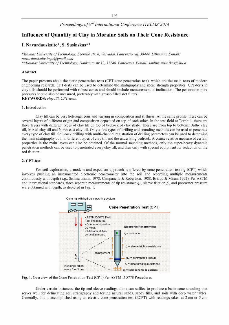
193

Proceedings of 9th International Conference ITELMS’2014 Influence of Quantity of Clay in Moraine Soils on Their Cone Resistance I. Navardauskaite*, S. Susinskas** *Kaunas University of Technology, Ezerelio str. 6, Vaivadai, Panevezio raj. 38444, Lithuania, E-mail: navardauskaite.inga@gmail.com **Kaunas University of Technology, Daukanto str.12, 37146, Panevezys, E-mail: saulius.susinskas@ktu.lt Abstract The paper presents about the static penetration tests (CPT-cone penetration test), which are the main tests of modern engineering research. CPT-tests can be used to determine the stratigraphy and shear strength properties. CPT-tests in clay tills should be performed with robust cones and should include measurement of inclination. The penetration pore pressures should also be measured, preferably with grease-filled slot filters. KEYWORDS: clay till, CPT-tests. 1. Introduction

Clay till can be very heterogeneous and varying in composition and stiffness. At the same profile, there can be several layers of different origin and composition deposited on top of each other. In the test field at Tornhill, there are three layers with different types of clay till on top of bedrock of clay shale. These are from top to bottom; Baltic clay till, Mixed clay till and North-east clay till. Only a few types of drilling and sounding methods can be used to penetrate every type of clay till. Soil-rock drilling with multi-channel registration of drilling parameters can be used to determine the main stratigraphy both in different types of clay till and the underlying bedrock. A coarse relative measure of certain properties in the main layers can also be obtained. Of the normal sounding methods, only the super-heavy dynamic penetration methods can be used to penetrated every clay till, and then only with special equipment for reduction of the rod friction. 2. CPT-test

For soil exploration, a modern and expedient approach is offered by cone penetration testing (CPT) which involves pushing an instrumented electronic penetrometer into the soil and recording multiple measurements continuously with depth (e.g., Schmertmann, 1978; Campanella & Robertson, 1988; Briaud & Miran, 1992). Per ASTM and international standards, three separate measurements of tip resistance qc , sleeve friction fs , and porewater pressure u are obtained with depth, as depicted in Fig. 1.

Fig. 1. Overview of the Cone Penetration Test (CPT) Per ASTM D 5778 Procedures

Under certain instances, the tip and sleeve readings alone can suffice to produce a basic cone sounding that

serves well for delineating soil stratigraphy and testing natural sands, sandy fills, and soils with deep water tables. Generally, this is accomplished using an electric cone penetration test (ECPT) with readings taken at 2 cm or 5 cm,

194

although a system for mechanical cone penetration testing (MCPT) is also available which is less prone to damage but which is advanced slower and provides coarser resolutions using an incremental vertical step of 20 cm intervals. With piezocone penetration testing (CPTU), transducers obtain readings of penetration porewater pressures that are paramount when conditions contain shallow groundwater conditions and fine-grained soils consisting of clays, silts, and sands with fines. The porewater pressures at the shoulder position are required for correcting the measured qc to the total cone tip resistance, designated qt . This is especially important in the postprocessing phase when determining soil engineering parameters, e.g., preconsolidation stress Pc', undrained shear strength su , lateral stress ratio K0 , pile side friction fp , etc. Additional sensors can be provided to increase the numbers and types of measurements taken, with Table 1 providing a quick summary of the various types of CPT commonly available [2].

Table 1 Basic Types of Cone Penetration Tests Available for Site Characterization

Type of CPT Acronym Measurements Taken Applications Mechanical Cone Penetration Test MCPT qc (or qc and fs) on 20 cm intervals. Uses

inner & outer rods to convey loads uphole. Stratigraphic profiling, Fill control, Natural sands, Hard ground

Electric Friction Cone ECPT qc and fs (taken at 1 to 5 cm intervals) Fill placement, Natural sands, Soils

above the groundwater table Piezocone Penetration Test

CPTu and PCPT

qc , fs and either face u1 or shoulder u2 (taken at 1 to 5 cm intervals)

All soil types. Note: Requires u2 for correction of qc to qt

Piezocone with Dissipation CPTù Same as CPTu with timed readings of u1

or u2 during decay Normally conducted to 50% dissipation in silts and clays

Seismic Piezocone Test SCPTu

Same as CPTu with downhole shear waves (Vs) at 1 m intervals

Provides fundamental soil stiffness with depth: Gmax = ρt Vs

2

Resistivity Piezocone Test RCPTu Same as CPTu with electrical conductivity

or resistivity readings Detect freshwater – salt water interface. Index to contaminant plumes

Notes: qc = measured point stress or cone tip resistance; fs = measured sleeve friction; u = penetration porewater pressure (u1 at face; u2 at shoulder); qt = total cone resistance; Vs = shear wave velocity.

With the CPT, results are immediately available on the computer for assessment in real time by the field

engineer or geologist. A 10 m (30 foot) sounding can be completed in about 15 to 20 min, in comparison with a conventional soil boring that may take between 1 to 1½ hours. No spoil is generated during the CPT, thus the method is less disruptive than drilling operations. Therefore, CPTs are especially advantageous when investigating environmentally-sensitive areas and/or potentially contaminated sites, as the workers are exposed to a minimal amount of hazardous materials. Cone penetration tests can be advanced into most soil types ranging from soft clays and firm silts to dense sands and hard overconsolidated clays, but they are not well suited to gravels, cobbles, or hard rock terrain, however. Soil samples are not normally obtained during routine CPT, thus may be a disadvantage to those who rely strictly on laboratory testing for specifications and state code requirements. Nevertheless, a large amount of high-quality in-situ digital data can be recorded directly by the CPT in a relatively short time period in the field. These data can be subsequently post-processed to provide quick delineations of the subsurface conditions, including layering, soil types, and geotechnical engineering parameters, as well as both direct and indirect evaluations of foundation systems, including shallow footings, driven pilings, drilled shafts, and ground modification [2].

As a complement to (or in some cases, as a replacement for) soil borings with SPT-N values, the cone can provide similar information on the subsurface stratigraphy, soil layers, and consistency. Fig. 2 shows a side-by-side comparison of an electric CPT point resistance (qc) profile with a boring log derived from two adjacent boreholes with SPT resistances (N-values) in downtown Memphis, TN. The continuous nature of the CPT point resistance is evident in the profiling of the various strata and soil types. The CPT resistance complements the discrete values from the SPTs at the site and helps to better define the interface between layers, thicknesses, and relative consistencies of each stratum [2].

CPT-test. Altogether, 25 CPT-tests were performed in the initial investigations. The tests were performed using a standard 5 ton CPT-probe with 1000 mm2 cross sectional area. The pore pressure was measured at the standard position behind the shoulder of the tip using a slot filter filled with grease, which has become common practice in CPT-tests in this type of soil [1].

The test results generally confirmed the picture of the layering in the profile with a thin layer of top soil on top of about 3 m of a relatively stiff soil, followed by about 3 m of a somewhat less stiff layer. Thereafter, the stiffness of the soil rapidly increased and all tests stopped at about 7 m depth, below which penetration was impossible with the equipment used, Figure 3. Apart from this unanimous general picture, the results were heavily scattered with large dips and peaks in an inconsistent pattern. Part of these anomalies can be expected to be related to coarse particles of gravel and stone sizes, and part may be assumed to originate from embedded pockets of sand and silt. However, it is very difficult to distinguish between these possibilities [1].

Existing charts for classification of soils on the basis of results from CPT-tests indicated soils ranging between silty clay and sand, with a concentration on silt. Since these charts classify “soil type behavior” rather than grain size

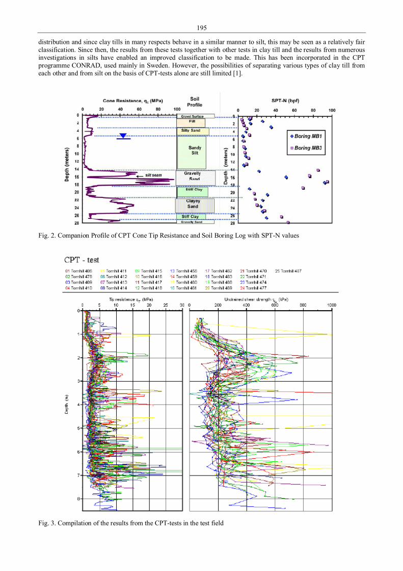
195

distribution and since clay tills in many respects behave in a similar manner to silt, this may be seen as a relatively fair classification. Since then, the results from these tests together with other tests in clay till and the results from numerous investigations in silts have enabled an improved classification to be made. This has been incorporated in the CPT programme CONRAD, used mainly in Sweden. However, the possibilities of separating various types of clay till from each other and from silt on the basis of CPT-tests alone are still limited [1].

Fig. 2. Companion Profile of CPT Cone Tip Resistance and Soil Boring Log with SPT-N values

Fig. 3. Compilation of the results from the CPT-tests in the test field

196

Dynamic probing tests. The dynamic probing tests were performed with a rather crude method and did not yield any detailed information, except that the penetration resistance increased rapidly from about 7 m depth. With this method, the tests penetrated to about 8 m depth, i.e. slightly more than the CPT-tests [1].

Field vane tests. The field vane tests showed a profile with undrained shear strength of generally 300 to 400 kPa between 1.5 and 3 m depth, dropping to about 200 kPa between 3 and 5 m depth and then increasing again. The scatter in the measured strength values was considerable. A comparison between these results and the results from the CPT-tests indicates that a cone factor NKT of between 10 and 12 would be appropriate. Cone factors of this size have been suggested from various Danish investigations in clay till, (Kammer Mortensen et al 1991, Jörgensen and Denver 1992, Luke 1996) [1]. 3. Equipment

A CPT system includes the following components: (1) an electrical penetrometer, (2) a hydraulic pushing system with rods, (3) cable or transmission device, (4) depth recorder, and (5) data acquisition unit. These items are briefly discussed in the following subsections. Additional details on these topics may be found in Robertson & Campanella (1984), Briaud & Miran (1992), and Lunne, Robertson, & Powell (1997).

Penetrometers. The standard cone penetrometer consists of a three-channel instrumented steel probe that measures: cone tip stress (qc), sleeve friction (fs), and penetration porewater pressure (um). The front end consists of a 60° apex conical tip that has a small lip (approx. 5 mm) at the upper portion. The penetrometers are normally available in two standard sizes: 1. A 35.7 mm (1.4 inch) diameter version having a corresponding crosssectional area Ac = 10 cm2 and sleeve area

As = 150 cm2. 2. A 44 mm (1.75 inch) diameter version (Ac = 15 cm2 and As = 200 to 300 cm2).

While the 10 cm2 size is the original standard size, many commercial firms have found the 15 cm2 version to be stronger for routine profiling and more easily outfitted with additional sensors in specific needs. As rod sizes are normally 35.7 mm in diameter, the 15 cm2 size cone also tends to open a larger hole and thus reduce side rod friction during pushing. Fig. 4 shows the basic styles of penetrometers in routine use and these are patterned after the original Fugro-type designs (De Ruiter, 1970) [2].

Fig. 4. Dimensions and measurements taken by standard 10 cm2 and 15 cm2 penetrometers

Depending upon the types of soils being tested, the porous filter is usually located either at the apex or midface

(termed Type 1) or at the shoulder (Type 2) just behind the cone tip, else positioned behind the sleeve (Type 3). For the proper correction of measured cone tip resistance to total resistance, the Type 2 is required by national and international standards, until proven otherwise (Campanella & Robertson, 1988).

An internal load cell is used to register the axial force at the front of the penetrometer (Fc). A second load cell is used to record the axial force either along the sleeve (Fs) within a “tension-type cone” design, or else located in the back and records the total tip force plus sleeve (Fc + Fs). In the latter (termed “subtraction-type cone”), the combined force minus the separately-measured front force provides the sleeve force.

State and provincial DOTs which engage in cone penetration work either use commercially-manufactured CPT systems, or else subcontract to firms that use commercial equipment or maintain an arsenal of their own in-house

197

penetrometers and data acquisition systems. Appendix B lists various CPT manufacturers and service companies, and related websites for additional information on equipment, data acquisition, and postprocessing.

In special instances, miniature cone penetrometers are available, with reduced cross-sectional sizes of 5 cm2 and 1 cm2 discussed in the open literature. These mini-cones have been used in laboratory testing programs, both in calibration chambers and centrifuges, yet also in field applications (e.g., Tumay, et al. 1998). Also, large diameter penetrometers have been developed for special projects, including a 33 cm2 version and a 40 cm2 model which can be pushed into gravelly soils. Fig. 4 shows a selection of various penetrometers. Based on the survey results, most DOTs are using 10 cm2 size penetrometers, with a few deploying the 15 cm2 type. Several are using advanced cones with seismic, video, or resistivity, while only 2 DOTs are using mini-cones and 1 DOT is operating a mechanical CPT.

a

b

c

Fig. 5. Selection of Penetrometers from: (a) van den Berg series, (b) Fugro series (left to right: 33, 15, 10, 5, and 1 cm2 sizes), and (c) Georgia Tech collection (bottom to top): 5 cm2 friction, four 10 cm2 piezocones (type 2, type 1, type 2 seismic, dual-piezo-element), and 15 cm2 triple-element type

Specifications on the machine tolerances, dimensions, and load cell requirements for electrical CPTs are

outlined in ASTM D 5778 and in the international reference test procedure (IRTP, 1999). For the older mechanical CPT systems, guidelines per ASTM D 3441 still remain on the books. Most penetrometers are constructed of tool-grade steel, although a few commercial units are available in stainless steel or brass. Periodically, the tip and sleeve elements are replaced due to wear or damage. It is common to replace the porewater filter after each sounding with either a disposable plastic ring type, or else a reusable sintered metal or ceramic type. The reusable types can be cleaned in an ultrasonics bath [2]. 4. Conclusions 1. CPT method is less disruptive than drilling operations. 2. The possibilities of separating various types of clay till from each other and from silt on the basis of CPT-tests alone

are still limited. 3. Depending upon the types of soils being tested, the porous filter is usually located either at the apex or midface or at

the shoulder just behind the cone tip, else positioned behind the sleeve. References 1. Larsson R. Investigations and Load Tests in Clay Till LINKÖPING 2001. p. 9, 19-20. 2. Mayne P. W. Cone Penetration Tesring State-of-Practice 12 February 2007. p. 4-6, 12-13.

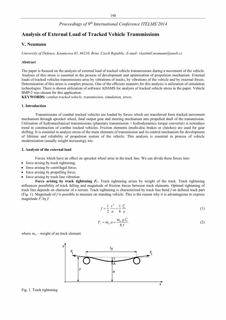
198

Proceedings of 9th International Conference ITELMS’2014 Analysis of External Load of Tracked Vehicle Transmissions V. Neumann University of Defence, Kounicova 65, 66210, Brno, Czech Republic, E-mail: vlastimil.neumann@unob.cz Abstract The paper is focused on the analysis of external load of tracked vehicle transmissions during a movement of the vehicle. Analysis of this stress is essential in the process of development and optimization of propulsion mechanism. External loads of tracked vehicles transmissions arise by vibrations of tracks, by vibrations of the vehicle and by external forces. Determination of this stress is complex process. One of the efficient manners for this analysis is utilization of simulation technologies. There is shown utilization of software ADAMS for analysis of tracked vehicle stress in the paper. Vehicle BMP-2 was chosen for this application. KEYWORDS: combat tracked vehicle, transmission, simulation, stress. 1. Introduction

Transmissions of combat tracked vehicles are loaded by forces which are transferred form tracked movement mechanism through sprocket wheel, final output gear and steering mechanism into propelled shaft of the transmission. Utilization of hydromechanical transmissions (planetary transmission + hydrodynamics torque converter) is nowadays trend in construction of combat tracked vehicles. Friction elements (multi-disc brakes or clutches) are used for gear shifting. It is essential to analyze stress of the main elements of transmission and its control mechanism for development of lifetime and reliability of propulsion system of the vehicle. This analysis is essential in process of vehicle modernization (usually weight increasing), too. 2. Analysis of the external load

Forces which have an effect on sprocket wheel arise in the track line. We can divide these forces into: • force arising by track tightening; • force arising by centrifugal force; • force arising by propelling force; • force arising by track line vibration.

Force arising by track tightening Ft . Track tightening arises by weight of the track. Track tightening influences possibility of track falling and magnitude of friction forces between track elements. Optimal tightening of track line depends on character of a terrain. Track tightening is characterized by track line bend f on defined track part (Fig. 1). Magnitude of f is possible to measure on standing vehicle. This is the reason why it is advantageous to express magnitude Ft by f:

al

axf

20

2

81

21

== (1)

f

lgmamF tetec 8

20== (2)

where mte – weight of an track element.

Fig. 1. Track tightening

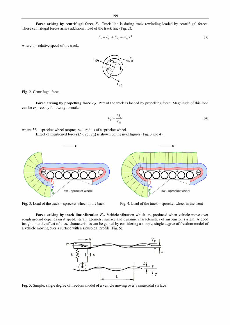
199

Force arising by centrifugal force Fc . Track line is during track rewinding loaded by centrifugal forces. These centrifugal forces arises additional load of the track line (Fig. 2):

221 vmFFF teooc =+= (3)

where v – relative speed of the track.

Fig. 2. Centrifugal force

Force arising by propelling force Fp . Part of the track is loaded by propelling force. Magnitude of this load

can be express by following formula:

hk

kp r

MF = (4)

where Mk – sprocket wheel torque; rhk – radius of a sprocket wheel. Effect of mentioned forces (Ft , Fc , Fp) is shown on the next figures (Fig. 3 and 4).

Fig. 3. Load of the track – sprocket wheel in the back Fig. 4. Load of the track – sprocket wheel in the front

Force arising by track line vibration Fv . Vehicle vibration which are produced when vehicle move over

rough ground depends on it speed, terrain geometry surface and dynamic characteristics of suspension system. A good insight into the effect of these characteristics can be gained by considering a simple, single degree of freedom model of a vehicle moving over a surface with a sinusoidal profile (Fig. 5).

Fig. 5. Simple, single degree of freedom model of a vehicle moving over a sinusoidal surface

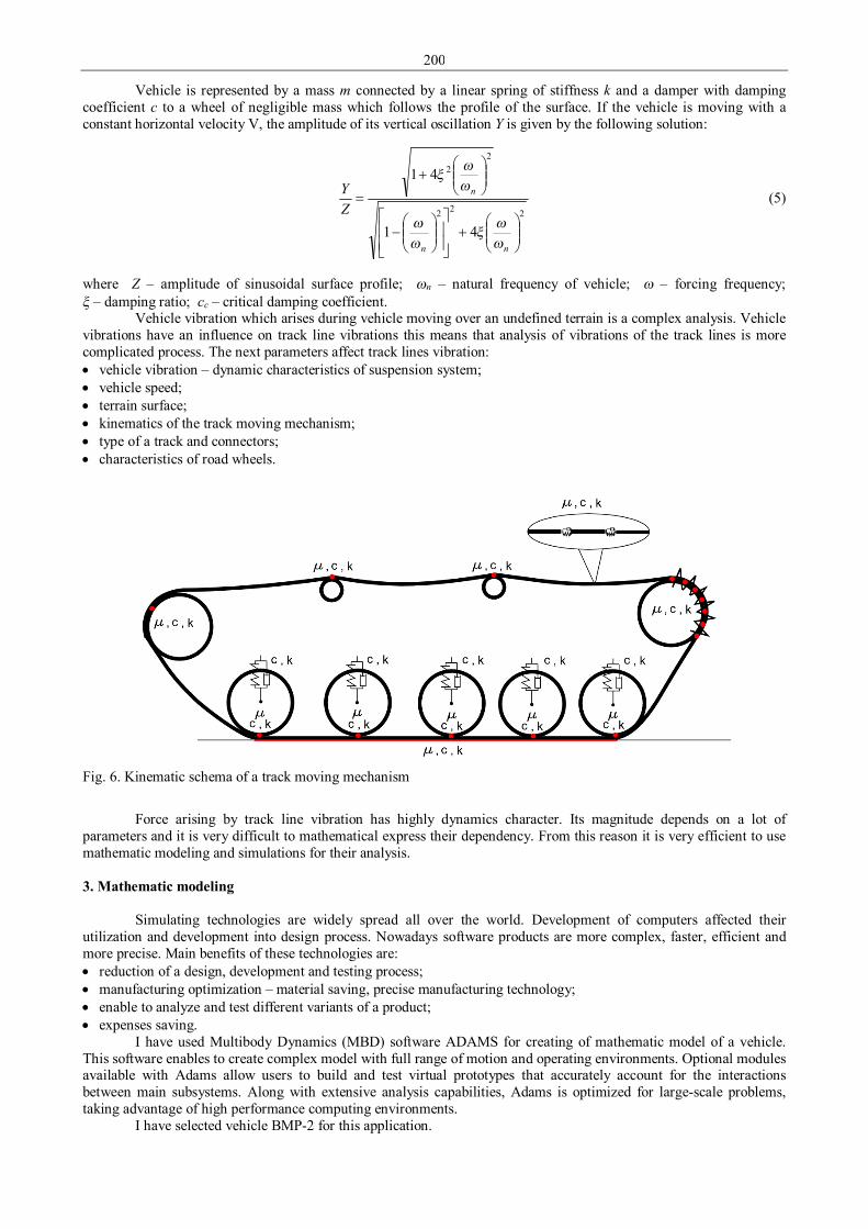
200

Vehicle is represented by a mass m connected by a linear spring of stiffness k and a damper with damping coefficient c to a wheel of negligible mass which follows the profile of the surface. If the vehicle is moving with a constant horizontal velocity V, the amplitude of its vertical oscillation Y is given by the following solution:

222

22

41

41

+

−

+

=

nn

n

ZY

ωωξ

ωω

ωωξ

(5)

where Z – amplitude of sinusoidal surface profile; ωn – natural frequency of vehicle; ω – forcing frequency; ξ – damping ratio; cc – critical damping coefficient.

Vehicle vibration which arises during vehicle moving over an undefined terrain is a complex analysis. Vehicle vibrations have an influence on track line vibrations this means that analysis of vibrations of the track lines is more complicated process. The next parameters affect track lines vibration: • vehicle vibration – dynamic characteristics of suspension system; • vehicle speed; • terrain surface; • kinematics of the track moving mechanism; • type of a track and connectors; • characteristics of road wheels.

Fig. 6. Kinematic schema of a track moving mechanism

Force arising by track line vibration has highly dynamics character. Its magnitude depends on a lot of

parameters and it is very difficult to mathematical express their dependency. From this reason it is very efficient to use mathematic modeling and simulations for their analysis. 3. Mathematic modeling

Simulating technologies are widely spread all over the world. Development of computers affected their utilization and development into design process. Nowadays software products are more complex, faster, efficient and more precise. Main benefits of these technologies are: • reduction of a design, development and testing process; • manufacturing optimization – material saving, precise manufacturing technology; • enable to analyze and test different variants of a product; • expenses saving.

I have used Multibody Dynamics (MBD) software ADAMS for creating of mathematic model of a vehicle. This software enables to create complex model with full range of motion and operating environments. Optional modules available with Adams allow users to build and test virtual prototypes that accurately account for the interactions between main subsystems. Along with extensive analysis capabilities, Adams is optimized for large-scale problems, taking advantage of high performance computing environments.

I have selected vehicle BMP-2 for this application.

201

Main parameters of the vehicle BMP-2: • combat weight 13900 kg; • max engine power 221 kW; • max engine torque 980 Nm; • track lines distance 2550 mm; • track width 300 mm; • length of track surface in touch with ground 3600 mm; • max speed 65 km/h; • width of a straight-walled ditches 2500 mm; • height of the step obstacle 700 mm.

Fig. 7. vehicle BMP-2

Created mathematic model of vehicle consists of:

• chassis; • 2× sprocket wheel; • 2× idler; • 12× road wheel; • 6× support roll; • 2× track line (85 track segments); • ground.

Fig. 8. Mathematic model of the vehicle BMP-2

For different simulations and basic analysis of the load was created next types of terrain:

• flat terrain with small bumpiness – unpaved road (Fig. 9); • bumpy road (Fig. 10); • road with step obstacle and straight-walled ditches (Fig. 11); • road with transverse sills (height 100 mm, length 100 mm, spacing 1000 mm) (Fig. 12).

202

Fig. 9. Unpaved road

Fig. 10. Bumpy road

Fig. 11. Step obstacle and straight-walled ditches

Fig. 12. Transverse sills

Physical parameters of the terrain meet the requirements of strengthened road = minimal deformations of the

road → stress of the main parts of the chassis is maximal, on this type of the ground. Propulsion system is active – keeps defined vehicle speed by torque change.

4. Simulations

Basic parameters of simulations were set: • The unpaved road – this terrain consists of two parts. 1st part is flat road (length 114 m) and 2nd part is unpaved road

(length 65 m, maximal height of bump 20 mm): o Vehicle speed 40 km/h, length of the simulation 14 s; o Vehicle speed 65 km/h, length of the simulation 9 s.

• The bumpy road – length of the road 80m, vehicle speed 40 km/h, length of the simulation 6 s.

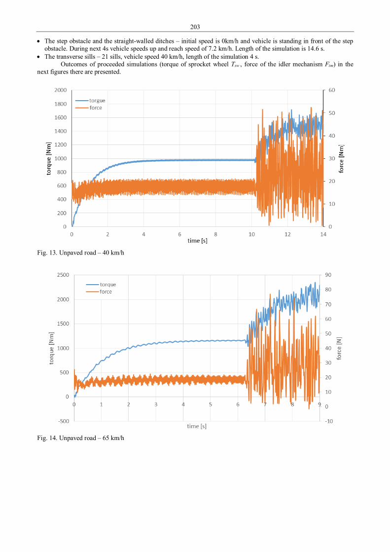
203

• The step obstacle and the straight-walled ditches – initial speed is 0km/h and vehicle is standing in front of the step obstacle. During next 4s vehicle speeds up and reach speed of 7.2 km/h. Length of the simulation is 14.6 s.

• The transverse sills – 21 sills, vehicle speed 40 km/h, length of the simulation 4 s. Outcomes of proceeded simulations (torque of sprocket wheel Tsw , force of the idler mechanism Fim) in the

next figures there are presented.

Fig. 13. Unpaved road – 40 km/h

Fig. 14. Unpaved road – 65 km/h

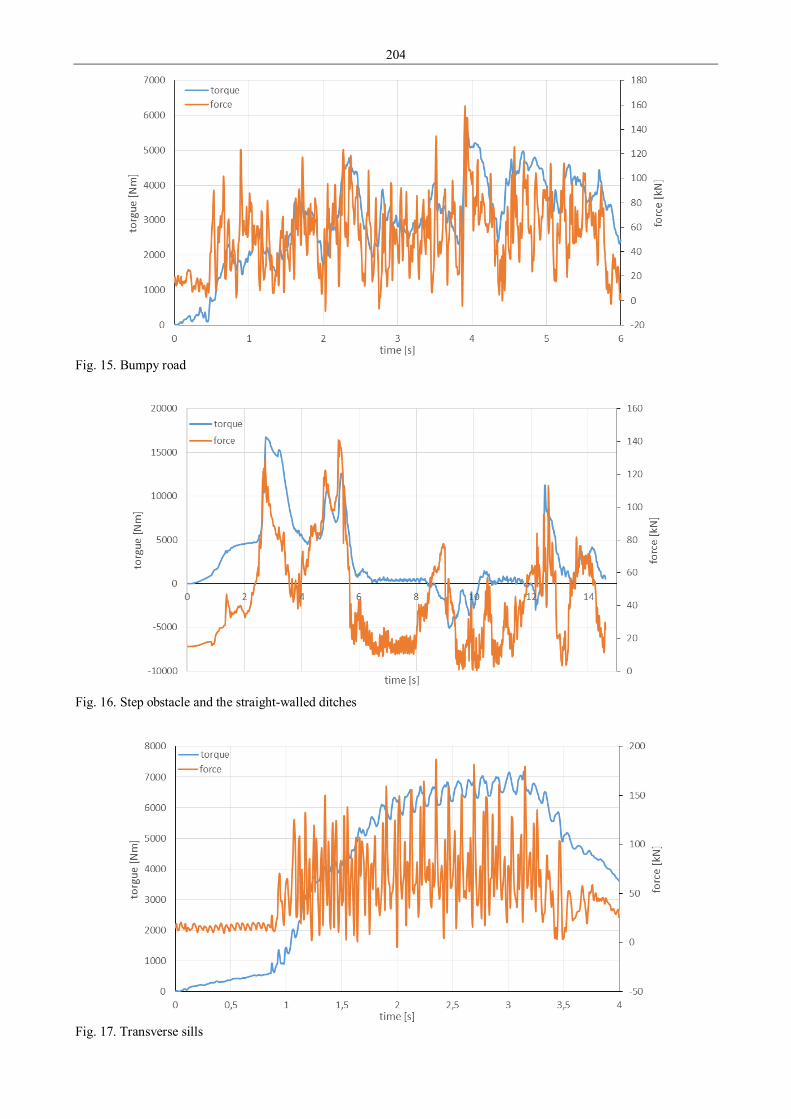
204

Fig. 15. Bumpy road

Fig. 16. Step obstacle and the straight-walled ditches

Fig. 17. Transverse sills

205

5. Conclusion

Sprocket wheel of tracked vehicles is loaded by forces arising by track tightening, by centrifugal force, by propelling force and by vibration of track lines. Vibrations of track lines highly dynamically load transmission system. Track line vibrations affect vehicle vibrations, vehicle speed, terrain surface, parameters of the chassis, type of a track and connectors and parameters of road wheels. The vehicle consists of a lot of movable parts, attachments and contacts defined by stiffness and damping. Magnitude and course of this dynamics stress depend on a lot of parameters and it is very difficult to mathematical express their dependency. From this reason it is very efficient to use mathematic modeling and simulations for analysis of stress of transmissions of tracked vehicles.

Simulating technologies offer a lot of advantages – e.g. evaluation of stress of the main parts of vehicle, evaluation of various vehicle configurations, simulation of various critical states of vehicle, comparison of vehicles in the same surrounding. On the other side for their usage must be done some development – this manner is sensitive to input data (their insufficient or lack of them).

For analysis of stress of sprocket wheel of track vehicle (load of transmission) was used Multibody Dynamics software ADAMS of MSC Software. For application of this manner was selected vehicle BMP-2. Simulation were proceeded on four types of terrain – unpaved road, bumpy road, step obstacle and straight-walled ditches and road with transverse sills. Torque of sprocket wheel (Tsw) and force of idler mechanism (Fim) were analyzed during the simulations.

From outcomes it is possible to make next conclusions: • course of sprocket wheel torque and force of idler mechanism have highly dynamic character; • maximal magnitudes of stress were measured: o unpaved road – speed 40 km/h – Tsw = 1715 Nm; Fim = 52 kN; o unpaved road – speed 65 km/h – Tsw = 2350 Nm; Fim = 95 kN; o bumpy road – Tsw = 5780 Nm; Fim = 157 kN; o step obstacle and straight-walled ditches – Tsw = 16 760 Nm; Fim = 140 kN; o transverse sills – Tsw = 7180 Nm; Fim = 186 kN;

• max load of the sprocket wheel was on step obstacle; • stress of the sprocket wheel on the step obstacle was 9.7 times higher than the stress on unpaved road with speed

40 km/h and 7.1 times higher than on unpaved road with max speed 65 km/h. Acknowledgement

Presented work has been prepared with the support of the Ministry of Defence of the Czech Republic, Partial Project for Institutional Development, K-202, Department of Combat and Special Vehicles, University of Defence, Brno. References 1. Ogorkiewicz R. M. Technology of tanks. Coulsdon, Surrey: Jane's Information Group, 1991, 2 v. (424 p.).

ISBN 07-106-0595-1. 2. Kolybelík I. Bojová pásová vozidla: Mechanika pohybu. Brno: Vojenská akademie, 1985, 412 s. 3. Allied vehicle testing publications. AVTP-1. 1994. 839P. 4. MCS.software [online]. Available from: < http://www.mscsoftware.com/product/adams > [cit. 2014-03-27]. 5. VOP CZ [online]. Available from: < http://www.vop.cz/cz/produkt/45-002-bvp-bmp.aspx > [cit. 2014-03-28].

206

Proceedings of 9th International Conference ITELMS’2014 Decisions of the Applied Tasks of External Ballistics A. Pincevicius*, V. Jonevicius**, S. Bekesiene* * The General Jonas Žemaitis Military Academy of Lithuania, Silo 5A, LT-10322 Vilnius, Lithuania, E-mail: pincev@cablenet.lt, svajone.bekesiene@mil.lt **Vilniaus Gedimino Technical University, Silo 5A, LT-10322 Vilnius, Lithuania, E-mail: vaclovas.jonevicius@vgtu.lt Abstract The problem of external ballistics is analysed. Features of shooting on a mountainous terrain are discussed. Values of the angles are found when there is a significant height difference between the opponents. Is analyzed a dispersion of submachine-gun bullets and hitting probability when a soldier is following various tactics in the battlefield. Possibilities of reducing the losses during the attack are also discussed. KEYWORDS: external ballistic, shooting on a mountainous terrain, dispersion of bullets, hitting probability. 1. Introduction

The article presents the decisions of some tasks of external ballistic. Features of shooting on a mountainous area are analyzed. Currently, localized battles are going on usually when several tens of soldiers are involved and the actions of each of them important become decisive and in the course of battle. Often fighting is going on in a village and the distances between the fighting opponents are small. In the article the assessment of the dispersion of submachine-gun bullets is made in accordance with the tactics of the attack. 2. Solution of the external ballistics task

External ballistics describes the movement of the bullets fired in the air, including all the factors affecting it. The main task is to identify what should be the elevation angle of the machine gun’s barrel, so that the bullet hits the foreseen point. Based on the solution of external ballistics’ task, tables are made for small arms of the riflemen [1-5].

Fired at the initial speed V0 , the bullet continues moving by inertia. Gravity force mg and resistance force Fp make a significant impact on the bullet moving in the air (see Fig. 1). Component Fpy of the air resistance force Fp stops the bullet’s movement upwards, and the component Fpy stops the bullet’s movement in the direction of x-axis, i.e. towards the target.

Fig. 1. Forces influencing the bullet moving in the air, components of the bullet‘s velocity. The pointing line (straight

line running from the rifleman's eye through the back sight to the target point) is reflected in dots and coincides with the x-axis, α – angle of sight, i.e. the angle between the elevation line (gun barrel direction) and lines of sight

The bullet’s movement is described by two second-order differential equations:

2

,2

2

,2

px

py

d xm Fdtd ym mg Fdt

= −

= − −

(1)

at the initial conditions:

'0(0) 0, (0) cos ,tx X V α= = '

0(0) 0, (0) sinty Y V α= = . (1a)

where: m – mass of the projectile; t – time; other markings apparent from Fig. 1.

V0 Vx0

Vy0

α

Fpy mg

Fpx

0

x

y

Fp

207

Air resistance force Fp depends on the bullet’s calibre and shape. It is described by an empirical formula [1-3]:

yp FyHg

dkF )(1000 2

= (2)

where: k – the form factor (it is close to 0.5); d – bore, m; g = 9.81 m/s2 – free fall acceleration; H(y) – correction due to environmental parameters change with increasing altitude (usually H(y) ≈ 1). Expression of the component of environment resistance force Fv that depends on the bullet’s velocity. When the bullet’s velocity is higher than the speed of sound in air (V > 330 m/s), the component shall bear the empirical formula:

803

−= VFv (2a)

If the speed is lower (V < 330 m/s) then

241021.1 VFv−⋅= (3)

When shooting in the plains, where the height difference between the rifleman and the target ∆h does not exceed ten meters, the speed component V0y is small and the environmental resistance force component Fpy may not be applied [1-5]. 3. Peculiarities of firing on a mountainous terrain

Even when firing with a submachine-gun on a mountainous area the pointing angle is relatively small and the speed component V0y < 330 m/s. Differential equations system (1) having considered formulas (2), (2a) and (3) is expressed as follows:

2 20

2

24 2

02

1000 80 ,3

1,21 10 .

x

y

Vd x kdmdt gd ym mg Vdt

−

= − − = − − ⋅

If the target distance is 400 m, the height difference between the rifleman and the target h = 100 m, we get the following shooting parameters (see Fig. 2 and 3): angle of sight α = 144 mils (8.64°), flying time = 0.67 s, speed of the bullet at the point of the target = 494 m/s (AK 4, V0 = 790 m/s), throwing angle β = 378 mils (22.7°).

When shooting on a plain territory, the bullet would drop at 2.5 km. Bullets’ dispersion is changing (see Fig. 5.), hitting probability decreases. Above we shall give the calculation angles of sight and other parameters when firing on a mountainous area (Tab. 1).

Fig. 2. Trajectory of the bullet of a machine gun: target

(marked in an asterisk) is in 400 m distance, the height difference ∆h = 100 m, α – pointing angle

Fig. 3. The trajectory of the bullet’s movement, if shooting in going on in the plain (β as – throwing angle, i.e. the angle between the horizon and the gun barrel direction)

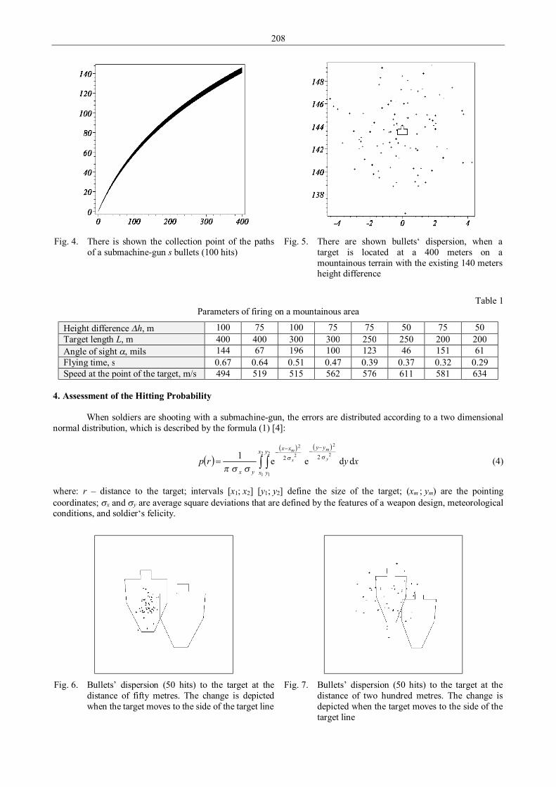
208

Fig. 4. There is shown the collection point of the paths

of a submachine-gun s bullets (100 hits) Fig. 5. There are shown bullets‘ dispersion, when a

target is located at a 400 meters on a mountainous terrain with the existing 140 meters height difference

Table 1

Parameters of firing on a mountainous area

Height difference ∆h, m 100 75 100 75 75 50 75 50 Target length L, m 400 400 300 300 250 250 200 200 Angle of sight α, mils 144 67 196 100 123 46 151 61 Flying time, s 0.67 0.64 0.51 0.47 0.39 0.37 0.32 0.29 Speed at the point of the target, m/s 494 519 515 562 576 611 581 634

4. Assessment of the Hitting Probability

When soldiers are shooting with a submachine-gun, the errors are distributed according to a two dimensional normal distribution, which is described by the formula (1) [4]:

( )( ) ( )

∫ ∫−

−−−

=2

1

2

1

2

2

2

2

ddee1 22x

x

y

y

yyxx

yxxyrp y

m

x

mσσ

σσπ (4)

where: r – distance to the target; intervals [x1; x2] [y1; y2] define the size of the target; (xm ; ym) are the pointing coordinates; σx and σy are average square deviations that are defined by the features of a weapon design, meteorological conditions, and soldier‘s felicity.

Fig. 6. Bullets’ dispersion (50 hits) to the target at the

distance of fifty metres. The change is depicted when the target moves to the side of the target line

Fig. 7. Bullets’ dispersion (50 hits) to the target at the distance of two hundred metres. The change is depicted when the target moves to the side of the target line

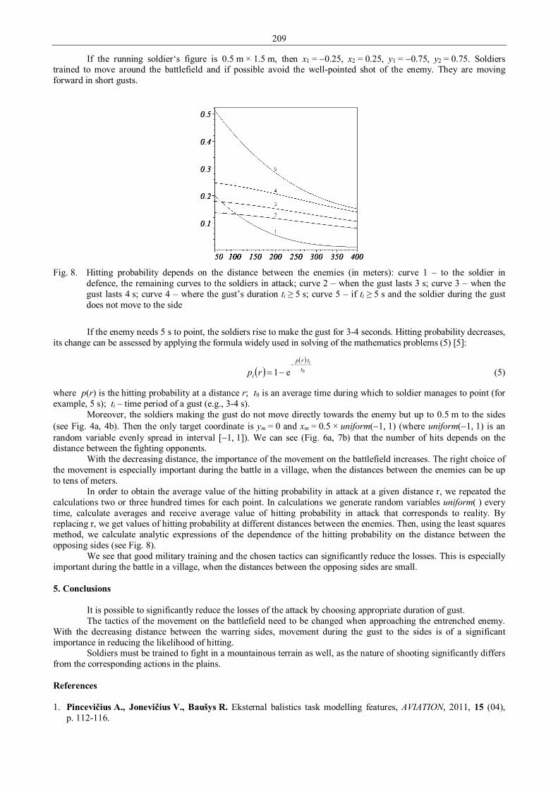
209

If the running soldier‘s figure is 0.5 m × 1.5 m, then x1 = −0.25, x2 = 0.25, y1 = −0.75, y2 = 0.75. Soldiers trained to move around the battlefield and if possible avoid the well-pointed shot of the enemy. They are moving forward in short gusts.

Fig. 8. Hitting probability depends on the distance between the enemies (in meters): curve 1 – to the soldier in

defence, the remaining curves to the soldiers in attack; curve 2 – when the gust lasts 3 s; curve 3 – when the gust lasts 4 s; curve 4 – where the gust’s duration ti ≥ 5 s; curve 5 – if ti ≥ 5 s and the soldier during the gust does not move to the side

If the enemy needs 5 s to point, the soldiers rise to make the gust for 3-4 seconds. Hitting probability decreases,

its change can be assessed by applying the formula widely used in solving of the mathematics problems (5) [5]:

( )( )

0e1 ttrp

i

i

rp−

−= (5)

where p(r) is the hitting probability at a distance r; t0 is an average time during which to soldier manages to point (for example, 5 s); ti – time period of a gust (e.g., 3-4 s).

Moreover, the soldiers making the gust do not move directly towards the enemy but up to 0.5 m to the sides (see Fig. 4a, 4b). Then the only target coordinate is ym = 0 and xm = 0.5 × uniform(−1, 1) (where uniform(−1, 1) is an random variable evenly spread in interval [−1, 1]). We can see (Fig. 6a, 7b) that the number of hits depends on the distance between the fighting opponents.

With the decreasing distance, the importance of the movement on the battlefield increases. The right choice of the movement is especially important during the battle in a village, when the distances between the enemies can be up to tens of meters.

In order to obtain the average value of the hitting probability in attack at a given distance r, we repeated the calculations two or three hundred times for each point. In calculations we generate random variables uniform( ) every time, calculate averages and receive average value of hitting probability in attack that corresponds to reality. By replacing r, we get values of hitting probability at different distances between the enemies. Then, using the least squares method, we calculate analytic expressions of the dependence of the hitting probability on the distance between the opposing sides (see Fig. 8).

We see that good military training and the chosen tactics can significantly reduce the losses. This is especially important during the battle in a village, when the distances between the opposing sides are small. 5. Conclusions

It is possible to significantly reduce the losses of the attack by choosing appropriate duration of gust. The tactics of the movement on the battlefield need to be changed when approaching the entrenched enemy.

With the decreasing distance between the warring sides, movement during the gust to the sides is of a significant importance in reducing the likelihood of hitting.

Soldiers must be trained to fight in a mountainous terrain as well, as the nature of shooting significantly differs from the corresponding actions in the plains. References 1. Pincevičius A., Jonevičius V., Baušys R. Eksternal balistics task modelling features, AVIATION, 2011, 15 (04),

p. 112-116.

210

2. Pincevičius A., Jonevičius V. Simulation in the military field. Proceedings of the 16th International Conference. Means of Transport, 2012, p. 281-285.

3. Pincevičius A., Baušys R., Bekesiene S., Kleiza V. The Intelligent Technologies Aplication for Artillery Control. Proceedings of the 4th International Conference. ITELMS’9, 2009, p. 164-169.

4. Pincevičius A., Baušys R., Bekesiene S., Kleiza V. The Effective Use of the Intelligent Technologies in Planning Infantry Attacks. Proceedings of the 4th International Conference. ITELMS’9, 2009, p. 169-174.

5. Misevičius G., Pincevičius A., Eidukevičius R., Rakauskas R. -J. Higher mathematics textbook and exercises with the computer. TEV, 1999, 469 p.

6. Венцель Е. С. Исследование операций. ”Москва Советское радио“, 1972, – 551 с.

211

Proceedings of 9th International Conference ITELMS’2014 Influence of Installation of Different Types of Bored Piles to the Ground T. Poska*, S. Susinskas**, J. Valickas*** *Kaunas University of Technology, Klaipedos str. 27-425, 35214, Panevezys, Lithuania, E-mail: tposka201@gmail.com **Kaunas University of Technology, Daukanto str. 12, 44556, Panevezys, Lithuania, E-mail: saulius.susinskas@ktu.lt ***Kaunas University of Technology, Daukanto str. 12, 44556, Panevezys, Lithuania, E-mail: jonas.valickas@ktu.lt Abstract This paper gives the information about the main influences of installation of 4 different types of bored piles models to the ground. Also, the verification of selected 1 type auger for progress development (AF auger) in new soil conditions is presentet. The most important is changes in soil properties and stress conditions during installation of pile. Also there are given compares of CFA, ASD and FSD pile models behavior: • AFP screwing in AF auger and pulling out none rotating while concreting. It was corrected according possibilities of

rig into screwing in AF auger and pulling out rotating in the same direction while concreting [2]. • AFS screwing in AF auger and unscrewing it while concreting [2]. • CFA screwing in CFA auger and pulling out none rotating while concreting [2]. • FDP pushing in prefabricated steel tube pile model with separate measurement base and shaft [2]. KEYWORDS: CFA pile, AFS pile, AFP pile, soil, model. 1. Introduction

Pile foundations are used to carry and transfer the whole load of the structure to the bearing ground located at some depth below ground surface. The main components of the foundation are the pile cap and the piles. Piles are long and slender members which transfer the load to deeper soil or rock of high bearing capacity avoiding shallow soil of low bearing capacity. On purpose to investigate changes in soil properties and stress conditions during installiation of pile model was conctructed the sand testing box with gages. Test box was filled by layers 0.5 m thickness and compacted by vibrator (BP 25/48 D). 2. Instruments and preparation used in the investigation

For the soil field testing was used one CPT and DPT near a centre of pile model location. Two CPT and one DPT close to installed pile model after setting of it concrete.

For measurement of changes in the ground were used gages in 4 locations of pile models equipped with 3 EPC (Geokon 4500VW) at a depth 1.50 m, 2,25 m and 3.00 m in a distance about 30 cm from pile model surface.

For the pile model instrumentation was used 2 strain gages (Geokon 4200VW) at 3 levels: • near top of pile; • near tip of pile; • in medium of pile length.

For the installation of pile models were used: • Pump ‘Putzmeister’ with adjustable flow ranging 0-60 l/min; • Augers: o -AF pitch 11 cm; o -CFA pitch 11 cm;

• Rig Foreuse; • Instrumentation record ENBESOL; • Geokon dataloger for EPC.

The composition of concrete mixture used for 1 m3: • Cement CEM I 42.5 470 kg; • Microsilica 80 kg; • Sand 0/4 425 kg; • Sand 0/1 1025 kg; • Water 245 l; • Dispersant 1.2 kg; • MAPE FLUID X404 5.875 kg.

Concrete compressive strength, after 7 days was 30.7 (29.0-31.6) MPa and after 28 days it was 39.7 (36.2-41.8) MPa. In the box filled sand could be described as medium to fine silty sand (Fig. 1) [1].

Also, the density of each layer was determined (Tab. 1).

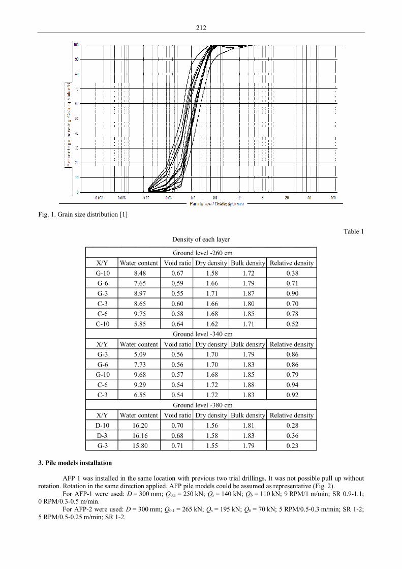
212

Fig. 1. Grain size distribution [1]

Table 1 Density of each layer

3. Pile models installation

AFP 1 was installed in the same location with previous two trial drillings. It was not possible pull up without rotation. Rotation in the same direction applied. AFP pile models could be assumed as representative (Fig. 2).

For AFP-1 were used: D = 300 mm; Q0.1 = 250 kN; Qs = 140 kN; Qb = 110 kN; 9 RPM/1 m/min; SR 0.9-1.1; 0 RPM/0.3-0.5 m/min.

For AFP-2 were used: D = 300 mm; Q0.1 = 265 kN; Qs = 195 kN; Qb = 70 kN; 5 RPM/0.5-0.3 m/min; SR 1-2; 5 RPM/0.5-0.25 m/min; SR 1-2.

X/Y Water content Void ratio Dry density Bulk density Relative densityG-10 8.48 0.67 1.58 1.72 0.38 G-6 7.65 0,59 1.66 1.79 0.71 G-3 8.97 0.55 1.71 1.87 0.90 C-3 8.65 0.60 1.66 1.80 0.70 C-6 9.75 0.58 1.68 1.85 0.78 C-10 5.85 0.64 1.62 1.71 0.52

X/Y Water content Void ratio Dry density Bulk density Relative densityG-3 5.09 0.56 1.70 1.79 0.86 G-6 7.73 0.56 1.70 1.83 0.86 G-10 9.68 0.57 1.68 1.85 0.79 C-6 9.29 0.54 1.72 1.88 0.94 C-3 6.55 0.54 1.72 1.83 0.92

X/Y Water content Void ratio Dry density Bulk density Relative densityD-10 16.20 0.70 1.56 1.81 0.28 D-3 16.16 0.68 1.58 1.83 0.36 G-3 15.80 0.71 1.55 1.79 0.23

Ground level -260 cm

Ground level -340 cm

Ground level -380 cm

213

AFP-2 AFP-3

AFP-1

AFS-1

AFS-2 AFS-3

AFS-4

CFA-1

CFA-2

Fig. 2. AFP piles models [1]

Fig. 3. AFP piles models parameters [1]

For AFP-3 were used: D = 300 mm; Q0.1 = 280 kN; Qs = 215 kN; Qb = 70 kN; 5 RPM/0.5-0.3m/min; SR 1-2;

5 RPM/0.5-0.25 m/min; SR 1-2. For AFS-1 were used: D = variable 200-500 mm; Q0.1 = 400 kN; Qs = 365 kN; Qb = 35 kN;

3-2 RPM/0.3-0.1 m/min; SR 1-2; 2-3 RPM/0.2-0.5; UR 0.5-1. For AFS-2 were used: D = variable 220-300 mm; Q0.1 = 400 kN; Qs = 345 kN; Qb = 55 kN;

3-2.5 RPM/0.5-0.2 m/min; SR 0.5-2; 3-2.5 RPM/0.3 m/min; UP 0.7-1. For AFS-3 were used: D = variable 200-280 mm; Q0.1 = 340 kN; Qs = 320 kN; Qb = 20 kN;

5 RPM/0.5-0.2 m/min; SR 1-2; 5 RPM/0.3-0.5 m/min; UR 1-2. For AFS-4 were used: D = variable 250-160 mm; Q0.1 = 375 kN; Qs = 260 kN; Qb = 115 kN;

15 RPM/0.7-0.4 m/min; SR 2.5-4.0; 7.5 RPM/0.5 m/min; UR 1-2.

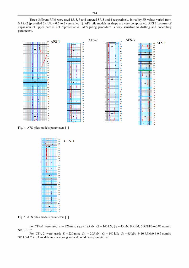
214

Three different RPM were used 15, 5, 3 and targeted SR 5 and 1 respectively. In reality SR values varied from 0.5 to 2 (prevailed 2), UR – 0.5 to 2 (prevailed 1). AFS pile models in shape are very complicated. AFS 1 because of expansion of upper part is not representative. AFS piling procedure is very sensitive to drilling and concreting parameters.

Fig. 4. AFS piles models parameters [1]

Fig. 5. AFS piles models parameters [1]

For CFA-1 were used: D = 220 mm; Q0.1 = 185 kN; Qs = 140 kN; Qb = 45 kN; 9 RPM; 5 RPM/0.6-0.85 m/min;

SR 0.7-0.9. For CFA-2 were used: D = 220 mm; Q0.1 = 205 kN; Qs = 140 kN; Qb = 65 kN; 9-10 RPM/0.6-0.7 m/min;

SR 1.5-1.7. CFA models in shape are good and could be representative.

AFS-2 AFS-3

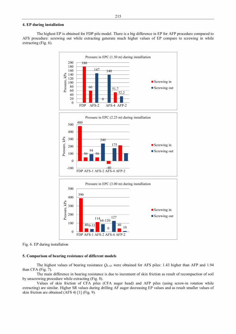
215

4. EP during installation

The highest EP is obtained for FDP pile model. There is a big difference in EP for AFP procedure compared to AFS procedure: screwing out while extracting generate much higher values of EP compare to screwing in while extracting (Fig. 6).

180

60

147

0

140

51,732,2

020406080

100120140160180200

Pres

sure

, kPa

FDP AFS-2 AFS-4 AFP-2

Pressure in EPC (1.50 m) during installiation

Screwing in

Screwing out

480

5094

50

240

-40

175

-100

0

100

200

300

400

500

Pres

sure

, kPa

FDP AFS-1 AFS-2 AFS-4 AFP-2

Pressure in EPC (2.25 m) during installiation

Screwing in

Screwing out

390

400-33

11464-120

0

127

4010

0

100

200

300

400

500

Pres

sure

, kPa

FDP AFS-1 AFS-2 AFS-4 AFP-2

Pressure in EPC (3.00 m) during installiation

Screwing in

Screwing out

Fig. 6. EP during installation

5. Comparison of bearing resistance of different models

The highest values of bearing resistance Q0.1D were obtained for AFS piles: 1.43 higher than AFP and 1.94 than CFA (Fig. 7).

The main difference in bearing resistance is due to increment of skin friction as result of recompaction of soil by unscrewing procedure while extracting (Fig. 8).

Values of skin friction of CFA piles (CFA auger head) and AFP piles (using screw-in rotation while extracting) are similar. Higher SR values during drilling AF auger decreasing EP values and as result smaller values of skin friction are obtained (AFS 4) [1] (Fig. 9).

216

250 265 280

400 400

340375

185 205

345

050

100150200250300350400450

Q 0.1D, kN

AFP-1 AFP-2 AFP-3 AFS-1 AFS-2 AFS-3 AFS-4 CFA-1 CFA-2 FDP Fig. 7. Bearing resistance

140195 215

265

345320

360

140 140 155

050

100150200250300350400

Qs, kN

AFP-1 AFP-2 AFP-3 AFS-1 AFS-2 AFS-3 AFS-4 CFA-1 CFA-2 FDP Fig. 8. Increment of skin friction

5967 74

0

128 124

95

70 6376

0

20

40

60

80

100

120

140fs, kN

AFP-1 AFP-2 AFP-3 AFS-1 AFS-2 AFS-3 AFS-4 CFA-1 CFA-2 FDP Fig. 9. Values of skin friction

6. Conclusions

The highest values of bearing resistance were obtained for AFS piles. This is as result of compaction and stress increase during screwing-out of AF tool. AFS pile with SR ≥ 3 during drilling-in show less values of skin friction. Shape of AFS piles are very sensitive to drilling and concreting parameters. The highest value of relative bearing resistance was obtained for FSD pile. Skin friction values of CFA and AFP piles are similar. The largest influence on the neighbouring soil is induced by FDP pile. EP values is about twice of that AF values. References 1. Furmanavičius L. Small scale testing. VGTU. 2. Sližytė D., Medzvieckas J., Mackevičius R. Pamatai ir pagrindai. – Vilnius: Technika, 2012. 248 p.

217

Proceedings of 9th International Conference ITELMS’2014 Ripples Formation on the Silicon Solar Cells Surface by Laser Irradiation E. Shatkovskis, V. Zagadskij, A. Jukna, J. Stupakova Department of Physics, Vilnius Gediminas Technical University, Sauletekio al. 11, LT-10223, Vilnius, Lithuania Abstract The surface and electric properties of the monocrystalline silicon solar cell treated by means of focused light from a 20-ns-pulsed YAG:Nd3+ laser (λ = 1.064 µm) at repetition rate of 12.5 Hz have been investigated. The laser beam was focused down to spot size of 1.2 × 0.04 mm2 by means of optical condenser consisting of spherical and cylindrical lenses onto surface of the solar cell in the area between two nearest contacts of the contact grid. Optical beam power was used in a sequence of 0.14 mW, 0.35 mW, 0.44 mW, 0.48 mW, 0.52 mW and 0.76 mW. The reference and laser treated samples cut from a single solar cell have been investigated experimentally by measuring current-voltage characteristics in dark and under illumination by a 5000 K Xenon lamp. Laser fluence greater than 4.5 mW/mm2 per pulse forms ripples on the sample surface along the length of the laser beam spot and repetitive along the beam scanning directions. The results of our electric measurements and images taken by optical microscope are presented and discussed. KEYWORDS: silicon solar cells, laser processing, ripples formation, current-voltage characteristics. 1. Introduction

Solar photovoltaic is one of the most important renewable energy sources in terms of globally installed capacity. The 102 GW installed capacity has been achieved in 2012 [1]. The advantages of photovoltaic become especially promised when talking about Building-Integrated Photovoltaic [2] which is one of the latest developments of photovoltaic technology to ensure green energy.

Crystalline silicon based solar cells still play a major role in the solar cells market. Considerable progress has been achieved in improving silicon solar cells technology increasing their efficiency. Laboratory-derived silicon solar cell efficiency of energy conversion is about 25 % however the efficiency of industrial solar cells does not exceed 20% [3]. Theoretical limit of the conversion efficiency for crystalline silicon solar cells is considered to be at 31 % [4]. The goal of research and development of the silicon solar cells is to reach mentioned theoretical limit and make solar cells more competitive with other existing sources of renewable energy.

An increase of energy conversion efficiency of the silicon solar cells can be reached by reducing their surface reflectivity, increasing minority carrier collection efficiency in short wavelength spectral range and increasing light absorbance of photon energies near the silicon band-gap energy by means of surface texturing. Silicon surface processing by means of ultra-short laser pulses [5-8] is one of the most efficient methods for decreasing reflectivity and increasing of absorbance of silicon solar cells. Operating with femtosecond or picosecond optical pulses one can expect a minimal influence of such processes as heat propagation through the planar p-n junction and recrystallization of heated material while it interacts with incident light. However, as it was shown in Ref. 9, the processing of surface of silicon (or other semiconductors) by means of nanosecond-optical-pulses enables to obtain surface structures in which quantum confinement effect has been observed [9].

The main purpose of our experiments is to demonstrate effect of nanosecond optical pulses incident onto surface of a silicon solar cell. For samples processing we used a pulsed YAG:Nd3+ laser, with pulse duration at FWHM around 20 ns at 12.5 Hz repetition rate of pulses. The results of measurements of surface morphology, of efficiency of energy conversion and of electrical properties of laser modified solar cells are discussed in current work. 2. Experiment

The silicon solar cells for our experiments were manufactured out of p-type, 200-μm-thick mono-crystalline silicon (100) wafer. The front surface of the solar cell was textured in the form of the regular inverse pyramids with facets and depth dimensions about of about 5 μm. The 0.25 ÷ 0.3 μm thick, n-type silicon emitter was made by means of phosphorus diffusion procedure. Continuous lower and the grid upper contacts were manufactured by room temperature sputtering of silver in a vacuum chamber. Finally, surface of the cell was protected by silicon nitride layer, which thickness was tens of nanometers.

For laser treatment procedures, a selected solar cell was cut into samples. Each sample contained bottom contact, two stripes of contact grid on its top surface and optically active area for energy conversion of 20 mm2 in between them. Pulsed YAG:Nd3+ laser with pulse duration at FWHM of 20 ns and repetition rate of pulse at 12.5 Hz has been used for surface of each sample processing. The laser beam power was controlled by changing both the YAG:Nd3+ excitation as well as neutral optical filters. This combination has allowed us to fairly small steps precisely controlling averaged output power of laser at 0.14 mW, 0.35 mW, 0.44 mW, 0.48 mW, 0.52 mW and 0.76 mW. The

218

laser beam was focused by optical condenser consisting of spherical and cylindrical lenses into area between two stripes of contact grids. Thus, the spot of the laser beam had a shape of the ~1.2 mm-long and ~40 µm-wide stretched rectangular with approximate area of ~0.05 mm2. Each sample was mounted onto X-Y stage which moves the sample perpendicularly to the laser beam using a computer controlled stepping motor. The sample’s position changing rate was adjusted by stepping motor so that the solar cell areas processed by adjacent pulses overlap no more than one third of beam’s spot area.

The current-voltage characteristics of reference (i.e. no processed by the laser) and treated by laser beam samples were measured in dark and illuminating the sample by Xenon lamp which emits light of 5000 K black-body-radiation spectrum. A computer controlled setup consisting of Tektronix CFG 253, Kethley 2000, Metex MXD 4660 multimeters and Tektronix TDS 3032B oscilloscope has been used for experimental data registration. 3. Results and Discussion

The optical microscope images of surfaces of the reference and modified solar cells are presented in Fig. 1. According to our estimations a surface texture of the reference sample contains pyramids with average height of 5 μm (Fig. 1a).

a

b

c

Fig. 1. Optical-microscope image of the top surface of reference sample (a) and of the sample after its laser treatment using beam’s power of 0.35 mW and 0.6 for the cases (b) and (c), respectively

The image shown in Fig. 1b of the surface modified by means of moderate power P ~ 35 mW of laser beam

shows the ripples (waves) formed along the entire length of the laser spot, and repetitive along beam’s scanning direction. Interaction of laser irradiation with material induced damages of the cell’s surface which were estimated to have a shape of inverted pyramids with a density much lower than that one observed onto surface of reference sample (Fig. 1a). A precise investigation of the surface images let us to estimate the distance between nearest ripples at 23 ÷ 25 μm.

The third part of the image (Fig. 1c) shows the surface of the sample which has been exposed to 0.6 mW power of the laser beam. The figure shows that laser beam modified uniformly surface of the solar cell. The ripples in the images of solar cells are not visible.

Fig. 2 represents the results of the solar cell current-voltage characteristics. The figure contains the current-voltage characteristics of the reference sample and, for comparison, the same characteristics after laser treatment of sample. The figure has four parts a, b, c, and d belonging to 0.14 mW, 0.35 mW, 0.44 mW and 0.52 mW laser beam power, correspondingly.

The current-voltage characteristics of all the samples were measured in the dark and under illumination by Xenon lamp of 15 klx and 44 klx luminous. Fig. 2a shows the current-voltage characteristics of the same sample after treatment at laser beam power of 0.14 mW. The observed current-voltage characteristic completely overlaps the characteristic of the reference sample. One can admit that such laser-fluence is too weak to induce the technological changes in the silicon solar cell material. Needs noting that optical microscope image of the surface also shows no changes of sample surface and fully meets a surface of the reference sample, which is shown in Fig. 1a.

Fig. 2b demonstrates the current-voltage characteristics of identical sample after its laser treatment at laser beam power of 0.35 mW. The characteristics are similar to those ones of reference sample represented in Fig. 1a, as all the samples were cut out from the single wafer of a solar cell. Meanwhile, after the laser treatment of solar cell, its current-voltage characteristics have changed significantly. Our result correlates well with the previously discussed results of changes of the solar cell’s surface.

At increased laser power of 0.44 and 0.52 mW the current-voltage characteristics of laser treated samples drastically changed if compare ones with the same characteristics of reference sample. As it is shown in Fig. 2c and 2d at laser power greater than 0.4 mW the nonlinear current-voltage dependences transfer in to almost linear and samples with p-n junction turns into simple resistors with almost linear current voltage characteristic and resistance almost independent on experimental conditions. Thus, according to our estimations laser fluence equal or greater than 4.5 mW/mm2 can affect irreversible changes of structure and electric characteristics of the solar cell, i.e. distortion of its

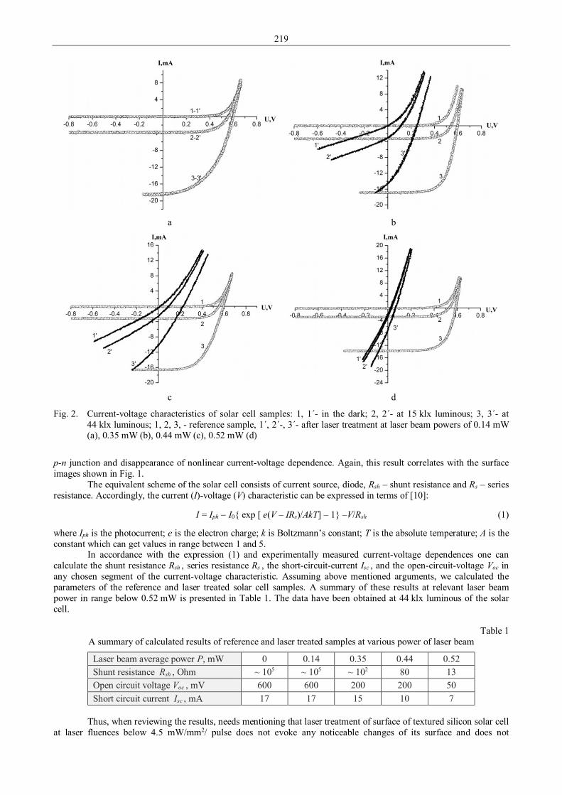
219

a

b

c

d

Fig. 2. Current-voltage characteristics of solar cell samples: 1, 1´- in the dark; 2, 2´- at 15 klx luminous; 3, 3´- at 44 klx luminous; 1, 2, 3, - reference sample, 1´, 2´-, 3´- after laser treatment at laser beam powers of 0.14 mW (a), 0.35 mW (b), 0.44 mW (c), 0.52 mW (d)

p-n junction and disappearance of nonlinear current-voltage dependence. Again, this result correlates with the surface images shown in Fig. 1.

The equivalent scheme of the solar cell consists of current source, diode, Rsh – shunt resistance and Rs – series resistance. Accordingly, the current (I)-voltage (V) characteristic can be expressed in terms of [10]:

I = Iph − I0{ exp [ e(V – IRs)/AkT] – 1} –V/Rsh (1)

where Iph is the photocurrent; e is the electron charge; k is Boltzmann’s constant; T is the absolute temperature; A is the constant which can get values in range between 1 and 5.

In accordance with the expression (1) and experimentally measured current-voltage dependences one can calculate the shunt resistance Rsh , series resistance Rs , the short-circuit-current Isc , and the open-circuit-voltage Voc in any chosen segment of the current-voltage characteristic. Assuming above mentioned arguments, we calculated the parameters of the reference and laser treated solar cell samples. A summary of these results at relevant laser beam power in range below 0.52 mW is presented in Table 1. The data have been obtained at 44 klx luminous of the solar cell.

Table 1 A summary of calculated results of reference and laser treated samples at various power of laser beam

Laser beam average power P, mW 0 0.14 0.35 0.44 0.52 Shunt resistance Rsh , Ohm ~ 105 ~ 105 ~ 102 80 13 Open circuit voltage Voc , mV 600 600 200 200 50 Short circuit current Isc , mA 17 17 15 10 7

Thus, when reviewing the results, needs mentioning that laser treatment of surface of textured silicon solar cell

at laser fluences below 4.5 mW/mm2/ pulse does not evoke any noticeable changes of its surface and does not

220

drastically change its electric characteristics. However, at laser fluences above 4.5 mW/mm2/pulse value, the light interaction with silicon material results in appearance of surface ripples and changes of texture map of the solar cell. Accordingly, changes in the solar cell parameters occurs in undesirable way decreasing values of the shunt resistance Rsh (see Table 1), open circuit voltage Voc , and the short circuit Isc . To use effectively a nanosecond pulsed laser for modification of surface structure of the solar cells needs to control precisely the laser fluence and operate the laser at average fluencies less or equal to 7 mW/mm2.

Needs adding that the modified at stronger laser fluencies surface of the solar cell is subject to faster degradation varying outdoor humidity and temperature. The degradation of the laser treated silicon solar cells is subject for our further investigations. 4. Conclusions

In conclusions, it is experimentally demonstrated that exposure of monocrystalline silicon solar cell with textured surface to pulsed-laser irradiation of nanosecond duration can cause distortion of the surface and changes of its electric properties. The effect on laser treated silicon surface can be controlled by choosing optimal average laser fluence below 7 mW/mm2 per pulse. At more intensive laser fluencies per pulse the light interaction with material affects irreversible changes of the silicon surface and undesirable changes of electrical properties of the solar cell. Most probably, a fully controllable modification of the surface of a solar cell can be performed by applying a regime of multiple scanning of the surface. It takes longer time to have surface modification, however it saves p-n junction from undesirable heat propagation through the sample and material’s distortion. However, these experiments are still in progress. Acknowledgement

This work was partly supported by the project VP1-3.1-ŠMM-08-K-01-009 of the National Programme “An improvement of the skills of researchers” launched by the Lithuanian Ministry of Education and Science. References 1. European PV Industry Assoc., Global Market Outlook for Photovoltaic 2013-2017, < www.epia.org > (2013). 2. Photovoltaic in the World and Lithuania (Fotoelektra pasaulyje ir Lietuvoje (in lithuan.) Vilnus (2010). 3. Miles R. W., Zoppi G., Forbes I. Materials Today 10(11), 20 (2007). 4. Schockley W., Queisser H. J. J. Appl. Phys. 32, 510 (1961). 5. Dunsky C. and Colville F. Proceedings of SPIE 6871 (2008). 6. Molpeceres C. and et al. Journal of Micromechanics and Microengineering 15, 1271, (2005). 7. Hermann J., Benfarah M., Coustillier G. et al. Applied Surface Science 252, 4814 (2006). 8. Raciukaitis G. and Gecys P. Journal of Laser Micro/Nanoengineering 5, 10 (2010). 9. Medvid A., Onufrijevs P., Lyutovich K., Oehme M. and Kasper E. Journal of Nanoscience and Nanotechnology

11,1 (2011). 10. Rauschenbach H. S. The Principles and Technology of Photovoltaic Energy Conversion, Van Nostrand Reinhold

Company, ps. 320, New-York (1980).

221

Proceedings of 9th International Conference ITELMS’2014 Influence of the Usage of the High-Energy Joining Technology on the Properties of Welds in High Strength Steel T. Slezak, L. Sniezek, K. Grzelak Military University of Technology, gen. S. Kaliskiego 2 str., 00-908 Warsaw, Poland, E-mail: tslezak@wat.edu.pl Abstract High strength steels HSS are used for heavy loaded welded elements of machines, vehicles and installations, for example telescopic jibs and chassis of mobile cranes, frames of goods vehicles or the elements of bridges. The usage of HSS steels is the most beneficial in the parts loaded by tensile stresses. Joining technology applied during production process influence on the structure strength properties in a fundamental way. Local changes of the stress state and the microstructure of paternal material or stress concentration in the originated geometrical notches are the factors most influencing the fatigue strength of the metals, especially the steels of high value of yield point. Improvement of the fatigue behavior of HSS steels was achieved changing the commonly used GSAW technique by high-energy joining technology, namely laser beam. Relatively narrow welds and reduced heat-affected zone (HAZ) have minimized the residual stresses and distortions. In the paper are presented the results of the studies focused on the mechanical properties of welded joints of high strength fine-grained steel S960QL. KEYWORDS: welded joints, laser welding, fatigue strength, high strength steel, fatigue life. 1. Introduction

Modern high strength structural steels HSS are characterised by unique properties. It results from the right weldability and the low temperature of ductile to brittle fracture transition when saving very high strength. Combination of the above mentioned properties causes the materials from the grade of HSS steels are widely used in welded structures e.g. telescopic jibs and chassis of mobile cranes, gantries frames, pressure vessels, offshore platforms or bridge structures, including the military mobile bridges [1-4]. The main advantages of usage these steels are the significant reduction of the structure’s dead weight or material and labour consumption during production processes.

Strength of the structure is dependent on strength in the weakest spot which are in welded structures the sites of weld beads. Non-homogenous microstructural changes and phase transitions taking place during the joining processes cause local increase of hardness and decrease of plasticity simultaneously. Described processes are connected with the welding thermal cycle and welding shrinkage. The phenomena result in post-welding residual stresses in the vicinity of the weldment. They are characterised by high gradient and the value of tensile stress which locally reaches the yield point of paternal material. High stresses can result in a distortion of the structure and local softening of the material. This local phenomenon influences the performance of the whole structure adversely.

In predominantly cases the service loads have variable characteristic. For this reason it is necessary to perform numerous researches of the high strength steels welded joints determining its mechanical properties, espetially fatigue characteristics and behaviour. Obtained results make it possible to assess the influence of joining technology on structure capacity.

Fine-grained structural steels are characterized by beneficial martensitic - low bainitic structure. Sensitivity to the cold cracking of the welded joints is decreased in comparison with the joints of the low-carbon normalized steels by similar carbon equivalent [5]. Despite abovementioned advantageous weldability of these steels is worst than normalized low-alloy constructional steels and get worse when the yield stress increase [6]. It is commonly known that fatigue strength of the steels does not increase with their ultimate strength proportioning. This phenomenon is observed first and foremost in the case of welded structures. For this reason the fatigue strength is a vital decisive factor to use steel on welding structure. Moreover, fatigue strength of welded elements made of high strength structural steels can be lower than joints made of low-carbon steels [7].

Many steel grades are difficult or impossible to weld using conventional arc welding may be joined with a laser beam, without having to modify the welding process [8]. Unquestionable advantages of laser beam welding are: small amount of the heat input, narrow heat affected zone HAZ and small distortions of welded structure. In economic terms the advantages include high welding speed and one-pass full penetration. The great disadvantages of this process are: high cooling rate, metal evaporation, the precise fit-up requirements for the joint geometry and accurate guidance the beam along the weld due to the high depth-to-width ratio of fusion zone FZ.

Welding of the steels with a yield stress above 460 MPa is conducted with some difficulties. It results from, firstly the necessity of using low value of the heat input, and secondly the temperature-time-cycle occurring during the welding operation, which is characterized by a single parameter, namely the cooling time t 8/5. It is the time during which the bead and its HAZ cool down from 800 °C to 500 °C. Use of these procedures makes it possible to decrease the grain growth and to control the phase transitions. Using the above welding conditions there will be finally achieved the weldment with the favorable strength properties. Implementation of the laser beam in joining the HSS steels permits

222

avoid these difficulties by using one pass welding [9, 10]. A high power density welding technology allows decreasing the amount of the heat input by reducing the total energy essential for performing single weld or in case of multilayer welds. Moreover, the laser welding technology provides full control and repeatability of welding conditions. 2. Research procedures

The research was conducted on high strength structural steel S960QL with the thickness of 6 mm. Chemical composition and strength properties are compiled in Table 1.

Table 1 Mechanical properties and chemical composition (Wt , %) of S960QL steel

Mechanical properties Chemical composition R0,2 , MPa Rm , MPa A, % Si Mn Cr Mo Ni V

1101 1273 9.5 0.38 1.08 0.68 0.70 1.97 0.06

Examined steel was fabricated in quenching and tempering process. Its microstructure in the delivery state is show in Fig. 1. This steel is characterized by fine-grained martensitic-bainitic structure with a grain size of 4-10 μm, made by the controlled thermo-mechanical treatment. The presence of vanadium alloying element affects the permanent carbides locking grain growth. As a result of hot rolling there have occurred band texture, with a number of ferrite precipitates within small amount of cementite released during the bainitic and martensitic transformations.

a b

Fig. 1. Microstructure of as-received S960QL steel

Laser beam welding was carried out at the Centre for Laser Technologies of Metals in Kielce with the CO2

continuous operation TRUMPH laser. Laser is equipped with a numerically controlled table and its maximum power is 6.0 kW. The nominal spot diameter was 0.43 mm. Joints were made with the following welding parameters: constant beam power P = 5.0 kW, weld travel speed v = 0.8÷1.5 m/min.

The details of processing parameters used in the study are presented in Table 2. The nominal heat input Q from the laser beam can be obtained from the following equation:

v

PQ 60⋅= , kJ/mm (1)

where P is the laser power, kW; v is the weld travel speed, mm/min.

Table 2 Joining parameters

Welding number Welding speed, m/min Laser power, kW Heat input, kJ/mm Steel S960QL

# 1 0.8 5.0 0.38 # 2 1.0 5.0 0.30 # 3 1.2 5.0 0.25 # 4 1.5 5.0 0.20

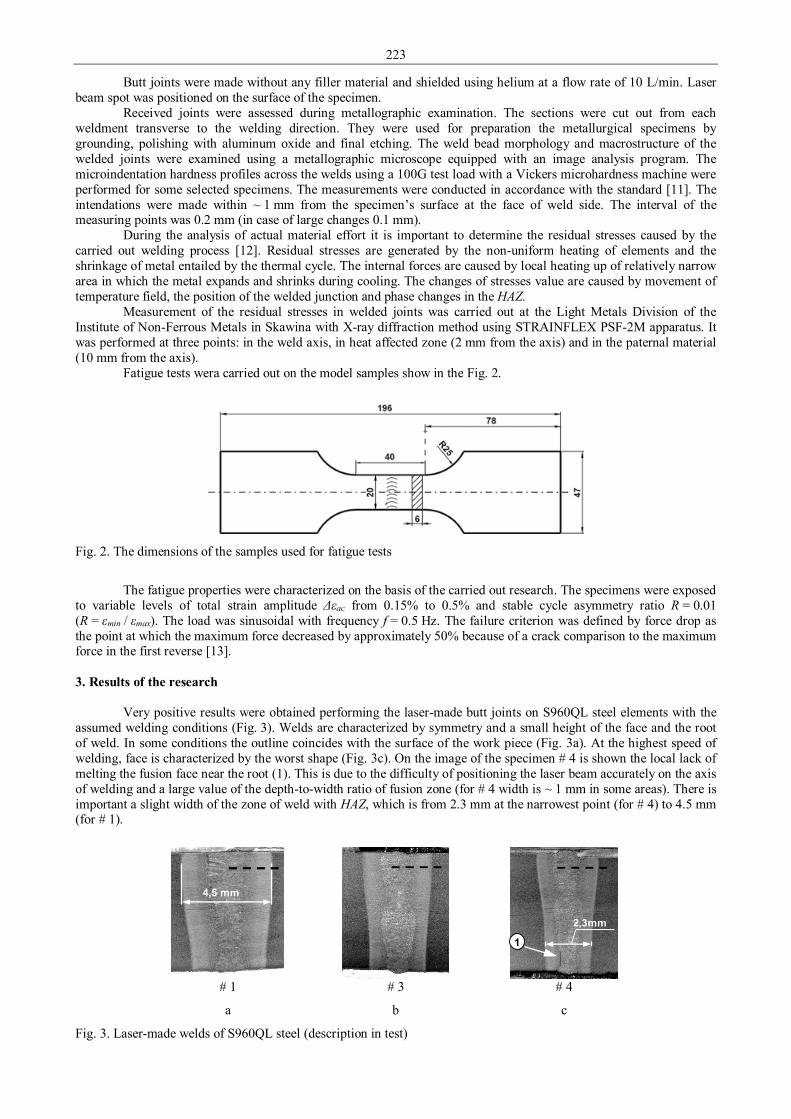
223

Butt joints were made without any filler material and shielded using helium at a flow rate of 10 L/min. Laser beam spot was positioned on the surface of the specimen.

Received joints were assessed during metallographic examination. The sections were cut out from each weldment transverse to the welding direction. They were used for preparation the metallurgical specimens by grounding, polishing with aluminum oxide and final etching. The weld bead morphology and macrostructure of the welded joints were examined using a metallographic microscope equipped with an image analysis program. The microindentation hardness profiles across the welds using a 100G test load with a Vickers microhardness machine were performed for some selected specimens. The measurements were conducted in accordance with the standard [11]. The intendations were made within ~ 1 mm from the specimen’s surface at the face of weld side. The interval of the measuring points was 0.2 mm (in case of large changes 0.1 mm).

During the analysis of actual material effort it is important to determine the residual stresses caused by the carried out welding process [12]. Residual stresses are generated by the non-uniform heating of elements and the shrinkage of metal entailed by the thermal cycle. The internal forces are caused by local heating up of relatively narrow area in which the metal expands and shrinks during cooling. The changes of stresses value are caused by movement of temperature field, the position of the welded junction and phase changes in the HAZ.

Measurement of the residual stresses in welded joints was carried out at the Light Metals Division of the Institute of Non-Ferrous Metals in Skawina with X-ray diffraction method using STRAINFLEX PSF-2M apparatus. It was performed at three points: in the weld axis, in heat affected zone (2 mm from the axis) and in the paternal material (10 mm from the axis).

Fatigue tests wera carried out on the model samples show in the Fig. 2.

Fig. 2. The dimensions of the samples used for fatigue tests

The fatigue properties were characterized on the basis of the carried out research. The specimens were exposed

to variable levels of total strain amplitude Δεac from 0.15% to 0.5% and stable cycle asymmetry ratio R = 0.01 (R = εmin / εmax). The load was sinusoidal with frequency f = 0.5 Hz. The failure criterion was defined by force drop as the point at which the maximum force decreased by approximately 50% because of a crack comparison to the maximum force in the first reverse [13]. 3. Results of the research

Very positive results were obtained performing the laser-made butt joints on S960QL steel elements with the assumed welding conditions (Fig. 3). Welds are characterized by symmetry and a small height of the face and the root of weld. In some conditions the outline coincides with the surface of the work piece (Fig. 3a). At the highest speed of welding, face is characterized by the worst shape (Fig. 3c). On the image of the specimen # 4 is shown the local lack of melting the fusion face near the root (1). This is due to the difficulty of positioning the laser beam accurately on the axis of welding and a large value of the depth-to-width ratio of fusion zone (for # 4 width is ~ 1 mm in some areas). There is important a slight width of the zone of weld with HAZ, which is from 2.3 mm at the narrowest point (for # 4) to 4.5 mm (for # 1).

# 1 # 3 # 4

a b c

Fig. 3. Laser-made welds of S960QL steel (description in test)

1

4,5 mm

2,3mm

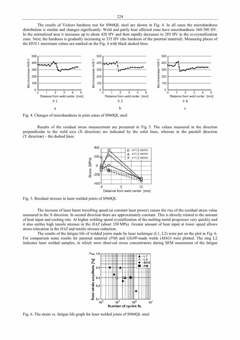
224

The results of Vickers hardness test for S960QL steel are shown in Fig. 4. In all cases the microhardness distribution is similar and changes significantly. Weld and partly heat affected zone have microhardness 360-380 HV. In the normalized area it increases up to about 420 HV and then rapidly decreases to 285 HV in the re-crystallization zone. Next, the hardness is gradually increasing to 335 HV (the hardness of the paternal material). Measuring places of the HV0.1 maximum values are marked on the Fig. 4 with black dashed lines.

# 1 # 3 # 4

a b c

Fig. 4. Changes of microhardness in joint zones of S960QL steel

Results of the residual stress measurement are presented in Fig. 5. The values measured in the direction

perpendicular to the weld axis (X direction) are indicated by the solid lines, whereas in the paralell direction (Y direction) – the dashed lines.

Fig. 5. Residual stresses in laser-welded joints of S960QL

The increase of laser beam travelling speed (at constant laser power) causes the rise of the residual stress value

measured in the X direction. In second direction there are approximately constant. This is directly related to the amount of heat input and cooling rate. At higher welding speed crystallization of the melting metal progresses very quickly and it also entiles high tensile stresses in the HAZ (about 350 MPa). Greater amount of heat input at lower speed allows stress relaxation in the HAZ and tensile stresses reduction.

The results of the fatigue life of welded joints made by laser technique (L1, L2) were put on the plot in Fig. 6. For comparison some results for paternal material (PM) and GSAW-made welds (MAG) were plotted. The sing L2 indicates laser welded samples, in which were observed stress concentrators during SEM assessment of the fatigue

Fig. 6. The strain vs. fatigue life graph for laser welded joints of S960QL steel

225

rupture, namely a lack of the fusion from root side. Of the two indicated cases, the lack of the fusion in the welded joint with lower fatigue life amounted to approximately 8% of the weld cross sectional area. Nevertheless, the fatigue life of this sample is comparable to the welded joints made by GSAW.

Laser welded joints have a significantly increased fatigue life than the welds performed using classic method. GSAW-made samples, examined under slight values of ∆εac = 0.25%, are ruptured approximately 50% earlier than laser-made examined under more unfavorable conditions (∆εac = 0.3%). This is due to a beneficial geometry of the weld face and root, narrower HAZ and lack of welding consumable. The crack of laser welded simple tested under load ∆εac = 0.5% propagated through the re-crystallization region. This phenomenon may indicate that the influence of welded joint shape ratio and connected with them stress concentration was less important, and the importance of local mechanical properties in the HAZ regions increased. There occurs a parallel to a quasi-static fatigue under large loads. Similar phenomenon was not observed in the case of the arc-welding joints.

The fractographic analysis was conducted on the basis of fatigue fractures of the samples tested under strain level ∆εac = 0.5% (Fig. 7). The places of fatigue cracks initiation indicated by arrows are analyzed in the further part of this paper.

In case of the laser-made weld crack propagation is stable and mild (Fig. 7). This character of cracking is caused by the facts that crack initiation and its first stage of growing is located in re-crystallization zone, which has low hardness and strength.

Fig. 7. Fatigue fracture of the laser-made weld joint tested under ∆εac = 0.5%

Rolling process caused that numerous and very hard mill scales were indented into surface. Welding has

caused local softening of the material strength properties and these indentations have become the initiators of fatigue fractures, indicated by arrows in Fig. 7. Cracking of these welds has ductile and brittle-ductile nature with many spaces of fracture inhibition and brittle-to-ductile shear zones.

a

b

Fig. 8. Place of crack intiation (a) and squashed fatigue striations (b) in the laser welded specimens examined under ∆εac = 0.5%

Example fractographic picture of fatigue fracture surface is presented in Fig. 8b. It is stage of high crack

propagation. There are shown the traces of squashed fatigue striations indicating that fracture propagates under high values of strains causing high compressive stresses (in compress phase of the load) and has ductile nature. There can be observed cracks oriented perpendicularly to the main fracture surface what demonstrates that high plastic strains occurred during failure. 4. Summary

The application of laser beam in joining the high-strength fine grained S960QL steel allows obtaining very good quality of weldment. Obtained joints are characterized by a small range of heat-affected zone and the preferred

226

shape of the face and root of weld, which significantly affects their strength properties. The strengthening mechanism of the steel, which results directly from their chemical composition and processing, influences on changes in microhardness and residual stress state. An increase of the heat input amount influences on the stress distribution positively but it extends the width of the weld cross-section with higher values of microhardness.

The presence of welded joints causes decrease of fatigue life of tested specimens, in comparison with the specimens without the welds, up to 50-60%. More beneficial shape of the welds decreasing stress concentration and lack of additional welding consumables improve the fatigue life, even if fracture initiators are found.

Crack propagation in laser welds has proceeded in stable way. The nature of initiation under test condition of strain amplitude ∆εac = 0.5% is not typical, because it has occurred in HAZ rather than in the vicinity of fusion line. In this case the initiators were rolled mill scales in the re-crystallization zone of HAZ. References 1. Günther H. P. Use and Application of High-Performance Steels for Steel Structures (Structural Engineering

Documents 8), IABSE, 2005 2. High-strength and ultra-high-strength heavy plates, Information on < www.voestalpine.com >. 3. Goss Cz., Marecki P. Test results of low cycle fatigue life of WELDOX 900 steel, Biuletyn WAT, Vol. LVII, № 1,

Warsaw 2008, pp. 89-99 (in polish). 4. Glodeža S. et al. Fatigue and fracture behaviour of high strength steel S1100Q. Engineering Failure Analysis, Vol.

16, Issue 7, October 2009, pp. 2348–2356. 5. Klimpel A, Luksa K., Warcaba L., Szorek T., Kielbasinski A. Robotnic GMA welding of S690 and S960 butt

joints, Archiwum Technologii Maszyn i Automatyzacji, Vol. 30, № 3, Poznan 2010, pp. 59-68 (in polish). 6. Willms R. High strength steel for steel constructions, Proceedings of the Nordic Steel Construction Conference

(NSCC 2009), September 2-4, Malmö, Sweden, 2009. 7. Miki C., Homma K., Tominaga T. High strength and high performance steels and their use in bridge structures,

Journal of Constructional Steel Research, Vol. 58, 2002 pp. 3-20. 8. EN-1011-6:2006, Welding – Recommendations for welding of metallic materials – Part 6: Laser beam welding. 9. Mazanek K., Śnieżek L., Ślęzak T. Fatigue research of welded joints of high strength S960QL steel, Biuletyn

WAT, Vol. LXII, № 1, Warsaw 2013, pp. 253-269 (in polish). 10. Ślęzak T., Śnieżek L. Fatigue Properties and Cracking of High Strength Steel S1100QL Welded Joints, Key

Engineering Materials Vol. 598 (2014), pp. 237-242. 11. EN ISO 9015-2:2011. Destructive tests on welds in metallic materials – Hardness testing – Microhardness testing of

welded joints. 12. Śnieżek L. et al. Analiza trwałości zmęczeniowej rurociągu przemysłowego (in Polish), Wojskowa Akademia

Techniczna, Warszawa 2010. 13. ASTM E 606-04. Standard Practice for Strain-Controlled Fatigue Testing, 2005

227

Proceedings of 9th International Conference ITELMS’2014 Multiple Criteria Analysis of Floor Installation for Logistics Centre V. Slivinskas*, S. Susinskas**, D. Aviza** *Kaunas University of Technology, Sakines str. 5, Panevezys, Lithuania, E-mail: vytslivinskas@pst.lt **Kaunas University of Technology, Daukanto str. 12, 44556, Panevezys, Lithuania, E-mail: saulius.susinskas@ktu.lt Abstract This paper examined technological processes of installing floor (installation of the base, laying concrete, arrangement of joints, processing and maintenance) also their impact on the final quality of the floor was established. A model was created for analysis and comparison of industrial floor installation options. Practical application of the model is also provided: objects for analysis of concrete floor installations were chosen; the chosen options for installing floor are described; a system of indicators was formed to compare the options; technical-economic and qualitative indicators were calculated for the options and by applying the method of multiple criteria analysis, rational option for floor installation was established. KEYWORDS: floor, concrete, covering, model, multiple criteria, evaluations, COPRAS, criterion. 1. Introduction

Modern construction market is extremely dynamic. With the help of the latest research and technology, as well as work experience of the builders, the old and often forgotten ideas are improved and the new ones are created. They are applied for the whole process of creating a building: in designing, building and operation. Different parts of the building are constantly affected by various loads, which are variable and fixed. For floor, which during the whole period of its operation gets especially heavy load, specific technical requirements are raised: it has to maintain its geometric form, to be resistant to mechanic effect and aggressive environment, as well as its surface needs to be processed well. All this is most effectively implemented by using concrete. Its components, ways of laying and compactions have a huge impact on the strength, abrasion, density, frost resistance, shrinkage, and water absorption of the floor. 2. Forming the options for installing floor in logistics centre

Industrial floor may be installed in buildings of various purposes, therefore its installation, including materials and the used equipment are chosen considering the specific building. However, rather similar requirements are raised for such floor, namely mechanic resistance, durability, no dusting, smoothness, and excellent features of operation [1].

Lithuania is a perfect place to dislocate logistics centre; therefore, recently a number of such centres were built throughout all the country.

Floor in logistics centres are affected by extremely huge static and dynamic loads, since heavy vehicles drive on them constantly, therefore the floor should be mechanically strong and durable. It is very important that the floor is smooth and convenient for operation. It should not interfere with intensive traffic of forklifts, and the joints should be arranged in such way that the going vehicles could move smoothly without any stronger rumbling as in such way the wheels wear less [3].

In this work the typical logistics centre of 20 000 m2 was chosen, where the racks of 8 meters are stored. Further, in Table 1, the description of floor options is provided. In all of the options, the thickness of concrete layer is 180 mm, and the base under the concrete is the same, i.e.

150 mm sand of 0/16 fraction, 70 mm rubble of 32/45 fraction and polyethylene film, which is 20 mm thick.

Table 1 Description of floor options

Serial No. Description of the proposed options for installing the floor

1. In this option, the strengthening of two reinforcement mesh is chosen (08AIII/08AIII/200/200). The joints are arranged in the network of 12x12. The concrete is brought into the building with the concrete mixer and spread by using the pump. The spread concrete is compacted and levelled by vibrating beams. Immediately after the concrete is vacuumed. A carpet with holes is put onto the surface of the concrete. On top of it – another carpet with a pipe taken out, through which the excess water and air affected by the atmospheric pressure are eliminated. Vacuuming takes about 1,5 minutes for the floor that is 1cm thick. After vacuuming the surface is daubed using the mechanized palettes. After the first daubing, the hardener with metal shavings is spread, which is mixed with Portland cement. When it gets fully wet the daubing with discs is repeated and later using trowels. The prepared surface is moistened and covered with polyethylene film for at least 7 days.

228

The sequel of Table 1 Serial No. Description of the proposed options for installing the floor

2. In this option the concrete is with kalmatron supplement. For the reinforcement, 1 armature net is chosen (08AIII/08AIII/2OO/2OO) and metal fibre. Concreting without joints is applied and the technological joints are arranged in the network of 36x36. The concrete is brought to the building and spread directly from the concrete mixer. The spread mixture is processed using laser compaction and smoothing machine, which quickly and accurately forms the surface of the floor plate. After the first ride with petrol daubing machines, concrete hardener with corund is spread. When it gets fully wet the daubing with discs is repeated and later using trowels. The surface of fully daubed concrete is covered with protective membrane so that the concrete would not lose the moisture too fast.

3. In this option metal fibre is used to strengthen the concrete. Concreting without joints is applied and the technological joints are arranged in the network of 36x36. In order to make the forklift traffic smoother, the technological joints are turned by 10°. The concrete is brought into the building and spread right from the concrete mixer. The spread concrete is processed using laser compaction and smoothing machine, which quickly and accurately forms the surface of the floor plate. After the first ride with petrol daubing machines, dry quartz hardener is dispersed using special trolley. When it gets fully wet the daubing with discs is repeated and later using trowels. The surface of fully daubed concrete is moistened with water and covered with polyethylene film for 14 days. This way it is protected from drying too fast. In order to increase the resistance to abrasion, the surface is additionally strengthened with chemical hardener after 14 days.

3. Determining the importance of the indicators using rank method

Determining the indicators is a very important stage when making a rational decision. It should reflect the pursued objective. If the evaluation indicators will be established accurately, the chosen rational options will satisfy all the groups concerned.

In order to establish the significance, the questionnaires were created, which were provided for the experts to evaluate. The respondents were offered to use a 10-point evaluation system. At first they had to choose the indicators, which, in their opinion, are the most significant and then to evaluate the remaining ones in comparison to them and to score them accordingly.

The evaluations received from the experts were calculated by applying rank method formulas. The results are provided in Tab. 2.

Table 2 The significance of indicators when installing floor in logistics centre

No. Name of the indicator Amount Sr* Deviation ΔS Significance

1 Armature tying quantity 36 -34.39 0.0284 2 Salary for concrete works 61 -9.39 0.0481 3 Number of joints 87 16.61 0.0687 4 Price for installing a joint 47 -23.39 0.0371 5 Quantity of fibre 53 -17.39 0.0418 6 Price of fibre 85 14.61 0.0671 7 Quantity of chemical surface hardener 78 7.61 0.0616 8 Quantity of dry surface hardener 78 7.61 0.0616 9 Price of chemical surface hardener 88 17.61 0.0695

10 Price of dry surface hardener 88 17.61 0.0695 11 Mechanisation level of work 76 5.61 0.0600 12 Time consumption of floor installation 51 -19.39 0.0403 13 Durability 100 29.61 0.0789 14 Convenience of concreting in a technological sense 59 -11.39 0.0466 15 Resistance to chemical impact 41 -29.39 0.0324 16 Exploitation of floor 100 29.61 0.0789 17 Smoothness 99 28.61 0.0781 18 Aesthetic view 40 -30.39 0.0316

Calculated using such technique [2]:

njbSn

jiji ,1,

1== ∑

= (1)

here bij – evaluation of i criterion by j expert, using points; Sį – total amount of evaluations for i criterion by all j experts; ∆Si – deviation from the average amount of ranks.

229

The average evaluation for each criterion is calculated:

njj

bS

m

iij

i ,1,1* ==∑= (2)

The average amount of ranks (S*) may be calculated based on such formula:

mim

SS

m

ii

,1,1* ==∑= (3)

here Sį – estimate amount of criteria i; m – number of criteria. Then the deviation from the average rank amount is calculated as follows:

*SSS ii −=∆ (4)

The significance of the criterion is established based on the formula:

∑=

= m

ii

ij

S

Sq

1

(5)

The reliability of the examination is expressed by the coefficient of expert opinion concordance, describing the overlap degree of individual opinions. The calculated average of evaluation results:

( ) 39.7040991004159100517688887878855347876136181

=+++++++++++++++++⋅

Calculate the sum of squared deviations:

( ) ( ) ( ) ( ) ( ) ++−++++++−+−++−+− 222222222222 39.2939.1961.561.1761.761.761.1439.1739.2361.1639.939.34

( ) ( ) ( ) 28.824239.3061.2861.2939.2939.11 22222 =−+++−+−+

Other necessary amount for the coefficient of concordance is indicator Tk or ranks related in k range, which is calculated using the formula:

( )∑=

−=iH

iiik hhT

1

3 (6)

here Tk –indicator of ranks related in range k; Hl – number of equal rank groups in k range; hl – equal ranks; l is number of related ranks in group, after the evaluation by expert k; k – number of experts.

1201 =T ; 2342 =T ; 1923 =T ; 1201 =T ; 1444 =T ; 4145 =T ; 1201 =T ; 1266 =T ; 1867 =T ; 1388 =T ; 1869 =T ; 14410 =T

Then their amount:

∑=

=r

jjT

11884

Concordance coefficient is calculated:

( ) 1758.0188410181810

88.82421232 =

⋅−−⋅⋅

=W

Since the concordance coefficient is greater than zero, we can assume that the reliability of the significance values received using rank method is sufficient.

The significance of concordance coefficient is established using this formula:

( )

578.2788.291884

11811181810

88.824212 22 =>=⋅

−−+⋅⋅

⋅= lentχχ

Since the calculated 88.292 =χ is greater than 578.272 =lentχ , the hypothesis of the ranges matched by experts is accepted and it is stated that the experts’ opinions match.

230

4. Establishing the rational option for installing floor in the logistics centre using the method of multiple criteria COmplex PRoportional ASsessment of projects (COPRAS)

In order to find rational floor installation options, the values for the indicators are established: quantitative values are provided in the estimate and calculated from schemes, while qualitative ones are established by researching the experts.

Primary data for comparison of options are provided in Tab. 3.

Table 3 Primary data, necessary to perform multiple criteria analysis for installations of floor in logistics centre

Criterion Measuring pcs. * Significance

Numerical value of criterion evaluation

V1 V2 V3 Armature tying quantity Pcs. – 0.0284 2 1 0 Salary for concrete works lt/m2 – 0.0481 14 11 9.5 Number of joints m/m2 – 0.0687 0.17 0.04 0.04 Price for installing a joint lt/kg – 0.0371 30.3 68.19 68.5 Quantity of fibre kg/m³ – 0.0418 0 25 35 Price of fibre lt/kg – 0.0671 0 2.9 2.9 Quantity of chemical surface hardener l/m2 + 0.0616 0 0 0.25 Quantity of dry surface hardener kg/m2 + 0.0616 8 7 6 Price of chemical surface hardener l/lt – 0.0695 0 0 16 Price of dry surface hardener lt/kg – 0.0695 2.8 1.8 1.2 Mechanisation level of work points + 0.0600 3.4 3.8 4.7 Time consumption of floor installation points – 0.0403 4.4 3.7 2.5 Durability points + 0.0789 4.8 4.5 4.7 Convenience of concreting in a technological sense points + 0.0466 2.6 3.6 4.8 Resistance to chemical impact points + 0.0324 3.9 4.3 4.3 Exploitation of floor points + 0.0789 3.5 4.5 4.8 Smoothness points + 0.0781 4 4.4 4.6 Aesthetic view points + 0.0316 3.3 3.7 4.3 Note: signs + (–) show that appropriately higher (lower) value of the criterion meets the requirements more.

Since it is not possible to compare separate measuring units, it is necessary to normalize them. Evaluated and normalized decision matrix is conducted [2]:

0189.0012

0189.0211 =

++⋅=d

…

0120.03.47.33.3

0316.03.4183 =

++⋅=d

Calculating amounts of minimalizing S-j and maximizing S+j of evaluated and normalized indicators, describing j option:

1436.00101.00235.00092.00240.00216.00110.00271.00171.00000.01 =++++++++=+S

1421.00167.00335.00000.00000.00000.00067.00476.00195.00189.01 =++++++++=−S

…

2301.0120.00276.00296.00111.00203.00265.00237.00176.00616.03 =++++++++=+S

1907.00095.00144.00695.00335.00244.00152.00110.001335.00000.03 =++++++++=−S

The relative significance of compared options (effectiveness) is established based on the descriptive positive (option ‘pluses’) S+j and negative (option ‘minuses’) S-j features:

( ) 3129.0

1907.01421.0

1375.01421.0

1421.01421.01421.0

1907.01375.01421.01421.01436.01 =

++⋅

++⋅+=Q

…

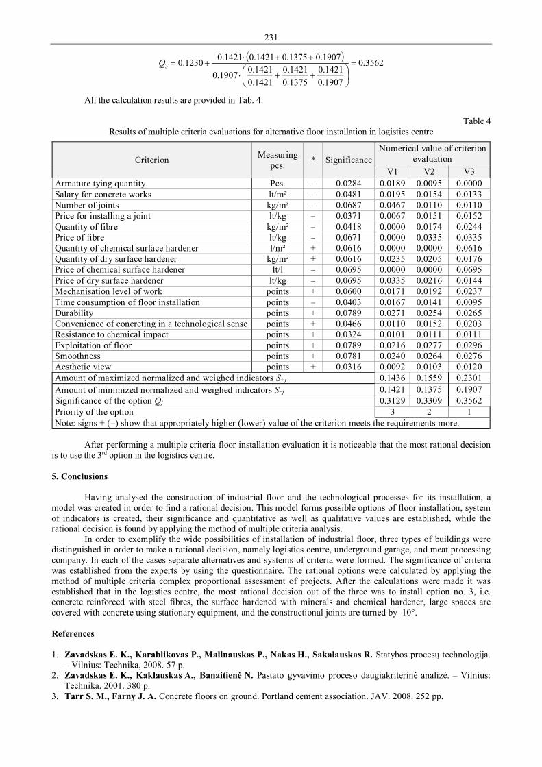
231

( ) 3562.0

1907.01421.0

1375.01421.0

1421.01421.01907.0

1907.01375.01421.01421.01230.03 =

++⋅

++⋅+=Q

All the calculation results are provided in Tab. 4.

Table 4 Results of multiple criteria evaluations for alternative floor installation in logistics centre

Criterion Measuring pcs. * Significance

Numerical value of criterion evaluation

V1 V2 V3 Armature tying quantity Pcs. – 0.0284 0.0189 0.0095 0.0000 Salary for concrete works lt/m² – 0.0481 0.0195 0.0154 0.0133 Number of joints kg/m³ – 0.0687 0.0467 0.0110 0.0110 Price for installing a joint lt/kg – 0.0371 0.0067 0.0151 0.0152 Quantity of fibre kg/m² – 0.0418 0.0000 0.0174 0.0244 Price of fibre lt/kg – 0.0671 0.0000 0.0335 0.0335 Quantity of chemical surface hardener l/m² + 0.0616 0.0000 0.0000 0.0616 Quantity of dry surface hardener kg/m² + 0.0616 0.0235 0.0205 0.0176 Price of chemical surface hardener lt/l – 0.0695 0.0000 0.0000 0.0695 Price of dry surface hardener lt/kg – 0.0695 0.0335 0.0216 0.0144 Mechanisation level of work points + 0.0600 0.0171 0.0192 0.0237 Time consumption of floor installation points – 0.0403 0.0167 0.0141 0.0095 Durability points + 0.0789 0.0271 0.0254 0.0265 Convenience of concreting in a technological sense points + 0.0466 0.0110 0.0152 0.0203 Resistance to chemical impact points + 0.0324 0.0101 0.0111 0.0111 Exploitation of floor points + 0.0789 0.0216 0.0277 0.0296 Smoothness points + 0.0781 0.0240 0.0264 0.0276 Aesthetic view points + 0.0316 0.0092 0.0103 0.0120 Amount of maximized normalized and weighed indicators S+j 0.1436 0.1559 0.2301 Amount of minimized normalized and weighed indicators S−j 0.1421 0.1375 0.1907 Significance of the option Qj 0.3129 0.3309 0.3562 Priority of the option 3 2 1 Note: signs + (–) show that appropriately higher (lower) value of the criterion meets the requirements more.

After performing a multiple criteria floor installation evaluation it is noticeable that the most rational decision

is to use the 3rd option in the logistics centre. 5. Conclusions

Having analysed the construction of industrial floor and the technological processes for its installation, a model was created in order to find a rational decision. This model forms possible options of floor installation, system of indicators is created, their significance and quantitative as well as qualitative values are established, while the rational decision is found by applying the method of multiple criteria analysis.

In order to exemplify the wide possibilities of installation of industrial floor, three types of buildings were distinguished in order to make a rational decision, namely logistics centre, underground garage, and meat processing company. In each of the cases separate alternatives and systems of criteria were formed. The significance of criteria was established from the experts by using the questionnaire. The rational options were calculated by applying the method of multiple criteria complex proportional assessment of projects. After the calculations were made it was established that in the logistics centre, the most rational decision out of the three was to install option no. 3, i.e. concrete reinforced with steel fibres, the surface hardened with minerals and chemical hardener, large spaces are covered with concrete using stationary equipment, and the constructional joints are turned by 10°. References 1. Zavadskas E. K., Karablikovas P., Malinauskas P., Nakas H., Sakalauskas R. Statybos procesų technologija.

– Vilnius: Technika, 2008. 57 p. 2. Zavadskas E. K., Kaklauskas A., Banaitienė N. Pastato gyvavimo proceso daugiakriterinė analizė. – Vilnius:

Technika, 2001. 380 p. 3. Tarr S. M., Farny J. A. Concrete floors on ground. Portland cement association. JAV. 2008. 252 pp.

232

Proceedings of 9th International Conference ITELMS’2014 Research of Property Fatigue Advanced Al/Ti Laminate L. Sniezek, I. Szachogluchowicz, V. Hutsaylyuk Military University of Technology, gen. S. Kaliskiego 2 str., 00-908 Warsaw, Poland, E-mail: lsniezek@wat.edu.pl Abstract The paper presents preliminary results of low cycle fatigue properties, including fatigue cracking, layered laminate AA2519-Ti6Al4. The test material obtained was combined with the method of explosive bonding in direct configuration, as well as the intermediate layer using a AA1050 alloy. During the study verified that the laminate will exhibit superior properties in August, combining the beneficial properties of titanium alloys and aluminum. In addition, impact tests were performed the Charpy method. Obtained during research breakthroughs were examined by SEM. KEYWORDS: explosive welding, layered composites, mechanical properties of the composites. 1. Introduction

Operating conditions responsible design, including aerospace structures are very difficult, because the materials used for this type of object structure puts the sometimes contradictory requirements, particularly in terms of mechanical properties. Fulfilling all the requirements by one material is often impossible; hence there was a need to seek opportunities for combining materials with different mechanical properties and structure. One of the methods is the preparation of a bimetal explosive cladding. This method is an important technology for the production capabilities of modern metal composites. It is an important complement to traditional production methods plater, such as welding or rolling steel products. The resulting bimetallic this way, the multi-layered composites consisting of more than two materials and have unique structural properties. They are characterized by: high strength, corrosion resistance, and in the case of the association of appropriate materials – including a substantial ballistic resistance. Bonded explosive materials can be connectable to conventional methods, as well as metals and alloys, for which the technology is not alternative. Combined materials can vary considerably in its properties, such as steel-aluminum, steel-titanium, or aluminum – titanium. In addition to the possibility of the production of new materials, the main premise of acting in favor of the use of this technology are the economic effects in the form of large savings resulting from the reduction in the consumption of expensive metals and their alloys with specific characteristics. It should be noted, however, that for some base material technology to obtain this type of call, as an extremely difficult and complex, was controlled only by the individual manufacturers, which entails extremely high prices of these products.

At present, this technology is most often used for joining sheets of different metals, not weldable by conventional methods. Products manufactured by this method are used in the manufacturing Mainly industry that improve the wear resistance or corrosion. Another very important application is that combine the explosive bonding is not weldable materials by conventional methods [1-5].

The country's leading company focusing its activities on the application and development of technology is the explosive metalworking Technology Department Energetic "EXPLOMET". Cooperation with this plant has also enabled the authors to undertake research aimed at obtaining and determine the performance of engineering plastics in the form of composite laminated Al-Ti with specific properties, which does not have a solid material. Research on fatigue properties of laminated composites obtained by combining the explosive are not heavily represented in world literature. Extensive discussion of the determination of the lower explosive limit parameters combine ensuring the correct execution of the connector are shown in the article [6]. The application of this type of material for engineering practice requires the characteristics relating, among others, extended recognition mechanisms of crack propagation and the impact of wider material properties at the speed of crack propagation, i.e. factors to ensure the required stability of the structure design. In [7] analyzed the structure and mechanical properties of composite materials of different types of steel after welding explosive then subjected to heat treatment. The presented study helped to determine the scope of the subsequent heat treatment of the composites obtained from alloyed steels, which provide high mechanical properties at an acceptable degree of structural heterogeneity. Work [8] devoted to modeling acceleration “upper” sheet involved in explosive welding. The presented results show that the computer analysis allows the prediction of the kinematic parameters of explosive welding process. The study of structural and mechanical properties of metallic composites produced by explosive welding and annealing subjects were the subject of work [9]. In the present paper presents the results of research on the composites of Al-Al3Ti-Ti complex even with 21 layers of aluminum and titanium. In such a complex combination of metallographic observed on metallographic section connection with the characteristic wave and no wave. The structure of the obtained material was examined using the connections TEM and SEM microscopy and by X-ray diffractometer. Impact strength was determined on samples of composites notched “v” using the Charpy hammer. Annealed samples show lower impact strength, and yet have not been completely broken, in contrast to the samples without heat treatment. In [10] the study was carried out on the combined detonation sheets of stainless steel and titanium. Plates were combined explosively with oblique location of metal striking. Weld examined using optical

233

microscopy and scanning electron (SEM). Studies were also performed on the tensile, shear, bending and checked hardness and corrosion resistance. Observations on an optical microscope and showed the presence of scanning flat and corrugated layers of the transition metals according to the explosion used for metal bonding. As a result of these observations, it was found that elements from explosively welded titanium and stainless steel may be used in industry, even in the form of bent.

Issues related to the martensitic transformation and changes in the physical properties of the composite metal "steel-titanium" resulting from the explosive welding are described in the article [11]. The paper focuses on the analysis of a very narrow transition layer between titanium and stainless steel. It was observed that the mixture of elements occurs only in a layer having a width of about 2 microns - 6 microns deep and 4 microns of titanium into the steel. It was found that the main effect of explosive welding on the properties of bimetallic composite is plastic deformation, which increases the hardness of the alloy and the partial reduction of martensitic transformations. While the phenomenon occurring during the production of multilayer composites containing in their structure intermetallic phase Al-Ti type are generally found in the literature [12-15], the information on the formation of such a connection using explosive welding methods are quite scarce. Composite materials containing titanium aluminides, produced during the manufacture of connectors of the Al-Ti, are widely used as a construction material in the field of aeronautical engineering. 2. Research procedures

Adopted a more practical work included examination of low cycle fatigue properties, including fatigue cracking, layered composite material system: Ti6Al4V titanium alloy/aluminum alloy AA1050/AA2519 aluminum alloy and Ti6Al4V/aluminum alloy AA2519, with the resulting diffusion layer type Al3Ti. It was assumed that such material will be characterized by unique properties that combine the beneficial properties of titanium and aluminum alloys (high strength and ductility) and alloys intermetallic phases Ti-Al (high hardness and rigidity). 3. Results of research 3.1. Low cycle fatigue strength

Determination of material behavior under variable loads in the range of a small number of cycles is particularly important due to the possibility of studying the mechanisms of cyclic deformation mechanisms which lead to the location of the deformation, cracking and, consequently, the destruction of the structure element.

The study was carried out under conditions of low cycle constant total strain amplitude (εac = const.) using two groups of flat samples: a central hole (Fig. 1a) and without a hole (Fig. 1b). Fatigue tests were carried out on a testing machine INSTRON 8802 companies. During the test total strain amplitude sinusoidal εac varied by a factor of cycle asymmetry R = 0. Tests carried out at a frequency f = 0.2 Hz.

a

b

Fig. 1. Dimensions of samples for low cycle

The study adopted three levels of deformation: εac = 0.3%, 0.4% and 0.5%. Levels were determined after the

analysis of strain graph static tension. Development of low cycle test results started from analysis of changes in the value of the dependent variable

(stress amplitude σa) as a function of the number of relapses. The results of these measurements carried out on samples without a hole for the acceptable level of deformation is shown in Fig. 2.

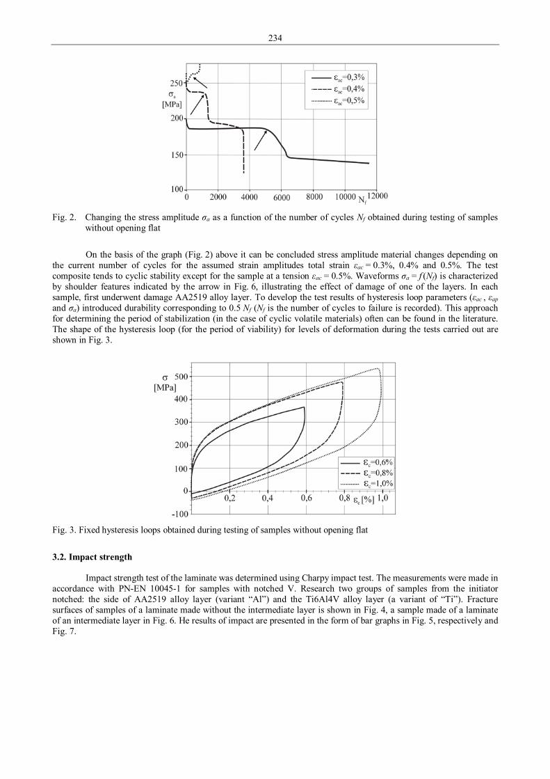
234

Fig. 2. Changing the stress amplitude σa as a function of the number of cycles Nf obtained during testing of samples

without opening flat

On the basis of the graph (Fig. 2) above it can be concluded stress amplitude material changes depending on

the current number of cycles for the assumed strain amplitudes total strain εac = 0.3%, 0.4% and 0.5%. The test composite tends to cyclic stability except for the sample at a tension εac = 0.5%. Waveforms σa = f (Nf) is characterized by shoulder features indicated by the arrow in Fig. 6, illustrating the effect of damage of one of the layers. In each sample, first underwent damage AA2519 alloy layer. To develop the test results of hysteresis loop parameters (εac , εap and σa) introduced durability corresponding to 0.5 Nf (Nf is the number of cycles to failure is recorded). This approach for determining the period of stabilization (in the case of cyclic volatile materials) often can be found in the literature. The shape of the hysteresis loop (for the period of viability) for levels of deformation during the tests carried out are shown in Fig. 3.

Fig. 3. Fixed hysteresis loops obtained during testing of samples without opening flat

3.2. Impact strength

Impact strength test of the laminate was determined using Charpy impact test. The measurements were made in accordance with PN-EN 10045-1 for samples with notched V. Research two groups of samples from the initiator notched: the side of AA2519 alloy layer (variant “Al”) and the Ti6Al4V alloy layer (a variant of “Ti”). Fracture surfaces of samples of a laminate made without the intermediate layer is shown in Fig. 4, a sample made of a laminate of an intermediate layer in Fig. 6. He results of impact are presented in the form of bar graphs in Fig. 5, respectively and Fig. 7.

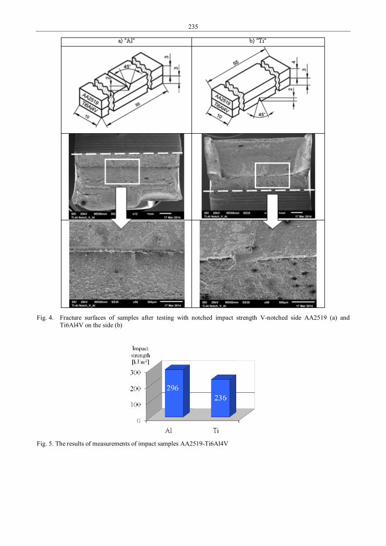
235

Fig. 4. Fracture surfaces of samples after testing with notched impact strength V-notched side AA2519 (a) and

Ti6Al4V on the side (b)

Fig. 5. The results of measurements of impact samples AA2519-Ti6Al4V

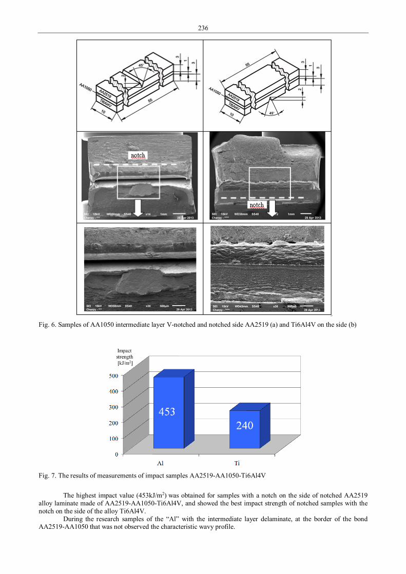
236

Fig. 6. Samples of AA1050 intermediate layer V-notched and notched side AA2519 (a) and Ti6Al4V on the side (b)

Fig. 7. The results of measurements of impact samples AA2519-AA1050-Ti6Al4V

The highest impact value (453kJ/m2) was obtained for samples with a notch on the side of notched AA2519

alloy laminate made of AA2519-AA1050-Ti6Al4V, and showed the best impact strength of notched samples with the notch on the side of the alloy Ti6Al4V.

During the research samples of the “Al” with the intermediate layer delaminate, at the border of the bond AA2519-AA1050 that was not observed the characteristic wavy profile.

237

4. Conclusions

Explosive bonding is a process of great technological importance to the possibility of production of modern composite panels. Conducted attempts to connect Ti6Al4V and AA2519 alloys are optimistic. The calls have satisfactory strength properties and susceptibility to plastic deformation in bending, assuming that the inner layer of the composite is made of aluminum alloy. The results set the direction for further research to determine the effect of annealing parameters in a high vacuum or in a protective gas atmosphere on the microstructure, phase transitions and structure stability and fatigue properties of composites of Al-Ti, obtained in the explosive bonding process. References 1. Niesłony A., Kurek A., Bański R., Čižek L. Badania wytrzymałościowe statyczne i zmęczeniowe materiałów

zgrzewanych wybuchowo typu stal-tytan, Zeszyty Naukowe Politechniki Opolskiej, Seria Mechanika, Z.97, Nr kol. 337/2010, Politechnika Opolska, Opole 2010, pp. 121-133.

2. Mierzynski J., Hutsaylyuk V. Fatigue crack growth in the D16CzATW aluminium alloy in the presence of a calibrated hole under simple bending., International Journal of Fatigue, Vol:39, 2012, pp: 54-60.

3. Karolczuk A. Pola naprężeń w elementach zgrzewanych wybuchowo poddanych zginaniu, Red: Olejnik A., Wasilewski M. Nauka i praktyka – staże zawodowe w przedsiębiorstwach. Edycja II Opole: Ofic. Wydaw. Politechniki Opolskiej, 2011, ss. 7-17.

4. Sulym H., Hutsaylyuk V. Pasternak, Stress-strain state of an elastic rectangular plate under dynamic load., Mechanika Issue: 6, 2013, pp: 620-626.

5. Kurek A., Niesłony A., Barański R., Polak-Micewicz M. Systems: Journal of transdisciplinary systems science, Vol. 16, Nr 2, 2012, pp. 243-251.

6. Lysak V. I., Kuzmin S. V. Lower boundary in metal explosive welding. Evolution of ideas, Journal of Materials Processing Technology, Vol. 212, 2012, pp. 150–156.

7. Trykov P., Stepanishchev I. B., Trudov A. F., Arisova V. N. Structure and properties of explosion-welded composites from steels of different kinds, Metal Science and Heat Treatment, Vol. 46, Nos. 3–4, 2004, pp. 167-169.

8. Benak M., Taraba B., Turna M. Contribution to modelling the effect of explosive on accelerated material in explosion welding, Annals of DAAAM for 2009, Volume 20, No. 1.

9. Bataev I. A., Bataev A. A., Mali V. I., Pavliukova D. V. Structural and mechanical properties of metallic–intermetallic laminate composites produced by explosive welding and annealing. Materials and Design 35, 2012, pp. 225–234.

10. Kahraman N., Gulenc B., Findik F. Joining of titanium/stainless steel by explosive welding and effect on interface, Journal of Materials Processing Technology, 169, 2005, pp. 127–133.

11. Belyaeva S., Rubanik V., Resninaa N., Rubanik Jr V., Rubanik O., Borisova V. Martensitic transformation and physical properties of ‘steel–TiNi’ bimetal composite produced by explosion welding, Phase Transitions, Vol. 83, No. 4, April 2010, pp. 276–283.

12. Wierzchoń T., Ossowski M. Struktura i wybrane właściwości kompozytów warstwowych: stop tytanu Ti6Al2Cr2Mo - fazy międzymetaliczne z układu Ti-Al, Kompozyty (Composites) 6, 2006, ss. 50-53.

13. Peng L. M., Wang J. H., Li H., Zhao J. H., He L. H. Synthesis and microstructural characterization of Ti–Al3Ti metal–intermetallic laminate (MIL) composites, Scripta Materialia, Vol. 52, 2005, pp. 243–248.

14. Xu L., Cui Y. Y., Hao Y. L., Yang R. Growth of intermetallic layer in multi-laminated Ti/Al diffusion couples, Materials Science and Engineering, A 435–436, 2006, pp. 638–647.

15. Rohatgi A., Harach D. J., Vecchio K. S., Harvey K. P. Resistance-curve and fracture behavior of Ti–Al3Ti metallic–intermetallic laminate (MIL) composites, Acta Materialia 51, 2003, pp. 2933–2957.

238

Proceedings of 9th International Conference ITELMS’2014 Selecting the Most Suitable Region in the Selected Country for the Placement of the Bi-Modal Freight Village Using the WSA Method O. Stopka*, L. Bartuska*, I. Kubasakova** *Institute of Technology and Business in České Budějovice, Okružní 517/10, 370 01 České Budějovice, Czech Republic. E-mail: stopka@mail.vstecb.cz, bartuska.vste@seznam.cz **University of Žilina, Faculty of Operation and Economics of Transport and Communications, Department of Road and Urban Transport, Univerzitná 8215/1, 010 26 Žilina, Slovak Republic, E-mail: iveta.kubasakova@fpedas.uniza.sk Abstract The paper presents the selecting the most suitable region in the selected country for the placement of the bi-modal (rail-road) freight village using the WSA method. The first part of the paper outlines the introduction to the given issue and the brief description of the WSA method. The second part describes the identification of the variants (regions) and the establishment of the evaluation criteria. The third part of the paper includes the creation of the criteria matrix and the last part provides the determination of the most suitable region in the selected country for the placement of the bi-modal freight village. KEYWORDS: freight village, bi-modal, WSA method, regions, criteria, criteria matrix. 1. Introduction

Selecting the place for the freight village can be viewed as a decision problem in which the final decision is influenced by a group of external factors. For the purpose of solving decision-making problems the methods of multi-criteria analysis are used and these methods can therefore be used in deciding this type of objects.

There are a number of methods that are used for solving multi-criteria analysis. The simple ones do not take into account the weight of each criterion and therefore are not appropriate for this article because in the group of criteria which influence the freight village, significant differences in the importance of criteria exist.

Methods for the selection of a variant are divided according to what information about the preference among the criteria they require for their work [1 - 2]: 1. Methods not requiring information about preference of criteria – methods that do not require information about

the preference between criteria are very simple and in their plain form are rarely used. 2. Methods requiring aspiration level of criteria – for methods that are based on work with aspiration information on

preferences between criteria, it is characteristic that they do not try to transform the information of a user into a weight vector. Information about the importance of the criteria is expressed as the aspiration level of the criteria. These methods are useful in cases where nominal information is known about the criteria, namely aspiration values of criteria and cardinal evaluation of the variants according to individual criteria.

3. Methods using ordinal information on the criteria – methods working with ordinal information about the criteria or variants require a specification of the order of criteria importance and the order of variants according to individual criteria. Some methods are very simple and the results are more or less indicative, others are quite complicated and provide a comprehensive view of the problem.

4. Methods requiring cardinal information about the criteria – there are several methods that require cardinal information about the criteria in terms of weights and about the variants in the form of a criteria matrix with cardinal values. In this area there are three basic approaches to the evaluation of variants, according to: o Maximizing the benefits; o Minimizing the distance from the ideal variant; o Preferential relationship.

The weighted sum method – WSA appears to be relatively easy to handle and easy to apply to the complex and difficult task of the bi-modal freight village placement.

The weighted sum method requires cardinal information, criteria matrix Y and a vector of criteria weightings v. It constructs the overall rating for each variant and so it can be used for finding one of the most suitable variants as well as for arranging variants on a scale from the best to the worst.

With this method we work with the weights of individual criterion, which are either entered or estimated appropriately. Thus we get the weighting sv = (v1 , v2 , ..., vk) for k of maximization criteria.

The method of weighted sum then maximizes the weighted sum i.e.:

∑ =kj ijjrv1 (1)

where: vj is vector of criteria weightings; rij is normalized criteria matrix.

239

Hence we calculate the value of the weighted sum for each variant and as a compromise variant select the one with the highest weighted sum [1]. 2. Identification of all regions and establishment of the evaluation criteria

A. Identification of variants In stage one, it is necessary to identify a set of variants from which the final solution will be chosen. The

regions of Slovakia where the bi-modal freight village should potentially be placed were identified as those of: Bratislava, Trnava, Trenčín, Nitra, Žilina, Banská Bystrica, Prešov and Košice. For a more accurate result it would be more appropriate to look at district level, but at this level it would be very difficult to obtain data to fulfil the criteria matrix (an essential part of multi-criteria analysis) because most of the data required is not available at district level.

B. Establishment of a set of criteria Stage two of the process of multi-criteria analysis involves establishing a set of criteria which influence the

process of decision-making in the selection of variants [3]. Developing a tailor-made system of evaluation criteria is an important step in the whole multi-criteria analysis

process, one which can significantly affect the overall outcome of the evaluation. The rational formation of evaluation criteria significantly depends on a thorough knowledge of the object of evaluation and on a systemic understanding of its structure and its functions. The set of criteria must be comprehensive i.e. it must reflect the essential characteristics of the objects (variants). If the latter is not the case, a gross distortion in the results may occur [3].

The selection and arranging of criteria into a final set of evaluation criteria is in itself a complex and often difficult process to implement. Another important prerequisite for the development of tailor-made systems is the correct classification of the evaluation criteria. Evaluation criteria can be classified according to their relevancy and their formality. From the point of view of relevancy, criteria can be classified into groups according to certain so-called, aspects of evaluation, such as social, environmental, technical, economic, cultural, aesthetic criteria, etc. [4].

From the point of view of formality it is necessary to differentiate the criteria according to the type of preference and the way (form) of expressing and measuring the results of evaluations based on such criteria. Criteria according to their type preference can be placed in order of [4 - 5]: • increasing preference (maximization, profit) – in which higher values are preferred over lower ones; • decreasing preference (minimization, loss) – which are the opposite of the above; • alternating preference - preference changes when a certain value is achieved.

Criteria by way of expression and measurement of evaluations of results [4 - 5]: • quantitatively, the values of which can be expressed numerically by the number of units of measure; • qualitatively, which can only be expressed verbally i.e. degrees of quality and a description of their intensity.

Table 1 Criteria layout related to the issue of the bi-modal freight village placement

in the Slovak Republic (source: authors according to [16-17])

Criteria Abbreviation GDP per capita (PPS) GDP Average GDP growth over 5 years GDPGR Amount of transported goods via public roads (thousands tonnes) TGR Number of large companies (> 250 employees) NBE Number of small and medium size companies (< 250 employees) NSME Average gross monthly wage (EUR) AGW State of road network (km) RN Regional connections with network of railway lines AGTC AGTC

Table 2

Actual values of the individual criteria (source: [6 – 12, 17])

Criterion Region GDP GDPGR TGR NBE NSME AGW RN AGTC

Bratislava region 43063 1.055 8255 180 49420 991 241.75 3 Trnava region 20078 1.067 5651 61 13136 705 360.87 3 Trenčín region 15823 1.057 8921 73 11781 657 508.52 2 Nitra region 14841 1.044 2875 51 14301 636 517.99 2 Žilina region 15826 1.072 4320 61 13390 686 593.54 2 Banská Bystrica region 13215 1.062 3968 48 12525 635 733.89 0 Prešov region 10104 1.041 4258 58 13120 594 715.43 2 Košice region 14109 1.047 6369 52 14744 716 371.88 2

240

After determining the objectives of the analysis of available knowledge, relevant to this paper, 8 criteria from socio-economic and transport fields were defined. For these criteria critical data were obtained based on the study of the functions and perspectives that are related to the activities carried out in a bi-modal freight village. Due to the prerequisite that all the data (associated with different factors) should be related to the same time period, only data collected for 2010 appears in this article. Data for 2011, 2012 or 2013 could only be obtained for a limited group of factors [4].

For clarity, the criteria (factors) are summarized in the following table (Tab. 1). Tab. 2 shows the specific values of criteria related to individual variants (regions in the Slovak Republic). 3. Creation of the criteria matrix

In the theory of Multiple Criteria Decision-Making we work with a general number of criteria k and with a general number of variants p. The value achieved by variant i for j-th criterion, is labelled as yij and is called the criterion value. The next step is to arrange these values into a matrix which we call the criteria matrix. The rows of the criteria matrix are formed by the individual variants. The columns of the criteria matrix correspond with the individual criteria.

In our case the criteria matrix looks the same as the Tab. 2. A. Transfer of criteria to the same type For the purposes of tasks related to the criteria matrix it is appropriate that all the criteria are of the same type

(minimization or maximization). Transfer of the criteria to the same type is not difficult because each minimization criterion can be easily converted to maximization criterion [1]: • The scale is given by the nature of the issue (e.g. grades in school). In this case we take the maximum value that can

be achieved (at school grade 5), and subtract from it the value of the criterion. • The scale is not given. In this case, we find the variant with the highest (worst) value and subtract from it the value of

the criterion. This step can be presented as protection against the worst variant. In our case it is necessary to perform a modification in the initial criteria matrix at the eighth criterion, that of

average monthly wage. For average wage the highest value is EUR 991, the transformation will replace the original criteria value yi8 with the value 991 -yi8 .

The adjusted criteria matrix looks like this:

43063 1.055 8255 180 49420 0 241.75 3 20078 1.067 5651 61 13136 286 360.87 3 15823 1.057 8921 73 11781 334 508.52 2 14841 1.044 2875 51 14301 355 517.99 2 15826 1.072 4320 61 13390 305 593.54 2 13215 1.062 3968 48 12525 356 733.89 0 10104 1.041 4258 58 13120 397 715.43 2 14109 1.047 6369 52 14744 275 371.88 2

B. Ideal and basal variant Ideal variant is the best option which can be theoretically or practically achieved.

• relative (highest in criteria matrix for a given criterion), • absolute (highest theoretically possible value).

Basal variant is the worst variant which can be theoretically or practically achieved. • relative (the lowest value in the criteria matrix for a given criterion), • absolute (the lowest theoretically possible value).

C. Normalization of criteria matrix If we know the ideal and basal variants, we simply normalize the criteria matrix. All values in the criteria

matrix will be in the interval <0, 1>, the ideal value of the criteria matrix will then be represented by the number 1 and the basal by the number 0. An important feature of this normalized criteria matrix that it is completely independent of the units [1].

If we mark the basal value for criteria j as Dj and the ideal value for criteria j as Hj then the normalized criteria matrix (rij) arises from the initial criteria matrix (yij) as follows:

jj

jijij DH

Dyr

−−

= (2)

where: rij is normalized criteria matrix; yj is initial criteria matrix; Dj is basal value for criteria j; Hj is ideal value for criteria j.

In our case, to normalize the criteria matrix, the following steps must be performed. We have a criteria matrix for maximizing criteria, we add lines with the ideal and basal variants and according to the above formula we complete a normalized criteria matrix (see Tab. 3).

241

Table 3 Adjusted criteria matrix and auxiliary lines with the ideal and basal variants

(source: authors according to [17])

Criterion Region GDP GDPGR TGR NBE NSME AGW RN AGTC

Bratislava 43063 1.055 8255 180 49420 0 241.75 3 Trnava 20078 1.067 5651 61 13136 286 360.87 3 Trenčín 15823 1.057 8921 73 11781 334 508.52 2 Nitra 14841 1.044 2875 51 14301 355 517.99 2 Žilina 15826 1.072 4320 61 13390 305 593.54 2 Banská Bystrica 13215 1.062 3968 48 12525 356 733.89 0 Prešov 10104 1.041 4258 58 13120 397 715.43 2 Košice 14109 1.047 6369 52 14744 275 371.88 2 Hj 43063 1.072 8921 180 49420 397 733.89 3 Dj 10104 1.041 2875 48 11781 0 241.75 0 Hj – Dj 32959 0.031 6046 132 37639 397 492.14 3

32959101041

1−

= ii

yr ,

100031

10001041

2

2

−=

i

i

yr ,

604628754

3−

= ii

yr ,

132485

4−

= ii

yr ,

37939117816

5−

= ii

yr ,

3978

6i

iy

r = ,

10049214

10024175

9

7

−=

i

i

yr ,

310

8i

iy

r =

According to the above formulae, we set up the required normalized criteria matrix (Tab. 4).

Table 4 Normalized criteria matrix (source: authors according to [17])

Criterion Region GDP GDPGR TGR NBE NSME AGW RN AGTC

Bratislava 1 0.4516 0.8898 1 1 0 0 1 Trnava 0.3026 0.8387 0.4591 0.0985 0.036 0.7204 0.242 1 Trenčín 0.1735 0.5161 1 0.1894 0 0.8413 0.5421 0.6667 Nitra 0.1437 0.0968 0 0.0227 0.067 0.8942 0.5613 0.6667 Žilina 0.1736 1 0.239 0.0985 0.0427 0.7683 0.7148 0.6667 Banska Bystrica 0.0944 0.6774 0.1808 0 0.012 0.8967 1 0 Prešov 0 0 0.2287 0.0758 0.0356 1 0.9625 0.6667 Košice 0.1215 0.1935 0.5779 0.0303 0.0787 0.6927 0.2644 0.6667

D. Determination of criteria weightings The individual criterion weights represent the importance of a given criterion for the selection of a variant

using multi-criteria analysis. The higher the criterion weight is, the greater the impact on the decision of the resulting variant [1, 13 - 14]

The determination of criteria weightings is made using the Saaty pairwise comparison method. The first step of the Saaty method is to determine the relationship between each pair of criteria when the preference is determined in a spot range among 1-9. This is determined with the help of 10 members of the research team. They were asked to determine preferences between individual criteria. Each of the ten members of the team set a preference for each pair of criteria. Subsequently for each element of the matrix a sum of the sub-matrices of all members of the team was established and then the average was calculated [14].

Determined elements of the Saaty method were used for further calculations. The values obtained for the individual criterion in the intermediate calculations and the final values of the vector of weights of individual criterion are given in Tab. 5.

242

Table 5 Values calculated by the Saaty method (source: authors)

Criterion Product of elements Geometric mean Weighted geometric mean 1. GDP 0.1089 0.7579 0.0785 2. GDPGR 0.000625 0.3976 0.0411 3. TGR 600 2.2247 0.2300 4. NBE 0.000625 0.3976 0.0411 5. NSME 0.25 0.8409 0.0869 6. AGW 16 1.4142 0.1462 7. RN 600 2.2247 0.2300 8. AGTC 16 1.4142 0.1462

∑ = 1.00000 4. Determination of the most suitable region

A. Calculation of normalized criteria matrix See Table 4. B. Multiplication of normalized matrix by the vector of weights (weighted geometric mean – Tab. 5) indicated

by Saaty method (Tab. 6)

Table 6 Multiplication of the normalized matrix by the values of the weighted geometric mean (source: authors)

Criterion Region GDP GDPGR TGR NBE NSME AGW RN AGTC

Bratislava 0.0785 0.0186 0.2046 0.0411 0.0869 0 0 0.1462 Trnava 0.0238 0.0345 0.1056 0.0040 0.0031 0.1053 0.0557 0.1462 Trenčín 0.0136 0.0212 0.2300 0.0078 0 0.1230 0.1247 0.0975 Nitra 0.0113 0.0040 0 0.0009 0.0058 0.1307 0.1291 0.0975 Žilina 0.0136 0.0411 0.0550 0.0040 0.0037 0.1123 0.1644 0.0975 Banská Bystrica 0.0074 0.0278 0.0416 0 0.0010 0.1311 0.2300 0 Prešov 0 0 0.0526 0.0031 0.0031 0.1462 0.2214 0.0975 Košice 0.0095 0.0079 0.1329 0.0001 0.0068 0.1013 0.0608 0.0975

C. Counting the elements of the matrix for all criteria and placing in the descending order (Tab. 7).

Table 7 Determination of the most suitable region (source: authors)

Region Relevant value Order of regions Bratislava 0.5759 2. Trnava 0.4782 5. Trenčín 0.6178 1. Nitra 0.3793 8. Žilina 0.4916 4. Banská Bystrica 0.4389 6. Prešov 0.5239 3. Košice 0.4168 7.

5. Conclusion

Based on the calculations performed regarding the decision on the placement of the bi-modal freight village in the Slovak Republic, using the weighted sum – WSA, the Trenčín region was determined as the most suitable variant.

And based on the calculations it can be stated, that WSA method is an appropriate method for the purpose of determining the most suitable place for the freight village in the selected country, as well.

The method allows the reducing and adding the number of criteria that are taken into account in search of solutions. Several calculations with different numbers of criteria were made and always with more or less the same result – the first position according to the method of weighted sum were always taken by the Trenčín region.

243

References 1. Belton V., Stewart T. J. Multi Criteria Decision Analysis - An Integrated Approach. Kluwer Academic Publishers.

Editor: Springer. 2002. 2. Zavadskas E. K., Turskis Z. Multiple criteria decision making (MCDM) methods in economics: an overview.

Technological and Economic Development of Economy, 17(2), pp. 397-427, doi:10.3846/20294913.2011.593291. 2011.

3. Triantaphyllou E. Multi-Criteria Decision Making: A Comparative Study. Dordrecht: Kluwer Academic Publishers, 2000. 320 s. ISBN 0-7923-6607-7.

4. Tučník P. Vícekriteriální rozhodování v multiagentových systémech. Accessible via: < http://hilbert.chtf.stuba.sk/KUZV/download/kuzv-tucnik.pdf > [cit 2014-01-29].

5. ÚSTAV AUTOMATIZACE A INFORMATIKY–internet. Vícekriteriální rozhodování. [electronic source]. 2010. Accessible via: < www.uai.fme.vutbr.cz/~jdvorak/vyuka/osa/Vicekrit.pp > [cit. 2013-10-23].

6. ŠTATISTICKÝ ÚRAD SR–internet page of National Office for Statistics. Regionálny HDP 1995 - 2010. [electronic source]. 2013 ©. Accessible via: < http://portal.statistics.sk/files/Sekcie/sek_300/330/rev_hdp/reg_rev_hdp_1995-2010.pdf > [cit. 2014-03-02].

7. SARIO–internet page of Slovakian Agency for Development Investment and Commerce. Prílev a odlev priamych zahraničných investícií v roku 2010. [electronic source]. 2009 © SARIO. Accessible via: < http://www.sario.sk/?pzi-prilev-odlev > [cit. 2014-02-07].

8. ŠTATISTICKÝ ÚRAD SR–internet page of Office for National Statistics. Ročenka dopravy 2011. [electronic Source]. 2013 ©. Accessible via: < http://portal.statistics.sk/showdoc.do?index=110&words=obyv&docid=108 > [cit. 2014-02-10].

9. ŠTATISTICKÝ ÚRAD SR–internet page of Office for National Statistics. Podnikateľské subjekty za rok 2010. [electronic source]. 2012 © Štatistický úrad SR. Accessible via: < http://portal.statistics.sk/showdoc.do? docid=1724 > [cit. 2014-02-15].

10. ŠTATISTICKÝ ÚRAD SR–internet page of Office for National Statistics. Vývoj obyvateľstva v SR v roku 2010. [electronic source]. 2013 ©. Accessible via: < http://portal.statistics.sk/files/Sekcie/sek_600/Demografia/ Obyvatelstvo/vyvoj_obyvatelstva_sr/vyvoj-2010.pdf > [cit. 2014-02-30].

11. ŠTATISTICKÝ ÚRAD SR–internet page of Office for National Statistics. Priemerná mesačná mzda zamestnanca hospodárstva SR v roku 2010. [electronic source]. 2013 ©. Accessible via: < http://portal.statistics.sk/showdoc.do? docid=187 > [cit. 2014-03-05].

12. SLOVENSKÁ SPRÁVA CIEST–internet page of Transport Databanks .Prehľad údajov o sieti cestných komunikácií. [electronic source]. 2013 ©. Accessible via: < http://www.cdb.sk/sk/Vystupy-CDB/Statisticke-prehlady/k-1-1-2011.alej > [cit. 2014-03-06].

13. Saaty Th. L. Priority Setting in Complex Problems, in Hansen, P. (Hrg.), Essays and Surveys on Multiple Criteria Decision Making. Proceedings of the Fifth International Conference on Multiple Criteria Decision Making, Berlin/Heidelberg/NewYork: Springer-Verlag. (pp. 326-336). 1983.

14. Saaty Th. L., Vargas L. G., Wendell R. E. Assessing Attribute Weights by Rations, in Omega, The International Journal of Management Science, 2, No. 1, (P. 9-13), 1983.

15. Kubasáková I., Kampf R., Stopka O. 2014. Logistics information and communication technology. In: Communications: scientific letters of the University of Žilina. Vol. 16, no. 2 (2014), pp. 14-19. ISSN 1335-4205. Available from: < http://www.uniza.sk/komunikacie/archiv/2014/2/2_2014en.pdf >.

16. Stopka O., Kolář J., Šulgan M. Setting of weightings of evaluation criteria in the allocation of public logistics centers using Saaty's pairwise comparison method. Železničná doprava a logistika, Žilina, Katedra Železničnej Dopravy: Žilinská univerzita v Žiline, 2013, roč. 2013, 1. ISSN 1336-7943.

17. Stopka O., Kampf R., Kolar J., Kubasakova I., Savage Ch. Draft guidelines for the allocation of public logistics centres of international importance. In: Communications: scientific letters of the University of Zilina. Vol. 16, no. 2 (2014), pp. 9-13. ISSN 1335-4205. Available from: < http://www.uniza.sk/komunikacie/archiv/2014/2/ 2_2014en.pdf >.

18. Vancura M., Bartuska L. City logistics as a tool for the greening of transport. In: Nová železniční technika Journal, Brno: KPM Consult, a.s., 2014. Vol. 22, n. 1, p. 22-26. ISSN 1210-3942.

244

Proceedings of 9th International Conference ITELMS’2014 Installation Technology for Bored Piles Foundations G. Stuglys*, S. Susinskas**, D. Aviza *Kaunas University of Technology, Tramvaju str.8, 10322, Vilnius, Lithuania, E-mail: gintaras@scapital.lt **Kaunas University of Technology, Daukanto str. 12, 44556, Panevezys, Lithuania, E-mail: saulius.susinskas@ktu.lt Abstract This paper provides details of the construction techniques, materials, and recommended practice for the construction of bored piles for transportation projects. The guide specification of this manual is a performance-based specification that allows the contractor to select the equipment, materials, and techniques to install a pile to provide the foundation capacity required for the job. This chapter is thus written with the performance-based specification in mind. Many types of equipment for installing CFA piles are presented, including some that are proprietary, which have been difficult to fit into the traditional design-bid-build project delivery method. Using a performance-based specification will allow for these systems to be considered more often because the contractor is bidding to provide the pile that meets the performance specifications at the least cost, regardless of pile type. KEYWORDS: drilled pile, bored piles pile CFA piles, foundation, auger pile. 1. Introduction

Piles are relatively slender shafts, cylindrical in shape, driven or bored into the ground to the required depth. Piles are used to carry vertical loads through weak soil to dense strata having high bearing capacity. In normal ground conditions, they can resist large uplift and horizontal load, hence can be used as foundations of multistoried buildings, transmission line towers, retaining walls, bridge abutments.

Pile foundations are the part of a structure used to carry and transfer the load of the structure to the bearing ground located at some depth below ground surface. The main components of the foundation are the pile cap and the piles. Piles are long and slender members which transfer the load to deeper soil or rock of high bearing capacity avoiding shallow soil of low bearing capacity the main types of materials used for piles are Wood, steel and concrete. Piles made from these materials are driven, drilled or jacked into the ground and connected to pile caps. Piles are classified depending upon type of soil, pile material and load transmitting characteristics.

Fig. 1. Types of pile foundation

245

Bored piles (Replacement piles) are generally considered to be non-displacement piles a void is formed by boring or excavation before piles is produced. Piles can be produced by casting concrete in the void. Some soils such as stiff clays are particularly amenable to the formation of piles in this way, since the bore hole walls do not requires temporary support except cloth to the ground surface. In unstable ground, such as gravel the ground requires temporary support from casing or bentonite slurry. Alternatively the casing may be permanent, but driven into a hole which is bored as casing is advanced. A different technique, which is still essentially non-displacement, is to intrude, a grout or a concrete from an auger which is rotated into the granular soil, and hence produced a grouted column of soil. 2. What is a Bored Pile

Bored pile is another type of reinforced concrete pile, which is used to support high building producing heavy vertical loads. Bored pile is a cast-in-place concrete pile where the bored piles have to be cast on the construction site, while other concrete piles like Spun Pile and Reinforced Concrete Square Pile are precast concrete piles. Bored piling is cast by using bored piling machine which has specially designed drilling tools, buckets and grabs, it’s used to remove the soil and rock. Normally, it can be drilling into 50 m depth of soil. The advantage of bored piling is because the drilling method produces little vibration and lower noise level.

Table 2 Range of implicit reliability values

The drilling method is depending on the soil condition, so the piling contractor has to do soil investigation and decide which drilling technology has to be carried on. Piling contractor decide the correct drilling technology and minimize disturbance of the surrounding soil. For cohesion-less soils such as sands, gravels, silts, etc., whether it’s under the water table or not, the pile bore hole must be supported using steel casing or stabilizing mud such as bentonite suspension. After these, reinforcement bar will be put into the bore hole and concrete will be poured into the bore hole.

Fig. 2. Installation of large diameter bored pile

246

3. Advantages and disadvantages of bored and cast in -place (non -displacement piles)

Advantages: • Length can be readily varied to suit varying ground conditions. • Soil removed in boring can be inspected and if necessary sampled or in- situ test made. • Can be installed in very large diameters. • End enlargement is possible up to two or three diameters in clays. • Material of piles is not dependent on handling or driving conditions. • Can be installed in very long lengths. • Can be installed with out appreciable noise or vibrations. • Can be installed in conditions of very low headroom. • No risk of ground heaves.

Disadvantages: • Susceptible to “waisting” or “necking” in squeezing ground. • Concrete is not placed under ideal conditions and cannot be subsequently inspected. • Water under artesian pressure may pipe up pile shaft washing out cement. • Enlarged ends cannot be formed in cohesionless materials without special techniques. • Cannot be readily extended above ground level especially in river and marine structures. • Boring methods may loosen sandy or gravely soils requiring base grouting to achieve economical base resistance. • Sinking piles may cause loss of ground I cohesion-less leading to settlement of adjacent structures.

Fig. 3. Installation of CFA pile

4. Specifications to construct CFA piles

Drilling Rigs. The rig must have adequate torque capacity to install the pile without excessive flighting of the soil during drilling. While specs may include a minimum torque provision, it seems most prudent to set as a performance requirement that the contractor provide a rig capable of doing the project. The torque and power of the rig will directly affect the depth to which piles can be installed and the resulting axial capacity that can be achieved.

Drilling. In order to avoid excessive flighting and to construct piles of consistent quality and axial capacity, target penetration rates must be established and maintained during drilling of CFA piles. It is essential that this parameter be controlled by the rig operator and monitored for verification. Automated monitoring systems must be used to provide direct feedback to the operator and verification of performance. It is essential that the installation method used for construction of production piles be consistent with that used for construction of load test (control) piles.

Placement of Grout or Concrete. Placement of grout or concrete through the auger is a critical part of the operation and must be monitored using automated systems to ensure that adequate volumes are pumped at a positive pressure at all times as auger withdrawal is in progress. Slow, steady pulling of the auger at a rate appropriate for the

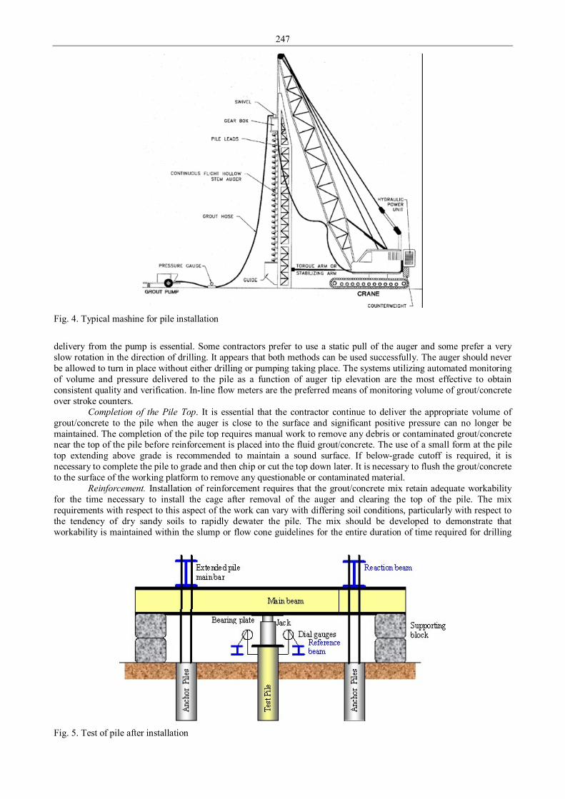
247

Fig. 4. Typical mashine for pile installation

delivery from the pump is essential. Some contractors prefer to use a static pull of the auger and some prefer a very slow rotation in the direction of drilling. It appears that both methods can be used successfully. The auger should never be allowed to turn in place without either drilling or pumping taking place. The systems utilizing automated monitoring of volume and pressure delivered to the pile as a function of auger tip elevation are the most effective to obtain consistent quality and verification. In-line flow meters are the preferred means of monitoring volume of grout/concrete over stroke counters.

Completion of the Pile Top. It is essential that the contractor continue to deliver the appropriate volume of grout/concrete to the pile when the auger is close to the surface and significant positive pressure can no longer be maintained. The completion of the pile top requires manual work to remove any debris or contaminated grout/concrete near the top of the pile before reinforcement is placed into the fluid grout/concrete. The use of a small form at the pile top extending above grade is recommended to maintain a sound surface. If below-grade cutoff is required, it is necessary to complete the pile to grade and then chip or cut the top down later. It is necessary to flush the grout/concrete to the surface of the working platform to remove any questionable or contaminated material.

Reinforcement. Installation of reinforcement requires that the grout/concrete mix retain adequate workability for the time necessary to install the cage after removal of the auger and clearing the top of the pile. The mix requirements with respect to this aspect of the work can vary with differing soil conditions, particularly with respect to the tendency of dry sandy soils to rapidly dewater the pile. The mix should be developed to demonstrate that workability is maintained within the slump or flow cone guidelines for the entire duration of time required for drilling

Fig. 5. Test of pile after installation

248

and grouting the pile and placing the rebar cage. In addition, other measures such as anti-washout admixtures may be required if soil conditions cause excessive dewatering of the mix after casting that results in rebar installation difficulties. Designers should include reinforcement cages that use: fewer heavy bars instead of many smaller bars; are no longer than the minimum necessary to provide structural capacity and anchorage; and allow the cage installation proceed with minimum difficulty. The contractor should tie the cage to permit handling without permanent distortion.

Test Piles and Test Installations. The recommended means of verifying that the installation plan will achieve the project requirements is using a carefully monitored test pile program. The program should consist of pre-production static load tests, production static and/or rapid and/or dynamic load tests, and post-installation integrity tests in sufficient quantities to provide the data necessary to demonstrate that the installed piles meet the load and deflection criteria established in the project plans with an appropriate factor of safety. It is imperative that the demonstrated installation procedure be followed for all production pile installations.

Installation Plan. The contractor should submit an installation plan including details of the equipment and methods proposed for the project. Many aspects of the construction work are performance-oriented with respect to the contractor’s equipment requirements and methodology. The installation details and monitoring of the installation are key components of verifying that the performance requirements are met. Contractors should be held accountable for developing an installation plan that will achieve the required objective. 5. Conclusions

Bored piles, namely auger cast-in-place piles and drilled displacement piles are used extensively in practice. The advantages of these piles are that their construction is fast, economic and environmentally friendly. These piles, depending on the method of installation, can be classified as partial- or full-displacement piles. Hence, their capacities are greater than that of drilled shafts with comparable length and diameter and, in many cases, approach that of driven piles. The installation methods and the quality control techniques for different types of auger piles were described, and the available design methods based on in-situ test results were presented. Analytical or numerical modeling of the installation of these piles combined with well-designed experiments and systematic monitoring of their installation in construction projects is needed for meaningful advances in analysis and design of these piles. References 1. LSIS. Pastatų konstruktoriaus ir statybininko žinynas. Kaunas: Naujasis lankas 2009. p. 94-104. 2. Zavadskas E. K., Karablikovas A., Marčiukaitis G., Malinauskas P., Mikšta P., Nakas H., Sakalauskas R.

Statybos procesų technologija. – Vilnius: Technika, 2008. p112-162. 3. Zavadskas E. K., Karablikovas A., Kriukeris V., Nakas H., Sakalauskas R. Pastatų statybos technologija. –

Vilnius: Technika, 2007. p 87-100. 4. Pile Design and Construction Practice, Fifth Edition; Michael Tomlinson, John Woodward; CRC Press, Nov 28,

2007. 5. Instructions for drilled piling; Helsinki 2003.

249

Proceedings of 9th International Conference ITELMS’2014 Impact of the Thermal Insulation Layer of Three-Layer Wall Panels on Energy Consumption of a Building S. Susinskas*, V. Zdanys** *Kaunas University of Technology, S. Daukanto str. 12, 35212, Panevezys, E-mail: s.susinskas@ktu.lt **Kaunas University of Technology, S. Daukanto str. 12, 35212, Panevezys, E-mail: v.zdanys@gmail.com Summary The article addresses the issues of energy efficiency of residential buildings through application of dynamic simulation of the building energy demand. The main object of the research is the influence of the thermal insulation layer of three-layer wall panels of individual house exterior walls on the building's energy demand. By means of the computer programs DesignBuilder and EnergyPlius, the energetic simulation has been done in order to determine the energy demand. For the existing individual house, three different simulations of the envelope construction thermal transmittance factor values and the thicknesses of thermal insulation layer have been done. We have presented the research results and conclusions. KEYWORDS: three-layer wall panel, simulation of energy demand, DesignBuider, EnergyPlius, calculated total energy consumption, thermal transmittance factor, dynamic methods of detailed simulation. 1. Introduction

During the last decade, the European Union has actively addresses the issues of energy resources. One of them is inefficient use of energy leading to extra depletion of at least 20% of total primary energy throughout Europe (European Parlament ... 2010).

Although, in the recent years, the efficiency of energy consumption has greatly increased, however, the biggest cost-saving opportunities are in the sectors of residential and public buildings. Here, it is possible to save approximately 27% to 30% of the current consumption of final energy (Commission of the European ... 2011). The energy consumption of a building is important because of this is the most expenditure throughout the entire life of the building. The factors of the highest influence upon the building energy consumption include climatic conditions, thermal comfort conditions, thermic, air tightness, architectural and structural peculiarities of the building, mode of the building usage, features of installed microclimate conditioning and energy supply systems to ensure the microclimate of the premises. This means that in order to determine an optimal level of the efficiency of the building energy consumption, it is necessary to consider a set of the energy end-use efficiency measures and the measures of integration of renewable energy.

In 2013, Lithuania adopted a Technical Construction Regulation STR 2.05.01:2013 'Building Energy Performance Designing'. The regulation is prepared in accordance with the Directive 2010/31/EU of the European Parliament and of the Council of 19 May 2010 on the Energy Performance of Buildings (OJ 2010 L 153, p. 13). The regulation conforms to the requirements of the Directive 2010/31/EU of 16 January 2012 delegated by the Commission, which supplements the Directive 2010/31/EU of the European Parliament and of the Council on the Energy Performance of Buildings by setting a comparative methodology framework for calculating the optimum level in terms of consumption and minimum energy performance requirements for buildings and building elements.

Pursuant to the aforementioned Technical Construction Regulation, buildings (elements thereof) are classified according to the energy performance into nine classes: A++, A+, A, B, C, D, E, F, G. The class A++ is considered the highest, it refers to the building (a part thereof) that uses almost no energy. For the new buildings constructed after the 1st of January 2014, the energy performance class shall be no less than B; after the 1st of January 2016, the energy performance class shall be no less than A; after the 1st of January 2018, the energy performance class shall be no less than A+; after the 1st of January 2021, the energy performance class shall be no less than A++. 2. Subject, aim and objectives of the research

The subject of the research is the influence of the thickness of thermal insulation layer of three-layer external walls of an individual residential house on the energy demand of the building.

The aim of the research is to perform a complex analysis of the characteristics of the thermal insulation layer of three-layer wall panels on the energy demand of indoor microclimate systems.

Objectives of the research: 1. To create a model of a real individual residential house and compare the results of the simulation with the results of

energy certification obtained with the program of energy certification of buildings NRG2. 2. According to the created model of the building, to carry out simulations for different thicknesses of facade (exterior

walls) heat insulation layers.

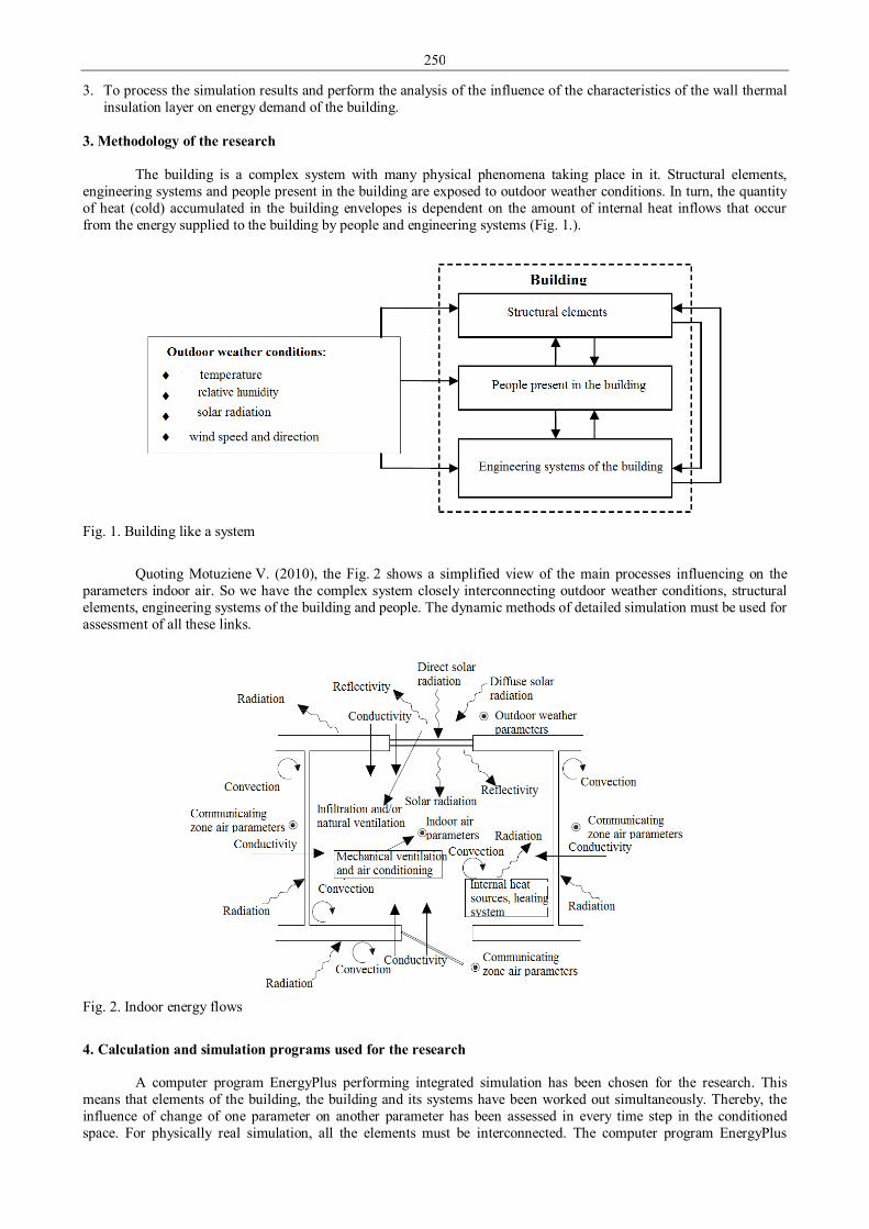
250

3. To process the simulation results and perform the analysis of the influence of the characteristics of the wall thermal insulation layer on energy demand of the building.

3. Methodology of the research

The building is a complex system with many physical phenomena taking place in it. Structural elements, engineering systems and people present in the building are exposed to outdoor weather conditions. In turn, the quantity of heat (cold) accumulated in the building envelopes is dependent on the amount of internal heat inflows that occur from the energy supplied to the building by people and engineering systems (Fig. 1.).

Fig. 1. Building like a system

Quoting Motuziene V. (2010), the Fig. 2 shows a simplified view of the main processes influencing on the

parameters indoor air. So we have the complex system closely interconnecting outdoor weather conditions, structural elements, engineering systems of the building and people. The dynamic methods of detailed simulation must be used for assessment of all these links.

Fig. 2. Indoor energy flows

4. Calculation and simulation programs used for the research

A computer program EnergyPlus performing integrated simulation has been chosen for the research. This means that elements of the building, the building and its systems have been worked out simultaneously. Thereby, the influence of change of one parameter on another parameter has been assessed in every time step in the conditioned space. For physically real simulation, all the elements must be interconnected. The computer program EnergyPlus

251

allows doing so through the simulation – the information of previous time steps is used to predict the system response and update the temperature of the zone at the present time step. Whereas the needs of power (heat or cold) of the zone determine all the processes, the power is used as a starting-point to determine the system needs. In this way, simulation of the system provides the existing supply capabilities and adjusts the temperature of the zone, as required. Such the EnergyPlus solution is called a process of prediction-correction. Detailed descriptions of EnergyPlus equations are provided in the documentation of the software – EnergyPlus Engineering Referece (2013).

A computer program DesignBuilder has been used for modelling. By means of the progam, we created a theoretical model of the building and inputted the required data. The program EnergyPlus performed the simulation of the building energy performance at selected time step for the period of a year, and the output data were provided in the program DesignBuilder. Processing of the data was done with the program Microsoft Excel. The scheme of the calculation and simulation of the selected building is showed in the Fig. 3.

Fig. 3. Scheme of programs used for calculation

5. Background data of the building under research

An individual residential house situated in Gruzdziai Village, Siauliai District was chosen for the reseach (Fig. 4).

Fig. 4. Schemes of the ground and attic floors of the building

The building is a single-storey house with an attic, the total area of the building is 189 m2, its capacity –

810 m3. The heated area is 189 m2. The existing architectural and structural solutions of the building are chosen for the research. The main facade of the house is facing to the north-east. The exterior walls of the building are of 520 mm thick silicate masonry with additional heat insulation of 150 mm thick polystyrene foam and coated with structural plaster. The internal load-bearing walls and partitions are of brick masonry. The plastic frame windows are with three-glass package (two of them are selective) filled with argon gas. The ratio between the areas of windows and external walls of the house is 20%. The house is with a single-pitch corrugated metal roof. The values of thermal transmittance factors of the main building envelopes are provided in Tab. 1.

252

Table 1 Thermal transmittance factors of the building envelopes, U, W/m2K

Envelope description Envelope thermal transmittance factor U, W/m2K Exterior walls 0.182 Roof 0.160 Floors on the ground 0.200 Windows 1.340 Exterior door 1.400

6. Creation of a theoretical model of the building

By means of the computer program DesignBuilder, we have created a theoretical model of the building. In the data base of the program, we have selected the location (Lithuania) and the time zone (GTM+02:00) of the building under the analysis; the annual climatic data of Kaunas typical meteorological year have been used for the energy simulation of the building and entered into the data base (IWEC 2013) of the international network of meteorology data IWEC (International Weather for Energy Calculations).

Based on the schemes of the floors of the residential house under research, we have created the theoretical model of the building in the program DesignBuilder (Fig. 6).

Fig. 6. Geometric model of the building in the program DesignBuilder

The next step in creation of the theoretical model of the building is attribution of purpose of the premises to

individual zones of human activities. The following main zones have been distinguished in the building: common area, kitchen, bedrooms and utility rooms; the number of people has been chosen according to the design standards – 4 people. Considering the purpose of the premises, human activity, natural lighting through the windows of the building, the program selects the required indoor lighting. According to the available project-based data of the building structures and their thermal transmittance factors, we have chosen the building structures with the corresponding values of thermal transmittance factors in the program (Tab. 1).

For designing of heating and ventilation with the reliability of 99.6%, we have used the designed outdoor air temperature of –19.51 °C. For designing of a cooling system with the same reliability, we have used the designed outdoor air temperature of 27.5 °C. In the program Design Builder, we have selected a condition that the heat is produced by a solid fuel boiler with an automatic mode. The heat efficiency of this heat source is 0.89. The heating system is manifold; the premises are heated by underfloor heating. Electric power is used for cooking. The building is equipped with a natural ventilation system.

Upon creation of the theoretical model of the selected building with the program Design Builder and simulation with the program EnergyPlius, we obtained the calculated total energy consumption per square meter of the useful space of the real building. According to the data of the program, the energy consumption of the building is 211.66 kWh/(m2 × year). To verify the reliability of the program, the obtained results were compared with the data of an Energy Performance Certificate of Building issued to the aforementioned building in 2013. The Certificate declares that the calculated total energy consumption per one square meter of the building's useful area is 212.22 kWh/(m2 × year). Upon the comparison of these two figures, it can be stated that the program EnergyPlus provides the data with sufficient accuracy (the variance reaches just 0.26%) in comparison with the data of the certification program of the energy performance of buildings “NRG-sert” (NRG2) used in Lithuania. 7. Analysis

The highest heat losses are incurred due to the heat conductivity through the building elements and due to air filtration. Control of the air movement through the building envelopes is very important in reducing the heat losses and protecting against moisture accumulation. The outgoing air carries heat and humidity to the outside in the form of water vapour. The water vapour carried by the air can condensate in the building envelope and cause damages to the building structures.

253

The air tightness of the building envelopes can be measured under a standard fan pressurization method as per EN 13829 by creating the difference of the building internal and external air pressure of 50 Pa and measuring the variance of the building air. The recommended building air variance must be equal or less than 1 time per hour.

Material thermal resistance (R) and thermal transmittance factor (U) of the structural construction are calculated by using the values of the material thickness and the coefficient of thermal conductivity.

One of the key issues which have a significant influence on the reduction of the energy demand, in particular for heating, is constant tightening of the requirements for thermal transmittance factors of the building envelope (STR 2.05.01:2013 “'Building Energy Performance Designing”') (Tab. 2).

Table 2 Standard values of wall thermal transmittance factor of residential buildings U, W/(m2K)

Envelope description Energy performance class of the building/Thermal

transmittance factor U, W/(m2K) B A A+ A++

Roofs 0.16 0.10 0.09 0.08 Floors Envelopes of heated premises contiguous with the ground 0.25 0.14 0.12 0.10 Floor above unheated basements and cellars Walls 0.20 0.12 0.11 0.10 Windows, skylights, bay windows and other transparent envelopes 1.60 1.00 0.85 0.70 Doors, gates 1.60 1.00 0.85 0.70

STR 2.05.01:2013 “Building Energy Performance Designing” requires that the buildings of the energy

performance classes C, B, A, A+ and A++ (or parts thereof) must be designed so that their air tightness, measured in accordance with the requirements of LST EN 13829:2002 Thermal performance of buildings – Determination of air permeability of buildings - Fan pressurization method (ISO 9972:1996, modified), would not exceed the values of air exchange shown in the Tab. 3 at the pressure difference between the building’s inside and outside of 50 Pa.

Table 3 Standard values of air exchange n50.N (1/h) at the pressure difference of 50 Pa

Purpose of the building Class of energy performance of the building n50.N , 1/h

Residential, administrative, educational and medical C, B 1.5 A, A+, A++ 0.6

8. Analysis of the simulation results

In order to explore the impact of the exterior wall envelope thermal insulation layer thickness on the calculated total energy consumption, we have entered different Uw values for the theoretical model of the building created by means of the computer program DesignBuilder.

The simulation is done with the following values of thermal transmittance factor U, W/(m2K) of the exterior wall: Version 1. A three-layer wall panel consisting of an outer concrete layer of 12 cm thickness, a layer of mineral wool

(U – 0.035 W/(m2K) of 20 cm thickness, an inner layer of concrete load-bearing wall of 20 cm thickness, plastered with thin plaster is chosen for the exterior wall of the building. The thermal resistance (R) of the envelope structure is equal to 6.41 m2K/W; thermal transmittance factor (U) is equal to 0.156 W/(m2K). We entered a standard value of air exchange n50.N (1/h) at the pressure difference of 50 Pa – 1.5 (STR 2.05.01:2013 “Building Energy Performance Designing”, the requirement for the energy performance class B).

Upon the simulation with the program EnergyPlius, we have established that the calculated total energy consumption per one square meter of the building's useful area is 210.27 kWh/(m2 × year).

With the same wall parameters we performed a simulation by entering the standard value of air exchange n50.N (1/h) at the pressure difference of 50 Pa – 0.6 (STR 2.05.01:2013 “Building Energy Performance Designing”, the requirement for the energy performance classes A, A+ and A++).

Upon the simulation, the program has calculated that the calculated total energy consumption per one square meter of the building's useful area is 133.12 kWh/(m2 × year).

We compared the obtained data and established that the energy consumption of the building decreased by 36.69 per cent.

With the same wall parameters we performed a simulation by entering a desirable value of air exchange n50.N (1/h) at the pressure difference of 50 Pa – 0.2.

Upon the simulation, the program showed that the calculated total energy consumption per one square meter of the building's useful area was 110.15 kWh/(m2 × year).

254

In this case, the energy consumption of the building decreased by 47.61 percent (in comparison of the values of air exchange 1.5 and 0.2 n50.N (1/h) at the pressure difference of 50 Pa).

Table 4 Input data and results of the analysis of the Version 1

Envelope structure

Thickness of thermal insulation layer of the structure (U – 0.035

W/(m2K)), cm

Thermal resistance of the structure R, m2K/W

Thermal transmittance

factor U, W/m2K

Value of air exchange n50.N , 1/h

Calculated total energy

consumption, kWh/(m2 × year)

Three-layer wall panel 20 6.41 0.156 1.5 210.27 0.6 133.12 0.2 110.15

The obtained simulation data is presented in the Fig. 7.

Fig. 7. Impact of air exchange on energy consumption for heating of the building, kWh/(m2 × year), thickness of

thermal insulation layer – 20 cm

Version 2. We insulated the same construction of the external wall with a layer of mineral wool of 30 cm thickness. The

thermal resistance (R) of the envelope structure is equal to 9.267 m2K/W; the thermal transmittance factor (U) is equal to 0.156 W/(m2K). We applied the analogous air exchange values n50.N (1/h) for the simulation in the program EnergyPlus: 1.5, 0.6 and 0.2 (Tab. 5).

The energy consumption of the building decreased to 37.26 and 52.59 percent, respectively.

Table 5 Input data and results of the analysis of the Version 2

Envelope structure

Thickness of thermal insulation layer of the structure (U – 0.035

W/(m2K)), cm

Thermal resistance of the structure R, m2K/W

Thermal transmittance

factor U, W/m2K

Value of air exchange n50.N , 1/h

Calculated total energy

consumption, kWh/(m2 × year)

Three-layer wall panel 30 9.267 0.108 1.5 206.78 0.6 129.74 0.2 98.03

The obtained simulation data is presented in the Fig. 8.

255

98,03

52,59

129,74

37,26

206,78

0,000

50

100

150

200

250

Energy consumptionfor heating of the

building, kWh/(m2 xyear)

Decrease of energyconsumption, %

n50.N (1/h) value =0,2

n50.N (1/h) value = 0,6

n50.N (1/h) value = 1,5

Fig. 8. Impact of air exchange on energy consumption for heating of the building, kWh/(m2 × year), thickness of

thermal insulation layer – 30 cm

Version 3. We insulated the same construction of the external wall with a layer of mineral wool of 15 cm thickness. The

thermal resistance (R) of the envelope structure is equal to 4,981 m2K/W; the thermal transmittance factor (U) is equal to 0.156 W/(m2K). The same values of air exchange n50.N (1/h) as per previous versions were applied for the simulation: 1.5; 0.6 and 0.2 (Table 6).

The energy consumption of the building decreased to 36.19 and 51.25 percent, respectively. The obtained simulation data is presented in the Fig. 9.

Table 6

Input data and results of the analysis of the Version 3

Envelope structure

Thickness of thermal insulation layer of the structure (U – 0.035

W/(m2K)), cm

Thermal resistance of the structure R, m2K/W

Thermal transmittance

factor U, W/m2K

Value of air exchange n50.N , 1/h

Calculated total energy

consumption, kWh/(m2 × year)

Three-layer wall panel 15 4.981 0.201 1.5 213.49 0.6 136.22 0.2 104.07

104,07

51,25

136,22

36,19

213,49

0,000

50

100

150

200

250

Energy consumption forheating of the building,

kWh/(m2 x year)

Decrease of energyconsumption, %

n50.N (1/h) value = 0,2

n50.N (1/h) value = 0,6

n50.N (1/h) value = 1,5

Fig. 9. Impact of air exchange on energy consumption for heating of the building, kWh/(m2 × year), thickness of

thermal insulation layer – 15 cm

Upon the comparison of all simulated versions, we attempted to estimate the impact of thickness of the thermal

insulation layer on the calculated total energy consumption per one square meter of useful area of the building considering the value of the building air tightness n50.N (1/h).

256

Fig. 10. Impact of the thickness of the envelope thermal insulation layer and air circulation on energy consumption for

heating of the building, kWh/(m2 × year)

The presented Fig. 10 shows that the thicknesses of 30 and 15 centimetres of the external wall thermal

insulation layer has a marginal impact on the annual energy consumption of the building. After the increase of the thickness of thermal insulation layer by 100% (from 15 cm to 30 cm), the change of the energy consumption totalled just 3.14%. Upon the comparison of the data with the impact of air circulation on the annual energy consumption of the building, we see that in case of any thickness of the thermal insulation layer (15 or 30 cm) the change due to the infiltration is very high – on the average 51.92%. The change of energy consumption again reaches just 5.8%.

The results clearly show that the heat savings are based on the air tightness. Upon the increase of thermal resistance of the thermal insulation layer by 83.88% (upon thickening of the layer from 15 cm to 30 cm, the thermal resistance of the construction (R) respectively increases from 4.981 to 9.159 m2·K/W), the heat savings reach just 3.14%. Such the insvestmest is ineffective. The results of the research lead to the conclusion that it is much more effective to invest to the security of air tightness of the house, because even the construction of the envelope with relatively low thermal resistance, if its air tightness is ensured, keeps most of the heat escaping from the premises. 9. Conclusions

The building is a complex system with many physical phenomena taking place in it. It is the complex system closely interconnecting outdoor weather conditions, structural elements, engineering systems of the building and people. The dynamic methods of detailed modelling must be used for assessment of all these links.

The energy performance of the building is determined to a large extent at an early stage of the design, therefore the design decisions taken at this stage have a decisive impact on the construction costs and energy consumption of the building in the phase of its usage.

The computer program EnergyPlius provides the simulation data with sufficient accuracy (in comparison of the actual energy consumption of the building with the simulated data, the variance is 0.26%), so it may be used for preliminary design solutions in Lithuania.

The results of the analyses clearly showed that the essence of heat savings was the air tightness. By reducement of the costs of thermal insulation layer, we will lower the cost price of the product and will be able to allocate more funds to the solutions of air tightness of the building. In this way, without increasing the construction costs, we will significantly improve the building's energy consumption rates throughout the life of the building. References 1. Commission of the European Communities 2011. Communication of commission: Energy Efficiency Plan 2011

[online]. Internet access: < http://europa.eu/rapid/press-release_MEMO-11-149_en.htm?locale=en > [accessed on 17 February 2014].

2. U.S. Departament of Energy 2013. EnergyPlus documentation. EnergyPlus Engineering Referece [online]. Internet access: < http://apps1.eere.energy.gov/buildings/energyplus/pdfs/engineeringreference.pdf > [accessed on 2 March 2014].

3. Technical Construction Regulation STR 2.05.01:2013 'Building Energy Performance Designing' [online]. Internet access: < http://www3.lrs.lt/pls/inter3/dokpaieska.showdoc_l?p_id=462390 > [accessed on 10 March 2014].

4. Motuziene V. Complex Analysis of the Influence of Glazing on Energy Demand of Public Buildings: Doctoral Dissertation. Vilnius Gediminal Technical University. – Vilnius: Technika, 2010, p. 29 – 59.

5. UAB „Paroc“ 2014. Envelope: Heat, Air Tightness and Moisture [online]. Internet access: < http://www.paroc.lt/ verta-zinoti/energinis-efektyvumas/pastatu-projektavimas/atitvaros > [accessed on 15 March 2014].

257

Proceedings of 9th International Conference ITELMS’2014 Theoretical Study of Fragmentation of Co6O7 Nanoparticle J. Tamuliene, L. Baliulyte Vilnius University, Universiteto g. 3, LT-01513, Lithuania, E-mail: Jelena.Tamuliene@tfai.vu.lt Abstract The investigation of fragmentation of t Co6O7 is presented in the paper aiming to show that a cobalt oxide particle or a cobalt particle covered with a cobalt oxide shell could be used as a precursor for Focused Electron Beam Induced Deposition. The stability and geometrical structure of the differently charged cobalt particle are determined. The appearance energy is evaluated. The distortion of the particle, formed during the fragmentation, is also established. KEYWORDS: fragmentation, nanoparticle, energy of appearance, density functional approach. 1. Introduction

Currently, metal nanoparticles, in particular those with magnetic properties such as Co nanoparticles, receive much attention due to their peculiar electronic, optical, catalytic, and magnetic properties [1-2]. The application of these particles is very broad: from ultrahigh density recording media to medicine and, in addition, they are traditional precursors of anode materials in Li-ion rechargeable batteries and an effective catalyst in the reduction of SO2 by Co and of NO by methane [3]. In order to achieve challenging technological goals, the magnetic particles need to be supported by or embedded in other materials such as semiconductors or insulators. However, it is proven that to prepare monodispersed nanoparticles by the traditional method is more complicated because the synthesis process is more complex [4].

At present, Focused Electron Beam Induced Deposition (FEBID), allows the structures to be deposited on the nanometer scale, is a very promising technique for nanofabrication, although it relies on precursors that are not optimized for the electron driven process. However, this technology is a one-step process and almost any desired geometry can be deposited. It is known, that FEBID structures are generated from a standard metal organic precursor under high vacuum conditions. Generally, the above precursors do not exceed a metal content by 15–75% and possess certain properties [6]. Currently, high purity deposits in FEBID have been obtained with the precursor molecule [Co2(CO)8] [5]. However, this precursor molecule exhibits poor stability in both the vacuum and air, potentially leading to polymerization reactions and the pressure build up in the precursor reservoir. Hence, investigations have been focused on an alternative candidate for electron beam induced Co deposition.

Our recent investigations reveal that the stability of the Co nanoparticles increases with the increase of the number of O atoms in the particle. The results of these investigations also proved that the magnetic properties of the Co nanoparticles are oxygen-atom-dependent, i.e. the Co nanoparticles could loose their magnetic properties due to oxidation [7]. On the other hand, O2 assisted with FEBID required much lower energy to induce a decomposition reaction, and secondary electrons achieved 90 % of the deposition process [6]. Referring to these results, we presumed that the Co shell-core nanoparticles could be applied to the electron induced fragmentation mechanisms occurring in FEBID to cover the surface by pure Co nanoparticles. In this sense, the fragmentation of the Co6O7 was investigated. A theoretical method is used to predict all possible fragmentation channels and other processes that could occur under the electron impact on the nanoparticle. 2. Method of Investigation

The structure of the molecule and its fragments has been studied by the Becke’s three-parameter hybrid functional applying the non-local correlation provided by Lee, Yang, and Parr (B3LYP) [8], – a representative standard DFT method. The most significant advantage of the DFT method is a significant increase in computational accuracy without the additional increase in computing time [9]. The present DFT method is derived for obtaining total energies as the function of the nuclei position and is often the method of choice for reaction calculations because the electron correlation energy is accounted, while ignoring the electron correlation is one of the most significant deficiencies of the Hartree-Fock method. However, the correlation energy, as well as the total energy of the investigated system, is highly dependent on the basis set used. Thus, our investigation was performed with the 6-31G to satisfy both accuraty of the investigations and appropriate computing time and resourses [10]. The structure parameters of the molecule and its fragments under study have been optimized with no symmetry constraint.

The following electron–molecule interaction processes relevant for FEBID such as vibrational excitation, electronic excitation, dissociative electron attachment, neutral dissociation, dissociative ionization, and bipolar dissociation / ion pair formation are mentioned. Taking in to account the aim our investigation: “is the fragmentation of small cobalt oxide particles possible?” the calculations for the initial and final states of the system are presented for the case of dissociation without taking into account the activation energy of the reverse reaction (Еr). In order to model the

258

fragmentation processes for the pure Co nanoparticle formation, we predict that the Co compounds could more probably posses only a positive charge, while that of O ones could be negative. Additionally, we predict that charge value of the both above compounds could vary from 0 to 6 during the fragmentation. The appearance energies were calculated as the difference between the total energy of the Co6O7 molecule and the sum of the total energies of the fragments predicted.

Using this methodology, we took into account the processes when the molecular ions formed with energies in excess of the ionization potential, may have no sufficient energy to be decomposed according to the lowest energy pathway. The GAMESS and the Gaussian program packages were applied here [11, 12]. Additionally, it is necessary to mention that not all investigations planed are finished yet and this is a reason why t more general conclusions are also not presented. 3. Results and discussions

Let us remember that the investigation of the fragmentation of Co6O7 particle is performed to show, that the above cobalt oxide or pure cobalt particle, covered by CoO layer, could be a precursor for FEBID to produce a pure cobalt particle. In this sense the formation of a pure cobalt nanoparticle from atoms or their derivatives formed due to electron impact are the most important results of the fragmentation. On the other hand, in any applications of the particles, the primary importance is to control the surface properties of nanoparticles because the surface of the particle could be the main factor determining stability. Therefore, several pathways have been followed to enhance the stability, i.e. from the use of specific surfactants to the control of surface charge [4]. Hence, we firstly paid our attention to the formation of the particle and stability of the compounds formed.

Referring to results achieved the possibility of the formation of Co derivatives possessing a neutral or an even positive charge is larger than that with odd positive charges. The comparison of the total energy of the neutral and charged Co fragments, that allows us to conclude, that the formation of the neutral Co nanoparticle due to the fragmentation is more probable than that of positive ones: the total energy of Co6

+2 is 15.32 eV higher than that of the neutral particles, while the energy of Co6

+4 other is much higher (Tab. 1).

Table 1 The total energy of the differently charged Co6 derivatives

Charge of Co derivatives investigated Total energy, a.u Difference of the

total energies, eV 0 -8295.80 0 2 -8295. 24 15.32 4 -8293.86 52.87

Our fragmentation simulations result also in joining of the Co6 derivatives, consisting of the Co isolated atoms,

to the particle. Hence, the formation of the neutral Co6 particle from Co6O7 due to electron impact is possible and we may speculate that the results of the fragmentation of cobalt oxide or a pure cobalt particle coated with it could be the formation of a pure cobalt nanoparticle.

Second, a very important requirement is the energy of the appearance of the Co derivatives that could not exceed the energy of FEBID. For FEBID the relevant energy range is 1 meV (slowed-down secondary electrons) and up to the keV regime (typical primary electron regime, forward and backscattered electrons) [13].

Table 2 Calculated appearance energies (in eV) for the O7 neutral and

differently charged Co6 fragments formed from the Co6O7 molecule

Charge of Co derivatives investigated Energy of appearance, eV 0 31.80 2 47.11 4 84.68

Referring to the results presented in Tab. 2 it is obvious that the energy of the Co6 particle appearance lies in

the relevant energy range for FEBID. It is emphasized, that the processes of the removing of all O atoms from Co6O7 (cleavage of all chemical bonds) requires the largest amount of the energy for the particle destruction. Hence, it is possible to foresee a less-energy-hungry fragmentation processes in which the energy of appearance does not exceed the energy range relevant for FEBID. The described above allows us to conclude that Co6O7 could be a precursor for FEBID as the one satisfying the second requirement.

However, it is necessary to mention that both geometrical structures of the neutral particle achieved when the fragmentation is simulated and when the stablest conformer of Co6 is searched is being searched for, are different (Fig. 1). The different geometrical structures obtained are not a surprise for us, because the previous results of our investigations exhibited the presence of several conformers of the Co6 particle, while the above observation shows the possibility of the formation of conformers due to the fragmentation [14]. Additionally, we would like to pay attention to

259

the simple rotation of one plane of the particle obtained when the fragmentation of Co6O7 is simulated that leads to formation of the stablest conformer of Co6.

Fig. 1. Geometrical structures of the Co6 particle obtained when the fragmentation of Co6O7 is simulated (on the left)

and the particle is being searched for the stables conformer

Hence, we may speculate that the molecule can move from one structure to the other via pseudo-rotation due to

a small barrier between these structures. The emission of the energy around 0.20 eV could follow the above rotation taking into account the difference of the total energies of the structures of the conformers investigated. Thus, from the first sign, the energy of the fragment appearance could be lower due to the energy emitted, but it is not clear how large the pseudo-rotational barrier is. We do not also know: if the cascade processes of the fragmentation due to electron impact are possible, which of them is more relevant, and which cascade processes is less energy-hungry, what electron–molecule interaction processes are more relevant for FEBID. However, despite the scarcity of research data, referring to results obtained, we may conclude that Co6O7 could be used as a precursor for FEBID. Acknowledgment

This work was conducted within the framework of the COST Action CM1301 (CELINA). Special thanks to InSpire and NGI.LT projects for the resources and technical support provided. References 1. Reynolds P. J. (Ed.) On Cluster and Clustering, Elsevier Science Publisher, Amsterdam (1993). 2. Gambardella P. and et al. Journal of Applied Physics, 99, 2006, 08Q501.1. 3. Wen G. H. and et al. Journal of Magnetism and Magnetic Materials, 270, (2004). 407. 4. Kobayashi Y. and et al. Preparation and Properties of Silica-Coated Cobalt Nanoparticles, J. Phys. Chem. B, 107

(30), 2003, 7420–7425. 5. Engmann S. F. Low Energy Electron Interactions with Precursor Molecules Relevant to Focused Electron Beam

Induced Deposition, Ph.D. thesis, 2013. 6. Beaulieu D. C. Electron beam chemical vapor deposition of platinum and carbon, Master degree thesis 2005. 7. Tamuliene J. and et al. Journal of Nanomaterials, 2009 (2009), Article ID 308276, 7 pages. 8. Becke A. D. J. Chem. Phys. 98,1993, p. 5648-5652. 9. Zhao Y. and et al. Phys. Chem. Chem. Phys. 6, 2004, p. 673–676. 10. Kendall R. A. and et al. J. Chem. Phys. 96, 1992, p. 6796–6806. 11. Schmidt M. W. and et al. J. Comp. Chem. 14, 1993, p. 1347–1363. 12. Gaussian 03, Revision C.02, Gaussian, Inc., Wallingford CT, 2004. 13. Huth M. and et al. Focused electron beam induced deposition: A perspective. Thematic Series "Radiation-induced

nanostructures: Formation processes and applications".Associate Editor: A. Gölzhäuser, Beilstein J. Nanotechnol. 2012, 3, 597–619.

14. Tamuliene J. and et al., Materials Physics and Mechanics 9, 1 2010, p. 35-41.

260

Proceedings of 9th International Conference ITELMS’2014 Investigation of Stability of N-(2,4,6-trinitrophenyl)-1H-1,2,4-triazol-3-amine J. Tamuliene*, J. Sarlauskas**, S. Bekesiene***, V. Kleiza**** *Vilnius University, Institute of Theoretical Physics and Astronomy, A. Gostauto 12, Lithuania, E-mail: Jelena.Tamuliene@tfai.vu.lt **Vilnius University, Institute of Biochemistry, Mokslininku 12,Vilnius, Lithuania, E-mail: jonas.sarlauskas@gmail.com ***The General Jonas Žemaitis Miltitary Academy of Lithuania, Silo g. 5A, LT-2005 Vilnius, Lithuania, E-mail: Svajone.Bekesiene@mil.lt ****Kaunas University of Technology, Daukanto 12, LT-35212 Panevezys, Lithuania, E-mail: vytautas.kleiza@ktu.lt Abstract The stability of the N-(2,4,6-trinitrophenyl)-1H-1,2,4-triazol-3-amine molecule due to the additional nitro group presence was studied theoretically using the density functional theoretical approach. The main emphasis was paid to the binding energy per atom with a special emphasis on the binding energy per atom dependence on the position of the additional nitro group. KEYWORDS: energetic materials, explosivestability. 1. Introduction

Recently, the research has been carred out into the synthesis of new energetic materials to be utilized as explosives aiming to couple high density with high energy. The detonation pressure approaching kilobars (kbar), a specific impulse and/or enhanced stability and insensitivity to such stimuli as impact, friction, and electrostatic discharge should also be considered [1]. Additionally, energetic materials could not be quite sensitive and hydrolytically unstable. Hence, the research is in progress worldwide searching for explosives with the combination of properties such as safety, reliability, stability, cost-efficiency and eco-friendliness. For the synthesis of thermally stable explosives, nitro compounds have received special attention because of their ability to withstand high temperatures and the low pressures encountered in space environments [2]. Currently, general approaches influencing the thermal stability of explosive molecules are very well known. These approaches are the following [3, 4]: • Introduction of amino groups; • Condensation with a triazole ring; • Salt formation; • Introduction of conjugation.

A lot of studies are performed to clarify the effect of the introduction of amino groups to various compound, e.g. 1,3,5 trinitrobenzene, 1,3-diamino-2,4,6- trinitrobenzene and etc. [5-7]. Reffering to these studies, it was concluded that the introduction of an amino (-NH2) group (in the ortho position) into a benzene ring already having a nitro (-NO2) group enhanced the thermal stability of explosives. On the other hand, the new explosives containing amino groups as well as ca onjugation were synthesized and investigated [8-10]. Some of these new materials have the unique distinction of being the most thermally stable explosive reported so far as compared to well known thermally stable explosives. Reffering to the above studies, we modelled N-(2,4,6-trinitrophenyl)-1H-1,2,4-triazol-3-amine molecule and performed theoretical investigations of it aiming to clear the influence of the nitro group and its position to both the stability and optical properties. It is emphasized that our general aim was to design and synthesize new energetic materials. Hence, we started our theoretical studies with the investigations of the molecules satisfying the first two approaches of those mentioned above. 2. Method of investgations

The structure of the molecule and its fragments has been studied by the Becke’s three-parameter hybrid functional applying the non-local correlation provided by Lee, Yang, and Parr (B3LYP) [11], – a representative standard DFT method. The most significant advantage of the DFT method is an increase in computational accuracy without the additional increase in computing time [12]. The present DFT method is derived for obtaining total energies as the function of the nuclei position and is often implemented as the method of choice for reaction calculations because the electron correlation energy is accounted, while one of the most significant deficiencies of the Hartree-Fock method is that ignoring the electron correlation. However the correlation energy, as well as the total energy of the investigated system, is highly dependent on the basis set used. Thus, our investigation was performed with the cc-pVTZ basis set [13]. The structure parameters of the molecules under study have been optimized with no symmetry constraint. We computed force constants and the resulting vibrational frequencies. The Gaussian program packages were applied [14].

261

3. Results and discussion

The views of the core molecule investigated are presented in Fig. 1. Substitutions R1, R2 and R3 are -H or -NO2. Here, the substitution –NO2 is introduced as ‘the additional NO2 (nitro) group’ in order to separate it from other groups in the core molecule. The largest number of the additional nitro groups attached to the core molecule is two and their placement is different (Fig.1, Table 1). Hence, the molecules under the study are different due to different number of the nitro groups and their placement in the core molecules. We indicated the molecules investigated as I-VI to simplify discussion.

Fig. 1. View of the core molecule investigated. The meaning of R1, R2 and R3 is presented in Tab. 1

Table 1

Substitutions of R1, R2 and R3 for the investigated molecules

Molecule investigated R1 R2 R3 I -H -H -H II -NO2 -H -H III -NO2 -NO2 -H IV -NO2 -H -NO2 V -H -H -NO2 VI -H -NO2 -H

To compare the stability of the derivatives investigated, the binding energy per atom is calculated and

presented in Tab. 2. It is evident, that the stability of the molecule I, where R1, R2 and R3 are H atoms, is the lowest in comparison to that of other investigated compounds. However, we may not state that the stability of these molecules investigated increases when one of the above substitutions is –NO2 , because the binding energy per atom of molecule II is only 0.013 eV, i.e. less than kT~0.02 eV, and there is no possibility to recognize which of the above mentioned molecules I or II is more stable. Moreover, the comparison of the binding energy per atom of molecule II and VI (which are different because of the additional nitro group attached to different N atoms (Fig. 1, Table 1)), allows us to predict that even the placement of the additional NO2 group influences insignificantly the stability of N-(2,4,6-trinitrophenyl)-1H-1,2,4-triazol-3-amine taking into account that in the both cases N-NO2 similar additional chemical bonds are formed.

Table 2 Binding energy per atom of the molecules investigated

Molecule investigated

Binding energy per atom, eV

Binding energy per atom in respect of the stablest molecule, eV

I 6.376 0.062 II 6.389 0.048 III 6.412 0.025 IV 6.438 0 V 6.430 0.008 VI 6.403 0.035

262

Molecules V and VI have also one additional -NO2 group that is attached to C and N atom of the triazole ring, respectively. Refering to the obtained rezults of the binding energy per atoms, it is evident that the stability of molecule V is larger than that of IV. Let us remember, that the stability of molecule II and VI, when only N-NO2 bond appered, is not different. These observations allow us to conclude, that the stability of the molecules investigated could increase because of the presence of the additional -C-–NO2 bond. A similar phenomenon is obtained in the case of molecules III and IV. These molecules possess the two additional –NO2 groups, and they are different due to the additional nitro group position in the triazole ring: in the case of molecule III, the N-NO2 bond is formed, while C-NO2 takes place in molecule IV. Hence, the stability of N-(2,4,6-trinitrophenyl)-1H-1,2,4-triazol-3-amine could increase when the additional nitro group is attached to C atom. It is interesting, that the number of the additional nitro groups has not influence on the stability of the investigated molecule: the binding energy per atom of molecule IV and molecule V is similar, although two and one additional nitro groups take place in these molecule respectively and one of them is attached to the C atom of the triazole ring. 3. Conclusions 1. An amino (-NH2) group (in the ortho position) in a benzene ring with a nitro (-NO2) group enhanced the thermal

stability of explosives. 2. The stability of the molecules investigated could increase because of the presence of the additional -C-–NO2 bond in

triazole ring. 3. The stability of molecule V is larger than that of IV, moreover, the comparison of the molecules III (possessing N-

NO2 bond) and IV (possessing C-NO2 bond) shows the increased stability of the later molecule. Acknowledgment

The present investigation carried out within the framework of the LMA scientific project “A theoretical and experimental investigations of new potentially explosive materials using quantum mechanical methods (NSPROG-I4)”. Special thanks to InSpire and NGI.LT projects for the resources and technical support provided. References 1. Wilson W. S. NAWCWPNS Technical Publication 8188, Published by Technical Information Department, 1994. 2. Agrawal J. P. Central European Journal of Energetic Materials, 2012, 9, p. 273-290. 3. Agrawal J. P., Hodgson R. D. John Wiley & Sons, UK, 2007. 4. Agrawal J. P. Pyrotech., Wiley-VCH, Germany, 2010. 5. Ayres J. N., Montesi L. J., Bauer R. J. Naval Ordnance Laboratory, Technical Report (NOLTR) No.73-132, 1973. 6. Gibbs T. R., Popolato A. University of California Press, Los Angeles, 1980, 157, p. 3. 7. Zeman S. Thermochim. Acta, 1993, 216, p. 157-168. 8. Bapat V. K., Surve R. N., Agrawal J. P. Proc. 2nd High Energy Materials Conference & Exhibits, IIT, Madras,

Dec. 8-10, 1998, p. 403-405. 9. Makashir P. S., Bapat V. K., Mahajan R. R., Mehilal, Agrawal J. P. Proc. of International Workshop on

Unsteady Combustion & Interior Ballistics, Vol. 1, St. Petersburg, Russia, June 25-30, 2000, p. 199-205. 10. Mehilal, Sikder N., Sikder A. K., Agrawal J. P. Indian J. Eng. & Mater. Sci., 2004, 11, p. 516-520. 11. Becke A. D. J. Chem. Phys, 1993, 98, p. 5648-5652. 12. Zhao Y. and et al. Phys. Chem. Chem. Phys. 6, 2004, p. 673–676. 13. Kendall R. A., Dunning T. H. Jr. and Harrison R. J. J. Chem. Phys. 96, 1992, p.6796–6806. 14. Gaussian 03, Revision C.02, Gaussian, Inc., Wallingford CT, 2004.

263

Proceedings of 9th International Conference ITELMS’2014 Corporate Governance Model in the Czech Republic P. Taraba*, K. Pitrova** *Tomas Bata University, Nám. T. G. Masaryka 5555, 76001, Zlín, Czech Republic, E-mail: taraba@flkr.utb.cz **Tomas Bata University, Nám. T. G. Masaryka 5555, 76001, Zlín, Czech Republic, E-mail: pitrova@flkr.utb.cz Abstract Of all the legal systems that have been developed so far in the world, two basic models of corporate governance have been created: one-level (unitary) model, also called Anglo-Saxon or Anglo-American model, and the two-level (dual) model, which is called European model. Exactly the corporate governance model has a significant impact on the way of the entire functioning of the organization. In the article the advantages and disadvantages of each model are presented and the dominant model used in the Czech Republic is confirmed KEYWORDS: Corporate Governance, Corporate Governance Model, Czech Republic. 1. Introduction

One-level corporate governance model. In one-level corporate governance model there are two main bodies: General Shareholders Meeting and Board of Directors [3, 4, 6 and 7].

One-level model of the administrative body does not have any institutional ownership control separated from the operational management of the company. The Board of Directors performs both of these functions. It is composed of senior managers accompanied with a relatively small number of non-executive directors. The strong position of the Board Chairman (President) in the organization is guaranteed by the dispersed capital. He is often also the Executive Director, who manages senior management. He generally chooses the members of the senior management, as well as other members of the Board, while the General Assembly only confirms his decision [3]. Board of Directors (similarly as the Supervisory Board in two-level model) can produce some committees, according to their momentary needs, the focus of which depends on the level of complexity and the trend of the organization [6].

Carati and Rad [1] highlight the important role of the market in the one-level corporate governance model. The role of the government is only to support a highly competitive environment, where individual companies operate. Within the market of products and services the companies are under constant pressure from customers, competitors etc. The competitive pressures affect the managers who govern the production factor market. The authors believe that the corporate governance role is to promote a high level of competition in individual markets and the effective market mechanism will naturally motivate the companies and their managers to meeting the best interests of shareholders.

At the same time, however, they add that the role of other stakeholders cannot be neglected. One of the tasks of the administrative body should be a clear definition of the role of stakeholders in corporate governance. From experience we know that the ratio satisfying the rights of shareholders and other stakeholders militates in favor of shareholders [1].

This corporate governance model is used mainly in the USA and Great Britain [2]. Two-level corporate governance model. In two-level model there are the General Shareholders Meeting

(Vollversammlung in German) operating in an organizational architecture of the Corporate Governance Model with the Supervisory Board (Aufsichtsrat in German) and the Managing or Management Board (Vorstand in German) [7]. In this context Hučka, Malý and Okruhlica [3] point out a mistake made by some Czech companies very often - the incorrect translation of the Managing Board as the Board of Directors in their annual report for example. This body is not present in the two-level model.

The Managing Board in the two-level model directs the organization with executive powers. This usually coincides with the executive of the organization or its selected members so that in the executive corps there can be more officials who are not members of the Managing Board. The Supervisory Board surveys the competence of the board, executive and senior management and monitors the economic activities of the organization. The General Shareholders Meeting may elect both bodies at the annual general meeting, but more usually the General Assembly elects the Supervisory Board and this is instructed to appoint the Managing Board [4].

This model is complemented by compulsory employee representation. The importance of employees, but also the satisfaction of other stakeholders interests (suppliers, customers, the public, etc.) within the two-level corporate governance model is also stressed by the authors Gregory [2], Ooghe and Vuyst [5] and others.

The two-level model is used mainly in continental Europe (in particular Germany, France and the Netherlands) and in some Asian countries [2].

Comparison of one-level and two-level corporate governance model. Before we start to compare these two systems a brief assessment of the fundamental differences in management boards modelling should be noted (Tab. 1):

264

Table 1 Comparison of One-Level and Two-Level Corporate Governance Model [3]

Characteristics One-Level Model Two-Level Model Executive Administrative Body Executive Directors of

the Board of Directors Managing Board

Controlling Administrative Body Non-Executive Directors of the Board of Directors

Supervisory Board

Role of the Board of Directors (Managing Board) Important Important Concentration of Power Board of Directors Managing Board Functionality of Non-Executive Directors (Supervisory Board) Insufficient Sufficient Independence of Non-Executive Directors (Supervisory Board) Advisable Low Representation of Banks in Administrative Bodies Unacceptable Strong Interference of Banks in the Management Forbidden Strong Representation of Employees in Administrative Bodies Undesirable Obligatory Representation of Political Sphere in Administrative Bodies Undesirable Indirect Management Methods Indirect Monitored by Owners

After the comparison of the organizational architecture of one-level and two-level corporate governance model

we can conclude that from the systemic point of view the concept is essentially identical, where the function of the Supervisory Board in the one-level system is performed by external members of the Board of Directors and the Managing Board corresponds to the Executive Committee composed of senior executives [3].

The most significant differences we can find in the role of stakeholders in company management. This is particularly the representation of employees, bank representatives and political spheres in administrative bodies, where their importance in the two-level model in comparison with the one-level model is significant. For one-level model the functioning of developed capital market is of great importance, whose role in the two-level model is not so important.

Diversity in corporate governance models are to be found in different EU Member States and beyond. 2. Testing procedures

Methodology. The sample consisted of 300 respondents. These respondents were selected on the basis of a deliberate choice. The decision about the examined sample choice was not the element of chance, but the judgment of the researcher. Control characters when creating quota sampling was their membership in the Board of Directors or Supervisory Board. The final number of processed questionnaires was 103, ie. The return rate was 34.33%.

For data collection there were predominantly Czech organizations in terms of their ownership structure to obtain. This criterion was met, as organizations with Czech ownership accounted for 58.25% share of organizations whose data were analyzed in the framework of qualitative research. There were also analyzed data from the 16.50% of European organizations with the majority of owners (17 organizations) and 25.24% of organizations that respondents considered to be global (26 organizations).

The questionnaire was sent by classical or by electronic mail. Data collection took place in two rounds in the months from April 2010 to April 2011 and in the months from January 2012 to June 2012.

The questionnaire was evaluated using descriptive statistics; the results of the questionnaire were processed in graphical form and then interpreted. Questionnaire as a method of quantitative research is appropriate to use under the terms when the author of the questionnaire has secured a sufficient return. Under this condition there is an applicable method with the main benefits: • low cost of data collection; • the possibility of recouping a large sample of respondents; • relatively low time-consuming.

The survey questionnaire return was assured through the help of colleagues and personal contacts gained during the period of cooperation with practice that contributed to the high rate of questionnaire return.

Questionnaire survey also has its limits. For the success of the questionnaire survey it was necessary to ensure that the respondents were only members of the authorities. This is related to a lower number of questionnaires evaluated, as these specific issues and potential research respondents were considerably workload and their attitude to the questionnaire survey was largely dismissive.

Analysis and findings. The main objective of the research was to find out which corporate governance model is dominant in the Czech Republic.

To the objectives the following hypothesis was set: In the Czech Republic the two-level corporate governance model is dominant. In 77.67% of the analysed companies the two-level corporate governance model was used. The one-level

model was used in only 23 organizations (22.33%). This was mainly related to organizations with foreign ownership share majority. There was a considerable pressure to enforce the one-level model by the foreign parent organization.

265

It was supposed that the respondents would prefer the two-level model as seen in the German corporate governance model.

We described the hypothesis as follows: H1: The two-level corporate governance model prevails in the Czech Republic. We set both hypothesis H0 and an alternative one H1: H0: Both one-level and two-level corporate governance models are used in the Czech Republic. H1: In the Czech Republic the one-level corporate governance model is not used the same way as the two-level one. Chí – square test (χ 2 – test)– correlation test We have constructed - W: W = (3.842, ∞) We have constructed a test criterion:

( ) 54.3177.1577.15

5.51)5.5123(

5.51)5.5180( 22

1

22 =+=

−+

−=

−= ∑

=

k

i i

ii

OOP

χ

We have set the validity of hypotheses: χ 2Î∈W H0 has been rejected and H1 has been accepted. Based on the conducted test, we can conclude: It has been shown on the significance level of 5 percent that both corporate governance models are not used the

same way in the Czech Republic. The two level model was used by up to 80 (77.67%) from 103 respondents. The one-level system was used only in 23 (22.33%) of organizations.

We calculated the interval estimate (interval of 95%) for the monistic (one-level) response (Yes 23 - No 80) p = 0.2233

( ) ( )

−+

−−

−− nppup

nppup 1;1

21

21 αα

⋅⋅+

⋅⋅−

1037767.02233.096.12233.0;

1037767.02233.096.12233.0

( )08.02233.0;08.02233.0 +−

( )3033.0;1433.0

Interval estimate (interval of 95%) for the two-level response (Yes 80% – No 23%) p = 0.7767

( ) ( )

−+

−−

−− nppup

nppup 1;1

21

21 αα

⋅⋅+

⋅⋅−

1032233.07767.096.17767.0;

1032233.07767.096.17767.0

( )08.07767.0;08.07767.0 +−

( )8567.0;6967.,0

14.33-30.33% of all respondents will respond with the probability of 95% that the two-level corporate governance model is dominant in the Czech Republic.

Based on these results it can be concluded that: There is dominant two-level corporate governance model in the Czech Republic.

3. Conclusions

Based on the analysis of available information sources of corporate governance bodies, and after numerous consultations with practitioners, we assumed that the organizations operating in the Czech Republic will use the two-level corporate governance model as their dominant modus operandi. This fact has been statistically validated as well.

The one-level system management is governed by two main bodies: the General Shareholders Meeting and Board of Directors.

The two-level model organisational structure, in addition to the General Shareholders Meeting, is also governed by the Managing Board and the Board of Directors.

It is the dominant two-level model, which enables the organisation in the Czech Republic to benefit from this model [7]:

266

• it provides the background to ensure a stable environment of the organization in the form of cooperative coexistence, based on the set of contracts,

• it is not prone to fluctuations of the capital markets, • it motivates managers to promoting the long-term objectives, • it governs organizations, which are conducted directly by owners, • the close ties with the financial sector predetermine an easier overcoming of temporary financial problems.

However, I also need to mention certain shortcomings of this model which should be given a closer attention to. Those are as follows: • organisations inflexibility towards possible market fluctuations, • extreme power of workers and trade unions towards the owners, • cross-ownership and bank ownership of non-financial organizations can lead to conflicts of interest between

individual subjects. It is the consistent understanding of corporate governance models and the selection of a suitable model, which

can represent a significant competitive advantage not only in the Czech Republic. References 1. Carati G., Rad A. T. Convergence of Corporate Governance Systems. Managerial Finance. 2000, 26(10), p. 66-83. 2. Gregory H. J. The Globalization of Corporate Governance. 2001. [on-line]. Available at:

< http://www.weil.com/wgm/cwgmhomep.nsf/Files/Gregory-Aug01DM/$file/Gregory-Aug01DM.pdf > [12 Apr. 2014].

3. Hučka M., Malý M., Okruhlica F. Správa společností. Praha: Kernberg Publishing, 2007. 4. Jirásek J. A. Podnikatelská správa akciových společností (Corporate Governance). Praha: Professional Publishing,

2001. 5. Ooghe H., Vuyst V. D. The Anglo-Saxon versus the Continental European Corporate Governance Model:

Empirical Evidence of Board Composition in Belgium. 2001. [on-line]. Available at: < http://www.vlerick.com/ en/5786-VLK/version/live/part/AttachmentData/data/vlgms-wp-2001-06 > [12 Apr. 2014].

6. Porvazník J., Ladová J. Celostní management. Bratislava: Iris, 2010. 7. Růčková P. Corporate Governance v České republice. Praha: Professional Publishing, 2007.

267

Proceedings of 9th International Conference ITELMS’2014 Driving Style Analysis using Spectral Features of Accelerometer Signals G. Zylius, V. Vaitkus, P. Lengvenis Faculty of Electrical and Electronics Engineering, Kaunas University of Technology, Lithuania, E-mail: gediminas.zylius@ktu.edu Abstract The paper presents analysis of 3-axis accelerometer driving data in order to estimate driving style. We assume that driving style could be roughly divided into two groups: aggressive driving and safe driving. Methodology used in this research is applicable to shuttle transport driving analysis and gives possibility to analyze driving style of different road segments. The results of this work show that longitudinal acceleration data could be used in order to effectively classify aggressive and safe driving trip by using short-time Fourier transform features of different road segments. KEYWORDS: driving style, 3-axis accelerometer, driver classification, spectral analysis. 1. Introduction

The analysis of driving style for the companies, such as public transport, delivery service or insurance could help to manage service quality and increase yield by giving the possibility to control or monitor driver behavior which is related to appropriate driving style.

Signals related to driving behavior could be divided into 3 main groups: vehicle’s signals, driver’s signals and environment signals. Vehicle signals are obtained from dynamics of vehicle, states and outputs (w.r.t. vehicle). Driver’s signals are obtained from driver’s state (physiological signals) and output (driver’s operating signals). Environment signals are signals that could be obtained from the traffic environment, such as states of surrounding vehicles, road signals (line markings, terrain, potholes, condition).

There are numerous researches done related to driving behavior analysis. In paper [1, 2] the experiment with instrumented vehicle was done with different drivers and analysis of driver’s operating signals (pressure of accelerator and brake pedals of the vehicle) by modeling each individual driver using Gaussian Mixture Models (GMM) showed that biometric driver identification could be done using those signals’ dynamic features combined with state and that they carry individual driver biometric information the most comparing other signals. Further researches of the same group of scientist [3] show that increase in driver identification rate is obtained using spectral features (i.e., cepstum) of brake and accelerator pedal pressure signals.

In [4] the experiment with driving behavior was done using in-vehicle CAN-bus signals. The research results showed that using available CAN-bus signals (such as steering wheel angle, brake/acceleration status and vehicle’s speed) using Hidden Markov Models (HMM) combined with GMM identification of driving maneuvers could be obtained without other external sensory data. Much later, using same vehicle, the experiment was done [5] that compared available CAN-bus signals and smart portable off-the-shelf device (i.e., tablet PC) sensory information. The results show that using portable device as a sensor platform the driving maneuver identification rate was higher that using CAN-bus information.

The use of smart portable device’s sensors for Driver Assistance Systems (DAS) emerges rapidly because of relatively rich sensor information available and that no additional external computational hardware is necessary. It is also is affected by the fact that more and more people are using smartphones and DAS could be implemented without additional hardware as an application program only which is very cheap and easy to apply. For example, in the smartphone as a sensor platform was applied in the [6] for aggressive driving and driving event recognition. The reseach of vehicle’s condition evaluation, road condition classification and driving behavior evaluation system also using smartphone was done in [7]. Both experiment used smartphone inertial measurement sensors (accelerometer or gyroscope) and GPS.

In this work we consider that driving style could be divided into two main groups: aggressive and safe driving (regardless the land vehicle type). Aggressive driving should be considered driving type containing all negative driving features that contribute to reckless driving, vehicle damaging, passengers’ discomfort and also fuel consumption. Safe driving should be considered driving type opposite to aggressive driving. Motivated by the previous experiments using vehicle’s inertial signals [6-10] in this experiment that show the effectiveness of inertial sensors in driving style capturing, we use only 3-axis accelerometer data to classify driving style into aggressive and safe driving.

Our experiment constraints are as follows: the same driver is driving the same vehicle in aggressive and safe driving style on the same route. The research results application will be related to shuttle transport services when the vehicle is driven the same route all the time and no different route consideration is necessary. Spectral analysis is used in order to obtain features from accelerometer signals that later are used for driving style classification into aggressive and safe.

Further the paper is divided into following sections: 1) Accelerometer signal pre-processing; 2) Spectral features extraction; 3) Feature selection; 4) Driving style classification; 5) Conclusions and future work.

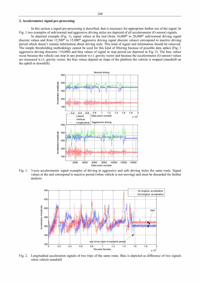
268

2. Accelerometer signal pre-processing

In this section a signal pre-processing is described, that is necessary for appropriate further use of the signal. In Fig. 1 two examples of safe/normal and aggressive driving styles are depicted of all accelerometer (G-sensor) signals.

In depicted example (Fig. 1), signal values at the end (from 16,000th to 20,000th safe/normal driving signal discrete values and from 12,500th to 15,000th aggressive driving signal discrete values) correspond to inactive driving period which doesn’t contain information about driving style. This kind of signal end information should be removed. The simple thresholding methodology cannot be used for this kind of filtering because of possible data spikes (Fig. 1 aggressive driving discretes >14,000) and bias values of signal in stop period (as depicted in Fig. 2). The bias values occur because the vehicle can stop in any position w.r.t. gravity vector and because the accelerometer (G-sensor) values are measured w.r.t. gravity vector, the bias values depend on slope of the platform the vehicle is stopped (standstill on the uphill or downhill).

0.2 0.4 0.6 0.8 1 1.2 1.4 1.6 1.8 2

x 104

100

200

300

400

500Normal driving

Acc

eler

atio

n am

plitu

de

Data point number

2000 4000 6000 8000 10000 12000 14000

100

200

300

400

500Aggressive driving

Acc

eler

atio

n am

plitu

de

Data point number

LateralVerticalLongitudinal

Fig. 1. 3-axis accelerometer signal examples of driving in aggressive and safe driving styles the same route. Signal

values at the end correspond to inactive period (when vehicle is not moving) and must be discarded for further analysis

0 0.2 0.4 0.6 0.8 1 1.2 1.4 1.6 1.8 2

x 104

320

340

360

380

400

420

440

Discrete Number

Acc

eler

atio

n A

mpl

itude

1st longitud. acceleration2nd longitud. acceleration

bias

end of trip (start of standstill period)

Fig. 2. Longitudinal acceleration signals of two trips of the same route. Bias is depicted as difference of two signals

when vehicle standstill

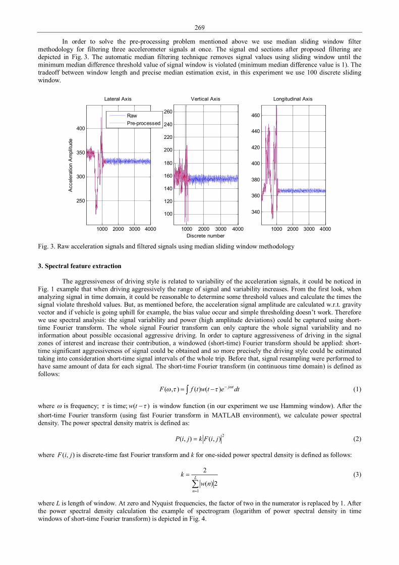
269

In order to solve the pre-processing problem mentioned above we use median sliding window filter methodology for filtering three accelerometer signals at once. The signal end sections after proposed filtering are depicted in Fig. 3. The automatic median filtering technique removes signal values using sliding window until the minimum median difference threshold value of signal window is violated (minimum median difference value is 1). The tradeoff between window length and precise median estimation exist, in this experiment we use 100 discrete sliding window.

1000 2000 3000 4000

250

300

350

400

Acc

eler

atio

n A

mpl

itude

Lateral Axis

RawPre-processed

1000 2000 3000 4000

100

120

140

160

180

200

220

240

260

Discrete number

Vertical Axis

1000 2000 3000 4000

340

360

380

400

420

440

460

Longitudinal Axis

Fig. 3. Raw acceleration signals and filtered signals using median sliding window methodology

3. Spectral feature extraction

The aggressiveness of driving style is related to variability of the acceleration signals, it could be noticed in Fig. 1 example that when driving aggressively the range of signal and variability increases. From the first look, when analyzing signal in time domain, it could be reasonable to determine some threshold values and calculate the times the signal violate threshold values. But, as mentioned before, the acceleration signal amplitude are calculated w.r.t. gravity vector and if vehicle is going uphill for example, the bias value occur and simple thresholding doesn’t work. Therefore we use spectral analysis: the signal variability and power (high amplitude deviations) could be captured using short-time Fourier transform. The whole signal Fourier transform can only capture the whole signal variability and no information about possible occasional aggressive driving. In order to capture aggressiveness of driving in the signal zones of interest and increase their contribution, a windowed (short-time) Fourier transform should be applied: short-time significant aggressiveness of signal could be obtained and so more precisely the driving style could be estimated taking into consideration short-time signal intervals of the whole trip. Before that, signal resampling were performed to have same amount of data for each signal. The short-time Fourier transform (in continuous time domain) is defined as follows:

dtetwtfF tjωττω −−= ∫ )()(),( (1)

where ω is frequency; τ is time; )( τ−tw is window function (in our experiment we use Hamming window). After the short-time Fourier transform (using fast Fourier transform in MATLAB environment), we calculate power spectral density. The power spectral density matrix is defined as:

2),(),( jiFkjiP = (2)

where ),( jiF is discrete-time fast Fourier transform and k for one-sided power spectral density is defined as follows:

∑

=

= L

nnw

k

12)(

2 (3)

where L is length of window. At zero and Nyquist frequencies, the factor of two in the numerator is replaced by 1. After the power spectral density calculation the example of spectrogram (logarithm of power spectral density in time windows of short-time Fourier transform) is depicted in Fig. 4.

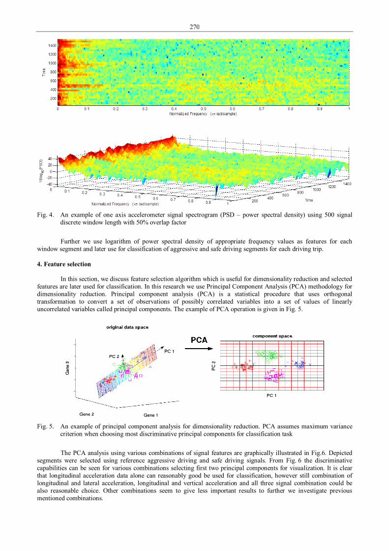
270

Fig. 4. An example of one axis accelerometer signal spectrogram (PSD – power spectral density) using 500 signal

discrete window length with 50% overlap factor

Further we use logarithm of power spectral density of appropriate frequency values as features for each

window segment and later use for classification of aggressive and safe driving segments for each driving trip. 4. Feature selection

In this section, we discuss feature selection algorithm which is useful for dimensionality reduction and selected features are later used for classification. In this research we use Principal Component Analysis (PCA) methodology for dimensionality reduction. Principal component analysis (PCA) is a statistical procedure that uses orthogonal transformation to convert a set of observations of possibly correlated variables into a set of values of linearly uncorrelated variables called principal components. The example of PCA operation is given in Fig. 5.

Fig. 5. An example of principal component analysis for dimensionality reduction. PCA assumes maximum variance

criterion when choosing most discriminative principal components for classification task

The PCA analysis using various combinations of signal features are graphically illustrated in Fig.6. Depicted

segments were selected using reference aggressive driving and safe driving signals. From Fig. 6 the discriminative capabilities can be seen for various combinations selecting first two principal components for visualization. It is clear that longitudinal acceleration data alone can reasonably good be used for classification, however still combination of longitudinal and lateral acceleration, longitudinal and vertical acceleration and all three signal combination could be also reasonable choice. Other combinations seem to give less important results to further we investigate previous mentioned combinations.

271

-400 -200 0 200 400-200

0

200longitudinal+lateral+vertical

Safe driving segmentsAggressive driving segments

-200 -100 0 100 200-100

0

100

200longitudinal

-200 -100 0 100 200-100

-50

0

50vertical

-200 -100 0 100 200-100

0

100lateral

-200 -100 0 100 200-200

0

200longitudinal+vertical

-200 -100 0 100 200-100

0

100

200longitudinal+lateral

-200 -100 0 100 200-100

0

100lateral+vertical

PC 2

PC 1 Fig. 6. Reference aggressive and safe driving segment PCA extracted features (two Principal Components (PC))

illustration after combining various signals’ original features (spectrograms)

5. Driving style classification

In previous section we used PCA analysis to investigate what combinations of features to use further for classification. In this section we use whole driving signal (aggressive and safe) segments using moving window with 50% overlap factor in order to generate spectrogram features and classify them, when classification method is trained with previously (section 4) depicted aggressive and safe driving segments. The purpose of this classification is as follows: each separate driving trip segments’ (after performing spectrogram feature generation) principal components (principal component eigenvectors are obtained from reference driving trips) are used as an input to the trained classifier in order to obtain score of driving trip (aggressiveness or safety of driving trip after classifying each driving segment into aggressive or safe). And we compare classification-based scores with the expert decisions about safe or aggressive driving trip.

For this task, we used Random Forest (RF) classifier with two principal components. No additional cross-validation checks were performed because of RF classifier (bagged decision trees in MATLAB) internal use of bagging (bootstrap aggregating) ensemble methodology. Classification results after out-of-bag error analysis favor longitudinal acceleration signal alone compared to other combinations (Fig. 7) achieving only ~3% error for aggressive and safe reference segments. So further we use only longitudinal acceleration signal in order to obtain aggressiveness and safety score for each driving trip.

The results of aggressiveness and safety of driving using experimental driving trips are summarized in Tab. 1.

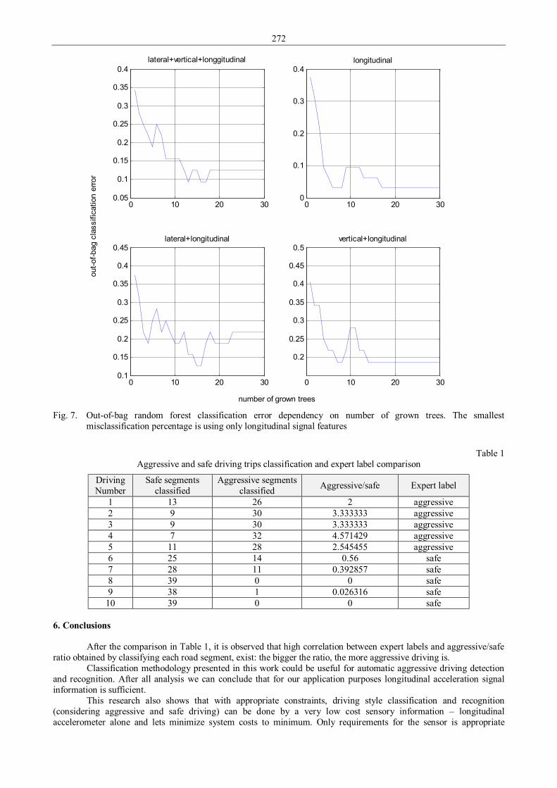
272

0 10 20 300.05

0.1

0.15

0.2

0.25

0.3

0.35

0.4lateral+vertical+longgitudinal

0 10 20 300

0.1

0.2

0.3

0.4longitudinal

0 10 20 300.1

0.15

0.2

0.25

0.3

0.35

0.4

0.45lateral+longitudinal

0 10 20 30

0.2

0.25

0.3

0.35

0.4

0.45

0.5vertical+longitudinal

out-o

f-bag

cla

ssifi

catio

n er

ror

number of grown trees Fig. 7. Out-of-bag random forest classification error dependency on number of grown trees. The smallest

misclassification percentage is using only longitudinal signal features

Table 1

Aggressive and safe driving trips classification and expert label comparison

Driving Number

Safe segments classified

Aggressive segments classified Aggressive/safe Expert label

1 13 26 2 aggressive 2 9 30 3.333333 aggressive 3 9 30 3.333333 aggressive 4 7 32 4.571429 aggressive 5 11 28 2.545455 aggressive 6 25 14 0.56 safe 7 28 11 0.392857 safe 8 39 0 0 safe 9 38 1 0.026316 safe

10 39 0 0 safe 6. Conclusions

After the comparison in Table 1, it is observed that high correlation between expert labels and aggressive/safe ratio obtained by classifying each road segment, exist: the bigger the ratio, the more aggressive driving is.

Classification methodology presented in this work could be useful for automatic aggressive driving detection and recognition. After all analysis we can conclude that for our application purposes longitudinal acceleration signal information is sufficient.

This research also shows that with appropriate constraints, driving style classification and recognition (considering aggressive and safe driving) can be done by a very low cost sensory information – longitudinal accelerometer alone and lets minimize system costs to minimum. Only requirements for the sensor is appropriate

273

attachment to vehicle body. This king of system would not interfere with any vehicle system devices and is easily to integrate with other system elements.

In future, we will use more inertial signals and are planning to expand the possibilities for this kind of system by minimizing constraints and integrating more features that would increase capabilities of transport management. References 1. Igarashi K., Miyajima C., Itou K., Takeda K., Itakura F. and Abut H. Biometric Identification Using Driving

Behavioral Signls. IEEE Int. Conf. Signals, Multimedia and Expo, vol. 1, Jun. 2004, p.65-68. 2. Wakita T., Ozawa K., Miyajima C., Igarashi K., Itou K., Takeda K. and Itakura F. Driver Identification Using

Driving Behavior Signals. IEEE Proc. Intelligent Transportation Systems, Sept. 2005, p.396-401. 3. Miyajima C., Nishiwaki Y., Ozawa K., Wakita T., Itou K. and Takeda K. Cepstral Analysis of Driving

Behavioral Signals for Driver Identification. IEEE Int. Conf. Acoustics, Speech and Signal Processing, vol. 5, May 2006, p.921-924.

4. Choi S., Kim J., Kwak D., Angkititrakul P. and Hansen J. H. L. Analysis and Classification of Driver Behavior using In-Vehicle CAN-Bus Information. 2007.

5. Sathyanarayana A., Sadjadi S. O. and Hansen J. H. L. Leveraging Sensor Information from Portable Devices towards Automatik Driving Maneuver Recognition. IEEE Int. Conf. Intelligent Transportation Systems, Sept. 2012, p. 660-665.

6. Johnson D. A. and Trivedi M. M. Driving Style Recognition Using a Smartphone as a Sensor Platform. IEEE Int. Conf. Intelligent Transportation Systems, Oct. 2011, p. 1609-1615.

7. Fazeen M., Gozick B., Dantu R., Bhukhiya M., Gonzalez M. C. Safe Driving using Mobile Phones. IEEE Trans. Intelligent Transportation Systems, vol. 13, no. 3, September 2012, p. 1462-1468.

8. Aljaafreh A., Alshabatat N. and Al-Din M. S. N. Driving Style Recognition Using Fuzzy Logic. IEEE Int. Conf. Vehicular Electronics and Safety, Jul. 2012, p. 460-463.

9. Ly M. V., Martin S., Trivedi M. M. Driver Classification and Driving Style Recognition using Inertial Sensors. Intelligent Vehicles Symposium, Gold Coast, Australia, June 23–28, 2013, p. 1040-1045.

10. Krotac T., Simlova M. The Analysis of the Acceleration of the Vehicle for Assessing the Condition of the Driver. Intelligent Vehicles Symposium, Alcalá de Henares, Spain, June 3–7, 2012, p. 571-576.

274

Authors Index

A Ahrens A. .....................................................11, 17 Andreeva N........................................................ 17 Aviza D. ..................................... 28, 104, 227, 244

B Baliulyte L. ...................................................... 257 Baltusnikiene R. ................................................. 28 Bartnicki A. ....................................................... 36 Bartuska L. ...................................................... 238 Bazaras Z. ................................................... 46, 109 Bekesiene S. ............................................. 206, 260 Berezin V........................................................... 57 Bulovas P. ......................................................... 48

C Cepauskas A. ..................................................... 54 Chausov M. ....................................................... 57 Cieslik K............................................................ 36 Cmiral T. ......................................................... 141

D Dabrowska A. .................................................... 64 Danyliuk I. M. ................................................. 189 Daunoravicius J. ................................................ 73 Demeniene A. ...............................................76, 80 Dobrzinskij N. ................................................... 85 Dragunas A. ....................................................... 92

F Furch J. .............................................................. 96

G Garskiene A. .................................................... 104 Girkontas E. ..................................................... 109 Glos J. ............................................................. 114 Gorobetz M...................................................... 118 Grzelak K. ....................................................... 221

H Hutsaylyuk V. ............................................. 57, 232

I Igakojyte-Bazariene J. ........................................ 46

J Jackuviene R. ................................................... 126 Jaskolowski M. B. ............................................ 131 Joneliukstiene I. ............................................... 137 Jonevicius V. ................................................... 206 Jukna A. .......................................................... 217

K Kampf R. ......................................................... 141 Karlapavicius S. ............................................... 151 Karpavicius R. .................................................. 126 Kaupiene J. .............................................. 104, 151 Kleiza V. ........................................... 126, 159, 260 Klimavicius K. ................................................. 162 Konopka S. ........................... 36, 64, 131, 165, 173 Konovalenko I. V. ............................................ 189 Krogul P. .................................................... 64, 180 Kubasakova I. .................................................. 238 Kumbar V. ....................................................... 114

L Laurikietyte R. ............................................. 76, 80 Lejskova P. ...................................................... 141 Lengvenis P...................................................... 267 Levchenkov A. ................................................. 118 Lochmann S. ...................................................... 11 Lopatka M. J. ................. 36, 64, 131, 165, 173, 180 Lukosevicius V................................................. 109

M Maruschak P. O. ............................................... 189 Muszynski T............................................. 165, 180

N Navardauskaite I. .............................................. 193 Neumann V. ..................................................... 198

P Panin S. V. ....................................................... 189 Partaukas N. ..................................................... 104 Pelenyte-Vysniauskiene L................................. 151 Pincevicius A. .................................................. 206 Pitrova K. ......................................................... 263 Poska T. ........................................................... 211 Potapovs A. ...................................................... 118 Przybysz M. ............................................. 165, 180 Pylypenko A....................................................... 57

R Rubiec A. ................................................. 131, 173

S Sarlauskas J. ..................................................... 260 Shatkovskis E. .................................................. 217 Slezak T. .......................................................... 221 Slivinskas V. .................................................... 227 Sniezek L. ........................................... 57, 221, 232 Spadlo K. ......................................................... 173 Stasiskis A. ...................................................... 151 Stopka O. ......................................................... 238

275

Striukiene D. .................................................76, 80 Stuglys G. ........................................................ 244 Stupakova J...................................................... 217 Susinskas S. ... 28, 48, 54, 73, 92, 137, 162, 193, 211,

227, 244, 249 Szachogluchowicz I. ........................................ 232

T Tamuliene J. ............................................. 257, 260 Taraba P. ......................................................... 263 Tilindis J. ......................................................... 159 Timofeev B. ....................................................... 46 Torzewski J........................................................ 57

V Vaiciulis P. ................................................... 76, 80 Vaitkus V. ........................................................ 267 Valackiene A. ..................................................... 80 Valickas J. ........................................................ 211 Vasileva N. ........................................................ 46 Vlasov I. V. ...................................................... 189 Vochozka M. .................................................... 141

Z Zacharoviene E............................................. 76, 80 Zagadskij V. ..................................................... 217 Zascerinska J. ..................................................... 17 Zdanys V.......................................................... 249 Zylius G. .......................................................... 267

INTELLIGENT TECHNOLOGIES IN LOGISTICS AND MECHATRONICS SYSTEMS (ITELMS’14). Proceedings of the 9th International Conference. Held on May 22-23, 2014, Panevezys, Lithuania. INTELEKTUALIOS TECHNOLOGIJOS LOGISTIKOJE IR MECHATRONINĖSE SISTEMOSE (ITELMS’14). 9-osios tarptautinės konferencijos, įvykusios Panevėžyje 2014 m. gegužės 22-23 d., pranešimų medžiaga (anglų kalba). Maketavo D. Vaiciulis

INTELLIGENT TECHNOLOGIES IN LOGISTICS AND MECHATRONICS SYSTEMS ITELMS'2014

PROCEEDINGS OF THE 9TH INTERNATIONAL CONFERENCE

ISSN 2351–6275

SL 344. 2014-07-22. 17,25 leidyb. apsk. l. Tiražas 35 egz.

Užsakymas 365.

Leidykla „Technologija“, Studentų g. 54, 51424 Kaunas