Emerging issues and challenges in conservation of biodiversity in the rangelands of Tanzania.
Upload
khangminh22Category
view
4download
0
Pooja LakhanpalJaydeep MukherjeeBiswajit NagDivya Tuteja Editors
Trade, Investment and Economic GrowthIssues for India and Emerging Economies

Trade, Investment and Economic Growth

Pooja Lakhanpal · Jaydeep Mukherjee ·Biswajit Nag · Divya TutejaEditors
Trade, Investmentand Economic GrowthIssues for India and Emerging Economies

EditorsPooja LakhanpalDepartment of ManagementIndian Institute of Foreign TradeNew Delhi, Delhi, India
Biswajit NagDepartment of EconomicsIndian Institute of Foreign TradeNew Delhi, Delhi, India
Jaydeep MukherjeeDepartment of EconomicsIndian Institute of Foreign TradeNew Delhi, Delhi, India
Divya TutejaDepartment of EconomicsIndian Institute of Foreign TradeNew Delhi, Delhi, India
ISBN 978-981-33-6972-6 ISBN 978-981-33-6973-3 (eBook)https://doi.org/10.1007/978-981-33-6973-3
© The Editor(s) (if applicable) and The Author(s), under exclusive license to Springer NatureSingapore Pte Ltd. 2021This work is subject to copyright. All rights are solely and exclusively licensed by the Publisher, whetherthe whole or part of the material is concerned, specifically the rights of translation, reprinting, reuseof illustrations, recitation, broadcasting, reproduction on microfilms or in any other physical way, andtransmission or information storage and retrieval, electronic adaptation, computer software, or by similaror dissimilar methodology now known or hereafter developed.The use of general descriptive names, registered names, trademarks, service marks, etc. in this publicationdoes not imply, even in the absence of a specific statement, that such names are exempt from the relevantprotective laws and regulations and therefore free for general use.The publisher, the authors and the editors are safe to assume that the advice and information in this bookare believed to be true and accurate at the date of publication. Neither the publisher nor the authors orthe editors give a warranty, expressed or implied, with respect to the material contained herein or for anyerrors or omissions that may have been made. The publisher remains neutral with regard to jurisdictionalclaims in published maps and institutional affiliations.
This Springer imprint is published by the registered company Springer Nature Singapore Pte Ltd.The registered company address is: 152 Beach Road, #21-01/04 Gateway East, Singapore 189721,Singapore

Foreword
The Indian Institute of Foreign Trade (IIFT) has established itself as an AcademicCentre of Excellence in International Business. It is committed to high standardsof teaching in international business as well as a centre for pioneering research andknowledgedissemination in the arena of foreign trade andpolicy issues. IIFThas beenorganizing the Empirical Issues in International Trade and Finance (EIITF) ResearchConference series since 2008. From the beginning, the conference has brought to thefore academic discussions and discourse on contemporary issues relevant to inter-national trade, finance and business as a whole. The themes of the conference serieshave reflected the rapid changes around the world, particularly contemporary themeswhich have been of interest to researchers in associated fields as well. The instituteorganized the Sixth EIITF on 18 and 19 December 2018 at its New Delhi Campus.In keeping with the latest developments, the themes of the conference were tech-nology disruptions, global capital flows and international trade-drivers for economicdevelopment. The conference was attended by academicians, policy researchers,multilateral agencies, industry bodies and policymaking communities from acrossthe globe.
The release of the current volume could not have been at a more appropriate time.International trade and capital flows, since the turn of the century, have been in astate of flux. In particular, international trade patterns have been marked by risinguncertainty, since the global financial crisis of 2008–2009 and the eurozone crisisof 2011–12. The world economy is currently reeling under an unprecedented healthcrisis due to spread of the COVID-19 pandemic which is expected to severely affectglobal economic activity. As a result, compared to the last year, growth in the globaleconomy is expected to fall by as much as 3 per cent in the current year. IMF’sWorld Economic Outlook (WEO) Update (April 2020) reports this to be much moresevere than the growth contraction resulting from the financial crisis of 2008–09.Assuming that the pandemic is contained in the second half of 2020 and in view ofthe expansionary policy measures,WEO (April 2020) projects that a bounce back isexpected in 2021, wherein the global economy is expected to expand by 5.8 per cent.
A key challenge for the global economy at the current juncture relates to theuncertainty regarding the time it would take for the pandemic to fade away and foreconomic activity to normalize. In the aftermath of the pandemic, consumer demand
v

vi Foreword
is expected to remain weak and employment in the informal sector is likely to remainstagnant. This is notwithstanding the bleak global growth prospects due to rising tradedisputes and geopolitical tensions in 2018–19. The advanced economies have had achoppy and long road to recovery post the global financial crisis of 2008–09 (Tradeand Development Report 2019 (UNCTAD)).
While there is an urgent need for monetary as well as fiscal expansion, there maybe limitations to the policy headroom. Another crucial aspect is the anchoring ofinflationary expectations through communication by the monetary authorities. Thereis a risk of a debt-deflation spiral whichmay be abated by a strong government policystance. In order to facilitate recovery, regulatory foresight in the form of strong insol-vency and debt enforcement frameworks is required. Finally,multilateral cooperationis the need of the hour, especially in the economic as well as medical arena. Thiswould mean the removal of tariff and non-tariff barriers to allow international tradeand functioning of global supply chains along with measures to boost the globalfinancial sentiment. Nations would need to work side by side to share informationabout the virus crucial for containment and development of the vaccine.
The present volume has been contributed by scholars who participated at theEIITF 2018 Conference and intends to make a significant contribution to the existingliterature by including selected empirical works on critical policy issues in thespheres of international trade and foreign capital flows and their role in fosteringeconomic growth and development in the context of India and several emergingmarket economies. Twenty papers included in the volume are classified appropri-ately under four broad themes, namely: (1) International Trade: Empirical and PolicyIssues, (2) Foreign Capital Flows and Issues in Finance, (3) Trade and Develop-ment Interface: Implications for India and Emerging Economies and (4) Analysis ofSector-level Growth and Development in India, all of which are extremely relevantin the current context. The chapters in the volume have been contributed by leadingacademicians and researchers involved in the applied area of economics. I am confi-dent that the empirical works presented in this comprehensive volume could serveas ready reference for academicians, researchers and policymakers, particularly inemerging economies facing similar challenges.
Prof. Manoj PantDirector and Vice Chancellor
Indian Institute of Foreign Trade (IIFT)New Delhi, India

Acknowledgements
All of the chapters included in this volume were originally presented in the 6thConference on Empirical Issues in International Trade and Finance (EIITF) orga-nized by the Indian Institute of Foreign Trade (IIFT) Delhi on 13 and 14 December2018. The conference focused on technology disruptions, global capital flows andinternational trade-drivers for economic development.
ProfessorManoj Pant, Director, IIFT, was a guiding light and extended his uncon-ditional support. We are obligated to Springer for making this collection of papersaccessible to students and researchers working in related fields in the form of a book.We are grateful to Nupoor Singh, Editor, Springer, and Daniel Joseph G. for theirconstant support in this endeavour. The authors are also grateful to two anonymousreferees for constructive suggestions and comments.
We are thankful to all the authors who contributed their research work forthe volume. We also gratefully acknowledge competent and diligent support fromAshima Puniani and Saloni Khurana, for compiling and editing the chapters in thevolume.Research support fromTanyaDawar is also gratefully acknowledged. Lastly,we thank our families for facilitating us in countless ways.
vii

Introduction1
This chapter introduces the background, recent developments, themes and the paperscontained in this conference volume titled Trade, Investment and Economic Growth:Issues for India and Emerging Economies. The first section presents the backgroundto the key issues covered in the volume. Subsequently, we discuss the recent devel-opments and performance of emerging economies in the second and third sections.The last section discusses the themes which form the focal point of the papers andbriefly outlines papers included in the present volume.
Background
The twenty-first century is being shaped by changing views on international trade inboth goods and services along with global capital flows and their role in affecting theeconomic outcomes of various countries. Lately, the global economy has been undera lot of strain and is facing sluggish economic growth. This may be attributed tothe dawdling trade along with mounting tariffs, unstable financial flows, decreasedbusiness confidence and rising policy uncertainty among others. Climate change,divergent public views on critical issues and an increasing distrust of political partiesare also risking the medium- and long-term growth. In view of changes in volumeas well as pattern of trade and investment flows, there is an urgent need to study theestablished paradigms of economics through a new lens with advances in theoreticaland empirical models.
To add to the fire, the intensified trade tensions among the USA and China, Brexitnegotiations, the shutdown of the US federal government, US-Iran trade rifts, Italy’sconflict with EU regarding public debt and uncertainty in Mexico’s policy directionunder the new government are some of the many upsetting policy news from allaround the world. China, one of the largest economies in the world, has been experi-encing a decline in its growth due to policy pressures in the face of a debt overhang,
1Diligent research work by Tanya Dawar is gratefully acknowledged.
ix

x Introduction
slower infrastructural investment and decline in exports as a result of the US tariffs.This has badly affected the imports in the economy and exports of its trade partnersin Asia and Europe. India too is also slowing down, and its exports to the world areexperiencing a secular decline.
With this backdrop, Indian Institute of Foreign Trade organized its 6th Conferenceon Empirical Issues in International Trade and Finance during 13–14December 2018at its New Delhi Campus. The editors of this volume have selected some of the bestpapers presented at the conference. The distinctive aspects of the volume are thatit covers topical issues pertaining to international trade, capital flows and finance,development and sector-level growth in India with a focus on the policy point of view.Secondly, the discourse focuses mainly on empirical work and econometric aspects.Finally, the overall focus is on the lessons learnt from the trade–capital flows–growthexperience of emerging economies.
Recent Developments
The global economy has been in a lot of flux lately; the paradigms for achieving ahealthy and steady economic growth are continuously getting redefined. The worldis currently staring at an unprecedented health crisis presented by the outbreak ofthe COVID-19 pandemic. The global economy, currently grappling with a healthcrisis resulting from the spread of COVID-19, is likely to witness a contraction inthe economic activity. However, it is not possible to stray away from the existingtheory, literature and evidence on the pillars of achievement of robust growth.
It is notable that the health crisis due to spread of COVID-19 is associated witha huge output loss. The growth in the global economy, year on year, is expected tofall by as much as 3 per cent. IMF’sWorld Economic Outlook (WEO) Update (April2020) reports this to be much more severe than the growth contraction resultingfrom the financial crisis of 2008–09. There is considerable ambiguity regarding theduration and intensity of this surprise. Clearly, innovative policy, both medical andeconomic, is the need of the hour to counter the effects of the crisis.
Assuming that the pandemic is contained in the second half of 2020, and in view ofthe expansionary policy measures, WEO (April 2020) projects that a bounce back isexpected in 2021, wherein the world economy is expected to expand by 5.8 per cent.The recovery in global economic activity in 2021 ismarked by enormous uncertainty.The implementation of effective policies is central to a gradual normalization ofeconomic activity and a recovery in 2021 (WEOUpdate, April 2020). Cross-countrycooperation onmedical supplies, vaccines, therapies andother interventions is criticalto slow down the transmission of the COVID-19 pandemic. However, countriesshould refrain from the imposition of additional trade restrictions and resort externalfunding wherever required. Apart from cooperation on healthcare systems, targetedpolicies, at both the local and national levels, are imperative at the current point intime.

Introduction xi
The articles included in this volume provide contemporary dynamics of the pre-COVID period which will probably remain important in the post-COVID world alsoas globalization has made a tectonic shift to economic management. Perhaps, thepost-COVID world will try to align the new reality with some of the fundamentalaspects of the twenty-first-century world which are expressed through the papers. Inparticular, issues related to the development of emerging economies through the tradeand finance channels are at the heart of the economic growth literature. Therefore,the papers in the volume bring to the fore critical issues which merit the attention ofthe policymakers and growth enthusiasts and these experiences will serve as lessonsfor the way forward in the post-COVID ‘normal’.
Performance of Emerging Economies
The critical role played by investment and trade in the context of engenderingeconomic growth cannot be emphasized enough. Truth be told, a vast majorityof advanced economies have been able to sustain the growth momentum in viewof conducive conditions for investment and trade. This is particularly true of theemerging and developing economies (EMDEs) which have struggled with the ‘twindeficits’ of trade deficit and budget deficit in the past. Before we delve further intothe role played by investment and trade in economic growth of a nation, we defineEMDEs and discuss their key economic performance measures.
As of June 2020, the World Bank has classified the countries given in Table 1 asemerging and developing economies (EMDEs) which include some of the largestand most populous economies of the world such as China, India and Brazil.
Table 1 Emerging market and developing economies (World Bank)
Country Continent group
China East Asia and Pacific
Indonesia
Thailand
Russia Europe and Central Asia
Turkey
Poland
Brazil Latin America and the Caribbean
Mexico
Argentina
Saudi Arabia Middle East and North Africa
Iran
Egypt
(continued)

xii Introduction
Table 1 (continued)
Country Continent group
India South Asia
Pakistan
Bangladesh
Nigeria Sub-Saharan Africa
South Africa
Angola
Source Global Economic Prospects, World Bank, June 2020
Table 2 presents the rate of growth of real GDP for the advanced and emergingmarket and developing economies (EMDEs) in 2015–21. Clearly, the EMDEs havebeen growing at a much faster rate than the advanced economies over the period2015–21. In particular, China and India have been the fastest growing and largestEMDEs during the last few years.
Table 2 Annual estimates and forecasts (f) of real GDP (World Bank)
2015 2016 2017 2018e 2019f 2020f 2021f
World 2.9 2.6 3.1 3.0 2.6 2.7 2.8
Advanced economies 2.3 1.7 2.3 2.1 1.7 1.5 1.5
USA 2.9 1.6 2.2 2.9 2.5 1.7 1.6
Euro area 2.1 2.0 2.4 1.8 1.2 1.4 1.3
Japan 1.2 0.6 1.9 0.8 0.8 0.7 0.6
Emerging market and developing economies(EMDEs)
3.8 4.1 4.5 4.3 4.0 4.6 4.6
Commodity-exporting EMDE 0.8 1.5 2.1 2.2 2.1 3.1 3.0
Other EMDE 6.1 6.0 6.1 5.8 5.2 5.5 5.5
Other EMDE excluding China 5.2 5.1 5.4 4.9 4.2 4.8 5.0
East Asia and Pacific 6.5 6.3 6.5 6.3 5.9 5.9 5.8
China 6.9 6.7 6.8 6.6 6.2 6.1 6.0
Indonesia 4.9 5.0 5.1 5.2 5.2 5.3 5.3
Thailand 3.1 3.4 4.0 4.1 3.5 3.6 3.7
Europe and Central Asia 1.1 1.9 4.1 3.1 1.6 2.7 2.9
Russia −2.5 0.3 1.6 2.3 1.2 1.8 1.8
Turkey 6.1 3.2 7.4 2.6 −1.0 3.0 4.0
Poland 3.8 3.1 4.8 5.1 4.0 3.6 3.3
Latin America and the Caribbean 0.1 −0.3 1.7 1.6 1.7 2.5 2.7
Brazil −3.5 −3.3 1.1 1.1 1.5 2.5 2.3
Mexico 3.3 2.9 2.1 2.0 1.7 2.0 2.4
Argentina 2.7 −2.1 2.7 −2.5 −1.2 2.2 3.2
(continued)

Introduction xiii
Table 2 (continued)
Middle East and North Africa 2.9 5.1 1.2 1.4 1.3 3.2 2.7
Saudi Arabia 4.1 1.7 −0.7 2.2 1.7 3.1 2.3
Iran −1.3 13.4 3.8 −1.9 −4.5 0.9 1.0
Egypt 4.4 4.3 4.2 5.3 5.5 5.8 6.0
South Asia 7.1 8.1 6.7 7.0 6.9 7.0 7.1
India 8.0 8.2 7.2 7.2 7.5 7.5 7.5
Pakistan 4.1 4.6 5.4 5.8 3.4 2.7 4.0
Bangladesh 6.6 7.1 7.3 7.9 7.3 7.4 7.3
Sub-Saharan Africa 3.0 1.3 2.6 2.5 2.9 3.3 3.5
Nigeria 2.7 −1.6 0.8 1.9 2.1 2.2 2.4
South Africa 1.3 0.6 1.4 0.8 1.1 1.5 1.7
Angola 0.9 −2.6 −0.1 −1.7 1.0 2.9 2.8
Source Global Economic Prospects, World Bank, June 2020
Table 3 Annual estimates and forecasts (f) of fixed investment rates in EMDEs (World Bank)
2015 2016 2017 2018e 2019f 2020f 2021f
East Asia and Pacific 6.5 6.6 5.3 5.3 5.1 5.1 4.9
Europe and Central Asia 0.4 −0.1 6.3 2.5 −0.9 3.3 3.6
Latin America and the Caribbean −4.5 −5.3 −0.2 2.2 1.3 3.1 4.4
Middle East and North Africa 1.6 −0.3 2.4 3.7 4.4 5.7 6.4
South Asia 3.5 7.7 7.0 10.5 8.3 7.8 7.9
Sub-Saharan Africa 3.7 −0.6 4.7 5.8 5.9 6.1 6.7
Source Global Economic Prospects, World Bank, June 2020
Table 3 depicts the fixed investment rates for EMDEs by region during 2015–21.We notice that the EMDEs located in Europe and Central Asia have had a relativelylow rate of fixed investment in the recent past. However, the South Asian EMDEshave displayed a relatively consistent and higher rate of fixed investment along withthose in East Asia and Pacific. EMDEs in Middle East and North Africa as well asthose in sub-Saharan Africa are showing much promise and have an upward trend inthe investment rates. Finally, the EMDEs located in Latin America and the Caribbeanhave a very volatile performance over the period 2015–21.
Table 4 focuses on the contribution of net exports or trade balance to GDP in caseof EMDEs.Wefind that, inmajority of the cases, the net exports’ contribution toGDPgrowth has been negative or at best low. In case of Europe and Central Asia as wellas Middle East and North Africa, the contribution has been consistently decreasingover 2015–21.
Figure 1 shows that general government gross debt levels of emerging economiesreduced sharply post 2008 due to the global financial crisis. It was also adversely

xiv Introduction
Table 4 Annual estimates and forecasts (f) of net exports’ contribution to growth in EMDEs (WorldBank)
2015 2016 2017 2018e 2019f 2020f 2021f
East Asia and Pacific −0.1 −0.8 0.4 −0.9 −0.4 −0.4 −0.5
Europe and Central Asia 3.0 0.3 −0.7 1.0 0.5 −0.1 −0.4
Latin America and the Caribbean 1.2 0.8 −0.4 −0.3 0.2 −0.2 −0.2
Middle East and North Africa 2.0 4.8 −0.2 1.4 −0.5 0.8 0.4
South Asia −0.2 −0.3 −2.0 −2.1 −0.6 −0.6 −0.6
Sub-Saharan Africa 0.0 1.6 1.2 −0.6 −0.2 −0.1 −0.2
Source Global Economic Prospects, World Bank, June 2020
0
10
20
30
40
50
60
70
80
90
2 0 0 5 2 0 0 6 2 0 0 7 2 0 0 8 2 0 0 9 2 0 1 0 2 0 1 1 2 0 1 2 2 0 1 3 2 0 1 4 2 0 1 5 2 0 1 6 2 0 1 7 2 0 1 8 2 0 1 9 2 0 2 0
GROSS DEBT LEVELS FOR EMERGING ECONOMIES
Emerging and developing Asia Emerging and developing Europe
ASEAN-5 Lan America and the Caribbean
Middle East and Central Asia Sub-Saharan Africa
Fig. 1 General government gross debt of emerging economies between 2005 and 2020 aspercentage of GDP (IMF). Source IMF World Economic Outlook Data (October 2020)
affected between 2014 and 2016 as a result of the collapse of commodity pricesworldwide. Finally, it has further deteriorated in 2020 due to the ongoing COVID-19pandemic.
Themes and Papers in the Current Volume
The current volume intends to contribute to the existing literature by covering selectworks on crucial policy issues in the international trade and financial flows and theirrole in fostering economic development in the context of India and several other

Introduction xv
emerging economies. In line with the research areas, twenty-one papers included inthe volume are classified under four broad areas, namely:
(1) International Trade: Empirical and Policy Issues,(2) Foreign Capital Flows and Issues in Finance,(3) Trade and Development Interface: Implications for India and Emerging
Economies and(4) Analysis of Sector-level Growth and Development in India.
The papers included in this volume have dealt with emerging research questionson these broad themes empirically. In addition, detailed literature survey, discussionson data availability and issues relating to statistical estimation techniques in theoret-ical background ensure that each paper significantly contributes to the ever-growingliterature on international trade and capital flows. The chapters in the current volumeare contributed by leading academicians and researchers involved in the applied areaof economics. The empirical evidences provided here could serve as ready referencefor academicians, researchers and policymakers, particularly in emerging economiesfacing similar challenges.
The first part concerns empirical and policy issues relevant to international tradeand includes six chapters, and it will be interesting to see how trade relations amongeconomies shape up in the post-COVID world. The coverage of different papers inthe volume is as follows. Chapter 1 of the volume is by Kanika Pathania, and it offersan understanding of the effective rate of protection by empirically estimating theinverted duty structure for 14 industries in India for the period 2000–2014. The studyutilizes a modified version of Corden’s measure of effective rate of protection. Thepaper finds that the higher the extent of positive protection, the lesser is the chance ofduty inversion. Inverse duty structure is found for the Indian industry segments, viz.electronics and optical products, paper and paper products, computer, pharmaceuti-cals, machinery and equipment, and other transport equipment. The paper assumessignificance as there is a suspected resurgence of ‘protectionism’ in recent times.The following chapter by Priyanta Ghosh and Aparna Sawhney focuses on whethera firm’s homemarket performance plays a role in its decision to participate in exportsfor Indian manufacturing firms for the period 2000–2014. The study utilizes micro-level panel data to estimate a random effects Probit model and discern the exportbehaviour of new exporters vs. non-exporters basis their performance in the homemarket. The paper finds the interesting conclusion that firms which perform betterin the home market are more likely to enter the export market in future. The thirdpaper in the section by Vaishnavi Sharma and Akhilesh Mishra discusses the Indo-African trade with a focus on the post global financial crisis period. They utilizea generalized gravity model for overall trade, imports and exports over the period1991–2014. The estimation results suggest that income levels of the trading part-ners, openness of the African nation, GDP of the African trade partner, inflation inIndia and the exchange rate are the key determinants of trade between India andAfrican economies. The next chapter by Ganapati Mendali tests for the validity ofthe J-curve for India vis-à-vis BRICS nations using monthly data from 2011 to 2017using panel co-integration methodology. The findings of the paper suggest that there

xvi Introduction
does not exist a J-curve for the Indian economy. This chapter indicates that poli-cies related to currency management merit further empirical attention. Chapter 5 byDivya Nagraj and Ishita Ghosh examines the challenges for trade between India andASEAN economies with an emphasis on factors that contribute to trade costs. Theauthors employ the Novy approach to the gravity model of trade and discover thatshipping connectivity and distance are major factors that contribute to rising tradecosts. There are other costs such as those of sanitization which have increased inthe current circumstances. The last chapter in the part by Areej Aftab Siddiqui andParul Singh studies the relationship between information and communications tech-nology (ICT) penetration and exports, imports and trade openness for major tradingeconomies over the period 2001–2018. The authors construct an ICT penetrationindex using principal component analysis based on data for the trade of ICT goodsand services, Internet use, mobile and broadband subscriptions. The authors utilizeother control variables such as financial development index, domestic investment,foreign direct investment, exchange rate and growth and investigate the relation-ship between trade and ICT penetration while controlling cross-country effects. Thechapter finds that there exists a significant link between ICT penetration and exports,imports and trade openness for the sampled countries. It is notable that the role ofICT in the post-COVID world cannot be emphasized enough.
The second part focuses on international capital flows as well as issues in financeand consists of six chapters, and these must be kept in mind while analysing thebehaviour of FDI flows in the post-COVID scenario. The first chapter in part twoby Ishita Ghoshal, Saylee Jog, Uday Sinha and Ishita Ghosh discusses the macroe-conomic factors that impact foreign direct investment (FDI) inflows into emergingeconomies. The panel data under consideration comprises 17 emerging economiesbetween 2000 and 2017. The findings suggest that capital formation, GDP growthrate, size of the economy, labour force participation rate, foreign exchange reservesand savings lead to higher FDI inflows into emerging economies. The subsequentchapter by Aparna Sawhney and Rashmi Rastogi studies the pattern of inwardFDI to India and assesses the factors affecting the FDI into Indian industries. Thechapter examines the composition of the FDI inflow by industry-specific charac-teristics (at disaggregated 3-digit industry classification) for Indian manufacturingfirms and evaluates the characteristics of high-income source nations determiningFDI in different Indian industries, over the period 2000 to 2014. The findings suggestthat capital-intensive industries have attracted significant FDI inflows. Further, thesource-country analysis shows FDI from capital-abundant, large nations, and espe-cially those with stringent environmental regulations has been flowing to pollutingindustries. Chapter 9 by Aneesha Chitgupi inspects the current account sustainabilityand intertemporal budget constraint for India using the autoregressive distributed lag(ARDL)methodology for quarterly data from 2000 to 2017. The analysis reveals thatexports and imports are co-integrated in the long run and the intertemporal budgetconstraint validity cannot be rejected for India. The next chapter by Saswata Chaud-hury, Nitya Nanda and Bhawna Tyagi focuses on the role played by FDI in economicgrowth of South Asia with a special emphasis on greenfield versus merger and acqui-sition. The results indicate that the strength and pattern of impact of FDI depend on

Introduction xvii
the nature of FDI (greenfield vs. M&A) as well as country-specific issues (suchas domestic investment, inflation, infrastructure, external trade, among others). Thefifth chapter in the part by P. K. Das discusses risk modelling by coherent measureusing a family of generalized hyperbolic distributions. The study identifies the appro-priate probability distribution for describing the return of BSE SENSEX to be thegeneralized hyperbolic family of distributions. The validity of the family of distribu-tions was found to be adequate for describing the probability density based on AICand likelihood function. The last chapter in the part by Kanika Dhingra and SheebaKapil analyses the impact of macroeconomic variables on stock market using co-integration analysis for monthly data from 1993 to 2019. The factors included in theanalysis include wholesale price index (WPI), money supply (M3), consumer priceindex (CPI), index of industrial production (IIP), trade balance (TB), gold price (GP),call money rate (CMR), exchange rate (ER) and foreign portfolio investment (FPI).
Trade and development interface with a focus on implications for India and otheremerging economies with five chapters is the next part of the volume. Trade hasserved as an engine of economic growth and development in the past. These chaptersare a key reminder during the ‘new normal’ of the manner in which developmentoutcomes may be achieved. The first paper in the part by Biswajit Nag and SaloniKhurana conducts a firm-level analysis to examine the relationship between employ-ment generation and trade for India. The study employs Annual Survey of Industriesdata from 2008–09 to 2015–16 and finds that exporting industries’ overall growthin employment is higher than the manufacturing sector as a whole for India. Thenext chapter by O. Olaiya and A. Bello assesses the complementary role of institu-tions to study the relationship between trade liberalization and poverty alleviation inNigeria. The paper uses the time-varying parameter (TVP) approach of state-spacemodel and fully modified ordinary least squares and shows that improvement inmacroeconomic policies, indicators and institutions was on an average a decliningfunction of poverty. Interestingly, policy inconsistencies have led to a sharp upwardand downward movement in poverty rate for Nigeria. The third chapter in this partby Manoj Pant and Nidhi Dhamija focuses on the interface between trade liberal-ization, growth and poverty in India. The chapter uses panel data techniques on thedata collected from NSSO’s thick survey rounds (1993–94, 2004–05, 2009–10 and2011–12) for 21 major states of India. The study concludes that trade liberalizationprocess has helped in raising the per capita income levels in the Indian economy.The next chapter in the part by Vijaya Katti analyses India’s labour-intensive exports(textile and clothing, leather products, gems and jewellery and electronic goods) andrecommended policies to enhance exports to the USA. The paper also focuses on thecompetitors for India in the US market for these products and the reasons for India’spoor performance in the US market relative to its competitions. The final chapterin the part by Debashis Chakraborty and Biswajit Nag presents empirical evidenceand policy suggestions in the context of United Nations Economic Commissionfor Europe (UNECE) Agreements on harmonization of vehicle standards in India.Using WITS-SMART simulation, the authors suggest that there could be a degreeof divergence in the pure tariff reduction outcomes in Indo-EU sectoral export andimports.

xviii Introduction
The last part deals with an analysis of trends in sectoral growth and developmentfor India and includes four chapters. With an enhanced focus on ‘Vocal for Local’ bythe Indian government, a sectoral perspective on growth and developmentmakes for afascinating exploration. Thefirst chapter bySanchitaRoyChowdhury andSiddharthaK. Rastogi evaluates the success of the ‘Make in India’ launched scheme by theGovernment of India in 2014. The study focuses on the electronics sector and chooses46 items of six-digit HS code under the broad category of ‘electrical and electronicsgoods’. The results show incongruent trends in terms of exports and imports fordifferent products. The scheme is extremely important in the post-COVID timeswhere looking inwards is the way forward in economic growth. The second chapterin the part by Taufeeque Ahmad Siddiqui and Kashif Iqbal Siddiqui utilizes thestructural equation modelling framework to investigate the causal linkage betweenfinancial inclusion and telecommunication for the Indian states of Kerala and Bihar.The results suggest that despite the variation in the development of the two states,there exists a causality between telecommunication and financial inclusion variablesin both states. The impact of telecom on financial inclusion is relatively higher,but the reverse causality is also found to be significant. The following chapter byMousamiPrasad andTruptiMishra examines the relationship between environmentalefficiency and trade theory and presents evidence from themetal sector for India. Theauthors utilize multiple output production technology in an output distance approachand stochastic frontier analysis to estimate the environmental efficiency. Findings ofthe study suggest that there exists a positive role of trade on environmental efficiencyin case of metal firms. The last chapter of the part is by Anil K. Kanungo andAbhishek Jha and evaluates the prospects for air services in Indonesia under theModified General Agreement on Trade in Services by focusing on the India–Chinadimension. The paper studies the future prospects in terms of providing air servicesto Indonesia by calculating the RCA index to arrive at export prospects. The researchmethodology includes World Input-Output Table and National Input-Output Table(NIOT) Database to evaluate Indonesia’s outlook in air services.
Pooja LakhanpalJaydeep Mukherjee
Biswajit NagDivya Tuteja
References
International Monetary Fund. (2020. April). World Economic Outlook. IMF WEO.International Monetary Fund. (2020, October). World Economic Outlook. IMF WEO.World Bank. (2020, June). Global Economic Prospects. World Bank.

Contents
Part I International Trade: Empirical and Policy Issues
1 Empirical Estimates of Inverted Duty Structure and EffectiveRate of Protection—The Case of India . . . . . . . . . . . . . . . . . . . . . . . . . . 3K. Pathania
2 Does the Past Performance in Home Market Affect ExportParticipation of New Exporters? Evidence from Indian Firms . . . . . 23Priyanta Ghosh and Aparna Sawhney
3 Indo-African Trade: A Gravity Model Approach . . . . . . . . . . . . . . . . . 37Vaishnavi Sharma and Akhilesh Mishra
4 The Validity of J-Curve: India Versus BRICS Countries:A Panel Cointegration Approach . . . . . . . . . . . . . . . . . . . . . . . . . . . . . . . 57Ganapati Mendali
5 Trade Costs Between India and ASEAN: A GravityFramework . . . . . . . . . . . . . . . . . . . . . . . . . . . . . . . . . . . . . . . . . . . . . . . . . . . 73D. Nagraj and I. Ghosh
6 Dynamics of ICT Penetration and Trade: Evidencefrom Major Trading Nations . . . . . . . . . . . . . . . . . . . . . . . . . . . . . . . . . . . 91Areej Aftab Siddiqui and Parul Singh
Part II Foreign Capital Flows and Issues in Finance
7 Macroeconomic Factors Affecting FDI Inflows into EmergingEconomies—A Panel Study . . . . . . . . . . . . . . . . . . . . . . . . . . . . . . . . . . . . 109I. Ghoshal, S. Jog, U. Sinha, and I. Ghosh
8 The Pattern of Inbound Foreign Direct Investment into India . . . . . 121A. Sawhney and R. Rastogi
xix

xx Contents
9 Sustainability of India’s Current Account Deficit: Roleof Remittance Inflows and Software Services Exports . . . . . . . . . . . . . 133Aneesha Chitgupi
10 Green-Field Versus Merger and Acquisition: Role of FDIin Economic Growth of South Asia . . . . . . . . . . . . . . . . . . . . . . . . . . . . . . 157S. Chaudhury, N. Nanda, and B. Tyagi
11 Risk Modeling by Coherent Measure Using Familyof Generalized Hyperbolic Distributions . . . . . . . . . . . . . . . . . . . . . . . . . 169Prabir Kumar Das
12 Impact of Macroeconomic Variables on StockMarket—An Empirical Study . . . . . . . . . . . . . . . . . . . . . . . . . . . . . . . . . . 177K. Dhingra and S. Kapil
Part III Trade and Development Interface: Implications forIndia and Emerging Economies
13 India’s Trade-Sensitive Employment: A ComprehensiveFirm-Level Analysis . . . . . . . . . . . . . . . . . . . . . . . . . . . . . . . . . . . . . . . . . . . 197B. Nag and S. Khurana
14 Trade Liberalization and Poverty Alleviation in Nigeria: TheComplementary Role of Institutions . . . . . . . . . . . . . . . . . . . . . . . . . . . . 215Muftau Olaiya Olarinde and A. A. Bello
15 Trade Liberalization, Growth and Poverty: EmpiricalAnalysis for India . . . . . . . . . . . . . . . . . . . . . . . . . . . . . . . . . . . . . . . . . . . . . 239M. Pant and N. Dhamija
16 An Analysis of Labour-Intensive Exports to USA: UnlockingIndia’s Potential . . . . . . . . . . . . . . . . . . . . . . . . . . . . . . . . . . . . . . . . . . . . . . 263Vijaya Katti
17 UNECE Agreements on Harmonization of Vehicle Standardsand India: Empirical Results and Policy Implications . . . . . . . . . . . . . 285D. Chakraborty and B. Nag
Part IV Analysis of Sector Level Growth and Development inIndia
18 Is ‘Make in India’ A Success? A Review from the ElectronicsSector in India . . . . . . . . . . . . . . . . . . . . . . . . . . . . . . . . . . . . . . . . . . . . . . . . 311S. Roy Chowdhury and S. Rastogi
19 Financial Inclusion and Telecommunication in India : A Studyon Spillover Effect . . . . . . . . . . . . . . . . . . . . . . . . . . . . . . . . . . . . . . . . . . . . . 341Taufeeque Ahmad Siddiqui and Kashif Iqbal Siddiqui

Contents xxi
20 Environmental Efficiency and Trade Theory: Evidencefrom Indian Metal Sector . . . . . . . . . . . . . . . . . . . . . . . . . . . . . . . . . . . . . . 363M. Prasad and T. Mishra
21 Prospects for Air Services in Indonesia Under ModifiedGeneral Agreement on Trade in Services: India–ChinaDimension . . . . . . . . . . . . . . . . . . . . . . . . . . . . . . . . . . . . . . . . . . . . . . . . . . . 375Anil K. Kanungo and Abhishek Jha

Editors and Contributors
About the Editors
Pooja Lakhanpal is Professor and Head, Executive Management ProgrammesDivision at Indian Institute of Foreign Trade, New Delhi. She obtained her Ph.D.in Humanities and Social Sciences from Indian Institute of Technology, Mumbai in2000. Dr. Lakhanpal has more than 27 years of work experience in both industryand academics. She has worked in the corporate sector with reputed firms like TataConsultancy Services, Drshti Strategic Research Services, AC Nielsen and Silver-line Industries amongst others, in domain areas of Strategic Consulting and BusinessResearch. She has also been associated with leading Indian corporates like RelianceIndustries, Godrej, M&M and globally reputed firms like Unilever, P&G, Samsung,Toyota, Bayer, J&J, Kellogg’s, BNP Paribas to name a few. Dr. Lakhanpal has alsoworked with various PSEs, Ministries, State Governments and Export PromotionOrganisations. She was also a recipient of National Education Leadership Awards“Best Teacher inHumanResourceManagement” in July 2016 andwas awarded “BestProfessor in Human Resource Management” by World HRD Congress in February2019. Her work was awarded “Best Paper” in the 5th International Conference onSocial Sciences held in September 2018 at Colombo, Sri Lanka. Her research inter-ests include sustainable business practices, business excellence and organisationaltransformation, corporate social responsibility, international business negotiations,human resource management etc.
Jaydeep Mukherjee is Associate Professor at Indian Institute of Foreign Trade,New Delhi. He was a GoldMedallist in Economics from Jadavpur University both atthe undergraduate (Bachelors) and postgraduate (Masters) levels and was awardedPh.D. from the same instiution in 2006. He has around 18 years of teaching andresearch experience and has completed more than 15 funded research projects spon-sored by reputed organizations in India and abroad, namely, International FinanceCorporation (IFC) under World Bank, DFID-UK, PwC, Reserve Bank of India,Ministry of External Affairs, Spices Board, Ministry of Statistics and ProgrammeImplementation, Ministry of Commerce and Industry, Government of India, Indian
xxiii

xxiv Editors and Contributors
Embassy in Iran, etc. Dr. Mukherjee research papers are published in reputed peer-reviewed international journals namely, Journal of PolicyModeling, Journal of AsianEconomics,Management Research Review, South Asian Journal of Macroeconomicsand Public Finance, Review of Market Integration, Journal of World Trade, Journalof World Investment and Trade, Global Business Review, etc. He has also edited abook titled Trade, Investment and Economic Development in Asia: Empirical andPolicy Issues. He is Associate Editor of Foreign Trade Review, quarterly journalof Indian Institute of Foreign Trade. His current areas of teaching and researchinterest include macroeconomic policy, open economymacroeconomy, internationalfinance, time-series econometric applications inmacroeconomics andfinance, energyeconomics.
Biswajit Nag is Head of Economics Division and Professor of Economics at theIndian Institute of Foreign Trade (IIFT), New Delhi. He has been involved in empir-ical economic research for more than two decades in addition to have taught both inIndia and overseas. He has been a Visiting Research Fellow at the Institute of Devel-oping Economies, Tokyo during 2018–19 and ICCR short term Chair Professor ofIndia Studies at Ukraine in Feb, 2014. Earlier he was associated with Poverty andDevelopment Division of UNESCAP, Bangkok in 2003–04. Dr. Nag has completednumber of projects for Government of India and international agencies such as UN,World Bank, ADB,WTO, EU,DFID, JICA etc. He is also an advisor onGlobal ValueChain to Asia Pacific Research and Training Network on Trade (ARTNet) promotedby the UN-ESCAP. He is also a member of GERPISA, a European Consortium ofResearchers onAutomobile Sector. His current research interest covers areas of inter-national production networks, global value chains, trade in services, regional tradeagreements, trade and development. He has authored and edited number of books:My World with Rafiki: An Economic Travelogue and Miscellany (2014), BusinessInnovation and ICT Strategies (co-authored, 2018), and India’s Trade Analytics:Trends and Opportunities (co-edited, 2019).
Prof. Divya Tuteja is Assistant Professor at the Indian Institute of Foreign Trade,Delhi since 2018. Earlier, she has also taught as Assistant Professor (Ad-hoc) at theDelhi School of Economics, University of Delhi from 2013 to 2018. She has alsoworked as a Manager in a reputed private bank for a year. She has taught courses attheMasters (MBAandMAEconomics) and Ph.D. levels in the following areas, Busi-ness Economics, Econometrics (both introductory and advanced), Growth Theory(introductory) and Macroeconomics. She has also conducted training programmesfor the Indian Economic Service (IES) officers. She received her doctoral degreefrom the Delhi School of Economics in 2015. She is recipient of the prestigious“Prof. M.J. Manohar Rao Award” bestowed to Young Economist for the year 2018.
Her research interests include macroeconomics, applications of time series andinternational financial markets where she has worked on inter-linkages across inter-national asset markets, impact of financial crises and the possibility of ‘financialcontagion’. She has published in international journals such as World Develop-ment, Economic Modelling, Singapore Economic Review and Macroeconomics and

Editors and Contributors xxv
Finance for Emerging Market Economies. She is currently involved in a governmentfunded research project as well. She has presented papers in more than 20 nationaland international conferences.
Contributors
A. A. Bello Department of Economics, Faculty of Social Sciences, UsmanuDanfodiyo University, Sokoto, Nigeria
D. Chakraborty Indian Institute of Foreign Trade, Kolkata, India
S. Chaudhury The Energy and Resources Institute, New Delhi, India
Aneesha Chitgupi Fiscal Policy Institute (FPI), Government of Karnataka,Bengaluru, India
S. Roy Chowdhury IIM Indore, Indore, India
Prabir Kumar Das Indian Institute of Foreign Trade, Kolkata, India
N. Dhamija Hindu College, University of Delhi, Delhi, India
K. Dhingra IIFT, Delhi, New Delhi, India
I. Ghoshal Fergusson College (Autonomous), Pune, India
I. Ghosh Symbiosis School of Economics, Symbiosis International (DeemedUniversity), Pune, Maharashtra, India
Priyanta Ghosh University of Gour Banga, Malda, India
Abhishek Jha Centre for the Study of Regional Development, Jawaharlal NehruUniversity, New Delhi, India
S. Jog Gokhale Institute of Politics and Economics, Pune, India
Anil K. Kanungo Lal Bahadur Shastri Institute of Management (LBSIM) Delhi,Dwarka, New Delhi, India
S. Kapil IIFT, Delhi, New Delhi, India
Vijaya Katti Indian Institute of Foreign Trade, New Delhi, India
S. Khurana Indian Institute of Foreign Trade, New Delhi, India
Ganapati Mendali Anchalik Kishan College, Bheden, Bargarh, Odisha, India
Akhilesh Mishra Department of Economics, SD (PG) College, Ghaziabad, India
T. Mishra India Institute of Technology, Bombay, India
B. Nag Indian Institute of Foreign Trade, New Delhi, India

xxvi Editors and Contributors
D. Nagraj Symbiosis School of Economics, Symbiosis International (DeemedUniversity), Pune, Maharashtra, India
N. Nanda Council for Social Development, New Delhi, India
Muftau Olaiya Olarinde Department of Economics, Faculty of Social Sciences,Usmanu Danfodiyo University, Sokoto, Nigeria
M. Pant Indian Institute of Foreign Trade (IIFT), Delhi, India
K. Pathania Department of Economics, Delhi School of Economics, Delhi, India
M. Prasad India Institute of Technology, Bombay, India
R. Rastogi Symbiosis Centre for Management Studies (Constituent of SymbiosisInternational (Deemed) University), Noida, India
S. Rastogi IIM Indore, Indore, India
Aparna Sawhney Centre for International Trade and Development, JawaharlalNehru University, New Delhi, India
Vaishnavi Sharma Indira Gandhi Institute of Development Research (IGIDR),Mumbai, India
Areej Aftab Siddiqui Indian Institute of Foreign Trade, New Delhi, India
Kashif Iqbal Siddiqui Centre for Management Studies, JamiaMillia Islamia, NewDelhi, India
Taufeeque Ahmad Siddiqui Centre for Management Studies, Jamia MilliaIslamia, New Delhi, India
Parul Singh Indian Institute of Foreign Trade, New Delhi, India
U. Sinha Fergusson College (Autonomous), Pune, India
B. Tyagi Alliance for an Energy Efficient Economy, New Delhi, India

Part IInternational Trade: Empirical and Policy
Issues

Chapter 1Empirical Estimates of Inverted DutyStructure and Effective Rateof Protection—The Case of India
K. Pathania
1 Introduction
One of themajor concernswith regard to the growth and development of the domesticindustries is to analyse their tariff structure. In 1991, India’s foreign exchange reserveshad dropped significantly, putting pressure on its balance of payment. As mentionedby Singh (2017), “The 1991 Budget recognised the significance of trade-policyreform as part of overall reform programme, stating, ‘The policies for industrialdevelopment are intimately related to policies of trade’”.
The 1991 tariff reforms led to a reduction in the peak tariff rates applied to non-agricultural goods, mainly on industrial products (Singh, 2017). In fact, as shownin Table 1, on an average, the peak tariff rates imposed on imports of these prod-ucts have experienced a decline since the year 1991–92. However, the country’stariffs on capital goods, chemicals, electronics, textiles and tyres, etc., have remainedhigh, mainly due to significantly high tariff peaks on manufactured goods other thanconsumer goods (Rasheed, 2012; Singh, 2017).
The 2002–03budget also expressed a vision that ‘by the year 2004–05, therewouldbe only two basic rates of custom duties—10% covering generally raw materials,intermediates and components and 20% covering generally final products’ (Singh,2017). Initially, it was expected that this tariff wall would give protection to final
This work is a part of my Ph.D. dissertation. Portions of this chapter have been adapted from thework Pathania and Bhattacharjea (2020). I would like to express my sincere gratitude to my super-visor, Prof. Aditya Bhattacharjea and co-supervisor, Prof. Uday Bhanu Sinha, for their invaluablesuggestions and guidelines in bringing the chapter in its present shape. I would also like to thankmy discussants and all the participants of the conferences held at the Indian Institute of ForeignTrade and Indian Statistical Institute, New Delhi, in the month of December 2018 for their usefulsuggestions. My sincere thanks are also due to Prof. Deb Kusum Das and all my professors at theDelhi School of Economics for their critical comments on empirical estimation.
K. Pathania (B)Department of Economics, Delhi School of Economics, Delhi 110007, Indiae-mail: [email protected]
© The Author(s), under exclusive license to Springer Nature Singapore Pte Ltd. 2021P. Lakhanpal et al. (eds.), Trade, Investment and Economic Growth,https://doi.org/10.1007/978-981-33-6973-3_1
3

4 K. Pathania
Table1
India’speak
tariffratesanno
uncedin
thebudg
etspeech
since19
91
Year
91–92
92–93
93–94
94–95
95–96
96–97
97–98
98–99
99–00
2000–01
2001–02
2002–03
2003–04
2004–05
2005–06
2006–07
2007–08
Peak
rate
(%)
150
110
8565
5052
4545
4038.5
3530
2520
1512.5
10
Source
Singh(2017)

1 Empirical Estimates of Inverted Duty Structure … 5
Table 2 India simple average tariff by stage of processing in manufacturing 1990–91 to 2014–15
Category 1990–91 1993–94 1995–96 1996–97 1997–98 2010–11 2014–15
Unprocessed 107 50 27 25 25 22.5 23.5
Semi-processed 122 75 44 38 35 8.6 9
Processed 130 73 43 42 37 12.2 13.6
Source Singh (2017)
goods sector and, in turn, would improve the efficiency of the domestic supply chainby offering inputs at a lower tariff rate. However, with a rise in the number of India’sregional trade engagements in the recent past, overall Most Favoured Nation (MFN)as well as the FTA tariff rates1 have come down drastically across the sectors, whichlead to the apprehension that large number of final goods would enter the countrydue to the significant tariff cuts under FTAs, as the duties on unprocessed goodsremain relatively higher. Table 2 shows that during the years 1990–1991 to 2014–2015, tariff rates imposed on imports of processed, semi-processed and unprocessedgoods fall significantly. If such a scenario remains, then it would negatively impactthe final goods producers as they need to compete with cheaper foreign commoditiesespecially from the East and South-East Asia. The technical term that describes thissituation is referred to as the inverted duty structure (IDS). It implies that the tariff onimport of intermediate inputs is more than tariff imposed on import of final outputof goods produced with those inputs. On the contrary, tariff escalation implies thatimport duties on finished products are higher than on semi-processed products andthe latter duties are higher than on raw materials. This practice protects domesticprocessing industries and inhibits the development of processing activities in thecountries where raw materials originate.2
This issue of duty inversion has also been recognised by the Indian policy makers.In an interactionwith themembers ofEconomicTimes, FinanceMinisterArun Jaitleysaid (Seth, 2015 March 1),
…I propose to reduce the rates of basic customs duty on certain inputs, raw materials,intermediates and components (in all 22 items) so as tominimize the impact of duty inversionand reduce the manufacturing cost in several sectors.
This is indeed required to promote domestic manufacturing as a part of its ‘MakeIn India’ campaign. In fact, in the past two years, various steps have been undertakento rectify this problem in major sectors of the Indian economy; however, till now,no concrete study has been done to verify the existence of IDS in manufacturingproduction. Of crucial importance is another concern regarding the existence ofnegative protection in India’s merchandise industries. If effective rate of protection
1‘FTAs are arrangements between two or more countries or trading blocs that primarily agree toreduce or eliminate customs tariff and non-tariff barriers on substantial trade between them. FTAsnormally cover trade in goods or trade in services’. Source: Indian Trade Portal.2https://www.wto.org/english/thewto_e/glossary_e/tariff_escalation_e.htm.

6 K. Pathania
(ERP)3 is positive in a sector which is characterised by duty inversion, then IDSmay not affect the industry negatively, and there is some level of positive protectionprovided by the tariff structure. But if the opposite holds true, i.e. if ERP is negative inthe presence of inverted duty structure, then the tariff structuremay negatively impactthe country’s manufacturing sector. Hence, there is an emergent need to relook atthe country’s tariff structure and calculate the rate of effective protection accordedby India.
Thus, in this study, we empirically investigate the tariff structures characterisingvarious Indian industries. We are particularly interested in analysing three rates oftariffs viz. nominal tariff (the duty imposed on imports of final goods, or NRP), inputtariffs (duty imposed on imports of intermediate goods) and effective tariffs (basedon input and output tariffs).
Subsequent sections of this chapter are structured as follows. Section 2 outlinesthe empirical methodology, followed by Sect. 3 explaining the data that we haveutilised to compute different rates of protection. Section 4 discusses the empiricalestimates of ERP, and the last section summarises the study.
2 Methodology
On the basis of the available data (World Input–Output Database), we modify thestandard measure of ERP given by Corden. As defined in his study, for any sector j ,
ERP j = VAT j − VAFT j
VAFT j
× 100 (1)
where VAT j refers to value added at basic price under restricted trade, and VAFT j
represents the value addedunder free trade at basic prices.BasedonCorden’smethod-ology and given the properties of our data which entails information on actual trade(rather than free trade), we can algebraically represent the former as follows:
VAT j = VO j −∑
i
(ICi j
)(2)
whereVO j represents sector j’s value of output at basic prices.ICi j represents intermediate consumption of good i required to produce output of
sector j at purchaser’s price.4
3ERP is defined as the percentage excess of domestic value added due to imposition of tariff andnon-tariff barriers over free trade value added.4We have to calculate the value of intermediate consumption at purchasers’ price asWIOD providesthe same at basic price. Therefore, we add net indirect taxes (or NIT = taxes-subsidy) and inter-national transport margin (ITM = lump sum international transport margins) to the value of IC atbasic price and compute its value at purchaser’s price.

1 Empirical Estimates of Inverted Duty Structure … 7
Since we would be referring to each year’s input–output table, whose values havebeen computed taking into account different rates of tariff imposed on imports of finaloutput and intermediate input, therefore, in order to find value added under free trade,we will normalise the ex-post value of output by the amount of tariffs charged oneach product, i.e.
(1 + t j
)and ex-post intermediate consumption by (1 + ti ). Thus,
we can write the value of VAFT j as follows:
VAFT j = VO j(1 + t j
) −∑
i
ICi j
(1 + ti )(3)
Here, t j refers to ad valorem tariff on import of final output j, and ti refers to advalorem tariff on imports of intermediate consumption.
Substituting the values from Eqs. (2) and (3) in Eq. (1), we find
ERP j = Eq. (2) − Eq. (2)
Eq.(4)× 100
ERP j =t jVO j
(1+t j)− ∑
iti ICi j
(1+ti )
VO j
(1+t j)− ∑
iICi j
(1+ti )
× 100 (4)
Equation (4), therefore, becomes our final equation of interest, and we wouldnow empirically estimate this equation. This Eq. (4) is actually a reformulation ofCorden’s measure based on the data that we use to compute the values of sectoralERPs. It is crucial to note that since one productmay employmore than one input in itsproduction, we will first find out the import-weighted average tariff on intermediateimports (Avti) and then utilise it to compute ERP estimates.
The existing literature suggests two different possibilities about the treatment ofnon-traded inputs,5 while calculating the measure of ERP—either to treat the non-traded inputs as part of value added (i.e. as primary factors as per Corden’s 1971study, or to consider them as traded inputs with zero tariff (Balassa, 1965). We haveproceeded to compute effective rates for Indian industries using both the assumptions,and in accordance with Pathania and Bhattacharjea (2020), we assume that the truevalue of ERP lies within the bounds of these two assumptions defined by Corden andBalassa.6
5Non-traded: ‘These are goods (and above all, services) where no significant part of domesticconsumption is imported or of production is exported so that they do not have their prices set in theworld market. They may be conceivably or physically tradeable, but because of transport costs orfor other reasons are not actually traded’. Corden (1971).6However, in such a case, even the value of non-traded inputs will get affected by exchange ratefluctuations. On the contrary, in case of Corden methodology, any change in the exchange rate willnot impact the value of non-traded inputs. It is important to note that in the analysis that follows,we have not considered the effect of exchange rate fluctuations in impacting the rate of effectiveprotection.

8 K. Pathania
We also check if inverted duty structure exists in any of the selected industriesfor these two assumptions on the treatment of non-traded goods. If Avti > tj, then itbecomes the case of IDS.
3 Collection and Processing of Data
Unlike the existing studies on calculation of ERP for Indianmanufacturing industries(e.g. Chand & Sen, 2002; Das, 2003; Nouroz, 2001; Das, 2012 among others), whichuse theNational Input–Output tables for calculating sectoral value added, we proposeto utilise the World Input–Output Database (WIOD) to compute data on value ofoutput and intermediate consumption. Even though both are based on the Supply-Use tables (SUTs) of the Indian economy,7 the problem with the former is that it islast available for the year 2007 and has not been formulated again afterwards. Theadvantage of the World Input–Output Database is that it consists of a time seriesdata and covers 28 EU countries and 15 other major countries (total of 43 countries),including India, for the period 1995–2014. The second difference with the nationaltables is that the use of products is also broken down according to their origin.
Other than the data on value of output, we also require information on importtariffs. World Integrated Trade Solution or WITS is a World Bank database thatprovides commodity-wise data on import tariffs for all the economies around theglobe. The advantage is that the data is also available in terms of ISIC rev. 3, whichcan be concorded with ISIC rev. 4. We would be referring to effectively appliedtariff rates for import-weighted tariff.8 We would refer to country-wise tariff lines tocalculate ERP in any industry j. While calculating the component
(t j
)in Eq. (4), we
will take the country’s import-weighted tariffs.9 In total, our analysis is based on 14industries including agriculture and allied activities, mining, computer, etc. All thecountries covered under WIOD are a part of our analysis.
7‘A supply table provides information on products produced by each domestic industry and a usetable indicates the use of each product by an industry or final user’. (Source: WIOD).8TheWorld Bank’sWorld Integrated Trading Solution (or WITS) entails information on effectivelyapplied tariff rates, sourced from the UNCTAD TRAINS database or the WTO’s IDB database. Inthe casewhen preferential tariff rates exist, they are used as the effectively applied tariffs. Otherwise,we use the MFN tariff rates.9t j = ∑
kmk ∗ tk j . Here, k refers to countries, mk represents the import weight of country k and is
computed as mk = import from country ktotal imports by India . tk j represents the tariff rate on final output ‘ j’ imposed by
India on country k’s exports.

1 Empirical Estimates of Inverted Duty Structure … 9
4 Sector-Wise Statistical Results and Analysis
This section will detail the results from our statistical analysis for 14 merchandiseindustries covered by WIOD. We use a graphical analysis to represent the trend invalues of different rates of tariffs for these industries.
4.1 Crop and Animal Production, Hunting and RelatedService Activities
As is evident fromFig. 1 and for the partners under consideration, the tariff on importsof this sector has increased steadily over time ranging from 11.53% in the year 2000to reach as high as 30.90% in 2014, with an average tariff rate of about 30.25%.
The consequences of higher import tariffs are clearly reflected in the rates ofeffective protection—it has been positive throughout the 15 years long time period.This is true for both the Corden’s and Balassa’s measures. In fact, the extent ofpositive effective protection has increased from about 15.98% in the year 2000 toreach as high as 45.84%by the year 2014, only to experience a fall to about 24% in theyear 2008. The estimates also suggest that the two rates of ERP almost coincide forthe period under consideration, which may imply that this industry is characterisedby very low amount of imports of non-traded intermediate inputs.
0
0.1
0.2
0.3
0.4
0.5
0.6
2000 2001 2002 2003 2004 2005 2006 2007 2008 2009 2010 2011 2012 2013 2014
ERP,
NRP
& T
ariff
on
Inpu
t
Year
Crop and animal production, hunting and related service activities
B-INPUT TARIFF C-INPUT TARIFF B-ERP C-ERP NRP
Fig. 1 Corden and Balassa ERP estimates of crop and animal production, hunting and relatedservice activities. Source Author’s own calculations

10 K. Pathania
0
0.05
0.1
0.15
0.2
0.25
2000 2001 2002 2003 2004 2005 2006 2007 2008 2009 2010 2011 2012 2013 2014
ERP,
NRP
& T
ariff
on
inpu
t
Year
Forestry and logging
B-INPUT TARIFF C-INPUT TARIFF B-ERP C-ERP NRP
Fig. 2 Corden andBalassaERPestimates of forestry and logging. SourceAuthor’s own calculations
4.2 Forestry and Logging
The import tariff on forestry and logging has remained relatively stable with anaverage tariff of 6.73% except with a maximum tariff of 7.66% in 2002, while theminimum tariff accorded in this sector is 5.55%.
As is evident from Fig. 2, Balassa’s and Corden’s measures have coincided witheach other, with maximum protection of 8.2% and minimum protection of 5.6% andan average protection of approximately 7.1%. Also, the analysis demonstrates twopoints about the co-movement of the three rates of tariffs: One, both ERP and NRPhave remained relatively stable throughout the period 2000–2014, while the rate ofimport tariffs on intermediate input initially increased and then started declining fromthe year 2003 onwards. This implies that in the case of this sector, tariffs imposedon import of inputs are quite high which lead to the lesser usage of foreign tradableinput into its production. This is what commonly known as ‘Water in tariff’.
4.3 Fishing and Aquaculture
As is evident fromFig. 3, the tariff on import of fishing and aquaculture has decreasedfrom 38.5% in 2000 to 17.6% in 2014. The year 2010 experienced a steep decline to5.88% in between; however, it was not so for the case of tariff on intermediate inputsin the industry.
What about the trend in ERP—has it increased or decreased over the years?—Overall the industry has experienced a fall in the rate of effective protection fromabout 41% in the year 2000 to approximately 17% by 2014. In fact, the rate hasfollowed the trend of NRP over the 15 years’ period. And this has happened despite

1 Empirical Estimates of Inverted Duty Structure … 11
0
0.05
0.1
0.15
0.2
0.25
0.3
0.35
0.4
0.45
2000 2001 2002 2003 2004 2005 2006 2007 2008 2009 2010 2011 2012 2013 2014
ERP,
NRP
& T
raiff
on
Inpu
t
Year
Fishing and aquaculture
B-INPUT TARIFF C-INPUT TARIFF B-ERP C-ERP NRP
Fig. 3 Corden and Balassa ERP estimates of fishing and aquaculture. Source Author’s owncalculations
the initial fluctuation in the rate of import tariffs on intermediate inputs and existenceof IDS in the year 2010. This implies that, in this specific case, the industry’s importsof intermediate inputs are enough to sufficiently trigger the movement of ERP. Aswas true for crop and animal production, hunting and related activities, here also thevalue of NRP falls short of ERP for most of the years under consideration.
4.4 Mining and Quarrying
As is evident from Fig. 4, the tariff on import of mining and quarrying has decreasedsteadily from 20.37% in 2000 to 2.20% in 2014, and it reached as low as 1.7% in2012.10
The consequence of lower import tariffs is clearly reflected in the rates of effectiveprotection—though it has been positive throughout the time period under considera-tion but the extent of protection has been falling. This is true for both theCorden’s andBalassa’s measures. In fact, the extent of positive effective protection has decreasedfrom about 27% in the year 2000 to reach 2.7 by the year 2014 and so is the case fortariff on imports of intermediate inputs. Thus, the co-movement of the three rates oftariffs (NRP, tariff on intermediate input and ERP) in addition to existence of IDS (asper Corden’s measure) during all the 15 years clearly signifies that the movements in
10In an attempt to promote external liberalisation, in almost every budget speech starting from theyear 2002 onwards, the Indian government has proposed to reduce the rates of import tariffs on allthe non-agriculture and non-dairy products. This is also evident from our discussion on trends inimport tariffs imposed on non-agricultural commodities.

12 K. Pathania
0
0.05
0.1
0.15
0.2
0.25
0.3
2000 2001 2002 2003 2004 2005 2006 2007 2008 2009 2010 2011 2012 2013 2014
ERP,
NRP
& T
ariff
on
Inpu
t.
Year
Mining and Quarrying
B-INPUT TARIFF C-INPUT TARIFF B-ERP C-ERP NRP
Fig. 4 Corden and Balassa ERP estimates of mining and quarrying. Source Author’s owncalculations
ERP are guided more by the value of output and tariff on final output than by tariffon intermediate input. As regards, the Balassa’s measure, duty inversion is evidentfor most of the years starting from 2006 onwards.
4.5 Manufacture of Wood and of Products of Woodand Cork, Except Furniture; Manufacture of Articlesof Straw and Plaiting Materials
Like in the case of item 4, here also, the co-movement between NRP and ERP (basedon both Balassa’s and Corden’s estimates) is quite evident from Fig. 5. Even thoughboth the rates have fallen over the years, with the rate of fall in ERP much greaterthan that of the NRP, the wood industry has always seemed to enjoy a relativelyhigher effective protection than what its nominal import tariff suggests—while, innominal terms, the tariff rate is equivalent to about 9%, in effective terms, it equalsapproximately 25% as of 2014. The shortage of input tariff vis-à-vis that of outputtariff obviously adds to the explanation as to why NRP must have fallen short ofERP in case of wood and products of wood and cork. Other than this, it could alsobe a possibility that the sector, at least during the initial years under coverage (from2000 to 2005), received higher subsidies, which, in turn, would have added to theireffective protection.

1 Empirical Estimates of Inverted Duty Structure … 13
0
0.2
0.4
0.6
0.8
1
1.2
1.4
2000 2001 2002 2003 2004 2005 2006 2007 2008 2009 2010 2011 2012 2013 2014
ERP,
NRP
& T
ariff
on
Inpu
t
Year
Manufacture of wood and of products of wood and cork, except furniture; manufacture of articles of straw and plaiting materials.
B-INPUT TARIFF C-INPUT TARIFF B-ERP C-ERP NRP
Fig. 5 Corden and Balassa ERP estimates of manufacture of wood and of products of wood andcork, except furniture; manufacture of articles of straw and plaiting materials. SourceAuthor’s owncalculations
4.6 Manufacture of Paper and Paper Products
The tariff on manufacture of paper and paper products has decreased over time from15.47% in 2000 to 8.82% in 2014. Similar is the case with input tariffs and rateof effective protection. In fact, as is evident from Fig. 6, ERP seems to follow themovement of both NRP and input tariffs, but the response is more than 1:1 for mostof the years, meaning thereby if say, output tariff and input tariff are declining by
0
0.2
0.4
0.6
0.8
1
1.2
1.4
1.6
2000 2001 2002 2003 2004 2005 2006 2007 2008 2009 2010 2011 2012 2013 2014
ERP,
NRP
& T
ariff
on
Inpu
t
Year
Paper and paper products
B-INPUT TARIFF C-INPUT TARIFF B-ERP C-ERP NRP
Fig. 6 Corden and Balassa ERP estimate of paper and paper products. Source Author’s owncalculations

14 K. Pathania
1%, then ERP is declining by more than 1%. Another observation is that during theperiod 2000–2011, the industry is characterised by existence of duty inversion, postwhich the rates of ERP have remained relatively stable.
4.7 Manufacture of Textiles, Wearing Apparel and LeatherProducts
As is evident from Fig. 7, the tariff on import of manufacture of textile, wearingapparel and leather products has decreased steadily from 30.51% in 2000 to 9.85%in 2014 with a minimum tariff of 9% in 2011. The average tariff remained at 16.73%.
Unlike other cases discussed so far, not onlyCorden’s andBalassa’s ERPestimatesare different, but also the two rates of input tariffs. In fact, higher the differencebetween the rates of input tariffs, higher is the difference between the correspondingERP estimates, thus, highlighting the role of the former in defining the extent ofprotection in this industry. Also, overtime, with the decline in the gap between thetwo measures of input tariffs, the gap between the two measures of ERP has alsofallen, thereby signifying the role of input tariffs in defining the extent of protectionin this specific industry. And, what explains the decline in the two rates of inputtariffs is nothing but the fall in the volume of non-traded (imports of service-inputs,in our case).
0
0.5
1
1.5
2
2.5
3
3.5
4
4.5
2000 2001 2002 2003 2004 2005 2006 2007 2008 2009 2010 2011 2012 2013 2014
ERP,
NRP
& T
ariff
on
inpu
t.
Year
Manufacture of textiles, wearing apparel and leather product
B-INPUT TARIFF C-INPUT TARIFF B-ERP C-ERP NRP
Fig. 7 Corden and Balassa ERP estimates of manufacture of textiles, wearing apparel and leatherproduct. Source Author’s own calculations

1 Empirical Estimates of Inverted Duty Structure … 15
0
0.5
1
1.5
2
2.5
3
3.5
4
4.5
5
2003
2004
2005
2006
2007
2008
2009
2010
2011
2012
2013
2014
ERP
YearB-ERP C-ERP
0
0.05
0.1
0.15
0.2
0.25
0.3
2003
2004
2005
2006
2007
2008
2009
2010
2011
2012
2013
2014
NRP
& T
ariff
on
Inpu
t
YearB-INPUT TARIFF C-INPUT TARIFF NRP
Fig. 8 Corden and Balassa ERP estimates of manufacture of basic pharmaceutical products andpharmaceutical preparation for 2003–2014. Source Author’s own calculations
4.8 Manufacture of Basic Pharmaceutical Productsand Pharmaceutical Preparations
This industry is also characterised by negative effective rate of protection as perBalassa’s technique and positive ERP as per Corden’s technique for the year 2001because of the deduction of ITM and NIT from value of output under free trade. Theindustry seems to have experienced relaxations in terms of the reduction in both inputand output tariffs, except for a rise in both in the year 2009, which is accompaniedby a rise in the industry’s ERP. This could be because of the higher proportionateincrease in the input tariff vis-à-vis that of the rise in output tariff in the same year(Fig. 8).
4.9 Manufacture of Computer, Electronic and OpticalProducts
Here also, all the three rates of tariffs viz. nominal, import-weighted input tariffsand effective tariffs have fallen during the 15 years’ period. Effective tariff is alwaysgreater than the rate of nominal tariffs and so are Corden’s input tariff estimatesthereby implying the existence of IDS in the computer, electronics and opticalindustry. During the initial 5 years, when both input and output tariffs were rela-tively higher in comparison with their rates in the last 10 years of the 15 years longperiod, ERP was high, and its responsiveness to the decline in input–output tariffswas also more. What does this imply? It seems reasonable to conclude here thatthe elasticity of ERP with respect to input and output tariffs is not constant and it

16 K. Pathania
depends on a lot of demand and supply side factors. The response of value of output/intermediate consumption to a change in rate of tariff be it input or output also playsa crucial role in determining the rates of effective tariff.
From 2005 onwards, however, the industry has experienced relatively stable andlower rates of all the three tariff rates, hence indicating the lower level of protectionthat is being accorded to its domestic firms (Fig. 9).
0
0.5
1
1.5
2
2.5
3
3.5
2000 2001 2002 2003 2004
ERP,
NRP
& In
put t
ariff
Year
Manufacture of computer, electronic and optical products
B-INPUT TARIFF C-INPUT TARIFF B-ERP C-ERP NRP
00.020.040.060.08
0.10.120.140.160.18
0.2
2005 2006 2007 2008 2009 2010 2011 2012 2013 2014
ERP,
NRP
& T
ariff
on
Inpu
t
Year
Manufacture of computer, electronic and optical products
B-INPUT TARIFF C-INPUT TARIFF B-ERP C-ERP NRP
a
b
Fig. 9 A Corden and Balassa ERP estimates of manufacture of computer, electronic and opticalproducts from 2000 to 2004. b Corden and Balassa ERP estimates of manufacture of computer,electronic and optical products from 2005 to 2014. Source Author’s own calculations

1 Empirical Estimates of Inverted Duty Structure … 17
0
0.5
1
1.5
2
2.5
3
3.5
2000 2001 2002 2003 2004 2005 2006 2007 2008 2009 2010 2011 2012 2013 2014
ERP,
NRP
& T
ariff
on
inpu
t
Year
Manufacture of machinery and equipment n.e.c.
B-INPUT TARIFF C-INPUT TARIFF B-ERP C-ERP NRP
Fig. 10 Corden and Balassa ERP estimates of manufacture of machinery and equipment n.e.c.Source Author’s own calculations
4.9.1 Manufacture of Machinery and Equipment N.E.C.
As is evident from Fig. 10, the industry has experienced a decline in the rate ofimport-weighted input, nominal and effective tariff over the 15 years’ period, eventhough the last two experienced a rise during 2002. Post 2002, all the three ratesstart declining and became relatively stable from 2006 onwards. In fact, during thelast few years, both B’s and C’s-based ERP estimates almost coincide and so do thecorresponding input tariff rates.
It is worth mentioning here that since ERP, by its very definition, depends onthe value added under free and restricted trade, a huge fall in its rate could also beexplained by reasons other than change in nominal or input tariffs. For instance, afall in subsidy or removal of any specialised treatment accorded to this industry (say,export promotion schemes) may have also reduced its ERP.
4.9.2 Manufacture of Motor Vehicles, Trailers and Semi-Trailers
Even though the industry is characterised by positive input and output tariffs (withformer lesser than the latter during each year), yet it suffered from negative effectiveprotection during the years 2000–2004 and 2011. In this case also, even though valueadded under restricted trade was positive but that under free trade, was negative,which guided the sign of ERP. A negative ERP may arise as a result of one of thefollowing three possibilities:
1. If value added under free trade as well as under restricted trade are positive.

18 K. Pathania
-30
-20
-10
0
10
20
30
40
5020
0020
0120
0220
0320
0420
0520
0620
0720
0820
0920
1020
1120
1220
1320
14
ERP
Year
Manufacture of motor vehicles, trailers and semi-trailers.
B-ERP C-ERP
0
0.05
0.1
0.15
0.2
0.25
0.3
0.35
0.4
2000
2001
2002
2003
2004
2005
2006
2007
2008
2009
2010
2011
2012
2013
2014
NRP
& T
ariff
on
Inpu
t
Year
Manufacture of motor vehicles, trailers and semi-trailers.
B-INPUT TARIFF C-INPUT TARIFF NRP
Fig. 11 Corden and Balassa ERP estimates of manufacture of motor vehicles, trailers and semi-trailers. Source Author’s own calculations
2. If value added under free trade is negative and that under restricted trade ispositive
3. If value added under restricted trade is negative while that under free trade ispositive, and the magnitude of the former is more than that of the latter.
In the present case, however, the negative value of ERP is because of the existenceof negative value added under free trade and existence of tariff escalation (Fig. 11).
For the year 2011, only Balassa’s estimate is negative, while the other ERP ispositive. This is because of the negative value under free trade for Balassa’s estimate.
4.9.3 Printing and Reproduction of Recorded Media
Overall, comparing the two extreme time periods, all the three tariff rates havefallen—nominal tariff, two measures of input tariffs and the two measures of effec-tive tariffs. However, ERP seems to be dependent upon the trend of nominal tariffmore than that of input tariffs—every fall in the latter rate is accompanied with afall in the former rate, and so does every rise. The response of ERP, however, ismore than proportionate to the change in rate of nominal protection. This is moreevident during the years 2005–06 when the gap between ERP and NRP reduced tothe minimum, and this is because, in these two years, even though value of industrialoutput increased and the rate of import tariff fell. However, the proportionate rise inthe former is much less than the proportionate fall in the latter, thus leading to a fallin the rate of effective protection (Fig. 12).

1 Empirical Estimates of Inverted Duty Structure … 19
0
0.5
1
1.5
2
2.5
3
3.5
2000 2001 2002 2003 2004 2005 2006 2007 2008 2009 2010 2011 2012 2013 2014
ERP,
NRP
& T
ariff
on
inpu
t
Year
Printing and reproduction of recorded media
B-INPUT TARIFF C-INPUT TARIFF B-ERP C-ERP NRP
Fig. 12 Corden and Balassa ERP estimates of printing and reproduction of recorded media. SourceAuthor’s own calculations
4.9.4 Manufacture of Other Non-Metallic Mineral Products
The industry is characterised by a fall in the rate of nominal tariff from about 35%in the year 2000 to 8.9% by the year 2014. The rate of import-weighted input tariffs(measured according to Balassa’s and Corden’s technique) has also experienced afall from an average of about 21.5% in 2000 to 3.3% in 2014 and so does the rateof effective protection. The latter fall at a higher rate during the first half of the lastdecade and then start rising gradually to reach 34.07% by the year 2014. In this casealso, ERP is greater than NRP for all the years, thus signifying the role of factorsother than tariffs in determining the former (Fig. 13).
4.9.5 Manufacture of Furniture; Other Manufacturing
As can be observed from Fig. 14, the industry’s ERP seems to have followed thetrend of the input and output tariff imposed on its imports. Started with a higherrate of effective protection of about 151% in the year 2000, the rate shot up furtherduring the year 2001 followed by an 8-years’ long period of decline. In the year2009, ERP again increased, dropped to 2.9% in 2010 and has been increasing sincethen. However, the responsiveness of ERP to changes in the rate of tariffs differs ineach year.
The industry also experienced IDS in the years 2008, 2010 and 2011, and this istrue for both the rates of input tariffs.

20 K. Pathania
0
0.5
1
1.5
2
2.5
3
3.5
4
4.5
2000 2001 2002 2003 2004 2005 2006 2007 2008 2009 2010 2011 2012 2013 2014
ERP,
NRP
& T
ariff
on
Inpu
t
Year
Manufacture of other non-metallic mineral products
B-INPUT TARIFF C-INPUT TARIFF B-ERP C-ERP NRP
Fig. 13 Corden and Balassa ERP estimates of manufacture of other non-metallic mineral products.Source Author’s own calculations
0
1
2
3
4
5
6
7
2000
2001
2002
2003
2004
2005
2006
2007
2008
2009
2010
2011
2012
2013
2014
ERP
YearB-ERP C-ERP
0
0.05
0.1
0.15
0.2
0.25
0.3
0.35
0.4
2000
2001
2002
2003
2004
2005
2006
2007
2008
2009
2010
2011
2012
2013
2014
NRP
& T
ariff
on
inpu
t
YearB-INPUT TARIFF C-INPUT TARIFF NRP
Fig. 14 Corden and Balassa ERP estimates of manufacture of furniture; other manufacturing.Source Author’s own calculations

1 Empirical Estimates of Inverted Duty Structure … 21
5 Concluding Remarks
Overall effective protection has declined, and so have the rates of nominal tariffsduring the 15 years’ period, thus highlighting the effect of trade liberalising policiesbeing implemented by the government of India. These results are in line with theestimates of Das (2003 and 2012). In recent years, many PTAs and FTAs havebeen signed in which major relaxations have been given to non-agricultural productsthan on agricultural products. As a consequence, tariffs on non-agricultural productshave fallen, while that on the agricultural and other allied activities have risen overtime. Moreover, as recorded in the budget speeches, the peak tariff rates have fallensignificantly in the past few years (Singh 2017).
It iswell-known that apart from tariffs, imports of agriculture commodities are stillrestricted by high levels of non-tariff barriers (NTBs). However, in our calculation ofERP, we do not incorporate the role of NTBs. Hence, it is important to note that ourmeasure of effective protection may not reflect the actual level of protection that isbeing accorded to firms in this sector, though it does indicate the association betweenexistence of inverted duty structure and the level of effective protection (calculatesusing information on tariff barriers).
Our analysis shows that in most of the industries under consideration, the rates ofeffective protection have been quite high during the initial 3–4 years (starting 2000)and have experienced a decline thereafter. This is because initially the rates of tariffwere quite high, thus leading to a higher value of effective tariff. Over the years, withfall in the rates of tariff, ERP also experienced a decline, though it still remainedabove nominal rates of tariffs in most of the cases. Further, we find that for mostof the years under consideration, IDS exists in computer, paper and paper products,electronics and optical products, pharmaceuticals, machinery and equipment andother transport equipment. A study by FICCI (2016) also shows that machinery,electronics as well as capital goods suffer from duty inversion in the case of theIndian economy. Similarly, in another study, Hoda and Rai (2014) have highlightedthe issue of IDS in commodities like ovens, refrigerators and the like.
Besides, we also find that the higher the extent of positive protection, the lesser isthe chance of inverted duty structure in any industry. This is obvious because higherextent of positive protection means more tariff on output. More so, it is evident fromour analysis that existence of IDS does not imply that ERP is negative. In all thecases discussed above, IDS is always accompanied with positive ERP though themagnitude of the two varies across different industries.
Overall, we do not have a case of negative ERP which arises in a situation whereVA under restricted trade falls short of VA under free trade. Negative ERP existsonly in manufacture of motor vehicles, trailers and semi-trailers in year 2000 forBalassa’s estimate, and it exists only when there exists negative VA under free trade.This was also implied by Corden (1971) as one of the implications in his analysis.

22 K. Pathania
References
Balassa, B. (1965). Tariff protection in industrial countries: An Evaluation. Journal of PoliticalEconomy 73 (6), 573–594.
Chand, S., & Sen, K. (2002). Trade liberalization and productivity growth: Evidence from Indianmanufacturing. Review of Development Economics, 6(1), 120–132.
Corden, W. M. (1971). The theory of protection. Oxford: Claredon Press.Das, D. K. (2003). Quantifying trade barriers: Has protection declined substantially in Indianmanufacturing. Economic and Political Weekly January 31st Issue.
FICCI. (2016). FICCI survey on inverted duty structure in Indian manufacturing sector. Retrievedfrom https://ficci.in/Sedocument/20375/FICCI-INVERTED-DUTY-Report-2016.pdf.
Hoda A, Rai D K (2014) Trade and investment barriers affecting international production networksin India. Working Paper 281 Indian Council for Research on International Economic Relations.
Nouroz, H. (2001). Protection in Indian manufacturing: An empirical study. Macmillan.Pathania, K., & Bhattacharjea, A. (2020). Inverted duty structures and the paradox of negativeeffective protection in India, 2000–2014. Foreign Trade Review, 55(2), 139–167. https://doi.org/10.1177/0972266119894131.
Rasheed, T. (2012). Implications of liberalizing trade and investment with India. State Bank ofPakistan Karachi.
Seth, D. (2015, March 1). Budget 2015: FM Arun Jaitely proposes to rectify inverted duty structurefor domestic units. The Economic Times. Retrieved from https://economictimes.indiatimes.com/news/economy/policy/budget-2015-fm-arun-jaitley-proposes-to-rectify-inverted-duty-structure-for-domestic-units/articleshow/46416455.cms.
Singh,H.V. (2017).Trade-policy Reform in India Since 1991 InRakeshMohan Indian Transformed:25 years of Economic Reforms (pp. 110–161). India: Penguin Random House Private Limited.
World Input-Output Database. https://www.wiod.org/database/wiots16. Accessed onMay 21, 2018.World Integrated Trade Solution. https://wits.worldbank.org/. Accessed on May 21, 2018.

Chapter 2Does the Past Performance in HomeMarket Affect Export Participationof New Exporters? Evidence from IndianFirms
Priyanta Ghosh and Aparna Sawhney
1 Introduction
The analysis of determinants of international competitiveness has been an importantissue for both developed and developing countries and gained further attention withthe increasing integration of countries in the global market. While early literature oncomparative advantage focused on the macro-factors, such as inter-country differ-ences in technology, factor endowment and exchange rates, more recent trademodelshave focused on micro-factors such as firm characteristics. Recognizing the firm asan active economic agent, the new trade theory emphasizes the role of firm hetero-geneity in international trade. Using firm-level data, several studies have shown thatonly a small percentage of firms participate in cross-border exchange, particularlyin export (Bernard and Jensen 1999). The characteristics of exporters differ substan-tially from non-exporters. Exporters are superior relative to non-exporters in termsof size, productivity, technology and factor payments (Bernard et al., 1995; Clerideset al., 1998; Bernard & Wagner, 2001; Wagner, 2012).
Exporting firms, however, are not a homogeneous category. Some are incumbentexporters,which have been in the export business for quite some time,while others arenew exporters entering the export market for the first time. Exporting is a more riskyand complex decision for new exporters, while less risky for incumbent exporterswho benefit from their previous experience in the export market. Unlike incumbentexporters, new exporters face bigger hurdles in entering the export market. Althoughthe literature on the role of sunk cost for export participation identified the differen-tial nature of export decision of incumbent exporters and new exporters (Robert &
P. Ghosh (B)University of Gour Banga, Malda, Indiae-mail: [email protected]
A. SawhneyCentre for International Trade and Development, Jawaharlal Nehru University, New Delhi, Indiae-mail: [email protected]
© The Author(s), under exclusive license to Springer Nature Singapore Pte Ltd. 2021P. Lakhanpal et al. (eds.), Trade, Investment and Economic Growth,https://doi.org/10.1007/978-981-33-6973-3_2
23

24 P. Ghosh and A. Sawhney
Tybout, 1997; Campa, 2004; Sinani & Hobdari, 2010; Alvarez et al., 2013; Padmaja& Sashidharan, 2016), no previous study on export participation solely focused itsattention on the new exporters.
There has been a lot of emphasis on the prior productivity difference betweenexporters and non-exporters, since prior productivity has been recognized as thekey factor determining firm-level export participation decision (Melitz, 2003; Awet al., 2007; Wagner, 2012; Temouri et al., 2013; Vu et al., 2016). However, noneof the studies has identified the reasons for a priori difference in the productivitylevels between exporters and non-exporters. The past experience in the home marketcould be one such reason. It is through its operation in the home market that firmsmay generate scale economies and become productive (Linder, 1961; Vernon, 1966;Basevi, 1970; Krugman, 1980; Porter, 1990). Firms that perform well in the homemarket are more likely to be the future exporters as they have better risk-takingabilities and resource base to undertake a risky activity like export.
Using the data on Indian manufacturing firms in this study, we analyse the deter-minants of export participation for new exporters with a particular focus on the roleof firms’ past performance in the homemarket. In our analysis, we consider a 15-yearperiod from 2000 to 2014, a decade after India embarked on the path of liberalization.Many firms entered the export business as new exporters; they include young as wellas the existing old firms, which earlier operated solely in the domestic market andthen transited to the world market. The 15-year period allows us to observe theirtransition behaviour, as it is long enough to trace the behaviour of new exportersand non-exporters and examine the role of the past home market performance in theexport entry decision of new firms.
The literature on the determinants of firm export participation is substantive,with several analyses focused on India. Many of these studies have dealt with theimportance of technology investment in export participation (Kumar & Siddharthan,1994; Aggarwal, 2002; Hasan & Raturi, 2003; Bhat & Narayanan, 2009, Chadha,2009). Nagaraj (2014) examined the relation between financial health of a firm and itspotential to export, whileAggarwal (2002) discussed the role of foreign ownership onexport. More recent studies have dealt with export-productivity linkages in Indiancontext (Haidar, 2012; Pattnayak & Thangavelu, 2014; Sharma & Mishra, 2015;Thomas & Narayanan, 2016; Gupta et al., 2018). However, no study has exploredthe role of the home market performance as a determinant of export entry, for newexporters among Indian manufacturing firms. To the best of our knowledge, this isthe first such study that attempts to contribute to this literature.
The paper is organized as follows. In Sect. 2, we briefly discuss the data, and inSect. 3, we describe the classification of firms and compare different categories offirms. In Sect. 4, we lay out an analytical model to examine the determinants of firmexport participation, including home market performance. Section 5 discusses theestimation results and Sect. 6 concludes.

2 Does the Past Performance in Home Market Affect Export … 25
2 Data
We use the Prowess database for information on the characteristics of Indian firms.Prowess provides longitudinal data on financial performance of Indian companiessince 1989 where each company is tracked over the years through unique companycode.1 Based on the main product produced by the firm, the database provides theindustry classification of the firms and covers companies from both manufacturingand service sectors. However, the present study includes only manufacturing firms.The database provides a good representation of the organized manufacturing sectorcovering around 80%of its total output as per the CMIEReport of 2009.We extracteddata of 8260 manufacturing firms from Prowess for the period 2000–2014; however,after cleaning, we are left with a sample of 5334 firms.2 Due to the irregular reportingof data by Indian firms, we have an unbalanced panel.3
3 Comparing New Exports to the Non-exports
3.1 Classification of Firms
In examining the determinants of export participation for new exporters, we clarifythe following: Who are new exporters? How are they different from incumbentexporters and non-exporters? New exporters are defined as firms that did not exportin the past but export in the present year. Incumbent exporters, on the other hand,are firms that had exported in some of the past years. Firms that are never observedto export in our sample are defined as non-exporters. It is evident that the classifi-cation of firms is conditional on our observation of export status in the past years.However, we cannot observe export status prior to 2000 since our sample coversperiod 2000–2014. As a result, export status in all the past years cannot be traced,especially, for the firms born prior to 2000 and such firms aremajority in our sample.4
In other words, for a large number of firms, full information of firm export status isnot observable.
In the absence of the full information of firm export status, we classify firms basedon an important feature of new exporters that distinguish them from incumbentexporters. Unlike incumbent exporters, export decisions of new exporters in thecurrent year do not depend on the past exporting experience. Some studies, such
1All actively listed companies in the Bombay stock exchange and some unlisted companies areincluded in Prowess. The availability of the audited report is the basis for the inclusion of a companyin this database. Apart from that, CMIE conducts its own surveys to collect information on smallcompanies that do not prepare annual reports.2While cleaning, we have dropped firms that did not have data on the key variables like sales, wagesand salaries, gross fixed assets for at least five years.3Only 25% firms have data for every year of the sample period.4There are only 358 firms out of 5334 firms which incorporated post 2000.

26 P. Ghosh and A. Sawhney
as Robert and Tybout (1997), showed that after exiting from export market if a firmdoes not export for at least two consecutive years, then it behaves like a new exporter.The reason being during the non-exporting years, a firm loses its foreign networksand faces similar difficulties in reappearing in the export market as a new exporterdoes when entering for the first time. Therefore, even if we cannot observe the exportstatus in all the past years, observing it for a few consecutive years is sufficient toidentify the new exporters.
We consider firms that are observed for at least five consecutive years in thedataset. Assuming the fifth year as the current period, we classify firms in two broadcategories—non-exporters and exporters, and the latter group is further categorizedinto new exporters and incumbent exporters. Firms which do not export in any of thefive consecutive years (including the current period) are classified as non-exporters.Exporters are the firms that export in the current period, i.e. in the fifth year, but mayor may not export in the past years. Among the exporters which export in at least oneof the past four years are the incumbent exporters, while those that do not export inany of the past four years are new exporters.
3.2 Differential Characteristics of Various Types of Firms
After categorizing firms based on export status, we examine the characteristics offirms in each category. The characteristics considered are— size, productivity, tech-nology and financial health. Here, our interest lies in understanding the nature of newexporters in comparison with the other two groups—non-exporters and incumbentexporters. In order to do so, we run the following regression equation.
Yit = α0 + α1Expi t + α2Expi t ∗ Newi t
+ α4Zit + δJ + ωt + εi t (1)
The dependent variable Yit denotes characteristic of the ith firm in tth year suchas size. We identify exporters by the dummy variable, Expi t , which takes value 1 ifthe firm is an exporter in tth year and 0 if it is a non-exporter. The dummy variable,Newi t , differentiates exporters between new exporters and incumbent exporters. Fornew exporters, it takes value 1, while for incumbent exporters, it takes value 0.Note that non-exporters form the omitted category. The coefficient of the interactionterm, α2, compares between new exporters and incumbent exporters within the groupof exporters. While the estimate of α1 gives the difference in the characteristics ofincumbent exporters from non-exporters, the sumofα1 andα2 gives themagnitude ofthe difference in the characteristics of new exporters from non-exporters. We reportthe exact percentage differences in firm characteristics between various types ofexporters in Table 1, such as (exp(α1)−1)∗100, providing the percentage differencebetween incumbent exporters and non-exporters in the respective firmcharacteristics.The vector of control variables is denoted by Zi t , and it constitutes of -log of age

2 Does the Past Performance in Home Market Affect Export … 27
Table1
Acomparisonof
firm
characteristicsacross
variou
scatego
ries
offirms
Dependent
variables
Variables
Sales
Capita
lstock
Totalfactor
prod
uctiv
ityCapita
lintensity
R&Dintensity
Technology
import
intensity
Liquidity
Exp
41.90*
**(0.038)
21.95*
**(0.020)
3.15
**(0.013)
−4.45*
*(0.020)
0.08
**(0.0002)
0.43
***(0.001)
0.03
***(0.010)
Exp
*New
−19.22
***(0.042)
−8.42*
**(0.015)
−1.19(0.027)
10.48*
**(0.031)
−0.06*
*(0.0002)
−0.41*
***(0.001)
−0.03*
*(0.012)
N22,747
22,747
22,747
22,747
22,747
22,747
22,747
Notes
The
repo
rted
values
arethepercentage
difference
intherespectiv
efirm
characteristicsbetw
eenvariou
scatego
ries
offirms:incumbent
expo
rtersand
newexporters,with
non-exportersbeingtheom
itted
category.D
ependent
variablesareexpressedin
logs,exceptliquidity.E
achregression
includes
ownership
dummies,industry
andyear
fixed
effects.A
(unbalanced)
panelof
3888
firmsisused.R
obuststandard
errors
arereported
inparentheses.‘***’and‘**’refer
1%and5%
levelo
fsignificance
Source
Authors’ow
ncalculations

28 P. Ghosh and A. Sawhney
and ownership dummies. Industry and year differences are accounted by includingindustry fixed effects (δJ ) at NIC3-digit level and year fixed effects (ωt ).
Table 1 draws a comparison between new exporters, incumbent exporters andnon-exporters. Within each industry and ownership category, incumbent exporterssell about 41.90%more than the non-exporters.Moreover, they possess 21.95%morestock of capital than non-exporters. Productivities of incumbent exporters are higherrelative to non-exporters, and they are more labour-intensive than non-exporters.Furthermore, technology investment and liquidity are higher for incumbent exportersvis-à-vis non-exporters.
The interaction term compares between two types exporters—new exporters andincumbent exporters. The coefficient is positive and significant for capital intensityindicating new exporters as 10.48%more capital-intensive than incumbent exporters.In terms of productivity, new exporters are no different from incumbent exporters.However, new exporters are smaller in size with respect to incumbent exporters bothin terms of sales and capital stock. Numerically, capital stock for new exporters is8.42% lesser than incumbent exporters. The negative coefficient of the interactionterm for R&D intensity and technology import intensity suggests that new exportersinvest less on technology acquisition relative to incumbent exporters. Incumbentexporters are also financially healthier than new exporters; however, the differenceis very small. Overall, new exporters are more capital-intensive but smaller, lesstechnology-intensive and less liquid vis-à-vis incumbent exporters.
The coefficient in the first and second row can be added to compare new exportersfrom non-exporters. Our findings suggest that new exporters are bigger than non-exporters by22.68%(13.53%) in termsof sales (capital stock).Newexporters are alsomore productive and use a more capital-intensive production technology relative tothe non-exporters.With respect to R&D investment, technology import and liquidity,however, the two categories of firms have no significant difference.
4 Role of Home Market Performance on Export Entryof Firms
In order to understand the role of home market performance on the export entrydecision of a firm, we focus on firms that have never exported before, i.e. newexporters along with non-exporters.5 To motivate our empirical exercise, we proceedby laying out an analytical model of export participation drawing from Robert andTybout (1997), Arnold and Hussinger (2005) among others.
5Unlike new exporters, home market performance of the incumbent exporters is likely to be influ-enced by their past export performance and therefore may not truly reflect the feature of the homemarket.

2 Does the Past Performance in Home Market Affect Export … 29
4.1 Export Decision Model
Export is a costly activity, as entering the export market requires payment of sunkcost. Let N be the sunk export entry cost and πi t be the incremental profit of theith representative firm from exporting in the tth time period. Suppose, to maximizeprofit, ith firm export qit amount of good at price pt where cit is the production cost.Then, profit from exporting in tth period is
πi t = ptqit − cit (Xit , ωt ) − N(1 − Expi t−1
)(2)
where X i t and ωt are the vector of firm characteristics and vector of time varyingexogenous factors, respectively. Firm does not pay the sunk cost, if the previousperiod export is positive, i.e. if Expi t−1 = 1.
Since, in the present exercise, our sample consists of new exporters and non-exporters, we have no firm with non-zero export in either of the previous four years.Consequently, profit becomes a function of only X i t and ωt .6
πi t = πi t (Xit , ωt ) (3)
In a multi-period model, a firm maximizes its composite profit which is the sumof current profit and the present values of the expected future profits. If ∗
i t is thecomposite profit, then, it can be expressed as
∗i t = πi t (Xit , ωt ) + Et (
∗i t+1|Expi t ) (4)
Applying non-structural approach, we derive a reduced form expression of thecomposite profit as follows.
∗i t = γ0 + γ1HPi t0 + γ2X i t0 + δJ + ωt + εi t (5)
Here, HPi t0 is the indicator of a firm’s past performance in the home market.This is the primary variable of interest. We call it home market performance andmeasure it by the average growth rate in the home market sales in the past years,specifically, in the past four years. Firm-level primitives such as, size, age, liquidity,R&D intensity, capital intensity, productivity, intensity of imported technology andownership categories are taken as the control variables. They form the control vectorX i t0 . The suffix t0 denotes realization in the past years. We take average of the pastfour years’ values of these variables.
Since in our sample firms did not export in the past years, realizations of the vari-ables are associated only with the home market. We use capital stock at replacementcost to represent firm size which we calculate using perpetual inventory method
6This is because qit depends X i t and ωt . We have assumed that price pt is constant across firms.Price, although varies across time, is controlled in the empirical exercise by use of price deflators.N is constant and does not vary across firms.

30 P. Ghosh and A. Sawhney
following Balakrishnan et al. (2000). Following Levinsohn and Petrin (2003), weestimate total factor productivity. Capital intensity is measured as the ratio of stockof capital and compensation to employees, where both the numerator and the denomi-nator are expressed in real terms. Control variables that capture technology are R&Dintensity and technology import intensity, and the former is the ratio of expendi-ture on R&D activities to sales, while the latter is the ratio of import of capitalgoods to sales. The control variable liquidity is a measure of financial situation ofthe firm. The current liability is subtracted from current assets and normalized bycurrent assets to obtain the measure of liquidity. We express all the control vari-ables except liquidity in natural logarithm. There are many observations with zerovalues of the control variables. To avoid their exclusion, we add 1 to the value of thecontrol variables, before taking log. To control the effect of ownership, we considertwo ownership dummies—private and the interaction of private with business groupaffiliation. Private dummy distinguishes private firms from state-owned/public firmswhere the latter is the omitted category. The interaction term differentiates businessgroup-affiliated private firms from other private firms. To account for industry andtime effects, we include industry fixed effects (denoted by, δJ ) and time fixed effects(denoted by, ωt ).
The composite profit ∗i t is a latent variable observed by the firm but not by us.
However, exporting behaviour of firm is observable, and it is likely that the firmchooses to export when profit from export is positive and vice versa. Hence,
Expi t =1 if ∗
i t > 00 if ∗
i t ≤ 0
(6)
5 Results and Discussions
Using Eqs. (5) and (6), we estimate the probit model to identify the factors thatdetermine export entry for new exporters. Primarily, our objective is to gauge theeffect of the past performance in the home market on export entry decision for a firmstarting to export for the first time. We use random effect probit model to exploit thepanel form of our data, and the estimated coefficients from various specifications arepresented in a staggered manner in Table 2. We find home market performance, firmsize, total factor productivity, import of foreign technology as well as liquidity to besignificant determinants that aid in the export decision of a firm, and the staggeredform suggests estimates are robust across specifications.
We find that home market performance is significant and positive across all spec-ifications. The result implies that higher growth rate in the domestic market in thepast years induces firms to enter the export market. While operating in the domesticmarket, some firms grow bigger than others. They gather essential resources through

2 Does the Past Performance in Home Market Affect Export … 31
Table2
Determinantsof
exportparticipationfornewexporters,2004–2014
Dependent
variable:exportstatus
Independentv
ariables
(1)
(2)
(3)
(4)
(5)
(6)
(7)
(8)
(9)
Hom
eperformance
0.047*
**0.048*
**0.046*
**0.043*
**0.045*
**0.045*
**0.041*
**0.042*
**0.040*
**
(0.009)
(0.009)
(0.009)
(0.009)
(0.009)
(0.009)
(0.009)
(0.009)
(0.009)
Size
0.014*
**0.015*
**0.018*
**0.020*
**0.020*
**0.020*
**0.020*
**0.025*
**
(0.002)
(0.002)
(0.002)
(0.002)
(0.002)
(0.002)
(0.002)
(0.003)
Age
−0.008
*−0
.006
−0.008
*−0
.008
*−0
.008
*−0
.007
−0.006
(0.004)
(0.004)
(0.005)
(0.005)
(0.005)
(0.005)
(0.005)
Prod
uctiv
ity0.025*
**0.023*
**0.023*
**0.023*
**0.018*
**0.017*
**
(0.006)
(0.006)
(0.006)
(0.006)
(0.006)
(0.006)
Capita
lintensity
−0.009
***
−0.009
***
−0.009
***
−0.008
**−0
.014
***
(0.003)
(0.003)
(0.003)
(0.003)
(0.004)
R&Dintensity
0.024
−0.053
−0.057
−0.029
(0.210)
(0.220)
(0.223)
(0.216)
Tech
impo
rtintensity
0.206*
*0.204*
*0.195*
*
(0.085)
(0.086)
(0.085)
Liquidity
0.037*
**0.036*
**
(0.011)
(0.011)
Private
0.088*
**
(0.018)
Private*business
group
−0.014
**
(0.007)
(contin
ued)

32 P. Ghosh and A. Sawhney
Table2
(contin
ued)
Dependent
variable:exportstatus
Independentv
ariables
(1)
(2)
(3)
(4)
(5)
(6)
(7)
(8)
(9)
Constant
−0.694
−0.675
−0.645
−0.654
−0.647
−0.647
−0.644
−0.628
−0.703
(1401.83)
(284.33)
(248.76)
(231.16)
(369.15)
(369.23)
(368.21)
(203.72)
(356.29)
Likelihoo
dvalue
−1652.43
−1627.74
−1626.14
−1616.97
−1613.32
−1613.32
−1610.38
−1604.01
−1588.21
Observatio
ns8098
8098
8098
8098
8098
8098
8098
8098
8098
Num
berof
firms
1961
1961
1961
1961
1961
1961
1961
1961
1961
NoteThe
analysispertains
totheperiod
2004–2014,
andthefirstthreeyears,2000–2003,
arenon-exportingyearsforboth
new
exportersandnon-exporters.
The
reported
values
areaveragepartialeffects.Standard
errors
areincluded
intheparentheses.Industry
andyear
dummiesareincluded
inallspecificatio
ns.
Privateandtheinteractionof
privatewith
business
grou
parethetwoow
nershipvariables.While
theform
errefers
toalltheprivatefirms,thelaterrefers
toprivatefirmsthoseareaffiliatedto
business
groups.S
tate-ownedfirmsform
theom
itted
category
ofow
nership.
Random
effectprobitmodelisem
ployed
inall
thespecificatio
ns.1%
(***),5%
(**)and10%
(*)sign
ificancelevel
Source
Owncalculation

2 Does the Past Performance in Home Market Affect Export … 33
their performance in the domestic market. Use of such resources increases the risk-taking capabilities of these firms enabling them to enter the exportmarket. Coefficientof home market performance varies only marginally across the specifications.
Firm size is significant and positive, implying that scale advantage enables thelarge firms to enter the export market. Firm age is negative but insignificant. Agemayaffect export positively or negatively. Older firms are experienced and therefore aremore likely to enter the foreign market. However, since their production technologyis deeply rooted, they cannot easily shift to a new modern technology like youngerfirms. Our result seems to suggest that the export propensity of both experienced andyoung exporters in our sample is likely offsetting the two types of age effects.
Wefind a significant negative association between capital intensity and the propen-sity to export indicating greater likelihood of labour-intensive firms to start exportcompared to the capital-intensive firms. It corroborates the traditional comparativeadvantage theory of trade that suggests that a labour abundant country like Indiawould export labour-intensive products. However, it is inconsistent with our findingin Table 1 that showed more intensive use of capital by new exporters compared tonon-exporters. The difference in the finding is likely due to the different measureof the capital intensity variable used in the two regressions. Here, in the probitmodel, we use the past values of capital intensity, whereas in Table 1, capital inten-sity was a contemporaneous variable. It seems that following entry, capital-intensivetechnology is used by the new exporters.
Our result supports the self-selection hypothesis since we find that prior produc-tivity increases the present probability of exporting. The result corroborates earlierstudies (see, Haidar, 2012; Gupta et al., 2018). As, financially, healthy firms aremore capable of paying the entry cost (Greenaway et al., 2007; Nagaraj, 2014),we find that probability of export entry is higher for financially healthy firms. Weuse two technology variables, namely R&D intensity and imported capital goods,while the former represents research and innovation activities within the firms, thelatter represents use of foreign technologies embodiedwithin importedmachines andother capital goods. We find that import of capital goods is a positive and significantdeterminant of export entry. R&D intensity, however, is insignificant. This is not asurprising result as Indian firms do less of innovation and more of imitation.7
Probability of export is more for private firms than state-owned firms. Thissuggests lack of incentives among public firms to improve their size and efficiencythat would help in improving productivity and likelihood of export. Business groupsaffiliated firms are more export oriented than other non-affiliated private firms sincethey have better business networks and technologies of the parent firm. However, wefind the opposite. This could be because of our sample choice. In our sample, we didnot consider the incumbent exporters, and this may have excluded many businessgroup-affiliated firms.
7Innovation activities exclusively happen in pharmaceuticals and chemicals industries in India.Importance of R&D therefore may get reflected in some industry-specific analysis where R&Dactivities are prevalent. On the other hand, in almost every industry, machines are imported andadapted to the local conditions.

34 P. Ghosh and A. Sawhney
6 Conclusion
We have attempted to empirically investigate the role of the past performance inthe home market on a firm’s decision to enter the export market in the context ofa developing country—India. We considered new exporters as a distinct category,different from incumbent exporters. For our analysis, we divided firms into threecategories—incumbent exporters, non-exporters and new exporters—based on theexport status of firms in a continuum of five years. We considered new exportersas firms that did not export in the past four years but enter the export market inthe current year. Incumbent exporters being firms had exported at least for one yearin the past. Firms that did not export in any of the five consecutive years weretermed as non-exporters. Comparing between the three groups of firms, we foundthat both newexporters and incumbent exporters are larger,more productive andmoretechnology-intensive than non-exporters. The comparison between a new exporterand an incumbent exporter revealed that the former is smaller in size relative to thelatter, but similar in productivity.
Our analytical model examined the determinants of export entry for new exportersfocusing on the role of the past performance in the home market. We measured thepast home market performance by the average growth rates in home market salesduring the four years prior to entry. Using random effect probit model, we foundthat the past performance in the home market has been a significant determinant ofexport entry, where firms that performed well in the domestic market prior to entryare more likely to venture into the export market. Among other factors, firm size,productivity, use of imported of technology and financial health are also confirmedto be important factors that enhance export entry.
References
Aggarwal, A. (2002). Liberalisation, multinational enterprises and export performance: Evidencefrom Indian manufacturing. Journal of Development Studies, 38(3), 119–137.
Alvarez, R., Faruq, H., & Lopez, R. A. (2013). Is previous export experience important for newexports. Journal of Development Studies, 49(3), 426–441.
Arnold, J. M., & Hussinger, K. (2005). Export behaviour and firm productivity in germenmanufacturing: A firm-Level analysis. Review of World Economics, 141(2), 219–243.
Aw, B. Y., Roberts, M. J., & Winston, T. (2007). Export market participation, investments in R&Dand worker training, and the evolution of firm productivity. The World Economy, 30(1), 83–104.
Balakrishnan, P., Pushpangadan, K., & Babu, M. S. (2000). Trade liberalization and productivitygrowth in manufactuirng: Evidence from firm-level panel data. The Economic and PoliticalWeekly, 353(41), 3679–3682.
Basevi, G. (1970). Domestic demand and ability to export. Journal of Political Economy, 78(2),330–337.
Bernard, A. B., & Jensen, J. B. (1999). Exceptional exporter performance: Cause, effect, or both?The Journal of International Economics, 47(1), 1–25.
Bernard, A. B., Jensen, J. B., & Lawrence, R. Z. (1995). Exporters, jobs and wages in U.S.manufacturing: 1976–1987. Brooking papers Econ Act. Micro, 1995, 67–112.

2 Does the Past Performance in Home Market Affect Export … 35
Bernard, A. B., & Wagner, J. (2001). Export entry and exit by German firms. WeltwirtschaftlichesArchiv, 137(1), 105–123.
Bhat, S., & Narayanan, K. (2009). Technological efforts, firm size and exports in the basic chemicalindustry in India. Oxford Development Studies, 37(2), 145–169.
Campa, J. M. (2004). Exchange rates and trade: How important is hysteresis in trade? The EuropeanEconomic Review, 48, 527–548.
Chadha, A. (2009). Product cycles, innovation, and exports: A study of Indian pharmaceuticals.World Development, 37(9), 1478–1483.
Clerides, S. K., Lach, S., & Tybout, J. R. (1998). Is learning by exporting important? micro-dynamic evidence from Colombia, Mexico, and Morocco. Quarterly Journal of Economics,113(3), 903–947.
Greenaway, D., Guariglia, A., & Kneller, R. (2007). Financial factors and exporting decisions. TheJournal of International Economics, 73(2), 377–395.
Gupta, A., Patnaik, I., & Shah, A. (2018). Exporting and firm performance: Evidence from India.Indian Growth Dev Rev, 12(1), 83–104.
Haidar, J. I. (2012). Trade and productivity: Self-selection or learning-by-exporting in India.Economic Modelling, 29(5), 1766–1773.
Hasan, R., & Raturi, M. (2003). Does investing in technology affect exports? evidence from Indianfirms. Rev Dev Econ, 7(2), 279–293.
Krugman, P. (1980). Scale economies, product differentiation, and the pattern of trade. AmericanEconomic Review, 70(5), 950–959.
Kumar, N., & Siddharthan, N. S. (1994). Technology, firm size and export behaviour in developingcountries: The case of Indian enterprises. Journal of Development Studies, 31(2), 289–309.
Levinsohn, J., & Petrin, A. (2003). Estimating production inputs to functions using control forunobservables. Review of Economic Studies, 70, 317–341.
Linder, S. B. (1961). An essay on trade and transformation. New York: John Wiley Sons.Melitz, M. J. (2003). The impact of trade on intra-industry reallocations and aggregate industryproductivity. Econometrica, 71(6), 1695–1725.
Nagaraj, P. (2014). Financial constraints and export participation. International Economics, 140,19–35.
Padmaja, M., & Sashidharan, S. (2016). Sunk costs, firm heterogeneity, export market entry andexit: Evidence from India. The Journal of Quantitative Economics, 15(2), 367–393.
Pattnayak, S. S., & Thangavelu, S. M. (2014). Productivity and learning by exporting: A firm-levelanalysis of Indian manufacturing. World Econ, 37(7), 1016–1026.
Porter, M. E. (1990). The competitive advantage of nations. New York: Free Press.Robert, M. J., & Tybout, J. R. (1997). The decision to export in Colombia: An empirical model ofentry with sunk costs. American Economic Review, 87(4), 545–564.
Sharma, C., & Mishra, R. K. (2015). Intenational trade and performance of firms: Unravellingexport, import and productivity puzzle. The Quarterly Review of Economics and Finance, 57,61–74.
Sinani, E.,&Hobdari, B. (2010). Exportmarket participationwith sunk costs andfirmheterogeneity.Applied Economics, 42(25), 3195–3207.
Temouri, Y., Vogel, A., &Wagner, J. (2013). Self-selection into export markets by business servicesfirms-evidence from France, Germany and the United Kingdom. Struct Change Econ Dyn, 25,146–158.
Thomas, R., & Narayanan, K. (2016). Productivity heterogeneity and export market participation:A study of Indian manufacturing firms. In F. De Beule & K. Narayanan (Eds.), Globalization ofIndian industries: Productivity, exports and investment. New York: Springer.
Vernon, R. (1966). International investment and international trade in the product cycle. QuarterlyJournal of Economics, 80(2), 190–207.
Vu, H. V., Holmes, M., Tran, T. Q., et al. (2016). Firm exporting and productivity: What ifproductivity is no longer a black box. Baltic Journal of Economics, 16(2), 95–113.

36 P. Ghosh and A. Sawhney
Wagner, J. (2012). International trade and firm performance: A survey of empirical studies since2006. Review of World Economics, 148(2), 235–267.

Chapter 3Indo-African Trade: A Gravity ModelApproach
Vaishnavi Sharma and Akhilesh Mishra
1 Introduction
Africa has been emerging as a promising trading partner of India in recent times. Theoverall trade between India andAfrica has been on a consistent rise since the nineties.The African continent comprises fifty-four nations characterized by variations inphysical, economic, political and social dimensions and displays diverse patternin economic development (World Bank, 2017). Despite facing the world’s mostformidable development challenges, this region has emerged as an important desti-nation of trade and investment, especially after the integration of the Sub-Saharancontinentwith the global economy.The competition betweenfirmsof India andChinato hold significance in African market in recent pasts has renewed the interest of thelong forgotten issues of international trade and economic development in generaland south–south trade in particular.
The political, cultural and trade relationship between nations of the Africansubcontinent and India predates to ancient times. The merchants of both sides mutu-ally gained through trade and exchange because of geographical proximity, easilynavigable routes and strong complimentary of demand and supply of goods andservices (Dubey & Biswas, 2016). The cultural and religious factors also played animportant role in promotion and sustenance of the trade for long time specificallyduring the Sultanate and later Mughal periods of medieval India. It was during thecolonial rule that the two subcontinents witnessed notable decline in volume of trade.
However, the recent decades have witnessed a drastic improvement in the socioe-conomic relationship between India and Africa. Besides exchange of goods and
V. Sharma (B)Indira Gandhi Institute of Development Research (IGIDR), Mumbai, Indiae-mail: [email protected]
A. MishraDepartment of Economics, SD (PG) College, Ghaziabad, Indiae-mail: [email protected]
© The Author(s), under exclusive license to Springer Nature Singapore Pte Ltd. 2021P. Lakhanpal et al. (eds.), Trade, Investment and Economic Growth,https://doi.org/10.1007/978-981-33-6973-3_3
37

38 V. Sharma and A. Mishra
services, there have been grants and issue-based support which has led the relation-ship (bilateral and multilateral) being scaled to new heights with greater focus oncapacity building, development cooperation, economic and technological initiativesand cultural ties. The comprehensive sets of diplomatic mechanisms and summitssuch as India–Africa ForumSummit (IAFS), India Regional Economic Communities(RECs) meetings, annual India–Africa trade ministers meeting, regular meetings ofjoint working groups, intergovernmental joint commissions, foreign office consul-tations and business enclaves have helped in fostering and strengthening India’srelation with Africa. The crucial ‘Pan-African e-Network’ project and interactionsat various multilateral forums such as ‘Indian Ocean Rim Association for RegionalCooperation’ (IOR–ARC)’ are opening opportunities for new vista of cooperation.
In the present paper,we focus on the determining factors of Indo-Africa trade usingpanel data estimation techniques. We have employed generalized gravity models tostudy our objective.
2 Literature Survey
The conventional trade theories had been interested in identifying the list of theproducts for trade between the nations that could enhance the welfare of the soci-eties through the gain from the specialization and exchange. But, these theories wereunsuccessful in explaining the precise reason behind the concentration of the tradeflows across the nations or among the geographical regions over the time. The gravitymodel derives its name fromNewton’s theory of gravitation, which simply states thattwo planets are attracted to each other in proportion to their sizes and proximity toeachother. Tinbergen (1962) usingNewton’s universal gravitation formula concludedthat bilateral trade between two countries is directly proportional to their size andinversely proportional to their distance, where levels of income symbolize size andthe physical distance characterizes proximity. Several other country-specific charac-teristics and trade costs1 are roped into the gravity model to study their impact in laterstage (Ranajoy & Tathagat, 2006). Anderson (1979) adopting a linear expendituresystem explained the gravity model for aggregate-level parameters. He postulatedthat preferences for a variety are homothetic and uniform across importing coun-tries. Bergstrand (1985, 1989) developed a microeconomic foundation to the gravitymodel. According to him, a gravity model is a reduced-form equation of a generalequilibrium of demand and supply systems. Since the reduced form eliminates allendogenous variables out of the explanatory part of each equation and gives scopefor inclusion of the income and prices as explanatory variables in bilateral trade. The
1Anderson andWincoop (2003) define trade costs to include ‘all costs incurred in getting a good to afinal user other than the marginal cost of producing the good itself: transportation costs (both freightcosts and time costs), policy barriers (tariffs and non-tariff barriers), information costs, contractenforcement costs, costs associated with the use of different currencies, legal and regulatory costs,and local distribution costs (wholesale and retail).’.

3 Indo-African Trade: A Gravity Model Approach 39
inclusion of the income and price in themodel gave the foundation for the generalizedgravity equation (Krishnakumar, 2002).
Evenett and Keller (2002) noted that the volume of trade is determined by theextent of product specialization, and argue that increasing returns to scale modelrather than the perfect specialization version of the Heckscher–Ohlin model is morelikely to be a candidate for explaining the success of the gravity equation. Theyfurther stipulated that models with imperfect product specialization are more likelyto explain variations better in the volume of trade than that of the models with perfectproduct specialization.
Eaton and Kortum (2002) derived the gravity equation in Ricardian frameworkusing cross-sectional data of nineteen Organisation for Economic Co-operation andDevelopment (OECD) countries. Their model captures the competing forces ofcomparative advantages promoting trade and of geographic barriers and exploredthe gains from trade, the effects of tariff reduction, usefulness of technology use andso on.
In the present study, we take up three gravitymodels to estimate the trade relationsbetween India and Africa. In the first model, we take up the estimation of overalltrade, i.e., sum of total exports and imports between India and its African tradingpartner. In the second and third models, we take up exports of India to Africa andimports of India from Africa, respectively.
The estimation results of the overall trade model suggest that the income levelsof both the trading partners (India and African nations) play an important (positive)role in determining the overall trade between them. The openness of the Africannation also plays a positive and significant factor in this context. For the gravitymodel of exports from India to Africa, GDP of the African trading partner of Indiaholds a positive and significant coefficient implying that as their economy grows,their demand for Indian goods (and services) increases. Interestingly, GNP per capitaof India exhibits a negative and significant coefficient implying India’s exports toAfrica decrease on account of rise in its per capita GDP. This may be due to theabsorption effect (the increase in income is absorbed due to either increase in importsor more consumption of the export items). The variable imports of Africa hold apositive and significant coefficient with the implication that exports from India toAfrica hold a prominent share in African import portfolio. In both these models, thedistance variable is associated with a negative and significant coefficient implyingthe gravity model’s other important attribute to hold. The estimation results of theimports of India from Africa also suggest the importance of the income levels ofthe trading partners. The findings also suggest that when inflation rates in India arehigh, i.e., money supply growth rate is high, India’s imports from Africa are on arise. The exchange rate is associated with a negative and significant coefficient. Thisis indicative of the fact that as exchange rate increases, which means that as Indiancurrency depreciates with respect to African currencies, the imports of India fromAfrica deteriorate.
The rest of the paper is organized as follows: In Sect. 2, we present some stylizedfacts of the Indo-African trade. Section 3 presents the sources of the employed data,

40 V. Sharma and A. Mishra
the variables undertaken and some descriptive statistics. In Sect. 4, we present themethodology, and empirical analysis is done in Sect. 5. Section 6 concludes.
3 Some Stylized Facts of Indo-African Trade
Table 1 shows a snapshot of change in GDP, population, export and import of India,Africa and world over between 1991 and 2014. As is evident from the table, about32.2% of the world population resided in India and countries of the African continentin 2014 but had disproportionately low shares in world GDP (5.25%), export (4.10%)and import (4.48%). Nevertheless, their shares in aforementioned macro-indicatorsof the world have started improving with gradual integrations with the rest of theworld.
Although nations of the African subcontinents were not privy to the financial andeconomic crisis of 2008, its impact is clearly visible on the growth of the macroe-conomic indicators of these countries through the spread effect (please see Table2).
Direction of Trade Statistics (DOTS) published the by International MonetaryFund (IMF) records notable progress in trade between India andAfrican nations post-economic liberalizations. India’s exports to African nations increased from 460.97million US dollar (2.6% of the total export value of India) in 1991–92 to 30.85 billionUS$ (9.7% of the total export value of India) in 2014–15. The export value increasedalmost 66.9 times between 1991 and 2014.Not only substantial increasewas recordedin export, but import also increased from 909.6 million US $ in 1991(4.7% of thetotal import value of India) to 34.81 billion US in 2014–15 (8.3% of the total importof India). Despite slow increase in import from Africa (almost 42.2 times between1991 and 2014), the trade balance remained negative throughout the period underanalysis for India.
As is evident from this table, India and Africa witnessed significant improve-ment in GDP, export and import growth in current dollar terms during 2001–08, butobserved notable decline in subsequent period particularly for Africa.
Figure 1 shows closer trade ties between India and African nations, especially inpost-liberalization period (1991 onwards). It is also lucid that post the global financialcrisis of 2008, the African market is of growing importance to India.
4 Data
4.1 Data Sources
Data sources areWorld Development Indicators (WDI) Database of theWorld Bank,United Nations Conference on Trade and Development (UNCTAD) Database of the

3 Indo-African Trade: A Gravity Model Approach 41
Table1
Trendsin
GDP,export,importandpopulatio
n(1991–2014)
Year
GDP
Export
Import
Populatio
n
(Current
billion
US$)
(Current
billion
US$)
(Current
billion
US$)
(Inmillions)
India
Africa
World
India
Africa
World
India
Africa
World
India
Africa
World
1991
274.8
405
23,917
2394
4483
2768
4448
888.1
583
5375.5
(1.15)
(1.69)
(100)
(0.51)
(2.1)
(100)
(0.61)
(1.53)
(100)
(16.5)
(10.8)
(100)
2001
494
453
33,367
62116
7670
7187
7621
1071.5
753
6201.3
(1.48)
(1.36)
(100)
(0.81)
(1.51)
(100)
(0.94)
(1.14)
(100)
(17.3)
(12.1)
(100)
2011
1815.9
1854
73,297
446
572
22,473
553
444
21,271
1247.2
973
7015
(2.48)
(2.53)
(100)
(1.99)
(2.55)
(100)
(2.6)
(2.09)
(100)
(17.8)
(13.9)
(100)
2014
2042.4
2113
79,131
486
491
23,865
553
443
22,726
1293.9
1048
7271.3
(2.58)
(2.67)
(100)
(2.04)
(2.06)
(100)
(2.43)
(1.95)
(100)
(17.8)
(14.4)
(100)
Not
eFigu
rein
bracketsindicatessharein
percent.
Sour
ceAuthors’calculations
from
World
DevelopmentIndicators(W
orld
Bank,
2018)

42 V. Sharma and A. Mishra
Table2
Annualg
rowth
ofGDP,exportandim
port
Region
GDP
Exportg
rowth
Importgrow
th
1991–00
2001–08
2009–14
1991–00
2001–08
2009–14
1991–00
2001–08
2009–14
India
6.9
15.5
6.7
11.1
26.9
12.1
12.2
28.7
10.2
Africa
2.1
17.7
9.7
3.2
265.3
3.5
24.4
6.5
World
3.8
105.5
6.3
15.3
86.3
14.9
7.9
Sour
ceAuthors’calculations
from
World
DevelopmentIndicators(W
orld
Bank,
2018)

3 Indo-African Trade: A Gravity Model Approach 43
Fig. 1 Trends in share of African nations in export and import of India. Source Based on authors’calculation from DOTS (IMF) and UNCTAD
United Nations and RBI’s Database on Indian Economy. For calculating the distancebetween two capital cities, we use the site https://www.distancecalculator.net/.
Wehave consideredfiftyAfricannations for our analysis basedondata availability.We have taken annual data on import and export (trade) between an African nationand India from UNCTAD. All the other annual data come from WDI database. Thetime period of the study is 1991–2014.
4.2 Variables Employed
(i) Gross domestic product (GDP)2: It is a representative of any economy’soverall size. With increase in the size of an economy, there is increase inlikelihood of higher trade. And hence, a positive association between GDPand trade is expected. We have taken the log of the GDP for India and theAfrican countries.
(ii) GDP per capita: An increase in GDP (or GNP) per capita is an indica-tion of overall development of any economy. We can say this as developedeconomies of the world have GDP per capita way higher than that prevailingin developing or poor economies. Hence, a rise in GDP per capita wouldimply better economic prospects and hence better economies of scale andhence enhanced trade. So,we expect a positive relationship betweenGDPpercapita and trade. On the other hand, if due to absorption effect, the country
2Alternatively, we also use gross national product (GNP).

44 V. Sharma and A. Mishra
produces less export than earlier then there would be a negative associa-tion between GDP per capita and trade. We have also used GDP per capitadifferential between India and African nations in our analyses.
(iii) Distance: This refers to the physical distance between India and an Africannation. As per the basic premise of gravity model, an increase in the physicaldistance between two trading nations has an adverse impact on the tradebetween them as this increases the transportation costs. We have taken thelog of distance for our analysis.
(iv) Trade tax: We have taken trade tax as taxes on international trade as percentof revenue. Any kind of tax on trade is expected to prevent free flow of trade.Hence, a negative association is expected between trade tax and trade.
(v) Inflation rate: An increase in inflation in a country would hurt exports but atthe same time encourage imports. Hence, an increase in the inflation rate inIndia would imply an increase in overall imports of India and decrease in itsoverall exports (of which African imports or exports would also be a part).
(vi) Exchange rate: An increase in exchange rate of a country implies deprecia-tion of the currency. Depreciation boosts exports while discourages imports.Hence, if Indian currency depreciates, Indian exports would be on a risewhile imports would fall.
(vii) Trade/GDP: This would be an indicator of how open an economy is. Withincrease in this ratio, an increase in exports or imports (or both) of thatparticular country is expected. We have also used import–GDP ratio andexport–GDP ratio for our different gravity models.
(viii) Export and import data: We have used total export and import data of Indiaand African nations and also exports of India to African nations and importsof India from these nations to study different objectives.
Wherever applicable, we have employed current USD. For India, for total trade(sum of imports and exports) we have used the sum of exports of goods and services(current USD, BOP) and imports of goods and services (current USD, BOP) sincedata on imports based on current USD were unavailable.
Table 3 presents the various variables employed in our study, their descriptionsand their sources.
4.3 Descriptive Statistics
Table 4 presents the summary statistics of the variables which we have used in ouranalysis. As is evident from the table, trade between India and the African nationsvaries significantly with each African nation. While the minimum value of tradebetween them is 0.19 (USD million per year), the maximum value is in the rangeof 19,000 USD million. Of the African nations, Nigeria, South Africa and Kenyaare the highest importers of Indian goods and services in recent times; Nigeria andSouth Africa are also among the highest exporters to India.

3 Indo-African Trade: A Gravity Model Approach 45
Table 3 Variables employed
Variable Unit Description Source(s)
Trade In USD million Sum of imports and exportsof India from Africannations
UNCTAD
Log (GDP_AN) Logarithm GDP of African nation WDI
Log (GDP_IN) Logarithm GDP of India WDI
GDP PC_AN In USD GDP per capita of Africannation
WDI
GDP PC_IN In USD GDP per capita of India WDI
Log (Distance) Logarithm Geographical distancebetween India and Africannation
https://www.distancecalculator.net/
ExchRate Per INR Currency of African nationper INR
WDI, RBI
Inflation_AN Percent Inflation rate in Africannation, CPI q−q% change
WDI
Inflation_IN Percent Inflation rate in India, CPIq−q% change
WDI
Trade/GDP_AN Ratio Trade as percent of GDP ofAfrican nation
WDI
Trade/GDP_IN Ratio Trade as percent of GDP ofIndia
WDI
Import_IN_AN In USD Import to India fromAfrican nation
UNCTAD
Export_IN_AN In USD Export of India to Africannation
UNCTAD
GNP PC_AN In USD GNP per capita of Africannation
WDI
GNP PC_IN In USD GNP per capita of India WDI
GNP PC_Diff In USD GNP per capita differentialbetween India and Africannation
WDI
Tradetax_AN*IN Percent Product of tax on trade inIndia and African nation
WDI
Log (GNP_AN*IN) Logarithm Product of GNP of Indiaand African nation
WDI
Export_AN Logarithm Total exports of Africannation
WDI
Export_IN Logarithm Total exports of India WDI
Import_AN Logarithm Total imports of Africannation
WDI
Import_IN Logarithm Total imports of India WDI
Source Authors’ calculations from World Development Indicators (World Bank, 2018)

46 V. Sharma and A. Mishra
Table 4 Summary statistics
Variable Mean Std. dev Min Max
Trade 455.16 1627.16 0.19 18,547.74
Log (GDP_AN) 22.31 1.59 18.10 27.07
Log (GDP_IN) 27.27 0.67 26.34 28.35
GDP PC_AN 1548.73 2630.80 64.81 23,347.66
GDP PC_IN 751.52 431.14 307.41 1576.82
Log (Distance) 8.87 0.23 8.30 9.18
ExchRate 13.45 36.16 0.00 404.55
Inflation_AN 76.95 1061.30 −35.84 24,411.03
Inflation_IN 7.65 2.98 3.68 13.23
Trade/GDP_AN 77.89 49.65 11.47 531.74
Trade/GDP_IN 34.72 12.99 18.21 56.10
Import_IN_AN 268.95 1248.35 0.00 15,674.13
Export_IN_AN 166.82 495.57 0.01 5614.39
GNP PC_AN 1407.82 2129.94 80 14,090
GNP PC_IN 745.00 423.51 330 1560
GNP PC_Diff −660.82 2054.17 −12,530 1290
Tradetax_AN*IN 354.87 276.85 3.38 1411.36
Log (GNP_AN*IN) 13.01 1.38 10.65 16.91
Export_AN 21.05 1.77 16.22 25.70
Export_IN 25.35 1.03 23.86 26.91
Import_AN 21.41 1.47 17.86 25.54
Import_IN 25.54 1.04 24.02 27.09
Source Authors’ calculations from World Development Indicators (World Bank, 2018)
If we look at the per capita income (per capita GDP/GNP) of the African nations,we find the standard deviation to be very high. This is so because while some of theAfrican nations have their per capita incomes quite high (much higher than India),others have their per capita incomes very low. This points to the huge disparity interms of income in the African nations. Even the inflation rate in Africa exhibitsstrikingly huge standard deviation.
5 Methodology
As per the generalized gravity model of trade, the volume of trade between twonations is a function of their income levels, populations in the two countries, thephysical distance between them, some other country-specific factors and a set ofdummy variables either facilitating or restricting trade between pairs of countries.

3 Indo-African Trade: A Gravity Model Approach 47
The econometric specification for gravity model can be presented as:
Xi j = β0Y B1i Y β2
j Nβ3i Nβ4
j Dβ5i j A6
i jUi j (1)
where Xi j is the trade between the two nations i and j. Y is the national income ofthe nations (GDP/GNP). N is the population, and Di j is the geographical distancebetween the capital cities of the two nations. A is the set of dummy variables, U isthe error term, and β ′s are parameters to be estimated.
Employing per capita income instead of population, the formulation in 1 can berewritten as:
Xi j = β0Y B1i Y β2
j yβ3i yβ4
j Dβ5i j A6
i jUi j (2)
where y is the per capita income.Since the gravity model is formulated in multiplicative form, for simplification
purposes (as we are interested in seeing the impact of each variable) we linearize themodel by taking the natural logarithm of all variables. Hence, the gravity model inlog-linear terms is given as:
LogXi j = β0 + β1LogYi + β2LogY j + β3Logyi
+ β4Logy j + β5LogDi j + β6LogAi j + Ui j (3)
We estimate the trade between India and Africa by employing three differentgravity models which are as follows:
1. Total Indo-African trade (exports + imports)2. India’s exports to Africa3. India’s imports from Africa.
For the first model, we have followed Frankel (1997). The dependent variable inthe gravity model is bilateral trade (sum of exports and imports) between India andAfrican nation. The product of GNP/GDP and the product of per capita GNP/GDPhave beenused as independent variables.Wehave added someadditional independentvariables in our model. Thus, the gravity model of trade in this study is:
LogXi j = α1 + α2Log(GNPi∗ GNP j )
+ α3Log(GNPPCi∗ GNPPC j )
+ α4Log(TRADETAXi∗ TRADETAX j )
+ α5Log(DISTANCEi j ) + α6Log(PCGNPDIFFi j )
+ α7(TRADE/GDP)i + α8(TRADE/GDP) j + Ui j (4)

48 V. Sharma and A. Mishra
where
X ij is the total trade between India (country i) and anAfrican country (country j).
GNPi(GNPj) is the gross national product of country i(j).GNPPCi(GNPPCj) is the GNP per capita of country i(j).TRADETAXi(TRADETAXj) is the trade tax as percent of revenue of country i(j).DISTANCEij is the distance between country i and country j.PCGNPDIFFij is the per capital GNP differential between country
i and country j.(TRADE/GDP)i is the trade–GDP ratio of country i.(TRADE/GDP)j is the trade–GDP ratio of country j.Uij is the error term.α’s are the parameters to be estimated.
In this gravity model of trade, a priori, we expect the coefficients of the productsof GNPs and GNPPCs to be positive, the coefficient of the product of TRADETAXs
to be negative, the coefficient of DISTANCE to be negative and the coefficient ofTRADE/GDP (for both i and j) to be positive for reasons explained in the ‘variablesemployed’ section. For the coefficient of PCGNPDIFF, two contradicting theoriescoexist. As per the Linder hypothesis which suggests that countries with similar percapita GNP would trade more, the coefficient of PCGNPDIFF should be negative(as larger the difference in per capita GNP of two countries, lesser would be thetrade) while as per the Heckscher–Ohlin theory which suggests that countries withdissimilar incomes should trade more based on their respective favorable factors ofproduction (which they can use the most intensely), the coefficient of PCGNPDIFFshould be positive.
For exports from India to Africa, we consider the following gravity model:
LogYi j = β1 + β2Log(GNPi ) + β3Log(GNP j )
+ β4Log(GNPPCi ) + β5Log(GNPPC j )
+ β6Log(DISTANCEi j ) + β7Log(PCGNPDIFFi j )
+ β8Log(EXCHRATEi j ) + β9Log(INFLi )
+ β10Log(INFL j ) + β11Log(TOTEXPi )
+ β12Log(TOTIMP j ) + β13(TRADE/GDP)i
+ β14(TRADE/GDP) j + Ui j (5)
where
Yij is the total exports from India (i) to an African nation (j).GNP denotes gross national product and GNPPC stands for GNP
per capita.DISTANCEij is the physical distance between the two countries.

3 Indo-African Trade: A Gravity Model Approach 49
PCGNPDIFF is the difference between per capita GNP between the twocountries.
EXCHRATE is the exchange rate prevailing between the two nations i andj.
INFL stands for inflation rate.TOTEXP stands for total exports.TOTIMP stands for total imports.And (TRADE/GDP) is the trade–GDP ratio.
In this case of the gravitymodel of exports from India toAfrica, a priori, we expectthe coefficients of GNPs to be positive. We expect the coefficient of exchange rate tobe positive as higher exchange rate (Indian rupee vis-à-vis African nation’s currency)would imply cheaper exports for African nations. We also expect β10 to be positiveas higher inflation rate in Africa would imply higher flow of money in their economywhich would imply higher demand for imports. Further, we expect the coefficientsof β11, β12, β13, β14 and β15 to be positive. We expect negative signs for β6 and β9. β4
and β5 may be of wither sign depending upon how the increase in per capita incomeis put to use. If this leads to increase in economies of scale, the coefficients wouldbe positive but if this leads to the absorption effect which would mean decrease inexports, then the coefficients would be negative. For reasons explained in the trademodel, the sign of the coefficients of β7 is also ambiguous.
For India’s imports from Africa, we consider the following gravity model:
LogZi j = δ1 + δ2Log(GNPi ) + δ3Log(GNP j )
+ δ4Log(GNPPCi ) + δ5Log(GNPPC j )
+ δ6Log(DISTANCEi j ) + δ7Log(EXCHRATEi j )
+ δ8Log(INFLi ) + δ9Log(INFL j ) + δ10(EXP/GDP) j
+ δ11(TRADE/GDP)i + δ12(TRADE/GDP) j + Ui j (6)
Here,
Zij is the total imports of India from Africa.(EXP/GDP) implies export–GDP ratio of African nation (j).
All the other variables are characterized in the same manner as in the exportgravity model. We expect positive signs for δ2, δ3, δ9, δ11, δ12 and δ13 and negativesigns for δ6, δ8 and δ10. For δ4, δ5 and δ7, the signs may be either positive or negative.
6 Empirical Analysis
First of all, we see if the data series employed to study our objectives are stationaryor not. This is important since a non-stationary data series tends to give us spuriousresults. We conduct fisher-type tests for checking the stationarity of our data series.

50 V. Sharma and A. Mishra
Table 5 Presence of unitroots
Variables Fisher-type Integration order
GNP_AN*IN Yes I(1)
GNPPC_AN*IN Yes I(1)
Tradetax_AN*IN No I(0)
GNP PC_Diff Yes I(1)
Trade/GDP_IN Yes I(1)
Trade/GDP_AN No I(1)
Exports_IN_AN Yes I(1)
GDP_IN Yes I(1)
GDP_AN Yes I(1)
GDP PC_IN Yes I(1)
GDP PC_AN Yes I(1)
Exchrate Yes I(1)
Inflation_IN No I(0)
Inflation_AN No I(0)
Export_IN Yes I(1)
Import_AN Yes I(1)
Imports/GDP_AN Yes I(1)
Import_IN_AN Yes I(1)
Exports/GDP_IN No I(0)
Population Yes I(1)
Trade Yes I(1)
Source Authors’ calculations fromWorld Development Indicators(World Bank, 2018)
Table 5 presents the results of the unit root tests. Except for trade tax between Indiaand Africa, trade–GDP ratio of Africa, export–GDP ratio of India and inflation rates,all the other series are found to be integrated of order one. We first difference theseries to make them stationary.
6.1 The Gravity Model of Overall Trade Between Indiaand Africa
In our estimation of the model, we have a strongly balanced dataset and individualeffects are included in the model. These individual effects can be fixed as well asrandom. We present results for both country fixed effects (FE) and random effects(RE). We do this for two reasons. First, with FE estimation the unobserved hetero-geneity among countries is taken into consideration which render us relatively unbi-ased estimates, whilewithRE estimation this unobserved heterogeneity is considered

3 Indo-African Trade: A Gravity Model Approach 51
Table 6 RE estimation results of trade between India and Africa
Log trade Random effects
(1991–2014)
Variables Coefficient Std. error t ratio P > |t|
Log (GNP_AN*IN) 0.627 0.230 2.730 0.006
Log (GNPPC_AN*IN) 0.070 0.311 0.220 0.823
Log (Tradetax_AN*IN) 0.358 0.144 2.480 0.659
Log (Distance) −0.155 0.353 −0.440 0.013
Log (GNPPC_Diff) −0.004 0.117 −0.030 0.973
Trade/GDP_AN 0.012 0.004 2.770 0.006
Trade/GDP_IN 0.013 0.013 0.950 0.341
Constant −30.587 8.973 −3.410 0.001
R2 0.556
No. of observations 171
No. of groups 21
Source Authors’ calculations from World Development Indicators (World Bank, 2018)
to be random which leads to biased estimates but then with RE estimation we getmore efficient estimates of those variables that do not change much over time like inour case, distance is a fixed factor but is quite important in our analysis (Nier et al,2014). Table 6 presents the results of the RE estimation of trade between India andAfrica.
As is evident from the findings, the coefficient of the product of the GNPs ofboth the trading partners which is a representative of their size, i.e., India andAfrican nation, is positive and significant implying growth of their economies leadsto increase in trade between them. The coefficient of distance between India and itsAfrican trading partner is negative and significant proving the gravity theorem to holdplace here. It is also found that as the total trade–GDP ratio (which shows how opena country is) of the African nation increases, its trade with India rises significantly.The other variables exhibit expected signs but do not emerge as significant. In Table7, we take the country fixed effects into consideration. Here, we find only distanceand trade–GDP ratio to be significant (with expected signs).
The country-specific effect comes significant for majority of the African nationsof our sample. This implies that country-specific characteristics play an importantrole in determining the trade between them and India.
6.2 The Gravity Model of Exports from India to Africa
Table 8 presents the estimation results of the gravity model of exports from India toAfrica.

52 V. Sharma and A. Mishra
Table 7 Country FE estimation results of trade between India and Africa
Log trade Country fixed effects
(1991–2014)
Variables Coefficient Std. error t ratio P > t
Log(GNP_AN*IN) 0.275 0.311 0.880 0.377
Log(GNPPC_AN*IN) 0.344 0.388 0.890 0.375
Log(Tradetax_AN*IN) 0.385 0.158 2.440 0.150
Log Distance −2.829 1.604 −1.760 0.078
Log(GNPPC_Diff) 0.084 0.127 0.660 0.507
Trade/GDP_AN 0.008 0.005 1.700 0.090
Trade/GDP_IN 0.021 0.013 1.560 0.119
Country fixed effects
Benin 1.878 1.065 1.760 0.078
Burkina Faso 0.462 1.123 0.410 0.681
Burundi −2.881 0.571 −5.050 0.000
Central African Rep −3.784 0.549 −6.900 0.000
Congo, Dem. Rep −1.117 0.640 −1.740 0.081
Cote d’Ivoire −0.130 0.537 −0.240 0.809
Ethiopia −4.218 2.375 −1.780 0.076
Ghana 2.161 1.077 2.010 0.045
Guinea 0.439 1.497 0.290 0.769
Kenya −1.883 1.799 −1.050 0.295
Madagascar −2.974 0.755 −3.940 0.000
Mali 1.024 1.248 0.820 0.412
Mozambique 1.548 0.560 2.770 0.006
Rwanda −2.985 0.839 −3.560 0.000
Senegal 2.676 1.482 1.810 0.071
Sudan −3.527 1.979 −1.780 0.075
Tanzania −0.155 1.096 −0.140 0.887
Togo 1.913 1.128 1.700 0.090
Zambia −2.637 1.494 −1.770 0.077
R2 0.896
No. of observations 171
No. of groups 21
Source Authors’ calculations from World Development Indicators (World Bank, 2018)

3 Indo-African Trade: A Gravity Model Approach 53
Table 8 RE estimation results of exports from India to Africa
Log exports from India to Africa Random effects
(1991–2014)
Variables Coefficient Std. err t ratio P > |t|
Log (GDP_IN) 1.539 1.305 1.180 0.238
Log (GDP_AN) 0.396 0.175 2.260 0.024
Log (GNP PC_IN) −1.387 0.771 −1.800 0.072
Log (GNP PC_AN) −0.277 0.106 −2.610 0.119
Log (Distance) −0.472 0.181 −2.610 0.009
Log (ExchRate) −0.071 0.020 −3.600 0.000
Log (Inflation_IN) −0.184 0.105 −1.760 0.078
Log (Inflation_AN) −0.026 0.028 −0.940 0.346
Log (Exports_IN) 0.595 0.834 0.710 0.476
Log (Imports_AN) 0.373 0.165 2.260 0.024
(Trade/GDP)_IN 0.008 0.021 0.380 0.704
(Trade/GDP)_AN −0.005 0.002 −3.140 0.200
Constant −57.902 13.983 −4.140 0.000
R2 0.629
No. of observations 898
No. of groups 47
Source Authors’ calculations from World Development Indicators (World Bank, 2018)
In this case, we find the coefficients of the GDP of the African trading partnerof India to hold a positive and significant coefficient implying that as their economygrows, their demand for Indian goods (and services) increases. Interestingly, GNPper capita of India exhibits a negative and significant coefficient implying India’sexports to Africa decrease on account of rise in its per capita GDP. This may be dueto the absorption effect (the increase in income is absorbed due to either increase inimports or more consumption of the export items). In this model too, the distancevariable is associatedwith a negative and significant coefficient. The variable importsof Africa hold a positive and significant coefficient with the implication that exportsfrom India to Africa hold a prominent share in African import portfolio.
6.3 The Gravity Model of Imports of India from Africa
Table 9 presents the estimation results of the gravity model of imports of India fromAfrica.
The estimation results suggest that with increase in the GDP of both India andits African exporter nation, the imports of India from Africa increase. This is also

54 V. Sharma and A. Mishra
Table 9 RE estimation results of imports of India from Africa
Log imports of India from Africa Random effects
(1991–2014)
Variables Coefficient Std. err t ratio P > |t|
Log (GDP_IN) 1.827 1.078 1.69 0.09
Log (GDP_AN) 0.926 0.179 5.16 0
Log (GNP PC_IN) −0.957 1.446 −0.66 0.508
Log (GNP PC_AN) −0.071 0.215 −0.33 0.742
Log (Distance) 0.463 0.336 1.38 0.168
Log (ExchRate) −0.151 0.053 −2.85 0.004
Log (Inflation_IN) 0.288 0.156 1.84 0.065
Log (Inflation_AN) 0.002 0.057 0.04 0.97
(Exports/GDP)_AN −1.274 0.991 −1.29 0.199
(Trade/GDP)_IN 0.019 0.016 1.2 0.232
(Trade/GDP)_AN 0.005 0.004 1.09 0.276
Constant −64.320 20.787 −3.09 0.002
R2 0.461
No. of observations 822
No. of groups 47
symbolic of how individual African nations’ growth in GDP boosts their exportsto India. The inflation rate of India is associated with a positive and significantcoefficient. This suggests that when inflation rates in India are high, i.e., moneysupply growth rate is high, India’s imports from Africa are on a rise. The exchangerate is associated with a negative and significant coefficient. This is indicative of thefact that as exchange rate increases, which means that as Indian currency depreciateswith respect to African currencies, the imports of India from Africa deteriorate.
7 Summary and Conclusion
There has been a considerable rise in the overall trade between India and Africa,particularly after the global financial crisis. The last decade has witnessed anunprecedented growing engagement of India with the African continent. Compe-tition between Indian and Chinese firms to trade more with Africa only proves itshidden trading potential. The present study tries to understand the underlying deter-minants of trade between India and Africa. We employ generalized gravity modelsto study our objective. Gravity model has been used extensively in the economicliterature to analyze the trade pattern between nations. In our analysis, we estimate

3 Indo-African Trade: A Gravity Model Approach 55
the gravity models of overall trade and also of import and that of export betweenIndia and Africa.
The estimation results of the overall trade model suggest that the income levelsof both the trading partners (India and African nations) play an important (positive)role in determining the overall trade between them. The openness of the Africannation also plays a positive and significant factor in this context. For the gravitymodel of exports from India to Africa, GDP of the African trading partner of Indiaholds a positive and significant coefficient implying that as their economy grows,their demand for Indian goods (and services) increases. Interestingly, GNP per capitaof India exhibits a negative and significant coefficient implying India’s exports toAfrica decrease on account of rise in its per capita GDP. This may be due to theabsorption effect (the increase in income is absorbed due to either increase in importsor more consumption of the export items). The variable imports of Africa hold apositive and significant coefficient with the implication that exports from India toAfrica hold a prominent share in African import portfolio. In both these models, thedistance variable is associated with a negative and significant coefficient implyingthe gravity model’s other important attribute to hold. The estimation results of theimports of India from Africa also suggest the importance of the income levels ofthe trading partners. The findings also suggest that when inflation rates in India arehigh, i.e., money supply growth rate is high, India’s imports from Africa are on arise. The exchange rate is associated with a negative and significant coefficient. Thisis indicative of the fact that as exchange rate increases, which means that as Indiancurrency depreciates with respect to African currencies, the imports of India fromAfrica deteriorate. Overall, the findings suggest that this south–south cooperation ofIndo-African trade has great potential benefits which if realizedwill lead to economicgains for both the trading partners.
References
Anderson, J. E., & van Wincoop, E. (2003). Gravity with Gravitas: A solution to the border puzzle.American Economic Review, 93(1), 170–192.
Anderson, J. E. (1979). A theoretical foundation for the gravity equation. American EconomicReview, 69, 106–116.
Bergstrand, J. H. (1985). The gravity equation in international trade: Some microeconomicfoundations and empirical evidence. Review of Economics and Statistics, 67(3), 474–481.
Bergstrand, J. H. (1989). The generalised gravity equation, monopolistic competition, and the factorproportion theory in international trade. Review of Economics and Statistics, 71(1), 143–153.
Dubey, A.K., & Biswas, A., (2016). India–Africa relations: historical goodwill and a vision for thefuture. India: Springer
Evenett, S. J., & Keller, W. (2002). On the theories explaining the success of the gravity equation.Journal of Political Economy, 110(2), 281–316.
Frankel, J. A. (1997). Regional trading blocks in the World economy. New York: Institute ofInternational Economics.
Krishnakumar, J. (2002). A SUR-EC-AR system gravity model of trade. Working Paper. Geneva,Switzerland: University of Geneva, Department of Economics.

56 V. Sharma and A. Mishra
Nier, E., Sedik, T. S., & Mondino, T. (2014). Gross private capital flows to emerging markets: canthe global financial cycle be tamed? (No. 14–196). International Monetary Fund.
Ranajoy, B., & Tathagat, B. (2006). Does the gravity model explain India’s direction of trade? APanel Data Approach W.P. No. 2006–09–01. IIM Ahmadabad
RBI’s Database on Indian EconomyTinbergen, J. (1962). Shaping the world economy: Suggestions for an international economic policy.New York, NY: The Twentieth Century Fund.
United Nations Conference on Trade and Development (UNCTAD) Database.World Bank. (2018). World Bank Annual Report 2018.World Development Indicators Database of the World Bank.

Chapter 4The Validity of J-Curve: India VersusBRICS Countries: A Panel CointegrationApproach
Ganapati Mendali
1 Introduction
Devaluation1 is amore effectivemacroeconomic policywhich helps in the attainmentof competitiveness in trade (Bahmani-Oskooee & Harvey, 2009). However, there isa diverse effect seen in the economy because of it. In the short run, there may bedeterioration in trade balance, but it would improve over the long run. It is normallydepicted as the J-curve phenomenon. It has achieved ample attention from scholarsin international economics (Magee, 1973).
Magee argued that in the post-devaluation period, the country’s (obliged) transac-tions made based on earlier contracts (i.e., before the declaration of devaluation) putpressure on the balance of trade (owing an increase in foreign currency) and influ-ence the short-run situation. When time passes, a brand new agreement is completedat fresh prices resulting in the rise of elasticities that exert a favorable effect onthe balance of trade. Junz and Rhomberg (1973) discovered five kinds of lags suchas recognition, decision, delivery, replacement, and production lags, which delayfavorable outcomes on the trade balance. Arndt and Dorrance (1987) believe thatstickiness in domestic currency prices of exports is responsible for the occurrence ofJ-curve.
According to economic theory, the positive result of devaluation depends on theelasticities of exports as well as imports. If the sum of elasticities of exports andimports is larger than one (popularly recognized as Marshall–Lerner stipulation),there will be an improvement in the balance of trade after currency devaluation.
G. Mendali (B)Anchalik Kishan College, Bheden, Bargarh, Odisha 768104, Indiae-mail: [email protected]
1Devaluation denotes decreasing the value of a country’s currencywith reference to other currenciesofficially, and depreciation shows decrease in the value of a country’s currency concerning othercurrencies owing to market forces. However, in this study, these terms are used interchangeably.
© The Author(s), under exclusive license to Springer Nature Singapore Pte Ltd. 2021P. Lakhanpal et al. (eds.), Trade, Investment and Economic Growth,https://doi.org/10.1007/978-981-33-6973-3_4
57

58 G. Mendali
However, Bahmani-Oskooee (1985) found the deterioration of trade balance evenwith the fulfilment of the Marshall–Lerner criterion.
It recommended that the focal point of trade ought to be on the short-run elementswhich could plot the post-devaluation conduct of trade balance. Bahmani-Oskooeeand Harvey (2012) demonstrated that the short-run response of the balance of tradeto currency devaluation does not adhere to a specific pattern. However, the exchangerate and trade balance are shown concrete evidence in the long run.
Devaluation of a currency is required to develop its trade balance by the way ofimpact on export (increase) and import (decline). But it takes some time to realizethe full effect. Junz and Rhomberg (1973) stated that it takes three years for 50%of the final long-run quantity response and five years for 90% to occur. Often, thedevaluating countrys may experience deterioration in its balance of trade in the shortrun before any improvement in its trade balance in the long run. This deteriorationof trade balance initially and its expansion latter resembles letter J and known as theJ-curve hypothesis. Since Magee introduced this phenomenon in 1973 (BrookingPapers on Economic Activity, 1, pp. 303–25), various endeavors aremade to examinethe occurrence of this.
Several studies established the reality of the J-curve. For example, Hacker andHatemi (2004) for Czech Republic, Hungary, and Poland; Bahmani-Oskooee (1985)for Greece, India, Korea, and Thailand; Narayan and Narayan (2004) for Fiji, andGomes and Paz (2005) for Brazil. There are also studies refuting this existence in thecountries, likeAustralia (Bahmani-Oskooee et al., 2005),Brazil (Moura andDaSilva,2005), China (Bahmani-Oskooee and Wang, 2006), Turkey (Halicioglu, 2008), andPakistan (Bahmani-Oskooee and Cheema, 2009). Rose and Yellen (1989) examinedthe instance of America and found that the balance of trade was not responding tothe real exchange rate both in the short and long run for neither the G-7 countriesnor a group of developing countries. Similarly, Hsing (2005) discovered the non-occurrence of the J-curve of the USA concerning bilateral trade of Japan, Korea, andTaiwan. Using quarterly data, Halicioglu (2008) studied bilateral J-curve elementsof Turkey with her 13 trading partners2 and found that there is no occurrence ofJ-curve with any of the trading partners.
However, some studies report mixed results of the J-curve. Bahmani-Oskooeeand Brooks (1999) established no hint of any short-run conduct of the J-curve expe-rience. Anyway, over the long haul, a real depreciation of the dollar positively affectsthe balance of trade of the USA concerning her six trading partners.3 By applying thecointegration techniques of the ARDL approach, Bahmani-Oskooee and Kantipong(2001) examined the J-curve trend of Thailand with her five biggest trading accom-plices (Germany, Japan, Singapore, the UK, and the USA) from 1973:I to 1997:IV.It established that J-curve happened in the bilateral trade balance between Thailandand Japan and between Thailand and the USA. Bahmani-Oskooee and Ratha (2007)
2The data is from 1985Q1 to 2002Q1 for Austria, Belgium, France, Germany, Holland, and Italy,and for Canada, Denmark, Japan, Sweden, Switzerland, UK, and the USA, it is from 1985: I to2005: IV.3Canada, France, Germany, Italy, Japan, and the UK.

4 The Validity of J-Curve: India Versus BRICS Countries … 59
investigated the impact of real depreciation of Swedish Krona on her balance of tradeboth in the short and long run by utilizing quarterly bilateral information of Swedenand her 17 trading accomplices.4 It discovered 14 out of 17 cases that there exists ashort-run impact of the depreciation of krona on the balance of trade. The J-curvephenomenon for Sweden occurs just with five countries, i.e., the UK, Netherlands,Austria, Denmark, and Italy. Then again, the short-run impacts do not keep going intothe long run. Bahmani-Oskooee and Harvey (2009) found a short-run impact of realdepreciation of rupiah in most of the cases while analyzing bilateral trade balancebetween Indonesia andher 13 tradingpartners.5 However, J-curve criteria are fulfilledonly in five out of 13 trading partners such as Singapore, Canada, Malaysia, Japan,and the UK. Similarly, Bahmani-Oskooee and Harvey (2012) established supportfor J-curve in four of 13 cases.6 The outcomes offer support for a J-curve betweenSingapore and the countries such as Saudi Arabia, the USA, Canada, and the Philip-pines. By using fully modified OLS for heterogeneous cointegrated panel (panelFMOLS) and panel error correction model (panel ECM), Wang et al. (2012) foundthe transformed J-curve hypothesis between China and its trading associates. It alsoestablished that the appreciation of renminbi does not affect the balance of trade ofChina in the long run.
It is also seen that there is a lot of advancement in the empirical literature interms of the methodology used in the estimations of J-curve. Bahmani-Oskooee andRatha (2004) have made a chronological survey of the empirical works related to J-curve. Most of the earlier papers used aggregate data7 which may cover the authenticmovement at the bilateral level (Bahmani-Oskooee andBrooks, 1999) and suffer fromaggregation bias (Bahmani-Oskooee and Brooks, 1999; Halicioglu, 2008). Later on(especially, since the latter part of the 1980s), studies used data related to bilateraltrade to examine the occurrence of J-curve. Both these categories have adopteddifferent models (like VAR, ECM,VECM,ARDL) alongwith different concepts andvariables but provide an overall conclusion of an inconclusive short-run trade balanceoutcome of currency depreciation. In the case of long-run outcomes, the modelsusing bilateral data yield higher positive trade balance outcomes than the aggregatetrade models. However, none of these two categories could highlight the sensitivityof specific export and import items (of comparative advantaged and disadvantagedones) to exchange rate change. This requires analysis using disaggregated trade data(commodity/industry-specific) of a country with its single trade partner. Breuer andClements (2003) studied the effect of taking 58 US commodities exports to Japan aswell as 50 US commodities imports from Japan. This study is followed by severalsuch industry-disaggregated investigations. Bahmani-Oskooee and Hegerty (2010)8
4The USA, France, Australia, Italy, New Zealand, Switzerland, Austria, Denmark, Japan, Norway,Canada, Finland, Germany, Netherlands, Portugal, Spain, and UK.5The USA, Australia, Hong Kong, Malaysia, Singapore, the UK, Canada, Japan, New Zealand,Saudi Arabia, China, Korea, and the Philippines.613 main trading partners of Singapore.7where trade flows of one nation with the rest of the world are considered.8It has also reviewed the studies based on aggregate as well as bilateral trade data.

60 G. Mendali
made a survey some of such studies. These studies using disaggregated data (industrylevel) reveal significant results that are not properly captured in the case of bilateraland aggregate data. Thus, more hold in favor of the J-curve is found from studiesusing disaggregated data (ibid).
Bahmani-Oskooee et al. (2011) investigated the bilateral trade connection betweenCanada and Mexico. It studied 27 industries from 1973 to 2006, using cointegrationanalysis. It found the J-curve experience for certain electrical and mechanical indus-tries. Bahmani-Oskooee et al. (2014) examined the US trade balance of the USA inthe company of Chile for 49 industries by employing the bounds testing ARDL coin-tegrationmethodology. There is a long-run improvement in the trade balance of 10 outof 40 cointegrated industries after dollar depreciation; however, the majority indus-tries react negatively in the short run. Taking the disaggregated trade data betweenIndonesia and the USA in terms of the commodity (from 1973 to 2011) and usingthe bound testing approach, Bahmani-Oskooee and Harvey (2015) established thetrade balances of nearly all industries which are influenced by the exchange ratechanges although the J-curve experience is found in only nine industries. Jelassiaet al. (2017) examined the reaction of the Tunisian trade balance due to changesin the exchange rate from 1993:01 to 2014:03 by using a state-space specificationmethod. It found significant effect on Tunisia’s trade balance due to real effectiveexchange rate. It demonstrated that an oscillating effect could be best portrayed as a“W-curve”. Using a medium-scale dynamic stochastic general equilibrium (DSGE)open-economy model, Ali and Anwar (2018) explained that when terms of trade(ToT) upset has both predictable and unforeseen apparatus, J-curve happens whenToT shock (unexpected part) and time lag required for recognition of the predictableupset are small.
Largely, these (industry-specific) studies are based on data of either USA or adeveloped country. Even among the studies using bilateral or aggregate data, themajority of them take the developed countries, for example, the two review papers(i.e., Bahmani-Oskooee andRatha, 2004;Bahmani-Oskooee andHegerty, 2010).Notmany investigations are found on the underdeveloped countries such as Aftab andAurangzeb (2002) for Pakistan; De Silva and Zhu (2004) for Sri Lanka; Rahman andIslam (2006) for Bangladesh. Thus, there are fewer studies on the underdevelopedcountries, and further no conclusive support for J-curve is found from these studies(of course, this is also true for the studies on developed countries). Hence, morestudies are required to improve knowledge regarding its operation. As it has beennoticed that model/data and the country characteristics influence the results, it isfelt that more studies on under-developed countries (UDCs) are required. India isone such country whose case was examined by Bahmani-Oskooee (1985), Himarios(1989), and Bahmani-Oskooee and Malixi (1992).
Bahmani-Oskooee (1985) examined four developing countries (India, Greece,Thailand, and Korea) from 1973 to 1980, operating under different exchange rateregimes.9 It used a different way of detecting the existence of the J-curve by imposing
9During the investigation time frame, Thailand and India are pegged their currency to the US dollar;Korea fixed its currency with the US dollar, and Greece adopted a managed float system.

4 The Validity of J-Curve: India Versus BRICS Countries … 61
an Almon lag structure on the exchange rate. It supports the presence of the J-curvephenomenon. Further extending the study to additional nine LDCs and period to 1985(earlier one was to 1980), Bahmani-Oskooee and Malixi (1992) as well establishedsupport of the J-curve operation in the four earlier mentioned countries includingIndia. However, this study also reports no standard pattern of short-run effect, i.e.,occurrence ofN,M, and I (shaped) curves in some cases. Favorable long-term effectsare found in most cases. In the case of India, the long-run effect was not found to befavorable (i.e., devaluation was ineffective to improve trade balance). Taking a muchlarger and different period (1953–73 and 1975–84), one relating to IMF’s peggedexchange rate and another post-IMF regime, Himarios (1989) studied the cases of27 countries experiencing 60 devaluation episodes in total. It found an apparentconfirmation of J-curve effects in four countries such as France, Greece, Zambiaand Ecuador. It did not found J-curve consequence concerning India; however, itdiscovered that real depreciation of Indian rupee has favorable results on the tradebalance in India.
The introduction of economic reforms and implementation of the floatingexchange rate in the nineties brought substantial changes in India, in its domesticarena and external sector. Its position in the international market improved sharply,requiring further investigation of short- and long-term consequences of exchangerate fluctuation on the balance of trade. Very few attempts like Arora et al. (2003)and Bahmani-Oskooee and Mitra (2009) are found capturing some of these aspects.The former utilized segregated bilateral data of India’s seven major trading partnersto examine the short- as well as long-run reaction of trade balance to currency depre-ciation. Quarterly data over 1977: I-1998: IV are engaged to perform the empiricalwork by using the ARDL cointegration approach. The J-curvemodel is not happenedaccording to the study. However, it found a long-term positive impact of real depre-ciation of Indian Rupee concerning the currencies of Italy, Japan, Germany, andAustralia on trade balance of India with every single one of these nations. Bahmani-Oskooee and Mitra (2009) likewise attempted to examine the J-curve taking a verylong period (i.e., the trade data from 1962 to 2006 of India with the USA) for ashigh as 38 industries. It employed the bounds testing method to cointegration anderror correction modeling to check short-run effects (J-curve) of real depreciation ofthe rupee and long-run impact on the trade balance. It established the occurrence ofJ-curve in eight industries only.
Thus, findings relating to the occurrence of J-curve in India are not conclusive.The vast majority of the literature has concentrated on developed nations. As thesignificance of emerging markets increases worldwide, it is imperative to examineif there exists any J-curve effect for emerging economies. Along these lines, theprincipal point of the study is to explore the occurrence of J-curve on a bilateralbasis for a growing emerging market, particularly India, for the period of 2011m1to 2016m7. The data period is chosen as BRICS10 formally came into effect at theend of 2010. It considers utilizing a panel cointegration procedure to examine tradedynamics of India with other BRICS nations such as Brazil, Russia, China, and
10Brazil, Russia, India, China, South Africa.

62 G. Mendali
South Africa. It contributes to the relevant literature as it spotlights on the BRICS,not earlier examined in this circumstance of the relevance of the J-curve of Indiadespite their growing importance.
1.1 Stylized Facts of BRICS
The BRICS came into force in the year 2010 although the BRIC emerges in theyear 2006. The BRICS assumes an inexorably significant job in the world economybecause of their quickly rising share inworld trade. These countries are also identifiedas the fastest-growing economies in the world. These nations represent 26.46% of theworld land region and 42.58% of the global population. As indicated by the IMF’sassessments, BRICS nations made 22.53% of the world GDP in 2015. It has alsoadded over half of world economic growth during the most recent 10 years.
India’s trade share and trade balance with four BRICS trading partners are shownin Table 1.
India has a trade surplus with Brazil, while she has a trade deficit with Russia,China, and South Africa from 2011 to 2017.
The framework is as per the following. Section 2 states the econometric modelingtechnique. Section 3 depicts the data and shows the empirical discoveries. Section 4sums up major findings and state final comments.
Table 1 India’s trade with BRICS countries from 2011 to 2017 (in US $ Millions)
Tradingpartners
Exports Exports/totalworld exports(%)
Imports Imports/totalworld exports(%)
Trade balance(+/−)
World* 1,917,478.006 100 2,851,881.786 100 −934,403.78
Brazil 30,501.23351 1.59 28,712.37498 1.01 1788.858524
Russia 12,849.81846 0.67 30,306.13652 1.06 −17456.31806
China 86,263.46836 4.50 372,047.9467 13.05 −285784.4783
SouthAfrica
29,352.44859 1.53 46,620.79507 1.63 −17268.34648
Source Author’s calculation from Direction of Trade and Statistics CD-ROM 2016 and 2017, IMF)*India’s total export to the world

4 The Validity of J-Curve: India Versus BRICS Countries … 63
2 Econometric Modeling
2.1 The Bilateral Trade Balance Model
The reduced bilateral trade balance model of Bahmani-Oskooee et al. (2006) andBahmani-Oskooee and Harvey (2015) is used which is expressed as follows:
ln T Bq,t = γ0 + γ1 ln RERq,t + γ2 ln YWq,t + γ3 ln YINDq,t + ut (1)
TBq,t implies trade balance; it is characterized as the proportion of India’s exportto country q over her imports from country q. The major advantage of this evaluationis that it is a unit of free estimation. It also can be construed as the balance of tradein real or nominal expression (Bahmani-Oskooee, 1991). It can also be articulated inlog type. YIND denotes India’s real income, which is also unit free. YWq is tradingpartner’s q real income and RERq is the real bilateral exchange rate between | andtrading partner q’s currency. It is defined in the way that the bilateral exchange rate| concerning trading partner q’s currency multiplied by the ratio of CPI of tradingpartner q’s by CPI of India. Therefore, a rise in RER is stated as real depreciation of|. All series are converted into natural logarithms.11
To utilize panel cointegration and to include a cross-sectional variable; conse-quently, it is astute to consider the joint impact of real income by setting up therestriction γ 3 = – γ 2. Therefore, the reduced trade balance model is as per thefollowing:
ln TB j,t = β0 + β1 ln RER j,t + β2 ln X j,t + ut (2)
where X j,t = ln(YW j,t/YIND j,t
)
If the J-curve trend exists, it is anticipated that in the short run, the coefficient ofthe real exchange rate should be negative and afterward transform into positive inthe long run due to real depreciation of the domestic currency.
3 Data and Empirical Findings
3.1 Data
Data on real income and trade balance are compiled from the International FinancialStatistics (IFS) CD-ROM, 2016 and 2017, Direction of Trade Statistics (DOTS) CD-ROM, 2017, of International Monetary Fund (IMF) and data of exchange rate arecollected from the Bloomberg database.
11The log-linear condition provides proficient outcomes in contrast to simple specifications.

64 G. Mendali
Table 2 Panel unit root tests
LLC IPS ADF-FC LLC IPS ADF-FC
Variable Level First difference
TB −3.94(0.00)
−3.91(0.00) 37.72(0.00)
0.97(0.83) −10.41(0.00) 93.14(0.00)
RER −0.75(0.22) −0.55(0.29) 8.90(0.35) −2.89(0.00) −8.33(0.00) 73.67(0.00)
X 1.74(0.95) −2.34(0.01) 37.15(0.00) 92.75(1.00) −1.97(0.00) 42.75(0.00)
Source Author’s calculation from Direction of Trade and Statistics CD-ROM 2016 and 2017, IMFand Bloomberg DatabaseNotes These three variables were brought together into one panel where sample N = 4, T = 78.The parenthesis values are the probability of rejection
3.2 Empirical Results
3.2.1 Panel Unit Root
Before employing panel cointegration tests, the unit root test of the series needsto be investigated by using panel unit root tests. Table 2 illustrates outcome of thethree-panel unit root test so as to appear to be Levin, Lin, and Chu (LLC), Im,Pesaran, and Shin (IPS), and augmented Dickey–Fuller–Fisher chi-square (ADF-FC) tests. LLC is general, whereas IPS and ADF-FC are individual unit root tests.The consequences of all tests do not discard the null hypothesis of non-stationary atlevel with individual effect except TB. However, most of the tests discard the nullhypothesis of nonstationarity at first difference. It indicates that these variables suchas TB, RER, and X are integrated of order one, i.e., an I(1) procedure. Therefore,these variables could be cointegrated.
3.2.2 Cointegration
The panel cointegration test is done by employing Pedroni panel cointegration tests.The results of Pedroni cointegration test are given in Table 3. To test the null hypoth-esis of no cointegration in heterogeneous panels, Pedroni presents seven statistics.By means of this procedure, two representations are established, i.e., (1) with nodeterministic trend and (2) with the deterministic trend. According to the outcomes,for both models, the null hypothesis of no cointegration is discarded for six tests outof seven tests at five percent level. This indicates that cointegration exists for thegroup as whole and individual countries of the panel.
Thus, utilizingPedroni cointegration test, a dynamic alliance among real exchangerate and difference of real income and trade balance in the long run is found. This isbecause additional tests bring about the refutation of no cointegration.
Kao residual cointegration test is also employed to verify the existence ofcointegration. The consequence of this is stated in Table 4.

4 The Validity of J-Curve: India Versus BRICS Countries … 65
Table3
Pedronip
anelcointegrationtests
Teststatistic
sNodeterm
inistic
trend
Deterministic
trend
Statistic
sProb
ability
Weigh
tedstatistic
sProb
ability
Statistic
sProb
ability
Weigh
tedstatistic
sProb
ability
Panelcointegration
statistics
(withindimension
)
Panelv
-statistic
s−0
.10
0.50
−0.56
0.71
−1.39
0.92
−1.90
0.97
Panelrho
-statistic
s−1
2.57
*0.00
−12.36
*0.00
−10.76
*0.00
−10.67
*0.00
PanelP
P-statistic
s−1
0.49
*0.00
−10.05
*0.00
−11.57
*0.00
−11.09
*0.00
PanelA
DF-statistic
s−8
.35*
0.00
−8.22*
0.00
−8.37*
0.00
−7.59*
0.00
Group
meanpa
nelcointegration
statistics(between-dimension)
Group
rho-statistics
−10.99
*0.00
−8.51*
0.00
Group
PP-statistic
s–10.64*
0.00
–10.23*
0.00
Group
ADF-statistics
–8.75
*0.00
–7.54
*0.00
Source
Author’scalculationfrom
Directio
nof
Trade
andStatisticsCD-ROM
2016
and2017,IMFandBloom
berg
Database
NoteItdescribesPedroni(2004)residu
alcointegrationtests.The
numberof
lagtrun
catio
nsem
ployed
inthecalculationof
statistic
sis1.
The
estim
ated
values
aredistributedN
(0,1
)*Sign
ificanceat5%
level

66 G. Mendali
Table 4 Kao residualcointegration Test
Model specification: ADF t-statistics Probability
No deterministic trend 2.96 0.00
SourceAuthor’s calculation fromDirection of Trade and StatisticsCD-ROM 2016 and 2017, IMF and Bloomberg DatabaseNoteAmaximum lag of 11 is used in the estimation which is basedon the automatic lag selection, i.e., Schwarz information criterion(SIC). The null hypothesis is that there exists no cointegration.Asymptotic Chi-square distribution is used to calculate probabilityvalues
The Kao Residual Cointegration test illustrates that the value of ADF t-statisticsis 2.96. Therefore, the null hypothesis of no cointegration is discarded at five percentlevel of significance. Hence, we can certainly say that there subsists a long-runrelationship among real exchange rate differences of real income and trade balancefor the panel of BRICS countries.
3.2.3 FMOLS Estimates
Pedroni (2001) Panel FMOLS technique is utilized to study individual coefficientswhich focused bilateral basis as well as the whole group. The assessed FM-OLScoefficients have appeared in Table 5.
The assessed long-run dynamics demonstrate that a real depreciation enhancesIndia’s trade balance with Brazil and China. Likewise, an expansion (decline) inreal income of Brazil and China in comparison with the real income of India getsbetter (worsens) trade balance of India with those nations. For the entire group,the FMOLS coefficients confirm that a real depreciation does improve India’s tradebalance, whereas an increase in real income does not. This is exact proof againstJ-curve.
Table 5 FMOLS estimates
Independent variable
RER Prob. X Prob.
Countries
Brazil 0.18* 0.00 3.15* 0.00
China 0.49* 0.00 −1.95* 0.00
Russia −1.68* 0.00 1.30 0.44
South Africa 0.22* 0.00 1.28 0.23
Panel group 1.15* 0.00 −0.35 0.29
Source Author’s calculation from Direction of Trade and Statistics CD-ROM 2016 and 2017, IMFand Bloomberg Database*Significance at 5% level

4 The Validity of J-Curve: India Versus BRICS Countries … 67
The existence of J-curve is likewise analyzed by utilizing impulse response func-tions. The generalized impulse response functions are obtained from vector errorcorrection model representations that are utilized to check the veracity of J-curve.The reaction of the trade balance to 1 SE depreciation in the real exchange rate isfollowed. On account of devaluation, if the J-curve effect is detected, trade balanceinitially gets worse and afterward recovers. Figures 1, 2, 3 and 4 show the generalizedimpulse response functions regarding all nations in the panel.
-.10
-.05
.00
.05
.10
.15
.20
.25
1 2 3 4 5 6 7 8 9 10
Response of TB to RER Innovationusing Cholesky (d.f. adjusted) Factors
Fig. 1 Generalized impulse response function of Brazil SourceAuthor’s calculation fromDirectionof Trade and Statistics CD-ROM 2016 and 2017, IMF and Bloomberg Database
-.12
-.08
-.04
.00
.04
.08
1 2 3 4 5 6 7 8 9 10
Response of TB to RER Innovationusing Cholesky (d.f. adjusted) Factors
Fig. 2 Generalized impulse response function ofRussia SourceAuthor’s calculation fromDirectionof Trade and Statistics CD-ROM 2016 and 2017, IMF and Bloomberg Database

68 G. Mendali
-.06
-.04
-.02
.00
.02
.04
.06
.08
1 2 3 4 5 6 7 8 9 10
Response of TB to RER Innovationusing Cholesky (d.f. adjusted) Factors
Fig. 3 Generalized impulse response of China SourceAuthor’s calculation fromDirection of Tradeand Statistics CD-ROM 2016 and 2017, IMF and Bloomberg Database
-.20
-.16
-.12
-.08
-.04
.00
.04
1 2 3 4 5 6 7 8 9 10
Response of TB to RER Innovationusing Cholesky (d.f. adjusted) Factors
Fig. 4 Generalized impulse response of South Africa. SourceAuthor’s calculation from Directionof Trade and Statistics CD-ROM 2016 and 2017, IMF and Bloomberg Database
The generalized impulse response functions demonstrate that J-curve impact doesnot exist. Table 6 sums up the results of all impulse response functions.

4 The Validity of J-Curve: India Versus BRICS Countries … 69
Table 6 Effect of devaluation on the trade balance
Trading partner The main impact of devaluation on the trade balance
Brazil Trade balance first improves and then deteriorates, but remains in the positivezone
Russia Trade balance initially worsens, after that improves and remains stagnant forsome time
China Trade balance initially gets better then deteriorate yet remains in the positivezone
South Africa Trade balance initially worsens, after that improves but remains in thenegative zone
4 Summary and Conclusion
This study examines the presence of J-curve by examining the dynamic relationshipbetween real income, real exchange rates, and trade balance of India with BRICScountries by utilizing the panel study. Both panel cointegration methods identifya long-run association of real depreciation which leads to better trade balance withBrazil and China on a bilateral basis and also with the entire panel of nations. Derivedgeneralized impulse response functions illustrate the absence of J-curve effect ofIndia with BRICS countries. The consequences of this investigation are very muchanalogous to other studies. While the J-curve phenomenon is not apparent in Indiawith BRICS trading partners, the monetary authority of the country would adopt |depreciation to encourage exports to BRICS countries.
References
Ali, S. Z., & Anwar, S. (2018). Anticipated versus unanticipated terms of trade shocks and the J-curve phenomenon. The Journal of International Money and Finance, 81, 1–19.
Arndt, H. W., & Dorrance, G. (1987). The J-curve. Aust. Economic Review, 20(11), 9–19.Aftab, A. Z., & Aurangzeb, (2002). The long-run and short-run impact of exchange rate devaluationon Pakistan’s trade performance. The Pakistan Development Review, 41(3), 277–286.
Arora, S., Bahmani-Oskooee, M., & Goswami, G. (2003). Bilateral J-curve between India and hertrading partners. Applied Economics, 35(9), 1037–1041.
Bahmani-Oskooee,M. (1985). Devaluation and the J-curve: Some evidence fromLDCs.TheReviewof Economics and Statistics, 67(3), 500–504.
Bahmani-Oskooee, M. (1991). Is there a long-run relation between the trade balance and the realeffective exchange rate of LDCs? Economics Letters, 36(4), 403–407.
Bahmani-Oskooee, M., & Malixi, M. (1992). More evidence on the J-curve from LDCs. Journal ofPolicy Modeling, 14(5), 641–653.
Bahmani-Oskooee M, Brooks TJ (1999) Bilateral J-curve between U.S. and her trading partners.Welt Arch Bd. 135(H1), 156–165
Bahmani-Oskooee, M., & Kantipong, T. (2001). Bilateral J-curve between Thailand and her tradingpartners. The Journal of Development Economics, 26(2), 107–117.

70 G. Mendali
Bahmani-Oskooee, M., & Ratha, A. (2004). The J-curve: A literature review. Applied Economics,36(13), 1377–1398.
Bahmani-Oskooee, M., &Wang, Y. (2006). The J-curve: China versus her trading partners. Bulletinof Economic Research, 58(4), 323–343.
Bahmani-Oskooee, M., & Ratha, A. (2007). The bilateral J-curve: Sweden versus her 17 majortrading partners. The International Journal of Applied Economics, 4(1), 1–13.
Bahmani-Oskooee, M., & Cheema, J. (2009). Short-run and long-run effects of currency depre-ciation on the bilateral trade between Pakistan and her major trading partners. The Journal ofDevelopment Economics, 34(1), 19–46.
Bahmani-Oskooee, M., & Harvey, H. (2009). The J-curve: Malaysia vs her major trading partners.Applied Economics, 42(9), 1067–1076.
Bahmani-Oskooee, M., & Harvey, H. (2012). J-Curve: Singapore versus her major trading partners.Economic Papers, 31(4), 515–522.
Bahmani-Oskooee, M., & Harvey, H. (2015). The J-curve: Evidence from industry-level databetween the U.S. and Indonesia. International Journal of Translation, 29(2), 103–114.
Bahmani-Oskooee, M., & Hegerty, S. W. (2010). The J- and S-curves: A survey of the recentliterature. Journal of Economic Studies, 37(6), 580–596.
Bahmani-Oskooee, M., & Mitra, R. (2009). The J-curve at the industry level: Evidence from US-India trade. Economics Bulletin, 29(2), 1531–1540.
Bahmani-Oskooee,M., Goswami, G., & Talukdar, B. (2005). The bilateral J-curve: Australia versusher 23 trading partners. Australian Economic Papers, 44(2), 110–120.
Bahmani-Oskooee, M., Economidou, C., & Goswami, G. (2006). Bilateral J-curve between the UKvis-a -vis her major trading partners. Applied Economics, 38(8), 879–888.
Bahmani-Oskooee,M.,Bolhassani,M.,&Hegerty, S.W. (2011). Industry trade betweenCanada andMexico:Will aweakening peso helpMexicanmanufacturing in the long run?TheNorth-AmericanJournal of Economics and Finance, 22, 89–101.
Bahmani-Oskooee, M., Harvey, H., & Hegerty, S. W. (2014). Industry trade and exchange-ratefluctuations: Evidence from the U.S. and Chile. The International Review of Economics andFinance, 29, 619–626.
Breuer, J. B., & Clements, L. A. (2003). The Commodity Composition of US-Japanese Trade andthe Yen/Dollar Real Exchange Rate. Japan and the World Economy, 15(3), 307–330.
De Silva, D., & Zhu, Z. (2004). Sri Lanka’s experiment with devaluation: VAR and ECM analysis ofthe exchange rate effects on trade balance and GDP. International Journal of Translation, 18(4),269–301.
Gomes, F. A. R., & Paz, L. S. (2005). Can real exchange rate devaluation improve the trade balance?The 1990-1998 Brazilian case. Applied Economics Letters, 12(9), 525–528.
Hacker, R. S., & Hatemi, A. J. (2004). The effect of exchange rate changes on trade balances in theshort and long run. Econ Tran, 12(4), 777–799.
Halicioglu, F. (2008). The bilateral J-curve: Turkey versus her 13 trading partners. The Journal ofAsian Economics, 19(3), 236–243.
Himarios, D. (1989). Do devaluations improve the trade balance? The evidence revisited. EconomicInquiry, 27, 143–168.
Hsing, H. M. (2005). Re-examination of J-curve effect for Japan, Korea and Taiwan. Japan and theWorld Economy, 17(1), 43–58.
Jelassia, M. M., Trabelsia, J., & Turki, M. (2017). Does the J-curve hypothesis hold for a smallopen economy? Evidence from time-varying coefficients of a distributed-lag model for TunisiaInt Econ. https://doi.org/10.1016/j.inteco.2017.06.002.
Junz, H. B., & Rhomberg, R. R. (1973). Price-competitiveness in export trade among industrialcountries. The American Economic Review, 63(2), 412–418.
Magee, S. P. (1973). Currency contracts, pass through and devaluation. Bro Pap Econ Act, 4(1),303–325.
Moura, G., & Da Silva, S. (2005). Is there a Brazilian J-curve? Economics Bulletin, 6(10), 1–17.

4 The Validity of J-Curve: India Versus BRICS Countries … 71
Narayan, P. K., & Narayan, S. (2004). The J-curve: evidence from Fiji. International Review ofApplied Economics, 18(3), 369–380.
Pedroni, P. (2001). Fully modified OLS for heterogeneous cointegrated panels. In B.H. Baltagi,T.B. Fomby, H.R. Carter (Eds.), Nonstationary panels, panel cointegration, and dynamic panels(Advances in Econometrics, Vol. 15, pp. 93–130), Bingley: Emerald Group Publishing Limited.
Pedroni, P. (2004). Panel cointegration: Asymptotic and finite sample properties of pooled timeseries tests with an application to the ppp hypothesis. Theo-economics, 20, 597–625.
Rahman,M.,& Islam,A. (2006). Taka-dollar exchange rate andBangladesh trade balance: Evidenceon J-curve or S-curve? International Journal of Economics andBusinessResearch, 5(2), 279–288.
Rose, A. K., & Yellen, J. L. (1989). Is there a J-curve? J Mon Econ, 24(1), 53–68.Wang, C. H., Lin, C. H., & Yang, C. H. (2012). Short-run and long-run effects of exchange ratechange on trade balance: Evidence from China and its trading partners. Japan and the WorldEconomy, 24, 266–273.

Chapter 5Trade Costs Between India and ASEAN:A Gravity Framework
D. Nagraj and I. Ghosh
1 Introduction
Trade costs have recently gained a lot of importance in policy-making and gover-nance related to international trade. The difference between the final price paid bythe consumer and the cost of the traded commodity is the cost of trading. In theglobalized world, these trade costs determine the trends and pattern of bilateral tradeand investment. Geographical distance, protection policies like import tariffs, poorgovernance and infrastructure, etc., affect trade costs. Miroudot and Shepherd (2015)describes that policy framework of each country has a significant contribution to tradecosts. He explains these policy measures as: (a) policies at the border (tariffs, customduty) (b) policies between the border (transportation) (c) policies behind the border(product standards, regulations). Higher trade costs can isolate countries from theglobal market, while production and trade patterns distort and countries cannot takefull advantage of economic gains derived from specialization. As a result, tradeflows are negatively impacted and thereby affecting the economic welfare and devel-opment of the country (World Trade Organization [WTO], 2015). Many countries inthe recent past have lowered or removed various tariffs, but trade costs in terms ofnon-tariff barrier still remain high, especially in developing nations.
Anderson andVanWincoop (2004) estimated that in the advanced economy, tradecost is as high as 170%. According to them, multilateral trade barriers affect inter-national trade, that is, the multilateral resistance term embedded in the augmentedgravity model of international trade.
D. Nagraj · I. Ghosh (B)Symbiosis School of Economics, Symbiosis International (Deemed University), Pune,Maharashtra, Indiae-mail: [email protected]
D. Nagraje-mail: [email protected]
© The Author(s), under exclusive license to Springer Nature Singapore Pte Ltd. 2021P. Lakhanpal et al. (eds.), Trade, Investment and Economic Growth,https://doi.org/10.1007/978-981-33-6973-3_5
73

74 D. Nagraj and I. Ghosh
Kee et al. (2009) mention that developing countries generally have higher tradecosts than developed countries, originating from both, tariffs and non-tariff barriers.Therefore, trade costs affect policy decisions and global competitiveness, which arecrucial for a country’s ability to participate in cross-border trade. It is also necessaryto recognize the sources of trade costs, and strategies, which could be adopted todiminish trade costs, for instance, trade facilitation, governance and bureaucracysystems, etc.
Tinbergen’s (1962) gravity equation of international specifies that distancebetween the two trading partners acts as a proxy variable for measuring trade costs.However, many proxy variables such as tariffs, transportation costs, infrastructure,common languages and culture have been used in place of distance to evaluate tradecosts.
Anderson (1979) reinforces the gravity literature with the estimation of bilat-eral trade flows by applying the concept of expenditure systems various countries.Assuming, distance and borders as proxy variables for trade costs, McCallum (1995)revealed that trade patterns between USA and Canada did not conform to the gravitymodel as expected. Trade between Canadian provinces was found to be 2200% timesthe trade between USA and Canada. He termed this outcome as the “border puzzle”.This “puzzle” solved by Anderson and Van Wincoop (2003) by establishing tradecosts exogenously to the model and introducing the multilateral resistance term—theresistance originating from various non-tariff barriers among trading partners.
Typically, the literature on trade costs focuses on the factors that affect suchcosts, as well its estimation by aggregating them (Arvis et al., 2011). Novy (2013)contributed to this literature by estimating trade costs using a “top-down” approachand examining the trends of trade across economies. The current study follows suchan approach to estimate trade costs between India, Japan, China, South Korea andthe ASEAN economies during 2006–2015. As a developing economy, India hastaken several trade facilitation measures to increase its integration with the globaleconomy. Regional studies pertaining to Asia suggests that India’s inclusion in tradeorganizations will prove to be advantageous for Asia in meeting the continent’s chal-lenges in trade (Asher & Sen, 2005). Greenaway et al. (2009) mention that with thedecreasing trends in tariff rates, studies are now concentrating on the impact of non-tariffs barriers among trading partners. The Indian government is also recognizingthe importance of mitigating such barriers (Ghoshal, 2009).
The current study aims to analyse the trade relation between India andAssociationof Southeast Asian Nations (ASEAN)1 by measuring the trade costs. India became asectoral dialogue partner of ASEAN in the year 1992 after it saw a relative increasein trade with the ASEAN countries to the rest of the world. These countries enteredinto a free trade agreement (FTA) under the initial framework of ASEAN–IndiaFree Trade Area (AIFTA) and gradually signed various other FTAs such as theRegional Comprehensive Economic Partnership (RCEP) and subsequently increasedmarket accessibility by introducing newFTApartners likeChina, Japan, SouthKorea,
1ASEAN = Indonesia, Malaysia, Philippines, Singapore, Thailand, Brunei, Vietnam, Laos,Myanmar and Cambodia.

5 Trade Costs Between India and ASEAN: A Gravity Framework 75
Australia and New Zealand. A key characteristic of an FTA is that they are intendedto reduce the trade barriers between the two trading partners and enhance the tradevolume. However, over time, the trade gap between India and ASEAN has beensteadily increasing (Economic Times, 2018). Thus, this study investigates the factorsresponsible for the creation these trade gaps by analysing the trade costs in thegoods market using gravity framework between India and ASEAN + 3 countries2
by considering the total value of trade only (without any sectoral detail).The paper is bifurcated into two parts: (a) understanding the challenges faced by
India and ASEAN in trade that contribute to trade costs and (b) applying the gravitymodel (Novy’s version) to measure the factors or variables that contribute to tradecosts. In addition, only factors affecting the trade costs from the perspective of Indiahave been considered here. Sectoral detailing can be considered for further research.The scope of this study can also be expanded to ASEAN + 6 region in the future.
2 Background
Free trade agreement between India and ASEAN is the result of common interests:to augment economic growth. The economies signed the goods FTA in 2009 and theagreement came into effect in 2010. Total trade volume between India and ASEANin the year 2015–16 was 65 bn USD (around 10% of India’s total trade). Bulkof the Indian trade was directed towards Singapore, Malaysia, Thailand, Indonesiaand Vietnam (ASEAN Trade Statistics, 2015). India has strong market potential inASEAN because of its superior R&D, knowledge base and human capital. Indiahas received notable FDI inflows in real estate sector, constituting 27.9% of totalthe FDI inflows from ASEAN, followed by coal, oil and natural gas sector. India’soutward FDI has been primarily directed towards coal, oil and natural gas and metalssectors, followed closely by the services sector such as IT services, financial servicesand business services (ASEAN Trade Statistics, 2015). However, India witnessed asurge in trade deficit with the ASEAN from USD 0.5 bn in 2005–06 to USD 14.6 bnin 2015–16. With respect to market share, India’s aggregate share of imports fromASEAN increased from7.3% in 2005–06 to 10.5% in 2015–16 and share of aggregateexports to ASEAN tumbled from 10.1 to 9.6% over the same period (ASEAN TradeStatistics, 2015).
ASSOCHAM (2016) reported that India had the highest trade deficit withIndonesia (USD 14.6 bn), followed by Malaysia (USD 5.4 bn) and then Thailand(USD2.5 bn) in 2015. India enjoyed trade surpluswithVietnam (USD2.7 bn), Philip-pines (USD826mn) and Singapore (USD416mn) in the year 2015. Economic Times(2018)mentions that India’s trade deficit with China and SouthKorea rose up toUSD63.12 bn and USD 11.96 bn, respectively, in 2017–18 from USD 51.11 bn and USD8.34 bn, respectively, in 2016–17. In contrast, India’s trade deficit with Lao, Bruneiand Cambodia dipped in 2017–18 (Table 1).
2ASEAN + 3 = ASEAN + Japan, China and South Korea.

76 D. Nagraj and I. Ghosh
Table 1 India’s trade deficit with ASEAN countries ($ million)
Year India export India import India share oftotal exports
India share oftotal imports
Tradebalance
Total trade
I II III IV V (II −III)
(II + III)
2006–07 12.61 18.11 10 9.7 −5.5 30.72
2007–08 16.41 22.67 10.1 9 −6.26 39.08
2008–09 19.14 26.2 10.3 8.6 −7.06 45.34
2009–10 18.11 25.8 10.1 8.9 −7.69 43.91
2010–11 25.63 30.61 10.3 8.3 −4.98 56.24
2011–12 36.74 42.16 12 8.6 −5.42 78.9
2012–13 33 42.87 11 8.7 −9.87 75.87
2013–14 33.13 41.28 10.5 9.2 −8.15 74.41
2014–15 31.81 44.71 10.2 10 −12.9 76.52
2015–16 25.2 39.84 9.6 10.5 −14.64 65.04
Source Ministry of Commerce (2016)
It was also observed that imports rose from the ASEAN countries significantlywhile exports to ASEAN did not show a similar pattern of increment. Lack of stan-dardization in tariff reduction rules and product specification, absence of propergovernance structure of customs, etc., are some of the major factors responsible forthe increased trade gap between India and ASEAN. For instance, the tariff reductionstructure under the ASEAN–India Free Trade Area (AIFTA) agreement mentionsthat tariffs over 4000 merchandize should be removed by 2016 and tariffs on sensi-tive products, reduced to 50% and 25% according to their respective category by2019. Major resistance for lowering tariffs comes from Indonesia. Indonesia hascommitted to reduce tariffs only on 50% of its items (EXIM Bank, 2018).
3 Literature Review: Trade Cost Between Indiaand ASEAN
3.1 Tariff Barrier
India and ASEAN have huge trade potential. However, it will require more effort interms of building connectivity and institutional linkageswith theASEANcounterpartand it is crucial; to realize this prospect. Francis (2011) found that India’s internationaltrade is shifting towards developing countries from developed countries of Asia.He observed that the labour-intensive and natural resource-based sectors of exportwere diminishing in volume. The author also mentions about significant growth inbilateral trade in several other sectors, owing to the rapid increase in regional as well

5 Trade Costs Between India and ASEAN: A Gravity Framework 77
as global integration, particularly with the ASEAN. Currently, India’s aggregatetrade balance with ASEAN is negative. Tariff elimination and reduction structures ingoods proposed under the AIFTA framework involve high tariff reductions that areway beyond the levels of the most-favoured-nations (MFN) arrangement. Therefore,farmers in India will face tremendous competition due to increased imports. Increasein agricultural production and distribution can be attributed to growing dominance ofmultinational corporations (MNCs). The factors responsible for this are technologicalchange, trade liberalization and foreign investment. The author argues that the smalland medium enterprises (SMEs) of India will not benefit much from this FTA butcountries like Thailand, Indonesia and Malaysia will (Chanda and Gopalan, 2009).
Tariff levels in India are higher compared to the other ASEAN member nations.India’s average agricultural tariff rate is above 34% vis-à-vis 13% in ASEAN. Simi-larly, MFN tariffs for manufacturing products are also greater than 10% as against7.5% for ASEAN. Though India and ASEAN countries focus on liberalizing tariffsin order to increase trade between partners, it is also important to highlight thattariff liberalization is necessary but not sufficient for boosting trade and economicintegration (Helble et al., 2007). Although many researchers were in the favour oftrade liberalization through tariff reduction through the FTA route, Joseph (2009)opposed this view as this could disproportionately increase imports, especially in theplantation sector, resulting in the waning of prices and diminishing the security ofdomestic manufacturers. In his analysis, it was found that the imports are affectednot only by the reduction in tariff but also by exchange rate, productivity and marketstructures.
Investigating the tariff structure, Pal andDasgupta (2009) concluded that India hasvery little to gain in terms ofmarket share from the India–ASEANFTA.Given the factthat the ASEAN economies have a higher export to GDP ratio coupled with India’scommitment for major tariff reduction shows that this FTA will provide ASEANbetter access to Indian markets and not vice versa and might trigger trade deficit forIndia. This agreementwould also lead to increase in competition for domestic playerssince ASEAN countries are competitive exporters of products like light manufac-turing and agricultural items. However, India can gain through economies of scale viaincreased market access. Singapore and Thailand are the two major countries whereIndia accounts for 60% of its export. Since India has a bilateral trade agreement withMyanmar, the India–ASEAN FTA will provide access to the remaining countries,like, Indonesia, Philippines, Malaysia and Vietnam. However, India could gain fromthe cheaper availability of intermediate goods from the ASEAN region. For somecompanies operating in India and ASEAN countries, this agreement could also leadto improvements in their intra-firm production networks.
The scope of the negative list was the main dispute in the trade in goods (TIG)understanding. After the initial hesitation, India included only five items in the sensi-tive list, that is, tea, coffee, pepper, crude palm oil and refined palm oil, and Pal andDasgupta (2008) recognized that India has maintained a defensive stance during thenegotiations because India faces a substantially large trade deficit with ASEAN anda further decline in tariff would only increase the deficit unless there was a boost inexport.

78 D. Nagraj and I. Ghosh
The major drawback faced by India in trading with ASEAN countries is thatdifferent sets of countries have different timeline and percentages for reduction intariffs. Least developed countries (LCDs) such as Vietnam, Myanmar, Cambodia,Indonesia and Lao impose high import tariffs and restriction measures which maketrade costlier to India. For instance, in the case of coffee, tea, spices, vegetable fats andnatural rubber, the number of tariff lines under the exclusion/sensitive lists was higherthan the number of tariff lines that were offered full duty concessions—implying alimited reduction in tariffs from already existing levels. Therefore, despite India’sincreasing trade deficit with ASEAN, tariff reductions under AIFTA have not had asignificant effect on import trends (Anderson and Neary, 2003; Batra, 2007).
According to themulti-country survey report presented by theAsianDevelopmentBank (ADB), there are various reasons which restrict economies to participate inFTAs; one of the major reason is that the businesses consider rules of origin (RoO) asrestrictive, followed by lack of information, administrative costs, non-tariff measuresand small preference margins (Kawai and Wignaraja, 2011). The rationale behind(RoO) was to prevent trade deflection, but due to its complexity, it actually increasesthe costs of doing business, as well as, the burden on origin certifying institutions(Rajan and Sen, 2004).
There are a few drawbacks regarding the rules of origin (RoO) under the AIFTAframework. India is relatively flexible in applying the RoO which encourages theentry of non-member country products into India through the preferential route.With respect to the rules of origin, India has determined these in two categories;they are—change in tariff heading and value addition. Although only 35% of valueaddition is limited in the rules of origin criteria, this dilution is crucial with respectto the above-mentioned criteria, and also, the 40% value addition rule which iscurrently in existence for the India–Singapore and India–Thailand free trade agree-ments. Furthermore, the revision of tariff classification norms show that rules underthe 6-digit classification in the ASEAN are less restrictive as compared to the 4-digitlevel tariff classification (ASSOCHAM, 2016).
3.2 Non-Tariff Barrier
Analysing the non-tariff measures through the surveys based on exporters’ percep-tions, Saqib and Taneja (2005) identified that 32.6% faced some kind of barrierfor the firms trading with less than 20 million of exports. Their case study furtherindicated that exporters face difficulties to meet with multiple product standardsset for each ASEAN member. Further, packaging, labelling, language, mark-up andenvironmental considerations create even more barriers. Other barriers faced by theexporters are lack of subsidies by domestic government and under invoicing demandby importers such as Sri Lanka.
One of themajor barriers for movement of skilled professionals is lack of recogni-tion of qualifications among nations. To avoid this problem, Pal and Dasgupta (2008)suggested having a mutual recognition agreement (MRA) among trading partners.

5 Trade Costs Between India and ASEAN: A Gravity Framework 79
Thus, the Indo-ASEAN trade in goods agreement may not be beneficial for India inthe short run, but it can be thought of as a part of a long-term strategy to improveIndia’s economic and strategic presence in the neighbourhood. Negotiations betweenIndia and ASEAN on services trade liberalization have just started, and it will be upto the Indian negotiators to ensure that the lack of tangible benefits accruing to Indiain the goods sector is offset through an agreement on trade in services.
TheUnitedNationsConference onTrade andDevelopment (UNCTAD)created anIntegrated Trade Intelligence Portal (I-TIP) that focuses on database which providesinformation on non-tariff barriers in the ASEAN region. According to I-TIP records,there are approximately 6000 non-tariff barriers. The results of I-TIP suggest that themajority of the existing non-tariff barrier is classified into two groups: (1) Sanitaryand Phytosanitary (SPS) and (2) Technical Barriers to Trade (TBT).
Majority of the SPS measures are applied on food and drink items, while TBTmeasures are applied on chemical products and allied industries. The rationale behindthe prohibition on import on some of these products may be valid for, for instance,in public safety or national security. However, these restrictive measures can also bemisused, particularly for protecting the domestic players.
The Integrated Trade Intelligence Portal’s results suggest that the country whichhas the maximum number of SPS and TBT measures among ASEAN countries isThailand. For example, SPS measures in Thailand is 20 times than that adopted byCambodia and Lao PDR and approximately 15 times the TBT measures as that inMyanmar. Thus, the differences cause hurdles to the growth of CLMV countries,who are the least developed ASEAN member nations. Furthermore, Thailand, at aglobal level, also imposes about 40% of the world’s existing SPS measures and 20%of TBT measures. Rapid increase of non-tariff barriers has negative effect on inter,as well as, intra-ASEAN trade (ATC, 2016).
Mohanty (2007) analysed the then on-going negotiations between India andASEAN to establish an FTA in merchandize by gradually removing the barriers,both, the tariff and non-tariff forms. He pointed out that the primary reason forhindrance was the list of items covered under the sensitive track. However, India’sapproach to these restrictions is more flexible as compared to ASEAN. India main-tains a uniform list of 489 products as negative items, which constitute less than 5%of the ASEAN exports to India. In contrast, each country of ASEAN maintains aseparate list of negative items. Further, India has offered to reduce customs duty oncrude palm oil and refined palm oil by 2018, but Malaysia (largest producer of palmoil in the world) and Indonesia are pressurizing to further reduce it. Similar is the casefor pepper and black tea. These are highly sensitive items, and if India reduces thetariffs further, then internally some lobbyists and political parties may raise objec-tions. The author also noted that India has been comparatively more flexible andmore receptive as compared to ASEAN. ASEAN must also show more appreciationand flexibility so as to close the deal soon (which has now been done).
Another aspect of trade cost explains that a country’s cross-membership inmultiple FTAs can lead to contradictions in obligations and can also create confusionfor investors about rules, obligations and incentives corresponding to the partners.

80 D. Nagraj and I. Ghosh
Thus, wider gaps in trade and investment may be observed between rich and lesswell-off economies because of power asymmetry (Rajan and Sen, 2004).
The tariffs in India are comparatively higher than tariffs in ASEAN countries, andthere is less scope of gains from trade for India in the goods agreement. Tariff rate inIndia for the agricultural sector is in excess of 34% as compared to 13% for ASEAN.Similarly, ASEAN has 7.5% MFN tariffs rates for manufacturing, which is loweras compared to the MFN tariffs prevalent in Indian manufactured goods—which isalso in excess of 10%. Currently, around 75% of Indian goods are available to theASEAN market at duty-free tariff rates. On the contrary, tariffs imposed by ASEANcountries have remained low for quite awhile, and themodificationsmade to generatebenefits from the FTA will not be so significant for India. The scope for gains toIndia from the FTA is smaller for merchandise trade as compared to trade in servicesand investment. Undoubtedly, the possibility for trade in services and investmentopportunities is huge, and globally, India rankswithin the top ten in exporting servicesglobally, wherein the ASEAN constitutes a large share in the import of services fromIndia (ASSOCHAM, 2016).
Karmakar (2005) has explained that India has large potential in the servicesmarketin ASEAN. ASEAN being a net importer of services, has service imports that are2.8 times more than India’s total service exports. Also, the demand for services inthe ASEAN region is rising due to the shortage of skilled labour at cheaper costsin service sector, resulting in the ASEAN countries’ rise in trade deficits in interna-tional services trades (unlike the favourable net merchandise trade balance). It hasbeen suggested that given that ASEAN countries and India are relatively closed toforeign service providers (even the member countries) and that they have limitedcommitments under GATS, they can make use of the service market potential in theregion. Negotiations should be based on market access and other consular coopera-tion. The countries can make use of India’s low-cost skilled professionals, especiallyfocusing the areas like education, IT, telecommunications, etc., tomaintain aggregateeconomic growth in the FTA. India will benefit from the Comprehensive EconomicCooperation Agreement (CECA) as this will provide opportunities to access ASEANmarkets.
4 Theoretical Framework for Trade Cost: Gravity Model
Trade costs constitute a significant part in describing the trends of bilateral trade andinvestment between two trading partners along with the distribution of productionon the basis of geography. The main focus of the empirical literature on the theoryof international trade has been on utilizing the gravity model to distinguish specificcomponents, for example, distance between geographies.
Amethod to estimate the cross-border flows empirically in international trade wasprovidedbyTinbergen (1962) in the formof the gravity equation.The referenceof thisequation has been taken from Newton’s law of gravity. The analogy being that tradebetween two countries is directly proportional to their economic sizes and inversely

5 Trade Costs Between India and ASEAN: A Gravity Framework 81
proportional to the distance between them. Here, distance between the two tradingpartners acts as a proxy variable for measuring trade costs. As mentioned previ-ously, Anderson (1979, 2003, 2004) and McCallum (1995) have made significantcontributions in refining the applications of the gravity model of trade.
Anderson and Van Wincoop (2004) attempted to bring together the literatureon different factors affecting trade costs. Their approach included a review ofvarious available literature and adding the trade costs, such as tariffs, transportationcosts and domestic distribution costs, to the existing models. Their results showedthat 170%of trade costs for developed nations comprised of 55%wholesale and retaildistribution costs, 44% cross-border trade barriers and 21% transportation costs.
Typically, the literature pertaining to trade costs focuses on the fundamental factorswhich affect these costs and then estimates the overall measure of the said trade costs,by summing them together (Arvis et al., 2011).
Arvis et al. (2011) argues that the development of assessing trade costs in theexisting literature is rather weak, with each paper, managing the best-case scenariowith a subset of variables that assumes to impact trade costs. This approach has twodisadvantages:
1. It does not help in providing an overall estimate of the trade cost level betweenthe trading partners, which is frequently used in theoretical models of trade.
2. Incorporation of fewer variables gives rise to an omitted variable bias, to theextent that the variables included in the model have a correlation with tradecosts.
To cope with these challenges, Novy (2013) used the “top-down” approach toestimate trade costs by analysing the trends of trade across economies. Similar toHead and Ries (2001), Novy (2013) expressed his views differently for measuringthe trade costs. He determined a comprehensive way to compute the trade costswhich have been constructed by observing the trade patterns to eliminate the singularapproach in his previous work. This new approach is straightforward and dependson the traditional gravity model. His analysis showed that factors contributing to thetrade costs along with the traditional trade costs sources include, for example, tariffsand other external factors such as geographical distance and digital connectivity andan array of trade policy components.
This study focuses on the Novy (2008) “Gravity Redux” approach. Novy’s deriva-tion of trade costs is derived fromAnderson and vanWincoop’s (2003) model, whereeach country produces different goods, and consumers enjoy vast assortment of prod-ucts. Utility maximization is characterized by identical preferences across countrieswith constant elasticity of substitution.
The principal component in this analysis is the exogenous bilateral trade costs(Anderson and van Wincoop, 2003). When the goods are delivered from country ito j, transportation costs and other various trade costs between the trading partnersadd up to the trade cost of each unit of goods delivered. Therefore, prices of goodsdiffer in each country, that is, if pi = net supply price of the goods originating fromcountry i, then pi j = pi ti j is the cost of the goods in country j, where ti j ≥ 1 is thegross bilateral trade cost factor, that is, one plus tariff equivalent. According to this

82 D. Nagraj and I. Ghosh
framework, Anderson and van Wincoop (2003) determined a micro-founded gravityequation with trade costs:
Xi j = yi y jyW
(ti j
πi Pj)(1−σ)
(1)
Here, Xi j represents nominal exports from country i to j, yi is nominal income ofcountry i and yW is world income defined as yW = ∑
j y j . σ > 1 is the elasticity ofsubstitution across goods. πi and Pj are country i’s and country j’s price indices. Thegravity equation infers that all things being constant, rich countries trade with eachother. Bilateral trade declines in the presence of bilateral trade costs ti j since theyhave to be calculated against πi and Pj . These indices are referred to as multilateralresistance variable since it involves trade costs with all other trading partners andcan be referred as average trade costs. πi is outward multilateral resistance and Pj
is inward multilateral resistance variable.Anderson and vanWincoop (2003) assume that bilateral trade costs are a function
of border barrier and geographical distance.The above mentioned is represented as “ti j = bi j dKi j”, where bi j is a border-
related indicator variable, di j is bilateral distance and K is the distance elasticity.Novy specifies that bilateral trade barrier not only affect international but also
affect intra-national trade. This can be seen formally by using gravity Eq. (1):
πi Pi =(
xiiyiyiyW
) 11−σ
tii (2)
The above equation explains that for a given trade cost (ti j ), the change in themultilateral resistance over time is easy to measure as it does not depend on time-invariant trade cost proxies such as distance.
Equation (1) holds the product of the inwardmultilateral resistance of one countryand outward multilateral resistance of another country. If Eq. (1) is multiplied for thetradeflows in the opposite direction, i.e.X ji , bidirectional gravity equation is obtainedcontaining both countries outward and inward multilateral resistance variable.
Xi j X ji = (yi y jyW
)2(
ti j t j iπi Piπ j Pj
)(1−σ)
(3)
Substituting the values of πi Pi from Eq. (2) and rearranging yields, we get
(ti j t j iti i t j j
)
= (xii x j j
xi j x ji)( 1
σ−1 )(4)
As shipping costs between i and j can be asymmetric, i.e. (ti j ) = (t ji ) and asdomestic trade costs can differ across countries, i.e. (tii ) = (t j j ), it is useful to takethe geometric mean of the barriers in both directions.

5 Trade Costs Between India and ASEAN: A Gravity Framework 83
Therefore, resulting trade cost measure (Ti j ):
Ti j = (ti j t j iti i t j j
)
12 − 1 = (
xii x j j
xi j x ji)
12 (σ−1) − 1 (5)
Bydeducting one from the aboveEq. (5),we get an expression for tariff equivalent.Ti j is the trade cost relative to domestic trade cost tii t j j . The basis behind Ti j isfairly simple. If bilateral trade flows xi j x ji rise with relation to domestic trade flowsxii x j j , it must be easier for the two countries to trade with each other versus tradingdomestically. This is captured by a fall in Ti j , and vice versa. The measure thuscaptures trade costs in an indirect way by inferring them from observable tradeflows. Since these trade flows differ over time, trade costs Ti j can be calculatednot only for cross-sectional data but also for time series and panel data. This is anadvantage over the procedure adopted by Anderson and van Wincoop (2003) whoonly use cross-sectional data. It is important to stress that bilateral barriers might beasymmetric (ti j ) = (t ji ) and that bilateral trade flows might be unbalanced xi j = x ji .Ti j indicates the geometric average of relative bilateral trade barriers (Arvis et al.,2011).
The Novy (2013) method has been practically implemented in various publishedpapers, although none of them have the geographical, sectoral or time-based scopeof the present one. Jacks et al. (2008) use the Novy (2013) methodology to estimatetrade costs in the first wave of globalization (1870–1914) through the help of dataon GDP and total trade flows for major economies. Subsequently, the authors haveapplied the same technique to examine the role of fluctuations in trade costs asdrivers of trade cycles in the long run. (Jacks et al., 2011). Correspondingly, Chenand Novy (2011) have examined trade costs among European countries by means ofcomprehensive trade and production data that differentiate between sectors and inaddition offer an econometric decomposition of trade costs that highlights the partthey play in that factors such as distance, non-tariff measures and memberships incertain European initiatives, such as the Schengen Agreement.
Although this paper considers only merchandise trade, Miroudot et al. (2013)apply the same methodology to services trade; however, their sample is much morerestricted than this study due to the general lack of availability of high-quality dataon services trade.
The technique portrayed above provides inferred estimates of bilateral trade costs,ti j . With respect to policy decision making, it will be useful to sum up trade costsacross partner countries in order to create a sole and reliable approach to calculatetrade costs for each country. To construct such ameasure, Arvis et al. (2011) augmentthe Novy (2013) approach by aggregating Eq. (5) which gives a symmetric gravityequation considering trade in both directions set to be equal to the geometric averageof actual trade.

84 D. Nagraj and I. Ghosh
5 Data Treatment and Methodology
The study uses panel data, and the data are obtained for 12 countries in total—Indiais the reporter country and following are the partner countries—Brunei Darussalam,China, Indonesia, Japan, Cambodia, South Korea (Korea, Rep.), Lao PDR,Malaysia,Singapore, Thailand and Vietnam.
5.1 Limitations
ASEAN is an amalgamation of developed, developing and less developed countries;the paper faces data constraints especially for less developed countries. Countrieslike Myanmar and Philippines have been dropped due to lack data availability formajority of the variables considered for analysis. Similarly, the study is limited to10 years. This study considers only total goods traded for the analysis and hencedoes not provide any detailed sectoral analysis.
Based on the above discussion, the Table 2 provides information about the data,definition of the variable, time period and source taken for analysis in this study.
5.2 Hypothesis
The ASEAN–India free trade agreement is expected to reduce the trade costs andthus support in increasing the trade flow between the two trading partners. Therefore,on the basis of this, the hypothesis for this study is presented as:
Set I:
H0 The free trade agreement between India and ASEAN has helped in reducingtrade costs.
Set II:
H0 Distance between India and ASEAN affect trade costsH0 Entry costs affect trade costsH0 Liner Shipping Connectivity Index affect trade costsH0 Tariffs affect trade costs.H0 Nominal exchange rate affect trade costsH0 GDP per capita affect trade costs.

5 Trade Costs Between India and ASEAN: A Gravity Framework 85
Table 2 Variable source, definition and time period considered
Variable Definition Year Source
Trade costs Geometric average tradecosts in country i and j
2006–2015 UNESCAP
Liner shippingConnectivity index(LSCI)
Geometric average ofcountry i’s and j’s score onliner shipping connectivityindex
2006–2015 UNCTAD
Entry costs Geometric average of thecost of starting a business incountry i and j
2006–2015 World bank—worlddevelopment indicators
Tariffs Weighted mean based onapplied rated weighted bythe product import sharescorresponding to eachpartner country. Data areclassified using the HScodes at the six- oreight-digit level
2006–2015 World bank—worlddevelopment indicators
Nominal exchangerate
Geometric average of thenominal exchange rate ofcountry i and j
2006–2015 World bank—worlddevelopment indicators
GDP per capita Geometric average of grossdomestic product per capita(PPP basis, constant terms)in country i and j
2006–2015 World bank—worlddevelopment indicators
Distance Weighted average distancebetween the country i and j
2006–2015 CEPII
5.3 Gravity Model Specification
The following equation is used to explain the determinants of trade cost level betweenIndia and ASEAN. This section follows the approach proposed by Chen and Novy(2011) by the way of regression analysis to investigate the factors contributing tobilateral trade costs. The focus here is on the factors that are principally the sourcesof international trade costs. It is important to note that the interpretation of thedependent variable—trade costs—in the regression analysis is the ratio of interna-tional to domestic trade costs, and also as is the case in Chen and Novy (2011), theinterpretation of the independent variables is in terms of their effect on dependentvariable—that is, trade costs.
Following is the gravity equation:
logti j = β0 + β1log(entr ycostsi j ) + β2log(LSC I i j
) + β3log(tari f f si j
)
+ β4log(ner i j
) + β5log(gdppci j
) + β6log(dist i j
) + εi j

86 D. Nagraj and I. Ghosh
where ti j is the geometric trade costs between the two trading partners and alsoacting as dependent variable, log(entr ycostsi j ) are the cost of doing business takenfromWorld Bank’s Doing Business project, acting as a proxy variable for the cost ofmarket entry, log
(LSC I i j
)represents as a proxy for international transport connec-
tivity, log(tari f f si j
)are the weighted mean applied rates between the exporting
and importing countries explaining that higher the tariffs, higher the trade costs,log
(ner i j
)are the nominal exchange rates of two countries involved in bilateral
trade representing the country’s competitiveness, log(gdppci j
)are the per capita
GDP explaining the country’s level of development and welfare, and log(dist i j
)is
the weighted average of distance between two trading countries.
6 Results
The empirical analysis involves running the panel fixed effect model, then panelrandom effect model and finally the Hausman specification test which will helpto determine to choose between random and fixed effect models. Hausman testconducted in this paper showed the value of Prob > chi2 greater than 0.05 (0.7747),which means that the random effect model will be accepted for analysis (Table 3).
The first variable under consideration is distance whose coefficient is positive at0.44, indicating that 1% increase in distancewill result in 44% increase in trade costs.Geographic distance represents transportation costs between the two trading partners.This is in line with themain idea of gravitymodel theory; as distance between the twotrading partner increases, the trade costs also increase. Hence, distance plays a crucialrole in the international trade. Though the ASEAN countries have close proximityto India, still there exists significant percentage of trade costs. The major factors
Table 3 Random effectmodel results
Independent variable Coefficient values P-value
Constant 0.31 0.00***
Distance (dij) 0.44 0.10*
Entry costs (entry costsij) 0.22 0.21
Liner shipping connectivityindex (lsciij)
−0.91 0.01***
Tariffs (tariffsij) 0.12 0.00***
Nominal exchange rate(nerij)
−0.06 0.01***
GDP per capita (gdppcij) −0.37 0.04**
R2 0.82
Source Author’s calculations*, ** and *** represents the coefficient is significant at 1%, 5%and 10% level of significance respectively

5 Trade Costs Between India and ASEAN: A Gravity Framework 87
attributed to this are lack of infrastructure and proper road, rail and sea connectivitywhich are as proxy variables for distance.
Entry cost is the cost of starting a business in any foreign country. TheWorld Banksays that “this indicator measures the procedures, time, cost and paid-in minimumcapital required for a small or medium-size limited liability company to start upand formally operate.” The second variable, “entry costs”, shows the expected posi-tive coefficient estimate and is insignificant. Although fixed costs of market entrycontribute to aggregate trade costs, in this case, it is insignificant. As per the results,India has been a favourable destination, providing a supportive environment to setup multinational businesses on its home-turf.
The Liner Shipping Connectivity Index (LSCI) shows negative parameters thatare significant at 1%, and the coefficient value is −0.90 which is quite high showinga strong correlation with the trade costs. LSCI variable is a proxy for internationaltransport connectivity. In an international trade, shipping has a huge impact on thetrade volume as well as on trade costs; better the port connectivity, better the tradevolumeand lesser the trade cost. Since the conditions of port infrastructure in India arenon-supportive to the trade, it contributes 90% to the trade costs. In order to facilitatetrade and economic growth, India should focus on improving port infrastructure.
The tariff variable is also positively correlated to the trade costs. Tariff is a resultof a country’s protection measures. If the levels of tariffs are more in a country,more will be the trade cost. Therefore, trade costs aggravate if India and its partnercountries apply the tariff rates. India has almost eliminated the tariffs for ASEANmember nations except for the goods included under highly sensitive track.
Nominal exchange rate variable included in the study is defined in terms of localcurrency units to the US dollar. The nominal exchange rate depicts country’s compet-itiveness and has a negative correlation with the trade costs. In viewing the exchangerate from India’s perspective, it signifies that if exchange rate rises, it will result indepreciation in the Indian currency. If the Indian currency depreciates, exports willincrease and imports may fall. Thus, aggregate trade volume rises, which also showsthat trade costs are decreasing, at ceteris paribus.
The distance variable is positively affecting the trade costs whichmeans that Indiais facing high trade costs from its far located trading partners.
The final variable considered under observation is per capita GDP. It shows aninverse relationship indicating that the 1% increase in GDP per capita will decreasethe trade cost by 3.6%. Finally, the value of overall R2 is 0.82 which means that theabovementioned factors of trade costs are explaining almost 80% of the calculatedtrade costs, and remaining 20% still remains unexplained. Hence, other variablessuch as logistics and transport costs (freight or iceberg) are also contributing to tradecosts in India.

88 D. Nagraj and I. Ghosh
7 Conclusion
This study has attempted to examine the determinants of trade cost as well asassessing the challenges faced by India andASEAN countries over the years, therebycontributing to trade costs. The estimates based on the empirical results showed thattrade cost levels are significant, giving a broader picture about the factors affectingthe trade cost.
From the policy perspective, the results were significant and indicated the level ofdecline of trade costs. In ASEAN countries, low-income countries face high levels oftrade costs—Cambodia, Lao PDR, Myanmar and Vietnam are such instances. Indiacan take advantage of low labour costs of production by investing in these countriesand thus increasing the market access. Though India and ASEAN have taken manyinitiatives to improve their trade relations through agreements in goods and servicesfor tariff reduction or elimination, there still remains a long path to achieve fullintegration.
The empirical results also show clearly that there are more non-tariff barriers thantariff barriers between India andASEAN+ 3 countries. The freemovement of goods,services, labour, capital and investment within the ASEAN Economic Community(AEC) will be beneficial for countries like Cambodia, Laos, Myanmar and Vietnam.However, since India is not a part of the AEC, it will hamper India’s prospects withrespect to the movement of skilled labours. Also, ASEAN economies are a hubfor global value chains (GVCs). India has immense opportunities to gain from byincreasing its participation in these value chains. However, India’s current approachtowards the FTA with ASEAN will erase the opportunity of integrating with valuechains.
One of the major obstacles in India’s trade comes from the lack of proper infras-tructure and connectivity. Various reasons such as finances, priorities of the rulingparties, political instability, etc., cause delay in completing the connectivity andlogistics projects which are adding up to the trade costs. Furthermore, India hasa comparative advantage in services sector, particularly in software. However, theservice sector in ASEAN remains largely protected, due to which India is unable toexplore the ASEAN market in the service sector.
The levels of reduction in trade costs have been low since the elimination of tariffsand some other non-tariff barriers have been planned in a slow and phased manner.India, in particular, is attempting to reduce the non-tariff barriers such as transportconnectivity, cost of doing business and infrastructure. For instance, India has intro-duced the “Sagarmala Project” which looks into port development and modification.Given the fact that port infrastructure is at the crux of international trade and alsothat the current state of India’s port system requires attention, these initiatives areimperative and should be implemented at the earliest.
The payoffs for ASEAN from the FTA with India are substantial. Benefits withrespect to economic arising from fall in prices, larger variety of products being avail-able through trade, increased efficiency of firms and more of foreign investments

5 Trade Costs Between India and ASEAN: A Gravity Framework 89
substantiates this fact. However, the FTA has also negatively impacted some indus-tries. Redistribution ofwealth to such industrieswill help. Besides, India can leverageits historical and cultural ties with the region to strengthen economic and politicalcooperation. Apart from the economic benefits, what the countries need to look forin regional associations is social and human development. This will ensure a widerand more sustainable development for every country.
In summary, the econometric results show that trade costs have significant impacton trade volumes and that the Indian andASEANeconomies should focus onboostingtrade facilitation infrastructure to reduce some of these costs at the earliest.
References
Anderson, J., & Neary, P. (2003). The mercantilist index of trade policy. International EconomicReview, 44(2), 627–649.
Anderson, J., & Van Wincoop, E. (2003). Gravity with gravitas: A solution to the border puzzle.American Economic Review, 93(1), 170–192.
Anderson, J., & Van Wincoop, E. (2004). Trade costs. Journal of Economic Literature, 42(3),691–751.
Arvis, J. F. (2011). Transit regimes. In G. McLinden, E. Fanta, D. Widdowson, & T. Doyle (Eds.),Border Management Modernization (Chapter 17, pp. 279–296). Washington D.C. Available at:http://publications.worldbank.org/index.php?main_page=product_info&products_id=23919.
Asher, M. G., & Sen, R. (2005). India-East Asia integration: A win-win for Asia. Economic andPolitical Weekly, 3932–3940.
Batra, A. (2007). Asian economic integration: ASEAN + 3 + 1 or ASEAN + 1. ASEAN EconomicBulletin, 181–204.
Chanda,R.,&Gopalan, S. (2009).Understanding India’s regional initiativeswithEast andSoutheastAsia. Asian-Pacific Economic Literature, 23(1), 66–78.
Chen, N., &Novy, D. (2011). Gravity, trade integration and heterogeneity across industries. Journalof International Economics, 85(2), 206–221.
Francis, S. (2011). A sectoral impact analysis of the ASEAN-India free trade agreement. Economicand Political Weekly, 46(2), 46–55.
Greenaway, D., McGowan, D., & Milner, C. (2009). Country trade costs, comparative advan-tage and the pattern of trade: Multi-country and product panel evidence, GEP research paper:2009/96. GEP Leverhulme Centre: University of Nottingham.
Ghoshal, B. (2009). India, Southeast Asia and the FTA: Strengthening economic integration.Institute of Peace and Conflict Studies, Issue Brief (114).
Head, K., & Ries, J. (2001). Increasing returns versus national production differentiation as anexplanation for the pattern of US-Canada trade. American Economic Review, 91(4), 858–876.
Helble, M., Shepherd, B., &Wilson, J. S. (2007). Transparency, trade costs, and regional integrationin the Asia Pacific.World Bank Policy Research Paper no: 4401, World Bank.
Jacks, D., Meissner, C., & Novy, D. (2008). Trade costs 1870–2000. American Economic Review,98(2), 529–534.
Jacks, D., Meissner, C., & Novy, D. (2011). Trade booms, trade busts, and trade costs. Journal ofInternational Economics, 83(2), 185–201.
Joseph, K. J. (2009). ASEAN-India pact and plantations: Realities of the myths, Economic andPolitical Weekly, 14–18.
Karmakar, S. (2005), India–ASEAN cooperation in services—An overview, Indian council forresearch on international economic relations (ICRIER). Working Paper (176).

90 D. Nagraj and I. Ghosh
Kawai, M., & Wignaraja, G. (2011). Asian FTAs: Trends, prospects and challenges. Journal ofAsian Economics, 22, 1–22.
Kawai,M.,&Wignaraja,G. (Ed.) (2011).Asia’s free trade agreements:How is business responding?Edward Elgar. Available for free download at http://www.adbi.org/files/2011.01.31.book.asia.free.trade.agreements.pdf.
Kee, H.-L., Nicita, A., & Olarreaga, M. (2009). Estimating trade restrictiveness indices. EconomicJournal, 119(534), 172–199.
McCallum, J. (1995). National borders matter: Canada-U.S. regional trade patterns. The AmericanEconomic Review, 85(3), 615–623. Retrieved February 22, 2021, from http://www.jstor.org/stable/2118191.
Miroudot, S., & Shepherd, B. (2015). Regional trade agreements and trade costs in services. RobertSchuman Centre for Advanced Studies Research Paper No. RSCAS 2015/85, SSRN ElectronicJournal. https://doi.org/10.2139/ssrn.2691497.
Miroudot, S., Sauvage, J., & Shepherd, B. (2013). Measuring the costs of international trade inservices.World Trade Review, 12(4), 719–735.
Mohanty, S. (2007). India-ASEAN FTA negotiations: The way forward. India and World Articles,2434.
Novy, D. (2013). Gravity redux: Measuring international trade costs with panel data. EconomicInquiry, 51(1), 101–121.
Pal, P., & Dasgupta, M. (2008). Does a free trade agreement with ASEAN make sense? Economicand Political Weekly, 8–12.
Pal, P., & Dasgupta, M. (2009). The ASEAN-India free trade agreement: an assessment. Economicand Political Weekly, 11–15.
Rajan, R. S., & Sen, R. (2004, July). The new wave of FTAs in Asia: With particular reference toASEAN, China and India.
High-level Conference on Asia’s Economic Cooperation and Integration at the Asian DevelopmentBank (pp. 1–2).
Saqib, M., & Taneja, N. (2005). Non-tariff barriers and India’s exports: the case of ASEAN andSri Lanka (No. 165). In Indian Council for research on international economic relations. NewDelhi, India.
Shepherd, B., & Wilson, J. S. (2008). Trade facilitation in ASEAN member countries: Measuringprogress and assessing priorities.World Bank Policy ResearchWorking Paper: 4615,World Bank.
The role of non-tariff measures in achieving AEC blueprint (2025), Asian Trade Centre (ATC),Policy Brief, Number 16-03, April, 2016.
Tinbergen, J. (1962). Shaping the world economy. New York: The Twentieth Century Fund.

Chapter 6Dynamics of ICT Penetration and Trade:Evidence from Major Trading Nations
Areej Aftab Siddiqui and Parul Singh
1 Introduction
The world has seen notable changes in the past few years which have come withthe proliferation of Information and Communication Technology (ICT) across coun-tries, industries, sectors, and organizations. Information technology and the Internettechnologies have been the key drivers for innovation, growth, research, and socialchange. Technology has thus become pervasive and has played a vital role inpromoting exports, imports, and trade openness. These three indicators, i.e., export,import, and trade openness, contribute to the growth and development of a countryprimarily by capital formation.At the country level, ICThas played a tremendous rolein expanding the growth of the nation. The literature demonstrates that investment inthe development of ICT infrastructure and its penetration at various levels substan-tially benefit the country. Penetration rate of technology is determined by income,youth dependency ratio, human capital, legal quality, telephone density, and bankingsector (Chinn & Fairlie, 2010). In case of developing countries, low rate of pene-tration of technology is mainly due to disparity in income, telephone density, legalquality, and human capital. ICT is no less than a transformation in relation to provideimproved labor skills, consumer intellect, and education which in turn drives thegrowth of the country directly or indirectly (Quah, 2002). The foremost indicators ofdevelopment of ICT have been recognized as investment in ICT (Sridhar & Sridhar,2009; Waverman et al., 2005) and ICT penetration (Vu, 2011). Apart from thesefactors, there are certain specific indicators such as Internet use, mobile networks,access to computers, and ICT trade (Sassi&Goaied, 2013; Freund&Weinhold, 2002;
A. A. Siddiqui (B) · P. SinghIndian Institute of Foreign Trade, New Delhi, Indiae-mail: [email protected]
P. Singhe-mail: [email protected]
© The Author(s), under exclusive license to Springer Nature Singapore Pte Ltd. 2021P. Lakhanpal et al. (eds.), Trade, Investment and Economic Growth,https://doi.org/10.1007/978-981-33-6973-3_6
91

92 A. A. Siddiqui and P. Singh
Yushkova, 2014; Sridhar & Sridhar, 2009; Siddiqui and Singh, 2020). ICT penetra-tion not only enhances economic growth of a country but also enhances productivityand trade openness (Sassi & Goaied, 2013; Hassan 2005). The improved ICT accessand e-commerce applications’ adoption accelerates bilateral trade flows at severallevels. For developing and least developed nations, ICT, high-speed Internet andsecured servers are important for exposing the e-trade potentials (Xing, 2018). Thehigher the level of ICT development in both the trading partner nations, the higher thebilateral services exports among them (Tee et al., 2020). Internet promotes interna-tional trade, especially in developing economies, and hence, trade positively boostsgrowth (Meijers, 2014). At the firm level, ICT has a vital role in its growth anddevelopment across various economic sectors as it shrinks the transaction costs andenhances production of the firms (Röller & Waverman, 2001).
This chapter further adds to the literature by creating an ICT index to assess theeffect of ICT on trade and its subsets, i.e., exports and imports. Hence, the studyprovides new directions for future scope of research on the ICT-trade nexus in majortrading nations from 2001 to 2018.
2 Linkage Between ICT and Trade: Review of Literature
Information and Communication Technology (ICT) can be understood as compo-nents and infrastructure that enables computing. It refers to the technologies thatmake available the access to the information using telecommunications. ICT hasinfluenced growth and development at all the levels—country level, industry level,firm level, and individual level. At the same time, a country’s trade openness andeducation can be deemed as a contributing factor of ICT innovation (Lee et al., 2016).
ICT impacts economic growth of the country through international trade. Theusage of ICT increases foreign trade as trade of ICT goods and services upsurgesin the international market. The increased flow of exports directs economic growthand development and creates opportunities for the employment (Yushkova, 2014).The deployment of ICT by the business sector decreases trade costs and facilitatestrade relations between countries. It can act as a source of comparative advantage intrade as it fosters export more in industries using intensive ICT. If, in a country, ICTdevelopment index and industry’s R&D intensity increases by 1 standard deviationeach, then export in one industry increases 10% (Wang & Li, 2017). ICT devel-opment has positive impact to the international trade growth as studied on selectservice items; as in certain number of services, it is found to have more importanceas that of access and skills for trade (Nath & Liu, 2017). The Internet technologiesare imperative in placing contacts between international organizations by enablingfixed-line and mobile phones. There is evidence of causal effect from the Internet ontrade in business services (Kneller & Timmis, 2016). In many nations, applicationof ICT for business process indicated by the amount of the Internet usage by thebusiness signifies a significant linkage with the export. Hence, the Internet adopted

6 Dynamics of ICT Penetration and Trade … 93
by the business sector promotes exports. Internet is also linked to the growth of inter-national trade in services sector. It is stated that 10% increase in Internet penetrationin an overseas market country is related with 1.7 and 1.1% points increase in thegrowth of the export and import, respectively (controlling GDP and exchange rate).It has been established that the development of the facilities related to the Internettechnologies increased services’ export to the USA. It can be concluded that growthof trade in services has positive effects for the growth at the world level (Freund &Weinhold, 2002). The work of Freund and Weinhold (2004) yielded three predic-tions. Firstly, bilateral trade growth between two countries is facilitated by the growthin Internet connectedness between these two countries. Secondly, in case of moreneighboring countries, Internet will offer advantage by greater import growth, conse-quently expanding the effect of distance on trade, and lastly, Internet advancementis expected to expand total trade.
Certain studies conducted at the country and/or regional level also suggest thatinvestment in ICT is crucial for the growth and productivity. Findings also underlinethe significance of ICT in improving exports by boosting productivity (UNCTAD,2008; Ahmed, 2008). This is evident in the case of 57 US industries (Stiroh, 2002).Another evidence comes from the study performed by Statistics Canada (2008) onICT investment made by the provinces and established that investment in ICT isimportant for the productivity growth (Sharpe & Arsenault, 2008). In numerousEuropean counties, there is a significant linkage between the use of ICT and firmsexporting (Kotnik et al., 2013). It is also witnessed in the case of Turkey that ICThas placed more positive effect on Turkish imports as that of Turkish exports. Exportvolume increases with increased access levels of ICT and skills (Ozcan, 2018). TheInternet technologies and increased Web connectivity promote trade in countries aswitnessed in case of Bolivia and support the country to gain a significant economicbenefit (Freund & Weinhold, 2004). In case of the effect of broadband on Europeantrade union, it has been found that it exerts positive effect on trade. The proximitybetween countries also increases the outcome of ICT. This is because knowledgeexchange takes place in activities related to the trade. The usage of ICT and proximitybetween regions brings in trade competitiveness (Ozcan, 2018). It is seen that ICTplaysmore important role in exports from developing economies. It helps in reducingsunk costswhich results inmore participation of developing countries in internationaltrade. Hence, ICT plays a largermarginal impact on developing economies (Tee et al.,2020). The conclusion is coherent that states that the Internet enables trade for goods,thus decreasing exporting costs (Freund & Weinhold, 2004).
Enhanced access to ICT and related skills are crucial factors to enhance the volumeof export. Also, increased level of ICT indices is crucial for an improved volume ofimport. In case of small- and medium-sized firms, there is a significant relationshipbetween ICT capacities and the engagement in export-related activities. There arealso signs that intensity of export is further strongly associated to improved capac-ities of ICT than the sheer choice to export (Hagsten & Kotnik, 2017). In terms ofnetwork effects, the Internet is the prime channel for both the manufacturing andservice sectors (Lee, 2012). ICT reduces the trade costs (Yushkova, 2014) includingmarket entry costs, transportation costs, and communication and information costs

94 A. A. Siddiqui and P. Singh
resulting in higher trade flows (Ozcan, 2018; Yushkova, 2014). Internet acceleratestrade by reducing fixed cost of trade. This boosts export growth and increases thewhole effect of distance on trade (Freund & Weinhold, 2004). There are ways bywhich ICT reduces the trade costs such as it brings in transparency and openness inthemarketwhich leads to decreasedmatch cost, search cost, and communication cost.It also decreases monitoring and management cost of the organizations (Venables,2001; Shemayev, 2014). Deployment of ICT creates organizational changes anddigitization resulting in lowered shipping cost of an organization which incorporatestransit time and further related costs (Venables, 2001). ICT also decreases informa-tion costs across international boundaries and hence affects trade positively (Matteset al., 2012). It reduces inefficiencies by acting as a mediation between sellers andbuyers and establishes an e-marketplace that reduces the buyer’s costs for obtaininginformation related to the product offerings and prices by the seller (Shemayev,2014). ICT offers better access to market information by the organizations whichbring in economic growth as witnessed by the countries such as Japan and HongKong in the late twentieth century (Vu, 2011). It is an essential driver in offeringaccess to information which accelerates faster growth because of improved invest-ment (Levine & Zervos, 1993). It enables generation and diffusion of informationaround diverse territories. The usage of ICT infrastructure decreases fixed transactioncosts for instance entry costs to foreign markets (Freund & Weinhold, 2004). It alsoplays a crucial role in overcoming trade costs associated with distance (Yushkova,2014; Ahmed, 2008). Usage of ICT brings in digitization and organizational changesand hence reducing shipping costs (Yushkova, 2014). It also reduces the transit timeand associated transport costs (Mattes et al., 2012; Yushkova, 2014).
Besides ICT and trade openness, financial development is also an important cata-lyst of growth. It holds an important role in shaping the performance of the exportsector as exporters need external finance and also face limitations around credits.According to a study performed on cross-country analysis, export diversification issignificantly impacted by access to the domestic financial services. This is becausefinancial services relieve the credit constraints of the exporters. Financial develop-ment affects extensive and intensivemargins of exports (Nieminen, 2020). It employsa significant causal effect on the level exports and also on the trade balance as seen incase of themanufactured goods. The sector havinggreater scale of economies benefitsmore for the higher level of financial development as that of the other sector. There-fore, countries with an improved and better financial development have a compara-tive advantage in sectors possessing high scale of economies. Also, economies withgreater intensity of financial development have greater shares of industrial exports inGDP and have a better trade balance in manufactured goods. Hence, it can be estab-lished that financial development is important for economic expansion (Beck, 2002).It leads to larger value of exports among trade partners (Berthou, 2007). Increasedfinancial development has a significant impact on the export value (Beck, 2002;Manova, 2005) among trading partners by growing the number of incumbent firms.It also has a constructive influence on the possibility that two countries are tradepartners (Berthou, 2007). Improved availability of the financial resources for theexporters with larger export values may lead to vital economic policy implications at

6 Dynamics of ICT Penetration and Trade … 95
both regional and national level (Kadochnikov & Fedyunina, 2017). Financial devel-opment also plays an important role in economic growth of the developing countries(Nieminen, 2020). In case of China, in the period 1971–2011, financial developmentand international trade along with other variables were found to have significanteffect on its economic growth (Shahbaz et al., 2013). Financial constraints limitan organization from entering the export market. Accordingly, government, whileforming export promotion policy, should consider and address the problem of creditconstraint met by the organizations (Nagaraj, 2014).
3 Framework and Methodology
To analyze the impact of ICTon exports and imports, an attempt ismade to develop anICT penetration index for the top trading nations for the time period 2001–2018. Theindex has been constructed using principal component analysis (PCA) on the compo-nents selected from the existing literature. As ICT penetration cannot be assessedby a single variable, PCA results in transforming a set of correlated variables intolinearly uncorrelated factors by orthogonal transformation and explains maximumvariability of data. Another index for explaining the financial development of theselected nations is also developed by applying PCA in a similarmanner. The variablesused for constructing the two indices are as listed in Table 1.
Once the ICT penetration and financial development index are developed, dataanalysis is carried out by first checking the stationarity, cointegration, regression,and finally causality test. To assess the objective of the paper, the relations which areexamined are as depicted in Eqs. (5), (6) and (7)
lnEx = β0 + β1lnICT+ β2lnGrowth + β3lnDI + β4lnFDI + β5lnFD + β6lnExR + ε (5)
lnIm = β0 + β1lnICT+ β2lnGrowth + β3lnDI + β4lnFDI + β5lnFD + β6lnExR + ε (6)
lnTr = β0 + β1lnICT+ β2lnGrowth + β3lnDI + β4lnFDI + β5lnFD + β6lnExR + ε (7)
where ICT is the ICT penetration index, Ex is the exports of goods and services,Im is the imports of goods and services, Tr is trade openness which is the ratio ofsum of exports and imports to GDP, FD is financial development index, growth isper capita GDP at constant prices, DI refers to domestic investment and is the grossfixed capital formation at constant prices, FDI refers to the foreign direct investmentas a percentage of GDP, ExR is the real effective exchange rate for each period andcountry. The data for the selected variables is accessed from World DevelopmentIndicators given by World Bank. Log values of the selected variables have beentaken to check the data for heteroskedasticity.
If the series are non-stationary, the results from regression may be spurious andthus have no meaning. Hence, the panel data is first checked forstationarity through

96 A. A. Siddiqui and P. Singh
Table 1 ICT penetration and financial development index
Variables Definitions
ICT penetration index
Fixed broadband subscriptions (per 100people)
It refers to fixed subscriptions to high-speedaccess to the public internet. it excludessubscriptions that have access to datacommunications (including the internet) viamobile cellular networks
Fixed telephone subscriptions (per 100 people) It refers to the sum of active number of analogfixed telephone lines, voice-over-IP (VoIP)subscriptions, fixed wireless local loop (WLL)subscriptions, ISDN voice-channel equivalents,and fixed public payphones
ICT trade (% of total trade) Exports and imports of computers andperipheral equipment, communicationequipment, consumer electronic equipment,electronic components, and other informationand technology goods (miscellaneous)
Individuals using the internet (% of population) Internet users are individuals who have usedthe internet (from any location) in the last3 months
Mobile cellular subscriptions (per 100 people) Mobile cellular telephone subscriptions aresubscriptions to a public mobile telephoneservice that provide access to the PSTN usingcellular technology
Financial development index
Private sector credit to GDP It indicates the financial resources provided toprivate sector by intermediaries other thancentral banks divided by GDP
Total assets held by deposit money banks as ashare of GDP
It indicates the assets held by commercialbanks and other financial institutions thataccept transferable deposits, such as demanddeposits
Central bank assets to GDP Central bank assets are claims on domestic realnonfinancial sector by the Central Bank. Itincludes ratio of central bank assets to GDP
Liquid liabilities of the financial sector to GDP It is a broad indicator comprising of the liquidliabilities of the financial system and iscurrency plus demand and interest-bearingliabilities of the financial sector as a percentageof GDP
Remittance inflows to GDP It is the remittances and compensation ofindividuals working abroad
(continued)

6 Dynamics of ICT Penetration and Trade … 97
Table 1 (continued)
Variables Definitions
M2 (ratio to monetary GDP) This is used as a primary indicator to forecastinflation as it includes currency in hand,savings, deposits, overnight repos atcommercial banks, and non-institutionalmoney market accounts
Financial system deposits to GDP This parameter is a total of demand, time andsaving deposits in deposit money banks, andother financial institutions as a share of GDP
Credit to government and state-ownedenterprises to GDP
This parameter is the ratio between credit bydomestic money banks to the government andstate-owned enterprises and GDP
Gross domestic savings as a share of GDP This parameter is derived by subtracting finalconsumption expenditure from GDP
The stock market capitalization to GDP ratio This parameter indicates the value of listedshares divided by GDP. The market value alsoknown as market capitalization is the productof share price and number of shares outstanding
Stock market total value traded to GDP This parameter refers to the total value ofshares traded during a period. It is used toverify market capitalization ratio, i.e., marketsize with trading
Total reserves to GDP (TR) This indicator is the sum of monetary gold,special drawing rights, reserves of IMFmembers and holdings of foreign exchange aspercentage of GDP
Source Authors Compilation from Definitions as given by World Development Indicators, WorldBank, and International Financial Statistics (IFS), International Monetary Fund (IMF)
panel root tests.1 As per practice, non-stationary series at level are transformed intostationary series by differencing and then checked for cointegration as per Engel andGranger. Long-run equilibriummay exist in non-stationary series of the series whichare cointegrated as per various tests of cointegration likeKao andPedroni. Regressionis applied to the data series once checked for stationarity and cointegration. Withinregression, a number of tests can be applied, and hence, the data set is checkedfor the applicability of fixed vs random effects by using Hausman specificationtest and pooled vs panel regression by using Breusch Pagan LM test. Primarily,pooled regression is applied to non-stationary series which are cointegrated and areeffective if no cross-dependencies exist.While in case of panel ordinary least squares,cross-sectional dependencies with fixed effects can be tested.
1Levin, Li andChu t test for commonunit root, Im, Pearson andShinW-test, ADF–Fisher chi-squareand PP-Fisher chi-square.

98 A. A. Siddiqui and P. Singh
4 Results and Discussions
To develop an index for ICT penetration, principal component analysis has beenused, and similarly, financial development index has been constructed. PCA has beenused as it resolves the problem of high correlation among the selected parametersand avoids the problem of multicollinearity and thus develops a single weightedindex. KMO and Bartlett’s tests for sampling adequacy for ICT penetration index aregreater than 64.8%,while for financial development index, it ismore than 75.4%. Theweightage allocated to each of the variables for ICT index and financial developmentindex is as indicated in Table 2 and Table 3 respectively.
The weights inferred through PCA find justification in the existing literaturewhich indicate that Internet, broadband, and cellular network are more importantas compared to trade in ICT (Sassi & Goaied, 2013, Sridhar & Sridhar 2009). ICT
Table 2 Component score coefficient matrix for ICT index
Components Coefficients
Internet users 0.417
Broadband users 0.482
Fixed telephone users −0.029
Mobile users 0.279
Total trade in ICT −0.203
Table 3 Component score coefficient matrix for financial development index
Components Coefficients
Broad money 0.045
Central bank assets to GDP (%) −0.189
Credit to government and state-owned enterprises to GDP (%) −0.030
Financial system deposits to GDP (%) 0.128
Liquid liabilities to GDP (%) 0.082
Private credit by deposit money banks and other financial institutions to GDP (%) −0.041
Remittance inflows to GDP (%) 0.134
Stock market total value traded to GDP (%) 0.211
Gross domestic savings (% of GDP) −0.093
Total reserves (% GDP) 0.214
Stock market capitalization to GDP (%) 0.276
Deposit money banks’ assets to GDP (%) 0.006
Extraction Method: Principal Component Analysis. Rotation Method: Varimax with KaiserNormalizationSource Authors Calculations

6 Dynamics of ICT Penetration and Trade … 99
penetration index for the present study can be now treated as a dependent variable.The variables indicate low correlation as depicted in Table 4.
The log-transformed data for exports, imports, trade openness, growth, foreigndirect investment, direct investment, and exchange rates was tested for stationarity;as if the panel data series are non-stationary, there is a risk of obtaining spuriousresults. The results are depicted in Table 5.
The results indicate that at the first difference level, none of the variables have aunit root and hence are stationary. As the data is stationary at first order of integration,Kao cointegration test is applied, and it is seen that the variables are cointegrated asdepicted in Table 6.
Thus, in order to analyze the relationship between ICT penetration and exports,imports and trade, panel least squares or pooled regressions can be applied to Eqs. (5),(6), and (7). The present model is best suited for panel least squares with fixed effectswith cross-sectional effects as indicated by Hausman specification test and Breuschand Pagan (1980) LM test as depicted in Table 7.
The results of the selected model to estimate the relationship of ICT penetrationwith the selected variables are presented in Table 8.
The results indicate that ICT penetration index constructed in the present study hasa positive and significant relationshipwith various variants of internationalmovementof goods like exports, imports, and trade openness. ICTpenetration has a considerableimpact on exports as compared to imports and trade. Thus, it can be said that ifICT penetration improves, then exports, imports, and trade all together will rise(Vemuri & Siddiqi, 2009). In terms of financial development, it is seen that there isno individual relationship between financial development and exports or imports buta significant relationship with trade openness though negative, pointing toward thefact that financial stimulus may favor domestic over international trade (Freund &Weinhold, 2002).
To examine the impact in each country, cross-sectional effect is seen in Table9. The effect of ICT on exports, imports, and trade openness is primarily positivefor Belgium, Germany, Hong Kong, Mexico, and Netherlands while negative forCanada, China, France, Italy, Japan, South Korea, Russia, Spain, United Kingdom,and Spain.
It has been seen that ICT adoption is used for promoting trade, and most of thecountries are in the process of adopting ICT applications and further developingpolicies of digitalizing trade (Nath and Liu 2017, Thiemann et al., 2012). The resultsindicate that ICT penetration is favorable for encouraging trade whether exports orimports.
There exists unidirectional causality from ICT penetration to exports, imports,and trade openness, and the results are depicted in Table 10.
The present study indicates the relationship of penetration of ICT on variousvariants of international transactions like exports, imports, and trade openness forthe selected nations, which has a significant and positive impact on internationaltrade (Yushkova, 2014; Freund&Weinhold, 2002). On examining individual countryeffects, the results are mixed, but in totality, the ICT penetration index developed bythe authors consisting of trade of ICT, broadband and cellular network penetration,

100 A. A. Siddiqui and P. Singh
Table4
Correlatio
nbetw
eenvariables
Exports
Imports
Trade
ICT
FinDev
FDI
Growth
Dom
estic
investment
Exchangerates
Exports
1.000
0.976
−0.222
0.600
−0.095
0.367
0.686
0.755
0.119
Imports
0.976
1.000
−0.255
0.568
−0.080
0.395
0.706
0.783
0.169
Trade
−0.222
−0.255
1.000
0.440
0.761
0.101
−0.850
−0.770
0.267
ICT
0.600
0.568
0.440
1.000
0.397
0.200
−0.015
0.112
0.179
Financiald
evelop
ment
−0.095
−0.080
0.761
0.397
1.000
0.188
−0.601
−0.525
0.282
FDI
0.367
0.395
0.101
0.200
0.188
1.000
0.149
0.135
0.084
Growth
0.686
0.706
−0.850
−0.015
−0.601
0.149
1.000
0.962
−0.134
Dom
estic
investment
0.755
0.783
−0.770
0.112
−0.525
0.135
0.962
1.000
0.014
Exchangerates
0.119
0.169
0.267
0.179
0.282
0.084
-0.134
0.014
1.000

6 Dynamics of ICT Penetration and Trade … 101
Table 5 Summary of panel root test
Variables Level Levin, Liand Chu ttest forcommonunit root
Im, Pesaran andShin W-test
ADF–Fisherchi-square
PP-Fisherchi-square
ICTpenetrationindex
Level −3.460***(0.000)
−3.521***(0.000)
60.274***(0.000)
296.455***(0.000)
Firstdiff
−7.722***(0.000)
−9.722***(0.000)
141.295***(0.000)
50.586***(0.010)
Financialdevelopmentindex
Level 1.028(0.848)
−0.959(0.168)
33.701(0.292)
51.839***(0.007)
Firstdiff
5.070***(1.000)
−3.343***(0.000) 61.380***(0.000)
132.185***(0.000)
Exports Level −8.105***(0.000)
−4.303***(0.000)
67.718***(0.000)
178.776***(0.000)
Firstdiff
−8.303***(0.000)
−5.793***(0.000)
86.775***(0.000)
119.197***(0.000)
Imports Level −7.656***(0.000)
−4.075***(0.000)
64.807***(0.000)
148.581***(0.000)
Firstdiff
−7.875***(0.000)
−5.535***(0.000)
82.815***(0.000)
120.878***(0.000)
Growth Level −3.62***(0.000)
0.249(0.598)
24.971(0.726)
67.052***(0.001)
Firstdiff
−7.848***(0.0000)
−5.593***(0.000)
86.236***(0.000)
118.659***(0.000)
Tradeopenness
Level −4.18***(0.000)
0.153(0.561)
30.415(0.343)
76.999***(0.000)
Firstdiff
−9.244***(0.0000)
−6.525***(0.000)
93.365***(0.000)
177.870***(0.000)
FDI Level −10.020***(0.000)
−7.505***(0.000)
106.788***(0.000)
85.758***(0.000)
Firstdiff
−8.523***(0.000)
−7.593***(0.000)
119.104***(0.000)
344.270***(0.000)
Exchangerates
Level −2.748***(0.000)
−1.544* (0.06) 39.514(0.114)
30.764(0.427)
Firstdiff
−7.843***(0.000)
−5.498***(0.000)
82.799***(0.000)
93.961***(0.000)
Domesticinvestment
Level −4.376***(0.000)
−3.418***(0.000)
59.746***(0.000)
69.098***(0.000)
Firstdiff
−5.573***(0.000)
−4.825***(0.000)
74.310***(0.000)
85.712***(0.000)
*Significant at 10%, **Significant at 5%, ***Significant at 1% level of significanceSource Authors’ Calculations

102 A. A. Siddiqui and P. Singh
Table 6 Kao cointegration test
t-statistic Prob
ADF −6.788 0.000
Residual variance 0.000
HAC variance 0.000
*Significant at 10%, **Significant at 5%, ***Significant at 1% level of significanceSource Authors’ Calculations
Table 7 Robustness tests
Test summary Hausman specificationtest (Prob)
Breusch–Pagan test(Prob)
Pesaran CD (Prob)
ICT penetration indexand exports
0.000 0.000 0.000
ICT penetration indexand imports
0.000 0.000 0.000
ICT penetration indexand trade openness
0.000 0.000 0.000
Source Authors’ Calculations
Table 8 Panel least squares with cross-sectional fixed effects
Independent variable Model 1 (Exports) Model 2 (Imports) Model 3 (Trade openness)
ICT penetration index 0.000***(0.103)
0.000***(0.087)
0.000***(0.04)
Financial developmentindex
0.573(−0.005)
0.996(0.000)
0.001***(−0.013)
Growth 0.000***(0.396)
0.204(0.107)
0.000***(0.483)
Foreign directinvestment
0.407(0.009)
0.437(0.006)
0.130(0.008)
Domestic investment 0.000***(0.447)
0.000***(0.687)
0.132(−0.045)
Exchange rates 0.010***(−0.259)
0.000***(−0.467)
0.094*(−0.085)
Constant 0.024(2.138)
0.000(3.341)
0.000(−5.483)
Source Authors’ Calculations
Internet usages, and mobile phone penetration indicates positive relationship withexports, imports, and trade openness.

6 Dynamics of ICT Penetration and Trade … 103
Table 9 Cross-sectional effect of ICT penetration index
Country Exports effect Imports effect Trade openness effect
1 Belgium 0.246 0.215 0.293
2 Canada −0.083 −0.073 −0.025
3 China −0.031 −0.131 −0.013
4 France −0.092 −0.055 −0.096
5 Germany 0.081 0.072 0.035
6 Hong Kong 0.518 0.476 0.702
7 Italy −0.048 −0.029 −0.102
8 Japan −0.341 −0.323 −0.348
9 Korea, Rep −0.025 −0.075 0.093
10 Mexico 0.084 0.086 −0.044
11 Netherlands 0.203 0.169 0.240
12 Russian Federation −0.013 −0.152 −0.186
13 Spain −0.090 −0.070 −0.081
14 United Kingdom −0.004 0.079 −0.063
15 United States −0.347 −0.142 −0.403
Source Authors’ Calculations
Table 10 Granger causality
Null hypothesis F-Stat Prob
ICT does not Granger cause exports 10.725 0.000***
Exports does not Granger cause ICT 0.864 0.423
ICT does not Granger cause imports 11.450 0.000***
Imports does not Granger cause ICT 1.591 0.206
ICT does not Granger cause trade openness 2.659 0.072*
Trade openness does not Granger cause ICT 2.331 0.100
Financial development does not Granger cause ICT 2.757 0.066*
ICT does not Granger cause financial development 0.456 0.634
Growth does not Granger cause ICT 0.824 0.440
ICT does not Granger cause growth 5.397 0.005***
Foreign direct investment does not Granger cause ICT 0.523 0.594
ICT does not Granger cause foreign direct investment 0.367 0.693
Domestic investment does not Granger cause ICT 2.441 0.089*
ICT does not Granger cause domestic investment 10.695 0.000***
Exchange rates does not Granger cause ICT 0.782 0.459
ICT does not Granger cause exchange rates 0.251 0.778
Source Authors Calculations

104 A. A. Siddiqui and P. Singh
5 Conclusion
Thus, as compared to studies in the past on examining the relationship betweenICT and trade, the present study draws a comparative examination between ICTpenetration and exports, imports, and trade for the top trading nations of the world.It is seen that the results are consistent across all three models. Trade being a majordeterminant of growth as established in the literature, it becomes imperative to assessthe role of ICT in enhancement of trade. The ICT penetration index developed usingprincipal component analysis has variations in country effects of trade.
Though a number of studies have been conducted at the national, regional andglobal level for the role of ICT in trade, no specific study has been carried out fortrading nations and the comparative role of ICT for export, import, and trade. Thepresent study thus adds another dimension to the existing literature by developing acomprehensive ICT index incorporating the broad dimensions of reach, development,and applicability of ICT. The cross-country effect in each nation indicates the need ofdevising policies for developing further linkages between ICT penetration and tradeacross nations. The results indicate that advancements in ICT lead to increase inexports, imports, and trade, thus indicating that use of technology in trade facilitatesit to a large extent. This is evident from the adoption of ICT in export and importclearances globally. Moving toward paperless trade has increased and will increasethe ease of doing business which at present has been done to a large extent.
References
Ahmed, E. M. (2008). ICT and human capital intensities impact on ASEAN5 productivity. TheJournal of Knowledge Economy & Knowledge Management, 4.
Beck, T. (2002). Financial development and international trade: Is there a link? Journal ofInternational Economics, 57(1), 107–131.
Berthou, A. (2007, June). Credit constraints and zero trade flows: The role of financial development.In Empirical investigations in international economics, 4th annual conference.
Chinn, M. D., & Fairlie, R. W. (2010). ICT use in the developing world: An analysis of differencesin computer and internet penetration. Review of International Economics, 18(1), 153–167.
Freund, C. L., & Weinhold, D. (2004). The effect of the internet on international trade. Journal ofInternational Economics, 62(1), 171–189.
Freund, C., & Weinhold, D. (2002). The internet and international trade in services. AmericanEconomic Review, 92(2), 236–240.
Hagsten, E.,&Kotnik, P. (2017). ICTas facilitator of internationalisation in small-andmedium-sizedfirms. Small Business Economics, 48(2), 431–446.
Hassan, M. K. (2005). FDI, information technology and economic growth in the Mena region. 10thERF paper.
International Financial Statistics (IFS), International Monetary Fund (IMF).Kadochnikov, S. M., & Fedyunina, A. A. (2017). The impact of financial and human resources onthe export performance of Russian firms. Economic Systems, 41(1), 41–51.
Kneller, R., & Timmis, J. (2016). Ict and exporting: The effects of broadband on the extensivemargin of business service exports. Review of International Economics, 24(4), 757–796.
Kotnik, P., Hagsten, E., & Sweden, S. (2013). ICT as Enabler of Exports.

6 Dynamics of ICT Penetration and Trade … 105
Lee, J. (2012). Network effects on international trade. Economics Letters, 116(2), 199–201.Lee, S., Nam, Y., Lee, S., & Son, H. (2016). Determinants of ICT innovations: A cross-countryempirical study. Technological Forecasting and Social Change, 110, 71–77.
Levine,R.,&Zervos, S. J. (1993).Whatwehave learned about policy and growth fromcross-countryregressions? The American Economic Review, 83(2), 426–430.
Manova, K. (2005). Credit constraints in trade: Financial development.Mattes, A., Meinen, P., & Pavel, F. (2012). Goods follow bytes: The impact of ICT on EU trade.Meijers, H. (2014). Does the internet generate economic growth, international trade, or both?International Economics and Economic Policy, 11(1–2), 137–163.
Nagaraj, P. (2014). Financial constraints and export participation in India. International Economics,140, 19–35.
Nath, H. K., & Liu, L. (2017). Information and communications technology (ICT) and servicestrade. Information Economics and Policy, 41, 81–87.
Nieminen, M. (2020). Multidimensional financial development, exporter behavior and exportdiversification. Economic Modelling, 93, 1–12.
Ozcan, B. (2018). Information and communications technology (ICT) and international trade:Evidence from Turkey. Eurasian Economic Review, 8(1), 93–113.
Quah, D. (2002). Technology dissemination and economic growth: Some lessons for the neweconomy. Technology and the New Economy, 3, 95–156.
Roller, L. H., & Waverman, L. (2001). Telecommunications infrastructure and economic develop-ment: A simultaneous approach. American Economic Review, 91(4), 909–923.
Sassi, S.,&Goaied,M. (2013). Financial development, ICTdiffusion and economic growth:Lessonsfrom MENA region. Telecommunications Policy, 37(4–5), 252–261.
Shahbaz, M., Khan, S., & Tahir, M. I. (2013). The dynamic links between energy consumption,economic growth, financial development and trade in China: Fresh evidence from multivariateframework analysis. Energy Economics, 40, 8–21.
Sharpe, A., & Arsenault, J. F. (2008). ICT investment and productivity: A provincial perspective(No. 2008-06). Centre for the Study of Living Standards.
Shemayev, V. (2014). An alloy of steel and information and communication technology (ICT): Doesit facilitate trade?
Siddiqui, A. A., & Singh, P. (2020). ICT penetration and economic growth: An empirical analysisof major trading nations. The Indian Economic Journal. https://doi.org/10.1177/0019466220951787.
Sridhar, K. S., & Sridhar, V. (2009). Telecommunications infrastructure and economic growth:Evidence from developing countries.
Stiroh, K. J. (2002). Are ICT spillovers driving the new economy? Review of Income and Wealth,48(1), 33–57.
Tee, B. A., Tham, S. Y., & Kam, A. J. Y. (2020). The role of ICT in ASEAN-5’s services exports:A panel study. Malaysian Journal of Economic Studies, 57(1), 1–19.
Thiemann, F., Fleming, E., & Mueller, R. A. F. (2012). Impact of information and commu-nication technology (ICT) on international trade in fruit and vegetables: A gravity modelapproach. Selected paper prepared for presentation at the InternationalAssociation ofAgriculturalEconomists (IAAE) Triennial Conference, Foz do Iguacu, Brazil, 18-24 August, 2012
United Nations Conference on Trade and Development (UNCTAD). (2008). Measuring the impactof ICT use in business: The case of manufacturing in Thailand. Geneva, Switzerland: Author.
Vemuri, V. K., & Siddiqi, S. (2009). Impact of commercialization of the internet on internationaltrade: A panel study using the extended gravity model. The International Trade Journal, 23(4),458–484.
Venables, A. J. (2001). Geography and international inequalities: The impact of new technologies.Journal of Industry, Competition and Trade, 1(2), 135–159.
Vu, K. M. (2011). ICT as a source of economic growth in the information age: Empirical evidencefrom the 1996–2005 period. Telecommunications Policy, 35(4), 357–372.

106 A. A. Siddiqui and P. Singh
Wang, Y., & Li, J. (2017). ICT’s effect on trade: Perspective of comparative advantage. EconomicsLetters, 155, 96–99.
Waverman, L., Meschi, M., & Fuss, M. (2005). The impact of telecoms on economic growth indeveloping countries. The Vodafone Policy Paper Series, 2(03), 10–24.
World Development Indicators, World Bank.Xing, Z. (2018). The impacts of information and communications technology (ICT) and E-commerce on bilateral trade flows. International Economics and Economic Policy, 15(3),565–586.
Yushkova, E. (2014). Impact of ICT on trade in different technology groups: Analysis andimplications. International Economics and Economic Policy, 11(1–2), 165–177.

Part IIForeign Capital Flows and Issues
in Finance

Chapter 7Macroeconomic Factors Affecting FDIInflows into EmergingEconomies—A Panel Study
I. Ghoshal, S. Jog, U. Sinha, and I. Ghosh
1 Introduction
Foreign capital inflow, particularly foreign direct investments (FDI), has been a focusof research in both the academic and corporate field over the past few decades.This is not surprising when one considers the power of FDI, and in the multina-tional corporations (MNC), it is so often associated with, to shape and transformthe economic landscapes of nations, perhaps none more than emerging economies.Rapid increases in inflows of foreign capital to emerging economies have gener-ally resulted in a far greater and speedy expansion in the global economy. Thiscan be seen right from the early days of the modern economy when the periodfrom about 1870s to the advent of World War I witnessed a huge increase in bondfinance, largely to recently established European colonies which were labour-scarceand resource-abundant economies. Another surge was witnessed in the 1990s, withthe development of better means of communications and processing information.This period witnessed a surge in both the amounts of foreign capital flows as well asthe variety of financial tools utilized to enable such flows. Both these periods saw arapid increase in international trade and levels of investment. However, these periodshave often ended in serious global upheavals in the form of a financial crisis. After
I. Ghoshal · U. SinhaFergusson College (Autonomous), Pune, Indiae-mail: [email protected]
U. Sinhae-mail: [email protected]
S. JogGokhale Institute of Politics and Economics, Pune, Indiae-mail: [email protected]
I. Ghosh (B)Symbiosis School of Economics, Symbiosis International (Deemed University), Pune, Indiae-mail: [email protected]
© The Author(s), under exclusive license to Springer Nature Singapore Pte Ltd. 2021P. Lakhanpal et al. (eds.), Trade, Investment and Economic Growth,https://doi.org/10.1007/978-981-33-6973-3_7
109

110 I. Ghoshal et al.
the 2008 crisis, the world is now primed for the next surge in foreign capital flow,and emerging markets are going to be central players in this next act. With continuedtechnological progress, general economic stability in the global economy and thedemographic dividends available to the most emerging economies, the expansionin foreign capital flows is set to potentially surge for the coming years and expandthe economies of these emerging markets very rapidly. However, recently, in 2017,there has been a sharp decline in global flows of FDI, with very minimal recoveryexpected for 2018 (UNCTAD, 2018). Such a decrease in the size of the FDI pie is acause for alarm for a lot of countries, particularly to those with emerging economies.Various studies have found a strong causal relation between the increase in levelsof inflows of FDI and growth of GDP (Hansen & Rand, 2006; Herzer et al., 2008;Hsiao & Hsiao, 2006; Nair-Reichert & Weinhold, 2001).
Under these circumstances, it becomes of utmost importance for emergingeconomies to try and win the biggest part of the pie that they can in order to bettertheir own economic prospects. This can be done only by understanding the factorswhich drive the flow of capital into a nation.
This paper tries to empirically investigate the major determinants of the levelof FDI in an economy with special attention to emerging economies. In order toachieve a better understanding of various macroeconomic factors determining theflow of FDI and the extent of the relationship, panel data analysis is employed acrossArgentina, Brazil, China, Egypt, India, Indonesia, Iran, Mexico, Nigeria, Pakistan,Poland, Russia, Saudi Arabia, South Africa, South Korea, Thailand and Turkey forthe period between 2000 and 2017. The authors have utilized a generalizedmethod ofmoments keeping in mind the similarity in the numbers of years (T) and the numberof cross observations (N) as well as to capture any endogeneity inherent in themodel.Identification of the nature of the determinants of FDI inflows will hopefully aid inboth policy formulations and in decision-making of foreign investors.
This paper is organized as follows. Section 2 discusses the findings of empir-ical literature on the determinants of FDI, while Sect. 3 describes the variables andmethodologies used in the paper. The empirical results and discussions are presentedin Sect. 4, and finally, in Sect. 5 conclusions are drawn.
2 Review of Literature
The notable growth in capital flows to developing economies and emerging marketssince the early 1990s has stirred an extensive debate in the literature on the determi-nants of these flows. Private capital flows to developing economies have increaseddramatically, from around $44 billion in 1990 to $257 billion in 2000 (WorldBank, 2005). This trend has been attributed to various factors such as changes incapital controls, exchange rates, global and country specific monetary shocks andinflationary pressures.
The literature highlights various effects and implications of foreign direct invest-ment and portfolio investment both individually as well as in aggregated manner.

7 Macroeconomic Factors Affecting FDI Inflows … 111
Igan, Ali and Mirzaei (2016) studied 22 emerging market economies from 1998 to2010 and found that the private capital inflows were associated with higher outputgrowth during the pre-crisis years in industries more dependent on external finance,which broke down during the crisis period. They further found that this associationwas significant only for debt inflows and not equity inflows, proving that composi-tion of capital inflows matters for growth. The study further concluded that a morecompetitive banking sector is a catalyst in reaping the benefits of capital inflowsby external finance-dependent firms, in the case for both equity and debt inflows.Yu and Walsh (2010) tried to see the determinants of FDI for primary, secondaryand tertiary sectors for data drawn from a sample of 27 emerging and developedeconomies, for the period of 1985–2008 and found that exchange rate affected eachsector differently. It hardly had any impact on the primary sector. However, a weakerreal effective exchange rate increased the level of FDI in the secondary sector but insome cases reduced the flow of FDI into the tertiary sector.
De Vita and Kyaw (2008) employed quarterly data from 1976–2001 for Brazil,Mexico, Korea, SouthAfrica and the Philippines and observed the range of variationsin foreign direct investment and portfolio flows that are because of push and pullfactors across time horizons. The reserach determined that the shocks to foreignoutput and domestic productivity clarify themajority of the variations in both foreigndirect investment and portfolio flows, while the foreign interest rate shock and thedomestic money shock are less responsible for various time horizons.
Conventional wisdom on the relationship between exchange rate and the foreigninvestment decision held that any change in the exchange rate would not affectthe decision of investment made by the firms. However, Froot and Stein (1991),in their paper, considered capital markets to be imperfect and found that empiricalevidence showed that currency depreciation led to an increase in inflows of FDI.Klein and Rosengren (1994) also managed to replicate this result by showing thatUS FDI increased due to depreciation in the exchange rate when he studied the sourcecountrywise disaggregated data for levels ofUSFDI. Blonigen (1997) studied data ofJapanese acquisitions in the Unites States of America and found that the maximum-likelihood estimates from discrete-dependent variable models supported the suppo-sition that as the Dollar depreciates in relation to the Yen, Japanese acquisitions ofAmerican industries become more and more likely.
Yang et al. (2013) used a panel data set covering six Asian countries and sevenLatin American countries in the period from 1981 to 2011 and found that the generalperception of GDP being an important determinant for any country to attract FDIinflowsholds true only in case of theAsian economies, asGDP fails to be an importantexplanatory variable in the case of LatinAmerican countries. Yang et al. (2013) founda positive impact for policy changes on FDI inflows for the Asian countries, whilea negative impact is for the Latin American ones. Further, expectation factors werefound to hold great importance with FDI and FPI in these regions, with FDI beingmore prone to be affected by economic expectation while FPI was linked to exchangerate expectation.
Ang (2008) additionally elaborated that the size of the market if given by the sizeof the real GDP of a country has a positive impact on the inflow of FDI in the case of

112 I. Ghoshal et al.
Malaysia in the period 1960–2005. The author also found evidence that the growthrate in GDP also provided a small positive boost to FDI inflows. The study also foundthat appreciation of the real exchange rate had a negative impact on the FDI inflowinto Malaysia.
By studying 15 developing countries grouped as per their income groups, Yasminet al. (2003) found that on application of panel data analysis techniques, it wasrevealed that urbanization, GDP per capita, standard of living, inflation, currentaccount and wages were affecting FDI significantly in low-income groups, urban-ization, labour force, domestic investment, trade openness, standard of living, currentaccount, external debt and wages in lower middle-income groups while urbaniza-tion, labour force, GDP per capita, domestic investment, trade openness and externaldebt in the sample upper middle-income countries. Additionally, Vijaykumar et al.(2010) found that a panel data analysis of BRICS nations for the period of 1975–2007revealed that for these countries the level of FDI inflows was determined primarilyby the variables—gross capital formation, labour costs, market size value of thecurrency and levels of infrastructure. However, inflation rate and trade openness donot determine the levels of FDI inflows in any significant manner.
A more recent study by Saini & Singhania (2018) concluded on investigating 20countries (11 developed and 9 developing) over a period of 2004–2013 using GMMand Hausman test that the FDI seeks policy-related determinants in developed coun-tries, whereas it showed positive association for economic determinants (gross fixedcapital formation, trade openness and efficiency variables) in the case of developingcountries.
Natural resources of any economy are paramount to its economic development,especially the resource of productive human capital. Liu & Li (2005) found that FDInot only affects economic growth directly, but indirectly as well through its interac-tions with human capital. The study also found a negative coefficient for FDI when itis interacted with the technology gap between the source and host economies. Simi-larly, Noorbakhsh et al., (2001) find that the level of human capital in host countriesmay affect the distribution of foreign direct investment to developing countries. Thestudy concluded that human capital is a statistically significant determinant of FDIinflows, whose importance is on the rise through time.
Belderbos and Sleuwaegen (1996) studied the decision-making criterion ofJapanese firms to set upmanufacturing plants in countries of South East Asia, Europeand North America by analysing micro data pertaining to the firms and found thatthe decisions to invest in countries of South East Asia were heavily influenced bylabour costs.
Erdogan and Unver (2015) measured the determinants of FDI inflows for 88countries during the period of 1985–2011, using both a static as well as dynamicpanel data analysis method. The study showed that urbanization rate, the ratio ofpopulation over the age of 65, social security spending and health spending have anegative impact on FDI, while per capita GDP, GDP growth, market size, inflationrate, unemployment rate, labour force growth, credit to private sector and control ofcorruption have a positive impact on FDI inflows.

7 Macroeconomic Factors Affecting FDI Inflows … 113
Based on the available literature, we can conclude that no specific research hasbeen conducted on various variables responsible for the flow of capital towardsemerging markets and developing economies, in particular for the top 17 emergingmarket economies as classified by the World Bank. This paper will look to establishthe impact of macroeconomic variables such as savings, GDP, interest rate, tradeopenness and foreign exchange on the rate of capital inflows to the above-mentionedcountries.
3 Data and Methods
Based on the above discussion, the study considers the ten big emergingmarkets (BEM) economies (Argentina, Brazil, China, India, Indonesia, Mexico,Poland, South Africa, South Korea and Turkey) and other major emerging markets(Egypt, Iran, Nigeria, Pakistan, Russia, Saudi Arabia, Taiwan and Thailand). Taiwancould not be included due to non-availability of data. The following variables are usedin the study for the above-mentioned economies for the time period of 2000–2017:
• Annual foreign direct investment, net inflows to the 17 countries from all over theworld
• Annual trade as a percentage of GDP of the home countries (to capture tradeopenness)
• Annual gross saving as a percentage of GDP (to capture future potential for capitalformation)
• Annual gross capital formation as a percentage of GDP• Annual GDP (to capture the market size of the home country)• Annual GDP growth rate• Annual GDP deflator (as a measure of inflation)• Annual exchange rate (LCU per US$)• Annual real interest rate• Annual total reserves minus gold (to capture foreign exchange reserves)• Annual undisbursed external debt• Annual labour force participation rate.
The data for these variables were collected from the World Development Indica-tors provided by the World Bank. Panel data for the 17 countries for the 18 yearsunder consideration have been used for the study.
The study checks whether the inflow of FDI into the emerging economies isaffected by the selected variables and in which direction does the effect work (ifthere exists an effect). The analysis begins by checking for the presence of unitroots in the panel data using the methods suggested by Levin et al. (2002) and Imet al. (2003). The tests check for stationarity of the variables and dictate the orderof integration to be considered for further analysis. Evidence from the unit root testsprompts whether the study should check for co-integrating relationships or not (if apair of variables are found to be integrated of order 1, then theymay be co-integrated).

114 I. Ghoshal et al.
Next, the authors check for causal relationships running from the selected variablesto the FDI flows into the emerging economies with the method suggested by Hurlinand Venet (2001). The study goes on to estimate the relationships running fromvarious selected variables to the inflow of FDI to the country. In the number of crosssections and time periods being very close to each other, the estimation method usedis generalizedmethod ofmoments (GMM) rather than the auto-regressive distributedlags (ARDL) model which otherwise would have been an appropriate choice giventhe orders of integration of the variables involved.
The equation that is to be estimated is as follows:
FDI Inflowi t = a + b1Capitali t + b2ERi t + b3GDP Growthi t+ b4GDPi t + b5Inflationi t + b6Interest Ratei t + b7LFPRi t
+ b8Debti t + b9FOREXi t + b10Savingsi t + b11Trade Opennessi t + εi t(1)
However, the number of cross-sectional units being 17 and the number of timeunits being 18, the above-mentioned model could not be estimated. This is due thefact that the number of parameters, 12 in this case, was toomany to be estimated giventhe numbers of cross-sectional and time units. Instead, the study clusters some vari-ables together and estimates multiple equations. In one model, interest rate, LFPR,debt and savings are included as explanatory variables to capture the effect of coremacroeconomic indicators on FDI inflows. In other model, inflation andGDP growthrate are included to seewhether growth conditions of the economy affect FDI inflows.The rest of the variables are found to be statistically insignificant and are hence notincluded in the estimation process. Hence, the following two models are estimated:
Model 1:
FDI Inflowi t = a + b1Interest Ratei t + b2LFPRi t + b3Debti t + b4Savingsi t + εi t(2)
Model 2:
FDI Inflowi t = a + b1Inflationi t + b2GDP Growthi t + εi t (3)
4 Results and Discussion
The results show that FDI inflow, growth rate, inflation, interest rate, LFPR, debt,savings and trade openness variables are stationary in level, i.e. they are integratedof order zero I(0). However, capital formation, exchange rate, GDP and foreign

7 Macroeconomic Factors Affecting FDI Inflows … 115
Table 1 Results for panel stationarity
Variable Im-Pesaran-Shin Levin-Lin-Chu
p-value
Level 1st diff Level 1st diff
FDI inflow 0.0072 0.0000
Capital 0.2466 0.0000 0.0458 0.0000
ER 1.000 0.0516 0.9998 0.0004
GDP growth 0.0000 0.0000
GDP 1.0000 0.0000 0.9841 0.0000
Inflation 0.0000 0.0000
Interest rate 0.0003 0.0000
Lfpr 0.0348 0.0011
Debt 0.0238 0.0593
FOREX 0.9570 0.0000 0.3681 0.0000
Savings 0.3157 0.04
Trade openness 0.0666 0.0005
Source Authors’ calculations
exchange reserves contain unit roots in level but they become stationary after takingfirst difference of the variables, i.e. they are integrated of order one I(1) (Table 1).
Since FDI inflow turn out to be stationary at level, there remains no possibilityof suspecting long-run co-integrating relationships running from any of the I(1)variables to FDI inflow. Hence, the study moves on to check for causal relationships.The results for the panel causality test to check for causality running from the selectedvariables to FDI inflows into the emerging economies are reported in the Table 2.
The panel causality results show that capital, GDP growth rate, size of theeconomy, LFPR, foreign exchange reserves and savings cause FDI inflows intothe emerging economies but exchange rate, inflation, interest rate, debt and tradeopenness do not have any causal effect.
Next, the study estimates the linear dependence of FDI inflows into the emergingeconomies on the selected macroeconomic indicators through the two modelsillustrated in Eqs. (1) and (2). The results are presented in the Table 3.
The results show that interest rate, LFPR, debt, savings and GDP growth rate havepositive and statistically significant effect on the inflows of FDI into the emergingeconomies; inflation has a negative effect on the FDI inflow, and this effect isalso statistically significant. Size of the economy, capital, trade openness, FOREXreserves and exchange rate does not have any significant effect on the FDI inflowsto emerging economies, and hence they are not reported here.
Given the observations from this study, it would be prudent for emergingeconomies to invest in human capital along with hard and soft infrastructure. Thesefactorswill enable existing sectors in the economy to open up and create newmarkets,

116 I. Ghoshal et al.
Table 2 Results for panelcausality
Causal Variable F statistic p-value
Capital 2.97 0.0534*
ER 1.46 0.2349
GDP growth 4.89 0.0083***
GDP 2.99 0.0517**
Inflation 0.24 0.7902
Interest rate 1.22 0.297
Lfpr 3.53 0.0308**
Debt 1.07 0.3433
FOREX 8.85 0.0002***
Savings 2.39 0.0939*
Trade openness 0.7 0.494
Source Authors’ calculations*, ** and *** represent the coefficient is significant at 10, 5 and1%, respectively
Table 3 Estimates of lineardependence of FDI inflowsinto the emerging economies
Model 1 Variable Coefficient t-statistic
Interest rate 0.02 2.5**
LFPR 0.05 4.81***
Debt 0.21 3.79***
Savings 0.06 5.49***
Model 2 Inflation −0.03 −2.92***
GDP growth 0.06 2.72***
Source Authors’ calculations*, ** and *** represent the coefficient is significant at 10, 5 and1%, respectively
as well. Employability will improve with augmented human capital and the appro-priate infrastructure in place. Undoubtedly, monetary policies that encourage savingsand investment will stimulate the economy to grow.
An inflated economy will take away from the FDI earnings and will clearly notbe an attractive indicator in terms of inward flow of funds from a foreign nation.Therefore, it makes sense to keep a check on inflation—a situation that is frequentlyrecorded in the case of many emerging economies either because of fuel or food-related factors, mostly; environmental disasters in smaller economies do triggerinflationary effects in the short and medium run, too.
The study has also indicated that debt is a positive and statistically significantfactor in attracting inward FDI. This is possibly explained by the fact that emergingeconomies would be fuelled to grow with more consumption and expenditure. At thesame time, external borrowings for development may bring about a debt burden. As

7 Macroeconomic Factors Affecting FDI Inflows … 117
long as the resources are being mobilized in the direction of building the economy,these debts will not affect the flow of inward FDI adversely.
Size of the economy, capital, trade openness, FOREX reserves and exchangerate for emerging economies are in many ways compromised because of the typicaleconomic and market characteristics associated with such nations. However, as longas the inward flow of funds is being channelized into sectors that reap profits forthe investing nations while benefitting the recipients, FDIs will typically continue toflow, keeping other factors constant.
The main restriction on the current study was posed by the availability of data forthe economies under consideration. Data for saving and foreign exchange reserveswere not available at all for Iran. Data for undisbursed debt were not available forSouth Korea, Poland and Saudi Arabia. Annual exchange rate was not available forcertain years for many of the economies. Interest rate was not available for Russia,Saudi Arabia and Turkey for any of the years and for Poland since 2007. Due tothis, the analysis had to rely on lesser number of observations than what was initiallyintended.
The studymay be extendedwith FII as the dependent variable to capture the finan-cial capital inflows instead of only FDI. A comparative analysis may be conducted tocheck the pattern of dependenceofFDI andFII onmacroeconomic andopen economyfactors for the emerging economies. Also, an extension to compare the current resultswith patterns and behaviours in the advanced economies may be useful in identifyingidiosyncrasies in the emerging economies and advanced economies, if any.
5 Conclusion
Academic investigations of this nature have often clearly indicated the prescribedpaths that emerging economies can take, spelling out each factor that may or may notaffect the inward flow of FDIs. However, such policies take time to be formulated,implemented and eventually take effect. Enhancing human capital and infrastructureare long-term plans in most emerging economies. Also, not all sectors grow at thesame pace—some sectors are dependent on other sectors to thrive on, especiallyin manufacturing that involve global value chains (GVCs). The economies underconsideration have rampant socio-economic shortcomings in terms of corruption,institutional, legislative and governance strength and quality, over and above grossdevelopmental issues that they are grappling with. In short, if the gaps betweenthe demand and supply sides of the economy can be matched, then the success ofattracting FDIs and actually translating emerging economies into global players maybe fulfilled. However, this is a long and difficult path in spite of various recommendedroutes that have been empirically carved out for such nations.

118 I. Ghoshal et al.
References
Ang, J. B. (2008). Determinants of foreign direct investment in Malaysia. Journal of PolicyModeling, 30(1), 185–189. https://doi.org/10.1016/j.jpolmod.2007.06.014.
Belderbos, R., & Sleuwaegen, L. (1996). Japanese firms and the decision to invest abroad: Businessgroups and regional core networks. The Review of Economics and Statistics, 78(2), 214. https://doi.org/10.2307/2109923.
Bevan, A. A., & Estrin, S. (2004). The determinants of foreign direct investment into Europeantransition economies. Journal of Comparative Economics. https://doi.org/10.1016/j.jce.2004.08.006.
Blonigen, B. A. (1997). Firm-specific assets and the link between exchange rates and foreign directinvestment. American Economic Review.
De Vita, G., & Kyaw, S. (2008). Determinants of capital flows to developing countries: A structuralVAR analysis. Journal of Economic Studies, 35(4), 304–322.
Erdogan, M., & Unver, M. (2015). Determinants of Foreign Direct Investments: Dynamic PanelData Evidence. International Journal of Economics and Finance, 7(5), 82–95. https://doi.org/10.5539/ijef.v7n5p82.
Froot, K. A., & Stein, J. C. (1991). Exchange rates and foreign direct investment: An imperfectcapital market approach. Quarterly Journal of Economics.
Igan, D., Ali, K. M., & Mirzaei, A. (2016). Real effects of capital inflows in emerging markets.International Monetary Fund.
Hansen, H., &Rand, J. (2006). On the causal links between FDI and growth in developing countries.World Economy. https://doi.org/10.1111/j.1467-9701.2006.00756.x.
Herzer, D., Klasen, S., & Nowak-Lehmann, D. (2008). In search of FDI-led growth in devel-oping countries: The way forward. Economic Modelling. https://doi.org/10.1016/j.econmod.2007.11.005.
Hsiao, F. S. T., & Hsiao, M. C. W. (2006). FDI, exports, and GDP in East and Southeast Asia-paneldata versus time-series causality analyses. Journal of Asian Economics. https://doi.org/10.1016/j.asieco.2006.09.011.
Hurlin, C., &Venet, B. (2001). Granger causality tests in panel data models with fixed coefficients.https://basepub.dauphine.fr/bitstream/handle/123456789/6159/3F117993d01.pdf?sequence=1
Hurlin, C., & Dumitrescu, E. (2012). Testing for Granger non-causality in heterogeneous panels.https://halshs.archives-ouvertes.fr/halshs-00224434/document
Im, K. S., Pesaran, M. H., & Shin, Y. (2003). Testing for unit roots in heterogenous panels. Journalof Econometrics, 115, 53–74.
Klein, M. W., & Rosengren, E. (1994). The real exchange rate and foreign direct investment inthe United States. Journal of International Economics, 36(3), 373–389. https://doi.org/10.1016/0022-1996(94)90009-4.
Levin, A., Lin, C. F., & Chu, C.-S.J. (2002). Unit root tests in panel data: Asymptotic and finitesample properties. Journal of Applied Econometrics, 108, 1–22.
Liu, X., & Li, X. (2005). Foreign direct investment and economic growth: An increasinglyendogenous relationship. World Development, 33(3), 393–407.
Nair-Reichert, U., & Weinhold, D. (2001). Causality tests for cross-country panels: A new look atFDI and economic growth in developing countries. Oxford Bulletin of Economics and Statistics.https://doi.org/10.1111/1468-0084.00214.
Noorbakhsh, F. F., Paloni, A., & Youssef, A. (2001). Human capital and FDI inflows to developingcountries: New empirical evidence. World Development, 29(9), 1593–1610.
Saini, N., & Singhania, M. (2018). Determinants of FDI in developed and developing countries: Aquantitative analysis using GMM. Journal of Economic Studies, 45, 348–382.
United Nations Conference on Trade and Development (UNCTAD). (2016). World InvestmentReport 2016—Investor nationality: Policy challenges. United Nations Publication, UNCTAD.
Vijayakumar, N., Sridharan, P., & Rao, K. C. S. (2010). Determinants of FDI in BRICS countries:A panel analysis. International Journal of Business Science and Applied Management, 5(3),

7 Macroeconomic Factors Affecting FDI Inflows … 119
1–13. https://www.business-and-management.org/library/2010/5_3--1--13-Vijayakumar,Sridharan,Rao.pdf
Yang, H., Xiong, Y., & Ze, Y. (2013). A comparative study of determinants of international capitalflows to Asian and Latin American emerging countries. Procedia Computer Science, 1258–1265.https://doi.org/10.1016/j.procs.2013.05.160
Yasmin, B., Hussain, A., & Chaudhary, M. A. (2003). Analysis of factors affecting foreign directinvestment in developing countries. Pakistan Economic and Social Review.
Yu, J., &Walsh, J. P. (2010).Determinants of ForeignDirect Investment: A Sectoral and InstitutionalApproach. IMF Working Papers. https://doi.org/10.5089/9781455202218.001

Chapter 8The Pattern of Inbound Foreign DirectInvestment into India
A. Sawhney and R. Rastogi
1 Introduction
Foreign direct investment (FDI) is a catalyst for economic development and remainsan important component of development strategies in a capital-scarce country likeIndia. Over the last three decades, reforms and liberalization policies adopted inIndia, since 1991, attempted to boost FDI by expanding the list of high-prioritymanu-facturing industries, increasing the foreign equity limit in manufacturing, allowingautomatic approval in all industries, and opening up of new sectors (in infrastructureand services). This systematic liberalization has resulted in a significant increase inFDI inflows into India.
While the total FDI into India remains abysmally small (considering that it is alarge emerging economy), the growth in FDI achieved is encouraging. For example,during 2000–2014, total FDI inflow increased more than sevenfold (at constantprices). In particular, the real FDI in manufacturing sector increased more thantenfold during this period. The increase in manufacturing FDI is important, sinceFDI stock and manufacturing in India have been found to be mutually reinforcing(Chakraborty & Nunnenkamp, 2008).
Manufacturing industries receiving the bulk of FDI inflows, however, are pollutingin nature. These industries received around 60% in total FDI inflows in India duringthe period 2000–2014. The increasingFDI inflows in Indianmanufacturing industriesand particularly in polluting industries raise an important question as to what factorshave been attracting FDI inflows in India.
A. SawhneyCenter of International Trade and Development, Jawaharlal Nehru University, New Delhi, Indiae-mail: [email protected]
R. Rastogi (B)Symbiosis Centre for Management Studies (Constituent of Symbiosis International (Deemed)University), Noida, Indiae-mail: [email protected]
© The Author(s), under exclusive license to Springer Nature Singapore Pte Ltd. 2021P. Lakhanpal et al. (eds.), Trade, Investment and Economic Growth,https://doi.org/10.1007/978-981-33-6973-3_8
121

122 A. Sawhney and R. Rastogi
There are several country-level features including capital abundance, skilledlabor abundance, and size of the economy (Chung, 2014; Waldkirch & Gopinath,2008) and industry-level features such as factor intensity (Helpman, 1984), scaleeconomies (Brainard, 1993; Markusen, 1998), and domestic market size (Markusen,1998) that serve as key determinants of FDI flows across countries. The strin-gency of environmental regulations is considered to be a key determinant of FDI inpolluting industries as the countries with more stringent environmental regulationsmay invest in pollution-intensive industries in developing countries with lax envi-ronmental regulations. The phenomenon is driven by comparative cost advantageenjoyed by developing countries which avoid pollution abatement cost. Pollutingindustries are typically capital-intensive in nature, and the literature on the flightof polluting industries from developed countries toward developing countries showsmixed results. An analysis of outbound FDI fromUSA intoMexico and Brazil foundevidence of pollution offshoring (Cole & Elliott, 2005), while the outbound invest-ment from developed countries like the USA, UK, and France toward developingcountries has not found any evidence ofmigration of polluting industries (Eskeland&Harrison, 2003; Elliott & Shimamoto, 2008; Manderson & Kneller, 2012). Analysesof inbound FDI in polluting industries from the perspective of developing countriescover countries like China and Mexico. A study of inbound FDI into Mexico fromhigh-income OECD countries (including the USA) also found evidence of pollutionoffshoring at disaggregated industry level (Waldkirch & Gopinath, 2008). Similarly,the studies for China have found evidence of migration of polluting industries in thecountry, and such firms, particularly, locate in provinces with relatively less stringentenvironmental regulations than source countries (Di, 2007; Dean et al., 2009).
While India has featured in some of the cross-country studies examining outboundinvestment of developed countries in polluting industries (Chung, 2014; Xing &Kolstad, 2002; Poelhekke & Ploeg, 2015; Mulatu, 2017), there is no study analyzingthe inboundFDI into India at the disaggregated industry-level to find the determinantsof FDI in manufacturing industries, specifically polluting industries, and to analyzethe characteristics of top 10 investing countries that have been investing in India froma long time. This study tries to fill that gap in the literature.
This study first analyzes the role of industry-specific characteristics that havebeen attracting foreign investment into Indian manufacturing during the last one andhalf decade. The study considers FDI inflows in India from the top 10 investingcountries, contributing around 85% of total FDI in the manufacturing sector. Ouranalysis covers a fifteen-year period from 2000 through 2014. Although systematicindustrial pollution or abatement data is not available in India, we glean severalindustry characteristics (at disaggregated 3-digit industrial classification) from theAnnual Survey of Industries andmatch themwith the FDI sectors in the data from theDepartment of Industrial Policy and Promotion (DIPP) for our analysis. Since dataon pollution load by industry is not available, we use the Central Pollution ControlBoard (CPCB) classification of polluting industries. Based on the pollution score,the CPCB of India categorizes industries into red, orange, green, and white, withred consisting of the most hazardous industries and white covering less-pollutingindustries.

8 The Pattern of Inbound Foreign Direct Investment into India 123
As several polluting industries (like iron and steel, chemicals, etc.) fall in thecategory of basic industries, there is a large domestic market for their output in adeveloping economy like India. Indeed, the large domestic market for basic pollutingindustries such as chemicals, metal products, and transport equipment industries hasbeen an attraction for foreign investors (Uchikawa, 1999; Nagaraj, 2003; Balasubra-manyam & Sapsford, 2007; Wei, 2005; Chakraborty & Nunnenkamp, 2008). So, weexpect that FDI in these industries in India would be market-seeking in nature ratherthan just resource-seeking, i.e., to avoid high labor costs or stringent environmentalregulations.
Since the migration of polluting industries under the pollution haven effect canbe in the nature of horizontal export-platform FDI (Tang, 2015), in order to servemarkets other than the host country, we also control for export- orientation of theindustries, among several other industry characteristics. We use the export data fromUNCOMTRADE Stats defined by ISIC Rev. 3, in order to track the annual industry-level exports of India. We also analyze the source-country characteristics for the FDIinflows into India, in various industries during the period from 2000 to 2014. Therest of the paper is organized as follows: Sect. 2 discusses the pattern of FDI inflowsin India; Sect. 3 discusses empirical model and data sources; Sect. 4 summarizesempirical results; Sect. 5 concludes the paper.
2 The Pattern of FDI Inflows in India
The pattern of FDI across manufacturing industries from top 10 investing countrieshas been explained earlier in Rastogi and Sawhney (2014) and Sawhney and Rastogi(2019). The set of top ten investing countries in Indian manufacturing have remainedthe same through the years and together have contributed about 85% of the total(cumulative) FDI received in manufacturing industries during 2000 through 2014(see Table 1). The contribution of these ten countries in total FDI into pollutingindustries (red and orange CPCB category) is around 86%. It is important to notethat although Mauritius appears to be the single largest source of FDI for India, itserves as a routing country for foreign investors due to tax benefits, and thus the FDIcannot be truly attributed to Mauritius completely.
Distinguishing between the FDI inflows into polluting industries (red and orangecategory ofCPCB) versus the relatively cleaner industries (green andwhite category),these ten countries contributed to 87% of the FDI in polluting industries. Among thetop investing countries, UK and Japan have been the most prominent investors inIndian manufacturing and, in particular, in polluting industries.
Considering the three-year moving average of FDI inflows (to smooth out theannual fluctuations) from the top 10 investing countries during 2000 through 2014,we observe that FDI increased sharply after 2004 (see Fig. 1). The initial decline ininflows during 2000–2004 may be seen as an aftermath of the Asian crisis (Baer& Sirohi, 2013), and the rise in foreign investment after 2004 may be creditedto the simplified procedures for approvals and increase in private equity (Rao &

124 A. Sawhney and R. Rastogi
Table 1 Percentage share oftop 10 countries in total FDIin India (Sawhney & Rastogi,2019)
Source country Manufacturing sector Pollutingindustries#
Cyprus 1.6 1.5
France 2.3 2.9
Germany 4.3 4.2
Japan 11.8 14.4
Mauritius 25.2 14.2
Netherlands 7.2 9.2
Singapore 11.5 9.8
United ArabEmirates
0.9 0.9
UK 14.4 23.1
USA 5.5 5.4
Subtotal 84.7 85.6
Source Sawhney and Rastogi (2019)
Fig. 1 FDI inflows in India from top 10 investing countries (in constant Rs. billion) (SourceSawhney & Rastogi, 2014)
Dhar, 2011). For instance, FDI in manufacturing sector rose sharply in 2006 whenthe limit of foreign equity increased from 51 to 100% through automatic route.1
The industries that received the bulk of FDI inflows during the last one and halfdecades include computer hardware and software (15.09%); drugs and pharma-ceuticals (14.6%); automobiles (12.0%); chemicals (other than fertilizers) (10.0%);petroleum and natural gas (7.4%); andmetallurgical (6.4%). Some of these industriesare polluting and come under the red and orange categories of CPCB.
1DIPP Press Note No. 4 (2006).

8 The Pattern of Inbound Foreign Direct Investment into India 125
3 Empirical Model and Data
The pattern of inbound investment into India is analyzed by examining the charac-teristics of Indian manufacturing industries and the characteristics of source (home)countries, including their environmental regulatory stringency, since 2000. We useFDI inflows to capture the FDI behavior across industries and countries.
(a) Industry analysis
We examine the characteristics of manufacturing industries that have been attractingFDI inflows in India, and the differential impact of these industry characteristics onFDI inflows in polluting industries.WhileRastogi andSawhney (2014) had examinedthe determinants of inbound FDI in Indian manufacturing industries during 2000–10and included several features of industries like capital intensity, scale economies,market size, industrial growth, and energy intensity,2 here we extend the model byincorporating several other industry features and expand the period of analysis from2000 to 2014. The FDI inflow in Indian manufacturing sector in industry i in year tis modeled as:
log(FDIit ) = β0 + φi + tt + β1 log(K/Lit−1) + β2[log(K/L)∗ Polluting
]i t−1
+ β3 ln(skill intensity i t−1
) + β4[ln(skill intensity)∗ Polluting
]i t−1
β5 Exportorientation i t−1 + β6[ Exportorientation ∗ Polluting ]i t−1
+ β7 Industria lg rit−1 + β8[ Industria lg r ∗ Polluting ]i t−1
+ β9 ln( Energy inti t−1) + vi t (1)
“Equation 1”FDIit is the natural logarithm of FDI inflow in industry i in yeart, modeled on the industry characteristics in India (host country), including capitalintensity of industries (K/L), export orientation of the industry, skill intensity, indus-trial growth, and energy intensity of production. Industry dummies (φi ) and timedummies (tt ) are introduced to control for unobserved effects not varying acrossindustries and years, respectively.We use two databases for industry-level analysis—DIPP data for FDI inflows and ASI data for industry characteristics. We matchedDIPP industry classification with NIC classification followed in ASI data at the 3digits to capture information at the disaggregated industry level.
We control for the polluting Indian industries by using a discrete variable,Polluting, that takes the value 1 for red and orange category industries, and 0 for theless-polluting industries.3 Dummy variable for pollution-intensive industries is inter-actedwith industry characteristics to distinguish the impact of industry characteristicson FDI inflows in pollution-intensive industries.
2Rastogi and Sawhney (2014) followed Cole and Elliott (2004) andWaldkirch and Gopinath (2008)to model the FDI inflows into Indian manufacturing sector at disaggregated industry level.3The polluting industries include metallurgical; petroleum refineries; chemicals and chemical prod-ucts; drugs; leather and leather products; cement; fermentation; paper and pulp; sugar; automobile;railway-related components; printing; glass; textiles; and food processing.

126 A. Sawhney and R. Rastogi
Alternatively, we control for energy intensity of the Indianindustries,Energy int i t−1, measured as the log of the ratio of value of fuelsconsumed in value of materials consumed in industry i in year t − 1. Since industrieswith relatively large energy consumption are polluting in nature (Eskeland &Harrison, 2003), this variable provides us a continuous variable control for thepolluting nature of industries. In case polluting industries in India are attractingmore FDI inflows to save environmental cost, we would expect the coefficient β9 tobe positive.
In Eq. (1), we control for factor intensity of industries by incorporating the capitalintensity of industries and the skill intensity of industries. The capital intensity ofindustries ismeasured by ratio of real net fixed assets to number ofworkers and expectboth the coefficients (β1 and β2) to be positive for a capital-scarce country like India,where FDI is expected to help capital-intensive industries and the polluting indus-tries are also capital-intensive in nature. Skill intensity of industries is representedby log of ratio of number of supervisors and managers to number of total personsengaged in industry. Skill labor-intensive production activities (namely “headquarterservices”) may locate in skill-abundant country, while production activities inten-sively using unskilled labor may locate to countries abundant in unskilled labor.India is a relatively unskilled labor-abundant country, so we expect β3 and β4 to benegative.
We control for the export orientation of Indian industries. The export orientationof industries is measured by ratio of exports of each industry to value of output of thatindustry. The definition of export orientation of industries is consistent with Sawhneyand Rastogi (2019). Export-oriented industries attract foreign investment; therefore,we expect the coefficientsβ5 andβ6 to be positive. Themodel also controls for growthin the output of each industry to capture the effect of fastest growing industries onFDI. Interaction term between industrial growth and dummy for polluting industriesdepicts industrial growth of polluting industries. The industries with high growthrate tend to attract more FDI; therefore, we expect the coefficient β7 and β8 to bepositive.
Data on actual FDI inflows from the top 10 investing countries for the period fromJanuary 2000 to December 2014 has been obtained from Directorate of IndustrialPolicy and Promotion (DIPP),Ministry of Commerce,Government of India. The dataon actual FDI inflows represents foreign equity inflows in various manufacturingindustries, and these industries follow DIPP industrial classification based on theIndustrial (Development and Regulation) Act, 1951. The top 10 investing countriesinclude Mauritius, Singapore, UK, Germany, USA, France, Netherland, Cyprus,United Arab Emirates, and Japan.
Data on various characteristics of industries is obtained from Annual Survey ofIndustries (ASI) at 3-digit NIC 2004 and NIC 2008 classification. In order to getcomprehensive dataset of FDI inflows and industry characteristics for each industry,the DIPP industry classification is concorded with the various versions of NationalIndustrial Classification (NIC).Data on India’s exports to rest of theworld by industryis obtained from UNCOMTRADE stats, using the ISIC (Rev.3) 3-digit industryclassification. Since the trade classification based on the ISIC Rev.3 matches with

8 The Pattern of Inbound Foreign Direct Investment into India 127
3-digit NIC-04 classification, the three industry classifications (DIPP, NIC, and ISIC)are matched to get comprehensive dataset.
(b) Country analysis
To test the characteristics of source FDI countries that have been investing in Indianmanufacturing industries, we follow an empirical model in Chung (2014),Waldkirchand Gopinath (2008) and Sawhney and Rastogi (2019). We examine the importantcharacteristics of the source countries investing in the manufacturing industries andparticularly in polluting industries. TheFDI from source country j in year t ismodeledas follows:
ln(FDI ) j t = α0 + δ j + tt + α1 ln(K/L) j t−1 + α2 ln(skill labor) j t−1
+ α3 ln(Carbon Intensity) j t−1 + α4 ln(GDP) j t−1
+ α5 ln(Trade openness) j t−1 + ε j t (2)
Dependent variable in “Eq. 2” is log of real FDI inflow in Indian manufacturingfrom source country j in year t. The dependent variables represent two groupsof manufacturing industries—aggregate FDI in all manufacturing industries andaggregate FDI in polluting industries.
The source-country characteristics include capital abundance, skilled labor, envi-ronmental stringency, domestic market size, and trade openness. Capital abundanceis measured by ratio of real capital stock to total persons engaged in source country.Skilled labor abundance of home country is represented through log of the ratio ofskilled labor to total workforce (wherein skilled labor is highly skilled labor workingas managers, professionals, technicians, and kindred workers). Environmental strin-gency in the home country is measured through log of carbon emissions per GDP.4
Size of the country is represented through real GDP. Openness of source country ismeasured as a ratio of total trade to GDP. We expect capital abundance (α1), skilledlabor abundance (α2), size of the country (α4), and openness (α5) to be positive, andenvironmental stringency (α3) to be negatively affecting FDI inflows in India.
Equation (2) also includes country dummies (δ j ) to control for unobserved hetero-geneity across countries that impacts FDI inflows in India, and year dummies (tt ) tocapture the time-varying economy-wide changes that affect decisions to invest in theIndian manufacturing sector.
4 Empirical Results
The results of Eqs. (1) and (2) are shown in Tables 2 and 3, respectively.We estimatedEq. (1) using fixed effects estimations, controlling for variations within the sector toestimate the effect of industry characteristics on FDI inflows in India.
4This is a proxy of stringency of environmental regulations. Countries with stringent regulationsof environment have relatively lower emissions as compared to the countries with lax environmentregulations.

128 A. Sawhney and R. Rastogi
Table 2 FE estimations of FDI inflow in India from top ten countries into Indian industries.Dependent variable is log (real aggregate FDI) in polluting industry in year t
Variables All industries Pollutingindustries
Less-pollutingindustries
R1 R2 R3 R4 R5 R6 R7
Ln(K/L) 0.294* 0.295* 0.308* 0.456** 0.454** −0.098 0.539***
[0.157] [0.158] [0.158] [0.189] [0.189] [0.299] [0.188]
Exportintensity
−0.002 −0.002 −0.001 −0.003* −0.002* 0.039*** −0.002*
[0.001] [0.001] [0.001] [0.001] [0.001] [0.010] [0.001]
Ln(energyintensity)
−0.197 −0.2 −0.576** −0.11
[0.140] [0.149] [0.258] [0.168]
Industrialgrowth
−0.00007 -0.0004 0.0002 −0.0003 0.001 −0.001
[0.001] [0.001] [0.002] [0.002] [0.002] [0.002]
Ln(skillintensity)
−0.151 −0.151 −0.162 −0.032 −0.067 −0.529 −0.099
[0.181] [0.182] [0.188] [0.199] [0.209] [0.461] [0.248]
Ln(K/L) *Poll
−0.225 −0.201
[0.254] [0.252]
Industrial Gr* Poll
0.001 0.002
[0.003] [0.003]
Exportintensity *Poll
0.035*** 0.036***
[0.010] [0.009]
Ln(Skill Int)* Poll
−0.799* −0.729
[0.448] [0.451]
Timedummies
Yes Yes Yes Yes Yes Yes Yes
Industrydummies
Yes Yes Yes Yes Yes Yes Yes
Observations 378 378 378 378 378 210 168
AdjustedR-squared
0.696 0.695 0.696 0.706 0.707 0.686 0.749
F test 11.26 10.57 10.07 9.606 9.294 7.516 5.644
Prob > F 0 0 0 0 0 0 0
Robust standard errors in parentheses. ***p < 0.01, **p < 0.05, *p < 0.1Note #Estimations are based on all 27 industries, Source Authors’ own calculations
We stagger the full specification of the regression (R1−R5) in order to check therobustness of the coefficient estimates. We also estimate our model separately forthe polluting and less-polluting industries (R6 and R7). We find that the coefficientsof our control variables to be robust through the staggered specifications.
We find that FDI inflows in India are concentrated in capital-intensive industries(R1−R3).When the binary variable for polluting industries is interactedwith industry

8 The Pattern of Inbound Foreign Direct Investment into India 129
Table 3 FE estimations of FDI inflow in India from top ten countries. Dependent variable is log(real aggregate FDI) in manufacturing industry i in year t
Variables All top 10 countries Top 9 countries (excludingMauritius)
All industriesR1
Polluting#R2
All industriesR3
Polluting#R4
lnKLhome 0.27 0.79 1.49* 2.09**
[0.70] [0.82] [0.81] [0.94]
Ln(gdp) 3.08*** 4.52*** 4.22*** 5.37***
[0.92] [1.03] [0.88] [0.96]
Lnskillhome −0.94 −0.38 0.96 2.04
[1.27] [1.42] [1.63] [1.79]
ln(Carbon Intensity) −1.02** −2.02*** −0.34 −1.41**
[0.51] [0.59] [0.65] [0.60]
Ln(TradeOpenness) 1.26 2.08** 0.97 1.89*
[0.79] [0.88] [0.84] [0.99]
Observations 150 148 135 133
R-squared 0.78 0.72 0.78 0.72
Adjusted R-squared 0.73 0.66 0.73 0.65
F test 12.68 14.15 14.46 24.2
Prob > F 0.00 0.00 0.00 0.00
Note All regressions contain country and year dummies. Robust standard errors are in brackets# includes FDI in all highly polluting industries taken togetherSource Authors’ own calculations
characteristics (R4−R5), we find that FDI in less-polluting industries is concentratedin capital-intensive, less export-oriented industries (indicating India’s large marketattracted these FDI). On the other hand, FDI in polluting industries is significant incapital-intensive, highly export-oriented, less skill-intensive industries.
Table 3 represents cross-country results of Eq. (2) for aggregate FDI in all indus-tries and a group of highly polluting industries.We estimate Eq. (2) using fixed effecttechnique for the top 10 investing countries.
Considering the aggregate investment from the top 10 investing countries, theresults indicate that FDI inmanufacturing industrieswas sourced from large countriesand those with relatively stringent environmental regulations. The results are similarfor aggregate FDI in polluting industries, with trade openness of source country alsobeing a significant determinant.
We check for robustness of our results by estimating Eq. (2) for a set of nine coun-tries excluding Mauritius as the latter has been the route for many countries for taxbenefits (R3−R4, Table 3). We expect that the exclusion of Mauritius from the groupof top 10 investing countries would yield more meaningful results, with respect to

130 A. Sawhney and R. Rastogi
the country characteristics analysis. Capital abundance and large size of source coun-tries are two significant determinants of FDI into aggregate Indian manufacturing, aswell as polluting manufacturing. Moreover, countries with stringent environmentalstandards are also found to be significant source of FDI in the polluting industries,reflecting a pollution haven effect (R6).
5 Conclusion
Following the liberalization of foreign direct investment policies in India, the FDIinflows in India have increased during the period 2000−2014. In particular, themanufacturing sector witnessed dramatic increase in FDI inflows during this period.However, FDI in polluting industries also increased substantially as compared toinflows in clean manufacturing industries. The increasing inflows in manufacturingsector and particularly in polluting industries raise the question as to what factorshave been attracting FDI inflows in India, and whether there is a pollution haveneffect. This question has been addressed at the disaggregated industry level and bysource country of FDI flows in Indian manufacturing.
We find that aggregate FDI inflows in Indian manufacturing are concentratedin capital-intensive industries, while inflows in polluting industries are significantin export-intensive industries. We infer that FDI in polluting industries is drivenby an export-platform motive (Tang, 2015). Our country-level analysis reveals thatFDI inflows in India are sourced from large size countries. Polluting industries havebeen attracting foreign investment from capital-abundant, large size countries, andcountrieswith stringent environmental regulations.We conclude that FDI in pollutingindustries in India is export-oriented and sourced from relatively large open countrieswith stringent environmental regulations and reflects the presenceof a pollutionhaveneffect.
References
Baer,W., & Sirohi, R. A. (2013). The role of foreign direct investments in the development of Braziland India: A comparative analysis. KYKLOS, 66, 46–62.
Balasubramanyam, V. N., & Sapsford, D. (2007). Does India need a lot more FDI? Economic andPolitical Weekly, 42, 1549–1555.
Brainard, S. L. (1993). A simple theory of multinational corporations and trade with a trade-offbetween proximity and concentration. NBERWorkingPapers 4269,NationalBureau ofEconomicResearch, Inc.
Chakraborty, C., & Nunnenkamp, P. (2008). Economic reforms, FDI and economic growth in India:A sector level analysis.World Development, 36, 1192–1212.
Chung, S. (2014). Environmental regulation and foreign direct investment: Evidence from SouthKorea. Journal of Development Economics, 108, 222–236.
Cole, M. A., & Elliott, J. R. (2005). FDI and the capital intensity of “dirty” sectors: A missing pieceof the pollution haven puzzle. Review of Development Economics, 9, 530–548.

8 The Pattern of Inbound Foreign Direct Investment into India 131
Dean, J. M., et al. (2009). Are foreign investors attracted to weak environmental regulations?Evaluating the evidence from China. Journal of Development Economics, 90, 1–13.
Di, W. (2007). Pollution abatement cost savings and FDI inflows to polluting sectors in China.Environment and Development Economics, 12, 775–798.
Elliott, J. R., & Shimamoto, K. (2008). Are ASEAN countries havens for Japanese pollution-intensive industry? The World Economy, 31, 236–254.
Eskeland, G. S., & Harrison, A. E. (2003). Moving to greener pastures? Multinationals and thepollution haven hypothesis. Journal of Development Economics, 70, 1–23.
Globerman, S.,&Shapiro,D. (2002).Global foreign direct investment flows: The role of governanceinfrastructure.World Development, 30(11), 1899–1919.
Hanna, R. (2010). US environmental regulations and FDI: Evidence from a panel of US-basedmultinational firms. American Economic Journal: Applied Economics, 2(3), 158–189.
Helpman, E. (1984). A simple theory of international trade with multinational corporations. Journalof Political Economy, 92, 451–471.
List, J. A., &Co, C. Y. (2000). The effects of environmental regulations on foreign direct investment.Journal of Environmental Economics and Management, 40, 1–20.
Manderson, E., & Kneller, R. (2012). Environmental regulations, outward FDI and heterogeneousfirms: Are countries used as pollution havens. Environmental and Resource Economics, 51, 317–352.
Markusen, J. R. (1998). Multinational firms, location and trade. The World Economy, 2(16), 733–756.
Mulatu,A. (2017).The structure ofUKoutboundFDI and environmental regulations.Environmentaland Resource Economics. https://doi.org/10.1007/s10640-017-0145-4.
Nagaraj, R. (2003). Foreign direct investment in India in the 1990s: Trends and issues. Economicand Political Weekly, 38, 1701–1712.
Poelhekke, S., & Ploeg, F. V. (2015). Green havens and pollution havens. The World Economy.https://doi.org/10.1111/twec.12219.
Rao, K. S. C., & Dhar, B. (2011). India’s FDI inflows—trend and concepts. Institute for Studies inIndustrial Development. Working Paper 01.
Rastogi, R., & Sawhney, A. (2014).What attracts FDI in Indian manufacturing industries? BerlinWorking Papers on Money, Finance, Trade and Development 2.
Sawhney, A., & Rastogi, R. (2019). FDI in Indian manufacturing: Whither high-tech industries?Economics Bulletin, 39(3), 2192–2209.
Tang, J. (2015). Testing the pollution haven effect: Does the type of FDI? Environmental andResource Economics, 60, 549–578.
Uchikawa, S. (1999). Economic reforms and foreign trade policies: Case study of apparel andmachine tools industries. Economic and Political Weekly 138–148.
Waldkirch, A., & Munisamy, G. (2008). Pollution control and foreign direct investment in Mexico:An industry-level analysis. Environmental and Resource Economics, 41, 289–313.
Wei, W. (2005). China and India: Any difference in their FDI performances. Journal of AsianEconomics, 16, 719–736.
Xing, Y., & Kolstad, C. D. (2002). Do lax environmental regulations attract foreign investment?Environmental and Resource Economics, 21, 1–22.

Chapter 9Sustainability of India’s Current AccountDeficit: Role of Remittance Inflowsand Software Services Exports
Aneesha Chitgupi
1 Introduction
Maintaining external stability and current account sustainability have been vital toIndia’smacroeconomic policies. Except for a fewyears in the early 2000s, India expe-rienced a perpetual current account deficit (CAD) due to large deficit in merchandisetrade, whereas invisibles1 component, which includes services trade, current trans-fers and current income, has contributed to lessen the CAD. In particular, exportsof software services and private transfers (remittances) have been important positivecontributors to India’s current account balance (CAB). Net software services exportswere 72.1%, and net private transfers (remittances) were 58.2% of total net invisiblesin 2016–17. Together, the remittance inflows and software services exports were 56%of invisibles (credit) in 2016–17.
The policy changes in the developed world with respect to increasing anti-immigration sentiments leading to tightening of immigration policies by US andEuropean countries are seen as a major challenge for India’s services export industry(especially software services), and labour market adjustment and preference for locallabour in Gulf Cooperation Council (GCC) countries are seen as new threat foraspiring Indian emigrants to these countries (GOI, 2018). Given that these adverse
This research work is an adaptation of the author’s working paper (Chitgupi, 2019). The authoris grateful to her Ph.D. supervisor, Prof. M. R. Narayana, for his guidance. Thanks are due tomembers of the Doctoral Committee and Bi-Annual Panel members at the Institute for Social andEconomic Change (ISEC) for their suggestions on earlier versions of this work, and to participants’comments and suggestions at the 6th EIITF Conference, Indian Institute of Foreign Trade, NewDelhi. However, the usual disclaimers apply.
A. Chitgupi (B)Fiscal Policy Institute (FPI), Government of Karnataka, Bengaluru, Indiae-mail: [email protected]
1Invisibles as per RBI Balance of Payments Manual (2010) include services (such as travel, trans-portation, insurance, software services), transfers (public and private) and income (compensationof employees and investment income).© The Author(s), under exclusive license to Springer Nature Singapore Pte Ltd. 2021P. Lakhanpal et al. (eds.), Trade, Investment and Economic Growth,https://doi.org/10.1007/978-981-33-6973-3_9
133

134 A. Chitgupi
conditions of increasing nationalist agenda among countries are here to stay and achange towards progressive and conducive environment for migration and towardsforeign workers seems uncertain in future, then the two main positive contributorstowards India’s current account, namely software services exports and remittances,may decline.
The paper investigates the sustainability of India’s current account by analysingthe relationship between imports and exports with and without key contributors(software services exports and remittances). How would a reduction in remittanceinflows and software services exports affect the current account balance (CAB) forIndia?Does the absence of software services exports and remittances from the currentaccount make it unsustainable? The analysis examines the individual and combinedimpact of these contributors on current account sustainability.
Rest of the paper is structured as follows: Sect. 2 discusses related literature;Sect. 3 presents some basic data on current account components. Section 4 discussesthe methodology, conceptual framework and theoretical background. Empirical esti-mation and results are discussed in Sect. 5, and Sect. 6 concludes with implicationsand recommendations.
2 Review of Literature
Sustainability of current account assessed on the basis of inter-temporal budgetconstraint (IBC) was developed by Sachs (1981) where the current account move-ments were driven by two sets of motives, ‘consumption tilting’ (preference forpresent or future consumption based on subjective discount rate and world interestrate) and ‘consumption smoothening’ (smoothening consumption during shocks tooutput, investment and fiscal spending) (Callen & Cashin, 1999). The theoreticalframework of IBC was further extended by Obstfeld and Rogoff (1996) under theassumption of perfect capital mobility and consumption smoothening behaviour.Using consumption smoothening approach, sustainability of India’s current accounthas been analysed by restricting or stabilising the net external debt-to-GDP ratio byCallen and Cashin (1999), Goyal (2012), Phillips et al. (2013) and IMF’ individualcountry-specific External Sector Reports.
Apart from viewing sustainability of the current account as a repayable level ofexternal liabilities, it can also be viewed in terms of stationarity (mean-revertingproperty) of current account. Developed by Husted (1992), this approach to assesscurrent account sustainability suggests that CADs are sustainable and IBC is valid fora country if the sum of discounted future values of current account surpluses is equalto the external borrowings. This implies that the current account is mean-reverting orstationary in nature and the exports/credit side of current account (exports of goodsand inflow of invisibles) and imports/debit side (imports of goods and outflow ofinvisibles) are co-integrated by the presence of a long-run co-integrating vector.
Employing the methodology developed by Husted (1992), numerous country-specific and panel studies have analysed current account sustainability and validity of

9 Sustainability of India’s Current Account Deficit … 135
IBC by examining the long-run relationship between exports and imports (includingnet invisibles). Country-specific studies include Husted (1992), Fountas and Wu(1999), Mann (2002), Christopoulos and León-Ledesma (2010) for the US currentaccount, andApergis et al. (2000) for Greece. Cross section and panel studies includeChen (2011) for a group of OECD countries, Baharumshah et al. (2005) for EastAsian Countries and Sahoo et al. (2016a) for SAARC nations. In panel study, Shastriet al. (2018) on SAARC countries, including India, Pakistan, Bangladesh, Sri Lankaand Nepal, for the period 1985–2016 found weak sustainability primarily due tolarge deficits in the goods trade account and recommend stronger control over theincreasing trade deficits in the face of fragility experienced in remittance inflowsfrom US, EU and Middle Eastern countries.
Not all studies establish the validity of IBC and sustainability of CAD. In a studyby Sahoo et al. (2016a) except Maldives and Sri Lanka, all other SAARC nationssuffered from unsustainable current account deficits, and Gundlach and Sinn (1992)also find non-stationarity for major industrialised nations in a sample of 23 countries.
India-specific studies which examine the sustainability of current account throughthe existence of co-integration between exports and imports include Holmes et al.(2011), Singh (2015), Sahoo et al. (2016b). The study by Holmes et al. (2011)employs three tests to examine the presence of co-integration between exportsand imports which include Johansen (1995), Saikonnen and Lütkepohl (2000) andBreitung (2002). Their results suggest against sustainability of current account priorto 1991 and in favour of sustainability towards the late 1990s. Singh (2015) employsthe OLS-based two-step estimator of Gregory and Hansen (1996) and maximumlikelihood system estimator of Johansen et al. (2000) to examine the long-run rela-tionship between exports and imports for India. The OLSGH analysis does not yieldany support for the presence of long-run co-integration, but MLE technique estab-lishes sustainability of current account by providing evidence in support for long-run co-integration between exports and imports. Sahoo et al. (2016b) use Bayer andHanck (2013) and ARDL (Pesaran et al. 2001) techniques to establish long-run co-integration between exports and imports for China and India and conclude that boththe tests support sustainability of current account for China and unsustainability ofcurrent account for India. Thus, studies pertaining to India give a mixed accountof sustainability of current account due to differing methodologies and varyingestimation techniques using different time periods for the study.
Hassan and Holmes (2016) analyse the importance of invisibles, specifically,remittances in attaining current account sustainability for a panel of 47 emergingand developed economies over the period 1990–2011, and their study highlightsthe role of remittances in achieving current account sustainability. Their analysisestimates the presence of co-integration between exports and imports (with andwithout remittances). They define imports as a sum of imports of goods and servicesand net invisibles and subtract remittances (from net invisibles) to capture the co-integration between imports (without remittances) and exports. The results of panelco-integration test of Pedroni (2004) based on group Phillips–Perron and groupaugmented Dickey–Fuller statistics suggested that there existed weak sustainability(i.e. co-integrating coefficient less than unity for exports and imports) when imports

136 A. Chitgupi
included remittances and null of no co-integration could not be rejected whenremittances were excluded.
3 Description of Basic Data
India is one of the leading exporters of software services in the world with 23.7% oftotal world software services in the year 2014 (IMF, 2017) and the largest recipientof remittance inflows which were US$ 72.7 billion for 2014 (World Bank, 2017).Software services exports and remittance inflows are important components of India’scurrent account in the balance of payments. Table 1 presents the trends in the majorcomponents of current account from 2000–01 to 2016–17.
Table 1 Components of current account in BOP as a percentage of GDP, 2000–01 to 2016–17,India
Year BOT Invisiblesa (net) Remittances (net) Software servicesexports (Net)
CAB
2000–01 −2.77 2.17 2.85 1.28 −0.59
2001–02 −2.47 3.20 3.29 1.47 0.73
2002–03 −2.07 3.30 3.17 1.71 1.23
2003–04 −2.19 4.44 3.45 1.97 2.25
2004–05 −4.55 4.22 2.77 2.28 −0.33
2005–06 −6.27 5.07 2.96 2.69 −1.20
2006–07 −6.27 5.30 3.03 2.95 −0.97
2007–08 −7.34 6.07 3.35 2.96 −1.26
2008–09 −10.81 8.28 4.03 3.95 −2.52
2009–10 −8.24 5.58 3.61 3.36 −2.66
2010–11 −7.29 4.54 3.04 2.91 −2.75
2011–12 −11.10 6.53 3.71 3.57 −4.57
2012–13 −10.71 5.88 3.52 3.47 −4.82
2013–14 −7.91 6.18 3.51 3.59 −1.73
2014–15 −7.30 5.95 3.34 3.54 −1.35
2015–16 −6.30 5.23 3.06 3.46 −1.07
2016–17 −4.81 4.16 2.42 3.00 −0.65
Source RBI (2018)Note Data for the Financial Year beginning 1 April to 31 MarchaThe invisibles (net) as a percentage of GDP is for some years less than remittances (net) andsoftware services exports (net) on account of larger outflows of other invisibles components suchas interest income, G.N.I.E and official transfers.BOT Balance of trade; CAB Current account balance

9 Sustainability of India’s Current Account Deficit … 137
Table 1 highlights the positive contribution of invisibles in maintaining currentaccount sustainability. The balance of trade (BOT), which is merchandise tradebalance, has stayed in deficit for the entire period (2000–01 to 2016–17). The lowestdeficit was 2.07% of GDP in 2002–03 and highest deficit of 11.1% in 2011–12attributed to the escalation in crude oil prices and gold imports. In contrast, the CABhas always experienced lower deficits when compared to trade deficit, even in 2011–12 when BOT suffered a peak deficit, CAB was half of it at 4.57% of GDP. Thus,surpluses in the invisibles offset the large deficits experienced in BOT. The CABmoves in tandem with the merchandise trade deficit, but the deficit experienced isfar less on account of invisibles’ surpluses. Net invisibles grew steadily from 2.17%of GDP in 2000–01 to peak in 2008–09 at 8.28% of GDP. Remittance inflows andsoftware services exports, the key contributors, peaked in 2008–09 with 4.03 and3.95% of GDP, respectively. Since 2014–15, these key contributors have steadilydeclined as a share of GDP and because they contribute towards more than half ofinvisibles’ surpluses, a decline is witnessed for net invisibles as well.
The other important aspect is that crude oil prices are closely linked to CAB byway of imports as well as through remittances. Nearly 55.6% of remittance inflowsinto India come from theMiddle East countries whose economic activity depends onoil exports. Increased oil prices ratchet up economic activities in these countries, thusincreasing demand for labour andwages. On the one hand, higher oil prices adverselyaffect BOT due to higher oil import bill but at the same time it increases remittanceinflows. In the present scenario, with a tilt towards domestic labour and restrictionson immigrant workers in Gulf Cooperation Council (GCC) countries, an increasein oil prices may not culminate into higher remittances, whereas it will continueto increase BOT deficit as India is dependent on crude oil imports for its domesticenergy requirements. At the same time, stringent immigration policy adopted by theUSA, UK and other European countries may adversely affect remittance inflows.The share of USA and UK to total remittance inflows for India in 2016 was 17 and5.7%, respectively (World Bank, 2016).
The impact of such nationalist, anti-immigrant policies may be felt not just onremittances but also on services exports, especially software services. For the year2014–15 and 2015–16, India’s software services exports witnessed a decline in mode1 (cross-border sales) from 68.4 to 64.8% of total software services exports andmode4 (presence of natural persons) from 17.1 to 16.1% whereas exports through mode 3(commercial presence) increased from 14.4 to 18.9% (RBI, 2016). This underscoresthe competitive advantage that India had in providing cheap and skilled labour maybe eroded as increased exports through commercial presence will require domestichiring constraints and wages decided by the host/client market. Apart from changesin the foreign trade and migration policies, another key contributor to volatility insoftware services exports could be the advent of new disruptive technologies suchas cloud computing, machine learning and artificial intelligence. India experienced aboom in its software exports on account of information technology (IT) services thatwere on the lower spectrum of the value chain such as website maintenance, datawarehousing and other customised services. A shift towards automation of theseservices may render India’s software industry obsolete.

138 A. Chitgupi
Given the above facts and changes inworld economy, the question that arises is thatwill India’s current account be sustainable in the absence of its invisibles component(especially remittance inflows and software services exports)? How important aresoftware services exports and remittances in contributing to India’s current accountsustainability?
4 Methodology
4.1 Conceptual Framework
Among the three definitions of CAB: (i) difference between imports and exports ofgoods and services; (ii) difference between national investments and savings; and (iii)change in international debt/investment position (Sachs, 1981), this chapter explainsthe concept of current account sustainability using the third definition of changein debt/investments of a country. Persistent deficits in the current account lead toaccumulation of borrowing from international capital markets making the country aninternational debtor with foreign investors having a claim on the country’s economicassets.
Thus, current account sustainability refers to a situation where a country is able torepay its external debts by generating current account surpluses in future. Using inter-temporal budget constraint of the economy, current account sustainability means thatthe present value of future current account surpluses is able to meet the existingexternal borrowings and interest payments. In practice, it refers to the solvency of acountry and its ability to honour external debts (Melesi-Ferretti & Razin, 1996).
Further, CAB in essence is change in the international debt position for a country.One way to ensure its sustainability is to link the size of net borrowings to thesize of the economy (GDP), thus restricting growth of liabilities to specified ratioof the GDP. External stabilisation, which is restricting or gradually reducing theCAD-to-GDP ratio and shifting towards surpluses over time, can be looked upon asreducing the level of what a country owes as a share of what it produces. Thus, currentaccount sustainability, which in a nutshell is paying the present deficits through futuresurpluses, leads to external stabilisation as it ensures gradual reduction in CAD toGDP and reduced dependence on foreign borrowings.
4.2 Theoretical Background
Current account is defined as the change in net foreign assets or borrowings, or netinternational investment position.
CABt = Bt−1 + r Bt−1 − Bt (1)

9 Sustainability of India’s Current Account Deficit … 139
Table 2 Description of notations
Notations Description
1 CABt Current account balance in time t
2 Xt Merchandise/goods exports in time t
3 Mt Merchandise/goods imports in time t
4 Bt Borrowings in time t
5 R Mean rate of interest
6 NIt Net invisibles
7 MMt Merchandise imports + net invisibles
8 λt Discount rate at time t
9 ro Current rate of interest
10 Zt Merchandise imports + net invisibles + difference in interest payments betweenlong-run mean interest rate r and current rate of interest ro
Source Author
where CABt is the current account balance in time period t, which is equal toexternal borrowings in time period t − 1 plus interest payments (rBt-1) minus anyfurther borrowings made during period t. Equation (1) is rewritten as:
CABt = Bt−1(1 + r) − Bt (2)
If borrowings in period t are greater than t − 1, then CAB would deteriorate bythe difference between Bt and Bt-1(1 + r) (Table 2).
Sustainability of current account requires establishing relationship betweencurrent account components. The methodology is co-integration of exports andimports to check for current account sustainability, originally developed by Husted(1992). It was modified by Hassan and Holmes (2016) to analyse the impact ofremittances on current account sustainability by way of including and excluding itfrom total imports in a panel analysis. Analysis in this paper modifies and uses themethodology of Hassan and Holmes (2016) to include SSE and remittances underinvisibles for India. In the first step towards analysing current account sustainability,the budget constraint for an economy is derived as follows:
Yt = Ct + It + (X − M)t + NIt (3)
where Y is a measure of national income which includes consumption expenditure(C), investment (I), balance of trade (X – M) and net invisibles (NI). Together,(X − M)t + NIt constitute the CAB for time t.
Net invisibles include the following:
NI = NST + NCT + NY (4)

140 A. Chitgupi
where NST stands for net services trade, NCT is net current transfers and NY is netcurrent income.
Substituting Eq. (2) in Eq. (3), one arrives at:
Ct = Yt − It + Bt − Bt−t (1 + r) (5)
where consumption is financed from income and external borrowings and rewrittenas:
Yt − Ct − It = (X − MM)t (6)
where (X − MM)t = CABt and MM = M + N ; if NI is positive, then M willreduce by the same extent and vice versa as imports are negative or debit item inCAB.
Equations (5) and (6) are used to derive the inter-temporal budget constraint (IBC).
(X − MM)t = Bt−1(1 + rt ) − Bt (7)
IBC is obtained by solving forward (Appendix Equations A.1):
Bt =∞∑
i=1
λi (X − MM)t+i + limn→∞λn Bt+n (8)
where λi = ∏ij=1
11+rt+ j
where λi is discount rate and defined as product of i terms of (1/1 + rt). Thus,discounted future value of current account balances (CAB = X –MM) is differencebetween present borrowing and present value of future borrowings in internationalfinancial markets. Thus, the accumulated current account balances is equal to totalchange in foreign borrowings (or lending) for a given time period. The study byHusted (1992) derived the above equations to state that term lim
n→∞λn Bt+n , if equal to
zero, ensures that present value of future current account surpluses is able to repaythe borrowings from international capital markets, whereas if positive it suggeststhat the country is ‘bubble financing’ its external borrowings, i.e. borrowing in thepresent for repaying past debts.

9 Sustainability of India’s Current Account Deficit … 141
4.3 Formation of Testable Hypothesis
Testable equation to analyse current account sustainability by establishing co-integrating relationship between exports (X) and imports plus invisibles (MM) isderived as follows:
Equation (7) is expanded to include prevailing interest rate (rt) in internationalfinancial markets, greater or less than long-run mean (r). The fluctuations in interestrate may affect interest burden of a country and thereby the CAB.
Zt = MMt + (rt − r)Bt−1 (9)
Zt + (1 + r)Bt−1 = Xt + Bt (10)
Rearranging Eq. (10)
Bt = Zt − Xt + (1 + r)Bt−1 (11)
The forward iterations of foreign borrowings in Eq. (11) yield (AppendixEquations A.2):
r Bt−1 + Zt = Xt +∑∞
j=1λ j
(Xt+ j − Zt+ j
) + r limn→∞λn+1Bt+n (12)
Substituting Eq. (9) in (12)
rt Bt−1 + MMt = Xt +∑∞
j=1λ j
(Xt+ j − Zt+ j
) + r limn→∞λn+1Bt+n (13)
The LHS of Eq. (13) is total imports plus invisibles including interest paymentson external borrowings.
Assuming that exports of goods (Xt) and imports of goods plus net invisibles (Zt ,which includes net services exports, net current transfers and net current income)are non-stationary series, i.e. they are random walks with drift (intercept term) andfollow auto-regression of order one AR(1) processes with representation as follows:
Xt = a1 + Xt−1 + e1t
Xt = a1 + e1t
Xt+ j = a1 + e1t+ j (14)
Similarly,
Zt = a2 + Zt−1 + e2t

142 A. Chitgupi
Zt = a2 + e2t
Zt+ j = a2 + e2t+ j (15)
where a1 and a2 are drift parameters and e1t and e2t are error terms.Substituting Eqs. (14) and (15) in Eq. (13), deterministic equation is transformed
into stochastic form as follows:
rt Bt−1 + MMt = Xt +∑∞
j=1λ j
(a1 + eit+ j − a2 + e2t+ j
) + r limn→∞λn+1Bt+n
(16)
rt Bt−1 + MMt = Xt +(a1 − a2
r
)+
∑∞j=1
λ j(eit+ j − e2t+ j
) + r limn→∞λn+1Bt+n
(17)
Because∑∞
j=1 λ j = ∑∞j=1
1(1+r) = 1
r
Xt = MMt + rt Bt−1 +(a2 − a1
r
)+
∑∞j=1
λ j(e2t+ j − e1t+ j
) − r limn→∞λn+1Bt+n
(18)
∞∑
j=1
λ j(e2t+ j − e1t+ j
) = ut
And,( a2−a1
r
) = aThis can be rewritten as:
Xt = α + β−Mt + ut (19)
where MMt + rt Bt−1 = −Mt and lim
n→∞λn+1Bt+n = 0.
The following section presents the empirical framework to estimate Eq. (19).
4.4 Technique of Estimation
In Sect. 4.3, mathematical derivations emanating from theory yielded Eq. (19) asthe testable equation, where stationarity of current account deficits is establishedby finding that exports and imports plus invisibles are co-integrated with a knownlong-run co-integrating vector β [1, −1].

9 Sustainability of India’s Current Account Deficit … 143
If β equals 1, then one % increase in−Mt leads to a percentage increase in Xt and
CAB remains at the same level as before, but in a situation where β is less than one
(β < 1) one % increase in−Mt is accompanied by β% increase in Xt which is less than
increase in−Mt culminating into an increase in CAD by (1 − β)%.
If there exists a long-run equilibrium between Xt and−Mt , the current account is
sustainable but in a weak sense, it settles at a higher deficit in the long run ratherthan return to its initial deficit level. As only a part of the increase in imports ismet by increase in exports, the excess deficit needs to be financed through externalborrowings at higher interest (Hassan & Holmes, 2016). Thus, a value of β closer toone gives stronger evidence of sustainability of current account.
Non-stationarity of current account indicates that discounted deficits do notconverge asymptotically to zero, making the country a net debtor as exports areinsufficient to pay for imports. The increased accumulation of foreign debt dueto increasing divergence between exports and imports may precipitate into BOPinstability.
Based on Eq. (19), to test for sustainability of current account, four alternatives of−M are used. In Eq. (19),
−M includes imports and net invisibles (N I ), and this is the
first measurement of−M . The second measurement excludes only net remittances
(−M −q), and other components of N I are included. The third measurement excludes
only SSE (−M −s), and the last measurement excludes both remittances and SSE (
−M
– q − s). The aim of this analysis is to assess the sensitivity of co-integration for
different measurements of−M .
In order to empirically estimate the testable hypothesis, the autoregressivedistributed lag (ARDL) model is used. The model is specified as follows:
Xt = α +m∑
i=1
λiXt−i +n∑
i=0
τi−Mt−i + ϕXt−1 + β
−Mt−1 + εt (20)
The bound-testing approach to ARDLmodel developed by Pesaran et al. (2001) isused to estimate the long-run relationship between (X) and differentmeasurements of
(−M). The ARDL method is known to incorporate differentiated lags for independentvariables and includes lagged values of dependent variable presented in Eq. (20).
4.5 Variables and Data Description
The RBI’s data on private transfers is similar to IMF’s BPM6 definition of personaltransfers. Items included in private transfers are workers’ remittances for familymaintenance, local withdrawals from Non-Resident Rupee Account (NRE/NRO),gold and silver brought in through passenger luggage and personal gifts, donations

144 A. Chitgupi
0
10
20
30
40
50
60
70
80
1975
-76
1977
-78
1979
-80
1981
-82
1983
-84
1985
-86
1987
-88
1989
-90
1991
-92
1993
-94
1995
-96
1997
-98
1999
-00
2001
-02
2003
-04
2005
-06
2007
-08
2009
-10
2011
-12
2013
-14
2015
-16
USD
bill
ion
RBI
IMF
Fig. 1 Comparison between RBI and IMF databases on total remittance inflows, 1975–76 to 2016–17, India. Source RBI (2018) and IMF (2017)
to charitable/religious institutions. The only items not included in personal trans-fers according to BPM6, but included in private transfers by RBI, are donations tocharitable/religious institutions. By definition, personal transfers are inter-householdtransfers, and gifts/donations to charitable/religious institutions are recorded insecondary income account under other current transfers and not personal transfers.Thus, the difference between IMF’s personal transfers and RBI’s private transfersis negligible as gifts/donations to charitable/religious institutions form a small partof total private transfer inflows (Fig. 1). This chapter uses the term remittancessynonymous to private transfers.
Data on software services as a separate item on the services trade is availablefrom 2000–01 and was included with miscellaneous services before 2000–01. As perRBI definition, software services exports include hardware consultancy and imple-mentation, software consultancy and implementation, database and data processingcharges, and repair andmaintenance of computers which is synonymous to computerservices exports as per IMF BPM6 (Tables 3 and 4).
5 Estimation Results
The sustainability of current account is tested usingARDLapproach to co-integration(Eq. 20) and quarterly data from 2000–2001: Q1 to 2016–17: Q3. The analysis
considers three cases, i.e.−M without net remittances (
−M – q),
−M without net soft-
ware services exports (−M – s) and
−M without net remittances and net software
services exports (−M – q – s) to study whether net remittances and net SSE are vital

9 Sustainability of India’s Current Account Deficit … 145
Table 3 Variables and data sources
Variables Measurement Sources
1 Merchandise exports Quarterly data, percentage of GDP atcurrent (market prices)
RBI (2018)
2 Merchandise imports
3 Private transfers/remittances
4 Software services exports
5 Net invisibles (net services, nettransfer and net income)
6 GDP at current (market prices) RBI (2018)
Source Author
Table 4 Descriptive statistics
Statistics (1) X (exports)−M(importsplus netinvisibles) (2)
−M − q(without netremittances)(3)
−M – s (withoutnet SSE) (4)
−M – q – s(without netremittances andnet SSE) (5)
Mean 13.39 12.95 16.21 15.78 19.03
Median 13.15 12.98 16.10 16.10 19.00
Maximum 18.26 20.43 24.28 23.78 27.94
Minimum 8.44 5.42 8.79 7.17 10.17
Std. dev 2.57 4.14 4.29 4.77 4.92
Observations 67 67 67 67 67
Source Author’s calculations
to ensure current account sustainability or whether their contributions are marginalwith minimal impact.
5.1 Test Results for Stationarity
The prerequisite before undertaking time series econometric analysis is to establishthe order of integration of the variables under study. Tables 5 and 6 present the
unit root tests for exports of goods (X) and imports (−M), under the four specific
measurements using the ADF and Phillips–Perron tests for stationarity. Results showthat all the series are integrated of order one, I(1).

146 A. Chitgupi
Table 5 Stationarity, augmented Dickey–Fuller test (Null hypothesis: series has unit root)
Variable t statistic
At level At first difference
None Intercept Intercept +Trend
None Intercept Intercept +Trend
X 0.16 – 2.02 – 1.12 – 4.09*** – 4.11*** – 4.48***−M – 0.19 – 1.51 – 0.89 – 4.28*** – 4.25*** – 4.43***−M-q – 0.21 – 1.54 – 0.87 – 4.13*** – 4.11*** – 4.42**−M-s 0.00 – 1.67 – 0.66 – 4.18*** – 4.19*** – 4.51***−M-q-s – 0.05 – 1.69 – 0.73 – 4.06*** – 4.08*** – 4.57***
Note ***, **denote significance at the 1 and 5% level, respectivelySource Author’s estimation with maximum lag length equal to 4 and based on AIC
Table 6 Stationarity, Phillips–Perron test (Null hypothesis: series has unit root)
Variable Adj. t statistic
At level At first difference
None Intercept Intercept +Trend
None Intercept Intercept +Trend
X 0.13 −2.47 −2.53 −10.8*** −11.21*** −23.98***−M −0.24 −2.17 −2.26 −11.17*** −12.01*** −12.77***−M-q −0.16 −2.08 −2.13 −9.04*** −9.09*** −10.58**−M-s −0.06 −2.12 −2.15 −9.69*** −10.47*** −12.71***−M-q-s −0.00 −2.02 −2.02 −8.56*** −8.73*** −10.7***
Note ***, **denote significance at the 1 and 5% level, respectivelySource Author’s estimation based on Newey–West using Bartlett kernel
5.2 ARDL Estimation Results
The presence of co-integration between variables in the ARDL model specified inEq. (20) is examined using F test. The F statistic is compared with two sets of criticalvalues or bounds (upper bound and lower bound). If the value of calculated F statisticis greater than the upper bound, then the null of no co-integration can be rejected.However, if the computed F statistic is smaller than the lower bound, the null cannotbe rejected. The test is inconclusive if the F statistic falls between the two bounds.
Table 7 presents the long-run co-integration coefficient for total exports (X) andtotal imports of goods (M) significant under all specifications. The error correctionterm (ECT), which tests whether the short-term deviations between exports and

9 Sustainability of India’s Current Account Deficit … 147
Table 7 Co-integrating equations and error correction term, 2000–2001: Q1 to 2016–17: Q3, India(Dependent variable: X)
M (totalgoodsimports) (1)
−M(importsplus netinvisibles) (2)
−M – q (withoutnet remittances)(3)
−M −s (withoutnet SSE) (4)
−M – q – s(without netremittancesand net SSE)(5)
Lag structure ofARDL
(2, 1) (1, 3) (2, 1) (1, 2) (2, 1)
Long-run coefficients
Import variable(β)
0.45***
(11.81)0.59***
(12.13)0.54***
(8.61)0.5***
(11.94)0.48***
(9.59)
Constant term 4.61***
(5.94)5.75***
(8.71)4.67***
(4.42)5.55***
(8.1)4.4***
(4.53)
Co-integrating form
Error correctionterm
-0.56***
(−4.27)−0.6***
(−5.58)−0.43***
(−3.99)−0.6***
(−5.28)−0.47***
(−3.92)
D(X(−1)) −0.28***
(-2.88)−0.27***
(−2.86)−0.23**
(−2.4)
D(Imports) 0.49***
(8.57)0.38***
(6.19)0.44***
(7.68)0.39***
(7.03)0.42***
(7.67)
D(Imports(−1)) −0.16***
(−2.85)−0.11**
(−2.02)
D(Imports(−2)) −0.10*
(−1.68)
F statistic 5.88*** 10.03*** 5.15** 9.01*** 4.97**
Critical value bounds
Significance Lowerbound
Upper bound
10% 3.02 3.51
5% 3.62 4.16
1% 4.94 5.58
Note ***, **, * denote significance at 1, 5 and 10%, respectivelySource Author’s calculations using Eq. (6.20)Values in parenthesis are t statisticLag selection is based on AIC
imports return to the equilibriumpath, is negative and highly significant indicating thepresence of long-run relationship between the variables across all the measurementsof imports (M). Also, the F statistic lies above the critical bounds at either 1% or5% level of significance. Thus, the null of no co-integration is rejected for all thespecifications estimated.
Column (1) shows the co-integrating coefficient for merchandise imports which is0.45 and highly significant. This indicates that for every one percentage point increase

148 A. Chitgupi
in total imports of goods, exports of goods increase by 0.45 percentage point. Thus,there exists a 0.55 percentage point deficit in the balance of trade (BOT). In the shortrun, however, 0.56% of the deviations in X are adjusted per quarter towards long-runequilibrium level. As the long-run equilibrium coefficient under this specification isfar less than one, India would suffer from weak sustainability of current account andlarger deficits.
In the second specification, imports include merchandise, services, transfers and
income (−M), thereby reducing the total imports as India enjoys surpluses in its invis-
ibles component. The long-run coefficient of 0.59 in column (2) implies that wheninvisibles are included, higher sustainability is ensured for India’s current account.The long-run coefficient improves from 0.45 to 0.59when net invisibles are included.In order to calculate the specific component of net invisibles contributing to highersustainability (higher β value), net remittances and net software services exports aresubtracted from net invisibles in columns (3) and (4), respectively.
It is observed that when net remittances and net SSE are subtracted from netinvisibles, the long-run coefficient reduces to 0.54 and 0.5, respectively, from 0.59 incolumn (2). This implies that individually net remittances and net software servicesexports make considerable contribution towards India’s current account sustain-ability. If net remittances are excluded from net invisibles, then one percentage point
increase in−M is accompanied by 0.54 percentage point increase in X and in the case
of exclusion of SSE, X would increase by 0.5 percentage point.In column (5), net remittances and net SSE are subtracted from net invisibles
which yields a long-run coefficient of value 0.48 which is closer to 0.45 in column(1) where net invisibles were excluded for estimation. This offers evidence for netremittances and net SSE as primary components of net invisibles, and their absenceyield results similar to a situation when net invisibles are excluded.
Analysing the speedof adjustment parameter or the error correction term (ECT), asmentioned earlier, is negative and significant for all the specifications. This evidencecan be used to justify the time taken to adjust towards long-run equilibrium after ashort-run shock. In column (1) where co-integration between imports and exports ofmerchandise goods is estimated, 45% of the short-run disequilibrium of the previousquarter is corrected in the current quarter, indicating that it would take slightly overtwo quarters for short-run shock to be absorbed by the system. In the case whereimport component included net invisibles (column (2)), 60% of the short-run shocksof previous quarter is corrected in current period. In comparison with the ECT incolumn (1), the time taken to correct the short-run disequilibrium improved in column(2). Thus, inclusion of net invisibles reduces the time taken to adjust the system tothe long-run path. In the absence of contributions from invisibles component, India’scurrent account would have taken comparatively more time to correct the short-run disturbances. Comparison between the ECTs of column (3) and column (4)which excludes net remittances and net SSE, respectively, shows that while 43%of short-run disequilibrium is corrected in the absence of remittance, about 60% iscorrected without SSE. This implies that contribution by remittances in ensuring

9 Sustainability of India’s Current Account Deficit … 149
current account sustainability is greater than SSE as it would take shorter time toadjust the disequilibrium in the presence of remittances rather than SSE.
The presence of co-integration between exports and imports for all specificationsimplies sustainability of India’s current account with and without net invisibles.However, sustainability isweaker in the absence of net invisibles implying that India’sdependence on foreign capital and external borrowings would be higher without thecontributions of net invisibles. This has two implications on the external stabilisation:(a) a larger deficit in the absence of invisibles may increase dependence on foreignfinancing to bridge the gap, further widening the CAD due to increased interestpayments and adversely affecting CAD/GDP ratio, and (b) increase in exposureto foreign capital and borrowings in the BOP may require larger surpluses to begenerated in future to repay the increased accumulated debt. Weak sustainabilityobserved in the absence of net invisibles, could lead to India increasing its dependenceon external sources of finance which may percolate to higher interest rates in thedomestic economy and increased vulnerability to external capital movements.
The necessary diagnostic tests presented in Table 8 indicate that the estimatedARDL model does not suffer from non-normality, serial correlation, heteroscedas-ticity or misspecification error. The table also provides the ARDL model repre-sentation across different measurements of imports used to calculate the long-runcoefficients.
6 Conclusion and Policy Implications
The trends in foreign capital flows suggest high volatility, especially post 2008–09GFC. This could lead to deterioration in quality of financing CAD with increasein external borrowings rather than non-debt capital flows. In the light of volatilemovements of foreign capital on the one hand and increased global uncertainty withrespect to trade and migration on the other, this paper attempts to provide a snapshotof the dependence of India’s current account on its invisibles components (especiallynet remittances and net SSE).
Using time series data for India from 2000–01 to 2016–17, the analysis high-lighted the magnitude of their contribution in reducing CAD by establishing a co-integrating relationship between exports and imports. The evidence supporting higherco-integrating coefficient in the presence of net invisibles highlights the importanceof remittances and SSE in ensuring current account sustainability in the long run. Inaddition, it was observed that in the absence of net invisibles, speed of adjustmentwas longer and the short-run economic shocks continued to persist in India’s currentaccount for a longer duration. This further underlines the importance of net invisiblesin arresting further deterioration in current account as the disequilibrium is adjustedswiftly in the presence of net invisibles. The analysis also probes into the individualcontribution of remittances and SSE. In doing so, it was found that remittances assistmore towards sustainability of India’s current account as compared to SSE. Thus,reductions in remittances could deteriorate the current account more than reductions

150 A. Chitgupi
Table 8 ARDLmodel representation, 2000–2001: Q1 to 2016–17: Q3, India (Dependent variable:X)
M (totalgoodsimports)(1)
−M(importsplus netinvisibles)(2)
−M – q(without netremittances)(3)
−M − s(withoutnet SSE)(4)
−M – q – s(without netremittancesand net SSE)(5)
Lag structure (2, 1) (1, 3) (2, 1) (1, 2) (2, 1)
X(−1) 0.16(1.25)
0.39***
(3.59)0.3**
(2.4)0.39***
(3.42)0.29**
(2.36)
X(−2) 0.29***
(2.82)0.27***
(2.79)0.233**
(2.36)
Imports 0.49***
(8.15)0.38***
(5.96)0.44***
(7.23)0.39***
(6.65)0.41***
(7.23)
Imports(−1) −0.25***
(−3.12)−0.18**
(−2.07)−0.21***
(−2.67)−0.19**
(−2.37)−0.19**
(−2.55)
Imports(−2) 0.06(0.76)
0.11*
(1.96)
Imports(−3) 0.10(1.64)
C 2.56***
(3.75)3.47***
(4.82)2.02***
(3.09)3.34***
(4.58)2.09***
(3.10)
R sq 0.89 0.87 0.87 0.87 0.88
DW stat 1.93 2.17 1.99 2.16 1.98
Diagnostic tests
Jarque–Bera: χ2
(normality)2.27(0.32)
1.35(0.21)
2.99(0.31)
2.42(0.74)
1.33(0.54)
Breusch–Godfrey: χ2 (noserial correlation)
0.34(0.85)
2.63(0.45)
0.24(0.88)
2.13(3.45)
0.04(0.97)
Breusch–Pagan–Godfrey:χ2
(homoskedasticity)
5.43(0.25)
3.29(0.65)
4.94(0.29)
4.75(0.31)
5.35(2.53)
Ramsey RESET: F-stat(model specification)
0.44(0.51)
0.48(0.49)
0.19(0.67)
0.69(0.41)
0.72(0.39)
Note ***, ** and * denote significance at 1, 5 and 10%, respectivelyValues in parenthesis are t statisticSource: Author’s calculations
in SSE. Sustainability of the current account is analysed in the context of inter-national debt position of a country. Exclusion of net remittances, specifically SSEand remittances, shows weakening of India’s current account sustainability. Reduc-tions in invisibles could enhance India’s dependence on foreign debt in the absenceof stable non-debt creating capital inflows. This may have detrimental impact onIndia’s external stabilisation as increased debt requires generation of larger future

9 Sustainability of India’s Current Account Deficit … 151
surpluses in the current account and larger current CAD due to increased interestpayments.
Increasing uncertaintywith respect to immigration policies in developed countriessuch as theUSA,UK, Europe andGCCdue to rise in nationalist agenda and increasedtrade frictions, may have a detrimental impact on key contributors of invisibles. Thus,policies need to be focused on developing new avenues and markets for migrationand services exports (specifically software services in which India holds compara-tive advantage). With the advent of disruptive technologies (artificial intelligence,cloud computing, machine learning etc.), a serious consideration in upgrading andenhancing the competiveness of India’s software services is the need of the hour inorder to maintain strong exports. In addition, there needs to be a thrust on exports ingeneral to reduce India’s dependence on foreign capital by bridging the gap betweenimports and exports.
Appendix
Equations A.1
Solving for IBC: Derivations for Eq. (8)
(X − MM)t = Bt−1(1 + rt ) − Bt
Bt = −(X − MM)t + Bt−1(1 + rt ) (a.1)
Bt+1 = −(X − MM)t+1 + Bt (1 + rt+1)
Bt+2 = −(X − MM)t+2 + Bt+1(1 + rt+2)
which can be rewritten as
Bt+2 = −(X − MM)t+2 − (X − MM)t+1(1 + rt+2) + Bt (1 + rt+1)(1 + rt+2)
Bt+3 = −(X − MM)t+3 − (X − MM)t+2(1 + r t+3) − (X − MM)t+1(1 + rt+2)(1 + r t+3)
+ Bt (1 + rt+1)(1 + rt+2)(1 + r t+3)
Bt+n = −(X − MM)t+n − (X − MM)t+n−1(1 + rt+n) − · · · − (X − MM)t+1(1 + rt+2)
. . . (1 + rt+n−1)(1 + rt+n) + Bt (1 + rt+1) · · · + (1 + rt+n−1)(1 + rt+n)

152 A. Chitgupi
Bt = (X − MM)t+n
(1 + rt+1) · · · + (1 + rt+n−1)(1 + rt+n)+ (X − MM)t+n−1
(1 + rt+1) · · · + (1 + rt+n−1). . .
+ (X − MM)t+1
(1 + rt+1)+ Bt+n
(1 + rt+1) · · · + (1 + rt+n−1)(1 + rt+n)
Bt =∞∑
i=1
λi (X − MM)t+i + limn→∞λn Bt+n (a.2)
where λi = ∏ij=1
11+rt+ j
Equations A.2
Iterative Dynamics of Foreign Borrowings: Derivations for Eq. (18)
Bt = Zt − Xt + (1 + r)Bt−1 (b.1)
Bt+1 = Zt+1 − Xt+1 + (1 + r)Bt
Bt+2 = Zt+2 − Xt+2 + (1 + r)Bt+1
which can be rewritten as
Bt+2 = Zt+2 − Xt+2 + (1 + r)(Zt+1 − Xt+1) + (1 + r)2Bt
Expanding Bt further
Bt+2 = Zt+2 − Xt+2 + (1 + r)(Zt+1 − Xt+1) + (1 + r)2(Zt − Xt ) + (1 + r)3Bt−1
Bt+3 = Zt+3 − Xt+3 + (1 + r)(Zt+2 − Xt+2) + (1 + r)2(Zt+1 − Xt+1)
+ (1 + r)3 (Zt − Xt ) + (1 + r)4Bt−1
Bt+n = Zt+n − Xt+n + (1 + r)(Zt+n−1 − Xt+n−1) + (1 + r)2(Zt+n−2 − Xt+n−2) + · · · + (1 + r)
Bt+n =n∑
j=0
(1 + r)n− j(Zt+ j − Xt+ j
) + (1 + r)n+1Bt−1
Bt−1 = Bt+n
(1 + r)n+1 −∑n
j=0 (1 + r)n− j (Zt+ j − Xt+ j )
(1 + r)n+1
Bt−1 = Bt+n
(1 + r)n+1 −∑n
j=0(Zt+ j − Xt+ j )
(1 + r)1+ j

9 Sustainability of India’s Current Account Deficit … 153
Bt−1 =n∑
j=0
λ1+ j(Xt+ j − Zt+ j
) + λn+1Bt+n (b.2)
whereλ = 1
(1 + r)
Solving the process till infinity yields
Bt−1 =∞∑
j=0
λ1+ j(Xt+ j − Zt+ j
) + limn→∞λn+1Bt+n (b.3)
Expanding the above equation
Bt−1 = λ(Xt − Zt ) + λ2(Xt+1 − Zt+1) + λ2(Xt − Zt )
+ λ3(Xt+2 − Zt+2) + λ3(Xt+1 − Zt+1) + · · · + limn→∞λn+1Bt+n
Bt−1 = λ(Xt − Zt ) + λ
∞∑
j=1
λ j (Xt+ j − Zt+ j ) + λ
∞∑
j=1
λ1+ j(Xt+ j − Zt+ j
) + · · · +
limn→∞λn+1Bt+n (b.4)
Rearranging Equation (b.3)
∞∑
j=0
λ1+ j(Xt+ j − Zt+ j
) = Bt−1 − limn→∞λn+1Bt+n (b.5)
Substituting (b.5) in (b.4)
Bt−1 = λ(Xt − Zt ) + λ
∞∑
j=1
λ j (Xt+ j − Zt+ j ) + λ[Bt−1 − lim
n→∞λn+1Bt+n
]+ · · · + lim
n→∞λn+1
Bt−1 = λ(Xt − Zt ) + λ
∞∑
j=1
λ j (Xt+ j − Zt+ j ) + λBt−1 + (1 − λ) limn→∞λn+1Bt+n
Bt−1 − λBt−1 = λ
⎡
⎣(Xt − Zt ) +∞∑
j=1
λ j (Xt+ j − Zt+ j ) + (1 − λ)
λlimn→∞λn+1Bt+n
⎤
⎦
1 − λ
λBt−1 + Zt = Xt +
∞∑
j=1
λ j (Xt+ j − Zt+ j ) + (1 − λ)
λlimn→∞λn+1Bt+n

154 A. Chitgupi
As 1−λλ
= r
r Bt−1 + Zt = Xt +∞∑
j=1
λ j (Xt+ j − Zt+ j ) + (1 − λ)
λ+ r lim
n→∞λn+1Bt+n (b.6)
References
Apergis, N., Katrakilidis, K. P., & Tabakis, N. M. (2000). Current account deficit sustainability:The case of Greece. Applied Economic Letters, 7, 599–603.
Baharumshah, A. Z., Lau, E., & Fountas, S. (2005). Current account deficit sustainability: A panelapproach. Journal of Economic Integration, 20(3), 514–529.
Bayer, C., &Hanck, C. (2013). Combining non-cointegration tests. Journal of Time Series Analysis,34(1), 83–95.
Breitung, J. (2002). Nonparametric tests for unit roots and cointegration. Journal of Econometrics,108, 343–363.
Callen, T., & Cashin, P. (1999). Assessing External Sustainability in India. IMFWorking Paper No.WP/99/181, International Monetary Fund, Washington DC.
Chen, S.W. (2011). Current account deficits and sustainability: Evidence from the OECD countries.Economic Modelling, 28(4), 1455–1464.
Chitgupi, A. (2019). Sustainability of India’s Current Account Deficit: Role of Remittance Inflowsand Software Services Exports. ISECWorking Paper No. 469. https://www.isec.ac.in/wp469.htm
Christopoulos, D., & León-Ledesma, M. A. (2010). Current account sustainability in the US: Whatdid we really know about it? Journal of International Money and Finance, 29(3), 442–459.
Fountas, S., & Wu, J. L. (1999). Are the U.S. current account deficits really sustainable?International Economic Journal, 13, 51–58.
Gregory, A., & Hansen, B. E. (1996). Residual-based tests for cointegration in models with regimeshifts. Journal of Econometrics, 70, 99–126.
GOI (2018) Economic Survey 2017–18. Department of Economic Affairs. New Delhi: Ministry ofFinance. Retrieved on November 27, 2018, from https://mofapp.nic.in:8080/economicsurvey/
Goyal, R. (2012). Sustainable Level of India’s Current Account Deficit. RBI Working Paper No.16/2012. Retrieved on September 18, 2017, from https://rbidocs.rbi.org.in/rdocs/Publications/PDFs/WPSSLI070812.PDF
Gundlach, E., & Sinn, S. (1992). Unit root tests of the current account: Implications for internationalcapital mobility. Applied Economics, 24(6), 617–620.
Hassan, G. M., & Holmes, M. J. (2016). Do remittances facilitate a sustainable current account?The World Economy, 39(11), 1834–1853.
Holmes, M. J., Panagiotidis, T., & Sharma, A. (2011). The sustainability of India’s current account.Applied Economics, 43, 219–229.
Husted, S. (1992). The emerging US current account deficit in the 1980s: A cointegration analysis.The Review of Economics and Statistics, 74(1), 159–166.
IMF. (2013). IMF Multilateral Policy Issues Report: 2013 Pilot External Sector Report. Retrievedon November 22, 2017, from https://www.imf.org/external/np/pp/eng/2013/062013.pdf
IMF. (2016). Balance of Payments and International Investments Position. Retrieved on February 3,2018, from https://data.imf.org/?sk=7A51304B-6426-40C0-83DD-CA473CA1FD52&sId=1390030341854
IMF. (2017). IMF Policy Paper 2017 External Sector Report. Retrieved on October 10, 2018, fromhttps://www.imf.org/external/pp/ppindex.aspx

9 Sustainability of India’s Current Account Deficit … 155
Johansen, S. (1995). Likelihood-based inference in cointegrated vector autoregressive models.Oxford: Oxford University Press.
Johansen, S., Mosconi, R., &Nielsen, B. (2000). Cointegration analysis in the presence of structuralbreaks in the deterministic trend. The Econometrics Journal, 3(2), 216–249.
Mann, C. L. (2002). Perspectives on the US current account deficit and sustainability. The Journalof Economic Perspectives, 16(3), 131–152.
Milesi-Ferretti, G.M., &Razin, A. (1996).Current-account sustainability. International EconomicsSection, Department of Economics: Princeton University, New Jersey.
Obstfeld,M., &Rogoff, K. (1996).Foundations of international macroeconomics. Cambridge:MITPress.
Obstfeld, M., & Rogoff, K. (2007). The unsustainable U.S. current account position revisited. In R.H. Clarida (Ed.), G7 current account imbalances: Sustainability and adjustment (pp. 339–375).University of Chicago Press.
Pedroni, P. (2004). Panel cointegration: Asymptotic and finite sample properties of pooled timeseries tests with an application to the PPP hypothesis. Econometric Theory, 20(3), 597–625.
Pesaran, M. H., Shin, Y., & Smith, R. J. (2001). Bounds testing approaches to the analysis of levelrelationships. Journal of Applied Econometrics, 16(3), 289–326.
RBI. (2016). Survey on computer software & information technology enabled services exports:2015–16. Retrieved on September 19, 2017, from https://rbidocs.rbi.org.in/rdocs/PressRelease/PDFs/PR981E3ABC6F678684C4AA9769D52B2BB9925.PDF
RBI. (2018).Database on Indian economy. RBI, Mumbai. Retrieved onMay 19, 2019, from https://dbie.rbi.org.in/DBIE/dbie.rbi?site=publications
Sachs, J. D. (1981). The current account and macroeconomic adjustment in the 1970s. BrookingsPapers on Economic Activity, 12(1), 201–282.
Saikkonen, P., & Lütkepohl, H. (2000). Testing for the cointegrating rank of a VAR process withan intercept. Econometric Theory, 16, 373–406.
Sahoo, M., Babu, S. M., & Dash, U. (2016). Current account sustainability in SAARC economies:Evidence from combined co-integration approach. Theoretical and Applied Economics, 23(4),281–298.
Sahoo, M., Babu, S. M., & Dash, U. (2016). Long-Run Sustainability of current account balance ofChina and India: New evidence from combined cointegration test. Intellectual Economics, 10(2),78–91.
Shastri, S., Giri, A. K., & Mohapatra, G. (2018). Testing the sustainability of current account formajor south Asian economies: A panel data approach. South Asia Economic Journal, 19(1), 1–21.
Singh, T. (2015). Sustainability of current account deficits in India: An intertemporal perspective.Applied Economics, 47(46), 4934–4951.
World Bank. (2017). World development indicators database. Washington, DC: World Bank.Retrieved on July 20, 2018, from https://databank.worldbank.org/data/source/world-development-indicators

Chapter 10Green-Field Versus Mergerand Acquisition: Role of FDIin Economic Growth of South Asia
S. Chaudhury, N. Nanda, and B. Tyagi
1 Introduction
Economic liberalization has opened the door for flow of foreign capital investmentin the majority of developing nations. Foreign investment, especially foreign directinvestment (FDI), is a prime source of foreign exchange reserves which eases outthe balance of payment constraint of economic growth. Additionally, it complementsand/or substitutes domestic investment necessary for economic growth. In the lastcouple of decades, some of the developing countries including South-East Asiancountries achieved significant economic growth by efficiently utilizing the largeamount of FDI. However, South Asian nations primarily adopted restrictive policiespost-independence. The success of other economies and persistence of low levelof economic growth, high level of unemployment and infrastructure bottlenecksinduced them to change their policy regime through economic reform. From thelate 80s, most of the nations in the South Asian region adopted a market-orientedpolicy framework and opened their door to welcome foreign investors to integratethe domestic economy with other economies.
The unutilized potential of the huge consumer market, availability of skilledresources, strengthening financial systems, emerging but limited entrepreneurialclass are some of the reasons making South Asian countries attractive destinationfor foreign investors. However, despite being the prime destination of investment,
S. Chaudhury (B)The Energy and Resources Institute, New Delhi, Indiae-mail: [email protected]
N. NandaCouncil for Social Development, New Delhi, Indiae-mail: [email protected]
B. TyagiAlliance for an Energy Efficient Economy, New Delhi, Indiae-mail: [email protected]
© The Author(s), under exclusive license to Springer Nature Singapore Pte Ltd. 2021P. Lakhanpal et al. (eds.), Trade, Investment and Economic Growth,https://doi.org/10.1007/978-981-33-6973-3_10
157

158 S. Chaudhury et al.
neither the investment pattern nor the economic growth experience is homogeneousacross South Asian countries. Thus, it is interesting to analyse the differential impactof FDI inflows on the economic growth in these countries. This may help the poli-cymakers to accommodate this differential aspect in the policy framework and focuson more sustainable and suitable strategy.
1.1 Trends in FDI—Global and South Asian Region
Global FDI inflows increased five folds in the last two decades and stood at USD1.76 trillion in 2015. The relative share of developing countries increased up to 2014in the total FDI inflows globally. In 2000–2014, the share of developing countries hasincreased from around 17% to 55%, while it has declined to 43% in 2015. During the2010–15, the average growth rate of global FDI was 6.2%, while the growth rate fordeveloped and developing countries was 12% and 4.2%, respectively. Post-1990s,Asian developing countries used to attract more than 50% of the FDI inflows amongall developing countries. In the Asian region, South-East Asian region becomes themost preferred FDI destination. South Asian nations witnessed FDI inflows at therate of 8.5% in this period.
Among South Asian countries, due to economic size and other factors such asinfrastructure, India continues to be the ‘most important’ FDI hub followed byBangladesh and Sri Lanka. Nearly 80% of South Asian FDI inflow destined towardsIndia. The share (within South Asian FDI inflow) of Afghanistan, Bhutan, Nepal andPakistan is less than 1%. Among other countries, Bangladesh (21%) witnessed thehighest growth rate of FDI inflows followed by Maldives (19%) and India (13%) inthe last five years.
Per capita FDI inflow was highest for developed countries at USD 474.4 in 2014compared to USD 129.2 for developing countries while the global average was atUSD 180.6. Among South Asian countries, it is the highest in Maldives at USD1033.3 per capita. In case of India, per capita FDI inflow (USD 27.2) was slightlyhigher than that of South Asian Region (USD 23.2). In 2014, the contribution of FDIinflow in global GDP stood at 1.7% compared to 2.6% and 1.1%, respectively, fordeveloping and developed countries. In the sameyear, FDI contributed approximately1.4% to South Asian regional GDP while 12.2 and 1.7% to GDP of Maldives andIndia, respectively. Global FDI inflow was about 6.9% of global merchandise trade(in 2014). The corresponding figure was 8.6% for South Asia and 10.7% for India,while it was 111% for the Maldives. In gross capital formation, the contribution ofFDI inflows was about 8–9% (average of 2010–14) at the global level, while it wasapproximately 4–5% for the South Asian region with an exceptional figure of morethan 50% for the Maldives. The next section discusses some important and/or recentliterature related to FDI-economic growth nexus.

10 Green-Field Versus Merger and Acquisition: Role of FDI … 159
2 Literature Review
Post-1990s, after the initiation of economic liberalization, the South Asian regionwitnessed significant growth in FDI inflows. However, FDI had a differential impacton individual countries depending on the domestic environment and the nature ofFDI. Thus, it attracts the attention of researchers and policymakers and creates ademand for a proper and holistic analysis of FDI-economic growth dynamics.
Globally, viewpoints differ regarding the impact of FDI on economic growth andlargely two schools of thoughts exist. First, the modernization theory argues that FDIcontributes positively to economic growth through capital investment and knowledgetransfer. The second school of thought is the dependency theory, which emphasizesthe negative relationship between FDI and economic growth. As per this view, FDIcreates a monopoly in the market and prevents full utilization of domestic resourcesand weakens the potential multiplier effect.
Many studies (e.g. Blomstrom et al. 1994 and Borenzstein et al. 1998) argued thatFDI inflow stimulates the economic performance of the destination country throughtechnology transfer and spillover effects. The spillover efficiency happens whenlocal firms absorb the tangible and intangible assets embodied in FDI. In contrast,some studies (like Bloomstorm & Kokko, 2003) argued that FDI inflow does notnecessarily ensure the knowledge spillover to the local industry. FDI benefit in termsof spillover effect can be only realized when domestic firms have the potential toabsorb such spillovers.
However, there are studies (e.g. Singer, 1950 and Griffin, 1970) that indicate theexistence of a negative relationship between FDI and economic growth, especiallyfor developing nations. Saqib et al. (2013) observed the negative impact of foreigninvestment on the economic performance of Pakistan whereas the positive impactof domestic investment. Herzer (2012) studied the data for thirty-five years timeperiod for developing countries and found a negative relationship between FDI andeconomic growth due to factors such as distortionary market policies, economic andpolitical instability and lack of natural resources. However, Minhaj et al. (2007)concluded that both in the short and long run, FDI inflows have the potential toimprove the socio-economic condition of an economy.
Some studies also indicated FDI has an insignificant effect on economic growth.Lund (2010) examined the relationship for both developed and developing coun-tries but found an insignificant impact of FDI in developing countries. This studyindicated that a minimum level of development is necessary to take full advantageof FDI. Similarly, Uwubanmwen and Ajao (2012) and Asheghian (2011) found aninsignificant impact of FDI on the economic performance of Nigeria and Canada,respectively.
There are many studies which have identified some other factors which influenceFDI-economic growth nexus. Trade openness has been identified by many studies(e.g. Iqbal et al. 2014; Agrawal, 2000 and Balasubramanyam et al. 1996) as a pre-requisite condition to utilize the potential benefits of FDI. Iram and Nishat (2009)found that factors such as macroeconomic stability, privatization and export-oriented

160 S. Chaudhury et al.
policies are critical to realizing the positive impact of FDI on the economic growthof Pakistan. On the other hand, Asheghian (2011) identified total factor productivityand domestic investment are key factors in economic growth for Canada. However,Blomstrom et al. (1994) and Blomstrom and Kokko (2003) identified a significantrole of the educated workforce to influence the impact of FDI through technologyspillovers.
FDI inflow comes either via green-field mode (where the investment is utilizedto build new facilities) or M&A route (where existing firms in the host country areacquired by the investor). But, it is well established (e.g. Blonigen (1997), Nocke andYeaple (2004 and 2007)) that these modes are significantly different in nature. Theyare neither perfect substitute for each other nor have a similar impact on economicgrowth. While UNCTAD (2000) acknowledged that M&A FDI is less beneficial,there are studies which postulate that green-field FDI is less beneficial (Blonigen andSlaughter (2001)) or M&A is more beneficial (Bresman et al. (1999) and Conyonet al. (2002)). On the other hand, Liu and Zou (2008) found that positive contributionof green-field investment ismore compared toM&Abecause the former induces bothintra-industry and inter-industry spillovers while the latter one augments only inter-industry spillovers. But, their conclusion is based on a study of firm-level panelanalysis for Chinese high-tech industries. However, Wang and Wong (2009) foundthat green-field investment has a significant positive impact on economic growthwhile the impact ofM&Ais negative using data for 84 countries over the period 1987–2001. On the other hand, using a cross-section analysis of 83 countries, Nanda (2009)concluded that not only M&A FDI is less beneficial for economic growth comparedto green-field FDI, but M&A FDI may have an adverse impact on economic growth.Similarly, Neto et al. (2008) used panel data from 1996 to 2006 for 53 countries andconcluded that green-field FDI has a significant positive impact both in developedand developing countries. They also found that M&A FDI has a significant negativeeffect on economic growth in developing countries but has an insignificant impacton developed countries.
Thus, there is no consensus in terms of the role of FDI and its composition (mode)in promoting economic growth in the existing literature. Moreover, there is a lack ofrecent data-based evidence especially in the context of South Asian countries. Thisstudy proposes to address this gap by conducting a holistic analysis of FDI-economicgrowth dynamics (role of FDI and its mode along with other factors) using the mostrecent data. The next section describes the methodology adopted to examine theFDI-economic growth nexus for South Asian countries.
3 Methodology
The paper hasmeasured the contribution of FDI (overall and route-wise) to economicgrowth using panel data of eight South Asian countries for the period (1990–2014).We identified the factors which have significant potential to augment or retard theimpact of FDI and analysed the role of those factors. However, ‘labour’ has been

10 Green-Field Versus Merger and Acquisition: Role of FDI … 161
dropped from the list of explanatory variables considered in this study, becauseall South Asian countries are labour surplus economies. On the other hand, due toinsufficient data on infrastructure (especially for Afghanistan and Bhutan), we havenot considered ‘infrastructure’ as an independent variable and failed to measure itsrole. Since FDI like other investment requires a gestation period to contribute towardseconomic growth,we have considered the lagged values of FDI. Based on literature aswell as statisticalmethods, the number of lags required has been identified.Moreover,the lagged FDI will also help to overcome the impact of economic growth on FDI.The next sections will describe the empirical model and the variables considered inthe study.
3.1 Measure the Impact of Overall FDI
The study has used following empirical model to examine the nature and degree ofFDI impact on economic growth:
Y gt = b0 + b1 ∗ FDIt−m + b2 ∗ Kt−m + b3 ∗ Pt + b4 ∗ ETt + b5 ∗ CVt + ε
where bi(i= 0, 1, 2…) refers to coefficients and measures the impact of independentvariables on economic growth and direction of impact is shown by the sign.
t and m refer to time period and lag (m = 1, 2, 3…), respectivelyYg refers to the economic performance of the country measured, i.e. a growth rate
of GDP.FDI refers to net FDI inflow-GDP ratio used as a proxy for total FDI inflows.K refers to the gross domestic capital formation which is a proxy for capital
investment.P refers to inflation and measured by GDP deflator/change in WPI (wholesale
price index) or CPI (consumer price index).ET refers to total export/total import/net export which is used as a proxy for
external trade.CV refers to other independent variables such as HDI (Human development
index used as a proxy for livelihood status) or gross enrolment ratio/mean year ofschool/literacy rate (used as a proxy for the level of education or human capitalfactor) and/or any health indicator such asper capita health expenditure/healthexpenditure-GDP ratio/health output like maternal mortality rate/infant mortalityrate.
And 1refers to the error term and explains the impact not being captured by anyof the explanatory variables.
3.2 Measure the Impact of Green-Field Versus M&A FDI
The study has used following empirical model to examine the differential impact ofM&A and green-field FDI:

162 S. Chaudhury et al.
Y gt = b0 + b1 ∗ JFDIt−m + b1 ∗ Kt−m + b3 ∗ Pt + b4 ∗ ETt + b5 ∗ CVt + ε
where bi(i= 0, 1, 2…) refers to coefficients and measures the impact of independentvariables on economic growth and direction of impact is shown by the sign.
t and m refer to time period and lag (m = 1, 2, 3 …), respectivelyYg refers to the economic performance of the country measured, i.e. a growth rate
of GDP.JFDI refers to net FDI inflow of specific routes to GDP ratio used as a proxy for
different routes (green-field/M&A) of FDI inflow.K refers to the gross domestic capital formation which is a proxy for capital
investment.P refers to inflation and measured by GDP deflator/change in WPI or CPI.ET refers to total export/total import/net export which is used as a proxy for
external trade.CV refers to other independent variables such as HDI (used as a proxy for liveli-
hood status) or gross enrolment ratio/mean year of school/literacy rate (used as aproxy for the level of education or human capital factor) and/or any health indicatorsuch as per capita health expenditure/health expenditure-GDP ratio/health outputlike maternal mortality rate/infant mortality rate.
And 1refers to the error term and explains the impact not being captured by anyof the explanatory variables.
We have tested and rectified for the presence of any specification errors or if anyoccurred due to simple model specification. The results of the empirical analysishave been discussed in the next section.
3.3 Data Source and Data Period
The data is sourced from the database of World Economic Outlook spanning from1990 to 2014 for variables such as GDP, inflation and exports. FDI flow data bothoverall, as well as route-wise (green-field and M&A), was retrieved from UNCTADFDI statistics. Other data were collected from the database of World DevelopmentIndicators.
4 Empirical Results
STATA has been utilized to measure the impact of FDI using the panel data andmodel structure described in the previous sections. Regression results of FDI impacton economic growth for various combination of control variables were tabulated inthe appendix section. This section will discuss the level and pattern of the impact ofFDI and other determinants on economic growth. Prior to the regression analysis, thedata was utilized to check for the presence of heteroscedasticity, auto-correlation andmulti-collinearity using relevant statistical tests. Suitable statistical measures wereapplied on the data to get rid of any such issue if present.

10 Green-Field Versus Merger and Acquisition: Role of FDI … 163
4.1 Impact of Overall FDI
Previous year FDI (one year lagged) has a direct and significant effect onGDPgrowthof South Asian countries (as indicated in Appendix Table 1). The robustness of thefinding confirmed by similarity in the nature of the impact even with several combi-nations of other control variables. Many other empirical studies (Germidis, 1977;Mansfield & Romeo, 1980 and Minhaj et al., 2007) found a similar positive signif-icant effect of FDI on economic growth in the context of various developing coun-tries. This study also found that domestic investment (measured by gross domesticcapital formation) is another important determinant of economic growth in SouthAsian countries along with FDI. This study found that current year domestic invest-ment has a consistent positive (but not statistically significant) impact on economicgrowth. Thus, it plays a complementary role of FDI in promoting economic growth.This study found that inflation has a significant inverse impact on economic growthin most cases. This finding indicates that the persistence of high inflation may harmeconomic growth and can even hinder the potential positive effect of FDI. Moreover,this study found a consistent positive (but not statistically significant) impact of HDIon the economic growth of South Asian countries. This indicates that improvementin HDI (in other words health and education) can promote economic growth andmay induce a positive role of FDI. Finally, the role of export on economic growthis found to be ambiguous in the case of South Asian countries. The effect is mixed(positive and negative) across various cases. This indicates that the composition ofexported items may determine economic growth.
4.2 Impact of M&A Versus Green-Field FDI
This study has found that previous year M&A FDI has an inverse effect on theeconomic growth of South Asian countries (as indicated in Appendix Table 2). Theeffect is not statistically significant but consistent across the choice of control vari-ables. Based on a cross-country analysis, Nanda (2009) concluded that FDI inflowis not always beneficial for economic growth especially if FDI enters as M&A. Thefinding of the current study is not only in linewithNanda (2009), but a step forward toestablish that in case of SouthAsian countries, FDImay even hinder economic growthwhen it flows as M&A. The study found that previous year domestic investment hasneither significant nor unambiguous effect on economic growth in the context ofSouth Asian countries. However, the current year domestic investment has a consis-tent significant positive effect on economic growth. The study found that in theSouth Asian context, domestic investment is relatively more important to promoteeconomic growth when the nature of FDI flow is M&A. Thus, domestic investmenthas the potential to offset the detrimental effect of M&A FDI on economic growth.The influential role of domestic investment in economic growth was also highlightedby Saqib et al. (2013). This study failed to get any significant effect of inflation andHDI on the economic growth of the South Asian countries. However, the study found

164 S. Chaudhury et al.
that, export (as a proxy of external trade) has a positive impact on economic growth,but not significant in all cases.
Previous year FDI flow in the form of green-field investment has a positiveand consistent (but not significant in all cases) effect on the economic growth ofSouth Asian countries (as indicated in Appendix Table 3). This result reveals thatFDI inflows will augment economic growth when FDI flows in the form of green-field investment (new business set-up, new job creation). This finding confirms theNanda (2009) conclusion that green-field FDI is more valuable as it results in knowl-edge transfer and hence favourable for economic growth. However, Nanda (2009)concluded the constructive role of green-field FDI with cross-country data, while thisstudy concluded the same using panel data in the South Asian context. On the otherhand, this study failed to reach any definite conclusion about the role of domesticinvestmentwhenFDI inflows in the formof green-field investment. Similarly, the roleof inflation and HDI on economic growth are also mixed and ambiguous. However,this study found that export has consistent and positive (significant in many cases)effect on economic growth.
5 Conclusion
Using panel data, this study has analysed the role of overall FDI inflow and its nature(M&A versus green-field) on the economic growth of South Asian countries. FDIneeds some gestation period to influence economic growth, while economic growthmay have some causal influence on current year FDI flow. Thus, this study hasconsidered the lagged period (previous year) FDI to avoid both the issues. The studyhas also identified some other factors which have a significant role in determiningeconomic growth and measured the level and extent of their impact. The study foundthat previous year FDI has a significant effect on economic growth in South Asia, butthe nature of FDI flow also plays an important role. FDI inflow in the form of M&Amay have a detrimental effect on economic growth and failed to serve the desiredpurpose. However, FDI as green-field investment is favourable for economic growththrough new employment generation and knowledge transfer. Domestic investmentalso plays an important role in supplementing the impact of FDI. Thus, policymakersneed to distinguish between the nature of FDI as well as to channelize the availableinvestment (both FDI and domestic investment) in a proper direction to ensure desiredeconomic growth. Unavailability of suitable data for the selected period in case ofAfghanistan and Bhutan (Nepal and Maldives also in some cases) is a shortcomingof the study. The presence of missing data led to lesser degrees of freedom in fewcases which might have reduced the significance level of some of the estimates.
Appendix
See Table 1, 2 and 3.

10 Green-Field Versus Merger and Acquisition: Role of FDI … 165
Table 1 Impact of overall FDI on growth
Dependent variable: Growth rate of GDP
Overall FDI
b/se b/se b/se b/se
FDI (lag 1) 366.152*** 260.102*** 266.385** 217.347**
(85.48) (72.23) (100.74) (76.89)
Inflation −0.371* −0.379* −0.318 −0.331*
(0.17) (0.15) (0.17) (0.15)
Domestic investment (lag 1) −0.103 −0.033
(0.10) (0.08)
HDI 14.085 15.091
(10.47) (14.11)
Export −0.087 0.03 −0.209 −0.033
(0.12) (0.09) (0.14) (0.10)
Domestic investment 0.137 0.072
(0.13) (0.09)
Constant 5.201 9.476*** 1.561 7.964**
(4.67) (2.36) (6.65) (2.75)
N 125 148 124 146
Note *Significant at 1% level, **Significant at 5% level and ***Significant at 10% level; SourceAuthor’s own calculations
Table 2 Impact of merger and acquisition FDI on Growth
Dependent variable: Growth rate of GDP
M&A FDI
b/se b/se b/se b/se b/se b/se
M&A FDI (lag 1) −192.178 −183.996 −193.174 −261.209 −282.929 −268.612
(240.66) (237.33) (239.76) (232.72) (230.41) (225.33)
Inflation -0.218 -0.178 0.289
(0.35) (0.32) (0.26)
Domestic investment (lag 1) 0.188 0.181 0.137 0.125 0.131 0.123
(0.26) (0.26) (0.25) (0.25) (0.25) (0.24)
HDI 0.067 0.008 -0.174 -0.164
(0.23) (0.22) (0.22) (0.21)
Export 65.022* 63.849* 13.797 16.647
(29.19) (28.70) (28.51) (28.20)
Domestic investment 0.730* 0.633* 0.840**
(0.33) (0.30) (0.25)
Constant −24.356 −23.327 0.765 −14.168 −16.792 −9.363
(13.27) (12.70) (6.35) (12.81) (12.34) (6.08)
N 74 74 78 74 74 77
Note *Significant at 1% level, **Significant at 5% level and ***Significant at 10% level; SourceAuthor’s own calculations

166 S. Chaudhury et al.
Table 3 Impact of green-field FDI on Growth
Dependent variable: Growth rate of GDP
Green-field FDI
b/se b/se b/se b/se b/se b/se
Green-field FDI(lag 1)
371.258** 352.142** 168.408 257.939* 212.316 115.374
(127.63) (119.33) (94.50) (129.82) (121.89) (96.20)
Inflation −0.391 −0.409 0.17
(0.22) (0.22) (0.13)
Domesticinvestment (lag 1)
−0.299 −0.292 −0.339* −0.342* −0.328 −0.308*
(0.17) (0.17) (0.15) (0.17) (0.17) (0.15)
HDI −0.07 0.083 −0.162 0.111
(0.16) (0.14) (0.16) (0.14)
Export 51.361* 52.982* 7.36 10.228
(21.29) (20.88) (20.70) (20.51)
DomesticInvestment
0.434 0.406 0.343*
(0.22) (0.22) (0.13)
Constant −7.403 -9 3.607 −2.373 −5.924 −1.659
(9.71) (8.95) (4.37) (9.55) (8.90) (4.71)
N 125 125 148 124 124 146
Note *Significant at 1% level, **Significant at 5% level and ***Significant at 10% level; SourceAuthor’s own calculations
References
Agrawal, P. (2000). Economic impact of foreign direct investment in South Asia. In A. Mattoo &R. M. Stern (Eds.), India and the WTO. Washington: World Bank and Oxford University Press.
Asheghian, P. (2011). Economic growth determinants and foreign direct investment causality inCanada. International Journal of Business and Social Science, 2(11), 1–9.
Balasubramanyam,V. N., Salisu,M., &Dapsoford, D. (1996). Foreign direct investment and growthin EP and IS countries. Economic Journal, 106, 92–105.
Blomstrom, M., & Kokko, A. (2003) The. Economics of foreign direct investment incentives.National Bureau of Economic Research Working Paper 9489
Blomstrom, M., Lipsey, R., & Zejan, M. (1994). What explains growth in developing countries?Convergence of productivity: Cross-national studies and historical evidence (pp. 243–259)
Blonigen, B. (1997). Firm-specific assets and the link between exchange rates and foreign directinvestment. American Economic Review, 87, 447–465.
Blonigen, B., & Slaughter, M. (2001). Foreign-affiliate activity and U.S. skill upgrading. Review ofEconomics and Statistics, 83, 362–376.
Bresman, H., Birkinshawand, J., & Nobel, R. (1999). Knowledge transfer in internationalacquisitions. Journal of International Business Studies, 30, 439–462.
Borenzstein, E., Gregorio, J. D. & Lee, J. W. (1998). How does Foreign direct investment affecteconomic growth? Journal of International Economics, 45, 115–35.
Conyon, M., Girma, S., Thompson, S., & Wright, P. (2002). The productivity and wage effect offoreign acquisition in the UnitedKingdom. Journal of Industrial Economics, 50, 85–102.

10 Green-Field Versus Merger and Acquisition: Role of FDI … 167
Germidis, D. (1977). Transfer of technology by multinational corporations. Paris: DevelopmentCentre of Organization for Economic Cooperation and Development.
Griffin, K. B. (1970). Foreign capital, domestic savings and development. Oxford Bulletin ofEconomics and Statistics, 32, 99–112.
Herzer, D. (2012)Howdoes FDI really affects developing countries growth?Review of InternationalEconomics, 20(2), 396–414
Iqbal, N., Ahmad, N., Haider, Z., & Anwar, S. (2014). Impact of foreign direct investment (FDI)on GDP: A case study from Pakistan. International Letters of Social and Humanistic Sciences,16, 73–80.
Iram and Nishat. (2009). Sector level analysis of fdi-growth nexus: a case study of Pakistan. ThePakistan Development Review, 48(4), 875–882.
Liu, X., &Zou, H. (2008). The impact of Greenfield FDI andmergers and acquisitions on innovationin Chinese high-tech industries. Journal of World Business, 43(3), 352–364
Lund, M. T. (2010). Foreign direct investment: catalyst of economic growth? Doctoral Dissertation,Department of Economics. The University of Utah
Mansfield, E., & Romeo, A. (1980). Technology transfers to overseas subsidiaries by US-basedfirms. Quarterly Journal of Economics, 95(4), 737–750
Minhaj, S. Q., Ahmed, R., & Hai, S. S. (2007). Globalization, foreign direct investment andthe human development index: The case of Pakistan. Department of Economics, University ofKarachi. Pakistan. Unpublished Paper
Nanda, N.(2009). Growth effects of FDI: Is green-field greener? Perspectives on Global Develop-ment and Technology, 8(1), 26–47
Neto, P., Brandão, A., & Cerqueira, A. (2008). The impact of FDI, cross border mergers and acqui-sitions and Greenfield investments on economic growth. TheIUP Journal of Business Strategy,24–44
Nocke, V., & Yeaple, S. (2004). Mergers and the composition of international commerce (No.w10405). National Bureau of Economic Research.
Nocke, V., & Yeaple, S. (2007). Cross-border mergers and acquisitions vs. greenfield foreign directinvestment: The role of firm heterogeneity. Journal of International Economics, 72(2), 336–365.
Saqib, N., Masnoon, M., & Rafique, N. (2013). Impact of foreign direct investment on economicgrowth of Pakistan. Advances in Management & Applied Economics, 3(1), 35–45.
Singer,H.W. (1950). The distribution of gains between investing and borrowing countries.AmericanEconomic Review, 40, 473–485.
The World Factbook CIA. https://www.cia.gov/llibrary/publications/the-world-factbook/fields/2012.html. Retrieved on December 12, 2016
The World Factbook CIA. https://www.cia.gov/Library/publications/the-world-factbook/fields/2048.html. Retrieved on December 12, 2016
Uwubanmwen, A. E., & Ajao, M. (2012). the determinants and impacts of foreign direct investmentin Nigeria. International Journal of Business and Management, 7(24), 67–77.
UNCTAD FDI Statistics data baseWang, M., & Sunny Wong, M. C. (2009). What drives economic growth? The case of cross-borderM&A and Greenfield FDI activities. Kyklos, 62(2), 316–330

Chapter 11Risk Modeling by Coherent MeasureUsing Family of Generalized HyperbolicDistributions
Prabir Kumar Das
1 Introduction
The value at risk (VaR) is a comprehensive probabilistic measure of market risk.We apply it for assessing risk and selection of portfolios, among other applications(RiskMetrics Group, 1994; McNeil et al., 2005, Jorion, 2006). However, VaR esti-mates can be subjected to model risk arising due to incorrect model specification andthe risk of error resulting from erroneous implementation. If a financial asset’s riskbehavior was not captured correctly, its price would be misleading and may result ininefficient allocation of funds. Under the occurrence of tail events, the loss can bemore than the estimate of VaR (Grootveld & Hallerbach, 2004). It is a stylized factthat the Indian market volatility is high, resulting in more probability of higher loss.This study computes Sensex’s market risk using the coherent risk measure, namelyexpected shortfall (ES). Coherent risk measure is theoretically more appealing thanVaR due to its axioms. These axioms are translational invariance, monotonicity,subadditivity, and positive homogeneity (Artzner et al., 1996, 1997; Artzner, 1999).The risk measures viz., VaR, and ES are quantile values located in the tails of a distri-bution. The stylized fact of the fat tail distribution of return cannot be modeled usinga normal probability distribution. The generalized hyperbolic family of distributionswas reported to be appropriate for describing return series (Barndorff-Nielsen, 1998;Eberlein & Prause, 1998; Prause, 1999). A review of estimation methods of theexpected shortfall was carried out by Nadarajah et al. (2014). Several studies wereconductedon riskmeasures (VaRandES) usingSensex (Jadhav et al., 2009;Chauhan,2011; Roy, 2011; Karmakar, 2013). Jadhav et al.’s (2009) work was based on thenonparametric estimation method, which lacks statistical power. Roy (2011) usedVaR and estimation method employed was a historical simulation. Extreme valuetheory was employed by Chauhan (2011) and Karmakar (2013). In recent work,
P. K. Das (B)Indian Institute of Foreign Trade, Kolkata, Indiae-mail: [email protected]
© The Author(s), under exclusive license to Springer Nature Singapore Pte Ltd. 2021P. Lakhanpal et al. (eds.), Trade, Investment and Economic Growth,https://doi.org/10.1007/978-981-33-6973-3_11
169

170 P. K. Das
Burdorf and Vuuren (2018) compared VaR and ES using a normal distribution. Tothe best of this author’s knowledge, no attempt was made to compute VaR and ESusing a generalized hyperbolic family of distributions for Sensex. This study’s objec-tives are as follows: (i) To identify the best-fit probability model for describing thereturn series of BSE Sensex (ii) To employ the best-fit probability model to computecoherent risk.
2 Methodology
The generalized hyperbolic distribution (GHD) and its variants, namely, the hyper-bolic (HYP) and normal inverse Gaussian (NIG) distributions can be used to modelreturn series. The probability density function of the GHD is given below:
gh(x; λ, α, β, δ, μ) = A(λ, α, β, δ)(δ2 + (x − μ)2)(λ− 12 )/2
∗ Bλ− 12
(α√
δ2 + (x − μ)2 exp(β(x − μ)), (1)
where A(λ, α, β, δ) is given by
A(λ, α, β, δ) = (α2 − β2)λ/2
√2παλ−1/2δλBλ(δ
√α2 − β2)
,
furthermore, Bv is the modified third-order Bessel function with index value v.Further details about the probability distribution are available in Barndorff–
Nielsen (1997, 1998). The emerging markets’ indices and the Bucharest stockexchange indexwere described usingNIG andGHD, respectively (Cepni et al., 2013;Baciu, 2015). The HYP and NIG can be obtained by setting λ = 1 and −1/2, respec-tively. The parameters of the distribution are estimated using themaximum likelihoodmethod. The log-likelihood (LL) function is maximized numerically. Coherent riskmeasures can be obtained from the best-fit model based onAkaike Information Crite-rion (AIC) and LL. AIC is a measure of the relative fit of the model to the sampledata. The best model is the one with the smallest AIC. The AIC is defined as
AIC = 2k − 2LL, (2)
where k is the number of parameters in the model, and LL is the maximum valueof the likelihood function of the fitted model. The ES is the average of the worst100(1−α)% of losses. For a continuous variable, it is defined as (Dowd 2005; Pfaff2016):
ESα = 1
1 − α
1∫
α
qpdp, (3)

11 Risk Modeling by Coherent Measure Using Family of Generalized … 171
where α is the confidence level, p = 1−α and qp is the p-quantile of a stock’sprofit/loss over some holding period. We define the VaR as
VaR = −qp. (4)
We employ the R software environment and IBM SPSS for carrying out thecomputation (R Core Team, 2016, IBM, 2017).
3 Results
We collected the daily adjusted closing values of BSE Sensex from Yahoo Finance(2018) https://in.finance.yahoo.com from November 6, 2013, to November 5, 2018.The missing observations were imputed using linear interpolation. The return serieswas obtained by
bseret = Pi − Pi−1
Pi−1, (5)
wherePi andPi−1 are the ith and the (i−1)th values of the original prices, respectively.The return series is denoted by bseret. The summary statistics of the series arepresented in Table 1.
The excess kurtosis and skewness were different from zero, indicating deviationfrom a normal distribution. The empirical distribution of the return series of BSESensex is depicted in Fig. 1. The density plot shows a fat tail on both ends, indicatingthe occurrence of extreme events. It depicts the deviation from the normal density.The QQ plot is drawn and is depicted in Fig. 2, to understand the extent of deviation
Table 1 Return of BSEsensex: summary statistics
Measure bseret
Mean 0.000453
Standard Error 0.000238
Median 0.000590
Standard deviation 0.008364
Sample variance 0.000070
Kurtosis 5.782999
Skewness −0.386318
Range 0.093157
Minimum −0.059362
Maximum 0.033795
Observations 1232
Source Author

172 P. K. Das
Fig. 1 Density plot of return series of BSE sensex. Source Author
Fig. 2 QQ plot of sensex return. Source Author
from normality. It shows that the deviation from normality is mostly on the two endsof the distribution.
In Table 2, we present the results of the analytical tests. The four tests of normality,
Table 2 Tests of normality Statistic df P-Value
Kolmogorov–Smirnova 0.047 1232 0.000
Shapiro–Wilk 0.979 1232 0.000
Anderson–Darling 3.899 0.000
Jarque–Bera 428.23 2 0.000
a Lilliefors Significance CorrectionSource Author

11 Risk Modeling by Coherent Measure Using Family of Generalized … 173
viz Kolmogorov–Smirnov, Shapiro–Wilk, Anderson–Darling, and Jarque–Bera,were employed. The results clearly show that the return series is not normallydistributed.
To obtain an appropriate probability distribution for the return series, probabilitydistributions viz. GHD, HYP, NIG, and normal were fitted to the return series. InFig. 3, we present the fitted densities superimposing on the empirical density.
The daily return of BSE Sensex fitted better with the GHD than with the HYPand NIG distributions, especially in the tail regions. In Fig. 4, we depict the plot ofempirical density and the probability density function of GHD.
In Table 3, out of three models, the GHD model is found superior over NIG andHYP based on AIC and LL values. However, the difference between the GHD andNIG log-likelihood is minimal, and so is the GHD andHYP. To find out if there is anysignificant difference in the explanatory power of GHD to HYP, and GHD to NIG,hypothesis testing can be conducted. The null hypothesis of the two distributions’equal explanatory power, namely GHD and HYP, is tested using the likelihood ratiotest (statistic L = 0.8456, p-value = 0.56). We cannot reject the null hypothesiswith one df at 95% confidence level. The corresponding test statistic for GHD andNIG (L = 0.9797,p-value = 0.84) depicts that we cannot reject the null hypothesisof the equal explanatory power of GHD and NIG with one df at 95% confidence
Fig. 3 Superimposed densities on empirical density. Source Author
Fig. 4 Empirical and GHD densities. Source Author

174 P. K. Das
Table 3 Results of distributions fitted to return series of BSE sensex
Distribution AIC LL λ α μ σ γ
NIG 8353.35 4180.67 −0.5 1.7214 0.0012 0.0083 −0.0008
HYP 8353.05 4180.53 1.0 1.4000 0.0012 0.0083 −0.0007
GHD 8351.39 4180.69 −1.4528 1.6094 0.0012 0.0083 −0.0008
Source Author
level. Hence, we can consider the GHD and its two variants HYP and NIG, equallyadequate in describing the return distribution of BSE Sensex. The VaR and ES arecomputed from GHD, HYP, and NIG probability distributions using Sensex’s returndata. The VaR of empirical and GHD, and the VaR of empirical, GHD, HYP, NIG,and normal are depicted in Figs. 5 and 6, respectively. These measures are computedover a range starting from 0.1 to 5%. The computed path of the VaR and ES iscompared to their empirical counterparts. Normal VaR and GHD family-based VaRare similar up to 97%, whereas normal VaR provides a conservative estimate beyond97%. However, ES’s estimate is found to be different for all the models, even at the95% level. The underestimation is less severe for the GHD family-based models thanthe normal distribution-based model for almost all the levels (Figs. 5, 6, and 7).
Fig. 5 VAR of empiricaland GHD. Source Author
Fig. 6 VAR of empiricaland fitted densities. SourceAuthor

11 Risk Modeling by Coherent Measure Using Family of Generalized … 175
Fig. 7 ES of empirical andpredicted densities. SourceAuthor
4 Conclusions
The normal distribution fails to capture extreme risk events of Sensex. The riskmeasures, viz. VaR, and ES, which are computed using the normal distribution,are too conservative. It is imperative to identify suitable probability distributionfor computation of risk measure, particularly the expected shortfall. The family ofgeneralized hyperbolic distributions is more appropriate than the normal distributionfor describing Sensex’s return series. The coherent risk measure, viz. the expectedshortfall, based on GHD, is found to adequately model the risk trajectory for levels ofsignificance ranging from 95 to 99.9%. Extreme value distributions and conditionaldistributions can be considered to present a comparative assessment of risk.
References
Artzner, P., Delbaen, F., Eber, J., & Heath, D. (1996). A characterization of measures of risk.Technical Report 1186. Ithaca, NY: School of Operations Research and Industrial Engineering,College of Engineering, Cornell University.
Artzner, P., Delbaen, F., Eber, J. M., & Heath, D. (1997). Thinking coherently. Risk, 10(11), 68–71.Artzner, P. (1999). Coherent measures of risk. Mathematical Finance, 9, 203–228.Baciu, O. A. (2015). Generalized hyperbolic distributions: Empirical evidence on Bucharest stockexchange. the Review of Finance and Banking, 7(1), 7–18.
Barndorff Nielsen, O. (1997). Normal Gaussian distributions and stochastic volatility modelling.Scandinavian Journal of Statistics, 24, 1–13.
Barndorff-Nielsen, O. (1998). Processes of normal inverse Gaussian type. Finance and Stochastics,2, 41–68.
Burdorf, T., & van Gay, V. (2018). An evaluation and comparison of value at risk and expectedshortfall. Investment Management and Financial Innovations, 15(4), 17–34.
Cepni, O., Goncu, A., Karahan, M. O., & Kuzubas, T. U. (2013). Goodness-of-fit of the Heston,Variance-Gamma and Normal-Inverse Gaussian models. Working Papers 2013/16, BogaziciUniversity, Department of Economics.
Chauhan, G. S. (2011). Modelling of extreme market risk using extreme value theory (EVT): Anempirical exposition for Indian and global stock indices Indore. Management Journal, 3(1),23–33.
Dowd, K. (2005). Measuring Market Risk (2nd ed.). New York: Wiley Finance, Wiley.

176 P. K. Das
Eberlein, E., & Prause, K. (1998). The generalized hyperbolic model: financial derivatives and riskmeasures. FDM Preprint 56, University of Freiburg.
Grootveld, H., & Hallerbach, W. G. (2004). Upgrading value-at-risk from diagnostic metric todecision variables: A wise thing to do? In G. Szego (Ed.), Risk Measures for the 21st Century(pp. 33–50). Chichester: Wiley.
IBM SPSS. (2017). IBM Corp. Released 2017. IBM SPSS Statistics for Windows, Version 25.0.Armonk, NY: IBM Corp.
Jadhav Deepak, T. V., Ramanathan, U. V., & Nimbalkar, N. (2009). Modified estimators of theexpected shortfall. Journal of Emerging Market Finance, 8(2), 87–107.
Jorian, P. (2006). Value at risk, the new Benchmark for managing financial risk (3rd edn.). McGrawHill.
Karmakar,M. (2013). Estimation of tail-related riskmeasures in the Indian stockmarket:An extremevalue approach. Review of Financial Economics, 22(3), 79–85.
McNeil, A., Frey, R., & Embrechts, P. (2005). Quantitative risk management: Concepts techniquesand tools. Princeton, NJ: Princeton University Press.
Nadarajah, S., Bo, Z., Stephen, C. (2014). Estimation methods for expected shortfall. Journal ofQuantitative Finance, 14(2), 271–291.
Pfaff Pfaff, B. (2016). Financial risk modelling and portfolio optimization with R (2nd ed.). Wiley.Prause, K. (1999). How to use NIG laws to measure market risk FDM Preprint 65. University ofFreiburg.
Roy, I. (2011). Estimating value at risk (VaR) using filtered historical simulation in the indian capitalmarket. Reserve Bank of India Occasional Papers, 32(2), 1–18.
RiskMetrics Group. (1994). RiskMetrics technical document Technical report, J.P. New York:Morgan.
R Core Team. (2016). R: A language and environment for statistical computing R foundation forstatistical computing Vienna. Austria.
Yahoo Finance. (2018). https://in.finance.yahoo.com.

Chapter 12Impact of Macroeconomic Variableson Stock Market—An Empirical Study
K. Dhingra and S. Kapil
1 Introduction
One of the most important areas of finance is investigating the influence of economicfactors on stock market returns. Since 1991 in Indian economy, under the changesbrought by economic reforms, capital market in India has witnessed changes, onadoption of liberalization and globalization policies by the Government. By stabi-lizing the financial sector, a sound financial market induces growth in economy,which plays a significant part in the base of a firm and effectual fiscal system ofan economy. Ray (2012) as well as Patel (2012) observed that stock markets repli-cate the health of the country’s economy, which plays a critical part in the financialsystem of each nation. It plays a main role in intermediation of emerging nations.From aggregate economy point of view, the stock market is of prime importance.Presently, stock markets are an essential driving force of market-built nation as wellas it is one of the chief elements of acquiring finances for Indian Companies, facil-itating the economic development. Flannery and Protopapadakis (2002) said thatdirectly or indirectly various national and international elements impact the perfor-mance of stock market. By utilizing investment towards the shareholders and theentrepreneurs, a vigorous and prosperous stock market can be taken as indicator ofnational economic growth.
Actually, Indian stock market is one the evolving markets in the sphere. In termsof volatility or unpredictability, the price range of securities changes in very shortspan of time. It has been observed that too much unpredictability proves to be astumbling block in functioning of financial markets. Further, according to Ahmed(2008), the stock markets of evolving nations counting India are subtle to elements
K. Dhingra (B) · S. KapilIIFT, Delhi, New Delhi, Indiae-mail: [email protected]
S. Kapile-mail: [email protected]
© The Author(s), under exclusive license to Springer Nature Singapore Pte Ltd. 2021P. Lakhanpal et al. (eds.), Trade, Investment and Economic Growth,https://doi.org/10.1007/978-981-33-6973-3_12
177

178 K. Dhingra and S. Kapil
such as variations in the level of economic activities, alterations in political andinternational economic environment and also connected to the transformations inother macroeconomic elements. Occasionally, share prices can seem separated fromeconomic factors, as movements in the stock market can be fairly unstable. Somefundamental causes have robust effect over the movement of share prices and thestock market in common. Gurloveleen (2015) explained that for any shareholder inthe stockmarket, unpredictability is the foremost concern as their return is contingenton numerous tasks in the economy system. It is one of the utmost significant featuresof any stock market, which is also an imperative necessary statistical risk process.According to Kumar (2011), instability can be expended to measure the market perilof a specific tool or an all-inclusive portfolio of implements. This can be conveyedin distinctive modes, and statistically, unpredictability of an arbitrary variable is itsstandard deviation. Sireesha (2013) elaborated that in everyday real-world lifetime,it is computed for all types of casual financial variables such as stock returns, interestrates and the market value of a portfolio where stock return impulsiveness measuresthe random inconsistency of the stock returns. This is to take the average range forall period, from the low-price worth to the high price worth. This range is then statedas a percentage of the commencement of the era. Standard Deviation of stock pricesexplains variation between actual or closing price and average value or mean closingprice. Higher the variation, more volatile the prices are in stock market.
The different school of thoughts like classical theory by Adam Smith, Theoryby David Ricardo, Malthus, John Stuart emphasized the significance of macroeco-nomic factors under various assumptions in an economy. The economic environmentcomposed of macroeconomic variables displays the trend in the economy. Also,according to Liu and Shrestha (2008), the economic policies of an economy impactthe stockmarket. According toHojatallah andRamanarayana (2011), therewas influ-ence of FPI on volatility of Indian Stock Market during Financial Crisis. Hosseinin(2011) opined that there stands relationship between stockmarket prices andmacroe-conomic variables of India and China. In another study by Tripathi (2011) examiningthe weak form of market efficiency and cause and effect relationship was establishedbetweenmacroeconomic variables and Indian stockmarket.Mishra (2012) have justi-fied the association between certain macroeconomic variables, namely, exchangerate, interest rate, FPI, industrial production with indices of stock exchange, i.e.Nifty and Sensex. As per some other scholars, Victor (1992), Peiro (1996), Srivas-tava (2010) andHumpe andMacmillan (2009), the stockmarket is efficient and couldpredict the changes in economic variables. On the other hand, authors like Rapachet al (2005), Schwert (1990) and Wasserfallen (1989) have analysed under differentcircumstances the factors impacting the national and international economics.Bhunia(2012) analysed that the growth rate of GDP was influenced by the stock prices,exchange rates and prices of oil. So, Indian stock market is subtle to factors likepolitical environment, economic environment, financial environment, internationalenvironment. The study takes into consideration nine macroeconomic variables—foreign portfolio investment (FPI), inflation (WPI&CPI), index of industrial produc-tion (IIP), exchange rate, trade balance, call money rate and gold prices and indicesof Indian stock market, Nifty and Sensex.

12 Impact of Macroeconomic Variables on Stock Market—An Empirical … 179
• Factors That Affect Volatility
– Interest Rates (CMR)
– Inflation (CPI & WPI)– Interest rates (CMR)– Exchange rate (Dollar Price)– Foreign portfolio investment (FPI)– Money supply (M3)– Trade balance (TB)– Gold price (GP)– Index of industrial production (IIP).
• Factors That Affect Volatility
The changes in economic factors such as tax and interest rate policy leads to unpre-dictability in the stock market. For example, the central bank arrays the short-terminterest rates for overnight borrowing by banks. When they make modificationthe overnight rate, it may reason stock markets to counter, occasionally viciously.Variations in inflationmovements affect the long-term stockmarket trends and unpre-dictability. Naka et al. (1999) explained that augmented stockmarket unpredictabilitycan also be triggered by industry and sector elements. For example, in the oil sector,a chief weather storm in a vital generating region can instigate prices of oil to jolt up.As a consequence, the price of oil-related stocks will trail suit. Some stakeholderswill get advantage from the higher prices of oil whereas other stakeholders will beupset due volatility of stock prices.
• Inflation (CPI & WPI)
Inflation is an upsurge in the overall level of prices, or, otherwise, it is a reduction inthe worth of money. Inflation is one of those macroeconomic variables that disturbevery Indian citizen, regardless of an investor, borrower or lender, practically everyday. Inflation is seen as unconstructive news by the stock markets, because it inclinesto restraint consumer expenditure and therefore corporate profits. It also disturbs theworth of the domestic currency unfavourably in the foreign exchange markets. Thetwo recurrently used processes of inflation in India are built on the wholesale priceindex (WPI) and the consumer price index (CPI).The overnight call money or theinter-bank money market rate is seemingly the most thoroughly observed variable ineveryday manner of monetary processes and often aids as a functioning object forpolicy reasons. This rate is entirely market-driven and reliant on the demand–supplyequilibrium relationships. Variations in the CMR disturb the Indian stock marketsby disturbing the corporate profits, general demand for goods and services in theeconomy.
• Exchange Rate (Dollar Price)
Apart fromelements such as interest rates and inflation, the exchange rate is one of theutmost significant causes of a nation’s relative level of economic health. Gay (2008)

180 K. Dhingra and S. Kapil
states that exchange rates show a dynamic part in a country’s level of trade, which isanalytical to each free market economy in the world. For this cause, exchange ratesare amongst the most observed and governmentally deployed economic measures. Ahigher currency builds a country’s exports more luxurious and imports inexpensivein foreign markets; a lower currency builds a country’s exports inexpensive and itsimports more luxurious in foreign markets. The stock market will get advantagewhen the domestic currency value is escalating.
• Foreign Portfolio Investment (FPI)
FPI comprises a shareholder or investment fund that is from or registered in a stateoutside of the one in which it is presently financing. Portfolio investors comprisehedge funds, insurance companies, pension funds and mutual funds. The period isused most ordinarily in India to mention to outside corporations financing in thefinancial markets of India. International institutional investors must register with theSecurities and Exchange Board of India to partake in the market. FPI is permissibleto arrive into our nation only through stock exchanges either in the form of equity ordebt. Thus, it creates an influence on the increase or decrease of Sensex, since FPI ispermitted to be purchased or sold daily. The everyday transaction of FPI is the objectfollowing the unpredictability in the stock markets undertaking to a larger level. Ithas been witnessed that Sensex upsurges when there are affirmative inflows of FPIsand decline when there are negative FPI inflows.
• Money supply (M3)
It is an imperative variable to steady the economy because it can be expended forinstantaneous transactions. Monetary aggregates, known also as “money supply”,are the quantity of currency obtainable within the economy to procurement of goodsand services. M3 is a broad monetary aggregate that contains all physical currencyflowing in the economy (banknotes and coins), operational deposits in central bank,money in current accounts, saving accounts, money market deposits, certificates ofdeposit and all other deposits.
• Trade balance (TB)
It displays the variance amongst the monetary value of imports and exports of anation. It may be favourable or unfavourable for a state. It disturbs their currencyrelative value. The huge trade deficits are apparent as challenging for an economy,but not the smaller ones. If it is favourable, it will produce sureness amongst thestakeholders. They would like to participate or vice versa.
• Index of Industrial Production (IIP)
Ameasure of real output or real economicpursuit frequently cast-off is gross domesticproduct (GDP) or index of industrial production (IIP). Since, this analysis is groundedon monthly data and due to the accessibility of only quarterly, half yearly and yearlyGDP data, IIP is selected as a measure of real output and a proxy to GDP. This IIP isthe usual IIP figured as the weighted average of all routine-based IIP, by the Ministryof Statistics and Programme Implementation, Government of India. IIP statistics

12 Impact of Macroeconomic Variables on Stock Market—An Empirical … 181
measures the manufacturing activity or industrial production in different economicsectors, it impacts stock prices by having effect on upcoming cash flows making itdifficult for prediction.
• Gold Price (GP)
Gold is chiefly a monetary asset and moderately a commodity. Gold is the realm’saged worldwide currency. It is a significant component of global monetary reserves.Gold is a supernumerary investment opportunity for Indian investors. Kudal (2014)expresses, as the gold price increases, Indian investors incline to spend fewer instocks, instigating stock prices to decrease. Therefore, an adverse association ispredictable amongst gold price and stock price. Thus, this very significant macroe-conomicvariable has also been comprised in this analysis. The remainder of this paperis prearranged as tracks; section two analyses are examining the association betweenmacroeconomic variables and stock market. Section three outlines the methodology,i.e. research variables, hypothesis and statistical techniques. Section four gives resultsof the paper, and lastly, section five concludes the study.
2 Literature Review
The conclusion given byChandniMakan (2012) elaborated that out of seven variablesimpacting stock market, three variables are comparatively more significant. Thosefactors are FII, call rate and exchange rate. Sensex has positive association with FIIand call rate. On the other hand, Sensex has negative association with exchange rate.According to the study of Singh (2014), the Indian stock market is being impactedby macroeconomic determinants. The factors impacting stock exchange were iden-tified as gold, exchange rate, FII and money supply. The paper of Rakesh Kumar(2013) highlighted that favourable macroeconomic determinants of stock marketimprove the price earning ratio. According to author, stock market is impacted byreal variables in the economy like growth of industry which is further impacted bymacro-economic environment. Wycliffe Ouma andMuriu (2014) investigated that inKenya the macroeconomic determinants of returns of NSE are inflation rate, moneysupply, exchange rate and interest rate. Sameer Yadav (2017) states that the stockmarket has different market cycles, the bull phase is analysed to have more volatility,gains and the bear phase has comparatively lesser gains or more of losses with lowvolatility in the market. M. Subramanian (2015) found that the macroeconomic vari-ables, i.e. GDP, inflation, CRR, index on industrial production and USD (US dollars,Forex) are influencing the stock market index (Sensex). Venkatraja (2014) discov-ered that any difference in the value of WPI, IIP, FII and REER has sturdy positiveencouragement on the BSE stock market performance. While an escalation in goldprice is uncovered instigating smash in stock market and vice versa. Walia (2012)mentioned supplementary, of the five variables, the coefficients of all the variablesexcluding IIP are statistically substantial. This clues to the conclusion that inflation,inflow of foreign institutional investment; exchange rate and gold price influence

182 K. Dhingra and S. Kapil
the Indian stock market performance meaningfully. Kumuda and Verghese (2015)exposed that interest rate; unemployment rate, inflation rate and GDP have a connec-tion with the stock index. It is discovered that inflation rate and unemployment rateare positively interrelated with Nifty while GDP and interest rate are negativelyinterconnected with Nifty. Kantesha Sanningammanavara et al. (2014) resolved thatthe depreciation in the rupee beside the Dollar has headed to reduction in the shareprices. It has an adverse impression on the stock prices, and rise in the inflation ratehas directed to reduction in the share prices. They also resolved that other than theexchange rate and inflation rate factors, there are other causes such as interest rate,global factors, performance of company, etc., which disturb the share prices of Indianstock market.
Lokeswar Reddy (2012) clarified that the explanatory variables accounted for95.6% of the difference in stock prices, which is revealed by regression analysis.While a lessening in interest and inflation rate ensued in augmented stock prices,amplified RDGP has a positive influence. Parmar (2013) and Sangmi and Mubasher(2013) observed the influence ofmacroeconomic variables on the Indian stock prices.Sangmi (2013) also explained that six variables inflation, exchange rate, industrialproduction, money supply, gold price, interest rate were chosen to plaid its conse-quence on the performance of three indices Sensex, Nifty and BSE 100. Multipleregressions have been pertained on monthly data, which specified a noteworthyconnexion amongst the dependent and independent variables, i.e. stockmarket pricesandmacroeconomic variables.Mohapatra andPanda (2012) correlated top ten escala-tions and top ten drops of Sensex with matching net flows of FIIs and also verified theinfluence of other macroeconomic factors alongside with FIIs disturbing Sensex fora 10 year period and establish that IIP and exchange rate (INR/USD) have a greatereffect than FIIs on the stock markets. Naik and Padhi (2012) witnessed bidirec-tional connectedness amongst industrial production and stock prices, unidirectionalcausativeness from money supply to stock price, stock price to inflation and interestrates to stockprices. The authors Jha andShing (2014) determine thatmacroeconomicvariables and the stock market index are co-integrated, and hence, a long-run equi-librium association subsists amongst them. Kalra (2012) witnessed that Forex rate,whole sale price index, inflation rate and gold price were the most noteworthy vari-ables. Kaur (2016), the researcher smeared multiple correlations, multiple regressionand Anova test to report the influence of macroeconomic variables on Indian stockmarket. The monthly data of nominated variables like cash reserve ratio, reverse reporate, gold price, silver price, inflation rate, whole sale price index, GDP and Forexrate were examined to attain the objectives.
3 Inferences and Research Gap
At final, it is to remark that from all those paper, which have been mentioned toin groundwork of this analysis, it has been decided that macroeconomic variables(foreign institutional investment, exchange rate, money supply, inflation and gold

12 Impact of Macroeconomic Variables on Stock Market—An Empirical … 183
price) have influenced the Indian stock market performance suggestively. The liter-ature is providing insights that the study is been conducted for macroeconomic vari-ables only almost all the time instead of defining them different variables or factorsnames as such in specific.
4 Research Approach
In this exploration, quantitative research approach is expended. The mathematicaland statistical grounded approaches and tools are cast off to gather the data andenumerate the outcomes, which aid the researcher to appeal conclusions.
5 Research Design
The co-relational research design is expended in this analysis. It is a design, whichis expended to discover out the association amongst two variables of the alike group.In supplement, it examines either there is any impression of one variable on the otheror not. In simple verses, variation in one variable (independent) carries variation inother variable (dependent) or not and to which degree this change occurs.
6 Sample Size and Period
In this analysis, the average closing monthly data of Sensex and Nifty, from theyear April 1993–December 2019, are occupied. Likewise, for all macroeconomicvariable, monthly data are acquired fromApril 1993—December 2019 accumulationof 312 months for every variable.
7 Data Source
Secondary data are the data that have been previously gathered by and freelyobtainable from other sources. In this reading, the secondary data are extricatedfrom the bona fide sources, which are the Websites of the RBI and TRADINGECONOMICS. Macroeconomic data such as exchange rate (Rs/USD), gold price,call money rate, money supply (M3), trade balance, foreign institutional investmentwere occupied from the official site of RBI’s Database on Indian Economy (DBIE).BSESensex andNiftymonthly average valuewere also appropriated from the officialsite of RBI’s Database on Indian Economy (DBIE). The monthly percentage change

184 K. Dhingra and S. Kapil
values for inflation rate (WPI), inflation rate (CPI), index of industrial productionare gained from the “trading economics” Website.
Variables Symbol Proxy
Rate of interest IR Weighted average rates of call money
Rate of exchange ER Monthly average rupees (per $)
Inflation IF Consumer price index (CPI), wholesale price index(WPI)
Index of industrial production IIP General index of industrial production (%)
Foreign portfolio investors FPI Monthly net investments in Rs. Crores
Money supply MS M3(Rs. Billion)
Trade balance TB Monthly trade balance (Rs. Billion)
Gold price GP Average rupee price of Mumbai (per 10 gms)
Stock indices BSE, Nifty Sensex and nifty monthly average price
8 Objective
• To analyse whether macroeconomic variables chosen for study namely portfolioinvestment (FPI), inflation (WPI & CPI), industrial production index, exchangerate, money supply, call rate, gold price and trade balance have influence on thestock exchange indices. BSE Sensex and NSE Nifty are the indices taken asindicators of Indian stock market.
• To study the direction and degree of relationship between selectedmacroeconomicenvironment indicators and Indian stock market indices.
9 Need of the Study
The stock market being one of the leading opportunities for investments, it befitssignificant to comprehend the elements that disturb it and thereby prediction of theforthcoming trend of the same. The main purposefulness of the reading is to compre-hend and discover association amongst stock market and macroeconomic variablesand get visions of the movement in the index at a theoretical level. The analysis ofmacroeconomic variables is also vital as countless foreign investors formerly buildingany investment always examine the factors like inflation rate, interest rate, industrialproduction, GDP rate, etc., of the nation, so it is vital that this elements must besteady which will surge the foreign investment and it will upturn the progression ofthe nation.

12 Impact of Macroeconomic Variables on Stock Market—An Empirical … 185
10 Hypothesis
The subsequent hypothesis has been made:
Null Hypothesis
H0 There is no momentous relation amongst all these macroeconomic variablesand Sensex.
H0 There is no noteworthy association amongst all thesemacroeconomic variablesand Nifty.
Alternate Hypothesis
Ha There is a momentous relation amongst all these macroeconomic variables andSensex.
Ha There is noteworthy association amongst all these macroeconomic variablesand Nifty.
11 Data Analytical Tools and Techniques
Time series analysis, correlation analysis and multiple regression analysis werecast off over SPSS and E views to unravel the connexion amongst macroeconomicvariables and stock market indices.
Time Series Analysis—Unit root test is used to check whether the time seriesdata are stationary or non-stationary. Stationary refers to the movement of timeseries around a mean value. Augmented Dickey Fuller test has been applied to findout the stationary of time series data. After stationary of data has been confirmed,the analysis has proceeded to check the co-integration between the endogenous andexogenous variables. The study has used Johansen co-integration test to analyse theco-integrating relationship amongst the selected variables. Co-integration analysisvalidates the long-run relationship between endogenous and exogenous variables.Granger causality test was used to check the causality.
Correlation Analysis—In this analysis, it defines the connection amid stockmarket and macroeconomic variables, which have been explored using Pearson’scorrelation analysis.
Regression analysis—In this analysis, it is a statistical extent, which tries toestablish association amongst a dependent variable and the other independent vari-ables. The multiple linear regression models have been pertained to recognize theconsequence of macroeconomic variables on stock market.
12 Data Analysis and Interpretation.
The results of stationarity tests are given in Table 1. It confirms non-stationarity

186 K. Dhingra and S. Kapil
Table 1 Stationary tests ofstock indices andmacroeconomic variablesusing augmented dickeyfuller test
Variables Probabilities (at first difference)
Rate of interest 0.0906
Rate of exchange 0.0014
Inflation 0.0201
Index of industrial production 0.0215
Foreign portfolio investors 0.0436
Money supply 0.0034
Trade balance 0.0003
Gold price 0.0022
Stock index (BSE Sensex) 0.0551
Stock index (Nifty) 0.0810
of variables and indices, and hence, we repeat stationarity tests on return series(estimated as first difference) which are also provided in Table 1, they are stationaryat first level of difference. The table describes the stock indices and macroeconomicvariables that have been tested using Augmented Dickey Fuller (ADF) 1981.
Table 2 summarizes the consolidated output of Johansen co-integration testapplied on stock indices and macroeconomic variables. After checking the timeseries of properties of variables through unit root test, the study is proceeded totest the co-integrating relationship between stock indices and macroeconomic vari-ables. Johansen co-integration analysis helps to find out whether there exists a co-integrating relationship between the variables or not. It enables to identify morethan one co-integration relationship between time series data. In order to accept theco-integrating relationship between variables, Trace and Max-Eigen Statistics valueshould be higher than the critical value at 5% significance level. The results exhibitthat all the variables are co-integrated with BSE Sensex and Nifty at 5% level ofsignificance. Further, the evaluation of co-integration is done by test for causality.
Causality is Explained by the Given Equation
X (t) =P∑
j=1
A11, j X (t − j) +P∑
j=1
A12, j Y (t − j) + ε1(t)
Y (t) =P∑
j=1
A21, j X (t − j) +P∑
j=1
A22, j Y (t − j) + ε2(t)
Table 3 signifies the outcomes of Granger causality test of stock indices andmacroeconomic variables. Granger causality analysis is a statistical hypothesis testfor defining whether one times series data are beneficial in forecasting one more.Granger causality test outcomes have revealed the unidirectional positive associationamongst stock indices and macroeconomic variables.

12 Impact of Macroeconomic Variables on Stock Market—An Empirical … 187
Table 2 Co-integration test of stock indices and macroeconomic variables
Pairwise Eigen value Trace statistic Critical value (5%) Max-eigen value
Rate of interest-BSESensex
0.134842 20.98515 15.49471 18.111215
Rate of exchange-BSESensex
0.050026 4.873933 3.841466 5.873933
Inflation-BSE Sensex 0.268198 26.83926 25.87211 27.79800
Index of industrialproduction-BSE Sensex
0.068444 14.041255 12.51798 15.041255
Foreign portfolioinvestors-BSE Sensex
0.122849 16.35151 15.49471 16.471353
Money supply-BSESensex
0.098018 5.880153 3.841466 5.880153
Trade balance-BSESensex
0.094926 18.514226 15.49471 17.685082
Gold price-BSE Sensex 0.048422 4.829144 3.841466 5.829144
Rate of interest-Nifty 0.120202 16.24945 15.49471 18.299557
Rate of exchange-Nifty 0.027604 4.949897 3.841466 5.165643
Inflation-Nifty 0.345678 26.86758 25.87211 28.934856
Index of industrialproduction-Nifty
0.057896 13.987465 12.51798 15.675439
Foreign portfolioinvestors-Nifty
0.134563 16.988876 15.49471 18.965464
Money supply-Nifty 0.045674 6.768655 3.841466 4.876567
Trade balance-Nifty 0.087435 17.675433 15.49471 16.879877
Gold price-Nifty 0.043253 4.765543 3.841466 4.889908
12.1 Macroeconomic Variables and BSE Sensex
Correlation AnalysisThis analysis is connected to influence of several macroeconomic variables onthe stock market in India. Variables recognized to as macroeconomic variables inthe study are anticipated to be correlated amongst themselves. Table 4 shows thecorrelation matrix of BSE Sensex with numerous macroeconomic variables.
The association amongst stock market and macroeconomic variables has beenstudied using Pearson’s correlation analysis. The correlation outcomes during theentire phase of analysis disclose the constructive connotation of BSE Sensex withexchange rate, consumer price index, gold price, money supply and foreign portfolioinvestors while unconstructive with trade balance, industrial production, wholesaleprice index and interest rate.Butmeaningfully, affirmative association is for exchangerate, gold price,money supply and foreign portfolio investorswithBSESensex. Thus,these variables havenoteworthy connotationwith stock index (Sensex). The exchangerate has substantial affirmative connotation with FPI (0.195). During the absolute

188 K. Dhingra and S. Kapil
Table 3 Granger causality test of stock indices and macroeconomic variables
Null hypothesis Ho F-statistic P-value
Rate of interest does not granger cause BSE Sensex 0.21538 0.8069
Rate of exchange does not granger cause BSE Sensex 0.17607 0.8391
Inflation does not granger cause BSE Sensex 2.39301 0.1012
Index of industrial production does not granger cause BSE Sensex 0.59887 0.5531
Foreign portfolio investors does not granger cause BSE Sensex 0.38909 0.6796
Money supply does not granger cause BSE Sensex 0.34564 0.5678
Trade balance does not granger cause BSE Sensex 0.26789 0.6543
Gold price does not granger cause BSE Sensex 2.86756 0.5453
Rate of interest does not granger cause Nifty 0.45363 0.2335
Rate of exchange does not granger cause Nifty 3.32456 0.6543
Inflation does not granger cause Nifty 1.23462 0.5666
Index of industrial production does not granger cause Nifty 0.56765 0.5003
Foreign portfolio investors does not granger cause Nifty 3.33456 0.6544
Money supply does not granger cause Nifty 0.34522 0.5632
Trade balance does not granger cause Nifty 0.23345 0.8534
Gold price does not granger cause Nifty 2.34543 0.2453
phase of analysis, money supply has extremely substantial affirmative connotationwith exchange rate (0.882) and also with gold prices (0.963) at 5% level of signifi-cance.Meaningfully, positive association also occurs amidmoney supply and foreignportfolio investors (0.279). Gold prices are another variable that displays positiveconnotation with foreign portfolio investors (0.326) at 5% level of significance. TheIIP has noteworthy positive relationship with trade balance (0.303).
The exchange rate and gold has extremely noteworthy connotation, which is 0.800at 5% level of significance. The escalation in the exchange rate clues to the degen-eration in the value of Indian rupee with respect to US dollars. Thus, the currencyconverts weaker in the international market, which is optimistically interrelated togold prices in India. As the second largest nation in the world in the utilization ofgold after China, India has enormous requirement of gold in the countrywide marketdue to numerous causes. This product has arisen as protected investment chance forthe shareholders because of its enormous return and high liquidity. Correlation coef-ficients are expended for observing short-run co-movements and multi-collinearityamid the variables. Some of the variables have correlation coefficient larger than 0.8.If correlation coefficient is larger than 0.8, it specifies that multi-collinearity subsists.To overcome the difficulty of multi-collinearity and have effectual outcomes, factoranalysis approach of data reduction has been pertained.

12 Impact of Macroeconomic Variables on Stock Market—An Empirical … 189
Table4
Correlatio
nmatrix
BSE
Sensex
Exrate
USD
IND
FPI
IIP
Infl.
CPI
Infl.
WPI
Money
Supply
Callm
oney
Rate
Trade
balance
Goldprice
BSE
Sensex
1
ExrateUSD
IND
0.781
0.000
1
FPI
0.328
0.000
0.195
0.001
1
IIP
−0.208
0.000
−0.446
0.001
−0.025
0.671
1
Infl.
CPI
0.048
0.414
−0.236
0.000
0.068
0.242
−0.049
0.396
1
Infl.
WPI
−0.362
0.000
−0.568
0.000
−0.083
0.155
0.183
0.002
0.712
0.000
1
Money
supply
0.960
0.000
0.882
0.000
0.279
0.000
−0.380
0.000
0.016
0.786
−0.398
0.000
1
Callm
oney
rate
−0.176
0.002
−0.253
0.000
−0.098
0.093
0.069
0.233
0.217
0.000
0.322
0.000
−0.174
0.003
1
Trade
balance
−0.873
0.000
−0.704
0.000
−0.316
0.000
0.303
0.000
−0.154
0.008
0.195
0.001
−0.879
0.000
0.137
0.018
1
Goldprice
0.917
0.000
0.800
0.000
0.326
0.000
−0.406
0.000
0.140
0.016
−0.246
0.000
0.963
0.000
−0.113
0.052
−0.919
0.000
1

190 K. Dhingra and S. Kapil
12.2 Macroeconomic Variables and Nifty
Correlation AnalysisThis analysis is connected to influence of numerous macroeconomic variables onthe stock market in India. Variables recognized to as macroeconomic variables in thestudy are predictable to be correlatedmidst them.Table 5 demonstrates the correlationmatrix of Nifty with several macroeconomic variables.
The association amongst stock market and macroeconomic variables has beenexamined exercising Pearson’s correlation analysis. The correlation consequencesthroughout the all-inclusive period of analysis disclose the affirmative connotationof Nifty with exchange rate, consumer price index, gold price, money supply andforeign portfolio investors while adverse with trade balance, industrial production,wholesale price index and interest rate. But meaningfully, affirmative association forexchange rate, gold price, money supply and foreign portfolio investors with Nifty.Thus, these variables have noteworthy connotation with stock index (Nifty).
Throughout the intact phase of analysis, money supply has extremely momentousprogressive connotation with exchange rate (0.882) and also with gold prices (0.963)at 5% level of significance.Meaningfully, affirmative association also occurs amongstmoney supply and foreign portfolio investors (0.279). Gold prices are additionalvariable that unveils constructive connotationwith foreign portfolio investors (0.326)at 5% level of significance. The IIP has noteworthy affirmative connotationwith tradebalance (0.303). The exchange rate and gold has extremely momentous relationship,which is 0.800 at 5% level of significance. The increase in the exchange rate hintsto the weakening in the value of Indian rupee with respect to US dollars. Thus, thecurrency develops fainter in the international market, which is confidently connectedto gold prices in India. As the second largest nation in the world in the utilizationof gold after china, India has enormous demand of gold in the nationwide marketdue to numerous purposes. This product has arisen as safe investment opportunityfor the financiers because of its enormous return and excessive liquidity. Correlationcoefficients are expended for probing short-run co-movements andmulti-collinearityamongst the variables. Certain of the variables have correlation coefficient larger than0.8. If correlation coefficient is larger than 0.8, it specifies that multi-collinearityoccurs.
13 Limitations
• This analysis chiefly focuses on chosen nine independent variables, which maynot totally epitomize the macroeconomic variables.
• The outcomes were sketched on the basis of time series analysis, correlationanalysis andmultiple regression. The distinctive statisticalmethods can be appliedto do the similar analysis.

12 Impact of Macroeconomic Variables on Stock Market—An Empirical … 191
Table5
Correlatio
nmatrixes
Nifty
ExrateUSD
IND
FPI
IIP
Infl.
CPI
Infl.
WPI
Money
Supply
CallM
oney
Rate
Trade
Balance
GoldPrice
Nifty
1
ExrateUSD
IND
0.790
0.000
1
FPI
0.325
0.000
0.195
0.001
1
IIP
−0.218
0.000
−0.446
0.001
−0.025
0.671
1
Infl.
CPI
0.037
0.525
−0.236
0.000
0.068
0.242
−0.049
0.396
1
Infl.
WPI
−0.372
0.000
−0.568
0.000
−0.083
0.155
0.183
0.002
0.712
0.000
1
Money
supply
0.965
0.000
0.882
0.000
0.279
0.000
−0.380
0.000
0.016
0.786
−0.398
0.000
1
Callm
oney
rate
−0.181
0.002
−0.253
0.000
−0.098
0.093
0.069
0.233
0.217
0.000
0.322
0.000
−0.174
0.003
1
Trade
balance
−0.872
0.000
−0.704
0.000
−0.316
0.000
0.303
0.000
−0.154
0.008
0.195
0.001
−0.879
0.000
0.137
0.018
1
Goldprice
0.920
0.000
0.800
0.000
0.326
0.000
−0.406
0.000
0.140
0.016
−0.246
0.000
0.963
0.000
−0.113
0.052
−0.919
0.000
1

192 K. Dhingra and S. Kapil
14 Conclusion
This analysis assesses the association amongst the stock market and a set of macroe-conomic variables by exercising monthly data for the phase April 1993 to December2019. The time period includes years like 1999 and 2008 which are period of struc-tural breaks in the economy leading to variations in data to a high or low whichhave been tried to be kept as constant to provide smooth data. The macroeconomicvariables are characterized by the industrial production index, consumer price index,wholesale price index, interest rate (call money rate), exchange rate, gold price,trade balance, foreign portfolio investment and money supply. It is supposed that,the particular macroeconomic variables characterize the state of the economy. TheBSE Sensex and Nifty is expended to signify the Indian stock market index. Thepaper used time series analysis, correlation analysis and multi-regression analysisto assess such associations. Outcomes specify that exchange rate, gold price, moneysupply, trade balance,wholesale price index, callmoney rate, IIP and foreignportfolioinvestors have noteworthy constructive association with Indian stock market.
It has been recognized that the numerousmacrovariables are extremely correlated.From the results, it can be displayed that Indian stock market is exceedingly abso-lutely responsive to the macroenvironment, economy rates and foreign investment.Numerous other elements like government policies, political turbulence, investorconfidence and social variables disturb variations in BSE Sensex and Nifty. Theanalysis approves the opinions that macroeconomic factors resume to disturb theIndian stock market. The outcome presented that all the data sets are stationaryat first difference, grounded on this consequence, Johansen co-integration tests aredirected. It is discovered that long-run associations occurs in amongst stock indicesand macroeconomic variables. It means, in long run, every nation’s stock exchangesare determined by nation explicit aspects. In order to quantify practicality of a timeseries in forecasting another in short run, theGranger causality is used. The outcomesof these tests propose that, the positive unidirectional association prevailing amongststock indices and macroeconomic variables signifying that the macroeconomic vari-ables when changing, it has a repelling impact in form of growth of stock marketswith the overall growth of nations.
References
Ahmed, S. (2008). Aggregate economic variables and stock market in India. International ResearchJournal of Finance and Economics, 14, 141–165.
Bhunia, A. (2012). The shock of the shock of crude price, stock price and selected macroeconomicvariables on the growth of Indian economy. Sumedha Journal of Management, 1, 82–89.
Chandni Makan, A. K. (2012). A Study of the effect of macroeconomic variables on stock market:Indian perspective. Munich Personal RePEc Archive.
Flannery, M. J., & Protopapadakis, A. A. (2002). Macroeconomic factors do influence aggregatestock returns. Review of Financial Studies, 15, 751–782.

12 Impact of Macroeconomic Variables on Stock Market—An Empirical … 193
Gay, R. D. (2008). Effect of macroeconomic variables on stock market returns for four emergingeconomies: Brazil, Russia, India and China. International Business & Economics ResearchJournal, 7(3), 1–8.
Gurloveleen, K. B. B. (2015). An impact of macroeconomic variables on the functioning of IndianStock Market: A study of manufacturing firms of BSE 500. Journal of Stock & Forex Trading,5(1), 1–7.
Hojatallah, G., & Ramanarayana, C. S. (2011). Empirical analysis of the impact of foreign institu-tional investment on the Indian stock market volatility during world financial crisis. InternationalJournal Economics of Finance, 3, 214–226.
Hosseini, M. A. (2011). The role of macroeconomic variables on stock market index in China andIndia. International Journal of Economics and Finance, 3, 233–243.
Humpe, A., &Macmillan, P. (2009). Can macroeconomic variables explain long-term stock marketmovements? A comparison of the US and Japan. Applied Financial Economics, 19, 111–119.
Jha, A. K., & Shing, N. K. (2014). Predicting the volatility of stock markets and measuring itsinteraction with macroeconomic variables: Indian evidence, case study of NIFTY & SENSEX.International Journal of Sciences: Basic & Applied Research, 13, 371–393.
Kalra, R. (2012). Impact of macroeconomic variables on Indian stock market. IUP Journal ofFinancial Risk Management, 9, 43–54.
Kantesha Sanningammanavara, K. K. (2014). Macro-economic forces and Indian stock market:An empirical relation. International Journal of Commerce, Business and Management, 3(3),457–465.
Kaur, H. J. S. (2016). Impact of macroeconomic variables on stock market: A review of literature.International Journal of Applied Business and Economic Research, 14(14), 9775–9804.
Kudal, P. (2014). Impact of macroeconomic variables on Indian stock market and strategies forinvestors—post global financial crisis. Tirpude’s National Journal of Business Research , 39–55.
Kumar, A. (2011). An empirical analysis of causal relationship between stock market and macroe-conomic variables in India. International Journal of Computer Science and Management Studies,11, 8–14.
Kumar, R. (2013). The effect of macroeconomic factors on Indian stock market performance: Afactor analysis approach. IOSR Journal of Economics and Finance, 1(3), 14–21.
Kumuda, P. R., & Verghese, S. S. (2015). Macro economic variables and stock prices—evidencefrom India. International Journal of Current Engineering and Scientific Research, 2(11), 15–19.
Mishra, S. (2012). Do macroeconomic variables explain stock market returns? Evidence using asemi-parametric approach. Journal of Asset Management, 28, 1–13.
Naik, K. P. (2012). The impact of macroeconomic fundamentals on stock price revisited: Evidencefrom Indian data. Eurasian Journal of Business and Economics, 5, 25–44.
Naka, A., Mukherjee, T., & Tufte, D. (1999). Macroeconomic variables and the performance of theIndian Stock Market. Financial Management Association meeting.
Ouma, W. N. (2014). The Impact of macroeconomic variables on stock market returns in Kenya.International Journal of Business and Commerce, 3(11), 1–31.
Padhi, P. K. (2012). The impact of macroeconomic fundamentals on stock prices revisited: evidencefrom Indian data. Eurasian Journal of Business and Economics, 5(10), 25–44.
Parmar, C. (2013). Empirical relationship among various macroeconomic variables and indianstock market. International Journal of Advance Research in Computer Science and ManagementStudies, 1(6), 2321–7782.
Patel, S. (2012). The effect of macroeconomic determinants on the performance of the Indian stockmarket. NMIMS Management Review, 12, 117–127.
Peiró,A. (1996). Stockprices, production and interest rates:Comparison of threeEuropean countrieswith the USA. Empirical Economics, 21, 221–234.
Rapach, D. E., Wohar, M. E., & Rangvid, J. (2005). Macro variables and international stock returnpredictability. International Journal of Forecasting, 21, 137–166.
Ray, S. (2012). Foreign exchange reserve and its impact on stock market capitalization: Evidencefrom India. Research on Humanities and Social Sciences, 2, 46–60.

194 K. Dhingra and S. Kapil
Reddy, D. V. (2012). Impact of inflation and GDP on stock market returns in India. InternationalJournal of Advanced Research in Management and Social Sciences, 1(6), 120–136.
Sangmi, M. D., &Mubasher, M. H. (2013). Macroeconomic variables on stock market interactions:The Indian experience. Advances in Management, 6(8), 39–51.
Schwert, G.W. (1990). Stock returns and real activity:A century of evidence. the Journal of Finance,45, 1237–1257.
Singh, P. (2014). Indian Stock market and macroeconomic factors in current scenario. InternationalJournal of Research in Business Management, 2(11), 43–54.
Sireesha, P. B. (2013). Effect of select macro economic variables on stock returns in India.International Journal of Marketing, Financial Services & Management Research, 2(6), 197–209.
Srivastava, A. (2010). Relevance of macro economic factors for the Indian stock market. Decision,37, 69–89.
Subramanian, M. (2015). A study on impact of macroeconomic variables in the stock market. SSRGInternational Journal of Economics and Management Studies, 2(5), 25–33.
Tripathy, N. (2011). Causal relationship between macro-economic indicators and stock market inIndia. Asian Journal of Finance & Accounting, 3, 208–226.
Venkatraja, B. (2014). Impact of macroeconomic variables on stock market. International Journalof Business Quantitative Economics and Applied Management Research, 1(6), 71–85.
Victor, Z. (1992). Major macroeconomic variables and leading indexes. In Z. Victor (Ed,), Businesscycles: theory, history, indicators and forecasting (pp. 357–382).
Walia, S. (2012). Impact of global economic crisis on Indian economy: An analysis. InternationalJournal of Latest Trends in Engineering and Technology, 1, 31–36.
Wasserfallen,W. (1989).Macroeconomic news and the stockmarket: evidence fromEurope. Journalof Banking and Finance, 13, 613–626.
Yadav, S. (2017). Stock market volatility—a study of Indian stock market. Global Journal ForResearch Analyses, 6(4), 629–632.

Part IIITrade and Development Interface:
Implications for India and EmergingEconomies

Chapter 13India’s Trade-Sensitive Employment:A Comprehensive Firm-Level Analysis
B. Nag and S. Khurana
1 Introduction
The relationship between international trade and employment growth is complex.Trade liberalisation in developing countries triggers a process of specialisation infavour of labour-intensive goods. Since labour is an abundant factor of productionin most developing countries, it implies that openness to trade increases the demandfor labour and hence has the potentiality to generate employment in large scale.However, the historical evidence shows mixed results. Many studies find that it istrue mostly in East and South East Asia (Milner and Wright, 1998; Orbeta, 2002,etc.). On the contrary,African andLatinAmerican economies have reported that tradeintegration has a negative impact on domestic employment (Mesquita and Najberg,2000; Ravenga, 1999; Rattso and Torvik, 1998; etc.). The idea that specialisationin labour-intensive industries in labour-abundant developing countries will generatesubstantial employment comes from the theoretical background of Heckscher–Ohlintypemodels which have a strong assumption on identical technology across the coun-tries. It is far from a realistic scenario. The new trade theories on the other hand withan assumption of technological differences among countries argue that trade liberal-isation produces multiple equilibria (Grossman and Helpman, 1991) and countriesmay land up with different equilibrium situation in the post-liberalisation scenario.Vivarelli (2002) opines in reference to ‘technological catch-up’ hypothesis that tradeopenness may bring new technologies in developing countries which potentiallyaffect employment adversely through an increase in total factor productivity. So,trade theories provide a conditional link between trade and employment, especiallyfor developing countries. Trade openness could increase employment by increasing
B. Nag (B) · S. KhuranaIndian Institute of Foreign Trade, New Delhi, Indiae-mail: [email protected]
S. Khuranae-mail: [email protected]
© The Author(s), under exclusive license to Springer Nature Singapore Pte Ltd. 2021P. Lakhanpal et al. (eds.), Trade, Investment and Economic Growth,https://doi.org/10.1007/978-981-33-6973-3_13
197

198 B. Nag and S. Khurana
output growth but it could hamper employment also by enhancing total factor produc-tivity. The final outcome depends on the interaction between these two competingeffects. According to Vivarelli (2002), the possibility of declining employment ishigh in countries those have significant supply-side constraints such as poor infras-tructure and inefficient labour market. Aho and Orr (1981) published a paper inthe Monthly Labour Review which analysed the trade-sensitive employment in theUS economy. The paper argues that with the expansion of exports, significant jobopportunities have been created in the USA. However, imports have also grown,slowing employment growth or displacing workers in import-competing industries.The net effect of the trade-related changes in employment opportunities is rela-tively small and is largely a function of the business cycle. But, the net effect masksthe impact on workers because international trade theory predicts that workers inexport- and import-competing sectors will possess different skills. Due to the rise ofthe global value chain and international production network, export-oriented sectorsalso outsource components and accessories internationally which rise the share offoreign value added in national exports. This also has a potential negative impact ondomestic employment even when total export rises.
Kucera et al. (2012) estimate the effects of the 2008–09 trade contraction onemployment in India and South Africa, using social accounting matrices (SAMs)in a Leontief multiplier model. The study finds that India and South Africa experi-enced substantial employment decline because of trade contraction with the Euro-pean Union and the USA. Wagner (2002) has evaluated the regular performance ofnon-exporters and export starters using matching approach. He established the factthat exports will lead to the growth of employment and wages but weaker evidencefor a positive impact on productivity. Hasan et al. (2012) studied the impact oftrade liberalisation on employment in India using state and industry-level unemploy-ment and trade protection data. The state-level analysis reveals that urban unem-ployment declines with trade liberalisation in states with flexible labour marketsand larger employment shares in net exporter industries; and industry-level anal-ysis indicates that workers in industries experiencing greater reductions in tradeprotection were less likely to become unemployed, especially in net export indus-tries. Vashisht (2015) noted that the direct impact of trade on manufacturing jobshas been positive. However, trade-induced decrease in labour demand is significantwhich neutralised direct job gains to a great extent. Therefore, unlike other Asianeconomies, the overall employment gain from trade has been minimal in India.Veeramani (2016) also found that employment supported by Indian exports (bothmerchandise and services) increased at an annual growth rate of 3.4% from about 34million in 1990–00 to 62.6 million in 2012–13, which is faster than that of country’stotal employment. However, while the export-led employment increased in absoluteterms, jobs supported per million dollars of exports declined during the period. Thiscan be attributed to change in the composition of exports in favour of more capitaland import-intensive sectors.
Studies conducted on Indian data have also recognised the change in employ-ment trend and structure. Several experts identified trade liberalisation as a majorcatalyst for this change. Mehrotra et al. (2014) noted that there has been a fall in

13 India’s Trade-Sensitive Employment: A Comprehensive … 199
demand for manufacturing exports and increasing capital intensity also resultedin a decline in manufacturing employment during 2004–05 to 2009–10. Kapoor(2016) also observed that with the growing capital intensity of production, the roleof labour vis-à-vis capital has declined in the production process, and in India, wehaveobserveddeclining share of labour payment as a percentageof gross value added.The share of skilled labour (non-production workers, i.e. supervisory and manage-rial staff) in the wage pie rose from 26.1 to 35.8%, while that of unskilled labour(production workers) fell from 57.6 to 48.8% of total wage bill during 2000/01–2011/12. However, we have observed the rise of unskilled and contractual workersin the production process.
The existing literature on India reveals that the employment structure has under-gone a significant change in the last two decades. On the one hand, more jobs arecreated for unskilled workers but their share in factor payments is not increasing.Secondly, technology integration in the production system, rising import of partsand components, increase in productivity, etc., have a negative impact on the jobgrowth. Jobs are created for more skilled workers in sectors which are embracingmore capital-oriented production system. Overall, there has been job growth whenexport rises steadily and it slows down when export stabilises or declines. Most ofthe studies look at one or two issues in one go and do not provide a holistic view. Inthis paper, our main attempt is to see at sector and firm1 level the relationship amongmajor variables such as employment, export, productivity and wages together. Thedynamics among the variables will help us to validate theoretical and empirical find-ings of earlier studies and let us know the extent of negative and positive forces todetermine the relationship between employment and exports in the Indian context.
2 Trade and Employment Equilibrium Framework: Basedon Substitution of Unskilled and Skilled Labour Force
The current section makes an attempt to discuss the above-mentioned issues throughgraphical exposition. Figure 1 below explains the stylised facts in a four-quadrantdiagram where the trade-off between skilled and unskilled workers plays an impor-tant role with respect to rising wages, increasing labour supply, skill enhancement,changing export demand (effect of the business cycle), etc.
In the model, labour demand constitutes two types of labour: unskilled labour(Lu) and skilled labour (Ls). The demand of both types of labour depends on thewage rate, while it is also considered that pool of the unskilled workers is more thanskilled workers and wages of unskilled workers are less than the wages of skilledworkers. Total labour supply is L = LS + LU . It is assumed that all these workersare absorbed, and hence, there is no unemployment. If L curve shifts out, it impliesthat economic system is able to absorb more workers, and if it shifts in, then there
1Firm is defined as per the size. Small firms are the firms which hires less than 50 people, mediumfirms hire more than 49 but less than 250, and large firms hire more than 249 people.

200 B. Nag and S. Khurana
Fig. 1 Trade and employment equilibrium framework. Source Authors’ output
is potential unemployment as labour demands drop. Unskilled labour demand is thenegative function of wages while skilled labour is the positive function of exports. Aswages of unskilled labour would increase, unskilled labour demand would decrease.In addition, as exports will increase, the demand for skilled labour would increase.
At the initial stage, export demand is X1 which requires LS1 and LU1 skilled andunskilled workers. The wage rate for unskilled workers isWU1. Total labour supplyof L is matched with a demand for skilled and unskilled labour.
Suppose export demand rises (X1–X2) may be due to favourable business cycle,then it demands more increased skilled labour (LS2). Keeping the labour supplyconstant atL1, this indicates a reduction in demand for unskilled workers whichpushes the wage rate up for unskilled workers eventually. However, in developingcountries, labour supply increases consistently and jobs can be created due to higherexport demand. This can be explained by pushing L1 curve outwards to L2. Undersuch situation, higher exports can support more skilled as well as unskilled workers,and wage rate can also be kept under control.
The lower wage rate for unskilled workers is feasible under full employmentassumption. However, the wage rate is not the only function of labour demand but italso depends on the bargaining power of workers, institutional policies on minimum

13 India’s Trade-Sensitive Employment: A Comprehensive … 201
wage rate, etc. It is natural that with the economic growth, wage rate will rise, andin such case, the industry will have a choice between skilled and unskilled workers.
If it pushes the wage rate of unskilled workers much, there will be some degree ofnegative impact on the export. The assumption of full employment is responsible forsuch a situation. Assuming the existence of unemployment, if more skilled labour isabsorbed to sustain the export growth, they will substitute unskilled labour, therebycreating a potential situation of significant job loss at the level of unskilled workersparticularly when wage rates for unskilled workers are sticky downwards.
To arrest such a situation, the government may take up skill developmentprogramme for unskilled workers. This will turn them to become semi-skilledworkers in short to medium term and push the labour demand curve for unskilledworkers outward along with a rise in wages of unskilled workers. Keeping every-thing constant, this will pull down the demand for skilledworkers and have a negativeimpact on the exports.
To come out from such situation, more capital is required to be infused into thesystem so that demand for skilled labour increases along with the export produc-tivity. Rising skill requires a matching capital for a balance in the job market sothat overall economies of scale are maintained. This is reflected in by an outwardshift of the X curve, which can sustain the higher supply of unskilled/semi-skilledand skilled workers. This process must continue with increasing labour supply. Themodel thus describes the virtuous cycle where higher export demand and produc-tivity can generate employment for skilled and unskilled workers. This is importantto note that if there is declining productivity, X curve can move backwards andimproved skill may not create sufficient jobs in the export sector and higher wageswill be responsible for the loss of comparative advantage eventually. Also, higherproductivity along with declining export demand can create a similar situation.
Thus, the complex relationship between trade and employment depends on howthe growth of labour supply is balanced through skill development and export produc-tivity growth. Not all sectors or even firms can keep this balance and thereby bringup a potential loss in employment as well as competitiveness. This is also true forsectors with a significant presence of SMEs who are incapable of increasing capitalsignificantly. With the increase in wages of unskilled workers, they slowly startsubstituting unskilled workers by skilled workers. Only bigger companies can moveahead and take the advantage of capital-driven productivity growth and provide ampleemployment opportunity especially when export demand rises, especially in the longrun.
3 Industry’s Outlook on Employment: An Empirical Model
Indian manufacturing sector has the advantage of the shifting labour supply. Thatimplies India has the potential to increase employment by increasing exports specif-ically in the period of the favourable business cycle. But the employment of whomwill increase skilled or unskilled workers, that is a question needs to be addressed.

202 B. Nag and S. Khurana
As per the above model, if additional skilled labour is engaged to sustain the exportgrowth, they will substitute unskilled labour that can result in significant job loss ofunskilled workers. Imbibing skill in the system can help maintain the balance. Butonly skill could not work alone, needs capital also in the framework to match thedemand for skilled labour that can together work on the export productivity.
Thus, to frame out this model, in our system we need to analyse the data pointsof Indian manufacturing industry as a whole and as well as with respect to their firmsize. Vital variables through which exports affect the employment are total factorproductivity, factor intensity, business cycle and firm size. Empirically, we will try tofind the exact linkage between them. Four sets of regressions have been conducted tostudy the effect of exports on employment by taking controls. Following equation2
is analysed using fixed effect:
(“x”)it = α0 + α1(worldgdp
)t + α2(export)it + α3(t f p_hat)i t
+ α4((“x”)wages)it + α4DL/Kit + α5
(L
K∗ D
D LK
)
i t
+ εit
The list of dependent variables (“x” in the equation is used for):
• All employed = direct male and female workers + contractual workers + super-visors and managers + other employees + unpaid family members + proprietor+ coop. members
• Workers employed through contractors• Supervisory and managerial staff.
Independent variables used in the regressions.
• Worldgdp: World per capita GDP at PPP• Export: Exports by the industries• tfp_hat: Estimated total factor productivity• ‘x’_wages: Average real wages and salaries of corresponding employee• DL/K : Dummy variable of labour-intensive industry• (
L/K ∗ DL/K): Interaction of dummy variable and corresponding labour by
capital ratio.
Subscripts used in the regression equation:
• i: industries at NIC 3-digit• t: time period, i.e. 2008/9–2015/16.
For this,we have used plant/firm levelAnnual Survey of Industries (ASI) database.Sample period considered for our empirical application is from 2008–09 to 2015–16as the year 2008–09 in a way represents a period where India was not having manyFTAs and 2015–16 is a representative year in post-FTA era. India signed number ofFTAs with Asian countries during 2010–2011.
2Log of all variables are considered in the equation.

13 India’s Trade-Sensitive Employment: A Comprehensive … 203
We estimated total factor productivity in our paper considering the Cobb–Douglas production function with three inputs: capital, labour and material (given inappendix).
3.1 Methodology Used
Factor IntensityThe vital task is to identify the industries/firms which are labour- or capital-intensive or changing behaviour with time in the manufacturing sector. Labourintensity is defined as the ratio of total workers over the capital. Here, workersinclude both directly employed and employed through contractors, employees otherthan workers (supervisory, managerial and other employees) and unpaid familymembers/proprietor, etc.
Das et al. (2009) andRadhickaKapoor (2016) have also operated on same groundsto ascertain the labour- and capital-intensive industries. In our paper, we are usingthe relatively different definition of labour- and capital-intensive industries:
An industry is classified as labour intensive if its labour intensity (identified using labour-capital ratio) is above the median value of all the industries given in a year. Similarly, anindustry is classified as capital intensive if its capital intensity is below the median value.
Labour-intensive industries:⎧⎪⎪⎪⎪⎪⎨
⎪⎪⎪⎪⎪⎩
for t ≥ 6,if(
LK
) ≥ median(LK
)
else,(LK
) ≥ mean(LK
)
⎫⎪⎪⎪⎪⎪⎬
⎪⎪⎪⎪⎪⎭
Capital-intensive industries:
⎧⎪⎪⎪⎪⎪⎨
⎪⎪⎪⎪⎪⎩
for t ≥ 6,if(
LK
)< median
(LK
)
else,(LK
)< mean
(LK
)
⎫⎪⎪⎪⎪⎪⎬
⎪⎪⎪⎪⎪⎭
For t < 6, industries are recorded as fluctuating.

204 B. Nag and S. Khurana
3.2 Measuring Capital Stock
To get the value of capital–labour ratios, capital stock for that year is prerequisites.However, capital which is given in ASI database is based on the book value of thefixed assets at the end of the year. We calculated capital stock for period t using theperpetual inventory accumulation method, which is defined as.
Kt = (1 − δ)Kt−1 + It , where δis depreciation rate and It is investment in periodt. Depreciation rate is determined endogenously following Srivastava (1996)
Dept = ADt+1 − ADt
And δt = 2/Lt, where, Lt = GFAt
Dept, Dept is the depreciation in year t and ADi is
the accumulated depreciation in year i.Thus, we have calculated the unique depreciation rate of all firms in all years by
taking mean of depreciation rate over all years. Now, capital stock can be determinedeasily, and to get K2008, we have used the ‘replacement value’ considering the ratioof gross capital formation at national level at current and constant prices.
3.3 Measuring Total Factor Productivity
One of the most important variables that can affect the employment in the exportingsectors is the total factor productivity. Frontier production function3 approach hasbeen deliberated to estimate the total factor productivity both at industry and firmlevel using Cornwell et al. (1990). Here, dependent and independent variables areconveyed in terms of log. Functional form of the model is
yit = αt + x ′itβ + vit
and
vi t ∼ (0, σ 2v ) = 1, 2, . . . , N , t = 1, 2, . . . , T
αi = α0 − ui , ui ≥ 0
To get the time-varying effect in themodel, αi is replaced by the quadratic functionof time
αit = Ci1 + Ci2t + Ci3t2
3We have considered a Cobb–Douglas production functionwith inputs (capital, labour andmaterial)to estimate the productivity.

13 India’s Trade-Sensitive Employment: A Comprehensive … 205
Or
W ′it = [1, t, t2]
And
ϑi = [Ci1 ,Ci2 ,Ci3]
Thus, the equation becomes
yi t = x ′i tβ + w′i tδ + vi t
Here, δi can be estimated by regressing the residuals of (yit − x′) for firm i on
w′it: that is on the quadratic function of time. Group OLS is used to get the estimated
value of αit which is consistent for all i and t asT → ∞. Thus, productivity of eachindustry i at time t can be calculated as follows:
TFPit = exp(αit)
4 Performance of Indian Industries
Indian manufacturing industries are producing the output to sell in the market butnot all firms are able to enter the export market. In this section, we will tap theperformance of Indian manufacturing sector and major exporting sector in termsof their firm size, employable capacity, factor intensity and productivity using theAnnual Survey of Industries data set.
Table 1 provides a snapshot of the output and employment growth of overallmanufacturing sector and export-oriented sector.4 It explains that prima facie overallemployment growth of exporting firms during the selected period is more thanemployment growth in the manufacturing sector as a whole but medium-sizedexporting firms have lesser employment growth. It is the large and small sizeexporting firms which grew substantially both in terms of output and employmentduring the period. One of the things to contribute to the expansion of exportableindustries is capital formation which is given in Table 2. Gross fixed capital forma-tion as the percentage of output is decreasing and capital–labour ratio increased forthe manufacturing and exporting sector as a whole implying capital deepening ofIndian industry. Output growth in export-oriented industries is also significant whichcorroborates the finding in Table 1.
4If an industry is exporting more than 15% of its ex-factory output, we have considered it anexporting industry.

206 B. Nag and S. Khurana
Table 1 Output and employment growth
Output by ASI (in billion) Employment by ASI (In million)
2008–09 2015–16 Growth(%)
2008–09 2015–16 Growth(%)
Manufacturing sector
Overall 27,821.00 39,779.00 5.2 10.90 13.72 3.3
Large firms 23,400.00 32,500.00 4.8 8.45 10.70 3.4
Medium firms 4150.00 6680.00 7.0 2.26 2.72 2.7
Small firms 271.00 599.00 12.0 0.19 0.29 6.2
Exporting Sector
Overall 1734.50 9312.80 27.1 1.67 2.83 7.8
Large firms 1410.00 8920.00 30.2 1.42 2.56 8.8
Medium firms 311.00 346.00 1.5 0.24 0.25 0.4
Small firms 13.50 46.80 19.4 0.01 0.02 12.0
Source Calculated from ASI firm-level data
Table 2 Important ratios in manufacturing and export-oriented sectors
2008–09 2013–14 Growth (%)
Manufacturing Sector
Gross fixed capital formation/output 0.09 0.08 −1.0
Capital/labour 1.35 1.42 1.1
Exporting Sector
Gross fixed capital formation/output 0.12 0.07 −10.1
Capital/labour 0.34 1.10 26.4
Source Authors’ calculations from ASI firm-level data
As discussed the factor intensity, it may be noted that employment growth hasbeen 2.1% in labour-intensive industries but it was 6.5% in the case of capital-intensive sectors as given in Table 3. This corroborates with the idea articulated inthe beginning that higher infusion of capital may increase productivity and in turn canalso increase employment. It is also observed that wages and salaries growth alsohas been higher in capital-intensive sectors compared to labour-intensive sectors.However, the total people employed in the labour-intensive sector have been muchhigher than the capital-intensive sector. Interestingly, the textile industry alone hasthe potential to employ more than total workers in the capital-intensive sector. Andoverall employment of textile industry grew at 1.60%. The growth of supervisoryand managerial staff and contractual workers in the capital-intensive sector has alsosuperseded the labour-intensive sector.
Another important aspect to look at to complete the factors discussed in our modelis productivity growth. It is interesting to observe that total factor productivity hasincreased for some of the labour-intensive exports and who are also export-oriented

13 India’s Trade-Sensitive Employment: A Comprehensive … 207
Table 3 Employment and wages as per ASI sata
Employment ( in million) Real wages and salaries (in Rsbillion)
2008–09 2013–14 Growth(%)
2008–09 2013–14 Growth(%)
Labour-intensive sector
Workersemployed throughcontractors
0.79 0.87 1.4 27.5 39.5 5.3
Supervisory andmanagerial staff
0.17 0.22 3.8 51.6 80.2 6.5
Total employees 2.53 2.93 2.1 180.0 258.0 5.3
Capital-intensive sector
Workersemployed throughcontractors
0.25 0.48 9.9 14.80 32.60 11.9
Supervisory andmanagerial staff
0.10 0.14 5.8 42.20 79.80 9.5
Total employees 0.87 1.35 6.5 115.00 203.00 8.5
Textile sector
Workersemployed throughcontractors
0.18 0.22 2.4 9.44 13.20 4.9
Supervisory andmanagerial staff
0.09 0.11 1.5 22.20 32.60 5.6
Total employees 1.40 1.57 1.6 98.00 133.00 4.5
Source ASI satabase
sectors during the period 2008/09 and 2015/16. For example, wood products, textileand apparel, etc., have higher TFPG. However, the majority of the industries is lost interms of productivity growth during this time. Table 4 arranges the industries in termsof productivity growth. In a dynamic sense, lower productivity has a negative impacton export competitiveness, and this gets accentuated in a situation with increasingwages. As a result, export-oriented sectors are unable to increase employment in thelong run. However, in the short run, a country can sustain higher employment in theexport-oriented industries in a situation with lower productivity if export demand ishigh. This may be analysed in Fig. 1.
Factors such as productivity growth, factor intensity and skill have a significantimpact to make on the industry’s output and employment. But as conversed in themodel, these factors cannot help alone to accomplish the benefits of exports onemployment growth. There exists a dependency on the factors that are not substi-tutable. Thus, in the next section, we have presented the empirical results of ourmodel.

208 B. Nag and S. Khurana
Table 4 Factor intensity and productivity growth
Industries Intensive TFPG
16 Manufacture of wood and products of wood and cork, exceptfurniture; manufacture of articles of straw and plaiting materials
Labour intensive 6.65
13 Manufacture of textiles Fluctuating 2.33
19 Manufacture of coke and refined petroleum products Capital intensive 2.25
20 Manufacture of chemicals and chemical products Capital intensive 1.50
14 Manufacture of wearing apparel Labour intensive 1.29
30 Manufacture of other transport equipment Fluctuating −0.67
17 Manufacture of paper and paper products Capital intensive −2.11
10 Manufacture of food products Labour intensive −2.66
28 Manufacture of machinery and equipment n.e.c Labour intensive −3.06
31 Manufacture of furniture Labour intensive −4.29
15 Manufacture of leather and related products Labour intensive −4.41
22 Manufacture of rubber and plastics products Capital intensive −4.71
11 Manufacture of beverages Capital intensive −5.09
18 Printing and reproduction of recorded media Labour intensive −5.89
29 Manufacture of motor vehicles, trailers and semi-trailers Capital intensive −6.09
23 Manufacture of other non-metallic mineral products Capital intensive −6.26
21 Manufacture of pharmaceuticals, medicinal chemical andbotanical products
Capital intensive −6.29
25 Manufacture of fabricated metal products, except machineryand equipment
Labour intensive −7.11
12 Manufacture of tobacco products Labour intensive −7.30
24 Manufacture of basic metals Capital intensive −7.60
26 Manufacture of computer, electronic and optical products Fluctuating −8.01
27 Manufacture of electrical equipment Labour intensive −12.16
32 Other manufacturing Labour intensive −21.50
*TFPG calculated for the period 2008/09–2013/14Manufacture of textiles seems to be fluctuating behaviour between labour- and capital-intensiveaccording to median of K /L. But as per mean, it is labour-intensive industry. Following NSSO data,in manufacturing sector, textile is among one of the sectors where the highest number of people isemployed, and hence, we have considered it separately to understand its employment structure inorganised sector
5 Estimation Results
Table 5 shows the impact of the factors that affect different kinds of employmenttogether at various levels.We can learn from these results that labour-intensive indus-tries have generated more employment significantly and have the potential to hiremore workers. And wages play the significant positive role to increase the employ-ment in the industry as well as at firm level. This accords with our equilibrium

13 India’s Trade-Sensitive Employment: A Comprehensive … 209
Tabl
e5
Regressionresults
ofem
ploymentatN
IC3digitindustryandfirm
level
Indu
stry
Small
Medium
Large
(1)
(2)
(3)
(4)
(5)
(6)
(7)
(8)
(9)
(10)
(11)
(12)
Variables
Contractual
workers
Supervisory
and
managerial
staff
Allworkers
Contractual
workers
Supervisory
and
managerial
staff
Allworkers
Contractual
workers
Supervisory
and
managerial
staff
Allworkers
Contractual
workers
Supervisory
and
managerial
staff
All
workers
World_g
dp0.63
94**
*0.26
77**
*0.27
96**
*2.46
40**
*1.24
28**
*1.46
76**
*−0
.631
5***
−0.248
2**
−0.429
1***
−0.293
8***
0.01
64−0
.005
3
(0.113
1)(0.079
1)(0.062
7)(0.318
0)(0.157
8)(0.152
5)(0.088
4)(0.097
2)(0.064
5)(0.107
6)(0.140
1)(0.088
0)
Deflated
expo
rt0.01
52*
0.01
74**
*0.01
01**
0.01
860.00
700.00
630.00
030.01
090.00
49−0
.015
60.03
96**
*0.01
87**
(0.008
0)(0.005
3)(0.004
2)(0.015
6)(0.007
1)(0.006
9)(0.007
5)(0.008
0)(0.005
0)(0.010
3)(0.013
3)(0.008
4)
tfp_
hat
−0.039
7**
−0.037
3***
−0.037
1***
−0.049
4*−0
.026
0*−0
.031
2**
0.02
97*
−0.078
7***
−0.053
2***
−0.002
1−0
.033
2−0
.037
5**
(0.016
0)(0.010
4)(0.008
2)(0.029
3)(0.013
2)(0.012
7)(0.017
6)(0.018
3)(0.011
5)(0.022
4)(0.028
6)(0.018
1)
“x”_wages
0.56
89**
*0.42
75**
*0.49
15**
*0.38
92**
*0.36
91**
*0.35
15**
*0.86
16**
*0.48
83**
*0.62
08**
*0.78
26**
*0.41
19**
*0.53
70**
*
(0.017
3)−0
.017
6(0.017
1)(0.033
2)(0.027
6)(0.030
9)(0.016
1)(0.024
3)(0.021
6)(0.023
8)(0.034
7)(0.027
8)
D_L
/K4.50
63**
*5.00
08**
*4.54
57**
*4.73
67**
*3.35
55**
*3.78
53**
*1.75
08**
*3.83
50**
*3.53
40**
*3.10
16**
*13
.048
2***
8.54
65**
*
(0.593
9)(0.383
9)(0.307
4)(1.146
5)(0.521
7)(0.504
7)(0.519
6)(0.531
6)(0.345
1)(0.891
3)(1.080
1)(0.708
0)
L/K*D
_L/K
0.32
54**
*0.36
27**
*0.32
67**
*0.33
54**
*0.23
86**
*0.26
52**
*0.12
92**
*0.28
03**
*0.25
92**
*0.22
41**
*0.96
44**
*0.62
68**
*
(0.044
9)(0.029
0)(0.023
2)(0.086
9)(0.039
5)(0.038
2)(0.039
2)(0.040
1)(0.026
0)(0.067
1)(0.081
6)(0.053
3)
Con
stant
−23.93
42**
*−1
0.28
07**
*−1
0.13
86**
*−8
1.06
62**
*−4
1.17
98**
*−4
6.52
03**
*12
.000
6***
5.37
11*
10.204
5***
3.27
02−1
.869
3−1
.609
8
(3.516
2)(2.382
6)(1.854
8)(10.02
36)
(4.824
6)(4.611
8)(2.725
9)(2.915
6)(1.852
9)(3.253
4)(4.186
8)(2.586
1)
Observatio
ns1,41
31,442
1,442
420
436
436
502
508
508
491
498
498
R-squ
ared
0.59
130.56
410.66
660.51
690.67
940.69
550.88
590.61
450.77
930.80
630.55
360.73
96
Num
berof
panel_id
202
203
203
6767
6769
6969
6667
67
Source
Autho
rs’ow
ncalculations

210 B. Nag and S. Khurana
model. The most vital variable is the exports, as manufacturing sectors (specificallythe labour-intensive sectors) accelerate its exports; it generates employment signifi-cantly at the industry level. It is starting to notice that when exports increase in thesmall, medium and large firms, they push the overall employment significantly inthe manufacturing sector. But the role of exports is drenched with the total factorproductivity of the firm. It is clearly visible that the role of productivity and exportsis acting in the opposite directions in employment generation. But both are playinga significant role in the employment status. Another important aspect to notice is therole of world GDP growth as the proxy of the business cycle which impacts differentkinds of employment and its coefficient value decreases as we move from small tolarge firms. One possible reason is large firms are serving both domestic and inter-national markets, and if business cycle is not in favour, they always have a chanceof serving the domestic market at large scale. But small businesses, especially thosewho are dealing in exports, have significant impact on employment due to the firmbase.
Substitution between contractual and supervisory workers mainly happens in thelarge size firms as the exports increase, and there is a decline in the unskilled labourforce and inclination in the skilled labour force. While for other sized firms, exportshelp to increase the employment but not significantly. Large firms are backed witha lot of capital invested but there exists a disequilibrium situation because of theunmatched skilled labour supply with the capital. With the increase in productivity,contractual employment decreases, especially in small-sized firms. It is noticed thatmedium firms are more aligned to hire the contractual workers. Contractual employ-ment is pushed for more working hours leading to more output per worker. Butlarge firms do not rely on the contractual employment as their export base increases.This is because they can afford technology and are in a better position to providethe benefits and hire permanent staff. So the increase in exports in large firms wouldincrease the supervisory andmanagerial staff significantly. Thus, the final increase inemployment is a function of factor intensity, export, business cycle and productivitygrowth and the size of firm as well.
We can conclude that Indian large firms are mostly dependent on the capitalintensity. They have the potential to hire more workers but with respect to capital,labour is relatively less and is decreasing in large size firm due to the advancement inthe technology. Large firms are majorly linked with the export growth that increasesthe employment. With the increase in the world GDP growth, large firms are inbetter position to hire supervisory workers and fire the contractual workers. Role ofproductivity is setting back with the presence of large capital unmatched with skilledlabour. Large firms have the potential to the increase the employment with exports,but it can be increasedwith the right set of skills in the labour force thatmakes difficultfor large firms to substitute capital for labour. Moving towards medium-sized firms,where capital is not too much, they equivalently rely majorly on employees. Theyprefer hiring the supervisory workers to enhance the exports. Here, the role of theexports starts decreasing, and the role of productivity and business cycle increases ascompared to large firms.With the last category of small firms, the role of productivitycomes to the main stage, here capital is less and small firms largely rely on the

13 India’s Trade-Sensitive Employment: A Comprehensive … 211
workers. Given the appropriate skill set and capital, small and medium firms havethe greater potential to increase the exports and employment in the Indian economy,especially in favourable business cycle environment. Indian economy suffers rightnow from the lack of adequate skills that act as a hindrance in creating employmentin the large-scale firms. This makes the large firms to substitute labour for capitaland somewhere rigid labour market regulations are also to blame at. While small andmedium firms have the potential to hire but these suffer from the adequate capitalproblem to enhance the export base of the country using indigenous employees.
6 Conclusion
The paper using ASI factory-level data is to explain the stylised facts of employmenttrend in Indian manufacturing industry with a special focus on exporting indus-tries. Though employment growth in exporting industries has been higher than themanufacturing sector as a whole during the period 2008/09–2015/16, it has beensignificantly different with respect to the size of the firms. This paper unearthedthe complex relationship between export and employment. It has been noticed thatfinal impact on employment generation due to rise in exports is dependent on theprogress in other parameters as well like wherever labour-intensive firms are present,the demand of the supervisor and managerial workers is more. For sure, there is ademand for skilled workers in the Indian tradable sector but due to its unavailability,large firms try to substitute labour with capital. However, the technology infusionproductivity has also increased in some sectors. Hence, the relationship betweenexport growth and employment generation is conditional. As export growth is afunction of the business cycle, it is important to note that global volatility also affectsemployment but its effect depends on variables such as productivity, factor intensityand size of the firm. Indian firms are trapped in the vicious cycle of capital, skills, firmsize, productivity and factor intensity. And the government could help to get out ofthis cycle by training people and bringing upgraded technology wherever required.
Acknowledgments This chapter has been adapted from the authors’ working paper, ‘“India’sTrade Sensitive Employment Analysis at the Sectoral Level”’, July 2018, IIFT Working Paper No:EC-18-34, http://cc.iift.ac.in/research/Docs/WP/34.pdf
Appendix
List of variables used in paper, necessary variables are deflated with WPI:
• Capital (K): It is the capital stock. This we have calculated using the perpetualinventory accumulation following the idea proposed by Srivastava (1996) andNag (2005).Model identifies the initial investment, constant growth rate of capital

212 B. Nag and S. Khurana
stock from the data of gross fixed capital and accumulated depreciation. To getcapital, the net values closing of all the fixed assets of firms are taken, whichincludes land, building, transport equipment, plant and machinery, computerequipment including software, pollution control equipment, others and capitalwork in progress. It is provided in Block-C of ASI data set.
• Labour (L): ASI provides the data in its Block-E regarding employment andlabour cost. For this, it classifies labour as following:
1. Female: Female workers employed directly2. Male: Male workers employed directly3. All directly employed: 1 + 24. Contractual workers: Workers employed through contractors5. Supervisor workers: Supervisory and managerial staff6. All workers: 3+4+5+unpaid familymembers/ proprietor/ coop.members
+ other employees.
• Wages (w): Wages/salaries (in Rs.) are given in Block-E of ASI data set for alltypes of workers discussed above.
• Material (M): Stock of raw materials is used as input. Rawmaterials and compo-nents and packing materials are the variable used to calculate the stock of rawmaterial, by taking its closing value difference from opening value. It is given inBlock D of ASI which tells about the opening and closing balance of workingcapital and loans.
• Output (Y): It is the output. Ex-factory value of output is given in the ASI datafor each firm which is considered as output variable at current prices.
• Accumulated depreciation (AD): As ASI reports the book value of the fixedassets, so, having difference between net and gross closing capital, we get theaccumulated depreciation.
• Depreciation (Dep): It is defined for time period t as follows: Dept = ADt+1 −ADt .
• Gross fixed assets (GFA): It is defined with the gross closing value of all fixedassets.
• Depreciation rate (δt): It tells the rate at which fixed assets are depreciated.• Investment (I): Investment in any time (t) is defined as the difference between
gross capital closing and opening.• Total factor productivity (TFP): It is the share of output not expounded by the
extent of inputs used in production.
References
Aho, C. M., & Orr, J. A. (1981). Trade-sensitive employment: Who are the affected workers?Monthly Labor Review, 104, 29–35.

13 India’s Trade-Sensitive Employment: A Comprehensive … 213
Cornwell, C., Schmidt, P., & Sickles, R. C. (1990). Production frontiers with cross-sectional andtime-series variation in efficiency levels. Journal of Econometrics. https://doi.org/10.1016/0304-4076(90)90054-W.
Das, D., Wadhwa, D., & Kalita, G. (2009). The employment potential of labor intensive industriesin India’s organized manufacturing (No. 236).
Grossman, G. M., & Helpman, E. (1991). Trade, knowledge spillovers, and growth. EuropeanEconomic Review. https://doi.org/10.1016/0014-2921(91)90153-A.
Hasan, R., Mitra, D., Ranjan, P., & Ahsan, R. N. (2012). Trade liberalization and unemployment:Theory and evidence from India. Journal of Development Economics. https://doi.org/10.1016/j.jdeveco.2011.04.002.
Kapoor, R. (2016). Technology, jobs and inequality evidence from India’s manufacturing sector(No. 313).
Kucera, D., Roncolato, L., & von Uexkull, E. (2012). Trade contraction and employment in Indiaand SouthAfrica during the global crisis.WorldDevelopment. https://doi.org/10.1016/j.worlddev.2011.11.003.
Mehrotra, S., Parida, J., & Singh, S. G. A. (2014). Explaining employment trends in the Indianeconomy : 1993–94 to 2011–12. Economic & Political Weekly, XLIX, 49–57.
Milner, C., & Wright, P. (1998). Modelling labour market adjustment to trade liberalisation in anindustrialising economy. Economic Journal. https://doi.org/10.1111/1468-0297.00301.
Nag, B. (2005). Impact of capacity utilisation and slow adjustments of Quasi-fixed factors onproductivity and efficiency measurement: An experiment with Indian pharmaceutical industry.Journal of Pharmaceutical, Finance, Economics and Policy, 14, 69–73.
Orbeta, A.C. (2002). Globalization and employment: The impact of trade on employment level andstructure in the Philippines. In PIDS Discussion Paper Series, No. 2002–04. Philippine Institutefor Development Studies (PIDS), Makati City.
Rattsø, J., & Torvik, R. (1998). Zimbabwean trade liberalisation: Ex post evaluation. CambridgeJournal of Economics. https://doi.org/10.1093/oxfordjournals.cje.a013719.
Revenga, A. (1999). Employment and wage effects of trade liberalization: The case of Mexicanmanufacturing 15. https://doi.org/10.1596/1813-9450-1524
Srivastav, V. (1996). Liberalization productivity and competition: A panel study of Indianmanufacturing. Oxford University Press.
Vashisht, P. (2015). Creating manufacturing jobs in India : Has openness to trade really helped?(No. 303).
Veeramani, C., Dhir, G. (2017). Reaping gains from global production sharing domestic valueaddition and job creation by Indian exports domestic value addition and job creation by Indianexports reaping gains from global production sharing, in: IARIW-ICIER conference.
Vivarelli, M. (2002). Globalisation, skills and within-country inequality in developing countries,in: Draft for ILO Project on understanding globalisation, employment and poverty reduction.Geneva: ILO.
Wagner, J. (2002). The causal effects of exports on firm size and labor productivity: First evidencefrom a matching approach. Economics Letters, 77, 287–292. https://doi.org/10.1016/S0165-1765(02)00131-3.

Chapter 14Trade Liberalization and PovertyAlleviation in Nigeria: TheComplementary Role of Institutions
Muftau Olaiya Olarinde and A. A. Bello
1 Introduction
There has been a renew interest in global economic integration, in particular tradeliberalization as a development strategy by most policy makers. This was based onthe intuition that both international and national equality will be achieved throughtrade increasing relative wages in labor-abundant economies and lowering themin labor-scarce countries. Above all, it raises real income of trading countries andensuring the efficient allocation of nations and world’s resource endowment (Todaro& Smith, 2011). The traditional trade theory is of the view that long-term effect oftrade policy (in particular tariff) aimed at improving the welfare of the poor eitherin a capital-endowed economy, exporting capital-intensive goods or labor endowedcountry, exporting labor-intensive goodswill result into higher rate of return to capitalor labor as the case may be. The higher rate of return to factors will be in theshort-run impact the relative price of imported goods (specifically in the importcompeting sector) positively and encouraging transfer of capital and labor from theexport sector to the import sector in the long run. The reallocation of factors betweensectors specifically in a capital-rich economy will ensure higher capital–labor ratioin both sectors, resulting in long-term effects of higher marginal product of laborand declining marginal product of capital in both sectors. The increase in marginalproduct of labor will translate into increase in real wage rate for workers that form thebulk of the poor and a declining return on capital in real term (Sodersten & Geoffery,1994).
M. O. Olarinde (B) · A. A. BelloDepartment of Economics, Faculty of Social Sciences, Usmanu Danfodiyo University, Sokoto,Nigeriae-mail: [email protected]
A. A. Belloe-mail: [email protected]
© The Author(s), under exclusive license to Springer Nature Singapore Pte Ltd. 2021P. Lakhanpal et al. (eds.), Trade, Investment and Economic Growth,https://doi.org/10.1007/978-981-33-6973-3_14
215

216 M. O. Olarinde and A. A. Bello
However, the present growth experience of many developing countries createsdoubt in the above prediction of neoclassical trade theories and provides evidence insupport of the opposing view. They argued that through redistribution, trade liberal-ization policy could actually result to growth in income but fail to ensure increase inwages of unskilled labor even in a labor-abundant country, thereby widening the gapof inequality between the rich and the poor, as well as increasing rate of poverty indeveloping economies (Topalova, 2007). The above assertion vividly portrayed thepresent poor state of development in African continent most especially Nigeria witha considerable level of economy openness.
Nigeria is an oil-rich economy and a labor abundant with oil proceeds accountingfor the largest percentage of its total GDP.Although at independence and early 1970s,Nigeria’s major exports were non-oil agricultural produce. Between 1970 and 1985,crude oil exports surpassed this feat and the sector accounted for about 93% ofthe total exports, and by 1998, it is increased to 96.05, by 2012 it experienced aninsignificant decline in its figures by 1.05%. Despite all efforts toward diversifyingthe economy away from oil, the total of value of crude oil export in the country stillremains high with a figure of 79.9% as at second quarter of 2016. Over this period,the share of non-oil exports declined to 4.0% in the same year. Within the non-oilexports, cocoa accounted for about 61.1% in the 1970s, and between 1986 and 1998,its share declined to 30.0%, (Mordi et al., 2010; NBS, 2017; Index Mundi, 2017).Overall, the non-oil export performance was discouraging. More disappointing wasthe total exists of some products such as groundnuts, cotton, hides and skin and palmoil among others. While the exports basket has been on the increase due to oil andgas exports, the import basket has been following the same trend. Most importantly,between 1980 and 1984 before the introduction of SAP, the importations of consumergoods top the list of imports. The import bill which averaged US$ 5899 million in1986 increased to US$ 18,172.86million by 2007. As at the end of the second quarterof 2016, the total import bill rose by 38.1% from the preceding year value.
In order to curtail this trend, a number of trade policy measures have beenintroduced in Nigeria targeted at restricting import volume to the available foreignexchange earning along with supply-side measures to boost exports, a strategy thathas been dynamic. The dynamic nature of the external trade policy takes the form ofa tightened exchange control from 1976 to 1979, between 1980 and 1986 the policythrust was in favor of trade liberalization, and by early 1990 the policy was aban-doned. Again, in July 1996 a liberalized trade regime became the policy thrust of thegovernment. In the recent time, the trade policy adopted was contained in a circularreleased in June 23, 2016, by the Central Bank of Nigeria excluding importers ofsome foods and agricultural items fromaccessing forex at the official rate of exchange(Export.gov, 2016; Mordi et al., 2010).
On the whole, it can be said that Nigeria keys into the wave of trade liberalizationas a condition for financial aid from international financial institutions. This wasrequired to overcome its poor state of the macroeconomic environment necessitatedby the global economic crisis in the 1980s (Mordi et al., 2010). Also, the adoptionof common external tariff (CET) under the Economic Community of West AfricanStates (ECOWAS) in2005which came into effect in 2015marked another era of a new

14 Trade Liberalization and Poverty Alleviation in Nigeria … 217
0
0.5
1
1.5
2
2.5
Tariff ratePov. RateExport Vol.IMPort Vol.
Fig. 1 Trend of annual consumer tariff rate, trade volume and poverty rate in Nigeria (1981–2015).SourceAuthors Computation using Data fromWorld Bank, (2014), World Bank, WITS 2016 NBS,Various Issues. *Note Data have been transformed into log values
trade policy regime in the country. The outcome of the above is an increasing degreeof openness of the economy, with very poor macroeconomic outcomes, making anoil-rich country one of the poorest economies of the world. For instance, the trendof Nigeria imports tariff rates, which stood at 150% in 1999 reduced to 50% and35% by 2008 and 2013, respectively, while weighted average tariff rate on consumergoods also experienced the same trend, declining from 38.28 to 17.82% and 14.87%over the same periods (World Bank, WITS 2016). Disappointedly, the worsenedstandard of living of most households only experienced a marginal improvementwith percentage of the population below the poverty line declining from 64.2% in2004 to just 62.0% in 2010 (see Fig. 1) while its level of inequality continues to getworsened as shown by Gini coefficient figures of 40.6 in 2003, increasing to 42.97in 2009 (UNDP, 2015).
In the same vein, commencing from 1991, import price has been on the increase,inmost cases higher than export prices, a scenario that has resulted in falling standardof living due to increasing level of consumer prices (see Fig. 2). Statistics availablepointed to the fact that the marginal improvement achieved in the rate of povertywill be unsustainable and that a disappointing situation is evident in the near futureto come. For example, between the years 2002 and 2011, the country recorded anaverage unemployment rate of 51.2% of the total population, higher than the rate inother countries in the region (UNDP, 2012). A careful look at the country-specificlevel of unemployment among the low- and middle-income countries portrays aclearer picture of worsening state of employment with Nigeria, having a rate ofunemployment that is higher than that of Libya at 23.95, Malaysia 3.7%, Brazil6.4% and Egypt at 11.85 in 2011 (UNECA, 2012; WDI, 2013).
The above scenarios create uncertainty on the postulates of trade theories, leavingthe question of how trade liberalization impacts poverty at the mercy of empiricalinvestigation. Empirical literature examining the effect of trade liberalization on

218 M. O. Olarinde and A. A. Bello
0
20
40
60
80
100
120
1988 1989 1990 1991 1992 1993 1994 1995 1996 1997
Price
Inde
x
Year
Imp. Price
Exp price.
Fig. 2 Figure showing Trend of Import and Export prices in Nigeria (1988–1997). SourceAuthor’sComputation using Data from World Bank (2016)
poverty is highly debated, and the empirical evidences are conflicting (see Geoferrey& Kamau, 2001; Pineopi & Nina, 2004; Topalova, 2007; Goff & Singh, 2012; Imran& Imran, 2013) and specifically on Nigeria are Olofin, Adenikinju and Iwayemi(2001), Nwafor et al. (2005), Adeoye (2008), Ayinde, (2013), Uexkull and Shui(2014) and Eric (2015). One noticeable gap in previous studies with the exceptionof Goff and Singh (2012) is that the scholars assumed the link between trade andpoverty to be direct. In actual sense, the impacts of trade policy on poverty may actthrough other complimentary factors like institution and level of education indicatingan indirect relationship (Winters, 2004 as cited by Goff & Singh, 2012). Examiningthis relationship, the possibility of nonlinearity was not considered, a situation thatmight impair the validity of inferences, and this provides an intuition for the presentstudy.
Also, previous empirical papers (Nwafor et al., 2005; Adeoye, 2008; Ayinde,2013; Eric, 2015) assumed the link between trade deregulation and poverty to bestatic, whereas policy and economic activities change overtime and as such theirshock is dynamic with varying intensity, a situation in which a technique based onstatic analysis could not be handled. This gap is covered in this study by estimatinga time-varying parameter (TVP) based on state-space model using Kalman filterapproach. Therefore, the present study examined the impacts of trade liberalizationon poverty taking into consideration the likelihood of structural breaks in the behaviorof the series. Specifically, the paper intends to investigate the responses of povertyto shocks in trade liberalization as well the impact of its complementary factorson poverty in Nigeria. To achieve these objectives, the paper has been divided intovarious sections. Following this section is the review of relevant literature, Sect. 3dwells on methodology while Sect. 4 contains data analysis, and Sect. 5 concludesand proffers recommendations.

14 Trade Liberalization and Poverty Alleviation in Nigeria … 219
2 Literature Review
2.1 Review of Theoretical and Empirical Literature
Defining liberalization as it relates to trade is as difficult as measuring the extentof liberalization itself. This is due to the fact that even if all restrictive policies areknown, the knowledge of the depth of implementation may not be known. In viewof this, trade liberalization could be taken to be reduced or partial removal of theinstitutional barriers to trade, which alter prices of both foreign and domestic goods,ensuring an unvarying policy treatment between different economic activities andallowed for competitive market (Winters, 2000a).
As difficult as it is in defining liberalization so also the concept of poverty. Povertycould be likened to a situation in which an individual was deprived of the basicnecessities of life required for a minimally acceptable standard of living. Theseinclude needs for food and other basic necessities of life like health, education andessential public goods (Kankwenda et al., 2000). For the purpose of this study, povertywill be viewed from the perspective of income, therefore an individual is consideredto be poor if his or her consumption falls short of a predetermined poverty lineand as such, he or she does not have sufficient income to achieve a certain level ofwell-being.
Theories explaining the trade–poverty link can be grouped into two main strands;mainstream theory of trade and new trade theory, each with different explanationsabout the trade internal distributional effects andhow it impacts the poor. For instance,Stopler-Samuelson (1941), Samuelson (1948, 1949) theorem on long-term effect oftariff based on assumption of a capital-endowed economy, an offshoot of Heckscher-Ohlin neoclassical orthodox trademodel, states that in a two inputs (capital and labor),two countries and two commodities model, a country will have relative opportunityin relatively intensive goods produced through relatively abundant factor (capital-intensive goods). The comparative advantage enjoyed in the form of higher rate ofreturn to capital due to increase in the relative price of imported goods (specifically inthe import competing sector) resulting into optimum reallocation of factors betweensectors and thus a higher marginal product of labor and declining marginal productof capital. The increase in the marginal product of labor will translate into increasingreal income of the factor with which the country is well endowed and a decrease inthat of the scarce input, thereby resulting increasing income and declining trend ofpoverty (Samantha & Nicollete, 2006).
The new trade theory as developed byWinters (2000a, b) and further expanded byMcCulloch et al. (2001) extends orthodox neoclassical trade theory and posits thatunderstanding the trade–poverty link goes beyond providing restrictive assumptionbut required detailed knowledge of three different transmission channels throughwhich trade can be linked to poverty. These channels are price mechanism channel,enterprise channel and government policy channel (McCulloch et al., 2001).
Explaining the price transmission channel, Winters (2000b) used as a case study,a household operating on both sides of the market in an economy, (consumer and

220 M. O. Olarinde and A. A. Bello
producer) in which trade liberalization is expected to affect the prices of export goodsas well as import substitutes. The overall impacts depend on either the underprivi-leged is a final consumer or producer of commodities whose price has been affected.A rise in the price of good of which the household is a final producer and a declinein the price of which is a final consumer will definitely result in increase welfare andvice versa (PRUS, 2001).
Providing for the role of institutions, Winters (2000b) opined that the price passthrough might not be direct due to the way channel of distribution is set up in theabsence of effective institutions. In an economy, tradable goods have to pass throughdifferent borders, adding to the production cost at each stage, thus reducing the pricereduction benefit expected to be gained by the poor. In other cases, a net producerof exported goods might not experience any increase in price due to liberalizationif the middlemen retain the increase in price as a profit. Also, in a situation whereeconomic liberalization eliminates certain market institutions (Marketing Board),creating a missing market and leaving small farmers at the mercy of private agents,the poor farmers can completely be isolated both in the existing market and newmarket opportunities. Therefore, efficient institutions are required to remove admin-istrative bottlenecks that can add to cost, safeguard poor producers from exploitationof private gents and market failure (McCulloch et al., 2001). Mukhopadhyay (2002)submits that unguided liberalizationwithout adequate government policies and stronginstitutions to safeguard the system against market failure can result into doom forthe poor in the periphery. This was the case in South Africa, where liberalization wasassociated with declining rate of employment, increasing prices of commodities thatare basically for the underprivileged.
Tracing the impact of trade on poverty through enterprise channel as it affectswages and employment, the theory posits that the elasticity of labor supply determinesthe extent at which fluctuations in prices of goods jointly produced by a firm andothers will result into changes in wages and employment (Winters, 2000b). If thesupply of labor in a liberalized economy is perfectly inelastic, a change in pricewill only be reflected in increase wages but not in employment level because workscompete with leisure (Branson, 1989). Conversely, in a state of perfectly elasticsupply of labor, the impact will be purely employment-driven based since wagesare assumed to be sticky downward as argued by the Keynesians. Increased pricesencourage higher output, real wage remains unchanged, and this translates into anincrease rate of employment, thereby reducing poverty rate, but with a neutral wageeffect (Bannister and Thugge, 2001).
In the third channel, trade liberalization may impact government expenditurethrough tax revenue. The increasing government spending on social safety net andtransfer through increased tax revenue will influence positively household income.A liberalized trade with a declining impact on government spending due to dwin-dling revenue could end up making the poor worse off. On the other hand, in orderto compensate for the loss in revenue, an attempt by the government to increasecharges and other taxes like value-added taxmight be considered; if these taxes affectgoods consumed by the poor, the outcomewill be poverty inducing (Winters, 2000b).Providing a counter argument on the above submission, Bannister and Thugge (2001)

14 Trade Liberalization and Poverty Alleviation in Nigeria … 221
submit that lower tariff rates due to trade liberalization may increase trade volume,reduce incentives for smuggling, thereby increases total traded goods and conse-quently also increases revenue. This preposition may be far from reality in mostdeveloping countries most especially in Nigeria characterized by economic rigiditywhere reduction in tariff due to trade Liberalization might have a declining impacton revenue. Therefore, the nature of the influence in various countries depends onthe types of the markets (perfect or imperfect), the strategic behavior of the firm, thenature of the institution of a country and the level of diversification among others.
Providing an empirical evidence in support of various channels through whichtrade could impact poverty as postulated by the new trade theory, Yoon and Nguyen(2006) using simple descriptive statistics asmethod of data analysis conclude that theeffects of trade liberalization on poor households in Vietnam could be transmittedthrough economic growth, enterprises, market and government. The study furtherrevealed that the import substitution policy has failed in improving the welfare of thepoor. This is because the increased level of industrialization achieved is insufficient togenerate increased labor demand and the most important economic resources ownedby the poor.
Hala (2012) examines the link between trade openness and poverty reduction inEgypt, using simple descriptive statistics to analyze data covering a period of 1999–2012. The paper revealed that the removal of trade restriction alone could not ensurean optimum declining impact of openness on poverty. Therefore, trade liberalizationneeds to be combined with relevant policies related to infrastructure and institutionaldevelopment, safety nets, adequate financial support and labor mobility in order toreduce the number of the poor.
Using an historical data covering a period of 1974–2001, Guillermo and Marcelo(2006) investigate whether the impacts of trade on skill premium depend on othercomplementary policies in Argentina. It was confirmed that education, governance(proxy for institutions), labor market and firm entry flexibility have a positive signif-icant influence on poor income both as a variable and when interacted with theopenness. The paper concludes that the impact of liberalized trade is dynamic overthe different periods and policy complementarities in the form of education, accessto credit, strong institutions among others can ensure that the underprivileged gainedfrom poverty reducing trade reforms. Dahai and Shantong (2014) investigated theimpact of globalization (through its influence on the exchange rate) on welfare ofChinese households’ consumption. The authors adopted feasible generalized leastsquares method to evaluate the effects of the renminbi appreciation on domesticprices and consumption. The results confirm that appreciation of renminbi is nega-tively related to prices of consumer goods in China. However, the poor householdsdo not benefit much from the currency appreciation compared to that of the wealthyfamilies.
In an Africa-related study, Dorosh and Sahn (1999) looked at the linkage betweentrade and exchange rate liberalization on poverty and income among some selectedAfrican countries using social accounting matrices (SAMS) for the period 1989–1993. Findings revealed that openness and liberalization of exchange rate benefit thelow-income families, both in urban and rural areas. Producing the same result is a

222 M. O. Olarinde and A. A. Bello
study by Decalawe et al. (1999) on the impact of export crop prices and import tariffon the level of poverty among African, the result of computable general equilibriumshows that reductions in import tariffs positively influence alleviation of poverty.
Building on the methodological approaches of earlier studies, Olayinka (2014)carried out a research on the nexus between domestic prices and wages and theircombine effects on household welfare in Nigeria. Feasible generalized least square(FGLS) based on cross-sectional time series was used to estimate different modelsincluding interacting term (distance and tariff). The result revealed that tariff reduc-tion benefits the consumers of agricultural products through the ECOWASCET. Thisbenefit tends to decline as they interact distance with tariff, and that households thatare closer to the ports greatly benefit more. In relation to the wage-earning channel,the result further revealed that the country wage rate is not associated with fallingdomestic prices.
Examining the prospects of the ECOWAS CET in relation to changes in tariffand its impact on total export and revenue for Nigeria using a trade model basedon partial equilibrium with imperfect substitution between imports under threescenarios. Uexkull and Shui (2014) simulation results revealed, that the whole setupof CET based on removal of import restriction will result in significant improvementin Nigerian consumer’s welfare with a reduction in consumption prices with about2.4%. Contrary to the above, imposition of ban and tariffs on certain imports andapplying CET on non-prohibited goods will result into increasing prices and furtherworsened the welfare of the poor. On the job creation impact of CET, it was revealedthat the employment creation rate of regional exporters is faster than that of globaland domestic exporters. Providing support for the role of institutions, Eric (2015)using FMOLS concludes that there exists a significant negative relationship betweentrade liberalization and level of development inNigeria, while both export and importimpact growth positively. The paper recommends for strong institutions capable oferadicating corrupt practices.
Following a different approach, Akinlo et al. (2013) adopted GMM techniqueto analyze time series data over a period of 1980–2009 with focus on the effect oftrade openness on poor household in Nigeria. The findings revealed that trade liber-alization does not significantly reduce poverty, with the exception of trade opennessthat marginally exerts a downward trend on poverty rate. These findings were laterrefuted by Ogungbowa and Eburajolo (2014) with empirical evidence obtained fromtheir error correction model indicating that globalization will result into a significantdeclining trend in the poverty rate in Nigeria.
2.2 Theoretical Framework
The basic theoretical model for this study follows Mcculloch et al. (2001) and Arneet al. (2007) with little modification. The framework identifies three basic chan-nels (enterprise, distribution and government channels) through which trade impacts

14 Trade Liberalization and Poverty Alleviation in Nigeria … 223
welfare of the poor and incorporates institutional and educational factors as endoge-nous factors which serve as complements to trade liberalization. Trade policy in theform of tariffs or taxes will have a short-run impact, firstly on boarder prices andthen on retail prices through distribution channels. The nature of the impact dependson the objective behind the imposition of tariffs. A reduction in tariffs on import isexpected to have declining impact on boarder prices with its multiplier effects onretail prices (Fig. 3).
Tracing the effect of tariff and tax policies, the figure shows a lower tariff rate willaffect the boarder price of factors (in particular goods produced by the poor) resultingin lower cost of production and firm’s (producer’s) profitability. Tax policy informsof tax holidays will also exert the same impact on the production cost through thegovernment channel. The pass-through effects of both channels (distributional andgovernment channels) will result into increasing levels of investment, employmentopportunities and income.
Distribu on
Trade Policy
Enterprise Channel
Firms
Cost of Product
Investment
Employment
Wages
TariffsExport
SubsidiesQuota
Tariff Revenue
Border Price Retail Price
Educa on Ins tu ons
Government Tax
Government Spending
Government Channel
Poverty Level
Fig. 3 Trade policy and poverty interaction. Source Author’s Concept

224 M. O. Olarinde and A. A. Bello
The long-run objectives behind trade liberalization using tariffs and taxes as instru-ments are to improve thewelfare of the poor as a consumer from the consumption sideand as producers from the factors market. Therefore, trade liberalization changes theprices (boarder and retail prices) that the poor face both as consumers and producers.It also ensures improved incomes for the poor since they are mostly a supplier ofhuman efforts. The figure shows that the long-run benefits of trade liberalizationmight not be automatic, but depends on the complementary roles played by institu-tions and quality of education of the set of people that the policy is meant to benefit.In an environment of weak institutions, the price reduction benefits that are expectedto be gained through distributional channel may be missing if the poor are left atthe mercy of the profit maximizing agents. Also, the employment and increasingwage benefits as a result of falling production cost might fail to benefit the poorlyeducated workers. This is particularly so in the world of technology innovation thatrequires professional skills. In conclusion, the nature of the long-run impact of tradepolicy on the poor depends on both the educational and institutional qualities thatare available.
3 Methodology
3.1 Data Sources and Description of Variables
Annual time series data for the period 1981–2015 were used in the study. A broadinvestigation of the literature shows different proxies that have been used as ameasure of trade liberalization. This has been grouped into outcome-based capturedby trade data and incidence-based measures using tariff data (Spilimbergo et al.,1999; Calderón et al., 2005 as cited by Golf & Singh, 2012). For the present study,trade liberalization will be measured both as outcome-based and incidence-based(Marta et al., 2009). As incidence-based, weighted average tariff on consumer goodssource from World Bank (World Bank, WITS 2016) was used, and this is predi-cated on the fact that significant period of study falls within the periods of structuraladjustment program (SAP) during which policy of deregulation was adopted and theintroduction of ECOWASCET that compel all members’ countries to remove almostall tariffs on intra ECOWAS trade. Although ECOWAS market for Nigeria remainsinsignificant when compared to the global trading partners, the fact that regionalexporters just like the domestic firms create more job opportunities and thus increasesources of income compared to the global exporter (Uexkull & Shui, 2014) makesthis a significant factor. Also, developing countries are major producers of primaryproducts of which Nigeria is not an exception. The producers of these commoditiesare significantly farmers; therefore, a change in the rate of tariff on any of the prod-ucts will impact significantly the earnings of both producers and consumers of suchcommodities. Globalization has been found to typically increase the volume of tradeand ensure availability of varieties of goods which presents consumers the freedom

14 Trade Liberalization and Poverty Alleviation in Nigeria … 225
to make choices among competing goods at a cheaper price. Consequently, tradeliberalization is also measured as the value of exports plus imports as a percentage ofGDP (Akinlo et al., 2013). Poverty headcount index has been defined as number ofhousehold members that fall below the poverty line (Kankwenda et al., 2000), and inthe present study it is measured as percentage of the total population below povertyline sourced from World Bank mega data line 320 (2014).
Level of education is proxy by secondary school enrollment measured in percent-ages. It is expected that the level of education of workers in a country determines therate at which such worker acquired new skills needed to meet up with modern daylabor demand due to globalization. Monetary policy proxy by the rate of inflationis considered more appropriate compared to interest rate, due to its relative influ-ence on consumer goods prices, mostly patronized by low-income groups. Also, alarger percentage of this group of people resides in the rural areas with little accessto financial facilities, thus, they care less about the rate of interest. The financialdevelopment which determines the capacity of a country to absorb financial inflowdue to openness is captured by broad money as ratio of the total GDP source fromWorld Bank (2014). In order to measure the effect of level of economic developmenton poverty, real growth in income proxy by real GDP is considered to be appropriate.
Quality of service delivery proxy by electricity consumption (in kilowatts) percapita was used as a measure of institutional quality (Ndebbio, 2006; Udah, 2010),source fromWorld Bank (2014). The use of this indicator is considered more appro-priate and free from criticisms of subjectivity mostly associated with the use ofindexes. Also, the indicator is considered more superior to other institutional indica-tors based on three major reasons. First, the effectiveness of policy implementationdetermined by the quality of social institutions and the level of public acceptanceof this policy can be evaluated based on the indicators. Also, the availability ofenergy has a great bearing on the sources of income as well as the overall welfare ofthe poor. In light of this, the ability to provide essential public services achievablethrough strong institution is germane in determining the poverty level in a country.For annual weighted average tariff on consumer goods and other variables, four yearsmoving average figure were used for years in which data were unavailable.
3.2 Model Specification and Estimation Procedure
In other to capture the responses of poverty to shocks from trade policy on one hand,and how liberalization impacts poverty on the other, the following baseline modelin its dynamic nature was specified and estimated with two distinct techniques:state-space model and fully modified OLS.
pov = β0 + βiXi +p∑
i=−p
δiXt−i + εi (1)

226 M. O. Olarinde and A. A. Bello
where β0 and δi ,δp are parameters to be estimated, and εi is the error term assumedto be normally and identically distributed. X is a vector of regressors, and is thelag operator. Expressing Eq. (1) in terms of the regressors in an estimable form, wehave
pov = β0 + β1tlib + β2opens + β3rgdp + β4ins + β5edu + β6fdep + εt (2)
Introducing the interacting term in Eq. (2) gives Eq. (3)
pov = β0 + β1t lib + β2opens + β3rgdp + β4 f dep
+ β5edu + β6ins + β7t lib ∗ χ5−6 + εt (3)
where POV represents poverty, and TLIB and OPENS denote trade liberalization(proxy by average tariff rate and openness index, respectively). inf, rgdp, edu, fdep,ins and εt represent inflation, real GDP, level of education, financial development,institutions and error term that is expected to be white noise, respectively, while χ5-6
are the set of variables interacted with trade liberalization. This is grounded on theintuition that the poverty reducing impacts of trade might not be direct but operate orbe impaired through the quality of institutions and level of education in the country.β1… β7 are the coefficients to be estimated. In order to guide against problemsof serial autocorrelation and heteroskedaciticy in the model, all the variables weretransformed into their natural log with the exception of openness and inflation thatwere expressed in rates (Jalilian et al., 2007).
The estimation of Eq. (2) commenced with the test of stationarity of the series isused in the model. Two traditional and one modern unit root tests were employed;the traditional tests used in the paper are and Phillips-Perron (PP) and AugmentedDickey-Fuller (ADF). The two traditional tests were used to test for consistency andwhere conflicts exist, to decide on the most appropriate option (see Hamilton, 1994).Confirming the stationarity of the series through unit roots test with structural breakbecomes imperative in a model set out to explain the dynamics between trade policyand household welfare that may likely be affected through structural changes. This isimportant, because the correct assessment of any policy that can result in significantstructural changes depends on the knowledge of the break dates (Piehl et al., 1999).In view of the above, Perron (1997) framework which deals with unit roots withstructural breaks was estimated to further investigate the stationarity of the variablesemployed.
The test of unit rootwas immediately followed by test of co-integration. Followingthe Johansen et al. (2000) test procedure, we accounted for the possible breaks inthe model before the conclusion was drawn. The technique involves an extensionof the standard vector error correction model (VECM) which takes into account theprobable exogenous breaks (in the form of dummy) in the levels and trends of thedeterministic components of a vector-valued stochastic process.
Using the response surface method, it generates the probability value with likelybreak dates based on the asymptotic distribution of the likelihood ratio (LR) or trace

14 Trade Liberalization and Poverty Alleviation in Nigeria … 227
statistic for co-integration. The confirmation of the existence of co-integration wasfollowed by estimation of Eq. (3). Conventionally, if series is co-integrated, staticOLS is consistent, but one shortcoming associatedwith the technique is that it is proneto produce non-Gaussian asymptotic distribution estimates, display asymptotic biasand are functions of non-scalar nuisance parameters. To make up for the shortcom-ings, we adopted fully modified OLS (FMOLS) developed by Phillips and Hansen(1990). The techniques do awaywith problems caused by correlation between the co-integrating equation and stochastic regressors in the long run through the employmentof semiparametric correction.
In an attempt to investigate the responses of poverty due to shocks in trade liberal-ization and other explanatory factors, the state-spacemodel (SSM) solved byKalmanfilter (1960) was estimated. The state-space model originally developed by engineersto control linear systems enclosed most of classical linear and Box–Jenkins models.The model has been used extensively in the representation of autoregressive inte-grated moving average model (ARIMA), modeling of unobservable components aswell as estimating time-varying parameter (TVP). Authors like Nelson and Kim(1988) and Pavel and Annia (2008), Moshen and Rafiel (2014) have used the latterapproach in modeling time series data; the same approach is adopted for the presentstudy.
Estimating a state-space model (SSM), two equations need to be specified, i.e.,state and observed equations. The measurement (observed) equation defines thelinkage between observed variables and unobservable state variables. For instance,taking Xt as a function of the random variables βt = βit, β2t , . . . βnt . where βt =vector of state variables, which occur at (t), but (t) is unobservable (latent). Then wehave the following measurement or observation equation,
Observation equation:Xt = ytβt + εt (4)
where εt is i.i.d, white noise sequence with zero mean and variance εtσ2ε .
The state equation will be specified as
βt+1 = Fβt + ηt+1 (5)
where ηt ~ i.i.d. N (0,Q), E(εt , ηt .) = 0(mutually independent) and F is a vector ofconstant with order K X K. Equation (4) describes how the observation depends onthe state vector while Eq. (5) shows the external shocks that entered into the system.This can be changed in policy shift at time t (Moshen and Rafiei, 2014).
In Eq. (4), Xt is a vector of 1 × 1 and represents the explained variable in ourcase poverty, which is measured at the time t. βt is a vector of K × 1 unobservablestate variable. yt is a vector 1 × kof observed exogenous variables (TLIB, EDU,GDPPC) that connect the observable vector Xt with the unobservable vector β t ;the εt of order 1 × 1 and the vector ηt of order k × 1 stand for residuals in theobserved and unobserved equations, respectively, that are independent and normallydistributed with zero mean.

228 M. O. Olarinde and A. A. Bello
It is assumed that the state vector element β1t = β1(t−1) +β2(t−2) +ηt is a movingaverage (MA) of its pass values making the new state vector a linear combination ofthe previous state vector and of process of error. Using Eq. (2), expressing a long-runassociation between poverty, trade liberalization, education and real GDP per capitain its dynamic form, we re-specified the model by attaching “t” as an index to eachof the coefficients. This results in Eq. (6) as specified below:
povt = β0t + β1t tlib + β2tedu + β3t rgdp + β4t inf +εt (6)
Therefore, β1t . . . β4t are state variables that are unobservable. Estimating thestate-space model required that the series are I (1) and co-integrated. Also, thepresence of deterministic variable is important for establishing a long-run relation-ship, and this was captured by independent term which also varies with time (Pavel& Annia, 2008). Equation (6) is then expressed in a state-space representation asfollows:
Observed equation:
povt = [1 log tlib log edu rgdp inf
]
⎡
⎢⎢⎢⎢⎢⎣
β0t
β1t
β2t
β3t
β4t
⎤
⎥⎥⎥⎥⎥⎦+ εt
State equation
⎡
⎢⎢⎢⎢⎢⎣
β0t
β1t
β2t
β3t
β4t
⎤
⎥⎥⎥⎥⎥⎦=
⎡
⎢⎢⎢⎢⎢⎣
α
0000
⎤
⎥⎥⎥⎥⎥⎦+
⎡
⎢⎢⎢⎢⎢⎣
1 0 0 0 00 1 0 0 00 0 1 0 00 0 0 1 00 0 0 0 1
⎤
⎥⎥⎥⎥⎥⎦+
⎡
⎢⎢⎢⎢⎢⎣
0δt
ηt
ωt
φt
⎤
⎥⎥⎥⎥⎥⎦
We should note that the coefficients of β1t … β4t exhibit random walk behaviorand with a permanent disturbances term. If β t tends to zero, then the coefficient willbe said to be constant and not dynamic in nature.
4 Result and Discussion
4.1 Pre-estimation Results
The results of both the conventional unit root tests and that of unit root test with struc-tural break are presented in Table 1 panel A and B, respectively. The results indicate

14 Trade Liberalization and Poverty Alleviation in Nigeria … 229
Table 1 Unit root tests
Panel A: Traditional unit root test results (with intercept and trend)
At level At first difference
Variable ADF PP ADF PP
LOGTLIB −0.8703 (0.9474) −3.8038**(0.0286)
−7.6875***(0.0000)
−12.8434***(0.000)
OPENS −2.3862 (0.3797) −2.3294(0.4078)
5.3418***(0.0012)
−10. 4310***(0.0000)
LOGPOV −2.1041 (0.5252) −2.0262(0.5666)
−6.1001***(0.0001)
−12.5491***(0.0000)
LOGINS −3.2552 (0.0941) −3.4051(0.0674)
−8.6673***(0.000)
−8.9042*(0.0000)
LGDPPC −2.6529 (0.2611) −2.6471(0.2634)
−5.3781***(0.0001)
−5.4032***(0.000)
INF −3.45187 (0.0661) -2.7634(0.2197)
-5.7469***(0.0002)
-10.5522***(0.0000)
EDU -1.8007 (0.6825) −2.0509(0.5535)
−4.7997***(0.0026)
−4.7372***(0.0031
M2/GDP −2.5001 (0.3261) −2.5405(0.3080)
−5.3801***(0.0006)
−5.8779***(0.0002)
Panel B Unit root tests with structural break
Innovative Outlier Model Additive Outlier Model
Variable t-statistics Break date Lag t-statistics Break date Lag
LOGTLIB −17.4636 2006 7 −4.8628 (0.051) 1996 0
OPENS −4.0656 (0.3319) 2009 0 −3.5453(0.6648)
2007 0
LOGPOV −3.7906 (0.5062) 2003 0 −3.9269(0.4186)
2003 0
LOGINS 4.6472 (0.0831) 1996 0 −3.9362 (1786) 2004 0
LGDPPC −3.4433 (0.4384) 1999 0 −2.9905(0.9142)
1992 0
EDU −3.3649 (0.7697) 2004 8 −3.1462(0.8643)
2010 4
M2/GDP 0.8082 (>0.99) 2009 0 −4.9667**(0.0365)
1999 8
LOGTLIB 18.5410***(<0.01)
2007 8 −4.9519***(<0.01)
1996 8
OPENS −6.6817***(<0.01)
2003 8 −8.4347***(<0.01)
2001 0
LOGPOV −6.4872***(<0.01)
2004 0 −7.5839***(<0.01)
2005 0
(continued)

230 M. O. Olarinde and A. A. Bello
Table 1 (continued)
Panel B Unit root tests with structural break
Innovative Outlier Model Additive Outlier Model
Variable t-statistics Break date Lag t-statistics Break date Lag
LOGINS −10.1961***((<0.01)
2002 1 −9.3385***(<0.01)
1999 0
LGDPPC −7.0508***((<0.01)
2003 0 −7.0847***(<0.01)
2005 0
EDU −5.3134**(0.0118)
2000 0 −5.5695***(<0.01)
2000 0
M2/GDP −3.3716 (0.4592) 2001 0 −5.775***(<0.01)
1998 0
Note *** and ** indicate significant at the 1% and 5% levels, respectively. The asymptotic criticalvalues of Vogelsang (1993) unit root test for model C (in Panel B) at 1%, and 5% are −5.719131and −5.175710, respectivelySource Authors’ computations
that all the variables were difference stationary. More importantly, the estimation ofstationarity tests with unknown break dates revealed that there were significant struc-tural breaks in the trend of the series in 1995, 1998 and in 2001 through 2008. Duringthese periods specifically between 1995 and 2001, there were tariff reforms aimedat ensuring optimum allocation of resources in which the country has comparativeadvantage, while in 2002 export promotion strategies were adopted for an enlargemarket through product diversification (Mordi et al., 2010). Above all, the conclusionthat could be drawn from both approaches is that on the average, all the series werenot level stationary but difference stationary.
The stationarity of the series at I (1) provides the theoretical bases for the test ofco-integration using Johasen et al. (2000) approach. In this respect, an ordinary VARmodel was first estimated in order to ascertain the optimum lag length and reliabilityof the model based on stability, serial autocorrelation and heteroskedacity tests, theresult of which provides evidence in support of the robustness and stability of themodel (see Table 1D, Panel A-D of the appendix). The result of the optimum lagselection indicates an optimum lag of one as shown in Table (1C), consequently thetest for co-integrationwas carried out. Doing this, correct intervention dummies wereintroduced to account for the break dates identified in the results presented in Table1 panel B. The co-integration test results presented in Table 1E of the appendixadopting Jahansen et al. (2000) suggest the acceptance of alternative hypothesis,indicating the existence of a long-run association between the series in the model.The results show that there are at least three co-integrating vectors at 1% level ofsignificance.

14 Trade Liberalization and Poverty Alleviation in Nigeria … 231
4.2 Analysis of the Inferential Statistics Results
Having confirmed the existence of co-integration among the series in the model,we estimated a FMOLS model and the estimated co-integrating coefficients are asshown in Table 2.
Table 2, model (1), represents the result of our base line Eq. (2). From the result,trade liberalizationmeasured as incidence based has positive, but insignificant impact(LOGTLIB) while as outcome-based measures (OPENS) its exhibits positive signif-icant impact on poverty at 1% level of significance in consistent with the work ofGoff and Singh, (2012), Beck et al. (2007) but refuting the work of Yoon and Nguyen(2009) and that ofOlayinka (2014). This implies that greater trade opennessmeasuredeither in terms of tariff reduction or increased volume of goods and services is nota declining function of level of poverty. Quality of institution measured as qualityof service delivery indicates an insignificant negative impact on the level of poverty.
Table 2 Fully modified OLS regression results
Dep. variable:POV
Model 1 Model 2 Model 3
Variable Coefficient t-Statistic Coefficient t-Statistic Coefficient t-Statistic
Constant 1.621777* 1.688509 – – – –
OPENS 0.49811*** 4.538754 0.54274*** 4.95828 0.514677*** 5.15824
LOGTLIB 0.151278 0.783291 1.48626*** 2.88461 1.627303*** 3.49186
EDU 0.01635*** 2.521316 0.07040*** 2.88461 0.01856*** 3.13194
LOGINS −0.07776 −0.26927 0.06372 0.20264 0.83938* 1.81198
LGDPPC −0.241879 −0.77005 −0.48025 −1.60328 −0.365636 −1.30955
M2_GDP 0.000149 0.043059 – – – –
INF – – −0.00099 −0.98311 −0.000374 −0.40872
LOGTLIB_ED −0.036482** −2.39869 – –
LOGTLIB_INS – – −0.71728** −2.81313
Diagnostics
R2 0.613133 0.5542 0.61873
Adjusted R2 0.527163 0.4551 0.5339
S.E. ofregression
0.071580 0.07683 0.0711
Long-runvariance
0.007660 0.00714 0.00588
Hansen LCStatistics
3.7977(0.001)
0.914992(0.0545)
0.930662(0.0508)
Jarque Bera 1.23717(0.5387)
0.5853(0.7463)
0.8284(0.6608)
Note ***, ** and * denote significant at the 1%, 5% and 10% levels, respectivelySource Authors’ computations

232 M. O. Olarinde and A. A. Bello
The insignificant of the impact may be alluded to the fact that institution on its owncannot engineer the process of a declining rate of poverty, but can only act as compli-mentary factors for poverty reduction policy. Real income per capita (LGDPPC) isnegative, but insignificant, indicating that the more developed an economy is, thelower the level of poverty in such economy (Goff & Singh, 2012). The insignificantimpact of the variable under consideration reflects the reality of the Nigeria growthexperience where growth in income has been confirmed to be non-inclusive and thusnot pro-poor.
Level of education also has a significant poverty-inducing effect against our apriori and in line with the earlier empirical result of Guillermo and Marcelo (2006).It is expected that higher level of education should be able to equip an individual withnecessary skills which increases worker mobility and easy adaptation to modern daylabor requirement, thereby increases job security. But disappointedly, the quality ofeducation in Nigeria has experienced a declining trend in the last decade, makinggraduate unemployable in the labor sector. Increasing level of education devoid ofentrepreneurship skills in an environment that is not investment friendly would nothave a declining impact on poverty. This assertion is supported by the data releasedby the National Bureau of Statistics which show that poverty is more among thefamily head with higher levels of education (NBS, 2012). Financial development hasa positive insignificant impact on poverty, indicating that the level of financial devel-opment in the country has not evolved to such a level that can be pro-poor. Worthyof note is the facts that a lot of services provided by the financial intermediaries havenot been pro-poor. A pro-poor financial service should be able to make available forthe poor loan at a cheaper rate. This is predicated on the belief that easier access tocheaper credit may allow the poor to benefit more from trade liberalization.
Model (2) and (3) presented results with the interaction terms, the results ofwhich provide evidence in support of trade policy complementarity: Looking attrade openness, the results mimicked its earlier behavior exhibited in Model (1)indicating that both measures of trade liberalization are not significantly povertyreducing in line with Goff and Singh (2012), Beck et al. (2007) and Kpodar andSingh (2011). They suggest that openness cannot be linked to either lower or higherlevels of poverty. Following the same trend is the coefficient of level of educationwhich also indicates that increasing rates of poverty are associated with a higher levelof education. Further into the result, quality of institutions and levels of economicdevelopment is insignificantly associatedwith lower levels of poverty. The coefficientof inflation tends to suggest that price level is poverty reducing corroborating theearlier findings by Carmen and Ganoza (2014).
Interacting trade liberalization with level of education resulted in change in signand significant levels of the effect of liberalization complimentedwith level of educa-tion. The result revealed that a unit change in LOGTLIB_EDwould result into 4% fallin poverty rates, providing empirical support for earlier researches. The conclusionthat could be drawn is that effort toward poverty alleviation using trade policy willremain elusive except in an economy where the right mix of education is present.It should be noted that for an economy to optimize the benefits that will presentitself through trade policy, qualitative education becomes imperatives. This is in line

14 Trade Liberalization and Poverty Alleviation in Nigeria … 233
with the result of Guillermo and Marcelo (2006), in which openness interacted witheducation positively impact and level of real income of the poor.
In Model (3), there is no significant difference in the relationship between the twoproxies of trade liberalization, inflation, financial development and poverty from theirearlier behaviors. The behavior of institutional variable proxy by quality of servicedelivery continues to modulate between positive and negative impacts. In the presentstudy, institution tends to be a positive function of poverty at 10% level of signifi-cance. Surprisingly not, the nature of the institution in the country has been extractiverather than inclusive overtime,which encourages rent seeking behavior among publicoffice holders and thus poverty inducing. Interacting institutional variables with tradeliberalization provides an interesting result. The result revealed that trade liberaliza-tion in an environment characterized by an efficient institution will result into about7.0% fall in the rate of poverty. It is believed that for gains from trade to translate intoa reduction in poverty rate, such gains must be evenly distributed among the citizens,the achievement of which will be elusive in the absence of qualitative institutions.Therefore, strong institutions are critical for the effectiveness of poverty reducingtrade impact. The changed in sign when interacted with trade liberalization indicatesthat the impact of trade on poverty might be indirect operating through qualitativeand efficient institutions. Therefore, institutions remain a complementary variablefor the gain from trade to be pro-poor, providing an empirical support for the argu-ment advanced by McCulloch et al. (2001). They argued, in a situation where tradeliberalization allows for the operation of the price mechanism and leaving smallfarmers at the mercy of private agents, the poor farmers can completely be isolatedor exploited both in the existing market and new market opportunities. This couldonly be avoided only in an economy where there is strong institution which ensuresprotection of property rights; otherwise the positive impact of trade reform on poorfarmers will be negligible or become worse off.
The goodness of fits of all the models estimated is adequate. On the average,the explanatory variables employed in the models account for about 55, 55 and 61%change in poverty level formodel one to three, respectively. TheHansen stability testsalso indicate that the alternative hypothesis of existence of co-integration among theseries could not be rejectedwhile the standard error of the regressions is also adequate.The insignificant Jarque–Bera statistics also indicate normality of the model (Table3).
The time-varying parameter estimate when interpreted based on the nature ofthe relationship between the series mimics the earlier result obtained in model (1)using fully modified OLS. The results revealed that trade liberalization and levelof education are positive function of poverty, although the coefficient of educationturns to be insignificant using this approach. Level of economic development andinflation rate maintained their behaviors in relation to the level of poverty with asignificant poverty reducing impact of real GDP. It is expected that an increase in percapita income of an individual will definitely translate into higher purchasing powerand ability to provide for the basic necessities of life, like health services, feeding,clothing, decent shelter and qualitative education among others. All of which ensuresimproved standard of living and reducing levels of poverty.

234 M. O. Olarinde and A. A. Bello
Table 3 Result of time-varying parameters
Space-state model result
Coeeficient Final State Root MSE z-Statistic Prob
LOGTLIB 11.27*** 866.0254 13.62000 0.0000
EDU 40.34 866.0254 0.466853 0.6406
LGGDPPC −25.28*** 866.0254 −2.988651 0.0028
INFL −55.57*** 866.0254 −11.06732 0.0000
Log likelihood −1099 Akaike info criterion 615.72
Parameters 0 Schwarz criterion 624.81
Diffuse priors 4 Hannan–Quinn criteria 613.70
***represent significant at 1%Source Authors Computation using Eviews 9.
The paper goes further to estimate one period ahead forecast of the response ofpoverty to socks in policy as shown in Fig. 4. The poverty models with time-varyingcoefficients show how poverty is responding to shocks from other variables, thus asuitable approach for representation of structural changes. The figure revealed thatthroughout the forecast periods, trade policy tends to produce a negative result in aneffort toward alleviating poverty, thus coefficient of the poverty remains negative.The figure explains the years where poverty experienced a sharp upward movementand a mild reduction in poverty rates. Between 1985 and 2000, the parameter variesslightly and so the rate at which level of poverty fluctuates could be said to be
-12.7
-12.6
-12.5
-12.4
-12.3
-12.2
1985 1990 1995 2000 2005 2010 2015
POV ± 2 RMSE
One-step-ahead POV Signal Residual
Fig. 4 One period ahead forecast error of the Kalman filter estimate 1981–20. Source Authors’Computation using Eviews 9.0

14 Trade Liberalization and Poverty Alleviation in Nigeria … 235
relatively stable. It should be noted that during these periods, specifically between1995 and 2001, there were different tariff reforms which aimed at protecting certainsector of the economy over which the country enjoys relative advantage and ensuresoptimum distribution of resources. During the period, the weighted average tarifffor the country experienced a declining trend. The rate fell from 34.3% in 1988 to20.4% in 1998. The bulk of these tariffs were for manufacturing sector capable ofgenerating employment opportunities and income. During this period, it could besaid that the policy had been able to keep a check at least on the rate of poverty inthe country.
A further analysis of the figure shows that in the year 2000, the poverty ratewas highly volatile with a very sharp rise and fall between 2000 and 2006 and thetrend continued until around 2009 when it becomes relatively stable. It should benoted that during the period, 2002–2007, export promotion policies were adoptedto provide support for exporters and encourage diversification. In 2006, destinationinspection of goods was introduced that was relatively imported restrictive in nature.The period also marked the era of a substantial reduction in tariffs on chemicalsranging from 15 and 80% based on the strategic importance attached to chemicalproducts (Mordi et al., 2010). Overall, various tariff policies adopted during theperiod aimed at improving Nigeria balance of trade through discouragement of non-essential imports and generate revenue. These inconsistencies in policies provide anexplanation behind sharp movements in response of poverty to shocks from policies.On the whole, going by Fig. 4, trade liberalization has failed in reducing the rate ofpoverty, but rather modulating between the negative values over the forecast period.
5 Summary and Conclusion
Adopting fully modified ordinary least squares (FMOLS) as a method of data anal-ysis along with state-space model solved with Kalman filter, the paper explores theimpacts of trade liberalization on the level of povertywith an emphasis onNigeria, forthe period 1981–2015. Also, there exists among the variables, a long-run equilibriumassociation.
The result of the empirical analyses of this study suggests that trade reform interms of liberalization has a long-run beneficial impact on the poor. Level of educa-tion, quality of institution and financial development are also poverty inducing withthe exception of inflation that tends to drag down poverty rate, though insignificantin its impacts. The result further revealed that the direct influence of trade liberal-ization on poverty will remain insignificant except when complimented with stronginstitutions and qualitative education, thus indicating an indirect impact. The adop-tion of a liberal trade policy through tariff reduction should be based on a holisticapproach to combat poverty. Gains from trade in terms of availability of goods atlower prices, employment opportunity, increase return on labor most especially inthe labor-intensive sector, improved terms of trade and efficient and equalization of

236 M. O. Olarinde and A. A. Bello
resource distribution capable of expanding opportunities for the poor will not be opti-mized unless complimentedwith other relevant factors like qualitative institution andeducation. It is thus concluded that in Nigeria, trade liberalization has been povertyinducing rather than reducing the number of the poor and the impact of the former onthe latter is statistically significant. The result of the time-varying parameter estimatealso mimics the results obtained from FMOLS, with poverty responding to shocksfrom trade policy negatively.
Therefore, to optimized the benefits of trade liberalization in alleviating poverty, itis recommended that efforts toward improving the quality of education in the countrybecome imperatives and this should be pursued alongwith building a qualitative insti-tution.Specifically, overhauling of the educational curricula capable of instilling inan individual skill in identifying opportunities and venture into risk where others donot as well as improvement in service delivery by the government are required. Inthis context, the integration and consistency of trade policy with all complimentaryvariables are germane to guarantee a significant reduction in the number of the poor.On a final note, trade policies that are selective in nature which could ensure avail-ability of cheaper commodities specifically those consumed by the poor and inputsfor the real sector of the economy in order to expand productivity and employmentopportunities should be encouraged.
References
Adeoye, T. A. (2008). International trade and poverty reduction in Nigeria. An M.Sc. Dissertationsubmitted to the Department of Economics and Development Studies, College of Business andSocial Sciences, Covenant University, Ota, Ogun State, Nigeria (Unpublished).
Akinlo, E. A., Adeleke, G., & Aremo, A. (2013). The effect of trade liberalization on some selectedpoverty indicators in Nigeria (1980–2009): Generalised method of moments (GMM) approach.American Journal of Economics, 3(5), 199–209.
Branson, H. W. (1989).Macroeconomic theory and policy. New York: Harper and Row Publishers.Carmen, C. M. J., & Ganoza, A. M. V. (2014) Estimation of the pass-through and welfare effectsof the tariff reduction for yellow corn in Peru between 2000 and 2011. In Proceeding of theUnited Nation Conference on Trade and Development (UNCTAD) with the theme Trade Policies,Household Welfare and Poverty Alleviation Case Studies from the Virtual. New York, Geneva:Institute Academic Network. UNCTAD/GDS/2014/3
Dahai, F., & Shantong, L. (2014). The consumption effect of the renminbi appreciation in ruralChina. Trade policies, household welfare and poverty alleviation: Case studies from the virtualinstitute academic network. InUnited Nations Conference on Trade andDevelopment (UNCTAD)UNCTAD/GDS/2014/3.
Decalawe, G., Partry, M., Savard, K., & Thorbecke, G. (1999). Environmental impacts of a NorthAmerican free trade agreement. In P. M. Garber (Ed.), The Mexico-US free trade agreement.Cambridge: MA MIT Press.
Dorosh, M., & Sahn, P. (1999) Trade openness and income inequality in developing countries.CSGR Working Paper Series 232/07.
Eric, O. O. (2015). Trade liberalization and economic growth in Nigeria: Do concern matters? 3(6),306–311.
Export.gov. (2016). Nigeria—Agriculture. Published on 20th of June, 2016, https://www.export.gov/apex/article2?id=Nigeria-Agriculture

14 Trade Liberalization and Poverty Alleviation in Nigeria … 237
Geoferry, J. B., & Kamau, T. (2001). International trade and poverty alleviation. IMF WorkingPaper No. WP/01/54, May 2001
Goff, M. L., & Singh, R. J. (2012). Does trade reduce poverty? A view from Africa. Presented atCentre for the Study of African Economies Conference. Oxford.
Guillermo, P., & Marcelo, O. (2006) Trade liberalization, inequality and poverty reduction in LatinAmerica. Paper presented at ABCDE. San Petersburg.
Hala, M. S. (2012). Trade policy and poverty eradication (with special reference to the EgyptianCase), Paper presented to the joint research workshop-paris 1 University and Cairo University
Hamilton, J. D. (1994). Time Series Analysis. Princeton: Princeton University Press.Imran, S. C., & Imran, F. (2013). Trade liberalization reduce poverty and inequality? Empiricalevidence from Pakistan. Pakistan Journal of Commerce and Social Sciences, 7(3), 569–587.
Johansen, S., Mosconi, R., &Nielsen, B. (2000). Cointegration analysis in the presence of structuralbreaks in the deterministic trend. Econometrics Journal, 3, 216–249.
Kalman, R. E. (1960). A new approach to linear filtering and prediction problems. Journal of BasicEngineering, 82(1). New York: American Society of Mechanical Engineering.
Kankwenda, M., Gregoire, L., Legros, H., & Ouedraogo, H. (2000). Poverty eradication: Wherestands Africa? London: Economica Ltd. United Nation Development Programme.
Marta, C., Marta, M., & Aude, S. (2009). trade liberalization, inequality and poverty in Brazil-lian states. Paris: Document de travail, Institute de recherche pour le development, dauphineUniversity. DT/2010–02.
Mcculloch, N., Winters, L. A., & Cirera, X. (2001). Trade liberalization and poverty: A Handbook.London: CEPR and DFID.
Mordi, N. O. C., Abwaku, E, &Banji. S. A. (2010). The changing structure of the Nigerian economy(pp, 257–262). The Research Department, Central Bank of Nigeria.
Moshen, M., & Rafiei, F. (2014). Energy consumption and economic growth: Kalman filterapproach. International Journal of Academic Research in Economics and Management Sciences,3(3), 204–210.
Mukhopadhyay, S. (2002). Consumer demand in South Africa. Paper presented at the trade andindustrial policy strategies (TIPS). Annual Forum, Glenburn Lodge, Muldersdrift.
National Bureau of Statistics. (2012). Annual abstracts of statistics. Abuja: National Bureau ofStatistics.
National Bureau of Statistics (NBS). (2017). Foreign trade statistics. Abuja: NBS.Ndebbio, J. E. U. (2006). The structural economic dimensions of underdevelopment associatedvicissitudes and imperatives: Agenda for positive change. Nigeria: Saesprint Publishers.
Nwafor, M., Kanayo, O., & Adenikinju, A. (2005). The impact of trade liberalization on povertyin Nigeria: micro simulation in a CGE model. Interim report to the poverty and economic policy(PEP) research network. Paper presented during the 4th PEP Research network general meeting.Colombo.
Okungbowa, F. O. E., & Eburajolo, O. C. (2014). Globalization and poverty rate in Nigeria: Anempirical analysis. International Journal of Humanities and Social Science, 4(11), 126–135.
Olayinka, I. K. (2014). The welfare impact in Nigeria of the ECOWAS common external tariff: Adistributional effects analysis. Proceeding of the united nation conference on trade and develop-ment (UNCTAD) with the theme trade policies, household welfare and poverty alleviation casestudies from the virtual institute academic network. New York, Geneva UNCTAD/GDS/2014/3.
Olofin, S., Adenikinju, A., & Iwayemi, A. (2001). A computable general equilibrium analysis ofNigeria’s trade competitiveness. CEAR Research Paper No 2001/01.
Pavel, V. A., & Annia, F. F. (2008). Trade-Growth Relationship in Cuba: Estimation Using theKalman Filter. CEPAL Review, 94, 97–116.
Perron, P. (1997). Further evidence on breaking trend functions inmacroeconomic variables. Journalof Econometrics, 80, 355–385.
Phillips Peter, C. B., & Hansen, B. E. (1990). Statistical inference in instrumental variablesregression with I (1) processes. Review of Economics Studies, 57, 99–125.

238 M. O. Olarinde and A. A. Bello
Piehl, A. M., Cooper, S. J., Braga, A. A., & Kennedy, D. M. (1999). Testing for structural breaksin the evaluation of programs. NBER working paper 7226.
Pineopi, K. G., &Nina, P. (2004). Trade, inequality, and poverty:What do we know? Evidence fromrecent trade liberalization episodes in developing countries. Paper presented at the 2004Brookingstrade forumon “globalization, poverty& inequality: ResearchUnit at SussexUniversity of SussexBrighton.
PRUS (Poverty Research Unit At Sussex). (2001). Trade and poverty. Available at: www.sussex.ac.uk/Units/PRU/notes5.pdf. [15th June 2016].
Samantha, D., & Nicolette, C. (2006). Theoretical approaches to the analysis of trade and povertyand a review of related literature on South Africa. Trade and poverty project, Southern Africalabor and development research unit.
Samuelson, P. A. (1948). International Trade and the equalisation of factor prices. the EconomicJournal, 58(230), 163–184.
Sodersten, B. O., & Geoffery, R. (1994). International economic (3rd ed.). London: PalgraveMacmillan.
Spilimbergo, A., Juan Londonõ, L., & Miguel Londonõ, S. (1999). Journal of DevelopmentEconomics, 59, 77–101.
Stolper,W.,&Samuelson, P.A. (1941). Protection andREALWAGES.Reviewof Economic Studies,9, 58–73.
Todaro, M. P., & Smith, S. C. (2011). Economic development (11th ed.). England: Addison-Wesley,Harlow.
Topalova, P. (2007). Trade liberalization, poverty and inequality: Evidence from Indian districts.In A. Harrison (Ed.), Globalization and poverty. Chicago and Cambridge MA: University ofChicago Press and NBER. Paper No. 6–1 https://www.nber.org/books-and-chapters/globalization-and-poverty or https://www.nber.org/chapters/c0110.
Uexkull, E. V., & Shui, L. (2014). Implementing the ECOWAS common external tariff challengesand opportunities for Nigeria. African trade practice. World bank working paper series, No. 5.
Udah, E. B. (2010). Industrial development, electricity crisis and economic performance in Nigeria.European Journal of Economics, Finance and Administrative Sciences, 18, 105–121.
UNECA. (2012). Economic transformation for Africa’s development”, United Nations, EconomicCommission for Africa, Macroeconomic policy Division, C-10 Meeting April. Washington D, C.
United Nation Development Project (UNDP). (2012). List of countries by human developmentindex, United Nation Development Project Download from the Web https://en.wikipedia.org/wiki/List_of_countries_by_Human_Development_Index [20/5/2016].
United Nation Development Project (UNDP). (2015). Human development report.hdr.undp.org/sites/.../hdr.../NG... downloaded from the web on 27th April, 2016.
Winters, L. A. (2000a). Trade liberalization and poverty. PRUS Working Paper No. 7, PovertyResearch Unit at Sussex, University of Sussex Falmer, Brighton. BN198, 2000.
Winters, L. A. (2000b) Trade, trade policy, and poverty: what are the links? Centre for economicpolicy research paper No. 2382.
WorldBankWTIS. (2016).WorldBankWorld IntegratedTradeSolution (WITS) database, availableat: https://wits.worldbank.org/wits.downloaded on 22/06/2016.
Yoon,H.,Nguyen,K.D. (2009).Trade liberalization and poverty theWorldEconomy (pp. 934–964).https://doi.org/10.1111/j.1467-9701.2009.01183.

Chapter 15Trade Liberalization, Growthand Poverty: Empirical Analysisfor India
M. Pant and N. Dhamija
1 Introduction
The effects of globalization on poverty have been important areas of concern forpolicy-makers and researchers alike, especially for developing countries. The devel-oped and developing countries are increasingly trading with each other, and manydeveloping countries are also experiencing high-income growth rates. Over the lastfew decades, there is evidence of robust decline in absolute income poverty, but theinequality is rising (Alvaredo & Gasparini, 2015). A pertinent question is whetherthis globalization process, especially openness of trade, reduces poverty?
India initiated the process of liberalization as a response to the severe balance ofpayments and fiscal crisis of 1991. The trade liberalization reforms reduced tariffsand non-tariff barriers and the gradual reduction of control over exchange rate. Thisled to significant increase in India’s trade/GDP ratio and also in its share of merchan-dise trade, in the last two decades. The growth rate of real GDP per capita alsoincreased sharply in the post liberalization period. There is no denying the fact thatpoverty has declined steadily in India since 1990s. The decline was observed in bothrural and urban sectors of the economy. The trend in inequality, however, is not soencouraging, and inequality has been rising, more so in the urban sector. It is henceimportant to enquire and analyse the role played by the process of trade liberalizationand accompanying increase in trade volumes, in the observed reduction of poverty.The present study thus focusses on analysing the impact of trade liberalization andaccompanying increase in trade volumes on poverty in India.
M. PantIndian Institute of Foreign Trade (IIFT), Delhi, Indiae-mail: [email protected]
N. Dhamija (B)Hindu College, University of Delhi, Delhi, Indiae-mail: [email protected]
© The Author(s), under exclusive license to Springer Nature Singapore Pte Ltd. 2021P. Lakhanpal et al. (eds.), Trade, Investment and Economic Growth,https://doi.org/10.1007/978-981-33-6973-3_15
239

240 M. Pant and N. Dhamija
According to Winters (2000) and Winters et al. (2004), the relationship betweentrade liberalization and poverty is not direct and operates via different channels,classified as static (further categorized into households, distribution, factor marketsand government) and dynamic (via growth and inequality) impacts of trade opennesson poverty. The dynamic channel of growth is considered to be more importantchannel in the literature, the channel operating through two causal relations—tradepromotes growth and growth leads to decline in poverty.
According to Bourguignon (2003), growth and income distributions haveto be studied simultaneously for analysing poverty reduction, depicted by thepoverty–growth–inequality (PGI) triangle. The reverse causality is present not onlybetween growth–inequality relationship but also between trade openness and growth(Rodriguez & Rodrik, 1999). This paper attempts to analyse the relation betweentrade liberalization and poverty by estimating a simultaneous equation model usingpanel data for 21 major states of India for years 1993–94, 2004–05, 2009–10 and2011–12.
The study is structured as follows: Sect. 2 presents the brief review of empiricalstudies; Sect. 3 presents the analytical framework and the econometric model to beestimated; Sect. 4 provides definitions of the variables and sources of the data; Sect. 5presents and discusses the results; and Sect. 6 concludes.
2 Review of Empirical Literature
There is a high level of interest in studying the effect of trade and trade liberalizationon poverty and inequality, over the last several years (Winters et al., 2004, Goldberg& Pavnick, 2007). There are various studies on the subject, and they vary acrossmany dimensions.
A number of cross-country studies based on macro analysis have attempted tounderstand the effect of trade reforms on economic growth (Dollar, 2001; Sachs &Warner, 1995; Edwards, 1998; Wacziarg & Welch, 2003; Harrison, 2006). Thesestudies found that trade openness leads to rapid growth. More recently, Villaverde& Maza (2011) also showed that economic globalization has led to a higher growthand also to the convergence of income globally. On the other hand, certain studieshave refuted this hypothesis (Rajan, 2002; Ravallion, 2004; Rodriguez & Rodrik,1999 and Harrison & Hanson, 1999), suggesting that there is no clear and directrelationship between trade liberalization and growth. McKay et al. (2000) arguedthat country’s domestic conditions, the way of implementing trade reforms and othercomplementary policies followed, play an important role.
The empirical studies analysing this relationship for India also found contradictoryresults (Marelli&Signorelli, 2011;Chatterji et al., 2013;Mallick, 2008; Sarkar, 2005,2008; Dash & Sharma, 2008). Singh (2010) provides a comprehensive review of theextensive literature.
There is, however, consensus that growth leads to decline in poverty levels asgiven by Dollar & Kraay (2002), Ravallion (2004), Ravallion & Chen (1997), etc.

15 Trade Liberalization, Growth and Poverty: Empirical Analysis … 241
Ravallion (2001) found that an increase in the per capita income by 1% can lead toaverage decline of proportion of poor people by about 2.5%.
In India, this hypothesis seemed to be relevant during the 1980s as the experiencesuggests that economic growth typically reduced poverty levels (Datt & Ravallion,2002).However, there is debate aboutwhat happened topoverty post 1991.Accordingto Bhalla (2000), there has been greater fall in poverty in the 1990s as compared tothe pre-reform period, whereas Sen (2001) argued that there has been no decline inpoverty in post 1990 period (poverty would have also increased). Datt & Ravallion(2002) showed that the poverty reduction in 1990s was at the same rate as wasobserved in 1980s. A more recent study by Datt & Ravallion (2011) calculated thegrowth elasticity of poverty and found the elasticity to be similar for both pre- andpost-reforms period for the Indian economy.
The researchers such as Dreze & Sen (2013), however, argue that growth is neces-sary but not sufficient for poverty reduction. In the presence of widening incomeinequalities accompanying growth, this relationship can reverse. Most of the empir-ical work supports the argument that inequality falls when the economy grows(Ravallion & Datt, 2002; Ravallion, 2001).
Topalova (2008) andCain et al. (2010a) analysed the change in poverty in India, bydecomposing it into growth effect and distribution effect for 1983–2004 period. Theirstudies showed that redistribution helped to enhance the poverty reduction in 1983–93, particularly in the rural areas. In the later post-reform period, the distributioneffect significantly reduced the extent of poverty reduction in rural as well as urbanareas. Radhakrishna et al. (2013) examined the factors contributing to decline inpoverty between 1993–94 and 2009–10 and found that the poverty would have fallenmore (by about 2 percentage points) in 2009–10 if the inequalities of the states weremaintained at the levels of the year 1993–94.
One of the important concerns is that the pattern of growth emerging from opentrade policies is biased towards the rich and worsens the economy’s income distri-bution (McCulloch et al., 2001). The studies provide substantial evidence that liber-alization can cause increase in inequality (between and within countries) in bothincome and assets (Kanji & Menon-Sen, 2001). Other studies like Edwards (1998)and Dollar & Kraay (2004), however argue against.
For the Indian economy, Mitra (2016) claimed that the tariff reductions werefound to be increasing inequality in a statistically significant way for the periodof 1981–2013. However, similar analysis for the sub-national level was followedin Krishna & Sethupathy (2011) and Topalova (2005). Their results showed thatinequality remained unaffected with trade liberalization.
Topalova (2005), Cain et al. (2010a) and Hasan et al. (2007) analysed the rela-tionship between trade liberalization and poverty levels of India in a single equa-tion (reduced form framework) by assuming explanatory variables as exogenous.However, this framework suffers from the limitation of relating trade policy directlyto poverty reduction without specifying the underlyingmodel for such a relationship.Topalova (2005) showed that in rural districts (where industries exposed to liberal-ization were found in higher concentration), the incidence of poverty and also gap inpoverty increased due to liberalization of trade. However, no statistically significant

242 M. Pant and N. Dhamija
relation was found for urban areas. Hasan et al. (2007) and Cain et al. (2010a) indi-cated that incidence of poverty on average was increasing with respect to protectionover time and across states.
From the review above, it can be concluded that the direct impact of trade open-ness on poverty has been ambiguous. It is also difficult to reach a definitive conclu-sion about the impact of trade liberalization on income growth, in contrast to well-established positive effect of growth on poverty. However, the effect of growth oninequality has been quite substantial but trade openness has not been found to besignificantly affecting inequality.
3 Analytical Framework and Model
Themodel of this study builds on poverty–growth–inequality triangle (also known asdevelopment triangle) of Bourguignon (2003) given below. According to it, declinein poverty at any point of time is determined by the growth rate of average income ofthe population and the change in income distribution. Thus, growth and incomedistributions have to be studied simultaneously for analysing poverty reduction(Fig. 1).
The interactions among these three variables lead to the following relations: First,consider the growth and poverty relationship. There is no dispute about the role ofgrowth in poverty reduction. A higher growth (given the constant level of inequality)would lead to fall in poverty. But how much of growth actually trickles down to thepoor is measured by the growth elasticity of poverty. However, inequality changesaccompanying growthwill determine the extent to which economic growth translatesinto fall in poverty.
Second is the impact of inequality on poverty. There is again no ambiguity in thisrelationship as less inequality (at a given rate of growth) would lead to reduction inpoverty. In fact, these last two effects reinforce each other for poverty reduction.
Third is the effect of growth on inequality. There are many ways in which growthimpacts inequality, most famously given by Kuznets ‘inverted U curve’, Todaro’s‘trickle-down’ theory and Lewis model. This hypothesis was found to be true acrosscountries in studies focussing on the decade of 1960s and 1970s. In the subse-quent evolution of inequality across countries, this empirical relationship was not
Fig. 1Poverty–growth–inequalitytriangle. Source Reproducedfrom Bourguignon (2003)for easy reference
Poverty – Growth – Inequality Triangle
Absolute poverty and poverty reduction
Distribution and distributional changes
Aggregate income level and growth

15 Trade Liberalization, Growth and Poverty: Empirical Analysis … 243
found (Deininger & Squire, 1996). However, it does not imply that there is nosignificant effect of growth on inequality but perhaps indicates the importance ofdomestic factors in determining this relationship and limitation in generalizing itacross countries (Bouguignon, 2003).
Fourth is the effect of inequality on growth, which is ambiguous in literature.Kaldor (1956) argued that inequality is beneficial for higher growth. Higher rate ofinequality favours higher savings rate (as richer population savemore than the poorerpopulation) and hence the rate of investment and growth. There are also various coun-teracting channels such as inequality induces crime and political stability; the impacton voting patterns and fiscal policy followed as a response; effect on the composi-tion of investment; fall in human capital (as poor would have lower investment inhuman capital); reduction in the domestic market size and the impact on the qualityof institutions (Janvry & Sadoulet, 2016).
According to Bourguignon (2003), due to the presence of reverse causality ingrowth–inequality relation, empirical verification from ‘growth’ equation by takinginequality as an independent variable would produce ambiguous results (because ofendogeneity bias). One way out of this ambiguity is to try estimate the ‘structural’model of the growth-inequality relationship formalizing various factors discussedabove on the distributional consequences of growth.
Themain objective of the paper is to study the impact of trade openness on povertyin India. For this, it superimposes trade openness on the PGI triangle (and relationsdepicted there), as the impact of trade openness on growth, and therefore, povertycannot be meaningfully studied independent of these relations.
The theory of trade is ambiguous about effect of trade openness on growth. Theo-retically, themodels supporting the argument are given byHarrod andDomar (trade ischaracterized as ‘engine of growth’), Romer (endogenous growth theory) and Todaro(trickle-down theory of growth). The counteracting arguments indicating no directlink between them have been argued by Solow and neoclassical growth models. Onthe other hand, division of total output of the economy is between domestic outputand exports. Hence, exports are determined by size of the country and its economicgrowth. Imports can also increase the productivity due to reduction in shortagesand provisioning of better inputs and newer technology. Also, imports are part ofconsumption in the economy and comprise largely ‘income elastic’ goods. Hence,per capita income increase would lead to increase in the share of imports and evenin the share of exports, to pay for the rising imports (Esfahani, 1991). Thus, bothexports and imports not only affect growth but get affected by it as well.
The reverse causality is thus present between trade openness and growth, similarto growth–inequality relationship. To account for these interrelations, the presentstudy adopts a simultaneous equations model of four structural equations, for thefour endogenous variables.1
PIit = α0 + α1 PCNSDPit + α2PCGovtExpit + α3Agrit+ α4Popit + α5INEit + α6Inflit + ε1i t (1)
1Natural logs of all variables are taken.

244 M. Pant and N. Dhamija
PCNSDPit = β0 + β1 Tradeit + β2 Wkgit + β3 GradPopit+ β4 PCGovtExpit + β5 INEit + β6 Inflit + ε2i t (2)
Tradeit = θ0 + θ1PCNSDPit + θ2PCCapExpit + θ3Creditit+ θ4Popit + θ5Infli t+ + ε3i t (3)
INEit = η0 + η1PCNSDPit + η2Tradeit + η3PCCapExpit+ η4GradPopit + η5Popit + η6Inflit + ε4it (4)
The four endogenous variables are as follows:
PI = poverty indicator (taken as poverty incidence)PCNSDP = per capita net state domestic productTrade = trade openness measure (trade as a percentage of GDP)INE = consumption inequality measure (Gini coefficient).The exogenous variables in the model are as follows:PCGovtExp = per capita government expenditure (taken as a measure of fiscalpolicy)Agr = share of agricultural sector in GDP (taken as a measure of growth of ruralsector in the economy)Pop = rate of growth of populationInfl = rate of inflation (CPI-IW) (taken as a measure of other macroeconomicfactors)Wkg = proportion of working population (in the age group 15–59) (taken as ameasure of labour force)GradPop= proportion of graduates and above in the population (more than 6 yearsof age) (taken as a measure of human capital)PCCapExp= per capita capital expenditure of the government (taken as ameasureof investment)Credit = private credit/GDP (taken as an indicator of financial deepening).
The model is specified based on the relevant theoretical and empirical researchliterature. The dependent variable of each equation comprises the endogenous vari-ables of the model, and rest are exogenous variables as there are no other declaredendogenous variables.
In the model, poverty (Eq. 1) is determined by two endogenous variables—percapita NSDP and inequality. In addition, government per capita expenditure (espe-cially on social and welfare schemes) is included because it plays a crucial role forpoverty reduction in India. Share of output of agriculture in GDP is expected tohave an impact on poverty reduction (Datt & Ravallion, 2011) and is included in theequation. Population growth is also typically assumed to affect the level of povertyadversely (Donald & Majeed, 2010). Inflation rate is a relevant variable (taken ascontrol variable) affecting the macroeconomic relations and is important to take into

15 Trade Liberalization, Growth and Poverty: Empirical Analysis … 245
account. It would affect the poverty levels as higher inflation is expected to adverselyaffect the poor, making it harder for them to meet the necessities of life and trappingthem in the vicious circle of poverty.
Using neoclassical growth theory, PCNSDP (Eq. 2) in present model, is specifiedas a function of the labour force (taken as the proportion of working population),human capital (taken as proportion of graduates and above in the population), percapita government expenditure and inflation (apart from two endogenous variables—trade openness and inequality). The investment level of the economy is an importantdeterminant but could not be included as comprehensive state wise data for invest-ment or capital formation is not available for India.2 To allow for the effects oftrade openness on growth through other factors, Wacziarg (2001) recommends toadd measure of government consumption and macroeconomic policy to the growthequation. The government consumption expenditure (which also denotes a measureof fiscal policy) and rate of inflation (to capture the overall macro environment andthe monetary policy of the economy) hence are added in the equation above.
Many important determinants of a country’s trade such as tariffs, exchange rate,relative price of domestic country vis-à-vis rest of the world, growth of principaltrading partners, WTO and bilateral agreements of trade cannot be included inEq. (3) which explains trade openness at the state level. Hence, important variablesexplaining state trade openness are taken as (apart from PCNSDP) investment (takenas per capita capital expenditure), financial deepening (taken as credit to GDP ratio),population growth rate and inflation. Investment is an important factor as infrastruc-tural bottlenecks delay transportation of goods and also affect the quality of goodsexported (Kumar, 2001).Another relevant variable is financial development as amoredeveloped financial sector is expected to positively affect the trade balance (Hasan,2010). Inflation captures the overall macroeconomic scenario and hence acts as thecontrol factor, controlling for other macroeconomic variables affecting trade.
In Eq. (4), inequality is specified as a function of per capita capital expenditure,proportion of graduates and above in the population of more than 6 years of age, rateof growth of population and inflation. The equation has PCNSDP and trade opennessas two other endogenous variables. Capital expenditure of the government directlyinfluences the development and infrastructural expenditure affecting the level ofinequality (Pal & Ghosh, 2007 and Topalova, 2008). The level of education of popu-lation is an important determinant of income inequality and is incorporated into theequation as the proportion of graduates and above in the population. The differencein the level of education is expected to increase the skill and productivity gaps in theworking population thereby leading tomore unequal distribution of income. Inflationleads to higher inequality in the existing income distribution by transferring wealthfrom poorer to richer sections of the population (Donald & Majeed, 2010).
2Oneway is to proxy it by taking capital expenditure of the government whichwill at least substitutefor public investment, as there is nomeasure available for private investment. But it has been droppedfrom this equation due to high correlation with per capita government expenditure leading to theproblem of multicollinearity.

246 M. Pant and N. Dhamija
4 Variables Definition and Data Sources
The definitions of variables and their data sources are detailed below.3
Poverty indicator: The main measure of poverty is the head count ratio or povertyrate calculated for the states of India. It is calculated by taking the proportion ofpopulation with monthly per capita expenditure below a given poverty line. The datafor household consumption expenditure are collected by the National Sample SurveyOffice (NSSO) of India, and for period covered under the study, data are availablefor five thick rounds of NSSO surveys for the years 1993–94, 1999–00, 2004–05,2009–10 and 2011–12. The present study uses poverty lines given by the TendulkarCommittee Report. Due to non-comparability of poverty estimates for the year 1999-00, this study excludes it from the empirical analysis and hence includes data foronly four remaining NSSO surveys. 4
Per capita NSDP: Real per capita NSDP is taken as the measure of income. The datasource for NSDP per capita (constant prices) is Central Statistical Office (CSO). Thedata are available at different base year prices and converted to constant 2004–05prices.
Trade openness: The state’s total trade (i.e. exports and imports) as a percentageof NSDP is taken as a measure of trade openness for the states in India. The datafor exports and imports of states are not available, and hence these variables areestimated.5 The export orientation of each state is calculated as the share of estimatedstate’s exports in India’s total exports (based on procedures outlined in UNCTADreport (2013) and Barua & Chakraborty (2010)).
Xi =[
L∑l=1
YilYl
∗ Xl
]
where Xi = state i’s exports; Yil = state’s i’s output in industry l; L = total number ofindustries;Yl = India’s total output in industry l; Xl= India’s exports of industry l. Thedata for state’s output in different industries and total output are taken from CentralStatistical Organization (CSO), and data for exports of India are taken from UnitedNations Commodity Trade Statistics database (UNCOMTRADE). The industriesfor which data have been utilized with the corresponding two digit industry codes of
3Three new states were formed in the year 2000, namely Chhattisgarh, Jharkhand and Uttaranchal.The new boundaries of the states are taken to maintain consistency across years, and data for thenewly formed states are constructed accordingly (data adjustment done for Madhya Pradesh, Biharand Uttar Pradesh, respectively) for period prior to the year 2000.4There is a general consensus in literature that the estimates based on the 55th NSSO round arebiased downwards due to a change in methodology of collecting data on household consumptionexpenditure (Datt & Ravallion, 2002). However, there is no agreement yet on the extent to whichpoverty has been underestimated.5The methodology to calculate exports and imports of the states is adopted from author’s anotherstudy, Dhamija (2019), and is reproduced here for ease of understanding.

15 Trade Liberalization, Growth and Poverty: Empirical Analysis … 247
ISIC (given in brackets) are (i) agriculture (01); (ii) forestry and logging (02); (iii)fishing (05); (iv) mining and quarrying (10+ 11+ 12+ 13+ 14); (v) manufacturing(15–36) and (vi) electricity, gas and water supply (40).
The total imports of the country are divided across states in accordance with theweight given by share of GSDP in total GDP of the economy for that period, to arriveat the imports of each state. 6
Mi =∑l
[M∗
l Yi/Y]
i = 1 to 21 and l = 1 to 6
whereMi= imports of state i;Ml = imports of industry l (six industries given above);Yi = GSDP at constant prices of state i; Y = GDP at constant prices of India.
Consumption inequality: The inequality is measured by computing the Gini index ofmonthly per capita expenditure of each state. This is calculated using data of house-hold consumption expenditure, collected by NSSO (as is used for the measurementof poverty indicator).
Per capita government expenditure: is calculated by adding government expenditureon both revenue and capital account. The data taken from various reports of StateFinances, RBI, are available at current prices, converted to constant 2004–05 pricesby using GDP deflators. Per capita government expenditure is obtained by dividingit by population.
Share of agriculture sector in total GDP: is calculated by taking GDP accruing fromthe agriculture sector of the state and dividing it by total GDP of the state. The datafor both variables are taken from CSO.
Populationgrowth rate: Thedata for populationof each state are taken fromEconomicand Political Weekly Research Foundation (EPWRF) to calculate the annual growthrate for the years in consideration.
Inflation rate: The inflation rate is calculated using the state-specific consumer priceindex of industrial workers (CPI-IW) for urban areas. The data are taken fromEPWRF. CPI-IW is available at different base years, which is then converted tocommon base year of 1982.
Proportion of working population: is calculated as the share of population agedbetween 15 and 59 in total population of the states and is calculated from data ofspecified rounds NSS employment and unemployment survey.7
6Barua and Chakraborty (2010) used the population share of state as weights, in place of GSDPshare as weights, used here. They based it on the assumption of homothetic preference for importsacross all states. However, according to the macroeconomic theory, imports are a positive functionof income. The studies have also largely linked magnitude of imports to the size of the economy(Kumar, 2001).7Sampling weights are used to derive population level for these variables.

248 M. Pant and N. Dhamija
Proportion of graduates and above in the population: (more than 6 years of age) ofthe states is also calculated from data of the NSS employment and unemploymentsurvey rounds.8
Per capita capital expenditure: The investment level of the economy is an importantfactor for economic growth. Capital expenditure of each state is taken as ameasure ofinvestment as comprehensive state wise data for investment or capital formation arenot available.9 The data at current prices are taken from EPWRF and GDP deflatorsare used to convert in constant 2004–05 prices. Per capita is obtained by dividing itby population
Credit: Financial deepening of the state is determined by private credit given bythe banks and financial institutions. Hence, private credit as a proportion of GDP istaken, and data for the same are collected from the banking statistics, RBI.
5 Analysis and Discussion of Results
5.1 Panel OLS Regression Results of the StructuralEquations
The model given in Eqs. (1)–(4) is estimated using panel data for 21 states of Indiafor the years 1993–94, 2004–05, 2009–10 and 2011–12. The simultaneous model isfirst estimated using the panel data OLS methodology on each equation by assumingall RHS variables to be exogenous. The results of different equations are shown inTable 1.10
It is important to note that in short panels where T is fixed and N → ∞, theFE estimation suffers from incidental parameter problem (Neyman & Scott, 1948and Lancaster, 2000). The estimates of individual effects (α + μi) are not consis-tent because as N → ∞, the number of fixed effects (μi) increases, and as only Tobservations are used to estimate each parameter, it gives inconsistent estimates. Insome circumstances such as nonlinear regression, binary variables regression, etc.,this would also lead to inconsistent estimates of the slope parameters. However, forlinear regression models, the FE estimators of slope parameters (β), which are mainparameters of interest, are consistent (Baltagi, 2008).
8Same as above.9The same approach of taking capital outlay as a proxy for investment at the state level has beenfollowed by Bathla et al. (2015) and Nayyar (2008).10The results of fixed effects and random effects specifications of each equation are not given in thepaper but are available on request. The choice between the two specifications is based on Hausmantest and Mundlak formulation (Greene, 2012). The Mundlak formulation is given preference overHausman test wherever contradictory results emerge. This is because the test statistic of Mundlakformulation is based on robust covariance matrix estimator, while Hausman test statistic is basedon non-robust covariance matrix estimator.

15 Trade Liberalization, Growth and Poverty: Empirical Analysis … 249
Table 1 Panel data OLS estimates
Explanatoryvariables
L. PI L. PCNSDP L. Trade L. Gini
L. PCNSDP −1.3893 0.8577 0.0602
(−7.64)*** (6.40)*** (0.60)
L. Trade 0.6610 −0.0683
(3.87)*** (−0.55)
L. Gini 0.7377 0.1264
(1.77)* (0.66)
L. PC government 0.0152 0.0010
expenditure (1.69) (0.07)
L. PC capitalexpenditure
0.0261 0.0149
(1.93)* (2.05)*
L. Share of credit 0.1050
(0.62)
L. Share ofagriculture
−0.2133
(−1.14)
L. Populationgrowth rate
−0.0695 0.0381 −0.0040
(−0.81) (0.79) (−0.15)
L. Workingpopulation
0.4723
proportion (1.52)
L. Proportion ofgraduates
0.2372 0.1290
(1.78)* (1.78)*
L. Inflation 0.0538 0.0658 −0.0220 −0.0273
(1.17) (2.20)** (−0.69) (−2.09)**
Constant 15.3349 5.0527 −5.813 2.8027
(5.50)*** (3.81)*** (−6.75)*** (3.63)***
Year dummies No No No No
F—test statistic F(6,20) = 97.94Prob > F = 0.00
F(6,57) = 99.38Prob > F = 0.00
F(5,20) = 104.32Prob > F = 0.00
F(6,57) = 6.86Prob > F = 0.00
R square 0.80 0.91 0.90 0.42
Selected model FE FE FE FE
F-statistic for statedummies
F(20, 57) = 5.30Prob > F = 0.00
F(20, 57) = 8.43Prob > F = 0.00
F(20, 58) = 18.99Prob > F = 0.00
F(20, 57) = 4.31Prob > F = 0.00
(continued)

250 M. Pant and N. Dhamija
Table 1 (continued)
Explanatoryvariables
L. PI L. PCNSDP L. Trade L. Gini
Observations 84 84 84 84
Notes ‘***’, ‘**’ and ‘*’ imply level of significance of 1, 5 and 10%, respectivelyThe numbers in parentheses are ‘t’ statistic corresponding to robust standard errorsThe R square is within R squareSource Author’s own calculations
5.2 Panel 2SLS Results of the Structural Equations
The Eqs. (1) to (4) above have endogenous variables on the RHS that are corre-lated with the error terms, therefore the estimates using FE and RE methods wouldbe inconsistent. This is termed as ‘simultaneity-bias’. The leading method to obtainconsistent estimates of the parameters of simultaneous equationsmodels is the instru-mental variable (IV) method such as two-stage least squares (2SLS). The 2SLSmethod addresses problem of endogeneity of RHS variables with the help of aninstrument obtained by linear combination of all other exogenous variables in themodel.
There are two widely used instrumental variable (2SLS) methods for panel data:fixed effects 2SLS (FE2SLS) and random effects 2SLS (RE2SLS). These estimatorsare presented in Baltagi (2008). Hausman (1978) suggested a test for the comparisonbetweenFE andREestimators in panel regression, to help choose between them. Thistest can be generalized to choose between FE2SLS and RE2SLS estimators (Baltagi,2008). This 2SLS estimator is consistent but not fully efficient as it ignores cross-equation relationships between error terms and any omitted endogenous variables.The 2SLS estimates of the four structural equations are presented in Table 2.11
The above results support the main hypothesis of the study that trade opennessleads to poverty reduction via its influence on growth and inequality. Inequality(at least empirically) is shown not playing a significant role in affecting per capitaincome, trade openness or poverty incidence, as the coefficients are not found to besignificant. The total effect (both direct and indirect) of any variable on poverty canbe obtained by two components: (a) coefficient of the variable of interest (whichestimates elasticity) in the poverty equation and (b) coefficients (elasticities) of othervariables which are affected by the variable of interest in the poverty equation (Bathlaet al., 2015). The total effect of trade openness on poverty is calculated from 2SLSresults, using the Formula: 12
11The results of FE and RE specifications along with Hausman test to choose final model for eachequation are given in Appendix 1.12Note that this calculation of the impact of trade openness on poverty can only be taken as impacteffects including both indirect channels into account (as there is no direct channel of effect in themodel) but omitting the feedback effect from PCNSDP (as this omits the feedback effect fromPCNSDP to trade and from PCNSDP to inequality).

15 Trade Liberalization, Growth and Poverty: Empirical Analysis … 251
Table 2 Panel data 2SLS estimates
Explanatoryvariables
L. PI L. PCNSDP L. Trade L. Gini
L.PCNSDP −1.2233 0.9755 −0.0855
(−4.51)*** (9.16)*** (−0.80)
L. Trade 1.3937 −0.1426
(4.50)*** (−1.06)
L. Gini −0.5577 −0.3913
(−0.67) (−0.43)
L. PC government 0.0271 −0.0063
expenditure (1.24) (−0.30)
L. PC capitalexpenditure
0.0143 0.0178
(0.92) (1.70)*
L. Share of credit −0.0045
(−0.04)
L. Share ofagriculture
−0.2817
(−1.92)*
L. Populationgrowth rate
−0.0615 0.0343 −0.0260
(−0.81) (0.79) (−0.97)
L. Workingpopulation
0.6570
proportion (0.99)
L. Proportion ofgraduates
−0.2228 0.2744
(−0.93) (1.96)**
L. Inflation 0.0042 −0.0232 −0.0261 −0.0008
(0.05) (−0.33) (−0.71) (−0.02)
Constant 18.2530 4.4621 −6.5667 4.2661
(7.46)*** (1.46) (−9.25)*** (3.83)***
Year dummies No No No No
F-test statistic Wald chi2 (6) =179.5Prob > chi2 =0.00
Wald chi2 (6) =334431Prob > chi2 =0.00
Wald chi2 (6) =61414Prob > chi2 =0.00
Wald chi2 (6) =46.05Prob > chi2 =0.00
R Square 0.69 0.84 0.34 0.31
Selected model RE FE FE RE
(continued)

252 M. Pant and N. Dhamija
Table 2 (continued)
Explanatoryvariables
L. PI L. PCNSDP L. Trade L. Gini
Observations 84 84 84 84
Notes ‘***’, ‘**’ and ‘*’ imply level of significance of 1%, 5% and 10%, respectivelyThe numbers in parentheses are ‘t’ (Z) statistic for FE (RE) estimates with non-robust standarderrorsWithin (Overall) R square is given for FE (RE) modelsSource Author’s own calculations
dPoverty
dTrade= ∂Poverty
∂PCNSDP
(∂PCNSDP
∂Trade
)
+ ∂Poverty
∂PCNSDP
(∂PCNSDP
∂Gini∗ ∂Gini
∂Trade
)+ ∂Poverty
∂Gini
(∂Gini
∂Trade
)
The total effect of trade openness on poverty incorporating only indirect effect (asthere is no direct effect) is thus, equal to−1.64 from 2SLS results. If only significanteffects are taken into account in the calculation, then only first term will be nonzeroand hence trade elasticity of poverty would be equal to −1.7. Thus, with such a highelasticity, trade openness is expected to play a significant role in poverty reductionthrough its impact on per capita income of the states.
5.3 Discussion of Regression Results
The simultaneous equations model depicts the important interdependencies amongthe four endogenous variables. These are indicated in Table 3 depicting the rela-tions found to be significant/insignificant in both OLS and 2SLS estimates. Thenature of significance of coefficients depicting interrelationships between endoge-nous variables is the same in both OLS and 2SLS results, except in one case. These
Table 3 Significance of relationships between the endogenous variables of the model
Equation for
RHS Endogenousvariables
PI PCNSDP Trade Gini
OLS 2SLS OLS 2SLS OLS 2SLS OLS 2SLS
PCNSDP√ √ √ √
n.s n.s
Trade√ √
n.s n.s
Gini√
n.s n.s n.s
Notes√Depicts significant relations
n.s implies non-significant relationsSource Author’s own calculations

15 Trade Liberalization, Growth and Poverty: Empirical Analysis … 253
relationships are robust to the inclusion of state fixed effects in the empirical analysis,implying that both within states and across states, these associations exist.
The first important relationship is responsiveness of poverty to increase in percapita income. This is a well-established hypothesis. Much evidence points in thedirection of how growth is essential for poverty reduction (Dollar & Kray, 2002,2013. For the Indian economy, Ravallion & Datt (1996), Datt & Ravallion (2011),Radhakrishna et al. (2013) and Datt et al. (2016) estimated the elasticity of povertywith respect to net domestic product per capita, stating that economic growth hadtypically been poverty reducing in India. In our results, this elasticity is −1.22 forthe period of 1993–94 to 2011–12.
The results above show that Gini coefficient is neither affecting PCNSDP, norgetting affected by it. Many studies employing cross-section data (listed in Benabou,2000) confirm the Kuznets hypothesis of negative impact of growth on inequality.However, Radhakrishna et al. (2013) estimated impact of GDP on inequality ofthe states of India for the period of 1993-94–2009-10, found the coefficient to besignificant and elasticity value of 0.27. According to the World Development Report(2006), growth has on average no impact on inequality. This apparent difference inthe results of various studies can be due to some methodological problems such asOLS results being inconsistent in the presence of endogeneity, measurement errorbias and omitted variable bias. Banerjee & Duflo (2003) attempted to explain thiscontrasting evidence for both sets of studies (using either cross section or panel data)stated that there exist a nonlinear relation between growth and inequality.
Our results show the absence of significant causal relationships between PCNSDPand inequality, and hence inequality is not expected to adversely affect poverty.According to Bourguinon (2003), inequality would not adversely affect the reductionin poverty only if the country grows at a rate high enough to offset the impact ofinequality. However, many observers have noted increase in inequality in the Indianeconomy and considered it to be one of the important factors dampening the impactof growth on poverty especially for the post-reform period. Topalova (2005) andRadhakrishna et al. (2013) claimed that poverty reduction would have been muchhigher at all India level (and also for urban and rural areas) if inequality had not beengrowing at such a high rate.
Another important relationship for the present analysis is between trade opennessand per capita income, which is a two-way relation. Both relations are found to bepositive and significant. So, it is not only that trade openness promotes growth, butalso higher per capita income pushes up trade. As already discussed, the literaturegives mixed evidence on this relation. Chandra (2002, 2003) and Dhawan & Biswal(1999) largely employed time series data and supported the two-way causality ofthese variables (more so between income and export growth). Chatterji et al. (2013),Marelli & Signorelli (2011) and Paul & Das (2012), studying the period of post1980s, found supporting evidence of the positive relation between trade opennessand growth.
One can draw an important inference from the results that the estimated values ofboth sides of causal relations between trade openness and per capita NSDP are higherfor panel data 2SLS results than panel data OLS results. Thus, even after accounting

254 M. Pant and N. Dhamija
for trade endogeneity states with higher trade openness experience higher per capitaincomes.13
In our results, trade openness does not impact inequality in any significant way.In a cross-sectional study for the period of 1981–2013, Mitra (2016) found that tradeas a percentage of GDP had insignificant impact on inequality but tariff reductionsled to increase in inequality. These results remained consistent even when countryeffects and time effects were included in the regression. But in a study by Krishna& Sethupathy (2011), which focussed on the states of India and incorporated Theilmeasure of inequality (and not Gini coefficient), the impact of tariffs on inequalitywas not found to be significant. This was also supported by Topalova (2005) forinequality at the district level for India.
6 Conclusion
This paper attempted to empirically analyse the impact of trade openness on poverty.It builds on PGI triangle proposed by Bourguignon (2003) to determine the impact oftrade openness on poverty through its effects on growth and inequality and examinethe interrelations among these four relevant variables. The structural equation model(SEM) consisting of a system of four Eqs. (1)–(4) of Sect. 3 is estimated from paneldata for 21 major states in India. Both OLS and 2SLS estimates of the four equationsare presented.
The key relations (among endogenous variables) emerging from the empiricalanalysis are as follows:
(1) There is a negative relation between PCNSDP and poverty incidence and hencethe higher the PCNSDP of a state, the lower is its poverty incidence.
(2) There is a positive relation between trade openness and PCNSDP. So the stateswhich are trading more experience higher PCNSDP. Also, PCNSDP positivelyinfluences trade openness.
From these two statements, one can conclude that trade openness leads to povertyreduction through its positive effect on growth.
(3) The two-way relation between PCNSDP and inequality is not found to besignificant.
(4) The relation between trade openness and inequality is also not found to besignificant.
13Frankel and Romer (1999), in their cross-section study of 150 countries for the year 1985, foundthe similar pattern inOLS and IV estimates of the coefficient of trade openness on per capita income.Irwin and Tervio (2002) also checked for the consistency of results of Frankel and Romer (1999)and found that instrumenting trade openness led to higher positive effect of trade openness on percapita income. However, they stated that this implied that either trade openness was not measuredcorrectly and/or it was not a good proxy for other factors that increased income due to interactionsbetween nations.

15 Trade Liberalization, Growth and Poverty: Empirical Analysis … 255
Thus, trade openness of the states would not affect inequality and through thischannel would have no effect on PCNSDP and hence poverty. This channel with thepossibility of negative impact on poverty is not found to be significant in the results.Hence, one can say with some confidence that trade openness through its impacton PCNSDP (and no impact on inequality from either trade openness or PCNSDP)would be beneficial for reduction in poverty incidence.
However, one needs to be careful in interpreting this result of no impact ofinequality on income and poverty incidence. Though poverty ratio has fallen in India,the number of poor has gone up over the years. According to Nayyar (2013), thistrend has been observed in bothAfrica andAsia (despite rapid economic growth). Theliterature also points to a nonlinear relation between PCNSDP and inequality, whichhas not been tested in this study. According to it, inequality negatively influencesper capita income after a certain level of growth, and in that case, higher inequalitywould adversely affect not only growth but also poverty incidence. Thus, it would beimperative for the economy to control the rising inequality. If it remains unchecked,it can become detrimental for the growth prospects of the economy and eventuallycan arrest the observed fall in poverty.
The majority view of the literature as well as the present empirical analysis pointtowards the importance of trade liberalization for growth and poverty reduction. Itis desirable not to place too much emphasis on globalization and exports as an easypath to rapid economic growth and development. Rodrik et al. (2004) have shown theimportance of domestic strategy, which includes building institutions and focussingon human and physical investment, to fully exploit the beneficial effects of tradeopenness, thus concluding that openness is a means to an end and not an end in itself.
Appendix 1
See (Tables 4, 5, 6 and 7)

256 M. Pant and N. Dhamija
Table 4 Panel data 2SLS estimates—poverty equation
Variables Fixed effects(1)
Random effects(2)
Final_Random effects(3)
L.PCNSDP −1.3712 −1.2233 −1.2233
(−2.84)*** (−4.51)*** (−4.51)***
L. Gini −0.4849 −0.5577 −0.5577
(−0.40) (−0.67) (−0.67)
L. PC governmentexpenditure
0.0327 0.0271 0.0271
(1.16) (1.24) (1.24)
L. Share of agriculture −0.3271 −0.2817 −0.2817
(−1.08) (−1.92)* (−1.92)*
L. Population growthrate
−0.0941 −0.0615 −0.0615
(−1.21) (−0.81) (−0.81)
L. Inflation 0.0222 0.0042 0.0042
(0.19) (0.05) (0.05)
Constant 19.5708 18.2530 18.2530
(5.05)*** (7.46)*** (7.46)***
Within R square 0.75 0.74 0.74
Between R square 0.69 0.69 0.69
Overall R square 0.69 0.69 0.69
F-test statistic Wald chi2 (6) = 17093Prob > chi2 = 0.00
Wald chi2 (6) =179.59Prob > chi2 = 0.00
Wald chi2 (6) = 179.5Prob > chi2 = 0.0000
Hausman p value $ 0.63
Selected model Random effects
Observations 84 84 84
Notes ‘***’, ‘**’ and ‘*’ imply level of significance of 1, 5 and 10%, respectivelyThe numbers in parentheses are ‘t’ (s) statistic for FE (RE) estimates with non-robust standarderrorsSource Author’s own calculations

15 Trade Liberalization, Growth and Poverty: Empirical Analysis … 257
Table 5 Panel data 2SLS estimates—income equation
Variables Fixed effects(1)
Random effects(2)
Final_Fixed effects(3)
L. Trade 1.3937 0.1007 1.3937
(4.50)*** (0.26) (4.50)***
L. Gini −0.3913 −1.3267 −0.3913
(−0.43) (−1.82)* (−0.43)
L. PC governmentexpenditure
−0.0063 0.0516 −0.0063
(−0.30) (2.63)*** (−0.30)
L. Working populationproportion
0.6570 2.3313 0.6570
(0.99) (3.13)*** (0.99)
L. Proportion ofgraduates
−0.2228 0.9572 −0.2228
(−0.93) (4.08)*** (−0.93)
L. Inflation −0.0232 0.0096 −0.0232
(−0.33) (0.11) (−0.33)
Constant 4.4621 2.8532 4.4621
(1.46) (0.69) (1.46)
Within R square 0.84 0.80 0.84
Between R square 0.00 0.86 0.00
Overall R square 0.17 0.83 0.17
F-test statistic Wald chi2 (6) =334431Prob > chi2 = 0.00
Wald chi2 (6) =345.94Prob > chi2 = 0.00
Wald chi2 (6) =334431Prob > chi2 = 0.00
Hausman p value $ 0.00
Selected model Fixed effects
Observations 84 84 84
Notes Same as Table 1

258 M. Pant and N. Dhamija
Table 6 Panel data 2SLS estimates—trade openness equation
Variables Fixed effects(1)
Random effects(2)
Final_Fixed effects(3)
L.PCNSDP 0.9755 0.8049 0.9755
(9.16)*** (6.62)*** (9.16)***
L. PC capitalexpenditure
0.0143 0.0174 0.0143
(0.92) (0.83) (0.92)
L. Share of credit −0.0045 −0.1369 −0.0045
(−0.04) (−1.20) (−0.04)
L. Population growthrate
0.0343 −0.0173 0.0343
(0.79) (−0.29) (0.79)
L. Inflation −0.0261 0.0472 −0.0261
(−0.71) (0.89) (−0.71)
Constant −6.5667 −4.5279 −6.5667
(−9.25)*** (−5.21)*** (−9.25)***
Within R square 0.90 0.88 0.90
Between R square 0.10 0.14 0.10
Overall R square 0.34 0.38 0.34
F-test statistic Wald chi2 (6) =61414Prob > chi2 = 0.00
Wald chi2 (6) =181.08Prob > chi2 = 0.00
Wald chi2 (6) = 61414Prob > chi2 = 0.0000
Hausman p value $ 0.00
Selected model Fixed effects
Observations 84 84 84
Notes Same as Table 1

15 Trade Liberalization, Growth and Poverty: Empirical Analysis … 259
Table 7 Panel data 2SLS estimates—inequality equation
Variables Fixed effects(1)
Random effects(2)
Final_Random effects(3)
L.PCNSDP −0.0860 −0.0855 −0.0855
(−0.46) (−0.80) (−0.80)
L. Trade 0.2522 −0.1426 −0.1426
(0.80) (−1.06) (−1.06)
L. PC capitalexpenditure
0.0096 0.0178 0.0178
(0.94) (1.70)* (1.70)*
L. Population growthrate
−0.0195 −0.0260 −0.0260
(−0.59) (−0.97) (−0.97)
L. Proportion ofgraduates
−0.0045 0.2744 0.2744
(−0.03) (1.96)** (1.96)**
L. Inflation −0.0398 −0.0008 −0.0008
(−1.35) (−0.02) (−0.02)
Constant 3.4608 4.2661 4.2661
(2.92)*** (3.83)*** (3.83)***
Within R square 0.31 0.34 0.34
Between R square 0.08 0.30 0.30
Overall R square 0.02 0.31 0.31
F-test statistic Wald chi2 (6) =125869Prob > chi2 = 0.00
Wald chi2 (6) = 46.05Prob > chi2 = 0.00
Wald chi2 (6) = 46.05Prob > chi2 = 0.00
Hausman p value $ 0.64
Selected model Random effects
Observations 84 84 84
Notes Same as Table 1
References
Alvaredo, F., & Gasparini, L. (2015). Recent trends in inequality and poverty in developingCountries. In A. Atkinson, & F. Bourguignon (Eds.), Handbook of income distribution, Vol.2.
Baltagi, B. H. (2008). Econometric analysis of panel data (4th ed.). New York: Wiley.Banerjee, A. V., & Duflo, E. (2003). Inequality and growth: What can the data say? Journal ofEconomic Growth, 8, 267–299.
Barua, A., & Chakraborty, P. (2010). Does openness affect regional inequality? A case study forIndia. Review of Development Economics, 14(3), 447–465.
Bathla, S., Yu,B., Thorat, S.,& Joshi, P. (2015).Accelerating agricultural growth and poverty allevi-ation through public expenditure: The experience of India”, Paper presented in 29th InternationalConference of Agricultural Economists, Milan, Italy.

260 M. Pant and N. Dhamija
Benabou, R. (2000). Unequal societies: Income distribution and the social contract. AmericanEconomic Review, 90(1), 96–129.
Bhalla, S. (2000). Growth and poverty in India: Myth and reality. Available at http://www.oxusresearch.com/economic.asp.
Bourguignon, F. (2003). The poverty-growth-inequality triangle. Paper presented at the Conferenceon Poverty, Inequality and Growth, on November 13, 2003, Paris, sponsored by the AgenceFrançaise de Dévelopment and the EU Development Network.
Cain, S. J., Hasan, R.,&Mitra,D. (2010a). Trade liberalization and poverty reduction:Newevidencefrom Indian States.Working Paper No. 2010–3, Columbia Program on Indian Economic Policies.
Chandra, N. (2002). Export growth and economic growth: An investigation of causality in India.Indian Economic Journal, 49(3), 64–73.
Chandra, N. (2003). Reinvestigating export-led growth in india using a multivariate cointegrationframework. Journal of Developing Areas, 37(1), 73–86.
Chatterji,M.,Mohan, S., Dastidar, S. G. (2013). Relationship between trade openness and economicgrowth of India: A time series analysis. Working Paper No. 274, Dundee Discussion Papers inEconomics, University of Dundee.
Dash, R. K. & Sharma, C. (2008). Government expenditure and economic growth in India. The IUPJournal of Public Finance, 6, 60–69.
Datt, G., & Ravallion, M. (2002). Is India’s economic growth leaving the poor behind? Journal ofEconomic Perspectives, 16(3), 89–108.
Datt, G., & Ravallion, M. (2011). Has India’s economic growth become more pro-poor in the wakeof economic reforms? World Bank Economic Review, 25(2), 157–189.
Datt, G., Ravallion, M., & Murgai, R. (2016). Growth, urbanization and poverty reduction in India.Working Paper No. 21983,NBERWorking Paper Series, National Bureau of Economics Research.
Deininger, K., & Squire, L. (1996). A new data set measuring income inequality. World BankEconomic Review, 10(3), 565–591.
Dhamija, N. (2019). Trade liberalization and unemployment in India: A state level analysis.MPRAPaper 95001, Germany: University Library of Munich.
Dhawan, U., & Biswal, B. (1999). Re-examining export-led growth hypothesis: A multivariatecointegration analysis for India. Applied Economics, 31(4), 525–530.
Dollar, D. (2001). Globalization, inequality and poverty since 1980. Washington, DC: Backgroundpaper, World Bank.
Dollar, D., & Kraay, A. (2002). Growth is good for the poor. Journal of Economic Growth, 7(3),195–225.
Dollar, D., & Kraay, A. (2004). Trade, growth, and poverty. The Economic Journal, 114(493),22–49.
Dollar, D., Kleineberg, T., & Kraay, A. (2013). Growth still is good for the poor. Policy ResearchWorking Paper, No. 6568, World Bank.
Donald, M. R. & Majeed, M. T. (2010). Distributional and poverty consequences of globalization:A dynamic comparative analysis for developing Countries, SIRE Discussion Paper No. 2010–62,Scottish Institute for Research in Economics.
Dreze, J., &Sen,A. (2013). In: An uncertain glory: India and its contradictions. PrincetonUniversityPress.
Edwards, S. (1998). Openness, productivity and growth: What do we really know? The EconomicJournal, 108, 383–398.
Esfahani, H. S. (1991). Exports, imports and economic growth in semi-industrialized Countries.Journal of Development Economics, 35, 93–116.
Goldberg, P., & Pavcnik, N. (2007). Distributional effects of globalization in developing countries.Journal of Economic Literature, 45(1), 39–82.
Greene, W. H. (2012). In Econometric analysis. 7th edn. Pearson.Harrison&Hanson. (1999).Who gains from trade reform? Some remaining puzzles.Working PaperNo. 6915, NBER Working Paper Series, National Bureau of Economics Research.

15 Trade Liberalization, Growth and Poverty: Empirical Analysis … 261
Harrison, A. (2006). Globalization and poverty. Working Paper No. 12347, NBER Working PaperSeries, National Bureau of Economics Research.
Hasan, R., Mitra, D., & Ural, B. P. (2007). Trade liberalization, labour-market institutions andpoverty reduction. IN India policy forum 2006–07, (Vol. 3), India: National Council of AppliedEconomic Research.
Hausman, J. A. (1978). Specification tests in econometrics. Econometrica, 46, 1251–1271.Janvry, A. D. & Sadoulet, E. (2016). Development economics—theory and practice. Routledge.Kaldor, N. (1956). Alternative theories of distribution. The Review of Economic Studies, 23(2),83–100.
Kanji, N. & Menon-Sen, K. (2001). What does the feminisation of labour mean for sustainablelivelihoods. Unpublished paper, International Institute for Environment and Development.
Krishna, P. & Sethupahy, G. (2011). Trade and inequality in India.Working Paper No. 17257, NBERWorking Paper Series, National Bureau of Economics Research.
Kumar, N. (2001). India’s trade in 2020: A mapping of relevant factors. Paper prepared for theCommittee on Vision 2020 for India, Planning Commission, Government of India.
Lancaster, T. (2000). The incidental parameter problem since 1948. Journal of Econometrics, 95,391–413.
Mallick, H. (2008). Government spending, trade openness and economic growth in India: A timeseries analysis. eSocialSciences Working Paper No. 1809.
Marelli, E., & Signorelli, M. (2011). China and India: Openness, trade and effects on economicgrowth. The European Journal of Comparative Economics, 8(1), 129–154.
McCulloch, N., Winters, L. A., & Cirera, X. (2001). Trade liberalisation and poverty: A handbook.UK: Centre for Economic Policy Research.
McKay, A., Winters, L. A. & Kedir, A. M. (2000). A review of empirical evidence on trade, tradepolicy and poverty. DFID White Paper on Eliminating Poverty: Making Globalisation Work forthe Poor, UK.
Mitra, D. (2016). Trade poverty and inequality. In J. Bhagwati, P. Krishna & A. Panagariya (Eds.),The World trade system-trends and challenges. MIT Press.
Nayyar, D. (2013). IN Catch up: Developing countries in the World economy. Oxford UniversityPress.
Nayyar, G. (2008). Economic growth and regional inequality in India. Economic and PoliticalWeekly, 43(6), 58–67.
Neyman, J., & Scott, E. L. (1948). Consistent estimation from partially consistent observations.Econometrica, 16(1), 1–32.
Pal, P., & Ghosh, J. (2007). Inequality in India: A survey of recent trends. DESA Working PaperNo. 45, Department of Economic and Social Affairs, United Nations.
Paul, B., & Das, A. (2012). Export-led growth in india and the role of liberalization. Margin: TheJournal of Applied Economic Research, 6(1), 1–26.
Radhakrishna, R., Ravi, C., & Reddy, B. (2013). Assessment of well-being in multidimensionalperspective in post reform period. Indian Economic Review, 48(1), 131–166.
Rajan,R. (2002).Trade liberalization andpoverty inAsia: Issues andpolicy options. Paper presentedat the Fourth Asia Development Forum, co-sponsored by the Asian Development Bank, KDI,KIEP and the World Bank, Seoul on November 3–5.
Ravallion, M., & Chen, S. (1997). What can new survey data tell us about recent changes indistribution and poverty? World Bank Economic Review, 11(2), 357–382.
Ravallion, M., & Datt, G. (1996). How important to India’s poor is the sectoral composition ofeconomic growth? World Bank Economic Review, 10(1), 1–25.
Ravallion, M. (2001). Growth, inequality and poverty: Looking beyond averages. World Develop-ment, 29, 1803–1815.
Ravallion, M. (2004). Competing concepts of inequality in the globalization debate. In SusanM. Collins & Carol Graham (Eds.), Brookings trade forum: 2004–Globalization, poverty andinequality. Washington, D.C: Brookings Institution Press.

262 M. Pant and N. Dhamija
Ravallion, M., & Datt, G. (2002). Why has economic growth been more pro-poor in some states ofIndia than others? Journal of Development Economics, 68, 381–400.
Rodriguez, F., & Rodrik, D. (1999). Trade policy and economic growth: A sceptic’s guide to thecross-national evidence.Working Paper No. 7081, NBERWorking Paper Series, National Bureauof Economics Research.
Rodrik, D., Subramanian, A., & Trebbi, F. (2004). Institutions rule: The primacy of institutions overgeography and integration in economic development. Journal of Economic Growth, 9, 131–165.
Sachs, J. D.&Warners,A. (1995). Economic reform and the process of global integration.BrookingsPapers on Economic Activity I, Washington D.C: Brookings Institution.
Sarkar, P. (2005). Is there any impact of trade liberalisation on growth? Experiences of India andKorea. MPRA Paper No. 5177, Munich Personal RePEc Archive.
Sarkar, S. (2008). Trade openness and growth: Is there any link? Journal of Economic Issues, 42(3),763–785.
Sen, A. (2001). Estimates of consumer expenditure and its distribution: Statistical priorities afterthe NSS 55th round. Economic and Political Weekly, 35(51), 4499–4518.
Singh, T. (2010). Does international trade cause economic growth? A survey. The World Economy,33(11), 1517–1564.
Topalova, P. (2005). Trade liberalization, poverty and inequality: Evidence from Indian districts.Working Paper 11614, NBER Working Paper Series, National Bureau of Economic Research.
Topalova, P. (2008). India: Is the rising tide lifting all boats?. IMF Working Paper No. WP/08/54,International Monetary Fund.
UNCTAD. (2013).Howare the poor affected by international trade in India:An empirical approach,United Nations.
Villaverde, J., & Maza, A. (2011). Globalisation, growth and convergence. The World Economy,34(6), 952–971.
Wacziarg, R., & Welch, K. H. (2003). Trade liberalization and growth: New evidence. WorkingPaper No. 10152, NBER Working Paper Series, National Bureau of Economics Research.
Wacziarg, R. (2001).Measuring the dynamic gains from trade.World Bank Economic Review, 15(3),393–429.
Winters, L. A. (2000). Trade, trade policy, and poverty: What are the links?World Economy, 25(9),1339–1367.
Winters, L. A.,McCulloch, N., &McKay, A. (2004). Trade liberalization and poverty: The evidenceso far. Journal of Economic Literature, 42, 72–115.
World Development Report. (2006). Equity and Development, World Bank.

Chapter 16An Analysis of Labour-Intensive Exportsto USA: Unlocking India’s Potential
Vijaya Katti
1 Background
The USA happens to be the leading import market of the world. Its share in theglobal import has remained fairly constant, at 13.2 and 13.6% during 2008 and2017, respectively. It has been noticed that China’s penetration in the US market isgrowing over the years, with the country’s share in US imports rising from 16.5% in2008 to 21.8% in 2017. In that comparison, India’s penetration in the US market hasbeen fairly slow, rising from 1.2% in 2008 to 2.1% in 2017. Even during 2016–17,US import from China increased at a rate of 8%, as compared to the correspondingfigure of 7% from India.
The high growth volume of US import from China has caused the bilateral tradedeficit to move in China’s favour. It has been noticed that trade deficit has reached afigure of $375 billion in 2017, with US exports to and imports from China standingat $130 billion and $505 billion, respectively. The lop-sided trade pattern recentlytriggered the USA to increase tariff protection on several imported goods. As a resultof thesemeasures, import in value terms fromChina has declined from $46.19 billionin December 2017 to $39.75 billion in March 2018 (US Census Bureau 2018).
Over the years, Indian export pattern to USA is becoming more value-added innature, which is reflected in the rising share of the country in US imports. Giventhe growing importance of the US market for Indian exports, it deserves the analysiswhether India would be able to occupy the space vacated by China. The profile ofvarious competitors of India for the products in labour-intensive sectors needs to beanalysed. Finally, possibilities of employment generation through boosting exportsof these products to the USA need to be explored.
Against this background, this paper has examined the possibility of India gainingan important position and trying to occupy the space which is being vacated by China
V. Katti (B)Indian Institute of Foreign Trade, New Delhi, Indiae-mail: [email protected]
© The Author(s), under exclusive license to Springer Nature Singapore Pte Ltd. 2021P. Lakhanpal et al. (eds.), Trade, Investment and Economic Growth,https://doi.org/10.1007/978-981-33-6973-3_16
263

264 V. Katti
in USA because of US-China trade war. Small and medium industries includinghandicrafts, leather, gems and jewellery, textiles, handlooms, etc., have been playinga very important role in Indian economy. Almost 45% of India’s merchandise exportsare being carried out by these industries belonging to mostly the unorganized sector.They are labour-intensive. Employment generation is possible with these items, andthey can help in India’s better economic development.
2 Objectives of This Paper are as Follows
• To study the pattern of imports of USA from different countries which are India’scompetitors in US market.
• To explore the possibility of India occupying the vacated space by China.• To analyse India’s export performance in key labour-intensive sectors and
recommend policies to enhance exports and employment of select products.• To identify the impediments for India in increasing its export share substantially
and provide necessary policy remedies to boost Indian exports significantly whichin turn will generate more employment opportunities.
To identify Indian potential of labour-intensive good exports to USA, four HScodes have been selected:
• HS Code 42—Articles of leather; saddlery and harness; travel goods, handbagsand similar containers; and articles of animal gut (other than silkworm gut).
• HS Code 61—Articles of apparel and clothing accessories, knitted or crocheted.• HS Code 64—Footwear, gaiters and the like; parts of such articles.• HS Code 71—Natural or cultured pearls, precious or semi-precious stones,
precious metals, metals clad with precious metal and articles thereof; imitationjewellery; coin.
(source for HS codes and commodities names—DGFT https://www.dgft.gov.in/CP/).
3 Methodology
The following indices have been selected to compare Indian position in thecontext of US imports from world:
1. Export Intensity Index (EII): This is a very important index which indicateswhether a region’s exports are more as a percentage to a specified destinationcompared to the average of the world.
2. Export Specialization Index (ESI): The index measures whether a country isexporting one product more intensively to the other, in terms of proportionalimportance in the export basket.

16 An Analysis of Labour-Intensive Exports to USA … 265
3. Revealed Trade Barrier (RTB) Index: This particular index examines whethera country exports more of a product as a percentage to a particular destinationcompared to the world on an average.
4. Revealed Comparative Index (RCI): The RCI is defined as the ratio of twoshares. The numerator is the share of a country’s total exports of the commodityof interest in its total exports. The denominator is share of world exports of thesame commodity in total world exports.
5. Export Similarity Index (E SIM): This particular index is nothing but thesummation of export categories of the smaller of the sectoral export shares andthat in comparison as a percentage of every country under the study.
6. Trade Complementary Index (TCI): This particular index indicates the sumof total absolute value of the difference which is there in import category sharesand that of export shares of different countries under the study and the wholedivided by two. Normally, this index has been converted to a percentage form.
Note EII, ESI, RTB, RCI, E SIM and TCI of four select product categories havebeen calculated, and results and analysis for each product are given in the paper tohighlight the possibility of India getting space in US market and capturing the same.
***Formulas for these indices have been given in Annexure 1. Graphicalpresentation of comparative position of India vis-à-vis other countries which areexporting these products to USA in last five years is given in Annexure 2.
4 Use of Indices Across Different Countries and HS Codes
It is worth mentioning that different sets of countries are chosen for comparisonfor same HS code with this research methodology. This is because certain indiceslike RCA are independent, others like TCI are calculated with trade partner country,and rest indices like export similarity index are generally calculated with an L2competitor country. Hence, the purpose of each of the indices being different callsfor different sets of countries. The insights drawn from these comparisons are thenused for a collective analysis.
5 India-US Relations—Current Scenario
The USA occupies a very important position as India’s trading partner. It comes intothe second number, and last year India has become its 10th largest trading partner. Inan attempt to move forward in the positive relationship, India and USA have signedthe Logistics Exchanged Memorandum of Agreement and USA has been declaredas a major defence partner by India. In 2015, both countries have renewed their 10-year Defense Framework Agreement that was signed on 2005. The collaborations

266 V. Katti
between Indian and American businesses have enhanced particularly in informationand communications technology (ICT), engineering and medical sectors.
Cordial Indo-US trade relations are certainly going to be very important for long-lasting and positive influence on the future world system, and this is the firm belief ofpremiers of both the nations that this will not only bring in stability but also boost thedrive for democracy, propel prosperity resulting in peace across the world. India-UStrade relations’ major characteristics are as follows:
• USCommerce Secretary andUSTRvisits in this particular year have given a boostto India-US trade relations, and issues of mutual interest including various issueson the Doha Round of Multilateral Trade Negotiations have been highlightedwithin the same.
• More transparent US licensing arrangement for Indian imports of sensitive itemsand technology have been enabled by the next steps in strategic partnership. Thishas given rise to the higher level of high-tech trade between the two countries.
• India-US relations have been characterized by the outsourcing of knowledgeworkto India by various US-based companies. This has resulted in higher level ofproduction and services between India and USA and influenced the general pricelevel in the interest of consumers in both countries.
• Sectors including telecom, IT, infrastructure, energy andknowledge industries likepharmaceuticals and biotechnology have received priority for economic coopera-tion between India and the USA. General Electric, Whirlpool, Ford (India), 3 M,TecumsehProducts (India)Limited, Pepsi, Proctor andGamble (India),Microsoft,Intel and IBM Corporation have been some important multinational corporationsof USA which are doing a profitable business in India.
Total two-way goods trade between India and the USA has been $74.3 billionduring 2017, and India is now occupying the position as 9th largest goods tradingpartner of USA. The deficit in trade in services of the USAwith India was of the orderof $4.4 billion in 2017. USA is 15th largest goods export market in 2017. US goodsexport to India was worth $25.7 billion, and the level was 18.7% higher comparedto 2016 and 71.6% from 2007. In 2017, US exports to India accounted for 1.7% ofoverall US exports.
6 Exports
The 15th largest goods exportmarket in 2017, India has accounted for 1.7%of overallUS exports in 2017. Top export categories at 2-digit level of HS in 2017 included avariety of products, e.g. precious metal and stone (diamonds) ($7.0 billion), mineralfuels ($2.8 billion), aircraft ($2.2 billion), machinery ($2.1 billion), and optical andmedical instruments ($1.4 billion). US total exports of agricultural products to Indiatotalled $1.6 billion in 2017. Leading domestic export categories include: tree nuts($738 million), cotton ($435 million), fresh fruit ($104 million), pulses ($53 million)and dairy products ($43 million). US exports of services to India were an estimated

16 An Analysis of Labour-Intensive Exports to USA … 267
$23.7 billion in 2017, 15.2% ($3.1 billion) more than 2016 and 174% greater than2007 levels. Leading services exports from the USA to India were in the travel, intel-lectual property (computer software, audio and visual-related products) and transportsectors.
7 Imports
Indiawas theUSA’s 11th largest supplier of goods imports in 2017.US goods importsfrom India totalled $48.6 billion in 2017, up 5.6% ($2.6 billion) from 2016 and up101.9% from 2007. US imports from India accounted for 2.1% of overall US importsin 2017. The top import categories (2-digit HS) in 2017 were: precious metal andstone (diamonds) ($10 billion), pharmaceuticals ($6.1 billion), mineral fuels ($2.7billion), machinery ($2.5 billion) andmiscellaneous textile articles ($2.5 billion). UStotal imports of agricultural products from India totalled $2.6 billion in 2017. Leadingcategories include: spices ($272million), tree nuts ($236million), essential oils ($182million), rice ($178 million), and processed fruit and vegetables ($125 million). USimports of services from India were an estimated $28.1 billion in 2017, 9.0% ($2.3billion) more than 2016 and 183% greater than 2007 levels. Telecommunications,computer and information services, research and development, and travel sector havebeen identified as leading services imports from India to the USA.
8 Trade Balance
Trade in Goods: Total trade growth between the two countries in two years timeperiod, i.e. 2016 to 2017, has been of the order of 9.7%. Absolute figures have been$25.7 billionUS exports to India and $48.6 billion imports from India. An impressivegrowth of exports at the rate of 18.8% was experienced, and imports of goods fromIndia rose by 5.4% from the 2016 level. Obviously, the trade deficit with India camedown from 2016 to 2017 with the figures of $22.9 billion (2017) over the previousyear’s $24.5 billion.
Trade in Services: The USA’s services trade deficit with India was ($5.6 billionin 2017), up 7.4% from the 2016 level of ($5.1 billion). Bilateral trade in servicesat ($51.8 billion) grew 11.5% over the previous year, with ($23.2 billion worth USexports to India and $28.7 billion) imports from India. 2017 US exports of services toIndia growth at 12% were balanced with (11.1% growth in U.S. imports from India),exhibiting a stable and consistent engagement on service trade from both sides.
Analysis has been undertaken with the help of various indices for 4 productgroups. Each index is calculated product by product, and results in terms of strongcompetitor, etc., have been furnished for each product country-wise.

268 V. Katti
9 Export Intensity Index (EII)
HS 42: Articles of leather; saddlery and harness; travel goods, handbags andsimilar containers; and articles of animal gut (other than silkworm gut)
• Mexico has the highest flow of trade with USA among all countries, but the valuehas decreased over the years due to more stringent laws of trade imposed by USA.
• Next come Philippines, Indonesia and Vietnam which have good trade flow withUSA. These countries can improve their share in US market with better laws asChina’s exports to USA are declining.
• Trade war and retaliatory tariffs have been threatening US hide, skin exportsurvival: US hides, skins and leather products would also face tariffs of either 5%or 25% fromChina. China and other trading partners did not undertake retaliatorytariffs (U.S. Hide, Skin and Leather Association).
• China is likely to face problems due to duty hike 5–25%.• India has to compete with Mexico and others.
HS 61: Articles of apparel and clothing accessories, knitted or crocheted
• China’s export intensity index is increasing despite slowing downof textile exportsto USA. On the other hand, Vietnam is making room in export intensity index inlast 5 years as it fell continuously.
• India’s export intensity index has been more or less stagnant, but countries likeCambodia are losing out continuously in last 5 years. Hence, India has a chanceto attain optimum share.
• Export intensity when it comes to textile exports to US, EII of Honduras decreasedsignificantly in last 5 years and hence has relatively become the player with lowestintensity in textile exports out of all the major players.
• Export intensity index of Vietnam, Cambodia and Honduras is decreasing, soIndia can occupy that space in textiles.
HS 64: Footwear, gaiters and the like; parts of such articles
• Mexico has the highest flow of trade with USA among all countries and remainsstable.
• Next comeDominican Republic, Vietnam, Indonesia, China and India which havegood trade flow with USA, could be increased with better laws and can use thefact that China’s share is slowing in imports of USA.
• Export flow between USA and Italy is the least followed by Spain.• Mexico, Dominican Republic, Vietnam, Indonesia and China are strong competi-
tors of India.• Italy and Spain are not strong, and India can take space.

16 An Analysis of Labour-Intensive Exports to USA … 269
HS 71: Natural or cultured pearls, precious or semi-precious stones, preciousmetals, metals clad with precious metal and articles thereof; imitation jewellery;coin
• EII values greater than 1 indicate export flow between countries/regions is largerthan expected given their importance in world trade.
• Mexico has the highest flow of trade with USA among all countries, but the valuehas decreased over the years due to more stringent laws of trade imposed by USA.
• Next come Israel, Canada, Peru and India which have good trade flow with USA,could be increased with better laws and can use the fact that China is slowing itsexports to USA.
• Export flow between USA and Belgium is the least followed by South Africa.• Mexico is the strong competitor, but value has decreased due to strong laws
imposed by USA.• In case of Israel, Canada and Peru, EII is declining.• Similarly, China is slowing so India stands a better chance to increase its exports
to USA.
10 Export Specialization Index (ESI)
HS 42: Articles of leather; saddlery and harness; travel goods, handbags andsimilar containers; articles of animal gut (other than silkworm gut)
• The export specialization (ES) index is nothing but a slightlymodifiedRCA index.The denominator is usually measured by specific markets or partners in this.This specialization aims at giving the information about the products on revealedspecialization in the export sector of a particular country. The index measureswhether a country is exporting one product more intensively to the other, in termsof proportional importance in the export basket.
• As far as trade shares are concerned, highor low specialization indices and changesover the time normally reflect various factors which are other than trade policy-related matters.
• Export specialization index of China for HS-42 has been decreasing over theyears, and this is a good opportunity for other players to step in.
• ESI for India has been steadily increasing for the past three years, indicating Indiacould be a good alternative to China for US imports of hides and skins.
• Export specialization is improving for India, and India can take space of Chinaas ESI for China decreasing.
HS 61: Articles of apparel and clothing accessories, knitted or crocheted
• India has a greater modified revealed comparative advantage, i.e. export special-ization index in exporting textiles to USA w.r.t China, and yet it is not able tocatch up with the space being vacated by China.

270 V. Katti
• India’s ESI has been fluctuating and is back to original levels in last 5 years,whereas that of China has been continuously decreasing.
• The export specialization index of Vietnam, India and Cambodia has beenincreasing over the last 5 years as well.
• Hence, an interesting trend can be seen here in terms of a lot of players movingin simultaneously to fill in the export space being vacated by China in textiles.
• India is improving and occupied the space of China where Vietnam is decreasing.
HS 64: Footwear, gaiters and the like; parts of such articles
• India can boost the exports of the product to USA, Dominican Republic for whichESI value trend increased over the years.
• Vietnam and Mexico take a value between 0 and 1. Values greater than 1 indicateexport specialization in these countries for this product.
• India increasing—Mexico and Vietnam between 0 and 1 so India can perform anddominate.
HS 71: Natural or cultured pearls, precious or semi-precious stones, preciousmetals, metals clad with precious metal and articles thereof; imitation jewellery;coin
• The index measures whether a country is exporting one product more intensivelyto the other, in terms of proportional importance in the export basket.
• There can be a boost to the exports of the product to USA from South Africa,Mexico for which ESI value trend has increased over the years.
• India, Israel and Belgium take a value between 0 and 1. Values greater than 1indicate export specialization in these countries for this product.
• ESI of India, Israel and Belgium is increasing.
11 Revealed Trade Barrier (RTB) Index
HS 42: Articles of leather; saddlery and harness; travel goods, handbags andsimilar containers; articles of animal gut (other than silkworm gut)
• Mexico has a value lesser than 1 which indicates that Mexico is exporting thiscommodity relatively more as compared to the rest of the world than it is to USA,possibly due to low barriers.
• Vietnam and Philippines have seen increasing trade barriers over the last fiveyears.
HS 61: Articles of apparel and clothing accessories, knitted or crocheted
• India enjoys an advantage in having lower trade barriers to export textiles to USAcompared to other countries. China has trade barriers at same level, and Mexicohas even lower than that. Over the period of last 5 years, trade barriers against

16 An Analysis of Labour-Intensive Exports to USA … 271
textile exports from India to USA have increased, whereas they have decreasedin case of Vietnam and Indonesia.
• Vietnam and Indonesia have managed quite well to decrease trade barriers faced.India should also try to negotiate a better agreement to counter trade barriers facedin USA while exporting textile products.
• Exceptionally low trade barriers faced by Mexico are a huge threat to Indianexports due to geographical vicinity of Mexico to USA.
• Mexico is a member of NAFTA, i.e. one more reason why Mexico enjoys lowtrade barriers from USA.
HS 64: Footwear, gaiters and the like; parts of such articles
• As the destination is USA, it can be seen that USA imports more of this productfrom India, China, Italy and Dominican Republic. Hence, these can be alternativeoptions for USA to import if China restricts its trade to USA.
• Mexico and Vietnam with values lesser than 1 show that India is exporting thiscommodity exported relatively more to the rest of the world than it is to thesecountries. This can be attributed to trade barriers.
• India–China, Dominican Republic and Italy; India can take space of China.
HS 71: Natural or cultured pearls, precious or semi-precious stones, preciousmetals, metals clad with precious metal and articles thereof; imitation jewellery;coin
• As the destination is USA, it can be seen that USA imports more of this productfrom Israel, South Africa, Peru, India, Belgium. Hence, these can be alternativeoptions for USA to import if China restricts its trade to USA.
• Mexico, China and Canada with values lesser than 1 show that India’s export ofthis commodity is greater to the world than it is to these countries. This can againbe attributed to trade barriers therein.
• Exports of Israel, Peru, South Africa and Belgium are very high to compete, soIndia can compete with China.
12 Export Similarity Index (E SIM)
HS 42: Articles of leather; saddlery and harness; travel goods, handbags andsimilar containers; articles of animal gut (other than silkworm gut)
• India faces high structural competition from Hong Kong and Vietnam, apart fromChina. While leather exports from China declined by about 11% in 2016-17,exports from Vietnam increased by nearly 46%.
• India’s leather production of 2.5 million sqft accounts for 13% of global leatherproduction. It manufactures products worth $18 billion out of which 90%consumed locally and India is world’s second largest producer of footwear and

272 V. Katti
leather garments after China, and fifth largest exporter of leather goods andaccessories.
• India’s competitors are Hong Kong, Vietnam and China
HS 61: Articles of apparel and clothing accessories, knitted or crocheted
• Although China is slowing down in absolute terms, the competitive profile ofChina for textile and clothing exports to USA is becoming relatively stronger.
• Bangladesh has a strongest and stable competitive profile against India inexporting textile products to USA. The competitiveness of Turkey is decreasingover last 5 years and that of Italy is increasing.
HS 64: Footwear, gaiters and the like; parts of such articles
• India faces high structural competition from Hong Kong, Turkey, Italy and Spainin service trade (higher when compared to China).
• Competition to India has been consistent over years in case of Turkey and Italy,while it has been decreasing in case of Cambodia and Vietnam.
• China and Vietnam show a low competition to India in this trade.• Intra-industry trade is possible with Vietnam and Cambodia and to some extent
with China with reduced hurdles.• This representation however does not consider the level of exports, so can be
misleading when the size of the economies is considered and it would be verydifferent. It is subject to aggregation bias.
HS 71: Natural or cultured pearls, precious or semi-precious stones, preciousmetals, metals clad with precious metal and articles thereof; imitation jewellery;coin
• India faces high structural competition from Hong Kong, Turkey, Italy andCambodia in service trade (higher when compared to China).
• Competition to India has been consistent over years in case of Hong Kong andCambodia, while it has been decreasing in case of Italy and Turkey.
• Spain, Germany and Switzerland show a low competition to India in this trade.• Intra-industry trade is possible with Spain, Germany and Switzerland and to some
extent with Turkey with reduced hurdles.• The representation does not consider the level of exports. That is why, this can
give the misleading picture when the size of the economies considered is verydifferent. It is subject to the aggregation bias because of that fact.
13 Trade Complementary Index (TCI)
HS 42: Articles of leather; saddlery and harness; travel goods, handbags andsimilar containers; articles of animal gut (other than silkworm gut)

16 An Analysis of Labour-Intensive Exports to USA … 273
• The extent to which the export profile of a report compliments the importer profileof a partner is evaluated with the help of the trade complementarity index. In thiscontext, whenever the profiles are strongly complementary, this may be indicativeof the fact that the sources of growth might be exploitable.
• Range: 0 to 100—Within this index, score of 100 indicates that these are idealtrading partners and a score of 0 indicates that the two countries are absolutecompetitors of each other.
• Normally, those countries which are geographically far away from each other orwhich are incurring high cost of transportation and transaction cost may not proveto be ideal trading partners despite a high complementarity index.
• This index may reveal the aggregation bias.• India has shown a lot of improvement on this front in recent years, while China’s
TCI has been more or less constant. Indonesia too has seen its TCI steadily risesover the years.
HS 61: Articles of apparel and clothing accessories, knitted or crocheted
• Stagnant export profile of China w.r.t USA in terms of trade complementary indexindicates structural potential for other players to increase the share.
• India’s position is worse than China as India’s profile is stagnant since last 5 yearsas against China’s which is stagnant since last 3 years.
• Vietnam, Cambodia and Bangladesh are catching up in making the export profilemore attractive to w.r.t USA in last 5 years.
• This indicates India’s export profile also has a structural stagnancy.• Incentives to not only export but skill development and technology transfer are
required to make better textile products.
HS 64: Footwear, gaiters and the like; parts of such articles
• Overall demand orientation of Cambodia and Indonesia is highly correlated tosupply orientation of USA. Next best orientation is that of China, El Salvador,Mexico and India.
• These countries should look for opportunity to push huge volumes and gain moreshare in country import basket.
• USA should try to build a revealed comparative advantage with Indonesia,Cambodia, El Salvador, India and Mexico compared to China in terms of costleadership or negotiating better tariff rates and trade agreements.
• China, El Salvador, Mexico and India—increasing TCI. Hence, India stands achance to gain.
HS 71: Natural or cultured pearls, precious or semi-precious stones, preciousmetals, metals clad with precious metal and articles thereof; imitation jewellery;coin
• Overall demand orientation of India is highly correlated to supply orientation ofUSA. Next best orientation is that of Canada and Belgium.

274 V. Katti
• Next come Israel, Mexico and South Africa which are better correlated with USAwhen compared to China.
• These countries should look for opportunities to push huge volumes and gainmore share in country import basket.
• USA should try to build a revealed comparative advantage with Canada, Belgium,Israel, Mexico, South Africa and India as compared to China in terms of costleadership or negotiating better tariff rates and trade agreements.
14 Revealed Comparative Index (RCI)
HS 42: Articles of leather; saddlery and harness; travel goods, handbags andsimilar containers; articles of animal gut (other than silkworm gut)
• Over 2013-2015, RCA for India has had a minimal increase, while for China ithas gone down steadily.
• Italy andVietnamhave also seen drops, while Philippines hasmanaged to increaseits RCI.
• CHINA WAGE INCREASES—China experienced limited expansion in worldmarkets because of the wage increases specially for labour-intensive products inrecent years. Other Asian partners including Bangladesh and Vietnam, however,gained relatively in a better manner compared with India.
• When in the context of apparel and leather products, Bangladesh and Vietnamhave obviously been more competitive, compared to India.
• China gone down; India minimal increase; Italy and Vietnam—drop leatherapparel; India to compete with Bangladesh and Vietnam.
• China wage increase—India can take space.
HS 61: Articles of apparel and clothing accessories, knitted or crocheted
• India has a greater revealed comparative advantage in exporting textiles to USAw.r.t China, and yet it is not able to catch up with the space being vacated byChina.
• India’s RCI has been constant, whereas that of China has been decreasing overthe last 5 years.
• The interesting trend is that RCI of many top 10 countries has been decreasingover last five years except Egypt.
• Hence, India can also collaboratewith Egypt in building a better RCI for exportingtextiles to USA. The labour-intensive industry needs a combined effort in termsof skilling for gaining advantage.

16 An Analysis of Labour-Intensive Exports to USA … 275
15 Policy Boost Required for Competing This FollowingCountries
India needs to compete with the following countries:
• HS 42 (Articles of leather; saddlery and harness; travel goods, handbags andsimilar containers; articles of animal gut (other than silkworm gut): China,Vietnam, Italy, France, Philippines, Indonesia,Mexico, Turkey, Cambodia, Spain,Hong Kong, Bangladesh, El Salvador, Honduras, Nicaragua, Sri Lanka.
• HS 61 (Articles of apparel and clothing accessories, knitted or crocheted):China, Vietnam, Salvador, Honduras, Nicaragua, Bangladesh, Mexico, Turkey,Cambodia, Spain, Hong Kong, Sri Lanka, Jordan, Pakistan, Egypt.
• HS 64 (Footwear, gaiters and the like; parts of such articles): China, Vietnam,Indonesia, Italy, Mexico, Cambodia, Dominican Republic, Spain, Brazil, HongKong, Germany, Honduras, Nicaragua, Sri Lanka.
• HS 71 (Natural or cultured pearls, precious or semi-precious stones, preciousmetals, metals clad with preciousmetal and articles thereof; imitation jewellery;coin): China, Belgium, Canada, Israel, Mexico, SA, Peru, Turkey, Cambodia,Hong Kong, Spain, Germany, Switzerland, USA.
• China, Vietnam, Cambodia, Mexico, Hong Kong and Spain are the commoncountries which are appearing as exporters to USA for all the four HS codes.
• India better thanChina—China decreasingother countries declining exceptEgypt.
16 India Vis-à-Vis Competitors
The USA happens to be the leading import market of the world. Its share in theglobal import has remained fairly constant, at 13.2 and 13.6% during 2008 and2017, respectively. It has been noticed that China’s penetration in the US market isgrowing over the years, with the country’s share in US imports rising from 16.5% in2008 to 21.8% in 2017. India’s penetration in the US market has been fairly slow,rising from 1.2% in 2008 to 2.1% in 2017. Even during 2016–17, US import fromChina increased at a rate of 8%, as compared to the corresponding figure of 7% fromIndia.
The high growth volume of US import from China has caused the bilateral tradedeficit to move in China’s favour. It has been noticed that trade deficit has reached afigure of $375 billion in 2017, with US exports to and imports from China standingat $130 billion and $505 billion, respectively. The lop-sided trade pattern recentlycaused the USA to increase tariff protection on several imported goods. As a result ofthese measures, import in value terms from China has declined from $46.19 billionin December 2017 to $39.75 billion in March 2018 (US Census Bureau 2018).

276 V. Katti
Economic growth gets a boost by export and augments employment of India’sgrowing workforce. Low and manufacturing space being vacated by China is beingcaptured byVietnam, South Korea and Indonesia as they are becomingmore compet-itive. India needs to take into consideration this aspect and take certain immediatesteps to make sure that India’s position does not deteriorate further.
17 Exports Declining in Labour-Intensive Sectors
India’s exports are not picking up, that too at a time when the global environmentis becoming more conducive for trade. The reason is not weak currency, but thelack of competitiveness. Exports from the labour-intensive sectors are not onlyimportant for the generation of foreign revenue, but the sectors need a boost forcreating more jobs. Vietnam, South Korea and Indonesia have taken lot of advan-tage of the situation which is changed because of the stronger trading environment.However, India has not been able to put that advantage. India has not experienced anymajor improvements in terms of national competitiveness in the context of manu-facturing sector. Manufacturing–export–GDP ratio and manufacturing trade balancehave deteriorated.
There are combinations of factors that are leading to the slowdown in this sector,including lack of diversification, dynamism and low level of competitiveness; theslow growth of the labour-intensive sectors is also caused by domestic developmentssuch as the ham-handed implementation of the GST. “The implementation of GSTand the associated glitches have hit the small and medium-scale enterprises thehardest, derailing growth in sectors such as textiles, gems and jewellery, and leather,where such enterprises dominate the supply chain”.
Textiles, jewellery and other labour-intensive export sectors face slowdown

16 An Analysis of Labour-Intensive Exports to USA … 277
India has been earning foreign exchange through the textile export sector of theorder of third largest foreign exchange earner in the country. India’s top foreignexchange earner has been petroleum products at the top followed by gems andjewellery as foreign exchange earners. There has been slight increase of 0.75% in2017-18 after a contraction of past two years. Apparel manufacturing, the largestsegment within textiles, registered a decline for the 11th straight month till March2018. The sector currently employs 12.9 million workers, and the ongoing slidehas hit several clusters. Bangladesh and Vietnam have exhibited growth in apparelexports, whereas India has been struggling hard due to the stagnation in exports.
18 Impediments in the India-US Trade Relations
• High tariff rates on imports.• High surcharges and taxes on a variety of imports.• Non-tariff barriers on US exports to India.• Labour-intensive products are increasing in terms of imports which may experi-
ence severe impact on employment.• Rigours ofGST could not bemanaged by small andmedium-sized exporters. They
found it difficult to copeup.Theproblemwas triggeredbecauseof demonetization.• Vietnam got a further push in the global apparel trade because of (a) the modified
Trans-Pacific Partnership and (b) the EU-Vietnam Free Trade Agreement.
19 Suggestion to Increase Its Competitiveness
• First, it will need to improve logistics to increase efficiency, in terms of both thetime and costs involved.
• Second, the government will need to move forward with reforms in the factormarket.

278 V. Katti
• Indian firms in the apparel and leather sectors are smaller than those in China,Vietnam and Bangladesh.
• Third, while there is a threat of rising protectionism, India needs to be preparedto protect its interests without compromising on its open trade policy.
• Fourth, it will be important to keep the currency competitive. This is not to suggestthat India needs an undervalued currency, but the Reserve Bank of India (RBI)should not allow the rupee to appreciate sharply.
• The government isworking on increasing the ease of doing business, which shouldalso help India’s exports. Policymakers would do well to increase the pace ofreforms as challenges on the export front may increase owing to the growingthreat of protectionism and rising automation.
• The current stringent laws of the US economy likely contributed to the decreasedgrowth of US imports of gems and jewellery. From ESI calculations above,Mexico, Canada and South Africa are most prospective countries for USA toimport gems and jewellery but again US recent restriction on Mexico comes intoplay. This is proved even from TCI calculations where they have index valuesgreater than that of China.
• The Jewellers Vigilance Committee in USA is a private association which statesthat personal imports of these items are usually cleared informally and do notrequire a custombond. There are sanctions against diamonds imported fromSierraLeone, Angola, Liberia and other countries.
***Sector-specific problems which are putting constraints on Indian competi-tiveness with respect to all these 4 sectors need to be addressed at micro-level. Formore detail, please see the reference no. 8,9,10 below.
Acknowledgements * Note—Thanks to the following students of IIFTMBA (IB) (2017-19) fortheir contribution in the paper:
• Darshansabalpara• Annie John C S• KavyasriJadala• Priya Kaur Dhamrait• Sachin Prabhakar• Shilpa A R• Lokesh M K.
Annexure 1
1. Trade Complementarity Index
[1−
(∑ ∣∣∣∣∑
w miwd∑w Mwd
−∑
w xisw∑w Msw
∣∣∣∣)÷ 2
]× 100

16 An Analysis of Labour-Intensive Exports to USA … 279
m—import; x—export; d—domestic country; w—world
Definition The sum of the absolute value of the difference between the importcategory shares and the export shares of the countries under study is divided bytwo. The index is converted to percentage form.
2. Export Similarity Index
∑imin
(∑w xisw∑w Xsw
,
∑w xidw∑w Xdw
)× 100
The index is the sum over export categories of the smaller of the sectoral exportshares (as a percentage) of each country under study.
3. Revealed Comparative Advantage Index
∑s xisd/
∑d Xsd∑
wd xiwd/∑
wd Xwd
The RCA index is defined as the ratio of two shares. The numerator is the shareof a country’s total exports of the commodity of interest in its total exports. Thedenominator is share of world exports of the same commodity in total world exports.
4. Export Intensity Index
X I Ii j = xi j/Xiw
xw j/Xww
xij is the dollar value of exports of country/region i to country/region j,Xiw is the dollar value of the exports of country/region i to the world,xwj is the dollar value of world exports to country/region j, andXww is the dollar value of world exports.
Definition EII tells one whether or not a region exports more (as a percentage) to agiven destination than the world does on average.
5. Revealed Trade Barrier Index
RT B jik =
M jik∑
k Mjik
/
∑i M
iik∑
i
∑k M
jik

280 V. Katti
Mjik is the dollar value of country j’s import from country i of product k,
Mjik is the dollar value of the imports of country j of all products from country
i,Mj
ik is the dollar value of country j’s import of product k from the world, and Mj
ik is the dollar value of the imports of country j of all products from theworld.
Definition RTB tells one whether or not a country exports more of a product (as apercentage) to a given destination than the world does on average.
6. Export Specialization Index
ES = (Xi j/Xit
)/(Xkj/Xkt
)
Xij is the export of product i from country j (to country t).Xit is the export of product i from country t (to country j).Xkj is the total export of country j to country t.Xkt is the total export of country t to country j.
Definition The index measures whether a country is exporting one product moreintensively to the other, in terms of proportional importance in the export basket.
Annexure 2
Export Intensity Index (EII) for all the four HS Codes

16 An Analysis of Labour-Intensive Exports to USA … 281
HS Code 42
EII HS Code 71
Export Specialization Index (ESI) for all the four HS Codes
ESI HS Code 64
ESI HS Code 71
Revealed Trade Barrier Index (RTB) for all the four HS Codes

282 V. Katti
Export Similarity Index (E SIM) for all the four HS codes

16 An Analysis of Labour-Intensive Exports to USA … 283
Trade Complementary Index (TCI) for all the four HS Codes
E SIM HS Code 64E SIM HS Code 71
Revealed Comparative Advantage (RCA) for Two HS Codes
HS Code 42
References
WITS, World Bank Database (https://wits.worldbank.org/).WDI, World Bank Database (http://data.worldbank.org/data-catalog/world development-indicators).
WTO Database (http://stat.wto.org/Home/WSDBHome.aspx?Language=E).

284 V. Katti
UNCTAD Database (http://unctadstat.unctad.org/EN/).US Census Bureau. (2018). https://www.census.gov/foreign-trade/balance/c5700.html#2018.https://www.sustainablegemstones.org/blog/2018/1/23/a-study-on-problems-faced-by-exporters-of-gems-and-jewellery-industry.
https://economictimes.indiatimes.com/industry/miscellaneous/leather-and-leather-footwear-export-facing-massive-challenges/articleshow/60955318.cms.
https://crimsonpublishers.com/tteft/pdf/TTEFT.000538.pdf.

Chapter 17UNECE Agreements on Harmonizationof Vehicle Standards and India:Empirical Results and PolicyImplications
D. Chakraborty and B. Nag
1 Introduction
In India, the industrialization drive, particularly since the nineties, has been closelywatched by the policymakers with one crucial long-term concern, i.e., whether thegrowing technology intensity in a sector may displace more workers vis-à-vis thenewer employment opportunities generated. Automotive sector is a prime exampleof this complex interface between long-term global competitiveness concerns anddomestic equity considerations. On the one hand, while the presence of the labor-intensive upstream segments generates significant employment among the smalland medium enterprises (SMEs) in auto-clusters (Barnes, 2018), the downstreamsegment, i.e., assembling in the capital-intensive brands (e.g., the 2-wheeler/ 4-wheeler producing corporates), is increasingly adopting automation in line withglobal trends (Miglani, 2019).
Given themodest competitiveness scenario, since early nineties the need to ensureFDI inflow and technology transfer in the sector was noted. It is important to under-stand how India perceived the automobile sector’s growth path in the long run.Recognizing the high employment generation capability of the automobile sector,Government of India has always accorded it with growth opportunities, yet protectingthe same from possible global challenges. For instance, the FDI inflow-related poli-cies in the sector were gradually reformed since nineties. However, the restrictiveframework, particularly the non-automatic import licenses on imports of automo-biles as completely built units (CBUs) and certain parts and components, and thesystem of granting import licenses only to local joint venture manufacturers who had
D. Chakraborty (B)Indian Institute of Foreign Trade, Kolkata, Indiae-mail: [email protected]
B. NagIndian Institute of Foreign Trade, New Delhi, Indiae-mail: [email protected]
© The Author(s), under exclusive license to Springer Nature Singapore Pte Ltd. 2021P. Lakhanpal et al. (eds.), Trade, Investment and Economic Growth,https://doi.org/10.1007/978-981-33-6973-3_17
285

286 D. Chakraborty and B. Nag
signed a Memorandum of Understanding (MoU) with the government, promising toconform to the local content and export balancing requirements, were successfullychallenged by the EU at the WTO dispute settlement body (DSB) (WTO, 2002).
The National Auto Policy (2002), which was released after India’s defeat at theWTODSB, understandably stressed on building of competitiveness through internalstructural changes for obvious reasons, ‘.. modernization of the industry and facil-itate indigenous design, research and development’ (GoI, 2018). Though the tariffbarriers continued, the objective of thegovernment graduallymoved toward attractingmore FDI and facilitates relocation of global auto majors in the country, as evidentfrom the Automotive Mission Plan (AMP) 2006–16 documents. For fulfilling thisobjective, while recognizing the global trends, the government slowly reformed theauto-sector by lowering tariff and tried to create a facilitating policy environmentfor the local players across all tiers (Nag et al., 2007). However, the competitivenessstill remained a concern area (Badri Narayanan & Vashisht, 2008). To encourageFDI and technology transfer further, India removed the much-contested no objectioncertificate (NOC) requirement from the domestic partner, which was mandatory toobtain before a foreign auto-major can initiate a new wholly owned subsidiary inthe country (Tendulkar & Bhavani, 2012). The removal of the NOC requirement in2011, which was introduced in 1998, crucially marks the change in policy emphasis.In addition, from 2010–11 onward India joined a number of regional trade agree-ments (RTAs) spread across East and Southeast Asia (Chaisse et al., 2011), whichincreased the appeal of the country as a final assembly location for foreign investors.The cumulative effects of the domestic economic growth, tariff reforms undertakenboth unliterally and through the RTAs and the gradual improvements in ease of doingbusiness helped India to draw significant FDI inflows from global OEMs, while localOEMs also expanded their operation. These developments, which also created incre-mental employment of 25million, enabled India to consolidate its position as a globalhub for passenger vehicle production (SIAM, 2016).
The policy focus on the automotive sector continued even in the subsequent period,when it was included as a focus industry under the ‘Make in India’ (MII) initia-tive in 2014. The MII envisioned to foster growth in the sector by developing thecountry as a global manufacturing hub in general and automobile hub in partic-ular, though enhanced foreign investment and technology transfer. The policy facil-ities extended to the Indian auto firms under the MII initiative included a diverseset of policies, including: automatic approval of FDI inflows (GoI, 2015), removalof minimum investment criteria (IBEF, 2018), fiscal supports (GoI, 2016), finan-cial supports including the supports through Merchandise Export Incentive Scheme(MEIS) (MII, undated), etc. In particular, for facilitating innovation and qualityimprovement, funds worth INR 3727 crore under the National Automotive Testingand R&D Infrastructure Project (NATRiP) have been arranged (GoI, 2016).
It is anticipated that the cumulative effects of the aforesaid policies would enhancethe competitiveness of the Indian automobile sector. Emboldened by these policyreforms, the AMP 2016–26 envisioned that by 2026 the global standing of Indianautomotive sector may improve to, ‘among the top three of the world in engineering,manufacture and export of vehicles and auto components… growing in value to over

17 UNECE Agreements on Harmonization of Vehicle … 287
12% of India’s GDP, and generating an additional 65 million jobs’ (SIAM, 2016).Along similar lines, the National Auto Policy (2018) estimated that India mightemerge among the top three auto-exporting nations while increasing, ‘… exportsto 35–40% of the overall output and become one of the major automotive exporthubs in the world… a global hub for research and development’ (GoI, 2018). Thepotential opportunities for the sector are currently being reviewed closely (Krishnanand Dayasindhu, 2020), particularly in light of the government’s recent launch of‘Atmanirbhar Bharat Abhiyan’ in May 2020 (GoI, 2020).
Despite the intense pace of policy interventions in India over the last two decades,as evident from the analysis so far, it is observed that the country is still among themid-level players in the global automobile value chain. There is a need to evaluateIndia’s trade opportunities in automobile sector not only through the simple prism oftariff and FDI policy reforms, but also from the perspective of global standard harmo-nization. Keeping note of the existing set of United Nations Economic Commissionfor Europe (UNECE) standards, the current article is arranged along the followinglines. Firstly, the article provides a brief overview of the UNECE forum discus-sions on harmonization of vehicle regulations under the WP.29 Forum. Secondly,Indian participation in the UNECE forums so far are briefly noted. Thirdly, Indianinvolvement in global trade on this front is briefly narrated. Fourthly, the possiblenon-tariff barriers (NTBs) on imports of auto-components in select partner countrieswith different UNECE membership backgrounds are analyzed. Fifthly, the possibleimpacts of tariff reforms on select auto-products in trade with the European Union(EU) are presented. Finally, based on the observations, certain policy conclusionsare drawn.
2 UNECE Forums and India
The intra-industry trade (IIT), i.e., simultaneous export and import of industrialproducts within narrower classifications, was observed in the developed countriesfrom fifties, given the rising cross-border trade in parts and components. The risingtrade in industrial products in turn created demand for product quality harmonizationacross countries. In Europe, the demand for such harmonization led to creation of aforum within UNECE for securing mutual recognition of the approval of equipmentand parts of motor vehicles in 1958, under the aegis of the WP.29. The UNECEdiscussion forum intends to: (i) improve vehicle safety (both passive and activeroad transport safety), (ii) protect the environment by controlling relevant pollu-tion standards (e.g., air quality and noise-related), (iii) promote energy efficiency(through engine efficiency and other abatement standards) and (iv) increase anti-theft performance (UNECE, undated a). The UNECE 1958 Agreement, which isprimarily managed by the European countries, covers 120 technical regulations onroad and passenger safety (UNECE, undated b). A second agreement was introducedin 1997 on periodic technical inspections, which is managed by Russia and mainlyhas the Commonwealth of Independent States (CIS) countries as members. The last

288 D. Chakraborty and B. Nag
and final agreement came to force in 1998 with explicit US patronage and focusedon mutual recognition of standards and harmonization of global technical regula-tions. There are 20 Global Technical Regulations (GTRs) under the UNECE 1998Agreement (UNECE, undated c).
Amajor advantage of joining a UNECE agreement is that trade flowswith anothermember country become smoother, without multiple checks and hindrances at theborder. On the face of it, there should be high demand for theUNECE forummember-ships. However, the 1958, 1997 and 1998 agreements have only 53, 15 and 38members, respectively. The continent-wise details of the members in these threeagreements are reported in Annex 1. It is clearly visible from the table that while inAfrica and Asia the spread of UNECE membership is quite narrow, Latin Americahas altogether shied away from the forum so far. On the other hand, the membershiphas been deeper in North America and European countries. The cautious approachadopted by the developing countries and less developed countries (LDCs) so farcan be explained by their threat perceptions. It is true that the UNECE agreementsare laden with certain flexibilities in terms of right to implement specific technicalregulations, in line with the national priorities (EC, 2015). However, the frameworkregarding decision-making across UNECE forums is not similarly democratic. Forinstance, UNECE 1958 can introduce a new regulation or amend an existing one, ifsuch a motion is passed by a two-third voting majority among the member countries.Given the predominance of the European counties in the forum, they can technicallyinfluence the decision-making process. Conversely, the 1998 Agreement operatesonly by consensus and any change of rules cannot be dictated by any particularmember or group of countries (Ramos, 2011). Given the concerns related to futuredecision-making, joining UNECE (1958) therefore can pose a challenge for India(Chakraborty et al., 2020).
The passenger safety concerns are currently dealt in India through the MotorVehicle Act (1988), and its periodic amendments as well as the CentralMotor VehicleRules (CMVR) are under the aegis of the Ministry of Road Transport and Highways(MoRTH).Moreover, aNational StandingCommittee (NSC) under theChairmanshipof Joint Secretary (MoRTH), helped by multiple stakeholders (including differentministries and test agencies), plays a crucial role in the decision-making process(UNECE, 2012).
With the domestic standard-setting structure in place, India until late nineties didnot feel the pressing need of joining any of the UNECE forums. However, in the newmillennium as the country aspired to emerge as both an exporter of auto-componentsand global auto-assembly hub (Exim Bank, 2017), the need to align with an interna-tional standard became apparent. The country initially joinedWP.29 as an observer in2003, before becoming a full-fledged member of UNECE 1998 Agreement in April2006, and agreeing to bring conformity between domestic standards with UN GTRs(Marathe, 2008). Amendments in theCMVRare followed after joiningUNECE1998forum (GoI, 2017), and it has been observed that ‘currently India has more than 70%safety regulations which are either partially or fully aligned with GTRs and UNRegulations while keeping in view the Indian specific driving and environmental

17 UNECE Agreements on Harmonization of Vehicle … 289
conditions’ (GoI, 2018). Moreover, the recent move toward Bharat Stage (BS) VIemission norms improved the domestic compliance scenario further (ICCT, 2016).
Over the last fourteen years, India has been approached by the EU members forjoining the 1958 Agreement at times (Sen, 2009), highlighting the improved safetyfor both car occupants and pedestrians that can be secured therein (OECD-UNECE,2016). The EU has also tried to engage with India through various activities underthe UNECE 1958 Agreement (Philippe, 2012). It is expected that the negotiatingpressure would surface in the future again, as the two sides are set to resume the RTAnegotiations (The Hindu, 2020). However, India is unlikely to humor EU soon owingto a number of reasons, namely: the discomfort with the reciprocity requirementembedded within the UNECE 1958 framework (GoI, 2018), potential adjustmentproblems to be faced by Tier III and Tier IV component manufacturers under theUNECE 1958 regime (Barnes, 2018) and incomplete legal reforms for preparing thedomestic setup for the procedural requirements (Marathe, 2008).
3 Evidence from India’s Trade Flows
Table 1 shows how India’s trade share has evolved in global automotive productand transport equipment (HS 87) trade the last two decades. For understanding thetemporal dimension, the time range is divided into four periods, namely: 2001–05,2006–10, 2011–15 and 2016–19. It can be observed that before joining the UNECE1998 forum in 2006, India’s share in global trade had been modest. In the subsequentperiod, the country’s share in global export and imports increased considerably over2006–10 to 2011–15. However, the change in export share has been slower overthe next period range (over 2011–15 to 2016–19), while import share remainedalmost constant. During 2019, India’s rank in global export and import canvas in theautomobile category has been 22 and 46, respectively.
Table 2 shows the top twenty export and import partners of India in terms of theirimportance in the trade basket, also viewed in light of their UNECE forum affiliation.It is revealed that India’s export partners primarily consist of countries with commonmembership in both UNECE 1958 and 1998 Agreements, i.e., are contracting partiesto both agreements (CommonCP) and countries without membership in anyUNECEagreement. USA (UNECE 1998 member) and Thailand (UNECE 1958 member) arealso among the major export destinations of India. While India’s trade relation withUSA is deep-routed, Thailand is part of the Indo-ASEAN FTA that India has enteredinto in 2010. Along similar lines, predominance of these two groups is observedamong the import sources as well. While two countries belonging to the UNECE1958 Agreement (Belgium and Thailand) are among the import sources, import fromonly Thailand has increased over the period, owing to the deepenedRTA relationship.It can be noted that countries characterized by only UNECE 1958 membership aregenerally not among India’s major trade partners in this product category.
It has been noted that in addition to the finished automobile products (HS 87),auto-components (represented by tariff lines at HS 6-digit level and covered by

290 D. Chakraborty and B. Nag
Table1
Presence
inworld
automotiveproductsandtransportequipment(HS87)trade—
Indiaandtopplayers
Globalexports(average
%share)
Globalimports(average
%share)
Rankin
2019
Cou
ntries
2001–05
2006–10
2011–15
2016–19
Rankin
2019
Cou
ntries
2001–05
2006–10
2011–15
2016–19
1Germany
18.59
18.83
18.45
17.30
1USA
25.11
17.76
18.91
20.26
2Japan
14.49
13.41
11.08
10.14
2Germany
7.60
7.84
7.45
8.47
3USA
9.61
9.00
9.78
8.90
3China
1.27
2.72
5.57
5.21
4Mexico
4.06
3.93
5.80
7.29
4UK
7.85
6.15
5.29
5.05
5China
1.23
2.98
4.35
4.74
5Canada
6.37
5.32
5.20
4.94
6Korea,R
epub
licof
3.35
4.30
5.30
4.27
6France
5.59
5.62
4.42
4.61
7Canada
8.14
4.88
4.42
4.27
7Belgium
3.97
3.93
3.37
3.64
8Belgium
4.88
4.00
3.34
3.45
8Mexico
2.58
2.26
2.53
2.91
9Sp
ain
4.85
4.40
3.65
3.77
9Italy
4.91
4.52
2.76
3.24
10France
7.00
5.12
3.61
3.52
10Sp
ain
4.70
4.00
2.64
3.00
11UK
4.19
3.64
3.75
3.61
11Netherlands
2.01
1.92
1.91
2.22
12Italy
3.47
3.36
2.81
2.91
12Australia
1.65
1.98
2.10
1.90
13Czech
Repub
lic1.18
1.92
2.23
2.63
13Po
land
0.89
1.41
1.22
1.55
14Netherlands
1.49
1.41
1.48
1.92
14Japan
1.62
1.32
1.52
1.55
15Po
land
0.87
1.87
1.66
1.88
15Russian
Federatio
n0.68
2.46
2.56
1.42
22India
0.23
0.55
0.97
1.14
46India
0.07
0.25
0.37
0.37
Sour
ceCom
putedfrom
Trade
Map
Data,ITC(undated)

17 UNECE Agreements on Harmonization of Vehicle … 291
Table2
India’stradein
automotiveproductsandtransportequipment(HS87)—
toppartners
Export
Import
Sl.
no.
Country
Average
share(%
)UNECE
mem
bership
Sl.
no.
Country
Average
share(%
)UNECE
mem
bership
2001–05
2006–10
2011–15
2016–19
2001–05
2006–10
2011–15
2016––19
1USA
12.95
10.14
8.73
12.53
1998
1China
2.56
15.01
21.75
24.26
1998
2Mexico
3.76
1.86
5.15
10.94
None
2So
uthKorea
23.17
23.05
14.58
13.88
Com
mon
CP
3So
uth
Africa
3.07
5.20
6.81
4.95
Com
mon
CP
3Germany
10.78
12.95
16.99
15.16
Com
mon
CP
4Bangladesh
4.53
2.92
3.44
5.44
None
4Japan
19.27
16.43
11.37
10.00
Com
mon
CP
5Nepal
3.38
1.82
1.88
4.18
None
5Thaila
nd3.65
3.39
6.67
8.31
1958
6Saudi
Arabia
0.83
0.91
1.12
2.29
None
6USA
5.13
2.79
4.24
5.48
1998
7Nigeria
2.93
1.95
3.30
2.20
Com
mon
CP
7Singapore
0.86
0.74
0.22
1.93
None
8United
Arab
Emirates
3.01
2.79
2.54
2.25
None
8Sw
eden
1.55
2.68
1.75
2.21
Com
mon
CP
9Germany
3.73
4.43
2.44
2.65
Com
mon
CP
9Mexico
0.15
0.58
0.83
1.59
None
10Indonesia
1.13
1.79
1.70
2.51
None
10UK
4.55
1.90
2.56
2.41
Com
mon
CP
11SriL
anka
8.00
6.24
5.55
3.10
None
11Italy
4.86
2.74
2.65
2.15
Com
mon
CP (contin
ued)

292 D. Chakraborty and B. Nag
Table2
(contin
ued)
Export
Import
Sl.
no.
Country
Average
share(%
)UNECE
mem
bership
Sl.
no.
Country
Average
share(%
)UNECE
mem
bership
2001–05
2006–10
2011–15
2016–19
2001–05
2006–10
2011–15
2016––19
12Italy
5.54
6.49
3.04
2.69
Com
mon
CP
12Indonesia
1.04
0.58
1.14
1.82
None
13Colom
bia
1.62
2.54
3.05
1.80
None
13Belgium
1.02
0.38
0.51
0.79
1958
14UK
6.01
4.90
4.95
2.89
Com
mon
CP
14France
1.11
1.12
1.57
1.03
Com
mon
CP
15Brazil
0.53
0.69
1.45
1.52
None
15VietN
am0.00
0.16
0.67
0.82
None
16Turkey
1.40
1.93
3.51
2.83
Com
mon
CP
16Sp
ain
0.78
0.79
2.08
1.14
Com
mon
CP
17Ph
ilipp
ines
0.75
0.95
1.49
1.57
None
17Brazil
3.77
0.73
0.54
0.52
None
18Thaila
nd0.79
1.48
1.97
1.51
1958
18Turkey
0.66
0.49
0.60
0.46
Com
mon
CP
19VietN
am0.12
0.12
0.70
1.15
None
19Netherlands
0.76
0.37
0.43
0.48
Com
mon
CP
20Japan
0.52
0.41
0.90
1.27
Com
mon
CP
20UnitedArab
Emirates
0.36
0.06
0.11
0.18
None
Sour
ceCom
putedfrom
Trade
Map
Data,ITC(undated)

17 UNECE Agreements on Harmonization of Vehicle … 293
both the 1958 and 1998 standards) are spread across nine product groups, namely:plastic products (HS 39), rubber products (HS 40), glass and glassware (HS 70),articles of iron and steel (HS 73), miscellaneous articles of base metal (HS 83),machinery and equipment (HS 84), electrical equipment (HS 85), vehicle and partsand accessories thereof (HS 87) and sign, cushion, etc. (HS 94) (IIFT, 2017). This HSclassification is explained by the dominance of material content over functionality.Table 3 summarizes India’s trade direction in these product categories with respectto the UNECEmembership. The analysis is done separately for the auto-componentsspread across categories as a collective group and automotive products. Two timeperiods, namely 2009-13 and 2014-18, have been considered here, both of whichdepict the dynamics in the aftermath of India’s UNECE 1998 Agreement accession.A couple of interesting observations emerge from the analysis. First, during 2014-18 while India’s relative exports of auto-components to the UNECE 1998 membercountries have increased, the same to other three groups have come downmoderately.Second, in case of automotive products, the export focus has considerably gravitatedtoward UNECE 1998 members as well as non-member countries. The observationcan be explained by the growing importance ofmany developing countries and LDCsin India’s value-added exports, who are not conforming to any UNECE standards.Third, India’s imports of auto-components have increased from both UNECE 1998members and non-member countries, perhaps underlining the importance of bothquality harmonization and cost-competitiveness considerations. Finally, in case ofautomobile products, only the relative importance of the countries with affiliationto both the UNECE provisions (i.e., Common CPs) has come down. The result
Table 3 India’s trade direction in automobile-related products by UNECE membership
Countrygroups byUNECEmembership
Trade in auto-components (acrosschapters)
Trade in automotive products andtransport equipment (HS 87)
Average share (%) Average share (%)
Export Import Export Import
2009–13 2014–18 2009–13 2014–18 2009–13 2014–18 2009–13 2014–18
UNECE1958
9.16 8.62 12.01 10.76 8.71 5.81 10.00 11.54
UNECE1998
22.78 25.20 24.26 32.60 8.95 11.88 22.92 28.87
Membershipin bothUNECE1958 and1998
35.92 34.96 57.14 49.55 37.14 28.64 61.80 52.79
Countrieswith noUNECEaffiliation
32.24 31.25 6.67 7.14 45.19 53.67 5.29 6.79
Source Chakraborty et al., (2020)

294 D. Chakraborty and B. Nag
underlines the evolving importance of the UNECE 1998membership for both India’sexports and imports.
The increasing two-way trade of India in automotive products and the associatedtrade integration can be understood from the bilateral ‘intra-industry trade’ (IIT)index that measures the level of trade overlap in product categories. The IIT indexcan be computed by following Grubel and Lloyd measure, by considering the simul-taneous export and import data for any given country pairs (Grubel & Lloyd, 1975).The Grubel–Lloyd uncorrected (GLU) and Grubel–Lloyd corrected (GLC) indicesof IIT, at a HS 2-digit level of classification, can be calculated by using the followingformula:
GLU =∑
i
(Xi j + Mi j
) − ∑i
∣∣Xi j − Mi j
∣∣
∑i (Xi j + Mi j )
× 100
GLC =∑
i
(Xi j + Mi j
) − ∑i
∣∣Xi j − Mi j
∣∣
∑i (Xi j + Mi j )− |∑i Xi j − ∑
i Mi j | × 100
Here, Xij and Mij denote the value of export and imports of the ith country (here,India) with the jth partner (say, USA) at HS 4-digit level, respectively. The IITindex calculated in this manner could vary between 0 and 100. When exports exactlymatch corresponding imports at each HS 4-digit classification (e.g., HS 87), it signi-fies growing production integration between the two countries and the IIT valuereaches 100. On the other hand, when either of export or import is zero, this impliesspecialization patterns in both countries are rather in complementary sectors andthe IIT index takes the value of zero. The GLC index corrects for aggregate tradeimbalances, if any. Interestingly, despite the trade being of IIT-type, the GLC indexcan take the value of 100 if the exports or imports are greater than the other seriesfor all the HS 4-digit headings within the HS 2-digit chapters. It is expected thatwhen two countries enter into FTAs (i.e., resulting into tariff reforms) or any formof trade facilitation agreement (i.e., resulting from a quality harmonization, like theones specified under the UNECE forum discussions), IIT-type trade deepens as firmsfrom both countries may engage into trade in parts and components and intermediateproducts across the border, due to lower cost of doing business.
It has been noted that India’s bilateral IIT in automobile sector has increased overthe period (Aggarwal & Chakraborty, 2019; Srivastava & Sen, 2015). The currentanalysis computes the IIT index involving four countries, namely: Germany andJapan (UNECE, 1958 and 1998 common membership), Thailand (UNECE, 1958member) and USA (UNECE, 1998 member), so as to compare the country’s rela-tive performance with each group. Moreover, while Japan and Thailand are in RTArelationship with India, both Germany (as EU member) and USA have expressedwillingness to enter into preferential trade relations with India in coming future. TheIIT results are noted in Table 4. While rise in the IIT index over the period had beennoticed, indicating deeper production integration with these countries, the decline inthe index value during some years signifies growing divergence between the exportand import series. India’s trade performance largely remained modest against the

17 UNECE Agreements on Harmonization of Vehicle … 295
Table 4 India intra-industry trade index with select trade partners in automotive products andtransport equipment (HS 87)
Trade partner 2001 2005 2010 2015 2019
Grubel–Lloyd uncorrected index
Germany 78.60 74.25 56.66 47.08 62.80
Japan 12.60 13.67 11.19 40.01 50.32
Thailand 56.10 75.74 91.70 62.45 66.19
USA 17.11 16.56 21.95 26.91 20.13
Grubel–Lloyd corrected index
Germany 83.25 76.74 97.90 97.32 83.09
Japan 100.00 95.89 100.00 94.70 73.71
Thailand 92.16 89.34 94.70 92.00 88.83
USA 73.61 78.55 57.56 93.25 92.79
Sectoral trade balance (Indian perspective)
Germany Positive Negative Negative Negative Negative
Japan Negative Negative Negative Negative Negative
Thailand Positive Negative Negative Negative Negative
USA Positive Positive Positive Positive Positive
Source Computed from Trade Map Data, ITC (undated)
partners (reflected in trade deficits), barring the exception of the USA, where Indiaenjoyed a positive trade balance. Interestingly for two years (2001 and 2010), theGLC value with Japan had been 100, signifying that Japan enjoyed a strong advan-tage in trade with India across all the HS 4-digit product lines within HS 87. Whilethe IIT indices underline growing trade integration of India with the partners, thepredominance of trade deficit is an area of policy concern.
4 Non-tariff Barriers on Indian Auto-Component Exports
The UNECE 1958 standards cover several major functional areas of the automobile,including: engine and emission system; crash-related (front and rear underrun protec-tion, etc.); strength of the superstructure; safety belt-related (child safety, seatingposi-tion, etc.) and airbags; alarm/ warning system; heating and climate control system;brakingmechanism/ speed limiting devices; and so on (IIFT, 2017;Chakraborty et al.,2019). It may be noted that Germany (as part of the EU) and USA generally havelower tariffs on auto-components, while Japan andThailand enjoy a preferential traderelationship with India. There is a need to assess whether the accession to UNECE1998Agreementmight help India to bypass the possibleNTBs (both explicit policies,e.g., specified domestic standards and non-transparent administrative measures) inthese markets. The tariff equivalent of the NTBs on auto-components at HS 6-digit

296 D. Chakraborty and B. Nag
level in the four countries considered earlier is determined through the price ratiomethod proposed by Bradford (2003), which is a two-step process. First, the ratio ofan importing country’s producer price to the world price is calculated:
ppri j =p p
i j
pwi
where ppri j , p pi j and pw
i represent the preliminary protection index of good i incountry j (the importer), producer price of good i in country j and the correspondingworld price, respectively. In line with existing literature, the average export price inan importer (say, Germany) has been used in place of the domestic price (Ardakaniet al., 2009). Similarly, the lowest import price faced byGermanyhas been consideredas the proxy for world price (Bradford, 2003). The idea is that if a UNECE 1958member country (e.g., Thailand) operates in a higher-quality plane, it would inflatethe sectoral domestic price, given the higher compliance requirements. Comparedwith respect to world, the PPR ratio reflects the policy-induced NTBs. However, inthe presence of high tariff barriers, the ppri j may fail to capture the actual protectionscenario. Hence, in the second step, the final NTB equivalent can be calculated bythe following Formula:
pri j = max(
ppri j , 1+ tari j)
where tari j and pri j are the applied tariff on the particular HS 6-digit level productand final NTB equivalent of good i in country j, respectively.
The NTB equivalent analysis involving all the auto-components across HSsections for the four countries over 2009–13 and 2014–18 period is reported inTable 5, as obtained from Chakraborty et al., (2020). The third column shows India’sRTA relationship with a partner, underlining possible emergence of mutual recog-nition agreements (MRAs). The purpose of considering two separate periods is tounderstand any systemic difference in the NTB behavior of partners shortly afterIndia’s accession to UNECE 1998 and after launching of the MII initiative at home.The last column shows the number of auto-components imported by a particularcountry during the two periods. The constructed NTB equivalents are arranged in sixdistinct ranges: 0–5, 5–10, 10–20, 20–50, 50–100 and greater than 100%, respec-tively, for understanding the distribution of stringency pattern in a partner country.It is clearly observed from the table that cutting across UNECE membership profile,the NTB equivalent has not come down significantly. On the contrary, the standard-related trade barriers in the top range (greater than 100%) have increased for bothUSA (UNECE, 1998 member) and Thailand (UNECE, 1958 member). The resultsunderline that incidence of high NTBs can hinder India’s export opportunities inseveral partner countries, irrespective of their membership in UNECE forums.

17 UNECE Agreements on Harmonization of Vehicle … 297
Table5
NTBequivalent
estim
ates
forauto-com
ponentsforselecttradepartners
2009-13
Country
UNECEmem
bership
RTA
partnership
with
India
Analysis
NTBequivalent
range(%
)To
taln
umberof
products
0–5
5–10
10–20
20–50
50–100
>100
USA
UNECE1998
None
Num
berof
auto-com
ponents
179
1118
919
83
Com
positio
n(%
)(20.48)
(10.84)
(13.25)
(21.69)
(10.84)
(22.89)
(100)
Germany
Com
mon
CP
BTIA
(negotiatio
nssince2007)
Num
berof
auto-com
ponents
00
02
1567
84
Com
positio
n(%
)(0.00)
(0.00)
(0.00)
(2.38)
(17.86)
(79.76)
(100)
Japan
Com
mon
CP
India-JapanCEPA
(since
2011)
Num
berof
auto-com
ponents
52
36
1850
84
Com
positio
n(%
)(5.95)
(2.38)
(3.57)
(7.14)
(21.43)
(59.52)
(100)
Thaila
ndUNECE1958
India-ASE
ANFT
A(since
2010)
Num
berof
auto-com
ponents
06
823
2324
84
Com
positio
n(%
)(0.00)
(7.14)
(9.52)
(27.38)
(27.38)
(28.57)
(100)
2014-18
Country
UNECEmem
bership
RTA
partnership
Analysis
NTBequivalent
range(%
)To
talp
rodu
cts
0–5
5–10
10–20
20–50
50–100
>100
USA
UNECE1998
None
Num
berof
auto-com
ponents
144
611
1140
86
Com
positio
n(%
)(16.28)
(4.65)
(6.98)
(12.79)
(12.79)
(46.51)
(100)
Germany
Com
mon
CP
BTIA
(negotiatio
nssince2007)
Num
berof
auto-com
ponents
00
06
1665
87
Com
positio
n(%
)(0.00)
(0.00)
(0.00)
(6.90)
(18.39)
(74.71)
(100)
(contin
ued)

298 D. Chakraborty and B. Nag
Table5
(contin
ued)
2009-13
Country
UNECEmem
bership
RTA
partnership
with
India
Analysis
NTBequivalent
range(%
)To
taln
umberof
products
0–5
5–10
10–20
20–50
50–100
>100
Japan
Com
mon
CP
India-JapanCEPA
(since
2011)
Num
berof
auto-com
ponents
62
47
1949
87
Com
positio
n(%
)(6.90)
(2.30)
(4.60)
(8.05)
(21.84)
(56.32)
(100)
Thaila
ndUNECE1958
India-ASE
ANFT
A(since
2010)
Num
berof
auto-com
ponents
18
312
1845
87
Com
positio
n(%
)(1.15)
(9.20)
(3.45)
(13.79)
(20.69)
(51.72)
(100)
Sour
ceChakraborty
etal.,(2020)

17 UNECE Agreements on Harmonization of Vehicle … 299
5 Tariff Reforms: Smart Simulation Results
Asnoted earlier, India has recently initiated talkswith theEUon entering into anRTA.There is a need to understand how the reduction of tariffs on various auto-componentsand final products may influence the corresponding trade flows. In line with existingliterature, a simulation exercise for that purpose has been undertaken with the help oftheWITS-SMART database, a partial equilibriummodeling tool (Nag&Chaturvedi,2019). In the partial equilibrium framework underWITS-SMART, only the effects oftariff reforms (i.e., reduction of the duty to 0%) in the import-recipient country (i.e.,EU/ India), where the tariff policy has been liberalized, are considered. The effectsof the hypothesized policy change (which involves tariff reduction in the currentexample) in other markets (e.g., Malaysia) are not considered.
Under the WITS-SMART framework, the supply side is centered on the assump-tion that export supply of a HS 6-digit product is a function of its price in the exportmarket. It is further assumed that export supply curves are flat; i.e., world pricesare exogenous in the constructed framework. Therefore, given inherent compara-tive advantage, the reduction of tariff in the reporter (i.e., importer) market wouldfacilitate exports from the partner (i.e., exporter) country. On the demand side, theWITS-SMART model is based on Armington assumption on consumer behavior,which in particular highlights the imperfect substitutability of the ith product (at HS6-digit level) coming from different partner countries. The crux of the assumptionis the postulated difference in varieties originating from different import sources,leading to a positive substitution elasticity. The Armington assumption implies thatany bilateral tariff liberalization through preferential rules of origin (ROO) wouldnot lead to complete shift in import pattern from a group of importers to the RTApartner, which is receiving the preferential tariff treatment in the aftermath of thepolicy change.
In the current context, a number of prominently traded auto-products are selectedand the possible effects of significant tariff reforms (lowered down to to 0%) on theirtrade are considered. First, the effect is considered in the EU market (i.e., analyzingeffects on Indian exports to EU), followed by the same exercise for India (i.e., onEU exports to India). While the WITS-SMART simulations run with zero tariffspecifications reports a set of tables including the trade effects for all the exportingcountries (trade creation and trade diversion), revenue effect, welfare effect, etc., thecurrent analysis only focuses on the export change for India (as exporter) in the EUmarket (as importer) and vice versa.
The summarized WITS-SMART simulation results on Indian exports in the EUmarket are reported in Table 6. Based on growth rate of exports in the pre- and post-tariff liberalization period, the results are segregated under three groups and reportedaccordingly. Two products fall under the high growth category, which is defined asexport changes above 10%. Nine products come under the medium export growthcategory, which is falling within the 5–10% range. Finally, for eleven products, theexpected growth rate has been defined as low; i.e., the products falling under this

300 D. Chakraborty and B. Nag
Table 6 Effect of reduction in tariff for select Indian automobile exports in European union market
Sl. no. HS code Exports before Exports after Export growth EU averagepercentage share inIndian exports
USD million (% change) 2010–14 2015–19
High export growth
1 840820 89.72 100.35 11.84 56.82 27.39
2 870840 44.70 49.28 10.24 10.77 20.11
Medium export growth
3 870850 124.82 136.05 9.00 40.46 26.61
4 840790 0.67 0.73 8.13 39.08 10.90
5 870894 14.62 15.80 8.03 29.37 12.68
6 840733 5.54 5.89 6.32 35.58 0.12
7 870810 7.34 7.79 6.16 23.07 16.46
8 870895 0.96 1.01 5.65 23.96 0.46
9 840734 0.74 0.77 5.19 2.70 0.70
10 870830 142.44 149.78 5.15 46.79 31.10
11 870880 40.22 42.27 5.09 23.56 18.72
Low export growth
12 853939 0.21 0.22 2.98 28.50 16.48
13 853921 18.34 18.88 2.95 64.64 66.54
14 853929 1.63 1.68 2.93 9.25 4.96
15 853990 1.62 1.67 2.82 17.15 22.71
16 850520 0.86 0.89 2.68 56.00 55.07
17 853931 6.90 7.09 2.65 49.78 17.40
18 853910 0.20 0.20 2.53 3.37 5.62
19 853922 5.07 5.19 2.42 56.07 0.00
20 851120 0.33 0.33 2.00 41.60 15.54
21 840731 0.02 0.02 1.94 17.26 20.69
22 840732 0.05 0.05 1.81 9.75 0.05
Source Own Estimation
list have witnessed export growth below 5%. It appears that for several machinery-related and electrical products, India is not expected to witness a high export growthin the EUmarket, even when the tariff barriers are totally liberalized. The underlyingreason can be explained by two arguments. First, the import tariff in most of theproduct categories in EU is already zero or near zero. Hence, benefits arising frompure tariff reforms are not going to be much for Indian exports. Second, India mightwitness a stiff challenge from competitors in the EU market, particularly from theUNECE 1958 members (e.g., CIS countries, Malaysia, South Africa), who havealready undertaken the necessary investments to align their production and safety

17 UNECE Agreements on Harmonization of Vehicle … 301
standards with the EU requirements. Just to understand the real opportunities forIndian auto-component exports, in the last two columns, the share of the EU playersin Indian exports is compared. It is observed that among the twenty-two productsconsidered in the analysis, the share of the EU in Indian exports has increased onlyfor five products.
The WITS-SMART simulation results on impact of the tariff reforms on Indianimports are summarized next in Table 7. It is observed that for eleven products theexpected export growth of the EU countries would be in high growth category (i.e.,export growth in excess of 10%), and five products fall under the medium and low
Table 7 Effect of reduction in tariff for select European Union automobile exports in Indianmarket
Sl. no. HS code Exportsbefore
Exportsafter
Exportgrowth
EU averagepercentage share inIndian imports
Average tariffbarrier (%)
USD million (%change)
2010–14 2015–19 2010–14 2015–19
High export growth
1 870324 49.46 2554.67 5064.99 90.8 86.0 92.0 86.0
2 870333 43.78 900.87 1957.85 71.8 66.8 92.0 86.0
3 870332 70.99 775.25 992.10 65.0 94.1 92.0 86.0
4 840820 272.37 758.29 178.40 29.8 22.4 7.5 10.5
5 870840 175.46 299.77 70.85 34.3 19.6 10.0 12.0
6 870830 55.13 90.85 64.79 37.9 33.5 10.0 12.0
7 870829 184.41 249.55 35.32 50.3 38.8 10.0 12.0
8 870893 31.58 40.44 28.03 40.3 43.6 10.0 12.0
9 870894 33.82 42.96 27.00 19.8 23.8 10.0 12.0
10 392690 123.98 144.96 16.92 20.3 20.3 10.0 10.3
11 848180 312.11 343.39 10.02 44.2 35.8 7.5 7.5
Medium export growth
12 870850 74.90 80.68 7.72 35.9 41.8 10.0 12.0
13 851220 55.30 59.32 7.27 47.8 36.7 9.2 10.3
14 848340 119.51 127.58 6.75 45.7 37.0 7.5 7.5
15 840999 241.80 257.56 6.52 45.5 40.7 7.5 10.5
16 870790 28.57 30.17 5.61 27.9 82.4 10.0 11.0
Low export growth
17 840734 33.29 34.74 4.33 23.7 23.1 7.5 10.5
18 840890 140.49 145.78 3.76 47.8 46.3 7.5 10.5
19 848360 56.33 56.68 0.61 54.7 54.3 7.5 7.5
20 870899 553.21 555.22 0.36 29.8 30.6 10.0 12.0
21 842119 30.09 30.09 0.00 56.2 58.9 6.7 7.5
Source Own Estimation

302 D. Chakraborty and B. Nag
growth categories each. The observation can be explained by the following drivers.First, given the longer operational duration and deeper spread of standards, the EUproducts might be on a higher-quality plane vis-à-vis the Indian varieties and otherimport sources. Given the fact that the EU is exporting high-value final products aswell as crucial auto-components, for which there might be limited competition inthe Indian market, the relatively higher growth rates become apparent. Second, asobserved from the table, the average tariff rates in India are quite high for severalproduct categories. In fact, in some cases the average tariffs have increased during2015–19 vis-à-vis the corresponding 2010–14 period. It is observed that among thetwenty-one products considered in the analysis, the share of the EU in Indian importshas increased only for eight products, which can be part explained by tariff barriers.Hence, tariff reforms would significantly reduce the landed price of EU imports inthe Indian market.
So, the conclusion is that reduction of tariff barriers in the EUmarket is not goingto provide significantmarket access to Indian exports, as reflected through simulationexercise. The result can be explained by the stiff competition in the EU market fromcountries already complying with the UNECE 1958 standards. On the other hand,the EU exporters are expected to gain significantly in the Indian market given thehigher tariff barriers as well as product quality harmonization. The decision to gofor RTAs with the EU, therefore, needs to be viewed in this light.
6 In Lieu of Conclusion
Nag (2011) depicted India’s emerging participation in global value chain in early2000 with an indication of technological upgrading, especially through ‘learning bydoing’ and ‘learning by exporting.’ Several Indian tier 1 suppliers have also improvedtheir global position since the study was conducted. India’s export of componentsto Europe and America has experienced a rising trend who mostly follow UNECEstandards. However, increasing NTBs, especially regulatory barriers and standard-related restrictions is still a major obstacle. India’s prospect of increasing exportsdepends on its agility to respond to the evolving standards in major auto-importingcountries. This brings up a strategic question of focusing on Atmanirbhar Bharat(Self-reliant India) with appropriate technology versus accepting UNECE 1958 withan expectation of more FDI inflow to India from Europe in the sector. The decision isdelicate as India’s exports to many non-members of UNECE forums on automobilesafety standard harmonization have also increased. We also need to remember thatUNECE 1998 provides more flexibility in developing common standards unlike1958 Agreement. At the same time, it is also noteworthy that several new membersof UNECE 1958 are slow in adopting the recommended standards. One option forIndia could be to enter into a tough negotiation with UNECE 1958 members foradopting UNECE 1998 kind of structure or provide sufficient flexibility to India.
Given the level of potential NTBs in the partner countries cutting across UNECEprofile, deliberate inaction from India may not be a prudent option for the country,

17 UNECE Agreements on Harmonization of Vehicle … 303
particularly when India is toying with the idea of entering into an RTA with theEU. It is apparent from the observed WITS-SMART simulation results that as faras the auto-sector is concerned, the proposed bloc might help EU more vis-à-visIndia. It might also be noted that the difference in perspectives over tariff reformsunder automobile sector earlier hindered theEU-IndiaBilateral Trade and InvestmentAgreement (BTIA) negotiations (Chaisse&Chakraborty, 2014).Discussions are alsoon the feasibility of an Indo-US FTA, which is a UNECE 1998 partner. However,as evident from the analysis, the presence of some form of NTBs in the US marketcannot be ruled out as well. Finally, one of the expectations behind India’s decisionto join the Indo-ASEAN FTA was to deepen participation in the East and SoutheastAsian production networks. However, this aspiration of India has only beenmodestlyfulfilled so far (Nag, 2016). While this may partly result from the modest pricecompetitiveness of the country in semi-processed and intermediate product categoriesvis-à-vis ASEAN players, the role of divergence in product standards cannot be ruledout. In particular, the ASEANmembers have decided in 2015 that the bloc’s sectoralMRAwouldbebasedonUNECE1958 standards, thoughonlyMalaysia andThailandare currentlymembers in that forum.As the other eight ASEANmembers are not CPsin any UNECE forum, the bloc has decided to deviate from strict conformity withUNECE 1958 standards in short run by introducing certain flexibilities (Thai Auto,undated). The speed of implementing the UNECE 1958 technical standards is quitefast in several ASEAN countries (Scoles, 2016), which can be a long-run concern forIndia. It may be noted that India’s auto-sector-specific trade balances with severalEast and Southeast Asian partners are negative irrespective of UNECE spectrum,e.g., Thailand (membership in UNECE 1958), Japan and South Korea (membershipin both UNECE 1958 and 1998) and China (membership in UNECE 1998). Moreexport focus toward African and Latin American countries, presently not part ofany agreement, may also be considered while developing India’s comprehensivestrategy. In particular, India’s sectoral trade relations with Mexico in this regard areencouraging.
Annex 1
Membership in various UNECE agreements on vehicle safety
Sl.no.
UNECEagreement
Numberofmembers
Member countries by continent
Asia andPacific
CIS Europe NorthAmerica
Africa
(continued)

304 D. Chakraborty and B. Nag
(continued)
Sl.no.
UNECEagreement
Numberofmembers
Member countries by continent
Asia andPacific
CIS Europe NorthAmerica
Africa
1 UNECE(1958)
53 Australia,Japan,Malaysia,NewZealand,Republicof Korea,Thailand
Armenia,Azerbaijan,Belarus,Georgia,Kazakhstan,Republic ofMoldova,RussianFederation,Ukraine
Albania,Austria,Belgium,Bosnia andHerzegovina,Bulgaria,Croatia,Czechia,Denmark,Estonia,EuropeanUnion,Finland,France,Germany,Greece,Hungary,Italy, Latvia,Lithuania,Luxembourg,Montenegro,Netherlands,NorthMacedonia,Norway,Poland,Portugal,Romania, SanMarino,Serbia,Slovakia,Slovenia,Spain,Sweden,Switzerland,Turkey, UKof GreatBritain andNorthernIreland
– Egypt,Nigeria,SouthAfrica,Tunisia
(continued)
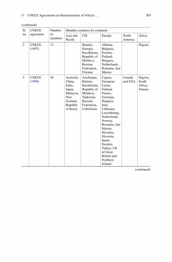
17 UNECE Agreements on Harmonization of Vehicle … 305
(continued)
Sl.no.
UNECEagreement
Numberofmembers
Member countries by continent
Asia andPacific
CIS Europe NorthAmerica
Africa
2 UNECE(1997)
15 – Belarus,Georgia,Kazakhstan,Republic ofMoldova,RussianFederation,Ukraine
Albania,Bulgaria,Estonia,Finland,Hungary,Netherlands,Romania, SanMarino
– Nigeria
3 UNECE(1998)
38 Australia,China,India,Japan,Malaysia,NewZealand,Republicof Korea
Azerbaijan,Belarus,Kazakhstan,Republic ofMoldova,Tajikistan,RussianFederation,Uzbekistan
Cyprus,EuropeanUnion,Finland,France,Germany,Hungary,Italy,Lithuania,Luxembourg,Netherlands,Norway,Romania, SanMarino,Slovakia,Slovenia,Spain,Sweden,Turkey, UKof GreatBritain andNorthernIreland
Canadaand USA
Nigeria,SouthAfrica,Tunisia
(continued)

306 D. Chakraborty and B. Nag
(continued)
Sl.no.
UNECEagreement
Numberofmembers
Member countries by continent
Asia andPacific
CIS Europe NorthAmerica
Africa
4 CommonMembershipin UNECE(1958) and(1998)Agreements
31 Australia,Japan,Malaysia,NewZealand,Republicof Korea
Azerbaijan,Belarus,Kazakhstan,Republic ofMoldova,RussianFederation
EuropeanUnion,Finland,France,Germany,Hungary,Italy,Lithuania,Luxembourg,Netherlands,Norway,Romania, SanMarino,Slovakia,Slovenia,Spain,Sweden,Turkey, UKof GreatBritain andNorthernIreland
– Nigeria,SouthAfrica,Tunisia.
Source Obtained from http://www.unece.org/transport/international-agreements/contracting-parties.html (accessed September 23, 2020)
References
Aggarwal, S. and D. Chakraborty (2019), ‘Which Factors Influence India’s Intra-Industry Trade?Empirical Findings for Select Sectors’, Global Business Review, available at: https://journals.sagepub.com/doi/10.1177/0972150919868343 (accessed March 11, 2021).
Ardakani, Z., Yazdani, S., & Gilanpour, O. (2009). Studying the effects of non-tariff barriers onthe export of the main agricultural products of Iran. American Journal of Applied Sciences, 6(7),1321–1326.
Thai Auto.(undated). see ASEAN MRA and Implementation Status. http://www.thaiauto.or.th/2012/Automotive-Summit/doc/ppt/2015/25–6-15/203_PM/10.ASEAN%20MRA%20and%20status%20of%20Implementation%20Rev%201.pdf.
Badri Narayanan, G., & Vashisht, P. (2008). Determinants of competitiveness of the indian autoindustry. Working Paper No. 201, New Delhi: Indian Council for Research on InternationalEconomic Relations.
Barnes, T. (2018). Making cars in the new India: Industry. New Delhi: Precarity and InformalityCambridge University Press.
Bradford, S. (2003). Paying the price: Final goods protection in OECD countries. The Review ofEconomics and Statistics, 85(1), 24–37.

17 UNECE Agreements on Harmonization of Vehicle … 307
Chaisse, J.,&Chakraborty,D. (2014). The evolving andmultilayeredEU-India investment relations:Policy conjectures and regulatory issues. European Law Journal, 20(3), 385–422.
Chaisse, J., Chakraborty, D., & Nag, B. (2011). The three-pronged strategy of india’s preferentialtrade policy—A contribution to the study of modern economic treaties. Connecticut Journal ofInternational Law, 26(2), 415–455.
Chakraborty, D., Chaisse, J., &Hussain, Z. (2019). Non-Tariff barriers on auto-components exports:application of select indices. In B. Nag&D. Chakraborty (Eds.), India’s trade analytics: Patternsand opportunities (pp. 299–315). New Delhi: Sage.
Chakraborty, D., Chaisse, J., & Pahari, S. (2020). Global auto industry and product standards: Acritical review of India’s economic and regulatory experience. Journal of International TradeLaw and Policy, 19(1), 8–35.
European Commission. (2015). Study on the impact of the revision of the UNECE 1958 Agreementon the global competitiveness of the EU automotive industry, EC, Luxembourg.
Export Import Bank of India. (2017). The Indian automotive industry: An international tradeperspective, Working Paper No. 59, Mumbai: EXIM Bank.
Government of India. (2020). PM gives a clarion call for Atmanirbhar Bharat. https://pib.gov.in/PressReleseDetail.aspx?PRID=1623391.
Government of India. (2018).National auto policy’ (Draft).NewDelhi:Ministry ofHeavy Industriesand Public Enterprises.
Government of India. (2017). Lok Sabha Unstarred Question No.4313 (to be answered on28.03.2017), Department of Heavy Industry, NewDelhi: Ministry of Heavy Industries and PublicEnterprises.
Government of India. (2016). Make in India: Automotive sector-achievements report. New Delhi:Department of Industrial Policy and Promotion and Department of Heavy Industries.
Government of India. (2015).Foreign trade policy 2015-20’. NewDelhi: Department of Commerce,Ministry of Commerce and Industry.
Grubel, H. G., & Lloyd, P. J. (1975). Intra-industry trade: The theory and measurement ofinternational trade in differentiated products. London: The Macmillan Press Limited.
India Brand Equity Foundation.(2018).Automobiles sector IBEF, NewDelhi. https://www.ibef.org/download/Automobiles-January-2018.pdf.
Indian Institute of Foreign Trade. (2017). Trade impact of WP 29 on India. New Delhi: ReportSubmitted to Society for Indian Automobile Manufactures (SIAM).
International Council on Clean Transportation. (2016). India bharat stage VI emission standards.ICCT, Washington DC: Policy Update.
International Trade Centre (undated). Trade Map database. Available at http://www.trademap.org/Index.aspx. (Accessed September 8, 2016).
Innovation, Economic Development, and Intellectual Property in India and China. (pp. 439–463)Cite as.
Krishnan, R. T.&Dayasindhu,N. (2020). Indianmotorcycle industry:A rolemodel forAtmanirbharBharat?.https://www.iimb.ac.in/sites/default/files/2020–08/Indian-motorcycle.pdf.
Make in India (undated). Automobile: Financial support. http://www.makeinindia.com/sector/automobiles.
Marathe, S. (2008, June 26). WP 29 1958 agreement: A view from India. Presentation at the SpecialSession to commemorate the 50th Anniversary of the 1958 agreement, Geneva.
Miglani, S. (2019). The growth of the indian automobile industry: Analysis of the roles of govern-ment policy and other enabling factors. In K. Liu & U. S. Racherla (Eds.), Innovation, economicdevelopment, and intellectual property in India and China: Comparing six economic sectors.Singapore: Springer.
Nag, B. (2016). Emerging production network between India and ASEAN: An analysis of value-added trade in select industries. In D. Chakraborty & J. Mukherjee (Eds.), Trade, investment andeconomic development in Asia: Empirical and policy issues (pp. 41–67). Abingdon: Routledge.
Nag, B. (2011).Trade liberalization and international production networks: Experience of the Indianautomotive sector. In Asia-pacific research and training network on trade (ARTNeT) study on

308 D. Chakraborty and B. Nag
‘fighting irrelevance: The role of regional trade agreements in international production networksin Asia. Bangkok: United National Economic and Social Commission on Asia and the Pacific
Nag, B., Banerjee, S., &Chatterjee, R. (2007). Changing features of the automobile industry in Asia:Comparison of production, trade and market structure in selected countries, ARTNeT WorkingPaper No 3707, UNESCAP, Bangkok.
Nag, B., & Chaturvedi, P. (2019). Implication of tariff reduction through partial simulation usingSMART: An analysis of india’s import of passenger vehicles from Japan and Germany. In B.Nag & D. Chakraborty (Eds.), India’s trade analytics: Patterns and opportunities (pp. 319–332).New Delhi: Sage.
Organisation for Economic Co-operation andDevelopment andUnitedNations Economic Commis-sion for Europe. (2016). International regulatory co-operation and international organisations:The case of the United nations economic commission for Europe (UNECE). Paris: OECD andUNECE.
Philippe, J. (2012). Review of the 1958 Agreement and IWVTA: EU objectives and perspectives,Presentation at the EU-Japan Policy Seminar. https://www.eu-japan.eu/sites/eu-japan.eu/files/presentation_23052012_jean.pdf
Ramos, J. (2011,November 9). InThe UNECE World forum for harmonization of vehicle regulations(WP.29). Geneva: Presentation at the World Trade Organization (WTO), TBT Committee.
Scoles, S. D. (ed) (2016). Harmonization of standards andmutual agreements on conformity assess-ment in Indonesia, Malaysia, Thailand and Vietnam. Research Project Report No. 15, Jakarta:Economic Research Institute for ASEAN and East Asia
Sen, S. (2009). Non-Tariff Barriers in Automotive Industry. Society of Indian AutomobileManufacturers. https://bis.gov.in/other/SIAM-NTB.pdf.
Society for IndianAutomobileManufactures. (2016).Automotive mission plan: 2016-26—A curtainraiser. New Delhi: SIAM.
Srivastava, S., & Sen, R. (2015). Production fragmentation in trade of manufactured goods in India:Prospects and challenges. Asia-Pacific Development Journal, 22(1), 33–66.
Tendulkar, S. D., & Bhavani, T. A. (2012). Understanding reforms: Post-1991 India. New Delhi:Oxford University Press.
The Hindu. (2020, July 14). EU-India summit to launch talks on resuming FTA negotiations,Chennai.
United Nations Economic Commission for Europe. (2012). In world forum for harmonization ofvehicle regulations (WP.29): How it works, how to join it, (3rd ed.), UN, New York and Geneva.
United Nations Economic Commission for Europe (undated a). WP.29-Introduction. https://www.unece.org/trans/main/wp29/introduction.html.
United Nations Economic Commission for Europe.(undated b). UN Vehicle Regulations-1958Agreement. https://www.unece.org/?id=39146.
United Nations Economic Commission for Europe (undated c). (1998). Agreement on GlobalTechnical Regulations (GTRs). https://www.unece.org/trans/main/wp29/wp29wgs/wp29gen/wp29glob_registry.html.
World Trade Organization. (2002). DS146: India—Measures affecting the automotive sector(Complaint by EU). https://www.wto.org/english/tratop_e/dispu_e/cases_e/ds146_e.htm.

Part IVAnalysis of Sector Level Growth
and Development in India

Chapter 18Is ‘Make in India’ A Success? A Reviewfrom the Electronics Sector in India
S. Roy Chowdhury and S. Rastogi
1 Introduction
India’s electronics and IT hardware manufacturing sector comprises close to 3,500electronics manufacturing and 250,000 small units engaged in electronics manufac-turing either directly or indirectly (DeitY, 2010). India produces only a minusculeamount of electronics compared to global production. The global production wasvalued at USD 2149 billion in 2012, out of which India produced goods valued atonly approximatelyUSD28 billion or 1.3%of the global production. China produced28%, and USA produced 29% of the global production in the year 2012 (EXIM,2015). Owing to the rising middle class in the country, combined with changinglifestyle pattern and better access to credit facilities, demand for electronics goodshas been rising at a rapid pace in India over the recent years (IBEF, 2015). The elec-tronics demand is estimated to reach USD 400 billion by the year 2020 from mereUSD 45 million in 2009 data (DeitY, 2010).
The estimated production of the electronics sector will reach approximately USD104 billion in 2020, leaving a gap of USD 296 billion. The sector is estimated to beable to attract USD 100 billion of foreign direct investment (DeitY, 2010). ThroughMake in India, a fresh policy approach is sought to fill this wide gap between demandand supply. This sector provides a huge scope for employment as well. Employmentin this sector was less than a million in the year 2009. The objective of the policiesis not only to increase production but also to create 28 million jobs in the sector by2020 and enhancing human capital by producing 2500 researchers annually (IBEF,2015).
S. Roy Chowdhury (B) · S. RastogiIIM Indore, Rau Pithampur Road, Indore 453556, Indiae-mail: [email protected]
S. Rastogie-mail: [email protected]
© The Author(s), under exclusive license to Springer Nature Singapore Pte Ltd. 2021P. Lakhanpal et al. (eds.), Trade, Investment and Economic Growth,https://doi.org/10.1007/978-981-33-6973-3_18
311

312 S. Roy Chowdhury and S. Rastogi
The primary policies of the government aimed at promoting the electronicsindustry are Electronic Manufacturing Cluster Scheme, schemes focused on tradesuch as Reduced Export Obligation and promoting Export Oriented Units, andManufacturing Special Incentive Package Scheme. The Make in India campaignhas provided the electronics manufacturing sector a well-needed push to harnessforeign direct investment as well as domestic investment. The overarching objectiveof our study is to observe whether the policy push under the Make in India campaignhas been successful in increasing electronics exports and reducing import to date.
In Sect. 2 of the paper, the objective ofMake in India and associated specific policysteps for electronics sector are presented. Section 3 details the data and methodologyused. Section 4 presents the results and analyses. Section 5 concludes with overallcomments.
2 Make in India and Related Policies
The primary goal of the Make in India campaign is to make India the manufacturinghub of the world. Various policies under the campaign aimed at promoting manu-facturing units. On the one hand, with the rise in manufacturing of intermediate andfinal goods, the export of the country can be expected to rise; on the other hand,the manufactured goods can help substitute imports. The campaign was expected toaccomplish all the objectives within a short duration by the then government. Theeconomy anticipated a drastic change with a rapid rise in the growth rate. Therefore,it is one of the most dominant campaigns which needs to be studied to assess thesuccess rate. However, to the best of our knowledge, no study has been conducted tounderstand the effect of the campaign on the trade balance of the country for any ofthe sectors so far. We have attempted to study the impact of the umbrella policy ofMake in India.
The electronics sector has been considered as one of the priority sectors underthe Make in India initiative (DeitY, 2012). The Indian electronics sector is broadlydivided into six segments, based on end use and valuation, which is depicted in Fig. 1.Due to the increasing upward pressure of laborwages inChina, otherAsian countries,like Vietnam, Cambodia, and India, are gaining popularity as possible manufacturinghubs. These countries have favorable product demand, labor cost, and government
Electronics Sector
Consumer electronics
Industrial eletronics
Communica on and
broadcas ng equipments
Strategic electronics
Electronic components Computers
Fig. 1 Six segments of the Indian electronics sector. Source DeitY, (2012)

18 Is ‘Make in India’ A Success? A Review … 313
policies. From the year 2012, the Government of India has been trying to use theabundant young talent and low wages to make India globally competitive in theelectronics sector. The government’s objective is to close the demand–supply gapand reach USD 400 billion worth of production by 2020 (IBEF, 2017).
2.1 Policy Measures Adopted by the Government
The Government of India has come up with a variety of policies to enable andencourage the expansion of Electronics System Design and Manufacturing (ESDM)sector in India. The policy purpose is to enhance production capacity as well asproduction diversity in the sector to meet the domestic demand indigenously andto gain a share of the global electronics trade. The policy steps, as stated in NSDC(2011) report, include:
1. Special purpose vehicles for ESDM2. M-SIPS or Manufacturing Special Incentive Package Scheme3. Electronics Hardware Technology Park (EHTP) Scheme4. The National Policy on Electronics5. 100% FDI permitted through automatic route in most sectors including ESDM
according to the consolidated FDI policy 20156. Implementation of ITA-I (Information Technology Act) under WTO7. Reduced export obligation (EO) for domestic procurement under Export
Promoting Capital Goods (EPCG) Scheme8. Export-Oriented Unit (EOU) Scheme.
There are various skill development initiatives undertaken under the ESDMScheme toward the goal of the creation of 28 million jobs, including:
1. Under the National Policy on Electronics, the objectives for human resourcedevelopment include significant enhancement in the availability of skilledmanpower in ESDM.
2. A scheme to support 3000 additional Ph.D., which includes 1500 in ESDMsector, was approved in 2014 at an estimated cost of USD 57 billion.
3. A scheme of financial assistance from the center to set up seven electronics andinformation and communications (ICT) academies in institutions.
4. A scheme of financial aid to select states/UTs (selected by an EmpoweredCommittee based on proposals received).
5. The National Institute for Electronics and Information Technology (NIELIT)launched a project ‘Capacity building in the areas of Electronic Design andProduction Technology.’
6. A project entitled ‘Special Manpower Development Program for Chips toSystems’ has been approved by the Department of Electronics and InformationTechnology (DeitY).

314 S. Roy Chowdhury and S. Rastogi
7. DeitY approved a project for skill development in electronics hardware.1
3 Data Collection and Methodology
To understand the impact of Make in India and associated policy measures, weconsider the changes in exports and imports as the proxy for the responsiveness ofthe umbrella campaign of Make in India. We choose the electronics products basedon their six-digit HS codes. The HS code 85 is termed as ‘electrical and electronicsgoods.’ We consider the list of all the items with HS code starting with 854, and 49items were found in this list. The generalized product categories listed as ‘others’ areremoved, and finally, 46 items are chosen for further study. These 46 products madeup around 1% of the total imports in 2009 and 2% in 2017, and approximately 0.6%of total Indian exports. The products alongwith their HS codes are listed in Appendix1.We chose the time frame from the financial year 2009–2017 to distinguish betweenpre- and post-policy impact. Data for imports and exports in terms of billions USDfor relevant items are collected from the Ministry of Commerce, Government ofIndia, Web site.
For all the products, line graphs for the change in exports and imports over theyears are plotted from the year 2009–2017 (refer to Appendix 2, Figs. 2 to 47).The results obtained are inconclusive due to high volatility. Therefore, we applydifference-in-difference (DID) method to examine the effects of the policies in thesector under consideration.
TheMake in India campaignprimarily came into effect in the year 2014.Hence,weconsider years 2009–2014 as the control period and years 2015–17 as the treatmentperiod. The CAGR from the pre-campaign period is expected to continue withoutpolicy, and the difference in CAGRwith post-campaign is calculated to determine theeffect of the policies. We use Eqs. (1)–(6) to calculate the required values (Table 1).
Imports CAGRexpected =(Imports2009−10−Imports2014−15)
Imports2009−10× 100
5(1)
Imports CAGRactual =(Imports2014−15−Imports2017−18)
Imports2014−15× 100
3(2)
Difference = Imports CAGRactual − Imports CAGRexpected (3)
1Details of the policies are available at: IESA (2017).https://meity.gov.in/writereaddata/files/Executive%20Summary%20of%20the%20IESA%20EY%20Report.pdf.https://meity.gov.in/writereaddata/files/Electronics_IT_Hardware_NSDC_Report_1732011%20%281%29.pdf.

18 Is ‘Make in India’ A Success? A Review … 315
Table 1 DID results on imports
HS code(1)
2009–2010(2)
2014–2015(3)
ExpectedCAGR(4)
ActualCAGR(5)
Difference(6)
Expected2017–18values(7)
Actual2017–2018values(8)
854011 165.34 81.40 −10.15 −32.62 −22.46 59.04 1.75
854020 10.54 17.64 13.47 −26.68 −40.15 25.77 3.52
854040 2.55 0.87 −13.18 7.28 20.46 0.57 1.06
854060 1.43 0.36 −14.97 27.78 42.74 0.22 0.66
854071 1.23 2.94 27.80 0.79 −27.01 6.14 3.01
854079 2.39 7.45 42.34 −30.65 −72.99 21.49 0.60
854081 0.93 0.32 −13.12 −19.79 −6.67 0.21 0.13
854089 2.62 2.32 −2.29 3.88 6.17 2.16 2.59
854091 18.65 0.23 −19.75 −20.29 −0.54 0.12 0.09
854099 11.25 5.85 −9.60 −13.39 −3.79 4.32 3.50
854110 127.31 154.19 4.22 5.78 1.55 174.56 180.91
854121 4.17 4.08 -0.43 61.93 62.36 4.03 11.66
854129 113.83 221.81 18.97 2.30 −16.67 373.52 237.12
854130 26.29 56.41 22.91 −2.87 −25.79 104.75 51.55
854140 329.65 1041.31 43.18 100.61 57.44 3056.31 4184.40
854150 16.66 15.06 −1.92 −4.67 −2.75 14.21 12.95
854160 23.16 35.64 10.78 −0.60 −11.38 48.45 35.00
854190 26.86 11.56 −11.39 64.59 75.98 8.04 33.96
854231 525.62 728.87 7.73 17.02 9.29 911.39 1101.04
854232 92.88 128.98 7.77 −4.97 −12.75 161.46 109.73
854233 19.53 11.21 −8.52 65.77 74.29 8.58 33.33
854290 82.45 30.07 −12.71 −17.54 −4.83 20.00 14.25
854310 4.32 2.41 −8.84 69.16 78.00 1.83 7.41
854320 10.50 24.06 25.83 −5.54 −31.37 47.93 20.06
854330 14.51 20.25 7.91 30.58 22.67 25.45 38.83
854370 246.12 499.92 20.62 −3.28 −23.90 877.41 450.74
854390 109.60 123.57 2.55 0.77 −1.78 133.26 126.44
854411 75.00 84.54 2.54 −4.71 −7.25 91.16 72.60
854419 120.24 95.24 −4.16 5.87 10.02 83.85 112.00
854420 153.57 115.40 −4.97 −5.52 −0.55 99.03 96.28
854430 34.14 85.09 29.85 9.23 −20.62 186.29 108.65
854442 37.60 93.12 29.53 38.04 8.51 202.38 199.40
854449 183.96 245.78 6.72 7.42 0.70 298.74 300.50
854460 53.33 186.47 49.93 −20.67 −70.60 628.46 70.85
(continued)

316 S. Roy Chowdhury and S. Rastogi
Table 1 (continued)
HS code(1)
2009–2010(2)
2014–2015(3)
ExpectedCAGR(4)
ActualCAGR(5)
Difference(6)
Expected2017–18values(7)
Actual2017–2018values(8)
854470 31.69 42.21 6.64 7.79 1.15 51.19 52.07
854511 61.10 42.83 −5.98 −10.26 −4.28 35.60 29.65
854519 72.38 84.06 3.23 −18.45 −21.68 92.46 37.53
854520 6.79 15.94 26.95 5.71 −21.24 32.61 18.67
854590 10.77 11.45 1.26 53.92 52.65 11.89 29.97
854610 2.70 7.26 33.78 −29.71 −63.48 17.38 0.79
854620 17.93 10.95 −7.79 5.66 13.45 8.59 12.81
854690 46.93 60.43 5.75 15.99 10.23 71.47 89.41
854710 2.27 5.24 26.17 −5.79 −31.96 10.52 4.33
854720 40.49 86.83 22.89 14.65 −8.24 161.14 124.99
854790 30.87 38.04 4.65 −2.68 −7.33 43.59 34.98
854810 0.76 38.40 990.53 62.00 −928.53 49801.18 109.82
Source Ministry of Commerce and Industry, Government of India (MCI, 2018) (columns 1–3),authors’ calculation (column 4–8)
Exports CAGRexpected =(Exports2009−10−Exports2014−15)
Exports2009−10× 100
5(4)
Exports CAGRactual =(Exports2014−15−Exports2017−18)
Exports2014−15× 100
3(5)
Difference = Exports CAGRactual − Exports CAGRexpected (6)
ApplyingDIDmethod, we calculate the CAGR for every product from 2009–10 to2014–15 (columns 4 in Tables 2 and 3) using Eqs. (1) and (4). We consider this valueas the expected cumulative annual growth rate of import and export, respectively, forthe next years, if there had not been any policy change. Based on the value of CAGRobtained, we calculate the expected 2017–18 import and export values (columns 7).However, ‘Make in India’ campaign was launched in 2014. Hence, we determinethe changed actual CAGR for the years 2014–15–2017–18 using Eqs. (2) and (5).The difference in the actual and the expected CAGR is used as an indicator for theeffectiveness of the campaign. The difference is represented in columns (6), which isobtained using Eqs. (4) and (6). The results for import analysis are shown in Table 1,and that for exports are shown in Table 2.

18 Is ‘Make in India’ A Success? A Review … 317
Table 2 DID results on exports
HS code(1)
2009–2010(2)
2014–2015(3)
ExpectedCAGR(4)
ActualCAGR(5)
Difference(6)
Expected2017–18values(7)
Actual2017–2018values(8)
854011 2.30 2.78 4.17 −5.64 −9.81 3.14 2.31
854020 1.25 0.87 −6.08 −27.59 −21.51 0.72 0.15
854040 0.20 0.01 −19.00 33.33 52.33 0.01 0.02
854060 0.05 0.00 −20.00 NA NA 0.00 0.00
854071 0.22 0.00 −20.00 NA NA 0.00 0.03
854079 0.29 0.68 26.90 −24.02 −50.92 1.39 0.19
854081 0.00 0.02 NA 50.00 NA NA 0.05
854089 1.81 1.53 −3.09 −28.32 −25.23 1.39 0.23
854091 0.67 0.80 3.88 −25.00 −28.88 0.90 0.20
854099 0.73 1.98 34.25 −22.90 −57.14 4.79 0.62
854110 2.23 2.16 −0.63 14.66 15.29 2.12 3.11
854121 1.26 0.69 −9.05 2.42 11.46 0.52 0.74
854129 4.41 3.71 −3.17 0.36 3.53 3.37 3.75
854130 2.77 0.96 −13.07 10.76 23.83 0.63 1.27
854140 359.86 179.12 −10.05 −5.67 4.37 130.38 148.65
854150 16.65 16.28 −0.44 −6.41 −5.96 16.06 13.15
854160 6.52 30.80 74.48 −21.88 −96.36 163.60 10.58
854190 4.55 4.50 −0.22 0.15 0.37 4.47 4.52
854231 23.07 22.84 −0.20 2.52 2.72 22.70 24.57
854232 14.53 10.99 −4.87 −18.65 −13.78 9.46 4.84
854233 0.94 0.90 −0.85 0.00 0.85 0.88 0.90
854290 20.22 10.33 −9.78 −25.72 −15.94 7.59 2.36
854310 0.97 0.43 −11.13 −21.71 −10.57 0.30 0.15
854320 9.52 5.46 −8.53 11.84 20.37 4.18 7.40
854330 4.16 1.93 −10.72 −9.67 1.05 1.37 1.37
854370 31.40 29.75 −1.05 28.83 29.88 28.82 55.48
854390 41.06 99.31 28.37 −16.96 −45.33 210.09 48.79
854411 50.42 60.88 4.15 2.26 −1.89 68.78 65.01
854419 34.67 73.43 22.36 −3.86 −26.22 134.52 64.92
854420 15.28 30.09 19.38 −21.34 −40.72 51.20 10.83
854430 34.74 162.88 73.77 8.41 −65.36 854.67 203.98
854442 16.71 41.41 29.56 13.44 −16.12 90.06 58.11
854449 55.12 45.31 −3.56 111.75 115.31 40.64 197.21
854460 89.62 248.60 35.48 −1.06 −36.54 618.18 240.71
(continued)

318 S. Roy Chowdhury and S. Rastogi
Table 2 (continued)
HS code(1)
2009–2010(2)
2014–2015(3)
ExpectedCAGR(4)
ActualCAGR(5)
Difference(6)
Expected2017–18values(7)
Actual2017–2018values(8)
854470 40.13 29.96 −5.07 −4.65 0.42 25.63 25.78
854511 160.43 237.88 9.66 27.17 17.51 313.65 431.77
854519 4.05 3.33 −3.56 −10.61 −7.06 2.99 2.27
854520 3.32 5.32 12.05 −4.51 −16.56 7.48 4.60
854590 2.36 5.66 27.97 −0.53 −28.50 11.86 5.57
854610 0.79 0.32 −11.90 82.29 94.19 0.22 1.11
854620 44.34 36.36 −3.60 9.76 13.36 32.57 47.01
854690 16.30 30.98 18.01 12.64 −5.37 50.92 42.73
854710 3.19 1.61 −9.91 −17.18 −7.28 1.18 0.78
854720 2.37 7.31 41.69 27.77 −13.92 20.79 13.40
854790 81.36 59.77 −5.31 −14.73 −9.43 50.75 33.35
854810 1.15 0.13 −17.74 30.77 48.51 0.07 0.25
Source Ministry of Commerce and Industry, Government of India (MCI, 2018) (columns 1–3),authors’ calculation (column 4–8)
4 Results and Analysis
Table 1 represents the results of difference-in-difference on imports. In Table 1, anegative actual CAGR represents that the rate of growth of import for a particularcommodity has been negative, or there has been a fall in imports from 2014–15 to2017–18. Similarly, a positive CAGR represents a rise in imports over the years.When we calculate the difference between the actual and expected CAGR, it showsthe import performance of the commodity above its expected value. Hence, a negativedifference is desirable, as it shows a positive effect in terms of trade.
From the above results, we see that column 6 has 28 negative values and 18positive values. It implies that the imports for 28 commodities have fallen overexpected figures from 2014 to 2017 whereas 18 commodities have witnessed anincrease in imports.
Table 2 represents the difference-in-difference results in exports. The exports areexpected to move in the opposite direction of the imports. In Table 2, a positive actualCAGR represents that the rate of growth of export for a particular commodity hasbeen positive, or there has been a comparative rise in exports over the expected trendfrom 2014–15 to 2017–18. Similarly, a negative CAGR represents a fall in exportsover the years. When we calculate the difference between the actual and expectedCAGR, it shows the export performance of the commodity above its expected value.Hence, a positive difference is desirable for exports, as falling exports would hurtthe terms of trade.

18 Is ‘Make in India’ A Success? A Review … 319
Table 3 Overall impact of Make in India policies on the trade of electronics commodities
HS code(1)
Commodity(2)
Import CAGRdifference(actual-expected)(3)
Export CAGRdifference(actual-expected)(4)
Final impactof campaign(5)
854011 Cathode ray TV picturetubes, including videomonitor cathode ray tubecolor
−22.46 −9.81 Inconclusive
854020 TV camera tube imageconvertors and intensifiers;other photocathode tubes
−40.15 −21.51 Inconclusive
854040 Data/graphic display tubes,color, with a phosphor dotscreen pitch < 0.4 mm
20.46 52.33 Inconclusive
854060 Other cathode ray tubes 42.74 NA Inconclusive
854071 Magnetrons −27.01 NA Inconclusive
854079 Other microwave tubes(e.g., traveling wave tubecarcinotrons), excelgrid-controlled tubes
−72.99 −50.92 Inconclusive
854081 Receiver/amplifier valvesand tubes
−6.67 NA Inconclusive
854089 Other valves and tubes 6.17 −25.23 Negativeimpact
854091 Parts of cathode ray tubes −0.54 −28.88 Inconclusive
854099 Other parts of the tubs andvalves of hdg 8540
−3.79 −57.14 Inconclusive
854110 Diodes, other thanphotosensitive orlight-emitting diodes
1.55 15.29 Inconclusive
854121 Transistors, other thanphotosensitive transistorswith a dissipation rate ofless than 1 W
62.36 11.46 Inconclusive
854129 Other transistor, other thanphotosensitive transistors
−16.67 3.53 Positiveimpact
854130 Thyristors, diacs, and triacs,other than photosensitivedevices
−25.79 23.83 Positiveimpact
(continued)

320 S. Roy Chowdhury and S. Rastogi
Table 3 (continued)
HS code(1)
Commodity(2)
Import CAGRdifference(actual-expected)(3)
Export CAGRdifference(actual-expected)(4)
Final impactof campaign(5)
854140 Photosensitivesemiconductor devicesincluding photovoltaic cellsw/n assembled inmodules/made up intopanels; light-emittingdiodes
57.44 4.37 Inconclusive
854150 Other semiconductordevices
−2.75 −5.96 Inconclusive
854160 Mounted piezoelectriccrystals
−11.38 −96.36 Inconclusive
854190 Parts of items of hdng 8541 75.98 0.37 Inconclusive
854231 Processors and controllers,whether or not combinedwith memories, converters,logic circuits, amplifiers,clock
9.29 2.72 Inconclusive
854232 Memories −12.75 −13.78 Inconclusive
854233 Amplifiers 74.29 0.85 Inconclusive
854290 Parts of electronicintegrated circuits andmicro-assemblies
−4.83 −15.94 Inconclusive
854310 Particle accelerators: 78.00 −10.57 Negativeimpact
854320 Signal generators −31.37 20.37 Positiveimpact
854330 Machines and apparatus forelectroplating,electrolysis/electrophoresis
22.67 1.05 Inconclusive
854370 Other machines andapparatus:
−23.90 29.88 Positiveimpact
854390 Parts of articles of heading8543
−1.78 −45.33 Inconclusive
854411 Winding wire of copper −7.25 −1.89 Inconclusive
854419 Winding wires of othermetals/substances, excelcopper
10.02 −26.22 Negativeimpact
854420 Coaxial cable and othercoaxial electricalconductors
−0.55 −40.72 Inconclusive
(continued)

18 Is ‘Make in India’ A Success? A Review … 321
Table 3 (continued)
HS code(1)
Commodity(2)
Import CAGRdifference(actual-expected)(3)
Export CAGRdifference(actual-expected)(4)
Final impactof campaign(5)
854430 Ignition wiring sets andother wiring sets of a kindused in vehicle aircraft/ships
−20.62 −65.36 Inconclusive
854442 Other electric conductors <1000 v fitted withconnectors:
8.51 −16.12 Negativeimpact
854449 Other electric conductors <1000 v not fitted withconnectors:
0.70 115.31 Inconclusive
854460 Other electric conductors,for a voltage exceeding1000 v
−70.60 −36.54 Inconclusive
854470 Optical fiber cables 1.15 0.42 Inconclusive
854511 Electrodes of a kind usedfor furnaces
−4.28 17.51 Positiveimpact
854519 Other electrodes −21.68 −7.06 Inconclusive
854520 Brushes −21.24 −16.56 Inconclusive
854590 Other articles used forelectrical purposes
52.65 −28.50 Inconclusive
854610 Electrical insulators of glass −63.48 94.19 Positiveimpact
854620 Electrical insulators ofceramics
13.45 13.36 Inconclusive
854690 Electrical insulators of othermaterials
10.23 −5.37 Negativeimpact
854710 Insulating fittings ofceramics
−31.96 −7.28 Inconclusive
854720 Insulating fittings of plastics −8.24 −13.92 Inconclusive
854790 Other insulating fittings −7.33 −9.43 Inconclusive
854810 Waste and scrap of primarycells, batteries, and electricaccumulators, spent primarycell batteries and spentelectric accumulators
−928.53 48.51 Positiveimpact
Source Ministry of Commerce and Industry, Government of India (MCI, 2018) (columns 1–2),authors’ calculation (column 3–5)

322 S. Roy Chowdhury and S. Rastogi
We find that exports have increased over the expected trend for 20 products andhave fallen from the expected trend for the remaining 26 products for the period from2014 to 2017.
To understand the overall impact of the Make in India campaign and associatedpolicies, we compare the import CAGR difference and the export CAGR differencein Table 3. A negative (positive) value in column 3 of Table 3 indicates the CAGR ofimport of the particular commodity has fallen (risen) from pre-campaign and post-campaign period and has benefitted (harmed) the trade balance of India. Similarly,for the export, a positive (negative) value in column 4 of Table 3 indicates the CAGRof export of the particular commodity has risen (fallen) from pre-campaign andpost-campaign period and has benefitted (harmed) the trade balance of India.
For the products that witnessed a rise in export and a fall in import, the campaign islabeled to be successful (positive impact). For products that witnessed a fall in exportand a rise in import, the campaign is labeled to be unsuccessful (negative impact).The products that show diverging trends for both (export and import simultaneouslyrising or falling), the campaign is labeled as inconclusive. From the above table,we see that the campaign has been clearly successful for only seven products andunsuccessful for fiveproducts. For the rest of the 34 items, the results are inconclusive.The rising imports and falling exports for these five items might be due to the natureof these items. These can be components which are used to produce some other finalproducts. The production of such final products might have seen an increasing trend.The reason behind the trend might be because additional manufacturing has beensuccessful to cater to domestic demand for most products, but excess supply hasnot been reached, which can promote export. Hence, imports have fallen, with no ornegative change in exports.
5 Conclusion
We attempt to study the overall effect of the ‘Make in India’ umbrella campaign onthe electronics sector of India. Since Make in India as a policy has been focused onexport promotion and import substitution, we analyze the export and import figuresfor 46 commodities from the sector as a proxy for growth in manufacturing, andas with the rise in local manufacturing, exports (imports) are expected to rise (fall).We employ difference-in-difference method to measure the deviation of exports andimports from their expected trend values. This is the first study which attempted toassess the performance of the ‘Make in India’ campaign.
Wefind thatMake in India has been successful for a fewproducts and unsuccessfulfor a few of them. However, no significant result could be drawn for 34 out of 46items in the electronics sector of India. The inconclusive trend might be a result ofthe short lag available post the policy initiative. Further, it is also possible that onesector benefitting from the policy initiative may create a stronger input demand inanother sector, leading to an increase or decrease in both the numbers for exports andimports. The increased production may have been successful in substituting imports

18 Is ‘Make in India’ A Success? A Review … 323
for the domestic market but unsuccessful in producing enough surplus to improveexport and cater to international demand.
The study has a few limitations, which can be addressed in the future research.We have considered only the electronics sector for the analysis. Further, we analyzedthe export and import figures in isolation from the other macroeconomic variables,which may have led to inconclusive or biased results. A similar analysis can becarried out on other sectors to observe the differences in the impact of the initiative.The data time frame is limited as Make in India was launched only four years back.With more data points in the future, a more conclusive study can be conducted.
Appendix 1
The list of all the product names with HS codes under study
HS code Product name
854011 Cathode ray TV picture tubes, including video monitor cathode ray tube color
854020 TV camera tube image convertors and intensifiers; other photocathode tubes
854040 Data/graphic display tubes, color, with a phosphor dot screen pitch <0.4 mm
854060 Other cathode ray tubes
854071 Magnetrons
854079 Other microwave tubes (e.g., traveling wave tube carcinotrons), excel grid-controlledtubes
854081 Receiver/amplifier valves and tubes
854089 Other valves and tubes
854091 Parts of cathode ray tubes
854099 Other parts of the tubs and valves of hdg 8540
854110 Diodes, other than photosensitive or light-emitting diodes
854121 Transistors, other than photosensitive transistors with a dissipation rate of less than1 W
854129 Other transistor, other than photosensitive transistors
854130 Thyristors, diacs, and triacs, other than photosensitive devices
854140 Photosensitive semiconductor devices including photovoltaic cells w/n assembled inmodules/ made up into panels; light-emitting diodes
854150 Other semiconductors devices
854160 Mounted piezoelectric crystals
854190 Parts of items of hdng 8541
854231 Processors and controllers, whether or not combined with memories, converters,logic circuits, amplifiers, clock
854232 Memories
854233 Amplifiers
(continued)

324 S. Roy Chowdhury and S. Rastogi
(continued)
HS code Product name
854290 Parts of electronic integrated circuits and micro-assemblies
854310 Particle accelerators:
854320 Signal generators
854330 Machines and apparatus for electroplating, electrolysis/electrophoresis
854370 Other machines and apparatus:
854390 Parts of articles of heading 8543
854411 Winding wire of copper
854419 Winding wires of other metals/substances, excel copper
854420 Coaxial cable and other coaxial electrical conductors
854430 Ignition wiring sets and other wiring sets of a kind used in vehicle aircraft/ships
854442 Other electric conductors <1000 v fitted with connectors:
854449 Other electric conductors <1000 v not fitted with connectors:
854460 Other electric conductors, for a voltage exceeding 1000 v
854470 Optical fiber cables
854511 Electrodes of a kind used for furnaces
854519 Other electrodes
854520 Brushes
854590 Other articles used for electrical purposes
854610 Electrical insulators of glass
854620 Electrical insulators of ceramics
854690 Electrical insulators of other materials
854710 Insulating fittings of ceramics
854720 Insulating fittings of plastics
854790 Other insulating fittings
854810 Waste and scrap of primary cells, batteries, and electric accumulators, spent primarycell batteries and spent electric accumulators
Source Ministry of Commerce and Industry, Government of India (MCI, 2018)
Appendix 2
See Figs. 2, 3, 4, 5, 6, 7, 8, 9, 10, 11, 12, 13, 14, 15, 16, 17, 18, 19, 20, 21, 22, 23,24, 25, 26, 27, 28, 29, 30, 31, 32, 33, 34, 35, 36, 37, 38, 39, 40, 41, 42, 43, 44, 45,46 and 47.

18 Is ‘Make in India’ A Success? A Review … 325
Fig. 2 Import–export forHS code 854011
050
100150200250
854011
Import Export
Fig. 3 Import–export forHS code 854020
010203040
854020
Import Export
Fig. 4 Import–export forHS code 854040
0246
854040
Import Export

326 S. Roy Chowdhury and S. Rastogi
Fig. 5 Import–export forHS code 854060
00.5
11.5
2854060
Import Export
Fig. 6 Import–export forHS code 854071
0246
854071
Import Export
Fig. 7 Import–export forHS code 854079
02468
854079
Import Export

18 Is ‘Make in India’ A Success? A Review … 327
Fig. 8 Import–export forHS code 854081
0204060
854081
Import Export
Fig. 9 Import–export forHS code 854089
02468
854089
Import Export
Fig. 10 Import–export forHS code 854091
010203040
854091
Import Export

328 S. Roy Chowdhury and S. Rastogi
Fig. 11 Import–export forHS code 854099
05
101520
854099
Import Export
Fig. 12 Import–export forHS code 854110
050
100150200
854110
Import Export
Fig. 13 Import–export forHS code 854121
05
10152025
854121
Import Export

18 Is ‘Make in India’ A Success? A Review … 329
Fig. 14 Import–export forHS code 854129
0100200300
854129
Import Export
Fig. 15 Import–export forHS code 854130
020406080
854130
Import Export
Fig. 16 Import–export forHS code 854140
0200040006000
854140
Import Export

330 S. Roy Chowdhury and S. Rastogi
Fig. 17 Import–export forHS code 854150
0102030
854150
Import Export
Fig. 18 Import–export forHS code 854160
020406080
854160
Series1 Series2
Fig. 19 Import–export forHS code 854190
0204060
854190
Import Export

18 Is ‘Make in India’ A Success? A Review … 331
Fig. 20 Import–export forHS code 854231
0500
10001500
854231
Import Export
Fig. 21 Import–export forHS code 854232
050
100150200250
854232
Import Export
Fig. 22 Import–export forHS code 854233
010203040
854233
Import Export

332 S. Roy Chowdhury and S. Rastogi
Fig. 23 Import–export forHS code 854290
050
100150
854290
Import Export
Fig. 24 Import–export forHS code 854310
02468
854310
Import Export
Fig. 25 Import–export forHS code 854320
0102030
854320
Import Export

18 Is ‘Make in India’ A Success? A Review … 333
Fig. 26 Import–export forHS code 854330
050
100150200
854330
Import Export
Fig. 27 Import–export forHS code 854370
0200400600
854370
Import Export
Fig. 28 Import–export forHS code 854390
0100200300
854390
Import Export

334 S. Roy Chowdhury and S. Rastogi
Fig. 29 Import–export forHS code 854411
050
100150
854411
Import Export
Fig. 30 Import–export forHS code 854419
050
100150200
854419
Import Export
Fig. 31 Import–export forHS code 854420
050
100150200
854420
Import Export

18 Is ‘Make in India’ A Success? A Review … 335
Fig. 32 Import–export forHS code 854430
0100200300
854430
Import Export
Fig. 33 Import–export forHS code 854442
0100200300
854442
Import Export
Fig. 34 Import–export forHS code 854449
0100200300400
854449
Import Export

336 S. Roy Chowdhury and S. Rastogi
Fig. 35 Import–export forHS code 854460
0100200300
854460
Import Export
Fig. 36 Import–export forHS code 854470
0204060
854470
Import Export
Fig. 37 Import–export forHS code 854511
0200400600
854511
Import Export

18 Is ‘Make in India’ A Success? A Review … 337
Fig. 38 Import–export forHS code 854519
050
100150200
854519
Import Export
Fig. 39 Import–export forHS code 854520
05
101520
854520
Import Export
Fig. 40 Import–export forHS code 854590
010203040
854590
Import Export

338 S. Roy Chowdhury and S. Rastogi
Fig. 41 Import–export forHS code 854610
0
5
10854610
Import Export
Fig. 42 Import–export forHS code 854620
0204060
854620
Import Export
Fig. 43 Import–export forHS code 854690
0
50
100854690
Import Export
Fig. 44 Import–export forHS code 854710
05
101520
854710
Import Export

18 Is ‘Make in India’ A Success? A Review … 339
Fig. 45 Import–export forHS code 854720
050
100150
854720
Import Export
Fig. 46 Import–export forHS code 854790. SourceMCI, (2018)
050
100150
854790
Import Export
Fig. 47 Import–export forHS code 854810
050
100150
854810
Import Export
References
DeitY. (2010). The Ministry of Electronics and Information Technology, Government of India-Report of Task Force to suggest measures to stimulate the growth of IT, ITES and Elec-tronics Hardware manufacturing industry in India. Retrieved from https://meity.gov.in/writereaddata/files/Suggest%20Measures%20to%20stimulate%20growth%20of%20IT,%20ITES%20and%20Electronics%20Hardware%20Manufacturing%20Industry%20in%20India%20(2009)%20(4961%20KB)(1).pdf. Accessed on July 5, 2018.

340 S. Roy Chowdhury and S. Rastogi
DeitY. (2012). The Ministry of Electronics and Information Technology, Government of India,2012. Promotion of Electronics/ IT Hardware Manufacturing (Annual Plan 2012–13). Retrievedfrom https://meity.gov.in/writereaddata/files/Annual%20Plan%202012-13%20_Promotion%20of%20Electronics%20IT%20Hardware%20Manufacturing%20(2012)%20(23%20KB)(1).pdf. Accessed on July 27, 2018.
EXIM. (2015). Export–Import Bank of India–Indian Electronic Goods Industry: Neutralizing TradeDeficit with China. Retrieved from https://www.eximbankindia.in/Assets/Dynamic/PDF/Publication-Resources/ResearchPapers/Hindi/7file.pdf. Accessed on July 15, 2018.
IBEF. (2015). India Brand Equity Foundation–Electronics. Retrieved from https://www.ibef.org/download/Electronics-March-2015.pdf. Accessed on July 30, 2018.
IBEF. (2017). India Brand Equity Foundation–Electronics. Retrieved from https://www.ibef.org/download/Electronics-June-2017.pdf. Accessed on August 28, 2018.
IESA. (2017). Indian Electronics and Semiconductor Association - Indian Electronics IndustryUpdate. Retrieved from https://meity.gov.in/writereaddata/files/Executive%20Summary%20of%20the%20IESA%20EY%20Report.pdf. Accessed on August 5, 2018.
MCI. (2018). Ministry of Commerce & Industry, Government of India–Export Import data Bank.Retrieved from https://commerce-app.gov.in/eidb/. Accessed on August 1, 2018.
National Skill Development Cooperation. (2011). Human Resource and Skill Requirements in theElectronics and IT Hardware Industry. Retrieved from https://meity.gov.in/writereaddata/files/Electronics_IT_Hardware_NSDC_Report_1732011%20%281%29.pdf. Accessed on August 21,2018.

Chapter 19Financial Inclusionand Telecommunication in India :A Study on Spillover Effect
Taufeeque Ahmad Siddiqui and Kashif Iqbal Siddiqui
1 Introduction
Literature has established an apparent positive relationship between efficient financialservices and economic growth. The Indian economy is one of the fastest-growing inthe world. The key to the inclusive growth of the country depends upon the statusof the rural population. According to the census 2011, nearly 70% of the Indianpopulation live in rural areas. Financial inclusion is an effort to bring these ruralpopulations into themainstream line. Financial inclusion has been a significant policyconcern for governments across the world.
Chakrabarty (2011) defines financial inclusion as ‘the process of ensuring accessto appropriate financial products and services needed by vulnerable groups such asweaker sections and low-income groups at an affordable cost fairly and transparentlyby mainstream institutional players’. Rural poor struggle with inadequate accessto finance (Siddiqui and Siddiqui, 2020). There are various initiatives taken by theGovernment of India and theReserveBankof India, such as no-frills accounts, branchexpansion, relaxed KYC norms, correspondent banking, and electronic payment toachieve the objectives of financial inclusion in India. The government is also makingefforts to promote financial inclusion through the Direct Benefit Transfer scheme,Pradhan Mantri Jan Dhan Yojna, and various other social upliftment schemes. As ofJune 24, 2020, 39.57 crore beneficiaries have opened their accounts under PMJDY,making this scheme as one of the most extensive financial inclusion programs in theworld (PMJDY, 2020).
Improving technology has accelerated the use of cellular phones to access finan-cial services. In terms of the number of subscribers, the Indian telecom industry is
T. A. Siddiqui · K. I. Siddiqui (B)Centre for Management Studies, Jamia Millia Islamia, New Delhi, Indiae-mail: [email protected]
T. A. Siddiquie-mail: [email protected]
© The Author(s), under exclusive license to Springer Nature Singapore Pte Ltd. 2021P. Lakhanpal et al. (eds.), Trade, Investment and Economic Growth,https://doi.org/10.1007/978-981-33-6973-3_19
341

342 T. A. Siddiqui and K. I. Siddiqui
the second largest in the world (GSMA, 2017). The sector has witnessed exponentialgrowth over the last few years. The overall teledensity of India is 88.56%, whereasrural teledensity is 56.67% (TRAI, 2020). Rural regions are well covered by telecom-munications networks and are now seeing growing penetration of smartphones andcomputers. Increased teledensity has reduced the digital divide between rural andurban India. The extraordinary growth of cellular telephony in India provides anopportunity that can be harnessed to expand access to financial services to unbankedsections of the population. The growth of the telecommunications infrastructure,particularly the penetration of cell phones, has provided an opportunity to providefinancial inclusion (Mishra and Bisht, 2013). Hence, telecom can play an active rolein providing significant support for the growth and transformation of the bankingindustry in rural areas. The latest technology, along with telecom infrastructure, mayplay a significant role in the financial inclusion revolution.
2 Brief Literature Review
Bagli and Dutta (2012), in their study, attempted to find out how fairly Indian stateshave delivered as far as financial inclusion is concerned. A rotated principal compo-nent analysis methodology was applied to compute a comprehensive measure offinancial inclusion for every state. According to the study, the computed values ofthe composite index of financial inclusion inferred that so far, the financial inclusionof the states in India is not encouraging. The study also confirms the strong positiverelationship between human development and financial inclusion in India.
Andrianaivo and Kpodar (2012), in their paper, tried to find out whether themobile phone development boosts economic growth through better financial inclu-sion. The results of the estimation throughGMMestimators revealed thatmobile tele-phone development contributes to economic growth in Africa. They further addedthat mobile phone penetration has the potential to improve financial inclusion byproviding cost-effective financial services to the poor and the unbanked.
Chakravarty and Pal (2013) developed an index to measure financial inclusion.They use panel data econometrics techniques to examine the effects ofmajor bankingpolicies onfinancial inclusion across states in India from1972 to 2009. Itwas reportedthat during 1977–1990, the social banking policy played a crucial role in fosteringfinancial inclusion across Indian states. Financial inclusion levels are significantlyinfluenced by a region’s economic development and its structure. They recommendedgeographic penetration of banking services and the availability of credit as two policyobjectives to foster financial inclusion across Indian states.
CRISIL (2015) measured the degree of financial inclusion in India in the form ofan index. CRISIL evaluated financial inclusion at the national/regional/state as wellas district levels. Nine districts hit the Inclusix score of 100. Six are from Kerala,namely, Pathanamthitta, Alappuzha, Ernakulam, Kottayam, Thiruvananthapuram,and Thrissur. Karaikal and Mahe are from Pondicherry and Coimbatore from TamilNadu.

19 Financial Inclusion and Telecommunication in India … 343
Wang and Guan (2017) examine the status of financial inclusion using the WorldBank Global Findex database across the countries. The results based on access andusage as a dimension of financial inclusion indicate a high level of financial inclu-sion in European and North American countries. They further studied the factorsassociated with financial inclusion using spatial regression. Income, education, andcommunication instruments are the main demand-side factors of financial inclusion.Additionally, financial depth andbanking health are the supply side factors explainingthe level of financial inclusion.
Chikalipah (2017) investigated the determinants of financial inclusion in Sub-Saharan Africa using theWorld Bank Global Findex database, 2014. Financial inclu-sionwas considered as a dependent variable represented by the ratio of the populationwith a bank account in the country. Literacy, GDP growth, population density, infras-tructure, and GNI per capita are the independent variables used in the study. Literacy,GDP growth, and GNI per capita have a significant and positive impact on finan-cial inclusion. The study concludes that enhancing literacy will strengthen financialinclusion in SSA countries.
Siddiqui and Siddiqui (2017), in their paper, analyzed the effect of telecomservices on financial inclusion in Haryana by moderating the impact of education. Asample of 200 was analyzed using SmartPLS. Outcomes of the study reveal a signif-icant impact of telecom services on financial inclusion. They have suggested that thesynergy and collaboration between telecom and the financial institution can be instru-mental in reaching the unbanked. In a similar study, Siddiqui and Siddiqui (2018)scrutinize the role of telecom and socioeconomic constructs to achieve financialinclusion.
Chatterjee and Das (2019), in their article, examine the role of information andcommunication technology in the dissemination of financial inclusion in India. Theresults indicate that technology plays a vital role in the diffusion of financial inclusionin India. They also added that older people in rural and urban areas are still notfamiliar with the Internet and mobile phones, which exclude them from the telecomrevolution.
In a similar study, Fanta and Makina (2019) examine the relationships betweenfinancial inclusion and technology. They have considered the Internet, mobile, tele-phone, and ATMs as components of technology, whereas the account ownership,electronic fund transfer, and deposits as a percentage of GDP as components of finan-cial inclusion. The results indicate a positive association between financial inclusionand technology. Technology fosters the access and usage of financial services.
Various aspects related to financial inclusion and telecommunication have beencovered individually in past studies. Someof the studieswhich are focusedon telecomare Kaur and Malhotra (2014), Ketkar et al. (2014) and Andrianaivo and Kpodar(2012). Conversely, some vital studies based on financial inclusion are Chikalipah(2017), Stephen and Tom (2015), and Aduda and Kalunda (2012). Moreover, thestudies cover both the realmswith someother related aspects, such as economicdevel-opment. Such studies are Scott et al. (2005), Nino-zarazua and Copestake (2008),Adeola and Evans (2017), and Stephen and Tom (2015). To the best of the authors’

344 T. A. Siddiqui and K. I. Siddiqui
knowledge, minimal research is available, which links telecom and financial inclu-sion directly. The present study is based on the causal relationship between telecomand financial inclusion, comparing two entirely different states.
3 Objectives
• To evaluate the impact of awareness about banking services, the ability to usebanking services and usage of banking services on the awareness about telecomservices, the ability to use telecom services, and usage of telecom services inBihar and Kerala.
• Toassess the impact of awareness about telecomservices, the ability to use telecomservices and usage of telecom services on the awareness about banking services,the ability to use banking services, and usage of banking services in Bihar andKerala.
4 Hypothesis
• H01: There is no significant impact of the awareness about banking services,the ability to use banking services, and the usage of banking services on theawareness about telecom services, the ability to use telecom services, and theusage of telecom services in Kerala.
• H02: There is no significant impact of the awareness about telecom services, theability to use telecom services, and the usage of telecom services on awarenessabout banking services, the ability to use banking services, and the usage ofbanking services in Kerala.
• H03: There is no significant impact of the awareness about banking services,the ability to use banking services, and the usage of banking services on aware-ness about telecom services, the ability to use telecom services, and the usage oftelecom services in Bihar.
• H04: There is no significant impact of the awareness about telecom services, theability to use telecom services, and the usage of telecom services on awarenessabout banking services, the ability to use banking services, and the usage ofbanking services in Bihar.
5 Research Methodology
In the current study, primary data were collected through a schedule from fourrandomly selected villages from Kerala and Bihar. Karanthur and Kanthapuram arethe two villages representing the Calicut district of Kerala, whereas Chaparia and

19 Financial Inclusion and Telecommunication in India … 345
Jagatpur are two villages from Madhubani district of Bihar. Two hundred sampleseach from the two states were collected, making the sample size of 400. A house-hold is the sampling unit used for the study. Kerala is ranked top and Bihar as thebottom on CRISIL Inclusix score published by CRISIL (CRISIL, 2015). Thus, thecomparison would be fruitful.
Smart PLS is used to test the hypothesis. This software package is one of theleading tools for partial least square structural equation modeling (Ringle et al.,2015; Sarstedt et al., 2014).
Hair et al. (2011) recommend the minimum sample size required for the multi-variate analysis technique of partial least square structural equation modeling. Theminimum sample size should be equal to ten times the highest number of indicatorsused to measure one construct. In the present study, 8 is the maximum indicatorloaded on a latent construct, and therefore, minimum required sample to run theSEM will be 80.
Formative and reflective indicators are the two measurements model in SEM(Edwards and Bagozzi, 2000). A formative indicator is a function of the indicatorsof a latent variable, whereas a reflective indicator is a function of the latent variable.In the case of a reflective indicator, change in a latent construct can determine thechanges in the value of its indicators (Hair et al., 2012). Hence, all the researchindicators are reflective of the current study.
In the present study, four hypothesized models have been developed. There aresix constructs used for the study. The ability to use banking services, the awarenessabout banking services, and the usage of banking services are constructs representingfinancial inclusion. In the same way, the constructs for telecommunication are theability to use telecom services, the awareness about telecom services, and the usageof telecom services. The constructs consist of 38 indicators. The list is depicted inAppendix 1.
In two models (model 1 and model 3), telecommunication is an endogenous vari-able, and financial inclusion is the exogenous variable for Kerala and Bihar, respec-tively. Likewise, another two models (model 2 and model 4) have financial inclusionas the dependent construct and telecommunication as an independent construct forKerala and Bihar, respectively.
6 Analysis
The inner and outer models are the two sub-models in structural equation modeling.The inner model stipulates the relationship between an independent and dependentconstruct that is known as a structural model. The measurement model specifies therelationship between latent constructs and their indicators, which is an outer model.Both outer and inner models are analyzed to confirm the relationship.

346 T. A. Siddiqui and K. I. Siddiqui
Model 1: Financial inclusion as independent and telecomasdependent construct(Kerala)
and
Model 2: Telecomas independent andfinancial inclusion as dependent construct(Kerala).
Indicator Reliability
Hulland (1999) recommended that indicator loading should be higher than 0.70. Anindicator loading of 0.40 is also acceptable for exploratory research. The item withloading ranging from 0.40 to 0.70 should be reviewed and may be retained if theyimprove the value of composite reliability.
Table 1 summarizes factor loading of the indicators of model 1 as well as model 2.‘DB’, ‘DO’, ‘FUCC’, ‘WMS’, UMFW’, ‘NFAC’, and ‘NFRC’ with a factor loadingof 0.322, 0.260, 0.217, 0.659, 0.371, 0.330, and 0.418, respectively, are eliminateddue to lower indicator loadings. The deletion of the indicators mentioned abovefrom the reflective scale leads to significant changes in the composite reliability andconvergent validity of the latent constructs. Out of the 38 indicators, nine are droppedfrom the original model to improve reliability and validity.
Internal Consistency Reliability
Composite reliability is the measure of internal consistency reliability. Compositereliability should be higher than 0.70, and 0.60 is considered acceptable forexploratory research (Bagozzi and Yi, 1988). Table 1 depicts the composite reli-ability of all the constructs of model 1 and model 2. The constructs AUTS, AWTS,UTS, AUBS, AWBS, and UBS with a value of 0.827, 0.896, 0.820, 0.938, 0.896,and 0.827, respectively, are above the stated limit.
Convergent Validity
For assessing convergent validity, the value of the average variance extracted (AVE)for each latent construct should be examined. According to Bagozzi and Yi (1988),the average variance extracted should be higher than 0.50, whichmeans that the latentvariables capture at least 50% of measurement variance. Table 1 also represents thevalue of the average variance extracted for model 1 and model 2. All the constructshave a value higher than 0.50. The ability to use banking services (AUBS), ability touse telecom services (AUTS), awareness about banking services (AWBS), awarenessabout telecom services (AWTS), usage of banking services (UBS), and usage oftelecom services (UTS) with AVE value of 0.792, 0.707, 0.524, 0.552, 0.547, and0.552, respectively, are above the threshold limit.
Discriminant Validity
Discriminant validity is the degree to which the measure of a single construct isdistinct from the other constructs of a model (Campbell and Fiske, 1959). ‘Square

19 Financial Inclusion and Telecommunication in India … 347
Table 1 Accuracy analysis statistics of model 1 and model 2
Constructs Indicators loadings Composite reliability AVE
Indicators Original Modified Original Modified Original Modified
UBS DB 0.322 0.771 0.827 0.329 0.547
DO 0.26
DS 0.601 0.702
FUAC 0.793 0.811
FUCC 0.217
WMATM 0.798 0.791
WMC 0.593 0.641
WMS 0.659 0.659
AWBS KAC 0.823 0.823 0.895 0.896 0.524 0.524
KACC 0.849 0.85
KAMF 0.475 0.48
KARD 0.687 0.691
KASA 0.823 0.824
KATM 0.74 0.737
KATMS 0.728 0.726
KIB 0.585 0.581
AUBS NFATM 0.913 0.916 0.952 0.938 0.8 0.792
NFC 0.928 0.944
NFCC 0.739 0.766
NFDM 0.93
NFWC 0.947 0.921
AUTS NFAC 0.33 0.701 0.828 0.4 0.707
NFAI 0.828 0.848
NFRC 0.418
NFSP 0.795 0.833
UTS UMFE 0.864 0.871 0.787 0.82 0.445 0.542
UMFG 0.613 0.623
UMFI 0.821 0.853
UMFW 0.371
UMSA 0.539 0.539
AWTS MK2G 0.818 0.911 0.896 0.564 0.552
MKID 0.736 0.756
MKMB 0.795 0.784
MKMNP 0.62 0.651
MKMP 0.668 0.665
(continued)

348 T. A. Siddiqui and K. I. Siddiqui
Table 1 (continued)
Constructs Indicators loadings Composite reliability AVE
Indicators Original Modified Original Modified Original Modified
MKMS 0.774 0.79
MKRO 0.805 0.769
MKSS 0.768 0.771
Source Compiled by Authors
Table 2 Discriminant validity for model 1
AUBS AUTS AWBS AWTS UBS UTS
AUBS 0.890
AUTS 0.693 0.841
AWBS 0.788 0.742 0.724
AWTS 0.729 0.694 0.714 0.743
UBS 0.592 0.582 0.740 0.490 0.737
UTS 0.346 0.427 0.430 0.554 0.500 0.736
Source Compiled by Authors
root of each construct’s AVE should be higher than the correlation with any otherconstruct’ (Fornell and Larcker, 1981). Table 2 captures the discriminant validity ofmodel 1. The values of the square root of the AVE of each construct are marked asbold. For UBS-AWBS, the value is problematic, but it can be ignored (Rahim andMagner, 1995). Hence, the overall discriminant validity of the model is acceptable.
Similarly, Table 3 encapsulates the discriminant validity values for model 2. Allthe values of correlation among the constructs are less than the value of the squareroot of AVE. The results confirm the discriminant validity of the constructs.
Table 3 Discriminant validity for model 2
AUBS AUTS AWBS AWTS UBS UTS
AUBS 0.890
AUTS 0.693 0.841
AWBS 0.789 0.743 0.724
AWTS 0.731 0.696 0.718 0.743
UBS 0.554 0.568 0.699 0.413 0.737
UTS 0.369 0.450 0.437 0.591 0.469 0.736
Source Compiled by Authors

19 Financial Inclusion and Telecommunication in India … 349
Multicollinearity
TheVariance Inflation Factor (VIF)measuresmulticollinearity severity in the regres-sion analysis. Hair et al. (2011) recommended the VIF values should be less thanor equal to 5. All the values are within a specified limit of 5 for VIF (inner) as wellas VIF (outer). Two indicators ‘MK2G’ and ‘NFDM’ with a factor loading of 0.818and 0.929, respectively, are removed from the modified model due to high VIF value.Hence, from the results, it can be concluded that there is a low level of collinearityamong the predictor variables.
Path Analysis
The path of the current model is examined through bootstrapping in smartPLS thatrepresents the hypothesized relationships between the constructs. Out of nine paths,four paths are statistically significant at a significance level of 5 percent, with a Tstatistics value greater than 1.96. Table 4 shows the significance of path coefficients.
There is a significant impact of the ability to use banking services on the aware-ness about telecom services, the awareness about banking services on the ability touse telecom services, the awareness about banking services on the awareness abouttelecom services, and the ability to use banking services on the usage of telecomservices.
Similarly, Table 5 shows the path coefficient. Out of nine paths, six are significant
Table 4 Path coefficient for model 1
Originalsample (O)
Sample mean(M)
Standarddeviation(STDEV)
T statistics(|O/STDEV|)
P values
AUBS →AUTS
0.284 0.275 0.163 1.744 0.082
AUBS →AWTS
0.442 0.441 0.131 3.385 0.001
AUBS →UTS
0.010 −0.012 0.106 0.090 0.928
AWBS →AUTS
0.469 0.475 0.139 3.371 0.001
AWBS →AWTS
0.434 0.442 0.161 2.692 0.007
AWBS →UTS
0.127 0.140 0.159 0.796 0.427
UBS →AUTS
0.067 0.058 0.124 0.540 0.589
UBS →AWTS
−0.092 −0.107 0.121 0.763 0.446
UBS → UTS 0.401 0.418 0.122 3.288 0.001
Source Compiled by Authors

350 T. A. Siddiqui and K. I. Siddiqui
Table 5 Path coefficient for model 2
Originalsample (O)
Sample mean(M)
Standarddeviation(STDEV)
T statistics(|O/STDEV|)
P values
AUTS →AUBS
0.366 0.347 0.123 2.968 0.003
AUTS →AWBS
0.472 0.477 0.128 3.681 0.000
AUTS →UBS
0.521 0.521 0.153 3.403 0.001
AWTS →AUBS
0.547 0.537 0.133 4.104 0.000
AWTS →AWBS
0.394 0.376 0.155 2.547 0.011
AWTS →UBS
−0.136 −0.150 0.181 0.749 0.454
UTS →AUBS
−0.119 −0.099 0.092 1.296 0.195
UTS →AWBS
−0.008 0.014 0.091 0.085 0.932
UTS → UBS 0.315 0.334 0.123 2.566 0.011
Source Compiled by Authors
in model 2 at a 5% significance level. The ability to use telecom services affects theability to use banking services, awareness about banking services, and the usage ofbanking services. Similarly, awareness about telecom services significantly affectsthe ability to use banking services and awareness about banking services. Likewise,the usage of telecom services affects the usage of banking services. Figures 1 and 2show the path diagram for model 1 and model 2, respectively.
Coefficient of Determination
The coefficient of determination (R2) explains the proportion of the variance of onevariable that another variable might predict. The value of R2 ranges from zero to one.The value of 0.25, 0.50, and 0.75 denoted as weak, moderate, and strong, respectively(Hair et al., 2011). Table 6 depicts the value of R2 for model 1 and model. R2 valuesfor the construct AUTS, AWTS, and UTS of model 1 are 0.369, 0.273, and 0.138,respectively.AUTSandAWTShave amoderate coefficient of determination,whereasUTS has a weak coefficient of determination. Similarly, R2 values for the dependentconstructs of model 2 are AUBS (0.609), AWBS (0.630), and UBS (0.388). All threeconstructs have a moderate coefficient of determination.

19 Financial Inclusion and Telecommunication in India … 351
Fig. 1 Path diagram for model 1. Source Authors
Fig. 2 Path diagram for model 2. Source Authors

352 T. A. Siddiqui and K. I. Siddiqui
Table 6 R2
Model 1 Model 2
Dependentconstructs
R2 Coefficient ofdetermination
Dependentconstructs
R2 Coefficient ofdetermination
AUTS 0.369 Moderate AUBS 0.609 Moderate
AWTS 0.273 Moderate AWBS 0.630 Moderate
UTS 0.138 Weak UBS 0.388 Moderate
Source Compiled by Authors
Model 3: Financial inclusion as independent and telecom as dependentconstructs (Bihar)
and
Model 4: Telecom as independent and financial inclusion as dependentconstructs (Bihar).
Indicator Reliability
Table 7 encapsulates the values of the indicator loadings of model 3. All the valuesof loadings are within the specified limit. FUCC is dropped due to the unit matrixproblem. Two indicators, i.e., DS and NFAC, are dropped due to lower indicatorloadings of 0.378 and 0.302, respectively.
Similarly, Table 8 indicates the values of the outer loadings of both the revisedand original model for model 4. The indicators, i.e., DS (0.337), UMSA (0.347),and NFAC (0.305), are dropped due to lower outer loadings. NFDM having an outerloading of 0.955 is dropped due to high VIF value from the model.
Internal Consistency Reliability
Table 7 depicts the composite reliability for the dependent and independent constructsof model 3. The composite reliability for constructs in the modified model is theabove-recommended limit. Likewise, Table 8 represents the composite reliability ofall the constructs of the model 4. They satisfy the required threshold value. There-fore, high internal consistency reliability levels were demonstrated among all sixconstructs.
Convergent Validity.
Tables 7 and 8 represent the value of the average variance extracted for models 3and 4, respectively. All the constructs have a value higher than 0.50. Thus, all theconstructs meet the required limit.
Discriminant Validity
Tables 9 and 10 show the discriminant validity statistics for model 3 and model 4,respectively. The square root of AVE of each construct is represented in bold, and

19 Financial Inclusion and Telecommunication in India … 353
Table 7 Accuracy analysis statistics for model 3
Constructs Indicators loadings Composite reliability AVE
Indicators Original Modified Original Modified Original Modified
UBS DB 0.803 0.801 0.844 0.857 0.458 0.514
DO 0.539 0.566
DS 0.378
FUAC 0.634 0.658
FUCC
WMATM 0.922 0.915
WMC 0.428 0.432
WMS 0.821 0.816
AWBS KAC 0.856 0.853 0.938 0.927 0.631 0.62
KACC 0.649 0.654
KAMF 0.589 0.598
KARD 0.868 0.867
KASA 0.863 0.859
KATM 0.83 0.826
KATMS 0.888 0.889
KIB 0.659 0.667
AUBS NFATM 0.95 0.941 0.909 0.888 0.683 0.637
NFC 0.729 0.782
NFCC 0.395 0.445
NFDM 0.953
NFWC 0.958 0.923
AUTS NFAC 0.302 0.869 0.897 0.547 0.674
NFAI 0.907 0.924
NFRC 0.59 0.562
NFSP 0.833 0.839
UTS UMFE 0.887 0.884 0.89 0.89 0.637 0.637
UMFG 0.907 0.904
UMFI 0.933 0.933
UMFW 0.765 0.771
UMSA 0.343
AWTS MK2G 0.913 0.912 0.928 0.928 0.593 0.593
MKID 0.887 0.886
MKMB 0.9 0.899
MKMNP 0.65 0.656
MKMP 0.551 0.557
(continued)

354 T. A. Siddiqui and K. I. Siddiqui
Table 7 (continued)
Constructs Indicators loadings Composite reliability AVE
Indicators Original Modified Original Modified Original Modified
MKMS 0.636 0.639
MKRO 0.829 0.826
MKSS 0.717 0.766
Source Compiled by Authors
correlation among the constructs is represented as non-diagonal elements. Thereis some problem in the discriminant validity for AUTS-AUBS, AWBS-AUBS,AWTS-AUBS, AWTS-AUTS, AWTS-AWBS as the values of correlations amongthe constructs are more than the square root of AVE of the respective construct. Itcan be accepted (Rahim and Magner, 1995). Rest all the other relationships satisfythe discriminant validity criteria.
Multicollinearity
The indicator ‘NFDM’ with VIF outer value of 89.662 is dropped from the modifiedmodel 3 due to high collinearity. The VIF values in the remaining cases are below5. Similarly, two indicators, MK2G (12.239) and NFDM (5.96), are dropped due tohigh VIF values in model 4. All the values of the VIF (outer) and VIF (inner) arewithin the above-mentioned limit in the modified model. Hence, it can be concludedthat there is a low level of collinearity among the predictor variables.
Path Analysis
Table 11 encapsulates the values of path analysis. Model 3 has all the significantpaths except 2.
The two insignificant paths are the awareness about banking services with theusage of telecom services and the usage of banking services with the ability to usetelecom services. Table 12 shows the path relationship statistics for model 4 also. Outof nine paths, seven paths are significant at a 5% significance level. AUTS positivelyimpacts AUBS. AWTS has a significant impact on AUBS, AWBS, and UBS.
Similarly, UTS positively impactsAUBS,AWBS, andUBS.Also, the relationshipof the ability to use telecom services (AUTS) with the awareness about bankingservices (AWBS) and the usage of banking services is not significant. Figures 3 and4 indicate the path relationship of model 3 and model 4, respectively.
Coefficient of Determination
Table 13 shows the value of R2 for Model 3 and Model 4. AUTS and UTS have amoderate coefficient of determination, whereas AWTS with an R2 value of 0.822indicates a strong coefficient of determination in Model 3. Similarly, AUBS (0.807)and AWBS (0.798) have a strong coefficient of determination, while the coefficientof determination for UBS (0.693) is moderate in Model 4.

19 Financial Inclusion and Telecommunication in India … 355
Table 8 Accuracy analysis statistics for model 4
Constructs Indicators loadings Composite reliability AVE
Indicators Original Modified Original Modified Original Modified
UBS DB 0.803 0.801 0.844 0.857 0.458 0.514
DO 0.539 0.566
DS 0.337
FUAC 0.64 0.658
FUCC
WMATM 0.92 0.915
WMC 0.422 0.432
WMS 0.835 0.816
AWBS KAC 0.853 0.853 0.938 0.938 0.632 0.632
KACC 0.654 0.654
KAMF 0.598 0.598
KARD 0.867 0.867
KASA 0.859 0.859
KATM 0.826 0.826
KATMS 0.889 0.889
KIB 0.666 0.667
AUBS NFATM 0.951 0.941 0.909 0.868 0.683 0.636
NFC 0.726 0.782
NFCC 0.387 0.445
NFDM 0.955
NFWC 0.959 0.923
AUTS NFAC 0.305 0.869 0.897 0.547 0.64
NFAI 0.906 0.924
NFRC 0.589 0.562
NFSP 0.834 0.839
UTS UMFE 0.883 0.884 0.89 0.89 0.636 0.636
UMFG 0.903 0.904
UMFI 0.932 0.933
UMFW 0.772 0.771
UMSA 0.347
AWTS MK2G 0.913 0.912 0.928 0.928 0.593 0.593
MKID 0.886 0.886
MKMB 0.899 0.899
MKMNP 0.653 0.656
MKMP 0.555 0.557
(continued)

356 T. A. Siddiqui and K. I. Siddiqui
Table 8 (continued)
Constructs Indicators loadings Composite reliability AVE
Indicators Original Modified Original Modified Original Modified
MKMS 0.637 0.639
MKRO 0.827 0.826
MKSS 0.758 0.766
Source Compiled by Authors
Table 9 Discriminant validity for model 3
AUBS AUTS AWBS AWTS UBS UTS
AUBS 0.798
AUTS 0.808 0.821
AWBS 0.890 0.790 0.787
AWTS 0.869 0.846 0.879 0.770
UBS 0.774 0.719 0.736 0.766 0.737
UTS 0.717 0.622 0.658 0.661 0.741 0.798
Source Compiled by Authors
Table 10 Discriminant Validity for model 4
AUBS AUTS AWBS AWTS UBS UTS
AUBS 0.798
AUTS 0.811 0.800
AWBS 0.889 0.782 0.795
AWTS 0.870 0.847 0.883 0.770
UBS 0.774 0.712 0.753 0.767 0.717
UTS 0.718 0.602 0.683 0.665 0.744 0.798
Source Compiled by Authors
7 Conclusion and Implication
Financially excluded individuals seem unable to engage in the country’s social andeconomic activities, leading to inequalities (Aduda and kalunda, 2012). This studyaims to explore the link between financial inclusion and telecommunication. Thestudy has proposed a causal model to show the relationship between the awareness,ability, and usage of banking services with awareness, ability, and usage of telecomservices using PLS structural equation modeling. For the study, the primary surveywas conducted in Bihar and Kerala states of India.
There is a noticeable impact of telecommunication on financial inclusion in thecase of both the states (Kerala and Bihar). The usage of telecom services positively

19 Financial Inclusion and Telecommunication in India … 357
Table 11 Path coefficient for model 3
Originalsample (O)
Sample mean(M)
Standarddeviation(STDEV)
T statistics(|O/STDEV|)
P values
AUBS →AUTS
0.394 0.392 0.167 2.360 0.019
AUBS →AWTS
0.314 0.317 0.122 2.562 0.011
AUBS →UTS
0.361 0.349 0.173 2.090 0.037
AWBS →AUTS
0.292 0.293 0.141 2.069 0.039
AWBS →AWTS
0.469 0.470 0.109 4.298 0.000
AWBS →UTS
−0.005 −0.007 0.168 0.028 0.978
UBS →AUTS
0.199 0.200 0.120 1.659 0.098
UBS →AWTS
0.179 0.175 0.078 2.282 0.023
UBS → UTS 0.464 0.483 0.100 4.663 0.000
Source Compiled by Authors
Table 12 Path coefficient for model 4
Originalsample (O)
Sample mean(M)
Standarddeviation(STDEV)
T statistics(|O/STDEV|)
P values
AUTS →AUBS
0.231 0.233 0.107 2.170 0.030
AUTS →AWBS
0.101 0.097 0.091 1.190 0.268
AUTS →UBS
0.166 0.154 0.141 1.178 0.239
AWTS →AUBS
0.519 0.517 0.119 4.348 0.000
AWTS →AWBS
0.688 0.691 0.103 6.666 0.000
AWTS →UBS
0.354 0.357 0.133 2.667 0.008
UTS →AUBS
0.234 0.233 0.069 3.380 0.001
UTS →AWBS
0.164 0.166 0.072 2.266 0.024
UTS → UBS 0.408 0.420 0.073 5.580 0.000
Source Compiled by Authors

358 T. A. Siddiqui and K. I. Siddiqui
Fig. 3 Path diagram for model 3. Source Authors
impacts the usage of banking services. The ability to use telecom services positivelyimpacts the awareness about banking services, the ability to use banking services,and the usage of banking services. Similarly, the awareness about telecom servicespositively impacts the awareness about banking services and the ability to use bankingservices. Out of nine, six paths are significant for both the states. Thus, the relationis more or less the same irrespective of the stage of development in both the states.
Similarly, the impact of financial inclusion on telecom is visible in both states.The ability to use banking services and awareness about banking services positivelyimpacts the awareness of telecom services. In the sameway, awareness about bankingservices impacts the ability to use telecom services,whereas the ability to use bankingservices impacts the usage of telecom services. Hence, four paths are significant inboth states. Therefore, the results are approximately similar irrespective of the levelof development in the states.
The results point toward the need for rigorous and cooperative steps by both theindustries as there is a causal relation between telecom and financial inclusion inboth the states. It indicates that despite the difference in the development of thestate, the impact is apparent. Although the impact of telecom on financial inclusionis comparatively more, the reverse is also significant.

19 Financial Inclusion and Telecommunication in India … 359
Fig. 4 Path diagram for model 4. Source Authors
Table 13 R2 for model 3 and model 4
Model 3 Model 4
Dependentconstructs
R2 Coefficient ofdetermination
Dependentconstructs
R2 Coefficient ofdetermination
AUTS 0.693 Moderate AUBS 0.807 Strong
AWTS 0.822 Strong AWBS 0.798 Strong
UTS 0.600 Moderate UBS 0.693 Moderate
Source Compiled by Authors
If the banks/financial institutes and telecom companies strategically support eachother, it will certainly pay them back. The banks can help telecom players in severalways, for instance, financing smartphones on affordable and customized installments,playing an influential role in telecom infrastructure, mainly in rural areas. The banksjoining telecom companies can initiate financial awareness and literacy programs invillages.

360 T. A. Siddiqui and K. I. Siddiqui
Appendix 1 (Constructs with Their Respective Indicators)
Telecom constructs and their indicators Financial inclusion constructs and theirindicators
Awareness about telecom services (AWTS) Usage of banking services (UBS)
Member having knowledge of 2G/3G (MK2G) Deposited by business or employment (DB)
Member having knowledge of ISD (MKID) Deposited by self (DS)
Member having knowledge of MB/GB(MKMB)
Frequency of using ATM card (FUAC)
Member having knowledge of SMS (MKMS) Deposited by others (DO)
Member having knowledge of MNP(MKMNP)
Withdraw money by ATM (WMATM)
Member having knowledge of mobile banking(MKMP)
Withdraw money by check (WMC)
Member having knowledge of STD (MKSS) Withdraw money by self (WMS)
Member having knowledge of roaming(MKNP)
Frequency of using credit card (FUCC)
Ability to use telecom services (AUTS) Ability to use banking services (AUBS)
Number of family member able to call (NFAC) Number of family can use check (NFC)
Number of family member able to receive call(NFRC)
Number of family member can use ATM(NFATM)
Number of family member able to send SMS(FASP)
Number of family member can use credit card(NFCC)
Number of family member able to use internet(NFAI)
Number of family member can withdraw cash(NFWC)
Usage of telecom services (UTS) Number of family can deposit money (NFDM)
Work-related use of mobile phone (UMFW) Awareness about banking services (AWBS)
Use of mobile phone for entertainment(UMFE)
Knowledge about check (KAC)
Use of mobile phone for internet (UMFI) Knowledge about credit card (KACC)
Use of mobile phone for social activities(UMSA)
Knowledge about mutual fund (KAMF)
Use of mobile phone for games (UMFG) Knowledge about RD&FD (KARD)
Knowledge about saving account (KASA)
Knowledge about ATM/debit card (KATM)
Knowledge about ATM services (KATMS)
Knowledge about internet banking (KIB)

19 Financial Inclusion and Telecommunication in India … 361
References
Adeola, O., & Evans, O. (2017). Financial inclusion, financial development, and economic diversi-fication in Nigeria. The Journal of Developing Areas, 51(3), 1–15. http://dx.doi.org/10.1353/jda.2017.0057.
Aduda, J., & Kalunda, E. (2012). Financial inclusion and financial sector stability with referenceto Kenya: A review of literature. Journal of Applied Finance and Banking, 2(6), 95–120.
Andrianaivo, M., & Kpodar, K. ( 2012). Mobile phones, financial inclusion, and growth. Review ofEconomics and Institutions, 3(2), 1-30. https://www.rei.unipg.it/rei/article/view/75.
Babajide, A. A., Adegboye, F. B., & Omankhanlen, A. E. (2015). Financial inclusion and economicgrowth inNigeria. International Journal of Economics andFinancial Issues, 5(3), 629–637. http://eprints.covenantuniversity.edu.ng/id/eprint/5426.
Bagli, S., & Dutta, P. (2012). A study of financial inclusion in India. Radix International Journalof Economics & Business Management, 1(8), 1–18.
Bagozzi, R. P., & Yi, Y. (1988). On the evaluation of structural equation models. Journal of theAcademy of Marketing Science, 16(1), 74–94. https://doi.org/10.1007/BF02723327.
Campbell, D. T., & Fiske, D. W. (1959). Convergent and discriminant validation by the multitrait-multimethod matrix. Psychological Bulletin, 56(2), 81–105. https://doi.org/10.1037/h0046016.
Chakrabarty, K. C. (2011). Financial inclusion. In Seminar on financial inclusion: Partnershipbetween banks, MFIs and communities, New Delhi (Vol. 14).
Chakravarty, S. R., & Pal, R. (2013). Financial inclusion in India: An axiomatic approach. Journalof Policy Modeling, 35(5), 813–837. https://doi.org/10.1016/j.jpolmod.2012.12.007.
Chatterjee, A., & Das, S. (2019). Information communication technology diffusion and financialinclusion: An inter-state analysis for India. Innovation and Development, 1–23. https://doi.org/10.1080/2157930X.2019.1678803.
Chikalipah, S. (2017). What determines financial inclusion in Sub-Saharan Africa? African Journalof Economic and Management Studies, 8(1), 8–18. https://doi.org/10.1108/AJEMS-01-2016-0007.
CRISIL. (2015). CRISIL Inclusix: An index to measure India’s progress on financial inclu-sion. Available at: https://www.crisil.com/content/dam/crisil/crisil-foundation/generic-pdf/CRISIL-Inclusix-Volume-III.pdf.
Edwards, J. R., & Bagozzi, R. P. (2000). On the nature and direction of relationships betweenconstructs and measures. Psychological Methods, 5(2), 155–174. https://doi.org/10.1037/1082-989X.5.2.155.
Fanta, A. B., & Makina, D. (2019). The relationship between technology and financial inclusion:Cross-sectional evidence. In D. Makina (Ed.), Extending financial inclusion in Africa (pp. 211–230). Academic Press. https://doi.org/10.1016/B978-0-12-814164-9.00010-4.
Fornell, C., & Larcker, D. F. (1981). Structural equation models with unobservable variables andmeasurement error: Algebra and statistics. Journal of marketing research, 18(3), 382–388. https://doi.org/10.1177%2F002224378101800313.
Hair, J. F., Ringle, C. M., & Sarstedt, M. (2011). PLS-SEM: Indeed a silver bullet. Journal ofMarketingTheory andPractice, 19(2), 139–152. https://doi.org/10.2753/MTP1069-6679190202.
Hair, J. F., Sarstedt, M., Pieper, T. M., & Ringle, C. M. (2012). The use of partial least squaresstructural equation modeling in strategic management research: A review of past practices andrecommendations for future applications. Long Range Planning, 45(5–6), 320–340. https://doi.org/10.1016/j.lrp.2012.09.008.
Hulland, J. (1999). Use of partial least squares (PLS) in strategic management research: A reviewof four recent studies. Strategic Management Journal, 20(2) 195–204. https://doi.org/10.1002/(SICI)1097-0266(199902)20:2%3C195::AID-SMJ13%3E3.0.CO;2-7.
Kaur, K., & Malhotra, N. (2014). Telecommunication and economic growth in India: Causalityanalysis. International Journal of Research in Business Management, 2(5), 31–46.

362 T. A. Siddiqui and K. I. Siddiqui
Ketkar, S. P., Shankar, R., & Banwet, D. K. (2014). Telecom KYC and mobile banking regulation:An exploratory study. Journal of Banking Regulation, 15(2), 117–128. https://doi.org/10.1057/jbr.2013.1.
Mishra, V., & Bisht, S. S. (2013). Mobile banking in a developing economy: A customer-centricmodel for policy formulation. Telecommunications Policy, 37(6–7), 503–514. https://doi.org/10.1016/j.telpol.2012.10.004.
Nino-Zarazua,M.M.,&Copestake, J. (2008). Financial inclusion, vulnerability, andmentalmodels:from physical access to effective use of financial services in a low-income area of Mexico City.Savings and Development, 32(4), 353–379. https://www.jstor.org/stable/41406477.
PMJDY. (2020). Progress Report. Available at: https://www.pmjdy.gov.in/account.Rahim, M. A., & Magner, N. R. (1995). Confirmatory factor analysis of the styles of handlinginterpersonal conflict: First-order factormodel and its invariance across groups. Journal ofAppliedPsychology, 80(1), 122-132. https://doi.org/10.1037/0021-9010.80.1.122.
Ringle, C. M., Wende, S., & Becker, J. M. (2015). SmartPLS 3. Boenningstedt: SmartPLS GmbH,https://www.smartpls.com.
Sarstedt, M., Ringle, C. M., Smith, D., Reams, R., & Hair, J. F., Jr. (2014). Partial least squaresstructural equation modeling (PLS-SEM): A useful tool for family business researchers. Journalof Family Business Strategy, 5(1), 105–115. https://doi.org/10.1016/j.jfbs.2014.01.002.
Scott, N., Garforth, C., Jain, R., Mascarenhas, O., &McKemey, K. (2005). The economic impact oftelecommunications on rural livelihoods and poverty reduction: A study of rural communities inIndia (Gujarat), Mozambique and Tanzania. Commonwealth Telecommunications Organizationfor UK Department for International Development.
Siddiqui, T. A., & Siddiqui, K. I. (2018). Scrutinizing Status of Financial Inclusion using StructuralEquation Modeling. Asian Journal of Research in Business Economics and Management, 8(1),90–100. https://doi.org/10.5958/2249-7307.2018.00008.7.
Siddiqui, T. A., & Siddiqui, K. I. (2020). FinTech in India: An analysis on impact of telecommu-nication on financial inclusion. Strategic Change, 29(3), 321–330. https://doi.org/10.1002/jsc.2331.
Siddiqui. T. A., & Siddiqui. K. I. (2017). Determining effect of telecom services on financialinclusion in Haryana using SEM. In M. K. Barua, U. Lenka, K. V. Pandya & P. N. Sinha (Eds.),International Conference on Research and Business Sustainability (pp. 436–441). New Delhi,Delhi: Excellent Publishing House.
Stephen, N., & Tom, T. R. (2015). The Role of Cooperative Banks in Financial Inclusion. IUPJournal of Bank Management, 14(3), 55-64.
GSMA (2017). The Mobile Economy. Available at: https://www.gsmaintelligence.com/research/?file=9e927fd6896724e7b26f33f61db5b9d5&download.
TRAI. (2020). Available at: https://main.trai.gov.in/sites/default/files/PR_No.17of2020.pdf.Wang, X., & Guan, J. (2017). Financial inclusion: Measurement, spatial effects and influencingfactors. Applied Economics, 49(18), 1751–1762. https://doi.org/10.1080/00036846.2016.1226488.

Chapter 20Environmental Efficiency and TradeTheory: Evidence from Indian MetalSector
M. Prasad and T. Mishra
1 Introduction
Metal sector is one of the important sectors to help India improve the share of themanufacturing sector in economy’s output to 25% by 2022. The sector has potentialto grow with low average per capita ferrous and non-ferrous metal consumption. Atpresent, the sector contributes more than 2% of the nation’s GDP and is the thirdlargest producer of crude steel in the world (The Energy and Resources Institute,2013). The sector has an output multiplier effect of 1.4× on GDP and increaseemployment by multiplier effect of 6.8× (Ministry of Steel, 2012).
Going forward, Ministry of Steel and Mines, is targeting a production of 300million tons of steel by 2025 (Ministry of Steel, 2012). Further, in order to accomplishgovernment’s target of 100% village electrification, infrastructure development ofrailways, irrigation, will lead to higher demand ofmetal products such as poles, struc-tural steel, wires, electrical steel. Apart from the significant potential to contributetowards economic development, the sector is also a key contributor to the nation’semission profile. As per the sectoral emission inventory, metal sector and others(cement, refineries and petrochemicals, fertilizer) contribute more than half of theindustrial emissions (like CO2, SO2, NOx and PM2.5) in India over last the severaldecades (Sadavarte & Venkataraman, 2014). The sector is highest in terms of energyintensity, consuming 15.01% of total industrial energy in India (Central StatisticsOffice, 2017) and meets its most of the energy requirement from fossil fuels that addto industrial emissions. Also, the firms in the metal sector are classified under the redcategory by pollution control boards on account of high pollution intensity (Ministryof Environment and Forest, 2015).
M. Prasad (B) · T. MishraIndia Institute of Technology, Bombay, Indiae-mail: [email protected]
T. Mishrae-mail: [email protected]
© The Author(s), under exclusive license to Springer Nature Singapore Pte Ltd. 2021P. Lakhanpal et al. (eds.), Trade, Investment and Economic Growth,https://doi.org/10.1007/978-981-33-6973-3_20
363

364 M. Prasad and T. Mishra
Managing economic growth along with environmental concerns is, therefore, achallenge in energy-intensive sectors likemetal. On one hand, there are proponents ofincreasing growth by economic integration in the form of foreign direct investmentand trade; while on the other hand, the evidence of the impact of the economicintegration of environmental issues remains an area of debate. Economic integrationis defined as the free flow of (a) goods and services and (b) capital. One of themost commonly used indicators for economic integration is trade (Marginean, 2015;OECD, 2018). However, the empirical evidence of trade on firms’ environmentalimpacts remains mixed in the case of developed countries and less investigated inthe case of developing nations. In India, Mukhopadhyay and Chakraborty (2005)found that trade liberalization did not result in pollution-intensive economic growthusing country-level data. A more recent study by Jayanthakumaran et al. (2012),however, did not find a clear relationship between emission intensity and trade eitherin the short run or in the long run.
This study, therefore, examines the impact of economic integration, indicatedby trade and environmental efficiency of firms in one of the most energy andpollution-intensive sector. Environmental efficiency measures the firms’ impact onthe environment and indicates the environmental performance of firms.
The remainder of the paper is organized as follows. The next section presents theliterature review followed by methodology in Sect. 3. Section 4 provides the resultsand discussion, and finally, conclusions is discussed in Sect. 6.
2 Literature Review
The literature on the role of trade suggests that there exists a mixed relationshipbetween exports and environmental efficiency (Taskin & Zaim, 2001). A literaturereview of previous empirical findings suggests that some studies have found, tradeled by exports, promote accelerated extraction of natural resources and increaseenergy consumption, to support increased production demand. Also, the firms incountries with stringent environmental regulations may shift some production to thecountries with laxity in the environmental regulations. This effect is known as ‘pollu-tion haven’ hypothesis, and the growth resulting from such expansion is pollution-intensive growth (Jayanthakumaran et al., 2012; Mukhopadhyay & Chakraborty,2005). According to this view, trade is likely to have a negative impact on environ-mental efficiency. However, some studies suggest a positive link between exportsand environmental efficiency. As per these studies, trade increases competitivenessof firms as foreign customersmay put pressure them to adopt environmental manage-ment practices. This influences firms to make optimum utilization of resources likeenergy, which can improve their environmental efficiency (Taskin & Zaim, 2001).
In India, the empirical evidence on the role of trade is mixed. However, manystudies have found that foreign customers create market pressure for firms to adoptenvironmental practices (Sandhu et al., 2012; Singh et al., 2015). This suggests thatfirms engaging in trade are likely to have better environmental practices, which

20 Environmental Efficiency and Trade Theory: Evidence … 365
will reduce their environmental impacts and improve efficiency. Also, the nationaddresses the environmental concerns by (a) command and control mechanism likeAirAct,WaterAct thatmandates firms to emitwithin prescribed limits; (b) disclosureprograms like social responsibility disclosure report, business responsibility reportand (c) market-based instruments like perform-achieve-trade that requires firms toreduce their energy intensity within a given time period. These policies may act as adeterrent for firms looking to use India as a pollution haven. With this background,we posit a positive relationship between trade and environmental efficiency.
3 Research Methodology
This is a descriptive study examining the impact of trade on environmental efficiencyof firms in an energy-intensive sector: metal sector. The unit of analysis is firm.
3.1 Data Sample
Metal firms were classified based on the National Industry Classification (NIC). Itincludes firms from iron and steel sector, non-ferrous and metal casting. Out of this,we shortlisted the metal firms based on the following criteria:
(a) The firms should have published annual reports during the financial year 2006–07 to 2014–15.
(b) The firms should have disclosed information on fuel-wise energy consumption.
Firms that were incorporated between 2006–07 and 2014–15 were excluded tokeep the firms the same over the study period. This was done to enable firm-wiseefficiency comparison over the years. The process resulted in unbalanced panel data.The details of year-wise sample firms are presented in Table 1.
The period of study was 2006–07 to 2014–15, to provide a comprehensive datasetfor examining the relationship. Also, the selected time period covers the majorenvironmental policies that impacted metal sectors.
3.2 Variables and Their Measurement
Trade: Previous studies in the Indian context suggest that foreign customerscreate market pressure for firms and influence them to adopt environmental stan-dard/practices. This is likely to reduce emissions and improve environmental effi-ciency. The trade variable is measured as a dummy variable that takes a value of 1 ifthe firm has exports or imports in that year and 0 otherwise.

366 M. Prasad and T. Mishra
Table1
Stud
ysampledescription
No.
offirms
2006–07
2007–08
2008–09
2009–10
2010–11
2011–12
2012–13
2013–14
2014–15
Manufacture
ofbasiciron
andsteel(241)
a76
7777
7777
7773
6927
Manufacture
ofbasicprecious
andothernon-ferrousmetals
(242)b
1818
1818
1818
1818
9
Castin
gof
metals(243
)26
2626
2626
2625
2212
Total
121
121
121
121
121
121
116
109
48
a Includesonepublicsector
unit:
SteelA
uthority
ofIndia(SAIL)
bInclud
eson
epu
blicsector
unit:
(NationalA
luminium
Com
pany
Lim
ited(N
ALCO)
Source
Authorssummary

20 Environmental Efficiency and Trade Theory: Evidence … 367
Environmental Efficiency: We estimated the environmental efficiency of the firmsusing output distance function and stochastic frontier analysis. Translog productionfunction was used to model the multiple outputs and multiple input production tech-nology. The output was measured in terms of good output: sales and bad output:emissions. The input variables were identified as labour, capital, raw materials andenergy consumption. The data for the firm variables were taken fromCMIE Prowess.However, the data for bad output: emissions were calculated from energy consump-tion as there is no firm-level emission inventory in India. The emission inventorywas, therefore built for the sample firms over the given period. The average emissioncoefficient, considering the national fuel characteristics, is presented in Table 2.
These emission coefficients were multiplied with the type of fuels to arrive atemissions. The emissions were then used in the production function as a measureof bad output to estimate environmental efficiency. Environmental efficiency is esti-mated under varying assumptions of undesirable output. The details of the efficiencymodels are used in given below:
(a) EE1—estimates environmental efficiency under the assumption of time-varying inefficiency and uses CO2 emission as undesirable output.
(b) EE2—estimates environmental efficiency under the assumption of time-varying inefficiency and uses CO2, SO2, NOx, PM2.5 emission as undesirableoutput.
Apart from the main variables of interest, trade and environmental efficiency,the firm heterogeneity literature suggests that characteristics of individual firms arealso an important aspect in influencing their emission/pollution profile (Holladay,2010). To control for this, we include firm variables like size, asset age, research anddevelopment intensity, sales-asset ratio, labour productivity, voluntary complianceto the environmental management system (EMS) and year dummies. These firmcharacteristics have been used most commonly in the literature on environmentalefficiency and energy efficiency. The description of these variables along with theirmeasurement is discussed below and is similar to Prasad and Mishra (2017).
Size: Large firms can adopt technological changes and environmental policies tolower their impact on the environment as they have the resources. We measure sizeas the natural log of sales.
Table 2 Average emission coefficient
Emissions Solid Liquid Gas Electricity
Unit Ton Ton Cubic metre MWh
CO2 (ton) 2.242 3.089 0.002 0.675
SO2 (kg) 6.84 19.23 19.23 7.18
NOx (kg) 2.46 7.32 7.32 4.3
PM2.5 (kg) 2.13 0.29 0.29 4.74
Source CO2 – Prasad and Mishra (2017)SO2,NOx , PM2.5—(Guttikunda et al., 2014; Mittal et al., 2012; Sadavarte & Venkataraman, 2014)

368 M. Prasad and T. Mishra
Asset age—Asset age influences the emission profile, with older assets, or firmswith higher asset age being associated with higher emissions as compared to young(new) plants (Khanna & Kumar, 2011). We measure the age of assets as total assetsof the firm (current assets plus net plant and machinery, net land and buildings plusother non-current assets) divided by its gross assets. Gross assets include total assetsplus accumulated depreciation on property, plant and equipment.
Research and Development—Firms that invest in research and development(R&D) have higher technical knowledge regarding their operations and are moreinnovative (Khanna & Anton, 2002). A dummy variable 1 and 0 to indicate thepresence of research costs incurred by a firm is used.
Labour productivity—Labour productivity is complementary to a decreasingfirm’s emission intensity as higher labour productivity indicates skilled labour, whichismore conversantwith energy efficiency and thereforemay contribute towards loweremissions (Mandal & Madheswaran, 2010).
Sales-asset ratio—Sales-asset ratio indicates capital intensity or capacity utiliza-tion (Khanna & Kumar, 2011). It indicates the efficiency with which the firm canuse its asset base to generate sales. Sales-asset ratio is measured as sales divided bytotal assets (Khanna & Kumar, 2011).
ISO 14001—ISO 14001 represents EMS. This is a binary variable and is taken as1 if at least one plant of the firm had ISO certification in the particular year.
3.3 Method
The regression model is specified as.Environmental Efficiencyi t = β0 + β(Tradei t )
+ qitβ + νi + ηi t , i = 1, . . . , N firms,
t = 1, . . . ,T years
whereβ0 is
constant,Tradeit indicates exports and imports of firm i in year t,qit is vector of observed exogenous firm-specific control variables like size, asset
age, research and development, labour productivity, sales-asset ratio, EMS for firmi in year t.
ν i is firm fixed effect,ïit is error term with zero mean and constant variance.
4 Results and Findings
Table 3 presents descriptive statistics. The mean environmental efficiency of themetal sector was estimated at 72–77%, suggesting a significant potential to reduceenvironmental impact and improve their efficiency.

20 Environmental Efficiency and Trade Theory: Evidence … 369
Table 3 Descriptive statistics
Variables Mean SD Min Max
EMS (Dummy) 0.42 0.49 0.00 1.00
Age of assets 0.82 0.11 0.25 1.00
Sales-asset ratio 1.25 0.80 0.00 7.31
Labour productivity 59.68 153.29 0.02 3652.56
Size (log) 8.29 2.00 4.04 13.93
R&D (Dummy) 0.21 0.40 0.00 1.00
Environmental Efficiencya
EE1 (CO2, time-varying inefficiency) 0.77 0.16 0.16 0.99
EE2 (CO2, SO2, NOx , PM2.5; time-varying inefficiency) 0.75 0.16 0.18 0.98
aThe environmental efficiency measurement considers varying assumptions to examine thesensitivity of the results to the model specification. First model (EE1) assumed CO2 as undesirableoutput, and while in second model, (EE2) SO2, NOx and PM2.5 were introduced as additionalemissions apart from CO2 as undesirable output. The estimation of environmental efficiency isdone using output distance approach and translog stochastic frontierSource Authors estimates
As the dependent variable ranges from 0 to 1, and the data is the panel in nature,Tobit panel regression is used. However, for comparison purposes and robustnesscheck, fixed effect regression is also estimated. In the present study, the estimatesfrom fixed effect regression provide baseline results. Further, it helps to examinewhether the model specification influences the results. The regression results arepresented in Table 4. The results find that export has a significant positive coefficient.This suggests that firms with exports have higher environmental efficiency.
The estimates of panel Tobit regression are presented in Model 3 and Model 4using EE1 and EE2 as a dependent variable, respectively. Export has a significantpositive coefficient under both Model 3 and Model 4, suggesting the positive impactof trade on environmental efficiency. This supports the initial results of the fixedeffect model.
In addition to the linear relationship examined inModel 1 toModel 4, the nonlinearrelationship of the control variables is considered that might influence the relation-ship. Past studies have found support for the nonlinear relationship between firm sizeand environment performance (Mandal & Madheswaran, 2010), labour productivityand environmental impact (CO2 emission) (Marin & Mazzanti, 2009), sales-assetratio and environmental performance (Fujii et al., 2013). The results of fixed effectregression and Tobit regression are presented in Table 5 as Model 5 to Model 8.
The estimates presented inModel 5 andModel 6 pertain to fixed effect regression,and estimates in Model 7 and Model 8 are obtained from Tobit regression. Thecoefficient of export is significantly positive across all the models, suggesting thattrade is associated with better environmental efficiency. This supports the initialresults from the linear relationship in Table 3 and the hypothesis that there is apositive relationship between trade and environmental efficiency.

370 M. Prasad and T. Mishra
Table 4 Regression results: linear relationship
Fixed effect regression Tobit regression
DV: EE1 DV: EE2 DV: EE1 DV: EE2
Model 1 Model 2 Model 3 Model 4
Trade 0.00687** 0.00427** 0.00715** 0.00436**
(0.00331) (0.00185) (0.00327) (0.00183)
EMS (0/1) 0.0151*** 0.00585** 0.0150*** 0.00590**
(0.00449) (0.00251) (0.00442) (0.00248)
Labour productivity(log)
0.00418 0.00256 0.00254 0.00214
(0.00290) (0.00162) (0.00285) (0.00160)
Sales-asset Ratio −0.0111*** −0.00570*** −0.0101*** −0.00546***
(0.00259) (0.00144) (0.00254) (0.00143)
Asset age 0.0137 0.0124 0.00846 0.0112
(0.0154) (0.00862) (0.0150) (0.00849)
R&D (0/1) 0.00105 0.000373 0.00134 0.000470
(0.00437) (0.00244) (0.00431) (0.00241)
D1 −0.00795*** −0.00588*** −0.00822*** −0.00590***
(0.00299) (0.00167) (0.00295) (0.00165)
D2 −0.0202*** −0.0141*** −0.0208*** −0.0142***
(0.00314) (0.00175) (0.00308) (0.00173)
D3 −0.0335*** −0.0226*** −0.0344*** −0.0227***
(0.00337) (0.00188) (0.00329) (0.00186)
D4 −0.0461*** −0.0305*** −0.0471*** −0.0306***
(0.00370) (0.00207) (0.00357) (0.00203)
D5 −0.0621*** −0.0401*** −0.0633*** −0.0403***
(0.00391) (0.00218) (0.00375) (0.00214)
D6 −0.0800*** −0.0507*** −0.0815*** −0.0509***
(0.00417) (0.00233) (0.00399) (0.00228)
D7 −0.102*** −0.0627*** −0.103*** −0.0629***
(0.00437) (0.00244) (0.00418) (0.00239)
D8 −0.124*** −0.0763*** −0.126*** −0.0765***
(0.00530) (0.00296) (0.00509) (0.00290)
Size (log) −0.0285*** −0.0177*** −0.0273*** −0.0176***
(0.00308) (0.00172) (0.00283) (0.00166)
Constant 1.031*** 0.912*** 1.027*** 0.912***
(0.0252) (0.0140) (0.0270) (0.0194)
Observations 1001 1001 1001 1001
R2 0.812 0.844
(continued)

20 Environmental Efficiency and Trade Theory: Evidence … 371
Table 4 (continued)
Fixed effect regression Tobit regression
DV: EE1 DV: EE2 DV: EE1 DV: EE2
Model 1 Model 2 Model 3 Model 4
Number of com 121 121 121 121
Model 1 and Model 3: Environmental efficiency (under assumption of time-varying inefficiencyusing CO2 emission as undesirable output)= a1 + B1 ISO 14001+ B2 Research and DevelopmentExpenditure+ B3 Labour Productivity+ B4 Asset Age+ B5 Sales-asset Ratio+ B6 Year Dummies+ B7 Size + B8 TradeModel 2 and Model 4: Environmental efficiency (under assumption of time-varying inefficiencyusing CO2, SO2, NOx , PM2.5 emission as undesirable output)= a1 + B1 ISO 14001+ B2 Researchand Development Expenditure + B3 Labour Productivity + B4 Asset Age + B5 Sales-asset Ratio+ B6 Year Dummies + B7 Size + B8 TradeStandard errors in parentheses*** p < 0.01, ** p < 0.05, * p < 0.1Source Authors estimates
Apart from the trade variable, the control variable like EMS was found to have asignificant positive relationship. Asset age, R&D expenses, sales-asset ratio were notsignificant, while labour productivity was associated with environmental efficiencyin a U shape relationship. The study has implications for corporate managers andpolicymakers.
5 Conclusion
With increasing globalization, firms are engaged in trade with other nations. Whilethe impact of trade on economic growth has been extensively investigated, the roleof trade on the environment remains a challenging area. There are some studiesfinding support for trade-related environmental benefitswhile some studies observingenvironmental degradation as a result of export supported growth strategy. This studyis an attempt to provide empirical evidence on the role of trade using data from thepollution-intensive sector: metal sector.
The regression results suggest a positive relationship between trade and environ-mental efficiency of firms using data from the metal sector over 2006–07 to 2014–15. The positive role of trade suggests that the market pressure influences firms,improves their environmental efficiency plausibly by adopting cleaner production.This results in lowering the firms’ emission and improves their environmental effi-ciency. Policymakers may find merit in promoting export within the sector as theforeign customers create market pressure that influences the firm behaviour towardsenvironment protection.
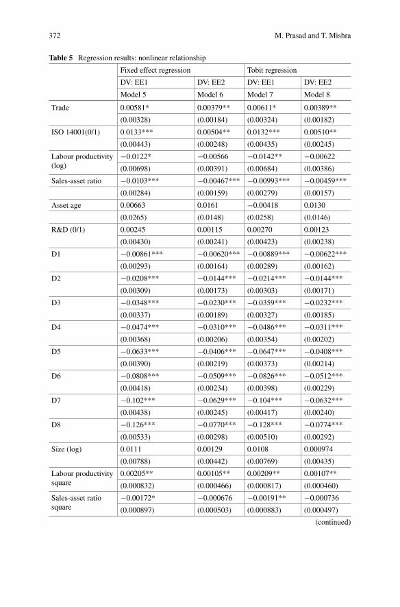
372 M. Prasad and T. Mishra
Table 5 Regression results: nonlinear relationship
Fixed effect regression Tobit regression
DV: EE1 DV: EE2 DV: EE1 DV: EE2
Model 5 Model 6 Model 7 Model 8
Trade 0.00581* 0.00379** 0.00611* 0.00389**
(0.00328) (0.00184) (0.00324) (0.00182)
ISO 14001(0/1) 0.0133*** 0.00504** 0.0132*** 0.00510**
(0.00443) (0.00248) (0.00435) (0.00245)
Labour productivity(log)
−0.0122* −0.00566 −0.0142** −0.00622
(0.00698) (0.00391) (0.00684) (0.00386)
Sales-asset ratio −0.0103*** −0.00467*** −0.00993*** −0.00459***
(0.00284) (0.00159) (0.00279) (0.00157)
Asset age 0.00663 0.0161 −0.00418 0.0130
(0.0265) (0.0148) (0.0258) (0.0146)
R&D (0/1) 0.00245 0.00115 0.00270 0.00123
(0.00430) (0.00241) (0.00423) (0.00238)
D1 −0.00861*** −0.00620*** −0.00889*** −0.00622***
(0.00293) (0.00164) (0.00289) (0.00162)
D2 −0.0208*** −0.0144*** −0.0214*** −0.0144***
(0.00309) (0.00173) (0.00303) (0.00171)
D3 −0.0348*** −0.0230*** −0.0359*** −0.0232***
(0.00337) (0.00189) (0.00327) (0.00185)
D4 −0.0474*** −0.0310*** −0.0486*** −0.0311***
(0.00368) (0.00206) (0.00354) (0.00202)
D5 −0.0633*** −0.0406*** −0.0647*** −0.0408***
(0.00390) (0.00219) (0.00373) (0.00214)
D6 −0.0808*** −0.0509*** −0.0826*** −0.0512***
(0.00418) (0.00234) (0.00398) (0.00229)
D7 −0.102*** −0.0629*** −0.104*** −0.0632***
(0.00438) (0.00245) (0.00417) (0.00240)
D8 −0.126*** −0.0770*** −0.128*** −0.0774***
(0.00533) (0.00298) (0.00510) (0.00292)
Size (log) 0.0111 0.00129 0.0108 0.000974
(0.00788) (0.00442) (0.00769) (0.00435)
Labour productivitysquare
0.00205** 0.00105** 0.00209** 0.00107**
(0.000832) (0.000466) (0.000817) (0.000460)
Sales-asset ratiosquare
−0.00172* −0.000676 −0.00191** −0.000736
(0.000897) (0.000503) (0.000883) (0.000497)
(continued)

20 Environmental Efficiency and Trade Theory: Evidence … 373
Table 5 (continued)
Fixed effect regression Tobit regression
DV: EE1 DV: EE2 DV: EE1 DV: EE2
Model 5 Model 6 Model 7 Model 8
Asset age square −0.00150 0.00752 −0.00851 0.00528
(0.0233) (0.0131) (0.0230) (0.0129)
Size square −0.00227*** −0.00108*** −0.00218*** −0.00106***
(0.000433) (0.000243) (0.000423) (0.000239)
Constant 0.901*** 0.850*** 0.902*** 0.852***
(0.0390) (0.0219) (0.0401) (0.0256)
Observations 1001 1001 1001 1001
R2 0.819 0.849
Number of com 121 121 121 121
Standard errors in parentheses*** p < 0.01, ** p < 0.05, * p < 0.1Source Authors estimates
References
Fujii, H., Iwata, K., Kaneko, S., & Managi, S. (2013). Corporate environmental and economicperformance of Japanese manufacturing firms: Empirical study for sustainable development.Business Strategy and the Environment, 22(3), 187–201.
Guttikunda, S. K., Goel, R., & Pant, P. (2014). Nature of air pollution, emission sources, andmanagement in the Indian cities. Atmospheric Environment, 95, 501–510.
Holladay, J. S. (2010). Are exporters mother nature’s best friends? Mimeo: New York UniversitySchool of Law.
Jayanthakumaran, K., Verma, R., & Liu, Y. (2012). CO2 emissions, energy consumption, trade andincome: A comparative analysis of China and India. Energy Policy, 42, 450–460.
Khanna, M., Anton, W. R. Q. (2002). Corporate environmental management: Regulatory andmarket-based incentives. Land Economics, 78(4), 539–558.
Khanna, M., & Kumar, S. (2011). Corporate environmental management and environmentalefficiency. Environmental and Resource Economics, 50(2), 227–242.
Mandal, S. K., &Madheswaran, S. (2010). Environmental efficiency of the Indian cement industry:An interstate analysis. Energy Policy, 38(2), 1108–1118.
Marginean, S. (2015). Economic globalization: From microeconomic foundation to nationaldeterminants. Procedia Economics and Finance, 27, 731–735.
Marin, G., & Mazzanti, M. (2009). The dynamics of delinking in industrial emissions: The role ofproductivity, trade and R&D. Journal of Innovation Economics & Management, 1(3), 91–117.
Ministry of Steel. (2012). National Steel Policy, Vol. 2012.Mittal, M. L., Sharma, C., & Singh, R. (2012). Estimates of emissions from coal fired thermal powerplants in India. International Emission Inventory Conference, 2012, 13–16.
Mukhopadhyay, K., & Chakraborty, D. (2005). Is liberalization of trade good for the environment?Evidence from India. Asia Pacific Development Journal, 12(1), 109.
OECD. (2018).Asian economic integration report 2018 toward optimal provision of regional publicgoods in Asia and the Pacific. Manila.
Prasad, M., &Mishra, T. (2017). Low-carbon growth for Indian iron and steel sector: Exploring therole of voluntary environmental compliance. Energy Policy, 100, 41–50.

374 M. Prasad and T. Mishra
Sadavarte, P., & Venkataraman, C. (2014). Trends in multi-pollutant emissions from a technology-linked inventory for India: I. Industry and transport sectors. Atmospheric Environment, 99, 353–364.
Sandhu, S., Smallman, C., Ozanne, L. K., & Cullen, R. (2012). Corporate environmental respon-siveness in India: Lessons from a developing country. Journal of Cleaner Production, 35,203–213.
Singh, N., Jain, S., & Sharma, P. (2015). Motivations for implementing environmental managementpractices in Indian industries. Ecological Economics, 109, 1–8.
Taskin, F., & Zaim, O. (2001). The role of international trade on environmental efficiency: A DEAapproach. Economic Modelling, 18(1), 1–17.
The Energy and Resources Institute. (2013). TERI Energy Data Directory and Yearbook 2012/13.New Delhi.

Chapter 21Prospects for Air Services in IndonesiaUnder Modified General Agreementon Trade in Services: India–ChinaDimension
Anil K. Kanungo and Abhishek Jha
1 Introduction
Trade in services in recent years has emerged as a priority area for growth in worldeconomy. Acceleration in growth due to trade in services sectors particularly in thelate 1990s and 2000s has motivated, especially some developing economies suchas India and a few ASEAN economies to embrace and accomplish liberalized andcomplementary policies to siege advantageous opportunities unfolding in the worldeconomy. Global economy subsequently has seen modern trends of services suchas outsourcing, rise of BPO, KPO1 and numerous retail administrations. With rapidpace of globalization and busy work schedule and lifestyle, consumerism in servicesis gaining momentum displaying a buoyant trend which is poised to give the sectora serious boost.
This work draws from the authors’ previously published work “Air Services in Indonesia: India–China Dimension” in Cambridge Journal of China Studies, Date of Publication: Volume 13, No.1,June 2018, Cambridge, UK, Pages of the Published Article: 59–73.
A. K. Kanungo (B)Lal Bahadur Shastri Institute of Management (LBSIM) Delhi, Plot No.-11/7, Sector-11, Dwarka,New Delhi 110075, Indiae-mail: [email protected]; [email protected]
A. JhaCentre for the Study of Regional Development, Jawaharlal Nehru University, New Delhi 110067,Indiae-mail: [email protected]
1After lowend business processing largely confined toBPOsector, globalMNCs started outsourcinghigh value-added business services. This activity has given rise to a new trend in outsourcing, whereknowledge and application of knowledge took precedence over just mechanical process, popularlycame to be known as knowledge process outsourcing (KPO). KPO includes research and work onIPRs, equity and finance, analytics, market research and data management.
© The Author(s), under exclusive license to Springer Nature Singapore Pte Ltd. 2021P. Lakhanpal et al. (eds.), Trade, Investment and Economic Growth,https://doi.org/10.1007/978-981-33-6973-3_21
375

376 A. K. Kanungo and A. Jha
As proliferation of trade in goods sector is largely supported by factors like tariffreduction and non-tariff barriers, services sector is largely controlled through regu-lation. It is crucial to see that even if regulation is a key determinant of rise in tradein services, but such regulations need to be deregulated at certain point of time toprovide boost to the sector.
While India’s integration with the global services market took place primarilythroughUSandEUmarket, slowdown in India’s serviceswas experienced largely dueto major collapse in these markets because of global financial crisis and USA turningprotectionist soon after. This propelled India to explore other markets like East andSoutheastAsia to find a foothold. SoutheastAsia presently looks promising having itsmacroeconomic fundamentals robust and stable.2 Earlier, due to the language barrierand cultural factors, Indian organizations were traditionally doing business trans-actions mainly with the Western companies and not with Southeast Asian nations.Currently, the services sector in ASEAN looks promising and continues to flourishsteadily. As of 2013, this sector represented about 47% of GDP on average for theASEAN economies. Even among Cambodia, Lao PDR, Myanmar and Vietnam,the contribution of the sector is substantial. In Singapore, around 60% of GDP iscontributed by the services sector. In Malaysia and the Philippines, more than half ofthe economy is driven by business activities in this sector. For trade in services underthe ASEAN Economic Community (AEC) Blueprint 2025, negotiations are due tocommence on the ASEAN Trade in Services Agreement that aims to strengthenthe existing ASEAN Framework Agreement on Services (Economic Outlook forSoutheast Asia, China and India 2017).3
This growing demand of services in Southeast Asian countries has permittedIndian firms to scout for prospects here, and as of now, Indian organizations arecarrying out more business with Japan, China, and other East Asian and ASEANnations. Scope is wide and is feasible for Indian firms to join the ASEAN productionsystems by utilizing information technology and enabled services to foster richereconomic and business linkages.
Formation of a vibrant and efficient services sector is fast becoming a prominentfeature of modern economies. For over two decades, advanced economies oftencontribute to about 66% of the world’s GDP through services. The shift from primarysector to secondary and then followed through services has been the focal pointof structural change and economic transformation for many developing economies(Nayyar, 2019). In accordance with this pattern, it is seen that many developingmarkets are as of now embraced serious efforts to support and develop servicesindustries and to put in place the regulatory structures required for more integratedinternational servicesmarkets. India and TheAssociation of Southeast AsianNations(ASEAN) are largely following this pattern in an attempt to make services sector asone of the main drivers of their economic integration with the world economy andprospective trade partners. Most of the developing economies from ASEAN regionand India are presently concentrating on the growth of the services sector. This
2World Bank data 2017.3https://www.oecd.org/dev/asia-pacific/SAEO2017_PV.pdf, accessed on December 27 2017.

21 Prospects for Air Services in Indonesia Under Modified … 377
is evident from the fact that India’s contribution of services to GDP is impressiveand bordering around 63% (Kapoor, 2014), thus contributing to economic activity,employment generation and growth.
Coupled with these factors, deregulation and liberalization of the service sectorand proliferation of these activities of service economy perform a critical role insecuring economic growth. Currently, travel and transport services command aprominent place in the service trade of many ASEAN nations (ITC Trade Map,COMTRADE). Indonesia is at the forefront of delivering such services to anexpanding consumer base. Ever since the Indonesian government deregulated theaviation industry in 2000, Indonesia’s aviation division has been developing at afaster pace in terms of travelers, carriers, armadas, flights, and air terminals. Suchexplosion in air services is noticed when one looks at the number of carrier travelersthat has expanded from 9 million in 1990 to around 90 million in 2016. The samegoes for the country’s carrier armadas which havemultipliedmore than ten-fold from102 aeroplanes in 1990 to 1030 in 2017 (Global Business guide).4
Indonesia’s aviation sector provides enormous investment opportunities fordomestic and foreign investors. There are several potential routes which are notso far completely encouraged particularly to destinations outside Java such as inKalimantan and Papua. Having a GDP growth rate of 5.2% in 2017 and inflationregistering around 4.2%, it can be an appropriate time for India to break into Indone-sian market. It is largely recognized that India’s competence in services does not liein air services so visibly as compared to sectors such as IT, computer and informa-tion services and financial, accountancy but having known that India’s strength in airservices is growing and Indian airline system is an activemember of International AirTransport Association (IATA), it is in the realm of exploration that India can ventureinto providing air services to Indonesian market after its open sky policies and canoperate from Indonesian base to provide air services to other Southeast Asian nation.India’s signing of ASEAN agreement and its “Look East Policy”5 may provide somestimulus to that extent.
Similarly looking at China’s aviation industry, it was discovered that Chinesegovernment is taking initiatives to create residential assembling potential, make newair terminals, give professional training to newpilots and swell domesticmaintenancecapacity. China’s top three emerging airlines—Air China, China Southern and ChinaEastern—are in the present days among the world’s best ten airlines in terms of
4https://www.gbgindonesia.com/en/services/article/2017/indonesia_s_aviation_industry_flying_high_11719.php, accessed on December 26 2017.5The Look East policy has emerged as an important foreign policy initiative of India in the post-ColdWar period. It was launched in 1991 by the Narasimha Rao government with the aim of developingpolitical contacts, increasing economic integration and forging security cooperation with countriesof Southeast Asia. The policy marked a shift in India’s perspective of the world, with the strategicand economic importance of Southeast Asia to India’s national interests being recognized. Thesecond phase, which began in 2003, extends the coverage of the Look East policy from Australia toEast Asia, with Association of Southeast Asian Nations (ASEAN) as its core. The new phase thusmarks a shift in focus from trade to wider economic and security cooperation, political partnerships,physical connectivity through road and rail links.

378 A. K. Kanungo and A. Jha
passenger volume. In 2005, the CAAC had reported that it would open up China’saviation sector to both domestic and foreign investment and empower private Chineseair carriers. This intends to spur the growth of private players in the sector such asOkay aviation routes, China’s first private carrier.
Geographical proximity plays a critical role in trade and commerce. China seemsto have that advantage vis-à-vis Indonesia. Besides, the familiarity of culture, raceand heritage will be added advantage for China to penetrate into Indonesian market.
In an augmented gravity model, Hao (2016) indicates that the distance is signifi-cantly negatively related with the air transport services. This sets against the above-said argument that the close geographic proximity facilitates the business. Also, theFTA have a flourishing effect on the services trade which Chinese airline undertakesin Asia–Pacific. On the whole, the air transport network in China is moving in a fastpace which signals potential competition for India in providing transport services toIndonesia.
Against this backdrop, the paper attempts to explore if Indian aviation sector canenter into the markets of Indonesia and whether they would be able to supply suchservices. It also tries to assess if certain value-added services in term of auxiliary airservices, which may be a current requirement for Indonesia, are India in a positionto deliver that? It is time that Indian services sector must develop core competencein other sectors as it has done in IT and ITES. It aims to suggest that India shouldtake forward the potentiality of this air services in Mode 3 andMode 2 to negotiatingtable as opportunity exists in these modes. India’s economic growth to an extentrests on such trade and cannot be confined to IT, financial, etc. If India to experience7% growth rate, it is imperative for the all stakeholders such as the government,policy makers, trade and industry to realize that certain sectors need serious attentionand negotiation for liberalized trade to occur in sector such as air services. Then,contribution of services sector will be fully realized.
2 Analysis of Air Service Sector
Observing the business potential and trade opportunities, it is witnessed that ASEANregion has a momentous contribution of Air Transport Services6 Industry to its GDP.It shows an upsurge and lucrative trend, marked by vigorous growth particularly incertain emerging markets of ASEAN region and more so in Singapore, Indonesia,Thailand.7 While global air cargo still persists somewhat at abated expectations,passenger progression is showing an upward trend, and air travelers are anticipatedto double by 2035.8 Globally, the air transport industry now supports 63 million jobsand contributes US$2.7 trillion to global GDP.
6Air transport services include commercial passenger services and air cargo.7World Bank Working Paper (Air Transport Annual Report).8See Footnote 7.

21 Prospects for Air Services in Indonesia Under Modified … 379
Quality performance of the global air services sector has made investments in airtransport more lucrative.
For a second year, airlines’ return on capital exceeded their cost of capital on aglobal scale, and many mid-sized airports in emerging markets are able to attractprivate capital to finance the needed infrastructure expansion. Every route or everyregion does not experience similar or improved financial performance. For example,the Asia–Pacific carriers were able to post a benefit of US$ 900 million in 2016,African airlines lost US$ 800 million, and many African airports still witness insuf-ficient traffic as a result not able to finance needed investments (Air Transport AnnualReport, World Bank, 2016).
Considering the prospects within the ASEAN nations and competency level ofIndian air services, it is desirable thatwith theopen skypolicy and approaches adoptedby ASEAN countries, India is in a comfortable position to explore opportunities inthat region. Now that FTA between the two is in place, India may negotiate hard totake advantage of the sector. Negotiation in services between India and ASEAN hasnot experienced any serious kick start yet, not even among trade and industry, butboth have realized the quantum of potential exists.
Analyzing broadly the requirement of ASEAN countries’ demand in services, itwas found that major ASEAN countries that are currently experiencing huge demandin these sectors are Singapore, Philippines, Thailand and Indonesia. Initial analysisof data9 and observations gave us an idea that India has competitive advantage insome of the mentioned sectors where demands of services of those sectors are quitesignificant in these four countries. India therefore has distinct advantage in thosesectors and can cater such services at competitive prices.
One of the key players in ASEAN countries currently is Indonesia whose require-ment in air services (Air transport) is enormous. Data from National Input–OutputTable provided by World Input–Output database10 give us an idea that in 2000 itwas 2.28 billion US$ from domestic value addition and imports component was 0.44billion UD$. Subsequent years onward, which means from 2001 to 2005 domesticvalue addition and imports contracted making the difference between the exports andimports to almost nil. From 2006 onwards, it showed a continuous increase to makedomestic consumption of air services to 18.5 billion, whereas the import componentprevailed at 0.53 bn US$. So, the domestic consumption of this air services andimport of services witnessed a CAGR of 53 and 1.2%; whereas exponential growthof domestic consumption of air transport services was 4.01%.11
It is observed that the structural change12 that happened within the domestic airservices in Indonesia has given rise to a huge number of domestic aircrafts joining thecompetition. In a way the industry has been solidified and enormous opportunities
9Managed by NWO (Netherlands Organization for scientific research).10See Footnote 9.11Based on author’s calculation by taking into account Nation WIOD database.12Indonesia deregulated its transport sector, including the air transport sector after the 1998 AsianFinancial Crisis. Themomentum for reform in the air transport sectorwas provided by the enactmentof the Competition Law in 1999 which led to liberalization of air services.

380 A. K. Kanungo and A. Jha
for local players are in place. With the reopening of the sector occurring in 2001,entry of airlines has been facilitated.
A historical perspective gives us an idea that the state-owned enterprises, GarudaIndonesia and Merpati Nusantara dominated the industry. In 1992, both capturedabout 90% of the market. In 1996, however, the share of these two dropped to 68%(ADB, 1997). In 1993, the government temporally closed the industry for new entry.However, the moratorium was lifted in 2001. As a result, a number of new airlinesemerged. By 2004, 28 new airlines were licensed. By this time, Merpati NusantaraandGaruda Indonesia had captured about 38% of Indonesia’s air travel market, whilethe new entrants captured 35% of the market (Damuri and Anas 2005).
This euphoria lasted for some time as some of the airlines could not sustain theirservices due to lack of technical capacity or because of financial constraints. Towardthe end of 2016, it was noticed that about 14 airlines are still in operation and activein domestic market by providing efficient air services (Input–Output Model–valueaddition—This can be accessed at www.wiod.org).
Since India has entered arrangement with ASEAN and Indonesia being a vitalpartner in that drive, India can consider providing such air services for the Indonesianconsumers. India has a competitive open sky policy where it has energized the privatesector to be the key service providers. As of now around six private airlines arecompeting in the market showing enough resilience to keep the sector buoyant anddynamic. Household consumption of air services both in household and imports is2.6 billion US$ in 2014 in India.13
Some of the important dominions where India could possibly explore its businessopportunities as far as Indonesian market is concerned are related to air connectivityand air services which are elaborated below. With the liberalization policies of airservices of Indonesia, and India already having a cordial and historical relationshipwith the country, chances of India establishing good business and trade relationshipwith the country are more likely.
Key areas.
1. India can become a partner in establishing digital connectivity with ASEANeconomies which will cater broadband services to the countries in the region.These computerized network ventures are of vital significance and can givesuperior air network and air services. This may cause a transformative effect onthe economy and participation between ASEAN and India.
2. India is committed to extend financial as well as technological backup forventures that aim to secure high-speed fiber optic systems, advanced towns,digital villages, countryside broadband, national knowledge network, securedcommunication systems and telecom training and skill development to avoid airaccidents which are currently faced Indonesian government (Damuri & Anas,2005).
3. India adopts aGeneralAgreement onTrade inServices (GATS) approach,whichcontains provisions on national treatment, market access, modes of delivery anddomestic regulation.
13WIOD database 2016.

21 Prospects for Air Services in Indonesia Under Modified … 381
0
500
1,000
1,500
2,000
2,500
3,000
2001 2002 2003 2004 2005 2006 2007 2008 2009 2010 2011 2012 2013 2014
Exports and Imports of Air Transport Services of Indonesia in USD Millions
Exports Imports
Fig. 1 Exports and imports of air transport services of Indonesia in USDMillions. SourceNationalInput Output Table (NIOT), World Input Output table
3 India–Indonesia Trade Framework
Indonesia is an important services trade partner of India as India exports 10.2%14 ofservices (excluding commercial air traffic as per annex GATS) to Indonesia amongall ASEAN economies. In terms of value addition done in Indonesian air transportservices, France and South Korea top the list, and India is unable to capitalize theopportunities thrown open by liberalization policies of Indonesia.
The air transport sector’s talent to bridge Indonesia to developing nations and fast-growing cities can secure increasing economic growth of the connecting economy.Asper the data provided by Oxford Economics,15 there are 108 direct flight destinationsamong the ten fastest growing countries in the world, on the basis of GDP growthand 119 direct flight destinations among the 20 fastest growing countries. China isleading the league, by connecting maximum direct flights to Indonesia among thefastest growing economies followed by Vietnam and Philippines.
As per the same source, there are seven16 direct weekly flights among the tenfastest growing cities in the world as measured by GDP growth and over 5500 directweekly flights among the 100, growing cities but India is missing in capturing thesebusiness opportunities (Fig. 1).
Analyzing this export–import figure of air transport services of Indonesia, it isarticulated that exports have truncated from2011 to 2014 due to several policy actionsof Indonesian government implemented in 2010. Few of these stringent policiesinclude enactment of national aviation safety programme, classification of carrierservices into full, medium and no frills. Apart from this, Indonesian government
14Calculated from ITC Trade Map, 2017.15IATA, Oxford Economics IMF National Statistics, can be accessed at www.oxfordeconomics.com, accessed on December 20, 2017.16Oxford Economics.
382 A. K. Kanungo and A. Jha
also applied surcharge if Avtur17 price experiences consecutive surge in price.18 Dueto these convoluted policy implications, services trade of Indonesian air transportplummeted. Looking at this, now India has an opportunity to invest and expand thebusiness of air transport services in Indonesia. The air transport subsector has alsobeen a driver of service sector growth. Albeit smaller than the combined commu-nication sectors, its GDP contributions have doubled in the last decade. After all,successful deregulation has again been a key driving force (Cristea et al., 2014). Thisargument juxtaposes the potential for Indian air transport service suppliers. An over-riding step favouring deregulation will certainly generate revenues and employmentin Indonesia and thus could be considered by Indonesian government as viable ordoable proposal.
As per ADB Report 2016,19 “The rapidly expanding demand for air transport,enhanced by the upcoming ASEAN Open Skies Policy, already exceeds the capacityof many Indonesian airports, requiring extensions and new airport developments.Since airports and airline operations are typically regarded as economically andfinancially viable, there is little demand for external support.”
As per the Indonesian Government policy, up to 49% of FDI in the form of foreignequity is allowed. Thus, there is a gateway for the Indian domestic business playersof aviation sector to be the part of this lucrative and robust service sector mainlydelivering under mode 3 (commercial presence abroad) and mode 2 (consumptionabroad).20
4 Signing of India-ASEAN Agreement a Boost to ThisOpportunity
The implementation of ASEAN open sky encompasses three agreements: theASEAN Multilateral Agreement on the Full Liberalization of Air Freight Services(MAFLAFS), the ASEANMultilateral Agreement on Air Services (MAAS) and theASEANMultilateral Agreement on the Full Liberalization of Passenger Air Services(MAFLPAS). Authorization of these three agreements will permit any airlines desig-nated by an ASEAN Member State to function both passenger and cargo scheduledservices between its home economy and a point with international airport in anotherMember State and then to a point with international airport of a third Member State,without limitations on capacity and schedule (APEC Policy support unit) (APEC,2017).
17Airlines aviation fuel.18APEC Policy Support Unit, May 2017.19https://www.opml.co.uk/sites/default/files/Growth%20in%20Indonesia_Drivers%20of%20recent%20economic%20growth.pdf20The service consumer crosses the border to where the service supplier is located to purchase andconsume services. Examples include holidays abroad, foreign education and overseas health care.

21 Prospects for Air Services in Indonesia Under Modified … 383
Here comes the role of India-ASEAN services FTA which needs to give impetuson air transport services and negotiate it in a requisite manner. The issue of enhancingair connectivity between India and Indonesia needs to be one of the pivotal themesunder the India-ASEAN services policy modifications. This issue of connectivitymay be taken up at the negotiating level as one of the key and front-runner agendabetween the two governments. This needs to be stepped up on a fast track basis;otherwise, any other country will usurp this opportunity. There is a clear need for acomprehensive ASEAN-India Air Transport Agreement and extending it to fall intothe scope of bilateral air services agreement (BASA).
Looking at increasing trade and business activities relating to air services, oneof the obstacles that the Indonesian government is facing as of now is frequentair accidents. Such mishaps have the potentiality to put the industry at high riskand devoid of any expansion unless the government quickly puts in place seriousmeasures to avoid such accidents. It was found that plethora of such mishaps arehappening with Indonesian carriers. Air safety becomes a prime concern and needsto be checked if business and buoyancy of the sector are to be improved. One ofthe plane security assessment Web sites surveyed 407 key airlines of the world,giving each a safety tally out of seven. Of the ten airlines that scored paltry onepoint or less, all but one was from Indonesia. On one hand, Indonesian airport, i.e.,Jakarta is considered as one of the top airports in the world which has recorded andis recording maximum number of passengers in Indonesia, and on other hand, nineout of ten airlines owned by Indonesia are ranked being least safe among the world.Detailed is mentioned below in a tabular format (Tables 1 and 2).
As safety of passengers seems to be a major concern in Indonesia, how India canprovide any support services to reduce such hazards could be an area of engagement.
Table 1 The airlines awardedthe lowest safety rating by thesurveyed web site
1 Airlines Country it Belongs to
1 Trigana Air Service Indonesia
2 Batik Air Indonesia
3 Citilink Indonesia
4 Kalstar Aviation Indonesia
5 Lion Air Indonesia
6 Sriwijaya Air Indonesia
7 Tara Air Nepal
8 TransNusa Air Services Indonesia
9 Wings Air Indonesia
10 Xpress Air Indonesia
Sourcewww.AirlineRatings.com, accessed onDecember 22, 2017

384 A. K. Kanungo and A. Jha
Table 2 Global top 20airports—passenger traffic2015
Rank 2015 Country Airport/Code Total passengers
1 USA Atlanta 101,491,106
2 China Beijing 89,938,628
3 UAE Dubai 78,010,265
4 USA Chicago 76,949,504
5 Japan Tokyo 75,316,718
6 UK London 74,989,795
18 Indonesia Jakarta 54,053,905
Source Airport traffic statistics, 2016
5 India’s Strength
India can conceivably improve Indonesian air transport services by making a differ-ence in giving way better pilot services, progressed technicalities and fair in timeservices. These measures may bolster the system to diminish such regular accidents.The track record and quality of services of Indian airlines such as Air India and othersare way ahead in security standard compared to national carriers of Indonesia.21
Indeed, in spite of the fact that Indonesia is an integral part of ASEAN, securityproceeds to be a concern for the travelers as well as for the government. With therate of deadly mishaps in Indonesia still being one of the highest in the world andmost of its commercial aircrafts are still on the EU boycott list, the government hasnot acted quite positively to reduce such accidents, and apparently, there is no suchsignificant policy in place to address this issue.
5.1 Revealed Comparative Advantage of Air TransportServices: India’s Upsurge on the Ladder
India’s air transport sector has so far buttressed close to 8million jobs and contributedto $72 billion in GDP. According to IATA’s recent 20-year air passenger forecast, itis estimated that India will surpass the UK to become the third largest market with278 million passengers in 2025. Further by 2035, India is likely to be a market of442 million passengers, with the aviation industry supporting 19.1 million jobs andcontributing to $172 billion in GDP. This liberalization step in the Indian aviationmarket has minimized the institutional barriers which have hindered the freedomand flexibility of air transport operations among private investors. Now, competitionwithin the aviation sector has become fiercer, the Airports Authority of India AAIand Public Private Partnership PPP in Indian airports are not only providing varied
21JACDEC Airline Safety Ranking 2017. In this survey, Air India stood at 40th position, whereasIndonesian airlines stood at 58th position.

21 Prospects for Air Services in Indonesia Under Modified … 385
services, but also attracting consumers with new infrastructure and full modernfacilities (Kumar et al., 2018). It is also found that the airports managed throughjoint ventures are more efficient than others (Kashiramka et al., 2016). According toOECD STRI database, Indonesia has not restricted but limited the land acquisitionfor a foreigner to buy as far as air transport services are concerned. Thus, it canbe observed India has a scope of JVs with the domestic partners or stakeholders ofIndonesian airlines.
It becomes vital for us to evaluate revealed comparative advantage of air transportservices exports of selected countries to compare the standing of India’s comparativeadvantage for air transport services exports. Going by Balassa (1965), the revealedcomparative advantage index (RCA) is estimated as
RCAi j =Xi j∑i Xi j
∑Xi j∑
i∑
j Xi j
where Xij represents country i and exports j.∑
iXij is the sum total of exports ofcountry i.
∑Xij is the world exports of jth commodity.
∑i∑
jXij is the sum totalof world exports. If the value of RCAij > 1, it indicates that a country is compet-itive in export and vice versa. The index suffers from a few limitations such asunstable distribution over time, feeble ordinal ranking property and its ability tocapture only exports (Yeasts 1985; Hinloopen and Van Marrewijk 2001). Further,the value of index varies from 0 to ∞ making it hard to compare the RCA of anexportable commodity having value >1. The main advantage of using RCA is that itconsiders the intrinsic advantage of a particular export commodity and is consistentwith the changes in an economy’s relative factor endowments and productivity. Thedisadvantage, however, is that it cannot distinguish between improvements in factorendowments and the pursuit of appropriate trade policies by a country (Batra&Khan,2005). It also suffers from the problem of asymmetry as “pure” RCA is basically notcomparable on both sides of unity as the index ranges from zero to one if a country isnot specialized in a given commodity while it ranges from one to infinity if a countryis specialized.
To address such limitations, several variants of Balassa index have evolved overthe period of which Vollrath (1991) and Dalum et.al. (1998) indexes merit attention.Vollrath proposed three alternative measures of RCA (1) Relative trade advantage(RTA) expressed as the difference between revealed export advantage (RXA) andrevealed import advantage (RMA) written as RTAij = RXAij – RMAij, Where RXA= (Xij/Xt)/(Xwj/Xwt), RMA = (Mij/Mt)/(Mwj/Mwt) and X andM denote exports andimports. (2) Logarithmic transformation of RCA = ln (RXAij).
(3) Revealed competitiveness (RC) expressed as difference between logarithmsof relative export advantage and relative import advantage: RC = ln (RXAij) – ln(RMAij). A positive value of each index indicates a revealed comparative advantage,whereas a negative value indicates a revealed comparative disadvantage.
Dallum (1998) symmetrical revealed comparative advantage (SRCA) is anapproximation of the log transformation of Balassa Index, ranging from −1 to +

386 A. K. Kanungo and A. Jha
1 with 0 as a neutral point. It is expressed as: SIi j = BIi j−1BIi j+1 where BIij is the Balassa
index of country i and commodity j. Country i will have a comparative advantagefor product j if the value of SRCA is greater than zero and disadvantage if it is lessthan zero. The distribution of Dallum index fulfills the normality assumption moreoften as compared to the Balassa index making it propitious to use for econometricanalysis (Laursen, 1998).
As per the table, USA, UK and Germany are having high potential in revealedcomparative advantage (RCA) in exports of their air transport services because theirRCA is exceeding one. For India though, the value of RCA is less than 1, but in thepast three years, there is an overall rise in the competitiveness of air transport servicesexports, hence the governmentmay like to signmore of joint ventures at an aggressivemanner, and at the same time, the government possibly can target Southeast Asiaas a key traffic zones for India because large number of Indians are traveling tothis region for eclectic purposes such as tourism and academics. This is expectedto further surge with the kind of policies the Indian government is implementinglike UDAAN scheme. In the way that Gaya, the major city in Bihar, has a centerof attraction for Buddhism, hence it can provide required impetus for the SoutheastAsian region’s connectivity. Indian government is trying to connect and modernizeregional airports, which will boost the connectivity and competitiveness and in theprocess of building many airports at different cities to provide better connectivity.
Looking at the Trade Map data of ITC, Indian exports of air transport serviceshave increased from US$1.4 billion in 2009 to US $5.8 billion in 2018 registeringfour times increase in exports.
It can be inferred from Table 3 that top three economies such as USA, Germanyand China are having more exports of air services because these three economiesare having more GDPs at nominal prices compared to India which is also reflectedin Table 3 as we see the exports of services in RCA of India are lower than theseeconomies.
One of the possible reasons of India’s RCA in exports of air transport servicesbeing lower is due to miniscule exports of air transport passengers. This miniscule
Table 3 Revealed comparative advantage of air transport services export
Economies 2014 2015 2016 2017 2018
China – – – 0.830 1.006
France 0.874 0.826 0.824 0.765 0.849
Germany 1.082 1.086 1.134 1.158 1.436
India 0.667 0.471 0.519 0.450 0.581
United Kingdom 1.060 1.127 1.127 1.119 –
United States of America 1.524 1.476 1.428 1.360 1.695
Source Authors’ calculation using ITC Trade Map Data compiled by COMTRADE

21 Prospects for Air Services in Indonesia Under Modified … 387
Table 4 Exports value of air transport services, in USD Billion
Economies 2014 2015 2016 2017 2018
China – – – 11.390 12.962
France 14.365 12.346 12.262 12.654 11.959
Germany 19.552 17.583 18.554 21.424 22.969
India 6.311 4.299 4.808 5.013 5.761
United Kingdom 23.869 23.445 22.459 24.001 –
United States of America 68.053 65.215 62.049 65.229 67.804
Source Authors’ calculation using ITC trade map data compiled by COMTRADE
value of exports of air passenger traffic in case of India is about 7.6%22 of total airtransport exports.
Table 4 mentions about the exports of air transport services in absolute terms,stating that USA tops the exports of air transports services in absolute terms, followedby UK, Germany and China. India is far behind these economies, but makingconcerted efforts to catch up with the other economies.
According to the Table 5, India’s exports to gross world output are maximum ascompared with USA and China. This clearly indicates that there is a predilectionfor air transport exports in the gross world output for India, although the absolutelevel of gross world output is lowest. This requires constructive policy interventionfrom the policymakers to address this issue and frame policies that would harnessthe sector to realize larger potential of the sector.23
6 Value Adding in Air Transport Services of Indonesia
Apart from standard transport air services, quality control and value addition in otherauxiliary services are vital to make aviation sector resilient, timely, user friendly andsecure. In the field of auxiliary services, India’s performance seems to be aheadof Indonesia. This dimension is echoed in India’s aviation industry when we takeinto account contribution of this sector to its economy. This further elaborated intwo different ways, namely through taxes and investment and by using advanced
22As per ITC Trade Map data, India’s exports for passenger air transport air services are US$ 0.444billion, whereas air transport services exports are US$ 5.761 billion.23Finance Minister Nirmala Sitharaman announced in 2019–2020 budget on July 05, 2019, that thegovernment will re-initiate disinvestment of national carrier Air India as well as open up ForeignDirect Investment (FDI) in aviation.
There is 100% FDI allowed in aviation, but foreign airlines can only invest up to49% in an Indian airline. Also, foreign investment in Air India is capped at 49%. Thegovernment’s decision to revisit privatization of Air India follows an attempt last year thatmet with failure when no private player came forward to express an interest in the debt-laden carrier. https://www.thehindu.com/business/budget/union-budget-2019-20-air-india-disinvestment-set-to-take-off-again/article28298695.ece accessed on July 09, 2019.

388 A. K. Kanungo and A. Jha
Table5
Exports,g
ross
world
output
and%
ofexportsto
world’sgrossoutput
ofairtransporto
fChina,U
SAandIndia,(inUSD
Million)
Year
China
USA
India
Exports
Gross
Output
%of
exportsto
World’s
grossoutput
Exports
Gross
Output
%of
exportsto
World’s
grossoutput
Exports
Gross
Output
%of
exportsto
World’s
grossoutput
2000
3728
13,311
28.00445
22,093
123,668
17.86
753
1700
44.29
2001
4188
15,135
27.67161
18,559
107,172
17.32
650
1647
39.44
2002
4938
16,834
29.33318
17,811
100,688
17.69
714
1649
43.33
2003
6088
17,800
34.20312
16,872
109,861
15.36
943
2450
38.51
2004
8686
20,956
41.44936
20,195
120,550
16.75
1297
2723
47.62
2005
10,425
25,692
40.57823
23,423
133,590
17.53
1683
2739
61.44
2006
13,998
28,541
49.04557
25,118
145,060
17.32
2061
3374
61.06
2007
18,207
33,962
53.60898
28,611
155,997
18.34
3438
3731
92.16
2008
22,461
41,477
54.15259
36,019
165,019
21.83
3224
3224
100.00
2009
17,892
42,909
41.69694
29,909
136,328
21.94
2354
3134
75.11
2010
22,277
49,294
45.19301
35,293
153,610
22.98
3585
4374
81.96
2011
24,976
60,566
41.23705
41,345
170,379
24.27
3554
5024
70.74
2012
24,052
68,138
35.29852
45,049
178,090
25.30
2891
4851
59.59
2013
23,583
76,094
30.99213
46,625
181,418
25.70
2389
4629
51.62
2014
22,923
84,735
27.05253
48,076
188,758
25.47
2367
5016
47.18
Source
Autho
rs’C
alculatio
nbasedon
WIO
DDatabase(D
atashow
ninTable4aretill201
4becausecurrentavaila
bilityof
datainWIO
Ddatabase
isup
to20
14)

21 Prospects for Air Services in Indonesia Under Modified … 389
Locally Based Airlines which includesfuel, catering, repair, distribu on and other financial services.
Aerospace Supply Chain
Ground Based Infrastrucutre and Non-airside supply chain including food and beverages, marke ng
Fig. 2 Schematic diagram of value chains in Indian aviation and air transport services
technology. The Indian aviation sector rather generates more gross value addition(GVA) per employee24 than the economy as a whole, raising the overall productivityof the economy. Such value addition, Indian government, can provide to Indonesianmarket through value chain.
This value addition which is foremost input of the airline business is in the realmof energy, and aircraft and its maintenance. Apart from those core inputs, the airlinebusiness also banks on other services, such as food and beverages services, trade andinsurance. ICAO (2013) in its assessment of the aviation value chain suggested toinclude aircraft leasing services and manufacturing, air navigation services, main-tenance repair and overhaul services, fuel supply, ground handling and systems forselling tickets including online systems. For Indonesia, fuel consists of 35% of thevalue addition followed by warehousing transport services, administrative services,retail trade of vehicles and food and accommodation services. Manufacturing foodand beverages consist of 5.7% of the total value chains.25 4.8 billion USS26 is thevalue-added exports by India to the world in terms of airlines hospitality serviceswhich could be one of the components of value addition that can be extended to theIndonesian market (Fig. 2).
Indonesian air services market has high potential as the government is determinedto improve its infrastructure to promote its tourism sector (Wang et al., 2017). Asdemand for air services is growing in Indonesia, more and more airports are goingto be built as Indonesia is a partner country of ASEAN, it will be able to connectmore to the Asia Pacific region by connecting itself to the East Asian and SouthAsian economies where India is an emerging economy and currently well positionedbecause of promising growth and integration with the world economy. There seemsto be synergy between India and Indonesia being further linked up through cultur-ally and historically. India had a long historical trade relation with Indonesia. Thisfamiliarity can be exploited to increase trade realization better.
The authors also analyzed Indonesia’s position in terms of services trade restric-tiveness of air transport. From the OECD STRI database, it was observed thatIndonesia is moderately restrictive in this sector hovering around 0.48 in a scale
24WIOD database 2016.25According to authors’ calculations from WIOD database by using NIOT.26Calculated from WIOD Table.

390 A. K. Kanungo and A. Jha
of 0 to 1. The five parameters that need to be explained are restriction on foreignentry, restriction to movement of people, other discriminatory measures, barriers tocompetition and regulatory transparency.
The first component which is the restriction on foreign entry says that there is arestriction of up to 49% equity regarding foreign ownership. With respect to acqui-sition, it is argued that acquisition is not prohibited, but there is a limitation. Aforeigner can only be granted the Right of Use or lease for a maximum of 25 yearswith possible extension for 20 further years. After the extension period has expired,the owner can request the renewal for the same period. An exception is in place forinvestment purposes, where investors can request extension and renewal of Right toUse in advance. Therefore, the investor can have the Right of Use for 90 years.
It is mandatory for an employer to appoint an Indonesian national as an asso-ciate to a foreign worker for technology and knowledge transfer purposes. Theassociate should also receive training to attain the same qualification as the posi-tion held by the foreign worker. This regulation exempts top executive positions ortemporary/emergency foreign workers.
The second component which talks of restriction of movement of people is fairlyliberal. The only requirement is to get permission from Ministry of Manpower fora foreigner to work in Indonesia. Requisite labor market test is applicable on IntraCorporate Transferees (ICT), contractual services supplier and independent servicessuppliers with respect to air transport services. Duration of stay for a foreigner isnormally 2 years in certain circumstances, and it can be for 4 years.
The third component which is about other discriminatory restrictions is found thatIndonesia does not have any restriction through the period from 2014 till 2017.
The fourth component which is barriers to competition is hardly restrictive inIndonesia. There is law on anti-monopoly and unfair competition which appliesto foreign firms as well. Minimum capital requirement to establish air freighttransportation company is US$ 7.5 million to be invested.
The last component which is regulatory transparency has been made liberal overlast four years. Number of working days to complete all mandatory proceduresto register a company has been significantly reduced from 75.5 days in 2014 to24.9 days in 2017. For China and India, it is fairly liberal, and it takes about 27 daysand 28.5 days, respectively.
The total cost to establish one company in Indonesia as a percentage incomeper capita has also reduced from 21.9% in 2014 to 19.4% in 2017. With respect topolicies on air transport services, there is symmetry with no outliers. Table 6 providestrade restrictiveness of Indonesia and other countries. As per the Table 6, Germanyseems to be most liberal in terms of air transport services and logistic cargo handlingservices. Indonesia is fairly less liberal in both sectors.

21 Prospects for Air Services in Indonesia Under Modified … 391
Table 6 Index of air transport services
Economics Services trade restrictive index of airtransport servicesa
Services trade restrictive index oflogistics cargo handling services
Indonesia 0.48 0.46
China 0.48 0.41
India 0.57 0.40
USA 0.53 0.25
Germany 0.37 0.15
UK 0.39 0.16
France 0.39 0.19
aSTRI lies between 0 and 1. 0 being least restrictive and 1 being most restrictiveSource OECD Services Trade Restrictive Index (STRI) database
7 Chinese Outlook in Indonesia’s Air Transport Services
China is the world’s second largest and one of the world’s fastest burgeoning civilaviation markets. The industry has grown at double-digit rates for several years.From 2000 to 2014, exponential growth rate of household consumption of air trans-port services of China remained at 18.127%. This figure is though impressive, butunable to articulate the real scenario. Comparing with world air transport services,role of Chinese’s air transport services is at miniscule. Exports of China’s air trans-port services for above-specified time period are again impressive from growth ratepoint of view, else is insignificant. China’s air transport network is still a point-to-point network instead of a hub-and-spoke system (Qiang et al., 2014). Close to88% of China’s air transport services are utilized by the domestic passengers itself,thus indirectly making Chinese aviation sector’s predilection for domestic services.Numbers reflect an enervated intra industry scenario for air services between Chinaand Indonesia. According to WIOD, 2014 Chinese’s air transport’s contribution inthe Indonesian’s output of air transport is USD 2 million. But relatively the finalconsumption expenditure byhouseholds of Indonesia isUSD8milliondue toChineseinput of air transport services.
Indonesian public administration and defense; compulsory social security hasreceived the maximum inputs from the Chinese air transport sector, which articulatesthe non-commercial usage ofChinese air transport services in Indonesian air services.
Still Chinesemanufacturing and allied services dominate the Indonesian domesticproduction framework. Manufacture of chemicals and chemical products is makingto top the list of inputs that have gone into all the sectors of the Indonesian sectors.Chinese services play a minimal role in providing the inputs to the Indonesianeconomy. Out of USD 22 Billion28 of inputs provided by the Chinese sectors, 93% iscoming from manufacturing and allied services. Thus, exercising of China-ASEAN
27Author’s calculation from National Input–Output Table provided by WIOD.28WIOD database author’s calculation.

392 A. K. Kanungo and A. Jha
FTA of services becomes crucial at this level from policy implication point of view.Article 8 of China-ASEAN air transport agreement talks about the security and oper-ational framework of aviation industries betweenChina andASEANmembers whichcould be expedited for expanding trade in air transport services.
8 Conclusion
The aviation sector in Indonesia has an optimistic prospect with great potential. Withan estimated population of 255 million people, Indonesia is the world’s fourth mostpopulous nation after China, India and theUSA. It is also the leadingmarket in South-east Asia as its population accumulates up to 40% of the 625million combined popu-lation of the ten ASEAN countries. Being an archipelago comprising over 17,000islands and with poor land-based transport infrastructure, Indonesia naturally neces-sitates robust air travel network for the mobility of its people and goods, and aviationseems to be the most indispensable sector as far as mobility and trade facilitation areconcerned.
In 2017, president of Indonesian agreed to prioritize five sectors which are infras-tructure, tourism, maritime, energy and food sectors. The Ministry of Transporta-tion will prioritize infrastructure development programs, especially accessibility thatsupports the tourism sector, including developing airports close to the leading touristdestinations.
Looking at the analysis, it was observed that the Chinese airlines are thoughgrowing, yet they have not made enough inroads into the Indonesian market asthe central government in China consciously focuses on the manufacturing aspectsof aviation and auxiliary services, instead of directly looking at the growth of thecommercial air passenger services. Chinese air services currently circumvented withdomestic meeting demand.
To avail these growing opportunities in Indonesian market, Indian governmentneeds to put it negotiation on a fast track assuming ASEAN countries’ engage-ment with India will move forward as their 25 years of cooperation promises deeperengagement in 2017.
Overall looking at the prospects of India’s entry into Indonesian air servicesmarket, it is found that India has relative strength in some of the air services whichcan be extended to Indonesianmarket. India has relative advantage in terms of pricingwhich can be replicated in Indonesian market if Indian domestic players like AirIndia, Indigo, Spice Jet, Jet airways are allowed to operate either through modes3 or mode 2 or through both (once air transport services are revisited by GATS forinclusion). This is possible because these are considered as low-cost airlines. Besides,Indian domestic players have already ventured into foreign territories29 by providingcompetitive, just in time and safe services which provides an edge to these airlines to
29Jet Airways everyday flight from Delhi to London and return. Similarly, Indigo Airlines isproviding air services to UAE, Middle East, Dubai, etc. What we intend to portray is after GATS

21 Prospects for Air Services in Indonesia Under Modified … 393
operate in the domestic Indonesian market and can provide other destination servicesto other countries of ASEAN. Service delivery through mode 3 and mode 2 is doablefor Indian domestic airlines. With the proven capability and services facilities ofthese Indian domestic airlines such as Air India, Indigo, Jet airways, and Spice Jet,India can deliver such services at competitive rate. Hence, Indian government needsto act bilaterally with Indonesian government to push its air services sector throughmode 3 and mode 2.
As there is a requirement for building airports in Indonesia, Indian companiessuch as GMR30 can build such airports as they have already done it in Philippineswhich is a neighbor country of Indonesia and also a part of ASEAN region. This canpromote India’s overseas foreign direct investment as well as establish brand imageand technological capability of Indian companies in the region and in Indonesia inparticular. India seems to be having some advantagewhere it can provide value-addedservices especially in the auxiliary services sector of air services.
There is a scope for India’s air services to be noticed and marketed abroad. Indiangovernment should provide adequate support and cooperation to Indian domesticairlines to be an active player in this global airline services industry.
In relation to services restrictiveness index, it was realized that though Indonesiais not the most restrictive country in air transport services, yet it is fairly restrictive.But looking at the current governmental initiatives and individual STRI measures, itis observed that it is slowly opening up.
revisit to air transport services for commercial traffic services, Indigo can provide flights fromDenpasar (Bali) to Jakarta (in a domestic framework).30GMR Group is also the only Indian airport developer to have developed and operated airportsoutside India. GMR Infrastructure in partnership with Megawide Construction Corporation ofPhilippines is operating and developing Mactan Cebu International Airport.

394 A. K. Kanungo and A. Jha
Annexure 1: Input–Output Model
As indicated in figure, all output must be used as an intermediate or final good at home or abroad.
World Input Output Database (WIOD) latest table provides data of 43 countries across 56 sectors.
X = AX + F,
where X is the GN × 1 vector of gross output, consisting of stacked vectors of grossoutput for each country. The N × 1 vector Xi denotes gross output of country i ineach sector:
X =⎡
⎢⎣
X1 · · ·...
. . ....
· · · XG
⎤
⎥⎦
TheGN ×GN matrixA provides the direct intermediate input–output coefficients,where Aij denotes the N × N matrix giving direct use of inputs supplied by eachsector of country i in each sector of country j.
A =⎡
⎢⎣
A11 · · · A1G...
. . ....
AG1 · · · AGG
⎤
⎥⎦
Final demand is given by the GN × 1 matrix F, which gives world demand forfinal goods. TheN × 1 vectorFi denotes the value of final goods produced in countryi.

21 Prospects for Air Services in Indonesia Under Modified … 395
=F1...
FG
where Fi = ∑i Fi j and Fi j = Di j + Ei j
⎡
⎢⎣
F11 · · · F1G...
. . ....
FG1 · · · FGG
⎤
⎥⎦ =
⎡
⎢⎣
D11 · · · 0...
. . ....
0 · · · DGG
⎤
⎥⎦ +
⎡
⎢⎣
0 · · · E1G...
. . ....
EG1 · · · 0
⎤
⎥⎦
where Dij is the N × 1 vector of final goods and services produced and consumeddomestically, and Eij denotes the N × 1 vector of final goods and services producedin i and exported to (and consumed in) country j.
X = (I − A)−1F = BF
where B is theGN × GN “Leontief inverse” matrix. Elements of this matrix expressthe total output, used both directly and indirectly, required to produce $1 of finalgoods and services. As with the direct coefficient matrix A, the Leontief inversematrix B is composed of N × N submatrices Bij that denote the value of output usedin each sector of country i to produce final goods in each sector of country j.
All gross output produced by country r must be used as an intermediate good ora final good at home or abroad, which can be expressed using the equation:
Xrr = Arr Xr + Ars XS + Yrs + Yrr
where Xr is the N × 1 gross output vector of country r, Yrs is the N × 1 final demandvector that gives demand in country s for final goods produced in r, and Ars is the N× N IO coefficient matrix, giving intermediate use in s of goods produced in r.
References
ADB. (1997). Report and recommendation of the president to the board of directors on a proposedloan and technical assistance grant to the republic of Indonesia For the Eastern Islands air transportdevelopment project.
Air Transport Services notes by WTO accessed through https://www.wto.org/english/tratop_e/serv_e/transport_e/transport_air_e.htm.
Air Transport Annual Report, World Bank. (2016).APEC. (2017). Indonesia: Structural reform in air transport service. APEC Policy Support Unit.Balassa, B. (1965). Trade liberalization and “revealed comparative advantage”.Manchester Schoolof Economic and Social Studies, 33, 99–123.

396 A. K. Kanungo and A. Jha
Batra, A., & Khan, Z. (2005). Revealed comparative advantage: An analysis for India andChina, Working Paper no.168. Indian Council for Research on International Economic Relation(ICRIER), New Delhi, pp. 1–53.
Cristea, A., Hillberry, R., & Mattoo, A. (2014). Open skies over the middle east policy researchworking paper; no. WPS 6937. Washington, DC: World Bank Group. https://documents.worldbank.org/curated/en/2014/06/19705719/open-skiesovermiddle-east.
Dalum, B., Laursen, K., & Villumsen, G. (1998). Structural change in OECD export specialisationpatterns: de-specialisation and ‘stickiness’. International Review of Applied Economics, 12(3),423–443.
Damuri, Y. R., & Anas, T. (2005). Strategic directions for ASEAN airlines in a globalizing world:The emergence of low cost carriers in South East Asia. REPSF Project, (04/008).
Hao, L. (2016). How to improve competitiveness of Chines airlines in the world’s cargo market? InAdvances in economics, Business and Management research (Vol. 16).
Kapoor. R. (2014). Creating jobs in India’s organizedmanufacturing sector.WorkingPaper of IndianCouncil for Research on International Economic Relations, 286.
Kashiramka, S., Banerjee, R., Kumar, A., & Jain, P. K. (2016). Efficiency analysis of airports inIndia in a changing environment: A data envelopment analysis approach. Journal of TransportEconomics and Policy, 50(4), 384–403.
Kumar, A., Dash, M. K., & Sahu, R. (2018). Performance efficiency measurement of airports: Acomparative analysis of airports authority of India and public private partnership. InternationalJournal of Strategic Decision Sciences, 9(2), 19–37.
Laursen, K. (1998). Revealed comparative advantage and the alternatives as measures of interna-tional specialization. DRUID Working Paper, No. 98–30. Danish Research Unit for IndustrialDynamics (DRUID).
Nayyar, D. (2019). Regional Asia: Diversity in development. New Delhi, India: Oxford UniversityPress.
Qiang, G., Wang, K., Fan, X. L., & Fu, X. W. (2014). Why Chinese airlines haven’t become leadingcargo carriers-analyzing air freight network and international trade drivers for mainland China.Journal of Economic Development, 10, 1–26.
State of Air transport, ICAO (2013).Wang, Z. et al. (2017). Measures of participation in global value chains and global business cycles.NBER Working Paper Series, 23222.
Vollrath, T. L. (1991). A theoretical evaluation of alternative trade intensity measures of revealedcomparative advantage.Weltwirtschaftliches Archive, 127, 265–279;Review ofWorld Economics,127, 265–280.
Copyright © 2022 FDOKUMEN