The Natural Interest Rate in Emerging Economies - Centro de ...
316
The Natural Interest Rate in Emerging Economies Editors: Ángel Estrada García Iván Kataryniuk Joint Research Program XXIII Meeting of the Central Bank Researchers Network
-
Upload
khangminh22 -
Category
Documents
-
view
3 -
download
0
Transcript of The Natural Interest Rate in Emerging Economies - Centro de ...
The Natural Interest Rate in Emerging Economies
Editors:Ángel Estrada García Iván Kataryniuk
Joint Research ProgramXXIII Meeting of the Central Bank Researchers Network

The Natural Interest Rate in Emerging Economies
The Natural Interest Rate in Emerging Economies
CENTER FOR LATIN AMERICAN MONETARY STUDIES
JOINT RESEARCH PROGRAM CENTRAL BANK RESEARCHERS NETWORK
iii
First edition, 2021
© Center for Latin American Monetary Studies, 2021 Durango núm. 54, Colonia Roma Norte, Delegación Cuauhtémoc, 06700 Ciudad de México, México. All rights reserved Printed and made in Mexico
Editors
Ángel Estrada García
Director General Financial Stability, Regulation and Resolution at Banco de España <[email protected]>
Iván Kataryniuk
Head of the European and Global Policies Unit at Banco de España <[email protected]>
iv
Table of Contents
About the editors ....................................................................... xii
Preface ........................................................................................xiv
Introduction .................................................................................1
Ángel EstradaIván Kataryniuk1. Methodologies for estimating
the natural interest rate ................................................ 5
2. The determinants of the natural interest rate in emerging economies ......................................... 7
3. The international dimension of natural interest rates ................................................. 8
References .............................................................................. 9
COUNTRY STUDIES: MEASUREMENT OF THE NATURAL INTEREST RATE
Assessing the Usefulness of the Neutral Rate of Interest to Monetary Policy in Jamaica ................................11
Alexander LeeCarey-Anne WilliamsAbstract ................................................................................ 11
1. Introduction ........................................................................... 11
2. Determinants of the Neutral Rate ......................................... 13
3. Estimating the Neutral Interest Rate for Jamaica ................ 16
3.1 Reduced Form ols ......................................................... 16
3.2 Time Varying Parameter var ......................................... 20
v
3.3 Applied dsge – Quarterly Projection Model ............... 24
Investment/Saving (IS) Curve .................................... 24
Aggregate Supply Curve .............................................. 25
Monetary Policy Rule ................................................... 25
Uncovered Interest Rate Parity in Real Terms ............ 26
Results ........................................................................... 26
3.4 hp Filter ......................................................................... 27
4. Statistical Properties of the Estimated Real Interest Rate Gaps for Jamaica..................................... 29
5. Conclusion ............................................................................. 33
References ............................................................................ 34
Monetary policy in Costa Rica: an assessment based on the neutral real interest rate .....................................37
Evelyn Muñoz-SalasAdolfo Rodríguez-VargasAbstract ................................................................................ 37
1. Introduction ........................................................................... 37
2. Data and methodology .......................................................... 39
2.1 Monetary policy rate ...................................................... 39
2.2 Estimation methods ...................................................... 41
2.2.1 Bayesian svar with changing coefficients .......... 41
2.2.2 Local linear trend model .................................... 44
2.2.3 Semistructural macroeconomic model with unobservable components ......................... 45
2.2.4 Implicit common stochastic trend ..................... 47
2.2.5 Dynamic Taylor rules .......................................... 48
2.2.6 Structural var with long-run restrictions ........... 49
3. Results ..................................................................................... 51
3.1 Estimates of the interest rate gap .................................. 51
3.2 Monetary policy in Costa Rica 2009-2018 .................... 65
vi
4. Conclusions ............................................................................ 68
References ............................................................................ 70
Appendix .................................................................................... 72
Long Term Neutral Real Interest Rate for Honduras .................76
Fredy Fernando ÁlvarezAbstract ................................................................................ 76
1. Introduction ........................................................................... 77
2. Review of literature and empirical evidence ........................ 78
2.1 Review of Literature ...................................................... 78
2.2 Empirical Evidence ....................................................... 79
3. Estimations methodologies .................................................. 83
3.1 Average of the ex ante real interest rate for periods of stable inflation ..................................... 83
3.2 Extraction of the trend through the hp filter .............. 83
3.3 Baxter and King bandpass filter ................................... 84
3.4 Uncovered interest rate parity ...................................... 84
3.5 Semi-structural model from the Kalman filter ............ 85
4.Results obtained and comparative analysis ........................... 87
4.1 Data................................................................................. 87
4.2 Results and Comparative Analysis ................................ 90
5.Conclusions ............................................................................. 96
References ............................................................................ 96
Appendix .................................................................................... 99
I. Original model by Laubach and Williams: ..................... 99
II. Comparative Inflation (Observed) vs. Expectations of Inflation: .................................... 100
III. Unit Root Test of the Variables: .................................. 100
IV. Specification of the Model State Space (Eviews ®): ... 101
vii
Neutral Rate of Interest: The Case of the Dominican Republic ...................................................102
José Manuel MichelAbstract .............................................................................. 102
1. Introduction ......................................................................... 102
2. Empirical strategy ................................................................. 104
2.1 Reduced-form model .................................................. 104
2.2 Interest rate parity method ......................................... 105
2.3 Marginal product of capital methodology ................. 106
3. Estimation Results ................................................................ 106
3.1 Reduced-form model .................................................. 106
3.2 Interest rate parity method ......................................... 109
3.3 Marginal product of capital method .......................... 112
4. Conclusion ........................................................................... 113
References .......................................................................... 114
The natural rate of interest: a benchmark for the stance of monetary policy in Bolivia ............................115
Paul Estrada CéspedesDavid Zeballos CoriaAbstract .............................................................................. 115
1. Introduction ......................................................................... 115
2. Referential Framework ......................................................... 116
3. Methodology and empirical results .................................... 117
3.1 Theoretical description of the model ........................ 117
3.2 The variables of the Bolivian case in the model ........ 121
3.3 Results .......................................................................... 122
4. Conclusions .......................................................................... 126
Appendix .................................................................................. 128
References .......................................................................... 127
viii
COUNTRY STUDIES: LONG RUN DETERMINANTS
The Natural Rate of Interest for an Emerging Economy: The Case of Uruguay ............................................130
Elizabeth BucacosAbstract .............................................................................. 130
1. Introduction ......................................................................... 131
2. Methodological approach ................................................... 135
2.1 Simple methods ........................................................... 135
2.1.1 Averages and trends .......................................... 136
2.1.2 Univariate statistical filters ............................... 136
2.1.3 Augmented Taylor rule ..................................... 138
2.2 Fundamentals-based model ........................................ 139
2.2.1 Long-run equilibrium ....................................... 141
2.2.2 Short-run equilibrium ...................................... 147
3. Results ................................................................................... 151
4. Concluding remarks ............................................................ 156
References .......................................................................... 158
Appendix .................................................................................. 161
The Longer-Term Convergence Level of the Neutral Rate of Interest in Mexico .............................162
Julio A. CarrilloRocio ElizondoCid Alonso Rodríguez-PérezJessica Roldán-PeñaAbstract .............................................................................. 162
1. Introduction ......................................................................... 163
2. International Evidence ........................................................ 165
2.1 Output Growth and Money-Market Rates in AEs and EMEs ....................................................... 165
2.2 Recent Estimates of r* Around the World ................. 167
ix
2.2.1 Advanced Economies ........................................ 168
2.2.2 Emerging Market Economies ........................... 169
3. Short-Run Neutral Rate in Mexico: A Summary ................ 171
4. Long-Run Convergence Level of r* in Mexico ................... 174
4.1 Augmented Taylor Rule ............................................... 174
4.2 Open-Economy rbc Model .......................................... 176
4.3 Affine Term Structure Model of the Interest Rate .................................................... 182
4.4 Summary of Quantitative Methods for r ∗ and Outlook .................................................... 185
4.5 Heuristic Analysis of Structural Factors in Mexico ...................................................... 187
5. Concluding Remarks ........................................................... 190
References .......................................................................... 191
Measuring the output gap, potential output growth, and natural interest rate from a semi-structural
dynamic model for Peru .......................................................195
Luis Eduardo CastilloDavid Florián HoyleAbstract .............................................................................. 195
1. Introduction ......................................................................... 196
2. Brief literature review .......................................................... 199
3. The MPT model as a multivariate filter .............................. 201
3.1 Main structure of model ............................................. 201
3.2 State-space representation of the model and the Kalman filter ................................................ 210
3.3 The observable variables ............................................. 212
4. Main results .......................................................................... 215
5. Historical shock decomposition:Explaining output gap dynamics ....................................... 222
x
6. Growth-accounting: Explaining the recent slowdown in potential output growth ............................... 224
7. comparison with univariate filters ....................................... 227
7.1 Decomposing Real GDP .............................................. 227
7.2 Decomposing the ex ante real monetary rate ..................................................... 234
8. Final Remarks ....................................................................... 239
References .......................................................................... 240
9. Appendix .............................................................................. 243
9.1 Data description .......................................................... 243
9.2 Historical shock decomposition: Detailed plots (%) ..................................................... 245
9.3 Prior distributions-Decomposition of GDP ............... 247
9.4 Prior distributions-Decomposition of ex ante real monetary rate .................................... 247
CROSS-COUNTRY STUDIES
The natural interest rate in Latin America ................................249
Javier G. Gómez-PinedaAbstract .............................................................................. 249
1. Introduction ......................................................................... 250
2. The model ............................................................................ 251
3. The data ................................................................................ 258
4. Calibration and estimation of the model coefficients .................................................... 260
5. Results for the natural interest rate ..................................... 262
6. Conclusions .......................................................................... 274
References .......................................................................... 274
xi
Common and Idiosyncratic Factors of Real Interest Rates in Emerging Economies ......................276
Ángel EstradaJesús GonzaloIván KataryniukAbstract .............................................................................. 276
1.Introduction .......................................................................... 277
2. The theoretical model and the empirical counterpart .......................................... 279
3. Empirical approach ............................................................. 281
4. The common global factor of real interest rates ................ 283
4.1 The global factor in emerging economies ................. 286
4.2 The global factor in advanced economies ................. 290
4.3 Joint properties of global interest rates in emerging and advanced economies .................... 294
5.Conclusions ........................................................................... 298
References .......................................................................... 299
Appendix .................................................................................. 300
xii
ABOUT THE EDITORS
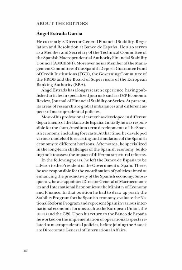
Ángel Estrada García
He currently is Director General Financial Stability, Regu-lation and Resolution at Banco de España. He also serves as a Member and Secretary of the Technical Committee of the Spanish Macroprudential Authority Financial Stability Council (AMCESFI). Moreover he is a Member of the Mana-gement Committee of the Spanish Deposit Guarantee Fund of Credit Institutions (FGD), the Governing Committee of the FROB and the Board of Supervisors of the European Banking Authority (EBA).
Ángel Estrada has a long research experience, having pub-lished articles in specialized journals such as imf Economic Review, Journal of Financial Stability or Series. At present, its areas of research are global imbalances and different as-pects of macroprudential policies.
Most of his professional career has developed in different departments of the Banco de España. Initially he was respon-sible for the short/medium-term developments of the Span-ish economy, including forecasts. At that time, he developed various models of forecasting and simulation of the Spanish economy to different horizons. Afterwards, he specialized in the long-term challenges of the Spanish economy, build-ing tools to assess the impact of different structural reforms.
In the following years, he left the Banco de España to be advisor to the President of the Government of Spain. There, he was responsible for the coordination of policies aimed at enhancing the productivity of the Spanish economy. Subse-quently, he was appointed Director General of Macroeconom-ics and International Economics at the Ministry of Economy and Finance. In that position he had to draw up yearly the Stability Program for the Spanish economy, evaluate the Na-tional Reform Program and represent Spain in various inter-national economic forums such as the European Union, the oecd and the G20. Upon his return to the Banco de España he worked on the implementation of operational aspects re-lated to macroprudential policies, before joining the Associ-ate Directorate General of International Affairs.
xiii
Ángel Estrada holds a Master degree in Monetary and Fi-nancial Economics from the Center for Monetary and Finan-cial Studies (cemfi) and a degree in Economics and Business from the Universidad Complutense de Madrid.
Iván Kataryniuk
Iván Kataryniuk is the Head of the European and Global Po-licies Unit at Banco de España. His main areas of expertise are the analysis of issues related to governance and Euro-pean construction, in order to establish the Bank's position in European and multilateral forums, as well as with the va-rious national and international institutions with which it collaborates closely on a regular basis, and the analysis and research on the main international economic policies. Pre-viously, he was a Senior Economist in the Latin American and Emerging Economies Unit, responsible of analysing the eco-nomic outlook of the main Latin American economies. He has also worked as an Advisor in the Economic Office of the Spanish President.
Iván Kataryniuk has published in several peer-reviewed journals, such as Oxford Economic Papers, Emerging Mar-kets Finance and Trade or Ensayos sobre Política Económica, in the fields of fiscal policy, emerging markets and European governance. He holds a Master degree in Monetary and Fi-nancial Economics from the Center of Monetary and Finan-cial Studies (CEMFI).
xiv
PREFACE
CEMLA’s Board of Governors created the Joint Research Program with the dual aim of promoting the exchange of knowledge among researchers from Latin American and Caribbean central banks, and of providing insights on topics that are of common interest to the region.
Previous volumes have included studies on the esti-mation and use of unobservable variables; inflationary dynamics, persistence, price and wage formation; do-mestic asset prices, global fundamentals, and financial stability; monetary policy and financial stability in Latin America and the Caribbean; international spill-overs of monetary policy; financial decisions of households and financial inclusion; and, inflation expectations, their measurement and degree of anchoring.
The present volume, entitled The Natural Interest Rate in Emerging Economies, is an important achievement in understanding the determinants of the natural interest rate in emerging economies and in providing prelimi-nary estimates for the region.
In recent years, several central banks, including many in Latin America, have shifted to a monetary policy based on targeting the level of inflation and in which the nom-inal short-term interest rate is the policy tool. The ef-fectiveness of this tool at achieving the desired target is inherently related to knowing the implicit real interest rate and its unobservable natural level.
At the same time, recent evidence on advanced econ-omies points to a secular decline in the level of their nat-ural interest rates. Thus, a proper measurement of the natural interest rate in emerging economies becomes even more relevant to understand what are the underly-ing processes that central banks face in the region, and
xv
what are the potential challenges for expansionary and contractionary monetary policies within the inflation targeting schemes.
The present volume provides evidence on that re-spect and complements the vast recent literature that has focused on advanced economies. The included pa-pers revisit a set of methodologies for estimating the natural interest rate, provide estimates for some econ-omies in the region, and discuss specific determinants of such rate affecting emerging market economies in the context of an integrated world economy. They represent the views of researchers from the central banks of Bolivia, Colombia, Costa Rica, Dominican Republic, Honduras, Jamaica, Mexico, Peru, Spain, and Uruguay.
We at CEMLA would like to thank all the authors, referees, and editors in this project. We hope that these papers contribute toward the improvement of poli-cy design in Latin American and Caribbean central banks.
1Introduction
Introduction
Ángel EstradaIván Kataryniuk
At present, most of central banks set an inflation target for monetary policy and move the relevant nominal short-term interest rate to hit that objective. The idea
is that higher (lower) nominal interest rates, in a context of price rigidity, implies higher (lower) real interest rates, and, this, through different channels, means lower (higher) aggregate demand. For a given (potential) supply, less (more) demand pressure implies a reduction (increase) in inflation. This approach implicitly assumes that we know with cer-tainty the level that the real interest rate should have when inflation is at the target and that it does not change over time. Thus, real interest rate above (below) that level will reduce (increase) the pressures on inflation. However, the reality is much more complex, as that equilibrium interest rate, or natural interest rate, is not observed and, therefore, should be estimated (thus introducing uncertainty) and, probably, it can change in line with the evolution of its structural determinants.
The economic literature provides various definitions of the natural interest rate, although all of them agree that it would be the real interest rate that would prevail in a con-text in which the main economic variables are maintained at levels that are considered desirable. In particular, Wood-ford (2003) considers that the natural interest rate would be the one that will arise in an economy in which all prices
2
and wages were perfectly flexible, thus implying that output will hit its po-tential level and inflation will be zero. On their part, Holston et al. (2016) define the natural interest rate as the one that guarantees that gdp grows at its potential rate and inflation remains constant. Likewise, Summers (2014) defines the natural interest rate, as that consistent with a situation of full employment. As a consequence, an optimal monetary policy design would be one in which the real interest rate approaches its natural level, so that variables such as gdp and employment are at their potential levels and inflation remains low and stable (Galesi et al., 2016). Thus, a real in-terest rate above the natural one is usually interpreted as an indicator of a “contractive” tone of monetary policy, while the reverse situation denotes an “expansive” monetary tone.The debate on the level of the natural interest rate has become increas-ingly popular in advanced economies, as the empirical evidence shows that it has diminished significantly, even reaching negative values. In fact, there are well-founded reasons supporting that empirical evidence. As the natural interest rate is the interest rate that equilibrates the supply and de-mand of loanable funds, any factor that shift any or both curves could imply a change in the natural interest rate. In particular, if the saving rate (the supply of funds) has increased permanently, the investment rate (demand of funds) has declined structurally, or both, the natural interest rate should have diminished. In this respect, the academics consider that structural forces like aging population or increasing uncertainty, plus other transitory but highly persistent elements such as the deleveraging process of house-holds and firms or the demand of safe assets by emerging economies, could have increased permanently the global saving rate. On its part, reduced productivity growth or the increasing relevance of the knowledge economy could have reduced permanently the global investment rate. These dis-placements of the supply and demand of funds curves would be so big that the natural interest rate could have become nil or negative.
This situation was denominated “secular stagnation” by L. Summers in a speech at the imf (Summers, 2014). When, in a context of low infla-tion, the natural interest rate is negative, conventional monetary policy would have serious difficulties to be effective, since there is a lower limit to the level that the nominal interest rate set by the central bank can reach. That limit would be zero or a slightly negative number, as households and firms have always the possibility of maintaining their liquid assets in form of cash, whose nominal yield is zero. If the lowest nominal interest rate is (slightly below) zero and inflation is very reduced, the minimum real
3Introduction
market interest rate that could be reached could be higher than the equi-librium one and the economy could enter a persistent situation of insuffi-cient demand and excessive unemployment.
The monetary policy has different options to face this situation. The first is to reduce the interest rates not only in the short term, as conventional monetary policy does, but also in the medium and long run, that probably are the horizons more relevant for the agents deciding on their savings and investments. One way of doing this is that the central bank commits with the agents to maintain in the future the very low interest rates actually observed (forward guidance). If the central bank is credible, this should re-duce the term premia of the interest rates. A second possibility is to imple-ment programmes of Quantitative Easing (qe). This non-conventional monetary policy action implies that the central bank buys in the second-ary markets public or private debt with medium and long-term maturities. As the agents selling those assets have to replace them in their portfoli-os, total demand increases and therefore their prices, thus reducing their yields and those of the closest assets, by cutting the risk premia. Notice that contrary to forward guidance, the effectiveness of that kind of pro-grammes does not depend on the credibility of the central bank. However, both alternatives could be implemented at the same time, as they reinforce each other. If the central bank does not comply with the forward guidance and its balance sheet is plenty of medium and long term debt, it is going to be the first in suffering the losses.
As it always happens in economy, the unconventional monetary policy is not free of charge. There is theoretical and empirical evidence showing that during periods of compress term and risk premia, the financial market participants accumulate more risks (Martínez-Miera and Repullo, 2018). Besides, it is well known that very reduced short and long-term interest rates for long periods of time damage the profitability of insurance com-panies and pension funds. More recently, a new concept of interest rate has been coined, the reverse rate (Brunnermeier and Koby, 2018), to cap-ture the negative nominal interest rate below which additional reductions damage bank profitability and solvency, thus impairing the transmission of monetary policy to the real economy. Therefore, it seems there is a limit to what monetary policy can do to face a secular stagnation problem and, in any case, the macroprudential policy should be ready to act in case that the accumulation of risks threatens the financial stability, thus aggravat-ing the problem of weakness in the real demand.
4
Since the global financial crisis, an increasing number of central banks have implemented measures that can be classified as unconventional mon-etary policy, but academics have proposed other possibilities. A possibility is increasing the inflation target of the central bank. This, mechanically, will reduce the real interest rate for a given nominal interest rate, thus al-lowing the central bank to hit more negative nature interest rates. The main problem with this approach is the credibility of the central bank. In most of the advanced economies is been proved very difficult to hit the current target, so achieving a higher one should be even more difficult. For these reasons, some analysts consider that other policies should also contribute to solve the problem. The first possibility is fiscal policy, thus using the pub-lic demand to complement the lack of private demand. In particular, public investment seems to be the most appropriate item to impulse, as, besides, by developing the infrastructures of a country, the private sector produc-tivity can be enhanced thus attracting private investment. The major prob-lem with this recommendation is that, currently, public debt shows a very high level and only the countries with fiscal space can implement fiscal expansions without putting at risk their fiscal sustainability. Other possi-bility is introducing structural reforms in the economy to reduce the age-ing problem and to increase potential growth of the economy. In this case, it should be taken into account that usually it takes time for these reforms to have relevant impacts in the economy.
Nowadays, it is difficult to think that emerging markets are facing a sim-ilar problem than most of the advanced economies. Population of emerg-ing countries is still relatively young and in most of the cases is growing at higher comparative rates. At the same time, their productivity level is well below that of the advanced economies, so only by converging in in-stitutions and technology to the advanced economies they can generate higher increases in total factor productivity (tfp). Furthermore, they will need to increase their capitalization rate, implying higher investment rates. Those factors will guarantee in the short to medium run a potential growth rate much higher than that of the advanced economies, and this is a crucial factor to guarantee that the natural interest rate stays in sig-nificant positive values.
However, nothing guarantees that the natural interest rate has re-mained stable and has not followed a downward path similar to that of the advanced economies. In fact, there are very good reasons to think this is the case. On the real side, the population dividend is diminishing rap-idly in the biggest emerging economies and there is evidence that tfp is
5Introduction
also decelerating. On the financial side, the last few decades can be char-acterized by a deep integration of the countries. Most of the barriers to free capital movements have been lifted, especially in the case of the emerging markets, and this has resulted in a surge in international capital flows, with the stock of foreign financial assets hold by all the countries reaching historical highs. Even taking into account that the global financial crisis slowed down that process, it is reasonable to think that natural interest rates is determined at a global level as the equilibrium outcome of global desired saving and desired investment. Obviously, in that configuration, the countries that are financial centers and are able to issue global safe assets would play a central role in the determination of financial prices. From that perspective, the evolution of the natural interest rates of emerg-ing economies can be rationalized as the sum of the natural interest rates of advanced economies plus the country-specific differential potential growth and risk profile.
Therefore, the adequate measurement of the equilibrium interest rate continues to be very relevant for emerging countries, since, depending on that, the tone of the monetary policy could change drastically for the same level of the nominal interest rates. This is the particular case of Lat-in-American economies, where some central banks have conjectured that the natural interest rate could have fallen significantly.
Based on these reflections, the research lines addressed in this book were classified in three major groups:
1. Methodologies for estimating the natural interest rate
The estimation of the natural interest rate, like any other unobservable variable, is subject to uncertainty and requires assumptions about the re-lationship between it and other observable variables. In addition, in the case of open economies such as most emerging markets, the natural inter-est rate will be influenced by the uncovered parity of interest rates, and, therefore, will be subject to variations in the perception of risk and the ex-change rate. Besides, different models can be used in the estimation pro-cess, ranging from univariate time series filters where the trend is identified with the natural interest rate, to general equilibrium models, based on the economic relations typical of the neo-Keynesian economy (Del Negro et al., 2015), plus semi-structural models (i.e. structural autoregressive vectors, svar), the possibilities are multiple.
In fact, the papers included in this section are well aware of the high un-certainty regarding the estimates of the natural interest rate, and then they
6
calculate and compare the estimates using different empirical approach-es. It consists of five papers studying two Caribbean economies ( Jamaica and Dominican Republic), two Central American economies (Costa Rica and Honduras) and a South American economy (Bolivia).
In Assessing the Usefulness of the Neutral Rate of Interest to Monetary Policy in Jamaica, Alexander Lee and Carey-Anne Williams present esti-mates of the natural interest rate in their country by means of four different techniques: a regression based on an interest rate parity condition, a var with time-varying parameters, a dsge model calibrated to the Jamaican economy and a statistical filter. They assess the validity of the estimates for inflation forecasting. All the estimates point to a decrease of the natu-ral rate in the last ten years, as a result of the decline of the foreign inter-est rate and the structural changes of the economy, leading to a decrease in the country risk premium. The estimates point to an accommodative monetary policy under current conditions, and a real natural interest rate in the range of -2.6 and 2.6.
Evelyn Muñoz Salas and Adolfo Rodríguez Vargas estimate the real neutral interest rate in Costa Rica using six different methodologies. The econometric analysis includes vars, the Laubach and Williams (2003) semi-structural model (henceforth LW) and modified Taylor rules. They select the estimates of the real policy rate gap that perform better in terms of a negative lead correlation with the output gap and core inflation, with the double objective of calculating the current value for the natural inter-est rate, which is around 1.5%, and to perform an assessment of the mon-etary policy stance in Costa Rica during the years 2009-2018.
In the same vein, the contribution of the Central Bank of Honduras, presented by Fredy Fernando Álvarez, uses several statistical methodolo-gies to calculate the current real natural interest rate in Honduras. Inter-estingly, the results corresponding to the dynamic methodologies, such as statistical filters or the LW methodology, show an increase in the natu-ral interest rate in the economy, as opposed to the general tendency pre-sented in the rest of the papers.
Somewhat differently, the fourth chapter, written by José Manuel Mi-chel of the Central Bank of the Dominican Republic, calculates the natu-ral interest rate using an interest rate parity condition and error correction models. He finds a decreasing trend in the natural interest rate in the Do-minican Republic, consistent with the high impact of external interest rates in the economy.
7Introduction
Finally, in the case of Bolivia, Paul Estrada Céspedes and David Ze-ballos Coria present estimates of the natural interest rate in Bolivia us-ing the LW methodology. Interestingly, in Bolivia there is not a reference interest rate, and it has to be derived from the different monetary policy operations of the Central Bank. They find that monetary policy has been, in general, very accommodative in the last few years, which is consistent with a positive and large output gap.
2. The determinants of the natural interest rate in emerging economies
As we pointed before, there is a wide literature on the determinants of the recent drop in the natural interest rate in advanced economies, both from the perspective of excess savings (for demographic, redistributive or global savings glut) as well as the shortage of investment (due, for example, to less innovation or a lower impact on the productivity of existing innovations). However, there are less references on the evolution of the natural inter-est rate in emerging economies. This section tries to fulfil this vacuum.
In particular, the studies included here both calculate the natural inter-est rate in the respective economies –Mexico, Peru and Uruguay– and also provide information about the main determinants. By focusing on long run factors, it is concluded that productivity growth, demography and ex-ternal developments are the main factors governing the evolution of the natural interest rates.
In the first chapter of this section, Carrillo et al. perform an analysis of the long run interest rate in Mexico. The long run interest rate is calcu-lated using several methodologies, including a neoclassical growth mod-el, an augmented Taylor rule –including the shadow interest rate in the us–, and an affine term structure model. All the estimates are consistent with a natural rate of interest around 2.5%, somewhat lower than in the previous decades. Behind this evolution, the authors make a heuristic in-vestigation, pointing to a higher supply of loanable funds resulting from more national and foreign savings, population and productivity dynamics.
In the second chapter, Luis E. Castillo and David Florian Hoyle use a multivariate filter on the Central Bank projection model to jointly derive the output gap, potential growth and the natural interest rate. They find a relatively stable natural interest rate, at around 1.3%, since the financial crisis, when it fell from previous higher levels. Potential growth has been declining in the last few years. In order to explain their results, they turn
8
to a reduction in tfp growth, partially explained by a persistent decline in terms of trade and the lack of structural reforms.
Finally, in the case of Uruguay, Elizabeth Bucacos provides different estimates of the natural rate of interest. The main contributions are cen-tered on studying different regimes of monetary policy –first targeting an interest rate, then targeting money aggregates– and distinguishing between short and long term. By defining the long term natural rate as the prevalent interest rate when all the relevant gaps are closed, she calcu-lates a long term natural rate of around 2.5%. Moreover, by estimating a fundamental-based model, the study concludes that aging, productivity growth, sovereign country risk and public indebtedness are all important determinants of the natural interest rate.
3. The international dimension of natural interest rates
The last section is devoted to cross-country analysis. As can be seen in the previous sections, emerging economies, in general, share a common trend in interest rates. This can be confirmed by estimating a common model across countries, as the first paper in this section does, and the global factor can be estimated using this cross-country variation, as it is carried out in the last paper in the book.
In the first paper, Javier G. Gómez-Pineda complements the LW meth-odology with some additional features, such as an Okun Law, a smoothing parameter for the interest rate gap, an interest rate parity condition and a framework for inflation expectations. He performs this analysis for five Latin American economies –Chile, Peru, Brazil, Mexico and Colombia. The findings point to a drop in the real natural interest rate in Brazil, Mex-ico and Colombia, and stability in low levels for Peru and Chile.
In the second paper, Estrada et al. calculate the common factor of interest rates in a sample of 16 emerging economies, using the Bai-Ng (2004) meth-odology, in order to find the global component in interest rates of emerging economies. They compare their estimate with a global factor stemming from advanced economies, and provide evidence supporting that both fac-tors share a common trend. As a conclusion, they state that the declining evolution of interest rates in emerging economies can be accounted by the pass-through of low rates in advanced economies.
9Introduction
References
Bai J. and S. Ng (2004): “A panic attack on unit roots and cointegra-tion” Econometrica, Nº 72(4), pp. 1127-1177.
Brunnermeier, Markus K. and Y. Koby (2018). “The reversal interest rate”. National Bureau of Economic Research, 2018.
Del Negro, M., M. P. Giannoni, and F. Schorfheide (2015). “Inf lation in the great recession and new Keynesian models”, American Economic Journal: Macroeconomics, 7, pp. 168196.
Galesi, A., G. Nuño and C. Thomas (2017). “The natural interest rate: concept, determinants and implications for monetary policy”, Economic Bulletin, no. 1/2017, Banco de España.
Holston, K., T. Laubach and J. C. Williams (2016). “Measuring the natural rate of interest: International trends and determinants”, Journal of International Economics.
Laubach, T. and J.c. Williams (2003). “Measuring the natural rate of interest”, Review of Economics and Statistics, 85, pp. 1063-1070.
Martinez-Miera, D. and R. Repullo (2019). “Monetary Policy, Mac-roprudential Policy, and Financial Stability”. CEPR Discussion Papers No. 13530.
Summers, L. H. (2014). “US economic prospects: Secular stagnation, hysteresis, and the zero lower bound”, Business Economics, 49, pp. 65-73.

Country Studies: Measurement of the
Natural Interest Rate
11Neutral Rate of Interest and Monetary Policy in Jamaica
Assessing the Usefulness of the Neutral Rate of Interest to Monetary Policy in Jamaica
Alexander LeeCarey-Anne Williams
Abstract
Since the early 1990’s, the transmission mechanism of monetary policy in Ja-maica has been extensively researched. Most of this research focused on the speed and the effectiveness of the transmission. This paper extends the exist-ing research by focusing on estimating and assessing the usefulness of the neutral rate of interest to the conduct of monetary policy. While the concept of the neutral rate is well-grounded in theory, as an unobservable variable, there are several proposed methods of estimation. In this paper, we estimate the neutral rate for Jamaica using four methods commonly found in the litera-ture. Based on these methodologies, the real neutral rate is estimated to range between -2.6% to 2.6%, or 2.4% to 7.6% in nominal terms. This implies that the Bank of Jamaica’s current monetary policy stance has been fairly ac-commodative given recent sub-optimal trends in inflation and growth.
Keywords: Monetary Transmission Mechanism, Neutral Interest Ratejel Classification: E52, E58, E43, C10.
1. INTRODUCTION
The Bank of Jamaica, the monetary authority in Jamaica, re-duced its policy rate consistently between the latter half of 2009 and 2018. Importantly, real ex-ante short term interest rates
in Jamaica became negative after December 2017. Notwithstanding this, the output gap for Jamaica remained negative over the period which contributed to inflation remaining below the Central Bank’s inflation target. This implies that the stance of monetary policy may have been less accommodative than required to encourage
12 A. Lee, C. Williams
a closure of the output gap and the achievement of the Bank’s infla-tion target.
The monetary policy transmission mechanism in Jamaica has been extensively researched. Most of the research focused on the speed of the transmission (e.g. Allen and Robinson 2004, Robinson and Wil-liams 2016) as well as its effectiveness (e.g. Dacass, McKenzie and Mur-ray 2015). This paper adds to the literature by estimating the neutral interest rate, which represents a benchmark to assess the stance of monetary policy.
We estimate the neutral rate using four popular methods, name-ly, a reduced form ordinary least squares (ols) regression, a time varying vector auto regression (tvp-var), an applied dynamic sto-chastic general equilibrium (dsge) model and the Hodrick-Prescott (hp) filter. These estimates are presented to show the recent trends in – and the level of – the real interest rate gap for Jamaica. We also assess the statistical properties of the estimates using correlations of the estimated gaps with inflation and output and an assessment of their leading indicator properties.
Consistent with a priori expectations, Jamaica’s neutral interest rate appears to be time varying and has declined, particularly over the last five years, due to structural changes in the economy. While there is a high degree of uncertainty with regard to the determination of the neutral rate, our findings further imply that the central bank’s policy rate at the end of 2018 was accommodative. Based on these methodologies, the point estimate for the real neutral rate is estimat-ed to range between -2.6% to 2.6%, or 2.4% to 7.6% in nominal terms as at September 2018. The estimate of the neutral rate derived from the tvp-var was found to display the best leading indicator proper-ties with regard to inflation while the ols was the least successful.
The remainder of the paper proceeds as follows. Section 2 outlines the main determinants of the neutral rate, particularly for small open economies. In section 3, we estimate the neutral rate for Jamaica using four methods commonly found in the literature. Section 4 provides an assessment of the statistical properties of the estimated real inter-est rate gaps (defined as the difference between the actual and neu-tral rate based on each methodology). Finally, Section 5 concludes.
13Neutral Rate of Interest and Monetary Policy in Jamaica
2. DETERMINANTS OF THE NEUTRAL RATE
While there are many definitions of the neutral rate, this paper focus-es on the definition made popular by Laubach and Williams (2003). The neutral rate is therefore the prevailing real interest rate at which the output gap is closed and inflation is stable. When market inter-est rates are consistent with their neutral level, then the economy is on a sustainable path, where the deviations away from this point of neutrality induces business cycles in an economy.1
The literature makes a distinction between a ‘contemporaneous’ and ‘medium-to-long-run’ neutral interest rate. The contempora-neous neutral rate is the rate of interest that ensures a zero output gap and stable prices in every period (Mendes (2014)). In this re-gard, the short-run or contemporaneous interest rate can be im-pacted by shocks as well as changes in potential output. It is usually estimated in ‘real-time’ using time series methodologies and there-fore reflects the level of interest rate that is required based on cur-rent economic conditions. The long-run neutral rate, on the other hand, is consistent with output at its potential level after business cycle shocks have dissipated.
The long run neutral rate can evolve based on structural chang-es in the economy. Generally, a decline (increase) in the neutral rate is caused by an outward (inward) shift in the economy’s savings supply curve or an inward (outward) shift in the demand for sav-ings (April 2014 World Economic Outlook). Changes in monetary and fiscal policy as well as private and public saving preferences re-sult in shifts in supply curve for savings. The latter includes changes in population growth and the age demographics of the population. As the population ages, the neutral rate has been found to decline. The demand curve for savings, on the other hand, shifts as a result of changes in expected investment profitability, productivity and the relative price of investment goods.
In small open economies, where capital can move freely across borders, domestic financing conditions are impacted not only by do-mestic savings but also the supply of net foreign savings through the balance of payments channel. Shifts in global savings and the re-sulting impact on the global neutral interest rate therefore impacts
1 In addition, the neutral rate can be viewed as one of the guides for the path of monetary policy over the long term.
14 A. Lee, C. Williams
the domestic neutral rate. Importantly the domestic neutral rate may differ from the global neutral rate in the long run due to the level of the country’s endogenous risk premium. If there is a trend increase in productivity growth for a country relative to its trading partners, the domestic neutral interest rate will rise as there will be a higher expected return on investments. Depending on foreign inves-tors’ risk appetite, the higher returns should: (1) incentivize capital inflows; (2) cause an appreciation of the exchange rate; (3) reduce the country’s level of competitiveness; and (4) place downward pres-sure on investment returns (counteracting the upward pressure to the neutral rate). Therefore, the overall net impact on the neutral rate should be a smaller increase relative to a closed economy framework.
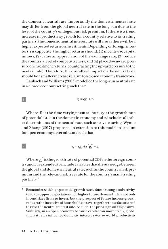
Laubach and Williams (2003) modelled the long–run neutral rate in a closed economy setting such that:
1 r cg zt t t= +
Where r cg zt t t= + is the time varying neutral rate, gt is the growth rate of potential gdp in the domestic economy and zt includes all oth-er determinants of the neutral rate, such as private saving. Wynne and Zhang (2017) proposed an extension to this model to account for open economy determinants such that:
2 r cg c g zt t t t= + +* *
Where gt* is the growth rate of potential gdp in the foreign coun-
try and zt is extended to include variables that drive a wedge between the global and domestic neutral rate, such as the country’s risk pre-mium and the relevant risk free rate for the country’s main trading partners.2
2 Economies with high potential growth rates, due to strong productivity, tend to support expectations for higher future demand. This not only incentivizes firms to invest, but the prospect of future income growth reduces the incentive of households to save, together these factors tend to raise the neutral interest rate. As such, the prior sign on c is positive. Similarly, in an open economy because capital can move freely, global interest rates influence domestic interest rates so world productivity
15Neutral Rate of Interest and Monetary Policy in Jamaica
There is a much uncertainty in the literature around the estimates for the neutral rate and most studies cite wide ranges for the neutral rate to capture this uncertainty. Among the recent literature on es-timating the neutral rate in a small economy or emerging market context are Dacass (2011), Baksa et al. (2013), Kreptsev et al. (2016), and Grui et al. (2018). Dacass (2011) estimated the neutral rate for Ja-maica using the methodology proposed by Laubach and Williams (2003). The author found that Jamaica’s neutral rate had declined since the 1990’s and that short term market interest rates were below the neutral rate between 2010 and 2011. Baksa et al. (2013), who esti-mated the neutral interest rate for Hungary, noted that the real un-covered interest parity condition as well as the Kalman filter could be considered as suitable techniques in cases where the neutral rate is viewed to be time varying. In particular, using the Kalman filter, the authors found that the real neutral rate for Hungary had de-clined to a range of 1.5% to 3.5% in 2012 from approximately 3.0% to 4.5% prior to 2003.
Kreptsev et al. (2016) developed a real business cycle general equi-librium model of the Russian economy to estimate both the contem-poraneous (or short run) and long run neutral rate. Similar to Baksa et al (2013), the authors’ indicated a high degree of uncertainty with regard to their estimates of the neutral rate. The contemporaneous neutral rate for Russia, based on semi structural methods, was es-timated to range between -9.5% and 10.5% with a point estimate of 0.5%. For the long run equilibrium, the point estimates ranged between 1.0% and 3.0%. Grui et al (2018) estimated the neutral rate for Ukraine using an open economy forward-looking New-Keynes-ian Quarterly Projection Model. The authors found that there was a trend reduction in the neutral rate since 2015 due largely to a fall in the global neutral rate.3
growth will also impact the domestic neutral rate, hence the prior sign on c* is also positive.
3 The smoothed estimates of the natural rate of interest in u.s. deter-mined by the Laubach-Williams (2003) methodology was used as a proxy for the global neutral rate.
16 A. Lee, C. Williams
3. ESTIMATING THE NEUTRAL INTEREST RATE FOR JAMAICA
Given the absence of a consensus on the appropriate method of esti-mating the neutral rate and the sensitivity of estimates to model spec-ification, we estimate the neutral rate using four methods, namely, a reduced form ordinary least squares (ols) regression, a time varying vector auto regression (tvp-var), an applied dynamic stochastic gen-eral equilibrium (dsge) model and the Hodrick-Prescott (hp) filter.
3.1 Reduced Form ols
Following Mendes (2014), we employ a reduced form modeling ap-proach that assumes that foreign and domestic factors impact the neu-tral rate for Jamaica. In a small open economy such as Jamaica, savings does not need to be equal to investments (from domestic sources), as the shortfall is financed by inflows of foreign capital. The domes-tic neutral rate may still differ from the global neutral rate, however, due to the risk premium.
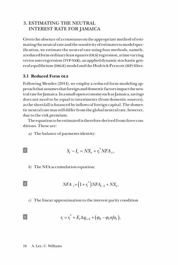
The equation to be estimated is therefore derived from three con-ditions. These are:
a) The balance of payments identity:
3 S I NX r NFAt t t t t− = + * ,
b) The NFA accumulation equation:
4 NFA r NFA NXt t t t= +( ) +−1 1* ,
c) The linear approximation to the interest parity condition
5 r r E q nfat t t t t= + + −( )+* ,∆ 1 0 1ϕ ϕ
17Neutral Rate of Interest and Monetary Policy in Jamaica
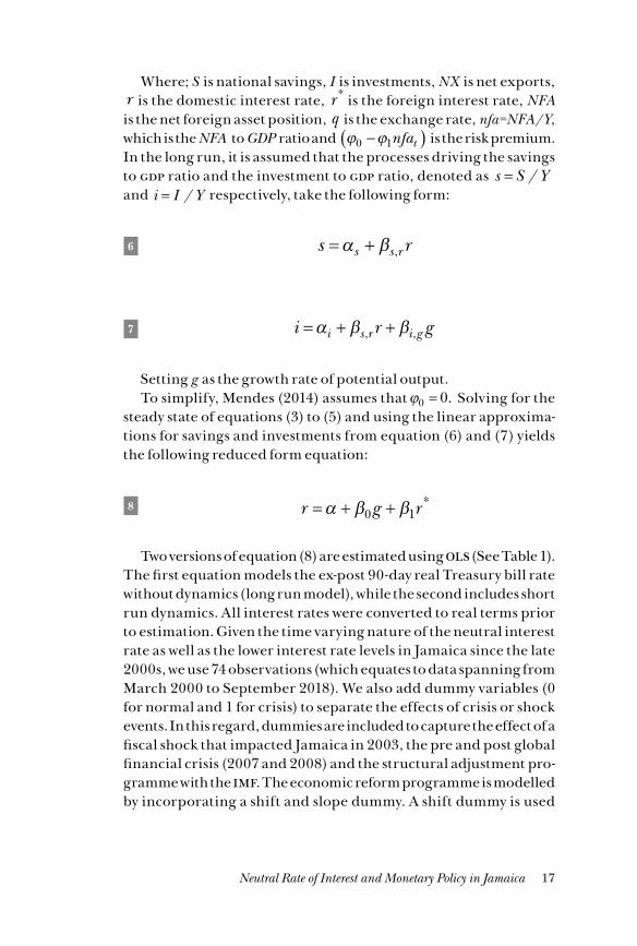
Where; S is national savings, I is investments, NX is net exports, r is the domestic interest rate, r * is the foreign interest rate, NFA is the net foreign asset position, q is the exchange rate, nfa=NFA/Y, which is the NFA to GDP ratio and ϕ ϕ0 1−( )nfat is the risk premium. In the long run, it is assumed that the processes driving the savings to gdp ratio and the investment to gdp ratio, denoted as s S Y= / and i I Y= / respectively, take the following form:
6 s rs s r= +α β ,
7 i r gi s r i g= + +α β β, ,
Setting g as the growth rate of potential output.To simplify, Mendes (2014) assumes thatϕ0 0= . Solving for the
steady state of equations (3) to (5) and using the linear approxima-tions for savings and investments from equation (6) and (7) yields the following reduced form equation:
8 r g r= + +α β β0 1*
Two versions of equation (8) are estimated using ols (See Table 1). The first equation models the ex-post 90-day real Treasury bill rate without dynamics (long run model), while the second includes short run dynamics. All interest rates were converted to real terms prior to estimation. Given the time varying nature of the neutral interest rate as well as the lower interest rate levels in Jamaica since the late 2000s, we use 74 observations (which equates to data spanning from March 2000 to September 2018). We also add dummy variables (0 for normal and 1 for crisis) to separate the effects of crisis or shock events. In this regard, dummies are included to capture the effect of a fiscal shock that impacted Jamaica in 2003, the pre and post global financial crisis (2007 and 2008) and the structural adjustment pro-gramme with the imf. The economic reform programme is modelled by incorporating a shift and slope dummy. A shift dummy is used
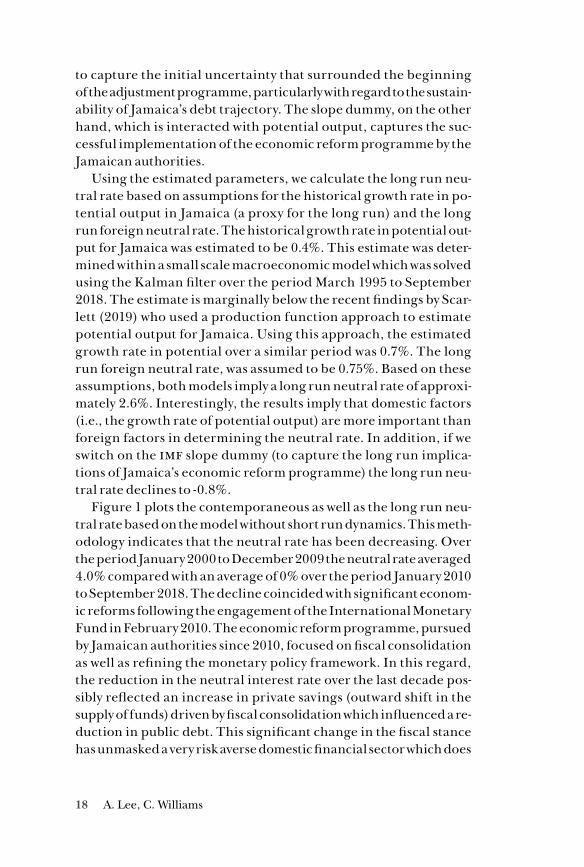
18 A. Lee, C. Williams
to capture the initial uncertainty that surrounded the beginning of the adjustment programme, particularly with regard to the sustain-ability of Jamaica’s debt trajectory. The slope dummy, on the other hand, which is interacted with potential output, captures the suc-cessful implementation of the economic reform programme by the Jamaican authorities.
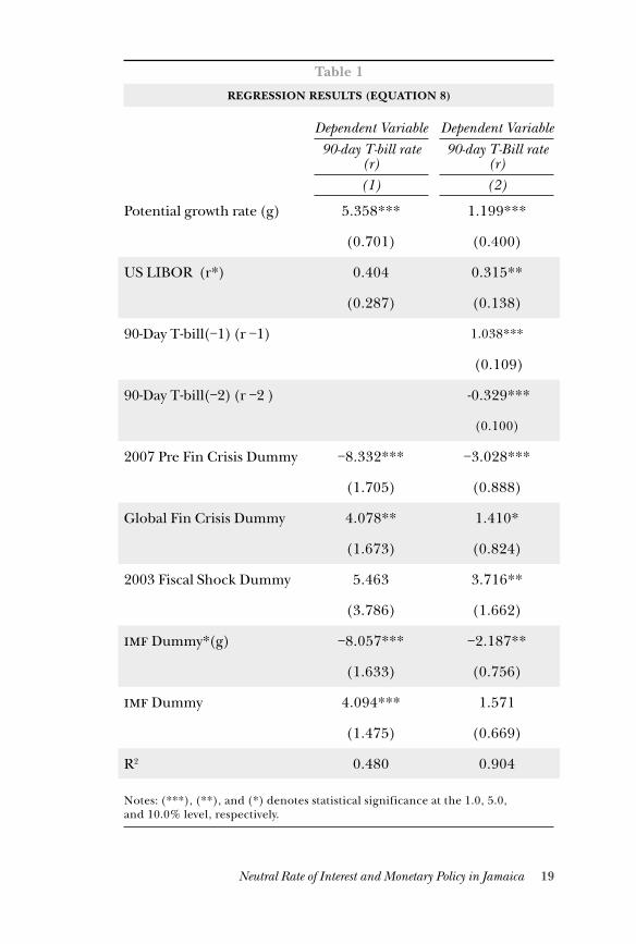
Using the estimated parameters, we calculate the long run neu-tral rate based on assumptions for the historical growth rate in po-tential output in Jamaica (a proxy for the long run) and the long run foreign neutral rate. The historical growth rate in potential out-put for Jamaica was estimated to be 0.4%. This estimate was deter-mined within a small scale macroeconomic model which was solved using the Kalman filter over the period March 1995 to September 2018. The estimate is marginally below the recent findings by Scar-lett (2019) who used a production function approach to estimate potential output for Jamaica. Using this approach, the estimated growth rate in potential over a similar period was 0.7%. The long run foreign neutral rate, was assumed to be 0.75%. Based on these assumptions, both models imply a long run neutral rate of approxi-mately 2.6%. Interestingly, the results imply that domestic factors (i.e., the growth rate of potential output) are more important than foreign factors in determining the neutral rate. In addition, if we switch on the imf slope dummy (to capture the long run implica-tions of Jamaica’s economic reform programme) the long run neu-tral rate declines to -0.8%.
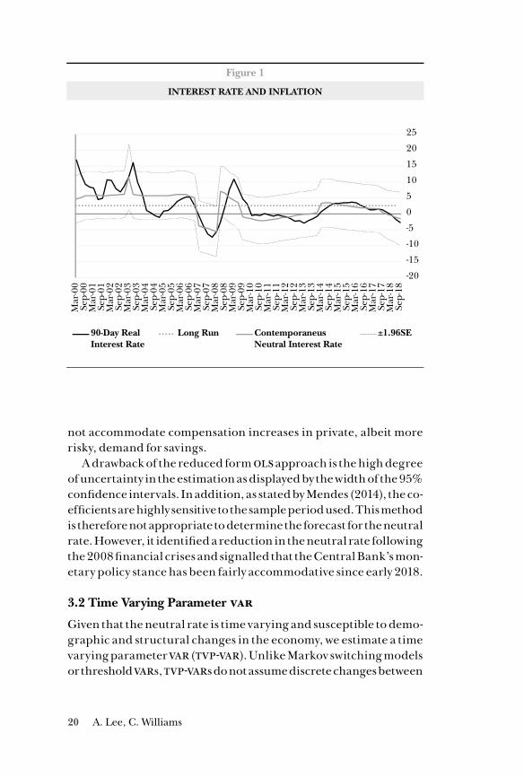
Figure 1 plots the contemporaneous as well as the long run neu-tral rate based on the model without short run dynamics. This meth-odology indicates that the neutral rate has been decreasing. Over the period January 2000 to December 2009 the neutral rate averaged 4.0% compared with an average of 0% over the period January 2010 to September 2018. The decline coincided with significant econom-ic reforms following the engagement of the International Monetary Fund in February 2010. The economic reform programme, pursued by Jamaican authorities since 2010, focused on fiscal consolidation as well as refining the monetary policy framework. In this regard, the reduction in the neutral interest rate over the last decade pos-sibly reflected an increase in private savings (outward shift in the supply of funds) driven by fiscal consolidation which influenced a re-duction in public debt. This significant change in the fiscal stance has unmasked a very risk averse domestic financial sector which does
19Neutral Rate of Interest and Monetary Policy in Jamaica
Table 1
REGRESSION RESULTS (EQUATION 8)
Dependent Variable Dependent Variable90-day T-bill rate
(r)90-day T-Bill rate
(r)(1) (2)
Potential growth rate (g) 5.358*** 1.199***
(0.701) (0.400)
US LIBOR (r*) 0.404 0.315**
(0.287) (0.138)
90-Day T-bill(−1) (r −1) 1.038***
(0.109)
90-Day T-bill(−2) (r −2 ) -0.329***
(0.100)
2007 Pre Fin Crisis Dummy −8.332*** −3.028***
(1.705) (0.888)
Global Fin Crisis Dummy 4.078** 1.410*
(1.673) (0.824)
2003 Fiscal Shock Dummy 5.463 3.716**
(3.786) (1.662)
imf Dummy*(g) −8.057*** −2.187**
(1.633) (0.756)
imf Dummy 4.094*** 1.571
(1.475) (0.669)
R2 0.480 0.904
Notes: (***), (**), and (*) denotes statistical significance at the 1.0, 5.0, and 10.0% level, respectively.
20 A. Lee, C. Williams
not accommodate compensation increases in private, albeit more risky, demand for savings.
A drawback of the reduced form ols approach is the high degree of uncertainty in the estimation as displayed by the width of the 95% confidence intervals. In addition, as stated by Mendes (2014), the co-efficients are highly sensitive to the sample period used. This method is therefore not appropriate to determine the forecast for the neutral rate. However, it identified a reduction in the neutral rate following the 2008 financial crises and signalled that the Central Bank’s mon-etary policy stance has been fairly accommodative since early 2018.
3.2 Time Varying Parameter var
Given that the neutral rate is time varying and susceptible to demo-graphic and structural changes in the economy, we estimate a time varying parameter var (tvp-var). Unlike Markov switching models or threshold vars, tvp-vars do not assume discrete changes between
Figure 1
INTEREST RATE AND INFLATION
-20
-15
-10
-5
0
5
10
15
20
25
Mar
-00
Sep-
00M
ar-0
1Se
p-01
Mar
-02
Sep-
02M
ar-0
3Se
p-03
Mar
-04
Sep-
04M
ar-0
5Se
p-05
Mar
-06
Sep-
06M
ar-0
7Se
p-07
Mar
-08
Sep-
08M
ar-0
9Se
p-09
Mar
-10
Sep-
10M
ar-1
1Se
p-11
Mar
-12
Sep-
12M
ar-1
3Se
p-13
Mar
-14
Sep-
14M
ar-1
5Se
p-15
Mar
-16
Sep-
16M
ar-1
7Se
p-17
Mar
-18
Sep-
18
90-Day RealInterest Rate
Long Run ContemporaneusNeutral Interest Rate
±1.96SE
21Neutral Rate of Interest and Monetary Policy in Jamaica
states. In particular, tvp-vars are well suited for cases where a priori information suggests that there is non-linear behaviour in the data (Lubik and Matthes (2015)). This flexible framework avoids the re-strictions imposed in structural models and allows for variation in model parameters (i.e., lag coefficients and the variances of the economic shocks) smoothly over time. However, the main drawback of this model, is that it is computationally demanding. The poste-rior simulation algorithm requires thousands of draws to ensure proper convergence.
To determine the neutral rate for the u.s., Lubik and Matthes (2015) estimated a three (3) variable tvp-var using real gdp growth (τt ), inflation (πt) and the real interest rate (rt ). We estimate a simi-lar tvp-var with forgetting factors as proposed by Koop and Koro-bilis (2012). The model is estimated using quarterly data for the real interest rate, real gdp growth and inflation for Jamaica over the pe-riod March 2000 to September 2018.
The state space representation of the model is:
9 Y Xt t t t= +θ ε
10 θ θ µt t t= +−1
Where, εt is i.i.d. N Vt0,( ) and µt is i.i.d. N Qt0, .( ) εt and µt are in-dependent of each other for all s and t.
Additionally:
11 X I Y Yt t t p= ∗( )− −1,...,
12 Vt t t= ′− −ε ε1 1
22 A. Lee, C. Williams
13 Q St t It= −( ) − −1 11 1λ
Where Yt is a vector of variables: rt t t, , ,τ π λ is the forgetting factor, which implies that observations j periods in the past have a weight of λ j in the filtered estimate of θt . The constant coefficient case can be estimated by setting λ =1, while λ = 0 99. implies that ob-servations five years ago receive approximately 80% as much weight as last period’s observations (See Koop and Korobilis (2012) for dis-cussion of forgetting factor approach). We set λ = 0 99. .
With regard to the priors, we assume that θ0 follows the typical Minnesota prior. All our data has been transformed to ensure sta-tionarity, hence we set the prior mean to be E θ0 0( ) = . Assuming a di-agonal Minnesota prior covariance matrix, then Var θ η0( ) = and ηi denotes the elements along the diagonal such that:
14 ηγ
αi t
t t p2 1, ,..., for coefficients on lag for
fo
=
rr constants
With regard to the hyperparameters, we set α =102, which is un-informative. For γ , which controls the degree of shrinkage in the var coefficients, we test the model’s sensitivity to alternative speci-fications. In this regard, we impose:
15 γ = − −[ ]e e10 5 0 001 0 005 0 01 0 05 0 01, , . , . , . , . , .
The neutral rate for Jamaica is determined using the conditional forecast generated by the tvp-var for the observed real rate. The fore-cast horizon is set at two years ahead and it is computed for each data point since 2010. This differs from Lubik and Matthes (2015) who proposed a conditional forecast 5-years ahead. That period was chosen to reflect the typical length of the u.s. business cycle. Ac-cording to Murray (2007), Jamaica’s business cycle typically ranges between two to four years.
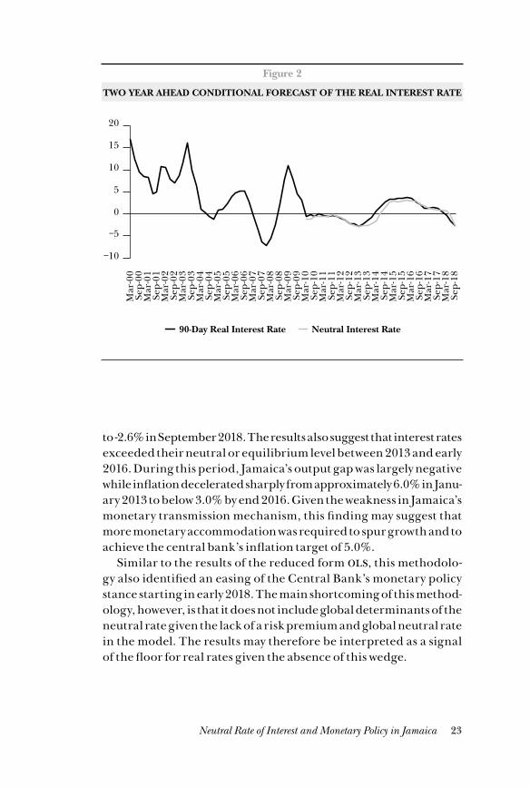
Figure 2 plots the neutral rate, based on the two year ahead con-ditional forecast of the real interest rate from March 2010, and the actual real rate. Consistent with expectations, this methodology im-plies that the neutral rate has declined from 3.0% in December 2015
23Neutral Rate of Interest and Monetary Policy in Jamaica
to -2.6% in September 2018. The results also suggest that interest rates exceeded their neutral or equilibrium level between 2013 and early 2016. During this period, Jamaica’s output gap was largely negative while inflation decelerated sharply from approximately 6.0% in Janu-ary 2013 to below 3.0% by end 2016. Given the weakness in Jamaica’s monetary transmission mechanism, this finding may suggest that more monetary accommodation was required to spur growth and to achieve the central bank’s inflation target of 5.0%.
Similar to the results of the reduced form ols, this methodolo-gy also identified an easing of the Central Bank’s monetary policy stance starting in early 2018. The main shortcoming of this method-ology, however, is that it does not include global determinants of the neutral rate given the lack of a risk premium and global neutral rate in the model. The results may therefore be interpreted as a signal of the floor for real rates given the absence of this wedge.
Figure 2
TWO YEAR AHEAD CONDITIONAL FORECAST OF THE REAL INTEREST RATE
90-Day Real Interest Rate Neutral Interest Rate
Mar
-00
Sep-
00M
ar-0
1Se
p-01
Mar
-02
Sep-
02M
ar-0
3Se
p-03
Mar
-04
Sep-
04M
ar-0
5Se
p-05
Mar
-06
Sep-
06M
ar-0
7Se
p-07
Mar
-08
Sep-
08M
ar-0
9Se
p-09
Mar
-10
Sep-
10M
ar-1
1Se
p-11
Mar
-12
Sep-
12M
ar-1
3Se
p-13
Mar
-14
Sep-
14M
ar-1
5Se
p-15
Mar
-16
Sep-
16M
ar-1
7Se
p-17
Mar
-18
Sep-
18
−10
−5
0
5
10
15
20
24 A. Lee, C. Williams
3.3 Applied dsge – Quarterly Projection Model
An estimate of the neutral rate is determined using an applied dsge model - the Bank of Jamaica ‘Quarterly Projection Model – qpm.’ This is a semi-structural, small-scale, forward-looking, open economy gap model with rational expectations. The output gap is dependent on real monetary conditions (a weighted average of the real interest rate gap and the real exchange rate gap) and the inflation rate is de-pendent on the output gap (the traditional Philips curve). In addi-tion, monetary policy is endogenously determined. Whilst the qpm is still in its development stages, it is calibrated to reflect the main stylised facts of the Jamaican economy and used to explain the core macroeconomic dynamics in Jamaica. Underlying the main theo-retical principles are five (5) transitional behavioural equations:
Investment/Saving (IS) CurveThe output gap y( )ˆ is defined as a deviation of the log of real output from its potential level and modelled as:
16 *y a y a E y a rmci a y a fiscimpt t t t t t ty= + − ∗( ) + + +− + −1 1 2 1 3 1 4 5 ε
17 rmci aa r aa zt t t= + −( ) −( )1 11
On a quarterly basis, the current output gap depends on its lagged estimates and model consistent expected values yt−1 and Et yt+1( ). Fur-thermore, it captures aggregate demand dynamics between real monetary conditions (rmcit ). This is a weighted sum of the real inter-est rate deviation (rt) from its neutral (noninflationary) equilibrium level and the deviation of the real effective exchange rate (zt ) from its equilibrium level. In this regard, tight monetary policy reduces the output gap either through higher real interest rate or stronger real exchange rate. Loose monetary policy has the opposite effects. External demand dynamics are accounted for in terms of the u.s. output gap ( *yt ), since the United States is Jamaica’s major trading partner. And finally, the IS curve includes the impact of the fiscal impulse ( fiscimpt ) and an aggregate demand shock (εt
y).
25Neutral Rate of Interest and Monetary Policy in Jamaica
Aggregate Supply CurveInflation dynamics are modelled through the standard open econ-omy forward-looking Phillips curve:
18 π π π πt t t t t t
t t
b E b b b b s z
b oil s
= + − − −( ) + + −( )+ + −
+ −
−
1 1 1 2 3 1 2
3 1
1 ∆ ∆
∆ ∆
*
∆∆ ∆oil z b rmct t t− −−( ) + ∗( ) +1 4 1 επ
19 rmc bb bb z bb rp bb bb yt t t
oilt= +( ) + + − +( )1 2 2 1 21ˆ ˆ
Current headline inflation (QoQ, at an annualized rate) depends mostly on the projected future and past levels for inflation. It also includes imported inflation, which consists of changes in the nomi-nal exchange rate (∆st), u.s. inflation (πt
*), and changes to the real exchange rate trend (∆z ). Because Jamaica is largely dependent on fuel imports, the PC relationship features an imported oil com-ponent ∆ ∆ ∆ ∆oil s oil zt t t− −+ − −1 1( ).. Furthermore, real marginal costs
rmct−1( ), a reflection of demand pressures or the output gap, and the intensity of oil prices and real exchange rate on production, contrib-utes to headline inflation.
Monetary Policy RuleThe short-term policy interest rate (it), is set according to a standard forward-looking monetary policy reaction function with an aim to stabilize inflation:
20 i c i c i c c yt t tn
tdev
t ti= + −( ) + +( ) +− +1 1 1 2 3 31 π εˆ
The equation features a smoothing of the policy rate, to reflect the fact that in practice, the Bank of Jamaica does not typically change the policy rate in large increments. Furthermore, the policy rate reacts to the nominal equilibrium interest rate, which is a sum of the real neutral interest rate and the Bank’s five percent inflation target. The policy rate also responds to inflation deviations from the target one year ahead, in addition to the output gap.

26 A. Lee, C. Williams
Uncovered Interest Rate Parity in Real TermsThe real neutral interest rate ( rt ) is determined as a function of the u.s. equilibrium real interest rate, Jamaica’s sovereign risk premium, and ex-pected changes in the real exchange rate.
21 r r prem zt t t t= + +* ∆
Where rt* is the US real interest rate trend, prem is Jamaica’s country
sovereign risk premium, ∆z is the expected change in the real exchange rate (an increase is a depreciation).
In this regard, the domestic neutral real interest rate must cover yield expectations in the u.s. capital market. Therefore, the domestic rate must satisfy the arbitrage condition such that the differential between domestic and u.s. interest rates must equate to Jamaica’s sovereign risk premium plus expected changes in the real exchange rate.
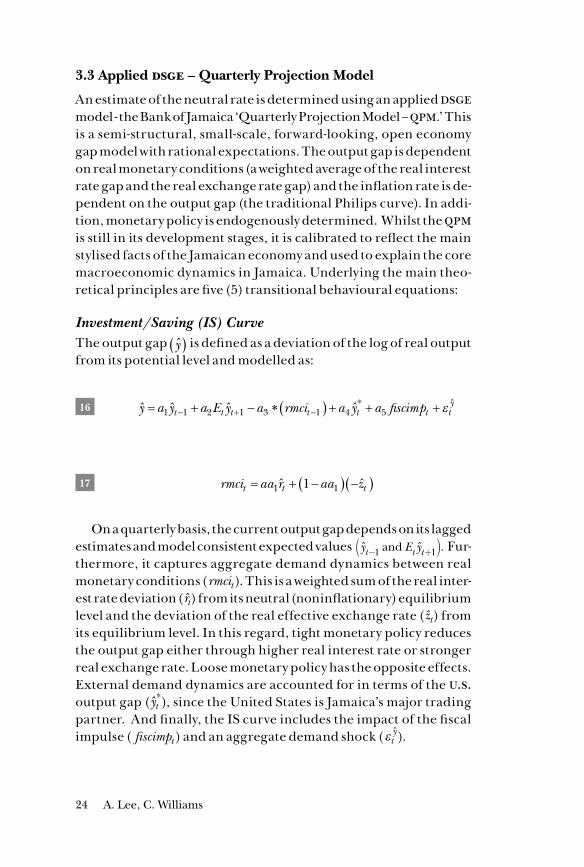
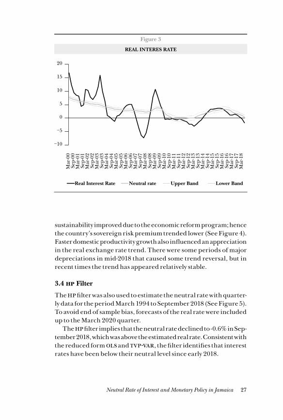
ResultsUsing the Kalman filter, we estimate the neutral real interest rate and its determinants, namely the real exchange rate trend and risk premium (Figure 3). The filtration approach implies that monetary policy was rel-atively tight in the periods 2000 to 2003 and in early 2009. This followed times of extreme inflationary pressures (the former being Jamaica’s do-mestic market financial crisis finsac in the 1990’s, and the latter being the shock from the Global Financial Crisis in 2008). Since 2016, mon-etary policy based on this estimate, has been fairly accommodative. Therefore, the Kalman filter does relatively well in capturing these piv-otal shifts and ultimately helps to identify changes in the policy stance. Given the assumption of a u.s. neutral rate of 0.75%, zero change in the equilibrium exchange rate and premium of -0.75%, the long run neu-tral rate using this methodology is estimated at 0%.
The trend in the u.s. neutral rate is estimated by a weighted equation that includes inertia and a steady state of 0.75%. Note that the prevailing low interest rate environment around the globe is captured in the foreign real interest rate equation post-2007 after the financial crisis, and has remained close to zero since 2017.4 Simultaneously, while these exter-nal yields spilled over into Jamaica’s domestic market, fiscal and debt
4 Grui et al. (2018) and Holsten et al. (2017) characterize this as a reflection of the global savings glut, ageing population, and slowing potential growth.
27Neutral Rate of Interest and Monetary Policy in Jamaica
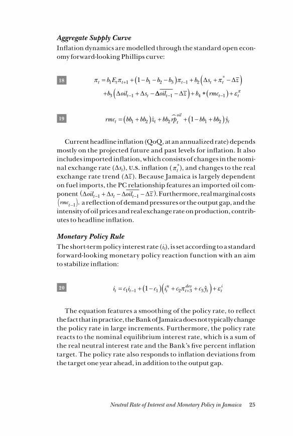
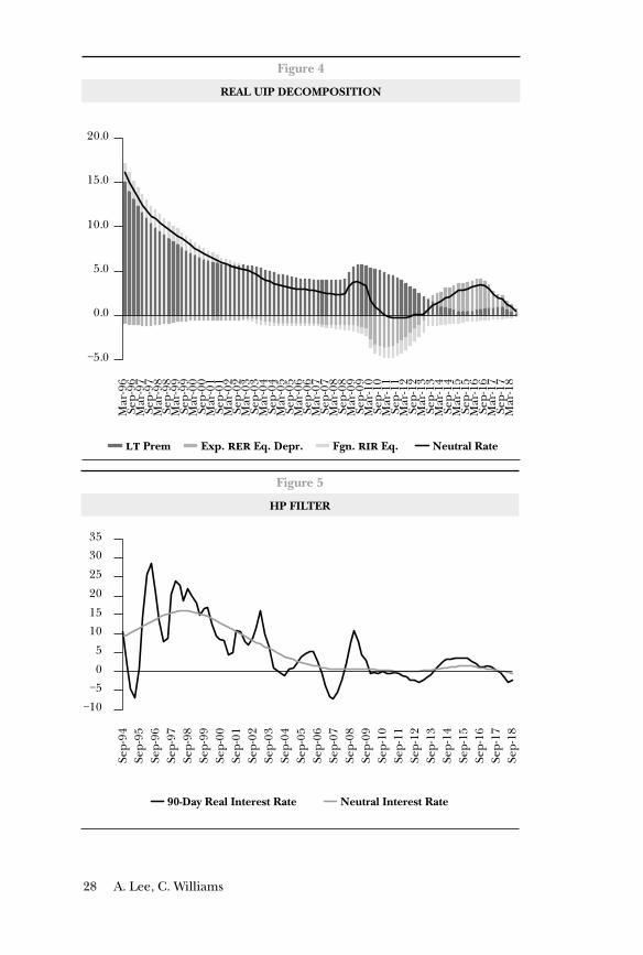
sustainability improved due to the economic reform program; hence the country’s sovereign risk premium trended lower (See Figure 4). Faster domestic productivity growth also influenced an appreciation in the real exchange rate trend. There were some periods of major depreciations in mid-2018 that caused some trend reversal, but in recent times the trend has appeared relatively stable.
3.4 hp Filter
The hp filter was also used to estimate the neutral rate with quarter-ly data for the period March 1994 to September 2018 (See Figure 5). To avoid end of sample bias, forecasts of the real rate were included up to the March 2020 quarter.
The hp filter implies that the neutral rate declined to -0.6% in Sep-tember 2018, which was above the estimated real rate. Consistent with the reduced form ols and tvp-var, the filter identifies that interest rates have been below their neutral level since early 2018.
Figure 3
REAL INTERES RATE
Real Interest Rate Neutral rate Upper Band Lower Band
−10
−5
0
5
10
15
20M
ar-0
0Se
p-00
Mar
-01
Sep-
01M
ar-0
2Se
p-02
Mar
-03
Sep-
03M
ar-0
4Se
p-04
Mar
-05
Sep-
05M
ar-0
6Se
p-06
Mar
-07
Sep-
07M
ar-0
8Se
p-08
Mar
-09
Sep-
09M
ar-1
0Se
p-10
Mar
-11
Sep-
11M
ar-1
2Se
p-12
Mar
-13
Sep-
13M
ar-1
4Se
p-14
Mar
-15
Sep-
15M
ar-1
6Se
p-16
Mar
-17
Sep-
17M
ar-1
8
28 A. Lee, C. Williams
Figure 4
REAL UIP DECOMPOSITION
lt Prem Exp. rer Eq. Depr. Fgn. rir Eq. Neutral Rate
−5.0
0.0
5.0
10.0
15.0
20.0M
ar-9
6Se
p-96
Mar
-97
Sep-
97M
ar-9
8Se
p-98
Mar
-99
Sep-
99M
ar-0
0Se
p-00
Mar
-01
Sep-
01M
ar-0
2Se
p-02
Mar
-03
Sep-
03M
ar-0
4Se
p-04
Mar
-05
Sep-
05M
ar-0
6Se
p-06
Mar
-07
Sep-
07M
ar-0
8Se
p-08
Mar
-09
Sep-
09M
ar-1
0Se
p-10
Mar
-11
Sep-
11M
ar-1
2Se
p-12
Mar
-13
Sep-
13M
ar-1
4Se
p-14
Mar
-15
Sep-
15M
ar-1
6Se
p-16
Mar
-17
Sep-
17M
ar-1
8
Figure 5
HP FILTER
90-Day Real Interest Rate Neutral Interest Rate
−10
−5
0
5
10
15
20
25
30
35
Sep-
94Se
p-95
Sep-
96Se
p-97
Sep-
98Se
p-99
Sep-
00Se
p-01
Sep-
02Se
p-03
Sep-
04Se
p-05
Sep-
06Se
p-07
Sep-
08Se
p-09
Sep-
10Se
p-11
Sep-
12Se
p-13
Sep-
14Se
p-15
Sep-
16Se
p-17
Sep-
18
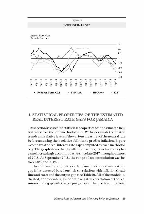
29Neutral Rate of Interest and Monetary Policy in Jamaica
4. STATISTICAL PROPERTIES OF THE ESTIMATED REAL INTEREST RATE GAPS FOR JAMAICA
This section assesses the statistical properties of the estimated neu-tral rates from the four methodologies. We first evaluate the relative trends and relative levels of the various measures of the neutral rate before assessing their relative abilities to predict inflation. Figure 6 compares the real interest rate gaps computed by each methodol-ogy. The graph shows that, by all the measures, monetary policy be-came increasingly accommodative since late 2017 throughout most of 2018. At September 2018, the range of accommodation was be-tween 0% and -2.4%.
The information content of each estimate of the real interest rate gap is first assessed based on their correlations with inflation (head-line and core) and the output gap (see Table 2). All of the models in-dicated, appropriately, a moderate negative correlation of the real interest rate gap with the output gap over the first four quarters.
Figure 6
INTEREST RATE GAP
-4.0
-3.0
-2.0
-1.0
0.0
1.0
2.0
3.0
mar
-10
sep-
10
mar
-11
sep-
11
mar
-12
sep-
12
mar
-13
sep-
13
mar
-14
sep-
14
mar
-15
sep-
15
mar
-16
sep-
16
mar
-17
sep-
17
mar
-18
sep-
18
Interest Rate Gap(Actual-Neutral)
Reduced Form OLS TVP-VAR HP-Filter K_F
30 A. Lee, C. Williams
The reduced form ols estimate displayed the strongest negative correlation with the output gap over four quarters. The neutral rate based on the hp filter was the least correlated with the output gap and underperformed relative to the tvp-var. With regard to headline inflation, the results were mixed. With the exception of the tvp-var, all measures were weakly negatively correlated with headline infla-tion up to four quarters.
All models performed better when assessed relative to core infla-tion. Over the first three lags the gaps based on the tvp-var estimate implied a positive relationship with core inflation which is contrary to a priori expectations. Interestingly, however, the tvp-var gaps displayed the strongest negative correlation with core inflation be-tween six and eight lags. This is not surprising, given the conditional forecast framework used in the estimation. The gaps determined using the Kalman and hp filter displayed the strongest negative cor-relation with core inflation at two to four lags.
While the correlations imply that underlying inflation in Jamaica, since 2000, has been related to changes in the real interest rate gap, a more robust assessment is required to determine the usefulness of the gaps in predicting inflation. The leading indicator proper-ties of the gaps for inflation may be investigated using the approach suggested by Garnier and Wilhelmsen (2008) and Neiss and Nelson (2003). These authors proposed a regression of inflation (πt) on a constant, its lagged value (πt −1) and lagged values of the real inter-est gap (rt k−
)such that:
22 π π εt t t k ta b b r= + + +− −1 1 2
23 r r rt k t k t k− − −= −
Given Jamaica’s susceptibility to supply shocks, we modify this ap-proach by assessing the leading indicator properties using core infla-tion, which removes the impact of the volatile agriculture and energy components from headline inflation. Table 3 – 5 shows the results of the regression of core inflation on the estimate of the neutral rate determined using the tvp var, the Kalman Filter and the hp filter.
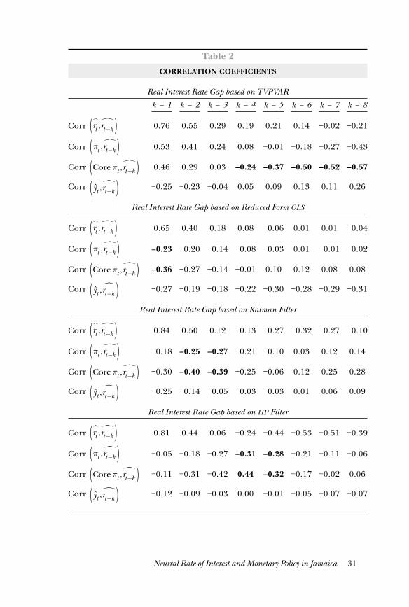
31Neutral Rate of Interest and Monetary Policy in Jamaica
Table 2
CORRELATION COEFFICIENTS
Real Interest Rate Gap based on TVPVAR
k = 1 k = 2 k = 3 k = 4 k = 5 k = 6 k = 7 k = 8
Corr rt!,rt−k!( ) 0.76 0.55 0.29 0.19 0.21 0.14 −0.02 −0.21
Corr πt ,rt−k!( ) 0.53 0.41 0.24 0.08 −0.01 −0.18 −0.27 −0.43
Corr Core πt ,rt−k!( ) 0.46 0.29 0.03 −0.24 −0.37 −0.50 −0.52 −0.57
Corr yt ,rt−k!( ) −0.25 −0.23 −0.04 0.05 0.09 0.13 0.11 0.26
Real Interest Rate Gap based on Reduced Form ols
Corr rt!,rt−k!( ) 0.65 0.40 0.18 0.08 −0.06 0.01 0.01 −0.04
Corr πt ,rt−k!( ) −0.23 −0.20 −0.14 −0.08 −0.03 0.01 −0.01 −0.02
Corr Core πt ,rt−k!( ) −0.36 −0.27 −0.14 −0.01 0.10 0.12 0.08 0.08
Corr yt ,rt−k!( ) −0.27 −0.19 −0.18 −0.22 −0.30 −0.28 −0.29 −0.31
Real Interest Rate Gap based on Kalman Filter
Corr rt!,rt−k!( ) 0.84 0.50 0.12 −0.13 −0.27 −0.32 −0.27 −0.10
Corr πt ,rt−k!( ) −0.18 −0.25 −0.27 −0.21 −0.10 0.03 0.12 0.14
Corr Core πt ,rt−k!( ) −0.30 −0.40 −0.39 −0.25 −0.06 0.12 0.25 0.28
Corr yt ,rt−k!( ) −0.25 −0.14 −0.05 −0.03 −0.03 0.01 0.06 0.09
Real Interest Rate Gap based on hp Filter
Corr rt!,rt−k!( ) 0.81 0.44 0.06 −0.24 −0.44 −0.53 −0.51 −0.39
Corr πt ,rt−k!( ) −0.05 −0.18 −0.27 −0.31 −0.28 −0.21 −0.11 −0.06
Corr Core πt ,rt−k!( ) −0.11 −0.31 −0.42 0.44 −0.32 −0.17 −0.02 0.06
Corr yt ,rt−k!( ) −0.12 −0.09 −0.03 0.00 −0.01 −0.05 −0.07 −0.07
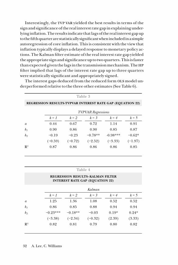
32 A. Lee, C. Williams
Interestingly, the tvp var yielded the best results in terms of the sign and significance of the real interest rate gap in explaining under-lying inflation. The results indicate that lags of the real interest gap up to the fifth quarter are statistically significant when included in a simple autoregression of core inflation. This is consistent with the view that inflation typically displays a delayed response to monetary policy ac-tions. The Kalman filter estimate of the real interest rate gap yielded the appropriate sign and significance up to two quarters. This is faster than expected given the lags in the transmission mechanism. The hp filter implied that lags of the interest rate gap up to three quarters were statistically significant and appropriately signed.
The interest gaps deduced from the reduced form ols model un-derperformed relative to the three other estimates (See Table 6).
Table 3
REGRESSION RESULTS-TVPVAR INTEREST RATE GAP (EQUATION 22)
TVPVAR Regressions
k = 1 k = 2 k = 3 k = 4 k = 5
a 0.44 0.67 0.72 1.14 0.91b1 0.90 0.86 0.90 0.85 0.87b2 −0.19 −0.23 −0.78** -0.98*** −0.62*
(−0.59) (−0.72) (−2.52) (−3.33) (−1.97)
R2 0.87 0.86 0.86 0.86 0.85
Table 4
REGRESSION RESULTS–KALMAN FILTER INTEREST RATE GAP (EQUATION 22)
Kalman
k = 1 k = 2 k = 3 k = 4 k = 5
a 1.25 1.36 1.08 0.52 0.52b1 0.86 0.85 0.88 0.94 0.94b2 −0.23*** −0.18** −0.03 0.19* 0.24*
(−3.38) (−2.34) (−0.32) (2.39) (3.33)
R2 0.82 0.81 0.79 0.80 0.82
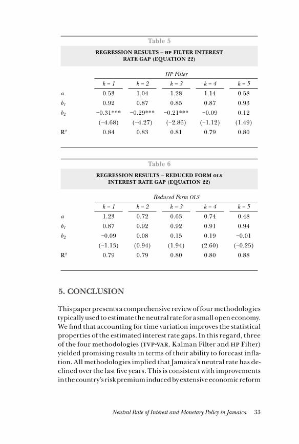
33Neutral Rate of Interest and Monetary Policy in Jamaica
5. CONCLUSION
This paper presents a comprehensive review of four methodologies typically used to estimate the neutral rate for a small open economy. We find that accounting for time variation improves the statistical properties of the estimated interest rate gaps. In this regard, three of the four methodologies (tvp-var, Kalman Filter and hp Filter) yielded promising results in terms of their ability to forecast infla-tion. All methodologies implied that Jamaica’s neutral rate has de-clined over the last five years. This is consistent with improvements in the country’s risk premium induced by extensive economic reform
Table 5
REGRESSION RESULTS – hp FILTER INTEREST RATE GAP (EQUATION 22)
hp Filter
k = 1 k = 2 k = 3 k = 4 k = 5
a 0.53 1.04 1.28 1.14 0.58b1 0.92 0.87 0.85 0.87 0.93b2 −0.31*** −0.29*** −0.21*** −0.09 0.12
(−4.68) (−4.27) (−2.86) (−1.12) (1.49)
R2 0.84 0.83 0.81 0.79 0.80
Table 6
REGRESSION RESULTS – REDUCED FORM ols INTEREST RATE GAP (EQUATION 22)
Reduced Form ols
k = 1 k = 2 k = 3 k = 4 k = 5
a 1.23 0.72 0.63 0.74 0.48b1 0.87 0.92 0.92 0.91 0.94b2 −0.09 0.08 0.15 0.19 −0.01
(−1.13) (0.94) (1.94) (2.60) (−0.25)
R2 0.79 0.79 0.80 0.80 0.88
34 A. Lee, C. Williams
during that period. Further demographic and structural changes should continue to support a low interest environment over the long run.
Based on our estimates, monetary conditions in Jamaica have been fairly accommodative since late 2017, which should support the authorities’ inflation and growth objectives. The point estimate for the long-run neutral rate is found to range between -2.6% to 2.6% or (2.4% to 7.6% in nominal terms). However, given that the neutral rate is unobservable, there is a high level of uncertainty with regard to its estimation. It is therefore important to support these estimates with robust discussions on the trends in the main macroeconomic variables as well as the effectiveness of the transmission mechanism of monetary policy.
References
2016 Article IV Consultation, Eleventh and Twelfth Reviews Under the Extended Fund Facility and Request for Modification of Performance Criteria--Press Release; Staff Report; and State-ment by the Executive Director for Jamaica. (2016). Interna-tional Monetary Fund: Country Report No. 16/181.
Amador, S., & Beltrán, P. A. (2016). Natural Rate of Interest Esti-mates for Colombia. Bano De La República,73-75.
Baksa, D., Felcser, D., Horváth, Á, Kiss, N., Köber, C., Krusper, B., Szilágyi, K. (2013). Neutral Interest Rate in Hungary. MNB Bulletin, Magyar Nemzeti Bank (Central Bank of Hungary),8, 7-13.
Carrillo, J. A., Elizondo, R., & Rodríguez-Pérez, C. A. (2017). What Determines the Neutral Rate of Interest in an Emerging Economy. Banco De México.
Clinton, K., Hlédik, T., Holub, T., Laxton, D., & Wang, H. (2017). Czech Magic: Implementing Inflation-Forecast Targeting at the CNB. imf Working Paper (WP/17/21), International Mon-etary Fund Research Department.
Cogley, T., & Sargent, T. J. (2001). Evolving Post-World War II u.s. Inflation Dynamics. NBER Macroeconomics Annual 2001,16, 331-388.
Dacass, T. (2011). Estimating the Natural Rate of Interest for Ja-maica. Bank of Jamaica Working Paper
35Neutral Rate of Interest and Monetary Policy in Jamaica
Del Negro, M., Giannoni, M. P., Giannone, D., & Tambalotti, A. (2017). Safety, Liquidity, and the Natural Rate of Inter-est. Brookings Papers on Economic Activity: Spring 2017,235-316.
Djoudad, R., Fung, B., Lam, J. P., & Poon, D. (2004). How Useful is the Neutral Interest Rate for Monetary Policy in Canada. Bank of Canada: Preliminary Paper.
Garnier, J., & Wilhelmsen, J. (2008). The natural rate of interest and the output gap in the euro area: a Joint Estimation, Springer-Verlag, 297–319.
Grui, A., Lepushynskyi, V., & Nikolaychuk, S. (2018). A Neutral Real Interest Rate in the Case of A Small Open Economy: Application to Ukraine. Visnyk of the National Bank of Ukraine, No. 243,4-20. Retrieved from https://bank.gov.ua/doccata-log/document?id=68661862.
Holston, K., Laubach, T., & Williams, J. C. (2016). Measuring the Natural Rate of Interest: International Trends and Deter-minants. Federal Reserve Bank of San Francisco Working Paper 2016-11. Retrieved from http://www.frbsf.org/economic-research/publications/working- papers/wp2016-11.pdf
Koop, G., & Korobilis, D. (2012). Large Time-Varying Parameter VARs. Munich Personal RePEc Archive: Paper No. 38591.
Kreptzev, D., Porshakov, A., & Seleznev, S. (2016). The Equilibrium Interest Rate: A Measurement of Russia. Bank of Russia: Work-ing Paper Series Wps13.
Laubach, T., & Williams, J. C. (2001). Measuring the Natural Rate of Interest. Board of Governors of the Federal Reserve System.
Laubach, T., & Williams, J. C. (2003). Measuring the Natural Rate of Interest. The Review of Economics and Statistics,85(4), 1063-1070. Retrieved from https://www.jstor.org/stable/3211826.
Lubik, T. A., & Matthes, C. (2015). Time-Varying Parameter Vector Autoregressions: Specification, Estimation, and an Applica-tion. Economic Quarterly,101(4), 323-352.
Lubík, T. A., & Matthes, C. (2015). Calculating the Natural Rate of Interest: A Comparison of Two Alternative Approaches. Fed-eral Reserve Board of Richmond: EB15-10,1-6.
McCririck, R., & Rees, D. (2017). The Neutral Interest Rate. RBA Bulletin, Reserve Bank of Australia, 09-18.
36 A. Lee, C. Williams
Mendes, R. R. (2014). The Neutral Rate of Interest in Canada. Bank of Canada: Discussion Paper 2014-5.
Mesonnier, J. S., & Renne, J. P. (2004). A Time Varying Natural Rate of Interest for the Euro Area. Money Macro and Finance (MMF) Research Group Conference 42, Money Macro and Finance Research Group.
Murray, A. (2007). Modelling the Jamaican Business Cycle: A Structural Vector Autoregressive Approach. Bank of Jamaica Working Paper
Nakajima, J. (2011). Time-Varying Parameter var Model with Stochastic Volatility: An Overview of Methodology and Em-pirical Applications. Monetary and Economic Studies; Bank of Japan,107-141.
Neiss K,. & Nelson, E. (2003). The real rate gap as an inflation indicator. Macroecon Dyn 7:239–262.
Plantier, C. L., & Scrimgeour, D. (2002). Estimating a Taylor Rule for New Zealand with a Time-Varying Neutral Real Rate. Re-serve Bank of New Zealand: Discussion Paper.
Robinson, W. & Williams, C. (2016). Evaluating the Transmission Mechanism of Monetary Policy in Jamaica: A Factor-Aug-mented Vector Autoregressive (favar) Approach with Time Varying Coefficients. Bank of Jamaica Working Paper
Scarlett, H. (2019). Estimating Jamaica’s Potential Output. Bank of Jamaica Working Paper
World Economic Outlook: Recovery Strengthens, Remains Uneven. (2004). International Monetary Fund.
Wynne, M. A., & Zhang, R. (2017). Estimating the Natural Rate of Interest in an Open Economy. Globalization and Monetary Policy Institute; Federal Reserve Bank of Dallas: Working Paper No. 316. Retrieved from https://www.dallasfed.org/~/media/documents/institute/wpapers/2017/0316.pdf.
37Monetary Policy in Costa Rica
Monetary policy in Costa Rica: an assessment based on the neutral real interest rate
Evelyn Muñoz-SalasAdolfo Rodríguez-Vargas
Abstract
In this study we assess the monetary policy stance in Costa Rica during the 2009-2018 period using an indicator of the real policy rate gap. We obtain estimates of the real neutral interest rate by using six methodologies, whose empirical consistency is evaluated in order to decide whether they are used in the final estimation. The updated value for the real neutral interest rate is 1.54%. The policy rate gap indicator shows appropriate empirical proper-ties, among them a negative lead correlation with the output gap and core in-flation. This suggests that the policy rate is successfully influencing the mar-ginal cost of liquidity for financial intermediaries. Our analysis suggests that monetary policy in Costa Rica has responded mainly to inflation movements not related to temporary shocks, and that some policy adjustments could have been swifter.
Key words: monetary policy, inflation, unobservable variables.jel codes: E12, E31, E52.
1. INTRODUCTION
In 1898, the Swedish economist Knut Wicksell introduced the con-cept of the natural (or neutral) interest rate as “a certain rate of interest on loans which is neutral in respect to commodity
prices, and tends neither to raise nor to lower them.” (Wicksell, 1938,
Evelyn Muñoz Salas <[email protected]>, Department of Economic Research. Adolfo Rodríguez-Vargas <[email protected]>, Department of Economic Research.
38 E. Muñoz, A. Rodríguez
pp.106). Wicksell argued that as long as the interest rate was lower than the natural rate of return on capital, there would be an incentive to borrow in order to accumulate capital. This accumulation process would eventually lead to an increase in the general price level due to the increase in aggregate demand. Thus, for Wicksell price stability would be achieved only if, all else constant, permanent discrepancies could be avoided between the current interest rate and the natural rate. Consequently, a discussion about the level of the interest rate would only make sense when it is compared to the level of the natural rate. However, Wicksell acknowledged that the natural rate is neither observable nor constant, since it would depend on the evolution of the factors that influence the return of capital.
The most relevant contribution to consolidate the concept of the natural interest rate in modern macroeconomics was made by Wood-ford (2003), who demonstrated that it is possible to derive a natural rate conceptually equivalent to that of Wicksell as a function of fun-damental variables (consumer preferences, shocks of productivity) within the framework of a neo-Keynesian model, and that such rate is the one that would prevail in the absence of nominal rigidities.
Therefore, Woodford formulated the theoretical fundamentals that support the strategy followed by many central banks to conduct economic policy of price stabilization, by demonstrating that it is feasible to perform monetary policy through a rule for the interest rate without explicitly taking into account the money supply. This is particularly relevant for central banks that follow an inflation tar-geting scheme.
The neutral real interest rate (nrir) is a fundamental reference to characterize, in real time and ex post, the monetary policy stance: contractive when the policy rate is higher than the nrir, expansive when it is lower. Therefore, it is very useful for a central bank to have reliable estimates of the gap between the monetary policy rate and the nrr when facing the monetary policy decision-making process. This is a challenge because the nrir is an unobservable variable.
The Central Bank of Costa Rica (bccr) has made several es-timates of the nrir for Costa Rica. The first exercise, by Muñoz and Tenorio (2007), used data for the period 1991-2006, under a crawling peg exchange rate regime. The nrir was estimated us-ing four methodologies: a semi-structural model proposed by Lau-bach and Williams (2003), the uncovered parity condition of interest, the Hodrick-Prescott filter to obtain a long-term trend, and an ad-hoc
39Monetary Policy in Costa Rica
approximation corresponding to the average of the effective real in-terest rate under a period of stable inflation.
Segura and Vindas (2012) used information for the period 2001-2011, which includes two exchange rate regimes (a crawling peg and a crawling band) and in addition to the methodologies used by Mu-ñoz and Tenorio, they included a var estimation proposed by Brzoza-Brzezina (2003, 2006). Muñoz y Rodríguez (2016) used data for the period 2009-2015 under a more flexible exchange rate regime, along with the methodologies used in previous studies, their estimations incorporate Taylor rule state space models.
International organizations like the imf (2016) and the oecd (2016) also estimated the nrir as part of their evaluations of the Costa Rican economy. The imf relied on a neo-Keynesian semi-structural model, a general equilibrium model, a monetary model and a Tay-lor rule augmented by expectations. This last method is also the one used by the oecd.
A common feature of previous studies for Costa Rica is their em-phasis on the estimation itself. The present investigation has the objective of approximating an interest rate gap with coherent em-pirical properties and then analyzing its relationship with the state of the Costa Rican economy, which would allow us to make conclu-sions about the stance of the bccr monetary policy. For the estima-tion of the nrir we add two more methods to those used in Muñoz and Rodriguez (2016).
This paper is organized as follows: the methodology description is presented in section 2. The main results and the evaluation of the policy stand are discussed in section 3, finally the main conclusions are presented in section 4.
2. DATA AND METHODOLOGY
2.1 Monetary policy rate
In 2005, the bccr began a process of modernization of its monetary policy in order to improve the compliance of the objective established by its Organic Law of maintaining the internal stability of the nation-al currency. This mandate is interpreted as the achievement of low and stable inflation, in line with that of the main trading partners
40 E. Muñoz, A. Rodríguez
of the country. This process led to the adoption of an inflation tar-geting monetary policy framework in January 2018.
An important decision in this process was the introduction of the monetary policy rate (mpr) as an instrument of monetary control, in June 20111. The greater variability of the exchange rate resulting from the adoption of the crawling band exchange rate regime at the end of 2006 and of the managed float at the beginning of 2015 has al-lowed an increasing independence for the use of the mpr, after de-cades of a crawling peg scheme that restricted the possibility of using the interest rate as a monetary policy instrument2.
The mpr is defined as “…interest rate target of the Central Bank of Costa Rica. This indicator corresponds to the interest rate the Cen-tral Bank of Costa Rica uses as a reference in guiding the cost of one-day operations in the Integrated Liquidity Market into a corridor determined by the interest rates of the permanent facilities of credit an deposit in that market.”3
By changing this rate the bccr aims to influence the marginal cost of liquidity for the financial intermediaries to channel the de-sired stance of monetary policy to the rest of interest rates in the fi-nancial system.
Before having this formal definition of the indicator, all empirical research requiring a monetary policy rate lacked a coherent monetary policy rate series long enough to allow quantitative analysis. For ex-ample, Muñoz and Tenorio (2007) and Segura and Vindas (2012) used the Deposit Basic Rate as an indicator of bccr’s policy rate.
To overcome this issue, Castro and Chaverri (2013) defines an in-dicator that reflects the monetary policy stance the bccr during the period January 1999 - May 2011. The data series resulting from linking the monetary policy rate indicator of Castro and Chaverri (2013) with the data of the mpr as of June 2011 is shown in Figure 1. This is the variable used as the rate of monetary policy throughout the present investigation.
1 Since 2005, the legal reserve requirement is at the maximum level al-lowed by the Organic Law.
2 The increasing exchange rate volatility associated to the adoption of more flexible Exchange regimes was documented in bccr (2018).
3 Monetary Policy Regulations, Title IV, Numeral 2, Literal D.
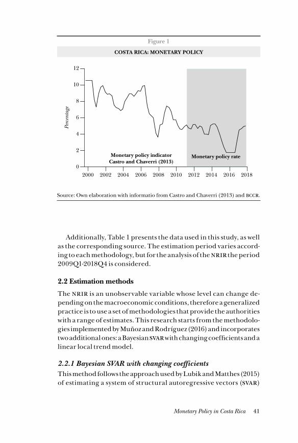
41Monetary Policy in Costa Rica
Additionally, Table 1 presents the data used in this study, as well as the corresponding source. The estimation period varies accord-ing to each methodology, but for the analysis of the nrir the period 2009Q1-2018Q4 is considered.
2.2 Estimation methods
The nrir is an unobservable variable whose level can change de-pending on the macroeconomic conditions, therefore a generalized practice is to use a set of methodologies that provide the authorities with a range of estimates. This research starts from the methodolo-gies implemented by Muñoz and Rodríguez (2016) and incorporates two additional ones: a Bayesian svar with changing coefficients and a linear local trend model.
2.2.1 Bayesian svar with changing coefficientsThis method follows the approach used by Lubik and Matthes (2015) of estimating a system of structural autoregressive vectors (svar)
Figure 1
COSTA RICA: MONETARY POLICY
Source: Own elaboration with informatio from Castro and Chaverri (2013) and .
10
8
6
4
201620142012201020082006200420022000 2018
2
12
0
Perc
enta
ge
Monetary policy indicatorCastro and Chaverri (2013)
Monetary policy rate
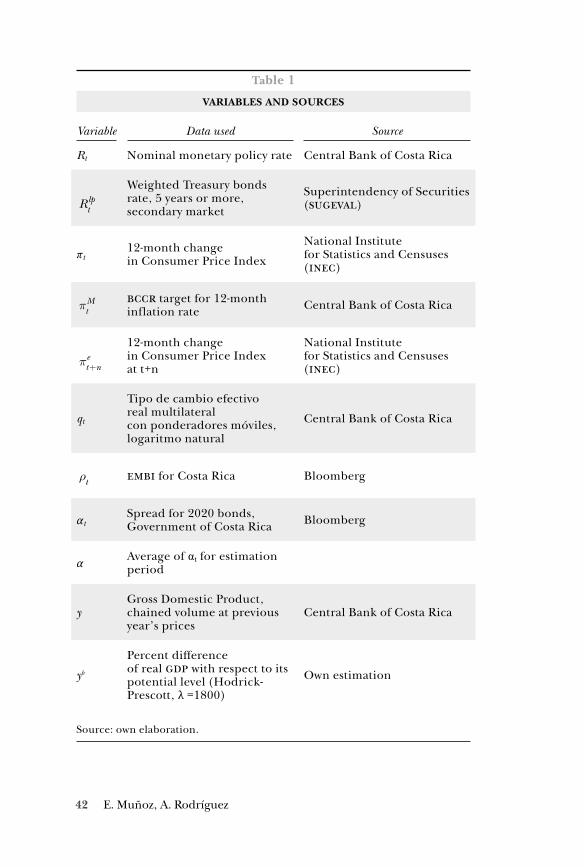
42 E. Muñoz, A. Rodríguez
Table 1
VARIABLES AND SOURCES
Variable Data used Source
Rt Nominal monetary policy rate Central Bank of Costa Rica
Weighted Treasury bonds rate, 5 years or more, secondary market
Superintendency of Securities (sugeval)
πt12-month change in Consumer Price Index
National Institute for Statistics and Censuses (inec)
bccr target for 12-month inflation rate Central Bank of Costa Rica
12-month change in Consumer Price Index at t+n
National Institute for Statistics and Censuses (inec)
qt
Tipo de cambio efectivo real multilateral con ponderadores móviles, logaritmo natural
Central Bank of Costa Rica
embi for Costa Rica Bloomberg
αtSpread for 2020 bonds, Government of Costa Rica Bloomberg
αAverage of αt for estimation period
yGross Domestic Product, chained volume at previous year’s prices
Central Bank of Costa Rica
yb
Percent difference of real gdp with respect to its potential level (Hodrick-Prescott, λ =1800)
Own estimation
Source: own elaboration.
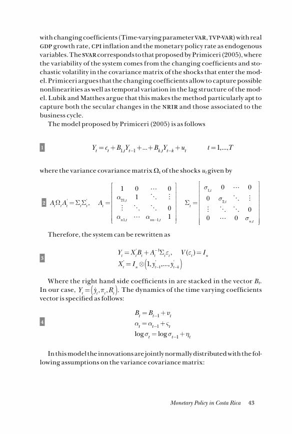
43Monetary Policy in Costa Rica
with changing coefficients (Time-varying parameter var, tvp-var) with real gdp growth rate, cpi inflation and the monetary policy rate as endogenous variables. The svar corresponds to that proposed by Primiceri (2005), where the variability of the system comes from the changing coefficients and sto-chastic volatility in the covariance matrix of the shocks that enter the mod-el. Primiceri argues that the changing coefficients allow to capture possible nonlinearities as well as temporal variation in the lag structure of the mod-el. Lubik and Matthes argue that this makes the method particularly apt to capture both the secular changes in the nrir and those associated to the business cycle.
The model proposed by Primiceri (2005) is as follows
1
where the variance covariance matrix Ωt of the shocks ut given by
2
Therefore, the system can be rewritten as
3
Where the right hand side coefficients in are stacked in the vector Bt. In our case, The dynamics of the time varying coefficients vector is specified as follows:
4
In this model the innovations are jointly normally distributed with the fol-lowing assumptions on the variance covariance matrix:
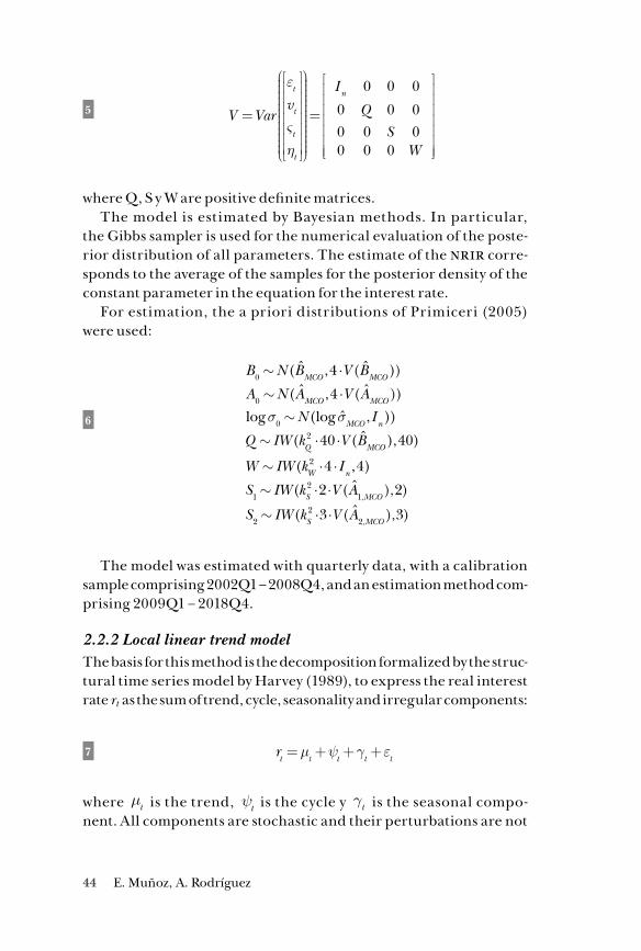
44 E. Muñoz, A. Rodríguez
5
where Q, S y W are positive definite matrices.The model is estimated by Bayesian methods. In particular,
the Gibbs sampler is used for the numerical evaluation of the poste-rior distribution of all parameters. The estimate of the nrir corre-sponds to the average of the samples for the posterior density of the constant parameter in the equation for the interest rate.
For estimation, the a priori distributions of Primiceri (2005) were used:
6
The model was estimated with quarterly data, with a calibration sample comprising 2002Q1 – 2008Q4, and an estimation method com-prising 2009Q1 – 2018Q4.
2.2.2 Local linear trend modelThe basis for this method is the decomposition formalized by the struc-tural time series model by Harvey (1989), to express the real interest rate rt as the sum of trend, cycle, seasonality and irregular components:
7
where is the trend, is the cycle y is the seasonal compo-nent. All components are stochastic and their perturbations are not
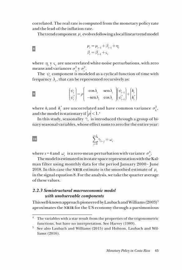
45Monetary Policy in Costa Rica
correlated. The real rate is computed from the monetary policy rate and the lead of the inflation rate.
The trend component evolves following a local linear trend model
8
where y are uncorrelated white-noise perturbations, with zero means and variances y
The component is modeled as a cyclical function of time with frequency that can be represented recursively as:
9
where kt and are uncorrelated and have common variance and the model is stationary if 4
In this study, seasonality is introduced through a group of bi-nary seasonal variables, whose effect sums to zero for the entire year:
10
where s = 4 and is a zero-mean perturbation with variance The model is estimated in its state-space representation with the Kal-
man filter using monthly data for the period January 2000– June 2018. In this case the nrir estimate is the smoothed estimate of in the signal equation 8. For the analysis, we take the quarter average of these values.
2.2.3 Semistructural macroeconomic model with unobservable components
This well-known approach pioneered by Laubach and Williams (2003)5 aproximates the nrir for the US economy through a parsimonious
4 The variables with a star result from the properties of the trigonometric functions, but have no interpretation. See Harvey (1989).
5 See also Laubach and Williams (2015) and Holston, Laubach and Wil-liams (2016).
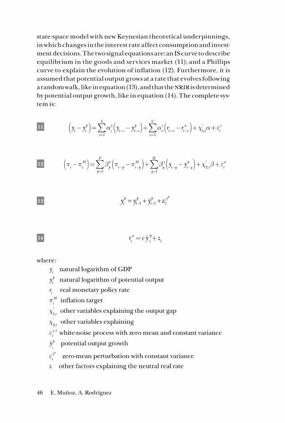
46 E. Muñoz, A. Rodríguez
state-space model with new Keynesian theoretical underpinnings, in which changes in the interest rate affect consumption and invest-ment decisions. The two signal equations are: an IS curve to describe equilibrium in the goods and services market (11); and a Phillips curve to explain the evolution of inflation (12). Furthermore, it is assumed that potential output grows at a rate that evolves following a random walk, like in equation (13), and that the nrir is determined by potential output growth, like in equation (14). The complete sys-tem is:
11
12
13 y y ytp
tp
tp
ty p
= + +− −1 1 ε
14
where:
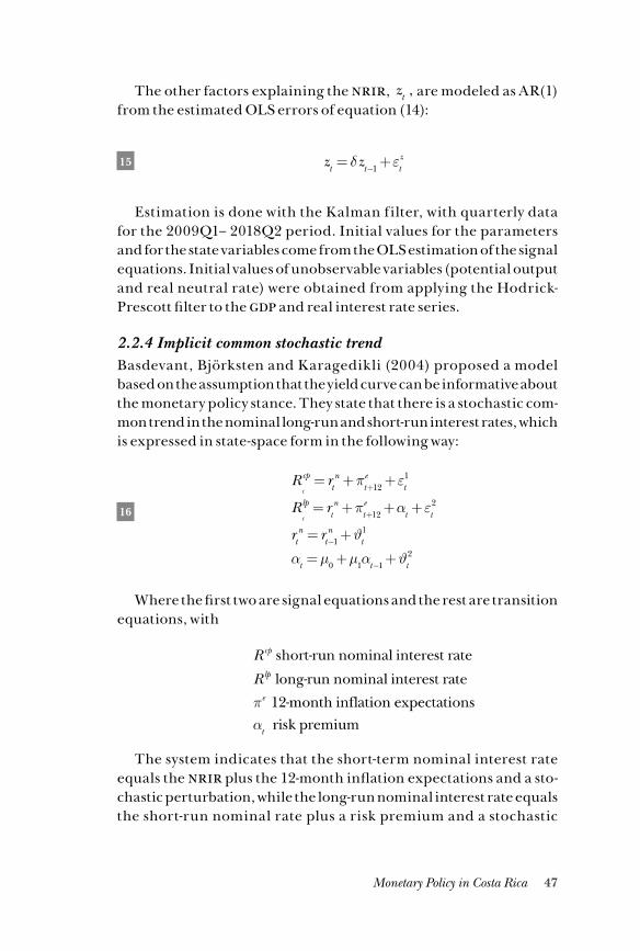
47Monetary Policy in Costa Rica
The other factors explaining the nrir, are modeled as AR(1) from the estimated OLS errors of equation (14):
15
Estimation is done with the Kalman filter, with quarterly data for the 2009Q1– 2018Q2 period. Initial values for the parameters and for the state variables come from the OLS estimation of the signal equations. Initial values of unobservable variables (potential output and real neutral rate) were obtained from applying the Hodrick-Prescott filter to the gdp and real interest rate series.
2.2.4 Implicit common stochastic trendBasdevant, Björksten and Karagedikli (2004) proposed a model based on the assumption that the yield curve can be informative about the monetary policy stance. They state that there is a stochastic com-mon trend in the nominal long-run and short-run interest rates, which is expressed in state-space form in the following way:
16
Where the first two are signal equations and the rest are transition equations, with
The system indicates that the short-term nominal interest rate equals the nrir plus the 12-month inflation expectations and a sto-chastic perturbation, while the long-run nominal interest rate equals the short-run nominal rate plus a risk premium and a stochastic
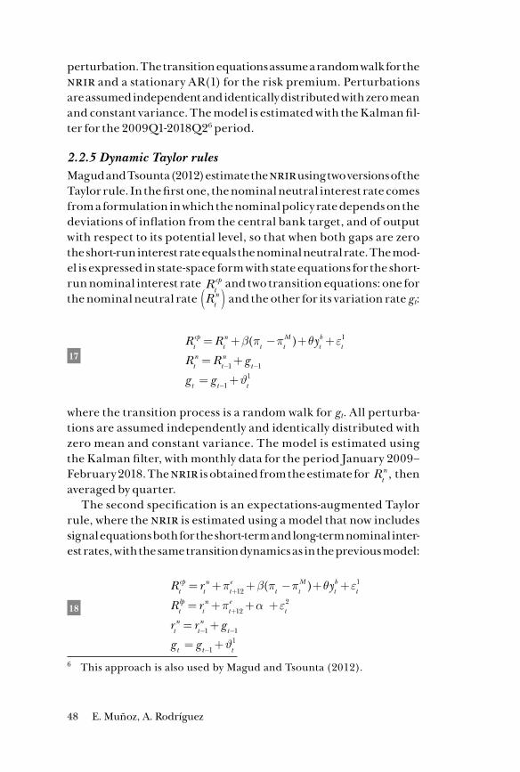
48 E. Muñoz, A. Rodríguez
perturbation. The transition equations assume a random walk for the nrir and a stationary AR(1) for the risk premium. Perturbations are assumed independent and identically distributed with zero mean and constant variance. The model is estimated with the Kalman fil-ter for the 2009Q1-2018Q26 period.
2.2.5 Dynamic Taylor rulesMagud and Tsounta (2012) estimate the nrir using two versions of the Taylor rule. In the first one, the nominal neutral interest rate comes from a formulation in which the nominal policy rate depends on the deviations of inflation from the central bank target, and of output with respect to its potential level, so that when both gaps are zero the short-run interest rate equals the nominal neutral rate. The mod-el is expressed in state-space form with state equations for the short-run nominal interest rate and two transition equations: one for the nominal neutral rate and the other for its variation rate gt:
17
where the transition process is a random walk for gt. All perturba-tions are assumed independently and identically distributed with zero mean and constant variance. The model is estimated using the Kalman filter, with monthly data for the period January 2009–February 2018. The nrir is obtained from the estimate for then averaged by quarter.
The second specification is an expectations-augmented Taylor rule, where the nrir is estimated using a model that now includes signal equations both for the short-term and long-term nominal inter-est rates, with the same transition dynamics as in the previous model:
18
6 This approach is also used by Magud and Tsounta (2012).
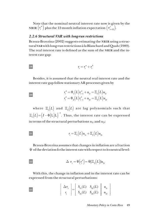
49Monetary Policy in Costa Rica
Note that the nominal neutral interest rate now is given by the nrir plus the 12-month inflation expectation
2.2.6 Structural var with long-run restrictionsBrzoza-Brzezina (2002) suggests estimating the nrir using a struc-tural var with long-run restrictions à la Blanchard and Quah (1989). The real interest rate is defined as the sum of the nrir and the in-terest rate gap:
19
Besides, it is assumed that the neutral real interest rate and the interest rate gap follow stationary AR processes given by
20
where a nd a re lag poly nomia ls such that
Thus, the interest rate can be expressed
in terms of the structural perturbations u1t and u2t:
21
Brzoza-Brzezina assumes that changes in inflation are a fraction of the deviation fo the interest rate with respect to its neutral level:
22
With this, the change in inflation and in the interest rate can be expressed from the structural perturbations:
23
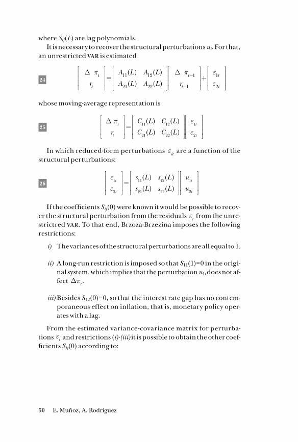
50 E. Muñoz, A. Rodríguez
where Sij(L) are lag polynomials.It is necessary to recover the structural perturbations ut. For that,
an unrestricted var is estimated
24
whose moving-average representation is
25
In which reduced-form perturbations are a function of the structural perturbations:
26
If the coefficients Sij(0) were known it would be possible to recov-er the structural perturbation from the residuals from the unre-strictred var. To that end, Brzoza-Brzezina imposes the following restrictions:
i) The variances of the structural perturbations are all equal to 1.
ii) A long-run restriction is imposed so that S11(1)=0 in the origi-nal system, which implies that the perturbation u1t does not af-fect
iii) Besides S12(0)=0, so that the interest rate gap has no contem-poraneous effect on inflation, that is, monetary policy oper-ates with a lag.
From the estimated variance-covariance matrix for perturba-tions and restrictions (i)-(iii) it is possible to obtain the other coef-ficients Sij(0) according to:
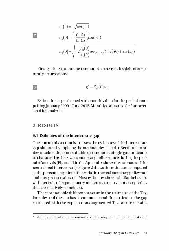
51Monetary Policy in Costa Rica
27
Finally, the nrir can be computed as the result solely of struc-tural perturbations:
28
Estimation is performed with monthly data for the period com-prising January 2009 – June 2018. Monthly estimates of are aver-aged for analysis.
3. RESULTS
3.1 Estimates of the interest rate gap
The aim of this section is to assess the estimates of the interest rate gap obtained by applying the methods described in Section 2, in or-der to select the most suitable to compute a single gap indicator to characterize the bccr’s monetary policy stance during the peri-od of analysis (Figure 11 in the Appendix shows the estimates of the neutral real interest rate). Figure 2 shows the estimates, computed as the percentage point differential in the real monetary policy rate and every nrir estimate7. Most estimates show a similar behavior, with periods of expansionary or contractionary monetary policy that are relatively coincident.
The most notable differences occur in the estimates of the Tay-lor rules and the stochastic common trend. In particular, the gap estimated with the expectations-augmented Taylor rule remains
7 A one-year lead of inflation was used to compute the real interest rate.
52 E. Muñoz, A. Rodríguez
negative during almost all the period considered, and the gaps re-sulting from the simple Taylor rule and the stochastic common trend show comparatively low values, stemming from nrir estimates very close to the effective real rate.
In order to select the gap estimates, three requisites have to be met. First, when the real interest rate is higher than the nrir, the monetary policy stance is contractionary, so that if that positive gap persists it is reasonable to expect a reduction in aggregate demand and then in the output gap and inflation. Thus, positive (negative) rate gaps should precede reductions (increases) in the output and inflation. Furthermore, even though monetary policy is forward-looking, it is also likely that policymakers respond to the contemporaneous behav-ior of inflation. Thus, it is also reasonable to assess whether the rate gap is correlated with it.
On the other hand, the evolution of each interest rate gap is com-pared with that of a Financial Condition Index (fci) for Costa Rica obtained from the combination of 33 financial indicators using prin-cipal components. These indicators include credit and monetary ag-gregates, prices, interest rates and margins (including the monetary policy rate), ratios and indicators of the financial system, and factors linked with the state of the global economy. For more details see Ál-varez (2016). Increases in the fci point to less restrictive financial conditions, while reductions in it indicate the opposite case. Since the monetary policy stance should be transmitted to the financial sec-tor, it should be expected that increases in the interest rate gap pre-cede or coincide with reductions in the fci.
Ideally, an interest rate gap should meet these criteria, so for computation of the final indicator estimates those that do not are dropped. To verify compliance, we compute correlation coef-ficients between the output gap, core inflation and the fci with sev-eral lags and leads of each interest rate gap8.
Most of the correlations with the output gap (Figure 3) show the ex-pected pattern, that is, the highest correlation within the policy
8 The output gap is the one used in the macroeconomic modelling by the bccr, which corresponds to an average of an estimate of potential out-put using a production function (Álvarez, 2018) and an estimate using a Hodrick- Prescott filter (λ = 1800). Details on trimmed-mean measure of core inflation can be found in Esquivel, Rodríguez and Vásquez (2011).

53Monetary Policy in Costa Rica
Figure 2
REAL RATE GAP ESTIMATES 2009Q1–2018Q2
Source: Own elaboration.
-
, (2003)
543210
−1−2
6
−320162015201420132012201120102009 2017
543210
−1−2
6
−320162015201420132012201120102009 2017
543210
−1−2
6
−320162015201420132012201120102009 2017
Perc
enta
gePe
rcen
tage
Perc
enta
ge
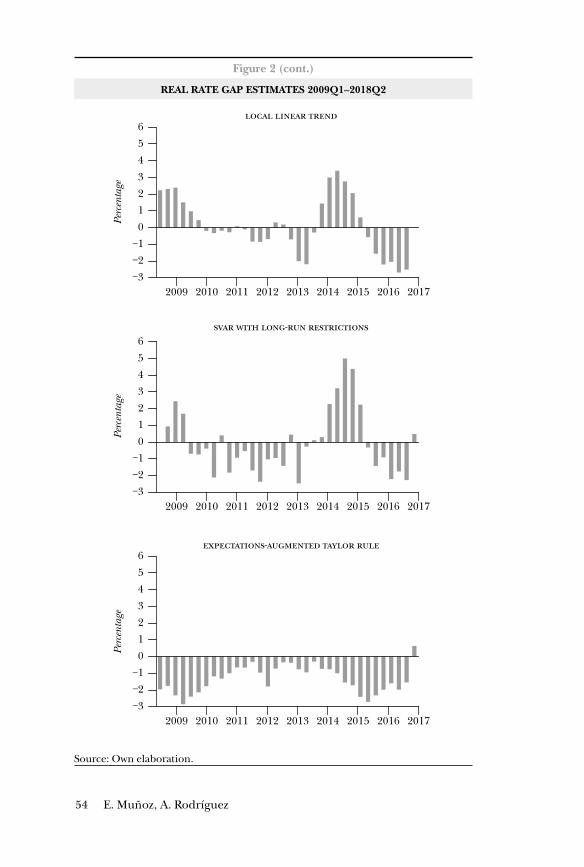
54 E. Muñoz, A. Rodríguez
Figure 2 (cont.)
REAL RATE GAP ESTIMATES 2009Q1–2018Q2
Source: Own elaboration.
-
-
543210
−1−2
6
−320162015201420132012201120102009 2017
543210
−1−2
6
−320162015201420132012201120102009 2017
543210
−1−2
6
−320162015201420132012201120102009 2017
Perc
enta
gePe
rcen
tage
Perc
enta
ge
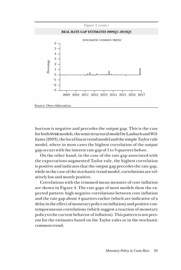
55Monetary Policy in Costa Rica
horizon is negative and precedes the output gap. This is the case for both svar models, the semi-structural model by Laubach and Wil-liams (2003), the local linear trend model and the simple Taylor rule model, where in most cases the highest correlation of the output gap occurs with the interest rate gap of 1 to 3 quarters before.
On the other hand, in the case of the rate gap associated with the expectations-augmented Taylor rule, the highest correlation is positive and indicates that the output gap precedes the rate gap, while in the case of the stochastic trend model, correlations are rel-atively low and mostly positive.
Correlations with the trimmed-mean measure of core inflation are shown in Figure 4. The rate gaps of most models show the ex-pected pattern: high negative correlations between core inflation and the rate gap about 4 quarters earlier (which are indicative of a delay in the effect of monetary policy on inflation) and positive con-temporaneous correlations (which suggest a reaction of monetary policy to the current behavior of inflation). This pattern is not pres-ent for the estimates based on the Taylor rules or in the stochastic common trend.
Figure 2 (cont.)
REAL RATE GAP ESTIMATES 2009Q1–2018Q2
Source: Own elaboration.
543210
−1−2
6
−320162015201420132012201120102009 2017
Perc
enta
ge
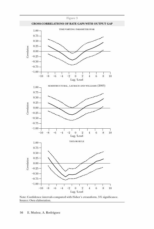
56 E. Muñoz, A. Rodríguez
Figure 3
CROSS-CORRELATIONS OF RATE GAPS WITH OUTPUT GAP
Note: Confidence intervals computed with Fisher’s z-transform, 5% significance.Source: Own elaboration.
-
Lag/Lead
Lag/Lead
Lag/Lead
, (2003)
Cor
rela
tion
Cor
rela
tion
Cor
rela
tion
−1.00
−0.75
−0.50
−0.25
0.00
0.25
0.50
0.75
1.00
−10 −8 −6 −4 −2 0 2 4 6 8 10
−1.00
−0.75
−0.50
−0.25
0.00
0.25
0.50
0.75
1.00
−10 −8 −6 −4 −2 0 2 4 6 8 10
−1.00
−0.75
−0.50
−0.25
0.00
0.25
0.50
0.75
1.00
−10 −8 −6 −4 −2 0 2 4 6 8 10
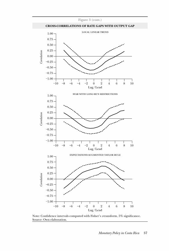
57Monetary Policy in Costa Rica
Figure 3 (cont.)
CROSS-CORRELATIONS OF RATE GAPS WITH OUTPUT GAP
Note: Confidence intervals computed with Fisher’s z-transform, 5% significance.Source: Own elaboration.
Lag/Lead
Lag/Lead
Lag/Lead
-
-
Cor
rela
tion
Cor
rela
tion
Cor
rela
tion
−1.00
−0.75
−0.50
−0.25
0.00
0.25
0.50
0.75
1.00
−10 −8 −6 −4 −2 0 2 4 6 8 10
−1.00
−0.75
−0.50
−0.25
0.00
0.25
0.50
0.75
1.00
−10 −8 −6 −4 −2 0 2 4 6 8 10
−1.00
−0.75
−0.50
−0.25
0.00
0.25
0.50
0.75
1.00
−10 −8 −6 −4 −2 0 2 4 6 8 10
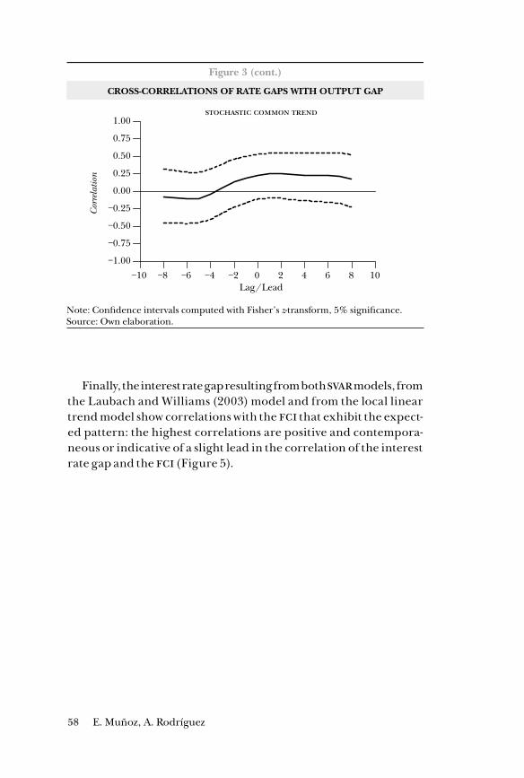
58 E. Muñoz, A. Rodríguez
Finally, the interest rate gap resulting from both svar models, from the Laubach and Williams (2003) model and from the local linear trend model show correlations with the fci that exhibit the expect-ed pattern: the highest correlations are positive and contempora-neous or indicative of a slight lead in the correlation of the interest rate gap and the fci (Figure 5).
Figure 3 (cont.)
CROSS-CORRELATIONS OF RATE GAPS WITH OUTPUT GAP
Note: Confidence intervals computed with Fisher’s z-transform, 5% significance.Source: Own elaboration.
Lag/Lead
Cor
rela
tion
−1.00
−0.75
−0.50
−0.25
0.00
0.25
0.50
0.75
1.00
−10 −8 −6 −4 −2 0 2 4 6 8 10
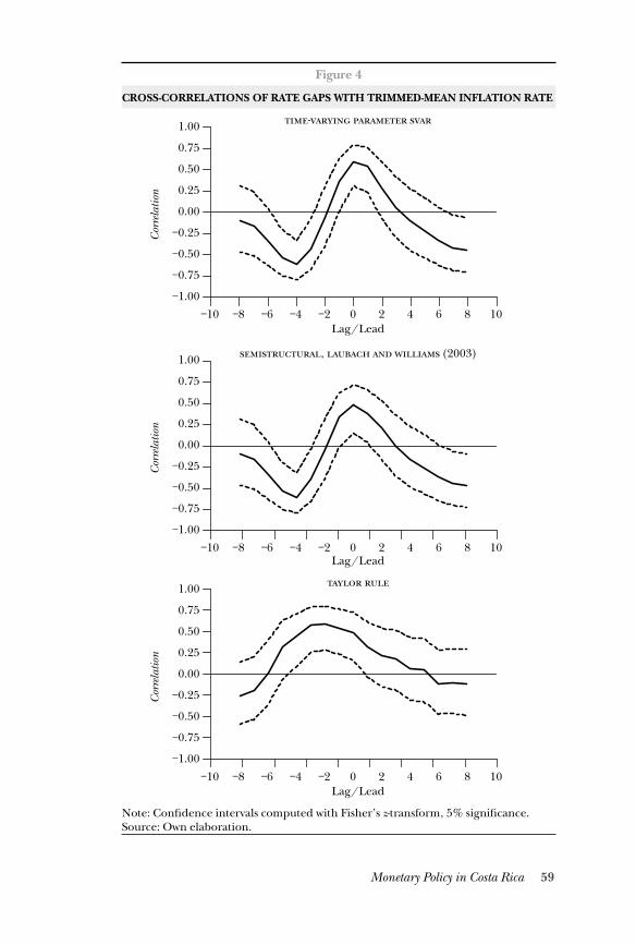
59Monetary Policy in Costa Rica
Figure 4
CROSS-CORRELATIONS OF RATE GAPS WITH TRIMMED-MEAN INFLATION RATE
Note: Confidence intervals computed with Fisher’s z-transform, 5% significance.Source: Own elaboration.
-
Lag/Lead
Lag/Lead
Lag/Lead
, (2003)
Cor
rela
tion
Cor
rela
tion
Cor
rela
tion
−1.00
−0.75
−0.50
−0.25
0.00
0.25
0.50
0.75
1.00
−10 −8 −6 −4 −2 0 2 4 6 8 10
−1.00
−0.75
−0.50
−0.25
0.00
0.25
0.50
0.75
1.00
−10 −8 −6 −4 −2 0 2 4 6 8 10
−1.00
−0.75
−0.50
−0.25
0.00
0.25
0.50
0.75
1.00
−10 −8 −6 −4 −2 0 2 4 6 8 10
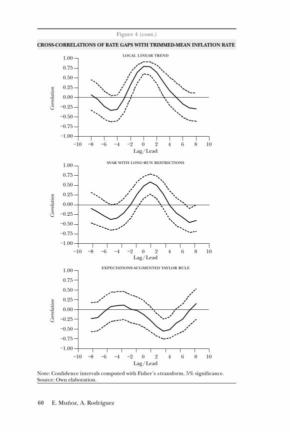
60 E. Muñoz, A. Rodríguez
Figure 4 (cont.)
CROSS-CORRELATIONS OF RATE GAPS WITH TRIMMED-MEAN INFLATION RATE
Note: Confidence intervals computed with Fisher’s z-transform, 5% significance.Source: Own elaboration.
Lag/Lead
Lag/Lead
Lag/Lead
-
-
Cor
rela
tion
Cor
rela
tion
Cor
rela
tion
−1.00
−0.75
−0.50
−0.25
0.00
0.25
0.50
0.75
1.00
−10 −8 −6 −4 −2 0 2 4 6 8 10
−1.00
−0.75
−0.50
−0.25
0.00
0.25
0.50
0.75
1.00
−10 −8 −6 −4 −2 0 2 4 6 8 10
−1.00
−0.75
−0.50
−0.25
0.00
0.25
0.50
0.75
1.00
−10 −8 −6 −4 −2 0 2 4 6 8 10
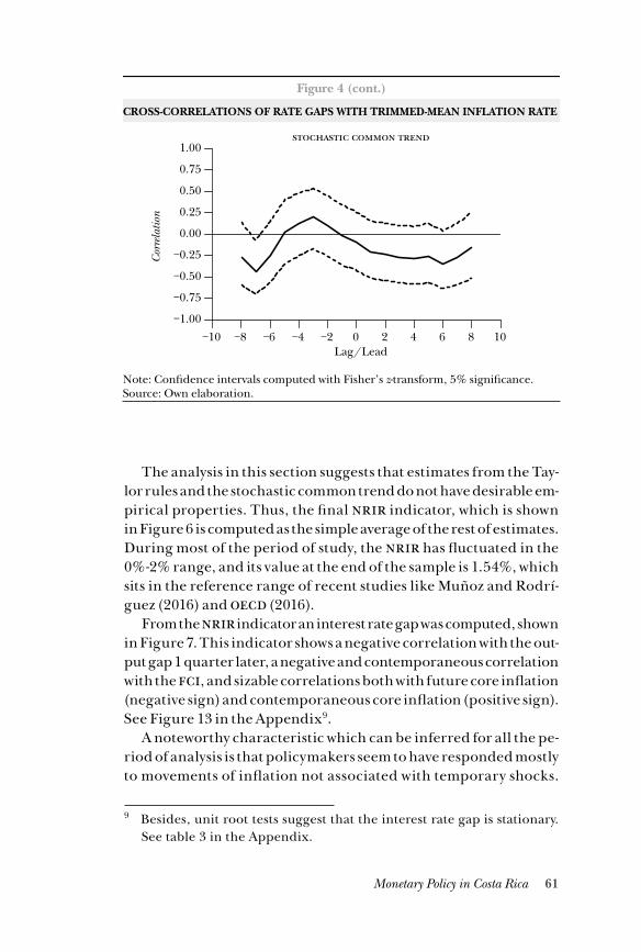
61Monetary Policy in Costa Rica
The analysis in this section suggests that estimates from the Tay-lor rules and the stochastic common trend do not have desirable em-pirical properties. Thus, the final nrir indicator, which is shown in Figure 6 is computed as the simple average of the rest of estimates. During most of the period of study, the nrir has fluctuated in the 0%-2% range, and its value at the end of the sample is 1.54%, which sits in the reference range of recent studies like Muñoz and Rodrí-guez (2016) and oecd (2016).
From the nrir indicator an interest rate gap was computed, shown in Figure 7. This indicator shows a negative correlation with the out-put gap 1 quarter later, a negative and contemporaneous correlation with the fci, and sizable correlations both with future core inflation (negative sign) and contemporaneous core inflation (positive sign). See Figure 13 in the Appendix9.
A noteworthy characteristic which can be inferred for all the pe-riod of analysis is that policymakers seem to have responded mostly to movements of inflation not associated with temporary shocks.
9 Besides, unit root tests suggest that the interest rate gap is stationary. See table 3 in the Appendix.
Figure 4 (cont.)
Note: Confidence intervals computed with Fisher’s z-transform, 5% significance.Source: Own elaboration.
CROSS-CORRELATIONS OF RATE GAPS WITH TRIMMED-MEAN INFLATION RATE
Lag/Lead
Cor
rela
tion
−1.00
−0.75
−0.50
−0.25
0.00
0.25
0.50
0.75
1.00
−10 −8 −6 −4 −2 0 2 4 6 8 10
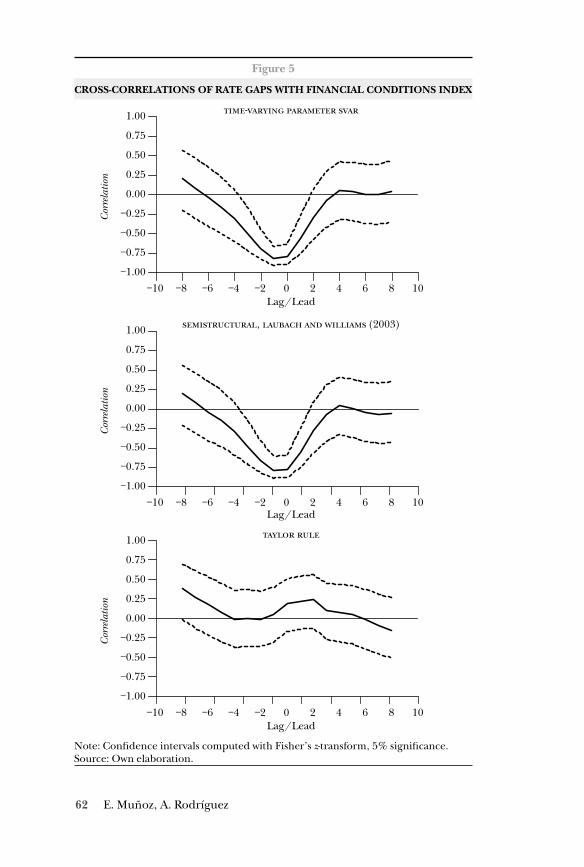
62 E. Muñoz, A. Rodríguez
Figure 5
CROSS-CORRELATIONS OF RATE GAPS WITH FINANCIAL CONDITIONS INDEX
Note: Confidence intervals computed with Fisher’s z-transform, 5% significance.Source: Own elaboration.
-
Lag/Lead
Lag/Lead
Lag/Lead
, (2003)
Cor
rela
tion
Cor
rela
tion
Cor
rela
tion
−1.00
−0.75
−0.50
−0.25
0.00
0.25
0.50
0.75
1.00
−10 −8 −6 −4 −2 0 2 4 6 8 10
−1.00
−0.75
−0.50
−0.25
0.00
0.25
0.50
0.75
1.00
−10 −8 −6 −4 −2 0 2 4 6 8 10
−1.00
−0.75
−0.50
−0.25
0.00
0.25
0.50
0.75
1.00
−10 −8 −6 −4 −2 0 2 4 6 8 10
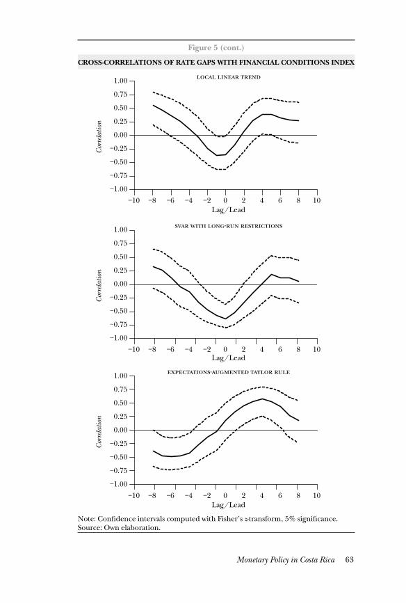
63Monetary Policy in Costa Rica
Figure 5 (cont.)
Note: Confidence intervals computed with Fisher’s z-transform, 5% significance.Source: Own elaboration.
CROSS-CORRELATIONS OF RATE GAPS WITH FINANCIAL CONDITIONS INDEX
Lag/Lead
Lag/Lead
Lag/Lead
-
-
Cor
rela
tion
Cor
rela
tion
Cor
rela
tion
−1.00
−0.75
−0.50
−0.25
0.00
0.25
0.50
0.75
1.00
−10 −8 −6 −4 −2 0 2 4 6 8 10
−1.00
−0.75
−0.50
−0.25
0.00
0.25
0.50
0.75
1.00
−10 −8 −6 −4 −2 0 2 4 6 8 10
−1.00
−0.75
−0.50
−0.25
0.00
0.25
0.50
0.75
1.00
−10 −8 −6 −4 −2 0 2 4 6 8 10
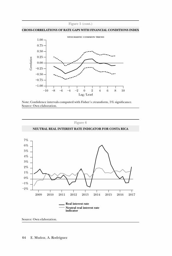
64 E. Muñoz, A. Rodríguez
Figure 5 (cont.)
Note: Confidence intervals computed with Fisher’s z-transform, 5% significance.Source: Own elaboration.
CROSS-CORRELATIONS OF RATE GAPS WITH FINANCIAL CONDITIONS INDEX
Lag/Lead
Cor
rela
tion
−1.00
−0.75
−0.50
−0.25
0.00
0.25
0.50
0.75
1.00
−10 −8 −6 −4 −2 0 2 4 6 8 10
Figure 6
NEUTRAL REAL INTEREST RATE INDICATOR FOR COSTA RICA
Source: Own elaboration.
−2%
−1%
0%
1%
2%
3%
4%
5%
6%
7%
2009 2010 2011 2012 2013 2014 2015 2016 2017
Real interest rateNeutral real interest rate indicator
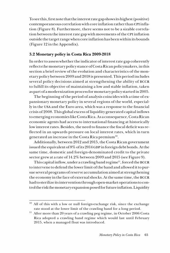
65Monetary Policy in Costa Rica
To see this, first note that the interest rate gap shows its highest (positive) contemporaneous correlation with core inflation rather than cpi infla-tion (Figure 8). Furthermore, there seems not to be a sizable correla-tion between the interest rate gap with movements of the cpi inflation outside the target range when core inflation has been within its bounds (Figure 12 in the Appendix).
3.2 Monetary policy in Costa Rica 2009-2018
In order to assess whether the indicator of interest rate gap coherently reflects the monetary policy stance of Costa Rican policymakers, in this section a brief review of the evolution and characteristics of the mon-etary policy between 2009 and 2018 is presented. This period includes several policy decisions aimed at strengthening the ability of bccr to fulfill its objective of maintaining a low and stable inflation, taken as part of a modernization process for monetary policy started in 2005.
The beginning of the period of analysis coincides with a time of ex-pansionary monetary policy in several regions of the world, especial-ly in the usa and the Euro area, which was a response to the financial crisis of 2008. This global excess of liquidity generated capital inflows to emerging economies like Costa Rica. As a consequence, Costa Rican economic agents had access to international financing at historically low interest rates. Besides, the need to finance the fiscal deficit was re-flected in an upwards pressure on local interest rates, which in turn generated an increase in the Costa Rica premium10.
Additionally, between 2012 and 2015, the Costa Rican government issued the equivalent of 8% of its 2014 gdp in foreign debt bonds. At the same time, domestic and foreign-denominated credit to the private sector grew at a rate of 14.2% between 2009 and 2015 (see Figure 9).
This capital inflow, under a crawling band regime11, forced the bccr to intervene to defend the lower limit of the band and allowed it to pur-sue several programs of reserve accumulation aimed at strengthening the economy in the face of external shocks. At the same time, the bccr had to sterilize its intervention through open-market operations to con-trol the risk the monetary expansion posed for future inflation. Liquidity
10 All of this with a low or null foreign-exchange risk, since the exchange rate stood at the lower limit of the crawling band for a long period.
11 After more than 20 years of a crawling peg regime, in October 2006 Costa Rica adopted a crawling band regime which would last until February 2015, when a managed float was introduced.
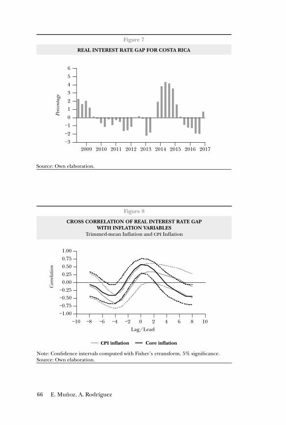
66 E. Muñoz, A. Rodríguez
Figure 7
REAL INTEREST RATE GAP FOR COSTA RICA
Source: Own elaboration.
543210
−1−2
6
−320162015201420132012201120102009 2017
Perc
enta
ge
Figure 8
CROSS CORRELATION OF REAL INTEREST RATE GAPWITH INFLATION VARIABLES
Trimmed-mean Inflation and Inflation
Note: Confidence intervals computed with Fisher’s z-transform, 5% significance.Source: Own elaboration.
Lag/Lead
cpi ination Core ination
Cor
rela
tion
−1.00−0.75−0.50−0.25
0.000.250.500.751.00
−10 −8 −6 −4 −2 0 2 4 6 8 10
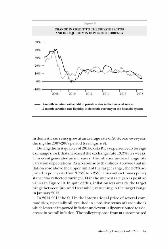
67Monetary Policy in Costa Rica
in domestic currency grew at an average rate of 20%, year-over-year, during the 2007-2009 period (see Figure 9).
During the first quarter of 2014 Costa Rica experienced a foreign exchange shock that increased the exchange rate 13.3% in 7 weeks. This event generated an increase in the inflation and exchange rate variation expectations. As a response to that shock, to avoid that in-flation rose above the upper limit of the target range, the bccr ad-justed its policy rate from 3.75% to 5.25%. This contractionary policy stance was reflected during 2014 in the interest rate gap as positive values in Figure 10. In spite of this, inflation was outside the target range between July and December, returning to the target range in January 2015.
In 2014-2015 the fall in the international price of several com-modities, especially oil, resulted in a positive terms-of-trade shock which lowered imported inflation and eventually contributed to a de-crease in overall inflation. The policy response from bccr comprised
Figure 9
CHANGE IN CREDIT TO THE PRIVATE SECTORAND IN LIQUIDITY IN DOMESTIC CURRENCY
12-month variation rate-credit to private sector in the nancial system
12-month variation rate-liquidity in domestic currency in the nancial system
−10%
0%
10%
20%
30%
40%
50%
2008 2010 2012 2014 2016 2018
68 E. Muñoz, A. Rodríguez
communication with the population to explain the transitory nature of the shock, along with gradual decreases in the monetary policy rate. During eleven months, between February 2015 and January 2016, eight adjustments to the rate were applied amounting to 350 b.p., leading this indicator to 1.75%. Coincidentally, from 2015Q2 until 2017Q3 inflation was below the target range, even showing negative values. In spite of this, the interest rate gap suggests that a contractionary monetary policy stance was in place until the end of 2015, which leads to question whether the cuts in the monetary policy rate could have been done less gradually and sooner.
The monetary policy rate was held at 1.75% for 15 months, from January 2016 until April 2017. During that time, international rate began to rise, which translated into a lower, even negative, premium for saving in domestic currency. This, along with a high and persis-tent fiscal deficit, brought incentives for economic agents to increase their relative preference for saving in dollars and at the same time to de-dollarize their debts.
In consequence, the bccr faced pressures in the FX market12, which in turn translated into expectations of higher exchange rate variation that could pass on to inflation expectations and ultimately to domes-tic prices. In order to restore the premium for saving in domestic cur-rency, it was decided to implement a gradual increase in the monetary policy rate, up to 300 b.p., between April and November 2017. Howev-er, the interest rate gap for this period still suggests a loose monetary policy stance during the first and second quarters of 2017 (Figure 10).
4. CONCLUSIONS
This study assesses the monetary policy stance for Costa Rica during the period 2009-2018 using an indicator of the real interest rate gap. This indicator is computed from a neutral real interest rate based on four estimates for which empirical coherence is evaluated. The val-ue of the neutral real interest rate for Costa Rica is estimated at 1.54%, in line with previous estimates.
The interest rate gap shows expected properties: negative correla-tion with future output gap, negative contemporaneous correlation
12 Several increases of the exchange rate were identified that were not co-herent with the long-run trajectory set by its fundamentals.
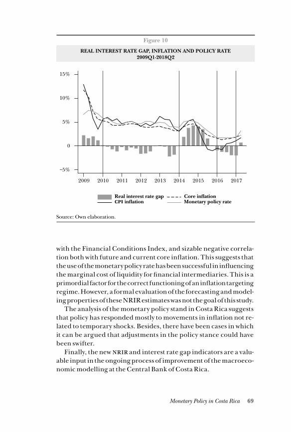
69Monetary Policy in Costa Rica
with the Financial Conditions Index, and sizable negative correla-tion both with future and current core inflation. This suggests that the use of the monetary policy rate has been successful in influencing the marginal cost of liquidity for financial intermediaries. This is a primordial factor for the correct functioning of an inflation targeting regime. However, a formal evaluation of the forecasting and model-ing properties of these NRIR estimates was not the goal of this study.
The analysis of the monetary policy stand in Costa Rica suggests that policy has responded mostly to movements in inflation not re-lated to temporary shocks. Besides, there have been cases in which it can be argued that adjustments in the policy stance could have been swifter.
Finally, the new nrir and interest rate gap indicators are a valu-able input in the ongoing process of improvement of the macroeco-nomic modelling at the Central Bank of Costa Rica.
Figure 10
REAL INTEREST RATE GAP, INFLATION AND POLICY RATE2009Q1-2018Q2
Source: Own elaboration.
Real interest rate gap cpi ination
Core ination Monetary policy rate
0
−5%
5%
15%
10%
2009 20172016201520142013201220112010
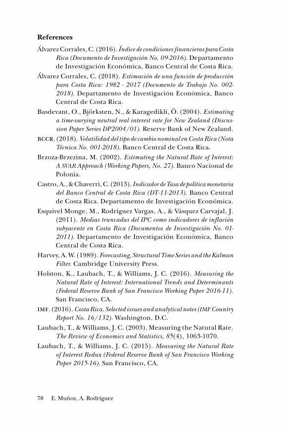
70 E. Muñoz, A. Rodríguez
References
Álvarez Corrales, C. (2016). Índice de condiciones financieras para Costa Rica (Documento de Investigación No. 09-2016). Departamento de Investigación Económica, Banco Central de Costa Rica.
Álvarez Corrales, C. (2018). Estimación de una función de producción para Costa Rica: 1982 - 2017 (Documento de Trabajo No. 002-2018). Departamento de Investigación Económica, Banco Central de Costa Rica.
Basdevant, O., Björksten, N., & Karagedikli, Ö. (2004). Estimating a time-varying neutral real interest rate for New Zealand (Discus-sion Paper Series DP2004/01). Reserve Bank of New Zealand.
bccr. (2018). Volatilidad del tipo de cambio nominal en Costa Rica (Nota Técnica No. 001-2018). Banco Central de Costa Rica.
Brzoza-Brzezina, M. (2002). Estimating the Natural Rate of Interest: A svar Approach (Working Papers, No. 27). Banco Nacional de Polonia.
Castro, A., & Chaverri, C. (2013). Indicador de Tasa de política monetaria del Banco Central de Costa Rica (DT-11-2013). Banco Central de Costa Rica. Departamento de Investigación Económica.
Esquivel Monge, M., Rodríguez Vargas, A., & Vásquez Carvajal, J. (2011). Medias truncadas del IPC como indicadores de inflación subyacente en Costa Rica (Documentos de Investigación No. 01-2011). Departamento de Investigación Económica, Banco Central de Costa Rica.
Harvey, A. W. (1989). Forecasting, Structural Time Series and the Kalman Filter. Cambridge University Press.
Holston, K., Laubach, T., & Williams, J. C. (2016). Measuring the Natural Rate of Interest: International Trends and Determinants (Federal Reserve Bank of San Francisco Working Paper 2016-11). San Francisco, CA.
imf. (2016). Costa Rica. Selected issues and analytical notes (imf Country Report No. 16/132). Washington, D.C.
Laubach, T., & Williams, J. C. (2003). Measuring the Natural Rate. The Review of Economics and Statistics, 85(4), 1063-1070.
Laubach, T., & Williams, J. C. (2015). Measuring the Natural Rate of Interest Redux (Federal Reserve Bank of San Francisco Working Paper 2015-16). San Francisco, CA.
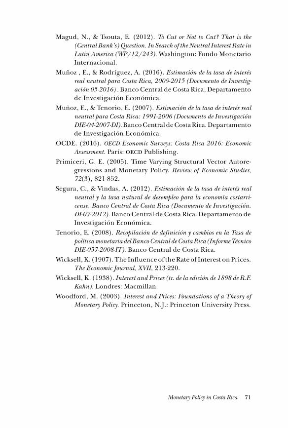
71Monetary Policy in Costa Rica
Magud, N., & Tsouta, E. (2012). To Cut or Not to Cut? That is the (Central Bank’s) Question. In Search of the Neutral Interest Rate in Latin America (WP/12/243). Washington: Fondo Monetario Internacional.
Muñoz , E., & Rodríguez, A. (2016). Estimación de la tasa de interés real neutral para Costa Rica, 2009-2015 (Documento de Investig-ación 05-2016) . Banco Central de Costa Rica, Departamento de Investigación Económica.
Muñoz, E., & Tenorio, E. (2007). Estimación de la tasa de interés real neutral para Costa Rica: 1991-2006 (Documento de Investigación DIE-04-2007-DI). Banco Central de Costa Rica. Departamento de Investigación Económica.
OCDE. (2016). oecd Economic Surveys: Costa Rica 2016: Economic Assessment. París: oecd Publishing.
Primiceri, G. E. (2005). Time Varying Structural Vector Autore-gressions and Monetary Policy. Review of Economic Studies, 72(3), 821-852.
Segura, C., & Vindas, A. (2012). Estimación de la tasa de interés real neutral y la tasa natural de desempleo para la economía costarri-cense. Banco Central de Costa Rica (Documento de Investigación. DI-07-2012). Banco Central de Costa Rica. Departamento de Investigación Económica.
Tenorio, E. (2008). Recopilación de definición y cambios en la Tasa de política monetaria del Banco Central de Costa Rica (Informe Técnico DIE-037-2008-IT). Banco Central de Costa Rica.
Wicksell, K. (1907). The Influence of the Rate of Interest on Prices. The Economic Journal, XVII, 213-220.
Wicksell, K. (1938). Interest and Prices (tr. de la edición de 1898 de R.F. Kahn). Londres: Macmillan.
Woodford, M. (2003). Interest and Prices: Foundations of a Theory of Monetary Policy. Princeton, N.J.: Princeton University Press.
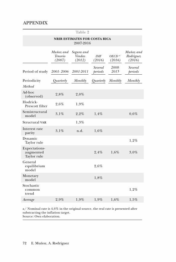
72 E. Muñoz, A. Rodríguez
APPENDIX
Table 2
NRIR ESTIMATES FOR COSTA RICA2007-2016
Muñoz and Tenorio (2007)
Segura and Vindas (2012)
imf (2016)
oecd a/ (2016)
Muñoz and Rodríguez
(2016)
Period of study 2001- 2006 2001-2011Several periods
2008-2015
Several periods
Periodicity Quarterly Monthly Quarterly Monthly Monthly
Method
Ad-hoc (observed) 2,8% 2,0%
Hodrick-Prescott filter 2,6% 1,9%
Semistructural model 3,1% 2,2% 1,4% 0,6%
Structural var 1,3%
Interest rate parity 3,1% n.d. 1,6%
Dynamic Taylor rule 1,2%
Expectations-augmented Taylor rule
2,4% 1,6% 3,0%
General equilibrium model
2,6%
Monetary model 1,8%
Stochastic common trend
1,2%
Average 2,9% 1,9% 1,9% 1,6% 1,5%
a/ Nominal rate is 4,6% in the original source, the real rate is presented after substracting the inflation target.Source: Own elaboration.
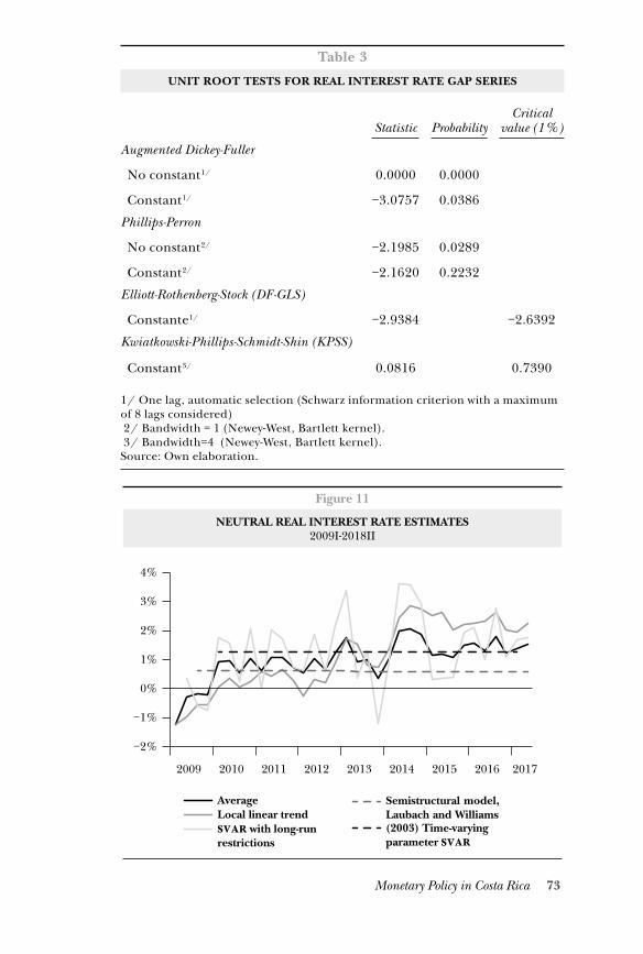
73Monetary Policy in Costa Rica
Table 3
UNIT ROOT TESTS FOR REAL INTEREST RATE GAP SERIES
Statistic ProbabilityCritical
value (1%)
Augmented Dickey-Fuller
No constant1/ 0.0000 0.0000
Constant1/ −3.0757 0.0386
Phillips-Perron
No constant2/ −2.1985 0.0289
Constant2/ −2.1620 0.2232
Elliott-Rothenberg-Stock (DF-GLS)
Constante1/ −2.9384 −2.6392
Kwiatkowski-Phillips-Schmidt-Shin (KPSS)
Constant3/ 0.0816 0.7390
1/ One lag, automatic selection (Schwarz information criterion with a maximum of 8 lags considered) 2/ Bandwidth = 1 (Newey-West, Bartlett kernel). 3/ Bandwidth=4 (Newey-West, Bartlett kernel).Source: Own elaboration.
Figure 11
NEUTRAL REAL INTEREST RATE ESTIMATES2009I-2018II
AverageLocal linear trendsvar with long-runrestrictions
Semistructural model,Laubach and Williams (2003) Time-varyingparameter svar
−2%
−1%
0%
1%
2%
3%
4%
2009 2010 2011 2012 2013 2014 2015 2016 2017
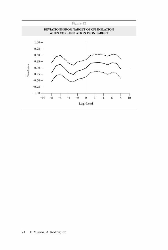
74 E. Muñoz, A. Rodríguez
Figure 12
DEVIATIONS FROM TARGET OF CPI INFLATIONWHEN CORE INFLATION IS ON TARGET
Lag/Lead
Cor
rela
tion
−1.00
−0.75
−0.50
−0.25
0.00
0.25
0.50
0.75
1.00
−10 −8 −6 −4 −2 0 2 4 6 8 10
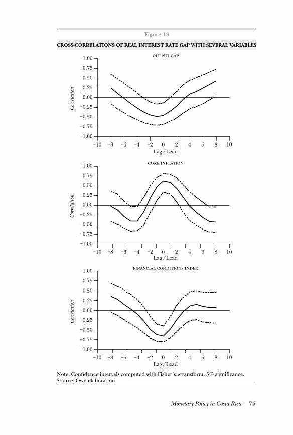
75Monetary Policy in Costa Rica
Figure 13
CROSS-CORRELATIONS OF REAL INTEREST RATE GAP WITH SEVERAL VARIABLES
Note: Confidence intervals computed with Fisher’s z-transform, 5% significance.Source: Own elaboration.
Lag/Lead
Lag/Lead
Lag/Lead
Cor
rela
tion
Cor
rela
tion
Cor
rela
tion
−1.00
−0.75
−0.50
−0.25
0.00
0.25
0.50
0.75
1.00
−10 −8 −6 −4 −2 0 2 4 6 8 10
−1.00
−0.75
−0.50
−0.25
0.00
0.25
0.50
0.75
1.00
−10 −8 −6 −4 −2 0 2 4 6 8 10
−1.00
−0.75
−0.50
−0.25
0.00
0.25
0.50
0.75
1.00
−10 −8 −6 −4 −2 0 2 4 6 8 10
76 F. Álvarez
Long Term Neutral Real Interest Rate for Honduras
Fredy Fernando Álvarez
Abstract
The purpose of this document is to present a first estimate of the Neutral or Natural Real Interest Rate (nrir) for Honduras, which is defined as the unobservable interest rate consistent with the potential Gross Domestic Product (gdp) of an economy and with an unemployment rate that does not accelerate inflation (nairu); therefore serves as a reference for the analysis of the monetary policy stance of central banks. For its measure-ment, quarterly information is used for the 2005-2016 period, using several method-ologies that although they differ in their approach, they do not present much variation in their results. On the other hand, because there is not a consensus on which is the most appropriate technique, the methodologies used for the estimations for Honduras are selected on the basis of the available information for the country. Therefore, the reults are obtained using: the average of the ex ante real interest rate for a long period in which inflation behaved relatively stable; the Hodrick-Prescott (hp) filter to extract the trend of the real interest rate; and the Baxter and King filter (bk) to extract the cyclical ele-ment from a series. In addition, an estimate is obtained from the uncovered interest rate parity condition and from a semi-structural model using the Kalman filter adapted to the conditions of the Honduran economy. The estimates obtained from these differ-ent techniques reveal an average for the period analyzed for the Neutral Interest Rate in current values between 6.69% to 8.08% and in real values from 0.77% to 2.16%; similarly, it is found that in recent years the interest rate has shown a gradual decrease associated in part to a lower Monetary Policy Rate (mpr), combined with low levels of inflation and relatively stable economic growth.
The expressed in this document is exclusive responsibility of the author and does not necessarily represent the opinion of the Central Bank of Honduras.
77Long Term Neutral Real Interest Rate for Honduras
1. INTRODUCTION
The nrir is a term widely discussed within the context of central banks, mainly because it is consistent with a level of potential output and a stable inflation rate; according to Wicksell (1898)
in the economy there is an interest rate that is neutral to prices, that is to say, one that does not tend to decrease or increase the level of prices and that serves to identify if the monetary policy stance is contractionary, when the real interest rate is above the neutral rate or if it is expansionary, when it is below, thus influencing the decision making of the monetary authority.
The estimation of this variable is not so simple, because it is not ob-servable, varies over time, and is related to the long-term evolution and real characteristics of the economy; however, there are different ways to approach it, either through the behavior of certain financial variables or using semi-structural models that describe the evolution of the economy and estimate the equilibrium interest rate.
In this document, we estimate the neutral rate for Honduras, us-ing quarterly information for the period 2005Q2-2016Q4 and im-plementing five different methodologies. The first one considers the analysis of the trend of the ex ante real interest rate registered during a period of relative inflation stability; two different univari-ate analysis, one consisting of extracting the trend of the series from the real interest rate through the hp filter and the other using the bk filter to extract the cyclical element from the series in which season-al components (short term) and the trend component (long term) are eliminated. The remaining methods are based on multivariate analysis, one is under the condition of uncovered interest rate par-ity for a small economy which is open to international trade and the other is a semi-structural model proposed by Laubach and Williams (2001) for the United States of America (usa) adapted to the Hondu-ran economy (method in which the algorithm of the Kalman filter is used, under a stage of state space used for approximations of non-observable variables).
The research is structured as follows: Section 2 reviews the liter-ature and empirical evidence under different approaches; Section 3 shows the methodologies used in the estimation; Section 4 analyzes the results obtained and their comparison between methodologies;
78 F. Álvarez
finally, sections 5, 6 and 7 present the conclusions, appendices, and bibliography, in this order.
2. REVIEW OF LITERATURE AND EMPIRICAL EVIDENCE
2.1 Review of Literature
According to the literature available, the nrir is known under dif-ferent concepts, such as the neutral real interest rate, natural inter-est rate, or the equilibrium real interest rate; the name has also been differentiated according to the time periods or horizons, either short or long term. However, the notion of the natural rate goes back to the late nineteenth century, when Knut Wicksell argued that the ob-served interest rate did not necessarily balance supply and demand in the market, since it was normal to see increases and decreases in the level of prices when there are differences between the observed in-terest rate and what would be a neutral interest rate that stabilizes the market. Wicksell (1898) commented that the nrir was by defi-nition, that which did not cause pressures of movement neither up-wards nor downwards in prices.
On the other hand, Archibald and Hunter (2001) stated that the long-term equilibrium real interest rate is the most stable, with which the economy and markets are balanced. Because it is often dif-ficult to capture a state of equilibrium, the neutral rate is the proxy that guides the goods, money, and labor markets, and that is consis-tent with production, inflation and potential output1.
Under the context of neo-Keynesian general equilibrium mod-els, the natural rate is the level of real interest rate that would prevail in equilibrium under the absence of nominal rigidities (Galí, 2002). This is equivalent to saying that the nrir is the appropriate interest rate to maintain the level of aggregate demand on par with the po-tential product, once the transitory effects of the economy cease (Blinder, 1999). The New Keynesians associate it with the steady state or long-term interest rate.
Laubach and Williams (2003) found for the usa an explicit rela-tionship between the nrir and the trend growth rate of the potential
1 Laubach and Williams (2003), Garnier and Wilhelmsen (2005).
79Long Term Neutral Real Interest Rate for Honduras
output. All this after estimating several equations such as the IS and Phillips curve, among others, by means of the maximum likelihood method using the Kalman filter, concluding in the end that the nat-ural rate varies with time.
In an attempt to answer the question of how the central bank should conduct monetary policy in practice, given the objective of achiev-ing low and stable inflation rates and reaching full employment, Or-phanides and Williams (2002) estimated the nrir specifying that this it is compatible with the natural rate of unemployment and with low and stable inflation. Likewise, they conclude that the natural rate varies with time, since it is likely to be influenced by variables such as fiscal policy and household preferences.
Finally, Brzoza-Brzezinay and Kotlowski (2012), affirm that the es-timates of the nrir, given its applicability to a monetary policy re-gime under inflation targeting, have contributed to achieving price stability.
2.2 Empirical Evidence
There are several methods for estimating the neutral interest rate, whose results differ among them, given certain limitations depend-ing on the amount of information required, which are applicable according to the economic conditions of each country. However, de-spite this, they help estimate this indicator, which is a relevant tool for conducting and making monetary policy decisions.
One of the most important researchs available for the nrir is car-ried out by Laubach and Williams (2001 and 2003) for the usa, us-ing a Kalman filter to jointly determine the neutral real interest rate, the potential output, and the growth trend; emphasizing that the variations in the growth trend are a determining factor in the movements of the rate. In addition, they demonstrated that the vari-ations of the neutral real interest rate have important implications in the design and implementation of monetary policy, since the ad-justments in this rate are crucial for the fulfillment of the stabiliza-tion goals in both the short and the long term.
Fuentes & Gredig (2007) rely on several methods to obtain the neu-tral interest rate for Chile, the first through the economic theory im-plicit in the prices of financial assets and through statistical models using macroeconomic data; followed by a semi-structural model with unobservable components through the Kalman filter algorithm,
80 F. Álvarez
allowing the latter to simultaneously estimate the natural real inter-est rate and the output gap.
On the other hand, González, Ocampo, Pérez, and Rodríguez (2013) use different methodologies to estimate the nrir for Colom-bia, two of which are based on statistical filters and the third is the estimation of a semi-structural model for a small and open econo-my. Neiss and Nelson (2001) examine the properties of the neutral real interest rate using a dynamic stochastic general equilibrium (dsge) model. Cartaya, Fleitas, and Vivas (2007) measure this in-dicator for the Venezuelan economy, based on the marginal pro-ductivity of capital and in another case taking into account the gap and the potential growth of the non-oil product; it is demonstrated that under both approaches the neutral real interest rate shows very little variability during the estimation period, in comparison with the observed values.
Similarly, Giammarioli, and Valla (2003) made estimates for the Euro Zone with a model that contains historical series of the short-term interest rate. These authors argue that the nrir in the area has gradually decreased since the mid-1990s, from around 4.0% to approximately 3.0% in 2000.
As a final point, Table 1 shows the different methodologies and re-sults obtained by several countries when calculating the nrir.
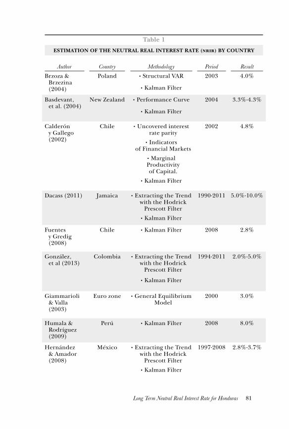
81Long Term Neutral Real Interest Rate for Honduras
Table 1
ESTIMATION OF THE NEUTRAL REAL INTEREST RATE (nrir) BY COUNTRY
Author Country Methodology Period ResultBrzoza &
Brzezina (2004)
Poland • Structural VAR 2003 4.0%
• Kalman Filter
Basdevant, et al. (2004)
New Zealand • Performance Curve 2004 3.3%-4.3%
• Kalman Filter
Calderón y Gallego (2002)
Chile • Uncovered interest rate parity
2002 4.8%
• Indicators of Financial Markets
• Marginal Productivity of Capital.
• Kalman Filter
Dacass (2011) Jamaica • Extracting the Trend with the Hodrick
Prescott Filter
1990-2011 5.0%-10.0%
• Kalman Filter
Fuentes y Gredig (2008)
Chile • Kalman Filter 2008 2.8%
González, et al (2013)
Colombia • Extracting the Trend with the Hodrick
Prescott Filter
1994-2011 2.0%-5.0%
• Kalman Filter
Giammarioli & Valla (2003)
Euro zone • General Equilibrium Model
2000 3.0%
Humala & Rodríguez (2009)
Perú • Kalman Filter 2008 8.0%
Hernández & Amador (2008)
México • Extracting the Trend with the Hodrick
Prescott Filter
1997-2008 2.8%-3.7%
• Kalman Filter
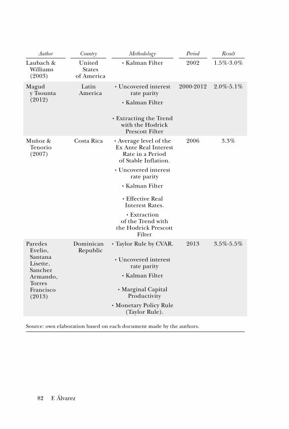
82 F. Álvarez
Author Country Methodology Period ResultLaubach &
Williams (2003)
United States
of America
• Kalman Filter 2002 1.5%-3.0%
Magud y Tsounta (2012)
Latin America
• Uncovered interest rate parity
2000-2012 2.0%-5.1%
• Kalman Filter
• Extracting the Trend with the Hodrick
Prescott Filter
Muñoz & Tenorio (2007)
Costa Rica • Average level of the Ex Ante Real Interest
Rate in a Period of Stable Inflation.
2006 3.3%
• Uncovered interest rate parity
• Kalman Filter
• Effective Real Interest Rates.
• Extraction of the Trend with
the Hodrick Prescott Filter
Paredes Evelio, Santana Lisette, Sanchez Armando, Torres Francisco (2013)
Dominican Republic
• Taylor Rule by CVAR. 2013 3.5%-5.5%
• Uncovered interest rate parity
• Kalman Filter
• Marginal Capital Productivity
• Monetary Policy Rule (Taylor Rule).
Source: own elaboration based on each document made by the authors.
83Long Term Neutral Real Interest Rate for Honduras
3.ESTIMATIONS METHODOLOGIES
According to the empirical evidence, the methods widely used to ob-tain an unobservable variable such as the nrir are the hp and Kal-man filters, since they have the advantage of detecting structural changes or large shocks that may occur in the economy; however, there is no consensus on which of the different methods available is the most appropriate and therefore analysis are carried out with several approaches in order to have a better estimate.
As a result of the above, in order to obtain the nrir of Honduras, the following methodologies are used:
• Average of the ex ante real interest rate for periods of stable inflation.
• Extraction of the trend through the hp filter.
• Baxter and King bandpass filter.
• Uncovered interest rate parity.
• Semi-structural model using the Kalman filter.
3.1 Average of the ex ante real interest rate for periods of stable inflation
When considering the nrir as an unobservable variable, Laubach and Williams (LW) (2001) argue that, as a first approximation, it can be obtained from the average of the ex ante real interest rate (rir), which is calculated as the difference between the monetary policy interest rate and inflation expectations, for a period where infla-tion is relatively stable. However, this approach has its weaknesses, such as the values used for inflation expectations and that it does not consider the variability of the rir observed over time; but, even so, it is used to establish comparisons with the results found with other methodologies.
3.2 Extraction of the trend through the hp filter
Under this approach, Hodrick and Prescott propose the separation of a time series in its trend component (using this as a proxy of the natural-level of the series) and cyclical component, carefully se-lecting the basic lambda smoothing parameter to obtain favorable
84 F. Álvarez
results. Like the previous method, it provides good estimates in pe-riods of stable inflation and output growth; nevertheless, it does not provide a good estimation when inflation is more volatile since it tends to underestimate the neutral rate for periods when inflation increases and overestimate it when inflation decreases.
3.3 Baxter and King bandpass filter
This method extracts the components of a series, whose frequency is within a certain time range, into very slow or low frequency move-ments (trend), medium components (cycle), and high frequency components (seasonal). Baxter and King (1999) argue that the per-fect filter is one that remains unchanged during a certain time in-terval, in which the density at all other frequencies is almost zero. This allows us to identify a route that the filter considers appropri-ate and to see if the estimated variable, in this case the nrir, is near or far from the values expected by the filter.
3.4 Uncovered interest rate parity
In a small and open economy, the long-term equilibrium interest rate should not move away from the international interest rate, according to Calderón and Gallego (2002), since free goods trade would pro-mote equal capital returns between nations and in the same way with the international interest rate. In this sense, we have:
NRIR = r *+E(e)+ ρ
Being (r*) the external real interest rate, E(e) the expectations of real depreciation and ρ( ) the country risk premium. The equation described above is understood as the rate at which investors are in-different between maintaining their financial assets in their country or abroad. Something very important is that the parity of real inter-est rates adjusted to country risk establishes relations - both short and long term - between the national real interest rate and the inter-national real interest rate.
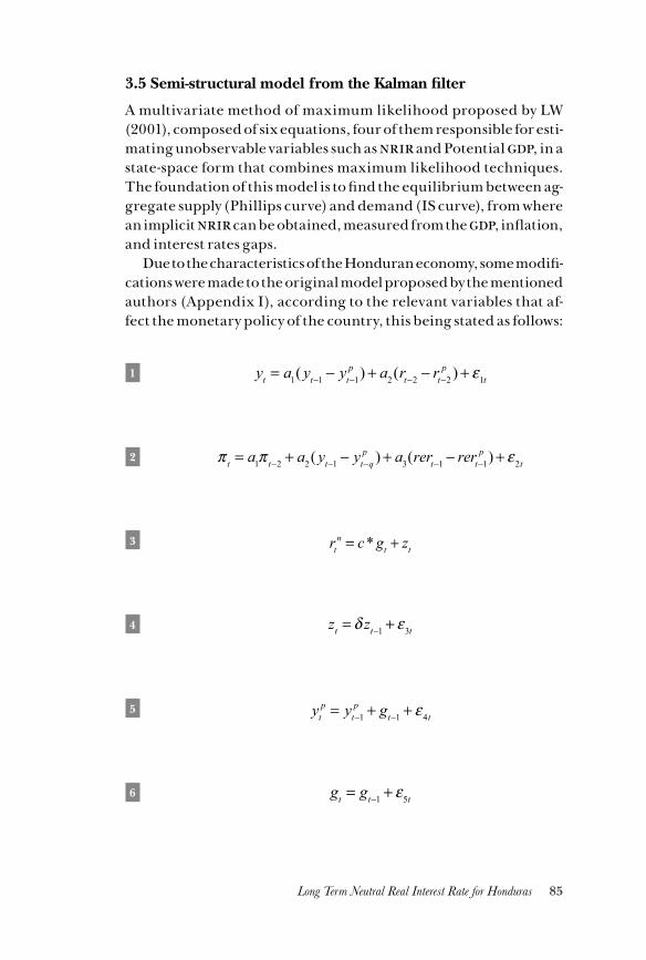
85Long Term Neutral Real Interest Rate for Honduras
3.5 Semi-structural model from the Kalman filter
A multivariate method of maximum likelihood proposed by LW (2001), composed of six equations, four of them responsible for esti-mating unobservable variables such as nrir and Potential gdp, in a state-space form that combines maximum likelihood techniques. The foundation of this model is to find the equilibrium between ag-gregate supply (Phillips curve) and demand (IS curve), from where an implicit nrir can be obtained, measured from the gdp, inflation, and interest rates gaps.
Due to the characteristics of the Honduran economy, some modifi-cations were made to the original model proposed by the mentioned authors (Appendix I), according to the relevant variables that af-fect the monetary policy of the country, this being stated as follows:
1 yt = a1( yt−1 − yt−1p )+ a2(rt−2 − rt−2
p )+ ε1t
2 π t = a1π t−2 + a2( yt−1 − yt−qp )+ a3(rert−1 − rert−1
p )+ ε2t
3 rtn = c* gt + zt
4 zt = δ zt−1 + ε3t
5 ytp = yt−1
p + gt−1 + ε4t
6 gt = gt−1 + ε5t
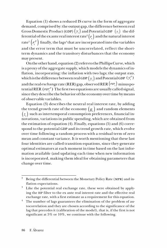
86 F. Álvarez
Equation (1) shows a reduced IS curve in the form of aggregate demand, comprised by: the output gap, the difference between real Gross Domestic Product (gdp) yt( ) and Potential gdp yt( ) the dif-ferential of the ex ante real interest rate2 rt( ) and the natural interest
rate3 rtp( ) finally, the lags4 that are incorporated into the variables
and the error term that must be uncorrelated, ref lect the short-term dynamics and the transitory disturbances that the economy may present.
On the other hand, equation (2) refers to the Phillips Curve, which is a proxy of the aggregate supply, which models the dynamics of in-flation, incorporating: the inflation with two lags; the output gap, which is the difference between real gdp yt( ) and Potential gdp ( yt
p )
and the real exchange rate (RER) gap, observed RER rert( ) minus po-tential RER (rert
p ) The first two equations are usually called signal, since they describe the behavior of the economy over time by means of observable variables.
Equation (3) describes the neutral real interest rate, by adding the trend growth rate of the economy gt( ) and random elements zt( ) such as intertemporal consumption preferences, financial in-
novations, variations in public spending, which are obtained from the estimation of equation (4). Finally, equations (5) and (6) corre-spond to the potential gdp and its trend growth rate, which evolve over time following a random process with a residual term of zero mean and constant variance. It is worth mentioning that these last four identities are called transition equations, since they generate optimal estimators at each moment in time based on the last infor-mation available (and updating each time when new information is incorporated, making them ideal for obtaining parameters that change over time.
2 Being the differential between the Monetary Policy Rate (mpr) and in-flation expectations.
3 Like the potential real exchange rate, these were obtained by apply-ing the hp filter to the ex ante real interest rate and the effective real exchange rate, with a first estimate as a requirement for this equation.
4 The number of lags guarantees the elimination of the problem of au-tocorrelation and they are chosen according to the significance of the lag that precedes it (calibration of the model), that is, if the first is not significant at 5% or 10%, we continue with the following.
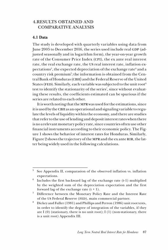
87Long Term Neutral Real Interest Rate for Honduras
4.RESULTS OBTAINED AND COMPARATIVE ANALYSIS
4.1 Data
The study is developed with quarterly variables using data from June 2005 to December 2016, the series used include real gdp (ad-justed seasonally and in logarithm form), the year-on-year growth rate of the Consumer Price Index (cpi), the ex ante real interest rate, the real exchange rate, the us real interest rate, inflation ex-pectations5, the expected depreciation of the exchange rate6 and a country risk premium7; the information is obtained from the Cen-tral Bank of Honduras (cbh) and the Federal Reserve of the United States (fed). Similarly, each variable was subjected to the unit root8 test to identify the stationarity of the series’, since without evaluat-ing these results, the coefficients estimated can be spurious if the series are related to each other.
It is worth noting that the mpr was used for the estimations, since it is used by the cbh as an operational and signaling variable to regu-late the levels of liquidity within the economy, and there are studies that refer to the use of lending and deposit interest rates when there is no a relevant monetary policy rate, since countries often use other financial instruments according to their economic policy. The Fig-ure 1 shows the behavior of interest rates for Honduras. Similarly, Figure 2 shows the trajectory of the mpr and the ex ante rir, the lat-ter being widely used in the following calculations.
5 See Appendix II, comparasion of the observed inflation vs. inflation expectations.
6 Includes the first backward lag of the exchange rate (t-1) multiplied by the weighted sum of the depreciation expectation and the first forward lag of the exchange rate (t + 1).
7 Difference between the Monetary Policy Rate and the Interest Rate of the us Federal Reserve (fed), main commercial partner.
8 Dickey and Fuller (1981) and Phillips and Perron (1986) unit root tests, in order to identify the degree of integration of the variables, if they are I (0) (stationary, there is no unit root); I (1) (non-stationary, there is a unit root) Appendix III.
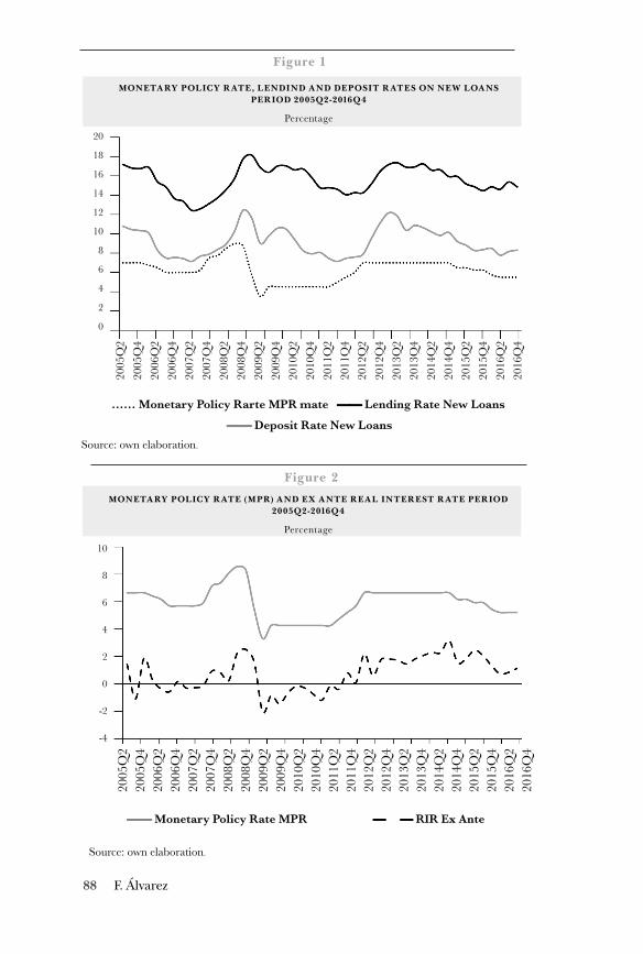
88 F. Álvarez
…… Monetary Policy Rarte MPR mate —— Lending Rate New Loans
—— Deposit Rate New Loans
20
18
16
14
12
10
8
6
4
2
0
2005
Q2
2005
Q4
2006
Q2
2006
Q4
2007
Q2
2007
Q4
2008
Q2
2008
Q4
2009
Q2
2009
Q4
2010
Q2
2010
Q4
2011
Q2
2011
Q4
2012
Q2
2012
Q4
2013
Q2
2013
Q4
2014
Q2
2014
Q4
2015
Q2
2015
Q4
2016
Q2
2016
Q4
Figure 1
Source: own elaboration.
MONETARY POLICY RATE, LENDIND AND DEPOSIT RATES ON NEW LOANS PERIOD 2005Q2-2016Q4
Percentage
—— Monetary Policy Rate MPR — — RIR Ex Ante
Figure 2
Source: own elaboration.
10
8
6
4
2
0
-2
-4
MONETARY POLICY RATE (MPR) AND EX ANTE REAL INTEREST RATE PERIOD 2005Q2-2016Q4
Percentage
2005
Q2
2005
Q4
2006
Q2
2006
Q4
2007
Q2
2007
Q4
2008
Q2
2008
Q4
2009
Q2
2009
Q4
2010
Q2
2010
Q4
2011
Q2
2011
Q4
2012
Q2
2012
Q4
2013
Q2
2013
Q4
2014
Q2
2014
Q4
2015
Q2
2015
Q4
2016
Q2
2016
Q4
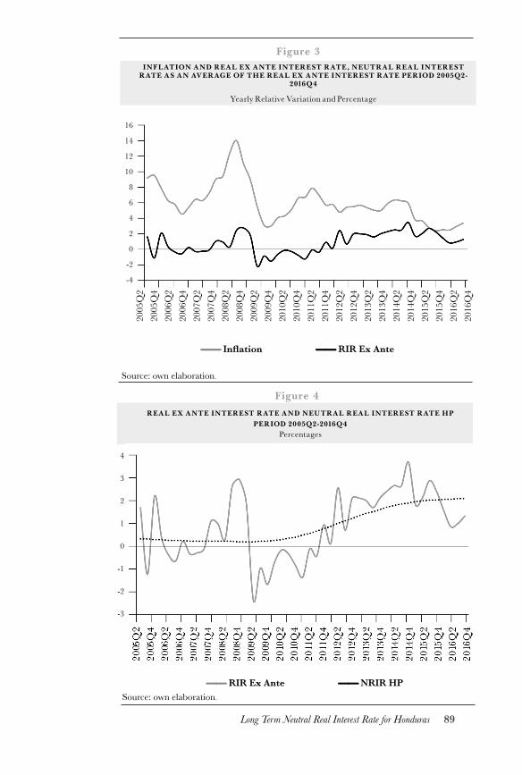
89Long Term Neutral Real Interest Rate for Honduras
REAL EX ANTE INTEREST RATE AND NEUTRAL REAL INTEREST RATE HPPERIOD 2005Q2-2016Q4
Percentages
Figure 3INFLATION AND REAL EX ANTE INTEREST RATE, NEUTRAL REAL INTEREST
RATE AS AN AVERAGE OF THE REAL EX ANTE INTEREST RATE PERIOD 2005Q2-2016Q4
Yearly Relative Variation and Percentage
16
14
12
10
8
6
4
2
0
-2
-4
2005
Q2
2005
Q4
2006
Q2
2006
Q4
2007
Q2
2007
Q4
2008
Q2
2008
Q4
2009
Q2
2009
Q4
2010
Q2
2010
Q4
2011
Q2
2011
Q4
2012
Q2
2012
Q4
2013
Q2
2013
Q4
2014
Q2
2014
Q4
2015
Q2
2015
Q4
2016
Q2
2016
Q4
Figure 4
—— Inflation —— RIR Ex Ante
Source: own elaboration.
4
3
2
1
0
-1
-2
-3
—— RIR Ex Ante —— NRIR HPSource: own elaboration.
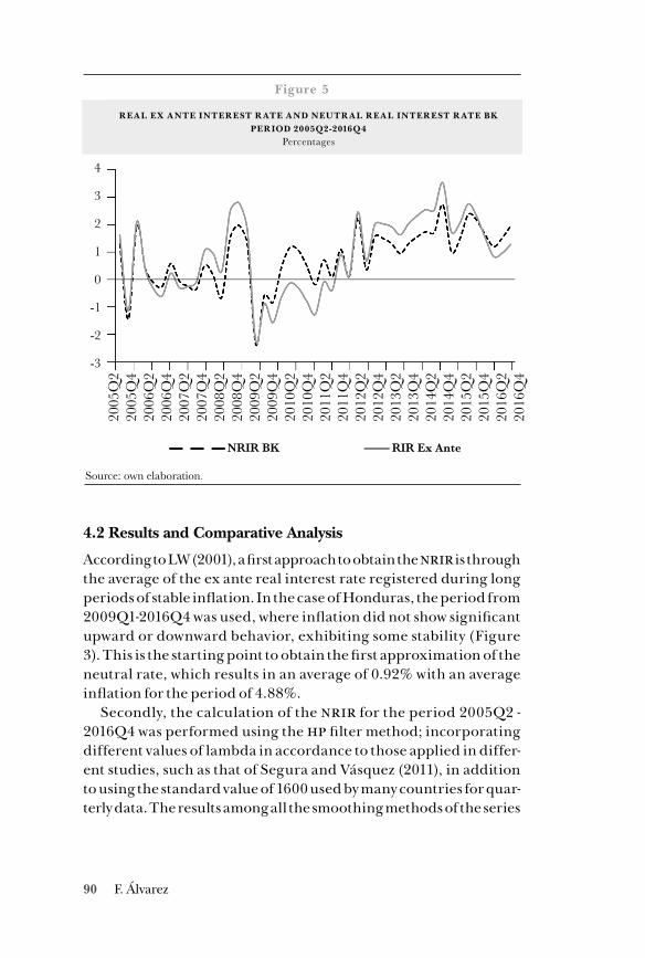
90 F. Álvarez
4.2 Results and Comparative Analysis
According to LW (2001), a first approach to obtain the nrir is through the average of the ex ante real interest rate registered during long periods of stable inflation. In the case of Honduras, the period from 2009Q1-2016Q4 was used, where inflation did not show significant upward or downward behavior, exhibiting some stability (Figure 3). This is the starting point to obtain the first approximation of the neutral rate, which results in an average of 0.92% with an average inflation for the period of 4.88%.
Secondly, the calculation of the nrir for the period 2005Q2 - 2016Q4 was performed using the hp filter method; incorporating different values of lambda in accordance to those applied in differ-ent studies, such as that of Segura and Vásquez (2011), in addition to using the standard value of 1600 used by many countries for quar-terly data. The results among all the smoothing methods of the series
REAL EX ANTE INTEREST RATE AND NEUTRAL REAL INTEREST RATE BKPERIOD 2005Q2-2016Q4
Percentages
2005
Q2
2005
Q4
2006
Q2
2006
Q4
2007
Q2
2007
Q4
2008
Q2
2008
Q4
2009
Q2
2009
Q4
2010
Q2
2010
Q4
2011
Q2
2011
Q4
2012
Q2
2012
Q4
2013
Q2
2013
Q4
2014
Q2
2014
Q4
2015
Q2
2015
Q4
2016
Q2
2016
Q4
4
3
2
1
0
-1
-2
-3
— — — NRIR BK —— RIR Ex Ante
Source: own elaboration.
Figure 5
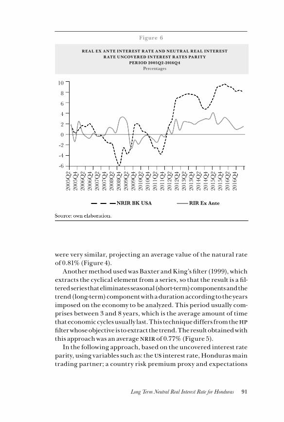
91Long Term Neutral Real Interest Rate for Honduras
were very similar, projecting an average value of the natural rate of 0.81% (Figure 4).
Another method used was Baxter and King’s filter (1999), which extracts the cyclical element from a series, so that the result is a fil-tered series that eliminates seasonal (short-term) components and the trend (long-term) component with a duration according to the years imposed on the economy to be analyzed. This period usually com-prises between 3 and 8 years, which is the average amount of time that economic cycles usually last. This technique differs from the hp filter whose objective is to extract the trend. The result obtained with this approach was an average nrir of 0.77% (Figure 5).
In the following approach, based on the uncovered interest rate parity, using variables such as: the us interest rate, Honduras main trading partner; a country risk premium proxy and expectations
REAL EX ANTE INTEREST RATE AND NEUTRAL REAL INTERESTRATE UNCOVERED INTEREST RATES PARITY
PERIOD 2005Q2-2016Q4Percentages
2005
Q2
2005
Q4
2006
Q2
2006
Q4
2007
Q2
2007
Q4
2008
Q2
2008
Q4
2009
Q2
2009
Q4
2010
Q2
2010
Q4
2011
Q2
2011
Q4
2012
Q2
2012
Q4
2013
Q2
2013
Q4
2014
Q2
2014
Q4
2015
Q2
2015
Q4
2016
Q2
2016
Q4
10
8
6
4
2
0
-2
-4
-6
Figure 6
— — — NRIR BK USA —— RIR Ex Ante
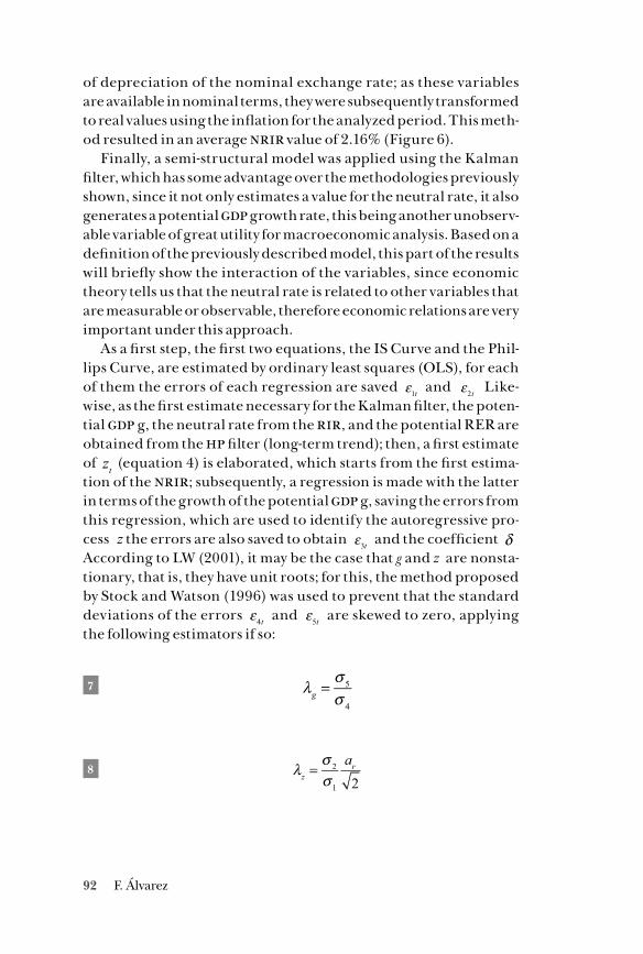
92 F. Álvarez
of depreciation of the nominal exchange rate; as these variables are available in nominal terms, they were subsequently transformed to real values using the inflation for the analyzed period. This meth-od resulted in an average nrir value of 2.16% (Figure 6).
Finally, a semi-structural model was applied using the Kalman filter, which has some advantage over the methodologies previously shown, since it not only estimates a value for the neutral rate, it also generates a potential gdp growth rate, this being another unobserv-able variable of great utility for macroeconomic analysis. Based on a definition of the previously described model, this part of the results will briefly show the interaction of the variables, since economic theory tells us that the neutral rate is related to other variables that are measurable or observable, therefore economic relations are very important under this approach.
As a first step, the first two equations, the IS Curve and the Phil-lips Curve, are estimated by ordinary least squares (OLS), for each of them the errors of each regression are saved ε1t and ε2t Like-wise, as the first estimate necessary for the Kalman filter, the poten-tial gdp g, the neutral rate from the rir, and the potential RER are obtained from the hp filter (long-term trend); then, a first estimate of zt (equation 4) is elaborated, which starts from the first estima-tion of the nrir; subsequently, a regression is made with the latter in terms of the growth of the potential gdp g, saving the errors from this regression, which are used to identify the autoregressive pro-cess z the errors are also saved to obtain ε3t and the coefficient δ According to LW (2001), it may be the case that g and z are nonsta-tionary, that is, they have unit roots; for this, the method proposed by Stock and Watson (1996) was used to prevent that the standard deviations of the errors ε4t and ε5t are skewed to zero, applying the following estimators if so:
7 λg =σ 5
σ 4
8 λz =σ 2
σ 1
ar2
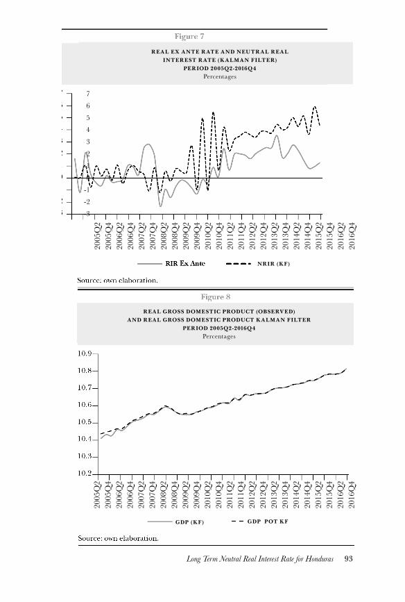
93Long Term Neutral Real Interest Rate for Honduras
REAL EX ANTE RATE AND NEUTRAL REALINTEREST RATE (KALMAN FILTER)
PERIOD 2005Q2-2016Q4Percentages
2005
Q2
2005
Q4
2006
Q2
2006
Q4
2007
Q2
2007
Q4
2008
Q2
2008
Q4
2009
Q2
2009
Q4
2010
Q2
2010
Q4
2011
Q2
2011
Q4
2012
Q2
2012
Q4
2013
Q2
2013
Q4
2014
Q2
2014
Q4
2015
Q2
2015
Q4
2016
Q2
2016
Q4
2005
Q2
2005
Q4
2006
Q2
2006
Q4
2007
Q2
2007
Q4
2008
Q2
2008
Q4
2009
Q2
2009
Q4
2010
Q2
2010
Q4
2011
Q2
2011
Q4
2012
Q2
2012
Q4
2013
Q2
2013
Q4
2014
Q2
2014
Q4
2015
Q2
2015
Q4
2016
Q2
2016
Q4
REAL GROSS DOMESTIC PRODUCT (OBSERVED)AND REAL GROSS DOMESTIC PRODUCT KALMAN FILTER
PERIOD 2005Q2-2016Q4Percentages
NRIR (KF)
GDP (KF) GDP POT KF
76543210
-1-2-3
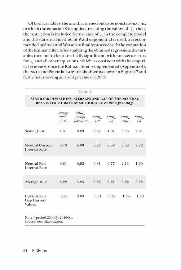
94 F. Álvarez
Of both variables, the one that turned out to be nonstationary is, to which the equation 8 is applied, rescuing the values of λz then, the restriction is included for the case of zt in the complete model and the statistical method of Wald exponential is used, as recom-mended by Stock and Watson to finally proceed with the estimation of the Kalman filter. After analyzing the obtained regression, the vari-ables turn out to be statistically significant, with non-zero errors for zt and all other equations, which is consistent with the empiri-cal evidence; once the Kalman filter is implemented (Appendix 4), the nrir and Potential gdp are obtained as shown in Figures 7 and 8, the first showing an average value of 1.90%.
Table 2
STANDARD DEVIATIONS, AVERAGES AND GAP OF THE NEUTRAL REAL INTEREST RATE BY METHODOLOGY: 2005Q2-2016Q4
Average 2005-2016
nrir_Average
Inflation*nrir_
hpnrir_
bknrir_uirp
nrir_FK
Stand_Desv. 1.31 0.89 0.67 1.01 3.63 2.01
Neutral Current Interest Rate
6.73 5.80 6.73 6.69 8.08 7.82
Neutral Real Interest Rate
0.81 0.92 0.81 0.77 2.16 1.90
Average mpr 6.22 5.83 6.22 6.22 6.22 6.22
Interest Rate Gap Current Values
−0.51 0.03 −0.51 −0.47 −1.86 −1.60
Note:* period 2009Q1-2016Q4.Source: own elaboration.
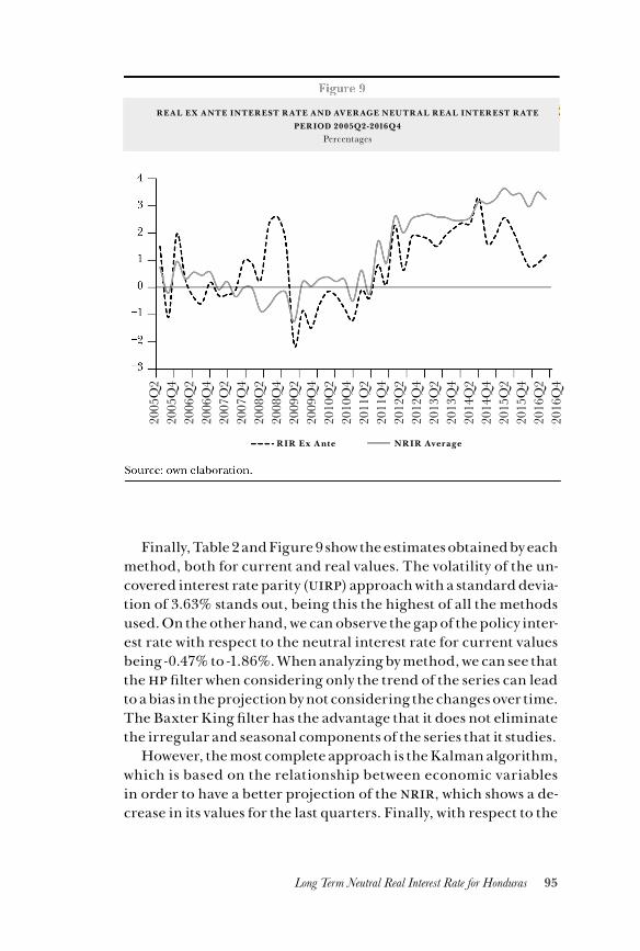
95Long Term Neutral Real Interest Rate for Honduras
Finally, Table 2 and Figure 9 show the estimates obtained by each method, both for current and real values. The volatility of the un-covered interest rate parity (uirp) approach with a standard devia-tion of 3.63% stands out, being this the highest of all the methods used. On the other hand, we can observe the gap of the policy inter-est rate with respect to the neutral interest rate for current values being -0.47% to -1.86%. When analyzing by method, we can see that the hp filter when considering only the trend of the series can lead to a bias in the projection by not considering the changes over time. The Baxter King filter has the advantage that it does not eliminate the irregular and seasonal components of the series that it studies.
However, the most complete approach is the Kalman algorithm, which is based on the relationship between economic variables in order to have a better projection of the nrir, which shows a de-crease in its values for the last quarters. Finally, with respect to the
REAL EX ANTE INTEREST RATE AND AVERAGE NEUTRAL REAL INTEREST RATE
PERIOD 2005Q2-2016Q4
Percentages20
05Q
220
05Q
420
06Q
220
06Q
420
07Q
220
07Q
420
08Q
220
08Q
420
09Q
220
09Q
420
10Q
220
10Q
420
11Q
220
11Q
420
12Q
220
12Q
420
13Q
220
13Q
420
14Q
220
14Q
420
15Q
220
15Q
420
16Q
220
16Q
4
RIR Ex Ante NRIR Average
96 F. Álvarez
relationship between the ex ante real interest rate and the estimated average of the neutral rate from the five remaining methods, Figure 9 reveals to a certain extent what the country’s monetary policy stance has been; that is, when the ex-ante rir is located above the nrir, mon-etary policy seems to have been contractionary during those periods, on the contrary, if it is below it has been expansionary.
5. CONCLUSIONS
• As a result of the estimates obtained from the different meth-ods, it is possible to obtain an estimate of the Neutral Real In-terest Rate for Honduras in current values ranging from 6.69% to 8.08% and from 0.77% to 2.16% in real values.
• The neutral rate is consistent with a gdp that converges to its potential level.
• Similarly, it is observed that the nrir varies over time and that it currently has a downward trend.
• From the beginning of 2007 to the beginning of 2009, the ex ante rir was above the natural rate, revealing a contraction-ary monetary policy during that period. On the other hand, during the period 2012-2016 it can be observed that the ex ante rir was below the nrir, showing an expansionary policy mainly for the years 2015-2016.
• Finally, considering that the present study is a first approxi-mation of the neutral policy interest rate, there is still more to be done on the subject, since there are other advanced meth-ods through the use of dynamic general equilibrium models, which would allow to strengthen more the results obtained.
References
Archibald Joanne and Hunter Leni, “What is the Neutral Real Inter-est Rate, and How Can We Use It?” Economics Department, Reserve Bank of New Zealand: Bulletin vol. 64 no.3.
Basdevant Olivier, Björksten Nils and Karagedikli Özer, “Estimating a time varying neutral real interest rate for New Zealand”, JEL classification: E43, E52, Discussion Paper Series, February 2004.
97Long Term Neutral Real Interest Rate for Honduras
Blinder Alan S., “Central Banking in Theory and Practice”; The MIT Press Cambridge, Massachusetts London, England; second MIT Press paperback edition, 1999.
Baxter Marianne, King Robert G. “Measuring Business Cycles Approximate Band-Pass Filters for Economic Time Series”, The Review of Economics and Statistics Vol. 81, No. 4 (Nov. 1999), pp. 575-593.
Brzoza Brzezinay Michal, Kotlowskiz Jaceck, “Measuring the Natural Yield Curve”; 6th February 2012.
Calderón M. César, Gallego Y. Francisco, “La Tasa de Interés Real Neutral en Chile”; Volumen 5, Nº2 / Agosto 2002.
Cartaya Virginia, Fleitas Cesar, Vivas José Rafael “Midiendo La Tasa de Interés Real Natural en Venezuela”; No.93, mayo 2007.
Dacass Tennecia, “Estimating the Natural Rate of Interest for Ja-maica”, Research Services Department Research and Eco-nomic Programming Division Bank of Jamaica, August 2011.
Fuentes S. Rodrigo, Gredig U. Fabián, “Estimating The Chilean Natural Rate Of Interest”; Banco Central de Chile, Documentos de Trabajo, N° 448; Diciembre 2007.
Garnier Julien & Wilhelmsen Bjorn Roger, “The Natural Real In-terest Rate and the Output Gap in the Euro Area”; Working Paper series no. 546 / November 2005.
Giammarioli Nicola & Valla Natacha, “The Natural Real Rate of Interest in The Euro Area”, European Central Bank, Working Paper Series, May 2003.
González Andrés, Ocampo Sergio, Pérez Julián, Rodríguez Diego; “Brecha del producto y medidas de la tasa de interés neutral para Colombia”; Monetaria, July- December, 2013.
Galí Jordi, “New Perspectives on Monetary Policy, Inflation, and the Business Cycle”; Working Paper 8767, National Bureau of Economic Research, February 2002.
Humala Alberto y Rodríguez Gabriel, “Estimation of a Time Vary-ing Natural Interest Rate for Perú”, Research Department Central Bank of Peru, 2009.
Hernández Zamudio Ociel, Amador Díaz Javier, “La tasa natu-ral en México: un parámetro importante para la estrategia de política monetaria”; Economic Research Department Nº 0807, Noviembre 2008.
98 F. Álvarez
Knut Wicksell Johan Gustaf, “Interest and Prices”; 1898.Laubach Thomas, Williams John C. “Measuring the Natural Rate
of Interest”; Board of Governors of the Federal Reserve System, No-vember 2001.
Laubach Thomas, Williams John C. “Measuring the Natural Rate of Interest”; Board of Governors of the Federal Reserve System, No-vember 2003.
Muñoz S. Evelyn y Tenorio Ch. Edwin, “Estimación de la Tasa de Interés Real Neutral para la Economía Costarricense (1991-2006)”, Banco Central de Costa Rica, División Económica, Departamento de Investigación Económica, Documento de Investigación, DIE-04-2007-DI, Noviembre, 2007.
Neiss Katharine S.& Nelson Edward, “The real interest rate gap as an inflation indicator”; Bank of England_ 2001, ISSN 1368-5562.
Orphanides Athanasios, Williams John C. “Robust Monetary Policy Rules with Unknown Natural Rates”; Board of Governors of the Federal Reserve System, Federal Reserve Bank of San Francisco. 2002.
Paredes Evelio, Santana Lisette, Sánchez Armando, Torres Fran-cisco, “Estimación de la Tasa de Interés Real en la Repub-lica Dominicana”; Banco Central de la República Domini-cana, Departamento de Programación Monetaria y Estudios Económicos, Junio 2013.
Stock James H. and Watson Mark W. 26. “Asymptotically Median Unbiased Estimation of Coefficient Variance in a Time Vary-ing Parameter Model”, Journal of the American Statistical Association, vol. 93, No. 441, March 1996, pp 349-358.
Segura Carlos Rodríguez y Vásquez José Pablo Carvajal, “Estimación del parámetro de suavizamiento del filtro de Hodrick y Prescott para Costa Rica”, División Económica, Departamento de Investigación Económica DEC-DIE-DT 006-2011.
Valdivia Daney D.C y Yujra Paola C. T. “Identificación de Ciclos Económicos en Bolivia 1970-2008”, 2008.
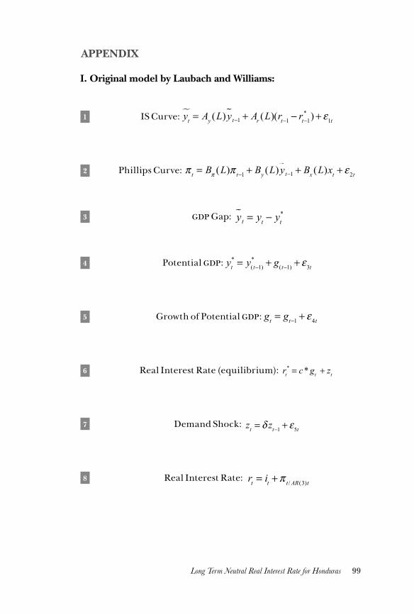
99Long Term Neutral Real Interest Rate for Honduras
APPENDIX
I. Original model by Laubach and Williams:
1 IS Curve: IS Curve yt! = Ay (L)y! t−1 + Ar (L)(rt−1 − rt−1
* )+ ε1t
2 Phillips Curve: Phillips Curve: π t = Bπ (L)π t−1 + By (L)y! t−1 + Bx (L)xt + ε2t
3 gdp Gap: GAP: y! t = yt − yt*
4 Potential gdp: Potencial GDP: yt* = y(t−1)
* + g(t−1) + ε3t
5 Growth of Potential gdp: Growth of Potencial GDP: gt = gt−1 + ε4t
6 Real Interest Rate (equilibrium): Real Interest Rate (equilibrium) : rt* = c* gt + zt
7 Demand Shock: Demand Shock: zt = δ zt−1 + ε5t
8 Real Interest Rate: Real Interest Rate: rt = it +π t /AR(3)t
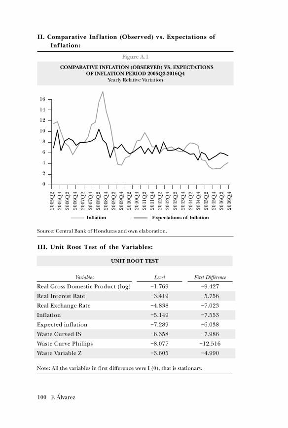
100 F. Álvarez
II. Comparative Inflation (Observed) vs. Expectations of Inflation:
Figure A.1
COMPARATIVE INFLATION (OBSERVED) VS. EXPECTATIONSOF INFLATION PERIOD 2005Q2-2016Q4
Yearly Relative Variation
Source: Central Bank of Honduras and own elaboration.
Ination Expectations of Ination
0
2
4
6
14
16
2005
Q2
2005
Q4
2006
Q2
2006
Q4
2007
Q2
2007
Q4
2008
Q2
2008
Q4
2009
Q2
2009
Q4
2010
Q2
2010
Q4
2011
Q2
2011
Q4
2012
Q2
2012
Q4
2013
Q2
2013
Q4
2014
Q2
2014
Q4
2015
Q2
2015
Q4
2016
Q2
2016
Q4
12
10
8
III. Unit Root Test of the Variables:
UNIT ROOT TEST
Variables Level First DifferenceReal Gross Domestic Product (log) −1.769 −9.427
Real Interest Rate −3.419 −5.756
Real Exchange Rate −4.838 −7.023
Inflation −5.149 −7.553
Expected inflation −7.289 −6.038
Waste Curved IS −6.358 −7.986
Waste Curve Phillips −8.077 −12.516
Waste Variable Z −3.605 −4.990
Note: All the variables in first difference were I (0), that is stationary.
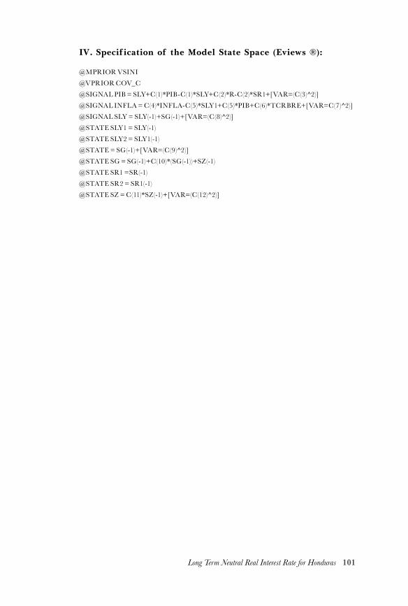
101Long Term Neutral Real Interest Rate for Honduras
IV. Specification of the Model State Space (Eviews ®):
@MPRIOR VSINI@VPRIOR COV_C@SIGNAL PIB = SLY+C(1)*PIB-C(1)*SLY+C(2)*R-C(2)*SR1+[VAR=(C(3)^2)]@SIGNAL INFLA = C(4)*INFLA-C(5)*SLY1+C(5)*PIB+C(6)*TCRBRE+[VAR=C(7)^2)]@SIGNAL SLY = SLY(-1)+SG(-1)+[VAR=(C(8)^2)]@STATE SLY1 = SLY(-1)@STATE SLY2 = SLY1(-1)@STATE = SG(-1)+[VAR=(C(9)^2)]@STATE SG = SG(-1)+C(10)*(SG(-1))+SZ(-1)@STATE SR1 =SR(-1)@STATE SR2 = SR1(-1)@STATE SZ = C(11)*SZ(-1)+[VAR=(C(12)^2)]
102 J. M. Michel
Neutral Rate of Interest: The Case ofthe Dominican Republic
José Manuel Michel
Abstract
The aim of this paper is to estimate the neutral rate of interest for the Dominican Republic. The methods used are reduced-form, interest rate parity, and marginal product of capital. Empirical evidence provides evidence in favor of the interest rate parity hypothesis as a useful tool for estimating the neutral rate of interest. The results suggest that nominal and real neutral rates of interest have fallen following the 2008 financial crisis. The reduced-form model and interest rate parity methods tell us that the average nominal neutral rate of interest of the post-financial crisis period stands at between 5.5% and 6.2%. These same methods yield values between 1.0% and 1.4% for the real neutral rate of interest. The marginal product of capital method estimates a real neutral rate of interest of 3.6%.Keywords: neutral rate of interest, monetary policy and cointegration.
1. INTRODUCTION
The tool most commonly used by central banks for implement-ing monetary policy is the short-term interest rate. The fore-going is a consequence of the adoption of the inflation tar-
get scheme. The use of interest rates as a policy instrument makes the study of natural or neutral rate of interest levels relevant. In this regard, the central bank of the Dominican Republic has implemented the inflation target scheme since 2012. The adoption of this scheme, together with falling interest rates and the problem of zero interest rates in developed economies, have generated additional interest in understanding natural rates of interest.
103Neutral Rate of Interest: The case of the Dominican Republic
Sustainable growth in an economy is achieved when efficient economic policies are formulated. Among these policies, monetary policy is responsible for maintaining price stability and consequent-ly ensuring a reasonably foreseeable future that facilitates investor and consumer decisions. The effective formulation of monetary pol-icy requires understanding of the economy’s neutral rate of interest.
The neutral rate of interest is the interest rate level that would exist in a scenario with no inflationary pressures. This definition of neutral rate of interest was provided by the Swedish economist Knut Wicksell in the 19th Century. In keeping with this definition, it can be said that the natural rate of interest level is the one under which prices remain stable. It must therefore be the interest rate level the central bank wants to achieve.
The contributions of modern authors reveal that the neutral rate of interest is the one that allows the observed product to converge with potential (Bomfim, 2001). In Keynesian models, the neutral rate of interest is defined as the rate that would exist in equilibrium with no nominal rigidities (Gali, 2002). In the new Keynesian econ-omy the neutral rate of interest is the steady-state or long-term rate.
In this context, the aim of this research paper is to obtain a solid estimate of the neutral rate of interest for the Dominican Republic. To achieve this, three estimation methodologies are used: the re-duced-form method, the interest rate parity method and the marginal product of capital method. The project covers the period 1996-2017 with quarterly data.
The reduced-form model consists of estimating a regression by minimum least squares where the interest rate is a function of the external interest rate and potential growth. In this method neutral rate of interest estimates correspond to the value derived from regres-sion. Therefore, the expected value of deviations between market and neutral rates of interest is equal to zero. Neutral rate of interest estimates using the interest rate parity method are obtained with the previous estimation of a Vector Error Correction (vec) mod-el. This model incorporates two co-integrated vectors that show the long-term relationship between the exchange rate and internal and external prices, and domestic and external interest rates. Last-ly, the marginal product of capital method is obtained by estimat-ing a production function using Vector Error Correction (vec).
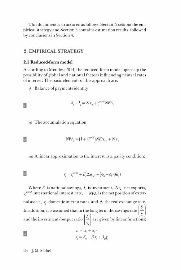
104 J. M. Michel
This document is structured as follows: Section 2 sets out the em-pirical strategy and Section 3 contains estimation results, followed by conclusions in Section 4.
2. EMPIRICAL STRATEGY
2.1 Reduced-form model
According to Mendes (2014) the reduced-form model opens up the possibility of global and national factors influencing neutral rates of interest. The basic elements of this approach are:
i) Balance of payments identity
1
ii) The accumulation equation
2
iii) A linear approximation to the interest rate parity condition:
3
Where is national savings, is investment, net exports, international interest rate, is the net position of exter-
nal assets, domestic interest rates, and the real exchange rate.
In addition, it is assumed that in the long term the savings rate
and the investment/output ratio are given by linear functions:
4
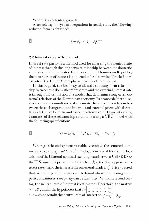
105Neutral Rate of Interest: The case of the Dominican Republic
Where gt is potential growth.After solving the system of equations in steady state, the following
reduced-form is obtained:
5
2.2 Interest rate parity method
Interest rate parity is a method used for inferring the neutral rate of interest through the long-term relationship between the domestic and external interest rates. In the case of the Dominican Republic, the neutral rate of interest is expected to be determined by the inter-est rate of the United States plus a measure of country risk.
In this regard, the best way to identify the long-term relation-ship between the domestic interest rate and the external interest rate is through the estimation of a model that determines long-term ex-ternal relations of the Dominican economy. In economic literature, it is common to simultaneously estimate the long-term relation be-tween the exchange rate and internal and external prices with the re-lation between domestic and external interest rates. Conventionally, estimates of these relationships are made using a vec model with the following specification:
6
Where yt is the endogenous variables vector; xt, the centered dum-mies vector, and Endogenous variables are: the log-arithm of the bilateral nominal exchange rate between US$/RD$ et; the u.s consumer price index logarithm, , the 30-day passive in-terest rate rt, and the interest rate on federal funds is It is expected that two cointegration vectors will be found where purchasing power parity and interest rate parity can be identified. With this second vec-tor, the neutral rate of interest is estimated. Therefore, the matrix π =αβ ' , under the hypotheses that
allows us to obtain the neutral rate of interest as
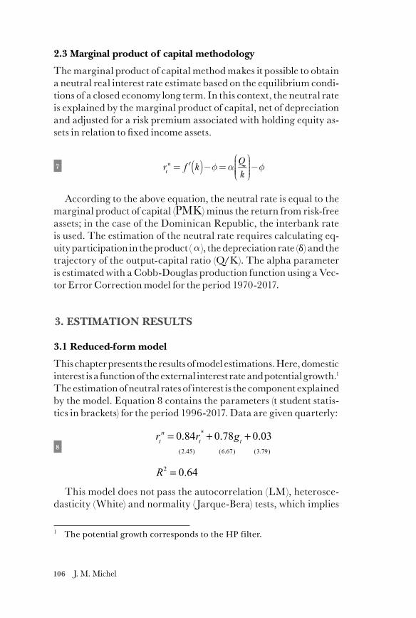
106 J. M. Michel
2.3 Marginal product of capital methodology
The marginal product of capital method makes it possible to obtain a neutral real interest rate estimate based on the equilibrium condi-tions of a closed economy long term. In this context, the neutral rate is explained by the marginal product of capital, net of depreciation and adjusted for a risk premium associated with holding equity as-sets in relation to fixed income assets.
7
According to the above equation, the neutral rate is equal to the marginal product of capital (pmk) minus the return from risk-free assets; in the case of the Dominican Republic, the interbank rate is used. The estimation of the neutral rate requires calculating eq-uity participation in the product ( ), the depreciation rate (δ) and the trajectory of the output-capital ratio (Q/K). The alpha parameter is estimated with a Cobb-Douglas production function using a Vec-tor Error Correction model for the period 1970-2017.
3. ESTIMATION RESULTS
3.1 Reduced-form model
This chapter presents the results of model estimations. Here, domestic interest is a function of the external interest rate and potential growth.1 The estimation of neutral rates of interest is the component explained by the model. Equation 8 contains the parameters (t student statis-tics in brackets) for the period 1996-2017. Data are given quarterly:
8 rtn = 0.84rt
* + 0.78gt + 0.03
(2.45) (6.67) (3.79)
R2 = 0.64
This model does not pass the autocorrelation (LM), heterosce-dasticity (White) and normality ( Jarque-Bera) tests, which implies
1 The potential growth corresponds to the HP filter.
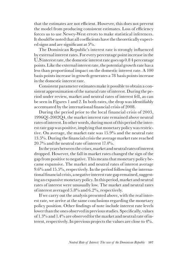
107Neutral Rate of Interest: The case of the Dominican Republic
that the estimates are not efficient. However, this does not prevent the model from producing consistent estimates. Loss of efficiency forces us to use Newey-West errors to make statistical inferences. It should be noted that all coefficients have the theoretically expect-ed signs and are significant at 5%.
The Dominican Republic’s interest rate is strongly influenced by external interest rates. For every percentage point increase in the u.s interest rate, the domestic interest rate goes up 0.84 percentage points. Like the external interest rate, the potential growth rate has a less than proportional impact on the domestic interest rate. A 100 basis points increase in growth generates a 78 basis points increase in the domestic interest rate.
Consistent parameter estimates make it possible to obtain a con-sistent approximation of the natural rate of interest. During the pe-riod under review, market and neutral rates of interest fell, as can be seen in Figures 1 and 2. In both rates, the drop was identifiably accentuated by the international financial crisis of 2008.
During the period prior to the local f inancial crisis of 2003, 1996Q1-2002Q4, the market interest rate remained above neutral rates of interest. In other words, during most of this period the inter-est rate gap was positive, implying that monetary policy was restric-tive. On average, the market rate was 15.9% and the neutral rate 13.5%. During the financial crisis the average market rate reached 20.7% and the neutral rate of interest 17.4%.
In the years between the crises, market and neutral rates of interest dropped. However, the fall in market rates changed the sign of the gap from positive to negative. This means that monetary policy be-came expansive. The market and neutral rates of interest average 9.6% and 15.5%, respectively. In the period following the interna-tional financial crisis, a negative interest rate gap remained, suggest-ing an expansive monetary policy. In this period, market and neutral rates of interest were unusually low. The market and neutral rates of interest averaged 5.8% and 6.2%, respectively.
If we carry out the analysis presented above, with the real inter-est rate, we arrive at the same conclusions regarding the monetary policy position. Other findings of note include interest rate levels lower than the ones observed in previous studies. Specifically, values of 1.3% and 1.4% are observed for the market and neutral rate of in-terest, respectively. In previous projects the values are close to 4%.
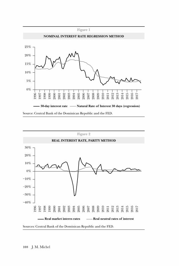
108 J. M. Michel
Figure 2
REAL INTEREST RATE, PARITY METHOD
Sources: Central Bank of the Dominican Republic and the FED.
Real market interes rates Real neutral rates of interest
1996
1997
1998
1999
2000
2001
2002
2003
2004
2005
2006
2007
2008
2009
2010
2011
2012
2013
2014
2015
2016
2017
−20%
−30%
−40%
−10%
0%
10%
20%
30%
Figure 1
NOMINAL INTEREST RATE REGRESSION METHOD
Source: Central Bank of the Dominican Republic and the FED.
30-day interest rate Natural Rate of Interest 30 days (regression)
1996
1997
1998
1999
2000
2001
2002
2003
2004
2005
2006
2007
2008
2009
2010
2011
2012
2013
2014
2015
2016
2017
0%
5%
10%
15%
20%
25%
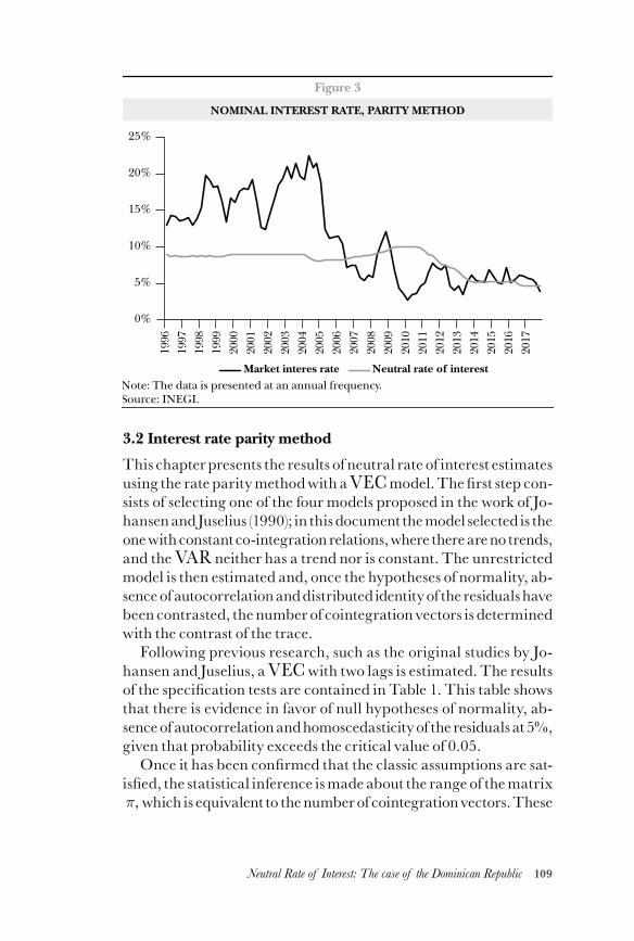
109Neutral Rate of Interest: The case of the Dominican Republic
3.2 Interest rate parity method
This chapter presents the results of neutral rate of interest estimates using the rate parity method with a vec model. The first step con-sists of selecting one of the four models proposed in the work of Jo-hansen and Juselius (1990); in this document the model selected is the one with constant co-integration relations, where there are no trends, and the var neither has a trend nor is constant. The unrestricted model is then estimated and, once the hypotheses of normality, ab-sence of autocorrelation and distributed identity of the residuals have been contrasted, the number of cointegration vectors is determined with the contrast of the trace.
Following previous research, such as the original studies by Jo-hansen and Juselius, a vec with two lags is estimated. The results of the specification tests are contained in Table 1. This table shows that there is evidence in favor of null hypotheses of normality, ab-sence of autocorrelation and homoscedasticity of the residuals at 5%, given that probability exceeds the critical value of 0.05.
Once it has been confirmed that the classic assumptions are sat-isfied, the statistical inference is made about the range of the matrix
which is equivalent to the number of cointegration vectors. These
Figure 3
NOMINAL INTEREST RATE, PARITY METHOD
Note: The data is presented at an annual frequency.Source: INEGI.
Market interes rate Neutral rate of interest
1996
1997
1998
1999
2000
2001
2002
2003
2004
2005
2006
2007
2008
2009
2010
2011
2012
2013
2014
2015
2016
2017
0%
5%
10%
15%
20%
25%
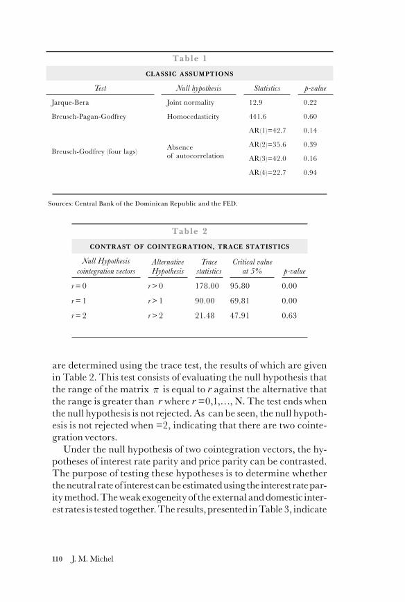
110 J. M. Michel
are determined using the trace test, the results of which are given in Table 2. This test consists of evaluating the null hypothesis that the range of the matrix is equal to r against the alternative that the range is greater than r where r =0,1,…, N. The test ends when the null hypothesis is not rejected. As can be seen, the null hypoth-esis is not rejected when =2, indicating that there are two cointe-gration vectors.
Under the null hypothesis of two cointegration vectors, the hy-potheses of interest rate parity and price parity can be contrasted. The purpose of testing these hypotheses is to determine whether the neutral rate of interest can be estimated using the interest rate par-ity method. The weak exogeneity of the external and domestic inter-est rates is tested together. The results, presented in Table 3, indicate
Table 1
CLASSIC ASSUMPTIONS
Test Null hypothesis Statistics p-value
Jarque-Bera Joint normality 12.9 0.22
Breusch-Pagan-Godfrey Homocedasticity 441.6 0.60
Breusch-Godfrey (four lags) Absence of autocorrelation
AR(1)=42.7 0.14
AR(2)=35.6 0.39
AR(3)=42.0 0.16
AR(4)=22.7 0.94
Table 2
CONTRAST OF COINTEGRATION, TRACE STATISTICS
Null Hypothesis cointegration vectors
Alternative Hypothesis
Trace statistics
Critical value at 5% p-value
r = 0 r > 0 178.00 95.80 0.00
r = 1 r > 1 90.00 69.81 0.00
r = 2 r > 2 21.48 47.91 0.63
Sources: Central Bank of the Dominican Republic and the FED.
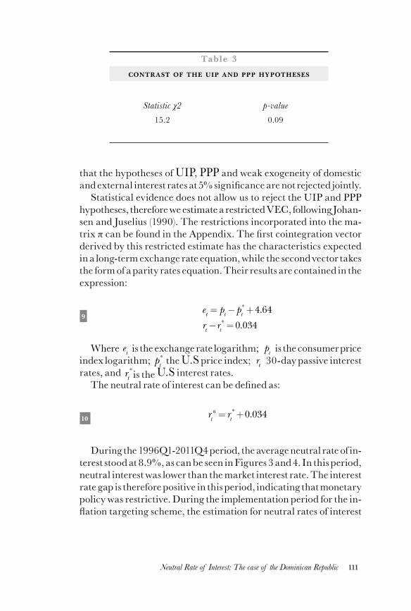
111Neutral Rate of Interest: The case of the Dominican Republic
that the hypotheses of uip, ppp and weak exogeneity of domestic and external interest rates at 5% significance are not rejected jointly.
Statistical evidence does not allow us to reject the UIP and PPP hypotheses, therefore we estimate a restricted VEC, following Johan-sen and Juselius (1990). The restrictions incorporated into the ma-trix π can be found in the Appendix. The first cointegration vector derived by this restricted estimate has the characteristics expected in a long-term exchange rate equation, while the second vector takes the form of a parity rates equation. Their results are contained in the expression:
9
Where is the exchange rate logarithm; is the consumer price index logarithm; the u.s price index; 30-day passive interest rates, and is the u.s interest rates.
The neutral rate of interest can be defined as:
10
During the 1996Q1-2011Q4 period, the average neutral rate of in-terest stood at 8.9%, as can be seen in Figures 3 and 4. In this period, neutral interest was lower than the market interest rate. The interest rate gap is therefore positive in this period, indicating that monetary policy was restrictive. During the implementation period for the in-flation targeting scheme, the estimation for neutral rates of interest
Table 3
CONTRAST OF THE uip AND ppp HYPOTHESES
Statistic χ2 p-value 15.2 0.09
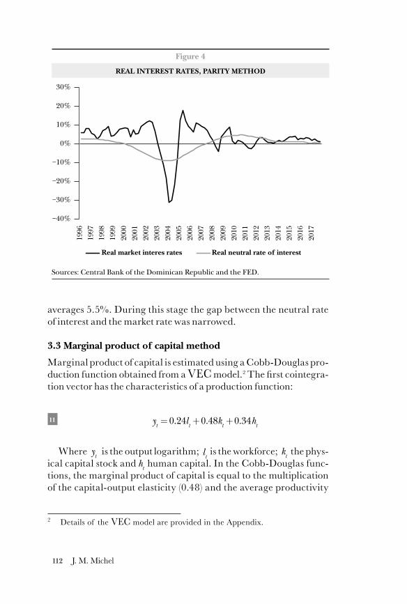
112 J. M. Michel
averages 5.5%. During this stage the gap between the neutral rate of interest and the market rate was narrowed.
3.3 Marginal product of capital method
Marginal product of capital is estimated using a Cobb-Douglas pro-duction function obtained from a vec model.2 The first cointegra-tion vector has the characteristics of a production function:
11
Where is the output logarithm; is the workforce; the phys-ical capital stock and human capital. In the Cobb-Douglas func-tions, the marginal product of capital is equal to the multiplication of the capital-output elasticity (0.48) and the average productivity
2 Details of the vec model are provided in the Appendix.
Figure 4
REAL INTEREST RATES, PARITY METHOD
Sources: Central Bank of the Dominican Republic and the FED.
Real market interes rates Real neutral rate of interest
1996
1997
1998
1999
2000
2001
2002
2003
2004
2005
2006
2007
2008
2009
2010
2011
2012
2013
2014
2015
2016
2017
−20%
−30%
−40%
−10%
0%
10%
20%
30%
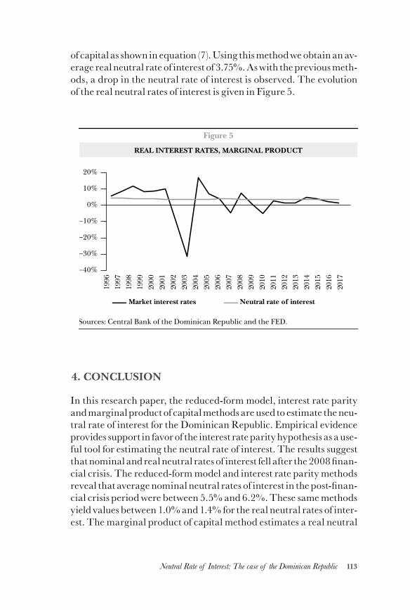
113Neutral Rate of Interest: The case of the Dominican Republic
of capital as shown in equation (7). Using this method we obtain an av-erage real neutral rate of interest of 3.75%. As with the previous meth-ods, a drop in the neutral rate of interest is observed. The evolution of the real neutral rates of interest is given in Figure 5.
4. CONCLUSION
In this research paper, the reduced-form model, interest rate parity and marginal product of capital methods are used to estimate the neu-tral rate of interest for the Dominican Republic. Empirical evidence provides support in favor of the interest rate parity hypothesis as a use-ful tool for estimating the neutral rate of interest. The results suggest that nominal and real neutral rates of interest fell after the 2008 finan-cial crisis. The reduced-form model and interest rate parity methods reveal that average nominal neutral rates of interest in the post-finan-cial crisis period were between 5.5% and 6.2%. These same methods yield values between 1.0% and 1.4% for the real neutral rates of inter-est. The marginal product of capital method estimates a real neutral
Figure 5
REAL INTEREST RATES, MARGINAL PRODUCT
Sources: Central Bank of the Dominican Republic and the FED.
Market interest rates Neutral rate of interest
1996
1997
1998
1999
2000
2001
2002
2003
2004
2005
2006
2007
2008
2009
2010
2011
2012
2013
2014
2015
2016
2017
–30%
–40%
–20%
–10%
0%
10%
20%
114 J. M. Michel
rate of interest of 3.75%. For future research, it is recommendable to broaden the analysis to the countries of Central America and con-sider structural changes by estimating an ms-vec.
References
Bomfim, Antulio N. (2001). “Measurement Error in General Equi-librium: The Aggregate Effects of Noisy Economic Indica-tors,” Journal of Monetary Economics, vol. 48, no. 3, pp. 585-603.
Fuente, Rodrigo (2007). “Tasa de interés real neutral: definicio-nes y evidencia para economía de latinoamericana.” Banco Central de Chile.
Jordi Gali, 2002. “New Perspectives on Monetary Policy, Inflation, and the Business Cycle,” NBER Working Papers 8767, Na-tional Bureau of Economic Research, Inc.
Mendes, Rhys R (2014). “The Neutral Rate of Interest in Canada.” Bank of Canada Discussion Paper 2014-5.
A Benchmark for Monetary Policy in Bolivia 115
The natural rate of interest: abenchmark for the stance of monetary policy in Bolivia
Paul Estrada CéspedesDavid Zeballos Coria
Abstract
This aim of this paper is to estimate Bolivia’s natural rate of interest consider-ing quarterly data for the period 1996 - 2017 during which changes occurred in the economic climate, affecting monetary policy and possibly the natural rate of interest, in particular an accelerated and substantial de-dollarization and strongly expansionary monetary policy over the last few years. A semi-structural model developed by Laubach and Williams (2003) is estimated, de-fining the natural rate of interest as the real interest rate consistent with stable inflation and output at its natural rate. In keeping with Holston, Laubach and Williams (2016), the methodology is enriched by analyzing the natural rate of interest as a time-varying process using the Kalman filter. The results reveal changes over time in the natural rate of interest, mainly from 2006, in-cluding a drop in recent years. These results have implications for monetary policy decision-making.
Key words: Natural rate of interest, monetary policy, Kalman filter.jel Classification: C32, E43, E52, O40.
1. INTRODUCTION
As a result of the recent economic climate, a great deal of at-tention was paid to monetary policy and its effects; in this regard one variable that grew in importance was the interest
rate. Expansionary monetary policies led to significant interest rate drops; for years central banks closely followed benchmark rate
This document does not necessarily reflect the views of bcb or its authorities. Its con-clusions are the exclusive responsibility of the authors.
116 P. Estrada, D. Zeballos
fluctuations in the US, Europe and certain Asian countries. In Bo-livia, adverse external circumstances led to the implementation of a countercyclical monetary policy with major unconventional or unorthodox characteristics. The expansionary approach pursued by Banco Central de Bolivia (bcb), in coordination with the govern-ment, allowed Financial System liquidity to grow to historical levels, leading to substantial decreases in monetary interest rates that were then passed on to the Financial System’s interest rates.
In this regard, the big question for central banks is whether inter-est rates are close to (below or above) their natural rate. The answer is crucial because it sets a benchmark for the direction of monetary policy. The aim of this paper is to estimate the natural rate of inter-est for Bolivia for the 1996 – 2017 period using quarterly data, during which changes occurred in the economic climate, affecting mone-tary policy and possibly the natural rate of interest.
To this end, a semi-structural model developed by Laubach and Williams (2003) is estimated, defining the natural rate of inter-est as the real interest rate consistent with stable inflation and output at its natural rate. Following Holston, Laubach and Williams (2016), the methodology is enriched by analyzing the natural rate of inter-est as a time-varying process using the Kalman filter. Similarly, giv-en the absence of a benchmark rate for monetary policy in Bolivia, a quantity-based weighted monetary interest rate (wmir) is deter-mined using the interest rates for monetary regulation security issues.
This paper is structured as follows: Section 2 describes the refer-ential framework with papers written on the subject and providing a brief analysis of Bolivia’s case, Section 3 describes the methodology and results of the estimations, and Section 4 contains conclusions.
2. REFERENTIAL FRAMEWORK
The natural rate of interest is a variable that is not directly observ-able; however, it is important for a central bank’s decision-making process because it provides a benchmark for measuring the direc-tion of monetary policy. If the short-term real interest rate is below its natural rate (negative natural rate gap), then monetary policy is ex-pansionary. This rate provides a benchmark for measuring the direc-tion of monetary policy, with expansionary (contractionary) policies if the real short-term interest rate is below (above) its natural rate.
A Benchmark for Monetary Policy in Bolivia 117
There are three ways to estimate the natural rate of interest (Fuen-tes, 2008). Firstly, a semi-structural model and state-space analysis can be used to relate latent variables (natural rate of interest) with the ones observed using an IS curve and a Phillips curve. Laubach and William (2003) follow this strategy and are later followed by oth-er authors for Latin American countries.
A second estimation method relies on market information, expect-ing the natural rate of interest to equal the market rate at some point in time. Studies such as Bomfin (2001) and Basdevant et al (2004) have been conducted in this regard. The first one uses a weighted average of rates for different terms, while the second one estimates the actual rate and a term premium (with a Kalman filter) using equa-tions with rates for different terms.
A third option involves estimating a ratio that guarantees that the present value of capital in a certain moment in time (t, when it tends to infinity) must be zero (transversality condition). This is done using an asset approach or an estimation of the marginal product of capital from which a risk premium is subtracted.
An exercise for Chile using all three methodologies is outlined in Fuentes and Gredig (2008). The authors show that the neutral rate of interest can be calculated using a semi-structural model with in-formation on the domestic financial market; each estimation pro-duces similar results, despite the disparities in the methodologies.
3. METHODOLOGY AND EMPIRICAL RESULTS
3.1 Theoretical description of the model
The semi-structural model developed by Laubach and Williams (2003) is enriched by Holston, Laubach and Williams (2016) by an-alyzing the natural rate of interest as a process that varies over time (time-varying process) using the Kalman filter (Roberts, 2001; Edge et al., 2007; Kahn and Rich, 2007).
A useful starting point for modeling the natural rate of interest is the neoclassical growth model. As described in Galí (2008), for a representative household with ces preferences, this model implies that the natural rate of interest varies over time in response to chang-es in the growth rate of output and preferences. In a stationary state,
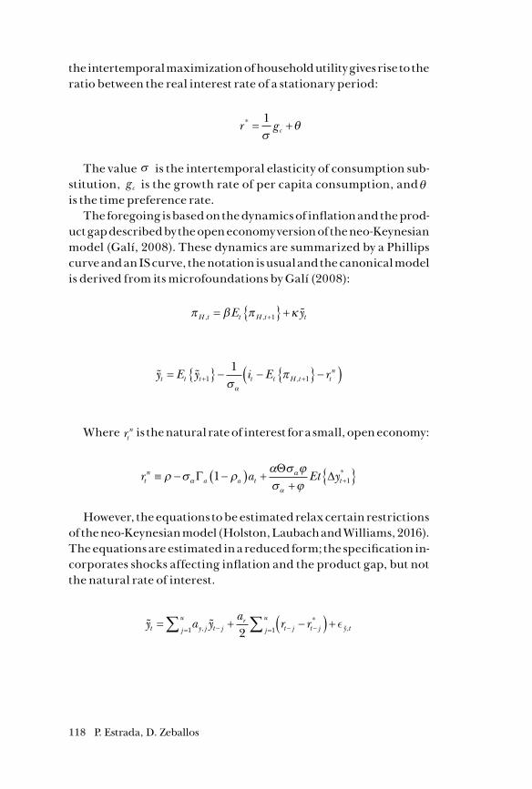
118 P. Estrada, D. Zeballos
the intertemporal maximization of household utility gives rise to the ratio between the real interest rate of a stationary period:
r g c* = +
1σ
θ
The value σ is the intertemporal elasticity of consumption sub-stitution, gc is the growth rate of per capita consumption, andθ is the time preference rate.
The foregoing is based on the dynamics of inflation and the prod-uct gap described by the open economy version of the neo-Keynesian model (Galí, 2008). These dynamics are summarized by a Phillips curve and an IS curve, the notation is usual and the canonical model is derived from its microfoundations by Galí (2008):
π β π κH t t H t tE y, ,= ++1
y E y i E rt t t t t H t tn= − − −( )+ +1 1
1σ
πα
,
Where rtn is the natural rate of interest for a small, open economy:
r a Et ytn
a a t t≡ − −( ) ++
+ρ σ ρα σ ϕσ ϕα
α
α
ΓΘ
∆1 1*
However, the equations to be estimated relax certain restrictions of the neo-Keynesian model (Holston, Laubach and Williams, 2016). The equations are estimated in a reduced form; the specification in-corporates shocks affecting inflation and the product gap, but not the natural rate of interest.
y a ya
r rt y j t jr
t j t j y tj
u
j
u= + −( ) +− − −== ∑∑ ,
*,2 11
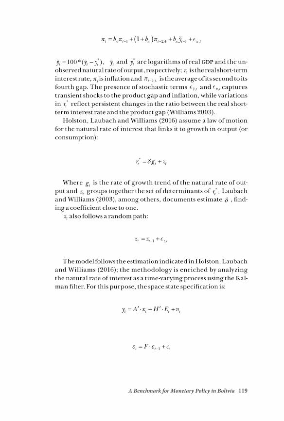
119
π π ππ π π πt t t t tb b b y= + +( ) + +− − −1 2 4 11 , ,
y y y yt t t t= −100*( ),* and yt* are logarithms of real gdp and the un-
observed natural rate of output, respectively; rt is the real short-term interest rate, πt is inflation and πt −2 4, is the average of its second to its fourth gap. The presence of stochastic terms
y t, and π ,t captures transient shocks to the product gap and inflation, while variations in rt
* reflect persistent changes in the ratio between the real short-term interest rate and the product gap (Williams 2003).
Holston, Laubach and Williams (2016) assume a law of motion for the natural rate of interest that links it to growth in output (or consumption):
r g zt t t* = +δ
Where gt is the rate of growth trend of the natural rate of out-put and zt groups together the set of determinants of rt
*. Laubach and Williams (2003), among others, documents estimate δ , find-ing a coefficient close to one.
zt also follows a random path:
z zt t z t= +−1 ,
The model follows the estimation indicated in Holston, Laubach and Williams (2016); the methodology is enriched by analyzing the natural rate of interest as a time-varying process using the Kal-man filter. For this purpose, the space state specification is:
y A x H E vt t t t= ′ ⋅ + ′ ⋅ +
ε εt t tF= ⋅ +−1
A Benchmark for Monetary Policy in Bolivia
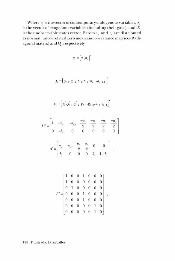
120 P. Estrada, D. Zeballos
Where yt is the vector of contemporary endogenous variables, xt is the vector of exogenous variables (including their gaps), and Et is the unobservable states vector. Errors vt and t are distributed as normal, uncorrelated zero mean and covariance matrices R (di-agonal matrix) and Q, respectively.
y yt t t= [ ]′,π
y y y r rt t t t t t t= ′
− − − − − −1 2 1 2 1 2 4, , , , , ,π π
εt t t t t t t ty y y g g z z= ′
− − − − − −* * *, , , , , ,1 2 1 2 1 2
′ =− −
− − − −
−
Ha a
a a a a
b
y yr r r r
y
12 2 2 2
0 0 0 0 0 0
1 2, , ,
′ =−
Aa a
a a
b b b
y yr r
y
, , ,1 2 2 20 0
0 0 0 1π π
′ =
F
1 0 0 1 0 0 01 0 0 0 0 0 00 1 0 0 0 0 00 0 0 1 0 0 00 0 0 1 0 0 00 0 0 0 0 1 00 0 0 0 0 1 0
,
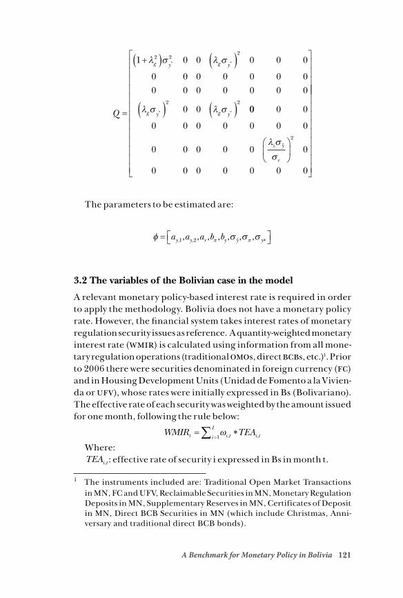
121
Q
g y g y
g y g y=
+( ) ( )
( ) ( )
1 0 0 0 0 0
0 0 0 0 0 0 00 0 0 0 0 0 0
0 0
2 22
2 2
λ σ λ σ
λ σ λ σ
* *
* * 00 0 0
0 0 0 0 0 0 0
0 0 0 0 0 0
0 0 0 0 0 0 0
2λ σ
σz y
r
The parameters to be estimated are:
φ σ σ σπ π= ∗a a a b by y r y y y, ,, , , , , , ,1 2
3.2 The variables of the Bolivian case in the model
A relevant monetary policy-based interest rate is required in order to apply the methodology. Bolivia does not have a monetary policy rate. However, the financial system takes interest rates of monetary regulation security issues as reference. A quantity-weighted monetary interest rate (wmir) is calculated using information from all mone-tary regulation operations (traditional omos, direct bcbs, etc.)1. Prior to 2006 there were securities denominated in foreign currency (fc) and in Housing Development Units (Unidad de Fomento a la Vivien-da or ufv), whose rates were initially expressed in Bs (Bolivariano). The effective rate of each security was weighted by the amount issued for one month, following the rule below:
WMIR TEAt i t i ti
I= ∗
=∑ ω , ,1
Where:TEAi t, : effective rate of security i expressed in Bs in month t.
1 The instruments included are: Traditional Open Market Transactions in MN, FC and UFV, Reclaimable Securities in MN, Monetary Regulation Deposits in MN, Supplementary Reserves in MN, Certificates of Deposit in MN, Direct BCB Securities in MN (which include Christmas, Anni-versary and traditional direct BCB bonds).
A Benchmark for Monetary Policy in Bolivia
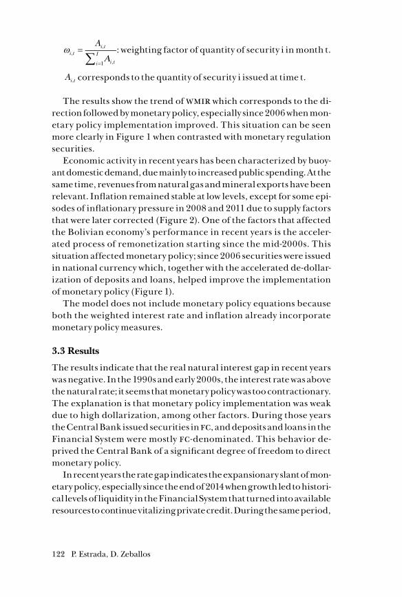
122 P. Estrada, D. Zeballos
ωΑ
i ti t
i ti
I
A,
,
,
==∑ 1
: weighting factor of quantity of security i in month t.
Ai t, corresponds to the quantity of security i issued at time t.
The results show the trend of wmir which corresponds to the di-rection followed by monetary policy, especially since 2006 when mon-etary policy implementation improved. This situation can be seen more clearly in Figure 1 when contrasted with monetary regulation securities.
Economic activity in recent years has been characterized by buoy-ant domestic demand, due mainly to increased public spending. At the same time, revenues from natural gas and mineral exports have been relevant. Inflation remained stable at low levels, except for some epi-sodes of inflationary pressure in 2008 and 2011 due to supply factors that were later corrected (Figure 2). One of the factors that affected the Bolivian economy’s performance in recent years is the acceler-ated process of remonetization starting since the mid-2000s. This situation affected monetary policy; since 2006 securities were issued in national currency which, together with the accelerated de-dollar-ization of deposits and loans, helped improve the implementation of monetary policy (Figure 1).
The model does not include monetary policy equations because both the weighted interest rate and inflation already incorporate monetary policy measures.
3.3 Results
The results indicate that the real natural interest gap in recent years was negative. In the 1990s and early 2000s, the interest rate was above the natural rate; it seems that monetary policy was too contractionary. The explanation is that monetary policy implementation was weak due to high dollarization, among other factors. During those years the Central Bank issued securities in fc, and deposits and loans in the Financial System were mostly fc-denominated. This behavior de-prived the Central Bank of a significant degree of freedom to direct monetary policy.
In recent years the rate gap indicates the expansionary slant of mon-etary policy, especially since the end of 2014 when growth led to histori-cal levels of liquidity in the Financial System that turned into available resources to continue vitalizing private credit. During the same period,
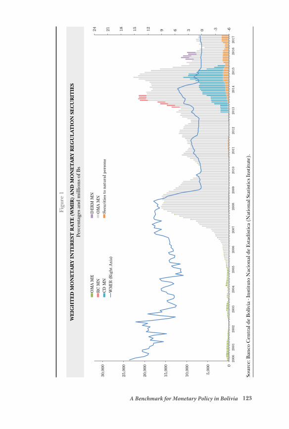
123
Figu
re 1
WE
IGH
TE
D M
ON
ET
AR
Y I
NT
ER
EST
RAT
E (
WM
IR)
AN
D M
ON
ET
AR
Y R
EG
UL
ATIO
N S
EC
UR
ITIE
SPe
rcen
tage
s and
mill
ions
of B
s
Sour
ce: B
anco
Cen
tral
de
Bol
ivia
- In
stit
uto
Nac
iona
l de
Esta
díst
ica
(Nat
iona
l Sta
tist
ics I
nsti
tute
).
-6-303691215182124
0
5,00
0
10,0
00
15,0
00
20,0
00
25,0
00
30,0
00
2000
2001
2002
2003
2004
2005
2006
2007
2008
2009
2010
2011
2012
2013
2014
2015
2016
2017
OM
A M
ED
ER
M M
NR
C M
NO
MA
MN
CD
MN
Sec
uri
ties
to
natu
ral p
erso
ns
WM
IR (R
ight
Axi
s)
A Benchmark for Monetary Policy in Bolivia
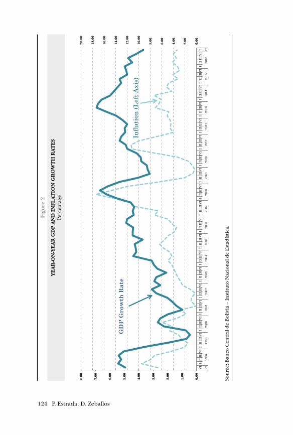
124 P. Estrada, D. Zeballos
Figu
re 2
YE
AR
-ON
-YE
AR
GD
P A
ND
IN
FLA
TIO
N G
RO
WT
H R
AT
ES
Perc
enta
ge
Sour
ce: B
anco
Cen
tral
de
Bol
ivia
– In
stit
uto
Nac
iona
l de
Esta
díst
ica.
0.00
1.00
2.00
3.00
4.00
5.00
6.00
7.00
8.00
0.00
2.00
4.00
6.00
8.00
10.0
0
12.0
0
14.0
0
16.0
0
18.0
0
20.0
0
VI
III
III
VI
III
III
VI
III
III
VI
III
III
VI
III
III
VI
III
III
VI
III
III
VI
III
III
VI
III
III
VI
III
III
VI
III
III
VI
III
III
VI
III
III
VI
III
III
VI
III
III
VI
III
III
VI
III
III
VI
III
III
VI
III
III
VI
I
9719
9819
9920
0020
0120
0220
0320
0420
0520
0620
0720
0820
0920
1020
1120
1220
1320
1420
1520
1617
Infl
ati
on
(L
eft
Ax
is)
GD
P G
row
th R
ate
125
Figu
re 3
NA
TU
RA
L R
AT
E O
F IN
TE
RE
ST A
ND
PR
OD
UC
T G
AP
Perc
enta
ge p
oint
s
Sour
ce: R
esul
ts fr
om th
e es
tim
ated
mod
el.
-18
-16
-14
-12
-10
-8-6-4-20246810121416
1997
1998
1999
2000
2001
2002
2003
2004
2005
2006
2007
2008
2009
2010
2011
2012
2013
2014
2015
2016
2017
Pro
du
ct G
ap
Ra
te G
ap
A Benchmark for Monetary Policy in Bolivia
126 P. Estrada, D. Zeballos
credit increased significantly, even considering the new regulations that set credit goals for each financial institution in the granting of loans for the productive sector and social housing. At the begin-ning of 2017 the rate gap began to close, although the Central Bank’s expansionary position remained unchanged.
An inverse relation is revealed when compared with the product gap; the natural interest rate gap decreased to the extent the product gap increased. The results of the estimations are shown in the Ap-pendix. During periods of increased inflation, it tended to decrease, thereby suggesting a contractionary monetary policy.
4. CONCLUSIONS
The estimation of the natural rate of interest is significant insofar as it provides a benchmark for measuring the direction of monetary policy. If the short-term real interest rate is below its natural rate (negative natural rate gap), then monetary policy is expansionary. The recent backdrop of low interest rate levels highlights the impor-tance of estimating the natural rate of interest to help central banks make decisions.
In this paper a semi-structural model is estimated following Holston, Laubach and Williams (2016), in which the natural rate of interest is defined as the real interest rate consistent with stable inflation and output at its natural rate. The results indicate that the Central Bank has held an expansionary monetary policy posi-tion in recent years, especially since late 2014, when growth caused historic levels of liquidity in the Financial System that turned into available resources to continue vitalizing private credit.
An inverse relation is revealed when compared with the product gap; the natural rate of interest gap decreased to the extent the prod-uct gap increased.
One important implication is that the natural rate of interest re-veals the expansionary position of monetary policy, consistent with the aim of fostering liquidity in the Financial System in order to in-ject resources into the economy through private credit.
127
References
Fuentes, Rodrigo (2008) “Tasa de Interés Real Neutral: Definiciones y Evidencia para Economías Latinoamericanas”. Centro de Estudios Monetarios Latinoamericanos (cemla).
Fuentes, R. y Gredig, F. (2008). “La tasa de interés neutral: estima-ciones para Chile”. Centro de Estudios Monetarios Latino-americanos (cemla).
Galí, Jordi (2008). “Monetary Policy, Inflation, and the Business Cycle: An Introduction to the New Keynesian Framework”. Princeton University Press.
Holston, Kathryn; Laubach, Thomas & Williams, John C. (2016). “Measuring the Natural Rate of Interest: International Trends and Determinants”. Federal Reserve Bank of San Francisco. Working Paper 2016-11. http://www.frbsf.org/economic-research/publications/workingpapers/wp2016-11.pdf.
Laubach, Thomas (2001). “Measuring the Nairu: Evidence From Seven Economies”. The Review of Economics and Statistics, Vol. 83, No. 2 (May, 2001), pp. 218-231. http://www.jstor.org/stable/3211601.
Laubach, Thomas & Williams, John C. (2003). “Measuring the Natural Rate of Interest”. The Review of Economics and Statistics, Vol. 85, No. 4 (Nov., 2003), pp. 1063-1070. http://www.jstor.org/stable/3211826.
Laubach, Thomas & Williams, John C. (2016). “Measuring the Natural Rate of Interest Redux”. Finance and Economics Discussion Series 2016-011. Washington: Board of Governors of the Federal Reserve System, http://dx.doi.org/10.17016/FEDS.2016.011.
Stock, James H. & Watson, Mark W. (1998). “Median Unbiased Estimation of Coefficient Variance in Time-Varying Param-eter Model”. Journal of the American Statistical Association. March 1998, Vol. 93, No. 441, Theory and Methods.
A Benchmark for Monetary Policy in Bolivia
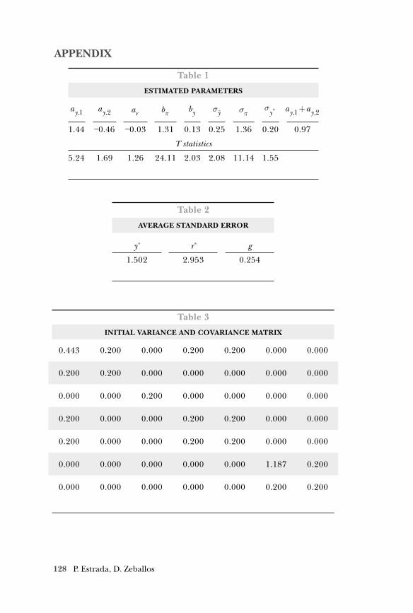
128 P. Estrada, D. Zeballos
APPENDIX
Table 1
ESTIMATED PARAMETERS
ay,1 ay,2 ar bπ by σ!y σπ σ
y* ay,1+ay,2
1.44 −0.46 −0.03 1.31 0.13 0.25 1.36 0.20 0.97
T statistics
5.24 1.69 1.26 24.11 2.03 2.08 11.14 1.55
Table 2
AVERAGE STANDARD ERROR
y* r* g
1.502 2.953 0.254
Table 3
INITIAL VARIANCE AND COVARIANCE MATRIX
0.443 0.200 0.000 0.200 0.200 0.000 0.000
0.200 0.200 0.000 0.000 0.000 0.000 0.000
0.000 0.000 0.200 0.000 0.000 0.000 0.000
0.200 0.000 0.000 0.200 0.200 0.000 0.000
0.200 0.000 0.000 0.200 0.200 0.000 0.000
0.000 0.000 0.000 0.000 0.000 1.187 0.200
0.000 0.000 0.000 0.000 0.000 0.200 0.200

Country Studies: Long Run Determinants
130 E. Bucacos
The Natural Rate of Interest for an Emerging Economy: The Case of Uruguay
Elizabeth Bucacos
Abstract
Vast evidence indicates that the so-called natural rate of interest has experienced a sustained fall in both advanced and emerging economies over the last 25 years. This situation threatens the central bank’s ability to guide relevant macroeco-nomic variables close to their welfare-maximizing path because the range of ma-neuver is reduced a great deal when interest rates descend to the zero lower bound. In this document, I try to estimate the natural interest rate (nir) for Uruguay, a small, open and dollarized emerging economy where monetary policy imple-mentation has changed drastically, splitting the sample in two. The methodolog-ical approach is aimed at providing a novel framework for analyzing the long-run fundamentals of the nir and also for explaining the reasons for short-run discrepancies between the real rate and its long-run equilibrium value. It is hoped that the fundamentals-based model adds to the myriad methods current in use at the Banco Central del Uruguay to estimate the nir.
Keywords: interest rate determination, monetary policy, Uruguay.jel Classification code: C10, E43, E52.
This research was developed within the framework of CEMLA’s Joint Research Pro-gram 2018, coordinated by the Bank of Spain. The opinions expressed in this publi-cation are those of the author and do not reflect the views of CEMLA or the Central Bank of Uruguay. She is thankful for comments and suggestions by Gerardo Lican-dro, Fernando Borraz, Verónica España, Rossana Fernández, Verónica Rodríguez, Magdalena Tubio, Cid Rodríguez-Pérez, Carey-Anne Williams, Alessandro Galesi, Ivan Kataryniuk, and participants of CEMLA Joint Research 2018 at the Workshop in Mex-ico City and at the XXIV Annual Meeting of the Central Bank Researchers Network. Also, I thank comments on typographic and semantic style made by a Winter intern from Harvard’s Program in Mexico that visited CEMLA, Samuel Zwickel. Contact in-formation for the author: Elizabeth Bucacos, Banco Central del Uruguay, Diagonal Fabini 777, Montevideo, Uruguay. [email protected].
131The Natural Rate of Interest for an Emerging Economy: The Case of Uruguay
1. INTRODUCTION
The concept of “natural interest rate” (nir) has recently been an increasingly important focus of both academics and poli-cymakers. There are different definitions of the nir based
on theoretical components of particular emphasis. Perfect flexibility in prices and wages, closed output gap, full employment, among other factors, are the ideas related to the nir. A satisfactory definition of the natural interest rate (also called neutral interest rate or simply r* in this document) is the level of the short-run real interest rate that is consistent with output near its potential and inflation near its target (Laubach and Williams, 2003). Through the interest rate gap, the natural interest rate is a key variable in the definition of the monetary policy stance. The interest rate gap is measured as the difference between the current real interest rate and the natural interest rate. As such, a negative interest rate gap would indicate an expansionary stance, while a positive interest rate gap would indicate a contractionary stance, very appropriate if the economy is experiencing inflation. Assessing the interest rate gap in order to monitor the effectiveness of monetary policy is applied according to central bank s differing regimes, that is, either the central bank is conducting an interest-rate management scheme or a money-targeting one. In an interest-rate scheme, the interest rate is the policy instrument, and the central bank can be made directly accountable; in a money-targeting framework, although interest rates are endog-enous, they still have a central role in the transmission of monetary policy. In both cases, the central bank prefers to fix/to induce real interest rates as close as possible to the natural interest rate in order to approximate relevant economic variables (output, inflation, etc.) to their welfare-maximizing path.
In recent years and primarily in advanced economies since the 2008 crisis, natural interest rates have been at historically low and even negative levels. That is worrying because it challenges central banks to perform monetary policy near the zero lower bound. Some emerging economies have also experienced this situation. Research-ers point to an increase of savings, a decrease of investment, or a com-bination of these factors. Population dynamics, for instance, could be an explanation because an aging population may increase the pro-pensity to save and raise the supply of funds, causing the natural
132 E. Bucacos
interest rate to fall. Additional factors at play may include nega-tive productivity perspectives which may reduce new business op-portunities and decrease the agent s willingness to invest, reducing the natural interest rate.
In 1898 and 1906 works, Knut Wicksell coined and developed the terms “market rate” and “natural interest rate”. With the first term, he referred to the effective value of the real interest rate; with the sec-ond, he referred to an equilibrium value of the same variable. As Lei-jonhufvud1 points out, the term “natural” is framed within what would be a “natural” monetary system, that is, “a monetary system in which all relative prices develop as they would be in a hypothetical world without paper money.” Wicksell points out three conditions of equilib-rium that the interest rate should meet, the first of which being that the market rate should equal the rate that would prevail if the capi-tal goods were borrowed in natura. The other two conditions refer to savings-investment coordination and price stability.
The interest rate must coordinate the savings decisions of house-holds with decisions of corporate investment and, in addition, must balance the supply and the demand of credit. If the supply of credit always coincided with the savings of the families and the demand for credit with the investment, both functions of the interest rate could be fulfilled simultaneously. But this relationship between saving and investment on the one hand and supply and demand for credit on the other does not necessarily occur. The presence of the banking system leading the creation of money can establish a gap between saving and investment, occurring when banks set a market rate lower than the “natural” rate necessary for the coordination of real activi-ties. As a result, inflation and endogenous growth of the money supply will be observed as long as the market rate is below the natural rate.
In standard models, the steady state natural rate of interest2 is de-termined for the marginal product of capital so that in the long run,
1 Leijonhufvud, Axel (1989).2 The steady state is a situation of the national economy predicted by some
classical economists (especially David Ricardo and RT Malthus) that would be reached in the long run when the profitability of productive investment was so low, because of the need to cultivate increasingly poor quality land to produce food, that the stimulus to invest would disappear. At that time, when the net investment was zero, the process of capital accumulation and population growth would stop and the steady state would have been reached. For Daly (1989) that state “is neither static nor eternal; it is a system
133The Natural Rate of Interest for an Emerging Economy: The Case of Uruguay
monetary policy has no effect on the real rate of return. Even in those models, where money is not superneutral3, the effect of inflation on the real return of equilibrium is small. However, in the medium and short term, monetary policy can create gaps between the mar-ket rate and the natural rate, thus producing real effects.
The European Central Bank has defined the natural interest rate as “the real short-term rate that is consistent in the long run (...) with the product at its potential level and with a stable inflation rate”4. In this way, nir could be considered as that steady state interest rate, consistent with a balanced growth path.
But the natural rate of interest is not observable and must be in-ferred from quantitative methods. In spite of the difficulties inherent in the measurement of an unobservable economic variable, the per-son in charge of conducting monetary policy needs to have some reli-able estimate of the nir, since it should be used as a reference when evaluating the monetary policy that is being implemented. Moreover, the nir varies over time in response to different real shocks, either structural (e.g. potential output growth, demographics, a country’s saving profile) or transitory (e. g. macroeconomic shocks5), which constitutes an additional challenge.
No single method best estimates the natural interest rate. Most of them are static (defining the nir as a parametrized, steady state point estimate) while others are dynamic (estimating the temporal path of nir). The former group includes the consumption-smoothing models and the uncovered interest rate parity condition. The latter group includes simple statistical filtering techniques – such as Ho-drick-Prescott filters, linear de-trending, and moving averages –, real interest rates and maximum likelihood estimation as well as DSGE models and small-scale macroeconomic models which are estimated using a Kalman filter. Each method has advantages and limitations, but no one is preferred over the others. As a result, it seems plausi-ble to apply a battery of models to estimate the natural interest rate and to present a consisted estimated range of values of it.
in dynamic equilibrium within the entropic biosphere that contains and sus-tains it”.
3 Money is superneutral when changes in the growth rate of the money supply have no effect on the growth rate of the real economic variables.
4 Monthly Bulletin, European Central Bank, May 2004.5 Woodford (2003).
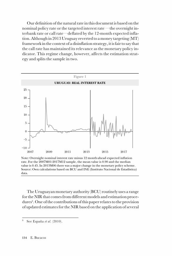
134 E. Bucacos
Our definition of the natural rate in this document is based on the nominal policy rate or the targeted interest rate —the overnight in-terbank rate or call rate—deflated by the 12-month expected infla-tion. Although in 2013 Uruguay reverted to a money targeting (mt) framework in the context of a disinflation strategy, it is fair to say that the call rate has maintained its relevance as the monetary policy in-dicator. This regime change, however, affects the estimation strat-egy and splits the sample in two.
The Uruguayan monetary authority (bcu) routinely uses a range for the nir that comes from different models and estimation proce-dures6. One of the contributions of this paper relates to the provision of updated estimates for the nir based on the application of several
6 See España et al. (2010).
Figure 1
URUGUAY: REAL INTEREST RATE
Note: Overnight nominal interest rate minus 12 month-ahead expected inflation rate. For the 2007M01-2017M12 sample, the mean value is 0.90 and the median value is 0.45. In 2013M06 there was a major change in the monetary policy scheme.Source: Own calculations based on BCU and INE (Instituto Nacional de Estadística) data.
2007 2009 2011 2013 2015 2017−10
−5
0
5
10
15
20
25
135The Natural Rate of Interest for an Emerging Economy: The Case of Uruguay
filters, the estimation of an augmented Taylor rule and, primarily, the adjustment of a fundamentals-based model. The latter is a novel approach for the Uruguayan case and focuses on the long-run de-terminants of the nir–which move slowly, such as demographic characteristics, productivity shifts, financial deepening, and indebt-edness profile, among others – and on the short-run shocks that move the short-run rate away from its long-run value. In essence, this is the main contribution of this paper because it presents a framework for understanding the difference between the nir at short- and long-run equilibrium, clearly defines a rather simple way to estimate the natural interest rate, and provides an explanation for the differ-ences between the long-run and short-run values.
The rest of the document is organized as follows. Section 2 dis-cusses the methodological approach and presents the short-run and medium-run estimates of nir for Uruguay. Section 3 analyzes the results. The final section concludes.
2. METHODOLOGICAL APPROACH
The natural interest rate is “difficult to estimateand impossible to know with precision”.
Alan Blinder (1998)
This section deals with methodological issues related to different estimation approaches applied in this document to the natural in-terest rate in Uruguay. Many other methods –not presented here– were previously used by other researchers7.
2.1 Simple methods
There are some rather simple and fast methods used to extrapolate the natural rate of interest in an economy. They can give a prior of the probable value of the nir but fail to reveal the drivers behind its performance.
7 España (2008), Bucacos (2010), España et al. (2010), Magud et al. (2012), Lambert (2016).
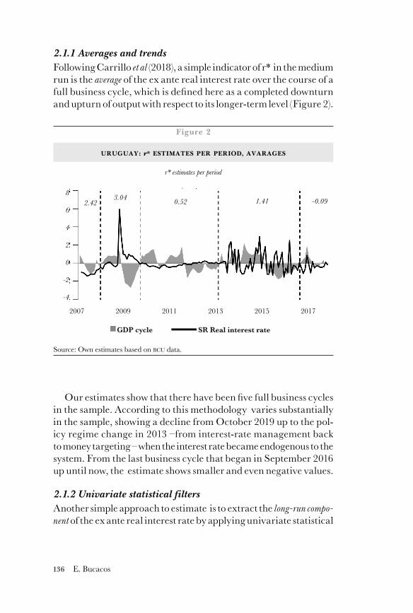
136 E. Bucacos
2.1.1 Averages and trendsFollowing Carrillo et al (2018), a simple indicator of r* in the medium run is the average of the ex ante real interest rate over the course of a full business cycle, which is defined here as a completed downturn and upturn of output with respect to its longer-term level (Figure 2).
Our estimates show that there have been five full business cycles in the sample. According to this methodology varies substantially in the sample, showing a decline from October 2019 up to the pol-icy regime change in 2013 –from interest-rate management back to money targeting – when the interest rate became endogenous to the system. From the last business cycle that began in September 2016 up until now, the estimate shows smaller and even negative values.
2.1.2 Univariate statistical filtersAnother simple approach to estimate is to extract the long-run compo-nent of the ex ante real interest rate by applying univariate statistical
Figure 2
URUGUAY: r* ESTIMATES PER PERIOD, AVARAGES
8
6
4
2
0
-2
-4
Source: Own estimates based on BCU data.
r* estimates per period
2007 2009 2011 2013 2015 2017
2.423.04 0.52 1.41 -0.09
GDP cycle SR Real interest rate
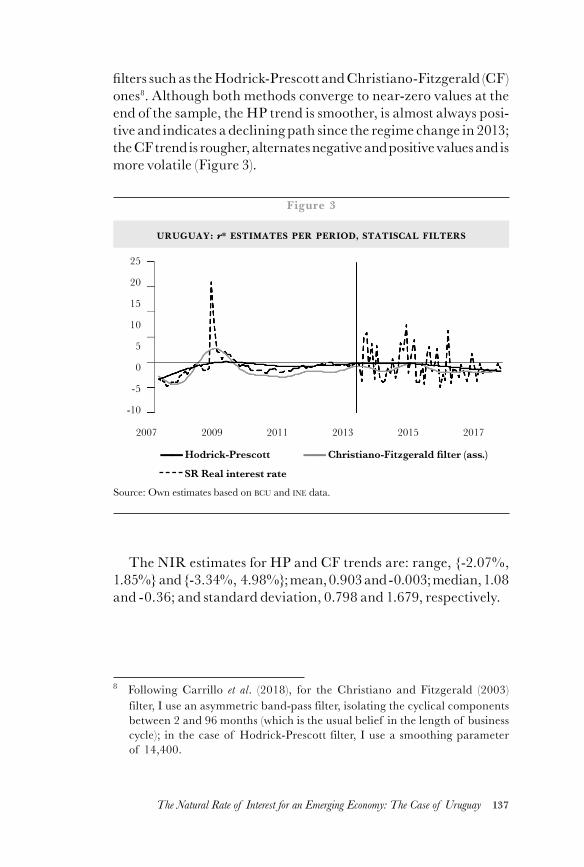
137The Natural Rate of Interest for an Emerging Economy: The Case of Uruguay
filters such as the Hodrick-Prescott and Christiano-Fitzgerald (CF) ones8. Although both methods converge to near-zero values at the end of the sample, the hp trend is smoother, is almost always posi-tive and indicates a declining path since the regime change in 2013; the CF trend is rougher, alternates negative and positive values and is more volatile (Figure 3).
The nir estimates for hp and CF trends are: range, -2.07%, 1.85% and -3.34%, 4.98%; mean, 0.903 and -0.003; median, 1.08 and -0.36; and standard deviation, 0.798 and 1.679, respectively.
8 Following Carrillo et al. (2018), for the Christiano and Fitzgerald (2003) filter, I use an asymmetric band-pass filter, isolating the cyclical components between 2 and 96 months (which is the usual belief in the length of business cycle); in the case of Hodrick-Prescott filter, I use a smoothing parameter of 14,400.
25
20
15
10
5
0
-5
-10
Figure 3
URUGUAY: r* ESTIMATES PER PERIOD, STATISCAL FILTERS
Source: Own estimates based on BCU and INE data.
2007 2009 2011 2013 2015 2017
—— Hodrick-Prescott —— Christiano-Fitzgerald filter (ass.)
SR Real interest rate
138 E. Bucacos
2.1.3 Augmented Taylor ruleAnother method used to infer the natural rate of interest involves the estimation of the central bank s reaction function or Taylor rule9. The Taylor principle points out that real interest rates need to in-crease when (expected) inflation10 exceeds the target and/or when there is a positive output gap.
The standard Taylor rule is
1
where Rt is the nominal overnight interest rate, r* is the natural in-terest rate, is the target inflation rate, is the inflation rate, is the output gap and captures any change in Rt not explained by the rule. The lag in the nominal interest rate shows that the cen-tral bank adjusts its policy rate gradually. The intercept r* denotes the level of the real interest rate that should prevail when inflation equals the inflation target and the output gap equals zero; that is, it denotes the natural interest rate. As the bcu is reported to pay great attention to the stability of the exchange rate, (1) can be modi-fied to allow the central bank to react whenever the spot exchange rate value differs from expected value in the long run11.
This rule, however, has to be modified for the money-targeting period. In July 2013, bcu switched from using the overnight in-terest rate as its operational target to announcing reference ranges for the growth of a monetary aggregate (M1’) within its inflation-ary target (IT) framework. This new money-targeting scheme has a gradually declining pattern of money growth to signal the bcu’s commitment to a disinflation path and a medium-term inflation objective12. As Portillo (2015) points out, money targets are ex ante consistent with the desired levels of interest rates, i.e., consistent at the time these targets are set. Ex post, deviations between targets and actual money growth are inevitable, though the central bank
9 John Taylor (1993).10 Hybrid Taylor rules have the expected inflation rate instead of the actual one.11 There is no exchange rate target in the sample period.12 Money targets are less indicative of the intended monetary stance than
interest-rate targets.
139The Natural Rate of Interest for an Emerging Economy: The Case of Uruguay
can try to steer money growth toward its target within the quarter by injecting or withdrawing liquidity and influencing short-term interest rates. That is why the central bank has to have a view about the level of short-term interest rate required to help stabilize in-flation; the main variable through which monetary policy can in-fluence aggregate demand, the exchange rate, and inflation is the short-term interest rate.
The modified Taylor rule for the money targeting period13 is:
2
where and are actual and target money growth rates, respec-tively.
This specification implies that positive money-target deviations increase interest rates as the central bank tightens its monetary pol-icy in order to force money growth towards its target. captures the degree of money target adherence; that is to say, the higher the more aggressive the monetary authority is in response to money target deviations.
Equations (1) and (2) are estimated recursively on a monthly ba-sis14. The results are not very plausible. In both cases, the goodness of fit is low, short-run interest rates only change in response to in-flation deviations from their targets and the rest of the gaps do not play any statistically significant role. Moreover, equation (2) reports a negative R2 statistics (the chosen model is worse than a horizontal line). Obviously, both Taylor rule specifications have to be improved. Figure 4 suggests missing arguments, and estimates for the whole sample seem to be overestimated.
2.2 Fundamentals-based model
In the long run, all variables are in equilibrium. In the medium and short run, several unexpected shocks may create a wedge between current values and their long-run equilibrium values. Consequently, short-run equilibrium values depend on long-run equilibrium values
13 The money-targeting period spans from 2013M7 to 2017M12.14 Both equations were estimated by applying ols. I thank Cid Rodríguez-
Pérez for his guidance.
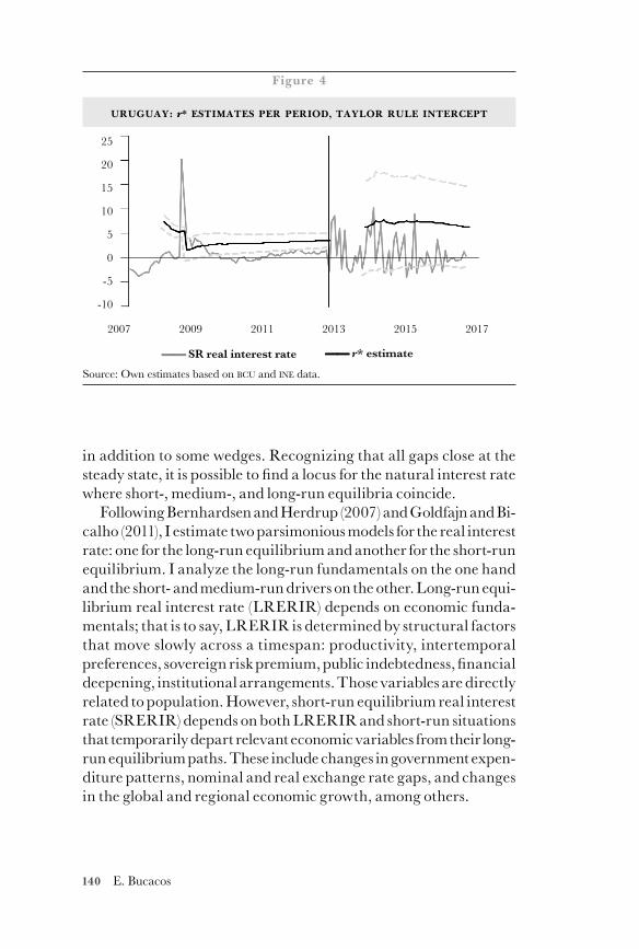
140 E. Bucacos
in addition to some wedges. Recognizing that all gaps close at the steady state, it is possible to find a locus for the natural interest rate where short-, medium-, and long-run equilibria coincide.
Following Bernhardsen and Herdrup (2007) and Goldfajn and Bi-calho (2011), I estimate two parsimonious models for the real interest rate: one for the long-run equilibrium and another for the short-run equilibrium. I analyze the long-run fundamentals on the one hand and the short- and medium-run drivers on the other. Long-run equi-librium real interest rate (lrerir) depends on economic funda-mentals; that is to say, lrerir is determined by structural factors that move slowly across a timespan: productivity, intertemporal preferences, sovereign risk premium, public indebtedness, financial deepening, institutional arrangements. Those variables are directly related to population. However, short-run equilibrium real interest rate (srerir) depends on both lrerir and short-run situations that temporarily depart relevant economic variables from their long-run equilibrium paths. These include changes in government expen-diture patterns, nominal and real exchange rate gaps, and changes in the global and regional economic growth, among others.
25
20
15
10
5
0
-5
-10
Figure 4
URUGUAY: r* ESTIMATES PER PERIOD, TAYLOR RULE INTERCEPT
Source: Own estimates based on BCU and INE data.
2007 2009 2011 2013 2015 2017
—— r* estimate—— SR real interest rate
141The Natural Rate of Interest for an Emerging Economy: The Case of Uruguay
2.2.1 Long-run equilibriumIncreasing public indebtedness pressures the demand for loans and higher domestic debt relative to domestic output may worsen the country’s credit record, pushing up its country risk, all of which increase the natural interest rate. Productivity gains encourage new investments and increase the willingness to invest, pushing up the natural interest rate. An ag-ing population exerts a downward pressure on the natural interest rate. According to Galesi et al (2017), “gradual population aging induces people to accumulate savings during their working lives so as to be able to pay for their retirement”, increasing the propensity to save. Accord-ing to ecb (2004) financial market efficiency may help to optimally allocate savings along the time. An improvement in the market struc-ture could, for example, widen the asset options in terms of returns, risk and liquidity available for those savers, just like a stimulus to savings, and would reduce the equilibrium real interest rate. A credit increase in the economy could be related with advances in those market struc-tures, with the development of new products which could tend to re-duce the interest rate. In sum, in the long-run relationship, we expect positive signs for the coefficients associated with public indebtedness, country risk and productivity and negative signs on the coefficients related to aging population and financial deepening.
A significance demographic shift has been taking place in Uru-guay for a long time. Long-run welfare policies implemented since the early twentieth century determined an increase in life expectan-cy at birth15 and, as a result, the percentage of people over 65 year-old has been steadily increasing16. The old-age support ratio, which indicates the number of working-age people (ages 15-64) per elderly person (65 and older), has declined from 4.10 to 3.82 in between 1996 and 2007 and remained close to that value since then17. Furthermore, “the Fourth Age”18 has shown an average annual growth rate of 2.8 %. But global population figures hardly grew19 which could be associated
15 The life expectancy at birth indicator reflects the overall mortality level of a population. It is the average number of years that a newborn is expected to live if current mortality rates continue to apply. For Uruguay, in 2013, it was 75.33 years and reached 77.55 years in 2017.
16 From 13.5% in 2007 to 14.2% in 2013.17 imf, Regional Economic Outlook 2018.18 The Fourth Age starts at about age 80 or 85 and includes the last years of adult-
hood.19 Total population was 3:358.794 and 3:493.205 people in 2007 and 2017,
respectively, according to official data. The natural growth rate was 0.433
142 E. Bucacos
with late motherhood20 and a drop in the fertility rate21. So, not only is Uruguayan population getting older on average, but an increasing proportion of elderly citizens has to financially support their old parents because life expectancy is high and the alredy low birth rate has not improved. The over-aging ratio, which measures the relative weight of 85-and-more-year old people related to 65-and-more-year old ones, shows a steady increase through the sample. See Figure 5.
Uruguay run fiscal deficits through the sample that required new debt issues every year resulting in an increase in the stock of public debt. Nevertheless, the net public debt-to-output ratio22 is lower in 2017 (40 % of gdp) than ten years before (48 % of gdp), mainly owing to sig-nificant output growth in the period. This improvement is also re-flected in Uruguay’s country risk level. In the second semester of 2015 public finances deteriorate and the debt increases pushing up the in-debtedness ratio.
In order for the credit to reduce the equilibrium real interest rate it is necessary that its expansion has been caused by asymmetric informa-tion reductions, institutional advances that accelerate the collateral recuperation, and other structural changes in the financial markets. But when credit increases are caused by demand, the impact of more credit on the equilibrium interest rate may be positive23.
and 0.366% for those years, respectively; if the migration rate is added, those figures become -0.034% and 0.366%, respectively. Source: Instituto Nacional de Estadística, ine.
20 The average age of motherhood index shows the mean age of women at first child-birth. For Uruguayan data, it was 27.48 in 2007 and 27.78 in 2017. In Western, Northern, and Southern Europe, first-time mothers are on average 27 to 29 years old, up from 23 to 25 years at the start of the 1970s.
21 The fertility rate gives the number of children born alive by a woman. This indicator shows the population change potential of a country. A value of two children per woman is considered the replacement rate for a population, be-cause it gives stability in terms of the global numbers. Fertility rates higher than two children show populations that grow in size and have diminishing average age. Fertility rates lower than two children indicate shrinking and aging popula-tions. In Uruguay, the fertility rate dropped from 1.98 in 2007 to 1.81 in 2017.
22 Net public debt measures the debt that the Government faces less the amount of its free disposal international reserves. The net public-debt-to-GDP ratio measures the capability of the country to pay its international obligations, that is, it relates the net debt to the income generated by the country.
23 That is the result found in the second regime. This outcome may be indicative of poor financial deepening.
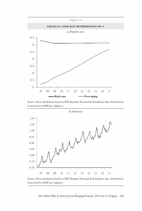
143The Natural Rate of Interest for an Emerging Economy: The Case of Uruguay
14.5
14
13.5
13
12.5
12
11.5
11
1.10
1.05
1.00
0.95
0.90
0.85
0.80
0.75
0.70
Figure 5
URUGUAY: LONG-RUN DETERMINANTS OF r*
Source: Own calculations based on INE (Instituto Nacional de Estadística) data. Productivity is measured as GDP per employee.
Source: Own calculations based on INE (Instituto Nacional de Estadística) data. Productivity is measured as GDP per employee.
(a) Population ratios
(b) Productivity
07
07
17
17
16
16
15
15
14
14
13
13
12
12
11
11
10
10
09
09
08
08
—— Birth rate —— Over-aging
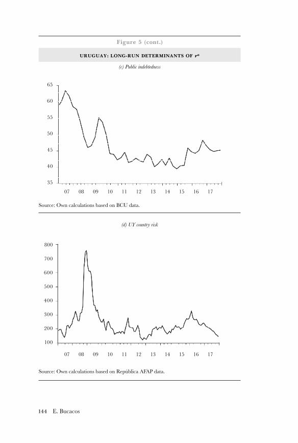
144 E. Bucacos
Source: Own calculations based on BCU data.
65
60
55
50
45
40
35
800
700
600
500
400
300
200
100
Figure 5 (cont.)
URUGUAY: LONG-RUN DETERMINANTS OF r*
Source: Own calculations based on República AFAP data.
(c) Public indebtedness
(d) UY country risk
07
07
17
17
16
16
15
15
14
14
13
13
12
12
11
11
10
10
09
09
08
08
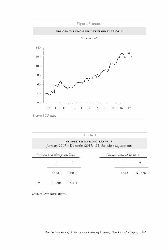
145The Natural Rate of Interest for an Emerging Economy: The Case of Uruguay
Source: BCU data.
140
120
100
80
60
40
20
Figure 5 (cont.)
URUGUAY: LONG-RUN DETERMINANTS OF r*
(e) Private credit
07 17161514131211100908
Table 1
SIMPLE SWITCHING RESULTS
January 2007 – December2017, 131 obs. after adjustments
Constant transition probabilities Constant expected durations
1 2 1 2
1 0.3187 0.6813 1.4678 16.9376
2 0.0590 0.9410
Source: Own calculations.
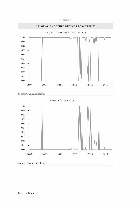
146 E. Bucacos
1.0
0.9
0.8
0.7
0.6
0.5
0.4
0.3
0.2
0.1
0.0
1.0
0.9
0.8
0.7
0.6
0.5
0.4
0.3
0.2
0.1
0.0
Figure 6
URUGUAY: SMOOTHED REGIME PROBABILITIES
A. REGIME 1: INTEREST RATE INSTRUMENT
B: REGIME 2; MONEY TARGETING
2007
2007
2009
2009
2011
2011
2013
2013
2015
2015
2017
2017
Source: Own calculations.
Source: Own calculations.
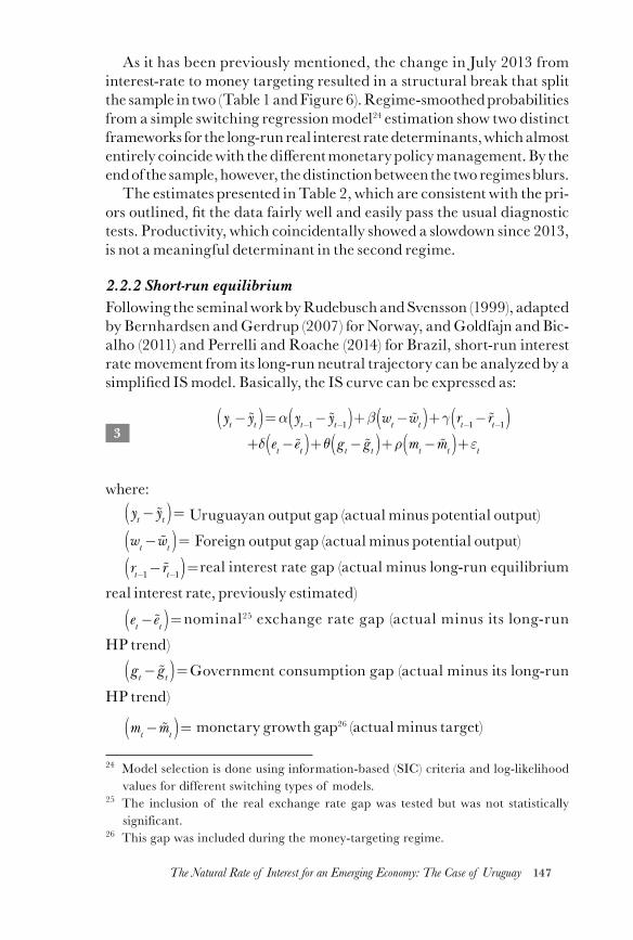
147The Natural Rate of Interest for an Emerging Economy: The Case of Uruguay
As it has been previously mentioned, the change in July 2013 from interest-rate to money targeting resulted in a structural break that split the sample in two (Table 1 and Figure 6). Regime-smoothed probabilities from a simple switching regression model24 estimation show two distinct frameworks for the long-run real interest rate determinants, which almost entirely coincide with the different monetary policy management. By the end of the sample, however, the distinction between the two regimes blurs.
The estimates presented in Table 2, which are consistent with the pri-ors outlined, fit the data fairly well and easily pass the usual diagnostic tests. Productivity, which coincidentally showed a slowdown since 2013, is not a meaningful determinant in the second regime.
2.2.2 Short-run equilibriumFollowing the seminal work by Rudebusch and Svensson (1999), adapted by Bernhardsen and Gerdrup (2007) for Norway, and Goldfajn and Bic-alho (2011) and Perrelli and Roache (2014) for Brazil, short-run interest rate movement from its long-run neutral trajectory can be analyzed by a simplified IS model. Basically, the IS curve can be expressed as:
3
where:
Uruguayan output gap (actual minus potential output)
Foreign output gap (actual minus potential output)
real interest rate gap (actual minus long-run equilibrium
real interest rate, previously estimated)
nominal25 exchange rate gap (actual minus its long-run
hp trend)
Government consumption gap (actual minus its long-run
hp trend)
monetary growth gap26 (actual minus target)
24 Model selection is done using information-based (SIC) criteria and log-likelihood values for different switching types of models.
25 The inclusion of the real exchange rate gap was tested but was not statistically significant.
26 This gap was included during the money-targeting regime.
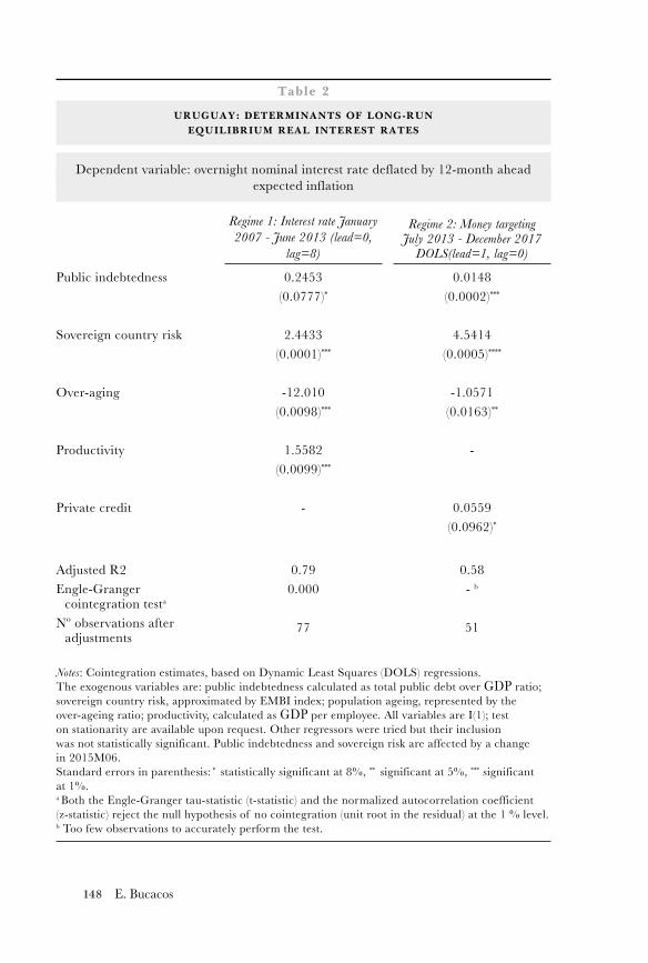
148 E. Bucacos
Table 2
URUGUAY: DETERMINANTS OF LONG-RUN EQUILIBRIUM REAL INTEREST RATES
Dependent variable: overnight nominal interest rate deflated by 12-month ahead expected inflation
Regime 1: Interest rate January 2007 - June 2013 (lead=0,
lag=8)
Regime 2: Money targeting July 2013 - December 2017
DOLS(lead=1, lag=0)
Public indebtedness
Sovereign country risk
Over-aging
Productivity
Private credit
0.2453(0.0777)*
2.4433(0.0001)***
-12.010(0.0098)***
1.5582(0.0099)***
-
0.0148(0.0002)***
4.5414(0.0005)****
-1.0571(0.0163)**
-
0.0559(0.0962)*
Adjusted R2Engle-Granger
cointegration testa
Nº observations after adjustments
0.790.000
77
0.58- b
51
Notes: Cointegration estimates, based on Dynamic Least Squares (DOLS) regressions. The exogenous variables are: public indebtedness calculated as total public debt over gdp ratio; sovereign country risk, approximated by EMBI index; population ageing, represented by the over-ageing ratio; productivity, calculated as gdp per employee. All variables are I(1); test on stationarity are available upon request. Other regressors were tried but their inclusion was not statistically significant. Public indebtedness and sovereign risk are affected by a change in 2015M06. Standard errors in parenthesis: * statistically significant at 8%, ** significant at 5%, *** significant at 1%.a Both the Engle-Granger tau-statistic (t-statistic) and the normalized autocorrelation coefficient (z-statistic) reject the null hypothesis of no cointegration (unit root in the residual) at the 1 % level. b Too few observations to accurately perform the test.
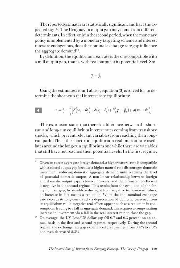
149The Natural Rate of Interest for an Emerging Economy: The Case of Uruguay
The reported estimates are statistically significant and have the ex-pected sign27. The Uruguayan output gap may come from different determinants. In effect, only in the second period, when the monetary policy is implemented by a monetary targeting scheme and interest rates are endogenous, does the nominal exchange rate gap influence the aggregate demand28.
By definition, the equilibrium real rate is the one compatible with a null output gap, that is, with real output at its potential level. So:
Using the estimates from Table 3, equation (3) is solved for to de-termine the short-run real interest rate equilibrium:
4
This expression states that there is a difference between the short-run and long-run equilibrium interest rates coming from transitory shocks, which prevent relevant variables from reaching their long-run path. Thus, the short-run equilibrium real interest rate oscil-lates around the long-run equilibrium one while there are variables that still have not reached their potential levels. In the first regime,
27 Given an excess aggregate foreign demand, a higher natural rate is compatible with a closed output gap because a higher natural rate discourages domestic investment, reducing domestic aggregate demand until reaching the level of potential domestic output. A non-linear relationship between foreign and domestic output gaps is found, however, and the estimated coefficient is negative in the second regime. This results from the evolution of the for-eign output gap; by steadily reducing it from negative to near-zero values, an increase in fact means a reduction. When the spot nominal exchange rate exceeds its long-run trend - a depreciation of domestic currency from its equilibrium value -negative real effects appear, such as a reduction in con-sumption, leading to a fall in aggregate demand; this requires a compensating increase in investment via a fall in the real interest rate to close the gap.
28 On average, the UY Peso/US dollar gap fell 0.7 and 0.3 percent on an an-nual basis in the first and second regimes, respectively. During the second regime, the exchange rate gap experienced great swings, from 0.4% to 7.0% and even decreased 8.3%.

150 E. Bucacos
Table 3
URUGUAY: DETERMINANTS OF SHORT-RUN EQUILIBRIUM REAL INTEREST RATES
Dependent variable: Uruguayan output gap
Regime 1: Interest rate January 2007 - June 2013
Regime 2: Money targeting July 2013 - December 2017
Uruguayan output gap-1
Uruguayan output gap-2
Foreign output gap
Foreign output gap-1
Foreign output gap-2
Real interest rate gap-1a
Nominal exchangerate gap
GovernmentConsumption gap
Monetary growth gap
1.7603(0.0000)***
-0.8181(0.0000)***
0.8619(0.0000)***
-1.5589(0.0000)***
0.7244(0.0000)***
-6.89e-05(0.0396)**
-
-
-
1.6857(0.0000)***
-0.7775(0.0000)***
-
-0.4130(0.0010)**
-
-0.0002(0.0021)***
-0.0178(0.0054)***
-
-
Notes: Own calculations.Standard errors in parenthesis: * statistically significant at 8%, ** significant at 5%, *** significant at 1%.a The inclusion of the long-run equilibrium real interest rate (a generated regressor) required a correction (White) to obtain a heteroskedasticity-robust variance-covariance matrix of the estimator.
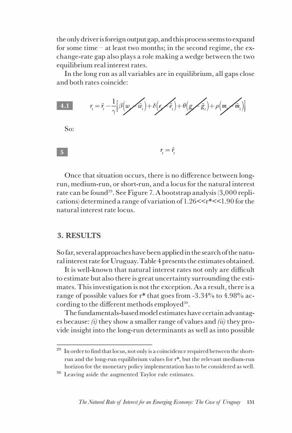
151The Natural Rate of Interest for an Emerging Economy: The Case of Uruguay
the only driver is foreign output gap, and this process seems to expand for some time – at least two months; in the second regime, the ex-change-rate gap also plays a role making a wedge between the two equilibrium real interest rates.
In the long run as all variables are in equilibrium, all gaps close and both rates coincide:
4.1
So:
5
Once that situation occurs, there is no difference between long-run, medium-run, or short-run, and a locus for the natural interest rate can be found29. See Figure 7. A bootstrap analysis (3,000 repli-cations) determined a range of variation of 1.26<<r*<<1.90 for the natural interest rate locus.
3. RESULTS
So far, several approaches have been applied in the search of the natu-ral interest rate for Uruguay. Table 4 presents the estimates obtained.
It is well-known that natural interest rates not only are difficult to estimate but also there is great uncertainty surrounding the esti-mates. This investigation is not the exception. As a result, there is a range of possible values for r* that goes from -3.34% to 4.98% ac-cording to the different methods employed30.
The fundamentals-based model estimates have certain advantag-es because: (i) they show a smaller range of values and (ii) they pro-vide insight into the long-run determinants as well as into possible
29 In order to find that locus, not only is a coincidence required between the short-run and the long-run equilibrium values for r*, but the relevant medium-run horizon for the monetary policy implementation has to be considered as well.
30 Leaving aside the augmented Taylor rule estimates.
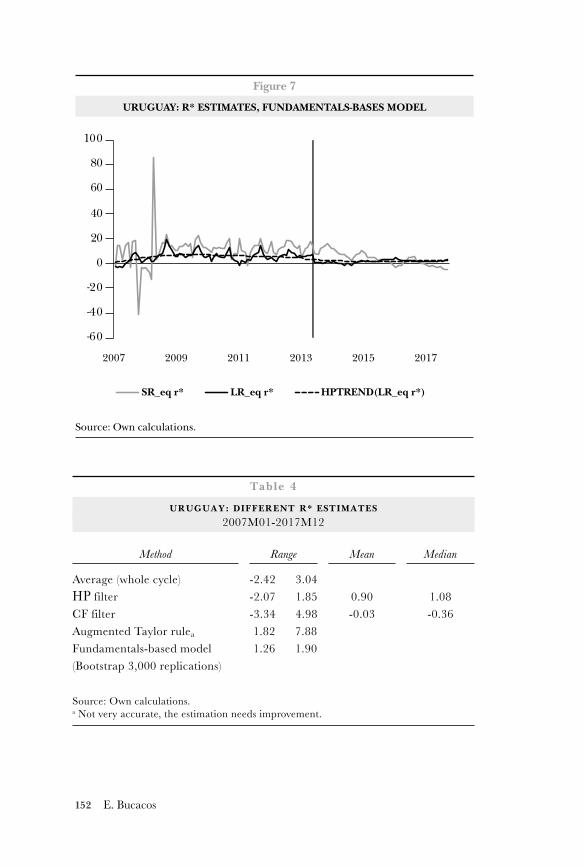
152 E. Bucacos
Table 4
URUGUAY: DIFFERENT R* ESTIMATES
2007M01-2017M12
Method Range Mean Median
Average (whole cycle)hp filterCF filterAugmented Taylor rulea
Fundamentals-based model(Bootstrap 3,000 replications)
-2.42 3.04-2.07 1.85-3.34 4.98 1.82 7.88 1.26 1.90
0.90-0.03
1.08-0.36
Source: Own calculations.a Not very accurate, the estimation needs improvement.
Figure 7
URUGUAY: R* ESTIMATES, FUNDAMENTALS-BASES MODEL
Source: Own calculations.
-60
-40
-20
0
20
40
60
80
100
2007 2009 2011 2013 2015 2017
SR_eq r* LR_eq r* HPTREND(LR_eq r*)
153The Natural Rate of Interest for an Emerging Economy: The Case of Uruguay
causes of fluctuations in the short-run. Thus, this approach combines the old tradition in economic literature regarding a long-run slowly moving equilibrium level with the concept of a short-run rate af-fected by transitory shocks. That is, in the long run, the natural rate should reflect the marginal product of capital goods and may only change as a result of structural factors, such as population dynamics, productivity, or other changes in the economic environment, such as financial deepening and public indebtedness. But in the short run, the interest rate can be affected by transitory shocks such as foreign demand and/or nominal exchange rate shocks.
The interest rate gap – calculated as the difference between the ac-tual short-run interest rate and the natural interest rate– r*, can shed some light on the monetary stance. We can see that for a majority of the time studied the monetary policy seems to have been expan-sionary; the 12-month inflation rate31 has followed the usual cor-responding pattern. See Figure 8, (a) and (b). However, as Magud and Tsounta (2012) point out, “… the estimated interest rate gap may not accurately reflect the current monetary stance given weaker mon-etary transmission mechanisms (reflected through a small response of market interest rates to a change in the monetary policy rate, e.g., due to excess liquidity); a monetary framework that is still under de-velopment; and segmented short-term funding markets which could result in policy rates that do not accurately reflect financing condi-tions in all markets.”
Magud and Tsounta (2012) point out that many factors could raise the effective market interest rate for the private sector, result-ing in tighter financial conditions than those captured by the policy rate. Among these factors, high financial dollarization and low fi-nancial intermediation, reduce the effectiveness of the policy rate by hindering the proper functioning of the transmission channel of monetary policy (see Medina Cas and others, 2011a, b). High lev-els of financial dollarization may reduce the impact that changes in the policy rate have on banks’ interest rates in local currency be-cause the borrowers can easily switch to foreign-currency instru-ments. A stylized fact of Uruguay is dollarization. There have been important attempts to alleviate this problem, but Uruguayan econ-omy still remains highly dollarized: as of December of 2017, almost
31 Calculated on the cpi.
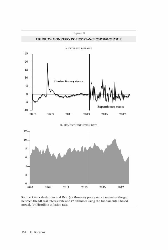
154 E. Bucacos
Figure 8
URUGUAY: MONETARY POLICY STANCE 2007M01-2017M12
Source: Own calculations and INE. (a) Monetary policy stance measures the gap between the SR real interest rate and r* estimates using the fundamentals-based model. (b) Headline inflation rate.
.
. 12-
-10
-5
0
5
10
15
20
25
2007 2009 2011 2013 2015 2017
Contractionary stance
Expantionary stance
0
2
4
6
8
10
12
2007 2009 2011 2013 2015 2017
155The Natural Rate of Interest for an Emerging Economy: The Case of Uruguay
80% of total deposits and close to 60% of total credits in the banking system are foreign currency-denominated32. However, the de-dol-larization process of the Uruguayan financial system that is be-ing implemented for more than ten years by now, has strengthened the interest-rate transmission (Leiderman et al., 2006).
Bank concentration limits competition and lowers banks’ reaction to the policy rate which may undermine the interest rate transmission mechanism. The response of banks’ rates to changes in the policy rate depends on the banks’ adjustment costs derived from the elas-ticity of demand for bank loans, which is influenced by the structure of the financial system (Cotarelli and Korelis, 1994; De Bond, 2002): relatively inelastic demand is more likely when there is higher bank concentration. When banks have substantial market power, policy rate changes may impact banking spreads rather than market rates because banks may try to profit from a reduction in the policy rate keeping lending rates fixed. The Uruguayan credit market is high-ly segmented33. The segmentation permeates the banking sector, which exhibits a high degree of concentration, particularly with regard to the peso deposit and credit markets. Indeed, the Herfin-dahl-Hirschman index (hhi) for the peso credit market yields a con-centration level of 0.26, while the u.s. dollar credit market is slightly less concentrated at 0.19.34
The development of the financial system strengthens the interest-rate transmission mechanism as more alternative sources of capital increase the elasticity of demand for bank loans (Cotarelli and Kore-lis, 1994). Financial shallowness is generally associated with higher excess liquidity in banks, discouraging the development of an active interbank market and reducing the effectiveness of transmission. Ac-cording to imf Uruguay Report (2016),
32 The main problem, though, is currency mismatches. According to recent studies, 87% of Uruguayan firms report to have liabilities denominated in currencies (mainly US dollars) different from those of their incomes (mainly Uruguayan pesos).
33 In 2014, 60% of total credit went to firms, 35% to households, and 5% to the public sector. Of the credit extended to firms, 87% was denominated in u.s. dollars, whereas for households, only 4% of credit was u.s. dollar denominated, and 35% in the case of the public sector. Consequently, 55% of total credit in 2014 was u.s. dollar denominated.
34 From a scale of 0 to 1, 1 being a perfect monopoly.
156 E. Bucacos
“A broad-based index of f inancial development indi-cates that Uruguay lags behind regional peers, and also relative to what could be expected given its own macro-economic fundamentals. Uruguay’s score of 0.2 in the composite financial development index (based on 2013 data) is equivalent to half the LA5 average, and below the individual scores of all LA5 countries (as reported in Heng and others, 2015). Furthermore, a regression analysis suggests that Uruguay scores worse on the index than would be predicted by its own economic fundamen-tals (including income per capita, government size, trade openness, inflation, educational attainment, and others). A decomposition of the results shows that this “under-development” relative to fundamentals mostly reflects low access to finance in Uruguay (both through financial institutions and through markets) and low financial in-stitution depth (measured through variables such as pri-vate sector credit). All other LA5 countries have index scores better than or equivalent to what their fundamen-tals would predict.”
These results point to the importance of complementing nrir estimations with, e.g., financial/monetary condition indices to bet-ter assess the monetary policy stance.
4. CONCLUDING REMARKS
In this document, we applied different methods to estimate the natu-ral rate of interest for Uruguay, a small, open, and dollarized econo-my. The natural rate of interest describes the real interest rate for a situation regarded as optimal from a particular point of view, such as price stability, full employment, or a rigidity-free environment. It follows that an optimal monetary policy should be conducted so as to approximate the actual real interest rate to that desirable rate because, consequently, gdp, unemployment, inflation, etc. should follow their welfare-maximizing paths. When the central bank’s in-strument is the nominal interest rate, that objective can be directly monitored; when the central bank has money targets, its fulfilment is hard to assess because the current real interest rate is endogenous
157The Natural Rate of Interest for an Emerging Economy: The Case of Uruguay
and fluctuates too much. In a dollarized economy, it is even more difficult because the monetary policy design has to take into account the presence of foreign currency demand together with the domestic currency either competing with or complementing with each other.
Notwithstanding those difficulties, we provide some estimates for the nir using varied approaches, we offer a useful framework where to analyze the difference between long-run and short-run dif-ferences, and we assess the monetary policy stance for the whole sam-ple period. Specifically, the fundamentals-based model helps us to deal with the difference between the short- and long-run nir and is intended to be an addition to the myriad approaches actually in use in the Banco Central del Uruguay (bcu).
Some discussion of the debate over decreasing nir is needed. Our estimates point to a sharp decrease in the movement in the short-run equilibrium natural rate since 2013 (owing to internation-al drivers) which is smaller in the long run. Long run equilibrium natural interest rate evolves smoothly with an almost unnoticeable deceleration (Figure 7). That seems to be the result of two oppos-ing forces: on the one hand, the increase –but at a declining speed– in the over-aging index augments the propensity to save and pushes the natural interest rate down; on the other, the increase in both public indebtedness and perceived country risk reduces the agents’ willingness to invest and pushes the natural interest rate up. Pro-ductivity – measured as output per occupied worker – reinforces this effect during the first regime.
As a corollary of this research, it can be said that “[u]nfortunately, we have as yet devised no method to estimate accurately and read-ily the natural rate of either interest or unemployment”.35 This is a work in progress.
35 Milton Friedman (1968).
158 E. Bucacos
References
Acosta-Ormachea, S., & Coble, D. (2011). The monetary trans-mission in dollarized economies: the cases of Chile, New Zealand, Peru, and Uruguay. imf Working Paper 11/87 (Washington: International Monetay Fund).
Bernhardsen, T., & Gerdrup, K. (2007). The neutral real interest rate. Norges Bank Economic Bulletin 2, Vol. 78, pp.52-64.
Bucacos, E. (2012). La tasa natural de interés para la economía uruguaya: un enfoque basado en un modelo DSGE. Mimeo, bcu.
Calderón, C., & Gallego, F. (2002). La tasa de interés real neutral en Chile. Banco Central de Chile, Vol. 11, Nº2.
Carrillo, J. A., Elizondo, R., Alonso Rodríguez-Pérez, C., & Roldán-Peña, J. (July, 2017). What determines the neutral rate of interest in an emerging economy? Banco de México.
Chananenco, P., & Savino, M. P. (2009). The natural rate of in-terest in Brazil between 1999 and 2005. Revista Brasileira de Economia, Rio de Janeiro, Vol. 63, Nº2, 103-18.
Cottarelli, C., & Kourelis, A. (1994). Financial structure, bank lending rates and the transmission mechanism of monetary policy. imf Working Paper WP/94/39.
Daly, H., & Cobb, J. (1989). For the common good. Boston Beacon Press.
De Bondt, G. (2002). Retail bank interest rate pass-through: new evidence at the Euro Area level. European Central Bank Work-ing Papar 136.
Del Negro, M., Giannone, D., Giannoni, M. P., & Tambalotti, A. (Spring 2017). Safety, liquidity, and the natural rate of interest. Brookings Papers on Economic Activity.
Duarte , J. (2010). Measuring the natural interest rate in Brazil. Institute of Brazilian Business and Public Management Is-sues (Washington: George Washington University).
Fuentes, R., & Gredig, F. (2008). La tasa de interés neutral: esti-maciones para Chile. Economía Chilena, Vol. 11, Nº2.
Galesi, A., Nuño, G., & Thomas, C. (2017). The natural interest rate: concept, determinants and implications for monetary policy. Analytical articles 2017, Banco de España, Eurosistema.
159The Natural Rate of Interest for an Emerging Economy: The Case of Uruguay
Goldfajn, I., & Bicalho, A. (2011). A longa travessia para a nor-malidade: os juros reais no Brasil. in Novos Dilemas da Politica Economica - Ensaios em homenagem a Dionisio Dias Carnerio, edited by E.L. Bacha e M. B. de Bolle Rio de Janeiro: Grupo Editorial Nacional.
González, A., Ocampo, S., Perez, J., & Rodriguez, D. (2012). Out-put gap and neutral interest rate measures for Colombia. Borradores de Economía, Nº726 (Bogotá: Banco de la República).
Heng, D., Iavanova, A., Mariscal, R., Ramaksidhnan, U., & Cheng Wong, J. (2016). Advancing financial development in Latin America and the Caribbean. imf Working Paper WP/16/81.
Holston , K., Laubach, T., & Williams, J. (December 2016). Mea-suring the natural rate of interest: international trends and determinants. Working paper 2016-11, Federal Reserve Bank of San Francisco.
imf. (2011). Dominican Republic: Fourth review under the Stand-by Arragement and Request of Waiver of Nonobservance of Performance Criterion - Staff Report. July (Washington: International Monetary Fund).
imf, Figliuoli, L., Flamini , V., Mowatt, R., Puig, J., Lambert, F., y otros. (2018). Growing pains: is Latin America prepared for population aging? Regional Economic Outlook, April 2018, imf.
Lambert, F. (2017). Uruguay’s neutral interest rate. imf Coun-try Report 17/29, Uruguay, selected issues, International Monetary Fund.
Leiderman, L., Maino, R., & Parrado, E. (2006). Inflation targeting in dollarized economies. imf Working Paper, WP/06/157.
Leijonhufvud, A. (1989). Natural interest rate and market interest rate. in: Money. The New Palgrave.
Licandro, G., Mello, M., & Odriozola, J. (2014). Uso de derivados en Uruguay. Documento de trabajo, Nº004-2014, Banco Central del Uruguay.
Magud, N., & Tsounta, E. (2012). To cut or not to cut? That is the (Central Bank’s) question. In search of the natural interest rate in Latin America. imf, Working Paper Series, WP/12/243.
Minella, A., Freitas, Goldfajn, I., & Muinhos, M. (2002). Inflation targeting in Brazil: lessons and challenges. Working Paper Series, Nº53, Banco Central do Brazil.
160 E. Bucacos
Perrelli, R., & Roache, S. (2014). Time-varying neutral interest rate - the case of Brazil. imf Working Paper 14/84.
Perrelli, R., & Roache, S. (2014). Time-varying neutral interest rate: the case of Brazil. imf Working paper, WP/14/84, In-ternational Monetary Fund.
Portillo, R., & Ustyugonova, Y. (2015). A model for monetary policy analysis in Uruguay. imf Working Paper Series, WP/15/170.
Roache, S. K. (2014). Inflation pesistence in Brazil - a cross country comparison. imf Working Paper, 14/55.
Rudebusch, G., & Svensson, L. (1999). Policy rules for inflation targeting. in Monetary policy rules, edited by J.B. Taylor. Chicago: University of Chicago Press.
Taylor, J. B. (1993). Discretion vs policy rules in practice. Carnegie-Rochester Conference Series on Public Policy 39, 195-214.
Woodford, M. (2003). Interest and prices. Princeton University Press.
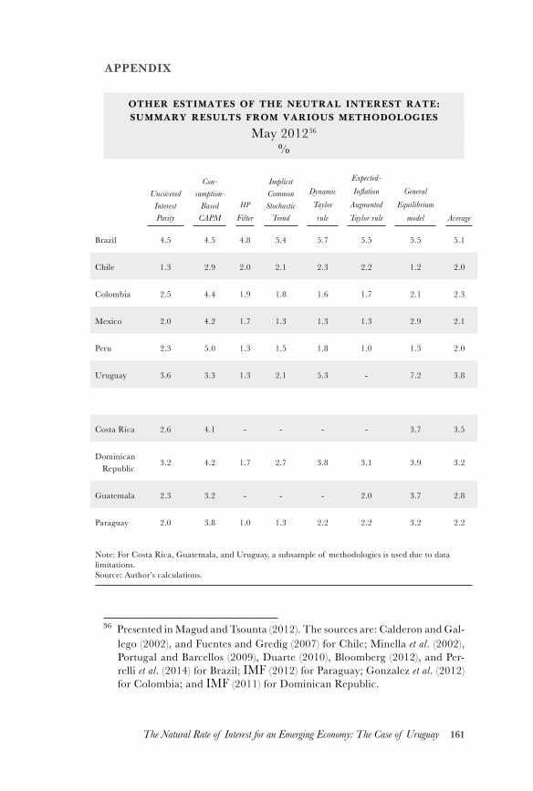
161The Natural Rate of Interest for an Emerging Economy: The Case of Uruguay
APPENDIX
OTHER ESTIMATES OF THE NEUTRAL INTEREST RATE: SUMMARY RESULTS FROM VARIOUS METHODOLOGIES
May 201236
%
Uncovered Interest Parity
Con-sumption-
Based CAPM
hp Filter
Implicit Common Stochastic
Trend
Dynamic Taylor rule
Expected-Inflation
Augmented Taylor rule
General Equilibrium
model Average
Brazil 4.5 4.5 4.8 5.4 5.7 5.5 5.5 5.1
Chile 1.3 2.9 2.0 2.1 2.3 2.2 1.2 2.0
Colombia 2.5 4.4 1.9 1.8 1.6 1.7 2.1 2.3
Mexico 2.0 4.2 1.7 1.3 1.3 1.3 2.9 2.1
Peru 2.3 5.0 1.3 1.5 1.8 1.0 1.3 2.0
Uruguay 3.6 3.3 1.3 2.1 5.3 - 7.2 3.8
Costa Rica 2.6 4.1 - - - - 3.7 3.5
Dominican Republic
3.2 4.2 1.7 2.7 3.8 3.1 3.9 3.2
Guatemala 2.3 3.2 - - - 2.0 3.7 2.8
Paraguay 2.0 3.8 1.0 1.3 2.2 2.2 3.2 2.2
Note: For Costa Rica, Guatemala, and Uruguay, a subsample of methodologies is used due to data limitations.Source: Author’s calculations.
36 Presented in Magud and Tsounta (2012). The sources are: Calderon and Gal-lego (2002), and Fuentes and Gredig (2007) for Chile; Minella et al. (2002), Portugal and Barcellos (2009), Duarte (2010), Bloomberg (2012), and Per-relli et al. (2014) for Brazil; imf (2012) for Paraguay; Gonzalez et al. (2012) for Colombia; and imf (2011) for Dominican Republic.
162 J. Carrillo, R. Elizondo, C. Rodríguez-Pérez, J. Roldán-Peña
The Longer-Term Convergence Level of the Neutral Rate of Interest in Mexico
Julio A. CarrilloRocio Elizondo
Cid Alonso Rodríguez-PérezJessica Roldán-Peña
Abstract
In this paper, we argue that foreign and domestic structural factors may explain the de-cline of the long-run convergence level of the neutral rate of interest in Mexico. In partic-ular, we find that low-frequency changes in the neutral rate may be attributed to increas-ing domestic savings, demographics shifts, and a decreasing global long-run real interest rate. These results are largely consistent with other studies showing that the neutral rate has decreased in the last 25 years in advanced and emerging economies alike.
Keywords: Neutral rate of interest, long-run determinants, Mexico.jel classification: C10, E43, E52.
Julio A. Carrillo <[email protected]>, Directorate General of Economic Research, Banco de México. Rocío Elizondo <[email protected]>. Cid Alonso Rodríguez-Pérez <[email protected]>, Jessica Roldán Peña <[email protected]>. We thank Ana María Aguilar, Daniel Chiquiar, Santiago García-Verdú, Juan Ramón Hernández, Claudia Ramírez, Alberto Torres, and Joris Wauters for their helpful comments, as well as Luis G. Hernández, Valeria Durán, and Julio Pierre-Audain for their invaluable re-search assistance. Jessica Roldán-Peña thanks the Directorate General of Economic Research of Banco de México, where she contributed to this project, while being Monetary Research Manager. Any views expressed herein are those of the authors and do not necessarily reflect those of Banco de México or Casa de Bolsa Finamex.
163The Longer-Term Convergence Level of the Neutral Rate of Interest in Mexico
1. INTRODUCTION
The neutral or natural rate of interest is defined as the level of the short-run real interest rate that is consistent with output near its potential or natural lev-el.1 It is also common to refer to the neutral rate of interest as r*. The domes-tic market for loanable funds determines r*. In this market, desired savings, composed of foreign and home portfolios in fixed-income markets, firms’ and households’ bank deposits, and other types of savings, establish the sup-ply, while investment demand, composed of public and private debt, determines the demand. The neutral rate helps to determine the stance of monetary policy,2 but unfortunately this variable is not observed and must be estimated.
Recent evidence on r* in both advanced and emerging economies (aes and emes) yields remarkably similar results: most estimates show a down-ward trend in r* over the past 25 years. Some commentators, such as Holston, Laubach and Williams (2017), have observed that potential growth and the neutral rate have co-moved in advanced economies during this time period. By contrast, this co-movement is not observed in emerging economies. A di-mension that has not been fully explored in the literature is the role of capital flows in the determination of r*. Sustained capital flows could have a long-lasting effect on the neutral rate of an eme since these flows affect the sup-ply of loanable funds in such an economy. Although this channel is present in both aes and emes, it could be more important in the latter given their greater sensitivity to external events.
In this document, we estimate the long-run convergence level of the neutral rate in Mexico, a prototype eme with a significant volume of internation-al trade and a financial market highly integrated with the global market. We also refer to the long-run convergence level of the neutral rate as r ∗ , i.e., with a bar accent over r*. Following the fomc Minutes of October 2015,
1 At this level of output, we also find the natural rate of unemployment, i.e., the level of unemployment at which inflation remains stable in the absence of shocks.
2 The monetary policy stance is neutral if the short-run real interest rate equals r* and it is contractionary (expansionary) if the short-run real rate is located above (below) r*. If the stance is contractionary, monetary policy slows down aggregate demand by setting an opportunity cost of funds for consumption and investment higher than it would normally be. The opposite happens if the stance is expansionary. If we add a measure of inflation expectations to r*, we get the level of the monetary-policy interest rate at which the policy is neutral.
164 J. Carrillo, R. Elizondo, C. Rodríguez-Pérez, J. Roldán-Peña
we formally define r ∗ as “the longer-run normal level to which the [short-run real interest] is expected to converge in the absence of further shocks to the economy.” We perform our estimations for the sample period January 2000 to De-cember 2017.
The long-run convergence level of r* is determined exclusively by struc-tural factors, such as potential growth, demographics, and financial-mar-kets development.3 To compute a robust measure of r ∗, we estimate three quantitative methods: an augmented Taylor rule which includes a control for a very persistent transitory (or non-structural) factor, an open-economy rbc model, and the 10-year expectation of the short-run nominal interest rate computed from an affine term- structure model. In contrast to stud-ies focusing on higher-frequency measures of the neutral rate, there are a limited number of techniques that can be used to estimate r ∗. A suitable method for the low-frequency measure must be able to disentangle the ef-fects of transitory and structural factors at the level of the neutral rate. This task becomes difficult when very persistent transitory factors are observed in the economy (e.g., the shocks that led to the global financial crisis, its af-termath, and the policy responses that followed). Since no method is per-fect, we also review some structural factors that are informative about upward and downward risks for r ∗ in Mexico.
Our results are as follows. The evidence suggests that the long-run con-vergence level of r* in 2017 is lower than the level that prevailed at the be-ginning of the 2000s, falling from around 3% in real terms to close to 2.5%.4 As mentioned above, a downward trend for r ∗ has also been estimated in several aes and emes.
We argue that both domestic and foreign structural factors account for the apparent fall in r ∗ registered from the 2000s to present. On the do-mestic side, we observe (1) sustained growth of national savings as a per-centage of gdp, (2) an increase in working-age share of the population,
3 See Carrillo, Elizondo, Rodríguez-Pérez and Roldán-Peña (2018) for a for-mal definition. In that paper, we also considered higher-frequency measures of r*, where we analyzed transitory factors (e.g. macro shocks) that diverted the neutral rate temporarily from its long-run fundamental value in Mexico. In Section 3, we briefly review the results and drivers of these higher-frequency measures of r*.
4 The former corresponds with the average of the estimates of r* for the short-, and medium-run during the period 2001Q1-2008Q4, while the latter is the average of the estimates of r ∗ in Section 4. It is worth mentioning that the uncertainty surrounding these estimates is quite significant, so punctual results must be taken with caution.
165The Longer-Term Convergence Level of the Neutral Rate of Interest in Mexico
(3) a declining outlook for the growth rate of the labor force, and (4) a flat trend in productivity. All four factors imply a lower long-run convergence level of the neutral rate. In the market for loanable funds, the first two fac-tors drive up the supply, while the last two reduce the demand (through their influence on investment). On the foreign side, the sustained reduction in the global long-term real interest rate seems to have pushed international long-term credit toward the Mexican market. The latter could have lowered the domestic long-term real interest rate through no-arbitrage conditions. Indeed, sustained capital inflows seem to have contributed to permanent increases in the supply of loanable funds in the economy, putting downward pressure on r ∗.
The remainder of the paper is organized as follows. Section 2 reviews in-ternational evidence on trend output growth and money-market rates in a large set of aes and emes. The section also reviews several studies that es-timate r* in several economies. Section 3 summarizes the findings on higher-frequency measures of the neutral rate in Mexico. In turn, Section 4 focuses on the long-run convergence level of the neutral rate in the country. The fi-nal section concludes.
2. INTERNATIONAL EVIDENCE
Holston et al. (2017) find that the estimated neutral rates and trend growth rates of four advanced economies (aes), namely the u.s., Canada, the u.k., and the Euro Area, have co-moved tightly over the past 25 years. These au-thors suggest that global factors may largely explain this behavior. In sharp contrast, this kind of co-movement does not hold for emerging market econ-omies (emes) as most of these countries grow at relatively high rates, while at the same time their neutral rates have fallen. In this Section, we first re-view data on the growth rates and short-run real interest rates for a large set of aes and emes that confirm the aforementioned trends. We then re-view some recent estimations of the neutral rate in different economies.
2.1 Output Growth and Money-Market Rates in AEs and EMEs
The imf’s World Economic Outlook of April 2018, Box 1.3, presents potential growth estimates for ten aes and five emes;5 the report finds that potential
5 In the imf’s study, aes include Australia, Canada, France, Germany, Italy, Japan, Korea, Spain, the u.k., and the u.s., while emes include Brazil, India, Mexico, Russia, and Turkey.
166 J. Carrillo, R. Elizondo, C. Rodríguez-Pérez, J. Roldán-Peña
growth has persistently decreased for the former, while it follows an in-verted U -shaped pattern for the latter. In particular, for the group of aes, trend growth fell from 2.5% in 2001 to 1.5% in 2017, while for the group of emes, trend growth was 4% for both years, with a peak at 5% in 2007.6
We now present complementary evidence to Box 1.3 using the Fund’s IFS data. Table 1 presents long-run averages of annual output growth rates and money-market real interest rates for a wider set of aes and emes, sev-enteen for the former and thirty for the latter.7 Money-market rates refer to the interest rate of assets with maturity of one year or less. These rates are therefore closely related to short-term government bond rates, such as T-bills. We compute ex-post real interest rates using annual inflation in each country. To compute the mean for each category, we weighted the observa-tion of each country by its proportion in world gdp. The average weight of aes’ gdp in the sample is 50.9% of the world production, while that of emes is 28%.8 The sample starts in 1993 due to issues with data avail-ability, especially for emes. Long-run averages cover 7 or 8 years, which is the typical length assumed for a business cycle. We opt for excluding the years 2008 and 2009 from the sample, since these years were severely affected by the global financial crisis (gfc, for short).9
6 When China is included in the emes sample, average trend growth of this subgroup is even stronger.
7 aes include Australia, Belgium, Canada, Denmark, France, Germany, Italy, Japan, Korea, the Netherlands, New Zealand, Singapore, Spain, Sweden, Switzerland, the u.k., and the u.s. In turn, emes include Algeria, Angola, Argentina, Brazil, Bulgaria, Chile, Colombia, Cote d’Ivoire, Hungary, India, Indonesia, Kuwait, Malaysia, Mexico, Morocco, Pakistan, Peru, the Philip-pines, Poland, Romania, Russia, Saudi Arabia, Serbia, South Africa, Thailand, Tunisia, Turkey, Ukraine, Venezuela, and Vietnam. China is not included since data for its mainland money markets are not available for most of the period of interest.
8 When computing the average money market real interest rate, we excluded observations for years in which the inflation rate is higher than 25%. The trimmed sample avoids thus distorted measures of real interest rates due to super-inflationary periods. In aes, there are zero episodes with such characteristics, while in emes there are 84, of which 56 occurred between 1993 and 1999.
9 Including these years into the calculation reduces the long-run average of output growth of aes, but not so much in emes.
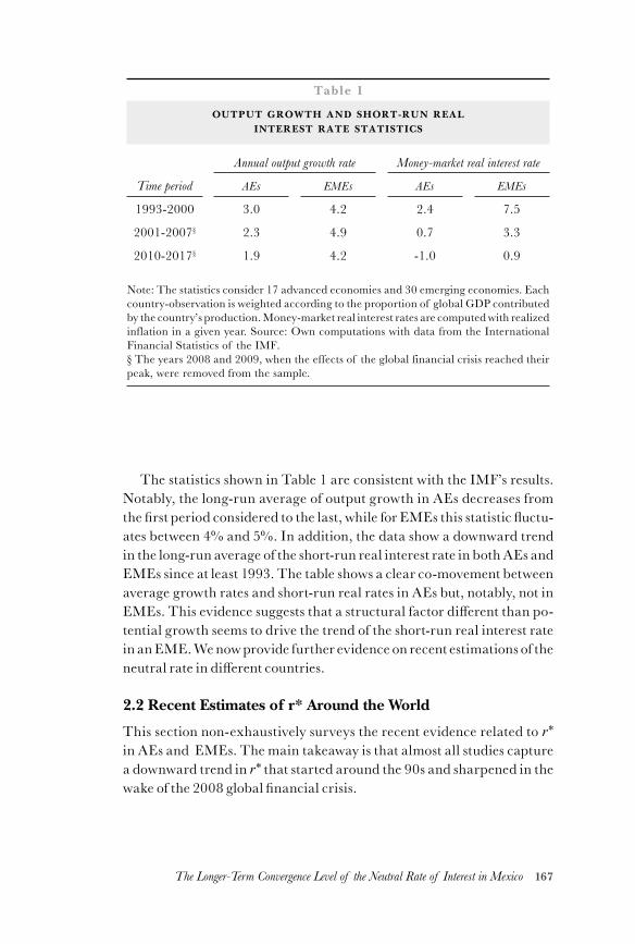
167The Longer-Term Convergence Level of the Neutral Rate of Interest in Mexico
The statistics shown in Table 1 are consistent with the imf’s results. Notably, the long-run average of output growth in aes decreases from the first period considered to the last, while for emes this statistic fluctu-ates between 4% and 5%. In addition, the data show a downward trend in the long-run average of the short-run real interest rate in both aes and emes since at least 1993. The table shows a clear co-movement between average growth rates and short-run real rates in aes but, notably, not in emes. This evidence suggests that a structural factor different than po-tential growth seems to drive the trend of the short-run real interest rate in an eme. We now provide further evidence on recent estimations of the neutral rate in different countries.
2.2 Recent Estimates of r* Around the World
This section non-exhaustively surveys the recent evidence related to r* in aes and emes. The main takeaway is that almost all studies capture a downward trend in r* that started around the 90s and sharpened in the wake of the 2008 global financial crisis.
Table 1
OUTPUT GROWTH AND SHORT-RUN REAL INTEREST RATE STATISTICS
Time period
Annual output growth rate Money-market real interest rate
aes emes aes emes
1993-2000 3.0 4.2 2.4 7.5
2001-2007§ 2.3 4.9 0.7 3.3
2010-2017§ 1.9 4.2 -1.0 0.9
Note: The statistics consider 17 advanced economies and 30 emerging economies. Each country-observation is weighted according to the proportion of global gdp contributed by the country’s production. Money-market real interest rates are computed with realized inflation in a given year. Source: Own computations with data from the International Financial Statistics of the imf.§ The years 2008 and 2009, when the effects of the global financial crisis reached their peak, were removed from the sample.
168 J. Carrillo, R. Elizondo, C. Rodríguez-Pérez, J. Roldán-Peña
2.2.1 Advanced EconomiesFor the u.s., Yellen (2015) presents a set of estimates of r* obtained from New-Keynesian dsge models developed by the Fed’s staff; these show that this variable plunged toward negative levels at the onset of the gfc and reached zero by the end of 2015. These models interpret the reduction in short-run r* as a response to persistent macro shocks to aggregate demand, such as tighter financing conditions and less access to credit, de-leveraging by households, lower global growth, and greater uncertain-ty.10 More flexible methodologies, such as state-space models with a time-varying structure, find similar results. For the case of the u.s., Laubach and Williams (2016) and Johannsen and Mertens (2016) estimate a clear downward trend in r* that has started at least since the 80s but has deep-ened since the financial crisis. Laubach and Williams (2016) relate the fall in r* to a decreasing potential growth. In contrast, Del Negro, Giannone, Giannoni and Tambalotti (2017), using both time-series and a dsge model, attribute the fall in r* to a rising premia for the liquidity and safety of Treasury bonds, also known as convenience yield. Their findings add to the literature showing that Treasury bonds are valued not only for their pecuniary return, but also for the safe and liquidity services they offer.
The evidence for a downward trend in r* is not exclusive to the u.s. Holston et al. (2017) find evidence that r* and potential growth in Canada, the Euro Area, and the u.k. have followed a downward trend for several decades.11 Additionally, they find that these estimates and those for the u.s. have a considerable amount of co-movement over time. Thus, the authors suggest that global factors play an important role in explaining trends in r* and potential growth in these economies. Similarly, Bouis, Rawdanow-icz, Renne, Watanabe and Christensen (2013) find that for seven oecd economies r* has generally fallen since 1980.12 They argue that the fall of r*
10 The estimates of these dsge models assume the existence of nominal rigidities and other frictions to capture transitory macroeconomic shocks. To estimate r ∗ the models compute the real interest rate that would prevail if prices and wages were flexible. Therefore, the estimated r ∗ in this type of model is a counterfactual measure, not observable, and highly volatile, since it is subject to a wide set of transitory shocks.
11 See also Berger and Kempa (2014) for Canada.12 The countries are the u.s., Japan, the Euro Area, the u.k., Canada, Swe-
den, and Switzerland. The last two countries are the exceptions, since their estimates of r* have remained stable, and relatively high, since the financial crisis.
169The Longer-Term Convergence Level of the Neutral Rate of Interest in Mexico
is likely the result of lower potential growth. In addition, they mention that, according to oecd projections, r* may converge to a lower level than that before the gfc. For Japan, Fujiwara, Iwasaki, Muto, Nishizaki and Sudo (2016) show that r* has followed a downward trend since the 90s, and they relate this trend to a slowdown in potential growth. Similarly, the European Central Bank (2004) finds that r* in the Euro Area has decreased since the mid-90s and argues that this trajectory may reflect the slowdown in productivity and population growth in the region.13 For Norway, Bernhardsen and Ger-drup (2007) find that r* has fallen since at least 1990, and they explain that one of the reasons is a lower inflationary risk premia, since inflation and its expectations stabilized toward low levels. For New Zealand, Basdevant, Björksten and Karagedikli (2004) find evidence that suggests a downward trend in r* since 1992, while Björksten and Karagedikli (2003) conclude that the reduction in r* can be partly attributed to a worldwide decline in natu-ral rates as well as to local factors. More recently, Richardson and Williams (2015) confirm this evidence for New Zealand. Schmidt-Hebbel and Walsh (2009) present more evidence on r* in other advanced economies.14 Although they do not find clear evidence of a downward trend in r* in all cases, they do show that the neutral rates of these economies are highly correlated.
2.2.2 Emerging Market EconomiesThe evidence for emes is not very different from that for aes. Neutral rates in emes have also shown a downward trend. In particular, Magud and Tsounta (2012), using different methodologies, document some stylized facts for r* in ten Latin American countries:15 (i) r* tends to be lower in coun-tries with stronger fundamentals; (ii) wider ranges in r* estimates are asso-ciated with weaker monetary policy frameworks and higher inflation risk
13 See also Cuaresma, Gnan and Ritzberger-Gruenwald (2004), Mesonnier and Renne (2007), Garnier and Wilhelm-Sen (2009), and Fries, Mésonnier, Mouabbi and Renne (2018).
14 The countries covered are the u.s., the Euro Area, Japan, and some inflation-targeting countries, such as Australia, Canada, New Zealand, Norway, the u.k., Sweden, and Chile.
15 The countries are Brazil, Chile, Colombia, Costa Rica, the Dominican Republic, Guatemala, Mexico, Paraguay, Peru, and Uruguay. The methodologies used by the authors include: the Hodrick-Prescott filter, an implicit common sto-chastic trend using short- and long-term interest rates, dynamic Taylor rules, expected-inflation augmented Taylor rules, the Laubach and Williams model, consumption-smoothing models, and the uncovered interest rate parity (uip) condition. Their sample spans from 2000 to 2012.
170 J. Carrillo, R. Elizondo, C. Rodríguez-Pérez, J. Roldán-Peña
premia, although the dispersion could be also caused by short samples and unavailable data; and (iii) r* experienced a downward trend in the past decade for most of the countries studied. Magud and Tsounta argue that this trend is possibly due to stronger economic fundamentals in the region, as well as to more accommodative global financing conditions that would have increased the supply of loanable funds in the studied countries.
In the same vein, Perrelli and Roache (2014) find a downward trend in the estimates of r* for a wider set of emes.16 These authors focus on the experience of Brazil and find that the fall in its neutral rate can be ex-plained by both domestic and foreign factors. For the former, they argue that financial deepening, a declining public debt, and a lower sovereign risk premium have contributed to increase the desired savings in the country. Concerning the latter, they find evidence suggesting that the global real interest rate has also contributed to the decrease in Brazil’s neutral rate.
In other individual-country analyses, Fuentes and Gredig (2008) and González, Ocampo, Pérez and Rodríguez (2012) study the cases of Chile and Colombia using a battery of models to estimate plausible paths for r*17. In the case of Chile from 1980 to 2007, all models find that the estimated r* trends downward. For Colombia, the estimates of r* vary significantly.
Finally, Zhu (2016) finds that, with the exceptions of China and Thai-land, estimates of r* have declined substantially since 2005 for a group of countries in the Asia-Pacific region.18 Consistent with the existing ev-idence, the author finds that for some economies (e.g. the u.s., Japan,
16 They include the following countries: Brazil, Chile, China, Colombia, the Czech Republic, Egypt, Hungary, India, Indonesia, Israel, Korea, Malaysia, Mexico, Peru, the Philippines, Poland, Russia, South Africa, Taiwan, Thailand, Turkey, and Uruguay. The authors use statistical filters to document the decline of r* in a sample spanning from 2002 to 2013. Furthermore, using a principal components analysis, the authors find that two common factors may explain about 45% of the common fluctuations in real policy rates of the analyzed countries. The first of these factors represents the common trend, while the second one is the common cycle.
17 The models used in these papers can be classified into three categories: (i) economic theory (traditional consumption model, uncovered parity interest rate condition, general equilibrium reduced-form models); (ii) implicit expec-tations of r* in financial instruments (forward rates, state-space models with common stochastic trend in short-run and long-run interest rates, and yield curve models); and (iii) statistical models (filters).
18 These countries are: Australia, China, Hong Kong, India, Indonesia, Japan, Korea, Malaysia, New Zealand, the Philippines, Singapore, Thailand, and the
171The Longer-Term Convergence Level of the Neutral Rate of Interest in Mexico
Korea, and Singapore), the downward trend in r* started in the 1980s. Additionally, Zhu finds that low- frequency movements in the neutral rate seem to be strongly related to demographics and global factors (e.g. trade and capital flows, global liquidity), while the relationship with potential growth appears to be weaker.
3. SHORT-RUN NEUTRAL RATE IN MEXICO: A SUMMARY
Carrillo, Elizondo, Rodríguez-Pérez and Roldán-Peña (2018), henceforth cerr for short, conduct detailed analysis of higher-frequency measures of the neutral rate in Mexico. For convenience, cerr call these measures of the neutral rate short-run r* or medium-run r*. cerr consider that transitory factors (e.g. macro shocks) divert the neutral rate temporari-ly from its long-run fundamental value, which is determined exclusively by structural factors. In this section, we provide a brief summary of the results in cerr, and we invite the interested reader to review the paper for further details.19
The takeaway from cerr’s analysis is that, the rise and fall of non-res-idents holdings of short- term Mexican debt in the aftermath of the gfc, which increased and then decreased the supply of loanable funds in the country, may explain the temporary dip of the neutral rate observed from 2010 to 2014 in Mexico. These capital inflows surged during the imple-mentation of unconventional monetary policies in advanced economies, and started to reverse when the Fed signaled for the first time the tapering of its QE programs in mid-2013. Therefore, before the gfc, long-term averages of the estimates of short-run r* seem to be good approximations of the long-run convergence level of the neutral rate in Mexico, since tran-sitory factors were not very persistent. However, after 2008 this is no longer the case because short-run r* was affected by very persistent transitory fac-tors, such as slack economic conditions and the implementation of ultra-accommodative monetary policies in aes.
To perform the short-, and medium-run estimations, cerr use the ex ante short-term real interest rate, measured as the overnight interbank
u.s. The sample spans from 1950 to 2014. The author exploits the spectral density of the data to find low-frequency changes.
19 cerr also provides a formal disambiguation between the neutral in the short run and its long-run convergence level.
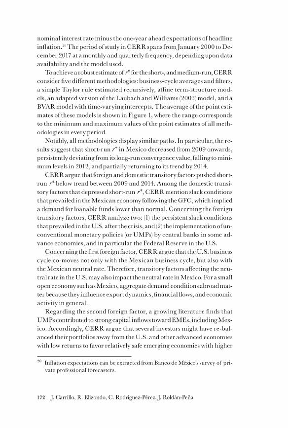
172 J. Carrillo, R. Elizondo, C. Rodríguez-Pérez, J. Roldán-Peña
nominal interest rate minus the one-year ahead expectations of headline inflation.20 The period of study in cerr spans from January 2000 to De-cember 2017 at a monthly and quarterly frequency, depending upon data availability and the model used.
To achieve a robust estimate of r* for the short-, and medium-run, cerr consider five different methodologies: business-cycle averages and filters, a simple Taylor rule estimated recursively, affine term-structure mod-els, an adapted version of the Laubach and Williams (2003) model, and a bvar model with time-varying intercepts. The average of the point esti-mates of these models is shown in Figure 1, where the range corresponds to the minimum and maximum values of the point estimates of all meth-odologies in every period.
Notably, all methodologies display similar paths. In particular, the re-sults suggest that short-run r* in Mexico decreased from 2009 onwards, persistently deviating from its long-run convergence value, falling to mini-mum levels in 2012, and partially returning to its trend by 2014.
cerr argue that foreign and domestic transitory factors pushed short-run r* below trend between 2009 and 2014. Among the domestic transi-tory factors that depressed short-run r*, cerr mention slack conditions that prevailed in the Mexican economy following the gfc, which implied a demand for loanable funds lower than normal. Concerning the foreign transitory factors, cerr analyze two: (1) the persistent slack conditions that prevailed in the u.s. after the crisis, and (2) the implementation of un-conventional monetary policies (or umps) by central banks in some ad-vance economies, and in particular the Federal Reserve in the u.s.
Concerning the first foreign factor, cerr argue that the u.s. business cycle co-moves not only with the Mexican business cycle, but also with the Mexican neutral rate. Therefore, transitory factors affecting the neu-tral rate in the u.s. may also impact the neutral rate in Mexico. For a small open economy such as Mexico, aggregate demand conditions abroad mat-ter because they influence export dynamics, financial flows, and economic activity in general.
Regarding the second foreign factor, a growing literature finds that umps contributed to strong capital inflows toward emes, including Mex-ico. Accordingly, cerr argue that several investors might have re-bal-anced their portfolios away from the u.s. and other advanced economies with low returns to favor relatively safe emerging economies with higher
20 Inflation expectations can be extracted from Banco de México’s survey of pri-vate professional forecasters.
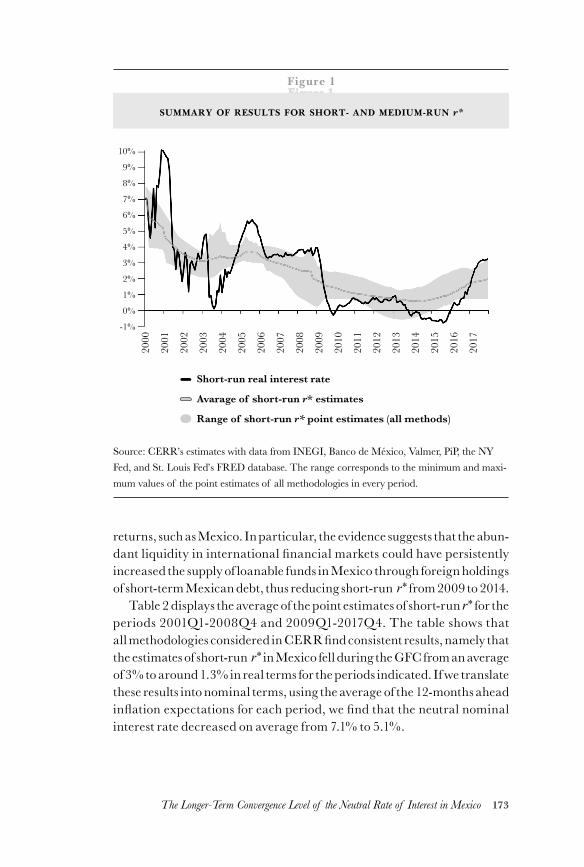
173The Longer-Term Convergence Level of the Neutral Rate of Interest in Mexico
returns, such as Mexico. In particular, the evidence suggests that the abun-dant liquidity in international financial markets could have persistently increased the supply of loanable funds in Mexico through foreign holdings of short-term Mexican debt, thus reducing short-run r* from 2009 to 2014.
Table 2 displays the average of the point estimates of short-run r* for the periods 2001Q1-2008Q4 and 2009Q1-2017Q4. The table shows that all methodologies considered in cerr find consistent results, namely that the estimates of short-run r* in Mexico fell during the gfc from an average of 3% to around 1.3% in real terms for the periods indicated. If we translate these results into nominal terms, using the average of the 12-months ahead inflation expectations for each period, we find that the neutral nominal interest rate decreased on average from 7.1% to 5.1%.
Figure 1Figure 1
SUMMARY OF RESULTS FOR SHORT- AND MEDIUM-RUN r*
10%
9%
8%
7%
6%
5%
4%
3%
2%
1%
0%
-1%
Short-run real interest rate
Avarage of short-run r* estimates
Range of short-run r* point estimates (all methods)
Source: CERR’s estimates with data from INEGI, Banco de México, Valmer, PiP, the NY Fed, and St. Louis Fed’s FRED database. The range corresponds to the minimum and maxi-mum values of the point estimates of all methodologies in every period.
2000
2001
2002
2003
2004
2005
2006
2007
2008
2009
2010
2011
2012
2013
2014
2015
2016
2017
174 J. Carrillo, R. Elizondo, C. Rodríguez-Pérez, J. Roldán-Peña
4. LONG-RUN CONVERGENCE LEVEL OF r* IN MEXICO
In this section, we present three different quantitative methods that esti-mate the long-run convergence level of the neutral rate, i.e. r ∗. We resort to these methods after the observation that a long-term average of the esti-mated of short-run r* might be a poor approximation of r ∗ due to the pres-ence of very persistent transitory factors affecting the Mexican economy after 2009. We first estimate an augmented Taylor rule that controls for the Fed’s umps. Second, we apply an open-economy rbc model to Mexico to get a long-run average of the equilibrium real interest rate. And third, we compute the implicit long-term expectation of the short-run policy rate that emerges from an affine term structure model. Finally, we pres-ent a heuristic analysis of structural factors affecting r ∗.
4.1 Augmented Taylor Rule
Taylor rules are commonly used tools that help to estimate the systematic behavior of a central bank’s monetary policy. In particular, the estimated interest-rate rule aims to approximate the reaction function of the poli-cy rate toward deviations of inflation from its target, and of output from its potential level. It is worth emphasizing that the resulting interest-rate rule should not be taken as the main policy directive of the central bank, but rather as a particular lens for interpreting the systematic behavior of monetary policy. Furthermore, notice that when inflation equals its tar-get and the output gap equals zero, r ∗ is given by the difference between the rule’s intercept and the inflation target. For example, consider the fol-lowing Taylor rule with interest rate smoothing:
1 Rt = (1+ ρ )[r*+π + ∂(π t −π )+θ yt ]+ ρRt−1 + ε t ,
where R is the overnight interbank nominal interest rate, π is the infla-tion, y is the output gap, and ε captures any change in the nominal inter-est rate not explained by the rule. Additionally, the specification includes a lag of R to capture gradual adjustments in this variable induced by the central bank. cerr estimate equation (1) recursively over the period 2001 to 2017 in order to capture changes in r ∗. The results from this exer-cise show that the estimate of falls from 2008 to 2014, partially reverting to pre-gfc levels afterwards. In light of these results, and the evidence
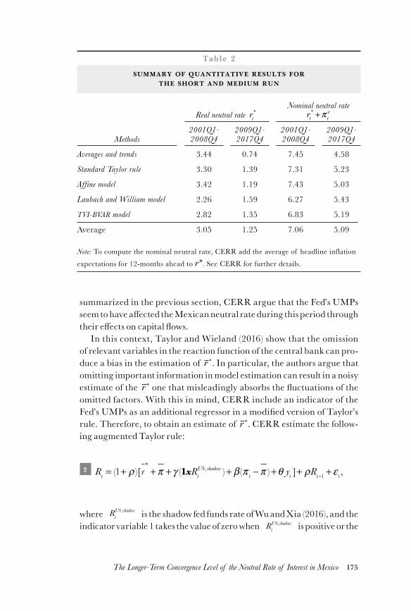
175The Longer-Term Convergence Level of the Neutral Rate of Interest in Mexico
summarized in the previous section, cerr argue that the Fed’s umps seem to have affected the Mexican neutral rate during this period through their effects on capital flows.
In this context, Taylor and Wieland (2016) show that the omission of relevant variables in the reaction function of the central bank can pro-duce a bias in the estimation of r ∗. In particular, the authors argue that omitting important information in model estimation can result in a noisy estimate of the r ∗ one that misleadingly absorbs the fluctuations of the omitted factors. With this in mind, cerr include an indicator of the Fed’s umps as an additional regressor in a modified version of Taylor’s rule. Therefore, to obtain an estimate of r ∗. cerr estimate the follow-ing augmented Taylor rule:
2 Rt = (1+ ρ )[r*+π + γ (1xRt
US ,shadow )+ β (π t −π )+θ yt ]+ ρRt−1 + ε t ,
where RtUS ,shadow is the shadow fed funds rate of Wu and Xia (2016), and the
indicator variable 1 takes the value of zero when RtUS ,shadow is positive or the
Table 2
SUMMARY OF QUANTITATIVE RESULTS FOR THE SHORT AND MEDIUM RUN
Methods
Real neutral rate rt*
Nominal neutral rate rt* +π t
e
2001Q1-2008Q4
2009Q1-2017Q4
2001Q1-2008Q4
2009Q1- 2017Q4
Averages and trends 3.44 0.74 7.45 4.58
Standard Taylor rule 3.30 1.39 7.31 5.23
Affine model 3.42 1.19 7.43 5.03
Laubach and William model 2.26 1.59 6.27 5.43
tvi-bvar model 2.82 1.35 6.83 5.19
Average 3.05 1.25 7.06 5.09
Note: To compute the nominal neutral rate, cerr add the average of headline inflation expectations for 12-months ahead to r*. See cerr for further details.
176 J. Carrillo, R. Elizondo, C. Rodríguez-Pérez, J. Roldán-Peña
value of one when RtUS ,shadow is negative (i.e. from July 2009 to December
2015).21 cerr only include information about the shadow rate during the zlb period as a proxy for the Fed’s umps. Therefore, they explicitly assume that these policies capture a very persistent transitory factor, not a structural factor.22
cerr estimate equation (2) recursively on a monthly basis, using the short-run nominal interest rate, headline annual inflation measured by the cpi, and a measure of the output gap using Mexico’s Global Indi-cator of Economic Activity (or igae, by its Spanish acronym), published monthly by inegi. To compute a measure of economic slack from igae, cerr use its percent deviation from trend, which they estimate using the Hodrick-Prescott filter with tail correction.
Figure 2 presents the results from this exercise. The results suggest that r ∗ has fluctuated around the level of 2.5% since 2009. This number trans-lates into a neutral nominal policy rate of 5.5%, if we add Banco de Méxi-co’s inflation target of 3%.
4.2 Open-Economy rbc Model
As an alternative means of measuring r ∗, we use a neoclassical growth mod-el for a small open economy. We follow the business-cycle model of Lama (2011) who, in a manner similar to Chari, Kehoe and McGrattan (2007), includes four sources of macroeconomic fluctuations in the model: an effi-ciency wedge (or tfp), a labor wedge, a capital wedge, and a bond wedge. These wedges allow the model to perfectly match the fluctuations of out-put, consumption, investment, and hours worked. Our estimate of r ∗ is the long-term average of the equilibrium real rate of capital returns, rk which is a model-consistent measure of the actual macro dynamics. We consider a long-period average of rk since the aforementioned wedges are reduced-form distortions that may capture both structural and transitory factors.23
21 We have considered alternative measures of the shadow fed funds rate, such as those proposed by Lombardi and Zhu (2014), and Krippner (2015). The re-sults remain quantitatively similar.
22 Note that if the long-run value of the Fed’s umps is not zero, the interpretation of the intercept as an estimator of r ∗ in the Taylor rule changes.
23 Recently, Caballero, Farhi and Gourinchas (2017) noticed that for the case of the u.s., there is a growing divergence between the return on productive capital and the return of safe assets. For the case of Mexico, it is not clear that such divergence is as secular as it is in the u.s. Nonetheless, we bear in mind that even a long-period average of r k might be a poor approximation of r ∗. We decided to keep
177The Longer-Term Convergence Level of the Neutral Rate of Interest in Mexico
Lama (2011)’s model includes a competitive firm and a representative household with an increasing number of members. The firm chooses la-bor and capital services to maximize profits:
maxlt ,ktAtkt
a ((1+ γ )t lt )1−α − wtlt − ztkt ,
where At is tfp, wt is the real wage, zt is the rental rate of capital, α is the share of capital income on gdp, and γ is the growth rate of techno-logical progress. A representative household chooses consumption per cap-ita ct international debt bt+1 investment it, the next period’s capital stock, and the labor supply in order to maximize its expected discounted utility, subject to a budget constraint, the law of motion for capital accumulation, and a supply of funds for international borrowing:
maxct ,bt+1,lt
Eo Ntβt logct +ψ log(1− lt )⎡⎣ ⎤⎦
t=0
∞
∑⎧⎨⎩
⎫⎬⎭,
subject to
( ) ( ) ( ) ( )( )1 1 1 1 11+ + + ≤ + + + + + + ++n b c i w l z k r bt t t lt t t kt t t bt tW
tτ τ τ ϒtt ,
(1+ n)kt+1 ≤ (1+ ∂)kt ≤ (1+ ∂)kt + it −φitkt
⎛
⎝⎜⎞
⎠⎟kt ,
1 1+ = +
r r b
btW W t
W( )υ
where β is the subjective discount factor, ψ is a normalizing constant, n is the population growth rate, ∂ is the capital depreciation rate, and υ > 0 is the elasticity of the supply of international borrowing. In turn, Nt is the size of the population, rW is the world real interest rate, ϒ t represent government transfers, and φ(it / kt ) =ϑ / 2x(it / kt − ∂
!)2 measures capital
the neoclassic analysis for two reasons. First, Dorich, Reza and Sarker (2017) perform a similar exercise for Canada and notice that potential output growth plays a prominent role in the determination of r ∗. Second, there are not many methods available in the literature to estimate r ∗.
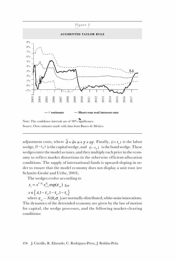
178 J. Carrillo, R. Elizondo, C. Rodríguez-Pérez, J. Roldán-Peña
adjustment costs, where ∂! = ∂+ n+ γ + nγ . Finally, (1+τ lt ) is the labor wedge, ( )1−τ kt is the capital wedge, and ( )1−τbt is the bond wedge. These wedges enter the model as taxes, and they multiply each price in the econ-omy to ref lect market distortions in the otherwise eff icient-allocation conditions. The supply of international funds is upward-sloping in or-der to ensure that the model economy does not display a unit root (see Schmitt-Grohé and Uribe, 2003).
The wedges evolve according toxt = x
1−ρx xt−1ρx exp(ε xt ) for
x ∈ A,1−τ l ,1−τ k ,1−τ b where ε xt ∼ N (0,σ x ) are normally-distributed, white-noise innovations.
The dynamics of the detrended economy are given by the law of motion for capital, the wedge processes, and the following market-clearing conditions:
%
Figure 2Figure 2
AUGMENTED TAYLOR RULE
— estimate — Short-run real interest rate
Note: The confidence intervals are of 90% significance.Source: Own estimates made with data from Banco de México.
2003
2004
2005
2006
2007
2008
2009
2010
2011
2012
2013
2014
2015
2016
2017
9%
8%
7%
6%
5%
4%
3%
2%
1%
0%
-1%
r ∗
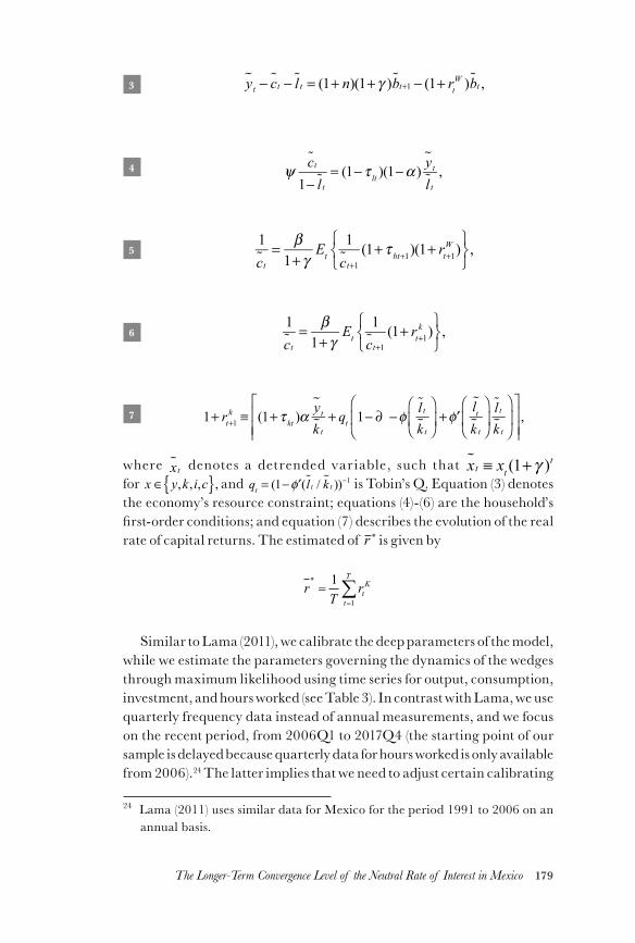
179The Longer-Term Convergence Level of the Neutral Rate of Interest in Mexico
3 y! t − c!t − l!t = (1+ n)(1+ γ )b! t+1 − (1+ rt
W )b! t ,
4 ψ c! t1− l!t
= (1−τ lt )(1−α )y! tl!t,
5 1c! t
= β1+ γ
Et1c! t+1(1+τ bt+1)(1+ rt+1
W )⎧⎨⎩
⎫⎬⎭,
6 1c! t
= β1+ γ
Et1c! t+1(1+ rt+1
k )⎧⎨⎩
⎫⎬⎭,
7 1+ rt+1k ≡ (1+τ kt )α
y! tk! t
+ qt 1− ∂ −φ l!tk! t
⎛
⎝⎜
⎞
⎠⎟ + ′φ
lt!
k! t
⎛
⎝⎜
⎞
⎠⎟l!tk! t
⎛
⎝⎜
⎞
⎠⎟
⎡
⎣⎢⎢
⎤
⎦⎥⎥,
where x! t denotes a detrended var iable, such that x! t ≡ xt (1+ γ )t
for x ∈ y,k,i,c , and qt = (1− ′φ (l!t / k! t ))−1 is Tobin’s Q. Equation (3) denotes the economy’s resource constraint; equations (4)-(6) are the household’s first-order conditions; and equation (7) describes the evolution of the real rate of capital returns. The estimated of r ∗ is given by
rT
rtK
t
T*=
=∑11
Similar to Lama (2011), we calibrate the deep parameters of the model, while we estimate the parameters governing the dynamics of the wedges through maximum likelihood using time series for output, consumption, investment, and hours worked (see Table 3). In contrast with Lama, we use quarterly frequency data instead of annual measurements, and we focus on the recent period, from 2006Q1 to 2017Q4 (the starting point of our sample is delayed because quarterly data for hours worked is only available from 2006).24 The latter implies that we need to adjust certain calibrating
24 Lama (2011) uses similar data for Mexico for the period 1991 to 2006 on an annual basis.
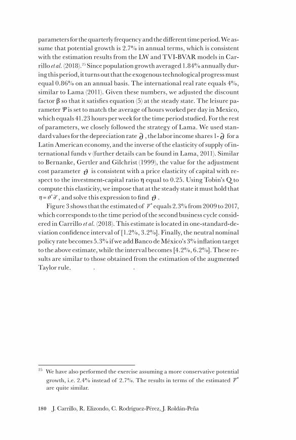
180 J. Carrillo, R. Elizondo, C. Rodríguez-Pérez, J. Roldán-Peña
parameters for the quarterly frequency and the different time period. We as-sume that potential growth is 2.7% in annual terms, which is consistent with the estimation results from the lw and tvi-bvar models in Car-rillo et al. (2018).25 Since population growth averaged 1.84% annually dur-ing this period, it turns out that the exogenous technological progress must equal 0.86% on an annual basis. The international real rate equals 4%, similar to Lama (2011). Given these numbers, we adjusted the discount factor β so that it satisfies equation (5) at the steady state. The leisure pa-rameter Ψ is set to match the average of hours worked per day in Mexico, which equals 41.23 hours per week for the time period studied. For the rest of parameters, we closely followed the strategy of Lama. We used stan-dard values for the depreciation rate ∂ , the labor income shares 1- ∂ for a Latin American economy, and the inverse of the elasticity of supply of in-ternational funds ν (further details can be found in Lama, 2011). Similar to Bernanke, Gertler and Gilchrist (1999), the value for the adjustment cost parameter ϑ is consistent with a price elasticity of capital with re-spect to the investment-capital ratio η equal to 0.25. Using Tobin’s Q to compute this elasticity, we impose that at the steady state it must hold that η =ϑ * ′∂ , and solve this expression to find ϑ .
Figure 3 shows that the estimated of r ∗ equals 2.3% from 2009 to 2017, which corresponds to the time period of the second business cycle consid-ered in Carrillo et al. (2018). This estimate is located in one-standard-de-viation confidence interval of [1.2%, 3.2%]. Finally, the neutral nominal policy rate becomes 5.3% if we add Banco de México’s 3% inflation target to the above estimate, while the interval becomes [4.2%, 6.2%]. These re-sults are similar to those obtained from the estimation of the augmented Taylor rule.
25 We have also performed the exercise assuming a more conservative potential growth, i.e. 2.4% instead of 2.7%. The results in terms of the estimated r ∗
are quite similar.
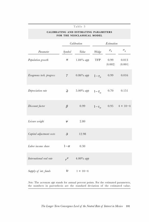
181The Longer-Term Convergence Level of the Neutral Rate of Interest in Mexico
Table 3
CALIBRATING AND ESTIMATING PARAMETERS FOR THE NEOCLASSICAL MODEL
Calibration Estimation
Parameter Symbol Value Wedgeρx σx
Population growth n 1.84% app tfp 0.99(0.002)
0.013(0.001)
Exogenous tech. progress γ 0.86% app 1−τ lt 0.99 0.016
Depreciation rate ∂ 5.00% app 1−τ kt 0.70 0.151
Discount factor β 0.99 1−τbt 0.95 4 × 10⁻⁴
Leisure weight ψ 2.80
Capital adjustment costs ϑ 12.98
Labor income share 1−α 0.30
International real rate rW 4.00% app
Supply of int. funds υ 1 × 10⁻⁴
Note: The acronym app stands for annual percent points. For the estimated parameters, the numbers in parenthesis are the standard deviation of the estimated value.
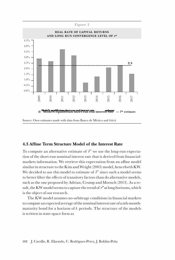
182 J. Carrillo, R. Elizondo, C. Rodríguez-Pérez, J. Roldán-Peña
4.3 Affine Term Structure Model of the Interest Rate
To compute an alternative estimate of r ∗ we use the long-run expecta-tion of the short-run nominal interest rate that is derived from financial-markets information. We retrieve this expectation from an affine model similar in structure to the Kim and Wright (2005) model, henceforth kw. We decided to use this model to estimate of r ∗ since such a model seems to better filter the effects of transitory factors than do alternative models, such as the one proposed by Adrian, Crump and Moench (2013). As a re-sult, the kw model seems to capture the trend of r* at long horizons, which is the object of our research.
The kw model assumes no-arbitrage conditions in financial markets to compute an expected average of the nominal interest rate of a nth-month-maturity bond for a horizon of k periods. The structure of the models is written in state-space form as
Model’s equilibrium short-run real interest rate estimate
Figure 3
REAL RATE OF CAPITAL RETURNSAND LONG RUN CONVERGENCE LEVEL OF r*
Source: Own estimates made with data from Banco de México and INEGI.
2009
2010
2011
2012
2013
2014
2015
2016
2017
4.5%
4.0%
3.5%
3.0%
2.5%
2.0%
1.5%
1.0%
0.5%
0.0%
Model’s equilibrium short-run real interest rate --- r* estimate
183The Longer-Term Convergence Level of the Neutral Rate of Interest in Mexico
8 Xt = µ +φXt−1 +ϑt+1, [Transition Equation]
9 itn = An +BnXt , [Measurement Equation]
where X is a vector of factors or state variables, in is the nominal interest rate of a bond with maturity of n months, ϑ is white-noise state innova-tions, φ and Bn are coefficient matrices, and µand An are coefficient vec-tors. The kw model includes three latent factors in vector X, each as a proxy for the following yield curve characteristics: i) level, ii) slope, and iii) curva-ture. We estimate the coefficients of the model using maximum likelihood estimation and the Kalman filter. We use the 2004 to 2017 sample of the yields of government zero-coupon bonds with selected maturities of 1, 3, 6, 12, 24, 36, 60, 84, and 120 months.26
From the model, we can obtain the average expected path of the nominal interest rate of 1-month maturity bonds for horizons running from 1 month to n years ahead, namely,
10 Et ,t+ni = 1
nEt it+k
1( ) k=1
n∑
Notice that form equation (10), we can recursively derive the long-run expectation of short-term nominal interest rate, i.e., Et it+k
1( ) where n cor-responds to the future period in years. In particular, we have that:
Et it+11( )⎡
⎣⎤⎦ = Et ,t+1
i
Et it+21( )⎡
⎣⎤⎦ = 2Et ,t+2
i − Et ,t+1i
26 More details about this methodology can be found in Kim and Wright (2005). In particular, the coefficients An and Bn are estimated recursively and de-pend on market risk parameters. When these parameters are equal to zero, we obtain the risk-free coefficients An
RF and BnRF . Using these coefficients,
we can compute the average expectation at time t of short-term interest rates over the next k periods.
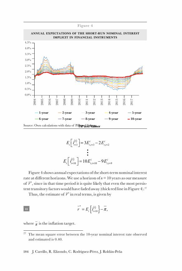
184 J. Carrillo, R. Elizondo, C. Rodríguez-Pérez, J. Roldán-Peña
Et it+31( )⎡
⎣⎤⎦ = 3Et ,t+3
i − 2Et ,t+2i
Et it+101( )⎡
⎣⎤⎦ = 10Et ,t+10
i − 9Et ,t+9i
Figure 4 shows annual expectations of the short-term nominal interest rate at different horizons. We use a horizon of n = 10 years as our measure of r ∗, since in that time period it is quite likely that even the most persis-tent transitory factors would have faded away (thick red line in Figure 4).27
Thus, the estimate of r ∗ in real terms, is given by
11 r*= Et it+10
1( ) −π ,where π is the inflation target.
27 The mean square error between the 10-year nominal interest rate observed and estimated is 0.40.
PiP and Valmer
Figure 4
ANNUAL EXPECTATIONS OF THE SHORT-RUN NOMINAL INTERESTIMPLICIT IN FINANCIAL INSTRUMENTS
— 1-year
— 6-year
Source: Own calculations with data of PiP and Valmer.
2004
2005
2016
2007
2008
2009
2010
2011
2012
2013
2014
2015
2016
2017
4.5%
4.0%
3.5%
3.0%
2.5%
2.0%
1.5%
1.0%
0.5%
0.0%
— 2-year
— 7-year
— 3-year
— 8-year
— 4-year
— 9-year
— 5-year
— 10-year
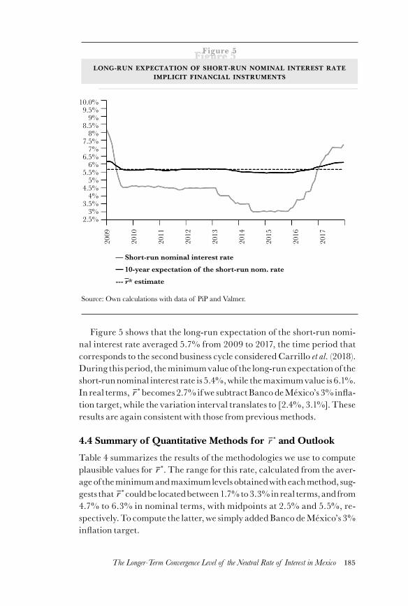
185The Longer-Term Convergence Level of the Neutral Rate of Interest in Mexico
Figure 5 shows that the long-run expectation of the short-run nomi-nal interest rate averaged 5.7% from 2009 to 2017, the time period that corresponds to the second business cycle considered Carrillo et al. (2018). During this period, the minimum value of the long-run expectation of the short-run nominal interest rate is 5.4%, while the maximum value is 6.1%. In real terms, r ∗ becomes 2.7% if we subtract Banco de México’s 3% infla-tion target, while the variation interval translates to [2.4%, 3.1%]. These results are again consistent with those from previous methods.
4.4 Summary of Quantitative Methods for r ∗ and Outlook
Table 4 summarizes the results of the methodologies we use to compute plausible values for r ∗. The range for this rate, calculated from the aver-age of the minimum and maximum levels obtained with each method, sug-gests that r ∗ could be located between 1.7% to 3.3% in real terms, and from 4.7% to 6.3% in nominal terms, with midpoints at 2.5% and 5.5%, re-spectively. To compute the latter, we simply added Banco de México’s 3% inflation target.
Figure 5Figure 5
LONG-RUN EXPECTATION OF SHORT-RUN NOMINAL INTEREST RATEIMPLICIT FINANCIAL INSTRUMENTS
— Short-run nominal interest rate 10-year expectation of the short-run nom. rate--- r* estimate
Source: Own calculations with data of PiP and Valmer.
2009
2010
2011
2012
2013
2014
2015
2016
2017
10.0%9.5%
9%8.5%
8%7.5%
7%6.5%
6%5.5%
5%4.5%
4%3.5%
3%2.5%
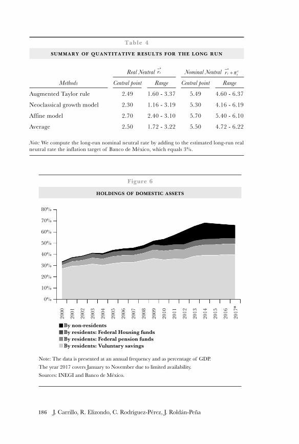
186 J. Carrillo, R. Elizondo, C. Rodríguez-Pérez, J. Roldán-Peña
Table 4
SUMMARY OF QUANTITATIVE RESULTS FOR THE LONG RUN
Methods
Real Neutral rt te*
+π Nominal Neutral rt te*
+π
Central point Range Central point Range
Augmented Taylor rule 2.49 1.60 - 3.37 5.49 4.60 - 6.37
Neoclassical growth model 2.30 1.16 - 3.19 5.30 4.16 - 6.19
Affine model 2.70 2.40 - 3.10 5.70 5.40 - 6.10
Average 2.50 1.72 - 3.22 5.50 4.72 - 6.22
Note: We compute the long-run nominal neutral rate by adding to the estimated long-run real neutral rate the inflation target of Banco de México, which equals 3%.
Figure 6
HOLDINGS OF DOMESTIC ASSETS
By non-residentsBy residents: Federal Housing fundsBy residents: Federal pension fundsBy residents: Vuluntary savings
Note: The data is presented at an annual frequency and as percentage of GDP.The year 2017 covers January to November due to limited availability.Sources: INEGI and Banco de México.
2000
2001
2002
2003
2004
2005
2006
2007
2008
2009
2010
2011
2012
2013
2014
2015
2016
2017
*
80%
70%
60%
50%
40%
30%
20%
10%
0%
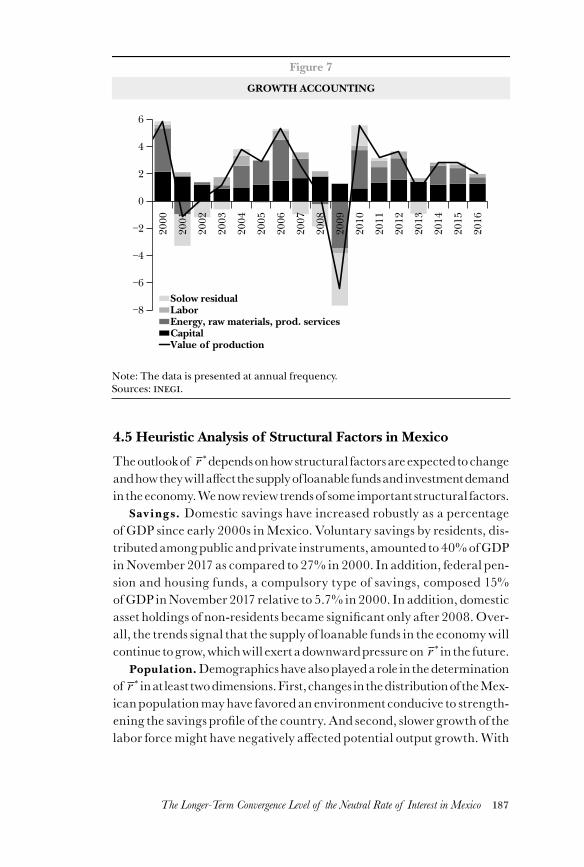
187The Longer-Term Convergence Level of the Neutral Rate of Interest in Mexico
4.5 Heuristic Analysis of Structural Factors in Mexico
The outlook of r ∗ depends on how structural factors are expected to change and how they will affect the supply of loanable funds and investment demand in the economy. We now review trends of some important structural factors.
Savings. Domestic savings have increased robustly as a percentage of gdp since early 2000s in Mexico. Voluntary savings by residents, dis-tributed among public and private instruments, amounted to 40% of gdp in November 2017 as compared to 27% in 2000. In addition, federal pen-sion and housing funds, a compulsory type of savings, composed 15% of gdp in November 2017 relative to 5.7% in 2000. In addition, domestic asset holdings of non-residents became significant only after 2008. Over-all, the trends signal that the supply of loanable funds in the economy will continue to grow, which will exert a downward pressure on r ∗ in the future.
Population. Demographics have also played a role in the determination of r ∗ in at least two dimensions. First, changes in the distribution of the Mex-ican population may have favored an environment conducive to strength-ening the savings profile of the country. And second, slower growth of the labor force might have negatively affected potential output growth. With
Figure 7
GROWTH ACCOUNTING
Note: The data is presented at annual frequency.Sources: .
Solow residualLaborEnergy, raw materials, prod. servicesCapitalValue of production
−8
−6
−4
−2
0
2
4
6
2000
2001
2002
2003
2004
2005
2006
2007
2008
2009
2010
2011
2012
2013
2014
2015
2016
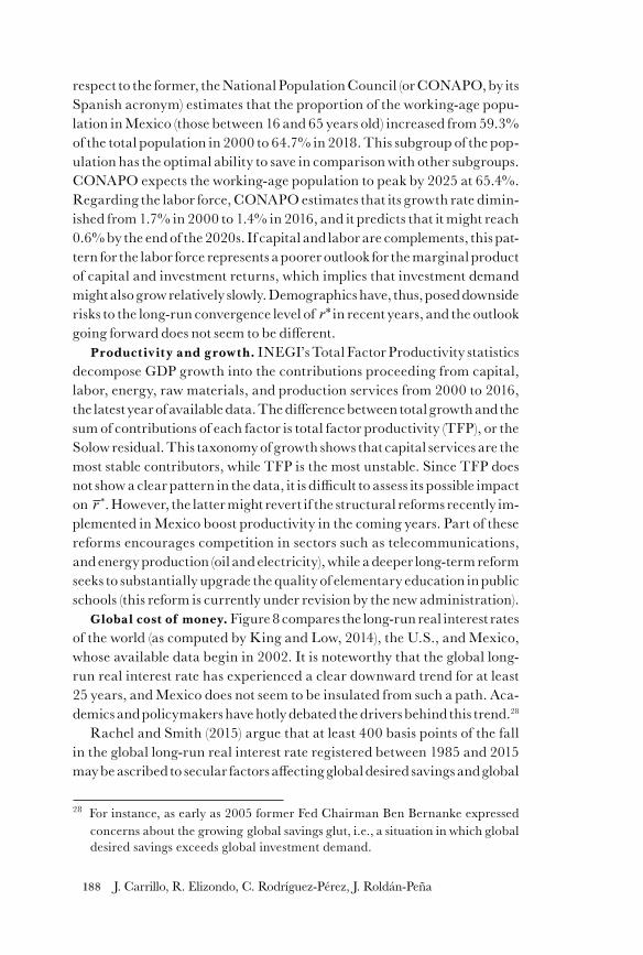
188 J. Carrillo, R. Elizondo, C. Rodríguez-Pérez, J. Roldán-Peña
respect to the former, the National Population Council (or conapo, by its Spanish acronym) estimates that the proportion of the working-age popu-lation in Mexico (those between 16 and 65 years old) increased from 59.3% of the total population in 2000 to 64.7% in 2018. This subgroup of the pop-ulation has the optimal ability to save in comparison with other subgroups. conapo expects the working-age population to peak by 2025 at 65.4%. Regarding the labor force, conapo estimates that its growth rate dimin-ished from 1.7% in 2000 to 1.4% in 2016, and it predicts that it might reach 0.6% by the end of the 2020s. If capital and labor are complements, this pat-tern for the labor force represents a poorer outlook for the marginal product of capital and investment returns, which implies that investment demand might also grow relatively slowly. Demographics have, thus, posed downside risks to the long-run convergence level of r* in recent years, and the outlook going forward does not seem to be different.
Productivity and growth. inegi’s Total Factor Productivity statistics decompose gdp growth into the contributions proceeding from capital, labor, energy, raw materials, and production services from 2000 to 2016, the latest year of available data. The difference between total growth and the sum of contributions of each factor is total factor productivity (tfp), or the Solow residual. This taxonomy of growth shows that capital services are the most stable contributors, while tfp is the most unstable. Since tfp does not show a clear pattern in the data, it is difficult to assess its possible impact on r ∗. However, the latter might revert if the structural reforms recently im-plemented in Mexico boost productivity in the coming years. Part of these reforms encourages competition in sectors such as telecommunications, and energy production (oil and electricity), while a deeper long-term reform seeks to substantially upgrade the quality of elementary education in public schools (this reform is currently under revision by the new administration).
Global cost of money. Figure 8 compares the long-run real interest rates of the world (as computed by King and Low, 2014), the u.s., and Mexico, whose available data begin in 2002. It is noteworthy that the global long-run real interest rate has experienced a clear downward trend for at least 25 years, and Mexico does not seem to be insulated from such a path. Aca-demics and policymakers have hotly debated the drivers behind this trend.28
Rachel and Smith (2015) argue that at least 400 basis points of the fall in the global long-run real interest rate registered between 1985 and 2015 may be ascribed to secular factors affecting global desired savings and global
28 For instance, as early as 2005 former Fed Chairman Ben Bernanke expressed concerns about the growing global savings glut, i.e., a situation in which global desired savings exceeds global investment demand.
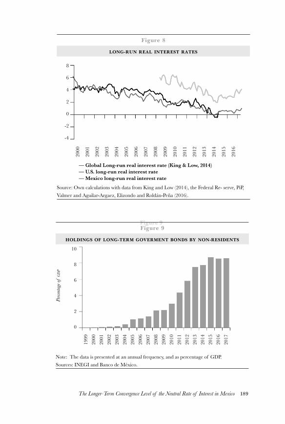
189The Longer-Term Convergence Level of the Neutral Rate of Interest in Mexico
Figure 9Figure 9
HOLDINGS OF LONG-TERM GOVERMENT BONDS BY NON-RESIDENTS
Note: The data is presented at an annual frequency, and as percentage of GDP.Sources: INEGI and Banco de México.
1999
2000
2001
2002
2003
2004
2005
2006
2007
2008
2009
2010
2011
2012
2013
2014
2015
2016
2017
10
8
6
4
2
0
Perce
ntag
e of
GDP
Figure 8
LONG-RUN REAL INTEREST RATES
Source: Own calculations with data from King and Low (2014), the Federal Re- serve, PiP, Valmer and Aguilar-Argaez, Elizondo and Roldán-Peña (2016).
2000
2001
2002
2003
2004
2005
2006
2007
2008
2009
2010
2011
2012
2013
2014
2015
2016
8
6
4
2
0
-2
-4
— Global Long-run real interest rate (King & Low, 2014)— U.S. long-run real interest rate— Mexico long-run real interest rate
190 J. Carrillo, R. Elizondo, C. Rodríguez-Pérez, J. Roldán-Peña
investment demand. The structural factors pushing outwards global desired savings are an increase in the proportion of the working-age population, higher inequality, and, to a lesser extent, the glut of precautionary sav-ings by emerging markets. In turn, structural factors that have negatively affected global investment demand are a falling relative price of capital, lower public investment, and an increase in the spread between the risk-free rate and the rate of capital returns. In contrast, Rachel and Smith ar-gue that economic growth seems not to have affected negatively the global long-run real interest rate until 2008. After that year, the prospect of lower global growth could have contributed to a fall of 100 basis points in the global long-run interest rate.
The global factors just described seem to have affected the Mexican long-run interest rate through international arbitrage. Figure 9 shows that there is a robust increase in the purchases of long-term public debt by foreign investors over the sample period studied. Non-residents hold-ings of these instruments seem to have accelerated since 2010, growing from 2.2% of gdp in 2009 to about 9% of gdp by 2014. These holdings have stabilized around that level for the last three years of the sample. Part of this acceleration may be due to the inclusion of Mexican peso-denom-inated debt in the Citigroup’s World Government Bond Index (wgbi) in October 2010. This index is used as a benchmark by institutional inves-tors who aim to buy highly-rated long-term debt.
In sum, the data suggest that capital inflows have permanently increased the supply of loanable funds in Mexico in recent years.
5. CONCLUDING REMARKS
In this paper, we argue that foreign and domestic structural factors, such as increasing domestic savings, demographic shifts, and a decreasing global long-run real interest rate, appear to explain the apparent fall in the Mex-ican neutral rate, from 3% in the period 2001-2008 to 2.5% after 2009. Going forward, downside risks to the long-run convergence level of the neutral rate in Mexico are given by an expected slowdown in the growth rate of the labor force, a larger working-age of the population, and a secu-lar reduction in the global long-run real interest rate. Upside risks, in turn, relate to a potential increase in productivity generated by recent structural reforms in the country.
191The Longer-Term Convergence Level of the Neutral Rate of Interest in Mexico
References
Adrian, T., Crump, R. K. and Moench, E. (2013) Pricing the Term Structure with Linear Regressions, Journal of Financial Economics, 110, 110–138.
Aguilar-Argáez, A., Elizondo, R. and Roldán-Peña, J. (2016) Descom-posición de la Compensación por Inflación y Riesgo Inflacionario, Working Paper 2016-22, Banco de México.
Basdevant, O., Björksten, N. and Karagedikli, O. (2004) Estimating a Time Varying Neutral Real Interest Rate for New Zealand, RBNZ Discussion Paper Series 2004/01, Reserve Bank of New Zealand.
Berger, T. and Kempa, B. (2014) Time-Varying Equilibrium Rates in Small Open Economies: Evidence for Canada, Journal of Macro-economics, 39, 203–214.
Bernanke, B., Gertler, M. and Gilchrist, S. (1999) The Financial Accel-erator in a Quantitative Business Cycle Framework, in Handbook of Macroeconomics (Eds.) J. B. Taylor and M. Woodford, Elsevier, vol. 1 of Handbook of Macroeconomics, chap. 21, pp. 1341–1393.
Bernhardsen, T. and Gerdrup, K. (2007) The Neutral Real Interest Rate, Norges Bank Economic Bulletin, 78, 52–64.
Björksten, N. and Karagedikli, O. (2003) Neutral Real Interest Rates Revisited, Reserve Bank of New Zealand Bulletin, 66, 1–11.
Bouis, R., Rawdanowicz, L., Renne, J.-P., Watanabe, S. and Christensen, A. K. (2013) The Effectiveness of Monetary Policy since the Onset of the Financial Crisis, oecd Economics Department Working Papers 1081, oecd Publishing.
Caballero, R. J., Farhi, E. and Gourinchas, P. O. (2017) Rents, Techni-cal Change, and Risk Premia: Accounting for Secular Trends in Interest Rates, Returns on Capital, Earning Yields, and Factor Shares, Working Paper 23127, National Bureau of Economic Research, Inc.
Carrillo, J. A., Elizondo, R., Rodríguez-Pérez, C. A. and Roldán-Peña, J. (2018) What Determines the Neutral Rate of Interest in an Emerging Economy?, Working Paper 2018-22, Banco de México.
Chari, V. V., Kehoe, P. J. and McGrattan, E. R. (2007) Business Cycle Accounting, Econometrica, 75, 781–836.
192 J. Carrillo, R. Elizondo, C. Rodríguez-Pérez, J. Roldán-Peña
Cuaresma, J., Gnan, E. and Ritzberger-Gruenwald, D. (2004) Search-ing for the Natural Rate of Interest: A Euro Area Perspective, Empirica, 31, 185–204.
Del Negro, M., Giannone, D., Giannoni, M. P. and Tambalotti, A. (2017) Safety, Liquidity, and the Natural Rate of Interest, Brookings Papers on Economic Activity, 48, 235–316.
Dorich, J., Reza, A. and Sarker, S. (2017) An Update on the Neutral Rate of Interest, Bank of Canada Review, 2017, 27–41.
European Central Bank (2004) The Natural Real Interest Rate in the Euro Area, Monthly Bulletin, May, European Central Bank.
Fries, S., Mésonnier, J. S., Mouabbi, S. and Renne, J. P. (2018) National Natural Rates of Interest and the Single Monetary Policy in the Euro Area, Journal of Applied Econometrics, forthcoming.
Fuentes, R. and Gredig, F. (2008) The Neutral Interest Rate: Estimates for Chile, Journal Economía Chilena (The Chilean Economy), 11, 47–58.
Fujiwara, S., Iwasaki, Y., Muto, I., Nishizaki, K. and Sudo, N. (2016) Developments in the Natural Rate of Interest in Japan, Supple-mentary Paper Series for the Comprehensive Assessment (2) 2016-E-12, Bank of Japan.
Garnier, J. and Wilhelmsen, B.-R. (2009) The Natural Rate of Inter-est and the Output Gap in the Euro Area: A Joint Estimation, Empirical Economics, 36, 297–319.
González, A., Ocampo, S., Pérez, J. and Rodríguez, D. (2012) Output Gap and Neutral Interest Measures for Colombia, Borradores de Economía 726, Banco de la República.
Holston, K., Laubach, T. and Williams, J. C. (2017) Measuring the Natural Rate of Interest: International Trends and Determinants, Journal of International Economics, 108, S59-S75.
International Monetary Fund (2018) World Economic Outlook: Cyclical Upswing, Structural Change, Tech. rep., International Monetary Fund.
Johannsen, B. K. and Mertens, E. (2016) The Expected Real Interest Rate in the Long Run: Time Series Evidence with the Effective Lower Bound, feds Notes 2016-02-09, Board of Governors of the Federal Reserve System (u.s.).
193The Longer-Term Convergence Level of the Neutral Rate of Interest in Mexico
Kim, D. H. and Wright, J. H. (2005) An Arbitrage-Free Three-Factor Term Structure Model and the Recent Behavior of Long-Term Yields and Distant-Horizon Forward Rates, Finance and Econom-ics Discussion Series 2005-33, Board of Governors of the Federal Reserve System (u.s.).
King, M. and Low, D. (2014) Measuring the ”World” Real Interest Rate, nber Working Papers 19887, National Bureau of Economic Research, Inc.
Krippner, L. (2015) Measures of the Stance of United States Monetary Policy, Tech. rep., Reserve Bank of New Zealand.
Lama, R. (2011) Accounting for Output Drops in Latin America, Review of Economic Dynamics, 14, 295–316.
Laubach, T. and Williams, J. C. (2003) Measuring the Natural Rate of Interest, The Review of Economics and Statistics, 85, 1063–1070.
Laubach, T. and Williams, J. C. (2016) Measuring the Natural Rate of Interest Redux, Finance and Economics Discussion Series 2016-11, Board of Governors of the Federal Reserve System (u.s.).
Lombardi, M. and Zhu, F. (2014) A Shadow Policy Rate to Calibrate US Monetary Policy at the Zero Lower Bound, BIS Working Papers 452, Bank for International Settlements.
Magud, N. E. and Tsounta, E. (2012) To Cut or Not to Cut? That is the (Central Bank’s) Question In Search of the Neutral Interest Rate in Latin America, imf Working Papers 12/243, International Monetary Fund.
Mesonnier, J.-S. and Renne, J.-P. (2007) A Time-Varying Natural Rate of Interest for the Euro Area, European Economic Review, 51, 1768–1784.
Perrelli, R. and Roache, S. K. (2014) Time-Varying Neutral Interest Rate: The Case of Brazil, imf Working Papers 14/84, Interna-tional Monetary Fund.
Rachel, L. and Smith, T. D. (2015) Secular Drivers of the Global Real Interest Rate, Staff Working Paper 571, Bank of England.
Richardson, A. and Williams, R. (2015) Estimating New Zealand’s Neutral Interest Rate, Reserve Bank of New Zealand Analytical Notes series AN2015/05, Reserve Bank of New Zealand.
194 J. Carrillo, R. Elizondo, C. Rodríguez-Pérez, J. Roldán-Peña
Schmidt-Hebbel, K. and Walsh, C. E. (2009) Monetary Policy and Key Unobservable: Evidence from Large Industrial and Selected Inflation-Targeting Countries, in Monetary Policy under Uncertainty and Learning (Eds.) K. Schmidt-Hebbel, C. E. Walsh, N. L. S. Editor) and K. S.-H. (Series, Central Bank of Chile, vol. 13 of Central Banking, Analysis, and Economic Policies Book Series, chap. 9, pp. 285–370.
Schmitt-Grohé, S. and Uribe, M. (2003) Closing Small Open Economy Models, Journal of Inter- national Economics, 61, 163–185.
Taylor, J. B. and Wieland, V. (2016) Finding the Equilibrium Real Interest Rate in a Fog of Policy Deviations, Economics Working Papers 16109, Hoover Institution, Stanford University.
Wu, J. C. and Xia, F. D. (2016) Measuring the Macroeconomic Impact of Monetary Policy at the Zero Lower Bound, Journal of Money, Credit and Banking, 48, 253–291.
Yellen, J. L. (2015) The Outlook for the Economy: A Speech at The Economics Club of Washington, Washington, D.C., December 2, 2015, Speech 851, Board of Governors of the Federal Reserve System (u.s.).
Zhu, F. (2016) Understanding the Changing Equilibrium Real Interest Rates in Asia-Pacific, BIS Working Papers 567, Bank for Inter-national Settlements.
195Output Gap, Potential Output Growth and Natural Interest Rate
Measuring the output gap, potentialoutput growth, and natural interest rate from a semi-structural dynamic model for Peru
Luis Eduardo CastilloDavid Florián Hoyle
Abstract
In this paper we use a calibrated version of the Quarterly Projection Model (MPT, for its acronym in Spanish) to jointly estimate the output gap, potential output growth ,and natural interest rate of the Peruvian economy during most of the inflation targeting regime (between 2002 and 2017). The MPT is a semi-structural dynamic model used by the Central Reserve Bank of Peru for fore-casting and policy scenario analysis. The model functions as a multiva-riate filter with a sophisticated economic structure that allows us to infer the dynamics of non-observable variables from the information provided by other variables defined ex ante as observable. As the results from the Kalman filter are sensible to these variables declared as observable, we use five groups of variables to be defined as such to build probable ranges for our estimates.The results indicate that the estimated output gap is large in amplitude and highly persistent, while potential output growth is very smooth. Therefore, most of the variation in economic activity during the inflation targeting re-gime can be attributed to the former. As expected from a small open economy, a historical decomposition exercise shows that output gap dynamics are main-ly influenced by external factors (real and financial). The estimation of the output gap also proves that monetary policy has been extensively responsive to this leading indicator of inflation. Meanwhile, the real natural interest rate
Luis Eduardo Castillo, Central Reserve Bank of Peru. David Florián Hoyle, Central Reserve Bank of Peru. We would like to thank Paul Castillo, Alessandro Galesi, Ivan Kataryniuk and specially Martin Martinez for insightful comments. We also thank seminar participants at the LACEA 2018 conference, and research seminars at CEM-LA and the Central Reserve Bank of Peru. The views expressed in this paper are those of the authors and do not necessarily represent the views of the Central Reserve Bank of Peru (BCRP).
196 L. Castillo, D. Hoyle
is estimated to be considerable stable, averaging 1.6% in the sample with only a sharp decline to 1.3% during the financial crisis.The main finding of the paper, however, is that there has been a steady decel-eration of potential output growth since 2012. A growth-accounting exercise proves that this trend is mostly explained by a reduction in total factor pro-ductivity (TFP) growth during the same time frame. Nonetheless, the drop of capital and labor contributions jointly explain almost a third part of aver-age potential output growth slowdown between 2010-2013 and 2014-2017.
JEL Clasification: C51, E32, E52Keywords: Potential output, Output gap, Natural Interest Rate, Kalman
Filter, Peru.
1. INTRODUCTION
Potential (or natural ) output is defined as the level of output that can be sustained indefinitely without adding pressures on inflation (Okun, 1962). Thus, periods in which inflation
is stable (inflation rate on its long-term value) are associated with output on its potential level. Meanwhile, the short-term interest rate that is consistent with both inflation rate on its long-term value and output on its potential level (i.e. no transitory disturbances) is called the natural interest rate.
Both potential output and the natural interest rate are non-ob-servable variables, in the sense that their dynamics can only be in-ferred from the behavior of other variables that can be measured (e.g. prices, gross domestic output, interest rates, exchange rate). Nonetheless, they are key components of monetary policy making. On the one hand, the difference between GDP and potential output, called the output gap, is considered a leading indicator of inflationary pressures. On the other hand, the natural interest rate enables poli-cymakers to identify whether current monetary conditions are being expansionary (real interest rate below its natural level) or contrac-tionary (real interest rate above its natural level). It is worth noting that the desirability of a specific monetary policy stance depends on inflation expectations and the stage of the business cycle, which is partly determined through the estimation of the output gap.
In this paper, we jointly estimate the output gap, potential out-put growth, and the natural interest rate of the Peruvian economy using quarterly data from the Inflation Targeting period (2002Q1
197Output Gap, Potential Output Growth and Natural Interest Rate
- 2017Q4). To do so, we apply the Kalman filter on the state-space rep-resentation of a calibrated version of the Quarterly Projection Model (MPT, for its acronym in Spanish), a semi-structural macroeconom-ic model used by the Central Reserve Bank of Peru for forecasting and policy scenario analysis. The MPT follows the neo-keynesian tradition for small open economies (Phillips curve, IS curve, Taylor rule and UIP equation), but it also includes specific features of the Peruvian economy (such as partial financial dollarization and slug-gish exchange rate adjustment). The Kalman filter algorithm allows us to obtain the optimal linear prediction of non-observable states using the information from other variables declared as observable; thus turning the MPT into a multivariate filter with an economic structure that replicates the medium-term behavior of the economy.
By construction, the results of the Kalman filter are sensible to which variables are declared as observable in the estimation pro-cess of the state variables, especially when using a calibrated model as the state equation. To account for the uncertainty risen from this feature, we use five different groups of observable variables. These groups are a combination of: real GDP growth, inflation without food and energy (core inflation), inflation expectations, impulse of business confidence (a proxy of the expected output gap), terms of trade growth, short-term interest rate (monetary policy rate), 3-Month LIBOR rate (proxy of the external interest rate), and the real effective exchange rate gap. These variables capture the main determinants of the output gap and the natural interest rate. With the different estimates we construct probable ranges for the output gap, potential output growth and natural interest rate.
From a statistical perspective, the state-space representation of the solution of a linear rational expectation macroeconomic model (such as the MPT) can be treated as a multivariate unobserved component (UC) model. In fact, the solution of the model is a statistical state vector that can be written as a restricted VAR where only some of the states are observable by the econometrician. Standard DSGE models such as Smets and Wouters (2007) introduce a measurement equa-tion that decomposes the GDP quarterly growth rate into the first difference of the cyclical component and a stationary growth rate for the trend component. In this paper, we follow the same approach: the rational expectation solution of the MPT model is augmented with a measurement equation for GDP expressed in quarterly growth
198 L. Castillo, D. Hoyle
rates, with the assumption that the growth rate of the trend compo-nent follows a stationary but persistent autoregressive process.
With the results from the Kalman filter, we make two additional exercises to understand the recent behavior of the output gap and po-tential output growth. First, we perform a historical shock decompo-sition on the output gap and relate it to a narrative that we construct for its evolution considering well-know domestic and international events. Then, we adopt a growth-accounting method to decompose potential output growth into three components: (i) contribution of capital, (ii) contribution of labor, and (iii) total factor productiv-ity (TFP) growth. This methodology assumes that aggregate output can be represented by a Cobb-Douglas function, and is useful to iden-tify which forces are driving the trend of potential output growth.
The results show that there has been a steady decline in potential output growth since 2012. The growth-accounting exercise proves that this trend follows mostly a reduction in TFP growth. Neverthe-less, the drop of capital and labor contributions also played a role, since they jointly explain almost a third part of the average poten-tial output growth deceleration between 2010-2013 and 2014-2017. The TFP reduction may be explained by the persistent decline of terms of trade growth (a sharp fall began in 2013 with the taper tantrum), or by the lack of structural reforms throughout the last de-cade, but deepening in its causes is beyond the scope of this paper.
Meanwhile, the natural interest rate has remained grossly stable during the inflation targeting regime, showing only a slight reduc-tion in recent years that probably reflects the dynamic of potential output growth. Finally, the estimation of the output gap demon-strates that the BCRP has been extensively responsive to this leading indicator of inflation, rapidly tightening or loosening its monetary policy stance depending on the position of the business cycle. More-over, the historical shock decomposition of the output gap supports the narrative of a Peruvian economy significantly affected by foreign shocks, and one in which domestic monetary conditions (influenced by the Central Bank) have mostly moved counter-cyclically.
The remainder of this paper is arranged as follows. Section 2 dis-cusses a brief literature review on UC models. Section 3 presents the estimation method, describing the MPT’s features, the Kalman filter and smoother, and the data. Then, the main results of the Kal-man filter, together with a brief analysis of output gap, potential out-put growth and natural interest rate dynamics are given in Section 4.
199Output Gap, Potential Output Growth and Natural Interest Rate
Section 5 presents the results from the historical shock decomposi-tion performed on the output gap. Section 6 specifies the assumptions made for the growth-accounting exercise, and discusses its results. Section 7 compares our estimates of the output gap and potential output growth with other popular methods found in the empirical literature. Finally, Section 8 gives our final remarks.
2. BRIEF LITERATURE REVIEW
Univariate UC models were first used by Watson (1986) and Clark (1987) to decompose the log-level of GDP into a cycle and trend component. The structure of traditional models of these types in-cludes a trend component modeled as a random walk with drift while the cycle component is defined as a stationary autoregressive pro-cess. A central assumption is the orthogonality restriction between trend and cycle innovations, which according to Morley et al. (2003) is fundamental to obtain a smooth trend and stationary cyclical com-ponents that explain much of the quarterly variability of GDP in the U.S economy. By contrast Beveridge and Nelson (1981) (BN), using an unrestricted ARIMA model to decompose U.S GDP, find that much of the variation in GDP is explained by fluctuations in the trend component and estimate a negative correlation between the unob-served trend and cycle innovations.
In subsequent research, Clark (1989), Kuttner (1994), Roberts (2001), and more recently Basistha and Nelson (2007), introduce multivariate UC models that employ not only information on GDP but also information on additional observable variables such as un-employment rate, inflation and inflation expectations. These models were born out of an effort towards introducing an economics- based approach into statistical methods. Thus, multivariate UC models re-quire additional economic structure to link the different proposed observable variables with GDP dynamics.
For instance, Clark (1989) includes GDP and the unemployment rate in a bivariate UC model in order to decompose U.S. GDP into its trend and cycle components, allowing a nonzero correlation be-tween trend and cycle innovations. The author incorporates economic structure into the estimation procedure by modelling the relation-ship between the cyclical component of GDP and the unemployment rate with an equation representing Okun’s law. Meanwhile, Kuttner
200 L. Castillo, D. Hoyle
(1994) introduces an alternative bivariate UC structure by adding inflation as an additional observable variable and assuming that in-flation and the cyclical component of GDP are linked through a stan-dard Phillips curve relationship. Along this line, Roberts (2001) uses labor hours, inflation and GDP as observable variables in a multivar-iate UC model with no restriction on the correlation between trend and cycle innovations. Both, Clark (1989) and Roberts (2001) find that the correlation between trend and cycle innovations is not statistically significant for U.S. data. More recently, Basistha and Nelson (2007) augment the standard UC structure for decomposing GDP with a for-ward looking Phillips curve using as observable variables U.S. GDP, the inflation rate and inflation expectations. The authors find a nega-tive significant correlation between GDP trend and cycle innovations together with a cycle that is large in amplitude and highly persistent.
Recently, multivariate UC models (or multivariate filters) take into account the complete structure of a macroeconomic model and not simply additional equations that partially describe the macroeconom-ic dynamics at play. This is done in order to use a much richer data set when decomposing output into its cycle and trend component. The macroeconomic structure used in this new generation of mul-tivariate UC models can be classified into semi-structural dynamic macroeconomic models and DSGE models.
The joint estimation of a set of non-observable variables that is con-sistent with the structure of a dynamic macroeconomic model togeth-er with a group of observable variables follows the current applied macroeconomic literature and is commonly used by Central Banks. Laubach and Williams (2003) first estimated the US output gap, trend output and natural interest rate using a backward- looking macro-economic model consisting of two main equations: a demand or IS equation and a Phillips curve. Since then, the method has been ex-tended by sophisticating the structure of the models and the numeri-cal techniques. Recent exercises include Pichette et al. (2015) from the Bank of Canada, Blagrave et al. (2015) from the IMF, and Holston et al. (2017).
The preference for this multivariate filter resides in the fact that common alternatives, i.e. univariate filters such as Hodrick-Prescott or Baxter-King, only incorporate information from the GDP and do not employ the economic structure. Besides, the scarce computation-al requirements and the Kalman filter’s recursive properties make it appealing over other filters. Furthermore, in comparison to DSGE
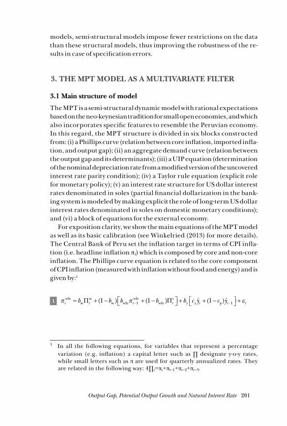
201Output Gap, Potential Output Growth and Natural Interest Rate
models, semi-structural models impose fewer restrictions on the data than these structural models, thus improving the robustness of the re-sults in case of specification errors.
3. THE MPT MODEL AS A MULTIVARIATE FILTER
3.1 Main structure of model
The MPT is a semi-structural dynamic model with rational expectations based on the neo-keynesian tradition for small open economies, and which also incorporates specific features to resemble the Peruvian economy. In this regard, the MPT structure is divided in six blocks constructed from: (i) a Phillips curve (relation between core inflation, imported infla-tion, and output gap); (ii) an aggregate demand curve (relation between the output gap and its determinants); (iii) a UIP equation (determination of the nominal depreciation rate from a modified version of the uncovered interest rate parity condition); (iv) a Taylor rule equation (explicit role for monetary policy); (v) an interest rate structure for US dollar interest rates denominated in soles (partial financial dollarization in the bank-ing system is modeled by making explicit the role of long-term US dollar interest rates denominated in soles on domestic monetary conditions); and (vi) a block of equations for the external economy.
For exposition clarity, we show the main equations of the MPT model as well as its basic calibration (see Winkelried (2013) for more details). The Central Bank of Peru set the inflation target in terms of CPI infla-tion (i.e. headline inflation πt) which is composed by core and non-core inflation. The Phillips curve equation is related to the core component of CPI inflation (measured with inflation without food and energy) and is given by:1
1 π πt m tm
m t te
y y tb b b b b c y cwfewfe
wfewfe= + − + − + + −−Π Π( ) ( ) (1 1 11 yy t ty) − +1 εˆ ˆ
1 In all the following equations, for variables that represent a percentage variation (e.g. inflation) a capital letter such as Π designate y-o-y rates, while small letters such as π are used for quarterly annualized rates. They are related in the following way: 4Πt=πt+πt−1+πt−2+πt−3.
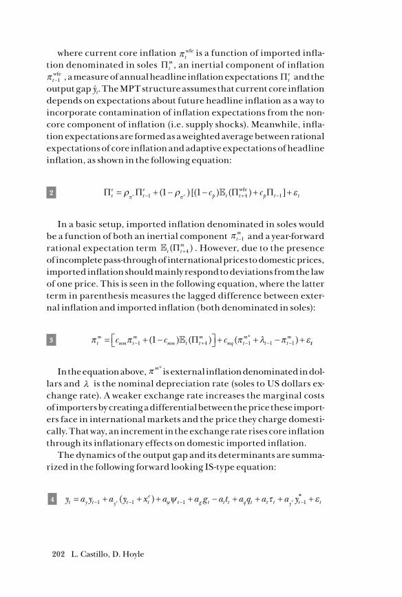
202 L. Castillo, D. Hoyle
where current core inflation πtwfe is a function of imported infla-
tion denominated in soles Πtm , an inertial component of inflation
πt −1wfe , a measure of annual headline inflation expectations Πt
e and the output gap yt. The MPT structure assumes that current core inflation depends on expectations about future headline inflation as a way to incorporate contamination of inflation expectations from the non-core component of inflation (i.e. supply shocks). Meanwhile, infla-tion expectations are formed as a weighted average between rational expectations of core inflation and adaptive expectations of headline inflation, as shown in the following equation:
2 Π Π Π Πte
te
p t t p t te e c c= + − − + +− + −ρ ρ επ π1 4 11 1( )[( ) ( ) ] wfe
In a basic setup, imported inflation denominated in soles would be a function of both an inertial component πt
m−1 and a year-forward
rational expectation term t tm( )Π +4 . However, due to the presence
of incomplete pass-through of international prices to domestic prices, imported inflation should mainly respond to deviations from the law of one price. This is seen in the following equation, where the latter term in parenthesis measures the lagged difference between exter-nal inflation and imported inflation (both denominated in soles):
3 π π π λ π εtm
mm tm
mm t tm
mq tm
t tmc c c= + − + + − +− + − − −1 4 1 1 11( ) ( ) ( )* Π tt
In the equation above, π m * is external inflation denominated in dol-lars and λ is the nominal depreciation rate (soles to US dollars ex-change rate). A weaker exchange rate increases the marginal costs of importers by creating a differential between the price these import-ers face in international markets and the price they charge domesti-cally. That way, an increment in the exchange rate rises core inflation through its inflationary effects on domestic imported inflation.
The dynamics of the output gap and its determinants are summa-rized in the following forward looking IS-type equation:
4 y a y a y x a a g a t a q a a yt y t y t te
t g t t t q t t y te= + + + + − + + +− − − −1 1 1 1( ) *ψ τψ τ ** +εt
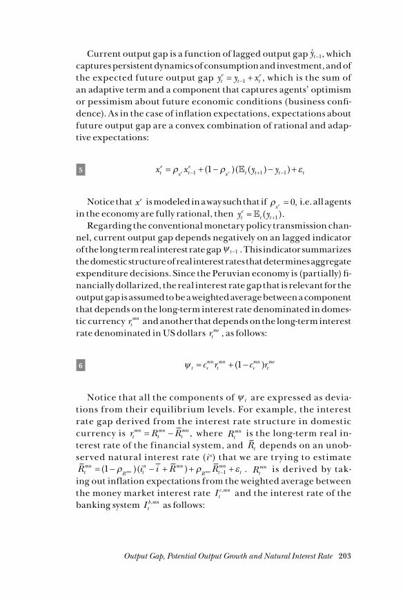
203Output Gap, Potential Output Growth and Natural Interest Rate
Current output gap is a function of lagged output gap yt −1ˆ , which
captures persistent dynamics of consumption and investment, and of the expected future output gap y y xt
et t
e= +−1 , which is the sum of an adaptive term and a component that captures agents’ optimism or pessimism about future economic conditions (business confi-dence). As in the case of inflation expectations, expectations about future output gap are a convex combination of rational and adap-tive expectations:
5 x x y yte
x te
x t t t te e= + − − +− + −ρ ρ ε1 1 11( )( ( ) )
Notice that xe is modeled in a way such that if ρxe = 0, i.e. all agents
in the economy are fully rational, then y yte
t t= + ( ).1
Regarding the conventional monetary policy transmission chan-nel, current output gap depends negatively on an lagged indicator of the long term real interest rate gap ψ t −1 . This indicator summarizes the domestic structure of real interest rates that determines aggregate expenditure decisions. Since the Peruvian economy is (partially) fi-nancially dollarized, the real interest rate gap that is relevant for the output gap is assumed to be a weighted average between a component that depends on the long-term interest rate denominated in domes-tic currency rt
mn and another that depends on the long-term interest rate denominated in US dollars rt
me , as follows:
6 ψ t rmn
tmn
rmn
tmec r c r= + −( )1
Notice that all the components of ψ t are expressed as devia-tions from their equilibrium levels. For example, the interest rate gap derived from the interest rate structure in domestic currency is r R Rt
mntmn
tmn= − , where Rt
mn is the long-term real in-terest rate of the financial system, and Rt depends on an unob-served natural interest rate (in) that we are trying to estimate R i i R Rt
mnR t
n mnR t
mntmn mn= − − + + +−( )( )1 1ρ ρ ε . Rt
mn is derived by tak-ing out inflation expectations from the weighted average between the money market interest rate I t
c mn, and the interest rate of the banking system I t
b mn, as follows:
204 L. Castillo, D. Hoyle
7 R c I c Itmn
bmn
tb mn
bmn
tc mn
te= + − −, ,( )1 Π
The interest rate of the banking system is a function of an iner-tial component I t
b mn−1, , and an expression that approximates the cost
of funds for banks. The latter depends on an autonomous term µIbmn
which measures the average margin charged by banks, the money market interest rate, and the gap of the reserve requirements rate e et
mn mn− . The term e mn should be understood as the reserve require-ment rate that would be in place in “normal” times, and the inclusion of this gap expression in the banking system’s interest rate structure seeks to account for the increase in funding costs due to macropru-dential considerations. The equation for I t
b mn, is shown below.
8 I I M I c e etb mn
bmn
tb mn
bmn
Ibmn mn
tc mn
emn
tmn mn, , ,( )[ (= + − + + −−ρ ρ µ1 1 ))] ,+εt
b mn
Meanwhile, the interest rate of the money market, which repre-sents the cost of funds faced outside the banking system (e.g. by is-suing bonds), is modeled as a yield curve that rests on the liquidity premium theory (an offshoot of the market expectation hypothe-sis) as follows:
9 I i i i itc mn
tmn
t tmn
t tmn
t tmn
tmn
t, [ ( ) ( ) ( )]= + + + + ++ + +
14 1 2 3 µ ε
In the equation above, itmn+1 is the inter-bank interest rate, which
measures the cost of short-term loans between banks i itmn
t+ = +1 ε , while µt
mn is the liquidity premium. That way, the expression is a sort of no-arbitrage condition, since the 1-year interest rate equals the ex-pected return from the respective 1-year forward short-term rates plus a liquidity premium (i.e. the longer-term interest rate matches its opportunity cost).
US-dollar interest rates denominated in soles are modeled ex-actly with the same structure as described in equations 7 through 9.
Real external conditions affect the dynamics of the output gap via: (i) the expenditure-switching effect of the real exchange rate gap qt ; (ii) the effect of global demand over domestic exports, summarized
205Output Gap, Potential Output Growth and Natural Interest Rate
by the output gap of Peru’s main trading partners yt∗ ; and (iii) the terms
of trade impulse τt , which reflects the effect of international com-modity prices over economic activity. Notice that yt
∗ and τt are as-sumed to follow exogenous processes since the model represents a small open economy. The expenditure-switching effect generated by changes in qt captures movements in the tradable sector output that occur when the real multilateral exchange rate differs from its long-run equilibrium level. Therefore, when qt is positive, the multilat-eral real exchange rate is above its equilibrium level and the relative price of domestic goods in terms of foreign goods falls, inducing an increase in exports.
Finally, fiscal policy variables, such as government expenditures gt and taxes tt, enter the output gap equation in the form of impulses and are considered to be exogenous.
Regarding the nominal exchange rate, the MPT takes a standard version of the uncovered interest rate parity (UIP) equation adjust-ed by a risk premium for investing in the domestic asset, and incor-porates sluggish adjustments of the nominal depreciation rate. This last feature simulates the effects of FX intervention over the dynam-ics of the exchange rate.2 We proceed to briefly explain how this ver-sion of the UIP is derived.
The conventional UIP equation (adjusted by a risk premium ξt) is given by:
i i s s equationtmn
tme
t te
t= + + −+ξ 4 1( ) * \end
Where st denotes the logarithm of the nominal exchange rate, st
e+1 is the expected nominal exchange rate, it
mn is the short-run nom-inal return of the domestic assets and it
me corresponds to the dollar denominated asset return. As it is well known, the UIP equation is an arbitrage equation that equalizes the nominal rate of return of do-mestic and foreign currency denominated assets. We are implicitly assuming that domestic and foreign assets are imperfect substitutes
2 The BCRP intervenes in the FX market to reduce FX volatility in a context of persistent partial financial dollarization. Although we do not model FX intervention explicitly, the sluggish adjustment of the the nominal depreciation rate allows us to incorporate its effects.
206 L. Castillo, D. Hoyle
in the sense that the return on the dollar is adjusted by an exchange rate and country risk premium.
To incorporate sluggish adjustments of the depreciation rate, the MPT assumes that expected exchange rate is a weighted aver-age of rational and ‘naive’ expectations (agents of this type expect future exchange rate to be equal to the observed exchange rate plus a random walk term ). Adaptive expectations should be more rel-evant if the effects of FX intervention are stronger. The expected exchange rate is thus modeled as:
s s ste
t te
t t+ + +=+
+
+
+1 1 11
11
ρρ ρλ
λ λ
( ) ( )
The above equations can be combined and written in quarterly annualized variations. By defining λt as the exchange rate variation, we get that λt t ts s= −+1 , and so the final expression for the nominal depreciation rate in the MPT is given by:
10 λ ρ λ ρ ξλ λt t t tme
t tmn
ti i= + + + − ++ ( ) ( )( )1 1
Finally, the Taylor rule shows that the Central Bank responds to future deviations of the core inf lation (four quarters ahead) from the target rate Π Π Π Πt t
wfetwfe= − = −( )+ + 4 4 2 , and to the current
and lagged output gap c fy= 0 5, . It also has an inertial component
as shown below:
11 i f i f i f f c y c yt i t i tn
t y fy t fy t t= + − + + + − +− −1 11 1( )[ ( ( ) ]π εΠ
The natural interest rate that we intend to estimate itn appears
in the Taylor rule as a drifting intercept, and can be rationalized as the trend interest rate that serves as a guideline for monetary pol-icy. This trend interest rate exists when the output gap and the core inflation rate are placed on their equilibrium values. Thus, it
n is con-sistent in the model with an economy with no transitory disturbances (similar to the definition of the natural interest rate).
207Output Gap, Potential Output Growth and Natural Interest Rate
The natural interest rate follows an autoregressive process, where the unconditional mean i is calibrated on 4.5%.3
12 i i itn
i i tn
tn n= − + +−( )1 1ρ ρ ε
The above description means that the MPT has no explicit role for potential output. In fact, it only determines the dynamic of the out-put gap (which by definition is the difference between real GDP and the potential output) among other modeled variables such as infla-tion, exchange rate, and interest rate. Therefore, we need to add a measurement equation that links the output gap with potential out-put growth. By definition, given the potential output Yt
* and real GDP Yt , the output gap yt is defined as:
ln ln*
* **y
Y YY
YY
Y Ytt t
t
t
tt t=
−= − ≈ −1
Subtracting the output gap from the previous period, we get:
(ln ln ) (ln ln ) % %* * *y y Y Y Y Y Y Yt t t t t t t t− = − − − ≈ −− − −1 1 1 ∆ ∆
The measurement equation that we add on the MPT is then given by the equation below. This equation states that real GDP growth (observed variable) equals potential output growth plus the varia-tion in the output gap.
13 ∆ ∆% % ( )*Y Y y yt t t t= + − −1
However, as we are introducing two new variables to the model, we need to incorporate an additional equation, defined below. This
3 This way of modelling the equilibrium interest rate is also followed by the IMF in their Global Projection Model (see for example Carabenciov et al. (2013)).
208 L. Castillo, D. Hoyle
equation states that potential output growth follows an autoregres-sive process.
14 ∆ ∆% %* **
*
Y Yt Y t tY= +−ρ ξ1
By the same token, notice that equations 11 and 12 can also be in-terpreted as a measurement equation for the nominal interest rate. Under this assumption, the Taylor rule (equation 11) may be viewed as decomposing the observed interest rate it into a systematic com-ponent (cycle component for the nominal interest rate) and a non-observed component related to the trend interest rate.
Table 1 summarizes the calibration used for our estimation pur-poses. The values assigned for the calibrated parameters are in line with the estimation results shown in Winkelried (2013), and are in fact the result of extensive judgment by the technical staff to im-prove the forecasting and explanatory power of the model. Using a set of calibrate parameters (instead of estimating them all) allows us to restrict uncertainty to the estimation of latent variables.
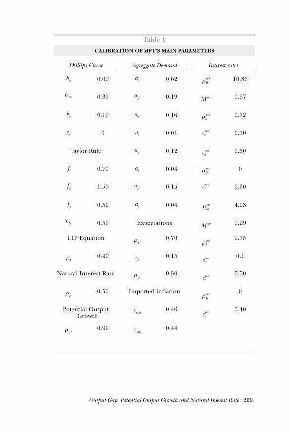
209Output Gap, Potential Output Growth and Natural Interest Rate
Table 1
CALIBRATION OF MPT’S MAIN PARAMETERS
Phillips Curve Agreggate Demand Interest rates
bm 0.09 ay 0.62 µIbmn 10.86
bwfe 0.35 aye 0.19 M mn 0.57
by 0.19 aψ 0.16 ρbmn 0.72
cy 0 at 0.01 cemn 0.30
Taylor Rule ag 0.12 cbmn 0.50
fi 0.70 aτ 0.04 ρRmn 0
f p 1.50 ay* 0.15 cr
mn 0.60
f y 0.50 aq 0.04 µIbme 4.03
c fy 0.50 Expectations M me 0.99
UIP Equation ρπ e
0.70ρb
me 0.75
ρλ 0.40 cp0.15
ceme 0.1
Natural Interest Rate ρxe
0.50cb
me 0.50
ρin
0.50 Imported inflationρR
me 0
Potential Output Growth
cmm0.46
crme 0.40
ρY *
0.99 cmq0.44
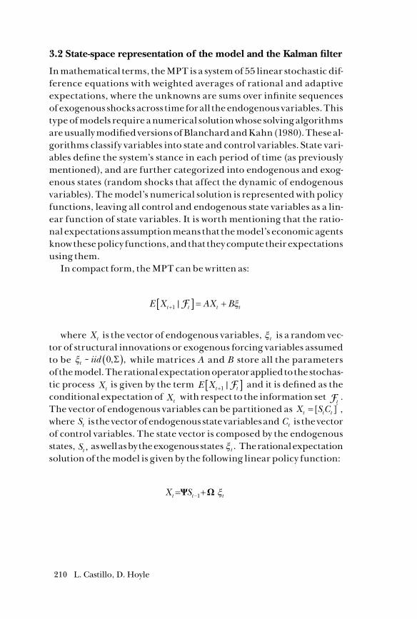
210 L. Castillo, D. Hoyle
3.2 State-space representation of the model and the Kalman filter
In mathematical terms, the MPT is a system of 55 linear stochastic dif-ference equations with weighted averages of rational and adaptive expectations, where the unknowns are sums over infinite sequences of exogenous shocks across time for all the endogenous variables. This type of models require a numerical solution whose solving algorithms are usually modified versions of Blanchard and Kahn (1980). These al-gorithms classify variables into state and control variables. State vari-ables define the system’s stance in each period of time (as previously mentioned), and are further categorized into endogenous and exog-enous states (random shocks that affect the dynamic of endogenous variables). The model’s numerical solution is represented with policy functions, leaving all control and endogenous state variables as a lin-ear function of state variables. It is worth mentioning that the ratio-nal expectations assumption means that the model’s economic agents know these policy functions, and that they compute their expectations using them.
In compact form, the MPT can be written as:
E X AX Bt t t t+[ ] = +1 |F ξ
where Xt is the vector of endogenous variables, ξt is a random vec-tor of structural innovations or exogenous forcing variables assumed to be ξt iid~ , ,0 Σ( ) while matrices A and B store all the parameters of the model. The rational expectation operator applied to the stochas-tic process Xt is given by the term E Xt t+[ ]1 |F and it is defined as the conditional expectation of Xt with respect to the information set Ft
. The vector of endogenous variables can be partitioned as X S Ct t t= ′[ ] , where St is the vector of endogenous state variables and Ct is the vector of control variables. The state vector is composed by the endogenous states, St , as well as by the exogenous states ξt . The rational expectation solution of the model is given by the following linear policy function:
X St t t= +−Ψ Ω1 ξ
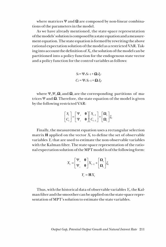
211Output Gap, Potential Output Growth and Natural Interest Rate
where matrices Ψ and Ω are composed by non-linear combina-tions of the parameters in the model.
As we have already mentioned, the state-space representation of the models’ solution is composed by a state equation and a measure-ment equation. The state equation is formed by rewriting the above rational expectation solution of the model as a restricted VAR. Tak-ing into account the definition of Xt, the solution of the model can be partitioned into a policy function for the endogenous state vector and a policy function for the control variables as follows:
St = ΨsSt−1 + Ωsξt
Ct = ΨcSt−1 + Ωcξt
where Ψs,Ψc,Ωs and Ωc are the corresponding partitions of ma-trices Ψ and Ω. Therefore, the state equation of the model is given by the following restricted VAR:
SC
SC
t
t
s
c
t
t
s
ct
=
+
−
−
ΨΨ
00
ΩΩ
1
1
ξ
Finally, the measurement equation uses a rectangular selection matrix H applied on the vector Xt to define the set of observable variables Yt that are used to estimate the non-observable variables with the Kalman filter. The state-space representation of the ratio-nal expectation solution of the MPT model is of the following form:
X Xts
ct
s
ct=
+
−
ΨΨ
00
ΩΩ1 ξ
Y Xt t=H
Thus, with the historical data of observable variables Yt, the Kal-man filter and the smoother can be applied on the state-space repre-sentation of MPT’s solution to estimate the state variables.
212 L. Castillo, D. Hoyle
3.3 The observable variables
From the explanation of the Kalman filter, it is straightforward to con-clude that the estimation results are sensible to the group of vari-ables that are declared as observable (the ones that are defined in the measurement equation). Therefore, the selection of variables must be done aiming to capture the main drivers of the non-observable variables to be estimated. It is also worth noting that if a time series used as input for the Kalman filter is updated (e.g. a historical revi-sion or new data for subsequent periods), the results will also vary.
To account for the uncertainty risen by the selection of observable variables, we employ five groups of variables to be declared as such. This way, we get a set of estimation results which we can use to define probable ranges for the non-observable variables.4 The five groups of variables (all of which are plotted in Figure 1) are:
i) Group 1: Real GDP growth, inflation without food and energy, inflation expectations (1- year forward), impulse of business confidence (proxy of the expected output gap), terms of trade growth and real effective exchange rate gap.5
ii) Group 2: Real GDP growth, inflation without food and energy, inflation expectations (1- year forward), impulse of business confidence, terms of trade growth, real effective exchange rate gap, short-term interest rate (BCRP’s monetary policy rate) and 3-Month LIBOR rate (proxy of external interest rate).
iii) Group 3: Real GDP growth, inflation without food and energy, inflation expectations (1- year forward), impulse of business confidence, terms of trade growth, real effective exchange rate gap and short-term interest rate (BCRP’s monetary policy rate).
4 The probable ranges are the difference between the maximum and mini-mum value of the five estimates at each period of time.
5 The real effective exchange rate (REER) gap is actually also a non-observable variable. However, it is one of the most important deter-minants of output gap dynamics. Thus, we use a satellite model based on cointegration relations (Behavioral Equilibrium Exchange Rate or BEER model) to estimate it and declare the REER gap as an ob-servable variable. For more references on the BEER methodology, see MacDonald and Clark (1998).
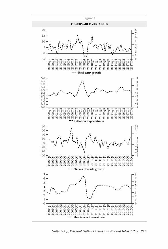
213Output Gap, Potential Output Growth and Natural Interest Rate
Figure 1
OBSERVABLE VARIABLES
15
10
5
0
20
−5
7654321
8
0
2017
Q1
2016
Q2
2015
Q3
2014
Q4
2014
Q1
2013
Q2
2012
Q3
2011
Q4
2011
Q1
Real gdp growth
2010
Q2
2009
Q3
2008
Q4
2008
Q1
2007
Q2
2006
Q3
2005
Q4
2005
Q1
2004
Q2
2003
Q3
2002
Q4
2002
Q1
2017
Q4
4.54.03.53.02.52.01.51.00.5
5.0
0.0
210
−1−2−3−4
3
−5
2017
Q1
2016
Q2
2015
Q3
2014
Q4
2014
Q1
2013
Q2
2012
Q3
2011
Q4
2011
Q1
Inflation expectations
2010
Q2
2009
Q3
2008
Q4
2008
Q1
2007
Q2
2006
Q3
2005
Q4
2005
Q1
2004
Q2
2003
Q3
2002
Q4
2002
Q1
2017
Q4
604020
0−20−40
80
−60
1086420
−2−4−6
12
−8
2017
Q1
2016
Q2
2015
Q3
2014
Q4
2014
Q1
2013
Q2
2012
Q3
2011
Q4
2011
Q1
Terms of trade growth
2010
Q2
2009
Q3
2008
Q4
2008
Q1
2007
Q2
2006
Q3
2005
Q4
2005
Q1
2004
Q2
2003
Q3
2002
Q4
2002
Q1
2017
Q4
654321
7
0
7654321
8
0
2017
Q1
2016
Q2
2015
Q3
2014
Q4
2014
Q1
2013
Q2
2012
Q3
2011
Q4
2011
Q1
Short-term interest rate
2010
Q2
2009
Q3
2008
Q4
2008
Q1
2007
Q2
2006
Q3
2005
Q4
2005
Q1
2004
Q2
2003
Q3
2002
Q4
2002
Q1
2017
Q4
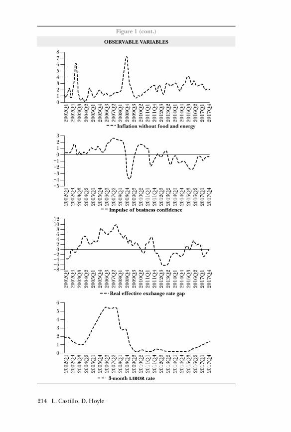
214 L. Castillo, D. Hoyle
Figure 1 (cont.)
OBSERVABLE VARIABLES
7654321
8
0
2017
Q1
2016
Q2
2015
Q3
2014
Q4
2014
Q1
2013
Q2
2012
Q3
2011
Q4
2011
Q1
Inflation without food and energy
2010
Q2
2009
Q3
2008
Q4
2008
Q1
2007
Q2
2006
Q3
2005
Q4
2005
Q1
2004
Q2
2003
Q3
2002
Q4
2002
Q1
2017
Q4
210
−1−2−3−4
3
−5
2017
Q1
2016
Q2
2015
Q3
2014
Q4
2014
Q1
2013
Q2
2012
Q3
2011
Q4
2011
Q1
Impulse of business confidence
2010
Q2
2009
Q3
2008
Q4
2008
Q1
2007
Q2
2006
Q3
2005
Q4
2005
Q1
2004
Q2
2003
Q3
2002
Q4
2002
Q1
2017
Q4
1086420
−2−4−6
12
−8
2017
Q1
2016
Q2
2015
Q3
2014
Q4
2014
Q1
2013
Q2
2012
Q3
2011
Q4
2011
Q1
Real effective exchange rate gap
2010
Q2
2009
Q3
2008
Q4
2008
Q1
2007
Q2
2006
Q3
2005
Q4
2005
Q1
2004
Q2
2003
Q3
2002
Q4
2002
Q1
2017
Q4
5
4
3
2
1
6
0
2017
Q1
2016
Q2
2015
Q3
2014
Q4
2014
Q1
2013
Q2
2012
Q3
2011
Q4
2011
Q1
3-month libor rate
2010
Q2
2009
Q3
2008
Q4
2008
Q1
2007
Q2
2006
Q3
2005
Q4
2005
Q1
2004
Q2
2003
Q3
2002
Q4
2002
Q1
2017
Q4
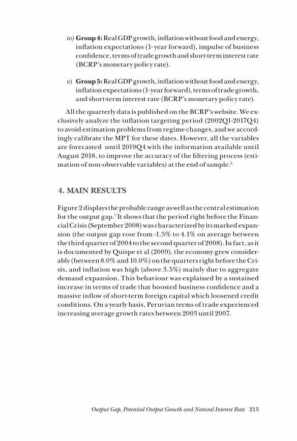
215Output Gap, Potential Output Growth and Natural Interest Rate
iv) Group 4: Real GDP growth, inflation without food and energy, inflation expectations (1- year forward), impulse of business confidence, terms of trade growth and short-term interest rate (BCRP’s monetary policy rate).
v) Group 5: Real GDP growth, inflation without food and energy, inflation expectations (1- year forward), terms of trade growth, and short-term interest rate (BCRP’s monetary policy rate).
All the quarterly data is published on the BCRP’s website. We ex-clusively analyze the inflation targeting period (2002Q1-2017Q4) to avoid estimation problems from regime changes, and we accord-ingly calibrate the MPT for these dates. However, all the variables are forecasted until 2019Q4 with the information available until August 2018, to improve the accuracy of the filtering process (esti-mation of non-observable variables) at the end of sample.6
4. MAIN RESULTS
Figure 2 displays the probable range as well as the central estimation for the output gap.7 It shows that the period right before the Finan-cial Crisis (September 2008) was characterized by its marked expan-sion (the output gap rose from -1.5% to 4.1% on average between the third quarter of 2004 to the second quarter of 2008). In fact, as it is documented by Quispe et al (2009), the economy grew consider-ably (between 8.0% and 10.0%) on the quarters right before the Cri-sis, and inflation was high (above 3.5%) mainly due to aggregate demand expansion. This behaviour was explained by a sustained increase in terms of trade that boosted business confidence and a massive inflow of short-term foreign capital which loosened credit conditions. On a yearly basis, Peruvian terms of trade experienced increasing average growth rates between 2003 until 2007.
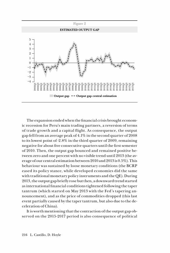
216 L. Castillo, D. Hoyle
The expansion ended when the financial crisis brought econom-ic recession for Peru’s main trading partners, a reversion of terms of trade growth and a capital flight. As consequence, the output gap fell from an average peak of 4.1% in the second quarter of 2008 to its lowest point of -2.8% in the third quarter of 2009, remaining negative for about five consecutive quarters until the first semester of 2010. Then, the output gap bounced and remained positive be-tween zero and one percent with no visible trend until 2013 (the av-erage of our central estimation between 2010 and 2013 is 0.5%). This behaviour was sustained by loose monetary conditions (the BCRP eased its policy stance, while developed economies did the same with traditional monetary policy instruments and the QE). During 2013, the output gap briefly rose but then, a downward trend started as international financial conditions tightened following the taper tantrum (which started on May 2013 with the Fed’s tapering an-nouncement), and as the price of commodities dropped (this last event partially caused by the taper tantrum, but also due to the de-celeration of China).
It is worth mentioning that the contraction of the output gap ob-served on the 2015-2017 period is also consequence of political
Figure 2
ESTIMATED OUTPUT GAP
Output gap Output gap central estimation20
12Q
120
12Q
320
13Q
120
13Q
320
14Q
1
2016
Q1
2015
Q3
2015
Q1
2014
Q3
2016
Q3
2017
Q1
2011
Q3
2011
Q1
2010
Q3
2010
Q1
2009
Q3
2009
Q1
2008
Q3
2008
Q1
2007
Q3
2007
Q1
2006
Q3
2006
Q1
2005
Q2
2005
Q1
2004
Q3
2004
Q1
2003
Q3
2003
Q1
2002
Q3
2002
Q1
2017
Q3
43210
−1−2−3
5
−4
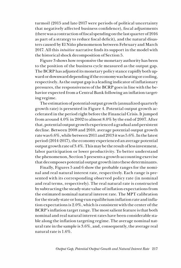
217Output Gap, Potential Output Growth and Natural Interest Rate
turmoil (2015 and late-2017 were periods of political uncertainty that negatively affected business confidence), fiscal adjustments (there was a contraction of fiscal spending on the last quarter of 2016 as part of a strategy to reduce fiscal deficit), and the natural disas-ters caused by El Niño phenomenon between February and March 2017. All this intuitive narrative finds its support in the model with the historical shock decomposition of Section 5.
Figure 3 shows how responsive the monetary authority has been to the position of the business cycle measured as the output gap. The BCRP has adjusted its monetary policy stance rapidly both up-ward or downward depending if the economy was heating or cooling, respectively. As the output gap is a leading indicator of inflationary pressures, the responsiveness of the BCRP goes in line with the be-havior expected from a Central Bank following an inflation target-ing regime.
The estimation of potential output growth (annualized quarterly growth rate) is presented in Figure 4. Potential output growth ac-celerated in the period right before the Financial Crisis. It jumped from around 4.0% in 2002 to almost 8.0% by the end of 2007. After that, potential output growth experienced a gradual and persistent decline. Between 2008 and 2010, average potential output growth rate was 6.6%, while between 2011 and 2013 it was 5.6%. In the latest period (2014-2017), the economy experienced an average potential output growth rate of 3.4%. This may be the result of less investment, labor participation or lower productivity. To better understand the phenomenon, Section 5 presents a growth-accounting exercise that decomposes potential output growth into these determinants.
Finally, Figures 5 and 6 show the probable ranges for the nomi-nal and real natural interest rate, respectively. Each range is pre-sented with its corresponding observed policy rate (in nominal and real terms, respectively). The real natural rate is constructed by subtracting the steady-state value of inflation expectations from the estimated nominal natural interest rate. The MPT calibration for the steady-state or long-run equilibrium inflation rate and infla-tion expectations is 2.0%, which is consistent with the center of the BCRP’s inflation target range. The most salient feature is that both nominal and real natural interest rates have been considerable sta-ble along the inflation targeting regime. The average nominal nat-ural rate in the sample is 3.6%, and, consequently, the average real natural rate is 1.6%.
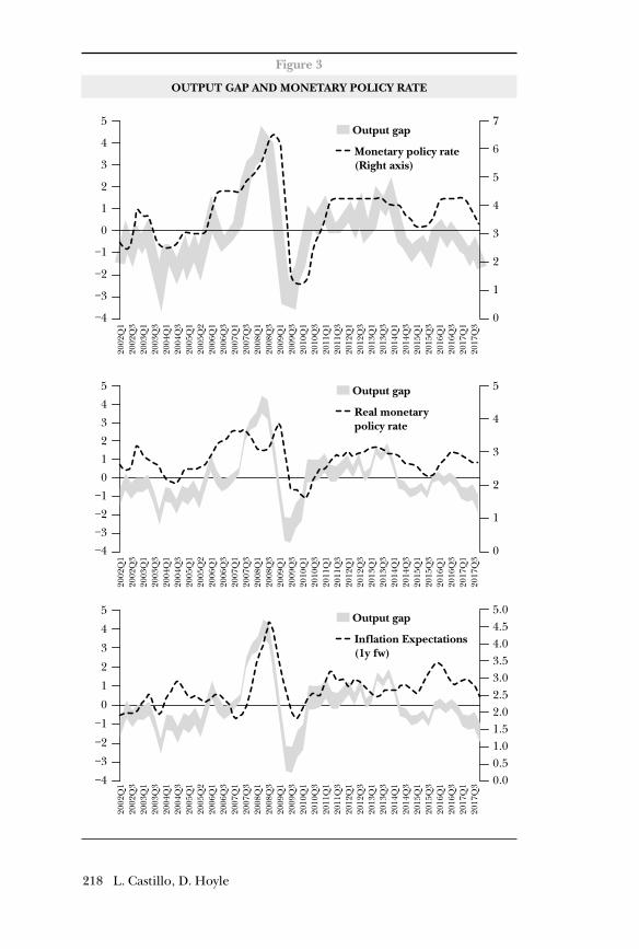
218 L. Castillo, D. Hoyle
Figure 3
OUTPUT GAP AND MONETARY POLICY RATE
2012
Q1
2012
Q3
2013
Q1
2013
Q3
2014
Q1
2016
Q1
2015
Q3
2015
Q1
2014
Q3
2016
Q3
2017
Q1
2011
Q3
2011
Q1
2010
Q3
2010
Q1
2009
Q3
2009
Q1
2008
Q3
2008
Q1
2007
Q3
2007
Q1
2006
Q3
2006
Q1
2005
Q2
2005
Q1
2004
Q3
2004
Q1
2003
Q3
2003
Q1
2002
Q3
2002
Q1
2017
Q3
4
3
2
1
0
−1
−2
−3
5
−4
4.54.03.53.02.5
5.0
2.01.51.00.50.0
Output gap
Inflation Expectations(1y fw)
2012
Q1
2012
Q3
2013
Q1
2013
Q3
2014
Q1
2016
Q1
2015
Q3
2015
Q1
2014
Q3
2016
Q3
2017
Q1
2011
Q3
2011
Q1
2010
Q3
2010
Q1
2009
Q3
2009
Q1
2008
Q3
2008
Q1
2007
Q3
2007
Q1
2006
Q3
2006
Q1
2005
Q2
2005
Q1
2004
Q3
2004
Q1
2003
Q3
2003
Q1
2002
Q3
2002
Q1
2017
Q3
4
3
2
1
0
−1
−2
−3
5
−4
4
3
2
1
5
0
Output gap
Real monetarypolicy rate
Output gap
Monetary policy rate(Right axis)
2012
Q1
2012
Q3
2013
Q1
2013
Q3
2014
Q1
2016
Q1
2015
Q3
2015
Q1
2014
Q3
2016
Q3
2017
Q1
2011
Q3
2011
Q1
2010
Q3
2010
Q1
2009
Q3
2009
Q1
2008
Q3
2008
Q1
2007
Q3
2007
Q1
2006
Q3
2006
Q1
2005
Q2
2005
Q1
2004
Q3
2004
Q1
2003
Q3
2003
Q1
2002
Q3
2002
Q1
2017
Q3
4
3
2
1
0
−1
−2
−3
5
−4
6
5
4
3
2
1
7
0
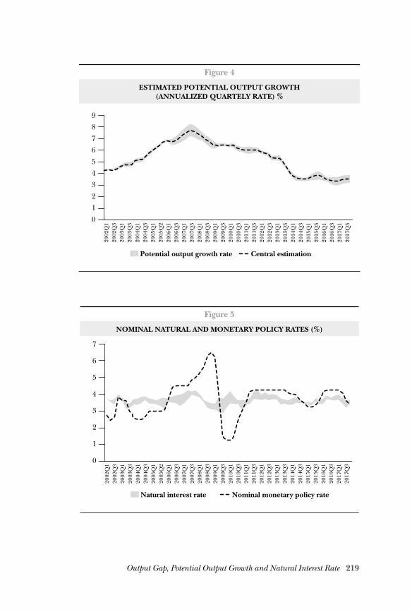
219Output Gap, Potential Output Growth and Natural Interest Rate
Figure 4
ESTIMATED POTENTIAL OUTPUT GROWTH(ANNUALIZED QUARTELY RATE) %
Potential output growth rate Central estimation20
12Q
120
12Q
320
13Q
120
13Q
320
14Q
1
2016
Q1
2015
Q3
2015
Q1
2014
Q3
2016
Q3
2017
Q1
2011
Q3
2011
Q1
2010
Q3
2010
Q1
2009
Q3
2009
Q1
2008
Q3
2008
Q1
2007
Q3
2007
Q1
2006
Q3
2006
Q1
2005
Q2
2005
Q1
2004
Q3
2004
Q1
2003
Q3
2003
Q1
2002
Q3
2002
Q1
2017
Q3
87654321
9
0
Figure 5
NOMINAL NATURAL AND MONETARY POLICY RATES (%)
Natural interest rate Nominal monetary policy rate
2012
Q1
2012
Q3
2013
Q1
2013
Q3
2014
Q1
2016
Q1
2015
Q3
2015
Q1
2014
Q3
2016
Q3
2017
Q1
2011
Q3
2011
Q1
2010
Q3
2010
Q1
2009
Q3
2009
Q1
2008
Q3
2008
Q1
2007
Q3
2007
Q1
2006
Q3
2006
Q1
2005
Q2
2005
Q1
2004
Q3
2004
Q1
2003
Q3
2003
Q1
2002
Q3
2002
Q1
2017
Q3
6
5
4
3
2
1
7
0
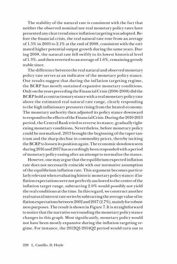
220 L. Castillo, D. Hoyle
The stability of the natural rate is consistent with the fact that neither the observed nominal nor real monetary policy rates have presented any clear trend since inflation targeting was adopted. Be-fore the financial crisis, the real natural rate rose from an average of 1.5% in 2005 to 2.1% at the end of 2008, consistent with the esti-mated higher potential output growth during the same years. Dur-ing 2008, the natural rate fell swiftly to its lowest historical level of 1.3%, and then reverted to an average of 1.6%, remaining grossly stable since.
The difference between the real natural and observed monetary policy rate serves as an indicator of the monetary policy stance. Our results suggest that during the inf lation targeting regime, the BCRP has mostly sustained expansive monetary conditions. Only on the years preceding the Financial Crisis (2006-2008) did the BCRP hold a contractionary stance with a real monetary policy rate above the estimated real natural rate range, clearly responding to the high inflationary pressures rising from the heated economy. The monetary authority then adjusted its policy stance downward to respond to the effects of the Financial Crisis. During the 2010-2013 period, the Central Bank tried to reverse its stance, gradually tight-ening monetary conditions. Nevertheless, before monetary policy could be normalized, 2013 brought the beginning of the taper tan-trum and the sharp decline in commodity prices, thereby inciting the BCRP to loosen its position again. The economic slowdown seen during 2016 and 2017 has accordingly been responded with a period of monetary policy easing after an attempt to normalize the stance.
However, one may argue that the equilibrium expected inflation rate does not necessarily coincide with our normative assumption of the equilibrium inflation rate. This argument becomes particu-larly relevant when evaluating historic monetary policy stance: if in-flation expectations were not perfectly anchored to the center of the inflation target range, subtracting 2.0% would possibly not yield the real conditions at the time. In this regard, we construct another real natural interest rate series by subtracting the average value of in-flation expectations between 2002 and 2017 (2.7%), mainly for robust-ness purposes. The result is shown in Figure 7. It is straightforward to notice that the narrative surrounding the monetary policy stance changes in this graph. Most significantly, monetary policy would not have been mostly expansive during the inflation targeting re-gime. For instance, the 2012Q1-2014Q2 period would turn out to
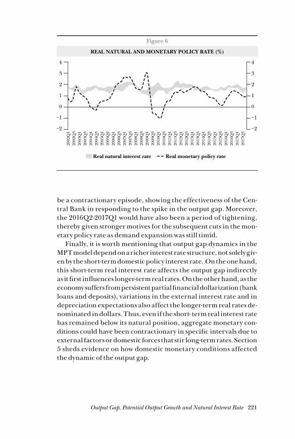
221Output Gap, Potential Output Growth and Natural Interest Rate
be a contractionary episode, showing the effectiveness of the Cen-tral Bank in responding to the spike in the output gap. Moreover, the 2016Q2-2017Q1 would have also been a period of tightening, thereby given stronger motives for the subsequent cuts in the mon-etary policy rate as demand expansion was still timid.
Finally, it is worth mentioning that output gap dynamics in the MPT model depend on a richer interest rate structure, not solely giv-en by the short-term domestic policy interest rate. On the one hand, this short-term real interest rate affects the output gap indirectly as it first influences longer-term real rates. On the other hand, as the economy suffers from persistent partial financial dollarization (bank loans and deposits), variations in the external interest rate and in depreciation expectations also affect the longer-term real rates de-nominated in dollars. Thus, even if the short- term real interest rate has remained below its natural position, aggregate monetary con-ditions could have been contractionary in specific intervals due to external factors or domestic forces that stir long-term rates. Section 5 sheds evidence on how domestic monetary conditions affected the dynamic of the output gap.
Figure 6
REAL NATURAL AND MONETARY POLICY RATE (%)
Real natural interest rate Real monetary policy rate
2012
Q1
2012
Q3
2013
Q1
2013
Q3
2014
Q1
2016
Q1
2015
Q3
2015
Q1
2014
Q3
2016
Q3
2017
Q1
2011
Q3
2011
Q1
2010
Q3
2010
Q1
2009
Q3
2009
Q1
2008
Q3
2008
Q1
2007
Q3
2007
Q1
2006
Q3
2006
Q1
2005
Q2
2005
Q1
2004
Q3
2004
Q1
2003
Q3
2003
Q1
2002
Q3
2002
Q1
2017
Q3
3
2
1
0
−1
−2
4
3
2
1
0
−1
−2
4
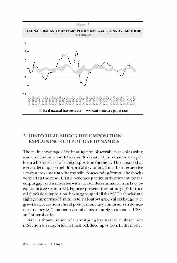
222 L. Castillo, D. Hoyle
5. HISTORICAL SHOCK DECOMPOSITION: EXPLAINING OUTPUT GAP DYNAMICS
The main advantage of estimating non-observable variables using a macroeconomic model as a multivariate filter is that we can per-form a historical shock decomposition on them. This means that we can decompose their historical deviations from their respective steady state values into the contributions coming from all the shocks defined in the model. This becomes particularly relevant for the output gap, as it is modeled with various determinants in an IS-type equation (see Section 3.1). Figure 8 presents the output gap’s histori-cal shock decomposition, having grouped all the MPT’s shocks into eight groups: terms of trade, external output gap, real exchange rate, growth expectations, fiscal policy, monetary conditions in domes-tic currency (S/), monetary conditions in foreign currency (US$), and other shocks.
As it is shown, much of the output gap’s narrative described in Section 4 is supported by the shock decomposition. In the model,
Figure 7
REAL NATURAL AND MONETARY POLICY RATES (ALTERNATIVE METHOD)Percentages
Real natural interest rate Real monetary policy rate
2012
Q1
2012
Q3
2013
Q1
2013
Q3
2014
Q1
2016
Q1
2015
Q3
2015
Q1
2014
Q3
2016
Q3
2017
Q1
2011
Q3
2011
Q1
2010
Q3
2010
Q1
2009
Q3
2009
Q1
2008
Q3
2008
Q1
2007
Q3
2007
Q1
2006
Q3
2006
Q1
2005
Q2
2005
Q1
2004
Q3
2004
Q1
2003
Q3
2003
Q1
2002
Q3
2002
Q1
2017
Q3
4
3
2
1
0
−1
−2
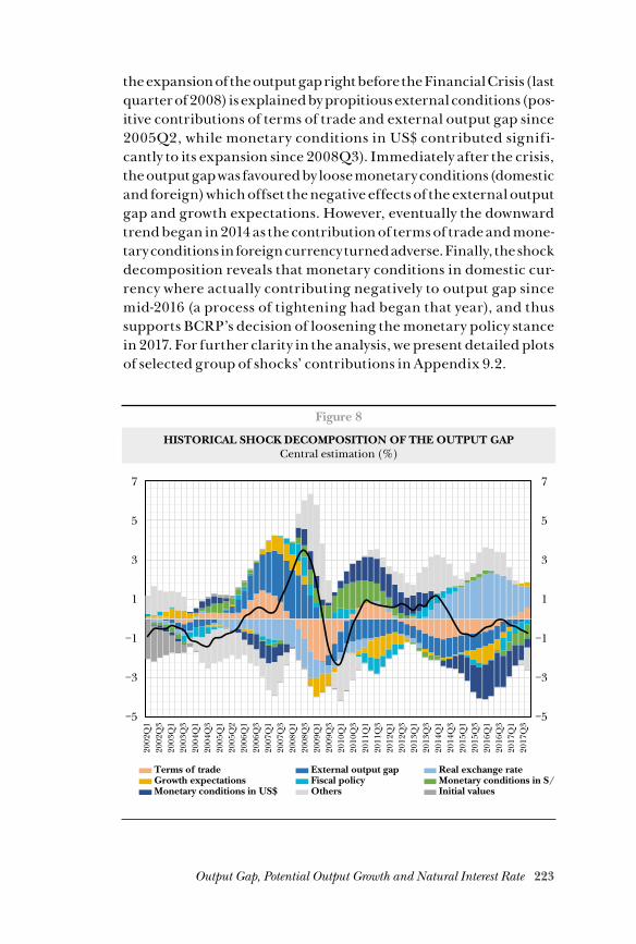
223Output Gap, Potential Output Growth and Natural Interest Rate
the expansion of the output gap right before the Financial Crisis (last quarter of 2008) is explained by propitious external conditions (pos-itive contributions of terms of trade and external output gap since 2005Q2, while monetary conditions in US$ contributed signifi-cantly to its expansion since 2008Q3). Immediately after the crisis, the output gap was favoured by loose monetary conditions (domestic and foreign) which offset the negative effects of the external output gap and growth expectations. However, eventually the downward trend began in 2014 as the contribution of terms of trade and mone-tary conditions in foreign currency turned adverse. Finally, the shock decomposition reveals that monetary conditions in domestic cur-rency where actually contributing negatively to output gap since mid-2016 (a process of tightening had began that year), and thus supports BCRP’s decision of loosening the monetary policy stance in 2017. For further clarity in the analysis, we present detailed plots of selected group of shocks’ contributions in Appendix 9.2.
Figure 8
HISTORICAL SHOCK DECOMPOSITION OF THE OUTPUT GAPCentral estimation (%)
2012
Q1
2012
Q3
2013
Q1
2013
Q3
2014
Q1
2016
Q1
2015
Q3
2015
Q1
2014
Q3
2016
Q3
2017
Q1
2011
Q3
2011
Q1
2010
Q3
2010
Q1
2009
Q3
2009
Q1
2008
Q3
2008
Q1
2007
Q3
2007
Q1
2006
Q3
2006
Q1
2005
Q2
2005
Q1
2004
Q3
2004
Q1
2003
Q3
2003
Q1
2002
Q3
2002
Q1
2017
Q3
5
3
1
−1
−3
−5
7
5
3
1
−1
−3
−5
7
Terms of trade External output gap Real exchange rateGrowth expectations Fiscal policy Monetary conditions in S/Monetary conditions in US$ Others Initial values
224 L. Castillo, D. Hoyle
6. GROWTH-ACCOUNTING: EXPLAINING THE RECENT SLOWDOWN IN POTENTIAL OUTPUT GROWTH
To better understand the recent trend of annual potential output growth, we decompose it through the growth-accounting method. This method rests on the assumption that potential output can be modeled with a Cobb-Douglas function such as:
15 Y A K Lt t t t* = −α α1
In the above equation, Yt* is the potential ouput, Kt is the physical
aggregate capital, Lt is the aggregate labor, and At is total factor pro-ductivity (TFP). TFP measures how much potential output will rise in addition to the effect of a one-unit increment in labor or capital, and is thus a proxy of economic efficiency. Meanwhile, the parame-ter α is both a measure of the elasticity of potential output to capital and of the share of total income that goes to this input (1−α denotes exactly the same for labor).
Equation 15 can be re-written on logarithm terms with annual variations as follows:
16 y y a a k k l lt t t t t t t t* * ( ) ( ) ( )( )− = − + − + − −− − − −1 1 1 11α α
This way, potential output growth y yt t* *− −1 is decomposed into
TFP growth a at t− −1 and the weighted average of factors of produc-tion growth. We set the parameter α on 0.485, which corresponds ap-proximately to the middle value of the range of estimations for the Peruvian economy (see Céspedes and Rondán (2016) for a summary of these estimates).
In terms of data, we use the annual series of Economically Active Population published by the National Institute of Statistics and Infor-mation (INEI, for its acronym in Spanish) as a proxy of labor. Since we are modelling potential output, we compute its trend component using the Hodrick-Prescott filter and employ it for our estimates.
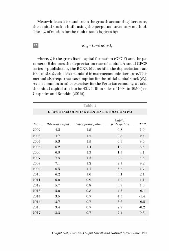
225Output Gap, Potential Output Growth and Natural Interest Rate
Meanwhile, as it is standard in the growth accounting literature, the capital stock is built using the perpetual inventory method. The law of motion for the capital stock is given by:
17 K K It t t+ = − +1 1( )δ
where, It is the gross fixed capital formation (GFCF) and the pa-rameter δ denotes the depreciation rate of capital. Annual GFCF series is published by the BCRP. Meanwhile, the depreciation rate is set on 5.0%, which is a standard in macroeconomic literature. This method also requires an assumption for the initial capital stock (K0). As it is common in other exercises for the Peruvian economy, we take the initial capital stock to be 42.2 billion soles of 1994 in 1950 (see Céspedes and Rondán (2016)).
Table 2
GROWTH-ACCOUNTING (CENTRAL ESTIMATION) (%)
Year Potential output Labor participationCapital
participation TFP
2002 4.3 1.5 0.8 1.9
2003 4.7 1.5 0.8 2.4
2004 5.3 1.5 0.9 3.0
2005 6.2 1.4 1.0 3.8
2006 6.8 1.3 1.3 4.1
2007 7.5 1.3 2.0 4.3
2008 7.1 1.2 2.7 3.2
2009 6.5 1.1 3.6 1.7
2010 6.2 1.0 3.1 2.1
2011 6.0 0.9 4.0 1.1
2012 5.7 0.8 3.9 1.0
2013 5.0 0.8 4.3 -0.1
2014 3.5 0.7 4.3 -1.4
2015 3.7 0.7 3.6 -0.5
2016 3.4 0.7 2.9 -0.2
2017 3.3 0.7 2.4 0.3
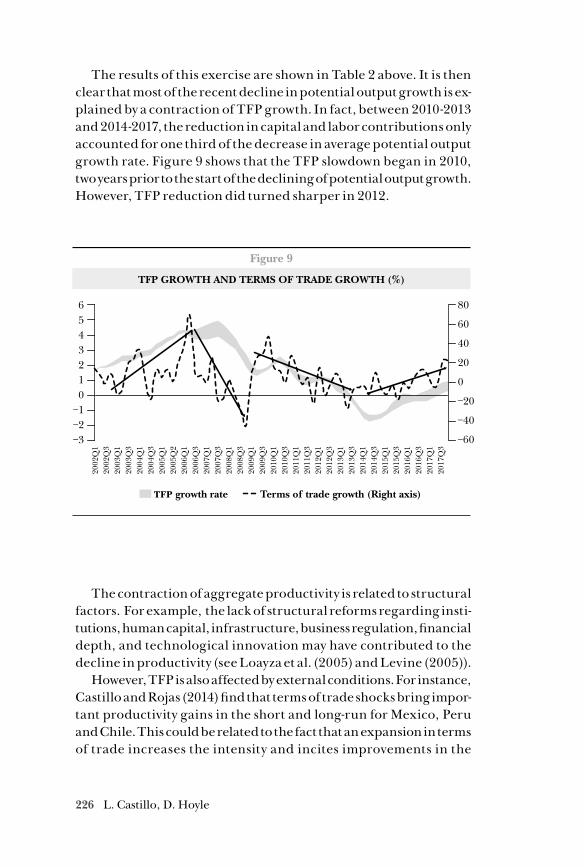
226 L. Castillo, D. Hoyle
The results of this exercise are shown in Table 2 above. It is then clear that most of the recent decline in potential output growth is ex-plained by a contraction of TFP growth. In fact, between 2010-2013 and 2014-2017, the reduction in capital and labor contributions only accounted for one third of the decrease in average potential output growth rate. Figure 9 shows that the TFP slowdown began in 2010, two years prior to the start of the declining of potential output growth. However, TFP reduction did turned sharper in 2012.
The contraction of aggregate productivity is related to structural factors. For example, the lack of structural reforms regarding insti-tutions, human capital, infrastructure, business regulation, financial depth, and technological innovation may have contributed to the decline in productivity (see Loayza et al. (2005) and Levine (2005)).
However, TFP is also affected by external conditions. For instance, Castillo and Rojas (2014) find that terms of trade shocks bring impor-tant productivity gains in the short and long-run for Mexico, Peru and Chile. This could be related to the fact that an expansion in terms of trade increases the intensity and incites improvements in the
Figure 9
TFP GROWTH AND TERMS OF TRADE GROWTH (%)
tfp growth rate Terms of trade growth (Right axis)
2012
Q1
2012
Q3
2013
Q1
2013
Q3
2014
Q1
2016
Q1
2015
Q3
2015
Q1
2014
Q3
2016
Q3
2017
Q1
2011
Q3
2011
Q1
2010
Q3
2010
Q1
2009
Q3
2009
Q1
2008
Q3
2008
Q1
2007
Q3
2007
Q1
2006
Q3
2006
Q1
2005
Q2
2005
Q1
2004
Q3
2004
Q1
2003
Q3
2003
Q1
2002
Q3
2002
Q1
2017
Q3
543210
−1−2−3
6
60
40
20
0
−20
−40
−60
80
227Output Gap, Potential Output Growth and Natural Interest Rate
use of factors of productions. Figure 9 above shows that there is in fact a close relation between TFP and terms of trade growth during the inflation targeting regime. The transitory sharp decline in terms of trade during the Financial Crisis did not affect TFP growth in the expected magnitude, probably due to the ephemeral nature of the shock. However, since 2010, as terms of trade decelerated and then contracted, TFP dropped as well.
7. COMPARISON WITH UNIVARIATE FILTERS
How much would our results differ if we had instead used univari-ate filters? We have already discussed that multivariate filters have the advantage of using multiple sources of information at the same time and defining an economic structure for the variables at play. However, it is worth comparing our estimates with the ones obtained with univariate filters due to their widespread use. In this section, we decompose GDP and the ex ante real monetary policy rate into a cycle and trend component using the standard Hodrick-Prescott filter (HP) with a lambda parameter of 1600, the Baxter-King band-pass filter (BK) considering business cycle frequencies between 6 and 32 quarters, and different specifications of unobserved com-ponent (UC) models estimated with Bayesian techniques following Grant and Chan (2017). Prior to presenting and comparing the re-sults, we briefly discuss the structure of the UC models employed in this section.
7.1 Decomposing Real GDP
We use two different specifications of UC models. Both specifications are unconstrained in the sense that there is no restriction imposed on the correlation between innovations of the cyclical and trend com-ponents. Following the literature, we label these models as UCUR (Unobserved Components Unrestricted Model). The first UCUR specification assumes an stochastic growth rate for the trend com-ponent and is based on Grant and Chan (2017). More precisely, the growth rate for the trend component follows a random walk, in contrast with more standard UC models in which the trend lev-el is modeled this way. Since the marginal likelihood of the UCUR model is sensitive to prior specifications, we use three different sets
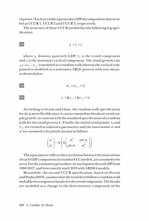
228 L. Castillo, D. Hoyle
of priors.8 Each set yields a particular GDP decomposition that we la-bel as UCUR 1, UCUR 2 and UCUR 3, respectively.
The structure of these UCUR models has the following log-spec-ification:
18 y ct t t= +τ
where yt denotes quarterly GDP, τt is the trend component and ct is the stationary cyclical component. The trend growth rate τ τ τt t t≡ − −1 is modeled as a random walk whereas the cyclical com-ponent is modeled as a stationary AR(2) process with zero mean, as shown below:
19 τ τ τt t tu= +−1
20 c c c ut t t tc= + +− −φ φ1 1 2 2
According to Grant and Chan, the random walk specification for ∆τt is more flexible since it can accommodate breaks in trend out-put growth, in contrast with the standard specification of a random walk for the trend process τt. Finally, the initial trend points, τ0 and τ−1, are treated as unknown parameters and the innovations uc and uτ are assumed to be jointly normal as follows:
u
utc
t
c c
cτ
τ
τ τ
σ ρσ σ
ρσ σ σ
~ , 02
2
The ρ parameter reflects the correlation between the innovations of each GDP component (in standard UC models, ρ is assumed to be zero). For the estimation procedure, we used quarterly real GDP from 1980-2017, and forecasted it until 2019 with ARIMA models.
Meanwhile, the second UCUR specification, based on Perron and Wada (2009), assumes that the trend level follows a random walk and adds two exogenous breaks for the trend component. The breaks are modeled as a change in the deterministic component of the
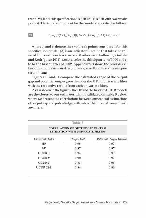
229Output Gap, Potential Output Growth and Natural Interest Rate
trend. We label this specification UCUR2BP (UCUR with two breaks points). The trend component for this model is specified as follows:
21 τ µ µ µ τ τt t tt t t t t t t u= < + ≤ < + ≤ + +−1 1 2 1 2 3 2 11 1 1( ) ( ) ( )
where t1 and t2 denote the two break points considered for this specification, while 1(A) is an indicator function that takes the val-ue of 1 if condition A is true and 0 otherwise. Following Guillén and Rodríguez (2014), we set t1 to be the third quarter of 1990 and t2 to be the first quarter of 2002. Appendix 9.3 shows the prior distri-butions for the estimated parameters, as well as the respective pos-terior means.
Figures 10 and 11 compare the estimated range of the output gap and potential output growth under the MPT multivariate filter with the respective results from each univariate filter.
As it is shown in the figures, the HP and the first two UCUR models are the closest to our estimates. This is validated on Table 3 below, where we present the correlations between our central estimations of output gap and potential growth rate with the ones from univari-ate filters.
Table 3
CORRELATION OF OUTPUT GAP CENTRAL ESTIMATION WITH UNIVARIATE FILTERS
Univariate Filter Output Gap Potential Output Growth
HP 0.96 0.97
BK 0.87 0.87
UCUR 1 0.94 0.97
UCUR 2 0.90 0.97
UCUR 3 0.83 0.96
UCUR 2BP 0.84 0.83
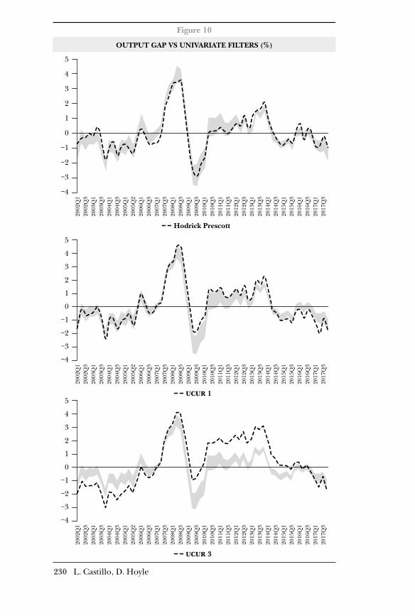
230 L. Castillo, D. Hoyle
Figure 10
OUTPUT GAP VS UNIVARIATE FILTERS (%)
Hodrick Prescott20
12Q
120
12Q
320
13Q
120
13Q
320
14Q
1
2016
Q1
2015
Q3
2015
Q1
2014
Q3
2016
Q3
2017
Q1
2011
Q3
2011
Q1
2010
Q3
2010
Q1
2009
Q3
2009
Q1
2008
Q3
2008
Q1
2007
Q3
2007
Q1
2006
Q3
2006
Q1
2005
Q2
2005
Q1
2004
Q3
2004
Q1
2003
Q3
2003
Q1
2002
Q3
2002
Q1
2017
Q3
4
3
2
1
0
−1
−2
−3
−4
5
ucur 1
2012
Q1
2012
Q3
2013
Q1
2013
Q3
2014
Q1
2016
Q1
2015
Q3
2015
Q1
2014
Q3
2016
Q3
2017
Q1
2011
Q3
2011
Q1
2010
Q3
2010
Q1
2009
Q3
2009
Q1
2008
Q3
2008
Q1
2007
Q3
2007
Q1
2006
Q3
2006
Q1
2005
Q2
2005
Q1
2004
Q3
2004
Q1
2003
Q3
2003
Q1
2002
Q3
2002
Q1
2017
Q3
5
4
3
2
1
0
−1
−2
−3
−4
ucur 3
2012
Q1
2012
Q3
2013
Q1
2013
Q3
2014
Q1
2016
Q1
2015
Q3
2015
Q1
2014
Q3
2016
Q3
2017
Q1
2011
Q3
2011
Q1
2010
Q3
2010
Q1
2009
Q3
2009
Q1
2008
Q3
2008
Q1
2007
Q3
2007
Q1
2006
Q3
2006
Q1
2005
Q2
2005
Q1
2004
Q3
2004
Q1
2003
Q3
2003
Q1
2002
Q3
2002
Q1
2017
Q3
5
4
3
2
1
0
−1
−2
−3
−4
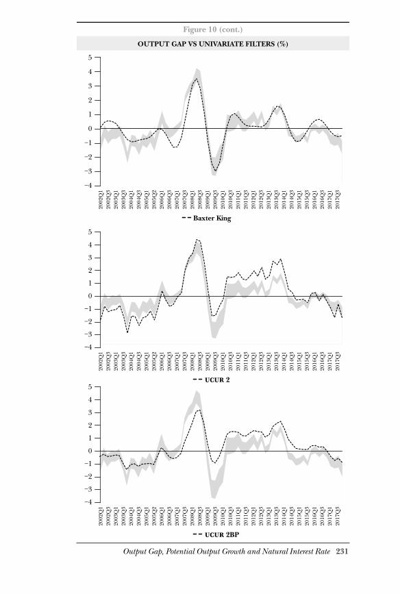
231Output Gap, Potential Output Growth and Natural Interest Rate
Figure 10 (cont.)
OUTPUT GAP VS UNIVARIATE FILTERS (%)
Baxter King
2012
Q1
2012
Q3
2013
Q1
2013
Q3
2014
Q1
2016
Q1
2015
Q3
2015
Q1
2014
Q3
2016
Q3
2017
Q1
2011
Q3
2011
Q1
2010
Q3
2010
Q1
2009
Q3
2009
Q1
2008
Q3
2008
Q1
2007
Q3
2007
Q1
2006
Q3
2006
Q1
2005
Q2
2005
Q1
2004
Q3
2004
Q1
2003
Q3
2003
Q1
2002
Q3
2002
Q1
2017
Q3
4
3
2
1
0
−1
−2
−3
−4
5
ucur 2
2012
Q1
2012
Q3
2013
Q1
2013
Q3
2014
Q1
2016
Q1
2015
Q3
2015
Q1
2014
Q3
2016
Q3
2017
Q1
2011
Q3
2011
Q1
2010
Q3
2010
Q1
2009
Q3
2009
Q1
2008
Q3
2008
Q1
2007
Q3
2007
Q1
2006
Q3
2006
Q1
2005
Q2
2005
Q1
2004
Q3
2004
Q1
2003
Q3
2003
Q1
2002
Q3
2002
Q1
2017
Q3
5
4
3
2
1
0
−1
−2
−3
−4
ucur 2BP
2012
Q1
2012
Q3
2013
Q1
2013
Q3
2014
Q1
2016
Q1
2015
Q3
2015
Q1
2014
Q3
2016
Q3
2017
Q1
2011
Q3
2011
Q1
2010
Q3
2010
Q1
2009
Q3
2009
Q1
2008
Q3
2008
Q1
2007
Q3
2007
Q1
2006
Q3
2006
Q1
2005
Q2
2005
Q1
2004
Q3
2004
Q1
2003
Q3
2003
Q1
2002
Q3
2002
Q1
2017
Q3
5
4
3
2
1
0
−1
−2
−3
−4
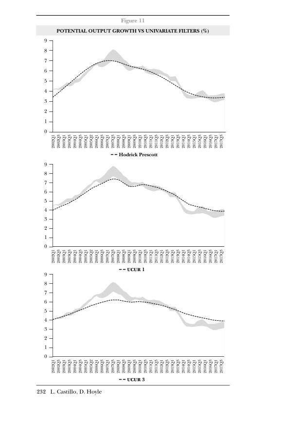
232 L. Castillo, D. Hoyle
Figure 11
POTENTIAL OUTPUT GROWTH VS UNIVARIATE FILTERS (%)
Hodrick Prescott20
12Q
120
12Q
320
13Q
120
13Q
320
14Q
1
2016
Q1
2015
Q3
2015
Q1
2014
Q3
2016
Q3
2017
Q1
2011
Q3
2011
Q1
2010
Q3
2010
Q1
2009
Q3
2009
Q1
2008
Q3
2008
Q1
2007
Q3
2007
Q1
2006
Q3
2006
Q1
2005
Q2
2005
Q1
2004
Q3
2004
Q1
2003
Q3
2003
Q1
2002
Q3
2002
Q1
2017
Q3
8
7
6
5
4
3
2
1
0
9
ucur 1
2012
Q1
2012
Q3
2013
Q1
2013
Q3
2014
Q1
2016
Q1
2015
Q3
2015
Q1
2014
Q3
2016
Q3
2017
Q1
2011
Q3
2011
Q1
2010
Q3
2010
Q1
2009
Q3
2009
Q1
2008
Q3
2008
Q1
2007
Q3
2007
Q1
2006
Q3
2006
Q1
2005
Q2
2005
Q1
2004
Q3
2004
Q1
2003
Q3
2003
Q1
2002
Q3
2002
Q1
2017
Q3
9
8
7
6
5
4
3
2
1
0
ucur 3
2012
Q1
2012
Q3
2013
Q1
2013
Q3
2014
Q1
2016
Q1
2015
Q3
2015
Q1
2014
Q3
2016
Q3
2017
Q1
2011
Q3
2011
Q1
2010
Q3
2010
Q1
2009
Q3
2009
Q1
2008
Q3
2008
Q1
2007
Q3
2007
Q1
2006
Q3
2006
Q1
2005
Q2
2005
Q1
2004
Q3
2004
Q1
2003
Q3
2003
Q1
2002
Q3
2002
Q1
2017
Q3
9
8
7
6
5
4
3
2
1
0
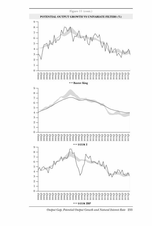
233Output Gap, Potential Output Growth and Natural Interest Rate
Figure 11 (cont.)
POTENTIAL OUTPUT GROWTH VS UNIVARIATE FILTERS (%)
Baxter King
2012
Q1
2012
Q3
2013
Q1
2013
Q3
2014
Q1
2016
Q1
2015
Q3
2015
Q1
2014
Q3
2016
Q3
2017
Q1
2011
Q3
2011
Q1
2010
Q3
2010
Q1
2009
Q3
2009
Q1
2008
Q3
2008
Q1
2007
Q3
2007
Q1
2006
Q3
2006
Q1
2005
Q2
2005
Q1
2004
Q3
2004
Q1
2003
Q3
2003
Q1
2002
Q3
2002
Q1
2017
Q3
8
7
6
5
4
3
2
1
0
9
ucur 2
2012
Q1
2012
Q3
2013
Q1
2013
Q3
2014
Q1
2016
Q1
2015
Q3
2015
Q1
2014
Q3
2016
Q3
2017
Q1
2011
Q3
2011
Q1
2010
Q3
2010
Q1
2009
Q3
2009
Q1
2008
Q3
2008
Q1
2007
Q3
2007
Q1
2006
Q3
2006
Q1
2005
Q2
2005
Q1
2004
Q3
2004
Q1
2003
Q3
2003
Q1
2002
Q3
2002
Q1
2017
Q3
9
8
7
6
5
4
3
2
1
0
ucur 2BP
2012
Q1
2012
Q3
2013
Q1
2013
Q3
2014
Q1
2016
Q1
2015
Q3
2015
Q1
2014
Q3
2016
Q3
2017
Q1
2011
Q3
2011
Q1
2010
Q3
2010
Q1
2009
Q3
2009
Q1
2008
Q3
2008
Q1
2007
Q3
2007
Q1
2006
Q3
2006
Q1
2005
Q2
2005
Q1
2004
Q3
2004
Q1
2003
Q3
2003
Q1
2002
Q3
2002
Q1
2017
Q3
9
8
7
6
5
4
3
2
1
0
234 L. Castillo, D. Hoyle
7.2 Decomposing the ex ante real monetary rate
Our UC model for the estimation of the ex ante real monetary pol-icy rate is based on Fiorentini et al. (2018), who make use of a local level model like Watson (1986) for the natural interest rate. In this model, the real monetary policy rate rt is assumed to be the sum of a permanent (or trend component) rt
* and a transitory component rtc .
Again, due to the fact that the marginal likelihood is sensitive to pri-or specifications, we use two alternative priors, and label the results as UC1 and UC2 (see Appendix 9.4).9 The structure of the models is given by the following equations:
22 r r rt t tc= +*
23 r r ut t tr* * *
= +−1
24 r r utc
tc
tr c
= +−α 1 ,
The innovations utr *
and utr c are assumed to be uncorrelated
and jointly normal ρ = 0 .We compare the results from these UC model estimations with
our multivariate estimation of the real natural interest rate in Fig-ure 12 (where the results from the HP and BK filters are also shown for comparison purposes). As it was explained in Section 4, we com-pute the real natural interest rate by subtracting 2.0% from the nomi-nal natural interest rate that we get from the MPT multivariate filter. However, following the previous discussion that the equilibrium ex-pected inflation rate does not necessarily coincide with this norma-tive assumption, we also proceed to compare the results with a real natural interest rate constructed by subtracting 2.7% (average infla-tion expectations between 2002 and 2017) in Figure 13. Finally, Ta-ble 4 presents the correlations between our central estimation of the real natural interest rate and the univariate results (the correlation coefficient is the same with any of the two assumptions on the equi-librium expected inflation).
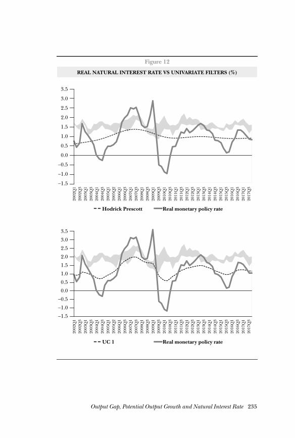
235Output Gap, Potential Output Growth and Natural Interest Rate
Figure 12
REAL NATURAL INTEREST RATE VS UNIVARIATE FILTERS (%)
Hodrick Prescott Real monetary policy rate
UC 1 Real monetary policy rate
2012
Q1
2012
Q3
2013
Q1
2013
Q3
2014
Q1
2016
Q1
2015
Q3
2015
Q1
2014
Q3
2016
Q3
2017
Q1
2011
Q3
2011
Q1
2010
Q3
2010
Q1
2009
Q3
2009
Q1
2008
Q3
2008
Q1
2007
Q3
2007
Q1
2006
Q3
2006
Q1
2005
Q2
2005
Q1
2004
Q3
2004
Q1
2003
Q3
2003
Q1
2002
Q3
2002
Q1
2017
Q3
3.0
2.5
2.0
1.5
1.0
0.5
0.0
–0.5
–1.0
–1.5
3.5
2012
Q1
2012
Q3
2013
Q1
2013
Q3
2014
Q1
2016
Q1
2015
Q3
2015
Q1
2014
Q3
2016
Q3
2017
Q1
2011
Q3
2011
Q1
2010
Q3
2010
Q1
2009
Q3
2009
Q1
2008
Q3
2008
Q1
2007
Q3
2007
Q1
2006
Q3
2006
Q1
2005
Q2
2005
Q1
2004
Q3
2004
Q1
2003
Q3
2003
Q1
2002
Q3
2002
Q1
2017
Q3
3.5
3.0
2.5
2.0
1.5
1.0
0.5
0.0
–0.5
–1.0
–1.5
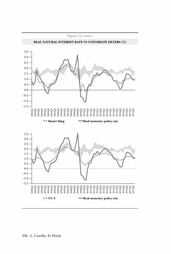
236 L. Castillo, D. Hoyle
Figure 12 (cont.)
REAL NATURAL INTEREST RATE VS UNIVARIATE FILTERS (%)
Baxter King Real monetary policy rate
UC 2 Real monetary policy rate
2012
Q1
2012
Q3
2013
Q1
2013
Q3
2014
Q1
2016
Q1
2015
Q3
2015
Q1
2014
Q3
2016
Q3
2017
Q1
2011
Q3
2011
Q1
2010
Q3
2010
Q1
2009
Q3
2009
Q1
2008
Q3
2008
Q1
2007
Q3
2007
Q1
2006
Q3
2006
Q1
2005
Q2
2005
Q1
2004
Q3
2004
Q1
2003
Q3
2003
Q1
2002
Q3
2002
Q1
2017
Q3
3.0
2.5
2.0
1.5
1.0
0.5
0.0
–0.5
–1.0
–1.5
3.5
2012
Q1
2012
Q3
2013
Q1
2013
Q3
2014
Q1
2016
Q1
2015
Q3
2015
Q1
2014
Q3
2016
Q3
2017
Q1
2011
Q3
2011
Q1
2010
Q3
2010
Q1
2009
Q3
2009
Q1
2008
Q3
2008
Q1
2007
Q3
2007
Q1
2006
Q3
2006
Q1
2005
Q2
2005
Q1
2004
Q3
2004
Q1
2003
Q3
2003
Q1
2002
Q3
2002
Q1
2017
Q3
3.5
3.0
2.5
2.0
1.5
1.0
0.5
0.0
–0.5
–1.0
–1.5
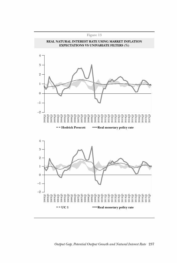
237Output Gap, Potential Output Growth and Natural Interest Rate
Figure 13
REAL NATURAL INTEREST RATE USING MARKET INFLATIONEXPECTATIONS VS UNIVARIATE FILTERS (%)
Hodrick Prescott Real monetary policy rate
UC 1 Real monetary policy rate
2012
Q1
2012
Q3
2013
Q1
2013
Q3
2014
Q1
2016
Q1
2015
Q3
2015
Q1
2014
Q3
2016
Q3
2017
Q1
2011
Q3
2011
Q1
2010
Q3
2010
Q1
2009
Q3
2009
Q1
2008
Q3
2008
Q1
2007
Q3
2007
Q1
2006
Q3
2006
Q1
2005
Q2
2005
Q1
2004
Q3
2004
Q1
2003
Q3
2003
Q1
2002
Q3
2002
Q1
2017
Q3
3
2
1
0
–1
–2
4
2012
Q1
2012
Q3
2013
Q1
2013
Q3
2014
Q1
2016
Q1
2015
Q3
2015
Q1
2014
Q3
2016
Q3
2017
Q1
2011
Q3
2011
Q1
2010
Q3
2010
Q1
2009
Q3
2009
Q1
2008
Q3
2008
Q1
2007
Q3
2007
Q1
2006
Q3
2006
Q1
2005
Q2
2005
Q1
2004
Q3
2004
Q1
2003
Q3
2003
Q1
2002
Q3
2002
Q1
2017
Q3
4
3
2
1
0
–1
–2
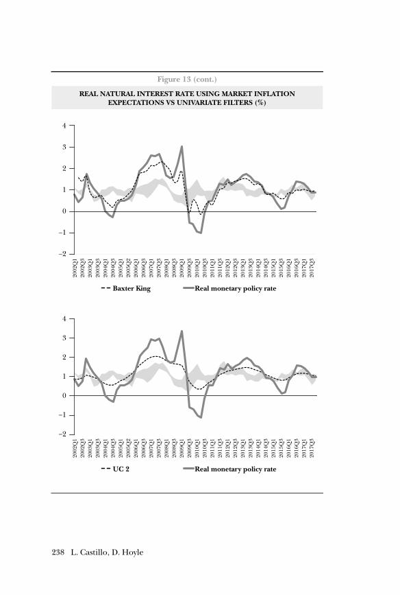
238 L. Castillo, D. Hoyle
Figure 13 (cont.)
REAL NATURAL INTEREST RATE USING MARKET INFLATIONEXPECTATIONS VS UNIVARIATE FILTERS (%)
Baxter King Real monetary policy rate
UC 2 Real monetary policy rate
2012
Q1
2012
Q3
2013
Q1
2013
Q3
2014
Q1
2016
Q1
2015
Q3
2015
Q1
2014
Q3
2016
Q3
2017
Q1
2011
Q3
2011
Q1
2010
Q3
2010
Q1
2009
Q3
2009
Q1
2008
Q3
2008
Q1
2007
Q3
2007
Q1
2006
Q3
2006
Q1
2005
Q2
2005
Q1
2004
Q3
2004
Q1
2003
Q3
2003
Q1
2002
Q3
2002
Q1
2017
Q3
3
2
1
0
–1
–2
4
2012
Q1
2012
Q3
2013
Q1
2013
Q3
2014
Q1
2016
Q1
2015
Q3
2015
Q1
2014
Q3
2016
Q3
2017
Q1
2011
Q3
2011
Q1
2010
Q3
2010
Q1
2009
Q3
2009
Q1
2008
Q3
2008
Q1
2007
Q3
2007
Q1
2006
Q3
2006
Q1
2005
Q2
2005
Q1
2004
Q3
2004
Q1
2003
Q3
2003
Q1
2002
Q3
2002
Q1
2017
Q3
4
3
2
1
0
–1
–2
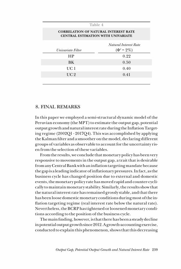
239Output Gap, Potential Output Growth and Natural Interest Rate
8. FINAL REMARKS
In this paper we employed a semi-structural dynamic model of the Peruvian economy (the MPT) to estimate the output gap, potential output growth and natural interest rate during the Inflation Target-ing regime (2002Q1 - 2017Q4). This was accomplished by applying the Kalman filter and a smoother on the model, declaring different groups of variables as observable to account for the uncertainty ris-en from the selection of these variables.
From the results, we conclude that monetary policy has been very responsive to movements in the output gap, a trait that is desirable from any Central Bank with an inflation targeting mandate because the gap is a leading indicator of inflationary pressures. In fact, as the business cycle has changed position due to external and domestic events, the monetary policy rate has moved rapid and counter-cycli-cally to maintain monetary stability. Similarly, the results show that the natural interest rate has remained grossly stable, and that there has been loose domestic monetary conditions during most of the in-flation targeting regime (real interest rate below the natural rate). Nevertheless, the BCRP has tightened or loosened monetary condi-tions according to the position of the business cycle.
The main finding, however, is that there has been a steady decline in potential output growth since 2012. A growth-accounting exercise, conducted to explain this phenomenon, shows that this decreasing
Table 4
CORRELATION OF NATURAL INTEREST RATE CENTRAL ESTIMATION WITH UNIVARIATE
Univariate FilterNatural Interest Rate
(Φe = 2%)HP 0.22BK 0.50
UC 1 0.40UC 2 0.41
240 L. Castillo, D. Hoyle
trend follows mostly a reduction in TFP growth. Capital and labor also played a role with diminishing contributions between 2010-2013 and 2014-2017. However, this reduction only explains a third part of the average potential output growth slowdown across these peri-ods. We do not deepen in the drivers behind TFP behaviour, leaving the analysis of this phenomenon for future studies. It is most likely that TFP reduction may reflect the persistent decline of terms of trade growth, or the lack of structural reforms throughout the last decades.
Therefore, the upward trend seen in commodity prices during 2017 and early 2018 may contribute to rise potential output growth by favouring investment in capital and by having positive effects on the TFP. These productivity gains may be more enduring if they are accompanied by: (i) reforms oriented toward improving infra-structure, connectivity and access to public services in Peru; (ii) the expansion of human capital by increasing the quality of educa-tional and health services, and by fostering well-thought flexibility of the labor market; and (iii) the implementation of public policies oriented towards technology diffusion and knowledge transfer.
References
Basistha, A. and Nelson, C. (2007). New measures of the output gap based on the forward-looking new keynesian phillips curve. Journal of Monetary Economics, 54(2):498–511.
Beveridge, S. and Nelson, C. R. (1981). A new approach to decompo-sition of economic time series into permanent and transitory components with particular attention to measurement of the ‘business cycle’. Journal of Monetary Economics, 7(2):151–174.
Blagrave, P., Garcia-Saltos, R., Laxton, D., and Zhang, F. (2015). A Simple Multivariate Filter for Estimating Potential Output. IMF Working Papers 15/79, International Monetary Fund.
Blanchard, O. J. and Kahn, C. M. (1980). The Solution of Linear Difference Models under Rational Expectations. Econometrica, 48(5):1305–1311.
Carabenciov, I., Freedman, C., Garcia-Saltos, R., Laxton, D., Ka-menik, O., and Manchev, P. (2013). GPM6; The Global Projection Model with 6 Regions. IMF Working Papers 13/87, International Monetary Fund.
241Output Gap, Potential Output Growth and Natural Interest Rate
Castillo, P. and Rojas, Y. (2014). Términos de intercambio y produc-tividad total de factores: Evidencia empírica de los mercados emergentes de América latina. Revista Estudios Econ´omicos, (28):27–46.
Clark, P. K. (1987). The Cyclical Component of U. S. Economic Activity. The Quarterly Journal of Economics, 102(4):797–814.
Clark, P. K. (1989). Trend reversion in real output and unemploy-ment. Journal of Econometrics, 40(1):15–32.
Céspedes, N. and Rondán, N. R. (2016). Estimación de la produc-tividad total de los factores en el Perú: enfoques primal y dual. In Céspedes, N., Lavado, P., and Rondán, N. R., editors, Productividad en el Perú: medición, determinantes e implicancias, volume 1 of Chapters of Books, chapter 2, pages 43–68. Fondo Editorial, Universidad del Pacífico.
Fiorentini, G., Galesi, A., Pérez-Quirós, G., and Sentana, E. (2018). The Rise and Fall of the Natural Interest Rate. CEPR Discus-sion Papers 13042, C.E.P.R. Discussion Papers.
Grant, A. L. and Chan, J. C. (2017). Reconciling output gaps: Un-observed components model and Hodrick–Prescott filter. Journal of Economic Dynamics and Control, 75(C):114–121.
Guillén, A. and Rodríguez, G. (2014). Trend-cycle decomposition for Peruvian GDP: application of an alternative method. Latin American Economic Review, 23(1):1–44.
Holston, K., Laubach, T., and Williams, J. C. (2017). Measuring the natural rate of interest: International trends and deter-minants. Journal of International Economics, 108(S1):59–75.
Kuttner, K. (1994). Estimating potential output as a latent variable. Journal of Business Economic Statistics, 12(3):361–68.
Laubach, T. and Williams, J. C. (2003). Measuring the Natural Rate of Interest. The Review of Economics and Statistics, 85(4):1063–1070.
Levine, R. (2005). Finance and Growth: Theory and Evidence. In Aghion, P. and Durlauf, S., editors, Handbook of Economic Growth, volume 1 of Handbook of Economic Growth, chapter 12, pages 865–934. Elsevier.
242 L. Castillo, D. Hoyle
Loayza, N., Fajnzylber, P., and Calderón, C. (2005). Economic Growth in Latin America and the Caribbean: Stylized Facts, Explanations, and Forecasts. Number 7315 in World Bank Publications. The World Bank.
MacDonald, R. and Clark, P. B. (1998). Exchange Rates and Eco-nomic Fundamentals; A Methodological Comparison of BEERs and FEERs. IMF Working Papers 98/67, International Monetary Fund.
Morley, J. C., Nelson, C. R., and Zivot, E. (2003). Why Are the Beveridge-Nelson and Unobserved- Components Decom-positions of GDP So Different? The Review of Economics and Statistics, 85(2):235–243.
Perron, P. and Wada, T. (2009). Let’s take a break: Trends and cycles in US real GDP. Journal of Monetary Economics, 56(6):749–765.
Pichette, L., St-Amant, P., Tomlin, B., and Anoma, K. (2015). Measuring Potential Output at the Bank of Canada: The Extended Multivariate Filter and the Integrated Framework. Technical report.
Roberts, J. M. (2001). Estimates of the Productivity Trend Us-ing Time-Varying Parameter Techniques. The B.E. Journal of Macroeconomics, 1(1):1–32.
Watson, M. W. (1986). Univariate detrending methods with sto-chastic trends. Journal of Monetary Economics, 18(1):49–75.
Winkelried, D. (2013). Modelo de Proyección Trimestral del BCRP: Actualización y novedades. Revista de Estudios Económicos, (26):9–60.
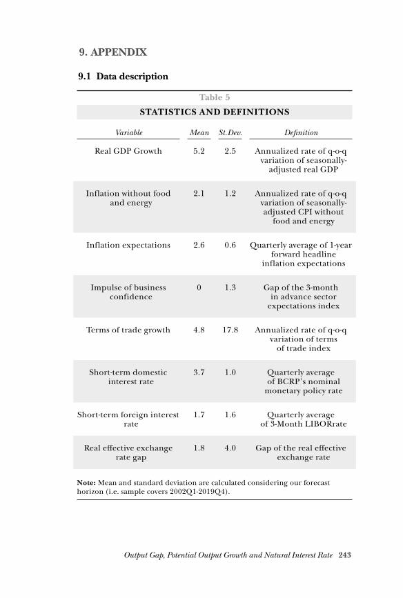
243Output Gap, Potential Output Growth and Natural Interest Rate
9. APPENDIX
9.1 Data description
Table 5
STATISTICS AND DEFINITIONS
Variable Mean St.Dev. Definition
Real GDP Growth 5.2 2.5 Annualized rate of q-o-q variation of seasonally-
adjusted real GDP
Inflation without food and energy
2.1 1.2 Annualized rate of q-o-q variation of seasonally-adjusted CPI without
food and energy
Inflation expectations 2.6 0.6 Quarterly average of 1-year forward headline
inflation expectations
Impulse of business confidence
0 1.3 Gap of the 3-month in advance sector
expectations index
Terms of trade growth 4.8 17.8 Annualized rate of q-o-q variation of terms
of trade index
Short-term domestic interest rate
3.7 1.0 Quarterly average of BCRP’s nominal
monetary policy rate
Short-term foreign interest rate
1.7 1.6 Quarterly average of 3-Month LIBORrate
Real effective exchange rate gap
1.8 4.0 Gap of the real effective exchange rate
Note: Mean and standard deviation are calculated considering our forecast horizon (i.e. sample covers 2002Q1-2019Q4).
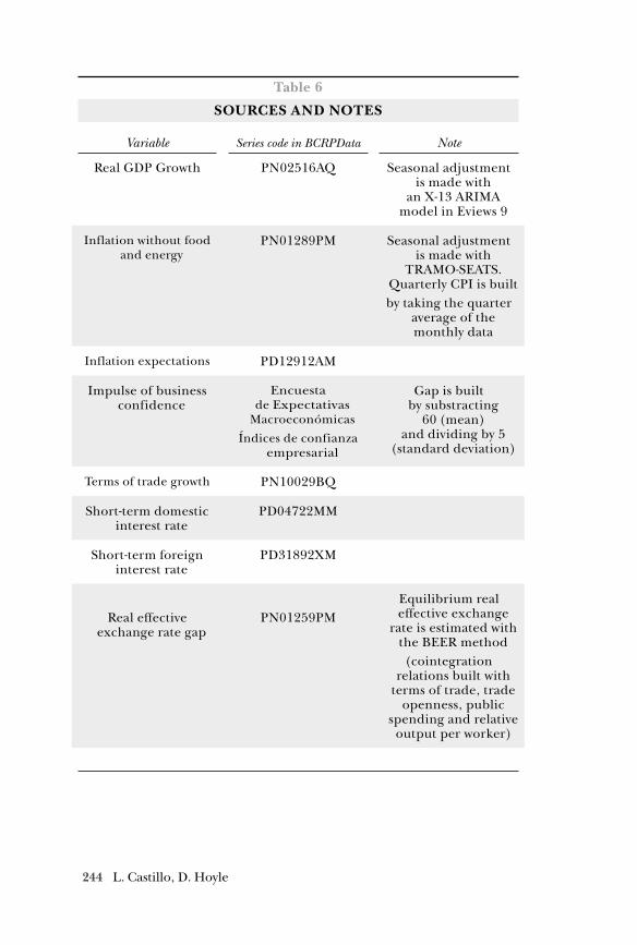
244 L. Castillo, D. Hoyle
Table 6
SOURCES AND NOTES
Variable Series code in BCRPData Note
Real GDP Growth PN02516AQ Seasonal adjustment is made with
an X-13 ARIMA model in Eviews 9
Inflation without food and energy
PN01289PM Seasonal adjustment is made with
TRAMO-SEATS. Quarterly CPI is builtby taking the quarter
average of the monthly data
Inflation expectations PD12912AM
Impulse of business confidence
Encuesta de Expectativas
MacroeconómicasÍndices de confianza
empresarial
Gap is built by substracting
60 (mean) and dividing by 5
(standard deviation)
Terms of trade growth PN10029BQ
Short-term domestic interest rate
PD04722MM
Short-term foreign interest rate
PD31892XM
Real effective exchange rate gap
PN01259PMEquilibrium real effective exchange
rate is estimated with the BEER method
(cointegration relations built with
terms of trade, trade openness, public
spending and relative output per worker)
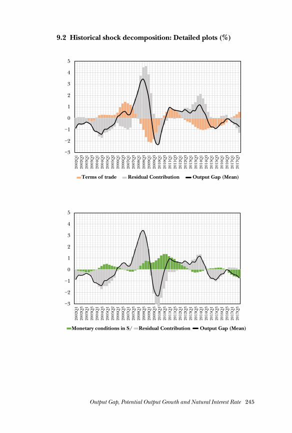
245Output Gap, Potential Output Growth and Natural Interest Rate
9.2 Historical shock decomposition: Detailed plots (%)
Terms of trade Residual Contribution Output Gap (Mean)
Monetary conditions in S/ Residual Contribution Output Gap (Mean)
2012
Q1
2012
Q3
2013
Q1
2013
Q3
2014
Q1
2016
Q1
2015
Q3
2015
Q1
2014
Q3
2016
Q3
2017
Q1
2011
Q3
2011
Q1
2010
Q3
2010
Q1
2009
Q3
2009
Q1
2008
Q3
2008
Q1
2007
Q3
2007
Q1
2006
Q3
2006
Q1
2005
Q2
2005
Q1
2004
Q3
2004
Q1
2003
Q3
2003
Q1
2002
Q3
2002
Q1
2017
Q3
4
3
2
1
0
−1
−2
−3
5
2012
Q1
2012
Q3
2013
Q1
2013
Q3
2014
Q1
2016
Q1
2015
Q3
2015
Q1
2014
Q3
2016
Q3
2017
Q1
2011
Q3
2011
Q1
2010
Q3
2010
Q1
2009
Q3
2009
Q1
2008
Q3
2008
Q1
2007
Q3
2007
Q1
2006
Q3
2006
Q1
2005
Q2
2005
Q1
2004
Q3
2004
Q1
2003
Q3
2003
Q1
2002
Q3
2002
Q1
2017
Q3
4
3
2
1
0
−1
−2
−3
5
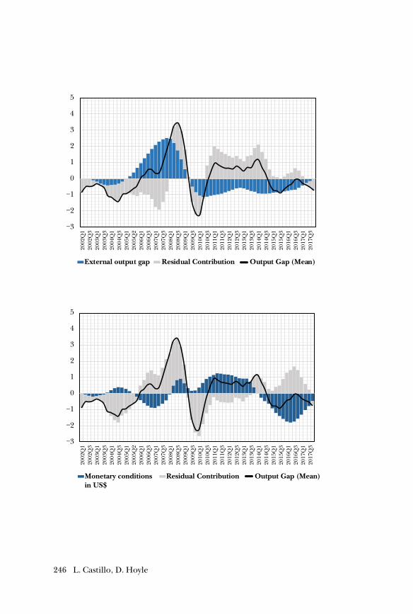
246 L. Castillo, D. Hoyle
External output gap Residual Contribution Output Gap (Mean)
Monetary conditionsin US$
Residual Contribution Output Gap (Mean)
2012
Q1
2012
Q3
2013
Q1
2013
Q3
2014
Q1
2016
Q1
2015
Q3
2015
Q1
2014
Q3
2016
Q3
2017
Q1
2011
Q3
2011
Q1
2010
Q3
2010
Q1
2009
Q3
2009
Q1
2008
Q3
2008
Q1
2007
Q3
2007
Q1
2006
Q3
2006
Q1
2005
Q2
2005
Q1
2004
Q3
2004
Q1
2003
Q3
2003
Q1
2002
Q3
2002
Q1
2017
Q3
4
3
2
1
0
−1
−2
−3
5
2012
Q1
2012
Q3
2013
Q1
2013
Q3
2014
Q1
2016
Q1
2015
Q3
2015
Q1
2014
Q3
2016
Q3
2017
Q1
2011
Q3
2011
Q1
2010
Q3
2010
Q1
2009
Q3
2009
Q1
2008
Q3
2008
Q1
2007
Q3
2007
Q1
2006
Q3
2006
Q1
2005
Q2
2005
Q1
2004
Q3
2004
Q1
2003
Q3
2003
Q1
2002
Q3
2002
Q1
2017
Q3
4
3
2
1
0
−1
−2
−3
5
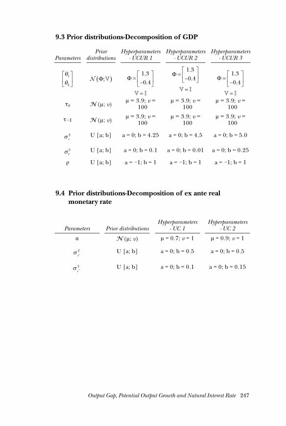
247Output Gap, Potential Output Growth and Natural Interest Rate
9.3 Prior distributions-Decomposition of GDP
9.4 Prior distributions-Decomposition of ex ante real monetary rate
ParametersPrior
distributionsHyperparameters
- UCUR 1Hyperparameters
- UCUR 2Hyperparameters
- UCUR 3
θθ
1
2
Φ;( ) Φ =
−
1 30 4..
V I=
Φ =−
1 30 4..
V I=
Φ =−
1 30 4..
V I=
τ0 N (µ; v)µ = 3.9; v =
100µ = 3.9; v =
100µ = 3.9; v =
100
τ−1 N (µ; v)µ = 3.9; v =
100µ = 3.9; v =
100µ = 3.9; v =
100
σ c2 U [a; b] a = 0; b = 4.25 a = 0; b = 4.5 a = 0; b = 5.0
στ2 U [a; b] a = 0; b = 0.1 a = 0; b = 0.01 a = 0; b = 0.25
ρ U [a; b] a = −1; b = 1 a = −1; b = 1 a = −1; b = 1
Parameters Prior distributionsHyperparameters
- UC 1Hyperparameters
- UC 2
α N (µ; v) µ = 0.7; v = 1 µ = 0.9; v = 1
σr c2 U [a; b] a = 0; b = 0.5 a = 0; b = 0.5
σr *2 U [a; b] a = 0; b = 0.1 a = 0; b = 0.15

Cross-Country Studies
249The Natural Interest Rate in Latin America
The natural interest rate in Latin America
Javier G. Gómez-Pineda
Abstract
The natural interest rate is a critical building block in the evaluation of a monetary policy stance. We estimate the natural interest rate for the five largest Latin American economies. We follow the method in Laubach and Williams (2003), complemented with rational and survey inflation expectations and adapted to Bayesian maximum likelihood estimation. The model is the standard neo-Keynesian model, complemented with equations for the natural interest rate in nominal terms and the rational inflation expectations. We find that in real terms the natural interest rate trends down and re-mains above zero in the larger economies (Brazil, Mexico and Colombia), while it re-mains without a noticeable trend although closer to zero in the smaller economies (Chile and Peru). We also find that in nominal terms, the natural rate trends down, in most economies a consequence of the drop in inflation and inflation expectations. Regarding the policy implications, the natural interest rate still does not pose a critical challenge for monetary policy in Latin America, as it does in advanced economies (Ball 2014). Nonetheless, in Chile and Peru the natural rate in nominal terms is just above 2% and 3%, respectively, offering narrow room for expansionary monetary policy.
Keywords: Natural interest rate; Semi-structural model; Inflation expectations; Ex-pansionary monetary policy
jel codes: E58; E37; E43
Javier G. Gómez Pineda <[email protected]>, Senior Economist at the Banco de la República (the central bank of Colombia). The paper was written under the cemla-Bank of Spain 2018 Joint Research Program. The author thanks Natalia Palacios for excellent re-search assistance. The views expressed herein do not commit Banco de la República or its Board of Directors.
250 J. Gómez-Pineda
1. INTRODUCTION
The natural interest rate is an important building block in the evaluation of a monetary policy stance. We estimate the natu-ral interest rate for the five largest Latin American economies.
We follow the method in Laubach and Williams (2003), complement-ing the ARIMA-type inflation expectations with rational and sur-vey inflation expectations. In the estimation, the semi-structural neo-Keynesian model is used. As is well-known, the semi-structural model contains some important elements of the New Neoclassical Synthesis (nns), which is the standing paradigm in monetary policy. The estimated natural interest rate is endogenous to the transmission mechanisms in this model.
The natural interest rate can be defined as that which would hold should variables such as output, inflation, and the exchange rate be at their long-term equilibrium levels (Holtson et al., 2016; Lau-bach and Williams, 2016; Summers, 2014). This definition fits well the semi-structural model used here1.
The natural interest rate has recently become a topic of increas-ing relevance in advanced economies, owing to its downward trend and in particular to its collapse into negative numbers since the global financial crisis of 2008. With strongly negative natural interest rates, monetary policy hardly has any room to stimulate aggregate demand due to the effective lower bound on policy interest rates. In turn, in emerging economies the real interest rate showed a significant drop during the global financial crisis, but the natural interest rate did not drop to such extent as to become a stringent constraint on monetary policy. Nonetheless, should current trends continue in some emerging economies, the natural interest rate could eventually become an im-portant restriction in the future.
The article is divided into six sections including this introduction. In the Section 2, we present the model. We emphasize the stochas-tic process of the natural interest rate, the definition of the stochastic process for the natural interest rate, the definition of the natural rate in nominal terms and the behavioral equation for the rational inflation expectations. In Section 3, we present the data sources. In Section 4,
1 Alternatively, in a definition more akin to the dsge neo-Kensesian model, the natural rate is that which would hold were all prices flexible (Wood-ford, 2003b).
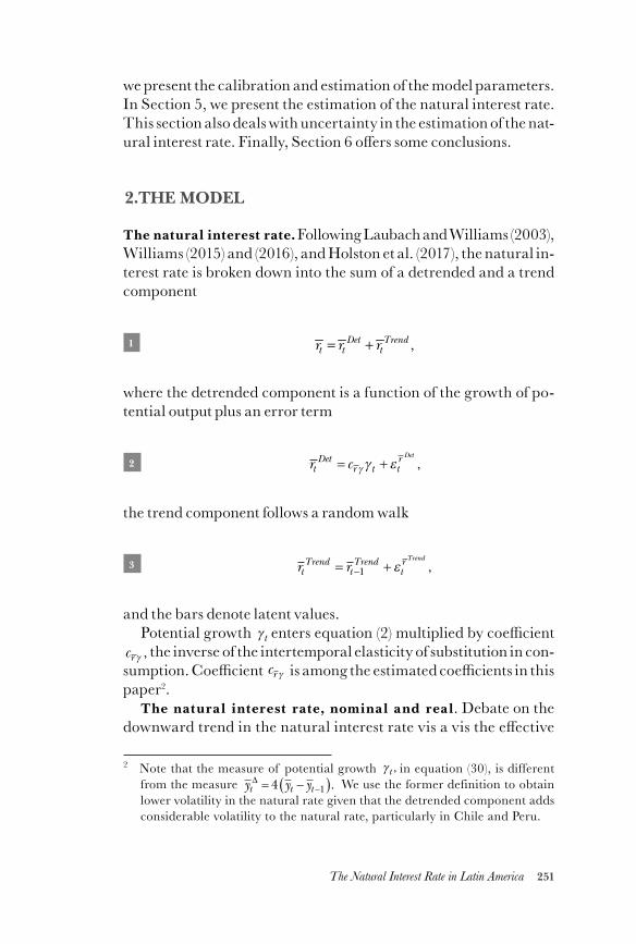
251The Natural Interest Rate in Latin America
we present the calibration and estimation of the model parameters. In Section 5, we present the estimation of the natural interest rate. This section also deals with uncertainty in the estimation of the nat-ural interest rate. Finally, Section 6 offers some conclusions.
2.THE MODEL
The natural interest rate. Following Laubach and Williams (2003), Williams (2015) and (2016), and Holston et al. (2017), the natural in-terest rate is broken down into the sum of a detrended and a trend component
1 = + ,Det Trendt t tr r r
where the detrended component is a function of the growth of po-tential output plus an error term
2 r ctDet
r t tr Det
= +γ γ ε ,
the trend component follows a random walk
3 r rtTrend
tTrend
tr Trend
= +−1 ε ,
and the bars denote latent values.Potential growth γ t enters equation (2) multiplied by coefficient
cr γ , the inverse of the intertemporal elasticity of substitution in con-sumption. Coefficient cr γ is among the estimated coefficients in this paper2.
The natural interest rate, nominal and real. Debate on the downward trend in the natural interest rate vis a vis the effective
2 Note that the measure of potential growth γ t , in equation (30), is different from the measure y y yt t t
∆ = −( )−4 1 . We use the former definition to obtain lower volatility in the natural rate given that the detrended component adds considerable volatility to the natural rate, particularly in Chile and Peru.
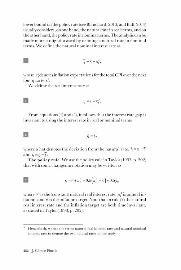
252 J. Gómez-Pineda
lower bound on the policy rate (see Blanchard, 2010; and Ball, 2014) usually considers, on one hand, the natural rate in real terms, and on the other hand, the policy rate in nominal terms. The analysis can be made more straightforward by defining a natural rate in nominal terms. We define the natural nominal interest rate as
4 i rt t te≡ +π ,
where πtedenotes inflation expectations for the total cpi over the next
four quarters3.We define the real interest rate as
5 r it t te≡ −π .
From equations (4) and (5), it follows that the interest rate gap is invariant to using the interest rate in real or nominal terms
6 = ˆˆ ,t tr i
where a hat denotes the deviation from the natural rate, r r rt t t= −ˆ and .i i it t t≡ −
The policy rule. We use the policy rule in Taylor (1993, p. 202) that with some changes in notation may be written as
7 i r yt t t t= + + −( ) +π π π4 40 5 0 5. . ,ˆ
where r is the (constant) natural real interest rate, πt4 is annual in-
flation, and π is the inflation target. Note that in rule (7) the natural real interest rate and the inflation target are both time invariant, as stated in Taylor (1993, p. 202).
3 Henceforth, we use the terms natural real interest rate and natural nominal interest rate to denote the two natural rates under study.
253The Natural Interest Rate in Latin America
But we use a variable natural real interest rate instead of a con-stant, “perhaps the most important suggested change in policy rules in recent years” Taylor (2017, p. 15). We then write the policy rule as
8 i r yt t t t t t= + + −( ) +π π π4 40 5 0 5. . ,ˆ
where a time subscript in the natural rate tr indicates that the natural rate is time-varying. Note that the inflation target is also time-vary-ing. Here we measure the inflation target with the Hodrick-Prescott filter of cpi inflation—an implicit inflation target.
Adding and subtracting inflation expectations πte at the right
hand side of equation (8) and using π πte
t , the following Taylor rule is obtained.
9 i i yt t t tt ti= + −( ) + +1 5 0 54. . .π π εˆ
This form of the policy rule appears in Svensson (1993, p. 614). In addition we have added a monetary policy shock or stance εt
i .Given definitions (5) and (4) for the real interest rate and the natural
nominal interest rate, policy rule (9) may be read either as a reaction function for the real interest rate gap . .,r yt C t t t
i= + +1 5 0 5π εˆˆˆ or as a reac-tion function for the nominal interest rate gap . .,i yt C t t t
i= + +1 5 0 5π εˆˆ ˆ , indistinctly.
To improve the estimation of the natural rate, we write the rule in the slightly more general form
10 i i c c yt t i C t iy t ti= + + + ,,ππ εˆ ˆ−
where coefficients ciπ and iyc are among the coefficients to be esti-mated.
The uncertainty in the estimation of the natural interest rate. According to Fiorentini et al (2018), the standard error of the natural interest rate can be improved by using a stationary real in-terest rate gap. Adding a smoothing term at the right hand side of the policy rule, the real interest rate gap follows the process
254 J. Gómez-Pineda
11 . . ,,r c r yt rr t C t t ti= + + +−1 0 5 0 5π εˆˆˆ ˆ
which is a stationary process for <1,rrc given that the inf lation and output gaps are stationary. Defining the quasi-difference of the interest rate as i i c it t ii t
∆ ≡ + −1, policy rule (11) can be formulated in nom-inal terms as
12 i i yt t C t t ti∆ ∆= + + +1 5 0 5. . .,π εˆ ˆ
This rule is similar to that in Svensson (1999, p. 614) but defined in the quasi-difference of the nominal interest rate.
Hereafter we use = 0rrc so that condition <1rrc is satisfied, the real interest rate gap is stationary and the policy rule is (10).
Okun’s law. As stated in equations (1) and (2), the growth of po-tential output is important in the estimation of the natural rate. To improve the estimation of the growth of potential output we incor-porate Okun’s Law into the model. Unemployment is broken down as u u ut t t= + ,ˆ where cyclical unemployment tu follows
13 ,u c u c yt uu t uy t tu= − +−1 εˆ ˆ ˆ ˆ
and the nairu tu follows the stochastic process
14 u ut t tu
tu= + +−1 γ ε ,
15 γ γ ε γtu
tu
tu
= +−1 .
The Phillips curve. Inflation πt is the aggregate of core πC t, and non-core πNC t, components
16 π π ππ πt c C t c NC tc c= + −( ), , .1
255The Natural Interest Rate in Latin America
Two Phillips curves are set up for each component
17 π π π επ π π ππ
C t e C te
e C t y t q t tc c c y c q C, , , ,= + −( ) + + +− −1 1
41ˆ ˆ
and
18 π π π ππ π π π πNC t e NC te
e NC t y t q t q NC tc c c y c q c, , , ,= + −( ) + + − −− −1 14
1∆ ππ επC t tNC
, ,−( ) +1ˆ ˆ
π π π ππ π π π πNC t e NC t
ee NC t y t q t q NC tc c c y c q c, , , ,= + −( ) + + − −− −1 1
41∆ ππ επC t t
NC, ,−( ) +1ˆ ˆ
where πC t, is quarterly core inflation and πC t,4 is annual core infla-
tion; similar definitions apply for non-core inflation.The term π πNC t C t, ,− at the right hand side of equation (18) can be
shown to be equal to the change in the relative price of non-core goods. The feedback in this term, −c qπ∆ , helps anchor non-core in-flation to core inflation.
It may be argued that non-core inflation is a pure supply shock and that hence it does not follow the output and exchange-rate gaps (or in other terms, that in equation (18) c cy qπ π= = 0). Nonetheless, food and energy inflation can follow supply shocks επt NC as well as marginal cost pressure given by the output and exchange-rate gaps4. Hence, we maintain here that c yπ and c qπ can both be differ-ent from zero.
In addition, to help improve the estimation of the Phillips curve, the observed core inflation πC t
NS, is split into signal πC t, and noise εt
N components
19 π π εC tNS
C t C tN
, , , .= +
Likewise, the breakdown applies to non-core inflation as follows:
20 π π εNC tNS
NC t NC tN
, , , .= +
4 Coefficients c yπ and c qπ appear identical in Phillips curves (17) and (18) merely for notational simplicity.
256 J. Gómez-Pineda
Inflation expectations. cpi inflation expectations πte are the
weighted sum of core πC te
, and non-core πNC te
, components
21 π π ππ πte
c C te
c NC tec c= + −( ), , .1
Core inflation expectations are unobserved and estimated as a forward- and backward-looking convulusion of core inflation
22 π π π επC te
ee C t t4
ee C te
tc ceC
, , | , .= + −( ) ++ −4 11
Non-core inflation expectations are also unobserved and likewise estimated as follows:
23 π π π επNC te
ee NC t t4
ee NC te
tc ce
NC, , | , .= + −( ) ++ −4 11
While core and non-core inflation expectations πC te
, and πNC te
, at the right-hand side of equation (21) are unobserved, cpi inflation expectations πt
e at the left-hand side of this equation can be either unobserved or observed. We study three measures of inflation ex-pectations. The first one is the rational or model-consistent inflation expectations where cpi inflation expectations are estimated as un-observed. The second and third measures are the survey and ARI-MA inflation expectations.
The exchange rate. The real multilateral exchange rate | ,CO WO tq is defined as a trade-weighted average of the real bilateral exchange rates against I trade partners q s p pCO i CO i i t CO t| | , , ,≡ + − 1... ,i I= where, for expositional purposes, Colombia, with subindex CO, is the base country, |CO is is the (log) nominal interest rate against trade partner
,, i ti p is the (log) price level of trade partner i, and ,CO tp is the (log) price level of Colombia.
We then turn to the theory of the real exchange rate, it is the un-covered interest rate parity condition (uip), formulated for conve-nience in real terms as
24 q q r rCO WO t CO WO t t CO tDet
WO tDet
CO WO t| , | , | , , | , ,= − −( ) ++114
χ
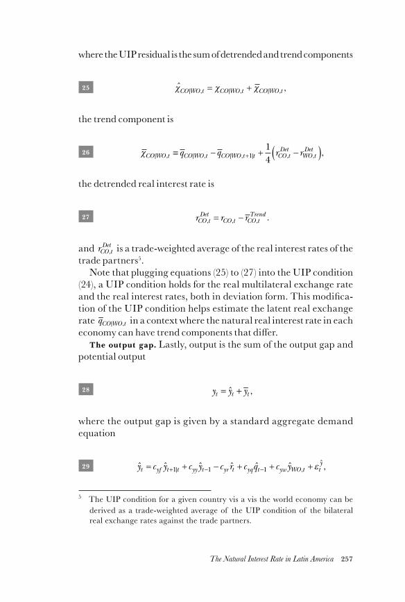
257The Natural Interest Rate in Latin America
where the uip residual is the sum of detrended and trend components
25 χ χ χCO WO t CO WO t CO WO t| , | , | , ,= +ˆ
the trend component is
26 χCO WO t CO WO t CO WO t t CO tDet
WO tDetq q r r| , | , | , | , , ,≡ − + −( )+1
14
the detrended real interest rate is
27 r r rCO tDet
CO t CO tTrend
, , , .= −
and ,Det
CO tr is a trade-weighted average of the real interest rates of the trade partners5.
Note that plugging equations (25) to (27) into the uip condition (24), a uip condition holds for the real multilateral exchange rate and the real interest rates, both in deviation form. This modifica-tion of the uip condition helps estimate the latent real exchange rate | ,CO WO tq in a context where the natural real interest rate in each economy can have trend components that differ.
The output gap. Lastly, output is the sum of the output gap and potential output
28 ˆ ,t t ty y y= +
where the output gap is given by a standard aggregate demand equation
29 ,| ,y c y c y c r c q c yt yf t t yy t yr t yq t yw WO t ty= + − + + ++ − −1 1 1 εˆ ˆ ˆ ˆ ˆ ˆ ˆ
5 The uip condition for a given country vis a vis the world economy can be derived as a trade-weighted average of the uip condition of the bilateral real exchange rates against the trade partners.
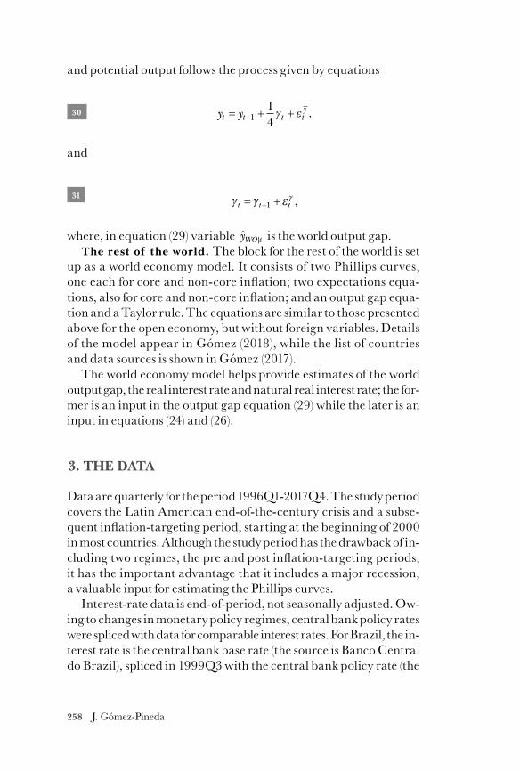
258 J. Gómez-Pineda
and potential output follows the process given by equations
30 y yt t t ty= + +−1
14γ ε ,
and
31 γ γ ε γt t t= +−1 ,
where, in equation (29) variable |WO ty is the world output gap.The rest of the world. The block for the rest of the world is set
up as a world economy model. It consists of two Phillips curves, one each for core and non-core inflation; two expectations equa-tions, also for core and non-core inflation; and an output gap equa-tion and a Taylor rule. The equations are similar to those presented above for the open economy, but without foreign variables. Details of the model appear in Gómez (2018), while the list of countries and data sources is shown in Gómez (2017).
The world economy model helps provide estimates of the world output gap, the real interest rate and natural real interest rate; the for-mer is an input in the output gap equation (29) while the later is an input in equations (24) and (26).
3. THE DATA
Data are quarterly for the period 1996Q1-2017Q4. The study period covers the Latin American end-of-the-century crisis and a subse-quent inflation-targeting period, starting at the beginning of 2000 in most countries. Although the study period has the drawback of in-cluding two regimes, the pre and post inflation-targeting periods, it has the important advantage that it includes a major recession, a valuable input for estimating the Phillips curves.
Interest-rate data is end-of-period, not seasonally adjusted. Ow-ing to changes in monetary policy regimes, central bank policy rates were spliced with data for comparable interest rates. For Brazil, the in-terest rate is the central bank base rate (the source is Banco Central do Brazil), spliced in 1999Q3 with the central bank policy rate (the
259The Natural Interest Rate in Latin America
source is imf International Financial Statistics). For Mexico, the in-terest rate is the 28-days interbank rate (the source is Banco de Mex-ico), spliced in 2008Q1 with the central bank policy rate (the source is Banco de Mexico). For Colombia, the interest rate is the central bank policy rate (the source is Banco de la República). For Chile, the interest rate is the central bank policy rate (the source is imf ifs). For Peru, the interest rate is the interbank rate (the source is Reserve Bank of Peru), spliced in 2003Q3 with the central bank policy rate (from source Reserve Bank of Peru).
Data for consumer and core price indices are end-of-period and seasonally adjusted. For Brazil, the source is the country statis-tics department. For Mexico and Colombia, the source is Departa-mento Administrativo Nacional de Estadística (dane). For Chile and Peru, the sources are their central banks.
As explained above, we use two measures of observed inflation expectations. Survey expectations are available since about 2000 for all countries. The source for survey expectations data is the coun-tries central banks. Survey expectations before 2000 are obtained with the Kalman filter as unobserved proceses. ARIMA expecta-tions can be constructed for the entire sample; however, the ARI-MA process tends to produce systematic forecast errors before 2000 as a consequence of the downward trend in inflation in all countries. Therefore, ARIMA expectations before 2000 were also obtained as unobserved6.
Real gdp data for Brazil and Colombia was obtained from the countries statistics departments. For Mexico, Chile, and Peru, the source is their central banks. Real gdp was seasonally adjusted.
Exchange rate data was not seasonally adjusted. The source is Bloomberg Financial Services.
6 We also experimented with one-year ahead break-even expectations. We do not present the results for break-even inflation expectations because the sample period was short. The sources for break-even inflation expectations are as follows: for Brazil and Mexico, data are available for both countries since 2012 from source Bloomberg. For Colombia, Chile, and Peru, data are for the return on nominal and real bonds. The source for this data for Colombia is Banco de la República, available since 2003Q1; for Chile is Bloomberg, since 2006Q2; for Peru is Bloomberg, starting in 2007Q3.
260 J. Gómez-Pineda
4. CALIBRATION AND ESTIMATION OF THE MODEL COEFFICIENTS
A set of coefficients was calibrated, and another was estimated. The calibrated coefficients were, first, those that define real persis-tence, ,yyc ,yfc uuc and nominal persistence, c eπ , ,eec (Table 1). Real persistance is calibrated to fit the length of the business cycle while nominal persistance is calibrated to obtain reasonable impulse re-sponses. With the calibrated levels of real and nominal persistance we proceeded to obtain the slopes of the aggregate demand and Phil-lips curve equations by estimation, as explained below. Other cali-brated coefficients were fixed parameters (the share of core inflation in cpi inflation c cπ ) and coefficients that are not critical for the es-timation of the natural interest rate.
The standard deviation of the shocks is also calibrated. The stan-dard deviation of εt
r Det is set at zero for simplicity. Two standard de-viations are also calibrated to obtain reasonable estimates of the natural interest rates and output gaps. The first relative standard deviation is εt
r Trend relative to the standard deviation of εti . The sec-
ond relative standard deviation is εty plus ε γt relative to the standard
deviation of εty (Table 1).
The estimated coefficients are the slope of the behavioral equa-tions, in the Phillips curve, c yπ and c qπ ; in the aggregate demand equation, yrc and ;yqc and in Okun’s Law, .uyc The coefficients in the policy rule, ciπ , ,iyc were also estimated. The process was carried out by Bayesian maximum likelihood estimation.
The estimated coefficients were estimated with model-consistent inflation expectations; they appear in Table 2. The prior for coef-ficient cr γ = 0 96. , is set at 0.8. This prior is obtained as the estimated coef-ficient for Colombia and Peru during a first round of estimation.7
Priors for coefficients c yπ were set at 0.12 to reflect relatively flat Phillips curves. Nonetheless, most estimated coefficients increased to the range (0.156, 0.194). Likewise, priors for coefficients yrc were also set at 0.12 to reflect relatively flat aggregate demand equations. The estimated coefficients also increased to the range (0.128, 0.171).
7 For the remaining economies, the data is not informative, meaning that the Bayesian posterior is equal to the prior. Although the estimated value for the world economy was cr γ = 0 96. , we decided to use cr γ = 0 8. , owing to the presumably larger volatility in the emerging economies in the study.
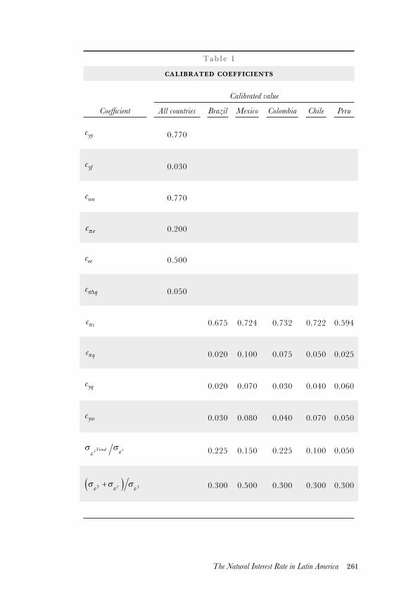
261The Natural Interest Rate in Latin America
Table 1
CALIBRATED COEFFICIENTS
Coefficient
Calibrated value
All countries Brazil Mexico Colombia Chile Peru
yyc 0.770
yfc 0.030
uuc 0.770
c eπ 0.200
eec 0.500
c qπ∆ 0.050
c cπ 0.675 0.724 0.732 0.722 0.594
c qπ 0.020 0.100 0.075 0.050 0.025
yqc 0.020 0.070 0.030 0.040 0.060
ywc 0.030 0.080 0.040 0.070 0.050
σ σε εr Trend i 0.225 0.150 0.225 0.100 0.050
σ σ σε ε εγy y+( ) 0.300 0.500 0.300 0.300 0.300
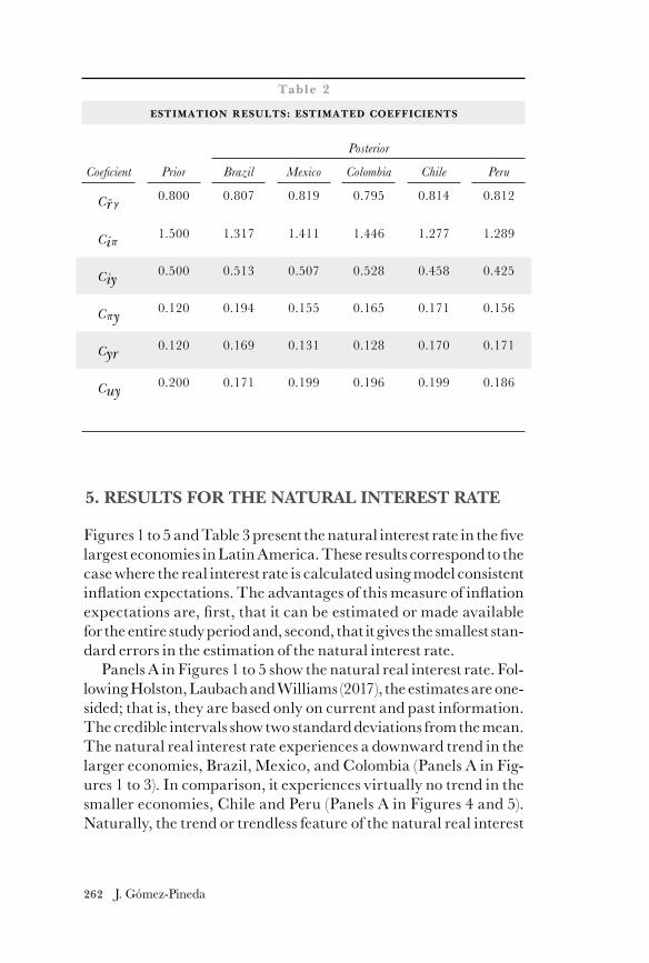
262 J. Gómez-Pineda
5. RESULTS FOR THE NATURAL INTEREST RATE
Figures 1 to 5 and Table 3 present the natural interest rate in the five largest economies in Latin America. These results correspond to the case where the real interest rate is calculated using model consistent inflation expectations. The advantages of this measure of inflation expectations are, first, that it can be estimated or made available for the entire study period and, second, that it gives the smallest stan-dard errors in the estimation of the natural interest rate.
Panels A in Figures 1 to 5 show the natural real interest rate. Fol-lowing Holston, Laubach and Williams (2017), the estimates are one-sided; that is, they are based only on current and past information. The credible intervals show two standard deviations from the mean. The natural real interest rate experiences a downward trend in the larger economies, Brazil, Mexico, and Colombia (Panels A in Fig-ures 1 to 3). In comparison, it experiences virtually no trend in the smaller economies, Chile and Peru (Panels A in Figures 4 and 5). Naturally, the trend or trendless feature of the natural real interest
Table 2
ESTIMATION RESULTS: ESTIMATED COEFFICIENTS
Coeficient Prior
Posterior
Brazil Mexico Colombia Chile Peru
Cr γ0.800 0.807 0.819 0.795 0.814 0.812
Ci π 1.500 1.317 1.411 1.446 1.277 1.289
Ciy 0.500 0.513 0.507 0.528 0.458 0.425
C πy 0.120 0.194 0.155 0.165 0.171 0.156
Cyr 0.120 0.169 0.131 0.128 0.170 0.171
Cuy 0.200 0.171 0.199 0.196 0.199 0.186
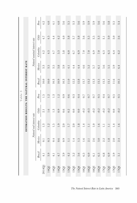
263The Natural Interest Rate in Latin America
Table
3
ESTIM
ATIO
N R
ESU
LTS: TH
E N
ATU
RA
L I
NTER
EST R
ATE
Natu
ral r
eal i
ntere
st ra
teNa
tura
l nom
inal
inter
est ra
te
Braz
ilM
exico
Colom
bia
Chile
Peru
Braz
ilM
exico
Colom
bia
Chile
Peru
2014
Q1
4.1
0.1
1.3
2.1
1.5
10.0
3.3
4.2
4.7
4.2
14Q
23.
90.
31.
21.
61.
210
.03.
54.
34.
54.
0
14Q
34.
10.
41.
51.
31.
310
.33.
54.
74.
44.
1
14Q
44.
70.
61.
90.
91.
210
.93.
85.
34.
24.
0
15Q
13.
90.
92.
00.
60.
910
.33.
95.
84.
03.
6
15Q
24.
21.
11.
70.
20.
611
.04.
16.
03.
83.
5
15Q
35.
21.
42.
00.
00.
312
.24.
46.
73.
73.
3
15Q
45.
61.
51.
80.
00.
412
.84.
46.
93.
83.
6
16Q
16.
51.
61.
4-0
.20.
713
.74.
67.
03.
63.
9
16Q
26.
02.
11.
1-0
.30.
713
.25.
27.
03.
53.
9
16Q
36.
12.
61.
0-0
.20.
713
.35.
76.
93.
53.
9
16Q
46.
53.
01.
6-0
.20.
513
.56.
17.
03.
33.
6
17Q
16.
82.
21.
1-0
.20.
413
.55.
66.
33.
13.
6
17Q
26.
91.
81.
1-0
.20.
713
.15.
56.
33.
03.
8
17Q
35.
92.
01.
40.
00.
511
.65.
96.
43.
03.
5
17Q
45.
12.
41.
6-0
.20.
510
.56.
46.
22.
63.
4
264 J. Gómez-Pineda
rate is explained by the trend component of the natural real interest rate (Panel D in Figure 6).
Panels B in Figures 1 to 5 show the results of the estimation of the unobserved natural nominal interest rate. The natural nominal in-terest rate experiences a downward trend in all economies. In the case of Brazil, the natural nominal interest rate trends down due to the downward trend in the natural real interest rate, meaning that inflation and inflation expectations virtually show no trend during the study period. In the remaining economies, the natural nominal interest rate trends down due to both the trend in the natural real interest rate and the downward trend in inflation and inflation ex-pectations8.
At the end of the sample, the room for expansionary monetary policy is still generous in the larger economies, where the natural real interest rate still trends down. In contrast, the room for expansionary monetary policy is not as generous in the smaller economies, where the natural real rate does not show a trend. In the smaller econo-mies, the natural real interest rate is close to zero, while the natural nominal interest rate is just above 2 percent.
The results of the estimation uncertainty appear in Table 4. The ta-ble shows two-standard-deviation credible intervals for the natu-ral real and natural nominal interest rates and for the detrended and trend components of the natural real interest rate. Estimation uncertainty is larger in the larger economies, where the trend com-ponent of the natural rate trends down, while smaller in the small-er economies where no trend is discernible. The credible intervals are also indicated in Figures 1 to 5.
8 Note that the results for the natural nominal interest rate, the natural real interest rate and the model-consistent inflation expectations are all estimation results for unobserved variables.
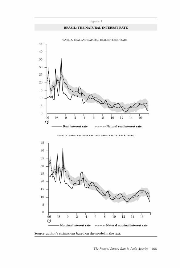
265The Natural Interest Rate in Latin America
Figure 1
BRAZIL: THE NATURAL INTEREST RATE
Source: author’s estimations based on the model in the text.
0
5
10
15
20
25
30
35
40
45
96Q1
98 0 2 4 6 8 10 12 14 16
0
5
10
15
20
25
30
35
40
45
96Q1
98 0 2 4 6 8 10 12 14 16
Real interest rate Natural real interest rate
.
Nominal interest rate Natural nominal interest rate
.
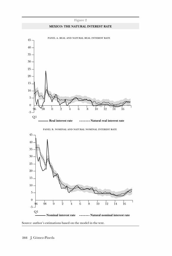
266 J. Gómez-Pineda
Figure 2
MEXICO: THE NATURAL INTEREST RATE
Source: author’s estimations based on the model in the text.
-5
0
5
10
15
20
25
30
35
40
45
96
Q1
98 0 2 4 6 8 10 12 14 16
-5
0
5
10
15
20
25
30
35
40
45
96
Q1
98 0 2 4 6 8 10 12 14 16
Real interest rate Natural real interest rate
.
Nominal interest rate Natural nominal interest rate
.
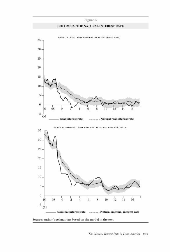
267The Natural Interest Rate in Latin America
Figure 3
COLOMBIA: THE NATURAL INTEREST RATE
Source: author’s estimations based on the model in the text.
-5
0
5
10
15
20
25
30
35
96
Q1
98 0 2 4 6 8 10 12 14 16
-5
0
5
10
15
20
25
30
35
96
Q1
98 0 2 4 6 8 10 12 14 16
Real interest rate Natural real interest rate
.
Nominal interest rate Natural nominal interest rate
.
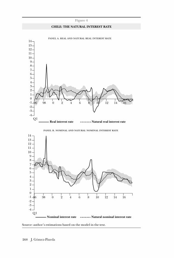
268 J. Gómez-Pineda
Figure 4
CHILE: THE NATURAL INTEREST RATE
Source: author’s estimations based on the model in the text.
-4-3-2-10123456789
1011121314
96
Q1
98 0 2 4 6 8 10 12 14 16
-4-3-2-10123456789
1011121314
96
Q1
98 0 2 4 6 8 10 12 14 16
Real interest rate Natural real interest rate
.
Nominal interest rate Natural nominal interest rate
.
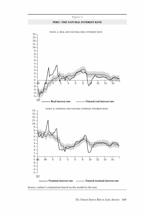
269The Natural Interest Rate in Latin America
Figure 5
PERU: THE NATURAL INTEREST RATE
Source: author’s estimations based on the model in the text.
-5-4-3-2-10123456789
1011121314
96
Q1
98 0 2 4 6 8 10 12 14 16
-5-4-3-2-10123456789
1011121314
96
Q1
98 0 2 4 6 8 10 12 14 16
Real interest rate Natural real interest rate
.
Nominal interest rate Natural nominal interest rate
.
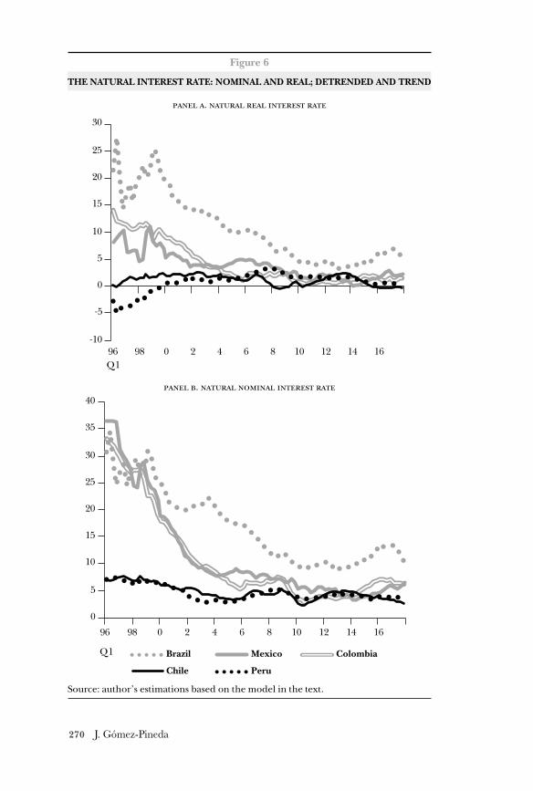
270 J. Gómez-Pineda
Figure 6
THE NATURAL INTEREST RATE: NOMINAL AND REAL; DETRENDED AND TREND
Source: author’s estimations based on the model in the text.
-10
-5
0
5
10
15
20
25
30
96Q1
98 0 2 4 6 8 10 12 14 16
Brazil Mexico Colombia
Chile Peru
0
5
10
15
20
25
30
35
40
96
Q1
98 0 2 4 6 8 10 12 14 16
.
.
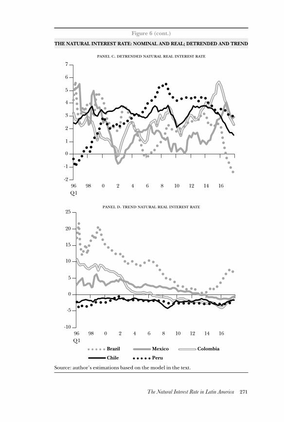
271The Natural Interest Rate in Latin America
Figure 6 (cont.)
THE NATURAL INTEREST RATE: NOMINAL AND REAL; DETRENDED AND TREND
Source: author’s estimations based on the model in the text.
-2
-1
0
1
2
3
4
5
6
7
96Q1
98 0 2 4 6 8 10 12 14 16
-10
-5
0
5
10
15
20
25
96Q1
98 0 2 4 6 8 10 12 14 16
.
.
Brazil Mexico Colombia
Chile Peru
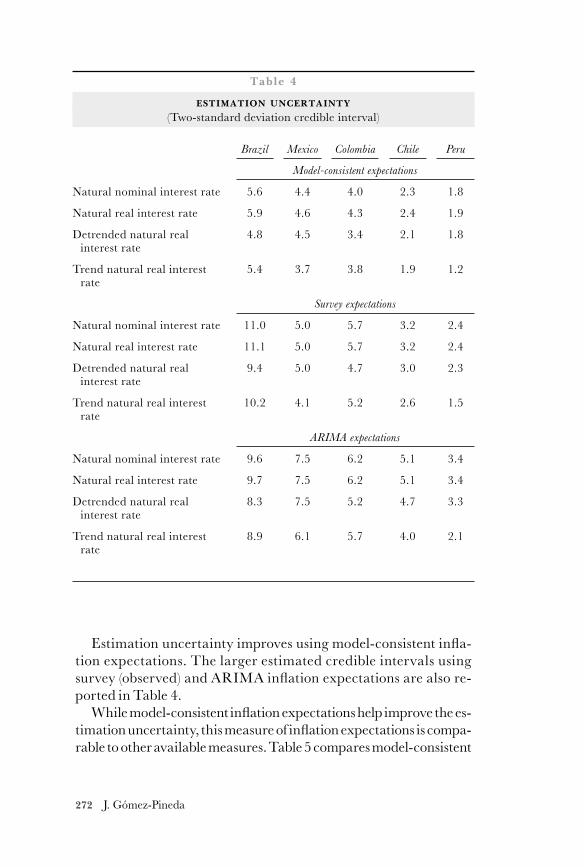
272 J. Gómez-Pineda
Estimation uncertainty improves using model-consistent infla-tion expectations. The larger estimated credible intervals using survey (observed) and ARIMA inflation expectations are also re-ported in Table 4.
While model-consistent inflation expectations help improve the es-timation uncertainty, this measure of inflation expectations is compa-rable to other available measures. Table 5 compares model-consistent
Table 4
ESTIMATION UNCERTAINTY
(Two-standard deviation credible interval)
Brazil Mexico Colombia Chile Peru
Model-consistent expectations
Natural nominal interest rate 5.6 4.4 4.0 2.3 1.8
Natural real interest rate 5.9 4.6 4.3 2.4 1.9
Detrended natural real interest rate
4.8 4.5 3.4 2.1 1.8
Trend natural real interest rate
5.4 3.7 3.8 1.9 1.2
Survey expectations
Natural nominal interest rate 11.0 5.0 5.7 3.2 2.4
Natural real interest rate 11.1 5.0 5.7 3.2 2.4
Detrended natural real interest rate
9.4 5.0 4.7 3.0 2.3
Trend natural real interest rate
10.2 4.1 5.2 2.6 1.5
ARIMA expectations
Natural nominal interest rate 9.6 7.5 6.2 5.1 3.4
Natural real interest rate 9.7 7.5 6.2 5.1 3.4
Detrended natural real interest rate
8.3 7.5 5.2 4.7 3.3
Trend natural real interest rate
8.9 6.1 5.7 4.0 2.1
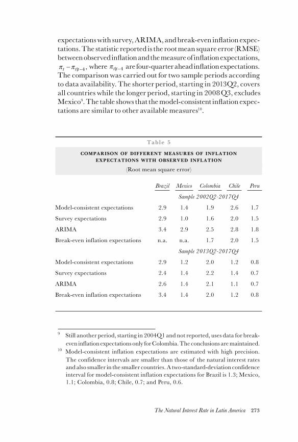
273The Natural Interest Rate in Latin America
expectations with survey, ARIMA, and break-even inflation expec-tations. The statistic reported is the root mean square error (rmse) between observed inflation and the measure of inflation expectations, π πt t t− −| ,4 where πt t| −4 are four-quarter ahead inflation expectations. The comparison was carried out for two sample periods according to data availability. The shorter period, starting in 2013Q2, covers all countries while the longer period, starting in 2008Q3, excludes Mexico9. The table shows that the model-consistent inflation expec-tations are similar to other available measures10.
9 Still another period, starting in 2004Q1 and not reported, uses data for break-even inflation expectations only for Colombia. The conclusions are maintained.
10 Model-consistent inflation expectations are estimated with high precision. The confidence intervals are smaller than those of the natural interest rates and also smaller in the smaller countries. A two-standard-deviation confidence interval for model-consistent inflation expectations for Brazil is 1.3; Mexico, 1.1; Colombia, 0.8; Chile, 0.7; and Peru, 0.6.
Table 5
COMPARISON OF DIFFERENT MEASURES OF INFLATION EXPECTATIONS WITH OBSERVED INFLATION
(Root mean square error)
Brazil Mexico Colombia Chile Peru
Sample 2002Q2-2017Q4
Model-consistent expectations 2.9 1.4 1.9 2.6 1.7
Survey expectations 2.9 1.0 1.6 2.0 1.5
ARIMA 3.4 2.9 2.5 2.8 1.8
Break-even inflation expectations n.a. n.a. 1.7 2.0 1.5
Sample 2013Q2-2017Q4
Model-consistent expectations 2.9 1.2 2.0 1.2 0.8
Survey expectations 2.4 1.4 2.2 1.4 0.7
ARIMA 2.6 1.4 2.1 1.1 0.7
Break-even inflation expectations 3.4 1.4 2.0 1.2 0.8
274 J. Gómez-Pineda
6. CONCLUSIONS
We estimate the natural interest rate in the five largest economies in Latin America. We use the standard neo-Keynesian model and the Laubach Williams (2003) method, complemented with a definition of the natural interest rate in nominal terms and behavioral equa-tions for the rational or model-consistent inflation expectations.
In the results we find that in the larger economies, Brazil, Mexi-co, and Colombia, the estimated natural real interest rate features a downward trend. Nonetheless, the estimated natural nominal in-terest rate still remains above zero, allowing ample room for expan-sionary monetary policy. In the smaller economies, Chile and Peru, the estimated natural real rate has hovered closer to zero. In these economies, the room for expansionary policy does not appear as ex-tensive, as the estimated natural nominal interest rate is just above 2 and 3 percent, respectively.
Estimation uncertainty is larger in countries where the real nat-ural rate trends down, Brazil, Mexico, and Colombia, and smaller in those countries with a more stable long-term natural real inter-est rate. Estimation uncertainty is sharply reduced by using model-consistent inflation expectations.
As to the policy implications, the natural interest rate still does not pose a critical challenge for monetary policy in Latin America, as it does in advanced economies. Nonetheless, the natural nomi-nal interest rate offers a narrow room for expansionary monetary policy in Chile and Peru.
References
Ball, Laurence, “The case for four percent inflation,” imf Work-ing Paper No. 14/192, 2014.
Blanchard, Oliver, Giovanni Dell’Ariccia and Paolo Mauro, “Re-thinking Macroeconomic Policy,” imf Staff Position Note, 10/03, 2010.
Fiorentini, G., A. Galessi, G. Pérez-Quiroz and Sentana, E. (2018), “The rise and fall of the natural interest rate,” CEPR Dis-cussion Paper 13042.
Gómez, J., (2017). “Volatility spillovers and systemic risk across economies: evidence from a global semi-structural model,” Borradores de Economía No. 1011, Banco de la República.
275The Natural Interest Rate in Latin America
Gómez, J., (2018). A well-timed raise in inflation targets,” Bor-radores de Economía No. 1042, Banco de la República.
Holston, K., Laubach, T., and Williams, J. (2017), “Measuring the Natural Rate of Interest: International Trends and Determinants,” Journal of International Economics 108 (2017), pp. 559-575.
Laubach, T., and Williams, J. (2003). “Measuring the Natural Rate of Interest,” The Review of Economics and Statistics, 85(4), 1063-1070. The MIT Press.
Summers, L. H. (2014), “US economic prospects: Secular stag-nation, hysteresis, and the zero lower bound,” Business Economics, 49, pp. 65-73.
Svensson, Lars (1999), “Inflation targeting as a monetary policy rule,” Journal of Monetary Economics, 43(3), 607-654.
Taylor, John (1993), “Discretion versus Policy Rules in Practice,” Carnegie-Rochester Conference Series on Public Policy 39, 195-214.
Taylor, John (2017), “Rules versus discretion: assessing the debate over the conduct of monetary policy,” NBER Working Papers No. 24149.
Williams, J. C. (2015), “The Decline in the Natural Rate of Inter-est,” Federal Reserve Bank of San Francisco. 50(2), 1—9.
Williams, J. C. (2016), “Monetary Policy in a Low R-star World,” Federal Reserve Bank of San Francisco Economic Letter , (23), 1-5
Woodford, M. (2003a), “Convergence in macroeconomics: Ele-ments of the new synthesis.” American Economic Journal: Macroeconomics 1, nº 1 (2009): 267-279.
Woodford, M. (2003b). Interest and Prices. Princeton University Press.
276 A. Estrada, J. Gonzalo, I. Kataryniuk
Common and Idiosyncratic Factors of Real Interest Rates in Emerging Economies
Ángel EstradaJesús Gonzalo
Iván Kataryniuk
Abstract
In this paper, we attempt to model real interest rates in advanced and emerging economies. We rely on an open economy general equilibrium model (Clarida, 2017) to derive a cointegrating structure in interest rates for advanced and emerg-ing economies. In this model, interest rates in an emerging economy would be the sum of a unit root process related to a global factor, another unit root process related to idiosyncratic factors and a stationary component. We account for these properties to estimate a global factor for emerging economies using the panic (2004) approach. The results show that a common factor is present in emerg-ing economies, and it is very similar to the cointegrating factor in advanced economies, while the residuals in emerging economies are still unit root, thus validating the theory.
Keywords: Interest rates, common factors, emerging economies, natural rate of interest
jel-Classification: G15, G12, E43
Ángel Estrada, Banco de España. Jesús Gonzálo, Universidad Carlos III de Madrid. Iván Kataryniuk, Banco de España. The authors thank Juan Carlos Berganza, Cid Alonso Rodríguez Pérez, Jessica Roldán, Alessandro Galesi and seminar participants at CEMLA. The views expressed in this paper are those of the authors alone and do not necessarily reflect the views of the Banco de España or the Eurosystem.
277Real Interest Rates in Emerging Economies
1.INTRODUCTION
The weak economic recovery that followed the global financial cri-sis and the slow rise in inflation has led some scholars to postulate that advanced economies are in a position of secular stagnation.
In this situation, the equilibrium real interest rate would be so negative that conventional monetary policy, restricted by the effective lower limit of nominal interest rates (slightly below zero), would not be able to reach that real interest rate, thus implying that aggregate demand (and, therefore, employment) would be very persistently below potential output, and no pressures on inflation (Summers, 2016).
As any other price, the equilibrium real interest rate is determined in a market; in this case, in the market of loanable and borrowable funds. If this price has diminished is because the fund demand curve (investment) has been displaced to the left or the fund supply curve has been displaced to the right, or both. From a theoretical perspec-tive, there exist very good reasons to think that this has been the case. For example, ageing population, lower productivity growth, higher demand of safe assets or less long-term events such as the deleveraging process or the uncertainty would explain that behavior. From an em-pirical perspective, the difficulty lies in that this equilibrium price is non-observable, so it has to be estimated. This is what Holston et al. (2017) did recently for various advanced economies, finding that there was a generalized decline in the equilibrium interest rate, reaching negative values by the end of the sample. The problem with these esti-mates is that they are estimated very imprecisely, although Fiorentini et al. (2018) show that precision increases substantially if the interest rate gap is considered stationary, without altering the downward trend in the equilibrium real interest rate in the final part of the sample.
The emerging economies have been absent from this debate. On the one hand, growth after the global financial crisis has been relatively high and there was no deflationary risk; on the other, nominal inter-est rates have been well above the effective lower limit. Besides, look-ing at the determinants of desired saving and investment, emerging economies have younger population, considerable margin to increase productivity (convergence process) and relative reduced indebted-ness, among others. Nonetheless, proper measurement of the equilib-rium interest rate is also very important in emerging economies, as it is crucial to determine the tone of monetary policy. However, it is well known, that, to some extent, the equilibrium interest rate in emerging economies depends on the evolution of foreign interest rates.
278 A. Estrada, J. Gonzalo, I. Kataryniuk
In this paper we try to estimate the equilibrium real interest rates of a selected sample of emerging economies. But, instead of apply-ing the Holston et al. (2017) procedure (or variants of it), we exploit the theoretical time-series and transversal properties that ex ante real interest of these countries must fulfil. Since, in the last few decades, most of emerging economies have opened their capital accounts to the international capital flows but they are not able to produce a safe asset, we assume that its equilibrium real interest rate is going to be determined as a spread over a common global equilibrium real in-terest rate of the advanced economies, that according to the empiri-cal evidence cited before should be a non-stationary variable. In the theoretical literature, there are several arguments to postulate that the spread could also be disaggregated in a non-stationary country specific component that would capture, among others, the difference in potential growth between advanced countries and each emerg-ing economy1, and a stationary country specific factor that would capture the remaining elements that determine the risk profile of a country, in particular, the different cyclical positions. Precisely this kind of disaggregation is what the panel analysis of non-stationarity in idiosyncratic and common components (panic) approach (Bai and Ng, 2004) allows to do for a multi-country panel of time series.
The results show that i) the behavior of the global common factor obtained for the ex ante real interest rates of emerging economies is very similar to the long run trend of interest rates in advanced economies; and ii) there is a country specific non-stationary com-ponent in the remaining part of interest rates. The influence of the global factor can be sizable in several emerging economies.
The paper is structured as follows. In the next section we moti-vate and specify the empirical approach we have adopted. In the Section 3 we present the empirical approach. The Section 4 pres-ents the database and the estimates of the equilibrium real interest rates of emerging market economies. Finally, in Section 5 we extract some conclusions.
1 Although, convergence would imply a stationary component, the mem-ory should be very long, provided the usual estimates on speed conver-gence.
279Real Interest Rates in Emerging Economies
2. THE THEORETICAL MODEL AND THE EMPIRICAL COUNTERPART
In order to motivate the empirical approach that we develop below, our departure point is the determination of the equilibrium real in-terest rate in a global context as it was specified in Clarida (2017). This author uses a variant of the two country dsge model by Clar-ida et al. (2002) in which nominal rigidities and cost push shocks can make the production to be below the flexible price output y( ). It is assumed that households in both countries extract utility from the consumption of domestic and foreign produced goods and have the same elasticity of intertemporal substitution (1/σ). Production requires the labor supplied by households and exogenous produc-tivity is also subjected to shocks. Besides, as firms operate under mo-nopolistic competition, they set prices as a mark-up over marginal costs a la Calvo.
In these circumstances, the home real equilibrium interest rate (r*), defined as the real interest rate that makes zero the home out-put gap (x) will be the following (see expression [9] in Clarida, 2017):
1
That is, the equilibrium real interest rate of the home country will be obtained as a spread over that of the foreign country (the super-script F refers to the foreign country variables). And that spread will depend on the differential of potential growth and on the different cyclical position of both economies. Notice that this last term could be positive, negative or even disappear depending on the elasticity of intertemporal substitution.
However, from the point of view of an advanced economy, if the emerging economies are sufficiently small, the model collapses to its closed economy counterpart and the foreign part of equation 1 will have a negligible effect. In this case, the equilibrium interest rate will only be related to domestic factors. As a result, it can be char-acterized as a unit root, reflecting expectations of future potential output growth and domestic cyclical positions, as it is usually as-sumed in the literature.
280 A. Estrada, J. Gonzalo, I. Kataryniuk
Alternatively, if we assume that the home country is an emerging economy and F the advanced countries, the time series properties of its real equilibrium interest rate would be the following. The first term would correspond to the equilibrium real interest rate of the advanced economies, which will be a unit root. The third term would reflect the difference in cyclical positions: as the output gaps are by definition stationary variables, this term would also be a sta-tionary variable.
The second term merits more attention. It captures the potential growth differential between the two areas. If we assume a Cobb-Douglas production function with constant returns to scale, poten-tial growth in each area will be the sum of population growth (∆n) and total factor productivity growth (∆tfp). Population growth is, in general, a slow-moving variable. Moreover, there exist very good reasons to think that productivity growth in advanced and emerging market economies are linked through processes of international dif-fusion of knowledge, in line with the proposal of Jones (2002). If that is the case, the growth of total factor productivity growth in emerg-ing markets will be explained by that of the advanced economies (the countries that determine the technological frontier) plus a fraction of the distance to that frontier:
2
Therefore, the differential potential growth will be:
3
Since the level of total factor productivity in emerging market economies is approximately 50% of that of us according to Penn World Tables vs 9,2 and the estimates of the convergence parameter λ oscillate between 0.03 y 0.06 (see Rodrik, 2011), it will take more than 100 years to converge. Thus, if advanced economies tfp is an integrated order 1 time series, that of emerging economies should be order 2 or at least an order 1 with a very long memory, and the
2 See: Groningen Growth and Development Centre | University of Groningen
281Real Interest Rates in Emerging Economies
differential with respect to advanced economies should be an inte-grated order 1 variable.
The implication for the equilibrium real interest rate of emerging economies is immediate: it should behave as the sum of two integrat-ed order 1 processes. The first unit root would correspond to a com-mon global factor, probably governed by the decreasing trend of the equilibrium real interest rate in advanced economies. The second one would be related to the real convergence process of the emerging market economies to the advanced ones; of course, this second fac-tor would be country-specific. Finally, there would be a third com-ponent, again country specific although stationary, as it is related to the differences in the cyclical position of each emerging economy with that of advanced ones.
3. EMPIRICAL APPROACH
The theoretical considerations explained in the previous section motivate our empirical approach to the estimate of the equilibrium real interest rates for emerging economies, which will consist on the following steps:
1) Check the time-series properties of the ex ante real interest rates of both developed and emerging economies, using stan-dard adf tests.
2) Apply the panic approach to the ex ante real interest ra-tes of those emerging economies that are integrated of order 1 and obtain the global component and the two country-spe-cific components.
3) Check the cointegration properties of the ex ante real interest rates in advanced economies.
4) Estimate the global component of advanced economies using the Gonzalo-Granger (1995) decomposition.
5) Compare both global factors and analyze the determinants of the country-specific components of emerging market eco-nomies.
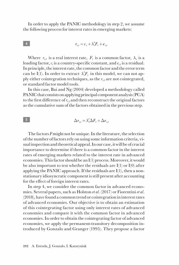
282 A. Estrada, J. Gonzalo, I. Kataryniuk
In order to apply the panic methodology in step 2, we assume the following process for interest rates in emerging markets:
4
Where ri,t is a real interest rate, Ft is a common factor, is a loading factor, ci is a country-specific constant, and ei,t is a residual. In principle, the interest rate, the common factor and the error term can be I(1). In order to extract in this model, we can not ap-ply either cointegration techniques, as the ri,t are not cointegrated, or standard factor model tools.
In this case, Bai and Ng (2004) developed a methodology called panic that consists on applying principal component analysis (PCA) to the first difference of ri,t and then reconstruct the original factors as the cumulative sum of the factors obtained in the previous step.
5
The factors F might not be unique. In the literature, the selection of the number of factors rely on using some information criteria, vi-sual inspection and theoretical appeal. In our case, it will be of crucial importance to determine if there is a common factor in the interest rates of emerging markets related to the interest rate in advanced economies. This factor should be an I(1) process. Moreover, it would be also important to test whether the residuals are I(1) or I(0) after applying the panic approach. If the residuals are I(1), then a non-stationary idiosyncratic component is still present after accounting for the effect of foreign interest rates.
In step 4, we consider the common factor in advanced econo-mies. Several papers, such as Holston et al. (2017) or Fiorentini et al. (2018), have found a common trend or cointegration in interest rates of advanced economies. Our objective is to obtain an estimation of this cointegrating factor using only interest rates of advanced economies and compare it with the common factor in advanced economies. In order to obtain the cointegrating factor of advanced economies, we apply the permanent-transitory decomposition in-troduced by Gonzalo and Granger (1995). They propose a factor
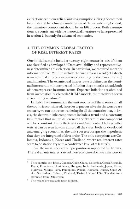
283Real Interest Rates in Emerging Economies
extraction technique reliant on two assumptions. First, the common factor should be a linear combination of the variables ri,t Second, the transitory component should be an I(0) process. Both assump-tions are consistent with the theoretical literature we have presented in section 2, but only for advanced economies.
4. THE COMMON GLOBAL FACTOR OF REAL INTEREST RATES
Our initial sample includes twenty-eight countries, six of them are classified as developed.3 Data availability and representative-ness determined this selection. In particular, we required monthly information from 2000 (to include the euro area as a whole) of a short-term nominal interest rate (quarterly average of the 3 months rate) and inflation. The ex ante real interest rate is defined as the nomi-nal interest rate minus expected inflation three months ahead, both of them expressed in annual terms. Expected inflation are obtained from (automatically selected) arima models, estimated with seven years rolling windows.4
In Table 1 we summarize the unit root tests of these series for all the countries considered. In order to put ourselves in the worst-case scenario, we run the tests considering for all the countries that, in lev-els, the deterministic components include a trend and a constant; this implies that in first differences the deterministic component will be a constant. Using the traditional Augmented Dickey-Fuller tests, it can be seen how, in almost all the cases, both for developed and emerging economies, the unit root test accepts the hypothesis that they are integrated of first order. The only exceptions are Co-lombia, Indonesia, Korea and Thailand, where real interest rates seem to be stationary with a confidence level of at least 5%.
Thus, the initial check of our proposition is supported by the data. The real ex ante interest rates of most economies behave as first order
3 The countries are: Brazil, Canada, Chile, China, Colombia, Czech Republic, Egypt, Euro Area, Honk Kong, Hungary, India, Indonesia, Japan, Korea, Malaysia, Mexico, Peru, Philippines, Poland, Romania, Russia, South Af-rica, Switzerland, Taiwan, Thailand, Turkey, uk and usa. The data were extracted from Datastream.
4 The results are available upon request.
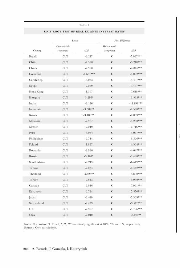
284 A. Estrada, J. Gonzalo, I. Kataryniuk
Table 1
UNIT ROOT TEST OF REAL EX ANTE INTEREST RATES
Country
Levels First Difference
Deterministic component adf
Deterministic component adf
Brazil C, T -2.247 C -7.037***
Chile C, T -2.588 C -5.218***
China C, T -2.950 C -4.814***
Colombia C, T -4.657*** C -6.002***
Czech Rep. C, T -3.033 C -4.497***
Egypt C, T -2.279 C -7.481***
Honk Kong C, T -1.307 C -7.618***
Hungary C, T -3.295* C -6.565***
India C, T -3.126 C -11.498***
Indonesia C, T -3.584** C -4.590***
Korea C, T -3.480** C -4.033***
Malaysia C, T -2.987 C -6.280***
Mexico C, T -2.249 C -3.716***
Peru C, T -3.054 C -4.067***
Philippines C, T -2.744 C -6.326***
Poland C, T -1.827 C -4.564***
Romania C, T -2.980 C -4.047***
Russia C, T -3.367* C -6.480***
South Africa C, T -2.213 C -6.619***
Taiwan C, T -2.034 C -4.442***
Thailand C, T -3.625** C -5.890***
Turkey C, T -2.643 C -6.980***
Canada C, T -2.046 C -7.961***
Euro area C, T -2.724 C -5.376***
Japan C, T -2.410 C -5.509***
Switzerland C, T -2.439 C -3.517***
uk C, T -2.397 C -5.756***
usa C, T -2.010 C -3.281**
Notes: C: constant, T: Trend; *, **, *** statistically significant at 10%, 5% and 1%, respectively.Sources: Own calculations.
Fig
ure
1
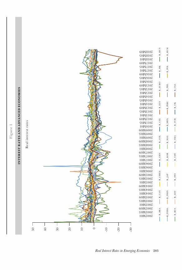
285Real Interest Rates in Emerging Economies
INTER
EST R
ATES A
ND
ADVA
NCED
ECO
NO
MIE
S
Rea
l int
eres
t ra
tes
——
R
_BR
A
——
R_I
ND
IA
——
R
_RU
S
——
R
_CA
N
——
R_I
ND
N
——
R
_SO
U
——
R
_CH
ILE
——
R
_JA
P
——
R
_SW
I
——
R
_CH
N
——
R
_KO
R
——
R
_TA
W
——
R
_CO
L
——
R_M
AL
——
R
_TH
A
——
R
_CZ
E
——
R_M
EX
——
R_T
UR
——
R
_EG
Y
——
R_P
ER
U
——
R
_UK
——
R
_EU
RO
——
R
_PH
L
——
R
_USA
——
R
_HK
——
R_P
OL
——
R
_HU
N
——
R
_RU
M
50 40 30 20 10 0
-10
-20
-30
2002M012002M052002M092003M012003M052003M092004M012004M052004M092005M012005M052005M092006M012006M052006M092007M012007M052007M092008M012008M052008M092009M012009M052009M092010M012011M052012M092013M012013M052013M092014M012014M052014M092015M012015M052015M092016M012016M052016M092017M012017M052017M092018M012018M052018M09
Fig
ure
1
286 A. Estrada, J. Gonzalo, I. Kataryniuk
integrated series. Now we can apply the panic approach to emerg-ing markets variables in order to extract the common component that should be integrated of first order. However, due to the existence of some extreme values that affected significantly the identification of the global factor, we decided to drop some countries: Egypt, In-dia, Indonesia, Romania, Russia and Turkey (see Figure 1). The in-clusion of these countries resulted in a common factor that basically replicated the evolution of the outlier.
4.1 The global factor in emerging economies
The application of the panic approach to the real interest rates of the sixteen remaining emerging economies generates a non-con-clusive number of common factors, according to the usual infor-mation criteria and the visual inspection. The Akaike information criterium finds a large amount of factors, while the visual analysis point to a number between 1 and 5. However, it is well known that the proposed statistics to select the number of common factors tends to overestimate them (Canner and Han, 2014).
Our approach relies on the economic meaning of the common factor. We are looking for a global factor in time series that might have several different common factors, for example, regional trends. In Table 2, we show the loadings of the autovector associated to the highest autovalue. It provides quite reasonable loadings (see Ta-ble 2), and therefore we use that as the global factor of real interest rates. Factors from 2 to 5 do not point to any common trend (see Ta-ble A.1 in the appendix). The highest weights correspond to Poland and Brazil, followed by a group of Chile, Thailand and Philippines. As can be seen, only Mexico enters with a negative (but very small) sign and all the emerging areas are represented. The three Latin American economies with the lowest loadings have underdeveloped domestic financial markets, which might be reflected on a lower pass-through of global interest rates. Perhaps, it could be expected a high-er loading in the case of China given its economic relevance, but it should be remembered that its capital account is still quite closed.
As can be seen in Figure 1, that common factor shows a declin-ing trend until the global financial crisis, when important fluctua-tions were recorded, and afterwards a certain stabilization. The unit root tests do not reject this variable to be a unit root with an adf
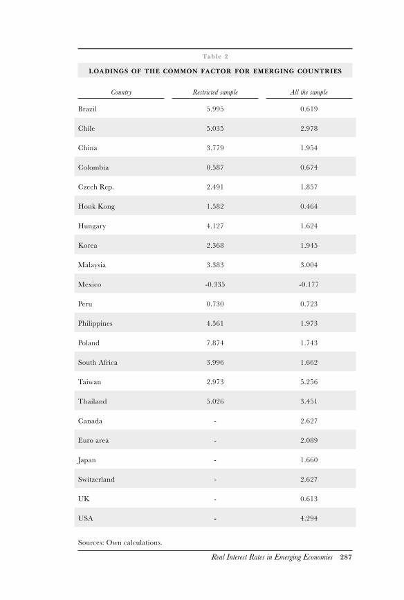
287Real Interest Rates in Emerging Economies
Table 2
LOADINGS OF THE COMMON FACTOR FOR EMERGING COUNTRIES
Country Restricted sample All the sample
Brazil 5.995 0.619
Chile 5.035 2.978
China 3.779 1.954
Colombia 0.587 0.674
Czech Rep. 2.491 1.857
Honk Kong 1.582 0.464
Hungary 4.127 1.624
Korea 2.368 1.945
Malaysia 3.383 3.004
Mexico -0.335 -0.177
Peru 0.730 0.723
Philippines 4.561 1.973
Poland 7.874 1.743
South Africa 3.996 1.662
Taiwan 2.973 5.256
Thailand 5.026 3.451
Canada - 2.627
Euro area - 2.089
Japan - 1.660
Switzerland - 2.627
uk - 0.613
usa - 4.294
Sources: Own calculations.
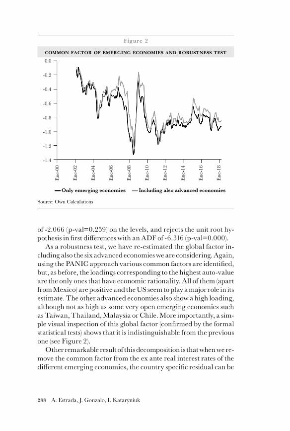
288 A. Estrada, J. Gonzalo, I. Kataryniuk
of -2.066 (p-val=0.259) on the levels, and rejects the unit root hy-pothesis in first differences with an adf of -6.316 (p-val=0.000).
As a robustness test, we have re-estimated the global factor in-cluding also the six advanced economies we are considering. Again, using the panic approach various common factors are identified, but, as before, the loadings corresponding to the highest auto-value are the only ones that have economic rationality. All of them (apart from Mexico) are positive and the us seem to play a major role in its estimate. The other advanced economies also show a high loading, although not as high as some very open emerging economies such as Taiwan, Thailand, Malaysia or Chile. More importantly, a sim-ple visual inspection of this global factor (confirmed by the formal statistical tests) shows that it is indistinguishable from the previous one (see Figure 2).
Other remarkable result of this decomposition is that when we re-move the common factor from the ex ante real interest rates of the different emerging economies, the country specific residual can be
Figure 2
COMMON FACTOR OF EMERGING ECONOMIES AND ROBUSTNESS TEST
Source: Own Calculations
Ene-
00
Ene-
02
Ene-
04
Ene-
06
Ene-
08
Ene-
10
Ene-
12
Ene-
14
Ene-
16
Ene-
18
0.0
-0.2
-0.4
-0.6
-0.8
-1.0
-1.2
-1.4
— Only emerging economies — Including also advanced economies
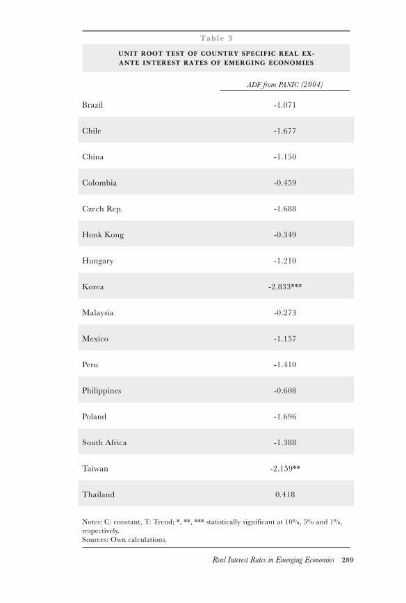
289Real Interest Rates in Emerging Economies
Table 3
UNIT ROOT TEST OF COUNTRY SPECIFIC REAL EX-ANTE INTEREST RATES OF EMERGING ECONOMIES
adf from panic (2004)
Brazil -1.071
Chile -1.677
China -1.150
Colombia -0.459
Czech Rep. -1.688
Honk Kong -0.349
Hungary -1.210
Korea -2.833***
Malaysia -0.273
Mexico -1.157
Peru -1.410
Philippines -0.608
Poland -1.696
South Africa -1.388
Taiwan -2.159**
Thailand 0.418
Notes: C: constant, T: Trend; *, **, *** statistically significant at 10%, 5% and 1%, respectively.Sources: Own calculations.
290 A. Estrada, J. Gonzalo, I. Kataryniuk
considered a first order integrated variable (see Table 3), which vali-dates the theory presented in Section 2.
4.2 The global factor in advanced economies
As we stated before, contrary to emerging markets, the real inter-est rates of advanced economies should cointegrate, as long as real convergence has been achieved (or it is very close). But if that is the case, the estimation of the global common factor would be more ro-bust if we exploit their cointegration properties using, for example, the Gonzalo-Granger (1995) methodology. Thus, the next step con-sists on checking the cointegration properties of the ex ante real in-terest rates of the advanced economies. We check that in two ways: first, considering all the different possible pairs that can be construct-ed; secondly, including all the countries at the same time. In the first case, the test used is that of Engle-Granger. In the second case, we use the trace statistic from the Johanssen approach.
As it can be seen in Table 4, the majority of the pairs cointegrate at 5% of statistical significance. The only exceptions (by a small margin) are usa/Japan, Euro-area/Japan, Euro-area/Canada and uk/Switzerland. As expected, all the estimated parameters are positive, but only in few cases are close to one (usa/Canada, Euro-area/Canada, Euro-area/Switzerland and Canada/Swit-zerland), showing that the fluctuations of the real interest rates vary from one country to another. The smallest coefficients are estimated for Japan, where the effective lower bound of the nominal interest rate was hit well before the other economies.
When checking the cointegration properties for all the countries at the same time, we find five cointegration relationships. Notice that the estimated coefficients are negative and significant with the ex-ception of the one of Japan.
Assuming that the only I(1) component of interest rates in aes is the global factor (consistent with Clarida, 2017), we can estimate this factor using the methodology of Gonzalo-Granger (1995) to ob-tain a common factor that is integrated of first order. This common trend should be our estimate of the equilibrium real interest rate. The results are presented graphically in Figure 3; they correspond to the following loadings: us: 0.43; euro area: 0.49; Japan: 0.08; uk: 1.29; Switzerland: 0.19 and Canada: 0.47. The highest loading cor-responds to the uk, which is small with respect to the Euro Area
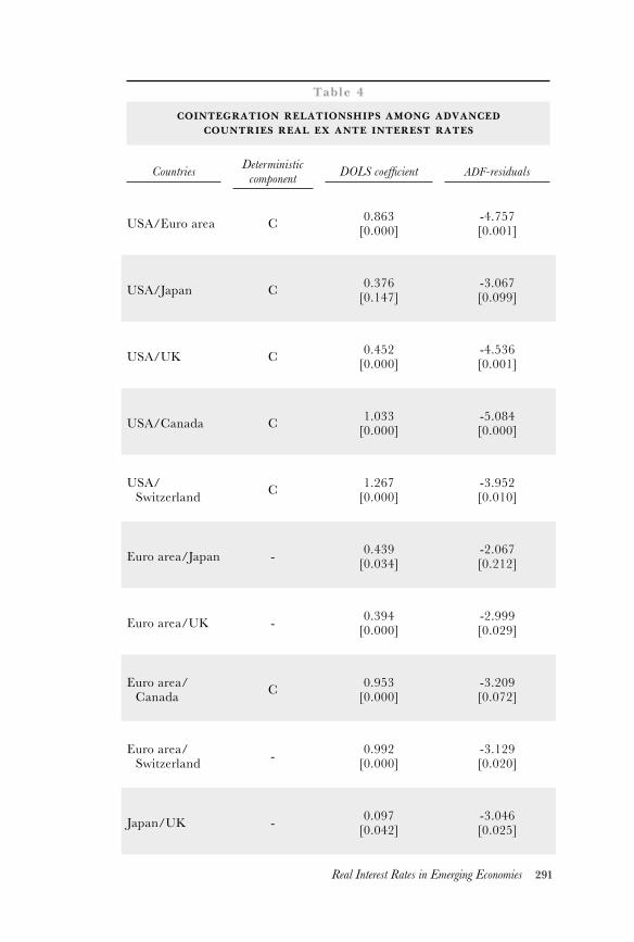
291Real Interest Rates in Emerging Economies
Table 4
COINTEGRATION RELATIONSHIPS AMONG ADVANCED COUNTRIES REAL EX ANTE INTEREST RATES
Countries Deterministic component DOLS coefficient adf-residuals
usa/Euro area C 0.863[0.000]
-4.757[0.001]
usa/Japan C 0.376[0.147]
-3.067[0.099]
usa/uk C 0.452[0.000]
-4.536[0.001]
usa/Canada C 1.033[0.000]
-5.084[0.000]
usa/Switzerland C 1.267
[0.000]-3.952[0.010]
Euro area/Japan - 0.439[0.034]
-2.067[0.212]
Euro area/uk - 0.394[0.000]
-2.999[0.029]
Euro area/Canada C 0.953
[0.000]-3.209[0.072]
Euro area/Switzerland - 0.992
[0.000]-3.129[0.020]
Japan/uk - 0.097[0.042]
-3.046[0.025]
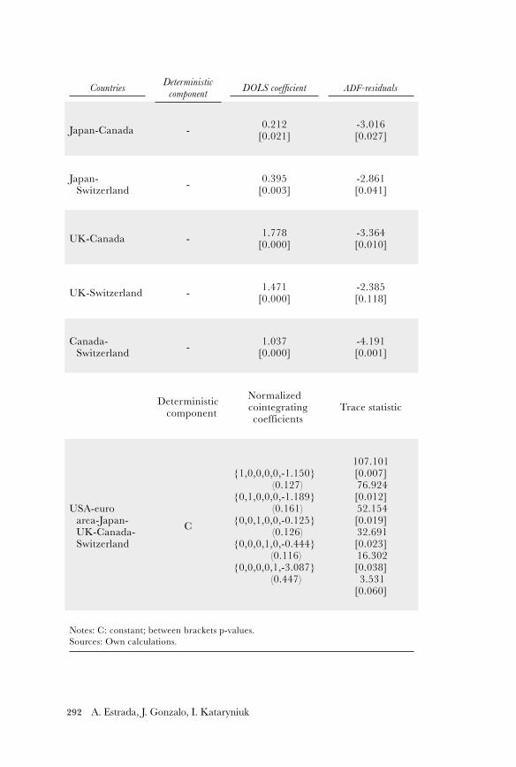
292 A. Estrada, J. Gonzalo, I. Kataryniuk
Countries Deterministic component DOLS coefficient adf-residuals
Japan-Canada - 0.212[0.021]
-3.016[0.027]
Japan-Switzerland - 0.395
[0.003]-2.861[0.041]
uk-Canada - 1.778[0.000]
-3.364[0.010]
uk-Switzerland - 1.471[0.000]
-2.385[0.118]
Canada-Switzerland - 1.037
[0.000]-4.191[0.001]
Deterministic component
Normalized cointegrating coefficients
Trace statistic
usa-euro area-Japan-uk-Canada-Switzerland
C
1,0,0,0,0,-1.150 (0.127)
0,1,0,0,0,-1.189 (0.161)
0,0,1,0,0,-0.125 (0.126)
0,0,0,1,0,-0.444 (0.116)
0,0,0,0,1,-3.087 (0.447)
107.101[0.007] 76.924[0.012] 52.154[0.019] 32.691[0.023] 16.302[0.038] 3.531[0.060]
Notes: C: constant; between brackets p-values.Sources: Own calculations.
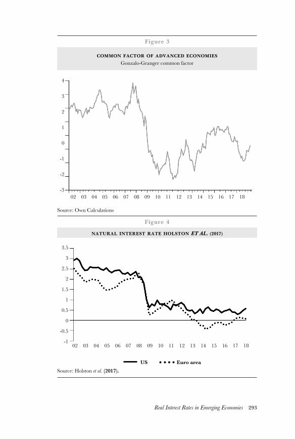
293Real Interest Rates in Emerging Economies
Figure 3
COMMON FACTOR OF ADVANCED ECONOMIES
Gonzalo-Granger common factor
Figure 4
NATURAL INTEREST RATE HOLSTON ET AL. (2017)
Source: Own Calculations
Source: Holston et al. (2017).
4
3
2
1
0
-1
-2
-3
3.5
3
2.5
2
1.5
1
0.5
0
-0.5
-1
02
02
10
10
06
06
14
14
04
04
12
12
08
08
16
16
03
03
11
11
07
07
15
15
05
05
13
13
09
09
17
17
18
18
US Euro area
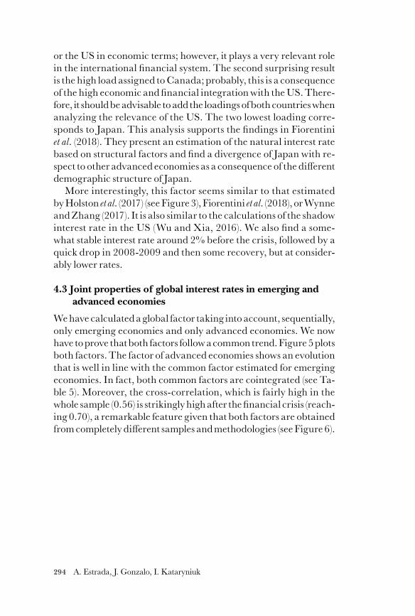
294 A. Estrada, J. Gonzalo, I. Kataryniuk
or the us in economic terms; however, it plays a very relevant role in the international financial system. The second surprising result is the high load assigned to Canada; probably, this is a consequence of the high economic and financial integration with the us. There-fore, it should be advisable to add the loadings of both countries when analyzing the relevance of the us. The two lowest loading corre-sponds to Japan. This analysis supports the findings in Fiorentini et al. (2018). They present an estimation of the natural interest rate based on structural factors and find a divergence of Japan with re-spect to other advanced economies as a consequence of the different demographic structure of Japan.
More interestingly, this factor seems similar to that estimated by Holston et al. (2017) (see Figure 3), Fiorentini et al. (2018), or Wynne and Zhang (2017). It is also similar to the calculations of the shadow interest rate in the us (Wu and Xia, 2016). We also find a some-what stable interest rate around 2% before the crisis, followed by a quick drop in 2008-2009 and then some recovery, but at consider-ably lower rates.
4.3 Joint properties of global interest rates in emerging and advanced economies
We have calculated a global factor taking into account, sequentially, only emerging economies and only advanced economies. We now have to prove that both factors follow a common trend. Figure 5 plots both factors. The factor of advanced economies shows an evolution that is well in line with the common factor estimated for emerging economies. In fact, both common factors are cointegrated (see Ta-ble 5). Moreover, the cross-correlation, which is fairly high in the whole sample (0.56) is strikingly high after the financial crisis (reach-ing 0.70), a remarkable feature given that both factors are obtained from completely different samples and methodologies (see Figure 6).
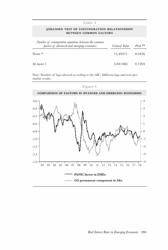
295Real Interest Rates in Emerging Economies
Table 5
JOHANSEN TEST OF COINTEGRATION RELATIONSHIPS BETWEEN COMMON FACTORS
Number of cointegration equations between the common factors of advanced and emerging economies Critical Value Prob.**
None * 15.49471 0.0426
At most 1 3.841466 0.1204
Note: Number of lags selected according to the AIC. Different lags and tests give similar results.
Figure 5
COMPARISON OF FACTORS IN DVANCED AND EMERGING ECONOMIES
0.0
-0.2
-0.4
-0.6
-0.8
-1.0
-1.2
-1.4
-1.6
4
3
2
1
0
-1
-2
-3
-402 1006 1404 1208 1603 1107 1505 1309 17 18
PANIC factor in EMEs
GG permanent component in AEs
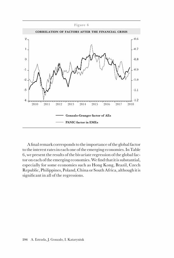
296 A. Estrada, J. Gonzalo, I. Kataryniuk
A final remark corresponds to the importance of the global factor to the interest rates in each one of the emerging economies. In Table 6, we present the results of the bivariate regression of the global fac-tor on each of the emerging economies. We find that it is substantial, especially for some economies such as Hong Kong, Brazil, Czech Republic, Philippines, Poland, China or South Africa, although it is significant in all of the regressions.
2010 2012 20152011 20142013 2016 2017 2018
PANIC factor in EMEs
Gonzalo-Granger factor of AEs
Figure 6
CORRELATION OF FACTORS AFTER THE FINANCIAL CRISIS
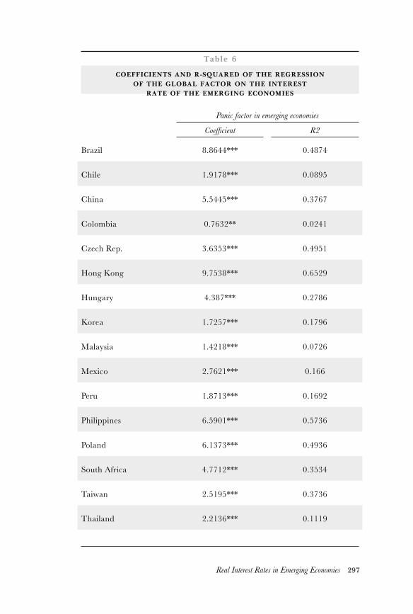
297Real Interest Rates in Emerging Economies
Table 6
COEFFICIENTS AND R-SQUARED OF THE REGRESSION OF THE GLOBAL FACTOR ON THE INTEREST
RATE OF THE EMERGING ECONOMIES
Panic factor in emerging economies
Coefficient R2
Brazil 8.8644*** 0.4874
Chile 1.9178*** 0.0895
China 5.5445*** 0.3767
Colombia 0.7632** 0.0241
Czech Rep. 3.6353*** 0.4951
Hong Kong 9.7538*** 0.6529
Hungary 4.387*** 0.2786
Korea 1.7257*** 0.1796
Malaysia 1.4218*** 0.0726
Mexico 2.7621*** 0.166
Peru 1.8713*** 0.1692
Philippines 6.5901*** 0.5736
Poland 6.1373*** 0.4936
South Africa 4.7712*** 0.3534
Taiwan 2.5195*** 0.3736
Thailand 2.2136*** 0.1119
298 A. Estrada, J. Gonzalo, I. Kataryniuk
5.CONCLUSIONS
In this paper, we have presented evidence on the existence of a glob-al factor in emerging economies. We consider a model of an open economy in which the equilibrium interest rate is a combination of two integrated processes. Taking this into account, we have used the panic approach to extract the global factor present in the in-terest rate of emerging economies. We have compared this factor to the cointegrating factor of advanced economies to prove that they share a common trend.
The paper sheds light on the formation of interest rates in emerg-ing economies. First, they have to take into account the evolution of interest rates in advanced economies. As the advanced economies are subject to a long process of low interest rates, emerging economies will import this behavior to their domestic interest rates. Second, it is expected that, in more open emerging economies, the comovement with interest rates of advanced economies will be greater.
We have not analyzed the remaining part of interest rates in emerg-ing economies after subtracting the influence of the global inter-est rate. In the theoretical literature, it depends on long and short run idiosyncratic trends. This discussion is left for future research.
299Real Interest Rates in Emerging Economies
References
Bai J. and, S. Ng (2004): “A panic attack on unit roots and coin-tegration” Econometrica, Nº 72(4), pp. 1127-1177.
Caner, M. and X. Han, (2014): “Selecting the correct number of factors in approximate factor models: the large panel case with group bridge estimators” J. Bus. Econom. Statist., 32.pp. 359-374
Clarida, R. (2017): “The global factor in neutral policy rates: some implications for exchange rates, monetary policy, and policy coordination” nber Working Papers Nº 23562.
Clarida, R., Galí, J. and M. Gertler (2002): “A simple framework for international monetary policy analysis” Journal of Mon-etary Economics, Nº 49, pp. 879-904.
Fiorentini, G., Galesi, A., Pérez-Quirós, G. and E. Sentana (2018): “The rise and fall of the natural interest rate” Documentos de Trabajo, Banco de España, Nº 1822.
Gonzalo, J. and C. Granger (1995): “Estimation of common long-memory components in cointegrated systems” Journal of Business & Economic Statistics, Vol. 13(1), pp. 27-35.
Holston, K., Laubach, T. and J. C. Williams (2017): “Measur-ing the natural rate of interest: international trends and determinants” Journal of International Economics, Nº 108, pp. S59-S75.
Jones, CH. I. (2002): “Sources of u.s. economic growth in a world of ideas” American Economic Review, Nº 92(1), pp. 220-239.
Rodrik, D. (2011): “The future of economic convergence” NBER Working Papers Nº 17400.
Summers, L. (2013): “imf economic forum: policy responses to crises” 14th imf Stanley Fisher’s Annual Research Confer-ence FMI, November 8th.
Wu, J. C., and Xia, F. D. (2016). “Measuring the macroeconomic impact of monetary policy at the zero lower bound” Journal of Money, Credit and Banking, 48(2-3), 253-291.
Wynne, M. A., and Zhang, R. (2018). “Measuring the World Natural Rate of Interest” Economic Inquiry, 56(1), 530-544.
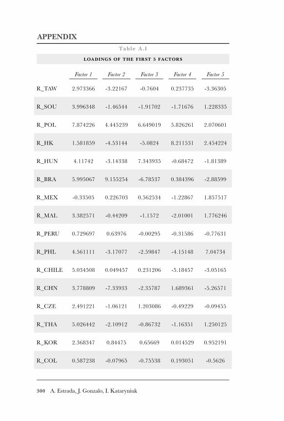
300 A. Estrada, J. Gonzalo, I. Kataryniuk
APPENDIXTable A.1
LOADINGS OF THE FIRST 5 FACTORS
Factor 1 Factor 2 Factor 3 Factor 4 Factor 5
R_TAW 2.973366 -3.22167 -0.7604 0.237735 -3.36305
R_SOU 3.996348 -1.46544 -1.91702 -1.71676 1.228335
R_POL 7.874226 4.445239 6.649019 5.826261 2.070601
R_HK 1.581859 -4.53144 -5.0824 8.211531 2.454224
R_HUN 4.11742 -3.14338 7.343935 -0.68472 -1.81389
R_BRA 5.995067 9.155254 -6.78537 0.384396 -2.88599
R_MEX -0.33505 0.226703 0.562534 -1.22867 1.857517
R_MAL 3.382571 -0.44209 -1.1572 -2.01001 1.776246
R_PERU 0.729697 0.63976 -0.00295 -0.31586 -0.77631
R_PHL 4.561111 -3.17077 -2.59847 -4.15148 7.04734
R_CHILE 5.034508 0.049457 0.231206 -5.18457 -3.05165
R_CHN 3.778809 -7.33933 -2.35787 1.689361 -5.26571
R_CZE 2.491221 -1.06121 1.203086 -0.49229 -0.09455
R_THA 5.026442 -2.10912 -0.86732 -1.16351 1.250125
R_KOR 2.368347 0.84475 0.65669 0.014529 0.952191
R_COL 0.587238 -0.07965 -0.75538 0.193051 -0.5626