Isoprene in the marine boundary layer (Southeast Asian Sea, eastern Indian Ocean, and Southern...

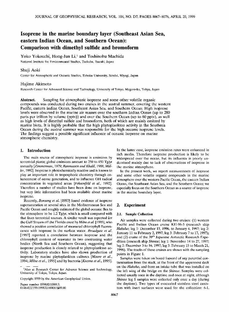
JOURNAL OF GEOPHYSICAL RESEARCH, VOL. 104, NO. D7, PAGES 8067-8076, APRIL 20, 1999

Isoprene in the marine boundary layer (Southeast Asian Sea, eastern Indian Ocean, and Southern Ocean)'

Comparison with dimethyl sulfide and bromoform

Yoko Yokouchi, Hong-Jun Li, 1 and Toshinobu Machida National Institute for Environmental Studies, Tsukuba, Ibaraki, Japan

Shuji Aoki Center for Atmospheric and Oceanic Studies, Tohoku University, Sendal, Miyagi, Japan

Hajime Akimoto Research Center for Advanced Science and Technology, University of Tokyo, Meguro-ku, Tokyo, Japan

Abstract. Sampling for atmospheric isoprene and some other volatile organic compounds was conducted during two cruises in the austral summer, covering the western Pacific, eastern Indian Ocean, Southeast Asian Sea, and Southern Ocean. High isoprene levels were observed in the marine air masses over the southern Indian Ocean (up to 280 parts per trillion by volume (pptv)) and over the Southern Ocean (up to 60 pptv), as well as high levels of dimethyl sulfide and bromoform, both of which are mainly emitted by marine biota. It is highly probable that the high phytoplankton activity in the Southern Ocean during the austral summer was responsible for the high oceanic isoprene levels. The findings suggest a possible significant influence of oceanic isoprene on marine atmospheric chemistry.

1. Introduction

The main source of atmospheric isoprene is emissions by terrestrial plants; global emissions amount to 250 to 450 Tg/yr annually [Zimmerman, 1979; Rasmussen and Khalil, 1988; Miil- let, 1992]. Isoprene is photochemically reactive and is known to play an important role in tropospheric chemistry through en- hancement of ozone generation, and to influence OH radical concentration in vegetated areas [Fehsenfeld et al., 1992]. Therefore a number of studies have been done on isoprene, but very little information had been available about marine isoprene.

Recently, Bonsang et al. [1992] found evidence of isoprene supersaturation at several sites in the Mediterranean Sea and Pacific Ocean and roughly estimated the global oceanic flux to the atmosphere to be 1.2 Tg/yr, which is small compared with that from terrestrial sources. A similar result was reported for the Gulf Stream off the Florida coast by Milne et al. [1995], who showed a positive correlation of measured chlorophyll fluores- cence with isoprene in the surface water. Broadgate et al. [1997] reported a correlation between isoprene and the chlorophyll content of seawater in two contrasting water bodies (North Sea and Southern Ocean), suggesting that isoprene production is closely related to phytoplankton activity. Laboratory studies have also shown production of isoprene by marine phytoplankton cultures [Moore et al., 1994; Milne et al., 1995] and by bacteria [Kuzma et al., 1995].

•Also at Research Center for Advance Science and Technology, University of Tokyo, Tokyo, Japan.

Copyright 1999 by the American Geophysical Union.

Paper number 1998JD100013. 0148-0227/99/1998JD 100013509.00

In the latter case, isoprene emission rates were enhanced in rich media. Therefore isoprene production is likely to be widespread over the ocean, but its influence is poorly un- derstood mainly due to lack of observations of isoprene in the marine atmosphere.

In the present work, we report measurements of isoprene and some other volatile organic compounds in the marine atmosphere over the western Pacific Ocean, the eastern Indian Ocean, the Southeast Asian Sea, and the Southern Ocean; we especially focus on the Southern Ocean as a source of isoprene in the marine boundary layer.

2. Experiment

2.1. Sample Collection

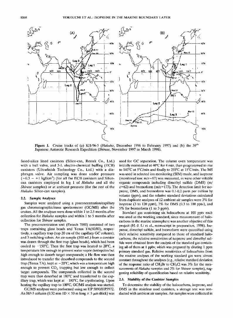
Air samples were collected during two cruises: (1) western Pacific and Indian Ocean cruise KH-96-5 (research ship Hakuho; leg 1: December 15, 1996, to January 4, 1997; leg 2: January 11 to February 2, 1997; leg 3: February 7 to 17, 1997); and (2) cruise of the 39 th Japanese Antarctic Research Expe- dition (research ship Shirase; leg 1: November 14 to 27, 1997; leg 2: December 3 to 16, 1997; leg 3: February 15 to March 21, 1998). The tracks of these cruises are shown with the sampling points in Figure 1.

Samples were taken on board forward of any potential con- tamination from the stack, at the front of the uppermost deck on the Hakuho, and from an intake tube that was installed on the left wing of the bridge on the Shirase. Samples were collected usually once in the daytime and once at night, although Shirase leg 1 samples were collected only once a day (during the daytime). Two types of evacuated stainless steel canisters with inert surfaces were used for the collection: 6-L

8067

8068 YOKOUCHI ET AL.' ISOPRENE IN THE MARINE BOUNDARY LAYER

Syowa

Leg 2

--'I" ..... 45"N

• 30øN

Leg 1 .... ;•- 15øN

135øE 150øE

Nov.27

i

Leg 3

....... • -- 15øS

..... 30øS

-• 45øS Mar.15

I 60øS

75øS

Figure 1. Cruise tracks of (a) KH-96-5 (Hakuho, December 1996 to February 1997) and (b) the 39 th Japanese Antarctic Research Expedition (Shirase, November 1997 to March 1998).

fused-silica lined canisters (Silico-can, Restek Co., Ltd.) with a ball valve, and 3-L electro-chemical buffing (ECB) canisters (Ultrafinish Technology Co., Ltd.) with a dia- phragm valve. Air sampling was done under pressure (+0.3 - + 1 kgf/cm 2) (for all the ECB canisters and Silico- can canisters employed in leg 1 of Hakuho and all the Shirase samples) or at ambient pressure (for the rest of the Hakuho Silico-can samples).

2.2. Sample Analyses

Samples were analyzed using a preconcentration/capillary gas chromatographic/mass spectrometer (GC/MS) after the cruises. All the analyses were done within 1 to 2.5 months after collection for Hakuho samples and within 1 to 5 months after collection for Shirase samples.

The preconcentration unit (Entech 7000) consisted of two traps containing glass beads and Tenax TA(60/80), respectively, a capillary trap (top 20 cm of the capillary GC column), and 3 switching valves. An air sample (500 mL) from a canister was drawn through the first trap (glass beads), which had been cooled to -150øC. Then the first trap was heated to 20øC, a temperature low enough to prevent water vapor desorption but high enough to desorb target compounds; a He flow was then introduced to transfer the desorbed compounds to the second trap (Tenax TA), kept at -20øC, which was a temperature high enough to prevent CO2 trapping but low enough to collect target compounds. The compounds collected in the second trap were then desorbed at 180øC and transferred to the capillary trap, which was kept at -180øC, for cryofocusing. Upon heating the capillary trap to 100øC, GC/MS analysis was started.

GC/MS analyses were performed using an HP 5890/HP5972. An HP-5 column (0.32 mm ID x 50 m long x 5/•m thick) was

used for GC separation. The column oven temperature was initially maintained at 40øC for 4 min, then programmed to rise to 140øC at 5øC/min and finally to 250øC at 15øC/min. The MS was used in selected ion monitoring (SIM) mode, and isoprene (monitored ion: m/z--67) was measured, as were other volatile organic compounds including dimethyl sulfide (DMS) (m/ z=62) and bromoform (m/z-173). The detection limit for isoprene, DMS, and bromoform was 0.1-0.2 parts per trillion by volume (pptv), and the relative standard deviations calculated from duplicate analyses of 12 ambient air samples were 3% for isoprene (3 to 120 pptv), 7% for DMS (0.3 to 100 pptv), and 5% for bromoform (1 to 3 pptv).

Standard gas containing six halocarbons at 100 pptv each was used as the working standard, since measurement of halocarbons in the marine atmosphere was another objective of this project (H.-J. Li et al., manuscript in preparation, 1998). Iso- prene, dimethyl sulfide, and bromoform were quantified using their relative sensitivity compared to those of standard halocarbons; the relative sensitivities of isoprene and dimethyl sulfide were obtained from the analysis of the standard gas containing all of them at 1 ppbv, which was prepared by diluting 1 ppm primary standard gas. Relative sensitivities of halocarbons from the routine analyses of the working standard gas were almost constant throughout the analyses (e.g., relative standard deviation of the response ratio of CH3Br to CH3C1 was 3% for the measurements of Hakuho samples and 2% for Shirase samples), suggesting reliability of quantification based on relative sensitivity.

2.3. Stability of the Canister Samples

To determine the stability of the halocarbons, isoprene, and DMS in the stainless steel canisters, a storage test was conducted with ambient air samples. Air samples were collected in

YOKOUCHI ET AL.' ISOPRENE IN THE MARINE BOUNDARY LAYER 8069

' r'

75•E

Feb.17

•::

..

..... ; ............. 45øN

30øN

135øE 150øE

15øN

• 0 ø

15øS

............ • ............ 30øS

Figure 2. Distribution of isoprene in the marine atmosphere during the Hakuho cruise.

20 canisters (five each for ECB pressurized (P), ECB ambient pressure (A), Silico-can pressurized (P), and Silico-can ambient pressure (A)) on the roof of the National Institute for Environmental Studies in October 1997. The concentrations of

the target compounds in the canisters were measured on the sampling day and 1, 2, 4, and 6 months after sampling, using one canister from each group on each of the measuring days.

There was a linear decrease of isoprene and DMS with time,

although change of halocarbon levels in the canisters was not so significant. The rate of isoprene decrease was 9%/month for Silico-can (P), 12%/month for Silico-can (A), 2%/month for ECB (P), and 4%/month for ECB (A). The rate of DMS decrease was 10%/month for Silico-can (P) and (A), and 4%/ month for ECB (P) and (A). We corrected the measured concentrations of isoprene and DMS accordingly for their storage loss, assuming the same decrease rates for all samples.

8070 YOKOUCHI ET AL.' ISOPRENE IN THE MARINE BOUNDARY LAYER

(A)

<>....•/• 24h 48h

-3o

-40

-5•

80 90 100 10 120

LONGITUDE

(•)

-4(

100 110 120

LONGITUDE

Figure 3. Two-day back trajectories of air masses: (a) 39 ø 18'S, 113 ø 0'E; January 12, 1400 (GST); (b) 32.4øS, 110.0øE, January 17, 0300 (GST).

There may be some error in this correction due to differences in air quality, but it would have little affect on our discussion of the significant atmospheric variations of these two compounds.

3. Results and Discussion

3.1. Isoprene, DMS, and Bromoform From the Hakuho Cruise

3.1.1. Isoprene. Isoprene concentrations in the air samples collected during the Hakuho cruise ranged from 0.1 to 286 pptv with great variability (Figure 2). This variability was in contrast with the concentrations of anthropogenic compounds such as tetrachloroethylene, which gradually decreases from the north to the tropics and is almost constant at around 1.5 pptv in the southern hemisphere (H.-J. Li et al., manuscript in preparation, 1998). Isoprene concentrations higher than 100 pptv were often observed near tropical islands (Kalimantan and the Lesser Sunda Islands) and over the southern Indian Ocean. Although these values are not abnormally high compared to terrestrial forest data (typically 100 to 2000 pptv), they are much higher than previously reported data for marine air masses: <5 pptv off the Florida coast and <36 pptv over the Hao Atoll [Bonsang et al., 1992; Milne et al., 1995]. Over the open Indian Ocean north of 30øS (in leg 2) and over the East China Sea (in leg 3), the isoprene concentration was generally low and rarely exceeded 10 pptv.

We attribute the elevated isoprene levels near tropical islands to atmospheric transport from terrestrial sources, since a great amount of isoprene is emitted by tropical forests and concentrations of several thousand pptv have been reported for tropical atmospheric isoprene [Greenberg and Zimmerman, 1984; Ayers and Gillett, 1988; Yokouchi, 1991]. On the other

hand, the high concentrations we observed over the southern Indian Ocean cannot be explained by long-range transport from sources on the continents, since southerly winds from the Southern Ocean were prevailing on the surface at those sampling sites when we sampled. For example, 2-day back trajectories calculated by the National Institute for Environmental Studies, Center for Global Environmental Research program (Figure 3), show that the air masses flowed from the west or south to the ship on January 12 and 17 when we observed isoprene concentrations of 250 and 140 pptv, respectively. Therefore the ocean itself is the most likely source of the elevated isoprene observed over the southern Indian Ocean, where high biological productivity in austral summertime has been reported [Davison et al., 1996]. If this is the case, then this is the first observation of oceanic isoprene levels high enough to contribute significantly to photochemical reactions in remote marine air. High variability of isoprene over the southern Indian Ocean could be due to its short lifetime (several hours) as well as spatially heterogeneous distribution of sources.

If phytoplanktons are sources of oceanic isoprene, then the generally low concentrations we observed over the Indian Ocean north of 30øS (in leg 2) are consistent with low biological activity in the open ocean waters. Over the Strait of Ma- lacca, situated between Sumatra and peninsular Malaysia, 74 pptv of isoprene was observed in a sample collected near Pen- ang, suggesting some land effect. Isoprene levels over the South China Sea between 10øN and 30øN (in leg 3) were lower than those over the western Pacific Ocean in the same latitu-

dinal range (in leg 1). Back trajectory calculation and observed higher levels of anthropogenic compounds such as tetrachloroethylene (H.-J. Li et al., manuscript in preparation, 1998) suggest greater contributions of continental air masses over the western Pacific Ocean in spite of greater distance from the continent.

3.1.2. DMS. DMS varied greatly, ranging from <0.2 to 640 pptv, with the maximum over the southern Indian Ocean as shown in Figure 4. DMS is known to be produced by some types of marine phytoplankton [Challenger and Simpson, 1948; Andreae, 1986], and significant seasonal variation in its concentration has been reported. The high concentration detected over the southern Indian Ocean during this cruise was similar to the austral summer DMS concentration measured at Am-

sterdam Island (37 ø 50'S, 77 ø 30'E) in the southern Indian Ocean [Putaud et al., 1992] and at Cape Grim (40 ø 41'S, 144 ø 41'E) [Ayers et al., 1995]. The high bioactivity in the southern Indian Ocean that produced the high levels of DMS in the present study could also be a strong source of isoprene. How- ever, isoprene and DMS concentrations along the cruise track were not clearly correlated with each other even for the southern Indian Ocean (R=0.38 for all the data; R=0.30 for the data from 35 ø S-45øS), and isoprene concentrations were much more variable than those of DMS. This difference might be due to different atmospheric lifetimes of these species or different types of source phytoplankton. The reaction constants of isoprene and DMS with OH radicals, which are the most important reactive species in the atmosphere, are 9.98 x 10 -• and 9.3 x 10 -•: cm 3 molecule -• s -l, respectively [Atkinson, 1986]; therefore isoprene is lost 10 times faster than is DMS.

3.1.3. Bromoform. Bromoform is known to be released

by temperate macroalgae [Gschwend et al., 1985], ice microal- gae [Sturges et al., 1992], and an additional planktonic source [Class and Ballschmiter, 1988]. Elevated atmospheric CHBr 3 concentrations have been found in more-productive coastal regions and over some shallow waters [Yokouchi et al., 1997].

YOKOUCHI ET AL.: ISOPRENE IN THE MARINE BOUNDARY LAYER 8071

•,:/ 60øE 75 E

Jan.4

,

i Feb. 17

45øN

I f Jan.13•l .:•

i

150øE

30øN

15øN

, 0 ø

15øS

30øS

45øS

75øS

Figure 4. Distribution of DMS in the marine atmosphere during the Hakuho cruise.

The present measurements were generally consistent with the previous data, with higher levels (>1 pptv) of bromoform near tropical islands,'over the Strait of Malacca, and over the western coast of Australia (Figure 5). Over the Indian Ocean, CHBr 3 concentration was generally around 0.4 pptv, with higher values near 40øS. Elevation of CHBr 3 levels in the south, not as marked as with DMS, might also be related to high bioactivity in the region. Other marine-derived halocarbons, dibromochloromethane and bromodichlorometh- ane, showed variation similar to that of bromoform.

3.2. Isoprene, DMS, and Bromoform From the "Shirase" Cruise

3.2.1. Isoprene. Isoprene levels measured during the Shirase cruise in the austral summer/autumn (1997/1998) are shown in Figure 6. Five samples from nearest points to Syowa Station (69 ø 00'S, 39 ø 35'E) were collected over partly ice- covered ocean. The isoprene concentration ranged from non- detectable (n.d.) (<0.1 pptv) to 57 pptv with an average of 13 pptv. Highest isoprene levels were observed over the Southern

8072 YOKOUCHI ET AL.: ISOPRENE IN THE MARINE BOUNDARY LAYER

75•E

Jan.4

I Jan.13

135øE

Feb.17

150øE

1

45øN

30øN

15øN

, 0 ø

15øS

30øS

Figure 5. Distribution of bromoform in the marine atmosphere during the Hakuho cruise.

Ocean (south of 45øS). The cruise from 30øN to 35øS covered almost the same track as leg 1 of the Hakuho cruise, but the observed isoprene concentrations were much lower, mostly around 3 pptv, except near Kalimantan and just south of Japan (31øN). Back trajectory studies for those areas showed that the difference was likely due to much reduced effects of land air masses during this cruise.

No increase of isoprene level was observed over the south-

ern Indian Ocean north of 45øS, where high isoprene levels (-280 pptv)were found in the "open-ocean air masses" during leg 2 of the Hakuho cruise. In the Shirase cruise, however, high concentrations of isoprene up to 57 pptv were observed farther south, over the Southern Ocean in the Subantarctic area, where strong wind (8 + 5 m s-•) was blowing from the west or south. Carbon monoxide in the air samples collected at the same time was almost constant (less than 100 ppbv) over the


.

! i Feb.15 Syowa

Isoprene

10 pptv •

ov.27

Nov. 15

.................... ? ........ 45øN {

{ 30øN

150øE :.

• 15øN

{

.... { 15Os

,.•

• ..... 30øS

•:"• Mar. l• 60Os

75øS

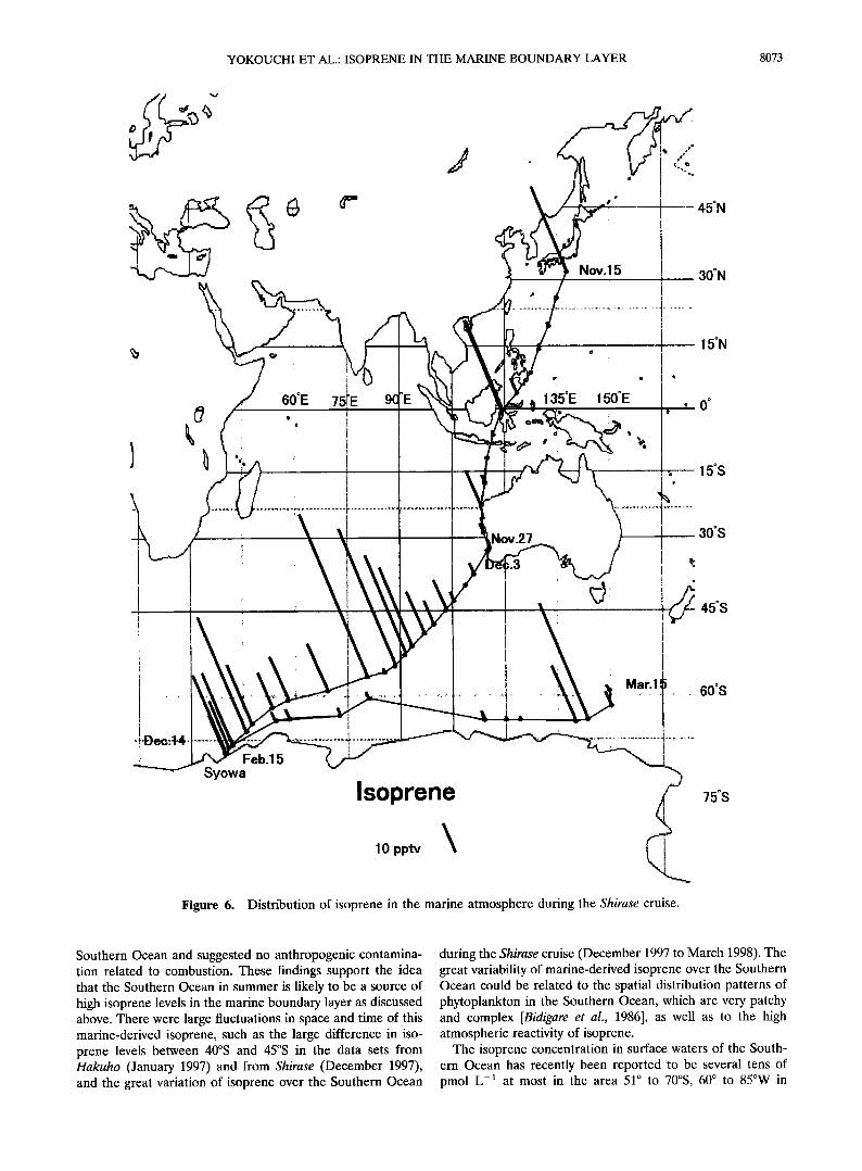
Figure 6. Distribution of isoprene in the marine atmosphere during the Shirase cruise.

Southern Ocean and suggested no anthropogenic contamina- tion related to combustion. These findings support the idea that the Southern Ocean in summer is likely to be a source of high isoprene levels in the marine boundary layer as discussed above. There were large fluctuations in space and time of this marine-derived isoprene, such as the large difference in isoprene levels between 40øS and 45øS in the data sets from Hakuho (January 1997) and from Shirase (December 1997), and the great variation of isoprene over the Southern Ocean

during the Shirase cruise (December 1997 to March 1998). The great variability of marine-derived isoprene over the Southern Ocean could be related to the spatial distribution patterns of phytoplankton in the Southern Ocean, which are very patchy and complex [Bidigare et al., 1986], as well as to the high atmospheric reactivity of isoprene.

The isoprene concentration in surface waters of the South- ern Ocean has recently been reported to be several tens of pmol L -1 at most in the area 51 ø to 70øS, 60 ø to 85øW in


Figure 7. Distribution of DMS in the marine atmosphere during the Shirase cruise.

November/December 1992 [Broadgate et al., 1997], similar to reported levels in other temperatc oceans [Bensang et al., 1992; Milne et al., 1995]. If this is the case for the whole Southern Ocean, the Ocean itself might not bc an outstanding source of isoprene; a much reduced conversion rate of isoprene in the gas phase might be an alternative reason for higher levels of isoprene in the Subantarctic regions. However, the data are too limited to be conclusive, considering the highly variable distribution of the source phytoplankton.

3.2.2. DMS. DMS levels from the data set of Shirase were

in the range n.d. (<0.2 pptv) to 370 pptv (Figure 7), being highest over the Southern Ocean. In the rcgion 35 ø to 45øS, where DMS levels of 250 to 640 pptv were found on the Hakuho cruises, Shirase samples showed concentrations of DMS lower than 2 pptv, except at 44øS. The general pattern was similar to that of isoprene, although the variation in concentration of the two compounds over the Southern Ocean was not well correlated.

The high level of DMS observed in this study is consistent


, Dec.'!4 Feb.15 Syowa

o.

150øE

• - ,

'i ! Mar. 15

Bromoform

1 pptv •

45øN

30øN

15øN

o

15øS

30øS

60øS

75øS

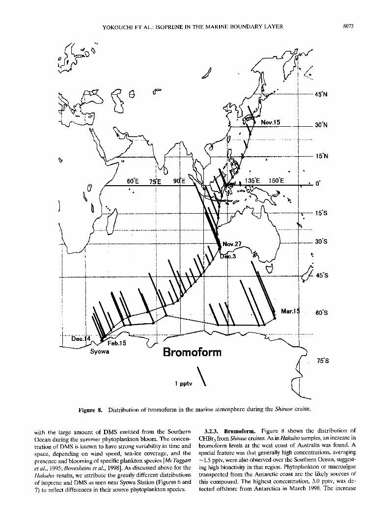
Figure 8. Distribution of bromoform in the marine atmosphere during the Shirase cruise.

with the large amount of DMS emitted from the Southern Ocean during the summer phytoplankton bloom. The concentration of DMS is known to have strong variability in time and space, depending on wind speed, sea-ice coverage, and the presence and blooming of specific plankton species [McTaggart et al., 1995; Berresheim et al., 1998]. As discussed above for the Hakuho results, we attribute the greatly different distributions of isoprene and DMS as seen near Syowa Station (Figures 6 and 7) to reflect differences in their source phytoplankton species.

3.2.3. Bromoform. Figure 8 shows the distribution of CHBr 3 from Shirase cruises. As in Hakuho samples, an increase in bromoform levels at the west coast of Australia was found. A

special feature was that generally high concentrations, averaging •--1.5 pptv, were also observed over the Southern Ocean, suggesting high bioactivity in that region. Phytoplankton or macroalgae transported from the Antarctic coast are the likely sources of this compound. The highest concentration, 3.0 pptv, was detected offshore from Antarctica in March 1998. The increase


might be due to transport of air masses containing CHBr 3 emitted by Antarctic algae as well as by phytoplankton blooms. The variation of CHBr3 levels was not as pronounced as that of DMS or isoprene, probably due to its longer lifetime or the more uniform distribution of bromoform-producing species.

4. Conclusions

Isoprene concentrations higher than 100 pptv were observed in the marine atmosphere near tropical islands and over the southern Indian Ocean during the Hakuho cruise from De- cember 1996 to February 1997. In the Shirase cruise, Novem- ber 1997 to March 1998, several tens pptv of isoprene were often found over the Southern Ocean and with a large fluctu- ation. We believe that the high levels of isoprene in the tropics are due to emissions from tropical forests, while those over the southern Indian Ocean and Southern Ocean are due to emis-

sions by phytoplankton or related marine biota in the Southern Ocean during the austral summer. High bioactivity in this region is supported by the data on DMS and bromoform, both of which are predominantly emitted by marine biota.

Isoprene over the remote marine atmosphere should play an important role in photochemistry there, since the levels of anthropogenic reactive hydrocarbons are very low in these regions. The present study has shown that the isoprene level over the Southern Ocean often exceeds 10 pptv, high enough to explain elevated HCHO levels in clean marine air at Cape Grim in November and December, and higher than predicted by current photochemical theory [Ayers et al., 1997].

This study provides the first data on atmospheric isoprene over the Southern Ocean, but the data cover only limited areas and only one season. More investigations, including on-site measurements of air and seawater samples, are required for further understanding of the global effect of oceanic isoprene.

Acknowledgments. This work was supported by Global Environ- ment Fund (Environmental Agency). We are grateful to the Ocean Research Institute and Toshitaka Gamo for the opportunity to participate in cruise KH-96-5, and to National Institute of Polar Research and Takashi Yamanouchi for the opportunity to participate in the 39 th Japanese Antarctic Research Expedition. We thank Yoko Inuzuka for her assistance with GC/MS analyses. We also would like to thank Yasushi Narita and Jing Zhang who helped us with air sampling during cruise KH-96-5.

References

Andreae, M. O., The ocean as a source of atmospheric sulfur compounds, in The Role of Air-Sea Exchange in Geochemical Cycling, edited by P. Buat-Menard, pp. 331-362, D. Reidel, Norwell, Mass., 1986.

Atkinson, R., Kinetics and mechanisms of the gas-phase reactions of the hydroxyl radical with organic compounds under atmospheric conditions, Chern. Rev., 86, 69-201, 1986.

Ayers, G. P., and R. W. Gillett, Isoprene emissions from vegetation and hydrocarbon emissions from bushfires in tropical Australia, J. Atmos. Chem., 7, 177-190, 1988.

Ayers, G. P., S. T. Bentley, J.P. Ivey, and B. W. Forgan, Dimethyl- sulfide in marine air at Cape Grim, 41øS, J. Geophys. Res., 100, 21,013-21,021, 1995.

Ayers, G. P., R. W. Gillet, H. Granek, C. de Serves, and R. A. Cox, Formaldehyde production in clean marine air, Geophys. Res. Lett., 24, 401- 404, 1997.

Berresheim, H., J. W. Huey, R. P. Thorn, F. L. Eisele, D. J. Tanner, and A. Jefferson, J. Geophys. Res., 103, 1629-1637, 1998.

Bidigare, R. R., T. J. Frank, C. Zastrow, and J. M. Brooks, The distribution of algal chlorophylIs and their degradation products in the Southern Ocean, Deep Sea Res., 33, 923-937, 1986.

Bonsang, B., C. Polle, and G. Lambert, Evidence for marine production of isoprene, Geophys. Res. Lett., 19, 1129-1132, 1992.

Broadgate, W. J., P.S. Liss, and S. A. Penkett, Seasonal emissions of isoprene and other reactive hydrocarbon gases from the ocean, Geophys. Res. Lett., 24, 2675-2678, 1997.

Challenger, F., and M. I. Simpson, Studies on biological methylation, 12, A precursor of the dimethyl-sulphide evolved by Polysiphonia fastigata, dimethyl-2-carboxyethyl sulphonium hydroxide, and its salt, J. Chem. Soc., 3, 1591-1597, 1948.

Class, T., and K. Ballschmiter, Chemistry of organic traces in air, VIII, Sources and distribution of bromo- and bromochloromethanes in

marine air and surfacewater of the Atlantic Ocean, J. Atmos. Chem., 6, 35-46, 1988.

Davison, B., C. O'Dowd, C. N. Hewitt, M. H. Smith, R. M. Harrison, D. A. Peel, E. Wolf, R. Mulvaney, M. Schwikowski, and U. Balt- ensperger, Dimethyl sulfide and its oxidation products in the atmosphere of the Atlantic and Southern Oceans, Atmos. Environ., 30, 1895-1906, 1996.

Fehsenfeld, F., et al., Emissions of volatile organic compounds from vegetation and the implications for atmospheric chemistry, Global Biogeochem. Cycles, 6, 389-430, 1992.

Greenberg, J.P., and P. R. Zimmerman, Nonmethane hydrocarbons in remote tropical, continental, and marine atmospheres, J. Geophys. Res., 89, 4767-4778, 1984.

Gschwend, P.M., J. K. MacFarlane, and K. A. Newman, Volatile halogenated organic compounds released to seawater from temperate marine macroalgae, Science, 227, 1033-1035, 1985.

Kuzma, J., M. Nemecek-Marshall, W. H. Pollock, and R. Fall, Bacteria produce the volatile hydrocarbon isoprene, Curt. Microbiol., 30, 97- 103, 1995.

McTaggart, A. R., H. R. Burton, and B.C. Nguyen, Emission and flux of DMS from the Australian Antarctic and Subantarctic Oceans

during the 1988/89 summer, J. Atmos. Chem., 20, 59-69, 1995. Milne, P. J., D. D. Riemer, R. G. Zika, and L. E. Brand, Measurement

of vertical distribution of isoprene in surface seawater, its chemical fate, and its emission from several phytoplankton monocultures, Mar. Chem., 48, 237-244, 1995.

Moore, R. M., D. E. Oram, and S. A. Penkett, Production of isoprene by marine phytoplankton cultures, Geophys. Res. Lett., 21, 2507- 2510, 1994.

Mfiller, J.-F., Geographical distribution and seasonal variation of surface emissions and depositional velocities of atmospheric trace gases, J. Geophys. Res., 97, 3787-3804, 1992.

Putaud, J.P., N. Mihalopouls, B.C. Nguyen, J. M. Campin, and S. Belviso, Seasonal variations of atmospheric sulfur dioxide and dim- ethylsulfide concentrations at Amsterdam Island in the Southern Indian Ocean, J. Atmos. Chem., 15, 117-1131, 1992.

Rasmussen, R., and M. A. K. -Khalil, Isoprene over the Amazon basin, J. Geophys. Res., 93, 1417-1421, 1988.

Sturges, W. T., G. F. Cota, and P. T. Buckley, Bromoform emission from Arctic ice algae, Nature, 358, 660-662, 1992.

Yokouchi, Y., Measurements of volatile organic compounds emitted from tropical forests (in Japanese), Rep. 01540498, Grant-in-Aid for Sci. Res., Monbusho, 1991.

Yokouchi, Y., H. Mukai, H. Yamamoto, A. Otsuki, C. Saitoh, and Y. Nojiri, Distribution of methyl iodide, ethyl iodide, bromoform, and dibromomethane over the ocean (east and southeast Asian seas and the western Pacific), J. Geophy. Res., 102, 8805-8809, 1997.

Zimmerman, P. R., Testing of hydrocarbon emissions from vegetation, leaf litter and aquatic surfaces, and development of a methodology for compiling biogenic emission inventories, Rep. EPA 450/4-79-004, Environ. Prot. Agency, Washington, D.C., 1979.

H. Akimoto, Research Center for Advanced Science and Technol- ogy, University of Tokyo, Meguro-ku, Tokyo 153-0041, Japan.

S. Aoki, Center for Atmospheric and Oceanic Studies, Tohoku Uni- versity, Sendal, Miyagi 980-8578, Japan.

H.-J. Li, T. Machida, and Y. Yokouchi, National Institute for En- vironmental Studies, Japan Environment Agency, P.O. Box 16-20n- ogawa, Tsukuba, Ibaraki 305-0053, Japan. (e-mail: yokouchi@ nies.go.jp)

(Received January 15, 1998; revised September 1, 1998; accepted September 9, 1998.)

Isoprene in the marine boundary layer (Southeast Asian Sea, eastern Indian Ocean, and Southern...

Documents

Transcript of Isoprene in the marine boundary layer (Southeast Asian Sea, eastern Indian Ocean, and Southern...