DN

B W

or

kiN

g P

aP

er

DNB Working Paper

Is this bank ill? The diagnosis of

doctor TARGET2

Ronald Heijmans and Richard Heuver

No. 316 / August 2011

Working Paper No. 316

August 2011

De Nederlandsche Bank NV P.O. Box 98 1000 AB AMSTERDAM The Netherlands

Is this bank ill? The diagnosis of doctor TARGET2 Ronald Heijmans and Richard Heuver * * Views expressed are those of the authors and do not necessarily reflect official positions of De Nederlandsche Bank.

Is this bank ill? The diagnosis of doctor TARGET2

Ronald Heijmans Richard Heuver∗

Augsut 2011

Abstract

We develop indicators for signs of liquidity shortages and potential financial problems ofbanks by studying transaction data of the Dutch part of the European real time gross settlementsystem and collateral management data. The indicators give information on 1) overall liquid-ity position, 2) the interbank money market, 3) the timing of payment flows, 4) the collateral’samount and use and 5) bank run signs. This information can be used both for monitoring theTARGET2 payment system and for individual banks’ supervision. By studying these data before,during and after stressful events in the crisis, banks’ reaction patterns are identified. These pat-terns are translated into a set of behavioural rules, which can be used in payment systems’ stressscenario analyses, such as e.g. simulations and network topology. In the literature behaviour andreaction patterns in simulations are either ignored or very static. To perform realistic paymentsystem simulations it is crucial to understand how banks react to shocks.

Key Words: behaviour of banks , wholesale payment systems, financial stability

JEL Codes: D23, E42, E58

∗Heijmans and Heuver can be reached ronald.heijmans@dnb.nl and richard.heuver@dnb.nl, respectively. We thank RonBerndsen, Hans Brits and Iman van Lelyveld for providing useful comments The views expressed are those of the authorsand do not necessarily represent the views of De Nederlandsche Bank.

1 Introduction

The financial crisis, which erupted in the United States in the summer of 2007, clearly showed the

mutual dependence of the banking system on a worldwide scale. The crisis intensified after the

failure of Lehman Brothers in September 2008. As a result of this failure the lending in the interbank

market decreased significantly, see e.g Heijmans et al. (2010) for the Dutch market, Guggenheim

et al. (2010) for the Swiss market and Akram and Christophersen (2010) for the Norwegian market.

As banks grew very reluctant to lend money to each other, central banks became worried that the

interbank market would dry up completely. To prevent this from happening central banks worldwide,

including the European Central Bank (ECB), responded with both conventional and unconventional

monetary policy.1 Studies on the structure of the interbank market can be found in Bech and Atalay

(2008), who studied the topology of the federal funds market, Wetherilt et al. (2010), who looked at

the sterling unsecured loan market during 2006-2008, and Imakubo and Soejima (2010), who studied

the microstructure of Japan’s interbank money market.

A bankruptcy or a bail out usually does not come as a complete surprise. Before a bank goes

bankrupt or has to be bailed out by the government or commercial parties in order to survive there are

often rumours about its financial soundness. When time progresses these rumours might even become

clear facts. The failure of Lehman obviously shocked the market, such a large bank to go bankrupt

and not be saved by the government. Besides the failure of Lehman Brothers many other news facts

shocked the market, such as failures of smaller banks, nationalisations of systemic important banks,

state support etc. These news facts impacted the market perception of the troubled bank, which can

become visible in the interbank money market (higher interest rates and lower borrowing volume)

and in delays in payments by and to the troubled bank. The changed behaviour of one or more banks

can consequently prompt many other banks to change their behaviour. This might in extreme cases

lead to a total gridlock in which everyone is waiting for someone else to make the first payment. Such

a situation will not only affect the payment system but can also jeopardise the financial system as a

whole. If a bank intends to delay payments or change interbank interest rates based on rumours (not

facts) it needs to trade off two kinds of risks: liquidity and reputation risk. A negative intraday position

or outstanding loans vis-a-vis a counterparty is risky if one party is worried about its counterparty’s

ability to meet its obligations to that party. Delaying payments based on incorrect information can

damage the debtor’s reputation.

The research question of this paper is how to identify liquidity problems of a bank using Large

Value Payment System (LVPS) transaction and collateral data. The literature focusses mainly on de-

velopments in the (unsecured) interbank money market, using an algorithm to identify interbank loans

from the LVPS transaction data, see beginning of this section. This paper looks at all main liquidity

influencing elements and actors behind these elements visible in the payment system. Besides, this

paper transfers behavioural changes found in the Large Value Payment System (LVPS), TARGET2-

NL, and collateral data into a set of behavioural rules, which can be used in scenario analyses. To

answer the main question we first look at the overall liquidity position of a bank. The overall devel-

1The unconventional monetary policy measures of the ECB consist of very long-term tenders (maturity up to 1 year)and the purchase of covered bonds.

1

opment of the liquidity position provides an overview of a bank’s liquidity streams and how it funds

itself. After the overall liquidity position we look into more detail at the developments of the funding

patterns. The developments in the interbank money market can e.g. show that one or more banks have

difficulties obtaining liquidity out of this market to fund their liquidity needs. It is also possible that

a bank or group of banks becomes more reluctant to lend their surplus liquidity to other banks as a

result of increased market stress. If a bank can obtain insufficient liquidity from the interbank market

it also has the option to borrow from the ECB (secured by its collateral) or use collateral to obtain in-

traday credit. If the use of collateral intensifies this can be a signal of near future liquidity shortages.

If a bank faces difficulties funding itself on the interbank market and cannot obtain more liquidity

from the ECB (based on the amount of its collateral) and as a result has no more liquidity available

to make payments, it has no other option but to delay payments until it has received payments. A

delay in outgoing payments can be a liquidity shortage signal. When the market suspects (serious)

liquidity/financial problems with a certain counterparty it can delay some of their payments to this

counterparty until it has received liquidity from this counterparty. A delay in incoming payments can

be a signal that the market perceives this bank as more risky. If a bank’s problems persist and its

customers might loose faith in their bank at some point and transfer their funds to another bank or

withdraw cash at the ATM, a bank run is born.

Figure 1: Overview of liquidity management elements.

2

Figure 1 gives an overview of the areas of interest with respect to the liquidity management of

a participant in the European Large Value Payment System (TARGET2). First there are the ”real”

payments (bottom right-hand panel). These are the day-to-day payments on behalf of a customer

or themselves which have no link with funding transactions or transactions to and from the ECB.

A second area is the interbank money market (top right-hand panel), which gives information on

interest rates and volume developments. Another area is the ECB facilities (top left-hand panel),

which provide information on the use of tenders and how banks fulfil the ECB’s reserve requirements.

Finally, the bottom left-hand panel is the collateral amount and use. Collateral can be used for long-

term loans (tenders), overnight credit (marginal lending) and intraday credit. The numbers in the

overview correspond to the order the figures are presented in Section 3.

The changes in reaction patterns can be used to closely monitor the payment system and as a sup-

port tool for the supervision of banks to get up-to-date information on the current status of individual

banks. As the payments data are available the next day, for most purposes the information on potential

changes in behaviour is very timely.2 A set of banks’ behavioural rules is developed by studying the

transaction data before and during the crisis. This set of rules can be used in e.g. scenario analyses of

payment systems or in developments of the network structure after a disruption. This paper only looks

at (potential) liquidity problems or ”illnesses” based on transaction and collateral data of participants

in the LVPS and does not purport to say anything about the underlaying causes (e.g. a risky business

model or bad management of a bank).

Relevant literature in the context of this paper is as follows. Banks are used to ”liquidity shocks”

arising from unexpected changes in liquidity demand. Allen and Gale (2000) distinguish between two

types of uncertainty. First, the idiosyncratic uncertainty, which arises from the fact that for any given

level of aggregate demand for liquidity there is uncertainty about which banks will face that demand.

The second type of risk concerns the aggregate uncertainty that is due to the fact that the overall

level of the demand for liquidity that banks face is stochastic. These unexpected liquidity fluctuations

impact the smooth operations of payments and Real Time Gross Settlement systems (RTGSs), besides

affecting the banks’ liquidity management (Iori et al., 2008), see for a description of LVPSs (and

RTGSs) Section 2. Banks use the interbank money market (both secured and unsecured) to solve

temporary shortages on their account. Cocco et al. (2009) show that relationships are important for

the banks’ ability to access interbank market liquidity. The bilateral nature of this market enables

banks to establish such relationships. Apart from access to liquidity, relationships do matter for both

smaller and larger banks in negotiating favourable when borrowing and lending terms (Cocco et al.,

2009; Carlin et al., 2007). We expect that relationship also plays a role in banks’ payment behaviour

and that banks are sooner inclient to delay payments if they expect a problem with a counterparty they

do not have a relationship with. This can be inferred by the fact that banks do not want to be known,

especially by one of their ’friends’, as the one that pushed you over the edge of bankruptcy.

McAndrews and Rajan (2000), McAndrews and Potter (2002) and Bech and Garratt (2003) argue

that the decisions made by banks in the U.S. LVPS Fedwire can be interpreted as a coordination

game. Bech and Garratt (2006) have developed a stylised game theoretical model in which the timing

of payments is reduced to two time periods: morning (in time) and afternoon (delayed). Abbink

2Real-time monitoring is performed by the operators of a Real Time Gross Settlement.

3

et al. (2010) have conducted an experimental game based on their theoretical model. In this game

they investigate how the behaviour in the payment system is affected by disruptions. Their main

findings are that when the equilibrium of the payment system moves to the inefficient one (delaying

payments) it is not likely that the behaviour moves back to the efficient equilibrium (paying in time).

Besides, coordination on the efficient equilibrium turns out to be easier in a market with a clear market

leader. Lastly, they find that small disruptions in coordination games can be absorbed easily, but when

frictions become larger the system quickly moves to the undesired equilibrium and stays there. The

fact that the payment system can be seen as a game illustrates that behaviour plays a role in these

systems, especially in stressed times which change this game’s dynamics.

Koponen and Soramaki (2005), Bech and Soramaki (2005), Ledrut (2007) and Heijmans (2009)

are examples of payment systems’ simulations, based on historical data. The behaviour of banks in

these papers does not represent realistic behavioural patterns. A description in networks’ terms, see

e.g Soramaki et al. (2007) or Propper et al. (2008), gives information on the critical participants and

the level of dependencies between the participants in the payment system. It does not give information

on how participants behave. Before the crisis started there was not much empirical evidence on how

banks behave in times of stress, as there were not many stressful events. The 9/11 attacks gave some

insight but there were no banks at that time facing severe liquidity problems over a longer time or that

went (almost) bankrupt, see Lacker (2004). In order to improve the realism of simulations and the

dynamics of network structures it is essential to include behaviour into the analysis.

The outline of the paper is straightforward. Section 2 describes the data set used for the analysis.

Section 3 describes how the TARGET2 transaction and collateral management data can be used to find

signs of liquidity shortages of individual banks. Section 4 describes the set of behavioural rules based

on evidence found during the crisis, and Section 5 concludes and gives policy recommendations.

2 Large value payment systems

Before we move on to the identification process of liquidity problems of banks and the behavioural

rules find in the LVPS data and collateral management data we first give a description of this LVPS.

Large value payment systems (LVPS) play an important role in the economy. With the help of these

systems, banks can settle their (customer) obligations immediately and irrevocably. The irrevocability

of the payment is very important in the LVPS as the receiving bank can reuse the liquidity without

running the risk that the liquidity has to be repaid to the sending bank in case of bankruptcy of

that bank. Because of their economic relevance, LVPS have to live up to high standards. They must

comply with the core principles which were developed by the central banks, co-ordinated by the Bank

for International Settlement (CPSS, 2001). The most important euro-LVPS is TARGET2.3 Another

system that is used is EURO1.4

3TARGET2: Trans-European Real Time Gross settlement Express Transfer.4EURO1 is a private sector owned payment system for domestic and cross-border single payments in euro between

banks operating in the European Union.

4

2.1 TARGET2

TARGET2 is the large value payment system of the eurosystem, which is used to execute time-critical

payments. Besides the euro countries, there are 6 non-euro European countries that are connected

to TARGET2 for the settlement of euro payments.5 Technically, it is a centralised system, which

means that there is one platform for all participants to settle their payments. Legally, TARGET2

is a decentralised system. Each country still has its own legal documentation. The conditions are,

however, maximally harmonised, but small deviations are allowed if required by national legislation.

In a legal and business sense, one of the central banks is the intermediary channel between a financial

institution and TARGET2.

TARGET2 can only be used by institutions which meet the access criteria. The most important

institution types that can gain access to TARGET2 are credit institutions established in the European

Economic Area (EEA), EU member states’ central banks including the ECB and central or regional

governments treasury departments of member states active in the money market. Most other financial

firms, non-financial firms and consumers do no meet the access criteria of TARGET2

All payments executed in TARGET2 are stored in a datawarehouse. The average daily turnover in

TARGET2 in 2010 was EUR 2,267 billion, which corresponds with an average number of transactions

of more than 340,000. The Dutch part of TARGET2, TARGET2-NL, accounts for 13% and 10%

respectively. For a more detailed description of large value payment systems see Heijmans et al.

(2010, Section 2).

The Dutch market is characterised by a few large banks and many small(er) ones. In TARGET2-

NL there is also a few large British banks.

2.2 Description of the data

Financial institutions settle various types of payments in TARGET2, such as payments on behalf of

a customer, bank-bank payments, payment of the cash leg of a security transaction, pay-in of CLS

(continuous linked settlement) to settle foreign exchange transactions, and so on. The data used in our

analysis contain transaction level data of TARGET2-NL (and its predecessor the Dutch RTGS TOP)

between 1 January 2005 and 28 February 2011 and the collateral’s amount and use of each individual

bank in TARGET2-NL (and TOP).6 The accounts of De Nederlandsche Bank and the Dutch Treasury

(including its agency) were excluded, as these institutions are no commercial banks.

3 Monitoring individual banks

Besides the Lehman Brothers’ failure several stressful events occurred in the Dutch financial system,

like the nationalisation of Fortis - ABN AMRO, the bankruptcy of DSB Bank and the state support

of several larger financial institutions. The effects of these events have to a lesser or greater extent

become visible in the TARGET2 transaction and collateral data. These data have been investigated to

develop a monitoring tool for both individual banks and the market as a whole. This section describes

5Bulgaria, Denmark, Estonia, Latvia, Lithuania, Poland and Romania (status July 2011).6TARGET2-NL was launched on 18 February 2008.

5

the monitoring tool. For illustration purposes the information in the figures is based on TARGET2-

NL data. Most graphs presented in this section could be shown for a single bank, group of banks or

the whole market. Section 4 translates the visible effects into a set of behavioural rules.

The monitoring tool consists of several different indicators. If only one indicator changes this

need not signal a problem, but if there are more indicators heading in a certain direction this may

be a sign that there are serious liquidity and/or financial problems with a bank. We have seen in

the data several banks with only one indicator showing potential liquidity problems while the other

indicators were neutral. However, with the banks in trouble (like Fortis and DSB) there were several

indicators heading in the direction of liquidity problems. This is comparable with the medical doctor’s

differential diagnoses. The doctor diagnoses the patient’s problem by asking the patient questions.

In some cases there might not be a medical problem at all or only a light flu which will be over in a

few days without treatment. But if more indicators point to a serious disease, immediate treatment

might be necessary. The differential diagnosis of the central banker is based on the changing reaction

patterns obtained from e.g. the TARGET2 and collateral data. By combining the different elements

we can see whether a bank (patient) has or may have serious liquidity or financial problems (illness)

and whether action from the central bank or supervisor authority is required.

Some caution is in order for banks which are not very active in the payment system or in the

interbank market. For Lack of sufficient payment transactions the monitoring tool provided in this

section might give misleading information in such cases.

3.1 ECG of liquidity

When a medical doctor examines a patient, he often listens to the heart. If the doctor hears abnormali-

ties he may decide to make an electrocardiograph (abbreviated to ECG). The ECG is the transthoracic

interpretation of the heart’s electrical activity over time captured and externally recorded by skin elec-

trodes. From the ECG a lot of information can be obtained on the physical state of a patient. Likewise

we seek information on the ”health” of banks. Supervisors want to have information on both the sol-

vency (long-term) and liquidity (short-term) position.7 Also operators of LVPSs want to know if a

bank faces liquidity or technical problems, as such problems may affect other banks in the payment

system. An additional complicating factor for supervisors is that the ECG of liquidity, in contrast to

patients, can be very different for each bank depending on their liquidity management and business

characteristics.

3.1.1 ECG of liquidity: Payment flows

Figure 2 shows the most important payment types’ liquidity flows of a bank (1st panel shows absolute

flow values and 2nd panel the relative values), distinguishing payments on behalf of a customer or

themselves or ”real” payments (grey bars), monetary policy (blue bars), standing facilities (deposit,

green bars; marginal lending, yellow bars) and money market lending (pink bars) and borrowing (red

7It is not possible to say anything about the solvency of a bank based on TARGET2 transaction or collateral data.

6

Figure 2: ECG of liquidity: flow of payments (top panel), relative flow of payments (bottom panel),18 February - 30 April 2011. The top 6 elements of the legend belong to the positive and the bottom6 to the negative vertical axis.

bars). The figure shows several maintenance periods.8 The white gaps in the figures (and also in the

graphs in the rest of this chapter) represent the separation between two maintenance periods. The

positive values refer to the incoming values and the negative values refer to the outgoing ones. The

reason for choosing the maintenance period is that there are strong cyclical patterns in e.g. money

market transactions which are used to level surplus or shortages, see Heijmans et al. (2010). They

have found e.g. that at the end of the maintenance period there is a significant increase in money

market transactions. The secured lending is not separately visible in this graph as it is not possible to

identify them (reliably) from the TARGET2 transaction data.

Figure 2 contains the following information. This figure first gives an overview of the value of

8A maintenance period is the time frame in which at the end of the business day banks must maintain an average levelof funds specified by the central bank. If a bank does not meet the maintenance requirement it will receive a penalty.

7

the most important payment flows in both the absolute (top panel) and the relative (bottom panel)

sense. Especially the activity at the interbank market is interesting from a risk perspective (see also

Section 3.2.2). If a participant’s loses trust in the market and as a result is not willing to lend its (full)

surplus, this will become visible by an increased use of the ECB’s overnight deposit. On the other

hand if a participant is unable to borrow the required liquidity at the interbank market, use of both

tenders and marginal lending are likely to increase, see Section 3.2.3 for a detailed view of the use of

ECB facilities. In other words the activity at the interbank market gives information on how banks

perceive the risk of the market and of individual participants. The figure also shows the development

and volatility over time of the several payments flows. Moreover, the figure gives information on

the potential demand for liquidity. A bank with a lot of real payments (grey bars) has potentially

more need for liquidity (tenders, interbank loans) in the absolute sense. A bank with a higher day-to-

day volatility in the real payment flows potentially needs relatively more liquidity (tenders, interbank

loans) while also its future liquidity position is more difficult to predict. As a modified example,

the blue circles in Figure 2 show two changes which can be identified from this graph.9 In the left

circle there is a shift from interbank lending to the overnight deposit’s use and the right circle shows

a period the bank uses the overnight deposit extensively. At the right part of this circle there is a

decrease again in overnight deposit and an increase of interbank lending and borrowing. This may

signal an increased trust in the market circumstances.

3.1.2 ECG of liquidity: outstanding values

Figure 3 shows the outstanding value of the payments flows. The positive vertical axis represents

the assets of a bank, including its pledged collateral at the central bank, its total daily incoming pay-

ments, its outstanding interbank lending, its overnight deposit, its account balance and its incoming

payments. The negative vertical axis on the other hand represents the liabilities of a bank, including

its interbank borrowing, marginal lending, tenders, total daily outgoing payment, free available col-

lateral (which can be seen as equity) and use of collateral for intraday credit. In other words Figure 3

presents a balance sheet of assets (positive vertical axis) and liabilities (negative vertical axis).

To illustrate the difference between Figure 3 and 2 we take the year tenders (blue bar) that the

banks were able to obtain from the ECB in July 2009. The year tenders are visible in Figure 2 as

two individual transactions one year apart: one incoming in July 2009 and the other outgoing July

2010. In Figure 3 the year tender stays visible the whole year starting in July 2009 until July 2010.

At the same time the free collateral will decrease/increase with the exact amount of the tender at the

start/end of this tender (assuming a bank does not change the amount of collateral at the start or end

of the tender). The same reasoning is true for interbank loans (lending pink bars and borrowing red

bars), except that there is no effect on the free collateral.

Figure 3 contains the following information. First, information about a bank’s differences in the

funding funding sources from interbank money market to the ECB or vice versa. If a bank moves its

funding from the interbank market to the ECB, this may indicate that a bank has difficulties in funding

itself in the market. Furthermore, the figure makes clear whether a bank is a lender or a borrower and9The data has been modified for confidentiality reasons. These data do however reflect what has been observed in the

data.

8

how lending and borrowing changes over time. The figure also shows changes in the amount and use

of collateral. If the amount of collateral e.g. decreases, the ability of a bank to withstand (new) shocks

decreases along. This is especially true for banks which have a relatively low amount of collateral

relative to their payments. Besides the shifts from lending/borrowing to overnight deposit and vice

versa which have also been identified by Figure 2, the red circle in Figure 3 also shows as an example

the period the bank suddenly used more intraday credit, which may be a sign of (near future) liquidity

problems.

Figure 3: ECG of liquidity: absolute outstanding value (top panel), relative outstanding value (bottompanel), 18 February - 30 April 2011. The top 5 elements of the legend belong to the positive and thebottom 6 to the negative vertical axis.

9

3.2 Demand and supply of liquidity

3.2.1 Reserve requirements

The ECB requires banks to hold a minimum cash reserve on average during the maintenance period.

The main reason for banks to borrow liquidity is that they have to meet the ECB’s requirements.

Due to natural fluctuations banks face shortages and surpluses on a regular basis, see Allen and Gale

(2000). If a bank expects that it will not meet its requirement it will use the interbank market or

the ECB facilities to meet them. In order to see if certain changes in the ability to lend liquidity are

worrisome it is necessary to know if a bank is in need of liquidity to meet its requirements. Figure 4

is an illustration of how a bank could or could not meet its cash reserve requirement. The green bars

denote when the bank has a surplus and the red bars when it has a shortage relative to its cash reserve

requirement.

Figure 4 enables us to answer three questions with respect to cash reserve requirements: 1) Does

a bank meet its reserve requirement? 2) When does a bank start to meet its reserve requirements? 3)

Has the timing of meeting the reserve requirement changed over time? In maintenance period I of the

figure, the bank steers the maintenance requirements on a daily basis. This means that the bank neither

has a large surplus nor shortage on any business day during the maintenance period. In maintenance

period II the bank starts with a surplus, which vanishes over the course of the period and ends in the

last week with values close to the reserve requirements, like in period I. In maintenance period III

the bank starts with a large surplus, which vanishes over the course of the whole period. In period

IV the bank starts with a relatively large shortage. This shortage decreases as the maintenance period

progresses. If a bank is unable to meet its requirements it can expect a penalty from the supervisors.

In period V the bank’s shortage relative to its maintenance requirements only increases. This will be

the case if the bank is no longer able to solve its problems.

Figure 4 also helps to determine if a bank needs liquidity from the interbank money market. If a

bank has a surplus relative to its reserve requirement (green at a certain point during the maintenance

Figure 4: Five stylistic examples of how a bank meets (I to IV) and fails to meet (V) its maintenanceperiods.

10

period), it does not need liquidity from the market but is able to lend liquidity to the market. Whether

it will do the latter depends on its expected liquidity need for the rest of the maintenance period and

on the perceived risk of counterparties which want to borrow from this bank.

3.2.2 Interbank lending and borrowing

If the market suspects liquidity or financial problems with a certain counterparty and has serious

doubts whether that counterparty is able to fulfil its payment obligations, banks become more hesitant

to provide liquidity. This will show up in the amounts banks are willing to lend to this counterparty

and/or in the interest rate this counterparty has to pay. Figure 5 shows the amount of interbank

overnight lending and borrowing over time by a bank. The algorithm used to filter the interbank loans

has been developed by Heijmans et al. (2010), which is based on the algorithm by Furfine (1999).10

The developments of the lending and borrowing amount reflect the bank’s market perception (lending)

or the market’s perception of this bank (borrowing).11 A bank’s lending and borrowing behaviour also

gives information on the bank’s type. Is a bank on average a lender, a borrower or a money broker

(both lending and borrowing at the same day)? In case a bank is generally a lender it is better able to

withstand liquidity shocks than a borrower, because it can decrease its lending amount. A borrower on

the other hand becomes even more dependent on other banks’ liquidity in case of liquidity shortages.

The blue circle in Figure 5 shows an example of the developments of both the interbank lending

and the interbank borrowing volumes, which may be seen as worrisome. First the lending amount

decreases and later on the borrowing amount. If a bank has liquidity shortages it will stop lending.

When the market suspects liquidity problems with a counterparty it will decrease or cease lending

to this counterparty. To see whether the decrease in lending and borrowing is indeed a problem

the information has to be combined with the use of ECB facilities and the way the bank meets its

maintenance requirements.

Figure 6 shows the development of bank borrowing rates relative to the Dutch average (or: the

”local” average) and the European average (EONIA).12 If the market perception towards a single

(or group of) participant(s) changes for better or worse, the interest rate will decrease or increase

as a consequence. The red circle in Figure 6 illustrates how interest rate developments may signal

potential bank’s liquidity problems. First the interest rates increase as a result of an increased market’s

risk perception to this bank. In other words the bank has to pay a higher price for its loans. When time

progresses these increased rates move slowly back to normal. If the interest rates for a single bank

increase significantly as shown in this graph this may be a signal of near future liquidity problems as

it becomes more difficult for this bank to fund itself. The data showed that the first signs of liquidity

10Even though the algorithm can detect loans up to 1 year, only overnight loans are used. The reason for this is thatmost of the loans (in value) are overnight and no shift has been identified during the crisis from long-term to short(er)-termlending. Therefore the overnight loans are an reliable indicator of changes in the ability to lend at all maturities. The loansidentified by Heijmans et al. (2010) will mainly be unsecured. However, it is possible that the algorithm also detects (some)secured loans. This might happen if the liquidity is settled in TARGET2 and the securities are transferred in ESES free ofpayment (fop: security shift from bank A to bank B without having the payments on the security platform).

11Lending and borrowing are most likely predominantly unsecured. However, exact numbers on how much of the loansis secured are not known due to lack of information on securities cleared in other systems connected to a (secured) loan inTARGET2.

12Local average based on algorithm and EONIA based on quotes.

11

Figure 5: Developments of the interbank lending and borrowing volume, 18 February 2008 - 30 April2011.

Figure 6: The relative development of the interest rate of a single participant compared to Dutchaverage and EONIA (black zero line), 18 February - 30 April 2011.

problems will appear in the interbank lending and borrowing rates and volumes.

3.2.3 ECB facilities

Besides the interbank market, banks can make use of the ECB tenders and standing facilities, see

Figure 7. The tenders vary in duration from 1 week up to 1 year. A shift from e.g. interbank borrowing

to ECB tenders can be a signal that a bank faces difficulties in fulfilling its obligations in the interbank

market.13 A bank’s extensive use of the overnight deposit can reflect a lack of trust of this bank in

its counterparties. However, during 2009 and 2010 the use of the overnight deposit was also (partly)

13During this crisis, the ECB year tenders where used intensively by many banks as a security measure to withstandpotential future shocks and not necessarily because they were highly required in the short term.

12

caused by the excess liquidity of the ECB.14 If a bank starts using the marginal lending intensively

in a short time frame it is usually a signal of its inability to borrow from other banks. Especially the

combination of a strong sudden decrease in the borrowed amount and/or a strong increase in interest

rates and at the same time intensive use of marginal lending clearly signifies that a bank is having

liquidity problems. This can be combined with a decrease in the amount of collateral, see Section 3.3.

To illustrate potential liquidity problems with the use of ECB facilities, the blue circle in Figure 7

shows an increase in both the amount and frequency of marginal lending. Under normal circum-

stances, a bank would borrow on the interbank market, as this is the cheapest option. For the bank

concerned, this was either not possible or did not yield sufficient funds to solve the liquidity shortage.

We observed that only banks facing extreme liquidity shortages (just before being nationalised or col-

lapsing) make intensive use of the marginal lending facility. Our data also showed that the overnight

deposit facility was most often used by banks with a surplus not willing to lend this surplus.

Figure 7: Use of ECB facilities by a bank (February 2008 - April 2011). The size of the vertical axesof the 3 graphs are not the same.

14It is easy to check if the central bank has put too many tenders into the market when banks use both tenders andovernight deposits close to the tender’s amount.

13

3.3 Collateral

The central bank provides credit to banks by monetary policy (tenders), overnight credit (marginal

lending) and intraday credit if banks meet the requirements for making use of the different types of

credit. In order for a bank to obtain credit it has to be collateralised. The more collateral is available,

the better a bank is potentially able to withstand temporary shocks. If, for example, a bank does not

receive any or insufficient incoming payments, the balance at its account will decrease and eventually

tend to drop below zero. Instead of delaying payments until it has received more payments, it can

already fulfil its obligations by making use of intraday credit, secured by its collateral.

To monitor the use of the intraday credit for the whole market Figure 8 can be used. This graph

shows the shares in the RTGS (this can be corrected for the weight a bank has in the total average

turnover) of banks that have used a certain percentage of their collateral for intraday credit. The green

part of the figure for example shows the banks’ share (scale on y-axis is the interval [0,1]) which has

used up to 30% of their collateral and the black part shows the share that has used up 90% to 100%.

The colours are comparable with a bushfire: the greener the figure the better the payment system can

withstand shocks. If, however, the figure shows less green and more black over time, this denotes that

more banks use (almost) all their collateral for intraday credit and the payment system becomes more

vulnerable to shocks given the amount of collateral. The blue circle in Figure 8 shows an example of

a clear increase in the market’s use of collateral for intraday credit. This can be seen by the decrease

of ”green” (low use of collateral for intraday credit) to an increase of yellow, orange red and black.

Figure 9 shows the total available amount of collateral for one bank and the use for monetary loans

(blue area), intraday credit (black area) and unused collateral for each day (grey area). The intraday

credit value is the maximum amount during a business day. A few aspects of the total amount and use

of collateral could be monitored: 1) the total available collateral’s amount, 2) the collateral’s use for

monetary loans and intraday credit and 3) the change in the amount and use over time. The collateral’s

use for intraday credit is connected to the payments’ timing when a bank has used (almost) all its free

collateral for intraday credit. It will then soon be unable to make any payments before it has received

incoming payments first. Especially if this bank expects or knows that it must make some very urgent

and time critical payments it has to make sure that it has sufficient liquidity at its disposal for this

purpose. It can do so by delaying less urgent and less time critical payments; see for the payment’s

timing Section 3.4. If a bank uses e.g. more than 90% of its collateral and it simultaneously shows

signs of payment delays, this is a sign of (temporary) liquidity or financial problems. The red circle in

Figure 9 shows, as an example, a period of increased intraday credit use. In our data we have observed

such an increase with banks facing difficulties funding themselves in the money market. Especially if

these bank simultaneously face an increased outflow of liquidity.

3.4 Timing of payments

3.4.1 Development of daily average timing of payments

Banks rely on each other’s liquidity to be able to make their own payments. Due to the gross nature of

RTGS systems the total amount settled on an average day are much higher than the available liquidity

14

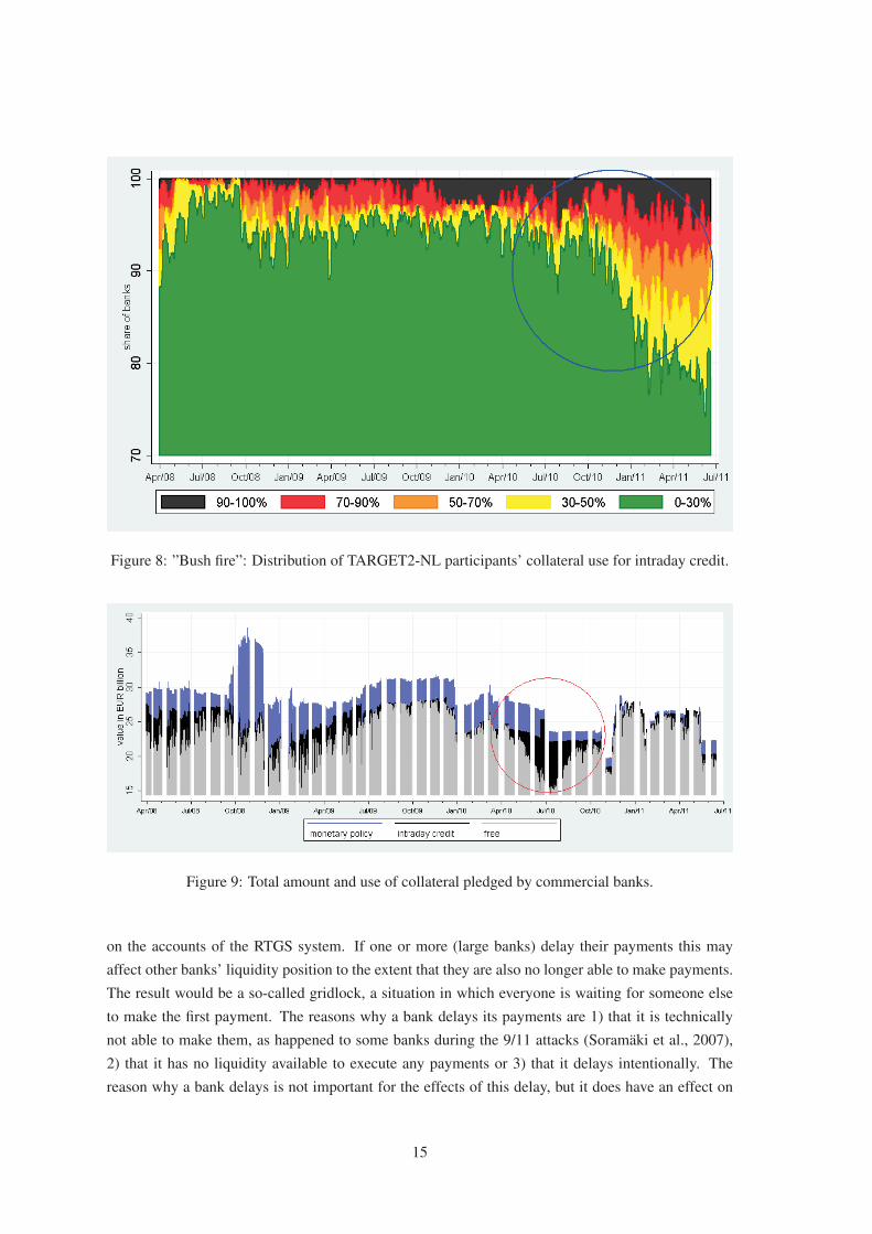
Figure 8: ”Bush fire”: Distribution of TARGET2-NL participants’ collateral use for intraday credit.

Figure 9: Total amount and use of collateral pledged by commercial banks.

on the accounts of the RTGS system. If one or more (large banks) delay their payments this may

affect other banks’ liquidity position to the extent that they are also no longer able to make payments.

The result would be a so-called gridlock, a situation in which everyone is waiting for someone else

to make the first payment. The reasons why a bank delays its payments are 1) that it is technically

not able to make them, as happened to some banks during the 9/11 attacks (Soramaki et al., 2007),

2) that it has no liquidity available to execute any payments or 3) that it delays intentionally. The

reason why a bank delays is not important for the effects of this delay, but it does have an effect on

15

the possibility to solve it quickly. This paper only focuses on either intentional delays or the inability

to make payments as a result of liquidity shortages.

Figure 10 shows the value-weighted average incoming (green line) and outgoing (red line) pay-

ments’ time. The green and red shaded areas are the corresponding 90% intervals. The graph dis-

tinguishes between bank-bank transactions excluding the interbank loan transactions and payments

on behalf of a client (client transactions). The reason for excluding these loan transactions is that

they differ in nature from ”real” payments. Besides, the current crisis has shown that the lending

activity decreased significantly, see e.g. Heijmans et al. (2010), without banks having any liquidity

problems. As interbank loans are generally of high value their partial disappearance could change all

payments’ average timing significantly even though not a single payment was delayed or paid earlier.

The client payments are usually not delayed as clients are assumed to have sufficient liquidity on their

accounts.15

By way of an example, the blue circle in Figure 10 shows an increase in the average outgoing

payments’ time to a level above the average incoming payments’ time, suggesting liquidity problems.

For the weeks before Fortis was nationalised, our data show evident changes in the average payments’

time. First there was a small increase in the outgoing payments’ time, in response to which the market

on average soon started delaying payments to Fortis. Fortis responded to this increase by reducing

its average outgoing payments’ time substantially. In other words: it began to transfer payments at a

very early stage. Fortis continued to do so as long as permitted by its liquidity position.

An interesting feature of the graph is the change-over from an early payer (red line below the

green one) to a late payer (red line above the green line), especially for banks known to be the payment

system’s liquidity provider. Over the years, most large banks in the Dutch payments system are known

to be early payers and provide the whole payment system with liquidity. The smaller banks use this

liquidity to execute their payment obligations. If these large banks start to pay later or even become

late payers this can seriously affect many banks’ liquidity positions and in the worst case lead to

a total gridlock. Large banks most likely provide so much liquidity to the payment system before

receiving liquidity because: 1) their relative large cash reserve requirements enables them to make

lots of payments before they have to use intraday credit and 2) as long as they receive their incoming

payments directly effecting their payments, there is only a short time interval of credit risk (in case of

a small bank’s failure).

Within the scope of payment system monitoring it is important to know when a change of the

average incoming or outgoing payments’ time can be taken as a signal. The day-to-day fluctuation

of Figure 10 is large and therefore not very meaningful for monitoring (noise). Looking at trend

variations (difference with the previous days), during 7 or 14 days, will be more useful. When defining

an automatic alarm signal a trade-off has to be made between the number of ”alarms” and the fact

that there is something going on. The more often a change of timing causes an alarm, the more often

the alarm will be false. However, if the change of timing chosen is very large there will hardly be

any hits, which might result in missing important changes. An alarm in the change of timing can be

shown by way of a traffic light. If the average incoming or outgoing time increases beyond e.g. the

95% interval once a yellow light can be given, and does so several times in a short period, a red light

15Anecdotal evidence obtained from liquidity managers of Dutch banks supports this idea.

16

Figure 10: Average time of incoming (green) and outgoing (red) payment flows (for February 2008 toFebruary 2011). Top graph displays bank-bank transactions excluding interbank loans. The bottomgraph shows the client transaction. The lines are the averages and the areas the 90% interval.

can be given. Anyhow, no matter what test or methodology is used there is always the probability of

a false positive or false negative, similar to tests in the medical world. The outcome of a medical test

can be positive, meaning you have the illness, but in fact you are not ill at all (false positive) or the

outcome is negative but you are ill (false negative).

If a yellow or red light is given for the average daily incoming or outgoing timing it is useful to

zoom in on the intraday payment patterns to see if there have been specific times there were delays.

Figure 11 shows the sum of the incoming (green bar) and outgoing (red bar) payment flows for every

15 minutes of the business day. The black lines show the comparison period to see the shift in timing.

The bottom graph shows the cumulative balance up until that time of the day. In contrast to the

average payments’ timing (Figure 10), it is possible to see intraday developments and a comparison

with a relevant other period. Figure 11 shows an example of a bank which has moved its outgoing

payments to the end of the day. The incoming payments of the other have also been moved towards

the end of the day.

3.5 Signals of a bank run

A bank facing liquidity and/or financial problems, which it is unable to solve, cannot keep these

problems silent for the general public (businesses and consumers) forever. If this public starts losing

faith in their bank and withdraw their money from this bank, the problems will accelerate and a bank

run is born. This loss of faith may e.g. be triggered by a steep decrease in the stock price of a bank,

as we have seen with Fortis, or a call for a bank run by an influential person as we have seen a few

weeks before the DSB bankruptcy.16

A start of a bank run becomes visible in the data of TARGET2-NL in five ways: 1) the banknote

withdrawals at the central bank, 2) the settlement of Equens (a Dutch settlement system), 3) client

16DSB used to be a non-systemic bank in the Netherlands.

17

Figure 11: Incoming (green bars) and outgoing (red bars) liquidity flows for each 15 minutes duringa business day or average business day of a month (top graph). Black line shows comparison period(another business day or average business of the previous month). The sum (blue bars) of the two ispresented in the bottom graph. The black line shows the comparison period.

payments and 4) urgent customer payments (TNS). The first two bank run types can be seen as ”retail”

bank runs since the net result of many customer transactions is settled in TARGET2. The last two

types can be seen as the ”wholesale” bank runs since each individual transaction become visible in

the TARGET2 data. An interesting aspect of each of the five bank run types is that the value settled

is generally very low compared to the total daily payment by a bank (below a few percentage points).

Nevertheless, by identifying the correct transactions of the bank run type from the TARGET2-NL

transactions data a clear signal of a bank run can become visible as soon as this bank run starts.

18

3.5.1 ”Retail” bank run

The most well-known bank run is the cash bank run. Customers who have lost faith in their bank,

stand in line of the their bank’s ATM or counter to withdraw their savings. As demand for cash

suddenly increases significantly, so does the commercial bank’s demand for cash (bank notes). The

bank can obtain the extra bank notes from their central bank, which brings bank notes into circulation.

Commercial banks’ cash withdrawals and deposits at the central bank are visible in TARGET2 as

individual transactions. The deposit and withdrawal patterns and the netted value differs from bank

to bank, depending on the banks’ clients which being more consumers withdrawing banknotes or

retailers depositing banknotes. Besides the overall positive or negative flow there are clear seasonal

effects, around e.g. Easter, Whitsun and Christmas. The reasoning behind these effects is that (for-

eign) consumers will hoard cash just before and during public holidays. The cash spent at retailers or

the surplus finds its way back to a bank, which deposits the surplus at the central bank. If the public

gets wind of a bank’s possible failure it will suddenly and massively start taking out cash from the

ATM or at the bank’s counter, which is the start of a bank run. A recent example of a bank run was

seen at Northern Rock in September 2007, see e.g. Shin (2009). Savers of this bank formed long

queues to withdraw their life savings.

A second retail bank run can be told from the data related to settlements in TARGET2-NL by

the settlement organisation (in the Netherlands this is Equens). Equens settles the debit card transac-

tions in the Netherlands in multiple cycles per day. The net position of all debit card transactions is

calculated and settled in TARGET2-NL. If customers of a bank suddenly spend much more of their

money this will become visible as a strong negative position for this bank. Just as for cash deposits

and withdrawals, whether a bank has a positive or negative position (in most settlement cycles) under

non-stressed circumstances depends on the type of clients (businesses or customers).

3.5.2 ”Wholesale” bank run

If banks’ customers, both companies and consumers, suspect a bank maybe about to fail, they can

transfer their money to another account. The large-value payments of companies will become visible

as client payments in the RTGS. The payments of consumers will become visible in the batch of

a settlement organisation (see Section 3.5.1) or directly in case of urgent payments. These urgent

payments are settled gross in TARGET2 within two hours after the instruction is given.

If customers have lost faith in their bank, they can massively send in client and urgent payment

instructions and transfer their funds to another bank. In this case the same will happen as with a

traditional bank run: the bank will soon run out of liquidity. The strength of this indicator compared

to the cash bank run is that there is less fluctuation over time. This makes it easier to define a deviation

from the normal patterns. Besides, banks might have sufficient cash available for the first few days of

a bank run, which means that the incidnet bank run becomes only available a few days after it started.

As a modified example, Figure 12 shows the in- and outflows of liquidity from client payments. A

sudden sharp increase in outflow in this graph may signal customers losing faith. In this modified

graph there was a strong outflow of liquidity in September 2009. After a few weeks this situation

normalises again, which can be the result of e.g. state support (liquidity injection or nationalisation).

19

Figure 12: Bank run client payments. Incoming (green line) and outgoing payments (red line.)September 2009 saw a temporary large outflow of client payments.

4 Behaviour of banks

4.1 Evidence from TARGET2-NL

As the payment system can be seen as a coordination game (McAndrews and Rajan, 2000; McAn-

drews and Potter, 2002 and Bech and Garratt, 2003), the participant’s behaviour during the game is

important. A study of the TARGET2-NL data of both the crisis period and the period before gives a

lot of information about what is ”normal” and ”stressful” behaviour. A close look at what happened

after Lehman Brothers’ failure or before the nationalisation of Fortis and ABN AMRO, DSB Bank’s

failure and the state support, provides a wealth of information about the way banks react to shocks.

4.1.1 Changes in interbank loans

The interbank market after Lehman Brothers’ failure decreased significantly. Evidence of this effect

has been found by Heijmans et al. (2010) for the Dutch market, Guggenheim et al. (2010) for the

Swiss market and Akram and Christophersen (2010) for the Norwegian market. Some banks in

20

the Dutch payment system lend no liquidity anymore after Lehman’s failure, even though they had

sufficient liquidity available to do so. This is probably due to the market’s increased perception of risk.

Some banks which were generally a lending bank decreased their lending significantly in response to

rumours and facts were known about these banks due to decrease in surplus. At the same time, when

borrowing became more difficult for these banks,they had to have recourse to liquidity provided by

the ECB (tenders and, in the end, marginal lending).

After the ECB had made year tenders available starting July 2009, many banks applied for these

tenders as a security for potential future shocks. This liquidity was in many cases not necessary for the

short term, as illustrated by the use of the overnight deposits directly after the tenders were received

by the banks. The use of overnight deposits showed a peak just before the repayment the year after

(July 2010) and gradually decreased to almost zero in March 2011.

4.1.2 Changes in timing of payments

Some banks that rumoured to suffer or actually facing liquidity and financial problems showed quire

interesting payment patterns. We expected to see a slow increase in outgoing payments over time as a

result of the worsened liquidity position. Initially this is exactly what happened. At first there was the

expected delay in the payments’, and also the average timing of incoming payments rose. However,

the increase in average outgoing payments’ timing was quickly followed by a sharp decrease to an

average time below the ”normal” timing, with the average timing of incoming payments decreasing

accordingly. This may reflect that the troubled banks wanted to give a clear signal to the market that

they could meet their payment obligations in time. A troubled bank will continue this behaviour until

it is no longer able to do this anymore for lack of sufficient liquidity.

4.1.3 Changes in collateral

In the heat of the crisis collateral was used much more often for intraday credit and monetary loans

than before the crisis. Especially after Lehman Brothers’ failure several banks faced difficulties fund-

ing themselves, which resulted in an increased use of collateral to keep fulfilling the payment obliga-

tions. The relative use of collateral increased for two reasons: 1) Some banks needed the collateral for

other purposes. If these banks use the same amount of collateral for intraday credit and monetary pol-

icy, the relative amount increases 2) Other banks had to use more collateral to fulfil their obligations.

In these cases also the absolute use of collateral for intraday credit and monetary policy increased.

4.1.4 Signs of a bank run

When the public became aware that a bank was having severe liquidity and financial problems and

started worrying about a potential bankruptcy the data showed substantial outflows of banknotes,

client payments and, in particular, emergency payments.

21

4.1.5 Existence of bilateral limits

It is expected that banks use bilateral limits to limit the maximum exposure to counterparties. Al-

though, in TARGET2, banks have the possibility to use bilateral limits, this feature is not used by the

banks participating through TARGET2-NL. This does not mean, however, that banks do not make

use of bilateral limits in their own systems. The transactions between participants have been analysed

for the existence of bilateral limits between participants. To find the limits in the data, we calculated

the running bilateral net positions of two banks, A and B, during the day. When no limit was set by

any of the banks, the running balances would be expected to follow a random walk. If, however, bank

A had limited its position to a certain amount, the bilateral net position would often lie just beneath

this limit, only to drop shortly as a result of incoming payments, and immediately to rise to this limit

again as a result of outgoing payments . Bilateral limits will therefore deviate from random walks

and thus immediately show up when time-weighted frequency counts of the bilateral balances are

produced. The transaction data showed signs of the use of bilateral limits and even counter-limits by

the other bank. When it was known that a bank was facing severe liquidity or financial problems, the

bilateral limits for this bank were tightened to limit the exposure even further. From the discussions

we have had with commercial banks, we also learned that banks grew more reluctant to allow a bank

that might run into trouble to have a large negative position. This corroborates our expectation that

such limits are applied.

4.2 Set of behavioural rules

Simulations are often based on historical transactions. The difficulty of using historical data is that

these data usually do not reflect the stress scenario of interest. Therefore these historical data have

to be modified to reflect this scenario. Part of this modification consists of introducing ”adequate”

behaviour of banks in order to obtain realistic outcomes. The rules defined in this section are set up

to be used for scenario analysis using historical data. Examples of scenarios are liquidity problems

with a single bank, decreased trust in the interbank money market, changing monetary policy of the

ECB, an operational outage of the payment system limiting the number of payments possible, etc.

The scenario determines which of the rules have to be applied.

4.2.1 Preparation rule

Historical data not only contain regular payments, deposits of collateral and monetary loans, but

also interbank loans, marginal lending and overnight deposit transactions. The latter are the result

of a temporary shortage or surplus at the RTGS account. A shortage signifies that the cash reserve

requirement cannot be met. A stress scenario for the payment system is designed to determine the new

liquidity position , i.e. the liquidity shortage or surplus, if the scenario were to materialise. Therefore,

when historical data are used the transaction data have to be cleaned for these funding transactions.

Preparation rule 1 Historical transaction data used for scenario analysis of payment systems have

to be cleaned for interbank loans, monetary policy transactions, marginal lending and ECB overnight

deposit.

22

4.2.2 Behavioural rules

The liquidity position of a bank can be influenced by all four elements in the overview of Figure 1:

monetary policy, interbank market, collateral deposited and ”real” payments. The behaviour (or pol-

icy) of the actor(s) behind these four elements determines what the effect on the liquidity position of

these banks will be. We identify the following actors:

A. Monetary policy: the central bank

B. (Part of) the interbank market: banks that enter the market for lending and/or borrowing

C. Payments: banks and bank’s customers (consumers and businesses)

D. Collateral: bank(s) depositing collateral for monetary and/or payment purposes. The central

bank steers the eligibility and haircuts of the collateral, thus determining in the collateral value.

Monetary policy. The central bank uses its monetary policy to tighten or widen the money supply

in the economy. If it wants to tighten the amount of liquidity, it can raise its main interest rate, the

refinancing rate, making lending from the central bank more expensive. The more a bank lends or

wants to lend the stronger the effect of a refinancing rate’s increase will be for that particular bank.

Another option central banks have, is to change the maintenance requirements. The higher/lower

the requirement, the higher/lower the average amount of cash on banks’ accounts need to be. This

requirement affects individual banks differently as the requirement is bank-specific.

Behavioural rule 1 Increase/decrease the access to tenders and/or decrease/increase cash reserve

requirements depending on the central bank’s role in the scenario.

The Interbank market. The participants in the LVPS have several options to influence their coun-

terparties’ liquidity positions. The first option they have is to change the lending amount in the

interbank money market. The level of trust a bank has in its counterparties determines the willingness

to lend. If a bank does not trust (some or all of) its counterparties, it will decrease or cease its lending.

If trust comes back, the lending amount will increase again.

Behavioural rule 2 Decrease/increase the amount a bank can borrow in the interbank money market

depending on the level of trust in this bank.

Payments. Besides the interbank market, a bank can set bilateral and/or multilateral limits to one or

more counterparties. A bilateral or multilateral limit is the most negative position this bank is willing

to accept from a single counterparty or all counterparties respectively. If a limit is reached, the bank

first needs to receive incoming payments either from the single participant (in case of bilateral limit)

or one of the participants in the payment system (multilateral limits) before continuing to make its

own payments. Section 4.1.5 described signs of bilateral limits’ existence in our data. This can be

translated into a behavioural rule by dividing the market into several groups:

A. Reliable banks: High rating and no rumours or negative news facts.

23

Table 1: An example of bilateral limits of banks between the three groups. The percentages mentionedrefer to the fraction of the total daily outgoing payment value.

��������������Sending bankReceiving bank

A B C

A 5% 2.5% 1%with max EUR 250 with max EUR 125 with max EUR 50

million million millionB 5% 2% 0.5%

with max EUR 250 with max EUR 100 with max EUR 25million million million

C 3% 1% 0.2%with max EUR 150 with max EUR 50 with max EUR 10

million million million

B. Less reliable banks: Lower rating or first rumours in the market.

C. Banks in trouble: Strong rumours and negative news facts regarding liquidity/financial prob-

lems.

Combining the three types of banks will lead to 9 possible outgoing payment flows with different

setups of the bilateral limits, see Table 1 for examples of these limits. Banks with a high rating (bank

type A) want to be seen as reliable by all counterparties. For other ”reliable” banks they will therefore

observe a high bilateral limit. Regarding B-bank they will be slightly more reluctant but still accept

a negative balance during the day. As regard to a bank which is the target of very negative publicity

A-banks will be very careful and will only accept a relatively small negative intraday position. B-

banks will observe slightly lower bilateral limits for B-banks and C-banks as their liquidity positions

are somewhat worsened as a result of the first rumours in the market. Banks in trouble (C-banks) are

basically compelled to change their limits to make sure they can pay as many counterparties. Due

to the strict limits applying, this bank has to make sure it can have a negative balance with as many

counterparties as needed in order to keep on receiving payments from its counterparties.

Behavioural rule 3 Set bilateral limits depending on the type of bank.

Clients. At the moment when clients start losing faith in their bank there will be an increase in the

outflow of liquidity. While the increase of payments as such cannot be controlled by the problem

bank, the moment when these payments are settled can be (see below). Even though client payments

are usually low relative to the total daily turnover of a bank’s payments in the LVPS, the bank will

increasingly be affected by the extra outflow and the liquidity position will worsen.

Behavioural rule 4 Increase the outgoing payments’ amount when the stress with respect to a bank

continues.

24

Bank in trouble. A bank facing liquidity problems cannot control the behaviour of its counterpar-

ties, central bank or its clients. It has however a few options to steer its liquidity position. We start

with setting priorities to payments. Not all transactions in TARGET2 are equally important in terms

of timing and impact. Continuous Linked Settlement (CLS) transactions e.g. have a very high priority

and are very time-critical.17 CLS is used by banks to settle foreign exchange transactions. The bene-

ficiary of the transaction may be in another time zone and another LVPS. If this party does not receive

the expected funds, it can face severe liquidity problems. The beneficiary commercial bank can either

be another bank than the sender or a branch of the sending bank. The payments executed to settle

the net balances of the EURO1 at the settlement account of the ECB and the payment obligations

which result from settlement organisations (like e.g. the Dutch settlement organisation Equens) are

also time-critical and therefore have a high priority.18 It can be assumed that banks do not ignore or

delay these time-critical payments intentionally.

Besides time-critical payments also payments on behalf of a customer will be executed relatively

timely. Payment orders of customers with sufficient liquidity on their accounts will be executed

within the normal time frame (of the contractual arrangement). Even though the bank might not have

sufficient liquidity on its account, the customer does, and therefore the bank is obliged to meet its

contractual obligations. Failure to do so might damage the bank’s reputation and result in customer

claims.

Due to the difference in time criticality the bank prioritises its outgoing payments. The most

time-critical payments, like CLS, EURO1, and settlement organisations have the highest priority

(priority 1). The client payments will have a slightly lower priority (priority 2). All other payments

are considered less time-critical and therefore have the lowest priority (priority 3). If required, it is

possible to define more levels of priorities.

Behavioural rule 5 Transactions in payment system’s scenario analysis have to be divided into pri-

orities e.g.: 1) very time-critical, 2) time-critical and 3) other payment transactions.

The second option a bank has to steer its liquidity position, is to change the timing of payments.

In the transaction data of TARGET2-NL we have found that the troubled bank pays as soon as pos-

sible (see Section 4.1.2), which means as long as liquidity (balance and intraday credit) is available.

If possible, it will start paying even earlier than it was used to do. If a bank were to delay its pay-

ments instead of paying in time and did so long enough, it would at some point not receive payments

anymore as all bilateral limits to this bank would have been reached. Depending on the aim of the

scenario, you let the bank in trouble pay as early as possible if you want to simulate a ”natural” reac-

tion by the troubled bank. If you want to investigate whether delaying payments by a bank will lead

to a gridlock, the payments should be delayed.

Behavioural rule 6 Change the timing of the outgoing payments.

17CLS is a settlement process by which a number of the world’s largest banks manage settlement of foreign exchangeamongst themselves (and their customers and other third-parties).

18EURO1 is a private sector owned payment system for domestic and cross-border single payments in euro betweenbanks operating in the European Union. It is a net settlement system. Payments are processed throughout the day. Balancesare settled at the end of the day via a settlement account at the European Central Bank.

25

Table 2: An example of collateral values of each bank type, which can be used for intraday credit.

bank type Collateral level sending bankA 5 * daily averageB 2 * daily averageC 0.5 * daily average

Collateral. The last option a bank in trouble has to change its liquidity position is to change the

amount of available collateral. As described in Section 4.1.3, our data showed that some banks in

liquidity problems lowered their amount of collateral. Even tough this was a voluntary action by the

bank in trouble, it had an adverse effect on their liquidity position. Ideally a bank in trouble brings

in more collateral to increase its liquidity position (use liquidity for tenders and/or intraday) credit.

Especially if the other actors (the market and clients) have changed their behaviour in such a way that

it affects the liquidity position of the problem bank. Table 2 shows an example of collateral values

banks have available for intraday credit for each of the three bank types, which can be used in scenario

analysis. The central bank steers the eligibility and haircuts of collateral that is (to be) deposited.

Behavioural rule 7 Decrease the collateral’s amount, which can be used for intraday credit and

tenders, when the stress scenario aims to simulate severe problems with a bank.

Behavioural rule 8 Decrease the collateral amount, caused by reduced eligibility and/or increased

haircuts of collateral.

5 Conclusions

This paper shows how the TARGET2 transaction and collateral data can be used to monitor banks.

The monitoring looks at 1) the overall liquidity position, 2) demand and supply of liquidity, 3) timing

of payments, 4) amount and use of collateral and finally 5) signs of a bank run. Combining the

different elements of the monitoring gives information on the liquidity position of an individual bank.

If just one of the indicator points in a certain direction, this need not mean much, but if more than

one indicators point in the same direction it is clear that a bank is facing liquidity problems. If there

are signs of liquidity or financial problems with a certain bank, this will first become visible in the

ability to borrow the required liquidity. If the market perceives the risk as higher (or too high) that

bank either has to pay higher interest rates for its loans due to this increased counterparty risk, or

cannot borrow sufficient liquidity to fulfil its (maintenance) obligations. As a result of the lack of

liquidity the troubled bank will proceed to make more intensive use of the ECB facilities (tenders and

intraday credit) more intensively. Besides the inability to borrow the troubled bank faces a second

liquidity decreasing measure by other banks by way of bilateral limit. These limits will reduce the

negative position other banks are willing to accept towards the troubled bank. Even though these

measures worsen its liquidity position, the troubled bank will seek to pay as early as possible to

give a clear signal to the market that it is able to fulfil its obligations. By doing so it decreases the

26

negative impact of the bilateral limits. The troubled bank is able to pay early as long as liquidity

is available. If it runs out of liquidity it has no other option than to delay payments. If customers

become aware of a bank’s problems and expects a failure, they will either withdraw cash from the

ATM or, more effectively transfer their money to another bank (either through client payments for

the larger customers, or using urgent payments through internet banking). The liquidity position of

the troubled bank then goes from bad to worse. Such a situation can usually only be solved with a

market intervention (one or more banks take over this bank) or a state intervention (in terms of state

support or nationalisation). If there is no intervention, the troubled bank will most likely collapse as

the liquidity or financial problems are too big to be solved by the bank itself.

The set of behavioural rules described in this paper can be used in payment system stress scenario

analyses, e.g. in simulations or network topology. The set of rules is based on the reaction patterns

found in the TARGET2-NL transaction data and collateral management data before, during and after

times of increased stress due to financial/liquidity problems of one or more banks. Using these rules

improves the realism of stress scenarios and therefore the usefulness of its outcomes. The key features

of the set of rules are divided into 1 preparation and 8 behavioural rules.

This paper shows that the TARGET2-NL transaction and collateral data gives valuable informa-

tion on the liquidity position of banks. Close monitoring of banks using this data may reveal early

signs of liquidity and/or financial problems. By looking into more detail it is possible to monitor the

funding need and methodology of single banks, and how they change over time. After first identifying

liquidity problems in the data or in other supervision information, the monitoring tool described in

this paper can give up-to-date information on the problems’ developments (up until the last business

day if required). The information obtained from the TARGET2-NL transaction and collateral data

renders it unnecessary to rely on the information given by banks themselves, which may be unreli-

able because facts may have been distorted or potential problems camouflaged. It is however not a

substitute for current supervision information but a useful addition.

References

Abbink, K., Bosman, R., Heijmans, R., and van Winden, F. (2010). Disruptions in large value pay-ment systems: An experimental approach. DNB Working Paper, 263.

Akram, F. A. and Christophersen, C. (2010). Interbank overnight rates - gains from systemic impor-tance. Norges Bank Working Paper, 11.

Allen, F. and Gale, D. (2000). Financial contagion. Journal of Political Economy, 108:1–33.

Bech, M. and Atalay, E. (2008). The topology of the federal funds market. Federal Reserve Bank ofNew York Staff Reports, 354.

Bech, M. and Garratt, R. (2003). The intraday liquidity management game. Journal of EconomicTheory, 109:198–210.

Bech, M. and Garratt, R. (2006). Illiquidity in the interbank payment system following wide-scaledisruptions. Federal Reserve Bank of New York Staff Reports, 239.

27

Bech, M. and Soramaki, K. (2005). Systemic risk in a netting system revisited. In Leinonen, H., editor,Liquidity, risks and speed in payment ad settlement systems - a simulation approach, number E:31in Proceedings form the Bank of Finland Payment and Settlement System Seminars 2005, pages151–178.

Carlin, B., Lobo, M., and Viswanathan, S. (2007). Episodic liquidity crisis: The effect of predatoryand cooperative trading. Journal of Finance, 62:2235–2274.

Cocco, J., Gomes, F., and Martins, N. (2009). Lending relationships in the interbank market. Journalof Financial Intermediation, 18:24–48.

Furfine, C. (1999). The microstructure of the federal funds market. Financial Markets, Institutionsand Instruments, 8:24–44.

Guggenheim, B., Kraenzlin, S., and Schumacher, S. (2010). Solving the puzzel: Evidence of theunsecured swiss franc money market. Swiss National Bank Working Paper, 5.

Heijmans, R. (2009). Simulation in the dutch interbank payment system: A sensitivity analysis. InLeinonen, H., editor, Simulation analyses and stress testing of payment networks, number E42 inProceedings form the Bank of Finland Payment and Settlement System Seminars 2007-2008, pages123–144.

Heijmans, R., Heuver, R., and Walraven, D. (2010). Monitoring the unsecured interbank moneymarket using target2 data. DNB Working Paper, 276.

Imakubo, K. and Soejima, Y. (2010). The microstructure of japan’s interbank money market: Sim-ulating contagion of intraday flow of funds using boj-net payment data. Monetary and Economicstudies, 28:151–180.

Iori, G., de Masi, G., Precup, O. V., Gabbi, G., and Caldarelli, G. (2008). A network analysis of theitalian overnight money market. Journal of Economic Dynamics & Control, 32:259–278.

Koponen, R. and Soramaki, K. (2005). Intraday liquidity needs in a modern interbank paymentsystem - a simulation approach. In Leinonen, H., editor, Liquidity risks and speed in payment andsettlement systems - a simulation approach, number E31 in Proceedings form the Bank of FinlandPayment and Settlement System Seminars 2005, pages 71–114.

Lacker, J. (2004). Payment system disruptions and the federal reserve following september 11 2001.Journal of Monetary Economics, 51(5):935–965.

Ledrut, E. (2007). Simulating relation in payment systems: Can banks control their exposure to afailing participant? DNB Working Paper, 133.

McAndrews, J. and Potter, S. (2002). Liquidity effects of september 11th. Federal Reserve Bank ofNew York Economic Policy Review, 8:59–79.

McAndrews, J. and Rajan, S. (2000). The timing and funding of fedwire funds transfers. FederalReserve Bank of New York Economic Policy Review, 6:17–32.

Propper, M., van Lelyveld, I., and Heijmans, R. (2008). Towards a network description of interbankpayment flows. DNB Working Paper, 177.

Shin, H. (2009). Reflections on northern rock: the bank run that heralded the global financial crisis.Journal of Economic Perspective, 23:101–119.

28

Soramaki, K., Bech, M., Arnold, J., Glass, R., and Beyeler, W. (2007). The topology of interbankpayment flows. Physica A, 379(1):317–333.

Wetherilt, A., Zimmerman, P., and Soramaeki, K. (2010). The sterling unsecured loan market during2006-2008: insights from network topology. BoE Working Paper, 398.

29

Previous DNB Working Papers in 2011 No. 276 Ronald Heijmans, Richard Heuver and Daniëlle Walraven, Monitoring the unsecured

interbank money market using TARGET2 data No. 277 Jakob Bosma, Communicating Bailout Policy and Risk Taking in the Banking Industry No. 278 Jakob de Haan and Fabian Amtenbrink, Credit Rating Agencies No. 279 Ralph de Haas and Neeltje van Horen, Running for the Exit: International Banks and

Crisis Transmission No. 280 I Kadek Dian Sutrisna Artha and Jakob de Haan, Labor Market Flexibility and the Impact

of the Financial Crisis No. 281 Maarten van Oordt and Chen Zhou, Systematic risk under extremely adverse market

conditions No. 282 Jakob de Haan and Tigran Poghosyan, Bank Size, Market Concentration, and Bank

Earnings Volatility in the US No. 283 Gabriele Galati, Peter Heemeijer and Richhild Moessner, How do inflation expectations

form? New insights from a high-frequency survey No. 284 Jan Willem van den End, Statistical evidence on the mean reversion of interest rates No. 285 Marco Hoeberichts and Ad Stokman, Price dispersion in Europe: Does the business cycle

matter? No. 286 Cai Cai Du, Joan Muysken and Olaf Sleijpen, Economy wide risk diversification in a three-

pillar pension system No. 287 Theoharry Grammatikos and Robert Vermeulen, Transmission of the Financial and

Sovereign Debt Crises to the EMU: Stock Prices, CDS Spreads and Exchange Rates No. 288 Gabriele Galati, Federica Teppa and Rob Alessi, Macro and micro drivers of house Price

dynamics: An application to Dutch data No. 289 Rob Alessie, Maarten van Rooij and Annamaria Lusardi, Financial Literacy, Retirement

Preparation and Pension Expectations in the Netherlands. No. 290 Mara Demertzis, Public versus Private Information No. 291 Enrico C. Perotti and Javier Suarez, A Pigovian Approach to Liquidity Regulation No. 292 Jan Willem Slingenberg and Jakob de Haan, Forecasting Financial Stress No. 293 Leo de Haan and Jan Willem van den End, Banks’ responses to funding liquidity

shocks: lending adjustment, liquidity hoarding and fire sales No. 294 Janko Gorter and Jacob A. Bikker, Investment risk taking by institutional investors No. 295 Eric J. Bartelsman, Pieter A. Gautier, and Joris de Wind, Employment Protection,

Technology Choice, and Worker Allocation No. 296 Maarten R.C. van Oordt and Chen Zhou, The simple econometrics of tail dependence No. 297 Franka Liedorp, Robert Mosch, Carin van der Cruijsen and Jakob de Haan, Transparency

of banking supervisors No. 298 Tiziana Assenza, Peter Heemeijer, Cars Hommes and Domenica Massaro, Individual

Expectations and Aggregate Macro Behavior No. 299 Steven Poelhekke, Home Bank Intermediation of Foreign Direct Investment No. 300 Nicole Jonker, Card acceptance and surcharging: the role of costs and competition No. 301 Mark Mink, Procyclical Bank Risk-Taking and the Lender of Last Resort No. 302 Federica Teppa, Can the Longevity Risk Alleviate the Annuitization Puzzle? Empirical

Evidence from Dutch Data No. 303 Itai Agur and Maria Demertzis, “Leaning Against the Wind” and the Timing of Monetary

Policy No. 304 Gabriele Galati, John Lewis, Steven Poelhekke and Chen Zhou, Have market views on the

sustainability of fiscal burdens influenced monetary authorities’ credibility? No. 305 Itai Agur, Bank Risk within and across Equilibria No. 306 Iman van Lelyveld and Marco Spaltro, Coordinating Bank Failure Costs and Financial

Stability No. 307 Enrico Perotti, Lev Ratnovski and Razvan Vlahu, Capital Regulation and Tail Risk

- 2 -

Previous DNB Working Papers in 2011 (continued) No. 308 Ayako Saiki, Exchange Rate Pass-Through and Monetary Integration in the Euro Area No. 309 Maria Demertzis and Nicola Viegi, Interdependence of Fiscal Debts in EMU No. 310 Matej Marinč and Razvan Vlahu, The Economic Perspective of Bank Bankruptcy Law No. 311 Jacob Bikker, Thijs Knaap and Ward Romp, Real Pension Rights as a Control Mechanism

for Pension Fund Solvency No. 312 Stefan Trautmann and Razvan Vlahu, Strategic Loan Defaults and Coordination: An

Experimental Analysis No. 313 Maarten van Rooij, Annamaria Lusardi and Rob Alessie, Financial Literacy, Retirement

Planning, and Household Wealth No. 314 Irina Stanga, Sovereign and Bank Credit Risk during the Global Financial Crisis No. 315 Carin van der Cruijsen, Jakob de Haan, David-Jan Jansen and Robert Mosch, Household

savings behaviour in crisis times

DN

B W

OR

KIN

GP

AP

ER

DNB Working PaperNo. 35/April 2005

Jan Kakes and Cees Ullersma

Financial acceleration of booms

and busts

De Nederlandsche BankDe Nederlandsche Bank