ionic composition of precipitation in marmaris station

IONIC COMPOSITION OF PRECIPITATION IN MARMARIS STATION

A THESIS SUBMITTED TO

THE GRADUATE SCHOOL OF NATURAL AND APPLIED SCIENCES

OF

MIDDLE EAST TECHNICAL UNIVERSITY

BY

GİZEM YÜCEL

IN PARTIAL FULLFILLMENT OF THE REQUIREMENTS

FOR

THE DEGREE OF MASTER OF SCIENCE

IN

ENVIRONMENTAL ENGINEERING

MAY 2019

Approval of the thesis:


submitted by GİZEM YÜCEL in partial fulfillment of the requirements for the degree

of Master of Science in Environmental Engineering Department, Middle East

Technical University by,

Prof. Dr. Halil Kalıpçılar

Dean, Graduate School of Natural and Applied Sciences

Prof. Dr. Bülent İçgen

Head of Department, Environmental Eng.

Prof. Dr. Gürdal Tuncel

Supervisor, Environmental Eng., METU

Examining Committee Members:

Prof. Dr. İpek İmamoğlu

Environmental Engineering, METU

Prof. Dr. Gürdal Tuncel


Assoc. Prof. Dr. Tuba Hande Ergüder Bayramoğlu


Assist. Prof. Dr. Zöhre Kurt


Assist. Prof. Dr. Ebru Koçak

Environmental Engineering, Aksaray University

Date: 08.05.2019

iv

I hereby declare that all information in this document has been obtained and

presented in accordance with academic rules and ethical conduct. I also declare

that, as required by these rules and conduct, I have fully cited and referenced all

material and results that are not original to this work.

Name, Surname:

Signature:

Gizem Yücel

v

ABSTRACT


Yücel, Gizem

Master of Science, Environmental Engineering

Supervisor: Prof. Dr. Gürdal Tuncel

May, 2019, 124 pages

In this study, wet-only rain samples were collected at a high-altitude rural site, by

General Directorate of Meteorology, between July 2011 and November 2016. The

sampling station was located at Marmaris Meteorological Radar, which has an altitude

of 1000 m from sea level and located 15 km to the North of Marmaris. Collected

samples were analyzed for major ions (SO42-, NO3

-, NH4+, H+, Ca2+, Mg2+, K+ and Na+)

by ion chromatography. Approximately 300 samples were collected and analyzed

during study period. Residence time calculations showed that the station is under the

influence of emissions at western Turkey and Balkan countries. Average pH of

rainwater is 6.0 indicating extensive neutralization, which can be attributed to CaCO3,

which is an abundant component in alkaline soil on the Mediterranean coast of Turkey.

Neutralization of rainwater acidity is almost complete during summer period and

decreases in winter, owing to limited resuspension of soil in winter. Trajectories of the

station are grouped into 5 clusters, residence time analysis of trajectory segments with

altitudes less than 500 m indicated that western parts of Turkey, Balkan countries,

Ukraine and the Black Sea coast of Russia are potential source regions affecting

composition of rainwater at Eastern Mediterranean. Most of the ions measured in this

work have higher concentrations during summer season. The positive matrix

factorization model revealed four factors, which were identified as two anthropogenic,

one marine and one crustal factors. Potential source regions for the anthropogenic

vi

components in rainwater were identified as to be western Ukraine, Western Black Sea

coast of the Turkey, Balkan Countries, North Africa and Georgia.

Keywords: Eastern Mediterranean, Wet Deposition, Rainwater Composition, Acid

Rain, Back Trajectory

vii

ÖZ

MARMARIS İSTASYONUNDA YAĞIŞIN İYONİK KOMPOZİSYONU

Yücel, Gizem

Yüksek Lisans, Çevre Mühendisliği

Tez Danışmanı: Prof. Dr. Gürdal Tuncel

Mayıs, 2019, 124 sayfa

Yağmur suyunun kimyasal bileşimi bir bölgeden diğerine kirletici taşınımının önemli

bir göstergesidir. Kıyı alanlarında daha da önemlidir, çünkü ıslak kirleticilerin

birikmesi deniz ortamında önemli bir kirlilik kaynağı olabilir. Bu çalışmada, Temmuz

2011 - Kasım 2016 tarihleri arasında Meteoroloji Genel Müdürlüğü tarafından yüksek

rakımlı bir kırsal alanda yağmur örnekleri toplanmıştır. Örnekleme istasyonu,

Marmaris Meteoroloji Radarı'na 1000 m. deniz seviyesi ve Marmaris'in 15 km

kuzeyine bulunmaktadır. Toplanan örnekler, iyon kromatografısi ile ana iyonlar (SO42-

, NO3-, NH4

+, H+, Ca2+, Mg2+, K+ ve Na+) için analiz edildi. Çalışma süresi boyunca

yaklaşık 300 örnek toplanmış ve analiz edilmiştir. Kalma süresi hesaplamaları,

istasyonun batı Türkiye ve Balkan ülkelerindeki emisyonların etkisinde olduğunu

gösterdi. Ortalama yağış suyu pH'ı, Türkiye’nin Akdeniz kıyılarındaki alkali

topraklarda bol miktarda bulunan CaCO3’a atfedilebilecek olan, geniş nötrleşme

olduğunu gösteren 6.0’dır. Yağmur suyunun asitliğinin nötralizasyonu yaz döneminde

neredeyse tamamlanmakta ve kışın toprağın yeniden süspansiyon haline gelmesi

nedeniyle kışın azalmaktadır. İstasyonun yörüngeleri 5 kümeye ayrılır, 500 m'den daha

düşük rakımlı yörünge bölümlerinin oturma süresi analizi, Türkiye'nin batı

bölgelerinin, Balkan ülkelerinin, Ukrayna'nın ve Rusya'nın Karadeniz kıyılarının,

Doğu Akdeniz'de yağmur suyunun bileşimini etkileyen potansiyel kaynak bölgeler

olduğunu göstermiştir. Bu çalışmada ölçülen iyonların çoğu yaz mevsiminde daha

viii

yüksek konsantrasyonlara sahiptir. Pozitif matris faktoring modeli, iki antropojenik,

bir deniz ve bir kabuksal faktör olarak tanımlanan dört faktör ortaya koydu. Yağmur

suyundaki antropojenik bileşenlerin potansiyel kaynak bölgelerinin batı Ukrayna,

Türkiye'nin Batı Karadeniz kıyıları, Balkan Ülkeleri, Kuzey Afrika ve Gürcistan

olduğu tespit edildi.

Anahtar Kelimeler: Doğu Akdeniz, Yaş Çökelme, Yağmur Suyu Kompozisyonu, Asit

Yağmuru, Geri Yörünge

ix

“There's a point, around age twenty, when you have to choose whether to be like

everybody else the rest of your life, or to make a virtue of your peculiarities.

Those who build walls are their own prisoners. I'm going to go fulfil my proper

function in the social organism. I'm going to go unbuild walls.”

― Ursula K. Le Guin

x

ACKNOWLEDGEMENTS

I would like to express my gratitude to my supervisor Prof. Dr. Gürdal Tuncel for his

advice, guidance and insight throughout the research. I would also like to thank Ali

İhsan İlhan, Tülay Balta and Yalçın Ün from the General Directorate of Meteorology

for providing us the rainwater data without which this work will not be possible.

I would like to thank my committee members Prof. Dr. İpek İmamoğlu, Assoc. Prof.

Dr. Tuba Hande Ergüder Bayramoğlu, Assist. Prof. Dr. Zöhre Kurt, Assist. Prof. Dr.

Ebru Koçak for their contributions.

I would like to especially thank Dr. İlker Balcılar for teaching me about the modeling

programs that I am supposed to use and guiding in the times when I needed. I also

would like to thank old and current members of our Air Pollution and Quality Research

Group Elif Sena Uzunpınar and Pınar Tuncer for their supports.

I also would like to thank my dear friends Elif Begüm Gökerküçük, Selin Özkul, Hazal

Aksu Bahçeci, Nazlı Barçın Doğan, Melike Kiraz, Ceren Ayyıldız for their endless

support and friendship.

Finally, I would like to express my deepest gratitude and love to my father, mother

and sister for their unconditional love and everything that they have done for me

throughout my life.

I gratefully acknowledge the financial support provided by The Scientific and

Technological Research Council of Turkey (TÜBİTAK) under project grant no:

115Y252.

xi

TABLE OF CONTENTS

ABSTRACT ................................................................................................................. v

ÖZ ............................................................................................................................ vii

ACKNOWLEDGEMENTS ......................................................................................... x

TABLE OF CONTENTS ............................................................................................ xi

LIST OF TABLES .................................................................................................... xiv

LIST OF FIGURES ................................................................................................... xv

LIST OF ABBREVIATIONS ................................................................................. xviii

CHAPTERS

1. INTRODUCTION ............................................................................................... 1

1.1. Aim of the Study ........................................................................................... 1

2. LITERATURE REVIEW..................................................................................... 3

2.1. Atmospheric Removal Mechanisms .............................................................. 3

2.2. Acid Deposition ............................................................................................. 3

2.2.1. Chemical Composition of Acid Precipitation ........................................ 4

2.2.1.1. Principle Precursors of Acidification .............................................. 5

2.2.1.2. Principle Precursors of Neutralization ............................................ 6

2.2.2. Studies of Acid Precipitation ................................................................. 6

2.2.2.1. Studies of Chemical Precipitation................................................... 6

2.3. Source Apportionment .................................................................................. 8

2.3.1. Source Oriented Models ......................................................................... 9

2.3.2. Receptor Oriented Models ..................................................................... 9

2.3.2.1. Trajectory Statistics ...................................................................... 10

xii

2.3.2.2. Potential Source Contribution Function ........................................ 11

2.3.2.3. Positive Matrix Factorization ........................................................ 12

2.4. Geography and Climatology of Study Area ................................................ 14

3. MATERIALS AND METHODS ....................................................................... 15

3.1. Sampling Site ............................................................................................... 15

3.2. Collection of Wet Deposition Samples ....................................................... 17

3.3. Sample Handling ......................................................................................... 18

3.3.1. Determination of Volume and pH ........................................................ 18

3.3.2. Preparation of Samples for Ion Chromatography ................................ 18

3.4. Analysis of Samples .................................................................................... 19

3.5. Data Quality Assurance ............................................................................... 20

3.5.1. Field Blanks .......................................................................................... 20

3.5.2. Calculation of Detection Limits ........................................................... 20

3.5.3. Quality Assurance ................................................................................ 21

3.6. Computation of Back Trajectories ............................................................... 22

3.6.1. Flow Climatology ................................................................................. 23

3.7. Potential Source Contribution Function ...................................................... 25

3.8. Positive Matrix Factorization ...................................................................... 27

4. RESULTS AND DISCUSSION ........................................................................ 29

4.1. General Characteristics of the Data ............................................................. 29

4.1.1. Distribution Characteristics of the Data ............................................... 31

4.1.2. Comparison of the Data with Literature ............................................... 34

4.2. Flow Climatology ........................................................................................ 45

4.2.1. Residence Time Analysis ..................................................................... 45

4.2.2. Sector-Based Flow Climatology .......................................................... 49

xiii

4.2.3. Cluster Analysis ................................................................................... 50

4.3. Ionic Composition of Wet Deposition ......................................................... 60

4.3.1. Ion Balance........................................................................................... 60

4.3.2. Contributions of Ions to Total Ion Mass .............................................. 61

4.4. Acidity of Wet Deposition .......................................................................... 66

4.4.1. pH of Rainwater ................................................................................... 66

4.4.2. Neutralization of Rainwater ................................................................. 68

4.5. Temporal Variations .................................................................................... 70

4.5.1. Seasonal Variations in Ion Concentrations .......................................... 71

4.5.2. Interannual Variations in Ion Concentrations ...................................... 77

4.6. Positive Matrix Factorization ...................................................................... 81

4.7. Deposition Fluxes ........................................................................................ 92

5. CONCLUSION AND RECOMMENDATIONS ............................................. 101

REFERENCES ......................................................................................................... 105

APPENDICES

A. CODES, NAMES AND LOCATIONS OF THE EMEP STATIONS ............ 119

xiv

LIST OF TABLES

TABLES

Table 3.1 Historical Temperature and Precipitation Data for the City of Muğla (MGM,

2017) ........................................................................................................................... 16

Table 3.2 Detection Limits of the Ions (Ayaklı, 2014) ............................................. 21

Table 3.3 Calculated and Measured Concentrations of the High Purity Salts (Genç

Tokgöz D. , 2013) ...................................................................................................... 22

Table 4.1 Statistical Summary of Ionic Composition (concentrations are in mg L-1)

.................................................................................................................................... 29

Table 4.2 Number and Percentage of Trajectories Allocated in Each Cluster .......... 53

Table 4.3 Median Concentrations of Measured Species (mg/L) ............................... 60

Table 4.4 Categories and Signal-to-noise Ratios of the Ions .................................... 82

xv

LIST OF FIGURES

FIGURES

Figure 3.1 Location of Marmaris MGM station from Google Earth ........................ 15

Figure 3.2 Precipitation Sampler of Marmaris Station ............................................. 17

Figure 3.3 Trajectory Calculation Window of TrajStat ............................................ 23

Figure 3.4 Study Domain for the Residence Time Analysis ..................................... 24

Figure 4.1 Frequency Distribution of Anions Measured in this Study ..................... 32

Figure 4.2 Frequency Distribution of Cations Measured in this Study ..................... 33

Figure 4.3 Comparison of pollution-derived ions measured in this study with

corresponding data from EMEP network. Different median values were generated

from EMEP stations depending on their location in Europe...................................... 38

Figure 4.4 Comparison of crustal and marine ions measured in this study with

corresponding data from EMEP network.. Different median values were generated

from EMEP stations depending on their location in Europe...................................... 40

Figure 4.5 Comparison of ionic composition determined in this study with

corresponding data generated in other locations in Turkey: Ions with anthropogenic

sources ........................................................................................................................ 42

Figure 4.6 Comparison of ionic composition determined in this study with

corresponding data generated in other locations in Turkey: Marine and crustal ions 44

Figure 4.7 Distribution of Air Mass Residence Times in Study Domain ................. 46

Figure 4.8 Seasonal Variation in Hourly Residence Times ...................................... 48

Figure 4.9 Hourly Residence Times of Air Masses in Wind Sectors ....................... 50

Figure 4.10 The Percentage Change in TRMSD to Cluster Numbers ...................... 52

Figure 4.11 Cluster Centroids of Clusters Calculated for Combined Trajectories ... 53

Figure 4.12 Trajectories Allocated to Different Clusters .......................................... 55

Figure 4.13 Residence Times of Air Parcels below 500 m for each Cluster ............ 56

Figure 4.14 Scatterplot of Equivalent ƩCations to Equivalent Ʃanions .................... 61

Figure 4.15 Contribution of Ions Measured in This Work to Total Ion Mass .......... 62

xvi

Figure 4.16 Variation of Ionic Contribution to Total Ionic Mass in Time ................ 64

Figure 4.17 Seasonal Variation in Ionic Contributions to Total Ion Mass ................ 65

Figure 4.18 pH Frequency Distributions in Marmaris Rainwater ............................. 67

Figure 4.19 Monthly Variation of Rainwater pH at Marmaris .................................. 68

Figure 4.20 Seasonal Variation of (H+)/([SO42-] + [NO3

-]) Ratio ............................. 69

Figure 4.21 Relation between H+ ion vs. NH4+ and Ca2+ ions .................................. 70

Figure 4.22 Monthly variation rainfall (mm) at Marmaris Meteorology Station ...... 71

Figure 4.23 Monthly Variation of Ion Concentrations and Summer to Winter

Concentration Ratio of Anthropogenic Ions .............................................................. 73

Figure 4.24 Monthly Variation of Ion Concentrations and Summer to Winter

Concentration Ratio of Natural Ions .......................................................................... 74

Figure 4.25 Summer-to-Winter Concentration ratios of Ions in Marmaris Rainwater

.................................................................................................................................... 76

Figure 4.26 Interannual Variation in Concentrations of Pollution Derived ions in

Marmaris Rainwater ................................................................................................... 79

Figure 4.27 Interannual Variation in Concentrations of Crustal and Sea Salt Ions in

Marmaris Rainwater ................................................................................................... 80

Figure 4.28 Factor 1 diagnostics: (a) factor loadings, (b) fractions of ion

concentrations explained by factor 1 and (c) monthly variations of factor scores ..... 84





Figure 4.31 Factor 3 potential source regions. Distribution of PSCF values computed

using Factor 2 sc ores. Trajectories that correspond to highest 40% of Factor 3 scores

were taken as polluted trajectories ............................................................................. 89


concentrations explained by factor 4 and (c) monthly variations of factor 4 scores .. 91

Figure 4.33 Monthly Variation in SO42- Wet Deposition Flux ................................. 93

Figure 4.34 Relation Between SO42- Wet Deposition Flux and Rainfall .................. 93

xvii

Figure 4.35 Relation Between Concentrations of Ions and Rainfall ......................... 94

Figure 4.36 Inter-annual variation in wet deposition fluxed of anthropogenic ions . 95

Figure 4.37 Inter-annual variation in wet deposition fluxed of marine and crustal ions

.................................................................................................................................... 96

Figure 4.38 Comparison of wet deposition fluxes of Pollution-derived ions measured

in this study with corresponding fluxes in EMEP network ....................................... 98

Figure 4.39 Comparison of wet deposition fluxes of marine and crustal ions measured

in this study with corresponding fluxes in EMEP network ....................................... 99

Figure 4.40 Episodic nature of wet deposition fluxes: Percentage of rain events

accounting for 90% of wet deposition fluxes of ions ............................................... 100

xviii

LIST OF ABBREVIATIONS

ABBREVIATIONS

BDL Below Detection Limit

CMB Chemical Mass Balance

DL Detection Limit

EMEP European Monitoring and Evaluation Programme

EPA Environmental Protection Agency

FA Factor Analysis

FC Flow Climatology

GIS Geographical Information Systems

HYSPLIT Hybrid Single Particle Lagrangian Integrated Trajectory

IC Ion Chromatography

MGM General Directorate of Meteorology

NOAA National Oceanic and Atmospheric Administration

PCA Principle Componen Analysis

PMF Positive Matrix Factorization

PSCF Potential Source Contribution Function

QA/QC Quality Assurance/Quality Control

TRMSD Total Root Mean Square Deviation

VWA Volume Weighted Average

1

CHAPTER 1

1. INTRODUCTION

Acid deposition considered as one of the primary environmental concerns since in

several regions large number of lakes were detected to be acidic and adverse effects

on forests and aquatic environments were started to be a concern; in a number of

conditions acid deposition can be harmful on human health (Watmoug, et al., 2016).

Acid rain, which can be identified as the precipitation with pH value under 5, is mainly

caused by anthropogenic activities such as combustion (fossil fuel and biomass) where

considerable amounts of SO2 and NOx is present. In atmosphere, SO2 is going into

reaction and gives the product of sulfuric acid (H2SO4) and from the reaction of NOx

and oxygen produces inorganic and organic nitrates. Due to their solubility these

products dissolve in the water droplets in the atmosphere and may form acid rain

(Liang, 2013).

By investigating the ionic composition of precipitation, possible sources for the

pollutants and potential source areas can be identified. And by determining source

locations it will be easier to recommend the solutions in order to decrease the pollution

amount.

1.1. Aim of the Study

In this study, measurements of rainwater composition in the Marmaris Station of

General Directorate of Meteorology, in the Mediterranean Region of Turkey, are used.

The objectives of this study can be listed as:

To analyze major ion composition in the rainwater at the West Mediterranean

Part of the Turkey.

To investigate the acidity and the neutralization of the rainwater in the study

area.

2

To determine the temporal variations of the measured ions.

To study the flow climatology of the region.

To determine the types of sources that are affecting the ion concentration in the

region.

To determine the source regions of the pollutants by using back trajectory

statistics.

3

CHAPTER 2

2. LITERATURE REVIEW

2.1. Atmospheric Removal Mechanisms

Pollutants present in the atmosphere eventually removed by several methods such as

dry deposition, wet deposition, sedimentation or reaction, apart from the fine

particulate matter, which can stay in the atmosphere remaining airborne for a long

time period (Vallero, 2008).

Process that transfers trace chemicals, which are present in the atmosphere, to the

surface of the Earth via movement of air is called dry deposition (Toyota, et al. 2016;

Wesely & Hicks, 2000). Dry deposition is dependent on the particle size, density,

terrain, vegetation, meteorological conditions and chemical species (Giardina &

Buffa, 2018).

Wet deposition process can be defined as the transfer of the airborne species to the

surface of the Earth in aqueous form (Seinfeld & Pandis, 1997). Wet deposition is

divided into two different processes: rainout and washout. Rainout is the process when

the gas molecule or the particle is removed via incorporation inside cloud droplets

which later transform to raindrops. Washout is the removal of pollutant by the

raindrops which are precipitating to the surface (Colls, 2002)

2.2. Acid Deposition

Acid deposition, which is defined as the precipitation with pH value below 5,

generally occurs as acid rain but may also refer to snow or fog. In recent years,

unpolluted precipitation has a pH value of 5.6, which is caused by the CO2

concentration in the atmosphere (Jacob, 1999).

4

Drop in the pH of precipitation is caused generally by oxidation of sulphur and

nitrogen, coming from anthropogenic sources such as domestic and industrial

combustion of sulphur dioxide, SO2, and nitrogen oxides, NOx. These chemicals later

form H2SO4 and HNO3 in the atmosphere (Chmielewski, 2011).

Acid rain is considered as an environmental pollution, which affects human health,

harms forestry, causes corrosion on metal structures and monuments and results in

acidification of aquatic and terrestrial ecosystems (Al-Khashman, 2005; Al-Momani,

et al., 1995).

2.2.1. Chemical Composition of Acid Precipitation

Pure water has pH value of 7, yet unpolluted rainwater has a pH of 5.6, which is acidic.

This acidity of the rainwater is caused by presence of substances such as CO2, NO and

SO2 in the troposphere, which are considered as acid precursors (Casiday & Frey,

1998; Bricker & Rice, 1993).

The reaction pure water goes through is as follows (Jacob, 1999):

𝐻2𝑂 ↔ 𝐻+ + 𝑂𝐻− (2.1)

The reactions carbon dioxide, which is the highest in concentration in the above three

substance, go through is shown in the following equations (Casiday & Frey, 1998):

𝐶𝑂2 + 𝐻2𝑂 ↔ 𝐻2𝐶𝑂3 (2.2)

𝐻2𝐶𝑂3 ↔ 𝐻+ + 𝐻𝐶𝑂3−

(2.3)

The decrease in the pH of rainwater is mainly caused by the nitric oxide and sulfur

dioxide. These oxides are mainly the end product of combustion processes and the

reactions of sulfuric acid, which is the source of the most of the acidity of rainwater,

are as follows (Casiday & Frey, 1998; Hartley, Jr, 1973):

𝑆𝑂2(𝑎𝑞) + 1

2𝑂2(𝑎𝑞) + 𝐻2𝑂(𝑙) ↔ 𝐻2𝑆𝑂4(𝑎𝑞) (2.4)

𝐻2𝑆𝑂4 → 𝐻𝑆𝑂4− + 𝐻+ (2.5)

5

𝐻𝑆𝑂4− → 𝑆𝑂4

2− + 𝐻+ (2.6)

The acidity of the precipitation can also be neutralized by the basic components

present in the atmosphere such as ammonia, NH3, or calcium carbonate, CaCO3.

Reactions of these components are (Jacob, 1999):

𝑁𝐻3 + 𝐻+ ↔ 𝑁𝐻4

+ (2.7)

𝐶𝑎𝐶𝑂3 + 𝐻+ → 𝐶𝑎2+ + 𝐻𝐶𝑂3

− (2.8)

Chemical composition of the rainwater is both influenced by acids and the neutralizers

existing in the atmosphere which will be discussed in detail in following sections.

2.2.1.1.Principle Precursors of Acidification

The main source for emission of sulfur dioxide is the combustion of fossil fuel,

primarily coal and oil. Also metal smelting and pulp and paper processing are

considered as important sources for sulfur (Bricker & Rice, 1993; Smith, et al., 2011).

Natural processes that release sulfur compounds to the atmosphere are volcanic

emissions, forest fires and biogenic sources (Bricker & Rice, 1993). Also, over the

oceans, considerable amounts of sulfur is being emitted as a consequence of sea spray

(Committee on Public Works, 1975).

The sum nitrogen dioxide and nitrogen oxide is called nitrogen oxides, NOx, which is

another precursor for acid rain additionally causes other environmental problems such

as smog and eutrophication. Nitrogen oxides are again similar to the sulfur: exhaust

emissions from vehicles (cars, trucks and planes), application of agricultural fertilizer

to the soil; lightning and decomposition of animal wastes and wildfires (Lu, et al.,

2015; Bricker & Rice, 1993).

These sulfur and nitrogen compounds can be transported tens to thousands of

kilometers from their sources, before they can reach back to the earth as acid

deposition. Throughout their transportation, these compounds interact with water

vapor, be oxidized and generate sulfuric acid and nitric acid, sulfate aerosols and

particulate sulfate. Since the NOx is generally emitted from the sources closer to the

6

ground with respect to SO2, it is generally oxidized faster than the SO2, which results

as deposition of NOx is mostly closer to its source (Bricker & Rice, 1993).

2.2.1.2.Principle Precursors of Neutralization

The acid-base status of the precipitation is a result of balance between acidifying

compounds and alkaline compounds, where acidifying compounds are generally

sulfur and nitrogen; alkaline compounds are ammonia and alkaline matter in the

windblown soil dust (Rodhe, et al., 2002).

Ca2+ is the main element that is involved with the neutralization of acidic components

(Sicard, et al., 2007). Also other cations such as Mg2+, K+ and Na+ play important role

on the chemical processes of acid deposition, because both the acidic and basic content

affects the acidity of the materials (van Leeuwen, et al., 1996).

Neutralization of acidity via CaCO3, calcium carbonate, which is present in the

airborne dust, is a common precursor, especially in the western part of Mediterranean

region due to soil properties in the area and transportation of Saharan dust, which is

also rich in terms of CaCO3 (Al-Khashman, 2005).

2.2.2. Studies of Acid Precipitation

Composition of precipitation is an important area of study, since the chemicals present

in the precipitation is an indicator of air pollution of the area and especially acidity of

the precipitation negatively affects not only human health but also damages

environmental ecosystems (Vazquez, et al., 2003). Also, in order to observe the

buffering effect, neutralization of the acidity in area of interest is a significant process.

Furthermore, studies on precipitation chemistry helps decision makers in the process

of policy implementations in order to reduce emissions.

2.2.2.1.Studies of Chemical Precipitation

On a global scale study made in 2014, 3 year averages of precipitation between 2000-

2002 and 2005-2007 are measured and the results obtained gave the information of

global patterns of pH are generally showed parallel trend to SO2 and NOx emissions.

7

North America, Europe, East Asia and central Africa showed the lowest pH values

and highest acidity. Areas that had low SO2 and NOx emissions and relatively acidic

precipitation due to long range transport of S and N compounds are parts of northeast

Canada and northern Scandinavia, where the transport of high emissions are believed

to be coming from the south. Northern Mediterranean, central Africa and south Asia

are the regions that show high pH values with low SO2 and NOx emissions and high

dust emissions (Vet, et al., 2014).

For Europe, a study shows that, non-marine sulphate concentrations in wet deposition

are highest in eastern and central Europe, border between Germany-Poland-Czech

Republic, also known as the Black Triangle, Ukraine and former Yugoslavia. These

large concentrations are told to be caused by SO2 emissions from industries and power

stations, where fossil fuel burning occurs. Also raise in nitrate concentrations are due

to NOx emissions from motor vehicle exhausts and again from industries and power

stations where burning processes are present (van Leeuwen, et al., 1996). As it comes

to base cations in Europe, a separation can be made as marine origin elements and

others (that mainly originate from calcareous soils, agricultural practices, and Saharan

dust). Marine originated elements (sodium, chloride and some extent magnesium)

showed a pattern that as distances from the sea increase elemental concentrations

decrease. Other base cations (potassium and calcium), showed little spatial variation

throughout the Europe continent (van Leeuwen, et al., 1996)

In a more recent study, in which the pH and some chemicals in wet deposition are

compared in 7 different locations in Europe, it was found that lowest pH is observed

in Poland and Greece whereas the highest SO42- concentrations are measured in

Romania (Arsene, 2007).

The eastern Mediterranean region is an important area in terms of precipitation

chemistry since the neutralization of acidity is commonly occurring in the area due to

airborne CaCO3 particles present in the soil (Al-Momani, et al., 1998). In a study

conducted in Athens, Greece, neutralization of acids in the rainwater is determined to

be the main process occurring in the rain, where the neutralization is originating

8

mainly from the ammonia that is coming from the fertilizers, marine water and dust

rising from the ground and the dust containing calcium carbonate is not only carried

from the urban area but also transported by the global atmospheric events (Nastos, et

al.,2007). Similar studies on rainwater that performed on West Bank, Jordan and

Turkey in areas close Mediterranean coasts showed the similarities on acidity of the

precipitation and neutralization patterns. In these studies of eastern Mediterranean

common conclusion is that the Saharan dust transported from North Africa is one of

the main reasons of acid neutralization of rainwater (Al-Khashman, 2005; Özsoy, et

al., 2008; Ghanem, et al. 2010).

Furthermore, for the studies made for Asia, a study sampled in North-Western

Himalayan Region of India, where volume average pH value was obtained higher than

5.6 (unpolluted rainwater pH), alkalinity of the precipitation was determined to be

caused mostly by Ca2+ and NH4+ and acidic compounds were specified to be

transported from power plants and other man made activities via wind (Tiwari, et al.

2012). In south China, one of the regions in the world which suffers from acid rain

problem, where rainwater pH reached the lowest value 3.6 in urban areas, a 5-year

study was conducted. After measurements, SO42- was found to be the most abundant

ion in the rainwater samples, which is the end-product of the coal burning, which is

stated as the primary energy source of the China. Sulphate is followed by Ca2+ and

NH4+ which indicates that the mineral particles such as CaCO3, CaCO3.MgCO3 and

CaSO4.2H2O which derived from the crust and the gaseous ammonia released from

the fertilizers, biomass burning and livestock breeding were all critical component in

terms of neutralizing in the sampling area atmosphere (Huang, et al., 2010).

2.3. Source Apportionment

For the management of air quality, determination of the sources of the pollution

materials, quantifications of the emission rates of the pollutants identification of the

transportation of the substances and the physical and chemical processes that

substances go through during transportation is essential (Hopke, 2009). Source

9

apportionment is a method for identifying the air pollution sources and the

quantification of their contribution to the pollution levels that has been measured. This

can be accomplished by different approaches such as emission inventories, source-

oriented models and receptor oriented models (Belis, et al., 2014).

2.3.1. Source Oriented Models

The source-oriented air quality models relies mainly on predicting the meteorological

properties of air pollution or air pollution concentrations using mathematical

descriptions of influential physical and chemical processes (Pitchford, et al., 2004).

Source-oriented models are confirmed with the help of comparison with the predicted

and measured spatial and temporal distribution of the pollutant concentrations

(Schauer, et al., 1996).

2.3.2. Receptor Oriented Models

Receptor-oriented models function by apportion measured mass of an atmospheric

pollutant at a given site to its emission sources by solving mass balance equation. This

models generally used for estimating the source contribution at local and regional

levels. Some examples for receptor models can be listed as: Positive Matrix

Factorization (PMF), Potential Source Contribution Function (PSCF), UNIMIX and

Chemical Mass Balance (CMB) (Hopke, 2009; Belis, et al., 2014; Karagulian, et al.,

2015).

Receptor models gives advantage on procuring the information that had been derived

from real-world measurements, which also means that a data set is required for the

model. This data set is used for determination of large number of chemical species,

for instance elemental concentrations of the samples, which is assumed to be result of

the summation of the mass contributions of a number of independent sources or source

types (Hopke, 2009; Karagulian, et al., 2015).

The general mass balance equation used for receptor models for a specie m in the n

samples as contributions from p-independent sources is as follows (Hopke, 2009):

10

𝑥𝑖𝑗 = ∑𝑔𝑖𝑝𝑓𝑝𝑗 + 𝑒𝑖𝑗

𝑝

𝑝=1

(2.9)

Where xij is the measured concentration of the jth specie in the ith sample, fpj is the

concentration of the jth specie in the material emitted by source p, gip is the

contribution of the pth source to the ith sample and eij is the portion measurement that

cannot fit to the model (Hopke, 2009).

For this study, both PSCF and PMF models has been used in order to determine

sources of the measured pollutants.

2.3.2.1.Trajectory Statistics

Trajectory can be simply defined as the path that air parcels take until it reaches to the

receptor site. Trajectory models are used for numerous purposes in meteorology to

environmental sciences; such as identifying the pathways of water vapors,

determining the transportation of desert dust and appointing the source-receptor

relationships for pollutants in the atmosphere (Stohl, 1998). For the determination of

pollution sources, calculated back trajectories of air parcels are combined with

measured pollutant concentrations, which give information on the source regions of

the pollutants.

The recent trajectory models, that has been developed, takes into account winds,

which have been observed, as horizontal component. As for vertical component

calculations, air parcels one of the isobaric, isentropic or kinematic properties are

used; in which constant surface pressure, constant temperature potential or movement

with vertical velocity wind fields are assumed respectively (Işıkdemir, 2006).

Two back-trajectory based calculations, trajectory statistics methods, flow

climatology and potential source contribution function are used in this study to

estimate and compare the regions contributing to the pollutants.

11

2.3.2.2.Potential Source Contribution Function

Potential Source Contribution Function (PSCF) is a model used for estimating the

probability of contribution of a given region to the pollutant concentration of a

receptor site (Petroselli, et al., 2018). PSCF receptor model is mostly used with

trajectory ensemble methods. Back trajectories of an air parcel which is ending at the

receptor site are used for representing segment endpoints. These endpoints have both

latitude and longitude which is the representative of the central location of the air

parcel for the specific time. Geographic region, which is covered with the back

trajectories, should be covered by the grid cells completely for the calculation of the

PSCF (Hopke, 2009).

Let the cell indices of the grid locations are defined as i and j, N is defined as the total

number of endpoints of the trajectory segments during the study period T, n is the

endpoints of the trajectory segments that are located in the ijth cell (shown as nij), the

probability of the event is defined as A and P[Aij] is the measurement of the residence

time of a randomly selected air parcel in the ijth cell in the time period T, formula

giving P[Aij] is as follows (Hopke, 2009):

𝑃[𝐴𝑖𝑗] = 𝑛𝑖𝑗

𝑁 (2.10)

Also for the same ijth cell, a subset mij is defined which corresponds to trajectories

passing from the segment and reaching to the receptor site with concentration values

higher than a specified value. The probability of this high concentration event, which

is defined as Bij, is given by the following formula of P[Bij] (Hopke, 2009):

𝑃[𝐵𝑖𝑗] = 𝑚𝑖𝑗

𝑁 (2.11)

Like P[Aij] this subset probability is related to the residence time of air parcel in the

ijth cell but the probability B is for the contaminated air parcels. The PSCF is

formulized as follows:

𝑃𝑖𝑗 = 𝑃[𝐵𝑖𝑗]

𝑃[𝐴𝑖𝑗]=

𝑚𝑖𝑗

𝑛𝑖𝑗 (2.12)

12

Pij is the conditional probability of the ijth cell, which air parcel with high

concentration passed through before arriving to the receptor point. Despite the

endpoints of the trajectory segments are matter to uncertainty, which can be ensured

to be accurate by adequate number of endpoints of the source locations, only if the

location errors are not systematic but random. Cells that are containing emission

sources can be defined with conditional probabilities close to one, if the trajectories

passing through these cells, are transporting the emitted pollutants to the receptor site

effectively. Hereby, the PSCF model procures geographic areas as potential of the

sources. The model does not provide the distribution of the sources for the measured

data from the receptor site (Hopke, 2009).

2.3.2.3.Positive Matrix Factorization

Positive Matrix Factorization is a multivariate factor analysis tool that distributes a

matrix of speciated sample data into two matrices as factor contributions and factor

profiles, which has been firstly developed by Paatero and Tapper in 1994. The

obtained factor profiles are needed to be interpreted by the user, using the measured

source profile information and emissions/discharge inventories, in order to identify

the source type which is contributing to the sample (Norris, et al. 2014).

PMF takes into consideration both sample concentration and uncertainty that has been

provided by the user associated with the sample data to weight individual points; this

raises the confidence of the measurements. Data below the detection limit can be

retained from the model and with the adjusted uncertainty data points below the

detection limit have less effect on the result than the ones above the detection limit

(Norris, et al. 2014).

PMF uses weighted least-squares fit with the known estimates of the elements of the

data matrix used to derive the weights. Quantitative non-negative solutions that is

derived from PMF can be written as:

𝑋 = 𝐺𝐹 + 𝐸 (2.13)

13

In this equation, X is the matrix of the measured chemical species. G (Factor

Contributions) and F (Factor Profiles) are the factor matrices that is aimed to be

determined. E is defined as a residual matrix. In PMF, known standard deviations for

each value of X are used to determine the matrix E (Rose, 2006).

At the beginning of the analysis the elements of the E which is defined as residual

matrix is defined as (Hopke, 2000):

𝑒𝑖𝑗 = 𝑥𝑖𝑗 −∑𝑓𝑖𝑘 ∗ 𝑔𝑘𝑗

𝑝

𝑘=1

(2.14)

Where, i is number of samples,j is chemical specie measured and k is the source

An object function Q, which is minimized as a function of matrices G and F can be

formulized as (Hopke, 2000):

𝑄(𝐸) =∑∑[𝑒𝑖𝑗

𝑠𝑖𝑗]

2𝑛

𝑗=1

𝑚

𝑖=1

(2.15)

Where sij is an estimate of uncertainty in the ith variable measured in the jth sample.

The factor analysis problem become minimizing the Q(E) with respect to matrices G

and F with the limitation of G and F elements should be non-negative (Hopke, 2000).

The problem is used to be solved iteratively using alternating least squares at first. In

alternating least-squares, one of the matrices, G or F, is taken as known and the chi-

squared (test that is used for comparing the observed data with obtained data) is

minimized with respect to the other matrix as a weighted linear-least-squares problem.

Then the roles of G and F are reversed so that the matrix that has just been calculated

is fixed and the other is calculated by minimizing Q. The process then continues until

convergence (Hopke, 2000; Fisher & Yates, 1963).

PMF can be applied to wide range of data, including particulate matter, size-resolved

aerosols, deposition, air toxics, high time resolution measurements and volatile

organic carbons (Norris, et al. 2014). Some of the studies are: Lee et al. measured

trace metals in Hong Kong between 1992 and 1994, source profiles obtained with

14

PMF; Lestari et al. used PMF to determine the sources on several trace metals and

some ions such as NO3-, SO4

2- and NH4+ for both dry and wet seasons where data

obtained is 6-year long and measured in an urban site in Indonesia; Emami et al. used

PMF for analyzing the particulate matter data measured between 2008 and 2010 in

Rochester, New York; Lu et al. combined PMF method with molecular marker

chemical mass balance (MM-CMB) for a source apportionment study that has been

conducted in early 2010 in Wuhan, China to obtain the sources of the organic carbon

and particulates with aerodynamic diameter of 2.5 µm or less (PM2.5) (Lee, et al, 1999,

Lestari & Mauliadi, 2009, Emami & Hopke, 2007; Lu, et al., 2018).

2.4. Geography and Climatology of Study Area

The Mediterranean Sea is located between three big land masses which are Europe,

Africa and Asia, excluding Black Sea its surface area is 2.5 million km2. The Strait of

Gibraltar is the barrier between Atlantic Ocean. The Mediterranean Sea is considered

as tha larges inland sea in the world (Lionello, 2012; Blondel, et al.2010). Some of the

countries that have boundaty to the Mediterranean Sea are France, Spain, Italy,

Tunusia, Libya, Syria and Turkey (Bottenberg, et al., 2006).

Mediterranean Climate is defined as soft winters and warm to hot summers. The land-

sea pattern of the Mediterranean is specified by islands, peninsulas and several

regional seas. These characteristics results as circulations on both sea and atmosphere,

which determine large spatial variability and availability of several subregional and

mesoscale attributes. Atmospheric circulation occurring is mostly influenced by the

topography, which plays an important role in terms of directing the air flow (Lionello,

et al., 2006)

Atmosphere of the Eastern Mediterranean is determined to be under the influence of

the following types of sources: anthropogenic sources located in the north and

northwest of the area; strong crustal sources from North Africa and the marine source

of the Mediterranean Sea (Işıkdemir, 2006).

15

CHAPTER 3

3. MATERIALS AND METHODS

3.1. Sampling Site

There are 10 rainwater collection stations located in different parts of Turkey

established by General Directorate of Meteorology (MGM). These stations are

generally in the coastal areas. Locations of stations in this network are: Amasra,

Antalya, Balıkesir, Çamkoru, Çatalca, Hatay, İzmir, Marmaris, Trabzon and Yatağan.

Stations except for Yatağan, are located away from urban areas. Data used in this work

is generated in Marmaris station in the network.

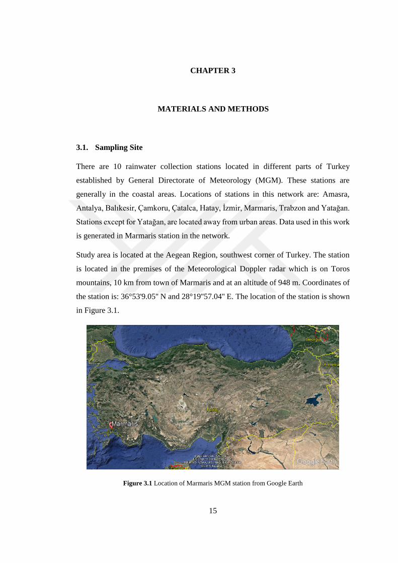
Study area is located at the Aegean Region, southwest corner of Turkey. The station

is located in the premises of the Meteorological Doppler radar which is on Toros

mountains, 10 km from town of Marmaris and at an altitude of 948 m. Coordinates of

the station is: 36°53'9.05'' N and 28°19''57.04'' E. The location of the station is shown

in Figure 3.1.

Figure 3.1 Location of Marmaris MGM station from Google Earth

16

Climate of the study area is similar to the general Mediterranean Climate with hot

summer and warm winters. Long term meteorological data, which are measured at

Muğla meteorological station between 1926 and 2017 are given in Table 3.1.

Table 3.1 Historical Temperature and Precipitation Data for the City of Muğla (MGM, 2017)

Average

Temp.

(°C)

Max

Average

Temp.

(°C)

Min

Average

Temp.

(°C)

Monthly

Average

Precipitation

(mm)

Max

Temp.

(°C)

Min

Temp.

(°C)

January 5.4 9.7 1.5 241.9 20.9 -12.6

February 6.1 10.8 1.8 178.4 25.5 -9.9

March 8.5 14.0 3.5 124.7 28.8 -8.5

April 12.6 18.7 6.9 64.7 31.2 -3.6

May 17.6 24.1 11.3 49.5 36.0 1.0

June 22.8 29.5 16.0 21.3 40.8 6.7

July 26.2 33.3 19.6 8.4 42.1 10.5

August 26.0 33.4 19.5 9.4 41.2 9.0

September 21.6 29.1 15.2 19.0 38.8 5.6

October 16.0 23.0 10.2 72.8 36.1 0.1

November 10.7 16.5 5.8 138.3 29.0 -7.0

December 7.1 11.4 3.1 265.7 21.0 -9.0

Annual 15.0 21.1 9.5 1194.1 42.1 -12.6

Coldest month in Muğla is January with average temperature of 5.4oC and the hottest

month is July with the average temperature of 26.2 oC. Also for Muğla, December has

been the month with the highest wet deposition amount, between the measurement

years, with average monthly precipitation of 295.7 mm (MGM, 2017).

Station is located 10 km away from the county of Marmaris and the nearest road to

the station is 5 km away, which indicates that anthropogenic sources are not affecting

the sampling. Station is in the premises of a Meteorological radar. The sampling

platform is shown in Figure 3.2.

Sample collection in the station started in June 2011 and still continuing; however,

samples collected between July 2011 and November 2016 are used in this study.

During this time period approximately 300 wet deposition samples are collected and

measured by the MGM for the major ion concentration.

17

3.2. Collection of Wet Deposition Samples

In all the stations established by MGM, samples are collected using the same

procedure. In stations samples are collected with a home-made automated wet and dry

sampler. The samplıng system have the same characteristics of the well-documented

Andersen wet-and dry sampler. Sampler that was used in this work can be seen in

Figure 3.2.

Figure 3.2 Precipitation Sampler of Marmaris Station

Sampler is consisting of two 30 cm-diameter buckets, one for dry deposition and one

for wet deposition. An automated cover, which receiver sıgnal from a rain sensor

moves to cover dry bucket when rain starts and the same cover moves to cover wet

bucket when rain ends. In this way, during the rain bucket is left open, but dry bucket

is closed and during non-rain period, dry bucket is left open and rain bucket is kept

closed.

Both buckets are lined with 10 L capacity polyethylene bags, which makes it easier to

collect the samples when the collection period is finished. Collection period for dry

deposition samples are one week, at the end of each week a new polyethylene bag is

18

replaced and the old one is taken for analyze. For wet deposition, bags containing

rainwater are replaced with fresh ones at the end of every rain event.

3.3. Sample Handling

3.3.1. Determination of Volume and pH

Volume and pH of collected samples were measured in the laboratory. Volume

measurement is done by the calibrated sampling bottles. The volume of the sample

and calibrated bottle height are compared at 25ºC, and the volume of the precipitation

is determined. Radiometer PHM 80 portable pH meter with a glass electrode is used

to measure pH. Before measuring, pH meter is calibrated with standard buffer

solutions at pH 4.0 and pH 7.0.

3.3.2. Preparation of Samples for Ion Chromatography

Ionic and trace element composition of samples were determined in MGM laboratory

at the central MGM campus at Keçiören, Trace element data were not used in this

work. For measurement of ion concentration, extensive sample treatment is not

required, but the fine particulate matter must be removed from the sample. To remove

the particulate matter samples are filtrated through 0.2 µm pore sized cellulose acetate

membrane filters. Filtration avoids the Ion Chromatography to clog with particles.

Sulphate, NO3-, NH4

+, Na+ and Cl- are 100% soluble in the rainwater samples,

therefore these ions are not affected from the filtration process. Nevertheless, Ca2+, K+

and Mg2+ ions are not dissolving in the rainwater samples completely, their

solubility’s are dependent on the acidity of the precipitation. In this study, only the

soluble part of these ions are taken into consideration. This approach of measuring

soluble fraction of ions is common in rain water research. Genç (2013) analyzed ions

in aerosol samples collected at Kırklareli station, first by IC after dissolving them with

water, then by ICMS after acid digestion with HNO3 – HF mixture which dissolves

alumina silicate matrix as well. The ICPMS-to-IC median ratio was 1.4 for Na, 3.5 for

Mg, 2.2 for K and 1.5 for Ca. Although the difference between water soluble and

insoluble fractions of these ions is significant, please note that insoluble fraction which

19

can be measured only after strong acid digestion is not bioavailable and cannot be

picked up by plants and animals. This is the rationale behind analysis of soluble

fractions of ions in most monitoring networks.

3.4. Analysis of Samples

Soluble fractions of ions were analyzed using Ion Chromatography (IC). IC is a

technique used to identify the ionic composition of liquid samples. With IC, common

anions (such as fluoride, chloride, nitrite, nitrate and sulfate), common cations (such

as lithium, sodium, ammonium and potassium), transition metals and low molecular-

weight organic acids can be measured within a liquid sample, in parts-per-million

(ppm) or parts-per-billion (ppb) quantities (Burke, 2006). Working principle of an IC

is as follows: sample to be analyzed (analyte) is injected to the carrier fluid (eluent);

the combination is passed through a column that contains a stationary adsorbent;

compounds, that are contained in the analyte, are partitioned between the adsorbent

and the moving eluent/analyte mixture; as the eluent flows through the column, the

components of the analyte will move down the column at different speeds and

therefore separate from one another; a detector is used to analyze the output at the end

of the column; each ion that exits from the column generates a peak on the

chromatogram (Stute, 2009).

For the samples in Marmaris Station, soluble fractions of the ions were analyzed in

MGM laboratory with a Dionex 120 Ion Chromatograph. Different columns were used

for anions and cations. The columns used for anion and cation measurements are

Dionex model AS9-HC and Dionex model CS12A, respectively. In addition to these

analytical columns, suppressor columns ASRS-ULTRA for anions and CSRS-

ULTRA for cations were also used. Eluent was 10 mM sodium carbonate (Na2CO3)

solution for anions and 18 mM methane sulfonic acid (MSA) solution for cations.

20

3.5. Data Quality Assurance

3.5.1. Field Blanks

Contamination of the collected rainwater samples is a problem that must not be

ignored. For the elimination of the possible effects of contamination, field blanks and

laboratory blanks must be collected. The field and laboratory blanks should be

collected using the same collection procedures and also should be analyzed the same

way with the collected rainwater samples (U.S. Geological Survey Techniques of

Water-Resources Investigation, 2006).

Field blanks are collected by pouring distilled water in the polyethylene bags which

are placed in the sampler, which then collected and analyzed as the same way with the

rainwater samples. Laboratory blanks are used in order to detect the potential

contamination from lab procedures. Neither field, nor lab blanks were significant for

any of the ions measured in this work.

3.5.2. Calculation of Detection Limits

Limit of detection is an analytical method simply defined as the lowest detectable

amount of analyte in a sample (Ogen, et al., 2018). The definition of limit of detection

adopted in this study is the “concentration that corresponds to three times the standard

deviation of ten replicate measurements at blank level”. Detection limits of major ions

calculated with this definition are given in Table 3.2. Figures in the table clearly

demonstrate that, measured average concentrations of ions are several orders of

magnitude than their corresponding detection limits and thus detection limits of ions

is not an important source of uncertainty in conclusions.

21

Table 3.2 Detection Limits of the Ions (Ayaklı, 2014)

Ion Detection Limit

(µg/L)

Average conc. in rainwater

(µg/L)

SO42- 0.021454 2000

NO3- 0.022668 890

Cl- 0.076439 3500

NH4+ 0.081163 390

Ca2+ 0.044752 1600

Na+ 0.018494 2000

K+ 0.020703 170

Mg2+ 0.007738 450

3.5.3. Quality Assurance

Quality Assurance/Quality Control (QA/QC) Programs are developed in order to

assure the accuracy, precision and, representativeness and completeness of the data

used in the studies. Quality control term is defined as “the routine application of the

procedures designed to achieve and sustain a determined level quality for a

measurement system” and quality assurance is defined as “a set of coordinated actions

that are used to ensure the measurement program can be quantifiable and procedure

data of known quality” (Acid Deposition Monitoring Network in East Asia, 2000).

For the purposes of this study, Dionex-120 Ion Chromatograph, was calibrated using

standards that are commercially available; Dionex Seven Anion Standard-II was used

for anions and Dionex Six Cation Standard-II for cations. For checking the accuracy

of the calibration, Standards prepared using high purity salts of measured ions (Merck,

suprapure NaCl, K2SO4, NaNO3, KCl, CaCl2 and NH4Cl) were used. Solutions

prepared were used to test the calibration occasionally. Results of one of the

calibration checks are given in Table 3.3. By comparing the measurements and

calculations, it was agreed that the calibration of the instrument is reliable.

22

Table 3.3 Calculated and Measured Concentrations of the High Purity Salts (Genç Tokgöz D. , 2013)

Ion

Calculated

Concentration

(mg/L)

Measured

Concentration

(mg/L)

SO42- 6.0 ± 0.3 6.25 ± 0.1

NO3- 6.0 ± 0.3 6.36 ± 0.12

Cl- 6.0 ± 0.3 6.26 ± 0.05

NH4+ 2.94 ± 0.15 3.1 ± 0.28

Ca2+ 3.1 ± 0.16 3.04 ± 0.24

K+ 3.05 ± 0.15 2.93 ± 0.3

Na+ 3.01 ± 0.15 2.96 ± 0.27

3.6. Computation of Back Trajectories

Trajectories are defined as the path a particle/air parcel will go, likewise the back

trajectory (also called backward trajectory) can be defined as the path it came from,

so back trajectories are often used in order to determine the relationships between the

sources and receptors (Stohl, et al., 2002).

Backtrajectories were calculated using HYSPLIT (Hybrid Single Particle Lagrangian

Integrated Trajectory), which is a 3D isentropic model developed by the National

Oceanic and Atmospheric Administration (NOAA). This model is integrated into

TrajStat, which is a GIS (Geographical Information System) based software that is

available in NOAA website.

Back trajectories of each sampling days were calculated using TrajStat. Calculations

were performed for 120 hours (five days) backward in time, starting at Marmaris

Station. Trajectories were calculated starting at 100 m, 500 m and 1500 m. altitudes.

All trajectory calculations were started at 12:00 UTC (Universal Time Coordinate).

The model is set to be isentropic trajectory type, in which air parcel is assumed to be

travel at potential temperature. Latitude and longitude of the receptor location is

converted from degree-minute-second format to decimal degree format. Also the

necessary monthly meteorological data for the software is downloaded from the

database of NOAA.

23

The screenshot from the trajectory calculation interface of the software TrajStat is

shown in Figure 3.3.

Figure 3.3 Trajectory Calculation Window of TrajStat

3.6.1. Flow Climatology

Flow climatology refers to air-flow patterns affecting the receptor. In our case it is

Marmaris station, or Marmaris region in general. When this information is combined

with concentrations of ions, it can provide some preliminary information about source

regions affecting chemical composition of precipitation in the Eastern Mediterranean.

Two different approaches were used to calculate flow patterns of upper atmospheric

air masses, before they were intercepted at our station. One of them is “residence time

analysis”, which is a method developed in our group. The second approach is more

conventional and bases on calculating time air masses spent in each wind sector. The

second approach can be seen frequently in literature.

24

In the first approach study domain, which extends from west of UK to East of Caspian

Sea in East –West direction and from North of Scandinavia almost to equator in North

– South direction, were divided to 1ºx1º grids. The study domain and grid system

superimposed to it is depicted in Figure 3.4. In the second step, number of trajectory

segments in each grid were counted and results were interpolated using MAPINFO

software to generate residence time distributions. Since back trajectories calculated by

HYSPLIT consisted of hourly segments which are characterized by x, y, z coordinates

and time, they were suitable for mapping. Consequently, number of segments in each

grid indicate number of hours air masses spent in that grid during study period (or

during the time interval for which flow climatology calculations are done). Residence

time distribution-maps were prepared for each starting altitude and for summer and

winter separately.

Figure 3.4 Study Domain for the Residence Time Analysis

25

As pointed out before residence time distribution was developed in our group and used

in a number of projects and thesis. However, unfortunately it does not allow us to

compare flow patterns calculated in this work with similar patterns reported in other

studies. To avoid this difficulty, flow climatology was also calculated in conventional

way, which can be found in literature, as well.

The study domain is divided into 8 wind sectors (N, NE, E, SE, S, SW, W, NW),

number of trajectory segments in each sector is counted. It should be noted that in

conventional approach assigning trajectories to a sector is always a problem, because

trajectories pass through two or more sectors, before they end up at our station. This

issue was bypassed by counting number of segments (hours air parcels spent) at each

sector.

3.7. Potential Source Contribution Function

For determining the potential source regions of the pollutants, Potential Source

Contribution Function (PSCF), which is a statistical tool in trajectory statistics was

used. PSCF shows the areas that contributed to high concentrations of pollutants at

the receptor, thus pointing to source areas of pollutants.

As in the approach used in flow climatology, PSCF calculations also include counting

trajectory segments in the grid system, described in previous section.

Trajectory files of the measured days are selected and the trajectories that correspond

to the highest 40% of pollutant concentration is grouped as “polluted” trajectories and

segments in these polluted trajectories are categorized as “polluted segments”.

Polluted and all (polluted + unpolluted) segments in each grid were counted and PSCF

value for that grid was calculated using Equation 3.1.

𝑃𝑆𝐶𝐹𝑖𝑗 =𝑚𝑖𝑗

𝑛𝑖𝑗

(3.1)

Where mij refers to the total number polluted trajectories in gird “i” and nij refers

to total number of all (polluted + unpolluted) segments in the same grid. “j” is a

trajectory counter.

26

One of the problems associated with PSCF approach is the small number of segments

at the peripheral grids in the domain. Trajectories calculated in this study is 5 days

long, which means there is 120 hourly segments in each back trajectory. Since there

is 302 samples (day), and 3 trajectories with different starting altitudes in day, total

number of segments used is 108720. However, a large majority of these segments are

in grids that are close to our station. There are few segments in grids that are located

at the boundaries of our grid system. PSCF values assigned with few trajectories can

have very large uncertainties and can lead to misleading conclusions. To avoid this, a

weighting approach, which was developed by Zhao ve Hopke (2006) and shown in

Equation 3.2 was used.

𝑊(𝑛𝑖𝑗) =

{

0.15 𝑛𝑖𝑗 ≤

𝑛𝑎𝑣𝑔2⁄

0.5 𝑛𝑎𝑣𝑔

2⁄ < 𝑛𝑖𝑗 ≤ 𝑛𝑎𝑣𝑔0.75 𝑛𝑎𝑣𝑔 < 𝑛𝑖𝑗 ≤ 2 ∗ 𝑛𝑎𝑣𝑔1.0 𝑛𝑖𝑗 > 2 ∗ 𝑛𝑎𝑣𝑔

(3.2)

where W(nij) is the weighting function,

navg is the average number of the segments in all grids

The equation implies that if total number of grids in a particular grid is at least twice

higher than average number of segments in all grids at the domain, then PSCF value

for that grid was multiplied by 1.0. If the number of segment is between avg number

of segments and 2 times average number, PSCF value of the grid was grids were

multiplied with 0,75. PSCF is multiplied by 0,5 if the number of segments in that grid

is between one-half of the average number of segments and average number of

segments. Finally PSCF value for a grid was multiplied by 0.15 if number of segments

in that grid I less than half of the average number. As can be seen from the equation,

importance of peripheral grids with few segments are significantly reduced in PSCF

distributions.

27

3.8. Positive Matrix Factorization

EPA PMF version 5.0 was for source apportionment part of the study. In order to

insert the measured data to the software, missing data and data below the detection

limit (given in Table 3.2), should be replaced. For missing data geometric mean of

that ion is used; for the data below detection limit (BDL) half of the detection limit is

used, but uncertainties of such data are increased so that this data do not affect the

“fit”.

Software also requires the uncertainty data referring to each measurement calculated

as (Norris, et al., 2014; Reff, et al, 2007):

𝜎𝑖𝑗 =

{

𝑅𝑒𝑎𝑙 𝐶𝑜𝑛𝑐𝑒𝑛𝑡𝑟𝑎𝑡𝑖𝑜𝑛, 𝑥𝑖𝑗 ∗ 0.05 +

𝐷𝐿

2

𝐵𝑒𝑙𝑜𝑤 𝐷𝑒𝑡𝑒𝑐𝑡𝑖𝑜𝑛 𝐿𝑖𝑚𝑖𝑡, 5

6∗ 𝐷𝐿

𝑀𝑖𝑠𝑠𝑖𝑛𝑔 𝐷𝑎𝑡𝑎, 4 ∗ 𝐺𝑒𝑜𝑚𝑒𝑡𝑟𝑖𝑐 𝑀𝑒𝑎𝑛

(3.3)

Where σij is analytical uncertainty, xij is the concentration of the specie j measured on

sample i, DL is the detection limit.

Object function that had been explained in Section 2.3.2.3. PMF software calculates

2 different Q values for each run: Qrobust and Qtrue. Also a theoretical Q value should

be calculated by following equation:

𝑄𝑡ℎ𝑒𝑜𝑟𝑒𝑡𝑖𝑐𝑎𝑙 = (𝑘 ∗ 𝑚) − 𝑡(𝑘 + 𝑚) (3.4)

Where k is the number of elements, m is the number of days and t is the number of

factors. While trying to determine the number of factors, several runs should be made

by the software and for each run software gives: Qrobust and Qtrue values which also

shoul be compared with: Qtheoretical . : Qtrue / Qtheoretical value should be around 1-1.5 for

the factor number to be accurate.

After the factor number is selected, by analyzing the correlation between species and

the factor profiles, it can be determined that which factor refers to which source.

29

CHAPTER 4

4. RESULTS AND DISCUSSION

4.1. General Characteristics of the Data

In this study, 302 rainwater samples collected by MGM between 2011 and 2016 were

analyzed. In these 302 samples, concentrations of nine major ions, including H+, SO42-

, NO3-, Cl-, NH4

+, Ca2+, Mg2+, K+ and Na+ were determined. General characteristics

of data are given in Table 4.1.

Table 4.1 Statistical Summary of Ionic Composition (concentrations are in mg L-1)

Volume

Weighted

Average

Mean Standard

Deviation Median Range

Number

of

Samples

pH 5.12 5.91 0.89 6.01 3.69 – 7.9 302

H+ 0.0076 0.0094 0.025 0.0009 1.26 *10-5 – 0.20 302

SO42- 2.03 3.11 4.63 1.76 0.06 – 47.69 296

NO3- 0.89 1.45 2.08 0.79 0.04 – 20.40 287

Cl- 3.49 4.05 7.37 2.00 0.02 – 105.04 300

NH4+ 0.39 1.09 4.82 0.19 0.002 – 56.06 259

Ca2+ 1.63 2.34 4.02 0.86 0.01 – 25.77 302

Mg2+ 0.45 0.57 1.48 0.28 0.01 – 20.44 297

K+ 0.17 0.34 1.08 0.12 0.01 – 11.68 289

Na+ 2.00 2.24 2.62 1.51 0.02 – 22.75 299

Volume weighted concentrations of constituents are used instead of regular averages

in studies aiming to determine rainwater composition, to avoid dilution effect.

Concentrations of elements and ions (and other constituents also) in rainwater is

inversely related with rainfall amount. Concentrations are lower in intense rains and

30

higher in rain with low precipitation amount, obviously due to dilution. This dilution

effect is avoided in volume weighted average concentrations of elements and ions, as

concentrations are normalized with rainfall amount.

Volume weighted averages (VWA) of the sample concentrations are calculated using

the following formula:

𝐶𝑥𝑝 = ∑(𝐶𝑥 ∗ 𝑉𝑝)

∑𝑉𝑝

(4.1)

Where Cxp stands for the volume weighted concentration of the specie x,

Cx stands for the concentration of the specie x in the given sample,

Vp stands for the precipitation volume of the sample.

The ratio of average concentrations of elements to their volume-weighted averages

vary between 1.1 and 2.7, for Na for NH4+, respectively. It is interesting to note that

the ratio for crustal and marine elements are low (the average-to-VWA ratio for Cl- is

1.2, for Na+ is 1.1, for Mg2+ is 1.3, for Ca2+ is 1.4) and ratios are high for pollution-

derived ions (for SO42- is 1.5, for NO3

- 1.6 and for NH4+ 2.7). This systematic

difference between crustal, marine and anthropogenic elements is probably due to the

way they are deposited to the surface. Crustal and marine ions that we measured in

our rainwater samples are from local sources and washed out by rain from the

atmosphere during very early phases of the rain event (10 – 30 min) (Al-Momani, et

al., 1998; Kaya & Tuncel, 1997). Pollution derived ions that we measure in rain

samples, on the other hand, are brought to Marmaris in clouds and when clouds rain,

they are deposited to the surface where we sample them. Their concentrations do not

change significantly throughout the rain (Al-Momani, et al., 1998; Kaya & Tuncel,

1997). A slight decrease is observed in the beginning of the rain event due to their

washed-out fraction. However the decrease is not as large as the concentration

decrease in crustal and marine ions and elements (Al-Momani, et al., 1998; Kaya &

Tuncel, 1997). This scenario suggests that concentrations of crustal and marine

elements in rainwater samples depends on how much seawater and crustal particles

31

exists in the atmosphere when rain starts. Their concentrations are independent of

rainfall amount, because they are washed out in first 10 – 15 minutes of rain and thus

do not depend on how long rain continues (rainfall amount). Concentrations of

pollution derived ions on the other hand, depends strongly on dilution of these ions

with rainfall amount. This scenario can explain observed polarity in AVG-to-VWA

concentration ratios of anthropogenic, crustal and sea salt ions. Volume weighted

average concentrations of ions vary between 0.4 mg L-1 for NH4+ ion and 3.5 mg L-1

for Cl- ion. Median concentrations of ions are approximately a factor 2 lower than

their average values. Lower median values together with high standard deviations are

indications of right skewed data as will be discussed in the next section of this

manuscript.

4.1.1. Distribution Characteristics of the Data

Distribution characteristics (frequency histograms) of anions and cations measured in

this study are given in Figure 4.1 and Figure 4.2, respectively. Atmospheric data have

always right skewed distributions, as depicted in these figures. There are many

different right-skewed distributions, but log-normal distribution is the most common

distribution observed in environmental data. The distribution characteristics of data

for each ion was tested using Chi-square goodness of the fit test with null hypothesis

that distributions are “log-normal”. The results showed that distributions are log

normal with > 95% statistical significance for H+, NO3-, NH4

+ Ca2+, Mg2+, K+ and

Cl-. However, null hypothesis was rejected for SO42- and Na2+ ions. Apparently, these

two ions have histograms that represent another right-skewed distribution. We did not

further investigate to find type distribution followed by these two ions.

32

Fig

ure

4.1

Fre

qu

ency

Dis

trib

uti

on

of

An

ion

s M

easu

red i

n t

his

Stu

dy

33

Fig

ure

4.2

Fre

qu

ency

Dis

trib

uti

on

of

Cat

ion

s M

easu

red

in

th

is S

tud

y

34

4.1.2. Comparison of the Data with Literature

Air quality in urban and industrial areas is assessed by comparing measured

concentrations of pollutants with air quality standards. Situation is more complicated

in air quality at rural airshed. Concentrations of pollutants are always lower than their

corresponding concentrations measured at urban or industrial areas, because rural

areas are not under direct influence of industrial, residential and traffic emissions.

However, standards are designed for human health, but at rural airshed, concern is the

health of ecosystem, which can be more vulnerable than humans due to very long-

term exposure to pollutants. For example, since forests are exposed to pollutants for

hundreds of years, they can be affected from fairly concentrations, which are safe for

humans. Since regulatory standards are useless in evaluating rural air quality, the only

way for such an assessment is to compare pollutant concentrations measured at the

rural station with corresponding data from rural areas reported in literature.

Furthermore, such a comparison can also provide information about transport

mechanisms of pollutants to the rural station.

In this study, generated data are compared with corresponding concentrations, which

are measured in two comparable networks. Data is first compared with similar data

generated in rain monitoring stations in Turkey. In the second step data generated in

this work are compared with similar ion data measured in EMEP network.

Rural rainwater data generated in Turkey is unexpectedly extensive. 13 rural rain

monitoring stations operated in Turkey up today. Among these 10 stations, namely,

Yatağan, Trabzon, Izmir, Hatay, Çatalca, Çamkoru, Balıkesir, Antalya 3, Marmaris

and Amasra were established and operated by General Directorate of Meteorology,

Research division (MGM network). These stations are strategically very important,

because MGM can operate them for long periods of time. Some of them are now in

operation more than 15 years. The network was initiated in 2004 by establishing a

bulk sampling station at Çamkoru. Çamkoru was the only station equipped with bulk

samplers. All other stations in the network were equipped with automated wet-and-

dry samplers. However, an automated wet-and-dry sampler was also installed to

35

Çamkoru station in 2014. Two additional stations also became operational in 2004.

One at Amasra and the other one at Balıkesir. Two additional stations, namely Antalya

and Çatalca were activated in 2005. These are followed by a station at Izmir and

Marmaris in 2011, at Yatağan in 2012, at Hatay 2013 and Trabzon in 2014. Stations

are named with cities to describe their geographical locations, but none of them,

except for Amasra station, are located in urban areas, most of them (Hatay, Marmaris,

Trabzon, Çatalca, İzmir, Balıkesir, Hatay) are located at Meteorological Doppler radar

sites, which are >10 km away from the urban area. Data set evaluated in this thesis is

the one generated at Marmaris station between 2011 and 2016. In all these stations,

samples are collected in polyethylene bags and shipped to MGM central laboratory at

Ankara, where they are analyzed for ions and trace elements.

The Çubuk station used in comparison is the only EMEP station in Turkey. It was

established in 1993 by the Ministry of Health, with financial assistance of the German

Government. It was successfully operated by the Refik Saydam Hıfzıssıhha Merkezi

between 1993 and 2006. In 2006, the station was transferred to Ministry of

Environment. It is not operating since then. Other stations. Namely Antalya 1, Antalya

2, Ankara, Bartın were operated in the past by our group.

EMEP network is the monitoring component in LRTAP (Long Range Transboundary

Air Pollution) convention. Operations in the network started in 1977 and it is still

operational. EMEP network consisted of approximately 180 stations (all of these

stations were not operational all time). Variety of parameters in aerosol, gas phase and

rainwater are being measure on an hourly and daily basis. Main objective of the

network is to generate data with high spatial coverage for model validation and

monitor long term trends in concentrations of pollutants.

Rain composition data was downloaded from EMEP database (EMEP, 2017). Data

included event-based concentrations of major ions from 176 stations in 37 countries,

between 1977 and 2015, locations of the stations are given in Appendix A. EMEP data

for each ion were then separated into seven categories, including All, Eastern Europe,

Western Europe, Northern Europe, Central Europe, Southern Europe and Islands.

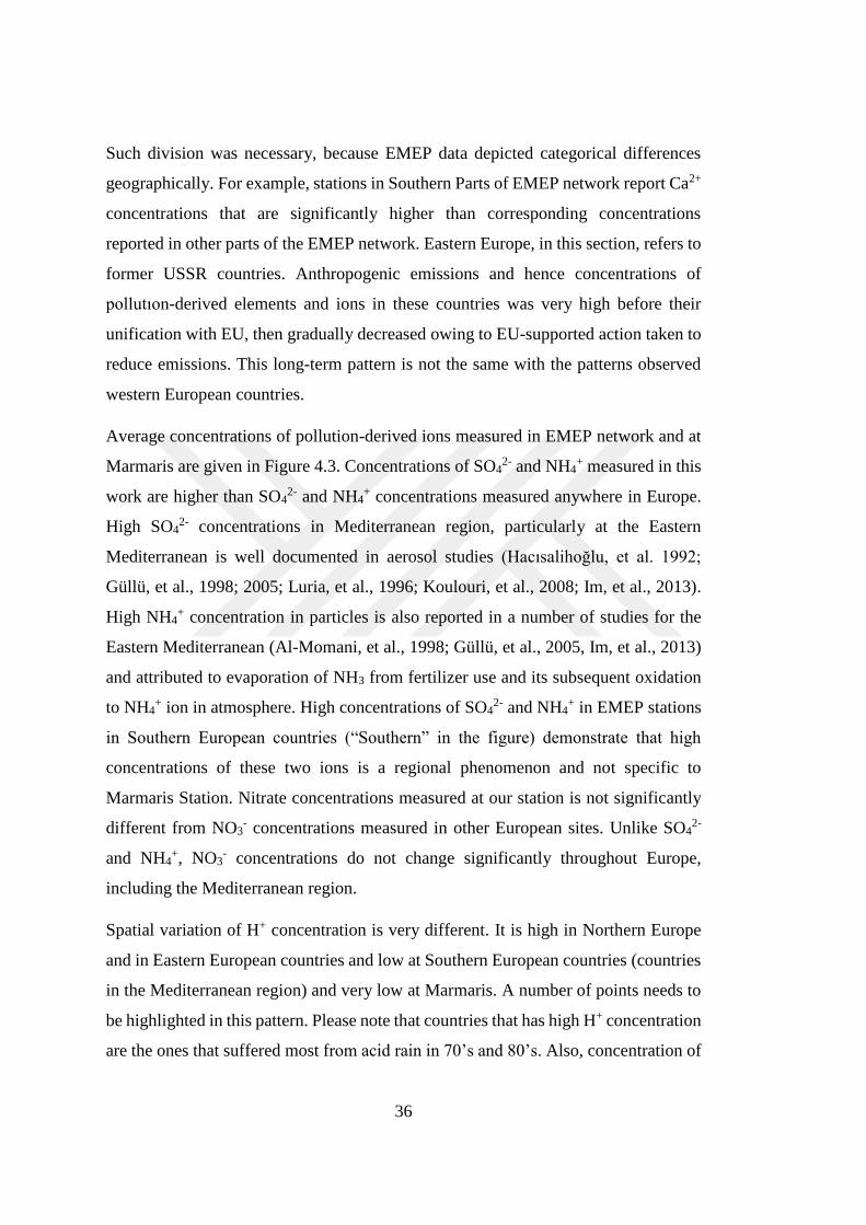
36

Such division was necessary, because EMEP data depicted categorical differences

geographically. For example, stations in Southern Parts of EMEP network report Ca2+

concentrations that are significantly higher than corresponding concentrations

reported in other parts of the EMEP network. Eastern Europe, in this section, refers to

former USSR countries. Anthropogenic emissions and hence concentrations of

pollutıon-derived elements and ions in these countries was very high before their

unification with EU, then gradually decreased owing to EU-supported action taken to

reduce emissions. This long-term pattern is not the same with the patterns observed

western European countries.

Average concentrations of pollution-derived ions measured in EMEP network and at

Marmaris are given in Figure 4.3. Concentrations of SO42- and NH4

+ measured in this

work are higher than SO42- and NH4

+ concentrations measured anywhere in Europe.

High SO42- concentrations in Mediterranean region, particularly at the Eastern

Mediterranean is well documented in aerosol studies (Hacısalihoğlu, et al. 1992;

Güllü, et al., 1998; 2005; Luria, et al., 1996; Koulouri, et al., 2008; Im, et al., 2013).

High NH4+ concentration in particles is also reported in a number of studies for the

Eastern Mediterranean (Al-Momani, et al., 1998; Güllü, et al., 2005, Im, et al., 2013)

and attributed to evaporation of NH3 from fertilizer use and its subsequent oxidation

to NH4+ ion in atmosphere. High concentrations of SO4

2- and NH4+ in EMEP stations

in Southern European countries (“Southern” in the figure) demonstrate that high

concentrations of these two ions is a regional phenomenon and not specific to

Marmaris Station. Nitrate concentrations measured at our station is not significantly

different from NO3- concentrations measured in other European sites. Unlike SO4

2-

and NH4+, NO3

- concentrations do not change significantly throughout Europe,

including the Mediterranean region.

Spatial variation of H+ concentration is very different. It is high in Northern Europe

and in Eastern European countries and low at Southern European countries (countries

in the Mediterranean region) and very low at Marmaris. A number of points needs to

be highlighted in this pattern. Please note that countries that has high H+ concentration

are the ones that suffered most from acid rain in 70’s and 80’s. Also, concentration of

37

SO42- is highest in Marmaris and Mediterranean countries (“Southern” in figure), but

these sites reported have the lowest H+ concentration. This peculiar spatial variation

in H+ concentration in Europe is due to neutralization of rainwater acidity and will be

extensively discussed later in the manuscript.

38

Fig

ure

4.3

Co

mp

aris

on

of

po

llu

tio

n-d

eriv

ed i

on

s m

easu

red

in

th

is s

tud

y w

ith

co

rres

po

nd

ing

dat

a f

rom

EM

EP

net

wo

rk.

Dif

fere

nt

med

ian

val

ues

wer

e

gen

erat

ed f

rom

EM

EP

sta

tio

ns

dep

end

ing

on t

hei

r lo

cati

on

in

Eu

rop

e

39

Concentrations of ions with natural sources in EMEP stations and in Marmaris are

given in Figure 4.4. Calcium concentration measured at Marmaris are the highest in

all data groups, which is followed by the Ca2+ concentration reported at “Southern”

European countries, indicating that high Ca2+ concentration is a regional process. High

Ca2+ in southern part of Europe is due to highly alkaline nature of the soil in the

Mediterranean region and will be discussed later in the manuscript in relation to

neutralization of rainwater acidity.

Na+ and Cl- are sea salt ions and their concentrations are high at “Island” station group,

as expected. Since concentrations of Na+ and Cl- are high in stations close to the sea,

higher concentration of these ions in “Northern” station group can be due to close

proximity of measurement stations to the sea in this station group. This is reasonable

explanation, because most of the stations in “Northern” group are located in Norway

and Sweden. Wherever a station is located, it will not be too far from the sea in these

countries. Concentrations of sea salt ions measured at Marmaris is higher than those

reported for “Eastern”, “Central” and “Southern” station groups, but not as high as

concentrations reported for “Island” and “Western” station groups. Marmaris station

is approximately 10 km from the sea. Low concentrations are probably due to high

altitude of the station.

40

Fig

ure

4.4

Co

mp

aris

on

of

crust

al a

nd

mar

ine

ion

s m

easu

red i

n t

his

stu

dy

wit

h c

orr

esp

ond

ing

dat

a fr

om

EM

EP

net

wo

rk.. D

iffe

ren

t m

edia

n v

alu

es w

ere

gen

erat

ed f

rom

EM

EP

sta

tio

ns

dep

end

ing

on t

hei

r lo

cati

on

in

Eu

rop

e

41

Average concentrations of pollution-derived ions at Marmaris and other stations in

Turkey are given in Figure 4.5. Levels of anthropogenic ions measured at Marmaris

station is not significantly different from their levels reported for other stations in

Turkey, with few exceptions. Average SO42- concentration at Marmaris station is

smaller than those measured Yatağan and Antalya. SO42- concentration reported for

Yatağan is significantly higher than SO42- concentrations measured at all stations. This

probably reflects presence of the Yatağan thermal power plant in the close proximity

of the station. High SO42- concentration reported for Antalya is an artifact.

Concentration reported for Antalya station is an average value from samples collected

between 1992 and 2001. In those years SO42- concentration in all Eastern

Mediterranean basin was were high. Average SO42- concentration measured at Antalya

3 station are more representative for the SO42- levels in the region today.

Concentrations of NO3- ion are high at Antalya station for the same reason. Average

NO3- concentration measured at Marmaris station is not significantly different from

NO3- concentrations reported in most of the stations in Turkey. Average concentration

of NH4+ measured in this work are also comparable to similar concentrations reported

in other parts of Turkey. However, higher NH4+ concentrations are reported for Hatay,

Izmir, Trabzon and Yatağan stations. Discussion of the reasons for these high

concentrations is beyond the scope of this study.

42

Fig

ure

4.5

Co

mp

aris

on

of

ionic

co

mp

osi

tio

n d

eter

min

ed i

n t

his

stu

dy

wit

h c

orr

espo

nd

ing

dat

a g

ener

ated

in

oth

er l

oca

tion

s in

Tu

rkey

: Io

ns w

ith

anth

ropo

gen

ic s

ou

rces

43

Concentrations of sea salt and crustal elements measured at Marmaris and elsewhere

in Turkey are given in Figure 4.6. Concentrations of Na+ and Cl- are the highest at

Antalya station, because at Antalya station was located at the coast. Concentrations of

these sea salt ions are not equally high at Marmaris because (1) station is

approximately 10 km from the coastline and (2) station was 1000 m above sea level.

Calcium concentration measured at Marmaris is comparable to concentrations

measured in other rainwater monitoring stations. The reason for unusually high Ca2+

concentration reported for Yatağan station is not known. Potassium concentration;

however, is high at Antalya, Bartin and Amasra stations, which are located on at the

coast. Please note that K+ concentration at coastal stations are also contributed by sea

salt. Please also note that concentrations of Na+ and Cl- are also high in these stations.

44

Fig

ure

4.6

Co

mp

aris

on

of

ionic

co

mp

osi

tio

n d

eter

min

ed i

n t

his

stu

dy

wit

h c

orr

espo

nd

ing

dat

a g

ener

ated

in

oth

er l

oca

tion

s in

Tu

rkey

: M

arin

e an

d

cru

stal

io

ns

45

4.2. Flow Climatology

Flow climatology is an important approach used in this study, as it signifies areas

where air masses spent most of their time before they arrive to our station. Such data

can provide information about source areas of pollutants that are intercepted at the

sampling point. Two different approaches were used in this study. In the first method,

hours spent by air masses at each grid of our study domain were computed. In the

second method, number of hours spent by air masses in wind sectors was computed.

Since trajectory information is necessary in both methods, 5-day long back trajectories

were calculated every day for 13 years, which is longer than our sampling period at

Marmaris station. For each day three different trajectories with starting altitudes 100

m, 500 m and 1500 m were calculated. Trajectories were consisted of 1-hour

segments. These segments were counted in grids and in wind sectors. Trajectories

were computed for a period longer than sampling period to reduce uncertainties in

calculated residence times and clusters. Please note that, since flow climatology and

cluster analysis do not depend on ion concentrations, trajectory calculations are not

limited with our sampling period in Marmaris station. Back trajectories for were

calculated for 13 years to minimize statistical uncertainty in residence time and cluster

calculations.

4.2.1. Residence Time Analysis

For residence time analysis, segment counts in grids are transformed to distribution

maps showing the time spent by air masses in different parts of the study domain.

Distribution of residence times of air masses in the study domain are given in Figure

4.7, (a), (b) and (c) in the figure are distributions for 100 m, 500 m and 1500 m starting

altitudes, respectively. Figure 4.7 (d), on the other hand, are prepared by combining

segments in all three starting altitudes. There are not substantial differences in

residence time distributions between different starting altitudes. The effect areas

appear to be expanded in Figure 4.7 (d), because it includes factor of three times more

segments than segments in individual starting altitudes.

46

The areas, where air masses spent most of their time before they arrive to Marmaris

are, western parts of Turkey, most of the Balkan countries (particularly Greece,

Bulgaria, Romania), Ukraine and the Black Sea coast of Russia, indicating that

sources in these areas have higher probability of contributing atmospheric

composition at Marmaris.

Figure 4.7 Distribution of Air Mass Residence Times in Study Domain

(a) 100 m starting altitude, (b) 500 m starting altitude,

(c) 1500 m starting altitude, (d) Segments in all starting altitudes

(a) (b)

(c) (d)

(hours)

47

For the calculation of summer and winter residence times, trajectories in summer and

winter months were separately counted. In this and in many other studies performed

in our group, summer season was assumed to be between April and September and

winter season was taken as the remaining part of the year. This summer-winter

partitioning was based rainfall in the Mediterranean area. In the Eastern

Mediterranean area approximately 20% of the annual rainfall occurs between April

and September (our summer season) and 80% of the rainfall occur in the remainder of

the year (our winter). Since wet scavenging is an important factor in temporal

variations of atmospheric constituents in atmospheric particles and precipitation, such

rainfall-based division of the year into seasons enhances summer winter differences

in concentrations of elements and ions and makes them easier to detect.

Summer (a) and winter (b) season distributions are given in Figure 4.8 along with the

distribution of summer - winter differences (c). In Figure 4.8 (c), positive numbers in

the legend indicate grids where air masses spent longer time in summer and negative

numbers indicate grids where air masses spent more time in winter. It is very clear

from figure that air masses, which we intercept at our station spent more time in North

and Northwestern parts of the study area in summer and spent more time in Western

Europe, North Africa and Middle East in winter. This was considered in the source

region apportionment part of the study.

48

Fig

ure

4.8

Sea

son

al V

aria

tio

n i

n H

ou

rly R

esid

ence

Tim

es

(a)

Su

mm

er R

esid

ence

Tim

es,

(b)

Win

ter

Res

iden

ce T

imes

, (c

) S

um

mer

-Win

ter

Dif

fere

nce

[“-”

sig

n m

ean

s lo

ng

er r

esid

ence

tim

e in

win

ter

and “

+”

sig

n i

nd

icat

es l

on

ger

res

iden

ce t

imes

in

su

mm

er]

(hou

rs)

(a)

(b)

(c)

49

4.2.2. Sector-Based Flow Climatology

Grid-based climatology, which was discussed in previous section is not a conventional

way of presenting flow climatology. We are using it for many years in our group and

we are satisfied with the results we are getting. However, we also investigated the

conventional way of presenting flow climatology. In this second approach, segments

in each of the eight wind sectors were counted on an annual basis and in different

seasons. Results are given in Figure 4.9. Results of sector-based approach are not

significantly different from results obtained in grid-based climatology. Grid-based

approach is more informative about potential source areas that can affect composition

of particles, gases and rainwater at Eastern Mediterranean basin.

Upper atmospheric air masses spent significantly longer times at N, NE, W and NW

sectors. Residence times are longer in summer at N and NE sectors and longer in

winter E, SE, S and SW sectors. They are comparable in W and NW sectors. This

conclusion is similar to conclusions reached in grid-based approach. This more

frequent flow from N, NE, W and NW sectors and seasonal differences discussed in

this section is a general characteristic of Eastern Mediterranean region, because it is

observed in a number of studies performed in the region (Güllü, et al., 1998; Zodiatis,

et al., 2003; Dayan, et al., 2017; Erel, et al., 2007).

50

Figure 4.9 Hourly Residence Times of Air Masses in Wind Sectors

4.2.3. Cluster Analysis

If they are properly associated with concentrations, back trajectories adds

geographical information to concentration data. As pointed before trajectories are the

paths followed by air masses before they are intercepted at our station. Back trajectory

calculations involve sophisticated modeling and include data from every single

rawinsonde station in Europe, parts of Africa and Asia. Because of such high input

data requirement, it was not practical to run the model in our own computers. Thus,

the model was run at NOAA computer system and only outputs were transferred to

our computers. The model used for this purpose is HYSPLIT, which is a three-

dimensional model developed at Air Resources Laboratory in National Oceanic and

Atmospheric Administration (NOAA) (Draxler & Hess, 1997; 1998). In this study

trajectories were calculated for five days backwards in time. Every day three separate

trajectories were calculated at three starting altitudes (at 100 m, 500 m and 1500 m).

Starting time of every trajectory was 12:00 noon and they were calculated for 5 days

backward in time. Trajectories were consisted of 120 hourly segments and each

segment consisted of x, y and z (latitude, longitude and altitude) coordinates. Every

day 3 back trajectories (at three starting altitudes) and 120x3 = 360 trajectory segments

0

50000

100000

150000

200000

250000

N NE E SE S SW W NW

Dry Season Wet Season

51

are computed. Since trajectory calculation continued for 13 years, a total of 14000

back trajectories and 1.7x106 trajectory segments are generated.

All of these trajectory and segment data were used in flow pattern studies, such as

flow climatology and cluster analysis, which are independent of measured

concentrations. However, only trajectories and segments computed in sampling days

were used in trajectory statistics, such as potential source contribution function

calculations, because trajectory segments are linked to measured concentrations in

PSCF. That group included 302 days, 906 trajectories and 108000 trajectory segments.

When there are few trajectories, they can be visually inspected to relate geographical

information with concentrations. However visual inspection is out of question when

there are approximately 14 000 trajectories. In such a case one uses statistics to group

trajectories with similar characteristics. In this study cluster analysis, which is a

multivariate technique that separates trajectories into groups (clusters) depending on

their curvature characteristics (Kumar & Verma, 2016; Anil, et al., 2017; Brankov, et

al., 1998, Bruno, et al., 2011, Cheng, et al., 2013) was used. TrajStat software was

used to form the clusters from the calculated trajectories. The software uses a

hierarchical method (Ward, 1963) to combine the closest trajectories. An Euclidean

distance formula, which is given in Equation 4.2, was used to calculate the distance

between two back trajectories (Wang, 2008);

𝑑12 = √∑((𝑋1(𝑖) − 𝑋2(𝑖))2+ (𝑌1(𝑖) − 𝑌2(𝑖))

2)

𝑛

𝑖=1

(4.2)

Where d12 distance between trajectories 1 and 2, X1 (Y1) and X2 (Y2) are reference

back trajectories 1 and 2, respectively. Trajectories with all three starting altitudes

were included in cluster analysis (Dorling, et al., 1992; Brankov, et al., 1998).

52

A two-step approach was used to determine optimum number of clusters. First,

number of clusters were incremented from 3 to 20 and root-means-square-deviation

was calculated for each case. Variation of RMSD with number of clusters is depicted

in Figure 4.10. Five percent was chosen to be the threshold value for TRMSD

(Brankov, et al., 1998). The cluster number that is before exceeding the 5% threshold

value is suggested to be chosen as the optimum number of clusters, which in this study

corresponds to either 6 or 10 clusters. In the second step cluster centroids were

inspected, which indicated that in 6-cluster solution cluster 6 was generated by

splitting cluster 5 and centroids of these two clusters were very close to each other.

This split does not give more information than the 5-cluster case. Consequently, the

5-cluster solution was selected as optimum.

Figure 4.10 The Percentage Change in TRMSD to Cluster Numbers

0

2

4

6

8

10

12

14

16

18

20

3 4 5 6 7 8 9 10 11 12 13 14 15 16 17 18 19 20

% C

han

ge in

TR

MSD

Number of Clusters

53

Figure 4.11 Cluster Centroids of Clusters Calculated for Combined Trajectories

Table 4.2 Number and Percentage of Trajectories Allocated in Each Cluster

Cluster Trajectory Number Ratio

1 4784 33.6 %

2 3031 21.3 %

3 3384 23.8 %

4 706 5.0 %

5 2342 16.4 %

The cluster centroids and trajectories associated with each cluster are given in Figure

4.11 and Table 4.2 respectively.

In this work, we also computed residence times of air masses with altitude lower than

500 m for each cluster. All trajectories that are intercepted and segments associated

with them are assigned equal probability to pick up pollutants when they cross over a

source area. However, this assumption is not entirely correct. Trajectory segments that

cross a source area at 3000 m altitude cannot have the same probability of picking up

of pollutants emitted at the surface with a segment crossing the same area at 200 m

altitude. This is the logic behind computing residence times of low-lying (z < 500 m)

Cluster 1

Cluster 2

Cluster 3

Cluster 4

Cluster 5

54

air masses (segments). In source apportionment part of this thesis we adopted a more

sophisticated approach and weighted the influence of segments based on their

altitudes. However, in clusters we only computed residence times of low-lying

segments to obtain some information about potential source areas affecting clusters.

Distribution of residence times of segments with z < 500 m are given in Figure 4.13.

55

Fig

ure

4.1

2 T

raje

cto

ries

All

oca

ted

to

Dif

fere

nt

Clu

ster

s

56

Fig

ure

4.1

3 R

esid

ence

Tim

es o

f A

ir P

arce

ls b

elo

w 5

00

m f

or

each

Clu

ster

57

Cluster 1 represents flow from NE sector. Since Balkan countries, Eastern European

Countries and some of the industrialized western European countries are in this sector,

one can expect these trajectories carry pollution to Eastern Mediterranean basin.

Trajectories in cluster 1 accounts for approximately 34% (approximately 4700

trajectories) of all computed trajectories. Distributions of low-lying segments

demonstrate that Sources from which emissions can be transported to our site with

trajectories in this cluster are relatively local. Western part of Turkey Balkan

countries, countries in the Middle East and northern bank of the Black Sea are impact

areas for cluster 1.

Please note that transport of pollutants from a certain grid depends on (1) frequency

of air mass transport from that grid and (2) magnitude of emissions in that grid. High

residence times of low-lying segments shown in Figure 4.13 for five clusters indicate

that frequency of air mass transport at z < 500 m are frequent from these grids, but it

does not include any information about emissions in those girds. However, since grids

with high residence times of low-lying segments for cluster 1 are all industrialized

regions, (Western Turkey, Ukraine, Israel, Balkan countries) and it accounts for 36%

of all trajectories, this cluster can be the most important one in terms of pollution

transport to Eastern Mediterranean atmosphere.

Cluster 2 includes trajectories originating from west and having moderate length.

Primary impact areas for this cluster can be in France, Italy and Greece. Since

trajectories in clusters are not on the cluster centroid all the time and shows a

distribution around the centroids, other source areas in Europe also can contribute to

pollution transport by trajectories in this cluster. Residence times of trajectory

segments with z < 500 m in Figure 4.13 demonstrate that grids with long residence

time of low-lying segments of cluster 2 trajectories are on the Mediterranean Sea itself

and grids on the north Africa, particularly Tunisia and Algeria. This distribution of

residence times suggests that cluster 2 can bring litophilic and marine species to our

station, but its contribution to pollution transport to Marmaris area is probably not

very likely.

58

Cluster 3 consisted of very short trajectories. Its centroid is toward west, but it is very

short. The short nature of trajectories in this cluster also reflects to residence times of

low segments. Cluster 3 has high residence times of low-lying segments near the

sampling location. High residence times are observed on the Mediterranean Sea itself,

Crete, Aegean part of Turkey, Libya, Egypt and southern parts of Greece. Cluster 3 is

an important contributor to rain water chemistry at Marmaris as it includes

approximately 24% of all trajectories.

Cluster 4 is an interesting one. It only includes very long trajectories, representing

unusually fast-moving air masses. These air masses, in five days (length of our

trajectory calculations), travel from North America (US and Canada) to our receptor.

It is shown that these air masses can bring emissions from boreal forest fires in Canada

to Europe (Forster, et al., 2001; Schreier, et al., 2014; Sigler, et al., 2003). Similar

clusters having long trajectories starting at North America was also observed as a

component in Eastern and Western Black Sea Aerosols (Genç Tokgöz & Tuncel,

2015; Balcılar, et al., 2018). It is not easy to differentiate pollution levels coming from

North America, because these trajectories crosses Europe before they are intercepted

at our station. They probably pick up pollutants emitted from source areas in Europe

on their way to Eastern Mediterranean. There are no grids with high residence times

of trajectory segments with z < 500 m., indicating that these are high trajectories,

which advect to surface near the station. Cluster 4 accounts for approximately 5%

(700 trajectories) of the computed trajectories.

Cluster 5 can be named as “European” cluster. It represent transport from NW sector.

Most of the trajectories associated with this cluster are on European they spent more

time on Eastern European countries. Trajectories in this cluster accounts for 16%

(approximately 2300 trajectories) of total trajectories. Residence times of low

segments are high in western Turkey and distributed uniformly in Balkan countries

and central European countries. Residence times are relatively small in distant

countries (countries on the Atlantic coast).

59

Median concentrations of measured ions in each cluster are given in Table 4.3.

Hydrogen ion concentration does not change significantly between clusters. Please

note that H+ ion concentration depends not only on the concentrations of acidifying

ions (SO42- and NO3

-), but also on concentrations of bases in rainwater (CaCO3 and

NH3), particularly CaCO3 in this work. This means H+ concentration in clusters

depends on relative abundances of acidifying and neutralizing species in that cluster.

When all these factors are combined H+ ion concentrations do not change much among

clusters. Although concentrations of SO42- and NO3

- ions, which accounts for all free

H+ ion are not same in all clusters, pH of rainwater does not show a parallel

distribution.

All ions measured in this study have higher concentrations in cluster 4. This is

interesting because, as discussed previously in this manuscript, cluster 4 includes very

long trajectories starting from North America. As pointed before, it is not easy to

associate these high concentrations to long-range transport from USA or Canada,

because these same trajectories cross whole Europe before they reach to Eastern

Mediterranean basin. Consequently, high concentrations of pollution-derived ions in

this cluster can originate from distant sources beyond the Atlantic Ocean or in Europe.

It should be noted that although concentrations of pollution-derived ions are high in

cluster 4, it does not mean that contribution of cluster 4 to rainwater chemistry in

Eastern Mediterranean is the highest, because cluster 4 accounts for only 5% of the

total number of trajectories, indicating that frequency of air mass movement from

these source areas, which results in high concentrations of ions in cluster 4, to Eastern

Mediterranean region is not frequent.

There are also few other patterns observed in clusters other than cluster 4.

Concentrations of sea salt elements, namely Na+ and Cl- are higher in clusters 2 and

3, probably because trajectories included in these clusters spent more time over the

Mediterranean Sea, than trajectories in other clusters. This can be seen in Figure 4.13,

where residence times of low-lying trajectory segments are shown. Ions with

anthropogenic origin, namely SO42-, NO3

- and NH4+, have slightly higher median

concentrations in cluster 1. This is not surprising, because trajectories in cluster 1

60

brings pollutants from western parts of Turkey, Balkan countries, Ukraine and Black

Sea coast of Russia, which are well-documented source regions in this region.

Table 4.3 Median Concentrations of Measured Species (mg/L)

Cluster 1 Cluster 2 Cluster 3 Cluster 4 Cluster 5

H+ 0.001 0.0008 0.001 0.0008 0.001

SO42- 1.786 1.618 1.363 2.830 1.554

NO3- 0.992 0.632 0.600 1.048 0.555

Cl- 0.770 3.042 1.335 4.981 1.261

NH4+ 0.189 0.130 0.130 0.201 0.105

Ca2+ 0.929 0.858 0.672 1.510 0.716

Mg2+ 0.222 0.368 0.212 0.497 0.254

K+ 0.094 0.121 0.094 0.210 0.130

Na+ 0.666 2.148 1.120 2.460 0.736

4.3. Ionic Composition of Wet Deposition

4.3.1. Ion Balance

The scatterplot of Ʃanions vs Ʃcations is given in Figure 4.14. Average Ʃanion -to-

Ʃcation ratio at our station is 0.72 ± 0.57 (median 0.65), indicating approximately 30%

deficiency in anions, compared to total cation equivalent concentration. The

deficiency is due to HCO3- ion, which was not measured in this study. Similar

deficiency in anion concentration in most of the rainwater studies in the Eastern

Mediterranean region (Al-Momani, et al., 1998; Işıkdemir, 2006).

61

Figure 4.14 Scatterplot of Equivalent ƩCations to Equivalent Ʃanions

4.3.2. Contributions of Ions to Total Ion Mass

Mass contributions of the ions measured in this work to total ionic mass is given in

Figure 4.15. From the pie chart, it is seen that the ions that contributes most to the total

ion mass are Cl- (25%), SO42- (22%), Na+ (18%), Ca2+ (14%) and NO3

- (11%). These

four ions account for 90% of total ion mass. Sulfate and NO3- ions, which are

secondary inorganic anions, accounts for a large fraction of ionic mass in most studies

(Al-Khashman, 2009; Huang, et al., 2010; Arsene, et al., 2007). High contribution of

Na+, and Cl- ions to ion mass is due to proximity of the station to the Mediterranean

coast (approximately 10 km).

y = 0.365x + 84.344R² = 0.3357

0

500

1000

1500

2000

2500

0 500 1000 1500 2000 2500

ΣAn

ion

s

ΣCations

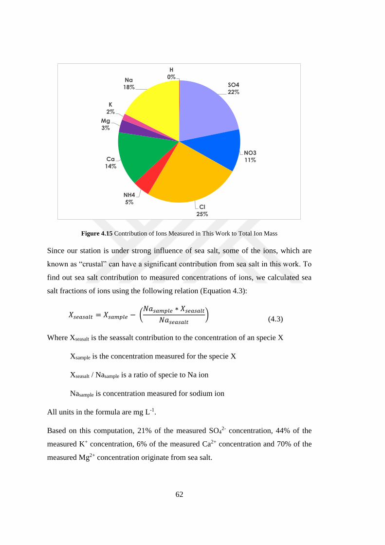
62

Figure 4.15 Contribution of Ions Measured in This Work to Total Ion Mass

Since our station is under strong influence of sea salt, some of the ions, which are

known as “crustal” can have a significant contribution from sea salt in this work. To

find out sea salt contribution to measured concentrations of ions, we calculated sea

salt fractions of ions using the following relation (Equation 4.3):

𝑋𝑠𝑒𝑎𝑠𝑎𝑙𝑡 = 𝑋𝑠𝑎𝑚𝑝𝑙𝑒 − (𝑁𝑎𝑠𝑎𝑚𝑝𝑙𝑒 ∗ 𝑋𝑠𝑒𝑎𝑠𝑎𝑙𝑡

𝑁𝑎𝑠𝑒𝑎𝑠𝑎𝑙𝑡)

(4.3)

Where Xseasalt is the seassalt contribution to the concentration of an specie X

Xsample is the concentration measured for the specie X

Xseasalt / Nasample is a ratio of specie to Na ion

Nasample is concentration measured for sodium ion

All units in the formula are mg L-1.

Based on this computation, 21% of the measured SO42- concentration, 44% of the

measured K+ concentration, 6% of the measured Ca2+ concentration and 70% of the

measured Mg2+ concentration originate from sea salt.

H

0%

SO4

22%

NO3

11%

Cl

25%

NH4

5%

Ca

14%

Mg

3%

K

2%

Na

18%

63

Long-term (interannual) variation in contribution of ions to total ion mass between

2011 and 2016 are given in Figure 4.16. The most striking point in the figure is

approximately 10% decrease in contribution of SO42- ion (from 35% in 2011 to 23%

in 2016), which indicates the success of actions taken to reduce SO2 emissions in

Turkey and in Europe as a whole.

Contributions of other ions (both anthropogenic and natural) did not change

significantly during sampling period. The only exception to this is the increase

observed in Na contribution from 11% in 2011 to 19% in 2016. This increase probably

an artifact to compensate the decrease in SO42- contribution.

64

Figure 4.16 Variation of Ionic Contribution to Total Ionic Mass in Time

H0%

SO435%

NO313%

Cl17%

NH42%

Ca17%

Mg3%

K1%

Na12%

2011 H0%

SO426%

NO313%

Cl23%

NH45%

Ca15%

Mg2%

K2%

Na14%

2012

H0%

SO421%

NO39%

Cl28%

NH42%

Ca18%

Mg3%

K2%

Na17%

2013H

0%

SO421%

NO311%

Cl26%

NH46%

Ca15%

Mg3%

K2%

Na16%

2014

H0% SO4

11%

NO311%

Cl29%NH4

10%

Ca5%

Mg7%

K2%

Na25%

2015H

0%SO423%

NO311%

Cl24%

NH42%

Ca17%

Mg3%

K1%

Na19%

2016

65

Seasonal changes in the contribution of ions to the total ion mass is given in Figure

4.17. Contributions of anthropogenic ions, SO42- and NO3

-, do not change significantly

from one season to another. Contributions of ions, which originate from the sea,

namely Na+ and Cl- are higher in winter months, due to increased production of sea

salt with stronger winds and longer windy periods winter season. On the contrary,

crustal ions Ca2+, Mg2+ and K+, have higher contributions to total ion mass during

summer months; due to easier resuspension of dry soil in summer. In winter, soil is

mostly wet (mud), hence resuspension of the soil particles to the atmosphere is more

difficult.

Figure 4.17 Seasonal Variation in Ionic Contributions to Total Ion Mass

H0%

SO424%

NO313%

Cl18%

NH47%

Ca19%

Mg4%

K2%

Na13%

H0%

SO421%

NO311%

Cl28%

NH44%

Ca13%

Mg3%

K1%

Na19%

Summer

Winter

66

4.4. Acidity of Wet Deposition

As pointed out in earlier sections, SO42- and NO3

- measured in Eastern Mediterranean

rainwater is among the highest measured in entire Europe, suggesting that pH should

be low as these the ions are the main source of acidity in wet deposition. However,

high pH of rainwater in Eastern Mediterranean atmosphere is also well documented

in literature (Al-Momani, et al., 1995; Özsoy, et al., 2008). This apparent dilemma is

due to extensive neutralization of acidity in rainwater and will be discussed in this

section.

4.4.1. pH of Rainwater

Annual, summer and winter frequency distribution of pH are given in Figure 4.18.

The pH values measured during the study varies between 3.7 and 7.9 with a median

value of 6.0. Since pH of a very clean rainwater varies between 5.0 and 5.6 due to

dissolution of CO2 and presence of natural SO2 in atmosphere, only, rain with pH <

5.0 is considered as acid rain (Jacob, 1999). Although relatively low pH values, such

as 3.7, were measured in some of the rainwater samples, only 17% of rain samples

have pH < 5 and can be considered as “acid rain”. Remaining 83% of all samples

collected at Marmaris station had pH > 5.0 and cannot be considered as “acid rain”.

This general pattern can also be seen in pH frequency histograms given in Figure 4.18.

Approximately 40% of pH data occurs between 5.5 and 6.5, 70% of data occurs

between pH 5 and 7, on an annual basis. There are some differences between summer

and winter histograms as well. There is a shift in frequency of occurrences toward

higher pH’s in summer. Approximately 44% of pH data occurs between pH’s 5.5 and

6.5 in winter histogram, whereas 55% of pH data is between pH 6 and pH 7 in summer,

indicating more extensive neutralization during summer season.

Monthly variation in pH values are given in Figure 4.19. There is a clear pattern of

higher pH values in summer. Observed seasonal behavior is also due to more extensive

neutralization of acidity in summer season, because SO42- and NO3

- concentrations are

higher during summer season and if free acidity originates from H2SO4 and HNO3, H+

ion concentration should also be higher in summer.

67

Figure 4.18 pH Frequency Distributions in Marmaris Rainwater

0

10

20

30

40

50

60

70

3,5 - 4 4 - 4,5 4,5 - 5 5 - 5,5 5,5 - 6 6 - 6,5 6,5 - 7 7 - 7,5 7,5 - 8

Nu

mb

er o

f O

ccu

ran

ce

pH Range

Annual

0

5

10

15

20

25

3,5 - 4 4 - 4,5 4,5 - 5 5 - 5,5 5,5 - 6 6 - 6,5 6,5 - 7 7 - 7,5 7,5 - 8

Nu

mb

er o

f O

ccu

ran

ce

pH Range

Summer

0

10

20

30

40

50

60

3,5 - 4 4 - 4,5 4,5 - 5 5 - 5,5 5,5 - 6 6 - 6,5 6,5 - 7 7 - 7,5 7,5 - 8

Nu

mb

er o

f O

ccu

ran

ce

pH Range

Winter

68

Figure 4.19 Monthly Variation of Rainwater pH at Marmaris

4.4.2. Neutralization of Rainwater

All pH measurements in Marmaris rainwater, which were discussed in previous

paragraphs demonstrate two basic facts; (1) SO42- and NO3

- concentrations are high

Marmaris rainwater, but (2) H+ ion concentration, which is expected to be correlated

with these two anions is very low. These two facts suggest that majority of H+

concentration in rain is neutralized by bases that are available in Marmaris

atmosphere.

Seasonality of the neutralization process was tested by calculating monthly median

equivalent ratio of H+/(SO42-+NO3

-). If the free acidity (H+ ions) that comes from

H2SO4 and HNO3 is not neutralized the ratio is expected to be unity. As H+ ions are

neutralized, the ratio deviates from unity and it becomes zero when all H+ are

neutralized. Monthly median H+/(SO42-+NO3

-) ratios are depicted in Figure 4.20. The

figure highlights two important points: (1) more than 85% of hydrogen ions in

Marmaris rainwater is neutralized throughout the year, (2) neutralization is more

complete during summer season. The ratio is approximately 0.12 in January and

December, indicating that 88% of acidity is neutralized in these months, but there is

almost no free hydrogen ion in rainwater from May through September.

69

Figure 4.20 Seasonal Variation of (H+)/([SO42-] + [NO3

-]) Ratio

The next question that should be answered is, “what neutralizes acidity in rainwater”?

There are two bases that can neutralize acidity in rain water, namely, NH3 and CaCO3.

Main sources of NH3 in atmosphere is fertilizer applications in agriculture (Pan, et al.,

2018; Personne, et al., 2015) and animal grazing (Behera, et al., 2013). Dominant

source of CaCO3 is the soil. Since soil in the Mediterranean region (not only along

Turkish coast, but throughout the Mediterranean basin) is highly enriched with CaCO3

(Federoff & Courty, 2013; Aydınalp & Cresser, 2008), CaCO3 is the likely base which

is responsible from high pH in Eastern Mediterranean rainwater. This can also be seen

in Figure 4.21, where hydrogen ion concentration is regressed against Ca2+ and NH4+

ions. Stronger correlation between hydrogen ion and Ca2+ is clear in the figure.

High pH of rainwater is not unique for this work. It is observed in most rainwater

studies performed in the Eastern Mediterranean region (Al-Momani, et al., 1995;

Alagha & Tuncel, 2003; Morales-Baquero, et al., 2013; Özsoy, 2003).

0

0.02

0.04

0.06

0.08

0.1

0.12

0.14

0.16

1 2 3 4 5 6 7 8 9 10 11 12

H/S

O4

+NO

3 e

qu

ival

ent

rati

o

Months

70

Figure 4.21 Relation between H+ ion vs. NH4+ and Ca2+ ions

4.5. Temporal Variations

Seasonal variations in pollutant concentrations refer to short term episodes, diurnal

variations, weekend-weekday variations, seasonal variations and interannual

variations. These information can be very informative to determine factors controlling

variability in concentrations of pollutants in urban atmosphere. However, in rural

atmosphere seasonal variations and interannual variations are the only types of

temporal variations that can be discussed.

71

4.5.1. Seasonal Variations in Ion Concentrations

Seasonal variations in concentrations of ions is generally due to variations in

meteorology, such as higher mixing height in summer, or seasonal variations in

transport patterns. Selection of geographical seasons may not be the best selection,

because it can mask some of the factors that controls seasonal variability in ion

concentrations. In this study seasons are selected based on rainfall data, because

variations in concentrations of ions and other particulate pollutants in rainwater and

aerosol is governed by variations in rainfall. Monthly rainfall at Marmaris Station is

depicted in Figure 4.22. Rainfall data, consisting of monthly averages between 1926

and 2007 were obtained from Marmaris Meteorological station. Based on this pattern

winter was selected as January, February, March, October, November and December,

whereas summer included April, May, June, July, August and September months.

With this division, approximately 14% of the annual rainfall, which is 1194 mm,

occurs in our summer and 86% of annual rainfall occurs in winter, which is typical for

the Eastern Mediterranean region.

Figure 4.22 Monthly variation rainfall (mm) at Marmaris Meteorology Station

0

50

100

150

200

250

300

1 2 3 4 5 6 7 8 9 10 11 12

Rai

nfa

ll (m

m)

Months

72

Monthly median concentrations of ions are given in Figure 4.23 and Figure 4.24. Ions

depict two different patterns, which is determined by four different factors.

Concentrations of SO42-, NO3

- and NH4+ in rainwater is clearly high during summer

season. Summer to winter median ratios of these ions are 1.8, 2.3 and 2.7 for NH4+,

SO42- and NO3

-, respectively.

73

Fig

ure

4.2

3 M

on

thly

Var

iati

on

of

Ion

Co

nce

ntr

atio

ns

and

Su

mm

er t

o W

inte

r C

on

cen

trat

ion

Rat

io o

f A

nth

ropo

gen

ic I

on

s

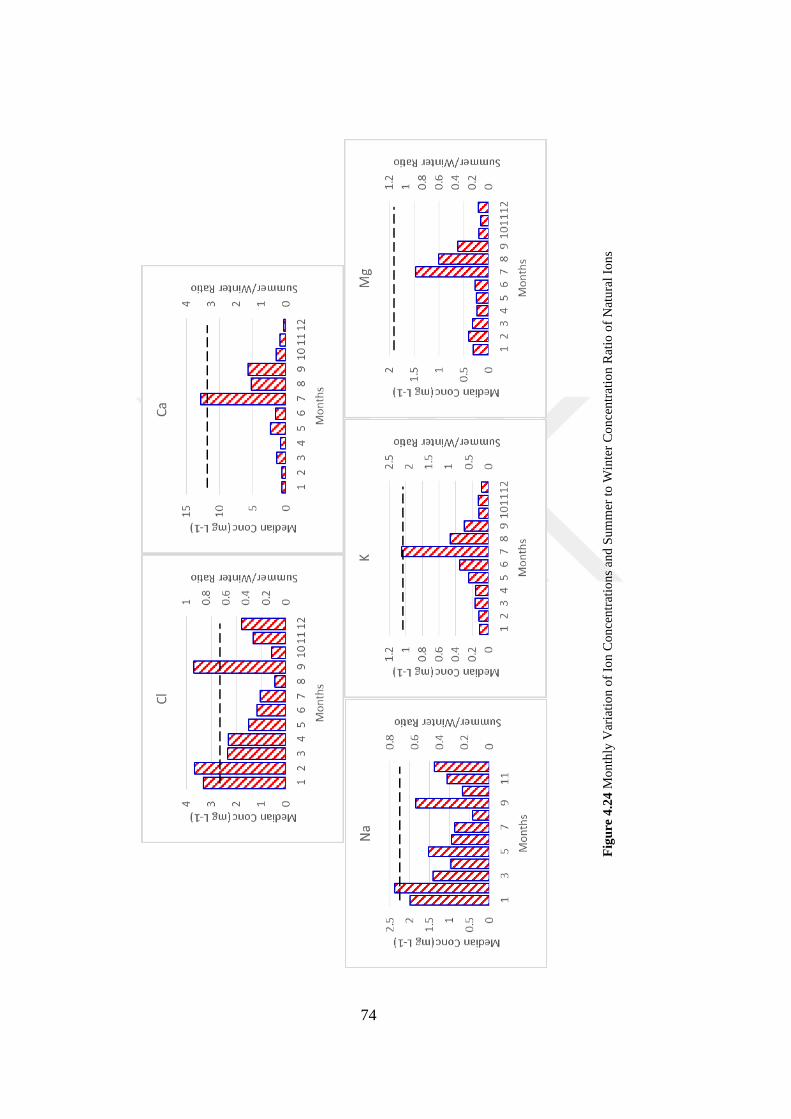
74

Fig

ure

4.2

4 M

on

thly

Var

iati

on

of

Ion

Co

nce

ntr

atio

ns

and

Su

mm

er t

o W

inte

r C

on

cen

trat

ion

Rat

io o

f N

atu

ral

Ion

s

75

Higher concentrations of these ions, particularly SO42- and NO3

-, in atmosphere during

summer months is attributed to faster gas-phase oxidation of SO2 and NO2 by more

vigorous photochemical activity in summer (Güllü, et al., 1998; Bardouki, et al., 2003;

Mihalopoulos, et al., 1997). More effective wet scavenging of particles and ions

associated with them during their long-range transport to Eastern Mediterranean

atmosphere in winter also contribute to observed higher concentrations of SO42-, NO3

-

and NH4+ in summer precipitation (Kubilay & Saydam, 1995; Al-Momani et al., 1998;

Güllü et al., 2005; Öztürk et al., 2012). For NH4+ ion, in addition to faster oxidation

in summer and more effective scavenging from atmosphere in winter, enhanced

evaporation of NH3 from applied fertilizers in summer and its subsequent oxidation

to NH4+ also contribute to its higher summer concentrations (Güllü et al., 1998).

Concentrations of Na+ and Cl-, on the other hand, are higher in winter. This is not

surprising, because both Na+ and Cl- are good indicators of marine aerosol, which

forms by bubble-bursting at the sea surface. Sea salt particle that are highly enriched

in Na+ and Cl- are formed in large quantities by increased storm activity in winter.

Higher concentrations of Na+ and Cl- in winter aerosol and precipitation samples in

not new in this work and reported frequently in literature (Güllü et al., 1998; 2005;

Al-Momani et al., 1998; Öztürk et al., 2012)

Like ions with anthropogenic sources, crustal ions, including Ca2+, Mg2+ and K+ have

also higher concentrations during summer seasons, but for a different reason.

Concentrations of soil related elements and ions in atmosphere depend on efficiency

of resuspension of soil particles, which is season dependent. Soil particles cannot

become airborne easily in winter, as the surface soil is permanently mud or ice

covered. No matter how strong winds are, it is difficult to get the soil particles

airborne. However, in summer surface is dry and soil particles can become airborne

even with moderate wind speeds. Since Ca2+, Mg2+ and K+ are associated with soil

particles, their concentrations are expected to be high in summer.

76

Hydrogen ion concentrations are much higher in winter and very low in summer. This

seasonal pattern is governed entirely by season-dependent neutralization of acidity,

which is a local process. High CaCO3 content of soil in in Mediterranean region and

how it neutralizes acidity in rain water was discussed in the previous section. Higher

atmospheric loading of crustal material (and CaCO3) in summer months results in

more extensive neutralization and very low H+ concentration during summer.

Summer-to-winter concentration ratios of ions measured in this work is depicted in

Figure 4.25. Summer-to-winter ratios computed for anthropogenic (SO42-, NO3

- and

NH4+) and crustal (Ca2+, Mg2+, K+) ions are > 1.0 and those for sea salt (Na+, Cl-) ions

and H+ are < 1.0. Reasons for these patterns were discussed in previous paragraphs.

Although summer-to-winter ratio > 1.0 for SO42-, NO3

-, NH4+, Mg2+, K+ and Ca2+, the

ratio is not the same for all of them. The highest ratio was computed for Ca2+, which

is followed by NO3- and SO4

2-.

Figure 4.25 Summer-to-Winter Concentration ratios of Ions in Marmaris Rainwater

0

0.5

1

1.5

2

2.5

3

3.5

H Cl Na Mg NH4 K SO4 NO3 Ca

Sum

mer

/Win

ter

Rat

io

77

It is expected to see higher summer-to-winter ratios for crustal elements, as their

generation rate is a very different between summer and winter. PM10 concentrations

measured at a station operated by the Ministry of Environment and Municipality

(MoEM) at Ören, which is approximately 30 km from Marmaris station are 224 µg

m-3 in summer and 39 µg m-3 in winter. This corresponds to summer-to-winter

concentration ratio of 5.6. The Summer/Winter ratios of crustal ions in precipitation

are lower than this ratio measured in aerosol. Summer-to-winter ratio of Ca2+, K+ and

Mg2+ are 4.9, 2.9 and 2.1, respectively.

Smaller Summer/Winter ratio that had been observed in the collected precipitation

samples compared to similar ratio found in atmospheric particles is probably due to

sea-salt contribution to concentrations of Ca2+, K+ and Mg2+. It was calculated in

Section 4.3.2 that 70% of Mg2+, 44% of K+ and 6% of Ca2+ can be accounted for by

sea salt particles at our station. Since sea-salt concentration in atmosphere is higher

during winter season, higher sea salt contribution to concentrations of these ions in

winter results in lower S/W ratios. Ordering of Summer/Winter ratios of these ions

also supports this hypothesis. Sea salt contribution is the highest for Mg2+, then to K+

and the least to Ca2+ (Al-Momani et al., 1998; Güllü et al., 1998; 2005). Since sea salt

contribution to Ca2+ is smaller than its contribution to Mg2+ and K+ concentrations,

Summer/Winter ratio for this ion is similar to the summer-to-winter ratio observed in

PM10 particles.

4.5.2. Interannual Variations in Ion Concentrations

Interannual variations in concentrations of ions, which demonstrate long-term trends,

is useful to assess results of actions taken to improve air quality. Although there are

tests to determine statistical significance of observed trends (such as Mann-Kendall

test), data generated in this study is not long enough for such trend analysis (generally

data longer than 10 years is needed). In this work we investigated visual increasing

and decreasing trends in concentrations of ions without testing its statistical

significance.

78

Box-and whisker plots that are prepared for ions with anthropogenic, marine and

crustal sources are depicted in Figure 4.26 and Figure 4.27. Different trends were

observed in concentrations of different ions. Among ions with anthropogenic sources,

concentrations of SO42-, NO3

- and H+ decreased between 2011 and 2015, then slightly

increased in 2016. How significant is the increase in 2016 is not clear, but decrease

between 2011 and 2015 is consistent with decreasing trend in their concentrations in

European rainwater and aerosol. There is no obvious decreasing or increasing pattern

in NH4+ concentrations, which is given in Figure 25d. Statistical significance of small

increases measured in 2014, 2015 and 2016 is not clear.

Concentrations of ions with crustal source, namely Ca2+ and K+, show trends that are

similar to anthropogenic ions. A decrease in their concentrations between 2011 and

2015, then a small increase in 2016 can be seen in Figures 26 (c) and (d). It is

interesting to note that a similar decreasing trend in concentrations of crustal element

(Al, Fe, Ca, K) was also observed in aerosol samples collected at a station that is

approximately 20 km to the west of Antalya (Öztürk et al., 2012). The decrease was

attributed to reduced frequency of Saharan Dust transport. The decrease in dust

transport to Mediterranean region is reported by other researchers as well (Mahowald,

et al., 2010; Ganor, et al., 2010). However, doubling of dust transport to Eastern

Mediterranean region is also reported (Floutsi, et al., 2016).

Concentrations of marine ions, namely Na+ and Cl- gradually increase between 2011

and 2016. This trend observed in concentrations of both Na+ and Cl- suggests an

increasing trend in storm activity during study period. However, there is no literature

information that support or oppose this observation.

79

F

igu

re 4

.26

In

tera

nn

ual

Var

iati

on

in

Co

nce

ntr

atio

ns

of

Po

llu

tio

n D

eriv

ed i

on

s in

Mar

mar

is R

ain

wat

er

80

F

igu

re 4

.27

In

tera

nn

ual

Var

iati

on

in

Co

nce

ntr

atio

ns

of

Cru

stal

an

d S

ea S

alt

Ion

s in

Mar

mar

is R

ain

wat

er

81

4.6. Positive Matrix Factorization

One of the rationale of measuring ionic composition of rainwater at Marmaris is to

find out source regions in and out of Turkey that affect our country and Eastern

Mediterranean in general. This can be answered in two steps using different statistical

tools. In the first step, types of sources that affect composition of rainwater at

Marmaris was determined using positive matrix factorization, which is a multivariate

statistical tool. In the second step locations of sources, which came out in the first step,

was found by applying “potential source contribution function” (PSCF), which is a

method in trajectory statistics.

Positive matrix factorization (PMF) is newer version of factor analysis (FA) and

principal component analysis (PCA), which are two widely used statistical tools in

receptor modeling. Despite these well-known multivariate tools, PMF found wide use,

because it has two important advantages over the other two methods. First advantage

is the quantitative nature of PMF, whereas results obtained from FA and PCA are

qualitative. The second advantage is that samples are not rejected from PMF due to

missing data, FA and PCA, on the other hand, require complete data sets.

Input to PMF consists of two sets of information, namely data file, which contains

measurement results and uncertainty file, which includes uncertainty information

about each datum. Based on these two information PMF assigns categories to each

specie with respect to their signal-to-noise ratios (S/N). Ions are classified as “Bad”,

“Weak” of “Strong”; where “Bad” is the specie with S/N below 0.5. “Weak” species

have S/N ratio between 0.5 and 1.0 and “Strong” category refers to the species with

S/N greater than 1.0.

Species categorized as “Bad” are removed entirely from analysis. Uncertainties of

weak species are increased so that they do not contribute to the “fit”, but contributions

of factors to these “weak” species are calculated and they are included to output.

Contribution of weak species to “fit” is avoided by multiplying their uncertainties by

three. “Strong” species are included in PMF run without modifying their uncertainties.

These “strong” parameters are used in the fit. The S/N values and categories of the

82

species measured in this study are given in Table 4.4. All of the ions measured in this

study are categorized as “strong” in PMF analysis.

Table 4.4 Categories and Signal-to-noise Ratios of the Ions

Species Category S/N

SO42- Strong 9.6

NO3- Strong 9.2

Cl- Strong 8.7

NH4+ Strong 3.2

Ca2+ Strong 8.4

Mg2+ Strong 9.2

K+ Strong 6.0

Na+ Strong 9.6

In PMF analysis, selection of proper number of factors is an important point and

unfortunately left to user. Unlike in FA and PCA there is no rule that defines the

number of factors that should be retained. However, there are some guidelines, which

can assist in selecting factors to be retained. First and the most important guideline is

the minimization of the “object function” Q. For each run with different factors, the

PMF software calculates a Qrobust value, which should be compared with Qtheoretical,

which is a function of number of parameters used in the fit and number of factors. The

difference between these two Q values should be minimized by changing number of

factors. Number of factors that corresponds to minimum Q is the factors that should

be extracted in PMF exercise. The second very important criteria in deciding factor-

number is that factors extracted should have physical meaning. There are few other

criteria to select factors, such as scaling residuals, but these two are the most important

ones.

After running PMF between four-to-seven factors and optimizing each run, solution

with four factors was accepted. The object function Qrobust calculated by the software

for 4 factors was 1565 and Qtheoretical calculated using the Equation 4.4 for same

83

number of factors was 1176. Higher number of factors had smaller Q but additional

factors did not make sense or they formed by splitting one of the existing factors

𝑄𝑡ℎ𝑒𝑜𝑟𝑒𝑡𝑖𝑐𝑎𝑙 = (𝑘 ∗ 𝑚) − 𝑡(𝑘 + 𝑚) (4.4)

Please note that resolution of PMF analysis depends strongly on number of samples

and number of parameters included in the fit. In this study, number of samples was

sufficient and did not cause a resolution problem. However, number of parameters

analyzed in this study (nine ions) was too small for a successful PMF. Four factors

found in this work does not mean there is only four source types (or components) in

rainwater. It means ions can resolve these four sources. If more parameters, such as

trace elements, carbon fractions or particulate organics, were measured, larger number

of factors, each representing a different source type, could be extracted.

Factor 1

Diagnostic figures for factor 1, which includes Factor loadings, percent contribution

of factor 1 on measured concentrations of ions and monthly median values of factor

scores are given in Figure 4.28. Factor 1 accounts for all of the measured NH4+

concentration, approximately 41% of the measured NO3- concentration and 22% of

the measured K+ concentration. High concentrations of NH4+ was reported both in

particles (Güllü et al., 1998; 2005; Öztürk et al., 2012) and rainwater (Al-Momani et

al., 1995; 1998) in the eastern Mediterranean region and attributed to oxidation of NH3

emitted from fertilizer application in the region. Higher factor 1 scores during summer

months support fertilizer source, because fertilizers are applied in spring and

evaporation of NH3 is expected to be maximum in summer due to high temperature.

Factor 1 also accounts for 22% of the measured K+ concentration. Potassium has three

important sources in the atmosphere, namely, crustal, sea salt and biomass burning

(Sullivan, et al., 2019; Sun, et al., 2019; Tunno, et al., 2019). Presence of K+ in the

same factor with NH4+ indicates a mixing of biomass burning particles with NH3

emitted from fields, or may indicate higher NH3 emission rates during forest fires.

Both of these hypotheses are highly speculative at this point, because there is no

84

supporting literature. Based on these arguments, factor 1 is identified as fertilizer

factor.

Figure 4.28 Factor 1 diagnostics: (a) factor loadings, (b) fractions of ion concentrations explained

by factor 1 and (c) monthly variations of factor scores

0

0.1

0.2

0.3

0.4

0.5

0.6

0.7

SO4 NO3 Cl NH4 Ca Mg K Na

Fac

tor

Pro

file

(fr

acti

on)

Factor 1

0

20

40

60

80

100


% o

f co

nce

ntr

atio

ns

exp

lain

ed

% of element concentrations

Explained by Factor 1

0

0.5

1

1.5

2

2.5

3

3.5

4

4.5

1 2 3 4 5 6 7 8 9 10 11 12

Fac

tor

1 S

core

s

Months

Factor 1 Scores

85

Factor 2

Diagnostic figures for factor 2 are given in Figure 4.29. Factor 2 is a very clear crustal

factor. It accounts for almost 87% of measured Ca concentration, 23% of measured

concentrations of Mg2+ and 37% of measured K+.

It can be seen in Figure 4.29 (c) that Factor 2 scores are high during summer and low

in winter. This supports crustal source for factor 2, because resuspension of surface soil

is easier during summer season when the soil is dry, as discussed previously Section

4.5.

86



0

0.5

1

1.5

2

2.5


Fac

tor

Pro

file

(fr

acti

on)

Factor 2

0

20

40

60

80

100


% o

f co

nce

ntr

atio

ns

exp

lain

ed



0

1

2

3

4

5

6

7

8

9

1 2 3 4 5 6 7 8 9 10 11 12

Fac

tor

2 S

core

s

Months

Factor 2 Scores

87

Factor 3

Diagnostic figures for factor 3 are given in Figure 4.30. Factor 3 is dominated by SO42-

and NO3- . It accounts for 82% of measured SO4

2- and 56% of the measured NO3-

concentrations. Factor scores depicted a well-defined seasonal pattern with higher

scores in summer. Factor 3 is a typical combustion factor, which was seen in most of

the previous aerosol and rainwater studies in the Eastern Mediterranean region. Factor

3 is identified as long range transport-combustion factor. It represent rain that brings

pollutants from distant sources. Emissions from power plants located at different parts

of our study domain are the main component in this factor.

Distribution of PSCF values calculated using Factor 3 scores are given in Figure 4.31.

Main industrial source regions affecting ionic composition of rain water at Marmaris

are İstanbul and Thrace area, Western Black Sea coast of Turkey, regions in

Azerbaijan and Dagestan Republic, South eastern part of Ukraine, Jordan - Saudi

Arabia border. There are also some minor source areas in Balkans and along African

Coast. Source areas at the inner parts of Africa can be due to too few segments in those

grids, which are in the outskirts of the study area. Although we applied the weighting

approach developed by Zhao and Hopke (2006), it does not completely eliminate the

limitation of PSCF, when there are few segments in a grid. Western parts of Turkey,

Balkan Countries Eastern parts of Ukraine, Black Sea coast of Russia appears as

primary sources regions in most of the aerosol and rainwater studies performed in our

group (Balcılar et al., 2014; Öztürk et al., 2012; Al-Momani et al., 1998; Alagha et al.,

2003; Tokgöz et al., 2015). Since effect of these source regions were consistently

identified in both Mediterranean and Black Sea regions of Turkey, they can be

identified as important foreign sources contributing to atmospheric composition in our

country.

Another important point to note in the figure is that most of the major cities in the

region, including Rome, Athens, Istanbul, Ankara, Cairo appears as source areas. This

observation suggests that factor 3 is not an exclusively industrial factor. It also

represent anthropogenic emissions from highly-populated urban areas.

88



0

0.5

1

1.5

2

2.5

3


Fac

tor

Pro

file

(fr

acti

on)

Factor 3

0

10

20

30

40

50

60

70

80

90

SO4 NO3 Cl NH4 Ca Mg K Na% o

f co

nce

ntr

atio

ns

exp

lain

ed



0

0.5

1

1.5

2

2.5

3

1 2 3 4 5 6 7 8 9 10 11 12

Fac

tor

3 S

core

s

Months

Factor 3 Scores

89

Fig

ure

4.3

1 F

acto

r 3

po

ten

tial

so

urc

e re

gio

ns.

Dis

trib

uti

on

of

PS

CF

val

ues

co

mp

ute

d u

sing

Fac

tor

2 s

c ore

s. T

raje

cto

ries

th

at c

orr

esp

ond

to

hig

hes

t 4

0%

of

Fac

tor

3 s

core

s w

ere

tak

en a

s p

oll

ute

d t

raje

cto

ries

90

Factor 4

Diagnostic figures for Factor 4 are given in Figure 4.32. Factor 4 is a clear marine

factor. This factor explains of 95 % of the Na+ and 96 % of Cl- concentrations, which

are the most abundant species in sea water (accounting for 36% and 55% of total

suspended solids in rain water, respectively). Factor 4 also accounts for 9% of SO42-

concentrations, 67% of Mg2+ concentrations and 28% of K+ concentration. These ions

are major components of sea water. Sulfate, Mg, K and Ca accounts for 8%, 3.7%,

2.4% and 1.2% of total dissolved solids in sea water respectively (Ault, et al., 2013;

Lowenstein, et al., 2005).

Factor scores are higher in winter months, which is expected from sea salt. Sea salt

particles are generated by bubble bursting at the sea surface, a process that strongly

depend on wind speed over the sea (Brooks & Thorton, 2018; Song, et al., 2019).

Higher scores in winter is due to stronger and more frequent storm activity in

Northeastern Mediterranean in winter season.

91


by factor 4 and (c) monthly variations of factor 4 scores

0

0.5

1

1.5

2

2.5

3

3.5


Fac

tor

Pro

file

(fr

acti

on)

Factor 4

0

20

40

60

80

100


% o

f co

nce

ntr

atio

ns

exp

lain

ed



0

0.2

0.4

0.6

0.8

1

1.2

1.4

1.6

1.8

1 2 3 4 5 6 7 8 9 10 11 12

Fac

tor

4 S

core

s

Months

Factor 4 Scores

92

4.7. Deposition Fluxes

Wet deposition fluxes of ions can be viewed from two perspective. First it is a mean

of cleaning atmosphere. However, it is also a mechanism of transport of pollutants

from atmosphere to surface and has a potential to contaminate receptor ecosystem

components. Several examples do exists that clearly demonstrate damage caused by

wet deposition of pollutants on lakes or forests. Acid rain is the best documented

example.

Wet deposition fluxes of ions measured in this study were calculated by multiplying

measured concentrations of ions (mg L-1) with rainfall for that event (mm or L m-2)

and correcting for surface area of the bucket. Since wet deposition fluxes of ions

depend strongly on the rainfall, higher fluxes during winter months, when

approximately 80% of the annual rainfall occur, is expected. Monthly variation of

SO42- deposition flux is given in Figure 4.33 as an example. Although SO4

2-

concentration is higher during summer season, its deposition flux is orders of

magnitude lower during summer, demonstrating strong dependence of wet deposition

fluxes on rainfall. However, relation between rainfall and SO42- wet deposition flux is

not as straightforward as expected, because although one expects to see a strong

correlation between rainfall and ion fluxes, which are calculated by multiplying

concentration with rainfall, the relation is not as strong as expected. This is shown in

Figure 4.34 where SO42- wet flux is plotted against rainfall per event. Although there

is a statistically significant [P(r,n) < 0.05] correlation between flux and rainfall, it is

not a strong correlation. This is due to inverse relation between ion concentrations and

rainfall, which is shown for NO3- in Figure 4.35 as an example. A decreasing trend

can be seen in NO3- concentrations with rainfall. The trend is not statistically

significant with 5% confidence, not because there is no relation between two

parameters, but because relation is not linear. Such non-linear inverse relation between

concentrations of elements or ions with rainfall are frequently reported in literature

and attributed to dilution of species (Lin, et al., 2017; Canovas, et al., 2012;

Matsumoto, et al., 2005; Al-Momani, et al. 1998). All these indicate that relation

93

between ion flux and rainfall is not very simple, and although a statistically significant

correlation between them do exist, it is not as strong as initially expected.

Figure 4.33 Monthly Variation in SO42- Wet Deposition Flux

Figure 4.34 Relation Between SO42- Wet Deposition Flux and Rainfall

94

Figure 4.35 Relation Between Concentrations of Ions and Rainfall

Interannual variability in deposition fluxes of ions with anthropogenic origin are given

in Figure 4.36. Hydrogen deposition flux does not show a clear, well-defined variation

between 2011 and 2016. This was not unusual, because variation of H+ concentration

from one year to another depends not only on the concentrations of acidic species,

namely H2SO42- and HNO3

- but also depends on concentrations of bases, namely

CaCO3 and NH3, particularly CaCO3.

Deposition fluxes of SO42- and NO3

- decrease between 2012 and 2016. Wet deposition

fluxes of all ions are low in the year 2011, because rain sampling at Marmaris station

started in June 2011. Since annual fluxes were generated by adding fluxes for each

event, 2011 fluxes turned low, because half of the events (before June 2011) were not

included in flux calculations. Statistical significance of these decreasing trends were

not tested, because data is not long-enough for trend analysis. But decreasing SO42-

and NO3- fluxes are obvious. This is due to decreasing concentrations of these ions

from 2010 to 2016, as discussed previously in this manuscript.

95

Fig

ure

4.3

6 I

nte

r-an

nu

al v

aria

tio

n i

n w

et d

epo

siti

on

flu

xed

of

anth

rop

ogen

ic i

on

s

96

Fig

ure

4.3

7 I

nte

r-an

nu

al v

aria

tio

n i

n w

et d

epo

siti

on

flu

xed

of

mar

ine

and

cru

stal

io

ns

97

Unlike flux variations in SO42- and NO3

-, NH4+ wet deposition flux does not show well

defined trend between 2012 and 2016. This is probably because main source of NH4+

at Marmaris is the fertilizer applications in the region, which did not change much in

last 10 years.

Interannual variation in wet deposition fluxes of crustal and marine ions are depicted

in Figure 4.37. Sea salt ions, namely Na+ and Cl- show a pattern that is very similar to

anthropogenic ions. Their fluxes decrease between 2013 and 2016. This pattern is

possible only if annual average wind speed decrease in time, but such decrease is wind

speed is not reported in literature. Crustal elements Ca2+ and Mg2+, on the other hand

did not show a consistent and well-defined pattern as expected.

Wet deposition fluxes of anthropogenic and crustal ions are compared with

corresponding fluxes in EMEP network in Figure 4.38 and Figure 4.39, respectively.

Unlike concentrations of ions, fluxes measured at Marmaris station is not high

compared to fluxes measured in the rest of the EMEP network. For example, SO42-

concentration is the highest among all EMEP stations, but SO42- flux is not. This is

due to smaller annual rainfall in the Mediterranean region, which strongly affects wet

deposition fluxes of ions. This pattern is not specific for anthropogenic ions but is

valid for crustal and marine ions as well.

98

Fig

ure

4.3

8 C

om

par

iso

n o

f w

et d

epo

siti

on

flu

xes

of

Po

llu

tio

n-d

eriv

ed i

on

s m

easu

red

in t

his

stu

dy

wit

h c

orr

espo

nd

ing

flu

xes

in

EM

EP

net

wo

rk

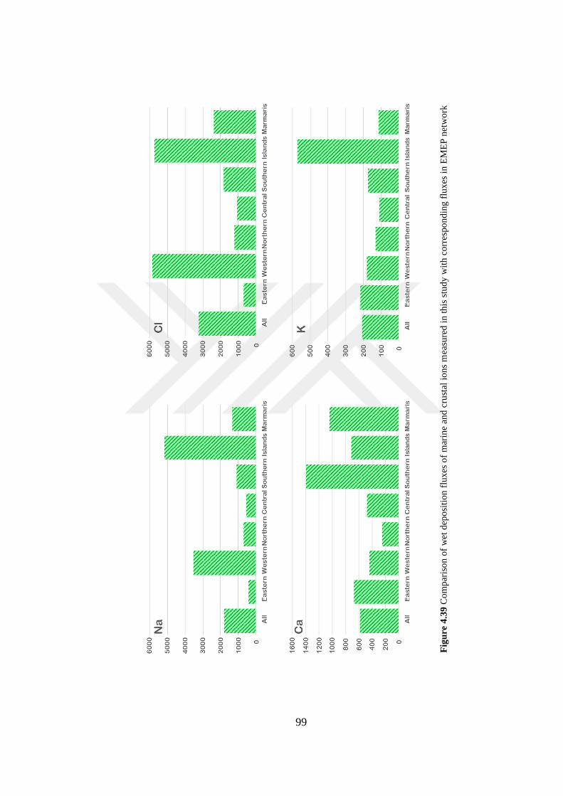
99

Fig

ure

4.3

9 C

om

par

iso

n o

f w

et d

epo

siti

on

flu

xes

of

mar

ine

and

cru

stal

io

ns

mea

sure

d i

n t

his

stu

dy

wit

h c

orr

espo

nd

ing

flu

xes

in

EM

EP

net

wo

rk

100

Another important point in wet deposition fluxes of ions is their episodic nature.

Percentage of rain events that account for 90% of ion deposition is depicted in Figure

4.40. Hydrogen ion is the most episodic parameter. Approximately 20% of events

accounted for 90% of H+ deposition. For the remaining ions 90% of their deposition

fluxes are accounted by 35% - 55% of rain events. Episodic nature of wet deposition

fluxes of ions is due to episodic nature of the rainfall. At Marmaris station 53% of rain

events account for 90% of annual deposition. However, more episodic nature of H+

ion cannot be explained only by episodic nature of rainfall. Two factors play an

important role in episodic nature of H+ wet deposition. One of them is, like all other

ions, episodic nature of rainfall. The second factor is the neutralization of free H+ ion,

which is dependent on CaCO3 (represented by Ca2+ in our data set). Since Ca2+

concentration and flux are also episodic, Hydrogen flux, and concentration becomes

more episodic than other ions.

Figure 4.40 Episodic nature of wet deposition fluxes: Percentage of rain events accounting for 90%

of wet deposition fluxes of ions

101

CHAPTER 5

5. CONCLUSION AND RECOMMENDATIONS

In this study, major ions (H+, SO42-, NO3

-, Cl-, NH4+, Ca2+, Mg2+, K+, and Na+) had

been measured in the Marmaris Station of MGM with ion chromatography between

the period 2011 and 2016. A total of 302 measurement days are present in the data set

which were analyzed for this study.

General characteristics of the data were measured, volume weighted average, mean

standard deviation, median values and ranges for all ions are calculated. Also by using

software Statgraphics distributions of the ions were visualized and same software gave

the information that the distributions are log-normal and right skewed.

Residence times of the air parcels reaching to the station is studied. Back trajectories

that had been calculated for a thirteen-year period were used to determine the

residence times for three different altitudes. The areas air masses spent time most

before reaching the station is western part of Turkey and the Balkans. The difference

of residence times with respect to dry and wet season was also calculated; in dry

season, summer, northern areas are more dominant, however southern areas,

especially North Africa, is dominant in winter, wet season. Dividing the study domain

into eight wind sectors as N, NE, E, SE, S, SW, W and NW; N and NE sectors were

dominant for summer months; E, SE, S and SW sectors had more segments in winter

months. Which means that in summer months pollutants from N and NE, whereas in

winter pollutants transported from E, SE, S and SW are more dominant. As a part of

the flow climatology, cluster analysis was made on the station showed that,

trajectories can be grouped as 5 clusters.

Contributions of the ions to the total ion mass was calculated and it is observed that

the ion with most contribution is Cl- in overall, followed by SO42- and Na+.

Contributions of the ions were examined seasonally; contributions of the

102

anthropogenic sourced secondary ions, SO42- and NO3

-, do not change depending on

the season, contributions of sea salt sourced Na+ and Cl-, are higher in winter months;

on the contrary, crustal ions Ca2+, Mg2+ and K+, have higher contributions in summer

months.

Temporal variation of the rainfall for the station was analyzed and dividing the winter

as October to March and summer as April to September; it was measured that

approximately 14% of the annual rainfall occurs in our summer and 86% of annual

rainfall occurs in winter, which is typical for the Eastern Mediterranean region.

As for the temporal variations of the ions; higher concentrations of ions, particularly

SO42- and NO3

- were observed in atmosphere during summer months, which is

attributed to both faster gas-phase oxidation of SO2 and NO2 by more vigorous

photochemical activity due to enhanced solar flux in summer. Concentrations of Na+

and Cl-, were higher in winter, because both ions are indicators of marine aerosol,

which forms by bubble-bursting at the sea surface. Crustal ions, including Ca2+, Mg2+

and K+ have higher concentrations during summer seasons, due to the amount of

suspended soil in the air, which is more likely to occur in summer months since the

soil is drier. H+ ion concentrations were much higher in winter and very low in

summer, pattern is governed entirely by season-dependent neutralization of acidity.

Rainwater samples were exposed to both natural and anthropogenic pollutants while

travelling to the station. In order to determine the sources and source locations of the

ions, Positive Matrix Factorization and Potential Source Contribution Function

models were used. The PMF model revealed four factors, which were identified as

two anthropogenic, one marine and one crustal factors. Potential source regions for

the anthropogenic components in rainwater were identified as to be western Ukraine,

Western Black Sea coast of the Turkey, Balkan Countries, North Africa and Georgia.

In this study, major ion composition of rain water is analyzed. Trace element

concentrations are not included in this work; so in future works, including trace

elements in addition to this data, will give more detailed and precise results, especially

in positive matrix factorization.

103

Since there are only nine ion concentration in PMF, obtained results are not

completely reliable. In future works, trace element and organic compound

concentrations, which are more specific source markers, should be included in the

PMF analysis. Including these data may result as more factor numbers with specific

marker species.

Also, in order to determine the statistical changes in temporal variations, longer

sampling should be done. Thus tests such as Mann-Kendall Test can be applied to the

data set, which will be statistically more accurate for long-term trends.

105

REFERENCES

Acid Deposition Monitoring Network in East Asia. (2000). Quality Assurance/Quality

Control (QA/QC) Program for Wet Deposition Monitoring in East Asia. Asia

Center for AirPollution Research.

Alagha, O., & Tuncel, G. (2003). Evaluation of Air Quality over the Black Sea: Major

Ionic Composition of Rainwater. Water, Air and Soil Pollution: Focus, 89-98.

Al-Khashman, O. A. (2005). Ionic composition of wet precipitation in the Petra

Region, Jordan. Atmospheric Research, 1-12.

Al-Khashman, O. A. (2005). Study of chemical composition in wet atmospheric

precipitation in Eshidiya area, Jordan. Atmospheric Environment, 6175-6183.

Al-Khashman, O. A. (2009). Chemical characteristics of rainwater collected at a

western site of Jordan. Atmospheric Research, 53–61.

Al-Momani, I. F., Aygun, S., & Tuncel, G. (1998). Wet deposition of major ions and

trace elements in the eastern Mediterranean basin. Journal of Geophysical

Research, 8287-8299.

Al-Momani, I. F., Tuncel, S., Eler, Ü., Örtel, E., Sirin, G., & Tuncel, G. (1995). Major

ion composition of wet and dry deposition in the eastern Mediterranean basin.

The Science of the Total Environment, 75-85.

Anil, I., Alagha, O., & Karaca, F. (2017). Effects of transport patterns on chemical

composition of sequential rain samples: Trajectory clustering and principle

component analysis approach. Air Quality, Atmosphere and Health, 1193-

1206.

106

Arsene, C., Olariu, R. I., & Mihalopoulos, N. (2007). Chemical composition of

rainwater in the northeastern Romania, Iasi region (2003–2006). Atmospheric

Environment, 9452-9467.

Ault, A. P., Moffet, R. C., Baltrusaitis, J., Collins, D. B., Ruppel, M. J., Caudra-

Rodriguez, L. A., & Grassian, V. H. (2013). Size-dependent changes in sea

spray aerosol composition and properties with differen seawater conditions.

Environmental Science and Technology, 5603-5612.

Ayaklı, G. (2014, February). Chemical Composition of Precipitation in Different Parts

of Turkey. M. Sc. Thesis. Ankara: Middle East Technical University.

Aydınalp, C., & Cresser, M. S. (2008). Red soils under Mediterranean type climate:

Their properties use and productivity. Bulgarian Journal of Agricultural

Science, 576-582.

Balcılar, İ., Zararsız, A., Kalaycı, Y., Doğan, G., & Tuncel, G. (2018). Temporal

variatioins of Eastern Black Sea aerosol. Global NEST Journal, 115-121.

Bardouki, H., Liakakou, H., Economou, C., Sciare, J., Smolik, J., Zdimal, V.,

Eleftheriadis, K., Lazaridis, M., Dye, C., Mihaloloulos, N. (2003). Chemical

composition of size-resolved atmospheric aerosols in the eastern

Mediterranean during summer and winter. Atmospheric Environment, 195-

208.

Behera, S. N., Shharma, M., Aneja, V. P., & Balasubramanian, R. (2013). Ammonia

in the atmosphere: A review on emission sources, atmospheric chemistry and

deposition on terrestrial bodies. Environmental Science and Pollution

Research, 8092-8131.

Belis, C. A., Larsen, B. R., Amato, F., El Haddad, I., Favez, O., Harrison, R. M.,

Hopke, P., Nava, S., Paatero, P., Prevot, A., Quass, U., Vecch, R., Viana, M.

(2014). European Guide on Air Pollution Source Apportionment with

Receptor Models. Ispra: Joint Research Centre of the European Commission.

107

Blondel, J., Aronson, J., Bodiou, J.-Y., & Boeuf, G. (2010). The Mediterranean

Region: Biological Diversity in Space and Time. New York: Oxford

University Press.

Bottenberg, C., Schanus, L., Kluss, R., & Kuball, C. (2006). The Mediterranean

Climate.

Brankov, E., Rao, S. T., & Porter, P. S. (1998). A Trajectory-clustering-correlation

methodology for examining the long-range transport of air pollutants.

Atmospheric Environment, 1525-1534.

Bricker, O. P., & Rice, K. C. (1993). Acid Rain. Annual Review of Earth and

Planetary Sciences, 151-174.

Brooks, S. D., & Thorton, D. C. (2018). Marine aerosols and clouds. Annual Review

of Marine Science, 289-313.

Bruno, F., Cocchi, D., & Greco, F. (2011). Clustering compositional data trajectories:

The case of particulate matter in the lower troposphere. Environmetrics, 975-

984.

Burke, K. (2006). Ion Chromatography. Retrieved from New Mexico State

University: https://web.nmsu.edu/~kburke/Instrumentation/IC.html

Canovas, C. R., Olias, M., Vazquez-Suñé, E., Ayora, C., & Nieto, J. M. (2012).

nfluence of releases from a fresh water reservoir on the hydrochemistry of the

Tinto River (SW Spain). Science of The Total Environment, 418-428.

Casiday, R., & Frey, R. (1998). Acid Rain. Retrieved from Washington University

Department of Chemistry:

http://www.chemistry.wustl.edu/~edudev/LabTutorials/Water/FreshWater/ac

idrain.html

Cheng, S., Wang, F., Li, J., Chen, D., Li, M., Zhou, Y., & Ren, Z. (2013). Application

of trajectory clustering and source apportionment methods for investigating

108

trans-boundary atmospheric PM10 pollution. Aerosol and Air Quality

Research, 333-342.

Chmielewski, A. G. (2011). Monitoring, Control and Effects of Air Pollution. Rijeka:

InTech.

Colls, J. (2002). Air Pollution. Spoon Press.

Committee on Public Works. (1975). Air Quality and Stationary Source Emission

Control. Washington: U.S. Government Printing Office.

Dayan, U., Ricaud, P., Zbinden, R., & Dulac, F. (2017). Atmospheric pollution over

the eastern Mediterranean during summer – a review. Atmospheric Chemistry,

13233-13263.

Dorling, S. R., Davies, T. D., & Pierce, C. E. (1992). Cluster analysis: A technique

for estimating the synoptic meteorological controls on air and precipitation

chemistry—Method and applications. Atmospheric Environment, 2575-2581.

Draxler, R. R., & Hess, G. D. (1997). Description of the HYSPLIT_4 modelling

system. Silver Spring: NOAA Technical Memorandum NOAA Air Resources

Laboratory.

Draxler, R. R., & Hess, G. D. (1998). An overview of the HYSPLIT_4 modelling

system for trajectories. Australian Meteorological Magazine, 295-308.

Emami, F., & Hopke, P. K. (2017). Effect of adding variables on rotational ambiguity

in positive matrix factorization solutions. Chemometrics and Intelligent

Laboratory Systems, 198-202.

EMEP. (2017, November). EMEP acidifying/eutrophying compounds. Retrieved from

EMEP: https://projects.nilu.no//ccc/emepdata.html

Erel, Y., Kalderon-Asael, B., Dayan, U., & Sandler, A. (2007). European atmospheric

pollution imported by cooler air masses to the eastern mediterranean during

the summer. Environmental Science and Technology, 5198-5203.

109

Federoff, N., & Courty, M. A. (2013). Revisiting the genesis of red Mediterranean

soils. Turkish Journal of Earth Sciences, 359-375.

Fisher, R. A., & Yates, F. (1963). Statistical tables for biological, agricultural and

medical research. Edinburgh: Oliver & Boyd.

Floutsi, A. A., Korras-Carraca, M. B., Matsoukas, C., Hatzianastassiou, N., & Biskos,

G. (2016). Climatology and trends of aerosol optical depth over Mediterranean

basin during the last 12 years (2002-2014) based on Collection 006 MODIS-

Aqua data. Science of the Total Environment, 551-552.

Forster, C., Wandinger, U., Wotawa, G., James, P., Mattis, I., Althausen, D., & Stohl,

A. (2001). Transport of boreal forest fire emissions from Canada to Europe.

Journal of Geophysical Research: Atmospheres, 22887-22906.

Ganor, E., Osetinsky, I., Stupp, A., & Alpert, P. (2010). Increasing trend of African

dust, over 49 years, in the eastern Mediterranean. Journal of Geophysical

Research: Atmospheres.

Genç Tokgöz, D. (2013, February). Temporal Variation in Aerosol Composition at

Northwestern Turkey. Ph. D Thesis. Ankara: Middle East Technical

University.

Genç Tokgöz, D. D., & Tuncel, G. (2015). Ionic composition of aerosols in

northwestern Turkey. International Journal of Global Warming, 161-172.

Ghanem, M., Shalash, I., & Al-Rimmawi, H. (2010). Hydrochemical Characteristics

of Rainwater in Ramallah District. Asian Journal of Earth Sciences.

Giardina, M., & Buffa, P. (2018). A new approach for model dry deposition velocity

particles. Atmospheric Environment, 11-22.

Güllü, G. H., Ölmez, İ., Aygün, S., & Tuncel, G. (1998). Atmospheric trace element

concentrations over the eastern Mediterranean Sea: Factors affecting temporal

variability. Journal of Geophysical Research, 21943-21954.

110

Güllü, G., Doğan, G., & Tuncel, G. (2005). Atmospheric trace element and major ion

concentrations over the eastern Mediterranean Sea: Identification of

anthropogenic source regions. Atmospheric Environment, 6376-6387.

Hacısalihoğlu, G., Eliyakut, F., Ölmez, I., & Balkas, T. I. (1992). Chemical

composition of particles in the black sea atmosphere. Atmosphric


Hartley, Jr, E. M. (1973). Sulfur Dioxide Reactions with Aqueous Solutions of

Manganase at High Temperature and with Ammonia in the Gas Phase, PhD

Thesis. Georgia: Georgia Institute of Technology.

Hopke, P. K. (2000). A Guide to Positive Matrix Factorization. New York: U.S.

Environmental Protection Agency.

Hopke, P. K. (2009). Air Quality and Ecological Impacts: Relating Sources to Effects.

Developments in Environmental Science.

Huang, X.-F., Li, X., He, L.-Y., Feng, N., Hu, M., Niu, Y.-W., & Zeng, L.-W. (2010).

5-Year study of rainwater chemistry in a coastal mega-city in South China.

Atmospheric Research, 185-193.

Im, U., Christodoulaki, S., Violaki, K., Zarmpas, P., Kocak, M., Daskalakis, N., &

Kanakidou, M. (2013). Atmospheric deposition of nitrogen and sulfur over

southern Europe with focus on the Mediterranean and the Black Sea.

Athmospheric Environment, 660-670.

Işıkdemir, Ö. (2006, January). Investigation of 8-Year-Long Composition Record in

the Eastern Mediterranean Precipitation. M. Sc. Thesis. Ankara: Middle East

Technical University.

Jacob, D. (1999). Introduction to Atmospheric Chemistry. Princeton: Princeton

University Press.

Karagulian, F., Belis, C. A., Dora, C. F., Prüss-Ustün, A. M., Bonjour, S., Adair-

Rohani, H., & Amann, M. (2015). Contributions to cities' ambient particulate

111

matter (PM): A systematic review of local source contributions at global level.


Kaya, G., & Tuncel, G. (1997). Trace element and major ion composition of wet and

dry depositon in Ankara, Turkey. Atmospheric Environment, 3985-3998.

Koulouri, E., Saarikoski, S., Theodosi, C., Markaki, Z., Gerasopoulos, E., Kouvarakis,

G., Makela, T., Hillamo, R., Mihalopoulos, N. (2008). Chemical composition

and sources of fine and coarse aerosol particles in the Eastern Mediterranean.


Kumar, D. B., & Verma, S. (2016). Potential emission flux to aerosol pollutants over

Bengal Gangetic plain through combined trajectory clustering and aerosol

source fields analysis. Atmospheric Reserch, 415-425.

Lee, E., Chan, C. K., & Paatero, P. (1999). Application of positive matrix factorization

in source apportionment of particulate pollutants in Hong Kong. Atmospheric


Lestari, P., & Mauliadi, Y. D. (2009). Source apportionment of particulate matter at

urban mixed site in Indonesia using PMF. Atmospheric Environment, 1760-

1770.

Liang, J. (2013). Chemical Modeling for Air Resources: Fundamentals, Applications,

and Corroborative Analysis. Academic Press.

Lin, J., Qi, J., Xie, D., & Meng, X. (2017). The concentrations and wet depositions

fluxes of inorganic ions in oceanic precipitation-study on precipitation over

the China Sea and northwest Pacific Ocean. Zhongguo Huanjing Kexue/China

Environmental Science, 1706-1715.

Lionello, P. (2012). The Climate of Mediterranean Region: From the Past to the

Future. London: Elsevier.

Lionello, P., Malanotte-Rizzoli, P., Boscolo, R., Alpert, P., Artale, V., Li, L.,

Lutherbacher, J., May, W., Trigo, R., Tsimplis, M., Ulbrich, U., Xoplaki, E.

112

(2006). The Mediterranean Climate: An Overview of the Main Characteristics

and Issues. Developments in Earth & Environmental Sciences, 1-26.

Lowenstein, T. K., Timofeeff, M. N., Kovalevych, V. M., & Horita, J. (2005). The

major-ion composition of permian seawater. Geochimica Et Cosmochimica

Acta, 1701-1719.

Lu, Z., Liu, Q., Xiong, Y., Huang, F., Zhou, J., & Schauer, J. J. (2018). A hybrid

source apportionment strategy using positive matrix factorization (PMF) and

molecular marker chemical mass balance (MM-CMB) models. Environmental

Pollution, 39-51.

Lu, Z., Streets, D. G., de Foy, B., Lamsal, L. N., Duncan, B. N., & Xing, J. (2015).

Emissions of nitrogen oxides from US urban areas: estimation from Ozone

Monitoring Instrument retrievals for 2005 - 2014. Atmospheric Chemistry and

Physics, 10367-10383.

Luria, M., Peleg, M., Sharf, G., Tov-Alper, D. S., Spitz, N., Ami, Y. B., Lifschitz, B.,

Yitzchaki, A., Seter, I. (1996). Atmospheric sulfur over the east Mediterranean

region. Journal of Geophysical Research: Atmospheres, 25917-25930.

Mahowald, N. M., Kloster, S., Engelstaedter, S., Moore, J. K., Mukhopadhyay, S.,

McConnell, J. R., Albani, S., Doney, S. C., Bhattacharya, A., Lawrence, D.

M., Lindsay K., Mayewski, P. A., Neff, J., Rothenberg, D., Thomas, E.,

Thorton, P. E., Zender, C. S. (2010). Observed 20th century desert dust

variability: Impact on climateand biogeochemistry. Atmospheric Chemistry

and Phsics, 10875-10893.

Matsumoto, K., Kawai, S., & Igawa, M. (2005). Dominant factors controlling

concentrations of aldehydes in rain, fog, dew water, and in the gas phase.


MGM. (2017). Resmi İstatistikler. Retrieved from Meteoroloji Genel Müdürlüğü:

https://www.mgm.gov.tr/veridegerlendirme/il-ve-ilceler-

istatistik.aspx?k=A&m=MUGLA

113

Mihalopoulos, N., Stephanou, E., Kanakidou, M., Pilitsidis, S., & Bousquet, P. (1997).

Tropospheric aerosol ionic composition in the Eastern Mediterranean region.

Tellus, 314-326.

Morales-Baquero, R., Pulido-Vilenna, E., & Reche, I. (2013). Chemical signature of

Saharan dust on dry and wet atmospheric deposition in the south-western

Mediterranean region. Tellus.

Nastos, P. T., Alexakis, D., Kanellopoulou, H. A., & Kelepertsis, A. E. (2007).

Chemical composition of wet deposition in a Mediterranean site Athens,

Greece related to the origin of air masses. Journal of Atmospheric Chemistry,

167-179.

Norris, G., Duvall, R., Brown, S., & Bai, S. (2014). EPA Positive Matrix Factorization

(PMF) 5.0 Fundamentals and User Guide. Washington D.C.: U.S.

Environmental Protection Agency.

Ogen, Y., Neumann, C., Chabrillat, S., Goldshleger, N., & Dor, E. B. (2018).

Evaluating the detection limit of organic matter using point and imaging

spectroscopy. Geoderma, 100-109.

Özsoy, T. (2003). Atmospheric wet deposition of soluable macro nutrients in Cilician

basin, north-eastern Mediterranean sea. Journal of Environmental Monitoring,

971-976.

Özsoy, T., Türker, P., & Örnektekin, S. (2008). Precipitation Chemistry as an

Indicator of Urban Air Quality in Mersin, North-Eastern Mediterranean

Region. Water Air Soil Pollution, 69-83.

Pan, Y., Tian, S., Liu, D., Fang, Y., Zhu, X., Gao, M., & Wang, Y. (2018). Source

apportionment of aerosol ammonium in an ammonia rich atmosphere: An

isotropic study of summer clean hazy days in urban Beijing. Journal of

Geophysical Research, 5681-5689.

114

Personne, E., Tardy, F., Génermont, S., Decuq, C., Gueudet, J., Mascher, N., &

Loubet, B. (2015). Investigating sources and sinks for ammonia exchanges

between the atmosphere and a wheat canopy following slurry application with

trailing hose. Agricultural and Forest Meteorology, 11-23.

Petroselli, C., Crocchianti, S., Moroni, B., Castellini, S., Selvaggi, R., Nava, S.,

Calzolai, G., Lucarelli, F., Cappelletti, D. (2018). Disentangling the major

source areas for an intense aerosol advection in the Central Mediterranean on

the basis of Potential Source Contribution Function modeling of chemical and

size distribution measurements. Atmospheric Research, 67-77.

Pitchford, M. L., Tombach, I., Barna, M., Gebhart, K. A., Green, M. C., Knipping, E.,

Kumar, N., Malm, W. C., Pun, B., Schichtel, B. A., Seigneur, C. (2004). Big

Bend Regional Aerosol and Visibility Observational Study. Fort Collins:

Colorado State University.

Reff, A., Eberly, S. I., & Bhave, P. V. (2007). Receptor Modeling of Ambient

Particulate Matter Data Using Positive Matrix Factorization: Review of

Existing Methods. Air & Waste Management Association, 146-154.

Rodhe, H., Dentener, F., & Schulz, M. (2002). The Global Distribution of Acidifying

Wet Deposition. Environmental Science & Technology, 4382-4388.

Rose, K. A. (2006). Source Allocation and Visibility Impairment in Two Class I Areas

with Positive Matrix Factorization. U.S Environmental Protection Agency.

Schauer, J. J., Rogge, W. F., Hildemann, L. M., Mazurek, M. A., & Cass, G. R. (1996).

Source apportionment of airborne particulate matter using organic compounds

as tracers. Atmospheric Environment, 3837-3855.

Schreier, S. F., Richter, A., Schepaschenko, D., Shvidenko, A., Hilboll, A., &

Burrows, J. P. (2014). Differences in satellite-derived NOx emission factors

between Eurasian and North American boreal forest fires. Atmospheric

Environment, 55-65.

115

Seinfeld, J. H., & Pandis, S. N. (1997). Atmospheric Chemistry and Physics: From

Air Pollution to Climate Change. Wiley-Interscience.

Sicard, P., Coddeville, P., Sauvage, S., & Galloo, J.-C. (2007). Trends in Chemical

Composition of Wet Only Precipitation at Rural French Monitoring Stations

Over the 1990-2003 Period. Water Air Soil Pollution: Focus, 49-58.

Sigler, J. M., Lee, X., & Munger, W. (2003). Emission and long-range transport of

gaseous mercury from a large-scale Canadian boreal forest fire. Environmental

Science and Technology, 4343-4347.

Smith, S. J., van Aardenne, J., Klimont, Z., Andres, R. J., Volke, A., & Delgado Arias,

S. (2011). Anthropogeniz sulfur dioxide emissions: 1850 - 2005. Atmospheric

Chemistry and Physics, 1101-1116.

Song, S., Shon, Z., Choi, Y., Son, Y., Kang, M., Han, S., & Bae, M. (2019). Global

trend analysis in primary and secondary of marine aerosol optical depth 2000-

2015. Chemosphere, 417-427.

Stohl, A. (1998). Computation, accuracy and applications of trajectories—A review

and bibliography. Atmospheric Environment, 947-966.

Stohl, A., Eckhardt, S., Forster, C., James, P., Spictinger, N., & Seibert, P. (2002). A

replacement for simple back trajectory calculations in the interpretation of

atmospheric trace substance measurements. Atmospheric Environment, 4635-

4648.

Stute, M. (2009, September 22). Ion Chromatograph to detect major anions in

precipitation (snow), groundwaters and drinking waters from New York.

Retrieved from Lamont-Doherty Earth Observatory, Columbia University

Earth Institute: https://www.ldeo.columbia.edu/~martins/eda/Ic_lec.html

Sullivan, A. P., Guo, H., Schroder, J. C., Campuzano-Jost, P., Jimenez, J. L., Campos,

T., & Weber, R. J. (2019). Biomass burning markers and reesidential burning

116

in the winter aircraft campaign. Journal of Geophysical Research:

Atmospheres, 1846-1861.

Sun, J., Shen, Z., Zhang, Y., Zhang, Q., Lei, Y., Huang, Y., & Li, X. (2019).

Characterization of PM 2.5 source profiles from typical biomass burning of

maize straw, wood branch, and their processed products (briquette and

charcoal) in China. Atmospheric Environment, 36-45.

Tiwari, S., Chate, D. M., Bisht, D. S., Srivastava, M. K., & Padmanabhamurty, B.

(2012). Rainwater chemistry in the North Western Himalayan Region, India.

Atmospheric Research, 128-138.

Toyota, K., Dastoor, A. P., & Ryzhkov, A. (2016). Parameterization of gaseous dry

deposition in atmospheric chemistry models: Sensitivity to aerodynamic

resistance formulations under statically stable conditions. Atmospheric


Tunno, B., Longley, I., Somervell, E., Edwards, S., Olivares, G., Gray, S., &

Clougherty, J. E. (2019). Separating spatial patterns in pollution attributable

to woodsmoke ad other sources, during daytime and nighttime hours, in

Christchuch, New Zealand. Environmental Research, 228-238.

U.S. Geological Survey Techniques of Water-Resources Investigation. (2006).

Collection of Water Samples. In National Field Manual for the Collection of

Water-Quality Data. Reston, VA: U.S. Geological Survey.

Vallero, D. (2008). Fundamentals of Air Pollution. San Diego: Elsevier.

van Leeuwen, E. P., Draaijers, G. P., & Erisman, J. W. (1996). Mapping wet

deposition of acidifying components and base cations over Europe using

measurements. Atmospheric Environment, 2495-2511.

Vazquez, A., Costoya, M., Pena, R. M., Garcia, S., & Herrero, C. (2003). A rainwater

quality monitoring network: a preliminary study of the composition of

rainwater in Galicia (NW Spain). Chemosphere, 375-386.

117

Vet, R., Artz, R. S., Carou, S., Shaw, M., Ro, C.-U., Aas, W., Baker, A., Bowersox,

V. C., Dentener, F., Galy-Lacaux, C., Hou, A., Pienaart, J. J., Gillett, R., Forti,

M. C., Gromov, S., Hara, H., Khodzeher, T., Mahowald, N. M., Nickovic, S.,

Rao, P. S. P., Reid, N. W. (2014). A global assessment of precipitation

chemistry and deposition of sulfur, nitrogen, sea salt, base cations, acidity and

pH, and phosphorus. Atmospheric Environment, 3-100.

Wang, Y.-Q. (2008). TrajStat Help V1.2. Maryland: National Oceanic and

Atmospheric Administration.

Ward, J. H. (1963). Hierarchical Grouping to Optimize an Objective Function.

Journal of the American Statistical Association, 239-244.

Watmough, S. A., Eimers, C., & Baker, S. (2016). Impediments to recovery from acid

deposition. Atmospheric Environment, 15-27.

Wesely, M. L., & Hicks, B. B. (2000). A review of the current status of knowledge on

dry deposition. Atmospheric Environment, 2261-2282.

Zhao, W., & Hopke, P. K. (2006). Source investigation for ambient PM 2.5 in

Indianapolis. Aerosol Science and Technology, 898-909.

Zodiatis, G., Lardner, R., Lascaratos, A., Georgiou, G., Korres, G., & Syirimis, M.

(2003). High resolution nested model for the Cyprus, NE Levantine Basin,

eastern Mediterranean Sea: Implementation and climatological runs. Annales

Geophysicae, 221-236.

119

APPENDIX A

A. CODES, NAMES AND LOCATIONS OF THE EMEP STATIONS

Code Country Station name Latitude Longitude Altitude

AM01 Armenia Amberd 40°23’04”N 044°15’38”E 2080.0m

AT02 Austria Illmitz 47°46’00”N 016°46’00”E 117.0m

AT03 Austria Achenkirch 47°33’00”N 011°43’00”E 960.0m

AT04 Austria St. Koloman 47°39’00”N 013°12’00”E 851.0m

AT05 Austria Vorhegg 46°40’40”N 012°58’20”E 1020.0m

AT48 Austria Zoebelboden 47°50’19”N 014°26’29”E 899.0m

BA06 Bosnia Hercegovina Ivan Sedlo 43°46’00”N 018°02’00”E 970.0m

BE01 Belgium Offagne 49°52’40”N 005°12’13”E 430.0m

BY04 Belarus Vysokoe 52°20’00”N 023°26’00”E 163.0m

CH01 Switzerland Jungfraujoch 46°32’51”N 007°59’06”E 3578.0m

CH02 Switzerland Payerne 46°48’47”N 006°56’41”E 489.0m

CH03 Switzerland Tänikon 47°28’47”N 008°54’17”E 539.0m

CH04 Switzerland Chaumont 47°02’59”N 006°58’46”E 1137.0m

CH05 Switzerland Rigi 47°04’03”N 008°27’50”E 1031.0m

CZ01 Czech Republic Svratouch 49°44’00”N 016°03’00”E 737.0m

CZ03 Czech Republic Kosetice (NOAK) 49°34’24”N 015°04’49”E 535.0m

CZ05 Czech Republic Churanov 49°04’00”N 013°36’00”E 1118.0m

DE01 Germany Westerland 54°55’32”N 008°18’35”E 12.0m

DE02 Germany Waldhof 52°48’08”N 010°45’34”E 74.0m

DE03 Germany Schauinsland 47°54’53”N 007°54’31”E 1205.0m

DE04 Germany Deuselbach 49°45’53”N 007°03’07”E 480.0m

DE05 Germany Brotjacklriegel 48°49’10”N 013°13’09”E 1016.0m

DE06 Germany Arkona 54°41’00”N 013°26’00”E 42.0m

DE07 Germany Neuglobsow 53°10’00”N 013°02’00”E 62.0m

DE08 Germany Schmücke 50°39’00”N 010°46’00”E 937.0m

DE09 Germany Zingst 54°26’00”N 012°44’00”E 1.0m

DE44 Germany Melpitz 51°31’49”N 012°56’02”E 86.0m

DK01 Denmark Færøerne 62°01’48”N 007°04’00”W 210.0m

DK03 Denmark Tange 56°21’00”N 009°36’00”E 13.0m

DK05 Denmark Keldsnor 54°44’47”N 010°44’10”E 10.0m

120


DK07 Denmark Færøerne-Akraberg 61°24’00”N 006°40’00”W 90.0m

DK08 Denmark Anholt 56°43’00”N 011°31’00”E 40.0m

DK12 Denmark Risoe 55°41’37”N 012°05’09”E 3.0m

DK20 Denmark Pedersker 55°01’01”N 014°56’45”E 5.0m

DK22 Denmark Sepstrup Sande 56°04’59”N 009°25’15”E 60.0m

DK31 Denmark Ulborg 56°17’26”N 008°25’39”E 10.0m

EE02 Estonia Syrve 57°57’00”N 022°06’00”E 2.0m

EE09 Estonia Lahemaa 59°30’00”N 025°54’00”E 32.0m

EE11 Estonia Vilsandi 58°23’00”N 021°49’00”E 6.0m

ES01 Spain San Pablo de los

Montes 39°32’52”N 004°20’55”W 917.0m

ES02 Spain La Cartuja 37°12’00”N 003°36’00”W 720.0m

ES03 Spain Roquetas 40°49’14”N 000°29’29”E 44.0m

ES04 Spain Logroño 42°27’28”N 002°30’11”W 445.0m

ES05 Spain Noya 42°43’41”N 008°55’25”W 683.0m

ES06 Spain Mahón 39°52’00”N 004°19’00”E 78.0m

ES07 Spain Víznar 37°14’00”N 003°32’00”W 1265.0m

ES08 Spain Niembro 43°26’32”N 004°51’01”W 134.0m

ES09 Spain Campisabalos 41°16’52”N 003°08’34”W 1360.0m

ES10 Spain Cabo de Creus 42°19’10”N 003°19’01”E 23.0m

ES11 Spain Barcarrota 38°28’33”N 006°55’22”W 393.0m

ES12 Spain Zarra 39°05’10”N 001°06’07”W 885.0m

ES13 Spain Penausende 41°17’00”N 005°52’00”W 985.0m

ES14 Spain Els Torms 41°24’00”N 000°43’00”E 470.0m

ES15 Spain Risco Llamo 39°31’00”N 004°21’00”W 1241.0m

ES16 Spain O Saviñao 43°13’52”N 007°41’59”W 506.0m

ES17 Spain Doñana 37°01’50”N 006°19’55”W 5.0m

FI04 Finland Ähtäri 62°32’00”N 024°13’18”E 162.0m

FI06 Finland Kökar 59°55’00”N 020°55’00”E 10.0m

FI07 Finland Virolahti 60°31’00”N 027°41’00”E 8.0m

FI09 Finland Utö 59°46’45”N 021°22’38”E 7.0m

FI17 Finland Virolahti II 60°31’36”N 027°41’10”E 4.0m

FI18 Finland Virolahti III 60°31’48”N 027°40’03”E 4.0m

FI22 Finland Oulanka 66°19’13”N 029°24’06”E 310.0m

FI36 Finland Pallas (Matorova) 68°00’00”N 024°14’14”E 340.0m

FR01 France Vert-le-Petit 48°32’00”N 002°22’00”E 64.0m

FR03 France La Crouzille 46°08’00”N 001°23’00”E 497.0m

FR05 France La Hague 49°37’00”N 001°50’00”W 133.0m

121


FR06 France Valduc 47°35’00”N 004°52’00”E 470.0m

FR07 France Lodeve 43°42’00”N 003°20’00”E 252.0m

FR08 France Donon 48°30’00”N 007°08’00”E 775.0m

FR09 France Revin 49°54’00”N 004°38’00”E 390.0m

FR10 France Morvan 47°16’00”N 004°05’00”E 620.0m

FR11 France Bonnevaux 46°49’00”N 006°11’00”E 836.0m

FR12 France Iraty 43°02’00”N 001°05’00”W 1300.0m

FR13 France Peyrusse Vieille 43°37’00”N 000°11’00”E 200.0m

FR14 France Montandon 47°18’00”N 006°50’00”E 836.0m

FR15 France La Tardière 46°39’00”N 000°45’00”W 133.0m

FR16 France Le Casset 45°00’00”N 006°28’00”E 1750.0m

FR17 France Montfranc 45°48’00”N 002°04’00”E 810.0m

FR18 France La Coulonche 48°38’00”N 000°27’00”W 309.0m

GB02 United Kingdom Eskdalemuir 55°18’47”N 003°12’15”W 243.0m

GB03 United Kingdom Goonhilly 50°03’00”N 005°11’00”W 108.0m

GB04 United Kingdom Stoke Ferry 52°34’00”N 000°30’00”E 15.0m

GB05 United Kingdom Ludlow 52°22’00”N 002°38’00”W 190.0m

GB06 United Kingdom Lough Navar 54°26’35”N 007°52’12”W 126.0m

GB07 United Kingdom Barcombe Mills 50°52’00”N 000°01’59”W 8.0m

GB13 United Kingdom Yarner Wood 50°35’47”N 003°42’47”W 119.0m

GB14 United Kingdom High Muffles 54°20’04”N 000°48’27”W 267.0m

GB15 United Kingdom Strath Vaich Dam 57°44’04”N 004°46’28”W 270.0m

GB16 United Kingdom Glen Dye 56°58’03”N 002°35’20”W 85.0m

GB36 United Kingdom Harwell 51°34’23”N 001°19’00”W 137.0m

GB48 United Kingdom Auchencorth Moss 55°47’32”N 003°14’34”W 260.0m

GR01 Greece Aliartos 38°22’00”N 023°05’00”E 110.0m

HR02 Croatia Puntijarka 45°54’00”N 015°58’00”E 988.0m

HR04 Croatia Zavizan 44°49’00”N 014°59’00”E 1594.0m

HU01 Hungary Kecskemét 46°58’00”N 019°35’00”E 125.0m

HU02 Hungary K-puszta 46°58’00”N 019°35’00”E 125.0m

IE01 Ireland Valentia Observatory 51°56’23”N 010°14’40”W 11.0m

IE02 Ireland Turlough Hill 53°02’12”N 006°24’00”W 420.0m

IE03 Ireland The Burren 53°00’00”N 009°06’00”W 90.0m

IE04 Ireland Ridge of Capard 53°07’00”N 007°27’00”W 340.0m

IE05 Ireland Oak Park 52°52’07”N 006°55’29”W 59.0m

IE06 Ireland Malin Head 55°22’30”N 007°20’34”W 20.0m

IE07 Ireland Glenveagh 55°03’07”N 007°56’24”W 44.0m

122


IE09 Ireland Johnstown Castle 52°17’56”N 006°30’39”W 62.0m

IS01 Iceland Rjupnahed 64°05’00”N 021°51’00”W 120.0m

IS02 Iceland Irafoss 64°05’00”N 021°01’00”W 66.0m

IS91 Iceland Storhofdi 63°24’00”N 020°17’00”W 118.0m

IT01 Italy Montelibretti 42°06’00”N 012°38’00”E 48.0m

IT02 Italy Stelvio 46°21’00”N 010°23’00”E 1415.0m

IT03 Italy Vallombrosa 43°44’00”N 011°33’00”E 1000.0m

IT04 Italy Ispra 45°48’00”N 008°38’00”E 209.0m

IT05 Italy Arabba 46°31’00”N 011°53’00”E 2030.0m

LT03 Lithuania Nida 55°21’00”N 021°04’00”E 17.0m

LT15 Lithuania Preila 55°22’34”N 021°01’50”E 5.0m

LV10 Latvia Rucava 56°09’43”N 021°10’23”E 18.0m

LV16 Latvia Zoseni 57°08’07”N 025°54’20”E 188.0m

MD12 Republic Of Moldova Leova 46°30’00”N 028°16’00”E 156.0m

MD13 Republic Of Moldova Leova II 46°29’18”N 028°17’01”E 166.0m

ME08 Montenegro Zabljak 43°09’00”N 019°08’00”E 1450.0m

MK07 Macedonia Lazaropole 41°32’10”N 020°41’38”E 1332.0m

NL02 The Netherlands Witteveen 52°49’00”N 006°40’00”E 18.0m

NL05 The Netherlands Rekken 52°06’00”N 006°43’00”E 25.0m

NL06 The Netherlands Appelscha 52°57’00”N 006°18’00”E 10.0m

NL07 The Netherlands Eibergen 52°05’00”N 006°34’00”E 20.0m

NL08 The Netherlands Bilthoven 52°07’00”N 005°12’00”E 5.0m

NL09 The Netherlands Kollumerwaard 53°20’02”N 006°16’38”E 1.0m

NL91 The Netherlands De Zilk 52°18’00”N 004°30’00”E 4.0m

NO01 Norway Birkenes 58°23’00”N 008°15’00”E 190.0m

NO08 Norway Skreådalen 58°49’00”N 006°43’00”E 475.0m

NO15 Norway Tustervatn 65°50’00”N 013°55’00”E 439.0m

NO30 Norway Jergul 69°27’00”N 024°36’00”E 255.0m

NO35 Norway Narbuvoll 62°21’00”N 011°40’00”E 768.0m

NO37 Norway Bjørnøya 74°31’00”N 019°01’00”E 20.0m

NO39 Norway Kårvatn 62°47’00”N 008°53’00”E 210.0m

NO41 Norway Osen 61°15’00”N 011°47’00”E 440.0m

NO55 Norway Karasjok 69°28’00”N 025°13’00”E 333.0m

NO56 Norway Hurdal 60°22’21”N 011°04’41”E 300.0m

NO99 Norway Lista 58°06’00”N 006°34’00”E 13.0m

PL01 Poland Suwalki 54°08’00”N 022°57’00”E 184.0m

PL02 Poland Jarczew 51°49’00”N 021°59’00”E 180.0m

123


PL03 Poland Sniezka 50°44’00”N 015°44’00”E 1603.0m

PL04 Poland Leba 54°45’00”N 017°32’00”E 2.0m

PL05 Poland Diabla Gora 54°09’00”N 022°04’00”E 157.0m

PT01 Portugal Braganca 41°49’00”N 006°46’00”W 690.0m

PT02 Portugal Faro 37°01’00”N 007°58’00”W 8.0m

PT03 Portugal Viana do Castelo 41°42’00”N 008°48’00”W 16.0m

PT04 Portugal Monte Velho 38°05’00”N 008°48’00”W 43.0m

RO01 Romania Rarau 47°27’00”N 025°27’00”E 1536.0m

RO02 Romania Stina de Vale 46°41’00”N 023°32’00”E 1111.0m

RO03 Romania Semenic 45°07’00”N 025°58’00”E 1432.0m

RO04 Romania Paring 45°23’00”N 023°28’00”E 1585.0m

RO05 Romania Fundata 45°28’00”N 025°18’00”E 1371.0m

RO06 Romania Turia 46°07’00”N 025°59’00”E 1008.0m

RS05 Serbia Kamenicki vis 43°24’00”N 021°57’00”E 813.0m

RU01 Russia Janiskoski 68°56’00”N 028°51’00”E 118.0m

RU08 Russia Lesogorsky 61°00’00”N 028°58’00”E 39.0m

RU13 Russia Pinega 64°42’00”N 043°24’00”E 28.0m

RU14 Russia Pushkinskie Gory 57°00’00”N 028°54’00”E 103.0m

RU16 Russia Shepeljovo 59°58’00”N 029°07’00”E 4.0m

RU18 Russia Danki 54°54’00”N 037°48’00”E 150.0m

RU20 Russia Lesnoy 56°31’48”N 032°56’24”E 340.0m

SE01 Sweden Ekeröd 55°54’00”N 013°43’00”E 140.0m

SE02 Sweden Rörvik 57°25’00”N 011°56’00”E 10.0m

SE03 Sweden Velen 58°47’00”N 014°18’00”E 127.0m

SE05 Sweden Bredkälen 63°51’00”N 015°20’00”E 404.0m

SE08 Sweden Hoburgen 56°55’00”N 018°09’00”E 58.0m

SE11 Sweden Vavihill 56°01’00”N 013°09’00”E 175.0m

SE12 Sweden Aspvreten 58°48’00”N 017°23’00”E 20.0m

SE13 Sweden Esrange 67°53’00”N 021°04’00”E 475.0m

SE14 Sweden Råö 57°23’38”N 011°54’50”E 5.0m

SI01 Slovenia Masun 45°39’00”N 014°22’00”E 1026.0m

SI08 Slovenia Iskrba 45°34’00”N 014°52’00”E 520.0m

SK02 Slovakia Chopok 48°56’00”N 019°35’00”E 2008.0m

SK04 Slovakia Stará Lesná 49°09’00”N 020°17’00”E 808.0m

SK05 Slovakia Liesek 49°22’00”N 019°41’00”E 892.0m

SK06 Slovakia Starina 49°03’00”N 022°16’00”E 345.0m

SK07 Slovakia Topolniky 47°57’36”N 017°51’38”E 113.0m

124


TR01 Turkey Cubuk II 40°30’00”N 033°00’00”E 1169.0m

UA05 Ukraine Svityaz 51°31’00”N 023°53’00”E 164.0m

UA06 Ukraine Rava-Russkaya 50°15’00”N 023°38’00”E 249.0m

UA07 Ukraine Beregovo 48°15’00”N 022°41’00”E 112.0m

ionic composition of precipitation in marmaris station

Documents

Transcript of ionic composition of precipitation in marmaris station