Multi-scale investigation of the performance of limestone in concrete
Upload
khangminh22Category
view
2download
0
Sustainability 2022, 14, 3681. https://doi.org/10.3390/su14063681 www.mdpi.com/journal/sustainability
Article
Investigation of Small-Scale Photovoltaic Systems for
Optimum Performance under Partial Shading Conditions
Mahmoud A. M. Youssef 1,*, Abdelrahman M. Mohamed 2, Yaser A. Khalaf 3 and Yehia S. Mohamed 2
1 Mechanical Engineering Department, Jouf University, Sakaka 72388, Saudi Arabia 2 Electrical Engineering Department, Minia University, Minia 61519, Egypt;
[email protected] (A.M.M.); [email protected] (Y.S.M.) 3 Electrical Engineering Department, Jouf University, Sakaka 72388, Saudi Arabia; [email protected]
* Correspondence: [email protected]
Abstract: Not only are small photovoltaic (PV) systems widely used in poor countries and rural
areas where the electrical loads are low but they can also be integrated into the national electricity
grid to save electricity costs and reduce CO2 emissions. Partial shading (PS) is one of the phenomena
that leads to a sharp decrease in the performance of PV systems. This study provides a comprehen-
sive performance investigation of small systems (consisting of ten modules or fewer) under all pos-
sible shading patterns that result from one shading level (300 W/m2 is chosen). The most common
configurations are considered for which a performance comparison is presented. Five small systems
of different sizes are studied under PS. A new simplifying method is proposed to identify the dis-
tinct PS patterns under study. Consequently, the number of cases to be studied is significantly re-
duced from 1862 to 100 cases only. The study is conducted using the MATLAB/Simulink environ-
ment. The simulation results demonstrate the most outperformed configuration in each case of PS
pattern and the amount of improvement for each configuration. The configurations include static
series-parallel (SP), static total-cross-tied (TCT), dynamic switching between SP and TCT, and TCT-
reconfiguration. The study provides PV systems’ owners with a set of guidelines to opt for the best
configuration of their PV systems. The optimum recommended configuration is TCT reconfigura-
tion, rather than dynamic switching between SP and TCT. The less recommended option, which
enjoys simplicity but is still viable, is the static TCT. It outperforms the static SP in most cases of PS
patterns.
Keywords: solar photovoltaic; partial shading; maximum power extraction; array interconnection
schemes
1. Introduction
1.1. Motivation
Day by day, the demand for electric energy increases, and the need for energy
sources to meet these needs increases [1]. Most of the demand for electric power is being
met by fossil fuels, which are a finite viable resource, along with the catastrophic environ-
mental problems they cause to the planet. These conditions shed light on renewable en-
ergy due to its lasting abundance, environmental friendliness, and low maintenance cost
[2,3]. Among the various renewable energy sources, photovoltaic (PV) energy has at-
tracted attention due to its small size and ease of installation in consumption areas, such
as rooftops, over-lighting poles, and others. Consequently, it leads to saving energy loss
through transmission wires from generation areas to consumption areas. By 2050, it is
expected that renewable energy will contribute to 79% of the total energy demand in the
world, and PV will be the largest contributor among these energies [4].
Residential small-scale PV systems are currently widely used, and many solutions
have been presented to integrate the PV systems in homes. It may be a stand-alone system
Citation: Youssef, M.A.M.;
Mohamed, A.M.; Khalaf, Y.A.;
Mohamed, Y.S. Investigation of
Small-Scale Photovoltaic Systems
for Optimum Performance under
Partial Shading Conditions.
Sustainability 2022, 14, 3681.
https://doi.org/10.3390/su14063681
Academic Editors: Emad M. Ahmed,
Luis Hernández-Callejo,
Mokhtar Aly and
Fernanda Carnielutti
Received: 7 February 2022
Accepted: 17 March 2022
Published: 21 March 2022
Publisher’s Note: MDPI stays neu-
tral with regard to jurisdictional
claims in published maps and institu-
tional affiliations.
Copyright: © 2022 by the authors. Li-
censee MDPI, Basel, Switzerland.
This article is an open access article
distributed under the terms and con-
ditions of the Creative Commons At-
tribution (CC BY) license (https://cre-
ativecommons.org/licenses/by/4.0/).

Sustainability 2022, 14, 3681 2 of 44
or with the integration with utility [5,6]. Many advantages have been achieved from the
renewable distribution generation as saving the losses of the transmission lines and im-
proving the network frequency [7,8].
However, the PV technology still faces many challenges at the present time, which
needs more research, including the problem of low energy generated due to environmen-
tal conditions [9]. Usually, there are several connections in series and parallel of the PV
modules to obtain the required values of voltage and current [10]. Under normal condi-
tions, sunlight is uniformly distributed over the PV modules, and the characteristic
power-voltage curve has a single maximum power point at which the highest power can
be extracted [11]. However, due to the presence of many causes of shading such as trees
and buildings nearby, the accumulation of dust and clouds passing, the PV modules may
not receive an equal amount of solar irradiance. Such effect is known as partial shading
(PS) [12]. The PS not only causes a decrease in the output power but also may cause the
arising of hotspots as a result of the increased mismatch between PV modules. In order to
protect the modules from this effect, bypassing diodes are added to bypass the shaded PV
cells or modules. However, this addition causes the appearance of several peaks in the
characteristic curve, which makes it difficult to use the traditional tracking techniques to
extract the maximum power. Various techniques have been addressed in the literature to
solve this problem using metaheuristic methods such as genetic algorithm, cuckoo search,
particle swarm optimization, ant colony optimization, and teaching-learning-based opti-
mization [13,14]. Nevertheless, almost all of these techniques require more complex cal-
culations and processing to extract the maximum power.
In [15,16], a simple method is proposed to detect partial shading easily in PV systems.
It presents a simple and easy-to-implement controller to track the global maximum power
point (MPP). It depends on estimating the voltages at the local maximum power points
using only two mathematical equations to control the DC/DC converter.
Recently, many researchers in this area focus on improving the performance of the
PV systems under the influence of different environmental conditions, including the par-
tial shading phenomenon. Some researchers focus on developing the internal configura-
tion of the modules to increase their ability to face this phenomenon. For example, article
[17] investigated the performance of PV modules with different bus bars configurations
for cells. It analyzed seven types of poly-Si PV cells and concluded that the five Busbar
cells are the most efficient under PS. Article [18] focused on the modeling and functioning
of a half-cell PV module under the PS using the MATLAB software package. Unlike oth-
ers, the authors of [19] inspected how to reduce the PS effect by using the half-cell mod-
ules. They concluded that half-cell modules increase the power by 1.48% in the Fill Factor
because of the reduction in electrical losses of cell connectors. The module current also is
enhanced by about 3%.
In contrast, another team of researchers focuses on the system as a whole and how to
deal with the shading of several modules within the system [20,21]. They investigate var-
ious systems under the influence of different PS patterns and experience new methods for
static and dynamic connection. Dynamic connection means changing the connection form
at the moment of shading. The attempts of this team are explained in detail in Section 1.2. The contribution of this work concludes all the applications of small-scale PV systems
(stand-alone and utility-connected systems). The study investigates the performance of
small-scale PV systems for optimum performance under partial shading conditions and
presents an effective solution for the PV systems’ owners with a set of guidelines to opt
for the best configuration of their PV systems. The recommendations increase the output
energy yield for the PV systems. Also, the study covers all the possible shading patterns,
and to achieve that, a new reduction methodology to eliminate the equivalent patterns
has been presented.

Sustainability 2022, 14, 3681 3 of 44
1.2. Literature Review
To enhance the performance of solar energy under PS conditions, many efforts have
been exerted in this regard. The authors of [20] tested various static configurations of the
modules inside the array under 20 different PS patterns. A comparison was made to get
the configuration that gives the best performance between static (series, parallel, series-
parallel, bridge-linked, and total cross-tied). The study included three systems of different
sizes (3 × 10), (4 × 5), and (5 × 5).
In research [21], a (4 × 4) system was studied under PS conditions to extract the high-
est possible power using several different connections. The results were tested and veri-
fied through practical experiments. The modeling and evaluation of the performance of a
system (7 × 7) under 14 shading patterns were discussed in [22]. The output power, volt-
age, and current at the maximum power point along with the number of local maximum
points were compared. In research [23], a (2 × 4) system was studied under several shading
patterns through MATLAB simulation and experimental verification. The results showed
that the total-cross-tied (TCT) method provided the best performance, but the research
did not include all possible shading patterns. In [24], six possible configurations for a (5 ×
4) system were tested under PS. TCT was the best one when a column is entirely and
unevenly shaded.
Due to the demerits of the static form of the PV configuration, researchers have pro-
posed to make a dynamic change of electrical connections according to the PS situation to
give the best performance. In [25], static and dynamic reconfiguration techniques were
studied to enhance a PV system’s performance. In [26], a (6 × 4) system was studied under
four different levels of solar irradiance and the results were experimentally verified. In
[27], a study was carried out on a (6 × 6) system under three levels of irradiance and a
comparison between the TCT technique and magic square technique was introduced.
In [28], the triple-tied configuration was studied and its performance was compared
with the other techniques. Authors in [29] studied different reconfiguration techniques
and a new scheme was presented to improve the performance of the system. Furthermore,
authors in [30] presented a comprehensive study about static, reconfiguration, and me-
taheuristic interconnection schemes. TCT, Su-Do-Ku, Dominance square, competence
square, and a proposed array configuration were studied in detail in [31]. A new Su-Do-
Ku PV configuration is proposed like hyper Su-Do-Ku and compared with the already
existing PV array configurations in [32]. Research [33] presented a new socio-inspired PV
reconfiguration approach, called democratic political to effectively reduce the mismatch-
ing power losses. Three case studies were carried out to verify the proposed technique.
On the other side, research [34] focused on large-sized systems such as (16 × 16) and (25 ×
25). Also, research [35] assessed the shading losses in a large PV power plant with 2.85
MW nominal power and 10,010 modules. It introduced a methodology for the assessment
of annual energy loss for the large PV stations.
An improved dynamic array reconfiguration strategy was proposed based on current
injection in [36]. In this strategy, the output power output and the multiple peaks in the
PV array characteristic curve were also avoided. However, it needed some modifications
in the power converters. A dynamic L-shaped reconfiguration was presented in [37], re-
lying on changing each array connection to be in the form of letter L to enhance the
amount of power generated from the system. In addition, a new array configuration was
presented. Re-allocation of a PV module-fixed electrical connection was introduced in [38]
where a new proposed “Shape-do-ku” puzzle was presented and simulated for a (4 × 4)
system.

Sustainability 2022, 14, 3681 4 of 44
1.3. Novelty of Work
Most of the past research focused on studying PV systems under the influence of a
specific number of shading patterns, but the PS patterns cannot be fully evaluated. More-
over, most of the previous studies focused on large systems, and there are no comprehen-
sive studies on small systems, despite their prevalence in the homes of low-consumption
rural areas. In addition, small PV systems can be used in urban houses to partially supply
the required electricity and to integrate into the public electricity grid. They can be some-
times used to energize streetlights on highways. On the other side, with the development
of manufacturing technology and the use of multilayer boards, the resulting capacity of
one module is increasing. That makes the PV systems need a smaller number of PV mod-
ules for the same power generated. However, the loss of electricity resulting from one
module as a result of partial shading is more effective.
Our study comes here as a good contributor in this area of research.
1. It provides a comprehensive investigation of the performance of small PV systems
(consisting of 10 modules or fewer) rather than for large systems as in most previous
studies.
2. PV systems are tested under all possible shading patterns as a result of a single shad-
ing level (300 W/m2) for common wiring configurations rather than for a set number
of patterns as in previous studies.
3. To be able to cover all possible PS patterns, a new reduction methodology is proposed
to eliminate the equivalent patterns. Consequently, the number of studied patterns
is limited to a feasible value as low as 100 cases.
4. The study affords a few recommendations for the proper choice of the PV system
configuration, seeking optimum performance under PS conditions.
2. Mathematical Modeling
There are several ways to model a PV cell as a single diode model (SDM), double
diode model, and triple diode model. SDM does not provide highly accurate results in
large systems due to inherent variations in cell characteristics [24].
However, since the study is concerned with small systems, SDM would be appropri-
ate for both simplicity and a reasonable level of accuracy. SDM PV equivalent circuit is
illustrated in Figure 1.
Figure 1. Single diode model PV equivalent circuit.

Sustainability 2022, 14, 3681 5 of 44
SDM is also available in Simulink as in Figure 2, which makes it easier to re-study for
similar systems with different variables. The current of PV cell is related to the module
voltage, thermal voltage, series and parallel resistance, and diode ideality factor as:
���= ��� − ��(����������
��� − �) − ���������
��� (1)
where IPV: output current of the PV cell, Iph: light generated current, I0: reverse saturation
current, RS: series resistance, a: diode ideality factor, Rsh: shunt resistance, and Vt: thermal
voltage of the module which is given as:
��= ����
� (2)
where K: Boltzmann’s constant, T: absolute temperature in Kelvins, q: electron charge, NS:
number of series cells. The generated current is directly related to the amount of irradiance
as:
���=(���,��� + ��(� − ����)) ∗ �
���� (3)
where G: solar irradiance, Ki: temperature coefficient of short circuit current, and TSTC: ref-
erence temperature at the standard test conditions (STC). The standard test conditions are
defined by: GSTC = 1000 W/m2, air mass ratio = 1.5, and temperature of the module = 25 °C.
Figure 2. Default MATLAB Simulink model.
Finally, the reverse saturation current can be extracted from open circuit voltage VOC
at STC and temperature voltage coefficient KV as:
��=���,������(������)
�
������������ ��
(4)
Suntech Power STD275-24-Vd PV module is used where its parameters and data
specification are taken from the database of National Renewable Energy Laboratory
(NREL) as in Table 1.

Sustainability 2022, 14, 3681 6 of 44
Table 1. Electrical characteristics of Suntech Power STD275-24-Vd PV module.
Parameter Value
Maximum power (W) 275.184
Cells per module Ns 72
Open circuit voltage (V) 44.7
Short circuit current (A) 8.26
Voltage at maximum power point (V) 35.1
Current at maximum power point (A) 7.84
Voltage temperature coefficient (%/°C) −0.313
Current temperature coefficient (%/°C) 0.053995
Diode saturation current I0 at STC (A) 4.8633 × 10���
Diode ideality factor 0.93444
Shunt resistance (Ω) 830.73
Series resistance (Ω) 0.57826
Module efficiency at STC 14.2%
Dimension 1.956 m × 0.992 m
To validate the model, the simulated results are compared with the practical data
(taken from the datasheet [39]) of the Suntech Power STD275-24-Vd PV module. Figure
3a,b represents the I-V and P-V curves for the designed model and datasheet. It is ob-
served that there is an agreement between the model results and the practical data.
(a) (b)
Figure 3. I-V and P-V curves at different radiation levels (a) Simulation results (b) Datasheet curves.
3. System Description
In this study, the focus is on small PV systems, which are identified as systems with
10 modules or fewer. A comprehensive study of these small systems under PS conditions
is introduced. Since there are not many possible ways to connect small systems (unlike
large systems), it can be considered that they are mainly limited to a small number of
common static configurations as (Series, Parallel, series-parallel (SP), and total-cross-tied
TCT).
Since the series configuration is characterized by being the least in the number of
connecting wires, it has several disadvantages such as: the low value of the current pro-
duced under normal conditions, the large value of the voltage on both ends of the system,

Sustainability 2022, 14, 3681 7 of 44
and the significant decrease in the generated power when PS occurs [14]. In contrast, the
parallel configuration is characterized by having one maximum power point under both
normal conditions and PS conditions. It also gives the highest power under PS conditions.
Nevertheless, it is disadvantaged by the large amount of current passing through the in-
stallation and into the inverter or batteries, as well as low output voltage levels [16]. This
makes both methods unfavorable options in most cases. Therefore, it can be considered
that the comparison is mainly between SP and TCT for static configurations. Also, dy-
namic switching between SP and TCT is proposed to be investigated in addition to TCT-
reconfiguration (in which the shaded module positions are changed according to the PS
pattern).
PV systems can be divided into two main types:
i. Symmetrical dimension systems: symmetrical systems that consist of 10 modules or
fewer with equal numbers of rows and columns are mainly configured in two sys-
tems (2 × 2) and (3 × 3).
ii. Asymmetrical dimension systems: asymmetrical systems are those in which the
number of rows is not equal to the number of columns. Asymmetrical systems that
consist of 10 modules or fewer are mainly configured in three systems (2 × 3), (2 × 4),
and (2 × 5).
4. Shading Patterns Description
Although the probability of some shading patterns is greater than other patterns, it
is difficult to predict the typical shading pattern. Moreover, some shading patterns arise
after the installation of the system. What distinguishes this research is the possibility of
studying all shadow patterns that may occur in small PV systems resulting from one level
of shading. A shading level of 300 W/m2 is chosen, while the normal condition is a solar
irradiance level of 1000 W/m2. It is also considered that the module temperature is con-
stant at 25 °C.
Because of the limited size of the system, all possible shading patterns can be identi-
fied and counted as in Table 2. There are 1862 possibilities for the five PV systems. A sim-
plifying method is presented to reduce the number of shading possibilities. In order to
avoid repetition, it is sufficient to keep one case in which the shading pattern is similar in
both connections’ SP and TCT. So, all patterns in which the number of shaded modules in
all rows and columns of the first pattern is equal to all rows and columns of the second
type are characterized by giving an equal performance in both configurations of SP and
TCT.
For example, when studying the system shown in Figure 4, it is noticed that both
patterns of PS give the same performance when connected to the two configurations un-
der study. Consequently, it is sufficient to study only one pattern of the two. In other
words, swapping a column for another column, or a row for another row does not affect
the performance of the system for both SP and TCT.

Sustainability 2022, 14, 3681 8 of 44
Figure 4. Examples to explain the simplifying method.
Table 2. Number of possible shading patterns before and after applying the simplifying method.
System Number of PS Patterns Can Be Simplified to a Repeated
Distinguish Patterns Number of
2 × 2
4C1 = 4 1
4C2 = 6 3
4C3 = 4 1
Total = (14) Total = (5)
2 × 3
6C1 = 6 1
6C2 = 15 3
6C3 = 20 3
6C4 = 15 3
6C5 = 6 1
Total = (62) Total = (11)
2 × 4
8C1 = 8 1
8C2 = 28 3
8C3 = 56 3
8C4 = 70 6
8C5 = 56 3
8C6 = 28 3
8C7 = 8 1
Total = (254) Total = (20)
3 × 3
9C1 = 9 1
9C2 = 36 3
9C3 = 84 6
9C4 = 126 6
9C5 = 126 6
9C6 = 84 6
9C7 = 36 3
9C8 = 9 1
Total = (510) Total = (32)

Sustainability 2022, 14, 3681 9 of 44
2 × 5
10C1 = 10 1
10C2 = 45 3
10C3 = 120 3
10C4 = 210 6
10C5 = 252 6
10C6 = 210 6
10C7 = 120 3
10C8 = 45 3
10C9 = 10 1
Total = (1022) Total = (32)
Five systems Total = 1862 Total = 100
This limits all possible shading patterns to a limited number for comparison. From
Table 2, it is clear that the proposed method reduces the probable cases from 1862 to only
100 cases, which can be conveniently studied.
5. Performance Parameters
To compare different configurations, performance assessment parameters must be
determined to choose the best configuration that gives the highest performance. Selected
factors are open-circuit voltage VOC, short-circuit current ISC, global maximum power point
voltage VGMPP, global maximum power point current IGMPP, power losses, and the number
of local maximum power points.
The mismatching power loss, PL % is given by:
����� ����, �� % = ���� − ����
����× ��� (5)
where PMPP and PPSC are the maximum power point values without any shading and with
PS condition, respectively. As the PL value is less, the performance of the PV system is
higher.
The ratio of maximum power output to the input irradiance power is called the effi-
ciency η% and calculated by (7):
����������, � % = ���� × ����
� × �× ��� (6)
where G is the solar irradiance and A is the net array area. As the η value is higher, the
performance of the PV system is better.
To measure the difference between static SP and TCT a simple equation is used. It is
considered that static TCT is better than static SP by (KT %) defined as:
�� % = ���� − ���
����× ��� (7)
Also, to measure the difference between static TCT and Reconfigurable TCT another
simple equation is used. It is considered that reconfigurable TCT is better than static TCT
by (KRT %) defined as:
��� % = ���� ��� − ����
���� ��� × ��� (8)
where PTCT max is the maximum power for the same number of shaded modules using
reconfigurable TCT technique

Sustainability 2022, 14, 3681 10 of 44
6. Simulation Results and Discussion
This section evaluates systems’ performance and shows the simulation results. The
diagram in Figure 5 demonstrates the research methodology. For every PS case, the results
are divided according to the number of shaded modules where the highest performance
data is bolded if any. The measured parameters are VOC, ISC, VGMPP, IGMPP, PGMPP, PL, effi-
ciency, and the number of local MPPs. The comparison for every case is between static SP,
static TCT, the dynamic change between them, and reconfigurable TCT.
Figure 5. Diagram explaining the research methodology.
The most important performance parameter in this comparative study is the global
maximum power of the PV system. For this reason, our discussion is fundamentally based
on the output power of the PV system under various shading patterns to evaluate differ-
ent connectivity configurations. The best connectivity configuration is the one that pro-
duces the highest power under specific shading conditions for the same system. Although
other performance parameters are of less importance, they are fully reported in the tables
of Appendix A for the sake of completeness. In addition, the I-V and P-V characteristic
curves of the different systems under study are also included in Appendix A for full char-
acterization of the system.

Sustainability 2022, 14, 3681 11 of 44
6.1. Symmetrical Dimension Systems
6.1.1. System 2 × 2
System 2 × 2 consists of five possible cases, which can be classified into four sections
according to the number of shaded modules. Figure 6 explains the output power for all
system 2 × 2 cases. For one shaded module (case 1), TCT presents a better performance
(with 774.6 W output power) than that of SP (726.2 W). The same observation can be ap-
plied when all the modules are shaded except one (as in case 5). Reconfigurable TCT can-
not add new information as there are no multiple cases to choose from for the same num-
ber of shaded modules.
Figure 6. Bar chart of the output power for all 2 × 2 system cases.
However, when two modules are shaded, there are three cases (Case 2, 3, and 4). In
case 2, TCT has the same performance as SP (with 539.1 W output). Case 3 also has the
same performance for SP and TCT (with 719.1 W output). In case 4, TCT (with 719.1 W) is
better than SP (with 539.1 W). So, it is observed that dynamic change between SP and TCT
is useful only for case 4 and cannot improve the performance in either case 2 or case 3. On
the other hand, with reconfigurable TCT, the shade pattern can be changed from case 2 to
case 3 or 4 with an improvement in output power by 25.09%. That ensures the best per-
formance for two shaded modules.
In the case of static configuration, it is clear that the TCT configuration achieves better
results in terms of the amount of power generated in three out of five possible cases, while
it is equal to the SP configuration in only two cases. As a result, the dynamic switching
between the two configurations does not introduce any advantage.
In the case of TCT-reconfiguration, the amount of improvement in the resulting
power is only in one case out of the five cases, with a noticeable increase in the amount of
power and a single MPP in the I-V curve. Reconfigurable TCT reduces the number of
maximum power points to the least possible value among all cases of TCT. Figure A1
shows the I-V and P-V characteristic curves of the five cases, divided according to the
number of shaded modules. The curves indicate the numbers and positions of local
200
300
400
500
600
700
800
900
1000
1100
1200
case 0 case 1 case 2 case 3 case 4 case 5
Ou
tpu
t p
ow
er
(W)
System 2 × 2 SP TCT
No Shading (0) 1 2 3

Sustainability 2022, 14, 3681 12 of 44
maximum power points as well as the position of the global maximum power point. VMPP
of TCT in all cases (except case 2) is near to the VOC values. In contrast, with TCT recon-
figuration, the VMPP of all cases is kept near to the VOC values. Table A1 presents more
details about the simulated results and of the performance parameters for various shading
cases.
6.1.2. System 3 × 3
Practically, system 3 × 3 is more common than 2 × 2. System 3 × 3 has 32 possible
shading cases, which can be divided into eight sections according to the number of shaded
modules. The bar chart of the output power for different cases is shown in Figure 7. Again,
for one shaded module (case 1), TCT presents a better performance (with 2067 W output
power) than SP (1914 W). The same conclusion can be drawn for case 32 with different
power levels. Thus, reconfigurable TCT cannot introduce any improvement for the first
and last cases. With two shaded modules (case 2, 3, and 4), the results are similar to that
of the 2 × 2 system. TCT reconfigurable ensures the best output power (with 1978 W)
where the dynamic change to SP improves case 2 (to 1674 instead of 1634). However, this
does not ensure the best performance for the two shaded module cases.
With three shaded modules, there are six possible cases (5 to 10). TCT reconfigurable
here has more effective results as it can choose from six different cases. It can change from
shade pattern in (case 5, 6, or 7) to give the highest possible power (of 1905 W). The im-
provement ratios are 14.2%, 22.3%, 22.3% for the three cases, respectively. The same result
can be observed at the state of four shaded modules, but with smaller improvement ratios
(8.76%, 3.56%, and 3.56% for cases 11, 13, and 14, respectively).
For the rest shading states, symmetry is observed. The states of five, six, seven, and
eight shaded modules are similar to four, three, two, and one shaded modules, respec-
tively. This is due to the symmetric dimension of the system.
Figure 7. Bar chart of the output power for all 3 × 3 system cases.
500
700
900
1100
1300
1500
1700
1900
2100
2300
2500
0 1 2 3 4 5 6 7 8 9 10 11 12 13 14 15 16 17 18 19 20 21 22 23 24 25 26 27 28 29 30 31 32
Ou
tpu
t p
ow
er
(W)
System 3 × 3 SP TCT
3 4 5 6 7 8

Sustainability 2022, 14, 3681 13 of 44
It can be inferred from Figure 7, that the TCT method is superior in 24 out of 32 pos-
sible cases, while it is equal to the SP method in only four cases. Consequently, in the case
of static configuration, SP configuration is not preferred, while the dynamic switching
between the two configurations improves only four cases by a small percentage in most
cases. The location of the same number of shaded modules significantly affects the system
performance. For this reason, reconfigurable TCT has a significant effect on the perfor-
mance. With the TCT reconfiguration technique, the performance is improved in 16 cases,
which represents 50% of all the possible cases, and the percentage of power improvement
is larger compared to the dynamic method. So, the TCT reconfiguration technique is
highly recommended. Five cases (4, 7, 14, 15, and 28) have significantly smaller VMPP in SP
than TCT, where only one case (27) has the opposite state. From Figure A2b, it is observed
that with TCT reconfiguration, case 3 may be the best replacement for the different shad-
ing patterns with a good position of the global MPP. The same observation can be ex-
tracted from Figure A2a–e. The simulated results of different performance parameters are
reported in Table A2.
6.2. Asymmetrical Dimension Systems
They comprise the systems in which the number of rows does not equal the number
of columns, including systems 2 × 3, 2 × 4, and 2 × 5. Here, 11, 20, and 32 cases are presented
for systems 2 × 3, 2 × 4, and 2 × 5, respectively.
6.2.1. System 2 × 3
The 2 × 3 system is considered one of the simplest cases of asymmetric systems and
is characterized by 11 possible PS cases for one level of shading when comparing between
TCT and SP. Figure 8 shows the bar chart of the output power for all system shading cases.
When one module is shaded, TCT presents better output power by 5.3% than SP. The
same result is found in the case of shading five modules (TCT is 4.9% better than SP). At
the state of two shaded modules, TCT is better than SP in case 2 (with output power 6.61%
higher) and case 4 (with output power 28.78% higher). However, TCT gives the same per-
formance as SP in case 3. Reconfigurable TCT can change the shading pattern in case 3 to
achieve an output power of 1270 W with an improvement ratio of 23.74%. Three and four
shaded modules states are similar to the two shaded in the output performance but with
a smaller output power owing to the wider shaded area. There is also an exception in case
8 where SP is better than TCT by a smaller ratio (0.5%). However, the optimum perfor-
mance for four shaded modules can be achieved with reconfigurable TCT as in cases 9
and 10. Thorough simulation results of the performance parameters under various shad-
ing conditions can be found in Table A3.
Sustainability 2022, 14, 3681 14 of 44
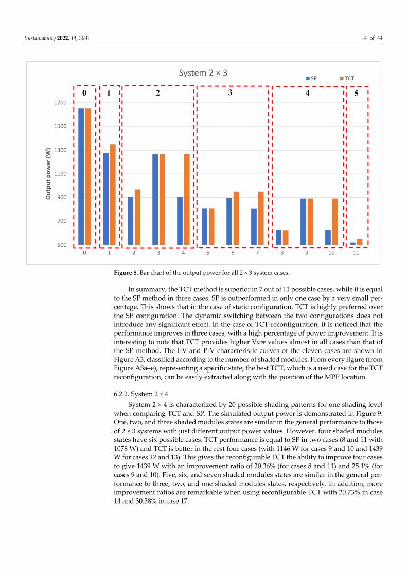
Figure 8. Bar chart of the output power for all 2 × 3 system cases.
In summary, the TCT method is superior in 7 out of 11 possible cases, while it is equal
to the SP method in three cases. SP is outperformed in only one case by a very small per-
centage. This shows that in the case of static configuration, TCT is highly preferred over
the SP configuration. The dynamic switching between the two configurations does not
introduce any significant effect. In the case of TCT-reconfiguration, it is noticed that the
performance improves in three cases, with a high percentage of power improvement. It is
interesting to note that TCT provides higher VMPP values almost in all cases than that of
the SP method. The I-V and P-V characteristic curves of the eleven cases are shown in
Figure A3, classified according to the number of shaded modules. From every figure (from
Figure A3a–e), representing a specific state, the best TCT, which is a used case for the TCT
reconfiguration, can be easily extracted along with the position of the MPP location.
6.2.2. System 2 × 4
System 2 × 4 is characterized by 20 possible shading patterns for one shading level
when comparing TCT and SP. The simulated output power is demonstrated in Figure 9.
One, two, and three shaded modules states are similar in the general performance to those
of 2 × 3 systems with just different output power values. However, four shaded modules
states have six possible cases. TCT performance is equal to SP in two cases (8 and 11 with
1078 W) and TCT is better in the rest four cases (with 1146 W for cases 9 and 10 and 1439
W for cases 12 and 13). This gives the reconfigurable TCT the ability to improve four cases
to give 1439 W with an improvement ratio of 20.36% (for cases 8 and 11) and 25.1% (for
cases 9 and 10). Five, six, and seven shaded modules states are similar in the general per-
formance to three, two, and one shaded modules states, respectively. In addition, more
improvement ratios are remarkable when using reconfigurable TCT with 20.73% in case
14 and 30.38% in case 17.
500
700
900
1100
1300
1500
1700
0 1 2 3 4 5 6 7 8 9 10 11
Ou
tpu
t p
ow
er
(W)
System 2 × 3 SP TCT
0 1 2 3 4 5

Sustainability 2022, 14, 3681 15 of 44
Figure 9. Bar chart of the output power for all 2 × 4 system cases.
In conclusion, the TCT method is superior in 15 cases, while it is equal to the SP
method in four cases only. SP is better in only one case by a slight percentage. It is notice-
able here that TCT presents higher VMPP values in seven cases than SP, while the voltage
values are almost equal in the rest cases.
Again, in the static configuration, the SP method is not highly preferred when com-
pared to TCT, while the dynamic switching between the two configurations does not add
any significant effect. In the case of TCT-reconfiguration, the performance improves in
seven cases, with a significant percentage of power improvement. For complete charac-
terization of the performance parameters, one may refer to Table A4. The I-V and P-V
characteristic curves of the 20 cases are shown in Figure A4.
6.2.3. System 2 × 5
System 2 × 5 has 32 cases and can be classified into nine groups according to the
number of shaded modules. Figure 10 explains the output power for all 2 × 5 system cases.
The TCT method is better than SP in 23 cases with a ratio of output power improvement
between 4% and 31.36%. In contrast, SP is slightly better in only three cases 16, 20, and 26
with output-power improvement percent of 0.82%, 0.26%, and 0.65%, respectively. For the
remaining six cases, SP gives the same performance as TCT. Again, in the static configu-
ration, the SP method is not preferred when compared to TCT, while the dynamic switch-
ing between the two configurations does not give any significant performance change.
Reconfigurable TCT can give an output power better than TCT. The performance is
improved in seven states when using TCT-reconfiguration, with a noticeable percentage
of power improvement. It can improve one case, in each group of two, three, seven, and
eight shaded modules, with 10.38% in case 2, 16.31% in case 5, 25% in case 26, and 25.4%
in case 29, respectively. The improvement is more significant in the states of four, five,
and six shaded modules. In each of the three states, there are six possible cases. Half of
them have the highest possible power, where reconfigurable TCT can improve the other
half to give output power as the first half. The improvement ratio can be as large as 32.26%
as in case 8.
600
800
1000
1200
1400
1600
1800
2000
2200
0 1 2 3 4 5 6 7 8 9 10 11 12 13 14 15 16 17 18 19 20
Ou
tpu
t p
ow
er
(W)
System 2 × 4 SP TCT
0 1 32 4 5 6 7

Sustainability 2022, 14, 3681 16 of 44
Figure 10. Bar chart of the output power for all 2 × 5 system cases.
Additionally, it is worth mentioning that the TCT introduces a higher VMPP value,
compared to that of SP, in a quarter of the possible cases, while it is almost equal in the
rest of the cases. Consequently, the TCT-reconfiguration method ensures the highest pos-
sible VMPP value in all cases.
From the I-V and P-V characteristic curves of the 32 cases that are shown in Figure
A5, the best case for the TCT reconfiguration can be determined along with the location
of the global MPP. Moreover, a comparison between the partial pattern and the unshaded
case may be conducted. The full simulated performance parameters are reported in Table
A5.
7. Conclusions
The present study presents a performance investigation of small PV systems under
all possible shading patterns. Small systems are defined as those consisting of 10 modules
or fewer. There are five configurations that are most commonly used; two of which are
symmetrical (2 × 2 and 3 × 3) and three are asymmetrical (2 × 3, 2 × 4, and 2 × 5). The main
techniques of small static systems are SP and TCT.
All possible shading patterns, arising from a single shading level (300 W/m2) under
the two wiring techniques (SP and TCT), are studied. A new simplifying method is uti-
lized to reduce the number of cases to be studied. The proposed method reduces the prob-
able cases from 1862 to only 100 cases for the five systems. TCT configuration shows su-
periority in most cases, which makes TCT configuration the best static configuration for
small PV systems. Some systems may follow the technique of dynamic switching between
the (SP and TCT) according to the PS pattern to choose the best one. However, by applying
this to small systems, it is notable that the amount of resultant improvement is slight or
even has no value such as a 2 × 2 system. Thus, the extra complexity associated with dy-
namic switching does not compensate for the expected improvement.
The technique of TCT-reconfiguration (in which the shaded modules positions are
re-arranged in the array according to the PS pattern by changing the electrical connec-
tions) is also tested to obtain the highest possible performance. Significant improvement
is observed in a large number of cases in all small PV systems. This improvement occurs
with the increase in the number of shaded units in half the system. The only drawback of
this method is the need for many connections. However, due to the limited size of these
systems, the required cable lengths are not long.
800
1000
1200
1400
1600
1800
2000
2200
2400
2600
2800
0 1 2 3 4 5 6 7 8 9 10 11 12 13 14 15 16 17 18 19 20 21 22 23 24 25 26 27 28 29 30 31 32
Ou
tpu
t p
ow
er
(W)
System 2 × 5 SP TCT
0 1 2 3 4 5 6 7 8 9

Sustainability 2022, 14, 3681 17 of 44
Hence, it is highly recommended to those who intend to develop their custom sys-
tems not to adopt dynamic switching configuration, but to implement TCT-reconfigura-
tion. Furthermore, those who prefer to stick to static-configuration systems for their sim-
plicity should follow the configurations of static TCT. Table 3 summarizes the number of
cases in which TCT excelled in static configurations, in front of the number of cases that
improved when transitioning to the dynamic switching between the SP and TCT config-
urations. The number of improved cases with TCT-reconfiguration techniques is also com-
pared to the static TCT.
Table 3. All possible numbers of improved cases according to the configuration.
Configuration\System 2 × 2 3 × 3 2 × 3 2 × 4 2 × 5
Static
TCT better 3 24 7 15 23
SP better 2 4 1 1 3
Equal 0 4 3 4 6
Dynamic better than static TCT by 0 4 1 1 3
TCT-Reconfiguration better than static TCT by 1 14 3 7 13
Total cases number 5 32 11 20 32
Author Contributions: Conceptualization, M.A.M.Y., A.M.M., and Y.S.M.; methodology, A.M.M.;
software, A.M.M.; validation, M.A.M.Y., Y.A.K., and Y.S.M.; formal analysis, M.A.M.Y.; investiga-
tion, A.M.M.; writing—original draft preparation, A.M.M.; writing—review and editing, A.M.M.,
Y.A.K., and M.A.M.Y.; supervision, M.A.M.Y. and Y.S.M.; project administration, M.A.M.Y.; fund-
ing acquisition, M.A.M.Y. All authors have read and agreed to the published version of the manu-
script.
Funding: This work was funded by the Deanship of Scientific Research at Jouf University under
grant No. (DSR-2021-02-03102).
Institutional Review Board Statement: Not applicable.
Informed Consent Statement: Not applicable.
Data Availability Statement: Not applicable.
Conflicts of Interest: The authors declare no conflict of interest.

Sustainability 2022, 14, 3681 18 of 44
Appendix A
Table A1. System 2 × 2 case studies and the resulted data.
Case
Nu
mb
er.
Nu
mb
er o
f Sh
ade
d
Mo
du
les
Partial
Shading
Pattern
Series-Parallel Total-Cross-Tied
KT%
KR
T%
VO
C
IS
C
VG
MP
P
IG
MP
P
PG
MP
P
PL
%
Efficien
cy %
Nu
mb
er o
f Lo
cal
MP
Ps
VO
C
IS
C
VG
MP
P
IG
MP
P
PG
MP
P
PL
%
Efficien
cy %
Nu
mb
er o
f Lo
cal
MP
Ps
0 0
0
89.4 16.7 70.2 15.7 1100 0.00 14.17 1 89.4 16.7 70.2 15.7 1100 0.00 14.17 1 0.00 0.00 0
0 0
1 1
1
88.5 16.7 71.3 10.2 726.2 33.98 9.36 2 88.5 16.7 73.9 10.5 774.6 29.58 9.98 2 6.25 0.00 0
1 0
2
2
2
87.3 16.7 34.4 15.7 539.1 50.99 6.95 2 87.3 16.7 34.4 15.7 539.1 50.99 6.95 2 0.00 25.09 0
1 1
3
1
87.7 10.8 70.6 10.2 719.7 34.57 9.27 1 87.7 10.8 70.6 10.2 719.7 34.57 9.27 1 0.00 0.00 1
2 0
4
1
87.3 16.7 34.4 15.7 539.1 50.99 6.95 2 87.7 10.8 70.6 10.2 719.7 34.57 9.27 1 25.09 0.00 1
1 1
5 3
2
86.3 10.8 35 10.2 356.1 67.63 4.59 2 86.5 10.8 76 4.85 369 66.45 4.75 2 3.50 0.00 1
2 1

Sustainability 2022, 14, 3681 19 of 44
(a)
(b)
(c)
Figure A1. (I-V) and (P-V) characteristic curves of the PV 2 × 2 system under different numbers of
shaded modules as follow: (a) One shaded module, (b) Two shaded modules, and (c) Three shaded
modules.

Sustainability 2022, 14, 3681 20 of 44
Table A2. System 3 × 3 case studies and the resulted data.
Case
Nu
m-
Nu
mb
er
of
Partial
Shading
Pattern
Series-Parallel Total-Cross-Tied KT%
KR
T%
VO
C
IS
C
VG
MP
P
IG
MP
P
PG
MP
P
PL
%
Effi-
cienc
y %
Nu
m
ber
VO
C
IS
C
VG
MP
P
IG
MP
P
PG
MP
P
PL
%
Effi-
cienc
y %
Nu
m
ber
0 0
0
134.1 25 105.4 23.5 2476 0.00 14.18 1 134.1 25 105.4 23.5 2476 0.00 14.18 1 0.00 0.00 0
0
0 0 0
1 1
1
133.4 25 106.3 18 1914 22.70 10.96 2 133.5 25 110.7 18.7 2067 16.52 11.84 2 7.40 0.00 0
0
1 0 0
2
2
2
132.8 25 71.4 23.5 1674 32.39 9.59 2 132.9 25 69.6 23.5 1634 34.01 9.36 2 −2.45 17.39 0
0
1 1 0
3
1
132.9 25 106.1 18 1912 22.78 10.95 2 133 25 107.9 18.3 1978 20.11 11.33 2 3.34 0.00 1
0
2 0 0
4
1
132.8 25 71.4 23.5 1674 32.39 9.59 2 133 25 107.9 18.3 1978 20.11 11.33 2 15.37 0.00 1
0
1 1 0
5
3
3
132 25 96.6 23.5 1634 34.01 9.36 2 132 25 96.6 23.5 1634 34.01 9.36 2 0.00 14.23 0
0
1 1 1
6
2
132.1 25 108.2 12.5 1355 45.27 7.76 3 132.3 25 113.7 13 1481 40.19 8.48 3 8.51 22.26 1
0
2 1 0
7 2
132 25 96.6 23.5 1634 34.01 9.36 2 132.3 25 113.7 13 1481 40.19 8.48 3 −10.33 22.26 1

Sustainability 2022, 14, 3681 21 of 44
0
1 1 1
8
1
132.4 19.2 105.6 18 1905 23.06 10.91 1 132.4 19.2 105.6 18 1905 23.06 10.91 1 0.00 0.00 1
1
3 0 0
9
1
132.1 25 108.2 12.5 1355 45.27 7.76 3 132.4 19.2 105.6 18 1905 23.06 10.91 1 28.87 0.00 1
1
2 1 0
10
1
132 25 96.6 23.5 1634 34.01 9.36 2 132.4 19.2 105.6 18 1905 23.06 10.91 1 14.23 0.00 1
1
1 1 1
11
4
3
131.3 25 70.1 18 1263 48.99 7.23 3 131.5 25 72.1 18.5 1334 46.12 7.64 3 5.32 8.76 1
0
2 1 1
12
2
131.6 19.2 107.2 12.54 1345 45.68 7.70 2 131.8 19.2 112.3 13 1462 40.95 8.37 2 8.00 0.00 1
1
3 1 0
13
2
131.6 25 107.9 12.5 1353 45.36 7.75 2 131.7 25 110.2 12.8 1410 43.05 8.07 2 4.04 3.56 2
0
2 2 0
14
2
131.3 25 70.1 18 1263 48.99 7.23 3 131.7 25 110.2 12.8 1410 43.05 8.07 2 10.43 3.56 2
0
1 2 1
15
2
131.3 25 70.1 18 1263 48.99 7.23 3 131.8 19.2 112.3 13 1462 40.95 8.37 2 13.61 0.00 1
1
1 1 2
16 1 131.6 25 107.9 12.5 1353 45.36 7.75 2 131.8 19.2 112.3 13 1462 40.95 8.37 2 7.46 0.00

Sustainability 2022, 14, 3681 22 of 44
2
1
2 2 0
17
5
3
130.7 25 71.6 12.5 897 63.77 5.14 3 130.8 25 74.3 12.9 959.4 61.25 5.49 3 6.50 31.08 2
0
2 2 1
18
2
131 19.2 107 12.6 1343 45.76 7.69 2 131.1 19.2 108.9 12.8 1392 43.78 7.97 2 3.52 0.00 2
1
3 2 0
19
2
130.7 25 71.6 12.5 897 63.77 5.14 3 131.1 19.2 108.9 12.8 1392 43.78 7.97 2 35.56 0.00 2
1
2 1 2
20
3
130.7 25 71.6 12.5 897 63.77 5.14 3 130.9 19.2 69.8 18 1257 49.23 7.20 2 28.64 9.70 1
1
2 1 2
21
2
130.8 19.2 70.1 18 1263 48.99 7.23 2 131.1 19.2 108.9 12.8 1392 43.78 7.97 2 9.27 0.00 1
2
3 1 1
22
3
130.8 19.2 70.1 18 1263 48.99 7.23 2 130.9 19.2 69.8 18 1257 49.23 7.20 2 −0.48 9.70 1
1
3 1 1
23
6
3
129.9 25 113.2 7.2 817.3 66.99 4.68 2 129.9 25 113.2 7.2 817.3 66.99 4.68 2 0.00 38.73 3
0
2 2 2
24
2
130.5 13.3 106.3 12.6 1334 46.12 7.64 1 130.5 13.3 106.3 12.6 1334 46.12 7.64 1 0.00 0.00 2
2
3 3 0

Sustainability 2022, 14, 3681 23 of 44
25
3
130 19.1 71.7 12.5 896.7 63.78 5.13 3 130.3 19.2 73 12.9 941.2 61.99 5.39 3 4.73 29.45 2
1
3 2 1
26
2
129.9 25 113.2 7.2 817.3 66.99 4.68 2 130.5 13.3 106.3 12.6 1334 46.12 7.64 1 38.73 0.00 2
2
2 2 2
27
3
129.9 25 113.2 7.2 817.3 66.99 4.68 2 130.3 19.2 73 12.9 941.2 61.99 5.39 3 13.16 29.45 2
1
2 2 2
28
2
130 19.1 71.7 12.5 896.7 63.78 5.13 3 130.5 13.3 106.3 12.6 1334 46.12 7.64 1 32.78 0.00 2
2
3 2 1
29
7
3
129.3 19.2 111.1 7.2 759.2 69.34 4.35 2 129.3 19.2 112.3 7.2 811.2 67.24 4.65 2 6.41 7.92 3
1
3 2 2
30
3
129.4 13.3 71.7 12.5 896.4 63.80 5.13 2 129.6 13.3 70.2 12.6 880.8 64.43 5.04 2 −1.77 0.00 2
2
3 3 1
31
3
129.3 19.2 111.1 7.2 759.2 69.34 4.35 2 129.6 13.3 70.2 12.6 880.8 64.43 5.04 2 13.81 0.00 2
2
3 2 2
32 8
3
128.6 13.3 109.4 7.1 778.8 68.55 4.46 2 128.7 13.3 111.1 7.2 802.1 67.61 4.59 2 2.90 0.00 3
2
3 3 2

Sustainability 2022, 14, 3681 24 of 44
(a)
(b)

Sustainability 2022, 14, 3681 25 of 44
(c)
(d)

Sustainability 2022, 14, 3681 26 of 44
(e)
(f)
(g)

Sustainability 2022, 14, 3681 27 of 44
(h)
Figure A2. (I-V) and (P-V) characteristic curves of the PV 3 × 3 system under different numbers of
shaded modules as follow: (a) One shaded module, (b) Two shaded modules, (c) Three shaded
modules, (d) Four shaded modules, (e) Five shaded modules, (f) Six shaded modules, (g) Seven
shaded modules, and (h) Eight shaded modules.

Sustainability 2022, 14, 3681 28 of 44
Table A3. System 2 × 3 case studies and the resulted data.
Case N
um
ber.
Nu
mb
er of S
had
ed
Mo
du
les
Partial
Shading
Pattern
Series-Parallel Total-Cross-Tied
KT%
KR
T %
VO
C
IS
C
VG
MP
P
IG
MP
P
PG
MP
P
PL
%
Efficie
ncy
%
Nu
mb
er of L
ocal
MP
Ps
VO
C
IS
C
VG
MP
P
IG
MP
P
PG
MP
P
PL
%
Efficie
ncy
%
Nu
mb
er of L
ocal
MP
Ps
0 0
0
89.4 25 70.2 23.5 1651 0.00 14.18 1 89.4 25 70.2 23.5 1651 0.00 14.18 1 0.00 0.00 0
0 0 0
1 1
1
88.8 25 70.8 18 1276 22.71 10.96 2 88.8 25 72.8 18.5 1347 18.41 11.57 2 5.27 0.00 0
1 0 0
2
2
2
88.1 25 72.2 12.5 904.5 45.22 7.77 2 88.8 25 75 12.9 968.5 41.34 8.32 2 6.61 23.74 0
1 1 0
3
1
88.3 19.2 70.4 18 1270 23.08 10.91 1 88.3 19.2 70.4 18 1270 23.08 10.91 1 0.00 0.00 1
2 0 0
4
1
88.1 25 72.2 15.5 904.5 45.22 7.77 2 88.3 19.2 70.4 18 1270 23.08 10.91 1 28.78 0.00 1
1 1 0
5
3
3
87.3 25 34.4 23.5 808.7 51.02 6.95 2 87.7 25 34.4 23.5 808.7 51.02 6.95 2 0.00 14.89 0
1 1 1
6
2
87.6 19.2 71.5 12.5 896.3 45.71 7.70 2 87.6 19.2 73.7 12.9 950.2 42.45 8.16 2 5.67 0.00 1
2 1 0
7
2
87.3 25 34.4 23.5 807.7 51.08 6.94 2 87.6 19.2 73.7 12.9 950.2 42.45 8.16 2 15.00 0.00 1
1 1 1
8
4
3
86.7 19.2 34.8 18 625.3 62.13 5.37 2 86.8 19.2 34.6 18 622.2 62.31 5.34 2 −0.50 30.06 1
2 1 1
9
2
87 13.3 70.9 12.6 889.6 46.12 7.64 1 87 13.3 70.9 12.6 889.6 46.12 7.64 1 0.00 0.00 2
2 2 0
10
2
86.7 19.2 34.8 18 625.3 62.13 5.37 2 87 13.3 70.9 12.6 889.6 46.12 7.64 2 29.71 0.00 2
2 1 1
11 5
3
86 13.3 73.3 7.1 521 68.44 4.48 2 86.1 13.3 75.3 7.3 548.1 66.80 4.71 2 4.94 0.00 2
2 2 1

Sustainability 2022, 14, 3681 29 of 44
(a)
(b)
(c)

Sustainability 2022, 14, 3681 30 of 44
(d)
(e)
Figure A3. (I-V) and (P-V) Characteristic curves of the PV 2 × 3 system under different numbers of
shaded modules as follow: (a) One shaded module, (b) Two shaded modules, (c) Three shaded
modules, (d) Four shaded modules, and (e) Five shaded modules.

Sustainability 2022, 14, 3681 31 of 44
Table A4. System 2 × 4 case studies and the resulted data.
Case
Nu
mb
er.
Nu
mb
er o
f Sh
aded
Mo
du
les
Partial
Shading
Pattern
Series-Parallel Total-Cross-Tied
KT%
KR
T%
VO
C
IS
C
VG
MP
P
IG
MP
P
PG
MP
P
PL
%
Efficien
cy %
Nu
mb
er o
f Lo
cal
MP
Ps
VO
C
IS
C
VG
MP
P
IG
MP
P
PG
MP
P
PL
%
Efficien
cy %
Nu
mb
er o
f Lo
cal
MP
Ps
0 0
0
89.4 33.3 70.2 31.4 2201 0.00 14.18 1 89.4 33.3 70.2 31.4 2201 0.00 14.18 1 0.00 0.00 0
0 0 0 0
1 1
1
89 33.3 70.6 25.9 1826 17.04 11.76 2 89 33.3 72.9 26.5 1913 13.08 12.32 2 4.55 0.00 0
1 0 0 0
2
2
2
88.5 33.3 71.3 20.4 1452 34.03 9.35 2 88.5 33.3 73.9 21 1549 29.62 9.98 2 6.26 14.89 0
1 1 0 0
3
1
88.5 33.3 71.3 20.4 1452 34.03 9.35 2 88.6 27.5 70.4 25.9 1820 17.31 11.72 1 20.22 0.00 1
1 1 0 0
4
1
88.6 27.5 70.4 25.9 1820 17.31 11.72 1 88.6 27.5 70.4 25.9 1820 17.31 11.72 1 0.00 0.00 1
2 0 0 0
5
3
3
87.9 33.3 35.1 31.1 1097 50.16 7.07 2 88 33.3 75.5 15.3 1159 47.34 7.47 2 5.35 23.80 0
1 1 1 0
6
2
88 27.5 71 20.4 1446 34.30 9.32 2 88.2 27.5 72.7 20.9 1521 30.90 9.80 2 4.93 0.00 1
2 1 0 0
7
2
87.9 33.3 35.1 31.1 1097 50.16 7.07 2 88.2 27.5 72.7 20.9 1521 30.90 9.80 2 27.88 0.00 1
1 1 1 0
8
4
4
87.3 33.3 34.4 31.1 1078 51.02 6.94 2 87.3 33.3 34.4 31.1 1078 51.02 6.94 2 0.00 25.09 0
1 1 1 1
9
3
87.6 27.5 72.2 14.9 1075 51.16 6.93 2 87.6 27.5 74.7 15.3 1146 47.93 7.38 2 6.20 20.36 1
2 1 1 0
10 3 87.3 33.3 34.4 31.1 1078 51.02 6.94 2 87.6 27.5 74.7 15.3 1146 47.93 7.38 2 5.93 20.36

Sustainability 2022, 14, 3681 32 of 44
1
1 1 1 1
11
2
87.7 21.7 70.6 20.4 1439 34.62 9.27 1 87.7 21.7 70.6 20.4 1439 34.62 9.27 1 0.00 0.00 2
2 2 0 0
12
2
87.5 27.5 72.2 14.9 1075 51.16 6.93 2 87.7 21.7 70.6 20.4 1439 34.62 9.27 1 25.30 0.00 2
1 2 1 0
13
2
87.3 33.3 34.4 31.1 1078 51.02 6.94 2 87.7 21.7 70.6 20.4 1439 34.62 9.27 1 25.09 0.00 2
1 1 1 1
14
5
4
86.8 27.5 34.6 25.8 894.7 59.35 5.76 2 86.8 27.5 34.5 25.8 891.8 59.48 5.74 2 −0.33 20.73 1
2 1 1 1
15
3
87 21.7 71.6 14.9 1067 51.52 6.87 2 87.1 21.7 73.5 15.3 1125 48.89 7.25 2 5.16 0.00 2
2 2 1 0
16
3
86.8 27.5 34.6 25.8 894.7 59.35 5.76 2 87.1 21.7 73.5 15.3 1125 48.89 7.25 2 20.47 0.00 2
1 1 2 1
17
6
4
86.3 21.7 35 20.3 712.2 67.64 4.59 2 86.5 21.7 76 9.7 738 66.47 4.75 2 3.50 30.38 2
2 2 1 1
18
3
86.6 15.8 71 14.9 1060 51.84 6.83 1 86.6 15.8 71 14.9 1060 51.84 6.83 1 0.00 0.00 3
2 2 2 0
19
3
86.3 21.7 35 20.3 712.2 67.64 4.59 2 86.6 15.8 71 14.9 1060 51.84 6.83 1 32.81 0.00 3
1 2 2 1
20 7
4
85.5 15.8 72.9 9.5 690.8 68.61 4.45 2 85.9 15.8 74.9 9.7 726.1 67.01 4.68 2 4.86 0.00 3
2 2 2 1

Sustainability 2022, 14, 3681 33 of 44
(a)
(b)
(c)
Sustainability 2022, 14, 3681 34 of 44
(d)
(e)
(f)

Sustainability 2022, 14, 3681 35 of 44
(g)
Figure A4. (I-V) and (P-V) Characteristic curves of the PV 2 × 4 system under different numbers of
shaded modules as follow: (a) One shaded module, (b) Two shaded modules, (c) Three shaded
modules, (d) Four shaded modules, (e) Five shaded modules, (f) Six shaded modules, and (g) Seven
shaded modules.

Sustainability 2022, 14, 3681 36 of 44
Table A5. System 2 × 5 case studies and the resulted data.
Case
Nu
mb
er.
Nu
mb
er o
f
Sh
ade
d M
od
ule
s
Partial
Shading
Pattern
Series-Parallel Total-Cross-Tied
KT%
KR
T%
VO
C
IS
C
VG
MP
P
IG
MP
P
PG
MP
P
PL
%
Efficien
cy %
Nu
mb
er of L
o-
cal MP
Ps
VO
C
IS
C
VG
MP
P
IG
MP
P
PG
MP
P
PL
%
Efficien
cy %
Nu
mb
er of L
o-
cal MP
Ps
0 0
0
89.4 41.6 70.2 39.2 2751 0.00 14.18 1 89.4 41.6 70.2 39.2 2751 0.00 14.18 1 0.00 0.00 0
0 0 0 0 0
1 1
1
89.4 41.6 70.5 33.7 2376 13.63 12.24 2 89 41.6 71.7 34.5 2475 10.03 12.76 2 4.00 0.00 0
1 0 0 0 0
2
2
2
88.6 41.6 71 28.2 2002 27.23 10.32 2 88.7 41.6 73.2 29 2124 22.79 10.95 2 5.74 10.38 0
1 1 0 0 0
3
1
88.6 41.6 71 28.2 2002 27.23 10.32 2 88.7 35.8 70.3 33.7 2370 13.85 12.21 1 15.53 0.00 1
1 1 0 0 0
4
1
88.7 35.8 70.3 33.7 2370 13.85 12.21 1 88.7 35.8 70.3 33.7 2370 13.85 12.21 1 0.00 0.00 1
2 0 0 0 0
5
3
3
88.3 41.6 71.8 22.7 1630 40.75 8.40 2 88.3 41.6 74.6 23.4 1745 36.57 8.99 2 6.59 16.31 0
1 1 1 0 0
6
2
88.4 35.8 70.7 28.2 1995 27.48 10.28 2 88.4 35.8 72.1 28.9 2085 24.21 10.75 2 4.32 0.00 1
2 1 0 0 0
7
2
88.3 41.6 71.8 22.7 1630 40.75 8.40 2 88.4 35.8 72.1 28.9 2085 24.21 10.75 2 21.82 0.00 1
1 1 1 0 0
8
4
4
87.8 41.6 34.9 39.1 1366 50.35 7.04 2 87.9 41.6 75.9 17.8 1348 51.00 6.95 2 −1.34 32.26 0
1 1 1 1 0
9
3
87.9 35.8 71.4 22.7 1622 41.04 8.36 2 88 35.8 73.8 23.4 1725 37.30 8.89 2 5.97 13.32 1
2 1 1 0 0
10 3 87.8 41.6 34.9 39.1 1366 50.35 7.04 2 87.8 41.6 34.9 39.1 1366 50.35 7.04 2 0.00 31.36

Sustainability 2022, 14, 3681 37 of 44
1
1 1 1 1 0
11
2
88 30 70.5 28.2 1990 27.66 10.26 1 88 30 70.5 28.2 1990 27.66 10.26 1 0.00 0.00 2
2 2 0 0 0
12
2
87.9 35.8 71.4 22.7 1622 41.04 8.36 2 88 30 70.5 28.2 1990 27.66 10.26 1 18.49 0.00 2
1 2 1 0 0
13
2
87.8 41.6 34.9 39.1 1366 50.35 7.04 2 88 30 70.5 28.2 1990 27.66 10.26 1 31.36 0.00 2
1 1 1 1 0
14
5
5
87.3 41.6 34.3 39.2 1348 51.00 6.95 1 87.3 41.6 34.3 39.2 1348 51.00 6.95 1 0.00 20.43 0
1 1 1 1 1
15
4
87.4 35.8 72.8 17.2 1255 54.38 6.47 2 87.6 35.8 75.3 17.8 1337 51.40 6.89 2 6.13 21.07 1
2 1 1 1 0
16
4
87.3 41.6 34.3 39.2 1348 51.00 6.95 1 87.6 35.8 75.3 17.8 1337 51.40 6.89 2 −0.82 21.07 1
1 1 1 1 1
17
3
87.6 30 71.1 22.7 1616 41.26 8.33 2 87.7 30 72.6 23.3 1694 38.42 8.73 2 4.60 0.00 2
2 2 1 0 0
18
3
87.4 35.8 72.8 17.2 1255 54.38 6.47 2 87.7 30 72.6 23.3 1694 38.42 8.73 2 25.91 0.00 2
1 1 2 1 0
19
3
87.3 41.6 34.3 39.2 1348 51.00 6.95 1 87.7 30 72.6 23.3 1694 38.42 8.73 2 20.43 0.00 2
1 1 1 1 1
20
6
5
86.9 35.8 34.6 33.7 1164 57.69 6.00 2 87 35.8 34.5 33.7 1161 57.80 5.98 2 −0.26 27.84 1
2 1 1 1 1
21
4
87.1 30 72.2 17.3 1245 54.74 6.42 2 87.2 30 74.5 17.8 1323 51.91 6.82 2 5.90 17.78 2
2 2 1 1 0
22
4
86.9 35.8 34.6 33.7 1164 57.69 6.00 2 87.2 30 74.5 17.8 1323 51.91 6.82 2 12.02 17.78 2
1 1 1 2 1
23 3 87.3 24.1 70.7 22.8 1609 41.51 8.29 1 87.3 24.1 70.7 22.8 1609 41.51 8.29 1 0.00 0.00

Sustainability 2022, 14, 3681 38 of 44
3
2 2 2 0 0
24
3
87.1 30 72.2 17.3 1245 54.74 6.42 2 87.3 24.1 70.7 22.8 1609 41.51 8.29 1 22.62 0.00 3
1 2 2 1 0
25
3
86.9 35.8 34.6 33.7 1164 57.69 6.00 2 87.3 24.1 70.7 22.8 1609 41.51 8.29 1 27.66 0.00 3
1 1 2 1 1
26
7
5
86.5 30 34.8 28.2 981.3 64.33 5.06 2 86.6 30 34.6 28.2 975 64.56 5.02 2 −0.65 25.00 2
2 2 1 1 1
27
4
86.7 24.1 71.6 17.3 1237 55.03 6.37 2 86.8 24.1 73.4 17.7 1300 52.74 6.70 2 4.85 0.00 3
2 2 2 1 0
28
4
86.5 30 34.8 28.2 981.3 64.33 5.06 2 86.8 24.1 73.4 17.7 1300 52.74 6.70 2 24.52 0.00 3
1 1 2 2 1
29
8
5
86.1 24.1 73.6 11.9 872.6 68.28 4.50 2 86.2 24.1 75.6 12.1 917.5 66.65 4.73 2 4.89 25.41 3
2 2 2 1 1
30
4
86.4 18.3 71.2 17.3 1230 55.29 6.34 1 86.4 18.3 71.2 17.3 1230 55.29 6.34 1 0.00 0.00 4
2 2 2 2 0
31
4
86.1 24.1 73.6 11.9 872.6 68.28 4.50 2 86.4 18.3 71.2 17.3 1230 55.29 6.34 1 29.06 0.00 4
2 2 2 1 1
32 9
5
85.7 18.3 72.7 11.8 860.9 68.71 4.44 2 85.8 18.3 74.5 12.1 903.2 67.17 4.65 2 4.68 0.00 4
2 2 2 2 1

Sustainability 2022, 14, 3681 39 of 44
(a)
(b)
(c)

Sustainability 2022, 14, 3681 40 of 44
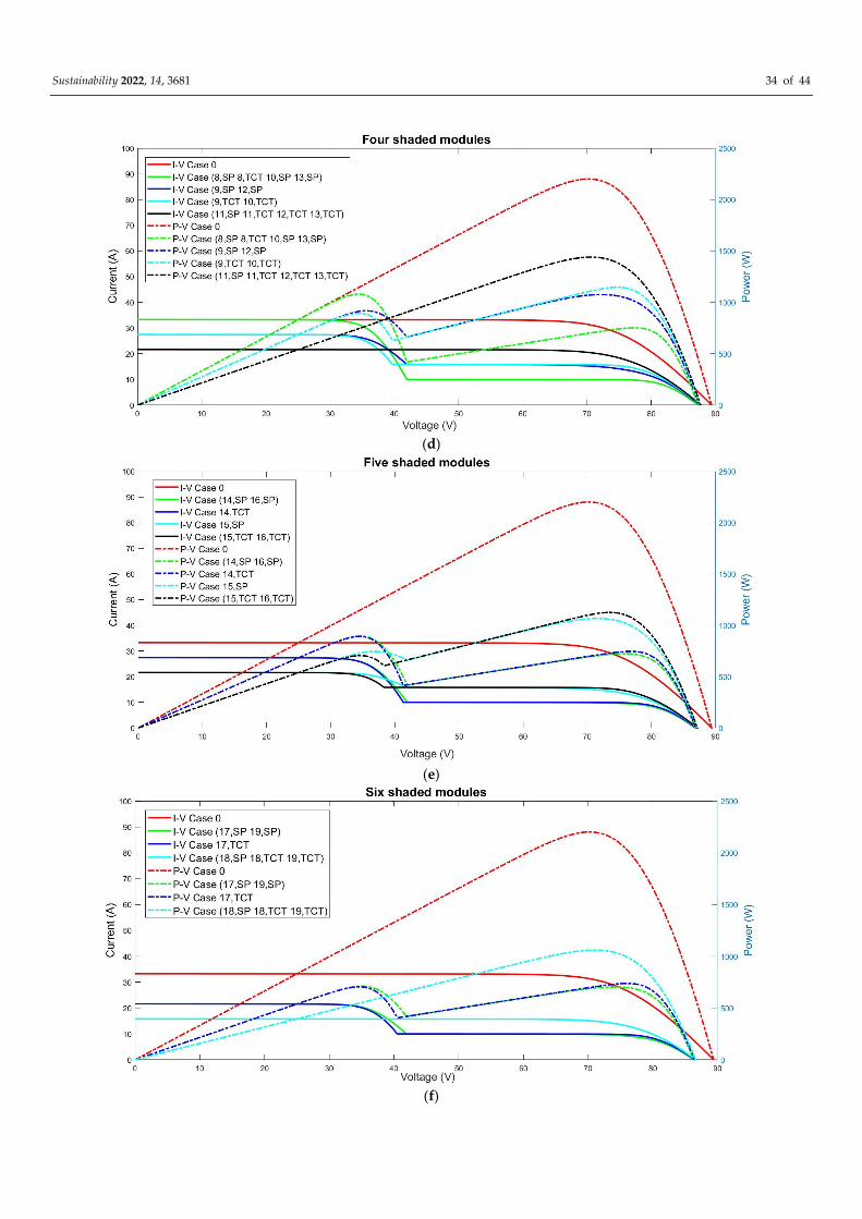
(d)
(e)

Sustainability 2022, 14, 3681 41 of 44
(f)
(g)

Sustainability 2022, 14, 3681 42 of 44
(h)
(i)
Figure A5. (I-V) and (P-V) characteristic curves of the PV 2 × 5 system under different numbers of
shaded modules as follow: (a) One shaded module, (b) Two shaded modules, (c) Three shaded
modules, (d) Four shaded modules, (e) Five shaded modules, (f) Six shaded modules, (g) Seven
shaded modules, (h) Eight shaded modules, and (i) Nine shaded modules.
References
1. Bollipo, R.B.; Mikkili, S.; Bonthagorla, P.K. Critical review on PV MPPT techniques: Classical, intelligent and optimization. IET
Renew. Power Gener. 2020, 14, 1433–1452. https://doi.org/10.1049/iet-rpg.2019.1163.
2. Subudhi, B.; Pradhan, R. A comparative study on maximum power point tracking techniques for photovoltaic power systems.
IEEE Trans. Sustain. Energy 2013, 4, 89–98. https://doi.org/10.1109/TSTE.2012.2202294.
3. Jiang, S.; Wan, C.; Chen, C.; Cao, E.; Song, Y. Distributed photovoltaic generation in the electricity market: Status, mode and
strategy. CSEE J. Power Energy Syst. 2018, 4, 263–272. https://doi.org/10.17775/CSEEJPES.2018.00600.
4. Wood, J. Renewable energy could power the world by 2050. Here’s what that future might look like. World Econ. Eorum 2020.
Available online: https://www.weforum.org/agenda/2020/02/renewable-energy-future-carbon-emissions/ (accessed on 3 Janu-
ary 2022).
5. Reindl, K.; Palm, J. Installing PV: Barriers and enablers experienced by non-residential property owners. Renew. Sustain. Energy
Rev. 2021, 141, 110829. https://doi.org/10.1016/j.rser.2021.110829.
6. Kılıç, U.; Kekezoğlu, B. A review of solar photovoltaic incentives and Policy: Selected countries and Turkey. Ain Shams Eng. J.
2022, 13, 101669. https://doi.org/10.1016/j.asej.2021.101669.

Sustainability 2022, 14, 3681 43 of 44
7. Almasri, R.A.; Alardhi, A.A.; Dilshad, S. Investigating the Impact of Integration the Saudi Code of Energy Conservation with
the Solar PV Systems in Residential Buildings. Sustainability 2021, 13, 3384. https://doi.org/10.3390/su13063384.
8. Mokhtara, C.; Negrou, B.; Settou, N.; Bouferrouk, A.; Yao, Y. Optimal design of grid-connected rooftop PV systems: An over-
view and a new approach with application to educational buildings in arid climates. Sustain. Energy Technol. Assess. 2021, 47,
101468. https://doi.org/10.1016/j.seta.2021.101468.
9. Yousri, D.; Babu, T.S.; Mirjalili, S.; Rajasekar, N.; Elaziz, M.A. A Novel Objective Function with Artificial Ecosystem-Based
Optimization for Relieving the Mismatching Power Loss of Large-Scale Photovoltaic Array. Energy Convers. Manag. 2020, 225,
113385. https://doi.org/10.1016/j.enconman.2020.113385.
10. Shimizu, T.; Hirakata, M.; Kamezawa, T.; Watanabe, H. Generation control circuit for photovoltaic modules. IEEE Trans. Power
Electron. 2001, 16, 293–300. https://doi.org/10.1109/63.923760.
11. Ali, A.; Almutairi, K.; Padmanaban, S.; Tirth, V.; Algarni, S. Investigation of MPPT techniques under uniform and non-uniform
solar irradiation condition—A retrospection. IEEE Access 2020, 8, 127368–127392. https://doi.org/10.1109/ACCESS.2020.3007710.
12. Sahu, H.S.; Nayak, S.K.; Mishra, S. Maximizing the Power Generation of a Partially Shaded PV Array. IEEE J. Emerg. Sel. Top.
Power Electron. 2016, 4, 626–637. https://doi.org/10.1109/JESTPE.2015.2498282.
13. Mohamed, A.M.A.; El-Sayed, A.; Mohamed, Y.S.; Ramadan, H.A. Enhancement of photovoltaic system performance based on
different array topologies under partial shading conditions. J. Adv. Eng. Trends 2021, 40, 49–62.
https://doi.org/10.21608/jaet.2021.82192.
14. Raj, A.; Gupta, M. Numerical Simulation and Comparative Assessment of Improved Cuckoo Search and PSO based MPPT
System for Solar Photovoltaic System Under Partial Shading Condition. Turk. J. Comput. Math. Educ. 2021, 12, 3842–3855. Avail-
able online: https://turcomat.org/index.php/turkbilmat/article/view/7755 (accessed on 3 January 2022).
15. Abri, W.A.; Abri, R.A.; Yousef, H.; Al-Hinai, A. A Simple Method for Detecting Partial Shading in PV Systems. Energies 2021,
14, 4938. https://doi.org/10.3390/en14164938.
16. Chalh, A.; Hammoumi, A.E.; Motahhir, S.; Ghzizal, A.E.; Derouich, A.; Masud, M.; AlZain, M.A. Investigation of Partial Shading
Scenarios on a Photovoltaic Array’s Characteristics. Electronics 2022, 11, 96. https://doi.org/10.3390/electronics11010096.
17. Seritan, G.-C.; Enache, B.-A.; Adochiei, F.-C.; Argatu, F.C.; Christodoulou, C.; Vita, V.; Toma, A.R.; Gandescu, C.H.; Hathazi, F.-
l. Performance Evaluation of Photovoltaic Panels Containing Cells with Different Bus Bars Configurations in Partial Shading
Conditions. In Revue Roumaine des Sciences Techniques—Electrotechnique et Energetique; Romanian Academy, Publishing House
of the Romanian Academy: 2020; Volume 65, pp. 67–70, ISSN 0035-4066. Available online: https://revue.elth.pub.ro/up-
load/77618212_GSeritan_RRST_1-2_2020_pp_67-70.pdf (accessed on 3 January 2022).
18. Sarniak, M.T. Modeling the Functioning of the Half-Cells Photovoltaic Module under Partial Shading in the Matlab Package.
Appl. Sci. 2020, 10, 2575. https://doi.org/10.3390/app10072575.
19. Hanifi, H.; Schneider, J.; Bagdahn, J. Reduced Shading Effect on Half-Cell Modules—Measurement and Simulation. In Proceed-
ings of the 31st European Photovoltaic Solar Energy Conference and Exhibition, Hamburg, Germany, 14–18 September 2015;
pp. 2529–2533, ISBN 3-936338-39-6. https://doi.org/10.4229/EUPVSEC20152015-5CV.2.25.
20. Nazer, M.N.R.; Noorwali, A.; Tajuddin, M.F.N.; Khan, M.Z.; Tazally, M.A.I.A.; Ahmed, J.; Ghazali, N.H.; Chakraborty, C.; Ku-
mar, N.M. Scenario-Based Investigation on the Effect of Partial Shading Condition Patterns for Different Static Solar Photovol-
taic Array Configurations. IEEE Access 2021, 9, 116050–116072. https://doi.org/10.1109/ACCESS.2021.3105045.
21. Madhu, G.M.; Vyjayanthi, C.; Modi, C.N. Investigation on Effect of Irradiance Change in Maximum Power Extraction From PV
Array Interconnection Schemes During Partial Shading Conditions. IEEE Access 2021, 9, 96995–97009.
https://doi.org/10.1109/ACCESS.2021.3095354.
22. Bonthagorla, P.K.; Mikkili, S. Performance investigation of hybrid and conventional PV array configurations for grid-con-
nected/standalone PV systems. CSEE J. Power Energy Syst. 2020, https://doi.org/10.17775/CSEEJPES.2020.02510.
23. Moballegh, S.; Jiang, J. Modeling, prediction, and experimental validations of power peaks of PV arrays under partial shading
conditions. IEEE Trans. Sustain. Energy 2014, 5, 293–300. https://doi.org/10.1109/TSTE.2013.2282077.
24. Elyaqouti, M.; Izbaim, D.; Bouhouch, L. Study of the Energy Performance of Different PV Arrays Configurations Under Partial
Shading. E3S Web Conf. 2021, 229, 01044. https://doi.org/10.1051/e3sconf/202122901044.
25. Muhammad, A.; Babu, T.S.; Ramachandaramurthy, V.K.; Yousri, D.; Ekanayake, J.B. Static and dynamic reconfiguration ap-
proaches for mitigation of partial shading influence in photovoltaic arrays. Sustain. Energy Technol. Assess. 2020, 40, 100738.
https://doi.org/10.1016/J.SETA.2020.100738.
26. Mishra, N.; Yadav, A.S.; Pachauri, R.; Chauhan, Y.K.; Yadav, V.K. Performance enhancement of PV system using proposed
array topologies under various shadow patterns. Sol. Energy 2017, 157, 641–656. https://doi.org/10.1016/j.solener.2017.08.021.
27. Malathy, S.; Ramaprabha, R. Reconfiguration strategies to extract maximum power from photovoltaic array under partially
shaded conditions. Renew. Sustain. Energy Rev. 2018, 81, 2922–2934. https://doi.org/10.1016/j.rser.2017.06.100.
28. Bonthagorla, P.K.; Mikkili, S. A novel fixed PV array configuration for harvesting maximum power from shaded modules by
reducing the number of cross-ties. IEEE J. Emerg. Sel. Topics Power Electron. 2021, 9, 2109–2121.
https://doi.org/10.1109/JESTPE.2020.2979632.
29. GSKrishna; Moger, T. Reconfiguration strategies for reducing partial shading effects in photovoltaic arrays: State of the art. Sol.
Energy 2019, 182, 429–452. https://doi.org/10.1016/j.solener.2019.02.057.

Sustainability 2022, 14, 3681 44 of 44
30. Pachauri, R.K.; Mahela, O.P.; Sharma, A.; Bai, J.; Chauhan, Y.K.; Khan, B.; Alhelou, H.H. Impact of partial shading on various
PV array configurations and different modeling approaches: A comprehensive review. IEEE Access 2020, 8, 181375–181403.
https://doi.org/10.1109/ACCESS.2020.3028473.
31. Venkateswari, R.; Rajasekar, N. Power enhancement of PV system via physical array reconfiguration based Lo Shu technique.
Energy Convers. Manag. 2020, 215, 112885. https://doi.org/10.1016/j.enconman.2020.112885.
32. Anjum, S.; Mukherjee, V.; Mehta, G. Hyper SuDoKu-Based Solar Photovoltaic Array Reconfiguration for Maximum Power
Enhancement Under Partial Shading Conditions. J. Energy Resour. Technol. 2022, 144, 031302. https://doi.org/10.1115/1.4051427.
33. Yang, B.; Shao, R.; Zhang, M.; Ye, H.; Liu, B.; Bao, T.; Wang, J.; Shu, H.; Ren, Y.; Ye, H. Socio-inspired democratic political
algorithm for optimal PV array reconfiguration to mitigate partial shading. Sustain. Energy Technol. Assess. 2021, 48, 101627.
https://doi.org/10.1016/j.seta.2021.101627.
34. Yousri, D.; Babu, T.S.; Beshr, E.; Eteiba, M.B.; Allam, D. A robust strategy based on marine predators’ algorithm for large scale
photovoltaic array reconfiguration to mitigate the partial shading effect on the performance of PV system. IEEE Access 2020, 8,
112407–112426. https://doi.org/10.1109/ACCESS.2020.3000420.
35. Zsiborács, H.; Zentkó, L.; Pintér, G.; Vincze, A.; Baranyai, N.H. Assessing shading losses of photovoltaic power plants based on
string data. Energy Rep. 2021, 7, 3400–3409. https://doi.org/10.1016/j.egyr.2021.05.038.
36. Karmakar, B.K.; Karmakar, G. A Current Supported PV Array Reconfiguration Technique to Mitigate Partial Shading. IEEE
Trans. Sustain. Energy 2021, 12, 1449–1460. https://doi.org/10.1109/TSTE.2021.3049720.
37. Srinivasan, A.; Devakirubakaran, S.; Sundaram, B.M.; Balachandran, P.K.; Cherukuri, S.K.; Winston, D.P.; Babu, T.S.; Alhelou,
H.H. L-Shape Propagated Array Configuration with Dynamic Reconfiguration Algorithm for Enhancing Energy Conversion
Rate of Partial Shaded Photovoltaic Systems. IEEE Access 2021, 9, 97661–97674. https://doi.org/10.1109/ACCESS.2021.3094736.
38. Pachauri, R.K.; Kansal, I.; Babu, T.S.; Alhelou, H.H. Power Losses Reduction of Solar PV Systems Under Partial Shading Con-
ditions Using Re-Allocation of PV Module-Fixed Electrical Connections. IEEE Access 2021, 9, 94789–94812.
https://doi.org/10.1109/ACCESS.2021.3093954.
39. MANUALZZ the Universal Manuals Library, STP275_270_24Vd1. Available online: https://manu-
alzz.com/doc/10607158/stp275_270_24vd1 (accessed on 10 March 2022).
Copyright © 2022 FDOKUMEN