Investigation of Electrophoretic Deposition as ... - DSpace@MIT

Investigation of Electrophoretic Deposition as a FabricationTechnique for High Performance Composites

by

Timothy R. Palmer

B.S., Aerospace EngineeringUniversity of California, San Diego, 2009

Submitted to the Department of Mechanical Engineeringin Partial Fulfillment of the Requirements for the Degree of

MASSACHU:T N 1-UTE

ARCI--

ARCHIVES

Master of Science in Mechanical Engineeringat the

Massachusetts Institute of Technology

September 2011

© 2009 Massachusetts Institute of TechnologyAll rights reserved.

Signature of Author.....................................................Department of Mechanical Engineering

August 5, 2011

C ertified by....................................................Cullen R. Buie

Professor of Mechanical EngineeringThesis Supervisor

Accepted by........................................................................ ......... ...........David E. Hardt

Professor of Mechanical EngineeringGraduate Officer

Investigation of Electrophoretic Deposition as a FabricationTechnique for High Performance Composites

by

Timothy R. Palmer

Submitted to the Department of Mechanical Engineeringon August 5, 2011 in Partial Fulfillment of the

Requirements for the Degree of Master of Science inMechanical Engineering

Abstract

Electrophoretic deposition (EPD) is a colloidal processing method for the deposition of materials fromcharged nanoparticles suspended in solution with the application of an external electric field. It is anincreasingly popular manufacturing method for engineered materials because of its low cost, simpleequipment, flexibility, and efficiency. Yet, little research has been done in the area of composite materialfabrication using EPD to infiltrate porous substrates (known as electrophoretic infiltration, or EPI). Inaddition, what work has been done has focused on 2-D porous substrates such as fiber mats or porousmembranes.

This thesis endeavors to demonstrate the applicability of EPD for the infiltration and coating ofporous materials to create advanced composites. The underlying theory of EPD is discussed to givefoundation for experiment parameters. Two'sample materials, boron carbide and silicon dioxide, aredeposited within and on commercially available porous stainless steel filter discs using constant voltageDC EPD. Surfaces are characterized using a scanning electron microscope (SEM) and energeticdispersive x-ray (EDX)/Auger spectrometers to visualize coating quality and penetration of the materialinto the substrate. Limitations of EDX/Auger spectroscopy are briefly discussed with respect to theanalysis of boron carbide.

After the first set of experiments using DC EPD, the study is expanded to include pulsed DCEPD. Pulsed DC EPD is a valuable technique for mitigating bubble formation due to electrolysis inaqueous suspensions, thus reducing macropore generation from gas evolution. The ability of EPD toinfiltrate into pores is confirmed by visual inspection of samples under a SEM and EDX. At low voltage,the deposited mass in constant voltage EPD increases linearly with time while at high voltage itasymptotically approaches a maximum yield of 1.988 grams. Pulsed EPD experiments demonstrate areduction in deposition yield but also elimination of pore generation in the low voltage case. A non-dimensional parameter, 4*, relating electrophoretic kinetics and diffusion is derived which improvesprocess design for pulsed EPD cells.

Thesis Supervisor: Cullen R. BuieTitle: Assistant Professor of Mechanical Engineering

Acknowledgments

The work included in this thesis would not have been completed with the love and support of severalindividuals. In the following paragraphs, I will attempt to convey my thanks and my appreciation.

First, I want to acknowledge God, the Father, my faith in whom was instrumental in giving methe strength to get me through the long nights of experiments gathering the data presented herein. WithoutHis Providence, none of this would have been possible.

Next, I want to express my deepest thanks to my advisor, Cullen Buie, whose guidance andencouragement helped me to solve problems and push myself to accomplish tasks I thought too difficult.He also generously funded this project through start-up funding from the Institute, without which I wouldnot have had the resources to proceed.

To all my friends and family, especially my parents, Brian and Bonnie Palmer, and my sister,Becky, thank you for all the encouragement and patience these past two years. Your willingness totolerate me during the times I was overwhelmed, and your courage to tell me to buck up when I wascomplaining too much are two things I appreciated the most.

Contents

Abstract....................................................----------........--. ----............................................................. 3Acknowledgments ...................................------------------------------ -......................................................... 5Contents---------...............----...---...............................................................................................................7

List of Figures..............................................................................................................................................9

List of Tables..........................................----------------------------------------................ -...................................... 12

1 Introduction....................................-------------------------------------... ----................. ................................ 13

1.1 Motivation ................................................................................................................. 14

1.2 Description of EPD..................-......................... . ................................................. 161.2.1 History of Electrophoresis and EPD.....................................16

1.2.2 Overview of the EPD Process ................................................................................... 17

1.3 Mathematical Theory of EPD................................................................................... ..... 19

1.4 Example Applications in Literature..........................--....................................................... 22

1.5 Research Objectives............................... . ................................................................ 231.5.1 Characterization of EPD with Boron Carbide............................................................... 231.5.2 Parametric Study of EPD Process to Determine Optimal Conditions.............................23

1.5.3 Engineering Investigation of Pulsed EPD...................................................................... 24

2 Constant Voltage DC EPD using Boron Carbide------------......................................................... 252.1 Experimental Materials...........................................................................................25

2.2 Experimental Procedures.............---------------------------.----------................................................ 332.3 Experimental Results..............---------------...................-----------...................................................... 35

3 Constant Voltage DC EPD using Silicon Dioxide...................................................................... 483.1 Experim ental M aterials.......................................................................................................... . 48

3.2 Experimental Procedures.....................................................................................................48

3.3 Experimental Results.................. ....-....--..---.............................................................. 504 Pulsed DC EPD using Silicon Dioxide-----------..............--...---............................................... 64

4.1 Experimental Materials ......................--.....----.....-.-------------------.................................................. 64

4.2 Experimental Procedures ............................................... ................ 65

4.3 Experim ental Results ................................................. . --------------------------------------......................... 67

5 Conclusions and Future Work......................--------...----------------------------...........................................92

5.1 Conclusions.......................--..-.-----------------------------------------------------...............................................92

5.2 Future Work............................ .......-- . .- - - --........................................................95

Appendix A.....................................--........ .-----..---------------------..................................-.........----- ...------97

Bibliography....................----..----.-----------------------------------------------------...............................................105

List of Figures

Figure 1.1: Schematic of electrophoretic deposition showing the basic components and operation..........17

Figure 2.1: Side-by-side comparison of Alfa Aesar particles (left) and American Elements particles (right)................................................................-------------.........-----. ----......................................................... 27

Figure 2.2: SEM image of an uncoated stainless steel filter disc used in this study as a substrate.....27

Figure 2.3: Sample EPD cell. Electrodes are the cathodes and the porous substrate is the anode.........31

Figure 2.4: Zeta potential and conductivity plots for the Alfa Aesar boron carbide particles in aqueoussuspension...............................................------------------.............--------.-...................................................... 36

Figure 2.5: SEM image of boron carbide sample on stainless steel sintered substrate taken at the sampleedge.........................................................---------------------------------- .. . . .. ........................................ 3 7

Figure 2.6: Bulk boron carbon deposit on stainless steel........................................................................38

Figure 2.7: (a) Theoretical stoichiometric composition of boron carbide. (b) EDX data showing atom %com parison of boron carbide coating...................................................................................................... 40

Figure 2.8: Additional regions examined on the same sample as in Figure 2.7......................................40

Figure 2.9: (a) Theoretical composition of boron carbide. (b) measured composition of Region 5, and (c)measured composition of Region 6 from the sample shown in Figure 2.8.............................................41

Figure 2.10: EDX data for Region 7 showing EDX accuracy for bare stainless steel...........................42

Figure 2.11: EDX data for 3 separate samples prepared by EPD of Alfa Aesar-manufactured boroncarbide nanoparticles .............................................................................................................. 43

Figure 2.12: Auger spectra for several sample areas of coatings prepared with American Elementsnanoparticles ............................................................................................................................... 44

Figure 2.13:Auger spectra for coatings prepared using EPD of Alfa Aesar nanoparticles suspended inH 20 . .........................................................--------------------------------------. -----------....................................... 4 6

Figure 2.14: SEM image of a sample prepared via EPD of Alfa Aesar boron carbide nanoparticlessuspended in w ater........................................................................................................................... 47

Figure 2.15: Corresponding Auger spectra, overlaid, for Regions 1 and 2 shown in Figure 2.14..........47

Figure 3.1: Zeta potential and conductivity data for the American Elements silicon dioxide particles inaqueous suspension.................................--------------.... ------....... -----........................................................ 51

Figure 3.2: Silica deposited on sintered stainless steel.......................................................................... 52

Figure 3.3:EDX map of the same region in Figure 3.2.......................................................................... 52

Figure 3.4: SEM image of CV2, run 1 (5 V, 360 seconds) showing pore geometry and coating crack

propagation at these experimental conditions........................................................................................ 54

Figure 3.5: SEM image of CV4, run 1 (5 V, 900 seconds), showing typical pore size and density for these

experimental conditions ................ ................................................................................... 55

Figure 3.6: SEM image of CV2, run 1 (5 V, 360 seconds), over a contiguous portion of the sample,showing typical pore generation..................................................................................56......56

Figure 3.7: Calculated porosity versus deposition time for the 5 V samples, CVI-CV4. ...................... 57

Figure 3.8: Calculated porosity versus deposition time for the 12.5 V samples, CV5-CV7. ................. 58

Figure 3.9: Average pore size versus deposition time for 5 V samples, CV1-CV4...............................59

Figure 3.10: Average pore size versus deposition time for 12.5 V samples, CV5-CV7.........................60

Figure 3.11: Deposited mass versus deposition time for all constant voltage, 5 V, samples..................61

Figure 3.12: Deposited mass versus deposition time for all constant voltage, 12.5 V, samples..............62

Figure 4.1: Deposition yield versus equivalent deposition time for 20%, 50%, and 80% duty cycles of 5 V

pulsed DC experiments and the 5 V constant voltage experiments........................................................68

Figure 4.2: Deposition yield versus pulse width for 5 V pulsed DC samples with frequencies of 2 Hz, 6

H z, and 10 H z.. ...................................................................---- . . ---------------------------------............................ 69

Figure 4.3: Average deposition rate versus pulse width for the 5 V, 2 Hz samples. .............................. 70

Figure 4.4: Average deposition rate versus c* for all 5 V pulsed DC samples......................................77

Figure 4.5: Average deposition rate versus * for all 12.5 V samples....................................................79

Figure 4.6: SEM image of N17, run2 (12.5 V, 2 Hz, 50% duty cycle, 1200 seconds total run time),showing typical gore generation for the pulsed EPD samples at these experimental conditions. .......... 82

Figure 4.7: SEM image of a reasonably uniform area on N17, run 2.........................................................82

Figure 4.8: SEM image of N200, run 2 (12.5 V, 10 Hz, 15% duty cycle, 600 seconds total run time),showing a typical pore and one of the expected surface cracks from shrinkage during the drying process.

............... 8...............................................83

Figure 4.9: SEM image of a uniform are of sample N200, run 2 at moderate magnification.........84

Figure 4.10: High magnification SEM image of the same area of N200, run 2 as featured in Figure 4.9..84

Figure 4.11: Optical microscope image of N24, run 3 (12.5 V, 6 Hz, 80% duty cycle, 1200 seconds total

run tim e), at 4x m agnification...............................................................-.........----. . ----------------.................... 85

Figure 4.12: The resulting image of N24, run 3, after being processed.................................................85

Figure 4.13: Porosity versus equivalent deposition time for all 5 V, N-series samples..........................86

Figure 4.14: Porosity versus equivalent deposition time for all 12.5 V, N-series samples.....................86

Figure 4.15: Average pore size versus equivalent deposition time for 12.5 V, N-series samples..........88

Figure 4.16: Porosity versus * for all N-series, 12.5 V samples..........................................................89

Figure 4.17: Average pore size versus * for all N-series, 12.5 V samples...........................................90

List of Tables

Table 2.1: EDX data for crucible samples comparing dry American Elements and Alfa Aesar powders.. 43

Table 3.1: Constant Voltage (CV) samples and corresponding experimental conditions.....................50

Table 4.1: Pulsed EPD samples and corresponding experimental conditions ....................................... 66

Table 4.2: Total deposited mass for 12.5 V samples with their corresponding conditions and (* values.. 80

1 Introduction

Electrophoretic deposition (EPD) is a colloidal processing method for the deposition of materials from

charged nanoparticles suspended in solution upon the application of an external electric field. It is an

increasingly popular manufacturing method for engineered materials because of its low cost, flexibility,

and efficiency.

This thesis endeavors to demonstrate the applicability of EPD for the infiltration and coating of 3-

D porous materials to create advanced composites. A parametric study of operating parameters is

performed, focusing on material penetration and optimization of EPD conditions.

This chapter will give background information on EPD, including a brief history of the field and

underlying physics with a general description of the mechanisms involved. Further, the mathematical

theory of electrophoresis and EPD will be examined in the context of the objectives of the current

research.

Subsequent chapters will cover the DC EPD experiments with boron carbide, silicon dioxide, and

the pulsed DC EPD experiments with silicon dioxide, respectively. In each chapter, particle

characterization data will be presented, along with both quantitative and qualitative aspects of the

deposition. Quantitative information will include parameters such as deposited mass, coating pore

density, and elemental distribution measured via energetic dispersive X-ray spectroscopy (EDX), while

qualitative data will appear mostly in the form of SEM images of the deposited surfaces.

1.1 Motivation

The ultimate goal of this work is the application of EPD to create high performance composites for

extreme conditions, specifically for the plasma-facing wall of a fusion reactor. Research into alternative

energy conversion technologies has recently surged due to increased political and social interest in energy

and climate change. Nuclear fusion is the "holy grail" of energy conversion with its large energy density,

abundant fuel, lack of pollution or CO2 generation, and limited radioactive waste. Unlike nuclear fission

technology, which generates radioactive waste as a by-product of fuel consumption, fusion's only

radioactive waste is the reactor containment vessel itself and the tritium fuel which is bred as needed from

non-radioactive lithium within the plant. The reactor is easily buried for storage, and if it uses carefully

chosen materials, need only be stored for about a century before radioactivity decreases to safe levels,

unlike fission wastes which must be stored for millennia.

Despite years of research, fusion for the purposes of power generation is still far from reality.

Currently under construction in France, the International Thermonuclear Experimental Reactor (ITER)

will be the first demonstration of significant breakeven fusion but is still a pulsed experimental device

incapable of sustained power generation. A demonstration commercial powerplant, the so-called

DEMOnstration Power Plant (DEMO), is currently planned but has yet to be designed and is decades

away from construction. Several recent studies and reports1 3 listed materials as a top priority research

area to enable commercial fusion power. Due to the need to contain plasma energy long enough for fusion

to occur, plasma interactions with the reactor vessel are extremely important for reactor operation.

Impurities transported to the plasma core radiate away plasma energy via Bremsstrahlung radiation,

which scales with the atomic number squared. In addition, plasma facing materials (PFMs) must handle

the thermal loads and shocks from the high temperature plasma, radiation and neutron loads resulting

from the nuclear reactions, and collisions of energetic ions and neutrals. Also of concern are how the

materials affect heat removal from fusion reactions to power generation cycles and the influence of

material choice on the tritium breeding ratio and fuel retention of the reactor.

It has recently been proposed that composite materials such as boron carbide in a tungsten mesh

may be a promising alternative for PFMs. Early tokamaks used unarmored containment vessels, typically

steel, but these materials severely reduced plasma confinement. Current reactors employ austenitic alloys

(steels or inconels) for the vacuum vessel, armored by some pure material like tungsten or beryllium, or a

carbon fiber composite. As the demands of the reactor environment increase, particularly for DEMO,

more robust materials will be required. Boron carbide has a high melting temperature, low atomic

number, sublimates rather than melts, and is more resilient to neutron irradiation than most materials. It

can protect the tungsten from damaging impacts of energetic ions and neutrals, and in turn the tungsten

provides added mechanical strength and increased thermal conductivity. Composite materials combining

the favorable properties of two or more components are an attractive alternative for future designs.

However, making these materials commercially viable demands a fast, low cost manufacturing technique.

We believe that electrophoretic deposition is a prime candidate for creating these advanced composite

materials. EPD is fast (as compared to chemical vapor deposition and related techniques), affordable, and

flexible (i.e. a wide variety of materials can be created). This study seeks to demonstrate EPD's

effectiveness as a manufacturing technique for 3-D composites suitable for the harsh environment of a

fusion reactor.

However, this research will also have broader impacts than simply in nuclear fusion materials as

it also investigates the fundamental principles of EPD. Given EPD's flexibility and versatility, findings of

this work could aid in manufacturing process design for a variety of novel materials with multiple

applications.

1.2 Description of EPD

1.2.1 History of Electrophoresis and EPD

The phenomenon of electrophoresis was first discovered in 1808 when a Russian scientist named Ruess

noticed clay particles in water migrated under an applied electric field. Since then, many scientists have

studied electrophoresis in an attempt to model the physics. The first person to attempt to quantify

electrophoresis was Smoluchowski6 in 1903 in the case of thin double layers. Henry modified

Smoluchowski's formula with a fitting parameter depending on particle size and Debye length so that the

equation applied for varying double layer thickness6. Over the next century, several other scientists

contributed to the theory with progressively more complex models. Wiersema et al.7 and Booth included

the electrophoretic retardation force and relaxation effect which manifests when the field is initially

applied. More recent researchers, such as Ohshima?''" and O'Brien and White 1 , have continued to fine-

tune the theories for regimes including larger zeta potentials and higher particle concentrations. These

adjustments enable the design of ever more accurate instruments based on electrophoresis for diagnostic

purposes such as separating compounds. However, for the purposes of electrophoretic deposition, the first

order approximations of Smulochowski and Henry have proved sufficient for current EPD systems.

Electrophoretic deposition was first used in 1933 to create emitters for electron tubes via the

deposition of thoria particles on a platinum electrode. It was largely neglected until the 1990s when it

rapidly began gaining popularity as a low-cost, inexpensive materials processing technique"1 2. Over the

years, several models have been proposed for EPD yield, the first by Hamaker13 in 1940. These theories

will be summarized in section 1.2. The majority of the work done has been in the form of application -

oriented parametric studies of deposition conditions and yields on planar electrodes, 2-D fiber mats, and,

in isolated cases, 3-D porous materials. Some of these studies and their applications will be presented in

section 1.3.

1.2.2 Overview of the EPD Process

EPD is a two step process in which the first step is the migration of particles towards the electrode via

electrophoresis, and the second step is the actual deposition of particles on the surface. Figure 1.1 is a

simplified schematic of the EPD process.

DC Voltage

Anode . .Cathode+ Deposition -

Particle

Figure 1.1: Schematic of electrophoretic deposition showing the basic components and operation

Electrophoresis is the well-known phenomenon in which particles in suspension with finite surface charge

move upon application of an external electric field due to electrostatics forces. It is well known that a

region of charge separation known as the electrical double layer forms at most solid/liquid interfaces.

The key characteristic of the electrical double layer is the inherent zeta potential, C, that results. Cis

defined as the potential at the plane of shear in the electrical double layer'4 . In the case of a particle

surrounded by a liquid electrolyte, application of an electric field induces a Coulombic force on the

particle. The resulting particle translation is known as electrophoresis. In electrophoretic deposition, this

process dominates as particles approach the oppositely charged electrode, but once the particles get close,

the deposition process begins to dominate.

No consensus exists within the literature regarding the actual mechanism by which deposition

takes place. Corni et al.12 summarize some of the candidate theories in their review article of EPD. The

generally accepted theory relies upon the Derjaguin-Landau-Verwey-Overbeek (DLVO) theory and

double layer modification due to applied external electric fields5. DLVO theory attempts to quantify

colloidal stability through quantification of interaction potentials between particles. Specifically, the

theory focuses on van der Waals attractions and electrostatic repulsions. There are three particularly

important factors in DLVO theory: the Hamaker constant (relating to van der Waals forces), the surface

potential of the particles (electrostatic forces), and electrolyte concentration (Debye screening length of

electrostatic effects) 6. The theory of EPD holds that an applied electric field changes the electrolyte

balance near the electrodes by reducing the concentration of co-ions and increasing the concentration of

counter ions. This in turn modifies the particle double layer and Debye screening length, possibly leading

to colloidal destabilization and deposition. Another prominent explanation in the literature includes

flocculation by particle accumulation13 . This mechanism basically treats the electrostatic force between

the particles and the externally applied field as a pressure force which is powerful enough to overcome

electrostatic repulsion between particles to the point that particles approach within van der Waals range.

Once close enough, van der Waals attraction takes over, causing flocculation and deposition. Comi et al.

list several other theories besides these two, but many do not completely explain observed experiments or

are contradicted by recent experimental data, and thus these other explanations will not be explored here.

Regardless of which mechanism accurately explains the physical reasons behind deposition,

mathematical models can be developed which explain the deposition yields in resulting materials. For the

fabrication of materials and engineering of the EPD process, these yield models are typically sufficient.

The next section presents several of these engineering models.

1.3 Mathematical Theory of EPD

A recent review paper by Ferrari and Moreno15 summarized the leading EPD models, and the main

equations are presented below. As mentioned earlier, Hamaker13 was the first to attempt to

mathematically model potentiostatic EPD yield, measured in deposited mass, as a function of system

parameters such as particle concentration, electrophoretic mobility, electric field strength, deposition area,

and deposition time:

m = CfpSEt (1.1)

where m is deposited mass (g), C is concentration (g/cm), p is electrophoretic mobility (cm 2s 1V'), S is

deposition area (cm2), E is electric field strength (V/cm), and t is time (s). This equation, which inherently

assumes a constant electric field, shows a linear dependence on time. In reality, it is only valid for short

depositions because the electric field is not constant, nor is the concentration as deposition of particles

necessarily reduces the concentration of particles in suspensions without mixing. Note that in an EPD

cell, a portion of the current is carried by the particles so that in the galvanostatic case, the current will be

proportional to the deposited mass.

In an attempt to more accurately model EPD under constant voltage, Sarkar and Nicholson5

derived a model in which they took into account the depletion of particles in suspension due to

deposition. They also introduced an 'efficiency factor' to capture the uncertainty in the EPD process and

whether all particles reaching the electrode also incorporate into the deposit. The underlying principle of

their model is that for infinitesimal time intervals, Hamaker's equation13 may be assumed valid, leading to

the differential equation:

dm- f pSEC (1.2)

dt

wheref is the efficiency factor,fs 1. Since the concentration, C, depends on the amount of mass

deposited over time, an expression can be written relating the two:

19

M= V-(CO - C) (1.3)

which represents the total deposited mass at any given time expressed as a function of suspension volume,

V (cm3), initial concentration, Co, and current concentration, C. After expressing initial concentration in

terms of suspension volume and initial mass, equations (1.2) and (1.3) can be combined and re-organized

to derive the differential equation:

-d =- 1 J(1.4)dt mo r m

where r is a characteristic timescale of the equation, given by:

V (1.5)ffpSE

The solution to this differential equation is an exponential function:

m(t)= mn 1-exp j (1.6)

The models proposed by Hamaker13 and Sarkar and Nicholson5 attempt to explain deposition yields on

planar electrodes. However, deposition kinetics are more complex for porous substrates such as those

envisioned for the motivating application of advanced composites for nuclear applications. In an attempt

to address this physics, Haber et al. 6 derived a theoretical model for electrophoretic penetration and

deposition within porous substrates.

The model of Haber et al. assumes cylindrical pores and particles with radii less than one-tenth

the pore radius. The latter assumption simplifies the equations by neglecting wall effects, thus eliminating

a radial dependence in the final solution. The solution also assumes that electroosmotic flow (due to finite

surface charge on the porous deposition substrate) is allowed to reach steady-state before the introduction

of particles in order to eliminate required modeling of transients. To capture the dependence of particle

penetration and deposition on random Brownian motion, Haber et al. calculated the deposition probability20

of particles as a function of the Peclet number, Damkohler number, and the ratio of axial position to mean

pore radius. The Peclet number determines the ratio of convective to diffusive transport while the

Damkohler number expresses the ratio between diffusion and deposition time scales. The Peclet number,

Pe, is given by:

UbPe =- (1.7)

D

where U is the particle velocity, including both electrophoretic and electroosmotic contributions, b is the

mean pore radius, and D is the diffusion coefficient. The Damkohler number, 2, is expressed as:

_VD~ ~ (1.8)-R D

where rD is the diffusion timescale, rR the deposition time scale, and K the local deposition rate. Haber et

al.16 state that calculating a numerical value for the local deposition rate is extremely difficult due to its

dependence on particle morphology, material properties, and the interaction of electrostatic and

hydrodynamic forces. Instead, Haber et al. suggest empirical measurement to determine the value of K.

The final equation for the deposition probability is:

M 1 2Pd (;Pe,2A) = 4E f7 (a))dq22an 2U9

-(= 2 +a J0 (a,) Pe2 +4a Pe2 +4a -Pe)

r7 = - (1.10)

b

= (1.11)b

and Jo is the zero-order Bessel function, an (n=1,2,3...) are the Bessel function roots, r is the radial

coordinate in the pore, and z is the axial coordinate. As a result of the assumption of cylindrical pores, this

expression applies only in the case of straight pores and not for substrates with high tortuosity. Haber et

al. calculate and plot the penetration depth in non-dimensional form for varying Peclet numbers and

Damkohler numbers. The penetration depth is defined as the depth at which particles have 90%

probability of having been deposited. Not surprisingly, maximum penetration depths are achieved by

maximizing the Peclet number (i.e. maximizing convection compared to diffusion) and minimizing the

Damkohler number (i.e. minimizing the deposition timescale to the diffusion timescale).

1.4 Example Applications in Literature

Corni et al. 2 provide a comprehensive review of the uses of electrophoretic deposition through 2008,

covering applications in coatings and thin films, porous materials, functionally graded materials,

composites, and nanostructured surfaces. EPD has seen extensive application in forming of traditional and

bulk ceramics17' 18, but has most recently been diversified into other applications. Examples include porous

electrodes and membranes for batteries' 9, capacitors20 , and fuel cells21'22 . Novak et al.2' and Wang et al.24

have used EPD to produce structural composites, the former using EPD to deposit a SiC matrix within

SiC fibers and the latter using co-deposition of borosilicate and diamond to produce hardened glass

composites. Several groups have used EPD to deposit barium titanate for electronic applications including

sensors, actuators, optoelectronics, etc2. Doped titania particles, both micrometer and nanometer scale,

have been deposited by EPD for other electronic applications including tunable microwave devices and

transparent electrodes 26.One group in particular, led by Aldo R. Boccaccini from Imperial College of

London, leads the field in EPD with applications in ceramic structural composites including the

previously mentioned work by Novak et al.2 , doped cathodes for intermediate temperature solid oxide

fuel cells , even bioactive materials using Bioglass@ particles on various substrates28 .The

aforementioned applications constitute only a portion of those published in the literature, demonstrating

EPD's usefulness in material processing and fabrication.

1.5 Research Objectives

1.5.1 Characterization of EPD with Boron Carbide

A major objective of this research is to characterize boron carbide nanoparticles for the electrophoretic

deposition process. Little data is available on this material in the literature. Given the extreme sensitivity

of EPD to material properties, the characterization of the boron carbide particles is required in order to

enable the use of EPD for the fabrication of the envisioned composites. The most important

characteristics to determine for the purposes of EPD are the zeta potential as a function of suspension

conductivity and of pH to determine conditions for maximum stability and minimum conductivity.

1.5.2 Parametric Study of EPD Process to Determine Optimal Conditions

The second objective of this study is to investigate the optimal conditions for the EPD process. These

conditions are dictated by the requirements on the final fabricated material. For the envisioned

application, maximum density, coating uniformity, and penetration into substrate pores are of the utmost

importance. The applied voltage and deposition time were varied to investigate the effects on deposition

yield and resulting coating qualities. Initial experiments used the boron carbide particles planned for use

in the nuclear materials application. However, due to uncertainties in composition of the boron carbide

particles, the majority of experiments presented utilized silicon dioxide. In addition to constant voltage

experiments, pulsed DC EPD was also investigated as suggested in the literature to alleviate gas evolution

and pore generation in aqueous suspensions. In this case, additional process parameters such as frequency

and duty cycle were also varied.

1.5.3 Engineering Investigation of Pulsed EPD

During the course of the pulsed DC experiments, experimental data suggested a physical approximation

of process kinetics through the balancing of electrophoretic and diffusive motion. A third objective

involves the derivation of a non-dimensional parameter relating these two processes in terms of

experimental parameters and particle and suspension properties. Experimental data shows that this non-

dimensional parameter predicted EPD process results better than any one process variable.

2 Constant Voltage DC EPD using BoronCarbide

In this chapter, the experimental procedure and results of EPD with boron carbide (B4C) will be

presented. As discussed previously (see Section 1.1), B4C is a material of interest for the continuous

matrix in a candidate metal-ceramic composite for fusion applications.

2.1 Experimental Materials

For reasons to be described later, two types of B4C nanoparticles were used in the experiments. Initial

experiments were performed using 95+% boron carbide nanoparticles manufactured by American

Elements (Los Angeles, CA) with diameters between 20 and 60 nm. Experiments for the purpose of

comparison utilized B4C nanoparticles made by Alfa Aesar (Ward Hill, MA) with diameters ranging from

1 to 7 pm. The dry powders are pictured in Figure 2.1.

The final materials for nuclear fusion should be based around a porous refractory metal like tungsten

or molybdenum. However, such materials are expensive. Thus for these preliminary experiments to study

the EPD chemistry of boron carbide, commercially available stainless steel filter discs were used as

substrates. The filter discs were produced by Applied Porous Technologies, Inc. via sintering of stainless

steel microparticles to produce discs 1 inch in diameter and 1/16 inch thick with 40 pm pores. Figure 2.2

shows an SEM image of a sample uncoated filter disc.

(THIS PAGE INTENTIONALLY LEFT BLANK)

Figure 2.1: Side-by-side comparison of Alfa Aesar particles (left) and American Elements particles (right)

Figure 2.2: SEM image of an uncoated stainless steel filter disc used in this study as a substrate.

Experimental suspensions were created by dispersing boron carbide particles in either water or

isopropanol, depending on the manufacturer. American Elements particles were dispersed in isoproponal

because water led to less stability. Conversely, Alfa Aesar particle suspensions in water had more stability

than isopropanol-based suspensions. Based on previous research29,30, boron carbide should be easily

dispersed in aqueous suspensions. Given the strong dependence of suspension stability on particle surface

characteristics, this suggests that the American Elements particles have some residual material or

compositional difference on the surface which alters the dispersion chemistry. The exact cause remains

unknown, and as will be shown in energetic dispersive x-ray spectroscopy data, no unexpected trace

elements were detected. In both cases, the electrolyte used was potassium hydroxide, added from a 2 M

stock solution, since previous research showed the highest magnitude of zeta potential occurs in basic

suspensions29

Featured in Figure 2.3 is a sample EPD cell assembly. Since the substrates used in these

experiments were conducting, a two-sided, direct EPD process was used where the substrate also served

as the working electrode. The counter electrodes were made of titanium to reduce corrosion. The mount

ring which holds the substrate is made of polypropylene while the plastic fasteners joining the cell

together are Nylon 6/6. Both plastics resist corrosion from both aqueous and isopropanol suspensions,

especially at the moderate pH range used in this study. Nylon standoffs were used to fix the electrode

separation distance to of an inch, or 6.35 mm. Some very preliminary experiments were also conducted

using planar titanium electrodes only (one anode, one cathode) spaced at 1.2 cm with a rubber standoff.

These coatings were prepared for the express purpose of EDX analysis of the different boron carbide

powders.

Figure 2.3: Sample EPD cell. Electrodes are the cathodes and the porous substrate is the anode.

31

2.2 Experimental Procedures

Prior to any deposition experiments, sample suspensions were prepared in order to measure the particle

zeta potentials. Measurements were performed on a Malvern ZetaSizer Nano-ZS at several pH values.

Malvern calls the diagnostic technique "electrophoretic light scattering". The procedure is essentially

laser Doppler anemometry in which laser light is scattered off of moving particles. The phase shift in the

scattered light contains the velocity information of the particles, which can be converted to particle

mobility using the known applied electric field. The zeta potential is then calculated using the known

viscosity of the suspending medium and applying either the Smulochowski or Huckel models31. In the

experiments presented here, the Smulochowski model was used because it is more accurate for aqueous

suspensions and moderate electrolyte concentrations.

Sample suspensions for zeta potential measurement were prepared with pH values of 3.5, 4.9, 8.0,

9.7, and 11.4 with a concentration of 0.1% by weight. Suspensions for EPD used a concentration of 1%

by weight, but the optical nature of the measurement technique combined with the black color of the

particles required the order of magnitude reduction in particle concentration for reliable measurements. If

the concentration or absorption of the sample is too high, too much light is absorbed or scattered away

from the detector to determine the phase shift in the light and thus the particle velocity. Particles were

dispersed into the suspending medium using a Qsonica probe sonicator set at 25% maximum magnitude

for 15 minutes.

After zeta potential measurement, aqueous suspensions were prepared for EPD using a particle

concentration of 1 wt% at a pH of 9.3. Depositions were carried out under an applied voltage of 15 V for

2 hours using the EPD cell. Non-aqueous suspensions using isoproponal were also mixed, using 2 pL of

2M KOH per 10 mL of isopropanol. Particles were suspended via sonication as in the zeta potential

33

measurements. Isopropanol-based suspensions were deposited on a pair of titanium electrodes separated

at a distance of 1.2 cm. After depositions, coatings were allowed to dry completely in air at room

temperature.

Coatings were characterized following the drying step using scanning electron microscopy (SEM)

and energetic dispersive x-ray spectroscopy (EDX) on a JEOL 5000 standard SEM with EDX accessories.

EDX on all samples was performed in object scan mode where specific areas within the field of view

were selected for analysis. Electron beam voltage was set for 15 kV during EDX imaging. The

magnification for the stainless steel substrate was 120X while only 10OX for samples prepared on

titanium. The enhanced magnification allowed for more precise imaging of the porous stainless steel.

Each sample is labeled with "Region X", where X is a number. This label corresponds to the selected

rectangular area in the corresponding image (see below). Data acquisition time for each scan was 2

minutes, ample time for the signal to stabilize and obtain a repeatable spectrum. However, note that EDX

of the stainless steel sample was performed on a different day than the others. Due to differences in

hardware operation between the two days, it had a stronger signal than all other samples.

Due to discrepancies between measured data and theoretical expectations, additional samples

were prepared expressly for EDX analysis of particles in an aluminum mold. The aluminum mold

featured 4 miniature "crucibles" created by drilling recesses into a plain aluminum block. Two

"crucibles" were filled with particles, one each of the American Elements particles and the Alfa Aesar

particles, and then heat-treated under rough vacuum (P = 0.018 bar). The heating program increased the

temperature to 100 *C from room temperature at a rate of 10 *C/min, followed immediately by heating to

500 'C at a rate of 20 'C/min. The particles were then held at 500 'C for 30 minutes after which the

vacuum was turned off and the chamber opened over 5 minutes. After cooling to room temperature, the

other two "crucibles" were filled with particles, again one each of American Elements and Alfa Aesar

particles. The entire mold was then heated to 50 'C at a rate of 10 "C/min and held at that temperature for

10 minutes. The goal of this heat treatment was to moderately outgas the newly added particles, reducing

the potential effect of impurities on EDX data and attempting to isolate effects of high temperature

heating on particle composition. The resulting samples were analyzed under the EDX at similar settings

as the coatings on stainless steel and titanium substrates, with the exception that a magnification of 550X

was used. Several samples were also made for examination under an Auger spectrometer to verify the

EDX data for reasons that will be discussed in the following section. All Auger spectra were taken over 5

m2 regions. All Auger spectra included in this chapter present the data in traditional derivative mode (i.e.

the derivative of measured counts per second with respect to electron energy expressed in arbitrary units).

Sample composition is determined based on the relative strengths and corresponding energies of the

various peaks measured. Since Auger spectroscopy measures electrons emitted by atoms undergoing

state-relaxing transitions, and electron energy levels are quantized, elements can be identified by the

measured intensity and energy of the emitted electrons. The sum of the signal at all emitted electron

energies indicates the relative abundance of each element.

2.3 Experimental Results

In the literature there is very little work utilizing boron carbide nanoparticles, but one study characterized

the zeta potential of several ceramic carbides including boron carbide29 . Characterization of the

nanoparticles used in the current study is shown in Figure 2.4. In this figure, and all other future figures

unless otherwise noted, each point represents the average of at least 3 samples and the error bars represent

a 95% confidence interval spanning roughly six standard deviations according to standard statistical

techniques.

-30

-40 F

E

~-500

0-

N

-60 F

-70'3

Zeta Potential and Conductivity vs pH

0 Zeta PotentialConductivity

Q'

0.8

0.6

E

E

0.44

0

0

0.2

O4 5 6 7 8 9 10 11 12

pH

Figure 2.4: Zeta potential and conductivity plots for the Alfa Aesar boron carbide particles in aqueoussuspension.

As evident in Figure 2.4, the boron carbide particles in this study have zeta potential values consistent

with those of the previous study by Varga et al.29 The zeta potential is always negative over the pH range

of interest and its magnitude exceeds 40 mV. The particles in this study did not exhibit the same strongly

asymptotic behavior with increasing pH as in Varga et al. In addition, the Alfa Aesar particles have a

higher maximum magnitude zeta potential than Varga's particles. It is well-known that production of

dense, uniform coatings using electrophoretic deposition requires stable suspensions with minimum

conductivity 3 15. To ensure suspension stability a pH of approximately 9 was chosen for EPD

experiments. While the conductivity minimum is at a pH of 8, pH of 9 is significantly more stable

because of the nearly 15 mV increase in zeta potential magnitude.

'

After determining the optimum pH for the suspensions, samples were prepared using EPD and

characterized under the SEM and EDX. Figure 2.5 is an image of the edge of one of the samples which

shows the contrast of boron-carbide coated stainless steel and bare stainless steel as well as apparent

deposition of boron carbide within the pores. Bare stainless steel appears light gray while coated stainless

steel appears shadowy. Bulk deposits of boron carbide are black regions with cracks resulting from the

drying step. The boxed regions indicate regions where boron carbide has been deposited within a pore in

the substrate. In each box, the bounding stainless steel at the right of the boxes appears raised compared to

the adjacent boron carbide deposits. This indicates deposition of boron carbide within the pore.

Figure 2.5: SEM image of boron carbide sample on stainless steel sintered substrate taken at the sample edge.Image shows contrast between uncoated stainless steel and boron carbide as well as penetration of boron

carbide into pores.

Similarly, Figure 2.6 features an SEM image of a region of bulk boron carbide coating. The coating

surface is quite uniform due to the small particle size. The extensive cracking was expected as it is well-

known that uncontrolled drying of the coatings leads to excessive internal stresses and fracture. Previous

studies32 have used controlled humidity chambers during drying of samples to regulate shrinkage rate and

relaxation in the coating in order to prevent failure. The required hardware to do this was unavailable for

the current study. Several alternative solutions were explored, including wrapping samples in soaked rags

to simulate a humid environment and placing them in a refrigerator to slow the evaporation of liquid from

the green deposit. However, all such solutions proved unsuccessful at preventing the cracking during

drying.

Figure 2.6: Bulk boron carbon deposit on stainless steel. Section labeled "Region 8" represents the regionfrom which EDX data "Region 8" was taken.

The EDX data corresponding to the labeled region is represented in Figure 2.7. Contrary to the expected

stoichiometric ratio of 80% boron and 20% carbon, the measured ratio was 92% carbon and only 7%

boron with trace elements consistent with stainless steel accounting for the remaining 1%. Even

38

accounting for the possible error in the measurements, the ratio of boron to carbon is significantly

different than expected. Additional regions were examined (see Figure 2.8), and the corresponding EDX

data are presented in Figure 2.9. The ratios of boron to carbon of the coating shown in Figure 2.9 are

completely consistent with those in Figure 2.7. To validate the accuracy of the instrument, EDX was

performed on Region 7, bare stainless steel, and compared to the theoretical composition of 316L

stainless steel as shown in Figure 2.10. Aside from a small signal from carbon and boron at a ratio

consistent with trace particles in the region, the spectrum was in excellent agreement with the elemental

composition ranges for 316L stainless steel. This indicates that with acceptable accuracy the EDX should

be able to measure composition of the EPD coatings. Thus far, all images and EDX data presented have

been for coatings utilizing particles manufactured by American Elements. The large discrepancy between

measured composition and theoretical composition of the boron carbide particles cast doubt on their

purity. The discrepancy motivated the use or Alfa Aesar's boron carbide particles. EDX analysis was

performed on the Alfa Aesar particles after deposition to compare the measured composition with the

American Elements particles, shown in Figure 2.11.

100

80

60

40

20

0

100

80

60

40

20

0

B C Ti Fe Mn(a)

B C Ti Fe Mn(b)

Mo Si Ni Cr

Mo Si Ni Cr

Figure 2.7: (a) Theoretical stoichiometric composition of boron carbide. (b) EDX data for Region 8 showingatom % comparison of boron carbide coating from particles manufactured by American Elements.

Figure 2.8: Additional regions examined on the same sample as in Figure 2.7. Region 7 is uncoated stainlesssteel while Regions 5 and 6 are boron carbide.

- 1

-

- -

I I I I I I I I I

I I I - I

B C Ti Fe Mn Mo Si Ni Cr

B C Ti Fe Mn Mo Si Ni Cr(b)

10080604020

0

10080604020

0

100806040200

Figure 2.9: (a) Theoretical composition of boron carbide. (b) measured composition of Region 5, and (c)measured composition of Region 6 from the sample shown in Figure 2.8.

B C Ti Fe Mn Mo Si Ni Cr(C)

316L Minimum CompositionMeasured Composition316L Maximum Composition

-. . I

B C TiI.E . .E N.Fe Mn Mo Si

ElementNi Cr

Figure 2.10: EDX data for Region 7 showing EDX accuracy for bare stainless steel.

While the ratio of carbon to boron was lower, it was still significantly higher than the theoretical ratio. To

eliminate any possibility of composition change due to electrochemical effects, dry powders were also

analyzed in crucibles as described in Section 2.2. Table 2.1 contains the EDX data from the analysis and

shows that the ratio of carbon to boron is still at least 2 to 1 when the chemical formula indicates it should

be 1 to 4.

70-

- BoronCarbon -

100

90

80

70

60

50

40

30

20

10

0

Figure 2.11: EDX data for 3 separate samples prepared by EPD of Alfa Aesar-manufactured boron carbidenanoparticles.

Table 2.1: EDX data for crucible samples comparing dry American Elements and Alfa Aesar powders.

American Elements Alpha Aesar American Elements Alpha Aesar(heated) (heated) (degassed only) (degassed only)

Element _________

Atom % Error, Atom % Error, Atom % Error, Atom % Error,

Boron 18.297 1.514 30.255 2.830 24.381 2.084 30.428 2.685

Carbon 53.240 4.283 66.694 6.678 70.257 6.121 66.104 6.289

Oxygen 28.447 3.108 2.860 0.573 5.156 2.539 3.226 0.626

Silicon 0.016 0.002 0.176 0.013 0.057 0.009 0.172 0.012

Aluminum 0.000 0.000 0.015 0.002 0.063 0.008 0.069 0.010

Titanium 0.000 0.000 0.000 0.000 0.085 0.010 0.000 0.000

2Sample

The discrepancies in the Alfa Aesar particle measurements combined with absence of evidence of

electrochemical effects on particle composition led to the conclusion that the EDX instruments available

were unable to differentiate effectively between carbon and boron, despite examples in the literature of

EDX analysis of boron carbide 33 .3 4 . For this reason, Auger spectroscopy was also performed on several

samples to verify the elemental ratios. Figure 2.12 shows Auger spectra for 3 sample areas of coatings

prepared with American Elements particles.

x 104

32 -2'-z -4

0 500 1000 1500 2000Kinetic Energy (eV)

x 104

-o -2'-S-

0 500 1000 1500 2000Kinetic Energy (eV)

X 104

.2 -

~ -40 500 1000 1500 2000

Kinetic Energy (eV)

Figure 2.12: Auger spectra for several sample areas of coatings prepared with American Elementsnanoparticles. The top two spectra are of coatings prepared with particles suspended in water, and the

bottom is of a coating prepared with particles suspended in isopropyl alcohol.

The three spectra in Figure 2.12 are essentially identical, indicating that the measured composition of the

coating is not only uniform but also independent of suspension medium during deposition. The measured

composition was 83.3% carbon and 16.7% boron for these coatings.

44

For the Alfa Aesar particles, the Auger also confirmed earlier EDX data. Figure 2.13 shows the

Auger spectra for 4 regions. Once again, all spectra are essentially identical. The measured composition

was 76.7% carbon and 23.3% boron, which is in good agreement with the EDX composition of 68-72%

carbon and 32-26% boron, respectively. Figure 2.14 is an SEM image of one of the Alfa Aesar samples

with two analysis regions marked. Figure 2.15 is an overlay of the two marked regions in Figure 2.14

which demonstrates clearly the virtually identical nature of the spectra. There was one region with an

unusually rough morphology on one of the samples with measured compositions of 57-58% boron and

43-42% carbon, which constitutes the only measurements of substantial depositions where the ratio of

boron to carbon was greater than 1. However, it is still significantly lower than the theoretical 4 to 1

boron:carbon ratio.

EPD is extremely sensitive to surface chemistry, therefore it is important to use well-

characterized particles. Also, due to the somewhat exotic nature of the boron carbide particles, there are

less expensive materials with which the mechanics of EPD of particles into porous substrates may be

investigated. For these reasons experiments on boron-carbide were postponed in favor of silicon dioxide.

These experiments will be discussed in the following chapters. Other analysis techniques such as mass

spectrometry or Rutheford backscattering (RBS) may have given more accurate measurements of the

boron-carbon ratio. However, mass spectrometry would require destruction of the coatings, and the

mechanical frailty of the coatings would have led to the same result under ion bombardment for RBS.

x 10420-

-2

0 200 400 600 800 1000 1200Kinetic Energy (eV)

600 800 1000 1200Kinetic Energy (eV)

x 10,20-%

-2-4'

0 200 400

x 104

1400 1600 1800 2000

1400 1600 1800 2000

Kinetic Energy (eV)

800 1000 1200Kinetic Energy (eV)

Figure 2.13:Auger spectra for coatings prepared using EPD of Alfa Aesar nanoparticles suspended in H2 0.

a a a a

a a a a - a

2000

Figure 2.14: SEM image of a sample prepared via EPD of Alfa Aesar boron carbide nanoparticles suspendedin water. Marked regions are the regions over which Auger analysis was performed.

X 104

500 1000 1500Kinetic Energy (eV)

2000

Figure 2.15: Corresponding Auger spectra, overlaid, for Regions 1 and 2 shown in Figure 2.14.

3 Constant Voltage DC EPD using SiliconDioxide

This chapter describes the procedures and results of EPD experiments using silicon dioxide (SiO 2). As

mentioned in the preceding chapter, SiO 2 is better characterized than boron carbide, and thus allows the

experiments to focus on the physics of electrophoretic deposition.


Many of the same materials described in Section 2.1 were used for these experiments. The same

sintered stainless steel air filters were used as substrates; the pH of suspensions was adjusted with 2 M

KOH. The EPD cell assembly remained the same as described previously and pictured in Figure 2.3. The

key difference was in the particles used in the suspensions which were from a 99% pure silicon dioxide

nanopowder manufactured by American Elements (Los Angeles, CA) with a nominal diameter of 20 nm.

Also, since SiO2 is naturally hydrophilic, all suspensions were aqueous to ensure suspension stability.


Previous research has shown that SiO 2 particles in aqueous suspension are negatively charged for pH

values above approximately 3 (see Bousse et al.35). Nevertheless, zeta potential measurements were

performed on the particles in order to confirm the surface chemistry and characterize the particles used in

this study. The measurements were performed using the Malvern Zetasizer as described in Section 2.2.

For these measurements, however, a titration was done in which an external titrator automatically

adjusted the pH from approximately 11 down to 3 using 0.01 M hydrochloric acid (HCl). Five

measurements were obtained at each pH. Like the boron carbide zeta potential measurements, the particle

concentration was 0.1% to ensure sufficient translucence for adequate signal.

After characterizing the particles to determine the optimum pH for stability and low conductivity,

EPD suspensions were prepared using a concentration of 10 wt% in order to increase particle density in

the green deposits. The following recipe was used in their preparation and reliably resulted in suspensions

with a pH of 9.1 ± 0.1 and conductivity of 210 ±20 pS. First, 70 mL of 18.2 MCI deionized water was

added to a glass beaker. Next, approximately 7 grams of SiO 2 nanopowder (more precisely 7.05 ± 0.008

g) was added. After adding the particles, the suspension was adjusted to the proper pH with 1.5 mL of 2

M KOH. Adding the electrolyte prior to the particles changes the suspension chemistry, requiring an

additional 0.5 mL of 2 M KOH to reach the same pH. One possible reason why this order is important is

that the sequence of adding either electrolyte or particles first changes the particle surface charge and

perhaps even the equilibration rate. Several suspensions were made shortly after solidification of the

standard recipe in which electrolyte was added before the particles. However, these suspensions required

approximately 250 pL of additional KOH to reach pH of 9 which resulted in conductivities approaching 1

mS. As long as the particles are added prior to adding the electrolyte, the aforementioned recipe will

consistently yield suspensions with the correct properties.

Suspensions were dispersed using the Qsonica probe sonicator. However, the program differed

from the procedure utilized in Chapter 2. For the suspensions used in these experiments, the sonicator was

set at 60% maximum amplitude (applying 70 W to the suspension) for 1.5 minutes and then reduced to

25% for another 3.5 minutes for a total of 5 minutes of sonication. The suspension was allowed to cool

for 5 minutes before measuring pH and conductivity to eliminate as much temperature variation in pH.

During depositions, either 5 V or 12.5 V was applied across the electrodes for varying periods of

time ranging from 4 minutes to 15 minutes. Table 3.1 lists the sample designations and their

corresponding experimental conditions. Samples were allowed to dry in air via evaporation at room

temperature. The mass change was recorded after drying to determine the amount of Si0 2 deposited, and

49

coating quality and porosity were characterized using SEM analysis and traditional optical microscopy.

Due to the insulating nature of the silica particles, SEM imaging proved difficult. Optical images were

easier to analyze to quantify porosity. Limited EDX analysis was also performed, mostly in the form of

mapping to demonstrate particle deposition in pores and crevices of the substrate.

Table 3.1: Constant Voltage (CV) samples and corresponding experimental conditions

Exp Name Voltage (V) Time (sec)

CV1 5 240CV2 5 360CV3 5 600CV4 5 900CV5 12.5 240CV6 12.5 480CV7 12.5 600


Due to the sensitivity of EPD to surface chemistry, it was important to characterize the actual particles

being used for these experiments. Figure 3.1 shows the zeta potential and conductivity measurements for

the silica particles over the entire pH range investigated during the titration. As expected, the particles

were negatively charged over the entire pH range, and strongly negative at higher pH values.

Zeta Potential and Conductivity vs pH

3 4 5 6 7 8 9 10pH

Figure 3.1: Zeta potential and conductivity data for the American Elements silicon dioxide particles inaqueous suspension used in the current study.

Solution properties were chosen to maximize EPD coating qualities. That is, maximum stability as

determined by zeta potential magnitude and minimum conductivity. Since the zeta potential does not

change significantly above pH 9 and conductivity decreases only slightly to a minimum at pH 10,

suspensions were mixed with a target pH of approximately 9.2. In reality, suspensions centered around a

pH of 9.1 ± 0.1 as mentioned above.

Samples prepared via EPD using these suspensions were analyzed under the SEM and EDX in a

similar manner as the boron carbide particles discussed in Chapter 2. Figure 3.2 is an SEM image of silica

nanoparticles deposited on a sintered stainless steel substrate. The outer coating (i.e. the layers above the

substrate) has been removed in order to image silica penetration into the pores and interstitial regions of

the stainless steel.

-10

-20

-30 \

-40 F

-50

0-U

. . - -

4 ~NtE)

' ' ' I I '

1.8

-1.6

E0

-1.4 W5E

-1.2 v0C0

-1

0.811

0 -*- -* - 0 - 0-

Figure 3.2: Silica deposited on sintered stainless steel. Standard SEM imaging is insufficient to differentiatematerials and results in charging of silicon dioxide surface (bright white in upper right corner).

Figure 3.3:EDX map of the same region in Figure 3.2. Red indicates stainless steel (iron), and green indicatessilica (silicon). Arrows indicate regions where silica particles have deposited in pores.

Unlike the boron carbide samples discussed in Chapter 2, normal SEM images do not adequately

display the difference between the deposited silica particles and the stainless steel. While boron carbide is

not as good a conductor as stainless steel, it is still considered a semi-conductor. Silica, however, is a

strong insulator, resulting in charging of the material (e.g. the large white area in the upper right corner of

Figure 3.2) and inability to distinguish between materials in the image. Yet, the larger atomic number of

silicon allows for easy identification using EDX. Figure 3.3 is an EDX map of the same region as in

Figure 3.2. The shading of the image represents large concentrations of silicon (silica; green) and iron

(stainless steel; red).It is easily seen in Figure 3.3 that the silicon dioxide particles have deposited around,

amongst, and on the stainless steel substrate represented by the iron. The black arrows in the image point

to locations where the deposition in pores and crevices is particularly clear because the surrounding iron

appears raised in relation to the green areas representing silicon.

While the silica particles were able to deposit within the pores of the stainless steel, one major

issue with using constant voltage in aqueous suspensions is pore generation due to gas evolution at the

electrodes. This issue is well-known and has been addressed in varying ways in the literature including

limiting voltage36, placing a porous membrane between the working electrode and substrate, or pulsed

DC EPD37'38. One of the objectives of this experimental series was to investigate how voltage changes

porosity of deposited coatings. Previous research which utilized voltage limitations had reported 5 V was

sufficiently low to mitigate pore generation. However, as can be seen in Figure 3.4, pore generation in

one of the 5 V conditions explored, CV2, was significant.

Figure 3.4: SEM image of CV2, run 1 (5 V, 360 seconds) showing pore geometry and coating crackpropagation at these experimental conditions.

The pores seem to have an odd shape, analogous to a crater with a smaller hole in the center. It is the

author's intuition that these structures are the result of gas evolution dynamics. Specifically, the run time

for the CV2 samples is sufficiently long enough for pore generation to just begin so that gas forms at the

substrate surface and forms bubbles on the surface which then burst during removal from suspension at

the completion of deposition. This would explain the smaller through-pores at the center of a "crater"

formed during bubble growth on the surface. As the deposition time is increased, the gas evolution

process expands the channel radius throughout the coating thickness until it expands to the critical

nucleation radius, thus eliminating the "crater" feature. The proposed process is analogous to the

evolution of nucleate boiling as described in basic heat transfer texts3 9.As the deposit grows and hinders

the diffusion of gas to the surface, gas accumulates in bubbles until they are large enough to detach just as

during the onset of nucleate boiling. The growing deposit attenuates the electric field because of its

insulating properties, focusing electric field lines into developing pores. The increased local field strength

in the pores also means a stronger driving force for electrolysis similar to increasing heat flux in nucleate

54

boiling. In boiling, increasing the heat flux towards the maximum heat flux triggers column boiling which

is a state of continuous vapor generation and transport from the surface leading to columns of rising

vapor. The analog in these EPD experiments would be a maximum electric flux that results in columnar

transport of electrolyzed gas through the coating. This theoretical mechanism is qualitatively supported by

Figure 3.5 which shows an SEM image of sample CV4, which has a run time 2.5 times longer than CV2.

The pores in CV4 appear straight and lack the crater feature apparent on CV2. Direct visualization or

modeling of this process is beyond the scope of this work. It is also worthwhile to note how the pores

serve as stress concentration features facilitating crack propagation as the coating shrinks during the

drying step.

Figure 3.5: SEM image of CV4, run 1 (5 V, 900 seconds), showing typical pore size and density for theseexperimental conditions.

Figures 3.4 and 3.5 can be misleading, seemingly indicating that CV2 has larger pores and greater

porosity than CV4 which has a much longer deposition time. However, Figure 3.4 is focused along one of

the cracks in the deposited coating while Figure 3.5 displays a contiguous portion of the coating on CV4.

For direct comparison, Figure 3.6 shows an SEM image of a contiguous portion of CV2.

Figure 3.6: SEM image of CV2, run 1 (5 V, 360 seconds), over a contiguous portion of the sample, showingtypical pore generation.

It is apparent in the comparison of images from contiguous sections of CV2 and CV4 that CV4 indeed

has larger pores and greater porosity than CV2 as expected. Figure 3.6 also seems to further support the

proposed mechanism of pore formation as it shows relatively consistent "crater" size with much smaller

through channels and cracks at the centers of the "craters".

In an attempt to quantify the porosity of these samples, a MATLAB script was written to process

the images and determine the porosity and average pore size generated at each experimental condition.

The basic methodology employed by the script is to load the microscope image and convert it to black

and white using a user-defined threshold, take the image complement, and find the largest boundaries.

The threshold for black and white conversion can be adjusted from image to image by examining an

intensity histogram and dynamically defining the threshold. All pores are considered cylindrical in nature

so that the porosity can be easily estimated using the percentage of pixels contained within the calculated

boundaries. It is important to note that porosity defined here is only an estimate and could more

appropriately be termed macro-porosity. Since EPD necessarily produces porous coatings, the actual

porosity of the deposited layer will be higher than estimated by this code. The average pore size is

calculated by finding the average hydraulic diameter of the calculated boundaries and multiplying by the

length per pixel. For the entire script (not including functions built into MATLAB's Image Processing

Toolbox), see Appendix A.

0.1

0.09

0.08

0.07

0.06

0.05

0.04

0.03

0.02

0.01 -

01200 300 400 500 600 700

Deposition Time (sec)800 900 1000

Figure 3.7: Calculated porosity versus deposition time for the 5 V samples, CV1-CV4.

I I I I

p a I I I I

0.2

0.18-

0.16-

0.14-

0.12-

0.100

0.08-

0.06-

0.04-

0.02-

0'200 250 300 350 400 450 500 550 600 650

Deposition Time (sec)

Figure 3.8: Calculated porosity versus deposition time for the 12.5 V samples, CV5-CV7.

Figures 3.7 and 3.8 show the calculated macro-porosity of the 5 V and 12.5 V samples,

respectively, as a function of deposition time. As qualitatively shown previously in the SEM images of

CV2 and CV4, porosity appears to increase with increasing deposition time for the 5 V samples,

seemingly requiring a certain amount of time to reach a steady-state gas evolution rate and resulting

porosity. The large error bars for CV3 are a result of mixed regions of low porosity and high porosity,

indicating that the deposition time for CV3 is near the critical time at which pore geometries transition

from the proposed crack-crater geometry seen in SEM images of CV2 to the larger, circular pores seen in

CV4. Figure 3.8, however, displays more interesting behavior with increasing deposition time in which

there is a minimum porosity at moderate deposition times. The higher porosity for CV5-CV7 as compared

to CVi -CV4 is a result of the higher voltage and thus electric field. While there is no clear explanation for

the decrease in observed porosity for longer deposition times in the 12.5 V sample series, one possibility

could be increased likelihood of incoming particles filling established pores during longer depositions.

The physical mechanism for this would be increasing local electric field strength within the pores as

growing deposit thickness elsewhere on the substrate shields electric fields lines. CV7 shows an increase

in average porosity but also a large increase in experimental uncertainty because of mixed regions of high

porosity and low porosity.

100-

90-

80-

70-

60-

50-

40-

30-

20-

10-

0-200 800 900

Figure 3.9: Average pore size versus deposition time for 5 V samples, CV1-CV4.

300 400 500 600 700Deposition Time (sec)

' ' '1000

50-U_0

0

D 40-

30-

20-

10200 250 300 350 400 450 500 550 600 650


Figure 3.10: Average pore size versus deposition time for 12.5 V samples, CV5-CV7.

The average pore size of the coatings displays similar trends to the porosity for each sample

series, as shown in Figures 3.9 and 3.10. For the 5 V samples, the pores asymptotically approach a steady-

state hydraulic diameter of approximately 50 pm. Once again, CV3 has large error bars due to a mix of

crack-crater and fully circular pore geometries. A decreasing trend in average pore size is observed with

increasing deposition time for samples CV5-CV7, leveling off at approximately 30 pm for longer

deposition times. As described previously, the large pore size for CV5, despite its short deposition time, is

a result of the higher voltage and correspondingly higher gas evolution rate (due to higher current). This

facilitates a faster pore evolution to larger pore size. As deposition time increases, the proposed

mechanism for decreasing porosity could also explain decreasing pore size as electric field concentration

in pores causes increased particle deposition and thus filling of pores. Based on these results, it seems that

for thin coatings in which little mass needs to be deposited, lower voltage and shorter deposition times

60

will reduce or eliminate pore generation and average pore size. However, if large amounts of material

need to be deposited, as would be the case in the proposed application of high performance bulk

composites, higher voltages and longer deposition times will yield greater mass deposits with reduced

porosity and corresponding average pore size.

Another objective of these experiments was to investigate how deposited mass yield changes with

varying operating conditions. For both sets of applied voltages, a deposition time of zero seconds was

assumed to correspond to zero grams deposited mass and will be plotted accordingly as a black circle on

all mass yield plots. Figure 3.11 shows the deposition yield for the 5 V samples (CV1-CV4) with their

associated error bars as a function of deposition time.

3-

o Constant Voltage, 5 VLinear Fit

- - - Hamaker Model

2--

ca-- 1.5 -

0. -C)

0(000.5 - .00

0 200 400 600 800 1000Depostion Time (sec)

Figure 3.11: Deposited mass versus deposition time for all constant voltage, 5 V, samples. The large errorbars for CV1 are a result of increasing effects of particle concentration and diffusion variation for short

deposition times as well as approaching limits of mass scale sensitivity.

Highlighted by the linear regression fit, the deposition yield is nearly linear with time. However,

Hamaker's model' 3 also predicts a linear relation between deposited mass and time as indicated by the

dashed black line. This model has a slope nearly four times that of the measured values. Precisely, the

model has a slope of 0.0026 kg/s while the present experiments have a slope of approximately 0.0007

kg/s with a goodness of fit of 97.2%. The physical explanation for the discrepancy is unknown at this

time.

The data for the 12.5 V experiments are presented in Figure 3.12 along with Hamaker's model

and an experimental fit. Hamaker's model reasonably predicts the measured deposition for CV5, however

CV6 and CV7 fall in the regime where Sarkar and Nicholson's model5 is required due to depletion of free

particles in suspension.

3.5 -

0 Constant Voltage, 12.5 V

3- Exponential Fit- - Hamaker Model

2.5-

c,)U)

a 2

0 1.5-

1-

0.5-

00 100 200 300 400 500 600 700


Figure 3.12: Deposited mass versus deposition time for all constant voltage, 12.5 V, samples. The blackdashed line is Hamaker's linear model for EPD and the red line is an exponential fit.

As mentioned above, it is known that CV6 and CV7 would require Sarkar and Nicholson's model5 due to

depletion of free particles in suspension. This model is not shown in the above plot because the calculated

characteristic timescale for the exponential function is much too long (697,000 seconds compared to the

228.8 seconds that the data indicates) to accurately model the experimental data. The exponential fit

shown here is of the same form as Sarker and Nicholson's model but with an asymptotic limit and

characteristic timescale fitted to the data. The fit predicts a maximum deposition yield of 1.988 grams

with a timescale of 228.8 seconds and an R2 value of 0.9906. One explanation for the discrepancy is that

Sarkar and Nicholson's model accounts only for particle depletion and not electric field attenuation due to

deposit growth. Accounting for the electric field attenuation would lead to a much shorter timescale. This

effect is particularly pronounced in the current experiments because of the use of the strongly insulating

silicon dioxide particles. Ciou et al."4 attempted to account for the voltage drop across the growing

deposit, thus enabling calculation of the electric field strength perceived by free particles in suspension as

a function of time. However, the resulting differential equation is highly non-linear and can only be

solved numerically. Its solution is beyond the scope of the present work and is reserved for future work,

but the underlying physical reasoning offers a valid explanation for the present data's departure from the

Sarkar-Nicholson model. Based on the experimental fit, which asymptotically approaches a value of

1.988 grams, there is an effective limit on coating thickness. If the coating had the same density as bulk

silicon dioxide, this maximum thickness would be 0.754 mm. However, since EPD inherently produces

green coatings with less than theoretical density, usually around 50%, the maximum thickness could be

on the order of several millimeters.

4 Pulsed DC EPD using Silicon Dioxide

Two methods described in the literature of eliminating macropore generation in aqueous EPD are pulsed

DC EPD37 '38 and placement of a porous membrane between the working electrode and the deposit23 . The

experiments described in this chapter utilize pulsed DC EPD in an attempt to eliminate or mitigate the

pore generation observed in the constant voltage experiments (see Chapter 3).


Since the pulsed EPD experiments are related to the constant voltage experiments, and thus only a

modification in how the driving electric field is applied, both sets of experiments share the same

experimental materials. The only addition was a computer with which to control the power supply. The

power supply available does not have a hardware triggering capability, and therefore finding another

method to pulse the DC field required additional equipment (in this case a PC running LabView). A

LabView VI was written which allows the user to specify voltage, frequency, duty cycle, and total

deposition time in the experiment. The VI then sends voltage setting commands to the power supply at

periodic intervals in order to replicate the chosen frequency and duty cycle. Since the power supply has a

response time on the order of nanoseconds, the resulting waveform is very nearly a square wave.

However, one major problem with this solution is that it relies on the computer to calculate when to send

each voltage command. Frequency and duty cycle determine the pulse duration (i.e. time "on"), and if this

time is too short, the computer cannot run the VI and calculations fast enough to accurately replicate the

desired square wave. This caveat limited the experiments to a maximum frequency of 10 Hz. One sample,

in particular, will be presented which pushed the limits of this system and most likely exceeded them.


The pulsed EPD experiments followed the same procedures as the constant voltage experiments.

Namely, suspensions were prepared using 10 wt%. SiO2, 18.2 M. deionized water, and 2 M KOH as the

electrolyte. The suspensions were mixed via sonication to ensure uniform particle dispersion prior to

deposition. Before and after deposition, the suspension properties and substrate mass were carefully

measured, and all samples were allowed to dry in air. For the specific details of each preparation step, see

Section 3.2. Since the deposited material was silicon dioxide, SEM imaging of the samples proved

difficult (as discussed in Section 3.3), so porosity analysis relied upon optical microscopy. Table 4.1 lists

the sample designations and their experimental conditions. Samples N1-N27 constitute the original

experimental set while samples N100 and NI 01, and N200 and N201, were added to further explore

regions of interest within the parameter space. The original sample set, Nl-N27, was created using

MODDE 9.0, a software package from Umetrics, which utilizes design of experiment principles and is

capable of multivariate analysis. The basis of design of experiment is the creation of a representative set

of experiments in which all variables remain independent despite being varied simultaneously. The goal is

to determine the important factors and how they interact with each other in order to reduce the total

number of experiments performed in parametric studies41. Sample N100 was added because preliminary

results from the original 5 V, 2 Hz samples implied a possible trend in deposition yield and average

deposition rate when plotted against pulse width. However, NI-N27 included only two pulse widths for

the 5 V, 2 Hz samples, so N100 was added to investigate the intermediate pulse width region. The

purpose of N101 was to investigate whether pulse width played the most important role or if frequency

and duty cycle had significant effects. Its experimental conditions were chosen to have the same voltage

and pulse width as N1 00, but the frequency and duty cycle were different. Samples N200 and N201 were

65

added to the 12.5 V set to further investigate the sparsely populated low- * regime. This non-dimensional

parameter, (*, is derived later (see Section 4.3 for motivation and derivation). Some of the samples in the

original set of N1 -N27 are not presented here either 1) because they were repeats of other samples only

with longer run times, or 2) because they belonged to the 20 V subset which, due to the high electric field,

produced coatings so thick that residual internal stress caused complete failure upon drying.

Table 4.1: Pulsed EPD samples and corresponding experimental conditions

Exp. Name Frequency (Hz) Voltage (V) Time (s) Duty Equivalent Time (s)

NI 2 5 600 0.2 120

N5 2 5 1800 0.2 360

N9 2 5 600 0.8 480

N1O 10 5 600 0.8 480

N17 2 12.5 1200 0.5 600

N18 10 12.5 1200 0.5 600

N19 6 5 1200 0.5 600

N21 6 12.5 600 0.5 300

N23 6 12.5 1200 0.2 240

N24 6 12.5 1200 0.8 960

N25 6 12.5 1200 0.5 600

N26 6 12.5 1200 0.5 600

N27 6 12.5 1200 0.5 600

N100 2 5 2400 0.5 1200

NIOI 3.2 5 1500 0.8 1200

N200 10 12.5 600 0.15 90

N201 10 12.5 600 0.45 270


One drawback of using pulsed DC EPD is, all other parameters being equal, it takes longer to deposit the

same thickness of material than using constant voltage. Figure 4.1 compares 5 V constant voltage and

pulsed DC samples by plotting deposition yield for both sample sets as a function of equivalent

deposition time. For the constant voltage samples, equivalent deposition time is simply the total

deposition time. However, for the pulsed samples, equivalent deposition time refers to the total time the

electric field was applied, not the total run time. As previously shown in Chapter 3, the deposition yield of

the constant 5 V samples is linear with time. The pulsed EPD samples also display a linear variation with

time, but the slopes vary depending on duty cycle. The 80% duty cycle samples are nearly collinear with

the constant voltage samples likely because the long duty cycle approximates a constant voltage

deposition. Thus, the 80% duty cycle samples do not demonstrate the same increase in required

equivalent deposition time to deposit the same amount of mass as in the constant voltage case.

The preceding data implies another method of viewing the data is required which takes into

account frequency and duty cycle. Figure 4.2 features the deposition yield plotted against pulse width

(time "on") for all 5 V pulsed samples. The plot shows a weak asymptotic trend in deposition yield with

increasing pulse width for the 2 Hz samples, after accounting for the large error bars on the higher yield

datapoint at 0.25 seconds. However, the data in this plot are not normalized for deposition time which, as

expected, has an effect on total yield. Normalized data in the form of average deposition rate is shown in

Figure 4.3 for the 5 V, 2 Hz samples. The asymptotic behavior is now more apparent without the added

effect of deposition time on the longest pulse width sample. Besra et al. 38 also reported similar asymptotic

behavior with zero yield at a finite pulse width which is counter to intuition. They plot both a constant

voltage curve and a constant current curve of deposition yield versus pulse width. Both curves show a

sharp decline at some finite pulse width, but that cut-off is different for each curve. Since applied voltage

varies in galvanostatic depositions, the difference between the two cases in critical pulse width for zero

67

deposition implies a dependence on applied voltage. One other noteworthy aspect of the data in Figure 4.2

and Figure 4.3 is the relationship between the samples with pulse widths of 0.25 seconds. Those samples

are samples N100 and N101, which are the two additional 5 V samples designed to fill gaps in the initial

parameter space. The run conditions for each sample were chosen specifically such that deposition time

and pulse width were equal but frequency and duty cycle were different. The equivalent deposition time

and pulse width were 1200 seconds and 0.25 seconds, respectively, for samples N100 and N1O1.

However, N100 was pulsed at a frequency of 2 Hz and 50% duty cycle while N101 used a frequency of

3.2 Hz and a 80% duty cycle. Thus the significance of pulse width in deposition yield and how varying

frequency and duty cycle affects the yield can be illuminated.

1.4-0 Constant VoltageL 80% Duty Cycle

1.2 - E 50% Duty CycleE 20% Duty Cycle

1-

2 0.8--0a) 4-I M0"i 0.6 -

0.4-

0.2-

00-M0 200 400 600 800 1000 1200 1400

Equivalent Deposition Time (s)

Figure 4.1: Deposition yield versus equivalent deposition time for 20%, 50%, and 80% duty cycles of 5 Vpulsed DC experiments and the 5 V constant voltage experiments. Equivalent deposition time refers to the

total time the electric field was "on".

o Freq. = 2 Hzo Freq. = 6 Hz

Freq. = 10 Hz

0 0.05 0.1 0.15 0.2 0.25Pulse Width (s)

N

0.3 0.35 0.4 0.45

Figure 4.2: Deposition yield versus pulse width for 5 V pulsed DC samples with frequencies of 2 Hz, 6 Hz, and10 Hz. The plot shows a weak asymptotic trend in deposited mass versus pulse width for the 2 Hz samples.

The low yield of N9 is due to its shorter equivalent deposition time (480 seconds compared to 1200 seconds ofN100 and N101, which have pulse widths of 0.25 seconds).

0.8-

0.6-

0.4-

0.2-

x 10-1-

0.9-

0.8-C,,

2?0.7-(,

0.6-0

i0.5-0

0 00.4 .0,

~50.3-

0.2-

0.1 +0 0.05 0.1 0.15 0.2 0.25 0.3 0.35 0.4 0.45

PulseWidth (s)

Figure 4.3: Average deposition rate versus pulse width for the 5 V, 2 Hz samples.

Besra et al. 38 attempt to explain the relationship between pulse width and deposition as a result of

a pH localization effect where electrochemical reactions at the electrode surface modify the local pH

allowing for coagulation and deposition. The pH localization process is affected by pulsing of the DC

field, thus affecting deposition. However, the variations described above in Figures 4.1-4.3 lead to an

explanation based on particle kinematics within the suspension.

The relevant kinematics, to first order, are electrophoretic motion in a finite electric field and

diffusion when the electric field is zero. If the suspension is conceived as a three dimensional lattice of

well-dispersed particles prior to deposition, application of the electric field causes an accumulation of

particles near the oppositely charged electrode. When the electric field is removed, the particles which

have not deposited will begin to diffuse against the concentration gradient established by the electric field.

70

For ratios of distance traveled during electrophoresis to diffusion length approaching unity, little to no

deposition is expected. At these low ratios, the particles do not have time to deposit before the electric

field falls to zero and diffusion drives them away from the oppositely charged electrode. It is

hypothesized that such a non-dimensional ratio should account for the voltage, frequency, and duty cycle

variations previously described.

The following is the derivation of the aforementioned non-dimensional ratio of distance traveled

during electrophoresis to diffusion length, denoted here by (*:

L, electrophoretic movement length

LD diffusion length

One can write the expected deposition results in various regimes of O* (*= O(1) leads to small

depositions because the diffusion length is the same order as the distance traveled due to electrophoresis.

Meanwhile, * << 1 indicates negligible electrophoretic deposition since the diffusion length is much

greater than the distance traveled due to electrophoresis. The limit as *- ao is the case of continuous

EPD, and the limit as * -+ 0 is when no electric field is applied.

The electrophoretic movement length, L, is expressed as:

Le = Vmax (4.2)

where v,nax is the steady-state velocity of the particles, 6 is the duty cycle, and r is the pulse period.

Similarly, the diffusion length, LD, can be expressed as:

LD= 2 vDt = 2D(1- 5) (4.3)

where D is the diffusivity of the particles in suspension. The non-dimensional parameter can then be

written as:

V~ax (4.4)2 D(1-S)

71

Smulochowski's formula for the diffusion coefficient for charged particles is4:

D ='''"' (4.5)q

where p is the electrophoretic mobility, kB is Boltzmann's constant, T is temperature, and q is particle

charge. To determine v,,m, one should find an expression for v(t) and take the limit as t -+ oo. Since this is

a first-order analysis, the force balance will only include first order effects, electrophoresis and viscous

drag. The Coulombic force which drives electrophoresis is given by:

F, = qE (4.6)

The equation for the viscous force, assuming Stokes (i.e. low Reynolds number) flow, as is expected in

electrophoretic phenomena, is well-known:

F, = -6xRRqv (4.7)

where R is the particle radius, I is the suspension viscosity, and v is the particle velocity. Thus, the

complete equation of motion is:

dvm-= qE -6cRrv (4.8)

dt4

m = p(- R 3) (4.9)3

q =4zRR2 . (4.10)

if we assume surface charge density is constant, which is true for non-conducting particles like SiO2. The

equation of motion then becomes:

dv+ v E (4.11)dt 2pR2 pR

This is a first-order, non-homogeneous equation to which the general solution is known:

v(t)= C(1-e *) (4.12)

where r* is the characteristic e-folding time for the velocity. The limit of this equation as time approaches

infinity is Co.

Given the geometry involved, we can consider a simple 1-D case where the x-direction is the

direction normal to the planar electrodes and substrate surface. It is easily shown that the solution for the

differential equation is:

2o-RvE(t) = -E(1-e 2pR2 (4.13)

3r7

And therefore:

2cRv. = E, (4.14)

377

Substituting into *:

, JR 4)rR2aS= RE, (4.15)

3q pkBT 1-

Since this is a scaling exercise, Smulochowski's formula for electrophoretic mobility will be assumed:

6E 80A = (4.16)

where e, is the relative permittivity of the suspending medium, co is the permittivity of free space, and (is

the zeta potential. Particle charging occurs due to absorption of ions on surface sites. Thus there is no free

charge for r < R. For r > R, the potential distribution is radially symmetric:

R<b(r)=(Do -e-" (4.17)

r

The definition of the zeta potential, C, is the potential at the plane of shear. Since the fluid within the plane

of shear moves with the particles, along with the ions contained within the plane of shear, the effective

surface charge of the particle will be the net free charge at the plane of shear. Also, the plane of shear is

generally within 2-3 molecular diameters of the particle surface, so that it is essentially equal to R:

RCD(r)= { e-r(r-R) (4.18)

rR R

E = -VCD =e-(r-R) ( + K

r r

Continuing the approximation of everything within the plane of shear as a solid sphere, one can

approximate the internal electric field as null and apply Gauss' Continuity Condition to find the surface

charge, a-

n -(Dout -DM)= (4.20)

1ErE0E, ir=R =a6 = Er-I+ K) (4.21)

R

In the thin double layer limit (i.e. K << R), this expression becomes:

c. = -Ereox K((4.22)

It will be shown later that this approximation is valid for the current experiments.

The other parameter for which an expression is needed is suspension viscosity, q. Due to the

addition of particles the viscosity of the surrounding suspension is increased. This theory is known as the

Einstein Theory of Viscosity of Dispersions6, given by the equation:

(1+0)= ( 2 (4.23))0 (1-o)2

where r/o is the unmodified viscosity of the suspending medium and * is the volume fraction of particles.

Experimental results show that this can be approximated as6:

S=+2.50 (4.24)77o

for volume fractions up to 0.1. It will be shown later that for this particular experiment this approximation

holds valid.

We can now write a general expression for * in terms of measureable parameters and physical

constants:

3 =K70J (4.25)2

This expression can then be re-written using the approximations discussed above for the surface charge,

Einstein's theory of viscosity of dispersions, and the expression for the Debye length in an electrolyte:

K= 2 e 2 (4.26)

where I is ionic strength in moles/m3. This gives:

1

. R2{ E 4 e,.eo(2NAe21)3 -(4.27)

3 r70 (1+2.5#) (kOT) 5 (1-(

All subsequent data which include (* utilize the above equation. Before presenting this data, however, the

simplifications of the viscosity and surface charge expressions will be justified.

The suspensions used in the supporting experiments were made of approximately 10 wt.% SiO 2

in H20 with an initial volume of water of 70 mL. Specifically, 7.0321 grams of SiO 2 was added to the

water to reach the proper concentration. The density of silica is 2.648 grams per cubic centimeter, so the

total volume of silica added was 2.656 mL, assuming the nanoparticles have the same density as bulk

silicon dioxide. The experiments are performed such that the mass of SiO2 in suspension is held

approximately constant by carefully measuring suspension mass and volume and substrate mass before

and after deposition. This procedure enables the determination of the approximate amount of material

deposited and water evaporated, allowing the particle volume to remain approximately constant.

Therefore, any variation in volume fraction will be a result of addition of water between experiments. The

initial suspension had a measured volume of 76 mL, which gives a volume fraction:

V 25r 2.656 = 0.035 (4.28)

VSS 76

Using the measurements of water (70 mL) and electrolyte (1.5 mL) added, however, the particles seem to

occupy a larger volume, or 4.5 mL, accounting for the remaining volume of the 76 mL suspension. This

yields:

V~ 45 5p - "a" -- '-0.059 (4.29)

Vm. 76

In either case, the volume fraction is well under the experimentally verified threshold of 0.1, so the

simplification is assumed valid. Calculations of (* used the method in Eq. (4.28) to calculate volume

fraction of the particles in suspension.

In order to simplify the expression for surface charge, K' must be much less than R (i.e. the thin

double layer approximation). Due to sonication, measured suspension temperature averaged 30 degrees

Celsius during deposition. The pH, particle concentration, and conductivity remain approximately

constant between samples, thus the ionic strength can also be assumed constant. The original suspension

can then be used to determine ionic strength.

c = 2 0.0015)=0.043M (4.30)(0.07)

I = 1000c = 43 molIm 3 (4.31)

Using this and interpolating to find the relative permittivity of water at 30 degrees Celsius,

_ CEnkBTK- = ' =1.467 x10~9 m (4.32)

2N~e2 I

The nominal radius, R, of the nanoparticles is 10 nm, which is nearly an order of magnitude larger than

the Debye length. So, K-' is significantly less than R, and the surface charge simplification will be

considered valid.

Having developed these expressions, 4* can be calculated for the samples in the experiments of

interest. In the 5 V series, * varies from approximately 4.8 to 38 and 4* varies from 3.8 to 55 in the 12.5

V series. Figure 4.4 shows the average deposition rate versus 4* for the 5 V samples.

x 10'1 -

0 Freq. = 2 Hz0.9- 0 Freq. = 6 Hz

Freq. = 10 Hz0.8-

UT,

a,9? 0.7-----(()

C 0.6 -

0. -

0

0.2 --

0)

a' 0.3 -#0

Io- 140-0.2--

0.11 - 0 0II

0 5 10 15 20 25 30 35 40

Figure 4.4: Average deposition rate versus (* for all 5 V pulsed DC samples. The black dashed line is a linearregression fit created by fixing the y-intercept at 0. The associated R-square is 0.9042.

In Figure 4.4, the 6 Hz and 10 Hz data points have been shifted over to the right compared with

their location in Figure 4.2 relative to the 2 Hz samples. Since the samples had various equivalent

deposition times and 4* does not account for time, it was necessary to normalize all data with respect to

deposition time. All samples are approximately linear, especially the 2 Hz samples which also appear

collinear with the origin. The fitted linear regression has a slope of 1.918x10-5 g/s and R-square of 0.9042.

The y-intercept was fixed at zero because zero deposition is expected if 4* equals zero (i.e. electric field is

also zero). However, if the regression analysis is performed allowing both slope and y-intercept to vary,

the slope of the best fit line decreases to 1.694x10 5 g/s with a y-intercept of 5.783x10-5 g/s (fitted line not

shown). The non-zero y-intercept can be explained by random deposition of particles even if no field is

applied. The 2 Hz samples vary only slightly from the regression fit while the 6 Hz and 10 Hz samples lie

farther away from the fitted line. Nonetheless, the 6 Hz and 10 Hz samples are roughly collinear with the

2 Hz samples, indicating that average deposition rate can be reasonably predicted via the linear variation

with respect to the non-dimensional parameter.

For comparison, Figure 4.5 contains the plot of average deposition rate for the 12.5 V samples.

The data with 4* < 21 are generally increasing with increasing values of 4* while data with 4* > 21 begin

decreasing. A linear regression analysis, shown in Figure 4.5, was performed on the samples with 4* < 21

to provide an approximate quantification of the increasing trend. Fixing the y-intercept at zero, the slope

was 1.24 1x10-4 g/s with an R-square of 0.1961. While R-square is low, the line does intersect with the

95% confidence intervals of most samples with (* < 21.

x 10-38-

0 Freq. = 2 Hz7 0 Freq. = 6 Hz

Freq. = 10 Hz- - -Linear fit

6-0)400

U 5-N200

4 ()-N21 -

N201

o N23

2- 10

101 0

N25-N27

0 10 20 30 40 50 60

Figure 4.5: Average deposition rate versus (* for all 12.5 V samples. The linear fit accounts only for sampleswith (* below N21, excluding N200.

Sample N200 (12.5 V, 10 Hz, 15% duty cycle, total run time of 600 seconds) is shown in Figure 4.5 for

completeness but is neglected in this analysis, and will be in future analysis, because it is an outlier, most

likely due to systematic error. Its running conditions of 10 Hz and 15% duty cycle exceed the limits at

which the author is confident the software-controlled switching of the power supple can adequately

reproduce a square wave. As described in Section 4.2, N200 was added to the initial sample set and its

running conditions specifically chosen to fill a gap in the dataset. Despite knowing the limits of the

LabView control program, the extreme frequency and duty cycle were required to achieve a (* between

zero and N23 (6 Hz, 20 % duty cycle, 4* = 6.8) because of the high electric field achieved in the 12.5 V

set. Sample N201 (10 Hz, 45% duty cycle) with its more reasonable duty cycle follows the increasing

trend as expected for samples below 4* = 21.

Based on Figures 4.4 and 4.5, the non-dimensional parameter does allow for linear modeling of

average deposition rate for the 5 V samples, and those 12.5 samples with moderate 4* values, albeit with

less confidence than with the 5 V samples. However, the effect of deposit growth is evident in Figure 4.5.

The samples with high 4* values have decreased averaged deposition rates due to attenuation of the

electric field at the deposit surface with increasing deposit thickness. This phenomenon was discussed in

detail in Section 3.3. Since the electric field in suspension is the driving force behind electrophoretic

deposition, the attenuation of the field by the growing deposition layer reduces the driving force and thus

the deposition rate. This effect can also be seen when examining samples N21 and the cluster N25-N27

(labeled in Figure 4.5). All these samples have running conditions of 12.5 V, 6 Hz, and 50% duty cycle,

leading to approximately equal (* values. The difference is that the run time for N25-N27 is twice that of

N21. N21 has the higher average deposition rate because the samples in N25-N27 are approaching

saturation in deposition yield. Table 4.2 lists the 12.5 V samples according to ascending 4* and the

corresponding absolute deposition yields.

Table 4.2: Total deposited mass for 12.5 V samples with their corresponding conditions and * values

Exp. Freq. Deposited Equivalent Average

Name (Hz) Voltage (V) Duty Mass (g) Deposition Time (s) Deposition Rate(g/s)

N200 10 12.5 0.15 3.9 0.3601 90 0.0040

N23 6 12.5 0.2 6.8 0.3092 240 0.0013

N201 10 12.5 0.45 14.6 0.7003 270 0.0026

N18 10 12.5 0.5 16.9 1.0945 600 0.0018

N25-N27 6 12.5 0.5 21.7 1.2489 600 0.0021

N21 6 12.5 0.5 22.2 0.8597 300 0.0029

N17 2 12.5 0.5 37.7 1.1446 600 0.0019

N24 6 12.5 0.8 55.0 1.2609 960 0.0013

With the exception of N21 which has a significantly shorter deposition time, the last 4 samples in Table

4.2 have approximately the same deposited mass of about 1.2 grams despite their increasing (* values.

This demonstrates the same asymptotic behavior in deposition yield as exhibited in the 12.5 V constant

voltage samples described in Section 3.3. The final noteworthy feature of figure 4.5 is the increased slope

of the linear portion for moderate (* values. For the 5 V case, the slope is 1.918x105 g/s while it is

1.241x10-4 g/s in the 12.5 V case. These effects imply a first-order derivation of the non-dimensional

parameter is likely insufficient as it does not capture the effect of total deposition time or, apparently, the

full effects of the applied electric field. Future work should focus on a more detailed formulation of *

which may allow the collapse of all voltages, frequencies, and duty cycles into a single plot.

In addition to measuring deposition yield, samples were imaged in a manner similar to those

described in chapter 3. Consistent with the constant voltage samples, SEM imaging of the SiO2 proved

too difficult due to its non-conducting nature and resulting charging of the material. Figure 4.6 is one of

the few acceptable SEM images obtained. It shows the highly porous nature of sample N17 (12.5 V, 2 Hz,

50% duty cycle, 1200 seconds run time) with its large macro-pore size. Figure 4.7 magnifies one of the

solid regions in N17 and shows a somewhat uniform coating. However, the degree of irregularity is

unexpected given the three orders of magnitude difference between image scale and the scale of the

particles. The large pores and high porosity of N17 is a result of the high voltage (12.5 V) and low

frequency (2 Hz) of the pulse, so that even though the sample uses pulsed DC EPD, the resulting coating

has similar porosity to the constant voltage samples. The similarity to the constant voltage case might also

explain the irregularity in the surface morphology in that the high porosity could result in electric field

line constriction leading to irregular deposition (for full explanation of this theory, see Section 3.3).

Another possible explanation, or even contributing factor, is particle clustering driven by

electrohydrodynamic flows43 ,44.

Figure 4.6: SEM image of N17, run2 (12.5 V, 2 Hz, 50% duty cycle, 1200 seconds total run time), showing

typical gore generation for the pulsed EPD samples at these experimental conditions.

Figure 4.7: SEM image of a reasonably uniform area on N17, run 2.

While pulsing the DC field did not significantly improve the porosity of N17, the higher frequency and

lower duty cycle of N200 (12.5 V, 10 Hz, 15% duty cycle, 600 seconds run time) reduced pore

generation, as evidenced in Figure 4.8. In addition, Figures 4.9 and 4.10 show magnified views of the

uniform surface of N200. Figure 4.9 has the same scale as Figure 4.7 but also a greater degree of

uniformity. At twice the magnification of Figure 4.7, the area in Figure 4.10 appears comparable in

morphology, indicating a more uniform deposition on sample N200.

Figure 4.8: SEM image of N200, run 2 (12.5 V, 10 Hz, 15% duty cycle, 600 seconds total run time), showing atypical pore and one of the expected surface cracks from shrinkage during the drying process. The bright

white areas are a result of charging of the surface.

Figure 4.9: SEM image of a uniform are of sample N200, run 2 at moderate magnification.

Figure 4.10: High magnification SEM image of the same area of N200, run 2 as featured in Figure 4.9.

In order to quantify pore generation, the remaining images were taken using the optical scope

used for images in Chapter 3. Figure 4.11 is one sample image, showing the surface of sample N24 (12.5

V, 6 Hz, 80% duty cycle, 1200 seconds run time), run 3. Running the image through the MATLAB image84

analysis script described in Chapter 3 produces Figure 4.12 which displays the pixels corresponding to the

identifying pores in white. The processed image faithfully reproduces the pore distribution of the original

image, thus accurately estimating porosity and pore size.

Figure 4.11: Optical microscope image of N24, run 3 (12.5 V, 6 Hz, 80% duty cycle, 1200 seconds total runtime), at 4x magnification.

Figure 4.12: The resulting image of N24, run 3, after being processed by the MATLAB script in Appendix A.The contrast between white (representing pores) and black (representing solid coating) allows for the

estimation of porosity and average pore size.

85

Figures 4.13 and 4.14 were produced after running all the N-series images through the MATLAB

script to quantify porosity. Figure 4.13 shows the porosity data for the 5 V samples while Figure 4.14

displays the data for the 12.5 V samples.

U.U1 4

0.012-

0.01 -

0.008-

0.006-

0.004-

0.002-

nl - dn

0 200 400 6SI0 800 1000Equivalent Deposition Time (s)

1200 1400

Figure 4.13: Porosity versus equivalent deposition time for all 5 V, N-series samples.

0.25

0.2-

0.15-

0 200 400 600 800 1000Equivalent Deposition Time (s)

Figure 4.14: Porosity versus equivalent deposition time for all 12.5 V,

86

N-series samples.

Figure 4.13 indicates that for the 5 V samples, pulsing the DC field had a strong effect on mitigating

porosity. In the constant voltage case presented in Chapter 3 (c.f. Figure 3.7), samples had a measureable

porosity as high as 1% for a deposition time of 400 seconds and a maximum measured porosity of

approximately 5%. For the 5 V pulsed samples, however, it is clearly shown that the maximum porosity

reached is only 0.8% for a deposition time of 1200 seconds. Even then, that porosity should be considered

abnormally high for pulsed EPD samples at 5 V because it corresponds to N101 (3.2 Hz, 80% duty cycle,

equivalent run time of 1200 seconds) which is an 80% duty cycle sample. The similarity in coating

properties between 80% duty cycle and constant voltage samples was previously discussed in this chapter.

Using a pulsed DC field seems to reduce the porosity of the 12.5 V samples with respect to their

constant voltage counterparts. However, pore generation is not eliminated completely as in the 5 V case.

The porosity instead follows a similar trend as samples CV 1 -CV4 described in Chapter 3. That is,

porosity increases asymptotically with deposition time to a maximum value around 10%. The far left

datapoint, which represents N200 (equivalent deposition time of 90 seconds), is excluded from the

previous statement because of the lack of confidence in the simulated square wave.

The image analysis also produces average pore size measurements for the various samples. As

expected, the average pore size for all 5 V samples (except NIO) is zero since their porosity is zero. For

sample N101, the only 5 V sample with finite porosity, the average pore size was 27.4 ± 10.5 gm. This

average pore size is of the same order as CV2-CV4 but about half as large as the maximum value

observed in the constant voltage experiments despite the longer equivalent deposition time. It would

appear pulsed EPD successfully reduced the average pore size, however a shorter deposition time than

N101 can eliminate the porosity altogether.

250

200-

E 150-a>N

CD

0 100 N200

a)

> 50- N23

0

-50 '

0 200 400 600 800 1000Equivalent Deposition Time (s)

Figure 4.15: Average pore size versus equivalent deposition time for 12.5 V, N-series samples.

Figure 4.15 plots the average pore size data for the 12.5 V samples. The 12.5 V samples show no

particular correlation to equivalent deposition time. Ignoring N200, all samples except N23 (6 Hz, 20%

duty cycle, 1200 seconds run time) hover around a pore size of 50-100 Pm. The zero porosity of N23

could be a result of its low duty cycle since it is the only sample with a duty cycle less than 50% (again,

excluding N200). This suggests that pore generation can be significantly mitigated or even eliminated for

low duty cycles; however the small sample space below 50% duty cycle precludes any authoritative

conclusions. Further experiments in the low duty cycle regime would more definitively determine if fast

pulsing of the electric field could effectively eliminate pore generation even for high electric field

strengths.

The same porosity and pore size data can be presented with respect to the non-dimensional

parameter developed in this chapter to determine if the ratio of electrophoretic movement length to

diffusion length of the particles has any bearing on pore generation. Since the dynamics of gas evolution

and its diffusion through the growing particle layer are essentially independent of both electrophoretic

movement length and diffusion length, one would expect no apparent pattern. In the 5 V set, only N101

(80% duty cycle, 1200 seconds of equivalent deposition time, 4* = 30.4) has finite porosity and pore size.

However, sample N9 (5 V, 2 Hz, 80% duty cycle, 480 seconds equivalent deposition time, * = 38.4) has

zero porosity and zero average pore size, implying no relationship in pore generation with *. Figures

4.16 and 4.17 display the porosity and average pore size data plotted against (* for the 12.5 V samples,

respectively.

0.25

0.2 F

0.15

0.1

0.05

0-

- N200

10 20 30 40 50 6

Figure 4.16: Porosity versus 4* for all N-series, 12.5 V samples.

250

200-

E 150-

N

N2000 -

> 50 - N23-

0 - BLa A

-50

1

0 10 20 30 40 50 60

Figure 4.17: Average pore size versus * for all N-series, 12.5 V samples.

The 12.5 V data has some semblance of a trend, especially in average pore size. The porosity data is

rather chaotic for the 12.5 V samples but does display a peak in porosity at moderate (* with decreasing

porosity as the non-dimensional parameter increases. However, since there is no trend to speak of, no

conclusions can be drawn regarding the relationship between porosity and (*. Figure 4.17 supports the

conclusion drawn from figure 4.15 that in the pulsed EPD case for 12.5 V there is a maximum pore radius

of between 50-100 pm. The data in Figure 4.17 also suggest that if (* is designed below 10 at 12.5 V,

pore generation may be eliminated completely (neglecting N200 for reasons previously mentioned). The

short pulse width of N23 with its 20% duty cycle likely explains this elimination of pore generation at

such a relatively high voltage. Shortening the pulse width via increasing frequency or decreasing duty

cycle (or both) simultaneously reduces (*, however as with respect to N200, hardware limitations

90

prevented further exploration of this experimental regime. Additional experiments using equipment

capable of hardware triggering would allow more precise control of pulse width and c*, permitting

additional data to be gathered in the high frequency or low pulse width regime.

5 Conclusions and Future Work

5.1 Conclusions

Electrophoretic deposition has gained recognition in recent years as a method for rapid, low-cost

production of advanced materials and coatings. The vast majority of research has focused on the

application rather than EPD kinetics, meaning that for each new application, the EPD process must first

be optimized. The present work involves EPD kinetics for both constant voltage and pulsed DC EPD in

aqueous suspensions, motivated by the final goal of creating bulk high performance composites for

nuclear applications.

Several parametric experiments were performed to determine the effects of various process

parameters on the morphology and quality of the fabricated coatings. The process parameters investigated

included voltage, deposition time, and in the case of the pulsed DC experiments, frequency and duty

cycle. Based on the results of the experiments, several conclusions can be drawn.

The experiments using boron carbide demonstrate the feasibility of using EPD to deposit material

within porous substrates. However, due to strong sensitivity to surface chemistry and uncertainty in the

EDX data, these experiments were postponed in favor of those using silicon dioxide.

The silicon dioxide experiments using constant voltage led to several conclusions. First, the

general forms of deposition yield models are confirmed in that deposition varies linearly with time for

low voltage and short times and asymptotically for higher voltages and longer times. The variations from

Hamaker's model13 in the 5 V case remain to be explained in future work, but a theory was presented to

explain the variation of the data from Sarkar and Nicholson's model5 in the 12.5 V case. It is proposed

that the difference in the experimental data and the Sarkar-Nicholson model is a result of electric field

attenuation, unaccounted for in the model, by the growing silicon dioxide deposit. The work of Ciou et

al." is discussed briefly, but due to the highly non-linear nature of that model, requiring numerical

simulation, confirmation of the proposed theory is left for future work.

The constant voltage experiments also lead to several conclusions about pore generation in

coatings prepared by electrophoretic deposition. Pore generation depends on deposition time and electric

field, and for a given field strength, a certain amount of deposition time is required to reach a steady state

pore size and porosity as demonstrated in the 5 V experiments. The 12.5 V experiments represent the

regime after this critical combination of field strength and deposition time, showing a decrease in porosity

and pore size with increasing deposition time. A theory is proposed to explain this phenomenon based on

local constriction of field lines increasing current generation in established pores. Future work modeling

gas evolution and pore formation would be useful to validate this theory. Based on the presented

experiments, constant voltage depositions trying to create uniform coatings of low to moderate thickness

should use low voltage, while thick coatings and bulk materials such as the ones that motivated this work

should use higher voltages and moderate deposition times.

The data from the pulsed EPD experiments offers a method to reduce pore generation and still

produce repeatable coatings. Pulsing the DC field eliminates pore generation in the 5 V case, and delays

the equilibration of pore size in the 12.5 V case so that the asymptotic behavior also evident in the

constant 5 V experiments is observed. However, pulsed EPD also reduces the deposition rate and thus the

deposition yield. Nevertheless, reducing deposit macro-porosity in exchange for longer deposition times

is a worthwhile, and often critical, trade-off for many applications of EPD, including nuclear fusion

application motivating these experiments. Despite these trends, the number of independent parameters in

a pulsed EPD process complicates process design. This larger number of independent parameters provides

increased control over the deposition by allowing greater flexibility in the process yet complicating

optimization. Therefore, it is desirable to find a figure of merit which reduces the amount of process

optimization required while maintaining the flexibility and effectiveness of pulsed EPD.

To better understand the process, a non-dimensional parameter was derived from first-order

effects. It was shown that using this non-dimensional parameter, (*, the average deposition rate for the 5

V cases and some of the 12.5 V data collapse on a single line. Further, though porosity is not strongly

correlated with the non-dimensional parameter, the average pore size of 12.5 V depositions was between

50 and 100 pm for all (*> 10. The non-dimensional parameter provides insight into pulsed EPD process

design as long as the deposit thickness does not exceed the thickness at which electric field attenuation

affects deposition rate. While the exact thickness at which the coating begins to noticeably attenuate the

electric field is impossible to determine from these observations, the asymptotic trend in the constant

voltage data suggests significant deposition ceases once the coating reaches 1-2 millimeters. However,

future work should expand the non-dimensional parameter definition to account for electric field

attenuation (total deposition time) and possibly second-order effects which depend on electric field

strength.

Through these experiments, a more complete understanding of the EPD process has been gained.

The non-dimensional parameter helps to explain the kinetics of pulsed EPD and improves the prediction

of deposition yield for pulsed EPD processes. Additionally, the experiments confirm the ability of EPD to

fabricate advanced composites through deposition of nanoparticles in porous substrates.

5.2 Future Work

Several ideas of avenues for future work are briefly mentioned among the conclusions in section 5.1 and

will be expanded on here. First, modeling of the reported data could be improved by incorporating field

attenuation effects of the growing deposit. Ciou et al." provide an en excellent starting plot, but their

formulation requires a numerical approach. Based on the observations in the current experiments, deposit

growth should have a measureable effect on apparent electric field strength in solution and thus reduce the

time constant of the asymptotic trend towards a maximum deposit mass. One possibly valuable result

from these simulations might be the formulation of an empirical relation for electric field at coating

surface as a function of time and measureable properties.

Another suggested model to better explain observed data is a simulation of gas evolution during

electrophoretic deposition. The evolution in pore morphology, size and coating porosity observed is

currently left without an adequate explanation. While a theory was offered trying to create an analogy

between pore generation and nucleate boiling in heat transfer, the theory is only qualitative in nature. A

simulation of gas evolution during EPD in aqueous suspensions may lead to increased understanding of

the underlying mechanisms, allowing more precise control of pore generation and improved process

design towards mitigating it. Based on the apparent attenuation of the electric field by growing deposits,

the author expects such a simulation would confirm local focusing of electric field lines in established

pores. However, what remains to be determined is whether this effect is indeed the driving force behind

pore shape evolution, or if it is even a contributing factor.

The final idea for future work involves the sophistication of the non-dimensional parameter, *,

proposed in this work. The varying slopes of the 5 V and 12.5 V datasets (c.f. Figures 4.4 and 4.5 in

Section 4.3) suggests additional effects dependent on electric field strength which are excluded from the

first-order derivation of (*. Some examples would be the electrophoretic retardation force and the

relaxation effect included in Wiersema's model7 of electrophoretic mobility. Inclusion of these effects

95

may lead to substantial increase in the (* values of the 12.5 V samples compared to the 5 V samples,

perhaps making both sets collinear. The other improvement to (* which remains to be added is a method

for accounting for the attenuation of the electric field. If the first suggestion is accepted and a numerical

simulation of deposit growth is performed, the resulting empirical relation would be ideal for the new

formulation of (*. In fact, accounting for field attenuation from first principles would preclude an

analytical solution for (*, meaning such an empirical relation is perhaps the best and only method for

maintaining the non-dimensional parameter's usefulness in pulsed EPD process design.

Appendix A

Description of MATLAB Script for PorosityAnalysis

A.1 Background

Materials and coatings prepared by electrophoretic deposition are inherently porous because of the

particles used to create the deposits. Traditionally, porosity is measured using a mercury porosimeter

which, in a very basic overview of its operation, forces mercury through a porous sample and determines

the porosity based on the pressure required. However, the only mercury porosimeter available for use is

limited to 0.5 inch diameter samples which would require destruction of the 1 inch diameter samples

prepared in this research. Even if the samples had been small enough to fit within the available device, the

mechanical strength of many, if any, of the coatings would be sufficient to withstand the pressures applied

during the measurement. Therefore an alternate nondestructive method for determining the porosity of the

samples is required. The solution applied here is to analyze microscope images of the sample's surface to

estimate porosity and average pore size based upon several simplifying assumptions.

A.2 Underlying Assumptions

The primary assumption enabling this analysis method is that each image is representative of the sample

as a whole, implying uniform pore distribution over the entire surface. Provided images are taken away

from the sample edge, this assumption is valid. At the edge, pore generation appeared increased in many

samples, mostly likely due to edge effects arising from geometrically induced gradients in the electric

field arising from planar cathodes and a smaller, circular anode.

The analysis also assumes that all pores are normal to the surface and straight through the entire

thickness of the coating. Porosity is defined as void volume to total volume. If the pores are straight as

assumed, then this ratio simplifies to the ratio of pore area to total image area and thus number of pore

pixels to total pixels. The script also calculates the perimeter of each pore in order to report average pore

size as the mean hydraulic diameter. Perimeters less than 30 pixels are assumed to be artifacts of the

image processing techniques employed and are therefore neglected. Assuming a cylindrical pore, a

perimeter of 30 pixels corresponds to a diameter of 9.55 pixels or approximately 10 pm. Given that the

majority of pores are easily observed with the naked eye, the assumption that pores must be 10 pm or

greater appears reasonable.

A.3 MATLAB Code

Below is the MATLAB script used to perform the analysis.

function [Output,AvgPoreSize,Porosity,BWdfil]=EPDImageAnalysis(image,mag)

% This script will analyze microscopy images of samples to determine

% average porosity and pore size. It does so by converting images to black

% and white using a user-defined threshold, taking the complement, finding

% the black and white boundaries, and running regionprops ().

% Porosity is returned as a percentage, calculated by assuming straight

% pores so that percent Image area of the complement image that is white

% (-I) is also the percent void volume.

% AvgPoreSize is the average hydraulic diameter of the pores calculated

98

% from the Area and Perimeter fields in regionprops(). Since discontiguous% regions return unexpected results for Perimeter, only those regions with% perimeters greater than 30 pixels (at least 30 microns) are counted. The% units of the returned value is in microns.

if isempty(image)[file,path] = uigetfile('*.*','Choose a file','MultiSelect','on');

end

if -iscell(file)filecell{l}=file;pathcell{l}=path;file=file_cell;path=path-cell;clear file-cell pathcell

end

backgrd_flag = input('Is there a background image to subtract?[y/n]');if backgrd-flag=='y'

[bgrd-file,bgrd-path] = uigetfile('*.*','Choose a file');bgrd-image = strcat(bgrd-path,bgrdfile);BGRD = imread(bgrdjimage);

elseBGRD = [];

end

AvgPoreSize = zeros(length(file),1);Porosity = zeros(length(file),1);for i=l:length(file)

image = strcat(path{i},file{i});[image,I,BW,outpathl=porosity-threshold_tp(image,BGRD);

BW-comp = imcomplement(BW);

[B,BWdfil] = bwboundaries(BW-comp);BWdfil = im2bw(BWdfil,1/255);[pathstr,name] = fileparts(image);proc-path = strcat(pathstr, '\',name, '_proc');figure(gcf+1)imshow(BWdfil)saveas(gcf,proc-path,'eps');[AvgPoreSize(i),Porosity(i)]=EPDPorosity(BWdfil,mag);

end

Output{:,l} = procpath;Output{:,2} = Porosity;Output{:,3} = AvgPoreSize;

function [image, I,BW, outpath]=porosity-threshold-tp (image, BGRD)

% Load Image, process to B&W

% Load image fileA = imread(image);

% Convert from color to gray scaleif length(size(A))>2

I = rgb2gray(A);

elseI = A;

clear Aend

if length(size(BGRD))>2I = I - rgb2gray(BGRD);

elseif -isempty(BGRD) && length(size(BGRD))<3I = I - BGRD;

end

I_med = medfilt2(I);

% Plot a histogram of the pixel intensity valuesfigurel = figure('color',1 1 1]);imhist(Ijmed)h = findobj(gca,'Type','patch');

set(h,'FaceColor','b','EdgeColor','b');

accept=1;while(accept)

% Convert image to B&Wthresh = input('Input threshold intensity for conversion to B&W');BW = im2bw(I-med,thresh/255);figure(2)imshow(BW)figure(3)imshow(Imed)useraccept=input('Accept converted image?[y/n]');if user-accept=='y'

accept=O;end

end

[pathstr,name]=fileparts(image);outpath=strcat(pathstr,'\',name,' thresh','.eps');imwrite(BW,outpath,'jpg');

function [AvgPoreSize,Porosity]=EPDPorosity(BWdfill,mag)

Porosity = sum(sum(BWdfill))/numel(BWdfill);

STATS = regionprops(BWdfill,'Area','Perimeter');

switch magcase 4

pixsize = 1.0121;

100

case 10pix-size = 0.40388;

end

j=1;for i=1:length(STATS)

Area = STATS(i).Area;Perimeter = STATS(i).Perimeter;if Perimeter > 30

D_h(j) = 4*pix_size*Area/Perimeter;j=j+1;

endend

AvgPoreSize = mean(D_h);

A.4 Code Operation

The beginning of the code determines the mode of operation of the script - single image or batch mode.

Once the image is loaded, a background image may be subtracted. This feature was not used for the

images analyzed in this work since images were taken with a digital microscope at low magnification.

The main function in the script, EPDImageAnalysis, calls several built-in Image Processing Toolbox

functions to process the image. It also calls a secondary script, the function of which is to convert the

input file into the required black and white format. First, images are converted from RGB to grayscale.

Next, a median filter is applied to the image to smooth out the pixels and prepare it for processing.

Finally, a histogram is created to aid the user in defining the threshold for the conversion from grayscale

to black and white. The program loops to allow the user to fine-tune the threshold until an acceptable

black and white conversion is created.

The main function in EPDImageAnalysis takes the returned black and white image, calculates

its complement (i.e. replaces black with white and vice versa), and calls MATLAB's imboundaries()

function to find the edges of the continuous white regions which represent the pores. The perimeters and

areas of these regions are easily determined using MATLAB's built-in regionprops( ) command. The

function EPDPorosity calculates the porosity by summing the non-zero entries in the black and white

101

image and dividing by the total number of entries in the image matrix. According to the assumptions

previously described, this leads to an estimation of the macro-porosity. The pore areas and perimeters,

assuming the perimeter is greater than 30 pixels, are used to calculate the respective hydraulic diameters.

Then, the mean is calculated and reported as the average pore size.

An example of the accuracy of the conversion process has already been shown in Figures 4.11

and 4.12. Figures A. 1 through A.4 further demonstrate the accuracy of the scripts.

Figure A.1: Surface image of CV3, run 4 (5 V, 600 seconds)

102

Figure A.2: Processed image of CV3, run4.

Figure A.3: Surface image of N25, run 2 (12.5 V, 6 Hz, 50% duty cycle, 1200 seconds total deposition time)

103

Figure A.4: Processed image of sample N25, run 2.

104

Bibliography

1. Priorities, Gaps and Opportunities: Towards a Long-Range Strategic Planfor Magnetic FusionEnergy; 2007.

2. Plasma Science: Advancing Knowledge in the National Interest; National Academies Press:Washington, D.C., 2007.

3. Research Needs for Magnetic Fusion Energy Sciences; U.S. DOE, Office of Fusion EnergySciences: Bethesda, MD, 2009.

4. Wong, C. P. C., Innovative tokamak DEMO first wall and divertor material concepts. Journal ofNuclear Materials, 2009, 390-391, 1026-1028.

5. Sarkar, P. and Nicholson, P.S., Electrophoretic deposition (EPD): Mechanism, Kinetics, andApplication to Ceramics. J. Am. Ceram. Soc., 1996, 79, 1987-2002.

6. Hiemenz, Paul C. and Raj Rajagopalan. Principles of Colloid and Surface Chemistry. 3 ed.;Marcel Dekker, Inc: New York, NY, 1997.

7. Wiersema, P.H.; Loeb, A.L.; Overbeek, J. Th. G., Calculation of the electrophoretic mobility of aspherical colloid particle. Journal of Colloid and Interface Science., 1966, 22, 78-99.

8. Booth, F. The cataphoresis of spherical, solid non-conducting particles in a symmetricalelectrolyte. Proc. R. Soc. Lond. A., 1950, 203, 514-533.

9. Ohshima, H., Dynamic electrophoretic mobility of spherical colloidal particles in concentratedsuspensions. Colloids and Surfaces A., 1999, 159, 293-297.

10. Ohshima, H., Approximate expression for the electrophoretic mobility of a spherical colloidalparticle in a solution of general electrolytes. Colloids and Surfaces A., 2005, 267, 50-55.

11. O'Brien, R.W. and White, L.R., Electrophoretic mobility of a spherical colloidal particle. J.Chem. Soc., Faraday Trans. 2. 1978,74, 1607-1626.

105

12. Corni, I.; Ryan, M.P.; Boccaccini, A.R., Electrophoretic deposition: from traditional ceramics tonanotechnology. Journal of the European Ceramic Society., 2008, 28, 1353-1367.

13. Hamaker, H. C., Formation of a deposit by electrophoresis. Transactions of the Faraday Society,1940, 35, 279-287.

14. Probstein, R. F., Physicochemical Hydrodynamics. 2 ed.; John Wiley & Sons: Hoboken, NJ,2003.

15. Ferrari, B. and Moreno, R., EPD kinetics: a review. Journal of the European Ceramic Society.,2010, 30, 1069-1078.

16. Haber, S. and Gal-Or, L., Deep electrophoretic penetration and deposition of ceramic particlesinside porous substrates. Journal of the Electrochemical Society, 1992, 139, 1071-1078.

17. Vandeperre, L.; van der Biest, 0.; Bouyer, F.; Persello, J.; Foissy, A., Electrophoretic forming ofsilicon carbide ceramics. Journal of the European Ceramic Society, 1997, 17, 373-376.

18. Harbach, F. and Nienburg, H., Homogeneous functional ceramic components throughelectrophoretic deposition from stable colloidal suspensions - basic concepts and application tozirconia. Journal of the European Ceramic Society, 1998, 18, 675-683.

19. Kanamura, K.; Hamagami, J.-i., Innovation of novel functional material processing technique byusing electrophoretic deposition process. Solid State Ionics, 2004, 172, (1-4), 303-308.

20. Wu, M.-S.; Huang, C.-Y.; Lin, K.-H., Facile Electrophoretic Deposition of Ni-Decorated CarbonNanotube Film for Electrochemical Capacitors. Electrochemical and Solid-State Letters, 2009,12, (7), A129-A131.

21. Morikawa, H.; Tsuihiji, N.; Mitsui, T.; Kanamura, K., Preparation of Membrane ElectrodeAssembly for Fuel Cell by Using Electrophoretic Deposition Process. Journal of theElectrochemical Society, 2004, 151, (10), Al 733-A 1737.

22. Jeng, K.-T.; Huang, W.-M.; Hsu, N.-Y., Application of low-voltage electrophoretic deposition tofabrication of direct methanol fuel cell electrode composite catalyst layer. Materials Chemistryand Physics, 2009, 113, (2-3), 574-578.

23. Novak, S.; Rade, K.; Konig, K.; Boccaccini, A.R., Electrophoretic deposition in the productionof SiC/SiC composites for fusion reactor applications. Journal of the European Ceramic Society,2008, 28, 2801-2807.

106

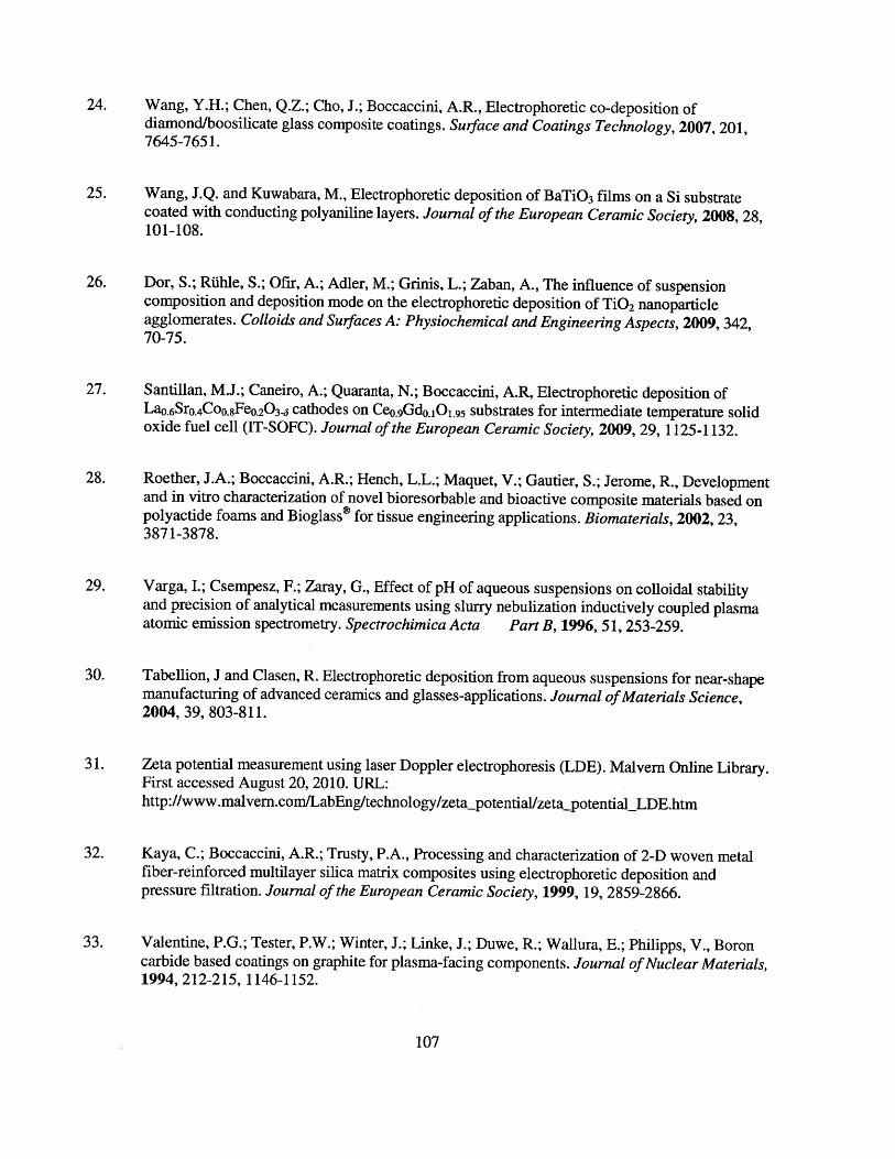
24. Wang, Y.H.; Chen, Q.Z.; Cho, J.; Boccaccini, A.R., Electrophoretic co-deposition ofdiamond/boosilicate glass composite coatings. Surface and Coatings Technology, 2007, 201,7645-7651.

25. Wang, J.Q. and Kuwabara, M., Electrophoretic deposition of BaTiO3 films on a Si substratecoated with conducting polyaniline layers. Journal of the European Ceramic Society, 2008, 28,101-108.

26. Dor, S.; RUhle, S.; Ofir, A.; Adler, M.; Grinis, L.; Zaban, A., The influence of suspensioncomposition and deposition mode on the electrophoretic deposition of TiO2 nanoparticleagglomerates. Colloids and Surfaces A: Physiochemical and Engineering Aspects, 2009, 342,70-75.

27. Santillan, M.J.; Caneiro, A.; Quaranta, N.; Boccaccini, A.R, Electrophoretic deposition ofLao.6 Sro.4Co0 .8Feo.20 3- cathodes on Ceo.9Gdo.101.95 substrates for intermediate temperature solidoxide fuel cell (IT-SOFC). Journal of the European Ceramic Society, 2009, 29, 1125-1132.

28. Roether, J.A.; Boccaccini, A.R.; Hench, L.L.; Maquet, V.; Gautier, S.; Jerome, R., Developmentand in vitro characterization of novel bioresorbable and bioactive composite materials based onpolyactide foams and Bioglass* for tissue engineering applications. Biomaterials, 2002, 23,3871-3878.

29. Varga, I.; Csempesz, F.; Zaray, G., Effect of pH of aqueous suspensions on colloidal stabilityand precision of analytical measurements using slurry nebulization inductively coupled plasmaatomic emission spectrometry. Spectrochimica Acta Part B, 1996, 51, 253-259.

30. Tabellion, J and Clasen, R. Electrophoretic deposition from aqueous suspensions for near-shapemanufacturing of advanced ceramics and glasses-applications. Journal ofMaterials Science,2004, 39, 803-811.

31. Zeta potential measurement using laser Doppler electrophoresis (LDE). Malvern Online Library.First accessed August 20, 2010. URL:http://www.malvem.com/LabEng/technology/zeta potential/zeta-potentialLDE.htm

32. Kaya, C.; Boccaccini, A.R.; Trusty, P.A., Processing and characterization of 2-D woven metalfiber-reinforced multilayer silica matrix composites using electrophoretic deposition andpressure filtration. Journal of the European Ceramic Society, 1999, 19, 2859-2866.

33. Valentine, P.G.; Tester, P.W.; Winter, J.; Linke, J.; Duwe, R.; Wallura, E.; Philipps, V., Boroncarbide based coatings on graphite for plasma-facing components. Journal of Nuclear Materials,1994, 212-215, 1146-1152.

107

34. Daring, J.-E.; VaBen, R.; Linke, J.; Stdver, D., Properties of plasma sprayed boron carbideprotective coatings for the first wall in fusion experiments. Journal of Nuclear Materials, 2002,307-311, 121-125.

35. Bousse, L.; Mostarshed, S.; van der Shoot, B.; de Rooij, N.F., Gimmel, P.; Gopel, W., Zeta

potential measurements of Ta20s and SiO 2 thin films. Journal of Colloid and Interface Science,1991, 147, 22-32.

36. Kaya, C.; Kaya, F.; Boccaccini, A.R., Electrophoretic deposition infiltration of 2-D metal fiber-reinforced cordierite matrix composites of tubular shape. Journal of Materials Science, 2002, 37,4145-4153.

37. Yu, B. and Khoo, S.B., Controllable zeolite films on electrodes - comparing dc voltageelectrophoretic deposition and a novel pulsed voltage method. ElectrochemistryCommunications, 2002, 4, 737-742.

38. Besra, L.; Uchikoshi, T.; Suzuki, T.S.; Sakka, Y., Application of constant current pulse to

suppress bubble incorporation and control deposit morphology during aqueous electrophoreticdeposition (EPD). Journal of the European Ceramic Society, 2009, 29, 1837-1845.

39. Kreith, Frank; Bohn, Mark S., Principles of Heat Transfer. 6 ed.; Brooks/Cole: Pacifc Grove,CA, 2001.

40. Ciou, S.-J.; Fung, K.-Z.; Chiang, K.-W., The mathematical expression for kinetics ofelectrophoretic deposition and the effects of applied voltage. Journal of Power Sources, 2007,172, 358-362.

41. Design of experiments: how it works. Umetrics Online Methods Library. First accessed February

15, 2011.URL: http://www.umetrics.com/default.aspx?id=8553&refid=79 4 8

42. Bard, Allen J. and Faulkner, Larry R., Electrochemical Methods: Fundamentals andApplications. 2 ed.; John Wiley & Sons, Inc: New York, NY, 2001.

43. Trau, M.; Saville, D.A.; Aksay, I.A., Assembly of colloidal crystals at electrode interfaces.Langmuir, 1997, 13, 6375-6381.

44. Prieve, D.C.; Sides, P.J.; Wirth, C.L., 2-D assembly of colloidal particles on a planar electrode.Current Opinion in Colloid & Interface Science, 2010, 15, 160-174.

108

Investigation of Electrophoretic Deposition as ... - DSpace@MIT

Documents

Transcript of Investigation of Electrophoretic Deposition as ... - DSpace@MIT