
Differential Detergent Fractionation for Non-electrophoretic Eukaryote Cell Proteomics
Upload
khangminh22Category
view
1download
0
The role of water in the
electrophoretic mobility of
hydrophobic objects
Die Rolle von Wasser bei der
elektrophoretischen Mobilität
von hydrophoben Objekten
Der Naturwissenschaftlichen Fakultät der
Friedrich-Alexander-Universität Erlangen-Nürnberg
zur
Erlangung des Doktorgrades Dr. rer. nat.
vorgelegt von
Zoran Mili£evi¢aus Slatina, Kroatien

Als Dissertation genehmigt
von der Naturwissenschaftlichen Fakultät
der Friedrich-Alexander-Universität Erlangen-Nürnberg
Tag der mündlichen Prüfung: 8. April 2016
Vorsitzender des Promotionsorgans: Prof. Dr. Jörn Wilms
Gutachter/in: Prof. Dr. Ana-Sun£ana Smith
Prof. Dr. Roland Roth


The beginning is the most important part of the work.
Plato

To my family
vi

vii
Zusammenfassung
Die Entdeckung der Hydrophobizität wird Hermann Boerhave anerkannt, welcher im
18. Jahrhundert die Fähigkeit des Wassers verschiedene Stoe zu lösen untersucht hat.
Heutzutage ist die Bedeutung der Hydrophobizität wohlbekannt, da dieser Eekt eine
wichtige Rolle bei Myriaden von Phänomenen spielt, angefangen bei der Faltung und der
Aktivität von Proteinen, dem Prozess der Selbstassemblierung von Phospholipidmembra-
nen, und aufgrund dessen auch bei dem Design und der Produktion von Metamaterialien,
um nur einige wenige Beispiele zu nennen. Um den hydrophoben Eekt zu verstehen,
wurde viel Aufmerksamkeit der Studie der Anordnung vonWasser an hydrophobe Objekte
gewidmet und heute wird weithin akzeptiert, dass Wasser um kleinere Objekte herum
Käge bildet, um das Netzwerk aus Wasserstobrücken zu erhalten. Auÿerdem ist
bestens bekannt, dass die Hydrophobizität einer Grenzäche, eines Tröpfchens oder
eines Partikels mittels eines externen elektrischen Feldes moduliert werden kann. Jedoch
werden die Eekte des elektrischen Feldes auf die Struktur des Wassers, welches ein
hydrophobes Objekt umgibt, noch nicht zufriedenstellend verstanden.
Das Anlegen eines homogenen elektrischen Feldes steuert die Wanderung eines
geladenen Partikels in einem Prozess, welcher Elektrophorese genannt wird. Bemerkens-
werterweise ist es aus experimenteller Sicht wohlbekannt, dass ungeladene Partikel wie
hydrophobe Objekte auch eine elektrophoretische Mobilität aufweisen. Allerdings wird
diese Mobilität nicht hinreichend verstanden. Die kürzlich erfolgte Anwendung von
Moleküldynamik-Simulationen hat die wissenschaftliche Diskussion über den wahren
Ursprung der elektrophoretischen Mobilität von hydrophoben Objekten nur intensiviert,
da die erhaltenen Ergebnisse oftmals widersprüchlich waren und zu einer Vielzahl an
Ad-hoc-Hypothesen geführt haben.
Der Fokus dieser Arbeit ist es, die Kontroversen rund um die Forschungsarbeiten
über Elektrophorese von hydrophoben Objekten durch Anwendung von Moleküldynamik-
Simulationen aufzuklären. Um dies zu ermöglichen, wurde ein Bottom-up-Ansatz verwen-
det und ein Minimalsystem entworfen, bei dem vermutet wird, dass es elektrophoretische
Mobilität aufweist. Dieses Minimalsystem besteht aus einem glatten, sphärischen Partikel,
welches nur durch ein Lennard-Jones-Potential mit Wasser wechselwirkt und deshalb als
Lennard-Jones-Partikel bezeichnet wird. Um ein tieferes Verständnis des Minimalsystems
zu erhalten, wurde, bevor wir das Verhalten in Gegenwart eines elektrischen Feldes
betrachten, das Verhalten ohne elektrisches Feld sorgfältig untersucht. Auÿerdem wurde
eine umsichtige Studie des statischen und dynamischen Verhaltens eines Systems, das
nur aus Wasser besteht, bei verschiedenen elektrischen Feldstärken durchgeführt.

viii
Trotz der stark ansteigenden Anzahl an elektrischen Anwendungen wurde der Eekt
eines externen elektrischen Feldes auf die dynamischen Eigenschaften von Wasser, wie die
Scherviskosität, noch nicht untersucht. Die Scherviskosität wird in dieser Arbeit durch
Ausnutzung der Vorzüge des Green-Kubo-Formalismus in dem Bereich der elektrischen
Feldstärke, bei welchem nicht-lineare Eekte vernachlässigt werden können, untersucht.
Um den Wert der Scherviskosität in dem elektrischen Feld abschätzen zu können, wurde
ein alternativer Ansatz, welcher den Kohlrausch Fit verwendet, erstellt. Es wurde
gefunden, dass das Feld die zu sich selbst senkrechten Komponenten der Scherviskosität
verringert und die parallelen Komponenten erhöht. Es ist hervorzuheben, dass das
Feld nur in der parallelen Richtung einen langsamen zusätzlichen Relaxationsprozess
erzeugt, welche den gesamten Relaxationsprozess im Bezug zur senkrechten Richtung um
beinahe ein Zehnfaches verlängert. Des Weiteren steigt die scheinbare Scherviskosität des
Wassers leicht mit der Feldstärke. Um eine Erklärung für das beobachteten Verhalten
der Scherviskosität zu erhalten, wurde eine detaillierte strukturelle Analyse des Wassers
durchgeführt, einschlieÿlich zweidimensionaler Paarverteilungsfunktionen zwischen Was-
sermolekülen, welche die axiale Symmetrie aufgrund des elektrischen Feldes berück-
sichtigen.
Die Ermittlung der Transportkoezienten von Kolloiden in Flüssigkeiten ist immer
noch eine anspruchsvolle Aufgabe für Computersimulationen. Neben technischen Schwie-
rigkeiten, konnten die Grenzen der Validität der Stokes-Einstein Relation noch nicht
vollständig bewiesen werden. Um über diese Probleme Aufschluss geben zu können,
wurden Berechnungen der Diusions- und Reibungskoezienten für das konstruierte,
nanometergroÿe Lennard-Jones-Partikel in Wasser ohne elektrisches Feld durchgeführt.
Es wurde ein Protokoll für die Bestimmung des hydrodynamischen Radius des Partikels
vorgeschlagen. Es wurde gezeigt, dass sowohl Diusions- als auch Reibungskoezienten
und somit auch die Scherviskosität des Wassers unabhängig voneinander und mit hoher
quantitativer, gegenseitiger Genauigkeit berechnet werden können. Dies wurde verwendet
um indirekt die Validität der Stokes-Einstein Relation in diesem System zu demonstrieren.
Es wurden verschiedene Ansätze untersucht und eine Analyse der Simulationsbedin-
gungen, insbesondere bezüglich der Masse des sphärischen Partikels und der Gesamtgröÿe
des Systems, welche für eine akkurate Vorhersage der Transportkoezienten nötig sind,
präsentiert.
Viele der jüngsten moleküldynamischen Studien, welche bei von Null verschiedenen
elektrischen Feldern durchgeführt wurden, zeigten eine enorme Empndlichkeit der Wan-
derungsgeschwindigkeit eines hydrophoben gelösten Stoes gegenüber der Behandlung
der weit reichenden Anteile der Van-der-Waals-Wechselwirkungen. Während der Ur-
sprung dieser Empndlichkeit nie erklärt wurde, wurde die Mobilität gegenwärtig als ein
Artefakt eines ungeeigneten Simulationssetups betrachtet. Diese kontroversen Ergebnisse
wurden in dieser Arbeit an dem System bestehend aus einem Lennard-Jones-Partikel in

ix
Wasser getestet. Es wurde beobachtet, dass eine unidirektionale feldinduzierte Mobilität
des hydrophoben Objektes dann auftritt, wenn die Kräfte einfach abgeschnitten werden.
Anhand der sorgfältigen Analyse der 100 ns langen Simulationen wurde gefunden, dass
nur in dem spezischen Fall, wenn die Kräfte abgeschnitten werden, eine von Null
verschiedene Van-der-Waals-Kraft im Mittel auf das Lennard-Jones-Partikel wirkt. Unter
Berücksichtigung des Satzes von Stokes kann gezeigt werden, dass diese Kraft quantitativ
mit der feldinduzierten Mobilität, die für dieses System gefunden wurde, übereinstimmt.
Im Gegensatz wird keine resultierende Kraft beobachtet wenn die Kräfte durchgehend
Behandelt werden. Auf diese Weise wird eine einfache Erklärung für die vorherigen
kontroversen Berichte erhalten.
Jedoch wird auch im Fall einer durchgehenden Behandlung der Van-der-Waals-
Kräfte eine unidirektionale Mobilität des Lennard-Jones-Partikels gefunden wenn die
Zeitskalen der Simulationen in den Bereich einer Mikrosekunde verlängert werden auch
wenn keine resultierende Kraft auf das Partikel wirkt. Um dies zu lösen wurde die
Wasserstruktur mit Hilfe von totalen Solute-Solvent-Korrelationsfunktionen analysiert,
welche die Orientierungsfreiheitsgrade des Solvens einschlieÿen. Um das Ausmaÿ des
Symmetrieverlustes zu analysieren, wurden die totalen Solute-Solvent-Korrelationsfunk-
tionen in zwei Dimensionen, unter Berücksichtigung der axialen Symmetry, rekonstruiert.
Es wurde gefunden, dass das elektrische Feld eine im Durchschnitt asymmetrische Vertei-
lung der Wassermoleküle um das Lennard-Jones-Partikel verursacht. Diese fungiert als
ein Steady-State-Dichtegradient, welcher eine phoretische Bewegung des hydrophoben
Objektes in Richtung der Bereiche mit höherer Wasserkonzentration induziert. Die
phoretische und Brownsche Bewegung können nur mittels der mittleren quadratischen
Verschiebung des Partikels bei Zeitskalen gröÿer als 15 ns unterschieden werden. Die
Daten wurden anhand der Derjaguin-Theorie für Diusiophorese interpretiert, welche die
Geschwindigkeit eines kolloidalen Partikels als eine Funktion des Konzentrationsgradi-
enten und des Solute-Solvent-Wechselwirkungspotential darstellt. Es wurde eine auÿerge-
wöhnliche Übereinstimmung zwischen der theoretisch vorhergesagten Geschwindigkeit
und den simulierten Ergebnissen gefunden.
Zusammenfassend werden in dieser Arbeit Ergebnisse von modernsten Molekül-
dynamik-Simulationen präsentiert, welche die Leistungsfähigkeit dieser Methoden im
Bezug zur quantitativen Berechnung der Transporteigenschaften von Wasser und kolloid-
alen Partikeln demonstrieren. Darüberhinaus wird ein plausibler Mechanismus für die
elektrophoretische Mobilität von hydrophoben Objekten vorgeschlagen.


xi
Abstract
The discovery of hydrophobicity is credited to Hermann Boerhave who in the 18th century
studied the eciency of water to dissolve various compounds. Nowadays the signicance
of hydrophobicity is well recognized as the eect plays an important role in a myriad of
phenomena ranging from the folding and activity of peptides and proteins, the process
of self assembly of phospholipid membranes and by this, the design and production of
meta-materials, to name just a few. In order to understand the hydrophobic eect a lot
of attention was devoted to the study of water ordering around hydrophobic objects and
now it is widely accepted that, around smaller objects, water forms cages to maintain
the network of hydrogen bonds. It is also well established that the hydrophobicity of an
interface, droplet or a particle can be modulated by an external electric eld. However,
the eects of the electric eld on water structure around a hydrophobic object are not
understood to a satisfactory level.
The application of a homogeneous electric eld drives the migration of a charged
particle in a process called electrophoresis. Remarkably, it is experimentally well known
that uncharged particles like hydrophobic objects also exhibit electrophoretic mobility.
However, this mobility is not satisfactorily understood. The recent application of molec-
ular dynamics simulations has only intensied the scientic discussion about the real
nature of the electrophoretic mobility of hydrophobic objects as the obtained results
were often contradictory and led to numerous ad hoc hypotheses.
The focus of the thesis is to elucidate the controversies surrounding the research
of the electrophoresis of hydrophobic objects through the application of molecular dy-
namics simulations. In order to achieve this a bottom-up approach is applied and a
minimal system that is expected to exhibit electrophoretic mobility is designed. This
minimal system consists of smooth spherical particle interacting with water molecules
only through a simple Lennard-Jones potential, and thereby the particle will be referred
to as the Lennard-Jones particle. To gain deeper understanding of our minimal system,
prior to looking at its behavior in the presence of an external electric eld, we metic-
ulously examine it in the absence of the electric eld. Moreover, a judicious study of
both the static and dynamic response of pure water at various electric eld strengths is
performed.
Despite a heavily increasing number of electrochemical applications, the eect of
the external electric eld on the dynamic properties of bulk water, like shear viscosity,
has not yet been investigated. The shear viscosity is studied here by exploiting the
merits of the Green-Kubo formalism in the range of the electric eld strengths where the

xii
non-linear eects are still negligible. To estimate the value of the shear viscosity in the
electric eld an alternative approach using the Kohlrausch t is constructed. It is found
that the eld decreases the component of the shear viscosity perpendicular to itself and
increases the components which are parallel. Importantly, the eld induces an additional
slow relaxation process only in the parallel direction, prolonging by almost tenfold the
overall relaxation process with respect to the perpendicular direction. Furthermore, the
apparent water shear viscosity increases slightly with the eld strength. To provide an
explanation for the observed behavior of the shear viscosity a detailed structural analysis
of water is performed, including the two-dimensional pair distribution functions between
water molecules that take into account the axial symmetry imposed by the electric elds.
Estimation of the transport coecients of colloids in liquids is still a challenging
task for computer simulations. Apart from technical diculties, the limits of the validity
of the Stokes-Einstein relation have not yet been fully established. To shed light on
these issues the calculation of the diusion and the friction coecients of the designed
nanometer-sized Lennard-Jones particle in water at zero electric eld is undertaken. A
protocol for dening the hydrodynamic radius of the particle is suggested. It is demon-
strated that both the diusion and the friction coecient, and hence the water shear
viscosity, can be calculated independently with a high quantitative mutual agreement.
This is used to indirectly demonstrate the validity of the Stokes-Einstein relation in this
regime. Various approaches are investigated and an analysis of simulation conditions
required for accurate predictions of transport coecients, with a particular emphasis on
the mass of the spherical particle, as well as the size of the system, is presented.
A number of recent molecular dynamics studies performed at nonzero electric elds
have shown a tremendous sensitivity of the migration rate of a hydrophobic solute to the
treatment of the long range part of the van der Waals interactions. While the origin of
this sensitivity was never explained, the mobility is currently regarded as an artifact of
an improper simulation setup. These controversial ndings are tested here on the system
consisting of the Lennard-Jones particle in water. It is observed that a unidirectional
eld-induced mobility of the hydrophobic object occurs only when the forces are simply
truncated. From the careful analysis of the 100 ns long simulations it is found that, only
in the specic case of truncated forces, a non-zero van der Waals force acts, on average,
on the Lennard-Jones particle. Using the Stokes law it is demonstrated that this force
yields quantitative agreement with the eld-induced mobility found within this setup.
In contrast, when the treatment of forces is continuous, no net force is observed. In this
manner, a simple explanation for the previously controversial reports is given.
However, when the simulations are prolonged toward a microsecond scale a uni-
directional mobility of the Lennard-Jones particle is also observed for continuous treat-
ments of the van der Waals forces, even though there is no net force acting on the particle.

xiii
To resolve this, the water structure is analyzed by means of the total solute-solvent cor-
relation function, which includes the orientational degrees of freedom of the solvent. To
evaluate the extent of the symmetry loss, the total solute-solvent correlation function
is reconstructed in two-dimensions, accounting for the axial symmetry. It is found that
the electric eld evokes on an average asymmetric distribution of the water molecules
around the Lennard-Jones particle. This acts as a steady state density gradient, inducing
a phoretic motion of the hydrophobic object towards the region of higher concentration
of water. The phoretic and Brownian motion can be distinguished in the mean square
displacement of the particle only at times larger than 15 ns. The data is interpreted on a
basis of the Derjaguin theory for diusiophoresis, which predicts the driving velocity of a
colloidal particle as a function of the concentration gradient and the solute-solvent inter-
action potential. An exceptional agreement between this theoretically predicted driving
velocity and the simulation results is obtained.
In summary, in this thesis are presented the results from extensive state-of-art
molecular dynamics simulations which demonstrate the ability of the approach to re-
trieve, with quantitative agreement, the transport properties of both water and colloidal
particles. More importantly, a plausible mechanism for the electrophoretic mobility of
hydrophobic objects is suggested.
Acknowledgements
First of all, this thesis would never have come into being without the unconditional
support, guidance and encouragement of my academic supervisor, Prof. Ana-Sun£ana
Smith. For this and for the opportunity to thrive from the association with the Cluster
of Excellence: Engineering of Advanced Materials (EAM), I am most highly thank-
ful. I would like to express my very great appreciation to my co-supervisor, Dr. David
M. Smith, for his comprehension, motivation and continuous help over the past years.
Thereby, Mr. & Mrs. Smith, you have my deepest respect and gratitude.
Financial support was provided by the Cluster of Excellence: Engineering of Ad-
vanced Materials (EAM), by BAYHOST, by the European Social Fund (ESF; project
MIPoMat), and by the Unity through Knowledge Fund (UKF).
I want to express my sincere gratitude to the EAM's administration, especially
Waltraud Meinecke, for the assistance and generous and prompt help provided in resolv-
ing numerous aairs. Also, many thanks go to Ina Viebach for prudent handling of my
packages.
I acknowledge the SUPERcomputing facilities provided by the Regionales Rechen-
zentrum Erlangen (RRZE), without which this work would remain in its infancy - just an
idea on a sheet of paper. Also, I would like to thank the competent sta at RRZE, espe-
cially Dr. Thomas Zeiser, for promptly resolving every issue and fullling my sometimes
slightly odd and extravagant requests (like installing antiquated versions of GROMACS).
The local help, both in Zagreb (Dr. Darko Babi¢ and Dr. Borislav Kova£evi¢) and Er-
langen (Roland Haberkorn), is appreciated. In particular, I would like to thank Roland
for his frequent rescues of my HDDs and demystifying GRUB.
Here I would like to express my gratitude to the members of the PULS group:
Jayant Pande, Sara Kaliman, Mislav Cvitkovi¢, Zlatko Brklja£a, Dr. Karmen ondi¢-
Jurki¢, Dr. Timo Bihr, Daniel Schmidt, Robert Stepi¢, Damir Vurnek and his wife Dra-
gana. Jayant, hvala (Croatian for thank you) for introducing me to Indian gastronomy,
regular chats on the NBA, and pedantic proof-reading of my English scribbles. Dear Sara,
thank you for the revealing and revelling discussions on more or less (usually more) ob-
scure topics. Mislav, thank you for being a multi-practical, multi-useful friend and, of
course, thank you for agitating me with your Kramer-like entrance into the room (sim-
ply priceless). Thanks for maintaining the noise at a constant level around 70 decibels
(all the time) go to Zlatko. On the other hand, Robert (aka SOMEONE FAMOUS),
please remain so cool. Timo & Daniel, thank you for the precious memories from DPG
conferences. Dear Vurneks, thank you for the supply of sweets and XXL packages of
ips. Dear Karmen, thank you for beers and for being always a support, I appreciate
it. Finally, thank you all for having so much patience and tolerance for my although
unavoidable (ab)use of your hard drive space.
xiv

xv
I am highly grateful to all members of the Institute for Theoretical Physics I and its
head, Prof. Klaus Mecke, for their hospitality and for providing a creative environment
during my years in Germany. Not to forget, I really have enjoyed being a part of the
annual Saufest. Here I would also like to acknowledge the group for quantum organic
chemistry (Rudjer Bo²kovi¢ Institute) for a comfortable and pleasant time in Zagreb.
Special thanks go to Dr. Momir Mali², a resort of wisdom, for his unselsh help on
multiple occasions and for sharing his FORTRAN expertise. For always pointing at the
bright side of life, thank you, comrade, Dr. Jurica Novak.
Last but not the least, I wish to express my gratitude to my loving parents who, I
know, are always there for me.

Contents
Zusammenfassung vii
Abstract xi
Acknowledgements xiv
1 Introduction 1
1.1 Hydrophobic Eect . . . . . . . . . . . . . . . . . . . . . . . . . . . . . . . 11.2 Electrophoretic Mobility . . . . . . . . . . . . . . . . . . . . . . . . . . . . 3
2 Theory and Methods 7
2.1 Molecular Dynamics Simulations . . . . . . . . . . . . . . . . . . . . . . . 72.2 Classical Force Fields . . . . . . . . . . . . . . . . . . . . . . . . . . . . . . 82.3 Numerical Integration of Newton's Equations of Motion . . . . . . . . . . 112.4 Molecular Dynamics and Thermodynamic Ensembles . . . . . . . . . . . . 13
2.4.1 Control of Temperature . . . . . . . . . . . . . . . . . . . . . . . . 142.4.2 Control of Pressure . . . . . . . . . . . . . . . . . . . . . . . . . . . 16
2.5 Treatment of the van der Waals Interactions . . . . . . . . . . . . . . . . . 172.6 Water Models . . . . . . . . . . . . . . . . . . . . . . . . . . . . . . . . . . 21
3 Properties of the Pure Water System Both in the Absence and Presenceof Electric Fields 25
3.1 Computational Details and Static Water Response . . . . . . . . . . . . . 263.2 Water Structure . . . . . . . . . . . . . . . . . . . . . . . . . . . . . . . . . 283.3 Shear Viscosity . . . . . . . . . . . . . . . . . . . . . . . . . . . . . . . . . 34
3.3.1 Shear Viscosity of Water in the Absence of External Electric Fields 363.3.2 Shear Viscosity in the Presence of Electric Fields . . . . . . . . . . 383.3.3 Dependence of the Apparent Shear Viscosity on the Electric Field
Strength . . . . . . . . . . . . . . . . . . . . . . . . . . . . . . . . . 413.4 Conclusions . . . . . . . . . . . . . . . . . . . . . . . . . . . . . . . . . . . 46
4 Transport Properties of a Nanosized Hydrophobic Object in Water 49
4.1 Computational Details . . . . . . . . . . . . . . . . . . . . . . . . . . . . . 514.2 Diusion of the Lennard-Jones Particle . . . . . . . . . . . . . . . . . . . . 52
4.2.1 Long-time Tails and Finite Size Eects . . . . . . . . . . . . . . . . 55
xvii
Contents xviii
4.3 Friction Coecient of the Lennard-Jones Particle . . . . . . . . . . . . . . 614.3.1 Mass Dependence . . . . . . . . . . . . . . . . . . . . . . . . . . . . 634.3.2 System Size Inuence . . . . . . . . . . . . . . . . . . . . . . . . . 64
4.4 Validity of the Einstein Relation and the Stokes-Einstein Relation . . . . . 664.5 Diusive Length Scale . . . . . . . . . . . . . . . . . . . . . . . . . . . . . 714.6 Conclusions . . . . . . . . . . . . . . . . . . . . . . . . . . . . . . . . . . . 74
5 Establishing Conditions for Simulating Hydrophobic Solutes in ElectricFields by Molecular Dynamics 77
5.1 Computational Details . . . . . . . . . . . . . . . . . . . . . . . . . . . . . 785.2 Water at the Interface of the LJ Particle . . . . . . . . . . . . . . . . . . . 805.3 Observed Time-dependent Displacement of the LJ Particle . . . . . . . . . 83
5.3.1 Observed Time-dependent Displacement of the Oil Droplet . . . . 875.3.2 Brownian Diusion of the LJ Particle . . . . . . . . . . . . . . . . 88
5.4 The Net van der Waals Force on the LJ Particle . . . . . . . . . . . . . . . 905.4.1 Consistency Between the Evaluated van der Waals Force and the
Observed Drift . . . . . . . . . . . . . . . . . . . . . . . . . . . . . 935.5 The Eects of the Thermostat and the Flying Ice Cube Eect . . . . . . 945.6 Conclusions . . . . . . . . . . . . . . . . . . . . . . . . . . . . . . . . . . . 97
6 Dynamics of a Hydrophobic Object in the Presence of Electric Fields:Long-time Scales 99
6.1 Computational Details . . . . . . . . . . . . . . . . . . . . . . . . . . . . . 996.2 Coordinate System . . . . . . . . . . . . . . . . . . . . . . . . . . . . . . . 1006.3 Radially Averaged Correlations . . . . . . . . . . . . . . . . . . . . . . . . 1016.4 Axially Averaged Correlations . . . . . . . . . . . . . . . . . . . . . . . . . 1066.5 Long-time Displacement of the LJ Particle . . . . . . . . . . . . . . . . . . 1146.6 Electro-diusiophoresis of the LJ Particle . . . . . . . . . . . . . . . . . . 1176.7 Conclusions . . . . . . . . . . . . . . . . . . . . . . . . . . . . . . . . . . . 126
7 Conclusions and Outlook 129
A Variation Analysis of the Kohlrausch Fit Procedure 135
A.1 Direction Perpendicular to the Electric Field . . . . . . . . . . . . . . . . . 136A.2 Direction Parallel to the Electric Field . . . . . . . . . . . . . . . . . . . . 138
B Two-dimensional Static Correlations 141
B.1 Two-dimensional Density Correlations of Water . . . . . . . . . . . . . . . 141B.2 2-D Correlations for the LJ Particle-Water System in the Absence
of Electric Fields . . . . . . . . . . . . . . . . . . . . . . . . . . . . . . . . 144B.3 Angular Correlations Between the Heptane Droplet and Water . . . . . . 146B.4 Angular Correlations for Neat Water . . . . . . . . . . . . . . . . . . . . . 146B.5 Dierent Treatments of the van der Waals Interactions . . . . . . . . . . . 148
List of Figures 149

Contents xix
List of Tables 155
Abbreviations 157
Symbols and Physical Constants 159
Bibliography 163
Curriculum Vitae 186
Publications and Conference Contributions 188

Chapter 1
Introduction
1.1 Hydrophobic Eect
The term hydrophobic (`water-fearing') is commonly used to describe substances that,
like oil, do not mix with water [1] and are also incapable of hydrogen bonding with water
[2]. Although it may appear that water repels oil, in reality the separation between the
molecules of water and oil is not the consequence of their repulsion but very favourable
hydrogen bonding between water molecules. Indeed, there exists mutual attraction be-
tween molecules of water and oil, but this attractions is very weak in comparison to
the attraction between water molecules itself [1]. Also, the hydrophobic hydration is a
collective phenomena [2] that involves certain number of water molecules depending on
the size of dissolved hydrophobic object.
The hydrophobic eect that arises from the interactions between hydrophobic
molecules is primarily associated with a small solubility of hydrophobic particles in wa-
ter [3]. However, this eective attraction between hydrophobic molecules (aggregates)
is stimulated by strong interactions between water molecules [1, 4]. Apart from be-
ing a cause for a low solubility of hydrophobic objects in water the implications of the
hydrophobic eect are vast. Typical examples involve the formation of water droplets
from thin water lms, the folding and activity of peptides and proteins, the process of
self-assembly (for example of micelles, vesicles and membranes) and by this, the design
and production of meta-materials [3, 5]. Thereby, the understanding of hydrophobic
interactions has developed into one of the central problems of the physical chemistry of
solutions [6].
The problem is intimately linked with the length scales since the `small' and the
`big' hydrophobic solutes exhibit diverse hydration behavior. Useful approach to interpret
the hydration process is to characterize its free energy of solvation ∆G. The latter is
related to the enthalpy (∆H) and the entropy (∆S) by ∆G = ∆H−T∆S, where T is the
absolute temperature of the system. The water can accommodate the small hydrophobic
1

Chapter 1. Introduction 2
objects, like atoms of noble gases or small alkane molecules, while preserving the network
of hydrogen (H-)bonds, i.e. preventing their breakage. However, in order to accommodate
the small solute the H-bonds have to reorient themselves [1, 7, 8]. Therefore, the expense
of hydrophobic hydration for small solutes is related to the number of ways in which
the hydrogen bonds can be formed, i.e. the free energy of hydration is dominated by
unfavourable entropy contribution (∆S < 0). For large solutes or surfaces, all H-bonds
cannot survive and, thereby, their number per water molecule near the hydrophobic
object-water interface is reduced. To minimize this loss of hydrogen bonding the water
orders itself in such a way that, on average, about one H-bond per water molecule is
sacriced relative to the bulk water [9]. Thus, the hydration of large solutes is driven by
enthalpy and not by entropy as it is the case with the small solutes.
The object size dierentiating `small' and `big' at which occurs the `crossover' of
the nature of hydrophobic hydration is known as the `crossover length' and is considered
to be around 0.5 nm in radius [7]. Apart from diering in the nature of the driving force
(enthalpy or entropy) the hydration of the small and the big solutes undergoes dierent
scaling phenomena [1, 7]. The free energy of solvation of small objects is proportional to
the volume of the object whereas for the large objects it is proportional to the surface
area of the interface between the solute and water.
Insightful approach to the hydration process is to inspect the water ordering around
the solute. As there is no long range periodicity in the positions of particles in a xed
coordinate system the microscopic structure of liquids is commonly related to the average
local structure obtained from averaged (i.e., most probable) positions in a coordinate
system with an arbitrary central atom [10]. Hence, the majority of our knowledge on the
water ordering near hydrophobic objects originates from the density-prole (e.g., radial
distribution function - RDF) of water in the vicinity of hydrophobic particles and walls
[9, 1113]. Thereby eects of the solute size have been analyzed in details [14, 15] and the
compressibility of hydration shells well characterized [16]. The RDFs also showed that
for rather small solutes (radius smaller than 0.4 nm) the density near the hydrophobic
object is twice the density of the bulk water and the surface of such objects is regarded
as `wet' [7]. This signicant increase of water density in the proximity of the particle is
the result of the elastic response of the liquid to the presence of the solute in which the
interfacial water molecules remain localized to maintain their H-bonds. Moreover, it is
still widely accepted that around small hydrophobic solutes `clathrate-like' cages of water
form that resemble those around gaseous hydrates [7, 9, 17]. However, this description
is doubtful since intermolecular correlations in water are not strong enough to support
this crystalline picture.
In contrast, for large solutes (radius larger than 1 nm) the density near the surface
does not increase signicantly or at all relative to the density in the bulk. The reason for
the appearance of this `dry' surface [9] is the breakage of the network of hydrogen bonds

Chapter 1. Introduction 3
near to the hydrophobic particle followed by a small translation of water molecules away
from the solute creating in that way a liquid-vapour-like interface. However, the fact
that crossover length does not exactly conform with the particle size dependence in the
transition from wet to dry surfaces indicates that unied theory explaining the hydration
of hydrophobic objects, both from the thermodynamic and static standpoint, is yet to
be developed.
It is well established that the hydrophobicity of an interface, droplet or a particle
can be modulated by an external electric eld in a process called electrowetting [18]. Such
change of surface characteristics allows for the regulation of macroscopic properties such
as adhesion or friction in micro and nano-uidics by the electric eld [19]. Microuidic
movement based on electrowetting is being used in an increasing number of applications,
such as, for example, for reective displays [20, 21]. While the eect of the electric eld
is reasonably well understood on the macroscopic scale [18], there are only few studies
of the origin of electrowetting on the nanometric scale [2224]. With the advent of
nano-electronics and the development of micro and nano-devices that can be powered by
electric elds [25], this becomes a more and more pressing problem. The understanding of
nanoscale electrowetting is intimately related to the structure of water near a hydrophobic
interface, which is also a key aspect of the hydrophobic eect.
Unlike at zero electric elds, the organization of water around hydrophobic objects
in the presence of an external electric eld has been studied very sparsely. Moreover,
both in the absence and presence of the electric elds, the coupling of the orientational
degrees of freedom to the presence of a hydrophobic object, which is evidently important
in the context of electric elds, has been explored in much less detail [2628]. A special
characteristic of the hydrophobic hydration is the possibility to signicantly alter the
position of the liquid-vapor-like interface as well as the average liquid density near a large
hydrophobic surface by simply modifying the van der Waals interactions between water
and the hydrophobic object [7, 29]. Although these changes are easy to implement in
the molecular dynamics simulations there are still no studies suggesting how the electric
eld aects this labile interface layer.
1.2 Electrophoretic Mobility
Both the directed and autonomous motion have attracted signicant attention in the
scientic community over the past decade. This can be partially assigned to the fact that
the autonomous motion is widely occurring phenomena in nature and is characteristic,
for example, of the motile bacteria [30, 31] or motor proteins (kinesins, myosins, and
dyneins) [32]. The latter move along complementary tracks in the cell, by converting
the energy released upon ATP (adenosine triphosphate) hydrolysis into mechanical work
[33], and perform a variety of indispensable functions like cytokinesis, signal transduction,

Chapter 1. Introduction 4
intracellular tracking, and locomotion of cellular components [34]. The appreciation of
the directed motion of micro- and nanoscale objects acts as an inspiration for the design of
various applications [34], performed either on a chip or in a biological environment, such
as self-assembly of superstructures, biosensing, targeted drug-delivery [35], transport of
emulsion droplets [36] and living cells [37].
On the other hand, the electrophoresis may be the main technique for molecular
separation in today's cell biology laboratory because it is a powerful method, and yet
reasonably easy and inexpensive. According to the denition, electrophoresis is the
migration of a solvated ion in response to the application of a homogeneous electric
eld [38]. The migration rate is ordinarily proportional to the strength of the applied
eld. Remarkably, the hydrophobic objects, such as oil droplets, which are essentially
uncharged also show electrophoretic activity [39].
Since the rst measurement of the electrophoretic mobility (EPM) of oil droplets
in 1938 by Carruthers [39], its origin has been heavily debated [40]. In the absence of
surfactants at neutral or high pH the droplets show negative electrophoretic mobility
whereas at low pH the mobility is positive [4144]. This observation made plausible to
explain the phenomena in terms of the charging of the oil droplets due to the adsorption
of hydroxide (OH) or hydronium ions (H3O+) to the hydrophobic surface, leading to an
excess of hydroxide ions at neutral or high pH and of hydronium ions at low pH [41, 45].
This view is supported by the observation that, in response to the application of a eld
to a solution containing oil droplets, a drop in pH occurs if the the initial pH is high or
neutral whereas a rise in pH occurs if the initial pH is low [42]. However, the fact that
the isoelectric point (the pH value at which the electrophoretic mobility vanishes) and
the point of zero charge (the pH at which the dispersion of particles in water does not
change the pH of the bulk water) do not coincide can be taken as evidence for a more
complex mechanism [46].
Even if the mechanism related with the charging of oil droplets is considered to
be an origin of the electrophoretic mobility it must be taken into account that the real
nature of the oil/water or the air/water interface is heavily debated in the scientic
community [40, 4750]. From `classical' techniques, like the measurements of the pH
dependence of the zeta potential, the unied view is that the interface is negatively
charged due to the adsorption of hydroxide ions (for example, see Refs. [41, 5153]).
Recently, Beattie et al. [42] measured the pH changes caused by the formation of an
emulsion with its large surface area and quantitatively determined the surface charge
density of oils such as hexadecane. In the absence of surfactants, they demonstrated that
OH ions charge and stabilize the oil-in-water emulsion droplets. The molecular dynamics
(MD) simulations have also suggested that hydroxide ion adsorption to a hydrophobic
surface can be induced by anisotropic water dipole orientation close to the surface [54].

Chapter 1. Introduction 5
In contrast, there is an increasing number of reports claiming that the interface
is positively charged due to the preferential adsorption of hydronium ions which are
more strongly attracted to the interface than hydroxide ions [40, 47, 5558]. These
experimental claims come primarily from novel and advanced spectroscopic methods:
the vibrational sum frequency generation (VSFG) [5860], the linear surface selective
synchrotron photoelectron spectroscopy (PES) [47], and the non-linear surface selective
measurements, i.e. the second harmonic generation (SHG) [61, 62]. In agreement with the
above mentioned spectroscopic ndings are both the ab-initio [47, 55] and classical MD
simulations [40, 5658, 63]. However, in distinction to the free water surface, hydroxide
was found to exhibit a certain anity for the hydrophobic interfaces, such as that between
water and graphene [64].
Logically, all these opposite ndings casts doubt onto the plausibility of the ad-
sorbed hydroxide/hydronium mechanism. As a possible solution of this dilemma Knecht
et al. [65] made the rst report of ion-less electrophoretic mobility based on their results
obtained from MD simulations of heptane-water mixtures, in both the droplet and slab
geometries. They observed negative EPM of the heptane phase relative to the water
phase in the absence of hydroxide or hydronium ions, in accordance with experimental
ndings for air bubbles and oil droplets. The results suggested that EPM does not solely
reect the net charge or electrostatic potential on the suspended particle. The authors
proposed that surface roughness and dipolar ordering at hydrophobic interfaces could be
playing a role in the electrophoresis of oil droplets [65].
However, an in depth study and theoretical modelling of the electrophoresis of
polyelectrolyte chains showed that mobility is not possible in the absence of ions [66].
Moreover, the results of Knecht and collaborators [65] were also refuted by a continuum
calculation on heptane and water ow elds [67, 68]. Therein, however, the orientational
degrees of freedom of the water molecules were treated only in a fully averaged fashion,
based on earlier results obtained in the absence of eld [26]. Further MD simulations,
in various slab-like geometries [67], led to the conclusion that the initially reported mo-
bility [65] was due to peculiarities in the abrupt truncation of the van der Waals (vdW)
interactions. That claim was seemingly conrmed [69] for the combination of a xed-
charge water model and a united-atom slab of decane. The electrophoretic mobility of
that system was, however, reportedly restored when polarization eects were taken into
account for an all-atom model. Similarly, the transport of water through hydrophobic
tubes was reported in the presence of static electric elds [70] or xed charges mimicking
the eld [71]. That result was subsequently found to be sensitive to parameters during
the simulation and the treatment of the non-bonded interactions [67, 68, 72, 73]. Since
both the ux of water through nanotubes and EPM of oil droplets were found to be
very sensitive to the treatment of the vdW interactions the mobility observed with the
Chapter 1. Introduction 6
truncated forces was attributed [7375] to the imprudent implementation of the Lennard-
Jones cut scheme in GROMACS [76]. Despite that, a quantitative explanation of the
observed sensitivity is not presented yet.
Given that the structural reorganization of water has been invoked as a possible
candidate to play an important role in the electrophoretic mobility of hydrophobic objects
[41, 65, 77], it is surprising that very little is known about the organization of water
around hydrophobic solutes under the electric eld. This limited interest is even more
staggering if the importance of water ordering in the hydrophobic phenomena in general
is taken into account.

Chapter 2
Theory and Methods
2.1 Molecular Dynamics Simulations
In general, computer simulations act as a bridge between models and theoretical pre-
dictions on one side and between models and experimental ndings on the other side
[78]. Moreover, the simulations have the capability to explore the problems which are
dicult to tackle in the laboratory or that are completely out of reach of the available
experimental techniques. This intrinsic framework implies that the performance of a
simulation, measured against experiment and/or theory, hugely depends on the model
which includes the representation of the system and a set of rules that describe the be-
havior of the system. Therefore, it is of the utmost importance to assure that choice of
the model is made accordingly to the phenomena under the study.
Among the class of computer simulations, Molecular Dynamics (MD) simulations
have gained a special status due to their ability to provide accurate insight, in principal,
into a wide range of condensed matter topics related to the behavior of (macro)molecules,
solutions, (complex) uids or liquid crystals to name just a few [79]. In its pure form the
MD method obeys classical dynamics as it considers the motion of particles (atoms) in
the classical limit. Following the Born-Oppenheimer approximation the nuclei move in
a conservative potential determined by the nuclear coordinates only, while the electrons
are assumed to be in the ground state and their rapid motion is averaged out. In this
classical description, the Hamiltonian H of a system of N molecules, with the position
vector1 q = (q1,q2, . . . ,qN ) and the momentum vector p = (p1,p2, . . . ,pN ) collecting
the positions and momenta of the molecules, can be written [78] as the sum of kinetic
K and potential energy function V
H (q,p) = K (p) + V (q) . (2.1)
1The generalized coordinates q are usually the set of Cartesian coordinates ri of each atom in thesystem.
7

Chapter 2. Theory and Methods 8
The kinetic term is then given as the sum of the kinetic energies of the molecules
K =
N∑i=1
p2i
2mi, (2.2)
where mi is the mass of molecule i.
As said, the potential energy of the system is given as a function of nuclear coordi-
nates only and, hence, the classical approximation to the quantum mechanical description
of a molecule and its interactions does not arise solely from `rst principles' [79]. Indeed,
it is the result of the synchronized adjustment of both structure and potential function
to a variety of dierent information obtained either from experiment (spectroscopic fea-
tures, transport properties, crystal structure, etc.) or from quantum mechanical energy
calculations. This simple classical description that enables an ecient computation of
forces on each atom, as well as the total energy, from the knowledge of position of each
atom is usually known as a force eld.
2.2 Classical Force Fields
A simple force eld, suitable for simulating large molecular systems, represents atoms (or
united atoms)2 as the mass points that move in the force eld and are also the origins for
the dierent terms in the force eld description [80]. Essentially, there are two types of
interactions: bonded interactions between dedicated groups of atoms, and assumed pair-
wise additive non-bonded interactions between atoms, based on their (changing) distance
[80].
The contribution to the total potential energy of the system from the bonded
interactions VBI can be written in a general functional form
VBI =∑bonds
kd2
(d− d0)2 +∑angles
kγ2
(γ − γ0)2 +∑
dihedrals
kζ [1 + cos(Nζ ζ − ζ0)] . (2.3)
Here, the three terms contributing to VBI correspond to the overall energies coming from
all covalent bonds, covalent bond angles, and dihedral angles present3 in the simulated
system, respectively. In the above equation the covalent bond and bond angle terms are
represented by the harmonic potential describing the oscillations of constituent atoms
around the equilibrium values of bond length d0 and bond angle γ0 with the force con-
stants kd and kγ . The instantaneous values of bond length d and angle γ are given
2In united-atom approaches some hydrogen atoms are merged into the atom to which they are bound.Typical example of this are hydrogen atoms bound to aliphatic carbon atoms, like in −CH
2or −CH
3
groups, which in the united atom representation is a single moving mass.3When simulating complex molecules that have planar groups (as aromatic rings) the improper
dihedrals are also dened that prevent pyramidalization by way of a harmonic restraining potential.

Chapter 2. Theory and Methods 9
by
d = |rj − ri| and γ = arccosrij · rkjrijrjk
. (2.4)
The dihedral potential can be depicted by a periodic function of amplitude kζ with Nζ
local minima (see Eq. 2.3) whereas the instantaneous dihedral angle ζ is dened by the
positions of four atoms i, j, k, and l as the angle between the normal vectors o1 and o2
to the two planes i,j,k and j,k,l
ζ = arccoso1 · o2o1o2
. (2.5)
Within the classical force elds the non-bonded interactions, i.e. the van der Waals
(vdW) and the electrostatic interactions, are pair-additive and a function of the distance
rij between the two atoms of each pair. Generally, the vdW interactions between all
dierent pairs of atoms i and j in the system are taken into account through the well
known 12-6 Lennard-Jones (LJ) potential
VLJ(rij) =∑j<i
4εij
[(σijrij
)12
−(σijrij
)6], (2.6)
consisting of the short-range repulsive term (r−12) and the longer attractive dispersion
term (r−6). Here, εij is the well depth of the potential and σij is the distance between
atoms i and j at which VLJ = 0. In order to make computation feasible the calculation
of the LJ interaction is truncated at relatively short distances (usually around 1 nm).
Because vdW interactions play an important role in our study of the mobility of hy-
drophobic objects in water an elaborate discussion of the treatment of the (long-range)
vdW interactions is presented in Sec. 2.5.
The electrostatic Coulomb interaction between charges or partial charges q on
atoms i and j is given by
VCoul(rij) =1
4πε0εr
qiqjrij
, (2.7)
where ε0 and εr are the vacuum permittivity and relative permittivity (i.e., dielectric
constant), respectively. Decaying with 1/r in space the electrostatic interactions are
clearly signicantly longer-ranged than dispersion interactions (r−6). Even though the
Coulomb interactions tend to cancel out at large distance because of overall charge neu-
trality they must be properly accounted for [80]. If the interactions are simply truncated
at some (short) cut-o radial distance then simultaneously with the introduction of ad-
ditional noise into the system a myriad of severe artefacts is expected to occur which,
for example, may involve the accumulation of charges at the cut-o distance and the
distortion of short-ranged structural ordering [81]. The easiest way to deal with these
unwanted eects is to apply a certain scheme to smooth the interaction function such

Chapter 2. Theory and Methods 10
that the resulting forces are continuous (see, for example, Ref. [82]). However, these
`smooth' cut-os strongly deviate from the correct Coulomb form (Eq. 2.7). Thus, it is
strongly encouraged to use some method that incorporates the long-range part of the
electrostatic interactions.
The most important methods that assess the problem of the treatment of the
long-ranged Coulomb interactions are:
• reaction eld method in conjunction with cut-o method incorporates the dielectric
response of the medium beyond the cut-o distance. This is accomplished through
the introduction of a reaction eld [83] which depends on the dielectric constant and
ionic strength of the environment and is proportional to the total dipole moment
within the cut-o sphere.
• continuum corrections [84] assume that dierences between the `computational
physics' (e.g., cut-os) and the `real world physics' are smooth and can be treated
by continuum methods. To demonstrate this, Wood [84] showed that hydration
energies of ions for various cut-os can be extracted exceptionally well after the
correction on the spatial distribution of solvent polarization is undertaken.
• lattice-sum methods split the total Coulomb interaction of periodic system4 into
short- and long-range parts. The long-range term is solved on a grid by Poisson's
equation. The representatives of this class of techniques are Ewald summation
[85], and its variants, the particle-particle particle-mesh (PPPM) [86, 87] and the
particle mesh Ewald (PME) [88, 89] method. The PME method gained popularity,
particularly for large molecular systems, due to its eciency.
This rather simplied picture of a force eld can become very complex by adding
weightless virtual interaction sites (like in common TIP4P-type water models) or dummy
particles that carry mass and simplify the rigid-body motions, by improving the electro-
static description through the replacement of partial charges with charge distributions,
multipoles or by explicitly accounting for polarizability, to name just a few possible ex-
tensions. When the `chemistry' (e.g., breaking/formation of bonds) occurring in the
system is of interest a part of the system is treated quantum mechanically (QM) whereas
the rest of the system remains described by classical molecular mechanics (MM). In
this QM/MM approach [90] the quantum part is always solved in the Born-Oppenheimer
approximation.
Unfortunately, the development of force elds did not follow the progress of the
MD method(s) and, especially the evolution of computational resources. The force eld
inaccuracies are becoming more transparent as the simulation extend over longer time4The lattice-sum methods are developed to treat periodic system (see the original paper by Ewald
[85]). However, these methods can be used eciently also for non-periodic system extended with theirperiodic images.

Chapter 2. Theory and Methods 11
spans and become more statistically accurate. Therefore, a general improvement of force
elds in terms of accuracy and transferability while retaining simplicity is becoming a
pressing problem [81]. Whether this will be achieved by the parametrization including
the tting to larger set of properties, by reducing the number of atom types, by the
inclusion of polarizability or by some other means, remains to be seen.
2.3 Numerical Integration of Newton's Equations of Motion
The principal idea behind molecular dynamics (MD) method is to solve Newton's equa-
tions of motion which govern the time evolution of a microscopic system consisting of N
particles with mass mi. Therefore, instead of dealing with macroscopic quantities like
pressure P and temperature T , the system is described by the instantaneous positions
ri and velocities vi of each particle i. Having conservative force eld (see Sec. 2.2) which
describes the interactions between particles we have all the ingredients to compute the
total potential energy Epot = V (r) and forces acting on particles Fi = −∇iV (r).
The Newton's equations of motion can be simply written as
ri = vi
vi =Fimi
,(2.8)
where the dots denote the dierentiation with respect to time t ( ˙ = d/dt). The total
energy of the system (Eq. 2.1) will be conserved [80]:
dH
dt=
d
dt
∑i
1
2miv
2i +
dV (r)
dt=∑i
mivi · vi +∑i
∂V
∂ri· vi
=∑i
(vi · Fi +
∂V
∂ri· vi)
= 0 .
(2.9)
From the above relation follows that exact solving of the equations produces a micro-
canonical (NVE) ensemble. However, the accumulation of numerical errors arising, in
principal, from the nite integration time step and the truncation of interaction range
(yields errors in forces) may cause a drift in energies. Since the temperature is dened
by the equipartition theorem, Ekin = 32NkBT , this may also produce a divergence of
the temperature from its target equilibrium value. Thus, in a typical computational
code number of modications is implemented to simple Newton's equations of motions
in order to generate long and numerically stable MD trajectories.
An acceptable algorithm to propagate MD trajectory has to preserve the time
reversibility of the Newtonian equations of motions and also conserve volume in phase
space [80], i.e. the algorithm should be symplectic [91]. Since the calculation of forces
determines the computational eort the ecient algorithm should employ only one force

Chapter 2. Theory and Methods 12
evaluation per time step. These requirements lead to the replacement of popular and
simple Gear algorithm [92], which was not complying to these requirements, with Verlet
[93] or leap-frog [94] algorithms which are more robust, reversible and also symplectic.
Although there is nowadays a vast plethora of algorithms on the market we will con-
centrate here only on the Verlet algorithm and its modications, namely the leap-frog
and the velocity-Verlet algorithms. The latter are also extensively used throughout this
work.
The Verlet algorithm starts from the Taylor expansion of the position vector r:
r(t+ ∆t) = r(t) + r(t)∆t+1
2!r(t)(∆t)2 +
1
3!
∂3r(τ)
∂t3
∣∣∣∣τ=t
(∆t)3 + · · · (2.10)
The method takes into account the sum of Taylor expansions at one time step ∆t forward
and backward. The terms beyond the third order are neglected. After the dierentiation
the terms of odd order are mutually cancelling which gives the nal expression
r(t+ ∆t) = 2r(t)− r(t−∆t) +F(t)
m(∆t)2 . (2.11)
According to Eq. 2.11 the position of each particle at the next time step is determined by
its instantaneous position and the position at the last step, and also by its acceleration
(ai = Fi/mi). Interestingly, the knowledge of the velocity, which can be useful if we want
to calculate properties independent of the momentum, is not necessary. Nevertheless,
the velocity can be obtained in retrospect form:
v(t) =1
2[v(t+ ∆t)− v(t−∆t)] + O((∆t)4) . (2.12)
Concerted propagation of the position vector and the velocity vector is accom-
plished by the modied Verlet algorithm, the so-called leap-frog5 algorithm. The expres-
sions for the time evolutions of position and velocity are obtained from the sum of the
corresponding Taylor expansions, up to the second order, around t+ ∆t/2:
r(t+ ∆t) = r(t) + v
(t+
∆t
2
)∆t
v
(t+
∆t
2
)= v
(t− ∆t
2
)+
F(t)
m∆t .
(2.13)
Because the position vector in Eq. 2.13 depends on the velocity vector calculated at
t+∆t/2 it is possible by adjusting the velocity to control the temperature of the system.
Moreover, the method produces the trajectories that are identical to the Verlet algorithm
and Eq. 2.11 can be easily retrieved [82]. The drawbacks of the leap-frog method are
5The algorithm is called leap-frog because r and v are estimated at dierent times and therefore itappears that they are leaping like frogs over each other's backs [79].
Chapter 2. Theory and Methods 13
omitting of the third order term in the Taylor expansion and the shift of the position
and velocity for ∆t/2 which can lead to a diminished numerical stability during the
integration.
When velocity-dependent forces are applied it is useful to know the velocity at the
time the position is predicted, rather than a time step later [80]. One of the algorithms
that does this is the velocity-Verlet algorithm [95]. The time evolution of position and
velocity can be written as
r(t+ ∆t) = r(t) + v(t)∆t+1
2
F(t)
m(∆t)2
v(t+ ∆t) = v(t) +1
2
F(t)
m∆t+
1
2
F(t+ ∆t)
m∆t .
(2.14)
Although not obvious from Eq. 2.14 the velocity-Verlet method is equivalent to the leap-
frog methods and they can be perceived as just having dierent starting points in the
cycle [80].
While the trajectory and thus potential energies are identical between leap-frog
and velocity-Verlet, the kinetic energy and temperature will not necessarily be identical
[82]. This is the consequence of the fact that velocity-Verlet uses the velocities at time
t to calculate the kinetic energy and temperature in time t. On the other hand, the
leap-frog algorithm uses the velocities at times t − ∆t/2 and t + ∆t/2 to obtain the
average kinetic energy at time t. This means that estimate of the kinetic energy is more
accurate with the half-step-averaged method.
2.4 Molecular Dynamics and Thermodynamic Ensembles
As elaborated in Sec. 2.3 the MD algorithms in their purest form generate a trajectory in
the microcanonical (NVE) ensemble. Primarily due to the inaccuracies in the numerical
integration of Newton's equations of motion the energy of the system may experience
a drift which also implies a drift in the temperature. Apart from these technical issues
it is often of interest to perform simulations under the conditions in which most of the
experiments are carried out. These conditions usually imply the maintenance of the
temperature and/or pressure of the system at desired value.
Whether the control of temperature and/or pressure will produce a well dened
thermodynamic ensemble depends on the `thermostat' method of choice. However, when
the sole purpose of achieving and maintaining a desired macroscopic value of thermody-
namic quantity is the equilibration of the system there is no need for the generation of a
correct ensemble. Therefore, in that case, any robust and ecient method is acceptable.
Indeed, a strict evolution of the system in proper thermodynamic ensemble is highly
recommended only when the properties of uctuations are used, for example, to obtain
higher derivatives of thermodynamic quantities like heat capacity [80].
Chapter 2. Theory and Methods 14
Here we present a brief overview of methods implemented in the GROMACS soft-
ware package [76] that were also employed in this work for various purposes.
2.4.1 Control of Temperature
Probably the most widely used method to control the temperature of the system is the
so-called Berendsen thermostat [96]. The method has weak-coupling character as only a
small perturbation is applied in order to smoothly reduce the temperature to a desired
value by a rst-order rate equation [80]. In other words, the velocities are rescaled in such
a way that the absolute temperature T of the system decays with a rst-order process
to the target temperature T0:dT
dt=T0 − Tτb
. (2.15)
Therefore, the deviation of temperature from T0 decays exponentially with a time con-
stant τb. An advantage of the Berendsen scheme is the possibility to adjust the coupling
strength with the thermostat according to the user needs through the scaling factor Θ
for the velocities:
Θ2 = 1 +∆t
τb
(T0
T (t−∆t/2)− 1
). (2.16)
In that sense, the time dependent factor Θ controls6 the inow and outow of the heat
by scaling the velocities of each particle.
From the above formulation of the Berendsen scheme it is clear that τb has to be
chosen with care as it only adjustable parameter (apart from the desired temperature).
If τb → ∞ the Berendsen thermostat is inactive and simulations eectively sample a
microcanonical ensemble. In other extreme, if τb is too small the temperature uctua-
tions are unrealistically small. Moreover, when τb = ∆t the velocity scaling is complete
and the temperature is exactly conserved [80]. In that case, the weak-coupling scheme
transform into the strong-coupling Gauss isokinetic thermostat. Empirically it is found
that convenient value of τb to use for condensed phase systems is around 0.1 ps.
The Berendsen algorithm is extremely ecient for relaxing a system to the target
temperature. However, as it suppresses the uctuations of the kinetic energy it does
not, rigorously, generate a proper canonical (NVT) ensemble. As this error scales with
1/N , for very large systems the ensemble averages will be only slightly aected with the
exception of the distribution of kinetic energy [82].
The Berendsen method can be modied by adding a properly constructed random
force to enforce the correct distribution for the kinetic energy Ekin and the generation
of an exact canonical ensemble. This approach is known simply as the velocity rescaling
6The denominator T (t−∆t/2) in Eq. 2.16 comes from the fact that the leap-frog algorithm is usedfor the time integration.
Chapter 2. Theory and Methods 15
thermostat [97]. The nal expression for an auxiliary dynamics can be written as
dEkin = (E0kin − Ekin)
dt
τvr+ 2
√EkinE
0kin
Ndof
dW√τvr
, (2.17)
where E0kin is the target value of the kinetic energy of the system, Ndof is the number of
degrees of freedom, dW a Wiener noise, and τvr an arbitrary parameter with the dimen-
sion of time which determines the time scale of the thermostat such as in Berendsen's
formulation. From Eq. 2.17 is obvious that the rst term is indeed an isokinetic vari-
ant of Berendsen's thermostat (compare with Eq. 2.15) while the second term describes
an additional stochastic term. In contrast to the `weak' Berendsen scheme the velocity
rescale7 algorithm generates a rigorous thermodynamic ensemble while keeping the rst-
order decay of temperature deviations and the simplicity of the Berendsen algorithm
(with the exception of random seed).
Another approach able to generate correct canonical ensemble is the Nosé-Hoover8
thermostat [98, 99]. The system is extended by introducing a thermal reservoir and a
friction term in the equations of motions which now read:
d2ridt2
=Fimi−pξQ
dridt
(2.18)
whereas the equation of motion for the heat bath parameter ξ is:
dpξdt
= T − T0 . (2.19)
Here pξ is the momentum of the friction parameter or heat bath variable and Q is the
constant coupling strength. From Eq. 2.19 follows that temperature deviation from the
bath temperature is driven by the time derivation of the scaling factor rather than the
scaling factor itself. This makes the equations of motion time reversible but, on the other
hand, the temperature is now controlled by a second-order dierential equation which
results in a oscillatory relaxation to equilibrium [80]. In comparison with the exponential
relaxation in the Berendsen scheme the Nosé-Hoover approach takes several times longer
to reach desired temperature. Another drawback of the Nosé-Hoover thermostat is that it
can exhibit nonergodic behaviour. Therefore, the method is extended by implementing
chains of thermostats [100]. Although this signicantly improves the sampling of the
phase space the full ergodic behavior can be achieved only in the theoretical limit of
innite number of chains.7While the Berendsen weak scheme is designed to work alongside the leap-frog algorithm the velocity
rescale algorithm is compatible with the time-reversible integrators such as velocity Verlet.8The method was originally developed by Nosé [98]. However, this initial description had somewhat
inconvenient time scaling and was later modied by Hoover [99] into what is now known as Nosé-Hooverthermostat.

Chapter 2. Theory and Methods 16
Apart from the weak- and strong-coupling schemes and the extended system meth-
ods like the Nosé-Hoover thermostat an alternative approach to control the temperature
of the system is by performing stochastic or velocity Langevin dynamics. The idea be-
hind this Langevin thermostat [80] is to mimic the eect of elastic collisions with light
particles that form an ideal gas at a given temperature by adding a frictional force and
a random force (noise term) to Newton's equations of motion:
mid2ridt2
= Fi − ξimidridt
+Ri(t) , (2.20)
where ξi is the friction constant and Ri(t) is a zero-average stationary random process
without memory:
〈Ri(0)Ri(t)〉 = 2miξikBTδ(t) . (2.21)
It can be shown that Langevin thermostat provides a smooth decay to the desired temper-
ature with rst-order kinetics while generating canonical ensemble. However, the friction
forces disturb the dynamic behavior on the time scales comparable to 1/ξi. When 1/ξi
is large (i.e., small ξi) compared to the time scales present in the system the stochastic
dynamics (SD) can be perceived as MD with stochastic temperature-coupling [82].
Although the use of the Langevin dynamics for the temperature control may be
appealing such a dynamics is not often used as it does not have an associated conserved
quantity, the integration step is hard to control, and the trajectories loose their physical
meaning if the friction constant is not small [97]. Moreover, the SD simulations cannot
be exactly continued since the state of the random generator is not stored [82].
2.4.2 Control of Pressure
Similar to the temperature coupling, the Berendsen algorithm [96] can be reformulated
and adapted to couple the system to a pressure bath [101]. Analogous to the Berendsen
thermostat the system is driven to the target pressure P0 according to the rst-order
equation [82]dP
dt=
P0 −P
τp, (2.22)
where τp is a time constant. Indeed, the pressure is regulated by the scaling of both the
particle coordinates and box vectors at every Npc steps with the scaling matrix µ which
is given by
µij = δij −Npc∆t
3τpβij [P0ij −Pij(t)] . (2.23)
Here, δij is the Kronecker delta and β = −(1/V )∂V/∂P is the isothermal compressibility.
Since the compressibility enters the algorithm only in the conjunction with τp its value
does not need to be precisely known [80].

Chapter 2. Theory and Methods 17
The advantages and disadvantages of the Berendsen barostat are alike those men-
tioned in the case of the Berendsen thermostat. While the algorithm eciently drives
the pressure deviations smoothly to the correct average pressure the generated ensemble
does not match any well dened thermodynamic ensemble. Therefore, when the uctua-
tions are important and a generation of an exact thermodynamic ensemble is mandatory
an alternative approach like Parrinello-Rahman barostat [102, 103] can be employed.
The Parrinello-Rahman barostat can be viewed as the pressure analogue of the
Nosé-Hoover thermostat. The Newton's equations of motions are extended and read [82]
d2ridt2
=Fimi−M
dridt
, (2.24)
where M is related to the time change of the matrix b containing the box vectors
M = b−1[b
db′
dt+
db
dtb′]b′−1. (2.25)
In order to achieve the drive toward the reference pressureP0 the box vectors (represented
by the matrix b) obey the equation of motion:
db2
dt2= V W−1b′
−1(P−P0) , (2.26)
where V is the volume of the simulation cell and W−1 is the inverse mass parameter
matrix that determines the coupling strength and the box deformations. The elements
of matrix W are given by (W−1)
ij=
4π2βij3τ2prLmax
. (2.27)
Here Lmax is the largest box matrix element and τpr is the pressure time constant which is
several times larger than the time constant in the Berendsen scheme. Since the relaxation
to the target pressure is oscillatory the method is not ecient when the system is far
away from the equilibrium which may cause the large oscillations of the simulation box.
Therefore, it is common practice to reach equilibrium with the weak Berendsen scheme
and then switch to the Parrinello-Rahman barostat to sample a proper NPT ensemble.
2.5 Treatment of the van der Waals Interactions
The majority of this section is already presented in a similar form in our publication
[104].
Chapter 2. Theory and Methods 18
As already mentioned in Sec. 2.2 the van der Waals (vdW) interactions in MD
simulations are usually described by the Lennard-Jones (LJ) potential [105],
VLJ(rij) = 4εij
[(σijrij
)12
−(σijrij
)6]
(2.28)
which is a special case of the Mie (n,m) potential model [106],
VMie(rij) =
(n
n−m
)( nm
)m/(n−m)εij
[(σijrij
)n−(σijrij
)m](2.29)
when n and m are replaced by 12 and 6, respectively. The parameters εij and σij are
the potential well depth and the distance between atoms i and j at which V = 0.
In the Lennard-Jones potential (Eq. 2.28) the exponent 6 is consistent with the
lowest exponent of the London dispersion forces between spherical-nonpolar molecules
[107]. In contrast, the exponent 12 is chosen primarily because of the computational
eciency and simplicity as the repulsive term becomes a squared attractive term. Over
the years the 12-6 Lennard-Jones form proved to be a satisfactory solution for the de-
scription of the vdW interactions in variety of cases. However, when a more realistic
description of the repulsive forces is necessary a Buckingham potential can be applied
in which the repulsive term is described by an exponential function which signicantly
increases the computational costs.
The main focus of this thesis is to get an insight in the behavior of hydrophobic
objects in water both in the absence and presence of electric elds. Although not ex-
clusively but as we expect that surface eects between a hydrophobic object (HO) and
water play an important role in the experimentally observed electrophoretic mobility of
HOs we model our spherical HO as big as possible to increase the surface area. Using the
Lennard-Jones potential an accessible size of the hydrophobic particle is σLJ-O = 1.5 nm
which makes this Lennard-Jones (LJ) particle signicantly larger compared to a water
molecule, σH2O= 0.31 nm. Because we focus on the nonbonded interactions of the LJ
particle with water, the cuto distance rc is chosen relatively large. More specically, we
explicitly take into account the interaction of the LJ particle with at least the 4 nearest
layers of water
rc & σLJ-O + 4σH2O. (2.30)
Hence, the cuto radius is rounded to 2.8 nm. The dierent treatments of the long-range
vdW interactions will be investigated in detail on our model system between a LJ particle
and water (see Figure 2.1).
An important characteristic of the LJ potential (Eq. 2.28) is its slowly varying
dispersion term, that makes the potential long-ranged. To make computation feasible,
the most common way is to neglect all interactions between atoms at distances larger
Chapter 2. Theory and Methods 19
−0.5
0
VL
J (k
J m
ol−1)
LJ potential
cut
switch
shift
1.6 2 2.4 2.8 3.2
r (nm)
−2
−1
0
FL
J (p
N)
(a)
(b)
r1
rc
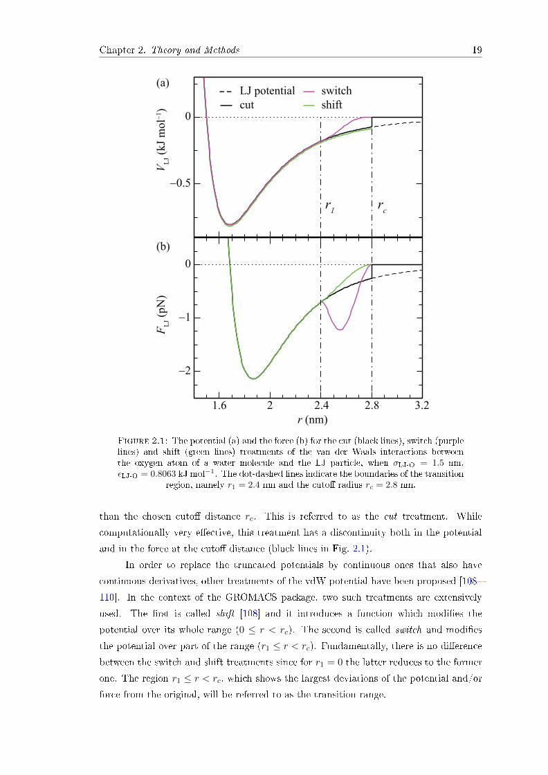
Figure 2.1: The potential (a) and the force (b) for the cut (black lines), switch (purplelines) and shift (green lines) treatments of the van der Waals interactions betweenthe oxygen atom of a water molecule and the LJ particle, when σLJ-O = 1.5 nm,εLJ-O = 0.8063 kJ mol−1. The dot-dashed lines indicate the boundaries of the transition
region, namely r1 = 2.4 nm and the cuto radius rc = 2.8 nm.
than the chosen cuto distance rc. This is referred to as the cut treatment. While
computationally very eective, this treatment has a discontinuity both in the potential
and in the force at the cuto distance (black lines in Fig. 2.1).
In order to replace the truncated potentials by continuous ones that also have
continuous derivatives, other treatments of the vdW potential have been proposed [108
110]. In the context of the GROMACS package, two such treatments are extensively
used. The rst is called shift [108] and it introduces a function which modies the
potential over its whole range (0 ≤ r < rc). The second is called switch and modies
the potential over part of the range (r1 ≤ r < rc). Fundamentally, there is no dierence
between the switch and shift treatments since for r1 = 0 the latter reduces to the former
one. The region r1 ≤ r < rc, which shows the largest deviations of the potential and/or
force from the original, will be referred to as the transition range.
Chapter 2. Theory and Methods 20
Within the switch treatment (purple lines in Fig. 2.1), the LJ interaction potential
(Eq. 2.28) is multiplied by a switch function S(r) dened as
S(r) =
1, if r ≤ r11− 10W 3 + 15W 4 − 6W 5, if r1 < r < rc
0, if r ≥ rc
(2.31)
where W = (r− r1)/(rc − r1). This multiplication drives the potential function towards
zero at the cuto distance. The van der Waals force in the switch method reads
Fsw(r) = −∇(VLJS) = FLJS(r)− VLJ∇S(r) , (2.32)
with FLJ = −∇VLJ(r). The rst derivative of the switch function ∇S(r), and hence the
contribution to the total force, is nonzero only in the transition region. Here, the force
Fsw(r) gains an additional and spurious second minimum (purple line in Fig. 2.1(b)),
consequences of which will become evident at a later stage.
In the shift treatment (green lines in Fig. 2.1) a function is added to the LJ potential
[108, 109]
V sh(r) = VLJ(r)− V cLJ + 4εij
[σ12ij A
rep − σ6ijAdis]
+ V shd (r) . (2.33)
Here, V cLJ is the value of the LJ potential at the cuto distance rc, whereas Arep and
Adis are the repulsion and dispersion corrections of the LJ potential depending only on
the values of r1 and rc
Arep =Krep
1
3(rc − r1)3 +
Krep2
4(rc − r1)4
Adis =Kdis
1
3(rc − r1)3 +
Kdis2
4(rc − r1)4 .
(2.34)
The constants K1 and K2 depend only on the values of r1 and rc and the nature
of the interaction, i.e. repulsive or attractive, and can be calculated from
K1 =p[(p+ 1)r1 − (p+ 4)rc]
rp+2c (rc − r1)2
K2 = − p[(p+ 1)r1 − (p+ 3)rc]
rp+2c (rc − r1)3
,
(2.35)
using p = 12 for the repulsion and p = 6 for the dispersion. In the case of the dispersion
the leading sign in the above equations needs to be changed.
The term V shd is nonvanishing only for r1 < r < rc and equals
V shd (r) = − 4
3εij(σ12ij K
rep1 + σ6ijK
dis1
)(r − r1)3
− εij(σ12ij K
rep2 + σ6ijK
dis2
)(r − r1)4 .
(2.36)

Chapter 2. Theory and Methods 21
Now it can be easily shown from Eqs. 2.33 and 2.36 that the vdW force on a particle
for the shift treatment arising from the particles in the transition region, r1 < r < rc,
readsFsh(r) = FLJ(r) + 4εij(σ
12ij K
rep1 + σ6ijK
dis1 )(r − r1)2
+ 4εij(σ12ij K
rep2 + σ6ijK
dis2 )(r − r1)3
(2.37)
while for r ≤ r1 the force is simply unmodied FLJ(r) and, of course, zero for r ≥ rc.The resulting potential V sh(r) deviates only slightly from VLJ(r) (green line in
Fig. 2.1(a)). Importantly, the resulting force Fsh(r) deviates from FLJ(r) only in the
transition region, where it smoothly approaches zero at rc due to the contribution
Fshd (r) = −∇V sh
d (r) (green line in Fig. 2.1(b)).
2.6 Water Models
As the most extensively studied compound water owes this immense theoretical and
practical interest to its unusual physicochemical properties. Therefore, an immense eort
was invested over the last half a century to design a microscopic model for water able to
reproduce its properties over a large range of thermodynamic conditions and transferable
to various environments (aqueous solutions, interfaces, conned spaces, etc.).
In parallel with the progress of the molecular dynamics method numerous water
models were developed (around 50 in 2002 [111]). A large majority of them are em-
pirical and based on the widely accepted opinion that the hydrogen bond is essentially
the result of a competition between an attractive interaction potential energy and a
repulsive electronic energy [112]. While the former is well approximated by classical
electrostatic interactions, and usually modelled by set of point charges, the electronic
repulsion is accounted for by the Lennard-Jones potential located on the oxygen atom
which incorporates the dispersion energy as well. Indeed, this theoretical framework was
the foundation of the rst realistic interaction potential for water proposed in 1933 in
pioneering work by Bernal and Fowler [113]. This so-called BF water model9 can be
considered the forerunner of modern three-point-charge models (e.g., SPC [115], SPC/E
[116] and TIP3P [117]) from the families of simple point charge (SPC) and transferable
intermolecular potentials (TIP). In common to these three-point-charge models is that
the charge distribution of the water molecule is modelled by point charges on the nuclei.
However, in 1951, Rowlinson [118] suggested a theoretical model in which the negative
charge was split above and below the molecular plane at the oxygen center in order to
improve the reproduction of the quadrupole moment of water molecule. This approach
can be regarded as predecessor of four- and ve-site water models like TIP4P [117],
TIP4P/2005 [119], TIP5P [120], etc.
9From the historical perspective a nice retrospect of the seminal paper on water by Bernal and Fowler[113] can be found in Ref. [114].

Chapter 2. Theory and Methods 22
Generally, during the construction of a water model force eld the geometrical pa-
rameters are xed to experimental values (e.g., bond length = 0.9572 Å, H−O−H angle
= 104.52) whereas the point charges and the repulsion-dispersion parameters are being
carefully adjusted by performing MD or Monte Carlo simulation in order to reproduce
chosen property of gas phase (e.g., dipole moment) or liquid phase under the room con-
ditions (e.g., density or heat of evaporation). It was recognized [121] that a water dipole
moment larger from that in the gas phase (1.85 D) leads to an improved description of
the liquid phase. Another way to improve the description of the interactions in water is
by allowing the exibility of the water model through the incorporation of intramolecular
vibrations. This is accomplished by adding the potential that describes the vibrational
modes (e.g., harmonic or Morse potential) to the rigid water model or by dening a new
family of potential just for this purpose. The drawback of the exible water models is
the narrowing of the H−O−H angle from 104.5 in the gas phase to 100 in the liquid
phase. Similarly, the inclusion of polarizability to the water model did not lead to de-
sired progress yet. Moreover, the non-polarizable models proved to be more adequate
in majority of studies. In the recent years the attention is turned to the development
of the force elds extracted from the computationally expensive ab initio calculations
where the results are analytically tted to obtain the potential function. Unfortunately,
the results gained from the small systems on which the computations are feasible are not
able to satisfactorily describe the properties of bulk water.
From the above discussion is apparent that no water model is able to reproduce
all its physical properties but only those it was tted against whereas it predicts other
properties with various degrees of error. However, very recently (2014) an unexpected
and signicant breakthrough was achieved by Izadi and collaborators with their optimal
point charge (OPC) model [122]. The architecture of this rigid model is identical to that
of TIP4P-models with the center of negative charge shifted away from the oxygen atom
(see Fig. 2.2). The authors applied an alternative and intuitive approach in which the
distribution of point charges was optimized in order to best reproduce the electrostatics
of the water molecule, i.e. targeted set of three lowest order multipole moments (dipole,
quadrupole and octupole), while allowing the geometrical parameters to be free as
well. The ideal parameters were identied as those giving the highest scoring function
(i.e., smallest error between predicted and experimental value) for the set of six bulk
water properties (static dielectric constant, self-diusion coecient, heat of vaporization,
density, and the height and position of the rst peak in oxygen-oxygen pair distribution
function). Remarkably, for each of these properties the obtained error was less than 1%.
Similar to exible models the disadvantage of the model is the deviation of its geometry
(O−H length is 0.8724 Å, ∠H−O−H = 103.6) from the experimental one. However,
the OPC model presents a major advance in the description of water interaction potential

Chapter 2. Theory and Methods 23
Table 2.1: Force eld parameters of water models employed in this thesis. ε and σ arethe Lennard-Jones parameters, qH is the charge on the hydrogen atoms, ∠H−O−H isthe water angle, dOH and dOM are O−H bond length and the distance between oxygenatom and M site on which the negative charge is located in the case of TIP4P-type
models. Negative charge qO always equals −2qH.
Model ε (kJ/mol) σ (Å) qH (e) dOH (Å) dOM (Å) ∠H−O−H
SPC/E 0.650 3.166 0.4238 1.0 - 109.47
TIP4P 0.648 3.154 0.520 0.9572 0.150 104.52
TIP4P/2005 0.7749 3.1589 0.5564 0.9572 0.1546 104.52
and demonstrates that further pursue using this direction for even better water model is
deemed to be fruitful and, therefore, should be undertaken.
Throughout this thesis the three most widely used water models are SPC/E,
TIP4P, and TIP4P/2005 which are schematically presented in Fig. 2.2 whereas their
force eld parameters are given in Table 2.1. All these common models very nicely
reproduce water density and heat of vaporization. The TIP4P/2005 model also excel-
lently reproduces the temperature of density maximum as well as the phase diagram
against which it was tted upon. The SPC/E predicts the best water dielectric constant
whereas all three models predict slightly lower dipole moment of 2.2-2.3 D compared to
experimental value of 2.5-3 D [123].
SPC/E model is a reparamaterized SPC water model with included self-energy
correction, i.e. energy needed for deformation of molecule into its polarized state. The
model better depicts values for density, diusion coecient, and structural features in the
oxygen-oxygen pair distribution function compared to its predecessor SPC model. More
HH
O
HH
O
104.52°109.47°
52.26°
1.0
Å
0.9
572 Å
SPC/E TIP4P
M
Figure 2.2: Geometry of the SPC/E (left) and the TIP4P water model (right) con-sisting of an oxygen atom (red) and two hydrogen atoms (blue). For each model isgiven the O−H bond length and the value of the angle ∠H−O−H. For the TIP4Pwater model is also indicated the position of the dummy site M which carries the neg-ative charge. Moreover, the positions of the negative charge and the positive chargesare indicated with `−' and `+', respectively. TIP4P/2005 water model is not explicitlyshown as it shares almost the same geometry with the TIP4P water model. For the
specicities of the TIP4P/2005 water model see Table 2.1.

Chapter 2. Theory and Methods 24
importantly, the SPC/E water is able to properly characterize the hydration properties
of simple hydrophobic objects (rare gases, methane, Lennard-Jones particles) [8, 124
126]. This is of particular importance to our study of both structural and dynamical
properties of hydrophobic objects in water. On the other hand, the TIP4P-type models
are primarily employed in the study of water dynamical properties and to demonstrate
the validity of the methodology developed for the evaluation of the water shear viscosity
in the presence of external electric elds.

Chapter 3
Properties of the Pure Water
System Both in the Absence and
Presence of Electric Fields
The immense advances in electrochemical nano- and microuidic applications in recent
years have been promoted by miniaturization, good sensitivity, and reliable microfabri-
cation [127, 128] of micro-devices, typically actuated by electric (E)-elds. This progress
was often based on the cross-fertilization of basic and applied research, an example of
which is the recently observed extraction of charged micrometer sized water droplets from
a superhydrophobic surface, where external E-elds are envisaged for enhancing anti-
icing, improving self-cleaning or in increasing condensation heat transfer [129]. Other
examples include paper-like display technologies [130], droplet transport/evaporation
[131], microuidic chemical reactors [132], or diverse bioanalytical utilizations like im-
munoassaying or clinical diagnostics [132].
Continued development depends on the understanding of intrinsic relaxation pro-
cesses in complex liquids. However, obtaining structural experimental data with the
atomic resolution has proven to be a strenuous task. Therefore, molecular dynamics
(MD) and Monte Carlo simulations became increasingly useful in studies of static and
dynamic properties of liquids including water. In the absence of external E-elds, the
consensus is that the long-range structure of water is isotropic, while the short-range
ordering is dominated by dipole-dipole interactions and the network of hydrogen bonds.
The latter give rise to a tetrahedral structuring of neighbouring water molecules, respon-
sible for the macroscopic behavior of water in the liquid and crystal phases. At nonzero
E-elds, however, water dipoles have a tendency to align with the eld vector in order to
minimize the dipole-eld interaction energy [133]. Consequently, a competition between
alignment with the eld and the maintenance of the tetrahedral structure as well as en-
tropy takes place. As a result, the eld breaks the symmetry, and the overall structure
25

Chapter 3. Properties of the Pure Water System 26
becomes anisotropic.
Our current understanding of the interaction of liquid water with E-elds emerges
from studies of small clusters (systems of up to 1000 H2O molecules) viable in the
nanoconnement [134, 135]. These studies elucidate the orientational relaxation and lo-
cal ordering of individual water molecules surrounded by few nearest neighbours, giving
rise to short term translational and rotational diusion coecients [135, 136]. However,
the eect of the externally applied E-eld on the dynamic properties of bulk water, like
shear viscosity, has remarkably not been investigated to our knowledge. Therefore, our
aim here is to rectify this situation by performing extensive MD simulations of pure
water under ambient conditions, the details of which are given in Sec. 3.1.
3.1 Computational Details and Static Water Response
The GROMACS 4.5.5 simulation package [76, 137] was employed to perform MD simu-
lations of pure water both in the absence and presence of an external electric eld. The
latter was imposed by using tinfoil boundary conditions [138]. The relaxation properties
are investigated for the three commonly used rigid water models, namely TIP4P [117],
SPC/E [116], and TIP4P/2005 [119]. Prior to the production runs in the NVT (T = 300
K) ensemble, the equilibration in the NPT (P = 1 bar) ensemble of the energy minimized
system was performed to determine the target water density (see Fig. 3.1(a) for E ≤ 1 V
nm−1), i.e. the volume of the cubic simulation cell at particular eld strength. Irrespec-
tive of the water model, in each simulation 23411 H2O molecules were accommodated in
the cubic simulation box with the edge length of about 8.8 nm. During the production
the desired temperature was maintained with the Nosé-Hoover thermostat [98, 99]. All
setups involved simulations with the time step of 1 fs, periodic boundary conditions,
non-bonded list update at each time step, and the LINCS [139] algorithm. The van
der Waals (vdW) interactions were treated by the shifted 12-6 Lennard-Jones potential
[104] (shift from 0.9 to 1.2 nm)1 whereas the long-range electrostatic interactions were
accounted for by the particle-mesh Ewald technique [88].
For each water model the shear viscosity η was evaluated at E-eld strengths
E = 0.0, 0.2, 0.4, and 0.6 V nm−1 (always imposed in +x direction). The simulations in
the absence of the E-eld were 120 ns long whereas those at E 6= 0 were 300 ns. The shear
viscosity was always calculated from the components of the stress tensor saved to disk at
every step. Although the above values of the electric eld may be perceived high, they are
still about tenfold smaller from the average local (internal) E-elds generated in water
[140], and are shown to be associated with a nearly constant susceptibility and linear
response. The investigated elds are too weak to induce crystallization [133] (found to
occur between 5 and 40 V nm−1) or even signicant structural changes [141, 142] (occur at
1Detail description of the treatments of the vdW interactions within GROMACS is given in Sec. 2.5.
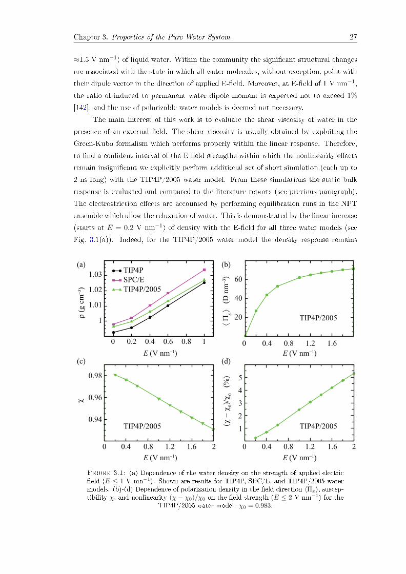
Chapter 3. Properties of the Pure Water System 27
≈1.5 V nm−1) of liquid water. Within the community the signicant structural changes
are associated with the state in which all water molecules, without exception, point with
their dipole vector in the direction of applied E-eld. Moreover, at E-eld of 1 V nm−1,
the ratio of induced to permanent water dipole moment is expected not to exceed 1%
[142], and the use of polarizable water models is deemed not necessary.
The main interest of this work is to evaluate the shear viscosity of water in the
presence of an external eld. The shear viscosity is usually obtained by exploiting the
Green-Kubo formalism which performs properly within the linear response. Therefore,
to nd a condent interval of the E-eld strengths within which the nonlinearity eects
remain insignicant we explicitly perform additional set of short simulation (each up to
2 ns long) with the TIP4P/2005 water model. From these simulations the static bulk
response is evaluated and compared to the literature reports (see previous paragraph).
The electrostriction eects are accounted by performing equilibration runs in the NPT
ensemble which allow the relaxation of water. This is demonstrated by the linear increase
(starts at E = 0.2 V nm−1) of density with the E-eld for all three water models (see
Fig. 3.1(a)). Indeed, for the TIP4P/2005 water model the density response remains
0 0.4 0.8 1.2 1.6
E (V nm−1)
20
40
60
⟨ Π
x ⟩ (
D n
m−
3)
(c)
1
2
3
4
5
(χ −
χ0)/
χ0 (
%)
0 0.4 0.8 1.2 1.6 2
E (V nm−1)
0.94
0.96
0.98
χ
0 0.4 0.8 1.2 1.6 2
E (V nm−1)
(d)
(b)
0 0.2 0.4 0.6 0.8 1
1
1.01
1.02
1.03
ρ (
g c
m−
3)
TIP4P
SPC/E
TIP4P/2005
(a)
E (V nm−1)
TIP4P/2005
TIP4P/2005
TIP4P/2005
Figure 3.1: (a) Dependence of the water density on the strength of applied electriceld (E ≤ 1 V nm−1). Shown are results for TIP4P, SPC/E, and TIP4P/2005 watermodels. (b)-(d) Dependence of polarization density in the eld direction 〈Πx〉, suscep-tibility χ, and nonlinearity (χ − χ0)/χ0 on the eld strength (E ≤ 2 V nm−1) for the
TIP4P/2005 water model. χ0 = 0.983.

Chapter 3. Properties of the Pure Water System 28
linear until water starts to freeze at E = 5.6 V nm−1 (data not shown) which is in
good agreement with previous reports. We furthermore evaluate the polarization of the
system. Therefore, the polarization density in the eld direction 〈Πx〉 is examined as the
function of the electric eld (Fig. 3.1(b)). Indeed, 〈Πx〉 can be reasonably reproduced by
the Langevin function l(E)
l(E) = A
[coth(BE)− 1
BE
], (3.1)
where A and B are constants [133]. In the MD simulations, with conducting boundary
conditions, the polarization density is related to the dielectric constant ε via the relation
[143145]
ε = ε0 +〈Πx〉E
, (3.2)
where ε0 is the vacuum permittivity. From the knowledge of the dielectric constant
the susceptibility χ of water is simply ε/ε0 − 1 and is shown in Fig. 3.1(c). Finally,
the nonlinearity is quantied by (χ − χ0)/χ0, where susceptibility at zero eld equals
χ0 = 0.983. The obtained results (see Fig. 3.1(d)) conrm that the response is apparently
linear (χ(E) ≈ χ0) until E . 0.2 V nm−1, and followed by minuscule loss of linearity
at higher elds. However, for E = 1 V nm−1, non-linear eects are smaller then 2.5%,
which is about quarter of what was previously suggested [133]. The dierence most likely
occurs due to the much larger larger system size with a relaxed bulk density used in this
work compared to previous studies. Thus, the non-linear eects for E ≤ 1 V nm−1 can
be considered insignicant and the use of Green-Kubo formalism to calculate transport
properties is validated.
3.2 Water Structure
The most convenient approach to experimentally describe the structure of a liquid is
via the radial distribution function (RDF) obtained by diraction techniques (X-ray and
neutron diraction) [146]. It is readily available property from the computer simulations
and as such it is used, for example, to establish the quality of designed force elds for
water models. The RDF g(r) simply depicts how the density of some species (atoms,
center-of-mass of molecule, particles, etc.) varies as a function of the radial distance
from reference particle. Therefore, it can be constructed between any two pairs of species
present in the system. For this particular case of water it means that the atom-atom
RDFs can be evaluated for the pairs oxygen-oxygen (gOO), oxygen-hydrogen (gOH), and
hydrogen-hydrogen (gHH). In the absence of an external electric eld, all constructable
atom-atom RDFs for the investigated water models have been studied in detail (for

Chapter 3. Properties of the Pure Water System 29
example, see Refs. [116, 117, 119, 147, 148]). Here, the attention is directed on the RDFs
at E 6= 0 and, thereby, those obtained at zero eld are shown in Appendix (Fig. B.1).
In the presence of electric elds, which break the otherwise present isotropic nature
of the system, the response of water is also asymmetric. This immediately arises from the
widely known fact that the E-eld tends to align water dipole vector parallel to itself (eld
always imposed in the +x direction). Surprisingly, the corresponding two-dimensional
RDFs (respecting the azimuthal symmetry) were not studied yet.
Without exception all 2-D RDFs g(x, a) presented in this work are calculated by
a self-made analysis tool. To respect the axial symmetry of the system at E 6= 0 the
cylinder (oriented in the eld direction) with radius a = κ/2 (where κ is smaller or equal
to the edge length of cubic simulation box) is extracted from the central simulation cell.
The appropriate value for κ is found to be 2.8 nm, i.e. a = 1.4 nm. This cylinder is then
divided into the half-cylindrical shells with the widths in the two respective directions
being ∆x = ∆a = 0.01 nm (yields in total 280 × 280 = 78400 volume elements). The
half-cylindrical bins mean that the upper (a > 0) and the lower half (a < 0) of the
cylinder are distinguished.2 The reasons for this are twofold. First and foremost, due
to the axial symmetry the density response must be symmetric with respect to the
line a = 0 and as such is an instantaneous indicator of the physical plausibility of the
obtained plots, i.e. a safety check of the results. Secondly, this representation is more
visually appealing, as will become evident later in this document when discussing the
water ordering around hydrophobic objects. Using the above dened binning scheme
the search is performed around the central atom (e.g., oxygen) and all other oxygen
atoms (when evaluating gOO(x, a)) that are found within the chosen radius (1.4 nm) are
assigned to the associated bin. The same procedure is repeated for all water molecules
(23411 in total) in each of 100 analyzed frames. Then to obtain the number density in
each bin the number of counts in that bin (Nc(x, a)) is divided with the number of total
time frames (Nfr), the total number of H2O molecules analyzed (Nw), and the volume
of the corresponding bin (V (x, a)):
ρ(x, a) =1
Nfr Nw V (x, a)
Nfr∑j=1
Nw∑i=1
Nc(x, a) . (3.3)
Finally, the 2-D RDF is realized by dividing the obtained density for each bin (ρ(x, a))
with the bulk water density found for the particular setup (water model and eld
strength). Of course, the same procedure applies for gOH(x, a) and gHH(x, a). The
two-dimensional RDFs both in the absence and in presence of the electric eld are shown
in Figs. B.1 (Appendix) and 3.2, respectively.
2Since a =√y2 + z2 represents the radius of a cylinder the negative values of a are impossible. The
minus sign of a in 2-D plots is nothing else but the indication of the lower half of the cylinder.

Chapter 3. Properties of the Pure Water System 30
As expected, from the 2-D RDFs at zero eld (Figs. B.1 in Appendix, left column)
very nice radial patterns are evident since the isotropic symmetry is preserved. Impor-
tantly, the line x = 0 (at positive a) extracted from each of the 2-D RDFs (gOO(x, a),
gOH(x, a), gHH(x, a)) excellently reproduces the corresponding RDF calculated in fully
radially averaged fashion (right column). This proves that the code performs well and
also captures all important features of the one-dimensional g(r). Hence, an adequate
spatial resolution is assumed for the nonzero elds.
All investigated water models show very similar ordering (even quantitatively) at
the same eld strength (data not shown). From the one-dimensional RDFs, obtained
in fully averaged fashion, the eld impact on the density correlations in water is found
to be proportional to its strength (see Fig. 3.3 or, better, Fig. B.2). Hence, in the
two-dimensional representation the changes are easier to visualize for stronger elds.
Thereby, the 2-D RDFs in Fig. 3.2 (left column) are represented with the data for the
SPC/E water model at the strongest eld examined (E = 1 V nm−1). Furthermore, in
the right column of Fig. 3.2 the dierences between the 2-D RDFs at E = 1 V nm−1
and at zero eld (from top to bottom: ∆gOO(x, a), ∆gOH(x, a), and ∆gHH(x, a)) are
shown. In contrast to E = 0, in the presence of the electric elds intriguing patterns are
obtained for all g(x, a) (and, thus, also for ∆g(x, a)) with the axial symmetry around
the line a = 0 being clearly recovered. However, this complex patterns are somewhat
anticipated outcome of the symmetry breaking even though the RDFs obtained in fully
averaged fashion for E 6= 0 (Fig. 3.3) show only minor changes of structuring (clearly
visible only after zooming in; see Fig. B.2). Moreover, with the increase of the E-eld
strength each g(r) suggests less ordering as the general tendency of maxima to decrease
and of minima to shallow is observed.
From Fig. 3.2 the density of the rst hydration shell3 in gOO(x, a) appears rather
unaected by the E-eld even at E = 1 V nm−1. However, there are regions of strongly
decreased density around [x ≈ 0, a ≈ ±0.27 nm] and the regions with strongly increased
density around [x ≈ ±0.27 nm, a ≈ 0] (see ∆gOO in Fig. 3.2 or gOO in Fig. 3.4) but
the (radial) average remains only weakly aected. Hence, the eects cannot be seen
in gOO(r). Importantly, the perturbation initiated at small distances propagates and
reects itself in the 2nd hydration shell which deforms and adopts a rectangular shape
(elongated in the eld direction). At larger distances from the central oxygen atom
the inuence of the E-eld weakens and consequently the 3rd hydration shell is only
slightly deformed. This is in agreement with the smaller changes in ∆gOO after the 2nd
hydration shell (see also Fig. B.2), the end of which coincides with the outer edge of the
blue moon-like shaped regions.3The end of particular hydration shell is taken to be the position of the corresponding minimum in
the oxygen-oxygen RDF. The same minimum also denotes the beginning of the adjacent hydration shellwhich ends at the position of the following minimum. This strategy is applicable until the structuringcan be clearly distinguished from the statistical noise.

Chapter 3. Properties of the Pure Water System 31
1.4
1
0.5
0
−0.5
−1
−1.4
1.4
1
0.5
0
−0.5
−1
−1.4
−1.4 −1 −0.5 0 0.5 1 1.4 −1.4 −1 −0.5 0 0.5 1
1.4
a (nm)
a (nm)
a (nm)
−1.4 −1 −0.5 0 0.5 1 1.4 −1.4 −1 −0.5 0 0.5 1 1.4
1.4
1
0.5
0
−0.5
−1
−1.4
1.4
1
0.5
0
−0.5
−1
−1.4
1.4
1
0.5
0
−0.5
−1
−1.4
1.4
1
0.5
0
−0.5
−1
−1.4
x (nm)
x (nm) x (nm)
x (nm)
1
0.6
0.2
−0.2
−0.6
−1
1.1
1
0.9
0.8
1.2
g(x,a)
∆g(x,a)
E
E
E
gOO(x,a)
gOH(x,a)
gHH(x,a)
∆gOO(x,a)
∆gOH(x,a)
∆gHH(x,a)
1.4
Figure 3.2: Two-dimensional radial distribution functions (RDF) g(x, a) for theSPC/E water model at E = 1 V nm−1 (left column) and the dierence of the RDFs∆g(x, a) obtained at E = 1 and E = 0 V nm−1 (right column). Shown are the corre-lation functions for the atom pairs oxygen-oxygen (top row), oxygen-hydrogen (middlerow), and hydrogen-hydrogen (bottom row). The color schemes for g(x, a) and ∆g(x, a)
are also shown. Each RDF is calculated from 100 frames of data.
The most curious is the ordering found for the oxygen-hydrogen pairs. The latter
arises from the preferential alignment of the water dipole vector with the direction of
applied E-eld. The result of this stimulus is the reorientation of all H2O molecules
contributing to the 1st density maximum from its right-hand side (RHS) is the breaking of
the corresponding shell (compare with Fig. B.1) which adopts the left-moon (`$') shape.

Chapter 3. Properties of the Pure Water System 32
0.2 0.4 0.6 0.8
r (nm)
0.6
1.2
1.8
2.4
3
0 V nm−1
0.2 V nm−1
0.4 V nm−1
0.6 V nm−1
1 V nm−1
gO
O(r
)
SPC/E
Figure 3.3: Comparison of the radially averaged radial distribution functions gOO(r)for dierent strengths of the homogeneous electric eld (between 0 and 1 V nm−1). Allresults are for the SPC/E water model. The arrows indicate the increasing strength of
the applied electric eld.
However, the deserted hydrogen atoms at RHS of the 1st density maximum are almost
fully replenished on the left-hand side (LHS) with the reorientation of water molecules
from the second density shell. Remarkably, these alien hydrogen atoms minimize the
overall decrease of the density as observed from the radially averaged RDF (Fig. B.2).
Furthermore, this −x/+x asymmetry from the rst hydration shell is persistent over the
entire correlation range. The asymmetry is even better evident in ∆gOH which illustrates
the astonishingly rich water structuring in the presence of the E-eld.
The behavior of gHH(x, a) captures something both from gOH(x, a) and gHH(x, a).
Similar to gOH(x, a), the shell corresponding to the rst density maximum is apparently
broken. However, this loss of density at [x ≈ 0, a ≈ ±0.23 nm] is only partial compared
to the RDF at zero eld. As expected, the overall symmetry is preserved both for the
oxygen-oxygen and hydrogen-hydrogen pairs and it can be also observed in plots for ∆gHH
and ∆gOO that appear somewhat similar. Furthermore, the second density maximum in
gHH(x, a) is clearly ellipsoidal with the elongation in the eld direction (similar to that
is observed in gOO(x, a)). Again the impact of the E-eld is minor beyond the second
hydration shell (see ∆gHH).
Curiously, the structuring at the planes perpendicular to the E-eld (i.e., in the x
direction) displays additional correlations which extend deeper into the bulk water com-
pared to the correlations observed in the absence of an external eld (see also Fig. B.1).
However, this increase of density is accompanied by depletion at the planes parallel with
the E-eld (i.e., in the a direction) is such a way that the long-range density variations
are not apparent upon radial averaging. This long-range density correlations are present
in all three g(x, a) and, perhaps, easiest to notice in gOO(x, a).
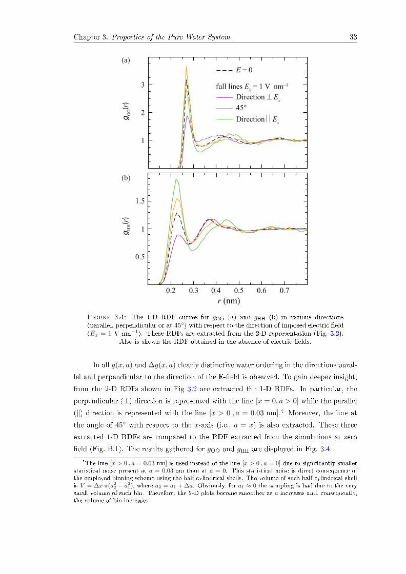
Chapter 3. Properties of the Pure Water System 33
1
2
3
E = 0
Direction ⊥ Ex
45°
Direction Ex
0.2 0.3 0.4 0.5 0.6 0.7
0.5
1
1.5
gO
O(r
) g
HH(r
)
r (nm)
full lines Ex = 1 V nm−1
(a)
(b)
Figure 3.4: The 1-D RDF curves for gOO (a) and gHH (b) in various directions(parallel, perpendicular or at 45) with respect to the direction of imposed electric eld(Ex = 1 V nm−1). These RDFs are extracted from the 2-D representation (Fig. 3.2).
Also is shown the RDF obtained in the absence of electric elds.
In all g(x, a) and ∆g(x, a) clearly distinctive water ordering in the directions paral-
lel and perpendicular to the direction of the E-eld is observed. To gain deeper insight,
from the 2-D RDFs shown in Fig 3.2 are extracted the 1-D RDFs. In particular, the
perpendicular (⊥) direction is represented with the line [x = 0, a > 0] while the parallel
(‖) direction is represented with the line [x > 0 , a = 0.03 nm].4 Moreover, the line at
the angle of 45 with respect to the x-axis (i.e., a = x) is also extracted. These three
extracted 1-D RDFs are compared to the RDF extracted from the simulations at zero
eld (Fig. B.1). The results gathered for gOO and gHH are displayed in Fig. 3.4.
4The line [x > 0 , a = 0.03 nm] is used instead of the line [x > 0 , a = 0] due to signicantly smallerstatistical noise present at a = 0.03 nm than at a = 0. This statistical noise is direct consequence ofthe employed binning scheme using the half-cylindrical shells. The volume of such half-cylindrical shellis V = ∆x π(a22 − a21), where a2 = a1 + ∆a. Obviously, for a1 ≈ 0 the sampling is bad due to the verysmall volume of such bin. Therefore, the 2-D plots become smoother as a increases and, consequently,the volume of bin increases.
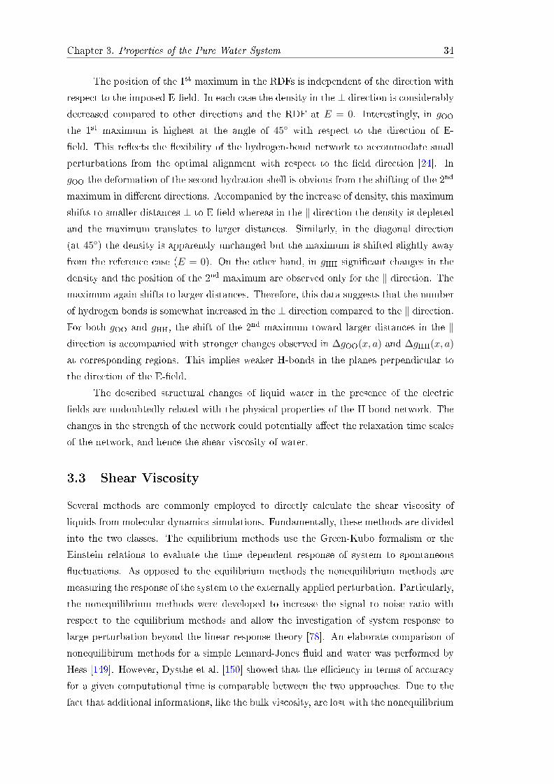
Chapter 3. Properties of the Pure Water System 34
The position of the 1st maximum in the RDFs is independent of the direction with
respect to the imposed E-eld. In each case the density in the ⊥ direction is considerably
decreased compared to other directions and the RDF at E = 0. Interestingly, in gOO
the 1st maximum is highest at the angle of 45 with respect to the direction of E-
eld. This reects the exibility of the hydrogen-bond network to accommodate small
perturbations from the optimal alignment with respect to the eld direction [24]. In
gOO the deformation of the second hydration shell is obvious from the shifting of the 2nd
maximum in dierent directions. Accompanied by the increase of density, this maximum
shifts to smaller distances ⊥ to E-eld whereas in the ‖ direction the density is depleted
and the maximum translates to larger distances. Similarly, in the diagonal direction
(at 45) the density is apparently unchanged but the maximum is shifted slightly away
from the reference case (E = 0). On the other hand, in gHH signicant changes in the
density and the position of the 2nd maximum are observed only for the ‖ direction. Themaximum again shifts to larger distances. Therefore, this data suggests that the number
of hydrogen bonds is somewhat increased in the ⊥ direction compared to the ‖ direction.For both gOO and gHH, the shift of the 2nd maximum toward larger distances in the ‖direction is accompanied with stronger changes observed in ∆gOO(x, a) and ∆gHH(x, a)
at corresponding regions. This implies weaker H-bonds in the planes perpendicular to
the direction of the E-eld.
The described structural changes of liquid water in the presence of the electric
elds are undoubtedly related with the physical properties of the H-bond network. The
changes in the strength of the network could potentially aect the relaxation time scales
of the network, and hence the shear viscosity of water.
3.3 Shear Viscosity
Several methods are commonly employed to directly calculate the shear viscosity of
liquids from molecular dynamics simulations. Fundamentally, these methods are divided
into the two classes. The equilibrium methods use the Green-Kubo formalism or the
Einstein relations to evaluate the time dependent response of system to spontaneous
uctuations. As opposed to the equilibrium methods the nonequilibrium methods are
measuring the response of the system to the externally applied perturbation. Particularly,
the nonequilibrium methods were developed to increase the signal to noise ratio with
respect to the equilibrium methods and allow the investigation of system response to
large perturbation beyond the linear response theory [78]. An elaborate comparison of
nonequilibirum methods for a simple Lennard-Jones uid and water was performed by
Hess [149]. However, Dysthe et al. [150] showed that the eciency in terms of accuracy
for a given computational time is comparable between the two approaches. Due to the
fact that additional informations, like the bulk viscosity, are lost with the nonequilibrium

Chapter 3. Properties of the Pure Water System 35
methods [149] the equilibrium methods retain their status of preferred method for the
calculation of the shear viscosity [151154].
Throughout this work we perform equilibrium molecular dynamics simulations and
calculate the shear viscosity η by exploiting the foundations of the Green-Kubo (GK)
formalism [155]. Assuming linear response, the latter relates η with the time integral of
the autocorrelation function Sαβ = 〈Pαβ(t)Pαβ(0)〉, where Pαβ (α, β = x, y, z) are the
o-diagonal elements of the stress tensor evaluated in simulations:
ηαβ(t) =V
kBT
∫ ∞0〈Pαβ(t)Pαβ(0)〉 dt . (3.4)
Here V is the volume of the simulation cell, kB is the Boltzmann constant, T is the
absolute temperature of the system, whereby the viscosity is obtained by nding the
limit
ηαβ = limt→∞
ηαβ(t) . (3.5)
Practically, this means that shear viscosity is taken to be equal the plateau value in
ηαβ(t). In the absence of E-elds (E = 0), due to the rotational invariance of water
molecule, the components (Pxx − Pyy)/2 and (Pyy − Pzz)/2 are equivalent and equal to
Pxy, Pxz, and Pyz [156]. Therefore, an averaging over ve independent components is
adopted to reduce the statistical errors associated with the value of shear viscosity at
zero eld η0.
It has been stipulated that the value of the shear viscosity depends only slightly
[157] or not at all [158] on the size of the simulation box. In accordance, the majority
of the calculations of the shear viscosity were performed on small systems up to 1000
particles (for examples see Refs. [149, 152, 159, 160]). From the large gathered data
on the Lennard-Jones uids Kabelac et al. [157] reported a linear dependence on the
inverse number of particles. However, for systems containing more than 1372 LJ particles
they found the dependence of the viscosity on the number of particles to be within the
statistical errors. In addition, due to the large pressure uctuations in a volume of
typical simulation cell the method exhibit very slow convergence. Therefore, to reduce
the pressure uctuations and minimize the nite size eects we choose to operate with
rather large system containing 23411 water molecules which drastically increases the
computational costs. Moreover, this particular size of our water system is almost identical
in size to our referent hydrophobic object-water system about which will be discussed in
detail in the following chapters.

Chapter 3. Properties of the Pure Water System 36
3.3.1 Shear Viscosity of Water in the Absence of External Electric
Fields
Before embarking on the inuence of E-elds on η, the results obtained at E = 0 (sub-
script 0) are summarized in Fig. 3.5. In panel (a) the averaged stress autocorrelation
functions normalized by their initial value, i.e. S(t)/S(0), are compared. All three rigid
water models inspected, namely TIP4P [117], SPC/E [116], and TIP4P/2005 [119], fol-
low a common time relaxation pathway of the stress correlations. After very preserved
and rapid decay (initial ca. 0.05 ps) the curves display damped oscillations that after
≈ 0.4 ps asymptotically approach zero. The exact time tp, when the correlations actu-
ally vanish (see inner graph of Fig. 3.5(a)), increases in the order TIP4P → SPC/E →TIP4P/2005 and resides in the time window between 3 and 7 ps.
The time evolution of the shear viscosity η0(t) is straightforwardly obtained by time
integration of S(t) according to Eq. 3.4 and is shown in Fig. 3.5(b). Independent of the
water model η0(t) rapidly reaches the plateau at tp and afterwards remains fairly at for
t ≤ 20 ps. Albeit the inherent noise in the plateau region appears insignicant, in practice
the estimate of η0 is done at times close to tp to reduce the associated statistical error
[154]. The obtained GK values: 4.7±0.1×10⁻⁴ Pa·s (TIP4P at t = 5 ps), 6.8±0.1×10⁻⁴
Pa·s (SPC/E at t = 5 ps), and 8.1±0.1×10⁻⁴ Pa·s (TIP4P/2005 at t = 7 ps) are in good
agreement with previous reports [149, 154, 160162]. Clearly, the TIP4P/2005 water
model predicts by far the best η0 at T = 300 K which was experimentally measured to
be 8.54 × 10⁻⁴ Pa·s [163]. Although major dierences among water models are evident
at intermediate times in the oscillatory part of S(t) (Fig. 3.5(a)) the quality of a water
model in reproducing the shear viscosity improves in the same order (TIP4P → SPC/E
→ TIP4P/2005) as the contribution to η0 of the long time tail in S(t) increases (see inset
0 0.2 0.4 0.6 0.8t (ps)
0
0.1
0.2
0.3
S(t
) / S
(0)
12 16t (ps)
2
4
6
8
η0(t
)
(1
0−
4 P
a∙s)
TIP4P
SPC/E
TIP4P/2005
Experiment
840
101 4
0
0.01
0.02
TIP4P/2005SPC/ETIP4P
(a) (b)
Figure 3.5: (a) Short-time behavior of the averaged stress autocorrelation function,S(t)/S(0), for TIP4P, SPC/E, and TIP4P/2005 water models. In the inner lin-loggraph are shown the slowly converging tails. (b) Time evolution of the shear viscosityη0(t) for each water model. All results are for the simulations performed in the absence
of an external E-eld, at T = 300 K, for 120 ns.

Chapter 3. Properties of the Pure Water System 37
in Fig. 3.5(a)). This implies that the long time dynamics has a crucial role in determining
the value of η whereas its accuracy is prescribed by the precise calculation of S(t) tail.
Even though we have obtained reliable estimates of η0 for the examined water
models the employed GK approach has the practical weakness that can be assigned
to the time-augmentative noise that makes the determination of tp, and hence of η,
imprecise. Whereas these issues can be neglected at E = 0 they will become severe at
nonzero elds as the relevant time increases. However, these issues can be, almost in
its entirety, circumvented by an alternative approach proposed by Guo et al. [164] and
later reestablished in publications studying both the shear and bulk viscosities of liquids
[153, 154].
The idea is to t S(t)/S(0) with a uniform two-step (denoted by subscript 2)
relaxation function Ψ2 consisting of fast (subscript f ) oscillatory and slow (subscript s)
Kohlrausch law [165],5
Ψ2(t) = (1− Cs) exp[−(t/τf )βf
]cos(ωt) + Cs exp
[−(t/τs)
βs], (3.6)
where ω is the oscillation frequency while Cs and (1− Cs) are the fractions of slow and
fast relaxation, respectively. The parameters τf , βf , τs, and βs have unclear physical
meaning [164]. Therefore, they are treated purely as the parameters of the stretched
exponential law exp[−(t/τ)β]. In contrast, the time integrals of the rst and the second
term represent the fast Tf and the slow Ts relaxation time, and their sum being the total
relaxation time Ttot = Tf +Ts [167] which should not be confused with tp (the time when
the stress correlations vanish). The shear viscosity can be then simply evaluated from
η =1
kBTS(0)TtotV . (3.7)
Before presenting the results for the nonzero E-elds we will demonstrate the ability of
the approach to reproduce the stress relaxation at E = 0 and, in turn, yield a reliable
estimate of η0 accompanied by virtually no error.
The Kohlrausch t of S(t)/S(0) for the TIP4P/2005 water at E = 0 is shown in
Fig. 3.6(a). The obtained parameters are found to be in agreement with those determined
previously [164], despite the potential issues with uniqueness of the multi-parametric t.
Globally, Ψ2(t) very nicely portrays the data. Small deviations from the data occur at
the intermediate times in the undulatory part whereas the largest visual objection to
the t function appears to be its inability to adequately recreate the stress relaxation
at the very initial times (t ≤ 0.01 ps). This has, however, indiscernible contribution
to the value of shear viscosity and can be readily recognized from Fig. 3.6(b) in η0(t).
As anticipated, ηt0 (t) matches almost perfectly with the raw data over ve orders of
5For a historical overview of the stretched exponential law and frequent misreferring of the originalKohlrausch work see paper by Cardona et al. [166].
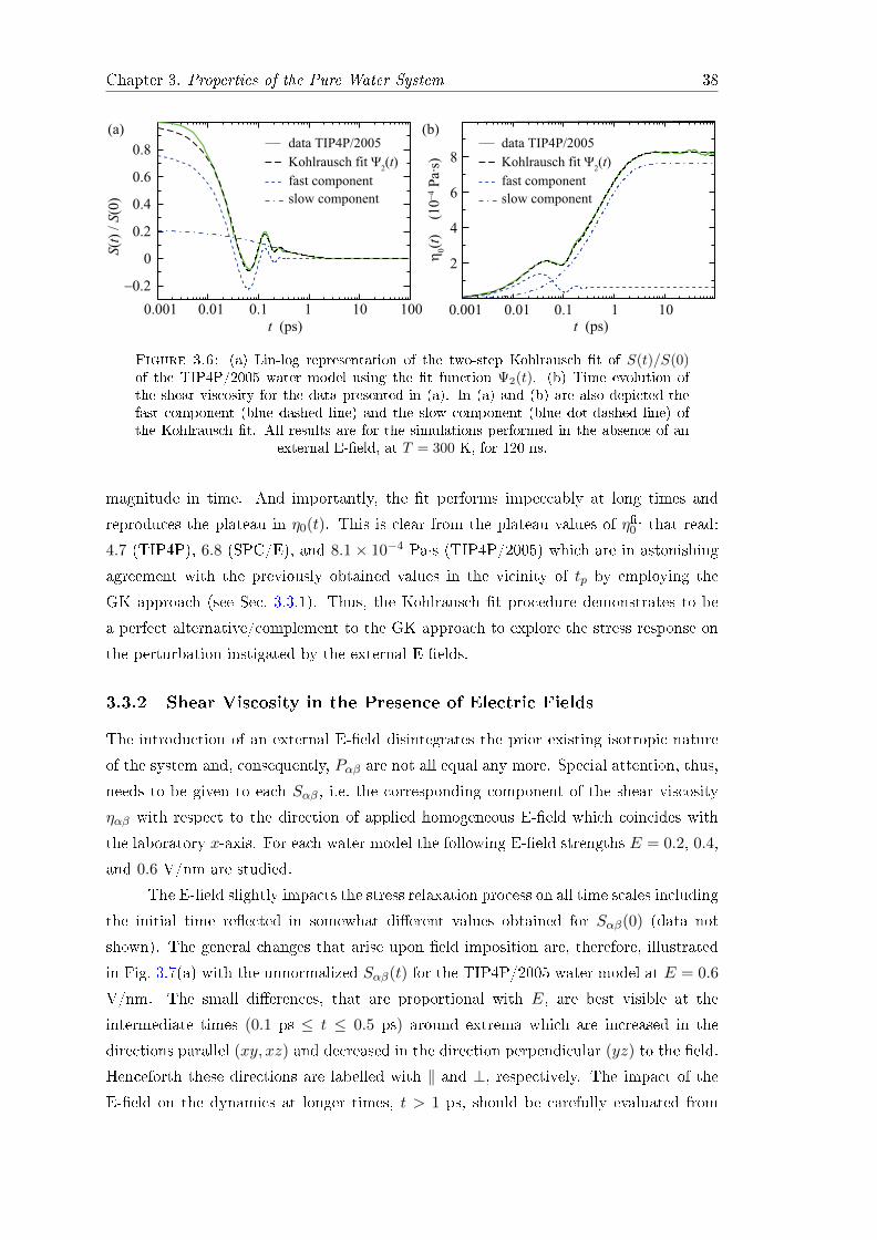
Chapter 3. Properties of the Pure Water System 38
0.001 0.01 0.1 10 100
t (ps)
−0.2
0
0.2
0.4
0.6
0.8data TIP4P/2005
Kohlrausch fit Ψ2(t)
fast component
slow component
0.001 0.01 0.1 10t (ps)
2
4
6
8
1 1
S(t
) /
S(0
)
η0(t
)
(1
0−
4 P
a∙s)
data TIP4P/2005
Kohlrausch fit Ψ2(t)
fast component
slow component
(a) (b)
Figure 3.6: (a) Lin-log representation of the two-step Kohlrausch t of S(t)/S(0)of the TIP4P/2005 water model using the t function Ψ2(t). (b) Time evolution ofthe shear viscosity for the data presented in (a). In (a) and (b) are also depicted thefast component (blue dashed line) and the slow component (blue dot-dashed line) ofthe Kohlrausch t. All results are for the simulations performed in the absence of an
external E-eld, at T = 300 K, for 120 ns.
magnitude in time. And importantly, the t performs impeccably at long times and
reproduces the plateau in η0(t). This is clear from the plateau values of ηt0 that read:
4.7 (TIP4P), 6.8 (SPC/E), and 8.1× 10⁻⁴ Pa·s (TIP4P/2005) which are in astonishing
agreement with the previously obtained values in the vicinity of tp by employing the
GK approach (see Sec. 3.3.1). Thus, the Kohlrausch t procedure demonstrates to be
a perfect alternative/complement to the GK approach to explore the stress response on
the perturbation instigated by the external E-elds.
3.3.2 Shear Viscosity in the Presence of Electric Fields
The introduction of an external E-eld disintegrates the prior existing isotropic nature
of the system and, consequently, Pαβ are not all equal any more. Special attention, thus,
needs to be given to each Sαβ , i.e. the corresponding component of the shear viscosity
ηαβ with respect to the direction of applied homogeneous E-eld which coincides with
the laboratory x-axis. For each water model the following E-eld strengths E = 0.2, 0.4,
and 0.6 V/nm are studied.
The E-eld slightly impacts the stress relaxation process on all time scales including
the initial time reected in somewhat dierent values obtained for Sαβ(0) (data not
shown). The general changes that arise upon eld imposition are, therefore, illustrated
in Fig. 3.7(a) with the unnormalized Sαβ(t) for the TIP4P/2005 water model at E = 0.6
V/nm. The small dierences, that are proportional with E, are best visible at the
intermediate times (0.1 ps ≤ t ≤ 0.5 ps) around extrema which are increased in the
directions parallel (xy, xz) and decreased in the direction perpendicular (yz) to the eld.
Henceforth these directions are labelled with ‖ and ⊥, respectively. The impact of the
E-eld on the dynamics at longer times, t > 1 ps, should be carefully evaluated from

Chapter 3. Properties of the Pure Water System 39
(a)
0 0.1 0.2 0.3 0.4 0.5t (ps)
−500
0
500
1000
(t
)
(b
ar2)
Direction || Ex
E = 0 V/nm
Direction ⊥ Ex
(b)
12 16t (ps)
2
4
6
8
η(t
)
(1
0−
4 P
a⋅s)
η|| (Ex= 0.6 V/nm)
η0 (E = 0 V/nm)
η⊥ (Ex = 0.6 V/nm)
4 8
Sα
β
TIP4P/2005 TIP4P/2005
(Ex= 0.6 V/nm)
Figure 3.7: (a) Impact of the externally applied static electric eld (Ex = 0.6 V/nm)on the unnormalized components of the stress autocorrelation function Sαβ(t) relativeto the eld free case. (b) Time evolution of the shear viscosity for the data presented
in (a). All data is for the TIP4P/2005 water model.
the behavior of the Sαβ(t) tail. Strikingly, an appreciably prolonged approach of the
correlations to zero is observed exclusively for the ‖ direction. However, this eect is nowfar more subject to the inherent noise (partially since only two components contribute
to S‖).
Although Sαβ(t) responds weakly to the breaking of the symmetry of the system
(see Fig. 3.7(a)), induced by the E-eld, the eects are far more evident after the inte-
gration (again using Eq. 3.4). The obtained ηαβ(t) are presented in Fig. 3.7(b). What
immediately strikes is that η⊥(t) resembles very much η0(t) albeit the plateau is lower in
the former case. Interestingly, the shear viscosity is obviously increased along the eld
(η‖(t)) with respect both to η⊥(t) and η0(t) at the same t. As indicated by S‖(t), η‖(t)
steadily increases for, at least, t ≤ 20 ps. Despite the signicant computational eort
(300 ns for each setup at E 6= 0), tp(‖) could not be detected with substantial condence
(irrespective of the water model and the eld strength). Therefore, we onward rely on the
Kohlrausch t procedure to disentangle the underlying dynamics of the stress relaxation
at nonzero external E-elds.
For the particular example considered in Fig. 3.7, the Kohlrausch ts using Ψ2(t)
for both directions (⊥,‖), alongside the referent t for η0(t), are shown in Fig. 3.8. In
accordance with previously observed similarities between η0(t) and η⊥(t), Ψ2(t) produces
an exquisite match to both of them whereas it fails to do the same for η‖(t). From
Fig. 3.8(b) it is obvious that this is only partially true as Ψ2(t) provides an excellent
description of η‖(t) for shorter times, t . 1 ps. This indicates that, independent of E,
the fast relaxation dynamics of stress remains remarkably preserved while the relaxation
to the presence of the E-eld occurs at large t. Thus, the contribution to η‖(t) at large t
should be attributed to an additional process of slow character, invoked by the E-eld.

Chapter 3. Properties of the Pure Water System 40
0.001 0.01 0.1 10
t (ps)
2
4
6
8
η(t
) (1
0−
4 P
a⋅s)
1
η⊥(t) E
x= 0.6 V/nm
Ψ2(t)
0.01 0.1 10 100
t (ps)
1
2
4
6
8
Ψ2(t)
Ψ3(t)
η||(t) E
x= 0.6 V/nm
TIP4P/2005 TIP4P/2005
(a) (b)
η0 (t) (E = 0 V/nm)
Figure 3.8: Lin-log representation of the time evolution of shear viscosity in thedirections perpendicular (a) and parallel (b) to the applied E-eld (Ex = 0.6 V/nm).In panel (a) is also shown η0(t). The Kohlrausch ts obtained by using two- and three-step t functions are depicted with blue and magenta dashed lines, respectively. All
data is for the TIP4P/2005 water model.
This additional process along the E-eld direction is again modelled by the stretched
exponential law. Consequently, we introduce a three-step Kohlrausch t function Ψ3(t):
Ψ3(t) = (1− Cs − Ci) exp[−(t/τf )βf
]cos(ωt)
+ Cs exp[−(t/τs)
βs]
+ Ci exp[−(t/τi)
βi]. (3.8)
Here subscript i denotes the eld-induced relaxation with the characteristic coecients
(Ci, τi, and βi). Accordingly, the fraction of fast relaxation is modied from (1−Cs) inΨ2(t) to (1−Cs−Ci). From Fig. 3.8(b) is evident that, congruent to our proposal, the t
obtained by using Ψ3(t) matches perfectly with the data for η‖(t). Additional examples
of the Kohlrausch ts employing Ψ2(t) and Ψ3(t) at nonzero elds, are presented in the
Appendix (see Figs. A.1 and A.2). Here we also accentuate that by employing a simple
exponential function for the eld-induced process it was not possible to reproduce the
observed relaxation dynamics at long times. In general this arises from the dependence
of relaxation on the entire spectrum of relaxation times which leads to non-linear and
not purely exponential behavior [168].
The exibility of the parameters of the stretched exponential law to describe various
dynamical processes is well documented [169174]. Therefore, some concerns may arise
about the uniqueness of the obtained Kohlrausch parameters. Although these claims
can be instantly abandoned at E = 0 [153, 164], the issue becomes pertinent at nonzero
elds. This is especially the case for the ‖ direction where we add an extra exp[−(t/τ)β]
term which yields, in total, 9 parameter t function Ψ3(t) (see Eq. 3.8). To clarify this
we have performed an extensive and systematic analysis of the Kohlrausch t parameters
encompassing all investigated setups. The procedure is described in detail in the variation
analysis section (Appendix A). Here are summarized the most relevant ndings. For
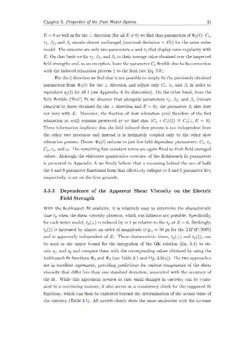
Chapter 3. Properties of the Pure Water System 41
E = 0 as well as for the ⊥ direction (for all E 6= 0) we nd that parameters of Ψ2(t): Cs,
τf , βf , and βs remain almost unchanged (maximal deviation < 4%) for the same water
model. The outcome are only two parameters ω and τs that display some regularity with
E. On that basis we x τf , βf , and βs to their average value obtained over the inspected
eld strengths and, as an exception, leave the parameter Cs exible due to its connection
with the induced relaxation process ‖ to the eld (see Eq. 3.8).
For the ‖ direction we nd that is not possible to simply x the previously obtained
parameters from Ψ2(t) for the ⊥ direction and adjust only Ci, τi, and βi in order to
reproduce η‖(t) for all t (see Appendix A for discussion). On the other hand, from the
fully exible (free) t we discover that alongside parameters τf , βf , and βs (remain
identical to those obtained for the ⊥ direction and E = 0), the parameter βi also does
not vary with E. Moreover, the fraction of slow relaxation (and therefore of the fast
relaxation as well) remains preserved as we nd that (Cs + Ci)(‖) ∼= Cs(⊥, E = 0).
These information implicate that the eld-induced slow process is not independent from
the other two processes and instead it is intimately coupled only to the other slow
relaxation process. Hence, Ψ3(t) reduces to just ve eld-dependent parameters: Ci, τi,
Cs, τs, and ω. The remaining four constant terms are again xed to their eld averaged
values. Although the elaborate quantitative overview of the Kohlrausch t parameters
is presented in Appendix A we rmly believe that a reasoning behind the use of both
the 6 and 9 parameter functional form that eectively collapse to 3 and 5 parameter ts,
respectively, is set on the rm grounds.
3.3.3 Dependence of the Apparent Shear Viscosity on the Electric
Field Strength
With the Kohlrausch t available, it is relatively easy to determine the characteristic
time tp when the shear viscosity plateaus, which was hitherto not possible. Specically,
for each water model, tp(⊥) is reduced by ≈ 1 ps relative to the tp at E = 0. Strikingly,
tp(‖) is increased by almost an order of magnitude (e.g., ≈ 50 ps for the TIP4P/2005)
and is apparently independent of E. These characteristic times, tp(⊥) and tp(‖), canbe used as the upper bound for the integration of the GK relation (Eq. 3.4) to ob-
tain η⊥ and η‖ and compare them with the corresponding values obtained by using the
Kohlrausch t functions Ψ2 and Ψ3 (see Table 3.1 and Fig. 3.9(a)). The two approaches
are in excellent agreement, providing predictions for various components of the shear
viscosity that dier less than one standard deviation, associated with the accuracy of
the t. While this agreement assures us that small changes in viscosity can be evalu-
ated in a convincing manner, it also serves as a consistency check for the suggested t
functions, which can then be exploited beyond the determination of the actual value of
the viscosity (Table 3.1). All models clearly show the same tendencies with the increase
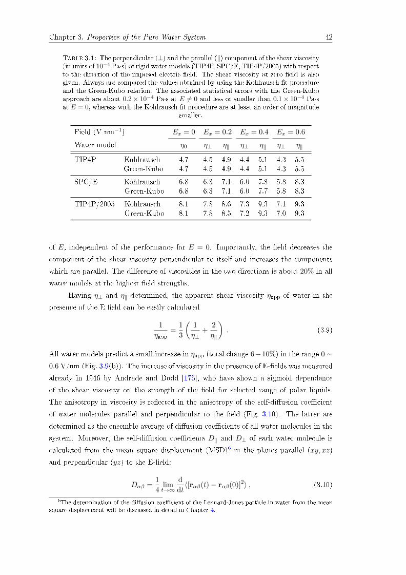
Chapter 3. Properties of the Pure Water System 42
Table 3.1: The perpendicular (⊥) and the parallel (‖) component of the shear viscosity(in units of 10−4 Pa·s) of rigid water models (TIP4P, SPC/E, TIP4P/2005) with respectto the direction of the imposed electric eld. The shear viscosity at zero eld is alsogiven. Always are compared the values obtained by using the Kohlrausch t procedureand the Green-Kubo relation. The associated statistical errors with the Green-Kuboapproach are about 0.2× 10⁻⁴ Pa·s at E 6= 0 and less or smaller than 0.1× 10⁻⁴ Pa·sat E = 0, whereas with the Kohlrausch t procedure are at least an order of magnitude
smaller.
Field (V nm−1) Ex = 0 Ex = 0.2 Ex = 0.4 Ex = 0.6
Water model η0 η⊥ η‖ η⊥ η‖ η⊥ η‖
TIP4P Kohlrausch 4.7 4.5 4.9 4.4 5.1 4.3 5.5Green-Kubo 4.7 4.5 4.9 4.4 5.1 4.3 5.5
SPC/E Kohlrausch 6.8 6.3 7.1 6.0 7.8 5.8 8.3Green-Kubo 6.8 6.3 7.1 6.0 7.7 5.8 8.3
TIP4P/2005 Kohlrausch 8.1 7.8 8.6 7.3 9.3 7.1 9.3Green-Kubo 8.1 7.8 8.5 7.2 9.3 7.0 9.3
of E, independent of the performance for E = 0. Importantly, the eld decreases the
component of the shear viscosity perpendicular to itself and increases the components
which are parallel. The dierence of viscosities in the two directions is about 20% in all
water models at the highest eld strengths.
Having η⊥ and η‖ determined, the apparent shear viscosity ηapp of water in the
presence of the E-eld can be easily calculated
1
ηapp=
1
3
(1
η⊥+
2
η‖
). (3.9)
All water models predict a small increase in ηapp (total change 6−10%) in the range 0 ∼0.6 V/nm (Fig. 3.9(b)). The increase of viscosity in the presence of E-elds was measured
already in 1946 by Andrade and Dodd [175], who have shown a sigmoid dependence
of the shear viscosity on the strength of the eld for selected range of polar liquids.
The anisotropy in viscosity is reected in the anisotropy of the self-diusion coecient
of water molecules parallel and perpendicular to the eld (Fig. 3.10). The latter are
determined as the ensemble average of diusion coecients of all water molecules in the
system. Moreover, the self-diusion coecients D‖ and D⊥ of each water molecule is
calculated from the mean square displacement (MSD)6 in the planes parallel (xy, xz)
and perpendicular (yz) to the E-eld:
Dαβ =1
4limt→∞
d
dt〈[rαβ(t)− rαβ(0)]2〉 , (3.10)
6The determination of the diusion coecient of the Lennard-Jones particle in water from the meansquare displacement will be discussed in detail in Chapter 4.

Chapter 3. Properties of the Pure Water System 43
0 0.2 0.4 0.66.4
7.2
8
8.8
9.6
Ex (V nm−1)
η (1
0−
4 P
a∙s)
(a)
0 0.2 0.4 0.64
6
8
ηap
p (1
0−
4 P
a∙s)
Ex (V nm−1)
TIP4P/2005
SPC/E
TIP4P
(b)
TIP4P/2005
ηapp
η||
η⊥
Figure 3.9: (a) The components of the shear viscosity in the directions perpendic-ular (η⊥) and parallel (η‖) to the E-eld obtained by using the Green-Kubo relation(Eq. 3.4). Also is shown the apparent shear viscosity (ηapp). For comparison the values(small red circles) obtained by using the Kohlrausch t procedure are displayed. Theresults are for the TIP4P/2005 water model. (b) Apparent shear viscosity of the rigidwater models TIP4P/2005, SPC/E, and TIP4P as a function of the E-eld strength
(for E ≤ 0.6 V nm−1).
where rαβ(t) is the position vector of the oxygen atom of water molecule in the plane
(α, β) = (x, y, z) at time t.
From Fig. 3.10 is obvious that values both for D⊥ and D‖ apparently follow the
empirical rule D ∝ 1/η for E ≤ 0.6 V nm−1 at which the shear viscosity is evaluated
(compare with Fig. 3.9(a)), supporting the still linear behavior of the response functions.
Furthermore, the decrease of diusivity ‖ to the E-eld is in agreement with the increases
of density in the same direction (see Fig. 3.2). In a similar manner, the decrease of
the water density ⊥ to the E-eld agrees with the somewhat higher mobility in the
corresponding direction. Although in Fig. 3.10 only the values for the TIP4P model are
shown, similar behavior with the same general tendencies is also found for the SPC/E
and TIP4P/2005 models. The value for the apparent diusion coecient Dapp of water
in the presence of the E-eld is obtained from simple relation
Dapp =1
3
(D⊥ + 2D‖
). (3.11)
Hence, the larger contribution of D‖ is reected in the behavior of Dapp which slightly
decreases compared to D(E = 0) in agreement with the behavior observed for ηapp, and
with somewhat increased density of water with the applied eld strength (see Fig. 3.1(a)).
Splitting of viscosity occurs despite the fact that there is a general increase of both
S⊥(0) and S‖(0) for at most 5% with switching on the E-eld. Actually, the change
in viscosity can be associated with changes in Ttot (Fig. 3.11 and/or Tab. A.6) that is
proportional to E - decreasing in the ⊥ direction and increasing in the ‖ direction, inagreement with the somewhat faster dynamics in ⊥ direction (Fig. 3.11).
The contribution to Ttot from the fast relaxation Tf is generally small, and its
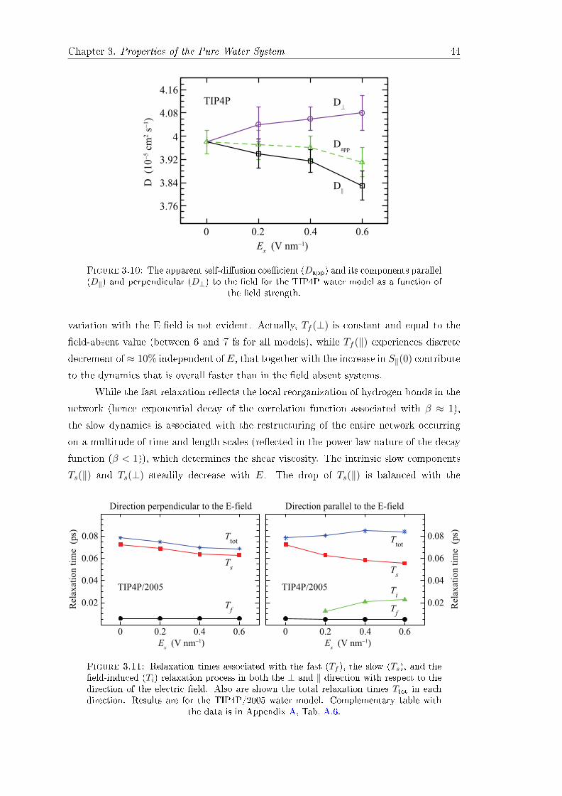
Chapter 3. Properties of the Pure Water System 44
3.76
3.84
3.92
4
4.08
4.16
0 0.2 0.4 0.6
TIP4P
Ex (V nm−1)
D⊥
D||
Dapp
D
(10
−5 c
m2 s
−1)
Figure 3.10: The apparent self-diusion coecient (Dapp) and its components parallel(D‖) and perpendicular (D⊥) to the eld for the TIP4P water model as a function of
the eld strength.
variation with the E-eld is not evident. Actually, Tf (⊥) is constant and equal to the
eld-absent value (between 6 and 7 fs for all models), while Tf (‖) experiences discrete
decrement of≈ 10% independent of E, that together with the increase in S‖(0) contribute
to the dynamics that is overall faster than in the eld absent systems.
While the fast relaxation reects the local reorganization of hydrogen bonds in the
network (hence exponential decay of the correlation function associated with β ≈ 1),
the slow dynamics is associated with the restructuring of the entire network occurring
on a multitude of time and length scales (reected in the power law nature of the decay
function (β < 1)), which determines the shear viscosity. The intrinsic slow components
Ts(‖) and Ts(⊥) steadily decrease with E. The drop of Ts(‖) is balanced with the
0 0.2 0.4 0.6
0.02
0.04
0.06
0.08
0 0.2 0.4 0.6
0.02
0.04
0.06
0.08
Rel
axat
ion
tim
e (
ps)
Rel
axat
ion
tim
e (
ps)
Ex (V nm−1) E
x (V nm−1)
Ttot
Ts
Tf
Ttot
Ts
Tf
Ti
TIP4P/2005 TIP4P/2005
Direction perpendicular to the E-field Direction parallel to the E-field
Figure 3.11: Relaxation times associated with the fast (Tf ), the slow (Ts), and theeld-induced (Ti) relaxation process in both the ⊥ and ‖ direction with respect to thedirection of the electric eld. Also are shown the total relaxation times Ttot in eachdirection. Results are for the TIP4P/2005 water model. Complementary table with
the data is in Appendix A, Tab. A.6.

Chapter 3. Properties of the Pure Water System 45
enhancement of relaxation to the imposed eld Ti such that overall slow relaxation ‖ tothe eld, Ts(‖) + Ti, increases with E (see Fig. 3.11).
Interestingly, the eld-induced relaxation is coupled to the intrinsic slow process,
suggesting that the fraction of the total slow relaxation remains constant (0.78 ∼ 0.82
depending on the water model) irrespective of the eld strength. This is reected in the
relation (Cs +Ci)(‖) ' Cs(⊥, E = 0) that emerges from the ts (see Tables A.4 and A.5
in Appendix A). Along the eld, this is achieved by Ci compensating the decrease of
Cs(‖) with E. However, the contribution of Ci to the overall relaxation remains very
small (≈ 1% at E = 0.6 V/nm), yet sucient to aect the apparent viscosity.
The fraction of slow relaxation was also found independent of temperature be-
tween −60 C and 30 C, even though ω decreased for about 3.6 ps−1 (corresponding
to 20 cm−1) with increasing temperature [164]. This suggested a larger population of
four-coordinated H2O molecules and enhanced order with decrease of T . In turn, the
change in ω gave rise to higher Raman intensity of the hydrogen bond stretch that was
assumed to increase the fraction of fast relaxation. Since the fast and slow relaxations
are mutually competing, the slow contribution must decrease to balance the increase of
the other. It was speculated that this decrease of the slow fraction is due to the presence
of single volume fraction of the crystal-like clusters [176] that controls the slow relax-
ation. However, in the presence of the electric eld it is highly unlike that crystal-like
structure can explain the constant fraction of the fast/slow relaxation. The unlikeness
of the crystalline structure is also supported by the analysis of the reorientation of the−→HH vector (data not shown), which showed that there is no signicant retardation of
dynamics in the presence of the E-eld.
Numerous experimental studies [177181], using Raman and infrared spectroscopy
as well as inelastic neutron scattering, assigned the oscillation frequency ω to the stretch-
ing vibrations of hydrogen bonds, providing a resonance frequency of the shear viscos-
ity at around 34 ps−1 (corresponding to 180 cm−1) at E = 0. Similar to previous
0 0.2 0.4 0.6
44
44.4
44.8
234
236
238
Ex (V nm−1)
ω
(ps−
1)
ω
(cm
−1)
TIP4P/2005 ⊥
||
(b)
0 0.2 0.4 0.640.8
41.2
41.6
218
220
222
Ex (V nm−1)
ω
(ps−
1)
ω
(cm
−1)
TIP4P
⊥
||
(a)
Figure 3.12: Dependence of the oscillation frequency ω (both in the units of ps−1 andcm−1) in the directions ⊥ and ‖ to the direction of the imposed electric eld. Shown
are the results for the TIP4P (a) and TIP4P/2005 (b) water models.

Chapter 3. Properties of the Pure Water System 46
computational reports [164, 182184], we nd ω between 41.3 (TIP4P) and 44.5 ps−1
(TIP4P/2005) (corresponding to 219 and 236 cm−1, respectively). This agrees reasonably
with the experimental data bearing in mind the simplicity of water models employed.
Interestingly, the E-eld splits this band, i.e. the oscillation frequency ⊥ and ‖ to the eldexhibit blue and red shifts proportional to the E-eld, respectively. From Figure 3.12
it is evident that this subtle eect (magnitude of the split is 4 − 5 cm−1 at E = 0.6 V
nm−1) is independent of the water model used and, could be recovered experimentally.
To gain deeper insight about the meaning and relevance of the obtained values
for ω from Kohlrausch ts additional analysis of both the translational and rotational
degrees of freedom of individual water molecules was performed. Therein, the autocorre-
lation functions of the translational velocity (both in Cartesian and internal coordinate
system) and of the rotational velocity were calculated and their power spectra evaluated
to obtain corresponding vibrational spectra. Indeed, these detailed analyses show that
the vibrational band of interest splits depending on the direction with respect to the
electric eld. Since the found split is very small (few cm−1) compared to the width of
the target band (∼ 200 cm−1) the corresponding analysis is not presented here.
3.4 Conclusions
Herein is demonstrated the necessity to complement the standard Green-Kubo approach
with the alternative Kohlrausch t procedure in order to obtain a reliable estimate of the
shear viscosity of uid in the presence of externally applied electric elds that break the
otherwise present isotropic nature of the system. We nd heavily increased statistical
noise at the relevant times, which are about tenfold larger in the two directions along
the eld than found both in the direction perpendicular to the eld or in its absence.
To eectively eliminate the inherent noise the Kohlrausch t function consisting of the
fast oscillatory and the slow stretched exponential term is employed. While the fast
process depicts the local reorganization of hydrogen bonds in the network, the slow
dynamics is associated with the restructuring of the entire network. Indeed, this two-
step Kohlrausch function excellently reproduces the relaxation process at E = 0 and in
the direction perpendicular to the eld. Moreover, it also indicates that in the direction
parallel to the eld an additional process of the slow type is invoked which is, again,
modelled by a stretched exponential function. The resultant three-step Kohlrausch t
provides an impressive match with the MD data.
From a detailed variation analysis of the Kohlrausch t parameters it is recognized
that the eld-induced process is essentially decoupled from the fast process but not
from the other slow process. Subsequent integration of the t functions to obtain the
time evolution of the shear viscosity revealed that the eld decreases the component
of the shear viscosity perpendicular to itself and increases the components which are

Chapter 3. Properties of the Pure Water System 47
parallel. Importantly, both for the parallel and perpendicular directions, the Kohlrausch
t procedure provided the characteristic time at which the stress correlations vanish and
that can be used as the upper bound for the integration of the Green-Kubo relation.
Using the latter approach the obtained values for the shear viscosity are found to be in
excellent agreement with those obtained by using the Kohlrausch t procedure.
On the other hand, the anisotropy of viscosity components leads to a slight in-
crease of the overall shear viscosity with the increase of the electric eld strength. The
observed electric-eld dependence of the viscosity components is found to be in reason-
able agreement with the self-diusion coecient of water in the corresponding directions.
Moreover, the anisotropy of viscosity also manifests itself in a stretching vibration along
the hydrogen bond. In particular, this resonant frequency of the shear viscosity expe-
riences a red and blue shift in the directions parallel and perpendicular to the eld,
respectively.
All these observations illustrate the importance of the internal water ordering on
the nanoscale and its relations with the hydrogen bond network. By taking into ac-
count the axial symmetry of the system the static density response of water is evaluated
through the two-dimensional radial distribution functions (RDF) between atom pairs
oxygen-oxygen, oxygen-hydrogen, and hydrogen-hydrogen. Each of these RDFs revealed
intriguing and immensely complex water structure. Importantly, the density correlations
are found to extend deeper into the bulk water than at the zero eld case. However, the
increase of density in the direction parallel to the eld is balanced by depletion in the
direction perpendicular to the eld in such a way that the long-range density correla-
tion are not present in the one-dimensional radially averaged RDFs. Furthermore, the
increase of the density in the direction parallel to the eld is accompanied by signicant
changes in the water structure that indicate weaker hydrogen bonds in that direction.


Chapter 4
Transport Properties of a Nanosized
Hydrophobic Object in Water
The comprehension of the relation between static and dynamic thermophysical proper-
ties of uids is of indisputable interest in various scientic branches, including physics,
chemistry, material synthesis, and in engineering [170]. Due to the complexity of the
involved physical mechanisms, computer simulations have proven to be an indispensable
tool for predicting transport properties of uids [185] as well as of particles (molecules)
dissolved in them. Therefore, a reliable force eld used in the computer simulations has
a challenging task to describe accurately both the static and dynamic properties of the
system of interest [186]. With the majority of available force elds being parametrized
to reproduce only the static thermodynamic properties signicant concern is present
about their performance in the prediction of transport properties. This is even more
accentuated when the medium of interest is a more complex uid such as water.
For decades numerous MD simulation studies have been pursuing the goal of reli-
able estimation of the transport properties of colloids, with the emphasis on the diusion
coecient and the friction coecient. Despite the fact that success of these studies was
usually limited it was regarded as bearable outcome due to numerous methodological and
computational issues. Apart from the intrinsic dependence on the quality of the force
eld, the theory postulates strict conditions which need to be satised to obtain reliable
results [155, 170, 187]. Unfortunately, these conditions could not be achieved as they
were/are computationally too demanding, primarily due to the incorporated prerequisite
of the thermodynamic limit, i.e. N →∞. For example, too small system size predicts a
diusion coecient that is signicantly underestimated in comparison to its true value
at innite dilution. The nite size eects arise from the hydrodynamic interactions of
the periodic images of the colloid and the inability to develop the vortex ow around
it [188], which gives a rise of the long-time tail in the velocity autocorrelation function.
Therefore, a decisive approach toward the thermodynamic limit for quantitative purposes
49

Chapter 4. Transport Properties of a Nanosized Hydrophobic Object in Water 50
was often, a priori, declared and treated as computationally inaccessible. This led to
the development of the approaches devoted to estimate, and correct for, the ubiquitous
nite size eects in the calculation of the diusion coecient and the friction coecient
of a colloid [189191].
Apart from the technical issues, the clouds of uncertainty surround the legitimacy
of use of the Einstein relation and its successor, the Stokes-Einstein relation to charac-
terize the motion of small sub-nanoscale objects. The aforementioned relations break far
from the Brownian limit which describes much heavier and larger solute compared to
solvent molecules. The limit is supposed to occur at the nanometer scale (particle size)
[170]. Moreover, the Stokes-Einstein relation incorporates the nature of the boundary
condition at the solute-solvent interface as well as the denition of the hydrodynamic
radius. When a quantitative estimate is needed both parameters should be considered
free [192], thus reecting their ambiguity at the atomic/molecular scale.
In this work we demonstrate for the rst time that is possible, by means of equi-
librium molecular dynamics, to provide an accurate estimate of the transport properties
both of the solute and the uid medium (for the latter consult Chapter 3). The former
are established by studying the motion of a spherical nanoscopic Lennard-Jones particle
in water (see Fig. 4.1). The water was characterized in depth in previous chapter with the
accent on the shear viscosity both in the absence and presence of an external electric eld.
Moreover, water is used as medium because of its overwhelming importance in everyday
life and its role as biological medium of transport. Therefore, by studying the motion
of a spherical particle we are mimicking the motion of larger biological molecules/ag-
gregates, e.g. proteins and DNA fragments, in an aqueous environment. However, the
Figure 4.1: A snapshot from the simulation of a Lennard-Jones particle (large greensphere) immersed in water.

Chapter 4. Transport Properties of a Nanosized Hydrophobic Object in Water 51
computer experiments calculating the diusion coecient and/or the friction coecient
of a (Brownian) particle so far were predominantly performed in the simple uids built
of hard spheres or Lenard-Jones particles, and not in more realistic compressible uids
like water (see Refs. [191, 193199]).
The remainder of this chapter is organized as follows. Section 4.1 provides details
of the performed simulations. The results are presented in several subsections in a such
way that one subsection is dedicated to the evaluation of the diusion coecient and
the friction coecient of the Lennard-Jones particle, respectively. The closing subsec-
tions establish the necessary conditions for the validity of the (Stokes-)Einstein relation.
Finally, in Sec. 4.6 some conclusions are presented.
4.1 Computational Details
Extensive molecular dynamics simulations of a nanoscopic hydrophobic object immersed
in a solvent bath are performed in the absence of an externally applied electric eld. The
solvent is represented by the SPC/E water model [116] while the hydrophobic object is
modelled with an uncharged Lennard-Jones sphere (see Fig. 4.1) interacting with the uid
molecules only through the already discussed LJ potential with the parameters σLJ-O =
1.5 nm and εLJ-O = 0.8063 kJ/mol. The vdW interactions1 were simply truncated
at rc = 2.8 nm.2 The choice of this particular setup (cut treatment with very large
cuto value) is elaborated and supported by extensive evidence given in Chapter 5.
Nevertheless, to test for possible sensitivity of diusion to the long-range treatment of
the vdW interactions the simulations with the lightest solute M = 50 u (unied atomic
mass units; 1 u = 1 g mol−1) on the default system size (Nw = 23419) employing the
shift and the switch treatments are also performed. Indeed, the diusion coecient of
the solute retrieved from these simulations (see Sec. 4.2) was found to be independent of
the treatment of the vdW interactions and the same insensitivity is assumed for other
values of M as well as Nw. Therefore, onwards only the cut treatment of the vdW
interactions is considered to reduce the computational costs. In addition, to account
for the inuence of the solute mass M in the calculation of both the friction coecient
and diusion coecient, the M is varied between 50 u and 1010 u. The investigated
simulation setups together with the total simulated time are summarized in Table 4.1.
All simulations have been done using the GROMACS software package (versions
4.0.5 and 4.5.5) [76]. Newton's equations of motion were integrated with the leap-frog
1The treatments of the vdW interactions are elaborated in detail in Sec. 2.5. In the presence of anexternal electric eld, the specicity of the vdW treatment has a decisive impact on the translationaldynamics of the LJ particle. Chapter 5 is dedicated to unravel this surprising dynamics.
2For the simulation with M = 2 × 10⁴ u on the smallest system S−2 due to the minimum imageconvention we used the shift treatment of the vdW interactions with the shifting range between 2.1 nmand 2.4 nm.

Chapter 4. Transport Properties of a Nanosized Hydrophobic Object in Water 52
Table 4.1: Simulation time (in ns) of the Lennard-Jones particle-water simulationsperformed for dierent system sizes (labelled with S−2 to S4) and the mass M of thesolute (in unied atomic mass units). Nw is the total number of water molecules present
in the respective system.
Systema Nw 50 u 103 u 2× 10⁴ u 105 u 106 u 107 u 1010 u
S−1 11130 120 120 300 80 40 20 100S0 23419 100b 50 250(50)c 150(50)c 100 20 100S1 50280 100 90 150 40 40 20 100S2 101260 40 60 100 30 30 20 100
aWe considered additional systems S−2, S3, and S4 containing 8679, 201350, and 408573
water molecules, respectively. The additional simulations performed are: for S−2 120 ns with
M = 2× 10⁴ u, for S0 50 ns and 100 ns with M = 104 and 108 u, for S3 60 ns and 50 ns for
M = 2× 10⁴ and 1010 u, and for S4 60 ns with M = 2× 10⁴ u.bThe simulations with the switch (100 ns) and the shift (200 ns) treatment of the vdW
interactions are also performed.cThe number in the brackets indicates how much data with the full system congurations
were saved and analysed in the calculation of the friction coecient. For the remaining part
of the simulation only the coordinates of the LJ particle were saved for the analysis of its
diusion coecient.
algorithm [94] in time steps of 2 fs. The cubic simulation cell with the edge length be-
tween approximately 6.5 nm (8679 H2O molecules) and 23.1 nm (408573 waters) was
supplemented with the periodic boundary conditions and the minimum image conven-
tion. After the initial energy minimization of the system the latter was equilibrated
(0.25-1 ns, NPT ensemble) to the target temperature of 300 K and pressure of 1 bar. For
each variable the weak coupling scheme of Berendsen [96] was used with the time relax-
ation constants of 0.1 ps and 0.5 ps for the temperature and the pressure, respectively.
This equilibration protocol was long enough to allow the volume of the system to fully
relax and began to uctuate around an equilibrium value. Subsequently, and again by
employing the Berendsen algorithm, an additional equilibration (0.25-1 ns) in the NVT
ensemble at the same temperature was performed. Bond lengths and angles of water
molecules were constrained using the LINCS algorithm [139]. The long-range electro-
static interactions were treated by the standard Particle Mesh Ewald (PME) techinque
[88, 89].
4.2 Diusion of the Lennard-Jones Particle
Numerous thermal collisions of solvent molecules with larger and heavier colloidal parti-
cle are the driving force of the non-directional (random) motion of the colloidal particle,
the so-called Brownian motion. The diusion coecient D of the LJ particle (model

Chapter 4. Transport Properties of a Nanosized Hydrophobic Object in Water 53
Brownian particle) can be expressed as the Green-Kubo integral of the velocity autocor-
relation function (VACF) or via its corresponding Einstein relation of the mean square
displacement (MSD):
D =1
3
∫ ∞0〈v(t) · v(0)〉dt , (4.1)
D =1
6limt→∞
d
dt〈[r(t)− r(0)]2〉 . (4.2)
Here r(t) and v(t) are the position and the velocity vector of the LJ particle at time t.
In practice, several implications need to be considered when evaluating the dif-
fusion coecient from MD simulations of a solitary solute moving in the bath of uid
molecules. First and foremost, this precludes the possibility to perform the average
over the ensemble of solute particles. Therefore, the accurate evaluation of the diusion
coecient using Eqs. 4.1 and 4.2 represents a formidable computational task. This is
true when calculating D both from MSD and VACF although it is widely accepted that
the latter method converges somewhat faster [76]. Furthermore, the mass M of the LJ
particle or, more strictly, the mass ratio M/m between the solute and solvent molecule
(m = 18.016 u) needs to be chosen carefully. For excessively large M the particle is
immobile on the available MD scales and both relations (Eqs. 4.1 and 4.2) fail to predict
the diusion coecient. On top of it, the diusivity is heavily inuenced by the nite
size eects of regularly constructed simulation boxes. Similar limitations are even more
severe in the calculation of the friction coecient and, thus, more attention it will be
given to them in Sec 4.3.
The inuence of the solute mass M on its mean square displacement is briey
discussed for the default system size S0 (Nw = 23419). The wide range of examined
solute masses (see Table 4.1) can be summarized by considering just two cases, a very
40 60 80−0.02
0
0.02
0.04
0.06
0.08
M = 105 u
20
t (ps)
∼t
∼t
(b)
2
0.004
0.008
0.012
4 60 2
t (ps)
∼t
(a)
M = 50 uMS
D (n
m2)
−lD
2
MS
D (n
m2)
Figure 4.2: The mean square displacement (full black line) and the linear t function(dashed red line) for the LJ particles having masses ofM = 50 u (a) andM = 105 u (b),respectively. In each case the results are for the simulations performed in the referencesystem size S0 (see Tab. 4.1). In panel (b) is also indicated the negative square of the
diusive length scale lD (see Sec. 4.5).

Chapter 4. Transport Properties of a Nanosized Hydrophobic Object in Water 54
light and a heavier solute. These are represented by M = 50 u and M = 105 u and
shown in Fig. 4.2(a) and (b), respectively. Interestingly, at very short times the behavior
of the light particle is clearly distinctive from the particle havingM = 105 u. The motion
of the former is characterized by the zig-zag correlations at t . 2 ps arising from many
backscattering eects that the LJ particle experiences over that time interval [200]. In
that regard, the particle can not be strictly considered a Brownian particle. However,
the theoretically predicted Brownian behavior with the ballistic part ∼ t2 at short times
is observed for the particles with M & 104 u. This is exemplied in Fig. 4.2(b) with the
MSD for the LJ particle of mass M = 105 u. As expected, with the increase of M the
transition from the ballistic to the diusive regime (∼ t) is shifting towards larger times
(not explicitly shown) indicating overall slower dynamics for heavier particles.
On the other hand, it is important to inspect the inuence of the solute mass M
on its diusion coecient. Without exception, all values for D presented in Fig. 4.3 are
obtained from the slope of the linear t of the mean square displacement of the solute.
In each case we nd an excellent agreement between the t and the calculated MSD.
For the reference setup S0 (in magenta; see inset) it is evident that D is eectively mass
independent for M ranging between 50 u and 103 u (3 . M/m . 60). Indeed, the
obtained values of D for particles belonging to this apparent hydrodynamic regime are:
2.64 ± 0.06 (cut; shown), 2.61 ± 0.03 (shift), and 2.62 ± 0.04 × 10⁻⁶ cm2 s−1 (switch)
for M = 50 u, whereas for M = 103 u is obtained 2.61 ± 0.09 × 10⁻⁶ cm2 s−1. With
10−8
10−7
10−6
10−9
101 102 103 104 105 106 107
M (u)
1.6
2
2.4
2.8
3.2
102 103 104 105
D (c
m2 s−1)
S−1
S2
Figure 4.3: Double logarithmic plot presenting the dependence of the diusion coef-cient D of the LJ particle on its mass M for the system sizes between S−1 and S2 (seeTable 4.1). Inset: enlarged view of D (unit is 10−6 cm2 s−1), with the corresponding
error bar, in the lin-log representation for M ≤ 105 u.

Chapter 4. Transport Properties of a Nanosized Hydrophobic Object in Water 55
the increase of M up to 2 × 10⁴ u (M/m ≈ 1.1 × 10³) the diusion coecient slightly
decreases but retains above 90% of the mass independent value. Further increase of M
heavily diminishes (up to two orders of magnitude) the mobility of the solute. Finally,
for M ≥ 108 u the position of the LJ particle remains unchanged on the investigated
time scales of 100 ns (see Table 4.1). However, the `frozen dynamics' of these heavy LJ
particles can be partially attributed to insucient precision of the calculation to resolve
minuscule changes in the position at each simulation step. On the other hand, even
with sucient resolution the estimated times necessary for these heavy particles to enter
the diusive regime are signicantly longer than 10 ns and, therefore, beyond practical
interest in this particular case.
A similar and, in fact, general retardation of the diusivity with the increase of
the solute mass is an inherent outcome of MD simulations. This is illustrated in Fig. 4.3
and the adjacent inset for the system sizes S−1, S1, and S2 (see Tab. 4.1) alongside the
previously discussed reference size S0. With the mass increase up to 105 u, for each
system size, we observe D reduced by at least 15% compared to its eectively mass
independent value. Likewise for S0 further increase of solute mass eventually results in
the complete lack of mobility of the LJ particle on the investigated time scales between
50 ns and 100 ns for M = 1010 u (see Table 4.1). Importantly, the mass independent
value of D increases with the enlargement of the simulation system. Furthermore, the
associated interval of the hydrodynamic regime in which the diusion appears to be mass
independent is also aected by the system size. It spreads roughly by a factor of 20 as the
upper bound increases fromM = 103 u for the smallest system S−1 to almostM = 2×10⁴
u for S2 (Nw ≈ 105). This implies that observation of the hydrodynamic regime does
not guarantee that the obtained value for D also incorporates the complete correction of
the nite size eects. Therefore, this correction has to be explicitly estimated.
4.2.1 Long-time Tails and Finite Size Eects
Hitherto it is demonstrated that the mass of the LJ particle (i.e., colloid) can pose a
serious problem in MD simulations and, thus, signicantly underestimate the diusion
coecient of the solute. Now we proceed to study the nite size eects on D by delib-
erately taking for the reference the LJ particle having M = 2× 10⁴ u.3 The reasons for
this choice are numerous. This particular solute exhibits the erratic Brownian motion
with the theoretically expected ballistic regime at short times that undergoes the transi-
tion into the diusive behavior at the time scales that are still relatively short (∼10 ps)
3Due to expectation of an immense computational time necessary to observe the algebraic powerlaw and, therefore, to achieve the converged diusion coecient of the LJ particle only one mass of thesolute could be thoroughly investigated. After careful and expensive preliminary study on the systemsizes S0 and S1, employing the solutes masses of 2 × 10⁴ u, 105 u, and 106 u (see Table 4.1), as themost prominent candidate for the observation of the power law decay was detected the LJ particle withM = 2× 10⁴ u.

Chapter 4. Transport Properties of a Nanosized Hydrophobic Object in Water 56
and, thus, the computation of dynamical properties with a high accuracy is expected.
A fortiori, the apparent mass density of the LJ particle (ρLJ = M/V ) is comparable to
the density of surrounding uid. In turn, this facilitates the formation of the vortices in
the uid [201, 202]. The latter manifest themselves in the complex long-time relaxation
patterns that are believed to be strongly constrained by the size of the simulation box
[203]. However, due to rather heavy mass of the chosen LJ particle the long-time tails
should be less aected by the propagation of longitudinal waves (sound modes). From
the another perspective,M = 2×10⁴ u is still small enough so that the mass dependence
of D of the LJ particle is rather minuscule (see Fig. 4.3), especially for the systems of
interest (S1 or larger). Henceforth, both the long-time relaxation and nite size eects
are explored thoroughly by studying the time evolution of D of the solute, with the latter
derived from the corresponding time dependence of the velocity autocorrelation function
VACF.
Figure 4.4(a) shows the dependence of the normalized velocity autocorrelation
function VACF(t)/VACF(0) on the size of the simulation cell. All curves display a rather
shallow minimum at ≈ 6 ps followed by a small maximum centred around 12 ps. In-
terestingly, with the increase of the system size the minimum becomes less pronounced
whereas the maximum rises and converges for the systems with Nw & 105 (S2 to S4). The
decrease of the anticorrelations indicates weaker restoring elastic forces of the medium,
i.e. smaller inuence of the neighbouring water molecules on the motion of the LJ par-
ticle, often referred to as the cage diusion [204]. While for the smaller systems (S−1to S1) we observe tiny elastic oscillations after the two more prominent extrema, the
larger systems display a slow and monotonic approach of the velocity correlations to zero
as the viscous forces prevail. They are characterized by the emergence of the vortex
diusion for very large systems (S2, S3, and S4).4 At even larger times, t & 30 ps, the
curves are heavily inuenced by the statistical noise. From the inset is clear that, for
example, at t = 100 ps the uctuations amount to about ±0.5% of VACF(0) after 100 ns
of simulation, which is about twice as much as observed for the stress autocorrelation
function SACF of neat water after 30 ns of simulation (data not shown).
The existence of the long-time tails in the velocity autocorrelation function has
proven to be one of breakthrough discoveries of the numerical statistical mechanics.
Although appeared as a surprise [205], the universality has been conrmed numerous
times by theoretical [206212], experimental [213215], and computational [188, 192, 199,
216] results. This remarkable algebraic decay ∼ t−3/2 is the signature of hydrodynamic
memory. The latter arises from the retardation of the viscous drag acting on the solute
by simultaneous eects of the vortex diusion and the inertia of the solute [212]. Apart
4The formal condition to enable the development of vortex diusion is that the edge length of thesimulation box equals at least 4 solute diameters (this apparently coincides with the system size S2).

Chapter 4. Transport Properties of a Nanosized Hydrophobic Object in Water 57
30
t (ps)
−0.12
−0.09
−0.06
−0.03
0
0.03
10 200
S−1
S4
VA
CF(t
) /
VA
CF(0
)
S−1
(a)
102 103
−0.01
0
0.01
30
S0
10
t (ps)
10−5
10−4
10−3
10−2
10−1
1
|VA
CF(t
) /
VA
CF(0
) |
20 283
S1
S4 ~ t −3/2
(b)
Figure 4.4: (a) Dependence of the normalized velocity autocorrelation functionVACF(t)/VACF(0) on the system size for the LJ particle having M = 2 × 10⁴ u. In-set: the amount of noise present at larger times after 100 ns of simulation time for thesystem size S0. (b) Double logarithmic plot of the absolute value of VACF(t)/VACF(0)
for the systems S1 and S4 with the indicated t−3/2 long-time power law decay.
from the theoretical importance the observation of the long-time algebraic decay is a
prerequisite for an accurate estimate of the diusion coecient [155].
Figure 4.4(b) shows the absolute value of VACF(t)/VACF(0) in a double loga-
rithmic plot for the two representative system sizes S1 and S4, whereas the data for
other system sizes is omitted for clarity. The above representation highlights the zero-
crossings (peaks). Interestingly, these peaks indicate that the behavior for smaller sys-
tems (Nw . 105), represented with the system S1, is very reminiscent of that of damped
harmonic oscillator [212]. Further increase of the system size (see curve for S4) alters this
purely elastic behavior. The emergence of vortex diusion is reected in the reduction

Chapter 4. Transport Properties of a Nanosized Hydrophobic Object in Water 58
40
t (ps)
0
1
2
3
D(t
) (10−6 c
m2 s−1)
S−1
S0
S1
S2
S4
S3
3010 20
Figure 4.5: The time evolution of the diusion coecient D of the LJ particle (M =2 × 10⁴ u) for the system sizes S−1 to S4. The time evolution is calculated from the
Green-Kubo integral of VACF(t) using Eq. 4.1.
of an innite number of zero-crossings to just two. Remarkably, following the oscilla-
tions we observe the long-time tail ∼ t−3/2 for the largest system studied (Nw ≈ 4×10⁵).
This ordering of features in VACF(t) is characteristic of a generalized Maxwell uid about
which more details can be found in the exquisite work of Grimm et al. [212]. The slope
of the long-time tail is obtained from the t between 17 ps and 28 ps and equals about
−1.4. The discrepancy from the ideal value of −1.5 is due to the understandable sen-
sitivity of VACF(t) at these times where it amounts only 3 − 7 % of the initial value.
Generally slow convergence of VACF(t) alongside this severe condition to achieve it at
times where VACF(t) amounts about 10−3 of VACF(0) in order to observe the desired
power law decay can perhaps explain why its existence is not conrmed for the systems
S2 and S3 (data not shown), even though signicant computational time is invested (see
Table 4.1).5 However, to the best of our knowledge, the long-lived tails observed herein
for the largest system (S4) are the rst evidence from the MD simulations for a Brownian
particle moving in a complex uid, such as water under ambient conditions.
Figure 4.5 presents the time evolution of the diusion coecient D(t), obtained
by the integration (using Eq. 4.1) of VACF(t) curves from Fig. 4.4. To obtain a reliable
estimate of D the upper integration limit is taken to be 40 ps. This is long enough to
capture the features of the long-time relaxation yet suciently short to avoid a signicant
accumulation of the statistical errors (see Fig. 4.4). Irrespective of the system size, very
similar time evolution of the diusion coecient is found. In particular, eachD(t) quickly
reaches the maximum followed by slight decay due to the minimum in VACF(t). The
5The increase of the mass of the LJ particle would give rise of VACF(t) but would also slower thevelocity relaxations and increase the times where ∼ t−3/2 is expected to occur. Thus, due to these twomutually cancelling eects, the increase of M is not expected to (signicantly) facilitate the observationof the desired algebraic decay for the employed LJ particle.

Chapter 4. Transport Properties of a Nanosized Hydrophobic Object in Water 59
40
t (ps)
0
0.02
0.04
0.06
MS
D (
nm
2)
302010
S−1
S0
S1
S2
S4
S3
S−1
S4
M = 2×10⁴ u
Figure 4.6: The mean square displacement (MSD) of the LJ particle (M = 2 × 10⁴
u) for the system sizes S−1 to S4. The presented MSDs are obtained by using Eq. 4.2.
evolution then consolidates and each D(t) exhibits a plateau for t > 20 ps. Remarkably,
due to the increase of the maximum in VACF(t) and the emergence of the long-time tails
with the enlargement of the system the plateau inD(t) elevates and, within the statistical
signicance, converges for the systems consisting of 2×10⁵ or more water molecules. This
also demonstrates the importance of the long-time correlations and their contribution to
the value of the diusion coecient as rst recognized by Kirkwood [155]. The values of
D obtained from the plateau for the systems S2, S3, and S4 are 2.93 ± 0.06, 3.0 ± 0.1,
and 3.01 ± 0.02 × 10⁻⁶ cm2 s−1, respectively. As expected, the same convergence of D
with the increase of system is also found when comparing corresponding MSD curves
(see Fig. 4.6). Furthermore, although not explicitly debated, the diusion coecients
obtained both from VACF(t) and MSD are in excellent accord for all presented data in
the text so far.
Henceforth we focus on estimating the complete nite size correction for the diu-
sion coecient. It was argued [217] that D at the innite-volume Dinf can be straight-
forwardly estimated by the extrapolation of the size dependent values of the diusion
coecient D(Nw) to a hypothetical value for the innitely large simulation box (i.e.,
L→∞) by applying the simple relation
D(Nw) = Dinf −Bc . (4.3)
The formula scales linearly with the reciprocal length 1/L of the simulation cell since
the correction term Bc is proportional to (kBT )/(hπηL) where constant h denes the
boundary conditions at the surface of the solute. The relation intends to subtract, from
an ideal innite nonperiodic system, the undesired hydrodynamic interactions between
the solute and its periodic images present in the scenario of the nite periodic simulation
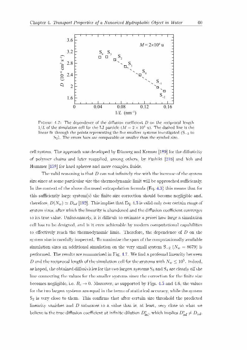
Chapter 4. Transport Properties of a Nanosized Hydrophobic Object in Water 60
0 0.04 0.08 0.12 0.16
1/L (nm−1)
1.6
2
2.4
2.8
3.2
3.6
D
(10−6 c
m2 s−1)
M = 2×10⁴ u
S−1
S0
S1
S2
S3
S4
S−2
Figure 4.7: The dependence of the diusion coecient D on the reciprocal length1/L of the simulation cell for the LJ particle (M = 2× 10⁴ u). The dashed line is thelinear t through the points representing the ve smallest systems investigated (S−2 to
S2). The errors bars are comparable or smaller than the symbol size.
cell system. The approach was developed by Dünweg and Kremer [189] for the diusivity
of polymer chains and later reapplied, among others, by Fushiki [218] and Yeh and
Hummer [158] for hard spheres and more complex uids.
The valid reasoning is that D can not innitely rise with the increase of the system
size since at some particular size the thermodynamic limit will be approached suciently.
In the context of the above discussed extrapolation formula (Eq. 4.3) this means that for
this suciently large system(s) the nite size correction should become negligible and,
therefore, D(Nw) ' Dinf [192]. This implies that Eq. 4.3 is valid only over certain range of
system sizes, after which the linearity is abandoned and the diusion coecient converges
to its true value. Unfortunately, it is dicult to estimate a priori how large a simulation
cell has to be designed, and is it even achievable by modern computational capabilities
to eectively reach the thermodynamic limit. Therefore, the dependence of D on the
system size is carefully inspected. To maximize the span of the computationally available
simulation sizes an additional simulation on the very small system S−2 (Nw = 8679) is
performed. The results are summarized in Fig. 4.7. We nd a profound linearity between
D and the reciprocal length of the simulation cell for the systems with Nw ≤ 105. Indeed,
as hoped, the obtained diusivities for the two largest systems S3 and S4 are clearly o the
line connecting the values for the smaller systems since the correction for the nite size
becomes negligible, i.e. Bc → 0. Moreover, as supported by Figs. 4.5 and 4.6, the values
for the two largest systems are equal in the terms of statistical accuracy, while the system
S2 is very close to them. This conrms that after certain size threshold the predicted
linearity vanishes and D saturates to a value that is, at least, very close to what we
believe is the true diusion coecient at innite dilution D∗inf, which implies D∗inf 6= Dinf.
Chapter 4. Transport Properties of a Nanosized Hydrophobic Object in Water 61
From another perspective, this suggests that the undesired hydrodynamic interactions
between the solute and its periodic images are becoming negligible and not visible after
certain system size threshold. Herein, the appearance of the threshold seems to nearly
coincide with the emergence of the vortex diusion. Quantitatively, our ndings suggest
that strict extrapolation to 1/L = 0 as proposed in Eq. 4.3 can lead to a considerable
overestimation of D∗inf while developed to correct the underestimated diusion coecient
calculated at commonly employed simulation size(s). In this particular case of the LJ
particle this means that the converged value for diusivity D∗inf ≈ 3×10⁻⁶ cm2 s−1 adds
the correction of ≈ 14% to D of the reference system size S0 while being ≈ 20% smaller
from Dinf = 3.6× 10⁻⁶ cm2 s−1 obtained by extrapolation of the linear t of D over all
simulation system sizes.
Our results may initially appear to contradict the previous reports (see Refs. [158,
182, 189, 217, 218]). However, all aforementioned studies were usually dealing with the
system sizes of about 10 000 particles or less (55 000 at most) and found that D(Nw)
scales linearly with 1/L, which is exactly we nd in the same range. In a more recent
publication Li [170] considered the system comprised of a single rough spherical particle
with diameter of 1 nm immersed in the Lennard-Jones uid. For a wide range of investi-
gated system sizes (0.07 nm−1 . 1/L ≤ 0.4 nm−1) author also found converging values
of D for the three largest systems. Yet, this was not recognized and the extrapolation
formula was applied over the entire range of simulated L. This corroborates the claim
that the value of the diusion coecient at the innite dilution is likely D∗inf instead of
Dinf as previously proposed.
4.3 Friction Coecient of the Lennard-Jones Particle
The Brownian particle experiences a friction force arising from systematic collisions with
solvent molecules which is directly proportional to its velocity, and the proportionality
constant is the friction coecient ξ [219]. Once again, the Green-Kubo theory [155]
provides an expression for the friction coecient of the Brownian particle:
ξF =1
3kBT
∫ ∞0〈F(t) · F(0)〉dt , (4.4)
where the term in the angular brackets, FACF(t), is the time autocorrelation function
of the total force F(t) experienced by massive Brownian particle (M → ∞). As the
particle (LJ sphere) has no net charge it is reasonable to assume that F(t) is equal to
the total van der Waals force FvdW(t) exerted by the solvent molecules on the particle.
We calculate FvdW(t) by adding the contributions from all water molecules found within

Chapter 4. Transport Properties of a Nanosized Hydrophobic Object in Water 62
cuto radius rc as
FvdW(tj) =∑Nw
k=1FvdW(rkj ; rkj < rc)
= −∑Nw
k=1∇VLJ-O(rkj ; rkj < rc) , (4.5)
where Nw is the total number of water molecules present in the system, and rkj is the
relative position of the oxygen atom (position of the vdW interaction site) of water
molecule k with respect to the position of the LJ particle at time frame j.
The rigorous projected operator formalism states that the friction coecient ex-
pressed in the terms of real force6 in Eq. 4.4 strictly holds only in the thermodynamic
limit [197]. Moreover, in the limit t → ∞ the friction coecient vanishes. This well-
known paradox is a consequence of the fact that three limits involved, the long time limit,
the thermodynamic limit, and the innite mass limit, do not always commute [195]. For
a massive Brownian particle the way to overcome this issue is to take the thermodynamic
limit on Nw before the limit t → ∞ is performed. After the reformulation of Eq. 4.4,
with taking into account F = FvdW, the time dependent friction coecient of the LJ
particle reads:
ξF (t) =1
3kBT
∫ t
0〈FvdW(t′) · FvdW(0)〉dt′ . (4.6)
Still, this relation lacks the practical information about the magnitude of the upper
bound in the integration. Historically, upon assumption that FACF(t) has an extremely
slow decay, Kirkwood concluded [155] that ξF (t) will then exhibit a plateau for all times
of practical interest where ξF (t) is almost constant. Largar'kov and Sergeev [190] sug-
gested to take explicitly for the upper integration time the moment of the rst zero of
FACF(t) which, of course, corresponds to the time at which ξF (t) reaches its maximum
ξmaxF . This proposal was later partially supported by Brey and Gómez Ordóñez [193].
Recently, following Refs. [220] and [195], Ould-Kaddour and Levesque [191] recognized
that if the decay of the uctuations of F(t) at large t is governed by the laws of macro-
scopic hydrodynamics then the relation ξF (t) = ξ0 exp[−(ξ0t)/(Nwm)] also holds. They
proposed that for suciently large Nw and t Nwm/ξ0 the friction coecient ξF (t)
decays linearly and its value ξ0 can be obtained from the expression
ξF (t) = ξ0
(1− ξ0
Nwmt+ · · ·
). (4.7)
The above discussion addresses the long time limit by decoupling it from the innite
mass limit and the thermodynamic limit. Within the MD method the limit M → ∞6The microscopic expression for the friction coecient obtained by using the projected operator
formalism is given in terms of projected force instead of real force on the Brownian particle. It can beshown that the two forces are identical in the thermodynamic limit. The projected force is propertyhardly accessible from MD simulations. Hence, to obtain ξ from MD simulations we use the real forceand probe the limit Nw →∞.

Chapter 4. Transport Properties of a Nanosized Hydrophobic Object in Water 63
can be eectively achieved by imposing on the solute the holonomic constraint (xing
the position) [195]. In contrast to this frozen dynamics, the limit Nw → ∞ has to be
explicitly investigated by performing simulations for increasing system sizes. This process
can be less computationally demanding and more ecient by incorporating the stochastic
boundary conditions in the MD scheme [196] (not implemented in GROMACS). Herein is
studied in detail both the innite mass limit and thermodynamic limit by systematically
performing two sets of simulations: one with variable mass of the solute particle (system
size xed) and the other with variable system size (xed M).
4.3.1 Mass Dependence
Prior to investigating the limit Nw → ∞ we study the inuence of the solute mass on
the friction coecient for the reference system size S0 (see Tab. 4.1). The results are
gathered in Fig. 4.8. The normalized force autocorrelation functions FACF(t)/FACF(0)
for `light' and `heavy' particles (those with M > 105 u) are shown in panels (a) and (b),
respectively. The behavior of the particle with M = 50 u (omitted for clarity) resembles
that of M = 103 u with more frequent and stronger oscillations that rapidly vanish (∼2ps). Generally, with the increase ofM the oscillations weaken and transform into a broad
minimum which shallows and extends to longer and longer times (& 100 ps). The time
of the rst zero-crossing simultaneously increases and converges to ≈ 4.4 ps for the two
heaviest particles (M = 108 u and 1010 u).
The time evolution of the friction coecient ξ(t) is presented in Fig. 4.8(c) and (d).
While ξ(t) for M = 50 u vanishes almost immediately (data not shown), for M = 103 u
it rapidly reaches a maximum (ξmaxF = 0.37±0.01×10⁻¹¹ kg s−1) and afterwards, due to
already mentioned oscillations of FACF(t), uctuates around zero before extinguishing.
Further increase ofM up to 105 u is accompanied with a steady increase of the maximum
(0.82 ± 0.02, 0.97 ± 0.01, 1.26 ± 0.02 × 10⁻¹¹ kg s−1) and a slower decay towards zero.
Intriguingly, for M = 105 u the decay can be nicely described with an exponential
function as predicted by the laws of macroscopic hydrodynamics [191].
Figure 4.8(d) reveals the convergence of ξmaxF (1.45±0.01, 1.47±0.04, 1.48±0.03×10⁻¹¹ kg s−1) as the particle becomes immobile. Importantly, for these `heavy' solutes
we observe slow linear decay of ξ(t) (see Eq. 4.7). From the t of the linear part (t
interval from 29 ps to 50 ps) and the extrapolation to t = 0 the following values are
obtained for ξ0: 1.12± 0.12, 1.25± 0.07, and 1.33± 0.10× 10⁻¹¹ kg s−1. The dierence
in ξ0 obtained for the two stationary particles (M = 108 u and 1010 u) is the result
of a pronounced sensitivity of the procedure on ne changes of the slope even though
the statistical noise is minuscule at these times. Moreover, at much larger times (≈ 1
ns) the uctuations amount to only about ±0.5% of FACF(0), as illustrated in the inset
of Fig. 4.8(b). However, relatively long simulations of about 100 ns are necessary to

Chapter 4. Transport Properties of a Nanosized Hydrophobic Object in Water 64
0 5 10t (ps)
−0.5
0
0.5
1F
AC
F(t
) / F
AC
F(0
)
101 102 103
0
0.1
0.2
0.3
−0.01
0
0.01
100
102 103
t (ps)
30
0
0.5
1
1.5
ξF(t)
(10−11 k
g s−1)
200 10t (ps)
FA
CF(t
) / F
AC
F(0
)
400
0.5
1
1.5
20 3010t (ps)
ξF(t)
(10−11 k
g s−1)
M=2×10⁴M=104
M=103
M=105
M=2×10⁴M=104
M=103
M=105
~exp(−t) M=108
M=106
M=1010
~t
M=106
M=1010
M=1010(a) (b)
(d)(c)
Figure 4.8: (a)-(b) The normalized force autocorrelation function FACF(t)/FACF(0)for the `light' solutes, M ≤ 105 u, and the `heavy' solutes, M ≥ 106 u. The inset inpanel (b) visualizes the amount of noise present at large times. (c)-(d) The runningvalues of the friction coecient ξF (t) obtained from Eq. 4.6 for the `light' (c) and the`heavy' solutes (d). By applying Eq. 4.7 the linear ts of the interval between 29 psand 50 ps and their extrapolations to t = 0 are presented by the dashed lines (M = 108
u is excepted for clarity).
satisfactorily converge FACF(t) and, therefore, ξ(t) as well to obtain a reliable estimate of
the friction coecient using the relation proposed by Ould-Kaddour and Levesque [191].
This is in stark contrast to obtaining ξmaxF accurately, for which only a few nanoseconds
are suitable.
4.3.2 System Size Inuence
A very versatile behavior was observed in the solvation process of very light solutes
compared to immobile solutes for both FACF(t) and ξ(t) in the case of xed system size
to Nw = 23419. The realized mass limit, represented here by M = 1010 u, shall be the
starting point in the investigation of the system size inuence on the solute's friction
coecient. Alongside the reference system size (S0), we perform simulations for four
additional system sizes enclosing between 11130 (S−1) and 201350 (S3) water molecules
(see Tab. 4.1).
Figure 4.9(a) presents the dependence of the normalized FACF(t) on the system

Chapter 4. Transport Properties of a Nanosized Hydrophobic Object in Water 65
size. For t . 2 ps all correlation functions share almost identical relaxation (not explic-
itly shown) followed by a very shallow minimum. After the integration this is reected in
ξF (t), shown in Fig. 4.9(b). With the system enlargement the maximum ξmaxF aestheti-
cally increases (1.44±0.02, 1.48±0.03, 1.50±0.03, 1.52±0.03, 1.51±0.03×10⁻¹¹ kg s−1)
and eectively converges for Nw ≥ 23419 (S0). Remarkably, due to non-obvious increas-
ingly decelerated approach of FACF(t) to zero after reaching progressively shallowing
minimum the overall ξF (t) experiences prominent changes with the enlargement of the
simulation cell. In cohesion with the elevation to higher values of the friction the interval
of the linear decay shifts to larger times since t ∝ Nwm/ξ0 (see Eq. 4.7). This also
implies smaller values of the slope [191, 194, 197]. In turn, the latter give rise to the
40 50
t (ps)
0
0.5
1
1.5
10 100t (ps)
−0.04
0
0.04
0.08
0.12
0.16
10 20 30
2
S−1
S3
~exp(−t)
~t
S−1
S0
S1
S3
S2
ξF(t
) (10−11 k
g s−1)
FA
CF(t
) /
FA
CF(0
)
(a)
(b)
Figure 4.9: (a) Dependence of the normalized force autocorrelation functionFACF(t)/FACF(0) on the system size in the lin-log representation. Mass of the solute isalways M = 1010 u. (b) The time evolution of the friction coecient ξF (t) obtained byusing Eq. 4.6. The dashed lines indicate the linear ts at larger times (29-50 ps) and
their extrapolation to t = 0 for systems S0-S3.

Chapter 4. Transport Properties of a Nanosized Hydrophobic Object in Water 66
`quasi-plateau' in ξF (t) for Nw & 100 000 for all times of practical interest as has been
foreseen by Kirkwood [155].
Again by performing the linear t procedure (between 29 ps and 50 ps) we ob-
tain for the friction coecient ξ0: 1.39 ± 0.06 (S1), 1.38 ± 0.06 (S2), and 1.35 ± 0.13 ×10⁻¹¹ kg s−1 (S3). Note that in the previous section was reported 1.33±0.10×10⁻¹¹ kg s−1
for the reference system size. Likewise for ξmaxF , the estimates for ξ0 are found to be within
statistical accuracy for all systems exhibiting linear decay, although it appears that they
tend to slightly increase with the increase of Nw. Interestingly, in this size domain the
predictions ξmaxF and ξ0 deviate less than 15%. The discussion about which method is
preferred we postpone for the next section (Sec. 4.4). However, this similarity of ξmaxF
and ξ0 indicates that for an accurate estimate of the friction coecient of an innitely
massive LJ particle (i.e., Brownian particle in general) is necessary to operate with very
large systems that approach but are not necessarily in the thermodynamic limit.
On the other side of Nw →∞ spectrum interesting changes are invoked in the time
evolution of ξF . By bisecting the reference system S0 to S−1 the behavior at larger times
switches from linear to purely exponential while apparently reducing ξF (t) for t > 10
ps. The exponential decay was also observed for the reference system size and particle
of M = 105 u (see Fig. 4.8) and reveals an interesting interplay between the system size
and the mass of the LJ particle. In either case the exponential t nicely overlaps with the
simulated data but yields drastically higher estimate for ξ0 of about 2.2× 10⁻¹¹ kg s−1.
Furthermore, to assess the importance of the simulation setup, additional simula-
tions are performed on the smaller system S−1. These simulations inspected the inuence
of the enhanced output writing frequency to 0.04 ps (otherwise 0.2 ps) and the smaller
timestep of 1 fs. The output frequency was found to have absolutely negligible inuence.
Similarly, ξF (t) of the two simulations with the timesteps 1 fs and 2 fs are found to agree
with each other to within the statistical errors after 40 ns of simulated time.
4.4 Validity of the Einstein Relation and the
Stokes-Einstein Relation
The study of transport properties of colloidal particle is amazing but also challenging
due to its inherent complexity. The complexity arises primarily from the diculty to
assess the quality of obtained value for a particular transport coecient based on a single
simulation without a signicant prior knowledge of the system behavior. Likewise, it is
dicult to establish the quality of the so far obtained results for the LJ particle without
cross-checking them one against another.

Chapter 4. Transport Properties of a Nanosized Hydrophobic Object in Water 67
This invites the use of the Einstein relation which relates the diusion coecient
of a Brownian particle to its friction coecient
D =kBT
ξ. (4.8)
The relation is very general and its validity was undoubtedly conrmed many times,
both experimentally and theoretically, for macroscopic Brownian particles. Therefore,
in numerous MD studies its validity was taken for granted. Additional factor for this
reasoning is governed by the fact that the validation of the Einstein relation requests sep-
arate evaluation of the friction coecient ξ. This was/is computationally too demanding
due to the incorporated prerequisite of the thermodynamic limit (see Sec. 4.3). However,
the applicability of the Einstein relation for the nanoscopic bodies is legitimate issue
as it is expected to break far from the Brownian limit (much heavier and larger solute
compared to solvent molecules). Thereby, the validity of Eq. 4.8 is explicitly checked for
the employed sub-nanoscopic LJ particle.
Applying the Einstein formula, Fig. 4.10 displays the values of ξD (full circles)
and ξD(inf) (full diamond) for the friction coecient. The latter values are calculated
by using the previously determined diusion coecients of the solute with M = 2 ×10⁴ u (see Sec. 4.2). These derived values ξD and ξD(inf) are then compared to the
values of the friction coecient retrieved from the force-force autocorrelations of the
immobile solute (M = 1010 u) while accounting for the proposals made by Largar'kov
& Sergeev (ξmaxF ) [190] and Ould-Kaddour & Levesque (ξ0) [191]. As the consequence
of the extensively elaborated dependence of D on 1/L (see Fig. 4.7), the convergence
of ξD to 1.38± 0.01× 10⁻¹¹ kg s−1 is obtained for the systems constituted from 105 or
more water molecules. Strikingly, this is in stunning agreement (within one standard
deviation) with ξ0 (squares) for all systems but the smallest S−1. Both ξD and ξ0 for
the smallest system severely overestimate the converged value of the friction coecient.
This demonstrates that for `purely' exponential decay of ξF (t) (see Fig. 4.9), where the
linear regime is absent at relevant times, the applied exponential t predicts too high a
value for friction, i.e. too low diusivity. Importantly, in cases in which ξF (t) exhibits a
linear decay, the linear t procedure [191] provides an accurate estimate for the friction
coecient. Curiously, the recommendation of Largar'kov and Sergeev [190] to take the
maximum value ξmaxF (triangles) for the friction coecient only slightly overestimates
(. 10%) the converged value of ξD for all systems, even for the smallest S−1. However,
the performance of this procedure could dier considerably for other size(s) of the LJ
particle. Furthermore, ξD(inf) obtained from Dinf (extracted from Eq. 4.3 as proposed by
Fushiki [218]) strongly underestimates (≈ 17%) the friction coecient.
To recapitulate, apart from unexpected similarity between ξD and ξmaxF , an ex-
traordinary and valuable agreement is achieved between ξD and ξ0 for Nw & 105. It
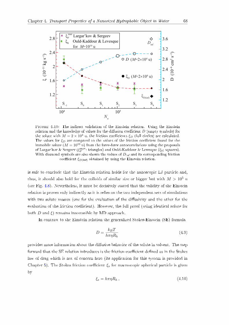
Chapter 4. Transport Properties of a Nanosized Hydrophobic Object in Water 68
104 105
Nw
ξ (10−11 k
g s−1)
1.2
1.6
2
2.4
2.8
1.2
1.6
2
2.4
2.8
3.2
3.6
D (10−6 c
m2 s−1)
ξD
max
ξ0
Ould-Kaddour & Levesque
D
ξF
Largar’kov & Sergeev
ξD(inf)
Dinf
S−1
S4
S0
S1
S2
S3
(M=2×10⁴ u)
(M=2×10⁴ u)
for M=1010 u
Figure 4.10: The indirect validation of the Einstein relation. Using the Einsteinrelation and the knowledge of values for the diusion coecient D (empty symbols) forthe solute with M = 2× 10⁴ u, the friction coecients ξD (full circles) are calculated.The values for ξD are compared to the values of the friction coecient found for theimmobile solute (M = 1010 u) from the force-force autocorrelations using the proposalsof Largar'kov & Sergeev (ξmaxF ; triangles) and Ould-Kaddour & Levesque (ξ0; squares).With diamond symbols are also shown the values of Dinf and its corresponding friction
coecient ξD(inf) obtained by using the Einstein relation.
is safe to conclude that the Einstein relation holds for the nanoscopic LJ particle and,
thus, it should also hold for the colloids of similar size or bigger but with M > 105 u
(see Fig. 4.8). Nevertheless, it must be decisively stated that the validity of the Einstein
relation is proven only indirectly as it is relies on the two independent sets of simulations
with two solute masses (one for the evaluation of the diusivity and the other for the
evaluation of the friction coecient). However, the full proof (using identical solute for
both D and ξ) remains inaccessible by MD approach.
In contrast to the Einstein relation the generalized Stokes-Einstein (SE) formula
D =kBT
hπηRh(4.9)
provides more information about the diusive behavior of the solute in solvent. The step
forward that the SE relation introduces is the friction coecient dened as in the Stokes
law of drag which is not of concern here (its application for this system is provided in
Chapter 5). The Stokes friction coecient ξs for macroscopic spherical particle is given
by
ξs = hπηRh , (4.10)

Chapter 4. Transport Properties of a Nanosized Hydrophobic Object in Water 69
where h is the constant describing the nature of the boundary conditions at the solute-
solvent surface and equals 4 for the slip and 6 for the stick boundary conditions, η is
the shear viscosity of the solvent, and Rh is the hydrodynamic radius of the LJ particle.
Many computational studies tried to establish the appropriate boundary conditions at the
solute-solvent surface as well as the denition of the hydrodynamic radius of the solute
by tting those to reproduce the values obtained for the diusion coecient. The clear
and indisputable answers are still missing as many of the results are contradictory. This
can be, at least partially, attributed to one or combinations of the following factors [221]:
the inappropriate use of the hard spheres to study the transport properties, ignoring the
nite size eects on diusivity or assuming the solute to be big enough so that the SE
relation holds. While the rst two factors are clearly addressed throughout this work
the strong indication that the designed LJ particle is large enough is supported above
by the indirect validation of the Einstein relation. Thus, we proceed with condence to
establish the aforementioned hydrodynamic conditions.
The correctness of the SE relation for the LJ particle-water system stems directly
from the above demonstrated validity of its predecessor, the Einstein relation. Therefore,
the SE relation is utilized to establish a quantitative connection between D, ξ, and
the hydrodynamic parameters. Indeed, when a quantitative estimate of the transport
property of colloidal particle is desired the hydrodynamic boundary conditions as well
as the hydrodynamic radius Rh should be considered as free parameters [192]. Instead
of allowing fully adjustable boundary conditions here are considered only two ideal and
theoretically well-dened cases. The latter correspond to the slip and the stick conditions
at the boundary. This implies that full exibility of the magnitude of the hydrodynamic
radius is allowed.
The results are summarized in Table 4.2. We exploit the SE relation (Eq. 4.9) and
take the values for the diusion coecient of the LJ particle and the water shear viscosity
to be 3.01±0.02×10⁻⁶ cm2 s−1 and 6.8±0.1×10⁻⁴ Pa·s, respectively. For the perfect slipboundary conditions is obtained Rh = 1.60± 0.03 nm. This is in remarkable coincidence
Table 4.2: The values of the hydrodynamic radius Rh estimated from the Stokes-Einstein relation (Eq. 4.9) by assuming the slip (h = 4) and the stick (h = 6) boundaryconditions. For the diusion coecient of the LJ particle and the water shear viscosityis taken D = 3.01 ± 0.02 × 10⁻⁶ cm2 s−1 and η = 6.8 ± 0.1 × 10⁻⁴ Pa·s, respectively.Also are given plausible denitions for the hydrodynamic radius originating from theradial distribution function (RDF) between the LJ particle and water hydrogen atoms
(gLJ-H(r)) and their respective values rRDF.
h Rh (nm) rRDF (nm) RDF feature
slip 1.60± 0.03 1.59± 0.01 1st maximumstick 1.07± 0.02 1.14± 0.01 excluded volume
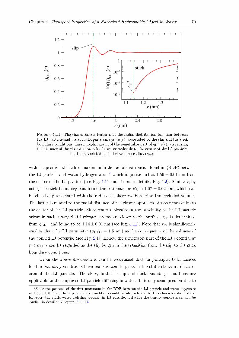
Chapter 4. Transport Properties of a Nanosized Hydrophobic Object in Water 70
1.2 1.6 2 2.4 2.80
0.2
0.4
0.6
0.8
1
1.2
gL
J−H(r
)
r (nm)
1.1 1.2 1.3
10−6
10−4
10−2
1
log
gL
J−H(r
)
rev
slip
stick
r (nm)
Figure 4.11: The characteristic features in the radial distribution function betweenthe LJ particle and water hydrogen atoms gLJ-H(r), associated to the slip and the stickboundary conditions. Inset: log-lin graph of the penetrable part of gLJ-H(r), visualizingthe distance of the closest approach of a water molecule to the center of the LJ particle,
i.e. the associated excluded volume radius (rev).
with the position of the rst maximum in the radial distribution function (RDF) between
the LJ particle and water hydrogen atom7 which is positioned at 1.59 ± 0.01 nm from
the center of the LJ particle (see Fig. 4.11 and, for more details, Fig. 5.2). Similarly, by
using the stick boundary conditions the estimate for Rh is 1.07 ± 0.02 nm, which can
be eectively associated with the radius of sphere rev bordering the excluded volume.
The latter is related to the radial distance of the closest approach of water molecules to
the center of the LJ particle. Since water molecules in the proximity of the LJ particle
orient in such a way that hydrogen atoms are closer to the surface, rev is determined
from gLJ-H and found to be 1.14± 0.01 nm (see Fig. 4.11). Note that rev is signicantly
smaller than the LJ parameter (σLJ-O = 1.5 nm) as the consequence of the softness of
the applied LJ potential (see Fig. 2.1). Hence, the penetrable part of the LJ potential at
r < σLJ-O can be regarded as the slip length in the transition from the slip to the stick
boundary conditions.
From the above discussion it can be recognized that, in principle, both choices
for the boundary conditions have realistic counterparts in the static structure of water
around the LJ particle. Therefore, both the slip and stick boundary conditions are
applicable to the employed LJ particle diusing in water. This may seem peculiar due to7Since the position of the rst maximum in the RDF between the LJ particle and water oxygen is
at 1.58 ± 0.01 nm, the slip boundary conditions could be also referred to this characteristic feature.However, the static water ordering around the LJ particle, including the density correlations, will bestudied in detail in Chapters 5 and 6.

Chapter 4. Transport Properties of a Nanosized Hydrophobic Object in Water 71
the extensive eort in literature to establish the connection between the surface roughness
and the nature of boundary conditions. Therein, the stick and the slip conditions are
linked to the rough surfaces and the smooth surfaces, respectively [199, 217]. However, it
is dicult to envisage an intuitive description of the smoothness/roughness at the level
of a single atom.
4.5 Diusive Length Scale
So far in this chapter attention was primarily focused on the calculation of the transport
properties of the LJ particle, i.e. the diusion coecient and the friction coecient.
Therein the simulations of the two-component system composed of the solute particle
immersed in water solvent were employed. These predictions forD and ξ are then coupled
with the pre-evaluated solvent shear viscosity η (see Sec. 3.3.1) to establish the validity of
the Stokes-Einstein relation (Eq. 4.9). However, the goal could be to estimate the shear
viscosity of medium without explicitly conducting the simulations of neat solvent. The
most prominent and reasonable approach is to recast the Stokes-Einstein (SE) formula
(Eq. 4.9) as
ηD =kBT
hπRhD. (4.11)
Moreover, the SE formula guarantees that the obtained values for ηD are accurate at the
same conditions that are established in Sec. 4.4 for the diusion coecient.
Alternatively, the estimate of ηD can be coarse by introducing the concept of
the diusive length scale lD. It represents the ensemble average of the distance that
a Brownian particle (i.e., the employed LJ particle) covers in a time interval equal to
the diusive time scale which ambiguously depicts the time scale on which the position
of the particle is proportional to√t [219]. The lD can be directly inferred from MSD
of the LJ particle. The extrapolation of the linear t of the diusive regime to t = 0
equals −l2D and is indicated in Fig. 4.2(b). As nicely pointed out by Dhont [219], we
can write η(lD) ≈ |p(0)|/(hπRhlD), where p is the momentum of the LJ particle. The
|p(0)| comes from the fact that at small times the particle did not yet change its velocity
due to collisions with solvent molecules. Use of the equipartition theorem yields |p(0)| ≈√〈|p|2〉 =
√3MkBT . Hence, the estimate of the shear viscosity from the diusive length
scale reads
η(lD) ≈√
3MkBT
hπRhlD. (4.12)
Although the information of lD is readily available from MSD and the above deriva-
tion of η(lD) is rather general we are not familiar of any previous MD simulation study
inspecting the performance of the procedure for nanoscopic particles. Several factors
could have been attributing to this state. First and foremost, until about a decade ago

Chapter 4. Transport Properties of a Nanosized Hydrophobic Object in Water 72
Table 4.3: The estimates of the solvent shear viscosity ηD and η(lD) obtained byusing Eqs. 4.11 and 4.12, respectively. The slip boundary conditions (h = 6) and thehydrodynamic radius Rh = 1.60 nm are used. The estimates are given for the threesystem sizes (S0, S1, and S2). The values for the shear viscosity are always given in
10−4 Pa·s.
S0 S1 S2
M (u) ηD η(lD) ηD η(lD) ηD η(lD)
50 7.8± 0.2 - 7.47± 0.03 - 7.0± 0.1 -103 7.9± 0.3 - 7.54± 0.08 - 6.9± 0.2 -2× 10⁴ 8.58± 0.07 9.9 7.7± 0.1 6.3 6.9± 0.1 5.5105 12.1± 0.2 9.2± 0.7 10.0± 0.03 7.1± 0.6 8.2± 0.3 6.2106 94.9± 0.5 39± 6 40.0± 0.3 19± 1 15.5± 0.1 6.7107 4161± 82 650± 52 1164± 20 277± 49 245± 3 65± 10
[164] it was a challenging task to even accurately predict η from pure solvent simula-
tions. As previously elaborated the validity of the (Stokes-)Einstein relation and the
nature of their ingredients (boundary conditions, hydrodynamic radius, etc.) are still
extensively debated. Additionally, the criterion of the size ratio lD/Rh necessitates large
solutes since it prescribes that the diusive length scale should be only a tiny fraction
(≈ 10−4 − 10−3) of the size of the LJ particle in order to acquire meaningful estimate of
the solvent shear viscosity from Eq. 4.12. In the simulations performed here, lD is found
to be up to few percent of Rh (irrespective of its denition).
103 104 105 106 107
M (u)
100
101
102
η (10−4 P
a⋅s)
ηD
S0
η
η(lD) S
0
η(lD) S
1
η(lD) S
2
Figure 4.12: Double logarithmic plot of the dependence of the solvent shear viscosityestimates ηD and η(lD) on the mass of the solute M . The estimates η(lD) are givenfor the three system sizes considered (S0-circles, S1-triangles, and S2-diamonds) whilefor clarity only the reference system size S0 is shown for ηD. All values are comparedto the target shear viscosity of η = 6.8× 10⁻⁴ Pa·s indicated by the dashed black line.The slip boundary conditions (h = 6) and the hydrodynamic radius Rh = 1.60 nm are
used.

Chapter 4. Transport Properties of a Nanosized Hydrophobic Object in Water 73
The estimates of the shear viscosity ηD and η(lD) are calculated from Eqs. 4.11
and 4.12 and presented in Table 4.3. These results are also summarized in Fig. 4.12.
In the previous section we demonstrated the compatibility of the two combinations of
the boundary condition and the hydrodynamic radius with the Stokes-Einstein relation.
Therefore, both the slip and stick conditions provide ηD and η(lD) of essentially the
same quality. For demonstration purposes, slip boundary conditions and Rh = 1.60
nm are used in Fig. 4.12 and Table 4.3, whereas the results for the stick conditions are
not shown. The estimates η(lD) are provided only for the solutes with M ≥ 2 × 10⁴
u since they perform the diusive motion that emerges from the ballistic motion which
is essential prerequisite to obtain a realistic estimate −l2D < 0, i.e. lD > 0, from their
MSD. For clarity only the estimates ηD for the reference system size S0 are depicted
in Fig. 4.12, whereas the two larger system sizes S1 and S2 are omitted. Similarly, the
values for M = 50 u are not included as they are always within the statistical accuracy
of values for M = 103 u. Approaching M → ∼ m, with the diusion overwhelmingly
mass independent (see Fig. 4.3) the estimates ηD t the expectation better, especially
with the increase of the system size towards S2. Moving in the direction M → ∞, as
expected, the ηD overestimate the reference shear viscosity value (6.8× 10⁻⁴ Pa·s) withthe error progressively increasing for heavier particles. A similar behavior is also observed
101 102 103 104 105 106 107 108 109 1010
M (u)
10−1
100
101
102
η (
10
−4 P
a⋅s)
ξ→ 0
ηD
(S1)
η(lD) (S
1)
η
ηξ
(S0)
M/m = 1
D = 0
M/m → ∞
Figure 4.13: Dependence of the estimated shear viscosities of water ηD (black circles),η(lD) (red squares), and ηξ (green triangles) on the mass M of the LJ particle. Theslip boundary conditions (h = 6) and the hydrodynamic radius Rh = 1.60 nm are usedto obtain each estimate of the shear viscosity. The black dashed line indicates thereference value of the shear viscosity η = 6.8× 10⁻⁴ Pa·s obtained from the pure watersimulations. The full symbols indicate that the estimate of the shear viscosity ηD, η(lD)or ηξ is within ≈ 10% of the reference value. The error bars are always smaller thanthe symbol size. The limits M/m = 1 and D = 0 (immobile particle) are marked by
the two dotted vertical lines.

Chapter 4. Transport Properties of a Nanosized Hydrophobic Object in Water 74
for the estimates obtained from the diusive length scale. Interestingly, η(lD) generally
overestimate the shear viscosity by less than ηD (with the exception ofM = 2×10⁴ u for
S0). This remarkable improvement can be up to almost an order of magnitude in some
cases. Astonishingly, for the large system S2 with the heavy solutes having M = 105
u and M = 106 u the obtained η(lD) are within ±10% of the target value. These two
values for η(lD) alongside ηD for the LJ particles with M ≤ 2 × 10⁴ u represent the
interval of almost six orders of magnitude of the solute mass over which are obtained,
at least, reasonably accurate estimates of the solvent shear viscosity without explicitly
conducting pure solvent simulations.
The last statement can be even more fortied by including the knowledge acquired
on the calculation of the friction coecient (see Sec. 4.3) which performs the best close
to the limit M →∞, i.e. for M > 106 u, where the diusion estimate fails. Exemplarily,
for the immobile solute dissolved in the large system S2 both the proposal of Largar'kov
& Sergeev (ξmaxF ) and that of Ould-Kaddour & Levesque (ξ0) predicted the friction
coecient with satisfactory accuracy. Even the predictions ξmaxF (which, in general,
show somewhat inferior performance) for the smaller reference system size (S0) were
reasonably accurate. Nevertheless, ξmaxF can be extracted over a much broader interval
of solute masses than estimates using the proposal of Ould-Kaddour & Levesque (limited
to masses for which ξF (t) exhibits linear decay). Thereby, for demonstration purposes,
we use these ξmaxF to estimate the shear viscosity from the Stokes law (Eq. 4.10), i.e.
ηξ = ξmaxF /(hπRh). In Fig. 4.13, predicted values for ηξ are compared to the estimates of
the shear viscosity ηD and η(lD) obtained from the diusion behavior of the LJ particle.
The gure nicely demonstrates that the solvent shear viscosity can be reliably obtained
both from D and ξ of the nanosized LJ particle dissolved in a moderately large solvent
bath (Nw ≈ 50 000) for essentially the entire range of interest of solute masses spanning
from M/m ∼ 1 to M → ∞ (m is the mass of a single solvent molecule). These two
seemingly incompatible limits are bridged by employing the concept of the diusive
length scale [219].
4.6 Conclusions
A series of large-scale molecular dynamics simulations of a spherical nanoscopic particle
dissolved in the SPC/E water has been performed using the GROMACS package. The
simulations covered an extensive range of both solute masses and system sizes to gain
an accurate prediction of the solute's diusion coecient and the friction coecient.
A systematic broadening of the eective hydrodynamic regime in terms of the solute
mass is observed with the increase of the solvent bath size. More detailed investigation
with the LJ particle having M = 2 × 10⁴ u revealed that, for the systems containing
more than 200 000 water molecules, the diusion coecient converges as the nite size

Chapter 4. Transport Properties of a Nanosized Hydrophobic Object in Water 75
eects eectively vanish. This is in contradiction with common practice to take the
diusion coecient at the innite dilution to be the extrapolated value of the system
size dependent values of the diusion coecient obtained for the hypothetical innite
simulation box. The latter approach, which intends to correct the underestimated value
of the diusion coecient, in actuality, predicts signicantly overestimated diusivity.
Moreover, the universal asymptotic behavior ∼ t−3/2 of the velocity autocorrelation
function is found for the largest system inspected (Nw ≈ 400 000).
On the other hand, the friction coecient was calculated from the Green-Kubo
integral of the force autocorrelation function of the solute. While the lighter solutes (M ≤105 u) exhibit complex time decay of the friction coecient, the linear decay is found
at larger times for almost and completely immobile solutes. For the systems enclosing
Nw ≥ 100 000 this linear decay becomes very slow and gives rise to the theoretically
predicted `quasi-plateau'. Furthermore, for the immobile LJ particles an extraordinary
agreement is found between the friction coecient calculated by exploiting the linear
decay as proposed by Ould-Kaddour & Levesque and the friction coecient expected
from the converged value of the diusion coecient according to the Einstein relation.
Interestingly, a reasonable agreement is obtained for much wider range of solute masses
by using the proposal of Largar'kov & Sergeev, i.e. by taking the friction coecient to
be the value of the maximum in its time evolution.
The obtained values for both the diusion and friction coecient are supplemented
with the water shear viscosity separately evaluated from the neat solvent simulations (see
Chapter 3). They served as a basis to indirectly demonstrate the validity and establish
the conditions at which the Einstein relation and the Stokes-Einstein formula are most
reliable. The ambiguity of the latter relation is evident in the fact that both choices
of the boundary conditions, with their corresponding hydrodynamic radii, provide a
quantitative agreement with the calculated transport properties. While the slip boundary
conditions are associated with the position of the rst maximum in the radial distribution
function between solute and water oxygen, the stick conditions are apparently linked to
the excluded volume of the LJ particle. Moreover, an alternative approach is proposed
to estimate the shear viscosity of solvent by relating it to the diusive length scale of the
LJ particle. This approach eectively covers the regime of the intermediate masses of
the solute where the estimates of the shear viscosity, both from the diusion coecient
and friction coecient using the Stokes-Einstein relation, are predicted with signicant
errors. Although this approach has its drawbacks for the rather small size of the employed
LJ particle, it could prove valuable for bigger solutes immersed in more complex uids,
the shear viscosity of which is challenging to obtain.


Chapter 5
Establishing Conditions for
Simulating Hydrophobic Solutes in
Electric Fields by Molecular
Dynamics
The majority of this chapter is already presented in our publication [104].
The hydrophobicity of an interface, droplet or a particle can be modulated by an
external electric eld in a process called electrowetting [18]. Such a change of surface
characteristics allows for the regulation of macroscopic properties such as adhesion or
friction in micro and nano-uidics by the electric eld [19]. Microuidic movement
[222] based on electrowetting is being used in an increasing number of applications, for
example, for reective displays [20, 21]. While the eect of the electric eld is reasonably
well understood on the macroscopic scale [18], there are only a few studies of the origin
of electrowetting on the nanometric scale [2224]. With the advent of nano-electronics
and the development of micro and nano-devices that can be powered by electric elds
[25], this becomes an increasingly pressing problem.
In the presence of a static electric eld, it has been found that the eld exerts
torques on non-spherical nano-particles [223]. This occurs through a coupling between
the interfacial hydrogen bonds and the alignment of the water molecules, which has also
been studied in the context of nanodrops on graphene surfaces [224] and for water in
nanopores [24, 225]. It is natural to expect that this coupling will also aect the hydration
of spherical nano-particles, and thus have implications on the self-assembly process, the
propulsive eciency of nano-devices, and the electrophoretic mobility of particles [226].
Recently, an interesting coupling between the electric eld and the solvent orga-
nization was suggested, supposedly leading to net water ux through carbon nanotubes
in the presence of static elds. The latter were directly imposed [70] or mimicked by an
77
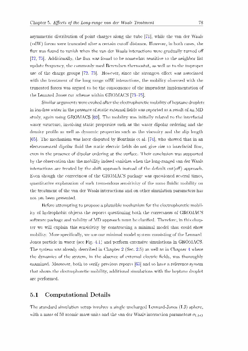
Chapter 5. Eects of the Long-range van der Waals Treatment 78
asymmetric distribution of point charges along the tube [71], while the van der Waals
(vdW) forces were truncated after a certain cuto distance. However, in both cases, the
ux was found to vanish when the van der Waals interactions were gradually turned o
[72, 75]. Additionally, the ux was found to be somewhat sensitive to the neighbor list
update frequency, the commonly used Berendsen thermostat, as well as to the improper
use of the charge groups [72, 73]. However, since the strongest eect was associated
with the treatment of the long range vdW interactions, the mobility observed with the
truncated forces was argued to be the consequence of the imprudent implementation of
the Lennard-Jones cut scheme within GROMACS [7375].
Similar arguments were evoked after the electrophoretic mobility of heptane droplets
in ion-free water in the presence of static external elds was reported as a result of an MD
study, again using GROMACS [69]. The mobility was initially related to the interfacial
water structure, involving static properties such as the water dipolar ordering and the
density prole as well as dynamic properties such as the viscosity and the slip length
[65]. The mechanism was later disputed by Bonthuis et al. [74], who showed that in an
electroneutral dipolar uid the static electric elds do not give rise to interfacial ow,
even in the presence of dipolar ordering at the surface. Their conclusion was supported
by the observation that the mobility indeed vanishes when the long-ranged van der Waals
interactions are treated by the shift approach instead of the default cut(o) approach.
Even though the correctness of the GROMACS package was questioned several times,
quantitative explanation of such tremendous sensitivity of the nano-uidic mobility on
the treatment of the van der Waals interactions and on other simulation parameters has
not yet been presented.
Before attempting to propose a plausible mechanism for the electrophoretic mobil-
ity of hydrophobic objects the reports questioning both the correctness of GROMACS
software package and validity of MD approach must be claried. Therefore, in this chap-
ter we will explain this sensitivity by constructing a minimal model that could show
mobility. More specically, we use our minimal model system consisting of the Lennard-
Jones particle in water (see Fig. 4.1) and perform extensive simulations in GROMACS.
The system was already described in Chapter 2 (Sec. 2.5) as well as in Chapter 4 where
the dynamics of the system, in the absence of external electric elds, was thoroughly
examined. Moreover, both to verify previous reports [65] and to have a reference system
that shows the electrophoretic mobility, additional simulations with the heptane droplet
are performed.
5.1 Computational Details
The standard simulation setup involves a single uncharged Lennard-Jones (LJ) sphere,
with a mass of 50 atomic mass units and the van der Waals interaction parameters σLJ-O

Chapter 5. Eects of the Long-range van der Waals Treatment 79
and εLJ-O of 1.5 nm and 0.8063 kJ mol−1, respectively. These were deliberately set to
create a particle that is signicantly larger than the water molecule (see Fig. 4.1). The
particle was dissolved in a cubic box of edge length 8.9 nm containing 23419 SPC/E
[116] water molecules. The energy of the system was rst minimized with the steepest
descent method. Subsequently, a short (0.5-1 ns, NPT) run was performed followed
by an additional equilibration run (0.5-1 ns, NPT) at nonzero eld for the simulations
in the presence of an external electric eld. The latter was chosen to have a strength
of 0.6 V nm−1, and was imposed using tinfoil boundary conditions [138]. During the
equilibration, the pressure was weakly coupled to a target value of P = 1 bar using the
Berendsen barostat [101]. In all cases, the volume of the system fully relaxed and began
to uctuate around an equilibrium value.
The production runs (each with a total length of 100 ns) were conducted in both
the NVT and the NPT ensembles, in the presence and absence of a static electric eld
(imposed in the +x direction). For the simulations in the NVT ensemble, the initial 0.5-1
ns was omitted from the analysis, to allow the relaxation of the system after xing its
volume, i.e. density. For all combinations of the ensemble and eld strength, the simula-
tions were performed for the three common treatments of the van der Waals interactions,
namely the cut, switch, and shift treatments.1
The standard setup involved simulations with a time step of 2 fs, the LINCS
algorithm [139], particle decomposition, and a non-bonded list update frequency (NLUF)
of 10 steps. Long range electrostatic interactions were accounted for by the Particle
Mesh Ewald (PME) technique [88]. A reference temperature of 300 K was achieved by
employing the Berendsen algorithm with a time relaxation constant of 0.1 ps [101]. To
ensure good statistics and adequate spatial and time resolution, the coordinates were
saved, with single precision, every 100 steps. To evaluate the results, single precision
simulations (forces, velocities, and positions) were compared to runs subject to double
precision evaluations (through all levels of the simulation).
Unless indicated otherwise, simulations were performed in the GROMACS 4.0.5
simulation package [137]. Additional simulations were executed in GROMACS 3.3.3,
4.5.5, and 4.6.4.
In the study of the eect of the thermostat (NVT ensemble accompanied with
NLUF=1 or NLUF=10), the standard Berendsen weak coupling scheme was replaced
with the Nosé-Hoover [98, 99] thermostat (with a period of oscillations of kinetic energy
set to 0.3 ps), or the advanced velocity rescaling [97] algorithm (relaxation time of 0.1
ps), as implemented in the 4.0.5 version of GROMACS. In addition, Langevin thermostat
(friction constant 0.5 ps−1) was implemented together with the Langevin dynamics [227].
1A detailed description of the cut, switch, and shift treatments of the van der Waals interactions, asimplemented in GROMACS, is given in Chapter 2, Sec. 2.5.
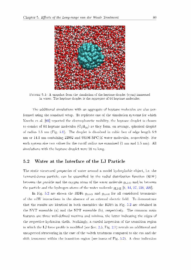
Chapter 5. Eects of the Long-range van der Waals Treatment 80
Figure 5.1: A snapshot from the simulation of the heptane droplet (cyan) immersedin water. The heptane droplet is the aggregate of 64 heptane molecules.
The additional simulations with an aggregate of heptane molecules are also per-
formed using the standard setup. To replicate one of the simulation systems for which
Knecht et al. [65] reported the electrophoretic mobility, the heptane droplet is chosen
to consist of 64 heptane molecules (C7H16) as they form, on average, spherical droplet
of radius 1.5 nm (Fig. 5.1). The droplet is dissolved in cubic box of edge length 8.9
nm or 14.1 nm containing 22992 and 93106 SPC/E water molecules, respectively. For
each system size two values for the cuto radius are examined (1 nm and 1.5 nm). All
simulations with the heptane droplet were 20 ns long.
5.2 Water at the Interface of the LJ Particle
The static structural properties of water around a model hydrophobic object, i.e. the
Lennard-Jones particle, can be quantied by the radial distribution function (RDF)
between the particle and the oxygen atom of the water molecule gLJ-O and/or between
the particle and the hydrogen atoms of the water molecule gLJ-H [8, 14, 27, 228, 229].
In Fig. 5.2 are shown the RDFs gLJ-O and gLJ-H for all considered treatments
of the vdW interactions in the absence of an external electric eld. To demonstrate
that the results are identical in both ensembles the RDFs in Fig. 5.2 are obtained in
the NVT ensemble (a) and the NPT ensemble (b), respectively. The common main
features are three well-dened maxima and minima, the latter indicating the edges of
the respective hydration shells. Strikingly, a careful inspection of the transition region
in which the LJ force prole is modied (see Sec. 2.5, Fig. 2.1) reveals an additional and
unexpected structuring in the case of the switch treatment compared to the cut and the
shift treatment within the transition region (see insets of Fig. 5.2). A clear indication
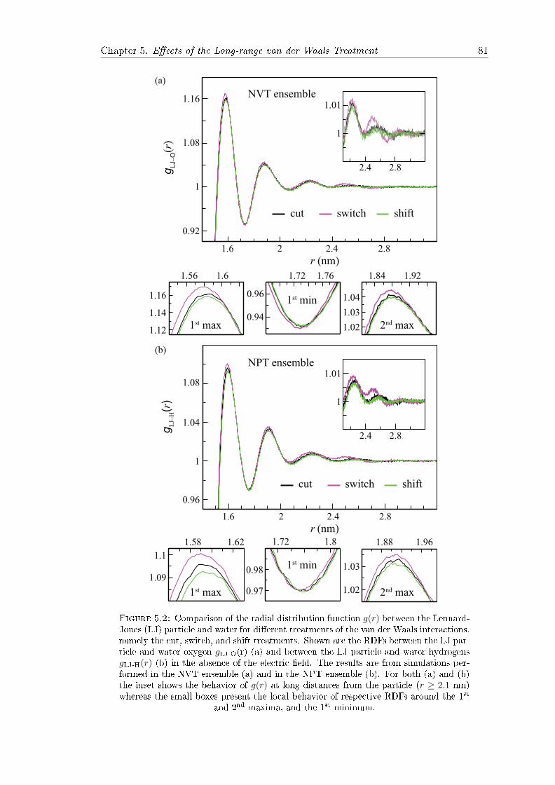
Chapter 5. Eects of the Long-range van der Waals Treatment 81
1.6 2 2.4 2.8
r (nm)
0.92
1
1.08
1.16
gLJ−O(r
)
cut switch shift
2.4 2.8
1
1.01
1.56 1.6
1.12
1.14
1.16
1.72 1.76
0.94
0.96
1.84 1.92
1.02
1.03
1.04
1st max
1st min
2nd max
1.6 2 2.4 2.8
r (nm)
0.96
1
1.04
1.08
gL
J−H(r)
2.4 2.8
1
1.01
1.58 1.62
1.09
1.1
1.72 1.8
0.97
0.98
1.88 1.96
1.02
1.03
1st max
1st min
2nd max
cut switch shift
(b)
(a)
NPT ensemble
NVT ensemble
Figure 5.2: Comparison of the radial distribution function g(r) between the Lennard-Jones (LJ) particle and water for dierent treatments of the van der Waals interactions,namely the cut, switch, and shift treatments. Shown are the RDFs between the LJ par-ticle and water oxygen gLJ-O(r) (a) and between the LJ particle and water hydrogensgLJ-H(r) (b) in the absence of the electric eld. The results are from simulations per-formed in the NVT ensemble (a) and in the NPT ensemble (b). For both (a) and (b)the inset shows the behavior of g(r) at long distances from the particle (r ≥ 2.1 nm)whereas the small boxes present the local behavior of respective RDFs around the 1st
and 2nd maxima, and the 1st minimum.

Chapter 5. Eects of the Long-range van der Waals Treatment 82
that these correlations, although small, are unphysical is the appearance of more negative
correlations (g < 1) at the position of the fourth minimum than at the third minimum.
Furthermore, even though the vdW force is identical for r < r1 in all three approaches
(see Fig. 2.1), the perturbation imposed in the transition region propagates towards
the hydrophobic object and manifests in subtle changes of water structure closer to the
hydrophobic object, as evidenced in the small graphs in the lower rows of each panel in
Fig. 5.2 representing gLJ-O(r) and gLJ-H(r) around the 1st and 2nd maxima, as well as the
1st minimum. Furthermore, this increase of the correlations with the switch treatment
is independent of the version of GROMACS and the precision at which the simulation is
executed.
It is important to stress that similar spurious correlations were not found in any
of the water-water RDFs (i.e., gOO, gHH, and gOH), supposedly because the employed
cutos are too large to have impact on the correlations of the much smaller solvent
molecules. However, even with transition regions at much shorter distances (0.6 − 0.9
nm, 0.7 − 1.0 nm, 0.9 − 1.2 nm, 1.5 − 1.8 nm), the described increase of correlations
was not found in the RDFs of the water molecules in simulations of a pure water box
1.6 2 2.4 2.8
r (nm)
0.92
1
1.08
1.16
gL
J-O(r
)
2.4 2.8
1
1.01
1.84 1.92
1.03
1.04
1.05
1.7 1.74
0.92
0.93
0.94
1.54 1.58
1.18
1.19
1.2
1st max
1st min
2nd max
cut switch shift
Figure 5.3: Comparison of the radial distribution function g(r) between the LJ par-ticle and water oxygen for the cut, switch and shift treatments of the van der Waalsinteractions. Inset: the behavior of g(r) at long distances, r ≥ 2.1 nm. Bottom row:the local behavior of g(r) at the positions of 1st and 2nd maxima, and 1st minimum,respectively. The results are for the simulations performed in the NVT ensemble in the
presence of external electric elds, E = 0.6 V nm−1.
Chapter 5. Eects of the Long-range van der Waals Treatment 83
and the switch treatment. This is presumably because at these distances the dominant
interactions between water molecules are of Coulomb type.
In the presence of the electric eld which breaks the otherwise present isotropic
nature of the system an averaging over two spatial coordinates respecting azimuthal
symmetry should be performed to fully resolve the distribution of water at the interface.
This analysis is presented in the next chapter and all RDFs presented herein are generated
in the radially averaged fashion. However, these one-dimensional RDFs still contain the
relevant information. In Fig. 5.3 are shown the RDFs gLJ-O for all considered treatments
of the vdW interactions in the NVT ensemble in the presence of external electric elds.
Although we only present data obtained in the NVT ensemble for gLJ-O, identical results
are obtained for gLJ-H in the NVT ensemble as well as in the NPT ensemble for both gLJ-Oand gLJ-H. Clearly, when the vdW interactions are treated with the switch function, the
same increase of structuring as in the absence of the eld can be seen. Such an observation
is in agreement with previous results on the treatment of electrostatic interactions with
an atom-based switch function [230]. Therein, it was shown that such an electrostatic
switch treatment induces articial dipolar ordering of water in the transition region [110].
It is clear that dierent treatments of vdW interactions indeed induce subtle
changes of the water structure around a hydrophobic object. However, it is not clear if
these small dierences can be related to the potentially dierent mobilities of LJ particles
in water. To see these eects, we further study the dynamics of the system.
5.3 Observed Time-dependent Displacement of the
LJ Particle
We rst investigate the time-dependent displacement ∆ of the LJ particle both in the
presence and absence of a static electric eld (Fig. 5.4). At zero eld, the average
displacement, 〈∆〉 = (∆x + ∆y + ∆z)/3, is fully comparable to a trajectory along a
particular coordinate. In the presence of the electric eld, we focus on the displacement
along the x axis which coincides with the direction of the eld.
Figure 5.4 summarizes the results for both the NVT and the NPT ensembles and all
three treatments of vdW interactions. Independently of the ensemble, the majority of the
displacement curves show a strong resemblance to trajectories expected from a particle
exhibiting Brownian motion. This is expected since in Chapter 4 was demonstrated that
the LJ particle of this size can be regarded as a Brownian particle. The switch treatment
provides an analogous behavior to the shift, despite the slight dierences in the static
organization of interfacial waters (see Figs. 5.2 and 5.3). On the time scale of 100 ns,
the displacements observed with these two treatments in the presence of the eld are
almost indistinguishable from those at zero eld. The exception is the supercially small

Chapter 5. Eects of the Long-range van der Waals Treatment 84
−40
−30
−20
−10
0
10
Dis
pla
cem
ent
(nm
)
cut
switch
shift
E0
= 0 V nm−1
40 60 80
−40
−30
−20
−10
0
40 60 80
t (ns)
0 20 0 20
E0 = 0.6 V nm−1
NVT ensemble
NPT ensemble
Figure 5.4: The displacement of the LJ particle in the absence (left) and the presenceof static electric elds (right). In the absence of electric elds the average displacementover three Cartesian directions is shown. In the presence of electric elds the displace-ment in the eld direction (imposed in the +x direction) is shown. In the upper andlower row are data for the NVT and the NPT ensemble, respectively. The total sim-ulation time for each setup is 100 ns. The dashed black lines are the linear ts of thedisplacement to illustrate the unidirectionality of the movement of the Lennard-Jones
particle.
preference to move in a direction opposite to the eld, which is an eect that is not
considered to be statistically relevant at these times scales. However, a stark contrast
can be seen in the displacements under the eld when using the truncated vdW forces.
These curves show a linear drift superimposed on the Brownian displacement, which is
suggestive of a net force acting on the particle. We nd eld-induced velocities of the
LJ particle of −0.45 m s−1 (NVT) and −0.41 m s−1 (NPT), obtained from linear ts
(dashed lines) to the respective data sets.
Comparable velocities were found in several previous studies with the cut treatment
on similar systems [65, 7174]. The latter was declared spurious after no net movement
(or water ux) was found on comparable time scales when the shift method was employed
with the eld [72, 74]. Actually, a non-zero ux of water molecules through a carbon
nanotube [73] was observed for the cut treatment even in the absence of the electric eld.
Here, a particular displacement of the LJ particle is not observed in the absence of the
externally applied electric eld. Therefore, the reported ux seems to be related to the
particularity of the investigated system.
Apart from the cut-o treatment, other parameters such as the time step, the

Chapter 5. Eects of the Long-range van der Waals Treatment 85
40 60 80
t (ns)
−40
−30
−20
−10
0
Dis
pla
cem
ent
(nm
)
0 20
BT, NLUF = 10
BT, NLUF = 1
VR, NLUF = 10
VR, NLUF = 1
Figure 5.5: The displacement of the LJ particle in the direction of the imposedstatic electric eld, Ex = 0.6 V nm−1. The simulations are performed in the NVTensemble and the vdW interactions are represented by the cut scheme. Legend: BT -Berendsen thermostat, VR - velocity rescale, NLUF - neighbour list update frequency
(# timesteps).
neighbour list update frequency (NLUF) or the Berendsen thermostat (BT) were sug-
gested to induce unphysical motion of water around a hydrophobic object in GROMACS,
although these results were based on relatively short simulations [72]. We test these pa-
rameters (BT, NLUF) in a set of 100 ns long simulations (cut treatment, NVT ensemble,
and E = 0.6 V nm−1), and show the results in Fig. 5.5, alongside the reference setup
(BT, NLUF = 10). A constant negative drift velocity is observed for each setup, while
the dierence between the curves is within the expected statistical noise. The insensi-
tivity of the drift motion on the NLUF indicates that the water molecules positioned
around rc, that actually contribute to the update of the neighbor list of the LJ particle,
do not cause the drift. Thus, the mechanism that drives the net movement of the LJ
particle in a direction opposite to the eld is most likely related to the solute-solvent in-
terface eects. Additionally, very similar displacements are obtained with the advanced
velocity rescaling (VR) algorithm [97] (−0.39 m s−1 for NLUF = 10 and −0.46 m s−1
for NLUF = 1) and the Berendsen algorithm (−0.45 m s−1 for NLUF = 10 and −0.35
m s−1 for NLUF = 1). Hence, the observed eld induced mobility can not be assigned
to the imperfections of the Berendsen thermostat, which does not rigorously reproduce
a correct thermodynamic ensemble [231].
In the above discussion it is irrefutably demonstrated that the use of both the
Berendsen thermostat and NLUF = 10 is not the cause of the unidirectional mobility of
the LJ particle opposite to the eld. Therefore, for this standard simulation setup (BT,
NVT ensemble, NLUF = 10), we investigate the sensitivity of the observed mobility to
the cuto radius rc and the system size. In each case a short simulation of 20 ns is
performed. The results are summarized in Fig. 5.6. In all cases, even on these short
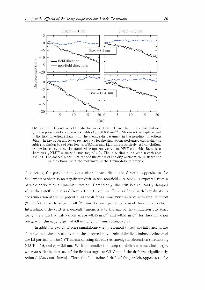
Chapter 5. Eects of the Long-range van der Waals Treatment 86
−20
−15
−10
−5
0
5
0 5 10 15 20−20
−15
−10
−5
0
0 5 10 15 20
t (ns)
Dis
pla
cem
ent
(nm
) field direction
non-field directions
Box = 12.4 nm
Box = 8.9 nm
cutoff = 2.1 nm cutoff = 2.8 nm
Figure 5.6: Dependence of the displacement of the LJ particle on the cuto distancerc in the presence of static electric elds (Ex = 0.6 V nm−1). Shown is the displacementin the eld direction (black) and the average displacement in the non-eld directions(blue). In the upper and lower row are data for the simulations performed employing thecubic simulation box of edge length of 8.9 nm and 12.4 nm, respectively. All simulationsare performed by using the standard setup: cut treatment, NVT ensemble, Berendsenthermostat, NLUF = 10, and time step of 2 fs. The total simulation time in each caseis 20 ns. The dashed black lines are the linear ts of the displacement to illustrate the
unidirectionality of the movement of the Lennard-Jones particle.
time scales, the particle exhibits a clear linear drift in the direction opposite to the
eld whereas there is no signicant drift in the non-eld directions as expected from a
particle performing a Brownian motion. Remarkably, the drift is signicantly damped
when the cuto is increased from 2.1 nm to 2.8 nm. This is related with how drastic is
the truncation of the LJ potential as the drift is almost twice as large with smaller cuto
(2.1 nm) than with larger cuto (2.8 nm) for each particular size of the simulation box.
Interestingly, the drift is apparently insensitive to the size of the simulation box (e.g.,
for rc = 2.8 nm the drift velocities are −0.45 m s−1 and −0.51 m s−1 for the simulation
boxes with the edge length of 8.9 nm and 12.4 nm, respectively).
In addition, two 20 ns long simulations were performed to test the inuence of the
time step and the eld strength on the observed magnitude of the eld-induced velocity of
the LJ particle, in the NVT ensemble using the cut treatment, the Berendsen thermostat,
NLUF = 10, and rc = 2.8 nm. With the smaller time step the drift was somewhat larger,
whereas with the decrease of the eld strength to 0.3 V nm−1 the drift was signicantly
reduced (data not shown). Thus, the eld-induced drift of the particle opposite to the
Chapter 5. Eects of the Long-range van der Waals Treatment 87
eld direction is proportional with the severity of the truncation of the LJ potential and
the eld strength while being insensitive on the general simulation parameters (time step,
thermostat, employed ensemble, NLUF or the system size).
5.3.1 Observed Time-dependent Displacement of the Oil Droplet
In similar manner, as in the case of the LJ particle we investigate the time-dependent
displacement of the center-of-mass of the heptane droplet in the presence of electric elds
(again of strength of 0.6 V nm−1). As elaborated in the computational details (Sec. 5.1),
the model oil droplet is the aggregate of 64 heptane molecules [65]. In the absence of
the electric eld the latter has, on average, a spherical shape with a radius of 1.5 nm
that is comparable to the LJ particle. Moreover, the interest is concentrated primarily
on the response of the oil droplet when the forces are abruptly truncated. Thereby, the
short simulations (20 ns) in the NVT ensemble employing the reference setup (Berendsen
thermostat, NLUF = 10, time step of 2 fs) are undertaken and the dependence of the
displacement on the cuttof radius and the system size is measured.
The results are presented in Fig. 5.7. What immediately strikes is the remark-
able resemblance to the time-dependent displacement observed for the LJ particle (see
Figs. 5.4, 5.5 and, especially, 5.6). During the inspected time interval of 20 ns, the av-
erage displacement in the non-eld directions remains around zero and is comparable
to that of the LJ particle. Thereby, the movement of the droplet can be regarded as
Brownian in the non-eld directions. Irrespective of the simulation setup, even on these
short time scales, the heptane droplet displays clear preference to move opposite to the
direction of the electric eld. This preference is indicated by the pronounced linearity
of the displacement and supported by the linear ts (dashed lines) of the displacements
that very nicely follow the simulation data.
The heptane droplet exhibits exactly the same dependence on the value of cuto
radius and the system size as was found for the LJ particle. The eld-induced velocity
of the heptane droplet in the eld direction is strongly reduced by increasing the cuto
radius from 1 nm to 1.5 nm (from −1.36 m s−1 to −0.51 m s−1 for the box with the edge
length L = 8.9 nm, and from −1.18 m s−1 to −0.55 m s−1 for L = 14.1 nm), whereas it
is apparently unaected by the size of simulation cell. Interestingly, the observed drift
for the oil droplet with rc = 1.5 nm (−0.51 m s−1 and −0.55 m s−1 for L = 8.9 nm
and L = 14.1 nm, respectively) is virtually the same as the drift observed for the LJ
particle with rc = 2.8 nm (−0.45 m s−1 and −0.51 m s−1 for L = 8.9 nm and 12.4
nm, respectively). This stunning reproducibility of the eld-induced drift between the
LJ particle and the heptane droplet indicates that the surface roughness and/or shape
uctuations are not likely the crucial factors in the eld-induced drift in which the overall
size of a hydrophobic object appears to be very important. Moreover, these observations

Chapter 5. Eects of the Long-range van der Waals Treatment 88
−30
−20
−10
0
5 10 15−30
−20
−10
0
0 5 10 15 20
Box = 14.1 nm
Box = 8.9 nm
Dis
pla
cem
ent
(nm
)
field direction
non-field directions
cutoff = 1 nm cutoff = 1.5 nm
t (ns)
Figure 5.7: Dependence of the displacement of the center-of-mass of the heptanedroplet on the cuto distance rc in the presence of static electric elds (Ex = 0.6V nm−1). Shown is the displacement in the eld direction (black) and the averagedisplacement in the non-eld directions (blue). In the upper and lower row are data forthe simulations performed employing the cubic simulation box of edge length of 8.9 nmand 14.1 nm, respectively. All simulations are performed by using the standard setup:cut treatment, NVT ensemble, Berendsen thermostat, NLUF = 10, and time step of2 fs. The total simulation time in each case is 20 ns. The dashed black lines are thelinear ts of the displacement to illustrate the unidirectionality of the movement of the
oil droplet.
strongly support the LJ particle as the model of a hydrophobic object which does not
suer from disadvantages like the surface roughness and/or shape uctuations (as, for
example, the heptane droplet) that considerably complicate the theoretical description,
the data analysis, and the construction of plausible hypothesis explaining the underlying
mechanism [65, 69]. Thus, in the remainder of this chapter and in the subsequent one,
the attention will be heavily directed to simulations with the LJ particle.
5.3.2 Brownian Diusion of the LJ Particle
To elucidate the origin of the observed drift, we rst analyze the underlying Brownian
displacement and determine the diusion coecient D of the LJ particle. To minimize
the mass dependence of the diusion coecient of the LJ particle all simulations have
been performed with the Lennard-Jones particle of mass M = 50 amu. The particle of
this mass has been found to be apparently in the hydrodynamic regime for the system
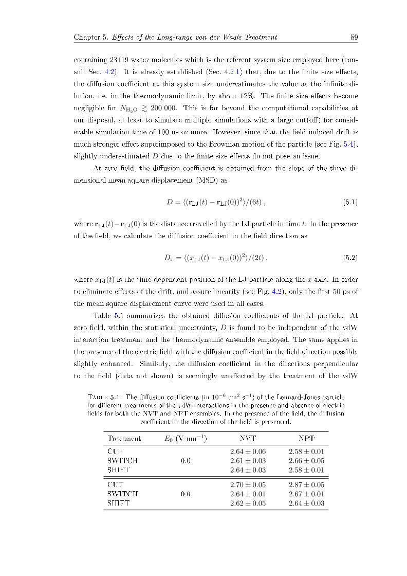
Chapter 5. Eects of the Long-range van der Waals Treatment 89
containing 23419 water molecules which is the referent system size employed here (con-
sult Sec. 4.2). It is already established (Sec. 4.2.1) that, due to the nite size eects,
the diusion coecient at this system size underestimates the value at the innite di-
lution, i.e. in the thermodynamic limit, by about 12%. The nite size eects become
negligible for NH2O& 200 000. This is far beyond the computational capabilities at
our disposal, at least to simulate multiple simulations with a large cut(o) for consid-
erable simulation time of 100 ns or more. However, since that the eld-induced drift is
much stronger eect superimposed to the Brownian motion of the particle (see Fig. 5.4),
slightly underestimated D due to the nite size eects do not pose an issue.
At zero eld, the diusion coecient is obtained from the slope of the three di-
mensional mean square displacement (MSD) as
D = 〈(rLJ(t)− rLJ(0))2〉/(6t) , (5.1)
where rLJ(t)−rLJ(0) is the distance travelled by the LJ particle in time t. In the presence
of the eld, we calculate the diusion coecient in the eld direction as
Dx = 〈(xLJ(t)− xLJ(0))2〉/(2t) , (5.2)
where xLJ(t) is the time-dependent position of the LJ particle along the x axis. In order
to eliminate eects of the drift, and assure linearity (see Fig. 4.2), only the rst 50 ps of
the mean square displacement curve were used in all cases.
Table 5.1 summarizes the obtained diusion coecients of the LJ particle. At
zero eld, within the statistical uncertainty, D is found to be independent of the vdW
interaction treatment and the thermodynamic ensemble employed. The same applies in
the presence of the electric eld with the diusion coecient in the eld direction possibly
slightly enhanced. Similarly, the diusion coecient in the directions perpendicular
to the eld (data not shown) is seemingly unaected by the treatment of the vdW
Table 5.1: The diusion coecients (in 10−6 cm2 s−1) of the Lennard-Jones particlefor dierent treatments of the vdW interactions in the presence and absence of electricelds for both the NVT and NPT ensembles. In the presence of the eld, the diusion
coecient in the direction of the eld is presented.
Treatment E0 (V nm−1) NVT NPT
CUT 2.64± 0.06 2.58± 0.01SWITCH 0.0 2.61± 0.03 2.66± 0.05SHIFT 2.64± 0.03 2.58± 0.01
CUT 2.70± 0.05 2.87± 0.05SWITCH 0.6 2.64± 0.01 2.67± 0.01SHIFT 2.62± 0.05 2.64± 0.03

Chapter 5. Eects of the Long-range van der Waals Treatment 90
interactions.
It is worth noting that the measured diusion coecients were not sensitive to the
version of GROMACS and most of the results fall within the statistical signicance of one
another. Although the system is not big enough to be in the rigorous thermodynamic
limit (see Sec. 4.2.1) where the averages of macroscopic observables become identical
in the two ensembles the system is large enough such that the dierence between the
NVT and NPT ensembles borders with the statistical accuracy. Thus, the two ensembles
appear indistinguishable.
5.4 The Net van der Waals Force on the LJ Particle
The linear displacement with the cut approach is indicative of a static net force acting
on the particle. As the LJ particle carries no charge, it is dicult to envisage a simple
electrostatic force. The only remaining possibility is a force originating in vdW interac-
tions, which is further supported by the sensitivity of the mobility to the vdW treatment.
We thus calculate the instantaneous total van der Waals force FvdW(t) in each Cartesian
direction exerted on the LJ particle by the solvent, by adding the contributions from all
water molecules found within the cut(o) radius rc. The net vdW force is taken to be
the time average of instantaneous forces
〈F vdWi 〉 =
1
Nfr
Nfr∑j=1
Nw∑k=1
F vdWi (rkj ; rkj < rc) , i ≡ x, y, z (5.3)
where Nfr is the total number of frames (system congurations) analyzed and equals 500
000 in each case, Nw is the total number of water molecules present in the system, and
rkj is the relative position of the oxygen atom (position of the vdW interaction site) of
water molecule k with respect to the position of the LJ particle at time frame j. The
specicity of the van der Waals treatment (cut, switch, shift) employed in each particular
setup is taken into account by using an appropriate expression for the force (for detailed
description see Sec. 2.5).
Table 5.2 shows the calculated net vdW forces in each Cartesian direction on the
LJ particle. In the absence of the external electric eld, independent of the treatment of
the vdW interactions and the thermodynamic ensemble, the net force in each Cartesian
direction is eectively zero. This is consistent with the observed lack of net drift of the
LJ particle. Similarly, with the switch and shift treatment at E0 = 0.6 V nm−1 the net
force remains eectively zero in all directions, as well as for the cut treatment in the
o-eld directions.
Strikingly, in the eld direction we nd a signicant net force of ≈ −6.6 pN acting
on the LJ particle. From Fig. 5.8 we observe that this force is quickly converging and

Chapter 5. Eects of the Long-range van der Waals Treatment 91
Table 5.2: The net van der Waals (vdW) force on the Lennard-Jones particle in eachCartesian direction for dierent treatments of the vdW interactions in the presence and
absence of static electric elds imposed in the +x direction.
NVT ensemble
Treatment E0 (V nm−1) 〈F vdWx 〉 (pN) 〈F vdW
y 〉 (pN) 〈F vdWz 〉 (pN)
CUT −0.02±0.07 −0.02±0.06 0.00±0.02SWITCH 0.0 −0.05±0.06 −0.01±0.15 0.05±0.08SHIFT −0.02±0.06 0.00±0.09 0.01±0.11
CUT −6.59±0.04 0.07±0.09 0.02±0.07SWITCH 0.6 −0.03±0.09 −0.04±0.11 0.01±0.13SHIFT 0.03±0.06 0.01±0.07 −0.02±0.08
NPT ensemble
CUT −0.01±0.07 −0.02±0.10 0.01±0.05SWITCH 0.0 0.03±0.04 0.02±0.15 0.01±0.13SHIFT 0.01±0.08 0.07±0.11 0.01±0.08
CUT −6.62±0.06 −0.03±0.15 0.04±0.11SWITCH 0.6 0.03±0.08 −0.02±0.02 0.05±0.13SHIFT 0.03±0.05 −0.01±0.13 0.02±0.10
exhibits a standard deviation of about 0.3 pN. While this force appears large, it is of
a similar magnitude to that exerted by a motor molecule on vesicular cargo. In the
aqueous context, this force is about the same as the one acting between the LJ particle
and a single water molecule at a distance of about 1.6 nm. Importantly, the magnitude
40 60 80
t (ns)
−8
−6
−4
−2
0
2
Fx (
pN
)
NVT ensemble
40 60 80
NPT ensemble
0 20 0 20
cut
switch
shiftE
x = 0.6 V nm−1
Figure 5.8: The time dependence of the net van der Waals force exerted by the solvent(water) on the Lennard-Jones particle in the direction of the applied external electriceld (x) of strength 0.6 V nm−1. The shown forces are obtained by performing therunning average of length 1 ns on the set of (instantaneous) forces saved and calculatedevery 0.2 ps. The results are shown both for the simulations performed in the NVT
(left) and NPT ensemble (right).

Chapter 5. Eects of the Long-range van der Waals Treatment 92
of this force is not related to the version of GROMACS, and is only associated with the
cut treatment of the vdW interactions. This is evidenced by the mean force of about
−6.6 pN determined in simulations with the standard setup in all studied versions of
GROMACS (i.e., 3.3.3, 4.5.5, and 4.6.4). In addition, test simulations performed with
double precision did not aect the result. The observed force with the cut treatment
was again −6.5 ± 0.1 pN, whereas the force was vanishing with the shift and switch
treatments.
In a more detailed analysis, we nd that reported vdW forces in Table 5.2 are
generated by water molecules belonging to the rst two hydration shells while the con-
tribution from waters in the transition region (2.4 nm ≤ r ≤ 2.8 nm) conforms to a
Gaussian distribution with zero mean. This is true for all setups, including the ones
with the switch treatment. To exemplify this, Fig. 5.9 shows the probability density
functions of the force contribution from the transition region to the total vdW force
on the LJ particle for the switch treatment (NVT ensemble) at Ex = 0.6 V/nm. The
anisotropy induced by the electric eld imposed in the +x direction can be seen in
slightly dierent force distributions between the eld direction and non-eld directions
−20 −10 20
FvdW
(pN)
0
0.02
0.04
0.06
Pro
bab
ilit
y d
ensi
ty
(1/p
N)
field direction
non-field directions
100
Figure 5.9: Probability density of the contribution to the total van der Waals forceon the Lennard-Jones particle arising from the transition region, 2.4 nm ≤ r ≤ 2.8nm. The results are obtained from the NVT simulations in the presence of the elec-tric eld (Ex = 0.6 V/nm) with the switch treatment of the vdW interactions. Thedistributions of the instantaneous force contribution in the eld direction and in thenon-eld directions (average over y and z directions) are shown by black and cyan sym-bols, respectively. The Gaussian ts of the distributions are displayed by dashed orange(eld direction) and dashed red (non-eld directions) lines. The vertical dashed line atF vdW = 0 is just eye guideline to visualize the symmetry of the distribution around
zero mean force.

Chapter 5. Eects of the Long-range van der Waals Treatment 93
(y, z). However, both distributions can be excellently tted with a Gaussian distribution
having eectively zero mean. This again demonstrates that the observed mobility of the
LJ particle is a phenomena related to the interfacial ordering of water.
Analogous analysis to that shown in Fig. 5.9 can be performed by using the total
vdW force generated by water molecules inside rc. From the obtained Gaussian ts a
mean value of the vdW force in each Cartesian direction can be extracted. Indeed, it
is found that all values presented in Table 5.2, obtained by employing Eq. 5.3, can be
recovered from Gaussian ts with discrepancy of at most 0.2 pN. However, since the
instantaneous vdW forces uctuate between −1200 and 1200 pN the force distributions
are wide and it is hard to visualize the shift of the mean from 0 to −6.6 pN. Therefore,
to retain simplicity and clarity these graphics are not shown here.
5.4.1 Consistency Between the Evaluated vdW Force and the Ob-
served Drift
If the evaluated force observed with the cut treatment is consistent with the observed
drift velocity, the Stokes law should apply
〈F vdWi 〉 = ξi · vi . (5.4)
Here vi is the drift velocity in the direction i of the net force acting on the particle. The
proportionality constant ξ is the friction coecient and is simply related to the diusion
constant by the Einstein relation ξi = kBT/Di (for more details see Sections 4.3 and
4.4).
Using Eq. 5.4, with Dx from Table 5.1, and 〈F vdWx 〉 from Table 5.2, for the cut
treatment under the eld, the predicted drift velocities are −0.43 m s−1 and −0.46 m s−1
for the standard setup of parameters in the NVT and the NPT ensemble, respectively.
This is in exceptional agreement with the eld-induced drift observed in the simulations
of −0.45 m s−1 (NVT) and −0.41 m s−1 (NPT). The small dierence between the
predicted and the observed drift velocity can be attributed to the intrinsically present
thermal noise resulting from the Brownian motion of the LJ particle. This agreement
clearly demonstrates that the observed eld-induced mobility of a hydrophobic object is
a result of a uctuating but, on average, non-zero force that is produced by truncating
the vdW forces. This force is directly related to the eld strength, as evidenced by its
decrease to −4.99± 0.03 pN at the eld strength of 0.3 V nm−1.
Consistent with the observed drifts discussed in previous sections, it is found that
the average net vdW force on the LJ particle in the eld direction for the cut treatment to
be independent of the chosen thermostat and NLUF employed. The forces obtained for
the test set of simulations in the NVT ensemble (see Fig. 5.5) are: −6.7±0.1 (VR, NLUF
= 10), −6.61± 0.07 (VR, NLUF = 1), and −6.58± 0.05 pN (BT, NLUF = 1). This is in

Chapter 5. Eects of the Long-range van der Waals Treatment 94
excellent agreement with 〈F cutx 〉 = −6.59±0.04 pN obtained for the standard setup (BT,
NLUF = 10). Naturally, the calculated vx arising from the 〈F vdWx 〉 (between −0.43 m s−1
and −0.46 m s−1) agrees well with the observed induced eld velocities (between −0.35 m
s−1 and −0.46 m s−1). With the increase of the system size to NH2O= 63596 we obtain
〈F cutx 〉 = −6.72±0.03 pN which is, expectedly, almost the same as in the smaller system.
The smaller time step of 1 fs slightly increases the net force to −7.0 ± 0.3 pN, which
is in agreement with the somewhat larger drift velocity observed. Since the diusion
coecient Dx is eectively independent of the simulation setup (data not shown), this
data demonstrates that the average net vdW force found on the hydrophobic object is
exclusively related to the cut treatment of the vdW interactions.
5.5 The Eects of the Thermostat and the Flying Ice Cube
Eect
In a number of experimental realizations of electrophoretic experiments, the total number
of particles is preserved and the overall system is canonical. Consequently, only the
average total energy is preserved. One can introduce this to molecular dynamics by
the application of appropriate thermostats, which modify the Newtonian MD scheme
such that a statistical ensemble is generated at a constant temperature. However, it
is well documented that inappropriate choices of thermostats may signicantly aect
the uctuations in the system and, in some cases, induce energy drifts caused by the
accumulation of numerical errors [232, 233].
To study these eects in our system, we have performed a set of simulations in a
standard setup with dierent thermostats at 300 K. The instantaneous velocity vx(LJ)
along the direction of the imposed eld is sampled for 10 ns. Since the system is expected
to be canonical, this distribution should be a Gaussian identical to the one-dimensional
Maxwell-Boltzmann distribution of velocities,
fv(vi) =
(M
2πkBT
)1/2
exp
(− Mv2i
2kBT
), i ≡ x, y, z , (5.5)
of a colloid with a mass associated with the LJ particle, generated at 300 K (symbols in
Fig. 5.10(a)).
Since it is expected that the canonical nature of the system is best reproduced by a
Langevin thermostat, we perform Langevin dynamics simulations [227]. In this stochas-
tic but ergodic scheme, each particle is coupled to a local heat bath, which removes heat
trapped in localized modes. While the momentum transfer in such simulations is de-
stroyed, making the diusion coecients inaccessible with this thermostat, the canonical
distribution is obtained accurately, as evidenced in Fig. 5.10.

Chapter 5. Eects of the Long-range van der Waals Treatment 95
−600 −300 0 300 600
vx(LJ) (m s−1)
0
0.5
1
1.5P
robab
ilit
y d
ensi
ty (10−3 s
m−1)
BTVR
NHLD
MB distribution
−600 −300 0 300 600
vx(LJ) (m s−1)
(a) (b)
BT-shiftBT-cut
LD-cutLD-shift
Figure 5.10: (a) Comparison of the distribution of the instantaneous velocity (savedat every step for 10 ns) of the LJ particle in the direction of the imposed static electriceld, Ex = 0.6 V nm−1 with the shift treatment. The simulations were performed withthe Berendsen thermostat (BT), advanced velocity rescaling (VR), Nosé-Hoover (NH),and by Langevin dynamics (LD). The expected Maxwell-Boltzmann distribution (MB)is shown with symbols. (b) Comparison of the cut (dashed lines) and shift (full lines)
treatments with the Berendsen (black) and the Langevin thermostats (orange).
In the context of Newtonian dynamics, an attractive and elegant thermostat is
that of Nosé-Hoover [98, 99]. It is deterministic, time reversible and in principle canoni-
cal (extra degree of freedom acts as thermal reservoir), but sometimes computationally
demanding. However, when the system is poorly ergodic, this approach may become
dicult and a chain of thermostats may have to be imposed. However, this does not
seem to be the case in the current simulations, and an excellent agreement with the
canonical distribution is obtained (Fig. 5.10(a)). An equally good agreement with the
Maxwell-Boltzmann distribution is obtained with the advanced velocity rescaling method
[97], within which the target temperature is drawn from the canonical probability distri-
bution, to produce the correct ensemble.
We compare the performance of these canonical thermostats to the commonly
used Berendsen weak coupling scheme [101]. The Berendsen approach gained popular-
ity because of its robustness, speed and easy implementation. The problem with this
approach is that it is not time-reversible or deterministic and the resulting distributions
do not strictly correspond to any ensemble. In practice, however, the deviations from
the canonical distribution are relatively small and decrease with increasing system size.
Specically in our system, the distribution generated with this treatment is within the
noise of distributions generated with more formal thermostats for the shift treatment
(Fig. 5.10(a)). For the cut treatment the Nosé-Hoover, the advanced velocity rescal-
ing and the Berendsen thermostats show small deviations around the maximum from
the distribution obtained with the Langevin thermostat, the latter coinciding with the
distributions obtained with the shift treatment (Fig. 5.10(b)).
The use of the Berendsen thermostat, as well as the imposition of truncation

Chapter 5. Eects of the Long-range van der Waals Treatment 96
0.5
1
1.5
2
Pro
bab
ilit
y d
ensi
ty (
10
−3 s
m−
1)
0−20 ns
20−40 ns
40−60 ns
60−80 ns
80−100 ns
−600 −400 −200 0 200 400 600
0.5
1
1.5
2
2.5
3
0−20 ns
20−40 ns
40−60 ns
Pro
bab
ilit
y d
ensi
ty (
10
−3 s
m−
1)
vx(LJ) (m s−1)
–
(a)
(b)
SHIFT
CUT
Figure 5.11: The distribution of the velocity of the LJ particle along the direction ofthe eld vx(LJ), calculated from the displacement of the LJ particle with the resolutionof 0.2 ps. The simulations were performed using the default setup (NVT, BT, NLUF= 10), with the vdW interactions treated using the shift (a) and the cut (b) approach.The distribution were generated over 5 and 3 successive intervals of 20 ns for the shiftand the cut treatments, respectively. The comparison of the results shows no timeevolution of the velocity distribution for both treatments of the vdW interactions. Thevertical dashed lines at vx(LJ) = 0 are just eye guidelines to visualize the symmetry of
the distribution.
schemes for the vdW forces is sometimes associated with localized and unwanted corre-
lated motions. Spurious drifts may appear due to the transfer of energy from fast to slow
degrees of freedom, which is known as the ying ice cube eect. There are several steps
which help in avoiding this eect, including the use of the here chosen Verlet algorithm
to propagate the system. Since this algorithm is time reversible, it is associated with
little or no long-term energy drain. Furthermore, it is important to remove all motion
of the center of mass of the system (translational and rotational) which we perform in
Chapter 5. Eects of the Long-range van der Waals Treatment 97
each molecular dynamics step [232]. Beside making relevant choices in setting the sim-
ulations, one can test for the ying ice cube eect a posteriori, by carefully analyzing
the entirety of the data, as discussed below.
Several arguments can be used to support our interpretation that the drift velocity
is associated with the net force acting on the particle, and not with the ying ice cube
eect. The rst is that employed system reproduces the canonical distribution very
well. Its size is such that the thermodynamic limit is approached in the sense that
dierences between system averages in the NVT and the NPT ensembles are basically
within the statistical accuracy. Furthermore, the same results (net force on the particle as
a function of the treatment of the van der Waals forces) are obtained independently of the
thermostat. Specically, in a set of 10 ns long simulations, we obtain a net average force
in the direction of applied electric eld of −6.7±0.2 pN, −6.5±0.1 pN, and −6.6±0.3 pN
with the Berendsen, the advanced velocity rescaling and the Nosé-Hoover thermostats,
respectively. Even the Langevin dynamics yields an average force of −6.9 ± 0.3 pN
with the cut treatment. On the other hand the shift treatment always leads to zero
force, independently of the thermostat and the integration algorithm. Furthermore, the
obtained drift is fully consistent with the observed force, which only occurs with the cut
treatment.
While we are able to condently associate the spurious motion of the LJ particle
in the electric eld to the cut treatment of the vdW interaction, slow energy transfer
could still be possible on even larger time scales. To exclude this, we test for the slow
draining of the kinetic energy into the translational degrees of freedom of the particle,
by checking its velocity distribution generated in intervals of 20 ns over 100 ns (original
protocol, Fig. 5.11). Here, the velocity was calculated from the actual displacement of
the LJ particle with a resolution of 0.2 ps. Importantly, the velocity distribution is fully
independent of time, with any of the treatment of the van der Waals interactions (see
Fig. 5.11 for the shift and the cut treatments), which convincingly excludes the existence
of drifts associated with ying ice cube eect in presented simulations.
5.6 Conclusions
Using a series of molecular dynamics simulations in GROMACS, we have investigated
the behavior of a solvated nanosized Lennard-Jones particle in the presence of a static
electric eld, as a function of the treatment of the long-range vdW interactions. Even
in the absence of the eld, we showed that the dierent treatments result in subtle
changes of the distribution of water molecules at the interface with the LJ particle.
These changes are not necessarily correct, as exemplied by the excessive correlations in
the transition region when the switch treatment is used. The observation of a uctuating
but non-zero vdW force on the LJ particle occurring in static electric elds with the cut

Chapter 5. Eects of the Long-range van der Waals Treatment 98
treatment can be considered in a similar way. Indeed, it is likely that similar forces
were responsible for the negative electrophoretic mobilities of hydrophobic objects, and
water uxes through carbon nanotubes, which were reported in previous studies. While
the accuracy of GROMACS was brought into question, it seems to be now clear that
these eects arise merely from the truncation of the forces, while the spread of the
previously reported results may also be associated with the relatively small system sizes
and simulation times. This is further supported by the fact, neither the artifacts in the
static radial distribution function with the switch treatment, nor the measured forces
with the cut treatment depend on the used version of GROMACS. Analogously, the
same reasoning can be used to rationalize why the shift implementation for the vdW
interactions apparently provides the most accurate results. Despite these clarications,
the subtleties in the organization of water in the rst two hydration shells, which give
rise to these eects, have yet to be properly characterized. The corresponding analysis
is presented in the following chapter.

Chapter 6
Dynamics of a Hydrophobic Object
in the Presence of Electric Fields:
Long-time Scales
6.1 Computational Details
All simulations were performed with GROMACS 4.0.5 simulation package [76]. Thereby,
a single uncharged Lennard-Jones (LJ) particle, with mass of 50 u and σ and ε parameters
of 1.5 nm and 0.8063 kJ/mol, respectively, was dissolved in a cubic box of edge length
of approximately 8.9 nm containing 23419 SPC/E [116] water molecules (see Fig. 4.1).
After the energy minimization of the system with a steepest descent algorithm the two
short (0.5 ns, NPT) MD runs were performed for the equilibration purposes. The rst
run, without the electric eld, was carried out with the pressure coupled to a target value
of P = 1 bar using the weak Berendsen scheme [101]. The second run was performed
with the same pressure coupling regime but in the presence of an external eld imposed
in the +x direction (E = 0.6 V nm−1). For the reasons of computational eciency, the
production data was collected from subsequent (NVT) simulations with the volume xed
at the equilibrium value. A typical such simulation employed a time step of 2 fs, the
LINCS algorithm [139], the particle decomposition, a reference temperature of 300 K, a
non-bonded cuto (rc) of 2.8 nm, and the Particle Mesh Ewald method [88].
In the previous chapter it was established that the excess mobility of the LJ par-
ticle in the direction opposite to the imposed electric eld is clearly a consequence of
the truncation of the van der Waals forces (vdW) and not an eect related with the
choice of thermostat or with the neighbour list update frequency (NLUF). Therefore, to
minimize the computational costs, the simulations with all three treatments of the vdW
interactions (cut, switch, and shift) were performed with the Berendsen thermostat [96]
and NLUF= 10. The total length of the simulations at Ex = 0.6 V/nm with the switch
99

Chapter 6. Long-time Scales 100
and shift treatments is 900 ns, whereas with the cut treatment is 300 ns. Additionally,
the simulations with the shift treatment in the absence of the electric eld are extended
to reach 300 ns. To guarantee an adequate time and spatial sampling for the analysis
the data was saved to disk every 100 steps with the output precision of coordinates set
to six decimal places (i.e., 0.000 001 nm).
For the qualitative comparison of the water ordering around the LJ particle and
the heptane droplet, the short simulations with the heptane droplet (see Sec. 5.3.1) are
also analyzed.
6.2 Coordinate System
To uniquely describe the distance and the orientation of the water molecules with respect
to the Lennard-Jones particle, three coordinates are required. In this work is adopted an
elegant yet simple description introduced by Smith [27] and shown in Fig. 6.1. Thereby,
the rst coordinate is the radius vector (r) connecting the center of the LJ particle with
the center of the water oxygen. The remaining two coordinates are angles which specify
the orientation of the plane of the water molecule with respect radius vector [27]. The
rst of these angles is the dipole angle (θ), dened by the center of the LJ particle, the
center of the oxygen of the water molecule, and the mid-point of the line connecting the
two hydrogen atoms (of the same water molecule). The second angle (φ) is chosen to be
the angle that a normal to the plane of the water molecule closes with the radius vector
r, in the center of the oxygen atom. Due to this denition, the second angle will be
simply called the normal angle.
The benet of this coordinate system is that it respects the internal symmetry of
the water molecule as well as the symmetry of an entire system [27]. Due to the internal
symmetry, the dipole angle ranges from 0 to 180, whereas the normal angle can assume
values ranging from 0 to 90. The same periodicity, as the angles θ and φ, have the
functions cos θ and cos2 φ, respectively. Since the sum of probabilities of all possible
orientations must equal one, the spherical functions of the rst and the second order,
P1(θ) = cos θ
P2(φ) = 3 cos2 φ− 1 ,(6.1)
are used to evaluate the angle correlation functions between the LJ particle and water.
In order to have the functions of only one variable, the spherical functions P1(θ) and
P2(φ) have to be averaged out. Thus, the total LJ particle-water correlation function
GLJ-W can be written as
GLJ-W(r, θ, φ) = GLJ-W(r, 〈P1(θ)〉, 〈P2(φ)〉) , (6.2)

Chapter 6. Long-time Scales 101
H
H
O
ϕ
θ
r
LJ
θ∈[0°,180°]
ϕ∈[0°,90°]
dipole angle
normal angle
Figure 6.1: The internal coordinate system of the Lennard-Jones (LJ) particle (gray)and a water molecule consisting of an oxygen atom (red) and two hydrogen atoms(blue). The radius vector between the center of the LJ particle and oxygen is denoted
with r.
and correlates the LJ particle with water molecules at distance r in averaged orientations
of the angles θ and φ which contribute through the average value of the spherical functions
P1(θ) and P2(φ). Note that the rst component of GLJ-W is just the radial distribution
function between the LJ particle and the oxygen atom of water. Instead of examining
the water ordering around hydrophobic object directly through the total solute-water
correlation function its each component will be examined separately to extract as much
structuring details as possible.
6.3 Radially Averaged Correlations
In this section is presented the water ordering around hydrophobic object obtained by
evaluating the components of the total solute-water correlation function in the radially
averaged fashion. The simulations are performed both in the presence and absence of
the static electric eld. Since in Sec. 5.2 the radial distribution functions (gLJ-O and
gLJ-H) at E = 0 have been discussed in details (see Fig. 5.2) we rst examine the angular
ordering around the LJ particle.
The angular correlation functions 〈P1(θ)〉 and 〈P2(φ)〉 are obtained in similar man-
ner as the radial distribution function. In a spherical shell (from r to r + ∆r, where ∆r
is the bin size), around the LJ particle in its center, the contributions of the correspond-
ing spherical functions P1(θ) and P2(φ) are added up. These sums are then normalized
with the number of particles (counts) Nc found in each spherical shell and also with the
number of time frames (system congurations) Nfr over which the counts are collected.
Chapter 6. Long-time Scales 102
This can be formally written as
〈P1(θ, rij)〉 =1
Nfr Nc
Nfr∑j=1
Nc∑i=1
(cos θ)ij
〈P2(φ, rij)〉 =1
Nfr Nc
Nfr∑j=1
Nc∑i=1
(3 cos2 φ− 1)ij ,
(6.3)
where rij has to satisfy the condition r < rij ≤ (r + ∆r).
Figure 6.2 shows the correlation functions for the dipole (θ) and the normal angle
(φ) at E = 0 for all three treatments of the vdW interactions, namely the cut, switch
and shift treatments. In the vicinity of the LJ particle both 〈P1(θ)〉 and 〈P2(φ)〉 displaypronounced negative correlations. The latter nicely reect the softness of the employed
LJ potential, i.e. the model LJ particle, as they occur exclusively in the soft-core (r <
σLJ-O). These negative correlations are followed by strong and broad maximum after
which the correlations become very weak. However, two more minima and one maximum
can be clearly discerned from the noise at large distances r & 2.4 nm. Therefore, the
angular correlations extend about 0.8 nm from the surface of the LJ particle (if the
surface is associated with the position of the 1st maximum in gLJ-O(r))1 into the water
bulk. Indeed, the same correlation length (depth) can be also found for the static density
correlation from gLJ-O(r) and gLJ-H(r).
The angular correlation functions in the absence of the eld are clearly independent
of the treatment of the vdW interactions as the curves overlap for all three investigated
treatments. Moreover, all three treatments behave exactly the same in the vicinity of
the particle. In Sec. 5.2 it was demonstrated that a perturbation in the transition region
(2.4 nm < r < 2.8 nm), induced by the switch treatment, invokes an unphysical density
correlations within the transition region that also propagate towards the surface of the
particle (see Figs. 5.2 and 5.3). Interestingly, in the transition region for the normal
angle correlations can be again noticed very weak but spurious behavior characterized
by stronger (more negative) correlations further from the hydrophobic object (see inset
of Fig. 6.2(b)). The remnants of a similar behavior in 〈P1(θ)〉 are not observed (inset
of Fig. 6.2(a)). However, this may be a mere issue of statistical nature arising from the
fact that the correlations are much more intense (almost tenfold) for the normal angle
compared to the dipole angle. This can be easily noticed by comparing the heights of
the 1st maximum in 〈P1(θ)〉 and 〈P2(φ)〉. Unfortunately, this rather low intensity of
the dipole angle correlations highlights the need for rather long simulations in order to
achieve sucient sampling also in the vicinity of the particle where the increase of the
correlations is oset by the small average number of water molecules present. Indeed,1It is convenient and informative to associate the surface of the LJ particle with the position of the 1st
maximum in gLJ-O(r), especially when comparing the water ordering around solutes of dierent size (seeRef. [27]). However, this denition should not be confused with the hydrodynamic radius (see Sec. 4.4).

Chapter 6. Long-time Scales 103
−0.18
−0.12
−0.06
0
0.06
1.6 2 2.4 2.8
r (nm)
−0.2
0
0.2
0.4
0.6
⟨P
1(θ
)⟩ ⟨P
2(ϕ
)⟩
2.4 2.8
−0.002
−0.001
0
0.001
2.4 2.8
−0.003
0
0.003
(a)
(b)
cut switch shift
Figure 6.2: The radially averaged angular correlation functions between the LJ par-ticle and water at E = 0. Shown are the correlation functions for the dipole (a) andthe normal angle (b) for all three treatments of the vdW interactions, namely thecut, switch and shift treatments. Insets: the behavior of 〈P1(θ)〉 and 〈P2(φ)〉 at long
distances, r ≥ 2.1 nm.
within the rst hydration shell of the LJ particle is found, on average, about 150 water
molecules.
In the presence of a static external electric eld (E = 0.6 V nm−1) the angular
correlations functions for various vdW treatments, as in the case of zero eld, do not
show dierences among each other and, therefore, they are not explicitly presented here.
However, the explicit impact of the eld is visualized in Fig. 6.3 by comparing the
correlation functions obtained for E = 0 and 0.6 V nm−1. The correlation functions
between the center-of-mass (COM) of the heptane droplet and water are also shown.
Figure 6.3(a) shows the radial distribution function gLJ-O(r) at zero eld strength
and when the electric eld is imposed in the x direction (Ex = 0.6 V nm−1). For the

Chapter 6. Long-time Scales 104
LJ particle (full lines) the correlations are somewhat increased under the eld compared
to those obtained at zero eld strength. The slight increase of the intensity of the rst
peak suggests a somewhat higher density of water in the rst hydration shell of the LJ
particle under the eld. In addition, both the maxima and minima in gLJ-O(r) are moved
to the left, to an extent that apparently increases with the intensity of the eld. The
eld thus shifts the water closer to the center of the LJ particle, apparently reducing the
associated excluded volume.
In the case of the heptane droplet (dashed lines) the RDFs are considerably distinct
from those found for the LJ particle.2 In the absence of electric elds the RDF (black
dashed line) is very simple, it smoothly rises and reaches the bulk density at about 1.7 nm
and afterwards remains at the same level. This loss of the local water ordering (hydration
shell structure) is the consequence of the perpetual shape uctuations of the aggregate.
The latter varies from a relatively spherical to a very elongated one (see small simulation
snapshots in Fig. 6.3(a)). Thus, even if the hydration shell structure exists it has been
erased by the shape uctuations that are of similar order in the distance as the density
correlations. Interestingly, g(r) at E = 0.6 V/nm (violet dashed line) provides more
information. The function itself is very similar to the one at zero eld, but is shifted
about 0.2 nm toward the COM of the heptane droplet and also rises more slowly to
reach the bulk density at r ≈ 2.4 nm, which is about the same range at which the water
ordering becomes unaected by the presence of the LJ particle. More importantly, the
heptane droplet adopts, on average, an ellipsoidal shape in the direction of the external
electric eld, the eect that already has been experimentally observed, for example, for
vesicles [234] and it is associated with the Maxwell stress. Due to this elongation the
average semi-axis of the heptane aggregate are dierent with one semi-axis being smaller
from the radius of the LJ particle. Thus, g(r) is shifted toward the COM of the droplet.
Figure 6.3 also shows the dipole (b) and the normal angle (c) correlation functions,
whose values at distance r are given by the mean value of P1(θ) and P2(φ) of all water
molecules found between r and r + ∆r, respectively. Surprisingly, in the absence of
the electric eld, 〈P1(θ)〉 and 〈P2(φ)〉 for the heptane droplet resemble very much those
obtained for the LJ particle. Although the ne structure after the broad and somewhat
lower 1st maximum is lost both for 〈P1(θ)〉 and 〈P2(φ)〉 the range of angular correlationsmatches with those found for the smooth LJ particle. Hence, the range of correlations
is not inuenced by the surface roughness. This also indicates, in accordance with the
conclusions drawn from the time-dependent displacement of the heptane COM (con-
sult Sec. 5.3.1), that the role of surface roughness is not crucial in the electrophoresis
of hydrophobic objects. Even more, it was already demonstrated [27] that the extent
2Although the density prole around the heptane droplet is presented for the correlations betweenthe COM of the heptane droplet and the oxygen atom of water molecules, the same message is retrievedalso for the RDF between the heptane and the hydrogen atoms. Hence, the latter is not shown to avoidunnecessary repeating.

Chapter 6. Long-time Scales 105
0
0.2
0.4
0.6
0.8
1
1.2
g(r
)
−0.2
−0.16
−0.12
−0.08
−0.04
0
0.04
1 1.5 2 2.5 3 3.5
r (nm)
−0.2
0
0.2
0.4
0.6
⟨P2(ϕ
)⟩
E = 0 V/nm E = 0.6 V/nm
full lines LJ PARTICLE
dashed lines OIL DROPLET
⟨P1(θ
)⟩
1 1.5 2 2.5 3 3.5
E
r (nm)(a)
(b)
(c)
Figure 6.3: The radially averaged correlation functions in the presence (in violet)and the absence (in black) of the electric elds for both the LJ particle (full lines)and heptane (oil) droplet (dashed lines). Shown are: the RDF (a), the dipole (b) andthe normal angle (c) correlation functions. In panel (a) are also displayed the twopredominant states of the heptane droplet. These include the spherical shape (usuallyfound at E = 0) and the elongated shape (characteristic in the presence of the electric
eld).

Chapter 6. Long-time Scales 106
of correlations is also independent of the size of the hydrophobic object. Therefore, a
conjecture can be made that the water ordering around hydrophobic object is not deter-
mined by its size (reected by the surface curvature) or the nature of the surface (smooth
or rough) since the water molecules eectively do not see an entire hydrophobic object
but only the surface, which to them always appear at (structureless).
Surprisingly, both for the LJ particle and heptane droplet there is very little
change in the correlation function of the dipole angle in response to the applied eld
(see Fig. 6.3(b)). However, 〈P1(θ)〉 for the heptane droplet shifts considerably toward
the COM of the heptane due to the already explained elongation of the droplet in the
direction of the imposed eld. In contrast, 〈P2(φ)〉 for both hydrophobic objects experi-
ences more drastic changes as considerable strengthening of the correlations is observed
but the most striking feature is the appearance of the extremely long range tail, which
extends much deeper into the bulk water than either the radial distribution function or
the dipole angle correlation function. The consequence of such a tail is a long range
eective interaction between a hydrophobic object and the water induced by the eld,
which thus necessitates the large system sizes investigated herein. For comparison, an
equivalent correlation function of neat water under a eld of 0.6 V/nm, with respect to
the center of the box (data not shown), shows no long range correlations. Hence, this
long-range eect can be uniquely associated with the presence of the hydrophobic object.
Moreover, an astonishing overlap of the tail in 〈P2(φ)〉 for the heptane droplet and the
LJ particle is another strong proof that a LJ particle is indeed an excellent model for
the studies of the hydrophobic objects. Even more, this long-ranged eld-induced corre-
lations implicate that, for suciently high volume fractions, two hydrophobic particles
in an electric eld may sense and interact with one another by means of the ordered
network of water molecules between them.
6.4 Axially Averaged Correlations
From the radially averaged curves, it is apparent that the electric eld indeed aects
the structure of the water around the hydrophobic object (see Fig. 6.3). Because the
eld (imposed in the +x direction) breaks the spherical symmetry of the hydrophobic
object-water system, one should not expect the response of the water to the eld to be
radially symmetric. To evaluate the extent of this symmetry loss, we have reconstructed
the correlation functions respecting the axial symmetry of the problem by using the
self-made code (already described in detail in Chapter 3, Sec. 3.2). In contrast to the
pure water system, where the code was used to evaluate the water RDFs (gOO, gOHand gHH), an additional functionality is implemented to the code which now calculates
all the components of the total solute-water correlation function plus, for example, the
projection of the water dipole vector onto the eld direction.
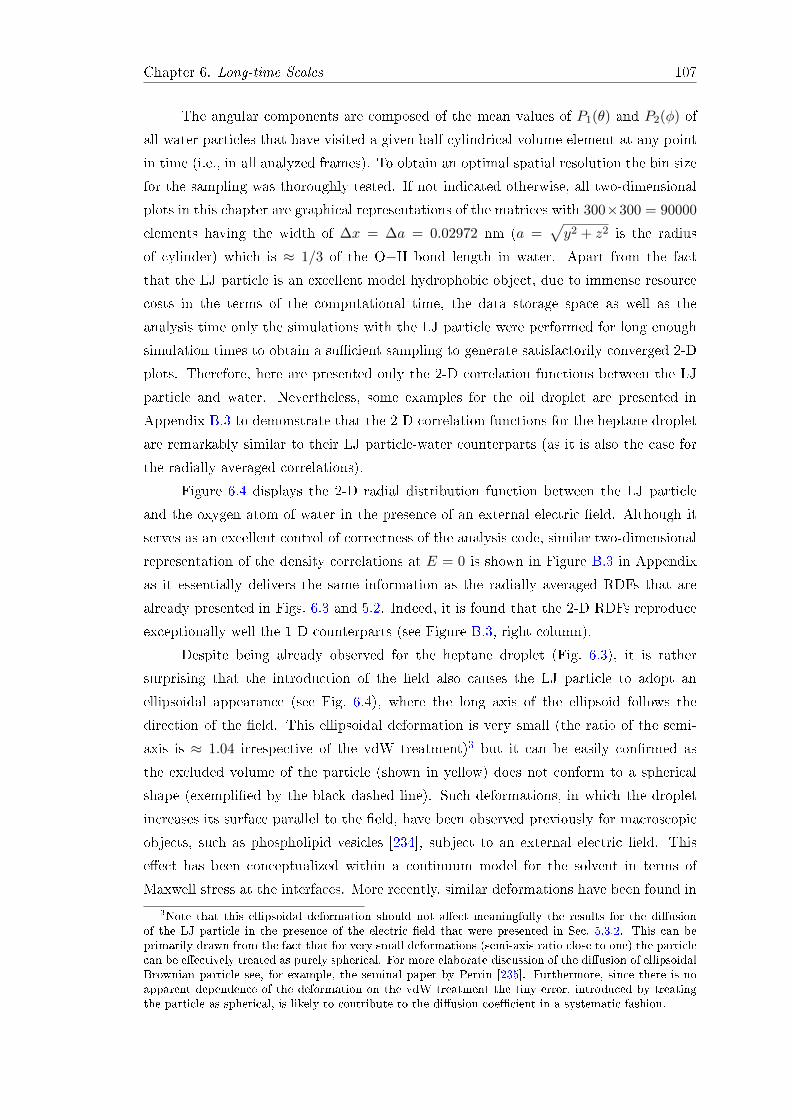
Chapter 6. Long-time Scales 107
The angular components are composed of the mean values of P1(θ) and P2(φ) of
all water particles that have visited a given half-cylindrical volume element at any point
in time (i.e., in all analyzed frames). To obtain an optimal spatial resolution the bin size
for the sampling was thoroughly tested. If not indicated otherwise, all two-dimensional
plots in this chapter are graphical representations of the matrices with 300×300 = 90000
elements having the width of ∆x = ∆a = 0.02972 nm (a =√y2 + z2 is the radius
of cylinder) which is ≈ 1/3 of the O−H bond length in water. Apart from the fact
that the LJ particle is an excellent model hydrophobic object, due to immense resource
costs in the terms of the computational time, the data storage space as well as the
analysis time only the simulations with the LJ particle were performed for long enough
simulation times to obtain a sucient sampling to generate satisfactorily converged 2-D
plots. Therefore, here are presented only the 2-D correlation functions between the LJ
particle and water. Nevertheless, some examples for the oil droplet are presented in
Appendix B.3 to demonstrate that the 2-D correlation functions for the heptane droplet
are remarkably similar to their LJ particle-water counterparts (as it is also the case for
the radially averaged correlations).
Figure 6.4 displays the 2-D radial distribution function between the LJ particle
and the oxygen atom of water in the presence of an external electric eld. Although it
serves as an excellent control of correctness of the analysis code, similar two-dimensional
representation of the density correlations at E = 0 is shown in Figure B.3 in Appendix
as it essentially delivers the same information as the radially averaged RDFs that are
already presented in Figs. 6.3 and 5.2. Indeed, it is found that the 2-D RDFs reproduce
exceptionally well the 1-D counterparts (see Figure B.3, right column).
Despite being already observed for the heptane droplet (Fig. 6.3), it is rather
surprising that the introduction of the eld also causes the LJ particle to adopt an
ellipsoidal appearance (see Fig. 6.4), where the long axis of the ellipsoid follows the
direction of the eld. This ellipsoidal deformation is very small (the ratio of the semi-
axis is ≈ 1.04 irrespective of the vdW treatment)3 but it can be easily conrmed as
the excluded volume of the particle (shown in yellow) does not conform to a spherical
shape (exemplied by the black dashed line). Such deformations, in which the droplet
increases its surface parallel to the eld, have been observed previously for macroscopic
objects, such as phospholipid vesicles [234], subject to an external electric eld. This
eect has been conceptualized within a continuum model for the solvent in terms of
Maxwell stress at the interfaces. More recently, similar deformations have been found in3Note that this ellipsoidal deformation should not aect meaningfully the results for the diusion
of the LJ particle in the presence of the electric eld that were presented in Sec. 5.3.2. This can beprimarily drawn from the fact that for very small deformations (semi-axis ratio close to one) the particlecan be eectively treated as purely spherical. For more elaborate discussion of the diusion of ellipsoidalBrownian particle see, for example, the seminal paper by Perrin [235]. Furthermore, since there is noapparent dependence of the deformation on the vdW treatment the tiny error, introduced by treatingthe particle as spherical, is likely to contribute to the diusion coecient in a systematic fashion.
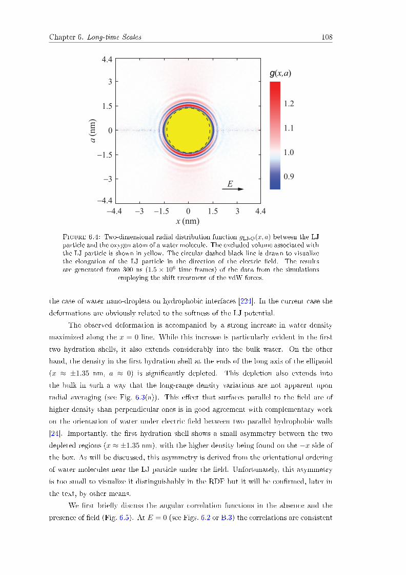
Chapter 6. Long-time Scales 108
−4.4 −3 −1.5 0 1.5 3 4.4
4.4
3
1.5
0
−1.5
−3
−4.4
x (nm)
a (nm)
g(x,a)
1.2
1.1
1.0
0.9
E
Figure 6.4: Two-dimensional radial distribution function gLJ-O(x, a) between the LJparticle and the oxygen atom of a water molecule. The excluded volume associated withthe LJ particle is shown in yellow. The circular dashed black line is drawn to visualizethe elongation of the LJ particle in the direction of the electric eld. The resultsare generated from 300 ns (1.5 × 10⁶ time frames) of the data from the simulations
employing the shift treatment of the vdW forces.
the case of water nano-droplets on hydrophobic interfaces [224]. In the current case the
deformations are obviously related to the softness of the LJ potential.
The observed deformation is accompanied by a strong increase in water density
maximized along the x = 0 line. While this increase is particularly evident in the rst
two hydration shells, it also extends considerably into the bulk water. On the other
hand, the density in the rst hydration shell at the ends of the long axis of the ellipsoid
(x ≈ ±1.35 nm, a ≈ 0) is signicantly depleted. This depletion also extends into
the bulk in such a way that the long-range density variations are not apparent upon
radial averaging (see Fig. 6.3(a)). This eect that surfaces parallel to the eld are of
higher density than perpendicular ones is in good agreement with complementary work
on the orientation of water under electric eld between two parallel hydrophobic walls
[24]. Importantly, the rst hydration shell shows a small asymmetry between the two
depleted regions (x ≈ ±1.35 nm), with the higher density being found on the −x side of
the box. As will be discussed, this asymmetry is derived from the orientational ordering
of water molecules near the LJ particle under the eld. Unfortunately, this asymmetry
is too small to visualize it distinguishably in the RDF but it will be conrmed, later in
the text, by other means.
We rst briey discuss the angular correlation functions in the absence and the
presence of eld (Fig. 6.5). At E = 0 (see Figs. 6.2 or B.3) the correlations are consistent

Chapter 6. Long-time Scales 109
−4.4 −3 −1.5 0 1.5 3 4.4
4.4
3
1.5
0
−1.5
−3
−4.4−4.4 −3 −1.5 0 1.5 3 4.4
0.6
0.4
0.2
0
−0.2
−0.4
−0.6E
⟨P1(θ)⟩ ⟨P
2(ϕ)⟩
x (nm) x (nm)
a (
nm
)
(a) (b)
Figure 6.5: Two-dimensional correlation functions 〈P1(θ)〉 and 〈P2(φ)〉 for the dipoleangle (a) and the normal angle (b), respectively. The same color scheme is used for bothcorrelation functions. The results are generated from 300 ns (1.5× 10⁶ time frames) of
the data from the simulations employing the shift treatment of the vdW forces.
with the fact that, for this particular size of the LJ particle, water molecules in the rst
hydration shell prefer to have one of their O−H bonds oriented parallel to the particle,
which is perpendicular to the radial vector. The imposition of the external eld, on the
other hand, introduces a preference for the dipole vectors to align parallel to the eld.
When the eld is present water molecules will, thus, have to strike a balance between
the optimal orientation with respect to the LJ particle and that with respect to the eld.
This indeed appears to be particularly challenging for molecules in the most dense, rst
hydration shell.
The result of this competition is reected in the rich and asymmetric patterns in
the dipole and normal angle correlation functions (see Fig. 6.5). This is particularly true
close to the LJ particle where the highly non-uniform distribution of water in the rst
hydration shells observed in gLJ-O is reected once again. Consequently, for both the
dipole and normal angles, very clear dierences are visible between the +x and the −xsides of the solute, particularly at short distances from the LJ particle.
At large distances from the LJ particle, the orientational constraints arising from
the LJ particle are reduced and the water dipoles may more freely orient in the direction
of the eld. This results in strong variations in the projection of the dipole moment onto
the radial vector (see Fig. 6.1) and hence the multicoloured appearance of the correlation
functions at far distances from the LJ particle. For example, 〈P1(θ)〉 ranges from nearly
−0.8 on the −x edge of the box to nearly +0.8 at the +x edge of the box, along the
a = 0 line (Fig. 6.5(a)). Despite the obvious asymmetry of the prole with respect to the
x = 0 line, the long-range radial average of 〈P1(θ)〉 is approximately zero, in agreement
with Fig. 6.3.
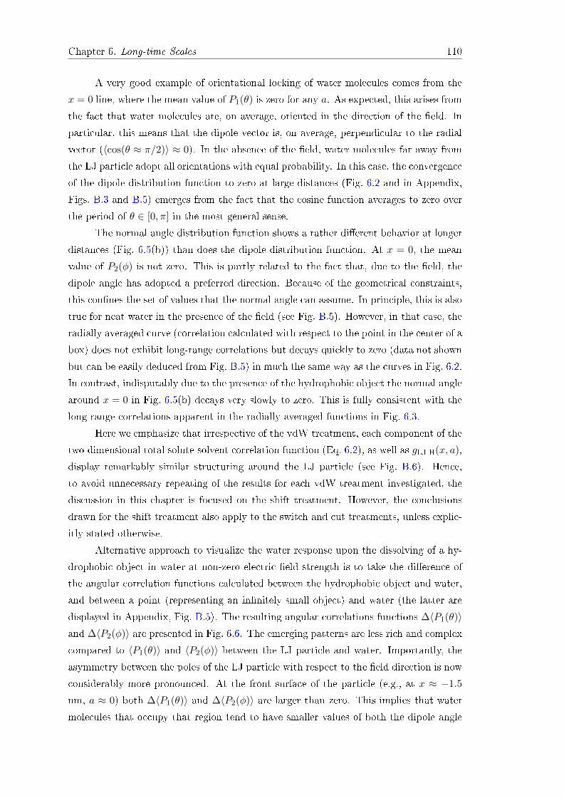
Chapter 6. Long-time Scales 110
A very good example of orientational locking of water molecules comes from the
x = 0 line, where the mean value of P1(θ) is zero for any a. As expected, this arises from
the fact that water molecules are, on average, oriented in the direction of the eld. In
particular, this means that the dipole vector is, on average, perpendicular to the radial
vector (〈cos(θ ≈ π/2)〉 ≈ 0). In the absence of the eld, water molecules far away from
the LJ particle adopt all orientations with equal probability. In this case, the convergence
of the dipole distribution function to zero at large distances (Fig. 6.2 and in Appendix,
Figs. B.3 and B.5) emerges from the fact that the cosine function averages to zero over
the period of θ ∈ [0, π] in the most general sense.
The normal angle distribution function shows a rather dierent behavior at longer
distances (Fig. 6.5(b)) than does the dipole distribution function. At x = 0, the mean
value of P2(φ) is not zero. This is partly related to the fact that, due to the eld, the
dipole angle has adopted a preferred direction. Because of the geometrical constraints,
this connes the set of values that the normal angle can assume. In principle, this is also
true for neat water in the presence of the eld (see Fig. B.5). However, in that case, the
radially averaged curve (correlation calculated with respect to the point in the center of a
box) does not exhibit long-range correlations but decays quickly to zero (data not shown
but can be easily deduced from Fig. B.5) in much the same way as the curves in Fig. 6.2.
In contrast, indisputably due to the presence of the hydrophobic object the normal angle
around x = 0 in Fig. 6.5(b) decays very slowly to zero. This is fully consistent with the
long range correlations apparent in the radially averaged functions in Fig. 6.3.
Here we emphasize that irrespective of the vdW treatment, each component of the
two-dimensional total solute-solvent correlation function (Eq. 6.2), as well as gLJ-H(x, a),
display remarkably similar structuring around the LJ particle (see Fig. B.6). Hence,
to avoid unnecessary repeating of the results for each vdW treatment investigated, the
discussion in this chapter is focused on the shift treatment. However, the conclusions
drawn for the shift treatment also apply to the switch and cut treatments, unless explic-
itly stated otherwise.
Alternative approach to visualize the water response upon the dissolving of a hy-
drophobic object in water at non-zero electric eld strength is to take the dierence of
the angular correlation functions calculated between the hydrophobic object and water,
and between a point (representing an innitely small object) and water (the latter are
displayed in Appendix, Fig. B.5). The resulting angular correlations functions ∆〈P1(θ)〉and ∆〈P2(φ)〉 are presented in Fig. 6.6. The emerging patterns are less rich and complex
compared to 〈P1(θ)〉 and 〈P2(φ)〉 between the LJ particle and water. Importantly, the
asymmetry between the poles of the LJ particle with respect to the eld direction is now
considerably more pronounced. At the front surface of the particle (e.g., at x ≈ −1.5
nm, a ≈ 0) both ∆〈P1(θ)〉 and ∆〈P2(φ)〉 are larger than zero. This implies that water
molecules that occupy that region tend to have smaller values of both the dipole angle
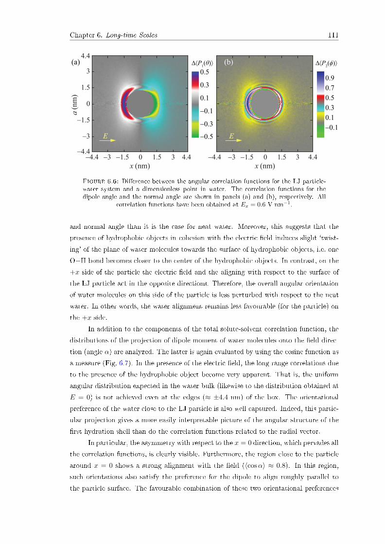
Chapter 6. Long-time Scales 111
0.5
0.3
0.1
−0.1
−0.3
−0.5
0.9
0.7
0.5
0.3
0.1
−0.1
−4.4 −3 −1.5 0 1.5 3 4.4
4.4
3
1.5
0
−1.5
−3
−4.4
x (nm)
a (nm
)
∆⟨P1(θ)⟩ ∆⟨P
2(ϕ)⟩
−4.4 −3 −1.5 0 1.5 3 4.4
x (nm)
(a) (b)
E E
Figure 6.6: Dierence between the angular correlation functions for the LJ particle-water system and a dimensionless point in water. The correlation functions for thedipole angle and the normal angle are shown in panels (a) and (b), respectively. All
correlation functions have been obtained at Ex = 0.6 V nm−1.
and normal angle than it is the case for neat water. Moreover, this suggests that the
presence of hydrophobic objects in cohesion with the electric eld induces slight `twist-
ing' of the plane of water molecules towards the surface of hydrophobic objects, i.e. one
O−H bond becomes closer to the center of the hydrophobic objects. In contrast, on the
+x side of the particle the electric eld and the aligning with respect to the surface of
the LJ particle act in the opposite directions. Therefore, the overall angular orientation
of water molecules on this side of the particle is less perturbed with respect to the neat
water. In other words, the water alignment remains less favourable (for the particle) on
the +x side.
In addition to the components of the total solute-solvent correlation function, the
distributions of the projection of dipole moment of water molecules onto the eld direc-
tion (angle α) are analyzed. The latter is again evaluated by using the cosine function as
a measure (Fig. 6.7). In the presence of the electric eld, the long range correlations due
to the presence of the hydrophobic object become very apparent. That is, the uniform
angular distribution expected in the water bulk (likewise to the distribution obtained at
E = 0) is not achieved even at the edges (≈ ±4.4 nm) of the box. The orientational
preference of the water close to the LJ particle is also well captured. Indeed, this partic-
ular projection gives a more easily interpretable picture of the angular structure of the
rst hydration shell than do the correlation functions related to the radial vector.
In particular, the asymmetry with respect to the x = 0 direction, which pervades all
the correlation functions, is clearly visible. Furthermore, the region close to the particle
around x = 0 shows a strong alignment with the eld (〈cosα〉 ≈ 0.8). In this region,
such orientations also satisfy the preference for the dipole to align roughly parallel to
the particle surface. The favourable combination of these two orientational preferences

Chapter 6. Long-time Scales 112
−4.4 −3 −1.5 0 1.5 3 4.4
4.4
3
1.5
0
−1.5
−3
−4.4
x (nm)
a (
nm
)
−4.4 −3 −1.5 0 1.5 3 4.4
x (nm)
E = 0 E
⟨P1(α)⟩
0.8
0.6
0.4
0.2
0
−0.2
(a) (b)
Figure 6.7: Two-dimensional plot of the mean projection of the water dipole vectoronto the x direction in the absence (a) and in the presence of an external electric eld(b). The results are generated from 200 ns (E = 0) and 300 ns (Ex = 0.6 V nm−1) of
the data from the simulations employing the shift treatment of the vdW forces.
means it is more likely for water molecules to occupy this region, which gives rise to the
increased density. Conversely, in the region around a = 0, the alignment with respect to
the LJ particle comes at the expense of an unfavourable orientation (〈cosα〉 ≈ 0.2, i.e.
the water dipoles are, on average, almost perpendicular to Ex) with respect to the eld,
which leads to a reduction in density. Interestingly, however, the unfavourable region is
smaller and less intense on the −x side of the particle than it is on the +x side, which
is the eect already explained in the discussion of ∆〈P1(θ)〉 and ∆〈P2(φ)〉 (see Fig. 6.6).Importantly, this eect is the cause of the small asymmetry in density observed between
these two regions.
As already commented, the visualization of the −x/+x asymmetry in density
around the LJ particle directly from gLJ-O(x, a) is an ungrateful task to perform (see
Fig. 6.4). For the angular correlations it is demonstrated that taking the dierence be-
tween the correlation functions obtained for the LJ particle-water system and pure water
improves the visibility of the −x/+x asymmetry. The same approach is not helpful in
the case of the density-density correlations since in the pure water there are no den-
sity correlations around an arbitrary point. However, a bypass to visualize the −x/+x
asymmetry in water density, while retaining the 2-D perspective of the entire simulation
box, is to exploit the clear asymmetry observed for the projection of the dipole vector
on the direction of the imposed electric eld (Fig. 6.7). Thereby, gLJ-O is multiplied
with 〈P1(α)〉. The product can be comprehended as the averaged eective dipole density
〈A(x, a)〉 and is shown in Fig. 6.8.
From the 2-D plot of 〈A(x, a)〉 (Fig. 6.8(a)) the dierence in the mean eective
dipole density between the regions centred around [x = −1.5 nm, a ≈ 0] and [x = 1.5
nm, a ≈ 0] is evident. For example, the green area at the left hand side is clearly larger

Chapter 6. Long-time Scales 113
4.4
3
1.5
0
−1.5
−3
−4.4
a (nm
)1
0.8
0.6
0.4
0.2
0
⟨A(x,a)⟩E
−4.4 −3 −1.5 0 1.5 3 4.4
x (nm)
|a|≅1.1 nm
−3 −1.5 0 1.5 3
0.2
0.4
0.6
0.8
x (nm)
⟨A(x,a)⟩
(a) (b)
Figure 6.8: The averaged eective dipole density 〈A(x, a)〉 of water around the LJparticle shown as the 2-D plot of the entire system (a) and as the line extracted around
|a| = 1.1 nm (b) from the corresponding 2-D representation.
than the corresponding area on the right hand side. However, the −x/+x asymmetry is
not restricted just to regions around a = 0 line but it also extends around the particle.
This is illustrated in Fig. 6.8(b) by taking the average of the lines a = −1.1 nm and
a = 1.1 nm. Therein, a rather strong dierence of 〈A(x, a)〉 from the two sides of the
particle (with respect to the direction of the electric eld) is found. This is in excellent
agreement with ndings of Bratko et al. [24], where the strongest dierence in water
density was observed when the electric eld was imposed at the angle of 45 with respect
to the hydrophobic wall. Thus, this is one more sign that the electric eld invokes an
asymmetric density distribution around a hydrophobic object.
Valuable addition to the so far discussed average water ordering is to evaluate
the preferential orientation of water molecules at specic positions with respect to the
position of the LJ particle. Here, the preferential orientation depicts the single most
preferable orientation of the water molecule at certain location. The target orientations
are obtained by making the distributions of the dipole angle θ and the normal angle
φ at some position (i.e., specic bin and its 1st neighbours). Then, the most probable
values of θ and φ from the distributions are combined with the information from 〈P1(α)〉to deduce the most preferred orientation of water molecule. In Fig. 6.9 is given the
schematic representation of the most probable orientation of water molecules at specic
positions (±x poles of the particle, and the three positions at the top surface of the LJ
particle at the angles of 45, 90, and 135 with respect to the x-axis) both in the absence
(left) and presence (right) of the electric elds. Due to the symmetry the orientations
at the bottom surface, i.e. a < 0, are simply the mirror images of the orientations at
the top surface. Additionally, the depth cueing is used which blends the objects further
from the camera into the background, e.g. the hydrogen atoms (in cyan) above the paper
plane have stronger color intensity.

Chapter 6. Long-time Scales 114
E
Field OFF Field ON
Figure 6.9: Schematic representation of the most probable orientations of watermolecules at dierent positions in the very proximity of the surface of the LJ particle(in grey) both in the absence (left) and presence (right) of the electric elds (Ex = 0.6V nm−1). The stronger color intensity of the hydrogen atom (in cyan) indicates thatparticular atom is above the paper plane. Also are indicated the direction of the electric
eld and the dipole vector of each water molecule.
As already mentioned, in the absence of the electric eld the water molecules
near the interface tend to orient parallel with their plane towards the LJ particle, i.e.
perpendicular to the x-axis and the plane of paper. In that way only one possibility
to establish hydrogen bond is sacriced. Moreover, the orientations are symmetric with
respect to the line x = 0 nm and the net dipole moment of the water molecules around
the LJ particle is zero. At nonzero elds the situation changes dramatically. The dipole
vector of each water molecule has a nonzero component in the eld direction (except,
perhaps, the water molecule at the +x pole of the particle) leading to the net dipole
moment of the water molecules close to the surface. Furthermore, all water molecules
twist their plane perpendicular to the surface of the LJ particle resulting in one O−Hbond directed towards the particle. Remarkably, the plane of the water molecules at the
+x pole and at the top (α = 90) coincides with the plane of paper. Other H2O molecules
have their plane slightly o the paper plane. The water molecules positioned at the two
poles (−x and +x) of the LJ particle have dierent most probable orientations and, thus,
implying the credibility of the asymmetric density distribution around the hydrophobic
object.
6.5 Long-time Displacement of the LJ Particle
The time-dependent displacement of the LJ particle on the time scales up to 100 ns
has been thoroughly investigated in Chapter 5. Therein was observed that continuous
treatments (switch and shift) of the vdW forces do not invoke a persistent unidirectional
movement of the LJ particle in the direction of the imposed electric eld that is in contrast
to the behavior found for the truncated forces (cut treatment). For each treatment of the

Chapter 6. Long-time Scales 115
vdW interactions, the observed displacements were demonstrated to be fully consistent
with the averaged net vdW force on the LJ particle exerted by water molecules. The force
was found to be eectively zero for the continuous treatments and ≈ −6.6 pN for the cut
treatment. Moreover, the latter force predicts the drift velocity of the LJ particle that is
in quantitative agreement with the simulation data for the cut treatment. In addition,
the absence of a signicant net drift in the eld direction with the continuous treatments
was sucient reason to treat the movement of the LJ particle as purely Brownian on the
`short-time' scale of 100 ns.
However, to fully resolve the distribution of water at the interface with the hy-
drophobic object, while respecting the azimuthal symmetry imposed by the electric eld,
the simulations of 100 ns are not sucient (consult Sec. 6.4). Therefore, the simulations
employing the continuous treatments of the vdW forces are extended to reach, in total,
the simulation time of 900 ns. Hereafter, the latter time scale will be referred to as the
`long-time' scale.4 Since the shift treatment proved to be the most reliable of the investi-
gated vdW treatments, the results presented here are exclusively for the shift treatment.
However, everything said for the shift treatment applies also for the switch treatment
and even the cut treatment.
While pursuing longer simulation times to improve the sampling in the proximity
of the LJ particle a remarkable dynamics of the LJ particle emerged in the presence
of an external electric eld (E = 0.6 V nm−1). For the shift treatment, the Cartesian
displacements of the LJ particle over the time interval of 900 ns are shown in Fig. 6.10.
Stunningly, the displacement of the LJ particle in the direction of the eld (imposed in
+x direction) is profoundly dierent from the displacement in the non-eld directions
(y, z). Moreover, the observed displacement in the x direction is strikingly reminiscent
of the behavior already seen for the cut treatment (see Fig. 5.4), which was clearly
demonstrated to be the result of the net (non-zero) vdW force acting on the particle.
However, the mobility observed herein with the shift treatment is elusive as the vdW force
is eectively zero during the entire simulation. On the other hand, the displacements
in the non-eld directions are reminiscent of those found with the shift and the switch
treatments (both at E = 0 and 0.6 V nm−1) at the time scale of 100 ns (Fig. 5.4). The
latter were associated with an ordinary Brownian diusion.
On the short-time scales the calculated diusion coecients D (see Table 5.1) for
dierent vdW treatments, both in the absence and presence of the eld, were found to
be equal within the statistical accuracy for all treatments. Moreover, the net drift of the
LJ particle in the Cartesian directions was found to be within or outside the boundaries
expected from the underlying Brownian displacement (estimated from D). On this basis,
4In the state-of-art MD simulations the achieved simulation time of 100 ns is commonly regardedas rather long. Herein, to distinguish the markedly dierent mobility of the LJ particle (using thecontinuous treatments of the vdW forces) at the time scale of 100 ns from the mobility at signicantlylarger time scales, the two time scales are denoted as the `short-time' and the `long-time', respectively.

Chapter 6. Long-time Scales 116
Dis
pla
cem
ent
(nm
)
20
0
−20
−40
0 600300
t (ns)
−60
−80
900
x
z
y
SHIFT
force-driven
(cut )
Figure 6.10: The displacement of the LJ particle in all three Cartesian directionsin the presence of the electric eld (Ex = 0.6 V nm−1). The results are for the shifttreatment of the vdW interactions. For comparison the estimated drift displacementin the x direction for the cut treatment (vd = 0.45 m s−1; consult Sec. 5.3) is also
displayed (dashed line).
the observed movement was regarded Brownian or non-Brownian. Indeed, the non-
Brownian behavior was identied only in the eld direction with the cut treatment.
Here, for the shift treatment on the long-time scales, the classication between
Brownian and non-Brownian behavior is made directly from the calculated mean square
displacement (MSD). In Fig. 6.11 is shown the simulated MSD for both directions with
respect to the direction of the imposed eld (x) alongside the theoretically expected MSD
for the LJ particle performing Brownian diusion (labelled `Brownian diusion'). The
latter is calculated by using the value of D for the shift treatment at E = 0 (Table 5.1).
The averaged MSD for the non-eld directions, MSD(y, z) = [MSD(y)+MSD(z)]/2,
reproduces nicely, for times t . 35 ns, the MSD expected for the LJ particle performing
Brownian diusion. In general, the MSD is slowly converging property and is expected
to be fully linear for times not larger than 10% (usually around 5%) of the entire trajec-
tory from which it is calculated. Thereby, it would be expected that MSD(y, z) remains
linear for times slightly larger than 35 ns. However, this small discrepancy from the
expectation can be attributed primarily to the very small mass of the employed LJ par-
ticle (M = 50 u), which is chosen to minimize the mass dependence of diusion that is
inherent to the MD simulations. In contrast, larger M would diminish the uctuations
of the position of the LJ particle, and therefore of the MSD as well, but would demand
a larger water bath to oset the unwanted mass dependence of diusion (see Fig. 4.2
and corresponding discussion therein). Unfortunately, simulations employing larger sim-
ulation boxes (e.g., edge length of 12 nm) are computationally too demanding and the

Chapter 6. Long-time Scales 117
10
20
MS
D(y
, z)
(n
m2)
Simulation
Brownian diffusion
t (ns)20 400 0 20 40 60
t (ns)
60
20
40
MS
D(x
) (
nm
2)
Simulation
Brownian diffusion
Non-field directions Field direction
Figure 6.11: The calculated mean square displacement (MSD) in the non-eld di-rections (y, z) (left) and in the eld direction (x) (right). In each case the calculatedMSD is compared to the theoretically expected MSD (dashed line) of the employed LJparticle performing Brownian diusion. All results are for the shift treatment of the
vdW interactions in the presence of an external electric eld (Ex = 0.6 V nm−1).
necessary simulation times of several hundreds of nanoseconds are beyond reach. How-
ever, the observed agreement for t . 35 ns is more than long enough to prove that the
LJ particle exhibits primarily the Brownian motion in the non-eld directions since the
MSD in the eld direction starts to deviate from the linear behavior already at t ≈ 12 ns.
Moreover, MSD(x) exhibits a clearly dierent pattern as it diverges from the theoretical
curve in a parabolic fashion. This ∼ t2 dependence of MSD(x) is a strong indication of
an additional process, superimposed to the Brownian diusion, that is propagating with
some constant speed.
The separation between Brownian and non-Brownian behavior at the time scales
around 12 ns in MSD(x) also explains why this additional process was not observed on the
short-time scales (100 ns). The reason simply lies in the fact that the time necessary to
observe the separation of the underlying dynamical behaviors is larger than 10 ns, which
is outside of the condence interval of the MSD. Moreover, this also suggests that MD
reports of the electrophoretic mobility (EPM), coming primarily from the simulations
not exceeding 100 ns, are likely related only with the force-based mechanism whereas
the mobility observed herein is a distinctive process. The theoretical explanation for this
sudden re-emergence of the EPM on the long-time scales, with the continuous treatments
of the vdW forces, will be given in the following section.
6.6 Electro-diusiophoresis of the LJ Particle
With the employed truncated treatment of the vdW interactions the cause for the ob-
served net drift of the LJ particle opposite to the direction of the applied electric eld was
indicated by the pronounced linearity of the time-displacement. The latter was the sign

Chapter 6. Long-time Scales 118
of a net non-zero vdW force on the particle, which was proved to agree exceptionally well
with the observed drift (consult Chapter 5). However, the re-emergence of net mobility
(in the eld direction) of the LJ particle on the long-time scales with continuous treat-
ments (shift, switch) of the vdW forces (Fig. 6.10) arises from a force-free (i.e., phoretic)
mechanism (see Table 5.2). Thus, to explain this sudden `electrophoretic' mobility5 of
the LJ particle, a signature of the phoretic mechanism has to be clearly identied and
demonstrated.
The most general prerequisite for the existence of phoretic mobility of an object
is the symmetry breaking in either or both of the pattern of `activity' and `mobility'
[236]. The symmetry breaking around an object is reected in gradients of a quantity,
which in turn induce motion through classical phoretic processes [236]. Depending on
the nature of the gradient possible phoretic mechanisms are: thermophoresis (migration
due to a temperature gradient) [237], diusiophoresis (migration due to a concentration
gradient) [238], electrophoresis (gradient in electrostatic potential) [239], to name just a
few. Obviously, as the temperature of the system is eciently controlled by using the
Berendsen thermostat during the entire course of the simulation, it is hard to envision
the existence of temperature gradients around the hydrophobic object and to construct
a plausible thermophoretic mechanism.
The electrophoresis can be also eliminated as a possible mechanism as pointed
out by Knecht and co-workers [65]. In the executed simulations the bare as well as
the net charge on the hydrophobic object is zero in the absence of any ions and, thus,
the application of an external electric eld does not exert any net force on the object
and the electrophoretic mobility should vanish. This reasoning of Knecht et al. remains
valid in our case, even though there is indisputable apparent charging of the LJ particle.
This charging is the reection of water ordering in the vicinity of the particle that is
characterized by the hydrogen atoms being, on average, closer to the surface than oxygen
atoms, even at E = 0. However, this is more pronounced at non-zero elds, where
the water molecules close to the surface prefer to point with one of their O−H bonds
toward the surface (Fig. 6.9). Therefore, the charging is not due to the presence of
ions that are, in traditional view, adsorbed to the surface and move together with the
particle. Moreover, the rst moment of the charge density distribution vanishes, despite
the asymmetry (data not shown). Thus, the best guess for the underlying motility
mechanism of the hydrophobic objects appears to be related to the diusiophoresis,
which requires an asymmetric distribution of water around the solute.6
5In the remainder of this chapter it will be demonstrated that instead of electrophoresis a dierentmechanism is responsible for the mobility of the LJ particle. Thus, it is not fully correct to call theobserved mobility the electrophoretic mobility.
6In studies of hydrophobic hydration it is inveterate to call the hydrophobic object `the solute'.However, this terminology collides with the one used in the `phoretic' community where the `solute' isthe species which exhibits the gradient in concentration around the moving object (swimmer). To avoidconfusion, we retain to regard the hydrophobic object (LJ particle/heptane droplet) as the `solute'.

Chapter 6. Long-time Scales 119
−4.4 −3 −1.5 0 1.5 3 4.4
4.4
3
1.5
0
x (nm)
a (
nm
) 40
35
30
nm−3
ρLJ-H
(x,a)
Figure 6.12: The 2-D plot of the density correlations between the LJ particle and thehydrogen atoms of water (ρLJ-H(x, a)) averaged over the two halves of the cylinder, i.e.a is the radius of the entire cylinder. The dot-dashed black line is drawn to distinguishbetween the front side (left-hand side) and the rear side (right-hand side) of the LJparticle. The results are generated from 300 ns (1.5×10⁶ time frames) of the data fromthe simulations employing the shift treatment of the vdW forces. Ex = 0.6 V nm−1.
In Sec. 6.4, a signicant eort was devoted to demonstrate (i.e., visualize) the
symmetry breaking around the LJ particle that is pertaining to all components of the
total LJ particle-water correlation function. The asymmetry is obvious for the angular
components (Figs. 6.5 and 6.6) as well as for the projection of the dipole vector on the
eld direction (Fig. 6.7). Apart from the clear dierence between the water density at
the surfaces parallel and perpendicular to the eld direction, the −x/+x asymmetry
remains somewhat fuzzy for the density correlations around the particle (see Fig. 6.4).
This remains to be the case even after the multiplication with 〈P1(α)〉 to obtain the
mean eective dipole density of water (Fig. 6.8). Therefore, to indisputably demonstrate
the existence of the excess water density around the LJ particle, with respect to the
direction of the applied electric eld, an elegant approach that exploits the symmetry of
the system is proposed.
Precisely, the 2-D plot of the density correlations (before the normalization with
the bulk density to obtain the RDF) between the LJ particle and water hydrogen (H)
atoms is considered (data not shown) instead of ρLJ-O. The reason lies in the fact that
the hydrogen atoms are closer to the center of the LJ particle and, therefore, depict
better the LJ particle-water interface. Moreover, the analysis code respects the axial
symmetry of the system but also dierentiates between the upper half of the cylinder
(a > 0 in 2-D plots, e.g. Fig. 6.4) and the lower half of the cylinder (a < 0). Thus, the
two halves of the density correlation plot are simply added and averaged out to obtain
ρLJ-H (see Fig. 6.12). Finally, the corresponding hydrogen densities at the rear side and
the front side of the particle are subtracted to obtain the excess water density (in terms
of ∆ρ(H)) at the front side of the particle (Fig. 6.13).

Chapter 6. Long-time Scales 120
−4.4 −3 −1.5 0
4.4
3
1.5
a (
nm
)
x (nm)
0.3
−0.3
0.6
−0.6
0
∆ρ(H) (nm−3)
E
rδ
Figure 6.13: The density dierence of water hydrogen atoms between the two sidesof the LJ particle with respect to the direction of the applied electric eld (Ex = 0.6 Vnm−1). The results are generated from 300 ns (1.5× 10⁶ time frames) of the data from
the simulations employing the shift treatment of the vdW forces.
Figure 6.13 reveals fascinating dierences in water ordering between the front side
(−x) and the rear side (+x) of the LJ particle induced by the electric eld. The observed
dierences are subtle (less than 1 H2O molecule per nm−3) but they are indisputable
as even the exchange of three layers with the excess density (in blue) with three layers
showing the depletion of water (in red) is nicely captured. Stunningly, this alternation
of 6 layers ends at about 1.7 nm from the center of the LJ particle, which coincides
with the end of the 1st hydration shell (dened as the position of the 1st minimum in
the radially averaged RDF gLJ-O(r), see Fig. 5.3). This amazingly rich water ordering,
exclusively within the 1st hydration shell, captures nicely the ellipsoidal deformation
of the LJ particle.7 Interestingly, the slight ellipticity of the nearest layer aects the
thickness of the layering further from the surface of the LJ particle (layering is thicker
at the surface perpendicular to the eld direction). Furthermore, the density dierences
in the nearest layer are largest at the angle of about 45 with respect to the x-axis as
already seen for the mean eective dipole density (Fig. 6.8). Even though the results
7On the basis of Fig. 6.12, in which there is no water within r < 1.5 nm, careful reader could beconfused with rich structuring obtained in Fig. 6.13 at the same distances. However, this is only theeect of the scale bar which starts at 30 nm−3 (in Fig. 6.12) which is about 90% of the bulk waterdensity. The reasons for this are multiple. First, it is practically impossible to visualize clearly all thedensity changes in the range from zero to about 40 nm−3 with a single color scheme. Moreover, thepurpose of Fig. 6.12 is in principal to explain, in visual way, the process of obtaining the excess waterdensity at the front side of the LJ particle. Finally, the scale bar starts at 30 nm−3 to emphasize the factthat the 1st layer of excess water density is conned to the soft-core region of the employed LJ potential.

Chapter 6. Long-time Scales 121
are shown only for the ordering of the hydrogen atoms using the shift treatment of the
vdW interactions, very similar (even quantitatively) pictures are obtained for the switch
and even the cut treatment for both the ordering of oxygen and hydrogen atoms. Thus,
the excess density of water in front of the hydrophobic object is an eect induced by the
electric eld and not the result of specic treatment of the vdW interactions.
Having conrmed the existence of the concentration gradient of water around the
LJ particle (Fig. 6.13) we can take a closer look why and how the latter can give rise to the
diusiophoretic motion of the object. Theoretically, when a particle (object) is placed in
a uid in which there is a non-uniform concentration of some species, it will move toward
higher or lower concentration depending on whether the species is attracted to or repelled
from the surface of the particle [240]. Even though the diusiophoresis is a mechanism
that involves an interplay of the surface science, mass transfer, and uid mechanics, its
plausibility can be proved from the principles of thermodynamics [241]. The system
energetics is determined at the particle/solution interface which has associated with it
an excess surface free energy per area, i.e. the interfacial tension %. For example, a
spherical particle (e.g., employed LJ particle) of radius R is transferred at constant T
from a solution with a concentration of water c1 to another solution of concentration
c2. If the particle-water interaction is eectively attractive the water adsorbs (`wets') on
the surface and lowers the interfacial tension from %1 to %2. The associated change in
free energy ∆G is ∆G = 4πR2(%2 − %1). For example, if c2 > c1 then %2 < %1 and the
movement process of the particle is spontaneous (∆G < 0) [241].
The above described discrete situation can be replaced by the case in which the
particle is immersed in solution of non-uniform concentration c [241]. Thereby, the
gradient of free energy for the particle reads
∇G = 4πR2∇% = 4πR2
(∂%
∂c
)T
∇c . (6.4)
In equilibrium, for dilute solution, the changes in the surface free energy with changes
of concentration equal (∂%
∂c
)T
=kBT Γ
c= −kBT Ω , (6.5)
where Γ is the Gibbs surface excess concentration of species adsorbed to the surface, and
Ω = Γ/c is the adsorption length and is a measure of how strongly the species is adsorbed
as c → 0. Equations 6.4 and 6.5 suggest that, for an attractive potential, the particle
can lower its free energy by moving toward regions of higher concentration [241]. While
able to predict the diusiophoretic mechanism, the thermodynamics fails to predict the
magnitude of the propulsive velocity of the migrating particle.
The credit for rst predicting diusiophoresis of rigid particles and explaining the
underlying physical principles must go to Derjaguin and co-workers [242245]. They

Chapter 6. Long-time Scales 122
realized that asymmetric density distribution of species (having diameter signicantly
smaller from the radius of the particle) around the particle will invoke, within the thin
surface lm only, a tangential pressure gradient along the surface of the particle [236, 241,
246]. This follows from the assumption that the surface lm is very thin compared to the
size of the particle. Therefore, the equilibration of the density prole within the surface
lm can be regarded to be fast along the direction normal to the surface compared with
the diusional relaxation time of the composition gradient along the surface of the particle
(which, for the ellipsoidal particle, involves a length scale of the order min(w1, w2), where
w1 and w2 are the semi-axis of an ellipsoid) [241, 246248]. Moreover, this implies the
formation of the spatial variations of density within the surface lm in the direction
normal to the surface of the migrating object [246]. Indeed, the spatial variations of
density are observed in the case of the LJ particle (see Fig. 6.13) but they are signicantly
more complex8 than the commonly assumed exponential decay of density distribution
(for example, consult Ref. [246]). Furthermore, the mechanical equilibrium of the solvent
within the surface lm along the direction normal to the surface in which there is no
ow necessitates the pressure gradient along the normal to be equal to the body force
densities due to eective interactions between the particle and the species in an excess
of concentration [240, 246]. This implies the dierence between the pressure inside the
surface lm from the pressure outside the lm by an osmotic pressure9 term. The latter
is proportional to the extra density ∆ρ in excess to that density in the outer region and
also experiences gradual changes along the surface of the particle. Actually, this lateral
pressure gradient is not balanced by any body force and invokes shear stress within
the surface lm, i.e. it induces hydrodynamic ow of the solution along the surface of
the particle and the propulsive motion of the particle with a steady-state velocity vp
[251]. Due to the azimuthal symmetry of the system, the motion is along the x-axis
which coincides with the direction of the electric eld and, thus, vp = vpex. In a similar
manner, due to symmetry, the components of the velocity in other directions (y, z) vanish.
The general expression for the phoretic velocity vp of the particle in the direction
of the applied electric eld (x) reads [33, 236, 247]
vp =kBT
ηapp
λ2
Rhρ1 , (6.6)
where ηapp = 7.3 × 10⁻⁴ Pa·s is the shear viscosity of water (SPC/E model) in the
8To the best of our knowledge, this is the rst observation of the density variations characterizedwith the alternating layers of excess and depleted density around the migrating object. Commonly,the concentration of the species in excess decays uniformly until it reaches the bulk concentration. Thisindicates that the atomic details have an important role in the propulsion of very small nanoscale objects.
9Due to this osmotic pressure term the diusiophoresis is sometimes called osmophoresis [249] or,even, osmiophoresis [250]. However, the name osmophoresis should be used for the systems in whicha vesicle-like-body (uid surrounded by a semi-permeable membrane) is placed in a solution havingnon-uniform concentration of impermeable species [239].

Chapter 6. Long-time Scales 123
presence of electric elds (Ex = 0.6 V nm−1) and Rh = 1.14 nm is the hydrodynamic
radius (taken as the radius of the excluded volume) of the LJ particle (see Secs. 3.3.3
and 4.4). In the steady-state, the rst moment of the asymmetric density distribution
around the particle leading to the phoretic motion is given by
ρ1 =
∫ π
0sinϑ cosϑ dϑ ρ(rδ, ϑ) . (6.7)
Here, ϑ is the `latitude' angle with the polar axis ex. Finally, λ in Eq. 6.6 is the length
scale and depends on the nature of the phoretic mechanism. For the diusiophoresis it
can be calculated through
λ2 =
∫ ∞Rh
rdr
[1− exp
(−VLJ(r)
kBT
)], (6.8)
where VLJ is the Lennard-Jones potential between the particle and water molecule (con-
sult Sec. 2.5), and r is the radial distance from the surface of the LJ particle.
From the above equations (Eqs. 6.6, 6.7, and 6.8) it is obvious that all prerequisites
are satised to theoretically predict the velocity at which the LJ particle propels through
the water in the presence of the electric eld. Instead of directly presenting the end
result for vp, we rst provide a brief discussion about ρ1 and λ2 as well as technical
details related to the their calculation. As mentioned above, the parameter λ provides
the typical length scale of the phenomena and, essentially, it quanties the strength of
the adsorption of the species in excess in the interfacial region of the migrating object.
In this study, the adsorption strength is directly related to the interaction between the
LJ particle and water, which is completely dened by the employed treatment of the LJ
potential VLJ.10 Therefore, it can be expected that the decrease of the well depth of
the interaction potential (in this study εLJ-O = 0.8063 kJ mol−1, see Sec. 2.5) leads to a
smaller phoretic velocity. As pointed out by Anderson [252], the basic idea behind strong
adsorption is that diusion of adsorbed species along the surface in the diuse region
can be suciently large that species must continually adsorb at the upstream edge of the
diuse region and continually desorb at the downstream edge. However, the adsorption
in the context of phoretic behavior should not be confused with the adsorption in the
classical sense, in which species adsorbs (sticks) to the surface of some particle and
moves with it. If the latter would actually happen, the phoretic velocity would vanish.
This illustrates nicely the necessity of the diuseness in the interfacial layer. Finally, to
obtain λ2 using Eq. 6.8, the integration is undertaken from the surface of the LJ particle
(taken as Rh = 1.14 nm) to the cut-o value of the employed vdW treatment (rc = 2.8
10In the experimental and theoretical studies the eective interaction potential between the migratingparticle and the species in excess of density is not known and has to be guessed or approximated byother parameters (for more details see, for example, reference [241]).

Chapter 6. Long-time Scales 124
20 40 60
t (ns)
60
0
20
40
MS
D(x
) (
nm
2)
Simulation
Brownian diffusion
Derjaguin displacement
Superposition
Figure 6.14: Comparison of the simulated (red line) and the theoretically predicted(black dot-dashed line) mean square displacement (MSD) of the LJ particle in theeld direction (x). The theoretically predicted MSD on the basis of Derjaguin theoryfor the diusiophoresis (see text). All results are for the shift treatment of the vdW
interactions.
nm) and the obtained value equals −0.16 nm2 (the minus indicates that the intrinsic
nature of the potential is attractive).
The rst moment of density distribution (Eq. 6.7) is a direct measure of an excess
density of water from one side of the LJ particle (i.e., measure of asymmetry). It is
calculated by an angle-dependent integration (the bin size ∆ϑ is taken to be 5) of
the non-normalized number density of the hydrogen atoms ρLJ-H(rδ, ϑ) (see Fig. 6.12),
where rδ is the upper boundary of the diuse layer (Fig. 6.13). Obviously, the choice of
value for the radial distance rδ is crucial for the resulting rst moment ρ1. Although,
it may seem that there is vast number of possible values for rδ, in reality there is only
one realistic choice and that is 1.5 nm. Taking into account that the diuse layer is
composed minimally of a single layer of water molecules the value of 1.5 nm apparently
coincides with the sum of excluded volume (in Chapter 4 the distance of closest approach
is identied to be 1.14 nm) plus the thickness of one layer of water (σH2O= 0.3166
nm). Additionally, this boundary coincides with the end of the 2nd layer in ∆ρ(H) (see
Fig. 6.13) which further strengthens the choice made. Even more, as this layering of
regions showing excess/depleted density ends at about 1.7 nm, there is no physical space
to accommodate two layers of water molecules. After the integration (using rδ = 1.5
nm) the obtained ρ1 is 0.115 nm−3.
Having all the necessary parameters, we insert them into the relation for the diu-
siophoretic velocity of the LJ particle and obtain −9.4 cm s−1. The minus sign indicates
the movement towards the region of higher concentration, i.e. in the direction opposite

Chapter 6. Long-time Scales 125
to the direction of the applied electric eld. On the rst sight, the obtained value for vpappears huge as the propulsive velocities for the particles in the micrometer size range
are, usually, in the range between nm s−1 and µm s−1 [253]. However, after taking into
account the 1/Rh dependence of vp on the size of the migrating particle and the fact that
the simulated LJ particle is about three orders of magnitude smaller than the particles
typically employed in experiment the calculated phoretic velocity in cm s−1 is not so sur-
prising. Even more, a larger eciency of nano-scale particles compared to those in the
µm size range is theoretically predicted [248]. On other hand, vp = −9.4 cm s−1 is small
enough, compared to the drift velocity, vd ≈ −45 cm s−1, found with the cut treatment
of the vdW interactions (Sec. 5.3). Therefore, the phoretic velocity was impossible to
discern with certainty and quantify on the time scales of 100 ns or shorter because only
about 10 ns of MSD can be extracted with signicant accuracy.
To inspect the agreement between the calculated propulsive velocity of the LJ par-
ticle and the observed drift for the shift treatment of the vdW interactions we return to
the mean square displacement (MSD) found for the shift treatment (shown in Fig. 6.11).
Therein was demonstrated that the simulated MSD for the eld direction diverges in a
parabolic manner (∼ t2) from the theoretical MSD expected for the LJ particle perform-
ing simple diusion. In honour of B. V. Derjaguin, the additional contribution to the
MSD(x) arising from the phoretic velocity we call Derjaguin displacement. The latter
can be simply obtained by using the identity MSD(x)= (vpt)2. After taking the sum
of the Derjaguin displacement and the Brownian displacement, the predicted MSD(x)
is in impeccable agreement with the simulated displacement. Even more, this quanti-
tative match is obtained on raw simulation data without any t parameters at all (all
parameters in Eq. 6.6 are separately calculated). Thus, a mechanism consistent with the-
ory and all available simulations is suggested here. Since the gradient of concentration
around the hydrophobic object is provoked by the electric eld we name the mechanism
electro-diusiophoresis.
Here we emphasize that the density gradient around the LJ particle (see Fig. 6.13)
is also observed for both the switch and cut treatments of the vdW interactions (data
not shown). Hence, it is not the consequence of the employed vdW treatment but the
result of the water response to the presence of the hydrophobic object under an external
electric eld. Moreover, the invoked propulsive velocity due to this density gradient is
found to be comparable for all three treatments of the vdW interactions. For the switch
treatment, where the averaged net vdW force on the LJ particle is eectively zero, the
obtained MSD is remarkably similar to that presented for the shift treatment. However,
for the truncated forces where the net non-zero vdW force (in the eld direction) acts on
the LJ particle the contribution of the phoretic mobility to the observed (overall) mobility
is very small and indiscernible (on the time scale of 100 ns; consult Chapter 5) from the
contribution due to the drift velocity. On the time scale of 300 ns (total simulation

Chapter 6. Long-time Scales 126
time with the cut treatment) the Derjaguin displacement can be clearly distinguished
(in MSD) from the drift contribution. The overall agreement between the simulated and
the theoretically predicted MSD(x) is reasonable for only 300 ns of simulation time (data
not shown). Importantly, the electro-diusiophoretic mobility is present irrespectively of
the treatment of the vdW interactions.
6.7 Conclusions
The study of the ordering of water around the employed nanosized Lennard-Jones (LJ)
sphere (and, to some extent, heptane droplet) in electric elds has been performed using
molecular dynamics. The description of the water structure around the hydrophobic
object was achieved through correlation functions which are related to the probability to
nd a water molecule in a specic angular orientation (the dipole and the normal angle)
at some distance r from the solute. Radially averaged correlation functions showed that
the electric eld indeed aects the structure of the water around the hydrophobic object.
The eld shifts the water closer to the center of the Lennard-Jones particle, apparently
reducing the associated excluded volume. In the case of the normal angle correlation
function an extremely long range tail, which extends much deeper into the bulk wa-
ter than either the radial distribution function (RDF) or the dipole angle correlation
function, is observed. This eect can be uniquely associated with the presence of the
LJ particle (i.e., hydrophobic object) and has a consequence that a long-range eective
interaction between the LJ particle and the water is induced by the electric eld.
The electric eld (imposed in the +x direction) breaks the otherwise present spher-
ical symmetry. To evaluate the extent of symmetry loss, correlation functions in two
dimensions (respecting the azimuthal symmetry) have been reconstructed. The RDF
shows that the LJ particle (and the heptane droplet) adopts an ellipsoidal appearance
in the presence of an external electric eld. Surfaces parallel to the eld are found to be
associated with higher density than perpendicular ones, which is in good agreement with
complementary work on the orientation of water under an electric eld between two par-
allel hydrophobic walls. Importantly, the rst hydration shell shows a small asymmetry
between two depleted regions with the higher density being found on the −x side of the
particle. Patterns in the dipole and normal angle correlation functions are very rich and,
again, asymmetric with respect to the direction of the eld. Similar to the components of
the total solute-solvent correlation function, the (2-D) mean projection of dipole moment
of water molecules onto the eld direction shows profound −x/+x asymmetry around
the solute. Moreover, the dipole projection also supports the viability of the asymmetric
density distribution as the unfavorable region (water dipole not align with the eld) is
smaller and less intense on the −x side of the particle than it is on the +x side.
Chapter 6. Long-time Scales 127
On the other hand, the pursuit of sucient sampling in the proximity of the LJ par-
ticle, by extending the simulations toward the microsecond scale, revealed the existence
of a unidirectional (opposite to the eld direction) movement of the particle even with
the continuous treatments (shift, switch) of the van der Waals interactions. While the
mobility in the non-eld direction is conrmed to be of Brownian origin, the mobility in
the eld direction cannot be associated exclusively to the Brownian motion, from which
it clearly deviates on time scales t & 12 ns. Since the net force on the LJ particle (with
the continuous treatments) is zero the mobility is related with a force-free mechanism.
The necessary condition for the existence of a phoretic mechanism is the symmetry
breaking around the migrating hydrophobic object. Although numerous indications of
the asymmetric density distribution around the LJ particle were observed in the static
correlations (RDF, dipole and the normal angle, dipole projection) the density asym-
metry is demonstrated directly by subtracting the corresponding densities from the two
sides (−x and +x) of the particle. This, on average, asymmetric density distribution of
water around solute acts as a steady state density gradient and induces the migration
of the solute in the direction of a higher water concentration, i.e. opposite to the eld.
The link between the observed mobility and the simulation data is analyzed by employ-
ing the Derjaguin theory for diusiophoresis. The theory predicts the phoretic velocity
from the knowledge of the apparent solvent shear viscosity in the presence of the electric
elds (calculated in Chapter 3), the hydrodynamic radius of the particle (established in
Chapter 4), the length scale of the phoretic mechanism (calculated from the employed
LJ potential), and the rst moment of the density distribution around the solute. The
theoretically predicted velocity is found to match astonishingly well with the simulation
data. Hence, a mechanism consistent with all simulation data is proposed. Finally, since
the observed mobility of the LJ particle is the result of the density asymmetry around the
particle, induced by the electric eld, the phenomenon is termed electro-diusiophoresis
instead of electrophoresis.


Chapter 7
Conclusions and Outlook
The aim of the work presented in this thesis was to elucidate the controversies surround-
ing the research of the electrophoresis of hydrophobic particles and to understand the
consequences of the various approaches used so far, through the application of molecu-
lar dynamics simulations. Thereby, the objective was to apply a bottom-up approach
and design a minimal system capable of exhibiting electrophoretic mobility (EPM) in
simulations. The system of choice was a smooth sphere interacting with ion-less water
only through a simple Lennard-Jones (LJ) potential and, thus, excludes the inuence of
the surface roughness and the presence of charged species. Moreover, this minimalistic
approach enables the description of the system on a high level of theory. On the other
hand, even if the system of choice were not to exhibit EPM, more than useful information
about water ordering around the hydrophobic object in the presence of electric (E)-elds
would still be gained.
To avoid any possible misinterpretation of the data coming from the simulations
of the LJ particle the simulations of pure water, both in the absence and presence of the
electric eld, have been performed. Interestingly, the inherent response of water transport
properties, like shear viscosity, to the externally applied E-eld has attracted very little
attention (experimental, theoretical, computational) over the last 70 years. Instead,
the computational eort was usually asserted to amenable properties like diusion or
reorientational relaxation of individual water molecules, and the water static response
characterized through the radially averaged correlation functions. Therefore, the two-
dimensional radial distribution functions (RDF) respecting the azimuthal symmetry are
reconstructed herein by using a self-made analysis tool. The RDFs revealed complex
water ordering in the presence of the E-eld that extends deeper into bulk water compared
to the zero eld case. Furthermore, the density is increased in the direction parallel (‖)to the E-eld and decreased in the direction perpendicular (⊥) to itself in such a way
that the long-range density correlations are not apparent in radially averaged RDFs.
Importantly, the profound changes of the water structure in the direction ‖ to the E-eld
129

Chapter 7. Conclusions and Outlook 130
can be related with weaker hydrogen bonds in that direction. Thus, this 2-D approach
has signicant potential to provide a detailed description of the water structure, and
is envisioned to be also helpful in studies of other solvents irrespective of their internal
structure or the strength of the external E-eld.
The shear viscosity is related to the autocorrelation function of the o-diagonal
elements of the pressure tensor by the Green-Kubo relation. However, in the presence
of the E-eld the relaxation of pressure correlations in the ‖ direction was found to be
prolonged by almost tenfold compared to the ⊥ direction or in the absence of the eld.
These eld-induced correlations make the estimate of the time when the correlations
vanish and, thus, of the shear viscosity almost impossible by using exclusively the Green-
Kubo approach. Therefore, a phenomenological approach is designed using the merits
of the stretched exponential function. This Kohlrausch t function, consisting of the
fast oscillatory and slow (straightforward) term, is found to reproduce exquisitely the
relaxation process at E = 0 and in the direction ⊥ to the eld. In the ‖ direction it is
found that an additional slow process is induced which can be properly accounted for
using the three-step Kohlrausch function. Importantly, the resultant function provides
an excellent description of the pressure relaxation ‖ to the E-eld. In addition, the
t procedure provides the upper integration limit for the Green-Kubo relation. The
shear viscosity is found to decrease in the ⊥ direction and increase in directions ‖ tothe eld resulting in the slight increase of the apparent shear viscosity in the presence
of the E-eld. Importantly, the values of the shear viscosity obtained from the Green-
Kubo relation are in excellent agreement with those obtained from the Kohlrausch t
function(s).
Although herein only the eects of the electric eld on the water shear viscosity
were explored, a similar response can be expected for other transport properties, e.g.
bulk viscosity or heat conductivity. In that manner, the study of water shear viscosity
represents a model platform to explore the behavior of uids in a symmetry broken
environment and/or when the invoked eects are small and, therefore, very sensitive to
the amount of the statistical noise present.
Prior to studying the mobility of the LJ particle in the presence of electric elds
it is advisable to establish whether is it possible to calculate accurately its transport
properties at zero eld. This doubt arises from the fact that estimation of the transport
coecients of colloids in liquids is still a challenging task for computer simulations.
Apart from technical diculties (huge systems required), the limits of the validity of the
Stokes-Einstein relation have not yet been fully established although it is expected that
the relation breaks far from the Brownian limit, which describes much heavier and larger
solutes compared to solvent molecules. To establish the necessary conditions for accurate
predictions of the friction coecient and the diusion coecient various approaches and
Chapter 7. Conclusions and Outlook 131
simulation conditions were investigated, with particular emphasis on the mass (M) of
the spherical particle (van der Waals radius of 1.5 nm) and the size of the system.
The diusion coecient D is found to be signicantly inuenced by the mass of the
particle. However, the hydrodynamic regime in which D is mass independent systemati-
cally broadens with the system size. For the particle withM = 2×10⁴ u (comparable to
hemoglobin) it is found that D converges to its value at innite dilution (i.e., nite size
eects become negligible) for systems with more than 100 000 water molecules. Even
more, for the largest system investigated (400 000 H2O) the algebraic decay (∼ t−3/2) ofthe velocity autocorrelation function is detected. The friction coecient of the particle is
calculated from the Green-Kubo integral of the force autocorrelation function. While the
lighter solutes (M ≤ 105 u) display a complex time decay of the friction coecient, the
theoretically expected linear decay at larger times is found for almost and completely
immobile solutes. For the large systems (NH2O& 100 000) this linear decay becomes
very slow and gives rise to a `quasi-plateau'. Importantly, for these immobile solutes
the friction coecient obtained by the extrapolation of the linear part is found to agree
exceptionally well with the friction coecient expected from the converged value for D
(for the particle with M = 2× 10⁴ u) according to the Einstein relation.
The indirectly demonstrated validity of the Einstein relation guarantees that its
successor, the Stokes-Einstein relation should be also valid at the same conditions for
the employed LJ particle. Using this assumption and the pre-evaluated value of the
water shear viscosity, the hydrodynamic radii Rh corresponding to the slip (h = 4) and
the stick (h = 6) boundary conditions are calculated. For the slip boundary conditions
Rh = 1.60 nm and coincides with the position of the rst maximum in the RDF between
the LJ particle and water hydrogen (positioned at 1.59 nm). On the other hand, Rh of
1.07 nm is calculated for the stick conditions and can be associated with the radius of
excluded volume (of the particle) which equals 1.14 nm. In addition, it is demonstrated
that the value of shear viscosity can be estimated from the transport properties (diusion
coecient, friction coecient or diusive length scale) of the LJ particle in water with
accuracy of ≈ 10% compared to the value obtained from neat simulations of water.
The simulation results presented here are the rst systematic conrmation of the
validity of the (Stokes)-Einstein relation for a nanoscopic object (although the conrma-
tion is not direct for a single solute mass). Therefore, this implicates that the relation
should predict accurately the transport coecients for solutes of similar size or bigger,
but only if they are of appropriate mass (for the calculation of the corresponding prop-
erty) and the system is large enough (larger solute requires larger simulation box). The
molecules/objects of biological interest (macromolecules, proteins, etc.) are signicantly
larger than the employed LJ particle implying that much larger system sizes are necessary
to quantitatively predict the transport properties of such objects. Unfortunately, these
computational requirements are beyond the reach of the commonly available resources

Chapter 7. Conclusions and Outlook 132
and, hence, signicant care must be taken when interpreting the results obtained on the
regularly employed system sizes.
From a dierent perspective, the denitions for the hydrodynamic radius (and
corresponding boundary condition) proposed here could serve as a basis for further in-
vestigation of the hydrodynamics of similar systems. Moreover, these conditions enable
insight into the vapour-like-interface between hydrophobic solute and water and their
relation with the thermodynamic signatures of hydrophobic hydration.
On the basis of the results in the absence of an external electric eld it is found
appropriate to dissolve the LJ particle (of mass 50 u) in ≈ 23400 water molecules to
study the eects of the electric eld and, especially, the sensitivity of the migration rate
to the treatment of the long range part of the van der Waals interactions. Although this
sensitivity was never explained, the mobility is usually assigned to be an artifact of an
improper simulation setup within the GROMACS software package. Indeed, in agree-
ment with previous reports, the unidirectional eld-induced mobility (in the direction
opposite to the eld) of the LJ particle (and heptane droplet as well) occurs only when
the forces are simply truncated. From extensive analysis of the numerous 100 ns long
simulations it is found that, only for the cut treatment of forces, a non-zero van der Waals
force acts, on average, on the LJ particle. The drift velocity of the particle is predicted
by employing the Stokes law. The predicted velocity yields quantitative agreement with
the eld-induced mobility found in simulations. In distinction, no net force is found with
the continuous treatments of the van der Waals forces (shift, switch). Thus, a simple
explanation for the previously controversial reports is given.
Despite these clarications, the subtleties in the organization of water around
the hydrophobic object, which give rise to these eects, are investigated using a set
of long simulations with each treatment of the vdW interactions (e.g., 900 ns for the
shift treatment). The water structure is analyzed by means of the total solute-water
correlation function, which includes the orientational degrees of freedom of the solvent.
Radially averaged correlation functions show that an electric eld indeed aects the
structure of the water around a hydrophobic object. For instance, the extremely long-
range tail in the normal angle correlation function, induced by the eld, is observed. The
latter breaks the otherwise present spherical symmetry. The extent of this symmetry
loss has been evaluated by reconstructing the total solute-solvent correlation function
in 2-D (using the upgraded self-made tool already applied for the pure water systems),
accounting for the axial symmetry.
The two-dimensional RDFs show that water wets the hydrophobic surface more
eectively when the applied eld is parallel to the interface as compared to when the
eld is perpendicular to the interface, which is in agreement with previous ndings in the
study of water orientation between two hydrophobic walls. Long-ranged, eld-induced
correlations are also observed in the cylindrical representations of the RDF, the normal

Chapter 7. Conclusions and Outlook 133
angle correlation function, and in the mean projection of the water dipole vector onto the
eld direction. This implies that for suciently high volume fractions, two hydrophobic
particles (objects) in an electric eld may sense and interact with one another by means
of the ordered network of water molecules between them. In this respect, this long-range
interactions could be a guidance to address the claims that hydrophobic objects may feel
each another even on the distance as far as 100 nm.
Remarkably, both the LJ particle and the heptane droplet adopt an ellipsoidal
appearance in the presence of the eld. This deformation is experimentally well known
and can be attributed to the Maxwell stresses arising at the interface. Thus, it would
be interesting to quantify the elongation for the oil droplets in this ion-less situation by
means of molecular dynamics (perhaps employing alternating E-elds) and compare it
to the experimental observations. In the case of a smooth particle, the work necessary
for the deformation could be theoretically estimated and related to the `softness' of the
employed interaction potential (e.g., LJ potential).
The long simulations performed, in order to obtain sucient sampling in the vicin-
ity of the LJ particle, revealed that the unidirectional migration of the particle (opposite
to the eld) emerges even with the continuous treatments (shift, switch) of the van der
Waals interactions. Since there is no net average van der Waals force acting on the
particle, the mechanism is obviously of a phoretic origin, i.e. force-free. We were able to
show that competition between the optimal orientation of water with respect to the eld
and the solute particle results in two low-density regions around the +x and −x poles
of the LJ particle, with the depletion being more pronounced on the +x side. This aver-
age asymmetric water distribution of the water molecules around the particle acts as a
steady state density gradient, inducing a phoretic motion of the particle toward region of
higher concentration (i.e., opposite to the eld). The magnitude of the phoretic velocity
is determined on a basis of the Derjaguin theory for diusiophoresis which predicts it
from the knowledge of the apparent shear viscosity of water in the presence of E-elds,
the hydrodynamic radius, the length scale of the phenomena, and the rst moment of
the gradient distribution of water around the particle. The predicted phoretic velocity
was found to match exceptionally well with the simulation data. Therefore, a mechanism
consistent with all simulations is proposed. Since the eld induces gradients in density
around the migrating object, this novel mechanism is named electro-diusiophoresis.
This work demonstrates that directive motion of (hydrophobic) objects is viable
in ion-less environments. Due to the immense complexity of the experimental systems
(presence of ions, impurities, etc.), the mechanism proposed herein is not likely to answer
all aspects of the experimentally observed `electrophoretic mobility' of hydrophobic ob-
jects. Therefore, the diusiophoresis should be view as integral element that contributes
substantially to the experimentally observed migration rates. While the presence of ions
Chapter 7. Conclusions and Outlook 134
and the network of hydrogen bonds complicates immensely the interpretation of the ex-
perimental data, the proposed mechanism could serve as an excellent basis for future
experimental investigations. For example, the signicant advances in the nanofabrica-
tion of particles could be coupled with the use of polar but aprotic (which are unable to
participate in intermolecular hydrogen bonding) solvents (e.g., acetonitrile, DMSO, ace-
tone). Therein, the potentially observed mobilities could be much more easily interpreted
both from the experimental and theoretical standpoints.
On the other hand, this work demonstrates the capability of MD simulations to
predict transport properties of both neat solvent and nanoscale hydrophobic objects
on the quantitative level. Hence, MD simulations are an insightful approach to study
phoretic phenomena. Apart from the ne temporal (∼fs) and spatial resolution (even
sub-atomic level) they present a highly controllable environment in many facets (de-
scription of interactions, physical conditions, `swimmer' design, etc.). In conclusion,
computer simulations and the mechanism presented here should help us to improve our
understanding of phoretic phenomena and also lead to the design of more ecient and
controllable swimmers.

Appendix A
Variation Analysis of the
Kohlrausch Fit Procedure
Here we provide the details of the Kohlrausch t procedure. The latter is an alternative
approach to determine the value of the shear viscosity η. As a reminder, in the main
text (see Sec. 3.3), the employed Kohlrausch t functions Ψ2(t) and Ψ3(t) are dened as:
Ψ2(t) = (1− Cs) exp[−(t/τf )βf
]cos(ωt) + Cs exp
[−(t/τs)
βs], and (A.1)
Ψ3(t) = (1− Cs − Ci) exp[−(t/τf )βf
]cos(ωt)
+ Cs exp[−(t/τs)
βs]
+ Ci exp[−(t/τi)
βi]. (A.2)
Here C, τ , and β are the parameters of the stretched exponential law whereas the
subscripts f , s, and i denote the fast, the slow, and the eld-induced relaxation pro-
cess, respectively. The oscillation frequency ω is usually assigned to the intramolecular
stretching vibration of hydrogen bonds (i.e., the vibration of H2O along the direction of
O−H· · ·O).Instead of showing the ts obtained on the stress autocorrelation functions S(t)
we will display their integrated counterpart, i.e. the time evolution of the shear viscosity
η(t). The reason for this is that minor alterations in the t of S(t) curve are much more
obvious after the integration in η(t) and, therefore, the quality of the t can be more
easily assessed.
The employed functions Ψ2(t) and Ψ3(t) consist of, in total, 6 and 9 parameters,
respectively. Hence, some concerns may arise about the uniqueness of the employed
multi-parametric ts. In this appendix we will demonstrate that the majority of these
parameters remain eectively unchanged across various electric eld strengths (E ≤ 0.6 V
nm−1) and can be treated as constants. Thus, only a few exible (variable) parameters
are found to be sucient to provide an excellent description of the stress relaxation
process both in the absence and presence of electric elds.
135

Appendix A. Variation Analysis of the Kohlrausch Fit Procedure 136
A.1 Direction Perpendicular to the Electric Field
Since all the three investigated water models (TIP4P, SPC/E, and TIP4P/2005) share
completely the same dependencies of the Kohlrausch t parameters only the results for
the TIP4P/2005 water model are presented. In the absence of the E-eld the initial
guess for Ψ2(t) parameters are the values reported by Guo et al. [164] for the SPC/E
water model at 303 K. Indeed, these initial ts are found to nicely reproduce the stress
relaxation on all time scales whereas some minor discrepancies (< 2%) can be noticed
at long times near and in the plateau region (data not shown). However, the small
corrections (on the third decimal place) of the parameters τs and βs yield an excellent t
of the data for all t (see Fig. 3.6 in the main text). Therefore, the parameters obtained at
E = 0 are used as the starting set at nonzero electric elds. In the direction perpendicular
(⊥) to the E-eld the same procedure is applied and the obtained Kohlrausch parameters
are summarized in Tab. A.1. Obviously, Ψ2(t) very accurately reproduces the stress
relaxation both at E = 0 and in the direction ⊥ to the E-eld (see Fig. A.1).
Table A.1: The parameters of the Kohlrausch t Ψ2(t) obtained for the TIP4P/2005water model in the direction perpendicular to the eld as well as in the absence of theeld. The maximal deviation (Max. dev.) is always calculated as [max(parameter)−
min(parameter)]/max(parameter) × 100%.
Ex (V nm−1) 0.0 0.2 0.4 0.6 Trend Max. dev.
Cs 0.215 0.211 0.214 0.219 const. 3.7 %τf (ps) 0.051 0.051 0.050 0.050 const. 1.4 %βf 0.846 0.843 0.841 0.848 const. 0.8 %ω (ps−1) 44.52 44.57 44.76 45.05 ↑ 1.2 %τs (ps) 0.219 0.220 0.204 0.191 ↓ 13.2 %βs 0.590 0.606 0.613 0.600 const. 3.8 %
From Tab. A.1 it is clear that in the direction perpendicular to the eld the pa-
rameters Cs, τf , βf , and βs are eectively constant for the investigated E-eld strengths
up to 0.6 V/nm. On the other hand, the parameters ω and τs increase and decrease,
respectively, with the increase of the eld strength. Hence, the constant parameters τf ,
βf , and βs are xed (`frozen') to their eld-averaged values whereas the parameter Csis chosen to remain free (i.e., exible) due to its link with the eld-induced process in
the ‖ direction (see Eq. A.2). After the xing of the aforementioned parameters the t
procedure was repeated and the results are given in Tab. A.2. Even from the quantitative
perspective it is obvious that the freezing of certain parameters from Ψ2(t) has negligible
inuence on the other parameters, with all trends being preserved (compare Tables A.1
and A.2). Moreover, this negligible inuence of freezing of the parameters is illustrated
in Fig. A.1 as there is no visible dierence between the ts before and after the xing.

Appendix A. Variation Analysis of the Kohlrausch Fit Procedure 137
Table A.2: The parameters of the Kohlrausch t Ψ2(t) obtained for the TIP4P/2005water model in the direction perpendicular to the eld as well as in the absence of theeld after the xing of parameters τf , βf , and βs from Tab. A.1. The xed parameters
are given in bold.
Ex (V nm−1) 0.0 0.2 0.4 0.6 Trend Max. dev.
Cs 0.213 0.211 0.214 0.218 const. 3.2 %τf (ps) 0.051 0.051 0.051 0.051 xed -βf 0.845 0.845 0.845 0.845 xed -ω (ps−1) 44.52 44.57 44.74 45.06 ↑ 1.2 %τs (ps) 0.227 0.218 0.200 0.192 ↓ 15.4 %βs 0.602 0.602 0.602 0.602 xed -
It is worth noting that other combinations of the xed parameters are evaluated
apart from the simultaneous xing of τf , βf , and βs at the same time. For instance, the
xing of only τf or the pair τf and βf has negligible impact on the values of the other
parameters. This also indicates that the fast relaxation process remains fairly preserved
in the direction ⊥ to the electric eld. Furthermore, the obtained results demonstrate
that a six-parameter t using Ψ2(t) reduces eectively to a three-parameter t in the ⊥direction and at E = 0.
0.01 0.1 10t (ps)
2
4
6
η⊥(t
) (
10
−4 P
a∙s)
data
before fixing
after fixing
1
TIP4P/2005
Ex= 0.4 V nm−1
Figure A.1: Lin-log representation of the time evolution of the shear viscosity in theperpendicular direction with respect to the applied E-eld (Ex = 0.4 V nm−1). TheKohlrausch ts using Ψ2(t) before and after the xing of parameters τf , βf , and βs totheir eld-averaged values are also shown. The results are for the TIP4P/2005 water
model.
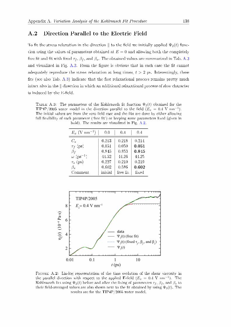
Appendix A. Variation Analysis of the Kohlrausch Fit Procedure 138
A.2 Direction Parallel to the Electric Field
To t the stress relaxation in the direction ‖ to the eld we initially applied Ψ2(t) func-
tion using the values of parameters obtained at E = 0 and allowing both the completely
free t and t with xed τf , βf , and βs. The obtained values are summarized in Tab. A.3
and visualized in Fig. A.2. From the gure is obvious that in each case the t cannot
adequately reproduce the stress relaxation at long times, t > 2 ps. Interestingly, these
ts (see also Tab. A.3) indicate that the fast relaxational process remains pretty much
intact also in the ‖ direction in which an additional relaxational process of slow character
is induced by the E-eld.
Table A.3: The parameters of the Kohlrausch t function Ψ2(t) obtained for theTIP4P/2005 water model in the direction parallel to the eld (Ex = 0.4 V nm−1).The initial values are from the zero eld case and the ts are done by either allowingfull exibility of each parameter (`free t') or keeping some parameters xed (given in
bold). The results are visualized in Fig. A.2.
Ex (V nm−1) 0.0 0.4 0.4
Cs 0.213 0.218 0.214τf (ps) 0.051 0.050 0.051βf 0.845 0.853 0.845ω (ps−1) 44.52 44.26 44.25τs (ps) 0.227 0.210 0.219βs 0.602 0.586 0.602Comment initial free t xed
data
Ψ2(t) (fixed τ
f , β
f , and β
s)
0.01 0.1 10t (ps)
2
4
6
η||(
t)
(10
−4 P
a∙s)
1
8
Ψ3(t)
Ψ2(t) (free fit)
TIP4P/2005
Ex= 0.4 V nm−1
Figure A.2: Lin-log representation of the time evolution of the shear viscosity inthe parallel direction with respect to the applied E-eld (Ex = 0.4 V nm−1). TheKohlrausch ts using Ψ2(t) before and after the xing of parameters τf , βf , and βs totheir eld-averaged values are also shown next to the t obtained by using Ψ3(t). The
results are for the TIP4P/2005 water model.

Appendix A. Variation Analysis of the Kohlrausch Fit Procedure 139
The eld-induced relaxation process (subscript i) is again modelled by the stretched
exponential law, exp[− (t/τf )β
]. The resultant three-step Kohlrausch t Ψ3(t) is given
by Eq. A.2. From thorough trial and error analysis it is deduced that it is not possible
to keep xed the parameters (except Cs), obtained for the ⊥ direction, and only vary
Ci, τi, and βi in order to obtain a good t of the data in the ‖ direction. In other words,
the eld-induced process is intimately coupled to the other slow process. Moreover, it
is common to all these trials that they fail to reproduce the slope (2 ps < t . 10 ps)
in η‖(t). However, the trials indicated that the exibility of βs is necessary in order to
obtain a satisfactory t. Thus, in the initial guess for Ψ3(t) the values of τf and βf
were kept xed while βs was allowed to vary. The obtained values of the Kohlrausch
parameters are given in Tab. A.4.
Table A.4: The parameters of the three-step Kohlrausch t obtained for theTIP4P/2005 water model in the direction parallel to the electric eld. The xed pa-
rameters are given in bold.
Ex (V nm−1) 0.0 0.2 0.4 0.6 Trend Max. dev.
Cs 0.213 0.203 0.203 0.197 ↓ 7.5 %τf (ps) 0.051 0.051 0.051 0.051 xed -βf 0.845 0.845 0.845 0.845 xed -ω (ps−1) 44.52 44.429 44.28 44.14 ↓ 0.9 %τs (ps) 0.227 0.223 0.209 0.205 ↓ 9.7 %βs 0.602 0.644 0.638 0.642 const. 6.5 %
Ci - 0.0045 0.0088 0.0127 ↑ 64.6 %τi (ps) - 1.582 1.392 1.088 ↓ 31.2 %βi - 0.528 0.554 0.559 const. 5.5 %
Cs + Ci 0.213 0.208 0.212 0.209 const. -
From Tab. A.4 it is obvious that alongside τf and βf , which are kept xed, the
values for βi are pretty much unaected by the electric eld and, thus, βi can be treated
as constant. Remarkably, βs(‖) experiences a small discrete increment with respect to
βs(⊥, E = 0). Furthermore, the sum Cs+Ci is found to be constant and eectively equal
to Cs(⊥, E = 0), meaning that a fraction of the fast relaxation remains independent of
the electric eld strength. Based on these observations the parameters βf , τf , βs, and βiare xed to their eld-averaged values and the t procedure is repeated. The obtained
values are gathered in Tab. A.5. In Fig. A.2 the t obtained by using Ψ3(t) for the ‖direction is also displayed. Clearly, the t reproduces excellently the stress relaxation
and thus η‖(t) as well.
Likewise for the ⊥ direction, the data in Tab. A.5 again demonstrates that the
xing of some parameters does not aect the quality of the obtained Kohlrausch ts.
Indeed, the ts before and after the xing of parameters are indistinguishable (as already

Appendix A. Variation Analysis of the Kohlrausch Fit Procedure 140
Table A.5: The parameters of the three-step Kohlrausch t obtained for theTIP4P/2005 water model in the direction parallel to the electric eld after xing τf ,
βf , βs, and βi from Tab. A.4. The xed parameters are given in bold.
Ex (V nm−1) 0.0 0.2 0.4 0.6 Trend Max. dev.
Cs 0.213 0.205 0.201 0.197 ↓ 7.5 %τf (ps) 0.051 0.051 0.051 0.051 xed -βf 0.845 0.845 0.845 0.845 xed -ω (ps−1) 44.52 44.42 44.28 44.14 ↓ 0.9 %τs (ps) 0.227 0.222 0.201 0.205 ↓ 9.7 %βs 0.602 0.642 0.642 0.642 xed 6.2 %
Ci - 0.0038 0.0094 0.0130 ↑ 70.8 %τi (ps) - 1.891 1.320 1.030 ↓ 45.5 %βi - 0.547 0.547 0.547 xed 9.1 %
Cs + Ci 0.213 0.208 0.211 0.210 const. -
observed for the ⊥ direction in Fig. A.1) and thus not shown explicitly. Importantly, the
t employing Ψ3(t) reduces to a t function with ve free parameters.
As already mentioned, identical behavior of the Kohlrausch t parameters is ob-
served for the SPC/E and TIP4P water models. However, the parameter that diers
between them is βi which is found to be about 0.5 and 0.75 for the SPC/E and the
TIP4P model, respectively.
In conclusion, the relaxation times of the fast (Tf ), the slow (Ts), and the eld-
induced (Ti) relaxation processes are calculated and shown in Tab. A.6. The total relax-
ation times in both directions with respect to the direction of the E-eld are also given.
The detailed discussion about the relaxation times is presented in the main text (consult
Sec. 3.3.3).
Table A.6: The relaxation times (fast Tf , slow Ts, eld-induced Ti, and total Ttot)obtained for the TIP4P/2005 water model. Maximal deviation is given with respect to
the zero eld case. All times are given in fs.
Ex (V nm−1) 0.0 0.2 0.4 0.6 Trend Max. dev.
Tf (⊥) 5.94 5.97 5.93 5.85 appears const. 2.0%Tf (‖) - 5.26 5.27 5.30 decrement 11.4 %Ts(⊥) 72.44 68.75 63.80 62.76 ↓ 13.4 %Ts(‖) - 62.79 58.45 55.66 ↓ 23.2 %Ti(‖) - 12.47 21.16 23.03 ↑ -
Ttot(⊥) 78.38 74.72 69.73 68.72 ↓ 12.3 %Ttot(‖) - 80.52 84.88 83.99 ↑ 6.7 %

Appendix B
Two-dimensional Static Correlations
B.1 Two-dimensional Density Correlations of Water
The atom-atom (oxygen-oxygen, oxygen-hydrogen, and hydrogen-hydrogen) radial dis-
tribution functions (RDF) for water in the absence of an external electric eld are shown
in Fig. B.1. The 2-D RDFs g(x, a) are calculated by a self-made analysis tool. From the
two-dimensional RDFs (left column in Fig. B.1) is evident that the isotropic nature of
the system is preserved for each RDF.
The correctness of the 2-D plots, and the analysis code itself, is checked by com-
paring the (red) line extracted at x = 0 nm (only the part a ≥ 0) with the fully ra-
dially averaged correlation functions (black lines) in the right column of Fig. B.1. In
each case the extracted line nicely reproduces the corresponding radially averaged RDF.
Thus, the analysis code performs well and also captures all important features of the
one-dimensional g(r).
From the radially averaged RDFs, the eld impact on the density correlations in
water is found to be proportional to its strength (between 0 and 1 V nm−1) but still
very weak (see Fig. 3.3 in the main text). Therefore, to better depict the impact of
the electric eld on g(r) the behavior of each RDF (gOO, gOH, and gHH) around the
1st maximum and the 1st minimum is shown in separate boxes in the right column of
Fig. B.2. Moreover, the behavior of each RDF at longer distances from the central atom
(0.35 nm ≤ r ≤ 1 nm) is also shown (left column). Although are shown only the results
for the SPC/E water model a very similar structuring is also found for the TIP4P and
TIP4P/2005 water models, both in the 1-D and 2-D representations.
141

Appendix B. Two-dimensional Static Correlations 142
−1.4 −1 −0.5 0 0.5 1 1.4
−1.4 −1 −0.5 0 0.5 1 1.41.4
1
0.5
0
−0.5
−1
−1.4
a (
nm
)a
(n
m)
a (
nm
)
1.4
1
0.5
0
−0.5
−1
−1.4
1.4
1
0.5
0
−0.5
−1
−1.4
1.1
1
0.9
0.8
1.2
g(x,a)
1.1
1
0.9
0.8
1.2
g(x,a)
1.1
1
0.9
0.8
1.2
g(x,a)
gOH
(x,a)
gOO
(x,a)
gHH
(x,a)
x (nm)
x (nm)
r [nm]
0.6
1.2
1.8
2.4
3radially averaged
line x = 0 nm from 2D plot
r [nm]
0.4
0.8
1.2
1.6
0.2 0.4 0.6 0.8 10
0.4
0.8
1.2
r (nm)
r (nm)
gO
O(r
)g
OH(r
)g
HH(r
)
0.2 0.4 0.6 0.8 1
Figure B.1: Radial distribution functions (RDF) for the SPC/E water model in theabsence of an external electric eld both in the two-dimensional (left column) and one-dimensional representation (right column). Shown are the correlation functions for thepairs oxygen-oxygen (top row), oxygen-hydrogen (middle row), and hydrogen-hydrogen(bottom row). The 1-D curves are obtained by evaluating the correlations in a fullyradially averaged manner (black lines) or extracted from the 2-D representation (leftcolumn) as the positive part (a ≥ 0) of the line x = 0 nm (red line). The same colorscheme is used for all the 2-D RDFs. The results are generated from 100 frames of the
data.

Appendix B. Two-dimensional Static Correlations 143
0.9
1
1.1
gO
O(r
)
E = 0 E = 0.2
E = 0.4 E = 0.6 E = 1
0.96
0.98
1
1.02
2nd min
0.32 0.36 0.4
0.9
0.27 0.28
2.9
3
0.4 0.5 0.6 0.7 0.8 0.9
0.96
1
1.04
1.08
1.12
1.16
0.4 0.5 0.6 0.7 0.8 0.9
0.4 0.5 0.6 0.7 0.8 0.9
0.4 0.5 0.6 0.7 0.8 0.9
r (nm)
gO
H(r
)g
HH(r
)
r (nm)
r (nm)
2nd max
0.17 0.18
1.4
1.5
1.6
0.24 0.26
0.2
0.22
0.22
1
0.23 0.24 0.25
1.26
1.32
0.28 0.3 0.32
0.72
0.76
0.8
1st min
1st max
1st max
1st min
1st min
1st max
2nd max
r (nm)
E (in V nm−1)
Figure B.2: Comparison of the water radial distribution function g(r) for dierentstrengths of the homogeneous electric eld. Shown are the RDFs for the atom pairs:oxygen-oxygen (top row), oxygen-hydrogen (middle row), and hydrogen-hydrogen (bot-tom row). The two small boxes at the right-hand side of each RDF show the behaviorof corresponding g(r) around the 1st maximum and the 1st minimum, respectively. Thebehavior at longer distances from the central atom (0.35 nm ≤ r ≤ 1 nm) is shown in
the large boxes at the left-hand side. All results are for the SPC/E water model.

Appendix B. Two-dimensional Static Correlations 144
B.2 2-D Correlations for the LJ Particle-Water System in
the Absence of Electric Fields
The two-dimensional plots for each component of the total solute-water correlation func-
tion at E = 0 are shown in Fig. B.3 (left column). The radial distribution function
gLJ-O shows nicely the structuring around the LJ particle. Three and two nicely dened
maxima and minima, respectively, can be easily distinguished from the bulk at large
distances. As expected, the spherical appearance of the LJ particle in the absence of ex-
ternal electric elds is captured. In contrast to the RDF the angular correlations 〈P1(θ)〉and 〈P2(φ)〉 show signicantly fewer details and, therefore, are rather uninteresting com-
pared to the their counterparts obtained in the presence of the electric elds. However,
for both the angles, the negative correlations in the very proximity of the LJ particle can
be noticed. These negative correlations are followed by well-dened maxima after which
their correlations are characterized by minuscule uctuations around zero.
The correctness of the 2-D plots, and the analysis code itself, is checked by compar-
ing the (red) line extracted at x = 0 nm (only the part a ≥ 0) with the fully radially aver-
aged correlation functions (black lines) in the right column of Fig. B.3. Although for each
correlation function only one line is extracted from the 2-D plot, the line nicely reproduces
the radially averaged functions. Moreover, the chosen bin width (∆x = ∆a = 0.02972
nm) in the 2-D representation is indeed sucient to capture all the relevant structuring
details obtained in the radially averaged manner (∆r = 0.002 nm).

Appendix B. Two-dimensional Static Correlations 145
4.4
3
1.5
0
−1.5
−3
−4.4
−4.4 −3 −1.5 0 1.5 3 4.4
4.4
3
1.5
0
−1.5
−3
−4.4
−4.4 −3 −1.5 0 1.5 3 4.4
4.4
3
1.5
0
−1.5
−3
−4.4
0.6
0.4
0.2
0
−0.2
−0.4
−0.6
0.6
0.4
0.2
0
−0.2
−0.4
−0.6
⟨P1(θ)⟩
⟨P2(ϕ)⟩
x (nm)
x (nm)
a (
nm
)a
(n
m)
a (
nm
)
g(x,a)
1.2
1.1
1.0
0.9
r / nm
0.9
1
1.1
radially averaged
line x = 0 nm from 2D plot
−0.18
−0.12
−0.06
0
0.06
1.6 2 2.4 2.8
−0.2
0
0.2
0.4
0.6
1.6 2 2.4 2.8
r (nm)
r (nm)
⟨P1(θ)⟩
⟨P2(ϕ)⟩
g(r)
Figure B.3: The correlations functions between the LJ particle and water in the ab-sence of an external electric eld both in the two-dimensional (left) and one-dimensionalrepresentation (right). Shown are: gLJ-O (top), 〈P1(θ)〉 (middle), and 〈P2(φ)〉 (bottom).The 1-D curves are obtained by evaluating the correlations in a fully radially averagedmanner (black lines) or extracted from the 2-D representation (left) as the positive part(a ≥ 0) of the line x = 0 nm (red line). The same color scheme is used for both theangular correlation functions. The results are generated from 200 ns (106 time frames)of the data from the simulations employing the shift treatment of the vdW forces.

Appendix B. Two-dimensional Static Correlations 146
B.3 Angular Correlations Between the Heptane Droplet and
Water
The remarkable similarity observed between the radially averaged correlation functions
for the LJ particle-water system and the heptane droplet in water is thoroughly discussed
in Sec. 6.3. This similarity is also expected to translate to the two-dimensional represen-
tations. To demonstrate this, the 2-D angular correlations functions 〈P1(θ)〉 and 〈P2(φ)〉for the heptane aggregate in water at Ex = 0.6 V nm−1 are shown in Fig. B.4.
−4.4 −3 −1.5 0 1.5 3 4.4 −4.4 −3 −1.5 0 1.5 3 4.4
x (nm) x (nm)
0.6
0.4
0.2
0
−0.2
−0.4
−0.6
E
⟨P1(θ)⟩ ⟨P
2(ϕ)⟩
4.4
3
1.5
0
−1.5
−3
−4.4
a (nm
)
Figure B.4: Two-dimensional angular correlation functions between the center-of-mass of the heptane droplet and water in the presence of the electric eld (Ex = 0.6V nm−1). The correlation functions for the dipole angle (left) and the normal angle(right) are shown. The same color scheme is used for both the correlation functions.
The results are generated from 20 ns (105 time frames) of the simulation data.
For both the dipole and normal angles, a striking resemblance to the correlations
found for the LJ particle-water system (Fig. 6.5) is immediately evident. Even though
only 20 ns (105 frames) are analyzed, rich and complex patterns emerge in the correlations
for both the dipole and normal angles. The noise arising from the small sampling volume
is strongly reected in the vicinity of the heptane droplet. Importantly, the −x/+x
asymmetry around the heptane droplet is still present but not as pronounced as in the
case of the LJ particle. This is likely related to the fact that the surfaces of the heptane
droplet perpendicular to the electric eld are smaller compared to those observed for the
LJ particle as the heptane droplet heavily elongates in the eld direction.
B.4 Angular Correlations for Neat Water
The angular correlations of neat water in the presence of external electric elds (Ex = 0.6
V nm−1), measured as 〈P1(θ)〉 and 〈P2(φ)〉, are shown in Fig. B.5. At each volume
element, for both the dipole angle (θ) and the normal angle (φ), the correlations are

Appendix B. Two-dimensional Static Correlations 147
evaluated between a water molecule occupying that space and the center of the simulation
box. In this manner, the dimensionless point in the center of the simulation cell with
respect to which the correlations are calculated can be understood as an innitely small
hydrophobic object.
From Fig. B.5 it is evident that around the center of the box the twofold symmetry
for the dipole angle and the fourfold symmetry for the normal angle are clearly recovered
in the presence of the electric elds. In other words, the angular symmetry of water
is preserved as expected from the denition of the employed coordinate system (see
Sec. 6.2). In a general sense, even from these simple symmetry considerations, a quick
convergence to zero of the radially averaged functions i.e. the absence of the long-ranged
angular correlations in neat water follows. As remarked already, the dipole angle adopts
a preferred direction with respect to the direction of the imposed electric eld. In turn,
this limits the available angles that the normal angle can obtain. Interestingly, this
orientational locking of the normal angle can be recognized even by the somewhat more
apparent noise in the normal angle correlations than in the dipole angle correlations (see
also Figs. 6.5 and B.4). However, a closer look reveals that rich and complex patterns
further from the box center are considerably maintained in both the angular correlation
functions between the LJ particle (or the heptane droplet) and water. Therefore, the
extent of the −x/+x asymmetry observed around the hydrophobic object can be directly
related to its size (see Figs. 6.5 and B.4).
−4.4 −3 −1.5 0 1.5 3 4.4
4.4
3
1.5
0
−1.5
−3
−4.4
−4.4 −3 −1.5 0 1.5 3 4.4
x (nm) x (nm)
a (nm
)
(a) (b)
0.6
0.4
0.2
0
−0.2
−0.4
−0.6E
⟨P1(θ)⟩ ⟨P
2(ϕ)⟩
Figure B.5: Angular correlations for neat water in the presence of external electricelds (Ex = 0.6 V nm−1). The correlations for the dipole (a) and the normal angle(b) are evaluated between each water molecule and the dimensionless point located inthe center of the simulation box. The same color scheme is used for both correlationfunctions. The results are obtained from 20 ns (105 time frames) of the simulation data.

Appendix B. Two-dimensional Static Correlations 148
B.5 Dierent Treatments of the van der Waals Interactions
4.4
3
1.5
0
−1.5
−3
−4.4
4.4
3
1.5
0
−1.5
−3
−4.4
4.4
3
1.5
0
−1.5
−3
−4.4
−4.4−3 −1.5 0 1.5 3 4.4
4.4
3
1.5
0
−1.5
−3
−4.4
CUT SWITCH SHIFT
x (nm)
a (
nm
)
x (nm) x (nm)
a (
nm
)a (
nm
)a (
nm
)
0.6
0.4
0.2
0
−0.2
−0.4
−0.6
⟨P1(θ)⟩
⟨P2(ϕ)⟩
−4.4−3 −1.5 0 1.5 3 4.4 −4.4
−3 −1.5 0 1.5 3 4.4
E
E
E
E
x (nm) x (nm) x (nm)
−4.4−3
−1.5 01.5 3 4.4
−4.4 −3−1.5 0
1.5 3 4.4−4.4 −3
−1.5 01.5 3 4.4
gLJ-O
(x,a)
gLJ-H
(x,a)
gLJ-H
(x,a)
gLJ-O
(x,a)
1.2
1.1
1.0
0.9
Figure B.6: Two-dimensional correlations functions between the LJ particle and waterin the presence of an external electric eld (Ex = 0.6 V nm−1) for dierent treatmentsof the van der Waals interactions (cut - left column, switch - middle column, and shift- right column). In rows, from top to bottom, are shown: gLJ-O, gLJ-H, 〈P1(θ)〉, and
〈P2(φ)〉.

List of Figures
2.1 The potential and the force for the cut, switch and shift treatments of thevan der Waals interactions between the oxygen atom of a water moleculeand the employed Lennard-Jones particle . . . . . . . . . . . . . . . . . . 19
2.2 Schematic representation of the geometry of the SPC/E and the TIP4Pwater model . . . . . . . . . . . . . . . . . . . . . . . . . . . . . . . . . . . 23
3.1 Dependence of density of the rigid water models (TIP4P, SPC/E, andTIP4P/2005) on the strength of applied electric eld (E ≤ 1 V nm−1).Also are shown the dependencies of the polarization density in the elddirection, susceptibility, and nonlinearity on the eld strength for theTIP4P/2005 water model . . . . . . . . . . . . . . . . . . . . . . . . . . . 27
3.2 Two-dimensional radial distribution functions (RDF) for the SPC/E watermodel at the electric eld strength of E = 1 V nm−1 and the dierenceof the RDFs obtained at E = 1 and E = 0 V nm−1. Shown are thecorrelation functions for the atom pairs oxygen-oxygen, oxygen-hydrogen,and hydrogen-hydrogen . . . . . . . . . . . . . . . . . . . . . . . . . . . . 31
3.3 Comparison of the radially averaged radial distribution functions gOO(r)for the SPC/E water model for dierent strengths of the homogeneouselectric eld (between 0 and 1 V nm−1). . . . . . . . . . . . . . . . . . . . 32
3.4 The one-dimensional radial distribution functions for pairs oxygen-oxygenand hydrogen-hydrogen of the SPC/E water model in various directions(parallel, perpendicular or at 45) with respect to the direction of imposedelectric eld (Ex = 1 V nm−1) . . . . . . . . . . . . . . . . . . . . . . . . . 33
3.5 Short-time behavior and the slowly converging tails of the averaged stressautocorrelation function for TIP4P, SPC/E, and TIP4P/2005 water mod-els. Also is shown the time evolution of the shear viscosity for each watermodel . . . . . . . . . . . . . . . . . . . . . . . . . . . . . . . . . . . . . . 36
3.6 The two-step Kohlrausch t of the averaged stress autocorrelation func-tion and the corresponding time evolution of the shear viscosity for theTIP4P/2005 water model in the absence of an external electric eld . . . . 38
3.7 Impact of the externally applied static electric eld (Ex = 0.6 V/nm) onthe unnormalized components of the stress autocorrelation function andthe corresponding time evolution of the shear viscosity relative to the eldfree case . . . . . . . . . . . . . . . . . . . . . . . . . . . . . . . . . . . . . 39
3.8 Time evolution of the shear viscosity (TIP4P/2005 water model) in thedirections perpendicular and parallel to the applied electric eld (Ex = 0.6V/nm). The Kohlrausch ts obtained by using two- and three-step tfunctions are also shown . . . . . . . . . . . . . . . . . . . . . . . . . . . . 40
149

List of Figures 150
3.9 Anisotropy of the shear viscosity for the TIP4P/2005 water model in thepresence of an external electric eld. Apparent shear viscosity of the rigidwater models TIP4P/2005, SPC/E, and TIP4P as a function of the electriceld strength (for E ≤ 0.6 V nm−1) . . . . . . . . . . . . . . . . . . . . . . 43
3.10 The apparent self-diusion coecient and its components parallel andperpendicular to the eld for the TIP4P water model as a function of theeld strength . . . . . . . . . . . . . . . . . . . . . . . . . . . . . . . . . . 44
3.11 Relaxation times associated with the fast, the slow, and the eld-inducedrelaxation process in both the perpendicular and parallel direction withrespect to the direction of the electric eld. Also shown are the totalrelaxation times in each direction. Results are for the TIP4P/2005 watermodel . . . . . . . . . . . . . . . . . . . . . . . . . . . . . . . . . . . . . . 44
3.12 Dependence of the oscillation frequency in the directions perpendicularand parallel to the direction of the imposed electric eld. Shown are theresults for the TIP4P and TIP4P/2005 water models . . . . . . . . . . . . 45
4.1 Snapshot of the Lennard-Jones particle immersed in water . . . . . . . . . 504.2 The mean square square displacement and the linear t function for the
Lennard-Jones particles having masses of 50 u and 105 u . . . . . . . . . . 534.3 Dependence of the diusion coecient of the Lennard-Jones particle on
its mass for the system sizes between 11130 and 101260 water molecules . 544.4 Dependence of the normalized velocity autocorrelation function on the
system size for the Lennard-Jones particle having mass of 2× 10⁴ u . . . . 574.5 The time evolution of the diusion coecient of the Lennard-Jones particle
(mass 2 × 10⁴ u) for the systems containing between 11130 and 408573water molecules . . . . . . . . . . . . . . . . . . . . . . . . . . . . . . . . . 58
4.6 The mean square displacement of the Lennard-Jones particle (mass 2×10⁴
u) for the systems containing between 11130 and 408573 water molecules . 594.7 The dependence of the diusion coecient on the reciprocal length of the
simulation cell for the Lennard-Jones particle with mass of 2× 10⁴ u . . . 604.8 The normalized force autocorrelation function and the running values of
the friction coecient for the `light' solutes (mass smaller or equal to105 u) and the `heavy' solutes (mass equal or larger than 106 u) . . . . . . 64
4.9 Dependence of the normalized force autocorrelation function and the timeevolution of the friction coecient on the system size for immobile solute . 65
4.10 The inidirect validation of the Einstein relation inspected by the depen-dence of the diusion coecient and the friction coecient of the Lennard-Jones particle on the system size . . . . . . . . . . . . . . . . . . . . . . . 68
4.11 The characteristic features in the radial distribution function between theLJ particle and water hydrogen atoms gLJ-H(r), associated to the slip andthe stick boundary conditions . . . . . . . . . . . . . . . . . . . . . . . . . 70
4.12 The estimates of the water shear viscosity as a function of mass of theLennard-Jones particle for various system sizes. The estimates are ob-tained either from the diusion coecient of the particle or from its dif-fusive length scale . . . . . . . . . . . . . . . . . . . . . . . . . . . . . . . 72
4.13 Dependence of the estimated shear viscosities on the mass of the Lennard-Jones particle. The estimates are obtained from the diusion coecient,the friction coecient, and the diusive length scale of the Lennard-Jonesparticle . . . . . . . . . . . . . . . . . . . . . . . . . . . . . . . . . . . . . 73

List of Figures 151
5.1 A snapshot from the simulation of the heptane droplet immersed in water 805.2 Comparison of dierent radial distribution functions (RDF) between the
Lennard-Jones particle and water for dierent treatments of the van derWaals interactions, namely the cut, switch, and shift treatments in theabsence of the electric eld. The local behavior of respective RDFs aroundthe 1st and 2nd maxima, and the 1st minimum is presented alongside thebehavior at large distances (r ≥ 2.1 nm) from the particle . . . . . . . . . 81
5.3 Comparison of the radial distribution function between the Lennard-Jonesparticle and water oxygen for the cut, switch and shift treatments of thevan der Waals interactions. The local behavior of respective RDFs aroundthe 1st and 2nd maxima, and the 1st minimum is presented alongside thebehavior at large distances (r ≥ 2.1 nm) from the particle. The resultsare for the simulations performed in the NVT ensemble in the presence ofexternal electric elds, E = 0.6 V nm−1 . . . . . . . . . . . . . . . . . . . 82
5.4 The displacement of the Lennard-Jones particle in the absence and thepresence of static electric elds. The results for the NVT and the NPTensemble are shown . . . . . . . . . . . . . . . . . . . . . . . . . . . . . . . 84
5.5 The displacement of the Lennard-Jones particle in the direction of theimposed static electric eld, Ex = 0.6 V nm−1. The simulations are per-formed in the NVT ensemble and the vdW interactions are represented bythe cut scheme for dierent thermostats (Berendsen and velocity rescale)and with dierent neighbour list update frequency . . . . . . . . . . . . . 85
5.6 Dependence of the displacement of the Lennard-Jones particle on the cut-o distance in the presence of static electric elds (Ex = 0.6 V nm−1) . . 86
5.7 Dependence of the displacement of the center-of-mass of the heptanedroplet on the cuto distance in the presence of static electric elds(Ex = 0.6 V nm−1) . . . . . . . . . . . . . . . . . . . . . . . . . . . . . . . 88
5.8 The time dependence of the net van der Waals force exerted by the watermolecules on the Lennard-Jones particle in the direction of the appliedexternal electric eld of strength 0.6 V nm−1 . . . . . . . . . . . . . . . . 91
5.9 Probability density of the contribution to the total van der Waals force onthe Lennard-Jones particle arising from the transition region, 2.4 nm ≤r ≤ 2.8 nm. The results are obtained from the NVT simulations in thepresence of the electric eld (Ex = 0.6 V/nm) with the switch treatmentof the vdW interactions . . . . . . . . . . . . . . . . . . . . . . . . . . . . 92
5.10 Comparison of the distribution of the instantaneous velocity of the Lennard-Jones particle in the direction of the imposed static electric eld, Ex = 0.6V nm−1 with the shift treatment. The simulations were performed withthe Berendsen thermostat, advanced velocity rescaling, Nosé-Hoover, andby Langevin dynamics . . . . . . . . . . . . . . . . . . . . . . . . . . . . . 95
5.11 The distribution of the velocity of the Lennard-Jones particle along thedirection of the eld, calculated from the displacement of the particle.The distributions for the shift and the cut treatment of the van der Waalsinteractions are shown . . . . . . . . . . . . . . . . . . . . . . . . . . . . . 96
6.1 The internal coordinate system of the Lennard-Jones particle and a watermolecule . . . . . . . . . . . . . . . . . . . . . . . . . . . . . . . . . . . . . 101
List of Figures 152
6.2 The radially averaged angular correlation functions between the Lennard-Jones particle and water in the absence of an external electric eld. Shownare the correlation functions for the dipole and the normal angle for thecut, switch and shift treatments of the van der Waals interactions . . . . . 103
6.3 The radially averaged correlation functions in the presence and the ab-sence of the electric elds for both the Lennard-Jones particle and heptanedroplet. Shown are: the radial distribution function, the dipole angle andthe normal angle correlation function . . . . . . . . . . . . . . . . . . . . . 105
6.4 Two-dimensional radial distribution function between the Lennard-Jonesparticle and the oxygen atom of a water molecule . . . . . . . . . . . . . . 108
6.5 Two-dimensional correlation functions for the dipole angle and the normalangle . . . . . . . . . . . . . . . . . . . . . . . . . . . . . . . . . . . . . . . 109
6.6 Dierence between the angular correlation functions for the Lennard-Jonesparticle-water system and a dimensionless point in water at the electriceld strength of 0.6 V nm−1 . . . . . . . . . . . . . . . . . . . . . . . . . . 111
6.7 Two-dimensional plot of the mean projection of the water dipole vectoronto the x direction in the absence (E = 0) and in the presence of anexternal electric eld (Ex = 0.6 V nm−1) . . . . . . . . . . . . . . . . . . . 112
6.8 The averaged eective dipole density of water around the Lennard-Jonesparticle shown as the 2-D plot of the entire system and as the extractedline around radius of 1.1 nm from the corresponding 2-D representation . 113
6.9 Representation of the most probable orientations of water molecules atdierent positions in the very proximity of the surface of the Lennard-Jones particle both in the absence and presence of the electric elds (Ex =0.6 V nm−1) . . . . . . . . . . . . . . . . . . . . . . . . . . . . . . . . . . . 114
6.10 The displacement of the Lennard-Joens particle in all three Cartesiandirections in the presence of the electric eld (Ex = 0.6 V nm−1) with theshift treatment of the van der Waals interactions . . . . . . . . . . . . . . 116
6.11 The calculated mean square displacement (MSD) in the non-eld direc-tions and in the eld direction. In each case the calculated MSD is com-pared to the theoretically expected MSD of the employed LJ particle per-forming Brownian diusion . . . . . . . . . . . . . . . . . . . . . . . . . . 117
6.12 The 2-D plot of the density correlations between the Lennard-Jones par-ticle and the hydrogen atoms of water averaged over the two halves of thecylinder . . . . . . . . . . . . . . . . . . . . . . . . . . . . . . . . . . . . . 119
6.13 The density dierence of water hydrogen atoms between the two sides ofthe Lennard-Jones particle with respect to the direction of the appliedelectric eld (Ex = 0.6 V nm−1) . . . . . . . . . . . . . . . . . . . . . . . . 120
6.14 Comparison of the simulated and the theoretically predicted mean squaredisplacement of the Lennard-Jones particle in the eld direction . . . . . . 124
A.1 Time evolution of the shear viscosity in the perpendicular direction withrespect to the applied electric eld (Ex = 0.4 V nm−1) for the TIP4P/2005water model. The two-step Kohlrausch ts before and after the xing ofparameters τf , βf , and βs are also shown . . . . . . . . . . . . . . . . . . . 137

List of Figures 153
A.2 Time evolution of the shear viscosity in the parallel direction with respectto the applied electric eld (Ex = 0.4 V nm−1) for the TIP4P/2005 watermodel. The Kohlrausch ts using the two-step function before and afterthe xing of parameters τf , βf , and βs to their eld-averaged values arealso shown next to the t obtained by using the three-step Kohlrausch tfunction . . . . . . . . . . . . . . . . . . . . . . . . . . . . . . . . . . . . . 138
B.1 Radial distribution functions (RDF) for the SPC/E water model in theabsence of an external electric eld both in the two-dimensional and one-dimensional representation. Shown are the RDFs for the pairs oxygen-oxygen, oxygen-hydrogen, and hydrogen-hydrogen . . . . . . . . . . . . . . 142
B.2 Comparison of the water radial distribution functions (radially averaged)at longer distances from the central atom (0.35 nm ≤ r ≤ 1 nm) for dier-ent strengths of the homogeneous electric eld. Shown are the radial dis-tribution functions for the atom pairs: oxygen-oxygen, oxygen-hydrogen,and hydrogen-hydrogen. The local behavior of corresponding functionsaround the 1st maximum and the 1st minimum is also shown . . . . . . . . 143
B.3 The correlation functions between the Lennard-Jones particle and waterin the absence of an external electric eld both in the two-dimensionaland one-dimensional representation. Shown are: the radial distributionfunction, the dipole angle and the normal angle correlation function . . . . 145
B.4 Two-dimensional angular correlation functions between the center-of-massof the heptane droplet and water in the presence of the electric eld (Ex =0.6 V nm−1). Shown are the correlation functions for the dipole angle andthe normal angle . . . . . . . . . . . . . . . . . . . . . . . . . . . . . . . . 146
B.5 Angular correlations for neat water in the presence of external electricelds (Ex = 0.6 V nm−1) . . . . . . . . . . . . . . . . . . . . . . . . . . . 147
B.6 Two-dimensional correlations functions between the Lennard-Jones par-ticle and water in the presence of an external electric eld (Ex = 0.6V nm−1) for dierent treatments of the van der Waals interactions (cut,switch, and shift) . . . . . . . . . . . . . . . . . . . . . . . . . . . . . . . . 148

List of Tables
2.1 Force eld parameters of water models employed in this thesis, namelyTIP4P, SPC/E, and TIP4P/2005 water models . . . . . . . . . . . . . . . 23
3.1 The perpendicular and the parallel component of the shear viscosity ofrigid water models (TIP4P, SPC/E, TIP4P/2005) with respect to thedirection of the imposed electric eld. The shear viscosity at zero eld isalso given . . . . . . . . . . . . . . . . . . . . . . . . . . . . . . . . . . . . 42
4.1 Simulation time (in ns) of the Lennard-Jones particle-water simulationsperformed for dierent system sizes and the mass of the solute . . . . . . . 52
4.2 The values of the hydrodynamic radius estimated from the Stokes-Einsteinrelation by assuming the slip and the stick boundary conditions. Also aregiven plausible denitions for the hydrodynamic radius originating fromthe radial distribution function between the Lennard-Jones particle andwater and their respective values . . . . . . . . . . . . . . . . . . . . . . . 69
4.3 The estimates of the solvent shear viscosity obtained both from the dif-fusion coecient and diusive length scale of the Lennard-Jones particleusing the slip boundary conditions. The estimate are given for the threesystem sizes containing 23419, 50280, and 101260 water molecules . . . . . 72
5.1 The diusion coecients of the Lennard-Jones particle for dierent treat-ments of the van der Waals interactions in the presence and absence ofelectric elds for both the NVT and NPT ensembles . . . . . . . . . . . . 89
5.2 The net van der Waals (vdW) force on the Lennard-Jones particle in eachCartesian direction for dierent treatments of the vdW interactions in thepresence and absence of static electric elds imposed in the +x direction . 91
A.1 The parameters of the two-step Kohlrausch t obtained for the TIP4P/2005water model in the direction perpendicular to the eld as well as in theabsence of the electric eld . . . . . . . . . . . . . . . . . . . . . . . . . . . 136
A.2 The parameters of the two-step Kohlrausch t obtained for the TIP4P/2005water model in the direction perpendicular to the eld as well as in theabsence of the eld after the xing of parameters τf , βf , and βs fromTab. A.1 . . . . . . . . . . . . . . . . . . . . . . . . . . . . . . . . . . . . . 137
A.3 The parameters of the two-step Kohlrausch t function obtained for theTIP4P/2005 water model in the direction parallel to the eld (Ex = 0.4V nm−1) . . . . . . . . . . . . . . . . . . . . . . . . . . . . . . . . . . . . . 138
A.4 The parameters of the three-step Kohlrausch t in the direction parallelto the electric eld obtained for the TIP4P/2005 water model . . . . . . . 139
155

List of Tables 156
A.5 The parameters of the three-step Kohlrausch t in the direction parallelto the electric eld after xing τf , βf , βs, and βi from Tab. A.4. Theresults are for the TIP4P/2005 water model . . . . . . . . . . . . . . . . . 140
A.6 The relaxation times (fast, slow, eld-induced, and total) obtained for theTIP4P/2005 water model for dierent electric eld strengths . . . . . . . . 140
Abbreviations
RDF Radial Distribution Function
ATP Adenosine Triphospate
EPM Electrophoretic Mobility
MD Molecular Dynamics
VSFG Vibrational Sum Frequency Generation
PES Photoelectron Spectroscopy
SHG Second Harmonic Generation
VdW Van der Waals
GROMACS Groningen Machine for Chemical Simulations
LJ Lennard-Jones
PME Particle Mesh Ewald
PPPM Particle-Particle Particle-Mesh
TIP Transferable Intermolecular Potential for Water
SPC Simple Point Charge Water Model
SPC/E Simple Point Charge Extended Water Model
OPC Optimal Point Charge Water Model
BF Bernal Fowler Water Model
QM Quantum Mechanics
MM Molecular Mechanics
SD Stochastic Dynamics
GK Green-Kubo Relation
SE Stokes-Einstein Formula
HO Hydrophobic Object
MSD Mean Square Displacement
NLUF Non-bonded List Update Frequency
LINCS Linear Constraint Solver
157
Abbreviations 158
BT Berendsen Thermostat
VR Velocity Rescale Thermostat
NH Nosé-Hoover Thermostat
MB Maxwell-Boltzmann Distribution
LD Langevin Dynamics
COM Center Of Mass
LHS Left-Hand Side
RHS Right-Hand Side
DMSO Dimethyl Sulfoxide

Symbols and Physical Constants
t time ps
∆t MD time step fs
r radius vector, position vector nm
v velocity vector nm ps−1 (103 m s−1)
a acceleration nm ps−2
F force kJ/(mol nm) (1.66054 pN)
p momentum kg m s−1
P pressure bar (105 Pa)
Pαβ element of the pressure tensor bar
P1 spherical function of the rst order -
P2 spherical function of the second order -
〈P1(θ)〉 dipole angle correlation function -
〈P2(φ)〉 normal angle correlation function -
T temperature K
Tf,s,i,tot relaxation times fs
Cf,s,i fraction of relaxation process -
V volume nm3
VLJ Lennard-Jones potential kJ mol−1
VCoul Coulomb potential kJ mol−1
Ekin kinetic energy kJ mol−1
Epot potential energy kJ mol−1
H (q,p) Hamiltonian function kJ mol−1
K (q) kinetic energy function kJ mol−1
V (r) potential energy function kJ mol−1
m mass u (1.6605402× 10⁻²⁷ kg)
M mass of a Lennard-Jones (LJ) particle u
159

Symbols and Physical Constants 160
A eective dipole density -
b matrix with simulation box vectors nm
L edge length of simulation box nm
Lmax largest box matrix element nm
l(E) Langevin function D nm−3
lD diusive length scale nm
g radial distribution function (RDF) -
Gs-w total solute-water correlation function -
∆G change of free energy kJ mol−1
∆H change of enthalpy kJ mol−1
∆S change of entropy kJ mol−1
x, y, z Cartesian directions nm
∆x bin width in the x Cartesian direction nm
rc cut(o) distance of the LJ potential nm
rδ upper boundary of diuse layer nm
a radius of a cylinder nm
R radius of a particle nm
Rh hydrodynamic radius nm
h hydrodynamic boundary condition const.
E electric eld strength V nm−1
n,m exponents of Mie(n,m) potential -
N number (in general) -
Nw number of water molecules -
Nc number of counts -
Ndof number of degrees of freedom -
Nfr number of frames -
D diusion coecient cm2 s−1
fv Maxwell-Boltzmann distribution of velocities s m−1
c (molar) concentration mol m−3
vd drift velocity cm s−1
vp phoretic velocity cm s−1
S(r) switch function for the vdW treatment -
S(t) stress autocorrelation function bar2

Symbols and Physical Constants 161
VACF(t) velocity autocorrelation function (103 m s−1)2
FACF(t) force autocorrelation function (kJ mol−1 nm−1)2
q partial charge e (1.602× 10⁻¹⁹ C)
d bond length nm
kd force constant for bond distance kJ mol−1 nm−2
kγ force constant for bond angle kJ mol−1 rad−2
o1,2 normal vectors nm
kζ amplitude of dihedral periodic function kJ mol−1
Nζ number of local minima in dihedral function -
w1,2 semi-axis of an ellipsoid nm
W switch parameter -
W−1 (inverse) mass parameter matrix kg−1
dW Wiener noise -
δij Kronecker delta -
ε well depth of the LJ potential kJ mol−1
σ van der Waals radius nm
εr relative permittivity -
ξ friction coecient 10−11 kg s−1
η shear viscosity 10−4 Pa·s
ρ density g cm−3
ρ1 rst moment of density distribution nm−3
γ bond angle deg
ζ dihedral angle deg
θ dipole angle deg
φ normal angle deg
ϑ latitude angle with polar axis ex deg
% interfacial tension mN m−1
Γ Gibbs surface excess concentration mol m−2
Ω adsorption length nm
ω oscillation frequency ps−1
λ length scale of phoretic mechanism nm
〈Π〉 polarization density D nm−3
Symbols and Physical Constants 162
χ susceptibility -
Ψ2,3 Kohlrausch t functions -
βij isothermal compressibility bar−1
βf,s,i exponent of the stretched exp function -
τf,s,i parameter of the stretched exp function ps
τb,vr,p,pr time constants of thermostats/barostats ps
Θ velocity scaling factor (Berendsen thermostat) -
µ scaling matrix for Berendsen barostat -
kB Boltzmann constant 1.3806488× 10⁻²³ J K−1
ε0 vacuum permittivity 8.854187817× 10⁻¹² F m−1

Bibliography
[1] D. Chandler. Hydrophobicity: Two faces of water. Nature, 417:491491, 2002.
[2] V. V. Yaminsky and E. A. Vogler. Hydrophobic hydration. Curr. Opin. Colloid
Interface Sci., 6:342349, 2001.
[3] E. E. Meyer, K. J. Rosenberg, and J. Israelachvili. Recent progress in understanding
hydrophobic interactions. Proc. Natl. Acad. Sci. USA, 103:1573915746, 2006.
[4] B. J. Berne. Inferring the hydrophobic interaction from the properties of neat
water. Proc. Natl. Acad. Sci. USA, 93:88008803, 1996.
[5] C. M. Soukoulis and M. Wegener. Optical metamaterials - more bulky and less
lossy. Science, 330:16631664, 2010.
[6] Yu. A. Mikheev, L. N. Guseva, E. Ya. Davydov, and Yu. A. Ershov. The hydration
of hydrophobic substances. Russ. J. Phys. Chem. A, 81:18971913, 2007.
[7] D. Chandler. Interfaces and the driving force of hydrophobic assembly. Nature,
437:640647, 2005.
[8] D. M. Huang and D. Chandler. The hydrophobic eect and the inuence of solute-
solvent interactions. J. Phys. Chem. B, 106:20472053, 2002.
[9] K. Lum, D. Chandler, and J. D. Weeks. Hydrophobicity at small and large length
scales. J. Phys. Chem. B, 103:45704577, 1999.
[10] I. M. Svishchev, A. Y. Zassetsky, and P. G. Kusalik. Solvation structures in three
dimensions. Chem. Phys., 258:181186, 2000.
[11] D. Chandler. Physical chemistry - oil on troubled waters. Nature, 445:831832,
2007.
163

Bibliography 164
[12] M. Mezger, F. Sedlmeier, D. Horinek, H. Reichert, D. Pontoni, and H. Dosch. On
the origin of the hydrophobic water gap: An X-ray reectivity and MD simulation
study. J. Am. Chem. Soc., 132:67356741, 2010.
[13] R. Godawat, S. N. Jamadagni, and S. Garde. Characterizing hydrophobicity of
interfaces by using cavity formation, solute binding, and water correlations. Proc.
Natl. Acad. Sci. USA, 106:1511915124, 2009.
[14] M. Kinoshita. Density and orientational structure of water around a hydrophobic
solute: eects due to the solute size. J. Mol. Liq., 119:4754, 2005.
[15] M. V. Athawale, G. Goel, T. Ghosh, T. M. Truskett, and S. Garde. Eects of
lengthscales and attractions on the collapse of hydrophobic polymers in water.
Proc. Natl. Acad. Sci. USA, 104:733738, 2007.
[16] S. Sarupria and S. Garde. Quantifying water density uctuations and compress-
ibility of hydration shells of hydrophobic solutes and proteins. Phys. Rev. Lett,
103:0378034, 2009.
[17] L. R. Pratt. Molecular theory of hydrophobic eects: She is too mean to have her
name repeated. Ann. Rev. Phys. Chem., 53:409436, 2002.
[18] R. Shamai, D. Andelman, B. Berge, and R. Hayes. Water, electricity, and between
. . . On electrowetting and its applications. Soft Matter, 4:3845, 2008.
[19] L. Robinson, A. Hentzell, N. D. Robinson, J. Isaksson, and M. Berggren. Elec-
trochemical wettability switches gate aqueous liquids in microuidic systems. Lab.
Chip, 6:12771278, 2006.
[20] M. G. Pollack, R. B. Fair, and A. D. Shenderov. Electrowetting-based actuation of
liquid droplets for microuidic applications. Appl. Phys. Lett., 77:17251726, 2000.
[21] R. A. Hayes and B. J. Feenstra. Video-speed electronic paper based on electrowet-
ting. Nature, 425:383385, 2003.
[22] J. Dzubiella and J.-P. Hansen. Electric-eld-controlled water and ion permeation
of a hydrophobic nanopore. J. Chem. Phys., 122:23470614, 2005.
[23] S. Vaitheeswaran, H. Yin, and J. C. Rasaiah. Water between plates in the presence
of an electric eld in an open system. J. Phys. Chem. B, 109:66296635, 2005.

Bibliography 165
[24] D. Bratko, C. D. Daub, and A. Luzar. Water-mediated ordering of nanoparticles
in an electric eld. Faraday Discuss., 141:5566, 2009.
[25] S. T. Chang, V. N. Paunov, D. N. Petsev, and O. D. Velev. Remotely powered
self-propelling particles and micropumps based on miniature diodes. Nat. Mater.,
6:235240, 2007.
[26] C. Lee, J. McCammon, and P. Rossky. The structure of liquid water at an extended
hydrophobic surface. J. Chem. Phys., 80:44484455, 1984.
[27] A.-S. Smith. The total solute-water correlation function for Lennard-Jones parti-
cles. Fizika A, 14:187194, 2005.
[28] J. Jane£ek and R. R. Netz. Interfacial water at hydrophobic and hydrophilic sur-
faces: Depletion versus adsorption. Langmuir, 23:84178429, 2007.
[29] B. Widom, P. Bhimalapuram, and K. Koga. The hydrophobic eect. Phys. Chem.
Chem. Phys., 5:30853093, 2003.
[30] J. B. Waterbury, J. M. Willey, D. G. Franks, F. W. Valois, and S. W. Watson. A
cyanobacterium capable of swimming motility. Science, 230:7476, 1985.
[31] D. Pantaloni, C. L. Clainche, and M.-F. Carlier. Mechanism of actin-based motility.
Science, 292:15021506, 2001.
[32] J. J. Schmidt and C. D. Montemagno. Bionanomechanical systems. Annu. Rev.
Mater. Res., 34:315337, 2004.
[33] R. Golestanian, T. B. Liverpool, and A. Ajdari. Propulsion of a molecular machine
by asymmetric distribution of reaction products. Phys. Rev. Lett., 94:2208014,
2005.
[34] W. F. Paxton, S. Sundararajan, T. E. Mallouk, and A. Sen. Chemical locomotion.
Angew. Chem. Int. Ed., 45:54205429, 2006.
[35] J. Kreuter. Colloidal drug delivery systems. CRC Press, 1994.
[36] P. Tierno, S. V. Reddy, J. Yuan, T. H. Johansen, and T. M. Fischer. Transport of
loaded and unloaded microcarriers in a colloidal magnetic shift register. J. Phys.
Chem. B, 111:1347913482, 2007.
Bibliography 166
[37] S. Sanchez, A. A. Solovev, S. Schulze, and O. G. Schmidt. Controlled manipulation
of multiple cells using catalytic microbots. Chem. Commun., 47:698700, 2011.
[38] R. J. Hunter. Zeta potential in colloid science. Academic Press, London, 1981.
[39] J. C. Carruthers. The electrophoresis of certain hydrocarbons and their simple
derivatives as a function of pH. Trans. Faraday Soc., 34:300307, 1938.
[40] V. Buch, A. Milet, R. Vácha, P. Jungwirth, and J. P. Devlin. Water surface is
acidic. Proc. Natl. Acad. Sci. USA, 104:73427347, 2007.
[41] K. G. Marinova, R. G. Alargova, N. D. Denkov, O. D. Velev, D. N. Petsev, I. B.
Ivanov, and R. P. Borwankar. Charging of oil-water interfaces due to spontaneous
adsorption of hydroxyl ions. Langmuir, 12:20452051, 1996.
[42] J. K. Beattie and A. M. Djerdjev. The pristine oil/water interface: Surfactant-free
hydroxide-charged emulsions. Angew. Chem. Int. Ed., 17:35683571, 2004.
[43] P. Creux, J. Lachaise, A. Graciaa, J. K. Beattie, and A. M. Djerdjev. Strong
specic hydroxide ion binding at the pristine oil/water and air/water interfaces. J.
Phys. Chem. B, 113:1414614150, 2009.
[44] W. Dickinson. The eect of pH upon the electrophoretic mobility of emulsions of
certain hydrocarbons and aliphatic halides. Trans. Faraday Soc., 37:140148, 1941.
[45] K. A. Karraker and C. J. Radke. Disjoining pressures, zeta potentials and surface
tensions of aqueous non-ionic surfactant/electrolyte solutions: theory and compar-
ison to experiment. Adv. Colloid Interface Sci., 96:231264, 2002.
[46] J. Dryzmala, Z. Sadowski, L. Holysz, and E. Chibowski. Ice/water interface: Zeta
potential, point of zero charge, and hydrophobicity. J. Colloid Interface Sci., 220:
229234, 1999.
[47] B. Winter, M. Faubel, R. Vácha, and P. Jungwirth. Behavior of hydroxide at the
water/vapor interface. Chem. Phys. Lett., 474:241247, 2009.
[48] A. Gray-Weale. Comment on `Behavior of hydroxide at the water/vapor interface'
[Chem. Phys. Lett. 474 (2009) 241]. Chem. Phys. Lett., 481:2224, 2009.
[49] J. K. Beattie, A. M. Djerdjev, and G. G. Warr. The surface of neat water is basic.
Faraday Discuss., 141:3139, 2009.

Bibliography 167
[50] R. Vácha, V. Buch, A. Milet, J. P. Devlin, and P. Jungwirth. Autoionization at the
surface of neat water: is the top layer pH neutral, basic, or acidic? Phys. Chem.
Chem. Phys., 9:47364747, 2007.
[51] J. Stachurski and M. Mihaªek. The eect of the zeta potential on the stability of
a non-polar oil-in-water emulsion. J. Colloid Interface Sci., 184:433436, 1996.
[52] C. Stubenrauch and R. von Klitzing. Disjoining pressure in thin liquid foam and
emulsion lms - new concepts and perspectives. J. Phys.: Condens. Matter, 15:
R1197R1232, 2003.
[53] R. Zimmermann, U. Freudenberg, R. Schweiÿ, D. Küttner, and C. Werner. Hy-
droxide and hydronium ion adsorption - A survey. Curr. Opin. Colloid Interface
Sci., 15:196202, 2010.
[54] R. Zangi and J. B. F. N. Engberts. Physisorption of hydroxide ions from aqueous
solution to a hydrophobic surface. J. Am. Chem. Soc., 127:22722276, 2005.
[55] P. B. Petersen and R. J. Saykally. Is the liquid water surface basic or acidic?
Macroscopic vs. molecular-scale investigations. Chem. Phys. Lett., 458:255261,
2008.
[56] P. Jungwirth and B. Winter. Ions at aqueous interfaces: From water surface to
hydrated proteins. Annu. Rev. Phys. Chem., 59:343366, 2008.
[57] R. Vácha, D. Horinek, M. L. Berkowitz, and P. Jungwirth. Hydronium and hydrox-
ide at the interface between water and hydrophobic media. Phys. Chem. Chem.
Phys., 10:49754980, 2008.
[58] M. Mucha, T. Frigato, L. M. Levering, H. C. Allen, D. J. Tobias, and L. X. Dang.
Unied molecular picture of the surfaces of aqueous acid, base, and salt solutions.
J. Phys. Chem. B, 109:76177623, 2005.
[59] T. L. Tarbuck, S. T. Ota, and G. L. Richmond. Spectroscopic studies of solvated
hydrogen and hydroxide ions at aqueous surfaces. J. Am. Chem. Soc., 128:14519
14527, 2006.
[60] S. Gopalakrishnan, D. Liu, H. C. Allen, M. Kuo, and M. J. Schultz. Vibrational
spectroscopic studies of aqueous interfaces: Salts, acids, bases, and nanodrops.
Chem. Rev., 106:11551175, 2006.

Bibliography 168
[61] P. B. Petersen and R. J. Saykally. On the nature of ions at the liquid water surface.
Annu. Rev. Phys. Chem., 57:333364, 2006.
[62] P. B. Petersen and R. J. Saykally. Evidence for an enhanced hydronium concen-
tration at the liquid water surface. J. Phys. Chem. B, 109:79767980, 2005.
[63] M. K. Petersen, S. S. Iyengar, T. J. F. Day, and G. A. Voth. The hydrated proton
at the water liquid/vapor interface. J. Phys. Chem. B, 108:1480414806, 2004.
[64] K. N. Kudin and R. J. Car. Why are water-hydrophobic interfaces charged? J.
Am. Chem. Soc., 130:39153919, 2008.
[65] V. Knecht, H. J. Risselada, A. E. Mark, and S. J. Marrink. Electrophoretic mobility
does not always reect the charge on an oil droplet. J. Colloid Interface Sci., 318:
477486, 2008.
[66] S. Fischer, A. Naji, and R. R. Netz. Salt-induced counterion-mobility anomaly in
polyelectrolyte electrophoresis. Phys. Rev. Lett., 101:1761034, 2008.
[67] D. J. Bonthuis, D. Horinek, L. Bocquet, and R. R. Netz. Electrokinetics at aqueous
interfaces without mobile charges. Langmuir, 26:1261412625, 2010.
[68] G. Zuo, R. Shen, S. Ma, and W. Guo. Transport properties of single-le water
molecules inside a carbon nanotube biomimicking water channel. ACS Nano, 4:
205210, 2010.
[69] V. Knecht, Z. A. Levine, and P. T. Vernier. Electrophoresis of neutral oil in water.
J. Colloid Interface Sci., 352:223231, 2010.
[70] S. Joseph and N. R. Aluru. Pumping of conned water in carbon nanotubes by
rotation-translation coupling. Phys. Rev. Lett., 101:0645024, 2008.
[71] X. Gong, J. Y. Li, H. Lu, R. Wan, J. C. Li, J. Hu, and H. Fang. A charge-driven
molecular water pump. Nat. Nanotechnol., 2:709712, 2007.
[72] J. Wong-ekkabut, M. S. Miettinen, C. Dias, and M. Karttunen. Static charges
cannot drive a continuous ow of water molecules through a carbon nanotube.
Nat. Nanotechnol., 5:555557, 2010.
Bibliography 169
[73] D. J. Bonthuis, K. F. Rinne, K. Falk, C. N. Kaplan, D. Horinek, A. N. Berker,
L. Bocquet, and R. R. Netz. Theory and simulations of water ow through carbon
nanotubes: prospects and pitfalls. J. Phys.: Condens. Matter, 23:18411010, 2011.
[74] D. J. Bonthuis, D. Horinek, L. Bocquet, and R. R. Netz. Electrohydraulic power
conversion in planar nanochannels. Phys. Rev. Lett., 103:1445034, 2009.
[75] D. J. Bonthuis, K. Falk, C. N. Kaplan, D. Horinek, A. N. Berker, L. Bocquet, and
R. R. Netz. Comment on Pumping of conned water in carbon nanotubes by
rotation-translation coupling. Phys. Rev. Lett., 105:2094011, 2010.
[76] B. Hess, C. Kutzner, D. van der Spoel, and E. Lindahl. GROMACS 4: Algorithms
for highly ecient, load-balanced, and scalable molecular simulation. J. Chem.
Theory Comp., 4:435447, 2008.
[77] J. N. Israelachvili. Intermolecular and surface forces. Academic Press, London,
1992.
[78] M. P. Allen and D. J. Tildesley. Computer simulations of liquids. Oxford Science
Publications, Oxford, 1987.
[79] D. C. Rapaport. The art of molecular dynamics simulation. Cambridge University
Press, New York, 2004.
[80] H. J. C. Berendsen. Simulating the physical world. Hierarchical modeling from
quantum mechanics to uid dynamics. Cambridge University Press, 2007.
[81] H. J. C. Berendsen. Molecular dynamics simulations: The limits and beyond. In:
Computational molecular dynamics: Challenges, methods, ideas. Springer-Verlag,
Berlin Heidelberg, 1999.
[82] D. van der Spoel, D. Lindahl, B. Hess, A. R. van Buuren, E. Apol, P. J. Meulenho,
and D. P. Tieleman. Gromacs user manual, version 4.5.6. www.gromacs.org, 2010.
[83] P. E. Smith and W. F. van Gunsteren. Methods for the evaluation of long-range
electrostatic forces in computer simulations of molecular systems In: Computer
simulation of biomolecular systems, theoretical and experimental applications, Vol.
2. Escom Science Publishers, Leiden, The Netherlands, 1993.

Bibliography 170
[84] R. H. Wood. Continuum electrostatics in a computational universe with nite cut-
o radii and periodic boundary conditions: Correction to computed free energies
of ionic solvation. J. Chem. Phys., 103:61776187, 1995.
[85] P. P. Ewald. Die Berechnung optischer und elektrostatischer Gitterpotentiale. Ann.
Phys., 64:253287, 1921.
[86] R. W. Hockney and J. W. Eastwood. Particle-Particle-Particle-Mesh (P3M) algo-
rithms. Computer simulation using particles. CRC Press, 1988.
[87] B. A. Luty, I. G. Tironi, and W. F. van Gunsteren. Lattice-sum methods for
calculating electrostatic interactions in molecular simulations. J. Chem. Phys.,
103:30143021, 1995.
[88] T. Darden, D. York, and L. Pedersen. Particle mesh Ewald: An N · log(N) method
for Ewald sums in large systems. J. Chem. Phys., 98:1008910092, 1993.
[89] U. Essmann, L. Perera, M. L. Berkowitz, T. Darden, H. Lee, and L. G. Pedersen.
A smooth particle mesh Ewald potential. J. Chem. Phys., 103:85778592, 1995.
[90] A. Warshel and M. Levitt. Theoretical studies of enzymic reactions: Dielectric, elec-
trostatic and steric stabilization of the carbonium ion in the reaction of lysozyme.
J. Mol. Biol., 103:227249, 1976.
[91] B. Leimkuhler and S. Reich. Symplectic integration of constrained Hamiltonian
systems. Math. Comput., 63:589605, 1994.
[92] C. W. Gear. Numerical initial value problems in ordinary dierential equations.
Englewood Clis, N.J., USA, 1971.
[93] L. Verlet. Computer experiment on classical uids. I. Thermodynamical proper-
ties of Lennard-Jones molecules. Phys. Rev., 159:98103, 1967.
[94] R. W. Hickney, S. P. Goel, and J. Eastwood. Quiet high resolution models of a
plasma. J. Comp. Phys., 14:148158, 1974.
[95] W. C. Swope, H. C. Andersen, P. H. Berens, and K. R. Wilson. A computer
simulation method for the calculation of equilibrium constants for the formation of
physical clusters of molecules: application to small water clusters. J. Chem. Phys.,
76:637649, 1982.

Bibliography 171
[96] H. J. C. Berendsen, J. P. M. Postma, A. DiNola, and J. R. Haak. Molecular
dynamics with coupling to an external bath. J. Chem. Phys., 81:36843690, 1984.
[97] G. Bussi, D. Donadio, and M. Parrinello. Canonical sampling through velocity
rescaling. J. Chem. Phys., 126:0141017, 2007.
[98] S. Nosé. A molecular dynamics method for simulations in the canonical ensemble.
Mol. Phys., 52:255268, 1984.
[99] W. G Hoover. Canonical dynamics: Equilibrium phase-space distributions. Phys.
Rev. A, 31:16951697, 1985.
[100] G. J. Martyna, M. L. Klein, and M. E. Tuckerman. Nosé-Hoover chains: The
canonical ensemble via continuous dynamics. J. Chem. Phys., 97:26352643, 1992.
[101] H. J. C. Berendsen, J. P. M. Postma, W. F. van Gunsteren, A. DiNola, and J. R.
Haak. Molecular-dynamics with coupling to an external bath. J. Chem. Phys., 81:
36843690, 1984.
[102] M. Parrinello and A. Rahman. Polymorphic transitions in single crystals: A new
molecular dynamics method. J. Appl. Phys., 52:71827190, 1981.
[103] S. Nosé and M. L. Klein. Constant pressure molecular dynamics for molecular
systems. Mol. Phys., 50:10551076, 1983.
[104] Z. Mili£evi¢, S. J. Marrink, A.-S. Smith, and D. M. Smith. Establishing conditions
for simulating hydrophobic solutes in electric elds by molecular dynamics: Eects
of the long-range van der waals treatment on the apparent particle mobility. J.
Mol. Model., 20:235911, 2014. doi: 10.1007/s00894-014-2359-5. URL http://
link.springer.com/article/10.1007%2Fs00894-014-2359-5.
[105] J. E. Lennard-Jones. Cohesion. Proc. Phys. Soc. London, 43:461482, 1931.
[106] G. Mie. Zur kinetischen Theorie der einatomigen Körper. Ann. Physik. Lpz., 11:
657697, 1903.
[107] M. Edalat, S. S. Lan, F. Pang, and G. A. Mansoori. Optimized parameters and
exponents of Mie (n,m) intermolecular potential energy function based on the
shape of molecules. Int. J. Thermophys., 1:177184, 1980.
Bibliography 172
[108] M. Christen, P. Hünenberger, D. Bakowies, R. Baron, R. Bürgi, D. P. Geerke, T. N.
Heinz, M. A. Kastenholz, V. Kraütler, C. Oostenbrink, C. Peter, D. Trzesniak,
and W. F. van Gunsteren. The GROMOS software for biomolecular simulation:
GROMOS05. J. Comput. Chem., 26:17191751, 2005.
[109] R. Baron, D. Trzesniak, A. H. de Vries, A. Elsener, S. J. Marrink, and W. F.
van Gunsteren. Comparison of thermodynamic properties of coarse-grained and
atomic-level simulation models. Chem. Phys. Chem., 8:452461, 2007.
[110] D. van der Spoel and P. J. van Maaren. The origin of layer structure artifacts in
simulations of liquid water. J. Chem. Theory Comput., 2:111, 2006.
[111] B. Guillot. A reapprasial of what we have learnt during three decades of computer
simulations on water. J. Mol. Liq., 101:219260, 2002.
[112] M. S. Gordon and J. H. Jensen. Understanding the hydrogen bond using quantum
chemistry. Acc. Chem. Res., 29:536543, 1996.
[113] J. D. Bernal and R. H. Fowler. A theory of water and ionic solution, with particular
reference to hydrogen and hydroxyl ions. J. Chem. Phys., 1:515548, 1933.
[114] J. L. Finney. Bernal and the structure of water. J. Phys.: Conf. Ser., 57:4052,
2007.
[115] H. J. C. Berendsen, J. P. M. Postma, W. F. van Gunsteren, and J. Hermans.
Intermolecular forces. Reidel, Dordrecht, 1981.
[116] H. J. C. Berendsen, J. R. Grigera, and T. P. Straatsma. The missing term in
eective pair potentials. J. Phys. Chem., 91:62696271, 1987.
[117] W. L. Jorgensen, J. Chandrasekhar, J. D. Madura, R. W. Impey, and M. L. Klein.
Comparison of simple potential functions for simulating liquid water. J. Chem.
Phys., 79:926935, 1983.
[118] J. S. Rowlinson. The lattice energy of ice and the second virial coecient of water
vapour. Trans. Faraday Soc., 47:120129, 1951.
[119] J. L. F. Abascal and C. Vega. A general purpose model for the condensed phase
of water: TIP4P/2005. J. Chem. Phys., 123:23450512, 2005.

Bibliography 173
[120] M. W. Mahoney and W. L. Jorgensen. A ve-site model for liquid water and the
reproduction of the density anomaly by rigid, nonpolarizable potential functions.
J. Chem. Phys., 112:89108922, 2000.
[121] A. Ben-Naim and F. H. Stillinger. Structure and transport processes in water and
aqueous solutions. Wiley-Interscience, New-York, 1972.
[122] S. Izadi, R. Anandakrishnan, and A. V. Onufriev. Building water models: A
dierent approach. J. Phys. Chem. Lett., 5:38633871, 2014.
[123] J. K. Gregory, D. C. Clary, K. Liu, M. G. Brown, and R. J. Saykally. The water
dipole moment in water clusters. Science, 275:814817, 1997.
[124] B. Guillot and Y. Guissani. A computer simulation study of the temperature
dependence of the hydrophobic hydration. J. Chem. Phys., 99:80758094, 1993.
[125] D. Paschek, T. Engels, A. Geiger, and W. von Rybinski. MD-simulation study of
the hydrophobic hydration of nonionic surfactants. Colloids Surf. A: Physicochem.
Eng. Asp., 156:489500, 1999.
[126] T. F. Miller III, E. Vanden-Eijnden, and D. Chandler. Solvent coarse-graining and
the string method applied to the hydrophobic collapse of a hydrated chain. Proc.
Natl. Acad. Sci. USA, 104:1455914564, 2007.
[127] A. Gencoglu and A. R. Minerick. Electrochemical detection techniques in micro-
and nanouidic devices. Microuid. Nanouid., 17:781807, 2014.
[128] F. Mugele and J.-C. Baret. Electrowetting: From basics to applications. J. Phys.:
Condens. Matter, 17:R705R774, 2005.
[129] N. Miljkovic, D. J. Preston, R. Enright, and E. N. Wang. Electrostatic charging
of jumping droplets. Nat. Commun., 4:2517, 2013.
[130] L. Shui, R. A. Hayes, M. Jin, X. Zhang, P. Bai, A. van den Berg, and G. Zhou.
Microuidics for electronic paper-like displays. Lab Chip, 14:23742384, 2014.
[131] V. Vancauwenberghe, P. Di Marco, and D. Brutin. Wetting and evaporation of a
sessile drop under an external electrical eld: A review. Colloids and Surfaces A:
Physicochem. Eng. Aspects, 432:5056, 2013.

Bibliography 174
[132] K. Choi, A. H. C. Ng, R. Fobel, and A. R. Wheeler. Digital microuidics. Annu.
Rev. Anal. Chem., 5:413440, 2012.
[133] G. Sutmann. Structure formation and dynamics of water in strong external electric
elds. J. Electroanal. Chem., 450:289302, 1998.
[134] S. V. Shevkunov and A. Vegiri. Equilibrium structures of the N = 64 water cluster
in the presence of external electric elds. J. Mol. Struct. (Theochem), 574:2738,
2001.
[135] A. Vegiri and S. V. Shevkunov. A molecular dynamics study of structural transi-
tions in small water clusters in the presence of an external electric eld. J. Chem.
Phys., 115:41754185, 2001.
[136] A. Vegiri. Dynamic response of liquid water to an external static electric eld at
T = 250 K. J. Mol. Liq., 112:107116, 2004.
[137] D. van der Spoel, E. Lindahl, B. Hess, G. Groenhof, A. E. Mark, and H. J. C.
Berendsen. GROMACS: Fast, exible and free. J. Comp. Chem., 26:17011718,
2005.
[138] P. Hünenberger. Simulation and theory of electrostatic interactions in solution:
Computational chemistry, biophysics, and aqueous solutions, pages 1783. Ameri-
can Institute of Physics, 1999.
[139] B. Hess, H. Bekker, H. J. C. Berendsen, and J. G. E. M. Fraaije. LINCS: A linear
constraint solver for molecular simulations. J. Comput. Chem., 18:14631472, 1997.
[140] I. M. Svishchev and P. G. Kusalik. Crystallization of liquid water in a molecular
dynamics simulation. Phys. Rev. Lett., 73:975978, 1994.
[141] M. Kiselev and K. Heinzinger. Molecular dynamics simulation of a chloride ion
in water under the inuence of an external electric eld. J. Chem. Phys., 105:
650657, 1996.
[142] D. H. Jung, J. H. Yang, and M. S. Jhon. The eect of an external electric eld on
the structure of liquid water using molecular dynamics simulations. Chem. Phys.,
244:331337, 1999.

Bibliography 175
[143] M. Neumann and O. Steinhauser. On the calculation of the dielectric constant
using the Ewald-Kornfeld tensor. Chem. Phys. Lett., 95:417422, 1983.
[144] M. Neumann. Dipole moment uctuation formulas in computer simulations of
polar systems. Mol. Phys., 50:841858, 1983.
[145] M. Neumann. Computer simulation and the dielectric constant at nite wavelength.
Mol. Phys., 57:97121, 1986.
[146] A. K. Soper. The radial distribution functions of water and ice from 220 to 673 K
and at pressures up to 400 MPa. Chem. Phys., 258:121137, 2000.
[147] T. Head-Gordon and G. Hura. Water structure from scattering experiments and
simulation. Chem. Rev., 102:26512670, 2002.
[148] C. Vega, C. McBride, E. Sanz, and J. L. F. Abascal. Radial distribution functions
and densities for the SPC/E, TIP4P and TIP5P models for liquid water and ices
Ih, Ic, II, III, IV, V, VI, VII, VIII, IX, XI and XII. Phys. Chem. Chem. Phys., 7:
14501456, 2005.
[149] B. Hess. Determining the shear viscosity of model liquids from molecular dynamics
simulations. J. Chem. Phys., 116:209217, 2002.
[150] D. K. Dysthe, A. H. Fuchs, and B. Rousseau. Fluid transport properties by equilib-
rium molecular dynamics. I. Methodology at extreme uid states. J. Chem. Phys.,
110:40474059, 1999.
[151] S. H. Lee. Molecular dynamics simulation study for transport properties of diatomic
liquids. Bull. Korean Chem. Soc., 28:16971704, 2007.
[152] J. S. Medina, R. Prosmiti, P. Villareal, G. Delgado-Barrio, J. V. Alemán,
B. González, and G. Winter. Filtered stress autocorrelation functions of liquid
water models. Int. J. Quantum Chem., 111:375386, 2011.
[153] J. S. Medina, R. Prosmiti, P. Villareal, G. Delgado-Barrio, G. Winter, B. González,
J. V. Alemán, and C. Collado. Molecular dynamics simulations of rigid and exible
water models: Temperature dependence of viscosity. Chem. Phys., 388:918, 2011.
[154] G. S. Fanourgakis, J. S. Medina, and R. Prosmiti. Determining the bulk viscosity
of rigid water models. J. Phys. Chem. A, 116:25642570, 2012.

Bibliography 176
[155] J. G. Kirkwood. The statistical mechanical theory of transport processes. I. General
theory. J. Chem. Phys., 14:180201, 1946.
[156] M. J. Gillan and D. Alfè. First-principles calculation of transport coecients. Phys.
Rev. Lett., 81:51615164, 1998.
[157] K. Meier, A. Laesecke, and S. Kabelac. Transport coecients of the Lennard-Jones
model uid. I. Viscosity. J. Chem. Phys., 121:36713687, 2004.
[158] I.-C. Yeh and G. Hummer. System-size dependence of diusion coecients and
viscosities from molecular dynamics simulations with periodic boundary conditions.
J. Phys. Chem. B, 108:1587315879, 2004.
[159] G.-J. Guo and Y.-G. Zhang. Equilibrium molecular dynamics calculation of the
bulk viscosity of liquid water. Mol. Phys., 99:283289, 2001.
[160] T. Chen, B. Smit, and A. T. Bell. Are pressure uctuation-based equilibrium
methods really worse than nonequilibrium methods for calculating viscosities? J.
Chem. Phys., 131:2461012, 2009.
[161] E. J. W. Wensink, A. C. Homann, P. J. van Maaren, and D. van der Spoel.
Dynamic properties of water/alcohol mixtures studied by computer simulation. J.
Chem. Phys., 119:73087317, 2003.
[162] Y. Wu, H. L. Tepper, and G. A. Voth. Flexible simple point-charge water model
with improved liquid-state properties. J. Chem. Phys., 124:02450312, 2006.
[163] NIST Chemistry WebBook. http://webbook.nist.gov/chemistry/uid (accessed
2011).
[164] G.-J. Guo, Y.-G. Zhang, K. Refson, and Y.-J. Zhao. Viscosity and stress autocor-
relation function in supercooled water: A molecular dynamics study. Mol. Phys.,
100:26172627, 2002.
[165] R. H. A. Kohlrausch. Theorie des Elektrischen Rückstandes in der Leidener Flasche.
Pogg. Ann. Phys. Chem., 91:179214, 1854.
[166] M. Cardona, R. V. Chamberlin, and W. Marx. The history of the stretched expo-
nential function. Ann. Phys. (Leipzig), 16:842845, 2007.

Bibliography 177
[167] R. D. Mountain and R. Zwanzig. Shear relaxation times of simple uids. J. Chem.
Phys., 44:27772779, 1966.
[168] R. S. Anderssen, S. A. Husain, and R. J. Loy. The kohlrausch function: properties
and applications. In J. Crawford and A. J. Roberts, editors, Proc. of 11th Com-
putational Techniques and Applications Conference CTAC-2003, volume 45, pages
C800C816, 2004.
[169] J. C. Phillips. Stretched exponential relaxation in molecular and electronic glasses.
Rep. Prog. Phys., 59:11331207, 1996.
[170] Z. Li. Critical particle size where the Stokes-Einstein relation breaks down. Phys.
Rev. E, 80:0612046, 2009.
[171] O. Laslett, S. Ruta, J. Barker, R. W. Chantrell, G. Friedman, and O. Hov-
orka. Interaction eects enhancing magnetic particle detection based on magneto-
relaxometry. Appl. Phys. Lett., 106:0124074, 2015.
[172] G. Staib, R. Sakurovs, and E. M. A. Gray. Dispersive diusion of gases in coals.
part I: Model development. Fuel, 143:612619, 2015.
[173] A. Shekhar, R. K. Kalia, A. Nakano, P. Vashishta, C. K. Alm, and A. Malthe-
Sørenssen. Universal stretched exponential relaxation in nanoconned water. Appl.
Phys. Lett., 105:1619074, 2014.
[174] A. A. Milischuk, V. Krewald, and B. M. Ladanyi. Water dynamics in silica
nanopores: The self-intermediate scattering functions. J. Chem. Phys., 136:
22470410, 2012.
[175] E. N. da C. Andrade and C. Dodd. The eect of an electric eld on the viscosity
of liquids. Proc. R. Soc. Lond. A, 187:296337, 1946.
[176] T. V. Lokotosh, S. Magazù, G. Maisano, and N. P. Malomuzh. Nature of self-
diusion and viscosity in supercooled liquid water. Phys. Rev. E, 62:35723580,
2000.
[177] D. Eisenberg and W. Kauzmann. The Structure and Properties of Water. Oxford:
Clarendon Press, 1969.

Bibliography 178
[178] G. E. Walrafen. Raman spectral studies of water structure. J. Chem. Phys., 40:
32493256, 1964.
[179] G. E. Walrafen, M. R. Fisher, M. S. Hokmabadi, and W.-H. Yang. Temperature
dependence of the low- and high-frequency Raman scattering from liquid water. J.
Chem. Phys., 85:69706982, 1986.
[180] D. A. Draegert, N. W. B. Stone, B. Curnutte, and D. Williams. Far-infrared
spectrum of liquid water. J. Opt. Soc. Am., 56:6469, 1966.
[181] K.-E. Larsson and U. Dahlborg. Some vibrational properties of solid and liquid H2O
and D2O derived from dierential cross-section measurements. J. Nucl. Energy,
16:8189, 1962.
[182] D. M. Heyes, M. J. Cass, J. G. Powles, and W. A. B. Evans. Self-diusion coecient
of the hard-sphere uid: System size dependence and empirical correlations. J.
Phys. Chem. B, 111:14551464, 2007.
[183] G. Sutmann and R. Vallauri. Hydrogen bonded clusters in the liquid phase: I.
analysis of the velocity correlation function of water triplets. J. Phys.: Condens.
Matter, 10:92319240, 1998.
[184] J. Martí, J. A. Padro, and E. Guàrdia. Molecular dynamics simulation of liquid
water along the coexistence curve: Hydrogen bonds and vibrational spectra. J.
Chem. Phys., 105:639649, 1996.
[185] G. Guevara-Carrion, C. Nieto-Draghi, J. Vrabec, and H. Hasse. Prediction of
transport properties by molecular simulation: Methanol and ethanol and their
mixture. J. Phys. Chem. B, 112:1666416674, 2008.
[186] E. Ruckenstein and H. Liu. Self-diusion in gases and liquids. Ind. Eng. Chem.
Res., 36:39273936, 1997.
[187] R. Zwanzig. Time-correlation functions and transport coecients in statistical
mechanics. Annu. Rev. Phys. Chem., 16:67102, 1965.
[188] A. McDonough, S. P. Russo, and I. K. Snook. Long-time behavior of the velocity
autocorrelation function for moderately dense, soft-repulsive, and Lennard-Jones
uids. Phys. Rev. E, 63:0261099, 2001.

Bibliography 179
[189] B. Dünweg and K. Kremer. Molecular dynamics simulation of a polymer chain in
solution. J. Chem. Phys., 99:69836997, 1993.
[190] A. N. Largar'kov and V. H. Sergeev. Molecular dynamics method in statistical
physics. Sov. Phys. Usp., 21:566588, 1978.
[191] F. Ould-Kaddour and D. Levesque. Determination of the friction coecient of a
Brownian particle by molecular-dynamics simulation. J. Chem. Phys., 118:7888
7891, 2003.
[192] F. Ould-Kaddour and D. Levesque. Diusion of nanoparticles in dense uids. J.
Chem. Phys., 127:154514, 2007.
[193] J. J. Brey and J. Gómez Ordóñez. Computer studies of Brownian motion in a
Lennard-Jones uid: The Stokes law. J. Chem. Phys., 76:32603263, 1982.
[194] L. F. Rull, J. J. Norales, and M. J. Nuevo. Friction coecient of a Brownian
particle: dependence on size and mass. Phys. Lett. A, 167:6568, 1992.
[195] P. Español and I. Zúñiga. Force autocorrelation function in Brownian motion
theory. J. Chem. Phys., 98:574580, 1993.
[196] G. Sutmann and B. Steen. Correction of nite size eects in molecular dynamics
applied to the friction coecient of a Brownian particle. Comput. Phys. Commun.,
147:374377, 2002.
[197] S. H. Lee and R. Kapral. Friction and diusion of a Brownian particle in a meso-
scopic solvent. J. Chem. Phys., 121:1116311169, 2004.
[198] G. R. Kneller and G. Sutmann. Scaling of the memory function and Brownian
motion. J. Chem. Phys., 120:16671669, 2004.
[199] D. Chakraborty. Velocity autocorrelation function of a Brownian particle. Eur.
Phys. J. B, 83:375380, 2011.
[200] F. Ould-Kaddour and D. Levesque. Molecular-dynamics investigation of tracer
diusion in a simple liquid: Test of the Stokes-Einstein law. Phys. Rev. E, 63:
0112059, 2000.
[201] E. H. Hauge and A. Martin-Löf. Fluctuating hydrodynamics and Brownian motion.
J. Stat. Phys., 7:259281, 1973.

Bibliography 180
[202] C. Kim and G. E. M. Karniadakis. Time correlation functions of Brownian motion
and evaluation of friction coecient in the near-Brownian-limit regime. Multiscale
Model. Simul., 12:225248, 2014.
[203] J. J. Erpenbeck and W. W. Wood. Molecular-dynamics calculations of the velocity-
autocorrelation function. Methods, hard-disks results. Phys. Rev. A, 26:16481675,
1982.
[204] S. D. Bembenek and G. Szamel. The role of attractive interactions in self-diusion.
J. Phys. Chem. B, 104:1064710652, 2000.
[205] B. J. Alder and T. E. Wainwright. Velocity autocorrelations for hard spheres. Phys.
Rev. Lett., 18:988990, 1967.
[206] M. H. Ernst, E. H. Hauge, and J. M. J. van Leeuwen. Asymptotic time behavior
of correlation functions. Phys. Rev. Lett., 25:12541256, 1970.
[207] M. H. Ernst, E. H. Hauge, and J. M. J. van Leeuwen. Asymptotic time behavior
of correlation functions. I. Kinetic terms. Phys. Rev. A, 4:20552065, 1971.
[208] J. R. Dorfman and E. G. D. Cohen. Velocity-correlation functions in two and three
dimensions: Low density. Phys. Rev. A, 6:776790, 1972.
[209] J. R. Dorfman and E. G. D. Cohen. Velocity-correlation functions in two and three
dimensions: Higher density. Phys. Rev. A, 12:292316, 1975.
[210] R. Zwanzig and M. Bixon. Hydrodynamic theory of the velocity correlation func-
tion. Phys. Rev. A, 2:20052012, 1970.
[211] R. Zwanzig and M. Bixon. Compressibility eects in the hydrodynamic theory of
Brownian motion. J. Fluid Mech., 69:2125, 1675.
[212] M. Grimm, S. Jeney, and T. Franosch. Brownian motion in a Maxwell uid. Soft
Matter, 7:20762084, 2011.
[213] G. L. Paul and P. N. Pusey. Observation of a long-time tail in Brownian motion.
J. Phys. A: Math. Gen., 14:33013327, 1981.
[214] D. A. Weitz, D. J. Pine, P. N. Pusey, and R. J. A. Tough. Nondiusive Brownian
motion studied by diusing-wave spectroscopy. Phys. Rev. Lett., 63:17471750,
1989.

Bibliography 181
[215] B. Luki¢, S. Jeney, C. Tischer, A. J. Kulik, L. Forró, and E.-L. Florin. Direct
observation of nondiusive motion of a Brownian particle. Phys. Rev. Lett., 95:
1606014, 2005.
[216] R. F. A. Dib, F. Ould-Kaddour, and D. Levesque. Long-time behavior of the
velocity autocorrelation function at low densities and near the critical point of
simple uids. Phys. Rev. E, 74:0112026, 2006.
[217] R. O. Sokolovskii, M. Thachuk, and G. N. Patey. Tracer diusion in hard sphere
uids from molecular to hydrodynamic regimes. J. Chem. Phys., 125:2045029,
2006.
[218] M. Fushiki. System size dependence of the diusion coecient in a simple liquid.
Phys. Rev. E, 68:0212036, 2003.
[219] J. K. G. Dhont. An introduction to dynamics of colloids. Elsevier, Amsterdam,
The Netherlands, 1996.
[220] L. Bocquet, J.-P. Hansen, and J. Piasecki. On the Brownian motion of a massive
sphere suspended in a hard-sphere uid. II. Molecular dynamics estimates of the
friction coecient. J. Stat. Phys., 76:527548, 1994.
[221] Z. Li and H. Wang. Gas-nanoparticle scattering: A molecular view of momentum
accommodation function. Phys. Rev. Lett., 95:0145024, 2005.
[222] B. Rotenberg and I. Pagonabarraga. Electrokinetics: insights from simulation on
the microscopic scale. Mol. Phys., 111:827842, 2013.
[223] C. D. Daub, D. Bratko, T. Ali, and A. Luzar. Microscopic dynamics of the orienta-
tion of a hydrated nanoparticle in an electric eld. Phys. Rev. Lett., 103:2078014,
2009.
[224] C. D. Daub, D. Bratko, K. Leung, and A. Luzar. Electrowetting at the nanoscale.
J. Phys. Chem. C, 111:505509, 2007.
[225] D. Bratko, C. D. Daub, K. Leung, and A. Luzar. Eect of eld direction on
electrowetting in a nanopore. J. Am. Chem. Soc., 129:25042510, 2007.
[226] R. W. O'Brien, J. K. Beattie, and A. M. Djerdjev. The electrophoretic mobility of
an uncharged particle. J. Colloid Interface Sci., 420:7073, 2014.
Bibliography 182
[227] W. F. van Gunsteren and H. J. C. Berendsen. A leap-frog algorithm for stochastic
dynamics. Mol. Sim., 1:173185, 1988.
[228] G. Hummer and S. Garde. Cavity expulsion and weak dewetting of hydrophobic
solutes in water. Phys. Rev. Lett., 80:41934196, 1998.
[229] H. S. Ashbaugh and M. E. Paulaitis. Eect of solute size and solute-water attractive
interactions of hydration water structure around hydrophobic solutes. J. Am.
Chem. Soc., 123:1072110728, 2001.
[230] A. R. Leach. Molecular modelling: principles and applications. Addison-Wesley
Longman, Harlow, U.K., 1996.
[231] T. Morishita. Fluctuation formulas in molecular-dynamics simulations with the
weak coupling. J. Chem. Phys., 113:29762982, 2000.
[232] S. C. Harvey, R. K. Z. Tan, and T. E. Cheatham. The ying ice cube: veloc-
ity rescaling in molecular dynamics leads to violation of energy equipartition. J.
Comput. Chem., 19:726740, 1998.
[233] S. W. Chiu, M. Clark, S. Subramaniam, and E. Jakobsson. Collective motion arti-
facts arising in long-duration molecular dynamics simulations. J. Comput. Chem.,
21:121131, 2000.
[234] S. Aranda, K. A. Riske, R. Lipowsky, and R. Dimova. Morphological transitions
of vesicles induced by alternating electric elds. Biophys. J., 95:L19L21, 2008.
[235] F. Perrin. Mouvement brownien d'un ellipsoide - I. Dispersion diélectrique pour
des molécules ellipsoidales. Biophys. J. Phys. Radium, 5:497511, 1934.
[236] R. Golestanian, T. B. Liverpool, and A. Ajdari. Designing phoretic micro- and
nano-swimmers. New J. Phys., 9:1268, 2007.
[237] R. Piazza. `Thermal forces': colloids in temperature gradients. J. Phys.: Condens.
Matter, 16:S4195S4211, 2004.
[238] H. J. Keh and Y. K. Wei. Diusiophoresis in a concentrated suspension of colloidal
spheres in nonelectrolyte gradients. Colloid Polym. Sci., 270:539546, 2000.
[239] J. L. Anderson. Transport mechanisms of biological colloids. Ann. N. Y. Acad.
Sci., 469:166177, 1986.

Bibliography 183
[240] J. L. Anderson, M. E. Lowell, and D. C. Prieve. Motion of a particle generated by
chemical gradients. Part 1. Non-electrolytes. J. Fluid Mech., 117:107121, 1982.
[241] J. L. Anderson and D. C. Prieve. Diusiophoresis: migration of colloidal particles
in gradients of solute concetration. Sep. Purif. Rev., 13:67103, 1984.
[242] B. V. Derjaguin, G. P. Sidorenkov, E. A. Zubashchenkov, and E. V. Kiseleva.
Kinetic phenomena in boundary lms of liquids. Kolloidn. Zh., 9:335347, 1947.
[243] B. V. Derjaguin, S. S. Dukhin, and M. M. Koptelova. Capillary osmosis through
porous partitions and properties of boundary layers of solutions. J. Colloid Inter-
face Sci., 38:584595, 1972.
[244] S. S. Dukhin and B. V. Derjaguin. Surface and colloid science. Wiley, New York,
1974.
[245] B. V. Derjaguin, N. V. Churaev, and V. M. Muller. Surface forces. Consultants
Bureau (Plenum), New York, 1987.
[246] M. N. Popescu, S. Dietrich, M. Tasinkevych, and J. Ralston. Phoretic motion of
spheroidal particles due to self-generated solute gradients. Eur. Phys. J. E, 31:
351367, 2010.
[247] J. L. Anderson. Colloid transport by interfacial forces. Ann. Rev. Fluid Mech., 21:
6199, 1989.
[248] B. Sabass and U. Seifert. Eciency of surface-driven motion: Nanoswimmers beat
microswimmers. Phys. Rev. Lett., 105:2181034, 2010.
[249] L. G. M. Gordon. Osmophoresis. J. Phys. Chem., 85:17531755, 1981.
[250] J. L. Anderson. Movement of a semipermeable vesicle through an osmotic gradient.
Phys. Fluids, 26:28712879, 1983.
[251] F. A. Morrison, Jr. Electrophoresis of a particle of arbitrary shape. J. Colloid
Interface Sci., 34:210214, 1970.
[252] J. L. Anderson and D. C. Prieve. Diusiophoresis caused by gradients of strongly
adsorbing solutes. Langmuir, 7:403406, 1991.

Bibliography 184
[253] L. Baraban, M. Tasinkevych, M. N. Popescu, S. Sanchez, S. Dietrich, and O. G.
Schmidt. Transport of cargo by catalytic Janus micro-motors. Soft Matter, 8:
4852, 2012.

Curriculum Vitae
Personal Information
Family name Mili£evi¢
Name Zoran
Date of birth 01.04.1985
Place of birth Virovitica, Croatia
Nationality Croatian
Education
Since May 2010 PhD studies in theoretical chemistry, Institute for Theoretical Physics and
Cluster of Excellence: Engineering of Advanced Materials (EAM),
University Erlangen-Nürnberg
Member of EAM Graduate School Advanced Materials and Processes
Topic: Role of water in the electrophoretic mobility of hydrophobic objects
Supervisor: Prof. Ana-Sun£ana Smith
Co-supervisor: Dr. David M. Smith
October 2004 - Diploma in chemistry, Faculty of Mathematics and Natural Sciences,
April 2009 University of Zagreb, Croatia
Diploma thesis
Topic: Study of hydrophobic hydration with molecular dynamics simulations
Supervisor: Dr. David M. Smith, Ruer Bo²kovi¢ Institute, Zagreb
Co-supervisor: Prof. Ana-Sun£ana Smith
Sep. 2000 - May
2004
Secondary school, Marko Maruli¢ Gymnasium, Slatina, Croatia
Work Experience and Training
October 2015 - Research assistant on the ESF project MIPoMat, Ruer Bo²kovi¢ Institute,
Zagreb, Group of Dr. David M. Smith
March 2015 - Research assistant on the UKF project Time resolved photoelectron
Sept. 2015 spectroscopy as a probe for ultrafast dynamics, Ruer Bo²kovi¢ Institute,
Zagreb, Group of Dr. Naa Do²li¢
May 2009 - Research assistant on a EU Framework 6 project at the Center for
March 2010 Computational Solutions in Life Sciences, Ruer Bo²kovi¢ Institute, Zagreb
Group of Dr. David M. Smith
November 2007 -
May 2008
Research project in the group of Prof. V. Tomi²i¢, Faculty of Mathematics and
Natural Sciences, Zagreb, Croatia
Thesis: Investigation of copper coordination in acetonitrile
186


Publications and Conference Contributions
Publications
• Z. Mili£evi¢, S. J. Marrink, A.-S. Smith, D. M. Smith. Establishing conditions for
simulating hydrophobic solutes in electric elds by molecular dynamics: Eects of
the long-range van der Waals treatment on the apparent particle mobility. J. Mol.
Model., 20:2359-11, 2014. DOI: 10.1007/s00894-014-2359-5.
• Z. Brklja£a, M. Klimczak, Z. Mili£evi¢, M. Weisser, N. Taccardi, P. Wasserscheid,
D. M. Smith, A. Magerl, A.-S. Smith. Complementary molecular dynamics and
X-ray reectivity study of an imidazolium-based ionic liquid at a neutral sapphire
interface. J. Phys. Chem. Lett., 6:549-555, 2015. DOI: 10.1021/jz5024493. (not
included in this thesis)
• Z. Mili£evi¢, D. M. Smith, A.-S. Smith. Slow anisotropic stress relaxation aects
shear viscosity of water in the presence of an electric eld. In preparation for J.
Phys. Chem. Lett.
• Z. Mili£evi¢, D. M. Smith, A.-S. Smith. Transport coecients of a colloid in water
from molecular dynamics simulations. In preparation for Phys. Rev. E
Conference Contributions
Scientic Talks
• New relaxation process for water in electric elds. Z. Mili£evi¢, D. M. Smith,
A.-S. Smith. Spring meeting of the Deutsche Physikalische Gesellschaft, Berlin,
Germany, March 2015.
• Determining the friction coecient of a nanometer sized colloid by molecular dy-
namics simulations. Z. Mili£evi¢, D. M. Smith, A.-S. Smith. Spring meeting of the
Deutsche Physikalische Gesellschaft, Dresden, Germany, March 2014.
• Electric eld driven motion of nanoscale sized hydrophobic object. Z. Mili£evi¢,
D. M. Smith, A.-S. Smith. Computational Life Sciences on Open Shell Species,
Primo²ten, Croatia, August 2013.
• General MD Tutorial & Electrophoretic mobility of hydrophobic particles. Ferien-
Akademie, Ph.D.-level course: Bridging Length and Time Scales in Simulations,
Sarntal/Südtirol, Italy, September 2012.
188
Publications and Conference Contributions 189
• Hydration of small hydrophobic objects: The eects of an electric eld.
Z. Mili£evi¢, D. M. Smith, A.-S. Smith. Spring meeting of the Deutsche Physikalis-
che Gesellschaft, Berlin, Germany, March 2012.
• Water ordering around small hydrophobic solutes in electric elds. Z. Mili£evi¢, D.
M. Smith, A.-S. Smith. 25th Molecular Modelling Workshop, Erlangen, Germany,
April 2011.
• Hydration of small particles in electric eld. Z. Mili£evi¢, D. M. Smith, A.-S. Smith.
EAM Winter School, Kirchberg, Austria, March 2011.
Posters
• Eect of electric elds on transport properties of small solutes in aqueous environ-
ments. Z. Mili£evi¢, D. M. Smith, A.-S. Smith. Symposium Physics & Medicine,
Erlangen, Germany, March 2015.
• New relaxation process for a water in electric elds. Z. Mili£evi¢, D. M. Smith,
A.-S. Smith. EAM Symposium, Kloster Banz, Germany, November 2014.
• The ordering of water around hydrophobic objects: The eects of an electric eld.
Z. Mili£evi¢, D. M. Smith, A.-S. Smith. 555WE-Heraeus Seminar, Wetting of
Structures with Complex Geometries, Bad Honnef, Germany, March 2014.
• Electric eld driven motion of nanoscale sized hydrophobic object. Z. Mili£evi¢,
D. M. Smith, A.-S. Smith. 49th Symposium on Theoretical Chemistry, Erlangen,
Germany, September 2013.
• Determining the shear viscosity of a solvent in the presence of electric elds.
Z. Mili£evi¢, D. M. Smith, A.-S. Smith. Spring meeting of the Deutsche Physikalis-
che Gesellschaft, Regensburg, Germany, March 2013.
• Determining the shear viscosity of a solvent in the presence of electric elds.
Z. Mili£evi¢, D. M. Smith, A.-S. Smith. 27th Molecular Modelling Workshop,
Erlangen, Germany, February 2013.
• Hydration of small hydrophobic objects: The eects of an electric eld. Z. Mili£evi¢,
D. M. Smith, S. J. Marrink, A.-S. Smith. Young Researchers in Life Sciences, Paris,
France, May 2012.
• Hydration of small hydrophobic objects: The eects of an electric eld. Z. Mili£evi¢,
D. M. Smith, S. J. Marrink, A.-S. Smith. 26th Molecular Modelling Workshop,
Erlangen, Germany, March 2012.

Publications and Conference Contributions 190
• The ordering of water around hydrophobic solutes in electric elds. Z. Mili£evi¢,
D. M. Smith, A.-S. Smith. WATOC, Santiago de Compostela, Spain, July 2011.
• Electrophoretic mobility of hydrophobic particles Z. Mili£evi¢, D. M. Smith, A.-S.
Smith. EAM Young Researchers' Day, Erlangen, Germany, July 2010.
• The study of the hydration of hydrophobic particles by molecular dynamics simula-
tions. Z. Mili£evi¢, D. M. Smith, A.-S. Smith. 24th Molecular Modelling Workshop,
Erlangen, Germany, March 2010.
• The study of the hydration of hydrophobic particles by molecular dynamics simu-
lations. Z. Mili£evi¢, D. M. Smith, S. J. Marrink, A.-S. Smith. The 3rd Adri-
atic Meeting on Computational Solutions in the Life Sciences, Primo²ten, Croatia,
September 2009.
Copyright © 2022 FDOKUMEN