INVESTIGATION IN THE USE OF PLASMA ARC WELDING AND ALTERNATIVE FEEDSTOCK DELIVERY METHOD IN ADDITIVE...

INVESTIGATION IN THE USE OF PLASMA ARC WELDING AND ALTERNATIVE FEEDSTOCK DELIVERY METHOD IN ADDITIVE

MANUFACTURE

By

Abdullah F. Alhuzaim

A thesis submitted in partial fulfillment of the

requirements for the degree of

Master of Science General Engineering

Montana Tech of the University of Montana

2014

ii

Abstract

The work conducted for this thesis was to investigate the use of plasma arc welding (PAW) and

steel shot as a means of additive manufacturing. A robotic PAW system and automatic shot

feeder were used to manufacture linear walls approximately 100 mm long by 7 mm wide and 20

mm tall. The walls were built, layer-by-layer, on plain carbon steel substrate by adding

individual 2.5 mm diameter plain carbon steel shot. Each layer was built, shot-by-shot, using a

pulse of arc current to form a molten pool on the deposit into which each shot was deposited and

melted. The deposition rate, a measure of productivity, was approximately 50 g/hour. Three

walls were built using the same conditions except for the deposit preheat temperature prior to

adding each new layer. The deposit preheat temperature was controlled by allowing the deposit

to cool after each layer for an amount of time called the inter-layer wait time. The walls were

sectioned and grain size and hardness distribution were measured as a function of wall

height. The results indicated that, for all specimens, deposit grain size increased and hardness

decreased as wall height increased. Furthermore, average grain size decreased and hardness

increased as interlayer wait time increased. An analytical heat flow model was developed to

study the influence of interlayer wait time on deposit temperature and therefore grain size and

hardness. The results of the model indicated that as wall height increased, the rate of deposit

heat removal by conduction to the substrate decreased leading to a higher preheat temperature

after a fixed interlayer wait time causing grain size to increase as wall height

increased. However, the model results also show that as wall height increased, the deposit

surface area from which heat energy is lost via convection and radiation increased. The model

also demonstrated that the use of a means of forced convection to rapidly remove heat from the

deposit could be an effective way to boost productivity and maintain smaller grain size and

therefore higher hardness and strength in the deposit. It was concluded that the use of PAW

welding with small shot as feedstock could offer a means to additively manufacture components

with reasonably small geometric details.

Keywords: Additive Manufacturing, Direct Manufacturing, Free from Fabrication, Metal

Deposit, Plasma Arc Welding, Shot Form Feedstock Delivery

iii

Dedication

This thesis dedicated to Latifa, Fahad, Tadi and Ibrahim. Thank you for going through all of this

with me. None of this would have been possible without all of your support.

iv

Acknowledgements

I would like to acknowledge and thank my mentor, thesis advisor, and graduate school academic

advisor, Dr. Bruce Madigan, for his guidance and encouragement throughout my graduate career

at Montana Tech of The University of Montana and for leading me down the road of Welding

Engineering. Because of Dr. Bruce, I learned that there is much more to welding than just “arcs

and sparks.”

Special thanks are reserved for my thesis committee members, Professor Jahan Bayat and

Professor K.V. Sudhakar of Montana Tech, for reviewing this thesis and for offering their expert

advice.

Many thanks are represented to Professor Denis Clark for providing me with his professional

knowledge of Welding Engineering and Eng. Mansour Alanizi for the help and support with

CAD program.

Moreover, I would like to thank Ronda Coguill for the help in the materials testing lab, and

Siobhan Wock for excellent assisting in English language editing. Also, I would like to express

my gratitude to Gloria Carter for the support and help in the structure of the thesis.

Also, I want to thank Dr. Moslih Alotabi “CEO of the Royal Commission of Jubail” and Dr. Ali

Assiri “General Manager of Colleges and Institutions Sector” for scholarship opportunity to

make this happen.

Lastly, I offer my regards and blessings to my family and friends who supported me during my

education and this research. The truth be told I would have much rather spent some of the hours I

spent on this research doing the things that were of the most leisure of activities. In the end it was

for a good cause, and the benefits cannot only be reaped by us but also by those closest to us.

Above all, utmost appreciation to the Almighty God for the divine intervention this academic

endeavor.

v

Table of Contents

ABSTRACT ................................................................................................................................................ II

DEDICATION ........................................................................................................................................... III

ACKNOWLEDGEMENTS ........................................................................................................................... IV

LIST OF TABLES ...................................................................................................................................... VII

LIST OF FIGURES ...................................................................................................................................... IX

GLOSSARY OF TERMS ............................................................................................................................. XV

1. INTRODUCTION ................................................................................................................................. 1

2. BACKGROUND ................................................................................................................................... 5

2.1. Additive Manufacturing ..................................................................................................... 6

2.2. Steel .................................................................................................................................. 15

2.3. Plasma Arc Process. ......................................................................................................... 28

3. EXPERIMENTAL APPARATUS ............................................................................................................... 41

3.1. Robot ................................................................................................................................ 41

3.2. Plasma Arc Welding Power Supply ................................................................................... 43

3.3. Shot feed stock – 1st

source .............................................................................................. 52

3.4. Shot feeder ....................................................................................................................... 55

3.5. Substrate .......................................................................................................................... 63

3.6. Camera System ................................................................................................................ 64

3.7. 3D Printer ......................................................................................................................... 65

3.8. Thermometer ................................................................................................................... 67

3.9. Control computer software programs .............................................................................. 67

4. EXPERIMENTAL DESIGN ..................................................................................................................... 76

4.1. Experimental Method....................................................................................................... 76

4.2. Build parameter Configurations ....................................................................................... 81

vi

4.3. Optimization of shot feed and arc current pulsing ........................................................... 88

4.4. Operating Manual ............................................................................................................ 89

4.5. Metallographic investigation of linear wall depositions. ................................................. 89

4.6. Hardness .......................................................................................................................... 90

5. RESULTS AND DISCUSSION ................................................................................................................. 91

5.1. Linear wall Specimen #1 (Baseline) .................................................................................. 91

5.2. Linear wall Specimen #2 ................................................................................................... 98

5.3. Linear wall Specimen #3 ................................................................................................. 105

5.4. Influence of Inter-layer wait time on Grain Size ............................................................. 111

5.5. Hardness ........................................................................................................................ 112

5.6. Prediction of Tensile Strength ........................................................................................ 115

5.7. Productivity and Quality consideration .......................................................................... 117

5.8. Deposit Distortion .......................................................................................................... 127

5.9. Inherence of cooling rate on deposit strength and productivity .................................... 129

6. ANALYTICAL HEAT FLOW MODEL ...................................................................................................... 131

6.1. Analytical Heat Flow Model Development ..................................................................... 131

6.2. Analytical Heat Flow Model Solution ............................................................................. 138

6.3. Analytical Heat Flow Model Assumptions and Solution Approach ................................ 139

6.4. Results and Discussion of the Analytical Heat Flow Model ............................................ 141

7. CONCLUSION ................................................................................................................................ 155

8. SUGGESTION FOR FUTURE WORK ...................................................................................................... 157

WORKS CITED ...................................................................................................................................... 160

APPENDIX A: RAW DATA ..................................................................................................................... 167

APPENDIX B: MATERIAL SAFETY DATA SHEET ...................................................................................... 180

APPENDIX C: SOLUTION TO THE ANALYTICAL HEAT FLOW MODEL ...................................................... 185

vii

List of Tables

Table 1: A36 Alloy Steel Chemical Composition .............................................................22

Table 2: A36 Alloy Steel Physical Properties ....................................................................22

Table 3: A36 Alloy Steel Mechanical Properties ..............................................................22

Table 4: Welding Zones .....................................................................................................35

Table 5: Argon Gas Data ...................................................................................................38

Table 6: New Power Supply Cost Comparison between Welding Processes Used in Additive

Manufacturing ........................................................................................................40

Table 7: 1018 Steel Shots Properties .................................................................................55

Table 8: Mode of Operation ...............................................................................................69

Table 9: Essential Variables for PAW ...............................................................................78

Table 10: Plasma Arc Welding Essential Process Parameters for Linear Wall Specimen #1

................................................................................................................................92

Table 11 Plasma Arc Welding Essential Process Parameters for linear wall Specimen #299


Table 13: Shot properties .................................................................................................120

Table 14: Experimental Pulse Variable ...........................................................................137

Table 15: Scale Factor Values Used in Heat Analysis ....................................................143

Table 16: Specimen #1, Height of Layers Row Data ......................................................167



Table 19: Hardness Test Raw Data for all Three Specimens ..........................................170

Table 20: Data of Tensile Strength for all Three Specimens ...........................................171

viii

Table 21: Specimen #1, Gran Size and Grain Size Number Row Data ...........................172

Table 22: Specimen #2, Grain Size and Grain Size Number Row Data..........................173

Table 23: Specimen #3, Gran Size and Grain Size Number Row Data ...........................174

Table 24: Tensile Strength to Hardness Conversion Chart ..............................................175

Table 25: Table 26: The experimental deposit temperature measurements Specimen #2178

Table 27: The experimental deposit temperature measurements Specimen #3 ...............179

Table 28: Properties Used to Solve the Analytical Heat Flow Model .............................185

Table 29: Tdep and Instantaneous Q as a Function of nt with λ = 0.6, ξ = 0.5, ζ = 0.5, ψ =1.0,

and δtt = 60 second ..............................................................................................186

Table 30: Tdep and Cumulative Q ...................................................................................193

Table 31: Tdep and Instantaneous Q as a Function of nt with λ = 0.6, ξ = 0.5, ζ = 0.5, ψ =1.0, and

δtt = 250 second ...................................................................................................200

Table 32: : Tdep and Cumulative Q .................................................................................207

Table 33: Tdep and Instantaneous Q as a Function of nt with λ = 0.6, ξ = 0.5, ζ = 0.5, ψ =1.0, and

δtt = 10 second .....................................................................................................214

Table 34: Tdep and Cumulative Q ...................................................................................221

ix

List of Figures

Figure 1: List of industrial additive manufacturing processes .............................................2

Figure 2: Stairsteps caused by using laminates (4) ..............................................................8

Figure 3: Unfinished parts made of direct laser deposition (source: Purdue university).....9

Figure 4: A large, finished titanium structure built for an aircraft application ..................10

Figure 5: Examples of simple fabricated SMD geometries are portrayed source (MTAdditive)

................................................................................................................................10

Figure 6: Additive Manufacturing as a Green Manufacturing Process (20) ......................13

Figure 7: Microscopic picture of low-carbon steel microstructure ....................................23

Figure 8: Crystal structures for steel (NDT news) .............................................................25

Figure 9: The iron-iron carbide (Fe-Fe3C) phase diagram (35) ........................................26

Figure 10: Comparison of GTAW and PAW ....................................................................29

Figure 11: Arc temperature profile ....................................................................................30

Figure 12: Plasma arc welding modes ...............................................................................31

Figure 13: Comparing GTAW to PAW in arc area to length ratio ....................................32

Figure 14: Plasma arc welding negative electrode polarity electron and ion flow ............32

Figure 15: PAW energy flow .............................................................................................34

Figure 16: Schematic drawing of the process ....................................................................41

Figure 17: shows the mill with its orientation. ..................................................................42

Figure 18: parts of torch holder .........................................................................................42

Figure 19: PAW torch mounted in the torch holder ..........................................................43

Figure 20: Thermal arc ULTIMA-150 plasma arc welding power supply ........................44

Figure 21: Plasma arc welding torch gauge and wrench assembly ...................................45

x

Figure 22: Tip used in the research ....................................................................................46

Figure 23: Torch part explosion from manual ...................................................................47

Figure 24: Steady state condition .......................................................................................47

Figure 25: Melting condition .............................................................................................48

Figure 26: Cooling condition .............................................................................................48

Figure 27: Process timing schematic .................................................................................49

Figure 28: Argon cylinder configuration used ...................................................................50

Figure 29: Schematic and actual picture for the analog output .........................................51

Figure 30: Schematic and actual digital inputs/outputs .....................................................52

Figure 31: A-Common shot gun shots contain rust, dirt. B-shot porosity .........................52

Figure 32: Porosity was observed in the first layer............................................................53

Figure 33: A - Shots Before Cleaning and B - Shots After Cleaning ................................54

Figure 34: Shot feeder parts ...............................................................................................55

Figure 35: Proximity sensor set-up ....................................................................................56

Figure 36: Plastic tubes connected to the ceramic tube connected by coupler. .................57

Figure 37: Ceramic tubes deliver the shot into the weld pool ...........................................58

Figure 38: Integrated circuit...............................................................................................59

Figure 39: shot sensor feed motor schematic .....................................................................60

Figure 40: Power supply and motor controller that drives the feed motor ........................61

Figure 41: Graphic of program’s continuous cycle ...........................................................62

Figure 42: Substrates were cut in 150mm long .................................................................63

Figure 43: Substrate dimensions ........................................................................................64

Figure 44: Camera system setup ........................................................................................65

xi

Figure 45: MakerBot Replicator 2 desktop 3D printer and polylactic filaments ...............66

Figure 46: EXTECH, 42529: Wide range IR thermometer dual reading temperature in workpiece

................................................................................................................................67

Figure 47: Screen shot of the WPM ...................................................................................68

Figure 48: Screen shot of wall program .............................................................................69

Figure 49: Screen Shot For Manual Mode .........................................................................72

Figure 50: Screen shot for a MDI mode ............................................................................73

Figure 51: Screen shot for Auto mode ...............................................................................74

Figure 52: Screen shot for auto mode with editor feature .................................................75

Figure 53: Positioning of the PAW torch and the shot delivery tube above substrate prior to

welding ...................................................................................................................77

Figure 54: Idealized weld metal deposit build progression ...............................................79

Figure 55: Example of a multi-layer linear wall deposit ...................................................80

Figure 56: First shot-feeder setup and 3D sensor design ...................................................82

Figure 57: First experimental setup design with shot feeder in a fixed location and linear to the Z

axis of the robot holding the torch .........................................................................83

Figure 58: Experimental first setup design schematic .......................................................84

Figure 59: Second experimental setup with modified torch and ceramic delivery tube angles and

elimination of shots free-falling into shot detector. ...............................................85

Figure 60: Experimental second setup design schematic ..................................................85

Figure 61: Third experimental setup ..................................................................................86

Figure 62: Shot-feeder tilt in 45 angle, shot-feeder with excess shot remover .................87

Figure 63: Torch and ceramic tube angle setup .................................................................87

xii

Figure 64: Optimization of shot feed and arc current pulsing ...........................................88

Figure 65: A scale in a microscopic picture.......................................................................90

Figure 66: Indenter progressing upward in cross section cut of one of the specimen .......90

Figure 67: Specimen #1 used as a baseline A) after 2 layers. B) After 10 layers. C) After 25

layers D) complete front side. E) Complete back side. F) Complete end view. ....93

Figure 68: Specimen #1 deposit height and robot position ................................................94

Figure 69: Location of transverse section and longitudinal section on specimen #1 ........95

Figure 70: Transverse macro section of baseline specimen #1 with example micrographs and

grain size at deposit heights ...................................................................................96

Figure 71: Baseline specimen #1 grain size vs. height ......................................................97

Figure 72: Specimen #2 A) Close view shows surface layer. B) Close view shows different

location of surface layer. C) Close view start side D) Close view end side. E) Close view

front side. F) Close view back side. .....................................................................100

Figure 73: Specimen #2, number of layers vs. buildup height and arc length .................101

Figure 74: Location of transverse section and longitudinal section on specimen #2 ......102

Figure 75: Transverse macro section of baseline specimen #2 with example micrographs and

grain size at deposit heights .................................................................................103

Figure 76: Grain size number for 1-minute specimen .....................................................104

Figure 77: Specimen #3 A) Close view front side. B) Close view back side. .................106

Figure 78: Specimen #3, number of layers vs. buildup height and arc length .................107

Figure 79: Location of transverse section and longitudinal section on specimen #3 ......108

Figure 80: Macro section of weld metal specimen 10 min wait time ..............................109

Figure 81: Specimen #3 grain size vs. height ..................................................................110

xiii

Figure 82: Different in grain size in all three specimens .................................................112

Figure 83: Hardness test regression analysis shows decrease in all specimens as a function of

Deposition Height. ...............................................................................................113

Figure 84: Hardness and relative grain size as a function of deposit height for specimen #2

..............................................................................................................................114


..............................................................................................................................115

Figure 86: Tensile strength regression analysis shows decrease in specimens ...............116

Figure 87: Walls tend to lose height at the start and stop transients ................................117

Figure 88: Reducer blocking the shots.............................................................................118

Figure 89: Schematic of the plastic tube connected to the ceramic tube using RTV ......119

Figure 90: Spatter build-up in ceramic tube ....................................................................119

Figure 91: Porosity in autogenic weld .............................................................................122

Figure 92: Porosity was observed in the first layer..........................................................122

Figure 93: A - Shots Before Cleaning and B - Shots After Cleaning ..............................123

Figure 94: Two kind of shots side to side ........................................................................124

Figure 95: Actual part location in specimen 3 was polished and tested ..........................125

Figure 96: pores in surface of a deposit section ...............................................................125

Figure 97: Series photos of a pore persisting through multiple layers ............................126

Figure 98: A-3rd layer was placed in the specimen, ........................................................127

Figure 99: the influence of substrate orientation on moment of inertia and resulting substrate

distortion (A) low distortion, (B) high distortion.................................................128

Figure 100: The effect on wait time to other factors .......................................................130

xiv

Figure 101: (A) shown A layer can be produced from multiple tracks laid side-by-side (B) shown

a Layer can be produced from a single track. ......................................................133

Figure 102: Different areas in the substrate .....................................................................134

Figure 103: Layers areas ..................................................................................................134

Figure 104: Arc pulsing parameters .................................................................................136

Figure 105: Experimental and Simulation as a function of nt ...............................142

Figure 106: Experimental and simulation Tdep as a function of nt for δtt = 1 minute....144

Figure 107: Tdep and cumulative Q as a function of nt for δtt = 60 Second ...................146

Figure 108: Tdep and instantaneous Q as a function of nt for δtt = 250 second. ............147

Figure 109: Tdep and cumulative Q as a function of nt for δtt = 250 second .................149

Figure 110: Tdep and instantaneous Q as a function of nt for δtt = 10 second. ..............151

Figure 111: Tdep and cumulative Q as a function of nt for δtt = 10 second ...................153

Figure 112: Suggested three torch orientation .................................................................158

xv

Glossary of Terms

Term Definition

A Ampere

Aarc Arc area (mm2)

AC Alternating current

Adep Cumulative deposit area (in².) Ain Inner surface area of deposit (in².)

Al Aluminum

AM Additive manufacturing

Ao Original substrate area (in².)

Aout Outer surface area of deposit (in².)

Ar Argon

ASTM American Society for Testing and Materials

AWS American welding society

A36 Plain carbon steel alloy

A286 Iron-based superalloy

bcc Body-centered cubic

C Carbon

CAD Computer-aided design

Cb Columbium

CC Constant current

cfh Cubic feet per hour

cm Centimeter

CNC Computer numerical control

cp Specific heat at constant pressure [J/(g∙°C)]

Cr Chromium

Cs Cesium

Cu Copper

darc Arc diameter (mm)

DC Direct current

DCEN Direct current electrode negative

DM Direct manufacturing

DW Driving Wheel

Earc Arc voltage (V)

EBF3 Electron beam free-form fabrication

EBW Electron beam welding

Eg Thermal energy generation in a control volume (J)

Ein Thermal and mechanical energy entering a control volume (J)

Eout Thermal and mechanical energy leaving a control volume (J)

etc. Etcetera

Fe Iron

FFF Free-form fabrication

ft Feet

ft∙lb Foot-pound

FZ Fusion zone

g Gram

GPa Gigapascal

xvi

GTAW Gas tungsten arc welding

H Hydrogen

HAZ Heat-affected zone

hcond Conduction heat transfer coefficient [W/(m2∙K)]

hconv Convection heat transfer coefficient [W/(m2∙K)]

hcp Hexagonal close-packed

He Helium

HLM Hybrid layered manufacturing

hspec1 Specimen 1 height (mm.)

hspec2 Specimen 2 height (mm.)

ht Weld track height (mm.)

Iarc Arc current (A)

In. Inch

ipm Inches per minute

IRspec Specimen inside radius (in.)

J Joule

K Kelvin

kg Kilogram

ksi 1,000 pounds per square inch

L Liter

La Lanthanum

lb. Pound

LBW Laser beam welding

lf Filler wire length (in.)

LM Layered manufacturing

m Meter

MD Metal deposition

mdep Cumulative deposit mass (kg)

min Minute

mm Millimeter

Mn Manganese

mo Original substrate mass (kg)

Mo Molybdenum

MPa Megapascal

MS Martensitic start temperature

Mt Megatonnes

N Nitrogen

Ni Nickel

Nb Niobium

nl Layer “n” in the deposit

Nl Number of layers per deposit

nt Track “n” in the deposit

Nt Number of tracks per layer

nw Number of filler metal welds between Day 1 and Day 2

O Oxygen

Pa Pascal

Parc Arc power (W)

PAW Plasma arc welding

xvii

Pd Palladium

PD Power density (W/mm2)

P/M Powder metallurgy

ppm Parts per million

psi Pounds per square inch

Q Deposit thermal energy lost (J)

Qcond Deposit thermal energy lost via conduction (J)

Qconv Deposit thermal energy lost via convection (J)

Qdep Accumulated deposit thermal energy (J)

Qrad Deposit thermal energy lost via radiation (J)

Qweld Deposit thermal energy gained via PAW (J)

RM Rapid manufacturing

RP Rapid prototyping

s Second

SAE Society of Automotive Engineers

SF shot-feeder

sl Substrate length (mm.)

sw Substrate width (mm.)

sh Substrate height (mm.)

Si Silicon

SMD Shaped metal deposition

Sn Tin

sv Substrate volume (mm³)

T∞ Fluid temperature (°C)

Ta Tantalum

Tdep Deposit temperature (°C)

Texp Experimental deposit surface temperature (°C)

Tfluid Fluid temperature (°C) (used in Mathcad analytical heat flow model solution)

Th Thorium

Ti Intermediate deposit temperature parameter

Ti Titanium

TiO2 Rutile

To Original deposit surface temperature (°C)

Ts Deposit temperature (°C) (used in Mathcad analytical heat flow model solution)

tspec Specimen thickness (mm.)

Tsur Surrounding/ambient temperature (°C)

tt Time to weld one track (s)

UNS Unified Numbering System for Metals and Alloys

V Vanadium

V Voltage

Vb Filler ball volume (mm.3)

W Tungsten

W Watt

wt% Weight percent

Y Yttrium

Zr Zirconium

δtt Wait time between weld tracks (min)

ΔAt Area added to substrate after each weld track (mm.2)

xviii

ΔEst Change in thermal and mechanical energy stored in a control volume (J)

Δmt Mass added to substrate after each weld track (kg)

ε Emissivity

ζ Scale factor to modify the convection heat transfer coefficient

ζhconv Modified effective convection heat transfer coefficient [W/(m2∙K)]

η PAW heat transfer efficiency (%)

λ Scale factor to modify the PAW heat transfer efficiency

λη Modified effective PAW heat transfer efficiency (%)

μm Micrometer (1 x 10-6 m)

ξ Scale factor to modify the conduction heat transfer coefficient

ξhcond Modified effective conduction heat transfer coefficient [W/(m2∙K)]

π Mathematical constant (≈ 3.14)

ρ Density (g/cm3)

σ Stefan-Boltzmann constant [5.67 x 10-8 W/(m2∙K4)]

Σ Summation

ψ Scale factor to modify the magnitude of heat lost due to radiation

ψσ Modified effective Stefan-Boltzmann constant [W/(m2∙K4)]

° Degree (angle)

°C Degree Celsius

°F Degree Fahrenheit

% Percent

± Plus-minus

< Less than

<< Much less than

> Greater than

>> Much greater than

≥ Greater-than or equal to

≈ Almost equal to

= Equal

# Number

II Roman numeral two

III Roman numeral three

304 Stainless steel alloy

3D Three-dimensional

VIII Roman numeral eight

1

1. Introduction

In February 2013, President Obama said "The 3-D printing has the potential to

revolutionize the way we make almost everything." Additive manufacturing is the industrial

version of 3-D printing. (Ref.1)

According to Baufeld et al. (2010), Additive Layer Manufacturing (ALM) is a technology

that enables the fabrication of complex, near-net-shape components by deposition of many

consecutive layers of a specific material. Near net shape, is an industrial manufacturing

technique. The name implies that the initial production of the item is very close to the final (net)

shape. The first applications of ALM, such as those described in Akula and Karunakaran (2006),

involved rapid prototyping of plastic components and facilitated shorter product development

times and product life cycles (Ref.2).

The main driving forces to advance are cost reduction and flexibility in both

manufacturing and product design (Ref.3). Free-form fabrication (FFF) is a direct manufacturing

(DM) method based on the addition of material under computer control. The FFF approach to

DM has been proven successful in several ways as an easily automated process that possesses

almost no limitation in part geometry that can be manufactured. The most common approach to

FFF is the layer-wise addition of material (Ref.4).

Layer creation is a precise and time-consuming step in all layer-based rapid prototyping

(RP) processes. Great difficulties in achieving accurate deposition of the layered base material

are encountered in most processes. The deposition of the layered base material is often the clue

to a successful or failing process (Ref.5).

2

A technical overview of the RP systems in industrial use today is given in Figure 1. The

processes are classified according to the type of bulk material used: liquid, powder, solid layers

or gas (6). Description of those systems can be found in (Ref.6) (Ref.7).

Figure 1: List of industrial additive manufacturing processes

The concept of directly manufacturing a component completely out of weld metal has

been a possibility for nearly 26 years (Ref.8) (Ref.9). Additive manufacturing (AM) offers the

potential to save significant amounts of energy and resources and overcome some limitations of

traditional manufacturing methods such as casting, forging and machining (Ref.5) (Ref.10).

Attention is now being turned to attaining acceptable mechanical properties and fine geometric

features in additively-manufactured deposits (Ref.11 and Ref.12). While the general processing

parameters required to produce certain microstructures and hence, the mechanical properties in

steel alloys are well known, it is difficult to achieve both high productivity and acceptable

mechanical properties simultaneously in additively-manufactured steel alloy deposits.

3

Iron and steel continue to be vitally important to society. Steels are by far the most

widely-used metallic materials and worldwide, Steel production continues to increase along with

economic growth. World crude steel production reached 1,607 megatonnes (Mt) for the year

2013, up by 3.5% compared to 2012. The growth came mainly from Asia and the Middle East,

while crude steel production in all other regions decreased in 2013 compared to 2012 (Ref.13).

Steel Production equates 202 kilograms of steel for each member of the world’s population.

Plasma arc welding (PAW) is an arc welding process similar to gas tungsten arc welding

(GTAW). The electric arc is formed between an electrode (which is usually, but not always,

made of sintered tungsten) and the workpiece. The key difference from GTAW is that in PAW,

the arc plasma can be separated from the shielding gas envelope by positioning the electrode

within the body of the torch. The plasma is then forced through a fine-bore copper nozzle, which

constricts the arc, and the plasma exits the orifice at high velocities (approaching the speed of

sound) and a temperature approaching 28,000 °C (50,000 °F) or higher. Arc plasma is the

temporary state of a gas. The gas becomes ionized after the passage of electric current through it

and becomes a conductor of electricity. In the ionized state, atoms break into electrons (-) and

ions (+), and the arc plasma contains a mixture of ions, electrons and highly excited atoms. The

degree of ionization may be between 1% and 100% i.e.; double and triple degrees of ionization.

Such states exist as more electrons are pulled from their orbits ground ions (14).

This thesis describes the research work conducted to investigate the likelihood of using

the PAW process to directly manufacture components made from steel shots (balls) feedstock.

The alloy of substrate is A36 low-carbon steel, because it is the most widely-used steel alloy, and

the feed material is 1018 low-carbon steel shots. Cross-sections of the steel wall components

created by PAW DM are examined. The essential PAW parameters used to construct the steel

4

wall specimens that were manufactured are presented. A simple analytical heat flow model of the

weld metal deposit build process was developed to predict the temperature of the deposit for

various essential welding parameters.

Section 2 of this thesis provides a detailed background on AM, general steel and A36

steel, 1018 steel shots, and PAW. Types, applications, and advantages of AM are discussed. The

history, physical and metallurgical properties, applications, and welding of steel are detailed.

Steel alloys are presented, including the effects of alloying elements. Finally, PAW is described

with an emphasis on the principles of operation, gas selection, and purpose of arc constriction,

arc modes, arc length, and essential process parameters.

5

2. Background

There is no interference between any tool used and the manufactured part with FFF, as

there is in metal cutting, forging, or sheet forming techniques. In the context presented,

interference refers to contact between any tool used and the manufactured part. The lack of

interference between the tool and the part is advantageous, since there are few constraints as to

on part geometries to be manufactured. Due to the lack of tool interference, the part geometry is

easily derived from computer-aided design (CAD) data. As a result, FFF is a quick and suitable

method for the manufacture of products, such as prototypes and production component (Ref.4).

Shape Metal Deposition (SMD), which is synonymous with FFF and other AM terminology, is

used to build near-net-shape components layer-by-layer. SMD can, especially for complex

shapes and small quantities, significantly lower the production cost of components by reducing

the buy-to-fly ratio and lead time for production, diminishing final machining and reducing scrap

(Ref.15).

Plain Carbon and Low-Alloy steels represent over 95% of the construction and

fabrication metals used worldwide. Good mechanical properties over a wide range of strengths,

combined with relatively low cost and ease of fabrication, account for their widespread use.

Because of these attributes, carbon and low-alloy steels are an excellent choice for appliances,

vehicles, bridges, machinery, railroad equipment ships, and a wide range of consumer products

(Ref.16).

From a weldabaility (joinability of a material refers to its ability to be welded) standpoint,

carbon and low-alloy steels can be divided into five groups according to their composition,

strength, heat, treatment, or high-temperature properties. The groups are identified as Carbon

6

steel, high-strength, quenched and tempered steels, heat-treatable low-alloy steels and

chromium-molybdenum steels.

In this project, only plain carbon steel was used. The composition of carbon steel

typically includes a weight percentage of up to 1.00% carbon, up to 1.65% manganese, and up to

0.60% silicon (Ref.16).

2.1. Additive Manufacturing

Additive manufacturing (AM) is a new technology where a 3D digital computer file can

be turned into an actual, physical 3D part. AM works by reading 3D files and replicating them on

an AM machine. 3D files can be designed using any 3D modeling program such as AUTOCAD

or FREECAD or simply downloading a file from the internet. Once a 3D part is designed,

“slicing” computer programs digitally slices the part into layers. Each layer is sent to an AM

machine which builds the part, layer by layer, until the part is realized in 3 dimensions.

All AM approaches are, by definition, based on the addition of material. AM process

could be combined with metal cutting process to produce a net-shape final product. There are

several techniques used in the AM of metal components (Ref.4). Metal is deposited as beads

side-by-side to form a layer and layer-by-layer in a desired pattern to build a complete

component or to add features on an existing part. Metal Deposition (MD) is flexible because it

provides for product development, manufacturing of components or specific geometries of

components, repair of tools and components, or for the unique tailoring of standard base

products. The added metal can be in either powder or wire. In this research, shots form as

feedstock was added (Ref.2).

Rapid Prototyping (RP) is another synonym for AM that generally refers to techniques

that produce shaped parts by the gradual creation or addition of solid material. RP, therefore, is

7

fundamentally different from forming and material removal manufacturing techniques (Ref.17).

RP is also referred to as Layered Manufacturing (LM), which offers total automation in

converting virtual computer-generated models into physical ones. Converting virtual computer-

generated models into physical ones is achieved by digitally slicing a three-dimensional (3D)

geometrical model into layers and the computer realizing each layer at a time (Ref.18). The

methods of using laminates and shots as AM techniques examined below.

2.1.1. Laminates

It is possible to combine thin and/or thick sheets of the same or different material into one

part by using sheet metal and glue the sheets together. Properties within the part can be

optimized by using a laminate approach. An advantage of using laminates is that only the

circumference of the part needs to be cut (Ref.4). Using laminates is a relatively fast and simple

method to make metal tools directly for injection molding (Ref.18).

Bonding the sheets together is a major problem with laminates. Using a polymer coating

to glue the sheets together by elevating the temperature is one approach. When heating the

polymer coating, it is important to control the gluing temperature and the ambient temperature.

Another technique is to use magnetic material as the sheet material, which utilizes magnetism to

bond the sheets together. This method eliminates the need for a polymer coating, which makes

the process thermally independent by not requiring temperature variations of the materials. If the

sheets are flat enough, natural adhesive forces could be used to bond the sheets together. The

natural adhesive forces bonding technique, does not require temperature variations (Ref.4).

One accuracy problem associated with using laminates is the formation of stairsteps.

Stairsteps form as the result of the layerwise addition of material. By using laminate techniques,

it is possible to use very thin foils of metal, which reduce the influence of the stairsteps on the

8

surface of the part. A compromise must be made, however, between thin layers of material and

manufacturing speed (Ref.4). An example of stairsteps created by using laminates is shown in

Figure 2:

Figure 2: Stairsteps caused by using laminates (4)

Figure 2A displays a layerwise-made part that utilizes laminates. The finished part is

approximately the correct shape. If a laser beam or other tool shapes the perimeter of the part,

stairsteps could be minimized or even eliminated, as revealed in Figure 2B. Figure 2B illustrates

that FFF can be combined along with metal cutting to obtain the finished product (Ref.4).

2.1.2. Shots Metal Deposition

Shots metal deposition (MD) is a new technique that will be investigated in this research.

One advantage of using shots MD is that the layerwise addition of material can be avoided, thus

avoiding stairsteps. Different materials can also be used at different locations within a part. The

use of different materials at different locations within a component allows for the production of

compositional and functionally gradient parts. Therefore, it is possible to make components with

different properties within the component. The sides of the part can be shaped to avoid any

stairsteps. The main problem with shots MD is controlling constant and reliable shot feeding, and

the temperature distribution within the part and the ambient environment.

9

2.1.3. Wire Metal Deposition

There have been several research investigations into additive manufacturing using continuous

wire metal deposition. Several techniques of wire MD include direct laser fabrication, electron beam

FFF, and gas tungsten arc welding (GTAW) (Ref.15). SMD creates near-net-shaped components by

AM that employs GTAW. The different welding techniques may be complementary and selected

depending on the required deposition velocity, size and surface quality, and on their applicability

considering the complexity of the technique and the necessary atmosphere (Ref.19).

Direct laser deposition is an established technique for creating metal parts. The laser setup is

typically large, requires a great deal of capital investment, and rigorous safety measures must be

integrated. An advantage of the direct laser deposition process is that a good surface finish is

obtained. When using an electron beam to assist with the deposition of metal, surface finish is not as

good as it is with laser deposition; however, mechanical properties are improved. Examples of direct

laser deposition are displayed in Figure 3:

Figure 3: Unfinished parts made of direct laser deposition (source: Purdue university)

Alternately, electron beam deposition required a high vacuum, which is more costly and

technically complex than an argon atmosphere used in direct laser deposition and SMD (Ref.19).

An example of a metal component manufactured by using electron beam is displayed in

Figure 4:

10

Figure 4: A large, finished titanium structure built for an aircraft application

using direct manufacturing technology that combines an electron beam

welding gun with wire feed additive layering.

This method can make parts as large as 19 ft x 4 ft x 4 ft. (Source: Sciaky Inc.)

SMD utilizes the GTAW process to produce fully dense components that are built layer-by-

layer in an inert atmosphere. The accuracy of features of complex parts and the surface finish are

usually not as good with SMD as they are for laser and electron-beam deposition processes.

However, parts of up to 1 can be produced and up to 1 kg of metal per hour can be deposited. The

speed of the SMD process and the ability to fabricate large near-net shapes, and fully dense parts

gives SMD an advantage over other AM techniques (Ref.19). Examples of simple fabricated SMD

geometries are shown in Figure 5.

A

B

Figure 5: Examples of simple fabricated SMD geometries are portrayed source (MTAdditive)

11

In Figure 5A, Direct Metal Deposition is capable of additively creating fully functional

metal parts from CAD data. One of the key features of Direct Metal Deposition technology is its

ability to remanufacture worn or damaged parts, like in the case of this turbine blade shown in

Figure 5B.

2.1.4. Applications for Additive Manufacturing

AM has the capability to be used in various applications. AM is used to develop

functional prototypes and functional parts. In addition, AM can be utilized for concept modeling

and for rapid tooling and to remanufacture worn or damaged parts (Ref.5).

2.1.4.1. Functional Prototypes

The prototypes produced by AM techniques vary from visual prototypes to more

functional prototypes. Functional prototypes may reproduce functions that require strength.

However, the properties of functional prototypes may not fully equate to those of the real

products that are produced in a different manner (Ref.5).

2.1.4.2. Concept Modeling

Several types of RP machines exist that are well-suited for use in a CAD office. These

particular RP machines, which usually produce plastic components instead of metal, are

relatively small, cheap, clean, and typically focus on an increase in speed at the expense of

quality (surface roughness, accuracy, and material strength). These types of RP machines are

referred to as “concept modelers” because they are predominantly used for the rapid check of the

geometry of initial CAD design concepts (Ref.5). In this research, Replicator 2 from MakerBot

was used to build several parts for our shot feeder and torch mount.

12

2.1.4.3. Functional Parts and Rapid Tooling

Improved material properties allow for the production of functional parts. An example of

an application where functional parts are produced by AM processes is found in tool making.

AM of tooling can drastically reduce the delay to produce molds and dies. These applications are

referred to as “rapid tooling.” Rapid tooling is achieved via direct methods or by indirect

methods. Mold components that are directly produced by AM are examples of a direct method.

A master model, first produced by AM and used to produce the mold by some positive or

negative reproduction technique (casting), is an example of an indirect method (Ref.5).

2.1.5. Advantages of Additive Manufacturing

AM is advantageous whenever a part is immediately needed. Examples of when a part is

immediately needed may include parts that are not in stock or when the need for the part is

located in inaccessible or remote locations. AM is useful whenever a part is needed that is not

manufactured. Examples of parts that are not manufactured include prototypes, custom

fabrication, and component-level repairs (Ref.20).

AM is considered a rapid metal-fabrication process. Components are used as-built or with a

small amount of final machining. AM is considered a “green” manufacturing process, since there are

minimal waste products, low consumables, and an efficient use of energy and feedstock associated

with AM (Ref.20). An example of why AM is considered a green manufacturing process is revealed

in Figure 6.

13

Figure 6: Additive Manufacturing as a Green Manufacturing Process (20)

In Figure 6, EBF³ simply stands for electron beam free-form fabrication, which is an AM

technique that employs an electron beam with the deposition of metal (Ref.20). Figure 6 shows

that with a subtractive manufacturing process, such as conventional machining, the

manufacturing process begins with too much material. Material that is not needed is removed to

create the finished product. With AM, on the other hand, manufacturing begins with a minimal

amount of material. Only the required amount of material is added to manufacture the

component.

Figure 6 shows an example of the difference in the buy-to-fly ratio between additive

manufacturing and subtractive manufacturing processes. For the example given in Figure 6, the

conventional machining manufacturing process has a buy-to-fly ratio of 20:1, indicating that the

finished product weighs 20 times less than the amount of materials used to manufacture it.

Conversely, the finished product produced via EBF³ has only a 2:1 buy-to-fly ratio. As a result,

AM offers significant savings in resources, such as raw materials, energy, fewer chemicals in the

14

form of cutting fluids, and lead time, over conventional manufacturing methods. The savings in

resources ultimately results in a significant reduction in costs (Ref.20).

AM possesses a wide variety of potential applications. Potential applications include:

aerospace, automotive, medical implants, tool and dies for casting/molding industries, sporting

goods, and repairs and fabrication in remote locations (Ref.20). Short lead times are achieved,

and design changes are easily incorporated. By omitting extensive machining, material costs and

scrap are reduced, leading to a lower environmental impact with good economic balance

(Ref.19).

When high strength properties are essential, castings may be suspect due to their less

consistent mechanical properties. Due to the more consistent solidification conditions made

possible by a deposition process, SMD may outperform polycrystalline castings of the same

chemistry in terms of mechanical properties. The basic mechanical performance will be

consistent to those seen in welds (Ref.21).

Hybrid layered manufacturing (HLM) is a RM process that builds metallic objects

through a combination of additive and subtractive processes (Ref.22) For high caliber

components, computer numerical control (CNC) machining (a subtractive method) is the

preferred technique (Ref.18). The inherently fast CNC machining realizes the desired geometric

quality (Ref.22). However, CNC machining demands human intervention to generate the CNC

programs and potentially large amounts of material removal, making it a slow and costly route

(Ref.18).

On the other hand, AM can convert the design into the physical object with little human

intervention (Ref.18). HLM focuses on material integrity, and the result is a near-net shape with

15

sufficient machining allowance. Each layer built through overlapping beads is face-milled to

remove the scales and scallops and to ensure the accuracy in the build direction (Ref.22).

Total automation comes with compromises in the qualities of geometry and material. An

HLM process combines the best features of both subtractive and additive methods. The near-net

shape of an object can first be built using weld MD. The near-net shape can be subsequently

finish-machined. The HLM process allows for time and cost savings, which are attributed to the

reduction in CNC programming and the elimination of rough machining (Ref.18). The near-net

shape can be subjected to stress-relieving or heat treatment as required before finish-machining

(Ref.22)

2.2. Steel

When iron is smelted from its ore by commercial processes, it contains more carbon than

is desirable. To become steel, it must be melted and reprocessed to reduce the carbon to the

correct amount, at which point other elements can be added. Liquid steel is then continuously

cast into long slabs or into ingots. Approximately 96% of steel is continuously cast, while only

4% is produced as ingots (Ref.23).

Carbon steels are alloys of iron and carbon in which carbon usually does not exceed

1.0%, manganese does not exceed 1.65%, and copper and silicon do not exceed 0.60%. Other

alloying elements normally are not present in more than residual amounts. Carbon steels

generally are categorized according to their carbon content. The properties and weldability of

these steels depend mainly on carbon content because other elements have only a limited effect

(Ref.16).

Iron and steel are used widely in the construction of roads, railways, appliances, buildings

and other infrastructure. Most large modern structures, such as stadiums, skyscrapers, bridges,

16

and airports, are supported by a steel skeleton. Even those with a concrete structure employ steel

for reinforcing. In addition, steel is in widespread use in the manufacture of major appliances and

cars. Despite growth in the usage of aluminum, steel is still the main material for car bodies.

Steel is used in a variety of other construction materials, such as bolts, nails, and screws

(Ref.24). With the advent of speedier and thriftier production methods, steel has become easier

to obtain and much cheaper. It has replaced wrought iron for a multitude of purposes. However,

the availability of plastics in the latter part of the 20th century allowed these materials to replace

steel in some applications because of their lower fabrication cost and weight (Ref.25).

Steel is an alloy of iron. Carbon is the primary alloying element, and its content in the

steel is between 0.002% and 2.1% by weight. Too little carbon content leaves (pure) iron quite

soft, ductile, and weak. Carbon contents higher than those of steel make an alloy commonly

called pig iron that is brittle and not malleable.

Additional elements may be present in steel such as manganese, phosphorus, sulfur,

silicon, and traces of oxygen, nitrogen and aluminum (Ref.26). Alloy steel is steel to which

additional alloying elements have been intentionally added to modify the characteristics of steel.

Common alloying elements include: manganese, nickel, chromium, molybdenum, boron,

titanium, vanadium and niobium.

2.2.1. Overview

Carbon, other elements, and inclusions within iron act as hardening agents that prevent

the movement of dislocations that naturally exist in the iron atom crystal lattices. Varying the

amount of alloying elements, their form in the steel either as solute elements or precipitated

phases, retards the movement of those dislocations that make iron so ductile and so weak, and it

controls qualities such as the hardness, ductility, and tensile strength of the resulting steel. Steel

17

can be made stronger than pure iron, but only by trading it for ductility, of which iron has an

excess.

Alloys with a higher than 2.1% carbon content, depending on other element content and

possibly on processing, are known as cast iron. Cast iron is not malleable even when hot, but it

can be formed by casting, as it has a lower melting point than steel and good castability

properties (Ref.26). Steel is also distinguishable from wrought iron which may contain a small

amount of carbon but large amounts of slag. Note that the percentages of carbon and other

elements quoted are on a weight basis.

Although steel had been produced in bloomery furnaces for thousands of years, steel's

use expanded extensively after more efficient production methods were devised in the 17th

century for blister steel and crucible steel. With the invention of the Bessemer process in the

mid-19th century, a new era of mass-produced steel began. This was followed by Siemens-

Martin process and Gilchrist-Thomas process that refined the quality of steel. With their

introductions, mild steel replaced wrought iron.

Further refinements in the process, such as basic oxygen steelmaking (BOS), further

lowered the cost of production, while increasing the quality of the metal and largely replaced

earlier methods. Today, steel is one of the most common materials in the world, with more than

1.607 billion tons produced annually. It is a major component in buildings, infrastructure, tools,

ships, automobiles, machines, appliances, and weapons. Modern steel is generally identified by

various grades defined by assorted standards organizations.

2.2.2. Steel Properties

Iron is found in the Earth's crust in the form of an ore, usually an iron oxide, such as

magnetite, hematite, etc. Iron is extracted from iron ore by removing the oxygen by combining it

18

with a preferred chemical partner, such as carbon, that is lost to the atmosphere as carbon

dioxide. This process, known as smelting, was first applied to metals with lower melting points,

such as tin, which melts at approximately 250 °C (482 °F) and copper, which melts at

approximately 1,100 °C (2,010 °F). In comparison, cast iron melts at approximately 1,375 °C

(2,507 °F) (Ref.27). Small quantities of iron were smelted in ancient times, in the solid state, by

heating the ore buried in a charcoal fire and welding the metal together with a hammer,

squeezing out the impurities. With care, the carbon content could be controlled by moving it

around in the fire.

All of these temperatures could be reached with ancient methods that have been used

since the Bronze Age. Since the oxidation rate of iron increases rapidly beyond 800 °C

(1,470 °F), it is important that smelting take place in a low-oxygen environment. Unlike copper

and tin, liquid or solid iron dissolves carbon quite readily. Smelting results in an alloy (pig iron)

that contains too much carbon to be called steel (Ref.27). The excess carbon and other impurities

are removed in a subsequent step.

Other materials are often added to the iron/carbon mixture to produce steel with desired

properties. Nickel and manganese in steel add to its tensile strength and make the austenite form

of the iron-carbon solution more stable; chromium increases hardness and melting temperature;

and vanadium also increases hardness while making it less prone to metal fatigue (Ref.28).

To inhibit corrosion, at least 11% chromium is added to steel so that a hard oxide forms

on the metal surface; this is known as stainless steel. Tungsten interferes with the formation of

cementite, allowing martensite to preferentially form at slower quench rates, resulting in high

speed steel. On the other hand, sulfur, nitrogen, and phosphorus make steel more brittle, so these

commonly found elements must be removed from the steel melt during processing (Ref.28).

19

The density of steel varies based on the alloying constituents but usually ranges between

7,750 and 8,050 kg/m3 (484 and 503 lb/cu ft), or 7.75 and 8.05 g/cm3 (4.48 and 4.65 oz/cu in)

(Ref.29).

Even in a narrow range of concentrations of mixtures of carbon and iron that make steel,

a number of different metallurgical structures with very different properties can form.

Understanding such properties is essential to making quality steel. At room temperature, the

most stable form of iron is the body-centered cubic (BCC) structure called ferrite or α-iron. It is a

fairly soft metal that can dissolve only a small concentration of carbon, no more than 0.021 wt%

at 723 °C (1,333 °F), and only 0.005% at 0 °C (32 °F). At 910°C (1670°F), pure iron transforms

into a face-centered cubic (FCC) structure, called austenite or γ-iron. The FCC structure of

austenite can dissolve considerably more carbon, as much as 2.1% (38 times that of ferrite)

carbon at 1,148 °C (2,098 °F), which reflects the upper carbon content of steel, beyond which is

cast iron (Ref.23).

When steels with less than 0.8% carbon, known as a hypoeutectoid steel, are cooled, the

austenitic phase (FCC) of the mixture attempts to revert to the ferrite phase (BCC), resulting in

an excess of carbon. One way for carbon to leave the austenite is for it to precipitate out of

solution as cementite, leaving behind iron that is low enough in carbon to take the form of ferrite,

resulting in a ferrite matrix with cementite inclusions. Cementite is a hard and brittle

intermetallic compound with the chemical formula of Fe3C. At the eutectoid, 0.8% carbon, the

cooled structure takes the form of pearlite, named for its resemblance to mother of pearl. It is a

lamellar structure of ferrite and cementite. For steels that have more than 0.8% carbon, the

cooled structure takes the form of pearlite and cementite (Ref.23).

20

Perhaps the most important polymorphic form of steel is martensite, a metastable phase

that is significantly stronger than other steel phases. When the steel is in an austenitic phase and

then quenched rapidly, it forms into martensite, as the atoms "freeze" in place when the cell

structure changes from FCC to BCC. Depending on the carbon content, the martensitic phase

takes different forms. Below approximately 0.2% carbon, it takes an α ferrite BCC crystal form,

but at higher carbon content it takes a body-centered tetragonal (BCT) structure. There is no

thermal activation energy for the transformation from austenite to martensite. Moreover, there is

no compositional change so the atoms generally retain their same neighbors (Ref.23).

Martensite has a lower density than austenite, so that the transformation between them

results in a change of volume. In this case, expansion occurs. Internal stresses from this

expansion generally take the form of compression on the crystals of martensite and tension on

the remaining ferrite, with a fair amount of shear on both constituents. If quenching is done

improperly, the internal stresses can cause a part to shatter as it cools. At the very least, they

cause internal work hardening and other microscopic imperfections. It is common for quench

cracks to form when steel is water quenched, although they may not always be visible (Ref.30).

2.2.3. Heat Treatment

There are many types of heat treating processes available to steel. The most common are

annealing, quenching and tempering. Annealing is the process of heating the steel to a

sufficiently high temperature to soften it. This process goes through three phases: recovery,

recrystallization, and grain growth. The temperature required to anneal steel depends on the type

of annealing and the constituents of the alloy (Ref.23).

Quenching and tempering first involves heating the steel to the austenite phase then

quenching it in water or oil. The rapid cooling results in a hard, but brittle, martensitic structure

21

(23). Tempering is just a specialized type of annealing to reduce internal stresses and defects,

which ultimately results in a more ductile and fracture-resistant steel (Ref.23).

2.2.4. Classes of steel

Mild steel: also called as plain-carbon steel or low-carbon steel, is the most common

form of steel because its price is relatively low, while it provides material properties that are

acceptable for many applications, more so than iron. Low-carbon steel contains approximately

0.05-0.3% carbon.

Medium carbon: steel approximately 0.30-0.59% carbon content. Balances ductility and

strength and has good wear resistance; used for large parts, forging and automotive components.

High-carbon steel: approximately 0.6-0.99% carbon content. It is very strong and can be

used for springs and high-strength wires.

2.2.5. Low-carbon steel

Carbon and low alloy steel can be welded by arc, oxyfuel, resistance, electron beam, laser

beam, electroslag and solid-state welding processes. These steels also can be joined by brazing,

soldering, and adhesive bonding (Ref.16). In this research, focus will only be on low-carbon

steel.

A36 steel is a low-carbon steel alloy that is used as a common structural steel (Ref.31).

The A36 standard was established by the standards organization ASTM International and is the

most commonly used mild and hot-rolled steel. It has excellent welding properties and is suitable

for grinding, punching, tapping, drilling, and machining processes. The yield strength of ASTM

A36 is less than that of cold roll C1018, thus enabling ASTM A36 to bend more readily than

C1018. Normally, larger diameters in ASTM A36 are not produced since C1018 hot roll rounds

22

are used. Tables 1, 2 and 3 show the chemical composition, physical and mechanical properties

of A36 alloy steel (Ref.32):

Table 1: A36 Alloy Steel Chemical Composition

Chemical

Composition

Content

(%)

Carbon, C 0.25-0.29

Copper, Cu 0.20

Iron, Fe 98.00

Manganese, Mn 1.03

Phosphorous, P 0.04

Silicon, Si 0.28

Sulfur, S 0.05

Table 2: A36 Alloy Steel Physical Properties

Physical

Properties

Metric

(g/cm3)

Imperial

(lb/ in3)

Density 7.85 0.284

Table 3: A36 Alloy Steel Mechanical Properties

Mechanical Properties Metric Imperial

Tensile Strength, Ultimate 400 - 550 MPa 58000 - 79800 psi

Tensile Strength, Yield 250 MPa 36300 psi

Elongation at Break (in 200 mm) 20.0 % 20.0 %

Elongation at Break (in 50 mm) 23.0 % 23.0 %

Modulus of Elasticity 200 GPa 29000 ksi

Bulk Modulus (typical for steel) 140 GPa 20300 ksi

Poissons Ratio 0.260 0.260

Shear Modulus 79.3 GPa 11500 ksi

2.2.6. Carbon equivalent

The heat of welding causes changes in the microstructure and mechanical properties in a

region of the heated steel that is referred to as the heat-affected zone (HAZ). The resulting

microstructure in the HAZ will depend upon the composition of the steel and rate at which the

steel is heated and cooled.

23

With some steels, the thermal cycle may result in the formation of martensite in the weld

metal and HAZ. The amount of martensite formed and the hardness of the steel depend upon

carbon content, as well as the time at elevated temperature and the cooling rate.

Although carbon is the most significant alloying element affecting weldability, the effects

of other elements can be estimated by equating them to an equivalent amount of carbon. Thus,

the effect of total alloy content can be expressed in terms of carbon equivalent (CE). One

empirical formula that can be used for judging carbon content in steels is:

(1)

2.2.7. Low-carbon steel microstructure

The microstructure of low-carbon steel, also known as mild steel, contains about 0.1% C

by weight, alloyed with iron. The steel has two major constituents, ferrite and pearlite. Figure 7

shows a microscopic picture of low-carbon steel microstructure:

Figure 7: Microscopic picture of low-carbon steel microstructure

24

The light colored region of the microstructure is the ferrite. The grain boundaries between

the ferrite grains can be seen quite clearly. The dark regions are the pearlite. It is made up from a

fine mixture of ferrite and iron carbide, which can be seen as a "wormy" texture.

Also small spots can be seen within the ferrite grains. These are inclusions or impurities

such as oxides and sulfides. The properties of the steel depend upon the microstructure.

Decreasing the size of the grains and decreasing the amount of pearlite improves the strength,

ductility and toughness of the steel. The inclusions can also affect the toughness. For example,

they can encourage ductile fracture. Mild steel is a very versatile and useful material. It can be

machined and worked into complex shapes, has low cost and good mechanical properties

(Manchester University).

2.2.8. Crystal Structures

The crystals in steel have a defined structure that is determined by the arrangement of the

atoms. There are two common crystal structures in iron: body-centered-cubic (BCC) and face-

centered-cubic (FCC). When the iron is arranged in the FCC structure, it is able to absorb higher

amounts of carbon than a BCC structure, because of an increase in interstitial sites where carbon

can sit between the iron atoms. During the alloying process, elements such as carbon are

introduced to the metal. These alloying elements interrupt the geometry of the individual crystal

structures therefore increasing strength. Thus, using the change in crystal structure is critical to

successful heat treating (Ref.33). Figure 8 shows crystal structures for steel.

25

BCC FCC

Figure 8: Crystal structures for steel (NDT news)

2.2.9. Low-carbon steel applications

Common applications include shipbuilding, pipelines, mining, offshore construction,

aerospace, white goods (e.g. washing machines), heavy equipment such as bulldozers, office

furniture, steel wool, tools, and armor in the form of personal vests or vehicle armor (better

known as rolled homogeneous armor in this role) (Ref.34).

2.2.10. Welding low-carbon steel

Low-carbon mild steel is not only the most widely used metal; it is also the easiest to

weld. Low-carbon steel is not supposed to harden because there is not enough carbon in low-

carbon steel to allow it to harden, as indicated by phase diagrams in Figure 9. It is also good

practice to not speed cool any steel. At least not until it gets below around 260 °C (500 °F).

Figure 9 shows The Iron-Iron Carbide (Fe-Fe3C) Phase Diagram:

26

Figure 9: The iron-iron carbide (Fe-Fe3C) phase diagram (35)

Figure 9 shows Phase Diagram in the x-access, the carbon content by weight and the

y-access is the temperature also different phases of the steel are shown.

Ferrite is a ceramic-like material with magnetic properties that is useful in many types of

electronic devices. Ferrites are hard, brittle, iron-containing, and generally gray or black and are

polycrystalline, made up of a large number of small crystals. They are composed of iron oxide

and one or more other metals in chemical combination.

A ferrite is formed by the reaction of ferric oxide (iron oxide or rust) with any number of

other metals, including magnesium, aluminum, barium, manganese, copper, nickel, cobalt, or

even iron itself (Ref.36).

27

Pearlite is a two-phased, lamellar (or layered) structure composed of alternating layers of

alpha-ferrite cementite (12%) that occurs in some steels and cast irons. It forms by a eutectoid

reaction as austenite is slowly cooled below 727 °C. The eutectoid composition of Austenite is

approximately 0.8% carbon; steel with less carbon content will contain a corresponding

proportion of relatively pure ferrite crystallites that do not participate in the eutectoid reaction

and cannot transform into pearlite. The appearance of pearlite under the microscope resembles

mother of pearl (also a lamellar structure), from which it takes its name.

A similar structure with lamelle much smaller than the wavelength of visible light lacks

this pearlescent appearance. Called bainite, it is prepared by more rapid cooling. Unlike pearlite,

whose formation involves the diffusion of all atoms, bainite grows by a displaced transformation

mechanism (Ref.37).

Austenite (or gamma phase iron) is a metallic, non-magnetic solid solution of iron and an

alloying element. In plain-carbon steel, austenite exists above the critical eutectoid temperature

of 1000 K (about 727 °C); other alloys of steel have different eutectoid temperatures. It is named

after Sir William Chandler Roberts-Austen (Ref.37).

Martensite is not shown in the equilibrium phase diagram of the iron-carbon system

because it is a metastable phase, the kinetic product of rapid cooling of steel containing sufficient

carbon. Since chemical processes (the attainment of equilibrium) accelerate at higher

temperature, martensite is easily destroyed by the application of heat. This process is called

tempering. In some alloys, the effect is reduced by adding elements such as tungsten that

interfere with cementite nucleation, but, more often than not, the phenomenon is exploited

instead. Since quenching can be difficult to control, many steels are quenched to produce an

overabundance of martensite, and then tempered to gradually reduce its concentration until the

28

right structure for the intended application is achieved. Too much martensite leaves steel brittle,

too little leaves it soft (Ref.37).

2.3. Plasma Arc Process.

Plasma is a gas heated to an extremely high temperature and ionized so that it becomes

electrically conductive. Similar to GTAW (TIG), the plasma arc welding process uses this

plasma to transfer an electric arc to a work piece. The metal to be welded is melted by the

intense heat of the arc and fuses together.

A Tungsten electrode is located within a copper nozzle having a small opening at the tip.

A pilot arc is initiated between the torch electrode and nozzle tip. This arc is then transferred to

the metal to be welded.

By forcing the plasma gas and arc through a constricted orifice, the torch delivers a high

concentration of heat to a small area. Plasma gases are normally argon. The torch also uses a

secondary gas, argon, argon/hydrogen or helium, which assists in shielding the molten weld

puddle, thus minimizing oxidation of the weld.

Plasma Arc Welding (PAW) is an evolutionary step in the overall development of

GTAW. Basically, the process uses an open, unrestricted gas tungsten arc that is “squeezed”

through a copper nozzle. The result is a “constricted” arc that is longer, thinner, and more

focused than a GTAW arc. Figure 10 illustrates the essential difference between the GTAW and

PAW processes.

29

Figure 10: Comparison of GTAW and PAW

The constriction process greatly increases arc voltage and the amount of ionization that

takes place. In addition to raising arc temperature, the hottest area of the plasma is extended

farther down toward the work surface. The overall result is a more concentrated heat source at a

higher arc temperature that greatly increases heat transfer efficiency; this promotes faster cutting

and welding speeds.

PAW is defined as an arc welding process that uses a constricted arc between a

nonconsumable electrode and the weld pool (transferred arc) or between the electrode and the

constricting nozzle (nontransferred arc). Shielding is obtained from the ionized gas supplied to

the torch, which may be supplemented by an auxiliary source of shielding gas. The process is

used without the application of pressure. Figure 11 shows arc temperature profile:

30

Figure 11: Arc temperature profile

Plasma arcs have an extremely wide range of operation. The nontransferred arc is used in

special welding applications where it is not desirable to make the workpiece part of the electric

circuit. It is also used for fusing nonmetallic materials, such as ceramics, and certain types of

glass. Operating currents range from 2-300 amps.

With the transferred arc, two basic welding methods are used: the Melt-in mode (which

can be used with or without filler metal) and Keyhole mode. Figure 12 for illustrations of these

methods. Although similar to GTAW, the Melt-in method has some advantages due to its longer,

more constricted arc shape. These include improved arc stability (particularly at low current

levels), less distortion of the workpiece, higher potential welding speed, and greater tolerance to

changes in torch-to-work distance. Figure 12 shows plasma arc welding modes.

31

Figure 12: Plasma arc welding modes

In Keyhole welding, the workpiece is fused through its entire thickness. Figure 12 shows

the plasma jet piercing through the molten metal, giving full penetration, and forming a welding

eyelet, which moves together with the arc in the direction of welding. Behind the plasma jet, the

molten metal flows together again as a result of surface tension, solidifies, and forms the

completed weld (Ref.38). As shown in Figure 13, the change in arc plasma area with a change in

stand-off distance is much greater with GTAW than with PAW. This has a major effect on

heating of the work and, subsequently, on penetration and weld shape.

32

Figure 13: Comparing GTAW to PAW in arc area to length ratio

2.3.1. The Plasma Arc

With DCEN polarity, electrons flow from the electrode (cathode) to the workpiece, and

positive ions are transferred from the workpiece (anode) to the electrode (Ref.14), as shown in

Figure 14.

Figure 14: Plasma arc welding negative electrode polarity electron and ion flow

33

The National Electrical Manufactures Association defines a CC arc welding power

supply as one which has means for adjusting the load current, and which has a static volt-ampere

curve that tends to produce a relatively constant load current. When a non-consumable electrode

is used such as with PAW, the load voltage is responsive to the electrode-to-workpiece distance.

Characteristics of CC power supplies are as such that if the arc length varies due to external

influences, which result in slight changes in arc voltage, the welding current remains

considerably constant (Ref.14).

The arc current is carried by plasma, the ionized state of a gas composed of nearly equal

numbers of electrons and ions. The electrons, which support most of the current conduction, flow

out of a negative terminal (anode). Mixed with the plasma are other states of matter, including

molten metals, slags, vapors, neutral and excited gaseous atoms, and molecules. The

establishment of the neutral plasma state by thermal means, that is, by collision processes,

requires the attainment of equilibrium temperatures according to the ionization potential of the

material from which the plasma is produced (Ref.39). Figure 15 illustrates PAW Energy flow.

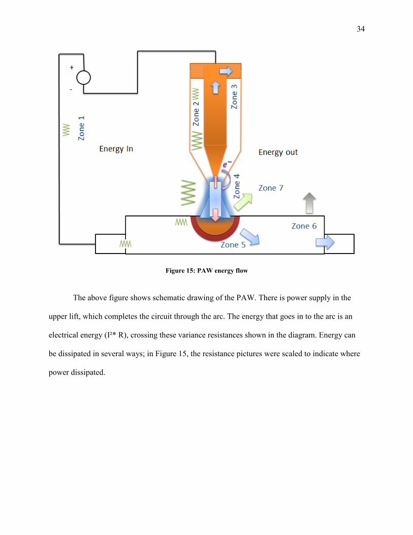
34

Figure 15: PAW energy flow

The above figure shows schematic drawing of the PAW. There is power supply in the

upper lift, which completes the circuit through the arc. The energy that goes in to the arc is an

electrical energy (I²* R), crossing these variance resistances shown in the diagram. Energy can

be dissipated in several ways; in Figure 15, the resistance pictures were scaled to indicate where

power dissipated.

35

Table 4: Welding Zones

Zone 1 Welding cable made of copper to minimize the power dissipated through the

voltage drop to maintain good control of the process.

Zone 2

(torch to weld

pool zone)

Generally does not have very large voltage drop in the cold part of the tungsten or

in the part near the copper clamp. As the electrode tapers and heats up, the

dissipated power increases, which is necessary to make electrons boil off the

cathode and attend to cool it. An adequate temperature of the tip of the electrode

needs to be maintained to get the current density needed to maintain the arc.

Zone 3

(cathode zone)

Here, electrons are emitted from the surface. Within the electrode, there is heat

coming from the arc, and the electrons essentially evaporate to cool it. Generally

use gas cooling or water cooling; the copper calotte in the top of the electrode in

the figure above is where the heat flows out where typically carried away by the

water or gas cooler.

Zone 4

(arc zone)

The arc zone has thermo balance. It is very hot, around 15,000 K, and it radiates

strongly both as black body and varices line wave length according to the electron

transition. Typically, as the arc gets longer, the voltage in the power supply will

increase, and the current will decrease and more radiation will be emitted, which

provides less heat in the workpiece. The arc both puts heat back in the electrode

and assists in the boiling off the electrons and puts heat in to the base metal.

Zone 5

(weld pool)

This is the weld pool steady state, where the size of the pool does not change

because the balance of the heat being extracted to the plate and radiated away, is

balanced by the electrical heat input. The moving weld is going to change

somewhat and it will melt the base metal and supply the heat of fusion to the solid

metal to turn it into liquid. Some of the heat is recovered as the weld pool is trailed

by, and the latent heat of fusion is released when the weld is solidified. The

isotherms in the weld pool are important features of solidification, which govern

the microstructure, the existence of segregation and the certain kinds of weld

defects that will be investigated in the specimen after being sectioned.

Zone 6

(fixturing zone)

Ultimately the heat in the workpiece has to come out somewhere. Fixturing is the

method of conducting the heat out, in this case the, especially in these research

welds were relatively small masses of material, and the fixturing was very

significant, and the amount of penetration and the weld shape is dependent on it.

Importantly, the temperature rise can cool by convection and radiation from the

solid surface. Those are all part of the energy balance that needs to be taken into

account when calculating efficiency.

Zone 7

(shielding gas)

This zone is a minor constituency of the energy balance, and usually it is ignored

by a researcher what can be affected metallurgically with the heat being carried

away by the shielding gas. The reason it is minor is that the shielding gas flow is

not that high, and thus not meant to carry away heat, it’s meant to shield the arc.

The reason it is mentioned in this research is fume generation, and allowable

exposure limits for elements like chromium and manganese. The energetic and

transport properties of the shielding gas can be studied more in the future.

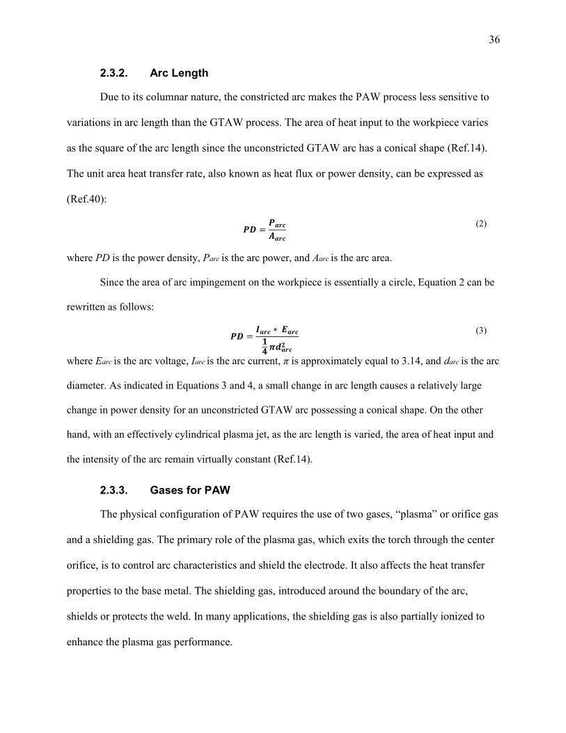
36

2.3.2. Arc Length

Due to its columnar nature, the constricted arc makes the PAW process less sensitive to

variations in arc length than the GTAW process. The area of heat input to the workpiece varies

as the square of the arc length since the unconstricted GTAW arc has a conical shape (Ref.14).

The unit area heat transfer rate, also known as heat flux or power density, can be expressed as

(Ref.40):

(2)

where PD is the power density, Parc is the arc power, and Aarc is the arc area.

Since the area of arc impingement on the workpiece is essentially a circle, Equation 2 can be

rewritten as follows:

(3)

where Earc is the arc voltage, Iarc is the arc current, π is approximately equal to 3.14, and darc is the arc

diameter. As indicated in Equations 3 and 4, a small change in arc length causes a relatively large

change in power density for an unconstricted GTAW arc possessing a conical shape. On the other

hand, with an effectively cylindrical plasma jet, as the arc length is varied, the area of heat input and

the intensity of the arc remain virtually constant (Ref.14).

2.3.3. Gases for PAW

The physical configuration of PAW requires the use of two gases, “plasma” or orifice gas

and a shielding gas. The primary role of the plasma gas, which exits the torch through the center

orifice, is to control arc characteristics and shield the electrode. It also affects the heat transfer

properties to the base metal. The shielding gas, introduced around the boundary of the arc,

shields or protects the weld. In many applications, the shielding gas is also partially ionized to

enhance the plasma gas performance.

37

2.3.4. Shielding Gasses

Argon is the preferred orifice gas because its low ionization potential ensures easy and

reliable starting. Argon/ helium and argon/hydrogen mixtures are also used for applications

requiring higher heat input. The choice of shielding gas is dependent on the type and thickness of

the base material. When welding, aluminum, carbon steel, and copper, the gases commonly used

are argon, helium, and argon/helium mixtures. It is generally recommended that the percentage

of helium be increased as the base-plate thickness increases. When welding low alloy steels,

stainless steels, and nickel alloys, the above-mentioned gases in addition to argon hydrogen

mixtures are used. Table 4, below shows properties data for argon the choice of gas used in this

research. When performing high current plasma arc welding also depends on the composition of

the material to be welded. In all but a few cases, the shielding gas is the same as the orifice gas.

2.3.5. Argon

Argon is a chemical element with symbol Ar and atomic number 18. It is in group 18 of

the periodic table and is a noble gas. Argon is the third most common gas in the Earth's

atmosphere, at 0.93% (9,300 ppm), and is colorless, odorless, tasteless, and nontoxic. As an inert

gas, argon does not react with other compounds or elements. Argon is about 1.4 times heavier

than air and cannot sustain life. The inert properties of argon make it ideal as a shield against

atmospheric contamination, thus it is used in many welding processes. Argon promotes good arc

starting characteristics and arc stability due to its low ionization potential (Ref.4).

38

Table 5: Argon Gas Data

Argon

Chemical Symbol Atomic Number Molecular Weight

Ar 18 39.95

Specific Gravity,

Air = 1

Density (lb/cu ft) at 0 C,

1 atmosphere

Ionization Potential

(ev)

1.38 0.1114 15.7

Thermal Conductivity

(10-3 x Btu/hr-ft- F)

Cubic ft/lb Cubic ft/gal

9.69 (32 F) 9.67 113.2

Minimum Purity

percentage (gas)

Minimum Purity

percentage (liquid)

Minimum Moisture*

(ppm)

99.995 99.997 120

Approximate Dewpoint

at Maximum Moisture

Content (C)

Approximate Dewpoint

at Maximum Moisture

Content (F)

* Moisture specifications

are measured at full

cylinder pressure.

-40 -40

In this experiment, argon was used. Argon is suitable as the orifice and shielding gas for

welding all metals, but it does not necessarily produce optimum welding results. In the Melt-in

mode, additions of hydrogen to argon produce a hotter arc and offer more efficient heat transfer

to the work. Limits on the percentage of hydrogen related to its potential to cause cracking and

porosity. However, when using the Keyhole technique, a given material thickness can be welded

with higher percentages of hydrogen. This may be associated with the Keyhole effect and the

different solidification pattern it produces.

Argon is used for welding carbon steel, high-strength steel and reactive metals such as

titanium and zirconium alloys. Even minute quantities of hydrogen in the gas used to weld these

materials may result in porosity, cracking, or reduced mechanical properties.

2.3.6. Gas Orifice

The pilot arc tends to start easier if the orifice gas flow rate is 1-1.5 CFH. This is one of

the important variables, and it should be the lower value in this process, because the high

pressure tends to blow the metal out. This process, called “humping,” occurs when the arc

pressure pushes down melting metal and allows for the liquid metal to rise up and freeze.

39

2.3.7. Radiation

The amount and character of radiation emitted by arcs depends upon the atomic mass and

chemical structure of the gas, the temperature, and the pressure. Radiation loss of energy may be

over 20 percent of the total input in the case of argon welding arcs. Intense radiation in the

ultraviolet, visible, and infrared wavelength is emitted by all exposed welding arcs. Ultraviolet

radiation from argon shielding arcs is particularly strong and, because of mass effects, little or no

self-absorption occurs within the plasma volume (Ref.40).

2.3.8. Cooling rate

The final metallurgical structure of the weld zone is primarily determined by the cooling

rate from the maximum temperature achieved during the weld cycle (peak temperature). The

critical cooling rate for the formation of martensite in these steels is often equal to those likely to

be encountered in welding. With carbon and low alloy steels, the temperature at which the

cooling rate is calculated is not critical, but should be the same for all calculations and

comparisons. Cooling rate calculation will be made at 550 °C. This temperature ( ) is quite

satisfactory for most steels.

2.3.9. Cost Comparison between Welding Processes

The cost of a new PAW power supply is much less than the costs of new LBW and EBW

power supplies that are also used for AM. A cost comparison of brand new welding power

supplies for these three welding processes is given in Table 6.

40

Table 6: New Power Supply Cost Comparison between

Welding Processes Used in Additive Manufacturing

Welding Process

New Power

Supply ($)

Plasma Arc Welding

(41)

7,000

Laser Beam Welding

(42)

500,000

Electron Beam Welding

(43) 1,000,000

Table 6 shows that a brand new PAW power supply costs significantly less than brand new

LBW and EBW power supplies. As a result, PAW has the potential to be a much more cost effective

method for the steel alloy components (Ref.44).

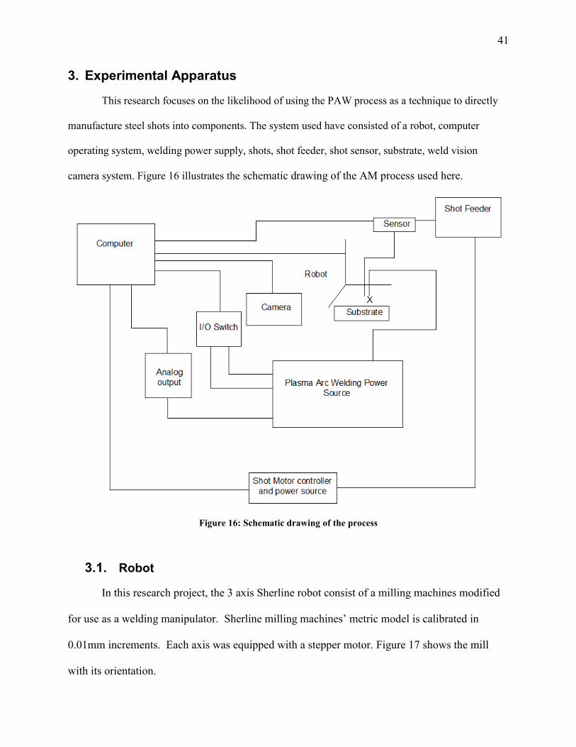
41

3. Experimental Apparatus

This research focuses on the likelihood of using the PAW process as a technique to directly

manufacture steel shots into components. The system used have consisted of a robot, computer

operating system, welding power supply, shots, shot feeder, shot sensor, substrate, weld vision

camera system. Figure 16 illustrates the schematic drawing of the AM process used here.

Figure 16: Schematic drawing of the process

3.1. Robot

In this research project, the 3 axis Sherline robot consist of a milling machines modified

for use as a welding manipulator. Sherline milling machines’ metric model is calibrated in

0.01mm increments. Each axis was equipped with a stepper motor. Figure 17 shows the mill

with its orientation.

42

Figure 17: shows the mill with its orientation.

The arrows for each axis point in the positive direction of the axis.

3.1.1. Torch Holder

The design of the torch holder was meant to be a part of the robot arm. The parts were

3D printed using the 3D plastic printer (see section 3.7). The basic C-clamp design was used to

hold the torch in place with a set of two screws for each clamp. A swivel controls the work

angle (up to 80 degrees of freedom) and also the travel angle of the torch. A plate with six holes

will hold the C-clamps and swivel together. Figure 18 shows parts of torch holder and Figure 19

shows the PAW torch mounted in the torch holder.

C-clamp

Plate with six holes

Swivel

Figure 18: parts of torch holder

43

Figure 19: PAW torch mounted in the torch holder

3.2. Plasma Arc Welding Power Supply

The PAW power supply used for this research is the Thermal Arc ULTIMA-150 made by

Victor (formerly Thermadyne). The Thermal Arc ULTIMA-150 is a direct current (DC) arc

welding power supply. (Ref.14). A photograph of the Thermal Arc ULTIMA-150 PAW power

supply used throughout this research is shown in Figure 20. This unique plasma welding system

is self-contained in a small package with a 150 amp power supply, coolant re-circulator and

control console (Ref.45).

44

Figure 20: Thermal arc ULTIMA-150 plasma arc welding power supply

The Thermal Arc ULTIMA-150 has a 100% duty cycle at 100A and a 50% duty cycle at

150A. There are two output current ranges. The low current output range is from 0.5A to 15A,

while the high current output range is from 5A to 150A. The power supply has an open circuit

voltage of 60V and a load voltage range of 12V to 25V. The plasma gas flow meter has a range

of 0.5 to 3.0 cfh, and the shielding gas flow meter has a range of 5 to 30 cfh (Ref.45). The PAW

power supply used operates in the constant current (CC), direct current electrode negative

(DCEN) mode (Ref.46).

3.2.1. Plasma Arc Welding Torch

In this research a torch from Thermal Dynamic was used. The torch number is 0-2006

PWH/M-3A (Refer to the manual for more information about the welding torch).

There are a couple of important notes that need to be made in regards to the electrode

setback process parameter. At the maximum operating range of the various orifice diameters for

the PAW power supply used, a stiff collimated arc is obtained with the electrode setback at its

maximum. Conversely, a softer, less constricted arc can be obtained by decreasing the electrode

45

setback. The minimum electrode setback is achieved when the tip of the electrode is flush with

the face of the constricting nozzle. By decreasing the electrode setback, the orifice gas flow rate

can be decreased while maintaining the higher current ratings of the constricting nozzle. This

result in a wider weld bead, and in most cases, allows for faster travel speeds (Ref.47).

A gauge and wrench assembly is used to properly assemble the welding torch that was

used during this research. One of the functions of the gauge and wrench assembly is to

appropriately position the electrode setback. Gauge settings are identified by the number of

rings on the gauge and wrench assembly. There are three different gauge settings distinguished

by 0, 1, and 3 rings (Ref.47). The gauge and wrench assembly is presented in Figure 21.

Figure 21: Plasma arc welding torch gauge and wrench assembly

As previously mentioned, the minimum electrode setback is achieved when the tip of the

electrode is flush with the face of the constricting nozzle. The next shortest electrode setback is

achieved when the gauge setting with one ring is used, followed by the gauge setting with zero rings.

The maximum electrode setback is obtained when the gauge setting of three rings is employed

(Ref.47). The manufacturer of the welding torch did not possess information on the physical

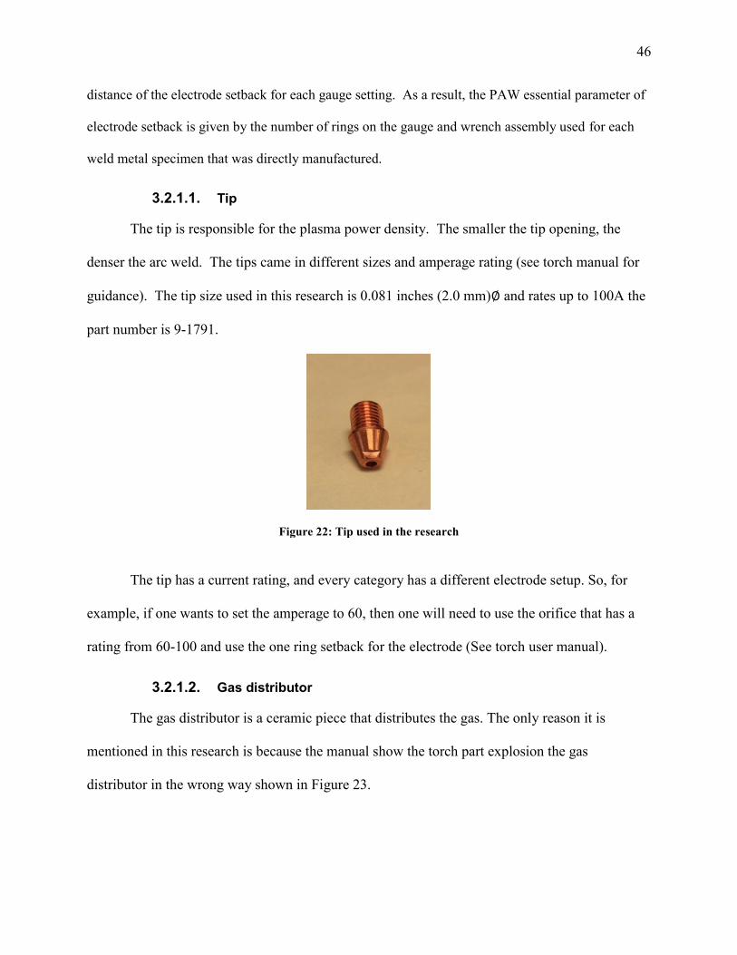
46

distance of the electrode setback for each gauge setting. As a result, the PAW essential parameter of

electrode setback is given by the number of rings on the gauge and wrench assembly used for each

weld metal specimen that was directly manufactured.

3.2.1.1. Tip

The tip is responsible for the plasma power density. The smaller the tip opening, the

denser the arc weld. The tips came in different sizes and amperage rating (see torch manual for

guidance). The tip size used in this research is 0.081 inches (2.0 mm) and rates up to 100A the

part number is 9-1791.

Figure 22: Tip used in the research

The tip has a current rating, and every category has a different electrode setup. So, for

example, if one wants to set the amperage to 60, then one will need to use the orifice that has a

rating from 60-100 and use the one ring setback for the electrode (See torch user manual).

3.2.1.2. Gas distributor

The gas distributor is a ceramic piece that distributes the gas. The only reason it is

mentioned in this research is because the manual show the torch part explosion the gas

distributor in the wrong way shown in Figure 23.

47

Figure 23: Torch part explosion from manual

If the manual is followed, the gas distributor will burn. It costs between 49-59 US dollars

for replacement.

3.2.2. Arc current pulse

Commonly are welding is done with non-pulsing current, that is the arc current is

maintained at a constant value during welding. Holding the current at a constant value develops a

steady-state heat flow condition where melting, solidification and cooling occur continuously as

the arc travels along the workpiece. Figure 24 illustrates the steady state heat flow condition.

Figure 24: Steady state condition

In this research, the arc current was pulsed to reduce the average heat input compared to

constant arc current. During the pulse, if the heat is going into the pool at a greater rate than the

heat being moved away, more melting will occur. Then, the arc should turn off. Figure 25

illustrates the melting condition. Arc current equals to zero was not achieved or arc off, the arc

current was 50 amps during the pulse period and 10 amps during background period.

48

Figure 25: Melting condition

The opposite is true when the heat is pulled away from the pool much faster than it’s

going in because, essentially, when the arc turns off the rate of heat in is zero. Figure 26

illustrates the solidification/cooling condition. During the arc-off or background current period.

Figure 26: Cooling condition

The robot moves forward 2 mm, and the pulse comes on. The rate of heat going in is

greater than the rate of heat going out, therefore deep penetration results and the arc is shot off.

The robot moves forward, and this result of cheating heat flow has to do with time. Instead of

steady state conditions, the process is always in transient condition. The purpose of pulsing is to

reduce heat input, reduce distortion and produce narrow/smaller bead size. The following

equation calculates the average amperage in pulsing mode:

49

(4)

where is pulsing time,

is current of pulsing,

is background time,

is background current and

is the average amperage in pulsing mode

Figure 27 shows the process schematic. The x-axis is time and y-axis is the amperage. At

some time the shot will be detected and the arc current is raised to the peak value, a molten pool

is formed, the shot enters the pool and is melted, the arc current is reduced to the background

level, the pool solidifies and cools. Then the robot will step up or move forward, another shot

will be detected and so on.

Figure 27: Process timing schematic

If the arc current pulse is too high, and the orifice gases is small enough, humping may

result after creating the melting pool, due to the pressure from the arc pushing down on the weld

50

pool. When is returned to the background level the arc time may be insufficient for the liquid to

flow back down in the weld pool .The result will be humping or excessive weld crater. So, there

is limitation in the upper limit bound of . The background current should be very low just to

keep the arc established. The peak time should be less than the background time.

3.2.3. Gas Selection

Argon was selected to be utilized as the shielding, and plasma gas. For this research, an argon

cylinder was employed to supply the argon. A photograph of the argon cylinder configuration used is

displayed in Figure 28.

Figure 28: Argon cylinder configuration used

The two hoses are used to supply argon for both the shielding and orifice gases. A pressure

regulator was used for both of these gases to ensure that there was a gas pressure of 35 psi.

3.2.4. Computer analog output for arc current control

A Phidget-Analog 4-Output Produces a voltage over -10V to +10V. The voltage is

produced with 12-bit resolution (4.8mV). The board is not isolated and all 4 channels share a

common ground. All the power is supplied by the USB bus (Ref.48).

51

A command will be sent to this device via the computer to control the voltage and

between two output pins. The analog output is a very low power device, so whatever interface

connected to the analog output must have very high impedance such as kilo or even mega ohms.

The total amount of power that this device needs to produce to get 10 volts across two pins is

very small. The analog output device is used to set the amplitude of the pulse and background

levels. Output zero has been used to control the amplitude of the arc current level. Figure 29 is

the schematic and actual picture for the analog output.

Figure 29: Schematic and actual picture for the analog output

3.2.5. Welding power source Digital I/O

A Phidget-Analog was used to switch the welding power source pilot and main welding

arc on and off. The Open Collector Digital Outputs can be used to directly control substantial

devices, switching up to 30VDC at up to 2 Amps. The Output acts as a switch to ground, so the

circuit switching will need an external power supply. Each output is protected from transient

voltages typical when switching inductive devices—relays, solenoids, and motors. The outputs

can be used to directly control devices requiring substantial power such as incandescent lights,

52

high power LEDs, relays, solenoids, and motors (Ref.48). Figure 30 shows the Digital Inputs/

Outputs and a schematic drawing that was used in this research.

Figure 30: Schematic and actual digital inputs/outputs

3.3. Shot feed stock – 1st source

Non-Plated Steel Shot #7 typically used in shot gun shells was the first source of shot in

this experiment. The non-plated steel shot has near spherical shape. The non-toxic steel shot

meets USFWS & SAAMI requirements (Precision reloading). Figure 19 shows shot #7

magnified 50 times. The shot size averaged around 2.5mm.

A

B

Figure 31: A-Common shot gun shots contain rust, dirt. B-shot porosity

As Figure 31 shows, the common shot gun shots contain rust, dirt, and significant

porosity, which are the main causes of porosity. After several trials building walls, they all failed

53

because of the aggressive porosity. Even though the substrate was cleaned and wire brushed, the

porosity was observed in the first layer. Figure 32 shows porosity in a sample specimen in first

layer.

Figure 32: Porosity was observed in the first layer.

One way to clean the shots is by pickling the steel. Pickling is chemical removal of

surface oxide (scale), and other contamination such as dirt from metal by immersion in an

aqueous acid solution (Metal Handbook). Sulfuric acid is the most common type of pickling

acid. Hydrochloric acid is used for many steels, particularly for special purposes, such as etching

before galvanizing.

3.3.1. Sulfuric acid

Sulfuric acid, , is the most common pickling liquor. It

produces satisfactory results when used (a) for batch descaling of carbon steel rod and wire (to

0.60% carbon), and (b) for continuous cleaning, provided the iron concentration in the bath is

less than 8% by weight.

3.3.2. Hydrochloric acid

Hydrochloric acid, , is preferred for batching pickling

hot rolled or heat treated high carbon steel rod and wire. Figure 33 shows samples of four shots

54

immersed in phosphoric acid for 10 minutes to dissolve the rust and clean the surface.

Phosphoric acid is not as strong as sulfuric or hydrochloric acids. After that, the sample was

rinsed with water and looked at under the microscope.

A

B

Figure 33: A - Shots Before Cleaning and B - Shots After Cleaning

In Figure 33, the shots appear cleaner. Most of the rust has been removed. However, this

process is not practical in this experiment because damp shots allow moisture to get into the

transport path to the weld pool. This moisture does not allow the shots to run smoothly in the

tube. Therefore, it is hard to control moisture and productivity at the same time.

3.3.3. Shot feed stock – 2nd source

New shots have been used from “Abbott,” which is carburized balls and case hardened

carbon steel balls. The steel type of the new balls is 1018 low-carbon steel. The carbon steel balls

are used in automotive applications, for semi-precision bearings, and in commercial applications

such as casters, locks, and drawer slides. Other applications for carbon steel balls include: locks,

bicycles, roller skates, slides, trolleys and conveyors.

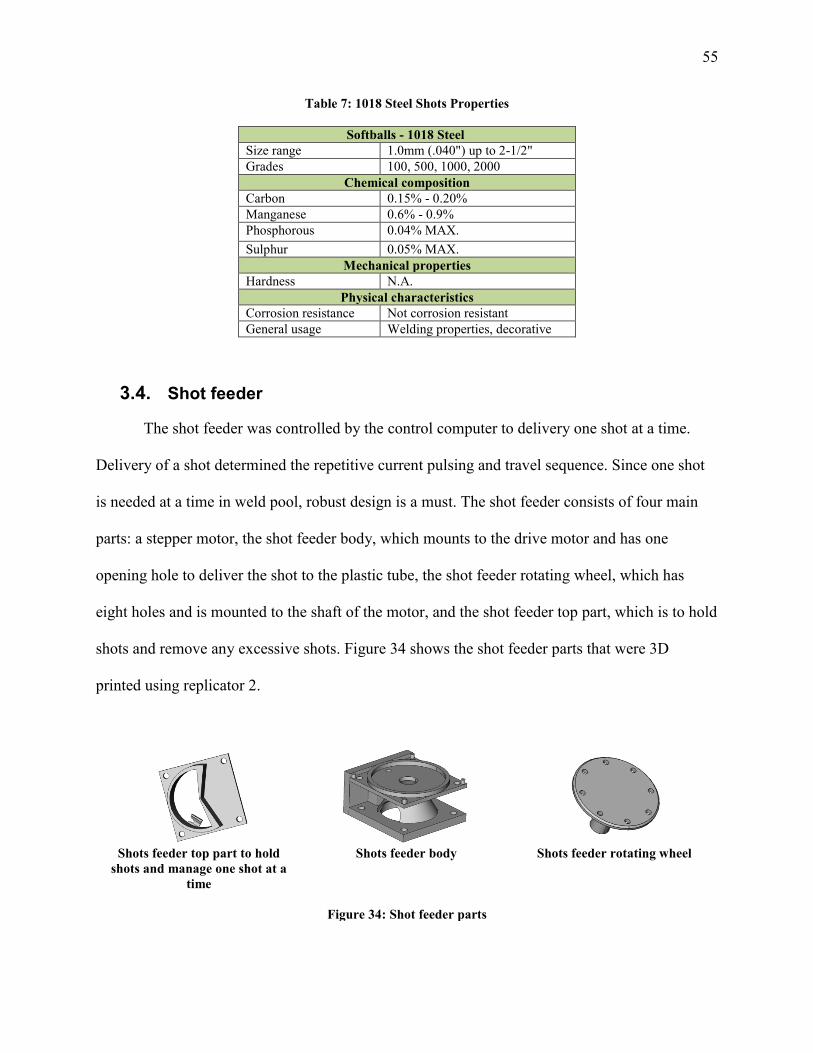
55

Table 7: 1018 Steel Shots Properties

Softballs - 1018 Steel

Size range 1.0mm (.040") up to 2-1/2"

Grades 100, 500, 1000, 2000

Chemical composition

Carbon 0.15% - 0.20%

Manganese 0.6% - 0.9%

Phosphorous 0.04% MAX.

Sulphur 0.05% MAX.

Mechanical properties

Hardness N.A.

Physical characteristics

Corrosion resistance Not corrosion resistant

General usage Welding properties, decorative

3.4. Shot feeder

The shot feeder was controlled by the control computer to delivery one shot at a time.

Delivery of a shot determined the repetitive current pulsing and travel sequence. Since one shot

is needed at a time in weld pool, robust design is a must. The shot feeder consists of four main

parts: a stepper motor, the shot feeder body, which mounts to the drive motor and has one

opening hole to deliver the shot to the plastic tube, the shot feeder rotating wheel, which has

eight holes and is mounted to the shaft of the motor, and the shot feeder top part, which is to hold

shots and remove any excessive shots. Figure 34 shows the shot feeder parts that were 3D

printed using replicator 2.

Shots feeder top part to hold

shots and manage one shot at a

time

Shots feeder body

Shots feeder rotating wheel

Figure 34: Shot feeder parts

56

3.4.1. Shot sensor

The shot feeder fed a single shot into a shot funnel/detector component. The shot detector

was used to trigger the welding arc current timing. Proximity Sensor used to detect the shots with

sensing ranges from 0.8 to 3mm with LED indicator “E57-08GS01-C.” These unique Cutler-

Hammer® Inductive Proximity Sensors are designed to be used in extremely small spaces. The

sensors are 3-wire devices that operate from 10 to 30 V DC (Ref.49).

Figure 35: Proximity sensor set-up

3.4.1. Plastic shot delivery tube and coupler

Clear PVC tubing is used to transport shots form shot feeder to ceramic tube. The plastic

provides flexibility and smooth interior to reduce sediment build-up. The plastic tubes used in

this research were 5.5mm OD and 3.5mm ID. The coupler was made out of steel to connect the

slightly different OD and ID in both tubes. Figure 36 shows plastic tubes connected to the

ceramic tube connected by coupler.

57

Figure 36: Plastic tubes connected to the ceramic tube connected by coupler.

3.4.2. Ceramic shot delivery tube

An alumina ceramic tube was used to deliver the shot into the weld pool. Alumina

provides the combination of low thermal expansion, superior thermal conductivity and high

compressive strength, making it thermal shock resistant and the ideal product for shot delivery.

Alumina ceramic tubes used in this research were 6.25mm OD and 3mm ID and cut in to 10cm

length using a surface grinder with diamond plat. Figure 37 shows ceramic tubes.

58

Figure 37: Ceramic tubes deliver the shot into the weld pool

3.4.3. Shot detector integrated circuit (IC)

When a shot is detected, a light will go on in the memory box (Integrated circuit), and the

computer sets a loop asking for a shot to pass by when the sensor gives the signal to the

computer. The computer will start the arc.

Capacitors were added at key points in the shot detector circuit to attempt to eliminate

electrical noise. The noise had been generated by the power supply because the shot feeder

seems to work consistently. When welding, obviously, there is current flowing through the

cables, which generates a magnetic field. When the magnetic field intercepts the conductors in

the wires it creates current in the wires in addition to the current generated by the sensor. The

circuit does not discriminate between the current that was generated by the sensor or a current

generated by another source. The capacitors were placed to eliminate the noise caused by the

welding current that is produced in the circuit. The capacitors will help in eliminating the

unwanted signals. Figure 38 shows the Integrated circuit used in this research.

59

Figure 38: Integrated circuit

The output of the shot detector circuit was read by a digital input on the control computer

to pulse the arc current after a shot was detected to be on its way to the weld pool. A 470

picofarad capacitor was added in the integrated circuit (IC) from ground to power which goes

from pin 7 to pin 14. Then, another 470 picofarad capacitor was added from pin 1 to ground.

Also, a 470 picofarad was added from pin 10 to ground. The capacitor was added to the output of

all the gates. Figure 39 shows shot sensor feed motor schematic

60

Figure 39: shot sensor feed motor schematic

The shot detector is based on a simple set-reset latch circuit. The computer resets or arms

the detector circuit. When a shot moves past the sensor, the circuit is set or triggered and the

circuit latches or remembers that a shot has been detected. The computer can then read the state

of the circuit and determine if a shot has moved past the sensor. If so, the computer resets the

circuit and the shot detection process can happen again.

3.4.4. Shots feed motor Power supply and motor controller

This device supplies the shot feeder motor with power and controls it through the

computer. Every time the robot gets into position, the computer will issue a command to the

power supply to move the feeder to deliver a filler metal shot, and at the same time will issue a

61

command to the sensor to look for a shot in case the hole is empty. Figure 40 shows the Power

supply and motor controller that drives the feed motor that was used in this research.

Figure 40: Power supply and motor controller that drives the feed motor

3.4.5. Weld Sequence operation

As the experiments progressed, a series of changes in equipment and procedures were

implemented to optimize the build process. In this experiment, a computer controls the entire

build process. The process equipment consists of the control computer shot feeder, the robot and

the PAW unit. To be able to sync all these devices, one needs to understand how this experiment

works. Figure 41 shows the different stages a single cycle goes through.

62

Figure 41: Graphic of program’s continuous cycle

For each shot delivered to the weld pool the following sequence of events were executed

by the control computer

1) The robot was moved to the location where the next shot was to be placed and motion

was stopped.

2) The shot feeder was actuated to release a single shot.

3) When the shot detected sensed the release of a shot, a time delay was implemented as the

shot traversed the shot delivery path.

4) As the shot approached the weld area, the arc current was change to the peak value to

prepare a weld pool for the shot to enter.

5) The arc current was held at the peak time to melt the shot

6) After the peak time, the arc current was returned to the background level.

7) The robot was moved to the next location and the entire sequence was repeated.

The entire build sequence was controlled by the CNC, G-code of the robot programming

language. In-house custom extensions to the G-code were written to incorporate the functionality

63

to actuate the shot feeder, detect shot delivery and modify arc current levels. The custom

extensions were introduced as M-code commands in 3.9.3.

3.5. Substrate

The substrate used in this research is low-carbon steel A36. Figure 42 shows the actual

substrate used in this research. After cutting the substrate to sizes, the substrates were sand

grinded and stored for a later use.

Figure 42: Substrates were cut in 150mm long

The substrates were cut to following dimensions: thickness of the substrate is 6.5mm, the

width is 32mm and the length is 150mm. Figure 43 shows the substrate cut to sizes.

64

Figure 43: Substrate dimensions

3.6. Camera System

In this research a weld ClearVision camera system was used to image the weld area. The

camera system is a digital video system that provides a clear view of the weld pool and weld

joint to the welding operator. It combines a digital video camera with small LED lighting to

produce a clear video image. The video camera is housed in a 2x2x4-inch rugged aluminum

case. For high-temperature applications, the camera housing can be water-cooled. The focus and

iris are controlled remotely. The video camera system and lights are positioned on the same sides

of the welding torch as it can be seen in Figure 44.

65

Figure 44: Camera system setup

3.7. 3D Printer

Several component used in this research work were built using a 3D plastic printer.

Several types of RP machines are well suited for operation in a CAD office. They are relatively

small (desk-top devices), cheap and clean (no liquid or powder material, and have no need for

messy post-processing). Efforts have been made to increase speed at the expense of quality (e.g.,

surface roughness, accuracy, material strength). Those machines are called “concept modelers”

because they are mainly used for rapid check of the geometry of initial CAD design concepts.

They are provided with software that tends to the simplicity of operation of a desk-top printer

(i.e., just sending a file to a printing queue), although some pre-processing (support definition,

STL triangulation, etc.) and post-processing (support removal) is often still required (5).

66

In this research, a 3D printer from MakerBot was used. This printer is a new standard in

desktop 3D printing with a resolution capability of 100 microns and a massive 410 cubic inch

build volume. The MakerBot Replicator 2 Desktop 3D Printer is an easy, fast, and affordable

tool for making quality models. On a 3D printer, quality is often measured by the height of each

layer, with smaller layers meaning higher resolution. The default layer height has been dropped

all the way down to 100 microns, giving smooth surfaces without any post-production (50).

Figure 45 shows the MakerBot Replicator 2 Desktop 3D Printer and its Polylactic filaments.

Figure 45: MakerBot Replicator 2 desktop 3D printer and polylactic filaments

3.7.1. Filaments

Polylactic Acid (PLA) filament used in this research is a biodegradable plastic with a lot

of features. It does not give off fumes like ABS does or warp nearly as much. It is also really

shiny. PLA is harder than ABS and more brittle, but it is super strong. When it does give, it is

more likely to snap than bend. PLA also stays flexible for a short while as it cools, which can be

handy, and it does not warp and crack on larger objects like ABS. The filament is also a

renewable bioplastic made from corn. The component built on this 3D printer for this work

67

include Shots feeder body, Shots feeder rotating wheel, Shots feeder top part, C-clamp, back plat

to hold the torch and shot sensor mount.

3.8. Thermometer

A non-contact thermometer was used to make deposit temperature measurements. The

thermometer was a dual laser InfraRed from EXTECH, 42529: most important features in the

Dual Laser InfraRed used are, wide range IR thermometer dual. Wide temperature range: 0 to

600°F (-20 to 320°C). Built-in laser pointer is °F/°C switchable. Fixed emissivity (0.95) covers

90% of surface applications, 6:1 narrow field of view, audible and visible over range indicators

and automatic Data Hold (51). Figure 46 shows Thermometer used in the research.

Figure 46: EXTECH, 42529: Wide range IR thermometer dual reading temperature in workpiece

3.9. Control computer software programs

3.9.1. Weld Parameter Manager

Weld Parameter Manager (WPM), is an in-house program written to control the welding

parameter from the computer and applies it to the welding machine at the same-time. This

program directly modifies welding parameters sent to the welding power source in real time. The

parameters this program can modify are Peak Delay Time ( ), Peak Current ( ), Peak Time

( ), Background Current ( ) and Background Time ( ). Figure 47 shows screen shot of the

WPM.

68

Figure 47: Screen shot of the WPM

WPM allows the welding parameter control to be integrated into the CNC G-code used to

control robot motion. In M103, if the value of 999 for P and Q was written, it would not make

any since from welding stand point. However, the program will read the values from the weld

manager, which can be manipulated and starts to take effect in real time “while it’s running.”

The value of the amperage and the pulse time from the program itself can be edited by going to

the editor, saving, and running it.

3.9.2. CNC robot control G-Code

G-Code is the programming language supported by a variety of CNC Mill Machines.

While it is standard in theory, many different manufacturers and different milling machines will

adapt G Code to serve their desired functionality.

3.9.3. M-code

The M-code is responsible to feed a shot and pulse the current. M103 is the program

written for this experiment. The main variables the program can control are the pulse current (in

69

Amperes) and the pulse time (in seconds). For example, in the G-Code, M103 P20 Q1 means

feed a shot and pulse the current to 20 A for 1 second.

Typing M107 in the MDI will strike the pilot arc, and typing M108 will turn the pilot arc

off (you might need to do it more than one time to get the pilot arc to strike). After turn the pilot

arc on, typing M105 in the MDI will strike the main arc, and typing M106 will turn the main arc

off. Additional modes can be seen in table 9:

Table 8: Mode of Operation

Pulse

Current

(Amp)

Pulse

Time

(Sec) Mode of operation

-1 -1 calibrate time from when a shot leaves the feeder to when the shot passes the sensor

0 0 sync the feeder so that if will produce a shot within the next few steps

1-149 1-149 use the pulse current and time values specified from the command line

>150 >150 use welding parameter values from the file called pp3d.wp

Wall_1.ngc is the program that can be run from the Sherline and builds the 100mm wall

Figure 48 is screen shot of wall program.

Figure 48: Screen shot of wall program

70

#1 travel step size Variable that can be changed and will have effect on how

many mm the robot will move

#2 travel distance Total travel distance the robot will travel before it will end

the program

#3 X start location Home position in the X axle and the distance traveled in the

program

#4 Y start location Home position in the Y axle and the distance traveled in the

program

#5 Speed How fast the travel step size moves

#6 Where is the program?

Running sum of how far the program moves. #6 is the logic

which says #6 is less than #2 + #1, so if #6 were deleted, it

would be an infinite loop

G1 goes to the position XY, where the argument of X is zero and the argument of Y is

zero, which means go to the start position. M103 and M104 are programs used in this

experiment. They are exactly the same except that the M104 command does not wait for the

shots to appear, which means M104 ignores any signals from the sensor.

Since there is no feedback from the power source, the program does not know if the torch

is on or off. It can integrate the M107 command, which starts the pilot arc on. However, this was

not done because the pilot arc sometimes does not start, especially when the system is cold. On

the other hand, even if it does start, it may take 30-60 seconds for the pilot arc to stabilize.

After editing the G code file, save it in a specific location. Go to save, desk top, G-code,

and save it in G-code file.

One can issue the command M103 P0 Q0 from the MDI. The system will slowly

increment the feeder until it detects a shot, and the feeder will rotate enough that the next shot

will be available after the next couple of steps. The time between when one issues the command

to when the next shot actually drops should be very small, and the feeder will rush ahead until

71

the next shot is just about to be dropped. Simultaneously, by the time one of the holes in the

wheel reaches the hole in the frame there is actually a shot in the hole.

3.9.4. Operating system

In this research, the operating system used was Sherline CNC (Metric) v4.51. based on

the EMC open-source machine control software package. The robot CNC operating system was

used to control all functions of the robot including:

3.9.4.1. Manual Mode

Manual mode shows a set of buttons along the bottom of the right-hand column. A green

button labeled “ALL ZERO” designates the present position as the home position. A machine of

this type would be simpler to operate if it did not use a machine home position. This button will

zero out any offsets and will home all axes right where they are marked.

3.9.4.2. Keyboard Jogging

When the control is in manual mode, the slides using the keyboard cursor control arrows

can also be controlled. The slides will move in the direction the arrows point, and the Z-axis can

be raised or lowered using the [Page Up] or [Page Down] keys. The speed the slides move at will

be determined by the manual feed rate setting. Figure 49 shows screen shot for a manual mode.

72

Figure 49: Screen Shot For Manual Mode

3.9.4.3. MDI

MDI mode allows one to enter single blocks and have the interpreter execute them as if

they were part of a program similar to a one-line program. Circles, arcs, lines and such can

executed. One can even test sets of program lines by entering one block, waiting for that motion

to end, and then entering the next block.

Below the entry window, there is a listing of all of the current modal codes. One can also

write this list to the message box in any mode if one looks under the info menu and selects active

g-codes. This listing can be very handy. G80 stops any motion. If it’s there remember to issue a

block like g00 x0 y0 z0. In MDI one is entering text from the keyboard to till the robot this is the

home position, so none of the main keys work for commands to the running machine. [F1] will

stop the control. Figure 50 shows screen shot for an MDI mode.

73

Figure 50: Screen shot for a MDI mode

3.9.4.4. Auto Mode

Sherline’s auto mode displays the typical functions that people come to expect from the

EMC. Along the top are a set of buttons which control what is happening in auto. Below them is

the window that shows the part of the program currently being executed. As the program runs,

the active line shows in white letters on a red background.

The first three buttons [Open], [Run], and [Pause] do about what one would expect.

[Pause] will stop the run. The next button, [Resume], will restart motion. They are like

“feedhold” if used this way. Once [Pause] is pressed and motion has stopped, [Step] will resume

motion and continue it to the end of the current block. Press [Step] again to get the motion of the

next block. Press [Resume], and the interpreter goes back to reading ahead and running the

program. The combination of [Pause] and [Step] work a lot like single block mode on many

74

controllers. The difference is that [Pause] does not let motion continue to the end of the current

block. Figure 51 shows screen shot for Auto mode.

Figure 51: Screen shot for Auto mode

3.9.4.5. Pop-in Editor

To edit a program that is already open, make sure the “Editor” button is active at the top

of the screen (Clicking on the box next to the word “Editor” will make it turn red, meaning it is

active). Clicking repeatedly on the work screen toggles between any functions that are active

(box is red) across the top row. In the Editor window one can edit the g-code for the file. When

this screen is opened, a small menu bar opens above the screen and will be seen with the usual

editing functions found under “File,” “Edit,” etc. These allow copying and pasting within the

program. The pop-in editor does not allow one to copy and paste between programs. Figure 52

shows screen shot for Auto mode with editor feature.

75

Figure 52: Screen shot for auto mode with editor feature

76

4. Experimental Design

The Experimental Design section contains the experimental method, setup and its

developments, the arc current cycle, and the operational manual. A description of the welding

procedure used throughout this research, an explanation of the method used to determine the

welding deposition rate, and the process involved with the weld metal metallographic inspection

are also presented.

4.1. Experimental Method

4.1.1. Welding Procedure

Initially several walls were built to understand and optimize the range of build parameters

including welding parameters and shot delivery parameters. This section describes the iterations

of system optimization. Once the system operation stabilized, the system was used to build 3

linear walls with all build parameters held consistent except the wait-time between layers. Wait-

time between layers was used to allow the deposit to cool varying amounts and therefore control

solidification and cooling rates thereby controlling deposit microstate.

Linear wall weld metal deposits were constructed on A36 low-carbon steel substrate.

Figure 53 shows the positioning of the PAW torch and shot delivery tube above the substrate

prior to welding.

77

Figure 53: Positioning of the PAW torch and the shot delivery tube above substrate prior to welding

As Figure 53 shows, the substrate was fixed on the positioner, and the torch standoff

distance was set by adjusting the arm torch positioner. The various essential PAW parameters

were then set and are shown in the Results and Discussion section for each wall specimen. The

essential PAW parameter ranges used to manufacture the weld metal specimens for the additive

manufacturing processes being developed at Montana Tech are given in Table 8.

78

Table 9: Essential Variables for PAW

Parameter Value/Range

Automation Level Mechanized/Robotic

Electrode Setback Gauge 1

Orifice Diameter 2.4mm

Shielding Gas Argon @ 18CFH

Plasma Gas Argon @ 2CFH

Voltage Vp = 20V Vb =16V

Amperage Ip = 50A Ib = 9A

Current Type DCEN

Tungsten Type/Size/Prep W+Th,La,Cs / 2.4mm / Pointed with landing

Travel Speed Actual 22.22mm/min Theoretical 20mm/min

Torch Stand-off 4mm

Filler Material 1018 Steel

Base Material Substrate A36 Steel

Transfer Mode Transferred Arc

Welding Mode Melt-In

The linear walls were built by placing individual weld layers on top of one another. Only

one weld track was used to build a single layer. Successive weld layers were placed one atop the

previous layer. The idealized weld metal deposit linear wall build progression is displayed in

Figure 54.

79

Figure 54: Idealized weld metal deposit build progression

After setting the torch standoff distance and properly positioning the ceramic shot

delivery tube, the weld metal deposit was ready to be built.

After completing the first deposit layer, the appropriate wait-time was allowed to pass for

the deposit temperature to cool. The time between layers is referred to as the inter-layer wait

time, . The temperature of the deposit, was then measured using infrared thermometer.

After recording , the torch standoff distance was raised by the layer height, the previous

steps were repeated, and the next weld layer was placed directly on top of the previous weld

layer. Figure 55 shows the formation of the straight weld metal deposit after accumulating

several layers on the substrate.

80

Figure 55: Example of a multi-layer linear wall deposit

After several iterations, the welding parameters were optimized and then fixed for the

reminder of the deposit builds.

Since the arc current has a peak and background level and both are function of time, then

the average arc current can be found using equation 5:

(5)

where is the background current, which is 9A,

is the background time, which is 3.5 sec.,

is the peak time which is 2 sec.,

is the peak current which is 50 amp., and

is the average amperage, which is approximately 24 amps.

81

The average voltage was found to be approximately 18 Volts.

The average welding heat input also can be found by using equation 6. The average arc

current from equation 5 and average arc voltage:

(6)

where P is arc power (w),

S is arc travel speed (mm/s),

is background current time and

is peak current time.

As previously indicated, the overall system parameters were optimized during the

building of several deposits. The following section describes the experimental setups

investigated and used to build linear walls.

4.2. Build parameter Configurations

The following section describes the various parameters used to optimize the build

parameters and produce linear walls with different inter-layer wait-time.

4.2.1. Experimental setup #1

This first experimental setup design was not practical because the angle of the tube was

not steep enough, which resulted in the shot being hung up in the ceramic tube. The shot being

stocked in the ceramic tube can cause the shot to be delayed in the tube until the next shot pushes

it down or cause a complete block in the tube. In this setup, the shot-feeder was fixed in an

external fixture.

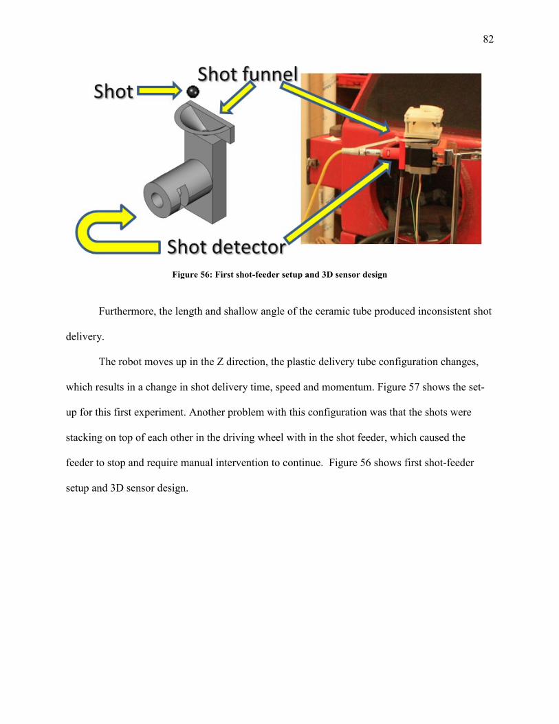
82

Figure 56: First shot-feeder setup and 3D sensor design

Furthermore, the length and shallow angle of the ceramic tube produced inconsistent shot

delivery.

The robot moves up in the Z direction, the plastic delivery tube configuration changes,

which results in a change in shot delivery time, speed and momentum. Figure 57 shows the set-

up for this first experiment. Another problem with this configuration was that the shots were

stacking on top of each other in the driving wheel with in the shot feeder, which caused the

feeder to stop and require manual intervention to continue. Figure 56 shows first shot-feeder

setup and 3D sensor design.

83

Figure 57: First experimental setup design with shot feeder in a fixed location and linear to the Z axis of

the robot holding the torch

In this configuration, the shots free-falling from the feeder into the funnel sometimes

failed to enter the plastic delivery tube or experienced significant variation in time before

entering into the plastic tube, which causes inconsistency in the shot delivery time. Inconsistent

shot delivery makes it difficult to adjust properly the welding parameters, such as the Peak

Current Delay Time (PDT) and the Peak Current Time (PT). Figure 58 shows experimental first

setup design schematic.

84

Figure 58: Experimental first setup design schematic

4.2.2. Setup #2

In this experimental setup design, the ceramic tube was shortened and both the torch and

the ceramic tube angle were changed angle was increased to 90 °C with the torch. Also, the

inconsistency caused by shots free-falling from the feeder into a funnel was eliminated by having

the shots exit the feeder via a plastic tube into the shot detector. The steeper ceramic tube angle

increased the speed of the shot and gives it more momentum. Therefore, the shots can overcome

some of the obstacles in the way to the weld pool. However, the lack of change in the Z axis

height between the torch and ceramic delivery tube still posed problem because the plastic tube

even shorter in this setup and small changes in the vertical axis may had big influence in the shot

delivery. Increasing the Z access too much will come create a point where no shot will be

delivered due to the angle of the plastic tube being too shallow for gravity to pull the shots down.

Figure 59 shows the second experimental setup and Figure 60 shows Experimental second setup

design schematic

85

Figure 59: Second experimental setup with modified torch and ceramic delivery tube angles and

elimination of shots free-falling into shot detector.

Figure 60: Experimental second setup design schematic

86

4.2.3. Setup #3

In this design, a fixture was welded to the center bolt of the Z “vertical” axis in the robot

to carry the shot feeder, shot detector and both plastic and ceramic delivery tubes and maintain

the same orientation as the Z axis was change for each new layer. Therefore, if any change the Z

access occurs, the whole feeding system moves with it, which makes it consistent in feeding

thereby maintaining the speed and momentum of the shot. The length of the path the shots will

travel to reach the weld pool is approximately 700 mm, and the height of the shot feed to

substrate was approximately 680 mm. Figure 61 shows the third and final experimental setup.

Figure 61: Third experimental setup

A 450 tilt in the shot-feeder was added in this design, and the cup of the shot-feeder was

redesigned to be taller to accumulate the shots in the lower side of the shot-feeder, such that

while the Driving Wheel (DW) transport only one shot to the shot exit. In case there were two

87

shots occupying in one hole, the excess shot remover takes it away. Figure 62 shows shot-Feeder

tilt in 45 angles and Shot-feeder cup with excess shot remover.

Figure 62: Shot-feeder tilt in angle, shot-feeder with excess shot remover

The torch was set to the far left of the substrate with an arc length of 4 mm and an angle

of 250. The ceramic tube is pointing to the weld pool with standoff distance of 4 mm. The angle

of the ceramic tube is 200. Figure 63 shows Torch and ceramic tube angle setup.

Figure 63: Torch and ceramic tube angle setup

88

4.3. Optimization of shot feed and arc current pulsing

The video system was used to investigate and optimize the shot feeding and arc current

pulsing timing and sequencing. Figure 64 shows the steps of the thermal cycle to build a deposit

and captured by the video system.

Robot Move

Arc on at background level

Arc on at pulse level

Waiting for shot

Shot leaving the tube pool

Shot hitting the weld pool

Shot melting

Arc on at background level

Weld pool solidification

Figure 64: Optimization of shot feed and arc current pulsing

Prior to the start of the building, the pilot arc is turned on. Then the main arc is turned on

at the background level. When the shot is detected, the arc current is pulse after the pulse delay

time. Then, the shot will land on the weld pool and melt. The arc current is returned to the

background level. Then, the robot will move the substrate (2 mm in this experiment) and repeat

the cycle again. Timing in this process is critical and mainly depends on the shot feeder.

89

4.4. Operating Manual

M103 is the main command that controls the shot feeding and welding processes. Travel

step size means it moves whatever variable was plugged in the program between pulses. Any

changes should be made in the editor, then saved and run again. Unfortunately, copying and

pasting cannot be done from the program file to a word document and changed because a simple

text and word file is not just simple text, the font and other accessories have been added to it.

4.5. Metallographic investigation of linear wall depositions.

After the walls were built, they were subjected to metallographic inspection. First the

walls were sectioned both transversely (perpendicular to the long axis of the wall) and

longitudinally (parallel to the long axis of the wall). The sections were then mounted, polished

and etched to reveal the grain microstructure. The sections were then photographed and

subjected to micro-hardness measurements. Grain size was determined from the photographs.

Then both grain size and hardness values were converted to wall height and inter-layer wait-

time.

4.5.1. Grain size measurement

The microscopic pictures were shots at 140X magnification. Each picture has a scale in

the lower right corner. The scale is 500 μm (0.5 mm) and is also divided into 10 units, which

makes every unit 50 μm. Ten grains were measured from each picture and the measurements

were averaged. Figure 65 shows the scale in a microscopic picture.

90

Figure 65: A scale in a microscopic picture.

4.6. Hardness

A Rockwell Harness Tester was used to indent the sample to determine the hardness. An

average B-scale hardness number was obtained using a 1/16” steel ball and a load of 100kg. The

first reading was from the middle of the substrate, and the rest of reading was from the HAZ, all

the way to the surface of the wall with approximately 1mm pitch from the center of the indenters.

Figure 66 shows the indenter progressing upward in a cross section cut of one of the specimen.

Figure 66: Indenter progressing upward in cross section cut of one of the specimen

91

5. Results and Discussion

Three linear wall weld metal specimens made from the A36 steel alloy were built using

1018 steel shots filler metal throughout this research. Here the results are presented and

discussed in regards to all of the weld specimens that were constructed. tt is the time to produce a

layer or track. δ is a coefficient to make the inter-layer wait time a function of the time to

produce a layer. δtt is the inter-layer wait-time. Essential process parameters, dimensions,

photographs of the specimens, mechanical properties plots of Tdep in relation to the number of

weld tracks in the weld metal deposit (nt), and weld metal microstructures are presented and

discussed. nt, Tdep after a minimum δtt of 1 minute and a maximum δtt of 10 minutes, and any

important comments pertaining to the weld tracks that were made are shown in Appendix A:

Raw Specimen Data.

5.1. Linear wall Specimen #1 (Baseline)

Specimen #1 was built with welding parameters that were considered as a “Baseline” to

compare the other specimens against. The PAW essential process parameters used to

manufacture the Specimen#1 are shown in Table 10. Specimen#1 was built using steel shots#7

from Precision.

92

Table 10: Plasma Arc Welding Essential Process Parameters for Linear Wall Specimen #1

Variable Value Unit Current Type DCEN ---

Current peak 55 Amp Current background 9 Amp Current pulse time 2 Sec Voltage Peak 24 Volt

Voltage background 16 Volt

Plasma orifice diameter 2.4 Mm Plasma Gas Composition --- Argon

Shielding Gas Composition --- Argon

Plasma gas flow rate 2 CFH Shielding gas flow rate 18 CFH Orifice/electrode setback 1 Gauge Torch angle 90 Degree Travel step size 2 Mm Shot delivery angle 10 Degree Shot delivery speed 22.22 mm/min

Travel Speed 1000 mm/min Electrode Type/ Composition 2% Thoriated Tungsten --- Electrode Diameter 2 Mm Arc Length/Stand off 5 Mm Inter-Track Wait Time Varied Min

The substrate was 150 mm long by 32 mm high and 6.5 mm thick. Wall#1 was 31 layers

producing a deposit 100 mm long by 32 mm high and 7 mm thick. Layer deposition always

started from the same end. After each layer, the deposit height was re-measured. The specimen

was cooled with random inter layer wait times between layers. Specimen #1 is shown in

Figure 67.

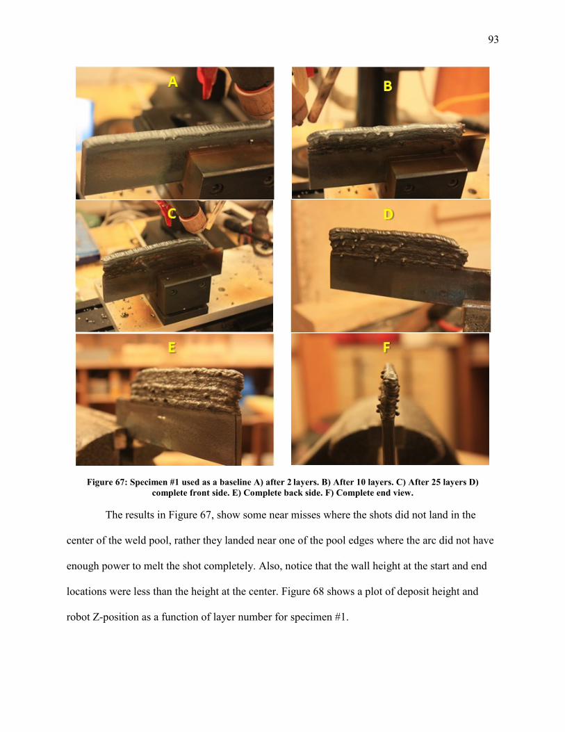
93

Figure 67: Specimen #1 used as a baseline A) after 2 layers. B) After 10 layers. C) After 25 layers D)

complete front side. E) Complete back side. F) Complete end view.

The results in Figure 67, show some near misses where the shots did not land in the

center of the weld pool, rather they landed near one of the pool edges where the arc did not have

enough power to melt the shot completely. Also, notice that the wall height at the start and end

locations were less than the height at the center. Figure 68 shows a plot of deposit height and

robot Z-position as a function of layer number for specimen #1.

94

Figure 68: Specimen #1 deposit height and robot position

Ideally after each layer was deposited, the torch would be raised an amount each to the

thickness of the layer just deposited. The thickness of each layer varied somewhat along the

length of the layer, an average layer thickness was calculated from two measurements at

locations along the deposit length that were accessible (locations outside the vise holding the

substrate.)

5.1.1. Metallography of Weld Metal Specimen #1 Baseline

The baseline specimen was one of the successful walls built without taking into

consideration wait time so the layers were randomly laid on top of each other. However, the wait

time of most layers was approximately 1-10 minutes

0

5

10

15

20

25

30

0 5 10 15 20 25 30 35

De

po

sit

he

igh

t an

d R

ob

ot

po

siti

on

Number of layer

Base line, Surface Profile Vs. Standoff Distance

Deposit height

Robot position

95

Specimen #1 was cut into longitudinal and transverse sections. As shown in Figure 69,

the transverse section was taken from the top of segment 2 and the longitudinal section was taken

from top of segment 7.

Figure 69: Location of transverse section and longitudinal section on specimen #1

The deposit grains change structure from a relatively microstructure and small grain size

near the substrate to a very coarse microstructure with a large grain size near the tip of the

deposit. Figure 70 shows specimen #1 grains change.

96

Figure 70: Transverse macro section of baseline specimen #1 with example micrographs and grain size at

deposit heights

The microstructure of the specimen near the substrate consisted of pearlite colonies (dark

contrast) and ferrite grains (light contrast). Both ferrite and pearlite grains were nearly equiaxed

grains, ranging from 12 to 19 μm in size.

The microstructure of the specimen near the surface, the light-colored region of the

microstructure, is the ferrite. The grain boundaries between the ferrite grains can be seen quite

clearly. The dark regions are the pearlite. It is made up from a fine mixture of ferrite and iron

carbide, which can be seen as a "wormy" texture. Both ferrite and pearlite grains were columnar

grains which are long, thin, coarse grains, ranging from 250 to 350 μm in size. Figure 71 shows

the growth in grain size of Specimen #1.

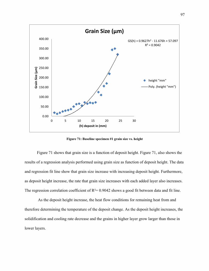
97

Figure 71: Baseline specimen #1 grain size vs. height

Figure 71 shows that grain size is a function of deposit height. Figure 71, also shows the

results of a regression analysis performed using grain size as function of deposit height. The data

and regression fit line show that grain size increase with increasing deposit height. Furthermore,

as deposit height increase, the rate that grain size increases with each added layer also increases.

The regression correlation coefficient of R²= 0.9042 shows a good fit between data and fit line.

As the deposit height increase, the heat flow conditions for remaining heat from and

therefore determining the temperature of the deposit change. As the deposit height increases, the

solidification and cooling rate decrease and the grains in higher layer grow larger than those in

lower layers.

GS(h) = 0.9627h2 - 11.676h + 57.097 R² = 0.9042

0.00

50.00

100.00

150.00

200.00

250.00

300.00

350.00

400.00

0 5 10 15 20 25 30

Gra

in S

ize

(µ

m)

(h) deposit in (mm)

Grain Size (µm)

height "mm"

Poly. (height "mm")

98

5.2. Linear wall Specimen #2

Specimen #2 was built with welding parameters that were considered in Specimen #1.

The waiting time between layers was 1 minute. The average temperature for the specimen before

building the next layer was 200 C. The PAW essential process parameters used to manufacture

the Specimen#2 are shown in Table 11. Specimen#2 was built using 1018 steel from Abbot.

99


Variable Value Unit Current Type DCEN



plasma orifice diameter 2.4 Mm Plasma Gas Composition --- Argon


plasma gas flow rate 2 CFH Shielding gas flow rate 18 CFH orifice/electrode setback 1 Gauge torch angle 90 Degree travel step size 2 Mm shot delivery angle 10 Degree shot delivery speed 22.22 mm/min

Travel Speed 1000 mm/min Electrode Type/ Composition 2% Thoriated Tungsten --- Electrode Diameter 2 Mm Arc Length/Stand off 5 Mm Inter-Track Wait Time 1 Min

The substrate was 150 mm long by 32 mm high and 6.5mm thick. Wall#2 was 26 layers



was allowed one minute to cool down between layers. Specimen #2 is shown in Figure 72.

100

Figure 72: Specimen #2 A) Close view shows surface layer. B) Close view shows different location of

surface layer. C) Close view start side D) Close view end side. E) Close view front side. F) Close view back

side.

The results in Figure 72, show some near misses where the shots did not land in the

center of the weld pool, rather they landed near one of the pool edges where the arc did not have

enough power to melt the shot completely. Also, notice that the wall height at the start and end

locations were less than the height at the center. Figure 73 shows a plot of deposit height and

robot Z-position as a function of layer number for specimen #2.

101

Figure 73: Specimen #2, number of layers vs. buildup height and arc length

After each layer was deposited, the torch would be raised an amount each to the thickness

of the layer just deposited. The thickness of each layer varied somewhat along the length of the

layer, an average layer thickness was calculated from 2 measurements at locations along the

deposit length that were accessible (locations outside the vise holding the substrate.)

There were cuts longitudinal and transverse. Cuts were made randomly, taking into

consideration location to show full height and most of transvers section.

5.2.1. Metallography of Weld Metal Specimen #2

Specimen #2 was built with wait time of 1 min between each layer. Specimen #2 was cut

into longitudinal and transverse sections. As shown in Figure 74, the transverse section was

0

5

10

15

20

25

0 5 10 15 20 25 30

De

po

sit

he

igh

t an

d R

ob

ot

po

siti

on

Number of layers

1 Minute wait time, Surface Profile Vs. Standoff Distance

Deposit height

Robot position

102

taken from the between of segment 1M and 1. The longitudinal section was taken from top of

segment 1M.





103

Figure 75: Transverse macro section of baseline specimen #2 with example micrographs and grain size at

deposit heights










104

Figure 76: Grain size number for 1-minute specimen









lower layers.

GS(h)= 0.6943h2 - 2.8331h R² = 0.7627

0

50

100

150

200

250

300

350

400

450

0 5 10 15 20 25 30

Gra

in S

ize

in (

µm

)

Height in mm

Grain Size (µm)

grain size (µm)

Poly. (grain size (µm))

105

5.3. Linear wall Specimen #3

Specimen #3 was built with welding parameters that were considered in Specimen #1.

The waiting time between layers was 10 minutes. The average temperature for the specimen

before building the next layer was 70 C. The PAW essential process parameters used to

manufacture the Specimen #3 are shown in Table 12. Specimen #3 was built using 1018 steel

from Abbot.


Variable Value Unit Current Type DCEN



plasma orifice diameter 2.4 Mm Plasma Gas Composition --- Argon


plasma gas flow rate 2 CFH Shielding gas flow rate 18 CFH orifice/electrode setback 1 Gauge torch angle 90 Degree travel step size 2 Mm shot delivery angle 10 Degree shot delivery speed 22.22 mm/min

Travel Speed 1000 mm/min Electrode Type/ Composition 2% Thoriated Tungsten --- Electrode Diameter 2 Mm Arc Length/Stand off 5 Mm Inter-Track Wait Time 10 Min

The substrate was 150 mm long by 32 mm high and 6.5 mm thick. Wall#3 was 38 layers



was allowed 10 minutes to cool down between layers. Also, building the specimen takes more

than 9 hours. Specimen #3 is shown in Figure 77.

106

Figure 77: Specimen #3 A) Close view front side. B) Close view back side.

The process shows consistency in shot feeding. Shot near misses or shots do not land in

the center of the weld pool and were almost eliminated. Figure 80 shows the layer number vs.

wall height and arc length.

The results in Figure 77, shows consistency in shot feeding. However, show some near

misses where the shots did not land in the center of the weld pool, rather they landed near one of

the pool edges where the arc did not have enough power to melt the shot completely. Also,

notice that the wall height at the start and end locations were less than the height at the center.

Figure 78 shows a plot of deposit height and robot Z-position as a function of layer number for

specimen #3.

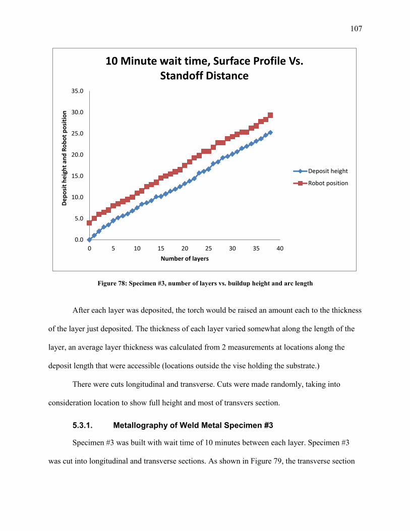
107

Figure 78: Specimen #3, number of layers vs. buildup height and arc length

After each layer was deposited, the torch would be raised an amount each to the thickness

of the layer just deposited. The thickness of each layer varied somewhat along the length of the

layer, an average layer thickness was calculated from 2 measurements at locations along the

deposit length that were accessible (locations outside the vise holding the substrate.)

There were cuts longitudinal and transverse. Cuts were made randomly, taking into

consideration location to show full height and most of transvers section.

5.3.1. Metallography of Weld Metal Specimen #3

Specimen #3 was built with wait time of 10 minutes between each layer. Specimen #3

was cut into longitudinal and transverse sections. As shown in Figure 79, the transverse section

0.0

5.0

10.0

15.0

20.0

25.0

30.0

35.0

0 5 10 15 20 25 30 35 40

De

po

sit

he

igh

t an

d R

ob

ot

po

siti

on

Number of layers

10 Minute wait time, Surface Profile Vs. Standoff Distance

Deposit height

Robot position

108

was taken from the segment next to segment 5. The longitudinal section was taken from top of

the large center segment.





109

Figure 80: Macro section of weld metal specimen 10 min wait time










110

Figure 81: Specimen #3 grain size vs. height









lower layers.

GS(h) = 0.9627h2 - 11.676h + 57.097 R² = 0.9042

0

50

100

150

200

250

300

350

400

0 5 10 15 20 25 30

Gra

in S

ize

(µ

m)

Height in mm

Grain Size (µm)

height "mm"

Poly. (height "mm")

111

5.4. Influence of Inter-layer wait time on Grain Size

The grain size results from all three specimens were put together for comparison and

analysis. Since Specimen #1 has variable and unknown wait time, the primary focus will be on

specimen #2 and #3. Then, from the known wait-times of specimens #2 and #3, Specimen #1’s

wait time will be predicted. From a heat flow standpoint, heat input, the lower the inter-layer

wait time the higher the effective deposit preheat temperature then, the larger the resulting grain

size. The larger grain size in all specimens near the top of the deposit is due to the decrease in

heat flow away from the top layers as the deposit height increases. Effectively this means that as

the deposit height increases the average temperature is higher as each new layer is applied. Large

grain size is the response of the metallurgical system to reduce internal energy by reducing the

total area of grain boundaries (Ref.52). That is to increase grain size Figure 82 shows the change

in grain size as a function of deposit height in all three specimens.

112

Figure 82: Different in grain size in all three specimens

The results in Figure 82 show the 1-minute wait time specimen has larger sized grains

compared to the 10-minute specimen. This result was expected since the 1-minute specimen was

exposed to higher heat input and shorter time to dissipate the heat and reduce deposit

temperature than the 10-minute specimen.

5.5. Hardness

The hardness-HRB results of the three specimens are plotted in Figure 83. A regression

analysis was performed for HRB as a function of deposit height on all three specimens. The

equations of the hardness trend lines are displayed in the graph. For all 3 specimens, hardness

decreases nearly linearly with increasing deposit height. Specimen #2 was completed with an

0

50

100

150

200

250

300

350

400

0 5 10 15 20 25 30

Gra

in S

ize

(µm

)

Height (mm)

Grain Size (µm)

Baseline

Expon. (specimen 3)

Expon. (specimen 2)

113

inter-layer wait time of 1 minute and specimen #3 was completed with a 10 minutes inter-layer

weight time, the average deposit temperature for specimen #2 was greater than that of specimen

#3. As results the decrease in hardness for specimen #1 as a function of deposit height (-1.88

HRB/mm) is nearly 5 times that of specimen #3 (-0.33 HRB/mm). while the HRB for specimen

#1 generally decreased with increasing deposit height, the random inter-layer wait time caused

corresponding variations in HRB values.

Figure 83: Hardness test regression analysis shows decrease in all specimens

as a function of Deposition Height.

Specimen #1 is HRB (BL), Specimen #2 is HRB (1min), and Specimen #3 is HRB (10min). For all

specimens hardness decreases nearly linearly as deposit height increase.

The decrease in hardness with increasing deposit height is a direct result of the observed

increase in grain size with increasing deposit height. The data of the hardness test analysis for all

three specimens is located in Appendix A, Table 19.

Figure 84 shows approximate relation between the hardness and the grain size for

Specimen #2.

HRB(1min) = -1.8778H + 89.57 R² = 0.5562

HRB(10min) = -0.3285x + 80.541 R² = 0.0726

HRB (BL) = -0.1121x + 69.469 R² = 0.0218

40.00

50.00

60.00

70.00

80.00

90.00

100.00

0 5 10 15 20 25 30

HR

B

Deposition Height (mm)

Hardness Test

Specimen #2

Specimen #3

BL

Linear (Specimen #2 )

Linear (Specimen #3)

Linear (BL)

114


The hardness is directly related to grain size. In general, the smaller the grain size, the

harder the material. Figure 84 shows that for the first five layers, the grain sizes as about 25-50

µm and the hardness was 93-74 HRB. For layers 10-15 the grains size was between 50-120 µm

and the hardness was between 77-70 HRB. Based on these results, the prediction of the grain size

for layers 16-20 was 250-400 µm and the hardness estimated to be 70-55 HRB.

Figure 85 demonstrates relation between the hardness and the grain size for Specimen #3.

115


The hardness is directly related to grain size. In general, the smaller the grain size, the

harder the material. Figure 85 show that for the first five layers, the grain sizes as about 18-29

µm and the hardness was 88-75 HRB. For layers 10-15 the grains size was between 40-90 µm

and the hardness was between 82-71 HRB. Based on these results, the prediction of the grain size

for layers 16-20 was estimated to be 180-320 µm and the hardness 68-52 HRB.

5.6. Prediction of Tensile Strength

Hardness values can be used to estimate tensile strength. The conversion chart use to

predict tensile strength from HRB values included in Appendix A, Table 20 (Ref.55). Figure 86

shows the results of regression analysis of tensile strength on the three specimens.

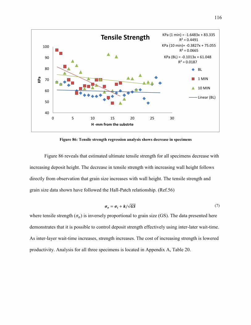
116

Figure 86: Tensile strength regression analysis shows decrease in specimens

Figure 86 reveals that estimated ultimate tensile strength for all specimens decrease with

increasing deposit height. The decrease in tensile strength with increasing wall height follows

directly from observation that grain size increases with wall height. The tensile strength and

grain size data shown have followed the Hall-Patch relationship. (Ref.56)

√ (7)

where tensile strength ( ) is inversely proportional to grain size (GS). The data presented here

demonstrates that it is possible to control deposit strength effectively using inter-later wait-time.

As inter-layer wait-time increases, strength increases. The cost of increasing strength is lowered

productivity. Analysis for all three specimens is located in Appendix A, Table 20.

KPa (BL) = -0.1013x + 61.048 R² = 0.0187

KPa (1 min) = -1.6483x + 83.335 R² = 0.4491

KPa (10 min)= -0.3827x + 75.055 R² = 0.0665

40

50

60

70

80

90

100

0 5 10 15 20 25 30

KP

a

H -mm from the substrte

Tensile Strength

BL

1 MIN

10 MIN

Linear (BL)

117

5.7. Productivity and Quality consideration

5.7.1. Wall end transients

As shown in section 4.3.3, the torch and the ceramic tube setup angles. This setup was

best for delivering shots to the weld pool with minimum lost number of shots. However, this

setup has a down side; at the end of the each layer the arc force tends to push the shot filler metal

away from the substrate. This is not notable until the build reaches about 6 mm height and

approximately 10 layers, and since there is no material at the end of the wall to support the filler

metal end the last several shots tend to wash away as sparks. Figure 87 shows the loss metal at

the end of walls.

Figure 87: Walls tend to lose height at the start and stop transients

118

5.7.2. Ceramic Tube

The ceramic tube diameter should be as small as possible so the shots will be directed to

the weld pool; however, the plastic tube was a slightly larger in diameter. A reducer was

designed and printed in the 3-D printer and inserted into the plastic tube. Increasing the angle of

the ceramic tube into the weld will provide faster shots, therefore becoming harder to control due

to the increase in potential energy. This potential energy will eventually convert to kinetic

energy. However, if we decrease the steepness of the angle of the ceramic tube it will not have

enough momentum to cross the reducer. It might work great for hundreds of shots, but one shot

may stick at any time. This is due to the size of the shots, which is small enough to cause non-

classical effects on Newton’s law may arise. That means any obstacles could stop the flow. The

ceramic tube should not touch the specimen. Touching the specimen may lead to change in tube

angle or block of shots. Figure 88 shows the reducer blocking the shots.

Figure 88: Reducer blocking the shots

The design was changed because the reducer proved inefficient. Then, the ceramic tube

was aligned perfectly to the plastic tube and cemented to the plastic tube using RTV silicon.

Figure 89 is a schematic of the plastic tube connected to the ceramic tube using RTV. This

connection method produced smooth connection between both tubes.

119

Figure 89: Schematic of the plastic tube connected to the ceramic tube using RTV

Controlling the shot landing was very hard because of variation on the shots’ sphirical

shape, which makes every single shot act slightly differently from others. Also, the height of the

open end of the ceramic tube make a difference. The closer the tube the easier to control the

shots landing. However, the ceramic tube may become blocked due to spatter.

Figure 90 shows spatter build up in the ceramic tube and blocking a shot.

Figure 90: Spatter build-up in ceramic tube

Because of some missing shots and/or some near miss shots, the surface profile of the

specimen is not constant. Therefore, it directly affects the arc length. Figure 66 shows the wall

height and the arc length inconsistently increasing. Again, this is caused by the stand-off

destance of the ceramic tube and the consistancy of the shot-feeder. The shorter the stand-off

distance, the more likely the ceramic tube will be blocked by the spatter flying from the weld

pool. A study from South Korea finds a solution for the inconsistency in surface profile, which

shows the process principle of 3D Welding and Milling. First, a layer is built by depositing

120

single beads. When deposited, the top surface of the layer is machined to a prescribed thickness

for further deposition (Ref.53).

5.7.3. Deposition rate

To calculate the volume of a shot “sphere” equation 7 was used

(8)

where is a universal constant and R is the radius of the shots (Diameter / 2)

(9)

Steel density is constant for all steel except some small variation due to steel purity.

Table 13 shows some of the shots properties.

Table 13: Shot properties

Variation Value Unit

(PI) 3.1416 Constant

radius R 1.25

Volume of a shot Steel density ρ 7900 kg/m3

Weight of single shot* 0.06561 Grams

* Weight of single shot is 65.61 mg = 0.06561 g

In this experiment, a layer built of 100 mm long will consist of 50 shots, the approximate

time to build a 100mm layer is 4.5 minute. Equation 9 shows the Deposition Rate:

(10)

where is the arc peak time and is arc background time. The deposit rate in this experiment

is 47 g/h, this can be boosted by developing faster shot feeder.

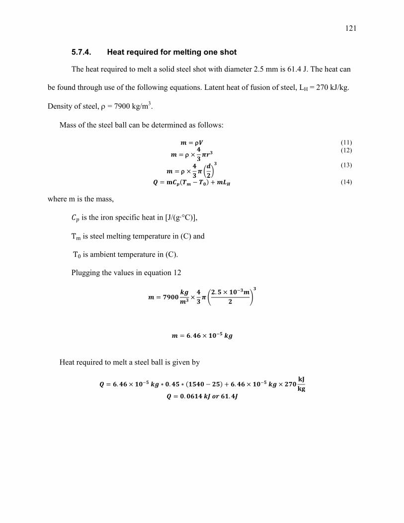
121

5.7.4. Heat required for melting one shot

The heat required to melt a solid steel shot with diameter 2.5 mm is 61.4 J. The heat can

be found through use of the following equations. Latent heat of fusion of steel, LH = 270 kJ/kg.

Density of steel, = 7900 kg/m3.

Mass of the steel ball can be determined as follows:

(11)

(12)

(

)

(13)

(14)

where m is the mass,

is the iron specific heat in [J/(g∙°C)],

is steel melting temperature in (C) and

is ambient temperature in (C).

Plugging the values in equation 12

(

)

Heat required to melt a steel ball is given by

122

5.7.5. Porosity

A substrate was ground and wire brushed, and then an autogenic weld was made in the

sample substrate. Even though the substrate was ground and cleaned, the substrate still shows

porosity. Figure 91 shows the porosity of the part being examined. However, this is a rare case.

Figure 91: Porosity in autogenic weld

Also, after several trials building walls, using the 1st shot feed stock source (precision

shots) they all failed because of the aggressive porosity. Even though the substrate was cleaned

and wire brushed, the porosity was observed in the first layer. Figure 92 shows porosity in a

sample specimen in first layer.

Figure 92: Porosity was observed in the first layer.

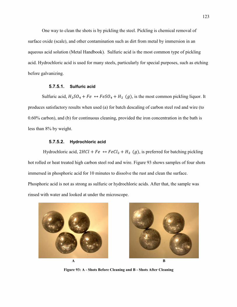
123

One way to clean the shots is by pickling the steel. Pickling is chemical removal of

surface oxide (scale), and other contamination such as dirt from metal by immersion in an

aqueous acid solution (Metal Handbook). Sulfuric acid is the most common type of pickling

acid. Hydrochloric acid is used for many steels, particularly for special purposes, such as etching

before galvanizing.

5.7.5.1. Sulfuric acid

Sulfuric acid, , is the most common pickling liquor. It

produces satisfactory results when used (a) for batch descaling of carbon steel rod and wire (to

0.60% carbon), and (b) for continuous cleaning, provided the iron concentration in the bath is

less than 8% by weight.

5.7.5.2. Hydrochloric acid

Hydrochloric acid, , is preferred for batching pickling

hot rolled or heat treated high carbon steel rod and wire. Figure 93 shows samples of four shots

immersed in phosphoric acid for 10 minutes to dissolve the rust and clean the surface.

Phosphoric acid is not as strong as sulfuric or hydrochloric acids. After that, the sample was

rinsed with water and looked at under the microscope.

A

B

Figure 93: A - Shots Before Cleaning and B - Shots After Cleaning

124

In Figure 93, the shots appear cleaner. Most of the rust has been removed. However, this

process is not practical in this experiment because damp shots allow moisture to get into the

plastic tubing. This moisture does not allow the shots to run smoothly in the tube. Therefore, it

is hard to control moisture and productivity at the same time. Figure 94 shows the two types of

shots side to side.

Figure 94: Two kind of shots side to side

In Figure 94, the new shots from Abbott look cleaner, shinier, and most importantly,

porosity free compared to the common shot gun shots. Material Safety Data Sheet is showing the

chemical composition and health hazard information is located in appendix B.

5.7.6. Deposit void density

A section from a location selected randomly test part was cut from specimen 3 ( 10

min) to assess deposit soundness. The location of the part is shown in Figure 95. The section was

polished, mounted and examined with an optical microscope. The examined part area, looking

from the top down, is approximately 132mm².

125

Figure 95: Actual part location in specimen 3 was polished and tested

In the specified area, there were 13 round pores. Most of the pores were approximately

0.5 mm in diameter, and assumed to be spherical. Figure 96 shows one of the pores in the surface

of the section with the scale used to measure the pore size.

Figure 96: pores in surface of a deposit section

126

The scale used was 6" satin chrome ruler, hardened and tempered 10ths and 50ths

(front), 64ths and 32nds (back) from SPI. The total area of pores in the section area is 8.49mm².

That means 6 percent of the surface of the section consists of voids. One of the pores was

showing deep penetration. Figure 97 shows the pores penetrating more than one layer.

A

B C D

E F

Figure 97: Series photos of a pore persisting through multiple layers

127

Figure 93 shows that a pore in one layer could grow into the layers placed on top of it.

That means that in additive manufacture, discontinuities may accumulate thru multiple layers.

5.8. Deposit Distortion

In the linear-wall specimens, build here there were distortions little noticeable because of

the orientation of the substrate. owever, if the substrate was rotated 90 , then significant

distortion occurred. After the 4th

layer, distortion become significant and produced variation in

arc length along the deposit. The variation in arc length was large enough to affect the shielding

gas, and porosity started to show in layers 7-9. After layer 9, the workpiece was repositioned to

minimize the variation of arc length. Then layer 10 was completed, and the wall showed severe

porosity. Figure 98 shows the distortion progression.

A

B C

Figure 98: A-3rd layer was placed in the specimen,

B-the 6th layer was placed, little distortion appears with two less than 1mm porosities, C-layer 10

Assuming no unusual initial stresses, the following equation (14) can be used to

demonstrate the amount of distortion or bending that will result from a longitudinal welding on a

given member. (Ref.54)

(15)

where is the total cross section area within the fusion line, of all welds, in².

C is the distance between the center of gravity of the weld group and the neutral axis of

the member in inches.

128

L is the length of the member, I is the moment of inertia of the member,

is the resulting vertical distortion in inches.

Assuming all variables are constant in both substrate orientations, the moment of inertia

changes with the orientation of the substrate. Equation 15 shows the Moment of inertia value,

(16)

where b is the breadth of the substrate, and d is the depth of the substrate. Figure 99 shows the

different orientation of substrate affect the moment of inertia.

Figure 99: the influence of substrate orientation on moment of inertia and resulting substrate distortion

(A) low distortion, (B) high distortion

Since d in both moments of inertia is to the power 3, and the moment of inertia has an

inverse relationship with distortion, then distortion in substrate orientation A will be far less than

the distortion in substrate orientation B.

129

5.9. Inherence of cooling rate on deposit strength and productivity

The final metallurgical structure of the weld zone primarily the grain size is primarily

determined by the cooling rate from maximum temperature achieved during the weld cycle (peak

temperature) (Ref.39). The cooling rate for both of 1 minute and of 10 minutes are

compared using the following equation (17):

( 17)

where R is the cooling rate at the weld center line C/s,

k is the thermal conductivity of the metal J/mm s C,

is the initial plate temperature, and is the temperature at which the cooling rate is

calculated in (C) and is the net welding heat input.

All variable were constant for specimen #2 ( = 1 min) and specimen #3 ( = 10 min)

except . Therefore equation 17 can be simplified to

( 18)

For specimen #2, the average deposit temperature 200°C and for specimen #3

70°C. = 550°C is commonly used for steels. Taking the ration:

Therefore, specimen #3 cooled approximately 19 times faster than specimen #2.

Therefore:

Specimen #3 > Specimen #2

>

GS Specimen #3 < GS Specimen #2

130

HRB Specimen #3 > HRB Specimen #2

This is the reason for > is directly attributed to specimen #3

> specimen #2. Again inter-layer wait-time is an effective method to control deposit

strength at the expense of the productivity.

Figure 100: The effect on wait time to other factors

Figure 100 illustrate the effect of wait time in the grain size the less wait time the bigger

the grain and the bigger the grain the less hard it be come. The hardness will affect the strength

proportionally.

Tensile Strength

Hardness

Grain Size

Inter-Layer Wait-Time

131

6. Analytical Heat Flow Model

The results of this work show that as inter-layer wait-time increase average deposit

temperature decrease, GS decreases and therefore hardness and tensile strength increase.

However, as increase productivity decreases. It is difficult to achieve both high productivity

and acceptable mechanical properties simultaneously in additively manufactured, low-carbon

steel alloy weld metal deposits. As a result, attaining acceptable mechanical properties while

maintaining a high level of productivity is now of great importance. Cross-sections of weld metal

deposits indicate that it is possible to control microstructure development by controlling

productivity (Ref.57). Experimental data from Specimen #2 1 min (60 second) or

=0.28 was used to tune a simple analytical heat flow model of the weld metal deposit build

process. The results of the model were used to investigate the relationship between productivity

and mechanical properties via .

6.1. Analytical Heat Flow Model Development

A simple analytical heat flow model, developed (Ref.44) was used to simulate the deposit

build temperature in previous work (Ref.57). That model was modified to suit the

experimental parameters used in this work. The results of the analytical heat flow model provide

the foundation on which to develop a strategy to manage deposit heat flow. The strategy to

manage deposit heat flow can identify an optimum compromise between productivity and obtain

acceptable microstructure and mechanical properties (Ref.57).

For many heat transfer problems, the first law of thermodynamics provides a useful, often

essential tool for heat flow analysis. The conservation of energy for a control volume is given as

(Ref.58):

132

(19)

where is the change in thermal and mechanical energy stored in a control volume,

is the thermal and mechanical energy entering a control volume,

is the thermal and mechanical energy leaving a control volume, and

is the thermal energy generation within a control volume.

Since no mechanical work is performed on the control volume, and no energy is

generated within the control volume, only thermal energy is considered. Equation 20 can be

rewritten as (Ref.57):

(20)

where is the accumulation of heat in the deposit,

is the amount of heat put into the deposit via PAW,

is the amount of heat lost via conduction through the bottom and sides of the

deposit,

is the amount of heat lost via convection from the deposit, and

is the amount of heat lost via radiation from the deposit surface.

Mass, surface area and heat are added to the deposit with each successive weld layer. The

model is designed for general methods of layers-based additive manufacturing. A layer can be

produced from multiple tracks laid side-by-side as shown in Figure 101 (A) or can be produced

from a single track as shown if Figure 101 (B).

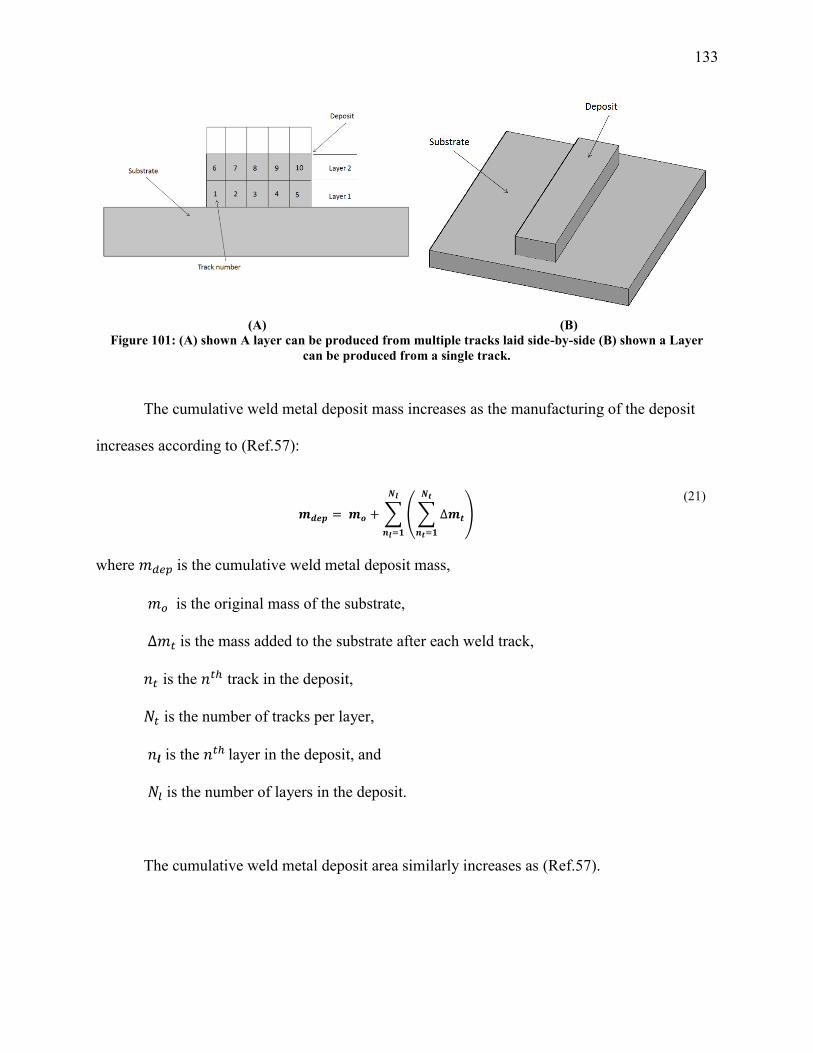
133

(A) (B)

Figure 101: (A) shown A layer can be produced from multiple tracks laid side-by-side (B) shown a Layer

can be produced from a single track.

The cumulative weld metal deposit mass increases as the manufacturing of the deposit

increases according to (Ref.57):

∑ (∑

)

(21)

where is the cumulative weld metal deposit mass,

is the original mass of the substrate,

is the mass added to the substrate after each weld track,

is the track in the deposit,

is the number of tracks per layer,

is the layer in the deposit, and

is the number of layers in the deposit.

The cumulative weld metal deposit area similarly increases as (Ref.57).

134

∑ (∑

)

(22)

where Adep is the cumulative weld metal deposit area and Ao is the original area of the substrate,

which is the sum of areas of the 2 faces and 2 sides and the bottom and top surface as shown in

Figure 102.

Figure 102: Different areas in the substrate

ΔAt is the area added to the substrate after each weld layer, which is the sum of areas of

the 2 faces and 2 sides. Figure 103 shows the different areas in each layer.

Figure 103: Layers areas

The deposit thermal energy gained via PAW for each weld track is given by:

135

(23)

where is a scale factor to modify the amount of heat added to the deposit by the PAW process,

is the average PAW arc voltage,

is the average PAW arc current,

η is the PAW heat transfer efficiency which equals 0.6, and

is the time it takes to weld one layer.

The term λ has physical significance in that it can represent PAW heat transfer efficiency

and accounts for heat losses during energy transfer from the arc to the deposit.

In this work, the arc was pulsed from a background level to peak level and back to the

background level for each shot delivered to the deposit. Thus each layer required multiple

current pulse cycles such that

( ) (24)

where is the total time to produce a layer

is the arc peak time period

is the arc background time period and

is the total number of arc pulse cycles in a track

To account for arc current pulsing equation 25 is written as

.

(25)

where is the background current,

is the background voltage,

is the background time,

is the peak current,

136

is the peak voltage,

is the peak time and

is the pulsing arc heat.

A single arc pulse period is duplicated in Figure 104. Table 14 lists the parameters used

in the experiment and their values.

Figure 104: Arc pulsing parameters

137

Table 14: Experimental Pulse Variable

Variable Value

50 Amp

2.0 sec

9 Amp

3.5 sec

50

To simplify the model solution, heat is the considered only to be lost while the arc is off

during the inter-layer wait-time Heat is lost via radiation according to:

(26)

where ε is the weld metal deposit surface area emissivity,

σ is the Stefan-Boltzmann constant,

is the temperature of the weld metal deposit (including the substrate), and

is the surrounding/ambient temperature.

The term ψ is the scale factor to modify the magnitude of heat lost from the deposit due

to radiation. The term ψ has physical significance and can be used as modification of the surface

area of the deposit, and/or variations of ε as deposit temperature changes and/or changes in the

temperature of the surroundings.

Heat loss by conduction occurred out the sides and bottom of the substrate into the

fixture. Heat is lost via conduction according to:

(27)

where is the conduction heat transfer coefficient at the interface between the substrate and

the fixture,

138

is the contact area between the fixture and the substrate, the value is fixed to

0.006

ξ is the scale factor to modify the magnitude of heat conducted from the substrate into the

fixture.

The term ξ has physical significance and can be used as modification of the contact area

between the substrate and the fixture, and/or the conduction heat transfer coefficient between the

substrate and the fixture, and/or changing the temperature of the fixture in contact with the

substrate.

Heat lost from the deposit via convection occurs according to (Ref.58):

(28)

where is the convection heat transfer coefficient associated with free convection. The term

ζ is the scale factor to modify the magnitude of heat lost due to convection from the deposit to

the environment. The term ζ has physical significance and can be used as modification of the

area, and/or the convection heat transfer coefficient from the deposit to the environment.

6.2. Analytical Heat Flow Model Solution

The primary objective of ongoing work in AM is the control of deposit microstructure to

control the deposit mechanical properties. Inter-track deposit temperature controls the deposit

solidification and cooling rate and, therefore, microstructure and mechanical properties (Ref.57).

Here, the analytical heat flow model is solved for the deposit temperature, , as a function of

the number of weld tracks, , in the weld metal deposit.

The amount of heat accumulated in the weld metal deposit at any instant can be

expressed as:

(29)

139

where is the specific heat at constant pressure of the deposit material.

If the right-hand-side of Equation 29 for is substituted into Equation 20, the result

becomes:

( )

(30)

Solving Equation 30 for Tdep results in:

(31)

By creating an intermediate temperature parameter, , representing the weld metal

deposit temperature at the start of each subsequent weld track and applying the conditions when:

(32)

and when

(33)

and by recognizing that , and are functions of time and, therefore,

weld track number, , the weld metal deposit temperature, Tdep, can be expressed as:

[ ]

(34)

where

(35)

6.3. Analytical Heat Flow Model Assumptions and Solution Approach

Several assumptions are used to simplify the analytical heat flow model. First, the weld

metal deposit thermal energy gained via PAW, , enters the deposit and diffuses evenly

140

throughout the substrate and deposit immediately after the track is completed. The first

assumption infers that the deposit thermal conductivity is large, and deposit diffusion distances

are small. Another assumption is that no heat is lost via conduction, convection, and radiation

during the time it takes to complete a weld track. , , and only occur during the

inter-track wait time, . The initial temperature of the substrate and of the fixture that the

substrate rests upon is assumed to be the ambient temperature environment ( ), (Ref.57).

To find the area added to the substrate after each weld track was completed, , the

height of each weld layer, needed to be experimentally determined. The average height of each

weld layer ( was found according to the average of the following equation:

(∑

∑

∑

)

(36)

where is the height of each experimental produced layer

is the number of layer in experimentally produced specimen

BL represent specimen #1

represent specimen #2 and

represent specimen #3

The average height per layer is 0.65 mm. Raw data for layer thicknesses can be found

in Appendix A, Tables 16, 17 and 18.

The approach taken to solve the analytical heat flow model on a track-by-track basis is

described as follows. and are added to the deposit. As a result of the newly added

mass and heat, an intermediate weld metal deposit surface temperature, Ti, is calculated. is

added to the deposit, and , , and are removed from the deposit at the

141

intermediate. As a result of the newly lost heat, the deposit temperature, , is calculated and

becomes the starting deposit temperature for the next weld track. Iterations continue for the

specified number of weld metal deposit layers.

6.4. Results and Discussion of the Analytical Heat Flow Model

The result of the analytical heat flow model is as a function of , λ, ψ, ξ, and ζ.

The coefficients λ, ψ, ξ, and ζ were adjusted to allow the analytical heat flow model deposit

temperature to approximate the experimental measured deposit temperature. two values were

used, specimen #2 = 60 sec and specimen #3 = 600 sec. The model is

capable of predicting (nt) for an unlimited number of layers, however in this research,

was limited to be 500 layers. The analytical heat flow model was solved by using a spreadsheet

computer program. Analytical heat flow model properties for low-carbon steel, along with their

typical values, are also shown in Appendix C. The analytical heat flow model properties and

mathematical formulas displayed in Appendix C were taken from Refs. (Ref.59), (Ref.60) and

(Ref.61).

Deposit mass, surface area and heat input increase linearly with . Increased mass

causes the deposit to contain more thermal energy, while increased surface area allows the

deposit to shed more thermal energy via radiation and convection. Increased deposit height

reduced the amount of heat loss to the fixture via conduction.

A maximum was selected for a steel deposit based on the Fe-C phase diagram.

Ideally, would stay below the eutectoid temperature (approximately 727 C) Lower

temperature reduces grain growth and produces a refined microstructure in the deposit, both of

which lead to better mechanical properties.

142

As mentioned the scale factors, λ, ψ, ξ, and ζ were adjusted to match the model simulated

deposit temperature to the experimental deposit temperature. Figure 106 shows experimental and

simulation as a function of . The experimental deposit temperature measurements are

shown in Tables 25 and 26 the values for the model scale factors λ, ψ, ξ, and ζ used in Figure 106

Figure 105: Experimental and Simulation as a function of nt

Since the model shows very close results from the beginning of the building to 26 layers,

a prediction can be made from the graph. For this solution to the analytical heat flow model,

= 1 minute (60 seconds), which is the same that was used to manufacture Specimen #2. Other

property values used to solve the analytical heat flow model are shown in Table 28 (located in

Appendix C). The values of λ, ξ, ψ, and ζ, are listed in Table 15.This allows the model

0.000

50.000

100.000

150.000

200.000

250.000

300.000

0 20 40 60 80 100 120 140 160 180 200

De

po

siti

on

Te

mp

retu

re T

de

p (

C)

Weld Tarck Number nt

Weld Metal Deposit Surface Temperature and Instantaneous Thermal Energy Losses in Relation to the Number of Layers in

the Deposit

Tdep Tdepexp

143

temperatures to predict the approximation of the experimental temperatures. Since the model

shows very close results from the beginning of the building to 26 layers, a prediction can be

made from the graph

The model was tuned using the perimeter reasonably match the experimental deposit

temperature. In Figure 106, the total number of experimental temperature reading results is

limited to the experimental range of layers ( With the values of (0.28) increases to a

peak value of approximately 300 °C after 26 layers. begins to decrease slightly after each

individual layer as predicted by the model.

Table 15: Scale Factor Values Used in Heat Analysis

Model

Property Value1

λ 0.60

ξ 0.50

ζ 0.50

ψ 1.00

144

Figure 106: Experimental and simulation Tdep as a function of nt for δtt = 1 minute

The conditions used to obtain the solution to the analytical heat flow model for specimen

#2 shown in Figure 106 represent a condition of high heat loss via conduction. Conduction is the

dominant heat loss mechanism for the prescribed conditions, as the number of layer increases the

heat loss via conduction decrease. The amount of heat loss by conduction is depending on the

temperature deposited and the distance of the heat have to travel through the specimen to the

fixture is linear with deposit height and deposit temperature. As the height of the deposit

0.0

500.0

1000.0

1500.0

2000.0

2500.0

3000.0

0.000

50.000

100.000

150.000

200.000

250.000

300.000

0 20 40 60 80 100 120 140 160 180 200

We

ld M

etal

De

po

sit

Inst

anta

neo

us

Ene

rgy

Loss

, Q (

J)

De

po

siti

on

Te

mp

retu

re T

de

p (

C)



the Deposit

Tdep Qcond Qconv Qrad

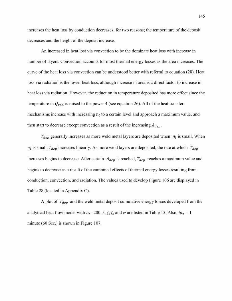
145

increases the heat loss by conduction decreases, for two reasons; the temperature of the deposit

decreases and the height of the deposit increase.

An increased in heat lost via convection to be the dominate heat loss with increase in

number of layers. Convection accounts for most thermal energy losses as the area increases. The

curve of the heat loss via convection can be understood better with referral to equation (28). Heat

loss via radiation is the lower heat loss, although increase in area is a direct factor to increase in

heat loss via radiation. However, the reduction in temperature deposited has more effect since the

temperature in is raised to the power 4 (see equation 26). All of the heat transfer

mechanisms increase with increasing to a certain level and approach a maximum value, and

then start to decrease except convection as a result of the increasing .

generally increases as more weld metal layers are deposited when is small. When

is small, increases linearly. As more weld layers are deposited, the rate at which

increases begins to decrease. After certain is reached, reaches a maximum value and

begins to decrease as a result of the combined effects of thermal energy losses resulting from

conduction, convection, and radiation. The values used to develop Figure 106 are displayed in

Table 28 (located in Appendix C).

A plot of and the weld metal deposit cumulative energy losses developed from the

analytical heat flow model with =200. λ, ξ, ζ, and ψ are listed in Table 15. Also, = 1

minute (60 Sec.) is shown in Figure 107.

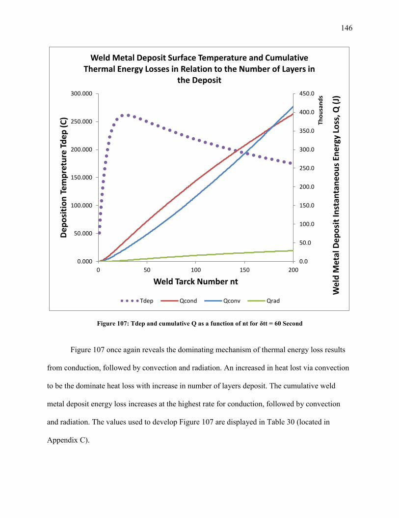
146

Figure 107: Tdep and cumulative Q as a function of nt for δtt = 60 Second

Figure 107 once again reveals the dominating mechanism of thermal energy loss results

from conduction, followed by convection and radiation. An increased in heat lost via convection

to be the dominate heat loss with increase in number of layers deposit. The cumulative weld

metal deposit energy loss increases at the highest rate for conduction, followed by convection

and radiation. The values used to develop Figure 107 are displayed in Table 30 (located in

Appendix C).

0.0

50.0

100.0

150.0

200.0

250.0

300.0

350.0

400.0

450.0

0.000

50.000

100.000

150.000

200.000

250.000

300.000

0 50 100 150 200

We

ld M

etal

De

po

sit

Inst

anta

neo

us

Ene

rgy

Loss

, Q (

J)

Tho

usa

nd

s

De

po

siti

on

Te

mp

retu

re T

de

p (

C)


Weld Metal Deposit Surface Temperature and Cumulative Thermal Energy Losses in Relation to the Number of Layers in

the Deposit


147

The analytical heat flow model shown in Figure 108 demonstrated that lower maximum

values of can be achieved by increasing to 250 second. This is a relatively large value

of ,which is effective at limiting . is limited at the expense of productivity as a

result of the relatively large of 250 second. A plot of the simulation developed from the

analytical heat flow model for = 200 is shown in Figure 108:

Figure 108: Tdep and instantaneous Q as a function of nt for δtt = 250 second.

0.0

500.0

1000.0

1500.0

2000.0

2500.0

3000.0

0.000

10.000

20.000

30.000

40.000

50.000

60.000

70.000

0 20 40 60 80 100 120 140 160 180 200

We

ld M

etal

De

po

sit

Inst

anta

neo

us

Ene

rgy

Loss

, Q (

J)

De

po

siti

on

Te

mp

retu

re T

de

p (

C)



the Deposit


148

Even though the wait time was increased more than 4 times all of the heat transfer

mechanisms behave the same as = 1 minute (60 Sec.). The conditions used to obtain the

solution to the analytical heat flow model for longer inter-layer wait-time in Figure 108 represent

a condition of high heat loss via conduction. Conduction is the dominant heat loss mechanism for

the prescribed conditions, as the number of layer increases the heat loss via conduction decrease.

Convection accounts for most thermal energy losses as the area increases. Heat loss via radiation

is the lower heat loss. All of the heat transfer mechanisms behave the same as = 1 minute (60

Sec.)

is smaller comparing to = 1 minute (60 Sec.). Generally, increases as more weld

metal layers are deposited when is small. When is small, increases. As more weld

layers are deposited, the rate at which begins to decrease linearly. After certain is

reached, reaches a maximum value and begins to decrease as a result of the combined

effects of thermal energy losses resulting from conduction, convection, and radiation. The values

used to develop Figure 108 are displayed in Table 31 (located in Appendix C).



minute (250 Sec.) is shown in Figure 109.

149

Figure 109: Tdep and cumulative Q as a function of nt for δtt = 250 second

Figure 109 reveals that all of the heat transfer mechanisms behave the same as = 1

minute (60 Sec.) with lower . The dominating mechanism of thermal energy loss results

from conduction, followed by convection and radiation. An increased in heat lost via convection

to be the dominate heat loss with increase in number of layers deposit. The cumulative weld

metal deposit energy loss increases at the highest rate for conduction, followed by convection

and radiation. However, the as increases, the energy loss via conduction decreases, and

energy loss via convection increases to be the dominant heat loss.

0.0

50.0

100.0

150.0

200.0

250.0

300.0

350.0

400.0

450.0

500.0

0.000

10.000

20.000

30.000

40.000

50.000

60.000

70.000

0 50 100 150 200

We

ld M

etal

De

po

sit

Inst

anta

neo

us

Ene

rgy

Loss

, Q (

J)

Tho

usa

nd

s

De

po

siti

on

Te

mp

retu

re T

de

p (

C)


Weld Metal Deposit Surface Temperature and Cumulative Thermal Energy Losses in Relation to the Number of Layers in

the Deposit


150

Lower values of reduce grain growth and produce a refined microstructure in the

deposit. Better mechanical properties are achieved as a result of reduced grain growth and

refined microstructures in the weld metal deposit. A standard is to keep below the mild steel

eutectoid temperature in the Fe-C phase diagram (about 727 C). The values used to develop

Figure 109 are displayed in Table 32 (located in Appendix C).

The analytical heat flow model shown in Figure 110 demonstrated that higher maximum

values of can be achieved by decreasing to 10 second. This is a relatively small value of

,which is effective at increasing productivity. Productivity can be boost at the expense of

mechanical properties. A plot of the simulation developed from the analytical heat flow

model for = 200 is shown in Figure 110.

151

Figure 110: Tdep and instantaneous Q as a function of nt for δtt = 10 second.

The wait time was decrease more than 6 times from the calibrated model. The heat

transfer mechanisms did not behave the same as = 1 minute (60 Sec.). The conditions used to

obtain the solution to the analytical heat flow model for shorter inter-layer wait-time in Figure

110 represent a condition of high heat loss via Radiation. The increase in temperature deposited

has direct effect in since the temperature in is raised to the power 4 (see equation 26).

Conduction also, increases to a peak level then as the number of layer increases the heat loss via

conduction decrease. Thermal energy loss via convection increase linearly as the area increases.

0.0

500.0

1000.0

1500.0

2000.0

2500.0

0.000

100.000

200.000

300.000

400.000

500.000

600.000

700.000

800.000

900.000

0 20 40 60 80 100 120 140 160 180 200

We

ld M

etal

De

po

sit

Inst

anta

neo

us

Ene

rgy

Loss

, Q (

J)

De

po

siti

on

Te

mp

retu

re T

de

p (

C)



the Deposit


152

is greater comparing to = 1 minute (60 Sec.). Generally, increases as more weld

metal layers are deposited when is small. When is small, increases. As more weld

layers are deposited, the rate at which begins to decrease linearly. After certain is

reached, reaches a maximum value and begins to decrease as a result of the combined

effects of thermal energy losses resulting from conduction, convection, and radiation. The values

used to develop Figure 110 are displayed in Table 33 (located in Appendix C).



Second. is shown in Figure 111.

153

Figure 111: Tdep and cumulative Q as a function of nt for δtt = 10 second

Figure 111 shows that the heat transfer mechanisms behave differently comparing to the

= 1 minute (60 Sec.) with greater . The dominating mechanism of thermal energy loss

results from Radiation, followed by conduction and convection. An increased in heat lost via

convection with increase in number of layers deposit. The cumulative weld metal deposit energy

loss increases at the highest rate for radiation, followed by conduction and convection. However,

the as increases, the energy loss via conduction decreases, and energy loss via convection

0.0

50.0

100.0

150.0

200.0

250.0

300.0

350.0

400.0

0.000

100.000

200.000

300.000

400.000

500.000

600.000

700.000

800.000

900.000

0 50 100 150 200

We

ld M

etal

De

po

sit

Inst

anta

neo

us

Ene

rgy

Loss

, Q (

J)

Tho

usa

nd

s

De

po

siti

on

Te

mp

retu

re T

de

p (

C)


Weld Metal Deposit Surface Temperature and Cumulative Thermal Energy Losses in Relation to the Number of Layers

in the Deposit


154

increases to be the dominant heat loss. The values used to develop Figure 111 are displayed in

Table 34 (located in Appendix C).

Higher values of increase grain growth and produce a columnar grains which are

long, thin, coarse grains microstructure in the deposit. Poorer mechanical properties are achieved

as a result of increase in grain growth and coarse microstructures in the weld metal deposit.

reaches the mild steel eutectoid temperature in the Fe-C phase diagram (about 727 C) which will

lead to eutectoid transformation to produce ferrite and cementite.

The possibility of improving thermal energy flow from the weld metal deposit is

demonstrated by the analytical heat flow model. Improving heat flow from the deposit controls

the weld metal microstructure while simultaneously maintaining high productivity. An important

step in the advancement of AM techniques is thermal management of the weld metal deposit.

Thermal management of the weld metal deposit controls the deposit temperature and, therefore,

microstructure development and the resulting mechanical properties (Ref.57).

155

7. Conclusion

Additive manufacturing techniques offer cost reduction and flexibility in both

manufacturing and product design over conventional manufacturing methods. The results of this

work leads to the following conclusions:

It is possible to build a linear wall deposit with good geometric detail shot-by-shot

and layer-by-layer using pulsed current PAW.

The consistent delivery of the shot into the molten pool created by the arc is requires

careful alignment and orientation between the shot delivery tube, the top surface of

the deposit and the welding arc.

The start and stop transients of a deposit as well as missed shots produce variations in

the desired geometric shape.

The method demonstrated here has low productivity, achieving a deposition rate of

approximately 50 g/hour.

Three walls were built using the same processing conditions except for the deposit

preheat temperature prior to adding each new layer. The deposit preheat temperature

was controlled by allowing the deposit to cool after each layer for an amount of time

called the inter-layer wait time. The results indicated that, for all specimens, deposit

grain size increased and hardness decreased as wall height increased.

The average grain size decreased and hardness increased as interlayer wait time

increased.

Voids in the form of pores where found in the deposits. The pores, once formed,

could persist through multiple layers. Care needs to be taken to ensure adequate

shielding coverage during processing. Also, the shot feedstock must be clean and not

156

contain significant amounts of dissolved gases.

An analytical heat flow model was developed to study the influence of interlayer wait

time on deposit temperature and therefore grain size and hardness. The results of the

model indicated that as wall height increased, the rate of deposit heat removal by

conduction to the substrate decreased leading to a higher preheat temperature after a

fixed interlayer wait time causing grain size to increase as wall height increased.

The model results also show that as wall height increased, the deposit surface area

from which heat energy is lost via convection and radiation increased. The model

also demonstrated that the use of a means of forced convection to rapidly remove heat

from the deposit could be an effective way to boost productivity and maintain smaller

grain size and therefore higher hardness and strength in the deposit.

The use of the PAW process and shot as feedstock is a possible approach to

additively manufacture steel components.

157

8. Suggestion for Future Work

Research work has shown that PAW has the potential to be a cost-effective method for

the additive manufacturing of low-carbon steel alloys components. Metallographic results of the

linear wall specimens revealed that further research is needed to control the linear wall deposit

surface temperature with deposit thermal management. Improving heat flow from the deposit

allows for control of the deposit microstructure and, therefore, the resulting acceptable

mechanical properties, while simultaneously attaining high levels of productivity during

manufacturing.

The surface temperature of the weld metal deposit needs to be developed to obtain more

consistent and reliable temperature data. The analytical heat flow model can be further tuned to

simulate linear wall deposit temperatures that agree well with the experimentally measured

deposit temperatures. Once more, reliable and consistent temperature data is obtained.

A procedure needs to be developed for the analytical heat flow model, to manage the

weld metal deposit thermal energy flow to simultaneously improve productivity and obtain

acceptable deposit microstructure and mechanical properties. The inter-track wait-time can be

decreased and adjusted in the analytical heat flow model to improve the manufacturing

productivity of the low-carbon steel alloys weld metal deposits.

An effective method of physically adjusting the scale factor to modify the conduction,

convection and radiation heat transfer coefficient needs to be developed. By increasing the rate at

which thermal energy is removed from the linear wall deposit via conduction and convection, the

maximum surface temperature of the deposit can be reduced.

Increasing the rate thermal energy is removed from the deposit by thermal conduction

could be an effective means of maintaining lower deposit temperature, while simultaneously

158

achieving higher productivity. The use of active substrate cooling via a chilled heat sink should

be investigated.

The use of a three torch configuration could be used to eliminate the loss of the end of the

layers when the torch tends to push the shot filler metal away from the substrate. Also, the

ceramic tube can be 90 , which will make the shots land straight right into the pool more constant

and reliable. Figure 112 shows the suggested three torch orientation.

Figure 112: Suggested three torch orientation

This torch configuration will also, help the arc to concentrate in a single point and if the

torch had to make turns the configuration will eliminate losses of material.

It is possible to make components with different properties within a component, using

multiple shot feeders with multiple materials can produce a component with multiple features.

These features can extend the lives of components by applying wear and/or corrosion resistant

coatings. Unlike conventional plating or coating, this is not limited to being a few microns thick,

but can be from microns to mm thick, depending on the requirements.

159

The variations in shot feed rate that resulted from the missing shots led to inconsistent

linear wall deposit surface profile and inconsistent overall deposit geometry. To develop reliable

PAW essential process parameters, an accurate feed stock welding method must be developed.

Closed-loop control of shots feed delivery is mandatory for consistent weld metal deposit build-

up.

160

Works Cited

1. Obama, President. Obama's speech highlights rise of 3-D printing. [Online] February

13, 2013. [Cited: March 29, 2014.] http://www.cnn.com/2013/02/13/tech/innovation/obama-3d-

printing/.

2. Journal of Material Processing Technology. June 2012, Vol. 212, pp. 1377-1389.

3. Charles, Corinne. Modelling Microstructure Evolution of Weld Deposited Ti-6Al-4V.

Luleå, Sweden : Luleå University of Technology, 2008.

4. Killander, Lena Apelskog and G. Sohlenius. Future Direct Manufacturing Of Metal

Parts With Free-Form Fabrication. Centro, Rio de Janeiro : Elsevier Science, 1995. pp. 451-

454.

5. Kruth, J. P., M. C. Leu, and T. Nakagawa. Progress In Additive Manufacturing And

Rapid Prototyping. s.l. : Elsevier, 1998. pp. 525-540.

6. Research And Development In Rapids Prototyping And Tooling In The United States.

leu, M.C Zhang, W. Beijing : Rapid Prototyping and Manufacturing, 1998.

7. Material Incress Manufacturing By Rapid Prototyping Techniques. Kruth, J. Leuven,

Belgium : Katholieke Universiteit Leuven/Belgium, 1991. CIRP Annals. pp. 603-614.

8. C.O. Brown, E.M. Breinan and B.H. Kear. Method for Fabricating Articles by

Sequential Layer Deposition. U.S. Patent 4,323,756 United States of America, 1982.

9. Edmonds, M.D. McAninch and D.P. Method and Apparatus for Building a

Workpiece by Deposit Welding. U.S. Patent 4,775,092 United States Of America, 1988.

10. Seagle, Stan R. The Fundamentals of Titanium." Fundamentals of Titanium. Las

Vegas, Nevada : International Titanium Association, 2008.

161

11. Wire Based Additive Layer Manufacturing: Comparison of Microstructure and

Mechanical Properties of Ti–6Al–4V Components Fabricated by Laser-Beam Deposition and

Shaped Metal Deposition. Baufeld, Bernd, Erhard Brandl, and Omer van der Biest. 2011,

Journal of Materials Processing Technology, pp. 1146-1158.

12. Plasma Arc Welding of Titanium Alloys - New Developments. Hughes, R. V. 1989,

Joining & Materials, pp. 333-335.

13. World Crude Steel Output Increases By 3.5% In 2013. Worldsteel Association.

[Online] January 23, 2014. [Cited: Fabruary 15, 2014.] https://www.worldsteel.org/media-

centre/press-releases/2014/World-crude-steel-output-increases-by-3-5--in-2013.html.

14. O'Brine, R. L. Welding Handbook. 8. Miami : American Welding Society, 1991.

Vol. 2.

15. Mechanical Properties of Ti-6Al-4V Specimens Produced by Shaped Metal

Deposition. Baufeld, Bernd and Omer van der Biest. s.l. : Science and Technology of

Advanced Materials, 2009, Science and Technology of Advanced Materials.

16. Oates, William R. and Saitta, Alexander M. Welding Handbook. eighth edition.

Miami : American Welding Society, 1998. Vol. VOLUME 4.

17. Kruth, J. P., M. C. Leu, and T. Nakagawa. Progress In Additive Manufacturing

And Rapid Prototyping. s.l. : CIRP Annals - Manufacturing Technology, 1998. pp. 525-540. Vol.

47.

18. Low Cost Integration Of Additive And Subtractive Processes For Hybrid Layered

Manufacturing. Karunakaran, K. P., S. Suryakumar, Vishal Pushpa, and Sreenathbabu

Akula. 2010, Robotics and Computer-Integrated Manufacturing, pp. 490-499.

162

19. Additive Manufacturing of Ti–6Al–4V Components by Shaped Metal Deposition:

Microstructure and Mechanical Properties. Baufeld, Bernd, Omer Van der Biest, and

Rosemary Gault. 2010, Materials & Design , pp. S106-S111.

20. Electron Beam Freeform Fabrication: A Metal Deposition Apparatus to Build

Components Directly from CAD. Taminger, Karen. Arlington, Texas : NASA Langley

Research Center, 2008. WBT Showcase.

21. Shaped Metal Deposition of a Nickel Alloy for Aero Engine Applications. Clark, D.,

M. R. Bache, and M. T. Whittaker. 2008, Journal of Materials Processing Technology 203, pp.

439-448.

22. Weld Bead Modeling and Process Optimization in Hybrid Layered Manufacturing."

Computer-Aided Design. Suryakumar, S., K. P. Karunakaran, Alain Bernard, U.

Chandrasekhar, N. Raghavender, and Deepak Sharma. 2011., pp. 331-344.

23. Smith, William F. and Hashemi, , Javad . Foundations Of Materials Science And

Engineering . Fourth. s.l. : McGraw-Hill, 2003.

24. Ochshorn, Jonathan. Steel in 20th Century Architecture. Oxon , UK : Taylor and

Francis Publishers, 2002.

25. Materials Science. 2007, Encyclopædia Britannica.

26. Ashby, Michael F. and Jones, David R. H. Engineering Materials 2. Oxford :

Oxford University, 1992.

27. Smelting. Britannica Academic Edition. [Online] 2007. [Cited: November 16, 2013.]

http://www.britannica.com/EBchecked/topic/549533/smelting.

28. Alloying of Steels. 2006-06-28, Metallurgical Consultants.

29. Elert, Glenn. Density of Steel. Madison : University of Wisconsin, 20 January 1998.

163

30. Quench Hardening of Steel. Total Materia. [Online] November 2000. [Cited:

December 10, 2013.]

http://www.keytometals.com/page.aspx?ID=CheckArticle&site=kts&LN=EN&NM=12.

31. Steel Construction Manual. 8th Edition, second revised edition. Bloomfield Hills,

MI : American Institute of Steel Construction, 1986. pp. ch. 1 pages 1–5.

32. AZo Journal of Materials Online. [Online] [Cited: February 12, 2014.]

http://www.azom.com/article.aspx?ArticleID=6117.

33. Callister, William D. Materials Science and Engineering. Hoboken, NJ : John Wiley

& Sons, Inc., 1994.

34. Steel in 20th Century Architecture. Ochshorn, Jonathan. 2002-06-11, Encyclopedia

of Twentieth Century Architecture.

35. MSE 300 Materials Laboratory Procedures. Knoxville : University of Tennessee,

Dept. of Materials Science and Engineering.

36. Ferrite. Encyclopaedia Britannica. Encyclopaedia Britannica Online Academic

Edition. [Online] [Cited: January 30, 2014.]

http://www.britannica.com/EBchecked/topic/205072/ferrite.

37. Pearlite, Martensite, Austenite dan Bainite. Alnahyan. [Online] [Cited: August 27,

2013.] http://nayhan.wordpress.com/pearlite-martensite-austenite-dan-bainite/.

38. Shielding Gases Selection Manual. Praxair. [Online] 1998. [Cited: December 3,

2013.] http://www.praxair.com/.

39. Connor, Leonard P. Welding Handbook. Miami : American Welding Society, 1989.

40. Jenney, Cynthia L. and Annette O'Brien. Welding Handbook. Ninth ed. Miami,

Florida : American Welding Society, 2001. Vol. 1.

164

41. Ness, Jerry. Personal Communication. [interv.] Joe N. Stavinoha. Butte, Montana :

General Distributing Co., March 23, 2012.

42. Grace, Pat. Personal Communication. [interv.] Joe N. Stavinoha. Farmington,

Connecticut : TRUMPF Inc, March 23, 2012.

43. Butrymowicz, Dale. Personal Communication. [interv.] Joe N. Stavinoha. Enfield,

Connecticut : PTR-Precision Technologies, Inc., March 23, 2012.

44. Stavinoha, Joe N. Investigation Of Plasma Arc Welding As A Method For The

Additive Manufacturing Of Ti-6Al-4V Alloy Components. Butte : Montana Tech, 2012.

45. ULTIMA-150 Plasma Welding Operating Manual. West Lebanon : s.n., 2002,

Thermal Dynamics Corporation.

46. Davis, Joseph R., Kelly Ferjutz, Nikki D. Wheaton, and Mara S. Woods, eds.

Welding, Brazing, and Soldering. ASM Handbook. Tenth. Materials Park, Ohio : ASM

International, 1993. Vol. 6.

47. PWH/M-3A Weldiing Tourch Instruction Manual . West Lebanon, New Hampshire :

Thermal Dynamics Corporation , 2007.

48. Products for USB Sensing and Control. Phidgets. [Online] 2012. [Cited: December 2,

2013.] http://www.phidgets.com/products.php?product_id=1012.

49. Procimity Sensor. Eaton. [Online] [Cited: December 3, 2013.]

http://www.eaton.com/EN/Eaton/ProductsServices/Electrical/ProductsandServices/Automationa

ndControl/SensorsLimitSwitches/InductiveProximitySensors/index.htm.

50. Replicator2. Makerbot. [Online] [Cited: December 5, 2013.]

http://store.makerbot.com/replicator2.

165

51. EXTECH. 42529: Wide Range IR Thermometer. [Online]

http://www.extech.com/instruments/product.asp?catid=62&prodid=382.

52. Hatherly, F. J. Humphreys and M. Recrystallization And Related Annealing

Phenomena. Second. Oxford, UK : Elsevier Ltd., 1995.

53. 3D Welding And Milling: Part I–A Direct Approach For Freeform Fabrication Of

Metallic Prototypes. Songa, Yong-Ak. Seoul, South Korea : Korea Institute of Science and

Technology KIST, 2005.

54. Blodgett, Omer W. Design of welding . Cleveland, Ohio : The James F. Lincon Arc

Welding Foundation, 1963.

55. Tensile Strength to Hardness Conversion Chart. Mwsco. [Online] [Cited: February

23, 2014.] http://www.mwsco.com/kb/articles/19990630e.htm.

56. FINDLEY, KIP O. Colorado School of Mines. [Online] April 3ed , 2014. [Cited:

April 5th, 2014.] http://inside.mines.edu/HallPetchEquation.

57. Measurement And Simulation Of Titanium Alloy Deposit Temperature In Electron

Beam Additive Manufacturing. Madigan, R. Bruce, Sean F. Riley, Mark J. Cola, Vivek R.

Dave, and John E. Talkington. Chicago, Illinois : ASM International,, 2012. Ninth

International Trends in Welding Research Conference.

58. Incropera, Frank P., David P. DeWitt, Theodore L. Bergman, and Adrienne S.

Lavine. Introduction to Heat Transfer. Fifth ed. Hoboken. New Jersey : John Wiley & Sons,

Inc., 2007.

59. Donachie, Matthew J. Titanium Technical Guide. Second. Materials Park, Ohio :

ASM International, 2000.

166

60. Messler, Robert W. Principles Of Welding: Processes, Physics, Chemistry, And

Metallurgy. s.l. : Weinheim, Baden-Württemberg, Germany: Wiley-VCH., 2004.

61. Association, Staff of Research and Education. The Handbook of Mechanical

Engineering. Piscataway, New Jersey : Research and Education Association., 2004.

62. Gleason, Bill. Personal Communication. Butte, Montana: : Montana Tech of The

University of Montana, June 22, 2012.

63. A36 steel bar. MatWeb . [Online] 2012. http://www.matweb.com.

64. Filament. Makerbot. [Online] [Cited: January 12, 2014.]

http://store.makerbot.com/filament.

65. MatWeb A36 Steel Bar. MatWeb. [Online] Retrieved 21 . [Cited: August 28, 2013.]

http://www.matweb.com/errorUser.aspx?msgid=2&ckck=nocheck.

66. Steel Construction Manual. 8th Edition, second revised edition. Bloomfield Hills,

MI : American Institute of Steel Construction, 1986. pp. 1–5.

67. Weld ClearVision. Weld Quality Control Solution. [Online] [Cited: December 2,

2013.] http://www.weldqc.com/wvs/WVSOver.aspx.

68. Low Carbon Steel. Manchester University. [Online] [Cited: January 13, 2014.]

http://pwatlas.mt.umist.ac.uk/internetmicroscope/micrographs/microstructures/low-carbon-

steel.html.

69. Smith, William F. Foundations Of Materials Science And Engineering. s.l. : Mc

Graw Hill, 1931.

167

Appendix A: Raw Data

Table 16: Specimen #1, Height of Layers Row Data

Specimen #1, Baseline

Height (mm)

Arc Length (mm)

Height in Z access

(mm)

Substrate 0.00 32.00 4.00 36.00

Layer 1.00 32.90 1.00 37.00

Layer 2.00 33.75 1.00 38.00

Layer 3.00 34.40 0.00 38.00

Layer 4.00 34.60 0.00 38.00

Layer 5.00 34.80 1.00 39.00

Layer 6.00 35.00 0.00 39.00

Layer 7.00 36.00 1.00 40.00

Layer 8.00 36.80 0.00 40.00

Layer 9.00 37.40 0.00 40.00

Layer 10.00 38.00 0.50 40.50

Layer 11.00 39.00 1.00 41.50

Layer 12.00 40.00 0.50 42.00

Layer 13.00 41.00 0.50 42.50

Layer 14.00 42.00 0.00 42.50

Layer 15.00 42.50 0.50 43.00

Layer 16.00 43.00 0.50 43.50

Layer 17.00 43.40 0.00 43.50

Layer 18.00 43.80 1.00 44.50

Layer 19.00 44.00 0.00 44.50

Layer 20.00 45.50 1.00 45.50

Layer 21.00 46.40 1.00 46.50

Layer 22.00 47.25 1.00 47.50

Layer 23.00 48.20 1.00 48.50

Layer 24.00 49.20 1.00 49.50

Layer 25.00 49.70 0.50 50.00

Layer 26.00 50.10 0.50 50.50

Layer 27.00 51.30 1.00 51.50

Layer 28.00 51.68 1.00 52.50

Layer 29.00 52.40 1.00 53.50

Layer 30.00 52.80 1.00 54.50

Layer 31.00 53.40 1.00 55.50

168


Specimen #2, 1-minute wait time

Height (mm)

Arc Length (mm)

Height in Z access

(mm)

Substrate 0.00 32.00 4.00 36.00

Layer 1.00 33.40 1.00 37.00

Layer 2.00 35.00 1.00 38.00

Layer 3.00 35.40 1.00 39.00

Layer 4.00 35.75 1.00 40.00

Layer 5.00 35.90 0.00 40.00

Layer 6.00 36.10 0.00 40.00

Layer 7.00 36.30 0.00 40.00

Layer 8.00 37.80 0.50 40.50

Layer 9.00 38.25 0.50 41.00

Layer 10.00 38.80 0.50 41.50

Layer 11.00 39.00 0.50 42.00

Layer 12.00 39.70 0.50 42.50

Layer 13.00 40.50 0.50 43.00

Layer 14.00 40.90 0.50 43.50

Layer 15.00 41.70 1.00 44.50

Layer 16.00 41.90 1.00 45.50

Layer 17.00 42.27 1.00 46.50

Layer 18.00 43.50 1.00 47.50

Layer 19.00 43.75 1.00 48.50

Layer 20.00 44.00 1.00 49.50

Layer 21.00 44.88 1.00 50.50

Layer 22.00 45.68 0.00 50.50

Layer 23.00 46.71 1.00 51.50

Layer 24.00 47.20 1.00 52.50

Layer 25.00 47.90 1.00 53.50

Layer 26.00 48.40 1.00 54.50

169


Specimen #3, 10-minutes wait time

#

Height

(mm)

Arc

Length

(mm)

Height in Z

access (mm)

Substrate 0 32.0 4.0 36.0

Layer 1 33.0 1.0 37.0

Layer 2 34.0 1.0 38.0

Layer 3 35.0 0.5 38.5

Layer 4 35.5 0.5 39.0

Layer 5 36.5 1.0 40.0

Layer 6 37.2 0.5 40.5

Layer 7 37.6 0.5 41.0

Layer 8 38.1 0.5 41.5

Layer 9 38.8 0.5 42.0

Layer 10 39.5 1.0 43.0

Layer 11 40.4 0.5 43.5

Layer 12 40.7 1.0 44.5

Layer 13 41.2 0.5 45.0

Layer 14 42.1 0.5 45.5

Layer 15 42.2 1.0 46.5

Layer 16 42.8 0.5 47.0

Layer 17 43.4 0.5 47.5

Layer 18 43.9 0.5 48.0

Layer 19 44.5 0.5 48.5

Layer 20 45.2 1.0 49.5

Layer 21 45.8 0.8 50.3

Layer 22 46.4 1.0 51.3

Layer 23 47.7 0.5 51.8

Layer 24 48.1 1.0 52.8

Layer 25 48.6 0.0 52.8

Layer 26 49.9 1.0 53.8

Layer 27 50.3 1.0 54.8

Layer 28 51.3 0.0 54.8

Layer 29 51.6 1.0 55.8

Layer 30 52.2 0.5 56.3

Layer 31 52.7 0.5 56.8

Layer 32 53.5 0.5 57.3

Layer 33 54.0 0.0 57.3

Layer 34 54.6 1.0 58.3

Layer 35 55.2 0.5 58.8

Layer 36 55.8 1.0 59.8

170

Specimen #3, 10-minutes wait time

#

Height

(mm)

Arc

Length

(mm)

Height in Z

access (mm)

Layer 37 56.6 0.5 60.3

Layer 38 57.3 1.0 61.3

Table 19: Hardness Test Raw Data for all Three Specimens

Harness test

BL 1 MIN 10 MIN

HRB

1 75.43 93.33 75.68

2 74.93 91.59 74.73

3 75.68 85.28 82.39

4 73.09 76.82 83.83

5 75.18 74.78 88.46

6 68.72 66.23 86.57

7 66.73 70.41 82.54

8 64.89 72.50 70.26

9 64.14 72.30 78.81

10 62.95 74.48 71.05

11 62.56 76.82 72.69

12 65.38 77.07 77.47

13 60.91 72.15 67.27

14 61.55 62.00 91.00

15 63.49 55.83 68.67

16 66.03 74.78 90.45

17 68.07 75.00 52.30

18 64.69 60.61

19 66.58 78.66

20 67.87 77.97

21 69.21 68.76

22 69.76 79.76

23 61.70 75.13

24 53.79 76.37

25 74.93 75.33

26 79.91

27 75.13

171

Table 20: Data of Tensile Strength for all Three Specimens

Tensile Strength

BL 1 MIN 10 MIN

KPa

1 68 97 68

2 66 94 66

3 68 82 76

4 65 70 80

5 67 67 87

6 60 58 83

7 58 62 77

8 56 65 62

9 56 64 71

10 55 66 63

11 55 70 65

12 56 70 70

13 52 64 59

14 53 54 93

15 55 49 60

16 58 66 91

17 60 67 49

18 56 53

19 58 72

20 59 71

21 61 61

22 61 74

23 53 67

24 49 68

25 66 67

26 72

27 67

172

Table 21: Specimen #1, Gran Size and Grain Size Number Row Data

Specimen #1,Baseline

Height (mm)

Grain size (µm)

1 12.500

2 19.000

3 13.000

4 18.500

5 62.500

6 50.000

7 70.000

8 55.000

9 50.000

10 63.000

11 59.000

12 65.000

13 120.000

14 95.000

15 85.000

16 110.000

17 30.000

18 40.000

19 100.000

20 90.000

21 310.000

22 250.000

23 200.000

24 190.000

173

Table 22: Specimen #2, Grain Size and Grain Size Number Row Data

Specimen #2, 1 min Height (mm) Grain size (µm)

1 25.0000

2 25.0000

3 31.2500

4 40.0000

5 50.0000

6 55.0000

7 55.0000

8 50.0000

9 60.0000

10 59.0000

11 70.0000

12 65.0000

13 72.0000

14 68.0000

15 69.0000

16 66.0000

17 150.0000

18 90.0000

19 125.0000

20 140.0000

21 250.0000

22 400.0000

23 420.0000

24 300.0000

174

Table 23: Specimen #3, Gran Size and Grain Size Number Row Data

Specimen #3, 10 min

Height (mm)

Grain size (µm)

1 18.750

2 12.500

3 18.000

4 25.000

5 29.000

6 32.000

7 37.000

8 50.000

9 62.500

10 65.000

11 55.000

12 72.000

13 65.000

14 70.000

15 68.000

16 72.000

17 125.000

18 110.000

19 156.000

20 170.000

21 220.000

22 343.750

23 350.000

24 320.000

175

Table 24: Tensile Strength to Hardness Conversion Chart

TENSILE STRENGTH TO HARDNESS CONVERSION CHART

Brinell

Vickers or Firth

Hardness No.

Rockwell

Sclero-scope No.

Approximate Tensile

Strength 1000 psi

Dia. (mm): 3000-kg

Load 10-mm Ball

Hardness No.

C 150-kgLoad

120° DiamondCone

B 100-kg Load

1/16" dia. Ball

2.05 898 440

2.10 857 420

2.15 817 401

2.20 780 1150 70 106 384

2.25 745 1050 68 100 368

2.30 712 960 66 95 352

2.35 682 885 64 91 337

2.40 653 820 62 87 324

2.45 627 765 60 84 311

2.50 601 717 58 81 298

2.55 578 675 57 78 287

2.60 555 633 55 120 75 276

2.65 534 598 53 119 72 266

2.70 514 567 52 119 70 256

2.75 495 540 50 117 67 247

2.80 477 515 49 117 65 238

2.85 461 494 47 116 63 229

2.90 444 472 46 115 61 220

2.95 429 454 45 115 59 212

3.00 415 437 44 114 57 204

3.05 401 420 42 113 55 196

3.10 388 404 41 112 54 189

3.15 375 389 40 112 52 182

3.20 363 375 38 110 51 176

3.25 352 363 37 110 49 170

3.3 341 350 36 109 48 165

3.35 331 339 35 109 46 160

3.40 321 327 34 108 45 155

3.45 311 316 33 108 44 150

3.50 302 305 32 107 43 146

3.55 293 296 31 106 42 142

176


Brinell

Vickers or Firth

Hardness No.

Rockwell

Sclero-scope No.

Approximate Tensile

Strength 1000 psi

Dia. (mm): 3000-kg

Load 10-mm Ball

Hardness No.

C 150-kgLoad

120° DiamondCone

B 100-kg Load

1/16" dia. Ball

3.60 285 287 30 105 40 138

3.65 277 279 29 104 39 134

3.70 269 270 28 104 38 131

3.75 262 263 26 103 37 128

3.80 255 256 25 102 37 125

3.85 248 248 24 102 36 122

3.90 241 241 23 100 35 119

3.95 235 235 22 99 34 116

4.00 229 229 21 98 33 113

4.05 223 223 20 97 32 110

4.10 217 217 18 96 31 107

4.15 212 212 17 96 31 104

4.20 207 207 16 95 30 101

4.25 202 202 15 94 30 99

4.30 197 197 13 93 29 97

4.35 192 192 12 92 28 95

4.40 187 187 10 91 28 93

4.45 183 183 9 90 27 91

4.50 179 179 8 89 27 89

4.55 174 174 7 88 26 87

4.60 170 170 6 87 26 85

4.65 166 166 4 86 25 83

4.70 163 163 3 85 25 82

4.75 159 159 2 84 24 80

4.80 156 156 1 83 24 78

4.85 153 153 82 23 76

4.90 149 149 81 23 75

4.95 146 146 80 22 74

5.00 143 143 79 22 72

5.05 140 140 78 21 71

5.10 137 137 77 21 70

5.15 134 134 76 21 68

177


Brinell

Vickers or Firth

Hardness No.

Rockwell

Sclero-scope No.

Approximate Tensile

Strength 1000 psi

Dia. (mm): 3000-kg

Load 10-mm Ball

Hardness No.

C 150-kgLoad

120° DiamondCone

B 100-kg Load

1/16" dia. Ball

5.20 131 131 74 20 66

5.25 128 128 73 65

5.30 126 126 72 64

5.35 124 124 71 63

5.40 121 121 70 62

5.45 118 118 69 61

5.50 116 116 68 60

5.55 114 114 67 59

5.60 112 112 66 58

5.65 109 109 65 56

5.70 107 107 64 56

5.75 105 105 62 54

5.80 103 103 61 53

5.85 101 101 60 52

5.90 99 99 59 51

5.95 97 97 57 50

6.00 95 95 56 49

178

Table 25: Table 26: The experimental deposit temperature measurements Specimen #2

Specimen #2, 1 min

# layer start middle end avg

0 22

1 130 150 220 167

2 170 176 260 202

3 168 180 300 216

4 175 195 300 223

5 175 179 325 226

6 175 180 338 231

7 175 180 335 230

8 178 185 335 233

9 180 180 330 230

10 180 190 335 235

11 195 190 335 240

12 185 210 335 243

13 189 210 332 244

14 190 210 335 245

15 192 212 338 247

16 193 212 338 248

17 194 213 339 249

18 198 216 340 251

19 198 216 340 251

20 198 216 340 251

21 198 216 340 251

22 198 216 340 251

23 198 216 340 251

24 199 220 340 253

25 199 220 340 253

26 199 220 340 253

179

Table 27: The experimental deposit temperature measurements Specimen #3

Specimen #3, 10 min

# layer start middle end avg

0 22

1 50 51 55 52

2 51 51 55 52

3 55 55 60 57

4 58 58 60 59

5 60 61 65 62

6 60 65 70 65

7 68 70 70 69

8 65 69 71 68

9 68 69 72 70

10 68 69 72 70

11 68 69 72 70

12 68 68 73 70

13 69 69 70 69

14 69 69 70 69

15 68 70 75 71

16 69 70 75 71

17 69 70 75 71

18 68 69 70 69

19 69 71 75 72

20 68 69 70 69

21 69 71 75 72

22 69 70 70 70

23 69 70 75 71

24 70 71 75 72

25 70 72 75 72

26 69 71 73 71

27 69 70 74 71

28 68 72 75 72

29 69 72 76 72

30 69 72 75 72

180

Appendix B: Material Safety Data Sheet

185

Appendix C: Solution to the Analytical Heat Flow Model

Table 28: Properties Used to Solve the Analytical Heat Flow Model

Model Property Value1

mo (g) 2607.400000

Δmt (g) 3.280500

Ao (m2) 0.011966

ΔAt (m2) 1.280000E-04

cp [J/(g∙°C)] 0.050000

ε 0.500000

σ [W/(m2∙K

4)] 5.670000E-08

Qweld (J) 11880.0

δtt (s) 60

hcond [W/(m2∙K)] 50

hconv [W/(m2∙K)] 13

λ 0.60

ξ 0.50

ζ 0.50

ψ 1.00

Tsur (°C) 22.00

186

Table 29: Tdep and Instantaneous Q as a Function of nt

with λ = 0.6, ξ = 0. , ζ = 0.5, ψ =1.0, and δtt = 60 second

Instantaneous layer

# Qweld Mdep Tdepi Qcond Qconv Qrad Qloss Qdepi Tdep Tde-pexp

1 4276.8 2611 54.764 294.0 154.5 0.180215 448.8 3828.0 51.363 22

2 4276.8 2614 113.375 820.0 435.5 3.430031 1259.0 3017.8 80.689 167

3 4276.8 2617 136.431 1027.0 551.2 7.273369 1585.4 2691.4 103.779 202

4 4276.8 2621 156.960 1211.2 656.8 12.87783 1880.9 2395.9 124.345 216

5 4276.8 2624 175.209 1375.0 753.2 20.20202 2148.4 2128.4 142.631 223

6 4276.8 2627 191.394 1520.2 841.3 29.06088 2390.5 1886.3 158.855 226

7 4276.8 2630 205.716 1648.8 921.6 39.17678 2609.5 1667.3 173.215 231

8 4276.8 2634 218.355 1762.2 994.8 50.22523 2807.2 1469.6 185.893 230

9 4276.8 2637 229.477 1862.0 1061.5 61.87171 2985.3 1291.5 197.053 233

10 4276.8 2640 239.234 1949.6 1122.2 73.79848 3145.6 1131.2 206.848 230

11 4276.8 2643 247.764 2026.1 1177.6 85.72215 3289.4 987.4 215.418 235

12 4276.8 2647 255.196 2092.8 1228.0 97.40328 3418.2 858.6 222.888 240

13 4276.8 2650 261.645 2150.7 1273.9 108.65 3533.2 743.6 229.376 243

14 4276.8 2653 267.218 2200.7 1315.7 119.3174 3635.8 641.0 234.988 244

15 4276.8 2657 272.011 2243.7 1353.9 129.3035 3727.0 549.8 239.820 245

16 4276.8 2660 276.112 2280.5 1388.8 138.5441 3807.9 468.9 243.959 247

17 4276.8 2663 279.598 2311.8 1420.8 147.0069 3879.6 397.2 247.485 248

18 4276.8 2666 282.543 2338.2 1450.0 154.6852 3942.9 333.9 250.468 249

19 4276.8 2670 285.008 2360.4 1476.8 161.5922 3998.8 278.0 252.972 251

20 4276.8 2673 287.052 2378.7 1501.6 167.7557 4048.0 228.8 255.055 251

21 4276.8 2676 288.725 2393.7 1524.3 173.214 4091.3 185.5 256.766 251

22 4276.8 2680 290.073 2405.8 1545.4 178.0122 4129.3 147.5 258.153 251

23 4276.8 2683 291.135 2415.4 1565.0 182.199 4162.5 114.3 259.254 251

24 4276.8 2686 291.948 2422.7 1583.2 185.8247 4191.7 85.1 260.106 251

25 4276.8 2689 292.543 2428.0 1600.2 188.9396 4217.1 59.7 260.740 253

26 4276.8 2693 292.949 2431.6 1616.1 191.5922 4239.3 37.5 261.183 253

27 4276.8 2696 293.188 2433.8 1631.1 193.8291 4258.7 18.1 261.462 253

28 4276.8 2699 293.284 2434.6 1645.2 195.6937 4275.5 1.3 261.596

29 4276.8 2703 293.255 2434.4 1658.6 197.2266 4290.2 -13.4 261.605

30 4276.8 2706 293.118 2433.2 1671.3 198.4649 4302.9 -26.1 261.506

31 4276.8 2709 292.887 2431.1 1683.4 199.4423 4313.9 -37.1 261.313

32 4276.8 2712 292.575 2428.3 1694.9 200.1895 4323.4 -46.6 261.040

33 4276.8 2716 292.194 2424.9 1706.0 200.734 4331.6 -54.8 260.696

34 4276.8 2719 291.752 2420.9 1716.7 201.1005 4338.7 -61.9 260.292

35 4276.8 2722 291.259 2416.5 1727.0 201.311 4344.8 -68.0 259.837

36 4276.8 2725 290.722 2411.6 1737.0 201.385 4350.0 -73.2 259.337

187

Instantaneous layer


37 4276.8 2729 290.147 2406.5 1746.6 201.3398 4354.5 -77.7 258.800

38 4276.8 2732 289.540 2401.0 1756.1 201.1906 4358.3 -81.5 258.231

39 4276.8 2735 288.906 2395.3 1765.2 200.951 4361.5 -84.7 257.635

40 4276.8 2739 288.249 2389.5 1774.2 200.6328 4364.2 -87.4 257.015

41 4276.8 2742 287.573 2383.4 1782.9 200.2463 4366.5 -89.7 256.376

42 4276.8 2745 286.881 2377.2 1791.5 199.8007 4368.5 -91.7 255.722

43 4276.8 2748 286.176 2370.8 1799.9 199.3041 4370.1 -93.3 255.054

44 4276.8 2752 285.460 2364.4 1808.2 198.7632 4371.4 -94.6 254.375

45 4276.8 2755 284.736 2357.9 1816.3 198.1844 4372.4 -95.6 253.688

46 4276.8 2758 284.005 2351.4 1824.4 197.5728 4373.3 -96.5 252.994

47 4276.8 2762 283.268 2344.8 1832.3 196.9332 4374.0 -97.2 252.294

48 4276.8 2765 282.528 2338.1 1840.1 196.2695 4374.5 -97.7 251.590

49 4276.8 2768 281.785 2331.4 1847.8 195.5853 4374.8 -98.0 250.884

50 4276.8 2771 281.040 2324.8 1855.4 194.8837 4375.1 -98.3 250.176

51 4276.8 2775 280.294 2318.1 1863.0 194.1673 4375.2 -98.4 249.466

52 4276.8 2778 279.549 2311.4 1870.5 193.4385 4375.3 -98.5 248.757

53 4276.8 2781 278.803 2304.7 1877.9 192.6993 4375.3 -98.5 248.048

54 4276.8 2785 278.059 2298.0 1885.2 191.9515 4375.2 -98.4 247.340

55 4276.8 2788 277.316 2291.3 1892.5 191.1965 4375.0 -98.2 246.634

56 4276.8 2791 276.576 2284.7 1899.7 190.4357 4374.8 -98.0 245.929

57 4276.8 2794 275.837 2278.1 1906.9 189.6703 4374.6 -97.8 245.226

58 4276.8 2798 275.101 2271.5 1914.0 188.9013 4374.3 -97.5 244.526

59 4276.8 2801 274.368 2264.9 1921.0 188.1295 4374.0 -97.2 243.829

60 4276.8 2804 273.638 2258.3 1928.0 187.3557 4373.7 -96.9 243.135

61 4276.8 2808 272.911 2251.8 1935.0 186.5806 4373.4 -96.6 242.444

62 4276.8 2811 272.188 2245.3 1941.9 185.8047 4373.0 -96.2 241.756

63 4276.8 2814 271.468 2238.8 1948.8 185.0285 4372.6 -95.8 241.071

64 4276.8 2817 270.751 2232.4 1955.6 184.2525 4372.3 -95.5 240.390

65 4276.8 2821 270.038 2226.0 1962.4 183.4771 4371.9 -95.1 239.712

66 4276.8 2824 269.329 2219.7 1969.1 182.7026 4371.5 -94.7 239.038

67 4276.8 2827 268.623 2213.3 1975.8 181.9292 4371.0 -94.2 238.368

68 4276.8 2830 267.922 2207.0 1982.4 181.1573 4370.6 -93.8 237.701

69 4276.8 2834 267.224 2200.8 1989.1 180.387 4370.2 -93.4 237.038

70 4276.8 2837 266.529 2194.5 1995.6 179.6185 4369.8 -93.0 236.379

71 4276.8 2840 265.839 2188.3 2002.2 178.852 4369.4 -92.6 235.723

72 4276.8 2844 265.153 2182.2 2008.7 178.0877 4368.9 -92.1 235.072

73 4276.8 2847 264.470 2176.0 2015.1 177.3257 4368.5 -91.7 234.424

74 4276.8 2850 263.791 2170.0 2021.6 176.566 4368.1 -91.3 233.779

75 4276.8 2853 263.116 2163.9 2028.0 175.8088 4367.7 -90.9 233.139

188

Instantaneous layer


76 4276.8 2857 262.445 2157.9 2034.3 175.0542 4367.2 -90.4 232.502

77 4276.8 2860 261.777 2151.9 2040.6 174.3023 4366.8 -90.0 231.869

78 4276.8 2863 261.113 2145.9 2046.9 173.553 4366.4 -89.6 231.239

79 4276.8 2867 260.453 2140.0 2053.2 172.8066 4366.0 -89.2 230.613

80 4276.8 2870 259.797 2134.1 2059.4 172.0629 4365.6 -88.8 229.991

81 4276.8 2873 259.144 2128.2 2065.6 171.3221 4365.2 -88.4 229.372

82 4276.8 2876 258.495 2122.4 2071.7 170.5842 4364.7 -87.9 228.757

83 4276.8 2880 257.850 2116.6 2077.9 169.8493 4364.3 -87.5 228.146

84 4276.8 2883 257.208 2110.9 2083.9 169.1173 4363.9 -87.1 227.538

85 4276.8 2886 256.570 2105.1 2090.0 168.3884 4363.5 -86.7 226.933

86 4276.8 2890 255.935 2099.4 2096.0 167.6624 4363.1 -86.3 226.332

87 4276.8 2893 255.304 2093.8 2102.0 166.9395 4362.7 -85.9 225.735

88 4276.8 2896 254.676 2088.2 2108.0 166.2197 4362.3 -85.5 225.140

89 4276.8 2899 254.052 2082.6 2113.9 165.5029 4362.0 -85.2 224.550

90 4276.8 2903 253.431 2077.0 2119.8 164.7892 4361.6 -84.8 223.962

91 4276.8 2906 252.814 2071.4 2125.7 164.0786 4361.2 -84.4 223.378

92 4276.8 2909 252.200 2065.9 2131.5 163.3712 4360.8 -84.0 222.797

93 4276.8 2912 251.589 2060.4 2137.3 162.6668 4360.4 -83.6 222.220

94 4276.8 2916 250.982 2055.0 2143.1 161.9656 4360.1 -83.3 221.646

95 4276.8 2919 250.378 2049.6 2148.8 161.2676 4359.7 -82.9 221.074

96 4276.8 2922 249.777 2044.2 2154.6 160.5726 4359.3 -82.5 220.507

97 4276.8 2926 249.179 2038.8 2160.2 159.8808 4358.9 -82.1 219.942

98 4276.8 2929 248.585 2033.5 2165.9 159.1922 4358.6 -81.8 219.380

99 4276.8 2932 247.994 2028.2 2171.5 158.5067 4358.2 -81.4 218.822

100 4276.8 2935 247.406 2022.9 2177.1 157.8243 4357.9 -81.1 218.266

101 4276.8 2939 246.821 2017.7 2182.7 157.1451 4357.5 -80.7 217.714

102 4276.8 2942 246.239 2012.4 2188.3 156.4691 4357.2 -80.4 217.165

103 4276.8 2945 245.661 2007.2 2193.8 155.7962 4356.8 -80.0 216.618

104 4276.8 2949 245.085 2002.1 2199.3 155.1264 4356.5 -79.7 216.075

105 4276.8 2952 244.512 1996.9 2204.7 154.4598 4356.1 -79.3 215.535

106 4276.8 2955 243.943 1991.8 2210.2 153.7964 4355.8 -79.0 214.997

107 4276.8 2958 243.376 1986.7 2215.6 153.136 4355.4 -78.6 214.463

108 4276.8 2962 242.812 1981.7 2221.0 152.4788 4355.1 -78.3 213.931

109 4276.8 2965 242.252 1976.6 2226.3 151.8248 4354.8 -78.0 213.402

110 4276.8 2968 241.694 1971.6 2231.6 151.1739 4354.4 -77.6 212.876

111 4276.8 2972 241.139 1966.7 2236.9 150.5261 4354.1 -77.3 212.353

112 4276.8 2975 240.586 1961.7 2242.2 149.8814 4353.8 -77.0 211.833

113 4276.8 2978 240.037 1956.8 2247.5 149.2398 4353.5 -76.7 211.315

114 4276.8 2981 239.491 1951.9 2252.7 148.6013 4353.2 -76.4 210.800

189

Instantaneous layer


115 4276.8 2985 238.947 1947.0 2257.9 147.966 4352.8 -76.0 210.288

116 4276.8 2988 238.406 1942.1 2263.1 147.3337 4352.5 -75.7 209.778

117 4276.8 2991 237.868 1937.3 2268.2 146.7045 4352.2 -75.4 209.271

118 4276.8 2994 237.332 1932.5 2273.3 146.0784 4351.9 -75.1 208.767

119 4276.8 2998 236.799 1927.7 2278.4 145.4554 4351.6 -74.8 208.266

120 4276.8 3001 236.269 1923.0 2283.5 144.8354 4351.3 -74.5 207.767

121 4276.8 3004 235.741 1918.2 2288.5 144.2185 4351.0 -74.2 207.270

122 4276.8 3008 235.217 1913.5 2293.6 143.6047 4350.7 -73.9 206.776

123 4276.8 3011 234.694 1908.8 2298.6 142.9938 4350.4 -73.6 206.285

124 4276.8 3014 234.175 1904.2 2303.5 142.386 4350.1 -73.3 205.796

125 4276.8 3017 233.657 1899.5 2308.5 141.7813 4349.8 -73.0 205.310

126 4276.8 3021 233.143 1894.9 2313.4 141.1795 4349.5 -72.7 204.826

127 4276.8 3024 232.631 1890.3 2318.3 140.5808 4349.2 -72.4 204.345

128 4276.8 3027 232.121 1885.7 2323.2 139.985 4348.9 -72.1 203.866

129 4276.8 3031 231.614 1881.2 2328.1 139.3923 4348.6 -71.8 203.389

130 4276.8 3034 231.110 1876.7 2332.9 138.8025 4348.4 -71.6 202.915

131 4276.8 3037 230.607 1872.1 2337.7 138.2157 4348.1 -71.3 202.444

132 4276.8 3040 230.108 1867.7 2342.5 137.6318 4347.8 -71.0 201.974

133 4276.8 3044 229.610 1863.2 2347.3 137.0509 4347.5 -70.7 201.507

134 4276.8 3047 229.115 1858.8 2352.0 136.4729 4347.2 -70.4 201.043

135 4276.8 3050 228.623 1854.3 2356.7 135.8978 4347.0 -70.2 200.580

136 4276.8 3054 228.133 1849.9 2361.4 135.3257 4346.7 -69.9 200.120

137 4276.8 3057 227.645 1845.6 2366.1 134.7564 4346.4 -69.6 199.662

138 4276.8 3060 227.159 1841.2 2370.8 134.1901 4346.2 -69.4 199.207

139 4276.8 3063 226.676 1836.9 2375.4 133.6266 4345.9 -69.1 198.754

140 4276.8 3067 226.195 1832.6 2380.0 133.066 4345.6 -68.8 198.303

141 4276.8 3070 225.717 1828.3 2384.6 132.5083 4345.4 -68.6 197.854

142 4276.8 3073 225.240 1824.0 2389.2 131.9534 4345.1 -68.3 197.407

143 4276.8 3077 224.766 1819.7 2393.7 131.4013 4344.8 -68.0 196.963

144 4276.8 3080 224.294 1815.5 2398.2 130.8521 4344.6 -67.8 196.520

145 4276.8 3083 223.824 1811.3 2402.7 130.3057 4344.3 -67.5 196.080

146 4276.8 3086 223.357 1807.1 2407.2 129.7621 4344.1 -67.3 195.642

147 4276.8 3090 222.891 1802.9 2411.7 129.2212 4343.8 -67.0 195.206

148 4276.8 3093 222.428 1798.7 2416.1 128.6832 4343.6 -66.8 194.772

149 4276.8 3096 221.967 1794.6 2420.6 128.1479 4343.3 -66.5 194.341

150 4276.8 3099 221.508 1790.5 2425.0 127.6154 4343.1 -66.3 193.911

151 4276.8 3103 221.051 1786.4 2429.4 127.0856 4342.8 -66.0 193.483

152 4276.8 3106 220.597 1782.3 2433.7 126.5585 4342.6 -65.8 193.058

153 4276.8 3109 220.144 1778.2 2438.1 126.0342 4342.3 -65.5 192.634

190

Instantaneous layer


154 4276.8 3113 219.693 1774.2 2442.4 125.5126 4342.1 -65.3 192.212

155 4276.8 3116 219.245 1770.2 2446.7 124.9936 4341.9 -65.1 191.793

156 4276.8 3119 218.798 1766.2 2451.0 124.4774 4341.6 -64.8 191.375

157 4276.8 3122 218.354 1762.2 2455.2 123.9638 4341.4 -64.6 190.960

158 4276.8 3126 217.912 1758.2 2459.5 123.4529 4341.2 -64.4 190.546

159 4276.8 3129 217.471 1754.3 2463.7 122.9446 4340.9 -64.1 190.134

160 4276.8 3132 217.033 1750.3 2467.9 122.4389 4340.7 -63.9 189.724

161 4276.8 3136 216.596 1746.4 2472.1 121.9359 4340.5 -63.7 189.316

162 4276.8 3139 216.162 1742.5 2476.3 121.4355 4340.2 -63.4 188.910

163 4276.8 3142 215.729 1738.6 2480.4 120.9376 4340.0 -63.2 188.506

164 4276.8 3145 215.298 1734.8 2484.6 120.4424 4339.8 -63.0 188.104

165 4276.8 3149 214.869 1730.9 2488.7 119.9497 4339.6 -62.8 187.703

166 4276.8 3152 214.443 1727.1 2492.8 119.4596 4339.3 -62.5 187.305

167 4276.8 3155 214.018 1723.3 2496.9 118.972 4339.1 -62.3 186.908

168 4276.8 3159 213.594 1719.5 2500.9 118.487 4338.9 -62.1 186.513

169 4276.8 3162 213.173 1715.7 2505.0 118.0045 4338.7 -61.9 186.120

170 4276.8 3165 212.754 1711.9 2509.0 117.5245 4338.5 -61.7 185.728

171 4276.8 3168 212.336 1708.2 2513.0 117.047 4338.2 -61.4 185.339

172 4276.8 3172 211.920 1704.4 2517.0 116.5719 4338.0 -61.2 184.951

173 4276.8 3175 211.506 1700.7 2521.0 116.0994 4337.8 -61.0 184.565

174 4276.8 3178 211.094 1697.0 2524.9 115.6293 4337.6 -60.8 184.181

175 4276.8 3181 210.684 1693.3 2528.9 115.1616 4337.4 -60.6 183.798

176 4276.8 3185 210.275 1689.7 2532.8 114.6964 4337.2 -60.4 183.417

177 4276.8 3188 209.869 1686.0 2536.7 114.2336 4337.0 -60.2 183.038

178 4276.8 3191 209.464 1682.4 2540.6 113.7732 4336.8 -60.0 182.661

179 4276.8 3195 209.060 1678.8 2544.5 113.3152 4336.6 -59.8 182.285

180 4276.8 3198 208.659 1675.2 2548.3 112.8596 4336.4 -59.6 181.911

181 4276.8 3201 208.259 1671.6 2552.2 112.4063 4336.2 -59.4 181.538

182 4276.8 3204 207.861 1668.0 2556.0 111.9555 4335.9 -59.1 181.167

183 4276.8 3208 207.464 1664.4 2559.8 111.5069 4335.7 -58.9 180.798

184 4276.8 3211 207.069 1660.9 2563.6 111.0607 4335.5 -58.7 180.431

185 4276.8 3214 206.676 1657.4 2567.4 110.6169 4335.4 -58.6 180.065

186 4276.8 3218 206.285 1653.9 2571.1 110.1753 4335.2 -58.4 179.700

187 4276.8 3221 205.895 1650.4 2574.9 109.736 4335.0 -58.2 179.338

188 4276.8 3224 205.507 1646.9 2578.6 109.299 4334.8 -58.0 178.977

189 4276.8 3227 205.120 1643.4 2582.3 108.8643 4334.6 -57.8 178.617

190 4276.8 3231 204.735 1640.0 2586.0 108.4319 4334.4 -57.6 178.259

191 4276.8 3234 204.352 1636.5 2589.7 108.0017 4334.2 -57.4 177.903

192 4276.8 3237 203.970 1633.1 2593.3 107.5737 4334.0 -57.2 177.548

191

Instantaneous layer


193 4276.8 3241 203.590 1629.7 2597.0 107.148 4333.8 -57.0 177.194

194 4276.8 3244 203.212 1626.3 2600.6 106.7245 4333.6 -56.8 176.842

195 4276.8 3247 202.835 1622.9 2604.2 106.3031 4333.4 -56.6 176.492

196 4276.8 3250 202.459 1619.5 2607.8 105.884 4333.2 -56.4 176.143

197 4276.8 3254 202.086 1616.2 2611.4 105.467 4333.1 -56.3 175.796

198 4276.8 3257 201.713 1612.8 2615.0 105.0523 4332.9 -56.1 175.450

199 4276.8 3260 201.342 1609.5 2618.5 104.6396 4332.7 -55.9 175.106

200 4276.8 3264 200.973 1606.2 2622.1 104.2291 4332.5 -55.7 174.763

201 4276.8 3267 200.605 1602.9 2625.6 103.8208 4332.3 -55.5 174.421

202 4276.8 3270 200.239 1599.6 2629.1 103.4145 4332.2 -55.4 174.082

203 4276.8 3273 199.874 1596.3 2632.6 103.0104 4332.0 -55.2 173.743

204 4276.8 3277 199.511 1593.1 2636.1 102.6083 4331.8 -55.0 173.406

205 4276.8 3280 199.149 1589.8 2639.6 102.2084 4331.6 -54.8 173.070

206 4276.8 3283 198.789 1586.6 2643.0 101.8105 4331.4 -54.6 172.736

207 4276.8 3286 198.430 1583.4 2646.5 101.4147 4331.3 -54.5 172.403

208 4276.8 3290 198.073 1580.2 2649.9 101.0209 4331.1 -54.3 172.072

209 4276.8 3293 197.717 1577.0 2653.3 100.6291 4330.9 -54.1 171.741

210 4276.8 3296 197.362 1573.8 2656.7 100.2394 4330.8 -54.0 171.413

211 4276.8 3300 197.009 1570.6 2660.1 99.85173 4330.6 -53.8 171.085

212 4276.8 3303 196.657 1567.5 2663.5 99.46603 4330.4 -53.6 170.759

213 4276.8 3306 196.307 1564.3 2666.8 99.08233 4330.2 -53.4 170.435

214 4276.8 3309 195.958 1561.2 2670.2 98.7006 4330.1 -53.3 170.111

215 4276.8 3313 195.610 1558.1 2673.5 98.32085 4329.9 -53.1 169.789

216 4276.8 3316 195.264 1555.0 2676.8 97.94306 4329.7 -52.9 169.469

217 4276.8 3319 194.919 1551.9 2680.1 97.56721 4329.6 -52.8 169.150

218 4276.8 3323 194.576 1548.8 2683.4 97.19331 4329.4 -52.6 168.832

219 4276.8 3326 194.234 1545.7 2686.7 96.82132 4329.2 -52.4 168.515

220 4276.8 3329 193.893 1542.7 2690.0 96.45126 4329.1 -52.3 168.199

221 4276.8 3332 193.554 1539.6 2693.2 96.0831 4328.9 -52.1 167.885

222 4276.8 3336 193.216 1536.6 2696.5 95.71683 4328.8 -52.0 167.573

223 4276.8 3339 192.879 1533.6 2699.7 95.35244 4328.6 -51.8 167.261

224 4276.8 3342 192.543 1530.5 2702.9 94.98993 4328.4 -51.6 166.951

225 4276.8 3346 192.209 1527.5 2706.1 94.62927 4328.3 -51.5 166.642

226 4276.8 3349 191.876 1524.6 2709.3 94.27047 4328.1 -51.3 166.334

227 4276.8 3352 191.545 1521.6 2712.5 93.91351 4328.0 -51.2 166.027

228 4276.8 3355 191.215 1518.6 2715.6 93.55838 4327.8 -51.0 165.722

229 4276.8 3359 190.886 1515.7 2718.8 93.20507 4327.7 -50.9 165.418

230 4276.8 3362 190.558 1512.7 2721.9 92.85356 4327.5 -50.7 165.115

231 4276.8 3365 190.231 1509.8 2725.1 92.50386 4327.4 -50.6 164.813

192

Instantaneous layer


232 4276.8 3368 189.906 1506.9 2728.2 92.15594 4327.2 -50.4 164.513

233 4276.8 3372 189.582 1504.0 2731.3 91.8098 4327.1 -50.3 164.214

234 4276.8 3375 189.260 1501.1 2734.4 91.46543 4326.9 -50.1 163.916

235 4276.8 3378 188.938 1498.2 2737.4 91.12282 4326.7 -49.9 163.619

236 4276.8 3382 188.618 1495.3 2740.5 90.78196 4326.6 -49.8 163.323

237 4276.8 3385 188.299 1492.4 2743.6 90.44283 4326.5 -49.7 163.028

238 4276.8 3388 187.981 1489.6 2746.6 90.10543 4326.3 -49.5 162.735

239 4276.8 3391 187.664 1486.8 2749.6 89.76975 4326.2 -49.4 162.443

240 4276.8 3395 187.349 1483.9 2752.7 89.43577 4326.0 -49.2 162.152

241 4276.8 3398 187.035 1481.1 2755.7 89.10349 4325.9 -49.1 161.862

242 4276.8 3401 186.722 1478.3 2758.7 88.7729 4325.7 -48.9 161.573

243 4276.8 3405 186.410 1475.5 2761.6 88.44399 4325.6 -48.8 161.285

244 4276.8 3408 186.099 1472.7 2764.6 88.11675 4325.4 -48.6 160.999

245 4276.8 3411 185.789 1469.9 2767.6 87.79117 4325.3 -48.5 160.713

246 4276.8 3414 185.481 1467.2 2770.5 87.46724 4325.1 -48.3 160.429

247 4276.8 3418 185.174 1464.4 2773.5 87.14494 4325.0 -48.2 160.146

248 4276.8 3421 184.868 1461.7 2776.4 86.82428 4324.9 -48.1 159.864

249 4276.8 3424 184.563 1458.9 2779.3 86.50524 4324.7 -47.9 159.583

250 4276.8 3428 184.259 1456.2 2782.2 86.18781 4324.6 -47.8 159.303

193

Table 30: Tdep and Cumulative Q

as a Function of nt with λ = 0.6, ξ = 0. , ζ = 0.5, ψ = 1.0, and δtt = 60 second

Cumulative

Qcond Qconv Qrad

294.0 2E+02 0.180215

1114.1 590.1 3.6

2141.0 1141.2 10.9

3352.3 1798.0 23.8

4727.2 2551.2 44.0

6247.4 3392.5 73.0

7896.2 4314.0 112.2

9658.4 5308.8 162.4

11520.4 6370.3 224.3

13470.0 7492.5 298.1

15496.1 8670.0 383.8

17588.9 9898.0 481.2

19739.6 11171.9 589.9

21940.3 12487.6 709.2

24184.0 13841.6 838.5

26464.6 15230.4 977.0

28776.4 16651.2 1124.0

31114.6 18101.2 1278.7

33475.0 19578.0 1440.3

35853.7 21079.6 1608.1

38247.4 22603.9 1781.3

40653.2 24149.3 1959.3

43068.6 25714.3 2141.5

45491.2 27297.5 2327.3

47919.2 28897.7 2516.3

50350.9 30513.8 2707.9

52784.6 32144.9 2901.7

55219.3 33790.1 3097.4

57653.7 35448.7 3294.6

60086.8 37120.0 3493.1

62517.9 38803.3 3692.5

64946.2 40498.3 3892.7

67371.0 42204.3 4093.4

69791.9 43921.0 4294.5

72208.4 45648.0 4495.9

194

Cumulative

Qcond Qconv Qrad

74620.0 47385.0 4697.2

77026.5 49131.6 4898.6

79427.5 50887.7 5099.8

81822.9 52652.9 5300.7

84212.3 54427.1 5501.3

86595.7 56210.0 5701.6

88972.9 58001.5 5901.4

91343.8 59801.4 6100.7

93708.2 61609.6 6299.5

96066.1 63425.9 6497.6

98417.5 65250.3 6695.2

100762.2 67082.5 6892.2

103100.3 68922.6 7088.4

105431.8 70770.4 7284.0

107756.5 72625.9 7478.9

110074.6 74488.8 7673.1

112386.0 76359.3 7866.5

114690.6 78237.2 8059.2

116988.6 80122.4 8251.1

119280.0 82014.9 8442.3

121564.7 83914.6 8632.8

123842.7 85821.5 8822.5

126114.2 87735.4 9011.4

128379.1 89656.5 9199.5

130637.4 91584.5 9386.8

132889.2 93519.5 9573.4

135134.5 95461.4 9759.2

137373.3 97410.2 9944.3

139605.8 99365.8 10128.5

141831.8 101328.1 10312.0

144051.4 103297.2 10494.7

146264.8 105273.0 10676.6

148471.8 107255.5 10857.8

150672.5 109244.5 11038.2

152867.1 111240.2 11217.8

155055.4 113242.3 11396.6

157237.6 115251.0 11574.7

159413.6 117266.2 11752.0

161583.6 119287.7 11928.6

195

Cumulative

Qcond Qconv Qrad

163747.5 121315.7 12104.4

165905.3 123350.0 12279.5

168057.2 125390.7 12453.8

170203.1 127437.6 12627.3

172343.1 129490.8 12800.1

174477.2 131550.2 12972.2

176605.5 133615.8 13143.5

178727.9 135687.5 13314.1

180844.5 137765.4 13484.0

182955.4 139849.3 13653.1

185060.6 141939.3 13821.5

187160.0 144035.3 13989.1

189253.8 146137.3 14156.1

191342.0 148245.3 14322.3

193424.5 150359.2 14487.8

195501.5 152479.0 14652.6

197572.9 154604.7 14816.6

199638.8 156736.2 14980.0

201699.3 158873.5 15142.7

203754.3 161016.6 15304.7

205803.9 163165.5 15465.9

207848.1 165320.0 15626.5

209886.9 167480.3 15786.4

211920.4 169646.2 15945.6

213948.6 171817.7 16104.1

215971.5 173994.8 16261.9

217989.1 176177.5 16419.0

220001.5 178365.8 16575.5

222008.8 180559.6 16731.3

224010.9 182758.8 16886.4

226007.8 184963.6 17040.9

227999.6 187173.7 17194.7

229986.4 189389.3 17347.8

231968.1 191610.3 17500.3

233944.7 193836.6 17652.1

235916.3 196068.2 17803.3

237883.0 198305.1 17953.8

239844.7 200547.4 18103.7

241801.5 202794.8 18253.0

196

Cumulative

Qcond Qconv Qrad

243753.3 205047.5 18401.6

245700.3 207305.4 18549.5

247642.5 209568.4 18696.9

249579.8 211836.6 18843.6

251512.3 214110.0 18989.6

253440.0 216388.4 19135.1

255362.9 218671.9 19279.9

257281.2 220960.4 19424.1

259194.7 223254.0 19567.7

261103.5 225552.6 19710.7

263007.7 227856.1 19853.1

264907.2 230164.6 19994.9

266802.1 232478.0 20136.1

268692.4 234796.3 20276.7

270578.1 237119.5 20416.7

272459.3 239447.6 20556.0

274336.0 241780.5 20694.8

276208.1 244118.2 20833.1

278075.8 246460.7 20970.7

279939.0 248808.0 21107.7

281797.7 251160.0 21244.2

283652.1 253516.7 21380.1

285502.0 255878.1 21515.4

287347.6 258244.2 21650.2

289188.8 260615.0 21784.4

291025.6 262990.4 21918.0

292858.2 265370.4 22051.1

294686.4 267755.0 22183.6

296510.4 270144.2 22315.5

298330.1 272537.9 22446.9

300145.6 274936.1 22577.8

301956.9 277338.9 22708.1

303764.0 279746.1 22837.9

305566.9 282157.8 22967.1

307365.6 284573.9 23095.8

309160.2 286994.5 23223.9

310950.7 289419.5 23351.5

312737.1 291848.8 23478.6

314519.4 294282.5 23605.2

197

Cumulative

Qcond Qconv Qrad

316297.7 296720.6 23731.2

318071.9 299163.0 23856.7

319842.0 301609.7 23981.7

321608.2 304060.7 24106.2

323370.4 306515.9 24230.2

325128.6 308975.4 24353.6

326882.8 311439.1 24476.6

328633.2 313907.1 24599.0

330379.6 316379.2 24720.9

332122.1 318855.5 24842.4

333860.7 321335.9 24963.3

335595.4 323820.5 25083.7

337326.3 326309.2 25203.7

339053.4 328802.0 25323.2

340776.7 331298.9 25442.1

342496.1 333799.8 25560.6

344211.8 336304.8 25678.6

345923.7 338813.8 25796.1

347631.9 341326.8 25913.2

349336.4 343843.8 26029.8

351037.1 346364.8 26145.9

352734.1 348889.8 26261.5

354427.5 351418.7 26376.7

356117.1 353951.5 26491.4

357803.2 356488.2 26605.6

359485.6 359028.8 26719.4

361164.3 361573.2 26832.7

362839.5 364121.6 26945.5

364511.1 366673.7 27057.9

366179.1 369229.7 27169.9

367843.5 371789.5 27281.4

369504.4 374353.1 27392.5

371161.8 376920.5 27503.1

372815.7 379491.6 27613.3

374466.0 382066.4 27723.0

376112.9 384645.0 27832.3

377756.3 387227.3 27941.2

379396.3 389813.3 28049.6

381032.8 392403.0 28157.6

198

Cumulative

Qcond Qconv Qrad

382665.9 394996.3 28265.2

384295.6 397593.3 28372.3

385921.9 400193.9 28479.0

387544.8 402798.1 28585.3

389164.3 405405.9 28691.2

390780.5 408017.3 28796.7

392393.3 410632.3 28901.7

394002.8 413250.9 29006.4

395609.0 415873.0 29110.6

397211.9 418498.6 29214.4

398811.5 421127.7 29317.8

400407.9 423760.3 29420.9

402000.9 426396.5 29523.5

403590.8 429036.0 29625.7

405177.3 431679.1 29727.5

406760.7 434325.6 29828.9

408340.9 436975.5 29929.9

409917.9 439628.8 30030.5

411491.6 442285.5 30130.8

413062.3 444945.6 30230.6

414629.7 447609.1 30330.1

416194.0 450276.0 30429.2

417755.2 452946.2 30527.9

419313.3 455619.7 30626.2

420868.2 458296.5 30724.1

422420.1 460976.7 30821.7

423968.9 463660.1 30918.9

425514.6 466346.8 31015.7

427057.3 469036.8 31112.2

428596.9 471730.0 31208.3

430133.4 474426.5 31304.0

431667.0 477126.2 31399.3

433197.5 479829.1 31494.3

434725.1 482535.2 31589.0

436249.6 485244.5 31683.2

437771.2 487957.0 31777.1

439289.8 490672.6 31870.7

440805.5 493391.4 31963.9

442318.2 496113.4 32056.8

199

Cumulative

Qcond Qconv Qrad

443828.0 498838.4 32149.3

445334.9 501566.6 32241.4

446838.9 504297.9 32333.2

448339.9 507032.2 32424.7

449838.1 509769.7 32515.8

451333.4 512510.2 32606.6

452825.9 515253.7 32697.0

454315.5 518000.3 32787.1

455802.2 520750.0 32876.9

457286.2 523502.6 32966.3

458767.3 526258.3 33055.5

460245.5 529016.9 33144.2

461721.0 531778.6 33232.7

463193.7 534543.2 33320.8

464663.7 537310.8 33408.6

466130.8 540081.3 33496.0

467595.2 542854.7 33583.2

469056.9 545631.1 33670.0

470515.8 548410.4 33756.5

471972.0 551192.6 33842.7

200

Table 31: Tdep and Instantaneous Q as a Function of nt with λ = 0.6, ξ = 0. , ζ = 0.5, ψ =1.0, and δtt = 250

second

Intsintanuce

layer # Qweld Mdep Tdepi Qcond Qconv Qrad Qloss Qdepi Tdep Tde- pexp

1 4276.8 2611 54.764 294.0 154.5 0.180215 448.8 3828.0 51.363 22

2 4276.8 2614 113.375 820.0 435.5 3.430031 1259.0 3017.8 80.689 167

3 4276.8 2617 136.431 1027.0 551.2 7.273369 1585.4 2691.4 103.779 202

4 4276.8 2621 156.960 1211.2 656.8 12.87783 1880.9 2395.9 124.345 216

5 4276.8 2624 175.209 1375.0 753.2 20.20202 2148.4 2128.4 142.631 223

6 4276.8 2627 191.394 1520.2 841.3 29.06088 2390.5 1886.3 158.855 226

7 4276.8 2630 205.716 1648.8 921.6 39.17678 2609.5 1667.3 173.215 231

8 4276.8 2634 218.355 1762.2 994.8 50.22523 2807.2 1469.6 185.893 230

9 4276.8 2637 229.477 1862.0 1061.5 61.87171 2985.3 1291.5 197.053 233

10 4276.8 2640 239.234 1949.6 1122.2 73.79848 3145.6 1131.2 206.848 230

11 4276.8 2643 247.764 2026.1 1177.6 85.72215 3289.4 987.4 215.418 235

12 4276.8 2647 255.196 2092.8 1228.0 97.40328 3418.2 858.6 222.888 240

13 4276.8 2650 261.645 2150.7 1273.9 108.65 3533.2 743.6 229.376 243

14 4276.8 2653 267.218 2200.7 1315.7 119.3174 3635.8 641.0 234.988 244

15 4276.8 2657 272.011 2243.7 1353.9 129.3035 3727.0 549.8 239.820 245

16 4276.8 2660 276.112 2280.5 1388.8 138.5441 3807.9 468.9 243.959 247

17 4276.8 2663 279.598 2311.8 1420.8 147.0069 3879.6 397.2 247.485 248

18 4276.8 2666 282.543 2338.2 1450.0 154.6852 3942.9 333.9 250.468 249

19 4276.8 2670 285.008 2360.4 1476.8 161.5922 3998.8 278.0 252.972 251

20 4276.8 2673 287.052 2378.7 1501.6 167.7557 4048.0 228.8 255.055 251

21 4276.8 2676 288.725 2393.7 1524.3 173.214 4091.3 185.5 256.766 251

22 4276.8 2680 290.073 2405.8 1545.4 178.0122 4129.3 147.5 258.153 251

23 4276.8 2683 291.135 2415.4 1565.0 182.199 4162.5 114.3 259.254 251

24 4276.8 2686 291.948 2422.7 1583.2 185.8247 4191.7 85.1 260.106 251

25 4276.8 2689 292.543 2428.0 1600.2 188.9396 4217.1 59.7 260.740 253

26 4276.8 2693 292.949 2431.6 1616.1 191.5922 4239.3 37.5 261.183 253

27 4276.8 2696 293.188 2433.8 1631.1 193.8291 4258.7 18.1 261.462 253

28 4276.8 2699 293.284 2434.6 1645.2 195.6937 4275.5 1.3 261.596

29 4276.8 2703 293.255 2434.4 1658.6 197.2266 4290.2 -13.4 261.605

30 4276.8 2706 293.118 2433.2 1671.3 198.4649 4302.9 -26.1 261.506

31 4276.8 2709 292.887 2431.1 1683.4 199.4423 4313.9 -37.1 261.313

32 4276.8 2712 292.575 2428.3 1694.9 200.1895 4323.4 -46.6 261.040

33 4276.8 2716 292.194 2424.9 1706.0 200.734 4331.6 -54.8 260.696

34 4276.8 2719 291.752 2420.9 1716.7 201.1005 4338.7 -61.9 260.292

35 4276.8 2722 291.259 2416.5 1727.0 201.311 4344.8 -68.0 259.837

201

Intsintanuce


36 4276.8 2725 290.722 2411.6 1737.0 201.385 4350.0 -73.2 259.337

37 4276.8 2729 290.147 2406.5 1746.6 201.3398 4354.5 -77.7 258.800

38 4276.8 2732 289.540 2401.0 1756.1 201.1906 4358.3 -81.5 258.231

39 4276.8 2735 288.906 2395.3 1765.2 200.951 4361.5 -84.7 257.635

40 4276.8 2739 288.249 2389.5 1774.2 200.6328 4364.2 -87.4 257.015

41 4276.8 2742 287.573 2383.4 1782.9 200.2463 4366.5 -89.7 256.376

42 4276.8 2745 286.881 2377.2 1791.5 199.8007 4368.5 -91.7 255.722

43 4276.8 2748 286.176 2370.8 1799.9 199.3041 4370.1 -93.3 255.054

44 4276.8 2752 285.460 2364.4 1808.2 198.7632 4371.4 -94.6 254.375

45 4276.8 2755 284.736 2357.9 1816.3 198.1844 4372.4 -95.6 253.688

46 4276.8 2758 284.005 2351.4 1824.4 197.5728 4373.3 -96.5 252.994

47 4276.8 2762 283.268 2344.8 1832.3 196.9332 4374.0 -97.2 252.294

48 4276.8 2765 282.528 2338.1 1840.1 196.2695 4374.5 -97.7 251.590

49 4276.8 2768 281.785 2331.4 1847.8 195.5853 4374.8 -98.0 250.884

50 4276.8 2771 281.040 2324.8 1855.4 194.8837 4375.1 -98.3 250.176

51 4276.8 2775 280.294 2318.1 1863.0 194.1673 4375.2 -98.4 249.466

52 4276.8 2778 279.549 2311.4 1870.5 193.4385 4375.3 -98.5 248.757

53 4276.8 2781 278.803 2304.7 1877.9 192.6993 4375.3 -98.5 248.048

54 4276.8 2785 278.059 2298.0 1885.2 191.9515 4375.2 -98.4 247.340

55 4276.8 2788 277.316 2291.3 1892.5 191.1965 4375.0 -98.2 246.634

56 4276.8 2791 276.576 2284.7 1899.7 190.4357 4374.8 -98.0 245.929

57 4276.8 2794 275.837 2278.1 1906.9 189.6703 4374.6 -97.8 245.226

58 4276.8 2798 275.101 2271.5 1914.0 188.9013 4374.3 -97.5 244.526

59 4276.8 2801 274.368 2264.9 1921.0 188.1295 4374.0 -97.2 243.829

60 4276.8 2804 273.638 2258.3 1928.0 187.3557 4373.7 -96.9 243.135

61 4276.8 2808 272.911 2251.8 1935.0 186.5806 4373.4 -96.6 242.444

62 4276.8 2811 272.188 2245.3 1941.9 185.8047 4373.0 -96.2 241.756

63 4276.8 2814 271.468 2238.8 1948.8 185.0285 4372.6 -95.8 241.071

64 4276.8 2817 270.751 2232.4 1955.6 184.2525 4372.3 -95.5 240.390

65 4276.8 2821 270.038 2226.0 1962.4 183.4771 4371.9 -95.1 239.712

66 4276.8 2824 269.329 2219.7 1969.1 182.7026 4371.5 -94.7 239.038

67 4276.8 2827 268.623 2213.3 1975.8 181.9292 4371.0 -94.2 238.368

68 4276.8 2830 267.922 2207.0 1982.4 181.1573 4370.6 -93.8 237.701

69 4276.8 2834 267.224 2200.8 1989.1 180.387 4370.2 -93.4 237.038

70 4276.8 2837 266.529 2194.5 1995.6 179.6185 4369.8 -93.0 236.379

71 4276.8 2840 265.839 2188.3 2002.2 178.852 4369.4 -92.6 235.723

72 4276.8 2844 265.153 2182.2 2008.7 178.0877 4368.9 -92.1 235.072

73 4276.8 2847 264.470 2176.0 2015.1 177.3257 4368.5 -91.7 234.424

74 4276.8 2850 263.791 2170.0 2021.6 176.566 4368.1 -91.3 233.779

202

Intsintanuce


75 4276.8 2853 263.116 2163.9 2028.0 175.8088 4367.7 -90.9 233.139

76 4276.8 2857 262.445 2157.9 2034.3 175.0542 4367.2 -90.4 232.502

77 4276.8 2860 261.777 2151.9 2040.6 174.3023 4366.8 -90.0 231.869

78 4276.8 2863 261.113 2145.9 2046.9 173.553 4366.4 -89.6 231.239

79 4276.8 2867 260.453 2140.0 2053.2 172.8066 4366.0 -89.2 230.613

80 4276.8 2870 259.797 2134.1 2059.4 172.0629 4365.6 -88.8 229.991

81 4276.8 2873 259.144 2128.2 2065.6 171.3221 4365.2 -88.4 229.372

82 4276.8 2876 258.495 2122.4 2071.7 170.5842 4364.7 -87.9 228.757

83 4276.8 2880 257.850 2116.6 2077.9 169.8493 4364.3 -87.5 228.146

84 4276.8 2883 257.208 2110.9 2083.9 169.1173 4363.9 -87.1 227.538

85 4276.8 2886 256.570 2105.1 2090.0 168.3884 4363.5 -86.7 226.933

86 4276.8 2890 255.935 2099.4 2096.0 167.6624 4363.1 -86.3 226.332

87 4276.8 2893 255.304 2093.8 2102.0 166.9395 4362.7 -85.9 225.735

88 4276.8 2896 254.676 2088.2 2108.0 166.2197 4362.3 -85.5 225.140

89 4276.8 2899 254.052 2082.6 2113.9 165.5029 4362.0 -85.2 224.550

90 4276.8 2903 253.431 2077.0 2119.8 164.7892 4361.6 -84.8 223.962

91 4276.8 2906 252.814 2071.4 2125.7 164.0786 4361.2 -84.4 223.378

92 4276.8 2909 252.200 2065.9 2131.5 163.3712 4360.8 -84.0 222.797

93 4276.8 2912 251.589 2060.4 2137.3 162.6668 4360.4 -83.6 222.220

94 4276.8 2916 250.982 2055.0 2143.1 161.9656 4360.1 -83.3 221.646

95 4276.8 2919 250.378 2049.6 2148.8 161.2676 4359.7 -82.9 221.074

96 4276.8 2922 249.777 2044.2 2154.6 160.5726 4359.3 -82.5 220.507

97 4276.8 2926 249.179 2038.8 2160.2 159.8808 4358.9 -82.1 219.942

98 4276.8 2929 248.585 2033.5 2165.9 159.1922 4358.6 -81.8 219.380

99 4276.8 2932 247.994 2028.2 2171.5 158.5067 4358.2 -81.4 218.822

100 4276.8 2935 247.406 2022.9 2177.1 157.8243 4357.9 -81.1 218.266

101 4276.8 2939 246.821 2017.7 2182.7 157.1451 4357.5 -80.7 217.714

102 4276.8 2942 246.239 2012.4 2188.3 156.4691 4357.2 -80.4 217.165

103 4276.8 2945 245.661 2007.2 2193.8 155.7962 4356.8 -80.0 216.618

104 4276.8 2949 245.085 2002.1 2199.3 155.1264 4356.5 -79.7 216.075

105 4276.8 2952 244.512 1996.9 2204.7 154.4598 4356.1 -79.3 215.535

106 4276.8 2955 243.943 1991.8 2210.2 153.7964 4355.8 -79.0 214.997

107 4276.8 2958 243.376 1986.7 2215.6 153.136 4355.4 -78.6 214.463

108 4276.8 2962 242.812 1981.7 2221.0 152.4788 4355.1 -78.3 213.931

109 4276.8 2965 242.252 1976.6 2226.3 151.8248 4354.8 -78.0 213.402

110 4276.8 2968 241.694 1971.6 2231.6 151.1739 4354.4 -77.6 212.876

111 4276.8 2972 241.139 1966.7 2236.9 150.5261 4354.1 -77.3 212.353

112 4276.8 2975 240.586 1961.7 2242.2 149.8814 4353.8 -77.0 211.833

113 4276.8 2978 240.037 1956.8 2247.5 149.2398 4353.5 -76.7 211.315

203

Intsintanuce


114 4276.8 2981 239.491 1951.9 2252.7 148.6013 4353.2 -76.4 210.800

115 4276.8 2985 238.947 1947.0 2257.9 147.966 4352.8 -76.0 210.288

116 4276.8 2988 238.406 1942.1 2263.1 147.3337 4352.5 -75.7 209.778

117 4276.8 2991 237.868 1937.3 2268.2 146.7045 4352.2 -75.4 209.271

118 4276.8 2994 237.332 1932.5 2273.3 146.0784 4351.9 -75.1 208.767

119 4276.8 2998 236.799 1927.7 2278.4 145.4554 4351.6 -74.8 208.266

120 4276.8 3001 236.269 1923.0 2283.5 144.8354 4351.3 -74.5 207.767

121 4276.8 3004 235.741 1918.2 2288.5 144.2185 4351.0 -74.2 207.270

122 4276.8 3008 235.217 1913.5 2293.6 143.6047 4350.7 -73.9 206.776

123 4276.8 3011 234.694 1908.8 2298.6 142.9938 4350.4 -73.6 206.285

124 4276.8 3014 234.175 1904.2 2303.5 142.386 4350.1 -73.3 205.796

125 4276.8 3017 233.657 1899.5 2308.5 141.7813 4349.8 -73.0 205.310

126 4276.8 3021 233.143 1894.9 2313.4 141.1795 4349.5 -72.7 204.826

127 4276.8 3024 232.631 1890.3 2318.3 140.5808 4349.2 -72.4 204.345

128 4276.8 3027 232.121 1885.7 2323.2 139.985 4348.9 -72.1 203.866

129 4276.8 3031 231.614 1881.2 2328.1 139.3923 4348.6 -71.8 203.389

130 4276.8 3034 231.110 1876.7 2332.9 138.8025 4348.4 -71.6 202.915

131 4276.8 3037 230.607 1872.1 2337.7 138.2157 4348.1 -71.3 202.444

132 4276.8 3040 230.108 1867.7 2342.5 137.6318 4347.8 -71.0 201.974

133 4276.8 3044 229.610 1863.2 2347.3 137.0509 4347.5 -70.7 201.507

134 4276.8 3047 229.115 1858.8 2352.0 136.4729 4347.2 -70.4 201.043

135 4276.8 3050 228.623 1854.3 2356.7 135.8978 4347.0 -70.2 200.580

136 4276.8 3054 228.133 1849.9 2361.4 135.3257 4346.7 -69.9 200.120

137 4276.8 3057 227.645 1845.6 2366.1 134.7564 4346.4 -69.6 199.662

138 4276.8 3060 227.159 1841.2 2370.8 134.1901 4346.2 -69.4 199.207

139 4276.8 3063 226.676 1836.9 2375.4 133.6266 4345.9 -69.1 198.754

140 4276.8 3067 226.195 1832.6 2380.0 133.066 4345.6 -68.8 198.303

141 4276.8 3070 225.717 1828.3 2384.6 132.5083 4345.4 -68.6 197.854

142 4276.8 3073 225.240 1824.0 2389.2 131.9534 4345.1 -68.3 197.407

143 4276.8 3077 224.766 1819.7 2393.7 131.4013 4344.8 -68.0 196.963

144 4276.8 3080 224.294 1815.5 2398.2 130.8521 4344.6 -67.8 196.520

145 4276.8 3083 223.824 1811.3 2402.7 130.3057 4344.3 -67.5 196.080

146 4276.8 3086 223.357 1807.1 2407.2 129.7621 4344.1 -67.3 195.642

147 4276.8 3090 222.891 1802.9 2411.7 129.2212 4343.8 -67.0 195.206

148 4276.8 3093 222.428 1798.7 2416.1 128.6832 4343.6 -66.8 194.772

149 4276.8 3096 221.967 1794.6 2420.6 128.1479 4343.3 -66.5 194.341

150 4276.8 3099 221.508 1790.5 2425.0 127.6154 4343.1 -66.3 193.911

151 4276.8 3103 221.051 1786.4 2429.4 127.0856 4342.8 -66.0 193.483

152 4276.8 3106 220.597 1782.3 2433.7 126.5585 4342.6 -65.8 193.058

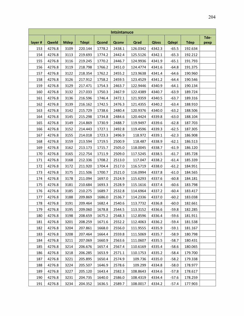
204

Intsintanuce


153 4276.8 3109 220.144 1778.2 2438.1 126.0342 4342.3 -65.5 192.634

154 4276.8 3113 219.693 1774.2 2442.4 125.5126 4342.1 -65.3 192.212

155 4276.8 3116 219.245 1770.2 2446.7 124.9936 4341.9 -65.1 191.793

156 4276.8 3119 218.798 1766.2 2451.0 124.4774 4341.6 -64.8 191.375

157 4276.8 3122 218.354 1762.2 2455.2 123.9638 4341.4 -64.6 190.960

158 4276.8 3126 217.912 1758.2 2459.5 123.4529 4341.2 -64.4 190.546

159 4276.8 3129 217.471 1754.3 2463.7 122.9446 4340.9 -64.1 190.134

160 4276.8 3132 217.033 1750.3 2467.9 122.4389 4340.7 -63.9 189.724

161 4276.8 3136 216.596 1746.4 2472.1 121.9359 4340.5 -63.7 189.316

162 4276.8 3139 216.162 1742.5 2476.3 121.4355 4340.2 -63.4 188.910

163 4276.8 3142 215.729 1738.6 2480.4 120.9376 4340.0 -63.2 188.506

164 4276.8 3145 215.298 1734.8 2484.6 120.4424 4339.8 -63.0 188.104

165 4276.8 3149 214.869 1730.9 2488.7 119.9497 4339.6 -62.8 187.703

166 4276.8 3152 214.443 1727.1 2492.8 119.4596 4339.3 -62.5 187.305

167 4276.8 3155 214.018 1723.3 2496.9 118.972 4339.1 -62.3 186.908

168 4276.8 3159 213.594 1719.5 2500.9 118.487 4338.9 -62.1 186.513

169 4276.8 3162 213.173 1715.7 2505.0 118.0045 4338.7 -61.9 186.120

170 4276.8 3165 212.754 1711.9 2509.0 117.5245 4338.5 -61.7 185.728

171 4276.8 3168 212.336 1708.2 2513.0 117.047 4338.2 -61.4 185.339

172 4276.8 3172 211.920 1704.4 2517.0 116.5719 4338.0 -61.2 184.951

173 4276.8 3175 211.506 1700.7 2521.0 116.0994 4337.8 -61.0 184.565

174 4276.8 3178 211.094 1697.0 2524.9 115.6293 4337.6 -60.8 184.181

175 4276.8 3181 210.684 1693.3 2528.9 115.1616 4337.4 -60.6 183.798

176 4276.8 3185 210.275 1689.7 2532.8 114.6964 4337.2 -60.4 183.417

177 4276.8 3188 209.869 1686.0 2536.7 114.2336 4337.0 -60.2 183.038

178 4276.8 3191 209.464 1682.4 2540.6 113.7732 4336.8 -60.0 182.661

179 4276.8 3195 209.060 1678.8 2544.5 113.3152 4336.6 -59.8 182.285

180 4276.8 3198 208.659 1675.2 2548.3 112.8596 4336.4 -59.6 181.911

181 4276.8 3201 208.259 1671.6 2552.2 112.4063 4336.2 -59.4 181.538

182 4276.8 3204 207.861 1668.0 2556.0 111.9555 4335.9 -59.1 181.167

183 4276.8 3208 207.464 1664.4 2559.8 111.5069 4335.7 -58.9 180.798

184 4276.8 3211 207.069 1660.9 2563.6 111.0607 4335.5 -58.7 180.431

185 4276.8 3214 206.676 1657.4 2567.4 110.6169 4335.4 -58.6 180.065

186 4276.8 3218 206.285 1653.9 2571.1 110.1753 4335.2 -58.4 179.700

187 4276.8 3221 205.895 1650.4 2574.9 109.736 4335.0 -58.2 179.338

188 4276.8 3224 205.507 1646.9 2578.6 109.299 4334.8 -58.0 178.977

189 4276.8 3227 205.120 1643.4 2582.3 108.8643 4334.6 -57.8 178.617

190 4276.8 3231 204.735 1640.0 2586.0 108.4319 4334.4 -57.6 178.259

191 4276.8 3234 204.352 1636.5 2589.7 108.0017 4334.2 -57.4 177.903

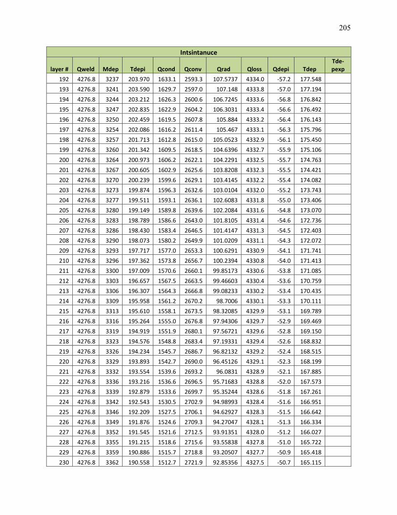
205

Intsintanuce


192 4276.8 3237 203.970 1633.1 2593.3 107.5737 4334.0 -57.2 177.548

193 4276.8 3241 203.590 1629.7 2597.0 107.148 4333.8 -57.0 177.194

194 4276.8 3244 203.212 1626.3 2600.6 106.7245 4333.6 -56.8 176.842

195 4276.8 3247 202.835 1622.9 2604.2 106.3031 4333.4 -56.6 176.492

196 4276.8 3250 202.459 1619.5 2607.8 105.884 4333.2 -56.4 176.143

197 4276.8 3254 202.086 1616.2 2611.4 105.467 4333.1 -56.3 175.796

198 4276.8 3257 201.713 1612.8 2615.0 105.0523 4332.9 -56.1 175.450

199 4276.8 3260 201.342 1609.5 2618.5 104.6396 4332.7 -55.9 175.106

200 4276.8 3264 200.973 1606.2 2622.1 104.2291 4332.5 -55.7 174.763

201 4276.8 3267 200.605 1602.9 2625.6 103.8208 4332.3 -55.5 174.421

202 4276.8 3270 200.239 1599.6 2629.1 103.4145 4332.2 -55.4 174.082

203 4276.8 3273 199.874 1596.3 2632.6 103.0104 4332.0 -55.2 173.743

204 4276.8 3277 199.511 1593.1 2636.1 102.6083 4331.8 -55.0 173.406

205 4276.8 3280 199.149 1589.8 2639.6 102.2084 4331.6 -54.8 173.070

206 4276.8 3283 198.789 1586.6 2643.0 101.8105 4331.4 -54.6 172.736

207 4276.8 3286 198.430 1583.4 2646.5 101.4147 4331.3 -54.5 172.403

208 4276.8 3290 198.073 1580.2 2649.9 101.0209 4331.1 -54.3 172.072

209 4276.8 3293 197.717 1577.0 2653.3 100.6291 4330.9 -54.1 171.741

210 4276.8 3296 197.362 1573.8 2656.7 100.2394 4330.8 -54.0 171.413

211 4276.8 3300 197.009 1570.6 2660.1 99.85173 4330.6 -53.8 171.085

212 4276.8 3303 196.657 1567.5 2663.5 99.46603 4330.4 -53.6 170.759

213 4276.8 3306 196.307 1564.3 2666.8 99.08233 4330.2 -53.4 170.435

214 4276.8 3309 195.958 1561.2 2670.2 98.7006 4330.1 -53.3 170.111

215 4276.8 3313 195.610 1558.1 2673.5 98.32085 4329.9 -53.1 169.789

216 4276.8 3316 195.264 1555.0 2676.8 97.94306 4329.7 -52.9 169.469

217 4276.8 3319 194.919 1551.9 2680.1 97.56721 4329.6 -52.8 169.150

218 4276.8 3323 194.576 1548.8 2683.4 97.19331 4329.4 -52.6 168.832

219 4276.8 3326 194.234 1545.7 2686.7 96.82132 4329.2 -52.4 168.515

220 4276.8 3329 193.893 1542.7 2690.0 96.45126 4329.1 -52.3 168.199

221 4276.8 3332 193.554 1539.6 2693.2 96.0831 4328.9 -52.1 167.885

222 4276.8 3336 193.216 1536.6 2696.5 95.71683 4328.8 -52.0 167.573

223 4276.8 3339 192.879 1533.6 2699.7 95.35244 4328.6 -51.8 167.261

224 4276.8 3342 192.543 1530.5 2702.9 94.98993 4328.4 -51.6 166.951

225 4276.8 3346 192.209 1527.5 2706.1 94.62927 4328.3 -51.5 166.642

226 4276.8 3349 191.876 1524.6 2709.3 94.27047 4328.1 -51.3 166.334

227 4276.8 3352 191.545 1521.6 2712.5 93.91351 4328.0 -51.2 166.027

228 4276.8 3355 191.215 1518.6 2715.6 93.55838 4327.8 -51.0 165.722

229 4276.8 3359 190.886 1515.7 2718.8 93.20507 4327.7 -50.9 165.418

230 4276.8 3362 190.558 1512.7 2721.9 92.85356 4327.5 -50.7 165.115

206

Intsintanuce


231 4276.8 3365 190.231 1509.8 2725.1 92.50386 4327.4 -50.6 164.813

232 4276.8 3368 189.906 1506.9 2728.2 92.15594 4327.2 -50.4 164.513

233 4276.8 3372 189.582 1504.0 2731.3 91.8098 4327.1 -50.3 164.214

234 4276.8 3375 189.260 1501.1 2734.4 91.46543 4326.9 -50.1 163.916

235 4276.8 3378 188.938 1498.2 2737.4 91.12282 4326.7 -49.9 163.619

236 4276.8 3382 188.618 1495.3 2740.5 90.78196 4326.6 -49.8 163.323

237 4276.8 3385 188.299 1492.4 2743.6 90.44283 4326.5 -49.7 163.028

238 4276.8 3388 187.981 1489.6 2746.6 90.10543 4326.3 -49.5 162.735

239 4276.8 3391 187.664 1486.8 2749.6 89.76975 4326.2 -49.4 162.443

240 4276.8 3395 187.349 1483.9 2752.7 89.43577 4326.0 -49.2 162.152

241 4276.8 3398 187.035 1481.1 2755.7 89.10349 4325.9 -49.1 161.862

242 4276.8 3401 186.722 1478.3 2758.7 88.7729 4325.7 -48.9 161.573

243 4276.8 3405 186.410 1475.5 2761.6 88.44399 4325.6 -48.8 161.285

244 4276.8 3408 186.099 1472.7 2764.6 88.11675 4325.4 -48.6 160.999

245 4276.8 3411 185.789 1469.9 2767.6 87.79117 4325.3 -48.5 160.713

246 4276.8 3414 185.481 1467.2 2770.5 87.46724 4325.1 -48.3 160.429

247 4276.8 3418 185.174 1464.4 2773.5 87.14494 4325.0 -48.2 160.146

248 4276.8 3421 184.868 1461.7 2776.4 86.82428 4324.9 -48.1 159.864

249 4276.8 3424 184.563 1458.9 2779.3 86.50524 4324.7 -47.9 159.583

250 4276.8 3428 184.259 1456.2 2782.2 86.18781 4324.6 -47.8 159.303

207

Table 32: : Tdep and Cumulative Q


Cumulative

Qcond Qconv Qrad

294.0 2E+02 0.180215

1114.1 590.1 3.6

2141.0 1141.2 10.9

3352.3 1798.0 23.8

4727.2 2551.2 44.0

6247.4 3392.5 73.0

7896.2 4314.0 112.2

9658.4 5308.8 162.4

11520.4 6370.3 224.3

13470.0 7492.5 298.1

15496.1 8670.0 383.8

17588.9 9898.0 481.2

19739.6 11171.9 589.9

21940.3 12487.6 709.2

24184.0 13841.6 838.5

26464.6 15230.4 977.0

28776.4 16651.2 1124.0

31114.6 18101.2 1278.7

33475.0 19578.0 1440.3

35853.7 21079.6 1608.1

38247.4 22603.9 1781.3

40653.2 24149.3 1959.3

43068.6 25714.3 2141.5

45491.2 27297.5 2327.3

47919.2 28897.7 2516.3

50350.9 30513.8 2707.9

52784.6 32144.9 2901.7

55219.3 33790.1 3097.4

57653.7 35448.7 3294.6

60086.8 37120.0 3493.1

62517.9 38803.3 3692.5

64946.2 40498.3 3892.7

67371.0 42204.3 4093.4

69791.9 43921.0 4294.5

72208.4 45648.0 4495.9

74620.0 47385.0 4697.2

77026.5 49131.6 4898.6

208

Cumulative

Qcond Qconv Qrad

79427.5 50887.7 5099.8

81822.9 52652.9 5300.7

84212.3 54427.1 5501.3

86595.7 56210.0 5701.6

88972.9 58001.5 5901.4

91343.8 59801.4 6100.7

93708.2 61609.6 6299.5

96066.1 63425.9 6497.6

98417.5 65250.3 6695.2

100762.2 67082.5 6892.2

103100.3 68922.6 7088.4

105431.8 70770.4 7284.0

107756.5 72625.9 7478.9

110074.6 74488.8 7673.1

112386.0 76359.3 7866.5

114690.6 78237.2 8059.2

116988.6 80122.4 8251.1

119280.0 82014.9 8442.3

121564.7 83914.6 8632.8

123842.7 85821.5 8822.5

126114.2 87735.4 9011.4

128379.1 89656.5 9199.5

130637.4 91584.5 9386.8

132889.2 93519.5 9573.4

135134.5 95461.4 9759.2

137373.3 97410.2 9944.3

139605.8 99365.8 10128.5

141831.8 101328.1 10312.0

144051.4 103297.2 10494.7

146264.8 105273.0 10676.6

148471.8 107255.5 10857.8

150672.5 109244.5 11038.2

152867.1 111240.2 11217.8

155055.4 113242.3 11396.6

157237.6 115251.0 11574.7

159413.6 117266.2 11752.0

161583.6 119287.7 11928.6

163747.5 121315.7 12104.4

165905.3 123350.0 12279.5

209

Cumulative

Qcond Qconv Qrad

168057.2 125390.7 12453.8

170203.1 127437.6 12627.3

172343.1 129490.8 12800.1

174477.2 131550.2 12972.2

176605.5 133615.8 13143.5

178727.9 135687.5 13314.1

180844.5 137765.4 13484.0

182955.4 139849.3 13653.1

185060.6 141939.3 13821.5

187160.0 144035.3 13989.1

189253.8 146137.3 14156.1

191342.0 148245.3 14322.3

193424.5 150359.2 14487.8

195501.5 152479.0 14652.6

197572.9 154604.7 14816.6

199638.8 156736.2 14980.0

201699.3 158873.5 15142.7

203754.3 161016.6 15304.7

205803.9 163165.5 15465.9

207848.1 165320.0 15626.5

209886.9 167480.3 15786.4

211920.4 169646.2 15945.6

213948.6 171817.7 16104.1

215971.5 173994.8 16261.9

217989.1 176177.5 16419.0

220001.5 178365.8 16575.5

222008.8 180559.6 16731.3

224010.9 182758.8 16886.4

226007.8 184963.6 17040.9

227999.6 187173.7 17194.7

229986.4 189389.3 17347.8

231968.1 191610.3 17500.3

233944.7 193836.6 17652.1

235916.3 196068.2 17803.3

237883.0 198305.1 17953.8

239844.7 200547.4 18103.7

241801.5 202794.8 18253.0

243753.3 205047.5 18401.6

245700.3 207305.4 18549.5

210

Cumulative

Qcond Qconv Qrad

247642.5 209568.4 18696.9

249579.8 211836.6 18843.6

251512.3 214110.0 18989.6

253440.0 216388.4 19135.1

255362.9 218671.9 19279.9

257281.2 220960.4 19424.1

259194.7 223254.0 19567.7

261103.5 225552.6 19710.7

263007.7 227856.1 19853.1

264907.2 230164.6 19994.9

266802.1 232478.0 20136.1

268692.4 234796.3 20276.7

270578.1 237119.5 20416.7

272459.3 239447.6 20556.0

274336.0 241780.5 20694.8

276208.1 244118.2 20833.1

278075.8 246460.7 20970.7

279939.0 248808.0 21107.7

281797.7 251160.0 21244.2

283652.1 253516.7 21380.1

285502.0 255878.1 21515.4

287347.6 258244.2 21650.2

289188.8 260615.0 21784.4

291025.6 262990.4 21918.0

292858.2 265370.4 22051.1

294686.4 267755.0 22183.6

296510.4 270144.2 22315.5

298330.1 272537.9 22446.9

300145.6 274936.1 22577.8

301956.9 277338.9 22708.1

303764.0 279746.1 22837.9

305566.9 282157.8 22967.1

307365.6 284573.9 23095.8

309160.2 286994.5 23223.9

310950.7 289419.5 23351.5

312737.1 291848.8 23478.6

314519.4 294282.5 23605.2

316297.7 296720.6 23731.2

318071.9 299163.0 23856.7

211

Cumulative

Qcond Qconv Qrad

319842.0 301609.7 23981.7

321608.2 304060.7 24106.2

323370.4 306515.9 24230.2

325128.6 308975.4 24353.6

326882.8 311439.1 24476.6

328633.2 313907.1 24599.0

330379.6 316379.2 24720.9

332122.1 318855.5 24842.4

333860.7 321335.9 24963.3

335595.4 323820.5 25083.7

337326.3 326309.2 25203.7

339053.4 328802.0 25323.2

340776.7 331298.9 25442.1

342496.1 333799.8 25560.6

344211.8 336304.8 25678.6

345923.7 338813.8 25796.1

347631.9 341326.8 25913.2

349336.4 343843.8 26029.8

351037.1 346364.8 26145.9

352734.1 348889.8 26261.5

354427.5 351418.7 26376.7

356117.1 353951.5 26491.4

357803.2 356488.2 26605.6

359485.6 359028.8 26719.4

361164.3 361573.2 26832.7

362839.5 364121.6 26945.5

364511.1 366673.7 27057.9

366179.1 369229.7 27169.9

367843.5 371789.5 27281.4

369504.4 374353.1 27392.5

371161.8 376920.5 27503.1

372815.7 379491.6 27613.3

374466.0 382066.4 27723.0

376112.9 384645.0 27832.3

377756.3 387227.3 27941.2

379396.3 389813.3 28049.6

381032.8 392403.0 28157.6

382665.9 394996.3 28265.2

384295.6 397593.3 28372.3

212

Cumulative

Qcond Qconv Qrad

385921.9 400193.9 28479.0

387544.8 402798.1 28585.3

389164.3 405405.9 28691.2

390780.5 408017.3 28796.7

392393.3 410632.3 28901.7

394002.8 413250.9 29006.4

395609.0 415873.0 29110.6

397211.9 418498.6 29214.4

398811.5 421127.7 29317.8

400407.9 423760.3 29420.9

402000.9 426396.5 29523.5

403590.8 429036.0 29625.7

405177.3 431679.1 29727.5

406760.7 434325.6 29828.9

408340.9 436975.5 29929.9

409917.9 439628.8 30030.5

411491.6 442285.5 30130.8

413062.3 444945.6 30230.6

414629.7 447609.1 30330.1

416194.0 450276.0 30429.2

417755.2 452946.2 30527.9

419313.3 455619.7 30626.2

420868.2 458296.5 30724.1

422420.1 460976.7 30821.7

423968.9 463660.1 30918.9

425514.6 466346.8 31015.7

427057.3 469036.8 31112.2

428596.9 471730.0 31208.3

430133.4 474426.5 31304.0

431667.0 477126.2 31399.3

433197.5 479829.1 31494.3

434725.1 482535.2 31589.0

436249.6 485244.5 31683.2

437771.2 487957.0 31777.1

439289.8 490672.6 31870.7

440805.5 493391.4 31963.9

442318.2 496113.4 32056.8

443828.0 498838.4 32149.3

445334.9 501566.6 32241.4

213

Cumulative

Qcond Qconv Qrad

446838.9 504297.9 32333.2

448339.9 507032.2 32424.7

449838.1 509769.7 32515.8

451333.4 512510.2 32606.6

452825.9 515253.7 32697.0

454315.5 518000.3 32787.1

455802.2 520750.0 32876.9

457286.2 523502.6 32966.3

458767.3 526258.3 33055.5

460245.5 529016.9 33144.2

461721.0 531778.6 33232.7

463193.7 534543.2 33320.8

464663.7 537310.8 33408.6

466130.8 540081.3 33496.0

467595.2 542854.7 33583.2

469056.9 545631.1 33670.0

470515.8 548410.4 33756.5

471972.0 551192.6 33842.7

214

Table 33: Tdep and Instantaneous Q as a Function of nt with λ = 0.6, ξ = 0. , ζ = 0.5, ψ =1.0, and δtt = 10

second

Instantaneous

layer # Qweld Mdep Tdepi Qcond Qconv Qrad Qloss Qdepi Tdep Tde-pexp

1 4276.8 2611 54.764 49.0 25.8 0.030036 74.8 4202.0 54.231 22

2 4276.8 2614 119.105 145.2 77.1 0.696473 223.1 4053.7 86.422 167

3 4276.8 2617 150.081 191.6 102.8 1.775509 296.2 3980.6 117.438 202

4 4276.8 2621 180.459 237.0 128.5 3.750771 369.3 3907.5 147.857 216

5 4276.8 2624 210.242 281.6 154.2 6.981597 442.8 3834.0 177.679 223

6 4276.8 2627 239.427 325.2 180.0 11.86254 517.0 3759.8 206.904 226

7 4276.8 2630 268.010 368.0 205.7 18.81247 592.5 3684.3 235.527 231

8 4276.8 2634 295.984 409.8 231.3 28.26334 669.4 3607.4 263.541 230

9 4276.8 2637 323.339 450.7 256.9 40.64858 748.3 3528.5 290.936 233

10 4276.8 2640 350.062 490.7 282.5 56.39109 829.5 3447.3 317.698 230

11 4276.8 2643 376.136 529.7 307.9 75.89082 913.4 3363.4 343.811 235

12 4276.8 2647 401.543 567.7 333.1 99.51222 1000.3 3276.5 369.258 240

13 4276.8 2650 426.263 604.7 358.2 127.5717 1090.4 3186.4 394.016 243

14 4276.8 2653 450.271 640.6 383.0 160.3257 1183.9 3092.9 418.064 244

15 4276.8 2657 473.546 675.4 407.6 197.9595 1280.9 2995.9 441.377 245

16 4276.8 2660 496.061 709.1 431.8 240.5774 1381.5 2895.3 463.931 247

17 4276.8 2663 517.793 741.6 455.7 288.1953 1485.5 2791.3 485.702 248

18 4276.8 2666 538.716 772.9 479.3 340.7351 1592.9 2683.9 506.664 249

19 4276.8 2670 558.809 802.9 502.4 398.0228 1703.3 2573.5 526.795 251

20 4276.8 2673 578.050 831.7 525.0 459.7892 1816.5 2460.3 546.073 251

21 4276.8 2676 596.420 859.2 547.1 525.6744 1932.0 2344.8 564.482 251

22 4276.8 2680 613.905 885.3 568.7 595.2357 2049.3 2227.5 582.004 251

23 4276.8 2683 630.492 910.2 589.7 667.9588 2167.8 2109.0 598.630 251

24 4276.8 2686 646.177 933.6 610.1 743.2711 2287.0 1989.8 614.352 251

25 4276.8 2689 660.954 955.7 629.9 820.5574 2406.1 1870.7 629.168 253

26 4276.8 2693 674.828 976.5 649.0 899.1776 2524.6 1752.2 643.079 253

27 4276.8 2696 687.805 995.9 667.4 978.4833 2641.8 1635.0 656.093 253

28 4276.8 2699 699.896 1014.0 685.2 1057.835 2757.0 1519.8 668.222

29 4276.8 2703 711.120 1030.8 702.3 1136.619 2869.6 1407.2 679.483

30 4276.8 2706 721.496 1046.3 718.7 1214.259 2979.2 1297.6 689.897

31 4276.8 2709 731.050 1060.6 734.4 1290.229 3085.2 1191.6 699.488

32 4276.8 2712 739.811 1073.7 749.4 1364.063 3187.1 1089.7 708.286

33 4276.8 2716 747.808 1085.6 763.8 1435.358 3284.8 992.0 716.320

34 4276.8 2719 755.077 1096.5 777.6 1503.78 3377.8 899.0 723.626

35 4276.8 2722 761.652 1106.3 790.7 1569.063 3466.1 810.7 730.239

36 4276.8 2725 767.572 1115.2 803.2 1631.007 3549.4 727.4 736.195

215

Instantaneous


37 4276.8 2729 772.872 1123.1 815.2 1689.478 3627.8 649.0 741.533

38 4276.8 2732 777.592 1130.2 826.6 1744.396 3701.2 575.6 746.290

39 4276.8 2735 781.770 1136.4 837.5 1795.736 3769.6 507.2 750.504

40 4276.8 2739 785.441 1141.9 847.9 1843.518 3833.3 443.5 754.212

41 4276.8 2742 788.643 1146.7 857.8 1887.802 3892.3 384.5 757.451

42 4276.8 2745 791.411 1150.8 867.3 1928.678 3946.8 330.0 760.256

43 4276.8 2748 793.778 1154.4 876.4 1966.265 3997.0 279.8 762.660

44 4276.8 2752 795.777 1157.4 885.1 2000.7 4043.2 233.6 764.695

45 4276.8 2755 797.439 1159.9 893.5 2032.134 4085.4 191.4 766.393

46 4276.8 2758 798.791 1161.9 901.5 2060.73 4124.1 152.7 767.782

47 4276.8 2762 799.862 1163.5 909.2 2086.655 4159.3 117.5 768.890

48 4276.8 2765 800.676 1164.7 916.6 2110.08 4191.4 85.4 769.740

49 4276.8 2768 801.257 1165.6 923.8 2131.172 4220.5 56.3 770.358

50 4276.8 2771 801.628 1166.1 930.7 2150.098 4246.9 29.9 770.765

51 4276.8 2775 801.807 1166.4 937.4 2167.02 4270.8 6.0 770.980

52 4276.8 2778 801.814 1166.4 943.9 2182.093 4292.4 -15.6 771.023

53 4276.8 2781 801.665 1166.2 950.2 2195.464 4311.9 -35.1 770.911

54 4276.8 2785 801.377 1165.8 956.4 2207.275 4329.4 -52.6 770.659

55 4276.8 2788 800.963 1165.1 962.3 2217.656 4345.1 -68.3 770.281

56 4276.8 2791 800.437 1164.3 968.2 2226.732 4359.2 -82.4 769.791

57 4276.8 2794 799.811 1163.4 973.8 2234.618 4371.9 -95.1 769.200

58 4276.8 2798 799.095 1162.3 979.4 2241.421 4383.2 -106.4 768.520

59 4276.8 2801 798.298 1161.1 984.9 2247.239 4393.3 -116.5 767.759

60 4276.8 2804 797.431 1159.9 990.2 2252.164 4402.2 -125.4 766.928

61 4276.8 2808 796.501 1158.5 995.5 2256.28 4410.2 -133.4 766.033

62 4276.8 2811 795.515 1157.0 1000.6 2259.662 4417.3 -140.5 765.083

63 4276.8 2814 794.480 1155.4 1005.7 2262.382 4423.5 -146.7 764.083

64 4276.8 2817 793.402 1153.8 1010.7 2264.504 4429.1 -152.3 763.040

65 4276.8 2821 792.286 1152.2 1015.7 2266.086 4433.9 -157.1 761.959

66 4276.8 2824 791.136 1150.4 1020.6 2267.18 4438.2 -161.4 760.845

67 4276.8 2827 789.958 1148.7 1025.4 2267.837 4441.9 -165.1 759.702

68 4276.8 2830 788.755 1146.9 1030.2 2268.099 4445.1 -168.3 758.534

69 4276.8 2834 787.531 1145.0 1034.9 2268.005 4447.9 -171.1 757.345

70 4276.8 2837 786.288 1143.2 1039.6 2267.593 4450.4 -173.6 756.137

71 4276.8 2840 785.029 1141.3 1044.2 2266.895 4452.4 -175.6 754.913

72 4276.8 2844 783.758 1139.4 1048.8 2265.939 4454.2 -177.4 753.677

73 4276.8 2847 782.476 1137.5 1053.4 2264.753 4455.6 -178.8 752.429

74 4276.8 2850 781.185 1135.6 1057.9 2263.36 4456.8 -180.0 751.173

75 4276.8 2853 779.888 1133.6 1062.4 2261.782 4457.8 -181.0 749.910

216

Instantaneous


76 4276.8 2857 778.585 1131.7 1066.9 2260.039 4458.6 -181.8 748.641

77 4276.8 2860 777.278 1129.7 1071.3 2258.149 4459.2 -182.4 747.369

78 4276.8 2863 775.968 1127.7 1075.7 2256.125 4459.6 -182.8 746.093

79 4276.8 2867 774.657 1125.8 1080.1 2253.985 4459.9 -183.1 744.817

80 4276.8 2870 773.346 1123.8 1084.5 2251.739 4460.0 -183.2 743.539

81 4276.8 2873 772.035 1121.9 1088.8 2249.399 4460.1 -183.3 742.262

82 4276.8 2876 770.725 1119.9 1093.2 2246.976 4460.0 -183.2 740.986

83 4276.8 2880 769.417 1117.9 1097.5 2244.479 4459.9 -183.1 739.712

84 4276.8 2883 768.111 1116.0 1101.8 2241.917 4459.7 -182.9 738.440

85 4276.8 2886 766.809 1114.0 1106.0 2239.297 4459.4 -182.6 737.172

86 4276.8 2890 765.510 1112.1 1110.3 2236.625 4459.0 -182.2 735.907

87 4276.8 2893 764.215 1110.2 1114.5 2233.908 4458.6 -181.8 734.645

88 4276.8 2896 762.925 1108.2 1118.8 2231.151 4458.1 -181.3 733.388

89 4276.8 2899 761.639 1106.3 1123.0 2228.359 4457.6 -180.8 732.136

90 4276.8 2903 760.358 1104.4 1127.2 2225.537 4457.1 -180.3 730.888

91 4276.8 2906 759.083 1102.5 1131.4 2222.687 4456.5 -179.7 729.646

92 4276.8 2909 757.812 1100.6 1135.5 2219.815 4455.9 -179.1 728.409

93 4276.8 2912 756.548 1098.7 1139.7 2216.922 4455.3 -178.5 727.178

94 4276.8 2916 755.289 1096.8 1143.8 2214.013 4454.7 -177.9 725.952

95 4276.8 2919 754.036 1094.9 1148.0 2211.088 4454.0 -177.2 724.732

96 4276.8 2922 752.789 1093.1 1152.1 2208.151 4453.3 -176.5 723.518

97 4276.8 2926 751.548 1091.2 1156.2 2205.204 4452.6 -175.8 722.310

98 4276.8 2929 750.313 1089.4 1160.3 2202.248 4451.9 -175.1 721.108

99 4276.8 2932 749.085 1087.5 1164.4 2199.285 4451.2 -174.4 719.912

100 4276.8 2935 747.862 1085.7 1168.5 2196.316 4450.5 -173.7 718.722

101 4276.8 2939 746.646 1083.9 1172.6 2193.343 4449.8 -173.0 717.538

102 4276.8 2942 745.436 1082.1 1176.6 2190.367 4449.1 -172.3 716.361

103 4276.8 2945 744.233 1080.3 1180.7 2187.389 4448.3 -171.5 715.190

104 4276.8 2949 743.036 1078.5 1184.7 2184.41 4447.6 -170.8 714.025

105 4276.8 2952 741.845 1076.7 1188.7 2181.43 4446.9 -170.1 712.867

106 4276.8 2955 740.660 1074.9 1192.8 2178.451 4446.2 -169.4 711.714

107 4276.8 2958 739.482 1073.2 1196.8 2175.473 4445.4 -168.6 710.568

108 4276.8 2962 738.310 1071.4 1200.8 2172.496 4444.7 -167.9 709.428

109 4276.8 2965 737.144 1069.7 1204.8 2169.522 4444.0 -167.2 708.294

110 4276.8 2968 735.985 1067.9 1208.8 2166.55 4443.3 -166.5 707.166

111 4276.8 2972 734.831 1066.2 1212.7 2163.581 4442.5 -165.7 706.045

112 4276.8 2975 733.684 1064.5 1216.7 2160.615 4441.8 -165.0 704.929

113 4276.8 2978 732.543 1062.8 1220.7 2157.653 4441.1 -164.3 703.820

114 4276.8 2981 731.408 1061.1 1224.6 2154.695 4440.4 -163.6 702.716

217

Instantaneous


115 4276.8 2985 730.278 1059.4 1228.6 2151.74 4439.7 -162.9 701.619

116 4276.8 2988 729.155 1057.7 1232.5 2148.791 4439.0 -162.2 700.527

117 4276.8 2991 728.038 1056.1 1236.4 2145.845 4438.3 -161.5 699.441

118 4276.8 2994 726.926 1054.4 1240.4 2142.905 4437.7 -160.9 698.361

119 4276.8 2998 725.821 1052.7 1244.3 2139.969 4437.0 -160.2 697.287

120 4276.8 3001 724.721 1051.1 1248.2 2137.038 4436.3 -159.5 696.218

121 4276.8 3004 723.627 1049.5 1252.1 2134.113 4435.6 -158.8 695.155

122 4276.8 3008 722.539 1047.8 1255.9 2131.192 4435.0 -158.2 694.098

123 4276.8 3011 721.456 1046.2 1259.8 2128.277 4434.3 -157.5 693.046

124 4276.8 3014 720.379 1044.6 1263.7 2125.367 4433.7 -156.9 692.000

125 4276.8 3017 719.307 1043.0 1267.6 2122.462 4433.0 -156.2 690.959

126 4276.8 3021 718.241 1041.4 1271.4 2119.563 4432.4 -155.6 689.923

127 4276.8 3024 717.180 1039.8 1275.3 2116.669 4431.7 -154.9 688.893

128 4276.8 3027 716.125 1038.2 1279.1 2113.781 4431.1 -154.3 687.869

129 4276.8 3031 715.074 1036.7 1282.9 2110.898 4430.5 -153.7 686.849

130 4276.8 3034 714.030 1035.1 1286.8 2108.02 4429.9 -153.1 685.835

131 4276.8 3037 712.990 1033.5 1290.6 2105.148 4429.3 -152.5 684.826

132 4276.8 3040 711.956 1032.0 1294.4 2102.281 4428.7 -151.9 683.822

133 4276.8 3044 710.926 1030.5 1298.2 2099.42 4428.1 -151.3 682.823

134 4276.8 3047 709.902 1028.9 1302.0 2096.565 4427.5 -150.7 681.829

135 4276.8 3050 708.883 1027.4 1305.8 2093.715 4426.9 -150.1 680.840

136 4276.8 3054 707.869 1025.9 1309.5 2090.87 4426.3 -149.5 679.856

137 4276.8 3057 706.860 1024.4 1313.3 2088.031 4425.7 -148.9 678.877

138 4276.8 3060 705.855 1022.9 1317.1 2085.197 4425.1 -148.3 677.902

139 4276.8 3063 704.856 1021.4 1320.8 2082.369 4424.6 -147.8 676.933

140 4276.8 3067 703.861 1019.9 1324.6 2079.546 4424.0 -147.2 675.968

141 4276.8 3070 702.871 1018.4 1328.3 2076.728 4423.5 -146.7 675.008

142 4276.8 3073 701.886 1016.9 1332.1 2073.916 4422.9 -146.1 674.052

143 4276.8 3077 700.906 1015.5 1335.8 2071.109 4422.4 -145.6 673.102

144 4276.8 3080 699.930 1014.0 1339.5 2068.308 4421.8 -145.0 672.155

145 4276.8 3083 698.958 1012.6 1343.2 2065.511 4421.3 -144.5 671.214

146 4276.8 3086 697.992 1011.1 1346.9 2062.72 4420.8 -144.0 670.276

147 4276.8 3090 697.029 1009.7 1350.6 2059.935 4420.2 -143.4 669.343

148 4276.8 3093 696.071 1008.2 1354.3 2057.154 4419.7 -142.9 668.415

149 4276.8 3096 695.118 1006.8 1358.0 2054.379 4419.2 -142.4 667.491

150 4276.8 3099 694.169 1005.4 1361.7 2051.609 4418.7 -141.9 666.571

151 4276.8 3103 693.224 1004.0 1365.3 2048.844 4418.2 -141.4 665.656

152 4276.8 3106 692.284 1002.6 1369.0 2046.084 4417.7 -140.9 664.744

153 4276.8 3109 691.348 1001.2 1372.7 2043.329 4417.2 -140.4 663.837

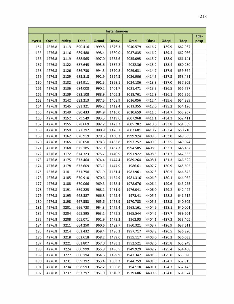
218

Instantaneous


154 4276.8 3113 690.416 999.8 1376.3 2040.579 4416.7 -139.9 662.934

155 4276.8 3116 689.488 998.4 1380.0 2037.835 4416.2 -139.4 662.036

156 4276.8 3119 688.565 997.0 1383.6 2035.095 4415.7 -138.9 661.141

157 4276.8 3122 687.645 995.6 1387.2 2032.36 4415.2 -138.4 660.250

158 4276.8 3126 686.730 994.3 1390.8 2029.631 4414.7 -137.9 659.364

159 4276.8 3129 685.818 992.9 1394.5 2026.906 4414.3 -137.5 658.481

160 4276.8 3132 684.911 991.5 1398.1 2024.186 4413.8 -137.0 657.602

161 4276.8 3136 684.008 990.2 1401.7 2021.471 4413.3 -136.5 656.727

162 4276.8 3139 683.108 988.9 1405.3 2018.761 4412.9 -136.1 655.856

163 4276.8 3142 682.213 987.5 1408.9 2016.056 4412.4 -135.6 654.989

164 4276.8 3145 681.321 986.2 1412.4 2013.355 4412.0 -135.2 654.126

165 4276.8 3149 680.433 984.9 1416.0 2010.659 4411.5 -134.7 653.267

166 4276.8 3152 679.549 983.5 1419.6 2007.968 4411.1 -134.3 652.411

167 4276.8 3155 678.669 982.2 1423.2 2005.282 4410.6 -133.8 651.559

168 4276.8 3159 677.792 980.9 1426.7 2002.601 4410.2 -133.4 650.710

169 4276.8 3162 676.919 979.6 1430.3 1999.924 4409.8 -133.0 649.865

170 4276.8 3165 676.050 978.3 1433.8 1997.252 4409.3 -132.5 649.024

171 4276.8 3168 675.185 977.0 1437.3 1994.585 4408.9 -132.1 648.187

172 4276.8 3172 674.323 975.7 1440.9 1991.922 4408.5 -131.7 647.353

173 4276.8 3175 673.464 974.4 1444.4 1989.264 4408.1 -131.3 646.522

174 4276.8 3178 672.609 973.1 1447.9 1986.61 4407.7 -130.9 645.695

175 4276.8 3181 671.758 971.9 1451.4 1983.961 4407.3 -130.5 644.872

176 4276.8 3185 670.910 970.6 1454.9 1981.316 4406.9 -130.1 644.052

177 4276.8 3188 670.066 969.3 1458.4 1978.676 4406.4 -129.6 643.235

178 4276.8 3191 669.225 968.1 1461.9 1976.041 4406.0 -129.2 642.422

179 4276.8 3195 668.387 966.8 1465.4 1973.41 4405.6 -128.8 641.612

180 4276.8 3198 667.553 965.6 1468.9 1970.783 4405.3 -128.5 640.805

181 4276.8 3201 666.723 964.3 1472.4 1968.161 4404.9 -128.1 640.001

182 4276.8 3204 665.895 963.1 1475.8 1965.544 4404.5 -127.7 639.201

183 4276.8 3208 665.071 961.9 1479.3 1962.93 4404.1 -127.3 638.405

184 4276.8 3211 664.250 960.6 1482.7 1960.321 4403.7 -126.9 637.611

185 4276.8 3214 663.432 959.4 1486.2 1957.717 4403.3 -126.5 636.820

186 4276.8 3218 662.618 958.2 1489.6 1955.117 4403.0 -126.2 636.033

187 4276.8 3221 661.807 957.0 1493.1 1952.521 4402.6 -125.8 635.249

188 4276.8 3224 660.999 955.8 1496.5 1949.929 4402.2 -125.4 634.468

189 4276.8 3227 660.194 954.6 1499.9 1947.342 4401.8 -125.0 633.690

190 4276.8 3231 659.392 953.4 1503.3 1944.759 4401.5 -124.7 632.915

191 4276.8 3234 658.593 952.2 1506.8 1942.18 4401.1 -124.3 632.143

192 4276.8 3237 657.797 951.0 1510.2 1939.606 4400.8 -124.0 631.374

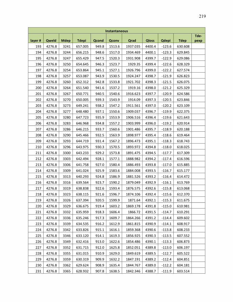
219

Instantaneous


193 4276.8 3241 657.005 949.8 1513.6 1937.035 4400.4 -123.6 630.608

194 4276.8 3244 656.215 948.6 1517.0 1934.469 4400.1 -123.3 629.845

195 4276.8 3247 655.429 947.5 1520.3 1931.908 4399.7 -122.9 629.086

196 4276.8 3250 654.645 946.3 1523.7 1929.35 4399.4 -122.6 628.329

197 4276.8 3254 653.864 945.1 1527.1 1926.796 4399.0 -122.2 627.574

198 4276.8 3257 653.087 943.9 1530.5 1924.247 4398.7 -121.9 626.823

199 4276.8 3260 652.312 942.8 1533.8 1921.702 4398.3 -121.5 626.075

200 4276.8 3264 651.540 941.6 1537.2 1919.16 4398.0 -121.2 625.329

201 4276.8 3267 650.771 940.5 1540.6 1916.623 4397.7 -120.9 624.586

202 4276.8 3270 650.005 939.3 1543.9 1914.09 4397.3 -120.5 623.846

203 4276.8 3273 649.241 938.2 1547.2 1911.561 4397.0 -120.2 623.109

204 4276.8 3277 648.480 937.1 1550.6 1909.037 4396.7 -119.9 622.375

205 4276.8 3280 647.723 935.9 1553.9 1906.516 4396.4 -119.6 621.643

206 4276.8 3283 646.968 934.8 1557.2 1903.999 4396.0 -119.2 620.914

207 4276.8 3286 646.215 933.7 1560.6 1901.486 4395.7 -118.9 620.188

208 4276.8 3290 645.466 932.5 1563.9 1898.977 4395.4 -118.6 619.464

209 4276.8 3293 644.719 931.4 1567.2 1896.473 4395.1 -118.3 618.743

210 4276.8 3296 643.975 930.3 1570.5 1893.972 4394.8 -118.0 618.025

211 4276.8 3300 643.233 929.2 1573.8 1891.475 4394.5 -117.7 617.309

212 4276.8 3303 642.494 928.1 1577.1 1888.982 4394.2 -117.4 616.596

213 4276.8 3306 641.758 927.0 1580.4 1886.493 4393.8 -117.0 615.885

214 4276.8 3309 641.024 925.9 1583.6 1884.008 4393.5 -116.7 615.177

215 4276.8 3313 640.293 924.8 1586.9 1881.526 4393.2 -116.4 614.472

216 4276.8 3316 639.564 923.7 1590.2 1879.049 4392.9 -116.1 613.769

217 4276.8 3319 638.838 922.6 1593.4 1876.575 4392.6 -115.8 613.068

218 4276.8 3323 638.115 921.6 1596.7 1874.106 4392.4 -115.6 612.370

219 4276.8 3326 637.394 920.5 1599.9 1871.64 4392.1 -115.3 611.675

220 4276.8 3329 636.675 919.4 1603.2 1869.178 4391.8 -115.0 610.981

221 4276.8 3332 635.959 918.3 1606.4 1866.72 4391.5 -114.7 610.291

222 4276.8 3336 635.246 917.3 1609.7 1864.266 4391.2 -114.4 609.602

223 4276.8 3339 634.535 916.2 1612.9 1861.815 4390.9 -114.1 608.917

224 4276.8 3342 633.826 915.1 1616.1 1859.368 4390.6 -113.8 608.233

225 4276.8 3346 633.120 914.1 1619.3 1856.925 4390.3 -113.5 607.552

226 4276.8 3349 632.416 913.0 1622.6 1854.486 4390.1 -113.3 606.873

227 4276.8 3352 631.715 912.0 1625.8 1852.051 4389.8 -113.0 606.197

228 4276.8 3355 631.015 910.9 1629.0 1849.619 4389.5 -112.7 605.522

229 4276.8 3359 630.319 909.9 1632.2 1847.191 4389.2 -112.4 604.851

230 4276.8 3362 629.624 908.9 1635.4 1844.767 4389.0 -112.2 604.181

231 4276.8 3365 628.932 907.8 1638.5 1842.346 4388.7 -111.9 603.514

220

Instantaneous


232 4276.8 3368 628.242 906.8 1641.7 1839.93 4388.4 -111.6 602.849

233 4276.8 3372 627.555 905.8 1644.9 1837.516 4388.2 -111.4 602.186

234 4276.8 3375 626.869 904.7 1648.1 1835.107 4387.9 -111.1 601.525

235 4276.8 3378 626.186 903.7 1651.2 1832.701 4387.6 -110.8 600.867

236 4276.8 3382 625.506 902.7 1654.4 1830.299 4387.4 -110.6 600.210

237 4276.8 3385 624.827 901.7 1657.6 1827.901 4387.1 -110.3 599.556

238 4276.8 3388 624.151 900.7 1660.7 1825.506 4386.9 -110.1 598.904

239 4276.8 3391 623.476 899.7 1663.8 1823.114 4386.6 -109.8 598.255

240 4276.8 3395 622.804 898.7 1667.0 1820.727 4386.4 -109.6 597.607

241 4276.8 3398 622.135 897.7 1670.1 1818.343 4386.1 -109.3 596.962

242 4276.8 3401 621.467 896.7 1673.3 1815.962 4385.9 -109.1 596.318

243 4276.8 3405 620.801 895.7 1676.4 1813.585 4385.6 -108.8 595.677

244 4276.8 3408 620.138 894.7 1679.5 1811.212 4385.4 -108.6 595.038

245 4276.8 3411 619.477 893.7 1682.6 1808.842 4385.1 -108.3 594.400

246 4276.8 3414 618.817 892.7 1685.7 1806.476 4384.9 -108.1 593.765

247 4276.8 3418 618.160 891.7 1688.8 1804.114 4384.6 -107.8 593.132

248 4276.8 3421 617.505 890.7 1691.9 1801.755 4384.4 -107.6 592.501

249 4276.8 3424 616.852 889.8 1695.0 1799.399 4384.2 -107.4 591.872

250 4276.8 3428 616.201 888.8 1698.1 1797.047 4383.9 -107.1 591.245

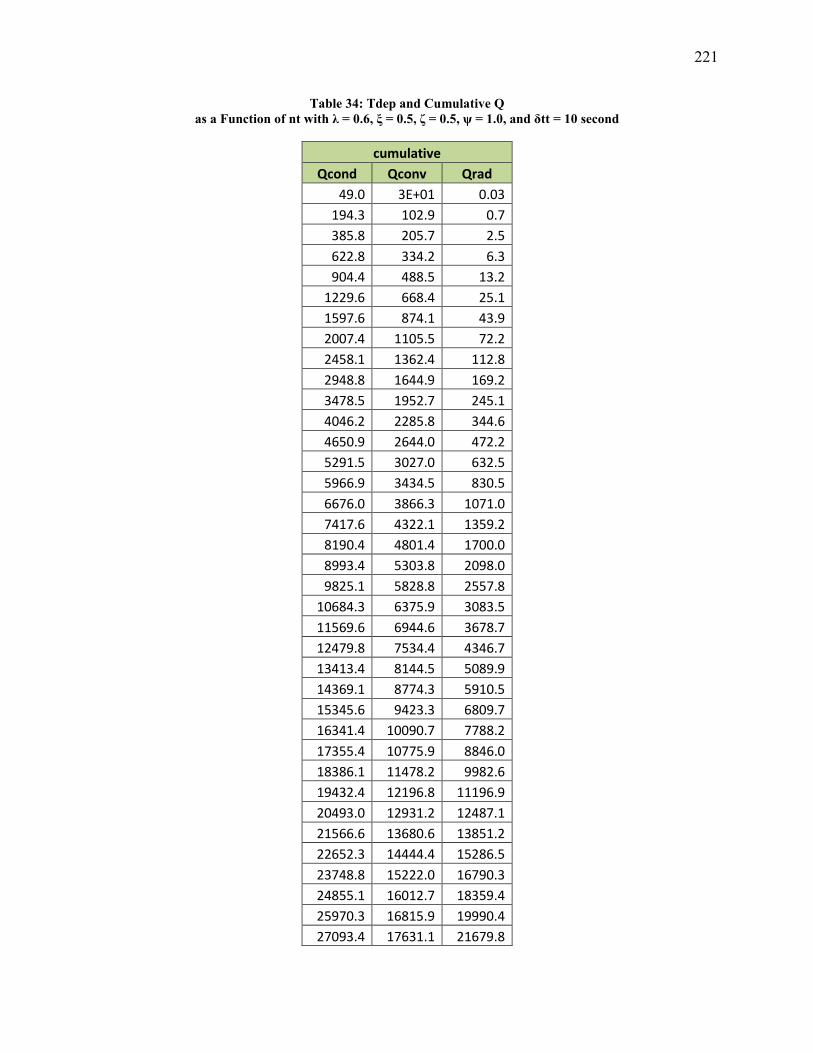
221

Table 34: Tdep and Cumulative Q


cumulative

Qcond Qconv Qrad

49.0 3E+01 0.03

194.3 102.9 0.7

385.8 205.7 2.5

622.8 334.2 6.3

904.4 488.5 13.2

1229.6 668.4 25.1

1597.6 874.1 43.9

2007.4 1105.5 72.2

2458.1 1362.4 112.8

2948.8 1644.9 169.2

3478.5 1952.7 245.1

4046.2 2285.8 344.6

4650.9 2644.0 472.2

5291.5 3027.0 632.5

5966.9 3434.5 830.5

6676.0 3866.3 1071.0

7417.6 4322.1 1359.2

8190.4 4801.4 1700.0

8993.4 5303.8 2098.0

9825.1 5828.8 2557.8

10684.3 6375.9 3083.5

11569.6 6944.6 3678.7

12479.8 7534.4 4346.7

13413.4 8144.5 5089.9

14369.1 8774.3 5910.5

15345.6 9423.3 6809.7

16341.4 10090.7 7788.2

17355.4 10775.9 8846.0

18386.1 11478.2 9982.6

19432.4 12196.8 11196.9

20493.0 12931.2 12487.1

21566.6 13680.6 13851.2

22652.3 14444.4 15286.5

23748.8 15222.0 16790.3

24855.1 16012.7 18359.4

25970.3 16815.9 19990.4

27093.4 17631.1 21679.8

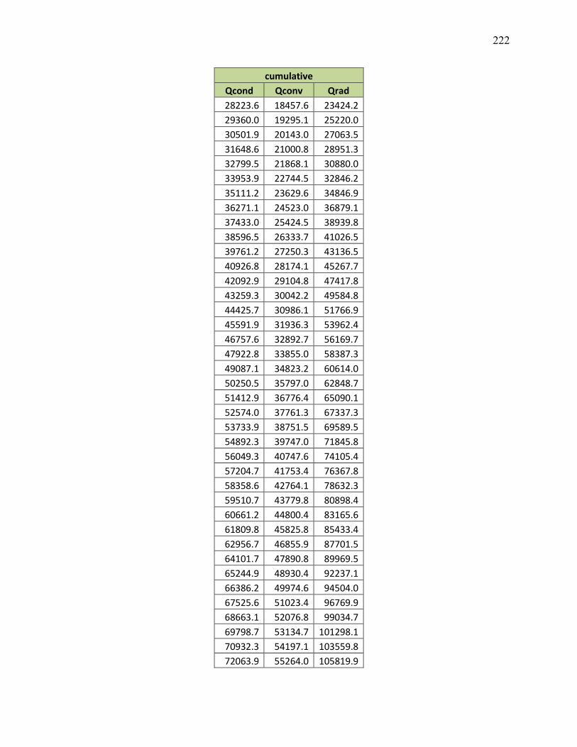
222

cumulative

Qcond Qconv Qrad

28223.6 18457.6 23424.2

29360.0 19295.1 25220.0

30501.9 20143.0 27063.5

31648.6 21000.8 28951.3

32799.5 21868.1 30880.0

33953.9 22744.5 32846.2

35111.2 23629.6 34846.9

36271.1 24523.0 36879.1

37433.0 25424.5 38939.8

38596.5 26333.7 41026.5

39761.2 27250.3 43136.5

40926.8 28174.1 45267.7

42092.9 29104.8 47417.8

43259.3 30042.2 49584.8

44425.7 30986.1 51766.9

45591.9 31936.3 53962.4

46757.6 32892.7 56169.7

47922.8 33855.0 58387.3

49087.1 34823.2 60614.0

50250.5 35797.0 62848.7

51412.9 36776.4 65090.1

52574.0 37761.3 67337.3

53733.9 38751.5 69589.5

54892.3 39747.0 71845.8

56049.3 40747.6 74105.4

57204.7 41753.4 76367.8

58358.6 42764.1 78632.3

59510.7 43779.8 80898.4

60661.2 44800.4 83165.6

61809.8 45825.8 85433.4

62956.7 46855.9 87701.5

64101.7 47890.8 89969.5

65244.9 48930.4 92237.1

66386.2 49974.6 94504.0

67525.6 51023.4 96769.9

68663.1 52076.8 99034.7

69798.7 53134.7 101298.1

70932.3 54197.1 103559.8

72063.9 55264.0 105819.9

223

cumulative

Qcond Qconv Qrad

73193.6 56335.3 108078.0

74321.4 57411.0 110334.2

75447.2 58491.1 112588.1

76571.0 59575.6 114839.9

77692.9 60664.5 117089.3

78812.8 61757.6 119336.3

79930.7 62855.1 121580.7

81046.7 63956.8 123822.7

82160.8 65062.9 126061.9

83272.9 66173.2 128298.6

84383.0 67287.7 130532.5

85491.3 68406.5 132763.6

86597.6 69529.4 134992.0

87702.0 70656.6 137217.5

88804.5 71788.0 139440.2

89905.1 72923.5 141660.0

91003.8 74063.2 143877.0

92100.6 75207.0 146091.0

93195.5 76355.0 148302.1

94288.6 77507.1 150510.2

95379.8 78663.3 152715.4

96469.2 79823.6 154917.7

97556.7 80988.0 157116.9

98642.5 82156.5 159313.3

99726.3 83329.0 161506.6

100808.4 84505.7 163697.0

101888.7 85686.3 165884.4

102967.2 86871.0 168068.8

104043.9 88059.8 170250.2

105118.8 89252.6 172428.6

106192.0 90449.3 174604.1

107263.4 91650.1 176776.6

108333.1 92854.9 178946.1

109401.1 94063.7 181112.7

110467.3 95276.4 183276.3

111531.8 96493.1 185436.9

112594.6 97713.8 187594.5

113655.7 98938.4 189749.2

114715.1 100167.0 191901.0

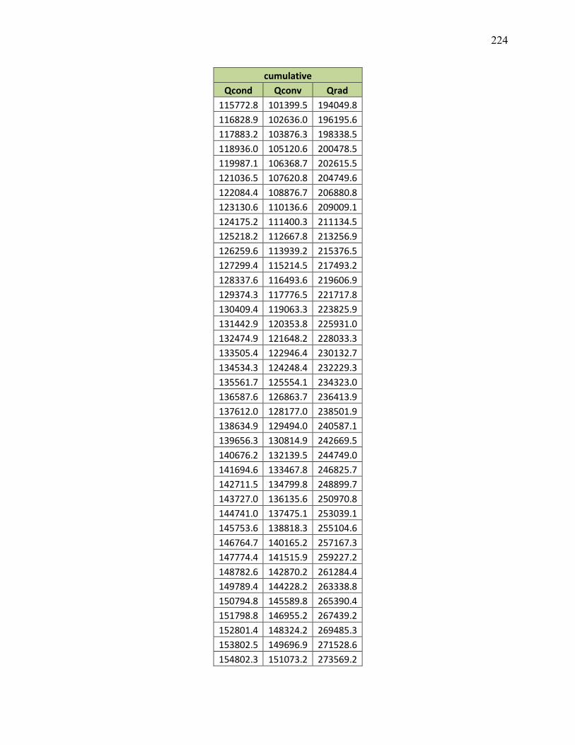
224

cumulative

Qcond Qconv Qrad

115772.8 101399.5 194049.8

116828.9 102636.0 196195.6

117883.2 103876.3 198338.5

118936.0 105120.6 200478.5

119987.1 106368.7 202615.5

121036.5 107620.8 204749.6

122084.4 108876.7 206880.8

123130.6 110136.6 209009.1

124175.2 111400.3 211134.5

125218.2 112667.8 213256.9

126259.6 113939.2 215376.5

127299.4 115214.5 217493.2

128337.6 116493.6 219606.9

129374.3 117776.5 221717.8

130409.4 119063.3 223825.9

131442.9 120353.8 225931.0

132474.9 121648.2 228033.3

133505.4 122946.4 230132.7

134534.3 124248.4 232229.3

135561.7 125554.1 234323.0

136587.6 126863.7 236413.9

137612.0 128177.0 238501.9

138634.9 129494.0 240587.1

139656.3 130814.9 242669.5

140676.2 132139.5 244749.0

141694.6 133467.8 246825.7

142711.5 134799.8 248899.7

143727.0 136135.6 250970.8

144741.0 137475.1 253039.1

145753.6 138818.3 255104.6

146764.7 140165.2 257167.3

147774.4 141515.9 259227.2

148782.6 142870.2 261284.4

149789.4 144228.2 263338.8

150794.8 145589.8 265390.4

151798.8 146955.2 267439.2

152801.4 148324.2 269485.3

153802.5 149696.9 271528.6

154802.3 151073.2 273569.2

225

cumulative

Qcond Qconv Qrad

155800.7 152453.1 275607.0

156797.7 153836.7 277642.1

157793.4 155223.9 279674.5

158787.6 156614.8 281704.1

159780.6 158009.3 283731.0

160772.1 159407.3 285755.2

161762.3 160809.0 287776.7

162751.2 162214.3 289795.5

163738.7 163623.1 291811.5

164724.8 165035.6 293824.9

165709.7 166451.6 295835.5

166693.2 167871.2 297843.5

167675.4 169294.3 299848.8

168656.3 170721.0 301851.4

169635.9 172151.3 303851.3

170614.2 173585.1 305848.6

171591.2 175022.4 307843.1

172566.9 176463.3 309835.1

173541.4 177907.7 311824.3

174514.5 179355.6 313810.9

175486.4 180807.0 315794.9

176457.0 182262.0 317776.2

177426.3 183720.4 319754.9

178394.4 185182.3 321730.9

179361.3 186647.7 323704.3

180326.9 188116.6 325675.1

181291.2 189589.0 327643.3

182254.3 191064.8 329608.8

183216.2 192544.1 331571.8

184176.8 194026.8 333532.1

185136.2 195513.0 335489.8

186094.5 197002.7 337444.9

187051.4 198495.7 339397.4

188007.2 199992.2 341347.4

188961.8 201492.2 343294.7

189915.2 202995.5 345239.5

190867.4 204502.3 347181.6

191818.4 206012.4 349121.2

192768.2 207526.0 351058.3

226

cumulative

Qcond Qconv Qrad

193716.8 209043.0 352992.8

194664.2 210563.3 354924.7

195610.5 212087.0 356854.0

196555.6 213614.1 358780.8

197499.6 215144.6 360705.1

198442.4 216678.5 362626.8

199384.0 218215.7 364545.9

200324.5 219756.2 366462.5

201263.8 221300.1 368376.6

202202.0 222847.4 370288.2

203139.1 224398.0 372197.2

204075.0 225951.9 374103.7

205009.8 227509.1 376007.7

205943.5 229069.7 377909.2

206876.0 230633.5 379808.2

207807.5 232200.7 381704.7

208737.8 233771.2 383598.6

209667.0 235345.0 385490.1

210595.1 236922.0 387379.1

211522.1 238502.4 389265.6

212448.0 240086.0 391149.6

213372.8 241672.9 393031.1

214296.5 243263.1 394910.2

215219.2 244856.5 396786.8

216140.7 246453.2 398660.9

217061.2 248053.2 400532.5

217980.6 249656.4 402401.7

218898.9 251262.8 404268.4

219816.2 252872.5 406132.7

220732.4 254485.4 407994.5

221647.5 256101.5 409853.8

222561.6 257720.8 411710.8

223474.6 259343.4 413565.3

224386.6 260969.1 415417.3

225297.5 262598.1 417266.9

226207.4 264230.3 419114.1

227116.3 265865.6 420958.9

228024.1 267504.2 422801.2

228930.9 269145.9 424641.2

227

cumulative

Qcond Qconv Qrad

229836.7 270790.8 426478.7

230741.4 272438.8 428313.8

231645.1 274090.1 430146.5

232547.8 275744.5 431976.8

233449.5 277402.0 433804.7

234350.1 279062.7 435630.2

235249.8 280726.6 437453.3

236148.5 282393.6 439274.0

237046.1 284063.7 441092.4

237942.8 285736.9 442908.3

238838.4 287413.3 444721.9

239733.1 289092.8 446533.1

240626.8 290775.4 448342.0

241519.4 292461.1 450148.5

242411.2 294149.9 451952.6

243301.9 295841.9 453754.3

244191.6 297536.9 455553.7

245080.4 299235.0 457350.8

INVESTIGATION IN THE USE OF PLASMA ARC WELDING AND ALTERNATIVE FEEDSTOCK DELIVERY METHOD IN ADDITIVE...

Documents

Transcript of INVESTIGATION IN THE USE OF PLASMA ARC WELDING AND ALTERNATIVE FEEDSTOCK DELIVERY METHOD IN ADDITIVE...