Inverse modeling of CO2 sources and sinks using satellite data: a synthetic inter-comparison of...

ACPD11, 4263–4311, 2011

Inverse modeling ofCO2 sources and

sinks

R. Nassar et al.

Title Page

Abstract Introduction

Conclusions References

Tables Figures

J I

J I

Back Close

Full Screen / Esc

Printer-friendly Version

Interactive Discussion

Discussion

Paper

|D

iscussionP

aper|

Discussion

Paper

|D

iscussionP

aper|

Atmos. Chem. Phys. Discuss., 11, 4263–4311, 2011www.atmos-chem-phys-discuss.net/11/4263/2011/doi:10.5194/acpd-11-4263-2011© Author(s) 2011. CC Attribution 3.0 License.

AtmosphericChemistry

and PhysicsDiscussions

This discussion paper is/has been under review for the journal Atmospheric Chemistryand Physics (ACP). Please refer to the corresponding final paper in ACP if available.

Inverse modeling of CO2 sources andsinks using satellite observations of CO2from TES and surface flaskmeasurementsR. Nassar1,*, D. B. A. Jones1, S. S. Kulawik2, J. R. Worden2, K. W. Bowman2,R. J. Andres3, P. Suntharalingam4, J. M. Chen5, C. A. M. Brenninkmeijer6,T. J. Schuck6, T. J. Conway7, and D. E. Worthy8

1Department of Physics, University of Toronto, 60 St. George Street, Toronto, Ontario, M5S1A7, Canada2Jet Propulsion Laboratory, California Institute of Technology, 4800 Oak Grove Drive,Pasadena CA, 91109, USA3Environmental Sciences Division, Oak Ridge National Laboratory, Oak Ridge, TN,37831-6335, USA4Environmental Sciences, University of East Anglia, Norwich, NR4 7TJ, UK5Department of Geography, University of Toronto, 45 St. George Street, Toronto, Ontario, M5S2E5, Canada

4263

http://www.atmos-chem-phys-discuss.net

http://www.atmos-chem-phys-discuss.net/11/4263/2011/acpd-11-4263-2011-print.pdf

http://www.atmos-chem-phys-discuss.net/11/4263/2011/acpd-11-4263-2011-discussion.html

http://creativecommons.org/licenses/by/3.0/

ACPD11, 4263–4311, 2011


sinks

R. Nassar et al.

Title Page



Tables Figures

J I

J I

Back Close

Full Screen / Esc



Discussion

Paper

|D

iscussionP

aper|

Discussion

Paper

|D

iscussionP

aper|

6 Max-Planck-Institut fur Chemie, Air Chemistry Division, Mainz, Germany7 Earth System Research Laboratory, National Oceanic and Atmospheric Administration,Boulder, CO, 80305-3337, USA8 Climate Research Division, Environment Canada, 4905 Dufferin St., Toronto, Ontario, M3H5T4, Canada∗ now at: Climate Research Division, Environment Canada, 4905 Dufferin St., Toronto, Ontario,M3H 5T4, Canada

Received: 19 December 2010 – Accepted: 24 January 2011 – Published: 7 February 2011

Correspondence to: R. Nassar ([email protected])

Published by Copernicus Publications on behalf of the European Geosciences Union.

4264





ACPD11, 4263–4311, 2011


sinks

R. Nassar et al.

Title Page



Tables Figures

J I

J I

Back Close

Full Screen / Esc



Discussion

Paper

|D

iscussionP

aper|

Discussion

Paper

|D

iscussionP

aper|

Abstract

We infer CO2 surface fluxes using satellite observations of mid-tropospheric CO2 fromthe Tropospheric Emission Spectrometer (TES) and measurements of CO2 from sur-face flasks in a time-independent inversion analysis based on the GEOS-Chem model.Using TES CO2 observations over oceans, spanning 40◦ S–40◦ N, we find that the hor-5

izontal and vertical coverage of the TES and flask data are complementary. This com-plementarity is demonstrated by combining the datasets in a joint inversion, whichprovides better constraints than from either dataset alone, when a posteriori CO2 dis-tributions are evaluated against independent ship and aircraft CO2 data. In particular,the joint inversion offers improved constraints in the tropics where surface measure-10

ments are sparse, such as the tropical forests of South America, which the joint inver-sion suggests was a weak sink of −0.17±0.20 Pg C in 2006. Aggregating the annualsurface-to-atmosphere fluxes from the joint inversion yields −1.13±0.21 Pg C for theglobal ocean, −2.77±0.20 Pg C for the global land biosphere and −3.90±0.29 Pg Cfor the total global natural flux (defined as the sum of all biospheric, oceanic, and15

biomass burning contributions but excluding CO2 emissions from fossil fuel combus-tion). These global ocean, global land and total global fluxes are shown to be in therange of other inversion results for 2006. To achieve these results, a latitude dependentbias in TES CO2 in the Southern Hemisphere was assessed and corrected using air-craft flask data, and we demonstrate that our results have low sensitivity to variations20

in the bias correction approach. Overall, this analysis suggests that future carbon dataassimilation systems can benefit by integrating in situ and satellite observations of CO2and that the vertical information provided by satellite observations of mid-troposphericCO2 combined with measurements of surface CO2, provides an important additionalconstraint for flux inversions.25

4265





ACPD11, 4263–4311, 2011


sinks

R. Nassar et al.

Title Page



Tables Figures

J I

J I

Back Close

Full Screen / Esc



Discussion

Paper

|D

iscussionP

aper|

Discussion

Paper

|D

iscussionP

aper|

1 Introduction

Inverse modeling has emerged as a key method for obtaining quantitative informationon the global carbon cycle. In this approach, CO2 measurements are combined withCO2 distributions from a 3-dimensional (3-D) transport model, weighting them accord-ing to their uncertainties in order to produce optimized estimates of surface source and5

sink strengths (fluxes). The terrestrial biospheric flux is the component of the globalcarbon cycle that currently exhibits the most interannual variability, the most geograph-ical heterogeneity and the greatest uncertainty (Denman et al., 2007, Ch.7, AR4). It isprimarily responsible for the high variability in the inferred global annual mean increaseof atmospheric CO2 near the surface, which has fluctuated between 0.67 to 2.90 ppm10

throughout the 1980 to 2010 period (www.esrl.noaa.gov/gmd/ccgg/trends). Strong evi-dence suggests a link to variations in the climate system, such as the El Nino SouthernOscillation (Bacastow, 1976; Keeling et al., 1995; Heimann and Reichstein, 2008), buta thorough understanding of these mechanisms is lacking and the ability to predictfuture global CO2 increases is still poor as a result of uncertainty in the strength and15

the spatial distribution of terrestrial CO2 sources and sinks on regional scales. Theuncertainty in surface fluxes remains a major issue for carbon cycle science, with fun-damental questions such as the latitudinal distribution of natural sources and sinks stillbeing revisited (Stephens et al., 2007).

For more than two decades, inverse modeling has been used to estimate biospheric20

CO2 fluxes (e.g., Tans et al., 1989; Enting and Mansbridge, 1989, Fan et al., 1998;Rodenbeck et al., 2003; Rodenbeck, 2005; Baker et al., 2006; Deng et al., 2007; Pe-ters et al., 2007; Chevallier et al., 2010a) using in situ observations from instruments atsurface stations, towers, ships and aircraft and/or flask samples collected from theseplatforms, then later analyzed in a laboratory (Conway et al., 1994). Measurement25

coverage has increased over the years, and forward and inverse modeling techniqueshave also improved, but a major limitation in achieving further reductions in CO2 fluxuncertainties is the sparse data coverage that remains throughout the tropics, extra-

4266





www.esrl.noaa.gov/gmd/ccgg/trends

ACPD11, 4263–4311, 2011


sinks

R. Nassar et al.

Title Page



Tables Figures

J I

J I

Back Close

Full Screen / Esc



Discussion

Paper

|D

iscussionP

aper|

Discussion

Paper

|D

iscussionP

aper|

tropical South America and Africa, throughout Boreal Asia and the Southern Hemi-sphere’s oceans. Figure 1 shows the stationary flask sampling locations from the Na-tional Oceanic and Atmospheric Administration (NOAA) and Environment Canada (EC)networks that collected data in 2006 (our year of investigation), along with additionalship-based and aircraft based sampling locations for that year. Although there are ad-5

ditional flask measurements (as well as other types of CO2 measurements) worldwidethat are made by other organizations, logistical, financial and political reasons will con-tinue to make it difficult to develop on-site measurement or sample collection capabilityin remote areas such as those mentioned above. Satellite observations, therefore, of-fer a means to measure CO2 without the spatial limitations of the current observing10

networks.Multiple Observing System Simulation Experiments (OSSEs), which use simulated

data, have explored the benefit of satellite observations of CO2 for inverse modelingof CO2 surface fluxes (Rayner and O’Brien, 2001; Pak and Prather, 2001; Houwelinget al., 2004; Baker et al., 2006a; Chevallier et al., 2007; Miller et al., 2007; Kadygrov15

et al., 2009; Hungershoefer et al., 2010). Although satellite observations of CO2 donot match the high precision of in situ or flask measurements, these studies all showthat the greatly increased data coverage provided by satellites can improve CO2 fluxestimates. At the same time, it is clear that the extent to which this potential canbe realized depends largely on the measurement characteristics of the different satel-20

lite instruments. CO2 has been retrieved from spectra recorded by multiple satelliteinstruments, although the majority of these instruments were not originally designedfor this purpose. They include the Television Infrared Observation Satellite (TIROS)Operational Vertical Sounder (TOVS) (Chedin et al., 2003), the Atmospheric InfraredSounder (AIRS) (Chahine et al., 2008), the Tropospheric Emission Spectrometer (TES)25

(Kulawik et al., 2010) and the Interferometric Atmospheric Sounding Instrument (IASI)(Crevoisier et al., 2009), which measure CO2 using thermal/mid-infrared emission andthe Scanning Imaging Absorption Spectrometer for Atmospheric Chartography (SCIA-MACHY) (Buchwitz et al., 2007), which measures CO2 using near-infrared reflected

4267





ACPD11, 4263–4311, 2011


sinks

R. Nassar et al.

Title Page



Tables Figures

J I

J I

Back Close

Full Screen / Esc



Discussion

Paper

|D

iscussionP

aper|

Discussion

Paper

|D

iscussionP

aper|

sunlight from the land surface. Few studies have inferred CO2 surface flux estimatesfrom real space-based CO2 observations. Chevallier et al. (2005) was the first study,using TOVS CO2 observations which have peak sensitivity in the upper troposphere(∼150 hPa), but concluded that the retrieved surface fluxes were unrealistic. In a morerecent analysis, Chevallier et al. (2009) directly assimilate AIRS radiances, but con-5

clude that an AIRS-based CO2 inversion performs worse than a surface flask-basedinversion. The weighting functions of the AIRS radiances of Chevallier et al. (2009)are provided in Engelen et al. (2009) and show that the sensitivity to tropospheric CO2peaks in the upper troposphere, where the impacts of surface flux perturbations onatmospheric CO2 are weakened by vertical transport.10

New measurements from the Greenhouse Gases Observing Satellite (GOSAT)(Yokota et al., 2009; Yoshida et al., 2010) and the upcoming Orbiting Carbon Observa-tory 2 (OCO-2) (Crisp et al., 2004; Miller et al., 2007) offer far greater sensitivity to CO2near the surface by measuring near-infrared CO2 spectral features and the O2 A-bandusing sunlight reflected from Earth’s surface to derive total atmospheric CO2 columns15

over both land and ocean. These new satellite data are expected to improve our un-derstanding of carbon cycle processes, especially when used in combination with thealready available measurement sets with longer observational records. This conceptof jointly assimilating observations from satellites and in situ data has been suggestedto be the most promising method for constraining CO2 fluxes by inverse modeling in20

the near future (Pak and Prather, 2001; Chevallier et al., 2009; Hungershoefer et al.,2010).

In this paper, we use the GEOS-Chem model’s CO2 simulation (Nassar et al., 2010)to examine the constraints on estimates of biospheric and oceanic fluxes of CO2 pro-vided by TES CO2 observations (Kulawik et al., 2010) and surface flask measurements25

of CO2 (Conway et al., 1994). TES CO2 observation sensitivity peaks in the mid-troposphere, but because this sensitivity strongly depends on temperature, the TESCO2 estimates are typically limited to latitudes between 40◦ S–40◦ N. Independently,TES CO2 observations over oceans provide a weaker constraint on global CO2 surface

4268





ACPD11, 4263–4311, 2011


sinks

R. Nassar et al.

Title Page



Tables Figures

J I

J I

Back Close

Full Screen / Esc



Discussion

Paper

|D

iscussionP

aper|

Discussion

Paper

|D

iscussionP

aper|

fluxes than data from the surface flask networks, but we demonstrate that these TESCO2 observations can be used together with the flask data to obtain improved esti-mates of CO2 surface fluxes. We find that the vertical sensitivity and horizontal cov-erage provided by the satellite and flask data are complementary and we show that aCO2 flux inversion combining these data sources gives the greatest flux uncertainty re-5

duction and the best agreement with independent ship-based and aircraft-based flaskdata. The integration of satellite observations of CO2 and surface flask CO2 data in thiswork is an important step toward the development of more sophisticated operationalcarbon assimilation systems in the future.

2 Method10

Data assimilation provides a statistical framework for combining data sources with nu-merical models of the Earth system, weighting each according to their uncertainties.The application of this concept to inverse modeling of CO2 fluxes involves integratinga forward model simulation and a set of observations to optimize the CO2 fluxes at thesurface. The details regarding the various components of our inverse modeling work15

are provided in the following subsections.

2.1 GEOS-Chem simulated CO2

GEOS-Chem (http://acmg.seas.harvard.edu/geos) is a 3-D chemical transport model(Bey et al., 2001) that uses Goddard Earth Observing System (GEOS) assimilatedmeteorology from the NASA Global Modeling and Assimilation Office (GMAO). The20

original GEOS-Chem CO2 simulation was described in Suntharalingam et al. (2004).In this work, we use version 8-02-01 with updates to the model that were presentedin Nassar et al. (2010), and are now included in v8-03-02 and subsequent versions.We simulate CO2 at a horizontal resolution of 2◦ latitude×2.5◦ longitude with 47 ver-tical levels from the surface to 0.01 hPa. Our forward simulations include CO2 fluxes25

4269





http://acmg.seas.harvard.edu/geos

ACPD11, 4263–4311, 2011


sinks

R. Nassar et al.

Title Page



Tables Figures

J I

J I

Back Close

Full Screen / Esc



Discussion

Paper

|D

iscussionP

aper|

Discussion

Paper

|D

iscussionP

aper|

from fossil fuel combustion (including emissions from shipping and aviation), cementproduction, ocean processes, the terrestrial biosphere (photosynthesis, respiration,biomass/biofuel burning) and the chemical production of CO2 from the atmosphericoxidation of other carbon species. Specific inventories used in our work are givenin Table 1 and a detailed description of their implementation is given in Nassar et5

al. (2010), where emphasis was placed on improving anthropogenic-related invento-ries, since these are not optimized in our flux inversion. In the present context, biomassburning and biofuel burning are considered “natural” rather than anthropogenic fluxes,since they relate to the biosphere even though they also involve anthropogenic activity.

The use of a global inventory of national fossil fuel combustion emissions with10

monthly variability (Andres et al., 2011), and the 3-D representation of CO2 emissionsfrom aviation and the chemical production of CO2 from the oxidation of other carbonspecies (CO, CH4 and other organics) in the troposphere are unique to our CO2 fluxinversions. Since this 3-D chemical production of CO2 (∼1.05 Pg C/yr) is typically notaccounted for in models, many emission inventories count CO2 precursor species (CO,15

CH4 and other carbon gases) as direct CO2 emissions at the surface in an attempt tobalance total CO2. This leads to a reasonable estimate of total CO2 over time, but anincorrect spatial distribution, since real chemical production of CO2 from these speciesoccurs at different times and locations from emission. The impact of neglecting the 3-Ddistribution of CO2 from the oxidation of other carbon species on the latitudinal gradient20

is demonstrated in Nassar et al. (2010). Omission of this capability from CO2 surfaceflux inversions has previously been shown to result in an overestimate of the northernland sink by ∼0.25 Pg C/yr (Suntharalingam et al., 2005). As discussed in Nassar etal. (2010), representing the chemical production of CO2 (∼1.05 Pg C/yr) and emissionof CO2 from aviation fossil fuel use (∼0.16 Pg C/yr), both of which are 3-D sources, is of25

increased importance when making model comparisons to CO2 satellite observations,especially those which have peak sensitivity significantly above the surface, such asTES CO2.

4270





ACPD11, 4263–4311, 2011


sinks

R. Nassar et al.

Title Page



Tables Figures

J I

J I

Back Close

Full Screen / Esc



Discussion

Paper

|D

iscussionP

aper|

Discussion

Paper

|D

iscussionP

aper|

Our model simulation was initialized on 1 January 2004 with a globally-uniform 3-DCO2 field of 375 ppm. Beginning the simulation from this state allows model transportand fluxes to reproduce the large-scale features of the CO2 distribution over time. Sim-ulations using this approach were evaluated in Nassar et al. (2010), where it was shownthat spinning up the model from this initial state produced CO2 distributions for 20065

that were in good agreement with independent data. In order to obtain even better ini-tial conditions for the start of the flux inversion on 1 January 2006, in the present work,we assimilated surface CO2 data from the stationary NOAA flask sites throughout 2004and 2005. Comparing the unconstrained model simulation and the assimilated CO2 in2005 with independent data comprised of over 800 ship-based flask measurements10

(which have a distribution very similar to that in Fig. 1) demonstrates this improvement.The 2005 annual model bias determined for all the ship-based flask measurementpoints was −0.37 ppm without assimilation, which is reduced to −0.15 ppm by assimi-lating the stationary flask observations.

2.2 TES CO215

TES is a nadir-viewing Fourier transform spectrometer on the Aura satellite, which is atthe back of the A-train in a 705 km sun-synchronous near-polar orbit with an equatorcrossing time of ∼13:40 (Beer et al., 2001). The retrieval of TES CO2 is described inKulawik et al. (2010) and an example showing two months of the TES data is providedin Fig. 2. In the present work, we focus on 2006, the first full year of TES CO2 data.20

Analysis of subsequent years will be carried out in future work. Since TES was not de-signed to produce measurements for carbon cycle science, it was not optimized for thispurpose and has low sensitivity to CO2 near the surface. TES observation sensitivityto CO2 ranges from approximately 800 hPa to the tropopause with a peak sensitivityin the middle troposphere (near 511 hPa or 5 km altitude). Because this sensitivity25

strongly depends on the thermal contrast between the surface and the atmosphere, itdecreases sharply poleward of 40◦ latitude; therefore CO2 data beyond this latitude arenot used in this work. Despite these limitations, TES CO2 data offer a few advantages

4271





ACPD11, 4263–4311, 2011


sinks

R. Nassar et al.

Title Page



Tables Figures

J I

J I

Back Close

Full Screen / Esc



Discussion

Paper

|D

iscussionP

aper|

Discussion

Paper

|D

iscussionP

aper|

for inverse modeling of CO2 surface sources and sinks that are not often recognized.Firstly, the TES CO2 retrieval peaks at a lower altitude than standard CO2 data prod-ucts from other thermal infrared sounders such as AIRS (Chahine et al., 2005) andIASI (Crevoisier et al., 2009), based on the spectral windows selected for the retrieval(Kulawik et al., 2010). As a result TES CO2 observations should contain stronger5

signatures from surface fluxes. Secondly, although TES provides less global coveragethan some other satellite instruments, it has the smallest footprint (5.3×8.3 km2) of anyspace-borne instrument now measuring CO2, giving it the highest proportion of obser-vations with negligible cloud interference. Thirdly, measurement of thermal infraredemission permits both day and night observations, which should reduce the diurnal10

sampling bias that is implicit to instruments measuring CO2 using reflected sunlightsuch as SCIAMACHY (Buchwitz et al., 2007), the GOSAT TANSO-FTS (Yokota et al.,2009; Yoshida et al., 2010) and OCO-2 (Crisp et al., 2004; Miller et al., 2007).

The TES retrievals are reported on five pressure levels (the surface, 511, 133, 10,and 0.1 hPa), which were selected to minimize the contribution of a priori information to15

the retrievals, while not incurring a significant increase in vertical representation error.The retrievals are conducted with respect to the logarithm of the volume mixing ratio ofCO2 and can be expressed as a linear expansion around the a priori state xa,

x=xa+A(xt−xa)+GxεT (1)

where x is the logarithm of the CO2 profile from the TES retrieval, xt is the logarithm20

of the true atmospheric CO2 profile, A is the TES averaging kernel matrix (Worden etal., 2004; Bowman et al., 2006), Gx is the gain matrix and εT is the TES measurementnoise vector. As shown in Kulawik et al. (2010), the averaging kernels peak in themid-troposphere near 511 hPa and span ∼800 hPa to lower edge of the tropopause,indicating a profile with coarse vertical resolution rather than a total column. In our25

analysis we, therefore, use only the retrieval values at the 511 hPa level in the retrievedprofile given by Eq. (1).

4272





ACPD11, 4263–4311, 2011


sinks

R. Nassar et al.

Title Page



Tables Figures

J I

J I

Back Close

Full Screen / Esc



Discussion

Paper

|D

iscussionP

aper|

Discussion

Paper

|D

iscussionP

aper|

The uncertainty on a single TES CO2 observation is about 10 ppm (Kulawik et al.,2010), which primarily consists of a random component with an additional bias compo-nent. Under the assumption that the measurement uncertainty is uncorrelated betweenobservations, the precision of N averaged observations improves according to

√N (Da-

ley, 1991). However, the more individual observations averaged in a bin, the fewer bins5

there will be for the inversion. Kulawik et al. (2010) demonstrated that for monthly-averaging at bin sizes of 10◦ ×10◦, 15◦ ×15◦ and 20◦ ×30◦, the tradeoff between in-creased precision and a decreased number of bins nearly balances, with a very slightadvantage to smaller bins. In this work, we average the TES observations at 5◦ ×5◦

to improve precision while maintaining a high number of bins. Dealing with biases in10

TES CO2 is more challenging. Biases can arise from errors in the spectroscopic pa-rameters or from spectral lines due to other species interfering with the retrieval. In thecurrent version of TES CO2, a global bias correction of +2.1% was applied, which gavethe best agreement with independent data (Kulawik et al., 2010), although the lack ofavailable CO2 data from other sources at suitable altitudes for comparison presents a15

challenge in quantifying TES CO2 biases. For determining remaining biases in TESCO2 data, we use aircraft flask measurements from the Comprehensive ObservationNetwork for TRace gases by AIrLiner (CONTRAIL) on flights between Japan and Aus-tralia (Matsueda et al., 2008; Machida et al., 2008). Although CONTRAIL data areprimarily gathered at higher altitudes (∼10–11 km) than the peak of TES CO2 sensitiv-20

ity (∼5 km), they are representative of the free troposphere with minimal stratosphericinfluence. We have adjusted the TES CO2 data for this work using various approaches(discussed in Sect. 3.3) based on comparisons between TES and CONTRAIL data.

The data used in this work have been filtered to remove observations with a cloudeffective optical depth greater than 0.50, since thicker clouds reduce sensitivity and25

can contribute to biases and errors. Although TES CO2 retrievals are carried out overboth land and ocean, the retrievals over land in the current version of TES CO2 suf-fer from spatially dependent biases likely due to surface silicate emissivity features inthe spectra that are not accounted for in the retrievals, so in the present work, only

4273





ACPD11, 4263–4311, 2011


sinks

R. Nassar et al.

Title Page



Tables Figures

J I

J I

Back Close

Full Screen / Esc



Discussion

Paper

|D

iscussionP

aper|

Discussion

Paper

|D

iscussionP

aper|

TES observations over the oceans are used. A newer version of TES CO2 data,based on retrievals that have accounted for spectral features from silicate emissivityand other interferents, is being processed, which shows clear improvements in com-parisons with independent CO2 data. Application of this upcoming version of TES CO2data is expected to lead to improved CO2 surface flux inversions, but will be left for fu-5

ture work. Since TES CO2 data over land have not been used, the flask data discussedin Sect. 2.3 are the only data collected over the land used in this work, however, theability of TES CO2 observations over ocean to constrain terrestrial sources and sinksis discussed in Sect. 3.1.

Figure 2 shows an example of two months of 5◦ ×5◦ monthly-averaged CO2 at10

511 hPa from TES along with CO2 simulated by GEOS-Chem. The model was sampledat the TES observation locations and times, within ±1 h, and was transformed with theTES observation operator, discussed in Sect. 2.5, to account for the low vertical res-olution of the retrieval. The TES – model difference (corresponding to the differenceof the two panels) is also shown. The large scale spatial patterns seen in the TES15

CO2 distribution, such as the latitudinal gradient at the start of the NH growing seasonin May are also seen in the model CO2 distribution; however, the model distribution ismuch smoother with smaller differences between maximum and minimum values.

2.3 Flask CO2

Figure 1 illustrates the locations of the 59 National Oceanic and Atmospheric Admin-20

istration Earth System Research Laboratory Global Monitoring Division (NOAA-ESRL-GMD) and Environment Canada (EC) stationary sampling sites used in this work aswell as NOAA ship-based sample collection locations in the central and western Pa-cific Ocean, and the Drake Passage. Figure 1 also shows the sampling locations foraircraft flask CO2 from CONTRAIL (described above) and CARIBIC (Civil Aircraft for25

the Regular Investigation of the atmosphere Based on an Instrument Container) (Bren-ninkmeijer et al., 2007; Schuck et al., 2009) flights between Frankfurt, Germany andSouth America or Asia. These ship and aircraft flask data are not used in the inversion,

4274





ACPD11, 4263–4311, 2011


sinks

R. Nassar et al.

Title Page



Tables Figures

J I

J I

Back Close

Full Screen / Esc



Discussion

Paper

|D

iscussionP

aper|

Discussion

Paper

|D

iscussionP

aper|

but only as an independent source of data for evaluation (ship and CARIBIC) or forcorrection of biases (CONTRAIL) in TES CO2 data.

Flask samples of whole air enable highly accurate and precise measurements ofCO2 (Conway et al., 1994) in a laboratory setting. The 1-σ measurement accuracydetermined from repeated analyses of CO2 from standard gas cylinders is ∼0.2 ppm.5

Significant effort is devoted to tracing calibration of the measurements to World Meteo-rological Organization (WMO) standards to put the CO2 values on this absolute scale.The 1-σ measurement precision determined from repeated instrumental analyses ofthe same air sample is ∼0.1 ppm. Routine intercomparisons between flask samplepairs collected in series at the same location are used to flag measurements with pair10

differences greater than 0.5 ppm, which have been excluded from our work. The long-term mean difference between pairs of flasks throughout the networks is ∼0.2 ppm,while for 2006 (the year of this investigation), the global mean difference between pairswas ∼0.1 ppm. Although the accuracy and precision of flask measurements are high,the uncertainties assigned to the data for inverse modeling are larger, since they must15

account for additional factors.The observation uncertainties for the flask inversion εF are calculated using the

statistics of the differences between the observations and the model simulation of theobservations using the a priori emissions (e.g. Palmer et al., 2003; Heald et al., 2004)

εF =xF−G(u)=εf+εr+εm+b (2)20

where εf are the flask measurement errors, εr are the representativeness errors, εmare the model errors, and b is the bias. Ensuring that the errors have mean values ofzero, we define the bias as the expectation of the difference between the model andobservations b= 〈xF−G(u)〉. This bias reflects the effects of systematic errors in themodel transport as well as discrepancies in the a priori flux estimates in the model.25

The observation error covariance, therefore, is calculated as

SF =⟨

(xF−G(u)−b)(xF−G(u)−b)T⟩

(3)

4275





ACPD11, 4263–4311, 2011


sinks

R. Nassar et al.

Title Page



Tables Figures

J I

J I

Back Close

Full Screen / Esc



Discussion

Paper

|D

iscussionP

aper|

Discussion

Paper

|D

iscussionP

aper|

We neglect horizontal correlations between the flask observation locations and assumethat the matrix is diagonal. Each element of the diagonal is based in the timeseries ofdata for 2006 at a given flask observation location. Because of the high precision ofthe flask data, the largest contribution to SF

ii comes from the representativeness error,which arises from the fact that flask measurements are essentially a point source when5

compared with a model grid box (∼50 000 km2 in this work), which has significant sub-grid variability, particularly over land in the daytime near strong flux regions (Gerbiget al., 2003a, b). In constructing the monthly averages of the flask data we do notdivide by

√N since representativenss errors do not necessarily average with more

measurements due to the fact that a gridbox has some random variability and some10

systematic variability, although we have ensured that 〈εf +εr +εm〉=0, as required forthe inversion approach. For example, the error associated with using a Mauna Loaflask measurement to represent the entire grid cell is primarily systematic and relatesto properties like the sharp altitude gradient (Nassar et al., 2010).

2.4 Flux region definitions and a priori error specification15

The TransCom3 project (i.e. Gurney et al., 2002; Baker et al., 2006b) divided the Earthinto a set of standard regions, namely 11 land, 11 ocean and one region where zeroflux is assumed (mainly consisting of Antarctica and Greenland). We use the sameocean regions but divide the land into 28 eco-regions based on geography and domi-nant vegetation types determined by the Advanced Very High Resolution Radiometer20

(AVHRR) (Hansen et al., 1998, 2000) to provide more detailed information about sur-face fluxes and reduce aggregation errors. An additional low-flux region consisting ofAntarctica, Greenland and a few isolated islands is also defined, which we refer to asthe Rest of the World (ROW). Theses 40 regions are explicitly identified in Kulawik etal. (2010) and are evident in Fig. 3.25

We allocate uncertainties to our a priori model terrestrial biospheric fluxes based onthe a posteriori uncertainties of Baker et al. (2006b), since these fluxes were used inthe derivation of our terrestrial flux climatology. The Baker et al. (2006b) uncertainties

4276





ACPD11, 4263–4311, 2011


sinks

R. Nassar et al.

Title Page



Tables Figures

J I

J I

Back Close

Full Screen / Esc



Discussion

Paper

|D

iscussionP

aper|

Discussion

Paper

|D

iscussionP

aper|

are disaggregated from 11 regions to our 28 as described in the appendix. Our a prioritotal biospheric flux with 1-σ uncertainty is −2.31±1.26 Pg C (assuming the uncertain-ties are uncorrelated and applying a sum of squares approach to combine the regionaluncertainties). The ocean fluxes used from Takahashi et al. (2009) were not providedwith regional uncertainty estimates, but Gruber et al. (2009) carried out an ocean inver-5

sion that agreed well with the Takahashi et al. (2009) climatology, in virtually all areasexcept for the southern ocean. Therefore, we apply the Gruber et al. (2009) a posterioriuncertainties as our prior uncertainties in this inversion so our global total ocean fluxwith 1-σ uncertainty is −1.41±0.33 Pg C. Since the fossil fuel combustion fluxes (in-cluding shipping and aviation) are held fixed (as in TransCom3 and most flux inversion10

work) and not optimized, any errors in their assumed values contribute to a posteriorierrors in terrestrial biosphere and ocean fluxes. This approach is also applied to ourCO2 production from oxidation of other carbon species.

Our a priori flux uncertainties are uncorrelated, therefore our a priori error covari-ance matrix Sa is diagonal; however, a posteriori uncertainties for land biospheric flux15

regions are correlated according to off-diagonal elements of the a posteriori covariancematrix that results from inversion (as in Baker et al., 2006b). As a result, the a poste-riori uncertainty for the aggregation of land regions will be lower than an uncorrelatedvalue based on summing the squares. Although, correlations could also be applied tothe ocean a posteriori uncertainties, or between ocean and land regions, this avoided20

here since it results in unrealistically low a posteriori uncertainties for the aggregatedglobal ocean or total global flux.

2.5 Inverse modeling approach

To quantify the CO2 terrestrial biosphere and ocean surface fluxes we use the maxi-mum a posteriori (MAP) approach described in Jones et al. (2003, 2009), in which we25

minimize the following cost function:

J(u)= (x−xm(u))TSε(x−xm(u))+ (u−ua)TS−1a (u−ua) (4)

4277





ACPD11, 4263–4311, 2011


sinks

R. Nassar et al.

Title Page



Tables Figures

J I

J I

Back Close

Full Screen / Esc



Discussion

Paper

|D

iscussionP

aper|

Discussion

Paper

|D

iscussionP

aper|

where x= (x,xF)T is the observation vector that consists of the TES CO2 retrievals x atthe 511 hPa level and the flask CO2 data at the surface xF, xm(u)= (F(u),G(u))T is themodel simulation of the observations, u is the state vector with elements representingthe CO2 flux from the regions described in Sect. 2.5, ua is the a priori state vector, Sa isthe a priori covariance matrix for the fluxes, and Sε is the observation error covariance5

matrix. We conduct a time-independent inversion in which x consists of all the monthlymean TES and flask data for 2006. Although the a priori fluxes are specified on amonthly basis, the inversion provides an optimized estimate of the annual mean fluxes.The seasonal variability of the fluxes is not adjusted in the inversion. It is used as a harda priori constraint. The observation error consists of the TES and the flask observation10

errors

Sε =

(ST 00 SF

)(5)

where ST is the TES observation error, provided with the TES retrievals, and SF isthe flask observation error. G(u) is the forward model which reflects the transportof the CO2 fluxes in the GEOS-Chem model, with the model sampled at the flask15

observation locations and times, and F(u) is the forward model that incorporates theTES observation operator (which accounts for the TES sensitivity and a priori profileas described in Eq. 1). Both the TES retrieval x and the forward model simulation ofthe TES observations are expressed with respect to the natural logarithm of the CO2volume mixing ratio (VMR). The forward model F(u) is given by:20

F(u)=xa+A(ln[H(u)−xa) (6)

where H(u) is the modeled CO2 profile interpolated onto the TES retrieval grid, xais the TES a priori (given in terms of the logarithm of the CO2 mixing ratio), and Ais the TES averaging kernel. Although we use only the 511 hPa level in F(u), wemust transform the modeled profile using Eq. (4) to account for the vertical smoothing25

of the TES retrieval. Since the TES retrievals at 511 hPa have some sensitivity to4278





ACPD11, 4263–4311, 2011


sinks

R. Nassar et al.

Title Page



Tables Figures

J I

J I

Back Close

Full Screen / Esc



Discussion

Paper

|D

iscussionP

aper|

Discussion

Paper

|D

iscussionP

aper|

CO2 in the lower stratosphere (Kulawik et al., 2010), and because the GEOS-ChemCO2 simulation has not been validated in the stratosphere, we minimize the impact ofbiases in the modeled stratospheric CO2 on the inversion by removing the mean biasbetween GEOS-Chem and TES CO2 at 133 hPa and 10 hPa before application of theTES observation operator.5

The optimal estimate or a posteriori estimate of the state vector that minimizes thecost function is given by

u=ua+SaKT(KSaKT+Sε)−1(x−xm(ua)) (7)

where u is the optimized state vector and K=∂xm(u)/∂u is the Jacobian, which givesthe sensitivity of the CO2 abundances to the surface fluxes. We solve for Eq. (7) using10

the sequential update algorithm described in Jones et al. (2003). The Jacobian wasestimated using separate tracers for the CO2 from each region in the state vector. Thedistribution of these tracers was spun up in a 2-year run, starting on 1 January 2005,and were archived every two model hours.

3 Results and discussion15

3.1 Regional flux estimates

Figure 3 shows the natural terrestrial and oceanic CO2 flux estimates from the a priori,the flask inversion, the TES inversion, and the joint TES-Flask inversion. Values forthe annual global ocean-atmosphere flux, global land-atmosphere flux and total globalsurface-atmosphere flux are provided on the figure. While the total annual global CO220

flux from the a priori and the a posteriori results (the bottom number on each panel)differ by only ∼8% (−3.6 to −3.9 Pg C/yr), much larger differences are seen at regionalscales, specifically for the land regions. Strong sinks were a common feature in the apriori and a posteriori results for Europe, US, Mexico, Boreal Asia, Central Asia, Japan,southern Africa, Australia and New Zealand, while sources were common for Central25

4279





ACPD11, 4263–4311, 2011


sinks

R. Nassar et al.

Title Page



Tables Figures

J I

J I

Back Close

Full Screen / Esc



Discussion

Paper

|D

iscussionP

aper|

Discussion

Paper

|D

iscussionP

aper|

America and the Caribbean and the north tropical African savannas. For some re-gions, the a posteriori flux showed a change of sign from the a priori, such as theAfrican tropical forest region. This region was a sink in the a priori with a flux of−0.087±0.198 Pg C, but our a posteriori estimate from the joint inversion infers a weaksource of 0.065±0.067 Pg C. The much lower a posteriori error relative to the a priori5

error suggests that the TES data are providing constraints on the African tropical forestflux. Furthermore, examination of the a posteriori error correlation matrix indicates thatthe flux estimate from this region is not strongly correlated with estimates from otherregions in the state vector, suggesting that the inversion is providing a strong constrainton the flux estimates for the African forests and that the estimated weak source inferred10

is likely not an artefact of the inversion. The TES and joint inversions also indicate thatthe North African grassland region is a strong source. This is likely a result of the sea-sonal biomass burning in this region which is responsible for some of the most intensefire emissions of CO2 in the world (van der Werf, et al., 2010).

The South American tropical forest region, which primarily consists of the Amazon15

forests, is a strong source in the a priori (0.71±0.56 Pg C), while the flask inversionsuggests that it is a much weaker source (0.11±0.26 Pg C). Both the TES inversionand joint inversion suggest that it is a weak sink with fluxes of −0.16±0.27 Pg C and−0.17±0.21 Pg C, respectively. In fact, the joint inversion shows essentially all of SouthAmerica as a sink. However, the 1-σ a posteriori uncertainties in all three inversions20

make it difficult to distinguish whether the South American tropical forest region is aweak sink or weak source. There is considerable debate regarding the plausibility ofthe Amazon being a strong source of CO2 (Stephens et al., 2007) as suggested by oura priori, but it is important to note that our a priori value was primarily based on the1991–2000 period (Baker et al., 2006b), during which time the Amazon was believed25

to be a strong CO2 source due to biomass burning and other deforestation activitiesthat have been greatly reduced in recent years (van der Werf et al., 2010; Tollefson,2010). Whether an Amazon sink is the new standard or whether 2006 is an anomalousyear for the region related to the 2006 El Nino, recovery from the 2005 drought (Phillips

4280





ACPD11, 4263–4311, 2011


sinks

R. Nassar et al.

Title Page



Tables Figures

J I

J I

Back Close

Full Screen / Esc



Discussion

Paper

|D

iscussionP

aper|

Discussion

Paper

|D

iscussionP

aper|

et al., 2009), or re-growth from the January 2005 wind-driven tree mortality (Negron-Juarez et al., 2010) can not be answered from a one-year inversion, but the absenceof a strong net source for the Amazon in our analysis is a robust result.

Although only TES CO2 observations over ocean were used in this work, Figure 4shows examples of the Jacobian or sensitivity of atmospheric CO2 near 511 hPa to the5

a priori fluxes for two terrestrial regions: the South American Tropical Forests and theAfrican Tropical Forests. Monthly-averages in units of ppm CO2 per Pg C year−1 areshown. The sensitivity of the modeled CO2 to fluxes from the South American TropicalForest peaks at about 4 ppm/Pg C year−1 over the west coast of South America and theeastern Pacific Ocean, between ∼0–5◦ S. As shown in Fig. 2, the TES-model mismatch10

in this region can be as large as 5–10 ppm. For the African Tropical Forest, there arepositive and negative nodes of sensitivity over the equatorial Atlantic, with somewhatlower values than from the South American Tropical forests. Jacobians for both regionsillustrate that as a result of the combined horizontal and vertical transport, TES CO2observations over the ocean do provide sensitivity to neighbouring terrestrial surface15

fluxes; however, their ability to constrain these terrestrial fluxes will of course be subjectto model transport biases.

The flux result for the North American Boreal forest region indicating a weak sourceis difficult to interpret, partly because it is for such a large area. Our approach does notreveal whether the weak source is distributed throughout the area or if it is an aggre-20

gation of smaller net source and net sink regions. Fluxes across the North AmericanBoreal region are known to be quite heterogeneous since the ability of these foreststo absorb CO2 is linked to stand age (Pan et al., 2010), which varies across the re-gion at various spatial scales. Furthermore, specific concentrated CO2 sources in theboreal forest are known to occur as a result of summer drought and biomass burning25

(Bond-Lamberty et al., 2007) or insect infestations that have devastated some west-ern Canadian forests, including severe mountain pine beetle infestations in 2005 and2006 (Kurz et al., 2008). Both types of disturbances exert large impacts on the carbonbalance of the affected areas, which might be enough to overcome the photosynthetic

4281





ACPD11, 4263–4311, 2011


sinks

R. Nassar et al.

Title Page



Tables Figures

J I

J I

Back Close

Full Screen / Esc



Discussion

Paper

|D

iscussionP

aper|

Discussion

Paper

|D

iscussionP

aper|

uptake of CO2 from the forests on a regional scale, giving a net source. The regionalso contains Alaskan and alpine tundra that may be releasing CO2 from permafrostthaw (Lee et al., 2010). This type of thawing is also a potential explanation for theweak source inferred for the primary North American tundra region. It is also possiblethat the flux estimate for one of both of these regions reflects the impact of biases in5

the modeled CO2 over the North Pacific (as shown in Nassar et al., 2010), which maybe linked to discrepancies in the trans-Pacific transport of Asian pollution in the model.Results for other regions of North America, such as the strong sink for the mixed forestsof the east or the agricultural areas of the central US, seem much more robust with allinversions showing good agreement.10

It is unclear why the TES inversion indicates that Maritime Asia (Indonesia, Malaysia,New Guinea, and The Philippines), was a sink when some of the highest levels ofIndonesian biomass burning on record occurred during late 2006, related to the droughtinduced by El Nino and the Indian Ocean Dipole (Nassar et al., 2009). The flaskinversion and the joint inversion indicate that the region was a CO2 source, although15

less strongly than the prior, which is more probable than a sink. Inverse modelingstudies using satellite observations of free tropospheric CO have shown that the COsource estimates for the Indonesian area are particularly sensitive to model errors(Arellano and Hess, 2006; Jiang et al., 2010). It is possible that this is also the casefor inverse modeling using free tropospheric CO2 data, which emphasizes the need for20

a more detailed assessment of the impact of model transport errors on inferred CO2fluxes (e.g., Houweling et al., 2010; Chevallier et al., 2010b), and suggests that theinterpretation of the flux from any single region from these inversions should be treatedwith caution.

3.2 Information content25

The degrees of freedom for signal ds for the inversions, which provide a metric for thenumber of independent elements that are constrained, can be calculated as the traceof the inversion resolution matrix (Rodgers, 2000):

4282





ACPD11, 4263–4311, 2011


sinks

R. Nassar et al.

Title Page



Tables Figures

J I

J I

Back Close

Full Screen / Esc



Discussion

Paper

|D

iscussionP

aper|

Discussion

Paper

|D

iscussionP

aper|

ds = tr(I−SS−1a ) (8)

where I is the identity matrix and S is the a posteriori error covariance matrix. Forthe 40-element state vector, if each element were perfectly constrained, the matrix inEq. (8) would be equal to the identity matrix and the ds would be 40. We obtain a ds of22.5 for the flask inversion, 12.0 for the TES inversion and 23.7 for the joint inversion,5

suggesting that many of the flux regions are only partially constrained in our inversions.Since the TES data are restricted to the 40◦ S–40◦ N range, they do not provide muchinformation on the fluxes in the middle and high latitudes and thus the ds is much lowerfor the TES inversion than the flask inversion. Furthermore, since we use a strong apriori constraint on the 11 ocean regions, we would expect these inversions to produce10

ds values that are significantly less than 40. It is important to note that although the dsis a useful measure of relative information content, it is not a definitive measure, due tonumerous assumptions included in the estimates of the a priori error covariance for thefluxes and the flask observation error covariance. A less restrictive specification of apriori error would result in more degrees of freedom, implying more information coming15

from the measurements.

3.3 Impacts of the bias correction

The sensitivity of our inversions to the bias correction approach was investigated byapplying different plausible bias corrections to the TES CO2 data and repeating theinversion. Kulawik et al. (2010) show that the current version of TES CO2, which had20

a global bias correction of +2.1% applied, has a further high bias of approximately 1–2 ppm for retrievals spanning July to December located close to the CONTRAIL flightpaths in the SH western Pacific. We therefore tested our joint inversion under 3 sce-narios. First, with no additional correction to the bias, second, with a uniform additionalcorrection of −1.5 ppm for 0–40◦ S at all longitudes for July to December, and third, with25

an additional bias correction based on the mean difference between TES and CON-TRAIL CO2 calculated for 10◦ latitude zones between 0–40◦ S for July to December.

4283





ACPD11, 4263–4311, 2011


sinks

R. Nassar et al.

Title Page



Tables Figures

J I

J I

Back Close

Full Screen / Esc



Discussion

Paper

|D

iscussionP

aper|

Discussion

Paper

|D

iscussionP

aper|

The results from multiple different inversions, forming a mini-ensemble, are plotted inFig. 5. This figure indicates that most regional flux values are relatively robust with re-spect to the different bias correction approaches applied since the ensemble memberstypically agree within their error bars, yet they often differ from the a priori values. Theflux estimate for the South American tropical forest region, shown in Fig. 5, is a good5

example in which the joint inversion is strongly influenced by the TES observations andis in agreement with the TES inversion, while the North American Boreal Forest is agood example of a case where the joint inversions are in good agreement with the flaskinversion and strongly influenced by the surface flask data. The change in size of theerror bars in Fig. 5 illustrates the error reduction relative to the a priori. The greater10

error reduction in the joint inversion on flux estimates for regions such South America,where surface observations are sparse, can be attributed to the additional informationprovided by the TES observations in the tropics. In contrast, there is little change in thea posteriori uncertainties between the flask and joint inversions for the high latitudesfluxes since TES provides little information in these regions.15

3.4 Comparison with other global inversions

One method of testing and comparing the overall inversion results is by aggregatingthe results to give global ocean, global land and global total values for the annualsurface-atmosphere fluxes. These global values are given in Fig. 3, while Table 2 com-pares these values with some publicly available results from the Max Planck Institute20

for Biogeochemistry in Jena (Rodenbeck et al., 2003; Rodenbeck, 2005), la labora-toire des sciences du climat et l’environnement (LSCE) (Chevallier et al., 2005, 2010),and CarbonTracker (Peters et al., 2007, 2010). Global flux results from our inversion,the Jena v3.1 inversion and the two CarbonTracker inversions all agree within ∼5%(0.17 Pg C), while the global fluxes from the others agree within ∼25% (1.09 Pg C).25

The large differences in the global flux are likely attributable to the use of different fossilfuel combustion inventories (C. Rodenbeck, personal communication, 2010), which aretreated as having zero error in all inversions. Total ocean-atmosphere CO2 fluxes fromthese inversions differ by a factor of 5, with our a posteriori flux of −1.13±0.21 Pg C

4284





ACPD11, 4263–4311, 2011


sinks

R. Nassar et al.

Title Page



Tables Figures

J I

J I

Back Close

Full Screen / Esc



Discussion

Paper

|D

iscussionP

aper|

Discussion

Paper

|D

iscussionP

aper|

as the median value and closest to the LSCE value of −1.35 Pg C. Although there isgood agreement between the two CarbonTracker ocean results, they began with a sim-ilar a priori value of −2.59±1.31 Pg C in 2006, which is an ∼85% stronger sink thanour value of −1.41 Pg C from Takahashi et al. (2009) with an uncertainty of ±0.32 Pg Cfrom Gruber et al. (2009). It should be noted that the total direct atmosphere-ocean5

flux is not equal to the total ocean sink, since the total ocean sink includes an addi-tional contribution of ∼0.45 Pg C transported to the ocean by rivers. Riverine carbonis not observed as an atmosphere-ocean flux in an atmospheric inversion but ratheran atmosphere-land flux, for which the carbon is laterally transported to the ocean byrivers at a later time. Proper accounting for riverine carbon is discussed in Jacobson et10

al. (2007), which lists total ocean-atmosphere fluxes of −1.3±1.0 to −1.9±0.9 Pg C/yrobtained by various methods for 1992–1996. The magnitude of our a priori value of−1.41 Pg C for 2000 from Takahashi et al. (2009) is at the low end of this range andTakahashi et al. (2009) acknowledge potential biases in their method, suggesting thata better estimate might be −1.6 or −1.7 Pg C for 2000, while an even stronger sink can15

be expected for 2006.The low magnitude of the total ocean-atmosphere flux obtained in our work can

partly be attributed to the choice of a priori, which was applied with more restrictiveconstraints on the ocean fluxes than those for the land, based on the converging re-sults for global atmosphere-ocean fluxes using various methods (Gruber et al., 2009).20

Tight constraints on a priori ocean fluxes are one method of reducing problems relatedto the use of only background surface sites in a traditional CO2 flux inversion, whichmeans that strong localized sources and sinks that are far from observations cannotbe adequately constrained. Since sources tend to be more localized than sinks, theirimpact is systematically estimated to be dispersed over a wider scale region, attribut-25

ing some component of the sources to the oceans, resulting in an erroneous oceansource term that effectively decreases the net ocean sink and increases the net landsink. This is a potential explanation for why most atmospheric inversions give weakerocean sinks than their a priori estimates, including our flask, TES and joint inversion

4285





ACPD11, 4263–4311, 2011


sinks

R. Nassar et al.

Title Page



Tables Figures

J I

J I

Back Close

Full Screen / Esc



Discussion

Paper

|D

iscussionP

aper|

Discussion

Paper

|D

iscussionP

aper|

results, all of which represent weaker total direct ocean-atmosphere fluxes than in Ja-cobson et al. (2007), but are well within the error bars. The same is true of the otherinversions in Table 2 and the mean of 13 separate inversions in Baker et al. (2006b),which yielded −1.06±0.47 Pg C for 1991–2000 for the total ocean-atmosphere flux,compared with an a priori of −2.13±0.88 Pg C. Using TES CO2 observation near 5 km5

over the oceans between 40◦ S–40◦ N, as we have done means that we are still subjectto this background sampling bias; however, inversions using satellite observations ofCO2 over land (i.e. from a subsequent version of the TES CO2 retrievals or from nadirNIR observations from GOSAT or OCO-2), should not be subject to this problem.

3.5 Comparisons with independent measurements10

We assess the impact of the a posteriori fluxes on the simulated CO2 distribution us-ing independent ship and aircraft flask measurements of atmospheric CO2. Figure 6shows comparisons of atmospheric CO2 values for the entire year from the a priori,the flask a posteriori, TES a posteriori and the joint a posteriori against NOAA ship-based flask data and CARIBIC aircraft-based flask data (Fig. 1), which were not used15

in the inversion. Three standard goodness-of-fit metrics from a statistical analysis ofvariance (ANOVA), the variance (σ2), correlation coefficient (R2) and the F-ratio (Wilks,2006), are provided in the figure for each comparison. For the linear regression of anindependent variable x and a dependent variable y , σ2 is a measure of how much thepoints spread from the regression line, R2 can be interpreted as the proportion of the20

variation in y that is accounted for by the regression (ranging from 0–1), and F can beinterpreted as a measure of how much the regression differs from a random distribution(F =1). Therefore, a better fit is indicated by a lower σ2, higher R2, higher F and in thiscase also a slope closer to 1.

The comparisons with the ship-based CO2 show that the a priori already exhibits25

a high level of agreement (slope=0.942, σ2 = 0.586 ppm, R2 = 0.894, F = 5400) sofurther improvement will be challenging, yet the flask inversion improves all four met-rics (slope=0.965, σ2 = 0.455 ppm, R2 = 0.919 and F = 7296). In contrast, the TES

4286





ACPD11, 4263–4311, 2011


sinks

R. Nassar et al.

Title Page



Tables Figures

J I

J I

Back Close

Full Screen / Esc



Discussion

Paper

|D

iscussionP

aper|

Discussion

Paper

|D

iscussionP

aper|

inversion produces a slight degradation in the agreement with the ship-based flaskdata, but combining the TES data with the stationary flask measurements in the jointinversion gives the best agreement to the ship-based flask data, with the slope in-creased to 1.01, the variance reduced to 0.474 ppm, the correlation increased to 0.923,and F increased to 7635. This suggests that although the TES data alone do not im-5

prove agreement with the independent surface data, they do provide useful additionalinformation on the surface fluxes when combined with the stationary flask data.

Comparisons with CARIBIC data show that the flask inversion gives the lowest vari-ance (0.71 ppm) but degrades the slope and the correlation of the fit. In contrast, theTES inversion improves the slope (0.87), the correlation (0.49), and the F-ratio (243) of10

the fit, while it degrades the agreement with respect to the variance (which increasesfrom 0.91 to 2.7 ppm). As with the validation using the ship data, we find that integrat-ing the TES data with the flask measurements gives the best fit to the CARIBIC data,suggesting that TES CO2 data are indeed providing useful additional constraints on thefluxes.15

The fact that the TES inversion provides the best agreement with the CARIBIC mea-surements near 10–11 km, whereas the flask inversion provides the best agreementwith the ship-based surface flask data suggests that model transport errors are a lim-itation for exploiting the information that mid-tropospheric measurements can provideabout the surface, or that surface measurements provide on CO2 in the middle and20

upper troposphere. However, it is extremely encouraging that the combination of TESand stationary flask CO2 provide the best overall constraint on CO2 as seen by thecomparisons with surface ship flask data based on 3 of 4 parameters (slope, R2 andF ) and with upper tropospheric aircraft data based on 2 of 4 parameters (R2 and F ).This suggests much promise in the concept of integrating satellite and surface CO225

data in joint assimilations or inversions of surface fluxes and is perhaps an indicationthat in addition to the more obvious complementarity in horizontal coverage betweenthe satellite and flask data, an additional benefit likely arises from the constraints thatcombining these data provide on the vertical distribution of CO2 in the troposphere.

4287





ACPD11, 4263–4311, 2011


sinks

R. Nassar et al.

Title Page



Tables Figures

J I

J I

Back Close

Full Screen / Esc



Discussion

Paper

|D

iscussionP

aper|

Discussion

Paper

|D

iscussionP

aper|

4 Conclusions

Using the GEOS-Chem model, we have conducted a time-independent Bayesian in-version for CO2 fluxes in 40 geographic regions, using TES CO2 observations andmeasurements of CO2 from the NOAA and Environment Canada surface flask net-works for 2006. Aggregating the results for these regions, we infer a global ocean flux5

of −1.13±0.21 Pg C, a global land biospheric flux of −2.77±0.20 Pg C and total globalflux of −3.90±0.29 Pg C, which are in the range of other inversion results for 2006.We showed that the spatial coverage provided by satellite observations of CO2 is animportant benefit to CO2 surface flux inversions especially in regions where the surfacedata are sparse such as South America or Africa. While TES CO2 data provide weaker10

constraints on the surface fluxes than the flask measurements, they are shown to becomplementary and combining them with the flask data produced an a posteriori CO2distribution that agreed best with independent ship flask measurements, as well as in-dependent aircraft flask measurements near 10 km altitude. Since the TES data arelimited to 40◦ S–40◦ N, the additional constraints on the surface fluxes were obtained15

mainly for the tropical regions, such as the tropical forests of South America and Africa.The joint inversion suggests that the tropical forests of South America could have beena weak sink (−0.17±0.20 Pg C) in 2006, compared to the strong source assumed inthe a priori (+0.71±0.56 Pg C). However, the uncertainty on the flux estimate is suffi-ciently large that it is difficult to definitively distinguish this estimate from a weak source.20

We also found that the joint inversion indicated that the tropical African forests are aweak source (+0.07±0.07 Pg C), compared to the weak sink assumed in the a priori(−0.09±0.20 Pg C).

The flask inversion improved the model agreement with independent ship-basedflask data, but degraded the agreement with independent aircraft data in the upper25

troposphere. Conversely, the TES inversion better reproduced the aircraft flask data inthe upper troposphere, but exacerbated the disagreement between the model and theship data. These different impacts of the inversions are most likely due to the influence

4288





ACPD11, 4263–4311, 2011


sinks

R. Nassar et al.

Title Page



Tables Figures

J I

J I

Back Close

Full Screen / Esc



Discussion

Paper

|D

iscussionP

aper|

Discussion

Paper

|D

iscussionP

aper|

of errors in the vertical transport in the model. Although the joint inversion improvedthe model agreement with both datasets, our results indicate the critical need to bettercharacterize and mitigate biases in vertical transport in the model to more accuratelyquantify the fluxes.

Our results also indicate that although thermal infrared observations of CO2 have5

limited sensitivity near the surface, they provide useful complementary information onthe horizontal and vertical distribution of CO2 to help constrain surface fluxes whenused in combination with surface data. This suggests that there is potential utilityin combining thermal infrared mid-tropospheric CO2 data with near-infrared GOSATor OCO-2 column observations, which will be explored in future work. Although the10

flux estimates for many of our regions are robust, more accurate quantification willrequire application of more sophisticated data assimilation techniques. In particular,conducting the inversion at the resolution of the model will significantly reduce potentialaggregation errors. Additional work is also needed to better characterize and improvethe biases in the TES CO2 retrievals.15

Although the time-independent Bayesian analytical inversion conducted here is asomewhat simple approach, it demonstrates the value of integrating TES data withthe flask measurements. Over the coming years, as CO2 satellite observations withdifferent vertical sensitivities and other complementary measurement characteristicsbecome more abundant, we expect that combining these satellite observations of CO220

along with in situ CO2 data, using more sophisticated data assimilation systems, willsignificantly enhance the accuracy and precision of the inferred flux estimates. This willundoubtedly improve our understanding of the global carbon cycle, and move the fieldtoward achieving the capability for operational monitoring of CO2 biospheric fluxes andemissions from fossil fuel combustion for the purpose of verifying emissions for treaties25

that aim to limit climate change (Pacala et al., 2010).

4289





ACPD11, 4263–4311, 2011


sinks

R. Nassar et al.

Title Page



Tables Figures

J I

J I

Back Close

Full Screen / Esc



Discussion

Paper

|D

iscussionP

aper|

Discussion

Paper

|D

iscussionP

aper|

Appendix A

Method for determining ocean and land region a priori uncertainties

The 30 Gruber et al. (2009) ocean region uncertainties were aggregated to our 11TransCom regions using a sum of squares approach (which assumes that the uncer-5

tainties are uncorrelated):

σ2 =Σσ2Gi

(A1)

where σGi is the uncertainty on a region from Gruber et al. (2009). Using the sameapproach to aggregate all regions, the global ocean flux uncertainty from Gruber etal. (2009) is ±0.32 Pg C.10

We use the TransCom 3 a posteriori uncertainties from Baker et al. (2006b) that cor-respond to our terrestrial fluxes as the a priori uncertainties for the current inversion.The 11 TransCom 3 land regions were divided into 28 smaller regions for the presentwork. Partitioning the uncertainties for the regions was done by weighting them accord-ing to area and separating them using the inverse of the sum of the squares approach15

used for aggregating the Gruber et al. (2009) ocean flux uncertainties.

σ2Trans =

N∑n=1

σ2i =

N∑n=1

σ2e =Nσ2

e (A2)

σ2Trans =

N∑n=1

[(1+xi )σe

]2(A3)

20

σi = (1+xi )σe =NAi

ATσe (A4)

Ai

AT=

1+xiN

(A5)

4290





ACPD11, 4263–4311, 2011


sinks

R. Nassar et al.

Title Page



Tables Figures

J I

J I

Back Close

Full Screen / Esc



Discussion

Paper

|D

iscussionP

aper|

Discussion

Paper

|D

iscussionP

aper|

where

AT =N∑

n=1

Ai (A6)

N is the number of sub-regions and Ai /AT are the ratios of the sub-region area to thefull region area.σe is the hypothetical uncertainty if the large region were to be subdivided into equal-5

area sub-regions. This can be calculated directly, then used to solve for σi usingthe fractional area ratios Ai /AT. The xi are positive or negative values for weight-ing the uncertainties. Errors for the two TransCom African regions were aggregatedbefore subdividing since our African Tropical Forest region encompassed segmentsof both TransCom African regions. Similarly, uncertainties for the TransCom regions10

Europe and Eurasian Boreal were aggregated then divided into our 4 European andEurasian Boreal regions (10–13) since our Eurasian Boreal Coniferous (Region 11)encompassed segments of both TransCom regions. We calculate that the aggregatedTransCom a posteriori uncertainty for 11 land regions (using sums of squares whichassume they are uncorrelated) is ±1.26 Pg C/yr, which is the same as the value ob-15

tained for our aggregated 28 land regions. It should be noted that in TransCom, thereis also a region 0 with no flux and no uncertainty which consists of Greenland, Antarc-tica, the Mediterranean and many major lakes. We define a region called the Rest ofthe World that also contains Greenland and Antarctica, but divide the Mediterraneanbetween neighbouring European and Northern African regions, while lakes correspond20

to their surrounding land masses.The only instances where we deviated from the above approach were for major

deserts (Northern Africa and Australia) to which we allocated lower uncertainties thanimplied by their area, since regions with such sparse vegetation should have very flowbiospheric fluxes.25

4291





ACPD11, 4263–4311, 2011


sinks

R. Nassar et al.

Title Page



Tables Figures

J I

J I

Back Close

Full Screen / Esc



Discussion

Paper

|D

iscussionP

aper|

Discussion

Paper

|D

iscussionP

aper|

Acknowledgements. Work at the University of Toronto was funded by the Natural Sciencesand Engineering Research Council (NSERC) of Canada. Work at the Jet Propulsion LaboratoryCalifornia Institute of Technology was carried out under contract to NASA. We thank T. Machidaand H. Matsueda for providing CONTRAIL CO2 flask data for this work. Thanks to all of thosewho have contributed to the Carboscope (www.carboscope.eu) and CarbonTracker (www.esrl.5

noaa.gov/gmd/ccgg/carbontracker) websites for these excellent resources that make CO2 fluxinversion results publicly available.

References

Andres, R. J., Gregg, J. S., Losey, L., Marland, G., and Boden, T. A.: Monthly, global emissionsof carbon dioxide from fossil fuel consumption, Tellus B, in review, 2011.10

Arellano, A. F. and Hess, P. G.: Sensitivity of top-down estimates of CO sources to GCTMtransport, Geophys. Res. Lett., 33, L21807, doi:10.1029/2006GL027371, 2006.

Bacastow, R. B.: Modulation of atmospheric carbon dioxide by the Southern Oscillation, Nature,261, 116–118, 1976.

Baker, D. F., Doney, S. C., and Schimel, D. S.: Variational data assimilation for atmospheric15

CO2, Tellus B, 58B, 359–365, 2006a.Baker, D. F., Law, R. M., Gurney, K. R., Rayner, P., Peylin, P. Denning, A. S., Bousquet, P.,

Bruhwiler, L., Chen, Y.-H. Ciais, P., Fung, I. Y., Heimann, M., John, J., Maki, T., Maksyu-tov, S., Masarie, K., Prather, M., Pak, B., Taguchi, S., and Zhu, Z.: TransCom 3 inversionintercomparison: Impact of transport model errors on the interannual variability of regional20

CO2 fluxes, 1988–2003, Global Biogeochem. Cy., 20, GB1002, doi:10.1029/2004GB002439,2006b.

Beer, R., Glavich, T. A. Rider, D. M.: Tropospheric Emission Spectrometer for the Earth Ob-serving System’s Aura satellite, Appl. Opt., 40, 2356–2367, 2001.

Bey, I., Jacob, D. J., Yantosca, R. M., Logan, J. A., Field, B. D., Fiore, A. M., Li, Q. B., Liu,25

H. G. Y., Mickley, L. J., and Schultz, M. G.: Global modeling of tropospheric chemistry withassimilated meteorology: Model description and evaluation, J. Geophys. Res., 106(D19),23073–23095, 2001.

Bond-Lamberty, B., Peckham, S. D., Ahl, D. E., and Gower, S. T.: Fire as the dom-

4292





www.carboscope.eu

www.esrl.noaa.gov/gmd/ccgg/carbontracker



ACPD11, 4263–4311, 2011


sinks

R. Nassar et al.

Title Page



Tables Figures

J I

J I

Back Close

Full Screen / Esc



Discussion

Paper

|D

iscussionP

aper|

Discussion

Paper

|D

iscussionP

aper|

inant driver of central Canadian boreal forest carbon balance, Nature, 450, 89–93,doi:10.1038/nature06272, 2007.

Bowman, K. W., Rodgers, C. D., Kulawik, S. S., Worden, J., Sarkissian, E., Osterman, G.,Steck, T., Lou, M., Eldering, A., Shephard, M., Worden, H., Lampel, M., Clough, S., Brown,P., Rinsland, C., Gunson, M., and Beer, R.: Tropospheric Emission Spectrometer: Retrieval5

method and error analysis, IEEE T. Geosci. Remote, 44(5), 1297–1307, 2006.Brenninkmeijer, C. A. M., Crutzen, P., Boumard, F., Dauer, T., Dix, B., Ebinghaus, R., Filippi,

D., Fischer, H., Franke, H., Frieß, U., Heintzenberg, J., Helleis, F., Hermann, M., Kock, H.H., Koeppel, C., Lelieveld, J., Leuenberger, M., Martinsson, B. G., Miemczyk, S., Moret, H.P., Nguyen, H. N., Nyfeler, P., Oram, D., O’Sullivan, D., Penkett, S., Platt, U., Pupek, M.,10

Ramonet, M., Randa, B., Reichelt, M., Rhee, T. S., Rohwer, J., Rosenfeld, K., Scharffe, D.,Schlager, H., Schumann, U., Slemr, F., Sprung, D., Stock, P., Thaler, R., Valentino, F., vanVelthoven, P., Waibel, A., Wandel, A., Waschitschek, K., Wiedensohler, A., Xueref-Remy,I., Zahn, A., Zech, U., and Ziereis, H.: Civil Aircraft for the regular investigation of the at-mosphere based on an instrumented container: The new CARIBIC system, Atmos. Chem.15

Phys., 7, 4953–4976, doi:10.5194/acp-7-4953-2007, 2007.Buchwitz, M., Schneising, O., Burrows, J. P., Bovensmann, H., Reuter, M., and Notholt, J.: First

direct observation of the atmospheric CO2 year-to-year increase from space, Atmos. Chem.Phys., 7, 4249–4256, doi:10.5194/acp-7-4249-2007, 2007.

Chahine, M., Barnet, C., Olsen, E. T., Chen, L., and Maddy, E.: On the determination of atmo-20

spheric minor gases by the method of vanishing partial derivatives with application to CO2,Geophys. Res. Lett., 32(22), L22803, doi:10.1029/2005GL024165, 2005.

Chahine, M. T., Chen, L., Dimotakis, P., Jiang, X., Li, Q. B., Olsen, E. T., Pagano, T., Randerson,J., and Yung, Y. L.: Satellite remote sounding of mid-tropospheric CO2, Geophys. Res. Lett.,35(17), L17807, doi:10.1029/2008GL035022, 2008.25

Chedin, A., Serrar, S., Scott, N. A., Crevoisier, C., and Armante, R.: First global measure-ment of midtropospheric CO2 from NOAA polar satellites: Tropical zone, J. Geophys. Res.,108(D2), 4581, doi:10.1029/2003JD003439, 2003.

Chevallier, F., Fisher, M., Peylin, P., Serrar, S., Bousquet, P., Breon, F.-M., Chedin, A., and Ciais,P.: Inferring CO2 sources and sinks from satellite observations: Method and application to30

TOVS data, J. Geophys. Res., 110, D24309, doi:10.1029/2005JD006390, 2005.Chevallier, F., Breon, F.-M., and Rayner, P. J.: Contribution of the Orbiting Carbon Observatory

to the estimation of CO2 sources and sinks: Theoretical study in a variational data assimila-

4293





ACPD11, 4263–4311, 2011


sinks

R. Nassar et al.

Title Page



Tables Figures

J I

J I

Back Close

Full Screen / Esc



Discussion

Paper

|D

iscussionP

aper|

Discussion

Paper

|D

iscussionP

aper|

tion framework, J. Geophys. Res., 112, D09307, doi:10.1029/2006JD007375, 2007.Chevallier, F., Engelen, R. J., Carouge, C., Conway, T. J., Peylin, P., Pickett-Heaps, C., Ra-

monet, M., Rayner, P. J., and Xueref-Remy, I.: AIRS-based versus flask-based estimation ofcarbon surface fluxes, J. Geophys. Res., 114, D20303, doi:10.1029/2009JD012311, 2009.

Chevallier, F., Ciais, P., Conway, T. J., Aalto, T., Anderson, B. E., Bousquet, P., Brunke, E. G.,5

Ciattaglia, L., Esaki, Y., Frolich, M., Gomez, A., Gomez-Pelaez, A. J., Haszpra, L., Krummel,P. B., Langenfelds, R. L., Leuenberger, M., Machida, T., Maignan, F., Matsueda, H., Morgui,J. A., Mukai, H., Nakazawa, T., Peylin, P., Ramonet, M., Rivier, L., Sawa, Y., Schmidt, M.,Steele, L. P., Vay, S. A., Vermeulen, A. T., Wofsy, S., and Worthy, D.: CO2 surface fluxes atgrid point scale estimated from a global 21 year reanalysis of atmospheric measurements,10

J. Geophys. Res., 115, D21307, doi:10.1029/2010JD013887, 2010a.Chevallier, F., Feng, L., Bosch, H., Palmer, P. I., and Rayner, P. J.: On the impact of transport

model errors for the estimation of CO2 surface fluxes from GOSAT observations, Geophys.Res. Lett., 37, L21803, doi:10.1029/2010GL044652, 2010b.

Conway, T. J., Tans, P. P., Waterman, L. S., Thoning, K. W., Kitzis, D. R., Masarie, K. A., and15

Zhang, N.: Evidence for interannual variability of the carbon cycle from the National Oceanicand Atmospheric Administration/Climate Monitoring and Diagnostics Laboratory Global AirSampling Network, J. Geophys. Res., 99(D11), 22831–22855, 1994.

Corbett, J. J. and Koehler, H. W.: Updated emissions from ocean shipping, J. Geophys. Res.,108(D20), 4650, doi:10.1029/2003JD003751, 2003.20

Corbett, J. J. and Koehler, H. W.: Considering alternative input parameters in an activity-based ship fuel consumption and emissions model: Reply to comment by Øyvind En-dresen et al. on “Updated emissions from ocean shipping”, J. Geophys. Res., 109, D23303,doi:10.1029/2004JD005030, 2004.

Crisp, D., Atlas, R. M., Breon, F.-M., Brown, L. R., Burrows, J. P., Ciais, P., Connor, B. J.,25

Doney, S. C., Fung, I. Y., Jacob, D. J., Miller, C. E., O’Brien, D., Pawson, S., Randerson, J.T., Rayner, P., Salawitch, R. J., Sander, S. P., Sen, B., Stephens, G. L., Tans, P. P., Toon,G. C., Wennberg, P. O., Wofsy, S. C., Yung, Y. L., Kuang, Z., Chudasama, B., Sprague, G.,Weiss, B., Pollock, R., Kenyon, D., and Schroll, S.: The Orbiting Carbon Observatory (OCO)mission, Adv. Space Res., 34(4), 700–709, 2004.30

Crevoisier, C., Chedin, A., Matsueda, H., Machida, T., Armante, R., and Scott, N. A.: First yearof upper tropospheric integrated content of CO2 from IASI hyperspectral infrared observa-tions, Atmos. Chem. Phys., 9, 4797–4810, doi:10.5194/acp-9-4797-2009, 2009.

4294





ACPD11, 4263–4311, 2011


sinks

R. Nassar et al.

Title Page



Tables Figures

J I

J I

Back Close

Full Screen / Esc



Discussion

Paper

|D

iscussionP

aper|

Discussion

Paper

|D

iscussionP

aper|

Daley, R.: Atmospheric Data Analysis, Cambridge University Press, 1991.Deng, F., Chen, J., Ishizawa, M., Yuen, C.-W., Mo, G., Higuchi, K., Chan, D., and Maksyutov, S.:

Global monthly CO2 flux inversion with a focus over North America, Tellus, 59B, 179–190,2007.

Denman, K. L., Brasseur, G., Chidthaisong, A., Ciais, P., Cox, P. M., Dickinson, R. E., hauglus-5

taine, D., Heinze, C., Holland, E., Jacob, D., Lohmann, U., Ramachandran, S., da Silva Dias,P. L., Wofsy, S. C., and Zhang, X.: Couplings between changes in the climate system andbiogeochemistry, in: Climate Change 2007: The Physical Science Basis. Contribution ofWorking Group I to the Fourth Assessment Report of the Intergovernmental Panel on Cli-mate Change, edited by: Solomon, S., Qin, D., Manning, M., Chen, Z., Marquis, M., Averyt,10

K. B., Tignor, M., and Miller, H. L., Cambridge University Press, Cambridge, UK and NewYork, NY, USA, 2007.

Endresen, Ø., Sørgard, E., Bakke, J., and Isaksen, I. S. A.: Substantiation of a lower estimatefor the bunker inventory: Comment on “Updated emissions from ocean shipping” by James J.Corbett and Horst W. Koehler, J. Geophys. Res., 109, D23302, doi:10.1029/2004JD004853,15

2004.Endresen, Ø, Sørgard, E, Behrens, H. L., Brett, P. O., and Isaksen, I. S. A.: A historical

reconstruction of ships fuel consumption and emissions, J. Geophys. Res., 112, D12301,doi:10.1029/2006JD007630, 2007.

Enting, I. G. and Mansbridge, J. V.: Seasonal sources and sinks of atmospheric CO2: Direct20

inversion of filtered data, Tellus, 41B, 111–126, 1989.Engelen, R. J., Serrar, S., and Chevallier, F.: Four-dimensional data assimilation of atmospheric

CO2 using AIRS observations, J. Geophys. Res., 114, D03303, doi:10.1029/2008JD010739,2009.

Fan, S., Gloor, M., Mahlman, J., Pacala, S., Sarmiento, J., Takahashi, T., and Tans, P.: A25

Large Terrestrial Carbon Sink in North America Implied by Atmospheric and Oceanic CarbonDioxide Data and Models, Science, 282, 442–446, 1998.

Friedl, R. R. (Ed.): Atmospheric Effects of Subsonic Aircraft: Interim Assessment Report of theAdvanced Subsonic Technology Program, NASA Ref. Publ. 1400, Nat. Aeronaut. and SpaceAdmin., Greenbelt, Md., 168 pp., 1997.30

Gerbig, C., Lin, J. C., Wofsy, S. C. Daube, B. C., Andrews, A. E., Stephens, B. B., Bakwin, P.S., and Grainger, C. A.: Toward constraining regional-scale fluxes of CO2 with atmosphericobservations over a continent: 1. Observed spatial variability from airborne platforms, J.

4295





ACPD11, 4263–4311, 2011


sinks

R. Nassar et al.

Title Page



Tables Figures

J I

J I

Back Close

Full Screen / Esc



Discussion

Paper

|D

iscussionP

aper|

Discussion

Paper

|D

iscussionP

aper|

Geophys. Res., 108(D24), 4756, doi:10.1029/2002JD003018, 2003a.Gerbig, C., Lin, J. C., Wofsy, S. C. Daube, B. C., Andrews, A. E., Stephens, B. B., Bakwin, P.

S., and Grainger, C. A.: Toward constraining regional-scale fluxes of CO2 with atmosphericobservations over a continent: 2. Analysis of COBRA data using a receptor-oriented frame-work, J. Geophys. Res., 108(D24), 4757, doi:10.1029/2003JD003770, 2003b.5

Gruber, N., Gloor, M., Mikaloff Fletcher, S. E., Doney, S. C., Dutkiewicz, S., Follows, M. J.,Gerber, M., Jacobson, A. R., Joos, F., Lindsay, K., Menemenlis, D., Mouchet, A., Muller, S.A., Sarmiento, J. L., and Takahashi, T.: Oceanic sources, sinks, and transport of atmosphericCO2, Global Biogeochem. Cy., 23, GB1005, doi:10.1029/2008GB003349, 2009.

Gurney, K. R., Law, R. M., Denning, S. A., Rayner, P. J., Baker, D., Bousquet, P., Bruhwiler, L.,10

Chen, Y.-H., Ciais, P., Fan, S., Fung, I. Y., Gloor, M., Heimann, M., Higuchi, K., John, J., Maki,T., Maksyotov, S., Masarie, K., Peylin, P., Prather, M., Pak, B. C., Randerson, J., Sarmiento,J., Taguchi, S., Takahashi, T., and Yuen, C.-W.: Towards robust regional estimates of CO2sources and sinks using atmospheric transport models, Nature, 415, 626–630, 2002.

Hansen, M. C., Defries, R. S., Townshend, J. R. G., and Sohlberg, R.: UMD Global Land Cover15

Classification, 1×1 degree resolution, Department of Geography, University of Maryland,College Park, Maryland, 1981–1994, 1998.

Hansen, M. C., Defries, R. S., Townshend, J. R. G., and Sohlberg, R.: Global land coverclassification at 1km spatial resolution using a classification tree approach, Int. J. RemoteSens., 21(6–7), 1331–1364, 2000.20

Heald, C. L., Jacob, D. J., Jones, D. B. A., Palmer, P. I., Logan, J. A., Streets, D. G., Sachse, G.W., Gille, J. C., Hoffman, R. N., and Nehrkorn, T.: Comparative inverse analysis of satellite(MOPITT) and aircraft (TRACE-P) observations to estimate Asian sources of carbon monox-ide, J. Geophys. Res., 109, D23306, doi:10.1029/2004JD005185, 2004.

Heimann, M. and Reichstein, M.: Terrestrial ecosystem carbon dynamics and climate feed-25

backs, Nature, 451, 6591, doi:10.1038/nature06591, 2008.Houweling, S., Breon, F.-M., Aben, I., Rodenbeck, C., Gloor, M., Heimann, M., and Ciais, P.:

Inverse modeling of CO2 sources and sinks using satellite data: a synthetic inter-comparisonof measurement techniques and their performance as a function of space and time, Atmos.Chem. Phys., 4, 523–538, doi:10.5194/acp-4-523-2004, 2004.30

Houweling, S., Aben, I., Breon, F.-M., Chevallier, F., Deutscher, N., Engelen, R., Gerbig,C., Griffith, D., Hungershoefer, K., Macatangay, R., Marshall, J., Notholt, J., Peters, W.,and Serrar, S.: The importance of transport model uncertainties for the estimation of CO2

4296





ACPD11, 4263–4311, 2011


sinks

R. Nassar et al.

Title Page



Tables Figures

J I

J I

Back Close

Full Screen / Esc



Discussion

Paper

|D

iscussionP

aper|

Discussion

Paper

|D

iscussionP

aper|

sources and sinks using satellite measurements, Atmos. Chem. Phys., 10, 9981–9992,doi:10.5194/acp-10-9981-2010, 2010.

Hungershoefer, K., Breon, F.-M., Peylin, P., Chevallier, F., Rayner, P., Klonecki, A., Houweling,S., and Marshall, J.: Evaluation of various observing systems for the global monitoring of CO2surface fluxes, Atmos. Chem. Phys., 10, 10503–10520, doi:10.5194/acp-10-10503-2010,5

2010.Jacobson, A. R., Mikaloff-Fletcher, S. E., Gruber, N., Sarmiento, J. L., and Gloor, M.: A joint

atmosphere-ocean inversion for surface fluxes of carbon dioxide: 1. Methods and globalscalefluxes, Global Biogeochem. Cy., 21, GB1019, doi:10.1029/2005GB002556, 2007.

Jiang, Z., Jones, D. B. A., Kopacz, M., Henze, D. K., and Heald, C.: Quantifying the impact of10

model errors on top-down estimates of carbon monoxide emissions using satellite observa-tions, submitted to J. Geophys. Res., 2010.

Jones, D. B. A., Bowman, K. W., Palmer, P. I., Worden, J. R., Jacob, D. J., Hoffman, R. N., Bey, I.,and Yantosca, R. M.: Potential of observations from the Tropospheric Emission Spectrometerto constrain continental sources of carbon monoxide, J. Geophys. Res., 108(D24), 4789,15

doi:10.1029/2003JD003702, 2003.Jones, D. B. A., Bowman, K. W., Logan, J. A., Heald, C. L., Liu, J., Luo, M., Worden, J., and

Drummond, J.: The zonal structure of tropical O3 and CO as observed by the TroposphericEmission Spectrometer in November 2004 – Part 1: Inverse modeling of CO emissions,Atmos. Chem. Phys., 9, 3547–3562, doi:10.5194/acp-9-3547-2009, 2009.20

Kadygrov, N., Maksyutov, S., Eguchi, N., Aoki, T., Nakazawa, T., Yokota, T. and Inoue, G.:Role of simulated GOSAT total column CO2 observations in surface CO2 flux uncertaintyreduction, J. Geophys. Res., 114, D21208, doi:10.1029/2008JD011597, 2009.

Keeling, C. D., Whorf, T. P., Whalen, M., and Vanderplicht, J.: Interannual extremes in the rateof rise of atmospheric carbon-dioxide since 1980, Nature, 375, 666–670, 1995.25

Kim, B. Y., Fleming, G. G., Lee, J. J., Waitz, I.A., Clarke, J.-P., Balasubramanian, S., Malwitz,A., Klima, K., Locke, M., Holsclaw, C. A., Maurice, L. Q., and Gupta, M. L.: System for as-sessing Aviation’s Global Emissions (SAGE), Part 1: Model description and inventory results,Transportation Research Part D, 12, 325–346, 2007.

Kulawik, S. S., Jones, D. B. A., Nassar, R., Irion, F. W., Worden, J. R., Bowman, K. W., Machida,30

T., Matsueda, H., Sawa, Y., Biraud, S. C., Fischer, M. L., and Jacobson, A. R.: Characteri-zation of Tropospheric Emission Spectrometer (TES) CO2 for carbon cycle science, Atmos.Chem. Phys., 10, 5601–5623, doi:10.5194/acp-10-5601-2010, 2010.

4297





ACPD11, 4263–4311, 2011


sinks

R. Nassar et al.

Title Page



Tables Figures

J I

J I

Back Close

Full Screen / Esc



Discussion

Paper

|D

iscussionP

aper|

Discussion

Paper

|D

iscussionP

aper|

Kurz, W. A., Dymond, C. C., Stinson, G., Rampley, G. J., Nielson, E. T., Carroll, A. L., Ebata,T., and Safranyik, L.: Mountain pine beetle and forest carbon feedback to climate change,Nature, 452, 987–990, doi:10.1038/nature06777, 2008.

Lee, H., Schuur, E. A. G., and Vogel, J. G: Soil CO2 production in upland tundra where per-mafrost is thawing, J. Geophys. Res., 115, G01009, doi:10.1029/2008JG000906, 2010.5

Machida, T., Matsueda, H., Sawa, Y., Nakagawa, Y., Hirotani, K., Kondo, N., Goto, K.,Nakazawa, T., Ishikawa, K., and Ogawa, T.: Worldwide Measurements of Atmospheric CO2and Other Trace Gas Species Using Commercial Airlines, J. Atmos. Ocean. Tech., 25(10),1744–1754, 2008.

Matsueda, H., Machida, T., Sawa, Y., Nakagawa, Y., Hirotani, K., Ikeda, H., Kondo, N., and10

Goto, K.: Evaluation of atmospheric CO2 measurements from new flask air sampling of JALairliner observation, Pap. Meteorol. Geophys., 59, 1–17, 2008.

Miller, C. E., Crisp, D., DeCola, P. L., Olsen, S. C., Randerson, J. T., Michalak, A. M., Alkhaled,Rayner, P., Jacob, D. J., Suntharalingam, P., Jones, D. B. A., Denning, A. S., Nicholls, M. E.,Doney, S. C., Pawson, S., Boesh, H., Connor, B. J., Fung, I. Y., O’Brien, D., Salawitch, R.15

J., Sander, S. P., Sen, B., Tans, P., Toon, G. C., Wennberg, P. O., Wofsy, S. C., Yung, Y. L.,and Law, R. M.: Precision requirements for space-based XCO2 data, J. Geophys. Res., 112,D10314, doi:10.1029/2006JD007659, 2007.

Nassar, R., Logan, J. A., Megretskaia, I. A., Murray, L. T., Zhang, L., and Jones, D. B. A.:Analysis of tropical tropospheric ozone, carbon monoxide and water vapor during the 2006 El20

Nino using TES observations and the GEOS-Chem model, J. Geophys. Res., 114, D17304,doi:10.1029/2009JD011760, 2009.

Nassar, R., Jones, D. B. A., Suntharalingam, P., Chen, J. M., Andres, R. J., Wecht, K. J.,Yantosca, R. M., Kulawik, S. S., Bowman, K. W., Worden, J. R., Machida, T., and Mat-sueda, H.: Modeling global atmospheric CO2 with improved emission inventories and CO225

production from the oxidation of other carbon species, Geosci. Model Dev., 3, 689–716,doi:10.5194/gmd-3-689-2010, 2010.

Negron-Juarez, R. I., Chambers, J. Q., Guimaraes, G., Zeng, H., Raupp, C. F. M., Marra, D.M., Ribeiro, G. H. P. M., Saatchi, S. S., Nelson, B. W., and Higuchi, N.: Widespread Amazonforest tree mortality from a single cross-basin squall line event, Geophys. Res. Lett., 37,30

L16701, doi:10.1029/2010GL043733, 2010.Olsen, S. C. and Randerson, J. T.: Differences between surface and column atmo-

spheric CO2 and implications for carbon cycle research, J. Geophys. Res., 109, D02301,

4298





ACPD11, 4263–4311, 2011


sinks

R. Nassar et al.

Title Page



Tables Figures

J I

J I

Back Close

Full Screen / Esc



Discussion

Paper

|D

iscussionP

aper|

Discussion

Paper

|D

iscussionP

aper|

doi:10.1029/2003JD003968, 2004.Pacala, S., Breidenich, C., Brewer, P. G., Fung, I., Gunson, M. R., Heddle, G., Law, B., Marland,

G., Paustian, K., Prather, K., Randerson, J. T., Tans, P., and Wofsy, S. C.: Verifying Green-house Gas Emissions: Methods to Support International Climate Agreements Committeeon Methods for Estimating Greenhouse Gas Emissions, National Research Council Report,5

National Academies Press, Washington, DC, ISBN 978-0-309-15211-2, 2010.Palmer, P. I., Jacob, D. J., Jones, D. B. A., Heald, C. L., Yantosca, R. M., Logan, J. A.,

Sachse, G. W., and Streets, D. G.: Inverting for emissions of carbon monoxide from Asiausing aircraft observations over the western Pacific, J. Geophys. Res., 108(D21), 8828,doi:10.1029/2003JD003397, 2003.10

Pak, B. C. and Prather, M. J.: CO2 source inversion using satellite observations in the uppertroposphere, Geophys. Res. Lett., 28(24) 4571–4574, 2001.

Pan, Y., Chen, J. M., Birdsey, R., McCullough, K., He, L., and Deng, F.: Age structureand disturbance legacy of North American forests, Biogeosciences Discuss., 7, 979–1020,doi:10.5194/bgd-7-979-2010, 2010.15

Peters, W., Jacobson, A. R., and Sweeny, C.: An atmospheric perspective on North Ameri-can carbon dioxide exchange: CarbonTracker, P. Natl. Acad. Sci., 104(48) 18925–18930,doi:10.1073pnas.0708986104PNAS, 2007.

Peters, W., Krol, M. C., van der Werf, G. R., Houweling, S., Jones, C. D., Hughes, J., Schaerfer,K., Masarie, K. A., Jacobson, A. R., Miller, J. B., Cho, C. H., Ramonet, M., Schmidt, M.,20

Ciattaglia, L., Apadula, F., Heltai, D., Meinhardt, F., di Sarra, A. G., Piacentino, S., Sferlazzo,D., Aalto, T., Hatakka, J., Strom, J., Haszpra, L., Meijer, H. A. J., van der Laan, S., Neubert,R. E. M., Jordan, A., Rodo, X., Morguı, J.-A., Vermueulen, A. T., Popa, E., Rozanski, K.,Zimnoch, M., Manning, A. C., Leuenberger, M., Uglietti, C., Dolman, A. J., Ciais, P., Heimann,M., Tans, P. P.: Seven years of recent European net terrestrial carbon dioxide exchange25

constrained by atmospheric observations, Glob. Change Biol., 16(4), 1317–1337, 2010.Phillips, O. L., Aragao, L. E. O. C., Lewis, S. L., Fisher, J. B., Lloyd, J., Lopez-Gonzalez, G.,

Malhi, Y., Monteagudo, A., Peacock, J., Quesada, C. A., Van Der Heijden, G., Almeida, S.,Amaral, I., Arroyo, L., Aymard, G., Baker, T. R., Banki, O., Blanc, L., Bonal, D., Brando, P.,Chave, J., De Oliveira, A. C. A., Cardozo, N. D., Czimczik, C. I., Feldpausch, T. R., Freitas,30

M. A., Gloor, E., Higuchi, N., Jimenez, E., Lloyd, G., Meir, P., Mendoza, C., Morel, A., Neill,D. A., Nepstad, D., Patino, S., Penuela, M. C. Prieto, A., Ramırez, F., Schwarz, M., Silva, J.,Silveira, M., Thomas, A. S., Steege, H. T., Stropp, J., Vasquez, R., Zelazowski, P., Davila, E.

4299





ACPD11, 4263–4311, 2011


sinks

R. Nassar et al.

Title Page



Tables Figures

J I

J I

Back Close

Full Screen / Esc



Discussion

Paper

|D

iscussionP

aper|

Discussion

Paper

|D

iscussionP

aper|

A., Andelman, S., Andrade, A., Chao, K.-J., Erwin, T., Di Fiore, A., Honorio, E. C., Keeling,H., Killeen, T., Laurance, W. F. , Cruz, A. P., Pitman, N. C. A., Vargas, P. N., Ramırez-Angulo,H., Rudas, A., Salamao, R., Silva, N., Terborgh, J., Torres-Lezama, A.: Drought Sensitivityof the Amazon Rainforest, Science, 323, 1344–1347, 2009.

Rayner, P. J. and O’Brien, D. M.: The utility of remotely sensed CO2 concentration data in5

surface source inversions, Geophys. Res. Lett., 28(1), 175–178, 2001.Rodenbeck, C., Houweling, S., Gloor, M., and Heimann, M.: CO2 flux history 1982–2001

inferred from atmospheric data using a global inversion of atmospheric transport, Atmos.Chem. Phys., 3, 1919–1964, doi:10.5194/acp-3-1919-2003, 2003.

Rodenbeck, C.: Estimating CO2 sources and sinks from atmospheric mixing ratio measure-10

ments using a global inversion of atmospheric transport, Technical Report, Max-Planck-Institut fur Biogeochemie, Technical Reports 6, ISSN 1615-7400, 2005.

Rodgers, C. D.: Inverse methods for Atmospheric Sounding: Theory and Practice, World Sci-entific, Singapore, 2000.

Schuck, T. J., Brenninkmeijer, C. A. M., Slemr, F., Xueref-Remy, I., and Zahn, A.: Greenhouse15

gas analysis of air samples collected onboard the CARIBIC passenger aircraft, Atmos. Meas.Tech., 2, 449–464, doi:10.5194/amt-2-449-2009, 2009.

Stephens, B. B., Gurney, K. R., Tans, P. P., Sweeney, C., Peters, W., Bruhwiler, L., Ciais, P.,Ramonet, M., Bousquet, P., Nakazawa, T., Aoki, S., Machida, T., Inoue, G., Vinnichenko, N.,Lloyd, J., Jordan, A., Heimann, M., Shibistova, O., Langenfelds, R. L., Steele, L. P., Francey,20

R. J., and Denning, A. S.: Weak northern and strong tropical land carbon uptake from verticalprofiles of atmospheric CO2, Science, 316(5832), 1732–1735, 2007.

Suntharalingam, P., Jacob, D. J., Palmer, P. I., Logan, J. A., Yantosca, R. M., Xiao, Y., Evans,M. J., Streets, D. G., Vay, S. L., and Sachese, G. W.: Improved quantification of Chinesecarbon fluxes using CO2/CO correlations in Asian outflow, J. Geophys. Res., 109, D18S18,25

doi:10.1029/2003JD004362, 2004.Suntharalingam, P., Randerson, J. T., Krakauer, N., Logan, J. A., and Jacob, D. J.: Influence of

reduced carbon emissions and oxidation on the distribution of atmospheric CO2: Implicationsfor inversion analyses, Global Biogeochem. Cy., 19, GB4003, doi:10.1029/2005GB002466,2005.30

Takahashi, T., Sutherland, S. C., Wanninkhof, R., Sweeney, C., Feely, R. A., Chipman, D. W.,Hales, B., Friederich, G., Chavez, F., Sabine, C., Watson, A., Bakker, D. C. E., Schuster, U.,Metzl, N., Yoshikawa-Inoue, H., Ishii, M., Midorikawa, T., Nojiri, Y., Kortzinger, A., Steinhoff,

4300





ACPD11, 4263–4311, 2011


sinks

R. Nassar et al.

Title Page



Tables Figures

J I

J I

Back Close

Full Screen / Esc



Discussion

Paper

|D

iscussionP

aper|

Discussion

Paper

|D

iscussionP

aper|

T., Hoppema, M., Olafsson, J., Arnarson, T. S., Tilbrook, B., Johannessen, T., Olsen, A.,Bellerby, R., Wong, C. S., Delille, B., Bates, N. R., and de Baar, H. J. W.: Climatologicalmean and decadal change in surface ocean pCO2, and net sea-air CO2 flux over the globaloceans, Deep-Sea Res. II, 56(8–10), 554–577, doi:10.1016/j.dsr2.2008.12.009, 2009.

Tans, P. P., Conway, T. J., and Nakazawa, T: Latitudinal distribution of the sources and sinks of5

atmospheric carbon dioxide derived from surface observations and an atmospheric transportmodel, J. Geophys. Res., 94, 5151–5172, 1989.

Tollefson, J.: Climate talks focus on lesser goals, Nature, 468, 488–489, doi:10.1038/468488a,2010.

van der Werf, G. R., Randerson, J. T., Giglio, L., Collatz, G. J., Kasibhatla, P. S., and Arellano10

Jr., A. F.: Interannual variability in global biomass burning emissions from 1997 to 2004,Atmos. Chem. Phys., 6, 3423–3441, doi:10.5194/acp-6-3423-2006, 2006.

van der Werf, G. R., Randerson, J. T., Giglio, L., Collatz, G. J., Mu, M., Kasibhatla, P. S.,Morton, D. C., DeFries, R. S., Jin, Y., and van Leeuwen, T. T.: Global fire emissions andthe contribution of deforestation, savanna, forest, agricultural, and peat fires (1997–2009),15

Atmos. Chem. Phys., 10, 11707–11735, doi:10.5194/acp-10-11707-2010, 2010.Wilkerson, J. T., Jacobson, M. Z., Malwitz, A., Balasubramanian, S., Wayson, R., Fleming,

G., Naiman, A. D., and Lele, S. K.: Analysis of emission data from global commercial avia-tion: 2004 and 2006, Atmos. Chem. Phys., 10, 6391–6408, doi:10.5194/acp-10-6391-2010,2010.20

Wilks, D. S.: Statistical Methods in the Atmospheric Sciences (2nd ed), Elsevier, Amsterdam,2006.

Worden, J., Kulawik, S. S., Shephard, M. W., Clough, S. A., Worden, H., Bowman,K., and Goldman, A.: Predicted errors of tropospheric emission spectrometer nadir re-trievals from spectral window selection, J. Geophys. Res.-Atmos., 109(D9), D09308,25

doi:10.1029/2004JD004522, 2004.Yevich, R. and Logan, J. A.: An assessment of biofuel use and burning of agricultural waste

in the developing world, Global Biogeochem. Cy., 17(4), 1095, doi:10.1029/2002GB001952,2003.

Yokota, T., Yoshida, Y., Eguchi, N., Ota, Y., Tanaka, T., Watanabe, H., and Maksyutov, S.:30

Global Concentrations of CO2 and CH4 Retreived from GOSAT: first Preliminary Results,Sci. Online Lett. Atmos., 5, 160–163, doi:10.2151/sola.2009-041, 2009.

Yoshida, Y., Ota, Y., Eguchi, N., Kikuchi, N., Nobuta, K., Tran, H., Morino, I., and Yokota, T.:

4301





ACPD11, 4263–4311, 2011


sinks

R. Nassar et al.

Title Page



Tables Figures

J I

J I

Back Close

Full Screen / Esc



Discussion

Paper

|D

iscussionP

aper|

Discussion

Paper

|D

iscussionP

aper|

Retrieval algorithm for CO2 and CH4 column abundances from short-wavelength infraredspectral observations by the Greenhouse Gases Observing Satellite, Atmos. Meas. Tech.Discuss., 3, 4791–4833, doi:10.5194/amtd-3-4791-2010, 2010.

4302





ACPD11, 4263–4311, 2011


sinks

R. Nassar et al.

Title Page



Tables Figures

J I

J I

Back Close

Full Screen / Esc



Discussion

Paper

|D

iscussionP

aper|

Discussion

Paper

|D

iscussionP

aper|

Table 1. Summary of emission inventories used in our GEOS-Chem CO2 model simulation.The first 4 inventories are held fixed and not optimized in the inversion. The last 5 inventoriesare used only as the a priori for natural fluxes from the terrestrial biosphere and oceans.

Flux Type Inventory Name Description 2006 GlobalAnnual Flux

References

National fos-sil fueland cementmanufacture

Carbon Dioxide Informa-tion Analysi Center(CDIAC) 1◦×1◦ monthly

1◦×1◦ monthly fossil fuel andcement manufacture CO2 emis-sions from national totals (ex-cludes international bunker fu-els)

8.23 Pg C Andres et al. (2011)

Shipping International Comprehen-sive Ocean-AtmosphereData Set (ICOADS)

0.1◦×0.1◦ monthly shippingemissions of CO2, scaled to2006

0.19 Pg C Corbett and Koehler (2003,2004)Endresen et al. (2004, 2007)

Aviation Atmospheric Effects ofAviation Project (AEAP)and System for Assess-ing Aviation Emissions(SAGE)

2◦×2.5◦ gridded flight track den-sity based on Friedl (1997) usedfor GEOS-Chem sulfate simula-tion, scaled to 2006 for aviationCO2 emissions

0.16 Pg C Friedl (1997), Kim etal. (2007), Wilkerson etal. (2010)

ChemicalSource

GEOS-Chem CO2 Chem-ical Source

Chemical production of CO2based on CO loss rates fromGEOS-Chem 4◦×5◦ simulations

1.05 Pg C Nassar et al. (2010)

ResidualAnnualTerrestrialExchange

TransCom climatology 1◦×1◦ annual climatology basedon TransCom CO2 inversion re-sults adjusted with GFEDv2 fireemissions

−5.29 Pg C Baker et al. (2006b), van derWerf et al. (2006)

BiomassBurning

Global Fire EmissionDatabase (GFED) v2

1◦×1◦ biomass burning CO2emissions (8-day averages)

2.16 Pg C van der Werf et al. (2006)

BiofuelBurning

Yevich and Logan 1◦×1◦annual inventory of bio-fuel (heating/cooking) CO2emissions for 1985 and scaledto 1995, excluding burning inagricultural fields

0.80 Pg C Yevich and Logan (2003)

BalancedBiosphere

Carenegie Ames StanfordApproach (CASA) bal-anced biosphere diurnalfluxes

1◦×1◦ 3-hourly Net EcosystemProductivity (NEP) for 2000

0.00 Pg C Olsen and Randerson (2004)

OceanExchange

Takahashi et al. (2009) 4◦×5◦ climatology of monthlyocean-atmosphere CO2 flux

−1.41 Pg C Takahashi et al. (2009)

4303





ACPD11, 4263–4311, 2011


sinks

R. Nassar et al.

Title Page



Tables Figures

J I

J I

Back Close

Full Screen / Esc



Discussion

Paper

|D

iscussionP

aper|

Discussion

Paper

|D

iscussionP

aper|

Table 2. Aggregated inversion values (Pg C) from the current work compared with publiclyavailable results for 2006.

Inversion Global Ocean Global Land Global Total

TES-Flask-GEOS-Chem (this work) −1.13 −2.77 −3.90LSCE v1.0a −1.35 −3.26 −4.79Jena v3.1a,b −0.51 −3.45 −3.96Jena v3.2 s96a,b −0.45 −4.46 −4.99Jena v3.2 s99a,b −0.43 −4.42 −4.92CarbonTracker-EU v2008a,c −2.35 −1.60 −3.95CarbonTracker-NOAA v2009c −2.26 −1.81 −4.07

a www.carboscope.eub www.bgc-jena.mpg.de/∼christian.roedenbeck/download-CO2/c www.esrl.noaa.gov/gmd/ccgg/carbontracker

4304





www.carboscope.eu

www.bgc-jena.mpg.de/~christian.roedenbeck/download-CO2/


ACPD11, 4263–4311, 2011


sinks

R. Nassar et al.

Title Page



Tables Figures

J I

J I

Back Close

Full Screen / Esc



Discussion

Paper

|D

iscussionP

aper|

Discussion

Paper

|D

iscussionP

aper|

40 No

40 So

0o

Fig. 1. Global distribution of CO2 flask sample collection locations from the 59 stationarysurface sites of NOAA and Environment Canada spanning 90◦ S–82◦ N (blue solid symbols),NOAA ship-based sampling locations in the Pacific Ocean and Drake Passage (red open sym-bols) and aircraft sampling locations from CARIBIC and CONTRAIL (green open symbols).TES observations of CO2 span the 40◦ S–40◦ N range denoted by the dotted lines.

4305





ACPD11, 4263–4311, 2011


sinks

R. Nassar et al.

Title Page



Tables Figures

J I

J I

Back Close

Full Screen / Esc



Discussion

Paper

|D

iscussionP

aper|

Discussion

Paper

|D

iscussionP

aper|

TES CO 2006-052 TES CO 2006-112

GEOS-Chem CO 2006-052 GEOS-Chem CO 2006-112

TES - model CO difference 2006-112TES - model CO difference 2006-052

ppm

ppm

ppm

Fig. 2. Monthly-averaged 5◦ ×5◦ TES CO2 (ppm) near 511 hPa (top), GEOS-Chem CO2 at theequivalent model level sampled at the TES observation locations and times (±1 h) with the TESaveraging kernel and constraint applied (middle), and the TES minus model difference (bottom)for May and November 2006. As a result of the seasonal cycle, the latitudinal gradient of CO2is strongest in May, while it is absent in November for both TES and the model (with the TESaveraging kernel and constraint applied).

4306





ACPD11, 4263–4311, 2011


sinks

R. Nassar et al.

Title Page



Tables Figures

J I

J I

Back Close

Full Screen / Esc



Discussion

Paper

|D

iscussionP

aper|

Discussion

Paper

|D

iscussionP

aper|

A priori fluxes Flask a posteriori fluxes

TES a posteriori fluxes TES + flask a posteriori fluxes

Ocean-0.99

Ocean-1.40

Ocean-1.23

Ocean-1.13

Land -2.31

Land -2.92 Land -2.77

Land -2.37

-3.7 PgC -3.6 PgC

-3.9 PgC-3.9 PgC

a) b)

c) d)

Fig. 3. (a) A priori CO2 fluxes and flux estimates from the (b) flask inversion, (c) TES inversionand d) combined (TES+ flask) inversion. The aggregated ocean, aggregated land and globaltotal annual CO2 flux values in PgC for the year 2006 are shown for each panel.

4307





ACPD11, 4263–4311, 2011


sinks

R. Nassar et al.

Title Page



Tables Figures

J I

J I

Back Close

Full Screen / Esc



Discussion

Paper

|D

iscussionP

aper|

Discussion

Paper

|D

iscussionP

aper|

Fig. 4. Examples of Jacobians or sensitivity functions for the biospheric fluxes from SouthAmerican Tropical Forest and the African Tropical Forest regions, which can be seen in Fig. 3.The location of the peak intensity of the Jacobians indicates that TES CO2 observations overthe oceans will contain information about terrestrial surface fluxes, but this will be subject totransport biases.

4308





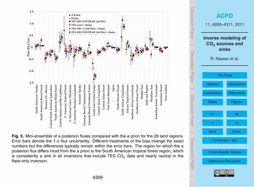
ACPD11, 4263–4311, 2011


sinks

R. Nassar et al.

Title Page



Tables Figures

J I

J I

Back Close

Full Screen / Esc



Discussion

Paper

|D

iscussionP

aper|

Discussion

Paper

|D

iscussionP

aper|

-1.5

-1.0

-0.5

0

0.5

1.0

1.5

Flu

x (P

g C

/yr)

No

rth

Am

eric

an T

un

dra

No

rth

Am

eric

an B

ore

al F

ore

st

Wes

tern

US

/ M

exic

o

Cen

tral

No

rth

Am

eric

an A

gri

cult

ure

No

rth

Am

eric

an M

ixed

Fo

rest

Cen

tral

Am

eric

a an

d t

he

Car

ibb

ean

S. A

mer

ican

Tro

pic

al F

ore

st

S. A

mer

ican

Co

ast

/ Mo

un

tain

s

S. A

mer

ican

Wo

od

ed G

rass

lan

ds

Eu

rasi

an T

un

dra

Eu

rasi

an B

ore

al C

on

ifer

ou

s F

ore

st

Eu

rasi

an B

ore

al D

ecid

uo

us

Fo

rest

So

uth

an

d C

entr

al E

uro

pe

Cen

tral

Asi

an G

rass

lan

ds

Cen

tral

Asi

an D

eser

t

Eas

t A

sian

Mai

nla

nd

Jap

an

No

rth

Afr

ican

Des

ert

No

rth

Afr

ican

Gra

ssla

nd

s

Afr

ican

Tro

pic

al F

ore

sts

So

uth

ern

Afr

ican

Gra

ssla

nd

s

So

uth

ern

Afr

ican

Des

ert

Mid

dle

Eas

t

Ind

ia a

nd

Reg

ion

Mar

itim

e A

sia

Au

stra

lian

Fo

rest

/ G

rass

lan

d

Au

stra

lian

Des

ert

New

Zea

lan

d

A Priori

TES (raw) + flasks

TES (SH -1.5 Jul-Dec) + flasks

TES (SH CONTRAIL Jul-Dec) + flasks

FlasksTES (SH CONTRAIL Jul-Dec)

Fig. 5. Mini-ensemble of a posteriori fluxes compared with the a priori for the 28 land regions.Error bars denote the 1-σ flux uncertainty. Different treatments of the bias change the exactnumbers but the differences typically remain within the error bars. The region for which the aposteriori flux differs most from the a priori is the South American tropical forest region, whichis consistently a sink in all inversions that include TES CO2 data and nearly neutral in theflask-only inversion.

4309





ACPD11, 4263–4311, 2011


sinks

R. Nassar et al.

Title Page



Tables Figures

J I

J I

Back Close

Full Screen / Esc



Discussion

Paper

|D

iscussionP

aper|

Discussion

Paper

|D

iscussionP

aper|

Fig. 6a. Scatter plots comparing a priori CO2 with a posteriori CO2 from the flask-based, theTES-based and the joint (TES and flask) inversions with CO2 measurements from CARIBIC(aircraft) and ship-based flasks for 2006. The ship and aircraft data were not used in the assim-ilation. The slope, variance, correlation coefficient (R2) and F-ratio are provided for each panelas metrics for gauging the agreement. Independently assimilating TES CO2 data improvesthe agreement with aircraft data (based on the slope and F ) but degrades the agreement withthe ship-based data (based on all metrics), while independently assimilating the flask data de-grades the agreement with aircraft data (based on 3 of 4 metrics) and improves the agreementwith the ship-based data (based on all metrics). The joint assimilation gives the best agreementwith both the aircraft data (based on R2 and F ) and ship-based data sets (based on 3 metrics).

4310





ACPD11, 4263–4311, 2011


sinks

R. Nassar et al.

Title Page



Tables Figures

J I

J I

Back Close

Full Screen / Esc



Discussion

Paper

|D

iscussionP

aper|

Discussion

Paper

|D

iscussionP

aper|

Fig. 6b. Continued.

4311





Inverse modeling of CO2 sources and sinks using satellite data: a synthetic inter-comparison of...

Documents

Transcript of Inverse modeling of CO2 sources and sinks using satellite data: a synthetic inter-comparison of...