Inventory-Service Optimization in Configure-to-Order Systems

Inventory-Service Optimization in Con�gure-to-Order Systems

Feng Cheng, Markus Ettl, Grace Lin

IBM Research Division, T.J. Watson Research Center

Yorktown Heights, NY 10598

fcheng,msettl,[email protected]

David D. Yao�

IEOR Department, 302 Mudd Building

Columbia University, New York, NY 10027

[email protected]

June, 2000; revision: March, December, 2001

Abstract

This study is motivated by a process-reengineering problem in PC (personal computer)manufacturing, i.e., to move from a build-to-stock operation that is centered around end-product (machine type model) inventory, towards a con�gure-to-order (CTO) operation thateliminates end-product inventory | in fact, CTO has made irrelevant the whole notion ofpre-con�gured machine types | and focuses instead on maintaining the right amount ofinventory at the components. Indeed, CTO appears to be the ideal operational modelthat provides both mass customization and a quick response time to order ful�llment. Toquantify the inventory-service tradeo� in the CTO environment, we develop a nonlinearoptimization model with multiple constraints, re ecting the service levels o�ered to di�erentmarket segments. To solve the optimization problem, we develop an exact algorithm for theimportant case of demand in each market segment having (at least) one unique component,and a greedy heuristic for the general (non-unique component) case. Furthermore, weshow how to use sensitivity analysis, along with simulation, to �ne-tune the solutions. Theperformance of the model and the solution approach is examined by extensive numericalstudies on realistic problem data. We demonstrate that the model can generate considerablenew insights into the key bene�ts of the CTO operation, in particular the impact of riskpooling and improved forecast accuracy. We present the major �ndings in applying ourmodel to study the inventory/service impacts in the reengineering of a PC manufacturingprocess.

�Research undertaken while an academic visitor at IBM Research Division, T.J. Watson Research Center.

1 Introduction

A con�gure-to-order (CTO) system is a hybrid of make-to-stock and make-to-order operations:

a set of components (subassemblies) are built to stock whereas the end products are assembled

to order. This hybrid model is most suitable in an environment where the time it takes to

assemble the end product is negligible, while the production/replenishment leadtime for each

component is much more substantial. The manufacturing process of personal computers (PC's)

is a good example of such an environment. By keeping inventory at the component level,

customer orders can be �lled quickly. On the other hand, postponing the �nal assembly until

order arrival provides a high level of exibility in terms of product variety, and also achieves

resource pooling in terms of maximizing the usage of component inventory. Therefore, the CTO

system appears to be an ideal business process model that provides both mass customization

and a quick response time to order ful�llment.

Such a hybrid model is often referred to as an assemble-to-order (ATO) system in the

research literature (e.g. [8, 16]). In an ATO system, usually there is a pre-con�gured set of end-

product types from which customers must choose. In contrast, a CTO system takes the ATO

concept one step further, in allowing each customer to con�gure a product in terms of selecting

a personalized set of components that go into the product. Aside from some consistency check

on the product so con�gured, there is no \menu" of product types that limits the customer's

choice.

From a modeling perspective, it might appear that the CTO system is no di�erent from the

ATO system: one can exhaust all possible con�gurations under CTO, and treat all the con�gu-

rations as part of a \mega-menu". In applications, however,this conceptual reduction does not

o�er anything practically useful, as one will have to deal with the curse of dimensionality, not

only in terms of computation, but also in terms of data collection and forecasting. For instance,

suppose any subset of n components is a possible con�guration. Then, one will have to deal

with the intractable task of forecasting 2n demand streams. The CTO model we develop here

formalizes what has become prevailing industry practice i.e., starting from forecasting on the

aggregate demand (say, of a market segment), along with the \feature ratios" (of component

usage) associated with such demand. Hence, suppose there are m aggregate demand streams

(or, product families). Then, demand forecast amounts to an e�ort of order O(mn), including

forecasts of feature ratios.

Our study reported here is part of a larger project that aims at helping IBM's Personal

Systems Group (PSG) to migrate from its existing operation to a CTO system. The PC

2

manufacturing at PSG is traditionally a build-to-plan (or build-to-forecast) process, a process

that is internally referred to as the MTM (\machine-type model") operation. There is a set of

end products, or MTM's. Demand forecasts over a future planning horizon are generated for

each MTM, and updated periodically for each planning cycle (typically, a weekly cycle). An

MRP-type (\material requirements planning") of explosion technique is then used to determine

the requirements for the components over the planning horizon based on the bill-of-materials

(BOM) structure of each end product. Because of the random variation involved in demand

forecasts, safety stock is usually kept for each end product between the channel partners and

IBM in order to meet a desirable customer service level. However, holding �nished goods

inventory for any length of time is very costly in the PC business, where product life cycle is

measured in months and price reduction takes place almost every other week.

To move from this business process to a web-based CTO operation (in particular, customer

orders will be taken from the Internet), the �nished-goods inventory will be eliminated, and the

emphasis will be shifted to the components, or \building blocks" (BB). Because of their long

leadtimes, the BB's will be powered o� a forecast and executed o� a replenishment process.

The focus of our study is on the inventory-service trade-o� of the new system, and on the

performance gains, in terms of reduced inventory cost and increased service level. There are

other bene�ts as well: The CTO operation can achieve better forecast accuracy through demand

aggregation. Customer demand is expected to increase, as orders will no longer be con�ned

within a restricted set of pre-con�gured MTM's. The optimization model we develop below

provides an analytical tool to quantify these performance impacts.

A brief review of related literature for the ATO system is in order. There are many stud-

ies of ATO systems that di�er quite substantially in the detailed modelling assumptions and

approaches. For example, Hausman, Lee and Zhang [9] and Zhang [20] study periodic-review

(discrete-time) models with multivariate normal demand and constant component replenish-

ment leadtimes. Song [14, 15] studies continuous-review models with multivariate compound

Poisson demand and deterministic leadtimes. Song et al. [16], Glasserman and Wang [8] and

Wang [19] also consider multivariate (compound) Poisson demand but the supply process for

each component is capacitated and modeled as a single-server queue. Gallien and Wein [6]

consider uncapacitated leadtimes, focusing on a single demand stream and assume order syn-

chronization. Cheung and Hausman [3] also assume uncapacitated leadtimes in the context of

a repair shop. They use a combination of order synchronization and disaggregation in their

analysis.

In terms of approaches, Song [14, 15] and Song et al. [16] focus on developing exact and

3

approximate performance evaluation procedures that are computationally eÆcient. Glasserman

and Wang [8] study the leadtime-inventory tradeo� using a large deviations approach, and

derive a linear relationship between leadtime and inventory in the limiting sense of high �ll

rates. Wang [19] further applies this asymptotic result in an optimization problem to minimize

average inventory holding cost with a constraint on the order �ll-rate. Swaminathan and Tayur

[18] use stochastic programming models to study three di�erent strategies at the assembly stage:

utilizing component commonality, postponement (the \vanilla box approach"), and integrating

assembly task design and operations. Other related recent works, not necessarily in the ATO

setting, include Aviv and Federgruen [1], Garg and Lee [7], Li [11], Mahajan and van Ryzin

[12], and Zipkin [21].

Whereas most studies in the literature focus on certain segments of the supply chain, mod-

eled as simple stand-alone queues, the recent work of Ettl et al. [5] aims at modeling large-scale,

end-to-end enterprise supply chains, such as those in the PC industry. In contrast, the model

we develop in this paper is simpler in the network con�guration | there are only two levels of

BOM: the components and the end products; but more demanding in service requirement |

the �ll rate of each product is essentially the o�-the-shelf availability of all its components. To

deal with this more stringent service requirement, we use a lower bound as a surrogate for the

analytically intractable �ll rate. This treatment is essentially in the same spirit as the approach

in [4, 16, 17]. The novelty of our approach here is to exploit the simpler BOM structure to

come up with algorithms that solve the optimization problem in a more eÆcient manner than

the gradient search in [5].

The rest of the paper is organized as follows. In the next three sections we present details

of our model: the given data required as input to the model (x2), the base-stock control policy

that we focus on (x3), the modeling of the customer service requirement (x4). The optimization

problem and the algorithms that solve the problem are presented in x5. These are followed by

x6, where the performance of the model and the solution technique is examined in detail. In

x7, we present the major �ndings in applying our model to study the inventory/service impacts

in reengineering PSG's business process. Brief concluding remarks are presented in x8.

2 The Model and Given Data

We consider a hybrid model, by which each end product is assembled to order from a set of

components, which, in turn, are built to stock. In other words, no �nished goods inventory is

kept for any end product, whereas each component (\building block") has its own inventory,

replenished from a supplier following a base-stock policy.

4

Each component inventory is indexed by i, i 2 S, where S denotes the set of all components.

Associated with each component is a \store," where the inventory is kept.

In the CTO environment, there is no pre-speci�ed product \menu"; in principle, every order

can require a distinct set of components. LetM denote the set of product/demand families that

use the same set of components. For instance, M = f low-end machines, high-end machines,

servers g; or M = f individuals, small business, corporations g. (Also, refer to Figure 1 for a

numerical example considered in x6.)

Time is discrete, indexed by t, with each time unit called a period. Let Dm(t) denote the

demand associated with product family m in period t. Each order of type m requires a random

number of units from component i, denoted as Xmi, which takes on non-negative integer values.

Denote:

Sm := S � fi : Xmi � 0g; Mi :=M�fm : Xmi � 0g:

That is, Sm denotes the set of components used in type m products, whereas Mi denotes all

the product families that use component i. (Here, Xmi � 0 means P(Xmi = 0) = 1.)

There are two kinds of leadtimes: those associated with the components, and those associ-

ated with the end products:

� Lini , i 2 S: the in-bound leadtime | the time for the supplier of component i to replenish

to store i once an order is placed. Assume this leadtime is known through a given

distribution. For instance, a normal distribution with mean and variance given.

� Loutm , m 2 M: the out-bound leadtime | the time to supply a customer demand of

type m, provided there is no stockout of any component i 2 Sm. This time includes the

order processing time, the assembly/recon�guration time, and the transportation time to

deliver the order. The distribution of this leadtime is also assumed known.

The �rst step in our analysis is to translate the end-product demand into demand for each

component i:

Di(t) =X

m2Mi

Dm(t+Loutm )X

k=1

Xmi(k); (1)

where Xmi(k), for k = 1; 2; :::; are i.i.d. copies of Xmi, and the inclusion of Loutm in the end-

product demand is a standard MRP type of demand-leadtime o�set. Assume the mean and the

variance of Xmi are known. For instance, these can be derived from empirical demand data.

Applying Wald's identity (refer to, e.g., [13]) and conditioning on Loutm , we can then derive the

5

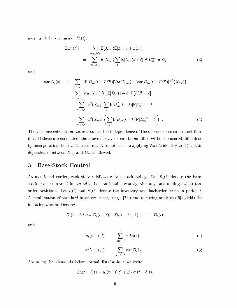
mean and the variance of Di(t):

E[Di(t)] =X

m2Mi

E(Xmi)E[Dm(t+ Loutm )]

=X

m2Mi

E(Xmi)X`

E[Dm(t+ `)]P[Loutm = `]; (2)

and

Var[Di(t)] =X

m2Mi

fE[Dm(t+ Loutm )]Var(Xmi) + Var[Dm(t+ Lout

m )]E2(Xmi)g

=X

m2Mi

Var(Xmi)X`

E[Dm(t+ `)]P[Loutm = `]

+X

m2Mi

E2(Xmi)

X`

E[D2m(t+ `)]P[Lout

m = `]

�X

m2Mi

E2(Xmi)

X`

E[Dm(t+ `)]P[Loutm = `]

!2

: (3)

The variance calculation above assumes the independence of the demands across product fam-

ilies. If these are correlated, the above derivation can be modi�ed without essential diÆculties

by incorporating the covariance terms. Also note that in applying Wald's identity to (1) certain

dependence between Xmi and Dm is allowed.

3 Base-Stock Control

As mentioned earlier, each store i follows a base-stock policy. Let Ri(t) denote the base-

stock level at store i in period t, i.e., on hand inventory plus any outstanding orders (on-

order position). Let Ii(t) and Bi(t) denote the inventory and backorder levels in period t.

A combination of standard inventory theory (e.g., [21]) and queueing analysis ([5]) yields the

following results. Denote:

Di(t� `; t) := Di(t� `) +Di(t� `+ 1) + � � � +Di(t);

and

�i(t� `; t) =tX

s=t�`

E[Di(s)]; (4)

�2i (t� `; t) =tX

s=t�`

Var[Di(s)]: (5)

Assuming that demands follow normal distributions, we write

Di(t� `; t) = �i(t� `; t) + Z � �i(t� `; t);

6

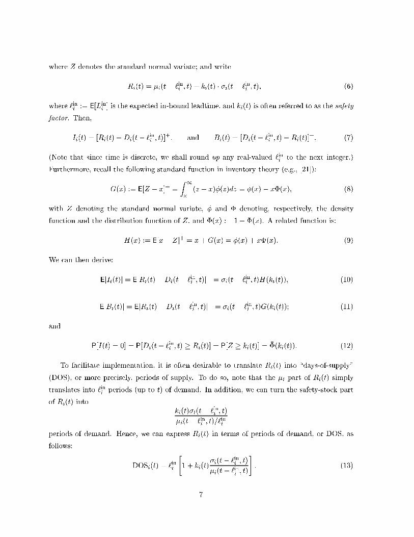
where Z denotes the standard normal variate; and write

Ri(t) = �i(t� ìni ; t) + ki(t) � �i(t� ìni ; t); (6)

where ìni := E[Lini ] is the expected in-bound leadtime, and ki(t) is often referred to as the safety

factor. Then,

Ii(t) = [Ri(t)�Di(t� ìni ; t)]+: and Bi(t) = [Di(t� ìni ; t)�Ri(t)]

+; (7)

(Note that since time is discrete, we shall round up any real-valued ìni to the next integer.)

Furthermore, recall the following standard function in inventory theory (e.g., [21]):

G(x) := E[Z � x]+ =

Z 1

x(z � x)�(z)dz = �(x)� x��(x); (8)

with Z denoting the standard normal variate, � and � denoting, respectively, the density

function and the distribution function of Z, and ��(x) := 1� �(x). A related function is:

H(x) := E[x� Z]+ = x+G(x) = �(x) + x�(x): (9)

We can then derive:

E[Ii(t)] = E[Ri(t)�Di(t� ìni ; t)]+ = �i(t� ìni ; t)H(ki(t)); (10)

E[Bi(t)] = E[Ri(t)�Di(t� ìni ; t)]+ = �i(t� ìni ; t)G(ki(t)); (11)

and

P[I(t) = 0] = P[Di(t� ìni ; t) � Ri(t)] = P[Z � ki(t)] = ��(ki(t)): (12)

To facilitate implementation, it is often desirable to translate Ri(t) into \days-of-supply"

(DOS), or more precisely, periods of supply. To do so, note that the �i part of Ri(t) simply

translates into ìni periods (up to t) of demand. In addition, we can turn the safety-stock part

of Ri(t) intoki(t)�i(t� ìni ; t)

�i(t� ìni ; t)=ìni

periods of demand. Hence, we can express Ri(t) in terms of periods of demand, or DOS, as

follows:

DOSi(t) = ìni

"1 + ki(t)

�i(t� ìni ; t)

�i(t� ìni ; t)

#: (13)

7

Note the intuitively appealing form of (13), in particular the safety-stock (or rather, safety

time) part, which is equal to the product of the safety factor and the coeÆcient of variation

(i.e., the ratio of standard deviation to mean) of the component demand over the (in-bound)

leadtime.

Next, suppose demand is stationary, i.e., for each product family m, Dm(t) is invariant in

distribution over time. Then, (4) and (5) reduce to the following (omitting the time arguments):

�i = ìni E[Di] and �2i = ìni Var[Di]: (14)

We can then write

Ri = ìni E[Di] + ki

qìni sd[Di]; (15)

and hence,

DOSi = Ri=E[Di] = ìni + ki�i

qìni = ìni [1 + ki

�iqìni

]; (16)

where �i := sd[Di]=E[Di] is the coeÆcient of variation of the demand per period for component

i. (Hence �i=qìni is the coeÆcient of variation of the demand over the leadtime ìni , which is

consistent with the general formula in (13).)

Sometimes it is more appropriate to adjust the demand distribution to account for non-

negativity. Speci�cally, instead of D = � + �Z, where Z is the standard normal variate, we

should have ~D = [�+ �Z]+. The adjusted mean follows from (8):

E[ ~D] = �E[Z � (��

�)]+ = �G(�

�

�): (17)

To derive the adjusted variance, note the following:

Ef[(Z � x)+]2g =

Z 1

x(z � x)2�(z)dz

= x�(x) + ��(x)� 2x�(x) + x2 ��(x)

= ��(x)� xG(x);

where the last equation makes use of (8). Hence,

Var[ ~D] = �2Varf[Z � (��

�)]+g

= �2Ef[(Z � (��

�))+]2g � [E( ~D)]2

= �2[��(��

�) +

�

�G(�

�

�)�G2(�

�

�)]: (18)

8

For moderately large x (say, x � 2), from (8), we have G(�x)�=x, and hence

E[ ~D]�=E[D]; Var[ ~D]

�=Var[D];

from (17) and (18). Therefore, the above adjustment is only needed when the coeÆcient of

variation of the demand, �=�, is relatively large, say, 0.5 or above. (In the numerical examples

of x6) we indeed implement this adjustment in the relevant cases.)

From (6), (15) and (16), it is clear that to identify the base-stock policy is tantamount to

specifying the safety factor ki for each component inventory. In the following sections, we discuss

how to set the safety factor values so as to achieve the best inventory-service performance as

speci�ed in the optimization problems below.

For ease of exposition, we shall focus on stationary demand. For non-stationary demand,

we can simply solve the optimization problems below period by period.

4 Service Requirement

4.1 O�-the-Shelf Availability

To start with, consider the special case of each order of type m requires exactly one unit of

component i 2 Sm. Let � be the required service level, de�ned here as the immediate (i.e.,

o�-the-shelf) availability of all the components required to assemble a unit of type m product,

for any m. Let Ei denote the event that component i is out of stock. Then, we require

P[[i2SmEi] � 1� �:

Making use of the well-known inclusion-exclusion formula (e.g., [13]):

P[[i2SmEi] =Xi

P(Ei)�Xi<j

P(Ei \Ej) +X

i<j<k

P(Ei \Ej \Ek)� � � � ;

where the indices i; j; k on the right hand side all belong to Sm, we have, as an approximation,

P[[i2SmEi]�=Xi2Sm

P(Ei) =Xi2Sm

��(ki) � 1� �: (19)

Note the essence of the above approximation is to ignore the probability of simultaneous stock-

out of two or more components.

There is another way to arrive at the above inequality. Suppose we express the service

requirement as follows:

Yi2Sm

�(ki) � �: (20)

9

Note that the left hand side in (20) is, in fact, a lower bound of the availability (no-stockout

probability) of the set of components in Sm that is required to assemble the end product m,

i.e., it is a lower bound of the desired immediate availability. This claim (of a lower bound) can

be argued by using stochastic comparison techniques involving the notion of association. (Refer

to, e.g., [13] for background materials.) Intuitively, since the component inventories are driven

by a common demand stream fDm(t)g, and hence positively correlated, the chance of missing

one or several components must be less than when the component inventories are independent,

which is what is assumed by the product on the left hand side of (20).

Since

Yi2Sm

�(ki) =Yi2Sm

[1� ��(ki)]�=1�

Xi2Sm

��(ki); (21)

combining the above and (20), we arrive at the same inequality in (19).

In the general setting, consider demand of product family m. Let A � Sm denote a certain

con�guration, which occurs in this demand stream with probability P(A). Then the no-stockout

probability,Qi2A�(ki), should be weighted by P(A). Hence, the service requirement in (20)

should be changed to

� �X

A�Sm

P(A)Yi2A

�(ki)

�X

A�Sm

P(A)[1 �Xi2A

��(ki)]

= 1�X

A�Sm

P(A)Xi2A

��(ki)

= 1�Xi2Sm

XA3i

P(A)

!��(ki):

Since

XA3i

P(A) = P(Xmi > 0) := rmi; (22)

the service requirement in (19) can be extended to the following:

Xi2Sm

rmi��(ki) � 1� �; (23)

where rmi follows (22).

Note that when the batch size Xmi is large, the stockout at component i should occur more

often than ��(ki) [cf. (12)]. To see this, �rst consider the case of unit (demand) arrivals, i.e.,

10

Xmi � 1. Then, the stockout probability is P[Di > Ri], or P[Di + 1 � Ri]. In the general case

of batch arrivals, the stockout probability is

P[Di +Xmi � Ri] = P[Z � ki �Xmi

�i] = ��(ki �

Xmi

�i);

which is larger than ��(ki). But this gap should be insigni�cant, since

Xmi

�i=Xmi

�i�i;

where �i := �i=�i, with �i and �i following (14); and the batch size of an incoming demand is

usually orders of magnitude smaller when compared against �i, which is the mean of demand

summed over all product types m 2Mi and over the leadtime. (Large-size orders will likely be

processed via separate contracts/channels, rather than in a CTO environment.) Hence, below

we shall simply use ��(ki) as the stockout probability. Also note that this underestimation of

the stockout probability is compensated by the overestimation involved in (20), since the latter

is a lower bound of the no-stockout probability.

4.2 Response-Time Serviceability

We now relate the immediate availability discussed above to another type of customer service

requirement, which is expressed in terms of order response time, Wm | the delay (waiting

time) between the time the order is placed and the time it is received by the customer.

Suppose the required service level of type m demand is:

P[Wm � wm] � �; (24)

where wm and � are parameters that specify the given requirement, e.g., ful�ll the order within

wm = 5 days with � = 99% probability.

We have the following two cases:

(i) When there is no stockout at any component i 2 Sm |denoting the associated probability

as �0m(t), the delay is simply Loutm , the out-bound leadtime.

(ii) Suppose there is a stockout at a component i 2 Sm. Denote the associated probability

as �im(t). Then, the delay becomes Loutm + �i, where �i is the additional delay before the

stocked-out component becomes available.

Hence, we can write

P[Wm � wm] � �0m(t)P[Loutm � wm] +

Xi2Sm

�im(t)P[Loutm + �i � wm]

= [Yi2Sm

rmi�(ki)]P[Loutm � wm] +

Xi2Sm

rmi��(ki)P[L

outm + �i � wm]: (25)

11

Note that in the above approximation, we have again ignored the probability of two or more

components stocking out at the same time.

In most applications, it is reasonable to assume Loutm � wm. For instance, this is the case

when the outbound leadtime Loutm is nearly deterministic, and the delay limit wm is set to be

\safely" larger than Loutm .

On the other hand, �i, which is quite intractable, can be approximated as follows (refer to

[5], eqn (7)):

�i � ìni �E(Bi)

��(ki)(Ri + 1):

From (11), we have

E(Bi) = �iG(ki) = �i[�(ki)� ki ��(ki)]:

Note that the following holds:

�(x)� x��(x)��(x)

��(x)

�(x)�

1

x;

for moderately large x (e.g., x � 3). Hence, making use of the above, along with (15), we have

�i � ìni ��i

ki(Ri + 1)

� ìni ��ikiRi

=ìni

qìni sd(Di)

ki[ìni E(Di) + ki

qìni sd(Di)]

=ìni

ki

qìni E(Di)=sd(Di) + k2i

: (26)

The above allows us to set wm such that wm � Louti + �i, for all i 2 Sm, then the response-time

serviceability in (25) can be met at almost 100% (i.e., modulo the approximation involved in

estimating �i). In other words, aiming for a high immediate availability (say, 95%) will enable

us to set a reasonable response-time target (wm) and to achieve a near-100% service level.

5 Inventory-Service Optimization

Our objective is to minimize the expected inventory cost (or, more precisely, inventory capital),

subject to meeting the service requirement for each product family as expressed in (23). The

problem can be presented as follows:

minXi2S

ci�iH(ki)

12

s:t:Xi2Sm

rmi��(ki) � ��m; m 2M

where rmi is the probability de�ned in (22), ci is the unit cost of the on-hand inventory of

component i, and ��m = 1 � �m with �m being the required service level for product family

m. Recall that �iH(ki) is the expected on-hand inventory of component i; refer to (10), and �i

follows the speci�cation in (14).

To solve the above optimization problem, we �rst rewrite the constraints as follows:

Xi2Sm

rmi�(ki) �Xi2Sm

rmi � ��m;

and (abusing notation) let

rmi rmiP

i2Sm rmi � ��m:

The optimization problem then becomes:

minXi2S

ci�iH(ki) (27)

s:t:Xi2Sm

rmi�(ki) � 1; m 2M: (28)

Several remarks are in order:

(i) Note that H(�) is an increasing and convex function, as evident from the �rst equality in

(9), while �(�) is an increasing function.

(ii) For any two product types, m and m0, if Sm0 � Sm, and rm0i � rmi for i 2 Sm0 , then the

constraint corresponding tom0 becomes super uous. We assume in the above formulation,

all such super uous constraints have already been removed through preprocessing.

(iii) Suppose a product family m involves a unique component, denoted im, i.e., im 62 Sm0

when m0 6= m. Then, the corresponding constraint must be binding. For otherwise,

we can always decrease the value of kim until the constraint becomes binding, without

a�ecting the other constraints, while decreasing the objective value (since H(�) is an

increasing function as explained in (i)).

The Lagrangian corresponding to the above optimization problem is:

L =Xi2S

ci�iH(ki)�Xm2M

�m

0@Xi2Sm

rmi�(ki)� 1

1A ; (29)

13

where �m � 0, m 2 M, are the Lagrangian multipliers. Hence, taking derivatives and setting

them to zero, taking into account

H 0(x) = �x�(x) + �(x) + x�(x) = �(x); (30)

we obtain the following system of non-linear equations that characterizes the optimal solution:

Xm2Mi

rmi�m = ci�i�(ki)

�(ki); i 2 S; (31)

Xi2Sm

rmi�(ki) = 1; m 2M and �m > 0: (32)

5.1 Unique Components

While solving the above system of non-linear equations is quite intractable in general, in the

following important case, we do have an eÆcient algorithm that solves the non-linear equations

and generate the optimal solution.

Suppose every product family m uses a unique component im that is not used in any other

product families. Then, as pointed out in the above Remark (iii), all the constraints in (28)

must be binding; i.e., the equations in (32) holds for all m 2 M, since all the Lagrangian

multipliers are positive.

Focusing on the unique components in (31), i = im, we have Mim = fmg, a singleton set,

and hence,

�m =cim�imrmim

��(kim)

�(kim); m 2M: (33)

Suppose we have derived the variables for all the unique components, kim , m 2 M. Then,

all the Lagrangian multipliers, �m, m 2 M, follow from (33). We can then derive ki, for all i

that is not a unique component, from the remaining equations in (31). That is,

�(ki)

�(ki)=

1

ci�i

Xm2Mi

rmi�m; i 2 S; i 6= im: (34)

To close this loop, we still have to derive the variables kim that correspond to the unique

components. But these are readily derived from the equations in (32), each involving exactly

one such variable, all the other variables corresponding to the non-unique components have

already been derived.

In particular, direct veri�cation establishes that �(k)=�(k) is increasing in k. Hence, we

know the variables corresponding to the non-unique components, (ki)i2S;i6=im , are increasing in

14

those of the unique components, (kim)m2M. Hence, denoting ym := �(kim) and y := (ym)m2M,

we can write (32) as

rmimym +Xi6=im

rmihmi(y) = 1; m 2M; (35)

where hmi(y) are increasing functions. Therefore, we can solve this system of equations using

a bisection-like algorithm detailed below.

1. For each m 2M, set kim = 0; set yLm = 0 and yHm = 1.

Set � = 10�6 (or any other desired accuracy).

2. For each m 2M, compute �m following (33).

3. For each non-unique component, i 6= im, compute ki from (34). (This can be done by

gradually incrementing ki until the ratio on the left reaches the same value as the right

hand side. Or, use bisection.)

4. For each m 2 M, set ym = �(kim), and compute the left hand side of (32), denoted

LHSm:

� If LHSm > 1 + �, set yHm ym and ym (ym + yLm)=2;

� if LHSm < 1 + �, set yLm ym and ym (ym + yHm)=2;

� derive kim = ��1(ym).

If maxm2M jym�y0mj � � (where y0m denotes the ym value of the previous iteration), stop;

else, go to 2.

While the above algorithm is guaranteed to converge, thanks to the bisection procedure,

it may not converge to the optimal solution. This can happen when, at convergence, the left

hand sides of (35) are not all equal to 1. This has been observed in our numerical studies, but

the gap to optimality is negligible.

On the other hand, convergence to the optimal solution is guaranteed if for each m, the

increase or decrease in the left hand side of (35) is dominated by the �rst term, i.e., a increase

(resp. decrease) in ym results in an increase (resp. decrease) in rmimym +P

i6=im rmihmi(y),

regardless of the increase or decrease in the other components of y. This appears to be the case

observed in many of the numerical examples we have run.

15

5.2 A Greedy Heuristic

Without the unique components, the main diÆculty in solving the optimization problem in

(27) and (28), has to do with the combinatorial nature of the equations in (32): we have to

consider all possibilities of the Lagrangian multipliers being zero or positive. Hence, we propose

a greedy heuristic as follows. We gradually decrease the left hand side of all the constraints to

1; at each step, we identify a variable ki such that decrementing its value will yield the largest

decrease in the objective value.

At each step in the algorithm, let �m denote the value of the left hand side of the constraint

m in (32), and let Æ := maxm2M �m. Denote

A := fi : �m < Æ; 8m 2Mig:

That is, the set A collects the indices of all variables that can be increased without increasing

Æ. We want to identify

i� = argmini2Afci�i[H(ki + Æi)�H(ki)]g;

where

Æi := minm2Mi

�Æ � �mrmi

�(36)

speci�es how much ki can be increased (without exceeding the current value of the constraint

Æ). Since Æi is a small increment, we can approximate the above di�erence by the derivative

(refer to (30)),

H 0(ki + Æi=2) � Æi = �(ki + Æi=2) � Æi:

To summarize, here is the algorithm:

1. For each i 2 S, set ki = 0.

For each m 2M, set �m = 0.

Set Æ = �.

2. Identify the set A := fi : �m < Æ; 8m 2Mig.

If Æ = 1 and A = ;, stop; else, continue.

3. If A = ; and Æ < 1, set Æ Æ +�.

Find i� = argmaxi2Afci�iÆi�(ki + Æi=2)g, where Æi follows (36).

Set ki� ki� + Æi� .

4. For m 2Mi� , set �m �m + rmi�ki� .

Go to 2.

16

5.3 Sensitivity and Inventory-Service Tradeo�

As is well-known, the Lagrangian multipliers in the optimization model discussed above have the

interpretation of \shadow prices." Speci�cally, suppose the right hand side of (28) is changed

from 1 to 1 � �, where � is a small positive quantity. Then, the change in the objective value,

around optimality, is approximately ��P

m2M �m; and this is evident from (29).

On the other hand, from the formulation of the optimization problem, we can verify that

the change of the right hand side of (28) from 1 to 1 � � corresponds to increasing ��m (the

no-�ll rate) by an amount

�(Xi2Sm

rmi � ��m):

Hence, the Lagrangian multipliers returned by the algorithms developed earlier can be used

to conduct sensitivity analysis. Speci�cally, we know that a reduction of the total inventory

cost by an amount d can be achieved by reducing the service requirement of product family m,

provided � > 0, from �m to

�m � �[Xi2Sm

rmi � (1� �m)];

with � = d=�m.

This sensitivity analysis can also be used in another way. Since, the service level used in

the optimization problem is a lower bound of the true value, the optimal solution is conser-

vative, in that it returns a service level that is higher than what is required. Our numerical

experience shows this typically results in an objective value that is 10-15% higher (than if the

true service levels were used). Therefore, after solving the optimization problem, we can use

the above sensitivity analysis to �nd the reductions on the �m values (required service levels)

that correspond to reducing the objective value by say, 10%; and then re-solve the optimization

problem using the reduced �m values. (Refer to the discussions on the results in Tables 4 and

5 of the next section.)

6 Numerical Results

For our numerical studies, we consider a family of desktop computers which are assembled from

a set of 12 di�erent components i = 1; 2; : : : ; 12 as illustrated in Figure 1.

FIGURE 1 ABOUT HERE

All components used in the assembly of an end product are purchased from external sup-

pliers. The supplier lead times are deterministic with E(Lini ) time units, which represent the

17

time required to manufacture the component and ship it from a supplier warehouse to the PC

assembly plant. The lead times, unit costs and demand con�gurations are summarized in Table

1. These are based on actual data from a PC assembly system, with the necessary alterations

to protect proprietary information. The modi�ed values, however, still provide a realistic prod-

uct representation. As the �nal assembly process for end products takes no more than a few

hours, which is an order-of-magnitude shorter than the component lead time, the system �ts

well within the framework discussed in x4.

P(Xmi > 0)

i category component lead time E(Lin

i ) unit cost ci low-end mid-end high-end

1 shell Base unit 5 215 1.0 1.0 1.0

2 memory 128MB card 15 232 1.0 1.0 1.0

3 motherboard 450 MHz board 12 246 1.0 { {

4 motherboard 500 MHz board 12 316 { 1.0 {

5 motherboard 600 MHz board 12 639 { { 1.0

6 storage 7GB disk drive 18 215 1.0 0.4 {

7 storage 13GB disk drive 18 250 { 0.6 1.0

8 software Pre-load A 4 90 0.7 0.5 0.3

9 software Pre-load B 4 90 0.3 0.5 0.7

10 options CD ROM 10 126 1.0 1.0 1.0

11 options Video graphics card 6 90 { 0.3 0.6

12 options Ethernet card 10 90 { 0.2 0.5

Table 1: Bill-of-materials structure for example con�gure-to-order system.

We consider 3 customer segments, i.e., m = 1; 2; 3, representing low-end, mid-end and high-

end demands, respectively. Orders for end products di�er by customer segment, in terms of the

possible selection of components that constitute the end product. We assume that each order

requires no more than one unit from component i. The random variables Xmi de�ned in x2

thus take on values of zero or one. The marginal distribution of Xmi is displayed in the last

three columns of Table 1 for each customer segment. It determines the possible combination

of components that can be selected by orders from each customer segment. The distribution

indicates the proportion of orders that request a speci�c component. For instance, for high-end

customers, 100% of the orders select a 13GB disk drive. For mid-end customers, 40% of orders

request a 7GB disk drive, and 60% request a 13GB hard drive. Each order requests exactly

one component from each component category. The only exception is the "options" category

of which more than one component can be selected.

18

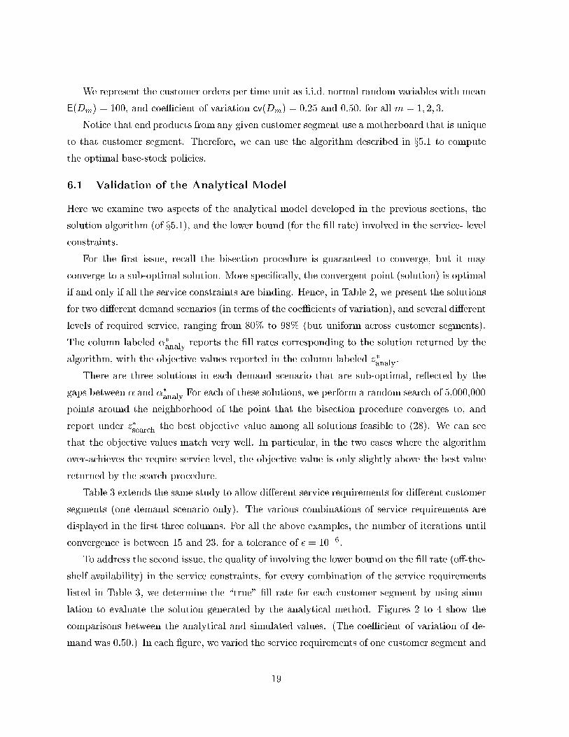
We represent the customer orders per time unit as i.i.d. normal random variables with mean

E(Dm) = 100, and coeÆcient of variation cv(Dm) = 0:25 and 0:50, for all m = 1; 2; 3.

Notice that end products from any given customer segment use a motherboard that is unique

to that customer segment. Therefore, we can use the algorithm described in x5.1 to compute

the optimal base-stock policies.

6.1 Validation of the Analytical Model

Here we examine two aspects of the analytical model developed in the previous sections, the

solution algorithm (of x5.1), and the lower bound (for the �ll rate) involved in the service- level

constraints.

For the �rst issue, recall the bisection procedure is guaranteed to converge, but it may

converge to a sub-optimal solution. More speci�cally, the convergent point (solution) is optimal

if and only if all the service constraints are binding. Hence, in Table 2, we present the solutions

for two di�erent demand scenarios (in terms of the coeÆcients of variation), and several di�erent

levels of required service, ranging from 80% to 98% (but uniform across customer segments).

The column labeled ��analy reports the �ll rates corresponding to the solution returned by the

algorithm, with the objective values reported in the column labeled z�analy.

There are three solutions in each demand scenario that are sub-optimal, re ected by the

gaps between � and ��analy For each of these solutions, we perform a random search of 5,000,000

points around the neighborhood of the point that the bisection procedure converges to, and

report under z�search the best objective value among all solutions feasible to (28). We can see

that the objective values match very well. In particular, in the two cases where the algorithm

over-achieves the require service level, the objective value is only slightly above the best value

returned by the search procedure.

Table 3 extends the same study to allow di�erent service requirements for di�erent customer

segments (one demand scenario only). The various combinations of service requirements are

displayed in the �rst three columns. For all the above examples, the number of iterations until

convergence is between 15 and 23, for a tolerance of � = 10�6.

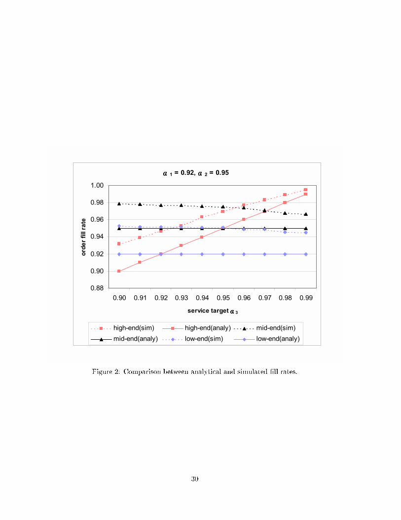
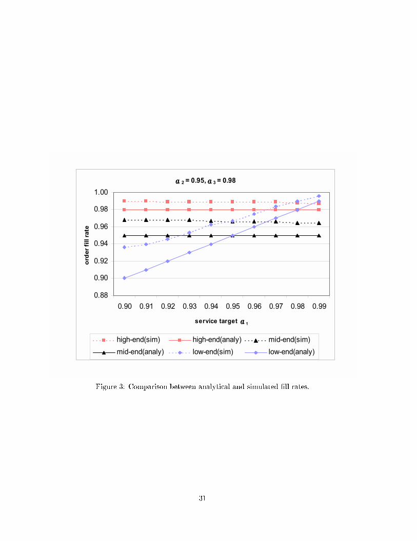
To address the second issue, the quality of involving the lower bound on the �ll rate (o�-the-

shelf availability) in the service constraints, for every combination of the service requirements

listed in Table 3, we determine the \true" �ll rate for each customer segment by using simu-

lation to evaluate the solution generated by the analytical method. Figures 2 to 4 show the

comparisons between the analytical and simulated values. (The coeÆcient of variation of de-

mand was 0.50.) In each �gure, we varied the service requirements of one customer segment and

19

cv(Dm) = 0:25 cv(Dm) = 0:50

� ��

analy z�

analy z�

search rel.dev. ��

analy z�

analy z�

search rel.dev.

.800 (.800,.800,.800) 437,637 { { (.800,.800,.800) 875,273 { {

.820 (.820,.819,.818) 450,311 451,121 0.2% (.820,.819,.818) 900,621 902,243 0.2%

.840 (.839,.837,.840) 462,308 463,088 0.2% (.839,.837,.840) 924,616 926,176 0.2%

.860 (.860,.860,.860) 477,489 { { (.860,.860,.860) 954,978 { {

.880 (.880,.880,.880) 494,050 { { (.880,.880,.880) 988,100 { {

.900 (.901,.900,.900) 513,383 512,050 -0.3% (.901,.900,.900) 1,026,766 1,024,199 -0.3%

.920 (.920,.920,.920) 536,004 { { (.920,.920,.920) 1,072,007 { {

.940 (.940,.940,.940) 564,446 { { (.940,.940,.940) 1,128,892 { {

.960 (.960,.960,.960) 602,862 { { (.960,.960,.960) 1,205,723 { {

.980 (.980,.980,.980) 664,478 { { (.980,.980,.980) 1,328,956 { {

Table 2: Quality of the algorithm: identical service target for all customer segments.

held the other two constant. For example, the service requirements (targets) for the high-end

and mid-end customer segments in Figure 4 were 0.98 and 0.95, respectively, while the service

target for the low-end segment varies between 0.90 and 0.99. (The simulation point estimates

are obtained by the batch-mean method, dividing every run into 10 batches of 5,000 arrivals

per customer segment.) Clearly, the analytical values, being a lower bound of the true �ll rate,

underestimate the achieved service level (i.e., over-achieve the service requirements). Overall,

however, the analytical curves track the simulated curves quite closely, and the gap decreases

as the service requirement increases.

FIGURES 2-4 ABOUT HERE

Next, we continue examining the second issue raised above, but from a di�erent angle: Since

the lower bounds involved in the service constraints over-achieve the service requirements, what

is the true optimal solution that exactly meets the service requirements? To study this, we �rst

apply simulation to the cases in Table 2, and report the results in Table 4, where the column

under ��analy lists the actual (i.e., simulated) service levels achieved by the analytical solutions,

and the column under z�analy lists the corresponding objective values (which are the same as

in Table 2). Next, we use the sensitivity analysis in x5.3, combined with simulation, to search

for the best solution that exactly meets the service requirements (as veri�ed by simulation).

Speci�cally, we gradually decrease the service requirements in the optimization model (i.e., the

�m values), using the sensitivity analysis as a guideline; solve the new optimization problem,

and then use simulation to �nd the achieved service levels. This procedure is repeated until

the analytical solution returns a set of simulated service levels that are within a pre-de�ned

tolerance of the original service requirements. Furthermore, when this procedure terminates, we

20

cv(Dm) = 0:50

�1 �2 �3 ��

analy z�

analy z�

search rel.dev.

.920 .950 .900 (.921,.950,.900) 1,083,953 1,085,977 0.2%

.920 .950 .920 (.920,.950,.920) 1,102,866 { {

.920 .950 .940 (.919,.950,.940) 1,128,973 1,131,144 0.2%

.920 .950 .960 (.919,.950,.960) 1,168,104 1,172,183 0.3%

.920 .950 .980 (.918,.948,.980) 1,239,232 1,244,627 0.4%

.920 .900 .980 (.918,.908,.980) 1,215,895 1,217,521 0.1%

.920 .920 .980 (.919,.925,.980) 1,224,201 1,226,235 0.2%

.920 .940 .980 (.916,.943,.980) 1,234,501 1,237,110 0.2%

.920 .960 .980 (.920,.964,.980) 1,256,906 1,255,050 -0.1%

.920 .980 .980 (.923,.980,.980) 1,292,961 1,290,429 -0.2%

.900 .950 .980 (.904,.947,.980) 1,233,337 1,238,372 0.4%

.920 .950 .980 (.918,.948,.980) 1,239,232 1,244,627 0.4%

.940 .950 .980 (.942,.949,.980) 1,251,034 1,254,381 0.3%

.960 .950 .980 (.958,.950,.980) 1,263,566 1,267,927 0.3%

.980 .950 .980 (.980,.955,.980) 1,298,052 1,297,527 0.0%

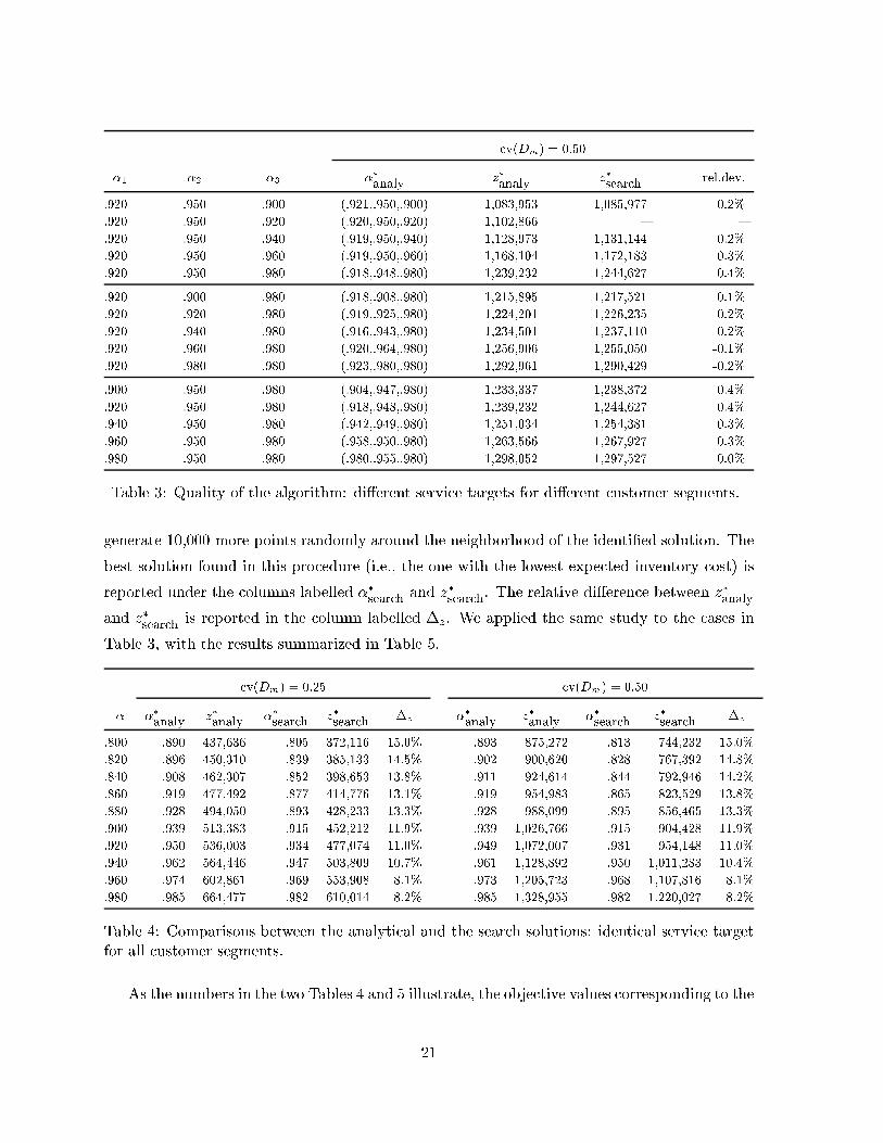
Table 3: Quality of the algorithm: di�erent service targets for di�erent customer segments.

generate 10,000 more points randomly around the neighborhood of the identi�ed solution. The

best solution found in this procedure (i.e., the one with the lowest expected inventory cost) is

reported under the columns labelled ��search and z�search. The relative di�erence between z�analy

and z�search is reported in the column labelled �z. We applied the same study to the cases in

Table 3, with the results summarized in Table 5.

cv(Dm) = 0:25 cv(Dm) = 0:50

� ��

analy z�

analy ��

search z�

search �z ��

analy z�

analy ��

search z�

search �z

.800 .890 437,636 .805 372,116 15.0% .893 875,272 .813 744,232 15.0%

.820 .896 450,310 .839 385,133 14.5% .902 900,620 .828 767,392 14.8%

.840 .908 462,307 .852 398,653 13.8% .911 924,614 .844 792,946 14.2%

.860 .919 477,492 .877 414,776 13.1% .919 954,983 .865 823,529 13.8%

.880 .928 494,050 .893 428,233 13.3% .928 988,099 .895 856,465 13.3%

.900 .939 513,383 .915 452,212 11.9% .939 1,026,766 .915 904,428 11.9%

.920 .950 536,003 .934 477,074 11.0% .949 1,072,007 .931 954,148 11.0%

.940 .962 564,446 .947 503,809 10.7% .961 1,128,892 .950 1,011,283 10.4%

.960 .974 602,861 .969 553,908 8.1% .973 1,205,723 .968 1,107,816 8.1%

.980 .985 664,477 .982 610,014 8.2% .985 1,328,955 .982 1,220,027 8.2%

Table 4: Comparisons between the analytical and the search solutions: identical service targetfor all customer segments.

As the numbers in the two Tables 4 and 5 illustrate, the objective values corresponding to the

21

�1 �2 �3 ��

analy z�

analy ��

search z�

search �z

.920 .950 .900 (.947, .969, .930) 1,083,953 (.925, .959, .901) 922,025 14.9%

.920 .950 .920 (.945, .968, .945) 1,102,866 (.925, .961, .920) 948,462 14.0%

.920 .950 .940 (.945, .966, .962) 1,128,973 (.932, .951, .941) 978,332 13.3%

.920 .950 .960 (.942, .964, .977) 1,168,104 (.926, .955, .966) 1,013,516 13.2%

.920 .950 .980 (.940, .958, .989) 1,239,232 (.927, .953, .982) 1,077,292 13.1%

.920 .900 .980 (.944, .919, .991) 1,215,895 (.924, .902, .980) 1,046,427 13.9%

.920 .920 .980 (.943, .936, .990) 1,224,201 (.924, .921, .986) 1,112,248 9.1%

.920 .940 .980 (.940, .953, .989) 1,234,501 (.922, .940, .983) 1,123,316 9.0%

.920 .960 .980 (.941, .972, .988) 1,256,906 (.920, .960, .981) 1,094,290 12.9%

.920 .980 .980 (.938, .986, .986) 1,290,429 (.926, .981, .981) 1,114,633 13.6%

.900 .950 .980 (.930, .958, .990) 1,233,337 (.901, .951, .981) 1,071,165 13.1%

.920 .950 .980 (.940, .958, .989) 1,239,232 (.927, .953, .982) 1,077,292 13.1%

.940 .950 .980 (.959, .956, .989) 1,251,034 (.941, .955, .981) 1,118,018 10.6%

.960 .950 .980 (.972, .955, .988) 1,263,566 (.962, .958, .981) 1,141,255 9.7%

.980 .950 .980 (.987, .956, .987) 1,297,527 (.985, .956, .980) 1,129,761 12.9%

Table 5: Comparisons between the analytical and the search solutions: di�erent service targetsfor di�erent customer segments.

analytical solution are about 8-15% sub-optimal, due to the lower bounds used in the service

constraints. In practice, the analytical method can be used to quickly generate a starting

solution. It can also be combined with with simulation and sensitivity analysis, as outlined

above, to �ne-tune the starting solution until optimality.

6.2 E�ect of Risk-Pooling

In the examples presented above, the inventory of each common component forms a common

bu�er from which the demand in all customer segments can draw upon (if the component is

needed). Hence, demand for each component is an aggregate of the demand over all customer

segments. To the extent that the safety stock of the component inventory is determined,

among other things, by the variability of this aggregate demand (on the component), the

required inventory level of this component to achieve a give service target can be lowered by

this aggregation, or risk pooling. In general, the impact of risk pooling become more signi�cant

when the number of product con�gurations is large and the correlation among demands is small

(e.g., Aviv and Federgruen [1], Brown et al. [2], Lee [10]).

To understand how risk-pooling in uences the performance of a CTO system, we compare

some examples studied above with their no risk-pooling counterparts. Speci�cally, we consider

the cases in Table 4, with the coeÆcient of variation of demand being 0.5. For the no risk-

pooling scenario, we apply the optimization to each customer segment separately, and then sum

22

up the expected inventory costs over all three customer segments. The comparison against the

risk-pooling results are plotted in Figure 5.

FIGURE 5 ABOUT HERE

In the �gure, the service levels are the actually realized values obtained by simulating the

analytical solutions. We observe that risk-pooling results in a signi�cant reduction of inventory

investment: For the same service target, the expected inventory cost is 20-25% lower with risk-

pooling, with the largest gap appearing at the high end: 25.8%. when � = 0:98. Our other

experiments indicate that the gap also increases with demand variability. For instance, when

the coeÆcient of variation of demand is reduced from 0.5 to 0.25, the relative di�erence at a

service target of 0.98 is 18.4%.

days-of-supply (risk-pooling) days-of-supply (no risk-pooling)

i component all segments low-end mid-end high-end

1 Base unit 1.6 2.5 2.6 2.7

2 128MB card 2.4 3.8 3.9 4.2

3 450 MHz board 3.0 3.5 { {

4 500 MHz board 3.0 { 3.3 {

5 600 MHz board 2.9 { { 3.0

6 7GB disk drive 3.2 4.2 4.7 {

7 13GB disk drive 3.2 { 3.7 4.4

8 Pre-load A 2.3 2.3 2.7 3.1

9 Pre-load B 2.3 3.0 2.7 2.5

10 CD ROM 3.3 3.7 3.8 4.0

11 Video graphics card 2.5 { 3.6 3.2

12 Ethernet card 3.4 { 4.8 4.2

Table 6: Comparison between risk-pooling and no risk-pooling scenarios, service target � = 0:90for all customer segments.

Table 6 shows the optimal component safety stock levels expressed in days-of-supply (as

de�ned in (16)) for both risk-pooling and no risk-pooling. As expected, risk-pooling requires a

lower days-of-supply value. Further, the amount of safety stock needed tends to be lower when

the commonality of a component is higher. For example, the 128MB memory card, which is

used in all customer segments, requires 2.4 days-of-supply, whereas the Ethernet card, which is

used in the high-end and mid-end segments, only requires 3.4 days-of-supply.

23

7 A Process Reengineering Application

Here we describe the study mentioned in the Introduction, which was part of a larger project

aimed at the reengineering of IBM/PSG's business process | from a build-to-stock operation

to a con�gure-to-order operation centered around \building blocks" (i.e., keeping inventory only

at the component level).

To carry out the study, we have developed two basic models: the \as-is" model that is a

re ection of PSG's present operation, and the \to-be" model that is based on the optimization

model described in the previous sections | in particular, with the component inventory levels

generated by the algorithm in x5. For both models, we aggregate PSG's production-inventory

system into two stages, the �rst stage consists of the components, or building blocks, and the

second stage includes the assembly and the order ful�llment.

Three factors have been identi�ed as focal points of our study:

(i) manufacturing strategy { the \as-is" operation versus the \to-be" model;

(ii) the accuracy of demand forecast at the end product level versus at the component level;

(iii) the e�ect of mass customization as a result of, for instance, direct sales over the Internet.

To study the �rst factor, we select a major product family at PSG, which consists of 18 end

products assembled from a total of 17 components. We use PSG's existing data { including

BOM, unit costs, assembly and procurement leadtimes { to run a detailed simulation model.

The demand for each end product is statistically generated, based on historical data. The

days-of-supply targets are set to meet a required service level of 95% (for all end products).

Following PSG's current practice, these targets are determined using a combination of simple

heuristic rules and judgement calls from product managers, and veri�ed by simulation (via trial

and error).

We then feed the same data, including the same statistically generated demand streams,

into the optimization model, which eliminates the �nished-goods inventory at the end-product

level and optimally sets the base-stock level for each component inventory. The optimization

model minimizes the overall inventory cost while meeting the same service level of 95% for all

end products. We take the optimal base-stock levels, and rerun the simulation to verify the

analytical results.

Figure 6 shows the comparison between the \as-is" and the \to-be" models, in terms of the

overall inventory cost. (To protect proprietary information, the vertical axis in all �gures is

normalized with respect to the inventory cost of the \as-is" model, which is 100. As expected,

24

the inventory cost at the end-product level is virtually eliminated in the \to-be" model. (The

cost shown is due to WIP; the cost due to �nished goods is nil.) In contrast, the \as-is"

model keeps a signi�cant amount of end-product inventory. On the other hand, the amount of

component inventory is higher in the \to-be" model, which is again expected, since the required

service level of 95% is common to both models. Overall, the \to-be" model reduces the overall

inventory cost by about 30%.

FIGURE 6 ABOUT HERE

Note in the above study, both models use the same demand forecast, at the end-product

level. The \to-be" model, however, can easily switch to forecasting demand directly at the

component level. This will result in improved forecast accuracy, as we can take advantage of

parts commonality, as each component is generally used in several end products. Hence, in

our study of the second factor, we evaluate the e�ect of forecast accuracy through a sensitivity

analysis. Figure 7 shows the overall inventory cost associated with three di�erent levels of

forecast accuracy. The �rst two columns repeat the comparison in the last �gure, i.e., both

\as-is" and \to-be" models assume 30% forecast error (i.e., the coeÆcient of variation equals

0.3) at the end-product level; the next two columns represent improved forecast errors, at 20%

and 30%, achieved by the \to-be" model through forecasting at the component level.

FIGURE 7 ABOUT HERE

Our study of the third factor aims at analyzing the impact on inventory when the system

supports a richer product set, in terms of product variety. The motivation is to support mass

customization: in the Internet-based, direct-sales environment, for instance, the number of

di�erent product con�gurations that customers want to order can be signi�cantly larger than

what is currently supported in the build-to-stock environment. Figure 8 shows the inventory

costs: the four columns on the left correspond to the current product set (1x), with the �rst

scenario (S1) being the \as-is" model, and the other three being the \to-be" model at the

current (S2) and improved (S3, S4) forecast accuracy levels, respectively; the four columns on

the right repeat these scenarios with a product set that is ten times as large in variety (10x),

while maintaining the overall volume. (Also refer to Table 7 for a summary of all the di�erent

scenarios.)

FIGURE 8 ABOUT HERE

25

Scenario Description 1x Cases 10x Cases

S1 \as-is"original product set, 30%forecast error, 90% service

ten times larger product set,30%�

p10 forecast error at

MTM level

S2 \to-be"forecast at MTM level,30% forecast error, 90%service

ten times larger product set,forecast error as in S2(1x)

S3 \to-be"forecast at BB level, 20%forecast error, 90% service


S4 \to-be"forecast at BB level, 10%forecast error, 90% service


Table 7: Summary of the scenarios used to study the e�ect of product variety.

Observe that as the product variety increases, a signi�cantly higher level of inventory is

required in the \as-is" model. This is because forecast accuracy will deteriorate when the end

products proliferate (i.e., larger varieties at smaller volumes). On the other hand, in the \to-be"

environment, the increase in inventory cost is very modest. This is because the proliferation

of end products will have minimal e�ect on the forecast accuracy at the building-block level,

due to parts commonality. This strongly supports the fact that the building-block model is the

right process to support an Internet-based, direct-sales operation.

8 Concluding Remarks

We have developed an analytical model for the con�gure-to-order operation, which has become

an important new business model in Internet commerce. We use the model to study the

optimal inventory-service tradeo�, formulated as a nonlinear programming problem with a set

of constraints re ecting the service levels o�ered to di�erent market segments. To solve the

optimization problem, we have developed an exact algorithm for the important case of demand

in each market segment having a unique component, and a greedy heuristic for the non-unique

component case. We have also shown how to use the sensitivity analysis, along with simulation,

to �ne-tune the solutions. On the qualitative side, we have highlighted several new insights to

some of the key bene�ts of the CTO operation, in terms of risk pooling and improved forecast

accuracy. As part of a larger project aimed at the reengineering of IBM/PSG's business process,

we have applied our model to study three factors, in terms of their impact on reducing inventory

capital and enhancing customer service: (i) manufacturing strategy { the machine-type-model

based operation versus the building-block based operation, (ii) the accuracy of demand forecast

26

at the end-product (machine con�gurations) level versus at the market segment level; (iii) the

e�ect of mass customization as a result of direct sales over the Internet.

Acknowledgements

We thank Maike Schwarz for her assistance in obtaining the CTO simulation results. We also

thank Lisa Koenig of the IBM Personal Systems Group for providing us with the opportunity

to work on this project.

References

[1] Aviv, Y. and Federgruen, A., The Bene�ts of Design for Postponement. In: Quan-

titative Models for Supply Chain Management, S. Tayur, R. Ganeshan and M. Magazine

(eds.), Kluwer Academic Publishers, Norwell, 1999, 553-584.

[2] Brown, A., Lee, H., and Petrakian, R., Xilinx improves its Semiconductor Supply

Chain using Product and Process Postponement, Interfaces, 30 (4), 2000, 65-80.

[3] Cheung, K.L. and Hausman, W., Multiple Failures in a Multi-Item Spare Inventory

Model, IIE Transactions, 27 (1995), 171-180.

[4] Connors, D.P. and Yao, D.D., Methods for Job Con�guration in Semiconductor Man-

ufacturing, IEEE Trans. Semiconductor Manufacturing, 9 (1996), 401-411.

[5] Ettl, M., Feigin, G.E., Lin, G.Y., and Yao, D.D., A Supply Network Model with

Base-Stock Control and Service Requirements, Operations Research, 48 (2000), 216-232.

[6] Gallien, J. and Wein, L., A Simple and E�ective Component Procurement Policy for

Stochastic Assembly Systems, Queueing Systems, 38 (2001), 221-248.

[7] Garg, A. and H.L. Lee, Managing Product Variety: an Operations Perspective. In:

Quantitative Models for Supply Chain Management, S. Tayur, R. Ganeshan and M. Mag-

azine (eds.), Kluwer Academic Publishers, Norwell, 1999, 467-490.

[8] Glasserman, P. and Wang, Y., Leadtime-Inventory Tradeo�s in Assemble-to-Order

Systems, Operations Research, 46 (1998), 858-871.

[9] Hausman, W.H., Lee, H.L. and Zhang, A.X., Order Response Time Reliability in a

Multi-Item Inventory System, European J. of Operational Research, 109 (1998), 646-659.

27

[10] Lee, H., E�ective Inventory and Service Management Through Product and Process Re-

design, Operations Research, 44 (1996), 151-159.

[11] Li, L., The Role of Inventory in Delivery-Time Competition. Management Science, 38

(1992), 182-197.

[12] Mahajan, S. and G.J. van Ryzin, Retail Inventories and Consumer Choice. In: Quan-

titative Models for Supply Chain Management, S. Tayur, R. Ganeshan and M. Magazine

(eds.), Kluwer Academic Publishers, Norwell, 1999, 491-552.

[13] Ross, S.M., Stochastic Processes, 2nd ed., Wiley, New York, 1998.

[14] Song, J.S., Evaluation of Order-Based Backorders, Management Science, to appear.

[15] Song, J.S., On the Order Fill Rate in a Multi-Item, Base-Stock Inventory System, Oper-

ations Research, 46 (1998), 831-845.

[16] Song, J.S., Xu, S. and Liu, B. Order Ful�llment Performance Measures in an Assembly-

to-Order System with Stochastic Leadtimes, Operations Research, 47 (1999), 131-149.

[17] Song, J.S. and D.D. Yao, Performance Analysis and Optimization in Assemble-to-Order

Systems with Random Leadtimes, Operations Research, to appear.

[18] Swaminathan, J.M. and S.R. Tayur, Stochastic Programming Models for Managing

Product Variety. In: Quantitative Models for Supply Chain Management, S. Tayur, R.

Ganeshan and M. Magazine (eds.), Kluwer Academic Publishers, Norwell, 1999, 585-624.

[19] Wang, Y. Service Levels in Production-Inventory Networks: Bottlenecks, tradeo�s, and

Optimization, Ph.D. Dissertation, Columbia University, 1988.

[20] Zhang, A.X. Demand Ful�llment Rates in an Assemble-to-Order System with Multiple

Products and Dependent Demands, Production and Operations Management, 6 (1997),

309-324.

[21] Zipkin, P., Foundations of Inventory Management, Irwin/McGraw-Hill, New York, 2000.

28

1

2

3

4

shell

memory

motherboard

storage

software

options

6

7

12

8

9

10

11

5

high-end desktop

2

1

mid-end desktop

low-end desktop

3

Figure 1: A con�gure-to-order system with three product families.

29

✍✍✍✍ 1 = 0.92, ✍✍✍✍ 2 = 0.95

0.88

0.90

0.92

0.94

0.96

0.98

1.00

0.90 0.91 0.92 0.93 0.94 0.95 0.96 0.97 0.98 0.99

service target ✍✍✍✍ 3

orde

r fil

l rat

e

high-end(sim) high-end(analy) mid-end(sim)

mid-end(analy) low-end(sim) low-end(analy)

Figure 2: Comparison between analytical and simulated �ll rates.

30

✍✍✍✍ 2 = 0.95, ✍✍✍✍ 3 = 0.98

0.88

0.90

0.92

0.94

0.96

0.98

1.00

0.90 0.91 0.92 0.93 0.94 0.95 0.96 0.97 0.98 0.99

service target ✍ ✍ ✍ ✍ 1

ord

er f

ill r

ate




31

✍✍✍✍ 1 = 0.92, ✍✍✍✍ 3 = 0.98

0.88

0.90

0.92

0.94

0.96

0.98

1.00

0.90 0.91 0.92 0.93 0.94 0.95 0.96 0.97 0.98 0.99

service target ✍✍✍✍ 2

ord

er f

ill

rate




32

800,000

1,000,000

1,200,000

1,400,000

1,600,000

1,800,000

2,000,000

0.86 0.88 0.90 0.92 0.94 0.96 0.98 1.00

order fill rate (simulated)

inve

ntor

y co

st ($

)

no risk pooling risk pooling

Figure 5: E�ect of risk pooling.

33

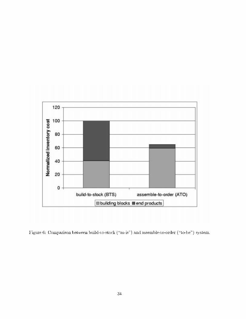
Figure 6: Comparison between build-to-stock (\as-is") and assemble-to-order (\to-be") system.

34

Figure 7: E�ect of improving forecast accuracy.

35

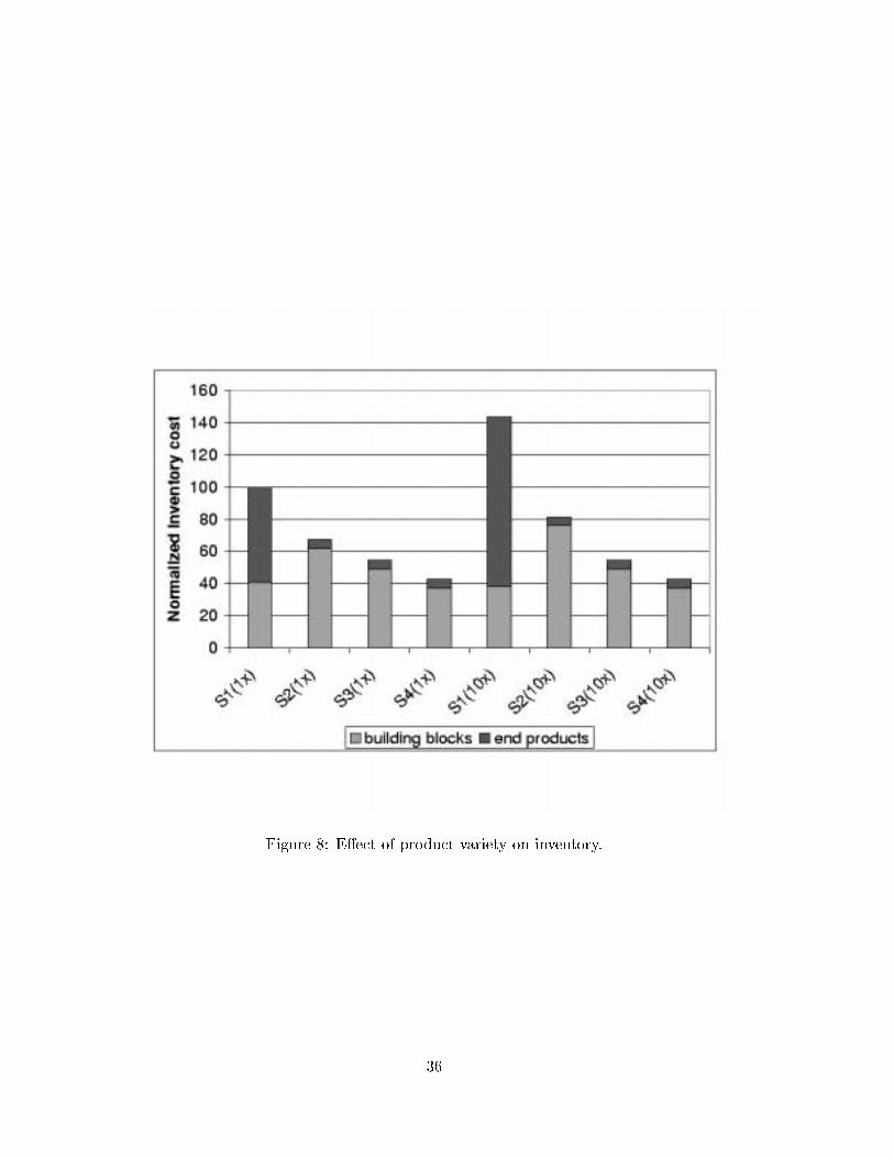
Figure 8: E�ect of product variety on inventory.

36

Inventory-Service Optimization in Configure-to-Order Systems

Documents

Transcript of Inventory-Service Optimization in Configure-to-Order Systems