Inventory model of deteriorating items with two-warehouse and stock dependent demand using genetic...

Yugoslav Journal of Operations Research 21 (2011), Number 2, #-#

DOI: 10.2298/YJOR100219005Y

INVENTORY MODEL OF DETERIORATING ITEMS WITH

TWO-WAREHOUSE AND STOCK DEPENDENT DEMAND

USING GENETIC ALGORITHM IN FUZZY

ENVIRONMENT

Dharmendra Yadav

Department of Mathematics, Keshav Mahavidyalaya, Delhi-34, India

[email protected]

S.R. Singh

Department of Mathematics, D.N (P.G.) College, Meerut (U.P) India.

[email protected]

Rachna Kumari

Department of Mathematics, Meerut College, Meerut (U.P) India.

[email protected]

Received:19.02.2010./ Accepted:08.02.2012.

Abstract: Multi-item inventory model for deteriorating items with stock dependent demand under two-warehouse system is developed in fuzzy environment (purchase cost, investment amount and storehouse capacity are imprecise ) under inflation and time value of money. For display and storage, the retailers hire one warehouse of finite capacity at market place, treated as their own warehouse (OW), and another warehouse of imprecise capacity which may be required at some place distant from the market, treated as a rented warehouse (RW). Joint replenishment and simultaneous transfer of items from one warehouse to another is proposed using basic period (BP) policy. As some parameters are fuzzy in nature, objective (average profit) functions as well as some constraints are imprecise in nature, too. The model is formulated so to optimize the possibility/necessity measure of the fuzzy goal of the objective functions, and the constraints satisfy some pre-defined necessity. A genetic algorithm (GA) is used to solve the model, which is illustrated on a numerical example.

D. Yadav, S.R. Singh, R. Kumari / Inventory Model of Deteriorating 2

Keywords: Possibility/Necessity Measures, Inflation, Time Value of Money, Deterioration, Genetic Algorithm.

MCN:

1. INTRODUCTION

The classical inventory models are mainly developed for the single storage facility. But, in the field of inventory management, when a purchase (or production) of large amount of units of items that can not be stored in the existing storage (viz., own warehouse-OW) at the market place due to its limited capacity, then excess units are stocked in a rented warehouse (RW) located at some distance from OW. In a real life situation, management goes for large purchase at a time, when either an attractive price discounts can be got or the acquisition cost is higher than the holding cost in RW. That’s why, it is assumed that the capacity of a rented warehouse is imprecise in nature i.e., the capacity of a rented warehouse can be adjusted according to the requirement. The actual service to the customer is done at OW only. Items are transferred from RW to OW using basic period (BP) policy.

In the present competitive market, the inventory/stock is decoratively displayed through electronic media to attract the customer and to push the sale. Levin et al. [1972] established the impact of product availability for stimulating demand. Mandal and Maiti

[1989] consider linear form of stock-dependent demand, i.e., D c dq= + , where ,D q

represent demand and stock level, respectively. Two constant ,c d are chosen so to fit the

demand function the best, whereas Urban [1992], Giri et al. [1996], Mandal and Maiti [2000], Maiti and Maiti [2005, 2006] and others consider the demand of the form

rD dq= where d, r are constant, chosen so to fit the demand function the best. Goyal and

Chang [2009] obtained the optimal ordering and transfer policy with stock dependent demand.

In general, deterioration is defined as decay, damage, spoilage, evaporation, obsolescence, pilferage, loss of utility, or loss of original usefulness. It is reasonable to note that a product may be understood as to have a lifetime which ends when its utility reaches zero. IC chip, blood, fish, strawberries, alcohol, gasoline, radioactive chemicals and grain products are the examples of deteriorating item. Several researchers have studied deteriorating inventory in the past. Ghare and Schrader [1963] were the first to develop an EOQ model for an item with exponential decay and constant demand. Covert and Philip [1973] extended the model to consider Weibull distribution deterioration. Mishra [1975] formulated an inventory model with a variable rate of deterioration with a finite rate of production. Several researchers like Goyal and Gunasekaran [1995], Benkherouf [1997], Giri and Chaudhuri [1998] have developed the inventory models of deteriorating items in different aspects. Kar et al. [2001] developed a two-shop inventory model for two levels of deterioration. A comprehensive survey on continuous deterioration of the on-hand inventory has been done by Goyal and Giri [2001]. Several researchers such as Yang [2004], Roy et al. [2007] analyze the effect of deterioration on the optimal strategy. Mandal et al. [2010] and Yadav et al. [2011] obtained the optimal ordering policy for deteriorating items.


It has been recognized that one’s ability to make precise statement concerning different parameters of inventory model diminishes with the increase of the environment complexity. As a result, it may not be possible to define the different inventory parameters and the constraints precisely. During the controlling period of inventory, the resources constraints may be possible in nature, and it may happen that the constraints on resources satisfy, in almost all cases, except in a very few where they may be allowed to violate. In a fuzzy environment, it is assumed that some constraints may be satisfied

using some predefined necessity, 2η (cf. Dubois and Prade [1983, 1997]). Zadeh [1978]

first introduced the necessity and possibility constraints, which are very relevant to the real life decision problems, and presented the process of defuzzification for these constraints. After this, several authors have extended the ideas and applied them to different areas such as linear programming, inventory model, etc. The purpose of the present paper is to use necessity and possibility constraints and their combination for a real-life two warehouse inventory model. These possibility and necessity resources constraints may be imposed as per the demand of the situation.

From financial standpoint, an inventory represents a capital investment and must compete with other assets within the firm’s limited capital funds. Most of the classical inventory models did not take into account the effects of inflation and time value of money. This was mostly based on the belief that inflation and time value of money do not influence the cost and price components (i.e., the inventory policy) to any significant degree. But, during the last few decades, due to high inflation and consequent sharp decline in the purchasing power of money in the developing countries like Brazil, Argentina, India, Bangladesh, etc., the financial situation has been changed, and so it is not possible to ignore the effects of inflation and time value of money. Following Buzacott [1975], Mishra [1979] has extended the approach to different inventory models with finite replenishment and shortages by considering the time value of money and different inflation rates for the costs. Hariga [1995] further extends the concept of inflation. Liao et al. [2000] studied the effects of inflation on a deteriorating inventory. Chung and Lin [2001] studied an EOQ model for a deteriorating inventory subjected to inflation. Yang [2004]develop a model for deteriorating inventory stored at two warehouses, and extended inflation to the idea of deterioration as amelioration when the environment is inflationary. Several related articles were presented dealing with such inventory problems (Chung and Liao [2006], Maiti and Maiti [2007], Rang et al. [2008], Chen et al. [2008], Ouyang et al. [2009]).

Here, a deteriorating multi-item inventory model is developed considering inflation and time value of money. Analysis of inventory of goods whose utility does not remain constant over time has involved a number of different concepts of deterioration. Maintenance of such inventory is of a major concern for a manager in a modern business organization. The quality of stocks maintained by an organization depends very heavily on the facility of its preserving. Keeping all this in mind, it is considered that items deteriorate with constant rate. Two rented warehouses are used for storage, one (own warehouse) is located at the heart of the market place and the other (rented warehouse) is located at a short distance from the market place. The items are jointly replenished and transferred from RW using basic period (BP) policy. Under BP, a replenishment and transfer of items from RW to OW are made at regular time intervals. Each item has a

https://www.researchgate.net/publication/222246612_Optimal_inventory_replenishment_models_for_deteriorating_items_taking_account_of_time_discounting?el=1_x_8&enrichId=rgreq-d5abe406-0394-475e-8895-38318021fe22&enrichSource=Y292ZXJQYWdlOzIyNzg1NDE1MjtBUzo5OTE3ODA1MTAxNDY2OEAxNDAwNjU3MzAyNDcz

https://www.researchgate.net/publication/222205407_The_optimal_ordering_policy_in_a_DCF_analysis_for_deteriorating_items_when_trade_credit_depends_on_the_order_quantity?el=1_x_8&enrichId=rgreq-d5abe406-0394-475e-8895-38318021fe22&enrichSource=Y292ZXJQYWdlOzIyNzg1NDE1MjtBUzo5OTE3ODA1MTAxNDY2OEAxNDAwNjU3MzAyNDcz


replenishment quantity sufficient to last for exactly an integer multiple of T. Similarly,

each item has a transferred quantity sufficient to last for exactly an integer multiple of tL .

Demand rate of an item is assumed to be stock dependent and shortages are not allowed. Here, the size of OW is finite and deterministic, but that of RW is imprecise. Although business starts with two rented warehouses of fixed capacity, in some extra temporary arrangement, it may be run near RW as it is away from the heart of the market place. This temporary arrangement capacity is fuzzy in nature. Therefore, the capacity of RW may be taken as fuzzy in nature, too. Unit costs of the items and the capital for investment are also fuzzy in nature. Hence, there are two constraints-one is on the storage space and the other on the investment amount, and these constraints will hold good to at

least some necessity α . Since purchase cost is fuzzy in nature, the average profit is

fuzzy in nature, too. As optimization of a fuzzy objective is not well defined, a fuzzy goal for average profit is set and possibility/necessity of the fuzzy objective (i.e., average profit) with respect to fuzzy goal is optimized under the above mentioned necessity constraints in optimistic/pessimistic sense.

2. OPTIMIZATION USING POSSIBILITY/NECESSITY MEASURE

A general single-objective mathematical programming problem should have the following form:

max ( , ) ....

subject to ( , ) 0, 1,2,3,........,i

f x

g x i n

ξ

ξ ≤ = (1)

where x is a decision vector, ξ is a crisp parameter, ( , )f x ξ is the return function,

( , )ig x ξ are continuous functions, 1,2,3,...,i n= . In the above problem, when ξ is a

fuzzy vector ξ% (i.e., a vector of fuzzy numbers), then return function ( , )f x ξ% and

constraints functions ( , )ig x ξ% are imprecise in nature and can be represented by a fuzzy

number whose membership function involve the decision vector x as the parameter, and

which can be obtained when membership functions of the fuzzy numbers in ξ% are

known (since f and ig are functions of decision vector x and the fuzzy number ξ% ). In

that case, the statements maximize ( , )f x ξ% as well as ( , ) 0ig x ξ ≤% are not defined. Since

( , )ig xξ% represents a fuzzy number whose membership function involves decision vector x,

and for a particular value of x, the necessity of ( , )ig xξ% can be measured by using formula

(58) (see Appendix 1), therefore a value xo of the decisions vector x is said to be feasible

if necessity measure of the event { }: ( , ) 0ig xξ ξ ≤ exceeds some pre-defined level iα in

pessimistic sense, i.e., if { }( , ) 0i ines g x ξ α≤ ≥ ,which may also be written as

{ }: ( , ) 0i ines g xξ ξ α≤ ≥% % . If an analytical form of the membership function of ( , )ig x ξ% is

available, then this constraint can be transformed to an equivalent crisp constraint (cf. Lemmas 1 and 2 of Appendix 1).


Again, as maximize ( , )f x ξ% is not well defined, a fuzzy goal of the objective

function may be as proposed by Katagiri et al. [2004], Mandal et al. [2005]. To make optimal decision, DM can maximize the degree of possibility/necessity that the objective function value satisfies the fuzzy goal in optimistic/pessimistic sense as proposed by

Katagiri et al. [2004]. When ξ is a fuzzy vector ξ% and 1 2( ( , ))G an LFN G G=% is the goal

of the objective function, then according to the above discussion, the problem (1) is reduced to the following chance constrained programming in optimistic and pessimistic sense, respectively

{ }( , )

max ( ),

subject to : ( , ) 0 ,

1, 2,3,........, ...

P f x

i i

Z G

nes g x

i n

ξπ

ξ ξ α

=

≤ ≥

=

%%

% % (2)

{ }( , )

max ( ),

subject to : ( , ) 0 ,

1, 2,3,........, ....

N f x

i i

Z N G

nes g x

i n

ξ

ξ ξ α

=

≤ ≥

=

%%

% % (3)

If the analytical form of membership function of ( , )f x ξ% (obtained using

formula (58) of Appendix 1) is a 1 2 3( ( ), ( ), ( ))TFN F x F x F x , then Lemma 3 of Appendix 1

gives 3 1

3 2 2 1

( )

( ) ( )p

F x GZ

F x F x G G

−=

− + −. Hence maximization of pZ implies maximization of

2 ( )F x (most feasible equivalent of ( , )f x ξ% ) and 3 ( )F x (least feasible equivalent of

( , )f x ξ% ) together and 1pZ = implies 2 2( )F x G≥ , i.e., most feasible profit function

achieves the highest level of profit goal 2( )G . Therefore, if DM is optimistic and allows

some risk, then she/he will take decision depending on possibility measure. On the other

hand, in this case Lemma 4 of Appendix 1 gives 3 1

3 2 2 1

( )

( ) ( )p

F x GZ

F x F x G G

−=

− + −. In this

case maximization of NZ implies maximization of 1( )F x (worst possible equivalent of

( , )f x ξ% and 2 ( )F x (most feasible equivalent of ( , )f x ξ% ) together and 1NZ = implies

1 2( )F x G≥ , i.e., worst possible profit function achieves the highest level of profit goal

2( )G . Thus, if any risk highly affects the company, the DM will go for optimization of

NZ to get optimal decision. However, one can optimize the weighted average of

possibility and necessity measures. In that case, the problem is reduced to

{ }

max (1 )

: ( , ) 0 ,

1,2,3,..., .

p N

i i

Z Z Z

subject to nes g x

i n

β β

ξ ξ α

= + −

≤ ≥

=

(4)


where pZ and

NZ are given by equation (2) and (3), respectively, and β is the

managerial attitude factor. Here, 1β = represents the most optimistic attitude, and 0β =

represents the most pessimistic attitude.

3. DETERMINATION OF FUZZY GOAL

Fuzzy goal G% of the fuzzy objective function ( , )f x ξ% %% is considered as a LFN

1 2( , )G G and the values of 1G , 2G can be determined in different ways. Here, the

following formulae are proposed and used in numerical illustrations for the fuzzy models. In the formulae, X denotes the feasible search of the problem:

00

00

1 0 0

2 0 0

inf ( inf ( , )),

sup(sup ( , )),

x X

x X

G f x

G f x

ξ ξ

ξ ξ

ξ

ξ

∈∈

∈∈

=

=

%

%

4. GENETIC ALGORITHM

Genetic Algorithm is exhaustive search algorithm based on the mechanics of natural selection and genesis (crossover, mutation, etc.). It was developed by Holland, his colleagues and students at the University of Michigan. Because of its generality and other advantages over conventional optimization methods, it has been successfully allied to different decision making problems.

In natural genesis, we know that chromosomes are the main carriers of hereditary factors. At the time of reproduction, crossover and mutation take place among the chromosomes of parents. In this way, hereditary factors of parents are mixed-up and carried over to their offspring. Again, Darwinian principle states that only the fittest animals can survive in nature. So, a pair of parents normally reproduces a better offspring.

The above-mentioned phenomenon is followed to create a genetic algorithm for an optimization problem. Here, potential solutions of the problem are analogous with the chromosomes, and the chromosome of better offspring with the better solution of the problem. Crossover and mutation among a set of potential solutions to get a new set of solutions are made, and it continues until terminating conditions are encountered. Michalewich proposed a genetic algorithm named Contractive Mapping Genetic Algorithm (CMGA) and proved the asymptotic convergence of the algorithm by Banach fixed point theorem. In CMGA, a movement from the old population to a new one takes place only if an average fitness of the new population is better than the fitness of the old

one. In the algorithm, ,c mp p are probability of crossover and probability of mutation

respectively, T is the generation counter and ( )P T is the population of potential

solutions for the generation T . M is an iteration counter in each generation to improve

( )P T and 0M is the upper limit of M . Initialize ( (1))P function generate the initial

population (1)P (initial guess of solution set) at the time of initialization. Objective

function value due to each solution is taken as fitness of the solution. Evaluate ( ( ))P T


function evaluates fitness of each member of ( )P T . Even though when fuzzy model can

be transformed into equivalent crisp model, only ordinary GA is used for a solution.

GA Algorithm:

1. Set generation counter 1T = , iteration counter in each generation 0M = .

2. Initialize probability of crossover cp , probability of mutation mp , upper

limit of iteration counter 0M , population size N .

3. Initialize ( ( ))P T .

4. Evaluate ( ( ))P T .

5. While 0( )M M< .

6. Select N solutions from ( )P T for mating pool using Roulette-Wheel

process.

7. Select solutions from ( )P T , for crossover depending on cp .

8. Make crossover on selected solutions.

9. Select solutions from ( )P T , for mutation depending on mp .

10. Make mutation on selected solutions for mutation to get population 1( )P T .

11. Evaluate 1( ( ))P T

12. Set 1M M= +

13. If average fitness of 1( )P T > average fitness of ( )P T then

14. Set 1( 1) ( )P T P T+ =

15. Set 1T T= +

16. Set 0M =

17. End if 18. End While

19. Output: Best solution of ( )P T

20. End algorithm.

5. ASSUMPTIONS AND NOTATIONS FOR THE PROPOSED MODEL:

The following notations and assumptions are used in developing the model.

Inventory system involves N items and two warehouse, one is Own warehouse

situated in the main market, and the other is a rented warehouse situated away from

the market place. They are respectively represented by OW and RW . The holding

cost of OW warehouse is higher than the one of RW .

1. Storage area of OW and RW are 1AR and 2AR units, respectively.

2. T is planning horizon.

3. MN orders are done during T .

4. oT is the basic time interval between orders, i.e., 0 / MT T N= .

5. M is the number of times items are transferred from RW to OW during

0T .


6. tL basic time interval between transferred of items from RW to OW . So,

/t oL T M= .

7. INV is the total investment.

8. Z is the profit per unit time.

9. G is the goal of Z (for fuzzy model).

10. 1β and 2β denote the confidence levels for investment and space

constraint, respectively.

11. pZ and NZ represent degree of possibility, necessity that the average profit

satisfies the fuzzy goal (for fuzzy model). F is the weighted average of pZ

and NZ , i.e., (1 )p NF Z Zβ β= + − and β is the managerial attitude factor.

12. I is the inflation rate.

13. d is the discount rate.

14. R d I= − .

15. omc is the major ordering cost.

16. tmc is the major transportation cost.

For thi item following notations are used.

17. in the number of integer multiple of oT when the replenishment of thi item

is part of group replenishment.

18. iL is the cycle length, i.e., 0i iL n T= .

19. im the number of integer multiple of tL when the transfer of thi item is a

part of group transfer from RW to OW .

20. tiT is duration between two consecutive shipments of the item from RW to

OW . So, ti i tT m L= .

21. Item is transferred from RW to OW in iN shipments. So

ii ti

ti

i

i

ti

i i

ti ti

Lif L isan integer multipleof T

T

N

L1 otherwise,

T

L Lwhere represents integralpart of

T T

= +

22. θ deterioration rate in OW and RW .

23. ( )hOW ic and ( )hRW ic are holding costs per unit quantity per unit time at OW

and RW , respectively, so ( ) ( )hOW i OW i pic h c= and ( ) ( )hOW i RW i pic h c=

24. Total cycles for thi item


i

i

i

i

Hif H is an integer multiple of L

L

M

H1 otherwise,

L

= +

i i

H Hwhere represents integral part of

L L

25. In the thj cycle item is transferred at 1 2,ij ijt T T= ,……, ijNiT , where

1 1( 1), ( 1)ij ijk ij tiT j T T k T= − = + − .

26. iA be the area required to store one unit.

27. A fraction iλ of 1AR is allocated for thi item. So, maximum displayed

inventory level 1 1

1

/ 1N

di i i

i

Q AR A andλ λ−

= =∑ .

28. ijQ is the order quantity at the beginning of thj cycle, which is the same in

all cycles except for the last.

29. 1iQ is the order quantity at the beginning of the last cycle.

30. OWijkQ is the stock level at OW at the beginning of thk − sub-cycle in thj

cycle, when items are transferred from OW to RW which is the same for

all sub-cycles except for the first sub cycle where 1 0OWsijQ = .

31. Fractions ( )OW ih and ( )RW ih of purchase cost are assumed as holding costs

per unit quantity per unit time at OW and RW , respectively, where

( ) ( )OW i RW ih h> .

32. oic is the minor ordering cost of the item in $, which is partly constant and

partly order quantity dependent and of the form: 1 2oi o i o i ic c c Q= + .

33. ( )OW iq is the inventory level at OW at any time t.

34. Demand of the item iD is linearly dependent on the inventory level at OW

and is of the form: ( ) ( )( )i OW i i i OW iD q x y q= + .

35. tic represents minor transportation cost in $ per unit item from RW to

OW .

36. pic represents minor transportation cost in $, and iη is the mark-up of

selling price si i pic cη= .


6. MODEL DEVELOPMENT AND ANALYSIS

Rented Warehouse (RW):

In the development of the model, it is assumed that the items are jointly replenished using BP policy. Under BP, the replenishment is made at regular time

intervals (every oT unit of time) and each item ( thi item) has a replenishment quantity

( )ijkQ sufficient to last for exactly an integer multiple ( )in of oT , i.e., thi item is ordered

at regular time intervals i on T . The inventory level at RW goes down discretely at a fixed

time interval during which the stock at RW is depleted continuously only due to

deterioration of the units. Hence, the inventory level ( ) ( )RW iq t at RW at any instant t

during 1ijk ijkT t T +≤ < , satisfies the differential equation

( )

1 RW(i) 1

( )= q (t)

RW i

ijk ijk

dq tfor T t T

dtθ +− ≤ < (5)

Therefore, in each time interval 1ijk ijkT t T +≤ < , ( ) ( )RW iq t continuously decreases

from the level ijkq but it has left-hand discontinuity at 1ijkT + , because from the model

description it is clear that 1

1

( )( )

( )ijk

RW i Tijk ijkt T

Lim q t Q q−

+→= + .

Using this condition, the solution of the differential equation is given by

1 1( )

( ) 1( ) ( ) ijkT t

RW i Tijk ijkq t Q q eθ + −

+= + (6)

for 1ijk ijkT t T +≤ < .

Moreover, ( ) ( )RW i ijk ijkq T q= , so we can deduce ijkq from equation (5)

1 1

1

1 1

1 1 1

( )

1

1

1 2

2

1 3

( )

( )

ijk ijk

ti

ti ti

ti ti ti

T T

ijk Tijk ijk

T

ijk Tijk ijk

T T

ijk Tijk ijk

T T T

ijk Tijk Tijk ijk

q Q q e

q Q q e or

q Q e q e

q Q e Q e q e

θ

θ

θ θ

θ θ θ

+ −

+

+

+ +

+ +

= +

= +

= +

= + +

Continuing in this way, we get 1 1

1

1 1

1

i

ti ti

ij i

N ks T T

ijk Tijk N k

s

q Q e q eθ θ

− −

+ − −=

= +∑

1 1

1

1

( 1)

11

i ti

ti

ti

N k TT

ijk Tijk T

eq Q e

e

θθ

θ

−− −

+

=

−

Since, 1 0iijN k

q − − =


Evaluation of Holding Cost at RW:

Stock at RW during 1 2,ijk ijk ijkT t T Q+≤ < is given by

2 1 1

k k

ijk ij Tijl i til lQ Q Q Tθ

= == − −∑ ∑

{ } ( )

2

1( ) i i tiy T

ijk ij di i i i i di

i i

kQ Q kQ x x y Q e

y

θθθ

− + −= − + − + + + +

Present value of holding cost at RW during 1ijk ijkT t T +≤ < is 2 2h i ijkc H , where

1

2

2ijk 2H (1 )ijk

ijkti

ijk

T

RTijk RTRt

ijk

T

QQ e dt e e

R

+

−−−= = −∫

Present value of holding cost at RW in first 1iM − cycles is 2 2h i Gc H , where

ti

1 1

2G 2

1 1

-RT ( 1)

1

( 1)( )

2

H =

1-e 1 1=

R 1

1( ( ) )

1

i i

ti i

ti

i i

i i ti

i

M N

ijk

j k

RT N

ij di iRT

i i

RL My T

i i i di RL

H

eQ Q S x

ye

ex y Q e S

e

θ

θ

θ

− −

= =

− −

−

− −− +

−

−− + −

+−

−+ + +

−

∑ ∑

(7)

where

( )

( 1)( 1)

1 2

( 1)1

11

ti iti i

titi

RT NRT N

i

RTRT

N eeS

ee

− −− −

−−

−− = −

− −

(8)

( )( )

( 2) ( 1)

2 2

1 ( 2)

11

ti ti iti i

titi

RT RT N RT N

i

RTRT

e e N eS

ee

− − − − −

−−

− − = −

− −

(9)

Own Warehouse:

On the other hand, the stock depletion at OW is due to demand and deterioration of the

items. Instantaneous state ( ) ( )OW idq t of thi item at OW is given by

( )

( ) ( ) 1

( )( ( )) ( )

OW i

i i OW i i OW i ijk ijk

dq tx y q t q t for T t T

dtθ += − + − ≤ ≤ (10)

With boundary conditions ( ) ( )OW i ijk didq T Q= for 1,2,3,..., 1ik N= −

From equation (10)


[ { } ( )( )

( )

1( ) ( )

( )i i ijky t T

OW i i i i i di

i i

q t x x y Q ey

θθ

θ

− + − = − + + + + (11)

{ } ( )

1

1( )

( )i i tiy T

sijk i i i i di

i i

Q x x y Q ey

θθθ

− +

+= − + + + +

(12)

Amount transferred from RW to OW at ,ijk Tijkt T Q= is given by

Tijk di sijkQ Q Q= − for 1, 2,3,..., 1ik N= − (13)

1

1

i

i

N

TijN ij Tijk

k

Q Q Q−

=

= − ∑ (14)

Instantaneous state ( ) ( )OW id t of thi item at OW in the last sub-cycle is given by

( )

1

( )( )

i

OW i

i i i i i ijN ij i

dq tx y q q for T t T L

dtθ= − + − ≤ ≤ + (15)

qRW(i)(t) QTijk

QTijk

Qij-Qdi

QTijk QTijk

QTijNi _ _ _ t Tij1 Tij2 Tij3 Tij4 TijNi Tij1+Li

Figure 1.

qRW(i)(t) QTihk QTihk QTihk QTihk QTihk Qdi

………………………………………………………


Qsijk Qsijk Qsijk Qsijk Qsijk _ _ _ _ t

Tij1 Tij2 Tij3 Tij4 TijNi Tij1+Li

Inventory Levels of ith

item in jth

cycle at RW and OW

Figure 2.

With boundary conditions

( ) 1( ) , ( ) 0OW i ijNi TijkNi sijNi i ij iQ T Q Q q T L= + + =

From equation (15)

(( )) ]( )( TijNi)

( ) TijNi sijNi

1

1( ) +(Q +Q ) i i

i

y t

OW i i i i i

i i

ijN ij i

q t x x y ey

for T t T L

θθθ

− + −= − + ++

≤ ≤ +

(16)

ti( )( ( 1)T )

( ) ijNi(T ) 1i i i iy L Ni

OW i

i i

xq e

y

θ

θ+ − − = − +

(17)

ti i ti( )T ( )( -(N -1)T )1( 1) ( ) 1i i i i iy y Li

ij i di i i i di

i i i i

xQ N Q x x yQ e e

y y

θ θ

θ θ− + +

= − − − + + − + + + (18)

Evaluation of holding cost at OW:

Present value of holding cost at OW in the thk sub-cycles of the th

j cycle is

{ }

1

( )

1 1

1( )

( )

1( ) (1 )

( 1)( )

ijk

Rtt e dt

ijk

i i ti

ti

h i ijk

T

h iOW i

T

y R Te RTijki i i diRTh i i

i i i i

c H

c q

x y Q ec xe

y R y R

θθ

θ θ

+

−

− + +−−

=

=

+ + −= − +

+ + +

∫ (19)

Present value of holding cost at OW in the last-cycle of the thj cycle is

{ }

( )1 1 1( )

( )( ( 1) )( ( 1) )1

( )

(1 )( 1) ( ) ( )

( )

ijk Li

Rtt e dt

ijNi

i i i i i ti

i i ti

T

h i ijNi h iOW i

T

e RTijN y R L N TR L N Th i i

i i i OW i ij i

i i i i

c H c q

c x ee x y q T N

y R y R

θ

θθ θ

+

−

− − + + − −− − −

= =

−= − + + +

+ + +

∫(20)


So, present value of holding cost at OW in the thj cycles is

1 1h i ijc H=

1

1 1 11

Ni

h i ijk ijNik

c H H−

== +∑

So, present value of holding cost at OW in the first 1iM − cycles is

1 1

1 1 1 1 11 1

i i

i

M N

h i G h i ijk ijN

j k

c H c H H− −

= =

= = +

∑ ∑

{ }

{ }

1

( )

1

( 1/ ) ( 1/ )

( ( 1) )

( )

1 (1 )( 1) ( )

( )

1 1 1

1 1

(1( 1) ( ) ( )

i i ti

ti

i ti i ti

ti

ti ti

i i ti

y R TRTi

h i i i i di

i i i i

R N Т R M ТRТ

RТ RТ

i i

R L N Tii i i OW i ijNi

x еc e x y Q

y R y R

е ее

уе е

x еe x y q T

R

θ

θθ θ

θ

θ

−

− + +−

− − − −−

− −

− − −

−= − + + + + +

− −+

+− −

−− + + +

1

( )( ( 1) / )

( 1)

)

( )

1

1

i i i i ti

i i

i Ni

y R L N Т

i i

RL MRT

RLi

y R

еe

e

θ

θ

− + − −

− −−

−

+ +

−

−

(21)

Evaluation of Sell Revenue:

Present value of sell revenue during 1ijk ijkT t T +≤ ≤ is

1

( )

1,2,3,...,

1 1ijk ti i i ti

ijk

si ijk i

RT RT y R TRTi i i

si di

i i i i i i

c SP k N

x e xe ec Q e

y R y y R

θθ

θ θ θ

−

− − − + +−

= =

− −= + +

+ + + +

(22)

Present value of sell revenue during the last cycle is

1

1

1

( )( )

( )

( )( )

( )

1( ( )

1

ij Li

ijNi

ijN ij i ijNi i

i i ijNi

i

i i ij i ijNi

TRT

si ijNi si iT

RT R T L Ty R Ti i i

si i OW i ijN

i i i i

y R T L T

i i

c SP c D t e dt

x e xec y q T e

y R y

e

y R

θ

θ

θ

θ θ

θ

+ −

− − + −− + +

− + + + −

= =

− = + +

+ +

−

+ +

∫

(23)

So, present value of sell revenue in the first Mi-1 cycle is


{ }

{ }

( 1) ( 1)( )

si

( 1)( ) ( 1)

( ) 1 1=c 1

1 1

( ) ( ) 11

1

ti i i i

i i ti

ti i

i i

i i i i i ti

i

RT N RL My R Ti i i di

si G RT RL

i i

RL Mi i i i ijN y R L R N T

RL

i i

x y Q e ec SP e

y R e e

x y q T ee e

y R e

θ

θ

θ

θ

θ

θ

− − − −− + +

− −

− −− + + − −

−

+ + − −−

+ + − −

+ + −+ −

+ + −

(24)

Evaluation of Transportation Cost: Present value of transportation cost in the first Mi-1 cycles CTG is given by

1 1-R-R

G

1 1

CT = Q e +Q e ijNijk i

ijk ijNi

Mi NiTT

ti T T

j k

c− −

= =

∑ ∑

( )( 1)

( 2) ( 1)

( ( ) )1

( )1

1 1

1 1

i i titi i

ti

ti i i i

ti i

y TRT N

i i i i di

ti di RT

i i

RT N RL M

RT RL

x x y Q eec Q

ye

e e

e e

θθ

θ

− +− −

−

− − − −

− −

− + + +− = −

+−

− −

− −

( 1)( 1)

( ( ) )( 1) ( 2)

( )

1

1

i i

ti i

i

i i i i di

ti ij i di i

i i

RL MRT N

RL

x x y Qc Q N Q N

y

ee

e

θ

θ

− −− −

−

− + + += − − + − +

−

−

(25)

Evaluation of replacement cost: Ordering cost in the first Mi-1 cycles OCG is given by

( ) 1

1

G 1 2

1

OC =i

ij

MRT

o i o i ij

j

c c Q e−

−

=

+∑ ( )( 1)

1 2

1

1

i i

i

RL M

o i o i ij RL

ec c Q

e

− −

−

−= +

− (26)

Evaluation of purchase cost: Present value of purchase cost in the first Mi-1 cycles is cpiPCG where

1

1 ( 1)

G

1

1PC =

1

i i i

ij

i

M RL MRT

ij ij RLj

eQ e Q

e

− − −−

−=

−=

− ∑ (27)

Formulation for the ith

item in last cycle, i.e., for TiiM t T≤ ≤

The last cycle length ( 1)i i iLl T M L= − − .

Items are transferred from RW to OW in Nli shipment where

int

1

ii ti

ti

i

i

ti

Llif Ll is an eger multipleof T

TNl

Llotherwise

T

=

+

(28)


Where i

ti

Ll

T

represent integral part of i

ti

Ll

T.

Items are transferred from RW to OW at t = 1TiiM , 2T

iiM ,………., Ti iiM Nl ,where

T ( 1) ( 1)iiM k i i tiM L k T= − + − , for 1,2,3,..., 1ik N= .

Own Warehouse: On the other hand, the stock depletion at OW is due to demand and deterioration of the

items. Instantaneous state ( ) ( )OW iq t of thi item at OW is given by

( )

( ) ( ) 1

( )( ( )) ( )

i

i i i i

OW

i i OW i OW iM k iM k

dq tx y q t q t for T t T

dtθ += − + − ≤ ≤ (29)

With boundary conditions ( ) 1( ) 1,2,3,..., 1OW i iMik di iq T Q for k N −= =

From equation (29)

{ } ( )( )

( )

1( ) ( )

( )

i i iM kiy t T

OW i i i i i di

i i

q t x x y Q ey

θθ

θ

− + − = − + + + + (30)

{ } ( )

1 1

1( ) 1, 2, ... 1

( )i i ti

i

y T

siM k i i i i di i

i i

Q x x y Q e for k Ny

θθθ

− +

+ −= − + + + = + (31)

QsiMi1=0

Amount transferred from RW to OW at iiM k

t T= , iTiM k

Q is given by

1 11, 2,3,...iTiM k di siMik iQ Q Q for k N −= − =

-1

1

-i

i i i i

N

TiM Nl iM TiM k

k

Q Q Q=

= ∑

Instantaneous state ( ) ( )OW iq t of thi item at OW in the last sub-cycle is given by

( )

1

( )( )

i i i

OW i

i i i i i iM Nl iM i

dq tx y q q for T t T L

dtθ= − + − ≤ ≤ + (32)

With boundary conditions QOW(i)(TiMiNi)=QTiMikNi+QsiMiNi , qi(TiMi1+Li)=0 From equation (32)

( )( )

( )

1( ) ( ( ))( ) i i i

i i

y t TiM Nli

OW i i i TiM Nli siM Nli i i

i i

q t x x Q Q y ey

θθθ

− + −= − + + + + +

1i i iiM Nl iM ifor T t T L≤ ≤ + (33)


( )( ( 1) )

( ) ( ) 1i i i i ti

i

y L Nl Ti

OW i iM Nli

i i

xq T e

y

θ

θ+ − − = − +

(34)

( ) ( )( -( -1) )1( 1) ( ) i i ti i i i i ti

i

y T y L Nl Ti

iM i di i i i di

i i i i

xQ Nl Q x x yQ e e

y y

θ θ

θ θ− + +

= − − − + + + + + (35)

Evaluation of holding cost at OW: Present value of holding cost at OW in the kth sub-cycles of the last cycle is

{ }

1

TiM kih1i

1 1

-1 ( )

( )c i

i

( )

x (1 )= ( 1) x ( )

( )

iM ki

iM ki

i i tiR

ti

i i

h i iMik

T

Rt

h i OW i

T

y R Te RT

i i diy

i i

c H

c q t e dt

ee y Q

R y R

θ

θθ

θ

+

− − + +−

+

=

=

−− + + + + +

∫ (36)

Present value of holding cost at OW in the last-cycle of jth cycle is

{

1

h1i

1 1 1

-

1 ( )

( )( ( 1) )c ( ( 1) )i

i ( )

( )

x (1 )( 1) x ( ) ( )

( )

iM Li i

iM Nli i

i i i i tiRTiM Nli ii i ti

ii i

h i iMiN i

T

Rt

h i OW i

T

y R L Nl Te R L N T

i i OW i ijNly

i i

c H

c q t e dt

ee y q T

R y R

θ

θθ

θ

+

− − + + − −− − −

= +

=

=

−− + + +

+ +

∫

So, present value of holding cost at OW in the jth cycles is

1 1

1

1 1 1

1

i

i

i i i

h i iM

Nl

h i iM k iM Nl

k

c H

c H H−

=

=

= +∑

So, present value of holding cost at OW in the last cycles is

{ }

1 1

1

1 1 1

1

1

1

1

( )( ( 1) )

( )

( 1) ( )

(1 )( 1)

( )

( ) (

i

i i i

i RTiM kiti

i i

i i ti RTiM Nli ii i ti

i i

i

h i L

Nl

h i iM k iM N

k

Nle RTi

h i i i i diyk

y R Te R L Nl Ti

y

i i

i i i OW i iM Nl

c H

c H H

xc e x y Q

R

xee

y R R

x y q T

θ

θ

θ

θ

θ

θ

−

−

−

=

−−

+=

− + +− − −

+

=

= +

= − + + +

− + − + +

+ + +

∑

∑

{ }( )( )( ( 1) )1

)( )

i i i i ti

i

y R L Nl T

i i

e

y R

θ

θ

− + + − − −+ +

(37)


Evaluation of Sell Revenue:

Present value of sell revenue during 1i iiM k iM kT t T +≤ ≤ is si iMikc SP=

11,2,3,..., 1ik N −= .

1 ( )( 1)

( )1 1

iM ki i i iM ki

iM ki

iM ki ti i i ti

iM ki

T y T RTi i

si i i diT

i i i i

RT RT y R TRTi i i

si di

i i i i i i

x xc x y Q e e dt

y y

x e xe ec Q e

y R y y R

θ

θ

θ θ

θ

θ θ θ

+ + − −

− − − + +−

= + − + + + +

− −= + +

+ + + +

∫

Present value of sell revenue during the last cycle is

1

1

1

1

( )( )

si ( )

( )( )

( )

1=c ( ( )

1

iM Li i

iM Ni i

iM N iM i iM Nli i i i i

i i iM Nli i

i i

i i iM i iM Nli i i

si iMiN i

TRT

si iT

RT R T L Ty R Ti i i

i OW i iM Nl

i i i i

y R T L T

i i

c SP

c D t e dt

x e xey q T e

y R y

e

y R

θ

θ

θ

θ θ

θ

+ −

− − + −− + +

− + + + −

=

=

− + +

+ +

−

+ +

∫

So, present value of sell revenue in the last cycle is

1

1 ( )

1

( )( )( )

1 1

1

iM kii ti i i ti

iM ki

iM Nl i i iM i iM Nli i i i i

i i iM Nli i

RTNl RT y R TRTi i i

si si di

k i i i i i i

RT y R T L Ty R Ti i

i i i i

x e xe ec SPL c Q e

y R y y R

x e ee

y y R

θ

θθ

θ

θ θ θ

θ

θ θ

−− − − + +−

=

− − + + + −− + +

− −= + + +

+ + + +

−

+ + +

∑

1( )

( )

1( )

iM i iM Nli i i

i i

R T L T

ii OW i iM Nl

i i

xey q T

R y θ

− + −

− + +

+

(39)

Evaluation of the holding cost at RW: Present Value of holding cost at RW in the last cycle is ch2iH2L where

{ }

- ( 1)

2 1

( ) ( 1)

2

1- 1 1

1

( ( ) )

ti ti i

ti

i i ti i i

RT RT Nl

L ij diRT

i i

y T RL M

i i i i di

e eH Q Q Sl

R ye

x x y Q e Sl eθ

θ

θ

− −

−

− + − −

−= − +

+−

− + + +

(40)

where


( 1)( 1)

1 2

( 1)1

(1 ) 1

ti iti i

ti ti

RT NlRT Nl

i

RT RT

Nl eeSl

e e

− −− −

− −

−− = −

− − (41)

( 1)( 2)

2 2

( 2)(1 )

(1 ) 1

ti iti ti i

ti ti

RT NRT RT Nl

i

RT RT

Nl ee eSl

e e

− −− − −

− −

−− = −

− − (42)

Evaluation of sell revenue in last cycle: Sell revenue =csiSPL

{ }

{ }

( 1)( ) ( 1)

( ) ( 1) ( 1)

( ) 11

1

( ) ( )1

ti i

i i ti i i

ti

i i i i i i i i

RT Nly R T RL Mi i i di

si RT

i i

i i i i iM Nl y R L R Nl RL M

i i

x y Q ec e e

y R e

x y q Te e e

y R

θ

θ

θ

θ

θ

θ

− −− + + − −

−

− + + − − − −

+ + −= − +

+ + −

+ + −

+ +

(43)

Present value of transportation cost in the last cycle CTL is given by:

-1- -

1

( )( 1)

( 2)( 1)

( ( ) )1

1

1( 1

1

i

iM k iM Nli i i

i i i

i i titi i

ti

ti i

i i

ti

NlRT RT

L ti TiM k TiM Nl

k

y TRT Nl

i i i i di

ti di RT

i i

RT NlRL M

ti iMi iRT

CT c Q e Q e

x x y Q eeCTL c Q

ye

ee c Q Nl

e

θθ

θ

=

− +− −

−

− −− −

−

= +

− + + +−= −

+−

−+ − −

−

∑

[

( )( 1) ( 1)

) ( 2)

( ( ) ) i i ti

ti i i i

di i

y TRT Nl RL Mi i i i di

i i

Q Nl

x x y Q ee e

y

θθ

θ

− +− − − −

+ −

− + + +

+

(44)

Evaluation of Ordering Cost in the last cycle: Present value of ordering cost in the last cycle CTL is given by

( 1)

1 2( ) i i

i

RL M

L o i o i iMOC c c Q e− −= + (45)

Evaluation of purchase cost in the last cycle: Present value of purchase cost in the last cycle is

( 1)i i

i

RL M

pi L iMc PC Q e− −= (46)

Formulation for major ordering and transportation costs: Present value of major ordering cost during the entire planning horizon, MOC, is given by

( 1)

1

1

1

M M o

o

o

N RN TR i T

om om RTi

eMOC c e c

e

−− −

−=

−= =

− ∑ (47)


Present value of major transportation cost during the entire planning horizon, MTC, is given by

-- ( -1)

-1

1-

1-

M M t

t

t

MN RMN LR i L

tm tm RLi

eMTC c e c

e=

= =

∑ (48)

Crisp Model:

Model 1: Present value of an average profit during the planning horizon, Z, is given by

{

}

]

1 1 1

1

2 2 2

( ) ( ) ( )

( ) ( ) ( )

N

si G L pi G L h i G L

i

h i G L G L

Z c SP SP c PC PC c H H

c H H OC OC CTG CTL

MOC MTC H

=

= + − + − + −

+ − + − +

+ +

∑

(49)

So the problem reduces to Maximize Z, Subject to

1

1

1

1

1 1 21

N

i pi

i

N

di

i

N

i i

i

Q c INV

Q AR

Q A AR AR

=

=

=

≤

=

≤ +

∑

∑

∑

(50)

Fuzzy Model: As discussed in section 1, it is very difficult to define different inventory

parameters precisely, i.e., as crisp numbers. It is easy to define these parameters as fuzzy. For example, purchase cost of an item fluctuates throughout the year. Hence, purchase cost of an item can be taken as about c per unit, which can be represented as a TFN (c-a, c, c+b). This implies that normally, price is near c and lies in the interval [c-a, c+b]. The possibility of price to be within (c-a, c) and (c, c+b) lies in (0.0, 1.0). Again, at the beginning, a business normally starts with some capital and its upper limit is fixed. But in the course of time, advantage of bulk transport, sudden increase of demand, price discount so as the decision of acquiring more items force the investor to augment the previously fixed capital by some amount in some situations. This augmented amount is clearly fuzzy in nature, in the sense of degree of uncertainty, and hence the total invested capital becomes imprecise in nature. The point is that the acquisition of extra amount of items needs some extra storage space in addition to the initially arranged warehouse area. Since the location of the rented warehouse, RW, is away from the heart of the market, the use of a temporary extra storage space can be arranged there. Thus, storage space of the far-away rented go-down, RW, is fuzzy in nature. Therefore, imprecise i.e., vaguely defined in some situations. Hence we take cpi, INV, AR2 as fuzzy numbers, i.e., as


, ,pic INV�

%2 ,AR% respectively. Then, due to this assumption, Z becomes fuzzy number Z% ,

and constraints in equation (50) also become imprecise in nature. Therefore, if G% (= an

LFN (G1,G2)) is the fuzzy goal of the objective Z% , then according to the discussion in section 2, the problem is reduced to the following, in optimistic sense, pessimistic sense and weighted average of optimistic and pessimistic sense, respectively,

Model 2:

Maximize Zp = ( ),Z

Gπ %%

Subject to

�

�

1 1

1

1

1

1 1 2 2

1

N

i pi

i

N

di

i

N

i i

i

Nes Q c INV

Q AR

Nes Q A AR AR

β

β

=

=

=

≤ ≥

= ≤ + ≥

∑

∑

∑

%

(51)

Model 3: Maximize Zp = ( ),Z

Gπ %%

Subject to the constraint of model 2 (52)

Model 4: Maximize (1 )p NF Z Zρ ρ= + −

Subject to the constraint of model 2 (53) Here, if it is assumed that

1 2 3( , , ),pi pi pi pic c c c=% �1 2 2( , , ),INV INV INV INV= �

2 21 22 23( , , )AR AR AR AR= as TFNs, then

using definition (58) we have 1 2 3( , , )Z Z Z Z=% where for j=1,2,3.

{ 1 1 11

( ) - ( ) - ( )N

j i G L G L i G L

i

Z SP SP PC PC h H Hη=

= + + +

∑

} } ]2 2 2- ( ) - ( ) - ( )i G L pij G L G Lh H H c OC OC CT CT MOC MTC H+ + + + +

and let 11

N

j i pij

i

P Q c=

=∑ for j=1,2,3. Then following lemmas 1-4, problems (51)-(53) are

reduced to respectively

Maximize 3 1

3 2 2 1

p

Z GZ

Z Z G G

−=

− + −

Subject to


3 11

2 1 3 2

1

1

1 1 2 11

2

2 2 2 1

1

1

N

d i i

i

N

i i

i

P IN V

IN V IN V P P

Q A A R

Q A A R A R

A R A R

β

β

=

=

−< −

− + −

=

− − < −−

∑

∑

(54)

2 1

2 1 2 1

subject to constraints of (54)

N

Z GMaximize Z

Z Z G G

− =

− + −

(55)

3 1

3 2 2 1

2 1

2 1 2 1

(1 )

subject toconstraintsof (54)

Z GMaximize F

Z Z G G

Z G

Z Z G G

ρ

ρ

−= +

− + − −

− − + −

(56)

These crisp problems can easily be solved using any non-linear optimization technique in crisp environment. GA is used here for this purpose.

7. Numerical Illustration:

The models are illustrated for three items (N=3). Common parametric values to illustrate the models are presented in Table-1. Other common parametric values are R=0.03, H=10, c0m=20, ctm=10, AR1=60.

Table 1. Common input data for different examples Item (i) x1 yi

iθ h1i h2i co1i co2i

1 10 3.20 .01 0.1 0.05 4 0.24 2 15 3.50 .01 0.1 0.05 6 0.18 3 12 3.42 .01 0.1 0.05 4 0.20

Item (i) cti

iη Ai

1 0.20 1.4 0.45 2 0.22 1.4 0.50 3 0.20 1.4 0.52

Example-1: Along with the common parametric values, other assumed parametric values are cp1=10, cp2=12, cp3=11, AR2=150, INV=$5000. Table-2 Results for Model (1) by using GA


Item (i) ni mi iλ NM M Z

1 2 1 0.16

2 2 1 0.31

3 2 1 0.25

10

3

579.62

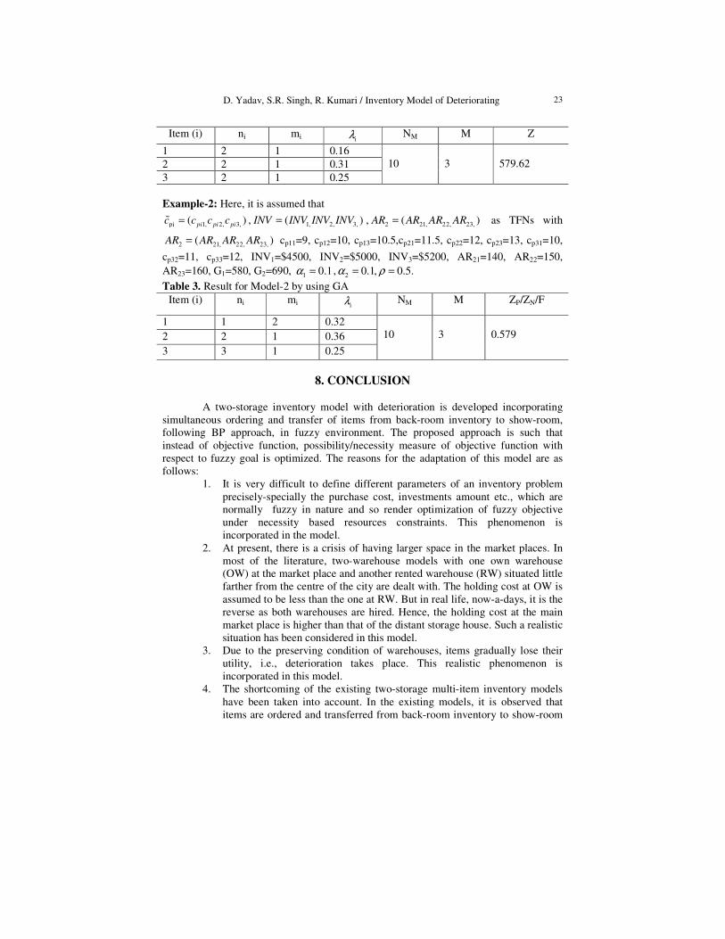
Example-2: Here, it is assumed that

pi 1, 2, 3,( )pi pi pic c c c=% , � 1, 2, 3,( )INV INV INV INV= , � 2 21, 22, 23,( )AR AR AR AR= as TFNs with

�2 21, 22, 23,( )AR AR AR AR= cp11=9, cp12=10, cp13=10.5,cp21=11.5, cp22=12, cp23=13, cp31=10,

cp32=11, cp33=12, INV1=$4500, INV2=$5000, INV3=$5200, AR21=140, AR22=150,

AR23=160, G1=580, G2=690, 1 0.1α = , 2 0.1, 0.5.α ρ= =

Table 3. Result for Model-2 by using GA

Item (i) ni mi iλ NM M ZP/ZN/F

1 1 2 0.32

2 2 1 0.36

3 3 1 0.25

10

3

0.579

8. CONCLUSION

A two-storage inventory model with deterioration is developed incorporating simultaneous ordering and transfer of items from back-room inventory to show-room, following BP approach, in fuzzy environment. The proposed approach is such that instead of objective function, possibility/necessity measure of objective function with respect to fuzzy goal is optimized. The reasons for the adaptation of this model are as follows:

1. It is very difficult to define different parameters of an inventory problem precisely-specially the purchase cost, investments amount etc., which are normally fuzzy in nature and so render optimization of fuzzy objective under necessity based resources constraints. This phenomenon is incorporated in the model.

2. At present, there is a crisis of having larger space in the market places. In most of the literature, two-warehouse models with one own warehouse (OW) at the market place and another rented warehouse (RW) situated little farther from the centre of the city are dealt with. The holding cost at OW is assumed to be less than the one at RW. But in real life, now-a-days, it is the reverse as both warehouses are hired. Hence, the holding cost at the main market place is higher than that of the distant storage house. Such a realistic situation has been considered in this model.

3. Due to the preserving condition of warehouses, items gradually lose their utility, i.e., deterioration takes place. This realistic phenomenon is incorporated in this model.

4. The shortcoming of the existing two-storage multi-item inventory models have been taken into account. In the existing models, it is observed that items are ordered and transferred from back-room inventory to show-room


individually, which incurred a large amount of ordering and transportation cost, too. In this model items are ordered and transferred from back-room to show-room simultaneously using BP policy.

5. The possibility/necessity measure on fuzzy goal as a decision making tool for inventory control problems has been used.

Appendix 1

Let a% and b% be two fuzzy numbers with membership function ( )a xµ%

and ( )b

xµ % ,

respectively.

{ }( * ) sup min( ( ), ( )), , , *a bpos a b x x x y x y Rµ µ= ∈%%

%% (57)

where the abbreviation pos represents possibility, and * is one of the relations >,<,=, ,≤ ≥ :

( * ) 1 ( * )nes a b pos a b= −% %% % (58)

where the abbreviation nes represents necessity.

Similarly, possibility and necessity measures of a% with respect to b% are denoted by

( )b

aΠ %% and ( )

bN a%

% , respectively and are defined as

{ }( ) sup min( ( ), ( )), ,ab ba x x x Rµ µΠ = ∈% %%% (59)

{ }( ) min sup( ( ),1 ( )),ab bN a x x x Rµ µ= − ∈% %%

% (60)

If , ( , )a b R and c f a b⊆ =% %% % % where :f R R R× → is a binary operation, then

membership function c of cµ%

% is defined as for each z R∈ ,

{ }( ) sup min( ( ), ( )), , ( , )c a bz x x x y R and z f x yµ µ µ= ∈ =%% %

(61)

Triangular fuzzy number (TFN): A TFN a% =(a1,a2,a3) (Fig.3) has three parameters a1,

a2, a3 where a1<a2<a3 and is characterized by the membership function ( )a xµ%

, given by

11 2

2 1

32 3

3 2

( )

0 .

a

x afo r a x a

a a

a xx fo r a x a

a a

o th erw ise

µ

−≤ ≤ −

−

= ≤ ≤−

%


( )a xµ%

1

0 a1 a2 a3 Figure 3. Membership function of triangular fuzzy number

α-cut of fuzzy number: α-cut of a fuzzy number A% in R with membership function

( )A

xµ % is denoted by α

A and defined as the following crisp

set: { }: ( ) , [0;1].A

A x x x R whereα µ α α= ≥ ∈ ∈%

αA is a non-empty bounded closed interval contained in R which can be denoted by

[ ( ), ( )].L RA A Aα α α=

Lemma.1: If 1 2 3( , , )a a a a=% , 1 2 3( , , )b b b b=% are TFNs with 0<a1 and 0<b1, then

( )nes a b α> ≥%% iff 3 1

2 1 3 2

1 .b a

a a b bα

−≤ −

− + −

Proof. We have { }( ) 1- ( )nes a b Pos a bα α> ≥ ⇒ ≤ ≥% %% % ( ) 1-Pos a b α⇒ ≤ ≤%% It is clear that

( )Pos a b δ≤ = =%% 3 1

2 1 3 2

b a

a a b b

−

− + − and hence, the result follows.

Lemma. 2: If 1 2 3( , , )a a a a=% be a TFN with 0<a1 and b is a crisp number, then

( )nes a b α> ≥%% iff 1

2 1

1 .b a

a aα

−≤ −

−

Proof: Proof follows from Lemma1.

Lemma. 3: If 1 2 3( , , )a a a a=% be a TFN and 1 2( , )b b b=% be a LFN with 0<a1 and 0<b1

then


2 2

3 12 2 3 1

3 2 2 1

1 ,

( ) ,

0 .

a

if a b

a bb if a b and a b

a a b b

otherwise

≥

−= < >

− + −

∏%

%

( )xµ

1

3 1

3 2 2 1

a b

a a b b

−

− + −

0 b1 b2 a1 a2 a3 x

Figure 4. Comparison of two triangular fuzzy numbers

Proof. Proof follows from formula (58) ( Fig. 4).

( )xµ

1

3 1

3 2 2 1

a b

a a b b

−

− + −

0 a1 a2 b1 b2 a3 x

Figure 5. Pictorial representation of ( )a

b∏ %

%

( )xµ

1


2 1

2 1 2 1

a b

a a b b

−

− + −

0 a1 b1 a2 b2 a3 x

Figure 6. Pictorial representation of ( )a

N b%

%

Lemma. 4: If 1 2 3( , , )a a a a=% be a TFN and 1 2( , )b b b=% be a LFN with 10 a< and 10 b< then

1 2

3 12 1 2 1

3 2 2 1

1 ,

( ) ,

0 .

a

if a b

a bN b if a b andb a

a a b b

otherwise

≥

−= < >

− + −

%

%

Proof. Proof follows from formula (59) (Fig. 6).

REFERENCES

[1] A. Roy, M.K. Maiti, S. Kar, and M. Maiti, (2007). “Two storage inventory model with fuzzy deterioration over a random planning horizon,” Mathematical and Computer Modelling, 46, 1419-1433.

[2] B.C. Giri, and K.S. Chaudhuri, (1998). “Deterministic models of perishable inventory with stock dependent demand rate and non-linear holding cost”, Euro. J. Oper. Res., 19, 1267–1274.

[3] B.N. Mandal, and M. Maiti, (1989). “An inventory model for deteriorating items and stock-dependent consumption rate,” Journal of the Operational Research Society, 40, 483-488.

[4] C. Giri, S. Pal, A. Goswami, and K.S. Chaudhiri, (1996). “An inventory model for deteriorating items with stock dependent demand rate,” European Journal of Operational Research, 95, 604-610.

[5] D. Dubois, and H. Prade, (1983). “Ranking fuzzy numbers if the setting of possibility theory,” Information Sciences, 30, 183-224.

[6] D. Dubois, and H. Prade, (1997). “The three semantics of fuzzy sets,” Fuzzy Sets and Systems, 90, 141-150.

[7] D. Yadav, S.R. Singh, and R. Kumari, (2011). A fuzzy multi-item production model with reliability and flexibility under limited storage capacity with deterioration via geometric programming. International Journal of Mathematics in Operational Research, 3(1), 78-98.

[8] G.P. Schrader, and P.M. Ghare, (1963). “A model for exponentially decaying inventory,” J. Ind. Eng. 14, 238–243.

[9] H. Katagiri, M. Sakawa, K. Kato, and I. Nishizaki, (2004). “A fuzzy random multiobjective 0-1 programming based on the expectation optimization model using possibility and necessity measures,” Mathematical and Computer Modelling, 40, 411-421.

[10] H.C. Liao, C.H. Tsai, and C.T. Su, (2000). “An inventory model with deterioration items under inflation when a delay in payment is permissible,” International Journal of Production Economics, 63, 207-214.

[11] H.L. Yang, (2004). “Two-Warehouse inventory models for deteriorating items with shortages under inflation,” European Journal of Operational Research, 157, 344-356.

[12] J.A. Buzacott, (1975). “Economic order quantities with inflation,” Operational Research Quarterly, 26, 553–558.


[13] K. Maity, and M. Maity, (2005). “Production inventory system for deteriorating multi-item with inventory-dependent dynamic demands under inflation and discounting,” Tamsui Oxford Journal of Management Sciences, 21, 1-18.

[14] K.J. Chung, and C.N. Lin, (2001). “Optimal inventory replenishment models for deteriorating items taking account of time discounting,” Computers and Operations Research, 28, 67-83.

[15] K.J. Chung, and J.J. Liao, (2006). “The optimal ordering policy in a DCF analysis for deteriorating items when trade credit depends on the order quantity,” International Journal of Production Economics, 100, 116-130.

[16] L.A. Benkherouf, (1997). “Deterministic order level inventory model for deteriorating items with two storage facilities,” Int. J. Prod. Economics, 48, 167–175.

[17] L.A. Zadeh, (1978). “Fuzzy sets as a basis for a theory of possibility,” Fuzzy Sets and Systems 1, 3-28.

[18] L.Y. Ouyang, J.T. Teng, S.K. Goyal, and C.T. Yang, (2009). “An economic order quantity model for deteriorating items with partially permissible delay in payment linked to order quantity,” European Journal of Operational Research, 194, 418-431.

[19] M. A. Hariga, (1995). “Effects of inflation and time value of money on an inventory model with time dependent demand rate and shortage,” European Journal of Operational Research, 81, 512-520.

[20] M. Mandal, and M. Maiti, (2000). “Inventory of damageable items with variable replenishment and stock-dependent demand,” Asia Pacific Journal of Operational Research, 17, 41-54.

[21] M. Rang, N.K. Mahapatra, and M. Maiti, (2008). “A two warehouse inventory model for a deteriorating item with partially/fully backlogged shortage and fuzzy lead time,” European Journal of Operational Research, 189, 59-75.

[22] M.K. Maiti, and M. Maiti, (2006). “Fuzzy inventory model with two warehouse under possibility constraints,” Fuzzy Sets and Systems, 157, 52-73.

[23] M.K. Maiti, and M. Maiti, (2007). “Two storage inventory model with lot size dependent fuzzy lead time under possibility constraints via genetic algorithm,” European Journal of Operational Research, 179, 352-371.

[24] M.S. Chen, H.L. Yang, J.T. Teng, and S. Papachristos, (2008). “Partial backlogging inventory lot-size models for deteriorating items with fluctuating demand under inflation,” European Journal of Operational Research, 191, 127-141.

[25] N.K. Mandal, T.K. Roy, and M. Maiti, (2005). “Multi-objective fuzzy inventory model with three constraints: A geometric programming approach,” Fuzzy Sets and Systems, 150, 87-106.

[26] R.B. Misra, (1975). “Optimum production lot-size model for a system with deteriorating inventory,” Int. J. Prod. Res. 13, 495–505.

[27] R.B. Misra, (1979). “A note on optimal inventory management under inflation,” Naval Research Logistics 26, 161–165.

[28] R.I. Levin, C.P. Mclaughlin, R.P. Lamone, and J.F. Kottas, (1972). “Production/Operation Management: Contemporary policy for managing operation system,” McGraw-Hill, New York.

[29] R.P. Covert, and G.C. Philip, (1973). “An EOQ model for item with Weibull distribution deterioration, “AIIE Trans. 5, 323–326.

[30] S. Kar, A. K Bhunia, and M. Maiti, (2001). “Inventory of multi-deteriorating items sold from two shops under single management with constraints on space and investment,” Comput. Oper. Res. 28, 1203–1221.

[31] S. Mandal, K. Maity, S. Mondal, and M. Maiti, (2010). “Optimal production inventory policy for defective items with fuzzy time period,” Applied Mathematical Modelling, 34, 810-822.

[32] S.K. Goyal, and A. Gunasekaran, (1995). “An integrated production inventory marketing model for deteriorating item,” Comput. Ind. Eng., 28,755–762.

[33] S.K. Goyal, and C.T. Chang, (2009). “Optimal ordering and transfer policy for an inventory with stock-dependent demand,” European Journal of Operational Research, 196(1), 177-185.


[34] S.K. Goyal, and B.C. Giri, (2001). “Recent trends in modeling of deteriorating inventory,” Euro. J. Oper. Res. 134, 1–16.

[35] T.L. Urban, (1992). “An inventory model with an inventory level dependent rate and related terminal conditions,” Journal of Operational Research Society, 43, 721-724.

Inventory model of deteriorating items with two-warehouse and stock dependent demand using genetic...

Documents

Transcript of Inventory model of deteriorating items with two-warehouse and stock dependent demand using genetic...