Intersections of Schubert varieties and eigenvalue inequalities in an arbitrary finite factor

arX

iv:0

805.

4817

v1 [

mat

h.O

A]

30

May

200

8

INTERSECTIONS OF SCHUBERT VARIETIES ANDEIGENVALUE INEQUALITIES IN AN ARBITRARY FINITEFACTORH. BERCOVICI, B. COLLINS, K. DYKEMA, W. S. LI, AND D. TIMOTINAbstra t. It is known that the eigenvalues of selfadjoint elements a, b, c witha + b + c = 0 in the fa tor Rω are hara terized by a system of inequalitiesanalogous to the lassi al Horn inequalities of linear algebra. We prove thatthese inequalities are in fa t true for elements of an arbitrary �nite fa tor. Inparti ular, if x, y, z are selfadjoint elements of su h a fa tor and x + y + z = 0,then there exist selfadjoint a, b, c ∈ Rω su h that a + b + c = 0 and a (respe -tively, b, c) has the same eigenvalues as x (respe tively, y, z). A (` omplete')matri ial form of this result is known to imply an a�rmative answer to anembedding question formulated by Connes.The main di� ulty in our argument is the proof that ertain generalizedS hubert ells ( onsisting of proje tions of �xed tra e) have nonempty inter-se tion. In �nite dimensions, this follows from lassi al interse tion theory.Our approa h is to exhibit an a tual element in this interse tion, given by aformula whi h applies generi ally regardless of the algebra (or of the dimensionof the underlying spa e). This argument requires a good understanding of the ombinatorial stru ture of honey ombs, and it seems to be new even in �nitedimensions. Introdu tionAssume that A, B, C are omplex selfadjoint n×n matri es, and A+B +C = 0.A. Horn proposed in [19℄ the question of hara terizing the possible eigenvalues ofthese matri es, and indeed he onje tured an answer whi h was eventually proved orre t due to e�orts of A. Klya hko [20℄ and A. Knutson and T. Tao [21℄. Toexplain this hara terization, list the eigenvalues of A, repeated a ording to mul-tipli ity, in nonin reasing order

λA(1) ≥ λA(2) ≥ · · · ≥ λA(n), hoose an orthonormal basis xj ∈ Cn su h that Axj = λA(j)xj , and denote byEA(j) the spa e generated by {x1, x2, . . . , xj}. Horn's onje ture involves, in addi-tion to the tra e identity

n∑

j=1

(λA(j) + λB(j) + λC(j)) = 0,1991 Mathemati s Subje t Classi� ation. Primary: 14N15; Se ondary: 15A42, 46L10, 46L54,52B05, 05E99.HB, KD, and WSL were supported in part by grants from the National S ien e Foundation.BC was supported in part by an NSERC grant.1

http://arXiv.org/abs/0805.4817v1

S hubert Varieties and Eigenvalue Inequalities BCDLTa olle tion of inequalities of the form∑

i∈I

λA(i) +∑

j∈J

λB(j) +∑

k∈K

λC(k) ≤ 0,where I, J, K ⊂ {1, 2, . . . , n} are sets with equal ardinalities. One way to provesu h inequalities is to observe thatTr(PAP + PBP + PCP ) = 0for any orthogonal proje tion P , and to �nd a proje tion P su h thatTr(PAP ) ≥∑

i∈I

λA(i), Tr(PBP ) ≥∑

j∈J

λB(j), Tr(PCP ) ≥∑

k∈K

λC(k).Now, if I = {i1 < i2 < · · · < ir}, the �rst ondition is guaranteed provided thatthe range M of P has dimension r, anddim(M ∩ EA(iℓ)) ≥ ℓ, ℓ = 1, 2, . . . , r.These onditions des ribe the S hubert variety S(EA, I) determined by the �ag

{EA(ℓ)}nℓ=1 and the set I. Thus, su h a proje tion an be found provided that

S(EA, I) ∩ S(EB , J) ∩ S(EC , K) 6= ∅.Klya hko [20℄ proved that the olle tion of all inequalities obtained this way issu� ient to answer Horn's question, and observed that Horn's onje tured answerwould also be proved if a ertain `saturation onje ture' were true. This onje turewas proved by Knutson and Tao [21℄. (See also [22℄ for a dire t proof of Horn's onje ture, and [15℄ for a very good survey of the history of the problem and itsrami� ations. Some earlier expositions are in [11, 14℄.)There are several in�nite-dimensional analogues of the Horn problem. One anfor instan e onsider ompa t selfadjoint operators A, B, C on a Hilbert spa e andtheir eigenvalues. This analogue was onsidered by several authors [13, 16℄, anda omplete solution an be found in [5℄ for operators su h that A, B, and −C arepositive, and [6℄ for the general ase. Without going into detail, let us say that thesesolutions are based on an understanding of the behavior of the Horn inequalitiesas the dimension of the spa e tends to in�nity. The analogue we are interestedin here repla es the algebra Mn(C) of n × n matri es by a �nite fa tor. This issimply a selfadjoint algebra A of operators on a omplex Hilbert spa e H su h thatA′ ∩A = C1H (where A′ = {T : AT = TA for all A ∈ A}), A′′ = A, and for whi hthere exists a linear fun tional τ : A → C su h that τ(X∗X) = τ(XX∗) > 0 forall X ∈ A \ {0}. The algebras Mn(C) are �nite fa tors. When A is an in�nitedimensional �nite fa tor, it is alled a fa tor of type II1. A omplete �ag in a II1fa tor A is a family of orthogonal proje tions {E(t) : 0 ≤ t ≤ τ(1H)} su h thatτ(E(t)) = t, and E(t) ≤ E(s) for t ≤ s. For any selfadjoint operator A ∈ Athere exist a nonin reasing fun tion λA : [0, τ(1H)] → R, and a omplete �ag{EA(t) : 0 ≤ t ≤ τ(1H)} su h that

A =

∫ τ(1H)

0

λA(t) dEA(t).2

S hubert Varieties and Eigenvalue Inequalities BCDLTThis is basi ally a restatement of the spe tral theorem. The fun tion λA is uniquelydetermined at its points of ontinuity, but the spa e EA(t) is not uniquely deter-mined on the open intervals where λA is onstant. Note thatτ(A) =

∫ τ(1H)

0

λA(t) dt,and therefore we have a tra e identity∫ τ(1H)

0

(λA(t) + λB(t) + λC(t)) dt = 0whenever A + B + C = 0.Many fa tors of type II1 an be approximated in a weak sense by matrix alge-bras. These are the fa tors that embed in the ultrapower Rω of the hyper�niteII1 fa tor R. For elements in su h fa tors one an easily prove analogues of Horn'sinequalities. More pre isely, assume that λ : [0, T ] → R is a nonin reasing fun tion.The sequen eλ(n)(1) ≥ λ(n)(2) ≥ · · · ≥ λ(n)(n)is de�ned by λ(n)(j) =

∫ jT/n

(j−1)T/n λ(t) dt. The following result was proved in [4℄. Weuse the normalization τ(1H) = 1 for the fa tor Rω .Theorem 0.1. Let α, β, γ : [0, 1] → R be nonin reasing fun tions. The followingare equivalent:(1) There exist selfadjoint operators A, B, C ∈ Rω su h that λA = α, λB = β,λC = γ, and A + B + C = 0.(2) For every integer n ≥ 1, there exist matri es An, Bn, Cn ∈ Mn(C) su h thatλAn

= α(n), λBn= β(n), λCn

= γ(n), and An + Bn + Cn = 0.Note that ondition (2) above requires, in addition to the tra e identity, anin�nite (and in�nitely redundant) olle tion of Horn inequalities. We will showthat these inequalities are in fa t satis�ed in any fa tor of type II1.Theorem 0.2. Given a fa tor A of type II1, selfadjoint elements A, B, C ∈ A su hthat A+B+C = 0, and an integer n ≥ 1, there exist matri es An, Bn, Cn ∈ Mn(C)su h that λAn= λ

(n)A , λBn

= λ(n)B , λCn

= λ(n)C , and An + Bn + Cn = 0.The proof of the relevant inequalities relies, as in �nite dimensions, on �ndingproje tions with pres ribed interse tion properties. In order to state our mainresult in this dire tion we need a more pre ise des ription of the Horn inequalities.Assume that the subsets I = {i1 < i2 < · · · < ir}, J = {j1 < j2 < · · · < jr}, and

K = {k1 < k2 < · · · < kr} of {1, 2, . . . , n} satisfy the identityr∑

ℓ=1

[(iℓ − ℓ) + (jℓ − ℓ) + (kℓ − ℓ)] = 2r(n − r).One asso iates to these sets a nonnegative integer cIJK , alled the Littlewood-Ri hardson oe� ient. The sets I, J, K yield an eigenvalue inequality in Horn's onje ture if cIJK 6= 0. Moreover, as shown by P. Belkale [1℄, the inequalities orresponding with cIJK > 1 are in fa t redundant. Thus, the pre eding theoremfollows from the next result. 3

S hubert Varieties and Eigenvalue Inequalities BCDLTTheorem 0.3. Given a fa tor A of type II1, selfadjoint elements A, B, C ∈ A su hthat A + B + C = 0, an integer n ≥ 1, and sets I, J, K ⊂ {1, 2, . . . , n} su h thatcIJK = 1, we have

∑

i∈I

λ(n)A (i) +

∑

j∈J

λ(n)B (j) +

∑

k∈K

λ(n)C (k) ≤ 0.This result follows from the existen e of proje tions satisfying spe i� interse -tion requirements. Before stating our result in this dire tion, we need to spe ify anotion of generi ity. Fix a �nite fa tor A with tra e normalized so that τ(1) = n.We will deal with �ags of proje tions with integer dimensions, i.e., with olle tions

E = {0 = E0 < E1 < · · · < En = 1}of orthogonal proje tions in A su h that τ(Ej) = j for all j. Given su h a �ag anda unitary operator U ∈ A, the proje tions UEU∗ = {UEjU∗ : 0 ≤ j ≤ n} formanother �ag. In fa t, all �ags with integer dimensions are obtained this way. Astatement about a olle tion of three �ags {E ,F ,G} will be said to hold generi ally(or for generi �ags) if it holds for the �ags {UEU∗, V EV ∗, WEW ∗} with (U, V, W )in a norm-dense open subset of U(A)3 (where U(A) denotes the group of unitariesin A). In �nite dimensions, this set of unitaries an usually be taken to be Zariskiopen.Note that �ags with integer dimensions always exist if A is of type II1. If

A = Mm(C), su h �ags only exist when n divides m.One �nal pie e of notation. Given variables {ej, fj , gj : 1 ≤ j ≤ n}, we onsiderthe free latti e L = L({ej, fj , gj : 1 ≤ j ≤ n}). This is simply the smallest olle tionwhi h ontains the given variables, and has the property that, given p, q ∈ L, theexpressions (p) ∧ (q) and (p) ∨ (q) also belong to L. We refer to the elements of Las latti e polynomials. If p is a latti e polynomial and {Ej , Fj , Gj : 1 ≤ j ≤ n} is a olle tion of orthogonal proje tions in a fa tor A, we an substitute proje tions forthe variables of p to obtain a new proje tion p({Ej, Fj , Gj : 1 ≤ j ≤ n}). The latti eoperations are interpreted as usual: P ∨ Q is the proje tion onto the losed linearspan of the ranges of P and Q, and P ∧ Q is the proje tion onto the interse tionof the ranges of P and Q. Note that we did not impose any algebrai relationson L. When we work with �ags, we an always redu e latti e polynomials usingthe relations ej ∧ ek = emin{j,k} and ej ∨ ek = emax{j,k}. Further manipulationsare possible be ause the latti e of proje tions in a �nite fa tor is modular, i.e.(P ∨ Q) ∧ R = P ∨ (Q ∧ R) provided that P ≤ R.As in �nite dimensions, the Horn inequalities follow from the interse tion resultbelow. Given a �ag E = (Ej)

nj=0 ⊂ A su h that τ(Ej) = j, and a set I = {i1 <

i2 < · · · < ir} ⊂ {1, 2, . . . , n}, we denote by S(E , I) the olle tion of proje tionsP ∈ A satisfying τ(P ) = r and

τ(P ∧ Eiℓ) ≥ ℓ, ℓ = 1, 2, . . . , r.Theorem 0.4. Given subsets I, J, K ⊂ {1, 2, . . . , n} with ardinality r, and withthe property that cIJK = 1, a �nite fa tor A with τ(1) = n, and arbitrary �ags

E = (Ej)nj=0, F = (Fj)

nj=0, G = (Gj)

nj=0 su h that τ(Ej) = τ(Fj) = τ(Gj) = j, theinterse tion

S(E , I) ∩ S(F , J) ∩ S(G, K)is not empty.For generi �ags, more is true. 4

S hubert Varieties and Eigenvalue Inequalities BCDLTTheorem 0.5. Given subsets I, J, K ⊂ {1, 2, . . . , n} with ardinality r, and withthe property that cIJK = 1, there exists a latti e polynomial p ∈ L({ej, fj, gj : 0 ≤j ≤ n}) with the following property: for any �nite fa tor A with τ(1) = n, and forgeneri �ags E = (Ej)

nj=0, F = (Fj)

nj=0, G = (Gj)

nj=0 su h that τ(Ej) = τ(Fj) =

τ(Gj) = j, the proje tion P = p(E ,F ,G) has tra e τ(P ) = r and, in additionτ(P ∧ Ei) = τ(P ∧ Fj) = τ(P ∧ Gk) = ℓwhen iℓ ≤ i < iℓ+1, jℓ ≤ j < kℓ+1, kℓ ≤ k < kℓ+1 and ℓ = 0, 1, . . . , r, where

i0 = j0 = k0 = 0 and ir+1 = jr+1 = kr+1 = n + 1.When A = Mn(C), the existen e and generi uniqueness of a proje tion P sat-isfying the tra e onditions in the statement is well-known. In fa t cIJK serves asan algebrai way to ount these proje tions. Our argument works equally well forlinear subspa es of Fn for any �eld F (ex ept that orthogonal omplements 1 − Pmust be repla ed by annihilators in the dual). The following result is generally falsewhen cIJK > 1.Theorem 0.6. Fix a �eld F, and omplete �ags E = (Ej)nj=0, F = (Fj)

nj=0, G =

(Gj)nj=0 of subspa es in Fn. Given subsets I, J, K ⊂ {1, 2, . . . , n} with ardinality

r, and with the property that cIJK = 1, there exists a subspa e M ⊂ Fn su h thatdimM = r, and

dim(M ∩ Eiℓ) ≥ ℓ, dim(M ∩ Fjℓ

) ≥ ℓ, dim(M ∩ Gkℓ) ≥ ℓfor ℓ = 1, 2, . . . , r.The sear h for proje tions P satisfying the on lusion of Theorem 0.4 is mu hmore di� ult when cIJK > 1. One of the simplest ases of this problem is equivalentto the invariant subspa e problem relative to a II1 fa tor A; this ase was �rstdis ussed in [9℄ where an approximate solution is found. The relative invariantsubspa e problem remains open but there was spe ta ular progress in the work ofU. Haagerup and H. S hultz [17, 18℄.The fun tion λA an be de�ned more generally for a selfadjoint element of a vonNeumann algebra A endowed with a faithful, normal tra e τ . The inequalities inTheorem 0.3 are in fa t true in this more general ontext. Rather than prove thisfa t dire tly, we will embed any su h von Neumann algebra in a II1 fa tor, in su ha way that the tra e is preserved. An alternative proof an be obtained using vonNeumann's redu tion theory.The remainder of this paper is organized as follows. In Se tion 1 we des ribe anenumeration of the sets I, J, K with cIJK > 0 in terms of a lass of measures onthe plane. This enumeration is essentially the one indi ated in [22℄; the measureswe use an be viewed as the se ond derivatives of hives, or the �rst derivatives ofhoney ombs. (The fa t that honey ombs enumerate S hubert interse tion problemsis proved in a dire t way in the appendix of [8℄; see also Tao's `proof without words'illustrated in [26℄.) We also des ribe the duality observed in [22, Remark 2 on p.42℄, realized by in�ation to a puzzle, and *-de�ation to a dual measure. In Se tion2, we use then the puzzle hara terization of rigidity from [22℄ to formulate the ondition cIJK = 1 in terms of the support of the orresponding measure m. Thisresult may be viewed as the N = 0 version of [22, Lemma 8℄. This hara terizationis used in Se tion 3 to show that a measure m orresponding to sets with cIJK = 1(also alled a rigid measure) an be written uniquely as a sum m1 + m2 + · · ·+ mpof extremal measures, and to introdu e an order relation `≺' on the set {mj :5

S hubert Varieties and Eigenvalue Inequalities BCDLT1 ≤ j ≤ p}. In Se tion 4 we provide an extension of the on ept of lo kwiseoverlay from [22℄, and show that `≺' provides examples of lo kwise overlays. Themain results are proved in Se tion 5. The most important observation is thatgeneral S hubert interse tion problems an be redu ed to problems orresponding toextremal measures. The order relation is essential here as the minimal measures mj(relative to `≺') must be onsidered �rst. A problem orresponding to an extremalmeasure has then a dual form (obtained by taking orthogonal omplements) whi his no longer extremal, ex ept for essentially one trivial example. Se tion 6 ontainsa number of illustrations of this redu tion pro edure, in luding expli it expressionsfor the orresponding latti e polynomials whi h yield the solution for generi �ags.In Se tion 7 we des ribe a parti ular interse tion problem whi h is equivalent tothe invariant subspa e problem relative to a II1 fa tor. In Se tion 8 we embed anyalgebra with a tra e in a fa tor of type II1, and we show that proje tions an bemoved to general position by letting them evolve a ording to free unitary Brownianmotion.There has been quite a bit of re ent work on the geometry and interse tion ofS hubert ells. Belkale [2℄ shows that the indu tive stru ture of the interse tionring of the Grassmannians an be justi�ed geometri ally. R. Vakil [26℄ provides anapproa h to the stru ture of this ring by a pro ess of �ag degenerations. He alsoindi ates [27, 26℄ that this an be used in order to solve e�e tively all S hubertinterse tion problems, at least for generi �ags. More pre isely, [27, Remark 2.10℄suggests that these solutions an be found, after an appropriate parametrization,by an appli ation of the impli it fun tion theorem whi h an be made numeri allye�e tive. These methods would apply to arbitrary values of cIJK , and it is not learthat they would yield the formulas of Theorem 0.5 when cIJK = 1. The method of�ag degeneration of [26℄ depends essentially on �nite dimensionality. A prospe tiveanalogue in a II1 fa tor would require a he kerboard with a ontinuum of squares,and would be played with a ontinuum of pie es. This kind of game is di� ult toorganize, as illustrated for instan e by the umbersome argument used in [3℄. Theresult proved with so mu h labor in that paper is dedu ed very simply from our urrent methods, as shown in Se tion 6 below.1. Horn Inequalities and MeasuresFix integers 1 ≤ r ≤ n, and subsets I, J, K ⊂ {1, 2, . . . , n} of ardinality r.We will �nd it useful on o asion to view the set I as an in reasing fun tion I :{1, 2, . . . , r} → {1, 2, . . . , n}, i.e., I = {I(1) < I(2) < · · · < I(r)}. The resultsof [22℄ show that we have cIJK > 0 if and only if there exist selfadjoint matri esX, Y, Z ∈ Mr(C) su h that X + Y + Z = 2(n − r)1Cr and

λX(r + 1 − ℓ) = I(ℓ) − ℓ, λY (r + 1 − ℓ) = J(ℓ) − ℓ, λZ(r + 1 − ℓ) = K(ℓ) − ℓfor ℓ = 1, 2, . . . , r. Thus, as onje tured by Horn, su h sets an be des ribed indu -tively, using Horn inequalities with fewer terms. In other words, we have cIJK > 0if and only ifr∑

ℓ=1

[(I(ℓ) − ℓ) + (J(ℓ) − ℓ) + (K(ℓ) − ℓ)] = 2r(n − r),6

S hubert Varieties and Eigenvalue Inequalities BCDLTands∑

ℓ=1

[(I(I ′(ℓ)) − I ′(ℓ)) + (J(J ′(ℓ)) − J ′(ℓ)) + (K(K ′(ℓ)) − K ′(ℓ))] ≥ 2s(n − r)whenever s ∈ {1, 2, . . . , r − 1} and I ′, J ′, K ′ ⊂ {1, 2, . . . , r} are sets of ardinality ssu h that cI′J′K′ > 0. The last inequality an also be written ass∑

ℓ=1

[(I(I ′(ℓ)) − ℓ) + (J(J ′(ℓ)) − ℓ) + (K(K ′(ℓ)) − ℓ)] ≥ 2s(n − s).The numbers cIJK an be al ulated using the Littlewood-Ri hardson rule whi hwe dis uss next. We use the form of the rule des ribed in [22℄, so we need �rst todes ribe a set of measures on the plane. Begin by hoosing three unit ve tors u, v, win the plane su h that u + v + w = 0.u w

vConsider the latti e points iu+jv with integer i, j. A segment joining two nearestlatti e points will be alled a small edge. We are interested in positive measures mwhi h are supported by a union of small edges, whose restri tion to ea h small edgeis a multiple of linear measure, and whi h satisfy the balan e ondition ( alled zerotension in [22℄)(1.1) m(AB) − m(AB′) = m(AC) − m(AC′) = m(AD) − m(AD′)whenever A is a latti e point and the latti e points B, C′, D, B′, C, D′ are in y li order around A.B′

C

B

C′

D

D′

A

If e is a small edge, the value m(e) is equal to the density of m relative to linearmeasure on that edge.Fix now an integer r ≥ 1, and denote by △r the ( losed) triangle with verti es0, ru, and ru + rv = −rw. We will use the notation Aj = ju, Bj = ru + jv, andCj = (r − j)w for the latti e points on the boundary of △r. We also set

Xj = Aj + w, Yj = Bj + u, Zj = Cj + vfor j = 0, 1, 2, . . . , r + 1. The following pi ture represents △5 and the points justde�ned; the labels are pla ed on the left.7

S hubert Varieties and Eigenvalue Inequalities BCDLTZ2

Z1

Z0C0B1B0

Y2Y1Y0

A0

X0

X1

C1

A1X2

Given a measure m, a bran h point is a latti e point in ident to at least three edgesin the support of m. We will only onsider measures with at least one bran h point.This ex ludes measures whose support onsists of one or more parallel lines. Wewill denote by Mr the olle tion of all measures m satisfying the balan e onditionabove, whose bran h points are ontained in △r, and su h thatm(AjXj+1) = m(BjY j+1) = m(CjZj+1) = 0, j = 0, 1, . . . , r.Analogously M∗

r onsists of measures m whose bran h points are ontained in Mr,and su h thatm(AjXj) = m(BjY j) = m(CjZj) = 0, j = 0, 1, . . . , r.Clearly, M∗

r an be obtained from Mr by re�e tion relative to one of the anglebise tors of △r.Given a measure m ∈ Mr, we de�ne its weight ω(m) ∈ R+ to beω(m) =

r∑

j=0

m(AjXj) =

r∑

j=0

m(BjYj) =

r∑

j=0

m(CjZj)and its boundary ∂m = (α, β, γ) ∈ (Rr)3, whereαℓ =

ℓ−1∑

j=0

m(AjXj), βℓ =

ℓ−1∑

j=0

m(BjYj), γℓ =

ℓ−1∑

j=0

m(CjZj), ℓ = 1, 2, . . . , r.The equality of the three sums giving ω(m) is an easy onsequen e of the balan e ondition.The results of [21, 22℄ imply that the sets I, J, K ⊂ {1, 2, . . . , n} of ardinalityr satisfy cIJK > 0 if and only if there exists a measure m ∈ Mr with weightω(m) = n − r, and with boundary ∂m = (α, β, γ) su h that

αℓ = I(ℓ) − ℓ, βℓ = J(ℓ) − ℓ, γℓ = K(ℓ) − ℓ, ℓ = 1, 2, . . . , r.The number cIJK is equal to the number of measures in Mr satisfying these on-ditions, and with integer densities on all edges. Moreover, as shown in [22℄, ifcIJK = 1, there is only one measure m satisfying these onditions, and its densitiesmust naturally be integers. In general, we will say that a measure m ∈ Mr is rigidif it is entirely determined by its weight and boundary.8

S hubert Varieties and Eigenvalue Inequalities BCDLTWe will also use the version of these results in terms of M∗r , so we de�ne for

m ∈ M∗r the weight

ω(m) =

r∑

j=0

m(AjXj+1) =

r∑

j=0

m(BjY j+1) =

r∑

j=0

m(CjZj+1)and boundary ∂m = (α, β, γ), whereαℓ =

r∑

j=r+1−ℓ

m(AjXj+1), βℓ =

r∑

j=r+1−ℓ

m(BjY j+1), γℓ =

r∑

j=r+1−ℓ

m(CjZj+1)for ℓ = 1, 2, . . . , r.Measures in Mr or M∗r are entirely determined by their restri tions to △r and,when the orners of △r are not bran h points, even by their restri tions to theinterior of △r. Indeed, the la k of bran h points outside △r implies that thedensities are onstant on the half-lines starting with AjXj , BjYj and CjZj . Notethat a restri tion m|△r with m ∈ Mr is not generally of the form m′|△r for some

m′ ∈ M∗r . The �rst pi ture below represents △r (dotted lines), and the support(solid lines) of a measure in△r. The se ond one represents the support of a measurein M∗

r .To on lude this se tion, we establish a onne tion between measures in Mr andthe honey ombs of [21℄. A honey omb is a fun tion h de�ned on the set of smalledges ontained in △r satisfying the following two properties:(i) If ABC is a small triangle ontained in △r, we have h(AB) + h(AC) +

h(BC) = 0.(ii) If A, B, C, D are latti e verti es in △r su h that B = A + u, C = A − v,D = A+w (or B = A+v, C = A−w, D = A+u, or B = A+w, C = A−u,D = A + v), then

h(AB) − h(CD) = h(BC) − h(AD) ≥ 0.The reason for the term honey omb is not visible in our de�nition. One anasso iate to ea h small triangle ABC ⊂ △r the point (h(AB), h(BC), h(AC)) inthe plane {(x, y, z) ∈ R3 : x+ y + z = 0}. These points form the verti es of a graphwhi h looks like a honey omb if it is not too degenerate ( f. [21℄).The following result will be required for our dis ussion of the Horn inequalitiesin Se tion 4.Lemma 1.1. Let m ∈ Mr be a measure with weight ω and ∂m = (α, β, γ). Thereexists a honey omb h with the following properties.(1) h(Aℓ−1Aℓ) = αℓ − 2ω/3, h(Bℓ−1Bℓ) = βℓ − 2ω/3, h(Cℓ−1Cℓ) = γℓ − 2ω/3for ℓ = 1, 2, . . . , r.(2) If B = A+u, C = A− v, D = A+w (or B = A+ v, C = A−w, D = A+u,or B = A + w, C = A − u, D = A + v) then h(AB) − h(CD) = m(AC).9

S hubert Varieties and Eigenvalue Inequalities BCDLTProof. This is routine. Condition (2) allows us to al ulate all the values of hstarting from the boundary of △r. To verify (ii) one must use the balan e onditionfor measures in Mr. �2. Inflation, Duality, and RigidityLet A be a �nite fa tor with tra e normalized so that τ(1) = n, and let E = {Eℓ :ℓ = 0, 1, . . . , n} be a �ag so that τ(Eℓ) = ℓ for all ℓ. Fix also a set I ⊂ {1, 2, . . . , n}of ardinality r and a proje tion P ∈ A with τ(P ) = r. We have P ∈ S(E , I),i.e. τ(P ∧ EI(ℓ)) ≥ ℓ for ℓ = 1, 2, . . . , r, if and only if τ(P ∧ Eℓ) ≥ ϕI(ℓ) forℓ = 0, 1, . . . , n, where

ϕI(ℓ) = p for I(p) ≤ ℓ < I(p + 1)for p = 0, 1, . . . , r,, and I(0) = 1, I(r + 1) = n + 1. With the notation P⊥ = 1 − P ,these onditions implyτ(P⊥ ∧ E⊥

ℓ ) = n − τ(P ∨ Eℓ)

= n − τ(P ) − τ(Eℓ) + τ(P ∧ Eℓ)

≥ n − r − ℓ + ϕI(ℓ).This implies that P ∈ S(E , I) if and only if P⊥ ∈ S(E⊥, I∗), where E⊥ = {E⊥n−ℓ :

ℓ = 0, 1, . . . , n} , and I∗ = {n + 1 − i : i /∈ I}. In general, we will have cI∗J∗K∗ =cIJK , and this equality is realized by a duality onsidered in [22℄. More pre isely,assume that m ∈ Mr. We de�ne the in�ation of m as follows. Cut △r alongthe edges in the support of m to obtain a olle tion of (white) puzzle pie es, andtranslate these pie es away from ea h other in the following way: the parallelogramformed by the two translates of a side AB of a white puzzle pie e has two sides oflength equal to the density of m on AB and 60◦ lo kwise from AB. The originalpuzzle pie es and these parallelograms �t together, and leave a spa e orrespondingto ea h bran h point in the support of m. Here is an illustration of the pro ess; thethinner lines in the support of the measure have density one, and the thi ker onesdensity 2. The original pie es of the triangle △r are white, the added parallelogrampie es are dark gray, and the bran h points be ome light gray pie es. Ea h lightgray pie e has as many sides as there are bran hes at the original bran h point( ounting the bran hes outside △r, whi h are not represented in this �gure, thoughtheir number and densities are di tated by the balan e ondition, and the fa t thatm belongs to Mr).

��

��

��

��

��

��

��The original triangle △r has been in�ated to a triangle of size r + ω(m), and thede omposition of this triangle into white, gray, and light gray pie es is known asthe puzzle asso iated to m. Ea h gray parallelogram has two light gray sides, i.e.sides bordering a light gray pie e, and two white sides. The length of the light grayside equals the density of the white sides in the original support of m in △r. Thispro ess an be applied to the entire support of m, but we are only interested in its10

S hubert Varieties and Eigenvalue Inequalities BCDLTe�e t on △r. (The white regions in the puzzle are alled `zero regions', and thelight gray ones `one regions' in [22℄. We use in our drawings a olor s heme di�erentfrom the one used in [22℄.)We an now apply a dual de�ation, or *de�ation, to the puzzle of m as follows:dis ard all the white pie es, and shrink the gray parallelograms by redu ing theirwhite sides to points. The segments obtained this way are assigned densities equalto the lengths of the white sides of the orresponding parallelograms. In the pi turebelow, the shrunken parallelograms are represented as solid lines.The result of this de�ation is a triangle with sides ω(m), endowed with a measuresupported by the solid lines whi h will be denoted m∗. The support of m∗ anbe obtained dire tly from the support of m as follows: take every edge of a whitepuzzle pie e, rotate it 60◦ lo kwise, and hange its length to the density of m onthe original edge. The new segments must now be translated so that the edgesoriginating from the sides of a white puzzle pie e be ome on urrent. Thus, thedual pi ture depends primarily on the ombinatorial stru ture of the support ofm. More pre isely, let us say that the measures m ∈ Mr and m′ ∈ Mr′ arehomologous if there is a bije tion between the edges determined by the support ofm and the edges determined by the support of m′ su h that orresponding edges areparallel, and on urrent edges orrespond with on urrent edges (the on urren epoint being pre isely the one di tated by the orresponden e of the edges). Thenm and m′ are homologous if and only if m∗ and m′∗ are homologous. For instan e,measures in Mr that have the same support are homologous.Assume now that the measure m ∈ Mr has integer densities, and I, J, K arethe orresponding sets in {1, 2, . . . , n = r + ω(m)}. Then the triangle obtained byin�ating m an be identi�ed with △n. Under this identi� ation the small edgesAi−1Ai are either white (if they border a white pie e, or they belong to a whiteedge of a gray parallelogram) or light gray. It is easy to see that the white smalledges are pre isely Aiℓ−1Aiℓ

for ℓ = 1, 2, . . . , r, and therefore the light gray edges orrespond with the omplement of I. Furthermore, the light gray triangle obtainedby *de�ation an be identi�ed with △n−r, and m∗ ∈ M∗n−r is a measure satisfying

ω(m∗) = r. This measure determines subsets of {1, 2, . . . , n} whi h are pre iselyI∗, J∗, K∗. This observation gives a bije tive proof of the equality cIJK = cI∗J∗K∗ .The passage from m to m∗ an be reversed by applying *in�ation to m∗, andthen applying de�ation to the resulting puzzle.Another important appli ation of the in�ation pro ess is a hara terization ofrigidity. Orient the edges of the gray parallelograms in a puzzle so that they pointaway from the a ute angles. Some of the border edges do not have a neighboringgray parallelogram and will not be oriented.11

S hubert Varieties and Eigenvalue Inequalities BCDLTIt was shown in [22℄ that a measure m is rigid if and only if the asso iated dire tedgraph ontains no gentle loops, i.e., loops whi h never turn more than 60◦. Notethat the number and relative position of the puzzle pie es depends only on thesupport of the measure m. The following result follows immediately.Proposition 2.1. Let m1, m2 ∈ Mr be su h that the support of m1 is ontainedin the support of m2. If m2 is rigid then m1 is rigid as well.It is also easy to see that the support of a rigid measure does not ontain sixedges whi h meet at the same point. Indeed, the in�ation reveals immediately agentle loop.

We will need to hara terize rigidity in terms of the support of the originalmeasure. Let A1A2 · · ·AkA1 be a loop onsisting of small edges AjAj+1 ontainedin the support of a measure m ∈ Mr. We will say that this loop is evil if ea h three onse utive points Aj−1AjAj+1 = ABC form an evil turn, i.e. one of the followingsituations o urs:(1) C = A, and the small edges BX, BY, BZ whi h are 120◦, 180◦, and 240◦ lo kwise from AB are in the support of m.(2) BC is 120◦ lo kwise from AB.(3) C 6= A and A, B, C are ollinear.(4) BC is 120◦ ounter lo kwise from AB and the edge BX whi h is 120◦ lo kwise from AB is in the support of m.(5) BC is 60◦ ounter lo kwise from AB and the edges BX, BY whi h are 120◦and 180◦ lo kwise from AB are in the support of m.Proposition 2.2. A measure m ∈ Mr is rigid if and only if its support ontainsnone of the following on�gurations:(1) Six edges meeting in one latti e point;(2) An evil loop.Proof. Assume �rst that m is not rigid, and onsider a gentle loop of minimal lengthin its puzzle. Use ai to denote white parallelogram sides in this loop, and bi lightgray parallelogram sides. The sides ai, bi may onsist of several small edges. Thegentle loop is of one of the following three forms:(1) a1a2a3a4a5a6,(2) b1b2b3b4b5b6,(3) a1a2 . . . ai1b1b2 · · · bj1ai1+1 · · ·ai2bj1+1 · · · bj2 · · · aip−1+1 · · · aipbjp−1+1 · · · bjp

,with at most �ve onse utive a or b symbols.12

S hubert Varieties and Eigenvalue Inequalities BCDLTIn ase (1), the loop runs ounter lo kwise around a white pie e, and it de�atesto a translation of itself whi h is obviously evil. In ase (2), the loop de�ates toa single point where six edges in the support of m meet. In ase (3), the loopde�ates to a′1a

′2 · · · a

′ip

, where ea h a′j is a translate of aj . The turns in this loop areobtained by de�ating a path of the form a1b1 · · · bja2 with 0 ≤ j ≤ 5. The edges

b1 · · · bj run lo kwise around a light gray pie e whi h must have at most �ve edgesbe ause the gentle loop was taken to have minimal length. When j = 0, the edgesa1 and a2 border the same white puzzle pie e, and it is obvious that a′

1a′2 is an evilturn. The remaining ases will be enumerated a ording to the number of edges inthe light gray pie e next to the edges bj.When this pie e is a triangle, we an onlyhave j = 1, and the situation is illustrated below. The dashed line in the de�ationindi ates a portion of the support of m.

When the light gray pie e is a parallelogram, we have j = 1 or j = 2. The threepossible de�ations are as follows.Next, the light gray pie e may be a trapezoid, and 1 ≤ j ≤ 3. For j = 1 we havethese four possibilities:For j = 2, 3 there are three more possibilities.Finally, if the light gray pie e is a pentagon, there are �ve situations when j = 1,13

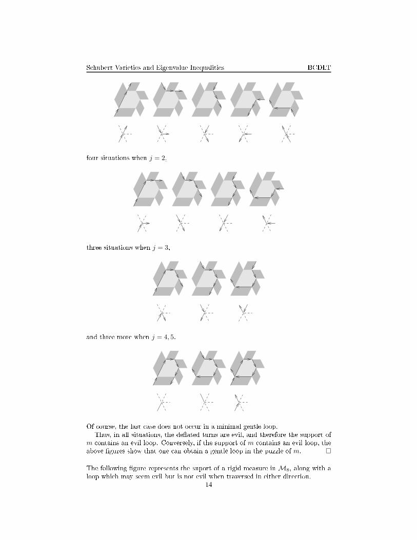
S hubert Varieties and Eigenvalue Inequalities BCDLTfour situations when j = 2,three situations when j = 3,and three more when j = 4, 5.Of ourse, the last ase does not o ur in a minimal gentle loop.Thus, in all situations, the de�ated turns are evil, and therefore the support ofm ontains an evil loop. Conversely, if the support of m ontains an evil loop, theabove �gures show that one an obtain a gentle loop in the puzzle of m. �The following �gure represents the suport of a rigid measure in M8, along with aloop whi h may seem evil but is not evil when traversed in either dire tion.14

S hubert Varieties and Eigenvalue Inequalities BCDLT

3. Extremal Measures and SkeletonsFor �xed r ≥ 1, the olle tion Mr is a onvex polyhedral one. Re all that ameasure m ∈ Mr is extremal (or belongs to an extreme ray) if any measure m′ ≤ mis a positive multiple of m. The support of an extremal measure will be alled askeleton. Clearly, an extremal measure is entirely determined by its value on anysmall edge ontained in its skeleton. Che king extremality is easily done by usingthe balan e ondition (1.1) at all the bran h points of the support to see how thedensity propagates from one edge to the rest of the support.In the following �gure of a skeleton, the thi ker edges must be assigned twi e thedensity of the other edges. (This skeleton ontains an evil loop, hen e the measuresit supports are not rigid.)It is not always obvious when a olle tion of edges supports a nonzero measure in

Mr. The reader may �nd it amusing to verify that the following �gure representssets whi h do not support any nonzero measure.We will be mostly interested in the supports of rigid extremal measures, whi hwe will all rigid skeletons. When r = 1, there are only the three possible skeletons,all of them rigid, pi tured below. 15

S hubert Varieties and Eigenvalue Inequalities BCDLTThe following �gure shows some rigid skeletons for r = 2, 3, 4, 5.

A greater variety of rigid skeletons is available for r = 6. In addition to largerversions (plus rotations and re�e tions) of the above skeletons, we have the ones inthe next �gure.For larger r, rigid skeletons an be quite involved. We provide just one moreexample for r = 8. This skeleton has edges with densities 2 and 3 whi h we did notindi ate.An important onsequen e of the hara terization of rigid measures in Mr is thefa t that su h measures an be written uniquely as sums of extremal measures. Fixa rigid measure m ∈ Mr, and let e = AB and f = BC be two distin t small edges.We will write e →m f , or simply e → f when m is understood, if one of these twosituations arises:(1) ∠ABC = 120◦ and the edge opposite e at B has m measure equal to zero;(2) e and f are opposite, and one of the edges making an angle of 60◦ with fhas m measure equal to zero.Note that in both ases we may also have f → e. The signi� an e of this relationis that e → f implies that m(e) ≤ m(f), with stri t inequality unless f → e aswell. More pre isely, if e → f and we do not have f → e, there is at least one edge16

S hubert Varieties and Eigenvalue Inequalities BCDLTg su h that g → f and the angle between e and g is 60◦. In this ase we have(3.1) m(f) = m(e) + m(g).Indeed, if e and f are opposite, the edge opposite g must have m measure equal tozero.A useful observation is that if XY → Y Z but Y Z 6→ XY , then the edgesY A, Y B, Y C whi h are 120◦, 180◦, 240◦ lo kwise from Y Z must be in the supportof m. In other words, ZY Z is an evil turn.The following result is a simple onsequen e of the fa t that the measure mexists.Lemma 3.1. Assume that a sequen e of edges e1, e2, . . . , en in the support of m issu h that

e1 → e2 → e3 → · · · → en → e1.Then we also haveen → en−1 → · · · → e1 → en.Proof. Indeed, if one of the arrows annot be reversed, then m(e1) < m(e1). �We an therefore de�ne a preorder relation on the set of small edges as follows.Given two small edges e, f , we write e ⇒ f if either e = f , or there exist edges

e1, e2, . . . , en su h thate = e1 → e2 → · · · → en = f.In this ase, we will say that f is a des endant of e and e is an an estor of f . Twoedges are equivalent, e ⇔ f , if e ⇒ f and f ⇒ e. The relation of des endan ebe omes an order relation on the equivalen e lasses of small edges. An edge e willbe alled a root if m(e) 6= 0 and e belongs to a minimal lass relative to des endan e.Clearly, every edge in the support of m is a des endant of at least one root.If m(e) 6= 0 and e ⇒ f , then there exists a path A0A1 · · ·Ak in the supportof m su h that Aj−1Aj → AjAj+1 for all j, A0A1 = e, and Ak−1Ak = f . Pathsof this form will be referred to as des endan e paths from e to f . All the turns

Aj−1AjAj+1 and Aj+1AjAj−1 in a des endan e path are evil.Lemma 3.2. Assume that e and f are in the support of a rigid measure m ∈ Mr,and A0A1 · · ·Ak and B0B1 · · ·Bℓ are two des endan e paths from e to f . ThenAk−1 = Bℓ−1 and Ak = Bℓ.Proof. Assume to the ontrary that Ak−1 = Bℓ. There are two ases to onsider,a ording to whether A0 = B1 or A0 = B0. In the �rst ase, the loop

A0A1 · · ·Ak−1Bℓ−1Bℓ−2 · · ·B1is evil, ontradi ting the rigidity of m. In the se ond ase, there is a �rst index psu h that Ap+1 6= Bp+1. Then the loopApAp+1 · · ·Ak−1Bℓ−1Bℓ−2 · · ·Bpis evil, yielding again a ontradi tion. �Lemma 3.3. Let e and e′ be inequivalent root edges in the support of a rigidmeasure m ∈ Mr, and let f be an edge whi h is a des endant of both e and e′.Consider a des endan e path A0A1 · · ·Ak from e to f , and a des endan e path

B0B1 · · ·Bℓ from e′ to f . Then Ak−1 = Bℓ−1 and Ak = Bℓ.17

S hubert Varieties and Eigenvalue Inequalities BCDLTProof. Assume to the ontrary that Ak = Bℓ−1. The edge f is not equivalent toeither e or e′. Therefore there exist indi es p, q su h that ApAp+1 6→ Ap−1Ap andBqBq+1 6→ Bq−1Bq. It follows that

ApAp+1 · · ·Ak−1Bℓ−1Bℓ−2 · · ·BqBq−1 · · ·Bℓ−2Bℓ−1Ak−1 · · ·Ap+1Apis an evil loop, ontradi ting rigidity. �These lemmas show that all the non-root edges in the support of a rigid measurem an be given an orientation. More pre isely, given a relation e ⇒ f with e aroot edge, hoose a des en en e path A0A1 · · ·Ak from e to f , and assign f theorientation Ak−1Ak. This will be alled the orientation of f away from the rootedges. Any ommon edge of two skeletons in the support of m an be oriented awayfrom the root edges; indeed, su h an edge is not a root edge. In the proofs of thenext two results, we will be on erned with the des endants of a �xed root edge e,and it will be onvenient to orient the other root edges equivalent to e away frome. The edge e an be oriented either way, as needed.Lemma 3.4. Fix a root edge in the support of a rigid measure m, and suppose thattwo des endants f = CX and g = DX have orientations pointing toward X. Thenthe turns CXD and DXC are not evil. In parti ular, the angle between f and g is60◦, and at least one of the edges C′X, D′X opposite f and g has m measure equalto zero.Proof. Assume to the ontrary that either CXD or DXC is an evil turn. Theassumed orientations imply that f 6→ g and g 6→ f . Sin e one of the edges in identto X must have measure zero, it follows f and g are not ollinear. Moreover, theedges f ′ = XC′ and g′ = XD′ opposite to f and g, respe tively, must be in thesupport of m; in the ontrary ase we would have f → g or g → f if the anglebetween f and g is 120◦, or the turn CXD would not be evil if the angle is 60◦. LetA0A1 · · ·Ak and B0B1 · · ·Bℓ be des endan e paths from e to f and g, respe tively.By assumption, we have Ak−1 = C, Bℓ−1 = D, and Ak = Bℓ = X . If A0 6= B0,then A0 = B1, A1 = B0, and learly

A0A1 · · ·AkBℓ−1Bℓ−2 · · ·B1or its reverse is an evil loop, ontradi ting the rigidity of m. Thus we must haveA0 = B0. Let p be the largest integer su h that Aj = Bj for j ≤ p. If p < min{k, ℓ},the loop

ApAp+1 · · ·AkBℓ−1Bℓ−2 · · ·Bpor its reverse is evil. Indeed, sin e Ap−1Ap → ApAp+1 and Ap−1Ap → BpBp+1,the turns Ap+1BpBp+1 and Bp+1BpAp+1 are both evil. We on lude that p =min{k, ℓ}. If p = k, it follows that the Bk−1Bk · · ·Bℓ is a des endan e path from fto g. Sin e f 6→ g, we must have Bk+1 = C′, and then the loop

BkBk+1 · · ·Bℓor its reverse is obviously evil, leading to a ontradi tion. The ase p = ℓ similarlyleads to a ontradi tion. �Theorem 3.5. Let m ∈ Mr be a rigid measure, and e a root edge in the supportof m. Then the olle tion of all des endants of e is a skeleton.18

S hubert Varieties and Eigenvalue Inequalities BCDLTProof. Sin e m an be written as a sum of extremal measures, there exists anextremal measure m′ ≤ m su h that m′(e) 6= 0. Sin e f →m g implies thatf →m′ g, the support of m′ is a skeleton ontaining all the des endants of e.Therefore it will su� e to show that the des endants of e form the support of somemeasure in Mr. We set µ(e) = 1, µ(f) = 0 if f is not a des endant of e, and forea h des endant f 6= e of e we de�ne µ(f) to be the number of des endan e pathsfrom e to f . Clearly, no edge o urs twi e in su h a path; su h an o uren e wouldimply the existen e of an evil loop. Thus the number µ(f) is �nite. To on ludethe proof, it su� es to show that µ ∈ Mr. The support of µ is ontained in thesupport of m. Therefore all the bran h points are in △r, and

µ(AjXj+1) = µ(BjY j+1) = µ(CjZj+1) = 0for all j. It remains to verify the balan e onditions. Consider a latti e point Xin △r. If no des endant of e is in ident to X , the six edges meeting at X haveµ measure zero, and the balan e ondition is trivial. Otherwise, the number ofdes endants of e in ident to X an be 1, 2, 3, 4 or 5; the value 6 is ex luded by therigidity of m. We �rst ex lude the ase where this number is 1. Assume indeed thatthere is only one des endant in ident to X , and let A0A1 · · ·Ak be a des endan epath from e with Ak = X . Sin e Ak−1Ak has no des endants of the form XY , itfollows that the turn Ak−1AkAk−1 is evil. On the other hand, sin e rigidity of minsures that one of the edges around X has measure zero, the edge Ak−1Ak is astri t de endant of some other edge XZ. In parti ular, Ak−1Ak is not a root edge,and therefore it is not equivalent to e. It follows that, for some p, we do not haveApAp+1 → Ap−1Ap, and this implies that the turn Ap+1ApAp+1 is evil. Thus

ApAp+1 · · ·Ak−1AkAk−1 · · ·Ap+1Apis an evil loop, ontrary to the rigidity of m.Consider now the ase when there are exa tly two des endants of e in ident to X , all them f and g. They annot both point away from X sin e this would requirethe existen e of a third des endant pointing toward X . They annot both pointtoward X . Indeed, if this were the ase, Lemma 3.4 insures that one of the edgesopposite f and g has measure zero, and therefore f or g has another des endantpointing away from X . Thus we an assume that f points toward X , and g awayfrom X , in whi h ase we have f → g. Then f and g must be ollinear, and everydes endan e path for g passes through f . Thus µ(f) = µ(g), whi h is the requiredbalan e ondition.Assume next that there are exa tly three des endants in ident to X . Two of themmust be non ollinear and of the form WX → XY , and the third des endant must beWX → XZ, with the three edges forming 120◦ angles. Every des endan e path foreither XY or XZ passes through WX , showing that µ(WX) = µ(XY ) = µ(XZ),and therefore satisfying the balan e requirement at X .Now, onsider the ase of exa tly four des endants in ident to X . If these fouredges form two ollinear pairs, then two of them must point towards X , and theywill form an evil turn, ontrary to Lemma 3.4. Therefore we an �nd among thefour des endants two non ollinear edges WX → XY , in whi h ase we also haveWX → XZ with these three edges forming 120◦ angles. The fourth des endant isnot ollinear with WX , so it makes a 60◦ angle with WX . If it points away fromX , it must be a des endant of the only in oming edge WX , and this is not possible.Therefore this fourth edge must be V X with V X → XY or V X → XZ. Assume19

S hubert Varieties and Eigenvalue Inequalities BCDLTV X → XY for de�niteness. In this ase, all des endan e paths forXZ pass throughWX , so that µ(XZ) = µ(WX). On the other hand, des endan e paths for XYpass either through WX or through V X , showing that µ(XY ) = µ(WX)+µ(V X).The balan e requirement is again veri�ed.Finally, if 5 des endants of e are in ident to X , then the sixth edge must havemass equal to zero, and it is impossible to orient the �ve edges so that every pairof in oming edges form a 60◦ angle, and every outgoing edge is a des endant of anin oming edge. Thus, this situation does not o ur. �The pre eding proof shows that a rigid skeleton does not ross itself transversely.In other words, a rigid skeleton does not ontain four edges meeting at the samepoint, su h that they form two ollinear pairs of edges. The following �gure showsthe possible ways (up to rotation) that the edges of a skeleton an meet, along withthe possible orientations. In ea h ase, a (or the) dotted edge must have densityequal to zero.The measure onstru ted in the above argument is the only measure supportedby the des endants of e su h that µ(e) = 1. We will denote this measure µe.Corollary 3.6. Let m ∈ Mr be a rigid measure, and let e1, e2, . . . , ek be a maximal olle tion of inequivalent root edges. Then we have

m =

k∑

j=1

m(ej)µej.Proof. Let us say that an edge f in the support of m has height ≥ p ≥ 2 if thereexists a des endan e path A0A1 · · ·Ap from some root edge e to f . If f has height

≥ p, we say that f has height equal to p if it does not have height ≥ p + 1. Therequirement that m ∈ Mr shows that the measure of any edge an be al ulatedin terms of the measures of edges of smaller height, as an be seen from (3.1).Therefore, m is entirely determined by the values m(ej), j = 1, 2, . . . k. On the otherhand, the measure m′ =∑k

j=1 m(ej)µejhas support ontained in the support of

m. Sin e m′(ej) = m(ej), we on lude that m = m′. �We mention one more useful property of rigid skeletons.Lemma 3.7. Let e and f be two edges in a rigid skeleton. There exists a pathC0C1 · · ·Cp in this skeleton su h that C0C1 = e, Cp−1Cp = f , and all the turnsCj−1CjCj+1 and Cj+1CjCj−1 are evil.Proof. The result is obvious if e is a root edge. If it is not, hoose des endan epaths A0A1 · · ·Ak from a root edge to e, and B0B1 · · ·Bℓ from the same root edgeto f . If A0 = B1, the path

AkAk−1 · · ·A1B1B2 · · ·Bℓsatis�es the requirements. If A0 = B0 one hooses instead the pathAkAk−1 · · ·Ar+1BrBr−1 · · ·Bℓ,20

S hubert Varieties and Eigenvalue Inequalities BCDLTwhere r is the �rst integer su h that Ar+1 6= Br+1. If no su h integer exists, one ofthe paths is ontained in the pther. For instan e, k < ℓ and Aj = Bj for j ≤ k. Inthis ase the desired path is Bk−1Bk · · ·Bℓ. �The path provided by this lemma is not generally a des endan e path.We on lude this se tion by introdu ing an order relation on the set of skeletons ontained in the support of a rigid measure m. Given two rigid skeletons S1 and S2,we will write S1 ≺0 S2 if S1 has ollinear edges AX, XB and S2 has ollinear edgesCX, XD su h that XA is 60◦ lo kwise from XC. The following �gure shows thefour possible on�gurations of S1 and S2 around the point X , up to rotation, andassuming that the two skeletons are ontained in the support of a rigid measure.The edges in S1 \ S2 are dashed, the edges in S2 \ S1 are solid without arrows, andthe ommon edges are oriented away from the root edges.

A

C D

B

A

C D

B

A

C D

BB

A

C DThe four turns AXC, AXD, BXC, and BXD are evil.Note that the point X ould be on the boundary of △r, but not one of the three orner verti es. It is possible that S1 ≺0 S2 and S2 ≺0 S1, as illustrated in thepi ture below (with S1 in dashed lines).We will show that this does not o ur when the skeletons are asso iated with a�xed rigid measure.Theorem 3.8. Fix a rigid measure m ∈ Mr and an integer n ≥ 1. There do notexist skeletons S1, S2, . . . , Sn ontained in the support of m su h that

S1 ≺0 S2 ≺0 · · · ≺0 Sn ≺0 S1.Proof. Assume to the ontrary that su h skeletons exist. Choose for ea h j ollinearedges AjXj , XjBj in the support of Sj and ollinear edges CjXj , XjDj in thesupport of Sj+1 (with Sn+1 = S1) su h that XAj is 60◦ lo kwise from XCj . Therigidity of m implies that one of the edges XY has measure zero. Therefore wemust have either XjAj → XjBj or XjBj → XjAj . Label these two edges fj andf ′

j so that fj → f ′j , and note that fj is not the des endant of any edge XY , ex eptpossibly f ′

j. Analogously, denote the edges Xj−1Cj−1 and Xj−1Dj−1 by ej and e′jso that e′j → ej. Sin e both ej and fj are ontained in Sj , Lemma 3.7 provides apath with evil turns joining ej and fj . A moment's thought shows that this patheither begins at Xj−1, or it begins with one of Cj−1Xj−1Dj−1, Dj−1Xj−1Cj−1. If21

S hubert Varieties and Eigenvalue Inequalities BCDLTthe se ond alternative holds, remove the �rst edge from the path. Performing theanalogous operation at the other endpoint, we obtain a path γj with only evil turnswhi h starts at Xj−1 ends at Xj (with Xj−1 = Xn if j = 0), its �rst edge is one ofXj−1Cj−1, Xj−1Dj−1, and its last edge is one of AjXj , BjXj . As noted above, theturn formed by the last edge of γj and the �rst edge of γj+1 is evil. We on ludethat the loop γ1γ2 · · · γn is evil, ontradi ting rigidity. �The pre eding result shows that there is a well-de�ned order relation on the setof skeletons in the support of a rigid measure m de�ned as follows: S ≺ S′ if thereexist skeletons S1, S2, . . . , Sk su h that

S = S1 ≺0 S2 ≺0 · · · ≺0 Sk = S′.The following �gure shows the support of a rigid measure m ∈ M6. The elementsof a maximal olle tion of mutually inequivalent root edges have been indi atedwith dots.For this measure, there is a smallest skeleton (relative to ≺) pi tured below. Thereader an easily draw all the other skeletons and determine the order relation.

4. Horn Inequalities and Clo kwise OverlaysThe results of [21, 22℄ show that the triples (α, β, γ) = ∂m with m ∈ Mr arepre isely those triples of in reasing nonegative ve tors in Rr with the property thatthere exist selfadjoint matri es A, B, C ∈ Mr(C) su h that

λA(ℓ) = αr+1−ℓ, λB(ℓ) = βr+1−ℓ, λC(ℓ) = γr+1−ℓ, ℓ = 1, 2, . . . , r,and A+B+C is a multiple of the identity, namely, 2ω(m)1Cr . The Horn inequalitiesfor these matri es are∑

i∈I

λA(i) +∑

j∈J

λB(j) +∑

k∈K

λC(k) ≤ 2sω(m)22

S hubert Varieties and Eigenvalue Inequalities BCDLTwhen I, J, K ⊂ {1, 2, . . . , r} have ardinality s and cIJK > 0. Applying this in-equality to the matri es −A,−B,−C instead and swit hing signs, we obtain∑

i∈I

λA(r + 1 − i) +∑

j∈J

λB(r + 1 − j) +∑

k∈K

λC(r + 1 − k) ≥ 2sω(m)Equivalently, ∑

i∈I

αi +∑

j∈J

βj +∑

k∈K

γk ≥ 2sω(m).Now, the sets I, J, K are obtained from some measure ν ∈ Ms with weight r − s,and we will see how this inequality follows from the superposition of the support ofm and the puzzle asso iated with ν. Let h be the honey omb provided by Lemma1.1. Let D ⊂ △r be a region bounded by small edges, and let XjYj , j = 1, 2, . . . , pbe an enumeration of the edges of ∂D, oriented so that D lies on the left of XjYj .For ea h j, there is εj = εXjYj

= ±1 su h that Yj − Xj ∈ {εju, εjv, εjw}. Thede�nition of honey ombs implies then the identity∑

XY ⊂∂D

εXY h(XY ) =

p∑

j=1

εjh(XjYj) = 0,whi h is easily dedu ed by indu tion on the size of D. We would like to verify thatthe sumS =

∑

i∈I

h(Ai−1Ai) +∑

j∈J

h(Bj−1Bj) +∑

k∈K

h(Ck−1Ck)is nonnegative, where I, J, K are given by a measure ν ∈ Ms with ω(ν) = r−s. Thein�ation of the measure ν yields a partition of △r into white pie es (the translatedparts of △s), gray parallelograms, and light gray pie es. Denote by D the union ofthe gray parallelograms P1, P2, . . . , Pσ and white pie es W1, W2, . . . , Wτ . The edgesAi−1Ai, i ∈ I, Bj−1Bj , j ∈ J , and Ck−1Ck, k ∈ K are ontained in the interse tion∂D ∩ ∂△. Sin e

∑

XY ⊂∂D

εXY h(XY ) =∑

XY ⊂∂Wℓ

εXY h(XY ) = 0, ℓ = 1, 2, . . . , τ,andS =

∑

white XY ⊂∂D∩∂△r

εXY h(XY ),we haveS = S −

∑

XY ⊂∂D

εXY h(XY ) +

τ∑

ℓ=1

∑

XY ⊂∂Wℓ

εXY h(XY )

= −

σ∑

ℓ=1

∑gray XY ⊂∂Pℓ

εXY h(XY ),where the last sums are taken over the light gray edges of Pℓ. Condition (3) impliesthat−

∑gray XY ⊂∂Pℓ

εXY h(XY ) =∑

e

m(e),where the sum is taken over all small edges ontained in Pℓ whi h are not parallelto the sides of Pℓ. This immediately implies the desired Horn inequality, and it alsotells us when equality is attained: this happens if and only if all the edges e ⊂ Pℓfor whi h m(e) > 0 are parallel to the edges of Pℓ, ℓ = 1, 2, . . . , s. In other words,23

S hubert Varieties and Eigenvalue Inequalities BCDLTthe support of m must ross ea h Pℓ along lines parallel to the edges of Pℓ. Thefollowing �gure illustrates the support of a measure ν, the in�ation of ν, and thesupport of a measure m whi h satis�es the Horn equality asso iated with ν. In thisexample the support of the measure m never rosses the white puzzle pie es.The next example involves basi ally the mirror image of the measure m, and itssupport never rosses the light gray pie es.This phenomenon is related with the fa t that the support of m is a tually a rigidskeleton in both ases. A rigid skeleton does not ross itself transversely. Thus,in a ase of equality, it annot have any bran h points in the interior of a grayparallelogram. It follows then that the skeleton always rosses these parallelogramsbetween white pie es or between gray pie es, but not both.Assume that we are in a ase of equality

∑

i∈I

h(Ai−1Ai) +∑

j∈J

h(Bj−1Bj) +∑

k∈K

h(Ck−1Ck) = 0.In this ase, we an de�ne a measure µ ∈ Ms by moving the support of m to △s inthe following way: those parts whi h are ontained in white puzzle pie es are simplytranslated ba k to △s (along with their densities); the segments in the support ofm whi h ross between white pie es are deleted; the segments whi h ross betweenlight gray pie es are repla ed by the oresponding parallel sides of white pie es, andthe density is preserved. It may be that several segments ross between light graypie es, in whi h ase the density of the orresponding side of a white pie e is thesum of their densities. When the measure µ an be obtained using this pro edure,we will say that µ is obtained by ontra ting m, and that µ is lo kwise from ν(or that (µ, ν) form a lo kwise overlay). This is easily seen to be an extension ofthe notion of lo kwise overlay introdu ed in [22℄ (see also item (1), se ond ase,in the proof of Theorem 4.2). Generally, a lo kwise overlay (µ, ν) an be obtained24

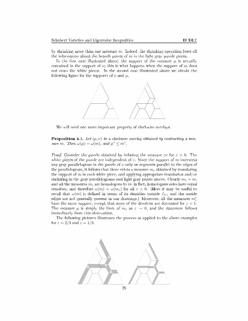
S hubert Varieties and Eigenvalue Inequalities BCDLTby shrinking more than one measure m. Indeed, the shrinking operation loses allthe information about the bran h points of m in the light gray puzzle pie es.In the �rst ase illustrated above, the support of the measure µ is a tually ontained in the support of ν; this is what happens when the support of m doesnot ross the white pie es. In the se ond ase illustrated above we obtain thefollowing �gure for the supports of ν and µ.We will need one more important property of lo kwise overlays.Proposition 4.1. Let (µ, ν) be a lo kwise overlay obtained by ontra ting a mea-sure m. Then ω(µ) = ω(m), and µ∗ ≤ m∗.Proof. Consider the puzzle obtained by in�ating the measure εν for ε > 0. Thewhite pie es of the puzzle are independent of ε. Sin e the support of m interse tsany gray parallelogram in the puzzle of ν only on segments parallel to the edges ofthe parallelogram, it follows that there exists a measure mε obtained by translatingthe support of m in ea h white pie e, and applying appropriate translation and/orshrinking in the gray parallelograms and light gray puzzle pie es. Clearly m1 = m,and all the measures mε are homologous to m; in fa t, homologous sides have equaldensities, and therefore ω(m) = ω(mε) for all ε > 0. (Here it may be useful tore all that ω(m) is de�ned in terms of its densities outside △r, and the ousideedges are not generally present in our drawings.) Moreover, all the measures m∗

εhave the same support, ex ept that some of the densities are de reased for ε < 1.The measure µ is simply the limit of mε as ε → 0, and the statement followsimmediately from this observation.The following pi tures illustrates the pro ess as applied to the above examplesfor ε = 2/3 and ε = 1/3.

25

S hubert Varieties and Eigenvalue Inequalities BCDLT�Unfortunately, the de�nition of lo kwise overlays is not quite expli it sin e theyare seen as the result of a pro ess � something akin to de�ning a ar as the endprodu t of ar manufa ture. We an however use the relation ≺0 between skeletonsto produ e an important lass of lo kwise overlays.Theorem 4.2. Let µ1, µ2 ∈ Mr be su h that µ1 + µ2 is rigid, the support Sj of µjis a skeleton, and S2 6≺0 S1. Then (µ1, µ2) is a lo kwise overlay.Proof. We need to in�ate µ2, and onstru t a measure m1 su h that µ1 is obtainedfrom m1 by the shrinking pro ess des ribed above. It is lear what the measure m1should be on the interior of every white puzzle pie e. The ommon edges of S1 and

S2 annot be root edges; orient them away from the root edges, and atta h them(along with their µ1 masses) to the white puzzle pie e on their right side. Whatremains to be proved is that this partialy de�ned measure an be extended so as tosatisfy the balan e ondition at all points. For this purpose we only need to analyzethe situation at latti e points where S1 and S2 meet. For ea h su h latti e point,there will be 2, 3, or 4 edges of ea h skeleton meeting at that point, and this givesrise to many possibilities. In order to redu e the number of ases we need to study,observe that the in�ation onstru tion is invariant relative to rotations of 60◦, andtherefore the position (but perhaps not the orientation) of the edges in one of theskeletons an be �xed. In the following �gures, the arrows indi ate the orientationon the edges in S1 ∩ S2. The other edges of S1 are dashed, and the other edges ofS2 are solid without arrows. In ea h ase, the extension required after in�ation isindi ated by dashed lines rossing (or on the boundary of) parallelogram pie es. Inhe following enumeration, the label (p, q) signi�es that S1 has p and S2 has q edgesmeeting at one point.(1) (2, 2) The edges of the skeletons may overlap, and after a rotation theorientation is as in the �gure below.No extensions are required in this ase. If the skeletons do not overlap, wehave two possibilities:

and �nally 26

S hubert Varieties and Eigenvalue Inequalities BCDLTwhi h would imply S2 ≺0 S1, ontrary to the hypothesis.(2) (3, 2) In this ase there is (up to rotations) only the ase illustrated in the�gure.

(3) (4, 2) Up to rotations, there are three possibilities. In the �rst one we havean extension as shown.The orientation shown above is the only one whi h is ompatible with therigidity of m. In the following �gure, the orientation given is also the onlypossible one.The third situationimplies S2 ≺ S1.(4) (2,3) The ase illustrated is the only one up to rotations.

��(5) (3, 3) There are two ases up to rotations.��

��

��

��

��

��

��

��

��

��

��

��The se ond ase is not ompatible with rigidity.27

S hubert Varieties and Eigenvalue Inequalities BCDLT��

��

��

��

��

��

��

��

��(6) (4, 3) There is only one position of S1 ompatible with rigidity, but thereare two possible orientations.

��

��

��

��

��

��

��

��

��

��

��The se ond orientation requires a di�erent extension.

��

��

��

��

��

��

(7) (2, 4) There are three possibilities up to rotation.��

��

��

��In the �gure above, there is no ambiguity in the orientation. For the illus-tration we assigned µ2 masses of 1 and 2 to the edges.��

��

��

The orientation is also lear in this ase. The third ase implies S2 ≺ S1.(8) (3, 4) There is only one position ompatible with rigidity, and there are onlytwo possible orientations.��

��

��

��

�� 28

S hubert Varieties and Eigenvalue Inequalities BCDLT��

��

��

��

��(9) (4, 4) When the two skeletons overlap ompletely, there are two possibleorientations.��

��

��

��

��

��

��

��

��When the skeletons do not overlap ompletely, there is only one relativeposition of the two skeletons whi h is ompatible both with rigidity andwith S2 6≺ S1. There is only one possible orientation.��

��

��

��

��

�The following result follows easily by indu tion, in�ating su essively the mea-sures µp, µp−1, . . . , µt+1.Corollary 4.3. Let m ∈ Mr be a rigid measure, and write it as m =∑p

ℓ=1 µℓ,where µℓ is supported on the skeleton Sℓ. Assume also that Si ≺ Sj implies thati ≤ j. Then the pair (∑t

ℓ=1 µℓ,∑p

ℓ=t+1 µℓ

) is a lo kwise overlay for 1 ≤ t < p.For the lo kwise overlays (µ1, µ2) onsidered in the pre eding two results thereis a anoni al onstru tion for the measure m1 ∈ Mr+ω(µ2). We will all thismeasure m1 the stret h of µ1 to the puzzle of µ2.5. Proof of the Main ResultsFix a triple (I, J, K) of subsets with ardinality r of {0, 1, . . . , n} su h thatcIJK = 1, and let m ∈ Mr be the orresponding measure. It will be onve-nient now to use the normalization τ(1) = n in a �nite fa tor. This will not require29

S hubert Varieties and Eigenvalue Inequalities BCDLTrenormalizations when passing to a subfa tor, and has the added bene�t of work-ing in �nite dimensions as well. In order to prove the interse tion results in theintrodu tion, we will want to prove the following related properties:Property A(I, J, K) or A(m). Given a II1 fa tor A with τ(1) = n, and given�ags E ,F ,G with τ(Eℓ) = τ(Fℓ) = τ(Gℓ) = ℓ, ℓ = 0, 1, 2, . . . , n, the interse tionS(E , I) ∩ S(F , J) ∩ S(G, K)is not empty.Property B(I, J, K) or B(m). There exists a latti e polynomial p ∈ L({ej, fj, gj :

1 ≤ j ≤ n}) with the following property: for any �nite fa tor A with τ(1) = n, andfor generi �ags E = (Ej)nj=0, F = (Fj)

nj=0, G = (Gj)

nj=0 su h that τ(Ej) = τ(Fj) =

τ(Gj) = j, the proje tion P = p(E ,F ,G) has tra e τ(P ) = r and, in additionτ(P ∧ Ei) = τ(P ∧ Fj) = τ(P ∧ Gk) = ℓwhen iℓ ≤ i < iℓ+1, jℓ ≤ j < jℓ+1, kℓ ≤ k < kℓ+1 and ℓ = 0, 1, . . . , r, where

i0 = j0 = k0 = 0 and ir+1 = jr+1 = kr+1 = n + 1.We will prove these properties by redu ing them to simpler measures for whi hthey are trivial. The basi redu tion is from an arbitrary measure to a skeleton.Proposition 5.1. Let m ∈ Mr a rigid measure, and write m =∑p

ℓ=1 µℓ, whereµℓ is supported by a skeleton Sℓ , and Si ≺ Sj implies i ≤ j. Let µ̃1 ∈ Mer,r̃ =

∑pℓ=2 ω(µℓ) be the stret h of µ1 to the puzzle of m′ =

∑pℓ=2 µℓ. If A(µ̃1) and

A(m′) (resp., B(µ̃1) and B(m′)) are true, then A(m) (resp., B(m)) is true as well.Proof. With the usual notation Ai = iu, X i = Ai +w, the edges AiX i are orientedin the dire tion of w (if they belong to the support of m). Let us set ai = m(AiX i),a(1)i = µ1(AiX i), and a′

i = m′(AiX i), so that ai = a′i + a

(1)i , and n = r +

∑ri=0 ai.The measure µ̃1 is asso iated with the triangle△r1 , where r1 = r+

∑ri=0 a′

i. Its sup-port may interse t the left side of this triangle only at the points Aℓ(i), where ℓ(0) =

0, and ℓ(i) = i +∑i−1

s=0 a′s for i > 0; this follows from the way the in�ation of m′is onstru ted, and from the outward orientation of the segments AiX i. Moreover,

µ̃1(Aℓ(i)Xℓ(i)) = a(1)i for i = 0, 1, . . . , r. Denote by I(1), J (1), K(1) ⊂ {1, 2, . . . , n}the sets determined by the measure µ̃1, and by I ′, J ′, K ′ ⊂ {1, 2, . . . , n1} those orresponding with m′, where we set n1 = n − ω(m1). For instan e, we have

I(1) =

r⋃

j=1

{s +

j−1∑

ℓ=0

a(1)ℓ +

j−2∑

ℓ=0

(a′ℓ + 1) : s = 1, 2, . . . , a′

j−1 + 1

},where the se ond sum is zero for j = 1, and

I ′ = {it −

t−1∑

ℓ=0

a(1)ℓ : t = 1, 2, . . . , r},where I = {i1, i2, . . . , ir}. Observe that i

(1)ℓ = it for ℓ = t +

∑t−1s=0 a′

s = i′t.Assume �rst that A(µ̃1) and A(m′) are true, and let E ,F ,G be arbitrary �ags ina II1 fa tor su h that τ(Ei) = τ(Fi) = τ(Gi) = i for i = 0, 1, . . . , n, and τ(1) = n.Property A(µ̃1) implies the existen e of a proje tion P1 ∈ A su h that τ(P1) = r1andτ(P1 ∧ E

i(1)ℓ

) ≥ ℓ, ℓ = 1, 2, . . . , r1.30

S hubert Varieties and Eigenvalue Inequalities BCDLTAs noted above, we have i(1)ℓ = it for ℓ = i′t, and therefore we have

τ(P1 ∧ Ei′t) ≥ t +

t−1∑

s=0

a′s = i′t, t = 1, 2, . . . , r,with analogous inequalities for F and G. Consider now the fa tor A1 = P1AP1with the tra e τ1 = τ |A1, so that τ1(1A′

1) = τ(P1) = r1. The inequalities aboveimply the existen e of a �ag E ′ in A1 su h that τ1(E

′j) = j for j = 1, 2, . . . , n1, and

E′i′p

≤ P1 ∧ Eip, p = 1, 2, . . . , r.Analogous onsiderations lead to the onstru tion of �ags F ′ and G′. Property

A(m′) implies now the existen e of a proje tion P ∈ A1 su h that τ1(P ) = r,τ1(P ∧ E′

i′p) ≥ p, p = 1, 2, . . . , r,and analogous inequalities are satis�ed for F ′ and G′. Clearly the proje tion Psatis�es

τ(P ∧ Eip) ≥ p, p = 1, 2, . . . , r,so that it solves the interse tion problem for the sets I, J, K.The ase of property B is settled analogously. The di�eren e is that P1 is givenas a latti e polynomial P1 = p1(E ,F ,G), and the proje tions E′

j an be taken to beof the form P1 ∧Ei, and hen e they too are latti e polynomials in E ,F ,G. Finally,the solution P is given as P = p′(E ′,F ′,G′), where the existen e of p′ is given byproperty B(m′). One must however assume that E ′,F ′,G′ are generi �ags, andthis simply amounts to an additional generi ity ondition on the original �ags. �The pre eding proposition shows that proving property A(m) or B(m) an beredu ed to proving it for simpler measures, at least when m is not extremal. A dualredu tion is obtained by re alling that a proje tion P belongs to S(E , I) if and onlyP⊥ = 1 − P belongs to S(E⊥, I∗). Moreover, if the sets I, J, K are asso iated tothe measure m ∈ Mr, then I∗, J∗, K∗ are the sets asso iated to the measure m∗.Therefore A(m) is equivalent to A(m∗) and B(m) is equivalent to B(m∗).To quantify these redu tions, we de�ne for ea h measure m ∈ Mr the positiveinteger κ(m) as the number of gray parallelograms in the puzzle obtained by in-�ating m. This is equal to the number of white pie e edges whi h have positivemeasure. Analogously, for m ∈ M∗

r , we de�ne κ∗(m) to be the number of grayparallelograms in the puzzle obtained by *in�ating m. With this de�nition it is lear thatκ(m) = κ∗(m∗), m ∈ Mr.Indeed, the two numbers ount pie es of the same puzzle.With the notation of the pre eding proposition, we have

κ(µ̃1) = κ(µ1) < κ(m), κ(m′) < κ(m),unless m = µ1. Indeed, κ(µ̃1) = κ(µ1) be ause µ1 and µ̃1 are homologous, andthe supports of µ1 and m′ are stri tly ontained in the support of m. In fa t, thesupport of m′ does not ontained the root edges of µ1, and the support of µ1 doesnot ontain the root edges of the extremal summands of m′. Thus the pre edingproposition also allows us to redu e the proof of these properties to measures withsmaller values of κ in ase eitherm orm∗ is not extremal. The ex eptional situations31

S hubert Varieties and Eigenvalue Inequalities BCDLTin whi h both m and m∗ are extremal are very few in number. To see this we needto use the stru ture of the onvex polyhedral oneCr = {∂m : m ∈ Mr},whose fa ets were determined in [22℄. If ∂m = (α, β, γ), these fa ets are of twokinds. The �rst kind are the hamber fa ets determined by an equality of the form

αℓ = αℓ+1, βℓ = βℓ+1, γℓ = γℓ+1 for 1 ≤ ℓ < r or αr = ω(m), βr = ω(m),γr = ω(m). The se ond kind are the regular fa ets determined by Horn identities

∑

i∈I

αi +∑

j∈J

βj +∑

k∈K

γk = ω(m),where I, J, K ⊂ {1, 2, . . . , r} have s < r elements and cIJK = 1.For a given measure m ∈ Mr, we de�ne the number of atta hment points Γ(m)to be the number of hamber fa ets to whi h m does not belong. The reason forthis terminology is that Γ(m) is pre isely the number of points on the sides of △rwhi h are endpoints of interior edges in the support of m. The verti es of △r shouldalso ounted as atta hment points when they are bran h points of the measure.Proposition 5.2. Let m ∈ Mr be an extremal rigid measure. If m∗ is extremalas well, then Γ(m) = 1.Proof. Assume that m and m∗ are both extremal, and Γ(m) > 1. Note �rst that∂m is extremal in Cr. Indeed, in the ontrary ase, we would have ∂m = ∂m1+∂m2with ∂m1 not a positive multiple of ∂m. This would however imply m = m1 + m2by rigidity, and hen e m1 is a multiple of m, a ontradi tion.Next, sin e Γ(m) = Γ(m′) for homologous m, m′, we may assume that m∗ = µefor some root edge e. Indeed, m∗ = m∗(e)µe is homologous to µe, and therefore mis homologous to µ∗

e.The de�nition of Γ(m) implies that ∂m belongs to 3r − Γ(m) = dimCr − Γ(m) hamber fa ets. However, an extremal measure must belong to at least dimCr −1 fa ets, and hen e ∂m belongs to at least one regular fa et. As seen earlier,there must then exist a lo kwise overlay (m1, m2) su h that m1 is obtained by ontra ting m. It follows from Proposition 4.1 that 0 6= m∗

1 ≤ m∗. Sin e m∗1has integer densities, we must have m∗

1 = m∗, and this implies that m1 = m, a ontradi tion. �Thus the repeated appli ation of the redu tion pro edure to m and m∗ leadseventually to one of the three skeletons pi tured below.For these, the interse tion problem is ompletely trivial. Indeed, onsider the �rstof the three on △r, and with ω(m) = s. We have then I = {1, 2, . . . , r} andJ = K = {s + 1, s + 2, . . . , s + r}, and the desired element in

S(E , I) ∩ S(F , J) ∩ S(G, K)32

S hubert Varieties and Eigenvalue Inequalities BCDLTis simply Er. Thus A(m) is true for this measure. To show that B(m) is true aswell, we must verify that generi ally we also haveτ(Er ∧ Fℓ) = τ(Er ∧ Gℓ) = max{0, r + ℓ − n}for ℓ = 1, 2, . . . n. This follows easily from the following result.Proposition 5.3. Let E and F be two proje tions in a �nite fa tor A. There isan open dense set O ⊂ U(A) su h thatτ(E ∧ UFU∗) = max{0, τ(E) + τ(F ) − τ(1)}for U ∈ O.Proof. Repla ing E and F by E⊥ and F⊥ if ne essary, we may assume that τ(E)+

τ(F ) ≤ τ(1). Sin e A is a fa tor, we an repla e F with any other proje tionwith the same tra e. In parti ular, we may assume that F ≤ E⊥. The onditionτ(E ∧ UFU∗) = 0 is satis�ed if the operator FUF is invertible on the range of F .The proposition follows be ause the set O of unitaries satisfying this ondition is adense open set in U(A). To verify this fa t, it su� es to onsider the ase in whi hthe algebra A is of the form A = B ⊗ M2(C) for some other �nite fa tor B, and

F =

[1 00 0

].An arbitary unitary U ∈ A an be written as

U =

[T (I − TT ∗)1/2W

V (I − T ∗T )1/2 −V T ∗W

],where T, V, W ∈ B, V and W are unitary, and ‖T ‖ ≤ 1. Sin e B is a �nite vonNeumann algebra, T an be approximated arbitrarily well in norm by an invertibleoperator T ′, in whi h ase U is approximated in norm by the operator

U ′ =

[T ′ (I − T ′T ′∗)1/2W

V (I − T ′∗T ′)1/2 −V T ′∗W

]with FU ′F invertible. In �nite dimensions, the omplement of O is de�ned by thesingle homogeneous polynomial equation det(FUF + F⊥) = 0. Thus O is open inthe Zariski topology. �Corollary 5.4. Properties A(m) and B(m) are true for all rigid measures m.This proves �nally Theorems 0.4 and 0.5. The fa t that Theorem 0.3 followsfrom Theorem 0.4 was already shown in [4℄.6. Some IllustrationsWe have just seen that proving property A(I, J, K) or B(I, J, K) an be redu ed,in ase cIJK = 1, to the ase in whi h the asso iated measure m has pre isely oneatta hment point. We will illustrate how this redu tion works in a few ases.Given a measure m ∈ Mr, a point Aℓ, ℓ = 1, 2, . . . , r, is an atta hment point of mpre isely when m(AℓXℓ) > 0. The solution to the asso iated S hubert interse tionproblem will only depend on the proje tions Ei(ℓ) where ℓ is an atta hment point.These proje tions, and the analogous Fj(ℓ), Gk(ℓ), will be alled the atta hmentproje tions for the problem. With the notation Proposition 5.1, the atta hmentproje tions of µ̃1 are exa tly the same as those of µ1, and are therefore amongthe atta hment proje tions of m. The atta hment proje tions of m∗ are of the33

S hubert Varieties and Eigenvalue Inequalities BCDLTform P⊥ = 1 − P , where P is an atta hment proje tion for m. These observationsallow us to onstru t solutions to interse tion problems without a tually having to onstru t the measure µ̃1 and fo us instead on the atta hment proje tions of µ1.We pro eed now to solve the interse tion problems asso iated with some skele-tons. Consider �rst an extreme measure m ∈ Mr with two atta hment points. Thefollowing pi ture shows the supports of m and m∗.For the illustration we took r = 3 and density 3 on the support, but the resultswill hold for the general ase. Note that m∗ is a sum of two extremal measureswith one atta hment point ea h. If X and Z are the atta hment proje tions ofm, the atta hment proje tions of these skeletons are X⊥ and Z⊥. Neither of thetwo skeletons pre edes the other, and following the method of Proposition 5.1, wesee that the solution of the interse tion problem asso iated with m∗ is generi allyX⊥∧Z⊥. It follows that the interse tion problem asso iated with m has the generi solution X ∨ Y .There are two kinds of skeletons with three atta hment points. The �rst one,and its dual, are illustrated below.Assume that the atta hment proje tions are X, Y and Z. As in the pre edingsituation, m∗ is a sum of three extremal measures with one atta hment point, andthere are no pre eden e relations among the skeletons. It follows that the generi solution of the interse tion problem is X ∨ Y ∨ Z.The two ases just mentioned orrespond to the redu tions onsidered in [25℄ for�nite dimensions, and in [9℄ for the fa tor ase. Note however that these papersalso apply these redu tions when cIJK > 1.Consider next the other kind of skeleton with three atta hment points, and withatta hment proje tions X, Y, Z.In this ase, m∗ is the sum of three extremal measures with two atta hment pointsea h, and with no pre eden e relations. The interse tion problems asso iated withthe three skeletons have then generi solutions X⊥ ∨ Y ⊥, X⊥ ∨Z⊥, and Y ⊥ ∨Z⊥.A ording to Proposition 5.1, the solution of the interse tion problem for m∗ willbe (generi ally) the interse tion of these three proje tions, so that the problem34

S hubert Varieties and Eigenvalue Inequalities BCDLTasso iated with m has the solution(X ∧ Y ) ∨ (X ∧ Z) ∨ (Y ∧ Z).Several of the proofs of Horn inequalities in the literature an now be dedu edby onsidering rigid measures whi h are sums of extremal measures with 1,2 or 3atta hment points. Consider, for instan e, a measure m ∈ Mr de�ned by

m = ρ +

r∑

ℓ=1

(µℓ + νℓ),where ρ has atta hment point Cr, µ1 has atta hment point Ar, ν1 has atta hmentpoint Br, µℓ has atta hment points Ar−ℓ+1 and Cℓ−1, and νℓ has atta hment pointsBr−ℓ+1 and Cℓ−1 for ℓ > 1.The only pre eden e relations are µℓ ≺0 νk and νℓ ≺0 µk for ℓ < k. Generi ally,the asso iated interse tion problem is solved as follows. Set P0 = Gr and

Pℓ+1 = [(Gℓ ∧ Pℓ) ∨ (Fr−ℓ ∧ Pℓ)] ∧ [(Gℓ ∧ Pℓ) ∨ (Er−ℓ ∧ Pℓ)]for ℓ = 1, 2, . . . , r − 1. The spa e Pr is the generi solution. The sets I, J, Kasso iated with m are easily al ulated. Using the notationsc = ω(ρ), aℓ = ω(µℓ), bℓ = ω(νℓ) for ℓ = 1, 2, . . . , r,we have

n = r + c +

r∑

ℓ=1

(aℓ + bℓ),and I = {n + 1 − (a1 + a2 + · · · + aℓ + ℓ) : ℓ = 1, 2, . . . , r}, J = {n + 1 − (b1 + b2 +· · ·+ bℓ + ℓ) : ℓ = 1, 2, . . . , r}, and K = {a1 + b1 + · · ·+ aℓ + bℓ + ℓ : ℓ = 1, 2, . . . , r}.These sets yield the eigenvalue inequalities proved in [23℄.Consider next sequen es of integers

0 ≤ z1 ≤ z2 ≤ · · · ≤ zp, 0 ≤ w1 ≤ w2 ≤ · · · ≤ wpsu h that zp + wp ≤ r, and onsider the measure m ∈ Mr de�ned bym =

p∑

i=1

µi,where µℓ has atta hment points Azℓ, Bwℓ

, and Cr−zℓ−wℓ.35

S hubert Varieties and Eigenvalue Inequalities BCDLTThe illustration uses p = 3, r = 6, z1 = 1,z2 = 2, z3 = 3, w1 = w2 = 1, andw3 = 2. We have µℓ ≺0 µk only when ℓ < k, wℓ < wk and zℓ < zk. If we setP1 = Ez1 ∨ Fw1 ∨ Gr−z1−w1 and

Pℓ+1 = (Ezℓ+1∧ Pℓ) ∨ (Fwℓ+1

∧ Pℓ) ∨ (Gr−zℓ+1−wℓ+1∧ Pℓ)for ℓ = 1, 2, . . . , d − 1, then Pd is the generi solution of the interse tion problem.Assume that ω(µi) = 1 for all i, and use the notation

1x<y =

{1 if x < y,

0 if x ≥ y.Then for the orresponding interse tion problem we have n = r + p, I(ℓ) = ℓ +∑pi=1 1zi<ℓ, J(ℓ) = ℓ +

∑pi=1 1wi<ℓ, and n + 1 − K(r + 1 − ℓ) = ℓ +

∑pi=1 1wi+zi<ℓfor ℓ = 1, 2, . . . , r. These sets yield the eigenvalue inequalities proved in [24℄.One an produ e su h families of inequalities using more ompli ated skeletons.Observe for instan e that, given integers a, b, c, d su h that a + b + c + d = r,there exists a skeleton in △r with atta hment points Aa, Aa+b+c, Bb+d, and Cc+d.Call µa,b,c,d the smallest extremal measure with integer densities supported by thisskeleton. A measure of the form

m =

p∑

ℓ=1

µaℓ,bℓ,cℓ,dℓwill be rigid if the following onditions are satis�ed:aℓ ≤ aℓ+1, dℓ ≤ dℓ+1, cℓ + dℓ ≤ cℓ+1 + dℓ+1, bℓ + dℓ ≤ bℓ+1 + dℓ+1for ℓ = 1, 2, . . . , p − 1. Moreover, µaℓ,bℓ,cℓ,dℓ

≺ µaℓ′ ,bℓ′ ,cℓ′ ,dℓ′implies ℓ ≤ ℓ′. The orresponding interse tion problem will be solved by dealing su essively with thesesummands. The reader will have no di� ulty writing out the sets I, J, K ⊂

{1, 2, . . . , n}, where n = r + 2p. The following �gure illustrates the ase p = 2with r = 8, a1 = d1 = 1, b1 = c1 = 3, a2 = 2, b2 = c2 = 1, and d2 = 4.36

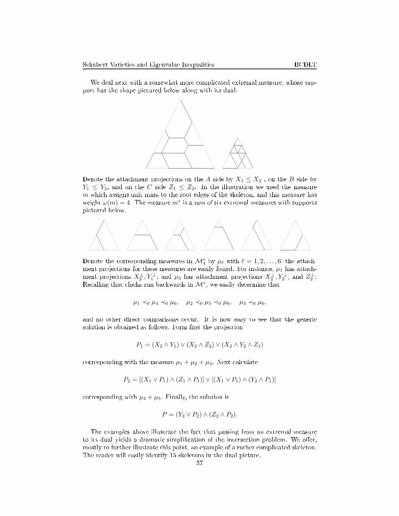
S hubert Varieties and Eigenvalue Inequalities BCDLTWe deal next with a somewhat more ompli ated extremal measure, whose sup-port has the shape pi tured below along with its dual.Denote the atta hment proje tions on the A side by X1 ≤ X2 , on the B side byY1 ≤ Y2, and on the C side Z1 ≤ Z2. In the illustration we used the measurem whi h assigns unit mass to the root edges of the skeleton, and this measure hasweight ω(m) = 4. The measure m∗ is a sum of six extremal measures with supportspi tured below.Denote the orresponding measures in M∗

4 by µℓ with ℓ = 1, 2, . . . , 6. the atta h-ment proje tions for these measures are easily found. For instan e, µ1 has atta h-ment proje tions X⊥2 , Y ⊥

1 , and µ3 has atta hment proje tions X⊥2 , Y ⊥

2 , and Z⊥2 .Re alling that lo ks run ba kwards in M∗, we easily determine that

µ1 ≺0 µ4 ≺0 µ6, µ2 ≺0 µ5 ≺0 µ6, µ3 ≺0 µ6,and no other dire t omparisons o ur. It is now easy to see that the generi solution is obtained as follows. Form �rst the proje tionP1 = (X2 ∧ Y1) ∨ (X2 ∧ Z2) ∨ (X2 ∧ Y2 ∧ Z1) orresponding with the measure µ1 + µ2 + µ3. Next al ulate

P2 = [(X1 ∨ P1) ∧ (Z1 ∧ P1)] ∨ [(X1 ∨ P1) ∧ (Y2 ∧ P1)] orresponding with µ4 + µ5. Finally, the solution isP = (Y2 ∨ P2) ∧ (Z2 ∧ P2).The examples above illustrate the fa t that passing from an extremal measureto its dual yields a dramati simpli� ation of the interse tion problem. We o�er,mostly to further illustrate this point, an example of a rather ompli ated skeleton.The reader will easily identify 15 skeletons in the dual pi ture.37

S hubert Varieties and Eigenvalue Inequalities BCDLTThe number 15 is, not oin identally, the number of atta hment points of theskeleton. 7. Conne tion to Invariant Subspa esThe smallest example of sets I, J, K with cIJK > 1 is given by I = J = K ={2, 4, 6} ⊂ {1, 2, 3, 4, 5, 6}. Fix a II1 fa torA with tra e normalized so that τ(1) = 2,and �x an element T ∈ A. We will view A as an algebra of operators on a Hilbertspa e H , and onsider the fa tor B = A⊗ M3(C) a ting on H ⊕ H ⊕ H . That is,B onsists of all operator matri es [Tij ]

3i,j=1 with Tij ∈ A, with tra e de�ned by

τ([Tij ]3i,j=1) =

3∑

j=1

τ(Tjj).We onstru t now the following spa es:X2 = {ξ ⊕ 0 ⊕ 0 : ξ ∈ H},

Y2 = {0 ⊕ ξ ⊕ 0 : ξ ∈ H},

Z2 = {0 ⊕ 0 ⊕ ξ : ξ ∈ H},

X4 = {ξ ⊕ η ⊕ η : ξ, η ∈ H},

Y4 = {η ⊕ ξ ⊕ η : ξ, η ∈ H},

Z4 = {η ⊕ Tη ⊕ ξ : ξ, η ∈ H}.It is easy to see that the orthogonal proje tions E2, F2, G2, E4, F4, G4 onto thesespa es belong to A andτ(Ej) = τ(Fj) = τ(Gj) = j, j = 2, 4.Indeed, we an write these proje tions expli itly:

E2 =

1 0 00 0 00 0 0

, F2 =

0 0 00 1 00 0 0

, G2 =

0 0 00 0 00 0 1

,

E4 =

1 0 00 1

212

0 12

12

, F4 =

12 0 1

20 1 012 0 1

2

,

G4 =

(1 + T ∗T )−1 (1 + T ∗T )−1T ∗ 0T (1 + T ∗T )−1 T (1 + T ∗T )−1T ∗ 0

0 0 1

.38

S hubert Varieties and Eigenvalue Inequalities BCDLTThe tra e of G4 is seen to be 4 be ause [(1 + T ∗T )−1 (1 + T ∗T )−1T ∗

T (1 + T ∗T )−1 T (1 + T ∗T )−1T ∗

] is therange proje tion of the partial isometry [(1 + T ∗T )−1/2 0

T (1 + T ∗T )−1/2 0

] whi h has initialproje tion [1 00 0

]. Assume that P ∈ S(E , I)∩S(F , J)∩S(G, K). In other words,τ(P ) = 3, τ(P ∧E2) ≥ 1,τ(P ∧F2) ≥ 1,τ(P ∧G2) ≥ 1,τ(P ∧E4) ≥ 2,τ(P ∧F4) ≥ 2,and τ(P ∧ G4) ≥ 2. It follows then that there exist proje tions Q, Q′, Q′′ ∈ A su hthat τ(Q) ≥ 1, τ(Q′) ≥ 1, τ(Q′′) ≥ 1, and P ≥ Q ⊕ Q′ ⊕ Q′′, whi h implies thatτ(Q) = τ(Q′) = τ(Q′′) = 1 and P = Q ⊕ Q′ ⊕ Q′′. Next observe that

P ∧ E4 = Q ⊕

[(Q′ ⊕ Q′′) ∧

[12

12

12

12

]]= Q ⊕

[12Q′ ∧ Q′′ 1

2Q′ ∧ Q′′

12Q′ ∧ Q′′ 1

2Q′ ∧ Q′′

].This proje tion must have tra e at least 2, and therefore Q′ = Q′′. Analogously, the ondition τ(P ∧ F4) ≥ 2 implies that Q = Q′′. We on lude that P = Q ⊕ Q ⊕ Q.Finally, τ(P ∧ G4) ≥ 2 will imply that QTQ = TQ, so that Q is an invariantproje tion for the operator T . Thus the solution of this parti ular interse tionproblem implies the existen e of invariant proje tions of tra e 1 for every T ∈ A.In [9℄ it is shown that this problem has an approximate solution. More pre isely,given ε > 0, there exist proje tions Q, Q1 ∈ A su h that τ(Q) = 1, Q ≤ Q1,

τ(Q1) < 1 + ε, and Q1TQ = TQ. This leads to an approximate solution of theinterse tion problem. One would expe t that solving the interse tion problem formore ompli ated sets with cIJK > 1 would require onsiderable progress in thestudy of II1 fa tors.8. Appli ations of Free ProbabilityIn this brief se tion we give two appli ations of free produ ts of von Neumannalgebras and free probability. First, we show that all �nite von Neumann algebraswith a normal, faithful tra e admit a tra e-preserving embedding into a fa tor oftype II1. This ompletes the proof of the Horn inequalities for selfadjoint elementsin su h algebras.Proposition 8.1. Let Aj be von Neumann algebras equipped with normal, faithful,tra ial states τj , j = 1, 2, and let (A, τ) = (A1, τ1) ∗ (A2, τ2) be the free produ t vonNeumann algebra. If A2 is di�use, i.e., it has no minimal proje tions, and A1 isnot a opy of the omplex numbers, then A is a II1 fa tor.Proof. Let B be the C*-subalgebra of A generated by the union of the opies ofA1 and A2 in A. Then B is isomorphi to the C*-algebra redu ed free produ tof (A1, τ1) and (A2, τ2), and it is dense in A in the strong operator topology. ByProposition 3.2 of [12℄, B has a unique tra ial state. It follows that A has a uniquenormal tra ial state. As A is learly in�nite dimensional, it is a II1 fa tor. �Next, we will argue that arbitrary proje tions in a fa tor of type II1 an beperturbed into general position by letting one of them evolve a ording to freeBrownian motion. This perturbation will take pla e typi ally in a larger fa torobtained as a free produ t, with the free Brownian motion in one of the fa tors.Let A be a II1 fa tor with tra e τ , and let P, Q ∈ A be two proje tions. Let Utbe a free right unitary Brownian motion, free from {P, Q}. Re all that a free right39

S hubert Varieties and Eigenvalue Inequalities BCDLTunitary Brownian motion is the solution of the free sto hasti di�erential equationU0 = 1, dUt = iUt dXt −

1

2Utt dt,where Xt is a standard additive free Brownian motion ( f. [7℄). For our purposes,the following three properties of a unitary Brownian motions are ru ial:(1) t 7→ Ut is norm- ontinuous;(2) for any ε > 0, U∗

t Ut+ε is free from Us for all s < t.For the purposes of the following result, we will say that P and Q are in generalposition if τ(P ∧ Q) = max{0, τ(P ) + τ(Q) − 1}.Theorem 8.2. The proje tions UtPU∗t and Q are in general position for every

t > 0.Proof. Fix t > 0, and set Pt = UtPU∗t . As in the proof of Proposition 5.3, we mayand shall assume that and τ(P )+τ(Q) ≤ 1. Arguing by ontradi tion, assume that

Pt ∧ Q 6= 0. Setting R = Pt ∧ Q, observe that the fun tionf(s) = τ((RPsR − R)2), s ≥ 0,is nonnegative, and therefore f has a minimum at s = t. The fa t that Ut is a freeBrownian motion, and Ito al ulus, imply that f is a di�erentiable fun tion, and

f ′(t) = τ(R)(−1 + τ(P ) + τ(R) − τ(R)τ(P )),where we used the fa t that (RPtR)2 = RPtR = R. Now, we have 0 < τ(R) ≤ τ(P )and 1 − τ(P ) ≥ τ(R), so that this relation impliesf ′(t) ≤ −τ(R)2τ(P ) < 0.This however is not ompatible with f(t) being a minimum. �If E and F are two �ags in A, the pre eding result yields a unitary U , arbitarrily lose to 1, so that the spa es of the �ag UFU∗ are in general position relative tothe spa es of E . Dealing with three �ags would require the use of two Brownianmotions, free from ea h other and from the �ags. In order to obtain �ags whi hare generi for a given interse tion of three S hubert ells, this onstru tion wouldhave to be iterated following the indu tive pro edure of Proposition 5.1.Referen es[1℄ P. Belkale, Lo al systems on P 1\S for S a �nite set, Compositio Math. 129(2001), no. 1,67�86.[2℄ ��, Geometri proofs of Horn and saturation onje tures. J. Algebrai Geom. 15(2006),no. 1, 133�173.[3℄ H. Ber ovi i and W. S. Li, Inequalities for eigenvalues of sums in a von Neumann algebra.Re ent advan es in operator theory and related topi s (Szeged, 1999), 113�126, Oper. TheoryAdv. Appl., 127, Birkhäuser, Basel, 2001.[4℄ ��, Eigenvalue inequalities in an embeddable fa tor, Pro . Amer. Math. So . 134(2006),no. 1, 75�80.[5℄ H. Ber ovi i, W. S. Li, and T. Smotzer, Continuous versions of the Littlewood-Ri hardsonrule, selfadjoint operators, and invariant subspa es, J. Operator Theory 54(2005), no. 1,69�92.[6℄ H. Ber ovi i, W. S. Li, and D. Timotin, The Horn onje ture for sums of ompa t selfadjointoperators, arXiv:math.FA/0709.1088.[7℄ Ph. Biane, Free Brownian motion, free sto hasti al ulus and random matri es, Free prob-ability theory (Waterloo, ON, 1995), 1�19, Fields Inst. Commun., 12, Amer. Math. So .,Providen e, RI, 1997. 40

S hubert Varieties and Eigenvalue Inequalities BCDLT[8℄ A. S. Bu h, The saturation onje ture (after A. Knutson and T. Tao). With an appendix byWilliam Fulton. Enseign. Math. (2) 46(2000), no. 1-2, 43�60.[9℄ B. Collins and K. Dykema, On a redu tion pro edure for Horn inequalities in �nite vonNeumann algebras, arXiv:math.OA/0711.3930.[10℄ ��, A Linearization of Connes' Embedding Problem, arXiv:math.OA/0706.3918[11℄ J. Day, W. So, and R. C. Thompson, The spe trum of a Hermitian matrix sum, LinearAlgebra Appl. 28 (1998), no. 2-3, 289�332.[12℄ K. Dykema, Simpli ity and the stable rank of some free produ t C*-algebras, Trans. Amer.Math. So . 351(1999), 1-40.[13℄ S. Friedland, Finite and in�nite dimensional generalizations of Klya hko's theorem, LinearAlgebra Appl. 319(2000), no. 1-3, 3�22.[14℄ W. Fulton, Eigenvalues of sums of Hermitian matri es (after A. Klya hko), Séminaire Bour-baki vol. 1997/1998, Exp. No. 845, Asterisque 252(1998), pp. 255�269.[15℄ ��, Eigenvalues, invariant fa tors, highest weights, and S hubert al ulus, Bull. Amer.Math. So . 37(2000), 209�249.[16℄ ��, Eigenvalues of majorized Hermitian matri es and Littlewood-Ri hardson oe� ients,Linear Algebra Appl. 319(2000), 23�36.[17℄ U. Haagerup and H. S hultz, Hanne, Brown measures of unbounded operators a�liated witha �nite von Neumann algebra, Math. S and. 100(2007), no. 2, 209�263.[18℄ ��, Invariant Subspa es for Operators in a General II1-fa tor, arXiv:math.OA/0611256.[19℄ A. Horn, Eigenvalues of sums of Hermitian matri es, Pa i� J. Math., 12(1962), 225�241.[20℄ A. A. Klya hko, Stable bundles, representation theory and Hermitian operators. Sele ta Math.(N.S.) 4(1998), no. 3, 419�445.[21℄ A. Knutson and T. Tao, The honey omb model of GLn(C) tensor produ ts. I. Proof of thesaturation onje ture, J. Amer. Math. So . 12(1999), no. 4, 1055�1090.[22℄ A. Knutson, T. Tao, and C. Woodward, The honey omb model of GLn(C) tensor produ ts. II.Puzzles determine fa ets of the Littlewood-Ri hardson one, J. Amer. Math. So . 17(2004),no. 1, 19�48.[23℄ R. C. Thompson and L. J. Freede, On the eigenvalues of sums of Hermitian matri es, LinearAlgebra and Appl. 4(1971), 369�376.[24℄ ��, On the eigenvalues of sums of Hermitian matri es. II, Aequationes Math. 5(1970),103�115.[25℄ R. C. Thompson and S. Therianos, On a onstru tion of B. P. Zwahlen. Linear and MultilinearAlgebra 1(1973/74), 309�325.[26℄ R. Vakil, A geometri Littlewood-Ri hardson rule. Appendix A written with A. Knutson,Ann. of Math. (2) 164(2006), no. 2, 371�421.[27℄ ��, S hubert indu tion, Ann. of Math. (2) 164(2006), no. 2, 489�512.HB: Department of Mathemati s, Indiana University, Bloomington, IN 47405, USAE-mail address: ber ovi �indiana.eduBC: Department of Mathemati s and Statisti s, University of Ottawa, Ottawa,Ontario K1N 6N5 Canada, and CNRS, Department of Mathemati s, Université ClaudeBernard, Lyon 1, Lyon, Fran eE-mail address: b ollins�uottawa.eduKD: Department of Mathemati s, Texas A&M University, College Station, TX77843�3368, USAE-mail address: kdykema�math.tamu.eduWSL: S hool of Mathemati s, Georgia Institute of Te hnology, Atlanta, GA30332-1060, USAE-mail address: li�math.gate h.eduDT: Simion Stoilow Institute of Mathemati s of the Romanian A ademy, PO Box1-764, Bu harest 014700, RomaniaE-mail address: Dan.Timotin�imar.ro 41

http://arXiv.org/abs/math/0611256

Intersections of Schubert varieties and eigenvalue inequalities in an arbitrary finite factor

Documents

Transcript of Intersections of Schubert varieties and eigenvalue inequalities in an arbitrary finite factor