doi:10.1006/jsco.2001.0506Available online at http://www.idealibrary.com on

J. Symbolic Computation (2002) 33, 507–517

A Mathematica Program for the Degrees of CertainSchubert Varieties

XU AN ZHAO† AND HAIBAO DUAN‡

†Department of Mathematics,Beijing Normal University, Beijing 100875, People’sRepublic of China

‡Institute of Mathematics, Chinese Academy of Sciences, Beijing 100080, People’sRepublic of China

This paper explains a Mathematica program that computes the degrees of Schubertvarieties on the flag manifold G/T for G = U(n), SO(n) and Sp(n).

c© 2002 Elsevier Science Ltd

1. Introduction

A fundamental invariant of a complex projective variety X ⊂ CPm is its degree, definedby

deg X =∫

X

κ(X)k, k = dimC X,

where κ(X) is the restriction of the standard Kaehler form on CPm to X. The importanceof this invariant is seen from its various interpretations (Griffith and Harris, 1978, P. 171).

(1) If F is a polynomial system on CPm whose zero locus is X, then deg X is thenumber of solutions to the system F = 0; L = 0, where L is a general linear systemon CPm of rank m− k;

(2) deg X is equal to the number of intersection points of X with a general linearsubspace of complementary dimension;

(3) the number k! deg X gives the volume of X.

Let G be a compact, connected Lie group with a fixed maximal torus T ⊂ G and Weylgroup W . The length function on W is denoted by

l : W → Z.

It is well known that the flag variety G/T admits a canonical decomposition into cells,indexed by elements in W ,

G/T =⋃

w∈W

Xw, dim Xw = 2l(w),

with each cell Xw a projective variety, known as a Schubert variety on G/T (cf. Chevalley,1958; Borel, 1969; Bernstein et al., 1973). This note concerns itself with the following.

†E-mail: zxachqlx@263.net‡E-mail: dhb@math.ac.cnDedicated to Prof. Boju Jiang on his 65th birthday.

0747–7171/02/040507 + 11 $35.00/0 c© 2002 Elsevier Science Ltd

508 X. Zhao and H. Duan

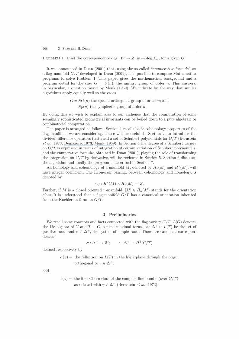
Problem 1. Find the correspondence deg : W → Z, w → deg Xw, for a given G.

It was announced in Duan (2001) that, using the so called “enumerative formula” ona flag manifold G/T developed in Duan (2001), it is possible to compose Mathematicaprograms to solve Problem 1. This paper gives the mathematical background and aprogram detail for the case G = U(n), the unitary group of order n. This answers,in particular, a question raised by Monk (1959). We indicate by the way that similaralgorithms apply equally well to the cases

G = SO(n) the special orthogonal group of order n; andSp(n) the symplectic group of order n.

By doing this we wish to explain also to our audience that the computation of someseemingly sophisticated geometrical invariants can be boiled down to a pure algebraic orcombinatorial computation.

The paper is arranged as follows. Section 1 recalls basic cohomology properties of theflag manifolds we are considering. These will be useful, in Section 2, to introduce thedivided difference operators that yield a set of Schubert polynomials for G/T (Bernsteinet al., 1973; Demazure, 1973; Monk, 1959). In Section 4 the degree of a Schubert varietyon G/T is expressed in terms of integration of certain variation of Schubert polynomials,and the enumerative formulas obtained in Duan (2001), playing the role of transformingthe integration on G/T by derivative, will be reviewed in Section 5. Section 6 discussesthe algorithm and finally the program is described in Section 7.

All homology and cohomology of a manifold M , denoted by H∗(M) and H∗(M), willhave integer coefficient. The Kronecker pairing, between cohomology and homology, isdenoted by

〈, 〉 : Hr(M)×Hr(M) → Z.

Further, if M is a closed oriented n-manifold, [M ] ∈ Hn(M) stands for the orientationclass. It is understood that a flag manifold G/T has a canonical orientation inheritedfrom the Kaehlerian form on G/T .

2. Preliminaries

We recall some concepts and facts connected with the flag variety G/T . L(G) denotesthe Lie algebra of G and T ⊂ G, a fixed maximal torus. Let ∆+ ⊂ L(T ) be the set ofpositive roots and π ⊂ ∆+, the system of simple roots. There are canonical correspon-dences

σ : ∆+ → W ; c : ∆+ → H2(G/T )

defined respectively by

σ(γ) = the reflection on L(T ) in the hyperplane through the originorthogonal to γ ∈ ∆+;

and

c(γ) = the first Chern class of the complex line bundle (over G/T )associated with γ ∈ ∆+ (Bernstein et al., 1973).

Compute Degree of Schubert Varieties 509

The natural action of W on G/T yields a faithful representation

W → Aut(H2(G/T ))(Duan and Zhao, 2000),

and W will be identified with its image group in Aut(H2(G/T )).Let Σn be the permutation group on {1, 2, . . . , n} and Sn, the full permutation group

on {±1,±2, . . . ,±n}. The kernel of the standard homomorphism

det : Sn → {±1}

is denoted by S+n . It is well known that the Weyl groups for the Lie groups

G = U(n), SO(2n), SO(2n + 1) and Sp(n)

are respectively Σn, S+n , Sn and Sn.

Let ei(z1, . . . , zn) be the ith elementary symmetric function in the variables z1, . . . , zn.If x ∈ Hr(G/T ) we write |x| = r. We describe now the integral cohomologies, and makethe above set-up more concrete for the four types of flag manifold

An = U(n)/T : Bn = SO(2n)/T ; Cn = SO(2n + 1)/T ; Dn = Sp(n)/T.

Borel (1967) and Duan and Zhao (2000) might be appropriate references to results listedbelow.

Theorem A-1. The integral cohomology of An can be given by

H∗(An) = Z[x1, . . . , xn]/〈ei(x1, . . . , xn), 1 ≤ i ≤ n〉, |xi| = 2;

so that the action of Σn on H2(An) = span{x1, . . . , xn} is

xi → xw(i), w ∈ Σn.

The set of positive roots ∆+ can be ordered as {γij | 1 ≤ i < j ≤ n}; so that

(1) π = {γi,i+1 | 1 ≤ i ≤ n− 1}; and(2) the correspondences σ : ∆+ → Σn; c : ∆+ → H2(An) are given respectively by

σ(γij) = (i, j); and c(γij) = xj − xi. 2

Theorem B-1. The integral cohomology of Bn can be given by

H∗(Bn) = Z[x1, . . . , xn;α1, . . . , αn−1]/〈ei(x1, . . . , xn)− 2αi,14ei(x2

1, . . . , x2n),

1 ≤ i ≤ n− 1〉, |xi| = 2;

so that the action of S+n on H2(Bn) = span{x1, . . . , xn} is

xi →{

xw(i) if w(i) > 0−x|w(i)| if w(i) < 0 , w ∈ S+

n .

The set of positive roots ∆+ can be ordered as {γij ;βij | 1 ≤ i < j ≤ n}; so that

(1) π = {γi,i+1, βn−1,n| 1 ≤ i ≤ n− 1}; and(2) the correspondences σ : ∆+ → S+

n ; c : ∆+ → H2(Bn) are given respectively by

σ(γij) = (i, j); σ(βij) = (−i,−j);

andc(γij) = xj − xi; c(βij) = xj + xi. 2

510 X. Zhao and H. Duan

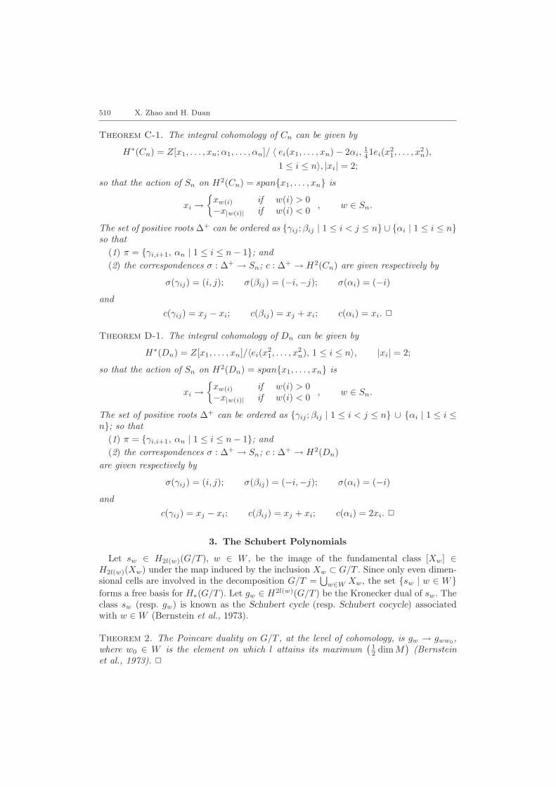
Theorem C-1. The integral cohomology of Cn can be given by

H∗(Cn) = Z[x1, . . . , xn;α1, . . . , αn]/ 〈 ei(x1, . . . , xn)− 2αi,141ei(x2

1, . . . , x2n),

1 ≤ i ≤ n〉, |xi| = 2;

so that the action of Sn on H2(Cn) = span{x1, . . . , xn} is

xi →{

xw(i) if w(i) > 0−x|w(i)| if w(i) < 0 , w ∈ Sn.

The set of positive roots ∆+ can be ordered as {γij ;βij | 1 ≤ i < j ≤ n} ∪ {αi | 1 ≤ i ≤ n}so that

(1) π = {γi,i+1, αn | 1 ≤ i ≤ n− 1}; and(2) the correspondences σ : ∆+ → Sn; c : ∆+ → H2(Cn) are given respectively by

σ(γij) = (i, j); σ(βij) = (−i,−j); σ(αi) = (−i)

andc(γij) = xj − xi; c(βij) = xj + xi; c(αi) = xi. 2

Theorem D-1. The integral cohomology of Dn can be given by

H∗(Dn) = Z[x1, . . . , xn]/〈ei(x21, . . . , x

2n), 1 ≤ i ≤ n〉, |xi| = 2;

so that the action of Sn on H2(Dn) = span{x1, . . . , xn} is

xi →{

xw(i) if w(i) > 0−x|w(i)| if w(i) < 0 , w ∈ Sn.

The set of positive roots ∆+ can be ordered as {γij ;βij | 1 ≤ i < j ≤ n} ∪ {αi | 1 ≤ i ≤n}; so that

(1) π = {γi,i+1, αn | 1 ≤ i ≤ n− 1}; and(2) the correspondences σ : ∆+ → Sn; c : ∆+ → H2(Dn)

are given respectively by

σ(γij) = (i, j); σ(βij) = (−i,−j); σ(αi) = (−i)

andc(γij) = xj − xi; c(βij) = xj + xi; c(αi) = 2xi. 2

3. The Schubert Polynomials

Let sw ∈ H2l(w)(G/T ), w ∈ W , be the image of the fundamental class [Xw] ∈H2l(w)(Xw) under the map induced by the inclusion Xw ⊂ G/T . Since only even dimen-sional cells are involved in the decomposition G/T =

⋃w∈W Xw, the set {sw | w ∈ W}

forms a free basis for H∗(G/T ). Let gw ∈ H2l(w)(G/T ) be the Kronecker dual of sw. Theclass sw (resp. gw) is known as the Schubert cycle (resp. Schubert cocycle) associatedwith w ∈ W (Bernstein et al., 1973).

Theorem 2. The Poincare duality on G/T , at the level of cohomology, is gw → gww0 ,where w0 ∈ W is the element on which l attains its maximum

(12 dim M

)(Bernstein

et al., 1973). 2

Compute Degree of Schubert Varieties 511

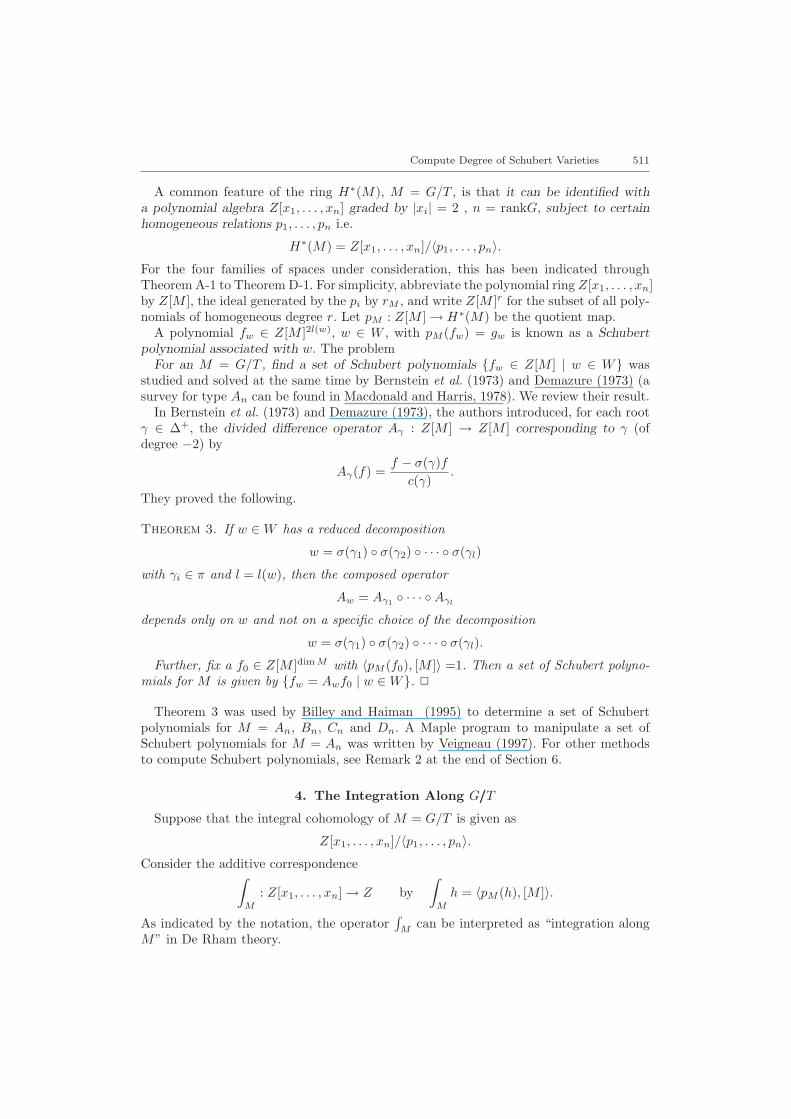
A common feature of the ring H∗(M), M = G/T , is that it can be identified witha polynomial algebra Z[x1, . . . , xn] graded by |xi| = 2 , n = rankG, subject to certainhomogeneous relations p1, . . . , pn i.e.

H∗(M) = Z[x1, . . . , xn]/〈p1, . . . , pn〉.

For the four families of spaces under consideration, this has been indicated throughTheorem A-1 to Theorem D-1. For simplicity, abbreviate the polynomial ring Z[x1, . . . , xn]by Z[M ], the ideal generated by the pi by rM , and write Z[M ]r for the subset of all poly-nomials of homogeneous degree r. Let pM : Z[M ] → H∗(M) be the quotient map.

A polynomial fw ∈ Z[M ]2l(w), w ∈ W , with pM (fw) = gw is known as a Schubertpolynomial associated with w. The problem

For an M = G/T , find a set of Schubert polynomials {fw ∈ Z[M ] | w ∈ W} wasstudied and solved at the same time by Bernstein et al. (1973) and Demazure (1973) (asurvey for type An can be found in Macdonald and Harris, 1978). We review their result.

In Bernstein et al. (1973) and Demazure (1973), the authors introduced, for each rootγ ∈ ∆+, the divided difference operator Aγ : Z[M ] → Z[M ] corresponding to γ (ofdegree −2) by

Aγ(f) =f − σ(γ)f

c(γ).

They proved the following.

Theorem 3. If w ∈ W has a reduced decomposition

w = σ(γ1) ◦ σ(γ2) ◦ · · · ◦ σ(γl)

with γi ∈ π and l = l(w), then the composed operator

Aw = Aγ1 ◦ · · · ◦Aγl

depends only on w and not on a specific choice of the decomposition

w = σ(γ1) ◦ σ(γ2) ◦ · · · ◦ σ(γl).

Further, fix a f0 ∈ Z[M ]dim M with 〈pM (f0), [M ]〉 =1. Then a set of Schubert polyno-mials for M is given by {fw = Awf0 | w ∈ W}. 2

Theorem 3 was used by Billey and Haiman (1995) to determine a set of Schubertpolynomials for M = An, Bn, Cn and Dn. A Maple program to manipulate a set ofSchubert polynomials for M = An was written by Veigneau (1997). For other methodsto compute Schubert polynomials, see Remark 2 at the end of Section 6.

4. The Integration Along G///T

Suppose that the integral cohomology of M = G/T is given as

Z[x1, . . . , xn]/〈p1, . . . , pn〉.

Consider the additive correspondence∫M

: Z[x1, . . . , xn] → Z by∫

M

h = 〈pM (h), [M ]〉.

As indicated by the notation, the operator∫

Mcan be interpreted as “integration along

M” in De Rham theory.

512 X. Zhao and H. Duan

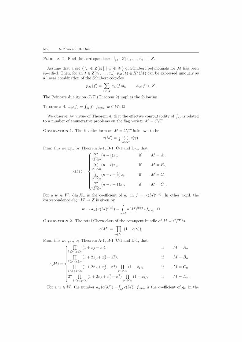
Problem 2. Find the correspondence∫

M: Z[x1, . . . , xn] → Z.

Assume that a set {fw ∈ Z[M ] | w ∈ W} of Schubert polynomials for M has beenspecified. Then, for an f ∈ Z[x1, . . . , xn], pM (f) ∈ H∗(M) can be expressed uniquely asa linear combination of the Schubert cocycles

pM (f) =∑

w∈W

aw(f)gw, aw(f) ∈ Z.

The Poincare duality on G/T (Theorem 2) implies the following.

Theorem 4. aw(f) =∫

Mf · fww0 , w ∈ W . 2

We observe, by virtue of Theorem 4, that the effective computability of∫

Mis related

to a number of enumerative problems on the flag variety M = G/T .

Observation 1. The Kaehler form on M = G/T is known to be

κ(M) = 12

∑γ∈∆+

c(γ).

From this we get, by Theorem A-1, B-1, C-1 and D-1, that

κ(M) =

∑1≤i≤n

(n− i)xi, if M = An∑1≤i≤n

(n− i)xi, if M = Bn∑1≤i≤n

(n− i + 12 )xi, if M = Cn∑

1≤i≤n

(n− i + 1)xi, if M = Cn.

For a w ∈ W , deg Xw is the coefficient of gw in f = κ(M)l(w). In other word, thecorrespondence deg : W → Z is given by

w → aw(κ(M)l(w)) =∫

M

κ(M)l(w) · fww0 . 2

Observation 2. The total Chern class of the cotangent bundle of M = G/T is

c(M) =∏

γ∈∆+

(1 + c(γ)).

From this we get, by Theorem A-1, B-1, C-1 and D-1, that

c(M) =

∏1≤i<j≤n

(1 + xj − xi), if M = An∏1≤i<j≤n

(1 + 2xj + x2j − x2

i ), if M = Bn∏1≤i<j≤n

(1 + 2xj + x2j − x2

i )∏

1≤i≤n

(1 + xi), if M = Cn

2n∏

1≤i<j≤n

(1 + 2xj + x2j − x2

i )∏

1≤i≤n

(1 + xi), if M = Dn.

For a w ∈ W , the number aw(c(M)) =∫

Mc(M) · fww0 is the coefficient of gw in the

Compute Degree of Schubert Varieties 513

polynomial c. The problem of expressing c(An) in terms of the Schubert cocycles gw onAn has been studied by Lascoux (1982). 2

Observation 3. Consider f = fu · fv, where u, v ∈ W . The number aw(f) is seen to bethe coefficient of gw in the product gu · gv. A historic account on this topic is given inFulton and Pragacz (1998, Section 9.10).

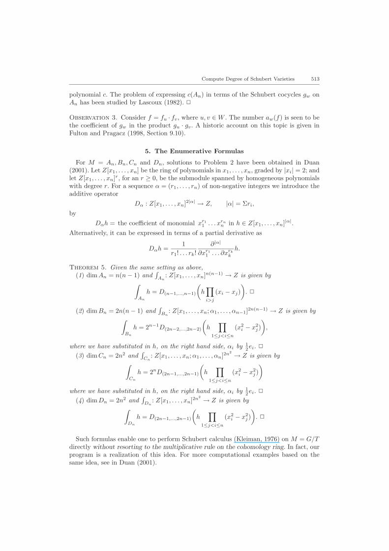
5. The Enumerative Formulas

For M = An, Bn, Cn and Dn, solutions to Problem 2 have been obtained in Duan(2001). Let Z[x1, . . . , xn] be the ring of polynomials in x1, . . . , xn, graded by |xi| = 2; andlet Z[x1, . . . , xn]r, for an r ≥ 0, be the submodule spanned by homogeneous polynomialswith degree r. For a sequence α = (r1, . . . , rn) of non-negative integers we introduce theadditive operator

Dα : Z[x1, . . . , xn]2|α| → Z, |α| = Σri,

byDαh = the coefficient of monomial xr1

1 . . . xrnn in h ∈ Z[x1, . . . , xn]|α|.

Alternatively, it can be expressed in terms of a partial derivative as

Dαh =1

r1! . . . rk!∂|α|

∂xr11 . . . ∂xrk

k

h.

Theorem 5. Given the same setting as above,(1) dim An = n(n− 1) and

∫An

: Z[x1, . . . , xn]n(n−1) → Z is given by∫An

h = D(n−1,...,n−1)

(h∏i>j

(xi − xj))

. 2

(2) dim Bn = 2n(n− 1) and∫

Bn: Z[x1, . . . , xn;α1, . . . , αn−1]2n(n−1) → Z is given by∫

Bn

h = 2n−1D(2n−2,...,2n−2)

(h

∏1≤j<i≤n

(x2i − x2

j ))

,

where we have substituted in h, on the right hand side, αi by 12ei. 2

(3) dim Cn = 2n2 and∫

Cn: Z[x1, . . . , xn;α1, . . . , αn]2n2 → Z is given by∫

Cn

h = 2nD(2n−1,...,2n−1)

(h

∏1≤j<i≤n

(x2i − x2

j ))

where we have substituted in h, on the right hand side, αi by 12ei. 2

(4) dim Dn = 2n2 and∫

Dn: Z[x1, . . . , xn]2n2 → Z is given by∫

Dn

h = D(2n−1,...,2n−1)

(h

∏1≤j<i≤n

(x2i − x2

j ))

. 2

Such formulas enable one to perform Schubert calculus (Kleiman, 1976) on M = G/Tdirectly without resorting to the multiplicative rule on the cohomology ring. In fact, ourprogram is a realization of this idea. For more computational examples based on thesame idea, see in Duan (2001).

514 X. Zhao and H. Duan

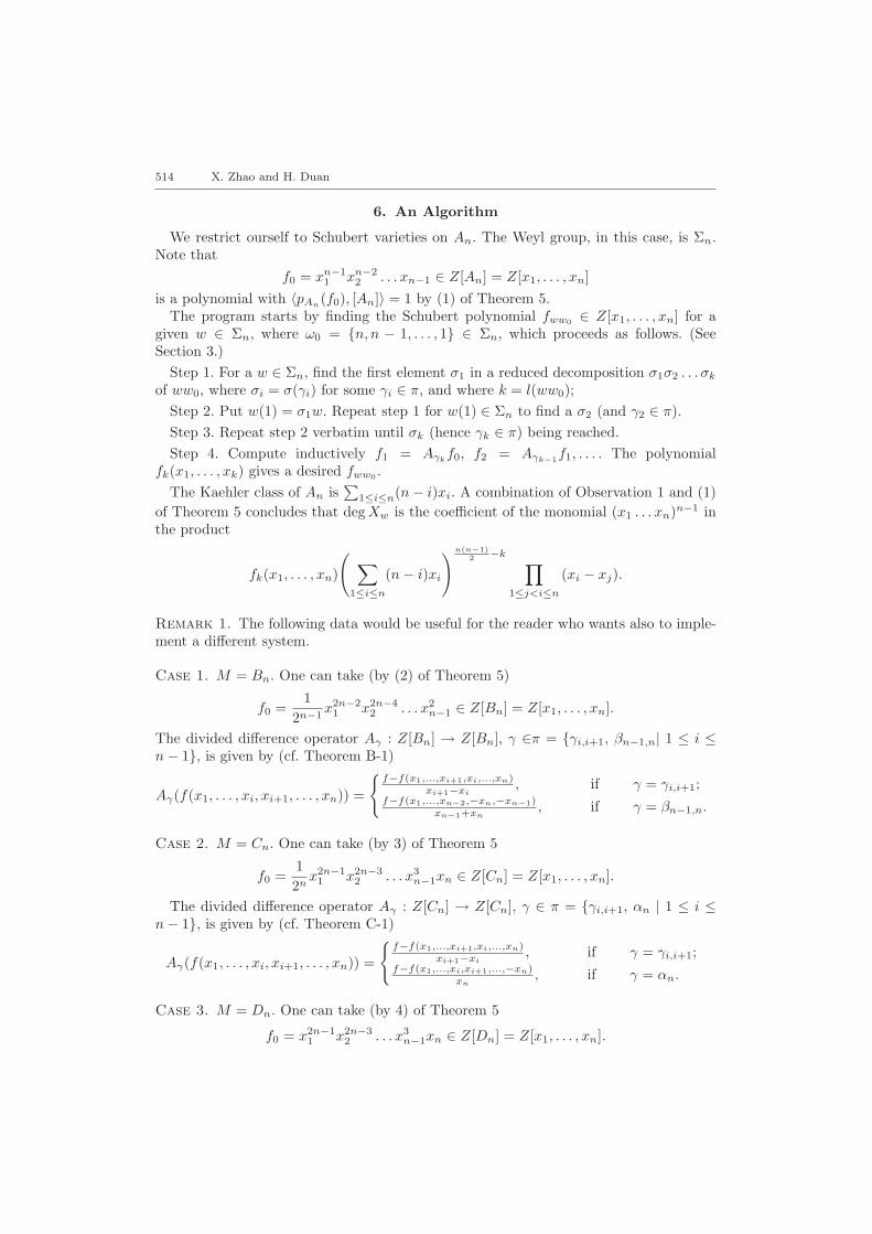
6. An Algorithm

We restrict ourself to Schubert varieties on An. The Weyl group, in this case, is Σn.Note that

f0 = xn−11 xn−2

2 . . . xn−1 ∈ Z[An] = Z[x1, . . . , xn]is a polynomial with 〈pAn

(f0), [An]〉 = 1 by (1) of Theorem 5.The program starts by finding the Schubert polynomial fww0 ∈ Z[x1, . . . , xn] for a

given w ∈ Σn, where ω0 = {n, n − 1, . . . , 1} ∈ Σn, which proceeds as follows. (SeeSection 3.)

Step 1. For a w ∈ Σn, find the first element σ1 in a reduced decomposition σ1σ2 . . . σk

of ww0, where σi = σ(γi) for some γi ∈ π, and where k = l(ww0);Step 2. Put w(1) = σ1w. Repeat step 1 for w(1) ∈ Σn to find a σ2 (and γ2 ∈ π).Step 3. Repeat step 2 verbatim until σk (hence γk ∈ π) being reached.Step 4. Compute inductively f1 = Aγk

f0, f2 = Aγk−1f1, . . . . The polynomialfk(x1, . . . , xk) gives a desired fww0 .

The Kaehler class of An is∑

1≤i≤n(n− i)xi. A combination of Observation 1 and (1)of Theorem 5 concludes that deg Xw is the coefficient of the monomial (x1 . . . xn)n−1 inthe product

fk(x1, . . . , xn)

( ∑1≤i≤n

(n− i)xi

)n(n−1)2 −k ∏

1≤j<i≤n

(xi − xj).

Remark 1. The following data would be useful for the reader who wants also to imple-ment a different system.

Case 1. M = Bn. One can take (by (2) of Theorem 5)

f0 =1

2n−1x2n−2

1 x2n−42 . . . x2

n−1 ∈ Z[Bn] = Z[x1, . . . , xn].

The divided difference operator Aγ : Z[Bn] → Z[Bn], γ ∈π = {γi,i+1, βn−1,n| 1 ≤ i ≤n− 1}, is given by (cf. Theorem B-1)

Aγ(f(x1, . . . , xi, xi+1, . . . , xn)) =

{f−f(x1,...,xi+1,xi,...,xn)

xi+1−xi, if γ = γi,i+1;

f−f(x1,...,xn−2,−xn,−xn−1)xn−1+xn

, if γ = βn−1,n.

Case 2. M = Cn. One can take (by 3) of Theorem 5

f0 =12n

x2n−11 x2n−3

2 . . . x3n−1xn ∈ Z[Cn] = Z[x1, . . . , xn].

The divided difference operator Aγ : Z[Cn] → Z[Cn], γ ∈ π = {γi,i+1, αn | 1 ≤ i ≤n− 1}, is given by (cf. Theorem C-1)

Aγ(f(x1, . . . , xi, xi+1, . . . , xn)) =

{f−f(x1,...,xi+1,xi,...,xn)

xi+1−xi, if γ = γi,i+1;

f−f(x1,...,xi,xi+1,...,−xn)xn

, if γ = αn.

Case 3. M = Dn. One can take (by 4) of Theorem 5

f0 = x2n−11 x2n−3

2 . . . x3n−1xn ∈ Z[Dn] = Z[x1, . . . , xn].

Compute Degree of Schubert Varieties 515

The divided difference operator Aγ : Z[Dn] → Z[Dn], γ ∈ π = {γi,i+1, αn | 1 ≤ i ≤n− 1}, is given by (cf. Theorem D-1)

Aγ(f(x1, . . . , xi, xi+1, . . . , xn)) =

{f−f(x1,...,xi+1,xi,...,xn)

xi+1−xi, if γ = γi,i+1;

f−f(x1,...,xi,xi+1,...,−xn)xn

, if γ = αn.

Remark 2. The method of computing Schubert polynomials that we used in the pre-ceding algorithm is not a satisfactory one. We are very grateful to our referees whokindly informed us that there are already other methods being implemented. Examplesare programs in C, SYMMETRCA at Bayreuth

http://www.mathe2.uni-bayreuth.de/and programs in Maple, ACE at Marne La Valle

http//phalanstere.univ-mlv.fr/.Both of the systems compute Schubert polynomials using a positive recursion on poly-nomials of a fixed degree, without using a chain of divided differences starting from thetop Schubert class.

7. The Program

The function “Permutations” in Mathematica generates all elements of Σn.

HeightA[w,n] computes l(w) for a w ∈ Σn:HeightA[w , n ] := Module[{i, j, s}, s = 0;

For[i = 1, i < n, i + +, For[j = i + 1, j < n + 1, j + +,If [Abs[w[[i]]] > Abs[w[[j]]], s = s + 1]]]; s]

Three functions will be employed to find the first transposition σ1 in a reduced decom-position of a given permutation w ∈ Σn. Namely if

σ1 = the transposition of i and j, 1 ≤ i, j ≤ n,we put

DePer0A[w,n] = σ1; DePer1A[w,n] = i; and DePer2A[w,n] = j.DePer2A[w , n ] := Module[{i, p}, For[i = 1, (i < n), i + +,

If [(w[[i]] > w[[i + 1]]), Continue[],d = Insert[Drop[w, {i, i}], w[[i]], i + 1]; p = n− i; i = n]]; p]

DePer1A[w , n ] := Module[{i, p}, For[i = 1, (i < n), i + +,If [(w[[i]] > w[[i + 1]]), Continue[],

d = Insert[Drop[w, {i, i}], w[[i]], i + 1]; p = n− i + 1; i = n]]; p]

DePer0A[w , n ] := Module[{i, p}, For[i = 1, (i < n), i + +,If [(w[[i]] > w[[i + 1]]), Continue[],

d = Insert[Drop[w, {i, i}], w[[i]], i + 1]; p = w[[i + 1]]; i = n]]; d]Further factors in a reduced decomposition of w are found by recurrence.

CharA[n] denotes the monomial f0 = xn−11 xn−2

2 . . . xn−1 (see in Section 5):CharA[n ] := Expand[Product[x[i](n− i), {i, 1, n− 1}]];

FA[w,n] is a Schubert polynomial corresponding to w ∈ Σn :FA[w , n ] := DifferentationA[F [n], w, n];

516 X. Zhao and H. Duan

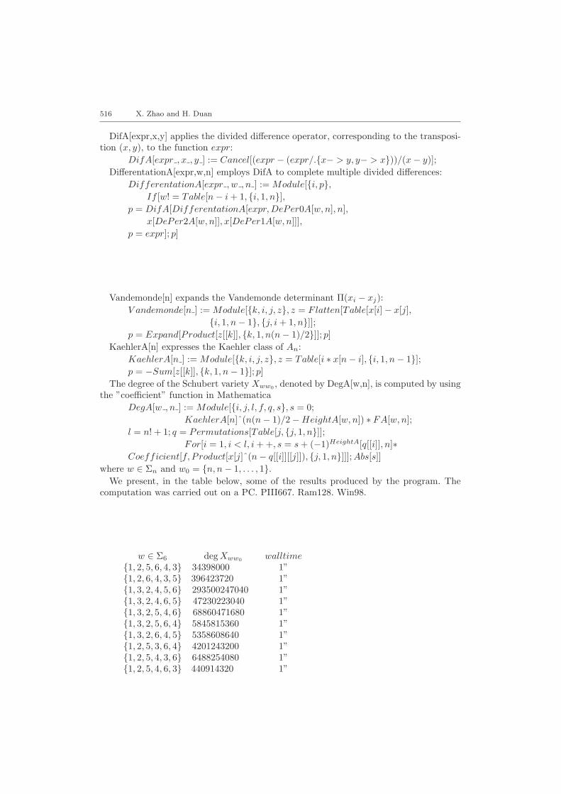
DifA[expr,x,y] applies the divided difference operator, corresponding to the transposi-tion (x, y), to the function expr:

DifA[expr , x , y ] := Cancel[(expr − (expr/.{x− > y, y− > x}))/(x− y)];DifferentationA[expr,w,n] employs DifA to complete multiple divided differences:

DifferentationA[expr , w , n ] := Module[{i, p},If [w! = Table[n− i + 1, {i, 1, n}],

p = DifA[DifferentationA[expr,DePer0A[w, n], n],x[DePer2A[w, n]], x[DePer1A[w, n]]],

p = expr]; p]

Vandemonde[n] expands the Vandemonde determinant Π(xi − xj):V andemonde[n ] := Module[{k, i, j, z}, z = Flatten[Table[x[i]− x[j],

{i, 1, n− 1}, {j, i + 1, n}]];p = Expand[Product[z[[k]], {k, 1, n(n− 1)/2}]]; p]

KaehlerA[n] expresses the Kaehler class of An:KaehlerA[n ] := Module[{k, i, j, z}, z = Table[i ∗ x[n− i], {i, 1, n− 1}];p = −Sum[z[[k]], {k, 1, n− 1}]; p]

The degree of the Schubert variety Xww0 , denoted by DegA[w,n], is computed by usingthe ”coefficient” function in Mathematica

DegA[w , n ] := Module[{i, j, l, f, q, s}, s = 0;KaehlerA[n]ˆ(n(n− 1)/2−HeightA[w, n]) ∗ FA[w, n];

l = n! + 1; q = Permutations[Table[j, {j, 1, n}]];For[i = 1, i < l, i + +, s = s + (−1)HeightA[q[[i]], n]∗

Coefficient[f, Product[x[j]ˆ(n− q[[i]][[j]]), {j, 1, n}]]]; Abs[s]]where w ∈ Σn and w0 = {n, n− 1, . . . , 1}.

We present, in the table below, some of the results produced by the program. Thecomputation was carried out on a PC. PIII667. Ram128. Win98.

w ∈ Σ6 deg Xww0 walltime{1, 2, 5, 6, 4, 3} 34398000 1”{1, 2, 6, 4, 3, 5} 396423720 1”{1, 3, 2, 4, 5, 6} 293500247040 1”{1, 3, 2, 4, 6, 5} 47230223040 1”{1, 3, 2, 5, 4, 6} 68860471680 1”{1, 3, 2, 5, 6, 4} 5845815360 1”{1, 3, 2, 6, 4, 5} 5358608640 1”{1, 2, 5, 3, 6, 4} 4201243200 1”{1, 2, 5, 4, 3, 6} 6488254080 1”{1, 2, 5, 4, 6, 3} 440914320 1”

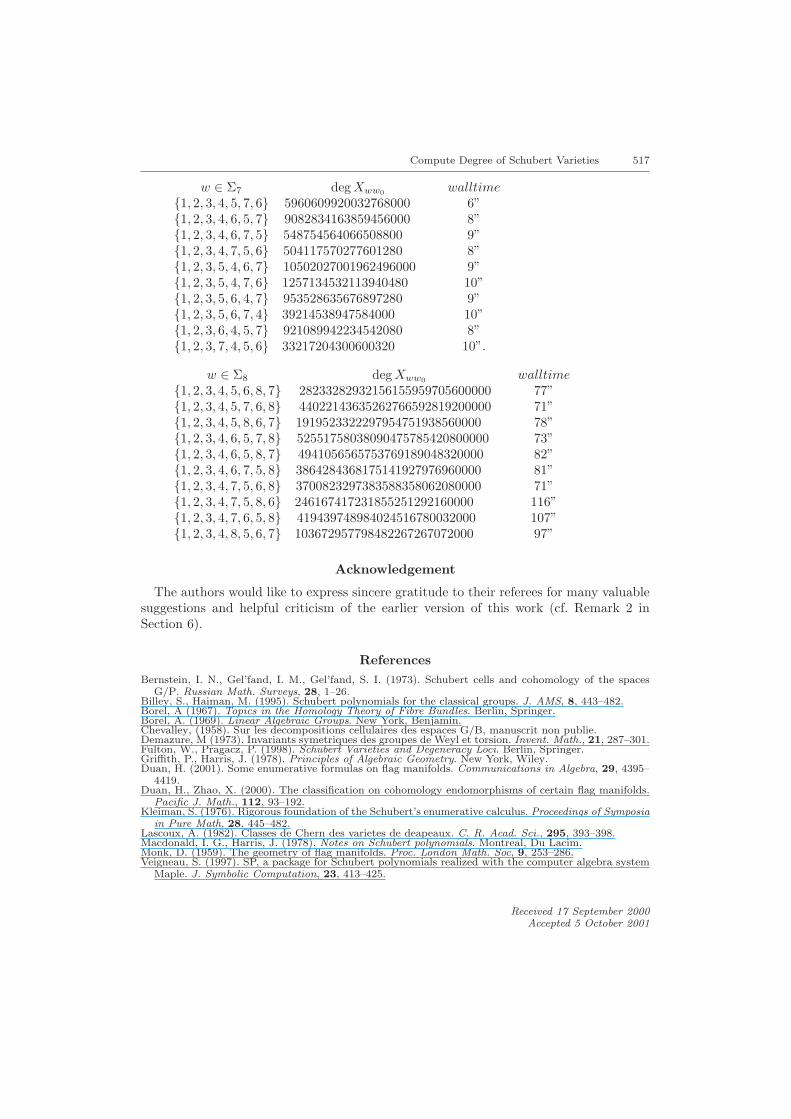
Compute Degree of Schubert Varieties 517

w ∈ Σ7 deg Xww0 walltime{1, 2, 3, 4, 5, 7, 6} 5960609920032768000 6”{1, 2, 3, 4, 6, 5, 7} 9082834163859456000 8”{1, 2, 3, 4, 6, 7, 5} 548754564066508800 9”{1, 2, 3, 4, 7, 5, 6} 504117570277601280 8”{1, 2, 3, 5, 4, 6, 7} 10502027001962496000 9”{1, 2, 3, 5, 4, 7, 6} 1257134532113940480 10”{1, 2, 3, 5, 6, 4, 7} 953528635676897280 9”{1, 2, 3, 5, 6, 7, 4} 39214538947584000 10”{1, 2, 3, 6, 4, 5, 7} 921089942234542080 8”{1, 2, 3, 7, 4, 5, 6} 33217204300600320 10”.

w ∈ Σ8 deg Xww0 walltime{1, 2, 3, 4, 5, 6, 8, 7} 28233282932156155959705600000 77”{1, 2, 3, 4, 5, 7, 6, 8} 44022143635262766592819200000 71”{1, 2, 3, 4, 5, 8, 6, 7} 1919523322297954751938560000 78”{1, 2, 3, 4, 6, 5, 7, 8} 52551758038090475785420800000 73”{1, 2, 3, 4, 6, 5, 8, 7} 4941056565753769189048320000 82”{1, 2, 3, 4, 6, 7, 5, 8} 3864284368175141927976960000 81”{1, 2, 3, 4, 7, 5, 6, 8} 3700823297383588358062080000 71”{1, 2, 3, 4, 7, 5, 8, 6} 246167417231855251292160000 116”{1, 2, 3, 4, 7, 6, 5, 8} 419439748984024516780032000 107”{1, 2, 3, 4, 8, 5, 6, 7} 103672957798482267267072000 97”

Acknowledgement

The authors would like to express sincere gratitude to their referees for many valuablesuggestions and helpful criticism of the earlier version of this work (cf. Remark 2 inSection 6).

ReferencesBernstein, I. N., Gel’fand, I. M., Gel’fand, S. I. (1973). Schubert cells and cohomology of the spaces

G/P. Russian Math. Surveys, 28, 1–26.Billey, S., Haiman, M. (1995). Schubert polynomials for the classical groups. J. AMS, 8, 443–482.Borel, A (1967). Topics in the Homology Theory of Fibre Bundles. Berlin, Springer.Borel, A. (1969). Linear Algebraic Groups. New York, Benjamin.Chevalley, (1958). Sur les decompositions cellulaires des espaces G/B, manuscrit non publie.Demazure, M (1973). Invariants symetriques des groupes de Weyl et torsion. Invent. Math., 21, 287–301.Fulton, W., Pragacz, P. (1998). Schubert Varieties and Degeneracy Loci. Berlin, Springer.Griffith, P., Harris, J. (1978). Principles of Algebraic Geometry. New York, Wiley.Duan, H. (2001). Some enumerative formulas on flag manifolds. Communications in Algebra, 29, 4395–

4419.Duan, H., Zhao, X. (2000). The classification on cohomology endomorphisms of certain flag manifolds.

Pacific J. Math., 112, 93–192.Kleiman, S. (1976). Rigorous foundation of the Schubert’s enumerative calculus. Proceedings of Symposia

in Pure Math, 28, 445–482.Lascoux, A. (1982). Classes de Chern des varietes de deapeaux. C. R. Acad. Sci., 295, 393–398.Macdonald, I. G., Harris, J. (1978). Notes on Schubert polynomials. Montreal, Du Lacim.Monk, D. (1959). The geometry of flag manifolds. Proc. London Math. Soc, 9, 253–286.Veigneau, S. (1997). SP, a package for Schubert polynomials realized with the computer algebra system

Maple. J. Symbolic Computation, 23, 413–425.

Received 17 September 2000Accepted 5 October 2001