Appendix A Practical implementation using Mathematica

Appendix A

Practical implementation using Mathematica

The purpose of this appendix is to illustrate some of the set partitions and diagramformulae we have encountered. We do this through a practical implementation of theseformulae by using the software program Mathematica12. The source code and moredetailed examples are contained in a companionMathematica notebook. This notebookcan be downloaded by using the link:

http://extras.springer.com, Password: 978-88-470-1678-1

To view the notebook you may use the freeMathematica Readerwhich you can down-load from the Internet or you can use theMathematica program itself. TheMathemat-ica program (version 7.0 or later) must be installed on your computer or remotelythrough your system if you want to execute the source code.

A.1 General introduction

The filename of a Mathematica notebook ends with a “.nb”. Place the notebook andthe style file StyleFile978-88-470-1678-1.nb in the same folder. This style file formatsthe notebook nicely but it is not absolutely necessary to have it.In Windows, double-clicking on the notebook will open the notebook and start

Mathematica (or the Mathematica Reader). It is best to begin by executing the entirenotebook because some functions depend on previously defined functions. To exe-cute the entire notebook (on Windows), press Control-A (to select all the cells in thenotebook), followed by Shift-Enter. (On a Mac, press Command-A followed by Shift-Enter.) These actions will execute all of the function definitions and examples in thisnotebook. This may take a little time. You will see “Running” on the top left of the

1 Mathematica is a computational software program developed by Wolfram Research.2 For further references on the use of Mathematica in the context of multiple stochastic inte-grals, see for example, [54], [155].

G. Peccati, M.S. Taqqu: Wiener Chaos: Moments, Cumulants and Diagrams –A survey with computer implementation.© Springer-Verlag Italia 2011

208 Appendix A. Practical implementation using Mathematica

notebook. After the execution has completed, you will be able to apply the functionscreated in this notebook to new set partitions or to create additional examples of yourown. You may type, paste, or outline a command and then press Shift-Enter to executeit. You may do this in the present notebook or, preferably, in a new notebook that youwould open.Please note that the execution of any of these functions requires the use of the

Combinatorica package inMathematica (which can be activated by executing the lineNeeds[“Combinatorica”]. We automatically execute this package in this note-book.To type a command, simply type the appropriate function and the desired

argument and press Shift-Enter to execute the cell in which the command is located.Mathematica will label the command as a numbered input and the output will benumbered correspondingly. One can recall previous outputs with commands like %5,which would recover the fifth output in the current Mathematica session. Unexecutedcells have no input label.

Warning. Some of the functions in this notebook use a brute-force methodology.The number of set partitions associated to a positive integer n grows very rapidly,and so any brute-force methodology may suffer from combinatorial explosion. Unlessyou have lots of time and computational resources at your disposal, it may be betterto investigate examples for which n is small.

Comment about In[ ] and Out[ ]. Mathematica, after execution of a command,automatically numbers it, for example, “In[1]:=”. The output lines are also numbered,for example, the corresponding output line will start with: “Out[1]=”. Here, we sym-bolically start a command input line with “In:=” and the corresponding output startswith “Out=” . Thus, in the sequel do not type, for example, “In:=” nor “In[269]:=”,as this is automatically generated by Mathematica after you execute the command bypressing Shift-Enter.

Comments about the time it takes to evaluate a function. To evaluate the timeit takes to simulate 1,000,000 realizations of a standard normal random variable, type:

In := RandomReal[NormalDistribution[0, 1], {1 000 000}]; // AbsoluteTimingOut= 0.2187612, Null

The semicolon suppresses the display of the output (except for the timing result),which is generated by AbsoluteTiming. The first part of the output is the number ofseconds it took Mathematica to generate 1,000,000 realizations of a standard normalrandom variable. The output was suppressed, which is why the symbol Null appearsin the second position.

A.2 When Starting 209

Comments about the function names.We typically give the functions long, in-formative names. In practical use, one may sometimes want to use a shorter name. Forexample, to have the function Chi do the same thing as the function CumulantVector-ToMoments, set:

In := Chi = CumulantVectorToMoments

A few similar functions may have different names because they are used in dif-ferent contexts. This is the case, for example, of the functions MeetSolve, PiStarMeetSolve and MZeroSets.

Comments about typing Greek symbols. To type symbols, such as μ and κ,either copy and paste them with the mouse from somewhere else in the notebook ortype respectively \[Mu] and \[Kappa]. Mathematica converts these immediately togreek.

Comments about Mathematica notation. In Mathematica, a set partition isdenoted in a particular way, for example, {{1, 2, 4}, {3}, {5}} is a set partition ofthe set {1, 2, 3, 4, 5}. The trivial, or maximal, partition consisting of the entire setis denoted {{1, 2, 3, 4, 5}} and the set partition consisting entirely of singletons isdenoted {{1}, {2}, {3}, {4}, {5}}.

Comments about hard returns. Mathematica ignores hard returns. Therefore, ifthe input line is long, one can press “Enter” in order to subdivide it.

Comments about stopping the execution of a function. Hold down the “Alt”key and then press the “.” key, or go to the menu at the top, choose “Evaluation” andthen choose “Abort Evaluation.”

Comments about the examples below. The examples are particularly simple.Their only purpose is to illustrate theMathematica commands. TheMathematica out-put will sometimes not be listed below, because it is either too long or would requirecomplicated formatting.

A.2 When Starting

Type first the following two commands:

In := Needs [“Combinatorica”] ; Off[First::first]

The first command loads the package Combinatorica. The second command shuts offan error message that does not impact any of the function outputs. These commandswill be executed in sequence.


Note: These two commands are listed at the beginning of the notebook. They willbe automatically executed if you execute the whole notebook.

A.3 Integer Partitions

A.3.1 IntegerPartitions

Find all nonnegative integers that sum up to an integer n, ignoring order; this is abuilt-in Mathematica function.

� Please refer to Section 2.1.

Example. Find all integer partitions of the number 5. The output {3, 1, 1} shouldbe read as the decomposition 5 = 3 + 1 + 1.

In := IntegerPartitions[5]Out= {{5}, {4, 1}, {3, 2}, {3, 1, 1}, {2, 2, 1}, {2, 1, 1, 1}, {1, 1, 1, 1, 1}}

Example. Count the number of integer partitions of the number 5.

In := Length[IntegerPartitions[5]]Out= 7

A.3.2 IntegerPartitionsExponentRepresentation

This function represents the output of IntegerPartitions in exponent notation; namely,1r1 2r2 · · ·nrn , where ri is the number of times that integer i appears in the decompo-sition, i = 1, ..., n.

Example. Find all integer partitions of the number 5, and express them inexponent notation. Thus 5 = 3 + 1 + 1 is expressed as {1220314050} since there are 2ones and 1 three.

In := IntegerPartitionsExponentRepresentation[5]Out= {{1020304051}, {1120304150}, {1021314050}, {1220314050},

{1122304050}, {1321304050}, {1520304050}}

A.4 Basic Set Partitions


A.4 Basic Set Partitions 211

A.4.1 SingletonPartition

Generates the singleton set partition of order n, namely 0 = {{1}, {2}, · · · , {n}}.This is a partition made up of singletons.

Example. Generate the singleton set partition of order 12.

In := SingletonPartition[12]Out= {{1}, {2}, {3}, {4}, {5}, {6}, {7}, {8}, {9}, {10}, {11}, {12}}

Example. Same example with grid display.

In := Grid[SetPartitions[3], Frame→ All]

Out= {1, 2, 3}{1} {2, 3}{1, 2} {3}{1, 3} {2}{1} {2} {3}

A.4.2 MaximalPartition

Generates the maximal set partition of order n, namely 1 = {{1, 2, ..., n}}.

Example. Generate the maximal set partition of order 12.

In := MaximalPartition[12]Out= {{1, 2, 3, 4, 5, 6, 7, 8, 9, 10, 11, 12}}

A.4.3 SetPartitions

Enumerates all of the set partitions associated with a particular integer n, namely allset partitions of {1, 2, · · · , n}; this is a built-in Mathematica function.


Example. Enumerate all set partitions of {1, 2, 3}.

In := SetPartitions[3]Out= {{{1, 2, 3}}, {{1}, {2, 3}}, {{1, 2}, {3}}, {{1, 3}, {2}},

{{1}, {2}, {3}}}


A.4.4 PiStar

Generates a set partition of {1, 2, · · · , n1 + · · · + nk}, with k blocks, the first of sizen1 and the last of size nk, that is,

π∗ = {{1, · · · , n1}, {n1 + 1, · · · , n1 + n2}, · · · , {n1 + · · ·+ nk−1 + 1, · · · , n}}.

� Please refer to Formula (6.1.1).

Example. Create a set partition π∗ with blocks of size 1, 2, 4, 7, and 9.

In := PiStar[{1, 2, 4, 7, 9}]Out= {{1}, {2, 3}, {4, 5, 6, 7}, {8, 9, 10, 11, 12, 13, 14},

{15, 16, 17, 18, 19, 20, 21, 22, 23}}

A.5 Operations with Set Partitions

A.5.1 PartitionIntersection

Finds the meet σ ∧ π between two set partitions σ and π; each block of σ ∧ π is anon-empty intersection between one block of σ and one block of π.

Example. Find the meet between the set partitions {{1, 4, 5}, {2}, {3}} and{{1, 2, 5}, {3}, {4}}.

In := PartitionIntersection [{{1, 4, 5}, {2}, {3}}, {{1, 2, 5}, {3}, {4}}]Out= {{1, 5}, {2}, {3}, {4}}

Example. If the partitions σ and π are not of the same order, then PartitionInter-section returns a message.

In := PartitionIntersection[ SingletonPartition[8], {{1, 2, 5, 6, 7}, {3}, {4}}]Out= Error

A.5.2 PartitionUnion

Finds the join σ ∨ π between two set partitions σ and π; that is, the union of blocks ofσ and π that have at least one element in common.

Example. Find the join between the set partitions {{1, 4, 5}, {2}, {3}} and{{1, 2, 5}, {3}, {4}}.

In := PartitionUnion [ {{1,4,5},{2},{3}} , {{1,2,5},{3},{4}} ]Out= {{1, 2, 4, 5}, {3}}

A.5 Operations with Set Partitions 213

A.5.3 MeetSolve

For a fixed set partition π , find all set partitions σ such that the meet of π and σ is thesingleton partition 0, that is, σ ∧ π = 0.


Example. Find all set partitions σ such that the meet of σ and {{1, 4, 5}, {2}, {3}}is the singleton partition 0.

In := MeetSolve[{{1, 4, 5}, {2}, {3}}]Out= {{{1}, {2, 3, 4}, {5}}, {{1}, {2, 5}, {3, 4}}, {{1}, {2, 3, 5}, {4}},

{{1}, {2, 4}, {3, 5}}, {{1, 2}, {3, 4}, {5}}, {{1, 2}, {3, 5}, {4}},{{1, 2, 3}, {4}, {5}}, {{1, 3}, {2, 4}, {5}}, {{1, 3}, {2, 5}, {4}},{{1}, {2}, {3, 4}, {5}}, {{1}, {2}, {3, 5}, {4}}, {{1}, {2, 3}, {4}, {5}},{{1}, {2, 4}, {3}, {5}}, {{1}, {2, 5}, {3}, {4}}, {{1, 2}, {3}, {4}, {5}},{{1, 3}, {2}, {4}, {5}}, {{1}, {2}, {3}, {4}, {5}}}

The output also displays the number of solutions (namely 17).

A.5.4 JoinSolve

For a fixed set partition π, find all set partitions σ such that the join of π and σ is themaximal partition 1, that is, σ ∨ π = 1.

Example. Find all set partitions σ such that the join of σ and {{1, 4, 5}, {2}, {3}}is the maximal partition 1.

In := JoinSolve[{{1, 4, 5}, {2}, {3}}]Out= {{{1, 2, 3, 4, 5}}, {{1}, {2, 3, 4, 5}}, {{1, 2}, {3, 4, 5}},

{{1, 2, 3}, {4, 5}}, {{1, 3}, {2, 4, 5}}, {{1, 2, 3, 4}, {5}},{{1, 5}, {2, 3, 4}}, {{1, 2, 5}, {3, 4}}, {{1, 3, 4}, {2, 5}},{{1, 2, 3, 5}, {4}}, {{1, 4}, {2, 3, 5}}, {{1, 2, 4}, {3, 5}},{{1, 3, 5}, {2, 4}}, {{1}, {2, 3, 4}, {5}}, {{1}, {2, 5}, {3, 4}},{{1}, {2, 3, 5}, {4}}, {{1}, {2, 4}, {3, 5}}, {{1, 2}, {3, 4}, {5}},{{1, 2}, {3, 5}, {4}}, {{1, 2, 3}, {4}, {5}},{{1, 3}, {2, 4}, {5}}, {{1, 3}, {2, 5}, {4}}}


A.5.5 JoinSolveGrid

Display the output of JoinSolve in a grid.

Example. Find all set partitions σ such that the join of σ and {{1, 2}, {3, 4}} isthe maximal partition 1.

In := JoinSolveGrid[{{1, 2}, {3, 4}}]Out= {1, 2, 3, 4}

{1} {2, 3, 4}{1, 3, 4} {2}{1, 2, 3} {4}{1, 4} {2, 3}{1, 2, 4} {3}{1, 3} {2, 4}{1} {2, 3} {4}{1} {2, 4} {3}{1, 3} {2} {4}{1, 4} {2} {3}

A.5.6 MeetAndJoinSolve

For a fixed set partition π, find all set partitions σ such that the join of π and σ isthe maximal partition 1 AND the meet of π and σ is the singleton partition 0. that is,σ ∧ π = 0 and σ ∨ π = 1.

Example. Find all set partitions σ such that the join of σ and {{1, 4, 5}, {2}, {3}}is the maximal partition 1 and such that the meet of σ and {{1, 4, 5}, {2}, {3}} is thesingleton partition 0. Include the timing of the computation.

In := MeetAndJoinSolve [{{1, 4, 5}, {2}, {3}}] // AbsoluteTimingOut= {0.2031250, {{{1}, {2, 3, 4}, {5}}, {{1}, {2, 5}, {3, 4}},

{{1}, {2, 3, 5}, {4}}, {{1}, {2, 4}, {3, 5}}, {{1, 2}, {3, 4}, {5}},{{1, 2}, {3, 5}, {4}}, {{1, 2, 3}, {4}, {5}},{{1, 3}, {2, 4}, {5}}, {{1, 3}, {2, 5}, {4}}}}

The output in the first position is the number of seconds it took to generate the restof the output. The number of solutions will also be specified (namely 9).

A.6 Partition Segments 215

A.5.7 CoarserSetPartitionQ

This is a built-in Mathematica function; CoarserSetPartitionQ[σ,π] yields “True” ifthe set partition π is coarser than the set partition σ; that is, if σ ≤ π, i.e., if everyblock in σ is contained in a block of π.

Example. Is the set partition π = {1, 2}, {3, 4}, {5} coarser than the set partitionσ = {{1, 2, 3, 4}, {5}} ?

In := CoarserSetPartitionQ[{{1, 2, 3, 4}, {5}}, {{1, 2}, {3, 4}, {5}}]Out= False

A.5.8 CoarserThan

For a fixed set partition π, find all set partitions σ such that σ ≥ π, i.e., all setpartitions such that every block of π is fully contained in some block of σ.

Example. Find all of the set partitions σ such that σ ≥ {{1, 2}, {3, 4}, {5}}.

In := CoarserThan[{{1, 2}, {3, 4}, {5}}]Out= {{{1, 2, 3, 4, 5}}, {{1, 2}, {3, 4, 5}}, {{1, 2, 3, 4}, {5}},

{{1, 2, 5}, {3, 4}}, {{1, 2}, {3, 4}, {5}}}

A.6 Partition Segments

A.6.1 PartitionSegment

For set partitions σ and π, find the partition segment [σ, π], that is, all set partitions ρsuch that σ ≤ ρ ≤ π.

� Please refer to Definition 2.2.4.

Example. Find all of the set partitions ρ such that

{{1}, {2}, {3}, {4, 5}} = σ ≤ ρ ≤ π = {{1, 2, 3}, {4, 5}}.

In := PartitionSegment[{{1}, {2}, {3}, {4, 5}}, {{1, 2, 3}, {4, 5}}]Out= {{{1, 2, 3}, {4, 5}}, {{1}, {2, 3}, {4, 5}}, {{1, 2}, {3}, {4, 5}},

{{1, 3}, {2}, {4, 5}}, {{1}, {2}, {3}, {4, 5}}}

The output also specifies the number of partitions in the segment (namely 5).


A.6.2 ClassSegment

For set partitions σ and π, with σ ≤ π, obtain the “class” of the segment [σ, π], namely

λ(σ, π) = (1r1 2r2 · · · |σ|r|σ|),

where ri is the number of blocks of π that contain exactly i blocks of σ (terms withexponent zero are ignored in the output).


Example. Compute the class segment when σ = {{1, 2}, {3}, {4, 5}} andπ = {{1, 2, 3}, {4, 5}}.

In := ClassSegment[{{1, 2}, {3}, {4, 5}}, {{1, 2, 3}, {4, 5}}]Out= (1121)

This is because only one block of π (namely, {4,5}) contains one block of σ andone block of π (namely, {1,2,3}) contains two blocks of σ. The answer could be morefully written as (112130).

A.6.3 ClassSegmentSolve

Given a partition σ, find all coarser partitions π with a specific class segment λ(σ, π) =(1r1 2r2 · · · |σ|r|σ|) written as {{1, r1}, {2, r2}, · · · , {|σ|, r|σ|}} with ri ≥ 0 or merelyri > 0. We want ri blocks of π to contain exactly i blocks of σ, for i = 1, ..., n.

Input format. ClassSegmentSolve[σ, λ(σ, π)]

Example. Find the set of all partitions π such that the class segment ofσ = {{1, 2}, {3}, {4, 5}} and π is equal to λ(σ, π) = (1121). We want r1 = 1 blockof π to contain one block of σ and r2 = 1 block of π to contain two blocks of σ.

In := ClassSegmentSolve[{{1, 2}, {3}, {4, 5}}, {{1, 1}, {2, 1}}]Out= {{{1, 2}, {3, 4, 5}}, {{1, 2, 3}, {4, 5}}, {{1, 2, 4, 5}, {3}}}

If π = {{1, 2}, {3, 4, 5}}, then {1,2} contains the block {1,2} in σ ={{1, 2}, {3}, {4, 5}} and {3,4,5} contains the blocks {3} and {4,5} of σ.

A.7 Bell and Touchard polynomials 217

A.6.4 SquareChoose

For a list of non-negative integers {r1, r2, ..., rn}, with 1r1 + 2r2 + · · · + nrn = n,compute [ n

λ

]=[ n

r1, ..., rn

]=

n!(1!)r1 r1! (2!)r2 r2! · · · (n!)rn rn!

.

If one relabels the integers and denote by {r1, r2, · · · , rk}, with k ≤ n and k equal tothe greatest integer in [n] such that rk > 0, then 1r1 + 2r2 + · · ·+ krk = n, and[ n

λ

]=[ n

r1, ..., rk

]=

n!(1!)r1 r1! (2!)r2 r2! · · · (k!)rk rk!

.


Example. For the list {1, 3, 0, 0, 0, 0, 0} or the list {1, 3} compute7!

[(1!)1(1!)][(2!)3(3!)].

In := SquareChoose[{1, 3, 0, 0, 0, 0, 0, 0}]In := SquareChoose[{1, 3}]

The output is 105 in both cases.

A.7 Bell and Touchard polynomials


A.7.1 StirlingS2

Obtain the Stirling numbers S(n, k) of the second kind, where 1 ≤ k ≤ n. This is abuilt-in mathematica function. Recall that

S(n, k) =∑

r1,...,rn−k+1

n!(1!)r1 r1! (2!)r2 r2! · · · (n− k + 1)!rn−k+1rn−k+1!

,

where the sum runs over all vectors on nonnegative integers (r1, ..., rn−k+1) satisfyingr1 + · · ·+ rn−k+1 = k and 1r1 + 2r2 · · ·+(n− k + 1) rn−k+1 = n.

� Please refer to Proposition 2.3.4.


Example. Get S(3, 2).

In := StirlingS2[3, 2]Out= = 3

Example. Get all the Stirling numbers of the second kind for n = 10.

In := Table[StirlingS2[10, k], k, 10]Out= 1, 511, 9330, 34105, 42525, 22827, 5880, 750, 45, 1

Example.Make a table of the Stirling numbers of the second kind for n = 1, ..., 10and k = 1, ..., n.

In := Table[If[n >= k, StirlingS2[n, k]], {n, 1, 10}, {k, 1, 10}] // MatrixForm

Out=⎛⎜⎜⎜⎜⎜⎜⎜⎜⎜⎜⎜⎜⎜⎜⎜⎝

1 Null Null Null Null Null Null Null Null Null1 1 Null Null Null Null Null Null Null Null1 3 1 Null Null Null Null Null Null Null1 7 6 1 Null Null Null Null Null Null1 15 25 10 1 Null Null Null Null Null1 31 90 65 15 1 Null Null Null Null1 63 301 350 140 21 1 Null Null Null1 127 966 1701 1050 266 28 1 Null Null1 255 3025 7770 6951 2646 462 36 1 Null1 511 9330 34105 42525 22827 5880 750 45 1

⎞⎟⎟⎟⎟⎟⎟⎟⎟⎟⎟⎟⎟⎟⎟⎟⎠The output has “Null” in the upper quadrant since the S(n, k) are either not defined orare set equal to 0 when k > n.

A.7.2 BellPolynomialPartial

Generate the partial Bell polynomials Bn,k(x1, ..., xn−k+1), defined for 1 ≤ k ≤ n.Recall that

Bn,k(x1, ..., xn−k+1) =∑r1,...,rn−k+1

n!r1!r2! · · · rn−k+1!

(x1

1!

)r1 · · ·(

xn−k+1

(n− k + 1)!

)rn−k+1

where the sum runs over all vectors on nonnegative integers (r1, ..., rn−k+1) satisfyingr1 + · · ·+ rn−k+1 = k and 1r1 + 2r2 · · ·+(n− k + 1) rn−k+1 = n.



Input format. BellPolynomialPartial[n, k, x] where 1 ≤ k ≤ n and x is a vector oflength at least n− k + 1 (the extra components are ignored). The index k can also be“All”. This outputs Bn,1, · · · , Bn,n in a list.

Example. Generate the partial Bell polynomial n = 4, k = 2 and 3 variablesx1, x2, x3, x4 . These form a vector and must be inserted with curly brackets.

In := BellPolynomialPartial[4, 2, {x1, x2, x3}]Out= 3x22 + 4x1x3

The output should be read as 3x22 + 4x1x3.

Example. Numerical computation with n = 70, k = 50 , and the variables takingconsecutive numerical values.

In := BellPolynomialPartial[40, 33, {1, 2, 3, 4, 5, 6, 7, 8}]Out= 794559498748278120

Example. Numerical computation with n = 70, k = 50 , and the variables takingconsecutive numerical values, defined through a table.

In := BellPolynomialPartial[70, 50, Table[i, {i, 1, 70 - 50 + 1}]]Out= 15438518873468196487426757812500000000000000000000

A.7.3 BellPolynomialPartialAuto

Automatically generates symbolic form of BellPolynomialPartial[n, k]without havingto input a vector. Moreover k can be ‘All’, in which case the output is Bn,1, · · · , Bn,n

in a list.

Example. Generate the partial Bell polynomial n = 4, k = 2 but with unspecifiedvariables.

In := BellPolynomialPartialAuto[4, 2]Out= 3x2

2 + 4x1x3

Example. Generate all the partial Bell polynomials with n = 4.

In := BellPolynomialPartialAuto[4,“All”]Out= {x4, 3x2

2 + 4x1x2, 6x21x3, x

41}


A.7.4 BellPolynomialComplete

Generate the complete Bell polynomial of order n, that is,

Bn(x1, x2, · · · , xn) =∑[ n

r1, ..., rn

]xr1

1 xr22 · · ·xrn

n

=∑ n!

(1!)r1 r1! (2!)r2 r2! · · · (n!)rn rn!xr1

1 xr22 · · ·xrn

n ,

where the sum is over all non-negative r1, r2, · · · , rn satisfying 1r1 + 2r2 + · · · +nrn = n.


Input format. BellPolynomialComplete[x] where x is a vector. The length of thevector determines the value of n.

Example. Generate the complete Bell polynomial with 4 variables x1, x2, x3, x4.These form a vector and must be inserted with curly brackets.

In := BellPolynomialComplete[{x1, x2, x3, x4}]Out= x14 + 6x12x2 + 3x22 + 4x1x3 + x4

The output should be read as x41 + 6x2

1x2 + 3x22 + 4x1x3 + x4.

Example. Generate the complete Bell polynomial with 4 identical variables.

In := BellPolynomialComplete[{x, x, x, x}]Out= x+ 7x2 + 6x3 + x4

A.7.5 BellPolynomialCompleteAuto

Automatically generates a symbolic form of complete Bell polynomial of order n.There is no need to input a vector.

Input format. BellPolynomialCompleteAuto[n].

Example. Obtain the complete Bell polynomial of order 4.

In := BellPolynomialCompleteAuto[4]Out= x4

1 + 6x21x2 + 3x2

2 + 4x1x3 + x4


Example.Make a table of Complete Bell polynomials of order 1 to 6.

In := TableForm[Table[BellPolynomialCompleteAuto[n], n, 1, 6],TableHeadings→ “n=1”, “n=2”, “n=3”, “n=4”, “n=5”, “n=6”, None]

Out=n=1 x1

n=2 x21 + x2

n=3 x31 + 3x1x2 + x3

n=4 x41 + 6x2

1x2 + 3x22 + 4x1x3 + x4

n=5 x51 + 10x3

1x2 + 15x1x22 + 10x2

1x3 + 10x2x3 + 5x1x4 + x5

n=6 x61 + 15x4

1x2 + 45x21x

22 + 15x3

2 + 20x31x3 + 60x1x2x3 + 10x2

3

+15x21x4 + 15x2x4 + 6x1x5 + x6

A.7.6 BellB

Gives the complete Bell polynomial when all the arguments are identical and computesthe Bell number of order n. These are buit-in mathematica functions.

Input format. BellB[n, x] where n is a non-negative integer and x is a scalar. This isequivalent to BellPolynomialComplete[{x, x, .., x, x}] with the scalar x appearing ntimes.

Example. Get BellPolynomialComplete[{x, x, x, x}] using BellB[4, x].

In := BellB[4, x]Out= x+ 7x2 + 6x3 + x4

Input format. BellB[n].

This is the Bell number of order n. It is equivalent toBellPolynomialComplete[{1, ..., 1}] with 1 appearing n times and also equiva-lent to Tn(1), where Tn is the Touchard polynomial.

Example. Get BellPolynomialComplete[{1, 1, 1, 1}] using BellB[4].

In := BellB[4]Out= 15

Example. Get the Bell numbers up to 20.

In := Table[BellB[k], {k, 20}]Out= {1, 2, 5, 15, 52, 203, 877, 4140, 21147, 115975, 678570, 4213597,

27644437, 190899322, 1382958545, 10480142147, 82864869804, 682076806159,5832742205057, 51724158235372 }


Example.Compute the sum of SquareChoose of over all values of its non-negativearguments, that is:

∑[ n

r1, ..., rn

]=∑ n!

(1!)r1 r1! (2!)r2 r2! · · · (n!)rn rn!

This amounts to evaluate the corresponding complete Bell polynomial with thevariables x all equal to 1 or BellB[n]. Do it for n = 5.

In := BellB[5]Out= 52

A.7.7 TouchardPolynomial

Obtain the Touchard polynomial Tn(x) of order n, where x is a scalar. It is, in fact,identical to BellB[n, x]. The Touchard polynomial of order n is equal to the momentof order n of a Poisson with parameter x.


Input format. TouchardPolynomial[n, x] where n is a non-negative integer and x isa scalar.

Example. Get the Touchard polynomial of order n = 4.

In := TouchardPolynomial[4, x]Out= x+ 7x2 + 6x3 + x4

Input format. TouchardPolynomial[n, x, “All”]. This generates a full list of TouchardPolynomials of order 0 up to order n.

Example. Get the Touchard polynomial of order 0 up to order 5.

In := TouchardPolynomial[5, x, “All”]Out= = {1, x, x+x2, x+3x2+x3, x+7x2+6x3+x4, x+15x2+25x3+10x4+x5}


A.7.8 TouchardPolynomialTable

Generates a table of Touchard polynomials from order 0 to n.

Example. Get a table of the Touchard polynomials of order 0 up to order 5.

In := TouchardPolynomialTable[5]

Out= n Tn

0 11 x

2 x+ x2

3 x+ 3x2 + x3

4 x+ 7x2 + 6x3 + x4

5 x+ 15x2 + 25x3 + 10x4 + x5

A.7.9 TouchardPolynomialCentered

Computes the centered Touchard polynomial of order n. It is equal to the moment oforder n of a centered Poisson with parameter x.


Input format. TouchardPolynomialCentered[n, x] where n is a non-negative integerand x is a scalar.

Example. Get the Touchard polynomial of order n = 5.

In := TouchardPolynomialCentered[5, x]Out= x+ 10x2

Input format. TouchardPolynomialCentered[n, x, “All”]. This generates a full list ofcentered Touchard polynomials of order 0 up to order n.

Example. Get the centered Touchard polynomial of order 0 up to order 5.

In := TouchardPolynomialCentered[5, x, “All”]Out= {1, 0, x, x, x+ 3x2, x+ 10x2}


A.7.10 TouchardPolynomialCenteredTable

Generates a table of centered Touchard polynomials from order 0 to n.

Example. Get a table of the centered Touchard polynomials of order 0 up toorder 5.

In := TouchardPolynomialCenteredTable[5]

Out= n Tn

0 11 02 x

3 x

4 x+ 3x2

5 x+ 10x2

A.8 Mobius Formula


A.8.1 MobiusFunction

For set partitions σ ≤ π, compute the Mobius function

μ (σ, π) = (−1)n−r (2!)r3 (3!)r4 · · · ((n− 1)!)rn

= (−1)n−rn−1∏j=2

(j!)rj+1 = (−1)n−rn−1∏j=0

(j!)rj+1 ,

where n = |σ|, r = |π|, and λ (σ, π) = (1r1 2r2 · · · nrn) (that is, there are exactly riblocks of π containing exactly i blocks of σ).

Input format.MobiusFunction[σ,π].

Example. Evaluation of the Mobius function with σ = {{1}, {2}, {3, 4}, {5, 6},{7}, {8, 9}} and π = {{1, 2}, {3, 4, 5, 6, 7, 8, 9}}.

In := MobiusFunction[{{1}, {2}, {3, 4}, {5, 6}, {7}, {8, 9}}, {{1, 2},{3, 4, 5, 6, 7, 8, 9}}]

Out= 6

A.8 Mobius Formula 225

Let’s check this result with ClassSegment.

In := [{{1}, {2}, {3, 4}, {5, 6}, {7}, {8, 9}}, {{1, 2}, {3, 4, 5, 6, 7, 8, 9}}]Out= (2141)

Thus r2 = 1, r4 = 1, n = 6, r = 2 which explains why μ(σ, π) = (−1)6−2

(3!)1 = 6.

A.8.2 MobiusRecursionCheck

Verify that the Mobius function recursion

μ (σ, π) = −∑

σ≤ρ<π

μ (σ, ρ) ,

holds; in the output, the number in the first coordinate is μ(σ, π) and the number inthe second coordinate is −∑σ≤ρ<π μ(σ, ρ); they should be equal.

Example. Check the Mobius function recursion when σ = {{1}, {2}, {3}, {4}}and π = {{1, 2, 3, 4}}.

In := MobiusRecursionCheck [{{1}, {2}, {3}, {4}}, {{1, 2, 3, 4}}]

The output is {−6,−6}, confirming equality.

A.8.3 MobiusInversionFormulaZero

Compute the Mobius inversion formula given by

F (π) =∑

0≤σ≤π

μ (σ, π)G (σ)

where F and G are functions taking set partitions as their arguments.

Input format. MobiusInversionFormulaZero[π].

Example. Let π = {{1, 2, 3}, {4, 5}}. For all 0 ≤ σ ≤ π, obtain the Mobiusfunction coefficient μ (σ, π) and print G(σ).

In := MobiusInversionFormulaZero[{{1, 2, 3}, {4, 5}}]


Out= Number of partitions in the segment = 10

σ μ(σ,π) G(σ)

{{1, 2, 3}, {4, 5}} 1 G[{{1, 2, 3}, {4, 5}}]{{1}, {2, 3}, {4, 5}} −1 G[{{1}, {2, 3}, {4, 5}}]{{1, 2}, {3}, {4, 5}} −1 G[{{1, 2}, {3}, {4, 5}}]{{1, 3}, {2}, {4, 5}} −1 G[{{1, 3}, {2}, {4, 5}}]{{1, 2, 3}, {4}, {5}} −1 G[{{1, 2, 3}, {4}, {5}}]{{1}, {2}, {3}, {4, 5}} 2 G[{{1}, {2}, {3}, {4, 5}}]{{1}, {2, 3}, {4}, {5}} 1 G[{{1}, {2, 3}, {4}, {5}}]{{1, 2}, {3}, {4}, {5}} 1 G[{{1, 2}, {3}, {4}, {5}}]{{1, 3}, {2}, {4}, {5}} 1 G[{{1, 3}, {2}, {4}, {5}}]{{1}, {2}, {3}, {4}, {5}} −2 G[{{1}, {2}, {3}, {4}, {5}}]

Here G is not specified so the output merely lists the various terms in the sum.For example, in the output, the term corresponding to σ = {{1}, {2, 3}, {4, 5}} is(−1)G({{1}, {2, 3}, {4, 5}}).

The function MobiusInversionFormulaZero is also useful for computing

G (π) =∑

0≤σ≤π

F (σ) .

Merely ignore μ(σ, π) and replace G(σ) by F (σ).

A.8.4 MobiusInversionFormulaOne

Compute the Mobius inversion formula given by

F (π) =∑

π≤σ≤1

μ (π, σ)G (σ)

where F and G are functions taking set partitions as their arguments.

Input format.MobiusInversionFormulaOne[π].

Example. Let π = {{1, 2, 3, }, {4, 5}}. For all π ≤ σ ≤ 1, obtain the Mobiusfunction coefficient μ (π, σ) and print G(σ).

In := MobiusInversionFormulaOne[{{1, 2, 3}, {4, 5}}]Out= Number of partitions in the segment = 2

σ μ(σ,π) G(σ)

{{1, 2, 3, 4, 5}} −1 G[{{1, 2, 3, 4, 5}}]{{1, 2, 3}, {4, 5}} 1 G[{{1, 2, 3}, {4, 5}}]

A.9 Moments and Cumulants 227

The output has 2 terms only in this case:

(−1)G[{{1, 2, 3, 4, 5}}] + (1)G[{{1, 2, 3}, {4, 5}}].The function MobiusInversionFormulaOne is also useful for computing

G (π) =∑

π≤σ≤1

F (σ) .

Merely ignore μ(σ, π) and replace G(σ) by F (σ).

A.9 Moments and Cumulants

� Please refer to Chapter 3. Recall the notation:

For every subset b = {j1, ..., jk} ⊆ [n] = {1, ..., n}, we write

Xb = (Xj1 , ...,Xjk) and Xb = Xj1 × · · · ×Xjk

,

where × denotes the usual product. For instance, ∀m ≤ n,

X[m] = (X1, ..,Xm) and X[m] = X1 × · · · ×Xm.

The function names below acquire their meaningwhen read from left to right. Thus,the function MomentToCumulants expresses a given moment in terms of cumulants.In practice, this function is used to transform cumulants into moments.

A.9.1 MomentToCumulants

Express the moment of a random variable in terms of the cumulants.

Input format. To express E[Xm] in terms of cumulants, use MomentToCumu-lants[m].


Example. Express the third moment E[X3] of a random variable X in terms ofcumulants.

In := MomentToCumulants[3]Out= χ1[X]3 + 3χ1[X]χ2[X] + χ3[X]

Notation: χ1[X]3 denotes the third power of the first cumulant of X .


A.9.2 MomentToCumulantsBell

Use complete Bell polynomials to express a moment in terms of cumulants. One canuse either the functionMomentToCumulantsBell or directly BellPolynomialComplete.


Input format.MomentToCumulantsBell[x] where x is a vector (of cumulants).

Example. Express the sixth moment of a random variableX in terms of cumulants(using Bell polynomials). Let k1, · · · , k6 denote the cumulants.

In := MomentToCumulantsBell[{k1, k2, k3, k4, k5, k6}]Out= k16 + 15k14k2 + 45k12k22 + 15k23 + 20k13k3 + 60k1k2k3 + 10k32 +

15k12k4 + 15k2k4 + 6k1k5 + k6

In := BellPolynomialComplete[{k1, k2, k3, k4, k5, k6}]Out= k16 + 15k14k2 + 45k12k22 + 15k23 + 20k13k3 + 60k1k2k3 + 10k32 +

15k12k4 + 15k2k4 + 6k1k5 + k6

Example. Express the second moment of a random variable X in terms of cu-mulants (using complete Bell polynomials). Let χ1[X], χ2[X] denote the cumulants.This example demonstrates that the arguments can be any expression.

In := BellPolynomialComplete[{χ1[X], χ2[X]}]Out= χ1[X]2 + χ2[X]

Example. Express the sixth central moment of a random variable X in terms ofcumulants (using complete Bell polynomials). Let k1, · · · , k6 denote the cumulants.This amounts to supposing that the mean, that is, the first cumulant k1 = 0.

In := BellPolynomialComplete[{0, k2, k3, k4, k5, k6}]Out= 15k23 + 10k32 + 15k2k4 + k6

Example. In the previous example, suppose that the random variable X isnormalized to have mean 0 and variance 1. This amounts to setting k1 = 0 andk2 = 1.

In := BellPolynomialComplete[{0, 1, k3, k4, k5, k6}]Out= 15 + 10k32 + 15k4 + k6


Example. Obtain the sixth moment of a standard normal. This amounts to settingin addition all cumulants higher than 2 equal to 0.

In := BellPolynomialComplete[{0, 1, 0, 0, 0, 0}]Out= 15

Remark. From now on, we shall sometimes adopt the notation χj [X] = κj , j =1, 2, ....

Example. Display the results in a table (up to order 5). For a more involved tableuse MomentToCumulantsBellTable.

In := Column[Table[ BellPolynomialComplete[ Table[Subscript[\[Kappa], i], i, 1,j]], j, 1, 5]]The output is a table:

κ1

κ21 + κ2

κ31 + 3κ1κ2 + κ3

κ41 + 6κ2

1κ2 + 3κ22 + 4κ1κ3 + κ4

κ51 + 10κ3

1κ2 + 15κ1κ22 + 10κ2

1κ3 + 10κ2κ3 + 5κ1κ4 + κ5.

A.9.3 MomentToCumulantsBellTable

Express moments in terms of cumulants and display the result in a table.

Input format. MomentToCumulantsBellTable[κ] , where κ is a vector of cumu-lants.

Proceed interactively. How many rows do you want to see?In := NumRows = 5Out= 5

Sometimes you may need to clear the previous definitions of μ and κ. To typethese symbols copy and paste them with the mouse from somewhere else in thenotebook or type respectively as \[Mu] and \[Kappa].

In := ClearAll[μ, κ]

Input is a list of cumulants, for example:In := κ = Table[Subscript[κ, i], i, 1, NumRows]Out= {κ1, κ2, κ3, κ4, κ5}


Then, you make a table by plugging this into MomentToCumulantsBellTable:In := MomentToCumulantsBellTable[κ]

Out= n μn

1 κ1

2 κ21 + κ2

3 κ31 + 3κ1κ2 + κ3

4 κ41 + 6κ2

1κ2 + 3κ22 + 4κ1κ3 + κ4

5 κ51 + 10κ3

1κ2 + 15κ1κ22 + 10κ2

1κ3 + 10κ2κ3 + 5κ1κ4 + κ5

To obtain centered moments, make the first element of your input equal to 0:In := \[Kappa][[1]] = 0Out= 0

Check the value of the vector κ and generate the table:In := κ

Out= {0, κ2, κ3, κ4, κ5}In := MomentToCumulantsBellTable[κ]

Out= n μn

1 02 κ2

3 κ3

4 3κ22 + κ4

5 10κ2κ3 + κ5

A.9.4 CumulantToMoments

Express the cumulant of a random variable in terms of moments.


Input format. To express χm[X] in terms of moments, use CumulantToMoments[m].


Example. Express the third cumulant χ3[X] of a random variable X in terms ofmoments.

In := CumulantToMoments[3]Out= 2E[X]3 − 3E[X]E[X2] + E[X3]

Notation: E[X]3 denotes the third power of the first moment of X .


A.9.5 CumulantToMomentsBell

Use partial Bell polynomials to express a cumulant in terms of moments.

Input format. CumulantToMomentsBell[x] where x is a vector (of moments).

Example. Express the moments in terms of cumulants (using partial Bell polyno-mials).

In := CumulantToMomentsBell[{m1,m2}]Out= −m12 +m2

Example. Display the conversion results in a table (up to order 5). For a moreinvolved table use CumulantToMomentsBellTable.

In := Column[Table[ CumulantToMomentsBell[Table[Subscript[\[Mu], i], i, 1,j]], j, 1, 5]]The output is a table:

μ1

−μ21 + μ2

2μ31 − 3μ1μ2 + μ3

−6μ41 + 12μ2

1μ2 − 3μ22 − 4μ1μ3 + μ4

24μ51 − 60μ3

1μ2 + 30μ1μ22 + 20μ2

1μ3 − 10μ2μ3 − 5μ1μ4 + μ5.

A.9.6 CumulantToMomentsBellTable

Express cumulants in terms of moments and display the result in a table.

Input format. CumulantToMomentsBellTable[μ] , where μ is a vector of moments.

Proceed interactively. How many rows do you want to see?In := NumRows = 5Out= 5

Sometimes you may need to clear the previous definitions of μ and κ. To type thesesymbols copy and paste them with the mouse from somewhere else in the notebook ortype respectively as \[Mu] and \[Kappa].

In := ClearAll[μ, κ]


Input is a list of moments, for example:In := μ = Table[Subscript[μ, i], i, 1, NumRows]Out= {μ1, μ2, μ3, μ4, μ5}

Then, you make a table by plugging this into CumulantToMomentsBellTable:In := CumulantToMomentsBellTable[μ]

Out= n κn

1 μ1

2 −μ21 + μ2

3 2μ31 − 3μ1μ2 + μ3

4 −6μ41 + 12μ2

1μ2 − 3μ22 − 4μ1μ3 + μ4

5 24μ51 − 60μ3

1μ2 + 30μ1μ22 + 20μ2

1μ3 − 10μ2μ3 − 5μ1μ4 + μ5

To obtain a table involving centered moments and cumulants, make the first ele-ment of your input equal to 0:

In := \[Mu][[1]] = 0Out= 0

Check the value of the vector μ and generate the table:In := μ

Out= {0, μ2, μ3, μ4, μ5}In := CumulantToMomentsBellTable[μ]

Out= n κn

1 02 μ2

3 μ3

4 −3μ22 + μ4

5 −10μ2μ3 + μ5

A.9.7 MomentProductToCumulants

Express the expected value of the product of random variables Xb = Xj1 · · ·Xjk,

where b = {j1, ..., jk} ⊆ [n] = {1, ..., n}, in terms of cumulants.



Example. Express the expected value EX{1,2} = EX1X2 in terms of cumulants.

In := MomentProductToCumulants [X, {{1, 2}}]Out= χ[X1]χ[X2] + χ[X1,X2]

A.9.8 CumulantVectorToMoments

Express the cumulant of a random vector Xb = (Xj1 , ...,Xjk), where

b = {j1, ..., jk} ⊆ [n] = {1, ..., n}, in terms of moments.


Example. Express the cumulant of X{1,2} = (X1,X2) which is the covariance ofX1 and X2, in terms of moments.

In := CumulantVectorToMoments[X, {{1, 2}}]Out= −E[X1]E[X2] + E[X1X2]

A.9.9 CumulantProductVectorToCumulantVectors

Express the joint cumulant of a random vector (Xb1 ,Xb2 , · · · ,Xbk) where

{b1, b2, · · · , bk} ⊆ [n], in terms of cumulants of random vectors whose compo-nents are not products (Malyshev’s formula).


Example. Express the cumulants χ[X1X2,X3] in terms of cumulants of randomvectors whose components are not products.

In := CumulantProductVectorToCumulantVectors[X, {{1, 2}, {3}}]Out= χ(X2)χ(X1,X3) + χ(X1)χ(X2,X3) + χ(X1,X2,X3)

A.9.10 GridCumulantProductVectorToCumulantVectors

Display the output of CumulantProductVectorToCumulantVectors in a grid.

Example. Display in a grid CumulantProductVectorToCumulantVectors ofχ[X1X2X3,X4].

In := GridCumulantProductVectorToCumulantVectors [X, {{1, 2, 3}, {4}}]


Out= Number of terms in summation = 10

χ [X2]χ [X3]χ [X1,X4] +χ [X1,X4]χ [X2,X3] +χ [X1]χ [X3]χ [X2,X4] +χ [X1,X3]χ [X2,X4] +χ [X1]χ [X2]χ [X3,X4] +χ [X1,X2]χ [X3,X4] +χ [X3]χ [X1,X2,X4] +χ [X2]χ [X1,X3,X4] +χ [X1]χ [X2,X3,X4] +χ [X1,X2,X3,X4] +

A.9.11 CumulantProductVectorToMoments

Express the joint cumulant of a random vector (Xb1 ,Xb2 , · · · ,Xbk) where{b1, b2, · · · , bk} ⊆ [n], in terms of moments.

Example. Express the cumulants χ[X1X2,X3] in terms of moments.

In := CumulantProductVectorToMoments[X, {{1, 2}, {3}}]Out= −E[X1X2]E[X3] + E[X1X2X3]

A.10 Gaussian Multiple Integrals

A.10.1 GaussianIntegral

This function can be used to compute multiple Gaussian integrals∫σ

f(x1, ..., xn)G(dx1) · · ·G(dxn)

over a set partition σ and∫≥σ

f(x1, ..., xn)G(dx1) · · ·G(dxn)

over all partitions at least as coarse as σ, where f(x1, ..., xn) is a symmetric function,for example, g(x1) · · · g(xn), and where G is a Gaussian measure with controlmeasure ν. This function generates the set partition data necessary to compute

A.10 Gaussian Multiple Integrals 235

multiple Gaussian integrals. This data is listed under two lists: “control measure ν”and “Gaussian measure G”. The output is “The integral is zero” when this is the case.

� Please refer to Theorem 5.11.1.

Example. When computing the multiple Gaussian integral over a set partitionwith a block size greater than or equal to three, the integral is zero.

In := GaussianIntegral[{{1, 2, 3}, {4, 5}, {6, 7}, {8}}]Out= The integral is zero.

Rules for interpreting the data listed in output:

Rule 1. To obtain a Gaussian multiple integral over σ, equate the variables listedunder “control measure ν” and integrate them with respect to ν; the variables listedunder “Gaussian measure G” are integrated with respect to G over the off-diagonals.

Rule 2. To obtain a Gaussian multiple integral over “≥ σ”, equate the variableslisted under “control measure ν” and integrate.

Example. Obtain the block data necessary to decompose the multiple Gaussianintegral over a particular set partition.

In := GaussianIntegral[{{1, 3}, {4, 5}, {6}, {7}, {2}}]Out=

Control measure ν

{1, 3}{4, 5}

Gaussian measure G

{6}{7}{2}

The output lists {1, 3}, {4, 5} under “control measure ν” and it lists {6}, {7}, {2}under “Gaussian measure G”.

Interpretation: Let σ = {{1, 3}, {4, 5}, {6}, {7}, {2}}. Integrating g(x1) . . . g(x7)over σ gives:

(∫g2(x)ν(dx)

)2∫

x2 �=x6 �=x7

g(x2)g(x6)g(x7)G(dx2)G(dx6)G(dx7).

If one integrates it over “≥ σ” instead, one obtains(∫g2(x)ν(dx)

)2(∫g(x)G(dx)

)3.


Integrating a symmetric function f(x1, · · · , x7) over σ gives∫x2 �=x6 �=x7

f(x3, x3, x5, x5, x2, x6, x7)ν(dx3)ν(dx5)G(dx2)G(dx6)G(dx7).

If one integrates it over “≥ σ” instead, one obtains∫f(x3, x3, x5, x5, x2, x6, x7)ν(dx3)ν(dx5)G(dx2)G(dx6)G(dx7).

A.11 Poisson Multiple Integrals

We first define some functions which are useful for the evaluation of Poisson multipleintegrals. Please refer to the main text.

A.11.1 BOne

For a given set partition σ, findB1(σ), that is, isolate the blocks of σ that are singletons.


Example. Find all of the singleton blocks of {{1, 2}, {3, 4}, {5}}.

In := BOne[{{1, 2}, {3, 4}, {5}}]Out= {{5}}

Example. The set partition {{1, 2, 3}, {4, 5}} has no singleton blocks.

In := BOne[{{1, 2, 3}, {4, 5}}]Out= {}

A.11.2 BTwo

For a given set partition σ, find B2(σ), that is, isolate the blocks of σ that are notsingletons.


Example. Find all the blocks of {{1, 2}, {3, 4}, {5}} that are not singletons.

In := BTwo[{{1, 2}, {3, 4}, {5}}]Out= {{1, 2}, {3, 4}}

A.11 Poisson Multiple Integrals 237

A.11.3 PBTwo

For a fixed set partition σ, find B2(σ); viewing B2(σ) as a set, find all orderedpartitions of B2(σ) with exactly two blocks, called R1 and R2.


Example. For the set partition [{{1, 2}, {3, 4}, {5, 6}, {7}}], findB2([{{1, 2}, {3, 4}, {5, 6}, {7}}]).

In := PBTwo[{{1, 2}, {3, 4}, {5, 6}, {7}}]Out= R1 R2

{{1, 2}} {{3, 4}, {5, 6}}{{3, 4}} {{1, 2}, {5, 6}}{{5, 6}} {{1, 2}, {3, 4}}

{{1, 2}, {3, 4}} {{5, 6}}{{1, 2}, {5, 6}} {{3, 4}}{{3, 4}, {5, 6}} {{1, 2}}

Example. For the set partition {{1, 2}, {3}}, PB2({{1, 2}, {3}}) is empty.

In := PBTwo[{{1, 2}, {3}}]Out= R1 R2

A.11.4 PoissonIntegral

LetN(dx) be a Poisson measure with control measure ν and let N be the correspond-ing compensated Poisson measure, that is,

N(dx) = N(dx)− EN(dx) = N(dx)− ν(dx).

The function “PoissonIntegral” can be used to compute multiple Poisson integrals∫σ

f(x1, ..., xn)N(dx1) · · · N(dxn)

over a set partition σ, where f(x1, ..., xn) is a symmetric function, for example,g(x1) · · · g(xn).

� Please refer to Theorem 5.12.2, Formula (5.12.91).


This function generates the set partition data necessary to compute multiple Pois-son integrals, namely

R1, R2, B1, B2.

Rules for interpreting the output. The integral of a symmetric function overσ with respect to a product of compensated Poisson measures N is a sum of K + 2terms, where K is the number of rows in the display (R1, R2, B1). They are obtainedas follows:

(1) The variables with indices in R1 are identified and integrated over ν; the vari-ables with indices in a block of R2 are identified. These identified variables, togetherwith the variables with indices in B1, are integrated over N on the off-diagonals. Thisis done for each row of the display (R1, R2, B1).

There are two other terms:

(2) The variables with indices in blocks of B2 are identified. These identifiedvariables, together with the variables inB1, are integrated over N on the off-diagonals.

(3) The variables with indices in each block of B2 are identified and integratedover ν; the variables with indices in B1 are integrated over N on the off-diagonals.

Example. Decompose a Poisson integral on σ = {{1, 2}, {3, 4}, {5}, {6}}.

In := PoissonIntegral[{{1, 2}, {3, 4}, {5}, {6}}]

The output is a chart with two groups of outputs. The first gives (R1, R2, B1). Thesecond gives B2, B1. The first group (R1, R2, B1) is as follows:

{{1, 2}} {{3, 4}} {{5}, {6}}{{3, 4}} {{1, 2}} {{5}, {6}},

the first column corresponding to R1, the second to R2, the last to B1. The secondgroup B2, B1 is as follows:

{{1, 2}, {3, 4}} {{5}, {6}}.

A.11 Poisson Multiple Integrals 239

This corresponds to the following decomposition:∫σ

g(x1) · · · g(x6)N(dx1) · · · N(dx6) =

2(∫

g2(x2)ν(dx2))∫

x4 �=x5 �=x6

g2(x4)g(x5)g(x6)N(dx4)N(dx5)N(dx6)

+∫

x2 �=x4 �=x5 �=x6

g2(x2)g2(x4)g(x5)g(x6)N(dx2)N(dx4)N(dx5)N(dx6)

+(∫

g2(x2)ν(dx2))2∫

x5 �=x6

g(x5)g(x6)N(dx5)N(dx6).

Integrating a symmetric function f(x1, · · · , x7) over σ gives∫σ

f(x1, · · · , x6)N(dx1) · · · N(dx6) =

2∫

x4 �=x5 �=x6

f(x2, x2, x4, x4, x5, x6)ν(dx2)N(dx4)N(dx5)N(dx6)

+∫

x2 �=x4 �=x5 �=x6

f(x2, x2, x4, x4, x5, x6)N(dx2)N(dx4)N(dx5)N(dx6)

+∫

x5 �=x6

f(x2, x2, x4, x4, x5, x6)ν(dx2)ν(dx4)N(dx5)N(dx6).

A.11.5 PoissonIntegralExceed

This function can be used to compute multiple Poisson integrals∫≥σ

f(x1, ..., xn)N(dx1) · · · N(dxn)

over all partitions at least as coarse as σ, where f(x1, ..., xn) is a symmetric function,for example, g(x1) · · · g(xn), and where N is a compensated Poisson measure withcontrol measure ν.

� Please refer to Theorem 5.12.2, Formula (5.12.90).

This function generates the set partition data necessary to compute multiplePoisson integrals, namely B2, B1.

Rules for interpreting the output. Equate the variables in each block of B2 andintegrate them with respect to the uncompensated Poisson measure N ; the variableslisted in B1 are integrated with respect to the compensated Poisson measure N .


Example. Decompose a Poisson integral over ≥ σ whereσ = {{1, 2, 3}, {4, 5}, {6}, {7}}.

In := PoissonIntegralExceed[{{1, 2, 3}, {4, 5}, {6}, {7}}]

The output is a chart listing B2, and B1 as follows:

{{1, 2, 3}, {4, 5}} {{6}, {7}}.

This corresponds to the decomposition∫≥σ

g(x1) · · · g(x7)N(dx1) · · · N(dx7) =∫g3(x3)N(dx3)

∫g2(x5)N(dx5)

(∫g(x7)N(dx7)

)2.

Integrating a symmetric function f(x1, · · · , x7) over ≥ σ gives∫≥σ

f(x1, ..., xn)N(dx1) · · · N(dxn) =∫f(x3, x3, x3, x5, x5, x6, x7)N(dx3)N(dx5)N(dx6)N(dx7).

A.12 Contraction and Symmetrization

� Please refer to Section 6.2 and Section 6.3.

A.12.1 ContractionWithSymmetrization

In the product of two symmetric functions of p and q variables, respectively, identifyr variables in each function and symmetrize the result.

Input format. ContractionWithSymmetrization[p, q, r], where r ≤ min{p, q}.

Example.

In := ContractionWithSymmetrization[2, 2, 1]

The input function is f(x1, x2)g(x3, x4). The output is a chart corresponding to

(1/2)(f(x1, x2)g(x1, x3) + f(x1, x3)g(x1, x2)).

A.13 Solving Partition Equations Involving π∗ 241

A.12.2 ContractionIntegration

In the product of two symmetric functions of p and q variables, respectively, identifyr variables in each function, and integrate l of these r variables. The integratedvariables are designated by an overtilde, e.g. 1.

Input format. ContractionIntegration[p, q, r, l], where l ≤ r ≤ min{p, q}.

Example. The input function is f(x1, x2, x3)g(x4, x5). Identify one variable andintegrate it.

In := ContractionIntegration[3, 2, 1, 1]Out= {{1, 2, 3}, {1, 4}}

The output corresponds to∫f(x1, x2, x3)g(x1, x4)ν(dx1).

A.12.3 ContractionIntegrationWithSymmetrization

In the product of two symmetric functions of p and q variables, respectively, identifyr variables in each function, integrate l of these r variables, and then symmetrize theresult.

Example. The input function is f(x1, x2, x3)g(x4, x5). Identify one variable,integrate it and then symmetrize the result.

In := ContractionIntegrationWithSymmetrization[3, 2, 1, 1]

The output gives the number of terms (namely 3) and displays a chart correspond-ing to

(1/3)∫f(x1, x2, x3)g(x1, x4) + f(x1, x2, x4)g(x1, x3) + f(x1, x3, x4)g(x1, x2)ν(dx1).

A.13 Solving Partition Equations Involving π∗

Some of the functions here are similar to earlier ones which involved an arbitrary setpartition π. Here, we are interested in partitions π of the form

π∗ = {{1, · · · , n1}, {n1 + 1, · · · , n1 + n2}, ..., {n1 + · · ·+ nk−1 + 1, · · · , n}},as defined in Section A.4.4. The input is a list (n1, ..., nk) of positive integers defin-ing π∗.


A.13.1 PiStarMeetSolve

For a finite sequence of positive integers, generate a unique set partition π∗ whoseblock sizes are equal to these integers, and then find all set partitions σ such thatσ∧π∗ is the singleton partition 0. The result is used in Rota andWallstrom’s Theorem.

Input format. PiStarMeetSolve[list], where ‘list” is a list of positive integers thatdefines the set partition π∗.

Example. For the sequence {2, 2}, generate π∗ and find the meets of π∗ that give0, that is, all partitions σ such that σ ∧ π∗ = 0.

In := PiStarMeetSolve[{2, 2}]

Here π∗ = {{1, 2}, {3, 4}}. The output gives the number of solutions (namely 7)and lists them:

Out= {{{1, 4}, {2, 3}}, {{1, 3}, {2, 4}}, {{1}, {2, 3}, {4}},{{1}, {2, 4}, {3}}, {{1, 3}, {2}, {4}}, {{1, 4}, {2}, {3}},{{1}, {2}, {3}, {4}}}

A.13.2 PiStarJoinSolve

For a finite sequence of positive integers, generate a unique set partition π∗ whoseblock sizes are equal to these integers, and then find all set partitions σ such thatσ ∨ π∗ is the maximal partition 1.

Input format. PiStarJoinSolve[list], where ‘list” is a list of positive integers definingthe set partition π∗.

Example. For the sequence {2, 2}, generate π∗ and find the joins of π∗ that give 1,that is, all partitions σ such that σ ∨ π∗ = 1.

In := PiStarMeetSolve[{2, 2}]

Here π∗ = {{1, 2}, {3, 4}}. The output gives the number of solutions (namely11) and lists them:

Out= 213]= {{{1, 2, 3, 4}}, {{1}, {2, 3, 4}}, {{1, 3, 4}, {2}}, {{1, 2, 3}, {4}},{{1, 4}, {2, 3}}, {{1, 2, 4}, {3}}, {{1, 3}, {2, 4}}, {{1}, {2, 3}, {4}},{{1}, {2, 4}, {3}}, {{1, 3}, {2}, {4}}, {{1, 4}, {2}, {3}}}

A.14 Product of Two Gaussian Multiple Integrals 243

A.13.3 PiStarMeetAndJoinSolve

For a finite sequence of positive integers, generate a unique set partition π∗ whoseblock sizes are equal to these integers, and then find all set partitions σ such thatσ ∧ π∗ is the singleton partition 0 and σ ∨ π∗ is the maximal partition 1. This functionis used in diagram formulae.

Example. For the sequence {2, 2}, generate π∗ and find the intersection of themeets of π∗ that give 0 and the joins of π∗ that give 1, that is, all partitions σ suchthat σ ∧ π∗ = 0 and σ ∨ π∗ = 1.

In := PiStarMeetAndJoinSolve[{2, 2}]

Here π∗ = {{1, 2}, {3, 4}}. The output gives the number of solutions to the meetand join problem (namely 6) and lists them:

Out= {{{1, 4}, {2, 3}}, {{1, 3}, {2, 4}}, {{1}, {2, 3}, {4}},{{1}, {2, 4}, {3}}, {{1, 3}, {2}, {4}}, {{1, 4}, {2}, {3}}}

A.14 Product of Two Gaussian Multiple Integrals

A.14.1 ProductTwoGaussianIntegrals

Computes the product IGp (f)IG

q (g) of two Gaussian multiple integrals, one of orderp ≥ 1 and one of order q ≥ 1; the function f has p variables and the function g has qvariables; both f and g are symmetric functions. Namely it computes

IGp (f) IG

q (g) =p∧q∑r=0

r!(p

r

)(q

r

)IGp+q−2r (f ⊗r g) ,

In the displayed output of the function,

coefficient = r!(p

r

)(q

r

).

Observe that IGp+q−2r (f ⊗r g) is equal to IG

p+q−2r

(f ⊗r g

)where ˜ denotes

symmetrization.


Input format. ProductTwoGaussianIntegrals[p, q].


Example. The input functions are f(x1) and g(x2). Compute IG1 (f)IG

1 (g).

In := ProductTwoGaussianIntegrals[1, 1]

The output is a chart corresponding to

IG2 (f ⊗0 g) + IG

0 (f ⊗1 g) =∫x1 �=x2

f(x1)g(x2)G(dx1)G(dx2) +∫f(x)g(x)ν(dx).

A.15 Product of Two Poisson Multiple Integrals

A.15.1 ProductTwoPoissonIntegrals

Computes the product INp (f)IN

q (g) of two Poisson multiple integrals, one of orderp ≥ 1 and one of order q ≥ 1; the function f has p variables and the function g has qvariables; both f and g are symmetric functions. Namely it computes

INp (f)IN

q (g) =p∧q∑r=0

r!(p

r

)(q

r

) r∑l=0

(r

l

)INp+q−r−l(f �

lr g).

In the displayed output of the function,

coefficient = r!(p

r

)(q

r

)(r

l

).

Observe that INp+q−r−l

(f �l

r g))is equal to IN

p+q−r−l

(f �l

r g)where ˜ denotes

symmetrization.


Input format. ProductTwoPoissonIntegrals[p, q].

Example. The input functions are f(x1) and g(x2). Compute IN1 (f)IN

1 (g).

In := ProductTwoPoissonIntegrals[1, 1]

The output is a chart corresponding to

IN2

(f ⊗0

0 g)

+ IN1

(f �0

1 g)

+ IN0

(f �1

1 g)

=∫

x �=y

f(x)g(y)N(dx)N(dy) +∫f(x)g(x)N(dx) +

∫f(x)g(x)ν(dx)

=∫

x �=y

f(x)g(y)N(dx)N(dy) +∫f(x)g(x)N(dx).

A.16 MSets and MZeroSets 245

A.16 MSets and MZeroSets

These sets appear in diagram formulae involving Gaussian and Poisson multiple in-tegrals. They have similar structure. Given a list (n1, · · · , nk) of positive integers,let n = n1 + · · · + nk and let π∗ be the special partition of [n] = {1, ..., n} de-fined in Section A.4.4. The MSets and MZeroSets are a collection of set partitions of[n] = {1, ..., n}.

The sets M2 ([n] , π∗) and M02 ([n] , π∗) appear in diagram formulae when

the random measure is Gaussian (see Section 7.3). The sets M≥2 ([n] , π∗) andM0≥2 ([n] , π∗) appear when the randommeasure is compensated Poisson (see Section

7.4). They are respectively subsets of M ([n] , π∗) (involving meet and join) andM0 ([n] , π∗) (involving meet only).


Input format. FunctionName[list], where “list” is a list (n1, ..., nk) of positiveintegers.

Example. Let the list be (2, 2) so that π∗ = {{1, 2}, {3, 4}}. Find the MSets andMZeroSets.

A.16.1 MSets

This function produces the same output as PiStarMeetAndJoinSolve. It provides theset partitions inM ([n] , π∗), namely all set partitions σ such that σ ∧ π∗ = 0 andσ ∨ π∗ = 1.

A.16.2 MSetsEqualTwo

This function produces all solutions to PiStarMeetAndJoinSolve containing partitionsonly of size two. It provides the set partitions inM2 ([n] , π∗).

A.16.3 MSetsGreaterEqualTwo

This function produces all solutions to PiStarMeetAndJoinSolve containing no single-tons. It provides the set partitions inM≥2 ([n] , π∗).

A.16.4 MZeroSets

This function produces the same output as PiStarMeetSolve. It provides the set parti-tions inM0 ([n] , π∗), namely all set partitions σ such that σ ∧ π∗ = 0.


A.16.5 MZeroSetsEqualTwo

This function produces all solutions to PiStarMeetSolve containing partitions only ofsize two. It provides the set partitions inM0

2 ([n] , π∗).

A.16.6 MZeroSetsGreaterEqualTwo

This function produces all solutions to PiStarMeetSolve containing no singletons. Itprovides the set partitions inM0

≥2 ([n] , π∗).

Example. (See above.) The (full) output also indicates the number of solutions.

In := MSets[{2, 2}]Out= {{{1, 4}, {2, 3}}, {{1, 3}, {2, 4}}, {{1}, {2, 3}, {4}},

{{1}, {2, 4}, {3}}, {{1, 3}, {2}, {4}}, {{1, 4}, {2}, {3}}}

In := MSetsEqualTwo[{2, 2}]Out= {{{1, 4}, {2, 3}}, {{1, 3}, {2, 4}}}

In := MSetsGreaterEqualTwo[{2, 2}]Out= {{{1, 4}, {2, 3}}, {{1, 3}, {2, 4}}}

In := MZeroSets[{2, 2}]Out= {{{1, 4}, {2, 3}}, {{1, 3}, {2, 4}}, {{1}, {2, 3}, {4}}, {{1}, {2, 4}, {3}},

{{1, 3}, {2}, {4}}, {{1, 4}, {2}, {3}}}, {{1}, {2}, {3}, {4}}}

In := MZeroSetsEqualTwo[{2, 2}]Out= {{{1, 4}, {2, 3}}, {{1, 3}, {2, 4}}}

In := MZeroSetsGreaterEqualTwo[{2, 2}]Out= {{{1, 4}, {2, 3}}, {{1, 3}, {2, 4}}}

Example. A case where the cardinality of π∗ is odd and, therefore, the output isempty when executing MZeroSetsEqualTwo.

In := MZeroSetsEqualTwo[{2, 2, 1}]Out= := {}

A.17 Hermite Polynomials 247

A.17 Hermite Polynomials

A.17.1 HermiteRho

Computes Hermite polynomials with a leading coefficient of 1 and parameter ρ >

0. They are orthogonal with respect to the Gaussian distribution with mean zero andvariance ρ. The generating function is etx− 1

2 ρt2.

These polynomials are defined by:

Hn(x, ρ) = (−ρ)nex2

2ρdn

dxne−

x2

2ρ , n ≥ 0,

and satisfy

Hn(x, ρ) =�n/2�∑k=0

(n

2k

)(2k − 1)!!(−ρ)kxn−2k, n ≥ 0.


Example. Compute the Hermite-Rho polynomial of order 5 with a leadingcoefficient of 1.

In := HermiteRho[5, x, ρ]Out= x5 − 10x3ρ+ 15xρ2

A.17.2 HermiteRhoGrid

Display the Hermite-Rho polynomials up to order n, using a leading coefficient of 1for each polynomial.

Example. Make a grid of the first 11 Hermite-Rho polynomials (that is, go up toorder 10).

In := HermiteRhoGrid[10]


The output is a chart:

0 1

1 x

2 −ρ+ x2

3 −3ρx+ x3

4 3ρ2 − 6ρx2 + x4

5 15ρ2x− 10ρx3 + x5

6 −15ρ3 + 45ρ2x2 − 15ρx4 + x6

7 −105ρ3x+ 105ρ2x3 − 21ρx5 + x7

8 105ρ4 − 420ρ3x2 + 210ρ2x4 − 28ρx6 + x8

9 945ρ4x− 1260ρ3x3 + 378ρ2x5 − 36ρx7 + x9

10 −945ρ5 + 4725ρ4x2 − 3150ρ3x4 + 630ρ2x6 − 45ρx8 + x10.

A.17.3 Hermite

Computes Hermite polynomials with a leading coefficient of 1. These polynomials areobtained by setting ρ = 1 and are defined as

Hn (x) = (−1)ne

x2

2dn

dxne−

x2

2 , x ∈ R.

Example. Compute the Hermite polynomial of order 5 with a leading coefficientof 1.

In := Hermite[5, x] // TraditionalFormOut= x5 − 10x3 + 15x

A.17.4 HermiteGrid

Display the Hermite polynomials up to order n, using a leading coefficient of 1 foreach polynomial.

Example.Make a grid of the first 11 Hermite polynomials.

In := HermiteGrid[10] // TraditionalForm

A.17 Hermite Polynomials 249

�4 �2 2 4

�200

�100

100

200

Fig. A.1. Hermite polynomial with n = 5


0 1

1 x

2 x2 − 1

3 x3 − 3x

4 x4 − 6x2 + 3

5 x5 − 10x3 + 15x

6 x6 − 15x4 + 45x2 − 15

7 x7 − 21x5 + 105x3 − 105x

8 x8 − 28x6 + 210x4 − 420x2 + 105

9 x9 − 36x7 + 378x5 − 1260x3 + 945x

10 x10 − 45x8 + 630x6 − 3150x4 + 4725x2 − 945.

Example. PlotH5(x) for −5 ≤ x ≤ 5. The output is Fig. A.1.

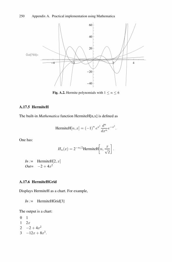
In := Plot[Hermite[5, x], {x, -5, 5}]

Example. PlotHk(x) for k = 0, · · · , 6 and −5 ≤ x ≤ 5. The output is Fig. A.2.

In := Plot[Evaluate[Hermite[#, x] & /@ Range[0, 6, 1]], {x, -5, 5}, PlotStyle→{}]


Out[793]=

�4 �2 2 4

�40

�20

20

40

60

Fig. A.2. Hermite polynomials with 1 ≤ n ≤ 6

A.17.5 HermiteH

The built-in Mathematica function HermiteH[n,x] is defined as

HermiteH[n, x] = (−1)nex2 dn

dxne−x2

.

One has:

Hn(x) = 2−n/2HermiteH

[n,

x√2

].

In := HermiteH[2, x]Out= −2 + 4x2

A.17.6 HermiteHGrid

Displays HermiteH as a chart. For example,

In := HermiteHGrid[3]


0 11 2x2 −2 + 4x2

3 −12x+ 8x3.

A.18 Poisson-Charlier Polynomials 251

A.18 Poisson-Charlier Polynomials

A.18.1 Charlier

Computes the Poisson-Charlier Polynomials. They are orthogonal with respect to thePoisson distribution with mean a. These polynomials cn(x, a), defined for n ≥ 0 anda > 0 , satisfy the orthogonality relation

∞∑k=0

cn(k, a)cm(k, a)e−a ak

k!=n!anδnm

and the recursion relation

c0(x, a) = 1

cn+1(x, a) = a−1xcn(k − 1, a)− cn(x, a), n ≥ 1.

� Please refer to Chapter 10.

Example. Compute the Poisson-Charlier polynomial with n = 8 and a = 1.

In := Charlier[8, x, 1] // TraditionalFormOut= x8−36x7+518x6−3836x5+15659x4−34860x3+38618x2−16072x+1

Example. Compute the Poisson-Charlier polynomial with n = 2 and a > 0.

In := Collect[Charlier[2, x, a], x] // TraditionalFormOut= x2

a2 +(− 1

a2 − 2a

)x+ 1

(“Collect” gathers together terms involving the same powers of x. )

A.18.2 CharlierGrid

Displays the Poisson-Charlier polynomials up to order n with Poisson mean a > 0.

Example.Make a grid of the Poisson-Charlier polynomials for 0 ≤ n ≤ 5.

In := ChalierGrid[5, a] // TraditionalForm


Out=

0 1

1 xa − 1

2 x2

a2 +(− 1

a2 − 2a

)x+ 1

3 x3

a3 +(− 3

a3 − 3a2

)x2 +

(2a3 + 3

a2 + 3a

)x− 1

4 x4

a4 +(− 6

a4 − 4a3

)x3 +

(11a4 + 12

a3 + 6a2

)x2 +

(− 6a4 − 8

a3 − 6a2 − 4

a

)x+ 1

5 x5

a5 +(− 10

a5 − 5a4

)x4 +

(35a5 + 30

a4 + 10a3

)x3 +

(− 50a5 − 55

a4 − 30a3 − 10

a2

)x2 +

(24a5 + 30

a4 + 20a3 + 10

a2 + 5a

)x− 1

Example. Plot the Poisson-Charlier polynomial with n = 5 and a = 1/2 over theinterval −1 ≤ x ≤ 3.

In := Plot[Charlier[5, x, 0.5], {x, -1, 3}, PlotRange→ All]

Example. Plot the Poisson-Charlier polynomials with a = 1 and 1 ≤ n ≤ 6 overthe interval −1 ≤ x ≤ 1. The output is Fig. A.3.

In := Plot[Evaluate[Charlier[#, x, 1] & /@ Range[1, 6]], {x, -1, 1}, PlotStyle→{ }]

Out[803]=�1.0 �0.5 0.5 1.0

�40

�20

20

40

Fig. A.3. Poisson-Charlier polynomials with 1 ≤ n ≤ 6

A.18 Poisson-Charlier Polynomials 253

A.18.3 CharlierCentered

These polynomials are defined by

Cn(x, a) = ancn(x+ a, a).

They are orthogonal with respect to the centered Poisson distribution with parametera > 0.

Example. Compute the centered Poisson-Charlier polynomial with n = 3.

In := Collect[CharlierCentered[3, x, a], x]Out= 2a+ (2− 3a)x− 3x2 + x3

Example. Compute the centered Poisson-Charlier polynomial with n = 3 anda = 1.

In := CharlierCentered[8, x, 1] // TraditionalFormOut= x8− 28x7 + 294x6− 1428x5 + 3059x4− 1428x3− 3326x2 + 2904x− 7

Example. Plot the centered Poisson-Charlier polynomials with a = 1 and1 ≤ n ≤ 6 over the interval −1 ≤ x ≤ 1. The output is Fig. A.4.

In := Plot[Evaluate[CharlierCentered[#, x, 1] & /@ Range[1, 6]], x, -1, 1, PlotRange→ All]

Out[808]=

�1.0 �0.5 0.5 1.0

�60

�40

�20

20

Fig. A.4. Centered Charlier polynomials with a = 1 and 1 ≤ n ≤ 6


A.18.4 CharlierCenteredGrid

Displays the centered Poisson-Charlier polynomials up to order n.

Example. Make a grid of the centered Poisson-Charlier polynomials for0 ≤ n ≤ 5.

In := ChalierCenteredGrid[5, a]Out=

0 1

1 x

2 x2 − x − a

3 x3 − 3x2 + (2 − 3a)x + 2a

4 x4 − 6x3 + (11 − 6a)x2 + (14a − 6)x + 3a2 − 6a

5 x5 − 10x4 + (35 − 10a)x3 + (50a − 50)x2 + (15a2 − 70a + 24)x − 20a2 + 24a

6 x6 − 15x5 + (85 − 15a)x4 + (130a − 225)x3 + (45a2 − 375a + 274)x2

+(−165a2 + 404a − 120)x − 15a3 + 130a2 − 120a

Appendix B

Tables of moments and cumulants

In the following tables, μn and κn denote respectively the nth moment and nth cumu-lant of a random variableX . IfX has mean zero, then μ1 = κ1 = 0 and μn and κn aresaid to be “centered”. If, in addition, X has variance one, then μ2 = κ2 = 1 as well,and μn and κn are said to be “centered and scaled”.

List of tables:

1. Centered and scaled Cumulant to Moments2. Centered Cumulant to Moments3. Cumulant to Moments4. Centered and scaled Moment to Cumulants5. Centered Moment to Cumulants6. Moment to Cumulants

G. Peccati, M.S. Taqqu: Wiener Chaos: Moments, Cumulants and Diagrams –A survey with computer implementation.© Springer-Verlag Italia 2011

256 Appendix B. Tables of moments and cumulants

Centered and scaled Cumulant to Moments

n κn =

1 0

2 1

3 μ3

4 −3 + μ4

5 −10μ3 + μ5

6 30 − 10μ23 − 15μ4 + μ6

7 210μ3 − 35μ3μ4 − 21μ5 + μ7

8 −630 + 560μ23 + 420μ4 − 35μ2

4 − 56μ3μ5 − 28μ6 + μ8

9 −7560μ3 + 560μ33 + 2520μ3μ4 + 756μ5 − 126μ4μ5 − 84μ3μ6 − 36μ7 + μ9

10 22680 − 37800μ23 − 18900μ4 + 4200μ2

3μ4 + 3150μ24 + 5040μ3μ5 − 126μ2

5 +

1260μ6 − 210μ4μ6 − 120μ3μ7 − 45μ8 + μ10

12 −1247400 + 3326400μ23 − 92400μ4

3 + 1247400μ4 − 831600μ23μ4 − 311850μ2

4 +

11550μ34 − 498960μ3μ5 + 55440μ3μ4μ5 + 16632μ2

5 − 83160μ6 + 18480μ23μ6 +

27720μ4μ6 − 462μ26 + 15840μ3μ7 − 792μ5μ7 + 2970μ8 − 495μ4μ8 − 220μ3μ9 −

66μ10 + μ12

13 −32432400μ3 + 14414400μ33 + 21621600μ3μ4 − 1201200μ3

3μ4 − 2702700μ3μ24

+120120μ3μ4μ6 + 72072μ5μ6 − 154440μ7 + 34320μ23μ7 + 51480μ4μ7 − 1716μ6μ7

+25740μ3μ8 − 1287μ5μ8 + 4290μ9 − 715μ4μ9 − 286μ3μ10 − 78μ11 + μ13

14 97297200 − 378378000μ23 + 33633600μ4

3 − 113513400μ4 +

151351200μ23μ4 + 37837800μ2

4 − 6306300μ23μ

24 − 3153150μ3

4 + 60540480μ3μ5 −3363360μ3

3μ5 − 15135120μ3μ4μ5 − 2270268μ25 + 252252μ4μ

25 + 7567560μ6 −

5045040μ23μ6 − 3783780μ4μ6 + 210210μ2

4μ6 + 336336μ3μ5μ6 + 84084μ26 −

2162160μ3μ7 + 240240μ3μ4μ7 + 144144μ5μ7 − 1716μ27 − 270270μ8 +

60060μ23μ8 + 90090μ4μ8 − 3003μ6μ8 + 40040μ3μ9 − 2002μ5μ9 + 6006μ10 −

1001μ4μ10 − 364μ3μ11 − 91μ12 + μ14

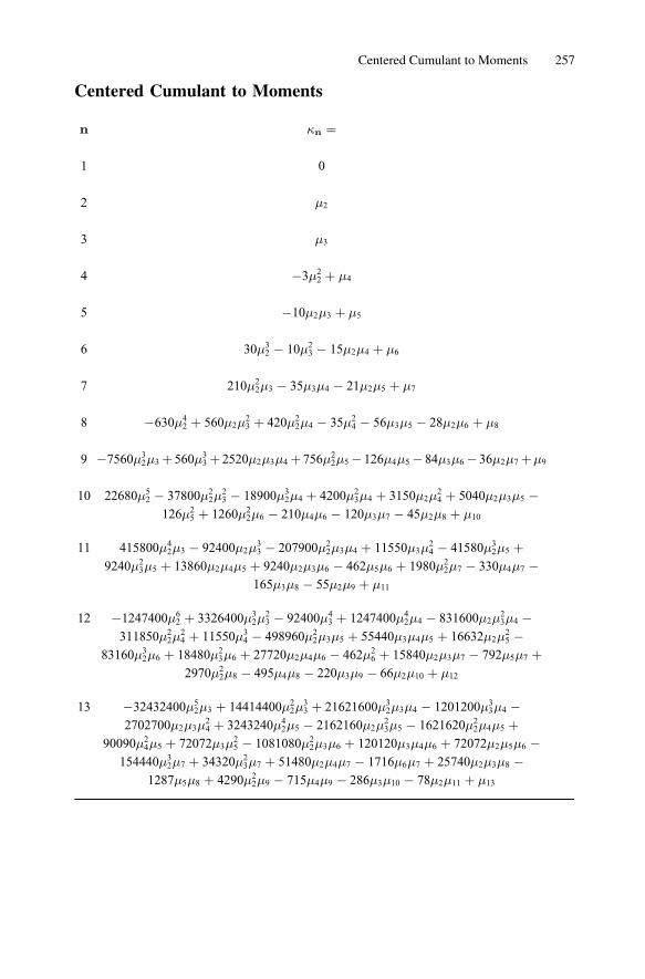
Centered Cumulant to Moments 257

Centered Cumulant to Moments

n κn =

1 0

2 μ2

3 μ3

4 −3μ22 + μ4

5 −10μ2μ3 + μ5

6 30μ32 − 10μ2

3 − 15μ2μ4 + μ6

7 210μ22μ3 − 35μ3μ4 − 21μ2μ5 + μ7

8 −630μ42 + 560μ2μ

23 + 420μ2

2μ4 − 35μ24 − 56μ3μ5 − 28μ2μ6 + μ8

9 −7560μ32μ3 + 560μ3

3 + 2520μ2μ3μ4 + 756μ22μ5 − 126μ4μ5 − 84μ3μ6 − 36μ2μ7 +μ9

10 22680μ52 − 37800μ2

2μ23 − 18900μ3

2μ4 + 4200μ23μ4 + 3150μ2μ

24 + 5040μ2μ3μ5 −

126μ25 + 1260μ2

2μ6 − 210μ4μ6 − 120μ3μ7 − 45μ2μ8 + μ10

11 415800μ42μ3 − 92400μ2μ

33 − 207900μ2

2μ3μ4 + 11550μ3μ24 − 41580μ3

2μ5 +

9240μ23μ5 + 13860μ2μ4μ5 + 9240μ2μ3μ6 − 462μ5μ6 + 1980μ2

2μ7 − 330μ4μ7 −165μ3μ8 − 55μ2μ9 + μ11

12 −1247400μ62 + 3326400μ3

2μ23 − 92400μ4

3 + 1247400μ42μ4 − 831600μ2μ

23μ4 −

311850μ22μ

24 + 11550μ3

4 − 498960μ22μ3μ5 + 55440μ3μ4μ5 + 16632μ2μ

25 −

83160μ32μ6 + 18480μ2

3μ6 + 27720μ2μ4μ6 − 462μ26 + 15840μ2μ3μ7 − 792μ5μ7 +

2970μ22μ8 − 495μ4μ8 − 220μ3μ9 − 66μ2μ10 + μ12

13 −32432400μ52μ3 + 14414400μ2

2μ33 + 21621600μ3

2μ3μ4 − 1201200μ33μ4 −

2702700μ2μ3μ24 + 3243240μ4

2μ5 − 2162160μ2μ23μ5 − 1621620μ2

2μ4μ5 +

90090μ24μ5 + 72072μ3μ

25 − 1081080μ2

2μ3μ6 + 120120μ3μ4μ6 + 72072μ2μ5μ6 −154440μ3

2μ7 + 34320μ23μ7 + 51480μ2μ4μ7 − 1716μ6μ7 + 25740μ2μ3μ8 −

1287μ5μ8 + 4290μ22μ9 − 715μ4μ9 − 286μ3μ10 − 78μ2μ11 + μ13


Cumulant to Moments

n κn =

1 μ1

2 −μ21 + μ2

3 2μ31 − 3μ1μ2 + μ3

4 −6μ41 + 12μ2

1μ2 − 3μ22 − 4μ1μ3 + μ4

5 24μ51 − 60μ3

1μ2 + 30μ1μ22 + 20μ2

1μ3 − 10μ2μ3 − 5μ1μ4 + μ5

6 −120μ61 + 360μ4

1μ2 − 270μ21μ

22 + 30μ3

2 − 120μ31μ3 + 120μ1μ2μ3 − 10μ2

3 +

30μ21μ4 − 15μ2μ4 − 6μ1μ5 + μ6

7 720μ71 − 2520μ5

1μ2 + 2520μ31μ

22 − 630μ1μ

32 + 840μ4

1μ3 − 1260μ21μ2μ3 + 210μ2

2μ3 +

140μ1μ23 − 210μ3

1μ4 + 210μ1μ2μ4 − 35μ3μ4 + 42μ21μ5 − 21μ2μ5 − 7μ1μ6 + μ7

8 −5040μ81 + 20160μ6

1μ2 − 25200μ41μ

22 + 10080μ2

1μ32 − 630μ4

2 − 6720μ51μ3 +

13440μ31μ2μ3 − 5040μ1μ

22μ3 − 1680μ2

1μ23 + 560μ2μ

23 + 1680μ4

1μ4 − 2520μ21μ2μ4 +

420μ22μ4 + 560μ1μ3μ4 − 35μ2

4 − 336μ31μ5 + 336μ1μ2μ5 − 56μ3μ5 + 56μ2

1μ6 −28μ2μ6 − 8μ1μ7 + μ8

9 40320μ91 − 181440μ7

1μ2 + 272160μ51μ

22 − 151200μ3

1μ32 + 22680μ1μ

42 + 60480μ6

1μ3 −151200μ4

1μ2μ3 + 90720μ21μ

22μ3 − 7560μ3

2μ3 + 20160μ31μ

23 − 15120μ1μ2μ

23 +

560μ33 − 15120μ5

1μ4 + 30240μ31μ2μ4 − 11340μ1μ

22μ4 − 7560μ2

1μ3μ4 +

2520μ2μ3μ4 + 630μ1μ24 + 3024μ4

1μ5 − 4536μ21μ2μ5 + 756μ2

2μ5 + 1008μ1μ3μ5 −126μ4μ5 − 504μ3

1μ6 + 504μ1μ2μ6 − 84μ3μ6 + 72μ21μ7 − 36μ2μ7 − 9μ1μ8 + μ9

10 −362880μ101 + 1814400μ8

1μ2 − 3175200μ61μ

22 + 2268000μ4

1μ32 − 567000μ2

1μ42 +

22680μ52 − 604800μ7

1μ3 + 1814400μ51μ2μ3 − 1512000μ3

1μ22μ3 + 302400μ1μ

32μ3 −

252000μ41μ

23 + 302400μ2

1μ2μ23 − 37800μ2

2μ23 − 16800μ1μ

33 + 151200μ6

1μ4 −378000μ4

1μ2μ4 + 226800μ21μ

22μ4 − 18900μ3

2μ4 + 100800μ31μ3μ4 −

75600μ1μ2μ3μ4 + 4200μ23μ4 − 9450μ2

1μ24 + 3150μ2μ

24 − 30240μ5

1μ5 +

60480μ31μ2μ5 − 22680μ1μ

22μ5 − 15120μ2

1μ3μ5 + 5040μ2μ3μ5 + 2520μ1μ4μ5 −126μ2

5 + 5040μ41μ6 − 7560μ2

1μ2μ6 + 1260μ22μ6 + 1680μ1μ3μ6 − 210μ4μ6 −

720μ31μ7 + 720μ1μ2μ7 − 120μ3μ7 + 90μ2

1μ8 − 45μ2μ8 − 10μ1μ9 + μ10

Centered and scaled Moment to Cumulants 259

Centered and scaled Moment to Cumulants

n μn =

1 0

2 1

3 κ3

4 3 + κ4

5 10κ3 + κ5

6 15 + 10κ23 + 15κ4 + κ6

7 105κ3 + 35κ3κ4 + 21κ5 + κ7

8 105 + 280κ23 + 210κ4 + 35κ2

4 + 56κ3κ5 + 28κ6 + κ8

9 1260κ3 + 280κ33 + 1260κ3κ4 + 378κ5 + 126κ4κ5 + 84κ3κ6 + 36κ7 + κ9

10 945 + 6300κ23 + 3150κ4 + 2100κ2

3κ4 + 1575κ24 + 2520κ3κ5 + 126κ2

5 + 630κ6 +

210κ4κ6 + 120κ3κ7 + 45κ8 + κ10

11 17325κ3 + 15400κ33 + 34650κ3κ4 + 5775κ3κ

24 + 6930κ5 + 4620κ2

3κ5 +

6930κ4κ5 + 4620κ3κ6 + 462κ5κ6 + 990κ7 + 330κ4κ7 + 165κ3κ8 + 55κ9 + κ11

12 10395 + 138600κ23 + 15400κ4

3 + 51975κ4 + 138600κ23κ4 + 51975κ2

4 + 5775κ34 +

83160κ3κ5 + 27720κ3κ4κ5 + 8316κ25 + 13860κ6 + 9240κ2

3κ6 + 13860κ4κ6 +

462κ26 + 7920κ3κ7 + 792κ5κ7 + 1485κ8 + 495κ4κ8 + 220κ3κ9 + 66κ10 + κ12

13 270270κ3 + 600600κ33 + 900900κ3κ4 + 200200κ3

3κ4 + 450450κ3κ24 + 135135κ5 +

360360κ23κ5 + 270270κ4κ5 + 45045κ2

4κ5 + 36036κ3κ25 + 180180κ3κ6 +

60060κ3κ4κ6 + 36036κ5κ6 + 25740κ7 + 17160κ23κ7 + 25740κ4κ7 + 1716κ6κ7 +

12870κ3κ8 + 1287κ5κ8 + 2145κ9 + 715κ4κ9 + 286κ3κ10 + 78κ11 + κ13

14 135135 + 3153150κ23 + 1401400κ4

3 + 945945κ4 + 6306300κ23κ4 + 1576575κ2

4 +

1051050κ23κ

24 + 525525κ3

4 + 2522520κ3κ5 + 560560κ33κ5 + 2522520κ3κ4κ5 +

378378κ25 + 126126κ4κ

25 + 315315κ6 + 840840κ2

3κ6 + 630630κ4κ6 +

105105κ24κ6 + 168168κ3κ5κ6 + 42042κ2

6 + 360360κ3κ7 + 120120κ3κ4κ7 +

72072κ5κ7 + 1716κ27 + 45045κ8 + 30030κ2

3κ8 + 45045κ4κ8 + 3003κ6κ8 +

20020κ3κ9 + 2002κ5κ9 + 3003κ10 + 1001κ4κ10 + 364κ3κ11 + 91κ12 + κ14


Centered Moment to Cumulants

n μn =

1 0

2 κ2

3 κ3

4 3κ22 + κ4

5 10κ2κ3 + κ5

6 15κ32 + 10κ2

3 + 15κ2κ4 + κ6

7 105κ22κ3 + 35κ3κ4 + 21κ2κ5 + κ7

8 105κ42 + 280κ2κ

23 + 210κ2

2κ4 + 35κ24 + 56κ3κ5 + 28κ2κ6 + κ8

9 1260κ32κ3 + 280κ3

3 + 1260κ2κ3κ4 + 378κ22κ5 + 126κ4κ5 + 84κ3κ6 + 36κ2κ7 + κ9

10 945κ52 + 6300κ2

2κ23 + 3150κ3

2κ4 + 2100κ23κ4 + 1575κ2κ

24 + 2520κ2κ3κ5 + 126κ2

5 +

630κ22κ6 + 210κ4κ6 + 120κ3κ7 + 45κ2κ8 + κ10

11 17325κ42κ3 + 15400κ2κ

33 + 34650κ2

2κ3κ4 + 5775κ3κ24 + 6930κ3

2κ5 + 4620κ23κ5 +

6930κ2κ4κ5+4620κ2κ3κ6+462κ5κ6+990κ22κ7+330κ4κ7+165κ3κ8+55κ2κ9+κ11

12 10395κ62 + 138600κ3

2κ23 + 15400κ4

3 + 51975κ42κ4 + 138600κ2κ

23κ4 + 51975κ2

2κ24 +

5775κ34 + 83160κ2

2κ3κ5 + 27720κ3κ4κ5 + 8316κ2κ25 + 13860κ3

2κ6 + 9240κ23κ6 +

13860κ2κ4κ6 + 462κ26 + 7920κ2κ3κ7 + 792κ5κ7 + 1485κ2

2κ8 + 495κ4κ8 +

220κ3κ9 + 66κ2κ10 + κ12

13 270270κ52κ3 + 600600κ2

2κ33 + 900900κ3

2κ3κ4 + 200200κ33κ4 + 450450κ2κ3κ

24 +

135135κ42κ5 + 360360κ2κ

23κ5 + 270270κ2

2κ4κ5 + 45045κ24κ5 + 36036κ3κ

25 +

180180κ22κ3κ6 + 60060κ3κ4κ6 + 36036κ2κ5κ6 + 25740κ3

2κ7 + 17160κ23κ7 +

25740κ2κ4κ7 + 1716κ6κ7 + 12870κ2κ3κ8 + 1287κ5κ8 + 2145κ22κ9 + 715κ4κ9 +

286κ3κ10 + 78κ2κ11 + κ13

14 135135κ72 + 3153150κ4

2κ23 + 1401400κ2κ

43 + 945945κ5

2κ4 + 6306300κ22κ

23κ4 +

1576575κ32κ

24 + 1051050κ2

3κ24 + 525525κ2κ

34 + 2522520κ3

2κ3κ5 + 560560κ33κ5 +

2522520κ2κ3κ4κ5 + 378378κ22κ

25 + 126126κ4κ

25 + 315315κ4

2κ6 + 840840κ2κ23κ6 +

630630κ22κ4κ6 + 105105κ2

4κ6 + 168168κ3κ5κ6 + 42042κ2κ26 + 360360κ2

2κ3κ7 +

120120κ3κ4κ7 + 72072κ2κ5κ7 + 1716κ27 + 45045κ3

2κ8 + 30030κ23κ8 +

45045κ2κ4κ8 + 3003κ6κ8 + 20020κ2κ3κ9 + 2002κ5κ9 + 3003κ22κ10 +

1001κ4κ10 + 364κ3κ11 + 91κ2κ12 + κ14

Moment to Cumulants 261

Moment to Cumulants

n μn =

1 κ1

2 κ21 + κ2

3 κ31 + 3κ1κ2 + κ3

4 κ41 + 6κ2

1κ2 + 3κ22 + 4κ1κ3 + κ4

5 κ51 + 10κ3

1κ2 + 15κ1κ22 + 10κ2

1κ3 + 10κ2κ3 + 5κ1κ4 + κ5

6 κ61 + 15κ4

1κ2 + 45κ21κ

22 + 15κ3

2 + 20κ31κ3 + 60κ1κ2κ3 + 10κ2

3 + 15κ21κ4 + 15κ2κ4 +

6κ1κ5 + κ6

7 κ71 + 21κ5

1κ2 + 105κ31κ

22 + 105κ1κ

32 + 35κ4

1κ3 + 210κ21κ2κ3 + 105κ2

2κ3 + 70κ1κ23 +

35κ31κ4 + 105κ1κ2κ4 + 35κ3κ4 + 21κ2

1κ5 + 21κ2κ5 + 7κ1κ6 + κ7

8 κ81 + 28κ6

1κ2 + 210κ41κ

22 + 420κ2

1κ32 + 105κ4

2 + 56κ51κ3 + 560κ3

1κ2κ3 + 840κ1κ22κ3 +

280κ21κ

23 + 280κ2κ

23 + 70κ4

1κ4 + 420κ21κ2κ4 + 210κ2

2κ4 + 280κ1κ3κ4 + 35κ24 +

56κ31κ5 + 168κ1κ2κ5 + 56κ3κ5 + 28κ2

1κ6 + 28κ2κ6 + 8κ1κ7 + κ8

9 κ91+36κ7

1κ2+378κ51κ

22+1260κ3

1κ32+945κ1κ

42+84κ6

1κ3+1260κ41κ2κ3+3780κ2

1κ22κ3+

1260κ32κ3+840κ3

1κ23+2520κ1κ2κ

23+280κ3

3+126κ51κ4+1260κ3

1κ2κ4+1890κ1κ22κ4+

1260κ21κ3κ4 + 1260κ2κ3κ4 + 315κ1κ

24 + 126κ4

1κ5 + 756κ21κ2κ5 + 378κ2

2κ5 +

504κ1κ3κ5+126κ4κ5+84κ31κ6+252κ1κ2κ6+84κ3κ6+36κ2

1κ7+36κ2κ7+9κ1κ8+κ9

10 κ101 + 45κ8

1κ2 + 630κ61κ

22 + 3150κ4

1κ32 + 4725κ2

1κ42 + 945κ5

2 + 120κ71κ3 +

2520κ51κ2κ3 + 12600κ3

1κ22κ3 + 12600κ1κ

32κ3 + 2100κ4

1κ23 + 12600κ2

1κ2κ23 +

6300κ22κ

23 + 2800κ1κ

33 + 210κ6

1κ4 + 3150κ41κ2κ4 + 9450κ2

1κ22κ4 + 3150κ3

2κ4 +

4200κ31κ3κ4 + 12600κ1κ2κ3κ4 + 2100κ2

3κ4 + 1575κ21κ

24 + 1575κ2κ

24 + 252κ5

1κ5 +

2520κ31κ2κ5 + 3780κ1κ

22κ5 + 2520κ2

1κ3κ5 + 2520κ2κ3κ5 + 1260κ1κ4κ5 + 126κ25 +

210κ41κ6 + 1260κ2

1κ2κ6 + 630κ22κ6 + 840κ1κ3κ6 + 210κ4κ6 + 120κ3

1κ7 +

360κ1κ2κ7 + 120κ3κ7 + 45κ21κ8 + 45κ2κ8 + 10κ1κ9 + κ10

11 κ111 + 55κ9

1κ2 + 990κ71κ

22 + 6930κ5

1κ32 + 17325κ3

1κ42 + 10395κ1κ

52 + 165κ8

1κ3 +

4620κ61κ2κ3 + 34650κ4

1κ22κ3 + 69300κ2

1κ32κ3 + 17325κ4

2κ3 + 4620κ51κ

23 +

46200κ31κ2κ

23 + 69300κ1κ

22κ

23 + 15400κ2

1κ33 + 15400κ2κ

33 + 330κ7

1κ4 +

6930κ51κ2κ4 + 34650κ3

1κ22κ4 + 34650κ1κ

32κ4 + 11550κ4

1κ3κ4 + 69300κ21κ2κ3κ4 +

34650κ22κ3κ4 + 23100κ1κ

23κ4 + 5775κ3

1κ24 + 17325κ1κ2κ

24 + 5775κ3κ

24 +

462κ61κ5 + 6930κ4

1κ2κ5 + 20790κ21κ

22κ5 + 6930κ3

2κ5 + 9240κ31κ3κ5+

27720κ1κ2κ3κ5 + 4620κ23κ5 + 6930κ2

1κ4κ5 + 6930κ2κ4κ5 + 1386κ1κ25 +

462κ51κ6 + 4620κ3

1κ2κ6 + 6930κ1κ22κ6 + 4620κ2

1κ3κ6 + 4620κ2κ3κ6 +

2310κ1κ4κ6 + 462κ5κ6 + 330κ41κ7 + 1980κ2

1κ2κ7 + 990κ22κ7 + 1320κ1κ3κ7 +

330κ4κ7 + 165κ31κ8 + 495κ1κ2κ8 + 165κ3κ8 + 55κ2

1κ9 + 55κ2κ9 + 11κ1κ10 + κ11

References

1. Adler R.J. (1990). An Introduction to Continuity, Extrema, and Related Topics for Gen-eral Gaussian Processes. Lecture Notes-Monograph Series 12, Institut of MathematicalStatistics, Hayward, California.

2. Aigner M. (1979). Combinatorial theory. Springer-Verlag, Berlin Heidelberg New York.3. Anshelevich M. (2001). Partition-dependent stochastic measures and q-deformed cumu-lants. Documenta Mathematica 6, 343-384.

4. Anshelevich M. (2005). Linearization coefficients for orthogonal polynomials usingstochastic processes. The Annals of Probabability 33(1), 114-136.

5. Baldi P., Kerkyacharian G., Marinucci D. and Picard D. (2008). High-frequency asymp-totics for wavelet-based tests for Gaussianity and isotropy on the torus. Journal of Multi-variate Analysis 99, 606-636.

6. Barbour A.D. (1986). Asymptotic expansions based on smooth functions in the centrallimit theorem. Probab. Theory Rel. Fields 72(2), 289-303.

7. Barndorff-Nielsen O., Corcuera J., Podolskij M. and Woerner J. (2009). Bipower varia-tions for Gaussian processes with stationary increments. Journal of Applied Probability46, 132-150.

8. Billingsley P. (1995). Probability and Measure, 3rd edition. Wiley, New York.9. Bitcheler K. (1980). Stochastic integration and Lp theory of semimartingales. The Annals

of Probability 9(1), 49-89.10. Breuer P. and Major P. (1983). Central limit theorems for non-linear functionals of Gaus-

sian fields. Journal of Multivariate Analysis 13, 425-441.11. Brodskii M.S. (1971). Triangular and Jordan Representations of Linear Operators.

Transl. Math. Monographs 32, AMS, Providence.12. Chambers D. and Slud E. (1989). Central limit theorems for nonlinear functionals of sta-

tionary Gaussian processes. Probability Theory and Related Fields 80, 323-349.13. Charalambides C.A. (2002). Enumerative Combinatorics. Chapman and Hall, New York.14. Chen L.H.Y. and Shao Q.-M. (2005). Stein’s method for normal approximation. In:

A.D. Barbour and L.H.Y. Chen (eds), An Introduction to Stein’s Method. Lecture NotesSeries No. 4, Institute for Mathematical Sciences, National University of Singapore, Sin-gapore University Press and World Scientific 2005, 1-59.

15. Chen L.H.Y., Goldstein L. and Shao Q.-M. (2001). Normal Approximation by Stein’sMethod. Springer-Verlag, Berlin Heidelberg New York.

16. Cohen S. and Taqqu M.S. (2004). Small and large scale behavior of the Poissonized Tele-com process.Methodology and Computing in Applied Probability 6, 363-379.

264 References

17. Corcuera J.M., Nualart D. and Woerner J.H.C. (2006). Power variation of some integrallong memory process. Bernoulli 12(4), 713-735.

18. de Blasi P., Peccati G. and Prünster I. (2008). Asymptotics for posterior hazards. TheAnnals of Statistics 37(4), 1906-1945.

19. Deheuvels P., Peccati G. and Yor M. (2006). On quadratic functionals of the Browniansheet and related processes. Stochastic Processes and their Applications 116, 493-538.

20. Dellacherie C., Maisonneuve B. and Meyer P.-A. (1992). Probabilités et Potentiel(Chapitres XVII à XXIV). Hermann, Paris.

21. Di Nunno G., Øksendal B. and Proske F. (2009). Malliavin calculus for Lévy processeswith applications to finance. Springer-Verlag, Berlin.

22. Dobinski G. (1877). Summirung der Reihe∑

nm/n! für m = 1, 2, 3, 4, 5, .... GrunertArchiv (Arch. für Mat. und Physik) 61, 333-336.

23. Dobrushin R.L. (1979). Gaussian and their subordinated self-similar random generalizedfields. The Annals of Probability 7, 1–28.

24. Dudley R.M. (1967). The sizes of compact subsets of Hilbert space and continuity of Gaus-sian processes. Journal of Functional Analysis 1, 290-330.

25. Embrechts P. and Maejima M. (2003). Selfsimilar Processes. Princeton University Press,Princeton.

26. Engel D.D. (1982). The multiple stochastic integral. Memoirs of the AMS 38, 1-82.27. Erhardsson T. (2005). Poisson and compound Poisson approximations. In: A.D. Barbour

and L.H.Y. Chen (eds.), An Introduction to Stein’s Method. Lecture Notes Series No.4, In-stitute forMathematical Sciences, National University of Singapore, Singapore UniversityPress and World Scientific 2005, 61-115.

28. Farré M., Jolis M. and Utzet F. (2008). Multiple Stratonovich integral and Hu-Meyer for-mula for Lévy processes. To appear in: The Annals of Probability.

29. Feigin P.D. (1985). Stable convergence of semimartingales. Stochastic Processes and theirApplications 19, 125-134.T.S.

30. Ferguson (1973). A Bayesian analysis of some non-parametric problems. The Annals ofStatistics 1(2), 209-230.

31. Fox R. and Taqqu M.S. (1987). Multiple stochastic integrals with dependent integrators.Journal of Multivariate Analysis 21(1), 105-127.

32. Fristedt B. and Gray L. (1997). A Modern Approach to Probability theory. Birkhäuser,Boston.

33. Giné E. and de la Peña V.H. (1999).Decoupling. Springer-Verlag, Berlin Heidelberg NewYork.

34. Giraitis L. and Surgailis D. (1985). CLT and other limit theorems for functionals of Gaus-sian processes. Zeitschrift für Wahrsch. verw. Gebiete 70, 191-212.

35. Goldberg J. and Taqqu M.S. (1982). Regular multigraphs and their applications to theMonte Carlo evaluation of moments of non-linear functions of Gaussian processes.Stochastic Processes and their Applications 13, 121-138.

36. Gripenberg G. and Norros I. (1996). On the prediction of fractional Brownian motion.Journal of Applied Probability 33, 400-410.

37. HandaK. (2005). Sampling formulae for symmetric selection.Electronic Communicationsin Probabability 10, 223-234 (Electronic).

38. Handa K. (2009). The two-parameter Poisson-Dirichlet point process. Bernoulli 15(4),1082-1116.

39. Hu Y. and Nualart D. (2005). Renormalized self-intersection local time for fractionalBrownian motion. The Annals of Probabability 33(3), 948-983.

40. Itô K. (1951). Multiple Wiener integral. J. Math. Soc. Japan 3, 157–169.

References 265

41. Jacod J., Klopotowski A. and Mémin J. (1982). Théorème de la limite centrale et con-vergence fonctionnelle vers un processus à accroissements indépendants: la méthode desmartingales. Annales de l’Institut H. Poincaré (PR) 1, 1-45.

42. Jacod J. and Shiryaev A.N. (1987). Limit Theorems for Stochastic Processes. Springer-Verlag, Berlin Heidelberg New York.

43. Jakubowski A. (1986). Principle of conditioning in limit theorems for sums of randomvariables. The Annals of Probability 11(3), 902-915.

44. James L.F., Lijoi A. and Prünster I. (2005). Conjugacy as a distinctive feature of the Dirich-let process. Scandinavian Journal of Statistics 33, 105-120.

45. James L., Roynette B. and Yor M. (2008). Generalized Gamma Convolutions, Dirichletmeans, Thorin measures, with explicit examples. Probability Surveys 5, 346-415.

46. Janson S. (1997). Gaussian Hilbert Spaces. Cambridge University Press, Cambridge.47. Jeulin T. (1980). Semimatingales et grossissement d’une filtration. Lecture Notes inMath-

ematics 833, Springer-Verlag, Berlin Heidelberg New York.48. Julià O. and Nualart D. (1988). The distribution of a double stochastic integral with respect

to two independent Brownian Sheets. Stochastics 25, 171-182.49. Kabanov Y. (1975). On extended stochastic integrals. Theory of Probability and its appli-

cations 20, 710-722.50. Kailath T. and Segall A. (1976). Orthogonal functionals of independent increment pro-

cesses. IEEE Trans. Inform. Theory IT-22, 287-298.51. Kallenberg O. and Szulga J. (1991). Multiple integration with respect to Poisson and Lévy

processes. Probability Theory and Related Fields 83, 101-134.52. Karatzas I. and Shreve S.E. (1991). Brownian Motion and Stochastic Calculus, 2nd edi-

tion. Graduate Texts in Mathematics, Volume 113, Springer-Verlag, Berlin HeidelbergNew-York.

53. Kemp T., Nourdin I., Peccati G. and Speicher R. (2010). Wigner chaos and the fourthmoment. Preprint.

54. Kendall W.S. (2005). Stochastic integrals and their expectations. The Mathematica Jour-nal. 9(4), 757-767.

55. Kingman J.F.C. (1967). Completely random measures. Pacific Journal of Mathematics21, 59-78.

56. Kung J.P.S., Rota G.-C. and Yan C.H. (2009). Combinatorics. The Rota Way. CambridgeUniversity Press, Cambridge.

57. Kuo H.-H. (1975). Gaussian measures in Banach spaces. LNM 463. Springer-Verlag,Berlin Heidelberg New-York.

58. Kuo H.-H. (1986). Introduction to Stochastic Integration. Springer-Verlag, Berlin Heidel-berg New York.

59. Kussmaul A.U. (1977). Stochastic integration and generalized martingales. Pitman re-search notes in mathematic, 11. London.

60. Kwapien S. and Woyczynski W.A. (1991). Semimartingale integrals via decoupling in-equalities and tangent processes. Probability and Mathematical Statisitics 12(2), 165-200.

61. Kwapien S. andWoyczynskiW.A. (1992).Random Series and Stochastic Integrals: Singleand Multiple. Birkhäuser, Basel.

62. Leonov V.P. and Shiryayev A.N. (1959). On a method of calculations of semi-invariants.Theory of Probability and its Applications 4, 319-329.

63. Lifshits M.A. (1995). Gaussian Random Functions. Kluwer, Dordrecht.64. LindeW. (1986). Probability in Banach spaces: stable and infinitely divisible ditributions.

Wiley, New York.65. Ma J., Protter Ph. and San Martin J. (1998). Anticipating integrals for a class of martin-

gales. Bernoulli, 4, 81-114.

266 References

66. Major P. (1981). Multiple Wiener-Itô Integrals. LNM 849. Springer-Verlag, Berlin Hei-delberg New York.

67. Malyshev V.A. (1980). Cluster expansion in lattice models of statistical physics and quan-tum fields theory. Uspehi Mat. Nauk 35, 3-53.

68. Marinucci D. (2006). High resolution asymptotics for the angular bispectrum of sphericalrandom fields. The Annals of Statistics 34, 1-41.

69. Marinucci D. and Peccati G. (2007). High-frequency asymptotics for subordinated sta-tionary fields on an Abelian compact group. Stochastic Processes and their Applications118(4), 585-613.

70. Marinucci D. and Peccati G. (2007). Group representations and high-frequency centrallimit theorems for subordinated random fields on a sphere. To appear in: Bernoulli.

71. Maruyama G. (1982). Applications of the multiplication of the Itô-Wiener expansions tolimit theorems. Proc. Japan Acad. 58, 388-390.

72. Maruyama G. (1985). Wiener functionals and probability limit theorems, I: the centrallimit theorem. Osaka Journal of Mathematics 22, 697-732.

73. Masani P.R. (1995). The homogeneous chaos from the standpoint of vector measures, Phil.Trans. R. Soc. Lond, A 355, 1099-1258.

74. McCullagh P. (1987). Tensor Methods in Statistics. Chapman and Hall, London.75. Mauldin R.D., Sudderth W.D. and Williams S.C. (1992). Pólya trees and random distri-

butions. The Annals of Statistics 20(3), 1203-1221.76. Meyer P.-A. (1976). Un cours sur les intégrales stochastiques. Séminaire de Probabilités

X, LNM 511. Springer-Verlag, Berlin Heidelberg New York, pp. 245-400.77. Meyer P.-A. (1992). Quantum Probability for Probabilists. LNM 1538. Springer-Verlag,

Berlin Heidelberg New York.78. Neuenkirch A. and Nourdin I. (2007). Exact rate of convergence of some approximation

schemes associated to SDEs driven by a fractional Brownian motion. Journal of Theoret-ical Probability 20(4), 871-899.

79. Neveu J. (1968). Processus Aléatoires Gaussiens. Presses de l’Université de Montréal,Montréal.

80. Nica A. and Speciher R. (2006). Lectures on the combinatorics of free probability. LondonMathematical Society Lecture Notes Series 335. Cambridge University Press, Cambridge.

81. Nourdin I. (2005). Schémas d’approximation associés à une équation différentielle dirigéepar une fonction höldérienne; cas du mouvement Brownien fractionnaire.C.R.A.S. 340(8),611-614.

82. Nourdin I. and Nualart D. (2010). Central limit theorems for multiple Skorohod integrals.Journal of Theoretical Probability 23(1), 39-64.

83. Nourdin I., Nualart D. and Tudor C.A. (2010). Central and non-central limit theoremsfor weighted power variations of fractional Brownian motion. To appear in: Annales del’Institut H. Poincarté (PR).

84. Nourdin I. and Peccati G. (2007). Non-central convergence of multiple integrals. The An-nals of Probability 37(4), 1412–1426.

85. Nourdin I. and Peccati G. (2008). Weighted power variations of iterated Brownian motion.The Electronic Journal of Probability 13, n. 43, 1229-1256 (Electronic).

86. Nourdin I. and Peccati G. (2008). Stein’s method on Wiener chaos. Probability Theoryand Related Fields 145(1), 75-118.

87. Nourdin I. and Peccati G. (2008). Stein’s method and exact Berry-Esséen asymptotics forfunctionals of Gaussian fields. The Annals of Probabnility 37(6), 2231-2261.

88. Nourdin I. and Peccati G. (2010). Cumulants on the Wiener space. The Journal of Func-tional Analysis 258, 3775-3791.

References 267

89. Nourdin I., Peccati G. and Reinert G. (2010). Invariance principles for homogeneous sums:universality of the Gaussian Wiener chaos. The Annals of Probability 38(5), 1947-1985.

90. Nourdin I., Peccati G. and Réveillac A. (2008). Multivariate normal approximation usingStein’s method and Malliavin calculus. Annales de l’Institut H. Poincaré (PR) 46(1), 45-58.

91. Nourdin I. and Réveillac A. (2008). Asymptotic behavior of weighted quadratic variationsof fractional Brownianmotion: the critical caseH = 1/4. The Annals of Probability 37(6),2200-2230.

92. Nualart D. (1983). On the distribution of a double stochastic integral. Z. Wahrschein-lichkeit verw. Gebiete 65, 49-60.

93. Nualart D. (1998). Analysis onWiener space and anticipating stochastic calculus. Lectureson Probability Theory and Statistics. École de probabilités de St. Flour XXV (1995), LNM1690. Springer-Verlag, Berlin Heidelberg New York, pp. 123-227.

94. Nualart D. (2006). The Malliavin Calculus and Related Topics, 2nd edition. Springer-Verlag, Berlin Heidelberg New York.

95. Nualart D. and Ortiz-Latorre S. (2007). Intersection local times for two independent frac-tional Brownian motions. Journal of Theoretical Probability 20(4), 759-767.

96. Nualart D. and Ortiz-Latorre S. (2008). Central limit theorems for multiple stochastic inte-grals andMalliavin calculus. Stochastic Processes and their Applications 118(4), 614-628.

97. Nualart D. and Pardoux E. (1988). Stochastic calculus with anticipating integrands. Prob-abability Theory Related Fields, 78, 535-581.

98. Nualart D. and Peccati G. (2005). Central limit theorems for sequences of multiple stochas-tic integrals. The Annals of Probability 33(1), 177-193.

99. Nualart D. and Schoutens W. (2000). Chaotic and predictable representation for Lévyprocesses. Stochastic Processes and their Applications 90, 109-122.

100. Nualart D. and Vives J. (1990). Anticipative calculus for the Poisson space based on theFock space. Séminaire de Probabilités XXIV, LNM 1426. Springer-Verlag, Berlin Heidel-berg New York, pp. 154-165.

101. Ogura H. (1972). Orthogonal functionals of the Poisson process. IEEE Transactions onInformation Theory 18(4), 473-481.

102. Peccati G. (2001). On the convergence of multiple random integrals. Studia Sc. Mat. Hun-garica 37, 429-470.

103. Peccati G. (2007). Gaussian approximations of multiple integrals. Electronic Communi-cations in Probability 12, 350-364 (Electronic).

104. Peccati G. (2008). Multiple integral representation for functionals of Dirichlet processes.Bernoulli 14(1), 91-124.

105. Peccati G. and Prünster I. (2008). Linear and quadratic functionals of random hazard rates:an asymptotic analysis. The Annals of Applied Probability 18(5), 1910-1943.

106. Peccati G., Solé J.-L., Utzet F. and Taqqu M.S. (2008). Stein’s method and Gaussian ap-proximation of Poisson functionals. The Annals of Probability 38(2), 443-478.

107. Peccati G. and Taqqu M.S. (2007). Stable convergence of generalized L2 stochastic inte-grals and the principle of conditioning. The Electronic Journal of Probability 12, 447-480,n. 15 (Electronic).

108. Peccati G. and Taqqu M.S. (2008). Limit theorems for multiple stochastic integrals. ALEA4, 393-413.

109. Peccati G. and Taqqu M.S. (2008). Central limit theorems for double Poisson integrals.Bernoulli 14(3), 791-821.

110. Peccati G. and Taqqu M.S. (2007). Stable convergence of multiple Wiener-Itô integrals.The Journal of Theoretical Probability 21(3), 527-570.

268 References

111. Peccati G. and Tudor C.A. (2005). Gaussian limits for vector-valued multiple stochasticintegrals. Séminaire de Probabilités XXXVIII, LNM 1857. Springer-Verlag, Berlin Hei-delberg New York, pp. 247-262.

112. Peccati G. and Yor M. (2004). Hardy’s inequality in L2 ([0, 1]) and principal values ofBrownian local times. Asymptotic Methods in Stochastics, AMS, Fields Institute Commu-nications Series, 49-74.

113. Peccati G. and Yor M. (2004). Four limit theorems for quadratic functionals of Brownianmotion and Brownian bridge. Asymptotic Methods in Stochastics, AMS, Fields InstituteCommunication Series, 75-87.

114. Peccati G. and Zheng C. (2010). Multi-dimensional Gaussian fluctuations on the Poissonspace. The Electronic Journal of Probability, to appear.

115. Pipiras V. and Taqqu M.S. (2000). Integration questions related to fractional Brownianmotion. Probability Theory and Related Fields 118(2), 251-291.

116. Pipiras V. and Taqqu M.S. (2001). Are classes of deterministic integrands for fractionalBrownian motion complete? Bernoulli 7(6), 873-897.

117. Pipiras V. and Taqqu M.S. (2010). Regularization and integral representations of Hermiteprocesses. To appear in Statistics and Probability Letters.

118. Pipiras V. and Taqqu M.S. (2003). Fractional calculus and its connection to fractionalBrownian motion. In: Long Range Dependence, 166-201, Birkhäuser, Basel.

119. Pitman J. (2006). Combinatorial Stochastic Processes. LNM 1875. Springer-Verlag,Berlin Heidelberg New York.

120. Privault N. (1994). Chaotic and variational calculus in discrete and continuous time forthe Poisson process. Stochastics and Stochastics Reports 51, 83-109.

121. Privault N. (1994). Inégalités de Meyer sur l’espace de Poisson. C.R.A.S. 318, 559-562.122. Privault N. (2009). Stochastic Analysis in Discrete and Continuous Settings: With Normal

Martingales. Springer-Verlag, Berlin Heidelberg New York.123. Privault N. (2010). Invariance of Poisson measures under random transformations.

Preprint.124. Privault N., Solé J.L. and Vives J. (2001). Chaotic Kabanov formula for the Azéma mar-

tingales. Bernoulli 6(4), 633-651.125. Privault N. and Wu J.-L. (1998). Poisson stochastic integration in Hilbert spaces. Ann.

Math. Blaise Pascal 6(2), 41-61.126. Protter P. (2005). Stochastic Integration andDifferential Equations, 2nd edition. Springer-

Verlag, Berlin Heidelberg New York.127. Rajput B.S. and Rosinski J. (1989). Spectral representation of infinitely divisible pro-

cesses. Probability Theory and Related Fields 82, 451-487.128. Revuz D. and Yor M. (1999). Continuous martingales and Brownian motion. Springer-

Verlag, Berlin Heidelberg New York.129. Rider B. and Virág B. (2007). The noise in the circular law and the Gaussian free field.

Int. Math. Res. Not. 2, Art. ID rnm006.130. Roman S. (1984). The Umbral Calculus. Academic press, New York.131. Rota G.-C. and Shen J. (2000). On the combinatorics of cumulants. Journal of Combina-

torial Theory Series A 91, 283-304.132. Rota G.-C. and Wallstrom C. (1997). Stochastic integrals: a combinatorial approach. The

Annals of Probability 25(3), 1257-1283.133. Rosinsky J. and Woyczynski W.A. (1984). Products of random measures, multilinear ran-

dom forms and multiple stochastic integrals. Proc. Conference of Measure Theory, Ober-wolfach 1983, LNM 1089. Springer-Verlag, Berlin Heidelberg New York, pp. 294-315.

134. Russo F. and Vallois P. (1998). Product of two multiple stochastic integrals with respectto a normal martingale. Stochastic Processes and their Applications 73(1), 47-68.

References 269

135. Samorodnitsky G. and Taqqu M.S. (1994). Stable Non-Gaussian Random Processes.Chapman and Hall, New York.

136. Sato K.-I. (1999). Lévy Processes and Infinitely Divisible Distributions. Cambridge Stud-ies in Advanced Mathematics 68. Cambridge University Press, Cambridge.

137. Schoutens W. (2000). Stochastic processes and orthogonal polynomials. Lecture Notes inStaistics 146. Springer-Verlag, Berlin Heidelberg New York.

138. Schreiber M. (1969). Fermeture en probabilité de certains sous-espaces d’un espace L2.Zeitschrift Warsch. verw. Gebiete 14, 36-48.

139. Sheffield S. (1997). Gaussian free field for mathematicians.Probab. Theory Related Fields139(3-4), 521-541.

140. Shigekawa I. (1980). Derivatives ofWiener functionals and absolute continuity of inducedmeasures. J. Math. Kyoto Univ. 20(2), 263-289.

141. Shiryaev A.N. (1984). Probability. Springer-Verlag, Berlin Heidelberg New York.142. Slud E.V. (1993). The moment problem for polynomial forms in normal random variables.

The Annals of Probability 21(4), 2200-2214.143. Solé J.-L. and Utzet F. (2008). Time-space harmonic polynomials associated with a Lévy

process. Bernoulli 14(1), 1-13.144. Solé J.-L. and Utzet F. (2008). On the orthogonal polynomials associated with a Lévy

process. The Annals of Probability 36(2), 765-795.145. Speed T. (1983). Cumulants and partitions lattices. Australian Journal of Statistics 25(2),

378-388.146. Stanley R. (1997). Enumerative combinatorics, Vol. 1. Cambridge University Press, Cam-

bridge.147. Stein Ch. (1986). Approximate computation of expectations. Institute of Mathematical

Statistics Lecture Notes - Monograph Series 7. Institute of Mathematical Statistics, Hay-ward, CA.

148. Steutel F.W. and van Ham K. (2004). Infinite divisibility of probability distributions onthe real line. Marcel Dekker, New York.

149. Stroock D.W. (1987). Homogeneous Chaos Revisited. Séminaire de Probabilités XXI,LNM 1247, Springer-Verlag, Berlin Heidelberg New York, pp. 1-8.

150. Surgailis D. (1984). On multiple Poisson stochastic integrals and associatedMarkov semi-groups. Probab. Math. Statist. 3(2), 217-239.

151. Surgailis D. (2000). CLTs for Polynomials of Linear Sequences: Diagram Formulae withApplications. In: Long Range Dependence. Birkhäuser, Basel, pp. 111-128.

152. Surgailis D. (2000). Non-CLT’s: U-Statistics, Multinomial Formula and Approximationsof Multiple Wiener-Itô integrals. In: Long Range Dependence. Birkhäuser, Basel, pp. 129-142.

153. Taqqu M.S. (1979). Convergence of integrated processes of arbitrary Hermite rank.Zeitschrift für Wahrscheinlichkeitstheorie und verwandte Gebiete 50, 53-83.

154. Taqqu M.S. (2003). Fractional Brownian motion and long-range dependence. In: P. Dou-khan, G. Oppenheim and M.S. Taqqu (eds.), Theory and Applications of Long-range De-pendence. Birkhäuser, Boston, pp. 5-38.

155. Tocino A. (2009). Multiple stochastic integrals withMathematica.Mathematics and Com-puters in Simulations. 79, 1658-1667.

156. Tsilevich N.V. and Vershik A.M. (2003). Fock factorizations and decompositions of theL2 spaces over general Lévy processes. Russian Math. Surveys 58(3), 427-472.

157. Tsilevich N., Vershik A.M. and Yor M. (2001). An infinite-dimensional analogue of theLebesgue measure and distinguished properties of the gamma process. J. Funct. Anal.185(1), 274-296.

270 References

158. Tudor C. (1997). Product formula for multiple Poisson-Itô integrals. Revue Roumaine deMath. Pures et Appliquées 42(3-4), 339-345.

159. Tudor C.A. and Vives J. (2002). The indefinite Skorohod integral as integrator on thePoisson space. Random Operators and Stochastic Equations 10, 29-46.

160. Üstünel A.S. and Zakai M. (1997). The construction of filtrations on Abstract WienerSpace. Journal of Functional Analysis 143, 10-32.

161. Vitale R.A. (1990). Covariances of symmetric statistics. Journal of Multivariate Analysis41, 14-26.

162. Wiener N. (1938). The homogeneous chaos. Amer. J. Math. 60, 879-936.163. Wolfe S.J. (1971). On Moments of Infinitely Divisible Distribution Functions. Ann. Math.

Statist. 42(6), 2036-2043.164. Wolpert R.L. and Taqqu M.S. (2005). Fractional Ornstein-Uhlenbeck Lévy Processes and

the Telecom Process: Upstairs and Downstairs. Signal Processing 85(8), 1523-1545.165. Wu L.M. (1990). Un traitement unifié de la représentation des fonctionnelles de Wiener.

Séminaire de Probabilités XXIV, LNM 1426, Springer-Verlag, Berlin Heidelberg NewYork, pp. 166-187.

166. Xue X.-H. (1991). On the principle of conditioning and convergence to mixtures of dis-tributions for sums of dependent random variables. Stochastic Processes and their Appli-cations 37(2), 175-186.

167. Yosida K. (1980). Functional analysis. Springer-Verlag, Berlin Heidelberg New York.

Index

Δϕn(C), 85

Bπ , 57Bn, 18Bn(x1, ..., xn), 17Bn,k(x1, ..., xn−k+1), 17Bf(x), 171C⊗j , 87Cn(x, a), 172Cϕ

n , 83Iϕ

n (f), 82Iϕ

1 (h), 64L2

s (νn), 81S(n, k), 15Tn(x), 17Zn

π , 57[σ, π], 12[n], 13[x, y], 24[ n

λ

], 13

ΔGn (A), 93

ΔNn (A), 98

Γ (π, σ), 45Λ(n), 7αB , 67χ (Xb), 31χn(X), 32δ(x, y), 210, 12– minimal element, 121, 12– maximal element, 12Γ (π, σ), 54

∫ ′′, 163∫ ′, 107∫Z

h (z) ϕ (dz), 64∫Z

hdϕ, 64λ n, 7λ(π, σ), 12〈·〉 (as expectation), 128(1r1 2r2 · · · nrn), 7|π|, 90, 12B1 (σ), 97B2 (σ), 97PB2 (σ), 97Xb, 31X[n], 31Xb, 31e (α), 154A∞, 152A∞,q , 153E (νn), 77E0 (νn), 81Es,0 (νn), 81I(P ), 21M ([n] , π∗), 132M0 ([n] , π∗), 132M0

≥2 ([n] , π∗), 133M2 ([n] , π∗), 133M0

2 ([n] , π∗), 133M≥2 ([n] , π∗), 133P(b), 9Zν , 59Zn

ν , 61Zn

s,ν = Zns , 79

272 Index

H�q , 153H⊗q , 153Sn, 79μ(σ, π), 19μ(x, y), 21⊗r(= �r

r), 116ρν , 68σ < π, 22σ ≥ π, 76σ ≤ π, 9σ � π, 19σ ∨ π, 10σ ∧ π, 10Stϕ,[n]

π (f), 78Tn(x), 43ϕ(h), 64ϕ[n], 61f , 79ζ(x, y), 21cn(x, a), 171f ∗ g, 21f �l

r g, 115f1 ⊗0 f2 ⊗0 · · · ⊗0 fk, 110fσ,k, 133gXb , 31i ∼π j, 9mn(ν), 39St

ϕ,[n]≥π (C), 77

Stϕ,[n]π (C), 76

Backward shift operator, 171Bell numbers, 18– generating function, 41Binomial type, 19Block, 9Borel isomorphism, 60Borel space, 57Brownian motion, 88

Canonical isomorphism, 155, 157Charlier polynomials, 171, 172, 175– as multiple Poisson integrals, 173, 174– centered, 172Chen-Stein Lemma, 42Class of a segment, 12CLT– on the Gaussian Wiener chaos, 182, 200– on the second Poisson chaos, 204Coarse, 9

Compound Poisson process, 75, 76Computational rules for Gaussian andPoisson measures, 92

Contraction (of two functions), 115– symmetrization, 117Contraction (on a Hilbert space), 156Control measure, 59– symmetric, 151Convolution on the incidence algebra, 21Convolutional inverse, 21Cumulants– homogeneity of, 32– joint, 31– of a gamma random variable, 144– of a Poisson random variable, 33– of a single random variable, 32– of an element of the second Wiener chaos,140

– order of, 32

Delta function, 21Diagonal measure, 85Diagram– circular, 49, 56– and contractions, 198

– connected, 47, 56– definition, 45– disconnected, 47– flat, 48– formulae, 3– for Gaussian measures, 133– for Poisson measures, 140– for stochastic measures, 129, 132– Malyshev, 50

– Gaussian, 48, 56– non-flat, 48, 56Dirichlet process, 75Divergence operator, 145Dobinski formula, 41Double factorial, 38Double Wiener-Itô integrals as series ofchi-square, 178

Dudley, R.M., 149

Edge, 46Elementary functions, 77Engel, D.D., 1, 4, 62Even function, 151

Index 273

Fourth cumulant condition, 182Fourth cumulant of a multiple integral(Gaussian case), 180

Fractional Brownian motion, 151, 166, 190Free probability, 5, 51Fubini, 106

Gaussian free field, 152Gaussian is determined by its moments, 39

Hermite polynomials, 145, 146, 154, 163,172, 175

Hermite processes, 165Hu-Meyer formulae, 5, 89Hypercontractivity, 92– for an isonormal Gaussian process, 155Hyperdiagonal, 107, 162Hypergraph, 46

Incidence algebra, 21Infinitely divisible, 65Integral notation for stochastic measures, 84Isomorphism of partially ordered sets, 25Isonormal Gaussian process, 3, 149, 187– built from a covariance, 150– spectral representation, 152, 157, 159

Join, 10

Kailath-Segall formula, 86– on the real line, 90Khintchine’s theorem, 66

Lévy measure, 67Lévy-Khintchine– characteristics, 67– exponent, 67– of a Gaussian single integral, 71– of a Poisson single integral, 72

– representation, 67Lévy process, 73, 88Lattice, 10, 27Length of a partition of an integer, 7Length of a segment, 24Leonov and Shiryaev formulae, 34Long memory, 148Long-range dependence, 148

Möbius function– of P(b), 19

– of a partially ordered set, 22– recursive computation, 25Möbius inversion formula– for random measures, 78– on P(b), 20– on a partially ordered set, 23Malliavin calculus, 5Malyshev formula, 34Mathematica, 3Meet, 10Method of (moments and) cumulants, 181Moments of a Gaussian random variable, 38Multigraph, 53Multiindex, 153Multiplication formulae– for isonormal Gaussian processes, 157, 187– Gaussian case, 118– general, 109– with diagrams, 112– with multigraphs, 112

– Poisson case, 122

Non-crossing partition, 51Normal martingales, 92

Partial ordering, 9Partition of a set, 9Partition of an integer, 7Partition segment (interval), 12Perfect matching, 49Polish space, 57Polynomials– centered Touchard, 44– Charlier, 171, 172, 175– as multiple Poisson integrals, 173, 174– centered, 172

– complete Bell, 17– Hermite, 145, 154, 163, 172, 175– as multiple integrals, 147– generalized, 146

– partial Bell, 17– Touchard (exponential), 17Prime, 107, 163Product of partially ordered sets, 25Purely diagonal set, 58

Random measure– additivity of, 60– compensated Poisson, 63– diagonals, 98

274 Index

– completely random (or independentlyscattered), 1, 59

– even, 159– gamma, 74– Gaussian, 63– diagonals, 93

– good, 61– Hermitian, 159– homogeneous, 73– in L2(P), 60– independently scattered (or completelyrandom), 1

– infinite divisibility of, 65– monotonicity of, 62– multiplicative, 128Rank, 197Rota, G.-C., 1, 4, 62, 109

Segment (interval) of a partially ordered set,24

Self-similar processes– Fractional Brownian motion, 151– Hermite processes, 165Size of a partition of a set, 9Spectral domain, 164–166Spectral representation, 159, 163Stein’s bound, 186Stein’s Lemma, 38Stein’s method, 38, 146, 186– and Malliavin calculus, 186Stirling numbers of the second kind, 15Stochastic Fubini, 106, 187Stochastic measure (of order n), 83Stochastic processes, 164Symmetric σ-field, 79

Symmetrization of a function, 79

Tensor product, 153– and symmetric functions, 153– symmetric, 153Tensor product of functions, 110Teugels martingales, 89Time domain, 164–166Total variation distance, 185Touchard polynomials as Poisson moments,40

Variation process, 89

Wallstrom, T.J., 1, 4, 62, 109Weak composition, 8Wick formula, 38Wick products, 5Wiener chaos, 2– definition, 83– isonormal Gaussian process, 154Wiener-Itô chaotic decomposition, 91– Poisson case, 174– as a Hilbert space decomposition, 92– Gaussian case, 148– unicity, 91Wiener-Itô integral– absolute continuity of the law, 178– isometry, 64, 83– multiple, 82, 83– non-Gaussianity, 178– single, 64– infinite divisibility of, 67

Zeta function, 21

B&SS – Bocconi & Springer Series

Series Editors:

Sandro SalsaDipartimento di MatematicaPolitecnico di MilanoMilano

Carlo Ambrogio FaveroDipartimento di FinanzaUniversita BocconiMilano

Peter MullerDepartment of BiostatisticsDivision of Quantitative SciencesThe University of TexasMD Anderson Cancer CenterHouston

Lorenzo PeccatiDipartimento di Scienzedelle DecisioniUniversita BocconiMilano

Eckhard PlatenSchool of Finance and Economics andSchool of Mathematical SciencesUniversity of TechnologySydney

Wolfgang J. RunggaldierDipartimento di Matematica Pura edApplicataUniversita degli Studi di PadovaPadova

Editor at Springer:

Francesca [email protected]

THE ONLINE VERSION OF THE BOOKS PUBLISHED IN THE SERIES IS AVAIL-ABLE ON SpringerLink

1. G. Peccati, M.S. TaqquWiener Chaos: Moments, Cumulants and Diagrams – A survey with computerimplementation2011, XIV+274 pp, ISBN 978-88-470-1678-1

2. A. PascucciPDE and Martingale Methods in Option Pricing2011, XVIII+720 pp, ISBN 978-88-470-1780-1

3. P. Hirsch, C. Profeta, B. Roynette, M.YorPeacocks and Associated Martingales, with Explicit ConstructionsTO BE PUBLISHED, ISBN 978-88-470-1907-2

For further information, please visit the following link:http://www.springer.com/series/8762

Appendix A Practical implementation using Mathematica

Documents

Transcript of Appendix A Practical implementation using Mathematica