International Journal of Image Processing (IJIP ... - CSC Journals
119
-
Upload
khangminh22 -
Category
Documents
-
view
1 -
download
0
Transcript of International Journal of Image Processing (IJIP ... - CSC Journals


International Journal of Image Processing (IJIP)
Volume 4, Issue 2, 2010
Edited By
Computer Science Journals www.cscjournals.org

Editor in Chief Professor Hu, Yu-Chen
International Journal of Image Processing
(IJIP) Book: 2010 Volume 4 Issue 2
Publishing Date: 31-05-2010
Proceedings
ISSN (Online): 1985-2304
This work is subjected to copyright. All rights are reserved whether the whole or
part of the material is concerned, specifically the rights of translation, reprinting,
re-use of illusions, recitation, broadcasting, reproduction on microfilms or in any
other way, and storage in data banks. Duplication of this publication of parts
thereof is permitted only under the provision of the copyright law 1965, in its
current version, and permission of use must always be obtained from CSC
Publishers. Violations are liable to prosecution under the copyright law.
IJIP Journal is a part of CSC Publishers
http://www.cscjournals.org
©IJIP Journal
Published in Malaysia
Typesetting: Camera-ready by author, data conversation by CSC Publishing
Services – CSC Journals, Malaysia
CSC Publishers

Editorial Preface
The International Journal of Image Processing (IJIP) is an effective medium for interchange of high quality theoretical and applied research in the Image Processing domain from theoretical research to application development. This is the second issue of volume four of IJIP. The Journal is published bi-monthly, with papers being peer reviewed to high international standards. IJIP emphasizes on efficient and effective image technologies, and provides a central for a deeper understanding in the discipline by encouraging the quantitative comparison and performance evaluation of the emerging components of image processing. IJIP comprehensively cover the system, processing and application aspects of image processing. Some of the important topics are architecture of imaging and vision systems, chemical and spectral sensitization, coding and transmission, generation and display, image processing: coding analysis and recognition, photopolymers, visual inspection etc. IJIP give an opportunity to scientists, researchers, engineers and vendors from different disciplines of image processing to share the ideas, identify problems, investigate relevant issues, share common interests, explore new approaches, and initiate possible collaborative research and system development. This journal is helpful for the researchers and R&D engineers, scientists all those persons who are involve in image processing in any shape. Highly professional scholars give their efforts, valuable time, expertise and motivation to IJIP as Editorial board members. All submissions are evaluated by the International Editorial Board. The International Editorial Board ensures that significant developments in image processing from around the world are reflected in the IJIP publications. IJIP editors understand that how much it is important for authors and researchers to have their work published with a minimum delay after submission of their papers. They also strongly believe that the direct communication between the editors and authors are important for the welfare, quality and wellbeing of the Journal and its readers. Therefore, all activities from paper submission to paper publication are controlled through electronic systems that include electronic submission, editorial panel and review system that ensures rapid decision with least delays in the publication processes.

To build its international reputation, we are disseminating the publication information through Google Books, Google Scholar, Directory of Open Access Journals (DOAJ), Open J Gate, ScientificCommons, Docstoc and many more. Our International Editors are working on establishing ISI listing and a good impact factor for IJIP. We would like to remind you that the success of our journal depends directly on the number of quality articles submitted for review. Accordingly, we would like to request your participation by submitting quality manuscripts for review and encouraging your colleagues to submit quality manuscripts for review. One of the great benefits we can provide to our prospective authors is the mentoring nature of our review process. IJIP provides authors with high quality, helpful reviews that are shaped to assist authors in improving their manuscripts. Editorial Board Members International Journal of Image Processing (IJIP)

Editorial Board
Editor-in-Chief (EiC)
Professor Hu, Yu-Chen Providence University (Taiwan) Associate Editors (AEiCs) Professor. Khan M. Iftekharuddin University of Memphis ()
Dr. Jane(Jia) You The Hong Kong Polytechnic University (China)
Professor. Davide La Torre University of Milan (Italy) Professor. Ryszard S. Choras University of Technology & Life Sciences ()
Dr. Huiyu Zhou Queen’s University Belfast (United Kindom)
Editorial Board Members (EBMs)
Professor. Herb Kunze University of Guelph (Canada)
Assistant Professor. Yufang Tracy Bao Fayetteville State University ()
Dr. C. Saravanan (India)
Dr. Ghassan Adnan Hamid Al-Kindi Sohar University (Oman)
Dr. Cho Siu Yeung David Nanyang Technological University (Singapore)
Dr. E. Sreenivasa Reddy (India)
Dr. Khalid Mohamed Hosny Zagazig University (Egypt)
Dr. Gerald Schaefer (United Kingdom) [
Dr. Chin-Feng Lee Chaoyang University of Technology (Taiwan) [
Associate Professor. Wang, Xao-Nian Tong Ji University (China) [ [
Professor. Yongping Zhang
Ningbo University of Technology (China )

Table of Contents Volume 4, Issue 2, May 2010.
Pages
89– 105
106 - 118
119 - 130
Determining the Efficient Subband Coefficients of Biorthogonal
Wavelet for Gray level Image Watermarking
Nagaraj V. Dharwadkar, B. B. Amberker A Novel Multiple License Plate Extraction Technique for Complex Background in Indian Traffic Conditions Chirag N. Paunwala Image Registration using NSCT and Invariant Moment Jignesh Sarvaiya
131 - 141
142 – 155
156 - 163
Noise Reduction in Magnetic Resonance Images using Wave
Atom Shrinkage J.Rajeesh, R.S.Moni, S.Palanikumar, T.Gopalakrishnan
Performance Comparison of Image Retrieval Using Fractional
Coefficients of Transformed Image Using DCT, Walsh, Haar and
Kekre’s Transform H. B. Kekre, Sudeep D. Thepede, Akshay Maloo
Contour Line Tracing Algorithm for Digital Topographic Maps Ratika Pradhan, Ruchika Agarwal, Shikhar Kumar, Mohan P. Pradhan, M.K. Ghose

164- 174
175 - 191
Automatic Extraction of Open Space Area from High Resolution
Urban Satellite Imagery Hiremath P. S, Kodge B. G
A Novel Approach for Bilingual (English - Oriya) Script
Identification and Recognition in a Printed Document Sanghamitra Mohanty, Himadri Nandini Das Bebartta
International Journal of Image Processing (IJIP) Volume (4) : Issue (2)

Nagaraj V.Dharwadkar & B. B. Amberker
International Journal of Image Processing Volume (4): Issue (2) 89
Determining the Efficient Subband Coefficients of Biorthogonal Wavelet for Gray level Image Watermarking
Nagaraj V. Dharwadkar [email protected] PhD Scholar, Department of Computer Science and Engineering National Institute of Technology (NIT) Warangal, (A.P), INDIA B. B. Amberker [email protected] Professor, Department of Computer Science and Engineering National Institute of Technology (NIT) Warangal, (A.P), INDIA
Abstract
In this paper, we propose an invisible blind watermarking scheme for the gray-level images. The cover image is decomposed using the Discrete Wavelet Transform with Biorthogonal wavelet filters and the watermark is embedded into significant coefficients of the transformation. The Biorthogonal wavelet is used because it has the property of perfect reconstruction and smoothness. The proposed scheme embeds a monochrome watermark into a gray-level image. In the embedding process, we use a localized decomposition, means that the second level decomposition is performed on the detail sub-band resulting from the first level decomposition. The image is decomposed into first level and for second level decomposition we consider Horizontal, vertical and diagonal subband separately. From this second level decomposition we take the respective Horizontal, vertical and diagonal coefficients for embedding the watermark. The robustness of the scheme is tested by considering the different types of image processing attacks like blurring, cropping, sharpening, Gaussian filtering and salt and pepper noise effect. The experimental result shows that the embedding watermark into diagonal subband coefficients is robust against different types of attacks. Keywords: Watermarking, DWT, RMS, MSE, PSNR.
1. INTRODUCTION The digitized media content is becoming more and more important. However, due to the popularity of the Internet and characteristics of digital signals, circumstantial problems are also on the rise. The rapid growth of digital imagery coupled with the ease by which digital information can be duplicated and distributed has led to the need for effective copyright protection tools. From this point of view, digital watermark is a promising technique to protect data from illicit copying [1][2]. The classification of watermarking algorithm is done on several view points. One of the viewpoints is based on usage of cover image to decode the watermark, which is known as Non-blind or private [3], if cover image is not used to decode the watermark bits that are known as

Nagaraj V.Dharwadkar & B. B. Amberker
International Journal of Image Processing Volume (4): Issue (2) 90
Blind or public watermarking algorithm [4]. Another view point is based on processing domain spatial domain or frequency. Many techniques have been proposed in the spatial domain, such as the LSB (least significant bit) insertion [5][6], these schemes usually have features of small computation and large hidden information, but the drawback is with weak in robustness. The others are based on the transformation techniques, such as, based on DCT domain, DFT domain and DWT domain etc. The latter becomes more popular due to the natural framework for incorporating perceptual knowledge into the embedded algorithm with conducive to achieve better perceptual quality and robustness [7]. Recently the Discrete Wavelet Transformation gained popularity since the property of multi-resolution analysis that it provides. There are two types of wavelets; Wavelets can be orthogonal (orthonormal) or Biorthogonal. Most of the wavelets used in watermarking were orthogonal wavelets. The scheme in [8] introduces a semi-fragile watermarking technique that uses orthogonal wavelets. Very few watermarking algorithms used Biorthogonal wavelets. The Biorthogonal wavelet transform is an invertible transform. It has some favorable properties over the orthogonal wavelet transform, mainly, the property of perfect reconstruction and smoothness. Kundur and Hatzinakos [9] suggested a non-blind watermarking model using Biorthogonal wavelets based on embedding a watermark in detail wavelet coefficients of the host image. The results showed that the model was robust against numerous signal distortions, but it is non-blind watermarking algorithm that required the presence of the watermark at the detection and extraction phases. One of the main differences of our technique than other wavelet watermarking scheme is in decomposing the host image. Our scheme decomposes the image using first level Biorthogonal wavelet then obtains the detail information of sub-band (LH or HL or HH) of it to be further decomposed as in [12], except we are directly embedding watermark bits by changing the frequency coefficients of subbands. Here we are not using pseudo random number sequence to represent watermark, directly the frequency coefficients are modified by multiplying with bits of watermark. In extraction algorithm we don’t need cover image its blind watermarking algorithm. The watermark is extracted by scanning the modified frequency coefficients. We evaluated essential elements of a proposed method, i.e. robustness and imperceptible under different embedding strengths. Robustness refers to the ability to survive intentional attacks as well as accidental modifications, for instance we took Blurring, noise insertion, region cropping, and sharpening as a intentional attacks. Imperceptibility or fidelity means the perceptual similarity between the watermarked image and its cover image using Entropy, Standard Deviation, RMS, MSE and PSNR parameters. The paper is organized as follows: In Section 2, we describe the Biorthogonal Wavelet Transformations. In Section 3, we describe the proposed watermark embedding and extraction model. In Section 4, we present our results. Finally, in section 5, we compare our method with reference and in Section 6, we conclude our paper
2. BIORTHOGONAL WAVELET TRANSFORMATIONS
The DWT (Discrete Wavelet Transform) transforms discrete signal from time domain into time-frequency domain. The transformation product is set of coefficients organized in the way that enables not only spectrum analyses of the signal, but also spectral behavior of the signal in time. Wavelets have the property of smoothness [10]. Such properties are available in both orthogonal and Biorthogonal wavelets. However, there are special properties that are not available in the orthogonal wavelets, but exist in Biorthogonal wavelets, that are the property of exact reconstruction and symmetry. Another advantageous property of Biorthogonal over orthogonal wavelets is that they have higher embedding capacity if they are used to decompose the image into different channels. All these properties make Biorthogonal wavelets promising in the watermarking domain [11].

Nagaraj V.Dharwadkar & B. B. Amberker
International Journal of Image Processing Volume (4): Issue (2) 91
2.1 Biorthogonal Wavelet System
Let (L, R) be the wavelet matrix pair of rank m and genus g and let :f Z mZ C be any discrete function. Then
1
0
'( )m
rrk n mk
r k Z
af n C
(1)
With
( ) r
n mkr n Zk
f n
m
aC
(2)
We can write this in the form
1
0
( ( ) )( )
'm
r r
n mk n mkr k Z n Z
f nf n
m
a a
(3)
We call r
n mkL a the analysis matrix of the wavelet matrix pair and 'r
n mkR a is the
synthesis matrix of wavelet matrix pair, and they can also be referred to simply left and right matrices in the pairing (L, R) The terminology refers to the fact that the left matrix in the above equation is used for analyzing the function in terms of wavelet coefficients and the right matrix is used for reconstructing or synthesizing the function as the linear combination of vectors formed from its coefficients. This is simply a convention, as a role of matrices can be interchanged, but in practice it can be quite useful convention. For instance, certain analysis wavelet functions can be chosen to be less smooth than the corresponding synthesis functions, and this trade-off is useful in certain contexts.
If f is a discrete function and
1
0
( )m
rrk n mk
r k Z
af n C
(4)
Equation (4) is its expansion relative to wavelet matrix A, then the formula
22
n r k
rkn c (5)
is valid. This equation describes "energy" represented by function f is partitioned among the
orthonormal basis functions *( )r
mla For wavelet matrix pairs the formula that describes the
Nagaraj V.Dharwadkar & B. B. Amberker
International Journal of Image Processing Volume (4): Issue (2) 92
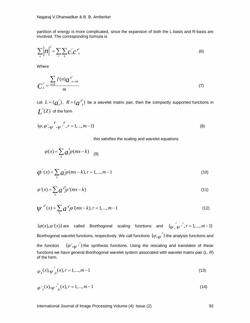
partition of energy is more complicated, since the expansion of both the L-basis and R-basis are involved. The corresponding formula is
2
'r r
k kn r k
n c c (6)
Where
'( ) 'r
n mkr n Zk
f n
m
aC
(7)
Let ( )r
kL a , ( )'r
kR a be a wavelet matrix pair, then the compactly supported functions in 2( )ZL of the form
{ , ', , , 1,..., 1}'r r
r m (8)
this satisfies the scaling and wavelet equations
(9)
( ) ( ), 1,..., 1r r
kk
x mx k r ma (10)
0'( ) '( )'kk
x mx ka (11)
( ) '( ), 1,..., 1' 'r r
kk
x mx k r ma (12)
{ ( ), '( )}x x are called Biorthogonal scaling functions and { , 1,..., 1}, 'r r
r m
Biorthogonal wavelet functions, respectively. We call functions { , }r
the analysis functions and
the function { ', }'r
the synthesis functions. Using the rescaling and translates of these
functions we have general Biorthogonal wavelet system associated with wavelet matrix pair (L, R) of the form.
( ), ( ), 1,..., 1r
k jkx x r m (13)
( ), ( ), 1,..., 1' 'r
k jkx x r m (14)
0( ) ( )kk
x mx ka

Nagaraj V.Dharwadkar & B. B. Amberker
International Journal of Image Processing Volume (4): Issue (2) 93
3. PROPOSED MODEL
In this section, we give a description about the proposed models used to embed and extract the watermark for gray-level image. The image is decomposed using Biorthogonal wavelet filters. Biorthogonal Wavelet coefficients are used in order to make the technique robust against several attacks, and preserve imperceptibility. The embedding algorithm and extraction algorithm for gray level images is explained in the following sections.
3.1 Watermark Embedding Algorithm
The embedding algorithm uses monochrome image as watermark and gray-level image as cover image. The first level Biorthogonal wavelet is applied on the cover image, then for second level decomposition we consider HL (Horizontal subband), LH (vertical subband), and HH (diagonal subband) separately. From these second level subbands we take LH, HL and HH respective subbands to embed the watermark. Figure 1 shows the flow of embedding algorithm.
.
FIGURE 1: Embedding Algorithm for LH subband coefficients. Algorithm : Watermark embedded by decomposing LH1 into second level. Input : Cover image (gray-level) of size m m , Watermark (monochrome) image of size
/ 4 / 4m m . Output : Watermarked gray level image.
1. Apply First level Biorthogonal Wavelet on input gray level cover image to get {LH1, HL1, HH1 and LL1} subbands as shown in Figure 2.
2. From decomposed image of step 1 take the vertical subcomponent LH1 where the size of LH1 is / 2 / 2m m for LH1 again apply first level Biorthogonal wavelet and get vertical subcomponent LH2 (as shown in Figure 3.), Where the size of LH2 is / 4 / 4m m and in LH2 subband we found frequency coefficients values are zero or less than zero.
3. Embed the watermark into the frequency coefficient of LH2 by scanning frequency coefficients row by row, using following formula ' (| | ) ( , )Y Y W i j , Where =
LH2
LH1
First Level DWT
watermark image
Embedding
Second Level DWT
Apply Twice Inverse DWT
watermarked image
Cover Image
Watermarked Image

Nagaraj V.Dharwadkar & B. B. Amberker
International Journal of Image Processing Volume (4): Issue (2) 94
0.009, Y is original frequency coefficient of LH2 subband, if watermark bit is zero then Y ' = 0 else Y’ > 1.
4. Apply inverse Biorthogonal Wavelet transformation two times to obtain watermarked gray level image.
5. Similarly the watermark is embedded separately into the HL (Horizontal) and HH (diagonal) subband frequency coefficients.
FIGURE 2: First Level Decomposition
FIGURE 3: Second Level Decomposition of LH1
3.2 Watermark Extraction Algorithm In extraction algorithm the first level Biorthogonal wavelet is applied on the watermarked gray-scale image. For second level decomposition we consider LH1 (Vertical subband) and from this second level decomposed image we take LH2 subband to extract the watermark. The extraction algorithm is as shown in Figure 4.
FIGURE 4: Extracting watermark from LH1 subband
LL1
HL1
HH1
LH1
LL1
HL1
HH1
LL2
LH2 HH2
HH2
LH2
LH1
First Level DWT
watermark image
Extraction
Second Level DWT
Cover Image

Nagaraj V.Dharwadkar & B. B. Amberker
International Journal of Image Processing Volume (4): Issue (2) 95
Algorithm : Watermark Extracted by decomposing LH1 into second level. Input : Watermarked Cover image (gray-level) of size m m . Output : Watermark.
1. Apply First level Biorthogonal Wavelet on watermarked gray level cover image to get {LH1, HL1, HH1 and LL1} subbands.
2. From decomposed image of step 1 take the vertical subcomponent LH1 where the size of LH1 is / 2 / 2m m for LH1 again apply first level Biorthogonal wavelet and get vertical subcomponent LH2 (as shown in Figure 3.), Where the size of LH2 is / 4 / 4m m .
3. From the subband LH2 extract the watermark by scanning frequency coefficients row by row. If frequency coefficient is greater than zero set watermark bit as 1 else set 0.
4. Similarly the watermark is extracted from the HL (Horizontal) and HH (diagonal) subband frequency coefficients.
4. RESULTS AND DISCUSSION The performance of embedding and extraction algorithm are analyzed by considering Lena image of size 256 256 as cover image and M-logo (Monochrome) image of size 30 35 as a watermark. The following parameters are used to measure the performance of embedding and extraction algorithms.
1. Standard Correlation ( SC) : It measures how the pixel values of original image is correlated with the pixel values of modified image. When there is no distortion in modified image, then SC will be 1.
Here, I(i, j) is original watermark, J(i, j) is extracted watermark, I' is the mean of original watermark and J’ is mean of extracted watermark.
2. Normalized Correlation (NC) : It measure the similarity representation between the original image and modified image.
Where I (i, j) is original image and I’(i, j) is modified image, M is Height of image and N is width of image
3. Mean Square Error (MSE): It measures the average of the square of the "error." The error is the amount by which the pixel value of original image differs to the pixel value of modified image.
[ ( ( , ) ' ) ( ( , ) ') ]1 1
2 2[ ( ( , ) ') ] [ ( ( , ) ' ) ]
1 1 1 1
M NI i j I J i j J
i jS CM N M NI i j I J i j Ji j i j
2
( , ) '( , )1 1
( , )1 1
M NI i j I i j
i j
M NI i j
i j
N C
2[ ( , ) '( , )]
1 1
M Nf i j f i j
i jMSEMN

Nagaraj V.Dharwadkar & B. B. Amberker
International Journal of Image Processing Volume (4): Issue (2) 96
Where, M and N are the height and width of image respectively. f(i, j) is the (i, j)th pixel value of the original image and f ′( i, j) is the (i, j)th pixel value of modified image.
4. Peak signal to noise ratio (PSNR): It is the ratio between the maximum possible
power of a signal and the power of corrupting noise that affects the fidelity of its representation. PSNR is usually expressed in terms of the logarithmic decibel. PSNR is given by.
4.1 Measuring Perceptual quality of watermarked image In this section we discuss the effect of embedding algorithm on cover image in terms of perceptual similarity between the original image and watermarked image using Mean, Standard Deviation, RMS and Entropy. The effect of extraction algorithm is calculated using MSE, PSNR, NC and SC between extracted and original watermark. As shown in Figure 5, watermark is embedded by decomposing LH1, HL1, HH1 separately further in second level and the quality of original gray scale image and watermarked image are compared. The parameters such as Mean, Standard Deviation, RMS and Entropy are calculated between the original gray level image and watermarked image. The results shows that there is only slight variation exist in above mentioned parameters. This indicates that the embedding algorithm will modify the content of original image by negligible amount. The amount of noise added to gray-level cover image is calculated by using MSE and PSNR. Thus the results from the experiments indicates that the embedding watermark into HH (diagonal) subband produces the better results in terms of MSE and high PSNR compared to other subbands.
FIGURE 5: Effect of Embedding algorithm in LH, HL and HH subband of cover image
LH SUBBAND HL SUBBAND HH SUBBAND Paramete
r Original image
Watermarked image
Original image
Watermarked image Original image Watermarked
image
Mean 97.18
97.18
97.18 97.18 97.18 97.18
RMS 110.51
110.52
110.51 110.52 110.51 110.51
Standard deviation
52 . 62
52 . 63
52 . 61 52.63 52.61 52.62
Entropy 7.57
7.58
7.57 7.58 7.57
7.58
MSE 1.39
1.11 0.72
PSNR 46.68 47.68 49.54
2( 1)210log
nPSNR
MSE
lena256.bmp

Nagaraj V.Dharwadkar & B. B. Amberker
International Journal of Image Processing Volume (4): Issue (2) 97
Parameter LH SUBBAND HL SUBBAND HH SUBBAND MSE 0.11 0.11 0.11 PSNR 57.41 57.44 57.48
Normalized correlation 1 1 1 Standard correlation 0.69 0.65 0.65
Original watermark
Extracted watermark
FIGURE 6: Effect of Extraction algorithm from LH, HL and HH subband coefficients on Watermark
Figure 6 shows the results of Watermark extraction by decomposing LH1, HL1, HH1 separately further in second level and the quality of Extracted watermark and original watermark are compared. The parameters such as MSE, PSNR, NC and SC are calculated between the extracted and original watermark. The results show that the extraction algorithm produces similar results for all subbands in terms above mentioned parameters.
4.2 Effect of Attacks In this section we discuss about the performance of extraction algorithm by considering different types of image processing attacks on watermarked gray-level image such as blurring, adding salt and pepper noise, sharpening, Gaussian filtering and cropping.
1. Effect of Blurring: Special type of circular averaging filter is applied on the watermarked gray-level image to analyze the effect of Blurring. The circular averaging (pillbox) filter filters the watermarked image within the square matrix of side 2 (Disk_ Radius) +1. The disk radius is varied from 0.5 to 1.4 and the effect of blurring is analyzed on extraction algorithm. Figure 7 shows the extracted watermark for different disk radius of LH, HL and HH subbands. Figure 8 shows the effect of blurring on watermarked image in terms of MSE, NC, SC and PSNR between original and extracted watermark. From the experimental results it was found that the extraction of watermark from HH subband produces NC is equal 1 for disk radius up to 1.4. The extracted watermark is highly correlated with original watermark, when the watermark is embedded into HH subbands. Figure 8 shows the effect of Blurring in terms of, NC and SC between original and extracted watermark and MSE, PSNR between original and watermarked image.
DISK RADIUS
Extracted Watermark from LH Subband
Extracted Watermark from HL Subband
Extracted Watermark from HH Subband
0.5
0.6
0.7
0.8
0.9
1.0

Nagaraj V.Dharwadkar & B. B. Amberker
International Journal of Image Processing Volume (4): Issue (2) 98
1.1
1.2
1.3
1.4
FIGURE 7: Extracted watermark from Blurred watermarked Gray-level images using LH, HL
and HH subbands (a) MSE between Original and Extracted Watermark (b) NC between Original and Extracted Watermark
(c) SC between Original and Extracted Watermark (d ) PSNR between Original and Extracted Watermark
FIGURE 8: Effect of Blurring on watermarked Grayscale image
2. Effect of adding salt and pepper noise: The salt and pepper noise is added to the watermarked image I, where d is the noise density. This affects approximately d (size(I)) pixels. Figure 9 shows the extracted watermarks from LH, HL and HH subbands for noise density varied from 0.001 to 0.007. Figure. 10 show the effect of salt and pepper noise on extraction algorithm. From the experimental results, it was found that extraction of watermark from HH subband is producing NC equal to 0.95. Thus embedding watermark into HH subbands is robust against adding salt and pepper noise.
Density
Extracted Watermark from LH Subband
Extracted Watermark from HL Subband
Extracted Watermark from HH Subband
0.001
0.002
0.000.020.040.060.080.100.120.140.160.180.20
0.5 0.6 0.7 0.8 0.9 1 1.1 1.2 1.3 1.4
Disk radius
MSE
LHHLHH
0.94
0.95
0.96
0.97
0.98
0.99
1
1.01
0.5 0.6 0.7 0.8 0.9 1 1.1 1.2 1.3 1.4
Disk Radius
Nor
mal
ized
Cor
rela
tion
LHHLHH
0
0.1
0.2
0.3
0.4
0.5
0.6
0.7
0.5 0.6 0.7 0.8 0.9 1 1.1 1.2 1.3 1.4
Disk Radius
Sta
ndar
d C
orre
latio
n
LHHLHH
54.5
55
55.5
56
56.5
57
57.5
58
0.5 0.6 0.7 0.8 0.9 1 1.1 1.2 1.3 1.4
Disk Radius
PSN
R LHHLHH

Nagaraj V.Dharwadkar & B. B. Amberker
International Journal of Image Processing Volume (4): Issue (2) 99
0.003
0.004
0.005
0.006
0.007
FIGURE 9: Extracted watermark from Salt and Pepper Noise added to watermarked images using LH, HL and HH subbands
(a) MSE between Original and Extracted Watermark (b) NC between Original and Extracted Watermark
(c) SC between Original and Extracted Watermark (d) PSNR between Original and Extracted Watermark
FIGURE 10: Effect of Salt and Pepper Noise on watermarked Grayscale image
3. Effect of Sharpening on Watermarked Image: A special type of 2D unsharp contrast enhancement filter is applied on watermarked image. The unsharp contrast enhancement filter enhances edges and other high frequency components in an image. By subtracting a smoothed ("unsharp") version of an image from the original image. Figure 11 shows the extracted watermark, when watermarked image is sharpened by varying sharpness parameter from 0.1 to 1. The effect of sharpening on extraction algorithm is measured by calculating MSE, PSNR, NC and SC between extracted and original watermark. From the Figure 12, we found that extraction of watermark from HH subband is producing NC equal to 0.99. Thus compared to other subbands, embedding watermark into HH subbands is robust against sharpening of watermarked image.
0
0.05
0.1
0.15
0.2
0.25
0.001 0.002 0.003 0.004 0.005 0.006 0.007
Density
MSE
LH
HLHH
0.75
0.80
0.85
0.90
0.95
1.00
1.05
0.001 0.002 0.003 0.004 0.005 0.006 0.007
Density
Nor
mal
ized
Cor
rela
tion
LH
HL
HH
0.00
0.10
0.20
0.30
0.40
0.50
0.60
0.70
0.001 0.002 0.003 0.004 0.005 0.006 0.007
Density
Sta
ndar
d C
orre
latio
n
LHHLHH
5353.5
54
54.5
55
55.5
56
56.5
57
57.5
0.001 0.002 0.003 0.004 0.005 0.006 0.007
Density
PSN
R LHHLHH

Nagaraj V.Dharwadkar & B. B. Amberker
International Journal of Image Processing Volume (4): Issue (2) 100
Sharpness
Extracted Watermark from LH Subband
Extracted Watermark from HL Subband
Extracted Watermark from HH Subband
0.1
0.2
0.3
0.4
0.5
0.6
0.7
0.8
0.9
1
FIGURE 11: Extracted watermark from sharpened watermarked images using LH, HL and HH subbands
(a) MSE between Original and Extracted Watermark (b) NC between Original and Extracted Watermark (c) SC between Original and Extracted Watermark (d) PSNR between Original and Extracted Watermark
FIGURE 12: Effect of Sharpening on watermarked Gray level image
0
0.02
0.04
0.06
0.08
0.1
0.12
0.14
0.1 0.2 0.3 0.4 0.5 0.6 0.7 0.8 0.9 1
Sharpness
MSE
LH
HL
HH
0.94
0.95
0.96
0.97
0.98
0.99
1.00
0.1 0.2 0.3 0.4 0.5 0.6 0.7 0.8 0.9 1
Sharpness
Nor
mal
ized
Cor
rela
tion
LH
HLHH
0.000.100.200.300.400.500.600.700.800.90
0.1 0.2 0.3 0.4 0.5 0.6 0.7 0.8 0.9 1
Sharpness
Stan
dard
Coe
ffici
ent
LH
HL
HH
55.5
56
56.5
57
57.5
58
58.5
59
59.5
0.1 0.2 0.3 0.4 0.5 0.6 0.7 0.8 0.9 1
Sharpness
PSNR
LH
HL
HH

Nagaraj V.Dharwadkar & B. B. Amberker
International Journal of Image Processing Volume (4): Issue (2) 101
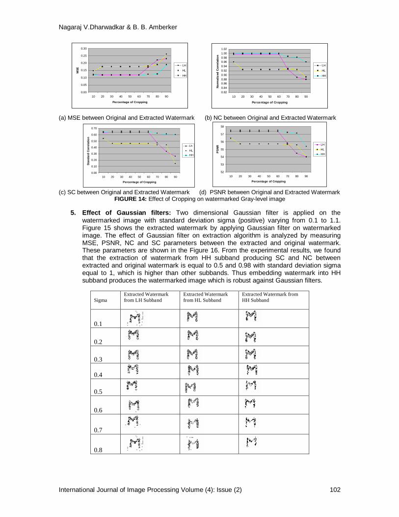
4. Effect of Cropping on Watermarked Image: The cropping is applied on watermarked image. The watermarked image is cropped in terms of percentage of the image size. The cropping is started at 10 percentages and continued in the intervals of 10 percentage up to 90 percentage. Figure 13 shows the cropped watermarked images and the extracted watermark from LH, HL and HH subbands. The effect of cropping on extraction algorithm is analyzed by comparing extracted watermark and original watermark for LH,HL and HH subbands. The quality of extracted watermark is measured using MSE, PSNR, NC and SC metrics. Figure 14 shows the effect of cropping on extracted watermark in terms of MSE, PSNR, NC and SC. From the experimental results we found extracting watermark from HH produces the NC equal to 0.96 and SC equal to 0.60 for 90 percentage of cropping, where as other subbands produces less correlated watermark at 90 percentage of cropping. Thus results prove that the embedding watermark at HH subband is produces highly rigid watermarked image.
Percentage of cropping
Cropped image and Extracted Watermark from LH Subband
Cropped image and Extracted Watermark from HL Subband
Cropped image and Extracted Watermark from HH Subband
10
out filename.bmp
out filename.bmp
outfilename.bmp
20
out filename.bmp
out filename.bmp
outfilename.bmp
30
out filename.bmp
out filename.bmp
outfilename.bmp
40
out filename.bmp
outfilename.bmp
outfilename.bmp
50
outfilename.bmp
outfilename.bmp
outfilename.bmp
60
out filename.bmp
out filename.bmp
outfilename.bmp
70
out filename.bmp
outfilename.bmp
outfilename.bmp
80
outfilename.bmp
outfilename.bmp
outfilename.bmp
90
outfi lename.bmp
out filename.bmp
out filename.bmp
FIGURE 13: Extracted watermark from Cropped watermarked images using LH, HL and HH subbands
Nagaraj V.Dharwadkar & B. B. Amberker
International Journal of Image Processing Volume (4): Issue (2) 102
(a) MSE between Original and Extracted Watermark (b) NC between Original and Extracted Watermark
(c) SC between Original and Extracted Watermark (d) PSNR between Original and Extracted Watermark FIGURE 14: Effect of Cropping on watermarked Gray-level image
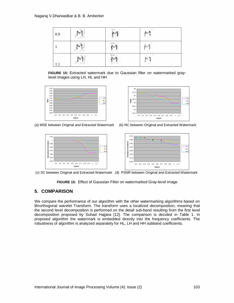
5. Effect of Gaussian filters: Two dimensional Gaussian filter is applied on the
watermarked image with standard deviation sigma (positive) varying from 0.1 to 1.1. Figure 15 shows the extracted watermark by applying Gaussian filter on watermarked image. The effect of Gaussian filter on extraction algorithm is analyzed by measuring MSE, PSNR, NC and SC parameters between the extracted and original watermark. These parameters are shown in the Figure 16. From the experimental results, we found that the extraction of watermark from HH subband producing SC and NC between extracted and original watermark is equal to 0.5 and 0.98 with standard deviation sigma equal to 1, which is higher than other subbands. Thus embedding watermark into HH subband produces the watermarked image which is robust against Gaussian filters.
Sigma
Extracted Watermark from LH Subband
Extracted Watermark from HL Subband
Extracted Watermark from HH Subband
0.1
0.2
0.3
0.4
0.5
0.6
0.7
0.8
0.00
0.05
0.10
0.15
0.20
0.25
0.30
10 20 30 40 50 60 70 80 90
Percentage of Cropping
MSE
LH
HL
HH
0.820.840.860.880.900.920.940.960.981.001.02
10 20 30 40 50 60 70 80 90
Percentage of Cropping
Nor
mal
ized
Cor
rela
tion
LH
HL
HH
0.00
0.10
0.20
0.30
0.40
0.50
0.60
0.70
10 20 30 40 50 60 70 80 90
Percentage of Cropping
Stan
dard
Cor
rela
tion
LhHLHH
52
53
54
55
56
57
58
10 20 30 40 50 60 70 80 90
Percentage of Cropping
PS
NR LH
HLHH
Nagaraj V.Dharwadkar & B. B. Amberker
International Journal of Image Processing Volume (4): Issue (2) 103
0.9
1
1.1
FIGURE 15: Extracted watermark due to Gaussian filter on watermarked gray-level images using LH, HL and HH
(a) MSE between Original and Extracted Watermark (b) NC between Original and Extracted Watermark
(c) SC between Original and Extracted Watermark (d) PSNR between Original and Extracted Watermark
FIGURE 15: Effect of Gaussian Filter on watermarked Gray-level image
5. COMPARISON
We compare the performance of our algorithm with the other watermarking algorithms based on Birorthogonal wavelet Transform. The transform uses a localized decomposition, meaning that the second level decomposition is performed on the detail sub-band resulting from the first level decomposition proposed by Suhad Hajjara [12]. The comparison is decided in Table 1. In proposed algorithm the watermark is embedded directly into the frequency coefficients. The robustness of algorithm is analyzed separately for HL, LH and HH subband coefficients.
0.000.020.040.060.080.100.120.140.160.180.20
0.1 0.2 0.3 0.4 0.5 0.6 0.7 0.8 0.9 1 1.1
Sigma
MS
E
LHHLHH
54.5
55
55.5
56
56.5
57
57.5
58
0.1 0.2 0.3 0.4 0.5 0.6 0.7 0.8 0.9 1 1.1
Sigma
PSN
R LHHLHH
0.94
0.95
0.96
0.97
0.98
0.99
1
1.01
0.1 0.2 0.3 0.4 0.5 0.6 0.7 0.8 0.9 1 1.1
Sigma
Nor
mal
ized
Cor
rela
tion
LHHLHH
0.00
0.10
0.20
0.30
0.40
0.50
0.60
0.70
0.1 0.2 0.3 0.4 0.5 0.6 0.7 0.8 0.9 1 1.1
Sigma
Stan
dard
Cor
rela
tion
LHHLHH

Nagaraj V.Dharwadkar & B. B. Amberker
International Journal of Image Processing Volume (4): Issue (2) 104
TABLE 1: Comparison of proposed algorithm with Suhad Hajjara proposed algorithm [12].
6. CONSLUSION In this paper we proposed a novel scheme of embedding watermark into gray-level image. The scheme is based on decomposing an image using the Discrete Wavelet Transform using Biorthogonal wavelet filters and the watermark bits are embedded into significant coefficients of the transform. We use a localized decomposition, meaning that the second level decomposition is performed on the detail sub-band resulting from the first level decomposition. For gray-scale image for embedding and extraction we defined separate modules for LH, HL and HH subbands, then the performance of these modules are analyzed by considering normal watermarked image and signal processed (attacked) images. In all these analysis we found that HH (diagonal) subband embedding and extraction produces the good results in terms of attacked and normal images.
Properties Suhad Hajjara [12]
Proposed Algorithm
Cover Data Gray level Gray-level
Watermark
Binary Image mapped to
Pseudo random Number( PRN)
Monochrome image (logo)
Domain of embedding Frequency Domain
Frequency Domain
Types of Filters DWT based Biorthogonal
DWT based Biorthogonal
Frequency bands considered for
embedding
Diagonal (HH),Vertical
(LH) and Horizontal (HL)
Diagonal (HH),Vertical (LH) and Horizontal (HL)
Embedding PRN is added to
frequency coefficients
Frequency coefficients are multiplied by
watermark bit
Effect of Attacks Analyzed
compression, Gaussian noise, median filtering, salt and pepper noise
Blurring, Adding salt and pepper noise, Sharpening, Gaussian filter and cropping.

Nagaraj V.Dharwadkar & B. B. Amberker
International Journal of Image Processing Volume (4): Issue (2) 105
7. REFERENCES 1. Ingemar J. Cox and Matt L. Miller, “The First 50 Years of Electronic Watermarking”,
EURASIP Journal on Applied Signal Processing Vol. 2, pp. 126–132, 2002. 2. G. Voyatzis, I. Pitas, “ Protecting digital image copyrights: A framework”, IEEE Computer
Graphics Application, Vol. 19, pp. 18-23, Jan. 1999. 3. Katzenbeisser S. and Petitcolas F. A. P., “Information Hiding Techniques for Steganography
and Digital Watermarking”, Artech House, UK, 2000. 4. Peter H. W. Wong, Oscar C. Au, Y. M. Yeung, “A Novel Blind Multiple Watermarking
Technique for Images”, IEEE Transactions on Circuits and Systems for Video Technology, Vol. 13, No. 8, August 2003.
5. Celik, M.U., et al., “Lossless generalized-LSB data embedding”, IEEE Transactions on Image Processing,, 14(2), pp.253-26, .2005.
6. Cvejic, N. and T. Seppanen, “Increasing robustness of LSB audio steganography by reduced distortion LSB coding”. Journal of Universal Computer Science, 11(1), pp. 56-65, 2005.
7. Ingemar J. Cox, Matthew L Miller, Jeffrey A. Bloom, Jassica Fridrich, Tan Kalker, “ Digital Watermarking and Steganography”, Second edition, M.K. Publishers, 2008.
8. Wu, X., J., Hu, Z.Gu, and J., Huang, 2005. “A Secure Semi-Fragile Watermarking for Image Authentication Based on Integer Wavelet Transform with Parameters”, Technical Report. School of Information Science and Technology, Sun Yat-Sen University, China, 2005
9. Kundur, D., and D., Hatzinakos, 1998. “Digital watermarking using multiresolution wavelet decomposition”, Technical Report., Dept. of Electrical and Computer Engineering, University of Toronto
10. Burrus, C. S., R. A., Gopinath, and H., Guo,. “Introduction to Wavelets and Wavelet Transforms: A Primer”, Prentice-Hall, Inc. 1998.
11. Daubechies, I., 1994. “Ten lectures on wavelets”, CBMS, SIAM, pp 271-280. 12. Suhad Hajjara, Moussa Abdallah, Amjad Hudaib, “Digital Image Watermarking Using
Localized Biorthogonal Wavelets”, European Journal of Scientific Research, ISSN 1450-216X Vol.26 No.4 (2009), pp.594-608 © EuroJournals Publishing, Inc. 2009.

Chirag N. Paunwala & Suprava Patnaik
International Journal of Image Processing (IJIP) Volume (4): Issue (2) 106
A Novel Multiple License Plate Extraction Technique for Complex Background in Indian Traffic Conditions
Chirag N. Paunwala [email protected] Dept. of Electronics and Communication Sarvajanik College of Engineering and Technology Surat, 395001, India Suprava Patnaik [email protected] Dept. of Electronics S.V. National Institute of Technology Surat, 395007, India
Abstract
License plate recognition (LPR) is one of the most important applications of applying computer techniques towards intelligent transportation systems (ITS). In order to recognize a license plate efficiently, location and extraction of the license plate is the key step. Hence finding the position of a license plate in a vehicle image is considered to be the most crucial step of an LPR system, and this in turn greatly affects the recognition rate and overall speed of the whole system. This paper mainly deals with the detecting license plate location issues in Indian traffic conditions. The vehicles in India sometimes bare extra textual regions, such as owner’s name, symbols, popular sayings and advertisement boards in addition to license plate. Situation insists for accurate discrimination of text class and fine aspect ratio analysis. In addition to this additional care taken up in this paper is to extract license plate of motorcycle (size of plate is small and double row plate), car (single as well as double row type), transport system such as bus, truck, (dirty plates) as well as multiple license plates present in an image frame under consideration. Disparity of aspect ratios is a typical feature of Indian traffic. Proposed method aims at identifying region of interest by performing a sequence of directional segmentation and morphological processing. Always the first step is of contrast enhancement, which is accomplished by using sigmoid function. In the subsequent steps, connected component analysis followed by different filtering techniques like aspect ratio analysis and plate compatible filter technique is used to find exact license plate. The proposed method is tested on large database consisting of 750 images taken in different conditions. The algorithm could detect the license plate in 742 images with success rate of 99.2%. Keywords: License plate recognition, sigmoid function, Horizontal projection, Mathematical morphology, Aspect ratio analysis, Plate compatible filter.

Chirag N. Paunwala & Suprava Patnaik
International Journal of Image Processing (IJIP) Volume (4): Issue (2) 107
1. INTRODUCTION License plate recognition (LPR) applies image processing and character recognition technology to identify vehicles by automatically reading their license plates. Automated license plate reading is a particularly useful and practical approach because, apart from the existing and legally required license plate, it assumes no additional means of vehicle identity. Although human observation seems the easiest way to read vehicle license plate, the reading error due to tiredness is main drawback for manual systems. This is the main motivation for research in area of automatic license plate recognition. Since there are problems such as poor image quality, image perspective distortion, other disturbance characters or reflection on vehicle surface, and the color similarity between the license plate and background vehicle body, the license plate is often difficult to be located accurately and efficiently. Security control of restricted areas, traffic law enforcements, surveillance systems, toll collection and parking management systems are some applications for a license plate recognition system. Main goal of this research paper is to implement a method efficient in recognizing license plates in Indian conditions because in Indian scenario vehicles carry extra information such as owner’s name, symbols, design along with different standardization of license plate. Our work is not restricted to car but is expanded to many types of vehicles like motor cycle (in which size of license plate is small), transport vehicles which carry extra text and soiled license plate. Our proposed algorithm is robust to detect vehicle license plate in both day and night conditions as well as multiple license plates contained in an image or frame without finding candidate region. The flow of paper is as follows: section 2 discusses about the previous works in the field of LPR. Section 3 is about the implementation of algorithm. Section 4 talks about the experimentation results of the proposed algorithm. Section 5 and 6 are about conclusion and references.
2. PREVIOUS WORK Techniques based upon combinations of edge statistics and mathematical morphology [1]–[4] featured very good results. A disadvantage is that edge based methods alone can hardly be applied to complex images, since they are too sensitive to unwanted edges, which may also show a high edge magnitude or variance (e.g., the radiator region in the front view of the vehicle). When combined with morphological steps that eliminate unwanted edges in the processed images, the LP extraction rate becomes relatively high and fast. In [1], the conceptual model underneath the algorithm is based on the morphological operation called “top-hat transformation”, which is able to locate small objects of significantly different brightness [5]. This algorithm, however, with a detection rate of 80%, is highly dependent on the distance between the camera and the vehicle, as the morphological operations relate to the dimensions of the binary objects. The similar approach was described in [2] with some modifications and achieved an accuracy around 93%. In [3], candidate region was extracted with the combination of edge statistics and top hat transformations and final extraction was achieved using wavelet analysis, with the success rate of 98.61%. In [4], a hybrid license plate detection algorithm from complex background based on histogramming and mathematical morphology was undergone which consists of vertical gradient analysis and its horizontal projection for finding out candidate region; horizontal gradient, its vertical projection and morphological deal of candidate region is used to extract exact license plate (LP) location. In [6], a hybrid algorithm based on edge statistics and morphology is proposed which uses vertical edge detection, edge statistical analysis, hierarchical-based LP location, and morphology for extracting the license plate. This prior knowledge based algorithm achieves very good detection rate for image acquired from a fixed distance and angle, and therefore, candidate regions in a specific position are given priority, which certainly boost the results to a high level of accuracy. But it will not work on frames with plates of different size and license plate more in number. In [7][8], technique was used that scans and labels pixels into components based on pixel connectivity. Then after with the help of some measurement features used to detect the region of interest. In [9] the vehicle image was scanned with pre-defined row distance. If the number of the edges is greater than a threshold value, the presence of a plate can be assumed.

Chirag N. Paunwala & Suprava Patnaik
International Journal of Image Processing (IJIP) Volume (4): Issue (2) 108
In [10], a block based recognition system is proposed to extract and recognize license plates of motorcycles and vehicles on highways only. In the first stage, a block-difference method was used to detect moving objects. According to the variance and the similarity of the MxN blocks defined on two diagonal lines, the blocks are categorized into three classes: low-contrast, stationary and moving blocks. In the second stage, a screening method based on the projection of edge magnitudes is used to find two peaks in the projection histograms to find license plates. But main shortcoming of this method is detection of false region or unwanted non text region because of projection of edges. In [11], a method using the statistics like mean and variance for two sliding concentric windows (SCW) was used as shown in Figure (1). This method encounters a problem when the borders of the license plate do not exhibit much variation from the surrounding pixels, same as edge based methods. Also, edge detection uses a threshold that needs to be determined which cannot be uniquely obtained under various conditions like illuminations. Same authors report a success rate of 96.5% for plate localization with proper parameterization of the method in conjunction with CCA measurements and the Sauvola binarization method [12].
(a) (b)
FIGURE 1: (a) SCW Method, (b) Resulting Image after SCW Execution [11]. In Hough transform (HT) based method for license plate extraction, edges in the input image are detected first. Then, HT is applied to detect the LP regions. In [13], a combination of Hough transform and contour algorithm was applied on the edge image. Then the lines that cross the plate frame were determined and a rectangular-shaped object that matched the license plate was extracted. In [14] scan and check algorithm was used followed by radon transform for skew correction. In [15] proposed method applies HL subband feature of 2D Discrete Wavelet Transform (DWT) twice to significantly highlight the vertical edges of license plates and suppress the surrounding background noise. Then, several promising candidates of license plates can easily be extracted by first-order local recursive Otsu segmentation [16] and orthogonal projection histogram analysis. Finally, the most probable candidate was selected by edge density verification and aspect ratio constraint. In [17,18], color of the plate was used as a feature, the image was fed to a color filter, and the output was tested in terms of whether the candidate area had the plate’s shape or not. In [19, 20] the technique based on mean-shift estimate of the gradient of a density function and the associated iterative procedure of mode seeking was presented and based on the same, authors of [21] applied a mean-shift procedure for color segmentation of the vehicle images to directly obtain candidate regions that may include LP regions. In [22], concept of enhancing the low resolution image was used for better extraction of characters. None of the above discussed algorithms focused on multiple plate extraction with different possible aspect ratio.
3. PROPOSED MULTIPLE LICENSE PLATE EXTRACTION METHOD Figure (2) shows the flow chart of the proposed algorithm, which shows the step by step
implementation of proposed multiple license plate extraction method in Indian traffic conditions.

Chirag N. Paunwala & Suprava Patnaik
International Journal of Image Processing (IJIP) Volume (4): Issue (2) 109
No
Yes
FIGURE 2: Flow Chart of Proposed Method
Input Image
Determination of Variance of the Input Image
Is Variance >Threshold
Edge Detection and Morphological deal for Noise Removal and Region Extraction
Contrast Enhancement using Sigmoid Function
Horizontal Projection and Gaussian Analysis
Selecting the Rows with Higher Value of Horizontal Projection
Morphological analysis for LP feature extraction
Connected Component Analysis
Rectangularity and Aspect Ratio Analysis
Plate Companionable Filtering
Final License Plate Output

Chirag N. Paunwala & Suprava Patnaik
International Journal of Image Processing (IJIP) Volume (4): Issue (2) 110
3.1 Preprocessing
This work aims on gray intensity based license plate extraction and hence begins with color to gay conversion using (1).
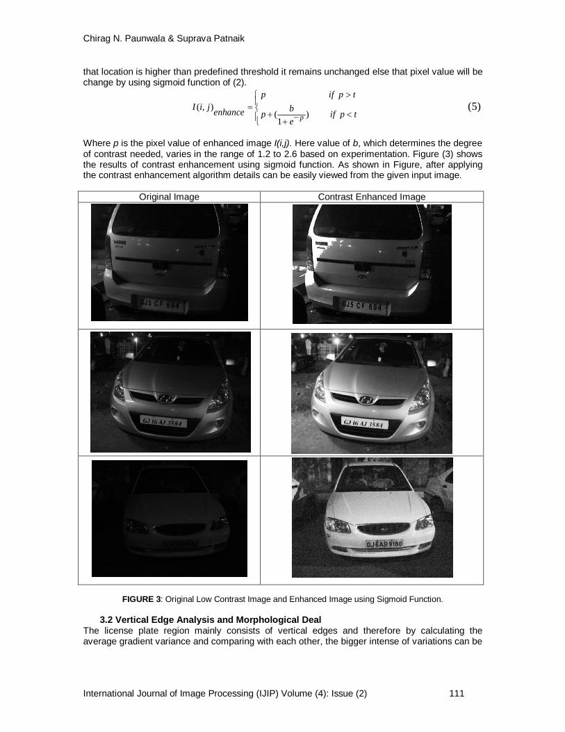
( , ) 0.114* ( , ,1) 0.587* ( , , 2) 0.299* ( , ,3)I i j A i j A i j A i j (1) where, I(i,j) is the array of gray image, A(i,j,1), A(i,j,2), A(i,j,3) are the R,G,B value of original image respectively. For accurate location of the license plate the vehicle must be perfectly visible irrespective of whether the image is captured during day or night or non homogenous illumination. Sometimes the image may be too dark, contain blur, thereby making the task of extracting the license plate difficult. In order to recognize the license plate even in night condition, contrast enhancement is important before further processing. One of the important statistical parameter which provides information about the visual properties of the image is variance. Based on this parameter, condition for contrast enhancement is employed. First of all variance of the image is computed. With an aim to reduce computationally complexity the proposed implementation begins with the thresholding of variance as a selection criterion for frames aspiring contrast enhancement. If the value is greater than the threshold then it implies that the corresponding image possesses good contrast. While if the variance is below threshold, then the image is considered to have low contrast and therefore contrast enhancement is applied to it. This method of contrast enhancement based on variance helps the system to automatically recognize whether the image is taken in daylight or in night condition. In this work, first step towards contrast enhancement is to apply unsharp masking on original image and then applying the sigmoid function for contrast enhancement. Sigmoid function which is also known as logistic function is a continuous nonlinear activation function. The name, sigmoid, obtained from the fact that the function is "S" shaped. The sigmoid has the property of being similar to the step function, but with the addition of a region of uncertainty [23]. It is a range mapping approach with soft thresholding. Using f(x) for input, and with α as a gain term, the sigmoid function is given by:
1( )1
f x xe (2)
For faultless license plate extraction, identification of edges is very important as license plate region consists of edges of definite size and shape. In blurry images identification of edges are indecent, so for the same sharpening of edges are must. By using the unsharp masking, sharpening of areas which have edges or lots of details can be easily highlighted. This can be done by generating the blurred copy of the original image by using laplacian filter and then subtracting it from the original image as shown in (3). ( , ) ( , ) ( , )I i j I i j I i jsharpe original blur (3)
The resultant image, obtained from (3) is then multiplied with some constant c and then added it to the original image as shown in (4). This step highlights or enhances the finer details but at the same time larger details will remain undamaged. The value of c chosen is 0.7 from experimentaiton. ( , ) ( , ) * ( , )I i j I i j c I i joutput orignal sharpe (4)
In the next step, smoothing average window size of MxM is apply on the output image obtain from (4). Since we are going for edge detection, value of M is equal to 3. After that finding out the mean at each location, it is compared with some pre defined threshold t. If the value of pixel at
Chirag N. Paunwala & Suprava Patnaik
International Journal of Image Processing (IJIP) Volume (4): Issue (2) 111
that location is higher than predefined threshold it remains unchanged else that pixel value will be change by using sigmoid function of (2).
( , )( ) 1 p
p if p tI i j benhance p if p t
e
(5)
Where p is the pixel value of enhanced image I(i,j). Here value of b, which determines the degree of contrast needed, varies in the range of 1.2 to 2.6 based on experimentation. Figure (3) shows the results of contrast enhancement using sigmoid function. As shown in Figure, after applying the contrast enhancement algorithm details can be easily viewed from the given input image.
Original Image Contrast Enhanced Image
FIGURE 3: Original Low Contrast Image and Enhanced Image using Sigmoid Function.
3.2 Vertical Edge Analysis and Morphological Deal The license plate region mainly consists of vertical edges and therefore by calculating the average gradient variance and comparing with each other, the bigger intense of variations can be

Chirag N. Paunwala & Suprava Patnaik
International Journal of Image Processing (IJIP) Volume (4): Issue (2) 112
determined which represents the position of license plate region. So we can roughly locate the horizontal position candidate of license plate from the gradient value using (6). ( , ) ( , 1) ( , ) g i j f i j f i jv (6)
Figure 4 shows the original gray scale image and the image after finding out vertical edges from the original.
FIGURE 4: Original Gray Scale Image and Vertical Gradient of Same Mathematical morphology [6] is a non-linear filtering operation, with an objective of restraining noises, extract features and segment objects etc. Its characteristic is that it can decompose complex image and extract the meaningful features. Two morphological operations opening and closing are useful for same. In opening operation erosion followed by dilation with the same structuring element (SE) is used as shown in (7). This operation can erase white holes on dark objects or can remove small white objects in a dark background. An object will be erased if the SE does not fit within it. In closing operation dilation followed by erosion with the same SE as shown in (8). This operation removes black holes on white objects. A hole will be erased if the SE does not fit within it.
A B A B B o (7) A B A B B (8)
In general scenario, license plate is white or yellow (for public transport in India) with black characters, therefore we have to begin with the closing operation as shown in Figure 5(a). Now, to erase white pixels that are not characters, an opening operation with a vertical SE whose height is less than minimum license plate character height is used as shown in Figure 5(b).
FIGURE 5: (a) Result after closing operation (b) Opening operation.
3.3 Horizontal Projection and Gaussian Analysis

Chirag N. Paunwala & Suprava Patnaik
International Journal of Image Processing (IJIP) Volume (4): Issue (2) 113
From last step, it is observe that the region with bigger value of vertical gradient can roughly represent the region of license plate. So the license plate region tends to have a big value for horizontal projection of vertical gradient variance. According to this feature of license plate, we calculate the horizontal projection of gradient variance using (9).
( ) ( , ) 1
nT i g i jvH i
(9)
There may be many burrs in the horizontal projection and to reduce or smoothen out these burrs in discrete curve Gaussian filter has to apply as shown in (10).
( ) ( , )1' ( ) ( )
1 ( ) ( , )
2( )/2where ( , ) ;
2 ( , ) 11
T i j h jw HT i T iH H jk T i j h jH
jh j ew
k h jj
(10)
In (10), TH(i) represents the original projection value, T’H(i) shows the filtered projection value, and i changes from 1 to n, where n is number of rows. w is the width of the Gaussian operator;
( , )h j is the Gauss filter and represents the standard deviation. After many experiments, the practicable values of Gauss filter parameters have been chosen w = 6 and = 0.05. The result of smoothening of horizontal projection by Gauss Filter is shown in Figure 6.
0 50 100 150 200 250 300 350 400 450 5000
20
40
60
80
100
120
Number of Rows
proj
ecte
d co
effic
ient
s
Horizontal Projection
After Gaussian Smoothing
FIGURE 6: Horizontal Projection Before and After Smoothing
As shown in the Figure 6, some rows and columns from the top and bottom are discarded from the main image on the assumption that license plate is not part of that region and thereby reducing computationally complexity. One of wave ridges in Figure 6 must represent the horizontal position of license plate. So the apices and vales should be checked and identified. For many vehicles may have poster signs in the back window or other parts of the vehicle that would deceive the algorithm. Therefore, we have used a threshold T to locate the candidates of the horizontal position of the license plate. The threshold is calculated by (11) where m represents the mean of the filtered projection value and wt represents weight parameter.

Chirag N. Paunwala & Suprava Patnaik
International Journal of Image Processing (IJIP) Volume (4): Issue (2) 114
T=wt*m (11)
Where wt = 1.2. If T’H(i) is larger than or equal to T, it considers as a probable region of interest. Figure 7 (a) shows the image containing rows which have higher value of horizontal projection. We apply sequence of morphological operations to this particular image to connect the edge pixels and filter out the non-license plate regions. The result after this operation is shown in Figure 7 (b).
Remaining Candidate Regions
FIGURE 7: (a) Remaining Regions after Thresholding (b) After Sequence of Morphological Deal
In subsequent step, the algorithm of connected component analysis is used to locate the coordinates of the 8-connected components. The minimum rectangle, which encloses the connected components, stands as a candidate for vehicle license plate. The result of connected component analysis is shown in Figure 8.
FIGURE 8: Connected Component Analysis
3.4 Filtration of non License Plate Region
Once the probable candidates using connected component analysis obtained, features of each component are examined in order to correctly filter out the non-license plate components. Various features such as the size, width, height, orientation of the characters, edge intensity, etc can be helpful in filtering of non-license plate regions. In this algorithm, rectangularity, aspect ratio analysis and plate companionable filter are defined in order to decide if a component is a license plate or not. Even though these features are not scale-invariant, luminance-invariant, rotation-invariant, but they are insensitive to changes like contrast blurriness and noise.
3.4.1 Rectangularity and Aspect Ratio Analysis The license plate takes a rectangular shape with a predetermined height to width ratio in each kind of vehicles. Under limited distortion, however, license plates in vehicle images can still be viewed approximately as rectangle shape with a certain aspect ratio. This is the most important

Chirag N. Paunwala & Suprava Patnaik
International Journal of Image Processing (IJIP) Volume (4): Issue (2) 115
shape feature of license plates. The aspect ratio is defined as the ratio of the height to the width of the region’s rectangle. From experimentations, (1) components have height less than 7 pixels and width less than 60 pixels, (2) components have height greater than 60 or width greater than 260 pixels (3) components for which difference between the width and height is less than 30 and (4) components having height to width ratio less than 0.2 and greater than 0.7 are discarded from the eligible license plate regions. In transportation vehicle and vehicles consisting of two row license plate aspect ratio varies nearer to 0.6. In aspect ratio analysis third parameter is very crucial as it helps to discard the component which satisfying first two conditions.
3.4.2 Plate Companionable Filter Some components may be misrecognized as candidates even after aspect ratio analysis as it satisfies all above mentioned conditions. To avoid this simple concept is employed, which is known as plate companionable filtering. According to the license plates characteristics, plate characters possess a definite size and shape and are arranged in a sequence. The variations between plate background and characters, such as the ones shown in Figure 9, are used to make the distinction. If the count value at the prescribed scanning positions which are H/3, H/2 and (H-H/3) correspondingly, where H is the height of the component, is more than desired threshold then it is considered as a license plate else it is discarded from the promising region of interest. A desirable threshold is around 30 in average from experimentation. Table 1 show some examples based on this concept. Because of this feature program is more robust for the multiple license plate detection. Our proposed algorithm will simultaneously search out the multiple license plates without filtering out the non-license plate regions. Figure 10 shows the final extracted license plate from an input image.
Figure 9: Concept of Plate Companionable Filter Parameter
s Component
1 Component
2 Component 3 Component 4 Componen
t 5 Candidates
Vertical Edges with scanning
line
Count at (H/3,H/2, H-H/3)
12,18,10 15,14,20 12,11,16 44,46,42 39,42,45
comments Non LP component
Non LP component
Non LP component
Accepted as LP
Accepted as LP
TABLE 1: Analysis of Plate Companionable Filter.
Figure 10: Final Extracted License Plate
4. EXPERIMENTATION RESULTS
Scanning line at three positions (H/3, H/2,
H-H/3)

Chirag N. Paunwala & Suprava Patnaik
International Journal of Image Processing (IJIP) Volume (4): Issue (2) 116
We have divided the vehicles in the following categories: Images consists of (1) single vehicle (2) more than one vehicle. Both the above two categories are further subdivided in day and night conditions; soiled license plate; plates consist of shadows and blurry condition. As the first step toward this goal, a large image data set of license plates has been collected and grouped according to several criteria such as type and color of plates, illumination conditions, various angles of vision, and indoor or outdoor images. The proposed algorithm is tested on a large database consisting of 1000 vehicle images of Indian condition as well as database received from [24].
Images consisting of License Plate with different AR
Input Image
Input Image
Images consisting of multiple License Plates
Input Image
Input Image
Images with Shadows (1 and 2) and Dirty LP (3)
Input Image
(1)
Input Image
(2)
Input Image
(3)
Images in Night Condition with different AR

Chirag N. Paunwala & Suprava Patnaik
International Journal of Image Processing (IJIP) Volume (4): Issue (2) 117
lp no. 1
Input Image
lp no. 1
Figure 11: Experimentation Results in Different Conditions The proposed algorithm is able to detect the license plate successfully with 99.1% accuracy from various conditions. Table 2 and Table 3 show the comparison of proposed algorithm with some existing algorithms. The proposed method is implemented on a personal computer with an Intel Pentium Dual-Core processor-1.73GHz CPU/1 GB DDR2 RAM using Matlab v.7.6.
Image set Proposed Method Method proposed in [7] Day 250/250 242/250
Night 148/150 140/150 Success rate 99.5% 95.5%
TABLE 2: Comparison of proposed method for single LP detection in different conditions
Image set Proposed Method Method proposed in [25]
Day 198/200 190/200 Night 148/150 130/150
Success rate 98.9% 91.4%
TABLE 3: Comparison of proposed method for multiple LP detection in different conditions
5. CONCLUSION & FUTURE WORK The proposed algorithm uses edge analysis and morphological operations, which easily highlights the number of probable candidate regions in an image. However, with the help of connected component analysis and then using different filtering conditions along with plate companionable filter, exact location of license plate is easily determined. As contrast enhancement is employed using sigmoid function, the algorithm is able to extract the license plates from the images taken in dark conditions as well as images with complex background like shadows on plate region, dirty plates, night vision with flash. The advantage of the proposed algorithm is that it is able to extract the multiple license plates contained in the image without any human interface. Our proposed algorithm is also able to detect plate if the vehicle is too far or too near from camera position as well as if contrast between plate and background is not clear enough. Moreover the algorithm works for all types of license plates having either white or black back-ground with black or white characters. The proposed work can be extended to identify plates from video sequence in which removal of motion blur is an important issue associated with fast moving vehicles.
6. REFERENCES [1] F. Martin, M. Garcia and J. L. Alba. “New methods for Automatic Reading of VLP’s (Vehicle
License Plates),” in Proc. IASTED Int. Conf. SPPRA, pp: 126-131, 2002. [2] C. Wu, L. C. On, C. H. Weng, T. S. Kuan, and K. Ng, “A Macao License Plate Recognition
system,” in Proc. 4th Int. Conf. Mach. Learn. Cybern., China, pp. 4506–4510, 2005. [3] Feng Yang,Fan Yang. “Detecting License Plate Based on Top-hat Transform and Wavelet
Transform”, ICALIP, pp:998-2003, 2008

Chirag N. Paunwala & Suprava Patnaik
International Journal of Image Processing (IJIP) Volume (4): Issue (2) 118
[4] Feng Yang, Zheng Ma. “Vehicle License Plate Location Based on Histogramming and Mathematical Morphology”, Automatic Identification Advanced Technologies, 2005. pp:89 – 94, 2005
[5] R.C. Gonzalez, R.E. Woods, “Digital Image Processing”, PHI, second edd, pp: 519:560 (2006) [6] B. Hongliang and L. Changping. “A Hybrid License Plate Extraction Method Based on Edge
Statistics and Morphology,” in Proc. ICPR, pp. 831–834, 2004. [7] W. Wen, X. Huang, L. Yang, Z. Yang and P. Zhang, “The Vehicle License Plate Location
Method Based-on Wavelet Transform”, International Joint Conference on Computational Sciences and Optimization, pp:381-384, 2009
[8] P. V. Suryanarayana, S. K. Mitra, A. Banerjee and A. K. Roy. “A Morphology Based Approach for Car License Plate Extraction”, IEEE Indicon, vol.-1, pp: 24-27, 11 - 13 Dec. 2005
[9] H. Mahini, S. Kasaei, F. Dorri, and F. Dorri. “An efficient features–based license plate localization method,” in Proc. 18th ICPR, Hong Kong, vol. 2, pp. 841–844, 2006.
[10] H.-J. Lee, S.-Y. Chen, and S.-Z. Wang, “Extraction and Recognition of License Plates of Motorcycles and Vehicles on Highways,” in Proc. ICPR, pp. 356–359, 2004.
[11] C. Anagnostopoulos, I. Anagnostopoulos, E. Kayafas, and V. Loumos. “A License Plate Recognition System for Intelligent Transportation System Applications”, IEEE Trans. Intell. Transp. Syst., 7(3), pp. 377– 392, Sep. 2006.
[12] J. Sauvola and M. Pietikäinen, “Adaptive Document Image Binarization,” Pattern Recognition, 33(2), pp. 225–236, Feb. 2000.
[13] T. D. Duan, T. L. H. Du, T. V. Phuoc, and N. V. Hoang, “Building an automatic vehicle license-plate recognition system,” in Proc. Int. Conf. Computer Sci. (RIVF), pp. 59–63, 2005.
[14] J. Kong, X. Liu, Y. Lu, and X. Zhou. “A novel license plate localization method based on textural feature analysis,” in Proc. IEEE Int. Symp. Signal Process. Inf. Technol., Athens, Greece, pp. 275–279, 2005.
[15] M. Wu, L. Wei, H. Shih and C. C. Ho. “License Plate Detection Based on 2-Level 2D Haar Wavelet Transform and Edge Density Verification”, IEEE International Symposium on Industrial Electronics (ISlE), pp: 1699-1705, 2009.
[16] N.Otsu. “A Threshold Selection Method from Gray-Level Histograms”, IEEE Trans. Sys., Man and Cybernetics, 9(1), pp.62-66, 1979.
[17] X. Shi,W. Zhao, and Y. Shen, “Automatic License Plate Recognition System Based on Color Image Processing”, 3483, Springer-Verlag, pp. 1159–1168, 2005.
[18] Shih-Chieh Lin, Chih-Ting Chen , “Reconstructing Vehicle License Plate Image from Low Resolution Images using Nonuniform Interpolation Method” International Journal of Image Processing, Volume (1): Issue (2), pp:21-29,2008 [19] Y. Cheng, “Mean shift, mode seeking, and clustering,” IEEE Trans. Pattern Anal. Mach.
Intell., 17(8), pp. 790–799, Aug. 1995. [20] D. Comaniciu and P. Meer. “Mean shift: A Robust Approach Towards Feature Space
Analysis,” IEEE Trans. Pattern Anal. Mach. Intell., 24(5), pp. 603–619, May 2002 [21] W. Jia, H. Zhang, X. He, and M. Piccardi, “Mean shift for accurate license plate localization,”
in Proc. 8th Int. IEEE Conf. Intell. Transp. Syst., Vienna, pp. 566–571, 2005. [22] Saeed Rastegar, Reza Ghaderi, Gholamreza Ardeshipr & Nima Asadi, “An intelligent control
system using an efficient License Plate Location and Recognition Approach”, International Journal of Image Processing (IJIP) Volume(3), Issue(5), pp:252-264, 2009
[23] Naglaa Yehya Hassan, Norio Aakamatsu, “Contrast Enhancement Technique of Dark Blurred Image”, IJCSNS International Journal of Computer Science and Network Security, 6(2), pp:223-226, February 2006
[24] http://www.medialab.ntua.gr/research/LPRdatabase.html [25] Ching-Tang Hsieh, Yu-Shan Juan, Kuo-Ming Hung, “Multiple License Plate Detection for
Complex Background”, Proceedings of the 19th International Conference on Advanced Information Networking and Applications, pp.389-392, 2005.

Jignesh Sarvaiya, Suprava Patnaik & Hemant Goklani
International Journal of Image Processing (IJIP), Volume (4): Issue (2) 119
Image Registration using NSCT and Invariant Moment
Jignesh Sarvaiya [email protected] Assistant Professor, ECED, S V NATIONAL INSTITUTE OF TECH. SURAT,395007,INDIA Suprava Patnaik [email protected] Professor, ECED, S V NATIONAL INSTITUTE OF TECH. SURAT,395007,INDIA Hemant Goklani [email protected] PG Student, ECED, S V NATIONAL INSTITUTE OF TECH. SURAT,395007,INDIA
Abstract
Image registration is a process of matching images, which are taken at different times, from different sensors or from different view points. It is an important step for a great variety of applications such as computer vision, stereo navigation, medical image analysis, pattern recognition and watermarking applications. In this paper an improved feature point selection and matching technique for image registration is proposed. This technique is based on the ability of Nonsubsampled Contourlet Transform (NSCT) to extract significant features irrespective of feature orientation. Then the correspondence between the extracted feature points of reference image and sensed image is achieved using Zernike moments. Feature point pairs are used for estimating the transformation parameters mapping the sensed image to the reference image. Experimental results illustrate the registration accuracy over a wide range for panning and zooming movement and also the robustness of the proposed algorithm to noise. Apart from image registration proposed method can be used for shape matching and object classification. Keywords: Image Registration, NSCT, Contourlet Transform, Zernike Moment.
1. INTRODUCTION Image registration is a fundamental task in image processing used to align two different images. Given two images to be registered, image registration estimates the parameters of the geometrical transformation model that maps the sensed images back to its reference image [1]. In all cases of image registration, the main and required goal is to design a robust algorithm that would perform automatic image registration. However, because of diversity in how the images acquired, their contents and purpose of their alignment, it is almost impossible to design universal method for image registration that fulfill all requirements and suits all types of applications [2][16].

Jignesh Sarvaiya, Suprava Patnaik & Hemant Goklani
International Journal of Image Processing (IJIP), Volume (4): Issue (2) 120
Many of the image registration techniques have been proposed and reviewed [1], [2] [3]. Image registration techniques can be generally classified in two categories [15]. The first category utilizes image intensity to estimate the parameters of a transformation between two images using an approach involving all pixels of the image. In second category a set of feature points extracted from an image and utilizes only these feature points instead of all whole image pixels to obtain the transformation parameters. In this paper, a new algorithm for image registration is proposed. The proposed algorithm is based on three main steps, feature extraction, correspondence between feature points and transformation parameter estimation. The proposed algorithm utilizes the new approach, which exploits a nonsubsampled directional multiresolution image representation, called nonsubsampled contourlet transform (NSCT), to extract significant image features from reference and sensed image, across spatial and directional resolutions and make two sets of extracted feature points for both images. Like wavelet transform contourlet transform has multi-scale timescale localization properties. In addition to that it also has the ability to capture high degree of directionality and anisotropy. Due to its rich set of basis functions, contourlet can represent a smooth contour with fewer coefficients in comparison to wavelets. Significant points on the obtained contour are then considered as feature points for matching. Next step of correspondence between extracted feature points is performed using Zernike moment-based similarity measure. This correspondence is evaluated using a circular neighborhood centered on each feature point. Among various types of moments available, Zernike moments is superior in terms of their orthogonality, rotation invariance, low sensitivity to image noise [3], fast computation and ability to provide faithful image representation [4]. Then after transformation parameters required to transform the sensed image into its reference image by transformation estimation by solving least square minimization problem using the positions of the two sets of feature points. Experimental results show that the proposed image registration algorithm leads to acceptable registration accuracy and robustness against several image deformations and image processing operations. The rest of this paper is organized as follows. In section 2 the basic theory of NSCT is discussed. In section 3 the proposed algorithm is described in detail. In section 4 experimental results of the performance of the algorithm are presented and evaluated. Finally, conclusions with a discussion are given section 5.
2. NONSUBSAMPLED CONTOURLET TRANSFORM (NSCT) It is observed that wavelets are frequently used for image decomposition. But due to its limited ability in two dimensions to capture directional information and curve discontinuity, wavelets are not the best selection for representing natural images. To overcome such limitation, multiscale and directional representations that can capture the intrinsic geometrical structures have been considered recently. The contourlet transform is a new efficient image decomposition scheme, introduced by Do and Vetterli [6] which provides sparse representation at both spatial and directional resolutions. The contourlet transform employs Laplacian pyramids to achieve multiresolution decomposition and directional filter banks to yield directional decomposition, such that, the image is represented as a set of directional subbands at multiple scales [11] [12]. One can decompose the representation at any scale into any power of two’s number of directions with filter blocks of multiple aspect ratios. Thus scale and directional decomposition become independent of each other and different scales can further decomposed to have different number of directional representation. This makes the whole analysis more accurate involving less approximation. The contourlet transform is not shift-invariant. When associated with down sampling and upsampling shifting of input signal samples causes Pseudo-Gibbs phenomena around singularities. However the property of shift invariance is desired for image analysis applications like image registration and texture classification that involve edge detection, corner detection, contour characterization etc. One step ahead of the contourlet transform is proposed by Cunha et al. [7] [10] is Nonsubsampled Contourlet Transform (NSCT), which in nothing but shift invariant

Jignesh Sarvaiya, Suprava Patnaik & Hemant Goklani
International Journal of Image Processing (IJIP), Volume (4): Issue (2) 121
version of contourlet transform. To obtain the shift invariance the NSCT is built upon iterated nonsubsampled filter banks. The construction design of NSCT is based on the nonsubsampled pyramid structure (NSP) that ensures the multiscale property and nonsubsampled directional filter banks (NSDFB) that gives directionality [13]. Fig. 1 (a) illustrates an overview of the NSCT. The structure consists in a bank of filters that splits the 2-D frequency plane in the subbands illustrated in Fig. 1 (b).
(a) (b)
Figure 1: Nonsubsampled Contourlet Transform (a) NSFB structure that implements the NSCT. (b) Idealized frequency partitioning obtained with the proposed structure [7].
2.1 Nonsubsampled Pyramid Structure (NSP)
The NSP is a shift invariant filtering structure, used to obtain the multiscale property of the NSCT. It gives sub band decomposition similar to that of the Laplacian pyramid. Only difference is that here two channel nonsubsampled 2-D filter banks were used. The perfect reconstruction condition is obtained provided the filter satisfy the Bezout identity.
H0(z)G0(z)+H1(z)G1(z)=1 To achieve multiscale decomposition and construct nonsubsampled pyramids by iterated filter banks as shown in Fig.2, filter H0(z) is upsampled by 2 and the realization generates H0(z2) in both directions. Thus the perfect reconstruction condition is satisfied at each level. Fig.3 illustrates the NSP decomposition with 3 stages.
Figure 2: Multiscale decomposition and construct nonsubsampled pyramids by iterated filter banks

Jignesh Sarvaiya, Suprava Patnaik & Hemant Goklani
International Journal of Image Processing (IJIP), Volume (4): Issue (2) 122
(a) (b)
Figure 3: Nonsubsampled pyramid is a 2-D multiresolution expansion. (a) Three stage pyramid decomposition. (b) Sub bands on the 2-D frequency plane [7].
2.2 Nonsubsampled Directional Filter Banks (NSDFB)
A shift invariant directional expansion is obtained with NSDFB. The NSDFB is constructed by eliminating down samplers and up samplers in the DFB [13]. This is done by switching off the downsamplers/upsamplers in each two channel filter bank in the DFB tree structure and up sampling the filters accordingly. Like NSP the NSDFB is constructed by eliminating the downsamplers in the FB tree structure and upsampling the filters accordingly. Filters are upsampled by quincunx matrix which adds rotation and is given by
More directional resolutions are obtained at higher scales by combination of NSP filters and NSDFB to produce wedge like subbands. The result is a tree structured filter bank that splits the 2-D frequency plane into directional wedges [8]. This result in a tree composed of two-channel NSFBs. Fig. 4 illustrates four channel decomposition.
(a) (b) Figure 4: Four channel nonsubsampled directional filter bank constructed with two channel fan filter banks.
(a) Filtering structure. (b) Corresponding frequency decomposition [7].

Jignesh Sarvaiya, Suprava Patnaik & Hemant Goklani
International Journal of Image Processing (IJIP), Volume (4): Issue (2) 123
2.3 Combining the NSP and NSDFB in the NSCT The NSCT is constructed by combining the NSP and NSDFB. NSP provide multiscale decomposition and NSDFB provide directional decomposition. This scheme can be iterated repeatedly on the low pass sub band outputs of NSPs. From the above mentioned theoretical statements, we say that the NSCT is a fully shift invariant, multiscale, multidirectional expansion that has a fast implementation. The primary motivation for this work is to determine effectiveness of the NSCT in extracting feature points for image registration.
3. The Proposed Registration Algorithm The NSCT not only provide multiresolution analysis, but it also provides geometric and directional representation and it is shift invariant such that each pixel of the original image in the same location, we can therefore able to gather the geometric information pixel by pixel from NSCT coefficients [7] [10]. In this section, the proposed registration algorithm is presented in detail. We take two images to be aligned. An image without distortions considered as reference image or base image another image with deformations considered as sensed image or distorted image or input image. The problem of image registration is actually estimation of the transformation parameters using the reference and sensed images. The transformation parameter estimation approach used in this paper is based on feature points extracted from reference image I and sensed image I’, which is geometrically distorted. The proposed registration process is carried out in three main steps. Feature points extraction, finding correspondence between feature points and transformation parameters estimation. This can be explained in detail as follows: 3.1. NSCT based Feature Points Extraction method The proposed method can automatically extract feature points from both images [13] [14]. This method can be summarized by following algorithm: (i) Compute the NSCT coefficients of reference image and sensed image for N levels and L
directional subbands. (ii) At each pixel, compute the maximum magnitude of all directional subbands at a specific level.
We call this frame “maxima of the NSCT coefficients”. (iii) A thresholding procedure is then applied on the NSCT maxima image in order to eliminate
non significant feature points. A feature point is considered only if NSCT maxima > Th; where Thj = C(σj+µj), where C is a user defined parameter, σj is standard deviation and j is mean of the NSCT maxima image at a specific level 2j. The locations of the obtained thresholded NSCT maxima Pi (i = 1, 2 . . ., K) are taken as the extracted feature points, where Pi = (xi, yi) is the coordinates of a point Pi and K is the number of feature points. An example of the feature points detected from reference image is illustrated in Fig. 5.
(a) (b)
Figure 5: Feature point extraction: (a) Reference image (b) NSCT maxima image marked by extracted 35 feature points when N is 2.

Jignesh Sarvaiya, Suprava Patnaik & Hemant Goklani
International Journal of Image Processing (IJIP), Volume (4): Issue (2) 124
Initially number of levels taken are 2. But for extraction of robust feature points, necessary for large geometrical deformations, we need to increase the N level in the proposed algorithm. 3.2. Feature point matching using Zernike moment After the strong feature points extracted from reference and sensed images, a correspondence mechanism is required between these two feature point sets. This correspondence mechanism fulfils the requirement of pairing the feature point of reference image with its correspondent one in the sensed image. In this proposed algorithm, Zernike moment based similarity measure approach is used to establish the correspondence between the two images. This correspondence is evaluated using a circular neighbourhood cantered on each and every feature point. Zernike moments possess a rotation invariance property [4] [9]. Rotating the image does not change the magnitude of its Zernike moment. This is the main and strong reason for selecting Zernike moments as feature descriptors. We can also achieve scale and translation invariant feature points by applying normalization process to regular geometrical moments. Thus we can say that the Zernike moment magnitude remains same after rotation. The correspondence between the feature point sets obtained from reference and sensed image is obtained as follows: [i] For every extracted feature point Pi, select a circular neighbourhood of radius R centred at this
point and construct a Zernike moments descriptor vector Pz as
1,1 , 10,10| |,....,| |,| | (1)z p qP Z Z Z Where | Zp,q | is the magnitude of Zernike moments of a nonnegative integer of order p, where p-|q| is even and |q|≤ p. While higher order moments carry fine details of the image, they are more sensitive to noise than lower order moments [5]. Therefore the highest order used in this algorithm is selected to achieve compromise between noise sensitivity and the information content of the moments. The Zernike moments of order p are defined as
( +1)= ( , ) A( , ) (2)π
*pq pq
pZ V r q x y
Where, x2+y2 ≤1, r = (x2+y2)1/2, θ=tan-1(y/x). ‘x’ and ‘y’ are normalised pixel location in the range -1 to +1, lying on an image size grid. Accordingly radius r can have maximum value one. Fig 4(b) shows the unit radius circle along with the significant feature points for the reference image. In the above equation Vpq
* denotes the Zernike polynomial of order p and repetition q. It can be defined
as iqθ
pqV ( , )= ( )e (3)pqr q R r Where Rpqthe is real-valued polynomial of radius r given by
( -| |/2)s 2
=0
( - )!= (-1) r (4)-2 +| | -2 -| |s! ! !
2 2
p qp s
pqs
p sR (r)p s q p s q
Rpq depends on the distance of the feature point from the image centre. Hence the proposed method has limitation to work well for rotations about image axis passing through the image centre. Fig. 6 illustrates the two images, reference image and sensed image with 60 degree rotation about the central image axis. Zernike moment vector magnitude for a feature pair is shown in Table 1.
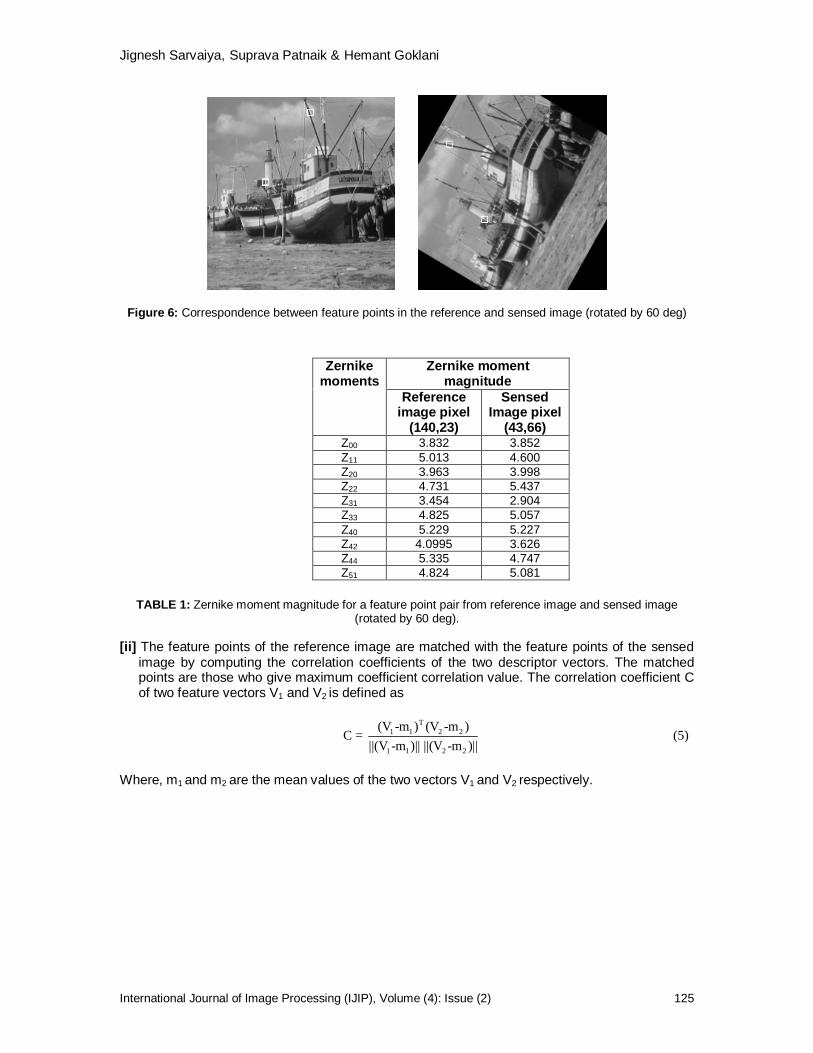
Jignesh Sarvaiya, Suprava Patnaik & Hemant Goklani
International Journal of Image Processing (IJIP), Volume (4): Issue (2) 125
Figure 6: Correspondence between feature points in the reference and sensed image (rotated by 60 deg)
TABLE 1: Zernike moment magnitude for a feature point pair from reference image and sensed image
(rotated by 60 deg).
[ii] The feature points of the reference image are matched with the feature points of the sensed image by computing the correlation coefficients of the two descriptor vectors. The matched points are those who give maximum coefficient correlation value. The correlation coefficient C of two feature vectors V1 and V2 is defined as
T
1 1 2 2
1 1 2 2
(V -m ) (V -m )C = (5)
||(V -m )|| ||(V -m )||
Where, m1 and m2 are the mean values of the two vectors V1 and V2 respectively.
Zernike moment magnitude
Zernike moments
Reference image pixel
(140,23)
Sensed Image pixel
(43,66) Z00 3.832 3.852 Z11 5.013 4.600 Z20 3.963 3.998 Z22 4.731 5.437 Z31 3.454 2.904 Z33 4.825 5.057 Z40 5.229 5.227 Z42 4.0995 3.626 Z44 5.335 4.747 Z51 4.824 5.081

Jignesh Sarvaiya, Suprava Patnaik & Hemant Goklani
International Journal of Image Processing (IJIP), Volume (4): Issue (2) 126
3.4. Example of Zernike moment Following examples shows calculations steps for Zernike moment for an 8 x 8 block.
5 10 15 20 25 30 35 4010 20 30 40 50 60 70 8015 30 45 60 75 95 105 12020 40 45 65 85 105 125 135
I =25 50 60 85 100 115 130 14530 60 75 105 115 130 145 16035 70 90 125 130 145 160 17540 80 105 135 145 160 175 190
Normalize the pixel locations for x and y varying from -1 to +1 with a step size 0.2857. Apply an 8 x 8 mask, with pixel values one within the unit circle, which is required for the calculation of Zernike moment.
0 0 0 0 0 0 0 00 0 1 1 1 1 0 00 1 1 1 1 1 1 00 1 1 1 1 1 1 0
Mask = 0 1 1 1 1 1 1 00 1 1 1 1 1 1 00 0 1 1 1 1 0 00 0 0 0 0 0 0 0
For z = x+ iy and mask = 1, calculate r and θ. Obtained,
r = [0.83, 0.72, 0.72, 0.83, …. .0.45, … 0.72, 0.83] 1x32
and θ = [-2.60, -2.94, 2.94, 2.60, ….-1.89, ...0.20, 0.54] 1x32
For finding Zernike moment at grid location (3,4), value of r and θ are 0.4518 and -1.89 respectively, which are 12th element of r and θ vectors. Pixel intensity, I(3, 4) = 60. For p=3 and q=1 satisfying the above mentioned condition, from equation (4), R31the polynomial value becomes -0.6269. Putting this value in equation 3, we get V31(r, θ) = 0.19825 + 0.59485i. Applying all the above values in equation 2, we get Z31=15.29 + 45.4588i. Finally in log scale we get [abs (log (Z31))] =4.0661. 3.4. Transformation parameters estimation Image geometrical deformation has many different ways of description. In this paper we have considered combination of rotation and scaling. Given the two sets of corresponding feature point coordinates, the estimation of the transformation parameters is required to map the sensed image into its original size, orientation, and position. This requires at least three feature point pairs having the maximum coefficient correlation. These parameters are estimated by solving a least-square minimization problem.
4. EXPERIMENTAL RESULTS In this section, the evaluation of the performance of the proposed algorithm is done by applying different types of distortions. A reference image is geometrically distorted and in addition noise is being added or the image is compressed or expanded. The parameters of the geometric distortion are obtained by applying the proposed algorithm using the reference and sensed images. A set of simulation has been performed to assess the performance of the proposed algorithm with respect to registration accuracy and robustness.

Jignesh Sarvaiya, Suprava Patnaik & Hemant Goklani
International Journal of Image Processing (IJIP), Volume (4): Issue (2) 127
(a) (b)
(c) (d)
(e) (f)
(g)
Figure 7: Experimental results (a) Reference image (b) Sensed image (rotated by 37 deg) (c) NSCT maxima image of reference image, N is 2 (d) NSCT maxima image of sensed image, N is 2 (e) Registered image (f) Registered image overlaid on Reference image (g) Enlarged portion of the overlaid image. A gray level “boat” image of size 256x256 is being used as a reference image. The simulation results have been obtained using MATLAB software package. The experiments were performed according to the following settings: NSCT decomposition of all test images performed using the NSCT toolbox, was carried out with N = 2 resolution levels. But to increase the capability of proposed algorithm for higher amount of distortions we need to increase resolution levels N to 3. The parameter C is user defined and ranges from 4 to 8 and the Zernike moment based descriptor neighbourhood radius R = 20. Results of registering the geometrically distorted images combined with other image processing operation are shown in Fig. 7. In this figure, first reference image and sensed images were shown. Then the NSCT maxima images of both the images have been shown. At the last registered image overlaid on the reference image is shown. To highlight the registration accuracy a small square section of the reference image which is not available in the sensed image after rotation has been magnified along with connected features from the sensed image. Perfect alignment between the two images justifies the registration accuracy.
Registered image
Reference image

Jignesh Sarvaiya, Suprava Patnaik & Hemant Goklani
International Journal of Image Processing (IJIP), Volume (4): Issue (2) 128
The applied distortions/ transformations are shown in below Figures. It can be seen that, the estimated transformation parameters are very close to the actual applied parameters. This illustrates the accuracy in image recovery, in the presence of noise, coarse compression or expansion of the image. Figures 8 to 11 shows simulation results with different rotation and scale which shows the accuracy of registration.
(a) (b)
(c) (d)
Figure 8: (a) Reference image (b) Sensed image (rotated by 100 degrees) (c) Registered image (d) Registered image overlaid on Reference image (N = 3).
(a) (b)
(c) (d)
Figure 9:(a) Reference image (b) Sensed image (rotated by 80 degrees Scaled by 0.8)
(c) Registered image (d) Registered image overlaid on Reference image (N = 2).

Jignesh Sarvaiya, Suprava Patnaik & Hemant Goklani
International Journal of Image Processing (IJIP), Volume (4): Issue (2) 129
(a) (b)
(c) (d)
Figure 10: (a) Reference image (b) Sensed image (rotated by 80 degrees Scaled by 2.2)
(c)Registered image (d) Registered image overlaid on Reference image (N = 2).
(a) (b)
(c) (d)
Figure 11 :( a) Reference image (b) Sensed image (rotated by 10 degrees with Gaussian noise,
mean 0 and variance 0.02) (c) Registered image (d) Registered image overlaid on Reference image (N = 2).

Jignesh Sarvaiya, Suprava Patnaik & Hemant Goklani
International Journal of Image Processing (IJIP), Volume (4): Issue (2) 130
5. CONCLUSION In the proposed algorithm major and basic elements of the feature based automated image registration has been explored. We use nonsubsampled contourlet transform (NSCT) based feature point extractor, to extract significant image feature points across spatial and directional resolutions. Zernike moments based similarity measure is used for feature correspondence. The experimental results clearly indicate that the registration accuracy and robustness is very acceptable. This confirms the success of the proposed NSCT based feature points extraction approach for image registration.
6. REFERENCES [1] Brown L G., “A survey of image registration techniques”. ACM Computing Surveys, 24(4),
325-376, 1992. [2] A. Ardeshir Goshtasby, “2-D and 3-D Image Registration for Medical, Remote Sensing, and
Industrial Applications”, A John Wiley & Sons, Inc., Publication, USA. [3] B. Zitova and J. Flusser, “Image Registration methods: A Survey”. Image Vision Computing,
21(11), 977-1000, 2003. [4] A. Khotanzad and Y.H. Hong, “Invariant Image Recognition by Zernike moment”. IEEE Trans.
PAMI, 12(5), 489-497, 1990. [5] Cho-Huak and R.T. Chin, “On Image Analysis by the method of moments”. IEEE Trans.
PAMI, 10(4), 496-513, 1988. [6] M.N. Do and M. Vetterli, “The Contourlet Transform: an Efficient Directional multiresolution
Image Representation”. IEEE Trans. on Image Processing, 14(12), 2091-2106, 2005. [7] A.L.Cunha, J. Zhou, and M.N. Do, “The Nonsubsampled Contourlet Transform: Theory,
Design, and Applications”. IEEE Trans. on Image Processing, 15(10), 3089-3101, 2006. [8] R. H. Bamberger and M. J. T. Smith, “A filter bank for the directional decomposition of
images: theory and design”. IEEE Trans. on Signal Processing, 40(7), 882-893, 1992. [9] S. X. Liao and M. Pawlak, “On the Accuracy of Zernike Moments for Image Analysis”. IEEE
Trans. on Pattern Analysis and Machine Intelligence, 20(12)1358-1364, 1998. [10] J. Zhou, A.L. Cunha, and M.N. Do, “The Nonsubsampled Contourlet Transform: Construction
and Application in Enhancement”. In Proceedings of IEEE Int. Conf. on Image Processing, ICIP 2005, (1), 469-472, 2005.
[11] P. J. Burt and E. H. Adelson, “The Laplacian pyramid as a compact image code”. IEEE Trans. on Commun., 31(4), 532–540, 1983.
[12] M. N. Do and M. Vetterli, “Framing pyramids”. IEEE Trans. Signal Process. 51(9),2329-2342, 2003.
[13] C. Serief, M. Barkat, Y. Bentoutou and M. Benslama, “Robust feature points extraction for image registration based on the nonsubsampled contourlet transform”. International Journal Electronics Communication, 63( 2), 148-152, 2009.
[14] Manjunath B S and Chellappa R. “A feature based approach to face recognition”. In Proceedings of IEEE conference on computer vision and pattern recognition, Champaign, 373–378, 1992.
[15] M.S. Holia and V.K.Thakar, “Image registration for recovering affine transformation using Nelder Mead Simplex method for optimization”,International Journal of Image
Processing(ISSN 1985 2304) , Vol.3, No.5, pp.218-228, November 2009 [16] R. Bhagwat and A. Kulkarni, “An Overview of Registration Based and Registration Free Methods for Cancelable Fingerprint Template”, International Journal of Computer Science and Security ISSN (1985-1553) Vol. 4 , No.1 pp.23-30, March 2010.

J.Rajeesh, R.S.Moni, S.Palanikumar & T.Gopalakrishnan
International Journal of Image Processing (IJIP), Volume(4) : Issue(2) 131
Noise Reduction in Magnetic Resonance Images using Wave Atom Shrinkage
J.Rajeesh [email protected] Senior Lecturer/Department of ECE Noorul Islam College of Engineering Kumaracoil, 629180, India R.S.Moni [email protected] Professor/Department of ECE Noorul Islam University Kumaracoil, 629180, India S.Palanikumar [email protected] Assistant Professor/Department of IT Noorul Islam University Kumaracoil, 629180, India T.Gopalakrishnan [email protected] Lecturer/Department of ECE Noorul Islam University Kumaracoil, 629180, India
Abstract
De-noising is always a challenging problem in magnetic resonance imaging and important for clinical diagnosis and computerized analysis, such as tissue classification and segmentation. It is well known that the noise in magnetic resonance imaging has a Rician distribution. Unlike additive Gaussian noise, Rician noise is signal dependent, and separating signal from noise is a difficult task. An efficient method for enhancement of noisy magnetic resonance image using wave atom shrinkage is proposed. The reconstructed MRI data have high Signal to Noise Ratio (SNR) compared to the curvelet and wavelet domain de-noising approaches. Keywords: De-noising, Gaussian noise, Magnetic Resonance Images, Rician noise, Wave Atom Shrinkage.
1. INTRODUCTION De-noising of magnetic resonance (MR) images remains a critical issue, spurred partly by the necessity of trading-off resolution, SNR, and acquisition speed, which results in images that still demonstrate significant noise levels [1]–[7]. Sources of MR noise [8] include thermal noise (from the conductivity of the system’s hardware), inductive losses (from the conductivity of the object being imaged), sample resolution, and field-of-view (among others). Understanding the spatial distribution of noise in an MR image is critical to any attempt to estimate the underpinning (true) signal. The investigation of how noise is distributed in MR images (along with techniques proposed to ameliorate the noise) has a long history. It was shown that pure noise in MR

J.Rajeesh, R.S.Moni, S.Palanikumar & T.Gopalakrishnan
International Journal of Image Processing (IJIP), Volume(4) : Issue(2) 132
magnitude images could be modeled as a Rayleigh distribution [1]. Afterwards, the Rician model [4] was proposed as a more general model of noise in MR images. Reducing noise has always been one of the standard problems of the image analysis. The success of many analysis techniques such as segmentation, classification depends mainly on the image being noiseless. Magnetic Resonance Imaging (MRI) is a notable medical imaging technique that has proven to be particularly valuable for examination of the soft tissues in the body. MRI is an imaging technique that makes use of the phenomenon of nuclear spin resonance. Since the discovery of MRI, this technology has been used for many medical applications. Because of the resolution of MRI and the technology being essentially harmless it has emerged as the most accurate and desirable imaging technology [9]. MRI is primarily used to demonstrate pathological or other physiological alterations of living tissues and is a commonly used form of medical imaging. Despite significant improvements in recent years, magnetic resonance (MR) images often suffer from low SNR or Contrast-to-Noise Ratio (CNR), especially in cardiac and brain imaging. This is problematic for further tasks such as segmentation of important features, three-dimensional image reconstruction, and registration. Therefore, noise reduction techniques are of great interest in MR imaging as well as in other imaging modalities. This paper presents a de-noising method in Magnetic Resonance Images using Wave Atom Shrinkage that leads to the improvement of SNR in low and high noise level images. The paper is organized with sections as follows. In section II, the work related to this paper is briefly explained, In section III, the theoretical concepts of wavelet transform, curvelet transform and wave atom transforms are described, in section IV, the application of wave atom transform, curvelet transform and wavelet transforms to MRI and observations are discussed. In section V, the paper is concluded by briefly explained the pros and corns of the proposed method.
2. RELATED WORKS The image processing literature presents a number of de-noising methods based on Partial Differential Equations (PDEs) [10], including some of them concentrated on MR Images [11] – [14]. Even though these methods have the advantage of simplicity and removal of stair case effect that occurs with the TV-norm filter. Such methods, however, impose certain kinds of models on local image structure that are often too simple to capture the complexity of anatomical MR images. Further, these methods entail manual tuning of critical free parameters that control the conditions under which the models prefer one sort of structure to another. These factors have been an impediment to the widespread adoption of PDE-based techniques for processing MR images. Another approach to image restoration is nonparametric statistical methods. For instance, in [15], [16] propose an unsupervised information-theoretic adaptive filter, namely UINTA, that relies on nonparametric MRF models derived from the corrupted images. UINTA restores images by generalizing the mean-shift procedure [17], [18] to incorporate neighborhood information. They show that entropy measures on first-order image statistics are ineffective for de-noising and, hence, advocate the use of higher-order/Markov statistics. UINTA, however, does not assume a specific noise model during restoration. In [19], [20] proposed a de-noising strategy along similar lines, namely NL-Means, but one relying on principles in nonparametric regression. Recently, many of the popular de-noising algorithms suggested are based on wavelet thresholding [21]–[24]. These approaches attempt to separate significant features/signals from noise in the frequency domain and simultaneously preserve them while removing noise. If the wavelet transform is applied on MR magnitude data directly, both the wavelet and the scaling coefficients of a noisy MRI image become biased estimates of their noise-free counterparts. Therefore, it was suggested [22] that the application of the wavelet transform on squared MR magnitude image data (which is noncentral chi-square distributed) would result in the wavelet

J.Rajeesh, R.S.Moni, S.Palanikumar & T.Gopalakrishnan
International Journal of Image Processing (IJIP), Volume(4) : Issue(2) 133
coefficients no longer being biased estimates of their noise-free counterparts. Although the bias still remains in the scaling coefficients, it is not signal-dependent and can therefore be easily removed [22], [24]. The difficulty with wavelet or anisotropic diffusion algorithms is again the risk of over-smoothing fine details particularly in low SNR images [25]. From points discussed above, it is understood that all the algorithms have the drawback of over-smoothing fine details. In [26], stated that oscillatory functions or oriented textures have a significantly sparser expansion in wave atoms than in other fixed standard representations like Gabor filters, wavelets and curvelets. Due to the signal dependent mean of the Rician noise, one can overcome this problem by filtering the square of the noisy MR magnitude image in the transformed coefficients [22].
3. THEORY 3.1. Wavelet Wavelet bases are bases of nested function spaces, which can be used to analyze signals at multiple scales. Wavelet coefficients carry both time and frequency information, as the basis functions varies in position and scale. The fast wavelet transform (FWT) efficiently converts a signal to its wavelet representation [27]. In a one-level FWT, a signal is split into an approximation part and a detail part. In a multilevel FWT, each subsequent is split into an approximation and detail. For 2-D images, each subsequent is split into an approximation and three detail channels as horizontally, vertically, and diagonally oriented details, respectively. The inverse FWT (IFWT) reconstructs each subsequent from approximation and detail channels. If the wavelet basis functions do not have compact support, the FWT is computed most efficiently in the frequency domain. This transform and its inverse are called the Fourier-wavelet decomposition (FWD) and Fourier-wavelet reconstruction (FWR), respectively. Assume that the observed data
)()()( tNtStX contains the true signal S(t) with additive noise N(t) as functions in time t to be sampled. Let W(.) and W−1(.) denote the forward and inverse wavelet transform operators. Let D(., ) denote the de-noising operator with hard threshold . To wavelet shrinkage de-noise X(t) in order to recover
)(tS
as an estimate of S(t). Then the three steps 1. Take the forward transform Y = W(X) (2) 2. Apply shrinkage Z = D(., ) (3)
3. Take inverse transform S = W−1(Z) (4)
summarize the procedure. For implementation MATLAB functions were used with db5 wavelet and the decomposition level depends upon the row size of the image (i.e. If the row size is N, then the decomposition level becomes log2N). 3.2. Curvelet The curvelet transform, like the wavelet transform, is a multiscale transform, with frame elements indexed by scale and location parameters. Unlike the wavelet transform, it has directional parameters, and the curvelet pyramid [28][29] contains elements with a very high degree of directional specificity. The elements obey a special scaling law, where the length of the support of a frame elements and the width of the support are linked by the relation width = length2. Curvelets are interesting because they efficiently address very important problems where wavelets are far from ideal. For example, Curvelets provide optimally sparse representations of objects, which display curve-punctuated smoothness except for discontinuity along a general curve with bounded curvature. Such representations are nearly as sparse as if the object were not singular and turn out to be far sparser than the wavelet decomposition of the object.
(1)

J.Rajeesh, R.S.Moni, S.Palanikumar & T.Gopalakrishnan
International Journal of Image Processing (IJIP), Volume(4) : Issue(2) 134
This phenomenon has immediate applications in approximation theory and in statistical estimation. In approximation theory, let mf be the m -term curvelet approximation (corresponding to the m largest coefficients in the curvelet series) to an object
)2(2)2,1( RLxxf . Then the enhanced sparsity says that if the object f is singular along a
generic smooth 2C curve but otherwise smooth, the approximation error obeys
232 .log.2 mmCff
Lm (5)
and is optimal in the sense that no other representation can yield a smaller asymptotic error with the same number of terms. The implication in statistics is that one can recover such objects from noisy data by simple curvelet shrinkage and obtain a MSE in order of magnitude better than what is achieved by more traditional methods. In fact, the recovery is asymptotically near optimal. The statistical optimality of the curvelet shrinkage extends to other situations involving indirect measurements as in a large class of ill-posed inverse problems [30]. For implementation software, we refer to the home page http://www.curvelet.org due to Demanet and Ying. 3.2. Waveatom Demanet and Ying [31] introduced so-called wave atoms, that can be seen as a variant of 2-D wavelet packets and obey the parabolic scaling of curvelets wavelength= (diameter) 2. Oscillatory functions or oriented textures (e.g., fingerprint, seismic profile, engineering surfaces) have a significantly sparser expansion in wave atoms than in other fixed standard representations like Gabor filters, wavelets, and curvelets. Wave atoms have the ability to adapt to arbitrary local directions of a pattern, and to sparsely represent anisotropic patterns aligned with the axes. In comparison to curvelets, wave atoms not only capture the coherence of the pattern along the oscillations, but also the pattern across the oscillations. In the following, we shortly summarize the wave atom transform as recently suggested in [31]. See also [32] for a very related approach.
Consider a 1-D family of wave packets )(, xjnm , Nnmj ,0,0 , centered in frequency
around mw jmj 2, with jj cmc 22 21 (where 21 cc are positive constants) and
centered in space around nx jnj
2, . For that purpose, let g be a real valued C bumb function
with compact support in 6/5,6/7 such that for 3/
122
2
gg (6)
2
22
2gg (7)
Then the function )(ˆ 0 m is determined by the formula
21
1212/ mmegmiemmegmiee (8)
where mme )1( and ))2/1()(2/( mm . The properties of g have to ensure that
0
20 1)(ˆm
m (9)

J.Rajeesh, R.S.Moni, S.Palanikumar & T.Gopalakrishnan
International Journal of Image Processing (IJIP), Volume(4) : Issue(2) 135
Then the translates )(.0 nm form an orthonormal basis of )(2 RL . Introducing the basis functions
)2(2)2()( 02/, nxnxx j
mjjj
mj
nm (10)
The transform )()(: 22 ZlRLWA maps a function u onto a sequence of wave atom coefficients
dujm
njiedxxjnmxunmjc )(ˆ)(2
21)(,)(,,
(11)
In the 2-D case, Let ),,( nmj , where )2,1( mmm and )2,1( nnn . We consider
)2(2,2
)1(1,1
)2,1( xjnmxj
nmxx (12)
and the Hilbert transformed wavelet packets
)2(2,2
)1(1,1
)2,1( xjnmxj
nmxx (13)
Where for decomposition
)()()( ,,,,, jnm
jnmnm i with )()( ,,,, j
nmj
nm and the Hilbert transform is defined by
)()()( ,,,,,
^ j
nmj
nm
j
nm iiH (14)
(Note that the above decomposition of nm,
^ is possible since nm, is real-valued). A
recombination
2,
2)2()1(
(15)
provides basis functions with two bumps in the frequency plane being symmetric with respect to the origin. Together, )1(
and )2( form a wave atom frame, and the wave atom coefficients
)1(uC , )2(
uC are the scalar products of u with )1( and )2(
. In [31], a discretization of this transform is described for the 1-D case, as well as an extension to two dimensions. The algorithm is based on the fast Fourier transform and a wrapping trick. For implementation software, we refer to the homepage http://www.waveatom.org/software.html due to Demanet and Ying. The wave atom shrinkage can be formulated as a hard threshold function given by
xx
xxxh,0
,)(2
(16)
Where is the standard deviation, estimated by histogram based techniques.
4. EXPERIMENTS AND RESULTS This section gives a detailed qualitative and quantitative analysis of the proposed MRI de-noising algorithm. It compares the performance of the proposed method with wavelet shrinkage and curvelet shrinkage. It is evaluated with simulated images and real images.

J.Rajeesh, R.S.Moni, S.Palanikumar & T.Gopalakrishnan
International Journal of Image Processing (IJIP), Volume(4) : Issue(2) 136
4.1. Simulated Images To validate the proposed method with simulated images, images were down loaded from Brainweb[33]. Rician noise is generated by adding independent and identically distributed (i.i.d.) additive Gaussian noise with the noise free image and, subsequently, taking the magnitude of the resulting complex-valued image [34]. Noisy image with different values of standard deviation are applied on the proposed de-noising method and the Signal to Noise ratio (SNR) [34] is obtained by
))ˆvar(/)(var(10log10 xxxSNR (17)
where x is noise free simulated image and x̂ is noisy image or de-noised image.
The shrinkage is obtained by
)(1 uTTuX (18)
where T denotes the transform and 1T denotes the inverse transform, is taken as a threshold function defined by a fixed threshold .0 Analysis is made with four conditions vide i) fixed high SNR for various threshold ii) fixed low SNR for various threshold iii) fixed low threshold for various SNR and iv) fixed high threshold for various SNR
i) The chosen SNR is 19.0505 dB and the threshold is varied from 0.03 to 0.3. The observations are given in Fig 1. It shows the wave atom shrinkage gives higher SNR on all threshold values compared to wavelet shrinkage and curvelet shrinkage. The performances of the models are given in Fig 2 for the threshold 0.06.
ii) The chosen SNR is 9.21 dB and the threshold is varied from 0.03 to 0.3. The observations are given in Fig 3. It shows the wave atom shrinkage gives higher SNR on all threshold values compared to wavelet shrinkage and curvelet shrinkage except for the threshold 0.03,0.06 and 0.3, where the curvelet shrinkage perform well. The performances of the models are given in Fig 4. for the threshold 0.24.
iii) Here the threshold is fixed at 0.06 and SNR is varied from 9.37 dB to 19.12 dB. It shows the proposed method increases the SNR to the maximum of 16.6% compared to wavelet by 14.6% and curvelet by 8%. The analysis is presented in Fig 5.
iv) Here the threshold is fixed at 0.24 and SNR is varied from 9.26 dB to 18.87 dB. It shows the proposed method increases the SNR to the maximum of 57% compared to wavelet by 52% and curvelet by 52%. The analysis is presented in Fig 6.
It is observed that the performance of all filters depends on the proper selection of threshold value and the SNR of the noisy image. Also, the performance of the proposed method is better with the maximum increase of 57% SNR compared to the methods given in [35] like anisotropic diffusion by 34% and UINTA by 18.1% increase of SNR.

J.Rajeesh, R.S.Moni, S.Palanikumar & T.Gopalakrishnan
International Journal of Image Processing (IJIP), Volume(4) : Issue(2) 137
FIGURE 1: De-noised image SNR for high SNR noisy image.
FIGURE 2: High SNR images (a) Noisy image (b) De-noised using Wave Atom (c) De-noised using Wavelet
(d) Den-noised using Curvelet.
FIGURE 3: De-noised image SNR for low SNR noisy image.

J.Rajeesh, R.S.Moni, S.Palanikumar & T.Gopalakrishnan
International Journal of Image Processing (IJIP), Volume(4) : Issue(2) 138
FIGURE 4: Low SNR images (a) Noisy image (b) De-noised using Wave Atom (c) De-noised using
Wavelet (d) Den-noised using Curvelet.
FIGURE 5: Performance between noisy and de-noised images with the threshold of 0.06.
FIGURE 6: Performance between noisy and de-noised images with the threshold of 0.24

J.Rajeesh, R.S.Moni, S.Palanikumar & T.Gopalakrishnan
International Journal of Image Processing (IJIP), Volume(4) : Issue(2) 139
4.2. Real Images Fig. 7 show the performance of the proposed method and the wavelet and curvelet shrinkage on corrupted MR images of adult human brains taken from Sree Chitra Tirunal Institute of Medical Sciences, Thiruvananthapuram, where the MRI scans were acquired on a 1.5T Vision System (Siemens, Erlangen, Germany). T1-weighted magnetization prepared rapid gradient echo (MP-RAGE) with the following specifications: FOV = 224, matrix = 256 x 256, resolution = 1 x 1 x 1.25 mm3, TR = 9.7 ms, TE = 4ms, flip angle = 10, TI = 20 ms, TD = 200ms. The voxel size of the image is 0.781x0.781x2mm3. The proposed method is able to recover the image features to a significant extent, qualitatively, despite a significant level of intensity inhomogeneity apparent in some images. The medical doctors validated the images.
FIGURE 7: Real (a) Noisy image (b) De-noised using Wave Atom (c) De-noised using Wavelet (d) Den-
noised using Curvelet
5. CONCLUSION A novel scheme is proposed for the de-noising of Magnetic Resonance Images using wave atom shrinkage. It is proved that the proposed approach achieves a better SNR compared to wavelet and curvelet shrinkages. The edge preserving property is clearly an advantage of the proposed method. Further, including a large dataset of real-time normal and pathological MR images will emphasize the efficiency of proposed method. The next work is to analyze the performance of the proposed method on other modalities of MRI such as T2 and PD.

J.Rajeesh, R.S.Moni, S.Palanikumar & T.Gopalakrishnan
International Journal of Image Processing (IJIP), Volume(4) : Issue(2) 140
6. REFERENCES 1. W. A. Edelstein, P. A. Bottomley, and L. M. Pfeifer.A signal-to-noise calibration procedure for nmr imaging systems. Med. Phys 1984;11:2:180–185.
2. E. R. McVeigh, R. M. Henkelman, and M. J. Bronskill. Noise and filtration in magnetic resonance imaging. Med. Phys 1985;12:5:586–591.
3. R. M. Henkelman. Measurement of signal intensities in the presence of noise in mr images. Med. Phys 1985;12:2:232–233.
4. M. A. Bernstein, D. M. Thomasson, and W. H. Perman. Improved detectability in low signal-to-noise ratio magnetic resonance images by means of phase-corrected real construction. Med. Phys 1989;16:5:813–817.
5. M. L. Wood, M. J. Bronskill, R. V. Mulkern, and G. E. Santyr. Physical MR desktop data. Magn Reson Imaging 1994;3:19–24. 6. H. Gudbjartsson and S. Patz. The Rician distribution of noisy MRI data. Magn Reson Med 1995;34:6:910–914.
7. A. Macovski. Noise in MRI. Magn Reson Med 1996;36:3:494–497.
8. W. A. Edelstein, G. H. Glover, C. J. Hardy, and R. W. Redington. The intrinsic SNR in NMR imaging. Magn Reson Med 1986;3:4:604–618. 9. G.A. Wright. Magnetic Resonance Imaging. IEEE Signal Processing Magazine 1997;1:56-66.
10. X. Tai, K. Lie, T. Chan, and S. Osher, Eds. Image Processing based on Partial Differential Equations 2005; New York: Springer. 11. G. Gerig, O. Kubler, R. Kikinis, and F. A. Jolesz. Nonlinear anisotropic filtering of MRI data. IEEE Trans Med Imag 1992;11:2:221–232. 12. M. Lysaker, A. Lundervold, and X. Tai. Noise removal using fourth-order partial differential equation with applications to medical magnetic resonance images in space and time. IEEE Trans Image Process 2003;12:12:1579–1590.
13. A. Fan, W. Wells, J. Fisher, M. Çetin, S. Haker, R. Mulkern, C. Tempany, and A.Willsky. A unified variational approach to denoising and bias correction in MR. Inf Proc Med Imag 2003;148–159. 14 S. Basu, P. T. Fletcher, and R. T. Whitaker. Rician noise removal in diffusion tensor MRI. Med Imag Comput Comput Assist Intervention 2006;117–125. 15. S. P. Awate and R. T. Whitaker. Higher-order image statistics for unsupervised, information-theoretic, adaptive, image filtering. Proc IEEE Int Conf. Comput Vision Pattern Recognition 2005;2:44–51. 16 S. P. Awate and R. T. Whitaker. Unsupervised, information-theoretic, adaptive image filtering for image restoration. IEEE Trans Pattern Anal Mach Intell 2006;28:3:364–376.
17. K. Fukunaga and L. Hostetler. The estimation of the gradient of a density function, with applications in pattern recognition. IEEE Trans Inf Theory 1975;21:1:32–40.
18. D. Comaniciu and P. Meer. Mean shift: A robust approach toward feature space analysis. IEEE Trans Pattern Anal Mach Intell 2002;24:5:603–619.
19. A. Buades, B. Coll, and J. M. Morel. A non-local algorithm for image denoising. IEEE Int Conf Comp Vis Pattern Recog 2005;2:60–65. 20. A. Buades, B. Coll, and J. M. Morel. A review of image denoising algorithms, with a new one. Multiscale Modeling Simulation 2005;4:2:490–530. 21. J. B. Weaver, Y. Xu, D. M. Healy Jr., and L. D. Cromwell. Filtering noise from images with wavelet transforms. Magn Reson Med 1991;21:2:288–295.
22. R. D. Nowak. Wavelet-based Rician noise removal for magnetic resonance imaging. IEEE Trans Image Process 1999;8:10:1408–1419.
23. A. M. Wink and J. B. T. M. Roerdink. Denoising functional MR images: A comparison of wavelet denoising and Gaussian smoothing. IEEE Trans Image Process 2004;23:3:374–387.

J.Rajeesh, R.S.Moni, S.Palanikumar & T.Gopalakrishnan
International Journal of Image Processing (IJIP), Volume(4) : Issue(2) 141
24. A. Pizurica, A. M. Wink, E. Vansteenkiste, W. Philips, and J. B. T. M. Roerdink. A review of wavelet denoising in MRI and ultrasound brain imaging. Current Med Imag Rev 2006;2:2:247–260.
25. D. Tisdall and M. S. Atkins. MRI denoising via phase error estimation. Proc SPIE Med Imag 2005;646–654.
26. Gerlind Plonka and Jianwei Ma. Nonlinear Regularised Reaction-Diffusion Filter for Denoising of Images with Textures. IEEE Trans. Image Processing 2008;17:8:1283–1294.
27. S. G. Mallat. A theory for multiresolution signal decomposition: The wavelet representation. IEEE Trans Pattern Anal Machine Intell 1989;l:11:674–693.
28. E. J. Candès and D. L. Donoho. Curvelets. [Online] Available: http://www-stat.stanford.edu/~donoho/Reports/1999/Curvelets.pdf. 29. M. N. Do and M. Vetterli. Framing pyramids. IEEE Trans Signal Proc 2003;2329–2342.
30. E. J. Candes and D. L. Donoho. Recovering edges in ill-posed inverse problems: Optimality of Curvelet frames. Ann. Statist. 30 (2002); 784 –842. 31. L. Demanet and L. Ying. Wave atoms and sparsity of oscillatory patterns. Appl Comput Harmon Anal 2007;23:3:368–387. 32. G. Cottet and L. Germain. Image processing through reaction combined with nonlinear diffusion. Math Comput 1993;61:659–673. 33. [Online]. Available: http://www.bic.mni.mcgill.ca/brainweb/ 34. A. Pizurica, W. Philips, I. Lemahieu, and M. Acheroy. A versatile wavelet domain noise filtration technique for medical imaging. IEEE Trans Med Imag 2003;22:3:323–331. 35. Suyash P. Awate and Ross T. Whitaker. Feature-Preserving MRI Denoising: A Nonparametric Empirical Bayes Approach. IEEE Trans Med Imag 2007;26:9:1242–1255.

Dr. H. B. Kekre, Sudeep D. Thepade, Akshay Maloo
International Journal of Image Processing (IJIP) Volume (4): Issue (2) 142
Performance Comparison of Image Retrieval Using Fractional Coefficients of Transformed Image Using DCT, Walsh, Haar
and Kekre’s Transform
Dr. H. B. Kekre [email protected] Senior Professor, Computer Engineering, MPSTME, SVKM’S NMIMS University, Mumbai, 400056, India Sudeep D. Thepade [email protected] Ph.D. Research Scholar and Asst. Professor, Computer Engineering, MPSTME, SVKM’S NMIMS University, Mumbai, 400056, India Akshay Maloo [email protected] Student, Computer Engineering, MPSTME, SVKM’S NMIMS University Mumbai, 400056, India
Abstract
The thirst of better and faster retrieval techniques has always fuelled to the research in content based image retrieval (CBIR). The paper presents innovative content based image retrieval (CBIR) techniques based on feature vectors as fractional coefficients of transformed images using Discrete Cosine, Walsh, Haar and Kekre’s transforms. Here the advantage of energy compaction of transforms in higher coefficients is taken to greatly reduce the feature vector size per image by taking fractional coefficients of transformed image. The feature vectors are extracted in fourteen different ways from the transformed image, with the first being considering all the coefficients of transformed image and then fourteen reduced coefficients sets (as 50%, 25%, 12.5%, 6.25%, 3.125%, 1.5625% ,0.7813%, 0.39%, 0.195%, 0.097%, 0.048%, 0.024%, 0.012% and 0.06% of complete transformed image) are considered as feature vectors. The four transforms are applied on gray image equivalents and the colour components of images to extract Gray and RGB feature sets respectively. Instead of using all coefficients of transformed images as feature vector for image retrieval, these fourteen reduced coefficients sets for gray as well as RGB feature vectors are used, resulting into better performance and lower computations. The proposed CBIR techniques are implemented on a database having 1000 images spread across 11 categories. For each proposed CBIR technique 55 queries (5 per category) are fired on the database and net average precision and recall are computed for all feature sets per transform. The results have shown performance improvement (higher precision and recall values) with fractional coefficients compared to complete transform of image at reduced computations resulting in faster retrieval. Finally Kekre’s transform surpasses all other discussed transforms in performance with highest precision and recall values for fractional coefficients (6.25% and 3.125% of all coefficients) and computation are lowered by 94.08% as compared to DCT. Keywords: CBIR, Discrete Cosine Transform (DCT), Walsh Transform, Haar Transform, Kekre’s Transform, Fractional Coefficients, Feature Vector.
1. INTRODUCTION The computer systems have been posed with large number of challenges to store/transmit and index/manage large numbers of images effectively, which are being generated from a variety of sources. Storage and transmission is taken care by Image compression with significant advancements been made [1,4,5].Image databases deal with the challenge of
Dr. H. B. Kekre, Sudeep D. Thepade, Akshay Maloo
International Journal of Image Processing (IJIP) Volume (4): Issue (2) 143
image indexing and retrieval[2,6,7,10,11], which has become one of the promising and important research area for researchers from a wide range of disciplines like computer vision, image processing and database areas. The thirst of better and faster image retrieval techniques is till appetising to the researchers working in some of important applications for CBIR technology like art galleries [12,14], museums, archaeology [3], architecture design [8,13], geographic information systems [5], weather forecast [5,22], medical imaging [5,18], trademark databases [21,23], criminal investigations [24,25], image search on the Internet [9,19,20].
1.1 Content Based Image Retrieval In literature the term content based image retrieval (CBIR) has been used for the first time by Kato et.al.[4], to describe his experiments into automatic retrieval of images from a database by colour and shape feature. The typical CBIR system performs two major tasks [16,17]. The first one is feature extraction (FE), where a set of features, called feature vector, is generated to accurately represent the content of each image in the database. The second task is similarity measurement (SM), where a distance between the query image and each image in the database using their feature vectors is used to retrieve the “closest” images [16,17,26]. For CBIR feature extraction the two main approaches are feature extraction in spatial domain [5] and feature extraction in transform domain [1]. The feature extraction in spatial domain includes the CBIR techniques based on histograms [5], BTC [2,16,23], VQ [21,25,26]. The transform domain methods are widely used in image compression, as they give high energy compaction in transformed image[17,24]. So it is obvious to use images in transformed domain for feature extraction in CBIR [1]. Transform domain results in energy compaction in few elements, so large number of the coefficients of transformed image can be neglected to reduce the size of feature vector [1]. Reducing the size feature vector using fractional coefficients of transformed image and till getting the improvement in performance of image retrieval is the theme of the work presented here. Many current CBIR systems use average Euclidean distance [1,2,3,8-14,23]on the extracted feature set as a similarity measure. The direct Average Euclidian Distance (AED) between image P and query image Q can be given as equation 1, where Vpi and Vqi are the feature vectors of image P and Query image Q respectively with size ‘n’.
n
iVqiVpi
nAED
1
2)(1 (1)
2. DISCRETE COSINE TRANSFORM The discrete cosine transform (DCT) [1,10,21,22,24] is closely related to the discrete Fourier transform. It is a separable linear transformation; that is, the two-dimensional transform is equivalent to a one-dimensional DCT performed along a single dimension followed by a one-dimensional DCT in the other dimension. The definition of the two-dimensional DCT for an input image A and output image B is
1010
,2
)12(cos2
)12(cos
NqMp
Nqn
MpmAB mnqppq
(2)
11,2
0,1MpM
pMp (3)
11,2
0,1NqN
qNq
(4)
where M and N are the row and column size of A, respectively. If you apply the DCT to real data, the result is also real. The DCT tends to concentrate information, making it useful for image compression applications and also helping in minimizing feature vector size in CBIR [23]. For full 2-Dimensional

Dr. H. B. Kekre, Sudeep D. Thepade, Akshay Maloo
International Journal of Image Processing (IJIP) Volume (4): Issue (2) 144
DCT for an NxN image the number of multiplications required are N2(2N) and number of additions required are N2(2N-2).
3. WALSH TRANSFORM Walsh transform matrix [1,11,18,19,26,30] is defined as a set of N rows, denoted Wj, for j = 0, 1, .... , N - 1, which have the following properties: Wj takes on the values +1 and -1. Wj[0] = 1 for all j. WjxWk
T=0, for j k and WjxWkT =N, for j=k.
Wj has exactly j zero crossings, for j = 0, 1, ...., N-1. Each row Wj is even or odd with respect to its midpoint.
Walsh transform matrix is defined using a Hadamard matrix of order N. The Walsh transform matrix row is the row of the Hadamard matrix specified by the Walsh code index, which must be an integer in the range [0, ..., N - 1]. For the Walsh code index equal to an integer j, the respective Hadamard output code has exactly j zero crossings, for j = 0, 1,..., N - 1. The step of the algorithm to generate Walsh matrix from hadamard matrix by reordering hadamard matrix is given below [30].
Step 1 : Let H be the hadamard matix of size NxN and W be the expected Walsh Matrix of same size
Step 2 : Let seq=0, cseq=0, seq(0)=0, seq(1)=1, i=0 Step 3 : Repeat steps 3 to 12 till i <= log2(N)-2 Step 4 : s=size(seq) Step 5 : Let j=1, Repeat steps 6 and 7 till j<=s(1) Step 6 : cseq(j)=2*seq(j) Step 7 : j=j+1 Step 8 : Let p=1, k=2*s(2) repeat steps 9 to 11 until k<=s(2)+1 Step 9 : cseq(k)=cseq(p)+1 Step 10 : p=p+1 and k=k-1 Step 11 : seq=cseq, Step 12 : i=i+1 Step 13 : Let seq=seq+1 Step 14 : Let x and y indicate the rows and columns of ‘seq’ Step 15 : Let i=0 Repeat steps 16 and 17 till i<= y-1 Step 16 : q=seq(i) Step 17 : i=i+1 Step 18 : Let i=0, repeat steps 19 to 22 till i<=s1-1 Step 19 : for j=0, repeat steps 20 and 21 till j<=s1-1 Step 20 : W(i,j)=H(seq(i),j) Step 21 : j=j+1 Step 22 : i=i+1
For the full 2-Dimensional Walsh transform applied to image of size NxN, the number of additions required are 2N2(N-1) and absolutely no multiplications are needed in Walsh transform [1].
4. HAAR TRANSFORM This sequence was proposed in 1909 by Alfréd Haar [28]. Haar used these functions to give an example of a countable orthonormal system for the space of square-integral functions on the real line. The study of wavelets, and even the term "wavelet", did not come until much later [29,31].The Haar wavelet is also the simplest possible wavelet. The technical disadvantage of the Haar wavelet is that it is not continuous, and therefore not differentiable. This property can, however, be an advantage for the analysis of signals with sudden transitions, such as monitoring of tool failure in machines. The Haar wavelet's mother wavelet function (t) can be described as:

Dr. H. B. Kekre, Sudeep D. Thepade, Akshay Maloo
International Journal of Image Processing (IJIP) Volume (4): Issue (2) 145
(5)
and its scaling function φ(t) can be described as:
(6)
5. KEKRE’S TRANSFORM Kekre’s transform matrix is the generic version of Kekre’s LUV color space matrix [1,8,12,13,15,22]. Kekre’s transform matrix can be of any size NxN, which need not have to be in powers of 2 (as is the case with most of other transforms). All upper diagonal and diagonal values of Kekre’s transform matrix are one, while the lower diagonal part except the values just below diagonal is zero.
Generalized NxN Kekre’s transform matrix can be given as:
1)1(..00011..000
11..12011..11111..111
NN
NN
K NxN
(7)
The formula for generating the term Kxy of Kekre’s transform matrix is:
(8)
For taking Kekre’s transform of an NxN image, the number of required multiplications are 2N(N-2) and number of additions required are N(N2+N-2).
DCT Walsh Haar Kekre’s
Number of Additions 2N2(N-1) 2N2(N-1) 2N2log2(N) N[N(N+1)-2] Number of Multiplications N2(2N) 0 0 2N(N-2)
Total Additions for transform of 256x256 image 301,858,816 33,423,360 1,048,576 17,882,624
Computations Comparison For 256x256 image 100 % 11.07% 0.35% 5.92%
[Here one multiplication is considered as eight additions for second last row computations and DCT computations are considered to be 100% for
comparison in last row]
TABLE 1: Computational Complexity for applying transforms to image of size NxN [1]

Dr. H. B. Kekre, Sudeep D. Thepade, Akshay Maloo
International Journal of Image Processing (IJIP) Volume (4): Issue (2) 146
1.a. Flowchart of proposed CBIR Technique
1.b. Feature Extraction for Proposed CBIR Techniques
FIGURE 1: Proposed CBIR Techniques using fractional Coefficients of Transformed Images
6. PROPOSED CBIR-GRAY TECHNIQUES Figure 1.a gives the flowchart of proposed CBIR technique for feature extraction and query execution. Figure 1.b explains the feature sets extraction used to extract feature sets for proposed CBIR techniques using fractional coefficients of transformed images. 6.1 Feature Extraction for feature vector ‘T-Gray’ Here the feature vector space of the image of size NxN has NxN number of elements. This is obtained using following steps of T-Gray
i. Extract Red, Green and Blue components of the colour image.

Dr. H. B. Kekre, Sudeep D. Thepade, Akshay Maloo
International Journal of Image Processing (IJIP) Volume (4): Issue (2) 147
ii. Take average of Red, Green and Blue components of respective pixels to get gray image.
iii. Apply the Transform ‘T’ on gray image to extract feature vector. iv. The result is stored as the complete feature vector ‘T-Gray’ for the
respective image. Thus the feature vector database for DCT, Walsh, Haar and Kekre’s transform are generated as DCT-Gray, Walsh-Gray, Haar-Gray, Kekre’s-Gray respectively. Here the size of feature vector is NxN for every transform. 6.2 Feature Vector Database ‘Fractional T-Gray’ The fractional coefficients of transformed image as shown in figure 1, are considered to form ‘fractional T-Gray’ feature vector databases. Here first 50% of coefficients from upper triangular part of feature vector ‘T-Gray’ are considered to prepare the feature vector database ‘50%-T-Gray’ for every image as shown in figure 1. Thus DCT-Gray, Walsh-Gray, Haar-Gray, Kekre’s-Gray feature databases are used to obtain new feature vector databases as 50%-DCT-Gray, 50%-Walsh-Gray, 50%-Haar-Gray, 50%-Kekre’s-Gray respectively. Then per image first 25% number of coefficients (as shown in figure 1) form the feature vectors database DCT-Gray, Walsh-Gray, Haar-Gray, Kekre’s-Gray are stored separately as feature vector databases as 25%-DCT-Gray, 25%-Walsh-Gray, 25%-Haar-Gray, 25%-Kekre’s-Gray respectively. Then for each image in the database as shown in figure 1, fractional feature vector set for DCT-Gray, Walsh-Gray, Haar-Gray, Kekre’s-Gray using 25%, 12.5%, 6.25%, 3.125%, 1.5625% ,0.7813%, 0.39%, 0.195%, 0.097%, 0.048%, 0.024%, 0.012% and 0.06% of total coefficients are formed.
6.3 Query Execution for ‘T-Gray’ CBIR Here the feature set of size NxN for the query image is extracted using transform ‘T’. This feature set is compared with each entry from the feature database using Euclidian distance as similarity measure. Thus DCT, Walsh, Haar, Kekre’s transform based feature sets are extracted from query image and are compared respectively with DCT-Gray and Walsh-Gray feature sets using average Euclidian distance to find the best match in the database.
6.4 Query Execution for ‘Fractional T-Gray’ CBIR For 50%-T-Gray query execution, only 50% number of coefficients of upper triangular part of ‘T’ transformed query image (with NxN coefficients) are considered for the CBIR and are compared with ‘50%-T-Gray’ database feature set for Euclidian distance computations. Thus DCT, Walsh, Haar, Kekre’s transform based feature sets are extracted from the query image and are compared respectively with 50%-DCT-Gray, 50%-Walsh-Gray, 50%-Haar-Gray, 50%-Kekre’s-Gray feature sets to find average Euclidian distances. For 25%, 12.5%, 6.25%, 3.125%, 1.5625% ,0.7813%, 0.39%, 0.195%, 0.097%, 0.048%, 0.024%, 0.012% and 0.06% T-Gray based query execution, the feature set of the respective percentages are considered from the ‘T’ transformed NxN image as shown in figure 1, to be compared with the respective percentage T-Gray feature set database to find average Euclidian distance.
7. PROPOSED CBIR-RGB TECHNIQUES 7.1 Feature Extraction for feature vector ‘T-RGB’ Here the feature vector space of the image of size NxNx3 has NxNx3 number of elements. This is obtained using following steps of T-RGB
i. Extract Red, Green and Blue components of the color image.

Dr. H. B. Kekre, Sudeep D. Thepade, Akshay Maloo
International Journal of Image Processing (IJIP) Volume (4): Issue (2) 148
ii. Apply the Transform ‘T’ on individual color planes of image to extract feature vector.
iii. The result is stored as the complete feature vector ‘T-RGB’ for the respective image.
Thus the feature vector database for DCT, Walsh, Haar, Kekre’s transform is generated as DCT-RGB, Walsh-RGB, Haar-RGB, Kekre’s-RGB respectively. Here the size of feature database is NxNx3. 7.2 Query Execution for ‘T-RGB’ CBIR Here the feature set of NxNx3 for the query image is extracted using transform ‘T’ applied on the red, green and blue planes of query image. This feature set is compared with other feature sets in feature database using Euclidian distance as similarity measure. Thus DCT, Walsh, Haar, Kekre’s transform based feature sets are extracted for query image and are compared respectively with DCT-RGB, Walsh-RGB, Haar-RGB, Kekre’s-RGB feature sets to find Euclidian distance. 7.3 CBIR using ‘Fractional-T-RGB’ As explained in section 6- 6.4 and section 7 – 7.2 the ‘T-RGB’ feature extraction and query execution are extended to get 50%,25%, 12.5%, 6.25%, 3.125%, 1.5625% ,0.7813%, 0.39%, 0.195%, 0.097%, 0.048%, 0.024%, 0.012% and 0.006% of T-RGB image retrieval techniques.
8. IMPLEMENTATION The implementation of the three CBIR techniques is done in MATLAB 7.0 using a computer with Intel Core 2 Duo Processor T8100 (2.1GHz) and 2 GB RAM. The CBIR techniques are tested on the image database [15] of 1000 variable size images spread across 11 categories of human being, animals, natural scenery and manmade things. The categories and distribution of the images is shown in table 2.
Category Tribes Buses Beaches Dinosaurs Elephants Roses No.of Images 85 99 99 99 99 99
Category Horses Mountains Airplanes Monuments Sunrise No.of Images 99 61 100 99 61
TABLE 2: Image Database: Category-wise Distribution

Dr. H. B. Kekre, Sudeep D. Thepade, Akshay Maloo
International Journal of Image Processing (IJIP) Volume (4): Issue (2) 149
FIGURE 2: Sample Database Images
[Image database contains total 1000 images with 11 categories] Figure 2 gives the sample database images from all categories of images including scenery, flowers, buses, animals, aeroplanes, monuments, and tribal people. To assess the retrieval effectiveness, we have used the precision and recall as statistical comparison parameters [1,2] for the proposed CBIR techniques. The standard definitions of these two measures are given by following equations.
retrievedimagesofnumberTotalretrievedimagesrelevantofNumberecision
________Pr
(5)
databaseinimagesreleventofnumberTotalretrievedimagesrelevantofNumbercall
__________Re (6)
9. RESULTS AND DISCUSSION For testing the performance of each proposed CBIR technique, per technique 55 queries (5 from each category) are fired on the database of 1000variable size generic images spread across 11 categories. The query and database image matching is done using average Euclidian distance. The average precision and average recall are computed by grouping the number of retrieved images sorted according to ascending average Euclidian distances with the query image. In all transforms, the average precision and average recall values for CBIR using fractional coefficients are higher than CBIR using full set of coefficients. The CBIR-RGB techniques are giving higher values of crossover points than CBIR-Gray techniques indicating better performance. The crossover point of precision and recall of the CBIR techniques acts as one of the important parameters to judge their performance [1,2,19,20].

Dr. H. B. Kekre, Sudeep D. Thepade, Akshay Maloo
International Journal of Image Processing (IJIP) Volume (4): Issue (2) 150
Figure 3 shows the precision-recall crossover points plotted against number of retrieved images for proposed image retrieval techniques using DCT. Uniformly in all image retrieval techniques based on gray DCT and colour DCT features 0.012% fractional feature set (1/8192th of total coefficients) based image retrieval gives highest precision and recall values. Figure 3.a gives average precision/recall values plotted against number of retrieved images for all DCT-Gray image retrieval techniques. Precision/recall values for DCT-RGB image retrieval techniques are plotted in figure 3.b. Figures 4.a and 4.b respectively shows the graphs of precision/recall values plotted against number of retrieved images for Walsh-Gray and Walsh-RGB based image retrieval techniques. Here 1/4096th fractional coefficients (0.024% of total Walsh transformed coefficients) based image retrieval gives the highest precision/recall crossover values specifying the best performance using Walsh transform.
3.a. DCT-Gray based CBIR
3.b. DCT-RGB based CBIR
FIGURE 3: Crossover Point of Precision and Recall for DCT based CBIR.

Dr. H. B. Kekre, Sudeep D. Thepade, Akshay Maloo
International Journal of Image Processing (IJIP) Volume (4): Issue (2) 151
4.a. Walsh-Gray based CBI
4.b. Walsh-RGB based CBIR
FIGURE 4: Crossover Point of Precision and Recall for Walsh T. based CBIR Figures 5.a and 5.b respectively shows the graphs of precision/recall values plotted against number of retrieved images for Haar-Gray and Haar-RGB based image retrieval techniques. Here 1/4096th fractional coefficients (0.024% of total Haar transformed coefficients) based image retrieval gives the highest precision/recall crossover values specifying the best performance when using Haar transform. Figure 6.a gives average precision/recall values plotted against number of retrieved images for all DCT-Gray image retrieval techniques. Precision/recall values for DCT-RGB image retrieval techniques are plotted in figure 6.b. Here 1/32th fractional coefficients (3.125% of total Kekre’s transformed coefficients) based image retrieval gives the highest precision/recall crossover values specifying the best performance when using Kekre’s transform.

Dr. H. B. Kekre, Sudeep D. Thepade, Akshay Maloo
International Journal of Image Processing (IJIP) Volume (4): Issue (2) 152
5.a. Haar-Gray based CBIR
5.b. Haar-RGB based CBIR
FIGURE 5: Crossover Point of Precision and Recall for Haar T. based CBIR
6.a. Kekre’s-Gray based CBIR

Dr. H. B. Kekre, Sudeep D. Thepade, Akshay Maloo
International Journal of Image Processing (IJIP) Volume (4): Issue (2) 153
6.b. Kekre’s-RGB based CBIR
FIGURE 6: Crossover Point of Precision and Recall for Kekre’s T. based CBIR Figure 7 shows the performance comparison of all the four transformsfor proposed CBIR techniques. Figure 7.a is indicating the crossover points of DCT-Gray, Walsh-Gray, Haar-Gray, Kekre’s-Gray CBIR for all considered feature vectors (percentage of coefficients of transformed gray images). Herefor upto 0.78 % of coefficients Kekre’s transform performs better than all discussed transforms after which Haar transform outperforms other transformsupto 0.012 % ofcoefficients and finally for 0.006 % of coefficients DCT gives highest crossover point value, as the energy compaction in Haar and DCT transform is better than other transform. For Kekre’s-Gray CBIR the performance improves with decreasing feature vector size from 100% to 0.195% and then drops indicating 0.195% as best fractional coefficients. In DCT-Gray CBIR the performance is improved till 0.012% and then drops. Overall in all, CBIR using Kekre’s transform with 3.125 % of fractional coefficients gives the best performance for Gray-CBIR techniques discussed here.
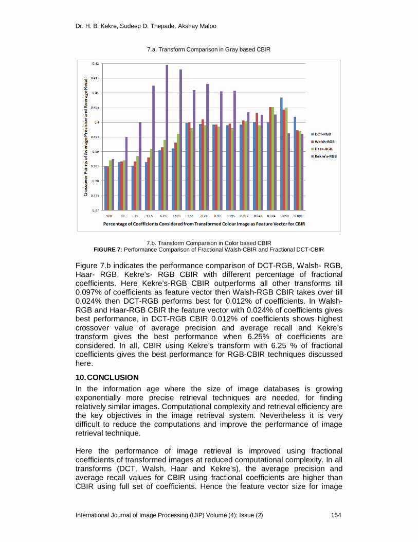
Dr. H. B. Kekre, Sudeep D. Thepade, Akshay Maloo
International Journal of Image Processing (IJIP) Volume (4): Issue (2) 154
7.a. Transform Comparison in Gray based CBIR
7.b. Transform Comparison in Color based CBIR FIGURE 7: Performance Comparison of Fractional Walsh-CBIR and Fractional DCT-CBIR
Figure 7.b indicates the performance comparison of DCT-RGB, Walsh- RGB, Haar- RGB, Kekre’s- RGB CBIR with different percentage of fractional coefficients. Here Kekre’s-RGB CBIR outperforms all other transforms till 0.097% of coefficients as feature vector then Walsh-RGB CBIR takes over till 0.024% then DCT-RGB performs best for 0.012% of coefficients. In Walsh-RGB and Haar-RGB CBIR the feature vector with 0.024% of coefficients gives best performance, in DCT-RGB CBIR 0.012% of coefficients shows highest crossover value of average precision and average recall and Kekre’s transform gives the best performance when 6.25% of coefficients are considered. In all, CBIR using Kekre’s transform with 6.25 % of fractional coefficients gives the best performance for RGB-CBIR techniques discussed here.
10. CONCLUSION In the information age where the size of image databases is growing exponentially more precise retrieval techniques are needed, for finding relatively similar images. Computational complexity and retrieval efficiency are the key objectives in the image retrieval system. Nevertheless it is very difficult to reduce the computations and improve the performance of image retrieval technique. Here the performance of image retrieval is improved using fractional coefficients of transformed images at reduced computational complexity. In all transforms (DCT, Walsh, Haar and Kekre’s), the average precision and average recall values for CBIR using fractional coefficients are higher than CBIR using full set of coefficients. Hence the feature vector size for image

Dr. H. B. Kekre, Sudeep D. Thepade, Akshay Maloo
International Journal of Image Processing (IJIP) Volume (4): Issue (2) 155
retrieval could be greatly reduced, which ultimately will result in faster query execution in CBIR with better performance. In all Kekre’s transform with fractional coefficients (3.125 % in Gray and 6.25 % in RGB) gives best performance with highest crossover points of average precision and average recall. Feature extraction using Kekre’s transform is also computationally lighter as compared to DCT or Walsh transform. Thus feature extraction in lesser time is possible with increased performance. Finally the conclusion that the fractional coefficients gives better discrimination capability in CBIR than the complete set of transformed coefficients and image retrieval with better performance at much faster rate can be done from the proposed techniques and experimentation done.
11. REFERENCES 1. H.B.Kekre, Sudeep D. Thepade, “Improving the Performance of Image Retrieval using
Partial Coefficients of Transformed Image”, International Journal of Information Retrieval (IJIR), Serials Publications, Volume 2, Issue 1, 2009, pp. 72-79(ISSN: 0974-6285)
2. H.B.Kekre, Sudeep D. Thepade, “Image Retrieval using Augmented Block Truncation Coding Techniques”, ACM International Conference on Advances in Computing, Communication and Control (ICAC3-2009), pp. 384-390, 23-24 Jan 2009, Fr. ConceicaoRodrigous College of Engg., Mumbai. Is uploaded on online ACM portal.
3. H.B.Kekre, Sudeep D. Thepade, “Scaling Invariant Fusion of Image Pieces in Panorama Making and Novel Image Blending Technique”, International Journal on Imaging (IJI), www.ceser.res.in/iji.html, Volume 1, No. A08, pp. 31-46, Autumn 2008.
4. Hirata K. and Kato T. “Query by visual example – content-based image retrieval”, In Proc. of Third International Conference on Extending Database Technology, EDBT’92, 1992, pp 56-71
5. H.B.Kekre, Sudeep D. Thepade, “Rendering Futuristic Image Retrieval System”, National Conference on Enhancements in Computer, Communication and Information Technology, EC2IT-2009, 20-21 Mar 2009, K.J.Somaiya College of Engineering, Vidyavihar, Mumbai-77.
6. Minh N. Do, Martin Vetterli, “Wavelet-Based Texture Retrieval Using Generalized Gaussian Density and Kullback-Leibler Distance”, IEEE Transactions On Image Processing, Volume 11, Number 2, pp.146-158, February 2002.
7. B.G.Prasad, K.K. Biswas, and S. K. Gupta, “Region –based image retrieval using integrated color, shape, and location index”, International Journal on Computer Vision and Image Understanding Special Issue: Colour for Image Indexing and Retrieval, Volume 94, Issues 1-3, April-June 2004, pp.193-233.
8. H.B.Kekre, Sudeep D. Thepade, “Creating the Color Panoramic View using Medley of Grayscale and Color Partial Images ”, WASET International Journal of Electrical, Computer and System Engineering (IJECSE), Volume 2, No. 3, Summer 2008. Available online at www.waset.org/ijecse/v2/v2-3-26.pdf.
9. Stian Edvardsen, “Classification of Images using color, CBIR Distance Measures and Genetic Programming”, Ph.D. Thesis, Master of science in Informatics, Norwegian university of science and Technology, Department of computer and Information science, June 2006.
10. H.B.Kekre, Tanuja Sarode, Sudeep D. Thepade, “DCT Applied to Row Mean and Column Vectors in Fingerprint Identification”, In Proceedings of International Conference on Computer Networks and Security (ICCNS), 27-28 Sept. 2008, VIT, Pune.
11. Zhibin Pan, Kotani K., Ohmi T., “Enhanced fast encoding method for vector quantization by finding an optimally-ordered Walsh transform kernel”, ICIP 2005, IEEE International Conference, Volume 1, pp I - 573-6, Sept. 2005.
12. H.B.kekre, Sudeep D. Thepade, “Improving ‘Color to Gray and Back’ using Kekre’s LUV Color Space”, IEEE International Advanced Computing Conference 2009 (IACC’09), Thapar University, Patiala, INDIA, 6-7 March 2009. Is uploaded and available online at IEEE Xplore.

Dr. H. B. Kekre, Sudeep D. Thepade, Akshay Maloo
International Journal of Image Processing (IJIP) Volume (4): Issue (2) 156
13. H.B.Kekre, Sudeep D. Thepade, “Image Blending in Vista Creation using Kekre's LUV Color Space”, SPIT-IEEE Colloquium and International Conference, Sardar Patel Institute of Technology, Andheri, Mumbai, 04-05 Feb 2008.
14. H.B.Kekre, Sudeep D. Thepade, “Color Traits Transfer to Grayscale Images”, In Proc.of IEEE First International Conference on Emerging Trends in Engg. & Technology, (ICETET-08), G.H.Raisoni COE, Nagpur, INDIA. Uploaded on online IEEE Xplore.
15. http://wang.ist.psu.edu/docs/related/Image.orig (Last referred on 23 Sept 2008) 16. H.B.Kekre, Sudeep D. Thepade, “Using YUV Color Space to Hoist the Performance of
Block Truncation Coding for Image Retrieval”, IEEE International Advanced Computing Conference 2009 (IACC’09), Thapar University, Patiala, INDIA, 6-7 March 2009.
17. H.B.Kekre, Sudeep D. Thepade, ArchanaAthawale, Anant Shah, PrathmeshVerlekar, SurajShirke,“Energy Compaction and Image Splitting for Image Retrieval using Kekre Transform over Row and Column Feature Vectors”, International Journal of Computer Science and Network Security (IJCSNS),Volume:10, Number 1, January 2010, (ISSN: 1738-7906) Available at www.IJCSNS.org.
18. H.B.Kekre, Sudeep D. Thepade, ArchanaAthawale, Anant Shah, PrathmeshVerlekar, SurajShirke,“Walsh Transform over Row Mean and Column Mean using Image Fragmentation and Energy Compaction for Image Retrieval”, International Journal on Computer Science and Engineering (IJCSE),Volume 2S, Issue1, January 2010, (ISSN: 0975–3397). Available online at www.enggjournals.com/ijcse.
19. H.B.Kekre, Sudeep D. Thepade,“Image Retrieval using Color-Texture Features Extracted from Walshlet Pyramid”, ICGST International Journal on Graphics, Vision and Image Processing (GVIP), Volume 10, Issue I, Feb.2010, pp.9-18, Available online www.icgst.com/gvip/Volume10/Issue1/P1150938876.html
20. H.B.Kekre, Sudeep D. Thepade,“Color Based Image Retrieval using Amendment Block Truncation Coding with YCbCrColor Space”, International Journal on Imaging (IJI), Volume 2, Number A09, Autumn 2009, pp. 2-14. Available online at www.ceser.res.in/iji.html (ISSN: 0974-0627).
21. H.B.Kekre, Tanuja Sarode, Sudeep D. Thepade,“Color-Texture Feature based Image Retrieval using DCT applied on Kekre’s Median Codebook”, International Journal on Imaging (IJI), Volume 2, Number A09, Autumn 2009,pp. 55-65. Available online at www.ceser.res.in/iji.html (ISSN: 0974-0627).
22. H.B.Kekre, Sudeep D. Thepade, “Image Retrieval using Non-Involutional Orthogonal Kekre’s Transform”, International Journal of Multidisciplinary Research and Advances in Engineering (IJMRAE), Ascent Publication House, 2009, Volume 1, No.I, pp 189-203, 2009. Abstract available online at www.ascent-journals.com (ISSN: 0975-7074)
23. H.B.Kekre, Sudeep D. Thepade, “Boosting Block Truncation Coding using Kekre’s LUV Color Space for Image Retrieval”, WASET International Journal of Electrical, Computer and System Engineering (IJECSE), Volume 2, Number 3, pp. 172-180, Summer 2008. Available online at http://www.waset.org/ijecse/v2/v2-3-23.pdf
24. H.B.Kekre, Sudeep D. Thepade, Archana Athawale, Anant Shah, Prathmesh Verlekar, Suraj Shirke, “Performance Evaluation of Image Retrieval using Energy Compaction and Image Tiling over DCT Row Mean and DCT Column Mean”, Springer-International Conference on Contours of Computing Technology (Thinkquest-2010), BabasahebGawde Institute of Technology, Mumbai, 13-14 March 2010, The paper will be uploaded on online Springerlink.
25. H.B.Kekre, Tanuja K. Sarode, Sudeep D. Thepade, VaishaliSuryavanshi,“Improved Texture Feature Based Image Retrieval using Kekre’s Fast Codebook Generation Algorithm”, Springer-International Conference on Contours of Computing Technology (Thinkquest-2010), BabasahebGawde Institute of Technology, Mumbai, 13-14 March 2010, The paper will be uploaded on online Springerlink.
26. H.B.Kekre, Tanuja K. Sarode, Sudeep D. Thepade, “Image Retrieval by Kekre’s Transform Applied on Each Row of Walsh Transformed VQ Codebook”, (Invited), ACM-International Conference and Workshop on Emerging Trends in Technology (ICWET 2010),Thakur College of Engg. And Tech., Mumbai, 26-27 Feb 2010, The paper is invited at ICWET 2010. Also will be uploaded on online ACM Portal.
27. H.B.Kekre, Sudeep D. Thepade, AkshayMaloo, “Image Retrieval using Fractional Coefficients of Transformed Image using DCT and Walsh Transform”, IJEST.
28. Haar, Alfred, “ZurTheorie der orthogonalenFunktionensysteme”. (German), MathematischeAnnalen, volume 69, No. 3, 1910, pp. 331–371.

Dr. H. B. Kekre, Sudeep D. Thepade, Akshay Maloo
International Journal of Image Processing (IJIP) Volume (4): Issue (2) 157
29. Charles K. Chui, “An Introduction to Wavelets”, Academic Press, 1992, San Diego, ISBN 0585470901.
30. H. B. Kekre, Tanuja K. Sarode, V. A. Bharadi, A. Agrawal. R. Arora,, M. Nair, “Performance Comparison of Full 2-D DCT, 2-D Walsh and 1-D Transform over Row Mean and Column Mean for Iris Recognition” International Conference and Workshop on Emerging Trends in Technology (ICWET 2010) – 26-27 February 2010, TCET, Mumbai, India.
31. M.C. Padma,P. A. Vijaya, “Wavelet Packet Based Features for Automatic Script Identification”, International Journal Of Image Processing (IJIP), CSC Journals, 2009, Volume 4, Issue 1, Pg.53-65.

Ratika Pradhan, Shikhar Kumar, Ruchika Agarwal, Mohan P. Pradhan & M. K. Ghose
International Journal of Image Processing (IJIP), Volume (4): Issue (2) 156
Contour Line Tracing Algorithm for Digital Topographic Maps Ratika Pradhan [email protected] Department of CSE, SMIT, Rangpo, Sikkim, INDIA Shikhar Kumar [email protected] Department of CSE, SMIT, Rangpo, Sikkim, INDIA Ruchika Agarwal [email protected] Department of CSE, SMIT, Rangpo, Sikkim, INDIA Mohan P. Pradhan [email protected] Department of CSE, SMIT, Rangpo, Sikkim, INDIA M. K. Ghose [email protected] Department of CSE, SMIT, Rangpo, Sikkim, INDIA
Abstract Topographic maps contain information related to roads, contours, landmarks, land covers and rivers etc. For any Remote sensing and GIS based project, creating a database using digitization techniques is a tedious and time consuming process especially for contour tracing. Contour line is very important information that these maps provide. They are mainly used for determining slope of the landforms or rivers. These contour lines are also used for generating Digital Elevation Model (DEM) for 3D surface generation from any satellite imagery or aerial photographs. This paper suggests an algorithm that can be used for tracing contour lines automatically from contour maps extracted from the topographical sheets and creating a database. In our approach, we have proposed a modified Moore’s Neighbor contour tracing algorithm to trace all contours in the given topographic maps. The proposed approach is tested on several topographic maps and provides satisfactory results and takes less time to trace the contour lines compared with other existing algorithms. Keywords: Topographic map, Contour line, Tracing, Moore neighborhood, Digital Elevation Map (DEM)
1. INTRODUCTION Topographic map is a type of map that provides detailed and graphical representation of natural features on the ground. Topographic maps conventionally show topography, or land contours, by means of contour lines. These maps usually show not only the contours, but also any significant streams, other water bodies, forest covers, built-up areas or individual buildings (depending on scale) and other features. These maps are taken as reference or base map for many Remote Sensing and GIS based application for generating thematic maps like drainage maps, slope maps, road maps, land cover maps etc. The important and distinct characteristic of these maps is that the earth’s surface can be mapped using contour lines. Digitization or vectorization process for generating contour map for a state like Sikkim where there is large variation of slope takes tremendous amount of time and manpower. Many research works are currently being conducted

Ratika Pradhan, Shikhar Kumar, Ruchika Agarwal, Mohan P. Pradhan & M. K. Ghose
International Journal of Image Processing (IJIP), Volume (4): Issue (2) 157
in this field to automate the entire digitization process. Till today, a fully automated digitization process does not provide satisfactory result.
Contour lines are imaginary lines that join points of equal elevation on the earth’s surface with reference to mean sea level or curves that connect contiguous points of the same altitude (isohypse). These lines are depicted brown in color in topographic maps, and are smooth and continuous curves with a width of three to four pixels. These lines runs almost parallel or they may be taken as nonintersecting lines except in steep cliffs. However, along with contour line, the topographic maps also contain text information overlaid on these lines. This makes the entire automation of extracting and tracing contour lines from the contour maps more complex and difficult.
Traditional method for vectorization of contour line involves mainly the following steps: Scanning paper topographic maps using high resolution scanner. Registration of one or more maps with reference to the nearest datum. Mosaicing or stitching various topographic maps. Vectorization of various contour lines manually using line tracing by rubber band method. Feeding depth information for each contour line. Generating digital elevation models (DEM) for 3D surface reconstruction.
Uses of computer and digital topographic maps have made the task simpler. Currently research is being carried out on automatic extraction of contour lines from topographic maps that involves following five main tasks.
Registration of topographic map. Filtering for enhancing map. Color segmentation for extracting contour lines. Thinning and pruning the binary images. Raster to vector conversion.
The proposed work suggests a method that efficiently extracts contour lines, performs tracing of contour lines and prepares a database wherein user can feed the height value interactively. In this paper, we have proposed a modified Moore’s Neighbor contour tracing algorithm to trace all contours in the given topographic maps. The content of the paper is organized as follows. In section II we have summarized the related work carried out in this area. In section III, we have discussed contour extraction and thinning algorithm. In section IV, we have discussed the original Moore’s Neighbor contour tracing algorithm, followed by Modified Moore’s Neighbor Algorithm in section V. Result and discussion in section VI provides detail result for study area and comparison of these two algorithms. Finally Conclusion and future scope is given in section VII.
2. RELATED WORK Many researchers have indulged themselves to come up with a technique to completely automate information extraction from topographic maps. Leberl and Olson [1] have suggested a method that involves the entire four tasks mentioned above for automatic vectorization of clean contour and drainage. Greenle [2] have made an attempt to extract elevation contour lines from topographic maps. Soille and Arrighi [3] have suggested image based approach using mathematical morphology operator to reconstruct contour lines. Most of these procedures fail at discontinuities. Frischknecht [4] have used hierarchical template matching algorithm for extracting text but fails to extract contour lines. Spinello [5] have used geometric properties to recognize the contour line that is based on global topology. It uses Delaunay triangulation to thin and vectorize contour line. Zhou and Zhen [6] have proposed deformable model and field flow orientation method for extracting contour lines. Dongjun et.al [7] has suggested a method based on Generalized Gradient Vector Flow (GGVF) snake model to extract contour lines. In this paper we have extended the work of Dongjun et.al [7] to trace the contour lines more efficiently and automatically using Modified Moore’s Neighbor tracing algorithm. It also prepares databases of these contour lines to feed the elevation value interactively. Since the topology of contour lines
Ratika Pradhan, Shikhar Kumar, Ruchika Agarwal, Mohan P. Pradhan & M. K. Ghose
International Journal of Image Processing (IJIP), Volume (4): Issue (2) 158
are well defined i.e. a set of non-intersecting closed lines, it makes the tracing of contour lines simpler.
There exists many contour tracing algorithms - Square tracing, Moore neighbor, Radial sweep, Theo Pavlidis’ tracing algorithms[8] etc. but each algorithm has its own pros and cons. Most of these algorithms fail to trace the contour of a large class of patterns due to their special kind of connectivity i.e. contour family of 8 connected patterns (that are not 4 connected). Disadvantage of these algorithms are that they do not trace holes present in the pattern. Hole searching algorithms are first used to extract holes and then tracing algorithms are applied to each hole in order to trace the complete contour. Another problem with this algorithm is defining the stopping criterion for terminating an algorithm.
3. CONTOUR EXTRACTION AND THINNING Contours are depicted as brown colored line in topographic maps usually of width four to five pixel length. After removing noise in the input images, we have used color segmentation technique to extract all the information given in brown color. There are many color spaces widely used to view digital images but most commonly RGB color space is used for the satellite imagery as it possesses compatibility with the computer displays. Since this color space is not perceptually uniform, selecting range of values for brown color in all the three bands is difficult and does not give satisfactory end result, therefore we have first transformed the satellite imagery from RGB to HSV color space and then color segmentation was performed on HSV color space. The color segmentation algorithm is given below: ALGORITHM Color Segmentation on HSV color space Input: A square tessellation T containing a connected component P of pixels in HSV color space. Output: A sequence B(b1, b2, …, bk) of brown colored pixels. Begin
Set B to be empty. From bottom to top and left to right scan the cells of T until a pixel, s, of P is found. Set the current pixel point, c, to s i.e. c = s. While c is not in B do
If hue_range of c between 0 to 0.11 and saturation_range of c between 0.2 to 0.7 o Insert c in B.
End if Advance c to the next pixel in P.
End while End The segmented information includes contours and altitude information. The filtered or segmented image is then thinned using morphological thinning algorithm [9] given below.
Divide the image into two distinct subfields in a checkerboard pattern.
In the first sub-iteration, delete pixel p from the first subfield if and only if the conditions G1, G2, and G3 are all satisfied.
In the second sub-iteration, delete pixel p from the second subfield if and only if the conditions G1, G2, and G3' are all satisfied.
Condition G1:

Ratika Pradhan, Shikhar Kumar, Ruchika Agarwal, Mohan P. Pradhan & M. K. Ghose
International Journal of Image Processing (IJIP), Volume (4): Issue (2) 159
(1) where
(2)
(3) x1, x2, ..., x8 are the values of the eight neighbors of p, starting with the east neighbor and numbered in counter-clockwise order. Condition G2:
(4) where
(5)
(6)
Condition G3:
(7) Condition G3':
(8) The processed image thus obtained contains broken contour lines, we have used broken contour lines reconnection algorithm [7] based on GGVF to connect the gaps in contour lines. 4. MOORE NEIGHBOR CONTOUR TRACING ALGORITHM Moore Neighborhood of a pixel, P, is the set of 8 pixels which share a vertex or an edge with that pixel. The basic idea is: - When the current pixel p is black, the Moore neighborhood of p is examined in clockwise direction starting with the pixel from which p was entered and advancing pixel by pixel until a new black pixel in P is encountered. The algorithm terminates when the start pixel is visited for second time. The black pixel walked over will be the contour of the pattern.

Ratika Pradhan, Shikhar Kumar, Ruchika Agarwal, Mohan P. Pradhan & M. K. Ghose
International Journal of Image Processing (IJIP), Volume (4): Issue (2) 160
FIGURE 1: Working of Moore’s Neighbor tracing algorithm.
The main weakness of Moore Neighbor tracing lies in the choice of stopping criteria i.e. visiting the start pixel for second time. If the algorithm depends on this criterion all the time it fails to trace contour of large family of patterns. Mostly it uses Jacob’s stopping criterion i.e.
i. Stop after visiting the start pixel n times, where n is at least 2, or
ii. Stop after visiting the start pixel second time.
Figure 1 demonstrates the working of Moore Neighbor contour tracing algorithm for an input pattern. In figure, line number indicates the iteration number of traversal. For the input pattern, start pixel is encountered three times when the algorithm ends.
5. MODIFIED MOORE NEIGHBOR CONTOUR TRACING ALGORITHM The original Moore Neighbor tracing algorithm is defined for contours of multiple pixel width. It requires either visiting start pixel 2 times or use Jacob’s stopping criteria to terminate the algorithm. In our algorithm the basic idea is: - When the current pixel is black, the Moore neighborhood of P is examined in clockwise direction till no more black pixels are encountered. Then, we move to the start pixel and the Moore Neighborhood of P is examined in an anti-clockwise direction until no new black pixels are left. The algorithm for the Modified Moore’s Neighbor tracing is given below:
ALGORITHM Modified Moore’s neighbor algorithm Input: A square tessellation T containing a connected component P of black cells. Output: A sequence B(b1, b2, …, bk) of boundary pixels i.e. the contour line. We define M(p) to be the Moore neighborhood of pixel p, c denotes the current pixel under consideration i.e. c is in M(p). Begin
Set B to be empty. From bottom to top and left to right scan the cells of T until a black pixel, s, of P is found. Insert s in B. Set the current boundary point, p, to s i.e. p = s. Set c to be the next clockwise pixel in M(p).

Ratika Pradhan, Shikhar Kumar, Ruchika Agarwal, Mohan P. Pradhan & M. K. Ghose
International Journal of Image Processing (IJIP), Volume (4): Issue (2) 161
While c is not in B do If c is black
o Insert c in B. o Set p=c.
End if Advance c to the next clockwise pixel in M(p).
End while Set B to be empty. Insert s in B. Set p=s. Set c to the next anticlockwise pixel in M(p). While c is not in B do
If c is black o Insert c in B. o Set p=c.
End if Advance c to the next anticlockwise pixel in M(p).
End while End
FIGURE 2: Working of Modified Moore’s Neighbor tracing algorithm.
Figure 2 demonstrate the working of Modified Moore’s Neighbor tracing algorithm. Line number in the figure indicates the pixels from where they are traced from. The algorithm terminates when no more black pixel in an input pattern is left. Unlike original Moore’s Neighbor tracing algorithm back tracking is not used here and is not dependent on the stopping criterion used by original Moore algorithm or Jacob stopping criterion. The start pixel is encountered only twice for terminating the algorithm for every pattern.
6. RESULTS AND DISCUSSION The study area taken into consideration is in and around Majitar, East Sikkim, situated between 27o09’00” and 28o13’48” north latitudes and 88o29’24” and 88o36’00” east longitude. The

Ratika Pradhan, Shikhar Kumar, Ruchika Agarwal, Mohan P. Pradhan & M. K. Ghose
International Journal of Image Processing (IJIP), Volume (4): Issue (2) 162
topographic map for the study area is on scale of 1:250000. Figure 3(a) is the topographic map of the study area. Figure 3(b) is the result of applying color segmentation algorithm. Figure 3(c) is the result of applying broken contour lines reconnection algorithm based on GGVF followed by thinning. 3(d) is the result of Moore Neighbor tracing using Jacob stopping criterion, 3(e) is the result of Modified Moore Neighbor tracing algorithm. Table 1 is the database prepared for the contour map traced using proposed method.
The efficiency of any algorithm entirely depends on the choice of stopping criterion. Original Moore Neighbor tracing algorithm using Jacob stopping criterion that needs N + (n-1) * (N-1) pixels to be traversed, where n is the number of times that the start pixel is visited and N is the number of black pixels that forms a contour line. The choice of scanning anticlockwise after we move to the start pixel in our algorithm is to avoid detection of black pixels already encountered in the clockwise scanning. Since we do not use backtracking, for every detection of black pixel, there is a maximum overhead of checking 6 pixel locations (worst case) before finding a black pixel. Using the Moore-neighbor algorithm, since the algorithm has to retrace the start pixel, there is an overhead of redetection of each and every already traced pixel.
In Modified Moore Neighbor algorithm we have removed the dependency of reaching the start pixel in order to stop the algorithm i.e. start pixel is no longer required as a landmark to indicate the end of algorithm. The proposed algorithm does not require hole searching algorithm to detect holes in the input pattern. The drawback of this algorithm however is consistent checking of every pixel encountered in the Moore Neighbor to decide whether it has been encountered before or not. For very large size images, checking pixels every time could be time consuming and costly. Another disadvantage of the algorithm is that it works only on contour lines of single pixel width. Hence the extracted contour map has to undergo thinning.
Figure3 a) Topographic map of the study area b) Contour Extraction using Color Segmentation c) Contour reconstructed using broken contour lines reconnection algorithm [7] based on GGVF d) Result obtained using Original Moore’s Neighbor tracing algorithms where holes are not detected e) Results obtained using Modified Moore’s Neighbor tracing algorithms with detected holes.

Ratika Pradhan, Shikhar Kumar, Ruchika Agarwal, Mohan P. Pradhan & M. K. Ghose
International Journal of Image Processing (IJIP), Volume (4): Issue (2) 163
No. of contours: 42 Starting Point End Point
Serial No: x y X Y Elevation
1 15 635 16 471 4000 2 15 598 16 494 3600 3 15 562 16 515 3200 4 15 446 52 644 2800 5 15 433 108 646 2400 . . . . . . . . . . . .
. . . . . .
TABLE 1: Database generated for the result obtained.
7. CONCLUSION AND FUTURE WORK The Modified Moore Neighbor algorithm works on pre-thinned contour lines (single pixel width). Its efficiency over the original Moore Neighbor algorithm lies in the stopping criterion as the complexity is greatly reduced and hole searching algorithm is not required which further reduces the time complexity. In order to overcome the disadvantage of rechecking black pixels in proposed algorithm, we can check whether the contour line on which the pixel exists has been traced or not rather than checking the pixel. This work can be refined further by automatically extracting altitude value from the topographic sheet by using and automated OCR method.
8. ACKNOWLEDGMENT We would like to thank All India Council for Technical Education (AICTE) for funding the project title “Contour Mapping and 3D Surface Modeling of State Sikkim” fully sponsored by All India Council of Technical Education, Govt. of India vide order no- 8023/BOR/RID/RPS-44/2008-09. We also like to thank Dr. A. Jeyaram, Head, Regional Remote Sensing Service Centre (RRSSC), IIT campus, Kharagpur for his valuable comments and support.
9. REFERENCES [1] F. Leberl, D. Olson, “Raster scanning for operatioal digitizing of graphical data”,
Photogrammetric Engineering and Remote Sensing, 48(4), pp. 615-627,1982. [2] D. Greenle, “Raster and Vector Processing for Scanned line work”, Photogrammetric and
Remote Sensing, 53(10), pp. 1383-1387, 1987. [3] P. Soille, P Arrighi, “From Scanned Topographic Maps to Digital Elevation Models”, Proc. of
Geovision, International Symposium on Imaging Appications in Geology, pp.1-4,1999. [4] S. Frischknecht, E. Kanani, “Automatic Interpretation of Scanned Topographic Maps: A
Raster – Based Approach”, Proc.Second International Workshop, GREC, pp.207-220, 1997. [5] S. Salvatore, P. Guitton, “Contour Lines Recognition from Scanned Topographic Maps”,
Journal of WSCG, pp. 1-3, 2004. [6] X. Z. Zhou, H. L. Zhen, “Automatic vectorization of comtour lines based on Deformable model
and Field Flow Orirntation”, Chiense Journal of Computers,vol 8, pp. 1056-1063, 2004. [7] Dongjum Xin, X. Z. Zhou, H.L.Zhen, “Contour Line Extraction from Paper- based Topographic
Maps”. [8] G. Toussaint, Course Notes: Grids, connectivity and contour Tracing
<http://jeff.cs.mcgill.ca/~godfried/teaching/pr-notes/contour.ps>. [9] Lam, L., Seong-Whan Lee, and Ching Y. Suen, "Thinning Methodologies-A Comprehensive
Survey," IEEE Transactions on Pattern Analysis and Machine Intelligence, Vol 14, No. 9, September 1992, page 879.
Hiremath P S & Kodge B G
International Journal of Image Processing (IJIP) Volume (4): Issue (2) 164
Automatic Extraction of Open Space Area from High Resolution Urban Satellite Imagery
Hiremath P. S. [email protected] Department of Computer Science Gulbarga University Gulbarga- 585106, Karnataka State, INDIA Kodge B. G. [email protected] Department of Computer Science S. V. College UDGIR – 413517, Maharashtra State, INDIA
Abstract
In the 21st century, Aerial and satellite images are information rich. They are also complex to analyze. For GIS systems, many features require fast and reliable extraction of open space area from high resolution satellite imagery. In this paper we will study efficient and reliable automatic extraction algorithm to find out the open space area from the high resolution urban satellite imagery. This automatic extraction algorithm uses some filters and segmentations and grouping is applying on satellite images. And the result images may use to calculate the total available open space area and the built up area. It may also use to compare the difference between present and past open space area using historical urban satellite images of that same projection. Keywords: Automatic open space extraction, Image segmentation, Feature extraction, Remote sensing
1. INTRODUCTION Extraction of open space area from raster images is a very important part of GIS features such as GIS updating, geo-referencing and geo spatial data integration. However extracting open space area from raster image is a time consuming operation when performed manually, especially when the image is complex. The automatic extraction of open space area is critical and essential to the fast and effective processing of large number of raster images in various formats, complexities and conditions.
How open space area are extracted properly from raster images depend on how open space area appear in raster image. In this paper, we study automatic extraction of open space area from high resolution urban area satellite image. A high resolution satellite image typically has a resolution of 0.5 to 1.0 m. Under such high resolution, an open space is not same any more in whole image, instead, objects such as lake(s), trees are easily identifiable. This class of images contains very rich information and when fused with vector map can provide a comprehensive view of a geographical area. Google, Yahoo, and Virtual Earth maps are good examples to demonstrate the power of such high resolution images. However, high resolution images pose great challenges for automatic feature extraction due to the inherent complexities. First, a typical aerial photo captures everything in the area such as buildings, cars, trees, open space area, etc. Second, different objects are not isolated, but mixed and interfere with each other, e.g., the shadows of trees on the road, building tops with similar materials. Third, roads may even look

Hiremath P S & Kodge B G
International Journal of Image Processing (IJIP) Volume (4): Issue (2) 165
quite differently within the same image, due to their respective physical properties. Assuming all open space area have the same characteristics will fail to extract total open space area. In addition, the light and weather conditions have big impact over images. Therefore, it is impossible to predict what and where objects are, and how they look like in a raster image. All these uncertainties and complexities make the extraction very difficult. Due to its importance, much effort has been devoted to this problem [3, 4]. Unfortunately, there are still no existing methods that can deal with all these problems effectively and reliably. Some typical high resolution images are shown in Figure 1 and they show huge difference among them in terms of the color spectrum and noise level. There are numerous factors that can distort the edges, including but not limited to blocking objects such as trees and shadows, surrounding objects in similar colors such as roof tops. As a matter of fact, the result of edge detection is as complicated as the image itself. Edges of open space area are either missing or broken and straight edges correspond to buildings, as shown in Figure 2. Therefore, edge-based extraction schemes will all fail to produce reliable results under such circumstances.
FIGURE 1(A): An aerial photo for an area in the Latur city
FIGURE 1(B): High resolution urban satellite image. (Image of Latur city, dated 23 Feb. 2003)

Hiremath P S & Kodge B G
International Journal of Image Processing (IJIP) Volume (4): Issue (2) 166
FIGURE 1(c): Google map satellite image.
FIGURE 1: Examples of high resolution images.
In this paper, we develop an integrated scheme for automatic extraction that exploits the inherent nature of open space area. Instead of relying on the edges to detect open space, it tries to find the pixels that belong to the same open area region based on how they are related visually and geometrically. Studies have shown that the visual characteristic of a open space is heavily influenced by its physical characteristics such as material, surface condition. It is impossible to define a common pattern just based on color or spectrum to uniquely identify the open space area. In our scheme, we consider a open space as a group of “similar” pixels. The similarity is defined in the overall shape of the region they belong to, the spectrum they share, and the geometric property of the region. Different from edge-based extraction schemes, the new scheme first examines the visual and geometric properties of pixels using a new method. The pixels are identified to represent each region. All the regions are verified based on the general visual and geometric constraints associated with a open space area. Therefore, the roof top of a building or a long strip of trees is not misidentified as a open space area segment. There is also no need to assume or guess the color spectrum of open space area, which varies greatly from image to image according to the example images.
FIGURE 2: Edge extraction (using canny method) of Fig. 1 (b).
As illustrated by examples in Figure 1, an open space area is not always a contiguous region of regular linear shape, but a series of segments with no constant shapes. This is because each

Hiremath P S & Kodge B G
International Journal of Image Processing (IJIP) Volume (4): Issue (2) 167
segment may include pixels of surrounding objects in similar colors or miss some of its pixels due to interference of surrounding objects. A reliable extraction scheme must be able to deal with such issues. In the following sections, we will discuss how to capture the essence of “similarity”, translate them and finally turn them into display.
2. AUTOMATIC EXTRACTION SCHEME The goal of the proposed system is to develop a complete and practical automatic solution to the extraction of open space area problem for high resolution aerial/satellite images.
The first stage extracts open space areas that are relatively easier to identify such as major grounds and the second stage deals with open space that are harder to identify. The reason for such design is a balance between reliability and efficiency. Some open space areas are easier to identify because they are more identifiable and contain relatively less noise. Since some open space area in the same image share some common visual characteristics, the information from the already extracted area and other objects, such as spectrum, can be used to simplify the process of identifying open space area that are less visible or heavily impacted by surrounding objects or by different colors. Otherwise, such areas are not easily distinguishable from patterns formed by other objects. For example, a set of collinear blocks may correspond to a open space or a group of buildings (houses) from the same block. The second stage also serves an important purpose to fill the big gaps for open space extracted in stage one. Under some severe noise, part of the area may be disqualified as valid open space region and hence missed in stage one, leaving some major gaps in open space area edges. With the additional spectrum information, these missed areas can be easily identified to complete the open space area extraction. Therefore, the two stage process eliminates the need to assume or guess the color spectrum of open space and allow them to extract much more complete.
FIGURE 3: Automatic extraction scheme.
Each major stage consists of the following three major steps: filtering, grouping and optimization, as shown in Figure 3. The details of each step will be discussed in the following section.

Hiremath P S & Kodge B G
International Journal of Image Processing (IJIP) Volume (4): Issue (2) 168
3. ALGORITHM In this paper, we assume images to satisfy the following two general assumptions. These two assumptions are derived based on the minimum conditions for open space area to be identifiable and therefore are easily met by most images.
• Visual constraint: majority of the pixels from the same open space area have similar spectrum that is distinguishable from most of the surrounding areas; • Geometric constraint: a open space is a region that is relatively has no standard shape, compared with other objects in the image;
These two constraints are different from the assumption. The visual constraint does not require a open space region to have single color or constant intensity. It only requires blank area to look visually different from surrounding objects in most parts. The geometric constraint does not require a smooth edge, only the overall shape to be a long narrow strip. So these conditions are much weaker and a lot more practical. As we can see, these assumptions can accommodate all the difficult issues very well, including blurring, broken or missing edge of open area boundaries, heavy shadows, and interfering surrounding objects. 3.1 Filtering The step of filtering is to identify the key pixels that will help determine if the region they belong to is likely an open space area segment. Based on the assumption of visual constraint, it is possible to establish an image segmentation using methods of edge detection. Notice that such separation of regions is required to be precise and normally contains quite a lot of noise. In the best, the boundaries between regions are a set of line segments for most images, as is the case shown in Figure 2. It certainly does not tell which region corresponds to which area and which is not based on the extracted edges. As a matter of fact, most of the regions are not completely separated by edges and are still interconnected based on 4-connect path or 8-connect path. In order to fully identify and separate open space regions from the rest of image, we proposed to invert them and again extract the edges using Sobel edge detector to highlight sharp changes in intensity in the active image or selection. Two 3x3 convolution kernels (show below) are used to generate vertical and horizontal derivatives. The final image is produced by combining the two derivatives using the square root of the sum of the squares.
FIGURE 4: Result after edge detection & outlier removal of figure 2.

Hiremath P S & Kodge B G
International Journal of Image Processing (IJIP) Volume (4): Issue (2) 169
1 2 1 1 0 -1 0 0 0 2 0 -2
-1 -2 -1 1 0 -1 The next step is a removal of outliers through we can replace a pixel by the median of the pixels in the surrounding if it deviates from the median by more than a certain value (the threshold). We used the following values for outlier removal.
R = 10.0 pixels, T = 2, OL = Bright R is Radius determines the area used for calculating the median (uncalibrated, i.e., in pixels). See Fig. 4 how radius translates into an area. The T (Threshold) determinates by how much the pixel must deviate from the median to get replaced, in raw (uncalibrated) units. Which Outlier OL determines whether pixels brighter or darker than the surrounding (the median) is replaced. 3.2 Segmentation The step of segmentation is to verify which region is a possible road region based on the central pixels. Central pixels contain not only the centerline information of a region, but also the information of its overall geometric shape. For example, a perfect square will only have one central pixel at its center. A long narrow strip region will have large number of central pixels. Only regions with ratios above certain thresholds are considered to be candidate regions. In order to filter out interference as much as possible for reliable extraction during the first major stage, a minimum region width can be imposed. This will effectively remove most of the random objects from the image. However, such width constraint will be removed during the second major step as improper regions can also be filtered out based on the color spectrum information obtained from stage one. Therefore, small regions with close spectrum are examined for possible small open space area in the second stage. In addition to the geometry constraint, some general visual information can also be applied to filter out obvious non-open space regions. For example, if the image is a color image, most of the tree and grass areas are greenish. Also tree areas usually contain much richer textures than normal smooth road surfaces. The intensity transformation and spatial and frequency filtering can be used to filter out such areas. The minimum assumption of the proposed scheme does not exclude the use of additional visual information to further improve the quality of extraction if they are available. 3.3 Grouping and optimization As the result of segmentation, the open space area segments are typically incomplete and disconnected due to heavy noise.
FIGURE 5: Result after applying upper & lower threshold values.

Hiremath P S & Kodge B G
International Journal of Image Processing (IJIP) Volume (4): Issue (2) 170
The purpose of this step is to group corresponding open space area segments together in order to find the optimal results for required area extraction. if enough information is available to determine the open space area spectrum, then optimization is better applied after all the segments are identified. The fig. 5 is the result of threshold use to automatically or interactively set lower=0 and upper=48 threshold values, segmenting the image into features of interest and background. The threshold features are displayed in white and background is displayed in red color i.e. the total open space area in the given projected satellite image.
FIGURE 6 (A): Available open space area on Feb 18 2006.
FIGURE 6 (B): Available open space area on Jan 11 2008.
FIGURE 6: Extracted open space area (Red color) using available historical images.
The extracted open space area from high resolution urban satellite imagery is shown in figure 7 with region wise numbers. The total available open space region’s labels, area and centroids are calculated and shown in table 1.

Hiremath P S & Kodge B G
International Journal of Image Processing (IJIP) Volume (4): Issue (2) 171
FIGURE 7: Labeled regions of extracted open space area (Feb. 2003).
Following table 1 showing the details of calculated area and centroids x1, y1 of labeled regions of figure 7.
Centroids Labels
Area x1 y1
1
33757
414.899
265.154
2 4079 446.027 281.925 3 3559 437.167 261.494 4 28865 488.196 248.630 5 5890 455.214 276.307 6 4368 445.361 271.004 7 11221 449.157 282.151
TABLE 1: Area and centroids of labeled regions of figure 7.
FIGURE 8: Labeled regions of extracted open space area (Feb. 2006).
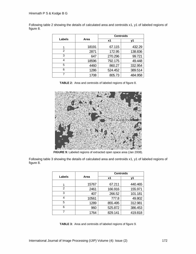
Hiremath P S & Kodge B G
International Journal of Image Processing (IJIP) Volume (4): Issue (2) 172
Following table 2 showing the details of calculated area and centroids x1, y1 of labeled regions of figure 8.
Centroids
Labels
Area x1 y1
1 18191 67.115 432.29 2 2871 172.95 138.836 3 647 270.296 99.721 4 18596 792.175 49.448 5 4460 860.27 332.954 6 1286 524.452 389.514 7 1708 805.73 484.958
TABLE 2: Area and centroids of labeled regions of figure 8.
FIGURE 9: Labeled regions of extracted open space area (Jan 2008).
Following table 3 showing the details of calculated area and centroids x1, y1 of labeled regions of figure 8.
Centroids Labels
Area x1 y1
1 15767 67.211 440.465 2 2461 166.916 155.971 3 407 266.52 101.181 4 10561 777.8 49.802 5 1289 855.495 312.981 6 960 525.872 386.453 7 1764 829.141 419.818
TABLE 3: Area and centroids of labeled regions of figure 9.

Hiremath P S & Kodge B G
International Journal of Image Processing (IJIP) Volume (4): Issue (2) 173
Based extracted areas from table 1, table 2, and table 3, the comparative study of open space area from existing historical images of year 2003, 2006 and 2008 is demonstrated below in the graph.
0
5000
10000
15000
20000
25000
30000
35000
40000
1 2 3 4 5 6 7
Labeled regions
Area
200320062008
Figure 10. Comparative results of extracted open space areas of imageries 2003, 2006 and 2008 respectively.
4. CONCLUSION In this paper, we proposed a new automatic system for extracting open space area and intersections from high resolution aerial and satellite images. The main contribution of the proposed system is to address the major issues that have caused all existing extraction approaches to fail, such as blurring boundaries, interfering objects, inconsistent area profiles, heavy shadows, etc. To address all these difficult issues, we develop a new method, namely automatic extraction of open space area from high resolution satellite imagery, to capture the essence of both visual and geometric characteristics of open space area. The extraction process including filtering, segmentation, and grouping and optimization, these processes eliminates the need to assume or guess the color spectrum of different open space areas. The proposed approach is efficient, reliable, and assumes no prior knowledge about the required open space area, conditions and surrounding objects. It is able to process complicated aerial/satellite images from a variety of sources including aerial photos from Google and Yahoo online maps. The quick application of the proposed study will helps to landing the helicopters in open space area.
5. REFERENCES 1. Y. Li, R. Briggs. Scalable and error tolerant automated georeferencing under affine transformations. IEEE International Geoscience and Remote Sensing Symposium, Boston, MA, July 2008.

Hiremath P S & Kodge B G
International Journal of Image Processing (IJIP) Volume (4): Issue (2) 174
2. Y. Li, R. Briggs. Automated georeferencing based on topological point pattern matching. The International Symposium on Automated Cartography (AutoCarto), Vancouver, WA, June 2006. 3. J.B. Mena. State of the Art on Automatic Road Extraction for GIS Update: a Novel Classification. Pattern Recognition Letters, 24(16):3037-3058, 2003. 4. M.-F. Auclair-Fortier, D. Ziou, C. Armenakis, and S. Wang. Survey of Work on Road Extraction in Aerial and Satellite Images. Technical Report 241, Département de mathématiques et d’informatique, Université de Sherbrooke, 1999. 5. G. Vosselman, J.D. Knecht. Road Tracking by Profile Matching and Kalman Filtering. Workshop on Automatic Extraction of Man-Made Objects from Aerial and Space Images, pages 265-274, 1995. 6. D.M. Mckeown, J.L. Denlinger. Cooperative Methods for Road Tracking in Aerial Imagery. Workshop Computer Vision Pattern Recognition, pages 662-672, 1988. 7. A. Gruen, H. Li. Semi-automatic Linear Feature Extraction by Dynamic Programming and LSB-Snakes. Photogrammet Eng. Remote Sensing 63, pages 985-995, 1997. 8. S.B. Hinz, A. Ebner. Modeling Contextual Knowledge for Controlling Road Extraction in Urban Areas. IEEE/ISPRS Joint Workshop Remote Sensing Data Fusion over Urban Areas, 2001. 9. T. Ohlhof, T. Emge, W. Reinhardt, K. Leukert, C. Heipke, K. Pakzad. Generation and Update of VMAP data using satellite and airbone imagery. Remote Sensing, vol 33, pages 763-768, 2000. 10. A. Baumgartner, C.T. Steger, H. Mayer, and W. Eckstein. Multi- Resolution, Semantic Objects, and Context for Road Extraction. In Wolfgang Förstner and Lutz Plümer, editors, Semantic Modeling for the Acquisition of Topographic Information from Images and Maps, pages 140–156, Basel, Switzerland, 1997. Birkhäuser Verlag. 11. A. Baumgartner, C.T. Steger, C. Wiedemann, H. Mayer, W. Eckstein, and H. Ebner. Update of Roads in GIS from Aerial Imagery: Verification and Multi-Resolution Extraction. Proceedings of International Archives of Photogrammetry and Remote Sensing, XXXI B3/III:53–58, 1996.

Sanghamitra Mohanty & Himadri Nandini Das Bebartta
International Journal of Image Processing (IJIP), Volume (4): Issue (2) 175
A Novel Approach for Bilingual (English - Oriya) Script Identification and Recognition in a Printed Document
Sanghamitra Mohanty [email protected] Faculty/Department of Computer Science Utkal University Bhubaneswar, 751004, India Himadri Nandini Das Bebartta [email protected] Scholar/ Department of Computer Science Utkal University Bhubaneswar, 751004, India
Abstract
In most of our official papers, school text books, it is observed that English words interspersed within the Indian languages. So there is need for an Optical Character Recognition (OCR) system which can recognize these bilingual documents and store it for future use. In this paper we present an OCR system developed for the recognition of Indian language i.e. Oriya and Roman scripts for printed documents. For such purpose, it is necessary to separate different scripts before feeding them to their individual OCR system. Firstly, we need to correct the skew followed by segmentation. Here we propose the script differentiation line-wise. We emphasize on Upper and lower matras associated with Oriya and absent in English. We have used horizontal histogram for line distinction belonging to different script. After separation different scripts are sent to their individual recognition engines. Keywords: Script separation, Indian script, Bilingual (English-Oriya) OCR, Horizontal profiles
1. INTRODUCTION Researchers have been emphasizing a lot of effort for pattern recognition since decades. Amongst the pattern recognition field Optical Character Recognition is the oldest sub field and has almost achieved a lot of success in the case of recognition of Monolingual Scripts. . In India, there are 24 official (Indian constitution accepted) languages. Two or more of these languages may be written in one script. Twelve different scripts are used for writing these languages. Under the three-language formula, some of the Indian documents are written in three languages namely, English, Hindi and the state official language. One of the important tasks in machine learning is the electronic reading of documents. All official documents, magazines and reports can be converted to electronic form using a high performance Optical Character Recognizer (OCR). In the Indian scenario, documents are often bilingual or multi-lingual in nature. English, being the link language in India, is used in most of the important official documents, reports, magazines and technical papers in addition to an Indian language. Monolingual OCRs fail in such contexts and there is a need to extend the operation of current monolingual systems to bilingual ones. This paper describes one such system, which handles both Oriya and Roman script. Recognition of bilingual documents can be approached by the following method i.e. Recognition via script identification. Optical Character Recognition (OCR) system of such a document page can be

Sanghamitra Mohanty & Himadri Nandini Das Bebartta
International Journal of Image Processing (IJIP), Volume (4): Issue (2) 176
made through the Development of a script separation scheme to identify different scripts present in the document pages and then run individual OCR developed for each script alphabets. Development of a generalized OCR system for Indian languages is more difficult than a single script OCR development. This is because of the large number of characters in each Indian script alphabet. On the other hand, second option is simpler for a country like India because of many scripts. There are many pieces of work on script identification from a single document. Spitz [1] developed a method to separate Han-based or Latin- based script separation. He used optical density distribution of characters and frequently occurring word shape characteristics for the purpose. Recently, using fractal-based texture features, Tan [5] described an automatic method for identification of Chinese, English, Greek, Russian, Malayalam and Persian text. Ding et al. [3] proposed a method for separating two classes of scripts: European (comprising Roman and Cyrillic scripts) and Oriental (comprising Chinese, Japanese and Korean scripts). Dhanya and Ramakrishnan [9] proposed a Gabor filter based technique for word-wise segmentation from bi-lingual documents containing English and Tamil scripts. Using cluster based templates; an automatic script identification technique has been described by Hochberg et al. [4]. Wood et al. [2] described an approach using filtered pixel projection profiles for script separation. Pal and Chaudhuri [6] proposed a line-wise script identification scheme from tri-language (triplet) documents. Later, Pal et al. [7] proposed a generalized scheme for line-wise script identification from a single document containing all the twelve Indian scripts. Pal et al. [8] also proposed some work on word-wise identification from Indian script documents.
All the above pieces of work are done for script separation from printed documents. In the proposed scheme, at first, the documents noise is cleared which we perform at the binarization stage and then the skew is detected and corrected. Using horizontal projection profile the document is segmented into lines. The line height for individual script is different. Along with this property one more uniqueness property in between the Roman and Oriya script is that each line consists of more number of Roman characters as compared to that of Oriya. Basing on these features we have taken a threshold value by dividing the line height of each line with the number of characters in a line. And after obtaining a unique value we sent these lines to their respective classifiers. The classifier which we have used is the Support Vector Machine. The Figure 1. below shows the entire process carried out for the recognition of our bilingual document.
FIGURE 1: The Schematic Representation of the Bilingual OCR system. In section 2 we have described the properties of the Oriya Script. Section 3 covers a brief description on binarization and skew correction. Section 4 gives a description on segmentation. In Section 5 we have described the major portion of our work which focuses on Script identification. Section 6 gives an analysis on the further cases that we have studied for bilingual script differentiation. Section 7 describes on Feature extraction part which has been achieved through Support Vector Machines. Section 8 discusses on the result that we have obtained.

Sanghamitra Mohanty & Himadri Nandini Das Bebartta
International Journal of Image Processing (IJIP), Volume (4): Issue (2) 177
2. PROPERTIES OF ORIYA SCRIPT The complex nature of Oriya alphabets consists of 268 symbols (13 vowels, 36 consonants, 10 digits and 210 conjuncts) among which around 90 characters are difficult to recognize because they occupy special size. The symbols have been shown in the character set of Oriya language. The components of the characters can be classified into: (a) Main component: Either a vowel or a symbol may be consonant. (b) Vowel Modifier: A character can also have a vowel modifier, which modifies the consonants. When the vowel modifier does not touch the main component, it forms separate component, which lies to left or right or top or bottom of the main component and hence does not lie within a line. (c) Consonant modifier: A symbol can be composed of two or more consonants, the main component and consonant modifier/s or half consonant. Spatially, the consonant modifier could be to bottom or top of the main component, and hence lie above or below the line. More than two up to four consonant vowel combinations are found. These are called conjuncts or yuktas. The basic characters of Oriya script are shown in Fig. 2. 1, Fig. 2. 2 and Fig. 2. 3.
FIGURE 2.1: 52 Oriya Vowels and Consonants.
FIGURE 2.2: Some of the Oriya Yuktas (Conjuncts).
FIGURE 2.3: 10 Oriya Digits.
From the above Figure it can be noted that out of 52 basic characters 37 characters have a convex shape at the upper part. The writing style in the script is from left to right. The concept of upper/lower case is absent in Oriya script. A consonant or vowel following a consonant sometimes takes a compound orthographic shape, which we call as compound character or conjuncts. Compound characters can be combinations of consonant and consonant, as well as consonant and vowel.

Sanghamitra Mohanty & Himadri Nandini Das Bebartta
International Journal of Image Processing (IJIP), Volume (4): Issue (2) 178
3. BINARIZATION AND SKEW CORRECTION Binarization The input of an OCR is given in from the scanner or a camera. After this we need to binarize the image. The image enhancement is followed using the spatial domain method that refers to the aggregate of pixels composing an image. Spatial domain processes is denoted by the expression O(x, y) =T [I(x, y)] where I(x, y) is the input image, O(x, y) is the processed image and T is an operator on I. The operator T is applied at each location (x, y) to yield the output. The effect of this transformation would be to produce an image of higher contrast than the original by darkening the levels below 'm' and brightening the levels above m in the original image. Here 'm' is the threshold value taken by us for brightening and darkening the original image. T(r) produces a two-level (binary) image[10]. Skew Correction Detecting the skew of a document image and correcting it are important issues in realizing a practical document reader. For skew correction we have implemented Baird Algorithm. It’s a horizontal profiling based algorithm. For skew detection, the horizontal profiles are computed close to the expected orientations. For each angle a measure is made of variation in the bin heights along the profile and the one with the maximum variation gives the Skew angle.
4. SEGMENTATION Several approaches has also been taken for segmentation of the script line wise word wise and character wise. A new algorithm for Segmentation of Handwritten Text in Gurmukhi Script has been done by Sharma and Singh [11]. A new intelligent segmentation technique for functional Magnetic Resonance Imaging (fMRI) been implemented using an Echostate Neural Network (ESN) by D. Suganthi and Dr. S. Purushothaman [12]. A Simple Segmentation Approach for Unconstrained Cursive Handwritten Words in Conjunction with the Neural Network has been performed by Khan and Muhammad [13]. The major challenge in our work is the separation of lines for script identification. The result of line segmentation which has been shown later, takes into consideration the upper and lower matras of the line. And this gives the differences in the line height for the distinction of the script. One more factor which we have considered for line identification of different script is the horizontal projection profiles which look into the intensity of pixels in different zones. Horizontal projection profile is the sum of black pixels along every row of the image. For both of the above methods we have discussed the output in script identification part and here we have discussed the concepts only.
The purpose of analyzing the text line detection of an image is to identify the physical region in the image and their characteristics. A maximal region in an image is the maximal homogenous area of the image. The property of homogeneity in the case of text image refers to the type of region, such as text block, graphic, text line, word, etc. so we define the segmentation as follows
A segmentation of a text line image is a set of mutually exclusive and collectively exhaustive sub regions of the text line image. Given an text line image, I, a segmentation is defined as
S= ,such that,
,and

Sanghamitra Mohanty & Himadri Nandini Das Bebartta
International Journal of Image Processing (IJIP), Volume (4): Issue (2) 179
∩ =ϕ i j.
Typical top-down approaches proceed by dividing a text image into smaller regions using the horizontal and vertical projection profiles. The X-Y Cut algorithm, starts dividing a text image into sections based on valleys in their projection profiles. The algorithm repeatedly partitions the image by alternately projecting the regions of the current segmentation on the horizontal and vertical axes. An image is recursively split horizontally and vertically until a final criterion where a split is impossible is met. Projection profile based techniques are extremely sensitive to the skew of the image. Hence extreme care has to be taken while scanning of images or a reliable skew correction algorithm has to be applied before the segmentation process.
5. SCRIPT IDENTIFICATION In a script, a text line may be partitioned into three zones. The upper-zone denotes the portion above the mean-line, the middle zone (busy-zone) covers the portion of basic (and compound) characters below mean-line and the lower-zone is the portion below base-line. Thus we can define that an imaginary line, where most of the uppermost (lowermost) points of characters of a text line lie, is referred as mean-line (base-line). Example of zoning is shown in Figure. 3. And Figure 4a and b show a word each of Oriya and English, and their corresponding projection profiles respectively. Here mean-line along with base-line partitions the text line into three zones.
FIGURE 3: Line Showing The Upper, Middle and Lower Zone.
For example from the Figure 4 shown below we can observe that the percentage of pixels in the lower zone in case of Oriya characters is more in comparison to English characters.
In this approach, script identification is first performed at the line level and this knowledge is used to identify the OCR to be employed. Individual OCRs have been developed for Oriya [14] as well as English and these could be used for further processing. Such an approach allows the Roman and Oriya characters to be handled independently from each other. In most Indian languages, a text line may be partitioned into three zones. We call the uppermost and lowermost boundary lines of a text line as upper-line and lower-line.

Sanghamitra Mohanty & Himadri Nandini Das Bebartta
International Journal of Image Processing (IJIP), Volume (4): Issue (2) 180
FIGURE 4: The Three Zones of (a) Oriya Word and (b) English Word.
For script recognition, features are identified based on the following observations. From the above projection profile we can observe that 1. The number of Oriya characters present in a line are comparatively less than that of the
Roman characters 2. All the upper case letters in Roman script extend into the upper zone and middle zone while
the lower case letters occupy the middle, lower and upper zones. 3. The Roman scripts has very few downward extensions(only for g, p, q, j, and y) and have low
range of the pixel density, whereas most of the Oriya line contains lower matras and have a high range of pixel density.
4. Few Roman scripts(taking into consideration the lower case letters) has very less upward extensions(only for b, d, f, h, l, and t) and have low range of the pixel density, whereas most of the Oriya line contains upper vowel markers (matras) and have a high range of pixel density
5. The upper portion of most of the Oriya script is convex in nature and touches the mean-line and the Roman script is dominated by vertical and slant strokes.
In consideration to the above features for distinction we have tried to separate the scripts on the basis of the line height. Figure 5 shows the different lines extracted for the individual scripts. Here we have considered the upper and lower matras for the Oriya characters. We have observed that, considering a certain threshold value for the line height, document containing English lines have a line height less than the threshold value and the Oriya lines have a value that is greater than the threshold value
. FIGURE 5: Shown Above is the Line with Their Upper and Lower Matras.

Sanghamitra Mohanty & Himadri Nandini Das Bebartta
International Journal of Image Processing (IJIP), Volume (4): Issue (2) 181
Line Number
Line Height
1 109 2 101 3 98 4 105 5 105 6 72 7 77 8 76 9 71 10 74 11 83 12 77 13 64
TABLE 1: Line Height for the Different Line Numbers.
For each of the line shown above, the number of characters present in each line has been calculated. Then a threshold value 'R' for both the scripts has been calculated by dividing the line height of each line by the number of characters present in the line. Thus, R can be written as R = Line height / Number of characters The values that we obtained has been shown in Table 2.From this values we can see that for Oriya script the value lies above 3.0 and for Roman it is below 3.0. So basing on these values the script has been separated. Line Number
Number of Characters
1 3.3
2 3.06
3 3.5
4 3.08
5 3.08
6 8
7 1.08
8 1.08
9 1.24
10 1.08
11 1.25
12 1.08
12 2
TABLE 2: The Ratio Obtained after Dividing Line Height with Number of Characters.

Sanghamitra Mohanty & Himadri Nandini Das Bebartta
International Journal of Image Processing (IJIP), Volume (4): Issue (2) 182
We have taken nearly fifteen hundred printed documents for having a comparison in between the output and deriving a conclusion. The above table and figure are represented for one of the document while carrying out our experiment.
6. FEATURE EXTRACTION The two essential sub-stages of recognition phase are feature extraction and classification. The feature extraction stage analyzes a text segment and selects a set of features that can be used to uniquely identify the text segment. The derived features are then used as input to the character classifier. The classification stage is the main decision making stage of an OCR system and uses the extracted feature as input to identify the text segment according to the preset rules. Performance of the system largely depends upon the type of the classifier used. Classification is usually accomplished by comparing the feature vectors corresponding to the input text/character with the representatives of each character class, using a distance metric. The classifier which has been used by our system is Support Vector Machine (SVM). Support Vector Machines Support vector machines are originally formulated for two-class classification problems [15]. But since decision functions of two-class support vector machines are directly determined to maximize the generalization ability, an extension to multiclass problems is not unique. There are roughly three ways to solve this problem: one against all, pair wise, and all-at-once classifications. Original formulation by Vapnik [15] is one-against-all classification, in which one class is separated from the remaining classes. By this formulation, however, unclassifiable regions exist. Instead of discrete decision functions, Vapnik [16, p. 438] proposed to use continuous decision functions. We classify a datum into the class with the maximum value of the decision functions. In pair wise classification, the n-class problem is converted into n(n − 1)/2 two-class problems. Kreßel [18] showed that by this formulation, unclassifiable regions reduce, but still they remain. To resolve unclassifiable regions for pair wise classification, Platt, Cristianini, and Shawe-Taylor [19] proposed decision-tree-based pair wise classification called Decision Directed Acyclic Graph (DDAG). Kijsirikul and Ussivakul [20] proposed the same method and called it Adaptive Directed Acyclic Graph (ADAG). The problem with DDAGs and ADAGs is that the generalization regions depend on the tree structure [17]. Abe and Inoue [21] extended one-against-all fuzzy support vector machines to pair wise classification. In all-at-once formulation we need to determine all the decision functions at once [22, 23], [16, pp. 437–440]. But this results in simultaneously solving a problem with a larger number of variables than the above mentioned methods. By decision trees, the unclassifiable regions are assigned to the classes associated with leaf nodes. Thus if class pairs with low generalization ability are assigned to the leaf nodes, associated decision functions are used for classification. Thus the classes that are difficult to be separated are classified using the decision functions determined for these classes. As a measure to estimate the generalization ability, we can use any measure that is developed for estimating the generalization ability for two-class problems, because in DDAGs and ADAGs, decision functions for all the class pairs are needed to be determined in advance. We explain two-class support vector machines, pair wise SVMs. and DDAGs. Two-class Support Vector Machines Let m-dimensional inputs xi (i = 1. . . M) belong to Class 1 or 2 and the associated labels be yi = 1 for Class 1 and −1 for Class 2. Let the decision function be

Sanghamitra Mohanty & Himadri Nandini Das Bebartta
International Journal of Image Processing (IJIP), Volume (4): Issue (2) 183
where w is an m-dimensional vector, b is a scalar, and
D( ) ≥ 1 - ξi for i = 1 ,….., M.
Here ξi are nonnegative slack variables. The distance between the separating hyper plane D(x) = 0 and the training datum, with ξi = 0, nearest to the hyper plane is called margin. The hyper plane D(x) = 0 with the maximum margin is called optimal separating hyper plane. To determine the optimal separating hyper plane, we minimize
subject to the constraints:
( ) ≥ 1 - ξi for i = 1,... ,M.
where C is the margin parameter that determines the tradeoff between the maximization of the margin and minimization of the classification error. The data that satisfy the equality in (4) are called support vectors.
To enhance separability, the input space is mapped into the high-dimensional dot-product space called feature space. Let the mapping function be g(x). If the dot product in the feature space is expressed by H(x, x_) =g(x)tg(x), H(x, x_) is called kernel function, and we do not need to explicitly treat the feature space. The kernel functions used in this study are as follows: 1. Dot product kernels
H =
2. Polynomial kernels

Sanghamitra Mohanty & Himadri Nandini Das Bebartta
International Journal of Image Processing (IJIP), Volume (4): Issue (2) 184
H =
where d is an integer. 3. Radial Basis Function kernels
H =
where γ value is found out by 1/number of dimension of input vectors. To simplify notations, in the following we discuss support vector machines with the dot product kernel. Pair wise Support Vector Machines In pair wise support vector machines; we determine the decision functions for all the combinations of class pairs. In determining a decision function for a class pair, we use the training data for the corresponding two classes. Thus, in each training the number of training data is reduced considerably compared to one-against-all support vector machines, which use all the training data. But the number of decision functions is n(n − 1)/2, compared to n for one-against-all support vector machines, where n is the number of classes [25].
FIGURE 6. Unclassifiable Regions by the Pair Wise Formulation. Let the decision function for class i against class j, with the maximum margin, be
Dij = +
where wij is an m-dimensional vector, bij is a scalar, and Dij (x) = −Dji (x). The

Sanghamitra Mohanty & Himadri Nandini Das Bebartta
International Journal of Image Processing (IJIP), Volume (4): Issue (2) 185
regions do not overlap and if x is in Ri , we classify x into class i. If x is not in Ri (i = 1, . . . , n), we classify x by voting. Namely, for the input vector x we calculate
where
sign(x) =
and classify x into the class
If x ε Ri , Di (x) = n − 1 and Dk (x) < n − 1. Thus x is classified into class i. But if any of Di (x) is not n, (12) may be satisfied for plural i’s. In this case, x is unclassifiable. If the decision functions for a three- class problem are as shown in Figure 6, the shaded region is unclassifiable since Di (x) = 1 (i = 1, 2, and 3).
Decision-tree Based Support Vector Machines: Decision Directed Acyclic Graphs
Figure 7 shows the decision tree for the three classes shown in Figure 6. In the

Sanghamitra Mohanty & Himadri Nandini Das Bebartta
International Journal of Image Processing (IJIP), Volume (4): Issue (2) 186
FIGURE 7: Decision-Tree-Based Pair Wise Classification.
FIGURE 8: Generalization Region by Decision Tree Based Pair Wise Classification.
Figure 7, shows that x does not belong to class i. As the top-level classification, we can choose any pair of classes. And except for the leaf node if Dij (x) > 0, we consider that x does not belong to class j, and if Dij (x) < 0 not class i. Then if D12 (x) > 0, x does not belong to Class 2. Thus it belongs to either Class 1 or 3 and the next classification pair is Classes 1 and 3. The generalization regions become as shown in Figure 8. Unclassifiable regions are resolved but clearly the generalization regions depend on the tree structure. Classification by a DDAG is executed by list processing. In list processing, first we generate a list with class numbers as elements. Then, we calculate the decision function, for the input x, corresponding to the first and the last elements. Let these classes be i and j and Dij (x) > 0. We delete the element j from the list. We repeat the above procedure until one element is left. Then we classify x into the class that corresponds to the element number. For Fig. 7, we generate the list {1, 3, and 2}. If D12 (x) > 0, we delete element 2 from the list; we obtain {1, 3}. Then if D13 (x) > 0, we delete element 3 from the list. Since only 1 is left in the list, we classify x into Class 1.
Training of a DDAG is the same with conventional pair wise support vector machines. Namely, we need to determine n (n − 1)/2 decision functions for an n-class problem. The advantage of DDAGs is that classification is faster than conventional pair wise support vector machines or pair wise fuzzy support vector machines. In a DDAG, classification can be done by calculating (n − 1) decision functions [24].
We have made use of DDAG support vector machine for the recognition of our OCR engine. And below we show types of samples used for training and testing and the accuracy rate which we have obtained for training characters.
7. RESULTS A corpus for Oriya OCR consisting of data base for machine printed Oriya characters has been developed. Collection of different samples for both the scripts has been done. Mainly samples have been gathered from laser print documents, books and news papers containing variable font style and sizes. A scanning resolution of 300 dpi is employed for digitization of all the documents. Figure 9 and Figure 10 shows some sample characters of various fonts of both Oriya and Roman script used in the experiment.

Sanghamitra Mohanty & Himadri Nandini Das Bebartta
International Journal of Image Processing (IJIP), Volume (4): Issue (2) 187
We have performed experiments with different types of images such as normal, bold, thin, small, big, etc. having varied sizes of Oriya and Roman characters. The training and testing set comprises of more than 10, 000 samples. We have considered gray scale images for collection of the samples. This database can be utilized for the purpose of document analysis, recognition, and examination. The training set consists of binary images of 297 Oriya letters and 52 English alphabets including both the lower and upper case letters. We have kept the same data file for testing and training for all types of different classifiers to analyze the result. In most of the documents the occurrence of Roman characters is very few as compared to that of Oriya characters. For this reason, for training purpose we have collected more samples for Oriya characters than that of English.
FIGURE 9: Samples of machine printed Oriya Characters Used for Training.
FIGURE 10: Samples of Machine Printed Roman Characters Used For Training.
Table below shows the effect on accuracy by considering different character sizes with different types of the images used for Oriya characters. Image type Size of the samples Accuracy percentage
Bold and small 92.78%
Bold and big 99.8%
Normal and small 96.98%
Normal and Bold 97.12%
TABLE 2: Effect on Accuracy by Considering Different Character Sizes with Different Types of the Images
used for Oriya Characters. Table 3 below shows the recognition accuracy for Roman characters with normal, large and bold and small fonts and it is observed that large sizes give better accuracy as compared to the other fonts. Size of the samples
Accuracy percentage

Sanghamitra Mohanty & Himadri Nandini Das Bebartta
International Journal of Image Processing (IJIP), Volume (4): Issue (2) 188
Large 92.13% normal 87.78%
Normal and small
88.26%
Normal and Bold 90.89%
TABLE 3: Recognition Accuracy for Roman Characters with Different Font Styles
Regarding the effect on accuracy by considering the different character sizes with different types of the images used for characters, for Oriya-Bold and big characters the accuracy rate is high and it is nearly 99.8 percentage of accuracy. The accuracy rate decreases for the thin and small size characters.
Figure 11 shows an example of a typical bilingual document used in our work. It can be seen that as per our discussion in the script identification section, all most all of the Oriya lines are associated with lower and upper matras. Thus finally after the different scripts being sent to the respective classifiers the final result that we got is shown below in Figure 12. The Figure 11 shows one of the images we have taken for testing. The upper portion of the image contains the English scripts and the lower half of the image consists of the Oriya script.
FIGURE 11: Sample of an Image Tested in Bilingual OCR.
For the image shown above the corresponding output is shown below in Figure 12.

Sanghamitra Mohanty & Himadri Nandini Das Bebartta
International Journal of Image Processing (IJIP), Volume (4): Issue (2) 189
FIGURE 12: Output of the Bilingual Document after Recognition.
8. CONCLUSION A novel method to script separation has been taken care of in this paper. In this work we have tried to distinguish between the English and Oriya documents through horizontal projection profiles for intensity of pixels in different zone along with the line height and the number of characters present in that line. Separation of the scripts is preferred because training both the scripts in a single recognition system decreases the accuracy rate. There is a probability of some Oriya characters to get confused with some Roman characters and similar problem can be faced during the period of post processing. We have tried to recognize the Oriya scripts and Roman script with two separate training set using Support Vector Machines. And finally those recognized characters are inserted into a single editor. Improved accuracy is always desired, and we are trying to achieve it by improving each and every processing task: preprocessing, feature extraction, sample generation, classifier design, multiple classifier combination, etc. Selection of features and designing of classifiers jointly also lead to better classification performance. Multiple classifiers is being tried to be applied to increase overall accuracy of the OCR system as it is difficult to optimize the performance using single classifier at a time with a larger feature vector set. The present OCR system deals with clean machine printed text with minimum noise. And the input texts are printed in a non italic and non decorative regular font in standard font size. This work in future can be extended for the development of bilingual OCR dealing with degraded, noisy machine printed and italic text. This research work can also be extended to the handwritten text. A postprocessor for both the scripts can also be developed to increase the overall accuracy. So in consideration to the above problems, steps are being taken for more refinement of our bilingual OCR. ACKNOWLEDGEMENT We are thankful to DIT, MCIT for its support and my colleague Mr. Tarun Kumar Behera for his cooperation
9. REFERENCES

Sanghamitra Mohanty & Himadri Nandini Das Bebartta
International Journal of Image Processing (IJIP), Volume (4): Issue (2) 190
1. A. L. Spitz. “Determination of the Script and Language Content of Document Images”. IEEE Trans. on PAMI, 235-245, 1997
2. J. Ding, L. Lam,and C. Y. Suen. “Classification of Oriental and European Scripts by using Characteristic Features”. In Proceedings of 4th ICDAR, pp. 1023-1027, 1997
3. D. Hhanya, A. G. Ramakrishna, and P. B. Pati. “ Script Identification in Printed Bilingual Documents”. Sadhana, 27(1): 73-82, 2002
4. J. Hochberg, P. Kelly, T. Thomas, and L. Kerns. “Automatic script Identification from Document Images using Cluster-Based Templates” IEEE Trans. on PAMI, 176-181, 1997
5. T. N. Tan. “Rotation Invariant Texture Features and their use in Automatic Script Identification”. IEEE Trans. On PAMI, 751-756, 1998
6. S. Wood, X. Yao, and K. Krishnamurthi, , L. Dang. “Language Identification for Printed Text Independent of Segmentation”. In Proc. Int’l Conf. on Image Processing. 428-431, 1995
7. U. Pal, and B. B Chaudhuri,. “Script Line Separation from Indian Multi-Script Documents”. IETE Journal of Research, 49, 3-11, 2003
8. U. Pal, S. Sinha, and B. B. Chaudhuri. “Multi-Script Line identification from Indian Documents”. In Proceedings 7th ICDAR, 880--884, 2003
9. S. Chanda, U. Pal, “English, Devnagari and Urdu Text Identification”. Proc. International Conference on Cognition and Recognition, 538-545, 2005
10. S. Mohanty, H. N. Das Bebartta, and T.K . Behera. “An Efficient Blingual Optical Character Recognition (English-Oriya) System for Printed Documents”. Seventh International Conference on Advances in Pattern Recognition, ICAPR. 398-401, 2009
11. R. K. Sharma, Dr. A. Singh, “Segmentation of Handwritten Text in Gurmukhi Script”. Computers & Security, 2(3):12-17, 2009
12. D. Suganthi, Dr. S. Purushothaman, “fMRI Segmentation Using Echo State Neural Network”. Computers & Security, 2(1):1-9, 2009
13. A. R. Khan, D. Muhammad, “A Simple Segmentation Approach for Unconstrained Cursive Handwritten Words in Conjunction with the Neural Network”. Computers & Security, 2(3):29-35, 2009
14. S. Mohanty, and H. K. Behera.” A complete OCR Development System for Oriya Script”. Proceedings of SIMPLE’ 04, IIT Kharagpur, 2004
15. B. V. Dasarathy. “Nearest Neighbor Pattern Classification Techniques”. IEEE Computer Society Press,New York, 1991
16. V. N. Vapnik. “The Nature of Statistical LearningTheory”. Springer-Verlag, London, UK, 1995.
17. V. N. Vapnik. “Statistical Learning Theory”. John Wiley & Sons, New York, 1998.
18. S. Abe. “Analysis of multiclass support vector machines”. In Proceedings of International Conference on Computational Intelligence for Modelling Control and Automation (CIMCA’2003), Vienna, Austria, 2003

Sanghamitra Mohanty & Himadri Nandini Das Bebartta
International Journal of Image Processing (IJIP), Volume (4): Issue (2) 191
19. U. H.-G. Kreßel. “Pair wise classification and support vector machines”. In B. Sch¨olkopf, C. J. C. Burges, and A. J. Smola, editors, Advances in Kernel Methods: Support Vector Learning, pages 255– 268. The MIT Press, Cambridge, MA, 1999
20. J. C. Platt, N. Cristianini, and J. Shawe-Taylor. “Large margin DAGs for multiclass classification”. In S. A. Solla, T. K. Leen, and K.-R. M¨uller, editors, Advances in Neural Information Processing Systems12, pages 547–553. The MIT Press, Cambridge, MA, 2000
21. B. Kijsirikul and N. Ussivakul. “Multiclass support vector machines using adaptive directed acyclic Graph”. In Proceedings of International Joint Conference on Neural Networks (IJCNN 2002), 980–985, 2002
22. S. Abe and T. Inoue. “Fuzzy support vector machines for multiclass problems”. In Proceedings of the Tenth European Symposium on Artificial Neural Networks (ESANN”2002), 116–118, Bruges, Belgium, 2002
23. K. P. Bennett. Combining support vector and mathematical programming methods for classification. In B. Sch¨olkopf, C. J. C. Burges, and A. J. Smola, editors, Advances in Kernel Methods: Support Vector Learning, pages 307–326. The MIT Press, Cambridge, MA, 1999
24. J. Weston and C. Watkins. Support vector machinesfor multi-class pattern recognition. In Proceedings of the Seventh European Symposium on Artificial Neural Networks (ESANN’99), pages 219–224, 1999
25. F. Takahashi and S. Abe. “Optimizing Directed Acyclic Graph Support vector Machines”. ANNPR , Florence (Italy), September 2003

CALL FOR PAPERS Journal: International Journal of Image Processing (IJIP) Volume: 4 Issue: 2 ISSN:1985-2304 URL: http://www.cscjournals.org/csc/description.php?JCode=IJIP About IJIP The International Journal of Image Processing (IJIP) aims to be an effective forum for interchange of high quality theoretical and applied research in the Image Processing domain from basic research to application development. It emphasizes on efficient and effective image technologies, and provides a central forum for a deeper understanding in the discipline by encouraging the quantitative comparison and performance evaluation of the emerging components of image processing. We welcome scientists, researchers, engineers and vendors from different disciplines to exchange ideas, identify problems, investigate relevant issues, share common interests, explore new approaches, and initiate possible collaborative research and system development. To build its International reputation, we are disseminating the publication information through Google Books, Google Scholar, Directory of Open Access Journals (DOAJ), Open J Gate, ScientificCommons, Docstoc and many more. Our International Editors are working on establishing ISI listing and a good impact factor for IJIP. IJIP List of Topics The realm of International Journal of Image Processing (IJIP) extends, but not limited, to the following: Architecture of imaging and vision
systems Autonomous vehicles
Character and handwritten text recognition
Chemical and spectral sensitization
Chemistry of photosensitive materials Coating technologies Coding and transmission Cognitive aspects of image
understanding Color imaging Communication of visual data Data fusion from multiple sensor inputs Display and printing Document image understanding Generation and display Holography Image analysis and
interpretation Image capturing, databases Image generation, manipulation,
permanence Image processing applications Image processing: coding

analysis and recognition Image representation, sensing Imaging systems and image
scanning Implementation and architectures Latent image Materials for electro-photography Network architecture for real-
time video transport New visual services over ATM/packet
network Non-impact printing
technologies Object modeling and knowledge
acquisition Photoconductors
Photographic emulsions Photopolymers Prepress and printing technologies Protocols for packet video Remote image sensing Retrieval and multimedia Storage and transmission Video coding algorithms and
technologies for ATM/p

CFP SCHEDULE Volume: 4 Issue: 3 Paper Submission: May 2010 Author Notification: June 30 2010 Issue Publication: July 2010

CALL FOR EDITORS/REVIEWERS CSC Journals is in process of appointing Editorial Board Members for International Journal of Image Processing (IJIP). CSC Journals would like to invite interested candidates to join IJIP network of professionals/researchers for the positions of Editor-in-Chief, Associate Editor-in-Chief, Editorial Board Members and Reviewers.
The invitation encourages interested professionals to contribute into CSC research network by joining as a part of editorial board members and reviewers for scientific peer-reviewed journals. All journals use an online, electronic submission process. The Editor is responsible for the timely and substantive output of the journal, including the solicitation of manuscripts, supervision of the peer review process and the final selection of articles for publication. Responsibilities also include implementing the journal’s editorial policies, maintaining high professional standards for published content, ensuring the integrity of the journal, guiding manuscripts through the review process, overseeing revisions, and planning special issues along with the editorial team. A complete list of journals can be found at http://www.cscjournals.org/csc/byjournal.php. Interested candidates may apply for the following positions through http://www.cscjournals.org/csc/login.php.
Please remember that it is through the effort of volunteers such as yourself that CSC Journals continues to grow and flourish. Your help
with reviewing the issues written by prospective authors would be very much appreciated.
Feel free to contact us at [email protected] if you have any queries.

Contact Information Computer Science Journals Sdn BhD M-3-19, Plaza Damas Sri Hartamas 50480, Kuala Lumpur MALAYSIA Phone: +603 6207 1607 +603 2782 6991 Fax: +603 6207 1697 BRANCH OFFICE 1 Suite 5.04 Level 5, 365 Little Collins Street, MELBOURNE 3000, Victoria, AUSTRALIA Fax: +613 8677 1132 BRANCH OFFICE 2 Office no. 8, Saad Arcad, DHA Main Bulevard Lahore, PAKISTAN EMAIL SUPPORT Head CSC Press: [email protected] CSC Press: [email protected] Info: [email protected]