http://www.kvisoft.com/pdf-merger/

Editor-In-Chief

Prof. Chetan Sharma Specialization: Electronics Engineering, India

Qualification: Ph.d, Nanotechnology, IIT Delhi, India

Editorial Committees

DR.Qais Faryadi

Qualification: PhD Computer Science

Affiliation: USIM(Islamic Science University of Malaysia)

Dr. Lingyan Cao

Qualification: Ph.D. Applied Mathematics in Finance

Affiliation: University of Maryland College Park,MD, US

Dr. A.V.L.N.S.H. HARIHARAN

Qualification: Phd Chemistry

Affiliation: GITAM UNIVERSITY, VISAKHAPATNAM, India

DR. MD. MUSTAFIZUR RAHMAN

Qualification: Phd Mechanical and Materials Engineering

Affiliation: University Kebangsaan Malaysia (UKM)

Dr. S. Morteza Bayareh

Qualificatio: Phd Mechanical Engineering, IUT

Affiliation: Islamic Azad University, Lamerd Branch

Daneshjoo Square, Lamerd, Fars, Iran

Dr. Zahéra Mekkioui

Qualification: Phd Electronics

Affiliation: University of Tlemcen, Algeria

Dr. Yilun Shang

Qualification: Postdoctoral Fellow Computer Science

Affiliation: University of Texas at San Antonio, TX 78249

Lugen M.Zake Sheet

Qualification: Phd, Department of Mathematics

Affiliation: University of Mosul, Iraq

Mohamed Abdellatif

Qualification: PhD Intelligence Technology

Affiliation: Graduate School of Natural Science and Technology

Meisam Mahdavi

Qualification: Phd Electrical and Computer Engineering

Affiliation: University of Tehran, North Kargar st. (across the ninth lane), Tehran, Iran

Dr. Ahmed Nabih Zaki Rashed

Qualification: Ph. D Electronic Engineering

Affiliation: Menoufia University, Egypt

Dr. José M. Merigó Lindahl

Qualification: Phd Business Administration

Affiliation: Department of Business Administration, University of Barcelona, Spain

Dr. Mohamed Shokry Nayle

Qualification: Phd, Engineering

Affiliation: faculty of engineering Tanta University Egypt

Contents : S.No

. Title Name Page No.

Version I

1. Development of A Powerful Signal Processing Approach Using Multi Resolution Analysis & Speech Denoising

N.V. Narendra Babu , Prof.Dr.G.Manoj Someswar

01-10

2. THEMIS: A Mutually Verifiable Billing Transactions For Cloud Computing Environment

B.Harshini , M. Venkata Krishna Reddy

11-14

3. Radio Spectrum Monitoring simulation and Design

Nabil Ali sharaf , Abdirasoul Jabar Alzubaidi

15-18

4. The Role of Processes Re-Engineering and Workflow In The Transformation Of E-Government

Faisal Mohammed Nafie, Samani A. Talab

19-25

5. Perturbation Technique and Differential Transform Method for

Mixed Convection Flow on Heat and Mass Transfer with Chemical

Reaction

J. Prathap Kumar, J.C. Umavathi

26-44

6. XMPP A Perfect Protocol for the New Era of Volunteer Cloud

Computing

Kamlesh Lakhwani , Ruchika Saini

45-52

7. Evaluation of Performance Measures of Bulk Arrival Queue With

Fuzzy Parameters Using Robust Ranking Technique

B.Palpandi ,G.Geetharamani

53-57

8. Development of Intensity-Duration-Frequency Relationships for Abha City in Saudi Arabia

Khalid K. Al-anazi, Dr.Ibrahim H. El-Sebaie

58-65

Version II

1. Framework for Data Mining In Healthcare Information System in Developing Countries: A Case of Tanzania

Salim Amour Diwani, Anael Sam

01-07

2. Design and Implementation A Home Cnc Open Control System

Abdal-Razak Shehab, Mohammed Falah Yasir,

08-12

3. Leaf Spring Analysis with Eyes Using FEA

B.Mahesh Babu , D.Muralidhar Yadav, N.Ramanaiah

13-17

4. SIRS Model For The Dynamics Of Non-Typhoidal Salmonella Epidemics

Ojaswita Chaturvedi, Shedden Masupe, Tiny Masupe

18-26

5. Cloud Computing Along Web-Os" (How Webos Uses the Concept of Cloudcomputing in Data Storage)

D.Bala Krishna , ,R.A.Melvin Meshach

27-30

6. Wide Band W-Shaped Microstrip Patch Antenna With Inverted U-Slotted Ground Plane For Wireless Applications

M. V. Annapurna, Ch. Vijay Sekhar Babu

31-38

7. Enhancement of Sharpness and Contrast Using Adaptive Parameters

Allabaksh Shaik , ,Nandyala Ramanjulu

39-46

8. Modelling the rip current flow on a quadratic beach profile

Dr. Evans F. Osaisai

47-62

Version III

1. KVL Algorithm: Improved Security & PSNR for Hiding Image In Image Using Steganography

Kamlesh Lakhwani , Kiran Kumari

01-06

2. Digital Video Watermarking Using Dwt and Pca

Supriya A. Patil , Prof. Navin Srivastava

07-10

3. A Novel Fault Recovery Scheme for Motion Analysis Testing Applications

S.Vasanth Vigneshwaran , R.S.Venkatesan

11-19

4. Materialized Optimization of Connecting Rod for Four Stroke Single Cylinder Engine

Marthanapalli HariPriya, K.Manohar Reddy

20-24

5. Acoustic Ear Scanning With Fingerprint Technology

S. Niveda , K. Dhavamani

25-29

6. Novel Design of A 4:1 Multiplexer Circuit Using Reversible Logic

Vandana Shukla, O. P. Singh, G. R. Mishra, R. K. Tiwari

30-35

7. 3-Phase Ac Motor Monitoring and Parameter Calculation Using Labview and Daq

Dr. K.Ravichandrudu, P.Suman Pramod Kumar,YN.Vijay Kumar, C.Praveen

36-48

8.

Impulse Noise Suppression and Edge Preservation of Digital Images Using Image Fusion

Geeta Hanji, M.V. Latte, Shilpa T

49-54

9. Effect of Angle Ply Orientation On Tensile Properties Of Bi Directional Woven Fabric Glass Epoxy Composite Laminate

K.Vasantha Kumar , Dr.P.Ram Reddy , Dr.D.V.Ravi Shankar

55-61

International Journal of Computational Engineering Research||Vol, 03||Issue, 10||

||Issn 2250-3005 || ||October||2013|| Page 1

Development of A Powerful Signal Processing Approach Using

Multi Resolution Analysis & Speech Denoising

1,

N.V. Narendra Babu , 2,

Prof.Dr.G.Manoj Someswar, 1,Asst. Professor, Department of Mathematics, GITAM University, Hyderabad, A.P., India.(First

Author) 2,B.Tech., M.S.(USA), M.C.A., Ph.D., Principal & Professor, Department of Computer Science & Enginering,

Anwar-ul-uloom College of Engineering &Technology, Yennepally, RR District, Vikarabad – 501101, A.P.,

India.(Second Author)

I. INTRODUCTION Schmidt [14 ]use NMF to do speech denoising under non-stationary noise, which is completely different

than classical statistical approaches. The key idea is that clean speech signal can be sparsely represented by a

speech dictionary, but non-stationary noise cannot. Similarly, non-stationary noise can also be sparsely

represented by a noise dictionary, but speech cannot.The algorithm for NMF denoising goes as follows. Two

dictionaries, one for speech and one for noise, need to be trained offline. Once a noisy speech is given, we first

calculate the magnitude of the Short-Time-Fourier-Transform. Second, separate it into two parts via NMF, one

can be sparsely represented by the speech dictionary, and the other part can be sparsely represented by the noise

dictionary. Third, the part that is represented by the speech dictionary will be the estimated clean speech.

The enhancement of speech by applying MMSE short-time spectral magnitude estimation in the

modulation domain. For this purpose, the traditional analysis-modification-synthesis framework is extended to

include modulation domain processing. We compensate the noisy modulation spectrum for additive noise

distortion by applying the MMSE short-time spectral magnitude estimation algorithm in the modulation domain.

A number of subjective experiments were conducted. Initially, we determine the parameter values that maximise

the subjective quality of stimuli enhanced using the MMSE modulation magnitude estimator. Next, we compare

the quality of stimuli processed by the MMSE modulation magnitude estimator to those processed using the

MMSE acoustic magnitude estimator and the modulation spectral subtraction method, and show that good

improvement in speech quality is achieved through use of the proposed approach. Then we evaluate the effect of

including speech presence uncertainty and log-domain processing on the quality of enhanced speech, and find

that this method works better with speech uncertainty. Finally we compare the quality of speech enhanced using

the MMSE modulation magnitude estimator (when used with speech presence uncertainty) with that enhanced using different acoustic domain MMSE magnitude estimator formulations, and those enhanced using different

modulation domain based enhancement algorithms. Results of these tests show that the MMSE modulation

magnitude estimator improves the quality of processed stimuli, without introducing musical noise or spectral

smearing distortion. The proposed method is shown to have better noise suppression than MMSE acoustic

magnitude estimation, and improved speech quality compared to other modulation domain based enhancement

methods considered.Speech enhancement methods aim to improve the quality of noisy speech by reducing

noise, while at the same time minimising any speech distortion introduced by the enhancement process. Many

enhancement methods are based on the short-time Fourier analysis-modification-synthesis framework.

ABSTRACT Speech denoising has been a long lasting problem in audio processing community. There exist

lots of algorithms for denoising if the noise is stationary. For example, Wiener filter is suitable for

additive Gaussian noise. However, if the noise is non-stationary, the classical denoising algorithms

usually have poor performance because the statistical information of the non-stationary noise is difficult

to estimate.

KEYWORDS : Short-Time-Fourier-Transform, modulation domain, image compression, Lossy

compression, Chroma subsampling, Discrete Wavelet Transform

Development Of A Powerful Signal Processing...

||Issn 2250-3005 || ||October||2013|| Page 2

Some examples of these are the spectral subtraction method (Boll 1979), the Wiener filter method

(Wiener, 1949), and the MMSE short-time spectral amplitude estimation method (Ephraim and Mala, 1984).

Spectral subtraction is perhaps one of the earliest and most extensively studied methods for speech

enhancement. This simple method enhances speech by subtracting a spectral estimate of noise from the noisy

speech spectrum in either the magnitude or energy domain. Though this method is effective at reducing noise, it

suffers from the problem of musical noise distortion, which is very annoying to listeners. To overcome this

problem, Ephraim and Mala in 1984 proposed the MMSE short-time spectral amplitude estimator, referred to throughout this work as the acoustic magnitude estimator (AME). In the literature (e.g., Cappe, 1984; Scalart

and Filho, 1996), it has been suggested that the good performance of the AME can be largely attributed to the

use of the decision-directed approach for estimation of the a priori signal-to-noise ratio (a priori SNR). The

AME method, even today, remains one of the most effective and popular methods for speech

enhancement.Recently, the modulation domain has become popular for speech processing. This has been in part

due to the strong psychoacoustic and physiological evidence, which supports the significance of the modulation

domain for the analysis of speech signals. Zadeh (1950) was perhaps the first to propose a two-dimensional bi-

frequency system, where the second dimension for frequency analysis was the transform of the time variation of

the magnitudes at each standard (acoustic) frequency. Atlas et al. (2004) more recently defines the acoustic

frequency as the axis of the first short-time Fourier transform (STFT) of the input signal and the modulation

frequency as the independent variable of the second STFT transform.

Early efforts to utilise the modulation domain for speech enhancement assumed speech and noise to be

stationary, and applied fixed filtering on the trajectories of the acoustic magnitude spectrum. For example,

Hermansky et al. (1995) proposed band-pass filtering the time trajectories of the cubic-root compressed short-

time power spectrum to enhance speech. Falk et al. (2007) and Lyons and Paliwal (2008) applied similar band-

pass filtering to the time trajectories of the short-time magnitude (power) spectrum for speech

enhancement.However, speech and possibly noise are known to be nonstationary. To capture this

nonstationarity, one option is to assume speech to be quasi-stationary, and process the trajectories of the

acoustic magnitude spectrum on a short time basis. At this point it is useful to differentiate the acoustic spectrum

from the modulation spectrum as follows. The acoustic spectrum is the STFT of the speech signal, while the

modulation spectrum at a given acoustic frequency is the STFT of the time series of the acoustic spectral

magnitudes at that frequency. The short-time modulation spectrum is thus a function of time, acoustic frequency and modulation frequency. This type of short-time processing in the modulation domain has been used in the

past for automatic speech recognition (ASR), Kingsbury et al. (1998) for example, applied a modulation

spectrogram representation that emphasized low-frequency amplitude modulations to ASR for improved

robustness in noisy and reverberant conditions. Tyagi et al. (2003) applied mel-cepstrum modulation features to

ASR to give improved performance in the presence of non-stationary noise. Short-time modulation domain

processing has also been applied to objective quality. For example, Kim and Oct (2004, 2005) as well as Falk

and Chan (2008) used the short-time modulation magnitude spectrum to derive objective measures that

characterise the quality of processed speech. For speech enhancement, short-time modulation domain processing

was recently applied in the modulation spectral subtraction method (ModSSub) of Paliwal et al. (2010). Here,

the spectral subtraction method was extended to the modulation domain, enhancing speech by subtracting the

noise modulation energy spectrum from the noisy modulation energy spectrum in an analysis-modification synthesis (AMS) framework. In ModSSub method, the frame duration used for computing the short-time

modulation spectrum was found to be an important parameter, providing a trade-off between quality and level of

musical noise. Increasing the frame duration reduced musical noise, but introduced a slurring distortion. A

somewhat long frame duration of 256 ms was recommended as a good compromise.

The disadvantages of using longer modulation domain analysis window are as follows. Firstly, we are

assuming stationarity which we know is not the case. Secondly, quite a long portion is needed for the initial

estimation of noise, and thirdly, as shown by Paliwal et al. (2011), speech quality and intelligibility is higher

when the modulation magnitude spectrum is processed using short frame durations and lower when processed

using longer frame durations. For these reasons, we aim to find a method better suited to the use of shorter

modulation analysis window durations. Since the AME method has been found to be more effective than spectral subtraction in the acoustic domain, in this paper, we explore the effectiveness of this method in the

short-time modulation domain. For this purpose, the traditional analysis-modification-synthesis framework is

extended to include modulation domain processing, then the noisy modulation spectrum is compensated for

additive noise distortion by applying the MMSE short-time spectral magnitude estimation algorithm. The

advantage of applying a MMSE-based method is that it does not introduce musical noise and hence can be used

with shorter frame durations in the modulation domain.

Development Of A Powerful Signal Processing...

||Issn 2250-3005 || ||October||2013|| Page 3

II. IMAGE COMPRESSION: The objective of image compression is to reduce irrelevance and redundancy of the image data in

order to be able to store or transmit data in an efficient form.

Figure 1 : A chart showing the relative quality of various jpg settings and also compares saving a file as

a jpg normally and using a "save for web" technique.

III. LOSSY AND LOSSLESS COMPRESSION Image compression may be lossy or lossless. Lossless compression is preferred for archival purposes

and often for medical imaging, technical drawings, clip art, or comics. This is because lossy compression methods, especially when used at low bit rates, introduce compression artifacts. Lossy methods are especially

suitable for natural images such as photographs in applications where minor (sometimes imperceptible) loss of

fidelity is acceptable to achieve a substantial reduction in bit rate. The lossy compression that produces

imperceptible differences may be called visually lossless.

Methods for lossless image compression are:

Run-length encoding – used as default method in PCX and as one of possible in BMP, TGA, TIFF

DPCM and Predictive Coding

Entropy encoding

Adaptive dictionary algorithms such as LZW – used in GIF and TIFF

Deflation – used in PNG, MNG, and TIFF

Chain codes

Methods for lossy compression:

Reducing the color space to the most common colors in the image. The selected colors are specified in the color palette in the header of the compressed image. Each pixel just references the index of a color in the

color palette, this method can be combined with dithering to avoid posterization.

Chroma subsampling. This takes advantage of the fact that the human eye perceives spatial changes of

brightness more sharply than those of color, by averaging or dropping some of the chrominance information

in the image.

Transform coding. This is the most commonly used method. In particular, a Fourier-related transform such

as the Discrete Cosine Transform (DCT) is widely used: N. Ahmed, T. Natarajan and K.R.Rao, "Discrete

Cosine Transform," IEEE Trans. Computers, 90-93, Jan. 1974. The DCT is sometimes referred to as "DCT-

II" in the context of a family of discrete cosine transforms; e.g., see discrete cosine transform. The more

recently developed wavelet transform is also used extensively, followed by quantization and entropy

coding.

Fractal compression.

Development Of A Powerful Signal Processing...

||Issn 2250-3005 || ||October||2013|| Page 4

IV. THE WAVELET TRANSFORM BASED CODING The main difference between the wavelet transform (WT) and the discrete cosine transform (DCT)

coding system is the omission of transform coder‘s sub-image processing stages in WT. Because WTs are both

computationally efficient and inherently local (i.e. their basis functions are limited in duration), subdivision of

the original image is not required. The removal of the subdivision step eliminates the blocking artifact. Wavelet

coding techniques are based on the idea that the coefficient of a transform which de-correlates the pixels of an

image can be coded more efficiently than the original pixels themselves [9]. The computed transform converts a large portion of the original image to horizontal, vertical and diagonal decomposition coefficients with zero

mean and Laplacian–like distribution. The 9/7 tap biorthogonal filters[10], which produce floating point wavelet

coefficients, are widely used in MIC techniques to generate a wavelet transform [11,12,13]. The wavelet

coefficients are uniformly quantized by dividing by a user specified parameter and rounding off to the nearest

integer. Typically, a large majority of coefficients with small values are quantized to zero by this step. The

zeroes in the resulting sequence are run-length encoded, and Huffman and arithmetic coding are performed on

the resulting sequence. The various subbands blocks of coefficients are coded separately, which improves the

overall compression [9]. If the quantization parameter is increased, more coefficients are quantized to zero, the

remaining ones are quantized more coarsely, the representation accuracy decreases, and the CR increases

consequently. Since the input image needs to be divided into blocs in DCT based compression, correlation

across the block boundaries is not eliminated. This results in ‗blocking artifacts‘ particularly at low bpp.

Whereas in WT coding, there is no need to block the input image and its basis functions have variable length hence wavelet schemes at higher CRs avoid blocking artifacts. The basic structure of WT based compression

process is shown in Figure 2 below. The other details of wavelet transform may be referred in [5, 14].

Figure 2: Basic Structure of WT based Compression

4.1.The Discrete Wavelet Transform

Wavelet Transforms are based on ‗basis functions‘. Unlike the Fourier transform, whose basis

functions are sinusoids, Wavelet Transforms are based on small waves, called ‗wavelets‘ of varying frequency

and limited duration. Wavelets are the foundation of a powerful signal processing approach, called Multi-

Resolution Analysis (MRA). As its name implies, the multi-resolution theory is concerned with the

representation and analysis of signals (or images) at more than one resolution. Hence features that might go

undetected at one resolution may be easy to spot at another. The Wavelet analysis is based on two important

functions viz. the scaling function and the Wavelet function. Calculating wavelet coefficients at every possible scale is a fair amount of work, and it generates lot of data. If chosen only a subset of scales and positions at

which to make the calculations, it turns out, rather remarkably, that if chosen scales and positions based on

powers of two — so called dyadic scales and positions — then the analysis will be much more efficient and just

as accurate. If the function being expanded is a sequence of numbers, like samples of a continuous function f(x),

the resulting coefficients are called the discrete wavelet transform (DWT) of f (x). The decomposition process of

high and low frequency components by using DWT is depicted in Figure 3 in the block diagram [14].

Development Of A Powerful Signal Processing...

||Issn 2250-3005 || ||October||2013|| Page 5

Figure 3

Figure 4: 2D discrete wavelet transform used in JPEG2000

In an example of the 2D discrete wavelet transform that is used in JPEG2000, the original image is high-pass filtered, yielding the three large images, each describing local changes in brightness (details) in the

original image. It is then low-pass filtered and downscaled, yielding an approximation image; this image is high-

pass filtered to produce the three smaller detail images, and low-pass filtered to produce the final approximation

image in the upper-left.

In numerical analysis and functional analysis, a discrete wavelet transform (DWT) is any wavelet transform for which the wavelets are discretely sampled. As with other wavelet transforms, a key advantage it

has over Fourier transforms is temporal resolution: it captures both frequency and location information (location

in time).

Examples Haar wavelets :The first DWT was invented by the Hungarian mathematician Alfréd Haar. For an

input represented by a list of numbers, the Haar wavelet transform may be considered to simply pair up input

values, storing the difference and passing the sum. This process is repeated recursively, pairing up the sums to

provide the next scale: finally resulting in differences and one final sum. Daubechies wavelets The most

commonly used set of discrete wavelet transforms was formulated by the Belgian mathematician Ingrid

Daubechies in 1988. This formulation is based on the use of recurrence relations to generate progressively finer

discrete samplings of an implicit mother wavelet function; each resolution is twice that of the previous scale. In

her seminal paper, Daubechies derives a family of wavelets, the first of which is the Haar wavelet. Interest in this field has exploded since then, and many variations of Daubechies' original wavelets were developed.[1]

The Dual-Tree Complex Wavelet Transform (ℂWT) The Dual-Tree Complex Wavelet Transform

(ℂWT) is relatively recent enhancement to the discrete wavelet transform (DWT), with important additional

properties: It is nearly shift invariant and directionally selective in two and higher dimensions. It achieves this

with a redundancy factor of only for d-dimensional signals, which is substantially lower than the undecimated

Development Of A Powerful Signal Processing...

||Issn 2250-3005 || ||October||2013|| Page 6

DWT. The multidimensional (M-D) dual-tree ℂWT is nonseparable but is based on a computationally efficient,

separable filter bank (FB).[2] Others Other forms of discrete wavelet transform include the non- or undecimated

wavelet transform (where downsampling is omitted), the Newland transform (where an orthonormal basis of

wavelets is formed from appropriately constructed top-hat filters in frequency space). Wavelet packet

transforms are also related to the discrete wavelet transform. Complex wavelet transform is another form.

Properties The Haar DWT illustrates the desirable properties of wavelets in general. First, it can be performed in

operations; second, it captures not only a notion of the frequency content of the input, by examining it at

different scales, but also temporal content, i.e. the times at which these frequencies occur. Combined, these two properties make the Fast wavelet transform (FWT) an alternative to the conventional Fast Fourier Transform

(FFT). Time Issues Due to the rate-change operators in the filter bank, the discrete WT is not time-invariant but

actually very sensitive to the alignment of the signal in time. To address the time-varying problem of wavelet

transforms, Mallat and Zhong proposed a new algorithm for wavelet representation of a signal, which is

invariant to time shifts.[3] According to this algorithm, which is called a TI-DWT, only the scale parameter is

sampled along the dyadic sequence 2^j (j∈Z) and the wavelet transform is calculated for each point in

time.[4][5]

Applications

The discrete wavelet transform has a huge number of applications in science, engineering, mathematics and computer science. Most notably, it is used for signal coding, to represent a discrete signal in a more

redundant form, often as a preconditioning for data compression. Practical applications can also be found in

signal processing of accelerations for gait analysis,[6] in digital communications and many others.[7] [8][9] It is

shown that discrete wavelet transform (discrete in scale and shift, and continuous in time) is successfully

implemented as analog filter bank in biomedical signal processing for design of low-power pacemakers and also

in ultra-wideband (UWB) wireless communications.[10]

V. DATA INTERPRETATION AND ANALYSIS

Comparison with Fourier transform

To illustrate the differences and similarities between the discrete wavelet transform with the discrete Fourier transform, consider the DWT and DFT of the following sequence: (1,0,0,0), a unit impulse.

The DFT has orthogonal basis (DFT matrix):

1 1 1 1

1 0 –1 0

0 1 0 –1

1 –1 1 –1

while the DWT with Haar wavelets for length 4 data has orthogonal basis in the rows of:

1 1 1 1

1 1 –1 –1

1 –1 0 0

0 0 1 –1

(To simplify notation, whole numbers are used, so the bases are orthogonal but not orthonormal.)

Preliminary observations include:

Wavelets have location – the (1,1,–1,–1) wavelet corresponds to ―left side‖ versus ―right side‖, while the

last two wavelets have support on the left side or the right side, and one is a translation of the other.

Sinusoidal waves do not have location – they spread across the whole space – but do have phase – the

second and third waves are translations of each other, corresponding to being 90° out of phase, like cosine

and sine, of which these are discrete versions.

Decomposing the sequence with respect to these bases yields:

Development Of A Powerful Signal Processing...

||Issn 2250-3005 || ||October||2013|| Page 7

The DWT demonstrates the localization: the (1,1,1,1) term gives the average signal value, the (1,1,–1,–

1) places the signal in the left side of the domain, and the (1,–1,0,0) places it at the left side of the left side, and

truncating at any stage yields a downsampled version of the signal:

Figure 5:

The sinc function, showing the time domain artifacts (undershoot and ringing) of truncating a Fourier series.

The DFT, by contrast, expresses the sequence by the interference of waves of various frequencies –

thus truncating the series yields a low-pass filtered version of the series:

Notably, the middle approximation (2-term) differs. From the frequency domain perspective, this is a better approximation, but from the time domain perspective it has drawbacks – it exhibits undershoot – one of

the values is negative, though the original series is non-negative everywhere – and ringing, where the right side

is non-zero, unlike in the wavelet transform. On the other hand, the Fourier approximation correctly shows a

peak, and all points are within of their correct value, though all points have error.

The wavelet approximation, by contrast, places a peak on the left half, but has no peak at the first point,

and while it is exactly correct for half the values (reflecting location), it has an error of for the other

values.This illustrates the kinds of trade-offs between these transforms, and how in some respects the DWT

provides preferable behavior, particularly for the modeling of transients.

Development Of A Powerful Signal Processing...

||Issn 2250-3005 || ||October||2013|| Page 8

VI. RESULTS & DISCUSSION 4.1.One level of the transform

The DWT of a signal is calculated by passing it through a series of filters. First the samples are

passed through a low pass filter with impulse response resulting in a convolution of the two:

The signal is also decomposed simultaneously using a high-pass filter . The outputs giving the detail

coefficients (from the high-pass filter) and approximation coefficients (from the low-pass). It is important that

the two filters are related to each other and they are known as a quadrature mirror filter.

However, since half the frequencies of the signal have now been removed, half the samples can be

discarded according to Nyquist‘s rule. The filter outputs are then subsampled by 2 (Mallat's and the common

notation is the opposite, g- high pass and h- low pass):

This decomposition has halved the time resolution since only half of each filter output characterises the

signal. However, each output has half the frequency band of the input so the frequency resolution has been

doubled.

Figure 6: Block diagram of filter analysis

With the subsampling operator

the above summation can be written more concisely.

However computing a complete convolution with subsequent downsampling would waste

computation time.

The Lifting scheme is an optimization where these two computations are interleaved.

Cascading and Filter banks This decomposition is repeated to further increase the frequency resolution and the approximation

coefficients decomposed with high and low pass filters and then down-sampled. This is represented as a binary

tree with nodes representing a sub-space with a different time-frequency localisation. The tree is known as a

filter bank.

Development Of A Powerful Signal Processing...

||Issn 2250-3005 || ||October||2013|| Page 9

Figure 7: A 3 level filter bank

In case of a 3 level filter bank, at each level in the above diagram the signal is decomposed into low

and high frequencies. Due to the decomposition process the input signal must be a multiple of where is the

number of levels.

For example a signal with 32 samples, frequency range 0 to and 3 levels of decomposition, 4 output

scales are produced:

Level Frequencies Samples

3 to 4

to 4

2 to 8

1 to 16

Figure 8: Frequency domain representation of the DWT

Other transforms

The Adam7 algorithm, used for interlacing in the Portable Network Graphics (PNG) format, is a

multiscale model of the data which is similar to a DWT with Haar wavelets.Unlike the DWT, it has a specific scale – it starts from an 8×8 block, and it downsamples the image, rather than decimating (low-pass filtering,

then downsampling). It thus offers worse frequency behavior, showing artifacts (pixelation) at the early stages,

in return for simpler implementation.

REFERENCES: [1] P. P. Vaidyanathan, Multirate Systems and Filter Banks. Englewood Cliffs, NJ: Prentice-Hall, 1993.

[2] G. Strang and T. Q. Nguyen,Wavelets and Filter Banks. Boston, MA: Wellesley-Cambridge, 1996.

[3] M. N. Do and M. Vetterli, ―The contourlet transform: An efficient directional multiresolution image representation,‖ IEEE Trans.

Image Process. vol. 14, no. 12, pp. 2091–2106, Dec. 2005 [Online]. Available:http://www.ifp.uiuc.edu/~minhdo/software/

[4] P. Burt and E. Adelson, ―The Laplacian pyramid as a compact image code,‖ IEEE Trans. Commun., vol. COM-31, no. 4, pp.

532–540, Apr.1983.

[5] E. Candès and D. L. Donoho, ―Curvelets—A surprisingly effective nonadaptive representation for objects with edges,‖ in Curves

and Surfaces Fitting, A. Cohen, C. Rabut, and L. L. Schumaker,

[6] Eds. Nashville, TN: Vanderbilt Univ. Press, 1999.

[7] J. L. Starck, E. J. Candes, and D. L. Donoho, ―The curvelet transform for image denoising,‖ IEEE Trans. Image Process., vol. 11,

no. 6, pp.670–684, Jun. 2002.

[8] E. Candès and D. L. Donoho, ―New tight frames of curvelets and optimal representations of objects with piecewise �

singularities,‖Commun. Pure and Appl. Math., pp. 219–266, 2004.

[9] Y. Lu and M. N. Do, ―CRISP-contourlet: A critically sampled directional multiresolution image representation,‖ in Proc. SPIE

Conf. Wavelet Applications in Signal and Image Processing, 2003, pp.655–665.

[10] Y. Lu and M. N. Do, ―A new contourlet transform with sharp frequency localization,‖ in Proc. Int. Conf. Image Processing, 2006,

. pp. 1629–1632.

Development Of A Powerful Signal Processing...

||Issn 2250-3005 || ||October||2013|| Page 10

[11] T. T. Nguyen and S. Oraintara, ―A class of multiresolution directional filter bank,‖ IEEE Trans. Signal Process., vol. 55, no. 3, pp

949–961,Mar. 2007.

[12] R. H. Bamberger and M. J. T. Smith, ―A filter bank for the directional decomposition of images: Theory and design,‖ IEEE

Trans. Signal Process., vol. 40, no. 4, pp. 882–893, Apr. 1992.

[13] R. H. Bamberger, ―New results on two and three dimensional directional filter banks,‖ in Proc. 27th Asilomar Conf. Signals, S.-I.

Systems and Computers, 1993, pp. 1286–1290.

[14] Park, M. J. T. Smith, and R. M. Mersereau, ―Improved structures of maximally decimated directional filter Banks for spatial R

image analysis,‖ IEEE Trans. Image Process., vol. 13, no. 11, pp. 1424–1431,Nov. 2004.

[15] . Eslami and H. Radha, ―A new family of nonredundant transforms using hybrid wavelets and directional filter banks,‖ IEEE

Trans. Image Process., vol. 16, no. 4, pp. 1152–1167, Apr. 2007.

[16] A.Said and W. A. Pearlman, ―A new, fast, and efficient image codec based on set partitioning in hierarchical trees,‖ IEEE Trans.

Circuits Syst. Video Technol., vol. 6, no. 3, pp. 243–250, Mar.1996.

International Journal of Computational Engineering Research||Vol, 03||Issue, 10||

||Issn 2250-3005 || ||October||2013|| Page 11

THEMIS: A Mutually Verifiable Billing Transactions For

Cloud Computing Environment

B.Harshini

1, M. Venkata Krishna Reddy

2

1 M.Tech Scholar, CSE Dept Jayaprakash Narayan College of Engg.

Mahabubnagar, Andhra Pradesh. 2Assoc. Professor, CSE Dept, Jayaprakash Narayan College of Engg.

Mahabubnagar, Andhra Pradesh.

I. INTRODUCTION Cloud computing is an important transition that makes change in service oriented computing

technology. Cloud service provider follows pay-as-you-go pricing approach which means consumer uses as

many resources as he need and billed by the provider based on the resource consumed. CSP give a quality of

service in the form of a service level agreement. For transparent billing, each billing transaction should be

protected against forgery and false modifications. Although CSPs provide service billing records, they cannot

provide trustworthiness. It is due to user or CSP can modify the billing records. In this case even a third party

cannot confirm that the user’s record is correct or CSPs record is correct. To overcome these limitations we

introduced a secure billing system called THEMIS. For secure billing system THEMIS introduces a concept of cloud notary authority (CNA). CNA generates mutually verifiable binding information that can be used to

resolve future disputes between user and CSP. This project will produce the secure billing through monitoring

the service level agreement (SLA) by using the S-Mon module. CNA can get a service logs from S-Mon and

stored it in a local repository for further reference. Even administrator of a cloud system cannot modify or

falsify the data.

II. EXISTING SYSTEM The billing systems with limited security concerns and the micropayment-based billing system require

a relatively low level of computational complexity: the non obstructive billing transaction latency is 4.06 ms for the former and 4.70 ms for the latter. Nevertheless, these systems are inadequate in terms of transaction

ABSTRACT : With the widespread adoption of cloud computing, the ability to record and account for the

usage of cloud resources in a credible and verifiable way has become critical for cloud service

providers and users alike. The success of such a billing system depends on several factors: the billing

transactions must have integrity and non-repudiation capabilities; the billing transactions must be non

obstructive and have a minimal computation cost; and the service level agreement (SLA) monitoring

should be provided in a trusted manner. Existing billing systems are limited in terms of security

capabilities or computational overhead. In this paper, we propose a secure and non-obstructive billing

system called THEMIS as a remedy for these limitations. The system uses a novel concept of a cloud

notary authority for the supervision of billing. The cloud notary authority generates mutually verifiable

binding information that can be used to resolve future disputes between a user and a cloud service provider in a computationally efficient way. Furthermore, to provide a forgery-resistive SLA

monitoring mechanism, we devised a SLA monitoring module enhanced with a trusted platform module

(TPM), called S-Mon. The performance evaluation confirms that the overall latency of THEMIS billing

transactions (avg. 4.89 ms) is much shorter than the latency of public key infrastructure (PKI)-based

billing transactions (avg. 82.51 ms), though THEMIS guarantees identical security features as a PKI.

This work has been undertaken on a real cloud computing service called iCube Cloud.

KEYWORDS: Non-obstructive, Non-repudiation, Verification, pricing, Records, Resource allocation

and Transaction processing.

Themis: A Mutually Verifiable…

||Issn 2250-3005 || ||October||2013|| Page 12

integrity, non-repudiation, and trusted SLA monitoring. In spite of the consensus that PKI-based billing

systems offer a high level of security through two security functions (excluding trustworthy SLA

monitoring),the security comes at the price of extremely complex PKI operations. Consequently, when a PKI-

based billing system is used in a cloud computing environment, the high computational complexity causes high

deployment costs and a high operational overhead because the PKI operations must be performed by the user

and the CSP.

III. PROPOSED WORK In this paper, we propose a secure and non obstructive billing system called THEMIS as a remedy for

these limitations. The system uses a novel concept of a cloud notary authority for the supervision of billing. The

cloud notary authority generates mutually verifiable binding information that can be used to resolve future

disputes between a user and a cloud service provider in a computationally efficient way.

IV. IMPLEMENTATION THEMIS Will use the components like Cloud service provider, User, Cloud Notary Authority and

SLA Monitor to provide a mutually verifiable billing transaction without asymmetric key operations of any

entities. The registration phase involves mutual authentication of the entities and the generation of a hash chain

by each entity. The hash chain element of each entity is integrated into each billing transaction on a chain-by-

chain basis; it enables the CNA to verify the correctness of the billing transaction. In addition, S Mon has a

forgery-resistive SLA measuring and logging mechanism. THEMIS consequently supervises the billing; and,

because of its objectivity, it is likely to be accepted by users and CSPs alike. The billing transactions can be

performed in two types of transactions: a service check-in for starting a cloud service session and a service check-out for finalizing the service session. These two transactions can be made in a similar way. Each billing

transaction is performed by the transmission of a message, called a μ-contract. A μ-contract is a data structure

that contains a hashed value of a billing context and the hash chain element of each entity. With the sole

authority to decrypt both the μ-contract from the CSP and the μ-contract of the user, the CNA can act as a third

party to verify the consistency of the billing context between the user and the CSP.

Figure 1. Architecture of THEMIS

Fig. shows the overall process of the billing transaction with our billing system. The main steps are as follow:

[1] The user generates a service check-in or check-out request message and sends it to the CSP.

[2] The CSP uses an element from the CSP’s hash chain to send the user a μ-contract-CSP as a digital

signature. [3] The user uses an element from the user’s hash chain to generate a μ-contract-User as a digital signature. The

user then combines the μ-contract-User with μ-contract-CSP and sends the combined μ-contract to the

CNA.

Themis: A Mutually Verifiable…

||Issn 2250-3005 || ||October||2013|| Page 13

[4] The CNA verifies the μ-contract from the user, and generates mutually verifiable binding information of the

user and the CSP to ensure the consistency of the μ-contract.

[5] The billing process is completed when the user and the CSP receive confirmation from the CNA.

[6] Finally, in the case of a service check-in, the S-Mon of the user’s cloud resource transmits authentication

data of the S-Mon to the CNA.

RESULTS Cloud Notary Authority Will ensure undeniable verification of any transaction between a cloud service

user and a CSP. Mutually verifiable billing protocol replaces prohibitively expensive PKI operations without

compromising the security level of the PKI, it significantly reduces the billing transaction overhead. we devised

a forgery-resistive SLA measuring and logging mechanism. By integrating the module into each cloud resource,

we made the billing transactions more objective and acceptable to users and CSPs.

Conclusion

THEMIS significantly reduces the billing transaction overhead. It provides a high securable and non

obstructive billing system. Cloud Notary Authority (CNA) generates the bill with binding information. It acts as forgery-resistive SLA measuring and logging mechanism. So even administrator of a cloud system cannot

modify or falsify the data.

REFERENCES [1] M. Armbrust and A. E. Fox, “Above the clouds: A Berkeley view of cloud computing,” EECS Department, University of

California, Berkeley, Tech. Rep. UCB/EECS-2009-28, Feb 2009.

[2] N. Santos, K. P. Gummadi, and R. Rodrigues, “Towards trustedcloud computing,” in Proc. of USENIX HotCloud 2009.

[3] R. T. Snodgrass, S. S. Yao, and C. Collberg, “Tamper detectionin audit logs,” in Proc. of 30th intl. conf. on Very large data

bases,ser. VLDB ’04. VLDB Endowment, 2004, pp. 504–515.

[4] L. C. M. C. Rob Byrom, Roney Cordenonsib, “Apel: An implementationof grid accounting using r -gma,” UK e-Science

AllHands Conference, Nottingham, September 2005.

[5] Frey, Tannenbaum, Livny, Foster, and Tuecke, “Condor-g: Acomputation management agent for multi-institutional

grids,”Cluster Computing, vol. 5, pp. 237–246, 2002.

[6] O.-K. Kwon, J. Hahm, S. Kim, and J. Lee, “Grasp: A gridresource allocation system based on ogsa,” in Proc. of the 13thIEEE

Intl. Sympo. on High Performance Distributed Computing.IEEE Computer Society, 2004, pp. 278–279.

[7] I. P. Release, “Tivoli: Usage and accounting manager,” IBM Press, 2009.

[8] A. Guarise, R. Piro, and Werbrouck, “A. datagrid accounting system - architecture - v1.0,” EU Data Grid, Tech. Rep., 2003.

[9] P. G., E. E., L. J, O. M., and T. S., “Scalable grid-wide capacity allocation with the swegrid accounting system (sgas),”

Concurr.Comput. : Pract. Exper., vol. 20, pp. 2089–2122, Dec 2008.

[10] A. Barmouta and R. Buyya, “Gridbank: A grid accounting services architecture (gasa) for distributed systems sharing and

integration,” in Proceedings of the 17th International Symposium onParallel and Distributed Processing, ser. IPDPS ’03.

Washington, DC, USA: IEEE Computer Society, 2003, pp. 22–26.

[11] G. von Voigt and W. Muller, “Comparison of grid accounting concepts for d-grid,” in Proceedings of Cracow Grid

Workshop2006. ACC Cyfronet AG“The Small World of File Sharing,” IEEE Trans. Parallel and Distributed Systems, vol. 22,

no. 7, pp. 1120-1134, July 2011.

[12] K.C.-J. Lin, C.-P. Wang, C.-F. Chou, and L. Golubchik, “SocioNet: A Social-Based Multimedia Access System for

Unstructured P2P Networks,” IEEE Trans. Parallel and Distributed Systems, vol. 21, no. 7, pp. 1027-1041, July 2010.

[13] Clauset, C.R. Shalizi, and M.E.J. Newman, “Power-Law Distributions in Empirical Data,” SIAM Rev., vol. 51, no. 4, pp. 661-

703, 2009.

[14] C. Tang, Z. Xu, and S. Dwarkadas, “Peer-to H, October 2006, pp. 459–466.

B.Harshini Pursuing M.Tech (CSE) at JayaPrakash Narayan College of Engineering, Mahabubnagar, Andhra

Pradesh. The graduation (B.Tech) was from S.S Institute Of Technology, Hyderabad, Andhra Pradesh. Her

areas of interest include networking, information security and currently focusing on Cloud computing.

Themis: A Mutually Verifiable…

||Issn 2250-3005 || ||October||2013|| Page 14

M. Venkata Krishna Reddy, Working as Assoc. Professor in CSE Dept. Jayaprakash Narayan College of

Engineering, Mahabubnagar, M.Tech(CSE) from Vidya Vikas Institute of Technology, Hyderabad.

B.Tech(CSE) from Sri Kottam Tulasi Reddy Memorial College of Engineering, Gadwal. His areas of Interest

are in Mobile Adhoc Networks, Data Mining, Networking and guided M. Tech and B. Tech Students IEEE

Projects.

International Journal of Computational Engineering Research||Vol, 03||Issue, 10|

||Issn 2250-3005 || ||October||2013|| Page 15

Radio Spectrum Monitoring simulation and Design

Nabil Ali sharaf1, Abdirasoul Jabar Alzubaidi

2

1, Department Of Electronics Engineering, 1Sudan Academy Of Sciences. 2,Electronics Engineering School, Sudan University Of Science And Technology

1. INTRODUCTION According to rapid development of communication industry, communication service varies. Since

Popularization of radio wave in use, technology development of new frequency band, technology revolution of

wireless communication increase in radio consumption, radio environment is charged with illegal wireless

equipment, unwanted electromagnetic signal, increase in wireless station, system variation, highly developed

communication configuration.So, we need radio monitoring system that can manage radio efficiently and

measure radio quality accurately through spectrum analysis for protecting wireless equipment and maintaining

quality level of radio, communication service. Also, since conventional radio monitoring system can't measure

frequency efficient use investigation and spectrum analysis that is equivalent to occupied bandwidth

measurement, broadband frequency measurement, high-speed spectrum measurement, unwanted

electromagnetic signal in radio quality measurement, radio monitoring system need to be developed for

executing efficient radio monitoring work with reservation measurement function and automatic result storage

function that can be done accurate radio measurement of local operators

II. SYSTEM COMPONENTS MT8870D/MT8870D-1

THE MT8870D/MT8870D-1 is a complete DTMF receiver integrating both the bandsplit filter and

digital decoder functions. The filter section uses switched capacitor techniques for high and low group filters;

the decoder uses digital counting techniques to detect and decode all 16 DTMF tone-pairs into a 4-bit code.

External component count is minimized by on chip provision of a differential input amplifier, clock oscillator

and latched three-state bus interface.

Figure.1 Pin connection [1]

ABSTRACT: With rapid development of communication industry, the kinds of communication service vary.

According to the increasing use of radio waves, the intelligent and effective radio monitoring system

needs to be developed, which is replaced for previous radio monitoring system. Next-Generation

Intelligent Radio Monitoring System based on ITU-R, Rule of wireless facilities, and Radio Waves Act

is used, and which can accurately and effectively function as effective radio monitoring system through

spectrum analysis of channel power, frequency deviation, offset, and an occupied frequency

bandwidth, about the analog and digital signal in On-Air of V/UHF bandwidth. In this paper, we

proposes method of radio measurement and radio management through the radio quality

measurement, unwanted electromagnetic signals(spurious, harmonic) measurement, high-speed

spectrum measurement, frequency usage efficiency investigation, illegal radio exploration.

KEYWORDS: Radio spectrum, monitoring station, management, mobile communication, GSM,

Digital radio receiver, simulation and design, licensing, assignment and billing

Keywords: Minimum 7 keywords are mandatory. Keywords should closely reflect the topic and

should optimally characterize the paper. Use about four key words or phrases in alphabetical order,

separated by commas. Introduction

Radio Spectrum Monitoring simulation….

||Issn 2250-3005 || ||October||2013|| Page 16

PC Computer:

PC computer hosts developed software using C++ programming language to simulation radio spectrum

monitoring system. The PC computer is connected with 8870 DTMF decoder via parallel port inputs and

mobile. The software dictates the processor and the database to handle monitoring process. A corresponding

signal is then sent via the output pins of the parallel port to the HD74LS373 latch IC[ 4].

DATABASE:

The Dada base consist a lot of authorized frequency that are licence by ITU-R and a NTC [2, 3]

Table.1 Operator’s service frequency in Sudan

MTN

Service Band Frequency Range Bandwidth

GSM 900 MHZ 890-898MHZ 8MHZ

GSM 900MHZ 935-943MHZ 8MHZ

GSM 900MHZ 898-900MHZ 2MHZ

GSM 900MHZ 943-944MHZ 1MHZ

GSM 1800MHZ 1710-1720MHZ 20MHZ

GSM 1800MHZ 1805-1815 10MHZ

CANAR

service Band Frequency Range Bandwidth

CDMA 450MHZ 452-457MHZ 5MHZ

CDMA 450MHZ 462-467MHZ 5MHZ

TD-SCDMA 2GHZ 2010-2025MHZ 15MHZ

P-TO-M 450MHZ2GHZ 450-452MHZ 2MHZ

WIRELESS LAN 450 MHZ 460-4622150MHZ 2MHZ

SUDANI

service Band Frequency Range Bandwidth

CDMA 800MHZ 825.030-834.33+

870.030-879.330960 835.680-844.320+

880.680-889.320A MHZ

9.3MHZ

8.64 MHZ

GSM 1800MHZ 1740-1760+ 1835-1855 MHZ

12.5MHZ

CDMA 2100MHZH 1960-1980+

2150-2170MHZ

15MHZ

ZAIN GSM 900MHZ 900-915MHZ 15MHZ

GSM 900MHZ 945-960MHZ 15MHZ

GSM 1800MHZ 1765-1785MHZ 20MHZ

GSM 2GHZ 1945-1960MHZ 15MHZ

III. METHODOLOGY The main goal of the proposed system is to send controlling signal remotely from mobile phone to

controlled machine using mobile network. The whole system can be divided into following stages:

Mobile Phone Stage: The C/t diagram, mobile one is a transmitter it send DTMF freq from the key bat 0 to 9 and in this C/t

from 0 to 5 in the data base was used as authorized transmitter frequency while DTMF freq,Tone from 6 to 9 is

treated as a non-Authorized freq tone. Form the data base.When DTMF frequency tone from 0 to 5 is received

by mobile 2 which is connected the pin no. 2 of IC 8870 it is decoded and output it by pins from 11 to 14 as Q1

to Q14 to as illustrated in table 2 functional decade table [1]

Table2 8870 DTMF output truth table

Radio Spectrum Monitoring simulation….

||Issn 2250-3005 || ||October||2013|| Page 17

L=LOGIC LOW, H=LOGIC HIGH, Z=HIGH IMPEDANCE

X = DON„T CARE

PC Computer Stage:

The data base cable (D-25 male connector) is connected to the computer pin no.10...13 to IC-74373

served as a buffer IC.

IC ULN 2001A:

ULN 2001A was served as a multi service I.C here used to control stepper motor, the relay and motor,

to control. The antenna that used to receive the signals to complete the simulation of the D.F, this c/t represent

only the inter connection between a receiver and a computer and the antenna of the D.F and not a c/t of D.F. The

antenna that used to receive the signals to complete the simulation of the D.F, this c/t represent only the inter

connection between a receiver and a computer and the antenna of the D.F and not a c/t of D.F [5 ]

III. SYSTEM ALGORITHM AND FLOWCHART Flowchart for Radio Spectrum monitoring

a) System Algorithm

Step1: Initialise of the Radio spectrum monitoring System

Step2: Start operation of real time data acquisition

Step3: Display the authorized reserved radio

Step4: Wait for acquisition of data transmission

Step5: If the transmission is authorized, give it permission

Step6: If the transmission is not authorized, give it rejection.

b) System Flowchart

NO YES

IV. CONCLUSION Depending on the theoretical study and simulation results presented in the thesis the following results

are drawn;

a. The radio frequency spectrum range from 3KHZ to 3000 GHZ

b. It is a scarce and valuable and must be monitored.

c. Each reserved band in this spectrum can be monitored and a licensed or non-licensed transmitter can be

detected and its position can be determined if a sets of directional finders was used.

Start

Check

Authentication?

Screen 2 Display the reserved spectrum

Display initialization

screen1

Display

-start operation

-real time data

Radio Spectrum Monitoring simulation….

||Issn 2250-3005 || ||October||2013|| Page 18

REFERENCES [1] Roshan Ghosh. DTMF Based Controller for Efficiency Improvement of a PV Cell & Relay Operation Control Smart Home

Systems, International Journal of Engineering Research and Applications. Vol. 2, Issue 3, May-Jun 2012, pp.2903-2911 [2] Malik Sikandar, Hayat Khiyal, Aihab Khan, and Erum Shehzadi. SMS Based Wireless Home Appliance Control System (HACS)

for Automation Appliances and Security. Journal of Informing Science and Information Technology, Volume 6 ,2009.

[3] Handbook on new technologies and new services the electronic bookshop of ITU: www.itu.int/puhlications [4] Basics of designing a digital Radio Receiver (Radio 101) Brad Brannon, Analog Derives, Inc. Greensboro, NC

[5] David B. Johnson and David A. Maltz, "Protocols for Adaptive Wireless and Mobile Networking", in IEEE Personal

Communications, Vol. 3, No 1, February 1996. [6] Stallings, W., Network and Internetwork Security: Principles and Practice. Englewood Cliffs, NJ: Prentice Hall, (1995). ISBN 0-02-

415483-0

[7] Mitola, J, „„technical challenges in the global station Software Radio, “ITU” communications Magazine, VOL. 37. No 2 library 1999 PP. 84 - 99.

[8] Recommendation ITU-R F.162 use of directional transmuting antennas in the fixed service operating in bands blew about 30 MHz [9] Recommendation ITU-R BS.705-1, HF transmitting and receiving antennas characteristics and diagrams**

[10] http://www.ic-on-line.cn/search.php?part=hd74ls373&stype=part

[11] Web site (http:// WWW.itu. int/barter/monitoring / ndex.html). and the correspond in g elect ionic files. [12] http://www.ntc.gov.sd/index.php?n=b3B0aW9uPWNvbV9jb250ZW50JnZpZXc9YXJ0aWNsZSZpZD0xOCZJdGVtaWQ9MjImbG

FuZz11aw%3D%3D

International Journal of Computational Engineering Research||Vol, 03||Issue, 10||

||Issn 2250-3005 || ||October||2013|| Page 19

The Role of Processes Re-Engineering and Workflow In The

Transformation Of E-Government

Faisal Mohammed Nafie1, Samani A. Talab

2

1 National Pension Fund, IT Department, Mogran, Jamhouria Street,Khartoum,Sudan,

2 Faculty of Computer Science, Alneelain University, Khartoum, Sudan

I. INTRODUCTION The general idea of the project is the computerization of manual procedures within state institutions

using computer techniques, tools and equipment eligible for such a workflow management systems which

allow organizations to define and control the various activities associated with a business process and used to

describe the actions of electronic automation functions transactions and internal models for any organization

that facilitates the flow of transactions by hierarchical and approval as well as used workflow systems

procedures any transaction fully or partially dependent on passing from one station to another for approval or to

take the necessary action, the process of vacations request starts when any employee of the organization

submits a vacation request, once the requirement is registered, the request is received by the immediate

supervisor of the employee requesting the vacation, the supervisor must approve or reject the request, if the

request is rejected the application is returned to the applicant/employee who can review the rejection reasons. If

the request is approved a notification is generated to the Human Resources Representative, who must complete

the respective management procedures each according to its validity and engines functioning work helps users to interact on documents and manage project tasks and building custom business handler on a document or item

level, workflow engine helps organizations restriction firm steps to address their business and therefore helps to

improve productivity and work efficiency [13] [16]Workflow is concerned with the automation of procedures

where documents, information or tasks are passed between participants according to a defined set of rules to

achieve, or contribute to, an overall business goal [8] [9].

Workflow may be manually organized, in practice most workflow is normally organized within the

context of an IT system to provide computerized support for the procedural automation and it is to this area that

the work of the Coalition is directed. Generally determined to work in any company or institution set of

incremental steps undertaken by a group of employees, and the Workflow Management System automate this

process where information is transmitted, tasks and documents from one person to another within a set of procedures and specific steps in advance and can simplify the idea of the system incoming alert officer given via

e-mail that asking him to task performance, and move this task to the next person when completed, and the

process will continue until you reach this task to the last point in a series of specific actions in advance, And one

of the most important steps for the successful development and automate the functions of any origin lies in the

documentation and characterization of their own actions. The procedures for the transition to e-government or

an environment that is free of paperwork requires careful definition and characterization of all the activities and

operations of the facility, internally and externally to provide its services to the beneficiaries of the individuals

or institutions. Workflow management Systems provides support for the definition and control of the various

activities (tasks) combined in business processes,

ABSTRACT: This paper aims to support the concept of workflow and the transition to e-government through

a new technology by applied Arabdox for workflow system and design models electronic transfer

operations from station to another (from one user to another) according to a high-security controls for users. Our case study is vacation request which various kinds in the National Pensions Fund (NPF)

and use monitors and reports showing the path of the flow process and follow-up workflow .This process

focuses in controlling the requests of vacations of the organization, from the initial request up to its

approval or rejection.

KEYWORDS: Arabdox,Workflow,E-government, BPR,WFMC,BPM,Reengineering.

The Role Of Processes Re-Engineering…

||Issn 2250-3005 || ||October||2013|| Page 20

making workflow used in the provision of structuring applications in one form or term tasks and also in

temporary information between tasks and applications work or only workflow implemented intraday by

procedures workflow conformity [8] [9] [10]. The objective of support for business processes is to reduce the

cost and reduce the time flow and to improve the productivity and quality of service, however, reduce the

procedures workflow in reality is a manual process is complex and subject to a percentage of errors and this

leads to problems in systems deployed in enterprises, it is important to the ability to distinguish accuracy measures the workflow before adopting [4].

Outfits governments around the world to establish a so-called e-government or digital government, in

every region of the world from developing countries to industrialized countries, put national governments and

localities with critical information on-line, and using the mechanism to streamline operations, which were

complicated in the past. And diffuse definition of e-government or is the use of digital information and

communication technology to support the effectiveness of government services and dealing with citizens in a

way that better and easier, and to allow access to the greatest amount of information, and make government

itself more responsive to the wishes of the citizens. May include providing e-government services via the

Internet and the Web, telephone, community centers, wireless gadgets or other communication systems

available. However, we should note that the e-government is not a substitute or stands for economic development and the provision of budget and efficient government, as it is not a single event may be changed

immediately and forever the current government situation. E-government is a process, or we can say, it is

developing or often conflict presenting the costs and financial and political risks, that the success of e-

government requires a change in how the work and performance of the government, how they interact with

information, how he sees the officials their jobs and interact with an audience of citizens? It also requires

achieving e-government active participation between government and citizens and the private sector and the

civil sector. And e-government needs to enter and feed continuously to and from the citizens and officials who

deal with e-government services and use. E-government can contribute significantly to the process of

transformation of the government towards a leaner, more cost effective government. It can facilitate

communication and improve the coordination of authorities at different tiers of government, within

organizations and even at the departmental level. Further, e-government can enhance the speed and efficiency of

operations, by streamlining processes, lowering costs, improving research capabilities, and improving documentation and record-keeping. However, the real benefit of e-government lies not in the use of technology

per se, but in its application to processes of transformation [7] [11] [12] [15].

Arabdox workflow system helps organizations automate a range of business processes and tasks. It

electronically routes the right information to the right people at the right time. With the help of Arabdox

workflow software, users are notified of pending work, and help manager's route approvals through the system

quickly. The benefits of automatic business process management are facilitating business process efficiency,

increasing business process quality and reducing operating costs, BPR is a structured approach to analyzing and

continually improving fundamental activities such as manufacturing, marketing, communications and other

major elements of a company’s operation[5]. Arabdox Workflow Administration offers powerful, centralized

capabilities and conveniences for remotely managing and administrating workflow processes to evaluate and improve their effectiveness[16][17].

II. WORKFLOW BENEFITS 1. Improving the efficiency of the work: and the resulting elimination of unnecessary steps.

2. Better control procedures: improving the management of business processes and achieve this by standard

methods of work and provide good attempts.

3. Improved customer service: ease and simplification of procedures leading to the expectations of the best on

the level of response from the customers.

4. Flexibility: Control software allows operations Redesign with changing business needs. 5. Improve business processes: a focus on business processes leads to the sequence and simplification.

6. Directed Cost Savings: Better use of staff (or reduction of staff).

7. Opportunities for Organizational Change: Workflow Management Systems can help agencies and

departments achieve the organizational changes necessary to operate effectively in today’s world.

8. Opportunities for Process Change: Since workflow systems force organizations to examine and define their

business processes, it is the ideal time to consider business process reengineering.

9. Improved/Increased Access to Information: Workflow management systems build corporate knowledge.

“Workflow takes the business intelligence that comes from experience and embeds it.

The Role Of Processes Re-Engineering…

||Issn 2250-3005 || ||October||2013|| Page 21

10. Improved Security & Reliability: Workflow management “provides secure storage and access to a

consistent set of all of the data related to a service [8] [11].

Business process reengineering (BPR) began as a private sector technique to help organizations

fundamentally rethink how they do their work in order to dramatically improve customer service, cut

operational costs, and become world-class competitors [2][4]. Reengineering is the fundamental rethinking and radical redesign of business processes to achieve dramatic improvements in critical, contemporary measures of

performance, such as cost, quality, service and speed [3]. Business Process Reengineering presented as a way or

a new way to meet the challenges of improving the quality of the business while reducing the cost, computing

systems group considered as a means of re-engineering actions and because it aims to improve the efficiency of

a group of people who cooperate in a set of actions. Especially those workflow management systems seem to

offer the best support for process re-engineering [1] [6].

III. ACTIVITIES AND THE BASICS OF PROCEDURES ENGINEERING Basics helps in thinking is necessary to change the structure of the proceedings. Basics are valuable

investigation and determine the most process re-engineering projects and how difficult or ease, especially

considering options to change procedures [14].

IV. BASICS THAT HAVE BEEN ASSUMED BY AUTHOR HAMMER AS FOLLOWS 1. Several functions combined in one post.

2. Help the two works on decision-making.

3. The steps in the process done on a regular basis and normal.

4. Procedures have several copies.

5. Get the job done in a manner closer to the logic. 6. Less possibilities and control while Application Control is important, case manager provides less time

communications [1] [10] [14].

The problem statement and motivation

Procedures for vacation request in NPF are in hand resulting from the accumulation of vacation

request s in employee file over time , slow and expensive procedure and a waste of time and effort of staff

affairs individuals in the search for the file and save requests be great for that was designed electronic forms to

vacation request of various types making it much easier on the staff and management of the affairs of

individuals to reduce the cycle time for the leave application procedures and application electronically with

employee e-file applying new technology to minimize the handling of papers in the organization, Arabdox

system for the flow of business.

The importance of the paper 1. The possibility ¬ mapping workflow.

2. The possibility of drawing the administrative structure through the Web.

3. Set up and adjust the relations between the participants in the work, each according to the powers and roles.

4. Integration workflow system with the administrative structure.

5. The possibility of integration with other systems.

6. System reports the flow of information on the web.

7. The possibility of organizing a calendar to enter holidays and holidays.

8. Alert by e-mail (SMS&VOICE MAIL).

9. Dealing with any action within the institution through electronic forms instead of papers. 10. Enterprise configuration and help to enter into the e-government portal for the state by documenting and

computerized procedures.

11. Application of total quality in the public sector institutions and private.

The objectives and benefits of the paper 1. Reduce labour costs: The use of workflow management system in the organization reduces the intensive

tasks that need to control, supervision and intervention by others. Employee needs only to finish his mission

and then sends an alert to another employee that he finished his mission and all that with one click and

without leaving the office.

The Role Of Processes Re-Engineering…

||Issn 2250-3005 || ||October||2013|| Page 22

2. Improved production: This is done by reducing the models and the presence of models and standard

documents and reduce the burden of treatment and implementation of the work in addition to avoid delays

which could finally getting through budget burdens distributed to employees in the organization.

3. Better services: the existence of the transition within the cycle of hard work in the sense to walk in the paths

steady work and take appropriate training to the nature of the new work you ensure better service in the

organization. So using workflow management system service will be provided faster, more accurate, and easier implementation. In the end, the Foundation will provide a high quality service to their employees and

customers.

4. Improving employee performance: to adopt workflow management system central like Arabdox system,

every employee in the organization focuses on the tasks assigned to him only and thus become more

productive. So there are no discomforts from other employees and there is no any error as long as the

employee performs the tasks assigned to it properly and finally, the employee will feel comfortable in the

execution of its duties.

5. To improve communication: communication between staff and tasks, including transmission will become

quickly and automatically using workflow management system. In this way, the information transmitted to

the right place and as soon as and with less effort.

6. Making the right decision at the right time: Using Workflow Management System is able to manage the institution monitor the status of the working sessions at any moment, find choke points and to improve

work performance redirect resources optimally and avoid delays and not reduce the rate of production in

addition to balancing the burden distributed staff, so that some tasks are routed to another employee in the

same class of the hierarchy based on a comparison the volume of work assigned to them. Always remember

that the decision-making easier when you know exactly what happens in detail and in the time that you

want.

7. Standard models to the requests of employees: work flow management system uses standard forms to staff

requests the employee can simply fill the demand with appropriate information and motivate to be

appropriate action. After that will be informed of the outcome of his application. Therefore, the system is

easy on the staff application procedures such as: vacation, complaints, and apologies.

Conceptual framework Arabdox System for the workflow helps of institutions to automate many functions and business

processes for the transfer of the right information electronically to the right people at the right time and with the

assistance Arabdox to business flow is notified users the work is not over yet, as able managers of the transfer

approval through system quickly and management benefits of the tasks of work in an automated fashion to

facilitate the task efficiency and increase quality and reduce costs. The operations designed one of the most

important components of the Arabdox work course. It is through this element that the institution can you design

a form of work on the unit and definition stages and select a user each stage on the basis of his job. Each process

is designed in the form of a map serve as a graphic representation shows how the process flow from one stage to

another and the steps that take place within each stage. Arabdox implementing a course of action by dividing it

into easy stages and determine the rules for the implementation of each stage. Stages are linked to each other

through "links" that make it easier for the user to define the process in the form of a flowchart, which is called the "process map".

Applied framework

In this case, we will show you a simple workflow process where the initiator applies avocation request

to the Direct Manager, then the Unit Manager and finally to the Administrative Affairs see fig (1).

Fig (1) Simple workflow process created design by Arabdox designer.

The Role Of Processes Re-Engineering…

||Issn 2250-3005 || ||October||2013|| Page 23

The initiator starts by applying the request. The task status is Active. Then, he/she progresses the

request to his/her Direct Manager. The status becomes removed at the initiator user step and Active at the Direct

Manager user step as shown below in fig (2).

Fig (2): The task status is Active in Initiator.

Following are the possibilities that may occur on this workflow process the request is approved by all

the recipients. The task is progressed by the Direct Manager to the Unit Manager. The status becomes removed at the Direct Manager user step and Active at the Unit Manager's see fig (3).

Fig (3) the process is active in Direct Manager.

Then the Unit Manager progresses the request to the Administrative Affairs ، the status becomes

removed at the Unit Manager User step and Active at the Administrative Affairs' see fig (4).

Fig (4) the process is removed at the Initiator and Unit Manager.

Then the Unit Manager progresses the request to the Administrative Affairs. The status becomes

removed at the Unit Manager User step and Active at the Administrative Affairs' see fig (5).

Fig (5) the status becomes removed at the Unit Manager and Active at the Administrative Affairs'.

The Direct Manager may return the request to the initiator for any errors in the request. The status

becomes returned at the Direct Manager user Step and Active at the initiators see fig (6).

The Role Of Processes Re-Engineering…

||Issn 2250-3005 || ||October||2013|| Page 24

Fig (6) The Direct Manager may return the request or send to another user.

The Direct Manager may reject the task for any reason. The status becomes aborted at the Direct Manager user

step see Fig (7).

Fig (7) the status becomes aborted at the Direct Manager.

V. RESULTS AND DISCUSSION Through this research was to reach the following conclusions: the purpose of the re-engineering of

business processes and work flow and the trend towards e-government to achieve the following:

1. Simplification of procedures: determining the course of operations and cancel all unnecessary steps.

2. Speed accomplishes tasks.

3. Define the powers and roles based on the structure of the institution.

4. Raise the work efficiency: there would be monitoring for personnel operations, each according to their

jurisdiction and their achievement of the tasks assigned to them.

5. Improve performance at work: the ratio of as few mistakes as possible because the deal is through the

electronic models and clear.

6. The division of labour on the staff equally.

7. The concept of TQM in the organization: develop clear strategies and vision for the future of the institution

and achieve the desired goals.

8. Earn the satisfaction of users and customers: the continuous improvement and service in a short time and service when requested by the user.

9. Control and monitoring processes: in the case of the failure of the employee of the action required of him in

the time limit for the process transformed the process automatically to the Director-top, leading to

accounting officer.

10. Spreading the concept and importance of modern technology among employees: be dealing through

computers and electronic models and train them to do so.

11. Speed of decision-making in the organization: the provision of information through the screens reports and

clear.

12. Speed shift towards e-government project which seeks the state in its implementation: Convert all manual

systems to computerized systems and minimize handling paperwork and dealing through electronic forms.

13. Save files and documents electronically archived automatically for long-term periods.

VI. RECOMMENDATIONS In order to achieve the concepts of this paper (the role of process re-engineering and work flow in the

transformation of e-government) must do the following:

1. Re-engineering procedures in government institutions.

2. Support from senior management and decision-making support for.

3. Determine the organizational structure of the institution and to be based on the powers and roles of each

institution's staff.

The Role Of Processes Re-Engineering…

||Issn 2250-3005 || ||October||2013|| Page 25

4. Spread the culture of e-government and staff training on TQM programs and technologies (prepare staff

electronically).

5. To promote research in this area because of its importance.

REFERENCES [1] Michael Hammer and James Shambe. Reengineering the corporation, may 2003.

[2] Gene L. Dodaro&Brian P. Crowley .Business Process Reengineering Assessment Guide, May 1997.

[3] Yih-Chang Chen .Empirical Modeling for Participative Business Process Reengineering, 2001.

[4] Sotiris Zigiaris. Business process reengineering, Jan 2000.

GUNASEKARAN & B. KOBU .Modeling and analysis of business process reengineering, 2002.

[5] Liam O’Brien .Reengineering, Carnegie Mellon University, 2005.

[6] Guido Bertucci .Un e-government survey. United Nations, New York, 2008.

[7] David Hollingsworth .Workflow Management Coalition the Workflow Reference Model . Hampshire, UK, 19-Jan-95.

[8] CTG.MFA – 002 .An Introduction to Workflow Management Systems. University at Albany / SUNY,1997.

[9] James G. Kobielus .Workflow Strategies, 1997.

[10] Dr. Ahab bin Abdul Aziz Arisen .The role of the workflow in the shift towards e-government. Ministry of Higher Education of

Saudi Arabia, Riyadh, 2008.

[11] Mohammed Mohamed Hade .Orientations security and transparency of information under the e-government, submitted in the

third Arab Conference on Information Technology and Administrative Development "transparency and information security

under the e-government", Sharm El Sheikh,2-6 October ,2004.

[12] Dr. Majid Bin Abdullah Al Mishari Al-Saudi . Business process re-engineering. Umm Al-Qura University, Saudi Arabia, 2010.

[13] Fahd Al-Sultan .Business Process Reengineering radical shift in concepts and technology management.Riyadh, 1419.

[14] Arab League . Arab document Towards an Arab information society, a joint action plan . Arab League and the Ministry of

Communications and Information Technology, Cairo ,2003.

[15] Sakhr Software Company . Arabdox user guide. Egypt, 2009.

[16] ArabDox Document Management . http: //najishukri.files.wordpress.com/2012/03/arabdox. Access Date: [29 of Aug, 2013-3:36

PM].

[17] Mathias Weske .Business Process Management Concepts, Languages, Architectures, Germany, 2007.

International Journal of Computational Engineering Research||Vol, 03||Issue, 10||

||Issn 2250-3005 || ||October||2013|| Page 26

Perturbation Technique and Differential Transform Method for

Mixed Convection Flow on Heat and Mass Transfer with

Chemical Reaction

1,J. Prathap Kumar And

2,J.C. Umavathi

Department of Mathematics, Gulbarga University, Gulbarga-585 106, Karnataka, India

I. INTRODUCTION

Study of mixed convection in the channel has been to the focus of lot of investigation during the last

three decades because of the multiple applications in which it is involved. These includes cooling of electronic

equipment, heat exchangers, chemical processing equipment, gas-cooled nuclear reactors and others. Tao [1]

analyzed the laminar fully developed mixed convection flow in a vertical parallel-plate channel with uniform

wall temperatures. Aung and Worku [2, 3] discussed the theory of combined free and forced convection in a

vertical channel with flow reversal conditions for both developing and fully developed flows. The case of

developing mixed convection flow in ducts with asymmetric wall heat fluxes was analyzed by the same authors

[4]. Recently, Prathap Kumar et al. [5] and Umavathi et al. [6, 7] studied the mixed convective flow and heat

transfer in a vertical channel for immiscible viscous fluids.

The rate of heat transfer in a vertical channel could be enhanced by using special inserts. Heat transfer

in such partially divided enclosures has received attention previously due to its applications to design energy

efficient buildings and reduction of heat loss from flat plate solar collectors. When the channel is divided into

several passages by means of plane baffles, as usually occurs in heat exchangers or electronic equipment, it is

quite possible to enhance the heat transfer performance between the walls and fluid by the adjustments of each

baffle position and strengths of the separate flow streams. In such configurations, perfectly conductive and thin

baffles may be used to avoid significant increase of the transverse thermal resistance. For a number of fluids, the

density-temperature relation exhibits an extreme. Because the coefficient of thermal expansion changes signs at

this extremum. Simple linear relations for density as a function of temperature are inadequate near the

extremum. Dutta and Dutta [8] first reported the enhancement of heat transfer with inclined solid and perforated baffles. Later Dutta and Hossian [9] did the experimental study to analyze the local heat transfer characteristics

in a rectangular channel with inclined solid and perforated baffles. Salah El-Din [10, 11] published a series of

papers on mixed convection in a vertical channel by introducing a perfectly conducting baffle.

ABSTRACT A new analytical solution is introduced for the effect of chemical reaction on mixed convective

heat and mass transfer in a vertical double passage channel. The vertical channel is divided into two

passages (by means of a baffle) for two separate flow streams. Each stream has its own individual

velocity, temperature and concentration fields. After placing the baffle the fluid is concentrated in one

of the passage. Approximate analytical solutions are found for the coupled nonlinear ordinary

differential equations using regular perturbation method (PM) and Differential Transform method

(DTM). The validity of the Differential Transform series solutions are verified with the regular

perturbation method. The velocity, temperature and concentration solutions are obtained and

discussed for various physical parameters such as thermal Grashoff number, mass Grashoff number,

Brinkman number and chemical reaction parameter at different positions of the baffle. It is found that the thermal Grashoff number, mass Grashoff number, Brinkman number enhances the flow whereas

chemical reaction parameter reduces the flow at all baffle positions. It is also found that as Brinkman

number increases the DTM and PM show more error.

KEYWORDS: Baffle, first order chemical reaction, mixed convection, perturbation method,

Differential Transform method.

Perturbation Technique And Differential…

||Issn 2250-3005 || ||October||2013|| Page 27

Mousavi and Hooman [12] studied numerically the fluid flow and heat transfer in the entrance region

of a two dimensional horizontal channel with isothermal walls and with staggered baffles. Heat transfer enhancement in a heat exchanger tube by installing a baffle was reported by Nasiruddin and Siddiqui [13]. They

found that the average Nusselt number for the two baffles case is 20% higher than the one baffle case and 82%

higher than the no baffle case. Recently, Prathap Kumar et al. [14, 15] studied the flow characteristics of fully

developed free convection flow of a Walters fluid (Model B’) in a vertical channel divided into two passages.

Umavathi [16] analyzed the effect of the presence of a thin perfectly conductive baffle on the fully developed

laminar mixed convection in a vertical channel containing micropolar fluid.

Combining heat and mass transfer problems with a chemical reaction are of importance in many

processes and have, therefore, received a considerable amount of attention in recent years. In such processes as

drying, energy transfer in a wet cooling tower, and the flow in a desert cooler, heat and mass transfer occurs

simultaneously. Mixed convection processes involving the combined mechanisms are also encountered in many natural processes, such as evaporation, condensation, and agricultural drying, and in many industrial

applications, such as the curing of plastics and the manufacture of pulp-insulated cables [17]. In many chemical

engineering processes, chemical reactions take place between a foreign mass and the working fluid which

moves due to the stretch of a surface.

The order of the chemical reactions depends on several factors. One of the simplest chemical reactions

is the first-order reaction in which the rate of the reaction is directly proportional to the species concentration.

Chamkha [18] studied the analytical solutions for heat and mass transfer by the laminar flow of a Newtonian,

viscous, electrically conducting and heat generating/absorbing fluid on a continuously moving vertical

permeable surface in the presence of a magnetic field and the first-order chemical reaction. Muthucumaraswamy

and Ganesan [19] studied the numerical solution for the transient natural convection flow of an incompressible

viscous fluid past an impulsively started semi-infinite isothermal vertical plate with the mass diffusion, taking into account a homogeneous chemical reaction of the first order.

The coupled nonlinear ordinary differential equations governing the flow are solved using regular

perturbation method which is the oldest method used by many researchers. In this paper a new method known as

Differential Transform method is applied to find the analytical solution. The main advantage of DTM is that it

can be applied directly to nonlinear differential equations without requiring linearization, discritization, or

perturbation. This method is well addressed in [20-24]. Recently Umavathi et al. [25] solved the coupled

nonlinear equations governing the flow for magnetoconvection in a vertical channel for open and short circuits

usng Differential Transform method. The aim of this paper is to investigate effect of first order chemical

reaction of viscous fluid in a vertical channel in the presence of a thin conducting baffle. After inserting the

baffle, the fluid in stream-1 is concentrated. Analytical solutions are found using PM and using DTM.

II. MATHEMATICAL FORMULATION Consider a steady, two-dimensional laminar fully developed free convection flow in an open ended

vertical channel filled with purely viscous fluid. The X-axis is taken vertically upward, and parallel to the

direction of buoyancy, and the Y-axis is normal to it. Walls are maintained at a constant temperature and the

fluid properties are assumed to be constant. The channel is divided into two passages by means of thin, perfectly

conducting plane baffle and each stream will have its own pressure gradient and hence the velocity will be

individual in each stream.

Perturbation Technique And Differential…

||Issn 2250-3005 || ||October||2013|| Page 28

The governing equations for velocity, temperature and concentrations are

Stream-I

2

2

1

1 1 0 2( ) 0

T W C

d UPg T T g C C

X d Y

(1)

22

1 1

20

P

d T d U

d Y C d Y

(2)

2

20

d CD kC

d Y (3)

Stream-II

2

2

2

2 20

T W

d UPg T T

X d Y

(4)

22

2 2

20

P

d T d U

d Y C d Y

(5)

subject to the boundary and interface conditions on velocity, temperature and concentration as

10U ,

11 W

T T ,1

C C , at Y h

20U ,

22 W

T T , at Y h

10U ,

20U ,

1 2T T , 1 2

d T d T

d Y d Y ,

2C C ,at

*Y h (6)

Introducing the following non-dimensional variables,

1

i

i

Uu

U ,

2

1 2

i W

i

W W

T T

T T

,

3

2

T

r

g T hG

,

3

2

C

C

g C hG

,

1 0

1 0

C C

C C

,

1R e

U h

,

2

1U

B rk T

,

2

1

h pp

U X

,

2 1W W

T T T ,1 0

C C C , *

*y

Yh

, y

Yh

(7)

where 1, 2i .

Stream - I Stream - II

Y

Y h *Y h Y h

X

Figure 1. Physical configuration.

Perturbation Technique And Differential…

||Issn 2250-3005 || ||October||2013|| Page 29

The momentum, energy and concentration equations corresponding to stream-I and stream-II become

Stream-I 2

1

120

T c

d uG R G R p

d y (8)

22

1 1

20

d d uB r

d yd y

(9)

2

2

20

d

d y

(10)

Stream-II 2

2

220

T

d uG R p

d y (11)

22

2 2

20

d d uB r

d yd y

(12)

subject to the boundary conditions,

10u ,

11 , 1 , at 1y

20u ,

20 , at 1y

10u ,

20u ,

1 2 , 1 2

d d

d y d y

, n ,at *y y (13)

where

2

,kh

D 2 0

1 0

C Cn

C C

.

III. SOLUTIONS The exact solution for concentration distribution is found using Eq. (10) and is given by

1 2B C o s h y B S in h y (14)

3.1 Perturbation Method

Equations (8), (9), (11) and (12) are coupled non-linear ordinary differential equations. Approximate

solutions can be found by using the regular perturbation method and Differential Transform method. The

perturbation parameter is considered as Brinkman number B r . Adopting this method, solutions for velocity and

temperature are assumed in the form

2

0 1 2. . .

i i i iu y u y B r u y B r u y (15)

2

0 1 2. . .

i i i iy y B r y B r y (16)

where the subscript 1i and 2 represents stream-I and stream-II respectively.

Substituting Eqs. (15) and (16) into Eqs. (8), (9), (11) and (12) and equating the coefficients of like

power of B r to zero and one, we obtain the zeroth and first order equations as

Stream-I

Zeroth order equations 2

1 0

20

d

d y

(17)

2

1 0

1 020

T c

d uG R G R p

d y (18)

Perturbation Technique And Differential…

||Issn 2250-3005 || ||October||2013|| Page 30

First order equations 2

2

1 01 1

20

d ud

d y d y

(19)

2

1 1

1 120

T

d uG R

d y (20)

Stream-II

Zeroth order equations 2

2 0

20

d

d y

(21)

2

2 0

2 020

T

d uG R p

d y (22)

First order equations 2

2

2 02 1

20

d ud

d y d y

(23)

2

2 1

2 120

T

d uG R

d y (24)

The corresponding zeroth order boundary conditions reduces to

1 00u ,

1 01 , at 1y

2 00u ,

2 00 , at 1y

1 00u ,

2 00u ,

1 0 2 0 ,

1 0 2 0d d

d y d y

, at *y y (25)

The corresponding first order boundary conditions reduces to

1 10u ,

1 10 at 1y

2 10u ,

2 10 at 1y

1 10u ,

2 10u ,

1 1 2 1 , 1 1 2 1

d d

d y d y

at *y y (26)

The solutions of zeroth and first order equations (17) to (24) using the boundary conditions as given in

Eqs. (25) and (26) are

Zeroth-order solutions

Stream-I

1 0 1 2C y C

(27)

2 3

1 0 2 1 1 2 4 5u A A y r y r y r C o s h y r S in h y (28)

Stream-II

2 0 3 4C y C

(29) 2 3

2 0 4 3 5 6u A A y r y r y

(30)

Perturbation Technique And Differential…

||Issn 2250-3005 || ||October||2013|| Page 31

First order solutions

Stream-I

2 3 4 5 6

1 1 2 1 1 2 3 4 5 6

7 8 9 1 0

2 2

1 1 1 2 1 3

2

2

G G y p y p y p y p y p y p C o s h y

p S in h y p C o s h y p S in h y p y C o s h y

p y S in h y p y C o s h y p y S in h y

(31)

2 3 4 5 6 7 8

1 1 6 5 1 2 3 4 5 6 7

8 9 1 0 1 1

2 2

1 2 1 3 1 4 1 5

2 2

u G G y R y R y R y R y R y R y R y

R C o sh y R S in h y R C o sh y R S in h y

R y C o sh y R y S in h y R y C o sh y R y S in h y

(32)

Stream-II 2 3 4 5 6

2 1 4 3 1 2 3 4 5G G y q y q y q y q y q y (33)

2 3 4 5 6 7 8

2 1 8 7 1 2 3 4 5 6 7u G G y S y S y S y S y S y S y S y (34)

3.2 Basic concepts of the differential transform method

The analytical solutions obtained in Section 3.1 are valid only for small values of Brinkman number

B r . In many practical problems mentioned earlier, the values of B r are usually large. In that case analytical

solutions are difficult, and hence we resort to semi-numerical-analytical method known as Differential

Transform method (DTM). The general concept of DTM is explained here: The kth differential transformation of

an analytical function F k is defined as (Zhou [20])

0

1

!

k

k

d fF k

k d

, (35)

and the inverse differential transformation is given by

0

0

k

k

f F k

, (36)

Combining Eqs. (35) and (36), we obtain

0

0

0 !

k k

k

k

d ff

k d

, (37)

From Eqs. (35)–(37), it can be seen that the differential transformation method is derived from Taylor’s

series expansion. In real applications the sum 0

k

k n

F k

is very small and can be neglected when n

is sufficiently large. So f can be expressed by a finite series, and Eqn. (36) may be written as

0

0

nk

k

f F k

, (38)

where the value of n depends on the convergence requirement in real applications and F k is the

differential transform of f . Table 1 lists the basic mathematics operations frequently used in the following

analysis.

Perturbation Technique And Differential…

||Issn 2250-3005 || ||October||2013|| Page 32

Table 1 The operations for the one-dimensional differential transform method.

Original function Transformed function

( ) ( ) ( )y g h )()()( kHkGkY

( ) ( )y g ( ) ( )Y k G k

( )( )

d gy

d

)1()1()( kGkkY

2

2

( )( )

d gy

d

)2()2)(1()( kGkkkY

( ) ( ) ( )y g h

k

l

lkHlGkY

0

)()()(

( )m

y 1, if

( ) ( )0 , if

k mY k k m

k m

Taking differential transform of Eqs. (8), (9), (11) and (12), one can obtain the transformed equations as

Stream-I

1 1

12

1 2T c

U k G R k G R k p kk k

(39)

1 1 1

0

2 1 1 1 11 2

k

r

B rk k r r U k r U r

k k

(40)

2

21 2

kk

k k

(41)

Stream-II

2 2

12

1 2T

U k G R k p kk k

(42)

2 2 2

0

2 1 1 1 11 2

k

r

B rk k r r U k r U r

k k

(43)

where, 1U k , 2

U k , 1k , 2

k and k are the transformed notations of 1u y , 2

u y ,

1y , 2

y and 1y respectively.

1, if 0( )

0 , if 0

kk

k

.

The following are the transformed initial conditions

1 10U c , 1 2

1U c , 2 30U c , 2 4

1U c ,

1 10 d , 1 2

1 d , 2 30 d , 2 4

1 d ,

10 e , 2

1 e (44)

Using the boundary condition (13), we can evaluate 1

c , 2

c , 3

c , 4

c , 1

d , 2

d , 3

d , 4

d , 1

e and 2

e .

Perturbation Technique And Differential…

||Issn 2250-3005 || ||October||2013|| Page 33

IV. RESULTS AND DISCUSSIONS The objective of the present study is to understand the characteristics of mixed convection of a viscous

fluid in a vertical double passage channel in the presence of chemical reaction. The solutions are found using

perturbation method and Differential Transformation method. The physical parameters such thermal Grashoff

number T

G R , mass Grashoff number C

G R , Brinkman number B r (or perturbation parameter) and chemical

reaction parameter , are fixed as 5, 5, 0.1, and 0.5 respectively, for all the graphs except the varying one. The

effect of these parameters on velocity, temperature and concentration are shown in Figs. 2 – 10. The effect of

thermal Grashoff number T

G R (ratio of Grashoff number to Reynolds number) on the velocity and temperature

is shown in Figs. 2a,b,c and Figs. 3a,b,c at all three different baffle positions (i.e. * 0 .8y , 0.0 and 0.8). As

the thermal Grashoff number increases, the velocity and temperature increases at all the baffle position whereas

the maximum velocity field is observed in the wider stream. It is also observed form Figs. 3a,b,c that the

temperature distribution is more effective near the left wall when compared to right wall. Further it is well-

known that since Grashoff number is the ratio of buoyancy force to viscous force, increase in Grashoff number

is to increase the buoyancy force and hence increases the concentration also. Therefore as the thermal

Grashoff number increases velocity and temperature increases at all baffle position in both the streams. The

effect of mass Gerashof number C

G R (ratio of modified Grashoff number to Reynolds number) is shown in

Figs. 4a,b,c for velocity field and in Figs. 5a,b,c for the temperature field. Here also the effect of C

G R is to

increase the velocity and temperature field in both the streams. It is seen from Figs. 4a and 5a ( * 0 .8y ) that

the effect of C

G R on the velocity and temperature fields is not effective whereas when the baffle position is at

* 0 .0y and 0.8 the flow field is enhanced as C

G R increases. The similar result is also observed by

Fasogbon [26] for irregular channel.

The effect of Brinkman number B r on the velocity and temperature fields are shown in Figs. 6a,b,c

and Figs. 7a,b,c respectively. As the Brinkman number increases, both the velocity and temperature increases in

both the streams at all baffle positions. One can see from temperature equation that increase in Brinkman

number increases the viscous dissipation and hence the temperature increases, which intern influences the

velocity and temperature. The effect of first order chemical reaction parameter , on the velocity,

temperature and concentration fields is shown in Figs. 8a,b,c, Figs. 9a,b,c and Figs. 10a,b,c respectively. As

increases the velocity and temperature decreases in stream-I, and remains invariant in stream-II when the baffle

position * 0 .8y . But when the baffle position is at * 0 & 0 .8y the effect of is more effective in

stream –I and less effective in stream –II. This is because the fluid is concentrated in stream-I only. The effect of

chemical reaction parameter is to decrease the concentration distribution as seen in Figs. 10a,b,c, which is

the similar result obtained by Srinivas and Muturajan [27] for mixed convective flow in a vertical channel. It is

observed from Tables 2a, 3a and 4a that results of DTM and PM agree well in the absence of Brinkman number

at all the baffle positions. For large values of Brinkman number 0B r , DTM and PM solutions show

difference as seen in Tables 2(b,c) to 4(b,c). It is also observed from these tables that the error of DTM and PM

is very less in smaller stream when compared to bigger stream at all baffle position for 0B r .

V. CONCLUSION The effect of first order chemical reaction in a vertical double passage channel filled with purely

viscous fluid was investigated. The solutions of the governing equations and the associated boundary conditions

have been obtained by using regular perturbation method and differential transform method. Main findings are

summarized as follows:

[1] Increasing thermal Grashoff number, mass Grashoff number and Brinkman number increases the velocity

and temperature in both the streams at all different baffle position.

[2] Increase in the chemical reaction parameter suppresses the velocity and temperate in stream-I and remains invariant in stream-II.

[3] The use of baffle in the flow channel resulted in the heat transfer enhancement as high as compared to the

heat transfer in a channel without baffle.

[4] Chemical reaction parameter was to decrease the flow field.

[5] An excellent agreement was observed with the results of DTM and PM for small values of Brinkman

number.

Perturbation Technique And Differential…

||Issn 2250-3005 || ||October||2013|| Page 34

REFERENCES [1] L.N. Tao, “On Combined Free and Forced Convection in Channel”, ASME Journal of Heat Transfer 82 (1960) 233–238.

[2] W. Aung, and G. Worku, “Theory of Fully Developed Combined Convection Including Flow Reversal”, ASME Journal of Heat

Transfer 108 (1986) 485–488.

[3] W. Aung, and G. Worku, “Developing Flow and Flow Reversal in a Vertical Channel with Symmetric wall Temperatures”, ASME

Journal of Heat Transfer 108 (1986) 299–304.

[4] W. Aung and G. Worku, “Mixed Convection in Ducts with Asymmetric wall Heat Fluxes”, ASME Journal of Heat Transfer 109

(1987) 947-951.

[5] J. Prathap Kumar, J.C. Umavathi and Basavaraj M Biradar, “Mixed Convective Flow of Immiscible Viscous Fluids in a Vertical

Channel”, Heat transfer Asian Research 40 (2011) 1-25.

[6] J.C. Umavathi and M. Shekar, “Mixed Convective Flow of two Immiscible Viscous Fluids in a Vertical Wavy Channel with

Traveling Thermal Waves”, Heat Transfer Asian Research 40 (2011)721-743.

[7] J.C. Umavathi, I.C. Liu, and M. Shekar, “Unsteady Mixed Convective Heat Transfer of two Immiscible Fluids Confined between a

long Vertical Wavy wall and a Parallel Flat wall”, Appl. Math. Mech.-Engl. Ed. 33 (2012) 931–950.

[8] P. Dutta, and S. Dutta, “Effect of Baffle size Perforation and Orientation on Internal heat Transfer Enhancement”, International

Journal of Heat Mass Transfer 41(1998) 3005-3013.

[9] P. Dutta, and A. Hossain, “Internal Cooling Augmentation in Rectangular Channel using two Inclined Baffles”, International

Journal of Heat Fluid Flow 26 (2005) 223-232.

[10] M.M. Salah El-Din, “Developing Laminar Convection in a Vertical Double-Passage channel”, Heat Mass Transfer 41 (1998) 3501-

3513.

[11] M.M. Salah El-Din, “Effect of Viscous Dissipation on Fully Developed on Laminar Mixed Convection in a Vertical Double-

Passage channel”, International Journal of Thermal Science 41 (2002) 253-259.

[12] S.S. Mousavi, and K. Hooman, “Heat and Fluid flow in Entrance Region of a channel with Staggered Baffles”, Energy

Conservation and Management 47 (2006) 2011-2019.

[13] M.H. Nasiruddin, and K. Siddiqui, “Heat Transfer Augmentation in a Heat Exchanger Tube using a Baffle”, International Journal of

Heat and Fluid Flow 28 (2007) 318-328.

[14] J. Prathap Kumar, J.C. Umavathi, Ali J. Chamkha and H. Prema, “Free Convection in a Vertical Double Passage Wavy channel

Filled with a Walters Fluid (model B’)”, International Journal of Energy and Technology 3 (2011) 1–13.

[15] J. Prathap Kumar, J.C. Umavathi, and H. Prema, “Free Convection of Walter’s Fluid Flow in a Vertical Double-Passage Wavy

channel with Heat Source”, International Journal of Engineering Science and Technology 3 (2011) 136-165.

[16] J. C. Umavathi, “Mixed Convection of Micropolar Fluid in a Vertical Double-Passage channel”, International Journal of

Engineering Science and Technology 3 (2011) 197-209.

[17] R. Kandasamy, and S.P. Anjalidevi, “Effects of Chemical Reaction, Heat and Mass Transfer on Nonlinear Laminar Boundary-Layer

Flow over a Wedge with Suction or Injection”, Computer Application in Mechanics 5 (2004) 21–31.

[18] A.J. Chamkha, “MHD Flow of a Uniformly Stretched Vertical Permeable Surface in the Presence of Heat Generation/Absorption

and Chemical Reaction”, International Communications in Heat Mass Transfer 30 (2003) 413–422

[19] R. Muthucumaraswamy, and P. Ganesan, “Natural Convection on a Moving Isothermal Vertical Plate with Chemical Reaction”,

Engineering Physics and Thermophysics 75 (2002) 113–119

[20] J.K. Zhou, “Differential Transformation and its Applications for Electrical Circuits”, Huarjung University Press; 1986. (in Chinese)

[21] A.S.V. Ravi Kanth, and K. Aruna, “Solution of Singular Two-Point Boundary Value Problems using Differential Transformation

Method”, Physics Letter A 372 (2008) 4671–4673.

[22] M.M. Rashidi, “The Modified Differential Transform Method for Solving MHD Boundary-Layer Equations”, Computer Physics in

Communication 180 (2009) 2210–2217.

[23] Ming-Jyi Jang, Yen-Liang Yeh, Chieh-Li Chen, Wei-Chih Yeh. “Differential Transformation Approach to Thermal Conductive

Problems with Discontinuous Boundary Condition”, Applied Mathematics and Computers 216 (2010) 2339–2350.

[24] D.D. Ganji, M. Rahimi, M. Rahgoshay, M. Jafari, “Analytical and Numerical Investigation of Fin Efficiency and Temperature

Distribution of Conductive, Convective, and Radiative Straight Fins”, Heat Trans Asian Research 40(3) (2011) 233–245.

[25] J.C. Umavathi, A.S.V. Ravi Kanth and M. Shekar, “Comparison study of Differential Transform Method with Finite Difference

Method for Magnetoconvection in a Vertical channel”, Heat Transfer Asian Research 42(3) (2013) 243–258.

[26] P.F Fasogbon, “Analytical Study of Heat and Mass Transfer by Free Convection in a Two-Dimensional Irregular channel”,

International Journal of Applied Mathematics and Mechanics 6(4) (2010) 17-37.

[27] S. Srinivas, and R. Muthuraj, “Effect of Chemical Reaction and Space Porosity on MHD Mixed Convective flow in a Vertical

Asymmetric channel with Peristalsis”, Mathematical and computer Modeling 1213-1227 (2011).

NOMENCLATURE

Br Brinkman number

2

1 1u

K T

1C the Concentration in Stream-I

0C reference concentration

pC specific heat at constant pressure

pc dimensionless specific heat at constant pressure

D diffusion coefficients

g acceleration due to gravity

Perturbation Technique And Differential…

||Issn 2250-3005 || ||October||2013|| Page 35

G r Grashoff number

3

2

h g T

cG modified Grashoff Number

3

2

g c C h

TG R thermal Grashoff number Re/Gr

CG R mass Grashof number Re/Gc

h channel width *

h width of passage

k thermal conductivity of fluid

p non-dimensional Pressure Gradient

2

1

( )h p

XU

R e Reynolds number 1( )U h

1 2,T T dimensional temperature distributions

1 2

,w w

T T temperatures of the boundaries

1U reference velocity

1 2,U U dimensional velocity distributions

1 2,u u non dimensional Velocities in Stream-I, Stream-II

*y baffle position

GREEK SYMBOLS

chemical reaction parameters

T coefficients of thermal expansion

C coefficients of concentration expansion

,T C difference in Temperatures & Concentration

perturbation Parameter

i non-dimensional temperature 2

1 2

i W

W W

T T

T T

kinematics viscosity

non-dimensional concentrations

density

viscosity

SUBSCRIPTS

i refer quantities for the fluids in stream-I and stream-II, respectively.

Acknowledgment The authors thank UGC-New Delhi for the financial support under UGC-Major Research Project.

Perturbation Technique And Differential…

||Issn 2250-3005 || ||October||2013|| Page 36

-1.0-0.5 0.0 0.5 1.00

2

4

6

8

10

12

-1.0-0.50.0 0.5 1.00

4

8

12

16

20

-1.0 -0.5 0.0 0.5 1.00

1

2

3

4

5

(a)

Br=0.1

GRc=5

p=-5

n=1

15

10

5

GRT=1

u

y (c)

15

10

5

GRT=1

u

y

Fig.2: velocity distribution for different values of thermal Grashof number GRT

at (a) y*=-0.8 (b)y*=0.0 (c) y*=0.8

(b)

15

10

5

GRT=1

u

y

-1.0 -0.5 0.0 0.5 1.00.0

0.3

0.6

0.9

1.2

1.5

1.8

2.1

-1.0 -0.5 0.0 0.5 1.00.0

0.2

0.4

0.6

0.8

1.0

1.2

1.4

1.6

1.8

-1.0 -0.5 0.0 0.5 1.00.0

0.5

1.0

1.5

2.0

2.5

3.0Br=0.1

p=-5

n=1

GRc=5

15

10

5

GRT=1

(a)

y

15

10

5

GRT=1

(b)

y

Figu.3: Temperature profile for different values of ratio of Grashof number to

Reynolds number GRT at (a)y*=0.8 (b)y*=0 (c)y*=0.8

15

10

5

GRT=1

(c)

y

Perturbation Technique And Differential…

||Issn 2250-3005 || ||October||2013|| Page 37

-1.0 -0.5 0.0 0.5 1.00.0

0.5

1.0

1.5

2.0

2.5

3.0

3.5

4.0

-1.0 -0.5 0.0 0.5 1.00.0

0.5

1.0

1.5

2.0

2.5

3.0

3.5

4.0

-1.0 -0.5 0.0 0.5 1.00

2

4

6

8

10

12

14

16

18

uu

(a)

GRc=1, 5, 10, 15

u

y (b)

Br=0.1

p=-5

GRT=5

n=1

15

10

5

GRc=1

y

Fig.4: Velocity profile for different values ofratio of modified Grashoff number to

Reynolds number GRC at (a)y*=-0.8 (b)y*=0 (c)y*=0.8

(c)

15

10

5

GRc=1

y

-1.0 -0.5 0.0 0.5 1.00.0

0.2

0.4

0.6

0.8

1.0

1.2

1.4

-1.0 -0.5 0.0 0.5 1.00.0

0.2

0.4

0.6

0.8

1.0

1.2

1.4

1.6

1.8

2.0

-1.0 -0.5 0.0 0.5 1.00.0

0.5

1.0

1.5

2.0

2.5

3.0

3.5

4.0

4.5

GRc=1, 5, 10, 15

(a)

y

15

10

5

GRc=1

(b)

Br=0.1

GRT=5

p=-5

n=1

y

Fig.5: Temperature profile for different values of ratio of modified Grashof number to

Reynolds number GRC at (a)y*=-0.8 (b)y*=0 (c)y*=0.8

15

10

5

GRc=1

(c)

y

Perturbation Technique And Differential…

||Issn 2250-3005 || ||October||2013|| Page 38

-1.0 -0.5 0.0 0.5 1.00

2

4

6

8

10

12

-1.0 -0.5 0.0 0.5 1.00.0

0.5

1.0

1.5

2.0

2.5

3.0

3.5

4.0

-1.0 -0.5 0.0 0.5 1.00

4

8

12

16

20

24

28

(a)

1

0.5

0.1

Br=0

u

y (b)

p=-5

GRc=5

GRT=5

n=1

1

0.5

0.1

Br=0

u

y

Fig.6: Velocity for different values of Brinkman number Br

(a)y*=-0.8 (b)y*=0 (c)y*=0.8

(c)

1

0.5

0.1

Br=0

u

y

-1.0 -0.5 0.0 0.5 1.00

1

2

3

4

5

6

-1.0 -0.5 0.0 0.5 1.00

1

2

3

4

5

6

-1.0 -0.5 0.0 0.5 1.00

2

4

6

8

10

12

14

1

0.5

0.1

Br=0

(a)

y

1

0.5

0.1

Br=0

(b)

GRc=5

GRT=5

p=-5

n=1

y

Fig.7: Temperature profile for different values of Brinkman number Br

at (a) y*=-0.8 (b)y*=0 (c) y*=0.8

1

0.5

0.1

Br=0

(c)

y

Perturbation Technique And Differential…

||Issn 2250-3005 || ||October||2013|| Page 39

-1.0 -0.5 0.0 0.5 1.00.0

0.5

1.0

1.5

2.0

2.5

3.0

3.5

4.0

-1.0 -0.5 0.0 0.5 1.00.0

0.5

1.0

1.5

2.0

2.5

3.0

-1.0 -0.5 0.0 0.5 1.00

1

2

3

4

5

6

7

8

Fig.8: Velocity profile for different values of chemical reaction parameter

at (a) y*=-0.8 (b)y*=0 (c) y*=0.8

(a)

u

y

=0.1, 0.5, 1, 1.5

(b)

GRc=5

GRT=5

p=-5

n=1

u

y

(c)

u

y

-1.0 -0.5 0.0 0.5 1.00.0

0.2

0.4

0.6

0.8

1.0

1.2

1.4

-1.0 -0.5 0.0 0.5 1.00.0

0.2

0.4

0.6

0.8

1.0

1.2

-1.0 -0.5 0.0 0.5 1.00.0

0.2

0.4

0.6

0.8

1.0

1.2

1.4

1.6

1.8

2.0

(a)

y

=0.1, 0.5, 1, 1.5

(b)

GRc=5

GRT=5

p=-5

n=1

y

=0.1, 0.5, 1, 1.5

Fig.9: Temperature profile for different values of chemical reaction parameter

at (a) y*=-0.8 (b)y*=0 (c) y*=0.8

(c)

y

Perturbation Technique And Differential…

||Issn 2250-3005 || ||October||2013|| Page 40

-1.00-0.95-0.90-0.85-0.80

0.988

0.990

0.992

0.994

0.996

0.998

1.000

-0.8 -0.4 0.0

0.76

0.80

0.84

0.88

0.92

0.96

1.00

-0.8 -0.4 0.0 0.4 0.80.4

0.5

0.6

0.7

0.8

0.9

1.0

GRc=5

GRT=5

p= -5

n1=1

n2=1

(a)

1.5

1

0.5

0.1

y

1.5

1

0.5

0.1

(b)

y

Figure10.Concentration profile for different values of chemical reaction parameter

at (a) y*=-0.8 (b)y*=0 (c) y*=0.8

1.5

1

0.5

0.1

(c)

y

Table 2a Comparison of velocity and temperature with 0Br , 5T

G R , 5C

G R , 5p and * 0 .0y .

Velocity Temperature

y DTM PM Error

DTM PM Error

-1 0 0 0.0000 1.000000 1.000000 0.0000

-0.75 1.266461 1.266461 0.0000 0.875000 0.875000 0.0000

-0.5 1.659656 1.659656 0.0000 0.750000 0.750000 0.0000

-0.25 1.227398 1.227398 0.0000 0.625000 0.625000 0.0000

0 0 0 0.0000 0.500000 0.500000 0.0000

0.25 0.605469 0.605469 0.0000 0.375000 0.375000 0.0000

0.5 0.781250 0.781250 0.0000 0.250000 0.250000 0.0000

0.75 0.566406 0.566406 0.0000 0.125000 0.125000 0.0000

1 0 0 0.0000 0 0 0.0000

Table 2b Comparison of velocity and temperature with 05.0Br , 5T

G R , 5C

G R , 5p and * 0 .0y .

Velocity Temperature

y DTM PM Error

DTM PM Error

-1 0 0 0.0000 1.000000 1.000000 0.0000

-0.75 1.339968 1.329565 0.0104 0.989529 0.973754 0.0158

-0.5 1.771965 1.755951 0.0160 0.933166 0.907116 0.0261

-0.25 1.321337 1.307845 0.0135 0.870308 0.834778 0.0355

0 0 0 0.0000 0.761836 0.722594 0.0392

0.25 0.682521 0.670711 0.0118 0.583393 0.551573 0.0318

0.5 0.870491 0.856765 0.0137 0.393647 0.371510 0.0221

0.75 0.622964 0.614236 0.0087 0.202259 0.190149 0.0121

1 0 0 0.0000 0 0 0.0000

Perturbation Technique And Differential…

||Issn 2250-3005 || ||October||2013|| Page 41

Table 2c Comparison of velocity and temperature with 15.0Br , 5T

G R , 5C

G R , 5p and * 0 .0y .

Velocity Temperature

y DTM PM Error

DTM PM Error

-1 0 0 0.0000 1.000000 1.000000 0.0000

-0.75 1.651154 1.455775 0.1954 1.465379 1.171263 0.2941

-0.5 2.249870 1.948541 0.3013 1.711319 1.221349 0.4900

-0.25 1.723060 1.468738 0.2543 1.925328 1.254333 0.6710

0 0 0 0.0000 1.915429 1.167783 0.7476

0.25 1.027983 0.801196 0.2268 1.514892 0.904720 0.6102

0.5 1.271710 1.007795 0.2639 1.040516 0.614531 0.4260

0.75 0.877917 0.709895 0.1680 0.554797 0.320447 0.2344

1 0 0 0.0000 0 0 0.0000

Table 3a Comparison of velocity and temperature with 0Br , 5T

G R , 5C

G R , 5p and * 0 .8y .

Velocity Temperature

y DTM PM Error

DTM PM Error

-1 0 0 0.0000 1.000000 1.000000 0.0000

-0.95 0.055395 0.055395 0.0000 0.975000 0.975000 0.0000

-0.9 0.073646 0.073646 0.0000 0.950000 0.950000 0.0000

-0.85 0.055082 0.055082 0.0000 0.925000 0.925000 0.0000

-0.8 0 0 0.0000 0.900000 0.900000 0.0000

-0.5 1.743750 1.743750 0.0000 0.750000 0.750000 0.0000

-0.2 2.700000 2.700000 0.0000 0.600000 0.600000 0.0000

0.1 2.936250 2.936250 0.0000 0.450000 0.450000 0.0000

0.4 2.520000 2.520000 0.0000 0.300000 0.300000 0.0000

0.7 1.518750 1.518750 0.0000 0.150000 0.150000 0.0000

1 0 0 0.0000 0 0 0.0000

Table 3b Comparison of velocity and temperature with 05.0Br , 5T

G R , 5C

G R , 5p and * 0 .8y .

Velocity Temperature y DTM PM Error DTM PM Error

-1 0 0 0.0000 1.000000 1.000000 0.0000

-0.95 0.056795 0.056380 0.0004 1.019848 1.006548 0.0133

-0.9 0.075886 0.075222 0.0007 1.039612 1.013017 0.0266

-0.85 0.057042 0.056460 0.0006 1.059364 1.019475 0.0399

-0.8 0 0 0.0000 1.079032 1.025854 0.0532

-0.5 2.076642 1.976262 0.1004 1.070430 0.974183 0.0962

-0.2 3.226545 3.067590 0.1590 0.925078 0.826975 0.0981

0.1 3.511194 3.337492 0.1737 0.748205 0.658004 0.0902

0.4 3.009255 2.861363 0.1479 0.565508 0.485024 0.0805

0.7 1.804303 1.717982 0.0863 0.341631 0.283674 0.0580

1 0 0 0.0000 0 0 0.0000

Table 3c Comparison of velocity and temperature with 09.0Br , 5T

G R , 5C

G R , 5p and * 0 .8y .

Velocity Temperature y DTM PM Error DTM PM Error

-1 0 0 0.0000 1.000000 1.000000 0.0000

-0.95 0.061213 0.057167 0.0040 1.160698 1.031787 0.1289

-0.9 0.082935 0.076482 0.0065 1.320672 1.063431 0.2572

-0.85 0.063199 0.057563 0.0056 1.480419 1.095055 0.3854

-0.8 0 0 0.0000 1.639913 1.126537 0.5134

-0.5 3.134164 2.162271 0.9719 2.084440 1.153530 0.9309

-0.2 4.901119 3.361663 1.5395 1.958644 1.008556 0.9501

0.1 5.341092 3.658485 1.6826 1.698429 0.824406 0.8740

0.4 4.567218 3.134453 1.4328 1.413275 0.633044 0.7802

0.7 2.713644 1.877367 0.8363 0.952144 0.390614 0.5615

1 0 0 0.0000 0 0 0.0000

Perturbation Technique And Differential…

||Issn 2250-3005 || ||October||2013|| Page 42

Table 4a Comparison of velocity and temperature with 0Br , 5T

G R , 5C

G R , 5p and * 0 .8y .

Velocity Temperature y DTM PM Error DTM PM Error

-1 0 0 0.0000 1.000000 0.850000 0.0000

-0.7 2.720194 2.720194 0.0000 0.700000 0.550000 0.0000

-0.4 4.232842 4.232842 0.0000 0.400000 0.250000 0.0000

-0.1 4.649777 4.649777 0.0000 0.100000 0.100000 0.0000

0.2 4.052842 4.052842 0.0000 0.075000 0.050000 0.0000

0.5 2.495194 2.495194 0.0000 0.025000 0 0.0000

0.8 0 0 0.0000 1.000000 0.850000 0.0000

0.85 0.019844 0.019844 0.0000 0.400000 0.250000 0.0000

0.9 0.026250 0.026250 0.0000 0.100000 0.100000 0.0000

0.95 0.019531 0.019531 0.0000 0.075000 0.050000 0.0000

1 0 0 0.0000 0.025000 0 0.0000

Table 4b Comparison of velocity and temperature with 01.0Br , 5T

G R , 5C

G R , 5p and * 0 .8y .

Velocity Temperature y DTM PM Error DTM PM Error

-1 0 0 0.0000 1.000000 1.000000 0.0000

-0.7 2.825637 2.816608 0.0090 0.924245 0.918020 0.0062

-0.4 4.412157 4.396750 0.0154 0.797661 0.789269 0.0084

-0.1 4.859428 4.841378 0.0181 0.658724 0.649363 0.0094

0.2 4.243934 4.227453 0.0165 0.517827 0.507653 0.0102

0.5 2.615207 2.604832 0.0104 0.362559 0.352732 0.0098

0.8 0 0 0.0000 0.160579 0.155260 0.0053

0.8 0 0 0.0000 0.160579 0.155260 0.0053

0.85 0.020506 0.020448 0.0001 0.120437 0.116447 0.0040

0.9 0.027007 0.026941 0.0001 0.080292 0.077632 0.0027

0.95 0.020005 0.019963 0.0000 0.040147 0.038817 0.0013

1 0 0 0.0000 0 0 0.0000

Table 4c Comparison of velocity and temperature with 05.0Br , 5T

G R , 5C

G R , 5p and * 0 .8y .

Velocity Temperature y DTM PM Error DTM PM Error

-1 0 0 0.0000 1.000000 1.000000 0.0000

-0.7 3.707230 3.202265 0.5050 1.536854 1.190102 0.3468

-0.4 5.914596 5.052384 0.8622 1.616169 1.146343 0.4698

-0.1 6.618204 5.607785 1.0104 1.571084 1.046814 0.5243

0.2 5.848729 4.925897 0.9228 1.507863 0.938267 0.5696

0.5 3.624481 3.043386 0.5811 1.314728 0.763661 0.5511

0.8 0 0 0.0000 0.674938 0.376298 0.2986

0.8 0 0 0.0000 0.674938 0.376298 0.2986

0.85 0.026132 0.022866 0.0033 0.506220 0.282234 0.2240

0.9 0.033437 0.029704 0.0037 0.337487 0.188161 0.1493

0.95 0.024023 0.021690 0.0023 0.168751 0.094085 0.0747

1 0 0 0.0000 0 0 0.0000

Perturbation Technique And Differential…

||Issn 2250-3005 || ||October||2013|| Page 43

Appendix

1

1

2C ,

2

1

2C ,

3

1

2C ,

4

1

2C ,

1

*,

* *

S in h y n S in hB

S in h y C o sh S in h C o sh y

2

*

* *

n C o s h C o s h yB

S in h y C o s h S in h C o s h y

,

2

1

2

Tp G R C

r

,

1

2

6

TG R C

r ,

1

3 2

cG R B

r

,

2

4 2

cG R B

r

, 4

5

2

Tp G R C

r

,

3

6

6

TG R C

r ,

2 3

1 2 3 4

1

* 1 * 1 * *

1 *

r y r y r C o sh y C o sh r S in h y S in h

Ay

,

2 1 1 2 3 4A A r r r C o s h r S in h ,

2 3

5 6

3

1 * 1 *

* 1

r y r yA

y

, 4 3 5 6A A r r

2 2 2 2 2

1 4 3

1

2

4

A r rp

, 1 1

2

2

3

A rp ,

2

1 1 2

3

4 6

1 2

r A rp

, 1 2

4

3

5

r rp ,

2

2

5

3

1 0

rp ,

2 2

3 4

6

8

r rp

, 3 4

7

4

r rp ,

2

1 4 1 3 2 4

8 3

2 8 3 6A r r r r rp

,

2

1 3 1 4 2 3

9 3

2 8 3 6A r r r r rp

,

1 4 2 3

1 0 2

4 2 4r r r rp

,

1 3 2 4

1 1 2

4 2 4r r r rp

,

2 4

1 2

6 r rp

,

2 3

1 3

6 r rp

,

2

3

1

2

Aq , 3 5

2

2

3

A rq ,

2

5 3 6

3

2 3

6

r A rq

,

5 6

4

3

5

r rq ,

2

6

5

3

1 0

rq ,

1 2 3 4 5 6 7 8

1

9 1 0 1 1 1 2 1 3

2 2p p p p p p C o sh p S in h p C o shT

p S in h p C o sh p S in h p C o sh p S in h

,

2 1 2 3 4 5T q q q q q ,

2 3 4 5 6 2 3 4 5 6

3 1 2 3 4 5 1 2 3 4 5

6 7 8 9

2 2

1 0 1 1 1 2 1 3

* * * * * * * * * *

2 * 2 * * *

* * * * * * * *

T q y q y q y q y q y p y p y p y p y p y

p C o s h y p S in h y p C o sh y p S in h y

p y C o sh y p y S in h y p y C o sh y p y S in h y

,

2 3 4 5 2 3 4 5

4 1 2 3 4 5 1 2 3 4 5

6 7 8 9

1 0 1 1

2

1 2 1 3

2 * 3 * 4 * 5 * 6 * 2 * 3 * 4 * 5 * 6 *

2 2 * 2 2 * * *

* * * * * *

2 * * * * 2 *

T q y q y q y q y q y p y p y p y p y p y

p S in h y p C o s h y p S in h y p C o s h y

p y S in h y C o s h y p y C o s h y S in h y

p y C o s h y y S in h y p y S in h

2

* * *y y C o s h y

,

4 1 2 3 4

1

*

2

y T T T T TG

,

1 2 3 4

2

1 *

2

T T T T yG

,

1 2 3 4

3

1 *

2

T T T T yG

,

4 2 3G T G , 2

1

2

TG R G

R , 1

2

6

TG R G

R ,

1

3

1 2

TG R p

R , 2

4

2 0

TG R p

R ,

3

5

3 0

TG R p

R , 4

6

4 2

TG R p

R , 5

7

5 6

TG R p

R ,

6

8 24

TG R p

R

, 7

9 24

TG R p

R

,

2

8 1 1 1 2

1 0 4

2 6T

p p p G RR

,

Perturbation Technique And Differential…

||Issn 2250-3005 || ||October||2013|| Page 44

2

9 1 0 1 3

1 1 4

2 6T

p p p G RR

,

1 0 1 3

1 2 3

4T

p p G RR

,

1 1 1 2

1 3 3

4T

p p G RR

,

1 2

1 4 2

TG R p

R

, 1 3

1 5 2

TG R p

R

, 4

1

2

TG R G

S ,

3

2

6

TG R G

S , 1

3

1 2

TG R q

S ,

2

4

2 0

TG R q

S ,

3

5

3 0

TG R q

S ,

4

6

4 2

TG R q

S ,

5

7

5 6

TG R q

S ,

1 2 3 4 5 6 7 8 9 10

5

11 12 13 14 15

2 2R R R R R R R R C o sh R S in h R C o shT

R S in h R C o sh R S in h R C o sh R S in h

2 3 4 5 6 7 8

1 2 3 4 5 6 7 8 9

7 1 0 1 1 1 2 1 3

2 2

1 4 1 5

* * * * * * * 2 * 2 *

* * * * * *

* * * *

R y R y R y R y R y R y R y R C o sh y R S in h y

T R C o sh y R S in h y R y C o sh y R y S in h y

R y C o sh y R y S in h y

7 5

5

1 *

T TG

y

, 6 8

7

1 *

T TG

y

,

6 5 5G T G ,

8 6 7G T G .

International Journal of Computational Engineering Research||Vol, 03||Issue, 10||

||Issn 2250-3005 || ||October||2013|| Page 45

XMPP A Perfect Protocol for the New Era of Volunteer Cloud

Computing

Kamlesh Lakhwani 1,

Ruchika Saini1

1(Dept. of Computer Science and Engineering, Gyan Vihar University, Jaipur, Rajasthan, India)

1. INTRODUCTION The concepts of cloud computing and volunteer computing are combined to form volunteer cloud computing. In volunteer cloud computing idle or non-dedicated resources [1] that are not designed to be cloud

infrastructure are harnessed so as to provide cloud capabilities or services. By volunteer cloud computing [2] [3]

[4] users and contributors can experience the impact of cloud computing by allowing users to share any type of

service be it physical resources, software resources, applications.

It offers some advantages [3] [5]:

Utilization of idle resources:

Volunteer cloud computing makes use of non-dedicated idle resources to build a cloud and so as to deploy

cloud services. Hence, it overall increases the efficiency of the system by exploiting these underused

resources.

Cost reduction : As volunteer cloud computing deals with the computing resources volunteered by individuals across the

world, it prevents the organization, scientists and researchers from making any kind of investment in the

resources. So it eliminates the requirement to have dedicated resources, as volunteer computing resources

altogether generate a massive computing power which is sufficient to fulfill the needs and requirements of

the projects and business.

reduce overall power consumption:

Presence of volunteer cloud decreases the need of particular framework for excessive power, cooling

systems and battery backup etc.

ABSTRACT:

Volunteer Cloud Computing is based on the concept where highly distributed non-

dedicated resources are harnessed to build a cloud so as to offer cloud services. By volunteer cloud computing, users and contributors can experience the impact of cloud

computing by allowing users to share any type of services be it physical resources, software

resources or applications. As volunteer clouds entities are allowed to communicate with each other and with other commercial clouds and clients also, it’s necessary to implement

an enhanced interoperable environment that can carry out effective communication between

the communicating parties. This thesis contributes toward developing an enhanced

interoperable environment where volunteer cloud entities are allowed to communicate with each other and also with other commercial clouds and clients via XMPP protocol

(Extensible messaging and presence protocol). In this paper we propose an XMPP based

messaging middleware architecture that can help in implementing such an environment

KEYWORDS: cloud computing, commercial cloud, interoperability, middleware

architecture, volunteer cloud, Service oriented architecture, security.

XMPP A Perfect Protocol For The…

||Issn 2250-3005 || ||October||2013|| Page 46

Non dedicated resources are used to constitute volunteer contributors clouds that can communicate with each

other and also with other commercial clouds. So in order to achieve interoperability between volunteer

contributor cloud and commercial cloud, and to deal with moving and reallocating data, we propose an XMPP

based messaging middleware architecture.

This paper is structured as follows: the next section presents what is the need to establish a communication

between volunteer clouds and commercial clouds and challenges for achieving the same, than we discuss literature review. Thirdly we present our proposed work and some possible solutions to these challenges. Finally

we end up with a conclusion and future work.

Scientific or research projects that cannot be able to have commercial cloud services can use volunteer clouds

where contributors and users voluntarily share their resources. For short and long term projects, our traditional

IT companies have to spend a lot of time in deploying new hardware and software resources, by procuring and

purchasing these new resources into their infrastructure.

Importance of volunteer computing:

Volunteer computing is designed to offer massive computing power which is a result of a large number of

PCs that exist in the world. This massive computing power is required to carry out scientific research

projects and development.

A research project that cannot afford expensive computing resources can make best use of volunteer

computing as computing power offered by volunteer computing cannot be purchased, it can only be earned.

People are now taking interest in various scientific and research projects and volunteer computing has made

it possible.

Volunteer cloud computing offers cloud services that are based on non dedicated resources without charging and

a way to cut down IT cost so that companies can benefit from the well planned budget and can make the best

use of it. We can make use of volunteer clouds, if a company wants to endeavor a project for a short duration of

time. So it’s time to move complex solutions to a volunteer cloud that can offer comparatively much faster response to the needs and requirements of business and can help companies lower overhead.

Consider few scenarios:

where an organization utilizes the services of a cloud provider A, but if the cloud provider A’s server

suffers a failure, then organization can make use of volunteer computing services offered by volunteer

cloud and can even bring their problems to the cloud. So communication is needed so that clients can easily

establish a communication with the volunteer cloud and can take benefit from its computing services.

To effectively manage the volunteer cloud architecture, there should exists a proper communication channel

so that various volunteer cloud entities can communicate with each other and can efficiently provide a

coordination amongst the various components of the volunteer cloud.

An enhanced interoperable environment should be made within the volunteer cloud architecture so as to

manage and control the volunteer cloud entities. In order to perform a specific task there should exists a

proper coordination between the components so that they can carry out any task.

Suppose a large number of computing resources are there in an organization which are kept unused for a

long time, then organization can contribute their idle resources to the volunteer cloud so that these resources

can be utilized in a proper way.

So there is a need to have a strong, reliable, secure communication to provide an interoperable environment

between volunteer cloud entities and also between volunteer cloud and its clients.

II. CHALLENGES Important challenges [6] that should be taken into consideration in order to achieve better

communication between volunteer clouds and commercial clouds are as follows:

One directional communication: When volunteer cloud entities interact with each other and also with other

clients and commercial clouds, one way communication is the biggest hurdle. Because if two parties wants to

communicate with each other effectively then there should be a proper two way communication so that

XMPP A Perfect Protocol For The…

||Issn 2250-3005 || ||October||2013|| Page 47

consumers and contributors can easily access and provide their computing resources and also various

components of volunteer cloud can coordinate with each other so as to carry out any specific task. So our

middleware should be such that it can help to establish a proper and clean two way communication.

Latency: interaction between nodes is somewhat shorter than interaction between clouds, so a middleware is

required that can perfectly handle such delays. As we know all the clouds are different, but still there’s one thing

which is common among all of them & it’s a general concept which says “Data is centralized but Users are distributed”.

This concept therefore highlights the need of properly planned deployment which can thus avoid any significant

latency issue between user & the application server. If we won’t plan a proper deployment, it can increase the

latency issue for the user

Availability: Resources should be made available easily as per the needs of the users. Enterprises concerns

about whether volunteer computing resources will have sufficient availability or not and also find out for how

much time the system is running perfectly by making use of presence information. So there should be a

mechanism that will allow an entity to broadcast its presence information or availability to other entities through

communication. So to manage the availability of volunteer cloud entities, presence information can be used.

Security: So when volunteer cloud entities communicate with each other or with other commercial clouds,

clients, security is a matter of concern because volunteer cloud deals with highly distributed resources and it is

also known as distributed cloud, so in order to achieve communication we need some effective mechanism that

will provide support for authentication, encryption, data protection and integrity.

Compatibility If we analyze today’s scenario, no 2 clouds are similar when talk about both the aspect:

1. Nature

2. IT

For example if we talk about Google’s Cloud it is way too different than that of Microsoft’s Cloud,

which in turn different from any other cloud which exists today.Today users expect higher magnitude of cross

compatibility between devices, between applications, between platforms & environment. But still there is something which makes each cloud entirely different, & surely it isn’t much about the way the work on the

inside, but the way interaction happens with the cloud, the way data gets into & out of cloud of each cloud, and

management of functionality of each cloud is done very differently.

III. LITERATURE REVIEW This section presents the following related work: volunteer cloud computing architecture and

cloud@home architecture. Volunteer cloud computing architecture [3] contains three layers: a service layer,

virtual layer and physical layer. Service layer, in this layer services are provided to customers via an interface

which is based on SOA approach. Next layer is the virtual layer it provides multiple functionalities like task

management and QoS management. Last layer is the physical layer that deals with resource aggregation,

allocation and monitoring.

Cloud@home [7] [8] deals with the reuse of domestic computing resources in order to deploy

voluntary clouds. By cloud@home users and contributors can share their resources and services of any kind.

This logical abstract model defines some layers: software environment, software infrastructure, software kernel

and firmware/hardware. Software environment layer deals with interoperability among clouds and also

responsible for checking services like availability and reliability. Next layer, software infrastructure, it provides

two basic services to end users: execution and storage services. Third layer software kernel, in order to manage execution and storage services at the above layer software kernel provides some mechanism and tools. Final

layer firmware/hardware, for the implementation of execution and software services this layer provides the

physical hardware resources to the upper layer. Even after these approaches, some challenges are still left that

should be taken into account in order to achieve interoperability.

IV. PROPOSED WORK A working procedure is presented over here to achieve better interoperable environment where

volunteer cloud entities are free to communicate with each other and with other commercial clouds and clients

also via XMPP protocol. In this regard, two different scenarios will come into play: first one deal with the communication between volunteer cloud entities using XMPP and second scenario deals with the

XMPP A Perfect Protocol For The…

||Issn 2250-3005 || ||October||2013|| Page 48

communication between clients and volunteer cloud. We now implement an XMPP protocol over middleware

layer so as to form XMPP based messaging middleware layer that can provide enhanced interoperability and can

help towards a solution for the challenges mentioned above.

4.1.XMPP: Extensible messaging and presence protocol (XMPP) is an open protocol for real time

communications based on XML (extensible markup language) that works as a communication protocol over

message oriented middleware. XMPP based messaging middleware architecture provides a wide range of services that deals with the issues that we have discussed earlier are interoperability, availability, faster two way

communication, flexibility, security.

Fig. XMPP based messaging middleware architecture

4.2.First Scenario

XMPP protocol is implemented over middleware layer so as to form XMPP messaging oriented

middleware layer that allow volunteer cloud entities or components to interact with each other by exchanging xml stanzas between components or entities. XMPP provides scalability which makes it easier for an

infrastructure to extend by adding multiple resources, services and nodes to the network. It also overcomes the

problem of single point of failure, as our volunteer cloud infrastructure can have multiple XMPP servers.

Volunteer cloud infrastructure contains various components or entities that further incorporate multiple sub-

components, each of them is responsible for performing a particular task. These entities perform task

scheduling, performance monitor, resource management, data management, network management etc. All the

communicating entities of volunteer cloud can make use of XMPP </presence> stanza which is based on

publish-subscribe method as it is responsible for managing and reporting the presence information. It allows an

entity to broadcast its network availability to other entities through communication. This can be made possible

through XMPP based messaging oriented middleware.

Fig.2. Flow chart for internal communication using XMPP

4.3. Second Scenario

XMPP A Perfect Protocol For The…

||Issn 2250-3005 || ||October||2013|| Page 49

In this scenario, a communication process is defined between volunteer cloud and clients by using

XMPP. It describes how the clients can interact with the volunteer cloud so as to fulfill their requirements and

needs. A scenario is defined with which clients can effectively consume and contribute their resources to the

volunteer cloud.

Fig.3. Sequence Diagram

One object will be our initiating XMPP server, it is considered to be client’s server which is responsible for

initiating the communication, second one is the receiving XMPP server, it is considered to be volunteer cloud

server with which the interaction is being setup, and the last one is the authentic server which is equivalent to

the Domain Name System.

It will start with the initiating XMPP server carrying out DNS lookup with the authentic XMPP server.

After receiving the response from the authentic server, initiating server establish a TCP connection with the

server (receiving XMPP server) with which it wants to communicate.

When the TCP connection is established its time to setup XML stream for TLS negotiation between the two

servers.

The two communicating server exchange certificates with each other in order to complete the TLS

negotiation.

Now a new stream is setup for the SASL negotiation then receiving XMPP server send a request for SASL

External Mechanism to the initiating server, now the initiating server will select an External Mechanism

and send it back to the receiving server. After the successful completion of the authentication process, the

receiving server will send a SUCCESS response to the initiating server.

After the authentication process both the servers are free to communicate with each other via exchanging

XML stanzas.

When they are done with the exchanging information and when their work is done, the initiating XMPP server can close the XML stream and TCP connection.

4.4. Implementation

XMPP A Perfect Protocol For The…

||Issn 2250-3005 || ||October||2013|| Page 50

Suppose ab.domainA.net is the initiating XMPP server or we can refer to it as server1 and domainB.net is

the receiving XMPP server or we can call it as server2. Initially server1 has to perform DNS lookup with the

authentic server and after clarifying a Service Record of _xmpp-server._tcp.domainB.net and then a request is

sent from server1 to server2 in order to establish a TCP connection.

Now server1 set up an XML stream with server2 in order to carry out TLS negotiation.

Features of stream along with a stream header are sent as a response from server2 to server1

In order to carry out TLS negotiation, a STARTTLS command is transmitted from server1 to server2.

Now both the servers exchange certificates so as to complete TLS negotiation. After the successful completion

of TLS negotiation, a new stream is set up by server1 for SASL authentication.

Features of stream (SASL External Mechanism) along with a stream header are sent as a response from server2

to server1.

An external mechanism is selected by server1, this selected external mechanism is sent as a response to server2

along with an encoded identity.

XMPP A Perfect Protocol For The…

||Issn 2250-3005 || ||October||2013|| Page 51

If the information given in the certificate matches with the encoded identity sent by server1, then server2 returns

SUCCESS in response.After the authentication process both the servers (client’s server and volunteer cloud

server) are free to communicate with each other via exchanging XML stanzas. The communicating servers now

can send any number of XML stanzas with each other.Suppose abc@domainA.net of domainA.net wants to

establish an interaction with xyz@domainB.net of domainB.net for consuming resources that are present on the

volunteer cloud’s server which we denote here as domainB.net. Now domainB.net check if the requested resources are available, if available then it grants the resources to the requesting party. It means that these

resources are logically present in domainA.net but are physically located on domainB.net.

If the servers of clients and volunteer cloud don’t want to communicate any further, initiating XMPP server

(server1) can close the XML stream by using handshake procedure.

The stream is closed by volunteer cloud server (server2) as well.

Finally, underlying TCP connecting can be closed by server1.

For clouds to interact with each other, a common format for messaging is used to allow the resources to

interoperate with each other and manifest how their services can be utilized. On different cloud network, if

resources are not implemented by XMPP and if the communication is to be established, then there is XMPP

gateway that can convert XMPP to a foreign protocol. Any user who wants to communicate with the user on the

other network, that user will first have to register with one of the gateways for the authentication purpose and

then only they can start the communication.With emerging cloud computing technologies, XMPP is an ideal middleware protocol. Cloud services often use SOAP and some other HTTP-based protocols, but the problem

with these protocols, is that they all offer one way communication that makes the services non real time, won’t

extend. There is another problem of long polling with HTTP based protocols, it means that server has to wait

until it receives an update and as soon as it receives an update, the server sends the response and then only client

can send further request. In this regard, we make use of XMPP as it offers faster and easy two way

communication and also eliminates long polling. XMPP is also designed to be scaled and it provides SASL and

TLS mechanism in order to provide robust security.

V. CONCLUSION The present study aimed at developing an effective interoperable environment so that volunteer cloud

entities can interact with each other and also with other clients via XMPP. It also aimed at providing solutions to

the challenges that should be taken into consideration in order to achieve effective communication and also

provides a well defined sequence of steps that are required to carry out communication. This study also brings

out the magnificent role XMPP play so as to establish effective communication between the communicating

entities. XMPP has proved to be the most suitable protocol and has emerged to offer solutions for the challenges

and also for carrying out a better communication between volunteer cloud entities and also with other clients as

it offers a wide variety of services that includes scalability, more security, implemented on a large scale,

internet-scale technology, stateful, support a large number of end users, offer two way communication, enhance

interoperability, extensible, reduce bandwidth and thousands of interoperable collection of code.

Fig.4. Feature Comparison

XMPP A Perfect Protocol For The…

||Issn 2250-3005 || ||October||2013|| Page 52

REFERENCES [1] A. Andrzejak, D. Kondo, and D. P. Anderson, “Exploiting non dedicated resources for cloud

computing,” 2010 IEEE Network Operations and Management Symposium - NOMS 2010, pp. 341-348, 2010.

[2] A. Marosi, J. Kovács, and P. Kacsuk, “Towards a volunteer cloud system,” Future Generation

Computer Systems, Mar. 2012

[3] Abdulelah Alwabel, Robert Walters and Gary Wills “towards an architecture for IaaS volunteer cloud”

digital research 2012.

[4] Fernando Costa, Luis Silva, Michael Dahlin, “ volunteer cloud computing: mapreduce over the

internet”, Parallel and Distributed Processing Workshops and Phd Forum (IPDPSW), 2011 IEEE

International Symposium on.

[5] D. Kondo, B. Javadi, P. Malecot, F. Cappello, and D. Anderson, “Costbenefit analysis of Cloud

Computing versus desktop grids”, in Proceedings of the 2009 IEEE international Symposium on

Parallel & Distributed Processing, pp. 1-12, May 2009

[6] T. Dillon, C. Wu, and E. Chang, “Cloud computing: Issues and challenges,” in 2010 24th IEEE International Conference on Advanced Information Networking and Applications, 2010, pp. 27–33.

[7] Vincenzo D. Cunsolo, Salvatore Distefano, Antonio Puliafito and Marco Scarpa, “Cloud@Home:

Bridging the Gap between Volunteer and Cloud Computing”, in ICIC'09 Proceedings of the 5th

international conference on Emerging intelligent computing technology and applications, 2009.

[8] V. D. Cunsolo, S. Distefano, A. Puliafito, and M. Scarpa, “Applying Software Engineering Principles

for Designing Cloud@Home,” 2010 10th IEEE/ACM International Conference on Cluster, Cloud and

Grid Computing, pp. 618-624, 2010.

International Journal of Computational Engineering Research||Vol, 03||Issue, 10||

||Issn 2250-3005 || ||October||2013|| Page 53

Evaluation of Performance Measures of Bulk Arrival Queue With

Fuzzy Parameters Using Robust Ranking Technique

1,

B.Palpandi 2,G.Geetharamani

1,Department of Mathematics, Anna University, BIT Campus,

Tiruchirappalli-620 024, TamiNadu, India.

I. INTRODUCTION Many of the systems produce arrivals in “bulks”, where much number of customers arrive

simultaneously at each arrival moment. Investigating bulk arrivals is a direct variation on our basic tagged

customer analysis, and serves as a good introduction to make to order modelling.The single server Bulk queues

are elaborately studied by many experts like Bailey [1], Bhat[2], Borthakur [3], Chaudhary and Templeton [4].

Bulk arrival queuing models are widely used in several situations such as manufacturing systems, tele

communication systems and computer networks [5]. For example in manufacturing, system will not begin till a

certain number of raw materials are accumulated during an idle period. We take a frequent analysis of this system by a bulk arrival queuing model which gives a powerful tool for calculating the system performance

measures. Within the context of classical queuing theory, the inter arrival time and service times are necessary

to follow certain probability distributions. However, in many real life applications, the statistical information

may be got subjectively, i.e., the arrival and service mode are more correctly described by linguistic terms

such as fast, slow (or) moderate, rather than by probability distributions. Hence fuzzy queues are much more

realistic than the regularly used crisp queues. Buckley [6] analysed elementary multiple server queuing models

with finite or infinite capacity and calling population. In that the arrivals and departures are followed by

possibility distributions. Ranking techniques have been analysed by such researchers like F.Choobinesh and

H.Li[7], R.R.Yager[8], S.H.Chen[9]. A. NagoorGani and V. Ashok Kumar[12] have analysed bulk arrival fuzzy

queues with fuzzy outputs. In this paper we develop a method that is able to provide performance measures in

terms of crisp values for bulk arrival queues with fuzzified exponential arrival rate (i.e. the expected number of arrivals per time period) and service rate (i.e the expected number of services per time period) and varying fuzzy

batch sizes. Here Robust ranking technique has been used to attain crisp values.

II. PRELIMINARIES Fuzzy set was first introduced by Zadeh [10] in 1965.It is a mathematical way of representing

Impreciseness or vagueness in everyday real life.

2.1 Definition.

A fuzzy set is characterized by a membership function mapping elements of a domain space, or

universe of discourse X to the unit interval [0,1].(i,e) A = {(x, (x)) ; x Є X}, Here : X →[0,1] is a mapping

ABSTRACT This paper proposes a procedure to find the various performance measures in terms of crisp

values for bulk arrival queuing systems with varying fuzzy batch sizes where the arrival rate, service

rate and batch sizes are fuzzy numbers. Here the inter arrival time, service time and batch sizes are

Trapezoidal as well as Triangular fuzzy numbers. The basic idea is to convert the fuzzy inter arrival rate, service rate and batch sizes into crisp values by applying Robust ranking technique. Then apply

the crisp values in the classical queuing performance measure formulas. Ranking fuzzy numbers plays

a vital role in decision making under fuzzy environment. This ranking technique is a very convenient

method, simple to apply and can be used for all types of queuing problems. Illustrations are given to

find the performance measures of the characteristics of bulk arrival queuing systems with varying fuzzy

batch sizes.

KEY WORDS: Bulk arrival queues, Fuzzy ranking, fuzzy sets (normal and convex), Membership

functions, Trapezoidal fuzzy number, Triangular fuzzy number.

Evaluation Of Performance Measures...

||Issn 2250-3005 || ||October||2013|| Page 54

called the degree of membership function of the fuzzy set A and (x ) is called the membership value of x Є X

in the fuzzy set A. These membership grades are often represented by real numbers ranging from [0,1].

2.2 Definition.

A fuzzy set A of the universe of discourse X is called a normal fuzzy set if there exists atleast one

x Є X such that (x )= 1.

2.3 Definition.

The fuzzy set A is convex if and only if for any , Є X, the membership function of A satisfies the

condition {λ +(1-λ) } ≥ min { ( ), ( )}. 0≤λ≤ 1.

2.4 Definition (Trapezoidal fuzzy number).

For a Trapezoidal number A(x), it can be represented by A(a,b,c,d;1) with membership function μ(x)

given by

μ(x) =

2.5 Definition (Triangular fuzzy number).

For a triangular number A(x), it can be represented by A(a,b,c;1) with membership function μ(x) given by

μ(x) =

2.6 Definition (α-cut of a fuzzy number)

The α-cut of a fuzzy number A(x) is defined as

A(α) = { x :μ(x) ≥ α, α Є [0,1]}

Addition of two Trapezoidal fuzzy numbers can be performed as

( , )+( , , , ) = + , + , + , + ).

Addition of two Triangular fuzzy numbers can be performed as

( , )+( , , ) = + , + , +

III. BULK ARRIVAL QUEUES IN FUZZY WITH VARIATION OF FUZZY BATCH SIZES Consider a bulk arrival queuing system in which customers arrive at a single service facility in batches

as a Poisson process with bulk arrival rate �̃� where �̃� is a fuzzy number and all service times follow exponential

distribution with fuzzy service rate . The bulk arrival with size k is represented by Trapezoidal fuzzy number.

Queue discipline is defined as a first-come-first serve (FCFS) and both the size of calling population and the

system capacity are infinite. This model will hereafter be denoted by F FM/1. With the help of the α-cuts,

the Trapezoidal arrival size can be represented by different levels of interval of confidences. Take this interval

of confidence be [ ]. Since probability distributions for the α-cut sets can be represented by uniform

distributions, we have

P( )= ,

Hence the mean of the distribution is

Evaluation Of Performance Measures...

||Issn 2250-3005 || ||October||2013|| Page 55

E( ) = ( )

Similarly for the second moment, we have

E( )= =

Hence Var( )=

Here the group arrival rate �̃� and service rate are approximately known and can be represented by convex

fuzzy sets.

Let (x) and (y) denote the membership functions of the group arrival rate and service rate respectively.

𝜆 ̃= {( x , (x ))/x ∈ S(�̃�)}

{(y, (y)/y ∈ S( }

Where S (�̃�) and S ( ) are the supports of �̃� and which denote the universal sets of the arrival rate and service

rate respectively. Without loss of generality, We assume that the performance measure is the expected number of customers in the queue Lq. From the known classical queuing theory [4, 5] under the steady-state condition

ρ= xE[K] / y<1, where E[K] denotes the expectation of K, the expected number of customers in the queue of a

crisp queuing system with bulk arrival is

=

IV. ROBUST RANKING TECHNIQUE – ALGORITHM To find the Performance measures in terms of crisp values we defuzzify the fuzzy numbers into crisp

ones by a fuzzy number ranking method. Robust ranking technique [11] which satisfies compensation, linearity,

and additive properties and provides results which are consistent with human intuition. Give a convex fuzzy

number ã, the Robust Ranking Index is defined by

R(ã) = )dα

Where ( , ) is the α –level cut of the fuzzy number ã.

In this paper we use this method for ranking the fuzzy numbers. The Robust ranking index R(ã) gives the

representative value of the fuzzy number ã . It satisfies the linearity and additive property.

V. NUMERICAL EXAMPLE 5.1.Example 1(For Trapezoidal fuzzy number)

Consider a manufacturing system in which jobs arrive in batches. The Trapezoidal arrival size is a

trapezoidal fuzzy number = [1, 2, 3, 4] and the interval of confidence be represented by [1+α, 4 - α]. Here the

group arrival rate and service rate are Trapezoidal fuzzy numbers represented by 𝜆 ̃=[2, 3, 4, 5] and

=[13,14,15,16] per minute Whose intervals of confidence are [2+α, 5 - α] and [13+α, 16- α] respectively. The

manager of the system wants to calculate the performance measures of the system such as the average number

of jobs in queue.

Now we evaluate R(1,2,3,4) by applying Robust ranking method. The membership function of the Trapezoidal

fuzzy number (1, 2, 3, 4) is

μ(x) =

The α –cut of the fuzzy number (1, 2, 3, 4) is ( , ) = (α+1, 4-α) for which

R( )= R(1,2,3,4) = , )dα= )dα = 2.5

Proceeding similarly, the Robust Ranking Indices for the fuzzy numbers�̃�, are calculated as:

R(𝜆 ̃)= 3.5 ,R( )=14.5

Evaluation Of Performance Measures...

||Issn 2250-3005 || ||October||2013|| Page 56

E(K)=E(2.5)=2.5,E( )=E(6.25)=6.25

It is clear that in this example the steady-state condition ρ=xE(K)/y<1 is satisfied

From =

= =2.059

Using Little’s Formula

= + =2.059+ =2.059+0.2413=2.3003

= = =0.588 minutes

= =0.6572 minutes

5.2. Example 2(For Triangular fuzzy number) Consider a manufacturing system in which jobs arrive in batches. Using α-cuts, the Triangular arrival

size is a Triangular fuzzy number = [1, 2, 4] and the interval of confidence be represented by [1+α, 4 - 2α].

Both the group arrival rate and service rate are Triangular fuzzy numbers represented by 𝜆 ̃=[2, 3, 5]and

=[13,14,16] per minute Whose intervals of confidence are [2+α, 5 - 2α] and [13+α, 16-2α] respectively. The

system manager wants to evaluate the performance measures of the system such as the expected number of jobs

in queue. Now we calculate R(1,2,4) by applying Robust ranking method. The membership function of the

Triangular fuzzy number (1, 2,4) is

μ(x) =

The α –cut of the fuzzy number (1, 2, 4) is ( , ) = (α+1,4-2α) for which

R( )= R(1,2,4) = , )dα= )dα = 0.5 =0.5[ ]=2.25

Proceeding similarly, the Robust Ranking Indices for the fuzzy numbers�̃�, are calculated as:

R(𝜆 ̃)= 3.25 ,R( )=14.25

E(K)=E(2.25)=2.25,E( )=E(5.062)=5.062

It is clear that in this example the steady-state condition ρ=xE(K)/y<1 is satisfied

From =

= =1.1996

Using Little’s Formula

= + =2.059+ =1.1996+0.2280=1.4276

= = =0.3691 minutes

= =0.4392 minutes

Evaluation Of Performance Measures...

||Issn 2250-3005 || ||October||2013|| Page 57

VI. CONCLUSION In this paper, Fuzzy set theory has been applied to bulk arrival queues. Bulk arrival queuing models

have been used in operations and service mechanism for evaluating system performance. This paper develops a

method to find the crisp values of performance measures of bulk arrival queues where the batch arrival size, arrival rate and service rate are fuzzy which are more realistic and general in nature. Moreover, the fuzzy

problem has been transformed into crisp problem using Robust ranking technique.Since the performance

measures such as the system length, the waiting time are crisp values, the manager can take the best and

optimum decisions. One can conclude that the solution of fuzzy problems can be obtained by Robust ranking

method effectively. The technique proposed in this paper provides realistic information for system manager.

REFERENCES [1] N.T.J. Bailey,On queuing process with bulk service, Journal of the Royal Statistical Society Vol.16.pp. 80-87 ,1954

[2] U.N. Bhat, Embedded Markov chain anaysis of bulk queues, Journal of theAustrlian Mathematical Society.Vol.4,pp. 244-263,1963

[3] A. Borthakur, A Poisson queue with general bulk service rule, Journal of the Assam Scientific Society .Vol.14,pp.162-167,1971

[4]. L. Chaudhary, J.G.C. Templeton, A First course in Bulk Queues, John Wiley and sons, New York 1983.

[5] D. Gross, C.M. Harris, Fundamentals of Queuing Theory, third ed., Willey, New York, 1998.

[6] J.J. Buckley, Elementary queuing theory based on possibility theory, Fuzzy sets and systems Vol.37,pp. 43-52,1990

[7] F.Choobinesh and H.Li, “ An index for ordering fuzzy numbers,” Fuzzy sets ans Systems, vol 54, pp.287-294,1993.

[8] R.R.Yager, “ A procedure for ordering fuzzy subsets of the unit interval, Information Sciences, Vol.24,pp.143-161,1981

[9] S.H.Chen, “ Ranking fuzzy numbers with maximizing set and minimizing set”, Fuzzy Sets and Systems, Vol.17,pp.113-129,1985

[10] Zadeh L.A, Fuzzy sets, Information and control.Vol.8 pp.338-353,1965

[11] R.NagarajanandA.Solairaju“Computing Improved Fuzzy Optimal Hungarian Assignment Problems with Fuzzy Costs under

RobustRanking Techniques,”Vol.6-no.13,pp.6-13,2010

[12] A. NagoorGani and V. Ashok Kumar “A Bulk Arrival Queuing Model with Fuzzy Parameters and Fuzzy varying Batch

Sizes”.Vol.2.no.3,2009.

International Journal of Computational Engineering Research||Vol, 03||Issue, 10||

||Issn 2250-3005 || October||2013 || 2013 Page 58

Development of Intensity-Duration-Frequency Relationships for

Abha City in Saudi Arabia

Khalid K. Al-anazi1, Dr.Ibrahim H. El-Sebaie

2

Master'student, Dept.of Civil Engineering, King Saud University, College of Engineer, Saudi Arabia1

Doctor, Dept.of Civil Engineering, King Saud University, College of Engineer, Saudi Arabia2

1. INTRODUCTION The project area of this study is Abha, located at latitude of 18

o 12

' 00 N and longitude of 42

o 29

' 00 E.

The altitude of the rainfall station is 2200 meter above the mean sea level. The kingdom of Saudi Arabia has

been divided into some five rainfall zones (Fig. 1) for facilitating the water resources studies and collection of

hydrologic data. Abha station is located in area Asir, which is adjacent to the Red Sea Coast, on the Asir

Mountains. South-western region of the kingdom receives the largest amount of rainfall. Rainfall in this region

is due to both monsoon from the Red Sea and India Ocean, and to polar air coming from Mediterranean Sea and

Atlantic Ocean, in winter and summer seasons. In the coastal strip referred as ' Tihama' and on the mountains

rainfall is large, about 400 mm/year, while toward east side of the mountains average annual rainfall reduces

sharply. Average annual temperature in Abha is 18.3oC with the maximum temperature of 32

0C occurring in

July. The minimum temperature usually in January, and the lowest temperature so far recorded is -3oC (Al-

Nimi, 1984).Known that rainfall study is very important subject for water resources designers to evaluate

problems related to rainfall as flood. This research presents some insight into the way in which the rainfall is

estimated in KSA. Since area of the kingdom of Saudi Arabia is large and has different climate conditions from

region to region. A relation for each region has to be obtained to estimate rainfall intensities for different

durations (10, 20, 30 min,……..,ect) and return periods ranging between 2 and 100 years. The establishment of

such relationships was done as early as in 1932 (Bernard 1932). Since then, many sets of relationships have

been constructed for several parts of the globe.

ABSTRACT: Intensity-Duration-Frequency (IDF) relationship of rainfall amount is one of the most

commonly used tools in water recourses engineering. The IDF relationships are used as an aid when

designing drainage works for any engineering project, and allow the engineer to design safe and

economical flood control measures. The main objective of this paper is to develop the rainfall

intensity-duration-frequency relationships (IDF) curves and to derive a relationship between

intensities and durations for a number of recurrence intervals through regression of generated IDF

curves for Abha city in the Kingdom of Saudi Arabia. These curves have been generated from a 34-

year recorded rainfall data for Abah region. Different frequency analysis techniques have been used

to develop the relationship from rainfall data between the rainfall intensity, storm duration, and

return periods from rainfall data for Abha region. These techniques are: Gumble, Log normal and

Log Pearson Type III distribution. In order to do that, good record of the rainfall data was obtained

for different durations. These methods were used to obtain the IDF curves for eight different

durations (10, 20, 30, 60, 120, 180, 360, 720 mints) and six frequency periods (2, 5, 10, 25, 50, 100

years). It was shown that there were small differences between the results obtained from the three

methods. Rainfall intensities obtained from three methods showed good agreement of the study

area. Derived equations for calculating rainfall intensity for Abha region was obtained using three

techniques based on the results obtained from IDF data. Estimation of the parameters of the IDF

equations for different return periods was performed by using linear regression analysis. One of the

goodness-of-fit tests (chi-square test) was used to choose the best statistical distribution among

them.

Development Of Intensity-Duration-Frequency…

||Issn 2250-3005 || October||2013 || 2013 Page 59

Many previous studies have been done on rainfall analysis in various regions of the world.

Koutsoyiannis et al.,(1998) and Koutsoyiannis( 2003) cited that the IDF relationship is a mathematical

relationship between the rainfall intensity i, the duration d, and the return period T (or, equivalently, the annual

frequency of exceedance, typically referred to as "frequency" only).Lekan oyebande (1982), studied " Deriving

rainfall intensity-duration-frequency relationship and estimates for regions with inadequate data" used type 1

extreme- value distribution (Gumbel) was applied to the annual extreme rainfall data sets generated by 11

rainfall zones to estimate the parameters and hence the intensity-duration-frequency (IDF) rainfall. The chi-

square test confirmed the appropriateness of the fitted distribution. Gumbel graphical plots and the computed

confidence limits also showed that the Gumbel EV-1 function fits well the empirical distributionIn 1998, a study

performed in Texas, “Regionalization of Precipitation Maxima for Texas” (Asquith, 1998) determined that the

annual maxima for the 12-hour and less durations were best fit using the generalized logistic distribution (GLO).

However, Asquith found that the generalized extreme value (GEV) distribution best fit his longer durations.

Mohammad Samawi and Najib Sabbagh (2004), studied application of motheds for analysis of rainfall

intensity in areas of Israeli, Jordanian, and Palestinian Interest. The purpose of that study was to describe the

meteorological conditions and precipitation data for a selected study area within the region, methods developed

to analyze precipitation data in the region, and results of a pilot application of the methods to analyze

precipitation data for selected precipitation stations in the study area. The methods included computer software

developed specifically for rainfall data compilation and analysis by the core parties, the management and

analysis of precipitation data. Naidal A. Hadadin, (2005), studied Rainfall Intensity–Duration–Frequency

Relationship in the Mujib Basin in Jordan. IDF equations were developed for each of the 8 rainfall recording

station in the basin. The 8 IDF equations obtained were compared with the curves obtained by Gumble method

and Water Authority of Jordan (WAJ). The results predicted by the writer were close to the measured values.

J.P.Raiford et al., (2007) developed Rainfall Depth-Duration-Frequency Relationships for South Carolina, North

Carolina, and Georgia using the available rainfall data. In this study, the product moment method and the L-

moment method with regional analysis were investigated for developing iospluvial maps and IDF curves for the

regions under study. The L-moment method with X-10 test was used to search for homogeneous regions within

the study area. The Map series was obtained at each site and fitted to the normal, lognormal, generalized

extreme value, Pearson type III, and log Pearson type III distribution for each duration. The distribution selected

based on the chi-square test was then used to find depth-duration-frequency (DDF) values at 2,10,25,50,and 100

years.

Marta bara et al, (2009), studied the estimation of IDF curves of extreme rainfall by simple scaling

theory to the intensity-duration-frequency (IDF) characteristics of short duration rainfall in Slovakia. The

rainfall data for the analysis consists of rainfall intensities of the durations ranging from 5 minutes to 180

minutes and daily rainfall amounts for 55 stations from the whole territory of Slovakia, taken from the historical

database. Al-Shaikh.A(1985) performed a study on the rainfall frequency for Saudi Arabia ,the purpose of the

study was to derive rainfall depth-duration-frequency relationship (DDF) for Saudi Arabia through analysis of

available rainfall intensity data for individual stations by using the EV1 (Gumble) distribution with the

application of maximum likelihood method. He divided Saudi Arabia to four regions by specifying certain

criteria, with curves and equations for each region by using EV1 (Gumble) distribution with application of

maximum likelihood method.

Jebreen M.Al-jebreen(1985) studied flood frequency analysis and a regional analysis for three basins in

South-Western region of the Kingdom. The magnitudes of floods for different return periods, 5,10,25,50 and

100 years, were calculated using the analytical and graphical extreme value Type I distribution and Log-Pearson

Type III distribution. The results obtained from the two distribution showed that the extreme value type I

distribution is the most suitable distribution for this region. And almost there is no difference between the results

of graphical and analytical solution. The Log Person Type III distribution gives inconsistent results, sometimes

over predicting magnitudes of floods, and in some cases the differences between say the 50 and 100 years floods

are very small.Al-Saleh.M(1994), studied frequency analysis of rainfall in al-auwayiyah area, Saudi Arabia. The

aim of this study was to identify the recurrence of the annual rainfall and the highest daily amount of rain per

year in the region. He used the probability distribution of the values of the maximum, and the method of "chi"

square (Goodness fit) to choose a good match for this distribution. He found that distribution is compatible with

the rainfall data at the level of 0.10, indicating that this distribution is compatible to a satisfactory degree. He

found also that the annual rainfall and the highest daily amount of rain per year follow the probability

distribution of the maximum values (EV1) at the significance level 0.10.

Development Of Intensity-Duration-Frequency…

||Issn 2250-3005 || October||2013 || 2013 Page 60

S.A. AlHassoun, 2011 developed empirical formulae to estimate rainfall intensity in Riyadh region. He

found that there is no much difference in results of rainfall analysis of IDF curves in Riyadh area between

Gumbel and LPT III methods. He attributed this to that Riyadh region has semi-arid climate and flat topography

where variations of precipitation from is not big. Awadallah A.G. et al., 2011 presented a methodology to

overcome the lack of ground stations rainfall by the joint use of the available ground data with TRMM satellite

data to develop IDF curves and he used a method to develop ratios between 24-hr rainfall depth and shorter

duration depths. Elsebaie, I.H., 2011 conducted a study for the formulation and construction of IDF curves using

data from recording station in KSA by using two distribution methods (Gumbel and Log Pearson type III

Distribution). He found that Gumbel method gave some larger rainfall intensities estimates compared to Log

Pearson type III Distribution. Also, He derived IDF equations for the two regions (Najran and Central & Eastern

province) for duration varying from 10 to 1440 min and return period from 2 to 100 years. In general, the results

obtained using the two approaches is very close at most of the return periods and have the same trend.

Fig. 1 Rainfall zones in Saudi Arabia.

II. DATA COLLECTION Rainfall intensity data are important for civil engineering works, because they are the basis on which

designs will be made. Data gathering are perhaps, the most difficult part of the paper. Historical rainfall

intensity data from different climatological stations were available from the Ministry of Water and Electricity

(MOWAE) in Riyadh, hydrology department (KSA), Abha station No.A-005. These data have been collected

since 1969 till 2003. So we have 34 years of record, which relatively a good record. The station A-005 which

collected the rainfall intensity is located at 18o 12

' N and longitude of 42

o 29

' E and 2200 meter above the mean

sea level. Annual maximum of these data was selected for each duration of (10, 20, 30, 60, 120, 180, 360, 720

minutes) and plotted on logarithmic scale paper to obtain intensity-duration-frequency relationship with few

missing data and the other stations have very few records of the data which are not presentable at all to be

considered in the study.

III. DEVELOPMENT OFINTENSITY DURATIONFREQUENCY CURVES

For many hydrologic analyses, planning or design problems, reliable rainfall intensity estimates are

necessary. Rainfall intensity duration frequency relationship comprises the estimates of rainfall intensities of

different durations and recurrence intervals. There are commonly used theoretical distribution function were

applied in different regions all over the world (e.g. GEV, Gumbel, Log normal, Pearson type III distributions).

Gumbel distribution methodology was applied on different region all over the world. Different commonly

Development Of Intensity-Duration-Frequency…

||Issn 2250-3005 || October||2013 || 2013 Page 61

frequency analysis techniques were used to develop the relationship between the rainfall intensity, storm

duration, and return periods from rainfall data for the regions under study. These techniques are: Gumbel

distribution, Log normal distribution, and log Pearson Type III distribution.

A. Gu

mbel distribution

This distribution was first proposed by Gumble in 1941 for analysis of flood frequencies. Gumble

distribution methodology was selected to perform the flood probability analysis. The Gumble theory of

distribution is the most widely used distribution for relationship intensity duration frequency (IDF) analysis and

relatively simple and uses only extreme events (maximum values or peak rainfalls). The Gumbel method

calculates the 2, 5, 10, 25, 50 and 100-year return intervals for each duration period and requires several

calculations. In this method, from the raw data to compute the maximum precipitation (P) and the statistical

variables (arithmetic average and standard deviation) for each duration (10, 20, 30, 60, 120, 180, 360, 720

minutes) were computed

.

B.

Log Pearson type III

The Log Pearson type III (LPIII) probability model is used to calculate the rainfall intensity at different

rainfall durations and studies return periods to form the historical data IDF curves for each station. It is

commonly used in Vietnam. Log Pearson type III distribution involves logarithms of the measured values. The

mean and the standard deviation (statistical variables) are determined using the logarithmically transformed

data, using these frequency distribution functions, the maximum rainfall intensity for considered durations 2, 5,

10, 20, 50 and 100 years studies return periods. In the same manner as with Gumbel method, the rainfall

intensity duration frequency is obtained using LPIII method but using the logarithm of variables in the relations.

C. Log normal distribution Application of normal logarithmic method requires converting rainfall values to logarithmic values (i.e.

logarithm values of the statistical variables). This distribution follows the same procedure of the Log Pearson

type III distribution but the Log normal distribution used KT by Gumbel method. Results of precipitation and

intensities value for eight durations(10, 20, 30, 60, 120, 180, 360 and 720 minutes) and six return periods using

Log normal distribution are obtained with same manner as before.

IV. DERIVATION OF IDF EQUATION

The intensity duration frequency (IDF) formulas are the empirical equations representing a relationship

among maximum rainfall intensity (as dependant variable) and other parameters of interest such as rainfall

duration and frequency (as independent variables). There are several commonly used functions relating those

variables previously mentioned found in the literature of hydrology applications (V.T.Chow, 1988).To derive an

equation for calculating rainfall intensity (It) for the regions of interest or the station, there are some required

steps for establishing an equation suit the calculation of rainfall intensity (It) for a certain recurrence interval and

specific rainfall period which depends mainly on the results obtained from the intensity duration frequency

(IDF) curves and the corresponding logarithmic conversion, where it is possible to convert the equation into a

linear equation, and thus to calculate all the parameters related to the equation (see Chow (1988); Nhat el al.

(2006); AlHassoun (2011) and Elsebaie (2001)).The empirical parameters values (c, m, and e) shown in the

proposed equation ( I = C*Trm/Td

e ) were estimated by analyzing the IDF data obtained from the applied

techniques using logarithmic relationships of dependent variables (Td and Tr ) against independent variable (It).

These parameters for Abha region are shown in Table (1).

Table (1) the parameters values used in deriving formulas.

Region Parameter Gumbel LPTIII Log normal Average

Ab

ah

c 331.94 369.82 287.42 329.73

m 0.196 0.142 0.307 0.215

e 0.613 0.608 0.611 0.611

Thus so, the intensity duration frequency formula that can be used to be obtain rainfall intensity (I t) for any

design storm of specific duration (Td) and return period (Tr) for Abha region will be in the relation.

Development Of Intensity-Duration-Frequency…

||Issn 2250-3005 || October||2013 || 2013 Page 62

It = (1)

This concludes that the derived formula can be used to estimate any frequency rainfall data and to get deign

storm in Abha region.

V. GOODNESS OF FIT TEST The aim of the test is to decide how good a fit is between the frequency of occurrence observed in a

sample and the expected frequencies obtained from the hypothesized distribution. A goodness-of-fit test

between observed and expected frequencies is based on the chi-square quantity, which is expressed as,

X2

2 / Ei (2)

Where,

X2 is a random variable whose sampling distribution is approximated very closely by the chi square

distribution. The symbols Oi and Ei represent the observed and expected frequencies, respectively, for the i-th

class interval in the histogram. The symbol k represents the number of class intervals. Since there is no fixed

rule for the choice of the number of class intervals. If the observed frequencies are close to the corresponding

expected frequencies, the X2 value will be small, indicating a good fit; otherwise, it is a poor fit. A good fit leads

to the acceptance of (null hypothesis), where as poor fit leads to its rejection. The critical region will, therefore,

fall in the right tail of the chi-square distribution. For a level of significance equal to , the critical value X2a is

found from readily available chi-square tables and X2 > constitutes the critical region (See A.A. Al-Shaikh,

1985). Table 2. Shows results of the chi-square goodness of fit test on annual series of rainfall.

Table (2): Results of chi-square goodness of fit test on annual maximum rainfall.

Region Distribution Duration (min)

10 20 30 60 120 180 360 720

Ab

ha Gumbel 8.01 3.29 4.64 6,71 2.94 6.97 3.23 5.33

LPT III 18.29 12.34 9.77 6.29 9.76 15.41 18.29 9.24

Log normal 10.2 14.2 9.1 14.7 15.4 14.7 13.3 8.6

VI. RESULTS AND ANALYSIS This study is about developing IDF curves and derives an empirical formula between intensities and

durations to estimate the rainfall intensity at Abha region in KSA. The curves allow the engineer to design safe

and economical flood control measures. Rainfall intensities (in mm/hr) estimates for various return periods and

different durations were analyzed using three techniques (Gumbel, Log normal and LPT III methods).

According to the IDF curves, rainfall intensities estimates are increasing with increase in the return period and

the rainfall intensities decrease with increase rainfall duration in the all return period. Rainfall intensities rise in

parallel with the rainfall return periods. The results obtained from the three methods have good consistency.

Figs 2-4 show results of the IDF curves obtained by Gumbel, LPIII and Log normal methods for Abha region. It

was shown that there were no much differences in the results of rainfall analysis of IDF curves in Abha area

between Gumbel, LPIII and Log normal methods. A derive equation, Eq. (1), was found to provide the best

correlated and consistent relationships of analytical and derived curves for Abha area. It used to estimate rainfall

intensity for various durations and different return periods to get deign storm in Abha region and can be used

instead of construction IDF curves. Also, goodness of –fit test were used to choose the best statistical

distribution among those techniques.. The results obtained from chi-square goodness of fit test for three methods

have good consistency, where Xcal < Xtab in all cases.

Development Of Intensity-Duration-Frequency…

||Issn 2250-3005 || October||2013 || 2013 Page 63

Fig. 2 IDF curves by Gumbel method at Abah station (Log scale).

Fig. 3 IDF curves by LPT III at Abah station (Log scale).

Development Of Intensity-Duration-Frequency…

||Issn 2250-3005 || October||2013 || 2013 Page 64

Fig. 4 IDF curves by Log normal method at Abah station (Log scale).

VII. CONCLUSTION

This study has been conducted to derive a relationship between intensities and durations for a number

of recurrence intervals ranging between 2 and 100 years and construction of IDF curves using data from

recording station for Abha region by using three distribution methods: Gumbel, LPIII and Log normal

distribution. The results obtained using the three approaches are very close at most of the return periods and

have the same trend, this agrees with the results obtained by Al-Shaikh (1985) (station Abha, A001), very close

from the station used in that research. The results obtained from that work are consistent with the results from

previous studies. It can be concluded that these differences observed between the results of this study and the

results done before by Al-Shaikh (1985); this can be attributed to the record lengths of the rainfall data used for

this study. In this study used long record of the historical data starting from 1969 to 2003. The parameters of the

design storm intensity for a given period of recurrence were estimated for Abha region. The results obtained

showed a good match between the rainfall intensity computed by the methods used and the values estimated by

the derive formula. The chi-square test was used to examine the combinations or contingency of the

observed and theoretical frequencies, and on the other hand, to decide about the type of distribution which the

available data set follows. The results of the chi-square test of goodness of fit showed that in all the durations

the null hypothesis that the extreme rainfall series have the Gumbel distribution, LPIII and Log normal

distribution are acceptable. Although the chi-square values are appreciably below the critical region using

Gumbel distribution, LPIII and Log normal distribution, it is difficult to say that one distribution is superior to

the other.

ACKNOWLEDGMENTS All gratitude is due to Allah. The writer is thankful to the Ministry of Water and Electricity (MOWAE)

in Riyadh, hydrology department (KSA) for providing the data needed for the research. We deep thanks to all

who offered any direct or indirect assistance in the completion of this research.

REFERENCES [1] V.T. Chow, "Handbook of Applied Hydrology", McGraw-Hill Book, 1988.

[2] Ministry of water and electricity (MOWE) in Riyadh (2011),"Hydrological Department" in Saudi Arabia. [3] Hassan Al-Niemi, " Rainfall frequency analysis of abha area " M.S. Thesis, Civil Engineering Department; King Saud

University, Riyadh (K.S.A), 1984.

[4] M.A.Al-Saleh," Frequency Analysis of Rainfall in Al-Quwayiyah Area, Saudi Arabia", Resarch Papers in Geography; King Saud University, Riyadh (K.S.A), 1994.

[5] A.A. Al-Shaikh, "Rainfall frequency studies for Saudi Arabia", M.S. Thesis, Civil Engineering Department; King Saud

University, Riyadh (K.S.A), 1985. [6] J.M.Al-Jebreen,"Flood Frequency and Regional Analysis For Some Selected Basins In Saudi Arabia", B.S. Project, Civil

Engineering Department; King Saud University, Riyadh (K.S.A), Decmber.1985.

Development Of Intensity-Duration-Frequency…

||Issn 2250-3005 || October||2013 || 2013 Page 65

[7] H.A. Al-Khalaf, " Predicting short-duration, high-intensity rainfall in Saudi Arabia", M.S. Thesis, Faculty of the college of

Graduate Studies; king Fahd University of Petroleum & Minerals, Dahran,(K.S.A), 1997. [8] D.Koutsoyiannis, D.Kozonis, and A.Manetas, "A mathematical Framework for Studing Rainfall Intensity-Duration-Frequency

Relationship",J.Hydrol., 206: 118-135, 1998.

[9] Asquith,William H."Regionalization of Precipation Maxima for Texas".U.S. Geological Survey, Water Resources Division, 1998.

[10] N.A. Hadadin,"Rainfall Intensity-Duration-Frequency Relationship in the Mujib basin in Jourdan ",Journal of

Applied Science 8(10):1777-1784,2005. [11] M. Samaw and, N. Sabbagh, "Application of Methods for Analysis of Rainfall Intensity in Areas of Israeli", Jordanian, and

Palestinian Interest, Jordanian Meteorological Department, Ministry of Water and Irrigation, Amman, Jordan, 2004.

[12] Marta bara,silvia kohnova,Ladislva gaal,Jan szolgay,Kamila hlavcova),"estimation of IDF curves of extreme rainfall by simple scaling in Slovakia". Contribution to Geophysics and Geodesy. Vol 39/3, 2009 (187-206,(2009).

[13] A.G. Awadallah, M. ElGamal, A. ElMostafa, and H. ElBadry, "Developing Intensity-Frequency Curves in Scarce Data Region:

An Approach using Regional Analysis and Satellite Data”, Scientific Research Publishing, Engineering, 2011,3,215-226. [14] J.P. Raiford, N.M. Aziz, A.A. Khan and D.N. Powel "Rainfall Depth-Duration-Frequency Relationships for Soujth Carolina, and

Georgia”, American Journal of Environmental Sciences 3 (2): 78-84, 2007.

[15] Elsebaie, I.H. “Rainfall Intensity-Duration-Frequency Relationship for some Regions in Saudi Arabia " International Journal of Sustainable Water and Environmental Systems (IASKS), ISSN: 1923-7537, Vol. 2 Issue: 01, pp. 7-16, 2011.

[16] S.A. AlHassoun "Developing an empirical formulae to estimate rainfall intensity in Riyadh region”, Journal of King Saud

University-Engineering Sciences (2011).

International Journal of Computational Engineering Research||Vol, 03||Issue, 10||

||Issn 2250-3005 || ||October||2013|| Page 1

Framework for Data Mining In Healthcare Information System

in Developing Countries: A Case of Tanzania

1,Salim Amour Diwani,

2,Anael Sam

School of Computational and Communications Science and Engineering, Nelson Mandela-African Institution of

Science and Technology (NM-AIST), Arusha, Tanzania.

,

I. INTRODUCTION Medical data are highly complex and difficult to analyze where as financial data are well organized but

pose limited clinical value. Clinical data are very poor from the point of view of automated analysis systems that

collect high quality data which will become part of routine clinical care, but are unlikely to have a large patient

impact in 5-10 years. In most cases medical data is highly complex and difficult to analyze while financial data

is well organized but has limited clinical value. Since the gap is between data gathering and comprehension, this

paper proposes the way to fill the gap in Tanzanian context. The proposed framework can be used to predict

future medical conditions for deadly diseases occurring in Tanzania.

Figure 1: Block diagram capturing data Gap

Take for example how Netflix recommends movies and TV shows or how Amazon.com suggests products to

buy. The framework makes predictions on what a patient has already experienced as well as the experience of

other patients showing serious medical history. This provides physicians with insights on what might come next

for a patient based on experiences of other patients. It also gives a prediction that is interpretable by patients.

ABSTRACT : Globally the healthcare sector is abundant with data and hence using data mining techniques

in this area seems promising. Healthcare sector collects huge amounts of data on a daily basis.

Transferring data into secure electronic system of medical health can save lives and reduce the cost of

healthcare services as well as early discovery of contagious diseases with advanced collection of

medical data. In this study we have proposed a best fit for data mining techniques in healthcare based

on a case study. The proposed framework aims to provide self healthcare treatments where by several

monitoring equipments using the cyberspace devices have been developed to help patients manage

their medical conditions at home for example, diabetic patients can test their blood sugar level by using

e-device, which ,with the click of a computer mouse, downloads the results to a healthcare practitioner,

minimizes time to wait for medical treatments, and minimizes the delay time in providing medical

treatments. Data mining is a new technology used in different types of sectors to improve the

effectiveness and efficiency of business model as well as solving problems in business world.

KEYWORDS : Healthcare, Data Mining, Knowledge Discovery, OLAP, NIMR, NGOs, DSS, KDD.

Framework For Data Mining In Healthcare…

||Issn 2250-3005 || ||October||2013|| Page 2

The proposed framework can share information across patients who have similar health problems. This

allows for better predictions when details of a patient‟s medical history are sparse. Data mining is an emerging

technology used in different types of organizations to improve the efficiency and effectiveness of business

processes. The application of data mining technologies would be of great benefit in assembling the required

information, for example, in increasing operational efficiencies, fraud detection and enhance the overall decision

making in organizations including public sectors [1,2]. Data mining techniques analyze large data sets to

discover new relationships between the stored data values. Healthcare is an information rich industry,

warehousing large amount of medical data. The health-care industry finds it difficult to manage and properly

utilize the huge medical data collected through different medical processes. Stored medical data collection is an

asset for healthcare organizations if properly utilized. The healthcare industry can use data mining techniques to

fully utilize the benefits of the stored medical datasets.

II. PROBLEM AND RELATED WORK There is a lack of knowledge of the status of implementation of data mining technology within the

healthcare system in Tanzania, the benefits of implementing such technologies and identification of best fit

framework. Medical data mining is a key technique used to extract useful clinical knowledge from medical

records. A number of scoring systems exist around the globe that use medical knowledge for various conditions

but we don't have any in Tanzania. We have number of examples which uses data mining for various reasons:

Arkansas data network evaluates re-admission and resources utilization, compares the data against current

scientific literature and then determines the best treatments to lower spending [3].

Group health co-operative sorts its patients by their demographic traits and medical conditions in order to

discover which groups use the most resources. In this way, programs can be developed to help educate

"problem" populations on how to better prevents or manage their conditions [3].

The Acute Physiology and Chronic Health Evaluation (APACHE) series of models are developed to predict

the individual patient's risk of hospital death in ICU, based on a number of physiological variables. The

original APACHE model was developed in 1981 as an export-based scoring system. The later versions are

based on logistic regression models. The models were trained on 17000 of cases in more than 40 hospitals

[4].

The Pneumonia Severity of Illness Index is another logistic regression model that predicts the risk of death

within 30 days for adult patients with pneumonia. The model was developed by the Pneumonia Patient

Outcome Research Team (PORT) in 1997 and was validated over 50000 patients in 275 hospitals in US and

Canada. The developers claim that by using this model, up to 30% of pneumonia patients can be treated

safely as outpatients, resulting in an annual savings of 1.2 billion dollars[4].

investigation of the possible effects of multiple drug exposures at different stages of pregnancy on preterm

birth, using Smart Rule, a data mining technique for generating associative rules [5].

framework for video mining in vivo microscopy images to track leukocytes in order to predict

inflammatory response which allows researchers to capture images of the cellular and molecular processes

in a living organism [6].

data mining based decision tools for evaluating treatment choices for uterine fibroids. The tool use data

mining techniques to predict treatments choice for fibroids[7].

III. DATA MINING

Data mining uses a variety of techniques to find hidden patterns and relationships in large pools of data

and infer from them that can predict future behaviors and guide in decision making [8]. Individuals and

organizations are recognizing that addition value lie within the vast amount of data that they store. By applying

data mining techniques, which are elements of statistics, artificial intelligence and machine learning;

organizations are able to identify trends within the data they did not know existed. Data mining is a step in the

knowledge discovery in databases (KDD) process and refers to algorithms that are applied to extract patterns

from the data. The extracted information can then be used to form a prediction or classification model, identify

trends and associations, refine an existing model, or provide a summary of the database being mined [9]. The

output of a data mining exercise can take the form of patterns, trends or rules that are implicit in the data.

Through data mining and the new knowledge it provides, individuals are able to leverage the data to create new

opportunities or value for their organizations. Data mining is the activity of extracting data obtained from a

variety of sources, usually held in a central data warehouse, for evaluation to assist in responding to questions

posed, for example, by management. Data mining is a technical term that can be explained in terms of an

individual‟s everyday life experiences;

Framework For Data Mining In Healthcare…

||Issn 2250-3005 || ||October||2013|| Page 3

we constantly extract data or information through our experiences and make decisions regarding our

activities based on this information. In technological terms, the concept of data mining is known as the process

of discovering new, valuable information from a large collection of raw data [10,11,12]and should enable better

decision making throughout an organization [13,14,15]. Because the architecture of a data mining model

integrates various techniques and fields, it has meant different things to different people and it is not surprising

that different ways of looking at the concept have taken place.

IV. Proposed Framework A proposed framework for Tanzania healthcare can be developed and grouped into four categories:

infrastructure, administrative, financial and clinical applications. In the proposed framework two web portals

can be developed: one for the clinician and the other one for patients. The framework can be beneficial for

Tanzanian people and prove that hospitals can get better results and efficient care through an integrated and

organized healthcare system. The figure below shows in detail how the framework should work. The common

core component of the framework is an application suite, consisting of different operational application across

Tanzania and integrated through a common operational database and this is important because it can ensure

standard data and interfaces for clinicians and other users. In order to develop the proposed framework in

Tanzania we introduced the following strategies.

Figure 2: Proposed Framework for Tanzania Healthcare System

4.1.Clinical Data Exchange standards in Tanzania Healthcare System

The goal of clinical data exchange standards is to develop a comprehensive record of patients that will

be available virtually anywhere in the country and accessible through any system. The lack of efficient data

exchange is the major barrier of many healthcare systems across the globe, hence we should overcome this

barrier in implementation. Once clinical data exchange have been implemented patients and drugs information

should be available from one point to another. If this is not implemented, clinicians can face difficulties to

exchange information with other clinicians across the country especially during disasters and emergency

response situations. Also medical information cannot be readily available at the point of care.

4.2.Align proposed system with Clinical and Administrative Process

The Tanzania Healthcare proposed system may not improve patient care if the system is not aligned

with clinical and operational processes. Clinical processes refers to the interdependent and collaborative

activities that are performed to provide effective and efficient patient care, while administrative process refers to

the interdependent and collaborative activities related to operational and financial matter pertinent to patient

Framework For Data Mining In Healthcare…

||Issn 2250-3005 || ||October||2013|| Page 4

care and organizational management. It is very important to take into consideration the alignment factor

otherwise it can lead to system failure, another important factor is the role of the organization to use IT

applications.

4.3.Web Based Interface for Tanzania Healthcare Administrative System

Advances in Internet and Internet based technologies have provided numerous opportunities not only in

healthcare but in other sectors as well. Web based delivery is gaining momentum among other sectors, but in

healthcare still more work is needed to be done. Hence, a common framework in healthcare needs to be

designed and developed in order to boost the efficiency of the healthcare system in Tanzania. Also, the lack of

security and privacy guidelines pertaining to patient information need to be structured. The web based system is

the solution to provide robust and timely retrieval of patient data from any location across the country during

disasters and emergencies. The system not only helps the clinician but also the patients and family members can

be benefit as well.

Figure 3: Proposed Architecture for Tanzania Healthcare System

4.4.Develop Enterprise Data Warehouse and Business Intelligence and integrate with proposed system

The goal of Enterprise Data Warehouse (EDW) is to capture and process important healthcare data

where the decision making body wants to get the overview of the data and not the details of the data. The EDW

architecture enables data from different operational systems across the country to be loaded through Extraction,

Transformation and Loading (ETL) processes. Data Marts will be developed to structure the data from different

subject areas of the warehouse such as outpatients encounters, inpatients encounters and pharmacy to enable

clinicians and other users to access data through a common business intelligence and data analytic interface. The

common interface powered by business intelligence and analytic tools presents the vast amount of patient data

accumulated over a long period of time in aggregate fashion to understand long term pattern, efficiency and

effectiveness of a certain procedure or medication. This involves patients care in two ways which clinicians can

make better decisions and the data from EDW can be used in medical research.

Framework For Data Mining In Healthcare…

||Issn 2250-3005 || ||October||2013|| Page 5

Figure 4: Proposed EDW Module for Tanzania Healthcare Administrative

Tanzania Healthcare Administrative will propose the plan to develop an EDW infrastructure created significant

enterprise synergies, economies of scale and enabled the following:

National Data Marts such as Lab, Pharmacy, Trauma, Pathology, Radiology, Primary care, Oncology,

Administrative (workload, cost, demographic, utilization), Access management and Quality management

Successful regional data warehouse by supplying standardized and cleansed data and by sharing best

practice and knowledge

Data/text mining, discovery and exploration for research and clinical purposes

Enhanced national level registries such as HIV, TB, Malaria, Diabetes and cancer to support national effort

and achieve better interoperability with partners such as Tanzania Ministry of Health and National Institute

of Medical Research (NIMR) and other healthcare related NGOs.

Feedback to other operational systems integrating analytic information to operational decision making.

4.5.Provide Decision Support Capability through Tanzania Healthcare proposed system

One of the major healthcare initiatives of the Tanzania Ministry of Health is to accelerate the diffusion

and dissemination of clinical research data for policy makers, sponsors, researchers and medical community at

large. Research findings and medical discoveries must be converted into useful products and service for

physician, patients and healthcare providers. Clinical Decision Support System (DSS) is a very important

component to enable this and can also substantially reduce the time of submission of higher quality research to

Institute of Medical Research (NIMR). Eventually an interoperable network of Tanzania Health Administrative

system is necessary to accelerate the process of transforming research into practice by integrating into national

and regional database of clinical DSS and thereby delivering up to date knowledge of clinician at point of care.

Clinical DSS can help reduce the risk to public health from dangers such as communicable diseases, hazardous

or unsafe foods and other catastrophes by disseminating critical information at the right time. In emergency it is

absolutely necessary to alert both clinician and consumers quickly. DSS can be updated and integrated with

systems from hospital, medical centers and public health agencies, thereby giving public health professionals all

the necessary information regarding the medical health to react early.

V. BENEFITS 5.1.Improve healthcare management efficiency

Data mining in healthcare can be able to identify and track patients in order to design appropriate

methods and algorithms as a means of lowering number of cases of diseases as well as patients medical claims.

Using web portal patients can search for their medical related problems, hence improving their knowledge

regarding their health related issues, and also can have one on one discussion with their physicians.

Framework For Data Mining In Healthcare…

||Issn 2250-3005 || ||October||2013|| Page 6

5.2.Better Patients Physician relationship

Patients-physician relationship is an important aspect within the healthcare sector. By understanding

patients " needs and wants we can significantly improve their level of satisfaction. Hence data mining can help

to find the hidden pattern for patients" needs and wants from their healthcare providers.

5.3.Decreased Insurance Frauds

Fraud related issues recently occurred in the National Health Insurance (NHIF) of Tanzania and this

sector is very new here. Data mining can be of a big help in the healthcare insurance frauds. It has the ability to

detect and identify fraud based on the situation by finding the hidden pattern. Data mining can be able to find

any abnormal behavior related to fraud and medical claims.

VI. DISCUSSION One of the major challenges in the adoption of healthcare in developing countries is lack of support

from major stakeholders, lack of patient unique identification, lack of funds, lack manpower, confidentiality and

security. The Institute of Medicine (IOM) in 1999 shocked the nation by reporting that as much as 98,000

people die in hospitals every year due to medical errors. These errors are also said to cost hospitals as much as

$29 billion every year. Of the many reasons identified for the medical errors, one critical reason is the

decentralized and fragmented nature of information related to patients, drugs, procedures and medical processes.

IOM also reported that about three out of four errors could have been eliminated by better healthcare system to

make drugs and patients information readily available when needed [16]. We argue that all these challenges can

be overcome if we have trust and strategies to implement such a system. The government of Tanzania is in the

process of implementing the National identification card which is the unique ID for every Tanzania Citizen

which is ran under National Identification Authority (NIDA). This is a good start but still the implementation

process is still slow, and so we propose that the process should move a little bit faster and in actionable manner.

The government of Tanzania is making a lot of effort to overcome the manpower in healthcare by establishing

healthcare institutions, encouraging students to take science subjects, and also organizing scientific conferences

like the National Human resource for health which is taking place for the first time in Tanzania with a major

agenda to discuss issues relating to manpower in health care and how to go about it. The conference is organized

by Benjamin Mkapa foundation, and we propose this type of conferences to take place more often. Also we

propose to use free open source software due to the lack of fund and the government to make more efforts in

training healthcare experts.

VII. CONCLUSION Healthcare is one of the major sectors which can highly benefit from the implementation and use of

information system. We have provided an overview of applications of data mining in infrastructure,

administrative, financial and clinical Health care system. We proposed a best fit data mining framework that can

greatly improve the healthcare sector in Tanzania. We discussed in detail how clinical data warehousing

together with data mining can improve healthcare system in Tanzania. The proposed framework presented here

can greatly benefit the healthcare sector by improving the quality of patients care, reducing medical cost,

reducing time to wait for medical treatment and improve patient physician relationships. Despite those benefits

we still have big challenges ahead of us such as high cost of implementation, lack of support from important

stakeholders, lack of patient unique identifier, lack of healthcare policies, lack of man-power and lack of

privacy, confidentiality and security concerns.

ACKNOWLEDGEMENTS

I would like to thank almighty and my family for their constant support during this work. I would also

like to thank my supervisors Dr. Anael Sam from Nelson Mandela African Institute of Science and Technology

and Dr. Muhammad Abulaish from Jamia Milia Islamia and last Dr. Yaw Nkansya-Gyekye from Nelson

Mandela African Institution of Science and Technology for their guidance and valuable support during this

work.

REFERENCES [1] Nemati, H.R., & Barko, C.D. (2002). 'Enhancing enterprise decision through organizational data mining'. The Journal of

Computer Information Systems, 42(4), 21-28. [2] Lampe, J. C., & Garcia, A. (2004). „Data Mining: An In-Depth Look‟. Internal Auditing, 19(2), 4-20.

[3] http://www.ikanow.com/blog/02/21/data-mining-for-healthcare--proven-remedy-for-an-ailing-industry

[4] Greens R., "Clinical Decision Support". Elsevier Inc., 2007. [5] Chen Y., Henning Pedersen L., Wesley W. Chu, Olsen J., "Drug Exposure Side Effects from Mining Pregnancy Data". ACM

SIGKDD Explorations Newsletter, 2007.

Framework For Data Mining In Healthcare…

||Issn 2250-3005 || ||October||2013|| Page 7

[6] Verma, R. Harper, J., “Life Cycle of a Data Warehousing Project in Healthcare”. JOURNAL OF HEALTHCARE

INFORMATION MANAGEMENT, VOL 15, PART 2, pages 107-118, 2001 [7] Kevin Campbell, N. Marcus Thygeson and Stuart Speedie. Exploration of Classification Techniques as a Treatment Decision

Support Tool for Patients with Uterine Fibroids; Proceedings of International Workshop on Data Mining for HealthCare

Management, PAKDD-2010. [8] Laudon and Loudon,(2004), Data Mining techniques and customer behaviors guide in decision making

[9] Fayyad, U., Piatetsky-Shapiro, G., & Smyth, P. (1996). „The KDD process for extracting useful knowledge from volumes of

data‟. Association for Computing Machinery Communications of the ACM, 39(11), 27-34. [10] Brabazon, T. (1997, Jun). Data mining: A new source of competitive advantage Accountancy Ireland, 29, 30-31.

[11] Firestone, J. M. „Data Mining and KDD: A Shifting Mosaic‟. (1997, March 12, 1997). from www.dkms.com/papers/dmkdd.pdf

(23 April, 2004) [12] Berry, M. J. A., & Linoff, G. (1997). Data Mining Techniques For Marketing, Sales, and Customer Support. New York: John

Wiley & Sons, Inc.

[13] Nemati, H. R., & Barko, C. D. (2002). „Enhancing enterprise decisions through organizational data mining‟. The Journal of Computer Information Systems, 42(4), 21-28.

[14] Fong, A. C. M., Hui, S.C., and Jha, G. (2002). „Data Mining for Decision Support‟. IEEE

[15] Wen, C. P. (2004). „Hierarchical Analysis For Discovering Knowledge in Large Databases‟. Information Systems Management, 81-88.

[16] Institute of Medicine. To err is human: Building a safer health system. In L. T. Cohn., J. M. Corrigan., and M. S. Donaldson

(Eds.) Committee on the Quality of Health Care in America. National Academies Press, Washington D.C., 1999. [17] http://www.mkapahivfoundation.org/index.php/en/

[18] veteran affairs transformed itself and what it means for the rest of us. Business Week (July 17, 2006), 50-56.

[19] Brown, S. A., Lincoln, M. J., Groen, P. J., and Kolodner R. M. VistA—U.S. Department of Veterans Affairs national-scale HIS. International Journal of Medical Informatics 69, (2003), 135-156.

[20] Carpenter, D. Spending spree. Hospitals and Health Networks 79, 5 (2005), 4-7.

[21] Hillestad, R., Bigelow, J., Bower, A., Girosi, F., Meili, R., Scoville, R., and Taylor, R. Can electronic medical record systems transform health care?: Potential health benefits, savings, and costs. Health Affairs 24, 5 (2005), 1103-1117.

[22] Frequently asked questions. URL: http://www.ideatel.com/info.html

International Journal of Computational Engineering Research||Vol, 03||Issue, 10||

|| Issn 2250-3005 || ||October||2013|| Pa Page 8

Design and Implementation A Home Cnc Open Control System

1,Abdal-Razak Shehab, Ph.D. ;

2,Mohammed Falah Yasir, Mr.

1,2,Dept. of Electrical Engineering, Kufa University, Republic of Iraq

I. INTRODUCTION Numerical control (NC) systems are hardware controls in which most of functions are carried out by

electronic hardware based upon digital circuit technology. Numerical Control is a technique for controlling

machine tools or processes using coded command instructions. These coded command instructions are interpreted

and converted by NC controller into two types of signals namely; motion control signals and miscellaneous control

signals. Motion control signals are a series of electric pulse trains that are used to control the positions and the

speed of the machine table and spindle, whereas miscellaneous control signals are set of ON/OFF signals to

execute the spindle rotation and direction, control of coolant supply, selection of cutting tools, automatic clamping

and unclamping, etc. In motion control signals, each pulse activates a motion of one basic length-unit (BLU). CNC

controls are soft-wired NC systems as control functions are controlled by software programs. Alternatively,

Computer Numerical Control is the numerical control system in which dedicated, stored program microprocessors

are built into the control to perform basic and advanced NC functions [1]. CNC (Computer Numerical Control) is

the process of manufacturing machined parts [2]. CNC technology has been one of manufacturing's major developments in the past fifty years. It not only resulted in the development of new manufacturing techniques and

the achievement of higher production levels, but it also helped increase product quality and stabilized

manufacturing costs [3, 4].

In the last two decades, a lot of efforts have been made in the development of open control systems for

machine tools. They were recognized as a solution to machine tool and controlmanufacturers endeavors to

elaborate common concepts, develop basic technologies and to produce basic components together, in order to

fulfill continuous demands for higher machine toolfunctionality and flexibility, product quality and costs reduction

[5].According to the IEEE, “an open system provides capabilities that enabled properly implemented applications

to run on a variety of platforms from multiple vendors, interoperate with other system applications and present a

consistent style of interaction with theuser ” (IEEE 1003.0). This means that, Open Architecture Controller (OAC) has to be flexible in hardware and software, for all control levels, i.e. must be standardized in the sense of

integration with other control systems and permit theintegration of independent application program modules,

control algorithms, sensors and computer hardware developed by different manufacturers [6]. With the ability of

implementation and integration of customer-specific controls by means of openinterfaces and configuration

methods, their implementation is particularly important in the development of reconfigurable manufacturing

systems [7]. This paper present home implementation of CNC Open loop control hard ware from the power supply

to output tools with demo software KCAM4, very cheap product and effective and efficient with 0,01 percentage of

error. Section two explained the essential component of this machine, in section three give us an idea about the

controller of motion and I/o controller finally in fourth the conclusions and future works.

ABSTRACT This paper presents a utilization of software KCAM4(Computer Aided Manufacture) based open

architecture control system (OAC) as a computer numerical control (CNC) solution for the plotter suggested. The characteristics of the chosen OAC solution, and implementation details are briefly

depicted. This work give us an ability to implementation of home CNC machine robust efficient and

inexpensive (about 250 $) with multipurpose utilization output tools. The implemented machine is rugged

and reliably work in all environment , the cost is very cheap comparing with that found in market, except

that it has the ability of changing the output tools to make others skills like drilling and figuration.

KEYWORDS: Open Control Systems, Enhanced Machine Control, KCAM4

Design And Implementation A Home…

|| Issn 2250-3005 || ||October||2013|| Pa Page 9

II. CNC OVERVIEW This paragraph present an overview of our suggestion CNC PLOTTER .Figure (1) show the general block

diagram of the PLOTTER beginning from the personal computer (PC) [the controller] and ending to the motors &

solenoid as output tools to execute the order.

Fig.(1) overview blocks diagram CNC plotter

It is CAM (Computer Aided Manufacturing) application. KCAM 4 is designed to control CNC axes andexecution

the given drawing. Typical CNC applications for KCAM 4 include routing, 3D Milling, PCB milling and drilling, and plasma Cutting. KCAM 4 is designed to read the files created by the CAD (Computer Aided Design) programs

such as AutoCAD &OrCAD and control the CNC tools linked to the PC a cross parallel port (LPT).

2.1 ELECTRONICS ADAPTER

It is adapts the personal computer (PC) signal with output tools "MOTORS & SOLENOID". Figure (2) show

the block diagram of the electronics adapter. In Figure (2) the electronics adapter blocks beginning from "BUFFER"

to "DRIVERS" blocks. Its function is taking the digital codes and analyze it by a digital ICs then give it to the

drivers to operate the stepper motors and the solenoid. The drivers are a power transistors, these transistors must be

compatible with the digital ICs.

Figure (2) Block diagram electronic adapter

2.2 MOTORS & SOLENOID

In CNC machines the motors are two types: servo-motors or stepper motors .The advantage of the stepper

motor it is easy to control by the computer and the disadvantage is open loop control , this is a drawback. The

advantage of the servo-motor is closed loop control , meaning that the servo-motor has a feedback circuit to process

the errors and the disadvantage of this type is needs more maintenance and the driver is not economical as in

stepper motor driver [4, 11 ]. In our PLOTTER the selected motor was stepper motor , because we need a simple

motion and light torque to carrying out the work. We can classify the stepper motors by sizes and the rating current

.Sizes of motors such as (42mm , 50mm , 56mm , 60mm , 86mm , 106mm) , this standards , and current ranging from (1A) for size 42mm to (6A) for 106mm. Our motor choice is 42mm (size) , 1A [ 8, 11 ].

PC

(KCAM SOFTWRE)

ELECTRONIC

ADAPTER

MOTORS &

SOLENOID

GREEN LED

INDICATOR

RED LED

INDICATOR

Design And Implementation A Home…

|| Issn 2250-3005 || ||October||2013|| Pa Page 10

2.3 COUPLING : The coupling between the motors and the mechanical sliders is MXL pulley & belt system. This

is a simplest manner to couple the motors with the mechanical parts as shown in following picture figure (3).

Figure (3) mechanical parts

III. ARCHITECTURE CNC CNC is composed from three components:

Motion Controller ,

Discrete I/O Controller ,

Text-based and graphical user interfaces(GU)

3.1.motion controller

To oriented the rotation of motor clockwise and counter clockwise by usindg directional control circuit, which

can be done by changing the status of binary counter outputs. In another words, invert the output of counter binary

or not.Directional control circuit can be design by a digital AND gates and NOT gates using ICs (74LS08 ) for

AND gate and (74LS04 ) for NOT gate.

Fig. (4) DIGITAL CONTROLLER

3-2 Discrete I/O cotroller It is very important circuit in our (CNC PLOTTER) ,its function is to prevent the stepper motor from burning. It

is digital circuit that receiving two signals one from the personal computer (PC) and another from the limit sensors

so be easy to taking the decision (motor enabled or not).It is consists from a simple logic gates, AND gates and

NOT gates using ICs (74LS08) and (74LS04) respectively, as shown in Figure (4 ).The delivered signals from the

PC are enable (E) and direction (DIR) signals. The receiving signals from the limit sensors are (1) logic level and

(0) logic level. Assume that the direction signal status control ,(1) logic level moving the axis in the left direction

and (0) logic level moving the axis in the right direction. When left limit sensor (LS) and right limit sensor (RS) are

giving (0) at the same time, meaning that the mover moving between the sensors (LS & RS),another words, the

mover don’t near from any sensor and in this case the enable and direction signals coming from the (PC) and pass

through the enable control circuit without interrupt from any limit sensor If the (LS) is giving (1) logic

Design And Implementation A Home…

|| Issn 2250-3005 || ||October||2013|| Pa Page 11

level,meaning that the mover near from the (LS) and this sensor making an interrupt case, the mover moving in the

right direction only (no motor enabled in the left direction) DIR=0 only .If the (RS) is giving (1) logic

level,meaning that the mover near from the (RS) and this sensor making an interrupt case,the mover moving in the

left direction only (no motor enable in the right direction) DIR=1 only .The case is that the two sensors (LS & RS)

giving (1) logic level at the same time, the mover don’t moving in the left direction and don’t moving in the right

direction, this is undesired case. The output of the circuit in Figure (4) directly connected to the control input of

Figure (5) ,(ENABLE CONTROL) line to control the motor activation.

Fig. (5)control the motor activation with limit switch

3-3 Text-based and graphical user interfaces(GU)

Import and saving option is to transfer the files from the CAD Programs to the CAM programs. Example,

making a file in AutoCAD programs and saving this file as DXF R12 format in a certain location in the hard disk.

In KCAM 4 importing this file from its location and the file will display in the KCAM 4 plot surface [9, 10].

Finally, turn on the machine from the panel and press on to start CNC button in automatic control mode , then the machine will operate to draw the file on the paper.At the end of the operation the plotted paper is complete, as

shown in Figure (6&7).

Figure (6) final sight of controller

Figure(7) executed order given.

Design And Implementation A Home…

|| Issn 2250-3005 || ||October||2013|| Pa Page 12

Dimension of stepper motor 42 mm, rated current (a/phase) 1A, holding torque (0.39 N.m), rotor inertia (0.056x10-

4 Kg.m2 ) and mass (0.29 Kg) [11].

IV. CONCLUSION This CNC and its electronics adapter is Homemade , in another words , designed and implemented with a

limited abilities and Most Economical cost (250 $). The ICs in the digital controller is considered principal ICs ,

such as 74LS04 (Hexa-Inverter), 74LS08 (Quad AND Gates) and 74LS76 (Dual J-K Flip-Flops)….etc. Also the

drive circuits are standard or simple drive. The implemented machine is rugged and reliably work in all

environment , the cost is very cheap comparing with that found in market,except that it has the ability of changing

the output tools to make others skills like drilling and figuration.

REFERENCES [1] Mason, F. (1986). “ Computerized cutting-tool management”, American Machinist and Automated Manufacturing, May, pp. 105-

120.

[2] 1 Nanfara, F., Uccello, T., and Murphy, D., The CNC Workshop-A Multimedia Introduction To Computer Numerical Control, pp. 2-

7, Second Edition, SDC Publications, 2002.

[3] 2Valentino, J. V., Goldenberg, J., Introduction to Computer Numerical Control, pp. 4-10, Second Edition, Prentice Hall, 2000.

[4] 3. Amic, P. J., Computer Numerical Control Programming, pp. 24-26, Prentice Hall, 1997

[5] Pritschow, G., Daniel, Ch., Junghans, G. Sperling, W., 1993, Open System Controllers

–A challenge for the Future of the Machine Tool Industry, CIRP Annals – Manufacturing

Technology, 42(1), p. 449-452.

[6] Asato, O.L., Kato, E.R.R., Inamasu, R.Y., Porto, A.J.V., 2002, Analysis of Open CNC

Architecture for Machine Tools, Journal of the Brazilian Society of Mechanical Sciences,

p. 208-212.

[7] Koren, Y. et al., 1999, Reconfigurable Manufacturing Systems, CIRP Annals –

Manufacturing Technology, 48(2), p. 527-540.

[8] Technical characteristics for digital servo controllers types DPCANIE-030A400 and

DPCANIE-060A400, Available from: http://www.a-m-c.com.

[9] KCAM4 from Kellyware company by the following link: http://www.Kellyware.com/Kcam.

[10] KCAM4 user manual.

[11] Technical characteristics for Sttepper motor types 103H5208-4240(Single shaft) SNYO DENKI company : http://www.SNYO

DENKI.com.

[12] Karunamoorthy, S., and Olliges, R. H., “Web Technology in Engineering Education –How and Why,”

Proceedings of the 2001 American Society for Engineering Education Annual Conference, Session 2793.

International Journal of Computational Engineering Research||Vol, 03||Issue, 10||

||Issn 2250-3005 || ||October||2013|| Page 13

Leaf Spring Analysis with Eyes Using FEA

B.Mahesh Babu 1, D.Muralidhar Yadav

2, N.Ramanaiah

3

1Assistant Professor, Dr.Samuel George Institute of Engineering & Technology, Markapur.

2 Associate Professor, Dr.Samuel George Institute of Engineering & Technology, Markapur.

3Assistant Professor, A1 Global Engineering & Technology, Markapur.

I. INTRODUCTION

A spring is defined as an elastic body, whose function is to distort when loaded and to recovers its

original shape when the load is removed. Semi- elliptic leaf springs are almost universally used for suspension

in light and heavy commercial vehicles. For cars also, these are widely used in rear suspension. The spring

consists of a number of leaves called blades. The blades are varying in length. The blades are us usually given

an initial curvature or cambered so that they will tend to straighten under the load. The leaf spring is based upon

the theory of a beam of uniform strength. The lengthiest blade has eyes on its ends. This blade is called main or

master leaf, the remaining blades are called graduated leaves. All the blades are bound together by means of

steel straps. The spring is mounted on the axle of the vehicle. The entire vehicle rests on the leaf spring. The

front end of the spring is connected to the frame with a simple pin joint while the rear end of the spring is

connected with a shackle. Shackle is the flexible link which connects between leaf spring rear eye and frame.

When the vehicle comes across a projection on the road surface, the wheel moves up, leading to deflection of

the spring. This changes the length between the spring eyes. If both the ends are fixed, the spring will not be

able to accommodate this change of length. So, to accommodate this change in length shackle is provided as one

end, which gives a flexible connection.Spring eyes for heavy vehicles are usually bushed with phosphor bronze

bushes. However, for cars and light transport vehicles like vans, the use of rubber has also become a common

practice. This obviates the necessity of lubrication as in the case of bronze bushes. The rubber bushes are quiet

in operation and also the wear on pin or the bush is negligible. Moreover, they allow for slight assembly

misalignment, “Silentbloc’ is an example of this type of bushes.

II. OBJECTIVE OF THE PROJECT

The automobile industry is showing increased interest in the replacement of steel spring with fibreglass

composite leaf spring due to high strength to weight ratio. Therefore; this project aims at comparative study of

design parameters of a traditional steel leaf spring assembly and composite leaf spring with bonded end joints.

By performing dynamic analysis using ANSYS WORK BENCH software and mathematical calculations, the

maximum bending stress and corresponding payload have to be determined by considering the factor of

safety.Determining and assessing the behaviour of the different parametric combinations of the leaf spring, their

natural frequencies are compared with the excitation frequencies at different speeds of the vehicle with the

various widths of the road irregularity. These excitation frequencies are calculated mathematically.

ABSTRACT: The objective of this present work is to estimate the deflection, stress and mode frequency

induced in the leaf spring. The component chosen for analysis is a leaf spring which is an automotive

component used to absorb vibrations induced during the motion of vehicle. It also acts as a structure to

support vertical loading due to the weight of the vehicle and payload. Under operating conditions, the

behaviour of the leaf spring complicated due to its clamping effects and interleaf contact, hence its

analysis is essential to predict the displacement, mode frequency and stresses. The leaf spring, which

we are analyzing, is a custom designed leaf spring with different eyes like viz., Berlin and upturned eyes

with different materials at different sections. In analysis part the finite element of leaf spring is

modelled. Appropriate boundary conditions, material properties and loads are applied selected as per

intended performance. The resultant deformation, mode frequencies and stresses obtained are

analyzed.

KEYWORDS: ANSYS, Clamping effects, Leaf spring, Pro-E.

Leaf spring analysis with eyes...

||Issn 2250-3005 || ||October||2013|| Page 14

III. Classification of Suspension springs

The Suspension springs may be classified as follows:

Steel Springs

(a) Leaf Spring

(b) Coil spring

(c) Torsion bar

Rubber Springs

(a) Compression spring

(b) Compression–shear spring

(c) Steel reinforced spring

(d) Progressive spring

(e) Face Shear Spring

(f) Torsion shear spring

IV. BENDING STRESS OF LEAF SPRING Leaf springs (also known as flat springs) are made out of flat plates. The advantage of leaf spring over

helical spring is that the ends of the spring may be guided along a definite path as it deflects to act as a structural

member in addition to energy absorbing device. Thus the leaf springs may carry lateral loads, brake torque,

driving torque etc., in addition to shocks.Consider a single plate fixed at one end and loaded at the other end.

This plate may be used as a flat spring. Let t= thickness of plate

b= width of plate, and

L= length of plate or distance of the load W from the cantilever end.

Fig. 1 Total Assembly of Leaf Spring

Bending stress = F= M/Z

V. MODELING OF ROAD IRREGULARITY An automobile assumed as a single degree of freedom system traveling on a sine wave road having

wavelength of L as shown in below Fig. 5.1. The contour of the road acts as a support excitation on the

suspension system of an automobile. The period is related to ω by t=2π/ω, ω and L is the distance travelled as

the sine wave goes through one period.`

L = v.t =2 π v/ ω

So excitation frequency ω=2 π v/L

L = Width of the road irregularity (WRI)

V = speed of the vehicle

The variation of road irregularities is highly random. However a range of values is assumed for the present

analysis i.e. 1m to 5m for the width of the road irregularity (L)

Leaf spring analysis with eyes...

||Issn 2250-3005 || ||October||2013|| Page 15

Fig .2 An automobile travelling on a sine wave road

VI. RESULTS & DISCUSSION

Fig.3 Maximum Principal Stress Fig.4 Minimum Principal Stress

Fig.5 Stress Intensity

Leaf spring analysis with eyes...

||Issn 2250-3005 || ||October||2013|| Page 16

Fig.6 Ansys Geometric model Fig .7 Ansys Finite element model

Fig .8 Boundary conditions and pressure Fig.9 Boundary conditions and pressure

Fig.10 Stress intensity Fig.11 Von-Mises Stress

Leaf spring analysis with eyes...

||Issn 2250-3005 || ||October||2013|| Page 17

Span Frequency (Hz at Modes)

mm 1 2 3 4 5 6 7 8 9 10

1120 3.896 6.281 9.803 15.423 17.617 19.471 27.401 28.192 31.062 42.924

1220 2.180 3.113 6.189 12.134 14.532 15.534 23.581 26.895 27.450 36.484

1320 2.126 3.012 4.509 11.643 12.625 13.925 21.420 23.920 25.102 27.959

1420 2.126 2.891 3.941 9.899 11.962 13.491 18.462 21.270 24.952 26.152

Table.1 Variation of natural frequency with span

VII. CONCLUSION The steel leaf spring width is kept constant and variation of natural frequency with leaf thickness, span,

camber and numbers of leaves are studied. It is observed from the present work that the natural frequency

increases with increase of camber and almost constant with number of leaves, but natural frequency decreases

with increase of span. The natural frequencies of various parametric combinations are compared with the

excitation frequency for different road irregularities. The values of natural frequencies and excitation

frequencies are the same for both the springs as the geometric parameters of the spring are almost same except

for number of leaves. study of this nature by varying the layer configuration higher strengths can be achieved.

Replacing the conventional leaf spring by composite leaf spring can be considered from strength, stiffness and

vehicle stability point of view in vehicle stability. Instead of mono composite material, multi composite

materials with multiple layers can be considered for study. An efficient design and manufacturing process of

composite material leaf spring can reduce the cost and weight of the vehicle.

REFERENCES

[1]. P. Beardmore, “Composite structure for automobiles,” 1986.

[2]. R.S. Khurmi, J.K. Kupta. “A text book of Machine Design,” 2000.

[3]. Shiva Shankar, Sambagam Vijayarangan. “Mono Composite Leaf Spring for Light Weight Vehicle – Design,End Joint Analysis

and Testing,” Gulur Siddaramanna - 2006

[4]. K. Tanabe, T. Seino, Y. Kajio, “Characteristics of Carbon/Glass Fiber Reinforced Plastic Leaf Spring”, 1982.

[5]. Dharam, C. K. “Composite Materials Design and Processes for Automotive Applications”. The ASME Winter Annual Meeting, San Francisco, December 10-15, 1978: pp. 19 – 30.

[6]. Vijayarangan, S., Ganesan, N. “Static Stress Analysis of a Composite Bevel Gear using a Three-dimensional Finite Element Method” Computer Structures 51 (6) 1994: pp. 771 – 783.

[7]. Tanabe, K., Seino, T., Kajio, Y. “Characteristics of Carbon/Glass Fiber Reinforced Plastic Leaf Spring”, SAE 820403 1982: pp. 1628 – 1634.

[8]. Yu, W. J., Kim, H. C. “Double Tapered FRP Beam for Automobile Suspension Leaf Spring” Comp. Structure 1998: pp. 279 – 300.

[9]. Jones, R. M. “Mechanics of Composite Materials”. 2e, Mc Graw-Hill Book Company, 1990.

[10]. ANSYS Inc: “ANSYS Users Manual”, Rev. 1995, 5.2-Vol. I – IV, Houston, PA.

International Journal of Computational Engineering Research||Vol, 03||Issue, 10||

||Issn 2250-3005 || ||October||2013|| Page 18

SIRS Model For The Dynamics Of Non-Typhoidal Salmonella

Epidemics

Ojaswita Chaturvedi1, Shedden Masupe

2, Tiny Masupe

3

1 Department of Electrical and Electronics Engineering, University of Botswana 2 Department of Electrical and Electronics Engineering, University of Botswana

3. School of medicine, University of Botswana

I. INTRODUCTION In the context of global health, the repeated threats presented by infectious diseases cannot be

disregarded. It has been recorded that in 2008, infectious diseases accounted for about 16% of deaths worldwide

[23]. Infectious diseases are also known as transmissible diseases and as the name suggests, these diseases can

be transmitted throughout a certain population. Considering a closed population, the introduction of an infective

individual or an external vector can result in the spread of an infectious disease within the population [1].

Examples of external vectors include water, air, body fluids or biological vectors which carry infectious agents such as protozoa, bacteria or virus. Among many other communicable diseases, water related diseases occupy a

significant position as water is essential to life and many diseases can easily be transmitted through water.

Direct or indirect ingestion of contaminated water containing pathogenic micro-organisms can cause the spread

of numerous infectious diseases.

1.1. Diarrhea – global and national burden

Diarrhea is one of the most common infectious diseases that is transmitted through contaminated water.

The WHO (World Health Organization) estimates that there are about 1.7 billion diarrhea cases per year around

world-wide [2]. Diarrhea is listed as the second leading cause of mortality in children causing around 700000

child deaths per year, with children under five at higher risks of getting severe diarrhea [2]. Although a land-

locked country, Botswana has predominant water bodies which contribute to the transmission of infectious

diseases to a noteworthy extent. Since their daily routine is very closely related to the natural water reservoirs, the inhabitants of the areas containing water bodies are very likely to catch the diseases and spread them as

infected individuals. According to the health statistics of the country, there were about 15000 cases of diarrhea

reported in 2012. Together with this, there were an approximate of about 200 deaths recorded due to diarrhea

[3]. Other neighboring countries show similar statistics in relation to diarrhea. Zambia also faces about 15000

deaths annually due to diarrhea [24] and about 30% of child mortality in Namibia is ruled by diarrhea [25]. The

situation was at extremes in Zimbabwe reporting approximately half a million diarrheal cases in 2012 [26]. This

shows that necessary prevention and precaution methods need to be employed so as to avoid health hazards in

Botswana.

1.2. Salmonellosis

Diarrhea is transmitted by several pathogens – virus, bacteria and protozoa.

ABSTRACT: A continuous mathematical model of salmonella diarrhea is introduced in this paper.

According to the pathogenesis of salmonella, the model had been designed as an SIRS system

comprising of a non-constant population. The disease-free state and the basic reproduction number (R0)

have been computed for this system. In epidemics, there are always two cases: R0 < 1 (disease-free

state) and R0 > 1 (epidemic existing state). Simulations of the system have been presented for both

these cases which show the variations of the population in different situations. Data that has been used

for examples and simulations is based on the demographics and disease outbreaks in Botswana.

KEYWORDS: Salmonella, Salmonellosis, Diarrhea, Mathematical Modeling, Epidemics, Epidemic

Modeling, Basic Reproduction Number

SIRS Model For The Dynamics…

||Issn 2250-3005 || ||October||2013|| Page 19

There are many types of each pathogen that can cause diarrhea as a disease or can cause other diseases

that result in diarrhea. Salmonella is a bacteria genus that is closely related to diarrhea. A specific serotype,

Salmonella enteritis, causes salmonellosis which is a communicable intestinal infection. Common symptoms of

salmonellosis include diarrhea, fever and abdominal cramps [4]. Extremes of age and immunosuppressive

conditions act as high risk factors and thus small children and elderly people are more prone to diseases like

salmonellosis [13]. Although the fecal–oral route plays a vital role in the transmission of the bacteria, there are certain foodstuffs that are considered to cause a large number of infections. On a global level, salmonella is the

second most common pathogen causing diarrhea. Even in Botswana, salmonella occupies a noteworthy rank in

the cause and spread of diarrhea. Based on research work at the National Health Laboratory in the country, it

was concluded that Salmonella is one of the most common bacterial pathogens that causes diarrhea [5]. Thus, a

system that incorporates the dynamics and transmission of salmonella diarrhea will prove to be of great

advantage in combating diarrheal outbreaks in the country. It is envisaged that the system will act as a tool that

will provide appropriate information as output results that can be used by the public health sectors to build up

prevention strategies which will be employed in controlling bacterial transmission and hence disease outbreaks.

1.3. Overview of the model

Epidemic modeling is a distinctive approach to understanding the disease dynamics. With the increasing threats of infectious diseases throughout the world, models depicting the respective transmission are

becoming more important. These models are simply tools that are used to predict the infections mechanisms and

future outbreaks of diseases. Although many treatment methods are employed across the globe to combat

epidemics such as the diarrhea, many individuals fail to receive or respond to these methods. Thus, the epidemic

models focus more on the prevention mechanisms. Various studies carried out in Botswana prove the

importance of prevention. One of the most common and strong treatments of diarrhea is the oral rehydration salt

(ORS) therapy. A research work in Botswana showed that a certain part of the population did not have the ORS.

Out of the people who had ORS at their residence, only 74% of them had the knowledge about the preparation

and usage. Therefore, while ORS was found out to be widely available, the expected result of successfully

defeating the disease was not gained [27]. In such situations, prevention is highly recommended which can be

obtained by exploiting the proposed model herewith.In the present study, a proposed model is portrayed which

aims to reduce the transmission and occurrence of salmonellosis. The model describes the dynamics of the disease and is predictive in nature. Any probability of a future disease outbreak will be alerted using this model

thus it will help in developing a prevention strategy. On completion, the structure will be incorporated into a

system of active maps of the country such that the future prediction will be shown on the maps using graphics

highlighting on the expected areas and time periods of infection. This feature will be greatly useful to the public

health sector of Botswana as it will ensure that the necessary prevention methods are employed to prevent

diarrheal outbreaks. A communication platform will also be included in the model which will present an

automated alert service to the general public. Using this communication interface, all the information about the

disease can be passed on to a major portion of the public. It is anticipated that once they receive alerts, the

public will also take the necessary steps to protect themselves such that the disease is avoided in every way. The

initial stage of building the dynamics of salmonella diarrhea has been elaborated in this paper. The model

presented herewith signifies as the base on which the further enhancements will be done to achieve the whole system.

Prevention methods will be greatly enhanced by the above model which will prove to be very

advantageous for the society. The population having a lower socio-economic level is most likely to catch a

disease like diarrhea. Individuals in such populations are generally not aware of the treatment methods and if at

all the treatment is given, they may not respond to it due to the unavailability of adequate facilities [27]. In such

a situation, prevention will help in reducing the untimely death of millions across the globe. On the other hand,

diseases such as salmonellosis cause heavy economic burdens under the veil of simple treatment. It has been

estimated that approximately $2.8 billion is spent annually in the United States for Salmonella infections [20].

The model described here is highly cost effective and does not require any profound knowledge for operation. If

such an undemanding model is exploited for the prevention of these diseases, it is exceptionally clear that

countries worldwide will benefit economically too.

II. BACKGROUND 2.1. Other Models

Epidemic models have been implemented in various forms with regard to infectious diseases. Among

them, continuous epidemic models are most common. In 1927, Karmack and McKendrick introduced a

SIRS Model For The Dynamics…

||Issn 2250-3005 || ||October||2013|| Page 20

compartmental epidemic model consisting of three compartments - the Susceptible-Infected-Recovered (SIR)

model [6]. In its simplest form, the SIR model can be shown as follows:

Figure 1. The basic SIR model

Ordinary Differential Equations and some defined parameters are used to define the SIR model as

shown below in equations (1) to (3). In the model, β represents the infectivity parameter and r is the rate of

recovery. This implies that no randomness is involved in the model [6]. 𝑑𝑆

𝑑𝑡= −𝛽𝑆𝐼 (1)

𝑑𝐼

𝑑𝑡= 𝛽𝑆𝐼 − 𝑟𝐼 (2)

𝑑𝑅

𝑑𝑡= 𝑟𝐼 (3)

The SIR model has been largely used in Epidemic modeling and is generally found to act as the basis

for other models.Using the above traditional model as a foundation, other continuous models have been built for epidemiology. The Biomedical Modeling Centre, LA uses this model for influenza [7]. By adding a few

extensions and modifications, a model which calculates the daily incidence of influenza for different

transmission rates has been prepared. The SIR model has also been used to develop other types of models for

epidemics. For example, the University of New South Wales, Australia, has used the basic SIR model and

created an agent based model for the Hepatitis C Virus which gives rise to liver diseases. This model uses inputs

such as age, sex and immigrant status and delivers outputs such as infections, cure and death rates related to the

disease [8]. Discrete modeling is also widely used in epidemics as data needed for modeling epidemics is

usually collected at discrete times [9]. Modeling in the discrete mode involves the calculation of the population

size for the next time interval. This characteristic of discrete models discloses the predictive ability of the model

and thus proves to be very advantageous. SARS (Severe Acute Respiratory Syndrome) in China has been

modeled using discrete modeling. Three more compartments are added to the basic SIR model namely the

exposed, quarantined and diagnosed individuals. In this model, the basic reproduction number was used to formulate the asymptotic behavior of the disease and prove the importance of quarantine for such diseases [10].

Some diseases can be modeled successfully using only two compartments from the basic SIR model – the

susceptible and infected classes. Gonorrhea and malaria are such examples. The dynamical behavior of these

diseases can be determined using discrete SI and SIS models [11]. An additional research on these diseases

included the effects of seasonality in the model. This work uses the fact that seasonal factors directly affect the

pathogens related to such diseases [12].

2.1. Disease epidemiology and pathogenesis

As the levels of infectious diseases are increasing at remarkable rates around the globe, several efforts

are being executed for their eradication. Epidemic modeling is one such effort that can be used to plan the

methods of prevention of infectious diseases. Prevention of diseases lessens the possibility of outbreaks and thus reduces economic requirements too. Infectious diseases can be classified into many subsets including water –

borne, vector – borne and food – borne. Water – borne diseases are infectious diseases spread mainly through

water and they have a significant impact on health, globally. One of the most widespread water related disease is

diarrhea and it continues to endanger the population at large.Diarrhea is caused by bacteria, virus or other

parasitic organisms and is predominantly transmitted through contaminated food and water. In order to reduce

the speed of the transmission of this disease, it is necessary to recognize the disease characteristics and

pathogenesis as this forms the basis of the methods that can be implemented to fight the diffusion of the

pathogens.Diarrhea is an infectious disease that is characterized by the passage of three or more liquid stools per

day. Other symptoms of diarrhea include abdominal pain, fever and dehydration [13]. Dehydration is the most

severe of all the symptoms as it results in the loss of many necessary salts and chemicals along with water. The

condition of dehydration can eventually turn out to be extremely harsh causing death, especially in small

children.Diarrhea can present in an individual as a disease on its own or a symptom of another disease. In both cases, there are many pathogens that can transmit diarrhea. According to the national health records of

Botswana, the four main pathogens that are attributed to diarrhea in Botswana are the rotavirus, the protozoan

SIRS Model For The Dynamics…

||Issn 2250-3005 || ||October||2013|| Page 21

cryptosporidium and the bacteria shigella and salmonella. Out of many other bacteria, salmonella is one

of the most common causes of diarrhea in Botswana [5]. Salmonella infections can cause typhoid or can be non-

typhoidal. Diarrhea appears as a major symptom in non-typhoidal salmonella infections. Although sometimes

overlooked, non-typhi serotypes of salmonella cause a higher proportion of infections in developed countries

[13]. The global burden of non-typhoidal salmonellosis is estimated to be approximately 93 million cases

annually. As the main transmission method of salmonella happens to be foodstuffs, 80 million of the above cases are food borne [14]. In humans, salmonella is widely acquired by the ingestion of contaminated food

material. Out of all foods, eggs and poultry are found to be often highly infected with salmonella. Apart from

contaminated food, indirect transmission by unhygienic hand washing habits and contaminated surfaces can also

occur. The bacteria can also be caught through pet reptiles and rodents [15]. The infective dose of the bacteria is

quite high ranging to about 100000 bacilli [13] but this does not reduce the danger of the pathogen due to its

easy transmission.

Symptoms begin to appear after about 24 hours following ingestion of contaminated food or water [16]

and may manifest in different forms like gastroenteritis, bacteremia and enteric fever [15]. Out of these,

gastroenteritis is associated with diarrhea which may last for about a week [15]. In general, an oral rehydration

therapy is carried out for treatment of gastroenteritis to replace the lost fluids and electrolytes. Antibiotics may be used in severe cases or for immunosuppressed individuals. Symptoms subside after a few days but the patient

may remain contagious for even months [17, 18]. Almost any person is susceptible to salmonella and can

become infected by the ingestion of contaminated food. Upon treatment, the infected individual may completely

recover which means that the total bacterial population is flushed out of the body, or may become an

asymptomatic carrier. An asymptomatic carrier does not show any symptoms but since the bacteria are still in

the body, they are shed into the environment perpetuating the spread of the disease. Both types of infected

people gradually become recovered with the exception cases of severity. As salmonellosis becomes more

severe, it results in further complications in the body such as septic arthritis and pneumonia [16]. At this point,

minor symptoms such as diarrhea normally fade away. Because this research is mainly based on the eradication

of diarrhea, the extreme severe cases of salmonellosis have not been included. After a certain time period of

recovery, a person becomes re-susceptible to the bacteria as the immune system gradually declines. The above

mentioned practical stages of infection have been implemented into a model and manipulated to show the dynamics of the disease.

III. THE MODEL 3.1. Description

The model considered herewith is a redesigned version of the fundamental SIR model based on the

properties of salmonella infections. There are four compartments included in the system, which can be described

as follows:

1. Susceptible (S) – this represents the individuals of the whole human population that can catch the disease 2. Symptomatic Infected (IS) – these are the individuals who have been infected by the bacteria and show

clinical manifestations of the disease. They are capable of transmitting the disease to other susceptible

individuals.

3. Asymptomatic Infected (IA) – the people in this group have externally recovered from the disease but

continue to carry the bacteria. They do not show any symptoms and are capable of infecting the susceptible

class.

4. Recovered (R) – this class consists of the individuals who have completely recovered from the disease

meaning they neither shoe symptoms nor do they carry the bacteria. These individuals gradually lose their

immunity and become susceptible after a certain period of time.

A schematic illustration of the model is given below. All the associated parameters are described in

Table 1.

SIRS Model For The Dynamics…

||Issn 2250-3005 || ||October||2013|| Page 22

Figure 2. The SIRS model

Table 1. Parameter Description Parameter Description

Population renewal rate

β Infectivity rate

µ Natural death rate

l Rate of losing symptoms

Direct recovery rate

Rate of pathogen prevalence in body

r Indirect recovery rate

α Immunity loss rate

The susceptible population, as the name suggests, is non-resistant to the disease and gets in contact with the

pathogen through the infected population. Both the infected classes contribute to the pathogen population and hence transmit the disease. Resolution of the symptoms could mean that one has become a bacteria carrier or he

has recovered. The asymptomatic carrier also recovers progressively as the pathogen clears from his body. For

some time, the body maintains an immunity level and the individual remains in the recovered class but

gradually, this immunity level can drop rendering the recovered population to become susceptible to the disease

again.

In the above described system, the following assumptions are made:

1. The shedding rate of bacteria by the infected population consists of both direct and indirect shedding

2. All individuals are born as susceptible

3. Salmonella persists in the environment for several days [19], hence the pathogen death rate is assumed to be

zero.

Using the above mentioned parameters and assumptions, the extended compartmental model can be defined

using the following equations: 𝑑𝑆

𝑑𝑡= Π − 𝜇𝑆 − 𝛽𝑆𝐼𝑆 − 𝛽𝑙𝛿𝑆𝐼𝑆 + 𝛼𝑅

𝑑𝑆

𝑑𝑡= Π − 𝜇𝑆 − 𝛽𝑆𝐼𝑆 1 + 𝑙𝛿 + 𝛼𝑅 4

Equation 4 describes the rate of change of the susceptible population. A constant population renewal rate adds to the susceptible population while a constant death rate µ reduces it. The susceptible class gains infections from

the symptomatic class at a rate β and from the asymptomatic class at the rate l. Susceptible individuals are related to the symptomatic class by the infectivity rate and they are related to the asymptomatic class through

the symptomatic group by the symptom loss and pathogen prevalence rates. Further additions are supplied to the

susceptible class by the recovered individuals who lose their immunity at the immunity loss rate.

SIRS Model For The Dynamics…

||Issn 2250-3005 || ||October||2013|| Page 23

𝑑𝐼𝑆𝑑𝑡

= 𝛽𝑆𝐼𝑆 1 + 𝑙𝛿 − 𝜇𝐼𝑆 − 𝑙𝐼𝑆 (5)

The above equation defines the change rates in the symptomatic infected group. The susceptible population that

becomes infected automatically joins this class. A constant death rate and symptom loss rate decrease the

symptomatic infected population.

𝑑𝐼𝐴𝑑𝑡

= 𝑙𝛿𝐼𝑆 − 𝜇𝐼𝐴 − 𝑟𝐼𝐴 (6)

The rate of change in the asymptomatic class can be described using equation 6 above. Symptomatic individuals

lose their symptoms at the rate l and preserve bacteria within their bodies at rate . These individuals add up into the asymptomatic class. Natural death and recovery reduce the population of this class also at the rate µ and r

respectively.

𝑑𝑅

𝑑𝑡= 𝑙𝜆𝐼𝑆 + 𝑟𝐼𝐴 − 𝜇𝑅 − 𝛼𝑅 7

Equation 7 represents the dynamics of the recovered class. The population of this class is increased as the

symptomatic individuals lose their symptoms at rate l and recover at a direct recovery rate and also as the asymptomatic people recover at rate r. Constant death rate µ and the immunity loss rate α reduce the population

of the recovered group.

3.2. Parameter calculations

For the analysis of the above model, the first step is to calculate the disease-free equilibrium. The

disease-free equilibrium (DFE) is the state at which there are no infections at all in the population. If the

population has to be free of the disease and pathogens, it directly implies that the infectious states need to be assumed to be zero, i.e. IA = IS = 0.Since the infectious population has been assumed to be zero, it entails that

there will be no recovered population either. Therefore R = 0. At this state, the only non-zero class is the

susceptible class. At the DFE, all the classes are denoted with an asterisk.In order to get the asymptotic state, the

non-zero components on the right hand side of equation (4) will be equated to zero. Because the infectious states

and the recovered state have been assumed to be zero, the population renewal parameter and death rate are the

only non-zero components on the right hand side of equation (4).

Π − 𝜇𝑆∗ = 0 (8)

𝑆∗ = Π

𝜇

Thus, the DFE can be described using equation 9 as follows:

𝐷𝐹𝐸 = Π

𝜇, 0,0,0 (9)

After the calculation of the DFE, the evaluation of the basic reproduction number (R0) follows. The

basic reproduction number is defined as the number of disease cases that are generated by a single infection

[20]. In epidemic models, the basic reproduction number has a crucial role as it is used to establish the existence

of the epidemic. It is stated that if R0>1, an epidemic exists as there are increasing number of cases. Likewise, if

R0<1, then there is no epidemic as the number of cases of infections are decreasing [21]. R0 can be calculated

using the next generation matrix, G [20]. The next generation matrix is computed using the infected state(s) and

is defined as follows:

𝐺 = 𝐹𝑉−1 (10)

Where F is the Jacobian matrix of the new infections matrix (f) and V is the Jacobian matrix of the other

changes matrix (v) in the infected state(s). Calculations here are done at the DFE state. R0 is defined as the

highest eigenvalue of the next generation matrix.For the system above, there are two infectious states, the

symptomatic infected and the asymptomatic infected. Using these two states, the two matrices f and v can be

expressed as follows:

𝑓 = 𝛽𝑆𝐼𝑠(1 + 𝑙𝛿)

𝑙𝛿𝐼𝑠 𝑣 =

(𝜇 + 𝑙)𝐼𝑆(𝜇 + 𝑟)𝐼𝐴

If calculated at the DFE, 𝑆∗ =Π

𝜇, therefore,

𝑓 = 𝛽Π𝐼𝑠(1+𝑙𝛿 )

𝜇

𝑙𝛿𝐼𝑠 𝑣 =

(𝜇 + 𝑙)𝐼𝑆(𝜇 + 𝑟)𝐼𝐴

SIRS Model For The Dynamics…

||Issn 2250-3005 || ||October||2013|| Page 24

Calculating the Jacobian matrices:

𝐹 = 𝛽Π𝐼𝑠(1+𝑙𝛿 )

𝜇0

𝑙𝛿 0 𝑉 =

(𝜇 + 𝑙) 00 (𝜇 + 𝑟)

Using the above matrices the next generation matrix, G is evaluated to be:

𝐺 =

𝛽Π(1 + 𝑙𝛿)

𝜇(𝜇 + 𝑙)0

𝑙𝛿

(𝜇 + 𝑙)0

By calculating the largest eigenvalue of the next generation matrix, the basic reproduction number of this model

is worked out as:

𝑅0 =𝛽Π(1 + 𝑙𝛿)

𝜇(𝜇 + 𝑙) (11)

3.3. Numerical simulations and discussion In order to show that the SIRS model depicts a steady system that complies with the stability theorem

based on R0, the model was simulated using MATLAB. Table 2 shows the values used for the variables during

simulation:

Table 2 – Values of parameters used for simulation

Parameter Value

10

µ 0.012 [22]

l 0.5

0.14

0.9

r 0.05

α 0.25

All other parameter values have been assumed other than the death rate, µ. The infectivity rate, β, is used to

govern the value of the basic reproduction number. Two circumstances have to be considered: R0<1 and R0>1.

For this, first the value of the infectivity rate will be worked out for R0 = 1. Using this value as a base, the

infectivity rate will be altered such that the above two situations are obtained.

For R0 = 1;

𝛱𝛽 1 + 𝑙𝛿 = 𝜇 𝜇 + 𝑙

𝛽 =𝜇 𝜇 + 𝑙

𝛱 1 + 𝑙𝛿 (12)

Using the above assumed values of the various parameters, the infectivity rate for R0 = 1 is calculated as

0.000423. Using equation (11), it can be seen that if β < 0.000423 then R0 < 1 and if β > 0.000423, R0 > 1.

Simulations have been done for different values of β and are shown below. These values have been divided into

the two different circumstances of epidemic existence and disease free state.

SIRS Model For The Dynamics…

||Issn 2250-3005 || ||October||2013|| Page 25

Figure 3. Simulations for disease free state

Figure 4. Simulations for the epidemic existence

0 0.5 1 1.5 2 2.5 3 3.5 4 4.5 50

10

20

30

40

50

60

70

80

time

Popula

tion

beta = 0.0004

Susceptible

Infected Symptomatic

Infected Asymptomatic

Recovered

0 0.5 1 1.5 2 2.5 3 3.5 4 4.5 50

10

20

30

40

50

60

70

80

time

Popula

tion

beta = 0.00004

Susceptible

Infected Symptomatic

Infected Asymptomatic

Recovered

0 0.5 1 1.5 2 2.5 3 3.5 4 4.5 55

10

15

20

25

30

35

40

45

50

time

Popula

tion

beta = 0.05

Susceptible

Infected Symptomatic

Infected Asymptomatic

Recovered

0 0.5 1 1.5 2 2.5 3 3.5 4 4.5 50

5

10

15

20

25

30

35

40

45

50

time

Popula

tion

beta = 0.1

Susceptible

Infected Symptomatic

Infected Asymptomatic

Recovered

0 0.5 1 1.5 2 2.5 3 3.5 4 4.5 50

10

20

30

40

50

60

time

Popula

tion

beta = 0.5

Susceptible

Infected Symptomatic

Infected Asymptomatic

Recovered

0 0.5 1 1.5 2 2.5 3 3.5 4 4.5 50

10

20

30

40

50

60

time

Popula

tion

beta = 0.8

Susceptible

Infected Symptomatic

Infected Asymptomatic

Recovered

SIRS Model For The Dynamics…

||Issn 2250-3005 || ||October||2013|| Page 26

Figure 3 shows the population variation for the values of β < 0.000546. In this case, the values of R0 is lesser

than 1 and there is no epidemic. If there is no disease within a population, the susceptible group of people

increases. The symptomatic infected population reduces and the asymptomatic infected class remains at the

same level. Since there is an overall reduction in the infected class, it follows that the recovered population will

also decrease. These statements are shown clearly in figure 3. It can also be seen from the graphs in figure 3 that

lowering the value of β further does not cause any significant changes in the population. Hence, it can be deduced that as long as R0 < 1, the population will remain disease – free.

Figure 4 illustrates the epidemic situation in the population. When β has higher values, R0 becomes more than 1

and an epidemic arises in the population. On the advent of the epidemic, it is obvious that the susceptible

population will begin to decline. Both the infected populations will grow in size. The recovered population

remains at about the same size as the infections increase highly thus individuals are not able to recover at a fast

rate. Furthermore, in an epidemic situation, immunity is lost faster and therefore the recovered population does

not show an increment in size. Figure 4 shows all the above described dynamics. Together with this, it should be

noted that as the value of β increases, the changes in the population size become steeper. When β increases, R0

also increases and as a consequence, the disease is now transmitted at higher rates. Respective changes in the

susceptible and infected states thus become higher and steeper. In this way, it can be deduced that all efforts should be made in order to keep the basic reproduction number very low.

IV. CONCLUSION This paper presented a continuous model on diarrhea caused by salmonella enteritis thus provided an

increased understanding of the dynamics of the disease in a country like Botswana. Analysis of the system was

done by evaluating the basic reproduction number and the model was simulated using this evaluated parameter.

It was proved that as long as the value of R0 is kept minimal, the disease can be eradicated from the population.

The model shows that the higher the value of R0, the more likely an epidemic will spread at higher rates. R0 can

be kept low by employing various policies such as increasing knowledge of public in terms of prevention and

treatment, increased hygiene conditions at work places and better water treatment facilities.

REFERENCES [1] Shim E., An Epidemic Model With Immigration of Infectives and Vaccination, University of British Columbia, 2004

[2] WHO – Diarrheal disease 2013, site: www.who.int/mediacentre, Accessed on 11/4/13

[3] IDSR data, Botswana Ministry of Health

[4] Salmonella, centers for Disease Control and Prevention, http://www.cdc.gov/salmonella/general/index.html, Accessed on 13/8/13

[5] Rowe J. S., Shah S. S., motlhagodi S., Bafana M., Tawanana E., Truong H. T., et al, An epidemiologic review of

enteropathogens in Botswana: Shifting patterns of resistance in an HIV endemic region, Plos one, 2010

[6] Debarre F., SIR model of epidemics, Institute of Integrative Biology, ETH Zurich,

[7] Coburn B. J., Wanger B. G., Blower S., Modeling influenza epidemics and pandemics, Biomedical Modeling Center, Biomedical

Modeling Center, 2009

[8] The Kirby Institute for infection and immunity in the society, http://www.kirby.unsw.edu.au/

[9] Brauer F., Feng Z., Chavez C. C., Discrete Epidemic Models, Mathematical Biosciences and Engineering, 2010

[10] Zhou Y., Ma Z., A discrete epidemic model for SARS transmission in China, Journal of Theoretical Biology, 2003

[11] Jian-quan Li, Jie L., Mei-zhi L., Some discrete SI and SIS models, Applied Mathematics and Mechanics, 2012

[12] Franke J. E., Yanuku A., Discrete-time SIS model in a seasonal environment, Journal of applied Mathematics, 2006

[13] Cianflone N. F. C., Salmonellosis and the GI tract: More than just peanut butter, National Institutes of Health, 2008

[14] Majowicz S.E., Musto J., Scallan E., Angulo F.J., Kirk M., O'Brien S.J. et al, The Global Burden of Non-typhoidal Salmonella,

Clinical Infectious Diseases, 2010

[15] Haeusler G. M., Curtis N., Non-typhoidal Salmonella in children, Advances in Experimental Medicine and Biology, 2013

[16] Nontyphoidal salmonellosis, Honmann E., Clinical Infectious diseases, 2001

[17] Salmonellosis, National Centre for Emerging and Zoonotic Infectious Diseases,

ww.cdc.gov/nczved/divisions/dfbmd/diseases/salmonellosis, Accessed on 23/8/2013

[18] Knott L., Salmonella, www.patient.co.uk/health/salmonella, Accessed on 31/8/2013

[19] Salmonellosis Control Guidelines, American Association of Equine Practitioners

[20] Jones J.H., Notes on R0, Stanford University

[21] Epidemic theory and techniques, Health knowledge, site: http://www.healthknowledge.org.uk, Accessed on 28/5/13

[22] Botswana demographics, site: www.indexmundi.com, Accessed on 29/5/13

[23] Bayor College of Medicine, Department of Molecular Virology and Microbiology, Research – Emerging Infectious Diseases

[24] Zambia launches multifaceted attacks to combat rotavirus and other causes of diarrhea, www.one.org, Accessed on 23/9/13

[25] Mobley C.C., Boerma J.T., Titus S., Lohrke B., Shangula K., Black R.E., Variation study of a verbal autopsy method for causes

of childhood mortality in Namibia, Journal of Tropical Pediatrics, 1996

[26] http://allafrica.com/stories/201301080251.html

[27] Jammalamadugu S.B., Mosime B., Masupe T., Habte D., Assessment of the household availability of oral rehydration salt in

rural Botswana, Pan African Medical Journal, 2013

International Journal of Computational Engineering Research||Vol, 03||Issue, 10||

||Issn 2250-3005 || ||October||2013|| Page 27

“Cloud Computing Along Web-Os”

(How Webos Uses the Concept of Cloudcomputing in Data

Storage)

1,D.Bala Krishna ,

2,R.A.Melvin Meshach

Dr. Mahalingam College of Engineering and Technology

Pollachi.

I. INTRODUCTION As the days progresses, the web applications and the usage of web also increases. This lead to the

development of many computing technologies and the recent computing technology is Cloud Computing. Since

cloud computing operates only with internet, this leads to the development of Web OS. Cloud computing makes

collaboration easier and can reduce platform-incompatibility problems. While the idea isn’t new, the

proliferation of users and applications distributed over the Web, including those at scattered corporate sites, has

made it more interesting, relevant, and, vendors hope, commercially viable. In addition, distributed groups can

collaborate via the technology. Currently, available Web Os include G.ho.st Inc.’s Global Hosted Operating

System (http://g.ho.st), Fearsome Engine’s Zimdesk (www. zimdesk.com), WebShaka Inc.’s experimental

YouOS (www.youos. com), the eyeOS Project’s open source eyeOS (www.eyeos.com), Sun Microsystems’

Secure Global Desktop (SGD, www.sun.com/ software/products/sgd/index.jsp), and Sapotek’s Desktoptwo

(English language, https://d esktoptwocom) and Computadora.de (Spanish, https://computadora.de). Of

course, the Web OS won’t replace the traditional operating system any time soon. But as users become more

comfortable working over the Web, the Web OS could become more popular.

Nonetheless, the technology still has several important shortcomings that proponents must address.

II. DRIVING THE WEB OS The Web OS—which functions much like a traditional operating system, although it doesn’t include

drivers for computer hardware—is becoming a subject of increasing interest. One contributing factor is Internet

technologies’ increasing bandwidth, which enables the faster movement of applications and data via the Internet

to and from Web OSs.

EARLY DEVELOPMENTS

One of the Web OS’s predecessors was Tarantella, which the Santa Cruz Operation launched in 1993.

It was a Unix-based X Window System that worked over corporate networks and let PCs display a Unix

desktop. However, the technology never caught on commercially. Sun acquired Tarantella in 2005 and

ABSTRACT : With the increasing use of high-speed Internet technologies during the past few years, the

concept of cloud computing has become more popular. Especially in this economy, cloud services can

provide speed, efficiencies and cost savings. In cloud computing, users work with Web-based, rather

than local, storage and software. These applications are accessible via a browser and look and act

like desktop programs. With this approach, users can work with their applications from multiple

computers. In addition, organizations can more easily control corporate data and reduce malware

infections. Now, a growing number of organizations are adding to the cloud concept by releasing

commercial and open source Web-based operating systems. This paper deals with how Web OS uses

cloud computing concept. The Web OS goes beyond basic desktop functionality. It also includes many

of a traditional OS’s capabilities, including a file system, file management, and productivity and

communications applications. In the case with Web-based applications, the Web OS functions across

platforms from any device with Internet access. The Web OSs that run on the browser are platform-

independent, since browsers are built to work across different operating systems. As users become

more comfortable working over the Web, the Web OS could become more popular.

Cloud Computing Along...

||Issn 2250-3005 || ||October||2013|| Page 28

integrated it into the SGD. In 1992, University of California, Berkeley, researchers began work on what, four

years later, became WebOS. The system delivered OS like functionality via the Internet. The effort

demonstrated the feasibility of technologies that could be used in Web-based operating systems, such as a file

system that identifies data by URLs, a location independent resource-naming system, and secure remote

execution, noted UC Berkeley professor David Culler, who worked on the project.

III. ADVENT OF WEB OS A key driving force behind the development of Web OSs has been the rise of Web-based applications.

Several of these applications have started gaining traction in recent years, particularly those for email (such as

Hotmail and Gmail), instant messaging, and storage (like X drive). Recently, there have also been Web-based

word-processing and spreadsheet applications (such as Google Docs and Numbler). With the first generation of

Web applications, implementing even some modest functions— like dragging and dropping files, making minor

changes to documents without having to refresh the entire page, and caching data locally—was difficult.

However, this has changed with technologies such as Ajax (Asynchronous JavaScript and XML), Adobe Flash,

Adobe Integrated Runtime (AIR), Google Gears, and Microsoft Silverlight, which enable the development of

rich Web applications, noted Guy Creese, analyst with the Burton Group, a market research firm. One of the

Web OS’s key challenges has been working around security limits, such as browsers’ sandbox functionality,

designed to restrict the local execution of Web applications.

IV. INSIDE THE WEB OS

Web OSs bring together Web-based applications using the browser as the interface, which is designed

to look like a traditional operating system’s interface, as Figure 1 shows. They work with a URL-based file

system that lets a Web-based application access files from the OS provider’s server online via a domain-name-

system query. Similarly, the technology uses a location-independent resource naming system that lets

applications make calls to services and resources on remote severs.

V. ARCHITECTURE Web OSs use variations on the same basic architecture. The SGD uses a three-tier architecture, noted

Mark Thacker, Sun’s group product manager for security and virtualization. The application server hosts virtual

machines that run programs and push

them to a presentation server, which manages the client connection. The thin client runs the application

and passes user input back to the application server. Either the Web OS provider or a host company or data

center can house the application and presentation servers. Simpler Web operating systems such as eyeOS use a

two-tier architecture in which one machine acts as both application and presentation server. The client is the

Cloud Computing Along...

||Issn 2250-3005 || ||October||2013|| Page 29

second tier. More complex systems, such as G.ho.st, use a group of servers in place of a single application

server and a single presentation server. In this case, the group of servers looks like one machine to the user. This

type of system leverages the multiple servers computing and storage capacity to provide more scalability and

reliability.

VI. NUTS AND BOLTS Because browsers are built to work across different operating systems, the Web OSs that run on them

are also platform-independent. Depending on the OS, the user can either execute applications locally via a

program such as Flash, or the Web OS servers can execute the program remotely and display it in the client’s

browser window. Either way, users modify data locally and the client uploads the modified data via the Internet

back to the Web OS server. When Web applications need overall changes or updates, the Web OS provider

uploads them within its servers. These changes appear the next time clients download the programs, without

users having to do anything. In G.ho.st, users have the option of storing data in a local cache so that they can

work with it offline. Communications between the browser-based interface and the Web OS server, between the

server and applications being used, and between programs that must interact with one another while clients are

working with them occur via standard protocols such as HTTP and FTP. Generally, the Web OS providers’

back-end servers handle file management and security, and help integrate applications with one another so that

they can interact. Web OSs use encryption to obfuscate data sent between the client and server. The

providers also run a standard suite of intrusion detection and antivirus applications. Users add security to their

Web OS operations via their own applications. Unless users choose to run applications or save data locally, they

leave no trace of their work on the

computers they use.

VII. APPLICATIONS Most Web OSs, such as eyeOS and Desktoptwo, feature APIs that let programmers write new programs for the

operating system.

Figure 1. Web-based operating systems, such as eyeOS, have interfaces designed to

look like those of traditional OSs, to make using them easier and more familiar.

VIII. DATA SECURITY As far as the internet is concerned, whatever the application that is published in the web is prone to

attack. So security is always the major issue to be concerned. But we have the solution to this problem. The

solution is the use of “Double Login System”. Whenever a user registered using his email id and password, a

secret key is generated and given to him. This key acts as a part of key for second login.

(Algorithm)

If(registered user)

Enter the email id and password.

If(email id and password are not valid)

Enter the valid email id and password.

Else

Cloud Computing Along...

||Issn 2250-3005 || ||October||2013|| Page 30

Goto second login page.

[Generate the key which is a part of the next login and send it to the valid email id. The key is then

concatenated with the secret key, which is provided at the time of registration for each user. This

concatenated key is used for second login.]

Enter the concatenated key.

If(concatenated key is not valid)

Enter the valid concatenated key.

Else

Goto the homepage.

Endif

Endif

Else[not a registered user]

Register using the email id and password.

Endif

IX. ADVANTAGES A Web OS runs on any Internet enabled computer or device. This is important for mobile workers or

people who don’t have their own computers and must work out of Internet cafes, libraries, or schools. Also,

Web OS users can work, log out, and then log in later from a different computer. In addition, because the same

Web OS can run on different computers, the technology facilitates collaboration among multiple work centers.

The traditional OS runs on only one computer. Extensions such as the Network File System—a way for different

machines to import and export local files—and remote desktop— a way to control one computer by using

another device—allow easier access to information from multiple locations and better user collaboration.

However, these techniques are limited to a set of machines on the same network or specific computers that have

been linked. With a Web OS, users can store, find, and otherwise manage files and services, such as calendars

and email, from a Web desktop. And storing applications, files, and services on an OS provider’s servers, rather

than on the user’s computer, makes them harder for a PC or laptop thief to use. Web OS users don’t have to

back up or archive work because the provider’s remote server handles these functions. The technology also

promises to reduce users’ long-term computer and device costs because much of the heavy processing is

concentrated in providers’ remote servers, Sun’s Thacker said. Because the Web OS operates across platforms,

it eliminates compatibility issues between applications and operating systems. Thus, the same Web OS will run

on a Windows, Mac, or Linux machine. Application developers create an application only once for a Web OS,

rather than many times for each of the traditional operating systems. And system administrators have to deploy

an application only once for a given Web OS. They can then easily distribute it online to users. Because the

Web OS and its applications are generally based in servers that can be monitored and secured from one location,

they provide centralized malware protection.

X. CONCLUSION

Thus the Web OS provide all the facilities and more UI interface similar to that of the traditional OS for the

users to work. If the limitations are overcame, then the users will shift to the Web OS from the traditional OS

and it will turned out to be the OS for the future.

REFERENCES [1]. Amazon Inc. Amazon Web Services EC2 site. http://aws.amazon.com/ec2, 2008

[2]. Express computer: Security in the cloud and cloud storage. [3]. www.howstuffworks.com

International Journal of Computational Engineering Research||Vol, 03||Issue, 10||

||Issn 2250-3005 || ||October||2013|| Page 31

Wide Band W-Shaped Microstrip Patch Antenna With Inverted

U-Slotted Ground Plane For Wireless Applications

1M. V. Annapurna,

2Ch. Vijay Sekhar Babu

1Student, M.Tech, Department of ECE, SRK

2Assistant Professor, Department of ECE, SRK

I. INTRODUCTION Microstrip Patch antennas are widely used because of its advantages like Low Profile, Ease of

installation, Low weight etc., but a drawback is narrow bandwidth. Many techniques are introduced to overcome

narrow bandwidth. One of the techniques is using parasitic elements [1]. Another technique is utilization of

thick substrates with less dielectric constant [2]. Because of large inductance introduced by increased length of

probe feed, it also not achieved more bandwidth. By using stacked patches, enhancement in bandwidth is

obtained but has a complexity in fabrication. The addition of U-shaped slots and L-shaped probes increased the

impedance bandwidth [3-4]. The use of various impedance matching and feeding techniques [5] and slot

antenna geometry [6] also improved the bandwidth of microstrip patch antennas. With the rapid development of

Wireless communications, slotted single patch antennas with wide bandwidth have gained more importance.

A single layer microstrip patch antenna is designed for wideband applications. The proposed antenna is

simulated using Finite Element method based High Frequency Structure Simulator version 13. The simulated

results are par to the theoretical results.

II. ANTENNA DESIGN

The proposed antenna has dimensions of 32mm x 32mm x 1.6mm. It is prototyped on FR4 substrate of

with dielectric constant, εr = 4.4 and fed by Co-axial probe having an impedance of 50ohms. The proposed

antenna model is shown in Figure 1. The model consists of a W shaped patch with equal arms of length 20mm.

Inverted U-shaped slots are made on ground plane which has arm length of 5mm. To increase the bandwidth of

the antenna, nine Inverted U-shaped slots are used.

Figure 1: Proposed W-shaped Antenna Model

ABSTRACT: In this paper, a Wide Band antenna with W-shaped patch prototyped on FR4 Substrate is

proposed and analyzed. The antenna is fed by co-axial probe with an impedance matching of 50 ohms. A

parametric study is performed by varying the feed location and the variations in Return Loss are

observed. The simulation results of the parameters like VSWR, Return loss, Radiation pattern etc.,

satisfied the theoretical conditions. An Impedance Bandwidth if 24.5% (9.55 GHz - 12.18 GHz) is

obtained with a ground plane having multiple inverted U-shaped slots. The model is analyzed using

Finite Element Method based Ansoft High Frequency Structure Simulator v.13.

INDEX TERMS: Co-axial feed, Impedance Bandwidth, Wide Band and VSWR.

Wide Band W-Shaped Microstrip…

||Issn 2250-3005 || ||October||2013|| Page 32

The proposed model is analyzed using High Frequency Structure Simulator. The simulation results

show that Voltage Standing Wave Ratio (VSWR) is less than 2 in the operating frequency range. This model

resonates at multiple frequencies with less return losses. An acceptable Gain is achieved and the radiation

patterns are quasi omni-directional patterns. Variations in the Return Loss are observed by varying the feed

location. An observation is made to find the impedance matching location by varying the feed locations.The

simulation results of practical importance like Return Loss, VSWR, Gain and Radiation Pattern are analyzed

and discussed in the next chapter.

III. RESULTS ANALYSIS A Co-axial probe fed W-shaped Microstrip patch antenna with Inverted U-shaped slots in ground plane

prototyped on FR4 substrate which has a dielectric constant of 4.4 is simulated using HFSS. By varying the feed

location, the variations in Return Loss are plotted and represented in Figure 2. The proposed model is analyzed

for different feed locations (0mm, 0mm), (7mm, 0mm) and (7mm, 7mm). Among these locations, at (0mm,

0mm), the proposed model exhibited wide band characteristics and resonated at multiple frequencies.

Figure 2: Return Loss curves for different feed locations

At (0mm, 0mm), the proposed model resonates at 6.6281 GHz, 9.9347 GHz, 10.6382 GHz and 11.6231 GHz.

The Return Loss at the resonant frequencies is -22.9217 dB, -25.7955 dB, -46.4759 and -16.6076 respectively.

The bandwidth of this model is 3.2477 GHz. The Frequency versus Return Loss plot is shown in figure 3.

6.00 7.00 8.00 9.00 10.00 11.00 12.00 13.00Frequency [GHz]

-50.00

-40.00

-30.00

-20.00

-10.00

0.00

S1

1

W+Inverted U shaped MPAReturn Loss ANSOFT

m1

m2

m3

m4

m5 m6 m7 m8

Curve Info

dB(St(1,1))Setup1 : Sw eep1

Name X Y

m1 6.6281 -22.9217

m2 9.9347 -25.7955

m3 10.6382 -46.4759

m4 11.6231 -16.6076

m5 6.4051 -10.0995

m6 7.0155 -10.0189

m7 9.5511 -10.0952

m8 12.1854 -10.0445

Figure 3: Frequency vs. Return Loss

The measure of reflected power of an antenna is defined as Voltage Wave Standing Ratio (VSWR) and the

permissible limit is less than 2. Figure 4 shows the VSWR and it is less than 2 in the operating range. The

VSWR at the resonant frequencies is are1.1539, 1.1082, 1.0095 and 1.3468 respectively.

Wide Band W-Shaped Microstrip…

||Issn 2250-3005 || ||October||2013|| Page 33

6.00 7.00 8.00 9.00 10.00 11.00 12.00 13.00Frequency [GHz]

0.00

1.00

2.00

3.00

4.00

5.00

6.00

7.00

8.00

9.00

10.00

VS

WR

W+Inverted U shaped MPAVSWR ANSOFT

m1 m2 m3

m4

Curve Info

VSWRt(coax_pin_T1)Setup1 : Sw eep1

Name X Y

m1 6.6281 1.1539

m2 9.9347 1.1082

m3 10.6382 1.0095

m4 11.6231 1.3468

Figure 4: VSWR vs. Frequency

For a transmitting antenna, Gain is defined as the measurement of the efficiency of converting input power to

radio waves in a specified direction and vice versa for receiving antenna. Antenna gain is measured with respect

to a hypothetical lossless Isotropic antenna and hence the units are dBi. For the proposed antenna, the Antenna

gain is shown in figure 5.

-200.00 -150.00 -100.00 -50.00 0.00 50.00 100.00 150.00 200.00Theta [deg]

-12.00

-10.00

-8.00

-6.00

-4.00

-2.00

0.00

2.00

4.00

dB

(Ga

inT

ota

l)

W+Inverted U shaped MPAGAIN ANSOFT

m1 Curve Info

dB(GainTotal)Setup2 : LastAdaptiveFreq='10.6382GHz' Phi='90deg'Name X Y

m1 -4.0000 3.2109

Figure 5: 2D Gain

The plot is Theta versus gain and it shows a peak gain of 3.2109 dBi at 10.6382 GHz at theta=-4

degrees. The variation of power radiated by an antenna as a function of direction away from the antenna is

defined as Radiation Pattern. There are two reference planes for an antenna. They are E-Plane and H-Plane

which are 90 degrees apart. The far-zone electric field lies in the E-Plane and far zone magnetic field lies in H-

Plane [7]. The Radiation pattern in both E-Plane and H-Plane for all the resonant frequencies 6.6281 GHz,

9.9347 GHz, 10.6382 GHz and 11.6231 GHz are shown in figure 6 and figure 7 respectively. In E-Plane, the

radiation patterns at Phi=0 degrees and 90 degrees are represented. In H-Plane, the radiation patters at Theta=0

degrees and 90 degrees are represented.

Wide Band W-Shaped Microstrip…

||Issn 2250-3005 || ||October||2013|| Page 34

Figure 6: E-Plane Radiation Patterns at Resonant Frequencies

The simulated radiation patterns typify a Quasi Omni-directional radiation pattern in both E-plane and H-plane

of the antenna.

Wide Band W-Shaped Microstrip…

||Issn 2250-3005 || ||October||2013|| Page 35

Figure 7: H-Plane Radiation Patterns at Resonant Frequencies

The Distribution of Electric field, Magnetic field and Surface Current density on the W-shaped patch at the

resonant frequencies 6.6281 GHz, 9.9347 GHz, 10.6382 GHz and 11.6231 GHz is shown in figure 8, figure 9

and figure 10 respectively.

Figure 8: E-field distribution at resonant frequencies

Wide Band W-Shaped Microstrip…

||Issn 2250-3005 || ||October||2013|| Page 36

Figure 9: H-field distribution at resonant frequencies

Wide Band W-Shaped Microstrip…

||Issn 2250-3005 || ||October||2013|| Page 37

Figure 10: Surface Current Density distribution

Wide Band W-Shaped Microstrip…

||Issn 2250-3005 || ||October||2013|| Page 38

IV. CONCLUSION A Co-axial probe fed W-shaped microstrip patch antenna with Inverted U-shaped slots in ground is

designed for wide band wireless applications. The antenna is very compact with minute dimensions of 32mm x

32mm x 1.6mm prototyped on FR-4 substrate. A comparative analysis is made for the identification of

impedance matching by varying the feed locations. All the parameters like Return Loss, VSWR, Gain and

Radiation patterns etc., are appreciable and can be used for wireless applications like WLAN, Wi-Fi, and

Bluetooth etc.

ACKNOWLEDGMENT: The Authors would like to express their gratitude towards the Department of ECE, SRK Institute of Technology

for their support during the work.

REFERENCES: [1] Fan Yang, Xue-Xia Zhang, Xiaoning Ye, and Yahya Rahmat-Samii, “Wide-Band E-Shaped Patch Antennas for Wireless

Communications”, IEEE Transactions on Antennas And Propagation, Vol. 49, No. 7, July 2001

[2] W. Chen and K. F. Lee, “Input Impedance of Coaxially Fed Rectangular Microstrip Antenna on Electrically Thick Sulxtrate,”

Microwave Opt. Technol. Lett., 6, 1993, pp. 387-390.

[3] R. Bhalla and L. Shafai, “Resonance Behavior of Single U-Slot Microstrip Patch Antenna,” Microwave Opt. Technol. Letf., 32,

5, 2002, pp. 333-33s. [4] C. L. Mak, K. M. Luk, K. F. Lee, and Y. L. Chow, “Experimental Study of a Microstrip Patch Antenna with an L-Shaped

Probe,” IEEE Transactions on Antennas and Propagation, AP-48, 2000, pp. 777-782.

[5] H. F. Pues and A. R. Van De Capelle, “An impedance-matching technique for increasing the bandwidth of microstrip antennas,” IEEE Trans. Antenna Propag., vol. AP-37, no. 11, pp. 1345–1354, Nov. 1989.

[6] S.-H. Wi, J.-M. Kim, T.-H. Yoo, H.-J. Lee, J.-Y. Park, J.-G. Yook, and H.-K. Park, “Bow-tie-shaped meander slot antenna for 5

GHz application,” in Proc. IEEE Int. Symp. Antenna and Propagation, Jun. 2002, vol. 2, pp. 456–459. [7] D. Ujwala, A. Gowtham, “Analysis of the effect of substrate thickness on rhombus shaped slot triangular patch antenna for

WLAN application” in IJERA, Vol.2 Issue-3, May-June 2012, pp 2503-2506.

International Journal of Computational Engineering Research||Vol, 03||Issue, 10||

||Issn 2250-3005 || ||October ||2013|| Page 39

Enhancement of Sharpness and Contrast Using Adaptive

Parameters

1,Allabaksh Shaik ,

2,Nandyala Ramanjulu,

1,Department of ECE , Priyadarshini Institute of Technology, Kanuparthipadu,Nellore-524004 2,Department of ECE , Sri Sai Institute of Technology & Science, Rayachoty,Kadapa District

I. INTRODUCTION Now a days in digital image processing applications requires an image that contains detailed

information. So we need to convert a blurry image and undefined image into a sharper image. So in application

orientation we need to enhance the contrast and sharpness of the image. While enhancing the qualities of the

image, it is clear that noise components enhancement is undesirable. In this view the enhancement of undershoot

and overshoot creates the effect called as halo effect. So ideally our algorithm should only enhance the image

details. To overcome this problem we need to use filters that are not sensitive to noise and do not smooth sharp

edges. In this paper we use log ratio approach to overcome the out of range problem. In this paper we proposed

a generalized system which is used for general addition and multiplication which is shown in below figure.

x y =ø-1

[ø(x) + ø(y)] (1)

And

α x = ø-1

[α ø (x)] (2)

Where x and y are sample signals, α is a real scalar and ø is non-linear function. And the remarkable property of

log ratio approach is that it is operable in the region (0, 1) gray scale and can overcome the out of range

ABSTRACT In the applications like medical radiography enhancing movie features and observing the

planets it is necessary to enhance the contrast and sharpness of an image. We propose a generalized

unsharp masking algorithm using the exploratory data model as a unified framework. The proposed

algorithm is designed to address three issues:1) simultaneously enhancing contrast and sharpness by

means of individual treatment of the model component and the residual,2)reducing the halo effect by

means of an edge-preserving filter, and 3)solving the out of range problem by means of log ratio and

tangent operations. We present a new system called the tangent system which is based upon a specific

bregman divergence. Experimental results show that the proposed algorithm is able to significantly

improve the contrast and sharpness of an image. Using this algorithm user can adjust the two

parameters the contrast and sharpness to have desired output

INDEX TERMS: Bregman divergence, exploratory data model, generalized linear system, image

enhancement, unsharp masking.

Enhancement Of Sharpness And Contrast…

||Issn 2250-3005 || ||October||2013|| Page 40

problem. The following are the main issues in contrast enhancement and sharpness enhancement in current

existing systems. The existing systems dealt these processes as two tasks which will increase the complexity.

The contrast enhancement does not lead to the sharpness enhancement. Many of the

existing systems facing the problem of halo effect. While enhancing the sharpness of an image, in parallel the

noise of the image also is increased. Though all the systems have enhanced the sharpness and contrast of the

image, this will give the best result only after careful rescaling process. This was not there in existing system.

These issues can be solved through our approach using exploratory data model and log ratio approach.

II. EXPLORATORY DATA ANALYSIS MODEL FOR IMAGE ENHANCEMENT A well known idea in exploratory data analysis is to decompose a signal into two parts. From This

point of view, the output of the filtering process, denoted y = f(x), can be regarded as the part of the image that

fits the Model. Thus,

x = y d (3)

Where d is called as detail signal (the residual) and defined as d = x y where Ꮎ is generalized subtraction.

The general form of unshaped masking algorithm is as follows.

V = h(y) g(d) (4)

Where v is the output and h(y) and g(d) are the linear or non-linear functions. Explicitly we can say that the

image model that is being sharpened is the residual. In addition, this model permits the incorporation of contrast

enhancement by means of a suitable processing function h(y) such as adaptive histogram equalization. As such,

the generalized algorithm can enhance the overall contrast and sharpness of the image.

Fig 2. Generalized unsharp masking algorithm block diagram

The following is the comparison between classical unsharp masking algorithm and generalized unsharp masking

algorithm.

y d h(y) g(d) Output

v

Re-

scale

UM LPF x-y Y y+g(d) Yes

GUM EPF x y ACE h(y)

g(d)

No

We address the issue of the halo effect by using an edge-preserving filter-the IMF to generate the signal. The

choice of the IMF is due to its relative simplicity and well studied properties such as the root signals. We

address the issue of the need for a careful rescaling process by using new operations defined according to the

log-ratio and new generalized linear system. Since the gray scale set is closed under these new operations We

address the issue of contrast enhancement and sharpening by using two different processes. The image y is

processed by adaptive histogram equalization and the output is called h(y). The detail image is processed by

g(d)= where is the adaptive gain and is a function of the amplitude of the detail signal d. The final

output of the algorithm is then given by

v = h(y) [ ] (5)

III. LOG-RATIO, GENERALIZED LINEAR SYSTEMS AND BREGMAN DIVERGENCE The new generalized operations will be defined using the equations (1) and (2). Here these operations

are defined based on the view vector space used logarithmic image processing.

A. definitions and properties of log-ratio operations:

Nonlinear Function: We consider the pixel gray scale x (0, 1) of an image. For an N-bit image, we can first add

a very small positive constant to the pixel gray value then scale it by 2-N

such that it is in the range (0, 1). The

nonlinear function is defined as follows:

(6)

To simplify notation, we define the ratio of the negative image to the original image as follows:

X = (7)

Enhancement Of Sharpness And Contrast…

||Issn 2250-3005 || ||October||2013|| Page 41

Using equation (1) the addition of two gray scales x1 and x2 can be defined as

x1 x2 = = (8)

And the multiplication of the gray scale x by a real scalar is defined using (2) as follows

x = (9)

This operation is called as scalar multiplication and we define a new zero scale denoted by e as follows

e x = x (10)

The value of can be defined as follows.

(11)

Negative image and subtraction operation:

The negative of the gray scale, denoted by, is obtained by solving

x = 1/2 (12)

Now we can define the subtraction operation using the addition operation defined in (8) as follows.

x1 Ꮎ x2 = x1 (Ꮎ x2)

=

= (13)

Properties:

Now when positive value a is added to the gray scale x then there will be fluctuations in output image y based

on the values of a given below.

Order of reflections of the log-ratio addition.

0< x a < min( x,a) x < x a < a

a < x a < x Min (x,a) < x a <1

Order of reflections of the log-ratio multiplication.

0< 0 < x < ½ > x

1/2 < x < 1

In case of log-ratio addition, based on the value of the constant „a‟ the variation of output gray value y is shown

in the above table. The variations in y depends on the positive and negative nature of the gray scale x and the

constant „a‟. While coming to log-ratio multiplication the result will be based on the gain value and the

polarity of the gray scale x.

Computation:

Computations can be directly performed using the new operations. For example, for any real numbers

and , the weighted summation is given by

( ( ) = (14)

the generalized weighted averaging operation is defined as

y = ( ( ) ( ……… ( )

= (15)

Where G = ( )1/N

and =( )1/N

are the weighted geometric means of the original and the

negative images, respectively.

An indirect computational method is through the nonlinear function (6).

y =

(16)

B. Log-Ratio, the Generalized Linear System and the Bregman Divergence:

We study the connection between the log-ratio and the Bregman divergence.

Enhancement Of Sharpness And Contrast…

||Issn 2250-3005 || ||October||2013|| Page 42

1) Log-Ratio and the Bregman divergence:

The Bregman divergence of two vectors x and y, denoted DF(X , is defined as follows:

DF = F(X) – F(Y) – (X-Y)T

(17)

Where F: is a strictly convex and differentiable function defined over an open convex domain and

is the gradient of F evaluated at point y. the weighted left-sided centroid is given by

CL = arg

= ( (18)

Comparing equations (17) and (19) we can see that is scalar and we can conclude as follows.

F(x) =

= -x log (x) – (1-x) log (1-x) (19)

Where the constant of the indefinite integral is omitted. The previous function F(x) is called the bit entropy and

the corresponding Bregman divergence is defined as

(20)

This is called as logistic loss. Therefore, the log-ratio has an intrinsic connection with the Bregman divergence

through the generalized weighted average. This connection reveals a geometrical property of the log-ratio which

uses a particular Bregman divergence to measure the generalized distance between two points. This can be

compared with the classical weighted average which uses the Euclidean distance. In terms of the loss function,

while the log-ratio approach uses the logistic loss function, the classical weighted average uses the squared loss

function.

2) Generalized Linear Systems and the Bregman Divergence:

we can derive the connections between the bregman divergence with other established generalized linear

systems such as the MHS with where and the LIP model

where . the corresponding bregman divergences are the kullback-Leibler(KL) for MHS

(21)

And the LIP

(22)

Respectively.

3) A new generalized system:

We can define a new generalized system by letting . This approach of defining a generalized

linear system is based upon using the Bregman divergence as a measure of the distance of two signal samples.

The measure can be related to the geometrical properties of the signal space. A new generalized linear system

for solving the out-of-range problem can be developed by using the following Bregman divergence

(23)

Which is generated by the convex function whose domain is (1,-1). The nonlinear unction

for the corresponding generalized linear system is as follows:

(24)

In this paper the generalized system is called as tangent system and the scalar addition and multiplication

(equation (1) and (2)) is called as tangent operations.

In image processing applications the pixel values from the interval [0,2N) is mapped into (1,-1).then the image is

processed using tangent operations and then the image is mapped to [0,2N) as reversible operation. The total

signal set is confined to (-1,1) and hence using this the out-of –range problem can overcome using log-ratio. We

can define the negative image and the subtraction operation, and study the order relations for the tangent

operations.

IV. PROPOSED ALGORITHM A. Dealing with Color Images

We first convert a color image from the RGB color space to the HSI or the LAB color space. The

chrominance components such as the H and S components are not processed. After the luminance component is

processed, the inverse conversion is performed. An enhanced color image in its RGB color space is obtained.

Enhancement Of Sharpness And Contrast…

||Issn 2250-3005 || ||October||2013|| Page 43

The rationale for only processing the luminance component is to avoid a potential problem of altering the white

balance of the image when the RGB components are processed individually.

B. Enhancement of the Detail Signal

1) The Root Signal and the Detail Signal: Let us denote the Median filtering operation as a function

which maps the input to the output. An IMF operation can be represented as: where

is the iteration index and . The signal is usually called the root signal of the filtering

process if . It is convenient to define the root signal as follows.

n = min k, subject to

Where is the suitable measure between the two images and is a user defined threshold.

It can be easily seen that the definition of the root signal depends upon the threshold.

2) Adaptive Gain Control: We can see from Fig. 3 that to enhance the detail signal the gain must be greater

than one. Using a universal gain for the whole image does not lead to good results, because to enhance the small

details a relatively large gain is required. However, a large gain can lead to the saturation of the detailed signal

whose values are larger than a certain threshold. Saturation is undesirable because different amplitudes of the

detail signal are mapped to the same amplitude of either 1 or 0.This leads to loss of information. Therefore, the

gain must be adaptively controlled. In the following, we only describe the gain control algorithm for using with

the log-ratio operations. Similar algorithm can be easily developed for using with the tangent operations. To

Control the gain; we first perform a linear mapping of the detail signal d to a new signal c

(30)

Such that the dynamic range of c is (-1, 1). A simple idea is to set the gain as a function of the signal c and to

gradually decrease the gain from its maximum value when ׀c < T to its minimum value when ׀c1→׀.

More specifically, we propose the following adaptive gain control function

(31)

Where is a parameter that controls the rate of decreasing. The two parameters α and β are obtained by solving

the equations:

γ (0) = and γ (1) = . For a fixed ή, we can easily determine the two parameters as follows:

(32)

And

(33)

Although both and could be chosen based upon each individual image processing task, in general it

is reasonable to set . This setting follows the intuition that when the amplitude of the detailed signal is

large enough, it does not need further amplification. For example, we can see that

= (34)

As such, the scalar multiplication has little effect. We now study the effect of and by setting .

C. Contrast Enhancement of the Root Signal

For contrast enhancement, we use adaptive histogram equalization implemented by a Matlab function in the

Image Processing Toolbox. The function, called “adapthisteq,” has a parameter controlling the contrast. This

parameter is determined by the user through experiments to obtain the most visually pleasing result. In our

simulations, we use default values for other parameters of the function.

V. RESULTS AND COMPARISON We first show the effects of the two contributing parts: contrast enhancement and detail enhancement.

Contrast enhancement by adaptive Histogram equalization does remove the haze-like effect of the original

image and contrast of the cloud is also greatly enhanced. Next, we study the impact of the shape of the filter

mask of the median filter. For comparison we also show the result of replacing the median filter with a linear

filter having a uniform mask. As we can observe from these results, the use of a linear filter leads to the halo

effect which appears as a bright line surrounding the relatively dark mountains (for Using a median filter, the

halo effect is mostly avoided, although for the square and diagonal cross mask there are still a number of spots

Enhancement Of Sharpness And Contrast…

||Issn 2250-3005 || ||October||2013|| Page 44

with very mild halo effects. However, the result from the horizontal-vertical cross mask is almost free of any

halo effect. In order to completely remove the halo effect, adaptive filter mask selection could be implemented:

the horizontal- vertical cross mask for strong vertical/horizontal edge, the diagonal cross mask for strong

diagonal edge and the square mask for the rest of the image. However, in practical application, it may be

sufficient to use a fixed mask for the whole image to reduce the computational time. We have also performed

experiments by replacing the log ratio operations with the tangent operations and keeping the same parameter

settings. We observed that there is no visually significant difference between the results.

The above shown graphs are the main differnces between the classical and generalized unsharp masking

algorithm. Here we show the clear difference between the addition and generalized addition. And at last we

show that the enhancement is more in generalized unsharp masking algorithm rather than in classical unsharp

masking algorithm.

Enhancement Of Sharpness And Contrast…

||Issn 2250-3005 || ||October||2013|| Page 45

Enhancement Of Sharpness And Contrast…

||Issn 2250-3005 || ||October||2013|| Page 46

The above are the two results which processed using generalized unsharp masking algorithm. These two output

images show that the sharpness and contrast get enhanced in an exponential manner. No rescaling process is

used here. And the out of range problem is not encountered here since the range of gray scale is (0, 1).

REFERENCES: [1] G. Ramponi, “A cubic unsharp masking technique for contrast enhancement,” Signal Process., pp. 211–222, 1998.

[2] S. J. Ko and Y. H. Lee, “Center weighted median filters and their applications to image enhancement,” IEEE Trans. Circuits

Syst., vol. 38,no. 9, pp. 984–993, Sep. 1991. [3] M. Fischer, J. L. Paredes, and G. R. Arce, “Weighted median image sharpeners for the world wide web,” IEEE Trans. Image

Process., vol.11, no. 7, pp. 717–727, Jul. 2002.

[4] R. Lukac, B. Smolka, and K. N. Plataniotis, “Sharpening vector median filters,” Signal Process., vol. 87, pp. 2085– 2099, 2007.

[5] A. Polesel, G. Ramponi, and V. Mathews, “Image enhancement via adaptive unsharp masking,” IEEE Trans. Image

Process., vol. 9, no. 3, pp. 505–510, Mar. 2000. [6] E. Peli, “Contrast in complex images,” J. Opt. Soc. Amer., vol. 7, no.10, pp. 2032–2040, 1990.

[7] S. Pizer, E. Amburn, J. Austin, R. Cromartie, A. Geselowitz, T. Greer, B. Romeny, J. Zimmerman, and K.

Zuiderveld, “Adaptive histogram equalization and its variations,” Comput. Vis. Graph. Image Process., vol. 39, no. 3, pp.

355–368, Sep. 1987.

[8] J. Stark, “Adaptive image contrast enhancement using generalizations

of histogram equalization,” IEEE Trans. Image Process., vol. 9, no. 5,pp. 889–896, May 2000. [9] E. Land and J. McCann, “Lightness and retinex theory,” J. Opt. Soc. Amer., vol. 61, no. 1, pp. 1–11, 1971.

[10] B. Funt, F. Ciurea, and J. McCann, “Retinex in MATLAB™,” J. Electron.

Imag., pp. 48–57, Jan. 2004. [11] M. Elad, “Retinex by two bilateral filters,” in Proc. Scale Space, 2005, pp. 217–229.

[12] J. Zhang and S. Kamata, “Adaptive local contrast enhancement for the

visualization of high dynamic range images,” in Proc. Int. Conf. Pattern Recognit., 2008, pp. 1–4.

International Journal of Computational Engineering Research||Vol, 03||Issue, 10||

||Issn 2250-3005 || ||October||2013|| Page 47

Modelling the rip current flow on a quadratic beach profile

Dr. Evans F. Osaisai Department of Mathematics, Niger Delta University, PMB 071, Yenagoa, Nigeria

Corresponding address: P.O.Box 1693, Yenagoa, Bayelsa State Tue Oct 15 14:35:24 2013

I. INTRODUCTION Wave transformation in the surf zone is the dominant factor in the hydrodynamics of the nearshore

circulation, and consequent sediment transport. A global description in terms of the spatial variation of such

quantities such as wave action, wave action flux and wave radiation stress are the driving entities we have used

to describe the generation by waves of mean currents in the nearshore zone. Studies on the interaction between

waves and currents span nearly half a century. Mainly driven by a combination of engineering, shipping and

coastal interests, there has been much research on shoaling nonlinear waves, on how currents affect waves and

how waves can drive currents. This last aspect is the main concern in this paper.

The basis for this subject was laid down by Longuet-Higgins & Stewart(1960, 1961), who analyzed the

nonlinear interaction between short waves and long waves (or currents), and showed that variations in the energy of the short waves correspond to work done by the long waves against the radiation stress of the short

waves. In the shoaling zone this radiation stress leads to what are now known as wave setup and wave setdown,

surf beats, the generation of smaller waves by longer waves, and the steepening of waves on adverse currents,

see Longuet-Higgins & Stewart (1962, 1964). The divergence of the radiation stress was shown to generate an

alongshore current by obliquely incident waves on a beach (Longuet-Higgins 1970).

The action of shoaling waves, and wave breaking in the surf zone, in generating a wave-generated

mean sea-level is well-known and has been extensively studied, see for instance the monographs of Mei (1983)

and Svendsen (2006). The simplest model is obtained by averaging the oscillatory wave field over the wave

phase to obtain a set of equations describing the evolution of the mean fields in the shoaling zone based on

small-amplitude wave theory and then combining these with averaged mass and momentum equations in the

surf zone, where empirical formulae are used for the breaking waves. These lead to a prediction of steady set-down in the shoaling zone, and a set-up in the surf zone. This agrees quite well with experiments and

observations, see Bowen et al (1968) for instance. However, these models assume that the sea bottom is rigid,

and ignore the possible effects of sand transport by the wave currents, and the wave-generated mean currents.

Hydrodynamic flow regimes where the mean currents essentially form one or more circulation cells are known

as rip currents. These form due to forcing by longshore variability in the incident wave field, or the effect of

ABSTRACT In this paper we develop an analytical theory for the interaction between waves and currents

induced by breaking waves on time-scales longer than the individual waves. We employed the wave-

averaging procedure that is commonly used in the literature. The near-shore zone is often

characterized by the presence of breaking waves. Hence we develop equations to be used outside the

surf zone, based on small-amplitude wave theory, and another set of equations to be used inside the

surf zone, based on an empirical representation of breaking waves. Suitable matching conditions are

applied at the boundary between the offshore shoaling zone and the near-shore surf zone. Essentially

we derive a model for the interaction between waves and currents. Both sets of equation are obtained

by averaging the basic equations over the wave phase. Thus the analytical solution constructed is a

free vortex defined in both shoaling and surf zones. The surf zone solution is perturbed by a longshore component of the current. Thus the presence of the rip current cell combined with the

longshore modulation in the wave forcing can drive longshore currents along the beach. The

outcome, for our set of typical beach profile, is a description of rip currents.

KEYWORDS: Wave-current interactions, surf zone, shoaling zone, matching conditions, wave-

averaging, rip currents, radiation stress.

Modelling the rip current flow-----

||Issn 2250-3005 || ||October||2013|| Page 48

longshore variability in the bottom topography (Kennedy 2003, 2005 ,Yu & Slinn 2003, Yu 2006 and others).

They are often associated with significant bottom sediment transport, and are dangerous features on many surf

beaches (Lascody 1998 & Kennedy 2005).

There is a vast literature on rip current due to wave-current interactions, see the recent works by

(Horikawa 1978 , Damgaard et al. 2002, Ozkan-Haller & Kirby 2003 ,Yu & Slinn 2003 , Yu 2006, Falques,

Calvete & Monototo 1998a and Falques et al 1999b, Zhang et al 2004 and others) and the references therein.

Our purpose in this paper is to extend the wave-current interaction model examined in [5] to the quadratic depth.

In section 2 we record the usual wave-averaged mean field equations that are commonly used in the

literature. In section 3 we introduce a description of the rip current formation and examine the consequences for

both shoaling and surf zones. Then in section 4 we employ section 3 to extend our previous results see

Osaisai, E. F (2013), now to include the rip currents behavior in a quadratic depth profile. We conclude with a

discussion in section 5.

II. MATHEMATICAL FORMULATION 2.1 Wave field

In this section we recall the wave-averaged mean flow and wave action equations that are commonly

used to describe the near-shore circulation (see Mei 1983 or Svendsen 2006 for instance). We suppose that the

depth and the mean flow are slowly-varying compared to the waves. Then we define a wave-phase averaging

operator ff >=< , so that we can express all quantities as a mean field and a wave perturbation, denoted by a

“tilde” overbar. For instance,

.~

= (1)

where is the free surface elevation above the undisturbed depth )(= xhh . Then outside the surf zone, the

representation for slowly-varying, small-amplitude waves is, in standard notation,

.cos),(~

atx : (2)

Here ).(= txaa is the wave amplitude and ),(= tx is the phase, such that the wavenumber k , frequency

are given by

.==),(=t

lkk (3)

The local dispersion relation is

HgUk tanh=,.=2

(4)

.=222

lkwhere

Here ),( txU is the slowly-varying depth-averaged mean current (see below), and ),()(=),( txxhtxH .

To leading order, the horizontal and vertical components of the wave velocity field are respectively

.sinsinh

)(sinh~,cos

sinh

)(cosh~

H

hzaw

H

hza

ku

:: (5)

Importantly, note that we have ignored here any reflected wave field, which is assumed to be very

weak when the bottom topography is slowly varying. The basic equations governing the wave field is then the

kinematic equation for conservation of waves

,0=t

k (6)

which is obtained from (3) by cross-differentiation, the local dispersion relation (4), and the wave action

equation for the wave amplitude

.0=)( AcAgt

(7)

Here /= EA , where /2=2

gaE is the wave energy per unit mass, and

)/=(,/== ddckcUcggkg

is the group velocity. Using the dispersion relation (4) in (6) we

get

Modelling the rip current flow-----

||Issn 2250-3005 || ||October||2013|| Page 49

,= exgt

kck (8)

.=etgt

c (9)

Here the subscript “e” denotes the explicit derivative of ),,( txk with respect to either x or t , when the

wavenumber k is held fixed. In this water case these explicit derivatives arise through the dependence of on

the mean height H and the mean current U .

2.2 Mean fields

The equations governing the mean fields are obtained by averaging the depth-integrated Euler

equations over the wave phase. Thus the averaged equation for conservation of mass is

.0=)( HUHt

(10)

Here hH = where )(= xhh is the time-independent undisturbed depth. For the velocity field we

proceed in a slightly different way, that is we define

,='

uUu (11)

where we define U so that the mean momentum density is given by

,><== dzuHUMh

(12)

But now we need to note that '

u does not necessarily have zero mean, and that U and u are not necessarily

the same. Indeed, from (11) and (12) we get that

.0>=<,><= dzuanduUu'

h

'

But )(=2

aOuu'

, so that ><'

u is )(2

aO and it follows that, correct to second order in wave amplitude,

.>=),0,(>=<<=,=

k

c

EtxuuHMwhereMHuM

'

ww (13)

The term w

M in (13) is called the wave momentum.

Next, averaging the depth-integrated horizontal momentum equation yields (Mei 1983)

.>)=(<><.=).()( hhzpdzpIuuHUUHU''

ht

Next an estimate of the bottom pressure term is made by averaging the vertical momentum equation to get

.><><.=)(>)=(<t

hh

dzwdzuwhghzp

For slowly-varying small-amplitude waves, the integral terms on the right-hand side may be neglected, and so

)(>)=(< hghzp . Using this in the averaged horizontal momentum equation, and replacing the

pressure p with the dynamic pressure )(= zpq yields

gHSHUUHUt

.=).( (14)

.>~

2<>][=<

2I

gdzqIuuSwhere

h

(15)

Here S is the radiation stress tensor. In the absence of any background current, so that U is )(2

aO ,

we may use the linearized expressions (2, 5) to find that

.]2

1[ I

c

cE

EkcS

g

g

(16)

where the phase speed /=c , correct to second order in the wave amplitude.

Modelling the rip current flow-----

||Issn 2250-3005 || ||October||2013|| Page 50

2.3 Shoaling zone

These equations hold in the shoaling zone outside the surf zone (defined below). In summary, the

equations to be solved are that for the conservation of waves (6) combined with the dispersion relation (4), the

wave action equation (7), the averaged equation for conservation of mass (10) and the averaged equation for

conservation of horizontal momentum (14), where the radiation stress tensor is given by (16). In this shoaling

zone, we assume that wave amplitudes are small, and that there is no background current. Then all mean

quantities are )(2

aO , and in particular we can systematically replace H with h throughout these equations.

Next we shall suppose that )(= xhh depends only on the offshore co-ordinate 0>x , where the

undisturbed shoreline is at 0=x defined by 0=(0)h . Further, in the near-shore region, including all of the

surf zone, we shall assume that 0>x

h . Then we seek steady solutions of the equation set in which all variables

are independent of the time t , and are also independent of the transverse variable y . It then follows from the

mean mass equation (10) that HU is constant, and since 0=H at the shoreline, it follows that we can set

0=U everywhere. Then in the dispersion relation (4) = . From the equation for conservation of waves

(6) we see that the frequency and the transverse wavenumber l are constants, and the the offshore

wavenumber k is then determined from the dispersion relation (4). As is well-known, it then follows that as

0H , || k , that is the waves refract towards the onshore direction, where we assume that the waves

are propagating towards the shoreline so that 0<k . The wave action equation (7) reduces to g

Ec is constant.

Near the shore, we can assume that the shallow water approximation holds and then 1/2

)( ghcg

, so that

,1/2

0

2

0

1/22haha (17)

where 0

a is the wave amplitude at a location offshore where 0

= hh . The surf zone )(=<,<bbb

xhhhxx

can then be defined by the criterion that b

h is that depth where cr

Aha =/ , defining an empirical breaking

condition. A suitable value is 0.44=cr

A , see Mei (1983) or Svendsen (2006).

The last step is to find the wave set-up from the mean momentum equation (14), which here

becomes

,,0=xx

gHS (18)

.)2

1(cos=

2E

c

cE

c

cSwhere

gg

Here is the angle between the wave direction and the onshore direction, and S is the “ xx ” component of

the tensor S . As 0h , /23,0, ESccg

, and we recover the well-known result of a wave set-

down in the shoaling zone

.4

=4

=3/2

1/2

0

2

0

2

h

ha

h

a (19)

Here we have assumed that is zero far offshore. Note that the first expression for does not need the use

of the shallow water approximation, as shown by Longuet-Higgins and Stewart (1962).

2.4 Surf zone

In the surf zone bb

hhxx <<,0<<0 , we make the usual assumption (see Mei (1983) for instance)

that the breaking wave height a2 is proportional to the total depth H , so that

,8

=,=2

22Hg

EorHa

(20)

Here the constant is determined empirically, and a typical value is 0.88.= . To determine the mean

height hH = , we again use the mean momentum equation (14), but now assume that

Modelling the rip current flow-----

||Issn 2250-3005 || ||October||2013|| Page 51

/2=/23=2

gHES where /83=2

, so that

,)(1

=,0=)(

b

bxx

hhHHthatsohHHHH (21)

where the constant bbb

hH = is determined by requiring continuity of the total mean height at b

xx = .

Note that using (19)

,/4=3/21/2

0

2

0 bbbhhahH

and since b

H must be positive, there is a restriction on either the deep-water wave amplitude 0

a or on the

breaker depth b

h ,

./</45/2

0

5/22

0

2

0hhha

b (22)

Note that the expression (21) is valid for any depth )( xh , although in the literature it is often derived only for a

linear depth profile xh = .

We are now in a position to determine the displaced shoreline s

xx = , defined by the condition that

0=H . That is, if )(=ss

xhh then )/1(=s

hhH , where

,)(1=bbs

hh (23)

Note that to use the expression (23) it may be necessary to extend the definition )( xh into 0<x . For instance

for a linear beach, xh = , this is straightforward, but for a quadratic beach profile, 2

= xh , the extension

for negative x should be 2

= xh say. Note that from (19),

,4

=3/2

1/2

0

2

0

b

b

h

ha

and, on combining this with the condition (22), it follows that the shoreline recedes (advances), that is

0)0(><s

h when

./<4

<1

,1

<4

5/2

0

5/2

2

0

2

0

5/2

0

5/2

5/2

0

5/2

2

0

2

0

hhh

a

h

hor

h

h

h

a

b

b

b

(24)

This anomalous result does seem only to have been recently noticed [5] [5] and [5]. Since there is an

expectation that the shoreline should advance (see Dean and Dalrymple (2002) for instance), essentially it states

that the present model is only valid for sufficiently small waves far offshore, defined by the first inequality in

(24), which slightly refines the constraint (22). Next we can normalized the generalized bottom profile

.1= s

hhH (25)

so that it can be written in the form

).(1

1=

b

s

bbh

h

h

h

h

H

(26)

Thus all the depths profiles we have examined can be plotted as normalized functions.

2.5 Linear depth

Now for the linear depth, this is just, for our parameters )//)(1/(1bsb

xxxx where

5/2

5/2

0

2

0

2

0

4)(1=

bb

s

h

h

h

a

x

x (27)

and so depends on the wave input 2

0

2

0/ha and the ratio ./

0 bhh The normalized plots are shown in

Modelling the rip current flow-----

||Issn 2250-3005 || ||October||2013|| Page 52

figure [1] below. It shows wave height for linear and quadratic beaches. Observe, in linear case the slope is,

)/(1 , and hence is smaller than the undisturbed slope, . The plot is a function of b

xx / from bs

xx / to

1 where we have evaluated bs

xx / . Hence the plots depend on these two parameters, and we choose say

0.1=/00

ha and 1/4=/0

hhb

(gives 0<s

x ), which gives 0.2.=/ bs

xx

2.6 Quadratic depth

The general bottom depth profile is given by equation (25). Our normalized parameters are

).)/(/||)(1/(122

bsbxxxxx Thus equation (27) is the same as that above for the linear depth case, except

that the left-hand side becomes

.4

)(1=5/2

5/2

0

2

0

2

0

2

2

bb

s

h

h

h

a

x

x

Here the depth is 2

x where the sign is for 0<s

x , or 0>s

x which can be written as .|| xx It follows

that for the same parameters the right-side is again 0.2 , and so 0.45.=/ bs

xx Figure [1] shows that they

agree at 0=x as the expression (25) already shows, but that the linear depth gives a greater setup in 0>x ,

but is weaker in the region 0<x .

Figure 1: Plot of normalized wave height given by equation (25) for linear and quadratic profiles which

depends on the ratios 0.1=/00

ha and 1/4.=/0

hhb

The values of x ranges from 1</<0.2b

xx for the

linear depth and 1</<0.45b

xx for the quadratic depth profile. Thus the graphs are plotted in the range

1</<0.45b

xx .

III. THE GENERAL DESCRIPTION FOR THE RIP CURRENT FORMATION

Here we consider a steady-state model driven by an incident wave field which has an imposed

longshore variability. The wave field satisfies equation (7) which in the present steady-state case reduces to

.0=)sin()cos( gg

EcyEcx (28)

Here we again assume that )(= xhh and that consequently the frequency and the longshore wavenumber

l are constants, while the onshore wavenumber K is then determined from equation (4). We have the wave

energy E of the form

,)(sin)(cos)(=000

xGKyxFKyxEE (29)

where the longshore period K/2 is imposed. These equations in the shoaling zone yields

0=sin)cos(00

gxg

cKFcE (30)

0=sin)cos(00

gxg

cKEcF (31)

0.=)cos(0 xgcG (32)

Modelling the rip current flow-----

||Issn 2250-3005 || ||October||2013|| Page 53

on collecting terms in Kycos , Kysin and the constant term, which form three equations for 0

E , 0

F

and 0

G . Equation (32) easily yields that .=cos0

constantcGg

In shallow water, we may approximate by

putting 1/2

ghcg and 1cos , so that then

1/2

0/hconstantG . For the remaining equations we can use

Snell’s law, bbb

cc =/sin=/sin (the constant value, here evaluated at the breaker line), and the shallow-

water approximation to get that

,0=})/){(2

0

22

0cEKccE

bxx (33)

while although 0

F satisfies the same equation, once 0

E has been found, then 0

F is given by either (30) or

(31). In practice, 1<<Kc and so approximately we can assume that constantcFE ),(00

, the usual

shallow-water expressions. Note that here ghc . In the surf zone, the expressions )(),(),(000

xGxFxE is

determined empirically.

Once the expression (29) has been determined, we may then substitute into the expressions (30,31 &

32) to obtain the radiation stress fields. Our aim here then is to describe how steady-state rip currents are forced

by this longshore modulation of the incident wave field, especially in the surf zone.

The forced two-dimensional shallow water equations that we use here are characteristic of many nearshore studies (Horikawa 1978 , Damgaard et al. 2002, Ozkan-Haller & Kirby 2003 ,Yu & Slinn 2003 , Yu

2006, Falques, Calvete & Monototo 1998a and Falques et al 1999b, Zhang et al 2004 and others). Then,

omitting the overbars as before, then equations (14) in the present steady-state case reduce to

],[=][x

xHgyUVxUUH (34)

],[=][y

yHgyVVxVUH (35)

where the stress terms are defined;

.==22211211

ySxSandySxSyx

(36)

Next we observe that equation (10) can be solved using a transport stream function ),( yx , that is

,1

=1

= xH

andyH

U (37)

Next, eliminating the pressure, we get the mean vorticity equation

x

y

y

x

xyyx

HHHH][][=)()(

(38)

where is define as

.)()(==y

y

x

x

yx

HHUV

(39)

We shall solve this equation (38) in the shoaling zone b

xx > and in the surf zone b

xx < , where as

before b

xx = is the fixed breaker line. It will turn out that the wave forcing occurs only in the surf zone, but

continuity implies that the currents generated in the surf zone must be continued into the shoaling zone.

3.1 Shoaling zone

In b

xx > we shall assume that hH as is )(2

aO . Then we shall use the expressions [30 ,31]

to evaluate the radiation stress tensor. For simplicity, we shall also use the shallow-water approximation that

ghccg

, and so we get that

Modelling the rip current flow-----

||Issn 2250-3005 || ||October||2013|| Page 54

)2

1sin(=,cossin==,)

2

1cos(=

2

222112

2

11 ESESSES (40)

These expressions are in principal known at this stage, and so we can proceed to evaluate the forcing

term on the right-hand side of (38). To assist with this we recall Snell’s law

bb

hh sin=sin

where b

h and b

are the water depth and incidence angle at the breaker-line. Now the energy equation (28) has

the approximate form

,0=)sin()cos(yx

cEcE

and using Snell’s law, this can be written as

0,=)cossin()cos(2

c

cEEE

x

yx

.2

1=

c

cEEsoand

x

xx

We can also deduce from (28) that

,0=)sin()cossin(2

yxEE

.2

1=

yyEsoand

We can now evaluate the right-hand side of (38), and find that its identically zero,

0.=][][x

y

y

x

hh

Thus in the shoaling zone there is no wave forcing in the mean vorticity equation, although of course there will

be a mean pressure gradient. However, this does not concern us since here our aim is to find only the flow field.

Note that the result that there is no wave forcing in the vorticity equation does not need the specific form (29),

and is based solely on the steady-state wave energy equation (28). The specific form (29) is only used in the surf

zone.

With no forcing term, the vorticity equation (38) can be solved in the compact form, noting that we

again approximate H with h ,

.)(= Fh

(41)

But here 0=)(F from the boundary conditions in the deep water as x , where the flow field

is zero. Thus our rip current model has zero vorticity in the shoaling zone. It follows that we must solve the

equation

0,=)1

()1

(=yyxx

hh (42)

in b

xx > . Since )(= xhh we can seek solutions in the separated form

)()(= yYxX (43)

with the outcome that

0.=,0=)(2

2

YKYh

XK

h

X

yyx

x (44)

We note the separation constant LK /2=2

must not be zero, and is in fact chosen to be consistent with the

Modelling the rip current flow-----

||Issn 2250-3005 || ||October||2013|| Page 55

modulation wavenumber of the wave forcing. Without loss of generality, we can choose

.sin= KyY (45)

For each specific choice of )( xh we must then solve for )( xX in b

xx > , with the boundary

condition that 0X as x . We shall give details in the following subsections. Otherwise we complete

the solution by solving the system (38) in the surf zone, and matching the solutions at the breakerline, b

xx =

where the streamfunction must be continuous, and in order to have a continuous velocity field we must also

have that x

is continuous.

3.2 Surf zone

To make sense of wave forcing, we assume that the expression (29) holds in this region. The functions

)(),(),(000

xGxFxE are then determined empirically. To determine the wave forcing term in the mean

vorticity equation (38) we shall assume that 1<<=b

so that, on using (??) and (40) we get that

.2

1=,

2

3=

yyxxEE

Then (38) now becomes, where we again approximate H with )( xh ,

,)(

=2

=~~

3/2

1/2

2h

Eh

h

hE

h

Exyyx

xyxyxy

(46)

where here h/=~

is the potential vorticity. Since the wave forcing is given by (29), that is

,)(sin)(cos)(=000

xGKyxFKyxEE (47)

we observe that the unmodulated term )(0

xG plays no role here at all, although of course it will

contribute to the wave setup. In order to match at b

xx = with the expression (45) for the streamfunction in the

shoaling zone, we should try for a solution of (46) of the form

.<,)(sin)(=b

xxinxGKyxF (48)

The matching conditions for the streamfunction and velocity field at the breakerline b

xx = require

that

.0=)(,0=)=(,)(=)(,)(=)(bxbbxbxbb

xGxxGxXxFxXxF

The expression (48) yields

GKyF~

sin~

= (49)

where F~

and G~

are differential operators where they are defined as;

h

FK

h

FF

x

x

2

)(=~

(50)

h

GZZG

x

x=,=

~ (51)

From equation (46) we get a set of three equations that are used to determine the rip-current flow field

in the surf zone. These are namely;

,0=)

~

(

~

xx

h

FF

h

FF (52)

Modelling the rip current flow-----

||Issn 2250-3005 || ||October||2013|| Page 56

,)(

=))

~

(

~

(3/2

0

1/2

h

Fh

h

GF

h

FG

x

x (53)

.0=)

(3/2

0

1/2

h

Ehx (54)

Equation (54) gives 1/2

01/ hE : , which is an unacceptable singularity as 0h . Hence we must infer

that in the surf zone at least, 0=0

E . The first of the three equations, that is (3.2a) suggests that

,=

~

onstantwhereCisacCFh

F (55)

and the second (3.2b) yields that

3/2

0

1/2)(

=))

~

((h

Fh

h

GCGF

x

x (56)

The boundary conditions at 0=x where 0=h are that both mass transport fields VU , should

vanish, that is from (37) constant= and 0=/hx

, which implies that

.0=,0=,=,0== xath

GconstantGFF

x

x (57)

As above there are also the matching conditions for both F and G separately at the breakerline, that is for F

we have that

b

b

bx

b

bxxxat

xX

xX

xF

xF=,

)(

)(=

)(

)(

where we note that here the right-hand side is a known quantity, depending only on K and b

x . Next we see

that equation (55) reduces to

ChFh

FK

h

F

x

x=)(

2

(58)

Together with the boundary conditions at b

xxx =0,= this is essentially an eigenvalue problem for

)( xF with eigenvalue C . In general it is solved approximately since we shall assume that 1<<b

Kx . Once

)( xF is known we can solve (56), together with the appropriate boundary conditions to get )( xG to complete

the solution.

Note that the amplitude of )( xF is an arbitrary constant in this solution, and so we can fix it by

specifying its value at b

xx = say. Indeed the solution we have constructed is essentially a free vortex defined

by KyxX sin)( in the shoaling zone b

xx > , and KyxF sin)( in the surf zone b

xx < , perturbed by a

longshore component )( xG in the surf zone. Note that in the presence of the wave forcing, both GF , are

non-zero, see (56). It is significant that unlike the longshore currents considered in the basic state which depend

on an ad hoc frictional parametrization, the presence of the rip current cell combined with the longshore

modulation in the wave forcing can drive a longshore current.

IV. APPLICATION TO A QUADRATIC DEPTH PROFILE

Osaisai, E.F (2013) examined the behavior of the rip-current for the case .= xh We here extend the

case for which 2

= xh . In the basic state we show that the linear depth gives a greater setup in 0>x , but is

weaker in the region 0<x , where both depths agreed at 0=x .

Modelling the rip current flow-----

||Issn 2250-3005 || ||October||2013|| Page 57

4.1 Shoaling zone

Now we let 2

= xh and then equation (44) now admits the differential equation of the form

0=)()(2)(2

xxXKxXxxX'''

(59)

whose solutions are explicitly the exponential functions of the form

1).(1)(=)(21

KxeCKxeCxXKxKx

From the behavior of the solutions as x we see that 0=1

C and so

.1)(=)(2

KxeCxXKx

(60)

Again note that the constant does not appear in this solution.

4.2 Surf zone

Similarly, let 2

= xh in (58), so that proceeding as for Osaisai, E.F (2013) we obtain the equation

,=2 7

0

2xAFKF

xF

xxx (61)

where now 2

= C , and as 0x , 3

0xAF . The solutions of the homogeneous equations are

known, these are 1)(=1

KxejKx

and 1)(=2

KxejKx

where 1

j and 2

j are linearly independent

solutions. The general solution is given by

,)()(=)(221121

jCjCjxBjxAxF (62)

where the Wronskian of 1

j and 2

j is 23

2= xKW , and

,122

=)(3

6

05

20

3

0

K

xAdxxj

K

AxA

x

.122

=)(3

6

05

10

3

0

K

xAdxxj

K

AxB

x

Thus A and B vanish at 0=x as 5

x and so 21

= CC . Also the normalization of F as 0x gives

2

01/23= KAC .

Now to apply the boundary condition at b

xx = which yields , we simplify the calculation by first

approximating A and B as above for small x . The outcome is that

.)36

(

9

3

0

xxAF

The boundary condition at b

xx = again yields an explicit equation for which can be simplified by the

assumption that 1.<<b

Kx Thus scales as 6

bx which may not be so good an approximation. In spite of

that the RHS may be approximated by .22

bxK Hence to leading order

.12=6

b

x (63)

This leads to the simple expression

,)3

(16

6

3

0

bx

xxAF (64)

Modelling the rip current flow-----

||Issn 2250-3005 || ||October||2013|| Page 58

and evidently 0x

F at b

xx = .

Figure 2: Plot of 0

)/( AxF against b

xx / , where 0

A is arbitrary as given by equation (64). Observe there is no

dependence on the slope but only a weak dependence on K . The value of )( xF also reaches a maximum

value of 0.7.)/(0AxF This shows that irrespective of ),( xh the maximum value )( xF can admit is

0.7 .

As in [5] we can now add correction terms, letting /121=6

bx . Expanding A and B we find

that

.)9

2

36

1[

72

1

4

1(=)(

112966443

0xKxxKxKxAxF

As before, we now find the leading order term for ,

./121=6

bx

Finally we get that

).334

1(1=)(

5

6

6

6

43

0

bbx

Kx

x

xxKxAxF (65)

Next, as before, we need to solve for )( xG from (56). As above, we approximate 3

0= xAF , and also we use

the empirical expression /8=22

0hF , see equation (20). Thus we get

0

22

42

8

5=

2

A

gZxCZ

xZ

xxx

(66)

Letting 3

= xu we get that

.

8

5=9

3

4

0

22

uA

gZZ

uu

As before the dominant balance in the particular solution is between uu

Z and the right-hand side, so that

2/3uconstantZ

p . We find that

.16

45=

0

222

A

xgZ

p

(67)

Modelling the rip current flow-----

||Issn 2250-3005 || ||October||2013|| Page 59

As in the linear depth case, this have the form as 0<

.3

cos3

sin=32

uC

uCZ

h

Here we recall that .= The total solution is then

.=hp

ZZZ

The boundary condition at 0=u gives 0.=3

C Again imposing the boundary conditions that 0=Z at the

breakerline b

xx = gives,

]).

3

2[sin

]3[2/sin

1(

16

45=

3

3

2

2

0

222

bb

b

x

x

x

x

A

xgZ

(68)

Finally we get G from hZGx

= and 0=G at ,=b

xx

.)]3[2/tan32

1

5

1]

3

2[cos

]3[2/sin32

1

5(

16

45=

3

3

5

5

0

532

bb

b

x

x

x

x

A

xgG

(69)

Figure 3: Depicts the plots of normalized )( xZ and )( xG given by equations (68) and (69) where each is

normalized by 0

222/1645 Axg

b and

0

522/1645 Axg

b respectively with

0A arbitrary. We observe as in

[5], here too as depicted in the figure, there is a small region of reversed flow near the breaker line.

The combined expressions (60, 64, 69) complete the solution, where we recall that the constant C is

given by (63) (since 2

= C ), or their respective higher-order corrections. Now the amplitude of )( xF at

bxx = is given by

.1)(=)(2

KxeCxFKx

b (70)

On using the approximation 1<<b

Kx , and the approximate expression (64), this reduces to

.=3

2=)(

2

3

0C

xAxF

b

b

The rip-current system contains a free parameter 0

A or its equivalent. We choose to define this free parameter

to be the value of )(b

xF and normalize the full solution by this value. Thus we get from (43, 45) in b

xx > ,

and (48, 64, 69) in b

xx < that the normalized streamfunction n

is given by

Modelling the rip current flow-----

||Issn 2250-3005 || ||October||2013|| Page 60

,>,)(sin)(

)(=

b

b

nxxforKy

xX

xX (71)

.<<0,(0)

)(sin

)(

)(=

b

b

nxxfor

G

xGRKy

xF

xF (72)

Here again )((0)/=b

xFGR is a free parameter. From (64, 69) we find that here

.)]3[2/tan32

1

5

1

3[2/sin32

1(

32

135=

2

0

223

A

xgR

b

(73)

Note that again 0<R , and that || R increases as the wave forcing increases, or as the curvature

increases, or as the depth 2

bx at the breaker line increases. In order to estimate typical values for R we again

note that from (64) the longshore velocity field in the “ )(sin Ky ”-component scales as bc

xAV /=0

, while

the longshore component then scales with c

RV . Taking account of the actual numerical values in the

expressions given above, we find that a suitable values are 0.1R . Plots of n

are shown in figure [4 & 5

] for same values of R as in the linear case, and again 0.2=b

Kx .

Figure 4: Plot of the rip current streamlines for a quadratic depth profile, given by equation (72) where )( xF

and )( xG are equations (64) and (69) respectively for 0.02= R in the left panel and 0.1= R in the right

panel.

Figure 5: As for figure 4 but 0.5= R in the left panel and 2= R in the right panel.

Overall these plots show the same kind of behaviour as those for the linear depth profile see [5].

Modelling the rip current flow-----

||Issn 2250-3005 || ||October||2013|| Page 61

However, the major difference is that the flow in the surf zone is rather weaker, and so the vortex centre is

slightly further offshore.

V. CONCLUSION We described qualitative solutions for rip currents which are essentially free vortices in both zones.

The free vortex in the surf zone is perturbed by a longshore modulation in the wave forcing. Rip current cell

combining with the longshore modulation in the wave forcing can drive longshore currents along the beach. Thus the dynamics of the shoaling zone is only dependent on the state-state wave energy equation.The wave

forcing in the surf zone sets the wave activities different from those of the shoaling zone. To determine wave

forcing in the mean vorticity equation we assume that the wave angle becomes smaller. We also note here that

the component of the radiation stress in the y momentum remains unchanged across the entire flow domain.

This shows that it is only the x component of the radiation stress that play a leading role in the wave forcing.

However, wave forcing encountered in the surf zone has an unmodulated term that does not play a role in the

vorticity equation but only contribute to wave setup.To ensure continuity of the streamfunctions in the shoaling

zone we match the solution at the breakerline by a matching condition with appropriate boundary conditions.

Thus the rip currents solution in the surf zone is provided by the terms in the matching condition. The terms in

the matching condition has a cross-shore width and a modulated longshore component. The cross-shore width

was determined by the application of perturbation method and variation of parameter. It would to interesting to

examine the effect of friction on the rip currents.

REFERENCES [1] Baldock, T.E, ( 2006), Long wave generation by the shoaling and breaking of transient wave groups on a beach, Proceedings of the

Royal society, vol.462, pp 1853-1876.

[2] Baldock, T.E., O’Hare, T.J. & Huntley, D.A, (2004), Long wave forcing on a barred beach, Journal of Fluid Mechanics, vol 503,

pp. 321-343.

[3] Battjies, J. A., (1988), Surf zone dynamics, Annual Rev. Fluid Mechanics, vol. 20, pp.257-293.

[4] Billigham, J & King, A.C., (2000), Wave Motion- Cambridge Texts in Applied Mathematics, Cambridge University Press.

[5] Brocchini, M., Kennedy, A., Soldini, L & Mancinelli, A., (2004) Topographically controlled, breaking-wave-induced

macrovortices. Part 1. Widely separated breakwaters, J. Fluid Mechanics, vol. 507, pp. 289-307.

[6] Buhler, O., (2000), On the vorticity transport due to dissipating or breaking waves in shallow-water flow, Journal of Fluid

Mechanics, vol 407, pp 235-263.

[7] Buhler, O. & Jacobson, T. E., (2001), Wave-driven currents and vortex dynamics on barred beaches, Journal of Fluid Mechanics,

vol 449, pp 313-339.

[8] Damgaard, J., Dodd, N., Hall, L. & Chesher, T., (2002), Morphodynamic modelling of rip channel growth, Coastal Engineering,

vol.45, pp 199-221.

[9] Davies, A. M. & Lawrence, J. (1995), Modelling the effect of wave-current interaction on the three-dimensional wind driven

circulation of the Eastern Irish Sea, Journal of Physical Oceanography, vol. 25, pp. 29-45.

[10] Falques, A., Calvete, D.& Monototo, A. (1998a), Bed-flow instabilities of coastal currents. In Physics of Estuaries and Coastal

Seas, pp. 417- 424. A. A. Balkema.

[11] Falques, A., Montoto, A. & Vila, D. (1999), A note on hydrodynamic instabilities and horizontal circulations in the surf zone,

Journal of Geophysical Research, vol. 104(C9), pp 20605-20615

[12] Falques, A., Coco, G & Huntley, D.A (2000), A mechanism for the generation of wave-driven rhythmic patterns in the surf zone,

Journal of Geophysical Research, vol. 105, No. C10, pp 24701-20615.

[13] Guza, R. T. & Davis, R. E. (1974), Excitation of edge waves by waves incident on a beach, Journal of Geophysical Research, vol.

79, C9, pp. 1285-1291.

[14] Horikawa, K (1978), An Introduction to Ocean Engineering, University of Tokyo Press.

[15] Kennedy, A.B. (2003), A circulation description of a rip current neck, Journal of Fluid Mechanics, vol. 497, pp. 225-234

[16] Kennedy, A.B. (2005), Fluctuating circulation forced by unsteady multidirectional breaking waves, Journal of Fluid Mechanics,

vol. 538, pp. 189-198

[17] Kennedy, A.B., Brocchini, M., Soldini, L., & Gutierrez. E., (2006), Topographically controlled, breaking-wave-induced

macrovortices. Part 2. Changing geometries, J. Fluid Mechanics, vol. 559, pp. 57-80.

[18] Lane, E.M & Restrepo, J.M (2007), Shoreface-connected ridges under the action of waves and currents, Journal of Fluid

Mechanics, vol. 582, pp. 23-52

[19] Lascody, L. L (1998), East central Florida rip current program, National Weather Digest, vol. 22, pp. 25-30.

[20] List, J.H. (1992), A model for the generation of two dimensional surf beat, Journal of Geophysical Research, vol. 97, pp. 5623-

5635.

[21] Longuet-Higgins, M.S. (1970), Longshore currents generated by obliquely incident sea waves, 1, J. Geophysical Research, vol. 75,

pp 6778-6789.

[22] Longuet-Higgins, M.S. (1970), Longshore currents generated by obliquely incident sea waves, 2, J. Geophysical Research, vol. 75,

pp 6790-6801.

[23] Longuet-Higgins, M.S & Stewart, R.W. (1960), The changes in the form of short gravity waves on long waves and tidal currents,

Journal of Fluid Mechanics, vol. 8, pp 565-583

[24] Longuet-Higgins, M.S & Stewart, R.W. (1961), The changes in amplitude of short gravity waves on on steady non-uniform

currents, Journal of Fluid Mechanics, vol. 10, pp 529-5549

[25] Longuet-Higgins, M.S & Stewart, R.W. (1962), Radiation stress and mass transport in gravity waves, with application ro surf beats,

Journal of Fluid Mechanics, vol. 13, pp 481-504

Modelling the rip current flow-----

||Issn 2250-3005 || ||October||2013|| Page 62

[26] Longuet-Higgins, M.S & Stewart, R.W. (1964), Radiation stress in water waves: a physical discussion with applications, Deep-sea

Research, vol. 11, pp. 529-562.

[27] Longuet-Higgins, M.S. (2005), On wave set-up in shoaling water with a rough sea bed, Journal of Fluid Mechanics, vol. 527, pp.

217-234

[28] Mei, C.C. (1983), Applied Dynamics of Ocean Surface Waves, John Wiley and Sons, Inc.

[29] Osaisai, E. F (2013), An analytical model of the rip current flow International Journal of Computational Engineering Research,

vol. 3, issue 9, pages 1-12

[30] Osaisai, E. F (2008), The interaction between waves and currents in the nearshore zone, PhD thesis, Loughborough University.

[31] Peregrine, D.H. (1998), Surf zone currents, Theoretical and Computational Fluid Dynamics, vol. 10, pp 295-309.

[32] Rahman, M. (2002), Mathematical methods with applications, WITPress, Southampton.

[33] Restrepo, J. M. (2001), Wave-current interactions in shallow waters and shore-connected ridges, Continental Shelf Research, vol.

21, pp. 1331-1360.

[34] Roger Grimshaw and Evans Osaisai (2012), Modeling the effect of bottom sediment transport on beach profiles and wave set-up,

ocean Modelling, 59-60 (2012) 24-30

[35] Shepard, F. P., Emery, K. O. & La Fond, E. C (1941), Rip currents: a process of geological importance, Translation of American

Geophysical Union, vol. 31, pp. 555-565.

[36] Tucker, M.J., (1950), Surf beats: sea waves of 1 to 5 min. period, Proc. R. Soc. London, vol. 202, pp. 565-573.

[37] Yu, J. & Mei, C.C. (2000), Formation of sand bars under surface waves, Journal of Fluid Mechanics, vol. 416, pp. 315 - 348.

[38] Yu, J. & Mei, C.C. (2000), Do longshore bars shelter the shore?, Journal of Fluid Mechanics, vol. 404, pp. 251 - 268.

[39] Yu, J. & Slinn, D.N. (2003), Effects of wave-current interaction on rip currents, Journal of Geophysical Research, vol 108 (C3),

3088.

[40] Yu, J. (2006), On the instability leading to rip currents due to wave-current interaction, Journal of Fluid Mechanics, vol. 549, pp.

403-428.

International Journal of Computational Engineering Research||Vol, 03||Issue, 10||

||Issn 2250-3005 || ||October||2013|| Page 1

KVL Algorithm: Improved Security & PSNR for Hiding Image

In Image Using Steganography

Kamlesh Lakhwani1

, Kiran Kumari2

1 Dept of Computer Science and Engineering , Suresh Gyan Vihar University,Jaipur,Rajasthan,India

2 Dept of Information Technology, Suresh Gyan Vihar University, Jaipur, Rajasthan, India

I. INTRODUCTION The existence of internet networks has encouraged new problems with security and confidentiality.

Having protected and consistent means for communicating with images and video is satisfying a need and its

correlated issues must be carefully considered. Hence, image protection and image encryption have become

significant. The image can be considered nowadays, one of the most important practical forms of information.

Image and video encryption have applications in various ways like internet communication, mobile

communication, and multimedia communication, and telemedicine, military and medical imaging

communication.In case of internet and mobile communication the images or videos are transferred hence, the

most important complication is speed of procedure. In the digital era nowadays, the protection of digital image

has become more and more important because of the advances in multimedia and communication technology.

We can appreciate that more and more works have been developed for security issues to protect the data from

possible unofficial instructions.

[1.1] Steganography Concept

Steganography refers to the science of “invisible” communication. Steganography is way by which

information in hide behind any other in such a way so it looks cool and no differences occurs in original and

Stego Information. Steganography basically gives importance to the hiding of information whereas the

cryptography based on transforming the information from one form to another based on some steps known as

algorithms and unique identifiers known as keys.

The basic structure of Steganography is made up of three components.

Cover /carrier image

Message to be hidden (Secret Image)

Key

ABSTRACT: The captivating increase in internet communication in the last few era, guide the necessity of

the secure communication of data between two or more remote receivers. Mainly security troubles a lot

during transmission of images and videos over internet communication. The methods or technique for

secure real time image transmission, in this technique cover (dummy) image will be used as a carrier of

secret (main/original) image will be hiding inside the cover image using LSB algorithm. In addition to

this a key will be generated with help of Triple DES algorithm using to hide secret image inside the

cover image. Secret image is encrypted using the key and then inserted into the cover image. The key is

same at the receiver side to release the hidden image inside the cover image.

KEYWORDS: LSB, DES, RLE, Image Steganography, Secret key, Cover Image, Secret Image.

Kvl Algorithm: Improved Security…

||Issn 2250-3005 || ||October||2013|| Page 2

Figure 1.1 illustrates Steganography Components.

Figure 1.1 Basic Concept of Steganography

[1.2] Steganography Categories

Steganography can be applied to images, text, videos, digital signals as well as continuous signals and

other information formats, but the preferred formats are those which repeat the data. Repetition can be in the

form of repetition of bits which are responsible to visualize the information [1]. Repeated bits of an object are

those bits that can be altered without the alteration being detected easily [2]. Image and video files especially

comply with these requirements, while research has also uncovered other file formats that can be used for

information hiding.

There are four main categories of file formats that can be used for Steganography shown in figure 1.2 below.

Figure 1.2 Categories of Steganography

[1.3] Image Steganography

Image Steganography is divided into two sub-categories

1) Image Domain Steganography

2) Transform Domain Steganography

Both image and transform domain Steganography further divided into sub categories as shown in figure1.3

given below.

Image domain also known as spatial domain methods insert messages in the intensity of the pixels directly.

Image domain Steganography take in bit-wise methods that apply bit insertion and noise manipulation.

Sometimes it is characterized as simple systems. The image formats that are most appropriate for image domain

Steganography are lossless Steganography and the techniques are normally dependent on the image format.

Figure 1.3 Categories of Image Steganography

Transform domain also known as frequency domain Steganography methods. In this method images are first

transformed and then the message is inserted in the image. Transform domain Steganography involves the

manipulation of image transforms and algorithms.

Kvl Algorithm: Improved Security…

||Issn 2250-3005 || ||October||2013|| Page 3

[1.4] Steganography Techniques

In all the methods of Steganography something is done to conceal a message; naturally, these actions or

techniques can be separated and analyzed to learn what is happening during the whole process. There are six

techniques of Steganography which are as follows:

[1] Substitution Techniques

[2] Transform Domain Techniques

[3] Spread Spectrum Technique

[4] Statistical Techniques cover bloc

[5] Distortion Techniques

[6] Cover Generation Techniques

II. PROPOSED METHODOLOGY Steganography was previously done on text and images many times using the LSB algorithm. In our

methodology we tried to come with a solution which can make it easy and perfect, we tried to provide concept

by which lossless communication can take place. As I previously mentioned that Image Steganography is of two

types; we have taken the goodness of both in our methodology. Using the Transform domain we changed the

Secret image to its RGB color components, converted their values in binary code and then using the RLE (RUN

LENGTH ENCDING) compression algorithm compressed the binary code up to 35 percent. To perform the

security task we provided encryption module, using the standard Triple DES and Hash code (MD5) Algorithms.

Then using the Image Domain Steganography we directly put this encrypted and compressed binary code to the

cover/dummy image and produced the Stego Image which is used for the communication over networks.

[2.1] Flow Chart

[2.1.1] Image Hiding [2.1.2] Image Extraction

Kvl Algorithm: Improved Security…

||Issn 2250-3005 || ||October||2013|| Page 4

[2.2] Algorithm

[2.2.1] Image Hiding

Hide (secret, cover, key)

[1] Start

[2] Resize Secret and Cover Image in 1:9

[3] Read Secret Image as Bitmap

[4] Read Cover Image as Bitmap

[5] Change Secret Image Pixel RGB component values to Binary Code

[6] Compress Binary Code using RLE Compression Algorithm

[7] Check for Key

[8] If Key is not blank

[9] Apply Triple DES Encryption using the key

[10] Embed Encrypted Binary Code in to the Cover Image Pixel Components using LSB Algorithm

[11] Save Stego Image to Computer

[12] Transfer it over the Network with the shared key

[13] Stop

[2.2.2] Image Extraction

Extract (stego_image, key)

[1] Start

[2] Read Stego Image as Bitmap

[3] Extract Secret Image Encrypted Binary Code from the Stego Image using LSB Algorithm

[4] If Key is not blank

[5] Apply Triple DES Decryption using the key

[6] Decompress Binary Code using RLE Compression Algorithm

[7] Convert RGB Binary Code to Secret Image RGB Component

[8] Save Secret Image to Computer

[9] Stop

III.COMPARATIVE ANALYSIS

Figure 3.1 Lena Cover Image Figure 3.2 Baboon Secret Image Figure 3.3 Lena Stego Image

Lena Image LSB3 Jae Gilyu First component

alteration

technique

Improved LSB KVL Method

PSNR 37.92 38.98 46.11 46.65 51.98

Table 3.1 Comparative study of various techniques with proposed Method

The results are then compared with various steganography methods as shown in the table 3.1[3, 4].

Experimental result had shown the strong point of this method as compare to other methods [3, 4]. For this

method we embedded the secret image in cover image and get stego image. The PSNR Peak Signal to Noise

Ratio) of stego-image is calculated and compared with previous work.

Kvl Algorithm: Improved Security…

||Issn 2250-3005 || ||October||2013|| Page 5

Figure 3.4 PSNR Analysis of different Steganography techniques

Comparative result in table 3.1shown that the PSNR will increase in proposed work so there is no difference in

visible quality of cover (original) image and stego image. This method is applicable for both 24-bit color image

and 8-bit grayscale image.

IV. CONCLUSION We have proposed KVL Algorithm for image hiding in image using the LSB based algorithm. In this

least significant bit of cover image are used and secret image most significant bits of color components are

hidden in them. 3 RGB Pixels are used to hide 8 bit information. Our technique gives the image quality of high

standards and with the necked eyes it is impossible to find the variations in the Stego image. The result

comparisons also support the statement strongly. Experimental result shows the effectiveness of the proposed

method. The results obtained also show significant improvement in PSNR than the method proposed in ref. [3,

4] with respect to image quality and computational efficiency.

V. FUTURE WORK KVL Algorithm shown great commitment in the still images; the quality it managed for the cover,

stego and extracted images are of extreme level. Now we are having a hope and going to implement this

algorithm in video-streaming also. Video is a collection of frames which are streamed at particular streaming

rate measured at a specific frame per second rate. We can collect pick any frame from the image and can use it

as cover/dummy image to hide the secret information or images. This will definitely give a great extend to the

security standards in the network based communication.

REFERENCES [1] Currie, D.L. & Irvine, C.E., “Surmounting the effect of lossy compression on Steganography”, 19th National Information System

Security Conference, 1996.

[2] Anderson, R.J. & Petitcolas, F.A.P., “On the limits of steganography”, IEEE Journal of selected Areas in Communications, May

1998. [3] Amanpreet Kaur1, Renu Dhir2, and Geeta Sikka3. “A New Image Steganography Based On First Component Alteration

Technique” (IJCSIS) International Journal of Computer Science and Information Security, Vol. 6, No.3, 2009.

[4] Vijay Kumar Sharma, Vishal Shrivastava, “A Steganography Algorithm for Hiding Image in Image by Improved LSB Substitution by Minimize Detection”, (JATIT) Journal of Theoretical and Applied Information Technology, Vol.36 No.1, February 2012.

[5] Mrs. Richa Raja Gautam, Prof Rakesh Kumar Khare, “Real Time Image Security For Mobile Communication Using Image

Steganography” (IJERT) International Journal of Engineering Research & Technology, Vol. 1 Issue 8, October 2012. [6] Sonia Sharma, Anjali Dua, “Design and Implementation of an Steganography Algorithm Using Color Transformation”, (IJRTE)

International Journal of Recent Technology and Engineering, Vol.1, Issue 2, June 2012.

[7] Himanshu Gupta, Prof. Ritesh Kumar, Dr. Soni Changlani, “Enhanced Data Hiding Capacity Using LSB- Based Image Steganography Method”, International Journal of Engineering Technology and Advanced Engineering, Vol 3, Issue 6, June 2013.

Kvl Algorithm: Improved Security…

||Issn 2250-3005 || ||October||2013|| Page 6

[8] Ravinder Reddy Ch, Roja Romani A, “ The Process of Encoding and Decoding of Image Steganography using LSB Algorithm”,

IJCSET, Vol 2, Issue 11, November 2012. [9] Priya Thomas, “Literature Survey on Modern Image Steganographic Techniques”, International Journal of Engineering &

Technology, Vol. 2 Issue 5, May 2013.

[10] Shikha Sharda, Sumit Budhiraja, “Image Steganography: A Review”, International Journal of Emerging Technology and Advanced Engineering, Vol. 3 Issue 1, January 2013.

International Journal of Computational Engineering Research||Vol, 03||Issue, 10||

||Issn 2250-3005 || ||Octoberr||2013|| Page 7

Digital Video Watermarking Using Dwt and Pca

Supriya A. Patil

1 , Prof. Navin Srivastava

2

1 M Tech Student Dept of Electronics Engineering, B.V.D.U.COE Pune, India

2 Prof. Dept of Electronics Engineering, B.V.D.U.COE Pune, India

I. INTRODUCTION The use of digital multimedia system content is increased large amount of data is transfer and

distributed [1] easily. Copying of digital media has become comparatively easy. These products can be

transmitted and redistributed easily without any authentication. So there is need for copyright protection of

multimedia data[2]. Digital watermarking is the process of hiding digital information in a carrier signal.

Information is nothing but name of creator, status, recipient, etc. Watermarking can be done for different types

of digital data where copyright needs to be protected. Digital watermarks are used to verify the authenticity of

the carrier signal. It is prominently used for tracing copyright violations. Like traditional watermarks, digital

watermarks are only perceptible under certain conditions, i.e. after using some algorithm. A watermark is a

digital code permanently embedded into cover content, in case of this system, into a video

sequence.Applications of watermarking are copying prevention, broadcast monitoring, authentication and data

hiding. The watermarking technique is used for data hiding. The main aspects of information hiding are

capacity, security and robustness[4-6]. Amount of information that can be hidden is capacity. Detecting the

information correctly is security and robustness refers to the resistance to modification of the cover content.

Video watermarking algorithms usually prefers robustness. A robust algorithm it is not possible to remove the

watermark without rigorous degradation of the cover content.

Video watermarking approaches will be classified in to two main classes based on the method

of hiding watermark bits in the host video. The two classes are: Spatial domain watermarking wherever

embedding and detection of watermark are performed by directly manipulating the pixel intensity values

of the video frame. Transform domain techniques[8-9], on the totally different hand, alter spatial pixel

values of the host video according to a pre-determined transform and are more robust than spatial

domain techniques since they disperse the watermark in the spatial domain of the video frame making

it tough to remove the watermark through malicious attacks like cropping, scaling, rotations and

geometrical attacks. The commonly used transform domain techniques are Discrete Fourier

Transform (DFT), the Discrete Cosine Transform (DCT), and the Discrete Wavelet Transform (DWT)

[8-9].

ABSTRACT Due to the extensive use of digital media applications, copyright protection and multimedia

security has gained tremendous importance. Digital Watermarking may be a technology used for the

copyright protection of digital applications. During this paper, a comprehensive approach for

watermarking digital video is introduced, and a hybrid digital video watermarking scheme based on

Discrete Wavelet Transform (DWT) and Principal Component Analysis (PCA). PCA helps in reducing

correlation among the wavelet coefficients obtained from wavelet decomposition of each video frame

thereby dispersing the watermark bits into the uncorrelated coefficients. The video frames are first

decompose using DWT and also the binary watermark is embedded in the principal components of the

low frequency wavelet coefficients. An imperceptible high bit rate watermark embedded is robust

against various attacks that will be carried out on the watermarked video, like filtering, geometric

attacks and contrast adjustment.

KEYWORDS : BinaryWatermark.; Digital Video, Principal Component Analysis, Discrete Wavelet

Transform , Inverse DWT , Inverse PCA

Digital Video Watermarking…

||Issn 2250-3005 || ||Octoberr||2013|| Page 8

II. WATERMARKING SCHEME Several researches concentrated on using DWT because of its multi resolution characteristics. PCA has

been used in different ways in image and video watermarking methods. For implementation of robust video

watermarking scheme following transforms are used.

Discrete Wavelet Transform (DWT)

Principle Component Analysis (PCA)

DWT is used to implement a simple watermarking scheme. The 2-D discrete wavelet transforms

(DWT) decomposes the image into sub-images. The approximation look like the original, only on the 1/4 scale.

The 2-D DWT is an application of the 1-D DWT in both the horizontal and also the vertical directions. The

DWT decompose an image into a lower resolution approximation image (LL) as well as horizontal (HL),

vertical (LH) and diagonal (HH) detail components.Due to its excellent spatial-frequency localization properties

DWT is very suitable to identify areas in the host video frame where a watermark can be embedded

imperceptibly. Embedding the watermark in low frequencies obtained by wavelet decomposition increases the

robustness with respect to attacks that have low pass characteristics like lossy compression, filtering, and

geometric distortions.

Figure a: Standard DWT decomposition

PCA is a method of identifying patterns in data, and expressing the data in such a way so as to

highlight their similarities and differences. PCA produces linear combinations of the original variables to

generate the axes, also known as principal components, or PCs. PCA transform is used to embed the watermark

in each colour channel of each frame of video. The main advantage of this approach is that the same or multi-

watermark can be embedded into the three colour channels of the image in order to increase the robustness of

the watermark.

Figure b Principal components

III. WATERMARK EMBEDDING PROCESS Here first video is divided into frames. Then luminance component of each frame is chosen and DWT

is applied to it which results into different sub bands. These bands are again divided into different blocks on

which PCA is applied. For each block covariance matrix is calculated. Then each block is transforms into PCA

components. watermark image is taken. This vector W is divided into four parts p1, p2, p3, and p4. Then each

part is embedded into each of the corresponding sub bands. Inverse PCA is applied on the modified sub bands

to obtain the modified wavelet block. By applying the inverse DWT watermarked luminance component of

the frames are obtained. Finally by reconstructing the watermarked frame watermarked video is obtained.

Digital Video Watermarking…

||Issn 2250-3005 || ||Octoberr||2013|| Page 9

Figure c Flowchart of watermark embedding process

IV. WATERMARK EXTRACTING PROCESS Here first video is divided into frames, RGB frame is converted into YUV frames. Then luminance

component of each frame is chosen and DWT is applied to it which results into different sub bands. These bands

are again divided into different blocks on which PCA is applied. For each block covariance matrix is calculated.

Then each block is transforms into PCA components. On the other hand RGB watermark image is converted

into binary image. This binary image is converted into a vector of zeros and ones. This vector W is divided into

four parts p1, p2, p3, and p4. Then each part is embedded into each of the corresponding sub bands. Inverse

PCA is applied on the modified sub bands to obtain the modified wavelet block. By applying the inverse DWT

watermarked luminance component of the frames are obtained. Finally by reconstructing the RGB watermarked

frame watermarked video is obtained.

Figure d Flowchart of watermark extraction process

Digital Video Watermarking…

||Issn 2250-3005 || ||Octoberr||2013|| Page 10

V. CONCLUSION The watermark is embedded into the maximum coefficient of the PCA block so we get high

imperceptibility where there is no noticeable difference between the watermarked video frames and the original

frames. Due to multi resolution characteristics of DWT this scheme is robust against several attacks. It will not

affect original quality of video.

REFERENCES [1] Yeo and M.M. Yeung, “Analysis and synthesis for new digital video applications,” icip, International Conference on Image

Processing (ICIP'97),vol. 1, pp.1,1997. [2] M. Natarajan , G. Makhdumi1,“Safeguarding the Digital Contents: Digital Watermarking,” DESIDOC Journal of Library &

Information Technology, Vol. 29, May 2009, pp. 29-35.

[3] C.I. Podilchuk, E.J. Delp “Digital watermarking: algorithms and applications,” Signal Processing Magazine, Vol 18,pp. 33-46, IEEE, July 2001.

[4] G. Doërr, J.L. Dugelay, “Security Pitfalls of Frame-by-Frame Approaches to Video Watermarking,” Signal Processing, IEEE

Transactions, vol. 52, pp. 2955 – 2964, 2004. [5] M. K. Thakur, V. Saxena, J. P.Gupta, “A Performance Analysis of Objective Video Quality Metrics for Digital Video

Watermarking,” Computer Science and Information Technology (ICCSIT), 2010, 3rd IEEE International Conference ,Vol. 4, pp.

12 - 17,2010. [6] S. Voloshynovskiy, S. Pereira, T. Pun, “Watermark attacks,”Erlangen Watermarking Workshop 99, October 1999.

[7] G. Langelaar, I. Setyawan, and R. Lagendijk, "Watermarking Digital Image and Video Data: A State of - Art Overview,"

IEEE Signal Processing Magazine, vol. , pp. 20-46, Sep. 2000. [8] F. Hartung and B. Girod, “Watermarking of uncompressed and compressed video,” Signal Processing, 1998,vol. 66, no. 3,pp.

283-301.

International Journal of Computational Engineering Research||Vol, 03||Issue, 10||

||Issn 2250-3005 || ||October||2013|| Page 11

A Novel Fault Recovery Scheme for Motion Analysis Testing

Applications

S.Vasanth Vigneshwaran1, R.S.Venkatesan

2

1PG Part Time Student, ECE Department, Anna University, Chennai, Tamilnadu, India

2 Assistant Professor, ECE Department, Kamaraj College Of Engineering and Technology,

Virudhunagar, Tamilnadu, India

I. INTRODUCTION Improved advancements in semiconductors, digital signal processing, and communication technologies

have made multimedia applications more flexible and reliable. A good example is the H.264 or MPEG-4 Part 10

Advanced Video Coding, which is the next generation video compression [1],[2]. that is necessary for a wide

range of applications to reduce the total data amount required for transmitting or storing video data. Among the

coding trends, a MA is of high importance in exploiting the temporal redundancy between subsequent frames

that provides the less computation time for coding. Moreover, while performing up to enormous computations

encountered in the entire coding system, a MA is widely regarded as the most computationally intensive of a

video coding system [3]. A MA generally consists of PEs with a size of NxN. Thus, increasing the speed of

manipulation towards a high dimension of PE array, particularly in devices having more resolution factor with a

large as N=4 for HDTV(High Definition Television) [4] search range. Also, the video quality and peak signal-

to-noise ratio (PSNR) are influenced for a given bit rate if a fault obtained in MA process. A testable design is

thus increasingly important to ensure the reliability of numerous PEs in a MA. Moreover, although the advance

of VLSI technologies facilitate the integration of a large number of PEs of a MA into every chip, the logic-per-

pin ratio is consistently increased, thereby slightly decreasing the logic testing efficiency on the chip. For the

commercial purpose, it is mandatory for the MA to enhance Design For Testability (DFT) [5]-[7]. DFT

concentrates on improving the usage of testing the devices, thus makes the system highly reliable. DFT

techniques depend on circuit re-configuration during testing to enhance the features of testable nature. Hence

Design For Testability methods improves the testability design of circuits [8]-[10]. Due to recent trends in

micron technologies and increasing complexity of electronic systems and circuits, the Built-In Self-Test (BIST)

schemes have supremely become necessary in this modern digital universe[11]-[14]. The rest of this paper is

organized as follows. Section 2 describes the overall Fault Recovery system.Section 3 & 5 then describes the

various modules and numerical example consideration of Fault Recovery process . Next, Section 4 generalizes

the methodology in designing of Fault Recovery process. Section 6 & 7 formulates the Simulation set up and its

results Section 8 evaluates the results and its discussion to demonstrate the feasibility of the proposed Fault

Recovery architecture for MA testing applications. Conclusions are finally drawn in Section 9.

II. FAULT RECOVERY DESIGN The conceptual view of the proposed Fault Recovery scheme, which comprises two major circuit

designs, i.e. Fault Detection Circuit (FDC) and data recovery circuit (DRC), to identify faults and recover the

corresponding data in a specific CUT. The test code generator (TCG) in Fig. utilizes the concepts of RP code to

generate the corresponding test codes for fault identification and data recovery. In other words, the test codes

from

ABSTRACT This paper develops a novel Fault Recovery(FR) architecture for Motion Analysis Computing

Arrays (MACA). Any single fault in each Processing Element (PE) in an MACA can be effectively

detected and corrected using the concept of Dual-Remnant codes i.e., Remnant and Proportionate (RP)

code. A Good Example is the H.264 video compression standard, also known as MPEG-4 Advanced

Video Coding application. It uses a context-based adaptive method to speed up the multiple reference

frames Motion Analysis by avoiding unnecessary reference frames computation. A large PE array

accelerates the computation speed especially in High Resolution devices such as HDTV(High Definition

Television).The Visual Quality and Peak Signal-to-Noise Ratio (PSNR) at a given bit rate are influenced

if a fault occurred in MA process.

KEYWORDS :Motion Analysis, Fault Recovery, Remnant and Proportionate Code, Processing lement.

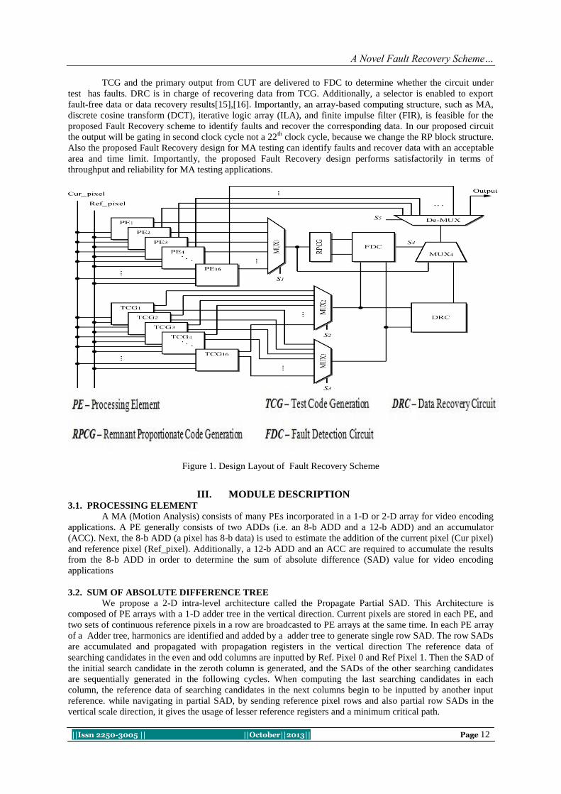
A Novel Fault Recovery Scheme…

||Issn 2250-3005 || ||October||2013|| Page 12

TCG and the primary output from CUT are delivered to FDC to determine whether the circuit under

test has faults. DRC is in charge of recovering data from TCG. Additionally, a selector is enabled to export

fault-free data or data recovery results[15],[16]. Importantly, an array-based computing structure, such as MA,

discrete cosine transform (DCT), iterative logic array (ILA), and finite impulse filter (FIR), is feasible for the

proposed Fault Recovery scheme to identify faults and recover the corresponding data. In our proposed circuit

the output will be gating in second clock cycle not a 22th

clock cycle, because we change the RP block structure.

Also the proposed Fault Recovery design for MA testing can identify faults and recover data with an acceptable

area and time limit. Importantly, the proposed Fault Recovery design performs satisfactorily in terms of

throughput and reliability for MA testing applications.

Figure 1. Design Layout of Fault Recovery Scheme

III. MODULE DESCRIPTION 3.1. PROCESSING ELEMENT

A MA (Motion Analysis) consists of many PEs incorporated in a 1-D or 2-D array for video encoding

applications. A PE generally consists of two ADDs (i.e. an 8-b ADD and a 12-b ADD) and an accumulator

(ACC). Next, the 8-b ADD (a pixel has 8-b data) is used to estimate the addition of the current pixel (Cur pixel)

and reference pixel (Ref_pixel). Additionally, a 12-b ADD and an ACC are required to accumulate the results

from the 8-b ADD in order to determine the sum of absolute difference (SAD) value for video encoding

applications

3.2. SUM OF ABSOLUTE DIFFERENCE TREE

We propose a 2-D intra-level architecture called the Propagate Partial SAD. This Architecture is

composed of PE arrays with a 1-D adder tree in the vertical direction. Current pixels are stored in each PE, and

two sets of continuous reference pixels in a row are broadcasted to PE arrays at the same time. In each PE array

of a Adder tree, harmonics are identified and added by a adder tree to generate single row SAD. The row SADs

are accumulated and propagated with propagation registers in the vertical direction The reference data of

searching candidates in the even and odd columns are inputted by Ref. Pixel 0 and Ref Pixel 1. Then the SAD of

the initial search candidate in the zeroth column is generated, and the SADs of the other searching candidates

are sequentially generated in the following cycles. When computing the last searching candidates in each

column, the reference data of searching candidates in the next columns begin to be inputted by another input

reference. while navigating in partial SAD, by sending reference pixel rows and also partial row SADs in the

vertical scale direction, it gives the usage of lesser reference registers and a minimum critical path.

A Novel Fault Recovery Scheme…

||Issn 2250-3005 || ||October||2013|| Page 13

3.2.1. SUM OF ABSOLUTE DIFFERENCE VALUE CALCULATION

By utilizing PEs, SAD shown in as follows, in a macro block with size N X N of can be evaluated

Where rxi,j,qxi,j and ryi,j ,qyi,j denote the corresponding RP code of Xi,j , Yi,j and modulo M. Importantly, and

represent the luminance pixel value of Cur_pixel and Ref_pixel subsequently.

3.3. REMNANT PROPORTIONATE CODE GENERATION ALGORITHM

In this RPCG Algorithm Remnant code is generally separable arithmetic codes by estimating a remnant

for data and appending it to data [17],[18]. Fault detection logic for operations is typically derived by a separate

remnant code, making the detection logic is simple and easily implemented. Fault detection logic for operations

is typically derived using a separate remnant code such that detection logic is simply and easily implemented.

However, only a bit fault can be detected based on the remnant code. Additionally, a fault can’t be recovered

effectively by using the remnant codes. Therefore, this work presents a proportionate code, which is derived

from the remnant code; to assist the remnant code in rectifying multiple faults[19].The corresponding circuit

design of the RPCG is easily realized by using the simple adders (ADDs).Namely, the RP code can be generated

with a low complexity and little hardware cost[20].

3.4. TEST CODE GENERATION

TCG is an important component of the proposed Fault Recovery Design. Notably, TCG design is based

on the ability of the RPCG Circuit to generate corresponding test codes in order to identify faults and recover

data.

3.5. FAULT DETECTION CIRCUIT

In this module indicates that the operations of fault detection in a specific PEi is achieved by using

FDC, which is utilized to compare the outputs between TCG and in order to determine whether faults have

occurred. The FDC output is then used to generate a 0/1 signal to indicate that the tested PEi is fault-free/faulty.

Using XOR operation can be identify the fault if any variation in terms of remnant and proportionate value.

Because a fault only affects the logic in the fan-out cone from the fault region. Concurrent fault simulation

exploits this fact and simulates only the differential parts of the whole circuit Concurrent fault simulation is

essentially an event-driven simulation with the fault-free circuit and faulty circuits simulated altogether.

3.6. DATA RECOVERY CIRCUIT In this module will be generate fault free output by proportionate multiply with constant value and add

with proportionate code. During data recovery, the circuit DRC plays a significant role in recovering RP code

from TCG.

IV. METHODOLOGY Coding approaches such as Parity code, Berger code, and Remnant code is considered only to identify

circuit faults. Remnant code R is a separable arithmetic codes by estimating a remnant for data and appending it

to data. i.e., R = |X|m .Binary Data X is coded as a pair (X,R) and modulus m= 2w -1 , w is word length.

Proportionate code P =X/m is derived from the Remnant code to identify and recover multiple faults. To

simplify the complexity of circuit design, the implementation is carried out using the simple Adders (ADDs).

A Novel Fault Recovery Scheme…

||Issn 2250-3005 || ||October||2013|| Page 14

V. NUMERICAL EXAMPLE

Table 1. Accumulation of Original data having pixel value of 128 in the (1,1) position of a 4x4 Current Macro

Block

Table 2. Injection of Fault data having pixel value of 120 in the (1,1) position of a 4x4 Current Macro Block

VI. SIMULATION SET UP 6.1. CREATING THE WORKING LIBRARY

ModelSim is a verification and simulation tool for VHDL, Verilog, System Verilog, and mixed

language designs.In ModelSim, all designs are compiled into a library. Typically start a new simulation in

ModelSim by creating a working library called "work". "Work" is the library name used by the compiler as the

default destination for compiled design units.

6.2. COMPILING YOUR DESIGN

After creating the working library, compile the design units into it. The Model Simlibrary format is

compatible across all supported platforms. Simulate the design on any platform without having to recompile the

design. Loading the Simulator with the Design and Running the Simulation. With the design compiled, load the

simulator with respective design by invoking the simulator on a top-level module (Verilog) or a configuration or

entity/architecture pair(VHDL).Assuming the design loads successfully, the simulation time is set to zero, and

enter a run command to begin simulation.

6.3. DEBUGGING RESULTS

If we don’t get the results as we expect, we can use Modelsim robust debugging environment to track

down the cause of the problem.

A Novel Fault Recovery Scheme…

||Issn 2250-3005 || ||October||2013|| Page 15

VII. SIMULATION RESULTS

Figure 2. Simulation Result of Processing Element Circuit obtaining Absolute Differences from the Current and

Reference pixels.

Figure 3. Simulation Result of SAD Generation Circuit obtaining its value from a suitable Candidate Block for a

specific PE

Figure 4. Simulation Result of RPCG Circuit obtaining its value from lowest distortion SAD value

A Novel Fault Recovery Scheme…

||Issn 2250-3005 || ||October||2013|| Page 16

Figure 5. Simulation Result of TCG Circuit obtaining its value from Current and Reference pixel values

Figure 6. Simulation Result of Fault Detection Circuit identifying the fault using RP Codes and Test Codes for a

Specific PE in a Motion Analysis Process

Figure 7. Simulation Result of Data Recovery Circuit identifying the fault using Test Codes for a Specific PE in

a Motion Analysis Process

A Novel Fault Recovery Scheme…

||Issn 2250-3005 || ||October||2013|| Page 17

Figure 8.Simulation Result of Fault Recovery design in identifying the fault and recovering the original data for

a Specific PE in a Motion Analysis Process

Figure 9. Simulation Result of Fault Recovery design in identifying the fault using RP Codes and Test Codes for

a Specific PE in a Motion Analysis Process

A Novel Fault Recovery Scheme…

||Issn 2250-3005 || ||October||2013|| Page 18

VIII. RESULTS AND ITS DISCUSSION Table 3. Design Specifications of Fault Recovery Design with 16 PEs and 16 TCGs in a Motion Analysis

Process for a specific Processing Element

Table 4. Performance Analysis of Fault Recovery Design with 16 PEs and 16 TCGs in a Motion Analysis

Process for a specific Processing Element

IX. CONCLUSION This work presents a novel Fault Recovery scheme for detecting the faults and recovering the data of

PEs in a MA. Based on the RP code, a RPCG-based TCG design is developed to generate the corresponding test

codes to identify faults and recover data. The proposed Fault Recovery scheme is also implemented by using

Verilog Hardware Description Language and synthesized by the synopsys Design Compiler with TSMC 0.18-

m1P6MCMOS technology. Experimental results indicate that that the proposed Fault Recovery design can

effectively identify faults and will recover data in PEs of a MA with an operating time of 10.973ns with

acceptable area cost.

A Novel Fault Recovery Scheme…

||Issn 2250-3005 || ||October||2013|| Page 19

REFERENCES [1] Chang-Hsin Cheng; Yu Liu; Chun-Lung Hsu , “Design of an Error Detection and Data Recovery Architecture for Motion

Estimation Testing Applications,” IEEE Trans. Vary Large Scale Integr. (VLSI) Systs., vol. 20, no. 4, pp. 665–672, Apr. 2007.

[2] L. Breveglieri, P. Maistri, and I. Koren, “A Note on Error Detection in RSA architecture by means of Residue Codes,” in Proc. IEEE Int. Symp. On-Line Testing, pp. 176-177, Jul. 2006.

[3] C. Y. Chen, S. Y. Chien, Y. W. Huang, T. C. Chen, T. C. Wang, and L. G. Chen, “Analysis and architecture design of Variable

Block Size Motion Estimation for H.264/AVC,” IEEE Trans. Circuits Syst. I, Reg. Papers, vol. 53, no. 3, pp. 578–593, Mar. 2006.

[4] C. H. Cheng, Y. Liu, and C. L. Hsu, “Low-cost BISDC design for Motion Estimation Computing Array,” in Proc. IEEE Circuits

Syst. Int. Conf., pp.1–4, 2009. [5] M. Y. Dong, S. H. Yang, and S. K. Lu, “Design for Testability techniques for Motion Estimation Computing Arrays,” in Proc.

Int. Conf. Commun., Circuits Syst., pp. 1188–1191, May 2008.

[6] C. L. Hsu, C. H. Cheng, and Y. Liu, “Built In Self Detection/Correction architecture for Motion Estimation Computing Arrays,” IEEE Trans. Vary Large Scale Integr.(VLSI) Systs., vol. 18, no. 2, pp. 319–324, Feb. 2010.

[7] Y. S. Huang, C. K. Chen, and C. L. Hsu, “Efficient Built In Self Test for video coding cores: A case study on Motion Estimation

Computing Array,” in Proc. IEEE Asia Pacific Conf. Circuit Syst., pp. 1751–1754, Dec. 2008.

[8] Y. W. Huang, B. Y. Hsieh, S. Y. Chien, S. Y. Ma, and L. G. Chen, “Analysis and complexity reduction of Multiple Reference

Frames Motion Estimation in H.264/AVC,” IEEE Trans. Circuits Syst. Video Technol., vol. 16, no. 4, pp. 507–522, Apr.

2006. [9] Y. S. Huang, C. J. Yang, and C. L. Hsu, “C-testable Motion Estimation design for video coding systems,” J. Electron. Sci.

Technol., vol. 7, no. 4, pp. 370–374, Dec. 2009.

[10] C. P. Kung, C. J. Huang, and C. S. Lin, “Fast fault simulation for BIST applications,” in Proceedings of the Fourth Asian Test Symposium, pp. 93–99, 1995.

[11] D. Li, M. Hu, and O. A. Mohamed, “Built In Self Test design of Motion Estimation Computing Array,” in Proc. IEEE Northeast

Workshop Circuits Syst., pp. 349–352, Jun. 2004. [12] J. F. Lin, J. C. Yeh, R. F. Hung, and C. W. Wu, “A Built In Self Repair design for RAMs with 2-D redundancy,” IEEE Trans.

Vary Large Scale Integr. (VLSI) Syst., vol. 13, no. 6, pp. 742–745, Jun. 2005.

[13] W. Y Liu, J. Y. Huang, J. H. Hong, and S. K. Lu, “Testable design and BIST techniques for Systolic Motion Estimators in the transform domain,” in Proc. IEEE Int. Conf. Circuits Syst., pp. 1–4, Apr. 2009.

[14] E. J. McCluskey, “Built In Self Test Technique,” IEEE Design and Test of Computers, vol. 2, no. 2, pp. 29–36, Apr. 1985.

[15] D. K. Park, H. M. Cho, S. B. Cho, and J. H. Lee, “A fast motion estimation algorithm for SAD optimization in sub pixel,” in Proc. Int. Symp. Integr. Circuits, pp. 528–531, Sep. 2007.

[16] S. J. Piestrak, D. Bakalis, and X. Kavousianos, “On the design of self testing checkers for modified Berger codes,” in Proc. IEEE

Int. Workshop On Line Testing, pp. 153–157, Jul. 2001. [17] J. M. Portal, H. Aziza, and D. Nee, “EEPROM memory: Threshold voltage Built In Self Diagnosis,” in Proc. Int. Test

Conf., pp. 23–28, Sep. 2003.

[18] S. Surin and Y. H. Hu, “Frame level pipeline Motion Estimation Array Processor,” IEEE Trans. Circuits Syst. Video Technol., vol. 11, no. 2,pp. 248–251, Feb. 2001.

[19] T. H. Wu, Y. L. Tsai, and S. J. Chang, “An efficient Design for Testability scheme for Motion Estimation in H.264/AVC,” in

Proc. Int. Symp.VLSI Design, Autom. Test, pp. 1–4, Apr. 2007. [20] N. A. Touba and E. J. McCluskey, “Pseudo Random pattern testing of bridging faults,” in International Conference on

Computer Design, pp. 54–60, 1997.

International Journal of Computational Engineering Research||Vol, 03||Issue, 10||

||Issn 2250-3005 || ||October||2013|| Page 20

Materialized Optimization of Connecting Rod for Four Stroke

Single Cylinder Engine

1, Marthanapalli HariPriya,

2, K.Manohar Reddy

1m.Tech (Me), Intl- Ananatapur (Dt), Affiliated To Jntua University, Andhra Pradesh, India.

2 Assistant Professor, Department Of Me, Intell Engg. College Anantapur (Dt), Affiliated To Jntua University,

Andhra Pradesh, India.

I. INTRODUCTION Connecting rod is among large volume production component in the internal combustion engine. It

connects the piston to the crankshaft and is responsible for transferring power from the piston to the crankshaft

and sending it in to transmission. They are different types of materials and production methods used in the

creation of connecting rods. The major stresses induced in the connecting rod are a combination of axial and

bending stresses in operation. The axial stresses are produced due to cylinder gas pressure (compressive only)

and the inertia force arising in account of reciprocating action (both tensile as well as compressive), where as

bending stresses are caused due to the centrifugal effects. It consists of a long shank, a small end and a big end.

The cross-section of the shank may be rectangular, circular, tubular, I-section or H-section. Generally circular

section is used for low speed engines while I-section is preferred for high speed engines. The most common type

of manufacturing processes is casting, forging, and powdered metallurgy. Connecting rod is subjected to a

complex state of loading. It undergoes high cyclic loads of the order of 10^8 to 10^9 cycles, which range from

high compressive loads due to combustion, to high tensile loads due to inertia. Therefore, durability of this

component is critical importance. Due to these factors, the connecting rod has been the topic of research for

different aspects such as production technology, materials, performance, simulation, fatigue etc.In modern

automotive internal combustion engines, the connecting rods are most usually made of steel for production

engines, but can be made of aluminum (for lightness and the ability to absorb high impact at the expense of

durability) or titanium (for a combination of strength and lightness at the expense of affordability) for high

performance engines, or of cast iron for applications such as motor scooters. They are not rigidly fixed at either

end, so that the angle between the connecting rod and the piston can change as the rod moves up and down and

rotates around the crankshaft. The small end attaches to the piston pin, gudgeon pin or wrist pin, which is

currently most often press fit into the con rod but can swivel in the piston, a "floating wrist pin" design. The big

end connects to the bearing journal on the crank throw, running on replaceable bearing shells accessible via the

con rod bolts which hold the bearing "cap" onto the big end.

A major source of engine wear is the sideways force exerted on the piston through the con rod by the

crankshaft, which typically wears the cylinder into an oval cross-section rather than circular, making it

impossible for piston rings to correctly seal against the cylinder walls. Geometrically, it can be seen that longer

con rods will reduce the amount of this sideways force, and therefore lead to longer engine life.

ABSTRACT Connecting rods for automotive applications are typically manufactured by forging from either

wrought steel or powdered metal. They could also be cast. An optimization study was performed on a

steel forged connecting rod with a consideration for improvement in weight and production cost. For

this optimization problem, the weight of the connecting rod has little influence on the cost of the final

component. Change in the material, resulting in a significant reduction in machining cost, was the key

factor in cost reduction. This study has two aspects. The first aspect was to investigate and to compare

fatigue strength of steel forged connecting rods with that of the powder forged connecting rods. The

second aspect was to optimize the weight and manufacturing cost of the steel forged connecting rod.

Constraints of fatigue strength, static strength, reducing inertia loads, reducing engine weight ,

improvised engine performance, fuel economy were also imposed. The fatigue strength was the most

significant factor in the optimization of the connecting rod.

KEYWORDS: PM Connecting rod, fatigue behavior, forged steel.

Materialized Optimization Of Connecting…

||Issn 2250-3005 || ||October||2013|| Page 21

However, for a given engine block, the sum of the length of the con rod plus the piston stroke is a fixed

number, determined by the fixed distance between the crankshaft axis and the top of the cylinder block where

the cylinder head fastens; thus, for a given cylinder block longer stroke, giving greater engine displacement and

power, requires a shorter connecting rod, resulting in accelerated cylinder wear.

The automobile engine connecting rod is a high volume production, critical component. It connects

reciprocating piston to rotating crankshaft, transmitting the thrust of the piston to the crankshaft. Every vehicle

that uses an internal combustion engine requires at least one connecting rod depending upon the number of

cylinders in the engine. Connecting rods for automotive applications are typically manufactured by forging from

either wrought steel or powdered metal. They could also be cast. However, castings could have blow-holes

which are detrimental from durability and fatigue points of view. The fact that forgings produce blow-hole-free

and better rods gives them an advantage over cast rods. Between the forging processes, powder forged or drop

forged, each process has its own pros and cons. Powder metal manufactured blanks have the advantage of being

near net shape, reducing material waste. However, the cost of the blank is high due to the high material cost and

sophisticated manufacturing techniques. With steel forging, the material is inexpensive and the rough part

manufacturing process is cost effective. The first aspect was to investigate and compare fatigue strength of steel

forged connecting rods with that of the powder forged connecting rods. The second aspect was to optimize the

weight and manufacturing cost of the steel forged connecting rod. Due to its large volume production, it is only

logical that optimization of the connecting rod for its weight or volume will result in large-scale savings. It can

also achieve the objective of reducing the weight of the engine component, thus reducing inertia loads, reducing

engine weight and improving engine performance and fuel economy.

II. MODELING The structural and modal analysis of connecting rod for both Aluminium Alloy A360 and Carbon steel are

shown as below:

Structural Analysis Of Connecting Rod -Section Using Aluminium Alloy A360

Fig 1.Structural Analysis of connecting rod I-section using Aluminium Alloy A360 ,Young’s modulus –

80000MPa Poisson ratio - 0.33, Density – 0.0000026kg/mm3

Modal Analysis Of Connecting Rod I-Section Using Aluminium Alloy A360

Fig 2.Modal Analysis of connecting rod I-section using Aluminium Alloy A360 ,Young’s modulus – 80000MPa

Poisson ratio - 0.33, Density – 0.0000026kg/mm3

Materialized Optimization Of Connecting…

||Issn 2250-3005 || ||October||2013|| Page 22

Structural Analysis Of Connecting Rod I-Section Using Carbon Steel

Fig 3. Structural Analysis of connecting rod I-section using Carbon steel ; Young’s modulus -

200000MPa,Poisson ratio – 0.295, Density – 0.000007872kg/m3

Structural Analysis Of Connecting Rod H-Section Using Carbon Steel

Fig 4.Structural Analysis of connecting rod H-section using Carbon Steel Young’s modulus -

200000MPa,Poisson ratio – 0.295, Density – 0.000007872kg/m3

Modal Analysis Of Connecting Rod I-Section Using Carbon Steel

Fig 5.Modal Analysis of connecting rod I-section using Carbon Steel Young’s modulus -200000MPa,Poisson

ratio – 0.295, Density – 0.000007872kg/m3

Modal Analysis Of Connecting Rod H-Section Using Carbon Steel

Materialized Optimization Of Connecting…

||Issn 2250-3005 || ||October||2013|| Page 23

Fig 6. Modal Analysis of connecting rod H-section using Carbon Steel , Young’s modulus -

200000MPa,Poisson ratio – 0.295, Density – 0.000007872kg/m3

III. RESULTS SECTION

H-SECTION

Materialized Optimization Of Connecting…

||Issn 2250-3005 || ||October||2013|| Page 24

IV. CONCLUSION In this paper,a connecting rod for a 150cc engine has been modeled in 3D modeling sftware

Pro/Engineer.The actual cross section connecting rod is I – section, which have been changed to cross section H

– section. By changing the cross section, the weight of connecting rod is reduced by 10gms.The material used

for connecting rod is carbon steel which is replaced with Aluminum alloy A360. By replacing it with Aluminum

alloy A360, the weight of the connecting rod reduces about 4 times than using Carbon steel since density of

Aluminum alloy A360 is very less as compared with Carbon Steel.The structural and modal analysis on the

connecting rod using two materials Carbon steel and Aluminum alloy A360 has been done and is concluded that

the stress values obtained for both materials are less than their respective yield stress values. So using

Aluminum alloy A360 is safe. By comparing the stress values for both materials, it is slightly less for Aluminum

alloy A360 than carbon steel.By observing the results, We can conclude that Aluminum alloy A360 is better for

connecting rod.

REFERENCES [1] A Textbook of Machine Design by R.S.KHURMI AND K.GUPTA.

[2] Engineering_fundamentals_of_the_internal_combustion_engine by Willard W. Pulkrabek.

[3] Mechanical Engineering Design by Budynas−Nisbet.

[4] Automotive Engineering by Patric GRANT.

[5] Handbook of mechanical engineering - modern manufacturing by Ed. Frank Kreith.

[6] Engineering Fundamentals of the Internal Combustion Engine by Willard W. Pulkrabek.

International Journal of Computational Engineering Research||Vol, 03||Issue, 10||

||Issn 2250-3005 || ||October||2013|| Page 25

Acoustic Ear Scanning With Fingerprint Technology

1,S. Niveda ,

2,K. Dhavamani

1,Department of Information Technology

2,Manakula Vinayagar Institute of Technology

I. INTRODUCTION: This is mainly to protect the electronic and portable devices from theft. The basis of this acoustic ear

scanning technology is that the new scan sends sound through earphones. Sound returns from the ear chamber's

"finger print ". Scientists have found a way of using the "acoustic fingerprint" of a person's ear to ensure no one

else can operate their iPods, mobile phones and other personal portable device. The technology can be extended

to protect bank accounts and passports.

Figure 1

Overseas researchers have discovered that they can identify individuals from the unique sound of the ear

chamber. The biometric "pin number" would be instantly detected by an iPod, mobile phone or any other device

fitted with an anti-theft acoustic fingerprint detector. Acoustic fingerprint can be used to pay bills or do banking

transactions securely with confirmation of identifying as easy as by simply wearing a headphone in the ear.

Electronic engineer, Arthur Rapos of the Elektra Company, believes biometric mapping will eventually lead to

microchip implants in humans. It isn't a flight of fancy to imagine someone being implanted with a removable

microchip that records that person's unique biological feature before travelling overseas."The sound the inside of

our ear makes is not the only unique things about an individual’s".

II. PRINCIPLES: The working principle of this technology is

• Biometric

• Image processing

2.1 BIOMETRIC:

Biometric recognition, or biometric refers to the automatic identification of a person based on

his/her anatomical (e.g., fingerprint) or behavioral (e.g., signature) characteristics or traits. This method of

ABSTRACT: We often hear about the theft of our valuable devices. Day-by-day it is increasing too. So, in

order to control the theft of electronic devices such as iPod, smart phones, scientists have introduced a

new technology called “acoustic ear scanning technology” for their security. The predecessor for this

technology is fingerprint scanning, face recognition, etc., but these all have a common disadvantage.

And to overcome that disadvantage, we have introduced finger print scanning along with it in our paper.

KEYWORDS: iPod, smart phones, earphone, biometric template.

Acoustic Ear Scanning With Fingerprint…

||Issn 2250-3005 || ||October||2013|| Page 26

identification offers several advantages over traditional methods involving ID cards (token) or pin numbers

(passwords) for various reasons:

[1] The person to be identified is required to be physically present at the point-of-identification.

[2] Identification based on biometric techniques obviates the need to remember a password or carry

a token with the increased integration of computers and the internet into our everyday lives, it is necessary

to protect sensitive and personal data by replacing PINs (or using biometrics in addition to PINs), biometric

techniques can potentially prevent unauthorized access to cell phones laptops, and computer networks.

Biometrics are used in computer science as a form of identification and access control. It is also used to

identify individuals in groups that are under surveillance.Biometric identifiers are the distinctive,

measurable characteristics used to label and describe individuals. Biometric identifiers are often categorized

as physiological versus behavioral characteristics. A physiological biometric would identify with one's

voice, DNA, hand print or behavior. Behavioral biometrics are related to the behavior of a person, including

but not limited to: typing rhythm, gait, and voice. In verification mode the system performs a one-to-one

comparison of a captured biometric with a specific template stored in a biometric database in order to verify

the individual is the person they claim to be.

Three steps involved in person verification.

• In the first step, reference models for all the users are generated and stored in the model database.

• In the second step, some samples are matched with reference models to generate the genuine and impostor

scores and calculate the threshold.

• Third step is the testing step.

This process may use a smart card, username or ID number (e.g. PIN) to indicate which template

should be used for comparison. 'Positive recognition' is a common use of verification mode, "where the aim

is to prevent multiple people from using same identity". In Identification mode the system performs a one-

to-many comparison against a biometric data base in an attempt to establish the identity of an unknown

individual.

Figure 2

The system will succeed in identifying the individual if the comparison of the biometric sample to a

template in the database falls within a previously set threshold. Identification mode can be used either for

'positive recognition' (so that the user does not have to provide any information about the template to be used)

or for 'negative recognition' of the person "where the system establishes whether the person is who she

(implicitly or explicitly) denies to be". The latter function can only be achieved through biometrics since other

methods of personal recognition such as passwords, PINs or keys are ineffective.The first time an individual

uses a biometric system is called enrollment. During the enrollment, biometric information from an individual

is captured and stored. In subsequent uses, biometric information was detected and compared with the

information stored at the time of enrollment. Note that it is crucial that storage and retrieval of such systems

themselves be secure if the biometric system is to be robust.

The first block (sensor) is the interface between the real world and the system; it has to acquire all the necessary

data. Most of the times it is an image acquisition system, but it can change according to the characteristics

desired.

The second block performs all the necessary preprocessing: it has to remove artifacts from the sensor, to

enhance the input (e.g. Removing background noise), to use some kind of normalization, etc.

Acoustic Ear Scanning With Fingerprint…

||Issn 2250-3005 || ||October||2013|| Page 27

A sensor (also called detector) is a convertor that measures a physical quantity and converts it into a

signal which can be read by an observer or by an (today mostly electronic) instrument. A sensor is a device

which receives and responds to a signal when touched. A sensor's sensitivity indicates how much the sensor's

output changes when the measured quantity changes. In the third block necessary features are extracted. This

step is an important step as the correct features need to be extracted in the optimal way. A vector of numbers or

an image with particular properties is used to create a template. A biometric template (also called a template) is

a digital reference of distinct characteristics that have been extracted from a biometric sample. Templates are

used during the biometric authentication process. A template is a synthesis of the relevant characteristics

extracted from the source. Elements of the biometric measurement that are not used in the comparison algorithm

are discarded in the template to reduce the file size and to protect the identity of the enrollee.

If enrollment is being performed, the template is simply stored somewhere (on a card or within a

database or both). If a matching phase is being performed, the obtained template is passed to a matcher that

compares it with other existing templates, estimating the distance between them using any algorithm (e.g.

Hamming distance). In coding theory Hamming (7,4) is a linear error -correcting code that encodes 4 bits of

data into 7 bits by adding 3 parity bits. It is a member of a larger family of hamming codes, but the

term Hamming code often refers to this specific code that Richard W. Hamming introduced in 1950. At the

time, Hamming worked at Bell Telephone Laboratories and was frustrated with the erroneous punched card

reader, which is why he started working on error-correcting codes. The matching program will analyze the

template with the input. This will then be output for any specified use or purpose. Selection of biometrics in any

practical application depending upon the characteristic measurements and user requirements. We should

consider Performance, Acceptability, Circumvention, Robustness, Population coverage, Size, Identity theft

deterrence in selecting a particular biometric. Selection of biometric based on user requirement considers Sensor

availability, Device availability, Computational time and reliability, Cost, Sensor area and power consumption.

2.2 IMAGE PROCESSING:

Image processing refers to the processing of a 2D picture by a computer. An image is considered to be

a function of two real variables, for example, a (x, y) with a as the amplitude (e.g. Brightness) of the image of

the real coordinate position (x, y). Modern digital technology has made it possible to manipulate multi-

dimensional signals with systems that range from simple digital circuits to advanced parallel computers.

Figure 3

The most requirements for image processing of images is that the images are available in digitized

form, that is, arrays of finite length binary words. The digitized image is processed by a computer. To display a

digital image, it is first converted into an analog signal, which is scanned onto a display. Before going to

processing an image, it is converted into a digital form. Digitization includes sampling of images and

quantization of sampled values. After converting the image into bit information, processing is performed. This

processing technique may be, Image enhancement, Image reconstruction, and Image compression

2.2.1 IMAGE ENHANCEMENT:

It refers to accentuation, or sharpening, of image features such as boundaries, or contrast to make a

graphic display more useful for display & analysis. This process does not increase the inherent information

content in data. It includes gray level & contrast manipulation, noise reduction, edge christening and sharpening,

filtering, interpolation and magnification, pseudo coloring, and so on.

Acoustic Ear Scanning With Fingerprint…

||Issn 2250-3005 || ||October||2013|| Page 28

2.2.2 IMAGE RESTORATION:

It is concerned with filtering the observed image to minimize the effect of degradations. Effectiveness

of image restoration depends on the extent and accuracy of the knowledge of degradation process as well as on

filter design. Image restoration differs from image enhancement in that the latter is concerned with more

extraction or accentuation of image features.

2.2.3 IMAGE COMPRESSION:

It is concerned with minimizing the no of bits required to represent an image. Application of

compression is on broadcast TV, remote sensing via satellite, military communication via aircraft, radar,

teleconferencing, facsimile transmission, for educational & business documents , medical images that arise in

computer tomography, magnetic resonance imaging and digital radiology, motion , pictures ,satellite images,

weather maps, geological surveys and so on.De-essing is any form of signal processing for which the input is an

image, such as a photograph or video frame; the output of image processing may be either an image or a set of

characteristics or parameters related to the image. Most image-processing techniques involve treating the image

as a two-dimensional signal and applying standard signal-processing techniques to it. Image processing usually

refers to digital image processing, but optical and analog image processing also is possible. This article is about

general techniques that apply to all of them. The acquisition of images (producing the input image in the first

place) is referred to as imaging. In modern sciences and technologies, images also gain much broader scopes

due to the ever growing importance of scientific visualization (to often large-scale complex

scientific/experimental data). Examples include microarray data in genetic research, or real-time multi-asset

portfolio trading in finance.

III. EXISTING SYSTEM: Acoustic ear scanning technology has been implemented to prevent the theft of iPods, mobile phones.

It works by, for the first time of using the device, an ear phone should be put into the ears. A minute sound is

sent into the ears. The microscopic hairs inside the ear responds the sound by producing its own sound. This

happens by, the sound that passes through the air after entering the ear, passes through the liquid medium.

During this time, the microscopic hair cells in the inner ear, bends to produce its own sound. The sound is

unique for each person varying according to the ear drum, ear bones, etc.,. The sound is then processed in digital

form and saved into a biometric template. Biometric template is a place where the digital form of the sound gets

stored.Now, whenever a person uses it for the second time, it insists the user to wear earphones. Once we wear

the earphone, a minute sound is sent in order to make hair cells produce their own sound. This sound is the

converted to digital form and compared with the standard biometric template. If they are same, the access will

be granted else the access is denied.

3.1 CONVERSIONS OF SOUND INTO DIGITAL FORM:

An analogue or acoustical input source such as microphone converts air pressure variation into an

electrical signal. An analog-to-digital convertor converts the signal into digital data by repeatedly measuring the

signal of the changes in voltage.

IV. PROPOSAL: This overcomes the disadvantage of ear scanning technology. It can be applied to systems also.

STEP 1: for the first time, when the user uses the device, a biometric of the fingerprint and ear sound is stored in

a database.

STEP 2: The user is requested to wear an ear phone while switching on the mobile.

STEP 3: Once the earphone is worn, a minute sound is sent to our ears which will be then converted into

biometric.

STEP 4: If the biometric matches with the template stored already, the access is granted.

STEP 5: Since this process provided security only at the time of opening, there might a chance of getting lost

after opened.

STEP 6: Hence, we introduced finger print technology along with it.

STEP 7: For every particular time period, the fingerprint is being scanned again and compared with the

biometric template of it.

STEP 8: If the biometric matches, the user can continue. Otherwise, it gets shut down automatically.

STEP 9: Once the device is switched off, again the user has to start from first.

STEP 10: This can be applied in the same way to systems, where the finger print has been implemented in most

used keys.

Acoustic Ear Scanning With Fingerprint…

||Issn 2250-3005 || ||October||2013|| Page 29

V. CONTROL FLOW DIAGRAM:

VI. CONCLUSION: Thus we proposed an idea which will be helpful in protecting the electronic devices even though the

device is kept opened. Acoustic ear scanning technology is a recent technology introduced to protect electronic

devices. Since it can provide security only at the time of opening, we introduced finger print scanning which

will not allow unauthorized access to it.

REFERENCES: [1] S. Prabhakar, S. Pankanti, A. K. Jain, "Biometric Recognition: Security and Privacy Concerns", IEEE Security & Privacy,

March/April 2003

[2] D. Maio, D. Maltoni, R. Cappelli, J. L. Wayman, A. K. Jain, "FVC2002: Fingerprint verification competition" in Proc. Int. Conf.

Pattern Recognition (ICPR), Quebec City, QC, Canada, August 2002 [3] Samir Nanvati, (2002), Biometrics: Identity Verification in a Networked World, New York: Wiley and Sons, Inc.

[4] Wayne Penny, (2002), Biometrics, A Double-Edged Sword

[5] Jensen, J.R. 1996. Introduction to Digital Image Processing : A Remote Sensing Perspective.Practice Hall, New Jersey

International Journal of Computational Engineering Research||Vol, 03||Issue, 10||

||Issn 2250-3005 || ||October||2013|| Page 30

Novel Design of A 4:1 Multiplexer Circuit Using Reversible Logic

Vandana Shukla1, O. P. Singh

1, G. R. Mishra

1, R. K. Tiwari

2

1Amity School Of Engineering & Technology, Amity University, Lucknow

2Dr. R. M. L. University, Faizabad

I. INTRODUCTION

An integrated circuit containing many identical cells which can be electrically programmed to become

almost any kind of digital circuit or system is called as Field Programmable Gate Arrays (FPGAs) [1].

Multiplexers play the key role in the functionalities of FPGAs, so to design a multiplexer with reversible logic

will generate the concept of designing low power loss circuits for FPGAs.Earlier digital circuits were made up

of conventional logic gates. These gates were irreversible in nature. Reversible circuit designing is the way of

today’s digital circuit designing. In 1961, R. Landauer has shown that these conventional irreversible circuits

dissipate some energy due to the information loss during the operation of the circuit [2]. After that in 1973,

Benette has shown that this energy loss can be minimized or even removed if the circuits are designed using

reversible gates [3].

II. REVERSIBLE LOGIC CIRCUIT DESIGN [2.1] Reversible Logic- conventional logic gates were generally (n:1) in nature. Where n represents the number

of input signals applied and 1 indicated the single output generated from the gate. Whereas reversible logic gates

are (n,n) logic gates. Here both, the number of input signals and the number of output signal are equal to n. In

conventional logic gates output signals are less in number as compared to the number of input signals. But in

reversible gates input and output signals are equal in number. The combination of output signal at any instance

can provide the exact status of input combination. This is the main reason to name these (n,n) gates, reversible

logic gates[4,5,6].

[2.2] Basic Reversible Gates- There are various basic reversible (n,n) gates[7,8,9,10,11,12,13]. For designing

multiplexer TKS gate[14] is the optimum choice. TKS gate is a (3,3) reversible gate. Its block diagram is shown

in figure 1 and output equations are given below the diagram.

Figure 1: TKS Gate

Where -

ABSTRACT: Area of reversible logic is attracting much attention of researchers nowadays. Reversible logic

concept of digital circuit designing is gaining wide scope in the area of nanotechnology, quantum

computing, signal processing, optical computing etc due to its ability to design low power loss digital

circuits. This paper presents an optimized multiplexer circuit based on reversible logic using various

available basic reversible gates. Optimization of the multiplexer circuit is achieved on the basis of total

number of gates used in the circuit and total number of outputs generated. These circuits are useful for

further circuit designing with low power loss.

KEYWORDS: Reversible circuit design, Basic reversible gates, Multiplexer circuit.

Novel Design Of A 4:1 Multiplexer…

||Issn 2250-3005 || ||October||2013|| Page 31

In any reversible gate if we know the status of output signals (P, Q, R in case of TKS Gate) we can deduct the

instance combination of input stage (A, B, C in case of TKS Gate).

[2.3] Proposed Reversible Gate (VSMT Gate)- VSMT is a new proposed (6,6) reversible gate. This gate

conforms to the necessary characteristics of the reversible logic gates. These characteristics are as follows-

(a) Number of inputs = Number of outputs.

(b) One to one mapping between input and output.

(c) Zero feedback.

(d) Individual output bits are high for a total of half the number of total input combinations.

The block diagram of VSMT gate is shown in figure 2. Here input signals are A, B, C, D, E and F, whereas

output signals are P, Q, R, S, T and U.

Figure 2: Block diagram of VSMT gate

Output equations of above gate is given as below-

The truth table of this gate has a total of 64 input combinations. Here in this gate each input combination

produce unique output combination. This VSMT gate is a reversible gate for 6 input signals. This paper shows

the application of VSMT gate to design multiplexer circuit. Apart from proposed multiplexer circuit there can be

various other applications of DSM gates to design other digital circuits in optimized manner.

[2.4] Multiplexer Circuit- A multiplexer (MUX) is a device which selects any one of the several input signals

applied and provide it to the single output line according to the combination of selection lines applied.

Multiplexers are generally used for the conversion of parallel data lines into serial one. These are also called as

Data Selectors, as multiplexer selects one of the given input for the output according to the condition [15].

Figure 3 gives the block diagram of a 2n:1 multiplexer. Here 2

n refers to the total number of input signal lines

and 1 refers to the single output signal line. Total number of selection lines required is n as shown in the figure.

Novel Design Of A 4:1 Multiplexer…

||Issn 2250-3005 || ||October||2013|| Page 32

Figure 3: Block Diagram of a 2n:1 Multiplexer

Where output equation is-

If we name input signals of the multiplexer as I0, I1, I2, ..... I2

n-1, selection lines as S0,S1, .... Sn-1 and output as Y

then truth table of a 2n:1 multiplexer can be shown as in Table 1.

Table 1: Truth Table of a 2n:1 multiplexer

S. No. Input Section Lines Output

Sn-1 .......... S1 S0 Y

1 0 .......... 0 0 I0

2 0 .......... 0 1 I1

- --------------- -

- --------------- -

2n 1 .......... 1 1 I2

n-1

As shown in the table 1 input selection lines combination decide the signal to be forwarded at the output lines

[16]. Multiplexers of different sizes can be designed by varying the number of selection lines i.e. n. Examples of

a simple multiplexer of size 4:1 is shown below-

4:1 MUX- a 4:1 multiplexer contains 2 selection lines and 4 input lines. Figure 5 shows the block diagram and

output equation of a 4:1 multiplexer.

Figure 4: Block Diagram of a 4:1 Multiplexer

Output equation can be written as-

III. MULTIPLEXER DESIGN USING REVERSIBLE LOGIC GATES Multiplexers are data selector circuits. To design a multiplexer circuit using reversible logic gates there

are few conditions of reversible circuit designing to be followed-

(a) There should be no feedback.

(b) There should be no fan-out.

(c) Garbage outputs should be minimum.

(d) Total number of gates should be minimum.

According to above conditions any digital circuit to be designed by reversible logic requires the optimum

selection of basic reversible gate for minimizing the said variants[17, 18, 19].

Earlier researchers have proposed to use TKS gates to design the multiplexer circuit. TKS gate is a (3,3)

reversible gate as explained in the subsection 2.2. Here we propose the designing of multiplexer circuit using the

combination of TKS and VSMT gates to achieve better circuits. Following subsection explain the designing of

4:1 multiplexers in detail-

Design of 4:1 MUX using reversible gates- As explained in the earlier subsection, a 4:1 MUX has 2 selection

lines and 4 input lines. The design of this multiplexer in reversible logic requires 3 TKS gates. Input signals are

A, B, C, D and selection lines used are S1 and S0. The output variable is denoted by Y. The design approach 1 of

the same using TKS gates only is shown in the figure 5 below.

Novel Design Of A 4:1 Multiplexer…

||Issn 2250-3005 || ||October||2013|| Page 33

Figure 5: Approach 1 to design a 4:1 MUX using reversible gates

Where various output equations are given below-

Where E1 and E2 are intermediate results of the circuit. Above design produces 6 garbage outputs using a total of

3 reversible gates. Now we will design the same 4:1 MUX circuit using the proposed 6X6 reversible gate i.e.

VSMT gate. This circuit design approach 2 is shown in the figure 6 below.

Figure 6: Approach 2 to design a 4:1 MUX using VSMT gate

Here various output equations are as shown below-

In the approach 2 only one VSMT gate is used to design the 4:1 multiplexer. Input combinations applied to

VSMT gate are by connecting A, B, C, D, S1, S0 i.e. input and selection line signals to the (A, B, C, D, E and F)

input lines of the reversible gate. Output Y is taken from the P output line of the gate. Other outputs of the

VSMT gate produce the garbage outputs (G1, G2, G3, G4, G5). Here a total of 5 garbage output signals are

produced by using single reversible gate. Comparison of these design approaches for 4:1 multiplexer is shown in

the table 4 below.

Table 2: Comparison of various approaches to design a 4:1 MUX using reversible gates

S. No. Variable Approach 1 Approach 2

1 Total Number of Reversible Gates used 3 1

2 Total Number of Garbage Outputs 6 5

3 1-Bit XORs 3 1

Novel Design Of A 4:1 Multiplexer…

||Issn 2250-3005 || ||October||2013|| Page 34

Figure 7: Comparison Chart for mux designs

Figure 8: Simulated waveform

IV. RESULT AND ANALYSIS As shown above in the table 2, the value of various variants to be considered in the process of

reversible circuit designing reduces when the circuit for 4:1 multiplexer using reversible gate is designed with

the help of the proposed VSMT gate. Here only one reversible gate is required to design the circuit of 4:1

multiplexer and the total number of garbage outputs produced are reduced to 5 as compared to 6 in the earlier

designs proposed.

V. CONCLUSION AND FUTURE SCOPE Reversible logic is becoming the modern way of digital logic circuit designing. Here in this paper we

have designed reversible circuits for 4:1 multiplexer. The optimized circuits are achieved with help of a

proposed reversible gate i.e. VSMT Gate, which is a (6,6) reversible gate. These designs can be further

expanded to achieve the reversible circuits for various other functions and devices. As multiplexers are the basic

building blocks of FPGA boards. These proposed multiplexers with reversible gates will help the researchers to

employ these FPGAs with reversible gates in low power logical design applications.

VI. ACKNOWLEDGMENT The authors are thankful to Mr. Aseem Chauhan (Additional President RBEF, Chancellor AUR), Maj.

General K. K. Ohri, AVSM (Retd.) Pro Vice Chancellor, AUUP, Lucknow Campus, Prof. S. T. H. Abidi

(Director, ASET) and Brig. Umesh K. Chopra (Director, AIIT, & Dy. Director, ASET) for their cooperation,

motivation and suggestive guidance.

Novel Design Of A 4:1 Multiplexer…

||Issn 2250-3005 || ||October||2013|| Page 35

REFERENCES [1] Christian Baumann, “Field Programmable Gate Array (FPGA)”, Summary paper for the seminar “Embedded System

Architecture”, University of Innsbruck, January 13, 2010.

[2] R. Landauer, “Irreversibility and Heat Generation in the Computational Process”, IBM Journal of Research and Development, 5, pp. 183- 191, 1961.

[3] C. H. Bennett, “Logical Reversibililty of Computation”, IBM J. Research and Development, pp. 525- 532, November 1973.

[4] M.P Frank, “Introduction to Reversible Computing: Motivation, Progress and Challenges”, Proceedings of the 2nd Conference on Computing Frontiers, pp. 385–390, 2005.

[5] T. Toffoli, “Reversible Computing”, Tech memo MIT/LCS/ TM-151, MIT Lab for Computer Science, 1980.

[6] E. Fredkin and T. Toffoli, “Conservative Logic”, Int’l J. Theoretical Physics, Vol. 21, pp. 219- 253, 1982. [7] H. Thapliyal and N. Ranganathan, “Design of Reversible Sequential Circuits Optimizing Quantum Cost, Delay and Garbage

Outputs,” ACM Journal of Emerging Technologies in Computing Systems, Vol. 6, No. 4, pp. 14:1–14:35, Dec. 2010.

[8] R. Feynman, “Quantum Mechanical Computers” , Optics News, Vol. 11, pp. 11-20, 1985. [9] Peres, “Rversible Logic and Quantum Computers”, Physical review A, 32:3266-3276, 1985.

[10] D. P. Vasudevan, P.K. Lala , J. Di and J.P Parkerson, “Reversible–Logic Design with Online Testability”, IEEE Trans. on

Intrumentation and Measurement, Vol. 55, No. 2, pp. 406 -414, April 2006. [11] P. Kemtopf, “Synthesis of Multipurpose Reversible Logic Gates”, Euromicro Symposium on Digital System Design (DSD’02),

pp. 259-267, 2002.

[12] H. G. Rangaraju, U. Venugopal, K. N. Muralidhara, K. B. Raja, “Low Power Reversible Parallel Binary Adder/Subtractor”,

International Journal of VLSI design and communication systems (VLSICS), Vol. 1, No. 3, Sept 2010.

[13] A. N. Nagamani, H. V. Jayashree, H. R. Bhagyalakshmi, “Novel Low Power Comparator Design using Reversible Logic gates”,

Indian Journal of Computer Science and Engineering ( IJCSE ), Vol. 2, No. 4 Aug- Sept 2011. [14] H. Thapliyal, M. B. Srinivas, “Novel Design and Reversible Logic Synthesis of Multiplexer Based Full Adder and Multipliers”,

IEEE, Vol. 2, pp.1593-1596

[15] M. M. Mano (1979), Digital logic and computer design, Prentice-Hall, Inc. (New York). [16] William I. Fletcher (1980), An engineering approach to digital design, PHI Learning Private Limited, (India).

[17] B. Raghu kanth, B. Murali Krishna, M. Sridhar, V. G. Santhi Swaroop, “A Distinguish between Reversible and Conventional

Logic Gates”, International Journal of Engineering Research and Applications (IJERA), Vol. 2, Issue 2, pp. 148-151, Mar-Apr 2012.

[18] H. P. Sinha, Nidhi Syal, “Design of Fault Tolerant Reversible Multiplier”, International Journal of Soft Computing and

Engineering (IJSCE), Vol. 1, Issue 6, pp. 120-124, January 2012. [19] Vandana Dubey, O.P.Singh, G.R.Mishra, “Design and Implementation of a Two-Bit Binary Comparator Using Reversible

Logic”, International Journal of Scientific and Research Publications (IJSRP), Vol. 2, Issue 7, pp. 1-4 July 2012.

[20] Vandana Shukla, O. P. Singh, G. R. Mishra, R. K. Tiwari, “Design of a 4-bit 2’s Complement Reversible Circuit for Arithmetic Logic Unit Applications”, IJCA Special Issue on International Conference on Communication, Computing and Information

Technology, ICCCMIT(2):1-5, February 2013. [21] D. Krishnaveni, M. Geetha Priya, “A Novel Design of Reversible Universal Shift Register with Reduced Delay and Quantum

Cost”, Journal of Computing, Vol. 4, Issue 2, pp. 164-173, February 2012.

International Journal of Computational Engineering Research||Vol, 03||Issue, 10||

||Issn 2250-3005 || ||October||2013|| Page 36

3-Phase Ac Motor Monitoring and Parameter Calculation Using

Labview and Daq

1Dr. K.Ravichandrudu,

2P.Suman Pramod Kumar,

3YN.Vijay Kumar,

4C.Praveen

1,Professor of EEE, Krishnaveni Engg College/Women, Guntur,A.P, India 2,Associate Professor of EEE, C.R.Engg College, Tirupathi, A.p, India

3Associate Professor of EEE, S.V.C.E.T, Chittoor, A.P, India

4Assistant Professor of EEE, C.R.Engg College, Tirupathi, A.p, India

I. INTRODUCTION

1.1: INTRODUCTION TO 3-PHASE MOTOR

An electric motor is a device which converts an electric energy into a mechanical energy. This

mechanical energy then can be supplied to various types of load the motors can operate on dc as well as single

and 3 phase ac supply. The motors operating on dc supply are called dc motors while motors operating on ac

supply are called ac motors. As ac supply is commonly available, the ac motors are popularly used in practice.

The ac motors are classified as single and 3 phase induction motors, synchronous motor and some special

purpose motors. Out of all these types 3 phase induction motors are widely used various industrial applications.

The important advantages of 3 phase induction motors over other types are self starting property, no need of

starting device, high power factor, good speed regulation and robotics construction. The working principle of 3

phase induction is based on the production of rotating magnetic field.

1.3. PRINCIPLE OF OPERATION

Fig: 1.1.Rotating Magnetic Field

ABSTRACT 3-phase AC motor monitoring and parameter calculation using lab VIEW is the project which

makes use of lab VIEW to monitor and control operation of the electrical machine. The real time

variables of electrical machine are measured and given to lab VIEW through DAQ. Lab VIEW allows

us to program as per our requirements. We continuously observe the operating voltage and current of

the motor and trip the circuit if the motor exceeds a safe value. A comparison has been made such that

the voitage or current above safe value would turn on an LED emitting red light. When the light glows,

a digital signal of 5V is generated at the selected line on DAQ. This 5V is drawn into the relay

arrangement, which is used to energized itself and trip the contact, hence isolating the machine from

the main supply.s A Data Acquisition Card (DAQ) is used to perform the core of the control action by

switching on the relay. The DAQ, USB 6009 is selected for this project. In order to provide precise

input voltages to the DAQ, such that change in each volt of voltage or amp of current is observable;

the current is read to the DAQ through current sensor. A suitable logic using is written into the DAQ

in the Lab VIEW. Observing the voltages that are obtained from the step down transformer the relay is

operated. When the voltage or current exceeds its operating range the relay is operated

KEYWORDS: 3-Ph Motor, LabView, DAQ, Voltage, Current

3-Phase Ac Motor Monitoring And Parameter…

||Issn 2250-3005 || ||October||2013|| Page 37

A three-phase power supply provides a rotating magnetic field in an induction motor. In both induction and

synchronous motors, the AC power supplied to the motor's stator creates a magnetic field that rotates in time

with the AC oscillations. Whereas a synchronous motor's rotor turns at the same rate as the stator field, an

induction motor's rotor rotates at a slower speed than the stator field. The induction motor stator's magnetic field

is therefore changing or rotating relative to the rotor. This induces an opposing current in the induction motor's

rotor, in effect the motor's secondary winding, when the latter is short-circuited or closed through an external

impedance. The rotating magnetic flux induces currents in the windings of the rotor; in a manner similar to

currents induced in transformer's secondary windings. These currents in turn create magnetic fields in the rotor

that react against the stator field. Due to Lenz's Law, the direction of the magnetic field created will be such as

to oppose the change in current through the windings. The cause of induced current in the rotor is the rotating

stator magnetic field, so to oppose this the rotor will start to rotate in the direction of the rotating stator magnetic

field. The rotor accelerates until the magnitude of induced rotor current and torque balances the applied load.

Since rotation at synchronous speed would result in no induced rotor current, an induction motor always

operates slower than synchronous speed. The difference between actual and synchronous speed or slip varies

from about 0.5 to 5% for standard Design B torque curve induction motors. The induction machine's essential

character is that it is created solely by induction instead of being separately excited as in synchronous or DC

machines or being self-magnetized as in permanent magnet motors.

For these currents to be induced, the speed of the physical rotor must be lower than that of the

stator's rotating magnetic field ( ), or the magnetic field would not be moving relative to the rotor conductors

and no currents would be induced. As the speed of the rotor drops below synchronous speed, the rotation rate of

the magnetic field in the rotor increases, inducing more current in the windings and creating more torque. The

ratio between the rotation rate of the magnetic field as seen by the rotor (slip speed) and the rotation rate of the

stator's rotating field is called slip. Under load, the speed drops and the slip increases enough to create sufficient

torque to turn the load. For this reason, induction motors are sometimes referred to as asynchronous motors. An

induction motor can be used as an induction generator, or it can be unrolled to form the linear induction motor

which can directly generate linear motion.

1.4. NEED FOR MONITORING Monitoring of ac motor is necessary for operating efficiently. There are many undesirable things

that happen to electric motors and other electrical equipment as a result of operating a power system in an over

voltage manner. Operating a motor beyond its nominal range of its voltage requirements will reduce its

efficiency and cause premature failure. The economic loss from premature motor failure can be devastating. In

most cases, the price of the motor itself is trivial compared to the cost of unscheduled shutdowns of the process.

Both high and low voltages can cause premature motor failure, as well as voltage imbalance.

So the best life and most efficient operation occur when motors are operated at voltages close to

the nameplate ratings. Monitoring of ac motor provides not only reducing the cost of the electricity bill, but also

extending the life of the electrical motors while

Preventing unexpected failures.

II. EFFECTS OF HIGH VOLTAGE For example, many motors are rated at 220/230 volts and had a tolerance band of plus/minus 10%.

Thus, the actual voltage range that they can tolerate on the high voltage connections would be at least 207 volts

to 253 volts. Even though this is the so-called tolerance band, the best performance of larger motors would

occur at or near the rated voltage. The extreme ends, either high or low, would be putting unnecessary stress on

the motor. Generally speaking, these voltage tolerance ranges are in existence, not to set a standard that can be

used all the time, but rather to set a range that can be used to accommodate the normal hour-to-hour swings in

received voltage. An operation of a motor on a continuous basis at either the high extreme or the low extreme

will shorten the life of the motor. Although this paper covers the effects of high and low voltage on motors, the

operation of other magnetic devices is often affected in similar ways. Solenoids and coils used in relays and

starters are punished by high voltage more than they are by low voltage. This is also true of ballasts in

fluorescent, mercury, and high pressure sodium light fixtures. Transformers of all types, including welding

transformers, are damaged in the same way. Incandescent lights are especially susceptible to high voltage

conditions. A 5% increase in voltage results in a 50% reduction in bulb life. A 10% increase in voltage above

the rating reduces incandescent bulb life by 70%. Overall, it is definitely in the equipment’s best interest to

have incoming voltage close to the equipment ratings. High voltage will always tend to reduce power factor and

increase the losses in the system which results in higher operating costs for the equipment and the system.

3-Phase Ac Motor Monitoring And Parameter…

||Issn 2250-3005 || ||October||2013|| Page 38

III. LOW VOLTAGE When electric motors are subjected to voltages below the nameplate rating, some of the characteristics

will change slightly and others will change more dramatically. A basic point to note is that to drive a fixed

mechanical load connected to the shaft, a motor must draw a fixed amount of power from the power line. The

amount of power the motor draws is roughly related to the voltage x current (amps). Thus, whenVoltage gets

low, the current must get higher to provide the same amount of power. The fact that current gets higher is not

alarming unless it exceeds the nameplate current rating of the motor. When amps go above the nameplate rating,

it is safe to assume that the buildup of heat within the motor will become damaging if it is left unchecked. If a

motor is lightly loaded and the voltage drops, the current will increase in roughly the same proportion that the

voltage decreases. For example, say a 10% voltage decrease would cause a 10% amperage increase. This would

not be damaging if the motor current stays below the nameplate value. However, if a motor is heavily loaded

and a voltage reduction occurs, the current would go up from an already fairly high value to a new value which

might be in excess of the full load rated amps. This could be damaging. It can thus be safely said that low

voltage in itself is not a problem unless the motor amperage is pushed beyond the nameplate rating. That is it

must be controlled in a safe range. Aside from the possibility of over-temperature and shortened lifespan created

by low voltage, some other important items need to be understood. The first is that the starting torque, pull-up

torque, and pull-out torque of induction motors, all change based on the applied voltage squared . Thus, a 10%

reduction from nameplate voltage (100% to 90%, 230 volts to 207 volts) would reduce the starting torque, pull-

up torque, and pull-out torque by a factor of .9 x .9. The resulting values would be 81% of the full voltage

values. At 80% voltage, the result would be .8 x .8, or a value of 64% of the full voltage value. In this case, it is

easy to see why it would be difficult to start “hard-to-start” loads if the voltage happens to be low. Similarly the

motor’s pull-out torque would be much lower than it would be under normal voltage conditions.To summarise:

low voltage can cause high currents and overheating which will subsequently shorten motor life. Too low

voltage can also reduce the motor’s ability to get started and its values of pull-up and pull-out torque. On lightly

loaded motors with easy-to-start loads, reducing the voltage will not have any appreciable effect except that it

might help reduce the light load losses and improve the efficiency under this condition.

IV. OVER CURRENT IN AC MOTOR Over current is a condition in electronics when too much current is running through an electrical

circuit. This problem is relatively common in the electrical engineering field. Over current protection is one of

the essential elements of a proper electrical installation. The problem has many symptoms and can eventually

lead to permanent damage to the motor or electrical device. A few of the symptoms of over current in a motor

are shorts, blown fuses and unintended switching on and off of the motor. An over current exists when the

normal load current for a circuit is exceeded. It can be in the form of an overload or short circuit. When applied

to motor circuits an overload is any current, flowing within the normal circuit path that is higher than the

motor’s normal Full Load Amps (FLA). A short-circuit is an Over current which greatly exceeds the normal full

load current of the circuit. Also, as its name infers, a short-circuit leaves the normal current carrying path of the

circuit and takes a “short cut” around the load and back to the power source. Motors can be damaged by both

types of currents. Single-phasing, overworking and locked rotor conditions are just a few of the situations that

can be protected against with the careful choice of protective devices. If left unprotected, motors will continue to

operate even under abnormal conditions. The excessive current causes the motor to overheat, which in turn

causes the motor winding insulation to deteriorate and ultimately fail. Good motor overload protection can

greatly extend the useful life of a motor. Because of a motor’s characteristics, many common over

currentdevices actually offer limited or no protection.

4.1.PROBLEM DEFINITION

The aim of the paper is to monitor the 3 phase ac motor so that when over voltages or under voltage

and over current or under current occur in motor, the motor can disconnects from the supply.

The problem is that there are many undesirable things that happen to electric motors and other electrical

equipment as a result of operating a power system in an over voltage manner. Operating a motor beyond its

nominal range of its voltage requirements will reduce its efficiency and cause premature failure.

The problem with low voltage in motor can cause high currents and overheating which will subsequently

shorten motor life. Too low voltage can also reduce the motor’s ability to get started and its values of pull-up

and pull-out torque. The problem with over current in motor has many symptoms and can eventually lead to

permanent damage to the motor or electrical device. A few of the symptoms of overcurrent in a motor are shorts,

blown fuses and unintended switching on and off of the motor.The problems with over voltage, under voltage

and over current can overcome by monitoring ac motor using NI-LabVIEW and DAQ.

3-Phase Ac Motor Monitoring And Parameter…

||Issn 2250-3005 || ||October||2013|| Page 39

4.2.HOW 3-PHASE AC MOTOR IS MONITORING

The monitoring is done by monitoring the parameters of the motor. These parameters include

voltage, current, speed. The motor is disconnected if the voltage exceeds its operating range. Each phase of the

ac motor is connected to the step-down transformer in order to step-down the voltage. The output of the step-

down transformer from each phase is connected to the voltage and current transducer (sensor). These voltage

and current transducer senses the voltage and currents which are act as input to the DAQ and it is connected to

a PC. By programming in PC using GUI, a relay is operated to disconnect the motor if the output voltage is out

of range.

V. SYSTEM SPECIFICATIONS 5.1.BLOCK DIAGRAM

Step down transformer

Step down transformer

Switching device

Step down transformer

3-phase ac motor

Current sensor

Current sensor

Current sensur

DAQ

PC

POWER SUPPLY

load

Analog

Analog Analog Analog

Analog

Analog

Analog

Analog

Analog

Analog

Analog

Analog

Analog

Analog

Fig 1.2: Monitoring of motor using DAQ Fig 2.1: Block Diagram of 3 Phase Ac

Motor Monitoring

5.2. DESCRIPTION

5.3.PHASE AC MOTOR

An induction or asynchronous motor is an AC motor in which all electromagnetic energy is

transferred by inductive coupling from a primary winding to a secondary winding, the two windings being

separated by an air gap. In three-phase induction motors, that are inherently self-starting, energy transfer is

usually from the stator to either a wound rotor or a short-circuited squirrel cage rotor. Three-phase cage rotor

induction motors are widely used in industrial drives because they are rugged, reliable and economical. Single-

phase induction motors are also used extensively for smaller loads. Although most AC motors have long been

used in fixed-speed load drive service, they are increasingly being used in variable-frequency drive (VFD)

service, variable-torque centrifugal fan, pump and compressor loads being by far the most important energy

saving applications for VFD service. Squirrel cage induction motors are most commonly used in both fixed-

speed and VFD applications.

Fig 2.2:3-Phase Ac Motor Fig 2.3: Stepdown Transformer

5.4.CURRENT SENSOR

Components used in designing the circuit

Hall Effect Base Linear Current Sensor

5.5.Functional Description The Winson WCS2720 provides economical and precise solution for both DC and AC current

sensing in industrial, commercial and communications systems. The unique package allows for easy

implementation by the customer. Typical applications include motor control, load detection and management,

over-current fault detection and any intelligent power management system etc…

3-Phase Ac Motor Monitoring And Parameter…

||Issn 2250-3005 || ||October||2013|| Page 40

The WCS2720 consists of a precise, low-temperature drift linear hall sensor IC with temperature

compensation circuit and a current path with 0.4 mΩ typical internal conductor resistance. This extremely low

resistance can effectively reduce power loss, operating temperature and increase the reliability greatly. Applied

current flowing through this conduction path generates a magnetic field which is sensed by the integrated Hall

IC and converted into a proportional voltage. The terminals of the conductive path are electrically isolated from

the sensor leads. This allows the WCS2720 current sensor to be used in applications requiring electrical

isolation without the use of opto-isolators or other costly isolation techniques and make system more

competitive in cost.

FUNCTIONAL BLOCK PIN CONFIGURATION AND RATINGS

Fig: 2.4.Functional Block Of Current Sensor Fig: 2 .5 .V-I Charecter ist ics Of Current

Sensor

5.6.DAQ (NI USB – 6009)

DAQ is data acquisition. It is device which contains both ADC & DAC in it. It is interface between

analog output of sensor and the PC. The data traditional experiments in it signal from sensors are sent to analog

or digital domain, read by experimenter, and recorded by hand. In automated data acquisition systems the

sensors transmit a voltage or current signal directly to a computer via data acquisition board. Software such as

Lab VIEW controls the acquisition and processing of such data. Here we have to consider the following

properties of the input signal.

1. Sampling rate

2. Resolution

3. Range

4. Amplification

Here the DAQ being used is NI USB – 6009.

NI USB – 6009

Features

8 analog inputs (14-bit, 48 kS/s)

2 analog outputs (12-bit, 150 S/s); 12 digital I/O; 32-bit counter

Bus-powered for high mobility; built-in signal connectivity

Compatible with LabVIEW, LabWindows/CVI, and Measurement Studio for Visual Studio .NET

Description

The NI USB – 6009 provides connection to eight single-ended analog input (AI) channels, two analog

output (AO) channels, 12 digital input/output (DIO) channels, and a 32-bit counter with a full-speed USB

interface. The National Instruments USB-6009 provides basic data acquisition functionality for applications

such as simple data logging, portable measurements, and academic lab experiments. It is affordable for student

use and powerful enough for more sophisticated measurement applications.

3-Phase Ac Motor Monitoring And Parameter…

||Issn 2250-3005 || ||October||2013|| Page 41

Block Diagram PIN Diagram

Fig: 2.6. Block Diagram of DAQ Fig: 2.7.Pin Diagram

Of DAQ

COMPUTER (Lab VIEW)

NI Lab VIEW is software where all the code is implemented and interfacing of DAQ is done.

Lab VIEW is a graphical programming environment used by millions of engineers and scientists

to develop sophisticated measurement, test, and control systems using intuitive graphical icons and wires that

resemble a flowchart. It offers unrivaled integration with thousands of hardware devices and provides hundreds

of built-in libraries for advanced analysis and data visualization – all for creating virtual instrumentation. The

Lab VIEW platform is scalable across multiple targets and OSs, and, since its introduction in 1986, it has

become an industry leader. The programming that is done in this Lab VIEW software is mainly Graphical

Programming that is Program with drag-and-drop, graphical function blocks instead of writing lines of text.

The representation is mainly Dataflow Representation which is easily developed, maintain, and understand

code with an intuitive flowchart representation.

Lab VIEW is the center piece of graphical system design and provides engineers and scientists

with the tools you need to create and deploy measurement and control systems. You can get more done in less

time with Lab VIEW through its unique graphical programming environment; built-in engineering-specific

libraries of software functions and hardware interfaces; and data analysis, visualization, and sharing features.

You can bring your vision to life with Lab VIEW. Through a world-class ecosystem of partners and technology

alliances, a global and active user community, and consistent annual releases, you can have the confidence to

continually innovate. Lab VIEW makes complex control simple and accessible.

Lab VIEW makes us better because code reuse saves time and effort because one of the most

efficient ways to shorten development time is through code reuse. By taking advantage of existing code,

whether it has already been written or is part of a resource library, developers and domain experts can focus on

their applications rather than committing valuable time and resources to programming. Lab VIEW is an ideal

platform for prototyping, designing, and deploying high-quality products to market fast. You can use one

development environment to quickly iterate on your embedded hardware and software designs and then reuse

the best parts in a final product.

VI. SYSTEM DESIGN 6.1.HARDWARE

Designing of this system is possible when you select the specific device and software to suite.

For this we selected NI USB – 6009, DAQ device and NI LabVIEW software. With the help of these, 3-phase

ac motor monitoring can be implemented successfully with the help of sensor technology. To the DAQ we

connected sensor circuit. Whenever the motor getting started, sensors detect the voltage and current of the ac

motor and sends the signal to computer (LabVIEW) through DAQ device. Based on the voltage and

current(Low, Medium and High), the motor operated through relay circuit.

3-Phase Ac Motor Monitoring And Parameter…

||Issn 2250-3005 || ||October||2013|| Page 42

6.2.HARDWARE SCHEMATIC

Fig 3.1: Schematic Diagram Of Hardware Component

Description

DAQ (NI USB – 6009) is connected through the USB port of a computer. In this project we

are using only the analog pins of the device. It has a total of 12 analog I/O ports. The output port of each sensor

is connected to the each port of the DAQ in a sequence in order to avoid complexity in connections. The

connections are made sequentially so that while interfacing the DAQ to the LabVIEW order of sensors may be

understood easily.

The power supply to the DAQ is through the USB of the computer. It has two positive voltage

pins i.e., one +2.5V and other 5V. sensors are connected to the +5V supply through connectors as shown. The

ground terminal of each IR Transceiver is connected to the GND pin of the DAQ.

6.7. SOFTWARE

Software used: NI LabVIEW (2011 version, 32-bit)

Opening a New VI from a Template

LabVIEW provides built-in template VIs that include the subVIs, functions, structures, and

front panel objects we need to get started building common measurement applications. Complete the following

steps to create a VI that generates a signal and displays it in the front panel window.

1. Launch LabVIEW.

2. In the Getting Started window, click the New or VI from Template link to display the New dialog box.

3. From the Create New list, select VI»From Template»Tutorial (Getting Started)»Generate and Display.

This template VI generates and displays a signal.

4. Click the OK button to create a VI from the template. We also can double-click the name of the template VI

in the Create New list to create a VI from a template. LabVIEW displays two windows: the front panel

window and the block diagram window.A preview and a brief description of the template VI appear in the

Description section. Figure below shows the new dialog box and the preview of the Generate and Display

template VI.

Fig 3.2: Creating New VI

5. Examine the front panel window. The user interface, or front panel, appears with a gray

background and includes controls and indicators. The title bar of the front panel indicates

that this window is the front panel for the Generate and Display VI.

Note If the front panel is not visible, we can display the front panel by

selecting Window»Show Front Panel. We also can switch between the front panel

window and block diagram window at any time by pressing the <Ctrl-E> keys. The <Ctrl>

3-Phase Ac Motor Monitoring And Parameter…

||Issn 2250-3005 || ||October||2013|| Page 43

key in keyboard shortcuts corresponds to the (Mac OS X) <Option> or <Command> key

or (Linux) <Alt> key.

6. Select Window»Show Block Diagram and examine the block diagram of the VI. The block diagram appears

with a white background and includes Vis and structures that control the front panel objects. The title bar of

the block diagram indicates that this window is the block diagram for the Generate and Display VI.

7. On the front panel toolbar, click the Run button, shown at left. We also can press the <Ctrl-R> keys to run a

VI. A sine wave appears on the graph in the front panel window.

8. Stop the VI by clicking the front panel STOP button, shown at left.

Configuring a VI to Run Continuously until the User Stops It

In the current state, the VI runs once, generates one signal, and then stops running. To run the VI until a

condition occurs, We can use a While Loop.

Complete the following steps to add a While Loop to the block diagram.

[1] Display the front panel and run the VI. The VI runs once and then stops. The front panel does not have a

stop button.

[2] Display the block diagram.

[3] Click the Search button, shown at left, on the Functions palette, and enter while in the text box.

LabVIEW searches as we type the first few letters and display any matches in the search results text box.

If there are objects with the same name, use the information in the brackets to the right of each object

name to decide which object to select. Some objects are located on multiple palettes because we can use

them for multiple applications.

[4] Double-click While Loop <<Execution Control>> to display the Execution Control subpalette and

temporarily highlight the While Loop on the subpalette.

[5] Select the While Loop on the Execution Control palette.

[6] Move the cursor to the upper left corner of the block diagram. Click and drag the cursor diagonally to

enclose all the Express VIs and wires, as shown in Figure.

[7] Release the mouse to place the While Loop around the Express VIs and wires.

[8] The While Loop, shown at left, appears with a STOP button wired to the

conditional terminal. This While Loop is configured to stop when the user clicks the

STOP button.

[9] Display the front panel and run the VI. The VI now runs until you click the STOP button. A While Loop

executes the VIs and functions inside the loop until the user clicks the STOP button.

[10] Click the STOP button and save the VI.

Fig 3.3: Working Of Stop Button

Controlling the Speed of Execution of a VI loop

To plot the points on the waveform graph more slowly, we can add a time delay to the block

diagram.

Complete the following steps to control the speed at which the VI runs.

3-Phase Ac Motor Monitoring And Parameter…

||Issn 2250-3005 || ||October||2013|| Page 44

[1] On the block diagram, search for the Time Delay Express VI, shown at left, on the Functions palette and

place it inside the While Loop. We can use the Time Delay Express VI to control the execution rate of the

VI.

[2] Enter 0.25 in the Time delay (seconds) text box. This time delay specifies how fast the loop runs. With a

0.25 second time delay, the loop iterates once every quarter of a second.

[3] Click the OK button to save the current configuration and close the Configure Time Delay dialog box.

[4] Display the front panel and run the VI.

[5] Click the Enable switch and examine the change on the graph. If the Enable switch is on, the graph

displays the reduced signal. If the Enable switch is off, the graph does not display the reduced signal.

[6] Click the STOP button to stop the VI.

Acquiring a Signal in NI-DAQmx

We will use the DAQ Assistant Express VI to create a task in NI-DAQmx. NI-DAQmx is a

programming interface we can use to communicate with data acquisition devices. Refer to the Getting Started

with LabVIEW» Getting Started with DAQ»Taking an NI-DAQmx Measurement in LabVIEW book on

the Contents tab in the LabVIEW Help for information about additional ways to create NI-DAQmx tasks. In the

following exercises, we will create an NI-DAQmx task that continuously takes a voltage reading and plots the

data on a waveform graph.

Creating an NI-DAQmx Task

In NI-DAQmx, a task is a collection of one or more channels, which contains timing,

triggering, and other properties. Conceptually, a task represents a measurement or generation you want to

perform. For example, we can create a task to measure temperature from one or more channels on a DAQ

device.

Complete the following steps to create and configure a task that reads a voltage level from a DAQ device.

[1] Open a new, blank VI.

[2] On the block diagram, display the Functions palette and select Express»Input to display the Input palette.

[3] Select the DAQ Assistant Express VI, shown at left, on the Input palette and place it on the block diagram.

The DAQ Assistant launches and the Create New Express Task dialog box appears.

[4] Click Acquire Signals»Analog Input to display the Analog Input options.

[5] Select Voltage to create a new voltage analog input task. The dialog box displays a list of channels on each

installed DAQ device. The number of channels listed depends on the number of channels you have on the

DAQ device.

[6] In the Supported Physical Channels list, select the physical channel to which the device connects the

signal, such as ai0, and then click the Finish button. The DAQ Assistant opens a new dialog box, shown in

Figure 4-1 that displays options for configuring the channel you selected to complete a task.

[7]

Fig 3.4: DAQ Assistant

Graphing Data from a DAQ Device

We can use the task you created in the previous exercise to graph the data acquired from a DAQ

device.Complete the following steps to plot the data from the channel on a waveform graph and change the

name of the signal.

[1] On the block diagram, right-click the data output and select Create» Graph Indicator from the shortcut

menu.

[2] Display the front panel and run the VI three or four times. Observe the waveform graph. Voltage appears in

the plot legend at the top of the waveform graph.

[3] On the block diagram, right-click the DAQ Assistant Express VI and select Properties from the shortcut

menu to open the DAQ Assistant.

[4] Right-click Voltage in the list of channels and select Rename from the shortcut menu to display the

Rename a channel or channels dialog box. You also can select the name of the channel and press the

<F2> key to display the Rename a channel or channels dialog box.

[5] In the New Name text box, enter First Voltage Reading, and click the OK button.

3-Phase Ac Motor Monitoring And Parameter…

||Issn 2250-3005 || ||October||2013|| Page 45

[6] In the DAQ Assistant dialog box, click the OK button to save the current configuration and close the DAQ

Assistant.

[7] Display the front panel and run the VI. First Voltage Reading appears in the waveform graph plot legend.

[8] Save the VI.

[9] Editing an NI-DAQmx Task

i. You can add a channel to the task so you can compare two separate voltage readings.

[10] You also can customize the task to acquire the voltage readings continuously.

[11] Complete the following steps to add a new channel to the task and acquire data continuously.

1. In the block diagram window, double-click the DAQ Assistant Express VI to open the DAQ Assistant.

2. Click the Add Channels button, shown at left, and select Voltage to display the Add Channels To Task

dialog box.

3. Select any unused physical channel in the Supported Physical Channels list, and click the OK button to

return to the DAQ Assistant.

4. Rename the channel Second Voltage Reading.

5. In the Timing Settings section of the Configuration page, select Continuous Samples from the

Acquisition Mode pull-down menu. When you set timing and triggering options in the DAQ Assistant,

these options apply to all the channels in the list of channels.

6. Click the OK button to save the current configuration and close the DAQ Assistant. The Confirm Auto

Loop Creation dialog box appears.

7. Click the Yes button. LabVIEW places a While Loop around the DAQ Assistant Express VI and the graph

indicator on the block diagram. A stop button appears wired to the stop input of the DAQ Assistant Express

VI. The stopped output of the Express VI is wired to the conditional terminal of the While Loop. The block

diagram should appear similar to Figure.

Fig 3.5: Block Diagram Of The Read Voltage VI

8. If an error occurs or you click the stop button while the VI is running, the DAQ Assistant Express VI stops

reading data and the stopped output returns a TRUE value and stops the While Loop.

IMPLEMENTATION, TESTING & RESULTS

Connect the step down transformers for each phase of the 3-phase ac motor. For the convenient daq ratings

with maximum 10v, the suitable step down transformer or the step down transformer with voltage divider

can be used.

Screen 1: Circuit Of The Project Screen 2: Pins Of DAQ

Connect the current sensors in series with the each phase of the 3- phase ac motor.

Place the IC for supplying constant 5v to energise the current sensor.

All those arrangements placed on the pcb for convenient purpose.

Connections are made to DAQ as shown in the hardware schematic. Use a common pin for ground and

+5V supply.

Connections should be made carefully such that there is no interference of connections in between.

3-Phase Ac Motor Monitoring And Parameter…

||Issn 2250-3005 || ||October||2013|| Page 46

PROGRAMMING

LabVIEW is a graphical user interface language where we can drag and drop the code instead of writing

The code design for this project is shown below.

Fig4.1: VI of 3-Phase Ac Motor Fig4.2: Sub VI for Voltage Monitoring Of Motor

Sub VI for calculate voltage used in the above code is shown below

Sub VI for calculate current used in the above code is shown below

Fig 4.3: Sub VI for Current Monitoring

Several functions used in the above code are

o Select function: Returns the value wired to the t input or f input, depending on the value of s. If s is TRUE,

this function returns the value wired to t. If s is FALSE, this function returns the value wired to f. The

connector pane displays the default data types for this polymorphic function.

o

Fig 4.7: Acquring signals through DAQ Fig 4.8: Selection of Ports in DAQ

[1] On the first screen, select Acquire Signals and then Digital Input for the Measurement Type.

[2] Next, select line input.

[3] The next screen lets the user to select the physical channel (or channels) for which the task is being created.

All supported data acquisition hardware devices should appear in the tree control, and the user can expand

them to view a list of the physical channels that can be selected for the task. To select more than one

channel, hold down the Ctrl button while clicking on the channel names.

3-Phase Ac Motor Monitoring And Parameter…

||Issn 2250-3005 || ||October||2013|| Page 47

[4] Click Finish to move on to the configuration stage.

After interfacing is done click run to run the program. The front panel of the LabVIEW will be used to

display the status of the motor.

Screen 3: Front Panel View of VI

Screen 4.4: System Testing

RESULTS Results include the successful operation of 3 phase Ac motor monitoring and parameter calculation. Whenever

the motor exceeds its ratings the pc detects and the signal is acquired by the DAQ. Based on the voltage and

current rating i.e., low, medium, and high, voltage and current rating is set.

Screen 4.5:Waveform of voltage Fig 4.9:Motor VI with DAQ assistance Screen 4.6:Front panal

of output VI of 3-phase ac motor

VII. CONCLUSION AND FUTURE SCOPE

7.1.CONCLUSION

The protection of 3-phase ac motor is largely dependent on the modern ways of power supply and

control. Advanced power technologies and control system contribute to the improvement of the motor

efficiency. we designed a system by which the motor voltage and current controlled automatically based upon

the supply. If motor exceeds its rating the motor will shut down automatically by switching the relay. So it

protect the motor from the damage. So the motor gives good efficiency and efficient voltage and current

waveforms. So it saves money and time. By comparing with normal operation of motor it will

measure all the parameters easily and efficiently. It will helpful to the industrial management.

7.2.FUTURE SCOPE

The 3 phase Ac motor monitoring system should be programmed and necessary circuitry added

to operate the motor in normal condition. The monitoring of 3 phase ac motor can be used in industrial purpose.

The control of ac motor is necessary for the continuous operation of motor. FEEDBACK CONTROL LOOPS

are implemented to increase dynamical performance or precision of scientific and industrial equipment. The

basic principle of such loops is to take into account actual measurements in order to compute appropriate

actuations that adjust the operational conditions to meet given requirements. Motion control and process control

3-Phase Ac Motor Monitoring And Parameter…

||Issn 2250-3005 || ||October||2013|| Page 48

are two major application areas of this paradigm. Due to this broad application field and its interdisciplinary

nature, Automatic Control is a fundamental subject usually taught in many engineering disciplines, such as

electrical, mechanical and chemical engineering. Implementing a complete control solution from scratch

requires knowledge not only of the matter studied but also of the different technologies needed to interface the

real process such as sensors and actuators, to the computer used to conduct the experiment.

BIBLIOGRAPHY [1] Electrical machines by "P.S.BIMBRA”

[2] Electrical machines by “J.B.GUPTHA”

[3] Douglas Lewin& David Protheroe (1992), Design of Logic Systems, 2ndEdition, Chapman and Hall, London. [4] Pallas-Areny, R., Webster, J., 2001, “Sensors and Signal Conditioning”,John Wiley & Sons.

[5] http://www.enggjournals.com/ijcse/doc/IJCSE12-04-09-070.pdf

[6] http://ethesis.nitrkl.ac.in/3836/2/FINAL_DOC.pdf

[7] http://www.ni.com/dataacquisition/nidaqmx.htm

[8] http://sine.ni.com/ds/app/doc/p/id/ds-218/lang/en

BIOGRAPHY Dr. K.Ravichandrudu obtained his M.Tech and Ph.D from S.V.University and Prasently Working as Professor of EEE in Krishnaveni Engg

College/Women.His area of interest are in Electrical Machines and Power systems.

P.Suman Pramod Kumar Obtained his B.Tech from N.B.K.R.I.S.T, S.V. University and M.Tech from Bharath Institute of Higher Education & Research, Chennai. Prasently Working as Associate Professor of EEE in Chadalawada Ramanamma Engg College, Tirupathi. His Area of

Interest are in AC Machines, Control Systems & Power system Stability.

YN. Vijay Kumar persuing his Ph.D from JNTU Kakinada and prasently working as Associate Professor of EEE in S.V.C.E.T, Chittor.

His Area of Interest are in Power system and Electrical Machines.

C.Praveen Kumar obtained his M.Tech From S.V.P.C.E.T, Puttur and Prasently working as Assistant Professor of EEE in Chadalawada Ramanamma Engg College, Tirupathi. His area of Interest are in Electrical Machines and Electromagnetic fields.

International Journal of Computational Engineering Research||Vol, 03||Issue, 10||

||Issn 2250-3005 || ||October||2013|| Page 49

Impulse Noise Suppression and Edge Preservation of Digital

Images Using Image Fusion

Geeta Hanji

1, M.V. Latte

2, Shilpa T

3

1 ECE Dept. PDA Engg. College, Gulbarga, Karnataka, India, 2 JSS Academy for Technical Education, Bangalore, Karnataka, India,

3M Tech (Communication Systems), PDA Engg.College,Gulbarga,Karnataka,India.

I. INTRODUCTION Digital image restoration is a field of concern so as to recover an original scene from degraded

observations. Hence developing techniques to perform the image restoration task are important. Image

restoration, usually, employs different filtering techniques. Broadly, filters may be classified into two categories:

Linear and Nonlinear. Order statistics filters exhibit better performance as compared to linear filters when

restoring images corrupted by impulse noise. Impulse noises are short duration noises which degrade an image.

Such a noise may occur during image acquisition, due to interference in the channel and due to atmospheric

disturbances during image transmission. The goal of the filtering action is to cancel noise while preserving the

integrity of edge and detail information. These schemes differ in their basic methodologies applied to suppress

noise. Some schemes utilize detection of impulsive noise followed by filtering whereas others filter all the pixels

irrespective of corruption. The schemes based on the characteristics of the filtering schemes can be classified as:

1.1 Filtering without Detection.

In this type of filtering a window mask is moved across the observed image. The mask is usually of

size (2n+1)2, where „n’ is a positive integer. Generally the center element is the pixel of interest. When the

mask is moved starting from the left-top corner of the image to the right-bottom corner, it performs some

arithmetical operations without discriminating any pixel.

ABSTRACT Digital images often get corrupted with impulsive noise during their acquisition,

transmission, or storage. Hence there is a need to recover an original image from the degraded observations making the image restoration an important field of concern. Nonlinear filters such as

median and median based filters serve to suppress the impulsive noise to the great extent. The

advantages and disadvantages of these filters are commonly known and focusing on these it is

necessary to mention that most of these filters are good in noise suppression, where as they fail to

preserve the important details of an image such as edge information, i.e. they suppress the noise with

image blurring, making it less visible leading to the depreciation of the amount of information on the

image rather than increasing its quality. In recent years there has been a trend to develop more

efficient procedures for improving image quality to meet the conflicting requirements of noise

suppression with edge preservation. Our work considers the concept of image fusion of filtered

images for impulse noise suppression and edge preservation. Image fusion is the process of

combining two or more images .into a single image while retaining the important features of the image and is widely used in military, remote sensing and medical applications. In our work five

different median based filtering algorithms are used individually for filtering the noisy images. Then

the filtered images are fused to obtain a high quality image compared to the individually filtered

images. Simulation results on a diverse set of images and the comparisons show that our work is

more robust and effective than many other well-known median based filtering algorithms and

combines simplicity, good filtering quality with edge preservation.

KEYWORDS: Salt and Pepper noise, noise suppression, image fusion, SNR, edge preservation.

Impulse Noise Suppression And Edge Preservation…

||Issn 2250-3005 || ||October||2013|| Page 50

1.2 Detection followed by Filtering

This type of filtering involves two steps. In first step it identifies noisy pixels and in second step it

filters those pixels. Here also a mask is moved across the image and some arithmetical operations are carried out

to detect the noisy pixels. Then filtering operation is performed only on those pixels which are found to be noisy

in the previous step, keeping the non-noisy intact.

1.3 Hybrid Filtering In such filtering schemes, two or more filters are suggested to filter a corrupted location. The decision

to apply a particular filter is based on the noise level at the test pixel location or performance of the filter on a

filtering mask. In our work the image is filtered in parallel with five different smoothing filters. The filtered

images obtained from these smoothing filters are fused to obtain a high quality image which is free from

impulse noise.

II. IMAGE NOISE Noise is undesired information that contaminates an image. Noise appears in image from various

sources. The digital image acquisition process, which converts an optical image into electrical signal that is then sampled, is the primary process by which noise appears in digital image. There are several ways through which

noise can be introduced in to an image, depends on how the image is created.

2.1 Noise Model

Noise is modeled as a salt and pepper impulse noise. Pixels are randomly corrupted by two fixed

extreme values, 0 and 255 (for 8-bit monochrome image), generated with same probability, that is for each

image pixel at location (i , j) with intensity value Si , j , the corresponding pixel of the noisy image will be Xi , j in

which probability density function of Xi j is

P/2 for X = 0

f(x)= 1-P X=Si,j (1)

P/2 for X = 255

where „P’ is noise density.

III. NOISE SUPPRESSION USING FILTERS As stated earlier, in our work five different median based filters for impulsive noise removal from the digital images are implemented whose details are given as follows:

3.1 Median I

The median filter considers each pixel in the image and in turn it looks at its nearby neighbors to

decide whether or not it is representative of its surroundings. It replaces the center pixel value of the image with

the median of those surrounding values. The median is calculated by first sorting all the pixel values from the

surrounding neighbors in to numerical order and then replacing the pixel being considered with the middle pixel

value. (If the neighborhood under consideration contains an even number of pixels, the average of the two

middle pixel values is used.)

3.2 Median II

This is a median filter with threshold. In this filter the value of the center pixel of interest is first

subtracted with the median value of the window under consideration. If the resultant value is greater than the

predefined threshold then the center pixel is replaced with the median of the window under consideration,

otherwise it is unchanged.

3.3 Progressive Switching Median (PSM) Filter - Progressive switching median filter l restores the images

corrupted by salt and pepper noise. The algorithm is developed based on the following schemes:

Impulse Noise Suppression And Edge Preservation…

||Issn 2250-3005 || ||October||2013|| Page 51

3.3.1 Switching scheme- an impulse detector algorithm is used before filtering, thus only a proportion of all

pixels will be filtered

3.3.2 Progressive method- both the impulse detection and noise filtering procedures are progressively applied

through several iterations.

3.4 Multi Stage Median (MSM) Filter Let { x (. , .) } be a discrete two-dimensional sequence, and consider the set of elements inside a(2 N + 1 ) X (

2 N + 1 ) square window W centered at the ( i , j )th pixel.

Define the following four subset of the window W,

W0,1(i , j)={x(i,j+k); -N ≤ k ≤ N } (2)

W1,1(i,j)={x(i+k,j+k);-N≤k≤N} (3)

W1,0(i,j)={x(i+k,j);-N≤k ≤ N } (4)

W1,-1(i,j)={x(i+k,j–k);-N≤k≤N} (5)

Suppose that Z k (i, j), k = (1, 2, 3, 4) are the median values of the elements in the four subsets, respectively, and

Yp(i,j)=min{Z1(i,j),Z2(i,j),Z3(i,j),Z4 ( i , j ) } (6)

Yq(i,j)=max{Z1(i , j ) , Z2( i , j ) , Z3( i ,j ) , Z4( i , j ) } (7)

Then output of the multistage median filter (MSM) is defined by,

Ym( i , j ) =med [ Yp ( i , j ), Yq( i , j ) ,x ( i , j )] (8)

3.5 Center Weighted Median (CWM) Filter

The weighted median filter is an extension of the median filter, which gives more weights to some

values within the window. The special case of weighted median filter called the center weighted median

(CWM) filter. This filter gives more weights to the centeral value of a window. CWM preserves more details at

the expense of less noise suppression.

IV. WAVELET FUSION The most important issue concerning image fusion is to determine how to combine the images. In

recent years, several image fusion techniques have been proposed. In our work we have used wavelet transform

for the fusion of filtered images. The wavelet transform decomposes the image into low-high, high-low, high-

high spatial frequency bands at different scales and the low-low band at the coarsest scale [4]. The L-L band

contains the average image information whereas the other bands contain directional information due to spatial

orientation. Higher absolute values of wavelet coefficients in the high bands correspond to salient features such

as edges or lines. With these premises, Li et al. propose a selection based rule to perform image fusion in the

wavelet transform domain. Since larger absolute transform coefficients correspond to sharper brightness

changes, a good integration rule is to select, at every point in the transform domain, the coefficients whose

absolute values are higher. Simple Average mechanism is a simple way of obtaining an output image with all

regions in focus. The value of the pixel P (i, j) of each image is taken and added. This sum is then divided by N to obtain the average. The average value is assigned to the corresponding pixel of the output image. This is

repeated for all pixel values. The Greatest Pixel Value algorithm chooses the in focus regions from each input

image by choosing the greatest value for each pixel, resulting in highly focused output. The value of the pixel P

(i, j) of each image is taken and compared to each other. The greatest pixel value is assigned to the

corresponding pixel of the output image. This is repeated for all pixel values.

Impulse Noise Suppression And Edge Preservation…

||Issn 2250-3005 || ||October||2013|| Page 52

Unlike the two previous algorithms, the Simple Block Replace algorithm takes into consideration the

neighboring pixels. For each pixel P (i, j) of each image its neighboring pixels are added and a block average is

calculated. After comparison, the pixel from the input image with the maximum block average is copied to the

output image. This is repeated for all pixel values. The wavelet based technique involves application of the

„Simple Average Algorithm‟ to each of the coefficients, once the images have been separated into their wavelet

coefficients. After this the final output image is reconstructed from the combined coefficients. The outputs of

the „Simple Average Algorithm‟ are taken as the wavelet coefficients of the output image from which the output is now reconstructed.

V. RESULTS AND DISCUSSIONS All the filters were implemented using MATLAB R2008a and tested for impulse noise corrupted 50

different grey scale images.In this paper simulation results obtained for Lena images corrupted with 20% Salt

and pepper noise are presented. The noise model of equation (1) is computer simulated. All the filters

considered in our work operate using 3X3, 5X5 and 7X7 processing windows depending on the amount of

impulse noise density considered, i.e. 20-40%, 40-65% and 65-80% respectively.

Performances of the median based impulse noise removal filters for the images corrupted with noise

densities from 20% to 80% are verified. Five median based filters are implemented : median I, median II,

progressive switching median filter, multistage median filter, center weighted median filter and the outputs of

these filters are fused using wavelet fusion technique. We have presented the PSNR results obtained for „Lena‟

image corrupted with 20% salt and pepper noise in figure 1 and figure 2 and it is seen that impulse noise is

significantly reduced and the image details have been satisfactorily preserved.

As stated earlier the noise cancellation behavior of the filtering and fusion techniques can be

appreciated by the visual analysis. The subjective performance evaluation of the filtering operation is quantified

and is calculated by the parameters PSNR (peak signal to noise ratio), MSE (mean square error) and MAE (mean absolute error) using the formulae given below:

MSE

255logx10PSNR

2

10 (9)

MSE j,ij,i

ji

XRMN

1

2 (10)

|XR|MN

1MAE

j,ij,i

ji

(11)

where Ri , j and Xi, j denote the pixel values of restored image and original image respectively and „M X N‟ is

the size of the image.

Original image

Noisy image

Impulse Noise Suppression And Edge Preservation…

||Issn 2250-3005 || ||October||2013|| Page 53

med filter

median2

CWM

a b

c d

e f

g h

Fig 1 . (a) Original image (b) Noisy image with noise density of 20% (c) Output of Median I (d) Output of

Median II

(e) Output of CWM (f) Output of MSM (g) Output of PSM (h) Fused Output

Fig.1. Signal to Noise Ratio ( in dB) of “Lena” image for different filters and fusion.

20 30 40 50 60 70 8028

29

30

31

32

33

34

35

36

Noise in percentage

snr

SNR

MED1

MED2

CWM

MSM

PSM

fus

Fig.2 .Noise density Vs. Signal to Noise Ratio (db) of Lena gray scale image

meanfus1

MSM

PSM

Impulse Noise Suppression And Edge Preservation…

||Issn 2250-3005 || ||October||2013|| Page 54

VI. CONCLUSION In this paper experiments are carried out for grey scale images corrupted with different noise densities

in the range 20-80%.All the filters under consideration perform well for the images corrupted with 20% of

impulse noise density. Above 20% of noise density median I, median II and multistage median filters show poor performance. Upto 40% noise density PSM, CWM filter performs well. Above 40% of density PSM and

CWM show poor performance.From the experiments conducted on a variety of images viz; natural and

synthetic images, it is found that few filters produce good images only in low noise condition and fail in high

noise condition, few other filters work well under higher noise densities but presents blurred images. Wavelet

Image fusion technique is one such technique which fuses all such images and restores the blurred and noisy

images even under high noise conditions with details preserved intact.

REFERENCES [1] R.C.Gonzalez, R.E. Wood: Digital Image Processing, Prentice Hall, India Second Edition, 2007.

[2] R.H.Laskar, B. Bhowmick, R. Biswas and S. Kar: Removal of impulse noise from color images, 2009 IEEE.

[3] James C Church, Yixin Chen and Stephen V Rice:A Spatial median filter for noise removal in digital images, 2008 IEEE.

[4] Hui Li, B.S. Manjunath, Sanjit K. Mitra: Multisensor Image Fusion Using the Wavelet Transform, Proc. first international

conference on image processing, ICIP 94, Austin, Texas, Vol. I, Pages 51-55, Nov 1994.

[5] T. Chen and H. R. Wu, Adaptive Impulse Using Center-Weighted Median Filters. IEEE Signal Processing Letters,

8(1):1-3, January 2001.

[6] Z. Wang and D. Zhang: Progressive Switching Median Filter for the Removal of Impulse Noise from Highly

Corrupted Images. IEEE Transactions on Circuits and Systems–II, Analog and Digital Signal Processing, 46(1):78 –

80, January 1999.

[7] Yang Yi Han, C Kang and Xin Han: An overview on pixel-level image fusion in remote sensing, IEEE conference on

automation and logistics, pp.2339-2344, Aug 2007.

[8] J. Harikiran, B.Saichandana, B.Divakar: Impulse Noise Removal in Digital Images, International Journal Of

Computer Applications, Vol.10-No.8, Nov 2010, pp 0975-8887.

[9] B. Chanda and D. Dutta Majumder: Digital Image Processing and Analysis, Prentice-Hall of India, 1st edition, 2002.

[10] Yang Yi Han, C Kang and Xin Han: An overview on pixel-level image fusion in remote sensing, IEEE conference,

automation and logistics, pp.2339-2344, Aug 2007.

[11] Local scale control for edge detection and blur estimation: IEEE Transactions on pattern analysis and machine

intelligence,Vol.20,No7,July1999.

International Journal of Computational Engineering Research||Vol, 03||Issue, 10||

||Issn 2250-3005 || ||October||2013|| Page 55

Effect of Angle Ply Orientation On Tensile Properties Of

Bi Directional Woven Fabric Glass Epoxy Composite Laminate

K.Vasantha Kumar

1 , Dr.P.Ram Reddy

2 , Dr.D.V.Ravi Shankar

3

1, Assistant Professor, Mechanical Engineering Department, JNTUHCE jagityal Karimanagr (Dist) 2 Former Registrar, JNTUH & Director MRGI campus III, Hyderabad.

3 Principal, TKR college of Engineering & Technology, Meerpet Hyderabad.

I. INTRODUCTION

Composite materials are manufactured from two or more materials to take advantage of desirable

characteristics of the components. A composite material, in mechanics sense, is a structure with the ingredients

as element transferring forces to adjacent members. In almost all engineering applications requiring high

stiffness, strength and fatigue resistance, composites are reinforced with continuous fibres rather than small

particles or whiskers. Continuous fiber composites are characterized by a two-dimensional (2D) laminated

structure in which the fibres are aligned along the plane (x- & y-directions) of the material,. A distinguishing

feature of 2D laminates is that no fibres are aligned in the through-thickness (or z-) direction. The lack of

through thickness reinforcing fibres can be a disadvantage in terms of cost, ease of processing, mechanical performance and impact damage resistance.FRP composites can be simply described as multi-constituent

materials that consist of reinforcing fibres embedded in a rigid polymer matrix. The fibres used in FRP materials

[5] can be in the form of small particles, whiskers or continuous filaments. Most composites used in engineering

applications contain fibres made of glass, carbon or aramid. Occasionally composites are reinforced with other

fibre types, such as boron, and thermoplastics. A diverse range of polymers can be used as the matrix to FRP

composites, and these are generally classified as thermoset (eg. epoxy, polyester) or thermoplastic (eg.

polyether-ether-ketone, olyamide) resins. Glass-reinforced plastic or GRP is a composite material made of a

plastic (resin) matrix reinforced by fine fibers made of glass. GRP is a lightweight, strong material with very

many uses, including boats, automobiles, water tanks, roofing, pipes and cladding.

ABSTRACT: This work investigates that the effects of angle ply orientation on tensile properties of a

woven fabric bi-directional composite laminate experimentally. Laminated Composite materials have

characteristics of high modulus/weight [1] and strength/weight ratios, excellent fatigue properties,

and non-corroding behaviour. These advantages encourage the extensive application of composite

materials, for example, in wind turbine blades, boat hulls, automobiles, water tanks, roofing, pipes

and cladding. and aerospace. The understanding of the mechanical behaviour of composite materials

is essential for their design and application. Although composite materials are often heterogeneous,

they are presumed homogeneous from the viewpoint of macro mechanics and only the averaged

apparent mechanical properties [2] are considered. For a transversely isotropic composite material,

five elastic constants are necessary to describe the linear stress-strain relationship. If the geometry of the material could be considered as two-dimensional, four independent constants are necessary due

to the assumption about the out-of-plane shear modulus or Poisson’s ratio. The most common method

to determine these constants is static testing. For composite materials, ten types of specimens with

different stacking sequences, [3] i.e., (±00, ±100, ±300, ±400, ±450, ±550, ±650, ± 750, and ±900) are

fabricated.

In this work, specimens are prepared in the laboratory using compression mould technique with bi-

woven epoxy glass as fiber & with epoxy resin as an adhesive. The specimens are prepared for testing as per ASTM standards to estimate the tensile properties.

KEYWORDS: compression moulding, E-glass, Epoxy, Degree of orientation, Resin, stacking

sequence, tensile property,

Effect Of Angle Ply Orientation On…

||Issn 2250-3005 || ||October||2013|| Page 56

Furthermore, by laying multiple layers of fiber on top of one another, with each layer oriented (stacking) in

various preferred directions, the stiffness and strength properties of the overall material can be controlled in an

efficient manner. In the case of glass-reinforced plastic, it is the plastic matrix which permanently constrains the

structural glass fibers to directions chosen by the designer

II. PREPARATION OF COMPOSITE LAMINATE BY COMPRESSION MOULDING

TECHNIQUE: Glass fiber material consisting of extremely thin fibers about 0.005–0.010 mm in diameter. The bi-

woven fabrics are available in the standard form 850 GSM. Bi-Woven fabrics are cut to the required size &

shape. These are stacked layer [8] by layer of about 4 layers to attain the thickness of 5 mm as per the ASTM D

3039 Standard Specimen. Bonding agent (epoxy resin) is applied to create bonding between 4 layers of sheet.

Epoxy is a copolymer; that is, it is formed from two different chemicals. These are referred to as the "resin" and

the hardener". The resin consists of monomers or short chain polymers with an epoxide group at either end. The process of polymerization is called "curing", and can be controlled through temperature and choice of resin and

hardener compounds; the process can take minutes to hours.

In this work the composite laminate is prepared using compression moulding technique. Here Four plies

of E-glass fiber are taken in a symmetric manner i.e. (+900, - 900, -900, + 900) one over the other and epoxy resin

is used as an adhesive. The size of the mould taken is 30 cm × 30 cm.

Type of resin Epoxy

Type of fiber E-Glass fiber of Bi-directional type

Hardener used Lapox K6

No. Plies per laminate 4

Nature of Laminate Symmetric type ( Ex. +900, - 900, -900, +900)

Method of preparation Compression moulding technique

Table 1: The lists of ingredients to prepare a composite Laminate

Initially the glass fiber is to be cut in required shape of the size 30 × 30 cms of required orientation. Two plies of

positive orientation (anti-clockwise) and other two in negative orientation (clockwise) are to be prepared. A thin

plastic sheet is used at the top and bottom of the mould in order get good surface finish for the laminate. The

mould has to be cleaned well after that PVA (Poly Vinyl Acetate) is applied in order to avoid sticking of the

laminate to the mould after curing of the laminate. Then a ply of positive orientation is taken is placed over the

sheet. Sufficient amount of resin which is prepared beforehand (hardener of quantity 10% of the resin is to be mixed with the resin and get stirred well) is poured over the ply. The resin poured in to the mould uniformly and

it is rolled in order to get the required bonding [4] using a rolling device. Enough care should be taken to avoid

the air bubbles formed during rolling. Then on this ply, other ply of negative orientation (clock wise) is placed,

after this, other two plies are placed and rolling is done. After the rolling of all plies, the covering sheet (plastic

sheet) is placed and the mould is closed with the upper plate. The compression is applied on the fiber- resin

mixture by tightening the two mould plates uniformly. Enough care should be taken to provide uniform pressure

on the laminate while fixing plates. After enough curing time (7-10 hrs) the laminate is removed from the mould

plates carefully.

Effect Of Angle Ply Orientation On…

||Issn 2250-3005 || ||October||2013|| Page 57

Fig 1: Various steps for preparing a composite laminate

III. PREPARATION OF SPECIMEN FOR THE TENSILE TEST: After preparing the laminate, in order to find the ultimate tensile strength of the composite laminate[8]

conduct the tensile test with UTM, and the specimen is prepared using ASTM standards D3039 The specimen

is prepared in dog-bone shape which has a gauge length of 150 mm. The specimens prepared are now tested on

the UTM machine and the ultimate tensile strength of the each specimen is determined. As there is a difference

in their orientation, each specimen exhibits a definite behaviour during failure

Fig 2: The specimens with different orientations are prepared for tensile test

IV. TENSILE TESTING: Mechanical characterization of composite materials is a complex scenario to deal with, either because

of the infinite number of combinations of fiber and matrix that can be used, or because of the enormous variety

of spatial arrangements of the fibers and their volume content. The foundation of the testing methods for the

measurement of mechanical properties is the classical lamination theory [6]; this theory was developed during

the nineteenth century for homogeneous isotropic materials and only later extended to accommodate features enhanced by fiber-reinforced material, such as in homogeneity, anisotropy, and elasticity. Two basic approaches

are proposed to determine the mechanical properties of composite materials: constituent testing and composite

sample testing The mechanical tests were carried out in an Universal testing machine. The Universal testing

machine is a highly accurate instrument.

Effect Of Angle Ply Orientation On…

||Issn 2250-3005 || ||October||2013|| Page 58

Fig 3: Failure of the Specimens after tensile test

V. RESULTS:

5.1 X - Axis Displacement (mm) Vs Y- Axis Load in KN ( Tensile Test)

Fig 4: Tensile properties of Bi Directional Woven Fabric Glass fiber with 00 orientations

Effect Of Angle Ply Orientation On…

||Issn 2250-3005 || ||October||2013|| Page 59

5.2 X- Axis Displacement (mm) Vs Y- Axis Load in KN ( Tensile Test)

Fig 5: Tensile properties of Bi Directional Woven Fabric Glass fiber with 300 Orientation

5.3 X- Axis Displacement (mm) Vs Y- Axis Load in KN ( Tensile Test)

Fig 6: Tensile properties of Bi Directional Woven Fabric Glass fiber with 450 Orientation

Effect Of Angle Ply Orientation On…

||Issn 2250-3005 || ||October||2013|| Page 60

5.4 X- Axis Displacement (mm) Vs Y- Axis Load in KN ( Tensile Test)

Fig7: Tensile properties of Bi Directional Woven Fabric Glass fiber with 750 Orientation

Table 2: Indicates the details of Max Load load, Maximum displacement and Tensile strength

S.No

Bi Directional Woven

Fabric with degree of

Orientation

Max Load in

KN Max Displacement in mm

Tensile strength in

MPA

1 ±00 32.75 15 262.00

2 ±100 24.60 10 196.80

3 ±300 15.35 15 122.80

4 ±400 11.10 15 88.80

5 ±450 12.40 10 92.43

6 ±500 11.85 15 95.60

7 ±550 13.00 10 104.00

9 ±700 18.80 10 118.28

10 ±750 16.05 15 128.40

Effect Of Angle Ply Orientation On…

||Issn 2250-3005 || ||October||2013|| Page 61

Fig 8: Ultimate Tensile Strength Vs Degree of Orientation

VI. CONCLUSIONS: Experiments were conducted on bi directional woven fabric Glass/Epoxy laminate composite

specimens with varying fiber orientation to evaluate the tensile properties. It is observed from the result that

glass/Epoxy with 00fiber orientation Yields’ high strength when compare to other degree of orientations for the

same load, size & shape In addition, we have conducted failure analysis for glass/Epoxy to evaluate different failure modes and recorded. Finally we observe, though glass/epoxy with 00orientation have higher strength,

stiffness and load carrying capacity than any other orientation. Hence, it is suggested that fiber orientation with

00 is preferred for designing of structures like which is more beneficial for sectors like, wind turbine blades,

Aerospace, automotives, marine, space and boat hull etc.

REFERENCES [1] L. Tong, A.P. Mouritz and M.K. Bannister 3D Fibre Reinforced Polymer Composites Elsevier 2002.

[2] Valery V, Vasiliev & Evgeny V Morozov Mechanics and Analysis of Composite Materials Elsevier 2001. [3] B. Gommers et.al, ―Determination of the Mechanical properties of composite materials by Tensile Tests‖, Journal

of composite materials, Vol 32, pp 102 – 122, 1998. [4] Nestor Perez FRACTURE MECHANICS kluwer Academic publishers New York, Boston, Dordrecht, London,

Moscow. [5] David Roy lance, Laminated Composite Plates, Department Of Materials Science And Engineering Massachusetts

Institute Of Technology, February 10, 2000. [6] K. Harries, Fatigue behaviour of bonded FRP used for flexural retrofit, Proceedings of the International

Symposium on Bond behaviour of FRP in Structures (BBFS 2005), December-2005. [7] J. T. Evans and A. G. Gibson, Composite angle ply laminates and netting analysis, 10.1098/rspa.2002.1066 [8] K. Rohwer, S. Friedrichs, C. Wehmeyer Analyzing Laminated Structures From Fibre-Reinforced Composite

Materia- An Assessment, Technische Mechanik, Band 25, Heft 1, (2005), 59-79.