Cambridge Centre forComputational Chemical

Engineering

University of CambridgeDepartment of Chemical Engineering

Preprint ISSN 1473 – 4273

A new explicit numerical scheme for large scale

combustion problems

Sebastian Mosbach1, Markus Kraft1

submitted: July 15, 2003

1 Department of Chemical EngineeringUniversity of CambridgePembroke StreetCambridge CB2 3RAUKe-Mail: sm453@cam.ac.uk,markus kraft@cheng.cam.ac.uk

Preprint No. 12

c4e

Key words and phrases. systems of stiff ordinary differential equations, explicit method, com-bustion.

Edited byCambridge Centre for Computational Chemical EngineeringDepartment of Chemical EngineeringUniversity of CambridgeCambridge CB2 3RAUnited Kingdom.

Fax: + 44 (0)1223 334796E-Mail: c4e@cheng.cam.ac.ukWorld Wide Web: http://www.cheng.cam.ac.uk/c4e/

Abstract

This paper introduces a new explicit numerical method with adaptive timestepping which is suited to large and stiff systems of ordinary differential equa-tions (ODEs). The algorithm, which is motivated by the theory of Markovjump processes, is very simple and can be easily programmed. Various numer-ical experiments are performed to assess the efficiency of the algorithm. Forthis the ignition of a stoichiometric mixture of n-decane and air at constantpressure and temperature is modelled using a large system of ordinary dif-ferential equations containing 1218 strongly coupled and stiff equations. Thenew algorithm is compared to the software packages DASSL and LSODE,which are shown to be outperformed for moderate precision. The numericalexperiments also indicate that the approximate solution obtained from thenew algorithm converges to the exact solution of the ODE.

1

Contents

1 Introduction 3

2 The algorithm 3

3 Numerical study 5

4 Conclusion 10

References 12

2

1 Introduction

The numerical solution of large systems of ordinary differential equations (ODEs) hasattracted considerable interest in the last few decades. Good reviews can be foundin references [2] and [4]. This can be attributed to the fact that many models forindustrial and physical processes are formulated in this way. One example studied inthis paper is the modelling of fuels consisting of higher hydrocarbons. The detailedchemical mechanisms derived for these fuels often contain up to a thousand chemicalspecies and several thousand chemical reactions occurring on time scales that candiffer by many orders of magnitudes. Hence, the chemical source terms in detailedcombustion models are very stiff [4, 2, 8].

For such models numerical methods based on implicit schemes have been developed.Implicit methods have very good stability properties which combined with adaptivetime stepping lead to very efficient numerical algorithms. However a nonlinearsystem of equations has to be solved for every time step which involves manipulatingthe Jacobi matrix. This necessitates the use of linear algebra routines, which canbecome very expensive for large systems. Explicit methods do not require the costlysolution of a nonlinear system of equations but suffer from severe stability problemswhich lead to extremely short time steps. Hitherto explicit methods have beendeveloped only for mildly stiff systems (see [12] and references therein). Very stiffproblems could not be solved at reasonable computational cost.

The purpose of this paper is to present a new explicit scheme for solving a largesystem of stiff ordinary differential equations as they appear in the combustion offuels containing higher hydrocarbons. This new explicit scheme is very efficient andvery easy to implement. Despite its explicit nature it is tailored to large and stiffsystems of ODEs but can also be used for solving (at moderate accuracy) any initialvalue problem (IVP) of the form

d

dtxj(t) = Qj

(x(t)

); j ∈ {1, . . . , S} (1)

with the initial conditionx(0) = x0 ∈ R

S.

For testing purposes we consider the combustion of a stoichiometric mixture of n-decane and air at constant pressure and temperature in a plug flow reactor. Theefficiency of the algorithm is studied by comparing the CPU time and errors withthe state-of-the-art software packages DASSL [1] and LSODE [9].

2 The algorithm

The new algorithm is motivated by the theory of Markov jump processes. It can beinterpreted as a deterministic version of such a process. More details on the generalrelationship between Markov jump processes and the numerical treatment of ODEs

3

can be found in reference [6]. The algorithm considered here can be regarded asa simple representative of a whole class of numerical algorithms, which is closelyrelated to the Euler scheme but possesses the following important differences:

1. In each step, not all components are altered, but only those whose predictedchange exceeds a certain value.

2. The changes in the chosen components are constant and are directly connectedto the time step. In other words, the solution is approximated by a stepfunction with jumps of a predefined size, where the time interval between thejumps is intimately related to their magnitude.

3. The time stepping is adaptive and is motivated by the mean waiting time ofthe underlying jump process.

In the same way as the Euler algorithm is the starting point for many explicitschemes that led, for example, to Runge-Kutta type schemes, the new algorithm canbe improved in several ways. However, in this paper we chose to study this genericalgorithm to demonstrate how successful even this simple explicit scheme can be,when applied to problems that, so far, could only be solved with very sophisticatedsoftware packages.

Our algorithm reads in algorithmic language:

1. Fix ATOL > 0, a stopping time tstop � 0, initialise the solution vector x = x0

and the change vector ∆x = 0 ∈ RS.

2. Update the change vector

∆x �→ ∆x + ∆t × Q = ∆x +ATOL∑ |Qi| × Q,

where Q is the right hand side of equation (1).

3. For each j ∈ {1, . . . , S}, if |∆xj| � ATOL then update

xj �→ xj + sign(∆xj) × ATOL

∆xj �→ ∆xj − sign(∆xj) × ATOL.

4. Update t �→ t + ∆t with ∆t = ATOL/∑ |Qi|.

5. If t < tstop then go to step 2.

In this algorithm ATOL is the user defined a priori absolute error tolerance. Thechange vector ∆x is updated in the second step and corresponds directly to theEuler method. In step three the method starts to differ from the Euler approach.Each component is checked whether it leaves a prescribed interval given by theerror tolerance. This concept implies that variations in the solution vector smaller

4

than ATOL cannot be accounted for. In the current version of the algorithm thesame error tolerance is chosen for all components but if the components differ inmagnitude one can introduce an error tolerance for each component separately. Forthe sake of simplicity we will not follow this route. All components that have beenupdated require an appropriate adjustment of the change vector. This step ensuresthe correct selection of components, which is motivated by the selection probabilityof each component in the corresponding stochastic process [6]. In step four the timeis updated according to ∆t = ATOL/

∑ |Qi|, which is derived from the mean waitingtime of the corresponding Markov jump process. Consequently, the time step ∆t isadjusted to comparatively small/large values whenever the magnitude of the righthand side is large/small (i.e. the solution is changing rapidly/slowly).

It is clear that for “bookkeeping” purposes the (constant) factor of ATOL can bedropped from the update of the changes ∆x. A FORTRAN 95 source code imple-menting this algorithm could look like the following:

Deltax = 0d0 !clear change vector

DO WHILE (t<tstop) !time loop

CALL rhs(x,Q) !calculate right hand side

QSum = SUM(ABS(Q)) !calculate sum

Deltax = Deltax+Q/QSum !update change vector

!update quantities and changes if necessary

DO j = 1,S

IF (ABS(Deltax(j))>=1d0) THEN

x(j) = x(j)+SIGN(ATOL,Deltax(j))

Deltax(j) = Deltax(j)-SIGN(1d0,Deltax(j))

ENDIF

ENDDO

t = t+ATOL/QSum !update time

ENDDO

The subroutine rhs(x,Q) evaluates the right hand side Q of equation (1) at x.Note that in the case QSum =

∑ |Qi| = 0 the algorithm has to terminate since thesolution is constant, which has to be intercepted appropriately. This algorithm isnot significantly longer than Euler’s method and very easy to implement. To thebest knowledge of the authors, such a deterministic algorithm using constant jumpstogether with automatic time adaptivity has not been considered previously.

3 Numerical study

In this section we study the numerical properties of our algorithm and compare itto several other numerical methods. The computations were carried out on an IntelPentium III PC at 866MHz running Microsoft Windows 2000. The executable wascreated using a COMPAQ FORTRAN compiler.

5

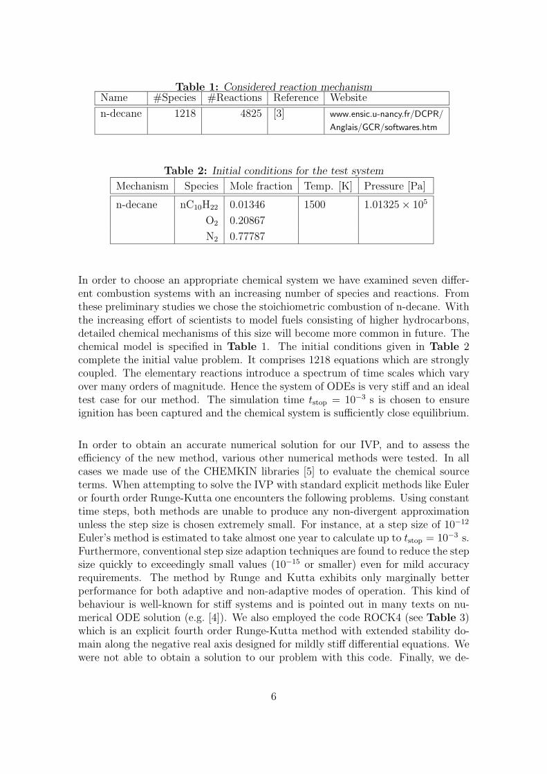
Table 1: Considered reaction mechanismName #Species #Reactions Reference Website

n-decane 1218 4825 [3] www.ensic.u-nancy.fr/DCPR/

Anglais/GCR/softwares.htm

Table 2: Initial conditions for the test system

Mechanism Species Mole fraction Temp. [K] Pressure [Pa]

n-decane nC10H22 0.01346 1500 1.01325 × 105

O2 0.20867

N2 0.77787

In order to choose an appropriate chemical system we have examined seven differ-ent combustion systems with an increasing number of species and reactions. Fromthese preliminary studies we chose the stoichiometric combustion of n-decane. Withthe increasing effort of scientists to model fuels consisting of higher hydrocarbons,detailed chemical mechanisms of this size will become more common in future. Thechemical model is specified in Table 1. The initial conditions given in Table 2complete the initial value problem. It comprises 1218 equations which are stronglycoupled. The elementary reactions introduce a spectrum of time scales which varyover many orders of magnitude. Hence the system of ODEs is very stiff and an idealtest case for our method. The simulation time tstop = 10−3 s is chosen to ensureignition has been captured and the chemical system is sufficiently close equilibrium.

In order to obtain an accurate numerical solution for our IVP, and to assess theefficiency of the new method, various other numerical methods were tested. In allcases we made use of the CHEMKIN libraries [5] to evaluate the chemical sourceterms. When attempting to solve the IVP with standard explicit methods like Euleror fourth order Runge-Kutta one encounters the following problems. Using constanttime steps, both methods are unable to produce any non-divergent approximationunless the step size is chosen extremely small. For instance, at a step size of 10−12

Euler’s method is estimated to take almost one year to calculate up to tstop = 10−3 s.Furthermore, conventional step size adaption techniques are found to reduce the stepsize quickly to exceedingly small values (10−15 or smaller) even for mild accuracyrequirements. The method by Runge and Kutta exhibits only marginally betterperformance for both adaptive and non-adaptive modes of operation. This kind ofbehaviour is well-known for stiff systems and is pointed out in many texts on nu-merical ODE solution (e.g. [4]). We also employed the code ROCK4 (see Table 3)which is an explicit fourth order Runge-Kutta method with extended stability do-main along the negative real axis designed for mildly stiff differential equations. Wewere not able to obtain a solution to our problem with this code. Finally, we de-

6

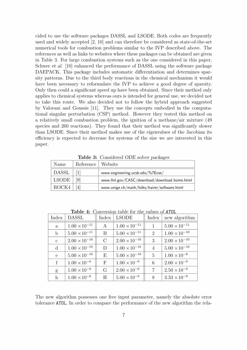
cided to use the software packages DASSL and LSODE. Both codes are frequentlyused and widely accepted [2, 10] and can therefore be considered as state-of-the-artnumerical tools for combustion problems similar to the IVP described above. Thereferences as well as links to websites where these packages can be obtained are givenin Table 3. For large combustion systems such as the one considered in this paper,Schwer et al. [10] enhanced the performance of DASSL using the software packageDAEPACK. This package includes automatic differentiation and determines spar-sity patterns. Due to the third body reactions in the chemical mechanism it wouldhave been necessary to reformulate the IVP to achieve a good degree of sparsity.Only then could a significant speed up have been obtained. Since their method onlyapplies to chemical systems whereas ours is intended for general use, we decided notto take this route. We also decided not to follow the hybrid approach suggestedby Valorani and Goussis [11]. They use the concepts embodied in the computa-tional singular perturbation (CSP) method. However they tested this method ona relatively small combustion problem, the ignition of a methane/air mixture (49species and 260 reactions). They found that their method was significantly slowerthan LSODE. Since their method makes use of the eigenvalues of the Jacobian itsefficiency is expected to decrease for systems of the size we are interested in thispaper.

Table 3: Considered ODE solver packages

Name Reference Website

DASSL [1] www.engineering.ucsb.edu/%7Ecse/

LSODE [9] www.llnl.gov/CASC/download/download home.html

ROCK4 [4] www.unige.ch/math/folks/hairer/software.html

Table 4: Conversion table for the values of ATOLIndex DASSL Index LSODE Index new algorithm

a 1.00 ×10−11 A 1.00 ×10−11 1 5.00 ×10−11

b 5.00 ×10−11 B 5.00 ×10−11 2 1.00 ×10−10

c 2.00 ×10−10 C 2.00 ×10−10 3 2.00 ×10−10

d 1.00 ×10−10 D 1.00 ×10−10 4 5.00 ×10−10

e 5.00 ×10−10 E 5.00 ×10−10 5 1.00 ×10−9

f 1.00 ×10−8 F 1.00 ×10−9 6 2.00 ×10−9

g 1.00 ×10−9 G 2.00 ×10−9 7 2.50 ×10−9

h 1.00 ×10−6 H 5.00 ×10−9 8 3.33 ×10−9

The new algorithm possesses one free input parameter, namely the absolute errortolerance ATOL. In order to compare the performance of the new algorithm the rela-

7

tive tolerances RTOL in DASSL and LSODE are chosen to be zero for the numericalexperiments. We found that for the test system considered, both packages performbest for RTOL = 0. Eight numerical experiments for each method with differentvalues of ATOL are presented here. Table 4 displays an index and the correspondingerror tolerance for each solver. Besides these experiments a high precision run wasperformed using DASSL with RTOL = 10−9 and ATOL = 10−15. In the following,the result of this run is referred to as the “exact” solution. As an estimate of theglobal error we measure the absolute overall deviation of the approximation x fromthe exact solution x of the ODE after the calculation has been performed (i.e. aposteriori). Specifically, we employ

ctot :=1

M + 1

M∑

j=0

∣∣x(tj) − x(tj)∣∣, (2)

where the time interval [0, tstop] is split into M subintervals of equal length via

tj := j × tstop

M.

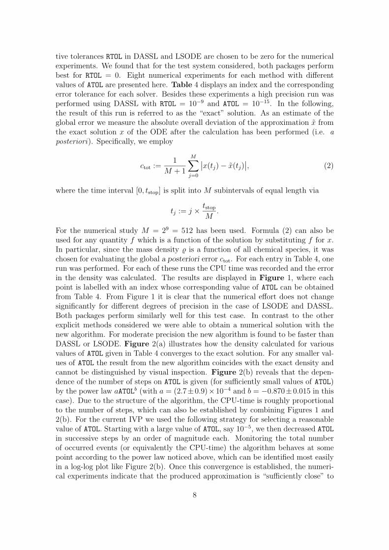
For the numerical study M = 29 = 512 has been used. Formula (2) can also beused for any quantity f which is a function of the solution by substituting f for x.In particular, since the mass density � is a function of all chemical species, it waschosen for evaluating the global a posteriori error ctot. For each entry in Table 4, onerun was performed. For each of these runs the CPU time was recorded and the errorin the density was calculated. The results are displayed in Figure 1, where eachpoint is labelled with an index whose corresponding value of ATOL can be obtainedfrom Table 4. From Figure 1 it is clear that the numerical effort does not changesignificantly for different degrees of precision in the case of LSODE and DASSL.Both packages perform similarly well for this test case. In contrast to the otherexplicit methods considered we were able to obtain a numerical solution with thenew algorithm. For moderate precision the new algorithm is found to be faster thanDASSL or LSODE. Figure 2(a) illustrates how the density calculated for variousvalues of ATOL given in Table 4 converges to the exact solution. For any smaller val-ues of ATOL the result from the new algorithm coincides with the exact density andcannot be distinguished by visual inspection. Figure 2(b) reveals that the depen-dence of the number of steps on ATOL is given (for sufficiently small values of ATOL)by the power law aATOLb (with a = (2.7±0.9)×10−4 and b = −0.870±0.015 in thiscase). Due to the structure of the algorithm, the CPU-time is roughly proportionalto the number of steps, which can also be established by combining Figures 1 and2(b). For the current IVP we used the following strategy for selecting a reasonablevalue of ATOL. Starting with a large value of ATOL, say 10−5, we then decreased ATOL

in successive steps by an order of magnitude each. Monitoring the total numberof occurred events (or equivalently the CPU-time) the algorithm behaves at somepoint according to the power law noticed above, which can be identified most easilyin a log-log plot like Figure 2(b). Once this convergence is established, the numeri-cal experiments indicate that the produced approximation is “sufficiently close” to

8

102

103

10-8

10-7

10-6

DASSL

LSODE

new algorithm

CP

U-t

ime

[s]

Error ctot

[g/cm3]

a

A

1

f

4E

7

d

5

6

8

2

3

h

H

BD

c b

F

gH

Figure 1: CPU-time of the considered algorithms as a function of the total errorctot of the mass density � for the n-decane mechanism

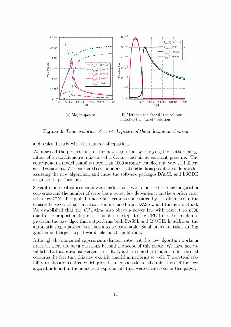
the exact solution. In Figure 3(a) the time evolution of some major species is dis-played. This result was obtained with the new algorithm choosing ATOL = 2× 10−10

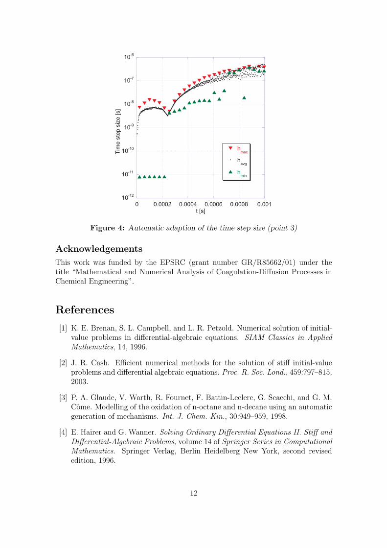
(corresponding to point 3 in Figure 1). The profiles from this simulation coincidewith the exact solution. In Figure 3(b), methane and the OH radical are shown,which have been chosen as examples of species whose concentration exhibits sharpgradients and small absolute values. Even for these species very good agreementbetween the exact solution and the approximation by new algorithm can be found,for this particular choice of ATOL. This also suggests that the error in the density isa good indicator for the error in the species concentrations. Figure 4 shows howthe automatic step size adaption works in practice (for point 3). Since the totalnumber of steps for this run is 74476 we decided to plot the step size not for everysingle step. Instead, the solution interval [0, tstop] is (as above) split into M = 512subintervals over each of which the maximum, average and minimum step size (hmax,havg and hmin respectively) is calculated. For the maximum and minimum curvesonly every twentieth data point is shown. In this diagram, one can recognise thefollowing characteristic features, which are desirable for any kind of step size adap-tion. At t = 0 and during the ignition (at t ≈ 2.5 ×10−4 s) the step size becomesrelatively small, because at these points in time the concentrations of several speciesare rapidly changing (the right hand side Q of equation (1) is large in magnitude).Recall that the step size is inversely proportional to the sum of the absolute valuesof the components of the right hand side. At later times the step size becomes com-

9

2.15 10-4

2.2 10-4

2.25 10-4

2.3 10-4

2.35 10-4

2.4 10-4

2.45 10-4

2.5 10-4

0 0.0002 0.0004 0.0006 0.0008 0.001

ATOL=3.3*10-9

(point 8)

ATOL=2.5*10-9

(point 7)

ATOL=10-9

(point 5)

exact

Density

[g/c

m3]

t [s]

(a) Time evolution of the mass den-sity for various values of ATOL

100

101

102

103

104

105

106

10-11

10-10

10-9

10-8

10-7

10-6

10-5

Steps

a*ATOLb

Ste

ps

ATOL

1

3

5

8

(b) Number of steps as a function ofATOL

Figure 2: Convergence properties of the new algorithm

paratively large as the system approaches equilibrium (i.e., small right hand side).Note also the large fluctuations, which reflect the sensitivity of the right hand sidetowards the quantities of interest.

Even though these numerical tests are not exhaustive, one is tempted to concludethat it is the idea of treating each component of the solution separately whichexplains the relatively high performance and suitability for stiff systems. FromFigure 1 it is also clear that this algorithm is only suitable for situations wheremoderate precision of the solution is sought. However, there are many situationswhere high precision is not required, in particular when a system of ODEs mustbe solved in the context of operator splitting (see for example [7]), where it isimportant that the start up costs of the ODE solver are low. This is the case forthe new algorithm due to its simple explicit structure. However, a great advantageof the new algorithm is that the numerical effort scales linearly with the number ofequations. This means that our algorithm is an ideal candidate for very large andvery stiff systems of ordinary differential equations. Such systems occur frequentlyin dynamic process simulation of large scale plants in the chemical industry andelectronic circuit design. Other examples can be found in the numerical treatmentof some partial differential equations.

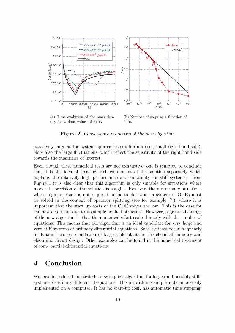
4 Conclusion

We have introduced and tested a new explicit algorithm for large (and possibly stiff)systems of ordinary differential equations. This algorithm is simple and can be easilyimplemented on a computer. It has no start-up cost, has automatic time stepping,

10

0 100

2.5 10-2

5 10-2

7.5 10-2

1 10-1

1.25 10-1

1.5 10-1

0 0.0002 0.0004 0.0006 0.0008 0.001

XO2

(t) (point 3)

XH2O

(t) (point 3)

XH2

(t) (point 3)

XCO

(t) (point 3)

XCO2

(t) (point 3)

Mole

fraction

t [s]

(a) Major species

0 100

1 10-3

2 10-3

3 10-3

4 10-3

5 10-3

6 10-3

0 0.0002 0.0004 0.0006 0.0008 0.001

XCH4

(t) (point 3)

XOH

(t) (point 3)

XCH4

(t) (exact)

XOH

(t) (exact)

Mole

fraction

t [s]

(b) Methane and the OH radical com-pared to the “exact” solution

Figure 3: Time evolution of selected species of the n-decane mechanism

and scales linearly with the number of equations.

We assessed the performance of the new algorithm by studying the isothermal ig-nition of a stoichiometric mixture of n-decane and air at constant pressure. Thecorresponding model contains more than 1000 strongly coupled and very stiff differ-ential equations. We considered several numerical methods as possible candidates forassessing the new algorithm, and chose the software packages DASSL and LSODEto gauge its performance.

Several numerical experiments were performed. We found that the new algorithmconverges and the number of steps has a power law dependence on the a priori errortolerance ATOL. The global a posteriori error was measured by the difference in thedensity between a high precision run, obtained from DASSL, and the new method.We established that the CPU-time also obeys a power law with respect to ATOL

due to the proportionality of the number of steps to the CPU-time. For moderateprecision the new algorithm outperforms both DASSL and LSODE. In addition, theautomatic step adaption was shown to be reasonable. Small steps are taken duringignition and larger steps towards chemical equilibrium.

Although the numerical experiments demonstrate that the new algorithm works inpractice, there are open questions beyond the scope of this paper. We have not es-tablished a theoretical convergence result. Another issue that remains to be clarifiedconcerns the fact that this new explicit algorithm performs so well. Theoretical sta-bility results are required which provide an explanation of the robustness of the newalgorithm found in the numerical experiments that were carried out in this paper.

11

10-12

10-11

10-10

10-9

10-8

10-7

10-6

0 0.0002 0.0004 0.0006 0.0008 0.001

hmax

havg

hmin

Tim

este

psiz

e[s

]

t [s]

Figure 4: Automatic adaption of the time step size (point 3)

Acknowledgements

This work was funded by the EPSRC (grant number GR/R85662/01) under thetitle “Mathematical and Numerical Analysis of Coagulation-Diffusion Processes inChemical Engineering”.

References

[1] K. E. Brenan, S. L. Campbell, and L. R. Petzold. Numerical solution of initial-value problems in differential-algebraic equations. SIAM Classics in AppliedMathematics, 14, 1996.

[2] J. R. Cash. Efficient numerical methods for the solution of stiff initial-valueproblems and differential algebraic equations. Proc. R. Soc. Lond., 459:797–815,2003.

[3] P. A. Glaude, V. Warth, R. Fournet, F. Battin-Leclerc, G. Scacchi, and G. M.Come. Modelling of the oxidation of n-octane and n-decane using an automaticgeneration of mechanisms. Int. J. Chem. Kin., 30:949–959, 1998.

[4] E. Hairer and G. Wanner. Solving Ordinary Differential Equations II. Stiff andDifferential-Algebraic Problems, volume 14 of Springer Series in ComputationalMathematics. Springer Verlag, Berlin Heidelberg New York, second revisededition, 1996.

12

[5] R. J. Kee, F. M. Rupley, E. Meeks, and J. A. Miller. Chemkin-III: A FORTRANchemical kinetics package for the analysis of gas-phase chemical and plasma ki-netics. Technical Report SAND96-8216 UC-405, Sandia National Laboratories,1996.

[6] S. Mosbach and M. Kraft. Stochastic modelling of large scale combustion sys-tems. Technical Report 13, Cambridge Centre for Computational ChemicalEngineering, 2003.

[7] R. D. Mott, E. S. Oran, and B. van Leer. A quasi-steady-state solver forthe stiff ordinary differential equations of reaction kinetics. J. Comp. Phys.,164:407–428, 2000.

[8] E. S. Oran and J. P. Boris. Numerical Simulation of Reactive Flow. CambridgeUniversity Press, 2nd edition, 2000.

[9] K. Radhakrishnan and A. C. Hindmarsh. Description and use of LSODE, theLivermore Solver for Ordinary Differential Equations. Technical Report UCRL-ID-113855, Lawrence Livermore National Laboratory, 1993.

[10] D. A. Schwer, J. E. Tolsma, W. H. Green, and P. I. Barton. On upgrading thenumerics in combustion chemistry codes. Combustion and Flame, 128:270–291,2002.

[11] M. Valorani and D. A. Goussis. Explicit time-scale splitting algorithm for stiffproblems: Auto-ignition of gaseous mixtures behind a steady shock. J. Comput.Phys., 169(1):44–79, 2001.

[12] J. G. Verwer. Explicit Runge-Kutta methods for parabolic partial differentialequations. Appl. Numer. Math., 22(1-3):359–379, 1996.

13