

January || 2014 - International Journal of Computational ...
225
-
Upload
khangminh22 -
Category
Documents
-
view
5 -
download
0
Transcript of January || 2014 - International Journal of Computational ...

Editor-In-Chief
Prof. Chetan Sharma Specialization: Electronics Engineering, India
Qualification: Ph.d, Nanotechnology, IIT Delhi, India
Editorial Committees
DR.Qais Faryadi
Qualification: PhD Computer Science
Affiliation: USIM(Islamic Science University of Malaysia)
Dr. Lingyan Cao
Qualification: Ph.D. Applied Mathematics in Finance
Affiliation: University of Maryland College Park,MD, US
Dr. A.V.L.N.S.H. HARIHARAN
Qualification: Phd Chemistry
Affiliation: GITAM UNIVERSITY, VISAKHAPATNAM, India
DR. MD. MUSTAFIZUR RAHMAN
Qualification: Phd Mechanical and Materials Engineering
Affiliation: University Kebangsaan Malaysia (UKM)
Dr. S. Morteza Bayareh
Qualificatio: Phd Mechanical Engineering, IUT
Affiliation: Islamic Azad University, Lamerd Branch
Daneshjoo Square, Lamerd, Fars, Iran
Dr. Zahéra Mekkioui
Qualification: Phd Electronics
Affiliation: University of Tlemcen, Algeria
Dr. Yilun Shang
Qualification: Postdoctoral Fellow Computer Science
Affiliation: University of Texas at San Antonio, TX 78249
Lugen M.Zake Sheet
Qualification: Phd, Department of Mathematics
Affiliation: University of Mosul, Iraq
Mohamed Abdellatif
Qualification: PhD Intelligence Technology
Affiliation: Graduate School of Natural Science and Technology

Meisam Mahdavi
Qualification: Phd Electrical and Computer Engineering
Affiliation: University of Tehran, North Kargar st. (across the ninth lane), Tehran, Iran
Dr. Ahmed Nabih Zaki Rashed
Qualification: Ph. D Electronic Engineering
Affiliation: Menoufia University, Egypt
Dr. José M. Merigó Lindahl
Qualification: Phd Business Administration
Affiliation: Department of Business Administration, University of Barcelona, Spain
Dr. Mohamed Shokry Nayle
Qualification: Phd, Engineering
Affiliation: faculty of engineering Tanta University Egypt

Contents: S.No. Title Name Page No.
Version I
1. Power System Planning and Operation Using Artificial Neural Networks
Ankita Shrivastava, Arti Bhandakkar
01-06
2. A Survey on Software Suites for Data Mining, Analytics and Knowledge Discovery R.Kiruba Kumari, V.Vidya, M.Pushpalatha
07-12
3.
Hydraulic Characteristics of a Rectangular Weir Combined with Equal and Unequal Size Three Rectangular Bottom Openings s Rafa H.Al-Suhaili, Jabbar H.Al-Baidhani, and NassrinJ.Al-Mansori
13-29
4.
An Investigation of the Effect of Shot Peening On the Properties of Lm25 Aluminium Alloy and Statistical Modelling Sirajuddin Elyas Khany, Obaid Ullah Shafi, Mohd Abdul Wahed
30-40
5.
Climate Change Analysis and Adaptation: The Role of Remote Sensing (Rs) And Geographical Information System (Gis) Nathaniel Bayode Eniolorunda
41-51
6.
Influence of Supply Chain Management On Its Operational Performance
Jagdish Ahirwar, Mahima Singh, B. K. Shrivastava, Alkesh Kumar Dhakde
52-55
7.
Processing Of Mammographic Images Using Speckle Technique A.M. Hamed, Tarek A. Al-Saeed
56-62
8.
An Ontology System for Ability Optimization & Enhancement in Cloud Broker Pradeep Kumar
63-69
9 Evaluation and Modeling of High Surface Area Activated Carbon from Date Frond and Application on Some Pollutants M.M.S. Ali, ,N. EL-SAID ,B. S. GIRGIS
70-78
Version 2 1.
A Survey of Protection Against DoS & DDoS Attacks Mrs.S.Thilagavathi , Dr.A.Saradha 01-10

2.
The Effect of Chemical Reaction on Mhd Free Convection Flow Of Dissipative Fluid Past An Exponentially Accelerated Vertical Plate P.M. Kishore, S. Vijayakumar Varma, S. Masthan Rao, K.S. Bala Murugan
11-26
3.
A Review on Parametric Optimization of Tig Welding
Naitik S Patel, Prof. Rahul B Patel
27-31
4.
MV Compensation Attack on fast Selective Video Encryptions Jay M. Joshi, Upena D. Dalal
32-38
5. Studies on the Variation in Coal Properties Of Low Volatile Coking Coal After Beneficiation
Vivek Kumar, V.K. Saxena
39-57
6.
Pre-Loading Impact on Mechanical Properties of Sand-Polystyrene-Cement Mix Aneke I.F., Agbenyeku E.E.
58-64
7. The Effect of Activating Flux in Tig Welding Akash.B.Patel , Prof.Satyam.P.Patel
65-70
8.
Independent and Total Strong (Weak) Domination in Fuzzy Graphs P.J.Jayalakshmi, S.Revathi , C.V.R. Harinarayanan
71--74
9.
Effect of discrete heating on natural convection heat transfer on square plate Dr. V Katti, S G Cholake, Anil Rathod
75-80
Version 3
1.
Slicing Algorithm for Controlling Backtracking In Prolog Divanshi PriyadarshniWangoo
01-05
2.
The Use Of The Computational Method Of Hamming Code Techniques For The Detection And Correction Of Computational Errors In A Binary Coded Data: Analysis On An Integer Sequence A119626 Afolabi Godfrey, Ibrahim A.A, Ibrahim Zaid
06-15
3
Intrusion Awareness Based On D-SA Prashant Shakya , Prof. Rahul Shukla
16-18
4.
A Review On Dry Sliding Wear Analysis On Brass Using Taguchi Technique Sachin P Patel , Prof. Tausif M Shaikh, Prof. Navneet K Prajapati
19-23
5.
Survey on Various Techniques of Brain Tumor Detection from MRI Images Mr.Deepak .C.Dhanwani , Prof. Mahip M.Bartere
24-26

6.
Transforming Satellite Campuses of Tertiary-education Institutions in Nigeria through Appropriate Application of Information Technology: A Case Study Adu Michael K
27-34
7.
Effect of boundary roughness on Kelvin-Helmholtz instability in Couple stress fluid layer bounded above by a porous layer and below by rigid surface Krishna B. Chavaraddi, N. N. Katagi,V. B. Awati, Priya M. Gouder
35-43
8.
Combinational Study of Mineral Admixture and Super Plasticizer in Usual Concrete Debabrata Pradhan, D. Dutta, Dr. Partha Ghosh
44-48
9. Design of Closed Loop Electro Mechanical Actuation System Oondla.Chiranjeevi, J.Venkatesu Naik
49-55
10. Effect Of In-Band Crosstalk For Datapath Routing In Wdm/Dwdm Networks Praveen Singh , Prof. R.L.Sharma
56-61

International Journal Of Computational Engineering Research (ijceronline.com) Vol. 04 Issue. 01
|| Issn 2250-3005 (online) || || January || 2014 || Page 1
Power System Planning and Operation Using Artificial Neural
Networks
Ankita Shrivastava1 and Arti Bhandakkar
2
1PG Scholar, Shriram Institute of Technology, Jabalpur
2Associate Professor, Shriram Institute of Technology, Jabalpur
I. INTRODUCTION Load Forecasting is an important component for power system energy management system. Load
forecasting means predicting the future load with the help of historical load data available. It is very important
for the planning, operation and control of power system. It plays a vital role in the deregulated electric industry
[1].
A good forecast reflects current and future trends in the power system. The accuracy of a forecast is
crucial to any electric utility. That is why, accurate models for load forecasting are essential for the operation
and planning of a utility company [2].
Since in power system the next day’s power generation must be scheduled every day, day- ahead short-
term load forecasting (STLF) is a necessary daily task for power dispatch. Its accuracy affects the economic
operation and reliability of the system greatly [3].
Short- term load forecasts helps in estimating the load flows. This helps in making decisions that can
prevent overloading and the result deeply influence the power systems’ safety and economy [4].
The short- term forecasts are not only needed for control and scheduling of power system but also used
as inputs to load flow study or contingency analysis i.e. for load management program. The short term
forecasting is also primarily used for the generation dispatch, capacitor switching, feeder reconfiguration,
voltage control, and automatic generation control (AGC) [5].
A little increase in the percentages of short-term prediction accuracy may bring many benefits in terms
of economy and reliability of power system. Therefore, precise short- term load forecasting not only enhances
the reliability of power supply but also increases economic benefits [6].
The research work in this area is still a challenge to the electrical engineering scholars because of its
high complexity. How to estimate the future load with the historical data has remained a difficulty up to now,
especially for the load forecasting of holidays, days with extreme weather and other anomalous days. But with
the recent development of new mathematical and artificial intelligence tools, it is potentially possible to improve
the forecasting results [7].
Load Forecasting can be performed using many techniques such as similar day approach, various
regression models, time series, statistical methods, fuzzy logic, artificial neural networks, expert systems, etc.
But application of artificial neural network in the areas of forecasting has made it possible to overcome the
limitations of the other methods mentioned above used for electrical load forecasting [8].
II. ARTIFICIAL NEURAL NETWORK Neural networks are essentially non-linear circuits that have the demonstrated capability to do non-linear
curve fitting. The outputs of an artificial neural network are some linear or non-linear mathematical function of
its inputs [9].
ABSTRACT: Load forecasting is essential part for the power system planning and operation. In this paper the
modeling and design of artificial neural network for load forecasting is carried out in a particular region
of India. Three ANN- techniques – Radial Basis Function Neural Network, Feed forward Neural Network
and Cascade- Forward Neural Network are discussed in this paper. Their performances are evaluated
through a simulation study. This gives load forecasts one hour in advance. Historical Load Data from
the Load Dispatch Centre Jabalpur are used for training, testing and showing the good performance of
the proposed method. The proposed model can forecast the load profile with a lead time of one to seven
days.
Keywords: Artificial Intelligence, Artificial Neural Network, Back-Propagation, Energy Consumption,
Load Forecasting.

Power System Planning and Operation Using Artificial Neural Networks
|| Issn 2250-3005 (online) || || January || 2014 || Page 2
ANN is usually formed from many hundreds or thousands of simple processing units, connected in
parallel and feeding forward in several layers. Because of the fast and inexpensive personal computers
availability, the interest in ANN’s has blossomed in the current digital world. The basic motive of the
development of the ANN is to make the computers do what a human being cannot do.
The three-layer fully connected feed-forward neural network which is generally used for load
forecasting. It comprises of an input layer, one hidden layer and an output layer.
Signal system is allowed only from the input layer to the hidden layer and from the hidden layer to the
output layer. Input variables come from historical data, which are date, hour of the day, past system load,
temperature and humidity, corresponding tothe factors that affect the load. The outputs are the forecasting
results. The number of inputs, the number of hidden nodes, transfer functions, scaling schemes, and training
methods affect the forecasting performance and, hence, need to be chosen carefully [10].
In applying a neural network to load forecasting, one must select one of a number of architectures (e.g.
Hopfield, back propagation, Boltzmann machine), the number and connectivity of layers and elements, use of
bi-directional or uni-directional links and the number format (e.g. binary or continuous) to be used by inputs and
outputs
Figure 1: Structure of Ann
This is the structure of ANN. There are three layers namely, input layer, hidden layer and output layer.
III. NETWORK DESIGN AND TESTING In this section three types of neural network architectures are presented for short term load forecasting.
Radial Basis Function Network
A radial basis function network is an artificial neural network that uses radial basis
functions as activation functions. Radial basis function (RBF) networks typically have three layers: an input
layer, a hidden layer with a non-linear RBF activation function and a linear output layer.
Figure 2: Architecture of Radial Basis Function Network

Power System Planning and Operation Using Artificial Neural Networks
|| Issn 2250-3005 (online) || || January || 2014 || Page 3
The input of a RBF network can be modelled as a vector of real numbers . The output of the
network is then a scalar function of the input vector, , and is given by
Also,
And,
Where,
N = the number of neurons in the hidden layer
=the center vector for neuron i
= the weight of neuron i in the linear output neuron.
The parameters , , are determined in a manner that optimizes the fit between and the data [11].
Feedforward backpropagation (FB) Neural Network
Feedforward BP Network consists of input, hidden and output layers. In a feed forward network
information always moves in one direction; it never goes backwards. Backpropagation learning algorithm was
used for training these networks. During training, calculations are carried out from input layer towards the
output layer, and error values are fed back to the previous layer [12]. The most popular artificial neural network
architecture for load forecasting is back propagation. This network uses continuously valued functions and
supervised learning. That is, under supervised learning, the actual numerical weights assigned to element inputs
are determined by matching historical data (such as time and weather) to desired outputs (such as historical
loads).
Figure 3: Architecture of Feed forward Back propagation Network
Feed forward networks often have one or more hidden layers of sigmoid neurons followed by an output
layer of linear neurons. Multiple layers of neurons with nonlinear transfer functions allow the network to learn
nonlinear and linear relationships between input and output vectors. The linear output layer lets the network
produce values outside the range –1 to +1. On the other hand, outputs of a network such as between 0 and 1 are
produced, then the output layer should use a sigmoid transfer function (tansig) [13].
Cascade Forward Back propagation Network
Cascade forward back propagation model is similar to feed-forward networks, but include a weight
connection from the input to each layer and from each layer to the successive layers. While two- layer feed-
forward networks can potentially learn virtually any input-output relationship, feed-forward networks with more
layers might learn complex relationships more quickly. The function newcf creates cascade-forward networks .

Power System Planning and Operation Using Artificial Neural Networks
|| Issn 2250-3005 (online) || || January || 2014 || Page 4
Cascade forward back propagation ANN model is similar to feed forward back propagation neural
network in using the back propagation algorithm for weights updating, but the main nature of this network is
that each layer of neurons is related to all previous layer of neurons. For example, a three layer network has
connections from layer 1 to layer 2, layer 2
to layer 3, and layer 1 to layer 3. The three-layer network also has connections from the input to all three layers
[12].
Figure 4: Architecture Of Cascade Forward Back- Propagation Network
Tan-sigmoid transfer function was used to reach the optimized status. The performance of cascade
forward back propagation and feed forward back propagation were evaluated using Mean Square Error (MSE)
[13].
2
IV. RESULTS AND DISCUSSIONS The acceptable criteria for a particular model is based upon the
i. Mean Square Error (MSE)
ii. Training Time
iii. Detection Time
Performance of RBF Network
Training with RBF network for 98 epochs taking goal=0.01 and spread=1 gives good performance in
terms of MSE (mean square error) equal to 1.62.
Figure 5: Performance of RBF Neural Network
Here MSE= 1.62, Training Time= 1.5744 and Detection Time= 0.0175.
Performance of FBPNN For different numbers of neurons the system has been trained and tested but the exact forecast is
obtained for 12,12 neurons.

Power System Planning and Operation Using Artificial Neural Networks
|| Issn 2250-3005 (online) || || January || 2014 || Page 5
Figure 6: Performance of FBPNN
Here MSE= 1.7032e+004, Training Time= 2.4981 and Detection Time= 0.0206
Performance of Cascade Forward BP Network
For different numbers of neurons the system has been trained and tested but we get the exact forecast
for 15, 15 neurons.
Figure 7: Performance of CF-BP Network
Here MSE = 3.2392e+004, Training Time = 15.5890 and Detection Time = 0.0254
V. CONCLUSIONS The result of the three neural network models (RBFNN, FFBPNN, CFBPNN) used for short term load
forecast for Jabalpur region, shows that the networks has good performances and accurate prediction is
achieved. Its forecasting reliabilities were evaluated by computing the mean square error (MSE) between the
exact and predicted values.
The results suggest that ANN model with the developed structure can perform good prediction with
least error and finally this neural network could be an important tool for short term load forecasting as well as
this work incorporates additional information such as Hour of the Day, Days of the month, and different weather
conditions into the network so as to obtain a more representative forecast of future load.

Power System Planning and Operation Using Artificial Neural Networks
|| Issn 2250-3005 (online) || || January || 2014 || Page 6
REFERENCES [1] Hong Chen, Claudio A. Canizares, Ajit Singh, “ANN- based Short- Term Load Forecasting in Electricity Markets”,
University of Waterloo, Canada
[2] Sanjib Mishra, Sarat Kumar Patra, “Short Term Load Forecasting using a Neural Network trained by A Hybrid Artificial
Immune System”, 2008 IEEE Region 10 Colloquium and the Third International Conference on Industrial and Information
Systems, Kharagpur, India December 8- 10, 2008
[3] J.P.S. Catalao, S.J.P.S. Mariano, V.M.F. Mendes, L.A.F.M. Ferreira, “Short Term electricity prices forecasting in a
competitive market: A neural network approach”, ScienceDirect, Electric Power Systems Research 77 (2007) 1297- 1304
[4] Ajay Gupta, Pradeepta K. Sarangi, “Electrcal Load Forecasting Using Genetic Algorithm Based Back- Propagation Method”, ARPN Journal of Engineering and Applied Sciences, vol. 7, no.8, August 2012
[5] Shu Fan, Yuan- Kang Wu, Wei- Jen Lee, Ching- Yin Lee, ”Comparative Study on Load Forecasting Technologies for
Different Geographical Distributed Loads”, proc of IEEE 2011
[6] Eugene A. Feinberg, Dora Genethliou, State University of New York, Stony Brook, “Chapter 12 LOAD FORECASTING”
[7] K.Y. Lee, Y.T. Cha, J.H. Park, “Short- Term Load Forecasting Using an Artificial Neural Network”, Transactions on Power Systems, vol. 7, No. 1, February 1992
[8] Muhammad Buhari, Sanusi Sani Adamu, “Short-Term Load Forecasting Using Artificial Neural Network”, Proc. of the
International MultiConference of Engineers and Computer Scientists 2012 Vol I, IMECS 2012, March 14- 16,2012, Hong Kong
[9] Gautham P. Das, Chandrasekar S., Piyush Chandra Ojha, “ Artificial Neural Network Based Short Term Load Forecasting for
the Distribution Utilities” Kalki Communication Technologies Ltd. Available at www.kalkitech.com
[10] Fatemeh Mosalman, Alireza Mosalman, H. Mosalman Yazdi, M. Mosalman Yazdi, “One day- ahead load forecasting by
artificial neural network”, Scientific Research and Essays Vol. 6 (13), pp. 2795- 2799, 4 July, 2011. Available at
www.academicjournals.org/SRE http://en.wikipedia.org/RadialBasisFunction (accessed on 28.9.2013). [11] H.Demuth, M. Beale and M.Hagan. “Neural Network Toolbox User‟ s Guide”. The MathWorks, Inc., Natrick, USA. 2009
[12] Dheeraj S. Badde, Anil k. Gupta, Vinayak K. Patki, “Cascade and Feed Forward Back propagation Artificial Neural Network
Models for Prediction of Compressive Strength of Ready Mix Concrete”, IOSR Journal of Mechanical and Civil Engineering (IOSR-JMCE) ISSN: 2278-1684, PP: 01-06 www.iosrjournals.org Second

International Journal Of Computational Engineering Research (ijceronline.com) Vol. 04 Issue. 01
|| Issn 2250-3005 (online) || || January || 2014 || Page 7
A Survey on Software Suites for Data Mining, Analytics and
Knowledge Discovery
R.Kiruba Kumari1, V.Vidya
2, M.Pushpalatha
3
1, HoD, Department of Computer Science, Padmavani Arts and Science College for Women, Salem
2, Asst.Prof. In Computer Science, Padmavani Arts and Science College for Women, Salem
3, Asst.Prof. In Computer Science, Padmavani Arts and Science College for Women, Salem
I. INTRODUCTION Today, a large number of standard data mining methods are available. The typical life cycle of new data mining
methods begins with theoretical papers based on in house software prototypes, followed by public or on-demand software
distribution of successful algorithms as research prototypes [1]. Then, either special commercial or open source packages
containing a family of similar algorithms are developed or the algorithms are integrated into existing open source or
commercial packages. This paper confers some of the commercial available software suits for data mining.
II. THE ADVANCEDMINER PROFESSIONAL SYSTEM The Advanced Miner Professional System developed by Stat Consulting is modern and advanced analytical
software. It provides a wide range of tools for data transformations, construction of Data Mining models, advanced data
analysis and reporting. Advanced Miner Professional [2] is an integrated environment dedicated to the development of
analytical projects. The system offers various tools supporting the work of analysts and programmers. The software not only
includes data processing tools, but also provides a wide range of statistical algorithms and Data Mining methods, which can
be used to construct effective analytical models. It provides tools for performing various tasks, such as classification,
approximation, clustering, association rules, and survival analysis.
The features of Advanced Miner Professional includes extracting and saving data from/to different database systems and files,
performing a wide range of operations on data, such as sampling, joining datasets, dividing into
testing/training/validating sets, assigning roles to attributes,
graphical and interactive data exploration,
outlier filtering, supplying missing values, PCA, various data transformations, etc.,
building association models, clustering analyses, variable importance analyses, etc.,
constructing various analytical models with the use of diverse Data Mining and statistical algorithms (such as
classification trees, neuron networks, linear and logistic regression, K-means, association rules),
creation of scoring code so that the models can be integrated with other IT applications (scoring code may include
the models as well as data transformations),
model quality evaluation and comparison of Data Mining models (LIFT, ROK, K-S, Confusion Matrix),
generation of model quality reports (MS Office, OpenOffice).
AdvancedMiner Professional is based on well-tested Java technologies, providing platform independence. The
system operates in MS Windows as well as in operating systems from the Unix family (including Linux). AdvancedMiner
Professional is compatible with relational database management systems which provide the JDBC/ODBC interface (e.g.
MySQL, MS SQL, Oracle, Sybase SQL Anywhere Studio).
Abstract Data mining automates the detection of relevant patterns in a database, using defined approaches and
algorithms to look into current and historical data that can then be analyzed to predict future trends.
Data mining software tools predict future trends and behaviors by reading through databases for
hidden patterns, they allow organizations to make proactive, knowledge-driven decisions and answer
questions that were previously too time-consuming to resolve. This paper presents some of the most
common commercially available data mining tools, with their most important features, side by side, and
some considerations regarding the evaluation of data mining tools by companies that want to acquire
such a system.
Keywords: data mining, data mining tools, features, software
A Survey on Software Suites for Data Mining, Analytics and Knowledge Discovery
|| Issn 2250-3005 (online) || || January || 2014 || Page 8
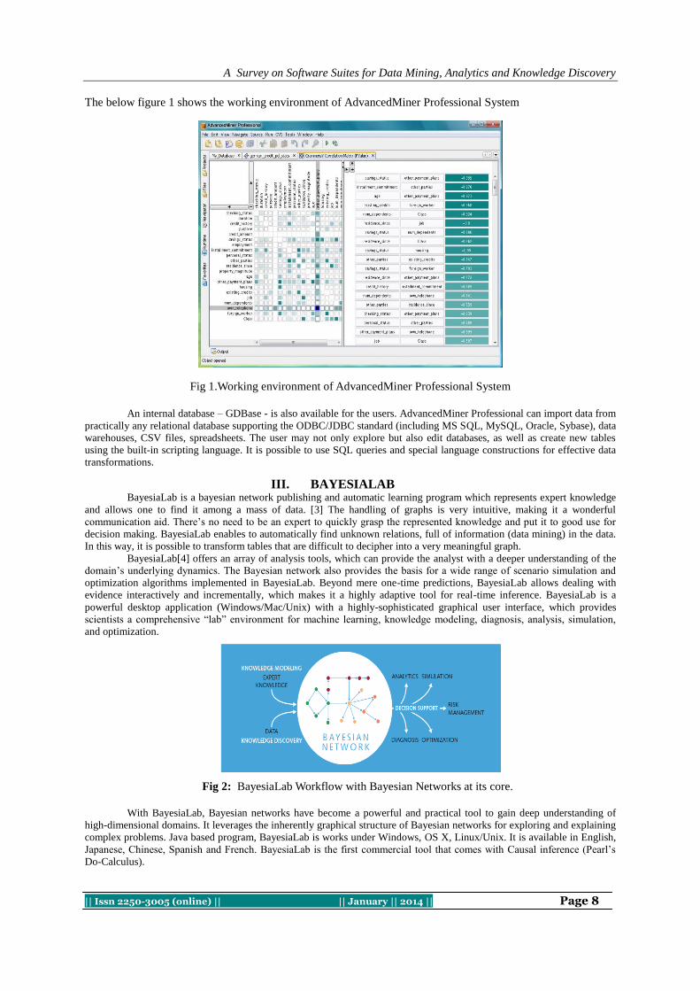
The below figure 1 shows the working environment of AdvancedMiner Professional System
Fig 1.Working environment of AdvancedMiner Professional System
An internal database – GDBase - is also available for the users. AdvancedMiner Professional can import data from
practically any relational database supporting the ODBC/JDBC standard (including MS SQL, MySQL, Oracle, Sybase), data
warehouses, CSV files, spreadsheets. The user may not only explore but also edit databases, as well as create new tables
using the built-in scripting language. It is possible to use SQL queries and special language constructions for effective data
transformations.
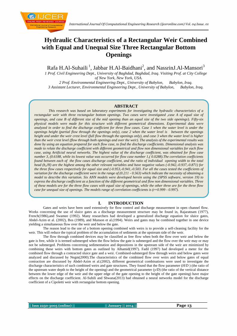
III. BAYESIALAB BayesiaLab is a bayesian network publishing and automatic learning program which represents expert knowledge
and allows one to find it among a mass of data. [3] The handling of graphs is very intuitive, making it a wonderful
communication aid. There’s no need to be an expert to quickly grasp the represented knowledge and put it to good use for
decision making. BayesiaLab enables to automatically find unknown relations, full of information (data mining) in the data.
In this way, it is possible to transform tables that are difficult to decipher into a very meaningful graph.
BayesiaLab[4] offers an array of analysis tools, which can provide the analyst with a deeper understanding of the
domain’s underlying dynamics. The Bayesian network also provides the basis for a wide range of scenario simulation and
optimization algorithms implemented in BayesiaLab. Beyond mere one-time predictions, BayesiaLab allows dealing with
evidence interactively and incrementally, which makes it a highly adaptive tool for real-time inference. BayesiaLab is a
powerful desktop application (Windows/Mac/Unix) with a highly-sophisticated graphical user interface, which provides
scientists a comprehensive “lab” environment for machine learning, knowledge modeling, diagnosis, analysis, simulation,
and optimization.
Fig 2: BayesiaLab Workflow with Bayesian Networks at its core.
With BayesiaLab, Bayesian networks have become a powerful and practical tool to gain deep understanding of
high-dimensional domains. It leverages the inherently graphical structure of Bayesian networks for exploring and explaining
complex problems. Java based program, BayesiaLab is works under Windows, OS X, Linux/Unix. It is available in English,
Japanese, Chinese, Spanish and French. BayesiaLab is the first commercial tool that comes with Causal inference (Pearl’s
Do-Calculus).

A Survey on Software Suites for Data Mining, Analytics and Knowledge Discovery
|| Issn 2250-3005 (online) || || January || 2014 || Page 9
The Causal Intervention is compatible with all the analysis tools that are available in BayesiaLab, and with all the
kinds of evidence (hard, soft, probability distribution, mean value). The type of inference, observation or intervention, can be
set for each variable. BayesiaLab is designed around the Bayesian network paradigm, as is illustrated in Figure2. It covers
the entire research work!ow from model generation to analysis, simulation, and optimization. The entire research workflow
is fully contained in a single “lab” environment, which provides analysts the ultimate flexibility in moving back and forth
between different elements of the research task.
In addition to the adaptation of BayesiaLab to Java 7, here is a small selection of features: An entirely redesigned Target Optimization Tool, which uses a Genetic Algorithm for comprehensive
optimizations.
Automatic Computation of Contributions for each network generated through Multi-Quadrant Analysis.
Disjunctive Inference and Negation of the Evidence Set for scenario analysis.
Workspace to start BayesiaLab with a set of previously opened networks.
A "Token Borrowing" functions for floating licenses, which allows users to work offline, e.g. while traveling.
The figure 3 depicts the interface of bayesia lab for clustering.
Fig 3: Interface of bayesia lab for implementing clustering
IV. SAS ENTERPRISE MINER SAS Enterprise Miner [5] streamlines the data mining process to create highly accurate predictive and descriptive
models based on large volumes of data from across the enterprise. It offers a rich, easy-to-use set of integrated capabilities
for creating and sharing insights that can be used to drive better decisions.
Features
Powerful, easy-to-use GUI, as well as batch processing for large jobs
Interactive GUI for building process flow diagrams.
Batch processing code for scheduling large modeling and scoring jobs.
Data preparation, summarization and exploration
Access and integrate structured and unstructured data sources.
Outlier filtering.
Data sampling.
Data partitioning.
File import.
Merge and append tools.
Univariate statistics and plots.
Bivariate statistics and plots.
Batch and interactive plots.
Segment profile plots.
Easy-to-use Graphics Explorer wizard and Graph Explore node.
Interactively linked plots and tables.
Data transformations.
Time series data preparation and analysis.
Interactive variable binning.
Rules Builder node for creating ad hoc data-driven rules and policies.
Data replacement.
Enterprise Miner 12.3 includes new pre-built Enterprise Miner data mining process flow diagram templates. The
data mining process flow diagram templates serve as examples of analytic data mining modeling approaches for
some of the more common specific business problems.

A Survey on Software Suites for Data Mining, Analytics and Knowledge Discovery
|| Issn 2250-3005 (online) || || January || 2014 || Page 10
The Enterprise Miner 12.3 client can now open to directly load a specific data mining project or diagram. The
Project Navigator tree now displays the most recently opened projects and process flow diagrams at the top.
The Enterprise Miner 12.3 Link Analysis node converts relational and transactional data into a data model that can
be visualized as a network of effects. The node can detect the linkages between any two variables' levels for
relational data and between two items' co-occurrence in transactional data. Multiple centrality measures and
community information are provided for users to better understand linkage graphs. The Link Analysis node
generates cluster scores from raw data that can be used for data reduction and segmentation. The Link Analysis
node also uses weighted confidence statistics to provide "next-best-offer" information to customers.
The Enterprise Miner 12.3 [6] Reporter node improves image and table displays for upgraded PDF and RTF
output. The Reporter node report files are smaller in size, but contain improved graphic displays and provide new
graphic output font scaling options.
The Enterprise Miner 12.3 Impute node now supports imputation of special missing values.
The Enterprise Miner 12.3 Survival node now supports time-varying covariates, as well as user-specified censor
and truncation dates.
The following figure 4 shows the layout of SAS Enterprise Miner
Fig 4: Layout of SAS Enterprise Miner
System Requirements:
Host Platforms/Server Tier
HP/UX on Itanium: 11iv3 (11.31)
IBM AIX R64 on POWER architecture 7.1
IBM z/OS: V1R11 and higher
Linux x64 (64-bit): Novell SuSE 11 SP1; Red Hat Enterprise Linux 6.1;
Oracle Linux 6.1
Server: Windows Server 2008 x64 SP2 Family; Windows Server 2008 R2 SP1 Family;
Windows Server 2012 Family
Solaris on SPARC: Version 10 Update 9
Solaris on x64 (x64-86): Version 10 Update 9; Version 11
Client Tier
Microsoft Windows (64-bit): Windows 7* x64 SP1; Windows 8** x64
Required software
Base SAS®
SAS/STAT®
SAS Rapid Predictive Modeler requires SAS Enterprise Miner to produce predictive models. The SAS Rapid
Predictive Modeler task is available from either SAS Enterprise Guide or SAS Add-In for Microsoft Office (Microsoft Excel
only).
With SAS Rapid Predictive Modeler, business analysts and subject-matter experts can rapidly explore and analyze
their data using either the familiar, visual interfaces available in Microsoft Excel or the guided analysis capabilities of SAS
Enterprise Guide. In addition, data mining specialists and statisticians can generate quick, baseline models when they are
short on time and resources.

A Survey on Software Suites for Data Mining, Analytics and Knowledge Discovery
|| Issn 2250-3005 (online) || || January || 2014 || Page 11
V. ESTARD DATA MINER ESTARD Data Miner (EDM) [7] is a data mining tool, able to discover most unexpected hidden information in the
data. Most databases contain data that is accumulated for many years. These databases (also called data warehouses) can
become a valuable source of new knowledge for analysis. The newest business intelligence techniques were incorporated
into ESTARD Data Miner for carrying out automated data analysis. User-friendly interface and wizards allow to start
working with the tool in a few clicks.
In comparison to common business intelligence tools, ESTARD Data Miner is able to provide with something
more than just operating statistics - it gives power to work with predictive analysis.
Predictive analysis is a business intelligence method for creating decision models. ESTARD Data Miner creates
predictive models in "if-then" form. Such models can be implemented in any field of business or science. For example, EDM
can create models describing customers with high risk of bad debt. These models can be used for detecting what a company
can expect from a new client. The unique feature of ESTARD Data Miner is the analysis flexability.ESTARD Data Miner is
based on unique data mining algorithms.
Some of tool functions are: importing data from various databases, statistical analysis, decision trees creation and
revealing all if-then rules describing hidden correlations in data. The data mining tool allows to create reports on discovered
knowledge and to export discovered data patterns to various files.
It is possible to create decision rules, revealing all the if-then rules in the data and also build decision trees.
Fig 5: Layout of ESTARD Data Miner
The obtained decision rules and decision trees are represented in a user-friendly, intuitive form.
Statistical module contains charts and reports that are easy to understand, print and save.
Reports on decision rules, decision trees and statistical analysis are provided.
Rules can be edited or deleted in case if users want to combine their own knowledge with discovered one.
Wizards for data mining and data base loading will ease the process of data mining.
Different analysis settings for expert data mining customization are available.
Save the discovered rules, trees and statistics for further exploration and usage.
Perform WHAT-IF analysis within few clicks
Discover data patterns in databases
Use previously saved, uploaded or just obtained rules and decision trees to analyze databases, discovering classes within
them.
REQUIREMENTS
Operating system: Microsoft Windows 98, Microsoft Windows NT, Microsoft Windows 2000, Microsoft Windows XP
Professional- or Home Edition, Windows Vista, Windows 7
Processor: 1 GHz or better
Memory: 256 MB RAM (512 MB recommended)
Disk space: The installation footprint is approximately 9 MB
Other: Data handling infrastructure

A Survey on Software Suites for Data Mining, Analytics and Knowledge Discovery
|| Issn 2250-3005 (online) || || January || 2014 || Page 12
VI. CONCLUSION The different methods of data mining are used to extract the patterns and thus the knowledge from this variety
databases. Selection of data and methods for data mining is an important task in this process and needs the knowledge of the
domain. Several attempts have been made to design and develop the generic data mining system but no system found
completely generic. Thus, for every domain the domain expert’s assistant is mandatory. The domain experts shall be guided
by the system to effectively apply their knowledge for the use of data mining systems to generate required knowledge. The
domain experts are required to determine the variety of data that should be collected in the specific problem domain,
selection of specific data for data mining, cleaning and transformation of data, extracting patterns for knowledge generation
and finally interpretation of the patterns and knowledge generation. Thus this paper has focused a variety of techniques,
approaches and different areas of the research which are helpful and marked as the important field of data mining
technologies.
REFERENCES [1] Ralf Mikut and Markus Reischl “Data mining tools” John Wiley & Sons, Inc. Volume 00, January/February 2011 [2] http://www.statconsulting.eu/assets/files/AdvancedMinerProfessional_EN.pdf
[3] BayesiaLab Professional Edition 5.0 www.bayesia.com
[4] Stefan Conrady, Dr. Lionel Jouffe “Introduction to Bayesian Networks & BayesiaLab”, September 3, 2013, www.bayesia.sg
[5] http://www.sas.com/technologies/analytics/datamining/miner/
[6] http://www.sas.com/resources/factsheet/sas-enterprise-miner-factsheet.pdf
[7] http://www.estard.com/
International Journal Of Computational Engineering Research (ijceronline.com) Vol. 04 Issue. 01
|| Issn 2250-3005 (online) || || January || 2014 || Page 13
Hydraulic Characteristics of a Rectangular Weir Combined
with Equal and Unequal Size Three Rectangular Bottom
Openings
Rafa H.Al-Suhaili 1, Jabbar H.Al-Baidhani
2, and NassrinJ.Al-Mansori
3
1 Prof. Civil Engineering Dept., University of Baghdad, Baghdad, Iraq. Visiting Prof. at City College
of New York, New York, USA.
2 Prof. Environmental Engineering Dept., University of Babylon, Babylon, Iraq.
3 Assistant Lecturer, Environmental Engineering Dept., University of Babylon, Babylon, Iraq.
I. INTRODUCTION Gates and weirs have been used extensively for flow control and discharge measurement in open channel flow.
Works concerning the use of sluice gates as a discharge measurement structure may be found in, Rajaratnam (1977),
French(1986),and Swamee (1992). Many researchers had developed a generalized discharge equation for sluice gates,
Abdel-Azim et al. (2002), Bos (1989), and Munson et al.(1994). Weirs and gates may be combined together in one device
yielding a simultaneous flow over the weir and below the gate.
The reason lead to the use of a bottom opening combined with weirs is to provide a self-cleaning facility for the
weir. This will reduce the typical problem of the accumulation of sediments at the upstream side of the weir.
The flow through combined devices may be classified as free flow when both the flow over weir and below the
gate is free, while it is termed submerged when the flow below the gate is submerged and the flow over the weir may or may
not be submerged. Problems concerning sedimentation and depositions in the upstream side of the weir are minimized by
combining these weirs with bottom gates as outlined by Alhamid(1997). Fadil (1997) had developed a meter for the
combined flow through a contracted sluice gate and a weir. Combined-submerged flow through weirs and below gates were
analyzed and discussed by Negm(2000).The characteristics of the combined flow over weirs and below gates of equal
contraction are discussed by Abdel-Azim et al.(2002), different geometrical combinations were used to investigate the
discharge characteristics of such combined weirs and gate structures. They found that the flow parameter (H/D ) (the ratio of
the upstream water depth to the height of the opening) and the geometrical parameter (y/D) (the ratio of the vertical distance
between the lower edge of the weir and the upper edge of the gate opening to the height of the gate opening) have major
effects on the discharge coefficient. Al-Suhili and Shwana(2013) had obtained a neural networks model for the discharge
coefficient of a Cipoletti weir with rectangular bottom opening.
ABSTRACT This research was based on laboratory experiments for investigating the hydraulic characteristics of a
rectangular weir with three rectangular bottom openings. Two cases were investigated ,case A of equal size of
openings, and case B of different size of the mid opening than an equal size of the two side openings(. Fifty-six
physical models were made for this structure with different geometrical dimensions. Experimental data were
analyzed in order to find the discharge coefficient for three flow cases. Case 1 when the water level is under the
openings height (partial flow through the openings only), case 2 when the water level is between the openings
height and under the weir crest level (full flow through the openings only), and case 3 when the water level is higher
than the weir crest level (flow through both openings and over the weir). The analysis of the experimental results was
done by using an equation prepared for each flow case, to find the discharge coefficients. Dimensional analysis was
made to relate the discharge coefficient with different geometrical and flow non dimensional variables for each flow
case, using Artificial neural networks. The highest value of the discharge coefficient, was obtained for flow case
number 3, (0.6188, while its lowest value was occurred for flow case number 1,( 0.0288).The correlation coefficients
found between each of the flow cases discharge coefficient, and the ratio of individual opening width to the total
head (bo/H) are the highest among the other relevant variables and have negative values (-0.942,-0.937,-0.871) for
the three flow cases respectively for equal size and (-0.953,-0.941,-0.503. For all the cases tested the coefficients of
variation for the discharge coefficient were in the range of (0.211 - 0.563) which indicate the necessity of obtaining a
model to describe this variation. Six ANN models were developed herein using the (SPSS software, version 19) to
express the discharge coefficient as a function of the different geometrical and flow non dimensional variables. Three
of these models are for the three flow cases with equal size of openings, while the other three are for the three flow
case for unequal size of openings. The models range of correlation coefficients is (r=0.999 - 0.997).

Hydraulic Characteristics of a Rectangular Weir Combined with Equal and Unequal Size Three…
|| Issn 2250-3005 (online) || || January || 2014 || Page 14
All of the above cited researches concerning weirs combined with only one bottom opening located at
the middle of the weir section. This is expected to help removing sediments accumulated at the upstream side
from the mid-section only, keeping the accumulated sediments at both sides. Al-Suhili et al. (2013) had obtained
ANN models for a rectangular weir with three equal sized bottom openings. The use of three bottom openings,
one at the middle of the section and one in each side will enhance the self-cleaning efficiency of the weir. This
will definitely remove the accumulated sediments from the whole section rather than from the mid-section only
removed by providing one mid bottom opening. The characteristics of the combined flow over a rectangular
weir with three equal sized and unequal sized rectangular bottom openings are experimentally investigated. The
aim of this research is to develop models for estimating the discharge coefficients of such structure for the three
flow cases expected, case one the partial flow through the openings only, case two the full flow through the
openings only, and case 3 the combined flow through the openings and over the weir simultaneously, for both
equal sized and unequal sized openings.
Theoretical background To compute the discharge through a combined rectangular weir with three rectangular bottom openings
an experimental work has been done, as mentioned above. Fifty six weir models were constructed and tested
with different geometrical dimensions of the opening and weir. Each model is designated as configuration
hereafter, as shown in table(1). The details of the experimental work will be explained later. First of all the
derivation of the equations that describes the flow relationship for each flow case is presented as follows:
CASE A: Three equal sized bottom openings:
For this case three flow cases equations were developed as follows:
Flow case no. (1)
This flow case is the partial flow from the bottom openings only, which occurs when the water level in the
flume is less than the height of the openings, and it's flow is designated as Qp. To compute the discharge through
the three bottoms rectangular openings of this flow condition consider first,
𝑄𝑝𝑡𝑒𝑜 =2
3. 𝑏𝑜 2𝑔. 𝐻
3
2 1
𝑄𝑝𝑡𝑜𝑡 = 3 𝑄𝑝𝑡𝑒𝑜 (2)
Where: Qptheo is the theoretical partial discharge through one opening Qtot𝑚3/𝑠); 𝑄𝑝𝑡𝑜𝑡 is the total
theoretical partial discharge through the three openings ; H is the total head (m), bo is the opening width (m), g is
the gravitational acceleration (m/s2). But the actual discharge for the opening is Qpacto which can be written as:
Qpacto =Cdp1 . Qptheo (3)
Where: Cdp1 is the discharge coefficient for one opening.
For the flow condition of three openings, the actual flow is:
Qpactot =Cdp . Qptot (4)
Where: Cdp is the discharge coefficient for three openings.
Flow case No. (2)
This flow case is the full flow from the openings only, which occurs when the water level in the flume
is more than the height of the openings and less than the height of the weir crest, and it's flow is designated as,
Qf, . The difference between this flow case and flow case 1 is the area of flow which is here (bo x ho) the width
and height of the opening rather than (bo x H). However the same equations of flow case 1 can be used for this
flow case, where the error can be accounted for by the discharge coefficient of this flow case.
Qfact = Cdf . Qptot (5)
Where: Cdf is the discharge coefficient for the three openings.
Flow case No. (3)
This flow case is the combined full flow from the openings and that over the weir, that occurs when the
water level in the flume is higher than the weir crest level, and it's flow is designated as, Qc . For this flow case,

Hydraulic Characteristics of a Rectangular Weir Combined with Equal and Unequal Size Three…
|| Issn 2250-3005 (online) || || January || 2014 || Page 15
the following equation can be obtained by adding the discharge over the weir and the discharge through three
openings as follows:
Qctheo= Qf tot + Qwtheo (6)
𝑄𝑓𝑡𝑒𝑜 =2
3. 𝑏𝑜 2𝑔. [(𝑃 + 1) − 𝑃 + 1 − 𝑜 ]
3
2 (7)
Which, can be approximated by:
𝑄𝑓𝑡𝑒𝑜 = 𝑏𝑜 . 𝑜 2𝑔𝐻 (8)
𝑄𝑓𝑡𝑜𝑡 = 3 𝑄𝑓𝑡𝑒𝑜 (9)
Qwtheo = (2/3) (2g)0.5
(h1)(2/3)
=2
3. 𝐵𝑤 2𝑔1
3
2 (10)
Where: Qftot is the total discharge through the openings same as mentioned before but with H=P+h1
;Qwtheo is the theoretical discharge over the rectangular weir; H is the total head (m); bois the opening width (m);
ho is the opening; height (m), g is the gravitational acceleration (m/s2); P is the crest height (m),P=d+ ho;𝐵𝑤 is
the width of the weir(m)and h1 is the head over the rectangular weir crest (m). But the actual discharge are: Qfact ,
Qwactfor the openings and the weir respectively.
Qf act =Cdf . Qftot (11)
Qw act =Cdw.Qwtheo (12)
Qc. act =Qf act + Qwact. (13)
Where: Cdf and Cdw are the discharge coefficients for the openings and the weir respectively. Then by
substituting equations (11 and 12) into equation (13) yield s:
𝑄𝑐 .𝑎𝑐𝑡 = 𝐶𝑑𝑐 . 2𝑔[ 3(𝑏𝑜 . 𝑜 𝐻) + (2
3𝐵𝑤1
3
2)] (14)
Where: Cdc𝐶𝑑𝑐 is the discharge coefficient for the combined flow.
CASE B: Three unequal Size bottom openings:
For this case similar equations could be obtained as in case A above for each flow case, but with
the modification for the flow area through the three openings, for example equation (2) will be:
𝑄𝑝𝑡𝑜𝑡 = 𝑄𝑝𝑡𝑒𝑜𝑚 + 2 𝑄𝑝𝑡𝑒𝑜𝑠 (15)
Where, Qptheom is the flow through the mid opening with area of (bo x H), and Qptheos is the flow from either the left
or right opening with area (bLx H) or(bRx H) since the left and right openings are equal in size , where bo,bL, and bR are the
width of the mid, left and right opening respectively. Similar modifications were made for the equations of the flow cases 2
and 3.
Experimental Setup: The experiments were carried out in a (17) m long horizontal channel (slope equal zero) of cross section (0.5) m
width and (0. 5) m height. The flume channel is fabricated from glass walls and a stainless steel floor. Two movable
carriages with point gauges were mounted on a brass rails at the top of channel sides see Figure (1).Fifty -six combined weirs
models were manufactured from a 10mm thickness glass, the configurations details of these models are shown in table (1)
and figure(2). For discharge measurements, a full width thin-plate sharp-crested rectangular weir was fixed at the tail end of
the flume channel section manufactured according to the British standards (1965). The head upstream of the standard weir
and head over the combined weir were measured with a precise point gauges whose least count was (0.1) mm.
Dimensional analysis for Discharge Coefficient
It is expected that the discharge coefficient of the three types of flow conditions mentioned above are
dependent on the geometry of the models as well as on the flow conditions, i.e.

Hydraulic Characteristics of a Rectangular Weir Combined with Equal and Unequal Size Three…
|| Issn 2250-3005 (online) || || January || 2014 || Page 16
Cd=f ( hL,bL,hM , bM,hR , bR, d ,Hw , Bw , h1,H, v ,g, ρ , µ ,So,σ, B) (16)
Where:
hL: is the height of left bottom opening
bL: is the width of left bottom opening
hM: is the height of middle bottom opening
bM: is the width of middle bottom opening,
hR: is the height of right bottom opening
bR: is the width of right bottom opening,
d: is the vertical distance between the top of the opening and bottom of weir (weir crest)
Hw: is the vertical distance between weir crest and top of the weir.
Bw: is the width of the weir,
h1: is the head measured over the weir for flow case no.(3),
H: is the total head measured for each flow case,
v: is the flow velocity.
g: is the gravitational acceleration.
ρ: is the water mass density.
µ: is the water viscosity.
So: is the flume slope.
σ: is the surface tension, and
B: is the flume width.
It should be noted that the flume bed slope and the flume width were kept constant. As well as v can be
represented by the variable H. Then, the discharge coefficient will be for case B:
Flow case No.(1)
The functional relationship which describes the discharge coefficient for this flow case may be written as:
Cdp=F1(hL/H ,bL/H , hM/H ,bM/H ,hR/H ,bR/H ) (17)
Flow case No.(2) The functional relationship which describes the discharge coefficient for this flow case may be written
as:
Cdf= F2(hL/H ,bL/H , hM/H ,bM/H ,hR/H ,bR/H,d/H ) (18)
Flow case no. (3) The functional relationship, which describes the discharge coefficient for this flow case can be written
as:
Cdc=F3(hL/H ,bL/H , hM/H ,bM/H ,hR/H ,bR/H,d/H ,Hw/H,Bw/H) (19)
Statistical analysis of the experimental results The experimental results obtained were classified according to the two cases A and B, where as
mentioned above the first one is that when the dimensions of three openings are equal, while the second one
when the dimension of the mid opening is different than the equal dimensions of the two sides openings.
Equations (17,18 and 19) are general and can be used for case B. For Case A these equation can be reduced as
follows:
a. Flow case no. (1): Cdp=F1(ho/H ,bo/H ) (20) b. Flow case no.(2): Cdf=F2(ho/H, bo/H ,d/H ) (21) c. Flow case no.(3): Cdc=F3(h1/H, ho/H, bo/H, d/H, Hw/H, Bw/H ) (22)
Tables (2,3 and 4) show the descriptive statics and the correlation analysis for each flow case for this case
of equal size openings( case A). In all of these tables, it is shown that the highest correlations of the three
discharge coefficients are with bo/H and have negative values, which indicates that the discharge coefficients

Hydraulic Characteristics of a Rectangular Weir Combined with Equal and Unequal Size Three…
|| Issn 2250-3005 (online) || || January || 2014 || Page 17
are inversely proportional with this variable and that this variable has the highest effect on the value of these
discharge coefficients among the other relevant variables.
Tables (5,6 and 7) show the descriptive statistics and the correlation analysis for each flow case for the
second case of different mid opening size than the two sides openings( Case B). In all these tables, same
observation as in the first case was found that is the highest correlations of these discharge coefficients are with
bo/H and have negative values.
Results and discussion:
Case A: Equal sized openings:
The variation of (Cdp,Cdf,Cdc) for this case, with each of the variables (ho/H, bo/H , d/H,h1/H,
Hw/H,Bw/H,) are shown in Figures (3 to 8), respectively . Even though these Figures indicate high scattering
which means single correlation between the Cd and each variable is low, it is expected that multiple correlation
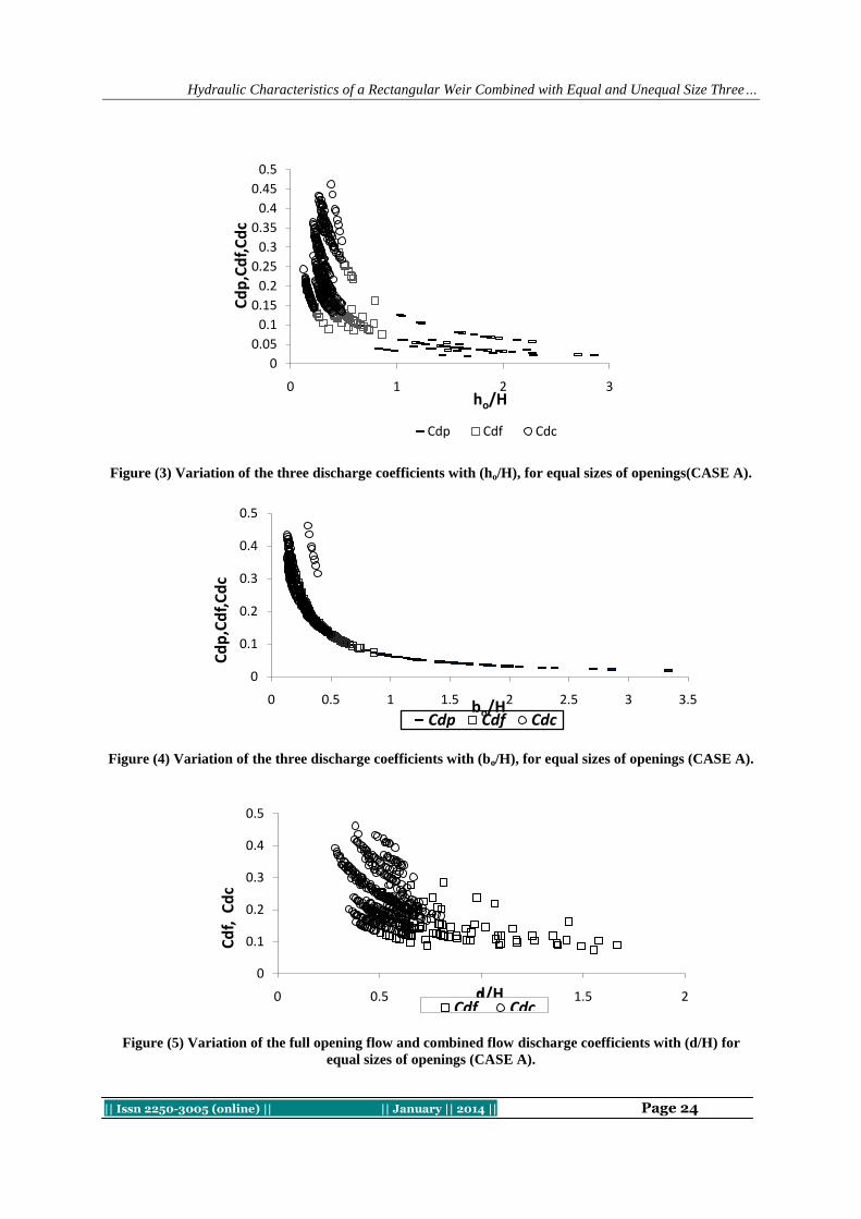
for Cd with these variables will be significant. Figure (3) shows the variation of discharge coefficients for the
flow cases (Cdp,Cdf,Cdc), with the value of (ho/H) ratio. It is clear that the maximum discharge coefficient is less
than 0.6188 and this means that the maximum correction that accounts for the assumptions of the theoretical
discharge equation is 38 % .Moreover it is found that the discharge coefficient decreases as (ho/H) increases.
Flow case no. (1), gives the lowest discharge coefficient followed by flow case no. (2), and finally flow case no.
(3). This may be attributed to the increase of losses as the head increased. Figure (4) shows the variation of the
discharge coefficients for the three flow cases (Cdp,Cdf,Cdc), with the values of (bo/H) ratio. Similar
observations are found as these observed in Figure (3), however, the relation exhibits less fluctuated results.
Figure (5) shows that in general the discharge coefficients for the flow cases (Cdf,Cdc),decreases when(d/H)
value increase. The presented values are not for fixed (d value) and variable (H) value but both are varied. For
the combined discharge, the variations are much higher than for Cdf (flow case no.2). For a given (d/H) value,
different discharge coefficient can be obtained and that is indicates the effect of the other relevant
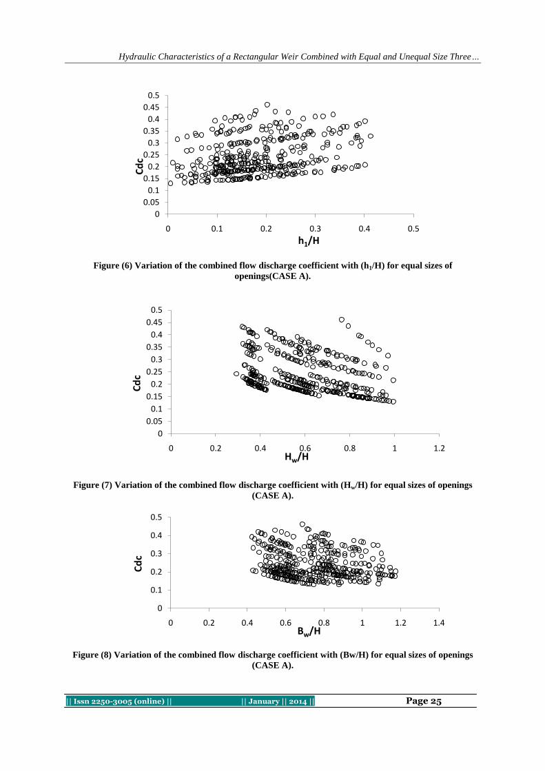
variables.Similarly, the variations of the three discharge coefficients with (h1/H), (Hw/H) and (Bw/H) are shown
in Figures (6), (7) and (8) respectively. These Figures indicate proportional variation of the first variable and
inverse proportional variation for the other two variables .However, for each unique value of the variables
different discharge coefficient values can be obtained which indicate the combined effects of the other relevant
variables.
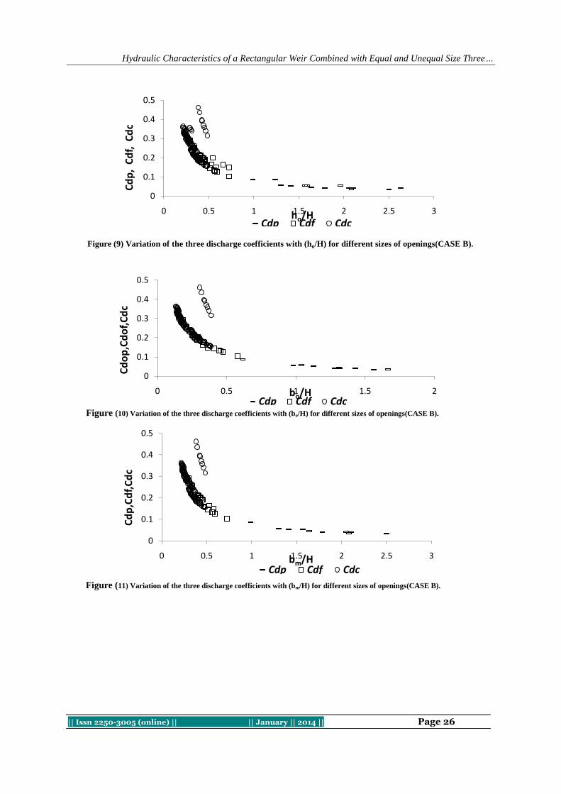
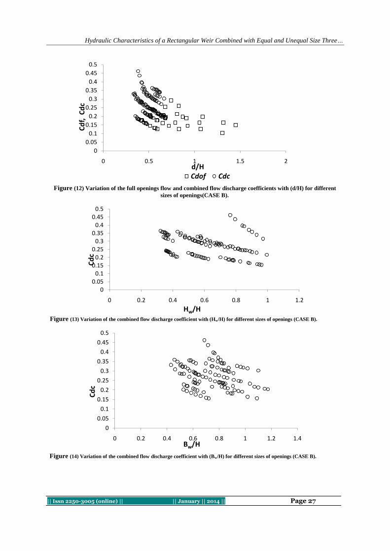
Case B: Unequal sized openings:
The variation of (Cdp,Cdf,Cdc) for this with each of the variables (ho/H, bo/H ,bM/H,d/H, Hw/H,Bw/H,)
are shown in Figures (9 to 14), respectively . Even though these Figures indicate high scattering which means
single correlation between the Cd and each variable is low, it is expected that multiple correlation for Cd with
these variables will be significant. The general observations found for this case are almost similar to those
observed for case A. The variations of the three discharge coefficients with any single variable had shown
considerable scattering, which reflects the effect of the other variables.
The observations obtained for the two cases indicates the necessity of relating the discharge
coefficients with all of the variables using a multivariate model , such as multiple regression or artificial neural
networks. The artificial neural networks model had proved recently its effectiveness, hence used herein for the
modeling process.
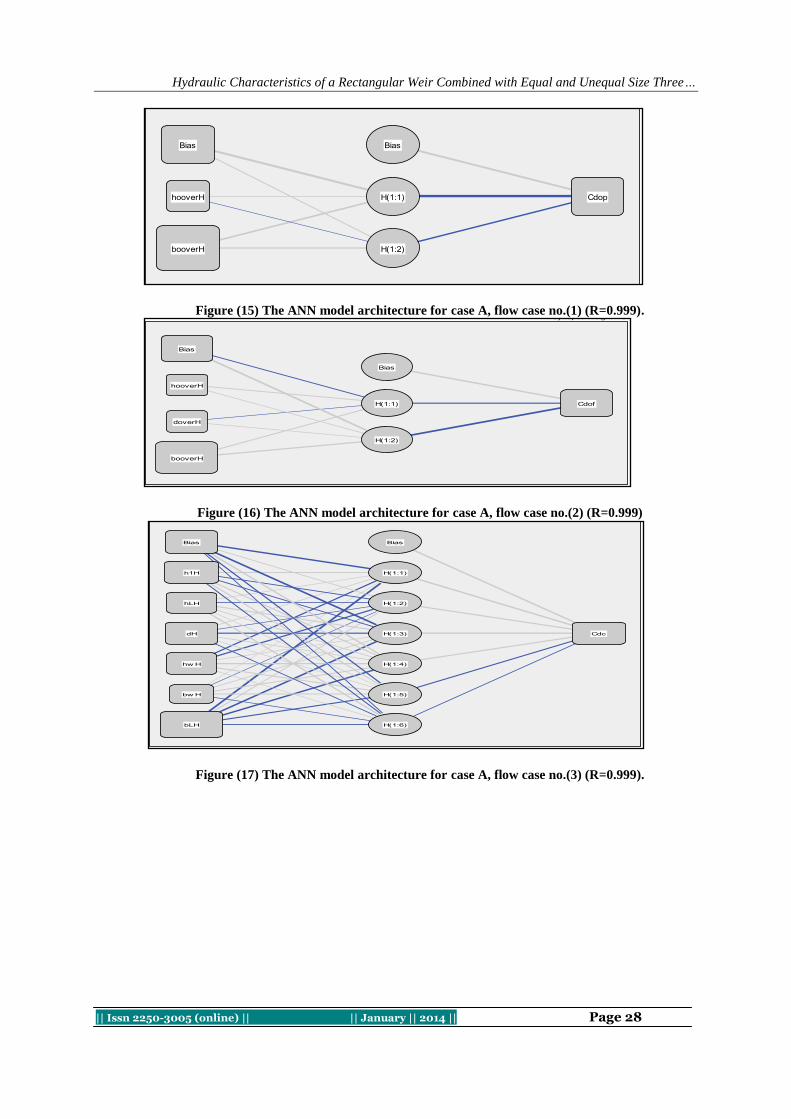
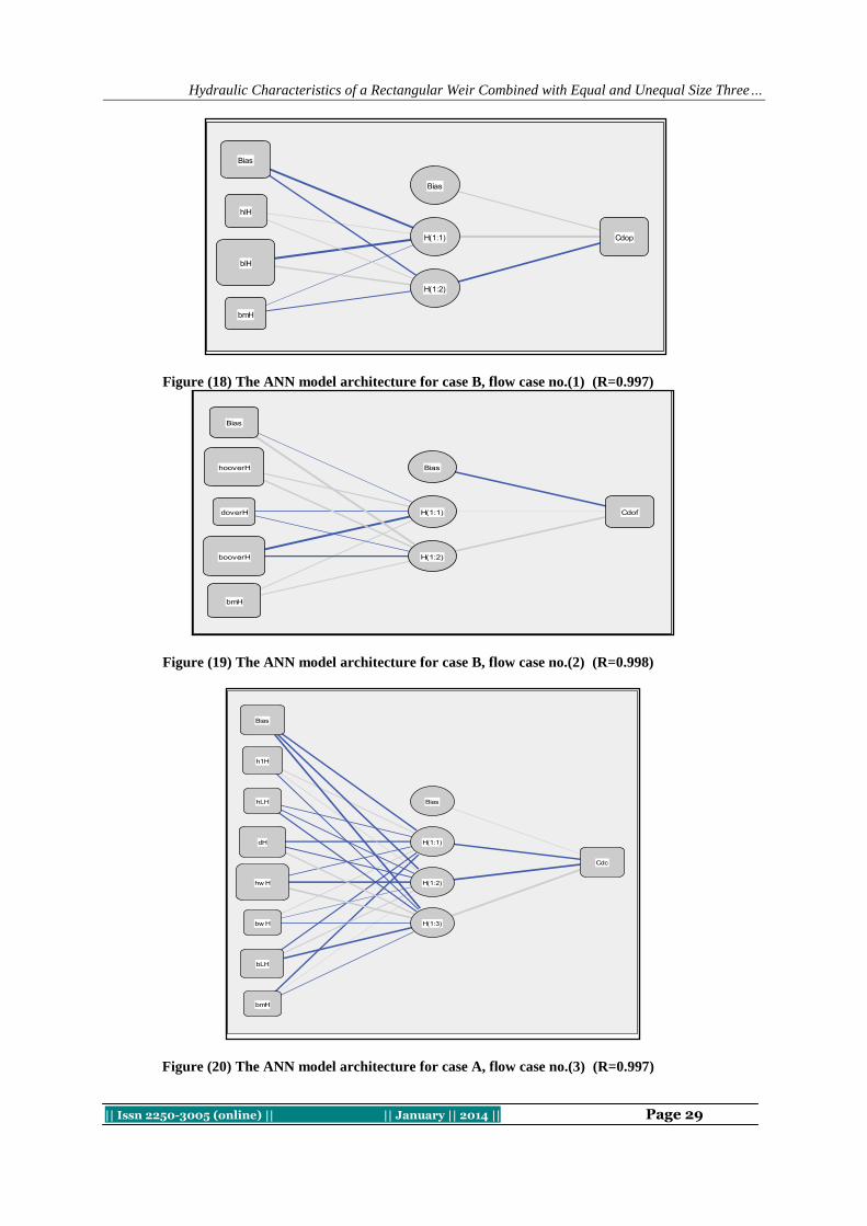
Artificial neural networks modeling for the discharge coefficient
The artificial neural network (ANN), is a mathematical model or computational model that is inspired
by the structure and/or functional aspects of the biological neural networks. A neural network consists of an
interconnected group of artificial neurons, and it processes information using a connectionist approach to
computation. Six artificial neural network models were developed for estimating the discharge coefficients (Cdp
,Cdf,Cdc) as a function of the variables listed in equations (17 to 22). These models are classified according to
the cases A and B and for each according to the flow case. These model were developed using the software
"SPSS,version 19", this software allows the modeling with different network architecture, and use back
propagation algorithm for adjusting the weights of the model. The software needs to identify the input variables
which are those mentioned above as shown in Figures (9, 10,11,12,13 and 14) respectively.
CONCLUSIONS
Under the limitations imposed in this study, the following conclusions are obtained:

Hydraulic Characteristics of a Rectangular Weir Combined with Equal and Unequal Size Three…
|| Issn 2250-3005 (online) || || January || 2014 || Page 18
1. All the flow conditions proposed exhibits sub critical flow at the upstream side of the structure, since
Froude number range is less than (1).
2. For each model, with specific dimensions, as the head increased, the discharge coefficients for all
three flow cases were increased. The highest value of the discharge coefficient, was obtained for flow case no.3,
(Cdc= 0.6188), while the lowest value of discharge coefficient was obtained for flow case no.1,(Cdp =0.0288).
3. For the case of equal size of the three openings and for flow case no.(3) ,the discharge coefficient
Cdc has the highest value for a size of opening of (5*10)cm, while the lowest value is for the size (10*10).This
indicates that the width of opening has the major effect on the values of Cdc .
4. Correlation analysis for all of the three flow cases between the discharge coefficients and the
variables involved, indicates that (Cdp) , (Cdf) ,(Cdc) have the highest correlation with (bo/H) with negative
values of (-0.942,-0.937,-0.871) respectively for equal sizss and that for unequal sizes(-0.953,-0.941,-0.503).
These negative values indicate inverse proportionality.
5. For all the cases tested the coefficient of variation for the discharge coefficient were in the range of
(0.6263 - 0.1643) for all of the three flow cases, which indicate the necessity of obtaining a model to describe
this variation.
6. The architecture of the three developed ANN models and the selected parameters and activation
functions shown in the related figures and tables are suitable for relating the discharge coefficient with the
geometry and the flow variables .The networks correlation coefficients between the observed and predicted
discharge coefficients were in the range of (0.999- 0.997), which can be considered as a very good correlation.
REFERENCES [1.] Abdel-Azim A.M.,(2002) ,"Combined of Free Flow Over Weirs and Below Gates ", Journal of
Hydraulic Research, vol.40,no.3.
[2.] Alhamid A.A., NegmA.M. and Al-Brahim A.M.,(1997),"Discharge Equation for Proposed Self-
Cleaning Device", Journal of King Saud University, Engineering ,Science, Riyadh, Saudia
Arabia,vol.9,no.1, pp.13-24.
[3.] Al- Suhili R.H. and Shwana A. J., (2013), "Prediction of the Discharge Coefficient for a Cipolletti Weir
with Rectangular Bottom Opening", submitted to journal of flow control and visualization, for
publication.
[4.] Al-Suhili R.H., Al-Baidhani J. H., and Al-Mansori N. J. , (2013),"Hydraulic characteristics of flow over
Rectangular weir with three EqualSize Rectangular bottom openings using ANN", accepted for
publication, Journal of Babylon university, Iraq.
[5.] Bos M.G.,(1989),"Discharge Measurement Structure” 3rd
ed.,Int. Confer. for Land Reclamation and
Improvement, Wageningen, the Netherlands.
[6.] British Standard Institution (BSI);(1965);"Thin-Plate Weirs and Venturi Flumes in Methods of
Measurement of Liquid Flow In Open Channel”,Part4A,BSI,3681,BSI,London.
[7.] FadilH.A.,(1997) ,"Development of a Meter for the Combined Flow Through Contracted Slice Gate and
Weir",Almuktar Science journal,No.4,University of Omar Almuktar ,Beida,Libya.
[8.] French,R.H.,(1986),"Open Channel Hydraulic", pp.343-353,McGraw Hill Book Co., New York.
[9.] Munson B.R.,YoungD.F. and OkllshiT.H.,(1994) ,"Fundamental of Fluid Mechanics", 2nd ed., John
Wiley and Sons,Inc.,New Yourk.
[10.] NegmA.M.,(2000), "Characteristics of Simultaneous Over Flow- Submerged Under Flow (Unequal
Contraction) ", Engineering, Bulletin, Faculty of Engineering,AinShams
University,vol.35,no.1,March,pp.137-154.
[11.] RajaratnamN.(1977),"Free Flow Immediately Below Sluice Gates", Proceeding ,ASCE, Journal of
Hydraulic Engineering Division, 103,No.HY4,pp.345-351.
[12.] Swamee P.K.,(1992),"Sluice-Gate Discharge Equation", Proceeding ,ASCE, Journal, Irrigation and
Drainage Engineering Division, vol.,93, no.IR3,pp.167-186

Hydraulic Characteristics of a Rectangular Weir Combined with Equal and Unequal Size Three…
|| Issn 2250-3005 (online) || || January || 2014 || Page 19
Table (1) Details of the weir models investigated.
Models Crest height
(P=ho+d)
cm
Crest
length (Bw) cm
Bottom Openings (bo x ho) cm
Left middle Right
1.a 1
.a.1 28 20 5*10 5*10 5*10
1
.a.2 10*10 10*10 10*10
1
.a.3 10*5 10*5 10*5
1
.a.4 10*8 10*8 10*8
1
.a.5 8*8 8*8 8*8
1
.a.6 8*10 10*10 8*10
1
.a.7 5*8 8*8 5*8
1.b 1
.b.1 28 27 5*10 5*10 5*10
1
.b.2 10*10 10*10 10*10
1
.b.3 10*5 10*5 10*5
1
.b.4 10*8 10*8 10*8
1
.b.5 8*8 8*8 8*8
1
.b.6 8*10 10*10 8*10
1
.b.7 5*8 8*8 5*8
2.a 2
.a.1 24 33 5*10 5*10 5*10
2
.a.2 10*10 10*10 10*10
2
.a.3 10*5 10*5 10*5
2
.a.4 10*8 10*8 10*8
2
.a.5 8*8 8*8 8*8
2
.a.6 8*10 10*10 8*10
2
.a.7 5*8 8*8 5*8
2.b 2
.b.1 24 25 5*10 5*10 5*10
2
.b.2 10*10 10*10 10*10
2
.b.3 10*5 10*5 10*5
2
.b.4 10*8 10*8 10*8
2
.b.5 8*8 8*8 8*8
2
.b.6 8*10 10*10 8*10
2
.b.7 5*8 8*8 5*8
2.c 2
.c.1 24 17 5*10 5*10 5*10
2
.c.2 10*10 10*10 10*10
2
.c.3 10*5 10*5 10*5
2
.c.4 10*8 10*8 10*8
2
.c.5 8*8 8*8 8*8
2
.c.6 8*10 10*10 8*10
2
.c.7 5*8 8*8 5*8
3.a 3
.a.1 20 23 5*10 5*10 5*10
3
.a.2 10*10 10*10 10*10

Hydraulic Characteristics of a Rectangular Weir Combined with Equal and Unequal Size Three…
|| Issn 2250-3005 (online) || || January || 2014 || Page 20
3
.a.3 10*5 10*5 10*5
3
.a.4 10*8 10*8 10*8
3
.a.5 8*8 8*8 8*8
3
.a.6 8*10 10*10 8*10
Table (1) continued
Models Cre
st height
(P=
ho +d) cm
Crest
length (Bw)
Cm
Bottom Openings
(bo x ho) cm
left Middle right
3.a 3
.a.7
20 23 5*8 8*8 5*8
3.b 3
.b.1
20 18 5*10 5*10 5*10
3
.b.2
10*10 10*10 10*10
3
.b.3
10*5 10*5 10*5
3
.b.4
10*8 10*8 10*8
3
.b.5
8*8 8*8 8*8
3
.b.6
8*10 10*10 8*10
3
.b.7
5*8 8*8 5*8
3.c 3
.c.1
20 15 5*10 5*10 5*10
3
.c.2
10*10 10*10 10*10
3
.c.3
10*5 10*5 10*5
3
.c.4
10*8 10*8 10*8
3
.c.5
8*8 8*8 8*8
3
.c.6
8*10 10*10 8*10
3
.c.7
5*8 8*8 5*8

Hydraulic Characteristics of a Rectangular Weir Combined with Equal and Unequal Size Three…
|| Issn 2250-3005 (online) || || January || 2014 || Page 21
Table (2) Descriptive statistics and correlation analysis for flow case1 of equal size openings.
Corr
elation with
Cdp Min. Max. Mean
Std.
Deviation
Coefficie
nt of variance C.V
Cdp 1 .0288 0.2464 0.08038 0.045 0.563
ho/H -
0.484
.3137 2.8571 1.47319 .4609 0.312
bo/H -
0.871
.3922 3.3333 1.47433 .5708 0.387
Table (3) Descriptive statistics and correlation analysis for flow case.2 of equal size openings.
Correl
ation
with
Cdf Min.
Max
. Mean
St
d. Deviation
Coefficient of
variance C.V
Cdf 1 .1118 .463 .219 .0
783
0.3560
ho/H -0.151 .2083 .862 .473 .1
503488
0.3174
d/H -0.5 .5051 1.66 .931 .3
140890
0.3370
bo/H -0.937 .2083 .862 .508 .1
485248
0.2919
Table (4) Descriptive statistics and correlation analysis for flow case.3 of equal size openings.
Correl
ation with Cdc Min.
Max
. Mean
Std.
Deviation
Coefficient of
variance
C.V
Cdc 1 .1233 .618 .3343 .109 0.3279
h1/H -0.035 .0019 1.00 .1905
4
.130 0.6263
ho/H 0.122 .1220 .512 .2962
88
.080 0.2718
d/H -0.374 .2825 .804 .5180
42
.099 0.1927
hw/H -0.384 .2927 1.02 .6041
75
.185 0.3066
bw/H -0.222 .4237 1.17 .7513
41
.180 0.2399
bo/H -0.942 .1333 .497 .2772
49
.091 0.3306

Hydraulic Characteristics of a Rectangular Weir Combined with Equal and Unequal Size Three…
|| Issn 2250-3005 (online) || || January || 2014 || Page 22
Table (5) Description of statistical and correlation analysis for flowcase.1 of unequal size
openings.
Corr
elation with
Cdp Min. Max. Mean Std.
Deviation
Coefficient
of variance C.V
Cdp 1 .0512 .1299 .0797
89 0.02
2147 0.278
ho/
H -
0.829 .9877 2.6316 1.568
840 .361
8480 0.230
bo/
H -
0.953 .6173 1.6667 1.149
196 .282
9684 0.2462
bm
/H -
0.891 .9877 2.5000 1.546
481 .340
0340 0.2199
Table (6) Description of statistical and correlation analysis for flowcase.2 of unequal size openings.
Corr
elation with
Cdf Min. Max. Mean St
d. Deviation
Coefficient
of variance C.V
Cdf 1 .1535 .4349 .257371 .0
544150 0.211
ho/H -
0.863 .2963 .7246 .486850 .0
935586 0.192
d/H -
0.267 .4184 1.4493 .785755 .2
758444 0.351
bo/H -
0.941 .1852 .5797 .347372 .0
870414 0.2505
bm/
H -
0.913 .2963 .7246 .481407 .0
879130 0.182
Table (7) Description of statistical and correlation analysis for flowcase.3 of unequal size openings
Corr
elation with
Cdc Min. Max. Mean
Std.
Deviation
Coeffi
cient of
variance C.V
Cdc 1 .2291 .5200 .37248
9
.082
3017
0.221
h1/H 0.318 .0100 .4123 .17998
9
.090
8628
0.504
ho/H -
0.462
.2145 .4854 .31712
0
.067
3664
0.2122
d/H -
0.015
.3343 .6667 .49295
2
.081
0564
0.1643
Hw/
H
-
0.242
.3217 .9950 .60821
5
.191
3325
0.3145
Bw/
H
-
0.240
.4310 1.1744 .74596
5
.170
9562
0.229
bo/H -
0.503
.1340 .3883 .22424
0
.072
1830
0.3219
bm/
H
-
0.489
.2145 .4854 .31467
7
.068
9368
0.219

Hydraulic Characteristics of a Rectangular Weir Combined with Equal and Unequal Size Three…
|| Issn 2250-3005 (online) || || January || 2014 || Page 23
Figure(1)Experimental setup used.
Figure (2) the physical model section of the proposed weir.
B
w
500 mm
bL
bm
bR
H
w
d
h
o
p
4 00
mm
Hydraulic Characteristics of a Rectangular Weir Combined with Equal and Unequal Size Three…
|| Issn 2250-3005 (online) || || January || 2014 || Page 24
Figure (3) Variation of the three discharge coefficients with (ho/H), for equal sizes of openings(CASE A).
Figure (4) Variation of the three discharge coefficients with (bo/H), for equal sizes of openings (CASE A).
Figure (5) Variation of the full opening flow and combined flow discharge coefficients with (d/H) for
equal sizes of openings (CASE A).
0
0.05
0.1
0.15
0.2
0.25
0.3
0.35
0.4
0.45
0.5
0 1 2 3
Cd
p,C
df,
Cd
c
ho/H
Cdp Cdf Cdc
0
0.1
0.2
0.3
0.4
0.5
0 0.5 1 1.5 2 2.5 3 3.5
Cd
p,C
df,
Cd
c
bo/HCdp Cdf Cdc
0
0.1
0.2
0.3
0.4
0.5
0 0.5 1 1.5 2
Cd
f, C
dc
d/HCdf Cdc
Hydraulic Characteristics of a Rectangular Weir Combined with Equal and Unequal Size Three…
|| Issn 2250-3005 (online) || || January || 2014 || Page 25
Figure (6) Variation of the combined flow discharge coefficient with (h1/H) for equal sizes of
openings(CASE A).
Figure (7) Variation of the combined flow discharge coefficient with (Hw/H) for equal sizes of openings
(CASE A).
Figure (8) Variation of the combined flow discharge coefficient with (Bw/H) for equal sizes of openings
(CASE A).
0
0.05
0.1
0.15
0.2
0.25
0.3
0.35
0.4
0.45
0.5
0 0.1 0.2 0.3 0.4 0.5
Cd
c
h1/H
0
0.05
0.1
0.15
0.2
0.25
0.3
0.35
0.4
0.45
0.5
0 0.2 0.4 0.6 0.8 1 1.2
Cd
c
Hw/H
0
0.1
0.2
0.3
0.4
0.5
0 0.2 0.4 0.6 0.8 1 1.2 1.4
Cd
c
Bw/H
Hydraulic Characteristics of a Rectangular Weir Combined with Equal and Unequal Size Three…
|| Issn 2250-3005 (online) || || January || 2014 || Page 26
Figure (9) Variation of the three discharge coefficients with (ho/H) for different sizes of openings(CASE B).
Figure (10) Variation of the three discharge coefficients with (bo/H) for different sizes of openings(CASE B).
Figure (11) Variation of the three discharge coefficients with (bm/H) for different sizes of openings(CASE B).
0
0.1
0.2
0.3
0.4
0.5
0 0.5 1 1.5 2 2.5 3
Cd
p,
Cd
f, C
dc
ho/HCdp Cdf Cdc
0
0.1
0.2
0.3
0.4
0.5
0 0.5 1 1.5 2
Cd
op
,Cd
of,
Cd
c
bo/HCdp Cdf Cdc
0
0.1
0.2
0.3
0.4
0.5
0 0.5 1 1.5 2 2.5 3
Cd
p,C
df,
Cd
c
bm/HCdp Cdf Cdc
Hydraulic Characteristics of a Rectangular Weir Combined with Equal and Unequal Size Three…
|| Issn 2250-3005 (online) || || January || 2014 || Page 27
Figure (12) Variation of the full openings flow and combined flow discharge coefficients with (d/H) for different
sizes of openings(CASE B).
Figure (13) Variation of the combined flow discharge coefficient with (Hw/H) for different sizes of openings (CASE B).
Figure (14) Variation of the combined flow discharge coefficient with (Bw/H) for different sizes of openings (CASE B).
0
0.05
0.1
0.15
0.2
0.25
0.3
0.35
0.4
0.45
0.5
0 0.5 1 1.5 2
Cd
f, C
dc
d/HCdof Cdc
00.05
0.10.15
0.20.25
0.30.35
0.40.45
0.5
0 0.2 0.4 0.6 0.8 1 1.2
Cd
c
Hw/H
0
0.05
0.1
0.15
0.2
0.25
0.3
0.35
0.4
0.45
0.5
0 0.2 0.4 0.6 0.8 1 1.2 1.4
Cd
c
Bw/H
Hydraulic Characteristics of a Rectangular Weir Combined with Equal and Unequal Size Three…
|| Issn 2250-3005 (online) || || January || 2014 || Page 28
Figure (15) The ANN model architecture for case A, flow case no.(1) (R=0.999).
Figure (16) The ANN model architecture for case A, flow case no.(2) (R=0.999)
Figure (17) The ANN model architecture for case A, flow case no.(3) (R=0.999).
Hydraulic Characteristics of a Rectangular Weir Combined with Equal and Unequal Size Three…
|| Issn 2250-3005 (online) || || January || 2014 || Page 29
Figure (18) The ANN model architecture for case B, flow case no.(1) (R=0.997)
Figure (19) The ANN model architecture for case B, flow case no.(2) (R=0.998)
Figure (20) The ANN model architecture for case A, flow case no.(3) (R=0.997)

International Journal Of Computational Engineering Research (ijceronline.com) Vol. 04 Issue. 01
|| Issn 2250-3005 (online) || || January || 2014 || Page 30
An Investigation of the Effect of Shot Peening On the Properties
of Lm25 Aluminium Alloy and Statistical Modelling
Sirajuddin Elyas Khany1 Obaid Ullah Shafi
2 Mohd Abdul Wahed
3
1. Associate Professor, Department of Mechanical Engg. M.J. College of Engineering &Technology,
Hyderabad AP-500034.
2. Assistant Professor, Department of Mechanical Engg. Deccan. College of Engineering &Technology,
Hyderabad AP-500001.
3. Assistant professor, Department of Mechanical Engg. NSA College of Engineering & Technology,
Hyderabad AP-500024.
I. INTRODUCTION The process of shot peening and parameters of shot peening effect the micro hardness of LM25 material. Benefits
obtained due to cold working include work hardening, intergranular corrosion resistance, surface texturing and closing of
porosity. The quality of peening is determined by the degree of coverage, magnitude and depth of the induced residual stress.
Various studies have demonstrated the improvements induced by the peening process; thus it can be widely used to enhance
the life of components operating in highly stressed environments and the other critical parts such as in motor racing, aero
engines and aero structures. The surface modifications produced by the shotpeening treatment are :( a) roughening of the
surface,(b) an increased near surface dislocation density (strain hardening), and (c) the development of a characteristic
profile of residual stresses.
II. EXPERIMENTAL ANALYSIS OF SPECIMEN AFTER SHOT PEENING
Fig 1. Testing specimen: LM 25 Aluminum Alloy
III. PHYSICAL PROPERTIES: Coefficient of Thermal Expansion (per oC at 20 -100 oC) 0.000022
Thermal Conductivity (cal/cm2/cm/oC/s at 25oC * 0.36
Electrical Conductivity (% copper standard at 20oC) * 39
Specific Gravity 2.68
Freezing Range (oC) Approx 615-550
Casting Characteristics:
FLUIDITY: Good, suitable for fairly thin castings.
PRESSURE TEST: Suitable for castings required to be leak tight.
HOT TEARING: The production of castings in this
Alloy very rarely introduces
Problems due to hot tearing.
ABSTRACT
In this work the effect of shot peening on the tensile strength, hardness and impact strength of mild steel is
studied using a compressed air shot-peening machine. This investigation examines the respective effects of
influencing parameters such as pressure, angle of impingement, nozzle distance and the exposure time in
enhancing micro hardness, tensile strength and average surface roughness. Further, statistical analysis
software such as MINITAB is used to predict the optimal process parameters for the responses such as
tensile strength, hardness and impact strength on the basis of taguchi analysis. These test results will be
useful to the industries in deciding the optimal levels for the shot peening parameters.
Keywords: shot peening, Minitab, tensile strength impact strength, hardness, taguchi analysis.

An Investigation of the Effect of Shot Peening On the Properties of Lm25 Aluminium Alloy and…
|| Issn 2250-3005 (online) || || January || 2014 || Page 31
IV. REGR ESSION ANALYSIS Regression technique is concerned with predicting some variables by knowing others. The process of
predicting variable Y using variable X. Multiple regression analysis is a simple regression analysis. In multiple
regressions two or more independent
Variables are used to estimate the values of a dependent variable. The general purposes of multiple
regression analysis are 1.To derive an equation which provides estimates of the dependent variable from values
of the two or more independent variable. 2. To obtain a measure of the error involved in using this regression
equation as a basis of estimation. 3. To obtain a measure of the proportion of variance in the dependent variable
accounted for or explained by the independent variable. If there are three variable x1, x2 & x3 the multiple
regressions will take the following form:
Y=ax1 +bx2 +cx3 ……………………………..…..1.
A regression equation is an equation for estimating a dependent variable, say y from the independent
variables
x1, x2, x3 and is called a regression equation of y on x1, x2, x3 and so on. For the case of three variables the
simplest regression equation of x1on x2 &x3 has the form of equation 1, Where a, b, c are constants, the least
square regression plane x1on x2 & x3 of has the equation 1.0 where a, b and c are determined by simultaneously
the normal equations.
∑y = a∑x1 + b∑x2 + ∑x3 …………...……………..2
∑x1y = a∑x12 +b∑x1x2 + c∑ x3…………………...3
∑x2y = a∑x1x2 + b∑x22 + c∑ x2 x3 ……………….4
By solving the above equations the values of a, b, c can be obtained. On substituting the values in eqn
1.0 we get the values of ‘y’ for different values of x1, x2 & x3. Correlation is a statistical technique used to
determine the degree to which two variables are related. Simple correlation also as called Pearson's correlation
or product moment correlation coefficient. It measures the nature and strength between two variables of the
quantitative type. The sign of ‘r’ denotes the nature of association while the value of ‘r’ denotes the strength of
association. If the sign is +ve this means the relation is direct (an increase in one variable is associated with an
increase in the other variable and a decrease in one variable is associated with a decrease in the other
variable).While if the sign is -ve this means an inverse or indirect relationship (which means an increase in one
variable is associated with a decrease in the other). The value of r ranges between (-1) and (+1). The value of r
denotes the strength of the association as illustrated
Table 1.Chemical composition of the specimen
If r = Zero this means no association or correlation between the two variables.
If 0 < r < 0.25 = weak correlation.
If 0.25 ≤ r < 0.75 = intermediate correlation.
If 0.75 ≤ r < 1 = strong correlation.
If r = l = perfect correlation
Correlation coefficient:
Chemical
composition cu Mg Si Fe Mn Ni Zn Pb Sb Ti Al
Percentage 0.1 0.2-0.6 6.5-7.5 0.5 0.3 0.1 0.1 0.1 0.05 0.2 Remainder

An Investigation of the Effect of Shot Peening On the Properties of Lm25 Aluminium Alloy and…
|| Issn 2250-3005 (online) || || January || 2014 || Page 32
Multiple regressions technique is used to predict a value using ‘n’ number of variables and Pearson’s correlation
coefficient explains the strength and type of correlation between predicted values and actual values. By which we can
recommend the optimum usage of input variables.
V. REGRESSION ANALYSIS USING MINITAB SOFTWARE: Linear regression investigates and models the linear relationship between a response (Y) and
predictor(s) (X). Both the response and predictors are continuous variables In particular, linear regression
analysis is often used to: determine how the response variable changes as a particular predictor variable
changes, predict the value of the response variable for any value of the predictor variable, or combination of
values of the predictor variables , The regression equation is an algebraic representation of the regression line
and is used to describe the relationship between the response and predictor variables. The regression equation
takes the form of: Response = constant + coefficient (predictor) + ... + coefficient (predictor)
y = bo + b1X1 + b2X2 + ... + bkXk
Predictor variable(s) is zero. The constant is also called the intercept because it determines where the regression
line intercepts (meets) the Y-axis. Predictor(s) (X) is the value of the predictor variable(s). Coefficients (b1, b2, bk) represent
the estimated change in mean response for each unit change in the predictor value. In other words, it is the change in Y that
occurs when X increases by one unit. P-Value The coefficient table lists the estimated coefficients for the predictors. Linear
regression examines the relationship between a response and predictor(s). In order to determine whether or not the observed
relationship between the response and predictors is statistically significant, you need to identify the coefficient p-values the
coefficient value for P (p-value) tells you whether or not the association between the response and predictor(s) is statistically
significant. Compare the coefficient p-values to your level; If the p-value is smaller than t -level you have selected, the
association is statistically significantly. A commonly used a-level is 0.05, Predicted values: Minitab displays the predicted
value table when you request the calculation of the mean responses or the prediction of new response values at certain
settings of the predictors. The Fit is the predicted (fitted) value for the response at the combination of predictor settings you
requested. Typical values, spread or variation, and shape, unusual values in the data. This pattern indicates skewness, long
tails and outlier i.e. bars away from other bars, because the appearance of the histogram can change depending on the
number of intervals used to group the data, use the normal probability plot and goodness-of-fit tests to assess whether the
residuals are normal. The residuals from the analysis should be normally distributed. In practice, for data with a large
number of observations, moderate departures from normality do not seriously affect the results In this work, First and fore
most thing is to compare the tensile strength, hardness and impact strength of peened and unpeened specimen .Secondly to
find the effectiveness of impact pressure and exposure time on tensile strength, hardness and average surface roughness of
the specimen. Thirdly to study the tensile strength, hardness and impact strength of Al alloy specimen at different input
parameters and compare it with predicted values of tensile strength, hardness and average surface roughness from MINITAB
software and by applying multiple regression technique and find the strength of correlation between experimental values
and predicted values. In un- peened specimen the tensile strength for as cast LM25 Aluminium alloy is approximately 210
N/mm2.Whereas after shot blasting the LM25 Aluminium alloy specimen the optimum tensile strength was observed as
217.98 N/mm2. Unpeened specimen hardness for as cast LM25 Aluminium alloy specimen is approximately 83 BHN,
whereas shotpeened LM25 Aluminium alloy specimen the optimum hardness was observed as 108 BHN. Unpeened
specimen has an Impact strength for an as cast LM25 Aluminium alloy as approximately 4.75 µm. Whereas after shot
blasting the LM25 Aluminium alloy specimen the optimum average surface roughness was observed as 7.78 µm. From the above discussion we can conclude that shot blasting of Aluminium LM25 alloy specimen increases its tensile strength,
Fig 2.Graph showing properties of LM25 Aluminum alloy specimen before and after shot peening

An Investigation of the Effect of Shot Peening On the Properties of Lm25 Aluminium Alloy and…
|| Issn 2250-3005 (online) || || January || 2014 || Page 33
From the readings taken from tensile test conducted on UTM we can say that with the increase in exposure time
the tensile strength will increase up to a certain time after that it will decrease. This is depicted in table and graph below.
Table 2, Fig 3 Effect of exposure time on tensile strength of specimen at constant pressure
Effect of impact pressure on tensile strength of LM25 Aluminum alloy specimen at constant time
From the readings taken from tensile test conducted on UTM we can say that with the increase in the impact
pressure tensile strength will decrease. This is explained in table and graph below.
Table 3 Effect of pressure and time on tensile strength of specimen
From the contour plot above we can say that the optimum tensile strength we can get when time of
exposure is approximately in between 10 min and 19 min and impact pressure is approximately in between 4 bar
and 7.5 bar. With the increase in exposure time the tensile strength will increase up to a certain time after that it
will decrease because the specimen will undergo internal compression up to certain time and then the specimen
will loose its compressive stress which is developed internally. With the increase in the impact pressure tensile
strength will decrease because the specimen will loose its tendency to produce internal compressive stresses as
the impact pressure increase.
VI. EFFECT OF EXPOSURE TIME ON HARDNESS OF LM25 ALUMINUM ALLOY
SPECIMEN AT CONSTANT PRESSURE From the readings taken from Hardness test conducted on Portable hardness tester we can say that with
the increase in exposure time the Brinell’s Hardness Number (BHN) will increase up to a certain time after that
it will decrease. This is explained in table and graph below.
Table 4. Effect of exposure time on Hardness of specimen at constant pressure
S.No Pressure(bar) Time
(min)
Tensile
strength
(N/mm2)
1 4 12 220
2 5 12 217.98
3 6 12 213.90
4 7 12 212.17
5 8 12 209.83
6 9 12 190.47
7 10 12 131.40
S.No Time
(min)
Pressure
(bar)
Hardness(BHN)
1 10 10 83
2 12 10 87
3 15 10 108
4 18 10 96
5 20 10 94
6 22 10 91
7 25 10 87
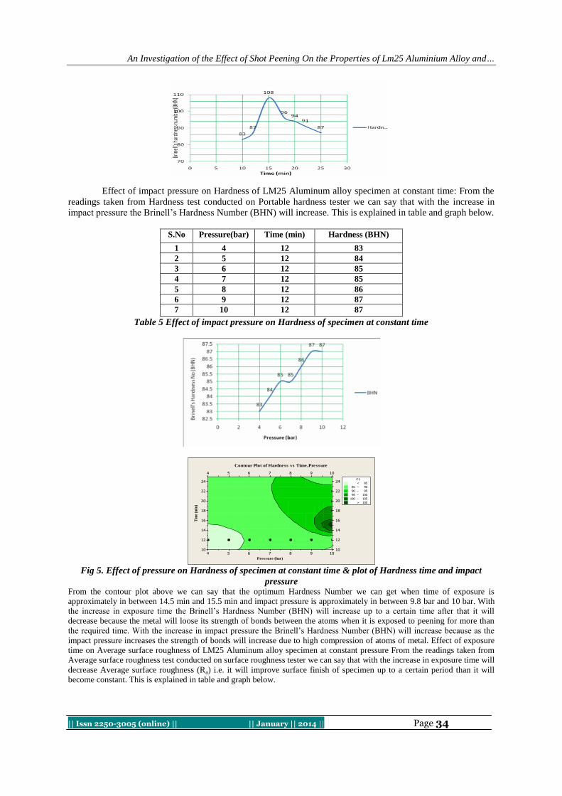
An Investigation of the Effect of Shot Peening On the Properties of Lm25 Aluminium Alloy and…
|| Issn 2250-3005 (online) || || January || 2014 || Page 34
Effect of impact pressure on Hardness of LM25 Aluminum alloy specimen at constant time: From the
readings taken from Hardness test conducted on Portable hardness tester we can say that with the increase in
impact pressure the Brinell’s Hardness Number (BHN) will increase. This is explained in table and graph below.
S.No Pressure(bar) Time (min) Hardness (BHN)
1 4 12 83
2 5 12 84
3 6 12 85
4 7 12 85
5 8 12 86
6 9 12 87
7 10 12 87
Table 5 Effect of impact pressure on Hardness of specimen at constant time
Pressure (bar)
Tim
e (m
in)
10987654
10987654
24
22
20
18
16
14
12
10
24
22
20
18
16
14
12
10
>
–
–
–
–
< 85
85 90
90 95
95 100
100 105
105
C1
Contour Plot of Hardness vs Time,Pressure
Fig 5. Effect of pressure on Hardness of specimen at constant time & plot of Hardness time and impact
pressure From the contour plot above we can say that the optimum Hardness Number we can get when time of exposure is
approximately in between 14.5 min and 15.5 min and impact pressure is approximately in between 9.8 bar and 10 bar. With
the increase in exposure time the Brinell’s Hardness Number (BHN) will increase up to a certain time after that it will
decrease because the metal will loose its strength of bonds between the atoms when it is exposed to peening for more than
the required time. With the increase in impact pressure the Brinell’s Hardness Number (BHN) will increase because as the
impact pressure increases the strength of bonds will increase due to high compression of atoms of metal. Effect of exposure
time on Average surface roughness of LM25 Aluminum alloy specimen at constant pressure From the readings taken from
Average surface roughness test conducted on surface roughness tester we can say that with the increase in exposure time will
decrease Average surface roughness (Ra) i.e. it will improve surface finish of specimen up to a certain period than it will
become constant. This is explained in table and graph below.

An Investigation of the Effect of Shot Peening On the Properties of Lm25 Aluminium Alloy and…
|| Issn 2250-3005 (online) || || January || 2014 || Page 35
S.No Time (min) Pressure (bar) Average surface roughness (µm)
1 10 10 7.50
2 12 10 7.30
3 15 10 7.10
4 18 10 6.37
5 20 10 5.20
6 22 10 4.75
7 25 10 4.75
Table 6 Effect of exposure time on Average surface roughness (Ra) of specimen at constant pressure
Effect of impact pressure on Average surface roughness of LM25 Aluminum alloy specimen at
constant time: From the readings taken from Average surface roughness test conducted on surface roughness
tester we can say that with the increase in impact pressure will decrease Average surface roughness (Ra) i.e. It
will decrease surface finish of specimen. This is explained in table and graph below
Table 7 Effect of exposure time on Average surface roughness (Ra) of specimen at varying pressure
Table 8 Effect of impact pressure on Average surface roughness of specimen at constant time
Pressure
Tim
e
10987654
10987654
24
22
20
18
16
14
12
10
>
–
–
–
–
–
< 5.0
5.0 5.5
5.5 6.0
6.0 6.5
6.5 7.0
7.0 7.5
7.5
C1
Contour Plot of Avg surface rougness vs Time,Pressure
Fig 6. Effect of impact pressure on Average surface roughness of specimen at constant time & contour plot
of Average surface roughness for time and impact pressure
From the contour plot above we can say that the optimum surface finish of the specimen will be when
time of exposure is approximately in between 22 min and 25 min and impact pressure is approximately in
between 9.5 bar and 10 bar. The increase in exposure time will decrease Average surface roughness (Ra) i.e. it
will improve surface finish of specimen up to a certain period than it will become constant because the shot
which is used for blasting is not in round steel balls but it is stainless steel cut wire type which is widely used for
cleaning and polishing of the surface of metal parts. The impact pressure nearly will not have any effect because
the amount of metal removed from the specimen is same irrespective of pressure.
S.No Pressure(bar) Time (min) Average surface roughness (µM)
1 4 12 7.78
2 5 12 7.70
3 6 12 7.67
4 7 12 7.67
5 8 12 7.60
6 9 12 7.54
7 10 12 7.30

An Investigation of the Effect of Shot Peening On the Properties of Lm25 Aluminium Alloy and…
|| Issn 2250-3005 (online) || || January || 2014 || Page 36
VII. RESULTS AND DISCUSSION Statistical analysis of tensile strength values using Minitab software and regression equation.
S.No Time (min) Pressure (bar) Exp (N/mm2)
1 10 10 130.38
2 12 10 131.40
3 12 9 190.47
4 12 8 209.83
5 12 7 212.17
6 12 6 213.90
7 12 5 217.98
8 12 4 220.00
9 15 10 179.68
10 18 10 211.86
11 20 10 207.79
12 22 10 138.52
13 25 10 134.45
Table 9. Tensile strength of specimen at various input parameters
Regression Analysis: Exp (N/mm2) versus Time (min), Pressure (bar)
The regression equation is
Exp (N/mm2) = 278 + 0.10 Time (min) - 11.3 Pressure (bar)
Predictor Coef SE Coef T P
Constant 277.61 36.97 7.51 0.000
Time (min) 0.097 2.124 0.05 0.964
Pressure (bar) -11.278 4.627 -2.44 0.035
S = 30.4014 R-Sq = 43.5% R-Sq (adj) = 32.2%
Table 10. Predicted values of tensile strength from equation and MINITAB software
S.No Time (min) Pressure (bar) Exp (N/mm2) Reg (N/mm2) FITS1
1 10 10 130.38 166.0 165.798
2 12 10 131.40 166.2 165.992
3 12 9 190.47 177.5 177.270
4 12 8 209.83 188.8 188.548
5 12 7 212.17 200.1 199.826
6 12 6 213.90 211.4 211.104
7 12 5 217.98 222.7 222.382
8 12 4 220.00 234.0 233.661
9 15 10 179.68 166.5 166.284
10 18 10 211.86 166.8 166.575
11 20 10 207.79 167.0 166.769
12 22 10 138.52 167.2 166.964
13 25 10 134.45 167.5 167.255

An Investigation of the Effect of Shot Peening On the Properties of Lm25 Aluminium Alloy and…
|| Issn 2250-3005 (online) || || January || 2014 || Page 37
50250-25-50-75
99
95
90
80
70
60
50
40
30
20
10
5
1
Residual
Perc
ent
Normal Probability Plot(response is Exp (N/mm2))
240230220210200190180170160
50
40
30
20
10
0
-10
-20
-30
-40
Fitted Value
Resi
dual
Versus Fits(response is Exp (N/mm2))
Fig 7. Normal probability plot showing distribution of residuals versus the fitted values
The interpretation of the regression equation follows: Exp (N/mm2) = 278 + 0.10 Time (min) - 11.3
Pressure (bar), the slope (b1 = 0.10) is the change in Tensile strength when time increases by 1minute. That is,
when the time increases by one unit, the Tensile strength increases by 0.10 units. The slope (b2 = -11.3) is the
change in Tensile strength when pressure increases by 1. That is, when the pressure increases by one unit, the
Tensile strength increases by -11.3 units. The relationships between the response, Experimental Tensile strength,
and the predictor, pressure (P = 0.035), is significant. The relationship between the response, Experimental
Tensile strength, and the predictor, Time (P = 0.964), is not significant because the p-value is higher than the
pre-selected α-level. The R2 indicates that the predictors explain 43.5% of the variance in Tensile strength. The
adjusted R2 32.4%, which accounts for the number of predictors in the model. Both values indicate that the
model fits the data not perfectly well. The Pearson correlation between experimental Tensile strength and
predicted Tensile strength is 0.660 which indicates there is direct intermediate correlation between experimental
values and predicted values. The histogram indicates that outliers may exist in the data, shown by a bar on the
far right side of the plot. The normal probability plot shows an approximately linear pattern consistent with a
normal distribution. The point in the upper-right corner of the plot may be outliers. Brushing the graph identifies
these points as 41.0207.
VIII. REGRESSION EQUATION BY MINITAB SOFTWARE S.No Time
(min)
Pressure
(bar)
Exp
Hardness
(BHN)
1 10 10 83
2 12 10 87
3 12 9 87
4 12 8 86
5 12 7 85
6 12 6 85
7 12 5 84
8 12 4 83
9 15 10 108
10 18 10 96
11 20 10 94
12 22 10 91
13 25 10 87
Table 11. Hardness of specimen at various input parameters

An Investigation of the Effect of Shot Peening On the Properties of Lm25 Aluminium Alloy and…
|| Issn 2250-3005 (online) || || January || 2014 || Page 38
Regression Analysis: Exp Hardness (BHN) versus Time (min), Pressure (bar)
The regression equation is Exp Hardness (BHN) = 73.6 + 0.221 Time (min) + 1.43 Pressure (bar)
Predictor Coef SE Coef T P
Constant 73.604 7.876 9.35 0.000
Time (min) 0.2213 0.4525 0.49 0.635
Pressure (bar) 1.4332 0.9858 1.45 0.177
S = 6.47679 R-Sq = 28.8% R-Sq (adj) = 14.5%
S.
N
o
Tim
e
(min
)
Pressu
re
(bar)
Exp
Hardnes
s
(BHN)
Reg
Hardne
ss
(BHN)
FITS1
1 10 10 83 90.100 90.1489
2 12 10 87 90.550 90.5914
3 12 9 87 89.122 89.1582
4 12 8 86 87.690 87.7251
5 12 7 85 86.262 86.2919
6 12 6 85 84.832 84.8587
7 12 5 84 83.402 83.4255
8 12 4 83 81.972 81.9923
9 15 10 108 91.215 91.2552
10 18 10 96 91.878 91.9191
11 20 10 94 92.320 92.3616
12 22 10 91 92.762 92.8041
13 25 10 87 93.425 93.4680
Table 12. Predicted values of Hardness from equation and MINITAB software
Correlations:
Exp Hardness (BHN), Reg Hardness (BHN)
Pearson correlation of Exp Hardness (BHN) and Reg Hardness (BHN) = 0.537
P-Value = 0.059
Exp Hardness (BHN), FITS1
Pearson correlation of Exp Hardness (BHN) and FITS1 = 0.536
P-Value = 0.059
20151050-5-10-15
99
95
90
80
70
60
50
40
30
20
10
5
1
Residual
Perc
ent
Normal Probability Plot(response is Exp Hardness (BHN))
94929088868482
20
15
10
5
0
-5
-10
Fitted Value
Res
idua
l
Versus Fits(response is Exp Hardness (BHN))
Fig 8. Normal probability plot showing distribution of residuals & Residuals versus the fitted values

An Investigation of the Effect of Shot Peening On the Properties of Lm25 Aluminium Alloy and…
|| Issn 2250-3005 (online) || || January || 2014 || Page 39
The interpretation of the regression equation follows: Exp Hardness (BHN) = 73.6 + 0.221 Time (min)
+ 1.43 Pressure (bar) , · The slope (b1 = 0.221) is the change in Tensile strength when time increases by
1minute. That is, when the time increases by one unit, the Tensile strength increases by 0.0.221 units. The slope
(b2 = 1.43) is the change in Tensile strength when pressure increases by 1. That is, when the pressure increases
by one unit, the Tensile strength increases by 1.43 units. The relationships between the response, Experimental
Hardness value, and the predictor, pressure (P = 0.117), is not significant because the p-value is higher than the
pre-selected α-level. he relationship between the response, Experimental Hardness value, and the predictor,
Time (P = 0.635), is not significant because the p-value is higher than the pre-selected α-level. The R2 indicates
that the predictors explain 28.8% of the variance in Hardness value. Both values indicate that the model fits the
data not perfectly well. The Pearson correlation between experimental Average surface roughness and predicted
Average surface roughness is 0.537 which indicates there is direct intermediate correlation between
experimental values and predicted values. The histogram indicates that outliers may exist in the data, shown by
a bar on the far right side of the plot. The normal probability plot shows an approximately linear pattern
consistent with a normal distribution. The point in the upper-right corner of the plot may be outliers. Brushing
the graph identifies these points as 16.748.
1. The plot of residuals versus the fitted values shows that the residuals get larger (away from the reference
line) as the fitted values increase
IX. REGRESSION EQUATION BY MINITAB SOFTWARE
S.No Time (min) Pressure(bar) Exp (µm)
1 10 10 7.50
2 12 10 7.30
3 12 9 7.54
4 12 8 7.60
5 12 7 7.67
6 12 6 7.67
7 12 5 7.70
8 12 4 7.78
9 15 10 7.10
10 18 10 6.37
11 20 10 5.20
12 22 10 4.75
13 25 10 4.75
Table 13. Average surface roughness of specimen at various input parameters
Regression Analysis: Exp (µm) versus Time (min), Pressure (bar)
The regression equation is
Exp (µm) = 10.8 - 0.221 Time (min) - 0.0769 Pressure (bar)
Predictor Coef SE Coef T P
Constant 10.7829 0.3398 31.73 0.000
Time (min) -0.22093 0.01952 -11.32 0.000
Pressure (bar) -0.07695 0.04253 -1.81 0.101
S = 0.279447 R-Sq = 95.2% R-Sq (adj) = 94.3%
X. CONCLUSION From this work it has been observed that by varying input parameters of shot peening process there is
variation in mechanical behavior of LM25 Al Alloy. The comparison between the peened and unpeened
specimens shows that the earlier has better tensile strength (217.98 N/mm2) and Hardness (108 BHN) but
inferior Average surface roughness (4.75µm). Various residual plots give the value of input parameters for
optimum Tensile strength, hardness and average surface roughness of best fit. Regression Analysis on various
input parameters has predicted the tensile strength, Hardness and Average surface roughness at various strength
of correlations enabling a reasonably good statistical model to predict the responses.

An Investigation of the Effect of Shot Peening On the Properties of Lm25 Aluminium Alloy and…
|| Issn 2250-3005 (online) || || January || 2014 || Page 40
REFERENCES [1] S.B. Mahagaonkar ,P.K.Brahmankar, Effect of shot peening on micro hardness of AISI 1045 and 316L material : an analysis using
DOE ,Int J Manufacturing technology 38(2008),563-574. [2] Gillespie, R. D, Shot peening media, its effect on process consistency and resultant improvement in fatigue
charachterstics,Cleveland,Ohio,USA (81-90).
[3] H.Guechichi, L.Castex, Fatigue limit prediction of materials, *Department of Mechanics, Mostaganem University, B. P 188 Mostaganem, Algeria. PP (221-228).
[4] T.Dorr, M.Hillpert & co, Influence of Shot peening on fatigue performance of High strength Al and Mg alloy, Tech university of
Brandenburg at Cottbus,Germany,pp (153-160). [5] Norihiko Hasegawa & co, Effect of shot peening on fatigue strength of carbon steel at elevated temperature, Daido institute of
technology, Japan, pp (157-162).
[6] T.Hanyuda and S.Nakmar, Effect of shot peening on fatigue strength and Titanium Alloy pp (139-148). [7] Jack Champaigne , shot peening overview (2001).

International Journal Of Computational Engineering Research (ijceronline.com) Vol. 04 Issue. 01
|| Issn 2250-3005 (online) || || January || 2014 || Page 41
Climate Change Analysis and Adaptation: The Role of Remote
Sensing (Rs) and Geographical Information System (Gis)
Nathaniel Bayode ENIOLORUNDA [email protected], [email protected] (+234(0)8035829009)
Geography Department, Faculty of Social Sciences, Usmanu Danfodiyo University, Sokoto
I. INTRODUCTION
1.1 Explanation of basic terms A critical and perhaps the dominant global environmental problem in the last three decades is global
warming, resulting from global climate change (Scholz and Hasse, 2008). Global Warming is an increase in
Earth’s average surface temperature, due mostly to the release of greenhouse gases (GHGs) such as carbon
dioxide (CO2), methane (CH4), water vapour, Nitrous oxide NO2, chloro-floro-carbons (CFCs), among others
into the atmosphere by human-fuelled activities such as increased fossil fuel consumption (Benson,
2008).Climate is the long-term weather pattern (for at least 30 years) in an area, including general patterns and
extremes of drought, rains, storms, and freezing temperatures (Waskey, 2008). Climate change is the long-term
change in global weather patterns, associated especially with increases in temperature, precipitation, and storm
activity (Benson, 2008).Climate change is a direct consequence of the continued increase in the atmospheric
CO2 mainly resulting from the anthropogenic emissions from fossil fuel burning (Cox et al., 2000; Post et al.,
2004; Lehmann, 2007; Scholz and Hasse, 2008; Sheikh et al., 2011). The concentration of CO2 in the atmosphere is said to be accelerating at an annual rate of 1.91 parts per
million (ppm) (Sheikh et al., 2011). CO2 has increased in volume by 30% since the industrial revolution and its
tripling is expected at the end of the 21st century (Post et al., 2004).During the last century, it has also increased
from 280 ppm to 367 ppm (Ordonez et al., 2008). The continued large-scale CO2 emission can produce adverse
environmental, economic, social, health, agricultural impacts on humanity (Kassas, 1995; Caldeira and Rau,
2000; Sheikh et al., 2011; Schilling et al., 2012) at local, regional and global scales (Sheikh et al., 2011).
Climate change manifests itself in different spatio-temporal dimensions and scales (Pittock, 2009).
Schilling et al. (2012) notice that negative precipitation, tendency towards warmer and drier conditions and
increase in the likelihood of drought risk would cause environmental degradation, decreased agricultural
productivity and consequent endangerment of food security and economic and societal instability particularly in
the Northern part of Africa. Climate change can result in significant land use change and land cover shift (Briner et al., 2012),
aggravate drought (Kassas, 1995) and modify the capacity of the ecosystem to provide ecosystem goods and
services (Briner et al., 2012). The effects of climate change range from ―shifts in ice freeze and break-up dates
on rivers and lakes; increases in rainfall and rainfall intensity in some areas with reversal in other areas;
lengthening of growing seasons; and precipitation of flowering of trees, emergence of insects, and egg-laying in
birds‖ (Pittock, 2009). The eventuality of these is that human survival is threatened.
ABSTRACT This review is presented in three parts. The first part explains such terms as climate, climate change,
climate change adaptation, remote sensing (RS) and geographical information systems (GIS). The second
part highlights some areas where RS and GIS are applicable in climate change analysis and adaptation.
Issues considered are snow/glacier monitoring, land cover monitoring, carbon trace/accounting,
atmospheric dynamics, terrestrial temperature monitoring, biodiversity conservation, ocean and coast
monitoring, erosion monitoring and control, agriculture, flood monitoring, health and disease, drought
and desertification. The third part concludes from all illustrated instances that climate change problems
will be less understood and managed without the application of RS and GIS. While humanity is still being plagued by climate change effects, RS and GIS play a crucial role in its management for continued human
survival.
Key words: Climate, Climate Change, Climate Change Adaptation, Geographical Information System
and Remote Sensing.

Climate Change Analysis and Adaptation: The Role of Remote...
|| Issn 2250-3005 (online) || || January || 2014 || Page 42
The climatic conditions on the Earth have ever been and will ever be changing. Amid the dire warming
of severe weather perturbations and global warming, scientists and policy makers have been searching for ways
of tackling the menacing threat of climate change (Herzog, 2001). For geo-scientists, understanding and
forecasting climate change are challenging, as climate is determined by a complex set of physical, chemical, and
biological interactions among the atmosphere, the hydrosphere and lithosphere (Hartmann, 1994). It therefore
suffices to state that understanding the dynamic influence of climate perturbations in these spheres both in real
time and at synoptic level (for human adaptation) will require a synergy of data collection and analytical
methods that are capable of capturing and processing data at a pace equal to or faster than those of the processes
that lead to and the manifestations of climate change. Remote Sensing (RS) and Geographic Information System (GIS) have found wide application areas in climate change analyses and adaptation.
From a plethora of definitions, RS is defined in this study according to Janssen (2004) as the process of
acquiring data on characteristics of the Earth’s surface by a device (sensor) that is not in contact with the objects
being measured and the processing of the data.GIS is the information tied to the earth’s surface (including the
zones immediately adjacent to the surface, and thus the subsurface, oceans, and atmosphere) (Longley et al.,
1999).RS enables the acquisition of large-scale comprehensive datasets whereas GIS provides a means of
displaying, overlaying, combining data from other sources and analysing the data (Chapman and Thornes,
2003).
The large collection of past and present RS imagery makes it possible to analyse spatiotemporal pattern
of environmental elements and impact of human activities in past decades (Jianya et al., 2008). For climate
change analysis, RS is a required tool for up-to-date environmental data acquisition both at local and synoptic levels. Scientists are now using satellite instruments to locate sinks and sources of CO2 in the ocean and land
(Science, 2007). GIS on the other hand has a very important role to play in environmental monitoring and
modelling for combining distributed field-based measurements and remotely sensed data (Larsen, 1999).
Chapmann and Thornes (2003) submit that climatological and meteorological phenomena are naturally spatially
variable, and hence GIS represents a useful solution to the management of vast spatial climate datasets for a
wide number of applications.
Climate change adaptation is living with climate change. It is an automatic or planned response to
climate change that minimises the adverse effects and maximises any benefits (Pittock, 2009). Strategies for
climate change adaptation include loss bearing, loss sharing, climate change threat modification, effect
prevention, change in land-use or activity, location change, furtherance of research on better methods of
adaptation and behavioural change (Pittock, 2009). Going by the range of options of adaptation, it is rational to
settle for prevention rather than cure. RS and GIS tools can help to capture and process relevant data for appropriate actions ahead of climate change events. This study reviews studies on the application of RS and GIS
to climate and climate change analysis particularly looking at CO2 sinks and the trajectory of climate change
effects.
II. ROLE OF RS AND GIS 2.1 Ice/Glacier Monitoring
The world-wide retreat of many glaciers during the past few decades is frequently mentioned as a clear
and unambiguous sign of global warming (Oerlemans, 2006). Rapid recession of the ice cap, permafrost, and
glaciers have been noticed in Mt Kilimanjaro, New Guinea and South America, Canada, the United States, China, Siberia, European Alps, among others, with accelerated environmental consequences (Pittock, 2009).
Such include problems with roads, pipelines and buildings, threat to the stability of some mountain peaks and
cable car stations, catastrophic release of water, among others (Pittock, 2009). Glaciers, ice caps, and ice sheets
are important components of Earth’s natural systems, very sensitive to climate change and difficult for scientists
to measure in terms of mass balance. However, satellite images of the ice sheets can track their growth and
recession over the years (Glacier, 2009).
Raup et al. (2007) reported the success of using RS and GIS in glacier monitoring and provision of
global glacier inventory by Global Land Ice Measurements from Space (GLIMS). The study stated that GLIMS’
glaciers monitoring involves the creation of a global glacier database of images such as ASTER, Landsat,
Synthetic Aperture Radar (SAR), air photos, maps and derived data, and the analyses producing information are
performed using a variety of methods including both automatic algorithms and manual interpretation in a distributed environment. Similarly, Bishop et al. (2004) had earlier reported the applicability and potential of
RS/GIS in glacier monitoring by GLIMS. Field and satellite investigations were reported to have indicated
many small glaciers and glaciers in temperate regions down-wasting and retreating. They concluded that
RS/GIS and field investigations are vital for producing baseline information on glacier changes, and improving
our understanding of the complex linkages between atmospheric, lithospheric, and glaciological processes.

Climate Change Analysis and Adaptation: The Role of Remote...
|| Issn 2250-3005 (online) || || January || 2014 || Page 43
In their view, Kaab et al. (2006) saw the need for the application of RS and GIS in glacier monitoring
due to physical inaccessibility and remoteness of glacier hazard sources (mountain ranges), rapidity of human
settlement expansion into areas historically unknown for glacier hazard occurrence and rapidity of glacier
change. The study examined some glacier change risks such as glacier burst, glacier surge, displacement waves,
overtopping of ice-dams, changing in run off and seasonality, para-glacial mass movement, ice and rock
avalanche, among others and concluded that the assessment of glacier and permafrost hazards requires
systematic and integrative approaches by the combination of RS, modelling with GIS or numerical models,
geophysical soundings and other local field surveys.
Ye et al. (2006) studied glacier variations in the Geladandong mountain region of central Tibet using RS and GIS technics. Data from Landsat images at three different times, 1973–76, 1992 and 2002 were
compared with glacier areas digitized from a topographic map based on aerial photographs taken in 1969.
Findings showed that there was accelerated glacier retreat in recent years, attributable to increase in summer air
temperature. Also, Rivera et al. (2012) studied the advance and retreat of tidewater glaciers of the Southern
Patagonian ice field, Chile from satellite data. A recession of 19.5km length and 390m depth was noticed
between 1898 and 2011, attributed to accelerating thinning rates and rapid ice velocities due to climate change.
Dai et al. (2012) measured snow depth and snow water equivalent from passive microwave remote
sensing data based on a priori snow characteristics in Xinjiang, China. Using a novel snow depth/water
equivalent (SWE) data retrieval algorithm from passive microwave brightness temperature, results obtained
were consistent with the snow measurements at thirteen meteorological stations in Xinjiang, China from 2003 to
2010 and compared with existing SWE products from the National Snow and Ice Data Centre (NSIDC), the Environmental and Ecological Science Data Centre for West China (WESTDC) and the European Space
Agency (ESA).
From the foregoing, RS and GIS tools are potentially useful for monitoring glaciers particularly in the
advancement and recession mapping, measurement of mass balance, glacier inventory, glacier hazard
monitoring, snow depth measurement, among others. As glaciers partially regulate atmospheric properties, sea
level variations, surface and regional hydrology and topographic evolution (Bishop et al., 2004), information
about them is very crucial for adaptation, and this can best be ensured by using RS and GIS.
2.2 Vegetation Change Monitoring Vegetation provides a range of ecosystem services such as food and shelter for wildlife, and it controls
the Earth’s climate by regulating evapotranspiration and sequestration of carbon (May, 2007; Czerepowicza et
al., 2012). Vegetation however is increasingly endangered mainly due to anthropogenic and climatic influences
(Steven, 2001).World forests increasingly appear finite, vulnerable, dangerously diminished, perhaps already
subject to irreparable damage (Steven, 2001). A most significant intellectual challenge to ecologists and bio-
geographers is to understand vegetation spatio-temporal patterns (Liu, 2007). RS is one of the widely used
approaches for providing scientific evidence of vegetation change (Omuto, 2010). For example, Chen and Rao
(2008) monitored vegetation using multi-temporal Landsat TM/ETM data in an ecotone between grassland and
cropland in northeast China between 1988 and 2001. Classification and change detection carried out showed
accelerated land degradation of the grassland around the salt-affected soil near the water bodies due to variation
in water sizes as a result of both climate change and anthropogenic activities.
Omuto (2010) while tracing the footprint of vegetation dynamics modelled a relationship between Advanced Very High Resolution Radiometer (AVHRR) / Moderate Imaging Spectro-radiometer (MODIS)
NDVI and rainfall using regression analysis. Results showed a high correlation between rainfall and NDVI
which proved that vegetation trend monitoring with RS and GIS can give accurate indication of climate change.
Li et al. (2008) assessed land-use/land-cover change pattern in Lake Qinghai watershed between 1977 and 2004
by combining Landsat MSS, TM and ETM data. Shrinkage in lake level and grassland degradation were
discovered in the study area, with the first being attributed to climate change and the latter to anthropogenic
disturbance.
Life on Earth is based on carbon, and the carbon cycle is the key to food, fuel, and fibre production for
all living things (Steffen et al., 2005). Therefore, vegetation degradation will result in food insecurity and
reduced carbon sequestration, thereby threatening human survival (Yelwa and Eniolorunda, 2012). The
monitoring of vegetation degradation processes is an important component in developing appropriate conservation strategies aimed at landscape management for continued human existence (Ferraz et al., 2009). RS
and GIS can suitably be used for characterizing vegetation phenology.

Climate Change Analysis and Adaptation: The Role of Remote...
|| Issn 2250-3005 (online) || || January || 2014 || Page 44
2.3 Carbon Trace/Accounting As an eligible action to prevent climate change and global warming in post-2012 when Kyoto protocol
expired (Kohl et al., 2011), Reduced Emission from Deforestation and Degradation (REDD+) was adopted in
2010 as a component under United Nations Framework Convention on Climate Change (UNFCCC) (Herold et
al, 2011), requiring among other things, carbon accounting which involves taking forest carbon stock (Eckert et
al., 2011). Studies have demonstrated the efficacy of RS and GIS in carbon accounting. Using a combination of
field measurements, airborne Light Detection and Ranging (LiDAR) and satellite data, Asner et al. (2012)
assessed high-resolution estimates of above ground carbon stocks in Madagascar. High carbon estimates were
noticed in the remote areas while low estimates were recorded in areas of high human activities. The study concluded that high resolution mapping of carbon stocks is a veritable way of carbon monitoring as a climate
change mitigation strategy. Similarly, Eckert et al. (2011) assessed aboveground biomass and carbon stock for
low degraded forest and degraded forest in the Analanjirofo region, North East of Madagascar. Carbon stock
within the two classes were calculated and linked to a multi-temporal set of SPOT satellite data acquired in
1991, 2004 and 2009 together with forest prediction for 2020 for the study area. These results are an important
spatial information regarding the priorities in planning and implementation of future REDD+ activities in the
area.
Ordonez et al. (2008) estimated the carbon content in vegetation, litter, and soil, under 10 different
classes of land-use and land-cover classes (LU/LC) in the Purepecha Region, located in the Central Highlands of
Mexico. Landsat ETM+ image of the year 2000 was classified to estimate the total area by the different LU/LC,
while carbon data for each of the LU/LC classes and the main pools (vegetation, soil and litter) were collected at 92 sites in 276 field plots and analysed. The results of the study showed relevance for national inventories of
carbon stocks and useful for derivation of greenhouse gas emissions (GHG). Similarly, Kronsedera et al. (2012)
estimated the above ground biomass across forest types at different degradation levels in Central Kalimantan,
Indonesia using LiDAR data. The study demonstrated the ability to quantify not only deforestation but also
especially forest degradation and its spatial variability in terms of biomass change in different forest ecosystems
using LiDAR. It Concluded that the combined approach of extensive field sampling and LiDAR have high
potential for estimating carbon stocks across different forest types and degradation levels and its spatial
variation in highly inaccessible tropical rainforests in the framework of REDD.
Alvaro-Fuentes et al. (2011) predicted soil organic carbon (SOC) stocks and changes in pasture, forest
and agricultural soils in northeast Spain using the Global Environmental Facility Soil Organic Carbon
(GEFSOC) system. The distribution of the different land-use categories and their change over time was obtained
by using the Corine database and official Spanish statistics on land use from 1926 to 2007. The study show that SOC in forest and grassland-pasture soils declined due to reduction in the soil surface occupied by both classes.
The greatest SOC gain was predicted in agricultural soils caused by changes in management, which led to
increases in C inputs. The study predicted that soil management in the area contributed to the sequestration of
substantial amounts of atmospheric CO2 during the last 30 years. Golinkoff et al. (2011) used Airborne Laser
Scanning (ALS) and optical remote sensing data to partition the variability across a forest in Mendocino County,
CA, USA with a pixel-based forest stratification method. This approach improved the accuracy of the forest
inventory, reduced the cost of field based inventory, providing a powerful tool for future management planning.
The use of ALS and optical remote sensing data can help reduce the cost of field inventory and can help to
locate areas that need the most intensive inventory effort.
2.4 Atmospheric Dynamics Early civilian satellite instruments were launched largely to meet the needs of weather forecasting,
among other applications (Sherbinin et al., 2002). Meteorological satellites are designed to measure emitted and
reflected radiation from which atmospheric temperature, winds, moisture, and cloud cover can be derived.
Hecker and Gieske (2004) listed a range of application of satellite data in the monitoring of atmospheric
dynamics. According to them, RS can be used for the determination of the atmospheric radiances, emissivity
and surface temperature. Burrows et al. (1998) measured the absorption cross-sections of NO2 using the global
ozone monitoring experiment (GOME) flight model (FM) Satellite spectrometer. The spectra have a resolution
of about 0.2 nm below 400 nm and of about 0.3 nm above 400 nm. The new absorption cross-sections are
important as accurate reference data for atmospheric remote-sensing of NO2 and other minor trace gases.
Foster and Rahmstorf (2011) took a time series assessment of global temperature (over land and ocean)
using three surface temperature records and two lower-troposphere temperature records based on satellite
microwave. All the five series show consistent global warming trends ranging from 0.014 to 0.018Kyr−1 with 2009 and 2010 as the hottest years.

Climate Change Analysis and Adaptation: The Role of Remote...
|| Issn 2250-3005 (online) || || January || 2014 || Page 45
Jones et al (2010) demonstrate the application of Advanced Microwave Scanning Radiometer for EOS
(AMSR-E) 18.7 and 23.8GHz and polarized brightness temperatures for deriving daily 2-m height air
temperature minima and maxima over land with minimal ancillary Land cover, elevation and weather station
temperature readings. The algorithms and results of the study are sufficiently accurate for regional analysis of air
temperature patterns and environmental gradients, and are appropriate inputs for atmospheric and land surface
models.
Aumann et al. (2011) separated a window channel and a channel with strong CO2 absorption from cold
cloud data in the tropical oceans from Atmospheric Infrared Sounder AIRS, Advanced Microwave Sounder Unit
(AMSU) and the Advanced Microwave Scanning Radiometer for EOS (AMSRE). Brightness temperatures directly observed from AIRS and AMSU are indicative of local distortion of the tropopause associated with
severe storms, the statistical long term trend of which could be linked to climate change.
Bogumil et al (2003) demonstrated the measurement of atmospheric trace gas absorption spectra using
the Scanning Imaging Absorption Spectrometer for Atmospheric Chartography (SCIAMACHY). Gas-phase
absorption spectra of the most important atmospheric trace gases (O3, NO2, SO2, O2, OClO, H2CO, H2O, CO,
CO2, CH4 and SO4) were measured. The spectra show high signal-to-noise ratio, high baseline stability and an
accurate wavelength calibration. The study concluded that the results are important as reference data for
atmospheric remote-sensing and physical chemistry.
2.5 Terrestrial Temperature Monitoring
Evapotranspiration (ET) is an important part of the planet’s hydrological cycle, and it is likely to change in a warming world as it is highly increased by high temperatures (Michon, 2008b). Accurate ET
estimation enables improvements in weather and climate forecasts, flood and drought forecasts, predictions of
agricultural productivity, and assessment of climate change impacts (Sun et al., 2012). Hecker and Gieske
(2004) posited that satellite data can be used for the determination of surface emissivity and temperature, rock
emissivity mapping and thermal hotspot detection such as forest fires or underground coal fires, or to volcanic
activity. Bradley et al. (2002) modelled spatial and temporal road thermal climatology in rural and urban areas
of west midlands UK using satellite land cover classification, field analysis of urban canyon characteristics,
physical variables of albedo, emissivity and surface roughness within a GIS environment. It was suggested that
the busier a stretch of road the likelier it is to have a higher road surface temperature and smaller diurnal range.
Road surface temperature forecast especially in the winter months is essential for highway road ice formation
monitoring.
In their study, Sun et al. (2012) estimated evapotranspiration from MODIS and Advanced Microwave Scanning Radiometer - Earth Observing System (AMSR-E) land surface temperature and moisture over of the
Southern Great Plains. Spatial patterns of modelled ET and of key model parameters indicate that radiation and
moisture availability are the controlling factors on ET in the study area. The spatial distributions of the
estimated parameters appear reasonable: they are smooth and not overly patchy or random; and they are
consistent with the land cover and soil moisture distribution through the area. Sutton et al. (2010) submitted that
Night-time satellite imagery captures radiation primarily from lightning, fires and most importantly: human
sources such as city lights, lantern fishing, and gas flare burns.
Anderson and Kustas (2008) derived land surface temperature (LST) from remote sensing data in the
thermal infrared (TIR) band (8–14 microns) to diagnose of biospheric stress resulting from soil moisture
deficiencies. The study concluded that TIR imagery can serve as an effective substitute for precipitation data,
providing much needed water information in data-poor regions of the world.
2.6 Erosion Monitoring and Control
Soils are the second largest terrestrial carbon (C) reservoir, containing about 3.3 times the amount of C
in the atmospheric pool and 4.5 times that in the biotic pool (Jia et al., 2012). This reservoir becomes a carbon
source as the rate of organic matter decomposition increases through erosion (Bridges and Oldeman, 1999).
Water erosion is the most significant type of soil degradation in all continents, except in western Asia and Africa
where water and wind erosion are almost of equal significance (Sentis, 1997; Bridges and Oldeman, 1999).
These are initiated by human overexploitation of natural resources (Bridges and Oldeman, 1999). However,
intensive use of natural resources calls for increasing detailed inventories (Adeniyi, 1993; Solaimani et al,
2009). Santillan et al. (2010) integrated RS, GIS and hydrologic models to predict land cover change impacts on
surface runoff and sediment yield in a watershed of Philippines. The method quantifiably predicted the potential
hydrologic implications useful for planners and decision makers as a tool for evaluating proposed land cover rehabilitation strategies in minimizing runoff and sediment yield during rainfall events in the ecosystem.

Climate Change Analysis and Adaptation: The Role of Remote...
|| Issn 2250-3005 (online) || || January || 2014 || Page 46
Goovaerts (1998) incorporated a digital elevation model (DEM) into the mapping of annual and
monthly erosivity values in the Algarve region Portugal. The combination of simple Kriging, Kriging with an
external drift and co-Kriging method of interpolation allowed for modelling sparse rainfall data in the study
area, allows for a good computation of the erosivity estimate. The relationship between LU/LC change and
erosion was established and predicted for a fast agricultural land of Neka River Basin, Iran by Solaimani et al
(2009). The study combined topographical, geological, land use maps and satellite data of the study area within
the GIS environment to model erosion. Results indicated decreased sediment yield after an appropriate LU/LC
alteration. This result highlights the potency of the tool for land management practice.
Mohammed and Abdo (2011) assessed the impact of El-Multagha agricultural project on some soil physical and chemical properties in Sudan. Soil samples were taken with Global Positioning System (GPS)
receiver and soil properties determined. Kriging was used to interpolate a continuous surface for each of the
properties within the GIS environment. Results showed that the soils are generally saline and texture varied
from clay to clay loam. GIS was found to be very useful for soil survey and precision farming.
2.7 Ocean and Coastal Monitoring
Climate variability modifies both oceanic and terrestrial surface CO2 flux with resultant strong impacts
on the land surface temperature and soil moisture (Okajima and Kawamiya, 2011). Sea surface temperature
(SST), El Nino, sea level, biomass, precipitation, surface wind and sea surface height relative to the ocean geoid
are important features that determine global weather conditions (Janssen, 2004; Issar and Zohar, 2007). These
can be captured very easily by satellite in space (Janssen, 2004). A number of studies have demonstrated the applicability of RS and GIS in this regard. For example, Kavak and Karadogan (2011) investigated the
relationship between phytoplankton chlorophyll and sea surface temperature of the Black Sea, using Sea-
viewing Wide Field-of view Sensor (SeaWiFS) and Advanced Very High Resolution Radiometer (AVHRR)
satellite imagery. The study discovered a high correlation between sea surface temperature and chlorophyll for
the same time, and it concluded that the information could be useful in connection with studies of global
changes in temperature and what effect they could have on the total abundance of marine life.
Kazemipour et al. (2012) applied hyper-spectral images of Bourgneuf Bay (French Atlantic coast) to
Micro-phytobenthos biomass mapping. The method used was capable of detecting and quantifying the main
assemblages of micro-phytobenthos at the ecosystem scale. Such a robust modelling approach is also suitable
for tracking and temporal monitoring of the functioning of similar ecosystems. Monitoring of micro-
phytobenthos can help determine the effect of climate change.
Politi et al. (2012) characterise temporal and spatial trends in water temperature of large European lakes using NOAA Advanced Very High Resolution Radiometer (AVHRR) thermal data. Validation of the
approach using archived AVHRR thermal data for Lake Geneva produced observations that were consistent
with field data for equivalent time periods. This approach provides the potentiality of using RS and GIS to
monitor the trajectory of lake water change with respect to climate change and anthropogenic effects.
2.8 Biodiversity Conservation
Livelihood primarily depends on the rich landscape biodiversity which today is largely bedevilled by
environmental uncertainties, arising from climate change linked global warming and globalization of economies
(Ramakrishnan, 2009). Palminteri et al. (2012) used airborne waveform light detection and ranging (LiDAR)
data in combination with detailed field data on a population of bald-faced Saki monkeys (Pitheciairrorata) to
assess the canopy structure in describing parameters of preferred forest types in the south eastern Peruvian Amazon. Results provide novel insights into the relationship between vegetation structure and habitat use by a
tropical arboreal vertebrate, highlighting capability of RS in predicting habitat occupancy and selection by forest
canopy species.
Bino et al (2008) used remote sensing tools to predict bird richness in the city of Jerusalem. Bird
richness was sampled in 40 1-ha sites over a range of urban environments in 329 surveys. NDVI and the
percentage cover of built-up area were strongly negatively correlated with each other, and were both very
successful in explaining the number of bird species in the study sites. It was suggested that remote sensing
approaches may provide planners and conservation biologists with an efficient and cost-effective method to
study and estimate biodiversity across urban environments that range between densely built-up areas, residential
neighbourhoods, urban parks and the peri-urban environment.

Climate Change Analysis and Adaptation: The Role of Remote...
|| Issn 2250-3005 (online) || || January || 2014 || Page 47
2.9 Drought and Desertification Kassas (1994) defined drought as a situation when annual rainfall is less than normal, monthly/seasonal
rainfall is less than normal and when river flow and ground water availability is decreased. Desertification is
decline in the biological or economic productivity of the soil in arid and semiarid areas resulting from land
degradation due to human activities and variations in climate (Hutchinson, 2009). Jeyaseelan (2003) stated that
satellites provide continuous and synoptic observations over large areas having the advantage of providing much
higher resolution imageries, which could be used for detailed drought and desertification monitoring, damage
assessment and long-term relief management. Advancements in the RS technology and the GIS help in real time
monitoring, early warning and quick damage assessment of both drought and flood disasters (Jeyaseelan, 2003). Laughlin and Clark (2000) submitted that data from NOAA Advanced Very High Resolution Radiometer
(AVHRR), Landsat, SPOT and RadarSat are used operationally in the assessment of drought, frost impact on
crop production and flooding in Australia.
Kogan (2000) tested the new numerical method of drought detection and impact assessment from
NOAA operational environmental satellites and validated the outcome against conventional data in 25 countries,
including all major agricultural producers. The study discovered that drought can be detected 4-6 weeks earlier
than before and delineated more accurately, and its impact on grain production can be diagnosed far in advance
of harvest, which is the most vital need for global food security and trade.
Sun et al. (2007) used GIS calculated Cost-distance connectivity measure with a 1997 land use map to
indicate desertification in Minqin County, China. The application of connectivity based on cost-distance
provides a straightforward, easily visualized description of desertification. It was concluded that desertification assessments using this method could be achieved at regional level for planning and decision-making. Collado et
al (2002) used two Landsat images acquired in 1982 and 1992 to evaluate the potential of using RS analysis in
desertification monitoring. Analysis revealed dune movement, re-vegetation trends and variations in water
bodies, as a result of changing rainfall and land use patterns.
Yelwa and Eniolorunda (2012) simulated the spatial trend of desertification in Sokoto and its environs,
Nigeria, using a time series 1-km SPOT Normalized Difference Vegetation Index (NDVI) and GIS. Results
showed the direction of desertification movement and that the inter-annual vegetation vigour exhibited a
diminishing trend over the time series.
2.10 Health and Disease
Scientific evidence have shown that climate change has serious health impact - the reason for the Sixty-
first World Health Assembly’s work-plan for scaling up WHO’s technical support to Member States for assessing and addressing the implications of climate change for health and health systems (WHO, 2009).
Climate change events such as flood, storm, and heat-waves cause short- and medium-term diseases, while
drought and desertification can limit poor people’s access to safe water (Haines, 2008). Severe changes in
temperature and weather (floods and storms) can cause food poisoning, respiratory problems from the damage
to surface ozone during the summer and mould growth in homes, skin cancer and cataracts, insect-borne disease
from an increase in flies and fleas and psychological stress (North Yorkshire and York, 2011). Remote sensing
is primarily used in the context of disease mapping, in which statistical associations are demonstrated between
ecological variables and processes that can be observed remotely (e.g., rainfall, temperature, vegetation cover,
wetness, etc.) (Sherbinin, 2002). Vector-borne infections are geographically restricted by climate and
topography which can be modelled using GPS, RS and GIS (Chapmann and Thornes, 2003).
Siri et al. (2008) produced a quantitative classification of Kisumu, Kenya, for malaria research using seven variables, having known relationship with malaria in the context of urbanization together with Satellite
and census data. Principal Components Analysis (PCA) was used to identify three most potent factors of malaria
epidemiology in the study area. The method was found effective for malaria epidemiology and control in related
urban areas.
Koita et al. (2012) examined the seasonality of malaria parasite prevalence in the dry northern part of
Mali at the edge of the Sahara desert. Results showed lower prevalence in hot dry than cold dry, Malaria
remained stable in the villages with ponds but varied between the 2 seasons in the villages without ponds
Malaria was meso-endemic in the study area. Sudhakar et al. (2006) used a combination of RS and GIS
approach to develop landscape predictors of sandfly abundance. Result showed that rural villages surrounded by
higher proportion of transitional swamps with soft stemmed edible plants and banana, sugarcane plantations had
higher sandfly abundance and would, therefore, be at higher risk prone areas for man-vector contact.

Climate Change Analysis and Adaptation: The Role of Remote...
|| Issn 2250-3005 (online) || || January || 2014 || Page 48
2.11 Flood Monitoring Climate change is expected to increase the risk of flooding for people around the world, both by raising global sea
levels and increasing severe inland flooding events, hence there is continuous desire to predict flooding (Michon, 2008a). Sanyal and Lu (2004) submitted that the conventional means of recording hydrological parameters of a flood often fail to
record an extreme event, thus RS and GIS become the key tool for delineation of flood zones and preparation of flood hazard maps for the vulnerable areas. Islam and Sado (2000) developed flood hazard maps for Bangladesh using RS data for the historical event of the 1988 flood with data of elevation height, and geological and physiographic divisions. Abas et al. (2009) successfully demonstrated the potential of using GIS for flood disaster Management for Allahabad Sadar Sub-District (India). The flood-prone areas were identified and various thematic maps include road network map, drinking water sources map, land use map, population density map, ward boundaries and location of slums were generated and stored for management and decision making.
Brivio et al. (2002) used two ERS-1 synthetic aperture radar (SAR) images (before and after) and ancillary topographic information to detect flooded areas at their peak and evaluated its potential with mapping using the flood that
occurred in Regione Piemonte in Italy in November 1994. After processing and interpretation, flood map derived accounted for 96.7% of the flooded area, making the procedure suitable for mapping flooded areas even when satellite data are acquired some days after the event, thus overcoming the constraint of temporal resolution in the application of SAR imagery in hydrology.
Ifabiyi and Eniolorunda (2012) assessed the watershed Characteristics of the Upper Sokoto Basin, Nigeria using RS and GIS. 44 variables generated showed that the basin has a high propensity of being flooded, recommending construction of levees to protect farmlands, efficient reservoir operation and sustainable watershed management for the purpose of environmental management in the basin.
2.12 Agriculture Lal (2009) averred that soil quality, water availability or drought stress and climate change are three biophysical
factors which need to be addressed for food security in the face of climate change. RS and GIS have been found useful for soil characteristics mapping, agro-climatic assessment, land use suitability for crop production, irrigation management, precision farming, crop type mapping, crop condition assessment, among others.
Satellite data provide a real-time assessment of crop condition. Ines et al. (2006) combined Landsat7 ETM+ images and derived distributed data such as sowing dates, irrigation practices, soil properties, depth to groundwater and water quality as inputs in exploring water management options in Kaithal, Haryana, India during 2000–2001 dry season. Results showed that under limited water condition, regional wheat yield could improve further if water and crop
management practices are considered simultaneously and not independently. Santhi et al. (2005) used GIS based hydrological model for estimating canal irrigation demand in the Lower Rio
Grande Valley in Texas. Estimated potential water savings were 234.2, 65.9, and 194.0 Mm3 for conservation measures related to on−farm management improvements. It concluded that GIS would be useful for irrigation planning. Bakhsh et al. (2000) combined yield records, farm input and soil attributes within the GIS environment to investigate the relationship between soil attributes and corn (Zea mays L.)-Soybean (Glycine max L.) yield variability using four years (1995-98) yield data from a 22-ha field located in central Iowa. It was concluded that interaction of soil type and topography influenced yield variability of this field. Frolking et al. (2002) combined county-scale agricultural census statistics on total cropland area and
sown area of 17 major crops in 1990 with a fine-resolution land-cover map derived from 1995–1996 optical remote sensing (Landsat) data to generate 0.50 resolution maps of the distribution of rice agriculture in mainland China. Haboudane (2002) combined modelling and indices-based approach to predicting the crop chlorophyll content from remote sensing data. Result showed chlorophyll variability over crop plots with various levels of nitrogen, and revealed an excellent agreement with ground truth, with a correlation of r 2=.81 between estimated and field measured chlorophyll content data.
III. CONCLUSION Basic terms tied to climate change have been explained in this study. Also highlighted are some areas where RS
and GIS are applicable in climate change analysis and adaptation but the study has by no means covered all the possible areas of application of the tools in the subject matter. Issues considered in this review are snow/glacier monitoring, land cover monitoring, carbon trace/accounting, atmospheric dynamics, terrestrial temperature monitoring, biodiversity conservation, ocean and coast monitoring, erosion monitoring and control, agriculture, flood monitoring, health and disease, drought and desertification. This review has shown from all cited examples that climate change will be less understood or
managed without the application of RS and GIS. As the earth’s system is continuously heating up by the year unavoidably due to anthropogenic emission of GHGs, more and more researches are being expanded into discovering efficient ways of sequestering CO2 from the atmosphere as the only way to prevent global warming. However, in the interim, climate change analysis will continue to benefit from the plethora of data volume generated by air and space vehicles and the sustained advancement in space and computer technology, thereby making RS and GIS play a crucial role in tracing the trajectories of climate change and its effects for human survival.
ACKNOWLEDGEMENTS This review is part of my on-going PhD research partly funded by Usmanu Danfodiyo University, Sokoto.

Climate Change Analysis and Adaptation: The Role of Remote...
|| Issn 2250-3005 (online) || || January || 2014 || Page 49
REFERENCES [1.] Abbas S. H., Srivastava R. K., Tiwari R. P. and BalaRamudu P. (2009) GIS-based disaster management: A case study for
Allahabad Sadar sub-district (India). International Journal of Environmental Quality Management, Vol. 20 No. 1, pp. 33-51.
[2.] Adeniyi P. O. (2003): Integration of Remote Sensing and GIS for Agricultural Resource Management in Nigeria. EARSel
Advances in Remote Sensing, vol. 2 (3), pp. 6-21.
[3.] Alvaro-Fuentesa J., Easter M., Cantero-Martinez C. and Paustian K. (2011): Modelling soil organic carbon stocks and their
changes in the northeast of Spain. European Journal of Soil Science, 62, 685–695.
[4.] Anderson, M. and W. Kustas (2008), Thermal Remote Sensing of Drought and Evapotranspiration.Eos Trans., 89(26), 233.
[5.] Asner G. P., Clark J. K., Mascaro J., Vaudry R., Chadwick K. D., Vieilleden G., Rasamoelina M., Balaji A., Kennedy-Bowdoin
T., Maatoug L., Colgan M. S. and Knapp D. E. (2012): Human and environmental controls over aboveground carbon storage in
Madagascar. Carbon Balance and Management, 2012, 7:2.
[6.] Aumann H. H., DeSouza-Machado S. G. and Behrangi A. (2011): Deep convective clouds at the tropopause. Atmospheric
Chemistry and Physics. 11, pp1167–1176.
[7.] Bakhsh A., Colvin T. S., Jaynes D. B., Kanwar R. S. and Tim U. S. (2000): Using soil attributes and GIS For Interpretation of
spatial variability in yield. Transactions of the American Society of Agricultural Engineers, vol. 43(4): 819-828.
[8.] Benson N. (2008): Climate Change, Effects. In Philander S. G. (ed): Encyclopaedia of Global Warming and Climate Change,
Vol. 1-3, Sage Publications, Inc.
[9.] Bino G., Levin N., Darawshi S., Van Der Hal N., Solomon R. A. and Kark S. (2008): Accurate prediction of bird species
richness patterns in an urban environment using Landsat-derived NDVI and spectral un-mixing. International Journal of Remote
Sensing, Vol. 29, No. 13, 3675–3700.
[10.] Bishop M. P. et al. (2004): Global Land Ice Measurements from Space (GLIMS): Remote Sensing and GIS Investigations of the
Earth’s Cryosphere. Geocarto International, Vol. 19, No. 2, pp. 57-84.
[11.] Bogumil K., Orphal J., Homann T., Voigt S., Spietz P., Fleischmann O.C., Vogel A., Hartmann M., Kromminga H.,
Bovensmann H., Frerick J. and Burrows J.P. (2003): Measurements of molecular absorption spectra with the SCIAMACHY pre-
flight model: instrument characterization and reference data for atmospheric remote-sensing in the 230–2380 nm region. Journal
of Photochemistry and Photobiology A: Chemistry, 157, 167–184.
[12.] Bradley A. V., Thornes J. E., Chapman L., Unwin D. and Roy M. (2002): Modelling spatial and temporal road thermal
climatology in rural and urban areas using a GIS. Climate Research, Vol. 22, 41–55.
[13.] Bridges E. M. and Oldeman L. R. (1999): Global Assessment of Human-induced soil degradation. Arid Soil Research and
Rehabilitation, 13, 319-325.
[14.] Briner S., Elkin C., Huber R. and Gret-Regamey A. (2012): Assessing the impact of economic and climate changes on land-use
in mountain regions: A spatial dynamic modelling approach. Agriculture, Ecosystems and Environment, 149, pp.50-63.
[15.] Brivio P. A., Colombo R., Maggi M. and Tomasoni R. (2002): Integration of remote sensing data and GIS for accurate mapping
of flooded areas. Int. J. Remote Sensing, vol.23 (3), 429–441.
[16.] Burrows J. P., Dehn A., deters B., Himmelmann S., Richter A., Voigt S. and Orphal J. (1998): Atmospheric remote-sensing
reference data from GOME: part 1. Temperature-dependent absorption cross-sections of no2 in the 231—794 nm range. J.
Quant. Spectrosc. Radiat. Transfer, vol. 60 (6), pp. 1025-1031.
[17.] Caldeira K. and Rau G. H. (2000): Accelerating carbonate dissolution to sequester carbon dioxide in the ocean: Geochemical
implications. Geophysical Research Letters, vol. 27 (2), pp. 225-228.
[18.] Chapman L. and Thornes J. E. (2003): The use of geographical information systems in climatology and meteorology. Climate
and Atmospheric Research Group, School of Geography and Environmental Science, University of Birmingham, Birmingham
B15 2TT, UK. Available at http:// citeseerx.ist.psu.edu/viewdoc/ download?doi =10.1.1.109.5160&rep = rep1&type= pdf.
[19.] Chen S. and Rao P. (2008): Land degradation monitoring using multi-temporal Landsat TM/ETM data in a transition zone
between grassland and cropland of northeast China. International Journal of Remote Sensing, Vol. 29 (7), pp. 2055-2073.
[20.] Collado A. D., Chuviecow E. and Camarasa A. (2002): Satellite remote sensing analysis to monitor desertification processes in
the crop-rangeland boundary of Argentina. Journal of Arid Environments 52: 121–133.
[21.] Cox P. M., Betts R. A., Jones C. D., Spall S. A. and Totterdell I. J. (2000): Acceleration of global warming due to carbon-cycle
feedbacks in a coupled climate model. Nature, vol. 408 (9), pp. 184-187.
[22.] Czerepowicza L., Caseb B.S. and Doscher C. (2012): Using satellite image data to estimate aboveground shelterbelt carbon
stocks across an agricultural landscape. Agriculture, Ecosystems and Environment, vol. 156, pp. 142– 150.
[23.] Dai L., Che T., Wang J. and Zhang P. (2012): Snow depth and snow water equivalent estimation from AMSR-E data based on a
priori snow characteristics in Xinjiang, China. Remote Sensing of Environment 127, 14–29.
[24.] Eckert S., Ratsimba H. R., Rakotondrasoa L. O., Rajoelison L. G. and Ehrensperger A. (2011): Deforestation and forest
degradation monitoring and assessment of biomass and carbon stock of lowland rainforest in the Analanjirofo region,
Madagascar. Forest Ecology and Management, 262, pp. 1996–2007.
[25.] Ferraz S. F. B., Vettorazzi C. A. and Theobald D. M. (2009): Using indicators of deforestation and land-use dynamics to support
conservation strategies: A case study of central Rondonia, Brazil.Forest Ecology and Management, 257, pp. 1586–1595.
[26.] Foster G. and Rahmstorf S. (2011) Global temperature evolution 1979–2010.Environmental Research Letters, 6 (2011) 044022
(8pp).
[27.] Frolking S., Qiu J., Boles S., Xiao X., Liu J., Zhuang Y., Li C., and Qin X. (2002) Combining remote sensing and ground censu s
data to develop new maps of the distribution of rice agriculture in China. Global Biogeochem Cycles, 16(4), 1091.
[28.] "Glacier."Microsoft Encarta 2009. Redmond, WA: Microsoft Corporation.
[29.] Golinkoff J., Hanus M. and Carah J.(2011): The use of airborne laser scanning to develop a pixel-based stratification for a
verified carbon offset project. Carbon Balance and Management, 2011, 6:9.
[30.] Goovaerts P, (1998): Using elevation to aid the geostatistical mapping of rainfall erosivity. Catena, 34, 227–242.
[31.] Haboudane D., Miller J. R., Tremblay N., Zarco-Tejada P. J. and Dextraze L. (2002): Integrated narrow-band vegetation indices
for prediction of crop chlorophyll content for application to precision agriculture. Remote Sensing of Environment, 81: 416–426.
[32.] Haines A. (2008): Climate Change and Health Strengthening the Evidence Base for Policy.American Journal of Preventive
Medicine, 35(5), pp. 441-413.
[33.] Hartmann L. D. (1994): Global Physical Climatology. Academic Press, 525 B Street, Suite 1900, San Diego, California 92101-
4495, USA.

Climate Change Analysis and Adaptation: The Role of Remote...
|| Issn 2250-3005 (online) || || January || 2014 || Page 50
[34.] Hecker C. A. and Gieske A. S. M. (2004): Thermal remote sensing. In Kerle N., Janssen L. L.F. and Huurneman G.C. (eds):
Principles of Remote Sensing, ITC, Netherlands.
[35.] Herold M., Román-Cuesta R. M., Mollicone D., Hirata D., Laake P. V., Asner G. P., Souza C., Skutsch M., Avitabile V. and
MacDicken K. (2011): Options for monitoring and estimating historical carbon emissions from forest degradation in the context
of REDD+. Carbon Balance and Management, 2011, 6:13.
[36.] Hutchinson C. F. (2009): Desertification. Microsoft Encarta 2009, Redmond, WA: Microsoft Corporation.
[37.] Ifabiyi I. P. and Eniolorunda N. B. (2012): Watershed Characteristics and Their Implication for Hydrologic Response in the
Upper Sokoto Basin, Nigeria. Journal of Geography and Geology; Vol. 4, No. 2, 147-155.
[38.] Ines A. V.M., Honda K., Das Gupta A., Droogers P. and Clemente R. S. (2006): Combining remote sensing-simulation
modeling and genetic algorithm optimization to explore water management options in irrigated agriculture. Agricultural Water
Management, 83, 221-232.
[39.] Islam M. M. and Sado K. (200) Development of flood hazard maps of Bangladesh using NOAA-AVHRR images with GIS.
Hydrological Sciences Journal, 45(3) , 337-355.
[40.] Issar A. S. and Zohar M. (2007): Climate Change – Environment and History of the Near East, 2ndEdition, Springer-Verlag,
Berlin, Heidelberg.
[41.] Janssen L. L. F. (2004): Introduction to remote sensing. In Kerle N., Janssen L. L.F. and Huurneman G.C. (eds): Principles of
Remote Sensing, ITC, Netherlands.
[42.] Jeyaseelan A. T. (Drought and flood assessment and monitoring using Remote sensing and GIS. Satellite Remote Sensing and
GIS Applications in Agricultural Meteorology, pp. 291-313.
[43.] Jia J. X., Ma Y. C. and Ziong Z. Q. (2012): Net ecosystem carbon budget, net global warming potential and greenhouse gas
intensity in intensive vegetable ecosystems in China. Agriculture, Ecosystems and Environment, vol. 150, pp. 27-37.
[44.] Jianya G., Haigang S., Guorui M. and Qiming Z. (2008): A review of multi-temporal remote sensing data change detection
algorithms. The International Archives of the Photogrammetry, Remote Sensing and Spatial Information Sciences. Vol. 37, Part
B7.
[45.] Jones L. A., Ferguson C. R., Kimball J. S., Zhang K., Chan S. T. K, McDonald K. C., Njoku E. G., and Wood E. F. (2010):
Satellite Microwave Remote Sensing of Daily Land Surface Air Temperature Minima and Maxima From AMSR-E. IEEE
Journal of Selected Topics in Applied Earth Observations and Remote Sensing, Vol. 3, No. 1, 111-123.
[46.] Kaab A., Huggel C. and Fischer L. (2006): Remote sensing technologies for monitoring climate change impacts on glacier- and
permafrost-related hazards. In Nadim F., Pottler R., Einstein H., Klapperich H. and Kramer S. (eds): 2006 ECI Conference on
Geohazards, Lillehammer, Norway.
[47.] Kassas M. (1995): Desertification: a general review. Journal of Arid Environments, 30, pp. 115-128.
[48.] Kavak M. T. and Karadogan S. (2011): The relationship between sea surface temperature and chlorophyll concentration of
phytoplanktons in the Black Sea using remote sensing techniques. J. Environ. Biol., 32, 493-498.
[49.] Kazemipour F., Launeau P. and Méléder V. (2012): Microphytobenthos biomass mapping using the optical model of diatom
biofilms: Application to hyperspectral images of Bourgneuf Bay. Remote Sensing of Environment, 127, 1–13.
[50.] Kogan F. N. (2000): Contribution of Remote Sensing to Drought Early Warning. In Wilhite D. A.,Sivakumar M.V.K. and Wood
D. A. (Eds): Early Warning Systems for Drought Preparedness and Drought Management, Proceedings of an Expert Group
Meeting held 5-7 September, 2000, in Lisbon, Portugal.
[51.] Köhl M., Lister A., Scott C. T., Baldauf T. and Plugge D. (2011): Implications of sampling design and sample size for national
carbon accounting systems. Carbon Balance and Management, vol.6:10, pp. 1-20.
[52.] Koita O. A., Sangaré L., Sango H. A., Dao S., Keita N., Maiga M., Mounkoro M., Fané Z., Maiga A. S., Traoré K., Diallo A. and
Krogstad D. J. (2012): Effect of seasonality and ecological factors on the prevalence of the four malaria parasite species in
northern Mali. Journal of Tropical Medicine, 2012;2012:367160
[53.] Kronsedera K., Ballhorna U., Böhmc V. and Siegert F. (2012): Above ground biomass estimation across forest types at different
degradation levels in Central Kalimantan using LiDAR data. International Journal of Applied Earth Observation and Geo-
information, 18, 37–48.
[54.] Lal R. (2009): Soils and Food Sufficiency: A Review. In Lichtfouse E., Navarrete M.,Debaeke P., Souchère V. and Alberola C.
(eds): Sustainable agriculture, Springer, New York.
[55.] Larsen L. (1999): GIS in environmental monitoring and assessment. In Longley P. A., Goodchild M. F., Maguire D. J. and Rhind
D. W. (eds) Geographical Information Systems, Vol. 1, 2nd Edition, John Wiley & Sons, Inc.
[56.] Laughlin G. and Clark A. (2000): Drought Science and Drought Policy in Australia: A Risk Management Perspective. Early
Warning Systems for Drought Preparedness and Drought Management, Proceedings of an Expert Group Meeting held 5-7
September, 2000, in Lisbon, Portugal.
[57.] Lehmann J. (2007): A handful of Carbon. Nature, vol. 447, pp. 143-144.
[58.] Li X. Y., Ma Y. J., Xu H. Y., Wang J. H. and Zhang D. S. (2008): Impact of land use and land cover change on environmental
degradation in Lake Qinghai-Tibet Plateau. Land Degradation and Development, 20, pp. 69-83.
[59.] Liu Y., Zhang Y. , He D., Cao M. and Zhu H. (2007): Climatic control of plant species richness along elevation gradients in the
Longitudinal Range-Gorge Region. Chinese Science Bulletin, vol. 52(2), pp. 50-58.
[60.] Longley P. A., Goodchild M. F., Maguire D. J. and Rhind D. W. (1999): Epilogue: seeking out the future. In Longley P. A.,
Goodchild M. F., Maguire D. J. and Rhind D. W. (eds) Geographical Information Systems, Vol. 1, 2nd Edition, John Wiley &
Sons, Inc.
[61.] May, S. (2007): Invasive Terrestrial Plants, 2nd
Ed, Infobase Publishing, Chelsea House, 132 West 31st Street, New York NY
10001.
[62.] Michon H. K. (2008a): Evaporation and Transpiration. In Philander S. G. (ed.): Encyclopaedia of Global Warming and Climate
Change vol. 1-3, SAGE Publications, Inc.
[63.] Michon H. K. (2008b): Climate change and flooding. In Philander S. G. (ed.): Encyclopaedia of Global Warming and Climate
Change, vol. 1-3, SAGE Publications, Inc.
[64.] Mohamed M. Y. and Abdo B. M. (2011): Spatial variability mapping of some soil properties in El-Multagha agricultural project
(Sudan) using GIS techniques. Journal of Soil Science and Environmental Management, vol.2(2), pp 58-65.
[65.] North Yorkshire and York (2011): Climate change and health. Public Health Factsheet, Issue 23, Feb/March 2011.
[66.] Oerlemans J. (2006): Extracting a Climate Signal from 169 Glacier Records. Science, vol. 308, pp. 675-677.

Climate Change Analysis and Adaptation: The Role of Remote...
|| Issn 2250-3005 (online) || || January || 2014 || Page 51
[67.] Okajima H. and Kawamiya M. (2011): Pacific climate variability and the possible impact on global surface CO2 flux. Carbon
Balance and Management, 6:8.
[68.] Omuto C. T. (2011): A new approach for using time-series remote sensing images to detect changes in vegetation cover and
composition in drylands: a case study of eastern Kenya. International Journal of Remote Sensing, 32 (21), pp. 6025-6045.
[69.] Ordonez J.A.B., deJong B.H.J., Garcia-Oliva F., Avina F.L., Perez J.V., Guerrero G., Martinez R. and Masera O. (2008): Carbon
content in vegetation, litter, and soil under 10 different land-use and land-cover classes in the Central Highlands of Michoacan,
Mexico. Forest Ecology and Management 255, 2074–2084.
[70.] Palminteri S., Powell G. V.N., Asner G. P. and Peres C. A. (2012): LiDAR measurements of canopy structure predict spatial
distribution of a tropical mature forest primate. Remote Sensing of Environment, 127, pp. 98-105.
[71.] Pittock P. A. (2009): Climate change: the science, impact and solution (2nd
ed) CSIRO PUBLISHING 150 Oxford Street (PO
Box 1139) Collingwood VIC 3066 Australia.
[72.] Politi E., Cutler M. E.J. and Rowan J. S. (2012): Using the NOAA Advanced Very High Resolution Radiometer to characterise
temporal and spatial trends in water temperature of large European lakes. Remote Sensing of Environment, 126, 1–11.
[73.] Post W. M., Izaurralde R. C., Jastrow J. D., McCarl B. A., Amonette J. E., Bailey V. L., Jardine P. M., West T. O. and Zhou J .
(2004): Enhancement of Carbon Sequestration in US Soils. BioScience, Vol. 54 (10), pp. 895-908.
[74.] Ramakrishnan P. S. (2009): Setting the scene for biodiversity conservation linked sustainable livelihood concerns; role of
knowledge systems. In Dutt R., Seeley J. and Roy P.: Proceedings on Biodiversity and Livelihood Conference, Write-Arm,
Bangalore 270, 1st floor, 1st Main, Defence Colony, Indiranagar, Bangalore 560 038.
[75.] Raup B., Kaab A., Kargel J. S., Bishop M. P., Hamilton G., Lee E., Paul F., Rau F., Soltesz D., Khalsaa S. J. S., Beedle M. and
Helm C. (2007): Remote sensing and GIS technology in the Global Land Ice Measurements from Space (GLIMS) Project.
Computers & Geosciences, vol. 33, pp104–125.
[76.] Rivera A., Koppes M., Bravo C. and Aravena J.C. (2012): Little Ice Age advance and retreat of Glaciar Jorge Montt, Chilean
Patagonia. Climate of the Past, 8, 403–414.
[77.] Santhi C., Muttiah R. S., Arnold J. G. and Srinivasan R. (2005): A GIS−based regional planning tool for irrigation demand
assessment and savings using SWAT. Transactions of the American Society of Agricultural Engineers. Vol. 48(1): 137−147
[78.] Santillan J. R., Makinano M. M. and Paringit E. C. (2010): Integrating Remote sensing and GIS and Hydrologic Models for
predicting land cover change impact on surface runoff and sediment yield in a critical watershed in Mindano, Philippines.
International Archives of the Photogrammetry, Remote Sensing and Spatial Information Science, Vol. 38, 8, 436-441.
[79.] Sanyal J. and Lu X. X. (2004): Application of Remote Sensing in Flood Management with Special Reference to Monsoon Asia:
A Review. Natural Hazards, 33: 283–301.
[80.] Schilling J., Freier. K. P., Hertig E. and Scheffran J. (2012): Cimate change, vulnerability and adaptation in North Africa with
focus on Morocco.Agriculture, Ecosystem and Environment. Vol. 150, pp. 12-26.
[81.] Scholz F. and Hasse U. (2008): Permanent wood sequestration: The solution to the Global Carbon dioxide problem.
Chemsuschem 1, 381-384.
[82.] Science (2007): How Satellites Help Us Understand Earth's Carbon Cycle. Available on-line:
www.science20.com/news/how_satellites_help_us_understand_earths_carbon_cycle.
[83.] Sentis I. P. (1997): A soil water balance model for monitoring soil erosion processes and effects on steep lands in the tropics. Soil
Technology, vol. 11, pp. 17-30.
[84.] Sheikh M. A., Kumar M., Bussman R. W. and Todaria N. P. (2011): Forest carbon stocks and fluxes in physiographic zones of
India. Carbon Balance and Management, 6:15.
[85.] Sherbinin A., Balk D.,Yager K., Jaiteh M., Pozzi F., Giri C. and Wannebo A. (2002): A CIESIN Thematic Guide to Social
Science Applications of Remote Sensing. Center for International Earth Science Information Network (CIESIN) Columbia
University, Palisades, NY, USA.
[86.] Siri J. G., Lindblade K. A., Rosen D. H., Onyango B., Vulule J., Slutsker L. and Wilson M. L. (2008): Quantitative urban
classification for malaria epidemiology in sub-Saharan Africa. Malaria Journal, vol. 7:34.
[87.] Solaimani K., Modallaldoust S. and Lotfi S. (2009): Investigation of land use changes on soil erosion process using geographic
information system. Int. J. Environ. Sci. Tech, 6 (3), pp. 451- 424.
[88.] Steffen, W., Sanderson, A. Tyson, P. D., Jager, J. P., Matson, Moore, A. B., Oldfield, Richardson, F. K., Schellnhuber, H. J.
Turner, B. L. and Wasson, R. J. (2005): Global Change and the Earth System: A Planet Under Pressure, Springer-Verlag Berlin
Heidelberg.
[89.] Steven E. F. (2001): Remote Sensing for Sustainable Forest Management. Lewis Publishers, Boca Raton London.
[90.] Sudhakara S., Srinivasb T., Palitc A., Karc S.K. and Battacharya S.K. (2006): Mapping of risk prone areas of kala-azar (Visceral
leishmaniasis) in parts of Bihar state, India: an RS and GIS approach Journal of Vector- Borne Diseases, 43, pp. 115–122.
[91.] Sun D., Dawson R. Li H., Wei R. and Li B. (2007): A landscape connectivity index for assessing desertification: a case study
of Minqin County, China. Landscape Ecology, 22:531–543.
[92.] Sun J. Salvucci G. D. and Entekhabi D. (2012): Estimates of evapotranspiration from MODIS and AMSR-E land surface
temperature and moisture over the Southern Great Plains. Remote Sensing of Environment, 127, 44–59.
[93.] Sutton P. C., Taylor M. J., and Elvidge C. D. (2010): Using DMSP OLS Imagery to Characterize Urban Populations in
Developed and Developing Countries. In Rashed T. and Jürgens C (eds): Remote Sensing of Urban and Suburban Areas, Vol. 10,
Springer, New York.
[94.] Waskey A. J. (2008): Climate Zones. In Philander S. G. (ed): Encyclopaedia of Global Warming and Climate Change, Vol. 1-3,
Sage Publications, Inc.
[95.] What Future for Carbon Capture and Sequestration? New technologies could reduce carbon dioxide emissions to the atmosphere
while still allowing the use of fossil fuels. Environmental Science and Technology, Vol. 35 (7), pp. 148 A – 153 A.
[96.] WHO (2009): Climate change and health. Sixty-Second World Health Assembly: Provisional agenda item 12.7.
[97.] Ye Q., Kang S., Chen F. and Wang J. (2006): Monitoring glacier variations on Geladandong Mountain, central Tibetan Plateau,
from 1969 to 2002 using remote-sensing and GIS technologies. Journal of Glaciology, Vol. 52, No. 179, pp. 537-545.
[98.] Yelwa, S. A. and Eniolorunda, N. B. (2012): Simulating the Movement of Desertification in Sokoto and its Environs, Nigeria
using 1km SPOT-NDVI Data. Environmental Research Journal, Vol. 6 (3): pp. 175-181.

International Journal Of Computational Engineering Research (ijceronline.com) Vol. 04 Issue. 01
|| Issn 2250-3005 (online) || || January || 2014 || Page 52
Influence of Supply Chain Management on Its Operational
Performance 1Jagdish Ahirwar,
2 Mahima Singh,
3B. K. Shrivastava,
4Alkesh Kumar Dhakde
IES College of Technology Bhopal (M.P.), India
I. INTRODUCTION
The Supply Chain Management (SCM) debate is central to the Operations Management field as demonstrated by the special issues of both Production and Operations Management Journal (POM) and International Journal of
Operations & Production Management (IJOPM), in 2006, and the Journal of Operations Management (JOM), in 2007. It faces, however, two important and related challenges: its theoretical development is still at early stages and it lacks full empirical evidence of its benefits.
On the theoretical development, Harland et al. (2006) demonstrated that SCM is still an emerging discipline and there is no consensus about its definition and constructs resulting in a fragmented literature, with difficulties in knowledge advance (Burgess, Singh, & Koroglu, 2006; Chen & Paulraj 2004; Mentzer et al.2001: Gibson, Mentzer, & Cook, 2005).
On the other hand the relationship of SCM with performance cannot be regarded as conclusive (Cousins, Lawson,
& Squire, 2006).Despite the increase of empirical research in the last decade, important surfaces. Differences in research design undermine comparability: lack of consensus about the definition and dimensionality of the SCM construct, use of different units of analysis, and different approaches to performance measurement. In addition, most studies used no probabilistic samples, mainly of American and European companies, limiting generalization to emerging economies. We will present preliminary results from a supply chain study that sheds light on problem areas across a range of relevant supply chain management processes and practices. We begin with a brief discussion of supply chain management. Next, we discuss the principles on which successful implementation of supply chain management are based. Then, we discuss our preliminary findings taken from supply chain buyers and sellers. Finally, we suggest the conclusions of our exploratory study
II. SUPPLY CHAIN MANAGEMENT The traditional view of supply chain management is to leverage the supply chain to achieve the lowest ini tial
purchase prices while assuring supply. Typical characteristics include: multiple partners; partner evaluations based on purchase price; cost-based information bases; arm’s-length negotiations; formal short-term contracts; and centralized
purchasing. Operating under these conditions encourages fierce competition among suppliers, often requiring playing one supplier against the others, and uses rewards or punishment based on performance. The fundamental assumption in this environment is that trading partners are interchangeable and that they will take advantage if they become too important. In addition, there is a belief that maximum competition, under the discipline of a free market, promotes a healthy and vigorous supply base which is predicated on the “survival of the fittest”. Developing a supply chain strategy is predicated on understanding the elements of sourcing strategy, information flows (internal and external), new product co-ordination, procurement,teamin7garrangements, commodity/component strategies, long term requirements planning, industry collaboration, and staff development.
ABSTRACT This paper empirically confirmed a positive relationship between Supply Chain Management
(SCM) and operational performance. A measurement model of the SCM construct was developed.
Operational performance was conceptualized using competitive priorities literature with four dimensions:
cost, quality, flexibility and delivery. Results showed positive effects of SCM on all performance
dimensions, offering further support for the cumulative capabilities perspective. We also found evidence of
an operational competence construct mediating the effect of SCM on performance, supported conceptually
by the resource-based and relational views of strategy. The need for a suitable management and
communication framework is thus becoming evident. We already have some examples showing that
information sharing is a key-point at certain levels of a supply chain network. As there are several
analogies between a company in a business network and an agent, the Multi-Agent System paradigm can be a valid approach for modeling supply chain networks.
Key words: supply chain management, performance, competitive priorities, resource-based view
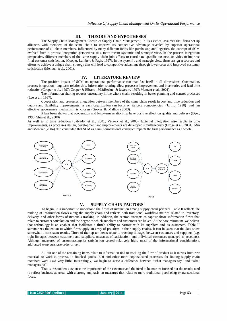
Influence Of Supply Chain Management On Its Operational Performance
|| Issn 2250-3005 (online) || || January || 2014 || Page 53
III. THEORY AND HYPOTHESES The Supply Chain Management Construct Supply Chain Management, in its essence, assumes that firms set up
alliances with members of the same chain to improve its competitive advantage revealed by superior operational performance of all chain members. Influenced by many different fields like purchasing and logistics, the concept of SCM evolved from a process integration perspective to a more recent systemic and strategic view. In the process integration perspective, different members of the same supply chain join efforts to coordinate specific business activities to improve final customer satisfaction. (Cooper, Lambert & Pagh, 1997). In the systemic and strategic view, firms assign resources and efforts to achieve a unique chain strategy that will lead to competitive advantage through lower costs and improved customer
satisfaction (Mentzer et al., 2001).
IV. LITERATURE REVIEW The positive impact of SCM on operational performance can manifest itself in all dimensions. Cooperation,
process integration, long term relationship, information sharing allow processes improvement and inventories and lead time
reduction (Cooper et al., 1997; Cooper & Ellram, 1993;Bechtel & Jayaram, 1997; Mentzer et al., 2001). The information sharing reduces uncertainty in the whole chain, resulting in better planning and control processes
(Lee et al., 1997). Cooperation and processes integration between members of the same chain result in cost and time reduction and
quality and flexibility improvements, as each organization can focus on its core competencies (Jarillo 1988) and an effective governance mechanism is chosen (Grover & Malhotra 2003).
It has been shown that cooperation and long-term relationship have positive effect on quality and delivery (Dyer, 1996; Shin et al., 2000)
As well as in time reduction (Salvador et al., 2001; Vickery et al., 2003). External integration also results in time improvements, as processes design, development and improvements are developed simultaneously (Droge et al., 2004). Min and Mentzer (2004) also concluded that SCM as a multidimensional construct impacts the firm performance as a whole.
V. SUPPLY CHAIN FACTORS
To begin, it is important to understand the flows of interaction among supply chain partners. Table II reflects the ranking of information flows along the supply chain and reflects both traditional workflow metrics related to inventory, delivery, and other forms of materials tracking. In addition, the section attempts to capture those information flows that
relate to customer satisfaction and the degree to which suppliers and customers are linked. At the bare minimum, we believe that technology is an enabler that facilitates a firm’s ability to partner with its suppliers and its customers. Table II summarizes the extent to which firms apply an array of practices in their supply chains. It can be seen that the data show somewhat inconsistent results. Three of the top ten items relate to tracking linkages between customers and suppliers (e.g. tight linkages between customers and suppliers, measures of satisfaction, and individual customers managed as accounts). Although measures of customer/supplier satisfaction scored relatively high, most of the informational considerations addressed were purchase order driven.
All but one of the remaining items relate to information tied to tracking the flow of product as it moves from raw
material, to work-in-process, to finished goods. EDI and other more sophisticated processes for linking supply chain
members were used very little. Interestingly, we begin to sense a difference between “what managers say” and “what managers do”.
That is, respondents espouse the importance of the customer and the need to be market-focused but the results tend to reflect business as usual with a strong emphasis on measures that relate to more traditional purchasing or transactional focus.

Influence Of Supply Chain Management On Its Operational Performance
|| Issn 2250-3005 (online) || || January || 2014 || Page 54
Reasons to engage in supply chain management Respondents were asked the reasons they engaged in supply chain
management. This list of questions was generated from conversations with practicing managers, trade publications, and
academic publications (e.g. Schary and SkjottLarsen, 1995). Table III summarizes the results. The findings reflect many of the common mantras evoked for explaining the virtues of supply chain management, ranging from increased end-customer satisfaction, to gaining a strategic market position, to reduced costs and improved productivity. It is encouraging to see that the reasons reflect both the cost reduction and the revenue enhancement side of supply chain management. Nonetheless,
when one examines the differences between buyers and sellers, one gains a better appreciation for the tension that exists within many supply chains. While not statistically significant in every case, the data suggest that buyers tend to focus more on the cost reduction aspects of supply chain management, and view securing a reliable source of supply, reduced lead time, and lower costs as key drivers of supply chain management. Conversely, sellers tend to highlight revenue enhancement and see profits, strategic market position, and customer satisfaction as prime drivers for supply chain management. If we were to focus on the overall means scores alone, we would not begin to develop an appreciation for what might be fundamental differences in “world views” between buyers and sellers.
VI. SUPPLY CHAIN MANAGEMENT PROCESSES Supply chain management processes explore what respondents say they do in their supply chain interactions.
These items explore how the respondents describe their relationships with suppliers/customers and tend to reflect the range of behaviors that support close relationships between buyers and sellers. Interestingly, two major themes dominate this set of questions. Respondents tend to take a more long-term view and state that they expect the relationship to last; that sustaining the relationship is important; and that they have plans to continue the relationship into future. The respondents also highlight
communications processes as an important second theme. They report that communications between the partner firms are frequent and that there is a high level of contact between trading parties. Partners have faith in each other and report that they share a sense of fair play. When we look at key differences between buyers and sellers, it appears that buyers are less willing to devote extra effort to their supply chain relationships.
VII. SUPPLY CHAIN PRACTICES Where the previous section examines what supply chain members say they do; this section examines what they
actually do.
Is akin to “talking the talk and walking the walk”. Interesting differences between the two sections exist in that,
from the previous section, one gets the strong impression that information is shared openly and that the boundary between firms is quite permeable. However, these findings addressing specific practices suggest that information sharing is less than
open and that technical information is shared only when necessary. In addition, mixed signals surface about the importance of price in evaluating one’s partner.

Influence Of Supply Chain Management On Its Operational Performance
|| Issn 2250-3005 (online) || || January || 2014 || Page 55
VIII. EFFECTS OF PERFORMANCE In order to explore the effects of several of these variables on measures of performance, a series of exploratory
OLS regression analyses were performed. Separate regression models were developed to explain the extent to which different measures of performance – cost reduction and revenue enhancement
(As measured by customer satisfaction) are affected by different supply chain processes and practices. Simply, we examined the extent to which elements of co-ordination, collaboration, and criticality affect two different measures of supply chain management performance. Traditional performance measures would reflect cost reduction while a more “enlightened” view should also deem revenue-enhancing elements as very important. Two different measures of performance were developed from the questionnaire. These findings imply that both trust and commitment contribute to satisfaction as the
elements of collaboration reported here imply a willingness to share information without the concern for it being used against either trading partner or a longer-term focus to the trading relationship. While the results for sustaining the relationship are counter-intuitive, co-ordination cannot substitute for closer ties between trading partners. The data suggest that interdependence and information sharing become key ingredients in an integrated supply chain whose goal is customer satisfaction.
IX. CONCLUSIONS A number of conclusions can be drawn from this study. It is apparent from these findings that although we espouse
the benefits of supply chain management and sing the virtues of closer ties throughout levels of the supply chain; the results suggest that business has not yet fully operationalized the concept of supply chain management. It appears that buyers tend to be reluctant players and are far more skeptical about the benefits afforded through such close integration. One can infer that buyers consider less favorably the benefits gained and are more likely to highlight the risks associated with heightened dependence on a smaller number of suppliers. We can infer also that buyers think about the gains afforded by an integrated supply chain and are more easily swayed by more traditional purchasing metrics related to cost or initial Performance – Performance – cost reduction customer satisfaction Collaboration – what is said Sustaining the relationship 0.532 (p< 0.00) Joint planning Frequent interaction Sharing information 1.208 (p= 0.02)a 0.072 (p< 0.00) Collaboration – what is done
Sharing technical information Training is important 0.13 (p< 0.00) Co-ordination Customer supplier linkages –0.096 (p <0.00) Frequent monitoring Order entry and tracking –1.209 (p< 0.00) 0.331 (p< 0.00) Raw material tracking Criticality 0.716 (p< 0.00)R20.27 0.29 Note: a= β= 1.208 Regression results showing factors contributing to types of procurement performance An empirical investigation 647 purchase price. Buyers consistently view the cost-saving aspects of supply chain management as more important than the revenue-enhancing benefits.
They seem to understand, on one level, the importance of customer-driven supply chains; the need to focus on core competencies; and, the importance of leveraging the skills and capabilities of their suppliers.
REFERENCES [1.] Anderson, J. C., & Gerbing, D. W. (1988). Structural equation modeling in practice: a review and recommended two step
approach. Psychological Bulletin, 103: 411-423.
[2.] Bagozzi, R. P., Yi, Y., & Phillips, L. W.(1991). Assessing construct validity in organizational research. Administrative
Science Quarterly, 36: 421-458.
[3.] Barney, J. B. (1991). Firm resources and sustained competitive advantage. Journal of Management,17:99-120.
[4.] Bechtel, C., & Jayaram, J. (1997). Supply chain management: a strategic perspective. The International Journal of
Logistics Management, 8: 15-34.
[5.] Boyer K.K., & Lewis, M.W. (2002). Competitive priorities: Investigating the need for trade-offs in operations strategy.
Production and Operations Management, 11: 9-20. Brown, T. A. (2006). Confirmatory Factor Analysis for Applied Research:
New York: The Guilford Press.
[6.] Burgess, K., Singh, P. J., & Koroglu, R. (2006). Supply chain management: a structured literature review and implications for
future research. International Journal of Operations & Production Management,26: 703-729.
[7.] Carr, A. S., & Kaynak, H. (2007). Communication methods, information sharing, supplier development and performance.
International Journal of Operations & Production Management, 27: 346-370.
[8.] Carr, A. S., & Pearson, J. N. (1999). Strategically managed buyersupplier relationships and performance outcomes. Journal of
[9.] Operations Management, 17: 497-519.Chen, I. J., & Paulraj, A. (2004). Towards a theory of supply chain management: the
constructs and measurements. Journal of Operations Management, 22: 119-150.
[10.] Chen, I. J., Paulraj, A., & Lado, A. (2004). Strategic purchasing, supply management and firm performance. Journal of
Operations Management, 22: 505-523.Cooper, M. C., & Ellram, L.M. (1993). Characteristics of Supply
[11.] Chain Management and the implications for purchasing and logistics strategy. The International Journal of Logistics
Management, 4(2): 13-24.
[12.] Cooper, M. C., Lambert, D. M., & Pagh, J. D. (1997). Supply Chain Management: More than a new name for Logistics. The
International Journal of Logistics Management,8(1): 1-14.
[13.] Corbett C., & Wassenhove, L.V. (1993). Trade-offs? What tradeoffs? Competence and competitiveness. California
Management Review, 35(4): 107 – 122.

International Journal of Computational Engineering Research||Vol, 04||Issue, 1||
||Issn 2250-3005 || ||January||2014|| Page 56
Processing Of Mammographic Images Using Speckle Technique
A.M. Hamed1 and Tarek A. Al-Saeed
2
1Physics Dept., Faculty of Science, Ain Shams University, 11566 Cairo, Egypt. 2Biomedical Eng., Faculty of Engineering, Helwan University, Cairo, Egypt.
I. INTRODUCTION Physicians are interested to have more information about medical images. One branch of imaging uses
the optical and laser microscopy which is useful to examine the blood cells and plasma. The other branch based
on x– ray, ultra sonic, and MRI imaging is useful to get more information since the resolution limit is improved
in the direction of frequency increase. In all cases of imaging, it is recommended to make image processing to
get more information and details [1-4]. For this reason, we make this study to distinguish between the normal,
benign, and malignant mammographic images using speckle techniques and correlation [5-12]. In this study, the
algorithm is based on speckle image formation modulated by the former mammographic images in presence of
randomly distributed function as a diffuser. The speckle images are compared with the corresponding speckle
image in absence of the former image. Another comparative technique based on correlation is investigated. A
circular aperture modulation is used during the formation of the above speckle images. Also, two circular
apertures are proposed in the formation of speckle of mammographic image and diffuser giving a grid structure
which facilitates the distinction between images. All speckle images and the grid structure of speckle images are
investigated giving better information in case of grid structure.
II. THEORETICAL ANALYSIS In this analysis, we represent the x- ray mammographic image by a function f(x, y). It is written in a
discrete form as a matrix of dimensions M x N as follows:
Where are the rectangle widths of the image and matrix dimensions are taken as M=1024 and
N= 1024. For the image of dimensions 4cm2,
Now a circular uniform aperture is used in the segmentation process, it is represented as follows:
Where (x, y) has the same dimensions like the image matrix of 1024x1024 pixels and the radial coordinate is 0
=(x2+y
2)
1/2 is 64 pixels.
The diffuser has a randomly distributed function represented as d(x, y) and has the same dimensions like the
above matrices. It is used to fabricate the ordinary speckle image in case of uniform circular aperture and in
absence of the image. Now, the multiplication of the three matrices in the same sequence will give a new
matrix of same dimensions like the other matrices.
ABSTRACT We study the malignant and benign mammographic x – ray images using speckle techniques.
Discrimination between the mammographic images is outlined using circular aperture segmentation.
The algorithm is based on the selection of the interested segment from the mammographic image. We
multiply the segment by a uniform circular aperture of diameter nearly equal the dimensions of the
segment. Then, we multiply the modulated segment by a diffuse function. Finally, we operate the Fourier
transform upon the three matrices to get a modulated speckle images. These modulated images are
dependent upon the information on the selected image segment. The modulated speckle images and
profiles of the mammographic images are investigated using mat-lab code.
Key Words: Mammographic x- ray images; modulated speckle images; correlation and contours of
benign and malignant images.

Processing Of Mammographic Images…
||Issn 2250-3005 || ||January||2014|| Page 57
The result is represented as follows:
The Fourier transform is operated upon the multiplication product to get this convolution product:
Referring to the convolution theorem, the simple product of the three matrices is transformed into convolution
product. For example, , etc.
In case of one circle, we substitute equation (2) in equation (3) and solve for the transformation to get:
w = (2π 0/f) (u2
+ v2)
1/2 is the reduced coordinate in the Fourier plane (u, v). is the wavelength of laser
radiation and f is the focal length of the Fourier transform lens.
Also, two circular apertures are proposed for the modulation, and we get a grid structure of the speckle image in
the following form:
It is noted that w has a dimensionless value as stated in equation (5).
III. WHAT IS BREAST CANCER
Breast cancer is a “malignant neoplasm of the breast.” A cancer cell has characteristics that differen-
tiate it from normal tissue cells with respect to: the cell outline, shape, structure of nucleus and most important-
ly, its ability to metastasize and infiltrate. When this happens in the breast, it is commonly termed as „Breast
Cancer‟. Cancer is confirmed after a biopsy (surgically extracting a tissue sample) and pathological evaluation.
IV. MORPHOLOGIC PRESENTATIONS As you can see from the mammograms and diagrams, the breast tissue comprises of small intricate
structures so pathology can easily be overlooked, especially if the film quality is not good. Not all structures are
cancers. Many structures or macro (big) calcifications are often benign. Some basic forms of pathology and
morphology presentations are (Addendum 3):
Masses and Densities
Masses‟ differ from „Densities‟ because „masses‟ are seen on two views whereas „densities‟ are seen on
one view only. Hence, two views of each breast to identify this abnormality. Masses with smooth rounded edge
are generally a fluid-filled cyst that can be confirmed by an ultrasound and aspirated to relieve pain for the
woman. Hard lesions with uneven edges might be reason for follow-up procedures. A mass could be palpable
(can feel it during a physical breast exam) depending on the size and proximity to the skin surface. A fat con-
taining mass looks radiolucent on the mammogram. Sometimes, it is very difficult for radiologists to differen-
tiate between a benign and a malignant mass off mammograms (as in Fig. below), so additional imaging modali-
ties and/or biopsy may be required.

Processing Of Mammographic Images…
||Issn 2250-3005 || ||January||2014|| Page 58
Examples of benign mass and a malignant mass Ref. [ *]
Micro calcifications
Calcifications are small calcium deposits that can be detected on a mammogram. Minute calcifications
are called micro calcifications and bigger ones are called macro calcifications. The latter is generally benign and
does not need additional follow-up. Sometimes, other structures mimic micro calcifications such as calcified
arteries that appear like „train tracks‟. This is normal. Artifacts on mammograms due to specs of dust may look
like micro calcifications, but the difference is that these specs are bright and shiny whilst a micro calcification
looks „milky white‟. Radiologists categorize the calcifications as malignant or benign based on (1) the location
of calcifications, (2) the arrangement (linear or scattered or clusters) (3) the total number of micro calcifications
(4) the changes with respect to the previous mammograms.
Quantitative results
The mammographic images shown in the figure (1) are investigated using speckle imaging and the
correlation techniques. The basic differentiation of the x-ray mammographic images is outlined in the above
section of morphological presentations.
Figure (1): Three mammographic images each have the same matrix dimensions 1024x1024 pixels.
As shown from the left is the normal mammogram” mdb003”, in the middle circular benign masses are shown
“mdb001”, while in the right a malignant micro-calcification is shown in the image “mdb213”. Now, referring to the figure (2), X1, X2, X3 represent the contour images of the normal, benign, and malignant
images as illustrated in the 1st row. In the graph, X1 has shown uniform elliptic shape in the range from
(800,600) up to (300, 700) while for the benign image X2, hallow is concentrated in the range from (700,500)
up to (800,450) around the center. The malignant image showed a deformed triangular shape. In the 2nd
row three contour images are shown. The 1st represent the autocorrelation X11 of the normal image X1 which
has a nearly isotropic shape while the cross correlation of the normal image X1 and benign image X2 is X12 has
shown asymmetric shape. Finally, the cross correlation of the malignant image X3 with the normal image X1
has shown an elongation along y axis and deformed from the left which its contour X13 has a different shape as
compared with the other correlation contours X11 and X12.
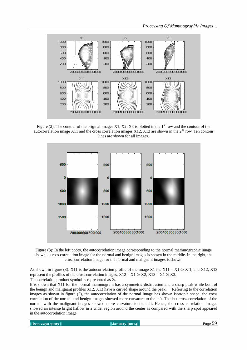
Processing Of Mammographic Images…
||Issn 2250-3005 || ||January||2014|| Page 59
Figure (2): The contour of the original images X1, X2, X3 is plotted in the 1st row and the contour of the
autocorrelation image X11 and the cross correlation images X12, X13 are shown in the 2nd
row. Ten contour
lines are shown for all images.
Figure (3): In the left photo, the autocorrelation image corresponding to the normal mammographic image
shown, a cross correlation image for the normal and benign images is shown in the middle. In the right, the
cross correlation image for the normal and malignant images is shown.
As shown in figure (3): X11 is the autocorrelation profile of the image X1 i.e. X11 = X1 X 1, and X12, X13
represent the profiles of the cross correlation images, X12 = X1 X2, X13 = X1 X3.
The correlation product symbol is represented as .
It is shown that X11 for the normal mammogram has a symmetric distribution and a sharp peak while both of
the benign and malignant profiles X12, X13 have a curved shape around the peak. Referring to the correlation
images as shown in figure (3), the autocorrelation of the normal image has shown isotropic shape, the cross
correlation of the normal and benign images showed more curvature to the left. The last cross correlation of the
normal with the malignant images showed more curvature to the left. Hence, the cross correlation images
showed an intense bright hallow in a wider region around the center as compared with the sharp spot appeared
in the autocorrelation image.
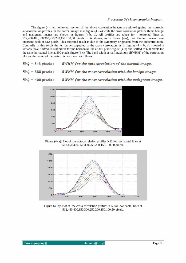
Processing Of Mammographic Images…
||Issn 2250-3005 || ||January||2014|| Page 60
The figure (4), ten horizontal section of the above correlation images are plotted giving the isotropic
autocorrelation profiles for the normal image as in figure (4 – a) while the cross correlation plots with the benign
and malignant images are shown in figures (4-b, c). All profiles are taken for horizontal lines at
512,450,400,350,300,250,200,150,100,50 pixels. It is shown, as in figure (4-a), that the ten curves have
invariant peak at 512 pixels. This expected result is due to the symmetry originated from the autocorrelation.
Contrarily to this result the ten curves appeared in the cross correlation, as in figures (4 – b, c), showed a
variable peak shifted to 600 pixels for the horizontal line at 300 pixels figure (4-b) and shifted to 650 pixels for
the same horizontal line at 300 pixels figure (4-c). The band width at half maximum (BWHM) of the correlation
plots at the center of the pattern is calculated as follows:
Figure (4- a): Plot of the autocorrelation profiles X11 for horizontal lines at
512,450,400,350,300,250,200,150,100,50 pixels.
Figure (4- b): Plot of the cross correlation profiles X12 for horizontal lines at
512,450,400,350,300,250,200,150,100,50 pixels.

Processing Of Mammographic Images…
||Issn 2250-3005 || ||January||2014|| Page 61
Figure (4 - c): Plot of the cross correlation profiles X13 for horizontal lines at
512,450,400,350,300,250,200,150,100,50 pixels.
Referring to the obtained speckle images calculated from equation (5) are represented as in figure (5 –
a), we observe that more luminous spots are appeared in case of benign and malignant images as compared with
the normal mammographic image. These luminous spots which discriminates one image from the other with the
weak patches of spots form the speckle images. In the normal image, three luminous spots are shown as
compared with more than nine spots visualized in case of benign mammographic image while four spots located
in a different position are seen in the malignant image. This difference between speckle images is attributed to
the scattering of different luminous spots of the original images in figure (1) for certain diffuser and circular
aperture with the same radius.
Figure (5-a): The three speckle photos are taken using a diffuser of 1024x1024 pixels and the original images
are obstructed with circular aperture of radius 64 pixels. The speckle images are of dimensions 128x128.
(5 -b): Two circles used in the formation of the grid structure of speckles shown in figure (4-b).

Processing Of Mammographic Images…
||Issn 2250-3005 || ||January||2014|| Page 62
The grid structure appeared in the speckle images shown in figure (5-b) is due to interference
originated from the two displaced circles located in the object plane superposed over the diffuser. The resulting
images are computed using equation (6). The grid structure originated inside the patches of the speckle images
facilitates the discrimination.
V. CONCLUSION We have used two different techniques to process the mammographic images based on speckle and
correlation techniques. Firstly, the contours obtained of the correlation images showed a good discrimination
between the normal, benign, and malignant mammographic images. Secondly, the different speckle images
obtained using specific randomly distributed function superimposed over the investigated images gave three
different images of different luminosity. This allows discriminate the images. We believe that the difference
between the speckle images is due to the convolution product of the Fourier spectrum of the original images
with the ordinary speckle pattern.
REFERENCES [1] B. Al Hadidi , M. H. Zubi , and H.N. Sulieman , “Mammogram breast cancer detection using image processing function ,
Information technology journal , vol. 6, pp.217-221, 2007.
[2] L. W. Basset, V.III Manjikian, etc. ,”Mammography and breast cancer screening(Review) Surg clinics of North America , pp. 775-
800 , 1990. [3] D.B. Kopans, “The potential impact of computer-aided diagnosis on clinical mammography”. Proc. of the 3rd International
workshop on Digital Mammography , 35.
[4] M. Heath, K. Kopans , etc. “Current status of the digital data base screening mammography” , Proc. of the 4th International
workshop on Digital mammography, pp. 457 - 4 60.
[5] M. Tebaldi, Luciano Angel Toro, Opt. Comm. vol. 182 (2000) pp. 95 – 105, New multiple aperture arrangements for speckle pho-
tography.
[6] Luciano Angel Toro, M. Tebaldi, Opt. Comm. 192 (2001) 37 – 47, Properties of speckle patterns generated through multi- aperture
pupils. [7] A. M. Hamed , J. Modern Opt. 56 (2009)1174 – 1181 , Numerical speckle images using modulated linear apertures : Simulation.
[8] A. M .Hamed , J. Modern Opt. 56 (2009)1633 – 1642 , Formation of speckle images using circular obstruction.
[9] A. M. Hamed , J. Opt. Eng. 50 (2011) 1 – 7, Discrimination between speckle images using diffusers modulated by some apertures :
Simulations.
[10] A. M. Hamed , Optics and photonics journal 1 (2011) 41-52 ,Computer generated quadratic and higher order apertures and its ap-
plication on numerical speckle images.
[11] J. W. Goodmann , "Introduction to Fourier optics and holography", Roberts & Company Publishers, Greenwood Village, United
States, third ed. , 2005. [12] J. W. Goodman , “Statistical properties of laser speckle patterns”, Springer – Verlag , New York 1984.

International Journal of Computational Engineering Research||Vol, 04||Issue, 1||
||Issn 2250-3005 || ||January||2014|| Page 63
An Ontology System for Ability Optimization & Enhancement in
Cloud Broker
Pradeep Kumar M.Sc. Computer Science (AI) Central University Of Rajasthan
I. INTRODUCTION: Cloud computing is becoming a well-known services area. Cloud computing provides various type of
services like IaaS, PaaS, SaaS, CaaS and DaaS. Many companies are providing services to users and these ser-
vices criterion will be decide by their performance and usability. The companies are using a new technology is
called Ontology based cloud services discover system (CSDS) [1] for providing the best services to users to
making profit and ranking high.
Figure 1(Simple Could System Image)
ABSTRACT: This Paper Presents The Service Providing Ability Optimization Of Cloud Brokers. The Concept Of
Service Ability Optimization Provides A Nearest Result Regarding User's Queries And Broker's Optimi-
zation System To Optimize The Result. This Concept Is Focusing 0n To Reduce Broker's Decision Mak-
ing Time And Helps In Improving His Services, Trust, And Feasibility In Users. It Is Specially Designed
For Cloud Brokers Who Want To Long Relationship With Users And Being In Existence In Marketplace
Successfully. In This Regard Cloud Broker System Works On Improved Ontology Based Cloud Services
Discover System (CSDS) And ROSP. The ROSP System Works For Enhancement Of Cloud Brokers
With Improved CSDS. The Concept Behind Optimization Is Adding New Type Of Similarity Reasoning
In Cloud Services Discover System, Is Called Protocol Similarity Reasoning. The Protocol Similarity
Reasoning Divides In Four Parts: - 1) SSL Similarity, 2) Authorization Similarity, 3) Popularity Simi-
larity And 4) Security & Ownership Similarity.
KEYWORDS: Cloud Computing, Cloud Service, Cloud Service Providers, Ontology, CSDS, Reason-
ing, Users, ROSP Algorithms, Optimization, Brokers, Cloud Broker System, Enhancement.

An Ontology System For Ability Optimization…
||Issn 2250-3005 || ||January||2014|| Page 64
The cloud brokers deal with user's queries and providing cloud services with feasible cost (The Basic Structure
of Cloud broker shown in figure 1). The brokers are using this technology to making more outcomes. The tech-
nology works for cloud brokers but not feasible for users every time according to their queries. The ontology
based CSDS is using ontology reasoning system.
This reasoning system contains a set of concepts, relationship among concepts and can be applied into
information retrieval to deal with users queries. The system applies reasoning to calculate similarity between
available objects, concepts and produce output according to similarity. The problem is, how new technology is
beneficial for users, brokers and what is further use in cloud computing. An ontology based improved CSDS
contains a new protocol similarity reasoning. The reasoning provides strength to CSDS in terms of security &
ownership, popularity, authorization and SSL. The previous ontology based cloud services discover system is
not the best option for deciding cloud services rating. Hence the improved CSDS is providing optimal result to
broker according the users queries and ROSP system more optimize this result to users. Thus improved CSDS
system is more beneficial for users and brokers. The British Broadcasting Corporation (BBC) proclaimed that
it’s shifting to totally tapeless content production and investment in development of their personal cloud system.
The advanced technology of the Cloud in terms of web, it is a good issue concerning cloud computing as a result
of while not webs it insufferable. However nowadays it is a bottleneck issue within which an outsized quantity
of information is send. The handling of users is additionally a good challenge in cloud computing at the time of
usage. It is still not resolved by anyone as a result of each user per second area unit increasing as per the popula-
tion like Republic of India. In this advanced world, Cloud Computing is in its developing stage but as per its
level of development it has got its importance .Cloud computing is increasing day by day in the IT markets and
becoming more popular in the management system. This is performing its work very fast in the IT Marketing
but yet most of people are confused in its activities done or provided by cloud Computing. Some of the concepts
related to the cloud computing as per the users need increasing day by day. It has many definitions given by
different people for different purposes. The main agenda is to talk about the resource managements in Cloud and
the process they are following.
II. ONTOLOGY ABSTRACT: "Ontology was one primarily theory to explore knowledge characteristics of life and real objects." On-
tologies are sets of classes with attributes, relations and instances between each other which allow the elabora-
tion of metadata to quickly identify the objects. "Ontology is a data model that represents a set of concepts with-
in a domain and the relationships among those concepts." Semantic phenomena are context independent. Prag-
matic phenomena are context-sensitive. Ontology contains a set of concepts and relationship between concepts,
and can be applied into information retrieval to deal with user queries [2]. It provides a shared understanding of
a domain of interest to support communication among human and computer agents [3].
Benefits of using Ontology:
In order to provide an environment for automatic searching of services, resources ontology is used. These are
some of the areas where Ontology is used in Cloud Computing .Intelligent Ontology based registries are used
for dynamic discovery of cloud computing resource across various cloud computing platforms. It can be used to
provide intelligent customization framework for SaaS. Easing the design of security system by proving role
based access control using ontology. The Ontology layers of Cloud Computing are
1) Firmware/Hardware (HaaS),
2) Software Kernel,
3) Cloud Software Infrastructure,
[1] Computational Resources (IaaS),
[2] Data storage (DaaS),
[3] Communication (CaaS),
4) Cloud Software Environment (PaaS),
5) Cloud application (SaaS).

An Ontology System For Ability Optimization…
||Issn 2250-3005 || ||January||2014|| Page 65
Figure 2 (The Problem Statement Condition)
III. PROBLEM STATEMENTS: If more than one companies having the same parameter then previous CSDS system produce rating the
same for all companies, at this stage the system building complex in finding difference between them and the
brokers are confused to decide their function. The broker needs more time to take decision for providing servic-
es to users. If the broker does not consider the CSDS result and provide services to users according to CSDS
result directly. Then users are also not deciding that which companies are giving good services and convenient.
In this situation users are not able to determine difference between provided ratings, because the system provid-
ing same data type value for companies and another problem is rise, which is the best rating for services and
provider (use upper figure). Example is shown in figure 2, there are two company having same path for one
product (one company is owner of product and other company is affiliate or member) and CSDS is calculate
equal rating or data lists for this product in result. The result is confusable for users and new brokers. With
wrong decision the brokers and users are getting penalties in terms of cost, time and resource. The objective of
this paper is providing the best techniques to improve existing ontology reasoning algorithms and concepts.
IV. METHODOLOGY: A. Methodology for optimization:-
The concept behind optimization is adding new types of similarity reasoning are called protocol simi-
larity. The protocol similarity divides in four parts, 1) SSL similarity: The SSL similarity is calculating verifica-
tion similarity of services (i.e. IGN Company is having SSL verification by global institute and Polji Company
not having a global verification then Polji similarity value is less than IGN, if both are having same level verifi-
cation then no value is calculating). 2) Authorization similarity: If available verification is same then checking
authorization by institute and organization (i.e. IGN company authorize by UNO and other Polji company is
authorize or verified by local institute, in this condition Polji get less value, if both company having same level
authorization (Same level authorization go to step 4) and ownership then no value is added in similarity).3)
Popularity similarity: If available authorization is same then checking popularity similarity of service provider
companies (reasoning checking popularity of company and services, it also check global level of company and
service).4) Security & Ownership similarity: Checking security similarity in virtualization, OS, hypervisor,
rootkits, vendors, ownership for services. Before calculating these similarities, filter results is coming by simi-
larity reasoning previous similarities (concept, object and data similarity reasoning).

An Ontology System For Ability Optimization…
||Issn 2250-3005 || ||January||2014|| Page 66
Figure 3 (Cloud Parameters for example)
Figure 4 (Figure 2 Result Calculating According to Algorithm 1)
Figure 5 (Rating Algorithm)

An Ontology System For Ability Optimization…
||Issn 2250-3005 || ||January||2014|| Page 67
B. Methodology for Enhancement :-
The basic definition of rough set is that sometimes an object neither belongs to positive non negative
then it is in the boundary. If the boundary is non-empty then we call it rough. The Rough set Theory is based on
the assumption that data and information is associated with every object of the universe. For each attribute
the value of
It is interesting to compare definitions of classical sets, fuzzy sets and rough sets. Classical set is a primitive
notion and is defined intuitively or axiomatically. Fuzzy sets are defined by employing the fuzzy membership
function, which involves advanced mathematical structures, numbers and functions. The value 1 and 0 are pre-
sented for the CSP. We have formed on the basis of relevance to users and CSP’s. The relevance generates a
threshold value for each attribute out of a scale of 10.
We have represented the CSP and their attributes in a tabular form called Information System. The rows of the
table contain the list of cloud service providers and the columns consist of the attributes of the respective cloud
service provider.
Figure 6 (Algorithm 2* that used the data of Algorithm 1)
V. RESULT AND SIMULATION: As proceeding with our previous ROSP Algorithm and methodology, in our new Simulation we have
created some packages in Net Beans and calculated the result of the reasoning formulated by the Ontology based
system. The output is shown in the below Figure 7, 8, 9. The result is more beneficial than without ontology
system, because the ontology based system is giving best hope to regarding to maximum optimized re-
sult.(Example by Figure 2 to 9)
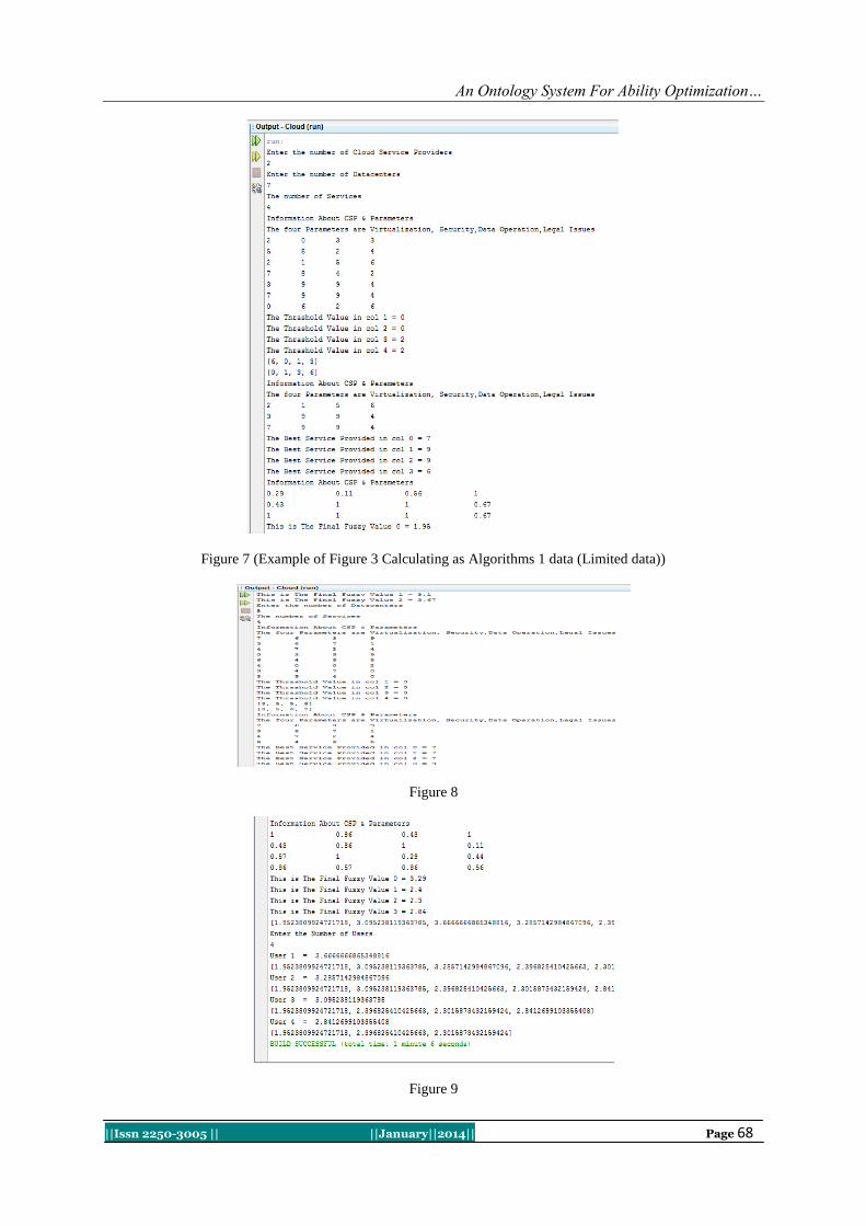
An Ontology System For Ability Optimization…
||Issn 2250-3005 || ||January||2014|| Page 68
Figure 7 (Example of Figure 3 Calculating as Algorithms 1 data (Limited data))
Figure 8
Figure 9

An Ontology System For Ability Optimization…
||Issn 2250-3005 || ||January||2014|| Page 69
Benefit of using this system: As proceeding with our system, the system is using ontology approach that
makes it more beneficial for service providers. The system is increasing search power.
VI. CONCLUSION: The cloud Ontology is introduced for enhancing performance of Cloud Broker system. The broker op-
timization system is reducing penalties in terms of time, cost and resource. The optimization technique may fur-
ther use in security of cloud computing and it's also helpful in vulnerability. This paper has presented a Broker
services providing ability optimization. It is specially designed for cloud brokers who want long relationship
with user and try to provide his excitation in marketplace. The cloud Ontology is also introduced for enhancing
performance of Cloud Broker system.
VII. FURTHER WORK: Converting method project in a real application that will be beneficial for Cloud Broker & Users.
REFERENCES: [1]. Taekgyeong Han and KwangMongSim , An Ontology-enhanced Cloud Service Discovery System , Proceedings of the International
Multi-
Conference of Engineers and Computer Scientists 2010 Vol I, IMECS2010, March 17-19, 2010, Hong kong. [2]. FIPA 2001, Foundation for intelligent physical agents. FIPA Ontology Service Specification,
http://www.fipa.org/specs/fipa00086/XC00086D.html. [3]. HeinerStucken Schmidt, Ontology-based information sharing in weekly structured environments, Ph.D. thesis, AI Department,
Vrije University Amsterdam, 2002.
----------------------------------------------- *I want to give special thanks to Ashish Tiwari (M.tech)* for background support.

International Journal of Computational Engineering Research||Vol, 04||Issue, 1||
||Issn 2250-3005 || ||January||2014|| Page 70
Evaluation and Modeling of High Surface Area Activated Carbon
from Date Frond and Application on Some Pollutants
1,M.M.S. Ali.
2 N. EL-SAI
3,B. S. GIRGIS
1,Atomic Energy Authority, Hot Labs. Center, P. Code 13759, Cairo, Egypt.
2,National Research Center, 2622, Dokki Cairo, Egypt
I. INTRODUCTION Activated carbons were obtained from date frond, DF by single-step steam pyrolysis or by chemical
treatment. DF as a huge solid waste in Egypt is of little or no economic value and highly abundant renewable
by-products, with good mechanical strength, and in fact presents a disposal problem. The quantity of DF has
been estimated to million tons per year. Products with highly developed porosity were obtained from H3PO4-
activation, whereas, microporous carbons with moderate porosity resulted from NaOH treatment or steam
activation schemes. Preparative methods for porous carbons are conventionally classified into physical
and chemical activation. The latter is carried out in a single heat treatment step in the presence of an
added chemical. Phosphoric acid is one of the most commonly used agents for the activation of different
precursors, such as coals of different ranks [1,2], viscous rayon fibers [3] and, especially, lignocellulosic
feedstocks [4–12]. Recently, H3PO4 has been used as chemical activating agent for porous polymers
[13,14]. Phosphoric acid activation of lignocellulosic materials is a conventional preparation method for
activated carbon [15–18]. In summary, the precursor is impregnated with a solution of phosphoric acid, heat
treated up to about 500 0C, and washed with water to extract the excess acid. When peach stones (particle size
around 3 mm) are used, it was shown that phosphoric acid penetrates the interior of the particles, reacts with the
material and modifies the thermal decomposition [19]. As a result, the carbonization temperature is reduced, the
exit of volatile matter is inhibited and the contraction of the particle is lower than in the carbonization of the un-
impregnated particle. The consequence is that a relatively low carbonization temperature leads to a high
conversion to carbon and to a final product with a well developed porosity, compatible with a relatively high
bulk density [19-20]. Activated carbons are widely used in gas purification, solvent recovery, waste water
treatment, etc. It is recognized that the pore structure is the most important property of activated carbons for their
application in adsorption processes [21]. Activated carbons have a very wide range of pore sizes, from the
angstrom Å scale of micropores to the micrometer scale of macropores. They are used in various applications
depending on their porous properties. For example, activated carbons with many micropores are used for gas
adsorption, mesopores are necessary for the adsorption of large molecules, e.g woods, coconut shell, coal,
lignite, peat, and etc. are usually chosen as raw materials for activated carbons. Various carbons differing in
porous properties can be obtained by changing the raw materials and/or the preparation conditions, i.e. the
carbonization and activation conditions. Many investigations have been performed to explore novel raw
ABSTRACT Activated carbons were prepared through chemical activation of date frond DF, using sodium hydroxide
and phosphoric acid as the chemical activating agents. The effect of different parameters, such as
particle size, method of mixing, chemical/corn ratio, to choose the suitable conditions for the studying
materials was chosen. The activation time and activation temperature, on SBET surface area of the
produced activated carbons were discussed. The porosity of the activated carbons was evaluated through
nitrogen adsorption. The storage capacity of the activated carbon was evaluated using natural gas.
Under the experimental conditions investigated, the optimal conditions for production of high surface
area carbons by chemical activation were identified. Products with highly developed porosity were
obtained from H3PO4-activation, whereas, micro porous carbons with moderate porosity resulted from
NaOH or steam activation schemes. The results were applied on and discussed adsorption of cations and
pollutants from aqueous solution.
KEY WORDS: Activated carbons, agricultural waste, chemical activation, adsorption

Evaluation And Modeling Of High Surface Area…
||Issn 2250-3005 || ||January||2014|| Page 71
materials (such as waste materials) and to optimize the preparation conditions to obtain activated carbons with
the desired porous properties. Optimization of the activation process has been extensively investigated [22,23].
II. EXPERIMENTAL 2.1.Adsorbents.
All series of activated carbons in these papers were prepared from the same precursor. Eight activated
carbons were obtained from air-dried and crushed the date frond, DF. Carbons (I and II) were prepared by
subjecting the agricultural waste to direct steam pyrolysis at 700 oC one or two hour hold. The raw material was
inserted into a stainless steel tube fitted with an internal wire diaphragm and held in a vertical position to
dispose of the formed tarry matter. Heating of the pyrolysis tube was started to attain 350 oC for 35 min. then
pure steam is admitted from top of the tube using a steam generator. After reaching 700 o
C (100-120min), the
heated mass was left for 1 or 2 h at either temperature. The cooled activated carbon was weighed to determine
burn-off and stored in tight glass containers. Carbons (III-V) were obtained by mixing 60 g of the crushed raw
material with 30 g of NaOH solid (wt/wt)g, left overnight, then heat-treated slowly up to holding temperatures
of 700, 750, and 800oC. Then the cooled product was thoroughly washed by distilled water till the pH value up
to 7.5, and finally dried at 110 oC. Carbons (VI-IX) were prepared by impregnating of the precursor with H3PO4
(50 vol.%) followed by thermal treatment at 400, 450, 500 oC for two hours. The cooled activated mass was
subjected to through washing with distilled water, so as get rid of extra acid and to attain pH values ≤ 6.5 in the
washing solution, and finally dried at 110 oC. The weight loss was determined and referred to the original
weight of precursor and denoted as "global burn-off" (GBO). Burn-off % = (weight of the raw material – weight
of final product)/ weight of the raw material x= 100.
2.2. Characterization of activated carbons.
This was achieved by the standard adsorption of N2 at 77k, using a sorpatometer of the type NOVA
1000e (Quantachrome). In spite of limitations of the BET method, in case of activated carbon, it has been and
will continue to be used for microporous adsorbents owing to its simplicity and reasonable [7]. Accordingly, the
adsorption isotherms were analyzed to get various porous parameters: By applying the BET-equation to
determine the SBET surface area, total pore volume (VP), from amount of nitrogen held at P/P0 =0.95, and
average pore dimension (radius) from R=2VP/SBET was evaluated. Other porous characteristics were estimated
from the t-plots constructed by plotting volume of gas adsorbed (Va) versus t-values of adsorption on non-
porous standard carbon as reported by Selles-Perez and Martin-Martinez [18]. The obtained α s-values were
transformed into t-values by multiplication with 1.52 x 3.54 (Ǻ) as suggested by the same authors. The
following porosity characteristics were calculated as follows: total surface area (St) from slope of early straight
line to zero, non-microporous surface area (Sn) from slope of the late straight portion, ultra micropore volume
(V0u) from early intercept of the base straight portion, and super micropore volume (Vos) from the late intercept
of the base straight portion with V-axis.
2.3. Adsorption capacity from the liquid phase.
Laboratory experiments were performed to evaluate the relative amenability of some water polluted
with organic pollutants e.g phenol P and methylene blue MB dye by the prepared activated carbon.
% Removal =[ C0-Ce/ Co] x 100
Where C0 is the initial concentration of the solute (mg/L), and Ce is the residual equilibrium concentration of the
solute (mg/L).
III. RESULTS AND DISCUSSION 3.1. Chemical activation with NaOH
The effects of NaOH on carbonization of carbonaceous materials have been studied by several authors.
Thus, studying the formation of active carbons from DF after their reaction with NaOH in the temperature range
700–800oC, indicated that the oxygen of the alkali can remove cross-linking and stabilizing carbon atoms in
crystallites. Na metal obtained at reaction temperatures may intercalate and force apart the separate lamellae of
the crystallite. Removal of sodium salts, by washing, and carbon atoms from the internal volume of the carbon,
by activation reaction, create the microporosity of the activated in the new structure. This mechanism is
indicated that high temperature and high NaOH/carbon ratio produced large pores in the carbon structure, due to
the presence of Na2O, derived from NaOH, expanded the carbon atomic layers. When the temperature exceeded
700oC, a considerable amount of Na was formed by the reduction of Na2 O with carbon. Since the inner carbon
atoms were consumed, pores were formed in the structure. SBET surface area, total pore volume, radius and pH
of the activated carbons obtained by the NaOH treatment are shown in Tables 1 and 2. Carbonization of DF
samples that treated by NaOH at 700-800oC to obtain slightly decrease in the surface area of the carbon. But
with regard to this blank sample, the chemical activation of DF samples with H3PO4 at 400-500 0C brought

Evaluation And Modeling Of High Surface Area…
||Issn 2250-3005 || ||January||2014|| Page 72
about a very large increase in the surface area and pore volumes, even for the lowest NaOH/time and
temperature. An increase in this ratio brought about an increase in all textural parameters. As a consequence of
the NaOH chemical activation, there was an increase in the micropores, mesopores and a decrease in the
diameter. The pH of the activated carbons obtained indicates that they are slightly acidic or almost neutral. It is
noteworthy the surface characteristics of activated carbon DF samples, with very high SBET surface area and
very large values of micro and macropore volumes.
3.2. Porous properties of the prepared activated carbons
3.2.1. N2 adsorption isotherms
Table.2. shows examples of N2 adsorption isotherms at 77 K on the prepared activated carbons. The amount of
N2 adsorbed on each group of carbons increases with global burn off as expected and suggest the formation of
mesopores.
3.2.2. Chemical activation with H3PO4
As in table.1.it is obvious that in the phosphoric acid activation method, temperatures around 400-
500oC produce the maximum development of porosity, even though the carbonization of the material can be
incomplete, because the effect of H3PO4 is to produce chemical changes and structural alterations at
temperatures lower than in the thermal treatment without impregnation. Phosphoric acid functions in two ways.
As an acidic catalyst in promoting bond cleavage reactions and formation of crosslinks; and by being able to
combine with organic species to form phosphate linkages, such as phosphate and polyphosphate esters, that can
serve to connect and crosslink biopolymer fragments. Thus, phosphoric acid appears to be able to function in
two ways (i) as an acid catalyst in promoting bond cleavage reactions and the formation of cross-links via
processes such as cyclization and condensation and (ii) by combining with organic species to form phosphate
linkages, such as phosphate and polyphosphate esters, that serve to connect and to cross-link biopolymer
fragments. This can be tested by removing (leaching) the phosphoric acid for example from a 250 °C product,
and then heating to 300 °C (to be compared with no leaching).
3.3. Nitrogen isotherms and analysis by BET and αs-methods
Nitrogen adsorption isotherm is a standard tool for the characterization of porous materials especially
porous carbonaceous adsorbents. The adsorption isotherm can be made to yield valuable information about the
surface area and the pore structure of the adsorbent, heat of adsorption and so on. The definition of pore size
originally proposed by Dubinin and now adopted by IUPAC as follows: micropores width less than 2 nm;
mesopores width from 2 to 50 nm and the macropore width greater than 50 nm. Micropores can be subdivided
into ultramicropores (less than 0.7 nm) and supermicropores (from 0.7 nm to 2 nm) . The nitrogen adsorption
isotherms obtained for different activated carbon samples are shown in Figs.(1-6). Isotherms have been observed
for different activated charcoal DF, in the most cases there is a more gradual approach to a rather ill defined
plateau located at higher p/po. The appearance of hysteresis loops in the nitrogen isotherms of samples shown in
the Figs. (1-3) indicate the existence of some mesoporosity.
The hysteresis loop of H4 is indicative of slit-shaped pore, where the adsorption and desorption
branches are parallel. The type I isotherm character associated with H4 type hysteresis is of course indicative of
microporosity. The type H4 (E) hysteresis loop according to de Boer, is produced by tubular pores which
contain a narrow constriction or closed pores of the ink bottle type. In almost all the samples 70% of the pore
volume is filled below p/po
=50, indicate these samples are highly microporous. After the sharp movements up
to p/po of 0.1 the isotherm slowly bends showing smaller increment in adsorption. After a p/p
o of 0.2 the
adsorption becomes further smaller but still continuing the adsorption process almost up to the saturation vapor
pressure. Analysis of this process in the light of Kelvin equation shows the presence of pores of almost all
diameters even though to different extent in most of the samples. These pores vary from thin micropore to
probably broader micropore even if they are present, and are wide open so that the evaporation takes place at the
same p/po as in the adsorption process. From Figs (1-3), It is observed that the adsorption in microporous
carbons to be taking place in two steps, a micropore filling step and a mesopore filling condensation step. The
BET-plots for microporous carbons were found to be linear in different ranges of relative pressure and the SBET
surface area was found to increase with increase in the relative pressure range. They observed that the SBET
surface area determined from the pressure range 0.1–0.3 was significantly overestimated because of the quasi-
capillary condensation. Meanwhile this range (0.1–0.3) was found to be the best range of validity of the BET-
equation for non-porous carbons compared with the as-values. They have recommended that the relative
pressure range of 0.01–0.05 for SBET surface area determination of microporous carbons. In the current study the
linearity between the points in the above range well extends up to a relative pressure of 0.2 and hence the

Evaluation And Modeling Of High Surface Area…
||Issn 2250-3005 || ||January||2014|| Page 73
evaluation of SBET surface area made in the range 0.005–0.20 bears equal validity as those obtained in the BET
analysis of Kaneko et al. The deviation of the BET-plot from linearity becomes clearly remarkable from the
relative pressure value of 0.2. The SBET surface area of different activated carbon samples obtained from BET-
analysis along with corresponding monolayer capacity Vm values are given in Table .1. The as-plots of the
activated carbon samples under study are shown in the Fig.2 (a1,b1&c1). According to them if the right
reference data, i.e. the data from a reference material having the same value as that of the test material, is not
used the straight line extended from the lower p/po values cuts the y-axis (volume adsorbed axis) for a positive or
a negative value of the adsorbed volume. The micropore volume for all the activated carbon were calculated and
tabulated in Table1. The pore size distribution curves have been constructed based on diving the pore system
into a number of fixed groups of pores, each characterized by a narrow range of pore sizes. The pore size
distribution curve for selected activated carbon samples are shown in Fig. 6(e–j). It can be seen from the
distribution curve that in the case of oxidized samples, there was decrease in pore volume in lower diameter
though the pores at higher diameters have not been affected much, as a result of oxidation, the oxygen groups
essentially fixed at the entrance of the micropores and inside the wider micropores, which increases nitrogen
constriction to the pores. The micropore volume calculated from the summation of volumes of individual groups
of pores Vot is given in Table1.
As comparison of micropore volume values obtained by different methods with the Vm value from
BET-method show that the latter value is the smallest among all the samples. This indicate the completion of
monolayer coverage on the surface of carbon before all the micropore are completely filled. Among the
micropore volume values, the one obtained from as-method has highest magnitude. These results clearly indicate
that the surface chemical nature as well as surface texture of the activated carbon were changed considerably
after oxidization with different oxidizing agent. Thus, the most important difference between the activation
mechanism with NaOH and H3PO4 is that, whereas the first mechanism remove and avoid the crosslinking,
stabilizing the carbon atoms in crystallites, the second mechanism involves an excessive crosslinking by both acid
catalysis and through the phosphate linkages. The activated samples, A1,A2,A3,A4,A5,A6,A7,A8,A9) ( where
DF is date frond , S is physical treatment by single step steam pyrolysis, H is symbol of phosphoric acid, Na is
symbol of NaOH, the first number is indicated to thermal treatment multiplication in 100 and the second is the
duration time per hour), are A1, A2, A3, A4, A5, A6, A7, A8 and A9 respectively).Treatment with NaOH and
H3PO4 brought about, with regard to the samples, a large decrease in the ash content and an increase in the
carbon content, which increased from sample A1-A3, A4-A5 and from A6-A9. The N and O content gradually
decreased with the increase in the temperature and duration time in NaOH/sample. High ash content in carbons
is undesirable because mechanical strength and adsorptive capacity are reduced. The high ash content of these
carbons can be due to several reasons such as: (i) The inorganic constituent of the raw material can combine
with phosphoric acid giving insoluble phosphates, which furthermore, can be trapped inside the carbon matrix
due to the crosslinking that produces the treatment with H3PO4 and (ii) phosphate and polyphosphate species are
incorporated to the carbon matrix, through C–O–P bonds, connecting and crosslinking different organic species.
The lowest ash content of sample A4 can be due to [19] steam inhibited the formation of condensed phosphates
and eliminated the phosphate groups previously attached to the carbon. Characteristics of activated carbons
obtained from phosphoric acid activation are shown in Tables 1 and 2. The activated carbons obtained by this
method had an ash content that depended on the atmosphere of the treatment. Thus, the treatment of DF, yielded
different ash content depending on the activated method, which in this case, was similar to that of the blank
samples. Furthermore, the ash content of these activated carbons was much higher than those prepared from the
NaOH method. SBET surface areas Table1, of the blanks,(A4 – A6), were much higher than those of the
corresponding activated carbons (A7–A9). Therefore, the H3PO4 activation increased the SBET surface area of the
samples, although in much higher extent than the activation with NaOH. SBET Surface area of the activated
carbons obtained seems to depend on their ash content, with higher ash content the lower SBET surface area. All
samples had very low mesopore and macropore volumes and a somewhat higher micropore volume. All these
surface characteristics make that the particle density of these samples be higher than in the case of the NaOH
treatment.
3.4. Effect of burn off on porous properties
As shown in Table 1, the porous properties of the prepared activated carbons vary from 60 to 1100
m2
/ g for the SBET surface area, from 0.005 to 0.3 m l / g for the micropore volume, and from 0.05 to 0.59 m l / g
for the mesopore volume. Some of these activated carbons have a SBET surface area more than, 1000 m2
/ g and
mainly contain micropores. It is noteworthy that the mesopore volume of (A5-A6), series carbons of groups are
quite large. Although the porous properties of (A7-A9), series carbons of all groups are quite similar, the
properties of the carbons become different with an increase in burn off. Micropore volume and mesopore
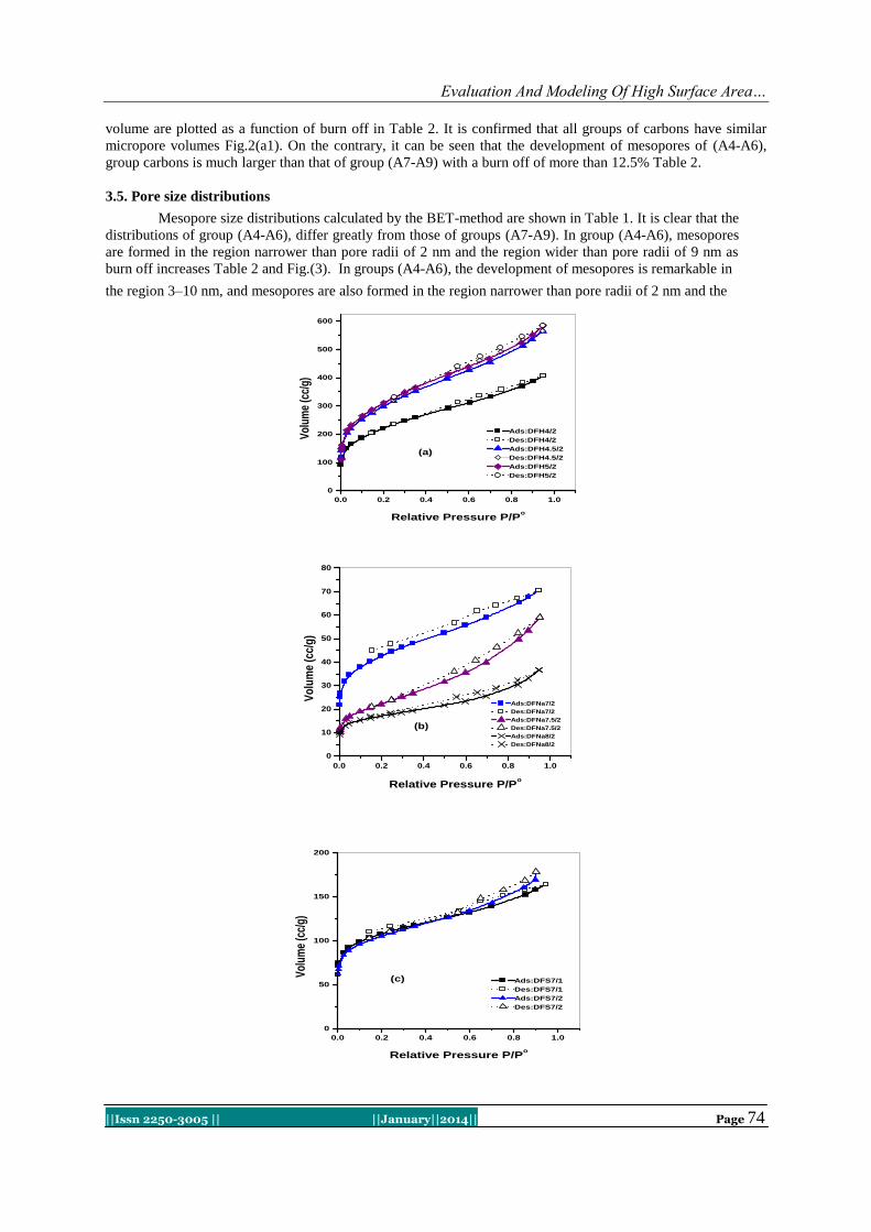
Evaluation And Modeling Of High Surface Area…
||Issn 2250-3005 || ||January||2014|| Page 74
volume are plotted as a function of burn off in Table 2. It is confirmed that all groups of carbons have similar
micropore volumes Fig.2(a1). On the contrary, it can be seen that the development of mesopores of (A4-A6),
group carbons is much larger than that of group (A7-A9) with a burn off of more than 12.5% Table 2.
3.5. Pore size distributions
Mesopore size distributions calculated by the BET-method are shown in Table 1. It is clear that the
distributions of group (A4-A6), differ greatly from those of groups (A7-A9). In group (A4-A6), mesopores
are formed in the region narrower than pore radii of 2 nm and the region wider than pore radii of 9 nm as
burn off increases Table 2 and Fig.(3). In groups (A4-A6), the development of mesopores is remarkable in
the region 3–10 nm, and mesopores are also formed in the region narrower than pore radii of 2 nm and the
0.0 0.2 0.4 0.6 0.8 1.0
0
100
200
300
400
500
600
(a)
Ads:DFH4/2
Des:DFH4/2
Ads:DFH4.5/2
Des:DFH4.5/2
Ads:DFH5/2
Des:DFH5/2
Vol
ume
(cc/
g)
Relative Pressure P/Po
0.0 0.2 0.4 0.6 0.8 1.0
0
10
20
30
40
50
60
70
80
(b)
Ads:DFNa7/2
Des:DFNa7/2
Ads:DFNa7.5/2
Des:DFNa7.5/2
Ads:DFNa8/2
Des:DFNa8/2
Vo
lum
e (c
c/g
)
Relative Pressure P/Po
0.0 0.2 0.4 0.6 0.8 1.0
0
50
100
150
200
(c) Ads:DFS7/1
Des:DFS7/1
Ads:DFS7/2
Des:DFS7/2
Vol
ume
(cc/
g)
Relative Pressure P/Po
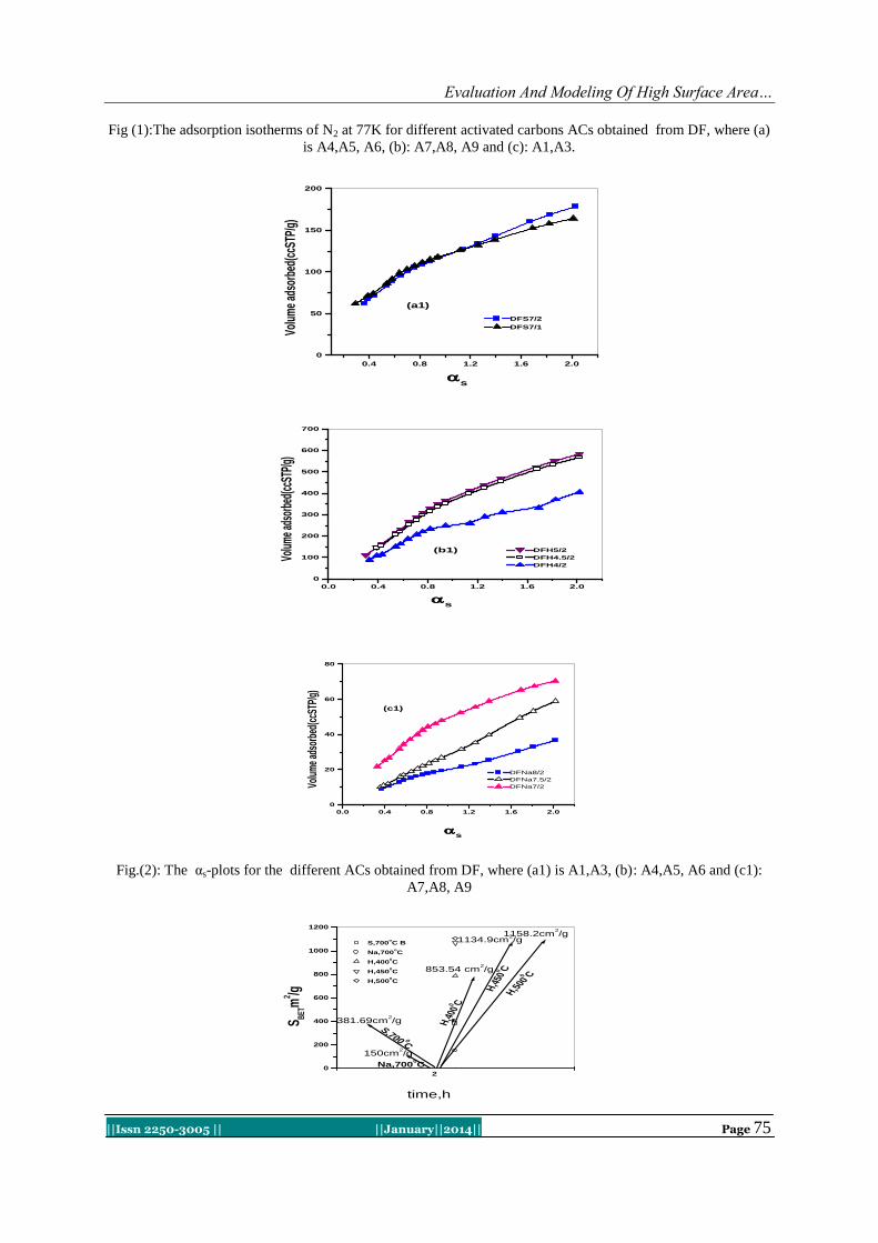
Evaluation And Modeling Of High Surface Area…
||Issn 2250-3005 || ||January||2014|| Page 75
Fig (1):The adsorption isotherms of N2 at 77K for different activated carbons ACs obtained from DF, where (a)
is A4,A5, A6, (b): A7,A8, A9 and (c): A1,A3.
0.4 0.8 1.2 1.6 2.0
0
50
100
150
200
(a1)
s
DFS7/2
DFS7/1Volu
me
adso
rbed
(ccS
TP/g
)
0.0 0.4 0.8 1.2 1.6 2.0
0
100
200
300
400
500
600
700
(b1)
s
DFH5/2
DFH4.5/2
DFH4/2
Volu
me a
dsor
bed(
ccST
P/g)
0.0 0.4 0.8 1.2 1.6 2.0
0
20
40
60
80
(c1)
s
DFNa8/2
DFNa7.5/2
DFNa7/2Volu
me
adso
rbed
(ccS
TP/g
)
Fig.(2): The αs-plots for the different ACs obtained from DF, where (a1) is A1,A3, (b): A4,A5, A6 and (c1):
A7,A8, A9
20
200
400
600
800
1000
1200
381.69cm2/g
S,700 0C
150cm2/g
Na,7000C
1134.9cm2/g
853.54 cm2/g
H,5000 C
H,45
00 C
H,40
00 C
1158.2cm2/g
S BET
m2 /g
time,h
S,700oC B
Na,700oC
H,4000C
H,4500C
H,5000C

Evaluation And Modeling Of High Surface Area…
||Issn 2250-3005 || ||January||2014|| Page 76
Fig.(3):Vector represention for the effect of chemical activation by H3 PO4 and
NaOH and physical activation by single step steam pyrolysis on SBET of DF.
2
0 200 400 600 800 1000
2h
381.69cm2/g
S,7000
C
150cm2/g
Na,7000C
1134.9cm2/g
853.54 cm2/g
H,5
000 C
H,4
500 C
H,4
000 C
1158.2cm2/g
SB
ET,m
2 /g
Fig.(4):Optimization of SBET of DF for the effect of chemical activation by H3 PO4, NaOH and physical
activation by single step steam pyrolysis for 2 h.
2h
450 C
1160 cm2 /g
700C
320 cm2 /g
700 C,hysical
150 cm2/g
chemical,H3PO4
chemical,NaOH
Fig.(5):Modeling of paths between chemical activation by H3 PO4 ,
NaOH and physical activation to obtain SBET
.
A1
A2
A3
A4 A
5
A6
A7 A
8
A9
1 2 3 4 5 6 7 8 90
20
40
60
80
100
Fig.6.Effect of activated carbons obtained by chemical and physical
activation on sorption of phenol(pH) and methylene blue(MB)
R%
sample
ph
MB

Evaluation And Modeling Of High Surface Area…
||Issn 2250-3005 || ||January||2014|| Page 77
Table 1.Surface characteristics of activated carbons obtained by chemical and physical activation
Groups Type of
ACs(DF)
Temp oC
SBET m²/g
Sαt
m2/g Sα
n m2/g
VP ml/g
Vmeso ml/g
V ou mL/g
V ot ml/g
Vos ml/g
A1 700 392.54 299.83 124.0 0.254 0.134 0.046 0.120 0.134
A2 700 385.11 302.55 134.88 0.266 0.158 0.042 0.102 0.094
A3 700 381.69 304.14 166.1 0.276 0.182 0.038 0.094 0.056
A4 400 788.07 853.54 407.2 0.629 0.465 0.008 0.164 0.164
A5 400 1066.02 1134.9 542.9 0.875 0.588 0.002 0.287 0.287
A6 500 1104.65 1158.2 547.6 0.903 0.599 0.001 0.304 0.304
A7 700 150.53 135.83 57.57 0.109 0.062 0.009 0.047 0.038
A8 750 78.21 95.78 82.70 0.091 0.091 0.006 0.066 0.037
A9 800 60.66 55.77 46.15 0.057 0.052 0.003 0.005 0.002
Table 2.Characteristics of activated carbons obtained by chemical and physical activation
Application
The activated samples was applied for adsorption of phenol and MB and it is found that uptake of MB
was in range (94-99%), while the uptake of phenol was in range (10-85%).
Modeling.
The surface area of DF-carbons were obtained by different methods of activation, i.e. chemical
activation (by H3PO4 or NaOH) or physical activation (i.e. single step steam pyrolysis) as in Figs. (3,4 & 5).
IV. CONCLUSIONS
The results of this study showed that DF can be successfully converted into activated carbon with
specific surface properties. It was found that the amount of H3PO4 used for chemical activation controls, the
characteristics of the carbons including surface area, micro and mesoporosity, and pore size distributions.
Detailed surface analyses using different mathematical models suggested that: (1) H3PO4 at 450 oC required
to obtain micropore and mesopore carbons, (2) a theoretical approach can provide complete information
about the surface structure of the produced activated carbons; (3) highly activated carbons with an extended
pore size distribution, the as-method estimates total micropore volume (volumes used for both primary and
secondary filling processes).
Type of
ACs(DF)
Temp oC
Ti
me,
h
pH Yield
%
%R
phenol
%R
MB
r (Ǻ) burn-
off
%
A1 700 1 7.5 19.67 85.25 99.63 12.94 80.33
A2 700 1.5 7.45 19.45 80.11 99.51 13.47 81.52
A3 700 2 7.4 18.33 77.87 99.49 14.46 81.67
A4 400 2 6.6 41.10 50.98 99.53 15.96 58.93
A5 400 2 6.5 40.40 55.02 99.60 16.42 59.60
A6 500 2 6.7 31.33 77.48 99.71 16.35 68.67
A7 700 2 7.5 9.77 10.23 94.81 14.5 90.23
A8 750 2 7.5 5.96 13.41 95.68 23.27 94.03
A9 800 2 7.5 5.46 26.81 96.33 18.79 94.53

Evaluation And Modeling Of High Surface Area…
||Issn 2250-3005 || ||January||2014|| Page 78
REFERENCES [1] Jagtoyen M, Thwaites M, Stencel J, McEnaney B, Derbyshire F. Adsorbent carbon synthesis from coals by phosphoric
acid activation. Carbon 1992; 30(7):1089–96.
[2] Teng H, Yeh TS, Hsu LY. Preparation of activated carbon from bituminous coal with phosphoric acid activation. Carbon 1998; 36(9):1387–95.
[3] Huidobro A, Pastor AC, Rodr~ıguez-Reinoso F. Preparation of activated carbon cloth from viscous rayon. Part IV.
Chemical activation. Carbon 2001;39(3):389–98.
[4] Laine J, Calafat A, Labady M. Preparation and characterization of activated carbons from coconut shell impregnated with
phosphoric acid. Carbon 1989; 27(2):191–5.
[5] Jagtoyen M, Derbyshire F. Some considerations of the origins of porosity in carbons from chemically activated wood. Carbon 1993; 31(7):1185–92.
[6] Molina-Sabio M, Rodr~ıguez-Reinoso F, Caturla F, Sell~es MJ. Porosity in granular carbons activated with phosphoric
acid. Carbon 1995; 33(8):1105–13.
[7] Jagtoyen M, Derbyshire F. Activated carbons from yellow poplar and white oak by H 3P O 4 activation. Carbon 1998;
36(7):1085–97.
[8] Benaddi H, Bandosz TJ, Jagiello J, Schwarz JA, Rouzaud JN,Legras D, et al. Surface functionality and porosity of activated carbons obtained from chemical activation of wood. Carbon 2000;38(5):669–74.
[9] Dastgheib SA, Rockstraw DA. Pecan shell activated carbon: synthesis, characteriza tion and application for the removal of
copper from aqueous solution. Carbon 2001; 39(12):1849–55.
[10] Girgis BS, El-Hendawy Abdel-Nasser A. Porosity development in activated carbons obtained from date pits under
chemical activation with phosphoric acid. Microporous Mesoporous Mater 2002; 52(2):105–17.
[11] Suarez-Garcıa F, Martınez-Alonso A, Tascon JMD. Pyrolysis of apple pulp: chemical activation with phosphoric acid. J Anal Appl Pyrol 2002;63(2):283–301.
[12] Fu R, Liu L, Huang W, Sun P. Studies on the structure of activated carbon fibers activated by phos phoric acid. J Appl
Polym Sci 2003; 87:2253–61.
[13] Puziy AM, Poddubnaya OI, Mart~ınez-Alonso A, Suarez-Garcıa F, Tasc~on JMD. Synthetic carbons activated with
phosphoric acid II. Porous structure. Carbon 2002;40(9):1507–19.
[14] Puziy AM, Poddubnaya OI, Mart~ınez-Alonso A, Su~arez-Garc~ıa F, Tasc~on JMD. Synthetic carbons activated with phosphoric acid I. Surface chemistry and ion binding properties. Carbon 2002; 40(9):1493–505
15] Bansal RC, Donnet JB, Stoeckli F. In: Active carbon, New York: Marcel Dekker; 1988, pp. 8–13.
[16] Baker FS. In: Carbon: activated carbon, Kirk–Othmer en-cyclopedia of chemical technology, vol. 4, Wiley; 1992, pp. 1015–37.
[17] Laine J, Calafat A, Labady M. Preparation and characterization of activated carbons from coconut shell impregnated with
phosphoric acid. Carbon 1989; 27(2):191–5.
[18 ]Jagtoyen M, Thwaites M, Stencel J, McEnaney B, Derby-shire F. Adsorbent carbon synthesis from coals by phosphoric acid activation. Carbon 1992;30(7):1089–96.
[19] Molina-Sabio M, Rodrıguez-Reinoso ´ F, Caturla F, Selles ´ MJ. Porosity in granular carbons activated with phosphoric acid.
Carbon 1995;33(8):1105–13.
[20] Molina-Sabio M, Caturla F, Rodrıguez-Reinoso ´ F. Influence of the atmosphere used in the carbonization of phosphoric acid
impregnated peach stones. Carbon 1995; 33(8):1180–2.
[21] Kyuya Nakagawa, Shin R. Mukai, Tetsuo Suzuki, Hajime Tamon, Carbon 41 (2003) [23–831
[22] Gonzalez ´ MT, Molina-Sabio M, Rodrıguez-Reinoso ´ F. Steam activation of olive stone chars, development of porosity. Carbon
1994; 32:1407–13.
[23] Rodrıguez-Reinoso ´ F, Molina-Sabio M, Gonzalez ´ MT. The use of steam and CO2 as activating agents in the preparation of activated carbons. Carbon 1995; 33:15–23

International Journal of Computational Engineering Research||Vol, 04||Issue, 1||
||Issn 2250-3005 || ||January||2014|| Page 1
A Survey of Protection Against DoS & DDoS Attacks
1,Mrs.S.Thilagavathi ,
2,Dr.A.Saradha
1,Head, Department of Computer Science, Terf’s Academy College of Arts&Science
Tirupur, Tamilnadu, India 2,Head, Department of Computer Science & Engineering, Institute of Road and Transport Technology
Erode, Tamilnadu, India
I. INTRODUCTION A denial of service (DoS) attack aims to deny access by legitimate users to shared services or
resources. This can occur in a wide variety of contexts, from operating systems to network-based services on the
Internet. A DoS attack aims to disrupt the service provided by a network or server. On February 9, 2000, Yahoo,
eBay, Amazon.com, E*Trade, ZDnet, Buy.com, the FBI, and several other Web sites fell victim to DDoS
attacks resulting in substantial damage and inconvenience. More importantly, traditional operations in essential
services, such as banking, transportation, power, health, and defense, are being progressively replaced by
cheaper, more efficient Internet-based applications. Internet-based attacks can be launched anywhere in the
world, and unfortunately any Internet-based service is a potential target for these attacks.This paper presents an
overview of the DoS problem in section 2 and it includes classification of DoS attacks and how they are accomplished. In section 3 existing solutions and section 4 follows the problem and proposed solutions. This
paper is concluded in section 5.
II. OVERVIEW OF DDOS ATTACKS One common method of attack involves saturating the target machine with external communications
requests, such that it responds so slowly as to be rendered effectively unavailable. Such attacks usually lead to a
server overload. In general terms, DoS attacks are implemented by either forcing the targeted computer(s) to
reset, or consuming its resources so that it can no longer provide its intended service or obstructing the
communication media between the intended users and the victim. A DDoS attack uses many computers to launch a DoS attack against one or more targets. A typical DDoS attack consists of four elements[6].
[1] The real Attacker;
[2] The handler who are capable of controlling multiple agents.
[3] The Zombie hosts who are responsible for generating a stream of packets toward the victim.
[4] The victim or the target host.
The virus-infected computers are called zombies – because they do whatever the DDoSer commands them to do. A large group of zombie computers is called a robot network, or botnet. The computer could be part
of a botnet without the knowledge of user. That’s because it may be busy participating in a DDoS attack at the
same time the user are using it. Or, the user might find out that the computer is infected when the Internet
service provider (ISP) drops the user service because of computer is sending an unusually high number of
network requests[19].
ABSTRACT Denial-of-Services (DoS) attacks cause serious threats to the today internet world. The problem of DoS
attacks has become well known, but it has been hard to find out the Denial of Service in the Internet. So
the users have to take own effort of a large number of protected system such as Firewall or up-to-date
antivirus software. If the system or links are affected from an attack then the legitimate clients may not be able to connect it. There have been a number of solutions and tools to detect the DoS attacks.
However there are no end solutions which can protect against the DoS attacks. This paper focuses on
techniques used in different DoS attacks and describes the characteristics of tools used in DoS attack
network and also presents the proposed solutions.
INDEX TERMS : Denial-Of-Service, Distributed Dos, DDoS Attack Tools, Traceback Mechanisms,
Intrusion Detection and Prevention Method, IP Address Spoofing, IP Address Monitoring, Blocked IP
Address, Client-Side Script.

A Survey Of Protection Against Dos…
||Issn 2250-3005 || ||January||2014|| Page 2
Figure 1: Architecture of DoS attack
Zombie computers in a botnet receive instructions from a command and control server, which is an infected web
server. DDoSers who have access to a command and control server can recruit the botnet to launch DDoS
attacks
2.1. Denial of Service type
There are many types of DDoS attacks. They target different network components – routers,
appliances, firewalls, applications, ISPs, even data centers – in different ways. DDoS attackers use a variety of
DDoS attack methods. The malicious hacker group Anonymous, for example, started with a tool that could
launch Layer 7 DDoS attacks and Layer 3 DDoS attacks from any computer. These attacks had a common
attack signature – that is, common code. As a result, the attacks could be detected and mitigated fairly
easily[19].Denial of service can be divided into three forms.
[1] DoS
In a DoS attack, one computer and one internet connection is used to flood a server with packets, with
the aim of overloading the targeted server’s bandwidth and resources[3]. Denial-of-service (DoS) attacks
exceeding 20G bps, which will overwhelm almost any online service's bandwidth, more than quadrupled so far
in 2013, compared with the previous year, according to the network management firm. While the attacks
account for only approximately 1 percent of all data floods, the increase in large-bandwidth DoS attacks
suggests that more serious groups are now using denial of service as a common tactic.[20]
DDoS attack
A distributed denial of service attack (DDoS) occurs when multiple systems flood the bandwidth or resources of a targeted system, usually one or more web servers. This is the result of multiple compromised
systems (for example a botnet) flooding the targeted system with traffic. When a server is overloaded with
connections, new connections can no longer be accepted[4].
[2] DRDoS
This type of attack is more detrimental than a typical DDoS attack. This is because a DRDoS attack has
more machines to share the attack, and hence the attack is more distributed. This is also creates a greater volume
of traffic because of its more distributed nature[3].

A Survey Of Protection Against Dos…
||Issn 2250-3005 || ||January||2014|| Page 3
III. EXISTING SOLUTIONS 3.1 Classification of DDoS Attack
DDoS attacks can be divided into two categories: Bandwidth attack and Resource attack.
In a bandwidth attack, simply try to generate packets to flood the victim’s network so that the legitimate
requests cannot go to the victim machine.
A resource attack aims to send packets that misuse network protocol or malformed packets to tie up
network resources so that resources are not available to the legitimate users any more.
Figure 2.Classification of DDoS Attack
3.1.1 Bandwidth Attacks
Flood attack: This attack occur when a network or service becomes so weighed down with packets
initiating incomplete connection requests that it can no longer process genuine connection requests.Once this buffer is full no further connections can be made, and the result is a Denial of Service.
TCP Flood : A stream of TCP Packets with various Flags set are sent to the victim IP Address. The
SYN,ACK and RST flags are commonly used.
ICMP Flood: A stream of ICMP packets are sent to a victim IP address.
UDP Flood: A stream of UDP packets are sent to the victim IP address.
Teardrop : This attack creates a stream of IP fragments with their offset field overload. The destination
host that tries to reassemble these malformed fragments eventually crashes or reboots.
Smurf attack: The victim is flooded with Internet Control Message Protocol. The attackers sends
numerous ICMP “echo-request” packets to the broadcast address of many subnets. These packets contain
the victim’s address as the source IP address [4][6][10].
3.1.2 Reflected attack
A distributed reflected denial of service attack (DRDoS) involves sending forged requests of some type
to a very large number of computers that will reply to the requests. Using Internet Protocol address spoofing, the
source address is set to that of the targeted victim, which means all the replies will go to the target.ICMP Echo Request attacks (Smurf Attack) can be considered one form of reflected attack, as the flooding host(s) sends
Echo Requests to the broadcast addresses of miss-configured networks, thereby enticing many hosts to send
Echo Reply packets to the victim. Some early DDoS programs implemented a distributed form of this
attack[16].

A Survey Of Protection Against Dos…
||Issn 2250-3005 || ||January||2014|| Page 4
TCP SYN Attack : This attack occurs during the three-way handshake that marks the onset of a TCP
connection. If an attack occurs, the attacker sends an abundance of TCP SYN packets to the victim.
Malformed Packet Attack : A ping of death is a type of attack on a computer that involves sending a malformed or otherwise malicious ping to a computer.
3.2 DDoS Attack Tools
There are many security problems in today’s Internet. But none of these problems have been completely
solved; some of the tools and technical solutions have been helped to reduce the danger from the intrusions [9].
There are several DDoS attack tools are available. But some of the well known DDoS tools are given below :
[1] Trinoo
[2] Tribe Flood Network(TFN),
[3] Tribe Flood Network 2000 (TFN2K),
[4] Stacheldraht,
[5] Mstream and [6] Shaft
[7] Trinity
[8] Knight
[9] Kaiten
Trinoo is one of DDoS attack tool and is able to launch packet flooding attacks. It has the ability to
control the duration of the attack as well as the size of the flooding packets .Trinoo is the first DDoS attack tool.
This is the first DDoS attack tool. It has been able to achieve bandwidth depletion and can be used to launch
UDP flood attacks against one or many addresses. The trinoo was the first attempt at client-server
programming by its author and was designed and implemented in a period of monthsTribe Flood Network (TFN)
is able to perform bandwidth depletion and resource depletion attacks. It is able to implement Smurf, UDP fl ood, TCP SYN flood, ICMP echo request flood, and ICMP directed broadcast. TFN2K is a derivative of TFN
and is able to implement Smurf, SYN, UDP, and ICMP flood attacksTribe Flood Network 2000 (TFN2K) has
the special feature of being able to add encrypted messages between all attack components. Stacheldraht is based
on early versions of TFN attempts to eliminate some of its weak points and implement Smurf, SYN flood, UDP
flood, and ICMP flood attacks. Mstream is a simple point-to-point TCP ACK flooding tool that is able to
overwhelm the tables used by fast routing routines in some switches.Shaft is a DDoS tool similar to Trinoo and
is able to launch packet flooding attacks. It has the ability to control the duration of the attack as well as the size
of the flooding packets [2][6]Trinit is the first DDoS tool that is controlled via IRC. Trinity is capable of
launching several types of flooding attacks on a victim site, including UDP, IP fragment, TCP SYN, TCP RST,
TCP ACK, and other floods[7].Knight is IRC based DDoS attack tool. It provides SYN attacks, UDP flood
attacks, and an urgent pointer. This is designed to run Windows Operating systems.Kaiten is another IRC based
DDoS attack tool. It includes code for UDP and TCP flooding attacks, for SYN attacks, It also randomizes the 32 bits of its source address[8].
3.3 Trceback Solutions
Dos attacks are easy to generate but very hard to detect. In denial of service attacks, the packets are
routed correctly but the destination becomes the target of the attackers. Once the target system is attacked, the
detection mechanisms are necessary to detect an attack with less false positive rate and more accuracy rate
ICMP Traceback method involves every router on the network pick a packet probabilistically and generate an
ICMP traceback message directed to the same destination as the selected packet.. The IP Trace is used to
identify the actual path of the attack[9] Algebric approach to IP Traceback scheme is based on algebraic
techniques.It generate traceback data using polynomial function and storing data in unused bits of IP header.
Fast Internet Traceback a new packet marking approach. FIT is scalable to vast scattered attacks with thousands of attackers. It uses path reconstruction algorithm with node marking instead of link marking at the end user
side. Performance and deployment ability of FIT is better than other packet marking schemes. It will take
minimal processing time of router to track very small number of attack packet. But it goes through the false
positive and negative rate[11].Advance and Authenticated Marking approach is more efficient and accurate for
the attacker path reconstruction within the seconds and has low false positive rate. Traces the origin of spoofed
IP packets[12].Hash Based IP Traceback has been proposed by Snoeren et al. In this method a Source Path
Isolation Engine (SPIE) is used which produces review track of traffic and it can trace origin of single IP packet.
The data (8 bytes) and the IP header (20 byte) both are logged on intermediate routers. This operation uses 28
byte data in hashing. The main advantages of this method are low storage of data and it ignores eavesdropping
but it create overhead to generate 28 byte hash[13]
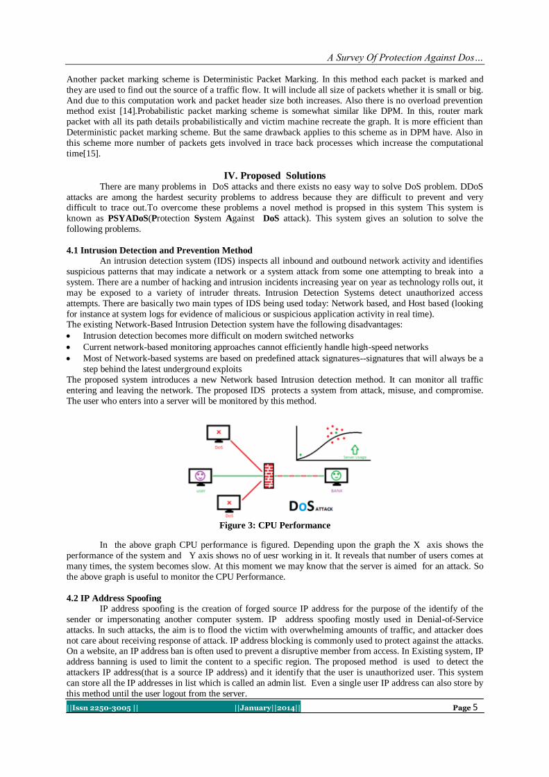
A Survey Of Protection Against Dos…
||Issn 2250-3005 || ||January||2014|| Page 5
Another packet marking scheme is Deterministic Packet Marking. In this method each packet is marked and
they are used to find out the source of a traffic flow. It will include all size of packets whether it is small or big.
And due to this computation work and packet header size both increases. Also there is no overload prevention method exist [14].Probabilistic packet marking scheme is somewhat similar like DPM. In this, router mark
packet with all its path details probabilistically and victim machine recreate the graph. It is more efficient than
Deterministic packet marking scheme. But the same drawback applies to this scheme as in DPM have. Also in
this scheme more number of packets gets involved in trace back processes which increase the computational
time[15].
IV. Proposed Solutions There are many problems in DoS attacks and there exists no easy way to solve DoS problem. DDoS
attacks are among the hardest security problems to address because they are difficult to prevent and very difficult to trace out.To overcome these problems a novel method is propsed in this system This system is
known as PSYADoS(Protection System Against DoS attack). This system gives an solution to solve the
following problems.
4.1 Intrusion Detection and Prevention Method
An intrusion detection system (IDS) inspects all inbound and outbound network activity and identifies
suspicious patterns that may indicate a network or a system attack from some one attempting to break into a
system. There are a number of hacking and intrusion incidents increasing year on year as technology rolls out, it
may be exposed to a variety of intruder threats. Intrusion Detection Systems detect unauthorized access
attempts. There are basically two main types of IDS being used today: Network based, and Host based (looking
for instance at system logs for evidence of malicious or suspicious application activity in real time). The existing Network-Based Intrusion Detection system have the following disadvantages:
Intrusion detection becomes more difficult on modern switched networks
Current network-based monitoring approaches cannot efficiently handle high-speed networks
Most of Network-based systems are based on predefined attack signatures--signatures that will always be a
step behind the latest underground exploits
The proposed system introduces a new Network based Intrusion detection method. It can monitor all traffic
entering and leaving the network. The proposed IDS protects a system from attack, misuse, and compromise.
The user who enters into a server will be monitored by this method.
Figure 3: CPU Performance
In the above graph CPU performance is figured. Depending upon the graph the X axis shows the
performance of the system and Y axis shows no of uesr working in it. It reveals that number of users comes at
many times, the system becomes slow. At this moment we may know that the server is aimed for an attack. So
the above graph is useful to monitor the CPU Performance.
4.2 IP Address Spoofing IP address spoofing is the creation of forged source IP address for the purpose of the identify of the
sender or impersonating another computer system. IP address spoofing mostly used in Denial-of-Service
attacks. In such attacks, the aim is to flood the victim with overwhelming amounts of traffic, and attacker does
not care about receiving response of attack. IP address blocking is commonly used to protect against the attacks. On a website, an IP address ban is often used to prevent a disruptive member from access. In Existing system, IP
address banning is used to limit the content to a specific region. The proposed method is used to detect the
attackers IP address(that is a source IP address) and it identify that the user is unauthorized user. This system
can store all the IP addresses in list which is called an admin list. Even a single user IP address can also store by
this method until the user logout from the server.

A Survey Of Protection Against Dos…
||Issn 2250-3005 || ||January||2014|| Page 6
4.3 IP Address Monitoring The PYSADOS tool is used to monitor the IP address also. The user press F5(refresh) more than once,
automatically this tool will be capture and store the user IP address into the database with the user’s details and the time of their login. The Algorithm in the below is used to capture and store the unauthorized IP address into
the database.
4.3.1 Algorithm for Monitoring Unknown IP address
vip=getip("address");
If (Ip!=ValidIp(vip)&& Ip<=proxy("vip"))Then
{
time=30;
gtime=refr("time");
If(rEcap("StrVal")==getstr("vstr")&& gtime>=1) Then {
ready->work;
get(login)=siteurl->vip;
}
else
{
banfile=fopen("$file_location_banlist","w")
setbanlist=add(vip);
print(banfile,"Str",gettime());
}
}
Figure 4:Screenshot of a IP Address Monitoring
4.4 Blocked IP address
Many users operate from shared IP addresses, often those belonging to proxies used by large networks
or home users with their Internet service providers. Since it is impossible to distinguish between individual users
operating from shared IP addresses, blocking one may affect a very large number of legitimate users (ranging up
to millions). Users operating from dynamic IP addresses change IP addresses periodically. This can compound
the auto block problem, particularly when they are also shared, because a block targeted at a malicious user may
shift to a legitimate user while the target shifts to an unblocked IP address. This proposed system is used to store
the blocked spam IP address. This address will be added to the Admin List.

A Survey Of Protection Against Dos…
||Issn 2250-3005 || ||January||2014|| Page 7
Figure 5 ; Screenshot of Blocked IP Address
4.4.1 Algorithm for storing Spam IP Address
Vip=getip("address");
function validip()
{
$pattern = "/^([1]?\d{1,2}|2[0-4]{1}\d{1}|25[0-5]{1})(\.([1]?\d{1,2}|2[0-4]{1}\d{1}|25[0-5]{1})){3}$/";
return (preg_match($pattern, $ip) > 0) ? true : false; }
if(rEcap()->fail)
{
//move ip to banlist
block("vip")
}
else //if it Ok
{
banfile=fopen("$file_location_banlist","w")
setbanlist=add(vip);
while(Ip==EoF)
{ record=FETCH("Banlistfile");
if(record==vip)
{
DELETE("Record");
}
else
{
Print("Spam IP");
}
}
}
Symbols used in description
Vip= user ip
rEcap=recatch Google Api
Proxy=Proxy ip Checker Function
vstr=users Replay String
gtime=gettime refresh "seconds">(aprox_value="30sec")

A Survey Of Protection Against Dos…
||Issn 2250-3005 || ||January||2014|| Page 8
4.5.Client-Side Script
Security on the web is based on a variety of mechanisms, including an underlying concept of trust
known as the same origin policy. This essentially states that if content from one site is granted permission to access resources on the system, then any content from that site will share these permissions, while content from
another site will have to be granted permissions separately. Cross side scripting vulnerabilities have been
reported and exploited since the 1990s. Prominent sites affected in the past include the social-networking sites
Twitter, Facebook, MySpace, YouTube and Orkut. In recent years, cross-site scripting flaws surpassed buffer
overflows to become the most common publicly reported security vulnerability, with some researchers in
viewing as many as 68% of websites as likely open to Cross side scripting attacks. Cross-site scripting uses the
known vulnerabilities in web-based applications, their servers, or plug-in systems. On which they rely.
Exploiting the fold malicious content into the content being delivered from the compromised site. By finding
ways of injecting malicious scripts into web pages, an attacker can gain elevated access-privileges to sensitive
page content, session cookies, and a variety of other information maintained by the browser on behalf of the
user. The expression "cross-site scripting" originally referred to the act of loading the attacked, third-party web application from an unrelated attack site, in a manner that executes a fragment of JavaScript prepared by the
attacker in the security context of the targeted domain. These are held in the existing client-side-script.
The proposed system aims to overcome the existing client side scripting. This system can check not
only the client side malicious content but also check the server side script of Code Execution, Command
Execution, Header Injection, File Disclosure, File inclusion, File Manipulation, LDAP Injection, SQL Injection.
It can display how long it has been scanned and how many numbers of files have been scanned. It can produce
the graph to identify where the errors are and how to replace the errors. It can also identify how much it has
been injured and can edit easily wherever the errors occurred. We can check to find out the errors by using two
methods of Top-Down and Bottom-Up approach.
Figure 8: Types of Files to be scanned in this System
The above figure is shows how to check the vulnerable type injections both in the Client side and Server Side
Figure 9: Result of Script Scanning

A Survey Of Protection Against Dos…
||Issn 2250-3005 || ||January||2014|| Page 9
4.6 Mathematical Model
This system is used to stop a DoS attack by identifying the Spam IP and discard them before reaching
the victim. The web surfer might surf the source code programs also. This system could check the client side and the server side scripting to avoid the harmful attackers. So this system is also examine the malicious
content into the content being delivered from the compromised site by applying the following equations
Where c can scan the script to find out the errors in the α coding.
C can check the malicious content of the Coding, t is to calculate the timings of C and n is the total timing
calculated by the c&C and also t.
α finding out the errors in the script
β finding out the vulnerable coding and
Ƴ rectifying the infected coding.
= safe
If α, β, Ƴ are correct then the script will be in safe.
4.7 Graphical Model
The graphical model shows the scanning of script wherever it has the errors in it and also it shows the
modification of error code. In its scanning if the white color displays there is no error and if the orange color
indicates there is changes made in it. If the red color is indicated the code must be completely modified.The
developers must be careful to be safe in the codings. This type of code is called the vulnerable code. The graph
model is useful to keep the script in safe.
Figure 10 : Graph Model
III. CONCLUSIONS DoS and DDoS attacks are advanced and powerful methods of attacking a network system to make it either unusable to the legitimate users or downgrade its performance. This survey indicates that an overall DoS
detection mechanism by combing different detectors in order to provide robust and effective detection. Since
Dos attacks are complex and difficult to combat till now. There is no single point solution, everyone is
vulnerable. This survey examines the possible solutions to this problem.

A Survey Of Protection Against Dos…
||Issn 2250-3005 || ||January||2014|| Page 10
We cannot separate good traffic system from the more attacks. This Proposed system is used to show the
Flood IP address and also it proves that the users are authentication user by using recapturing techniques. It can
defend against blocking,based on the analysis of existing solutions, the proposed desirable solutions are to defend DDoS.
REFERENCES : [1] David karig and Ruby Le, “Remote Denial of Service Attacks and Countermeasures,” Princeton University Department of
Electrical Engineering Technical Report CE-L2001-02
[2] Helna Sandstrom, ”A Survey of the Denial of Service Problem,” Lulea University of Technology,Sweden.
[3] Charalampos Patrikakis, Michalis Masikos and Olga Zouraraki, “The Internet Protocol- Vol 7, Number 4”.
[4] Jelena Mirkovic,Sven Dietrich,David Dittrich,Peter Reiher, “Internet Denial of Service:Attack and Defencse Mechanisms”.
[5] Georgios Loukas and Gulay Oke, “Protection against Denial of Service attacks: A Survey,” Intelligent Systems and Networks
Group, Imperial College, London.
[6] Shibia Lin Chiueh, , “ASurvey on solutions to Distribuited Denial of Service Attacks,” Stony Brook University, Stony Brook.
[7] http://users.atw.hu/denialofservice/ch04lev1sec4.html.
[8] http://www.scribd.com/doc//DDoS-Tool-Knight-and-Kaiten
[9] A.John,T.Sivakumar,Ramanujam, “DDoS Survey of Traceback Methods,” International Journal of Recent Trends in
Engineering, Vol.1,No.2,May 2009
[10] Arun Raj Kumar,P and S.Selvakumar, “Distributed-Denial-of-Service(DDoS) Threat in Collaborativem Environment-A Survey
on DDoS AttackTools and Traceback Mechanisms,” IEEE International Advance Computing Conference(IACC 2009).
[11] Abraham Yaar,Adrian Perring, Dawn Song, “Fast Internet Traceback,”Carnegie Mellon University.
[12] Dawn Xiaodong Song & Adrian Perrg, ”Advanced And Authenticated Marking Schemes For IP Traceback,” IEEE INFOCOM
2001.
[13] A.Snoeren,C.Partidge,L.Sanchez,C.Jones,F.Tchakountio,B.Schwartz,S.Kent and W.Strayer, “Single-Packet IP TracEkback,”
IEEE/ACM Trans. Networking, Vol 10, no.6,PP.721-734,2002.
[14] Andrey Belenky, Nirwan Ansar, “On deterministic packet marking,” Computer Networks, Volume 51, Issue 10, 11 July 2007,
Pages 2677–2700.
[15] Pegah Sattari, Minas Gjoka, Athina Markopoulou, “A Network Coding Approach to IP Traceback,” University of California,
Irvine
[16] Randal Vaughn and Gadi Evron, “Dns amplification attacks preliminary release,” March 17,2006.
[17] http://www.ddosmitigation.biz/
[18] http://www.watchguard.com/infocenter/editorial/41649.asp
[19] http://www.prolexic.com/knowledge-center-what-is-ddos-denial-of-service.html
[20] Aleksei Zaitsenkov, Dos Attack

International Journal of Computational Engineering Research||Vol, 04||Issue, 1||
||Issn 2250-3005 || ||January||2014|| Page 11
The Effect of Chemical Reaction on Mhd Free Convection Flow
Of Dissipative Fluid Past An Exponentially Accelerated Vertical
Plate
P.M. Kishore1, S. Vijayakumar Varma
2 S. Masthan Rao
3 and K.S. Bala
Murugan3
1 Department of Mathematics, Narayana Engineering College, Nellore - 524001 (A.P), India. 2 Department of Mathematics, S.V. University, Tirupathi-517502 (A.P), India.
3 Deparment of Mahematics, R.V.R & J.C. College of Engineering, Guntur, (A.P), India.
I. INTRODUCTION
Free convection flow involving coupled heat and mass transfer occurs frequently in nature and in
industrial processes. A few representative fields of interest in which combined heat and mass transfer plays an
important role are designing chemical processing equipment, formation and dispersion of fog, distribution of
temperature and moisture over agricultural fields and groves of fruit trees, crop damage due to freezing, and
environmental pollution. Hydromagnetic flows and heat transfer have become more important in recent years
because of its varied applications in agricultural engineering and petroleum industries. Recently, considerable
attention has also been focused on new applications of magneto-hydrodynamics (MHD) and heat transfer such
as metallurgical processing. Melt refining involves magnetic field applications to control excessive heat transfer
rate. Other applications of MHD heat transfer include MHD generators, plasma propulsion in astronautics,
nuclear reactor thermal dynamics and ionized-geothermal energy systems.
Pop and Soundalgekar [1] have investigated the free convection flow past an accelerated infinite plate. Singh and Soundalgekar [2] have investigated the problem of transient free convection in cold water past an
infinite vertical porous plate. An excellent summary of applications can be found in Hughes and Young
[3](1966). Takar et al. [4] analyzed the radiation effects on MHD free convection flow past a semi-infinite
vertical plate using Runge-Kutta-Merson quadrature. Recently the natural convection flow of a conducting
visco-elastic liquid between two heated vertical plates under the influence of transverse magnetic field has been
studied by Sreehari Reddy et al. [5].The studies of convective heat transfer in porous media have been more
concerned in the past, with steady state conditions (Nield, D.A. and Bejan, A., [6]. Meanwhile, recent
engineering developments have led also to an increasing interest in accurate investigations of the transient
processes in these media. A detailed review of the subject including exhaustive list of references can be found in
the papers by Bradean et.al. [7]. Mass diffusion effect on transient convection flow past a surface was eludicated
by Cheng et.al. [8]. Chaundhary et.al. [9] analyzed free convection effects on flow past a moving vertical plate embedded in porous medium by Laplace – transform technique.In all these investigations, the viscous
dissipation is neglected. The viscous dissipation heat in the natural convective flow is important, when the flow
field is of extreme size or at low temperature or in high gravitational field. Such effects are also important in
geophysical flows and also in certain industrial operations and are usually characterized by the Eckert number.
ABSTRACT: Aim of the paper is to investigate the the chemical reaction effect on the unsteady mhd free convection
flow, heat and mass transfer characteristics in a viscous, incompressible and electrically conducting
fluid past an exponentially accelerated vertical plate by taking into account the heat due to viscous
dissipation. The problem is governed by coupled non-linear partial differential equations. The dimensionless equations of the problem have been solved numerically by the unconditionally stable finite
difference method of Dufort – Frankel’s type. The effects of governing parameters on the flow variables
are discussed quantitatively with the aid of graphs for the flow field, temperature field, concentration
field, skin-friction, Nusselt number and Sherwood number.
KEY WORDS: MHD, free convection, viscous dissipation, finite difference method, exponentially
accelerated plate, chemical reaction.
.
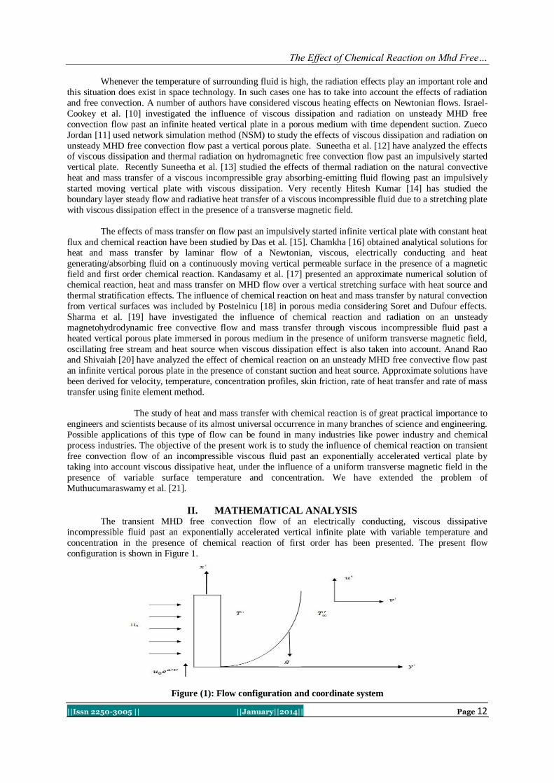
The Effect of Chemical Reaction on Mhd Free…
||Issn 2250-3005 || ||January||2014|| Page 12
Whenever the temperature of surrounding fluid is high, the radiation effects play an important role and
this situation does exist in space technology. In such cases one has to take into account the effects of radiation
and free convection. A number of authors have considered viscous heating effects on Newtonian flows. Israel-
Cookey et al. [10] investigated the influence of viscous dissipation and radiation on unsteady MHD free
convection flow past an infinite heated vertical plate in a porous medium with time dependent suction. Zueco
Jordan [11] used network simulation method (NSM) to study the effects of viscous dissipation and radiation on
unsteady MHD free convection flow past a vertical porous plate. Suneetha et al. [12] have analyzed the effects of viscous dissipation and thermal radiation on hydromagnetic free convection flow past an impulsively started
vertical plate. Recently Suneetha et al. [13] studied the effects of thermal radiation on the natural convective
heat and mass transfer of a viscous incompressible gray absorbing-emitting fluid flowing past an impulsively
started moving vertical plate with viscous dissipation. Very recently Hitesh Kumar [14] has studied the
boundary layer steady flow and radiative heat transfer of a viscous incompressible fluid due to a stretching plate
with viscous dissipation effect in the presence of a transverse magnetic field.
The effects of mass transfer on flow past an impulsively started infinite vertical plate with constant heat
flux and chemical reaction have been studied by Das et al. [15]. Chamkha [16] obtained analytical solutions for
heat and mass transfer by laminar flow of a Newtonian, viscous, electrically conducting and heat
generating/absorbing fluid on a continuously moving vertical permeable surface in the presence of a magnetic field and first order chemical reaction. Kandasamy et al. [17] presented an approximate numerical solution of
chemical reaction, heat and mass transfer on MHD flow over a vertical stretching surface with heat source and
thermal stratification effects. The influence of chemical reaction on heat and mass transfer by natural convection
from vertical surfaces was included by Postelnicu [18] in porous media considering Soret and Dufour effects.
Sharma et al. [19] have investigated the influence of chemical reaction and radiation on an unsteady
magnetohydrodynamic free convective flow and mass transfer through viscous incompressible fluid past a
heated vertical porous plate immersed in porous medium in the presence of uniform transverse magnetic field,
oscillating free stream and heat source when viscous dissipation effect is also taken into account. Anand Rao
and Shivaiah [20] have analyzed the effect of chemical reaction on an unsteady MHD free convective flow past
an infinite vertical porous plate in the presence of constant suction and heat source. Approximate solutions have
been derived for velocity, temperature, concentration profiles, skin friction, rate of heat transfer and rate of mass
transfer using finite element method.
The study of heat and mass transfer with chemical reaction is of great practical importance to
engineers and scientists because of its almost universal occurrence in many branches of science and engineering.
Possible applications of this type of flow can be found in many industries like power industry and chemical
process industries. The objective of the present work is to study the influence of chemical reaction on transient
free convection flow of an incompressible viscous fluid past an exponentially accelerated vertical plate by
taking into account viscous dissipative heat, under the influence of a uniform transverse magnetic field in the
presence of variable surface temperature and concentration. We have extended the problem of
Muthucumaraswamy et al. [21].
II. MATHEMATICAL ANALYSIS The transient MHD free convection flow of an electrically conducting, viscous dissipative
incompressible fluid past an exponentially accelerated vertical infinite plate with variable temperature and
concentration in the presence of chemical reaction of first order has been presented. The present flow
configuration is shown in Figure 1.
Figure (1): Flow configuration and coordinate system

The Effect of Chemical Reaction on Mhd Free…
||Issn 2250-3005 || ||January||2014|| Page 13
The 'x - axis is taken along the plate in the vertically upward direction and the 'y – axis is taken
normal to the plate. Since the plate is considered infinite in 'x - direction, all flow quantities become self-similar
away from the leading edge. Therefore, all the physical variables become functions of t and y only. At time
0t , the plate and fluid are at the same temperatureT and concentration C
lower than the constant wall
temperature w
T and concentration w
C respectively. At 0t , the plate is exponentially accelerated with a
velocity 0' e x p ' 'u u a t in its own plane and the plate temperature and concentration are raised linearly
with time 't . Also, it is assumed that there is a homogeneous chemical reaction of first order with rate constant
lk between the diffusing species and the fluid. The reaction is assumed to take place entirely in the stream. A
uniform magnetic field of intensity H0 is applied in the 'y – direction. Therefore the velocity and the magnetic
field are given by ,q u v and 00 ,H H .The fluid being electrically conducting the magnetic
Reynolds number is much less than unity and hence the induced magnetic field can be neglected in comparison
with the applied magnetic field in the absence of any input electric field. The heat due to viscous dissipation is taken into an account. Under the above assumptions as well as Boussinesq‟s approximation, the equations of
conservation of mass, momentum, energy and species governing the free convection boundary layer flow past
an exponentially accelerated vertical plate can be expressed as:
0v
y
(1)
2 22
* 0
2
eHu u
g T T g C C ut y
(2)
22
2p
T T uC k
t y y
(3)
2
2 l
C CD K C C
t y
(4)
with the following initial and boundary conditions:
0 ,u T T
;C C
for all , 0y t
00 : e x p ,t u u a t ,
wT T T T A t
,
wC C C C A t
at 0y
0u , ,T T
,C C
as y
Where
2
0u
A
, w
T and w
C are constants not wall values (5)
On introducing the following non-dimensional quantities:
2 2 2
0 0 0
2
0 0
', , , , ,
e
w
t u y u Hu T Tu t y M
u T T u
2
0
3 2
0 0
, P r , ,pw
p w
Cg T T u aG r E a
u k C T T u
(6)
*
3 2
0 0
, , ,w l
w
g C C KC CG c C S c K
u C C D u
in equations (1) to (5), lead to 2
2
u uG r G c C M u
t y
(7)

The Effect of Chemical Reaction on Mhd Free…
||Issn 2250-3005 || ||January||2014|| Page 14
22
2
1
P r
uE
t y y
(8)
2
2
1C CK C
t S c y
(9)
The initial and boundary conditions in non-dimensional quantities are
0 ,u 0 , 0C for all , 0y t
0 :t e x p ,u a t ,t C t at 0y (10)
0 ,u 0 0C as y
The skin-friction, Nusselt number and Sherwood number are the important physical parameters for this
type of boundary layer flow, which in non-dimensional form respectively are given by:
0y
u
y
(11)
0y
N uy
(12)
0y
CS h
y
(13)
III. NUMERICAL TECHNIQUE
Equations (7) – (9) are coupled non-linear partial differential equations and are to be solved under the
initial and boundary conditions of equation (10). However exact solution is not possible for this set of equations
and hence we solve these equations by the unconditionally stable explicit finite difference method of DuFort –
Frankel‟s type as explained by Jain et. al. [22]. The finite difference equations corresponding to equations (7) –
(9) are as follows:
, 1 , 1 1, , 1 , 1 1,
, 1 , 122 2
i j i j i j i j i j i j
i j i j
u u u u u u G r
t y
, 1 , 1 , 1 , 1
2 2i j i j i j i j
G c MC C u u
(14)
2
, 1 , 1 1, , 1 , 1 1, 1, ,
2
1
2 P r
i j i j i j i j i j i j i j i ju u
Et yy
(15)
, 1 , 1 1, , 1 , 1 1,
, 1 , 12
1
2 2
i j i j i j i j i j i j
i j i j
C C C C C C KC C
t S c y
(16)
Initial and boundary conditions take the following forms
, 0 ,0 ,00 , 0 0
i i iu C for all 0i
0 ,e x p . . ,
ju a j t
0 ,.
jj t
0 ,.
jC j t
,0
L ju ,
,0
L j ,
,0
L jC (17)
Where L corresponds to .

The Effect of Chemical Reaction on Mhd Free…
||Issn 2250-3005 || ||January||2014|| Page 15
Here the suffix „i‟ corresponds to „y‟ and „j‟ corresponds to„t‟. Also 1j j
t t t
and 1i i
y y y
.
Here we consider a rectangular grid with grid lines parallel to the coordinate axes with spacing ∆y and ∆t in
space and time directions respectively. The grid points are given by yi = i.∆y, i = 1,2,3,---,L-1 and tj = j.∆t, j =
1,2,3,---, P. The spatial nodes on the jth time grid constitute the jth layer or level. The maximum value of y was
chosen as 12 after some preliminary investigations, so that the two of the boundary conditions of equation (17)
are satisfied. Here the maximum value of y corresponds to y = . After experimenting with few sets of mesh sizes, they have been fixed at the level Δy = 0.05 and the time step Δt = 0.000625, in this case, spacial mesh size
is reduced by 50% and the results are compared. It is observed that when mesh size is reduced by 50% in y –
direction, the result differ only in the fifth decimal place.
The values of C, and u are known at all grid points at t = 0 from the initial conditions. The values of
C, and u at time level „j+1‟ using the known values at previous time level „j‟ are calculated as follows. The values of „C‟ are calculated explicitly using the equation (16) at every nodal point at (j+1)th time level. Thus, the
values of „C‟ are known at every nodal point at (j+1)th time level. Similarly the values of „‟ are calculated from
equation (15). Using the values of „C‟ and „‟ at (j+1)th time level in equation (14), the values of „u‟ at (j+1)th time level are found in similar manner. This process is continued to obtain the solution till desired time„t‟. Thus
the values of C, and u are known, at all grid points in the rectangular region at the desired time level.The local truncation error is O(∆t+∆y+(∆t/∆y)2) and it tends to zero when (∆t/∆y) tends to zero as ∆y tends to zero. Hence
the scheme is compatible. The finite difference scheme is unconditionally stable. Compatibility and stability ensures the convergence of the scheme.The derivatives involved in equatiosn (11) - (13) are evaluated using five
point approximation formula. The accuracy of the present model has been verified by comparing with the
theoretical solution of Muthucumaraswamy et al. [31] through Figure 2 and the agreement between the results is
excellent. This has established confidence in the numerical results reported in this paper.
IV. RESULTS AND DISCUSSION It is very difficult to study the influence of all governing parameters involved in the present problem
“the effects of viscous dissipation, heat and mass transfer on the transient MHD free convection flow in the
presence of chemical reaction of first order”. Therefore, this study is focused on the effects of governing parameters on the transient velocity, temperature as well as on the concentration profiles. To have a physical
feel of the problem we, exhibit results to show how the material parameters of the problem affect the velocity,
temperature and concentration profiles. Here we restricted our discussion to the aiding of favourable case only,
for fluids with Prandtl number Pr = 0.71 which represent air at 200 C at 1 atmosphere. The value of thermal
Grashof number Gr is taken to be positive, which corresponds to the cooling of the plate. The diffusing
chemical species of most common interest in air has Schmidt number (Sc) and is taken for Hydrogen (Sc =
0.22), Oxygen (Sc = 0.66), and Carbon dioxide (Sc = 0.94). Extensive computations were performed. Default
values of the thermo physical parameters are specified as follows:Magnetic parameter M = 2, thermal Grashof
number Gr = 5, mass Grashof number Gc = 5, acceleration parameter a = 0.5, Prandtl number Pr = 0.71(air),
Eckert number E = 0.05, Schmidt number Sc = 0.22 (hydrogen), chemical reaction parameter K=1 and time t =
0.2 and 0.6. All graphs therefore correspond to these values unless otherwise indicated. The effects of governing parameters like magnetic field, thermal Grashof number as well as mass Grashof number,
acceleration parameter, viscous dissipation, Prandtl number, and time on the transient velocity have been
presented in the respective Figures 3 to 9 for t = 0.2 and t = 0.6 in presence of foreign species ‘Sc = 0.22’.
Figure (3) illustrate the influences of ‘M’. It is found that the velocity decreases with increasing
magnetic parameter for air (Pr = 0.71) in presence of Hydrogen. The presence of transverse magnetic field
produces a resistive force on the fluid flow. This force is called the Lorentz force, which leads to slow down the
motion of electrically conducting fluid. Figs. (4) and (5) reveal the velocity variations with Gr and Gc for t = 0.2
and t = 0.6 respectively. It is observed that greater cooling of surface (an increase in Gr) and increase in Gc
results in an increase in the velocity for air. It is due to the fact increase in the values of thermal Grashof number
and mass Grashof number has the tendency to increase the thermal and mass buoyancy effect. This gives rise to
an increase in the induced flow. The effect of acceleration parameter (a) on the transient velocity (u) is plotted in Figure (6). It is noticed that an increase in acceleration parameter leads to increase in u. Fig.(7) display the
effects ‘E’ on the velocity field for the cases Gr > 0, Gc > 0 respectively. Eckert number is the ratio of the
kinetic energy of the flow to the boundary layer enthalpy difference. The effect of viscous dissipation on flow
field is to increase the energy, yielding a greater fluid temperature and as a consequence greater buoyancy force.
The increase in the buoyancy force due to an increase in the dissipation parameter enhances the velocity in
cooling of the plate.

The Effect of Chemical Reaction on Mhd Free…
||Issn 2250-3005 || ||January||2014|| Page 16
The effect of Prandtl number ‘Pr’ on the velocity variations is depicted in Fig (8) for cooling of the
plate. The velocity for Pr=0.71 is higher than that of Pr=7. Physically, it is possible because fluids with high
Prandtl number have high viscosity and hence move slowly.The effect of time‘t’ on the velocity in cooling of
the plate is shown in Fig. (9). It is obvious from the figure that the velocity increases with the increase of
time„t‟. It is seen from Fig. 10 that under the influence of chemical reaction, the flow velocity reduces. The
hydrodynamics boundary layer becomes thin as the chemical reaction parameter increases.Figure (11) reveals
the transient temperature profiles against y (distance from the plate). The magnitude of temperature is maximum at the plate and then decays to zero asymptotically. The magnitude of temperature for air (Pr=0.71) is greater
than that of water (Pr=7). This is due to the fact that thermal conductivity of fluid decreases with increasing
„Pr’, resulting a decrease in thermal boundary layer thickness. Also the temperature increases with an increase
in the time‘t’ for both air and water. It is marked from Fig. (12) that the increasing value of the viscous
dissipation parameter enhancing the flow temperature for t = 0.2 and t = 0.6.
Figure 13 illustrate the dimensionless concentration profiles (C) for Schmidt number. A decrease in
concentration with increasing ‘Sc’ is observed from this figure. Also, it is noted that the concentration boundary
layer becomes thin as the Schmidt number increases.Figure 14 demonstrate the dimensionless concentration
profiles (C) for chemical reaction (K). A decrease in concentration with increasing ‘K’ is observed from this
figure. Also, it is noted that the concentration boundary layer becomes thin as the chemical reaction parameter increases.The effects of magnetic field, thermal Grashof number, mass Grashof number acceleration parameter,
Prandtl number, Eckert number, Schmidt number and chemical reaction on the skin-friction against time t are
presented in the figure 15. It is noticed that the skin friction increases with an increase in magnetic field, Prandtl
number, Schmidt number, acceleration parameter and chemical reaction parameter while it decreases with an
increase in thermal Grashof number, mass Grashof number and Eckert number for air. Figure 16 depicts the
Nusselt number against time„t‟ for various values of parameters ‘M, Gr, Gc, Pr, E, Sc and a’. Nusselt number
for Pr=7 is higher than that of Pr=0.71. The reason is that smaller values of Pr are equivalent to increasing
thermal conductivities and therefore heat is able to diffuse away from the plate more rapidly than higher values
of Prandtl number. Hence, the rate of heat transfer is enhanced. It is found that the rate of heat transfer falls with
increasing Gr, Gc, E. Also Nusselt number increases as magnetic parameter „M, Schmidt number Sc,
acceleration parameter a and chemical reaction parameter K‟ increases.It is marked from Fig. (17) that the rate
of concentration transfer increases with increasing values of magentic parameter ‘M’, Schmidt number ‘Sc’, Pradtl number, acceleration parameter ‘a’ and chemical reaction parameter „K‟ while it decreases with an
increase in Gr, Gc, E.
V. CONCLUSIONS In this paper effects of viscous dissipation and MHD on free convection flow past an exponentially accelerated
vertical plate with variable surface temperature and concentration have been studied numerically. Explicit finite
difference method is employed to solve the equations governing the flow. From the present numerical
investigation, following conclusions have been drawn:
It is found that the velocity decreases with increasing magnetic parameter (M) and it increases as Gr, Gc and acceleration parameter „a‟ increases.
An increase in the dissipation parameter enhances the velocity in cooling of the plate.
The velocity for Pr=0.71 is higher than that of Pr=7.
Under the influence of chemical reaction, the flow velocity reduces while the velocity increases with the
increase of time‘t’
The increasing value of the viscous dissipation parameter enhancing the flow temperature as well as
temperature increases with an increase in the time‘t’ for both air and water. However, significantly, it is
observed that the temperature decreases with increasing Pr.
A decrease in concentration with increasing Schmidt number as well as chemical reaction parameter is
observed.
Skin friction increases with an increase in magnetic field, acceleration parameter, Schmidt number and chemical reaction parameter while it decrease with an increase in thermal Grashof number, mass Grashof
number, Eckert number for air. The magnitude of the Skin-friction for water is greater than air.
It is found that the rate of heat transfer falls with increasing magnetic field, acceleration parameter and
Eckert number while it increases with an increase in thermal Grashof number and chemical reaction
parameter.
The rate of concentration transfer increases with increasing values of magentic parameter, Schmidt number,
Pradtl number, acceleration parameter and chemical reaction parameter while it decreases with an increase
in thermal Grashof number, mass Grashof number, Eckert number.

The Effect of Chemical Reaction on Mhd Free…
||Issn 2250-3005 || ||January||2014|| Page 17
REFERENCES: [1] Pop, I. and. Soundalgekar, V.M. (1980). Free convection flow past an accelerated infinite plate, Z. Angew.Math.Mech. 60, 167 –
168.
[2] Singh, A.K. and Soundalgekar, V.M. (1990). Transient free convection in cold water past an infinite vertical porous plate, Int. J.
of Energy Res 14, 413 -420.
[3] Huges, W.F., Yong, F.J. (1966). The electro-Magneto-Dynamics of fluids, John Wiley & Sons, New york, USA.
[4] Takar, H.S., Gorla, R.S.R. and Soundalgekar, V.M. (1996). Radiation effects on MHD free convection flow of a radiating fluid
past a semi – infinite vertical plate. Int. J. Numerical Methods for Heat & Fluid Flow, 6, 77 – 83.
[5] Sreehari Reddy, P., Nagarajan, A.S. and Sivaiah, M. (2008). Hydro magnetic Elastic Free convection of a conducting elastico –
viscous liquid between heated vertical plates, Journal of Naval Architecture and Marine Engng, 2, 47 – 56.
[6] Nield, D.A. and Bejan, A. (1999). Convection in Porous Media, Springer, Berlin.
[7] Bradean, R., Ingham, D.B., Heggs, P.J. and Pop, I. (1998). Convective heat flow from suddenly heated surfaces embedded in
porous media,Transport Phenomena in Porous Media (Ingham, D.B. and Pop,I. (eds.)), Oxford , Pergamon Press, 411-438.
[8] Cheng, Ching-Yang (2000). Transient heat and mass transfer by natural convection from vertical surfaces in porous media, J.
Phys. D: Appl. Phys., 33, 1425-1430.
[9] Chaudhary, R.C. and Jain, A. (2007). Combined heat and mass transfer effects on MHD free convection flow past an oscillating
plate embedded in porous medium, Rom. J. of Phy., 52, 505-524.
[10] Israel – cookey, C., Ogulu, A., Omubo – Pepple, V.M. (2003). The influence of viscous dissipation and radiation on unsteady
MHD free convection flow past an infinite heated vertical plate in a porous medium with time depedent suction. Int. J. Heat Mass
Transfer, 46, 13, 2305 – 2311.
[11] Zueco Jordan, J. (2007). Network Simulation Method Applied to Radiation and Dissipation Effects on MHD Unsteady Free
Convection over Vertical Porous Plate. Appl.Math., Modeling, 31, 20, 2019 – 2033.
[12] Suneetha, S., Bhaskar Reddy, N. and Ramachandra Prasad, V. (2008). The thermal radiation effects on MHD free convection
flow past an impulsively started vertical plate with variable surface temperature and concentration. Journal of Naval Architecture
and Marine engineering, 2, 57 – 70.
[13] Suneetha, S., Bhaskar Reddy, N. and Ramachandra Prasad, V. ( 2009). Radiation and mass transfer effects on MHD free
convection flow past an impulsively started isothermal vertical plate with dissipation. Thermal Science, 13, 2, 71 – 181.
[14] Hitesh Kumar (2009). Radiative Heat Transfer with Hydro magnetic flow and viscous dissipation over a stretching surface in the
presence of variable heat flux. Thermal Science 13, 2, 163 – 169.
[15] Das. U.N., Deka, R. and Soundalgekar V.M. (1994). Effects of mass transfer on flow past an impulsively started infinite vertical
plate with constant heat flux and chemical reaction, Forsch. Ingenieurwes., 60, pp. 284–287.
[16] Chamkha, A.J. (2003). MHD Flow of a Uniformly Stretched Vertical Permeable Surface in the Presence of Heat
Generation/Absorption and Chemical Reaction. Int. Comm. Heat Mass Transfer, V30, N3, pp. 413-422.
[17] Kandasamy, R., Periasamy, K., Prabhu, K.K.S. (2005). Chemical Reaction, Heat and Mass Transfer on MHD Flow Over a
Vertical Stretching Surface with Heat Source and Thermal Stratification Effects, Int. J.Heat Mass Transfer, V48, pp. 4557-4561.
[18] Postelnicu, A. (2007). Influence of Chemical Reaction on Heat and Mass Transfer by Natural Convection from Vertical Surfaces
in Porous Media Considering Soret and Dufour Effects, Heat Mass Transfer, V43, pp. 595-602.
[19] [19] Sharma, P. R., Navin Kumar and Pooja Sharma. (2011). Influence of Chemical Reaction and Radiation on Unsteady MHD
Free Convective Flow and Mass Transfer through Viscous Incompressible Fluid Past a Heated Vertical Plate Immersed in Porous
Medium in the Presence of Heat Source, Applied Mathematical Sciences, Vol. 5, No.46, 2249 – 2260.
[20] Anand Rao, J. and Shivaiah, S. (2011). Chemical reaction effects on an unsteady MHD free convective flow past an infinite
vertical porous plate with constant suction and heat source Int. J. of Appl. Math and Mech. 7 (8): 98-118.
[21] Muthucumaraswamy, R. and Valliamma, V. (2012). MHD flow past an exponentially accelerated vertical plate with variable
temperature and mass diffusion in the presence of chemical reaction, Annals Of Faculty Engineering Hunedoara – International
Journal Of Engineering, 1, 151-154.
[22] Jain, M.K., Iyengar, S.R.K., Jain, R.K., Computational Methods for Partial Differential Equations, Wiley Eastern Limited,
(1994).
NOMENCLATURE
, ,A a a Constants
pC Specific heat at constant pressure
1 1.J kg K
C Species concentration 3
.kg m
C Dimensionless concentration
D Mass Diffusion coefficient 2 1.m s
E Eckert number
G r Thermal Grashof number
G c Mass Grashof number
g Acceleration due to gravity 2
.m s
0H Magnetic field intensity
1.A m
k Thermal conductivity 1 1
. .W m K
'k permeability of the porous medium
ek mean absorption coefficient

The Effect of Chemical Reaction on Mhd Free…
||Issn 2250-3005 || ||January||2014|| Page 18
lK Chemical reaction coefficient
1s
K Dimensionless chemical reaction parameter
1K permeability parameter
M Magnetic parameter
N u Nusselt Number
P r Prandtl number
rq the radiation heat flux.
S c Schmidt number
T Temperature of the fluid near the plate K T Dimensionless temperature of the fluid near the plate
t Time s
t Dimensionless time
u Velocity of the fluid in the x - direction 1
.m s
0u Velocity of the plate
1.m s
u Dimensionless velocity
y Coordinate axis normal to the plate m
y Dimensionless coordinate axis normal to the plate
Greek symbols
Volumetric coefficient of thermal expansion 1
K
* Volumetric coefficient of thermal expansion with concentration 1
K
Dimensionless temperature
Coefficient of viscosity .P a s
e Magnetic permeability
1.H m
Kinematic viscosity 2 1
m s
Density of the fluid 3
.K g m
Electrical conductivity of the fluid 1 1
V A m
s Stefan – Boltzmann Constant
Dimensionless shear stress
Subscripts
w Conditions at the wall
Conditions in the free stream
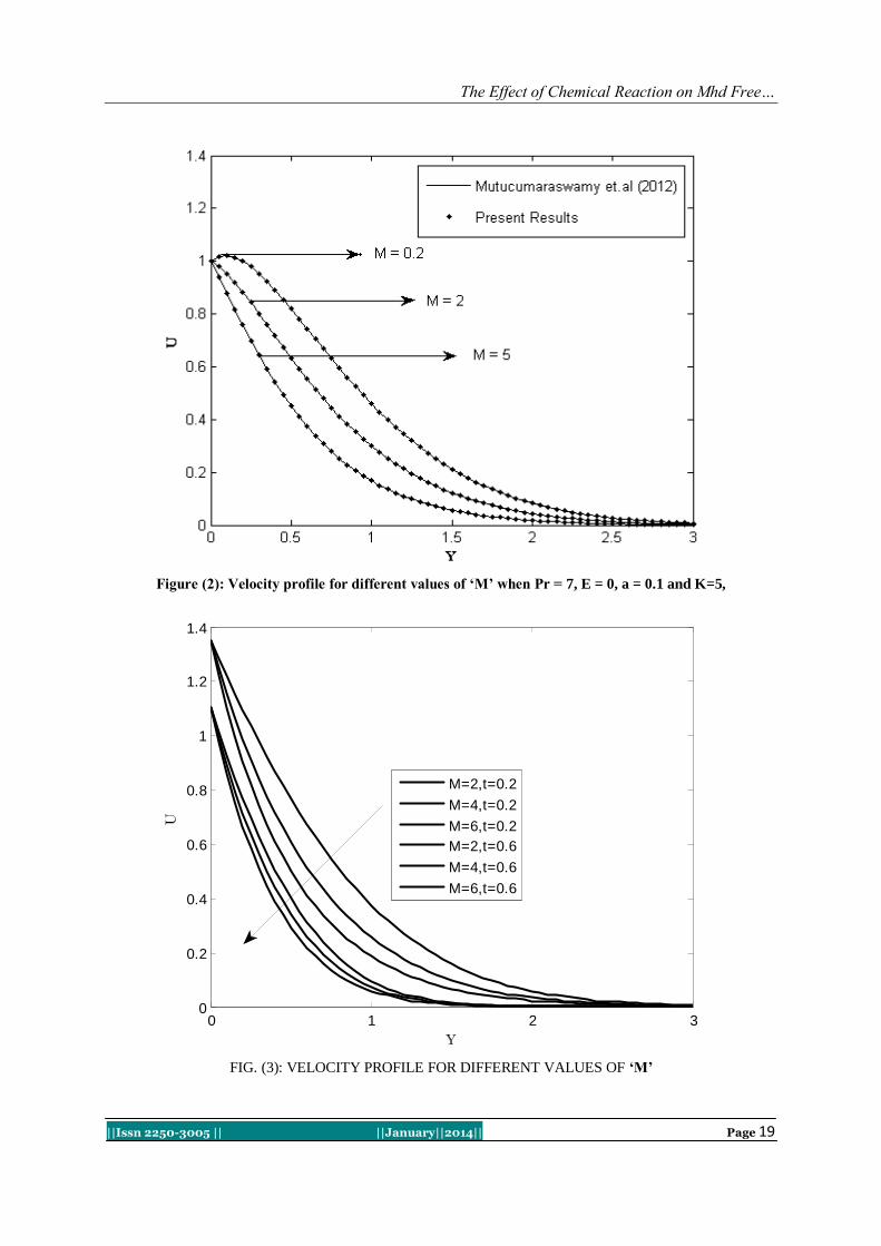
The Effect of Chemical Reaction on Mhd Free…
||Issn 2250-3005 || ||January||2014|| Page 19
Figure (2): Velocity profile for different values of ‘M’ when Pr = 7, E = 0, a = 0.1 and K=5,
0 1 2 30
0.2
0.4
0.6
0.8
1
1.2
1.4
Y
U
M=2,t=0.2
M=4,t=0.2
M=6,t=0.2
M=2,t=0.6
M=4,t=0.6
M=6,t=0.6
FIG. (3): VELOCITY PROFILE FOR DIFFERENT VALUES OF ‘M’
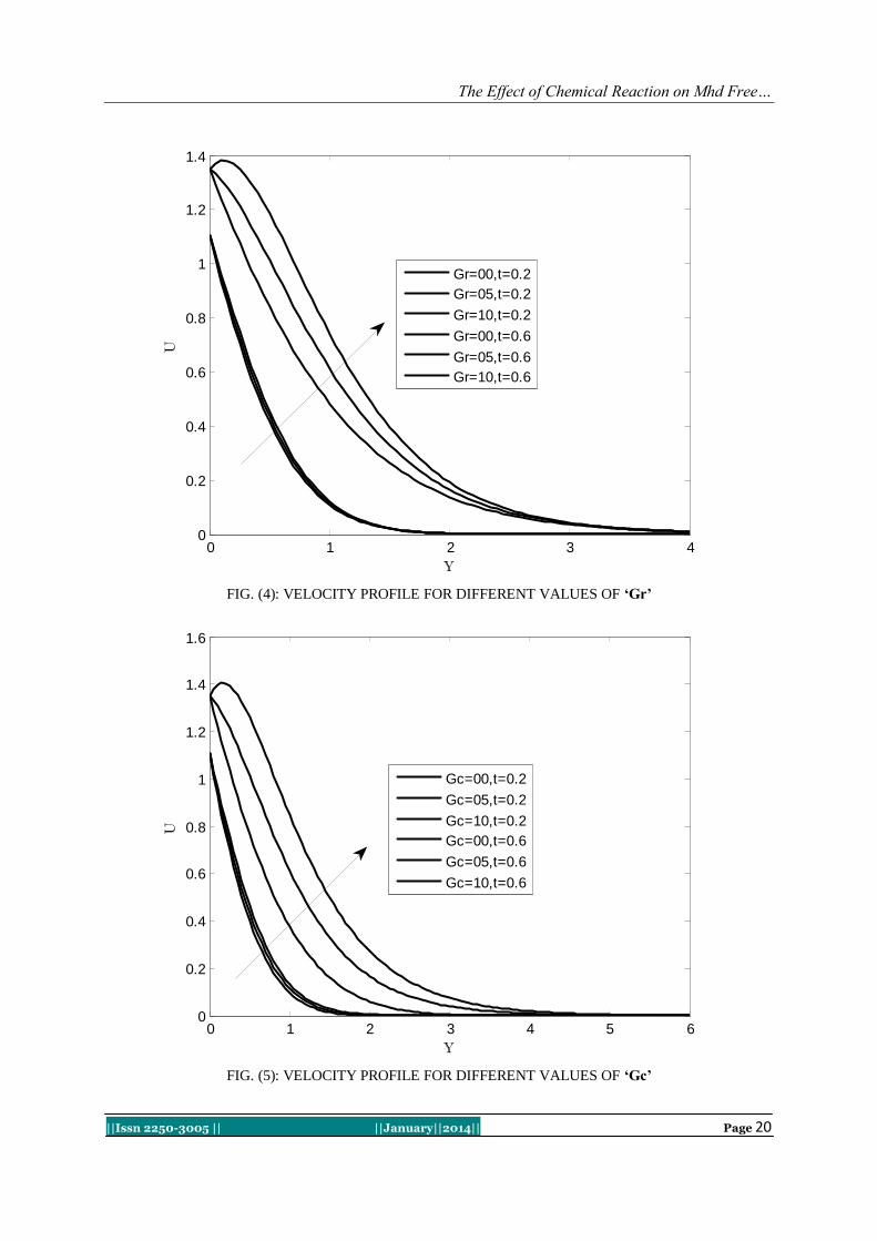
The Effect of Chemical Reaction on Mhd Free…
||Issn 2250-3005 || ||January||2014|| Page 20
0 1 2 3 40
0.2
0.4
0.6
0.8
1
1.2
1.4
Y
U
Gr=00,t=0.2
Gr=05,t=0.2
Gr=10,t=0.2
Gr=00,t=0.6
Gr=05,t=0.6
Gr=10,t=0.6
FIG. (4): VELOCITY PROFILE FOR DIFFERENT VALUES OF ‘Gr’
0 1 2 3 4 5 60
0.2
0.4
0.6
0.8
1
1.2
1.4
1.6
Y
U
Gc=00,t=0.2
Gc=05,t=0.2
Gc=10,t=0.2
Gc=00,t=0.6
Gc=05,t=0.6
Gc=10,t=0.6
FIG. (5): VELOCITY PROFILE FOR DIFFERENT VALUES OF ‘Gc’
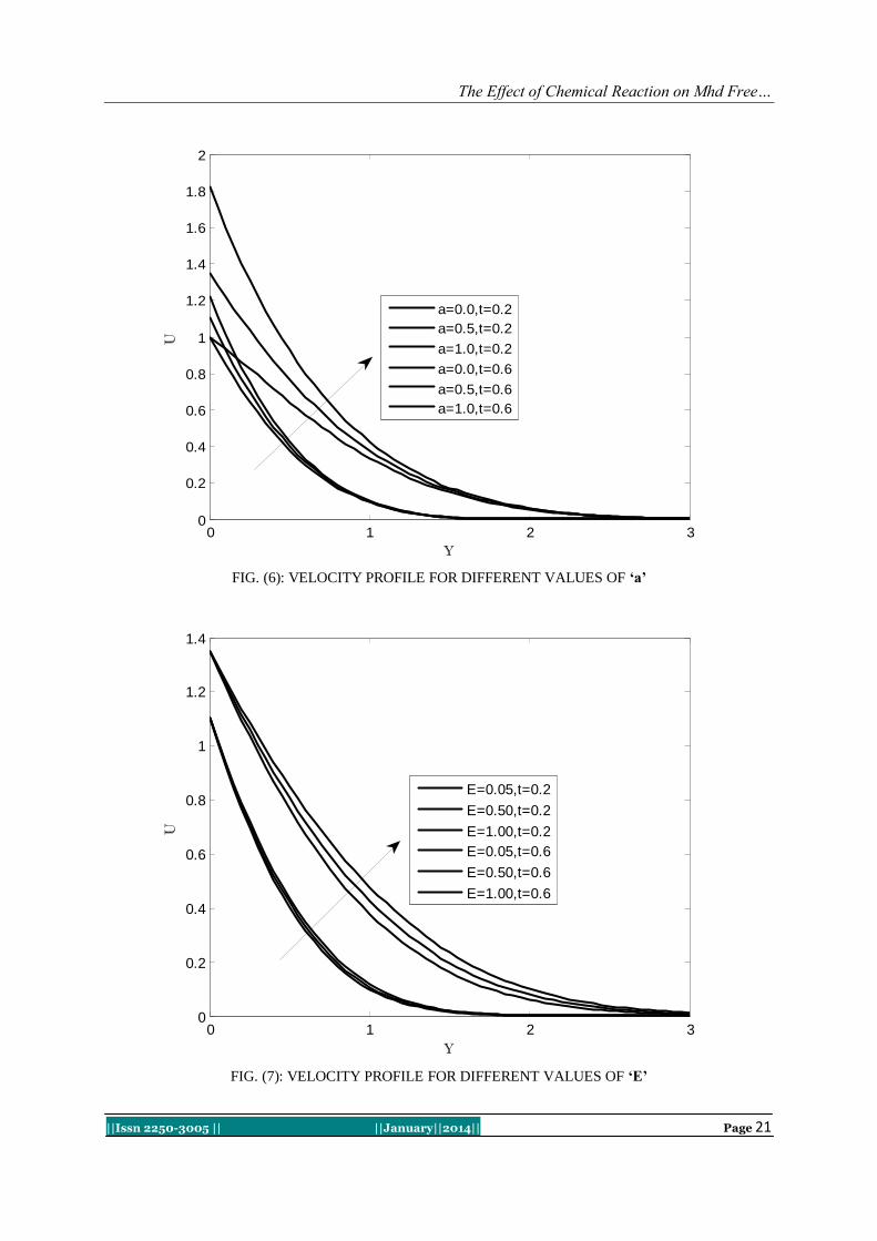
The Effect of Chemical Reaction on Mhd Free…
||Issn 2250-3005 || ||January||2014|| Page 21
0 1 2 30
0.2
0.4
0.6
0.8
1
1.2
1.4
1.6
1.8
2
Y
U
a=0.0,t=0.2
a=0.5,t=0.2
a=1.0,t=0.2
a=0.0,t=0.6
a=0.5,t=0.6
a=1.0,t=0.6
FIG. (6): VELOCITY PROFILE FOR DIFFERENT VALUES OF ‘a’
0 1 2 30
0.2
0.4
0.6
0.8
1
1.2
1.4
Y
U
E=0.05,t=0.2
E=0.50,t=0.2
E=1.00,t=0.2
E=0.05,t=0.6
E=0.50,t=0.6
E=1.00,t=0.6
FIG. (7): VELOCITY PROFILE FOR DIFFERENT VALUES OF ‘E’
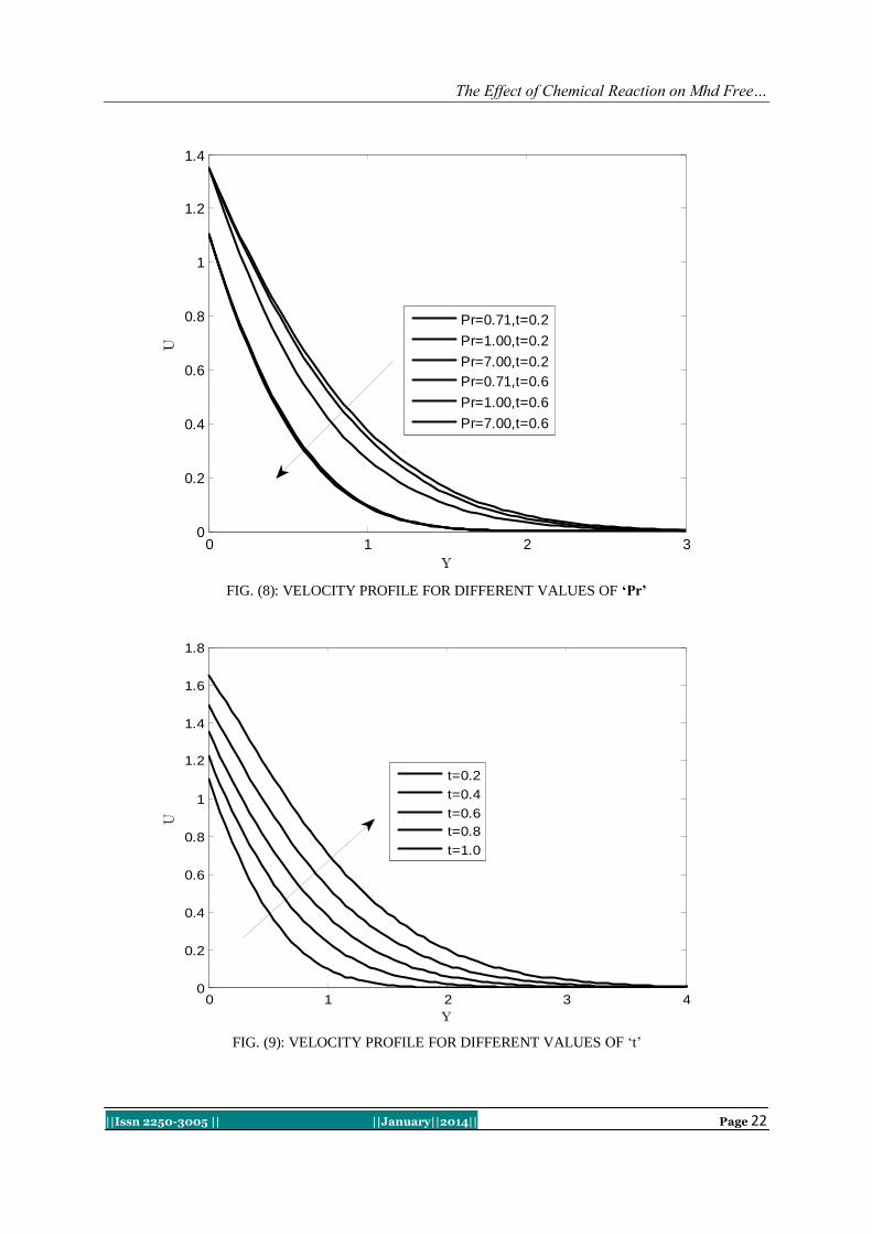
The Effect of Chemical Reaction on Mhd Free…
||Issn 2250-3005 || ||January||2014|| Page 22
0 1 2 30
0.2
0.4
0.6
0.8
1
1.2
1.4
Y
U
Pr=0.71,t=0.2
Pr=1.00,t=0.2
Pr=7.00,t=0.2
Pr=0.71,t=0.6
Pr=1.00,t=0.6
Pr=7.00,t=0.6
FIG. (8): VELOCITY PROFILE FOR DIFFERENT VALUES OF ‘Pr’
0 1 2 3 40
0.2
0.4
0.6
0.8
1
1.2
1.4
1.6
1.8
Y
U
t=0.2
t=0.4
t=0.6
t=0.8
t=1.0
FIG. (9): VELOCITY PROFILE FOR DIFFERENT VALUES OF „t‟
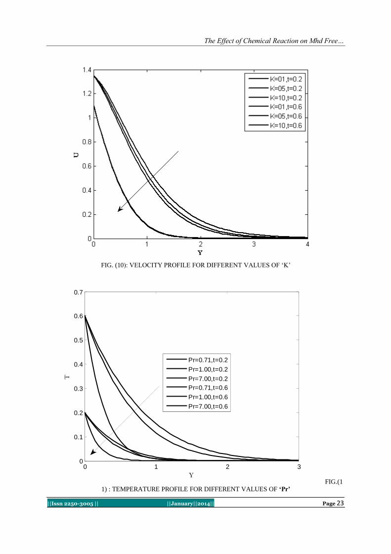
The Effect of Chemical Reaction on Mhd Free…
||Issn 2250-3005 || ||January||2014|| Page 23
FIG. (10): VELOCITY PROFILE FOR DIFFERENT VALUES OF „K‟
0 1 2 30
0.1
0.2
0.3
0.4
0.5
0.6
0.7
Y
T
Pr=0.71,t=0.2
Pr=1.00,t=0.2
Pr=7.00,t=0.2
Pr=0.71,t=0.6
Pr=1.00,t=0.6
Pr=7.00,t=0.6
FIG.(11) : TEMPERATURE PROFILE FOR DIFFERENT VALUES OF ‘Pr’
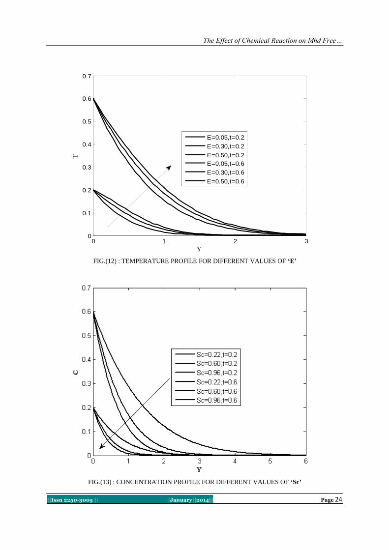
The Effect of Chemical Reaction on Mhd Free…
||Issn 2250-3005 || ||January||2014|| Page 24
0 1 2 30
0.1
0.2
0.3
0.4
0.5
0.6
0.7
Y
T
E=0.05,t=0.2
E=0.30,t=0.2
E=0.50,t=0.2
E=0.05,t=0.6
E=0.30,t=0.6
E=0.50,t=0.6
FIG.(12) : TEMPERATURE PROFILE FOR DIFFERENT VALUES OF ‘E’
FIG.(13) : CONCENTRATION PROFILE FOR DIFFERENT VALUES OF ‘Sc’
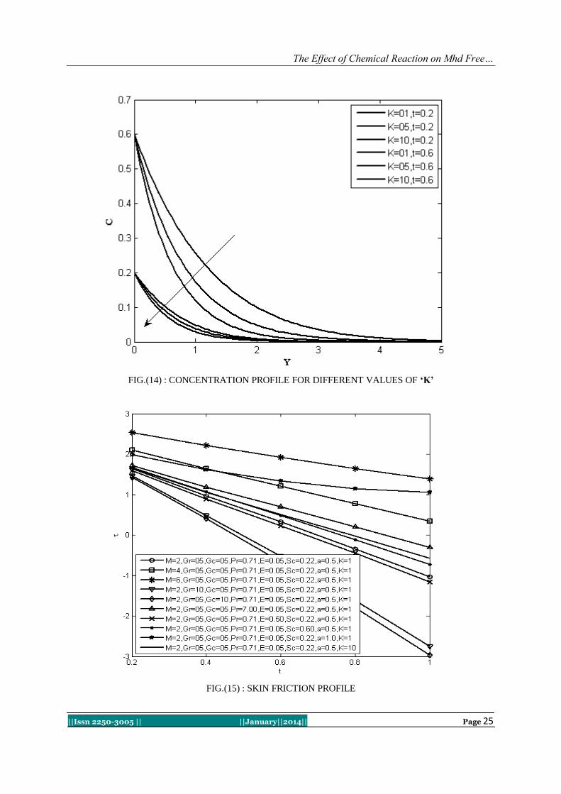
The Effect of Chemical Reaction on Mhd Free…
||Issn 2250-3005 || ||January||2014|| Page 25
FIG.(14) : CONCENTRATION PROFILE FOR DIFFERENT VALUES OF ‘K’
FIG.(15) : SKIN FRICTION PROFILE
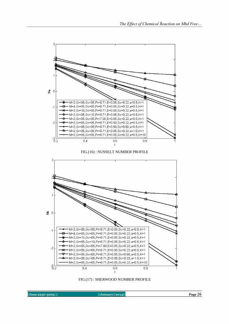
The Effect of Chemical Reaction on Mhd Free…
||Issn 2250-3005 || ||January||2014|| Page 26
FIG.(16) : NUSSELT NUMBER PROFILE
FIG.(17) : SHERWOOD NUMBER PROFILE

International Journal of Computational Engineering Research||Vol, 04||Issue, 1||
||Issn 2250-3005 || ||January||2014|| Page 27
A Review on Parametric Optimization of Tig Welding
1Naitik S Patel,
2Prof. Rahul B Patel
I. INTRODUCTION
Electrical arc was first described by davy in England in the year 1809,but the beginning of arc
welding could become possible only with the improvements in electric dynamos or generators between
1877and 1880. Auguste de meritens established arc welding process in 1881 which was applied to join certain
components of electrical storage batteries. Arc and molten pool shielding with an inert gas (co2) was
advantage by Alexander in USA in year 1928 and the patent for TIG welding was received by Hobart and
Devers in 1930 in USA. First gas tungsten arc spot welding torch based upon TIG welding was introduced
around 1946.TIG is an abbreviation for tungsten-inert-gas(fig-1). The process is also termed as gas-tungsten-
arc welding and designated as GTAW. In this process, an arc is struck between a non-consumable tungsten
electrode and the base metal. The arc is shielding by the inert argon or helium or argon-helium mixture. A
filler wire may or may not be Used. When it is used, it is fed externally into the arc in the form of rod or strip
by the welder. The welder also has to control the arc length and travel speed.
Fig: 1
Equipment: [1] Welding power source, high frequency unit, dc suppressor unit and cables.
[2] Welding torch, tungsten electrode and filler metals.
[3] Inert gas cylinder, pressure regulator and flow meter.
[4] Cooling water supply.
[5] Water and gas solenoid valves.
ABSTRACT: Quality and productivity play important role in today’s manufacturing market. Now a day’s due
to very stiff and cut throat competitive market condition in manufacturing industries . The main
objective of industries reveal with producing better quality product at minimum cost and increase
productivity.TIG welding is most vital and common operation use for joining of two similar or
dissimilar part with heating the material or applying the pressure or using the filler material for
increasing productivity with less time and cost constrain. To obtain main objective of company
regards quality and productivity. In the present research project an attempt is made to understand the
effect of TIG welding parameters such as welding current , gas flow rate ,welding speed ,that are
influences on responsive output parameters such as hardness of welding, tensile strength of welding,
by using optimization philosophy. The effort to investigate optimal machining parameters and their
contribution on producing better weld quality and higher Productivity.
.

||Issn 2250-3005 || ||January||2014|| Page 28
Inert Gases Used In TIG welding:
[1] Argon: Argon is most commonly used gas for TIG welding .It can be used on all metals.
[2] Helium: Pure helium can be used for welding aluminum and copper alloys.
[3] Helium-argon mixtures: Helium-argon mixtures give deeper penetration, greater heat input and hence
faster welding.
[4] Argon-hydrogen mixture: Addition of hydrogen to argon increases the arc voltage and provides benefits
similar to helium.
Working Principle of TIG Welding Operation:
Fig: 2
TIG is an arc welding process, as shown in Fig2. Wherein coalescence is produced by heating the
work piece with an electrical arc struck between a tungsten electrode and the job. The electrical discharge
generates a plasma arc between the electrode tip and the work piece to be welded. It is an arc welding process
wherein coalescence is produced by heating the job with an electrical arc struck between a tungsten electrode
and the job. The arc is normally initialized by a power source with a high frequency generator. This produces a
small spark that provides the initial conducting path through the air for the low voltage welding current.
The arc generates high-temperature of approximately 6100 C and melts the surface of base metal to form a
molten pool. A welding gas (argon, helium, nitrogen etc) is used to avoid atmospheric contamination of the
molten weld pool. The shielding gas displaces the air and avoids the contact of oxygen and the nitrogen with
the molten metal or hot tungsten electrode. As the molten metal cools, coalescence occurs and the parts are
joined. The resulting weld is smooth and requires minimum finish.
ADVANTAGES:
[1] No flux is used, hence there is no danger of flux entrapment when welding refrigerator and air conditioner
components.
[2] Because of clear visibility of the arc and the job, the operator can exercise a better control on the welding.
[3] This process can weld in all positions smooth and sound welds with less spatter.
[4] TIG welding is very much suitable for high quality welding of thin material
[5] It is a very good process for welding nonferrous metals(aluminum)and stainless steel
DISADVANTAGES:
[1] Tungsten if it transfers to molten weld pool can contaminate the same. Tungsten inclusion is hard and
brittle.
[2] Filler rod end if it by change comes out of the inert gas shield can cause weld metal contamination.
[3] Equipment costs are higher than that for flux shielded metal are welding.

||Issn 2250-3005 || ||January||2014|| Page 29
APPLICATIONS:
[1] Welding aluminum, magnesium ,copper ,nickel and their alloys, carbon, alloys or stainless steel, inconel
,high temperature and hard surfacing alloys like zirconium, titanium etc.
[2] Welding sheet metal and thinner sections.
[3] Welding of expansion bellows, transistor cases, instrument diaphragms, and can-sealing joints.
[4] Precision welding in atomic energy, aircraft, chemical and instrument industries.
[5] Rocket motor chamber fabrications in launch vehicles.
II. LITRETURE REVIEW
Many investigators have suggested various methods to explain the effect of process parameter on Tig welding
process in material properties.
Ugur Esme et al, [1] were carried out investigated the multi-response optimization of tungsten inert gas
welding (TIG) welding process for an optimal parametric combination to yield favorable bead geometry of
welded joints using the Grey relational analysis and Taguchi method. Sixteen experimental runs based on an
orthogonal array of Taguchi method were performed to derive objective functions to be optimized within
experimental domain. The objective functions have been selected in relation to parameters of TIG welding
bead geometry; bead width, bead height, penetration, area of penetration as well as width of heat affected zone
and tensile load. The Taguchi approach followed by Grey relational analysis to solve the multi-response
optimization problem. The significance of the factors on overall quality characteristics of the weldment has
also been evaluated quantitatively by the analysis of variance method (ANOVA). Optimal results have been
verified through additional experiments. This shows application feasibility of the Grey relation analysis in
combination with Taguchi technique for continuous improvement in product quality in manufacturing
industry.
S.C. Juang et al, [2] were carried out the selection of the process parameters for TIG welding of stainless
steel with the optimal weld pool geometry has been reported. The optimal weld pool geometry has four
smaller-the-better quality characteristics, i.e. the front height, front width, back height and back width of the
weld pool. The modified Taguchi method is adopted to solve the optimal weld pool geometry with four
smaller-the better quality characteristics. Experimental results have shown that the front height, front width,
back height and back width of the weld pool in the TIG welding of stainless steel are greatly improved by
using this approach.
S. Krishnanunni et al, [3] were carried out found that the effect of welding condition on hardness of pure
titanium material. This research paper variation of macro hardness and micro hardness at the weld heat
affected zone of grade-2 pure titanium is presented. Butt welding of thin pure Ti sheets is prepared by TIG
welding using argon gas as the shielding gas. Amount of shielding gas and number of passes are taken as the
variables in welding conditions. It was found that the maximum value of hardness is obtained corresponding to
shielding gas flow rate of 7 l/min and 4 numbers of welding passes.
Raghuvir Singh et al, [4] were carried out investigated the effect of TIG welding parameters like welding
speed, current and flux on depth of penetration and width in welding of 304L stainless steel has been studied.
From the study it was observed that flux used has the most significant effect on depth of penetration followed
by welding current. However Sio2 flux has more significant effect on depth. Optimization was done to
maximize penetration and having less bead width.
Wenchao Dong et al, [5] were investigated the oxygen content is high, the weld shape is narrow and deep
because of the inward convection induced by both the Marangoni force and the electromagnetic force for
different welding parameters. When the welding speed or electrode gap increases, the temperature gradient on
the pool surface is decreased and the inward Marangoni convection is weakened, which makes the weld D/W
ratio decrease. Under the higher welding current, the inward convection induced by the electromagnetic force
is strengthened and the higher weld D/W ratio is obtained. Under low oxygen content, the outward Marangoni
convection is the main convection mode in the weld pool and makes the weld shape wide and shallow. The
inward convection induced by the electromagnetic force is contributive to the increase of the weld depth. The
weld width weakly increases compared with the weld depth. Therefore, the weld D/W ratio slightly decreases
with the increasing welding parameters.

||Issn 2250-3005 || ||January||2014|| Page 30
Fig. 1. Marangoni convection mode in the weld pool.
Dongjie Li et al, [6] were investigated the effect of two typical weld pool shapes, wide-shallow and narrow-
deep. Marangoni convection was considered to be the main factor controlling fluid flow in the liquid pool.
Inward Marangoni convection leads the heat flux to transfer from the edges of the weld pool to the centre and
form a deep and narrow weld pool shape. Changes in the welding parameters directly change the heat input
and the pattern of the Marangoni convection, thus controlling the shape of the molten pool. For the pure-He-
shielded TIG process, the outward Marangoni convection was weakened with increasing oxygen content; thus,
the D/W ratio increased slightly. For the double-shielded TIG process, the convection was enhanced with
increasing oxygen content over a certain range, up until a large amount of oxide was formed. The heavy oxide
layer on the pool surface weakens the inner direction of Marangoni convection so as to affect the heat flow
fluid from the outer part to the inner part of weld pool surface, and harm the welding efficiency. The double-
shielded TIG process is an appropriate method for adding an active element, such as oxygen, into the weld
pool so as to transform the outward flow of Marangoni convection into an inward flow. This method allows
for a wider range of welding parameters to obtain a narrow and deep weld pool.
Parikshit Dutta et al, [7] were carried out the conventional regression analysis and neural network-based
approaches. The NN-based approaches were seen to be more adaptive compared to the conventional
regression analysis, for the test cases. It could be due to the reason that the NN-based approaches were able to
carry out interpolation within the ranges of the variables and Genetic-neural (GA-NN) system outperformed
the BPNN in most of the test cases (but not all). It is so, because a GA based search was used in the former
approach, in place of a gradient-based search utilized in the latter approach. BPNN showed a slightly better
performance compared to the genetic-neural system initially, but after about 60,000 iterations, the latter started
to perform better than the former.
Shanping Lu et al, [8] were investigated the Arc ignitability and stability of He (gas) shielded GTA welding
can be significantly improved when Ar gas is mixed into the He shielding. Adding a small amount of oxygen
to the He–30%Ar and He–50%Ar shielding, the GTA weld shape significantly changes from a wide shallow
type to a narrow deep one. The electrode tip work distance is an important parameter affecting the GTA weld
shape in He–30% Ar–O2 and He–50%–O2 shielding.
Paulo J. Modenesi et al, [9] were investigated the use of fluxes, even of extremely simple formulation, can
greatly increase (up to around 300%) the weld penetration in TIG welding. It was possible to obtain full
penetration welds in 5 mm thick plates of austenitic stainless steel with no preparation and currents of about
230 A. The operational characteristics of the ATIG process were not very different from those of conventional
TIG welding. The arc voltage changed by <3%, and, in most cases, the voltage variation was <1 V.
Comparison of the operational parameters, of the arc shape, and of the geometric parameters of the beads,
suggests that factors acting on the weld pool are, possibly, responsible for the changes in weld bead shape.
III. CONCLUSION
From various literature survey efforts to identify in TIG welding process most of welding
parameters like welding current, welding speed, depth to width ratio are generally used in research work. Also
identify TIG welding carried out on different materials like mild steel , titanium alloy, brass, carbon, stainless
steel etc.., But we may be choose work piece material differ from above for experimental work and most
applicable in industrial practices. We may be try to find out welding hardness, tensile strength, by theoretical
equations and experimentally measure with help of different input parameter. For achieving the prosperious
result of experiment the austentic type stainless steel with the grade E310 is used.

||Issn 2250-3005 || ||January||2014|| Page 31
IV. REFERENCES [1] Ugur Esme, Melih Bayramoglu, Yugut Kazancoglu, Sueda Ozgun Optimization of weld bead geometry in Tig welding process
using grey relation analysis and taguchi method. Original scientific article/Izvirni znanstveni clanek -2009, P 143 149. [2] S.C. Juang, Y.S. Tarng Process parameter selection for optimizing the weld pool geometry in the tungsten inert gas welding of
stainless steel. Journal of Materials Processing Technology 122 (2002), P 33–37.
[3] S. Krishnanunni, Dr. Josephkunju Paul C, V Narayanan Unni Effect of Welding Conditions on Hardness of Commercially Pure Titanium Akgec International Journal of Technology, Vol. 3, No. 2, P 19-24.
[4] Raghuvir Singh, Dr. N.M Suri, Prof. Jagjit Randhawa Optimization of Process Parameters for TIG welding of 304L Stainless
Steel using Response Surface Methodology. International Journal of Mechanical Science and Civil Engineering Volume 2 Issue 2 (June 2013 Issue), P 36-40.
[5] Wenchao Dong, Shanping Lu, Dianzhong Li, Yiyi Li GTAW liquid pool convections and the weld shape variations under helium
gas shielding. International Journal of Heat and Mass Transfer 54 (2011), P 1420–1431. [6] Dongjie Li, Shanping Lu, Wenchao Dong, Dianzhong Li, Yiyi Li Study of the law between the weld pool shape variations with
the welding parameters under two TIG processes. Journal of Materials Processing Technology 212 (2012), P 128– 136. [7] Parikshit Dutta, Dilip Kumar Pratihar Modeling of TIG welding process using conventional regression analysis and neural
network-based approaches. Journal of Materials Processing Technology 184 (2007), P 56–68.
[8] Shanping Lu, Hidetoshi Fujii, Kiyoshi Nogia Arc ignitability, bead protection and weld shape variations for He–Ar–O2 shielded GTA welding on SUS304 stainless steel. Journal of materials processing technology 209 (2009), P 1231–1239.
[9] Paulo J. Modenesi, Eustaquio R. ApolinaArio, Iaci M. Pereira TIG welding with single-component fluxes. Journal of Materials
Processing Technology 99 (2000), P 260-265.

International Journal of Computational Engineering Research||Vol, 04||Issue, 1||
||Issn 2250-3005 || ||January||2014|| Page 32
MV Compensation Attack on fast Selective Video Encryptions
Jay M. Joshi1, Upena D. Dalal
2
1 S. V. M. Inst. of Tech., Bharuch-392001, Gujarat, India,
2 S. V. National Institute of Standards and Technology, Surat, Gujarat, India
I. INTRODUCTION With continuing development of internet and mobile technology, video data is being used more and
more widely, in application such as video on demand, video conferencing, broad casting etc. Now video data is
closely related to many aspects of daily life, including education, commerce, and politics. In order to maintain
privacy, video data needs to be secure before transmission and distribution. Different video applications need
different levels of security. In general video applications can be differentiated according to the security level
they demand in two categories: entertainment applications like Video on Demand, Video broadcasting, and
sensitive video applications, such as telemedicine, military conferences and business meetings. Sensitive video
applications usually have strict security requirements equal to those demanded for text encryption. The
encryption algorithms have to withstand not only classical cryptanalytic attacks, e.g. ciphertext–only attacks,
known–plaintext attacks, or chosen–plaintext attacks, but also the perceptual attacks in order to ensure that no
visible information related to the business communication is disclosed.
Video compression removes redundancy, making it hard to guess information about one part of a
compressed bitstream from another. Also, compression algorithms often exhibit concentration, a higher
dependency of reconstruction quality on some parts of the compression syntax than on others. Combining these
properties suggest selective encryption, the idea that a compressed bitstream can be adequately secured from
eavesdroppers with only part of the whole bitstream encrypted. Reducing the fraction encrypted can help to
reduce the total complexity of implementation which further leads to reduce the encryption and decryption time.
Selective encryption has been suggested for a number of specific real time applications. In this paper, slices in a
picture are compressed by H.264/AVC using baseline constrained profile with quantization parameter 16 [1]. In
this paper, section 2 describes proposed selective encryption. Section 3 represents the result analysis of proposed
selective encryption based on quality analysis, speed of encryption and complexity cost and compression
efficiency after experimentation on different benchmark videos and compare with other selective parameter
encryption. Section 4 checks the robustness of the proposed encryption based on perceptual attack using Motion
Vector Compensation technique.
II. PROPOSED ALGORITHM (IDCPMV) The proposed algorithm described here is based on encryption of lowest nonzero DCT coefficient of
CAVLC in I frame with MV in P frame encryption named as IDCPMV. Encryption is done using AES-CTR
(Counter mode). The other selective encryption all non-zero values of CAVLC (treated here as „NZs in
CAVLC‟) described in [2] and [28] and MV encryption described in [2] are compared with the proposed
algorithm.
ABSTRACT: Many researchers had published their papers related with privacy and security of multimedia data which
combine the property of compression and encryption. In compression many sensitive parameters are
available, without these decoding have no meaning. Encrypting only sensitive parameters make
encryption faster and reduce complexity overhead of encryption. Such sensitive parameters in video
codec are non–zeros in CAVLC and motion vectors, which are used commonly in many papers.
Proposed encryption method is shown with the use of standard 128-bit AES algorithm in counter mode
and compare with other selective encryption methods. This paper deals with sensitive application which
demands strict security levels. This paper shows cryptanalysis of proposed algorithm using MV
compensation technique and compare with non-zeros in CAVLC and motion vector encryption.
KEYWORDS: CAVLC, Motion Vector, Motion Compensation, Selective Encryption, Video Security,
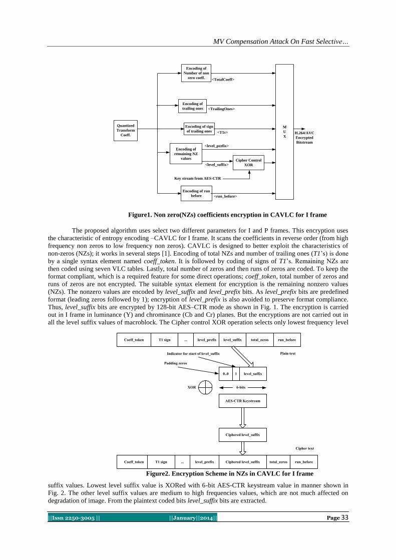
MV Compensation Attack On Fast Selective…
||Issn 2250-3005 || ||January||2014|| Page 33
The proposed algorithm uses select two different parameters for I and P frames. This encryption uses
the characteristic of entropy encoding –CAVLC for I frame. It scans the coefficients in reverse order (from high
frequency non zeros to low frequency non zeros). CAVLC is designed to better exploit the characteristics of
non-zeros (NZs); it works in several steps [1]. Encoding of total NZs and number of trailing ones (T1‟s) is done
by a single syntax element named coeff_token. It is followed by coding of signs of T1‟s. Remaining NZs are
then coded using seven VLC tables. Lastly, total number of zeros and then runs of zeros are coded. To keep the
format compliant, which is a required feature for some direct operations; coeff_token, total number of zeros and
runs of zeros are not encrypted. The suitable syntax element for encryption is the remaining nonzero values
(NZs). The nonzero values are encoded by level_suffix and level_prefix bits. As level_prefix bits are predefined
format (leading zeros followed by 1); encryption of level_prefix is also avoided to preserve format compliance.
Thus, level_suffix bits are encrypted by 128-bit AES–CTR mode as shown in Fig. 1. The encryption is carried
out in I frame in luminance (Y) and chrominance (Cb and Cr) planes. But the encryptions are not carried out in
all the level suffix values of macroblock. The Cipher control XOR operation selects only lowest frequency level
suffix values. Lowest level suffix value is XORed with 6-bit AES-CTR keystream value in manner shown in
Fig. 2. The other level suffix values are medium to high frequencies values, which are not much affected on
degradation of image. From the plaintext coded bits level_suffix bits are extracted.
Encoding of
Number of non
zero coeff.
Quantized
Transform
Coeff.
Encoding of
trailing ones
Encoding of sign
of trailing ones
Encoding of
remaining NZ
values
Encoding of run
before
Cipher Control
XOR<level_suffix>
<TotalCoeff>
<TrailingOnes>
<T1s>
<level_prefix>
<run_before>
M
U
X
Key stream from AES-CTR
H.264/AVC
Encrypted
Bitstream
Figure1. Non zero(NZs) coefficients encryption in CAVLC for I frame
Coeff_token T1 sign level_prefix level_suffix total_zeros run_before
Plain text
level_suffix1
Indicator for start of level_suffix
0..0
Padding zeros
6-bits
AES-CTR Keystream
XOR
Ciphered level_suffix
Coeff_token T1 sign level_prefix total_zeros run_before
Cipher text
Ciphered level_suffix
...
...
Figure2. Encryption Scheme in NZs in CAVLC for I frame

MV Compensation Attack On Fast Selective…
||Issn 2250-3005 || ||January||2014|| Page 34
Normally, level_suffix values have 0 to 6 bits. Lowest frequency value of level_suffix has
approximately 4 to 6 bits. If level_suffix bits are less than 6 bits, it is preceded by 0...1. The last padding bit 1
indicates the start of level_suffix bits. This padded level_suffix bits are XORed with 6-bits of AES-CTR
keystream and generated cipher level_suffix. This ciphered level_suffix put in place of plain level_suffix which
become ciphertext. Reason of this padding and converting into 6-bits put more randomness in pixel intensity
after decoding without decryption compared to other proposed methods [3-6]. One execution of AES–CTR
generates 128-bits keystream, which encrypt twenty one values of level suffix. Therefore, one execution of
AES–CTR encrypts at least twenty one mcroblocks (16 X 16 for luminance or 8 X 8 for chrominance) of the
frame.In P frame, proposed algorithm encrypts only the Motion vectors (MVs). For each 16 X 16 macroblock
contains only two values of MV(x, y) which is encoded using Expo- Golomb code. That contains very few bits
in whole NAL unit, which reduces complexity overheads in P frame. Expo- Golomb code produces two part of
bitstream [M zeros 1] and INFO. The encryption is done only on INFO part and other predefined format [M
zeros 1] is avoided to preserve format compliance. Motion Estimation engine uses the search area 46 X 46 for
luminance. Hence, the range of MVs is -15 to 15. These MVs are applied to Expo- Golomb code after passing
through se() map [1] which converts the range of MV in 0 to 30. Expo-Golomb code give M = 0 and
INFO = NULL (bitstream: < 1 >) for zero MV and M = 4 and INFO = 4 (bitstream: < 000011111 >) for thirty
MV. In 55% of total MV are zeros which does not carry any bits in INFO. INFO encryption without any
padding bits are proposed by the other authors [4, 7, 8, 9, 10] which does not encrypt 55% of MV bitstream.
Proposed method for MV encryption scheme is described in Fig. 3. Encryption engine PME (Partial Motion
Encryption) encrypts INFO bits of each MV with three bits of AES–CTR keystream. Maximum encrypted
INFO bits are 3, if the number of bits in INFO for one MV value is lower than three bits than it is padded by
zeros followed by 1. One execution of AES–CTR can encrypt at least 42 MVs of P frame. The idea behind both
methods is to make encryption in every frame in every macroblock and take different parameters for I and P
frame to make attacking harder.
MVs from
Motion
Estimation
Exponential
Golomb
Code
[M zeros 1]
INFO
Cipher
control
XOR
M
U
X
MV
Encrypted
bit stream
Keystream generated from
AES-CTR Figure3. Motion Vectors Encryption in P frame
(a) (b) (c) (d)
Figure 4. (a) Plain video frame of News and Mother-daughter sequences; Encrypted frame of (b) News (Y-
PSNR=9.425dB, Y-SSIM=0.0552),and Mother-daughter (Y-PSNR=10.448dB, YSSIM=0.061513), using NZs in
CAVLC; (c) News (Y-PSNR=16.806dB, Y-SSIM=0.4) Mother-daughter (Y-PSNR=21.60dB, Y-SSIM=0.6409)
using MV encryption; (d) News (Y-PSNR=10.5813dB, Y-SSIM=0.077134) Mother-daughter (Y-
PSNR=11.3357dB, Y-SSIM=0.1383) using IDCPMV (Proposed) encryption

MV Compensation Attack On Fast Selective…
||Issn 2250-3005 || ||January||2014|| Page 35
Table 1. Average Y-PSNR and Y-SSIM of Encrypted Videos
Video NZs in CAVLC Encryption MV Encryption IDCPMV Encryption
Y-PSNR Y-SSIM Y-PSNR Y-SSIM Y-PSNR Y-SSIM
News 8.76 0.0454 17.7 0.3967 10.5 0.06434
Bus 9.44 0.0183 15.4 0.23 10.5 0.04711
City 9.98 0.0191 19.7 0.326 11.99 0.05683
Crew 9.89 0.0251 20.2 0.446 11.9 0.07976
Flower 6.88 0.0371 14.9 0.389 7.20 0.07507
Foreman 8.24 0.02914 18.0 0.49 8.96 0.07327
Hall 9.16 0.041 18.3 0.538 10 0.1058
Harbour 8.79 0.0251 16.9 0.282 9.8 0.04652
Mobile 8.6 0.0288 22.0 0.267 9.6 0.04867
Mother-daughter 10.5 0.0951 22.5 0.6 11.6 0.1105
Soccer 9.3 0.02073 16.9 0.3771 10.5 0.06052
Stefan 9.3 0.0316 16.1 0.33 10.3 0.06515
Tempete 9.1 0.0266 17.9 0.3374 10.9 0.05954
Table 2. Encryption Time Ratio ( ETR %) of Encrypted videos
Video NZs in
CAVLC MV IDCPMV
News 76.7 6.06 9.72
Bus 64.9 7.08 8.76
City 66.4 6.9 8.97
Crew 64.5 6.66 8.54
Flower 72.9 7.51 9.44
Foreman 68.03 7.99 8.79
Hall 75.6 8.36 9.69
Harbour 72.25 7.56 8.9
Mobile 68.9 7.18 8.74
Mother-daughter 75.6 7.72 9.19
Soccer 75.7 7.54 9.01
Stefan 64.6 6.82 8.48
Tempete 74.7 6.85 8.64
III. EXPERIMENTAL RESULT The standard video sequence from SFU IVB database in CIF format and standard „News‟ sequence in
QCIF format with SD resolution have been used here. The results in this section are carried out in the way of
perception analysis, Compression efficiency and Speed of encryption.
3.1 Perception Analysis
Proposed IDCPMV algorithm provides good level of degradation in video and no perception sequences
as shown in Fig. 4 compared with MV encryption. In spatial domain every pixel values are get randomize in all
three planes and it is observed abrupt changes at the boundary values of macroblock except MV encryption. In
temporal domain, luma and chroma values rise to maximum and get back to minimum values within the one to
two frames and this cycle is repeated. Lots of transitions are observed in values of color and brightness in both
spatial and temporal domain. Peak Signal to Noise (PSNR) is good metric to measure the perception analysis.
Average Y-PSNR (for luminance frame) is shown in Table 1. Proposed algorithm provides slightly higher
PSNRs compared to NZs in CAVLC. However, their PSNR values of proposed algorithm is still lower than
algorithm described in paper [11-14], which proves more degradation in video and does not give any perceptual
information. The PSNR metric suffers from a number of limitations. Hence, perception security is better
measured using Structural Similarity Index (SSIM) [27]. Table 4 compares the average SSIM of 150 frames for
all standard videos. It is seen from the table that the encrypted videos‟ SSIMs from the proposed method are
lower as compared to [9, 28] as well as MV encryption. Thus, proposed algorithm and NZs in CAVLC
encryption achieve a high perception security, which does not give any perception.

MV Compensation Attack On Fast Selective…
||Issn 2250-3005 || ||January||2014|| Page 36
Table 3. Change in Compression Ratio( CCR %)
Video NZs in
CAVLC MV IDCPMV
News 0.067 0.0023 0.016
Bus 0.103 0.006 0.008
City 0.108 0.009 0.014
Crew 0.113 0.006 0.009
Flower 0.123 0.007 0.008
Foreman 0.115 0.009 0.012
Hall 0.125 0.006 0.008
Harbour 0.107 0.004 0.008
Mobile 0.12 0.005 0.006
Mother-daughter 0.091 0.004 0.013
Soccer 0.099 0.01 0.011
Stefan 0.113 0.005 0.007
Tempete 0.124 0.004 0.007
3.2 Speed of encryption
Encryption algorithm should be efficient so that it does not delay the transmission or access the
operations for real time video applications. To measure the encryption speed Encryption Time Ratio (ETR) is
the better choice [15]. ETR is the percentage ratio of encryption time with decryption time to encoding time
with decoding time. ETR is calculated by considering 250 frames for News sequence in QCIF format and 300
frames for other CIF format videos (See table 2). MV encryption provides lowest ETR. NZs in CAVLC
provides very high ETR. Proposed encryption gives slightly higher ETR compared to MV. However, proposed
encryption provides lower encryption speed compared to method described in [4, 10, 16, 17, 18, 19, 20] and
higher encryption speed compared to the method described in [5, 13, 21, 22, 23] based on encryption time and
ETR. If ETR ≤ 10%, encryption/decryption operations is very efficient compared with the encoding/decoding
and does not affect the real time system [15]. Therefore, MV and IDCPMV encryption algorithms are suitable
for real time applications.
3.3 Compression efficiency
Selective encryptions described earlier are applied to video data after compression. Ideally video
encryption algorithms should not change the compression ratio or should at least keep the changes in a small
range. This is especially important in wireless or mobile applications, in which the channel bandwidth is limited.
To evaluate the effects on bandwidth, change in compression ratio (CCR) is used as the ratio between the
changed data size and the original data size [15]. IDCPMV provides lower CCR compared to NZs in CAVLC
algorithm (See table 3). CCR value is also lower compared to the algorithms presented in [5, 10, 11, 12, 18, 19,
24, 25, 26]. As CCR ≤ 10%, proposed algorithm have near constant bandwidth and suitable for wireless and
mobile applications [15].
IV. MV COMPENSATION ATTACK Proposed algorithms described, uses counter mode 128-bit AES algorithm which withstands all the
classical attack at bits level. However, at the pixel level it might have to check robustness against various attacks
in different environment. For all three techniques, it is assumed that the all encrypted frames are degraded in
video quality, and it might be improved by perceptual attack which gives some perceptible information.In these
techniques, two properties were taken into account: 1) I frames have less degradation than P frames and 2) the
consecutive frames have similar characteristics. MV compensation is done only in encrypted P frame shown in
Fig. 4. Attack deals with two different approaches: 1. Ciphered I frame is used as a reference frame for
estimating the motion vectors of all the macro blocks and compensation is applied on ciphered P frame. 2. Same
work is done using plain I frame as reference frame.
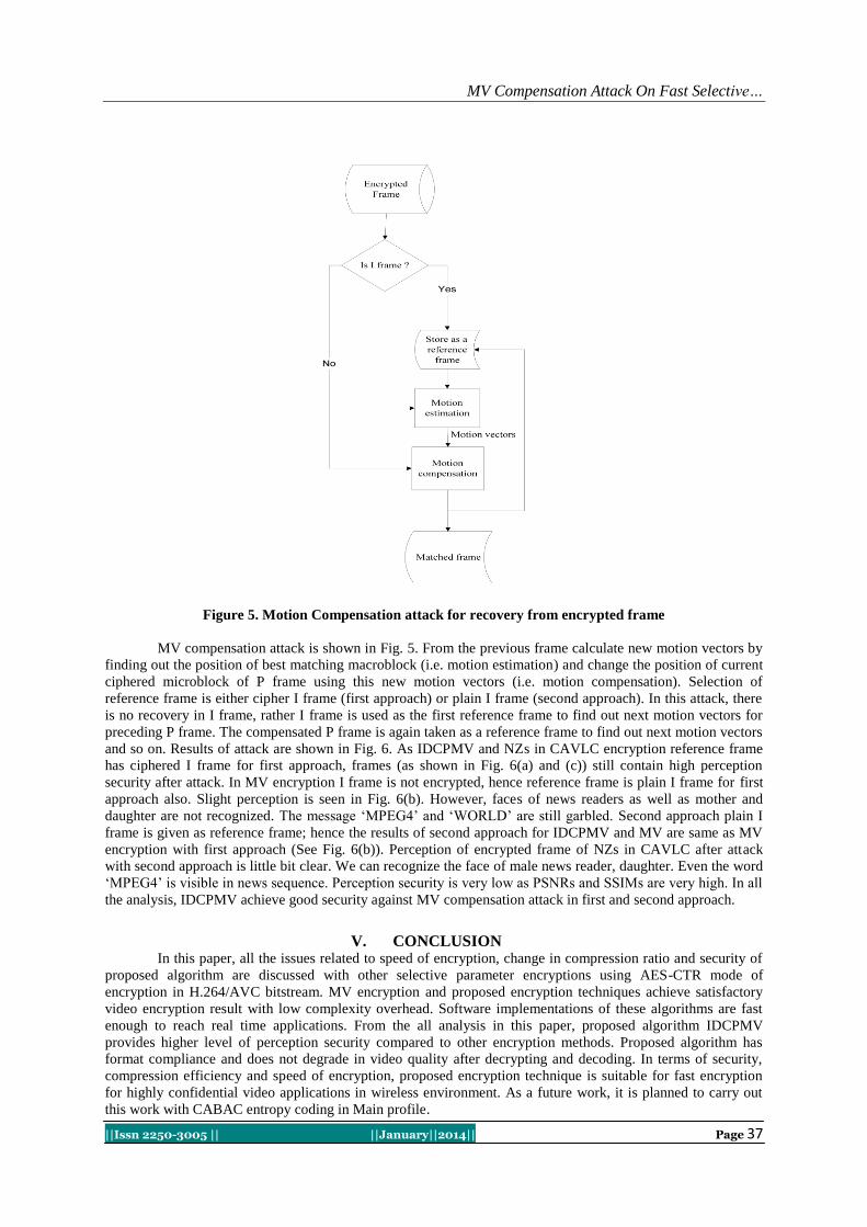
MV Compensation Attack On Fast Selective…
||Issn 2250-3005 || ||January||2014|| Page 37
Figure 5. Motion Compensation attack for recovery from encrypted frame
MV compensation attack is shown in Fig. 5. From the previous frame calculate new motion vectors by
finding out the position of best matching macroblock (i.e. motion estimation) and change the position of current
ciphered microblock of P frame using this new motion vectors (i.e. motion compensation). Selection of
reference frame is either cipher I frame (first approach) or plain I frame (second approach). In this attack, there
is no recovery in I frame, rather I frame is used as the first reference frame to find out next motion vectors for
preceding P frame. The compensated P frame is again taken as a reference frame to find out next motion vectors
and so on. Results of attack are shown in Fig. 6. As IDCPMV and NZs in CAVLC encryption reference frame
has ciphered I frame for first approach, frames (as shown in Fig. 6(a) and (c)) still contain high perception
security after attack. In MV encryption I frame is not encrypted, hence reference frame is plain I frame for first
approach also. Slight perception is seen in Fig. 6(b). However, faces of news readers as well as mother and
daughter are not recognized. The message „MPEG4‟ and „WORLD‟ are still garbled. Second approach plain I
frame is given as reference frame; hence the results of second approach for IDCPMV and MV are same as MV
encryption with first approach (See Fig. 6(b)). Perception of encrypted frame of NZs in CAVLC after attack
with second approach is little bit clear. We can recognize the face of male news reader, daughter. Even the word
„MPEG4‟ is visible in news sequence. Perception security is very low as PSNRs and SSIMs are very high. In all
the analysis, IDCPMV achieve good security against MV compensation attack in first and second approach.
V. CONCLUSION In this paper, all the issues related to speed of encryption, change in compression ratio and security of
proposed algorithm are discussed with other selective parameter encryptions using AES-CTR mode of
encryption in H.264/AVC bitstream. MV encryption and proposed encryption techniques achieve satisfactory
video encryption result with low complexity overhead. Software implementations of these algorithms are fast
enough to reach real time applications. From the all analysis in this paper, proposed algorithm IDCPMV
provides higher level of perception security compared to other encryption methods. Proposed algorithm has
format compliance and does not degrade in video quality after decrypting and decoding. In terms of security,
compression efficiency and speed of encryption, proposed encryption technique is suitable for fast encryption
for highly confidential video applications in wireless environment. As a future work, it is planned to carry out
this work with CABAC entropy coding in Main profile.

MV Compensation Attack On Fast Selective…
||Issn 2250-3005 || ||January||2014|| Page 38
REFERENCES [1]. ITU-T Rec H.264, ITU-T: Advanced video coding for generic audiovisual services, v11, 2009.
[2]. Joshi J, Dalal U., “Enhancing selective ISMACryp video encryption for real time applications in handheld devices”, in Proc
TENCON 2011 - 2011 IEEE Region 10 Conference, 2011; p.p. 274 –278, doi:10.1109/TENCON. 2011.6129107. [3]. Dubois L, Puech W, Blanc-Talon J. “Smart selective encryption of cavlc for H.264/AVC video”, Information Forensics and
Security (WIFS), 2011 IEEE International Workshop on, 2011; p.p. 1–6, doi:10.1109/WIFS. 2011.6123130.
[4]. Lian S, Sun J, Liu G, Wang Z. “Efficient video encryption scheme based on advanced video coding”, Multimedia Tools and Applications 2008; 38(1):75–89, 2008; doi:10.1007/s11042-007-0150-7
[5]. Qian Z, Jin-mu W, Hai-xia Z. “Efficiency video encryption scheme based on H.264 coding standard and permutation code
algorithm”, in Proc Computer Science and Information Engineering, 2009 WRI World Congress on, vol. 1, 2009; p.p. 674–678, doi:10.1109/CSIE.2009.334.
[6]. Feng Wang L, dong Wang W, MA J, XIAO C, Qiao Wang K., “Perceptual video encryption scheme for mobile application based
on H.264”, Journal of China Universities of Posts and Telecommunications 2008; 15, Supplement(0): p.p. 73–78,2008; doi:http://dx.doi.org/10.1016/S1005-8885(08) 60159-4.
[7]. Bhargava B, Shi C, Wang SY. “MPEG video encryption algorithms”, Multimedia Tools and Applications, 2004; 24(1), p.p. 57–79,
doi: 10.1023/B:MTAP.0000033983.62130.00.
[8]. Lian S, Chen X. “Secure and traceable multimedia distribution for convergent mobile TV services”, Computer Communications
2010; 33(14), p.p. 1664–1673.
[9]. Boho A, Van Wallendael G, Dooms A, De Cock J, Braeckman G, Schelkens P, Preneel B, Van de Walle R. “End-to-end security for video distribution: The combination of encryption, watermarking, and video adaptation”, Signal Processing Magazine, IEEE
2013; 30(2), p.p. 97–107, doi:10.1109/MSP.2012.2230220.
[10]. Varlakshmi L, Sudha G, Jaikishan G. “An efficient scalable video encryption scheme for real time applications”, Procedia Engineering, 2012; 30(0), p.p. 852–860, doi:http:// dx.doi.org/10.1016 /j.proeng.2012.01.937.
[11]. Dufaux F, Ebrahimi T. “Scrambling for privacy protection in video surveillance systems”, Circuits and Systems for Video
Technology, IEEE Transactions on, 2008; 18(8), p.p. 1168–1174,doi:10.1109/TCSVT.2008. 928225. [12]. Dai F, Tong L, Zhang Y, Li J. “Restricted H.264/AVC video coding for privacy protected video scrambling”, Journal of Visual
Communication and Image Representation 2011; 22(6), p.p. 479 – 490, doi:http://dx.doi.org /10.1016/j.jvcir.2011.05.006.
[13]. Hong GM, Yuan C, Wang Y, Zhong YZ. “A quality controllable encryption for H.264/AVC video coding”, Advances in Multimedia Information Processing - PCM 2006, vol. 4261, Springer Berlin Heidelberg, 2006; p.p. 510–517, doi:10.1007/
11922162 59.
[14]. Zeng W, Lei S. “Efficient frequency domain selective scrambling of digital video”, Multimedia, IEEE Transactions on 2003; 5(1), p.p. 118–129, doi:10.1109/ TMM.2003.808817.
[15]. Lian S., Multimedia Content Encryption: Techniques and Applications, CRC Press: Taylor & Francis Group, 2009; p.p. 15–16.
[16]. Wang X, Zheng N, Tian L. “Hash key-based video encryption scheme for H.264/AVC”, Signal Processing: Image Communication 2010; 25(6), p.p. 427–437, doi:http://dx.doi.org/10. 1016/j.image.2010.03.005.
[17]. Raju C, Srinathan K, Jawahar C. “A real-time video encryption exploiting the distribution of the DCT coefficients”, in Proc
TENCON 2008 - 2008 IEEE Region 10 Conference, 2008; p.p. 1–6, doi:10.1109/TENCON.2008. 4766482. [18]. Kodikara Arachchi H, Perramon X, Dogan S, Kondoz A. “Adaptation aware encryption of scalable h.264/avc video for content
security”, Signal Processing: Image Communication 2009; 24(6), p.p. 468 – 483.
[19]. Qiao L, Nahrstedt K., “A new algorithm for mpeg video encryption”, In Proc. of The First International Conference on Imaging Science, Systems, and Technology (CISST97), 1997; p.p. 21–29.
[20]. Tosun A., Feng Wc. “On error preserving encryption algorithms for wireless video transmission”, In Proceedings of the ninth ACM
international conference on Multimedia, MULTIMEDIA ’01, ACM:New York, NY, USA, 2001; p.p. 302–308, doi:10.1145/500141. 500187.
[21]. Akkus I, Ozkasap O, Civanlar M. “Secure transmission of video on an end system multicast using public key cryptography”,
Multimedia Content Representation, Classification and Security, vol. 4105, Springer Berlin Heidelberg, 2006; p.p. 603–610, doi: 10.1007/ 11848035 80.
[22]. Kumar A, Ghose M. “Extended substitution–diffusion based image cipher using chaotic standard map”, Communications in
Nonlinear Science and Numerical Simulation 2011; 16(1), p.p. 372 – 382, doi:http://dx.doi.org/10. 1016/j.cnsns.2010.04.010. [23]. Patidar V, Pareek N, Purohit G, Sud K. “Modified substitution diffusion image cipher using chaotic standard and logistic maps”,
Communications in Nonlinear Science and Numerical Simulation 2010; 15(10), p.p. 2755 – 2765, doi:http://dx.doi.org/10.
1016/j.cnsns.2009.11.010. [24]. Magli E, Grangetto M, Olmo G. “Transparent encryption techniques for h.264/avc and H.264/SVC compressed video”, Signal
Processing 2011; 91(5), p.p. 1103 – 1114, doi:http://dx.doi.org/ 10.1016/j.sigpro.2010.10.012.
[25]. Liu Z, Li X, Dong Z. “A lightweight encryption algorithm for mobile online multimedia devices” Web Information Systems – WISE 2004, vol. 3306, Springer Berlin Heidelberg, 2004; p.p. 653–658, doi:10.1007/978-3-540-30480-7 67.
[26]. Tang L. “Methods for encrypting and decrypting MPEG video data efficiently”, In Proc. of the fourth ACM international
conference on Multimedia, MULTIMEDIA ’96, ACM: New York, NY, USA, 1996; p.p. 219–229, doi:10.1145/244130.244209. [27]. Wang Z, Bovik A, Sheikh H, Simoncelli E. “Image quality assessment: from error visibility to structural similarity”, Image
Processing, IEEE Transactions on 2004; 13(4):600–612, doi:10.1109/TIP.2003.819861. [28]. Shahid Z, Chaumont M, Puech W. “Fast protection of h.264/avc by selective encryption of CAVLC and CABAC for I and P
frames”, Circuits and Systems for Video Technology, IEEE Transactions on 2011; 21(5):565–576, doi:10.1109/TCSVT.
2011.2129090.

International Journal of Computational Engineering Research||Vol, 04||Issue, 1||
||Issn 2250-3005 || ||January||2014|| Page 39
Studies on the Variation in Coal Properties of Low Volatile
Coking Coal after Beneficiation
Vivek Kumar
1, V.K. Saxena
2
1 M.Tech, Ism Dhanbad, 2 P.Hd, Ism, Dhanbad
I. INTRODUCTION The relative abundance of coal in India compared to other fossil fuels makes it a natural choice as the
primary source of fuel, be it for steel making, power generation or for other uses. Total reserves of coal in the
country are estimated to the order of 267 Billion Tons. Coking coal, which is merely 14% of the total deposits,
is available mainly in Eastern part of India. Coking coal is an essential prerequisite for manufacture of Iron & Steel through blast furnace route. In India, the annual requirement of coking coal for various metallurgical
purposes may be up to the tune of 35 million tones, out of which the availability from the indigenous sources is
about 10 million tones only. The rest of the coking coal requirements are managed through imports from
different countries.To meet the increased demand of coking coal concerted efforts have to be made to correct the
imbalance between need and availability by increasing the production of coal of desired quality through better
management of available resources of inferior grade. Low volatile coking coal (LVCC), though inferior in
qualities but abundantly available in Eastern part of the country may be an immediate choice. The present
production from LVCC is about 16 to 18 mt per year, and is primarily used for power generation. These coals,
being of lower seams are likely to be more matured (Ro~1.30%) than the upper seams and consequently exhibit
lower values of volatile matter. The country has a moderate reserve of such coal, amounting to about 50% of the
total coking coal reserve. Proper utilization of these LVCC coals for metallurgical purpose after suitable may
minimize improper utilization of scarce commodity coking coal.(Ref. Geological Survey of India (GSI) Report, Government of India 2009: Inventory of Indian Coal Resources.)
1.1 Definition of Coal:
Coal is a combustible compact black or dark-brown carbonaceous sedimentary rock formed from
compaction of layers of partially decomposed vegetation and occurs in stratified sedimentary deposits.
1.2 Formation of coal: Coal is formed by biological, physical and chemical processes, governed by temperature and pressure,
over millions of years on plant remains, deposited in ancient shallow swamps. The degree of alteration
(metamorphism), caused by these processes, during the temporal history of development determine their
position or rank in the coalification series which commence at peat and extend through lignite to bituminous coal and finally anthracite. The relative amount of moisture, volatile matter, and fixed carbon content varies
from one to the other end of the coalification series.
ABSTRACT
Coal is the main ingredient for the various industries like; Iron & steel industries, Power
generation industries, Cement industries etc. and its calorific value is the back bone for the processing.
The calorific value of coal depends on various factors on which ash content is the major one.Coking coal is an essential prerequisite for production of Iron & Steel through blast furnace route. Systematic
R&D studies on the availability of desired quality coking coal from indigenous resources have become
imperative to minimize the dependence on imported coals. The Low Volatile Coking Coal (LVCC)
constitutes about 50% of the total coking coal reserves in India. These coals are characterized by high
ash content and difficult in cleaning potential. This high ash content will be reduced by washability
process. Washability analysis is the basis for nearly all coal preparation plant and it is carried out for
the analysis of ash reduction in different specific gravity portion of coal and it’s characterization
defines how and which process can be applied for the certain quality of coal for specific separation

Studies on The Variation In Coal Properties…
||Issn 2250-3005 || ||January||2014|| Page 40
The moisture and volatile matter decrease with enhancement of rank while carbon content increases
i.e., carbon content is lowest in peat and highest in anthracite.
1.3 Type / Grade:
Coal: It is classified into different types mainly on the basis of certain chemical (ash, moisture and volatile
matters) and physical (caking index, coke type and swelling index) parameters. However, different modes of
classifications are being followed in different countries mainly on the basis of prevalent industrial need. The
Indian coal is broadly classified into two types – Coking and Non-Coking. The former constitute only a small
part of the total coal resources of the country. These two are further subdivided as follows on the basis of certain physical and chemical parameter as per the requirement of the industry.
[1] Coking Coal
[2] Prime Coking - Mainly used for metallurgical purpose.
[3] Medium Coking - Mainly used in steel industry.
[4] Semi Coking - Mainly in cement, fertilizer and sponge iron industries.
Non Coking Coal: Non- coking coal comprises lion’s share of Indian coal. Based on Useful Heat Value
(UHV), it is classified into grades A to G for commercial use. A to C grades are considered as Superior and are used in cement, fertilizer and sponge iron industries. D to G grade, available in almost in all the coalfields, is
considered as Inferior and is mostly used in power sector.
Lignite: Lignite is the youngest coal from geological perspective. It is a soft coal composed mainly of volatile
matter and moisture content with low fixed carbon. It is commonly known as
brown coal and is classified into grades A to C on the basis of Gross Calorific Value as per the requirement of
the industries. It is considered as apt fuel for power generation especially due to its low ash content.
The common coals used in Indian industry are bituminous and sub-bituminous coal. The gradation of Indian
coal based on its calorific value is as follows:
Grade Calorific Value Range
( in Kcal/kg)
A
B
C
D
E
F
G
Exceeding 6200
5600 – 6200
4940 – 5600
4200 – 4940
3360 – 4200
2400 – 3360
1300 – 2400
Normally D,E and F coal grades are available to Indian Industry.
1.4 Intrusion Of Ash Forming Material In Indian Coking Coal Indian coking coal is drift originated coal. During the drifting process coal swamp are contacted with
marine environment. Volcanic eruption zone & igneous zone.On this time various volcanic igneous and marine
materials are mixed with the coal swamp and they affect the properties of Indian coal. Some coking coal gets
contacted with sulfuric environment and some ironic environment. That creates different type of impurities in
coal forming zone. These intrusions are mixed thoroughly with coal so difficult to wash some time.For the
utilization coal should have certain properties. For the characterization of coal different analysis are carried out.
The basic analysis for the separation of coal is based on specific gravity difference. For these purpose we
concerned with particle size distribution not about particle size. For these analysis washability characteristics of
coal is determined. That characterizes significance of particle size distribution and washing parameter like yield,
ash, cut point density, NGM.
1.5 Objective: Washability of coal is carried out for the analysis of ash reduction in different specific gravity portion
of coal. Washabilty characterization defines how and which process can be applied for the certain quality of coal
for specific separation. So the objective of washability is ash reduction with maximum utilizable coking coal.

Studies on The Variation In Coal Properties…
||Issn 2250-3005 || ||January||2014|| Page 41
1.6 Method For The Analysis
For the washabilty characterization Standard float and sink test is used. This is based on the specific
gravity of coal. In different specific gravity portion have different density because of some heavy particle in
coal. These heavy particle causes ash in coal. That is undesirable for use.
Washability characteristics of coal are generated from float/sink analysis of core samples, as mined samples, or
from preparation plant feed samples. In addition to the float/sink analysis. Different steps in float and sink test:
[1] Sample Collection
[2] Sample Preparation For float and sink test.
[3] Different Density Media Preparation. [4] Utilization of Media for the coal flotation.
[5] Ash determination in different density fraction of floated coal.
[6] Preparation of Washability Data.
[7] Graph of washability Data
Bulk sample Preparation:
The bulk sample should be spread on an impervious base, preferably under shelter. The sample should
be dried and sieved in accordance with ASTM test Method.
1.7 Preparation Of Washability Data:
Run of mine coal comprises fragments of material which have density from the lower to highest in a continuous range. But the proportion of each varies. Those with low density have the lowest ash but the higher
heat value and those with the highest density vice versa.Washability curve shows the relationship between ash
content and the amount of float and sink produced at very particular relative density. Because the test is
conducted under very controlled condition the result obtained relate to an almost perfect separation.From the
sink & float masses together with the individual ash content of each relative fraction the washability data can be
calculated. Different terms which used for the Data preparation are specific gravity, weight percentage, ash
percentage, cumulative float weight and ash percentage, cumulative sink weight and ash percentage,
characterize, NGM.
1.8 Washability Curve:
A curve or graph showing the results of a series of float-and-sink tests. A number of these curves are
drawn to illustrate different conditions or variables, usually on the same axes, thus presenting the information on one sheet of paper. Washability curves are essential when designing a new coal or mineral washery. There are
four main types of washability curves: characteristic ash curve, cumulative float curve, cumulative sink curve,
and densimetric or specific gravity curve.
II. EXPERIMENTAL WORK:
The following experimental work was carried out.
Coal is thoroughly investigated through various tests. Proximate test gives general overview of coal;
Ultimate Analysis gives its elemental composition. HGI test gives idea about the hardness of coal, sink float test
for different size fraction and analysis the ash.
2. Collection Of Coal Sample: The coal samples were taken for the desired objective of project. Coal sample was taken from
Ghanuadih coal mine. The coal sample was low volatile coking coal.
The coal sample was subject to Proximate analysis, Ultimate analysis, Gross CalorificValue, Free Swelling
Index, Hardgrove grindability index, Specific Gravity, sink-float tests for categorization of sample.

Studies on The Variation In Coal Properties…
||Issn 2250-3005 || ||January||2014|| Page 42
SAMPLE CHARACTERIZATION
Original sample (54.3Kg)
Coining and Quartering
2.504 Kg Reserved
12.5mm sieving
1.222Kg 1.218 Kg
3mm sieving
0.596 Kg 0.584Kg
1mm sieving
0.298Kg0.283Kg
(-72 mesh) fine coal size occurs, when it pulverizes in pulverizers for proximate analysis of overall coal sample.
2.1. Proximate Analysis-
Determination of Moisture Content:-
About 1 gram of finely powdered (-212 μ) air dried coal sample was weighed in a silica crucible and
was then placed inside an electronic hot air oven, maintained at 108±2˚C. The crucible with the coal sample was allowed to remain in the oven for 1 hours and was taken out with a pair of tongs cooled in a desiccator for about
15 minutes and then weighed. The loss in weight is reported as moisture (on percentage basis). The calculation
is done as per the following:
% moisture (% M) = (Y-Z)/(Y-X)*100
Where, X=Wt. of crucible in grams
Y=Wt. of coal + Crucible in grams (Before heating)
Z= Wt. of coal + Crucible in grams (After heating)
Determination of Volatile Matter content (VM):-
About 1 gram of finely powdered (-212μ) air dried coal sample was weighed in a VM crucible and was
then placed inside a muffle furnace maintained at 925˚C. The crucible was then covered with its lid. The heating
was carried out for exactly 7 minutes, after which the crucible was removed, cooled in air and then in a desiccators and weighed again. The calculation is done as follows:
% volatile matter (% VM) = (Y-Z)/(Y-X)*100
Where, X=Wt. of crucible in grams
Y=Wt. of coal + Crucible in grams (Before heating)
Z= Wt. of coal + Crucible in grams (After heating)

Studies on The Variation In Coal Properties…
||Issn 2250-3005 || ||January||2014|| Page 43
Determination of Ash content (Ash)
About 1 gram of finely powdered (-212μ) air dried coal sample was weighed and taken in an empty
silica crucible. Before that the crucibles were heated at 850˚C for about 1 hr. to remove any foreign particles in
the crucible. The crucible along with the sample was put in a muffle furnace at 450˚C for about 30 minutes.
After that the temperature of the furnace was raised to 850˚C and the sample was heated for about 1 hr. at that
temperature.
The calculation is done as follows:
% Ash = (Z-X)/(Y-X)*100 Where, X= Wt. of crucible in grams
Y=Wt. of coal + Crucible in grams (Before heating)
Z= Wt. of coal + Crucible in grams (After heating)
Estimation of Fixed Carbon (C)
The fixed carbon content of coal is given by the following formulae- %FC = 100 – (%M+%VM+% Ash)
2.2. Ultimate Analysis
Determination of total carbon, hydrogen, nitrogen, oxygen and sulphur percentages in coal comprises its ultimate analysis. Ultimate analysis give the elemental composition of coal i.e. carbon, hydrogen, nitrogen,
sulphur and oxygen content of coal. Vario EL III CHNS analyser from Elementar Germany was used for
determination of Carbon, Hydrogen, Nitrogen and Sulphur. Oxygen was calculated using the following
relations:
O% = 100 – (C% + H% + N% + S + M +Ash %).
Procedure for Analysis
To start the analysis first of all the carousel from the Vario EL III was removed and the position of carousel hole was adjusted to zero. The main power of analyser was switched on, after a while the carousel of
the analyser start moving and comes to original position i.e. zero. Now the carousel was placed at top at original
position. Before performing the sample analysis the analyser is first run with few blank determination (No
sample) and thereafter few samples of standard Sulfanilic acid (whose composition is known) is run to calibrate
the analyser. It is to be ensured that calibration factor of the analyser should not be less than 90%.
To perform the ultimate analysis of coal, pre manufactured tin boat was weighed in precession digital
balance. Few mg (say 4-5 mg) of Tungsten oxide, which acts as a catalyst, is mixed with approximately 10 mg
of coal sample of -200 mesh size. The tin boat inside with tungsten oxide and coal samples was made to pellet
with the help of pellet maker. Now the pellet is transferred to the slots provided in the Carousel (upper portions)
of Vario EL III CHNS analyser. There are 79 slots in the analyser.Two types of gases namely helium and
oxygen are used for the analysis. Helium is used as carrier gas and oxygen for combustion purpose. During the experiment helium gas flow is maintained at the rate of 200 ml/min and oxygen dosage is 90 sec for each
sample. Before the gases come into contact with the pellet it is passed through drying agents. Vario EL III
CHNS analyser consists of various parts and instrumentation which includes; oxidation tube, reduction tube and
absorption columns for absorbing N2, CO2, water vapour, SO2. In the oxidation tube there is ash finger.
Oxidation tube is placed in the oxidation furnace the temperature of which goes to around 1150oC. The product
gas which is emitting from oxidation tube passes through reduction tube having temperature of 8500C first and
then these gases goes to absorption columns for absorbing N2, CO2, water vapour, SO2. TCD detects the
presence and quantity of these gases by measuring the peaks and the area under peaks. The quantity of gases
absorbed under the peaks is converted in to the elemental composition i.e., N, C, H, and S in the instrument
itself by way of a machine dedicated programme. The results are displayed in the computer attached to analyser
machine after giving required commands. After completion of analysis the result was obtained by printing the result from the computer. Approximately one sample takes 15 min. for complete analysis.
Determination of Oxygen: It is deduced indirectly as follows.
% of oxygen in coal = 100 – (% of C +H+N+S+Moisture+Ash %)

Studies on The Variation In Coal Properties…
||Issn 2250-3005 || ||January||2014|| Page 44
Fig .1: Vario EL III CHNS analyser
Relationship Between Ultimate Analysis and Proximate Analysis
%C = 0.97FC+ 0.7(VM - 0.1A) - M(0.6-0.01M)
%H = 0.036FC + 0.086 (VM -0.1xA) - 0.0035*M*2* (1-0.02M)
%N2 = 2.10 -0.020 VM
where
FC = % of fixed carbon
A = % of ash
VM = % of volatile matter
M = % of moisture
Note: The above equation is valid for coal containing greater than 15% Moisture content.
2.3 HGI (HardgroveGrindability Index) of Coal:-The grindability of Coal is a measure of the ease with
which it can be ground fine enough for Use a pulverized fuel, & it also shows the physical properties of coal like
hardness, tenacity and fracture. There is a fixed relationship between Grind ability and rank of coal in the
natural series from brown coal to lignite & anthracite. Coals easier to grind have 14 to 30 percent volatile
matter. Coals with higher volatile matter are more difficult to grind. However Petrography & mineral
constituents influence grindability. The Hardgrove Index of coal is affected by its moisture content and hence on
the humidity of the atmosphere in which the test is carried out.
Figure 2 Cross section of HGI test apparatus
Experimental Procedure:
1 kg of coal sample was taken and crushed to pass through 4.75mm sieve. The resulting Sample was
put in two sieves of 32 mesh sieve (upper sieve) and 16 mesh size (lower Sieve). Sieve the material for 2
minutes until the entire material pass through 32 mesh sieve. 150 grams of the coal sample passing through

Studies on The Variation In Coal Properties…
||Issn 2250-3005 || ||January||2014|| Page 45
30mesh sieve retaining on 16 mesh size sieve was collected for HGI test. Three coal samples of 50 gm. are
prepared for HGI test. The 50gm Sample was taken in a ball mill along with 8 iron balls having diameter of
one inch. The mouth of the ball mill was closed and it was set to rotate for about 60 revolutions, after 60
rotations, the machine was stopped. The sample left in the ball mill was then collected along with any powdered
substance sticking to the surface of the machine with the help of a brush. This sample was then put in a sieve of
200mesh size and was shaken for about 10 minutes. After sieving for about 5 minutes, the sample which passes
through 75μ Size was Collected and weighed on the balance.
Calculation- The hard groove grind ability index of coal is calculated using the following formula. HGI = 13 + 6.93 W, Where
W = weight of the test sample passing through 200 mesh size sieve after grinding.
2.4 Calorific Value
Calorific value determination of coal sample was done in Bomb Calorimeter. In this a known amount
fuel is burnt and heat liberated was absorbed in water to increase its temperature. The rise in temperature of
water is determined and water equivalent of bomb is taken into account and from this heat of combustion is
determined. The empty weight of crucible of bomb calorimeter was weighed and the balance was tarred. Now
coal, diesel and coal oil mixture sample was taken in the crucible and weighed. Burette of two liters which was attached to the calorimeter was allowed to fill and after filling, the bottom tap was open and water was collected
in the calorimeter bucket. Crucible was put in the bomb assembly and the two terminals in the bomb assembly
were joined by platinum wire. Now the lid was tightened. The bomb was filled by oxygen up to a pressure of
410 psi. The bomb is placed in the bucket filled with water and electrical terminal is inserted in the bomb. The
lid is put on machine and current is supplied. Due to flow of current the platinum wire ignites and the sample
catches fire. After 8 minutes the result was displayed and it was printed by printer attached to it.
2.5 Free Swelling Index (Fsi):
For the determination of Free swelling index the method specified in IS (Indian Standard) 1353: 1993
was used. One gram of coal was taken in a standard silica crucible with lid. After that it was lightly tapped for
10 to 12 times on the table to level the surface. Covered silica crucible was placed in free swelling furnace for 4 minutes. It is essential that apparatus be adjusted to give proper temperature in the crucible in the specified time
i.e. 800 +10°C in the first 1.5 minutes and 820 +/- 5°C in the next 2.5 minutes from the start of the tests. The
crucible was removed from the furnace and allows cooling. The coke bottom obtained was compared with
standard profile, numbered from 1 to 9.
FSI ≥ 1.0, Semi Coking coal - Mainly used in cement, fertilizer and sponge iron industries.
≥ 2.5, Medium Coking coal- Mainly used in steel industry.
≥ 3.5, Prime Coking - Mainly used for metallurgical purpose.
(Ref. O.P.GUPTA., 1990, Fuels, Furnaces and Refractory, 1st edition, Khanna Publication, Delhi.)
2.6 Determination Of Specific Gravity Of Different Samples: The specific gravity of the coal samples is
largely affected by the particle size distribution of the coal. This is because the void space between the
coal particles is lesser if the size of the coal particle is small, whereas the void space is more in the bigger coal
particle size. So the packing density is much more affected by particle size distribution of the coal.
PROCEDURE: A specific gravity meter of 25 ml was taken and cleaned & dried well so as no moisture left in
it. Now the weight of the empty specific gravity meter was taken. Then it is filled fully with water and its weight
was taken. After this it is again dried fully and now the specific gravity meter filled fully with kerosene oil and
its weight was taken. Then it is again cleaned, dried and approximately 50% filled with coal and weight was
taken. Now it is partially filled with kerosene oil and cap was loosed and shakes well so as to dissolve the coal
fully in the kerosene oil. After dissolving the specific gravity meter was filled fully with kerosene oil and cap
was closed. The outer surface was of the specific gravity meter was cleaned with cotton and then its weight was
taken.
Calculation: Weight of empty specific gravity meter bottle = w1
Weight of empty specific gravity meter bottle + full water = w2
Weight of empty specific gravity meter bottle + full kerosene = w3
Weight of empty specific gravity meter bottle + 50% filled with coal sample = w4
Weight of empty specific gravity meter bottle + 50% filled with coal sample +50% filled with kerosene oil = w5

Studies on The Variation In Coal Properties…
||Issn 2250-3005 || ||January||2014|| Page 46
Specific gravity = [ (w4 - w1) * (w3 - w1) ] / [ { (w3-w1) – (w5-w4) } * (w2 - w1) ]
Specific gravity of various samples is shown in Table in chapter 4.
2.7 Calculating Washability Data (Tromp,1937.)
There are many ways washability data can be manipulated to show results of combining the various
screen and gravity fractions. These mathematic manipulations involve nothing more than multiplication, division, and an understanding of weighted averages. There is no difficulty in calculating the washability data in
a usable form.
Plotting Washability Data:As the full value of the washability data cannot be interpreted until the data has
been plotted on graph paper. There are two types of graph paper that can be used, rectangular coordinate graph
paper and a combination of semi-log and rectangular coordinate graph paper. Plotting on rectangular coordinate
paper is most common because rectangular coordinate paper is easy to obtain, but the combination semi
log and rectangular coordinate gives results that can be read accurately and easier (Keller., et al 1948.) The latter
type of graph paper can be home made by pasting a sheet of semi.log paper beside a sheet of rectangular
coordinate paper or it can be especially printed. Rectangular coordinate paper must be used in conjunction with
semi.-log paper since the specific gravity curves must be plotted on rectangular graph paper.
There are five washability curves plotted on this chart. They are: Cum. floats – Ash curve, cum. Sinks – Ash curve & Washability Characteristic curve or Instantaneous Ash
curve. The representation of the above said curves are as follows:
Curve 1 – Total floats – Ash curve
Curve 2 – Total Sinks – Ash curve
Curve 3 – Characteristic curve
Curve 4 – Yield curve
Curve 5 – NGM curve
[1] The specific gravity curve is a plot of the cumulative float weight percent against the specific gravity.
[2] The cumulative float curve is a plot showing the cumulative float weight percent plotted against the
cumulative float ash percent. [3] The cumulative sink curve is a plot of the cumulative sink weight percent against the cumulative sink ash
percent.
[4] The elementary ash curve is drawn by plotting Ordinate “Z” against the direct percent of ash.
Ordinate “Z” =A+B/2 in which, A = the cumulative weight percent of the float material down to but notincluding the specific gravity fraction.
B = the weight percent of the material in the gravity fraction.
5. The ±0.1specific gravity distribution curve is drawn by plotting the cumulative float weight percent, against
the corresponding specific gravities. If the wash ability study includes material that has a gravity higher than
1.90 the ± 0.10% values are calculated slightly different.
2.8 Float & Sink Analysis
„Heavy liquids‟ used in laboratory:
• Zinc Chloride
• Bromoform
• CTC (Carbon Tetra Chloride)
Float & Sink analysis: Procedure
[1] Correct densities in series of containers (test with hydrometer).
[2] Place sample in container (start at lowest or highest relative density depending on sample). [3] Remove floats, remove sinks.
[4] Remove dense liquids from floats and sinks – filtering and/or washing.
[5] Dry samples.
[6] Weigh and analyses samples.
[7] Calculate washability and plot curves
The specific gravity at which a coal is to be cleaned is determined from the washability data and economic
considerations. The ease of washing at this specific gravity may be judged from the amount of near gravity
material (ngm) present in the coal. The amount of this material is defined as the percentage of the coal that will float in a range within plus minus 0.10 specific gravity of the separation value. The presence of ngm causes

Studies on The Variation In Coal Properties…
||Issn 2250-3005 || ||January||2014|| Page 47
misplacements of sinks in floats and floats in sinks. The larger the amount of ngm, the more difficult the
cleaning operation, and vice versa. The following table shows the estimate of coal washing problem from the
amount of near-gravity material.
Degree of separation difficulty according to B.M.Bird
(Ref. Bird, B. M., 1931, Interpretation of Float-and-sink Data, Proceedings of the Third International
Conference on Bituminous Coal, Pittsburgh. Vol. 2)
2.9 Washability Characteristics The raw coal contains impurities after its primary sizing operations. It contains the minerals matter with
which it was associated underground and some other materials getting mined up during handling. But these
should not be operation by which coal is cleaned is known as coal cleaning. The properties which are used in
coal cleaning are specific gravity, shape and size of the particles, friction, resilience, surface tension etc.
Cleaning process generally depends upon differences in density between clean coal and its impurities. They
suitably remove the free dirt but not the inherent dirt. The extent of removal of free dirt on the amenability of a
coal to improvement in quality is more commonly known as the “washability” of coal and is more commonly
indicated by the “float and sink” analysis of coal. These washability investigations are conducted before average
proposal for installation of a coal washery is considered.
(Ref. James G. Speight, Mercel Dekker, 1994, The Chemistry and Technology of coal . 1st edition.D.V.
SubbaRao, Coal Its Beneficiation, M.K. Publications, 2003.
Tsai, S. C., “Fundamental of Coal Beneficiation and Utilization”, Elsevier, Amsterdam, 1982)
III. RESULTS AND DISCUSSION This chapter presents the results obtained from the experiment carried out during the course of study,
related discussions are presented. Experimental results obtained from characterizations study, size analysis,
proximate analysis, ultimate analysis, gross calorific value (GCV), HGI, free swelling index (FSI), Specific
gravity, washability analysis tests in the forms of tables.
3.1 Characteristics Of Feed Coal
Table 3.1: Proximate Analysis
ASH(%) MOISTURE (%) VOLATILE MATTER (%) FIXED CARBON (%)
35.13 0.37 17.56 46.94
Amount of ngm % Degree of difficulty Comments
Greater than Less than
0 7 simple Almost any process, high tonnages
7 10 Moderately difficult Efficient process, high tonnages
10 15 Difficult Efficient process, good operation, medium tonnages
15 20 Very difficult Efficient process, expert operation,low tonnages
20 25 Exceedingly difficult Very efficient process, expert operation, low
tonnages
25 - Formidable Limited to a few exceptionally efficient processes, expert operation, low tonnages

Studies on The Variation In Coal Properties…
||Issn 2250-3005 || ||January||2014|| Page 48
Table 3.2: Ultimate Analysis
CARBON
(%)
HYDROGEN
(%)
NITROGEN
(%)
SULPHER
(%)
OXYGEN
(%)
54.50 3.62 1.09 0.37 4.92
GROSS CALORIFIC VALUE = 5169.30 kcal/kg
HARDGROVE GRINDIABILITY INDEX =87.08
FREE SWELLING INDEX= 1
3.2 Size Analysis
Table 3.3: Size Analysis Of Each Size Fraction Of Rom Coal
SIZE(MM) WEIGHT (%) CUMMULATIVE
PASSING
CUMMULATIVE
RETAINING
50.8 11.52 - 11.52
-50.8+38 12.04 88.48 23.56
-38+25.4 13.70 76.44 37.26
-25.4+19 8.44 62.74 45.70
-19+12.6 10.07 54.30 55.77
-12.6+6.3 12.11 44.23 67.88
-6.3+3.2 7.37 32.12 75.25
>3.2 24.75 24.75 -
Fig.3 Size analysis of each size fraction of rom coal
Table 3.4: Size analysis of each size fraction of rom coal
d50 10mm
d90 39mm
d10 48mm
3.3: Screening And Size Wise –Proximate, Ultimate, Gcv, Hgi, Fsi & Specific Gravity Analysis
Table3.5: Proximate Analysis
SIZE
(mm)
ASH
(%)
MOISTURE
(%)
VM
(%)
FC
(%)
50.8 31.03 0.21 17.32 51.44
-50.8+38 35.49 0.29 17.64 46.58
-38+25.4 33.54 0.19 17.37 48.90

Studies on The Variation In Coal Properties…
||Issn 2250-3005 || ||January||2014|| Page 49
-25.4+19 37.47 0.18 17.43 44.92
-19+12.6 36.39 0.13 17.61 45.47
-12.6+6.3 35.87 0.33 17.32 46.48
-6.3+3.2 35.05 0.35 17.23 52.63
>3.2 30.12 0.39 18.46 51.03
Table 3.6: Ultimate Analysis
SIZE
(mm)
CARBON
(%)
HYDROGEN
(%)
NITROGEN
(%)
SULPHER
(%)
OXYGEN
(%)
50.8 59.55 3.36 1.06 0.42 4.37
-50.8+38 54.38 3.52 1.07 0.37 4.88
-38+25.4 56.09 3.58 1.04 0.50 5.06
-25.4+19 53.23 3.47 1.10 0.39 4.16
-19+12.6 53.00 3.65 1.06 0.28 5.49
-12.6+6.3 49.89 4.30 1.02 0.86 7.73
-6.3+3.2 54.67 3.56 1.06 0.42 4.89
>3.2 59.95 3.76 1.24 0.78 3.76
Table 3.7: Gross Calorific Value:
SIZE(mm) GCV(KCAL/KG)
50.8 5707.9
-50.8+38 5275.8
-38+25.4 5388.7
-25.4+19 5086.1
-19+12.6 5163.3
-12.6+6.3 5214.3
-6.3+3.2 5228.0
>3.2 5652.4
Table 3.8: Hardgrove Grindability Index:
SIZE(mm) HGI
50.8 88.26
-50.8+38 84.17
-38+25.4 96.16
-25.4+19 79.94
-19+12.6 83.82
-12.6+6.3 89.50
-6.3+3.2 81.74
>3.2 119.37

Studies on The Variation In Coal Properties…
||Issn 2250-3005 || ||January||2014|| Page 50
Fig. 4 Hardgrove Grindability Index
Table 3.9: Free Swelling Index:
SIZE(mm) FSI
50.8 1
-50.8+38 1
-38+25.4 1
-25.4+19 1
-19+12.6 1
-12.6+6.3 1
-6.3+3.2 1
>3.2 1.5
Table 3.10: Specific Gravity Of Rom Coal
SIZE SPECIFIC GRAVITY
-200# 1.5123
Table 3.11: Specific Gravity Of Each Size Fraction Of Rom Coal
SIZE(mm) SPECIFIC GRAVITY
50.8 1.7059
-50.8+38 1.6328
-38+25.4 1.5953
-25.4+19 1.5804
-19+12.6 1.5514
-12.6+6.3 1.5311
-6.3+3.2 1.5283
>3.2 1.5047

Studies on The Variation In Coal Properties…
||Issn 2250-3005 || ||January||2014|| Page 51
3.4 Washability Characteristic Of Low Volatile Coking Coal:
Table 3.12: Washability Characteristic For Size Fraction -6.3+3.2 mm
Sp.
Gravity
Wt.% Ash% Cumulative
Float Wt.%
Cumulative
Float Ash%
Cumulative
Sink Wt.%
Cumulative
Sink Ash.%
ngm Z
<1.3 1.44 5.45 1.44 5.45 100 32.8 10.85 0.72
1.3-1.4 9.41 10.76 10.85 10.05 98.56 33.19 32.09 6.14
1.4-1.5 22.68 20.24 33.53 16.94 89.15 35.56 50.88 22.19
1.5-1.6 28.20 28.37 61.73 22.16 66.47 40.79 39.19 47.63
1.6-1.7 10.99 35.27 72.72 25.83 38.27 49.94 38.27 67.22
>1.7 27.28
55.86 100 32.8 27.28 55.86 35 86.36
Fig.5 washability characteristic for size fraction -6.3+3.2 mm
Acc
(%)
Ycc
(%)
CDcc/m NGMcc/m
(%)
Am
(%)
Ym
(%)
CDm/r NGMm/r
(%)
Ar
(%)
Yr
(%)
17 34 1.4 51 31.41 44 1.63 35 60 22
Table 3.13: Washability Characteristic For Size Fraction -12.6+6.3 mm
Sp. Gravity
Wt.% Ash% Cumulative Float Wt.%
Cumulative Float Ash%
Cumulative Sink Wt.%
Cumulative Sink Ash. %
NGM Z
<1.3 0.75 4.93 0.75 4.93 100 33.71 6.65 0.37
1.3-1.4 5.90 11.77 6.65 10.99 99.25 33.93 30.62 3.7
1.4-1.5 24.72 20.24 31.37 18.28 93.35 35.33 60.33 19.01
1.5-1.6 35.61 30.78 66.98 24.92 68.63 40.77 46.81 49.17
1.6-1.7 11.20 39.78 78.18 27.05 33.02 51.54 33.02 72.58
>1.7 21.82 57.58 100 33.71 21.82 57.58 24 89.09

Studies on The Variation In Coal Properties…
||Issn 2250-3005 || ||January||2014|| Page 52
Fig.6 washability characteristic for size fraction -12.6+6.3 mm
Acc
(%)
Ycc
(%)
CDcc/m NGMcc/m
(%)
Am
(%)
Ym
(%)
CDm/r NGMm/r
(%)
Ar
(%)
Yr
(%)
17 26 1.38 55 31.49 53 1.62 31 60 21
Table 3.14: Washability Characteristic For Size Fraction -19+12.6 mm
Sp. Gravity
Wt.% Ash% Cumulative Float Wt.%
Cumulative FloatAsh%
Cumulative Sink Wt.%
Cumulative Sink Ash.%
NGM Z
<1.4 4.15 13.11 4.15 13.11 100 34.64 24.6 2.07
1.4-1.5 20.45 19.83 24.6 19.69 95.85 35.97 60.72 14.37
1.5-1.6 40.27 29.02 64.87 25.1 75.4 39.84 48.32 44.74
1.6-1.7 8.05 37.64 72.92 26.48 35.13 52.25 35.13 68.89
>1.7 27.08 56.6 100 34.64 27.08 56.6 25 86.46
Fig.7 washability characteristic for size fraction -19+12.6
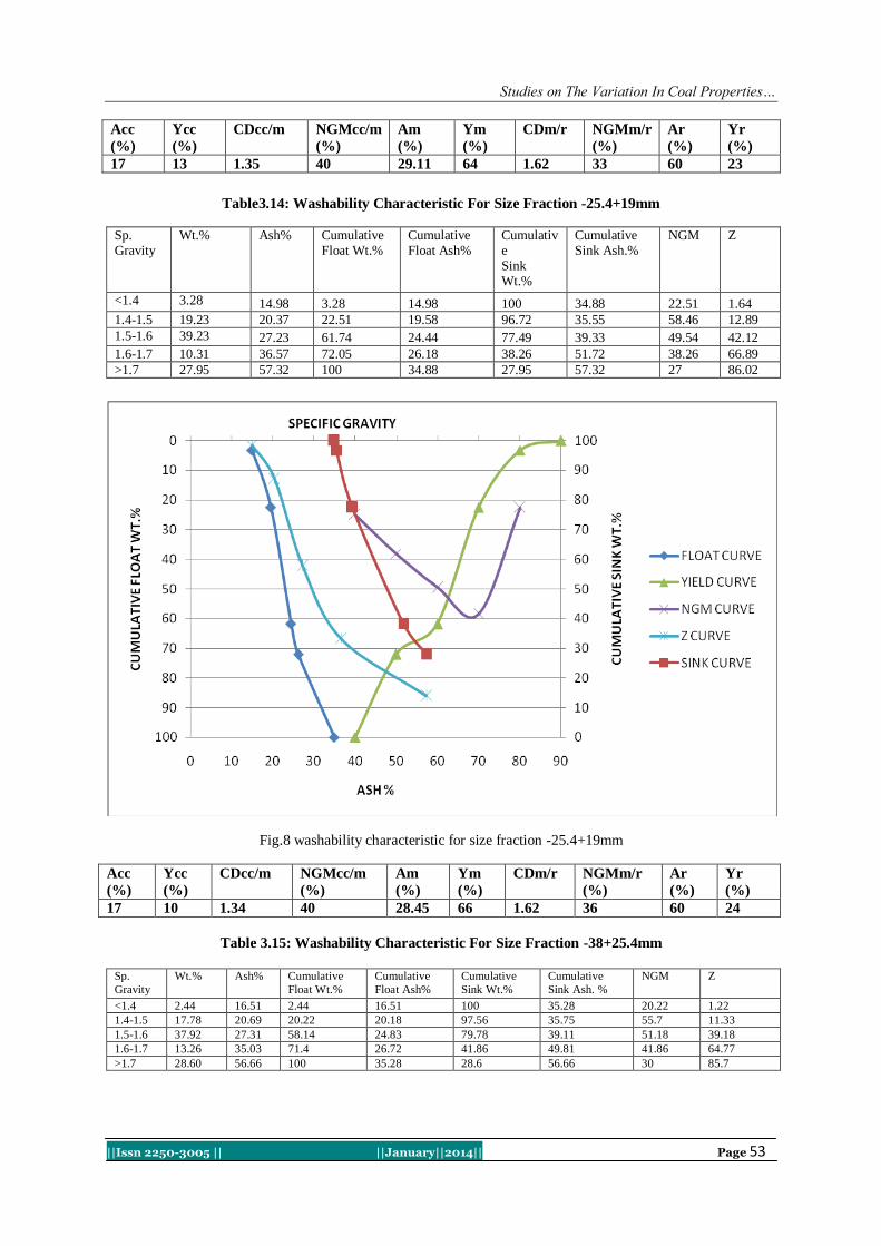
Studies on The Variation In Coal Properties…
||Issn 2250-3005 || ||January||2014|| Page 53
Acc
(%)
Ycc
(%)
CDcc/m NGMcc/m
(%)
Am
(%)
Ym
(%)
CDm/r NGMm/r
(%)
Ar
(%)
Yr
(%)
17 13 1.35 40 29.11 64 1.62 33 60 23
Table3.14: Washability Characteristic For Size Fraction -25.4+19mm
Sp. Gravity
Wt.% Ash% Cumulative Float Wt.%
Cumulative Float Ash%
Cumulative Sink Wt.%
Cumulative Sink Ash.%
NGM Z
<1.4 3.28 14.98 3.28 14.98 100 34.88 22.51 1.64
1.4-1.5 19.23 20.37 22.51 19.58 96.72 35.55 58.46 12.89
1.5-1.6 39.23 27.23 61.74 24.44 77.49 39.33 49.54 42.12
1.6-1.7 10.31 36.57 72.05 26.18 38.26 51.72 38.26 66.89
>1.7 27.95 57.32 100 34.88 27.95 57.32 27 86.02
Fig.8 washability characteristic for size fraction -25.4+19mm
Acc
(%)
Ycc
(%)
CDcc/m NGMcc/m
(%)
Am
(%)
Ym
(%)
CDm/r NGMm/r
(%)
Ar
(%)
Yr
(%)
17 10 1.34 40 28.45 66 1.62 36 60 24
Table 3.15: Washability Characteristic For Size Fraction -38+25.4mm
Sp.
Gravity
Wt.% Ash% Cumulative
Float Wt.%
Cumulative
Float Ash%
Cumulative
Sink Wt.%
Cumulative
Sink Ash. %
NGM Z
<1.4 2.44 16.51 2.44 16.51 100 35.28 20.22 1.22
1.4-1.5 17.78 20.69 20.22 20.18 97.56 35.75 55.7 11.33
1.5-1.6 37.92 27.31 58.14 24.83 79.78 39.11 51.18 39.18
1.6-1.7 13.26 35.03 71.4 26.72 41.86 49.81 41.86 64.77
>1.7 28.60 56.66 100 35.28 28.6 56.66 30 85.7
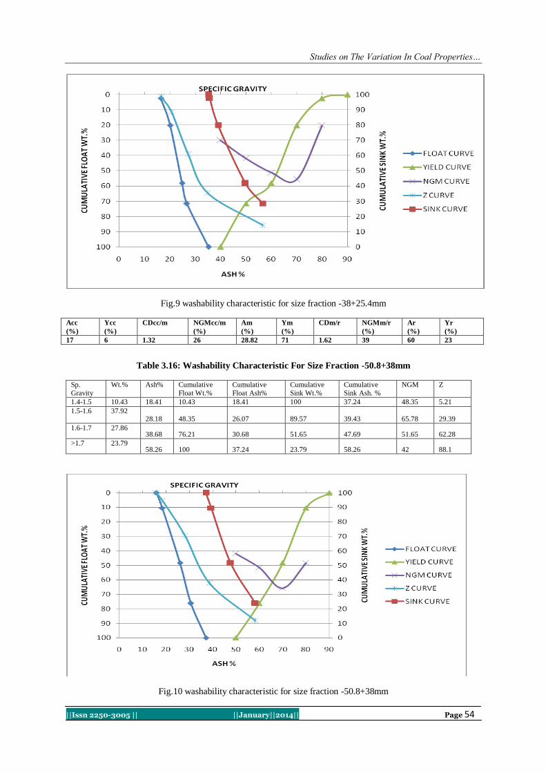
Studies on The Variation In Coal Properties…
||Issn 2250-3005 || ||January||2014|| Page 54
Fig.9 washability characteristic for size fraction -38+25.4mm
Acc
(%)
Ycc
(%)
CDcc/m NGMcc/m
(%)
Am
(%)
Ym
(%)
CDm/r NGMm/r
(%)
Ar
(%)
Yr
(%)
17 6 1.32 26 28.82 71 1.62 39 60 23
Table 3.16: Washability Characteristic For Size Fraction -50.8+38mm
Sp.
Gravity
Wt.% Ash% Cumulative
Float Wt.%
Cumulative
Float Ash%
Cumulative
Sink Wt.%
Cumulative
Sink Ash. %
NGM Z
1.4-1.5 10.43 18.41 10.43 18.41 100 37.24 48.35 5.21
1.5-1.6 37.92 28.18 48.35 26.07 89.57 39.43 65.78 29.39
1.6-1.7 27.86 38.68 76.21 30.68 51.65 47.69 51.65 62.28
>1.7 23.79 58.26 100 37.24 23.79 58.26 42 88.1
Fig.10 washability characteristic for size fraction -50.8+38mm
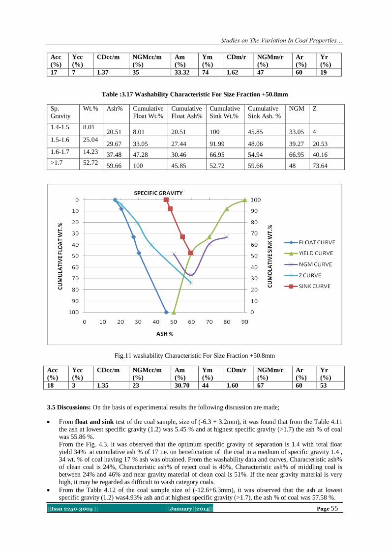
Studies on The Variation In Coal Properties…
||Issn 2250-3005 || ||January||2014|| Page 55
Acc
(%)
Ycc
(%)
CDcc/m NGMcc/m
(%)
Am
(%)
Ym
(%)
CDm/r NGMm/r
(%)
Ar
(%)
Yr
(%)
17 7 1.37 35 33.32 74 1.62 47 60 19
Table :3.17 Washability Characteristic For Size Fraction +50.8mm
Sp.
Gravity
Wt.% Ash% Cumulative
Float Wt.%
Cumulative
Float Ash%
Cumulative
Sink Wt.%
Cumulative
Sink Ash. %
NGM Z
1.4-1.5 8.01 20.51 8.01 20.51 100 45.85 33.05 4
1.5-1.6 25.04 29.67 33.05 27.44 91.99 48.06 39.27 20.53
1.6-1.7 14.23 37.48 47.28 30.46 66.95 54.94 66.95 40.16
>1.7 52.72 59.66 100 45.85 52.72 59.66 48 73.64
Fig.11 washability Characteristic For Size Fraction +50.8mm
Acc
(%)
Ycc
(%)
CDcc/m NGMcc/m
(%)
Am
(%)
Ym
(%)
CDm/r NGMm/r
(%)
Ar
(%)
Yr
(%)
18 3 1.35 23 30.70 44 1.60 67 60 53
3.5 Discussions: On the basis of experimental results the following discussion are made;
From float and sink test of the coal sample, size of (-6.3 + 3.2mm), it was found that from the Table 4.11
the ash at lowest specific gravity (1.2) was 5.45 % and at highest specific gravity (>1.7) the ash % of coal
was 55.86 %.
From the Fig. 4.3, it was observed that the optimum specific gravity of separation is 1.4 with total float
yield 34% at cumulative ash % of 17 i.e. on beneficiation of the coal in a medium of specific gravity 1.4 ,
34 wt. % of coal having 17 % ash was obtained. From the washability data and curves, Characteristic ash%
of clean coal is 24%, Characteristic ash% of reject coal is 46%, Characteristic ash% of middling coal is
between 24% and 46% and near gravity material of clean coal is 51%. If the near gravity material is very
high, it may be regarded as difficult to wash category coals.
From the Table 4.12 of the coal sample size of (-12.6+6.3mm), it was observed that the ash at lowest
specific gravity (1.2) was4.93% ash and at highest specific gravity (>1.7), the ash % of coal was 57.58 %.

Studies on The Variation In Coal Properties…
||Issn 2250-3005 || ||January||2014|| Page 56
From the Fig 4.4, it can be seenthat the optimum specific gravity of separation is 1.38 with total float yield
26% at cumulative ash % of 17 i.e. on beneficiation of the coal in a medium of specific gravity 1.38,26%
wt. of coal having 17 % ash is achievable. From the washability data and curves, Characteristic ash% of
clean coal is 23%, Characteristic ash % of reject coal is 49%, Characteristic ash % of middling coal is
between 23% and 49% and Near gravity material of clean coal is 55%.
From the Table 4.13 of the coal sample size of (-19+12.6mm),it was found that the ash at lowest specific
gravity (1.3) was13.11% ash and at highest specific gravity (>1.7), the ash % of coal was 56.60 %.
From the Fig 4.5 , it can be depictedthat the optimum specific gravity of separation is 1.35 with total float
yield 13% at cumulative ash % of 17 i.e. on beneficiation of the coal in a medium of specific gravity 1.35, only13 wt. % of coal having 17 % ash could be obtained. From the washability data and curves,
Characteristic ash% of clean coal is 20%, Characteristic ash % of reject coal is 46%, Characteristic ash % of
middling coal is between 20% and 46% and Near gravity material of clean coal is 40%.
From the Table 4.14 of the coal sample size of (-25.4+19mm), it was observed that the ash at lowest
specific gravity (1.3) was14.98% ash and at highest specific gravity (>1.7), the ash % of coal was 57.32 %.
It was It may be observed from Fig 4.6, that the optimum specific gravity of separation is 1.34 with total
float yield 10% at cumulative ash % of coal having 17 % ash. From the washability data and curves,
Characteristic ash% of clean coal is 19%, Characteristic ash % of reject coal is 45%, Characteristic ash % of
middling coal is between 19% and 45% and Near gravity material of clean coal is 40%.
From the Table 4.15 of the coal sample size of (-38+25.4mm), it was found that the ash at lowest specific
gravity (1.3) was16.51% ash and at highest specific gravity (>1.7), the ash % of coal was 56.66 %. It was observed from the Fig 4.7 that the optimum specific gravity of separation is 1.32 with total float yield
6% at cumulative ash %of coal having 17 % ash. From the washability data and curves, Characteristic ash%
of clean coal is 19%, Characteristic ash % of reject coal is 46%, Characteristic ash % of middling coal is
between 19% and 46% and Near gravity material of clean coal is 26%.
From the Table 4.16 of the coal sample size of (-50.8+38mm), it was found that the ash at lowest specific
gravity (1.4) was18.41% ash and at highest specific gravity (>1.7), the ash % of coal was 58.26 %.
It was observed from the Fig 4.8 that the optimum specific gravity of separation is 1.37 with total float yield
7% at17 % cumulative ash %. From the washability data and curves, Characteristic ash% of clean coal is
20%, Characteristic ash % of reject coal is 51%, Characteristic ash % of middling coal is between 19% and
46% and Near gravity material of clean coal is 35%.
From the Table 4.17 of the coal sample size of (+50.8) it was found that the ash at lowest specific gravity (1.4) was20.51% ash and at highest specific gravity (>1.7), the ash % of coal was 59.66 %.
From the Fig4.9, it was observed that the optimum specific gravity of separation is 1.35 with total float
yield 3% at18 % cumulative ash. From the washability data and curves, Characteristic ash% of clean coal is
23%, Characteristic ash % of reject coal is 49%, Characteristic ash % of middling coal is between 23% and
49% and Near gravity material of clean coal is 23%.
IV. CONCLUSION From the experimental result and subsequent discussion the following conclusion are drawn.
Large size fractions of coal contains very high ash% so small size fraction of coal was used for the washing
purpose because it contain comparatively low ash% as it is observed in washability data such as size
fraction from +50.8mm contain high ash% as compare to small size fraction from -6.3+3.2mm as very low
ash%.
Generally, washability of low volatile medium coking coal can be improved by crushing it to lower size.
Most of the washaries wash the LVMC coal up to a size of -13mm but on further grinding it to lower sizes
of around -3mm increases the yield further. Difficult washability characteristics of LVMC coal is due to
fine dissemination of mineral particles with macerals and ash% of marketable product which can further be
improved by making coal blendable with prime coking coal, so that this coal can be used in various steel plants.
On the basis of results obtained by conducting different experiments and considering different aspects of
beneficiation, a complete cost-benefit analysis is necessary prior to taking decision of washing these coals.
Crushing at lower size involves increased cost of size reduction, cost of beneficiation and the handling cost
of materials although there is increase in the yield of the beneficiated coal.
From the washability analysis, crushing of coal to less than ½ inch is economical.
From the washability data it is observed that for coal crushed to 1/8 -1/4 inch at 17% ash the yield is 34 %
at 1.4 cut gravity.
Washing at 17% ash, NGM is very high. It indicates difficult washing. So there is need for blending LVMC
(after beneficiation) with prime coking coal.

Studies on The Variation In Coal Properties…
||Issn 2250-3005 || ||January||2014|| Page 57
The clean coal can be used as a blend constituent for coke making in steel plants and the middling’s can be
used in power plants.
Utilization of LVMC coals after suitable beneficiation can reduce the import of coking coal, thereby saving
considerable amount of foreign exchange.
REFERANCES [1] Geological Survey of India (GSI) Report, Government of India 2009: Inventory of Indian Coal Resources.
[2] J. W. Leonard “Coal Preparation, Ed.”, SMME, CO. 1991.
[3] Osborne, DG 1988. Coal Preparation Technology, Vol. 1
[4] SAMEER SARKAR,1996, Fuels and Combustion, 2nd edition, Orient Longman Publication, Mumbai.
[5] Indian Standard: 13810, 1993, Code of Practice for Float and Sink analysis of Coal, Bureau of Indian Standards, New Delhi.
[6] O.P.GUPTA., 1990, Fuels, Furnaces and Refractory, 1st edition, Khanna Publication, Delhi.
[7] Bird, B. M., 1931, Interpretation of Float-and-sink Data, Proceedings of the Third International Conference on Bituminous Coal,
Pittsburgh. vol 2,
[8] James G. Speight, Mercel Dekker, 1994, The Chemistry and Technology of coal. 1st edition
[9] D.V. SubbaRao, Coal Its Beneficiation, M.K. Publications, 2003.
[10] Tsai, S. C., “Fundamental of Coal Beneficiation and Utilization”, Elsevier,
[11] Amsterdam, 1982
[12] Hills L M, Solid fuel grindability: Literature review
[13] SN 2986 Portland cement Association, Skokie, [14] Illinois USA 2007

International Journal of Computational Engineering Research||Vol, 04||Issue, 1||
||Issn 2250-3005 || ||January||2014|| Page 58
Pre-Loading Impact on Mechanical Properties of Sand-
Polystyrene-Cement Mix
Aneke I.F.1, Agbenyeku E.E.
2
1 & 2 Department of Civil Engineering science, University of Johannesburg, P.O Box-524, Auckland Park
2006, South Africa
I. INTRODUCTION Recently lightweight geomaterial particularly the expanded polystyrene (EPS) block geofoams have
been more widely used in infrastructure rehabilitation and construction of roads and embankments (Frydenlund,
2001). Studies on the properties of EPS materials have been looked into by Chun et. al., (2004). The benefits of
ESP geo-blocks were also discussed by Stark et. al., (2004). Nonetheless there are disadvantages in the
applications of ESP (Deng, 2001) which include;
[1] Prefabrication of EPS blocks off-site and which involves cost of transportation.
[2] Stiffness and properties of ESP blocks cannot be changed easily to suit in-situ soil properties.
[3] EPS blocks are made into irregular shaped blocks and cannot readily fill irregular volumes.
[4] EPS materials have poor fire tolerance i.e. its level of fire resistance is very low.
However when the use of EPS blocks becomes difficult, lightweight materials made with EPS-sand and
cement becomes an alternative Yoonz et. al., 92004). The strength of the EPS beads increases due to cement
hydration effect and water is used in enhancing the workability of the mix and to activate hydration in the
presence of cement. The densities and properties of the cement-polystyrene-sand (CPS) can be changed easily
by adjusting the EPS-sand or cement-sand ratios which also change the densities when pre-loading stresses are
applied to the specimens after 12hours before the specimens completely set. The lightweight geomaterial have a
low density and yet adequate strength. The main advantage of (CPS) mix lightweight geomaterial is that it can
be produced in slurry form and poured to any formwork to set. Hence, it is particularly suitable for use as a load
carrying lightweight geomaterial.Although, there is still insufficient information on the application from any
standard or code as such, this study is based on laboratory experimentations. The different compositions of EPS-
sand, cement-sand, water-sand and the pre-loading effects on density, UCS and Young modulus, E, of the CPS
specimens were investigated.
II. EXPERIMENTAL DETAILS 2.1. Materials
Four material constituents were used in the study; cement, EPS, sand and water. The EPS beads were
round in shape with diameters ranging between 1.5-2mm which was compressible and almost weightless. Fine
aggregate commonly called river sand was collected from a local river in Pretoria, South Africa. Physical
constituent properties of the sand are shown in Table 1. Ordinary Portland cement was used as binder and tap
water was used for the mixing and curing sessions.
ABSTRACT: A laboratory study on the formation of lightweight material by blending sand with polystyrene (EPS)
and cement is presented. The effects of pre-loading compositions of EPS-sand, cement-sand and water-
sand ratios on strength and densities of lightweight geomaterial were investigated. Mixes of 40%EPS-
60%sand (as fine aggregate) and 50%EPS-50%sand with 15%cement to both mixes made up the
specimens composition. The density of the control specimen was 1681.3kg/m3 which was reduced to
1185.8kg/m3 and 1070.23kg/m
3 when 40% and 50%EPS were added respectively. Hence it was
observed that the mixture of 40%EPS and 60%sand with 15% cement content under a pre-loading
stress of 600kPa had the highest unconfined compressive strength (UCS) and density. The volumetric
mix design used in this study can be applied when robust or lightweight carrying geomaterial is
required in construction.
KEYWORDS: Unconfined compressive strength, Lightweight, Polystyrene, Pre-loading

Pre-Loading Impact On Mechanical Properties…
||Issn 2250-3005 || ||January||2014|| Page 59
2.2. Mix ratio and material preparation
The mixing ratio in this study is defined as a ratio of two different components batched by percentage volume,
i.e. water-soil (w/s), cement-sand (c/s) and EPS-sand (eps/s). The mixing ratios studied herein are given in Table
2. These ratios were selected based on trial mixes of different ratios.
Table 1: Physical constituent properties of sand
Parameters Results
Water content, w (%) 0.6
Dry Density γ(kg/m3) 1681.304
Specific Gravity (Gs) 1.6
Particles Size 0.2 - 0.4
The mechanical performances of the lightweight geomaterial were observed to vary. The effect of different mix
ratios on the strength as well as pre-loading stresses on the densities and UCS of the lightweight product were
recorded. Nevertheless it is noted that the trail mix design was tracked by volumetric batching since EPS were
almost weightless.
Table 2: Component ratios of EPS by mass volume to sand
EPS/S (%)
Ratio
Water/Cement
Cement (%)
Ratio
Cement/Sand Density ɣ (kg/m
3)
Total
volume (m3)
10-90 0.4 15 0.17 1541 3.289 x 10⁻⁴
20-80 0.4 15 0.19 1359 3.289 x 10⁻⁴
30-70 0.4 15 0.22 1264.82 3.289 x 10⁻⁴
40-60 0.4 15 0.25 1185.80 3.289 x 10⁻⁴
50-50 0.4 15 0.3 1070.23 3.289 x 10⁻⁴
60-40 0.4 15 0.38 933.40 3.289 x 10⁻⁴
70-30 0.4 15 0.5 796.59 3.289 x 10⁻⁴
2.3 Test Method
Measurement by volume of the specimen cylinder with 40-60% and 50-50% of EPS-sand mix was
taken based on the targeted density of the lightweight product. 60% sand by volume of the cylinder was
measured out and filled to the brim with the corresponding volume of EPS after which water was added
according to the mix design. This was homogenous mixed into slurry for 5mins and 15% cement was added.
The slurry production took approximately 15mins. After a thorough mix the slurry was cast for the different
percentage variations as shown in Figures 1 and the pre-loading stresses were applied after the specimens were
allowed to set for 12hours as seen in the pre-loading setup in Figure 2.
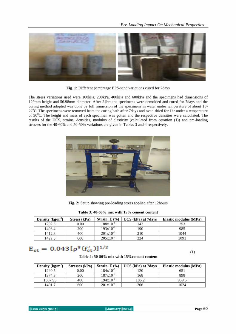
Pre-Loading Impact On Mechanical Properties…
||Issn 2250-3005 || ||January||2014|| Page 60
Fig. 1: Different percentage EPS-sand variations cured for 7days
The stress variations used were 100kPa, 200kPa, 400kPa and 600kPa and the specimens had dimensions of
129mm height and 56.98mm diameter. After 24hrs the specimens were demolded and cured for 7days and the
curing method adopted was done by full immersion of the specimens in water under temperature of about 18-
220C. The specimens were removed from the curing bath after 7days and oven-dried for 1hr under a temperature
of 300C. The height and mass of each specimen was gotten and the respective densities were calculated. The
results of the UCS, strains, densities, modulus of elasticity (calculated from equation (1)) and pre-loading
stresses for the 40-60% and 50-50% variations are given in Tables 3 and 4 respectively.
Fig. 2: Setup showing pre-loading stress applied after 12hours
Table 3: 40-60% mix with 15% cement content
Density (kg/m3) Stress (kPa) Strain, Ε (%) UCS (kPa) at 7days Elastic modulus (MPa)
1292.5 0.00 188x10-6
142 753
1403.4 200 193x10-6
190 985
1412.3 400 201x10-6
210 1044
1422.5 600 205x10-6
224 1091
(1)
Table 4: 50-50% mix with 15%cement content
Density (kg/m3) Stresses (kPa) Strain, Ε (%) UCS (kPa) at 7days Elastic modulus (MPa)
1240.5 0.00 184x10-6
120 651
1374.3 200 187x10-6
168 898
1387.95 400 194x10-6
186.2 959.5
1401.7 600 201x10-6
206 1024

Pre-Loading Impact On Mechanical Properties…
||Issn 2250-3005 || ||January||2014|| Page 61
III. RESULT AND DISCUSSION 3.1 Effects of EPS-sand variations on Density
The results of densities for the tested specimens prepared using different ratios of both EPS and sand
are presented in Figure 3. It was observed that by mixing 40%EPS-60%sand the density of the specimen was
reduced to 1185.8kg/m3 which is a significant improvement as compared to the density of the control sample of
1628 kg/m3. Density change with the ratio of EPS-sand added caused a 1.4kg/m
3 decrease as compared to the
control density.
Fig. 3: EPS-sand ratio effect on density of specimens
However, the effect of cement/sand ratio contributed to reasonable increments in the densities of the mix and a
significant increase in densities were observed for pre-loaded specimens. The addition of 15% cement was
observed to increase the density by 1.2kg/m3 thereby recording a reduction in the density of the control
specimen as the EPS percentage increased as shown in Figure 4. A slight increase in the density with a constant
15%cement content was observed with the addition of water and at a constant W/C = 0.4.
Fig. 4: Cement-sand ratio effect on density of specimens
3.2 Effects of EPS-sand variations on UCS
The EPS-sand ratios were found to have significant effects on the UCS of the respective specimens
such that, the percentage variations showed increase in UCS as the densities of the specimens increased.
However, over the 7days curing periods the UCS values for the 40-60% mix ratios were observed to be higher
than the 50-50% mixes as shown in Figure 5.
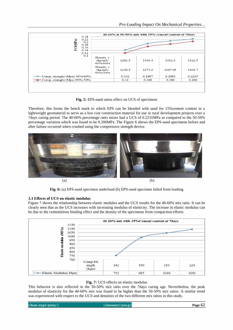
Pre-Loading Impact On Mechanical Properties…
||Issn 2250-3005 || ||January||2014|| Page 62
Fig. 5: EPS-sand ratios effect on UCS of specimens
Therefore, this forms the bench mark to which EPS can be blended with sand for 15%cement content in a
lightweight geomaterial to serve as a low cost construction material for use in rural development projects over a
7days curing period. The 40-60% percentage ratio mixes had a UCS of 0.2235MPa as compared to the 50-50%
percentage variation which was found to be 0.206MPa. The Figure 6 shows the EPS-sand specimens before and
after failure occurred when crushed using the compressive strength device.
(a) (b)
Fig. 6: (a) EPS-sand specimen underload (b) EPS-sand specimen failed from loading
3.3 Effects of UCS on elastic modulus
Figure 7 shows the relationship between elastic modulus and the UCS results for the 40-60% mix ratio. It can be
clearly seen that as the UCS increases with increasing modulus of elasticity. The increase in elastic modulus can
be due to the cementitious binding effect and the density of the specimens from compaction efforts.
Fig. 7: UCS effects on elastic modulus
This behavior is also reflected in the 50-50% mix ratio over the 7days curing age. Nevertheless, the peak
modulus of elasticity for the 40-60% mix was found to be higher than the 50-50% mix ratios. A similar trend
was experienced with respect to the UCS and densities of the two different mix ratios in this study.

Pre-Loading Impact On Mechanical Properties…
||Issn 2250-3005 || ||January||2014|| Page 63
Fig. 8: UCS effects on elastic modulus
A peak modulus of elasticity value for the 40-60% mix was gotten as 1091MPa as against 1024MPa for the 50-
50% mix ratio. The relationship between elastic modulus and the UCS results for the 50-50% ratios in shown in
Figure 8.
3.4 Effects of Pre-loading on UCS
The pre-loading effects on the strength of the EPS-sand geomaterial for the different stresses are
displayed in Figure 9. It is observed that as the pre-loading stress increases the UCS also increased. The
compactness of the specimens was found to increase under the increasing stresses such that the densities were
also found to increase. Pre-loading stresses of 200kPa, 400kPa and 600kPa were initiated in this study.
Fig. 9: Pre-loading effects on UCS
Reductions in the heights of the specimens were observed to increase under increased pre-loading effects. The
highest UCS values for both mix ratios were achieved under a pre-loading stresses of 600MPa. UCS values of
0.2235MPa and 0.206MPa for 40-60% and 50-50% ratios were achieved under pre-loading stresses of for
600MPa respectively.
3.5 Stress-strain behavior of EPS-sand specimens
The behavioral pattern of the tested specimens shows a direct correlation between the stresses and
strains (calculated from the modulus of elasticity) of the specimens from both mixes. It is clearly revealed in
Figure 10 that the strain on the samples increased with increasing applied stresses.

Pre-Loading Impact On Mechanical Properties…
||Issn 2250-3005 || ||January||2014|| Page 64
Fig. 10: Stress-strain relationship
The 40-6% ratios were found to have the highest strain values as compared to the 50-50% mix ratios. Hence, for
a stress value of 223.5MPa a corresponding strain value of 205MPa was achieved for the 40-60% mix while a
206MPa stress created a strain of 201MPa for a mix ratio of 50-50% over the 7days curing period.
Comparison of respective sample mix ratios
Comparisons made between the 40%-60 % and 50%-50 % mix ratios showed their densities ranged
from 1400kg/m3-1430kg/m
3 for the 600kPa pre-load samples but for the 0kPa (non pre-loaded control samples)
the density was between ranges of 1200kg/m3-1300kg/m
3. The 600kPa stresses had the highest effects on both
the 40-60 % and 50-50% mixes. Furthermore, the elastic modulus for the 40-60% ratios was still higher as
compared to the 50-50% ratios across the various stresses of 600kPa, 400kPa, 200kPa and 0kPa. Therefore
from this study, the bench mark for durable lightweight geomaterial mix ratios is a mixture of 40-60% under a
stress effect of 600kPa which can be applied in single and double leave masonry wall but is however noted that
the load carrying light weight geomaterial is directly proportional to the pre-loading stress applied to the geo-
product.
IV. CONCLUSION Laboratory tests were conducted on the formation of lightweight material by blending sand with EPS and
cement. The effects of pre-loading compositions of EPS-sand, cement-sand and water-sand ratios on strength
and densities of lightweight geomaterial were investigated and the following conclusions were reached;
The UCS of light weight geomaterial is affected by the mix proportion and the cement content.
Curing effect on the specimen was very significant even for a short curing age of 7days.
Lightweight material can be produced from a mixture of CPS having a density in the ranges of 1750kg/m3-
2150 kg/m3.
15%cement content increased the UCS of the mix due to cement hydration effect.
The density and UCS properties of the geomaterial mix are made flexible by adjusting the CPS material
constituent ratios.
REFERENCES [1] Frydenlund, T.E and Aabo , R., “ Long term performance and durability of EPS as a lightweight filling material”, EPS Geofoam 3rd
Intern. Conf.,Salt Lake City, Utah, 2001.
[2] Chun, B.S, Lim, H , S, Sagong, m,Kim, K, 2004, Development of hyperbolic constitutive mode ( for expanded polystyrene (Eps)
geofoams under triaxial compression tests. Geotextiles & Geomembrane 22, 223-237. [3] Stark, T D, Arellans, D, Horvart, J.S, Leishchinsky, D, 2004 Geofoam application in the design and construction of highway
embankments. NCHRP Web Document, Vol .65, Transportation Research Board, USA.
[4] Yoonz, G, Jeon, S, Kim, B, 2004, mechanical characteristics of lightweighted soil using dredged materials. Marine Georesources & Geotechnology 22 (4), 215-229.
[5] Deng, A 2001, The influence of different soils properties on stabilization behavior of reinforced soil. Soil Engineering &
Foundation 15 (2), 31-34.

International Journal of Computational Engineering Research||Vol, 04||Issue, 1||
||Issn 2250-3005 || ||January||2014|| Page 65
The Effect of Activating Flux in Tig Welding
Akash.B.Patel 1, Prof.Satyam.P.Patel
2
I. INTRODUCTION Until the end of the 19th century, the only welding process was forge welding, which blacksmiths had
used for centuries to join iron and steel by heating and hammering. Arc welding and oxyfuel welding were
among the first processes to develop late in the century, and electric resistance welding followed soon after.
Welding technology advanced quickly during the early 20th century as World War I and World War II drove the
demand for reliable and inexpensive joining methods. Following the wars, several modern welding techniques
were developed, including manual methods like shielded metal arc welding, now one of the most popular welding methods, as well as semi-automatic and automatic processes such as gas metal arc welding, submerged
arc welding, flux-cored arc welding and electro slag welding.Welding is a fabrication or sculptural process that
joins materials, usually metals or thermoplastics, by causing coalescence. This is often done by melting the work
pieces and adding a filler material to form a pool of molten material (the weld pool) that cools to become a
strong joint, with pressure sometimes used in conjunction with heat, or by itself, to produce the weld. This is in
contrast with soldering and brazing, which involve melting a lower-melting-point Material between the work
pieces to form a bond between them, without melting the work pieces.
Fig. 1 – Schematic diagram of the Diagram of arc and weld area, in shielded metal arc welding.
1. Coating Flow
2. Rod
3. Shield Gas
4. Fusion
5. Base metal
6. Weld metal
7. Solidified Slag
Welding is used as a fabrication process in every industry large or small. It is a principal
means of fabricating and repairing metal products. The process is efficient, economical and dependable as a
means of joining metals. This is the only process which has been tried in the space. The process finds its
applications in air, underwater and in space.
ABSTRACT Quality and productivity play important role in today’s manufacturing market. Now a day’s due
to very stiff and cut throat competitive market condition in manufacturing industries . The main objective
of industries reveal with producing better quality product at minimum cost and increase
productivity.TIG welding is most vital and common operation use for joining of two similar or dissimilar
part with heating the material or applying the pressure or using the filler material for increasing
productivity with less time and cost constrain. To obtain main objective of company regards quality and
productivity. In the present research project an attempt is made to understand the effect of TIG welding
parameters such as welding current , gas flow rate ,electrode angle ,that are influences on responsive output parameters such as weld penetration, depth to width ratio, strength of weld joint by using
optimization philosophy. The effort to investigate optimal machining parameters and their contribution
on producing better weld quality and higher Productivity

The Effect Of Activating Flux On Tig Welding…
||Issn 2250-3005 || ||January||2014|| Page 66
Why welding is used, because it is suitable for thicknesses ranging from fractions of a millimetre to a third of a
meter Versatile, being applicable to a wide range of component shapes and sizes.
Flux:
The term Flux is overcome from Latin word fluxus and it means flow.
It is a chemical cleaning agent, flowing agent, or purifying agent.
Flux are mainly used to remove oxide impurities of weld and also absorb impurities from slag. The activator in flux used to reduce corrosive effect at room temperature and increase the temperature of job at
certain level.
For most welding operation commonly used fluxes are SiO2 , TiO2 , Cr2O3 , ZrO2 , Al2f3 etc .
Inert Gases Used In TIG welding:
[1] Argon: Argon is most commonly used gas for TIG welding .It can be used on all metals.
[2] Helium: Pure helium can be used for welding aluminum and copper alloys.
[3] Helium-argon mixtures: Helium-argon mixtures give deeper penetration, greater heat input and hence faster
welding.
[4] Argon-hydrogen mixture: Addition of hydrogen to argon increases the arc voltage and provides benefits
similar to helium.
INTRODUCTION TO TIG WELD
Fig. 1: schematic diagram of TIG welding
Equipment:
[1] Welding power source, high frequency unit, dc suppressor unit and cables.
[2] Welding torch, tungsten electrode and filler metals.
[3] Inert gas cylinder, pressure regulator and flow meter. [4] Cooling water supply.
[5] Water and gas solenoid valves.
It is an arc welding process wherein coalescences produced by heating the job with an electric struck
between a tungsten electrode and the job. A shielded gas (argon, helium, nitrogen, etc) is used to avoid
atmospheric contamination of the molten weld pool.A filler metal may be added, if required.Welding current,
water and inert gas supply are turned on. The arc struck either by touching the electrode with a scrap tungsten
piece or using a high frequency unit.In the first method arc is initially struck on a scrap tungsten piece and then broken by increasing the arc length. This procedure repeated twice or thrice warms up the tungsten electrode.
The arc is then struck between the electrode and precleaned job to be welded. This method avoids breaking
electrode tip, job contamination and tungsten loss.In the second method, a high frequency current is
superimposed on the welding current. The welding torch (holding the electrode) is brought nearer to the job.
When electrode tip reaches within a distance of 3 to 2 mm from the job, a spark jumps across the air gap
between the electrode and the job. The air path gets ionized and arc is established.After striking the arc, it is
allowed to impinge on the job and a molten weld pool is created. The welding is started by moving the torch
along the joint as in oxy-acetylene welding. At the far end of the job, arc is broken by increasing the arc length.
The shielding gas is allowed to impinge on the solidifying weld pool for a few seconds even after the arc is
extinguished. This will avoid atmospheric contamination of the weld metal.

The Effect Of Activating Flux On Tig Welding…
||Issn 2250-3005 || ||January||2014|| Page 67
The welding torch and filler metal are generally kept inclined at angles of 70-80˚ and 10-20˚
respectively with the flat work piece. A leftward technique may be used. A flux (derived from Latin fluxes
meaning “flow”), is a chemical cleaning agent, flowing agent, or purifying agent. Fluxes may have more than
one function at a time. They are used in both extractive metallurgy and metal joining.The role of a flux in
joining processes is typically dual: dissolving of the oxides on the metal surface, which facilitates wetting by
molten metal, and acting as an oxygen barrier by coating the hot surface, preventing its oxidation. In some
applications molten flux also serves as a heat transfer medium, facilitating heating of the joint by the soldering
tool or molten solder
ADVANTAGES:
[1] No flux is used; hence there is no danger of flux entrapment when welding refrigerator and air conditioner
components.
[2] Because of clear visibility of the arc and the job, the operator can exercise a better control on the welding.
[3] This process can weld in all positions smooth and sound welds with fewer spatters.
[4] TIG welding is very much suitable for high quality welding of thin material
DISADVANTAGES: [1] Tungsten if it transfers to molten weld pool can contaminate the same. Tungsten inclusion is hard and
brittle.
[2] Filler rod end if it by change comes out of the inert gas shield can cause weld metal contamination.
[3] Equipment costs are higher than that for flux shielded metal are welding
APPLICATIONS:
[1] Welding aluminum, magnesium ,copper ,nickel and their alloys, carbon, alloys or stainless steel, inconel
,high temperature and hard surfacing alloys like zirconium, titanium etc. [2] Welding sheet metal and thinner sections.
[3] Welding of expansion bellows, transistor cases, instrument diaphragms, and can-sealing joints.
[4] Precision welding in atomic energy, aircraft, chemical and instrument industries.
[5] Rocket motor chamber fabrications in launch vehicles.
II. LITRETURE REVIEW From 1995, there are lot of articles are published on effect of flux in Tig welding. Not all the articles
are directly related to our work, especially, those articles which were focused on computational work. Many
articles addressed experimental findings and remaining discussed various theories. In this subsection, we are
going to discuss only those articles (experimental and/or theoretical work) which are directly related to current
work.
JAGJIT RANDHAWA[1] was carried out Tig welding process and experimental investigations towards Effect
Of A-Tig Welding Process Parameters On Penetration In Mild Steel Plates are conducted. TIG welding is
mostly used to weld thin sections for high surface finish. A major drawback in the processes having very small
penetration as compare to other arc welding process. The problem can be avoided by using active flux in
conventional TIG welding. In the present study investigate the optimization of A-TIG welding process on mild steel for an optimal parameter by using Taguchi technique. The effect of various process parameters (welding
current (I), welding speed (V), active flux) .IN the present study efforts were made to increase the weld
penetration by Appling the active flux and to optimize the process parameters.
J. NIAGAJ[2] The impact of activating flux and selected fluorides on A-TIG welding of Grade 2 titanium. The
paper also presents the dimensions and macrostructure of welds and describes welded joints produced with BC-
Ti activating flux as well as the mechanical properties such as strength, impact energy and hardness of specific
weld zones. In addition, the article contains information about performed bend tests and results of
macrostructure investigation.
A.R. Ibrahim[3] Gas tungsten arc welding is fundamental in those industries where it is important to control the
weld bead shape and its metallurgical characteristics. However, compared to the other arc welding process, the shallow penetration of the TIG welding restricts its ability to weld thick structures in a single pass (~ 2 mm for
stainless steels), thus its productivity is relativity low. This is why there have been several trials to improve the
productivity of the TIG welding. The use of activating flux in TIG welding process is one of such attempts. In
this study, first, the effect of each TIG welding parameters on the weld’s penetration depth was shown and then,

The Effect Of Activating Flux On Tig Welding…
||Issn 2250-3005 || ||January||2014|| Page 68
the optimal parameters were determined using the Taguchi method with L9 (34) orthogonal array. SiO2 and TiO2
oxide powders were used to investigate the effect of activating flux on the TIG weld penetration depth and
mechanical properties of 316L austenitic stainless steel. A camera was used to observe and record images of the
welding arc, and analyze the relationship between increasing the penetration depth and arc profile. The
experimental results showed that activating flux aided TIG welding has increased the weld penetration, tending
to reduce the width of the weld bead. The SiO2 flux produced the most noticeable effect. Furthermore, the
welded joint presented better tensile strength and hardness.
Syarul Asraf Mohamat[4] Flux Core Arc Welding (FCAW) is an arc welding process that using continuous flux-cored filler wire. The flux is used as a welding protection from the atmosphere environment. This project is
study about the effect of FCAW process on different parameters by using robotic welding with the variables in
welding current, speed and arc voltage. The effects are on welding penetration, micro structure and hardness
measurement. Mild steel with 6mm thickness is used in this study as a base metal. For all experiments, the
welding currents were chosen are 90A, 150A and 210A and the arc voltage is 22V, 26V and 30V respectively.
20, 40 and 60 cm/min were chosen for the welding speed. The effect will studied and measured on the
penetration, microstructure and hardness for all specimens after FCAW process. From the study, the result
shown increasing welding current will influenced the value depth of penetration increased. Other than that, the
factors that can influence the value of depth of penetration are arc voltage and welding speed.
Cheng-Hsien Kuo[5] The effect of oxide fluxes on surface appearance, weld morphology, angular distortion,
and weld defect obtained with activated tungsten inert gas (TIG) process applied to the welding of 6 mm thick dissimilar metal plates between JIS G3131mild steel and SUS 316L stainless steel. The CaO, Fe2O3, Cr2O3, and
SiO2 fluxes used were packed in powdered form. The results indicated that the surface appearance of TIG welds
produced with oxide flux formed residual slag. TIG welding with SiO2 powder can increase joint penetration
and weld depth-to-width ratio, and therefore the angular distortion of the dissimilar weldment can be reduced.
Furthermore, the defects susceptibility of the as-welded can also be reduced.
I. SAMARD[6] The influence of the activating flux on the weld joint properties at the drawn arc stud welding
process with ceramic ferrule is analyzed. In the experimental part of the paper, the arc stud welding process is
applied with the application of the activating flux for ATIG process. In order to evaluate the influence of the
activating flux on the welding process parameters variations, the main welding parameters were monitored by
an on-line monitoring system. Besides monitoring of welding current and voltage, the influence of the active-
ting flux on the weld joint appearance is investigated. The macro sections of the weld joints welded with the
same parameters, but with and without the presence of activating flux.
Michael lui[7] Conventional gas-shielded arc welding processes remain the most applied technique for joining
titanium and titanium alloys. To improve upon single pass weld bead penetration and enhance joining
productivity, augmented tungsten inert gas (A-TIG) welding has been used with fluxes that contain activating
ingredients, such as fluorides of the alkali and alkali earth metals. The effects of cryolite (Na3 AlF6), a complex
fluoride, on weld bead morphology was studied and compared to the effects from the simple fluoride, MgF2.
Cryolite was shown to increase single-pass penetration through a slight arc construction and increase current
density mechanism.
LI Qing-Ming[8] The effects of activating fluxes on welding arc were investigated. A special set of water-
cooling system and stainless steel were used as parent material. During welding process, high-speed camera
system and oscillograph were used for capturing instantaneous arc shape and arc voltage respectively. The experimental results indicate that the SiO2 flux can increase the arc voltage, while TiO2 has no this effect on arc
voltage. Compared with conventional tungsten inert gas welding (C-TIG), it is found that the arc shape of A-
TIG welding used with the SiO2 flux has changed obviously.
P.K. Palani[9]: Austenitic stainless steel cladding is generally used to attain better corrosion resistance
properties to meet the re-quirements of petrochemical, marine, and nuclear applications. The quality of cladded
components depends on the weld bead geometry and dilution, which in turn are controlled by the process
parameters. In this investigation, the effect of cladding parameters such as welding current, welding speed, and
nozzle-to-plate distance on the weld bead geometry was evaluated. The objectives of controlling the weld bead
geometry can easily be achieved by developing equations to pre-dict these weld bead dimensions in terms of the
process parameters. Mathematical equations were developed by us-ing the data obtained by conducting three-
factor five-level factorial experiments. The experiments were conducted for 317L flux cored stainless steel wire of size 1.2 mm diameter with IS:2062 structural steel as a base plate. Sensitivity anal-ysis was performed to

The Effect Of Activating Flux On Tig Welding…
||Issn 2250-3005 || ||January||2014|| Page 69
identify the process parameters exert-ing the most influence on the bead geometry and to know the parameters
that must be most carefully controlled. Studies reveal that a change in process parameters affects the bead width,
dilution, area of penetration, and coefficient of internal shape more strongly than it affects the penetration,
reinforce-ment, and coefficient of external shape.
Dr. M. Vasudevan[10]: Specific activated flux has been developed for enhancing the penetration performance
of the TIG welding process for welding of type 304 LN and type 316LN stainless steels. A significant increase
in penetration of over 300% has been observed in single pass TIG welding. The significant improvement in
penetration was attributed to constriction of the arc and the reversal of Marangoni flow. The use of flux has been found to overcome the variable weld penetration observed during auto genous TIG welding of austenitic
stainless steel with less than 50 ppm silver. There was no degradation in the microstructure and mechanical
properties of welds produced by A-TIG welding compared to that of conventional TIG welding process.Liming
Liu[11]: The Cadmium Chloride flux increases the weld penetration evidently in the Alternating Current
Tungsten inert gas (AC TIG) welding of magnesium alloy. In the present study, in order to investigate the effect
of the CdCl2 active flux on the weld shape and arc voltage, bead-on-plate specimens are made on AZ31B
magnesium alloy pre-placed with CdCl2 active flux by the AC TIG process. Weld pool cross-sections and the
arc voltage are analyzed under different welding parameters, welding speed, weld current and arc length. The
results showed that compared to the conventional AC-TIG, welding penetration and the weld depth/width with
CdCl2 flux are both two times greater than that of without flux under optimal parameters. The voltage decreases with decreasing of travel speeds and arc length decreasing. Besides, the phenomenon of arc trailing in the EN
period and arc contraction in the EP period were observed in AC TIG welding of magnesium alloy with CdCl2
flux. It found that the arc voltage increases with the increases of welding current, more energies are supplied for
welding, resulting in the increases of arc voltage and weld penetration.T. Kannan[12]: The main problem faced
in duplex stainless steel cladding is the selection of the optimum combination of process parameters for
achieving the required quality of clad. This paper highlights an experimental study carried out to analyse the
effects of various flux cored arc welding (FCAW) process parameters on important clad quality parameters in
duplex stainless steel cladding of low carbon structural steel plates. The experiments were conducted based on
four-factor five level central composite rotatable design with full replications technique and having
mathematical models developed using multiple regression method. The effects of the input process parameters
on clad quality parameters have been presented in graphical form, which helps in selecting welding process parameters to achieve the desired clad quality quickly.
H. Y. Huang[13]: The aim of the present study was to investigate the effect of specific oxide fluxes on the
surface appearance, weld morphology, retained d ferrite content, hot cracking susceptibility, angular distortion
and mechanical properties obtained with the tungsten inert gas (TIG) process applied to the welding of 5 mm
thick austenitic stainless steel plates. An autogenous gas tungsten arc welding process was applied to stainless
steels through a thin layer of activating flux to produce a bead on plate welded joint. The MnO2 and ZnO fluxes
used were packed in powdered form. The experimental results indicated that the 80% MnO2–20% ZnO mixture
can give full penetration and also a satisfactory surface appearance for type 304 stainless steel TIG flux welds.
TIG welding with MnO2 and/or ZnO can increase the measured ferrite number in welds, and tends to reduce hot
cracking susceptibility in as welded structures. It was also found that TIG flux welding can significantly reduce
the angular distortion of stainless steel weldments.
P. Kanjilal[14]: Rotatable designs based on statistical experiments for mixtures have been developed to predict
the combined effect of flux mixture and welding parameters on submerged arc weld metal chemical composition
and mechanical properties. Bead-on-plate weld deposits on low carbon steel plates were made at different flux
composition and welding parameter combinations. The results show that flux mixture related variables based on
individual flux ingredients and welding parameters have individual as well as interaction effects on responses,
viz. weld metal chemical composition and mechanical properties. In general, two factor interaction effect are
higher than the individual effect of mixture related variables. Amongst welding parameters, polarity is found to
be important for all responses under study.
Chunlin Dong[15]: This paper deals with a basic Understanding about arc welding with the activating flux. The
effect of various fluxes on the penetration depth and welding arc profiles is investigated in conventional TIG
welding of stainless steel. Arc contraction can be verified with the result of video observation. The fluid flow be heavier is visualized in real-time scale by the use of micro-focused X-ray transmission high-speed video
observation system. Stronger inward fluid flow patterns leading to weld beads with narrower width and deeper
penetration can be apparently identified in the case of A TIG welding.

The Effect Of Activating Flux On Tig Welding…
||Issn 2250-3005 || ||January||2014|| Page 70
It is understood that the activating flux, which draws a lot of attention in increasing welding penetration
and improving welding productivity for TIG welding of stainless steel, will be positively applied in other fields
when more merits of the active flux are identified and qualified, such as eliminating undercutting in keyhole
mode plasma arc welding of stainless steel.Chunli YANG[16]: The mechanism of penetration depth increased
by activating flux in activating tungsten inert gas (A-TIG) welding was studied by measuring the distribution of
trace element Bi in the weld and monitoring the change of arc voltage during A-TIG welding of stainless steel
0Crl8Ni9 with fluxes Si02 and Ti02- The results show that the mechanism of penetration depth in A-TIG
welding depends on the sort of flux used. The weld pool convection after coating the flux S1O2 and flux T1O2
is changed inversely compared with convectional TIG welding without flux. The arc voltage is increased by flux Si02 whilst flux Ti02 does not have effect on the arc voltage. The reason of penetration depth increase for Si02
is due to the constriction of arc plasma and the change of surface tension gradient. The increase of weld
penetration depth with Ti02 only ascribes to the change of surface tension gradient.
III. CONCLUSION From various literature survey efforts to identify in TIG welding process most of welding parameters
like welding flux, welding current, welding speed, depth to width ratio are generally used in research work. Also
identify TIG welding carried out on different materials like mild steel , titanium alloy, brass, carbon, stainless
steel etc.., But we may be choose work piece material differ from above for experimental work and most applicable in industrial practices. We may be try to find out welding penetration, depth to width ratio, strength
of welding joint by theoretical equations and experimentally measure with help of different input parameter. For
achieving the proseperious result of experimental work and from the letureture study of various research paper
the austentic type stainless steel with grade E321 is selected and fluxes are SIO2&TIO2.
REFERENCES [1] Jagjit Randhawa, Were Carried Out “Effect Of A-Tig Welding Process Parameters On Penetration In Mild Steel Plates.
[2] J. Niagaj, Were Carried Out “Peculiarities Of A-Tig Welding Of Titanium And Its Alloys”.
[3] E. Ahmadi, A.R. Ibrahim, were carried out “The effect of activating fluxes on 316L stainless steel weld joint characteristic in TIG
welding using the Taguchi method”
[4] Syarul Asraf Mohamat, were carried out “The Effect of Flux Core Arc Welding (FCAW) processes on different parameters “
[5] Cheng-Hsien Kuo, were carried out “Effect of activated TIG flux on performance of dissimilar welds between mild steel and
stainless steel”
[6] I. SAMARD, were carried out “INFLUENCE OF THE ACTIVATING FLUX ON WELD JOINT PROPERTIES AT ARC STUD
WELDING PROCES”
[7] MICHAEL LIU, were carried out “A-TIG Welding of CP Titanium Plates Using Cryolite-Containing Flux Pastes and Flux-Cored
Wires”
[8] LI Qing-ming,WANG Xin-hong was carried out “Effect of activating flux on arc shape and arc voltage in tungsten inert gas
welding.” .
[9] P.K. Palani was carried out Sensitivity Analysis for Process Parameters in Cladding of Stainless Steel by Flux Cored Arc Welding.
[10] Dr. M. Vasudevan was carried out Penetration Enhancing Activated Flux for TIG Welding of Stainless Steels.
[11] Liming Liu was carried out Effect of Cadmium Chloride Flux in Active Flux TIG Welding of Magnesium Alloys.
[12] T. Kannan was carried out Effect of flux cored arc welding process parameters on duplex stainless steel clad quality.
[13] H. Y. Huang was carried out Evaluation of TIG flux welding on the characteristics of stainless steel.
[14] P. Kanjilala was carried out Combined effect of flux and welding parameters on chemical composition and mechanical properties of
submerged arc weld metal.
[15] Chunlin Dong was carried out Preliminary Study on the Mechanism of Arc Welding With the Activating Flux.
[16] Chunli YANGt was carried out Research on the Mechanism of Penetration Increase by Flux in A-TIG Welding.

International Journal of Computational Engineering Research||Vol, 04||Issue, 1||
||Issn 2250-3005 || ||January||2014|| Page 1
Independent and Total Strong (Weak) Domination in
Fuzzy Graphs
P.J.Jayalakshmi1, S.Revathi
2 , C.V.R. Harinarayanan
3
1Associate Professor,Department of Mathematics,Indra Ganesan College of Engineering, Trichy-
12, Tamilmadu, India 2Assistant Professor,Department of Mathematics,Saranathan Engineering College, Trichy,
Tamilmadu, India 3Research Supervisor&Assistant Professor, Department of Mathematics,Government Arts College,
Paramakudi, Tamilnadu,India
I. INTRODUCTION The study of dominating sets in graphs was begun by Ore and Berge, the domination
number, independent domination number are introduced by Cock-ayne and Hedetniemi. Rosenfeld
[1] introduced the notion of fuzzy graph and several fuzzy analogs of graph theoretic concepts such
as paths, cycles and connectedness.
A.Somasundram and S.Somasundram[2] discussed domination in fuzzy graphs. They
defined domination using effective edges in fuzzy graph. Nagoor Gani and Chandrasekaran[3]
discussed domination, independent domination and irredundance in fuzzy graph using strong arcs.
The concept of Strong (Weak) domination [6] in graphs was introduced by Sampathkumar and
Pushpalatha. The notion of Domination of Domination in fuzzy graphs [7] was developed by
A.Somasundaram and S.Somasundaram.
II. FUZZY INDEPENDENT SET:
Definition 1.1 Let G = (ζ, μ) be a fuzzy graph. Two nodes in a fuzzy graph G are said to be fuzzy
independent if there is no strong arc between them. A subset S of V is said to be fuzzy independent
set for G if every two nodes of S are fuzzy independent.
Definition 1.2 Let G = (ζ, μ) be a fuzzy graph. A fuzzy independent set S of G is said to be
maximal fuzzy independent set if there is no fuzzy independent set whose cardinality is greater
than the cardinality of S. The maximum cardinality among all maximal fuzzy independent set is
called fuzzy independence number of G and it is denoted by γ (G).
FUZZY DOMINATING SET
Definition 1.3 Let G = (ζ, μ) be a fuzzy graph. A subset D of V is said to be a dominating set of G if
for every v ε V - D; there exists a u ε D such that u dominates v.
ABSTRACT Let G be a fuzzy graph. Then D V is said to be a strong (weak) fuzzy dominating set of G if every vertex v ε V- D is strongly(weakly) dominated by some vertex u in D. We denote a strong(weak) fuzzy
dominating set by sfd-set(wfd-set). The minimum scalar cardinality of a sfd-set(wfd-set) is called the
strong(weak) fuzzy domination number of G and is denoted by TGD- number γ sf (G)( γwf (G)). In this
paper we introduce the concept of strong(weak) domination in fuzzy graphs and obtain some
interesting results for this new parameter in fuzzy graphs.
KEY WORDS: Fuzzy Graphs, Fuzzy Domination, Total domination,Fuzzy independent set,
strong(weak)fuzzy domination number, Total strong(weak)fuzzy domination number.

Independent and Total Strong (Weak…
||Issn 2250-3005 || ||January||2014|| Page 2
Definition 1.4 A dominating set D of a fuzzy graph G is called minimal dominating set of G is
there does not exist any dominating set of G, whose cardinality is less than the cardinality of D.
Minimum cardinality among all minimum dominating set in G is called domination number of G is
denoted by γ(G). The smallest cardinality of all independent fuzzy dominating set of G is called
independent fuzzy domination number of G and is denoted by i (G).
FUZZY DOMINATION NUMBER:
Definition 1.5 Let G = (V,ζ, μ ) be a fuzzy graph. Then D V is said to be a fuzzy dominating set of G if
for every v ε V- D, there exists u in D such that μ (u,v) = ζ (u) Λζ(v). The minimum scalar
cardinality of D is called the fuzzy domination number and is denoted by γf(G).
NEIGHBOURHOOD AND EFFECTIVE DEGREES OF A VERTEX:
Definition 1.6 Let G be a fuzzy graph. The neighbourhood of a vertex v in V is defined by N (v) =
{u ε V; μ (u,v) = ζ(u) Λ ζ(v)}. The scalar cardinality of N (v) is the neighbourhood degree of v,
which is denoted by dN(v) and the effective degree of v is the sum of the weights of the edges
incident on v, denoted by dE(v).
STRONG (WEAK) FUZZY VERTEX DOMINATION:
Definition 1.7 Let u and v be any two vertices of a fuzzy graph G. Then u strongly dominates v (v weakly
dominates u) if
(i) μ (u,v) = ζ(u) Λ ζ (v) and (ii) dN (u) ≥ dN (v).
STRONG (WEAK) FUZZY DOMINATION NUMBER:
Definition 1.8 Let G be a fuzzy graph. Then Then D V is said to be strong(weak) fuzzy dominating set of G if for
every vertex v ε V- D is strongly(weakly) dominated by some vertex u in D. We denote a
strong(weak) fuzzy dominating set by sfd-set(wfd-set). The minimum scalar cardinality of a sfd-
set(wfd-set) is called a strong(weak) fuzzy domination number of G and it is denoted by
γsf (G)( γwf (G)).
TOTAL DOMINATION:
Definition 1.9 The set S is said to be total dominating set if for every vertex v ε γ(G), v is adjacent to atleast one
vertex of S.
TOTAL STRONG (WEAK) FUZZY VERTEX DOMINATION:
Definition 1.10 Let u and v be any two vertices of a fuzzy graph G. Then u strongly dominates v (v weakly
dominates u) if
(i) μ (u, v) ≥ ζ(u) Λ ζ(v) and (ii) dN (u) ≥ dN (v) and (iii) for every vertex v ε γ(G); v is adjacent to
atleast one vertex of S.
Proposition 1.11 Let D be a Total minimal sfd-set of a fuzzy graph G. Then for each vεD, one of the following
holds:
1. No vertex in D strongly dominates V. 2. There exists u ε V- D such that v is the only vertex in D which strongly dominates u.
3. If for every vertex v ε V (G), v is adjacent to atleast one vertex of S.

Independent and Total Strong (Weak…
||Issn 2250-3005 || ||January||2014|| Page 3
Proposition 1.12 For a fuzzy graph G of order p,
(1) γtf (G) ≤ γ tsf (G) ≤ p - ΔN(G) ≤ p – ΔE (G).
(2) γtf (G) ≤ γtsf (G) ≤ p - ΔN(G) ≤ p – ΔE (G), where ΔN (G)[ ΔE(G)] and δN(G)[δE(G)] denote the maximum and minimum neighbourhood degrees(effective degrees) of G.
Definition 1.13 A set D contained V of a fuzzy graph G is said to be Total Independent if
(i) μ(u,v)= ζ(u) Λ ζ(v) for all u,v in D
(ii) if for every vertex v ε V(G), v is adjacent to atleast one vertex of S.
MINIMUM AND MAXIMUM NEIGHBOURHOOD OF VERTEX DEGREE
Definition 1.14
VδN = {v ε V : dN (v) = δN(G)} and VΔN = {v ε V : dN (v) = ΔN (G)}.
Lemma 1.15
Let G is a fuzzy graph. If D is an TIWFDS (Total Independent Weak Fuzzy
Dominating Set) of G, then D ∩ VδN ≠ Ф.
Proof:
Let v ε VδN. Since D is an TIWFDS, V ε D or there exists a vertex u ε D such that
μ(u,v)= ζ(u) Λ ζ(v) for which dN (u) ≤ dN (v).
If v ε D, then clearly D ∩ VδN ≠ Ф. On the other hand, dN (u) = dN (v), since dN
(v) = δN(G) which implies u ε VδN. Therefore, D ∩ VδN ≠ Ф.
Proposition 1.16:
Let G be a fuzzy graph. Then itwf (G) = p - δN(G) iff V- (v) is Total independent
for every v ε VδN.
Proof:
Let D be an TIWFDS of G. Then by Lemma 1.15, D ∩ VδN ≠ Ф.
Let v ε D ∩ VδN . since D is independent, D ∩ N(v) = Ф which implies D
contained V – N(v) which implies |D|f ≤ |V – N(v)|f
Then itwf(G) ≤ |D|f ≤ |V – N(v)|f .
We state the following results without proving theorem, since they are
analogous to the results on itwf(G).
Lemma 1.17
Let G be a fuzzy graph. If D is an TISFDS of G, then D ∩ VδN ≠ Ф.
Proposition 1.18
For a fuzzy graph G, itsf(G) ≤ p - ΔN(G).
Proposition 1.19
Let G be a fuzzy graph with itsf(G) ≤ p - ΔN(G) and Let v ε VΔN Then V – N(v) is
independent.
Proposition 1.20
Let G be a fuzzy graph. Then itsf(G) ≤ p - ΔN(G) iff V - N(v) is independent for
every v ε VΔN.

Independent and Total Strong (Weak…
||Issn 2250-3005 || ||January||2014|| Page 4
EXAMPLE:
[1.] A.Nagoor Gani, and V.T.Chandrasekaran, Domination in Fuzzy Graph, Advances in Fuzzy Sets and Systems, 1
(1)(2006),17-26.
[2.] 2..Nagoor Gani, P.Vadivel, Contribution to the Theory of Domination, Independence and Irrenundance in Fuzzy
Graph, Bulletin of Pure and Applied Sciences, Vol-28E(No-2) 2009, 179-187.
[3.] A.Nagoor Gani, P.Vadivel, On Domination, Independence and Irrenun-dance in Fuzzy Graph, International Review
of Fuzzy Mathematics, Volume 3, No 2, (June 2008) 191-198.
[4.] A.Nagoor Gani, P.Vadivel, On Irredundance in Fuzzy Graph, Proceed-ing of the National Conference on Fuzzy
Mathematics and Graph Tho-ery, Jamal Mohamed college, Tiruchirappalli, March 2008., 40-43.
[5.] agoor Gani, P.Vadivel, On the sum of the Cardinalities of Indepen-dent and Independent Dominating S sets in
Fuzzy Graph, Advances in fuzzy sets and systems, Volume 4, Number 2, 2009, page 157-165.
[6.] A.Nagoorgani, P.Vadivel, Relation between the Parameters of Indepen-dent Domination and Irredance in Fuzzy
Graph, International Journal of Algorithms, Computing and Mathematics, Volume 2, Number 1, February 2009.
[7.] A.Somasundaram and S.Somasundaram, Domination in fuzzy graphs-I, Pattern recognition Letters 19(1998), 787-
791.
[8.] E.J.Cockayne and S.T.Hedetniemi, Towards a theory of domination in graphs, Networks,(1977), 247-261.
[9.] 9 J.N.Mordeson and P.S.Nair, Fuzzy graphs and Fuzzy Hypergraphs, Physica Verag, Heidelberg, 1998; second
edition 2001.
[10.] A.Rosenfeld Fuzzy graphs, in; L.A.Zadeh, K.S.Fu, M.Shimura(Eds.), Fuzzy sets and their Applications to
Congnitive and Decision Processes, Academic Press, New York, 1975, 77-95.
[11.] E.Sampathkumar, L.Pushpalatha, Strong, Weak domination and dom-ination balance in a graph, Discrete Math.
161(1996), 235-242.
[12.] Domke et. Al, On parameters related to strong and weak domination in graphs, Discrete Mathematics 258(2002), 1-
11.
[13.] 13 T.W.Haynes et. Al, Fundamentals of Domination in graphs, Marcel
[14.] Dekker, New York, 1998.

International Journal of Computational Engineering Research||Vol, 04||Issue, 1||
||Issn 2250-3005 || ||January||2014|| Page 75
Effect of discrete heating on natural convection heat transfer on
square plate
Dr. V Katti, Asst. prof. S G Cholake, Anil Rathod PG student Dept. of Mechanical engineering
BLDEA’S DR. P G HALAKATTI college of Engineering and Technology Bijapur, India
I. INTRODUCTION With advances in science and technology, modern machines are operated by electronic instruments with use of
integrated circuit board which in turn chips are mounted on circuit board. These chips act as a source of heat located at discrete
points on board. Location of these discrete points plays a vital role in heat transfer by natural convection.
Most of the literatures available worked on numerical analysis with least work on experimental analysis as given
by lino et.al[1] presented experimental and numerical study of flat vertical plate with constant heat flux resulted in correlation
of local nusselt number as a fuction of Rayleigh number mohamad et.al[2] numerically studied natural convection through
horizontal enclosure heated discretely by varying Rayleigh number and aspect ratio efforts has been carried on size and
arrangement of heat source and sink the result is well documented by deng[3]. The heat transfer and fluid flow charecteristics
was greatly influenced by material properties tang ei al.[4] conducted 2D numerical study on porous rectangular enclosure
with saturated fluid and Brinkman extended Darcy model was used to formulate fluid flow in the cavity. younghe ghae[5]
investigated on vertical porous annulus the governing fluid flow equation was solved by an implicit finite volume method for a
wide range of Rayleigh Darcy number for different heat source length and location. The placing of the discrete heat source is
significant when the heat source is placed in an enclosure which is well presented in M. sankar[6] were heat source was varied
along the inner wall of rectangular porous enclosure while the outer wall is maintained lower temperature the numerical result
reveals that the maximum temperature decreases with Rayleigh number. Some other researchers carried their work on
parameters such as porosity of the media, aspect ratio of the enclosure and Darcy number the variation of these parameters
greatly influence the average Nusselt number investigated by j m lopeze et al.[7].
The present study experimentally and numerically investigates the effect of discrete heat source length and location
on a rectangular flat plate with fixed aspect ratio and the variation of Nusselt number. Numerical analysis is performed using
commercially available CFD software ANSYS FLUENT to solve the governing differential equation. The experimental results are in good agreement with numerical result.
II. EXPERIMENTAL SETUP
Experiment was build to evaluate effect of discrete heating on flat horizontal plate for natural convection heat transfer
mode. The atmospheric air is used as convective fluid and resistance type of heater is employed for heat source on left side
wall while the upper portion is exposed to convective currents, the unheated portion and bottom wall are kept adiabatic with
proper insulation as shown in the fig. 1 the exposed surface of the plate is put in non dimensional aspect ratio (l/b) equal to 1,
the thickness of the plate is 6mm available commercially. The mechanical and thermal properties of the copper plate and air
are standard values from [8]. The heater is of resistance type made up of mica sheet and nichrome wire, wound to mica sheet
fig.2. The two terminals of the heater are shouldered and given to power supply with proper electric circuits as shown in fig. 1.
Abstract Experimental and numerical analysis is presented for steady state natural convection from discrete heating
inside a two dimensional square copper plate. The study has been made for different heater length and
location. The left side wall is heated discretely at an interval of 12.5 mm keeping remaining portion
unheated portion adiabatic. The experimental study is performed on an experimental setup designed in
order to assuming, with a good approximation, those adopted natural convection hypotheses on a heated
horizontal flat plate. The finite volume method is used to solve the dimensionless governing equations.
The temperature distribution are presented at different heater length and location which reveals, Nusselt
number increases when heater is located at mid height from base distributing heat uniformly setting up
proper convection currents as compared to other positions and with increase in heater length temperature
increases at hot wall. The results obtained from experiment are found to be in good agreement with
numerical results and previous researchers.
Index Terms— Natural convection, discrete heating, heat transfer enhancement.

Effect of discrete heating on natural…
||Issn 2250-3005 || ||January||2014|| Page 76
Fig. 1- Experimental setup with electric connection.
The ammeter and voltmeter are arranged in serial and parallel respectively to record current and voltage
across heater, dimmer stat is used to regulate current through the circuit. The preparation of heater is shown in fig.
2
Fig. 2- Heater arrangement and lengths.
Heater lengths and location are chosen to be 25, 50, 75 and 100 mm given in terms of non dimensional
number [8]. The insulation is provided with glass wool with minimum losses in downstream, the unheated side
walls are made adiabatic with Bakelite sheet. A graduated scale is provided towards left side to locate the heater.
The energy input is through electric supply by carefully recording ammeter and voltmeter reading, the radiations
emitted by the plate is captured in IR camera to measure the temperature distribution on the pate, keeping the
emissivity of the plate uniform. The measured values are in good agreement with CFD software results.
III. DATA REDUCTION
in the present work the energy input to the specimen is by electric supply which is calculated by Q=VI where
V is voltage, I is current. The loss of energy is minimum and is neglected, the only mode of energy transfer is by
convection through exposed top surface calculated as
Q = V I= h A (Ts-Ta) , Nu = hL/k, q = ½(Q/A)
Q is heat input in Watt, h is heat transfer coefficient in W/m2K, A is exposed surface area, Ts & Ta are surface and
ambient air temperature in Kelvin, L is characteristic length in m and k is thermal conductivity in W/m-K.
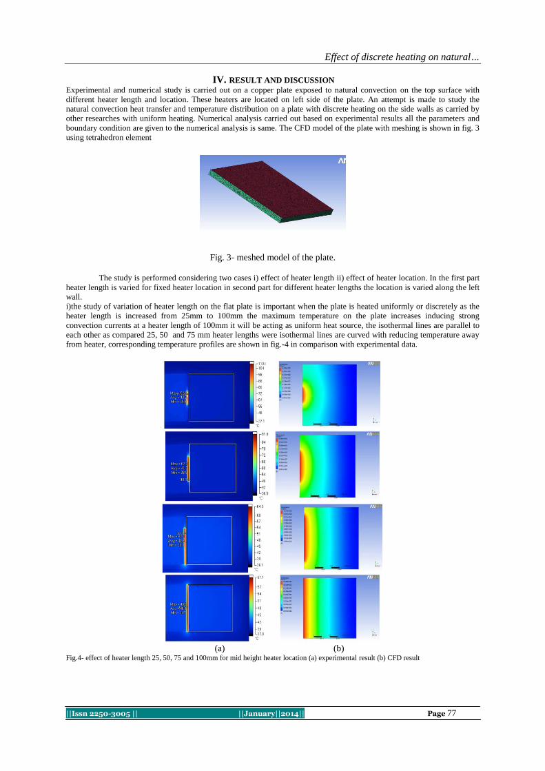
Effect of discrete heating on natural…
||Issn 2250-3005 || ||January||2014|| Page 77
IV. RESULT AND DISCUSSION Experimental and numerical study is carried out on a copper plate exposed to natural convection on the top surface with
different heater length and location. These heaters are located on left side of the plate. An attempt is made to study the
natural convection heat transfer and temperature distribution on a plate with discrete heating on the side walls as carried by
other researches with uniform heating. Numerical analysis carried out based on experimental results all the parameters and
boundary condition are given to the numerical analysis is same. The CFD model of the plate with meshing is shown in fig. 3
using tetrahedron element
Fig. 3- meshed model of the plate.
The study is performed considering two cases i) effect of heater length ii) effect of heater location. In the first part
heater length is varied for fixed heater location in second part for different heater lengths the location is varied along the left
wall.
i)the study of variation of heater length on the flat plate is important when the plate is heated uniformly or discretely as the
heater length is increased from 25mm to 100mm the maximum temperature on the plate increases inducing strong
convection currents at a heater length of 100mm it will be acting as uniform heat source, the isothermal lines are parallel to
each other as compared 25, 50 and 75 mm heater lengths were isothermal lines are curved with reducing temperature away
from heater, corresponding temperature profiles are shown in fig.-4 in comparison with experimental data.
(a) (b)
Fig.4- effect of heater length 25, 50, 75 and 100mm for mid height heater location (a) experimental result (b) CFD result
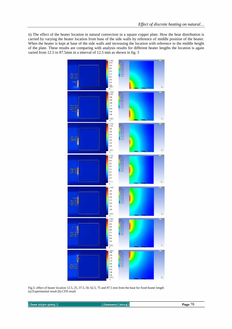
Effect of discrete heating on natural…
||Issn 2250-3005 || ||January||2014|| Page 78
ii) The effect of the heater location in natural convection in a square copper plate. How the heat distribution is
carried by varying the heater location from base of the side walls by reference of middle position of the heater.
When the heater is kept at base of the side walls and increasing the location with reference to the middle height
of the plate. These results are comparing with analysis results for different heater lengths the location is again
varied from 12.5 to 87.5mm in a interval of 12.5 mm as shown in fig. 5
Fig.5- effect of heater location 12.5, 25, 37.5, 50, 62.5, 75 and 87.5 mm from the base for fixed heater length (a) Experimental result (b) CFD result
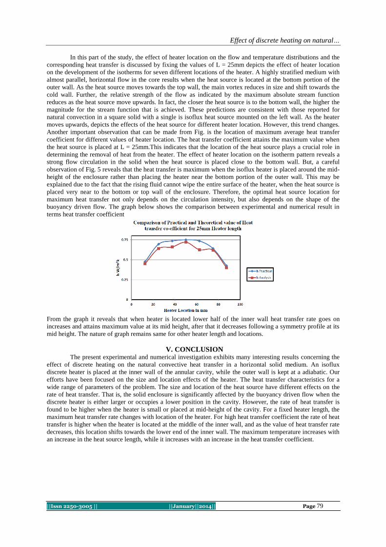
Effect of discrete heating on natural…
||Issn 2250-3005 || ||January||2014|| Page 79
In this part of the study, the effect of heater location on the flow and temperature distributions and the
corresponding heat transfer is discussed by fixing the values of L = 25mm depicts the effect of heater location
on the development of the isotherms for seven different locations of the heater. A highly stratified medium with
almost parallel, horizontal flow in the core results when the heat source is located at the bottom portion of the
outer wall. As the heat source moves towards the top wall, the main vortex reduces in size and shift towards the
cold wall. Further, the relative strength of the flow as indicated by the maximum absolute stream function
reduces as the heat source move upwards. In fact, the closer the heat source is to the bottom wall, the higher the
magnitude for the stream function that is achieved. These predictions are consistent with those reported for
natural convection in a square solid with a single is isoflux heat source mounted on the left wall. As the heater
moves upwards, depicts the effects of the heat source for different heater location. However, this trend changes.
Another important observation that can be made from Fig. is the location of maximum average heat transfer
coefficient for different values of heater location. The heat transfer coefficient attains the maximum value when
the heat source is placed at L = 25mm.This indicates that the location of the heat source plays a crucial role in
determining the removal of heat from the heater. The effect of heater location on the isotherm pattern reveals a
strong flow circulation in the solid when the heat source is placed close to the bottom wall. But, a careful
observation of Fig. 5 reveals that the heat transfer is maximum when the isoflux heater is placed around the mid-
height of the enclosure rather than placing the heater near the bottom portion of the outer wall. This may be
explained due to the fact that the rising fluid cannot wipe the entire surface of the heater, when the heat source is
placed very near to the bottom or top wall of the enclosure. Therefore, the optimal heat source location for
maximum heat transfer not only depends on the circulation intensity, but also depends on the shape of the
buoyancy driven flow. The graph below shows the comparison between experimental and numerical result in
terms heat transfer coefficient
From the graph it reveals that when heater is located lower half of the inner wall heat transfer rate goes on
increases and attains maximum value at its mid height, after that it decreases following a symmetry profile at its
mid height. The nature of graph remains same for other heater length and locations.
V. CONCLUSION The present experimental and numerical investigation exhibits many interesting results concerning the
effect of discrete heating on the natural convective heat transfer in a horizontal solid medium. An isoflux
discrete heater is placed at the inner wall of the annular cavity, while the outer wall is kept at a adiabatic. Our
efforts have been focused on the size and location effects of the heater. The heat transfer characteristics for a
wide range of parameters of the problem. The size and location of the heat source have different effects on the
rate of heat transfer. That is, the solid enclosure is significantly affected by the buoyancy driven flow when the
discrete heater is either larger or occupies a lower position in the cavity. However, the rate of heat transfer is
found to be higher when the heater is small or placed at mid-height of the cavity. For a fixed heater length, the
maximum heat transfer rate changes with location of the heater. For high heat transfer coefficient the rate of heat
transfer is higher when the heater is located at the middle of the inner wall, and as the value of heat transfer rate
decreases, this location shifts towards the lower end of the inner wall. The maximum temperature increases with
an increase in the heat source length, while it increases with an increase in the heat transfer coefficient.

Effect of discrete heating on natural…
||Issn 2250-3005 || ||January||2014|| Page 80
VI. NOMENCLATURE A exposed surface area to air (m
2)
L length of the plate (m)
B breadth of the plate (m)
l/b aspect ratio
h heat transfer coefficient (W/m2K)
k thermal conductivity (W/mK)
q heat flux (W/m2)
Ts,Ta surface and ambient air temperature (K)
Nu Nusselt number (hL/k)
REFERENCES
[1] Douglas machado and Ramos Rodrigo Carriji “Natural convection On Verticle Flat Plates: A numerical and experimental study”
international congress of mechanical dept(2003)
[2] Sezai and mohamad A A “ Natural convection from a discrete heat source on the bottom of a horizontal enclosure”,int. J. Heat and mass transfer43(2000)
[3] Qi-Hong Deng “ fluid flow and heat transfer characteristics of natural convection in square cavities due to discrete source-sink pairs”
int. J. heat and mass transfer vol. 29(2008)
[4] Fu-yun zhao, di liu, guang fa tang “ Natural convection in an enclosure with localized heating and salting from below”,Int. J. of Heat
and mass transfer p.no 2889-2904, vol.51(2008)
[5] Sankar. M.,youngyong park, lopez. J.M and younghae do “ Numerical study of natural convection in vertical porous annulus with
discrete heating” Int. J. Heat and mass transfer(2010)
[6] Sivasankaran. S, younghae do and sankar m “Effect od discrete heating on natural convection in a rectangular porous enclosure”
springer science busuness media B.V.(2010)
[7] Lopez J.M, youngyong park m.sankar “ double-diffusive convection from a discrete heat and solute source in a vertical porous annulus” Journal of mathematical and statistical science(2000)
[8] Incropera and Dewitt “Fundamentals of heat and mass transfer” 5th edition John Wiley publications.

International Journal of Computational Engineering Research||Vol, 04||Issue, 1||
||Issn 2250-3005 || ||January||2014|| Page 1
Slicing Algorithm for Controlling Backtracking In Prolog
Divanshi PriyadarshniWangoo CSE & IT Department
ITM University, Gurgaon, Haryana, India
I. INTRODUCTION Prolog is a programming language for non-numeric and symbolic computations describing
relationships between objects. It comprises of a set of basic mechanisms including pattern matching, tree based
data structuring and automatic backtracking. Spatial relationships between objects are an easy mechanism in
prolog.Relations between objects can be defined by two approaches- either defining relations by facts or
defining relations by rules. A prolog program basically consists of clauses followed by one or more goals.
Prolog clauses are of three types-facts, rules and questions. Facts declare things that are unconditionally true,
rules hold things that are true depending on a given condition and the user can ask the program what things are
true through questions [1]. Recursive rules help in determining the predecessor relation in a family hierarchy program. The programming flow in prolog is defined in the form of structural relations and processing queries
to those relations. The process of determining that whether an object satisfies a query by the means of questions
is often a complicated procedure involving logical inferences, exploring alternatives and backtracking. The
cognitive process of backtracking in prolog system is automatic and is often shrouded from the user.
Uncontrolled backtracking leads to errant execution of prolog clauses and goals. Therefore there is a need of
some strategy involving backtracking that would work efficiently in the situations where the basic backtracking
mechanisms fail under certain conditions. One such structural strategy is slicing which relates the co generic
association between the prolog clauses and goals. This paper is centralized on designing of backtracking
algorithm using dynamic slicing technique. The algorithm is called BTrack_Slicer which takes as input the
Backtrack Dependency Graph (BDG). The BDG is a dependency graph which would relate the clauses in a
prolog program with their respective goals. The BTrack_Slicer algorithm is a novel backup approach for the
prevention of backtracking. It works effectively specially in the cases where the cut and negation process fails in determining the valuable correspondence between the declarative and procedural meaning of the programs.
II. PAPER ORGANIZATION The remaining part of the paper is organized as follows. In Section three, the different slicing
techniques are discussed. Section four states the method of defining the prolog’s recursive rules through
slicing. The designing of the backtracking algorithm with the help of slicing is discussed in section five of the
paper. Section six discusses the results of the BTrack_Slicer algorithm. The last section concludes the paper.
ABSTRACT: This paper focuses on building an efficient slicing algorithm for controlling backtracking in prolog.
Prolog has a built-in backtracking mechanism which alleviates the programmer of explicit
backtracking. The automatic backtracking mechanism is often veiled from the user of the system.
Uncontrolled backtracking causes inefficiency in a program and may lead to interrupted execution.
Slicing technique renders the structural relationship through the ordering of clauses and goals. It
facilitates the backtracking prevention mechanisms through relative structuring of parent goal and the
relative cut in the program. The algorithm is preferential for the events where the cut and negation
mechanisms break down under certain conditions. The slicing algorithm is called BTrack_Slicer and it
takes as input the Backtrack Dependency Graph (BDG) which comprises of all dependencies arising
out of backtracking. Employing the algorithm for use in various application programming structures would lessen the vast execution time expended as a consequence of indefinite backtracking.
KEYWORDS: Backtracking, Backtrack Dependency Graph (BDG),BTrack_Slicer, Dynamic System
Dependence Graph (DSDG) System Dependence Graph (SDG),Prolog.

Slicing Algorithm for Controlling…
||Issn 2250-3005 || ||January||2014|| Page 2
III. SLICING TECHNIQUES Slicing technique is associated with the construction of program slices which are computed with the
help of slicing criterion. The slicing criterion <v, S> defines those part of the program statements that are
actually affected by the slicing criterion, where v is the variable name defined at the program statement number S [2]. Program slicing is done with the construction of the System Dependence Graph (SDG) which is a directed
dependency graph that relates the dependencies occurring between the statements in a program [2]. Researchers
have defined various types of slicing depending on the type of programming applications, the basic types are
static slicing and dynamic slicing. Static slicing determines all the parts of a program that might have an effect
on the slicing criterion and certainly do not make any assumptions regarding the input [3]. Dynamic slicing
defines the dependencies that occur in a specific execution of a program and has an advantage in the run time
execution of the program [3,4]. Dynamic slicing is a more powerful slicing technique as it takes the run time
execution race of the program variables and exactly states the actual affected statements. The dynamic slicing
criterion takes as input the program variable and the statement number. The statements which are actually
affected by the slicing criterion are determined as compared to static slicing which states all the possible input
statements. This results in the construction of precise slices at run time and eliminates unnecessary statements. Thus, dynamic slicing proves to be the highly efficient in determining run time execution traces of a program.
The backtracking algorithm designed in this paper would use the dynamic slicing strategy that will help in
setting the breakpoints at run time execution of the prolog program. The goals would be satisfied for their
related clauses based on the dynamic slicing criterion at run time of the program.
The main aim of using dynamic slicing in the backtracking algorithm is its precise computation of
slices which would be built graphically in the form of Backtrack Dependence Graph (BDG). The BDG would
relate the dependency between the rules of the clauses. The mutual dependency between the rules of the clauses
would be depicted in the form of arcs defined through dependency edges. The breakpoints where the goals fail
would determine the backtracking path in the BDG. The BDG would be taken as input in the BTrack_Slicer
algorithm that works efficiently where the cut and negation fails under the closed world assumption.
IV. STATING PROLOG’S RECURSIVE RULES THROUGH SLICING Prolog’s recursive rules helps in determining the predecessor relationship that exists in a set of clauses.
The predecessor relation can be defined with the help of two rules- direct and indirect. The former aims at
determining the immediate predecessors and the second determine the indirect predecessors [1]. The slicing
criterion that would be taken here for the parent relationship example is dynamic slicing. The Dynamic System
Dependence Graph (DSDG) is specially designed for the recursive procedure rules in prolog. The DSDG
would determine the direct as well as indirect predecessors by taking the slice points in the graph. The solid
directed lines represent direct control dependency and dashed lines represent indirect control dependency
between the nodes. The family relation program is defined in Fig.1 and its corresponding DSDG is defined in Fig2 as follows.
F1 offspring (Y, X) :-
F2 parent (X, Y).
F3 mother (X, Y):-
F4 parent (X, Y),
F5 female (X).
F6 grandparent (X, Z):-
F7 parent (X, Y),
F8 parent (Y, Z).
F9 sister(X, Y):-
F10 parent (Z, X), F11 parent (Z, Y),
F12 female (X),
F13 different (X, Y).
F14 predecessor (X, Z):-
F15 parent(X, Z).
F16 predecessor (X, Z):-
F17 parent (X, Y),
F18 predecessor (Y, Z).
Fig.1 The family hierarchy program in prolog

Slicing Algorithm for Controlling…
||Issn 2250-3005 || ||January||2014|| Page 3
Fig.2 The DSDG of Fig.1
The conventions used for the DSDG of Fig.2 are as follows. The blue color nodes represent the head clauses and
the green color nodes represent the body clauses of the program in Fig.1. The DSGD is useful in getting the
indirect relationships between the clauses defined through recursive rules. The slice point A and slice point B
are the points where the predecessor indirect relationship occurs in the program.
V. BACKTRACKING ALGORITHM USING DYNAMIC SLICING Backtracking in prolog is an automatic process and it executes under the necessary constraints of
satisfying a goal. There are situations which lead to uncontrolled and indefinite backtracking process which
leads to inefficiency in the program execution. Although, prolog has in built mechanisms to prevent and control
backtracking, but these mechanisms prove to be disadvantageous as there are certain reservations against their
use. One of the reservations for the use of backtracking prevention mechanism like cut comes from the fact that
by using cut in a prolog program, it can lose the valuable correspondence between the declarative and
procedural meaning of the programs. Basically there are two levels of meaning of prolog programs- the
declarative meaning and the procedural meaning. The former is concerned only with the relations defined by the
program whereas the latter specifies how the prolog system actually evaluates the relation. Change in the order of the clauses in the presence or absence of cuts can lead to two different outputs which would further lead to
ambiguous results. In such cases there is need of a backtracking algorithm that would be using the dynamic
slicing technique for the prevention of backtracking in the absence of cuts. The backtracking algorithm using
dynamic slicing is called BTrack_Slicer that sets the breakpoints in the program that would lead to backtracking.
The BTrack_Slicer algorithm takes as input the Backtrack Dependency Graph (BDG) and marks the backtrack
breakpoints through the computation of slice points. These slice points are called BTrack slice points and would
work as an alternative to the cut mechanism. Thus, the algorithm turns out to work more efficiently in the
absence of prolog’s in built backtracking prevention mechanisms.
Backtrack Dependency Graph (BDG)
The Backtrack Dependency Graph (BDG) is a directed dependency graph where the nodes of the graph
represent the clauses and the arcs or the edges between the nodes determine the dependencies existing between the structural clauses. The BDG is basically designed to represent the relationships between the objects. It is
used as an input to the BTrack_Slicer algorithm for the processing of the BTrack slice points and sets up the
breakpoints which would trail the backtracking path. The example program that would be used for the
construction of the BDG is to find the largest of the three numbers. The program and its corresponding BDG are
represented in Fig.3 and Fig.4 respectively.
L1 max (X, Y, Z, Max)
L2 max (X, Y, Z, X):-
L3 X>=Y,
L4 X>=Z. L5 max (X, Y, Z, Y):-
L6 X<Y,
L7 Z<Y.
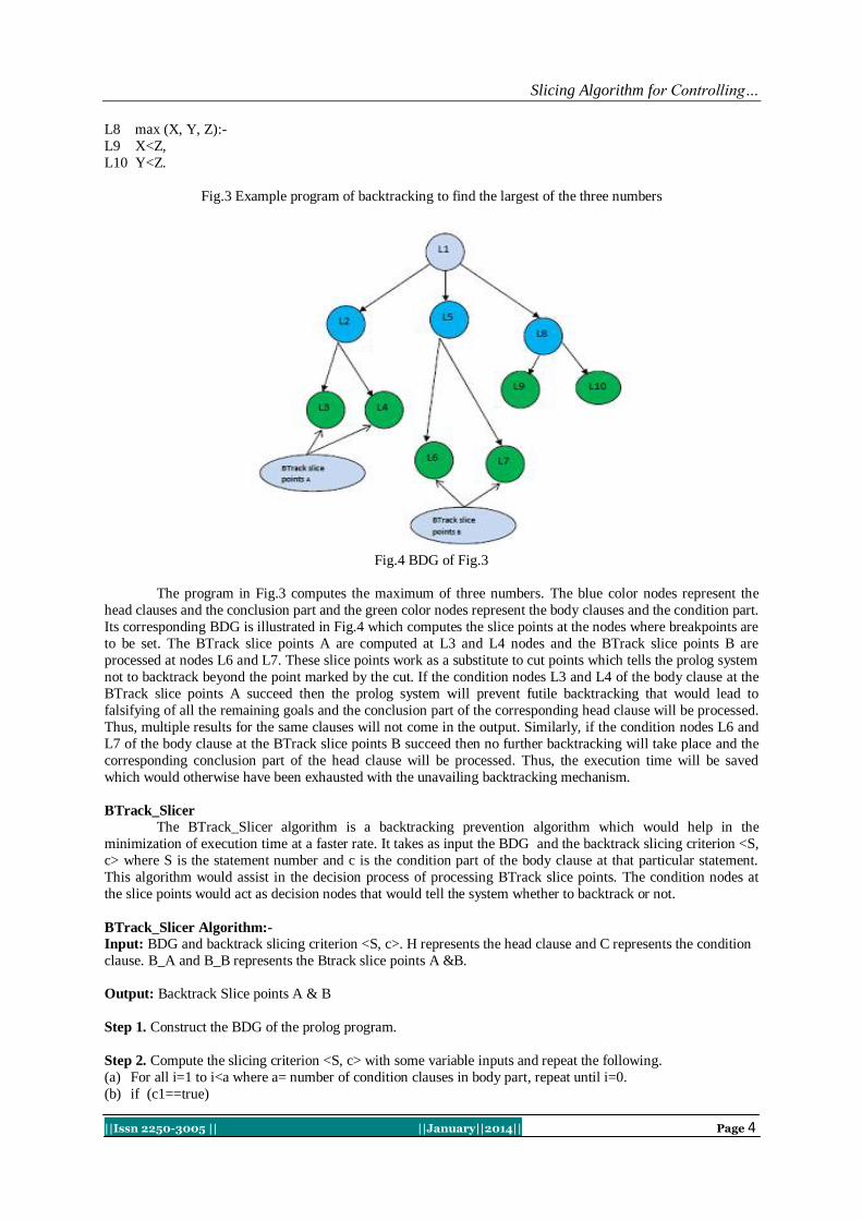
Slicing Algorithm for Controlling…
||Issn 2250-3005 || ||January||2014|| Page 4
L8 max (X, Y, Z):-
L9 X<Z,
L10 Y<Z.
Fig.3 Example program of backtracking to find the largest of the three numbers
Fig.4 BDG of Fig.3
The program in Fig.3 computes the maximum of three numbers. The blue color nodes represent the
head clauses and the conclusion part and the green color nodes represent the body clauses and the condition part.
Its corresponding BDG is illustrated in Fig.4 which computes the slice points at the nodes where breakpoints are
to be set. The BTrack slice points A are computed at L3 and L4 nodes and the BTrack slice points B are
processed at nodes L6 and L7. These slice points work as a substitute to cut points which tells the prolog system
not to backtrack beyond the point marked by the cut. If the condition nodes L3 and L4 of the body clause at the
BTrack slice points A succeed then the prolog system will prevent futile backtracking that would lead to
falsifying of all the remaining goals and the conclusion part of the corresponding head clause will be processed.
Thus, multiple results for the same clauses will not come in the output. Similarly, if the condition nodes L6 and
L7 of the body clause at the BTrack slice points B succeed then no further backtracking will take place and the
corresponding conclusion part of the head clause will be processed. Thus, the execution time will be saved
which would otherwise have been exhausted with the unavailing backtracking mechanism.
BTrack_Slicer
The BTrack_Slicer algorithm is a backtracking prevention algorithm which would help in the
minimization of execution time at a faster rate. It takes as input the BDG and the backtrack slicing criterion <S,
c> where S is the statement number and c is the condition part of the body clause at that particular statement.
This algorithm would assist in the decision process of processing BTrack slice points. The condition nodes at
the slice points would act as decision nodes that would tell the system whether to backtrack or not.
BTrack_Slicer Algorithm:-
Input: BDG and backtrack slicing criterion <S, c>. H represents the head clause and C represents the condition
clause. B_A and B_B represents the Btrack slice points A &B.
Output: Backtrack Slice points A & B
Step 1. Construct the BDG of the prolog program.
Step 2. Compute the slicing criterion <S, c> with some variable inputs and repeat the following.
(a) For all i=1 to i<a where a= number of condition clauses in body part, repeat until i=0.
(b) if (c1==true)

Slicing Algorithm for Controlling…
||Issn 2250-3005 || ||January||2014|| Page 5
(c) if( c2==true)
(d) then stop backtracking and print the corresponding H, B_A & B_B.
(e) elseif (c1==false)
(f) elseif (c2==false)
(g) then proceed backtracking
(h) else backtrack(c1, c2) (i) else backtrack c(i)
(j) result print false goals
(k) else print output H, B_A &B_B
(l) stop
Step 3. End
VI. RESULTS AND ANALYSIS OF BTrack_Slicer ALGORITHM The BTrack_Slicer algorithm takes the dynamic slicing criterion execution trace <S, c> for the condition part of the body clauses and gets the slice point as output which will locate the dependency between
the node clauses and prevent the backtracking at that point. The Table 1 below gives an accurate analysis of the
BTrack_Slicer algorithm and locates the actual number of statements affected and which would be the execution
path in the case where backtracking prevails. The algorithm is accurate under all conditions and is the best
alternative solution to the inbuilt backtracking prevention mechanism.
Table 1
BTrack_Slicer
Algorithm
Execution traces Backtracking
points in
BTrack_Slicer
Statements
affected
Accuracy attained
BTrack_Slicer <L3, X> BTrack slice points A
L2, L1 Yes
<L4, X> BTrack slice
points A
L2, L1 Yes
BTrack_Slicer <L6, Y> BTrack slice points B
L5, L1 Yes
<L7, Y> BTrack slice points B
L5, L1 Yes
VII. CONCLUSION The backtracking controlling algorithm BTrack_Slicer works effectively in the cases where the
backtrack prevention mechanisms fail. The unexpected outcomes and errant executions resulting out of
indefinite backtracking are reduced by employing the BTrack_Slicer algorithm. Also, the execution time of the
program increases rapidly at a faster rate. The utility of the algorithm can be best carried through instances of
pattern matching and categorization grounded problems.
REFERENCES [1] Ivan Bratko, Prolog Programming for Artificial Intelligence, Pearson Education Asia, 3
rd edition, 2001
[2] Donglin Liang and Mary Jean Harrold , “Slicing Objects using System Dependence Graphs,”International Conference on Software
Maintenance,Washington,D.C,pp.358-67,November 1998.
[3] F. Tip. A survey of program slicing techniques. Journal of Programming Languages, 3(3):121–189, Sept. 1995.
[4] N.Sasirekha,A.Edwin Robert and Dr.M.Hemalatha ,” Program Slicing Techniques and its Applications “, International Journal of
Software Engineering & Applications (IJSEA), Vol.2, No.3,pp 50- 64, July 2011

International Journal of Computational Engineering Research||Vol, 04||Issue, 1||
||Issn 2250-3005 || ||January||2014|| Page 6
The Use Of The Computational Method Of Hamming Code
Techniques For The Detection And Correction Of Computational
Errors In A Binary Coded Data: Analysis On An Integer
Sequence A119626.
Afolabi Godfrey1, Ibrahim A.A
2 & Ibrahim Zaid
3
1Department of Mathematics, Joda International School, P.M.B 1031, Kebbi State, Nigeria. 2Department of Mathematics, Sokoto State University, Nigeria. 3Department of Mathematics, Sokoto State University, Nigeria.
I. INTRODUCTION It has been generally observed that in communication, which is the process of transmission and
reception of data from one place to another at some distance or in computational analysis involving integer
sequences are not without error(s). There are a number of reliable codes that can be used to encode data, that is,
adding parity code to the original result (data) obtained so that any error(s) that may occur can be detected and
corrected. Until this is done, communication or computational results obtained will not be efficient talk more of
been reliable. According to [1], the binary coded data (binary number system) is widely used in digital
communication systems. Although the binary number system has many practical advantages and it is widely
used in digital computer, in many cases, it is convenient to work with the decimal number system, especially
when the interaction between human beings and machine is extensive. This is because, most numerical data
generated by humans is basically in terms of decimal numbers. Thus, to simplify the challenges encountered in communication (interaction) or computation between human and machine, several codes have been devised in
which decimal digits are represented by sequences of binary digits that is, in binary coded data form.
Hamming code is one of such codes. It is a set of error-correction codes that can be used to detect and
correct bit errors that can occur when data (information or results obtained) is transmitted, stored or computed as
in [2]. Like other error-correction code, Hamming code makes use of the concept of parity and parity bits, which
are bits that are added to data (say, k parity bits are added to an n-bit data to form a new word of n + k bits), so
that the validity and reliability of the data are being checked when it is read or after it has been transmitted or
computed and received as data. Using more than one parity bit, an error-correction code can not only identify a
single bit error in the data unit, but also its position in that data unit according to [2]. In a Hamming encoder,
parity bits are decided so as to place a fixed parity on different combinations, which are then checked for. In the
decoder, parity bits are set for the fixed parity combinations which were checked. The binary equivalence of this combination decides the position of the error. Then that particular bit is flipped (interchanged from either ‘0’ to
‘1’ or ‘1’ to ‘0’) to correct the erroneous bit. Hamming code is a single error correction code, that is, it can
detect a single error and proceed to correct it. It can also detect multiple (double) errors only on the condition
that no correction is attempted. Error correction may be avoided at certain cases where retransmission of the
computed or sent information (data) is feasible and effective. But, error detection on the other hand, is a must in
all cases. Once there is a deviation from the original information (data) computed or transmitted, the cause
(error) of such deviation must be detected and corrected as the case may be. Error control therefore, is the major
concern of this paper.
ABSTRACT: This paper presents a review of the Computational method of Hamming codes techniques for detection
and correction of computational errors in a binary coded data, analysis in an integer sequence
A119626. This integer sequence is obtained from computing the difference in the number of inverted
pairs of the first and the last cycles which in turn is obtained from a special (123)-avoiding permutation
pattern. The computation in this paper was restricted to values of n = 1, 2, 3, 4, and 5 respectively. This
paper simply considered the execution time (T) and rate (R) for any given time t of the Computational
method of analysis based on the number of iterations (steps) involved in the general procedure of
encoding, detection and correction of errors for all the values of n.
KEY WORDS: Computational method, binary coded data, execution time (T) and rate (R), Hamming
codes and integer sequence A119626.

The use of the Computational Method of Hamming Code…
||Issn 2250-3005 || ||January||2014|| Page 7
Hence, the analysis of the Computational method of Hamming code techniques for detection and correction of computational errors in a binary coded data in an integer sequence A119626 shall be discussed in this paper. This special integer sequence A119626 is obtained from computing the difference in the number of inverted pairs of the first and the last
cycles which in turn is obtained from a special (123)-avoiding permutation pattern. They are: 3, 6, 12, 30, 84, 246, 732, 2790, 8364, 25086, etc generated by the formula 3 + 3n, with n taking values from 0, 1, 2, 3… , as in [3]. The computation in this paper shall be restricted to values of n = 1, 2, 3, 4, and 5 respectively and the results shall in no small measure contribute to the knowledge of error control.
II. DEFINITION OF TERMS USED Throughout this paper, the following terms as used are defined as follows:
i. Binary coded data: According to [4], in most digital and communication systems, information is
transmitted in form of binary coded data that is, messages are in the form of the symbols ‘0’ and ‘1’.
Communication is the process of transmitting information by [4]. This transmission can either be made
between two distinct places, say a telephone call or between two points in time. As an example, the
writing of this paper so that it could be read latter is a form of communication.
ii. Binary coded decimal: Binary coded decimals are those codes in which error detection and
correction is done in binary information (bits). Hence, after the error is detected or located, correction
means only flipping the bit found erroneous as in [4]. E.G: The decimal number in the complete four-bit
reverse (that is, parity position) binary code is shown in the Table below: (DN= Decimal number)
DN 20 = 1 21 = 2 22 = 4 23 = 8
0 0 0 0 0
1 1 0 0 0
2 0 1 0 0
3 1 1 0 0
4 0 0 1 0
5 1 0 1 0
6 0 1 1 0
7 1 1 1 0
8 0 0 0 1
9 1 0 0 1
10 0 1 0 1
11 1 1 0 1
12 0 0 1 1
13 1 0 1 1
14 0 1 1 1
15 1 1 1 1
iii. Computational method: In the computational method, the following procedures are involved: (a) the bit
positions are numbered in sequence from 1 to n + k in a tabular form. Those positions numbered with
powers of two are reserved for the parity bits. The remaining bits are the data bits. (b) Identify the data positions with ‘1’, obtain their respective binary equivalences and set parity to ‘1’ if odd numbers of 1’s
and to ‘0’ if even numbers of 1’s along their respective columns, the result from the table gives the parity
code.
iv. Parity operator: This is the process of reversing parity bit set. E.G, the even parity (XOR) operator is the
reversing of parity bit sets of the comparison between the parity code of the encoded (sent) data and that
of the received (re-calculated) data when detecting an even data error location. While the odd parity
(XNOR) operator is the reversing of both the parity bit sets of the received data positions having ‘1’ and
the comparison of the encoded (sent) parity code with that of the received (re-calculated) parity code
when detecting an odd data error location as in [5].
v. DATA PRESENTATION AND ANALYSIS The results obtained from the computation of the integer sequence A119626 generated by the formula 3
+ 3n, with n taking values from 1-5, along with their respective binary coded data (binary equivalences), parity
codes and encoded data are shown in the table below:

The use of the Computational Method of Hamming Code…
||Issn 2250-3005 || ||January||2014|| Page 8
Table 3.0 (Results obtained from the computation of the integer sequence)
n 3 + 3n Binary coded data Parity code Encoded data
1 6 110 011 011110
2 12 1100 011 0111100
3 30 11110 1110 111111100
4 84 1010100 0011 00110101100
5 246 11110110 0110 011111100110
… … … … …
Source: Researcher’s calculation
From TABLE 3.0 above, the computational results of the integer sequence A119626 using the formula 3 + 3n,
with n = 1-5, were obtained as follows:
When n = 1; 3 + 31 = 6, when n = 2; 3 + 32 = 12, when n = 3; 3 + 33 = 30, when n = 4; 3 + 34 = 84,
when n = 5; 3 + 35 = 246.
Their respective parity codes and encoded data were obtained by the analysis of the Computational
method as follows: (where: DP = Data position, ES = Encoded sequence, PBS = Parity bit set and DEP = Data
error position)
[6]: 1 1 0 arrange the given bytes data in their respective positions in a table, leaving space for parity bits, that is
positions 1, 2 and 4 respectively. This is shown in the table below:
Table 3.1: (Data and parity bit position)
DP 1 2 3 4 5 6
ES X X 1 X 1 0
Source: Researcher’s calculation
We observed that data positions 3 and 5 have 1’s respectively, using our previous binary conversion
table, their respective binary equivalences are obtained and parity bit is set to a ‘1’ for odd numbers of 1’s and to
a ‘0’ for even numbers of 1’s. This is shown in the table below:
Table 3.2: (Binary equivalence of data position with 1’s) DP Binary Equivalence
3 0 1 1
5 1 0 1
PBS 1 1 0
Source: Researcher’s calculation
The parity bit set obtained are reversed to form the parity code then placed back in their proper location in the original table 3.1 above. This is shown in the table below:
Table 3.3 (Data and parity bit position) DP 1 2 3 4 5 6
ES 0 1 1 1 1 0
Source: Researcher’s calculation
Thus the encoded data is: 0 1 1 1 1 0.
[12]: 1 1 0 0 arrange the given bytes data in their respective positions in a table, leaving space for parity bits, that is positions 1, 2 and 4 respectively. This is shown in the table below:
Table 3.4 (Data and parity bit position) DP 1 2 3 4 5 6 7
ES X X 1 X 1 0 0
Source: Researcher’s calculation
We observed that data positions 3 and 5 have 1’s respectively, using our previous binary conversion
table, their respective binary equivalences are obtained and parity bit is set to a ‘1’ for odd numbers of 1’s and to
a ‘0’ for even numbers of 1’s. This is shown in the table below:

The use of the Computational Method of Hamming Code…
||Issn 2250-3005 || ||January||2014|| Page 9
Table 3.5 (Binary equivalence of data position with 1’s)
DP Binary Equivalence
3 0 1 1
5 1 0 1
PBS 1 1 0
Source: Researcher’s calculation
The parity bit set obtained are reversed to form the parity code then placed back in their proper location
in the original table 3.4 above. This is shown in the table below:
Table 3.6 (Data and parity bit position)
DP 1 2 3 4 5 6 7
ES 0 1 1 1 1 0 0
Source: Researcher’s calculation
Thus the encoded data is: 0 1 1 1 1 0 0.
[30]: 1 1 1 1 0 arrange the given bytes data in their respective positions in a table, leaving space for parity bits, that is positions 1, 2, 4 and 8 respectively. This is shown in the table below:
Table 3.7 (Data and parity bit position)
DP 1 2 3 4 5 6 7 8 9
ES X x 1 X 1 1 1 X 0
We observed that data positions 3, 5, 6 and 7 have 1’s respectively, using our previous binary
conversion table, their respective binary equivalences are obtained and parity bit is set to a ‘1’ for odd numbers of 1’s and to a ‘0’ for even numbers of 1’s. This is shown in the table below:
Table 3.8 (Binary equivalence of data position with 1’s)
DP Binary Equivalence
3 0 0 1 1
5 0 1 0 1
6 0 1 1 0
7 0 1 1 1
PBS 0 1 1 1
Source: Researcher’s calculation
The parity bit set obtained are reversed to form the parity code then placed back in their proper location in the
original table 3.7 above. This is shown in the table below:
Table 3.9 (Data and parity bit position)
DP 1 2 3 4 5 6 7 8 9
ES 1 1 1 1 1 1 1 0 0
Source: Researcher’s calculation
Thus the encoded data is: 1 1 1 1 1 1 1 0 0.
[84]:1 0 1 0 1 0 0 arrange the given bytes data in their respective positions in a table, leaving space for parity
bits, that is positions 1, 2, 4 and 8 respectively. This is shown in the table below:
Table 3.10 (Data and parity bit position)
DP 1 2 3 4 5 6 7 8 9 10 11
ES X x 1 X 0 1 0 X 1 0 0
We observed that data positions 3, 6 and 9 have 1’s respectively, using our previous binary
conversion table, their respective binary equivalences are obtained and parity bit is set to a ‘1’ for odd numbers
of 1’s and to a ‘0’ for even numbers of 1’s. This is shown in the table below:

The use of the Computational Method of Hamming Code…
||Issn 2250-3005 || ||January||2014|| Page 10
Table 3.11 (Binary equivalence of data position with 1’s)
DP Binary Equivalence
3 0 0 1 1
6 0 1 1 0
9 1 0 0 1
PBS 1 1 0 0
Source: Researcher’s calculation
The parity bit set obtained are reversed to form the parity code then placed back in their proper location
in the original table 3.10 above. This is shown in the table below:
Table 3.12 (Data and parity bit position)
DP 1 2 3 4 5 6 7 8 9 10 11
ES 0 0 1 1 0 1 0 1 1 0 0
Thus the encoded data is: 0 0 1 1 0 1 0 1 1 0 0.
[246]: 1 1 1 1 0 1 1 0 arrange the given bytes data in their respective positions in a table, leaving space for parity
bits, that is positions 1, 2, 4 and 8 respectively. This is shown in the table below:
Table 3.13 (Data and parity bit position)
DP 1 2 3 4 5 6 7 8 9 10 11 12
ES X x 1 X 1 1 1 X 0 1 1 0
Source: Researcher’s calculation
We observed that data positions 3, 5, 6, 7, 10 and 11 have 1’s respectively, using our previous binary
conversion table, their respective binary equivalences are obtained and parity bit is set to a ‘1’ for odd numbers of 1’s and to a ‘0’ for even numbers of 1’s. This is shown in the table below:
Table 3.14 (Binary equivalence of data position with 1’s)
DP Binary Equivalence
3 0 0 1 1
5 0 1 0 1
6 0 1 1 0
7 0 1 1 1
10 1 0 1 0
11 1 0 1 1
PBS 0 1 1 0
Source: Researcher’s calculation
The parity bit set obtained are reversed to form the parity code then placed back in their proper location
in the original table 3.13 above. This is shown in the table below:
Table 3.15 (Data and parity bit position)
DP 1 2 3 4 5 6 7 8 9 10 11 12
ES 0 1 1 1 1 1 1 0 0 1 1 0
Source: Researcher’s calculation
Thus the encoded data is: 0 1 1 1 1 1 1 0 0 1 1 0.
VI. Analysis of the Computational method of Hamming code techniques for detection and
correction of computational errors in a binary coded data of an integer sequence A119626 The results obtained from the computation of integer sequence A119626 generated by the formula 3 + 3n, with n
taking values from 1-5, their respective encoded (computed) data, erroneous results (data) obtained instead with their binary coded data (binary equivalences) and the positions of the erroneous data (DEP) are shown in the table below:

The use of the Computational Method of Hamming Code…
||Issn 2250-3005 || ||January||2014|| Page 11
Table 4.1 (Results of error detection and correction obtained from the computation of the integer sequence
A119626)
n 3 + 3
n Binary
Equivalence
Parity
Code
Encoded Data 3 + 3n error Binary
Equivalence
Parity Code Encoded Data DEP
1 6 110 011 011110 7 111 000 001011 6
2 12 1100 011 0111100 13 1101 100 1010101 7
3 30 11110 1110 111111100 22 10110 0100 011001100 5
4 84 1010100 0011 00110101100 85 1010101 1110 11110100101 11
5 246 11110110 0110 011111100110 118 01110110 1010 100111100110 3
… … … … … … … … … …
Source: Researcher’s calculation
From the TABLE above, the parity code, encoded data and the data error positions of the respective
erroneous results (data) obtained in the process of computation are shown using the analysis of the
Computational method as follows:
[7]: Suppose 0 1 1 1 1 0 was computed but 0 1 1 1 1 1 was obtained instead. Since error data is in position
6, we use the even parity operator (XOR) that is, reverse the binary equivalence at the comparison of encoded
data and re-calculated data parity codes respectively (parity bit set). At the receiver’s end, the following encoded
sequence was seen as shown in the table below:
Table 4.2 (Data and parity bit position)
DP 1 2 3 4 5 6
ES 0 1 1 1 1 1
Source: Researcher’s calculation
We observed that data positions 3, 5 and 6 have 1’s respectively, using our previous binary conversion
table, their respective binary equivalences are obtained and parity bit is set to a ‘1’ for odd numbers of 1’s and to
a ‘0’ for even numbers of 1’s. This is shown in the table below:
Table 4.3 (Binary equivalence of data position with 1’s)
DP Binary Equivalence
3 0 1 1
5 1 0 1
6 1 1 0
PBS 0 0 0
Source: Researcher’s calculation
The re-calculated parity information is then compared with the encoded (computed) parity. If they are
both the same, the results will be all 0’s. But if a single bit was corrupted, the resulting parity set will be the
position of the corrupted or erroneous data. This is shown in the table below:
Table 4.4 (Re-calculated parity code compared with the encoded parity)
Encoded (computed) Parity code 0 1 1
Re-calculated parity code 0 0 0
Parity Bit Set 0 1 1
Source: Researcher’s calculation
The parity bit set 1 1 0 forms the parity code and is equivalent to 6 in our binary conversion table.
Therefore, data position 6 of the obtained result was corrupted. To correct the result obtained, data position 6 is
flipped from ‘1’ to ‘0’. Thus, 0 1 1 1 1 0 would eventually be obtained as final result.[13]: Suppose 0 1 1 1 1 0 0
was computed but 0 1 1 1 1 0 1 was obtained instead. Since error data is in position 7, we use the odd parity
operator (XNOR),that is reverse binary equivalence both at the parity bit set of data positions 1’s and the

The use of the Computational Method of Hamming Code…
||Issn 2250-3005 || ||January||2014|| Page 12
comparison of encoded data and re-calculated data parity codes respectively. At the receiver end, the following
encoded sequence was seen as shown in the table below:
Table 4.5 (Data and parity bit position)
DP 1 2 3 4 5 6 7
ES 0 1 1 1 1 0 1
Source: Researcher’s calculation
We observed that data positions 3, 5 and 7 have 1’s, using our previous binary conversion table, their
binary equivalence are obtained and parity bit is set to a ‘1’ for odd numbers of 1’s and to a ‘0’ for even
numbers of 1’s. This is shown in the table below:
Table 4.6 (Binary equivalence of data position with 1’s)
DP Binary Equivalence
3 0 1 1
5 1 0 1
7 1 1 1
PBS 0 0 1
Source: Researcher’s calculation
The re-calculated parity information is then compared with the encoded (computed) parity. If they are
both the same, the results will be all 0’s. But if a single bit was corrupted, the resulting parity set will be the
position of the corrupted or erroneous data. This is shown in the table below:
Table 4.7 (Re-calculated parity code compared with the encoded parity)
Encoded (computed) Parity 0 1 1
Recalculated Parity 1 0 0
Parity Bit Set 1 1 1
Source: Researcher’s calculation
The reversed parity bit 1 1 1 form the parity code and is equivalent to 7 in our binary conversion table.
Therefore, data position 7 of the obtained result was corrupted. To correct the result obtained, data position 7 is
flipped from ‘1’ to ‘0’. Thus, 0 1 1 1 1 0 0 would eventually be obtained as final result.[30]: Suppose 1 1
1 1 1 1 1 0 0 is computed but 1 1 1 1 0 1 1 0 0 was obtained instead. Since error data is in position 5, we use the odd parity operator (XNOR),that is reverse binary equivalence both at the parity bit set of data positions 1’s and
the comparison of encoded data and re-calculated data parity codes respectively. At the receiver end, the
following encoded sequence was seen as shown in the table below:
Table 4.8 (Data and parity bit position)
DP 1 2 3 4 5 6 7 8 9
ES 1 1 1 1 0 1 1 0 0
Source: Researcher’s calculation
We observed that data positions 3, 6, and 7 have 1’s, using our previous binary conversion table, their
binary equivalence are obtained and parity bit is set to a ‘1’ for odd numbers of 1’s and to a ‘0’ for even
numbers of 1’s along their respective columns. This is shown in the table below:
Table 4.9 (Binary equivalence of data position with 1’s)
DP Binary Equivalence
3 0 1 1
6 1 1 0
7 1 1 1
PBS 0 1 0
Source: Researcher’s calculation

The use of the Computational Method of Hamming Code…
||Issn 2250-3005 || ||January||2014|| Page 13
The re-calculated parity information is then compared with the encoded (computed) parity. If they are
both the same, the results will be all 0’s. But if a single bit was corrupted, the resulting parity set will be the
position of the corrupted or erroneous data. This is shown in the table below:
Table 4.10 (Re-calculated parity code compared with the encoded parity)
Encoded (computed) Parity 1 1 1 0
Recalculated Parity 0 1 0 0
Parity Bit Set 1 0 1 0
Source: Researcher’s calculation
The reversed parity bit set 0 1 0 1 forms the parity code and is equivalent to 5 in our binary conversion
table. Therefore, data position 5 of the obtained result was corrupted. To correct the result obtained, data
position 5 is flipped from ‘0’ to ‘1’. Thus, 1 1 1 1 1 1 1 0 0 would eventually be obtained as final result.[85]:
Suppose 0 0 1 1 0 1 0 1 1 0 0 is computed, but 0 0 1 1 0 1 0 1 1 0 1 was obtained instead. Since error
data is in position 11, we use the odd parity operator (XNOR),that is reverse binary equivalence both at the
parity bit set of data positions 1’s and the comparison of encoded data and re-calculated data parity codes
respectively. At the receiver end, the following encoded sequence was seen as shown in the table below:
Table 4.11 (Data and parity bit position)
DP 1 2 3 4 5 6 7 8 9 10 11
ES 0 0 1 1 0 1 0 1 1 0 1
Source: Researcher’s calculation
We observed that data positions 3, 6, 9 and 11 have 1’s, using our previous binary conversion table,
their respective binary equivalence are obtained and parity bit is set to a ‘1’ for odd numbers of 1’s and to a ‘0’
for even numbers of 1’s. This is shown in the table below:
Table 4.12(Binary equivalence of data position with 1’s)
DP Binary Equivalence
3 0 0 1 1
6 0 1 1 0
9 1 0 0 1
11 1 0 1 1
PBS 0 1 1 1
Source: Researcher’s calculation
The recalculated parity information is then compared with the encoded (computed) parity. If they are
both the same, the results will be all 0’s. But if a single bit was corrupted, the resulting parity set will be the
position of the corrupted or erroneous data. This is shown in the table below:
Table 4.13 (Re-calculated parity code compared with the encoded parity)
Source: Researcher’s calculation
The reversed parity bit set 1 0 1 1 forms the parity code and is equivalent to 11 in our binary
conversion table. Therefore, data position 11 of the obtained result was corrupted. To correct the result obtained,
data position 11 is flipped from ‘1’ to ‘0’. Thus, 0 0 1 1 0 1 0 1 1 0 0 would eventually be obtained as final
result.
[118]: Suppose 0 1 1 1 1 1 1 0 0 1 1 0 was computed but 0 1 0 1 1 1 1 0 0 1 1 0 was obtained instead. Since error
data is in position 3, we use the odd parity operator (XNOR),that is reverse binary equivalence both at the parity
bit set of data positions 1’s and the comparison of encoded data and re-calculated data parity codes respectively.
At the receiver end, the following encoded sequence was seen as shown in the table below:
Encoded (computed) Parity 0 0 1 1
Recalculated Parity 1 1 1 0
Parity Bit Set 1 1 0 1

The use of the Computational Method of Hamming Code…
||Issn 2250-3005 || ||January||2014|| Page 14
Table 4.14 (Data and parity bit position)
DP 1 2 3 4 5 6 7 8 9 10 11 12
ES 0 1 0 1 1 1 1 0 0 1 1 0
Source: Researcher’s calculation
We observed that data positions 5, 6, 7, 10, and 11 have 1’s, using our previous binary conversion
table, their respective binary equivalence are obtained and parity bit is set to a ‘1’ for odd numbers of 1’s and to
a ‘0’ for even numbers of 1’s along their respective columns. This is shown in the table below:
Table 4.15 (Binary equivalence of data position with 1’s)
DP Binary Equivalence
5 0 1 0 1
6 0 1 1 0
7 0 1 1 1
10 1 0 1 0
11 1 0 1 1
PBS 0 1 0 1
Source: Researcher’s calculation
The re-calculated parity information is then compared with the encoded (computed) parity. If they are
both the same, the results will be all 0’s. But if a single bit was corrupted, the resulting parity set will be the
position of the corrupted or erroneous data. This is shown in the table below:
Table 4.16 (Re-calculated parity code compared with the encoded parity)
Encoded (computed) Parity 0 1 1 0
Recalculated Parity 1 0 1 0
Parity Bit Set 1 1 0 0
Source: Researcher’s calculation
The reversed parity bit set 0 0 1 1 forms the parity code and is equivalent to 3 in our binary conversion
table. Therefore, data position 3 of the obtained result was corrupted. To correct the result obtained, data
position 3 is flipped from ‘0’ to ‘1’. Thus, 0 1 1 1 1 1 1 0 0 1 1 0 would eventually be obtained as final
result.From the analysis above, the total number of steps (iterations) and their respective total execution time (T)
and rate (R), for any given time t, involved in the general analysis for encoding, detection and correction of
computational error(s) using the Computational method of Hamming code techniques is summarized in the table
below. Where the time of execution (T) and rate (R) are given as follows: T = i x t (that is, number of iteration i
multiplied by the time t taken) and R = i / t (that is the number of iteration i divided by the time t taken).
Table 4.32 (Results of the total number of steps, execution time and rate)
n 3+3n CME CMEDC T CMET CMER
1 6 2 4 6 6 x t 6 \ t
2 12 2 4 6 6 x t 6 \ t
3 30 2 4 6 6 x t 6 \ t
4 84 2 4 6 6 x t 6 \ t
5 246 2 4 6 6 x t 6 \ t
Total 10 20 30 30 x t 30 \ t
Source: Researcher’s calculation
(Where: CME = computational method of encoding, CMEDC = computational method of error
detection and correction, T = total, CMET = computational method of execution time, CMER = computational
method of execution rate):From the analysis of the Computational method of Hamming code techniques for
encoding, detection and correction of computational error(s) in a binary coded data of an integer sequence
A119626 discussed in this paper, it is observed that for each value of n computed all have a total of six (6)
number of steps (iterations) respectively. Thus, the total number of steps (iterations) for values of n = 1-5, is
thirty (30). Therefore, the execution time (T) and rate (R) for any given time t, would be obtained by multiplying
and dividing T and R by t respectively.

The use of the Computational Method of Hamming Code…
||Issn 2250-3005 || ||January||2014|| Page 15
III. CONCLUSION According to [6] the fewer the number of steps (iterations) involved in the analysis of any method of
computation, the faster the execution time (T) and rate (R) and the more efficient is that method. From the
analysis in this paper, the computational method has a fewer total number of steps (iterations) which is thirty
(30) involved in the process of computation and lesser execution time (T) and rate (R) for any given time t when
compared to that of the Algorithmic method which was found to be forty six (46) in my previous analysis [7].
Since the analysis of the Computational method has a fewer total number of steps (iterations) which is thirty (30) involved in the process of computation and lesser execution time (T) and rate (R)for any given time t when
compared with that of the Algorithmic method which is forty six (46).Therefore, the Computational method of
Hamming code techniques has a faster execution time (T) and rate (R) for any given time t, and thus, is a more
efficient analysis for encoding, detection and correction of computational error(s) in a binary coded data of an
integer sequence A119626 when compared with the Algorithmic method. Although the computation in this
paper was restricted to values of n = 1-5 of the integer sequence A119626, however, the results obtained can be
applied generally on computation involving binary coded data.
REFERENCES [1.] I. Koren, Computer arithmetic algorithms (Natrick MA): A. K. Peters, 2002.
[2.] R. W. Hamming, Bell system Technology, Journal of Error Detecting and Correcting Codes vol. 29, April, 1950, pp. 147-160.
[3.] A. A. Ibrahim, Mathematics Association of Nigeria, the journal On the Combinatorics of A Five-element sample Abacus of vol.
32, 2005, No. 2B: 410-415.
[4.] B. Sklar, Digital communication: fundamentals and applications (Second Edition: Prentice-Hall, 2001).
[5.] Moon & K. Todd, Error correction coding (http://www.neng.usu.edu/ece/faculty/tmoon/eccbook/book.html). (New Jersey: John
Wiley, 2005 and sons ISBN 978-0-471-64800-0).
[6.] Nirandi, Computational complexity of a longest path algorithm with a recursive method, 2010.
[7.] A. Godfrey & A. A. Ibrahim, IOSR Journals of Mathematics (IOSR- JM) e – ISSN: 2278, p – ISSN: 2319 – 7676. Volume 9,
Issue 2 (Nov. – Dec. 2013) pp 33 -37. www.iosrjournals.org.

International Journal of Computational Engineering Research||Vol, 04||Issue, 1||
||Issn 2250-3005 || ||January||2014|| Page 16
Intrusion Awareness Based On D-SA
Prashant Shakya1 , Prof. Rahul Shukla
2
1,2Computer Science and Engineering
1,2College of Science and Engineering, Jhansi
I. INTRODUCTION
Network based intrusion detection system monitor network activities. A network consists of two or more computers that are linked to share resources, exchange files and allow electronic communications. Intrusion
detection is the process of monitoring the events occurring in a computer system or network and analyzing them for
signs of possible incidents, which are violations or imminent threats of violation of computer security policies,
acceptable use policies[9]. Intrusion detection systems (IDPS) are primarily focused on identifying possible
incidents, logging information about IDS, and reporting them to security administrators. IDSs basically record
information related to observed events, notify security administrators of important observed events, and produce
reports. The main objective of employing fusion is to produce a fused result that provides the most detailed and
reliable Information possible. Fusing multiple information sources together also produces a more efficient
representation of the data [10]. The DSA methodology comprises three main parts. In the first part, the knowledge
owned by each party in each phase of the operation is elicited. Critical Decision Method has been used for this task.
The second part is to extract „knowledge objects‟ from the Critical Decision Method. Content Analysis has been
used for this task. The third and final part is to represent the relations between „knowledge objects‟ and identify in which phase(s) they are activated. Propositional Networks were used for this task, comprising „subject‟, „relation‟
and „object‟ network structures of the knowledge required by the system to describe any given situation. In Section
II, we present KDDCUP‟99 dataset. The Preliminary work of security attack detection and classification is
formulated in Section III. In section IV FSVM is proposed. In section V Experimental and result analysis. In section
V conclusion and future work.
II. KDDCUP99 DATASET To check performance of the proposed algorithm for distributed cyber attack detection and classification,
we can evaluate it practically using KDD‟99 intrusion detection datasets [6]. In KDD99 dataset these four attack
classes (DoS, U2R, R2L, and probe) are divided into 22 different attack classes that tabulated in Table I. The 1999 KDD datasets are divided into two parts: the training dataset and the testing dataset[14]. The testing dataset contains
not only known attacks from the training data but also unknown attacks. Since 1999, KDD‟99 has been the most
wildly used data set for the evaluation of anomaly detection methods. This data set is prepared by Stolfo et al. [11]
and is built based on the data captured in DARPA‟98 IDS evaluation program [12]. DARPA‟98 is about 4 gigabytes
of compressed raw (binary) tcp dump data of 7 weeks of network traffic, which can be processed into about 5
million connection records, each with about 100 bytes. For each TCP/IP connection, 41 various quantitative
(continuous data type) and qualitative (discrete data type) features were extracted among the 41 features, 34 features
(numeric) and 7 features (symbolic). To analysis the different results, there are standard metrics that have been
developed for evaluating network intrusion detections. Detection Rate (DR) and false alarm rate are the two most
famous metrics that have already been used [16]
ABSTRACT:- Intrusion awareness system is device or software applications that monitor network or system activities for
malicious activities or policy violation. Mainly Two types of Intrusion detection systems are network based
and host based. This paper is only discussed about network based intrusion system. Matching algorithms
are used for detection intrusion. In this paper we proposed a novel method for intrusion awareness using
Distributed situational awareness (D-SA). Data fusion work on the biases of features gathering of event.
Support vector machine is a super classifier of data. In this paper we used SVM for the detection of closed
item of ruled based technique. In Our proposed method, we used KDD1999 DARPA data set and get better
empirical evaluation result in comparison of Rule based technique and Distributed Situational Awareness.
KEYWORDS: - intrusion awareness, D-SA, data fusion, SVM and KDDCUP1999.

Intrusion Awareness Based ….
||Issn 2250-3005 || ||January||2014|| Page 17
TABLE I. DIFFERENT TYPES OF ATTACKS IN KDD99 DATASET
DR is computed as the ratio between the number of correctly detected attacks and the total number of
attacks, while false alarm (false positive) rate is computed as the ratio between the number of normal connections
that is incorrectly misclassified as attacks and the total number of normal connections. In the KDD Cup 99, the
criteria used for evaluation of the participant entries is the Cost Per Test (CPT) computed using the confusion matrix
and a given cost matrix .A Confusion Matrix (CM) is a square matrix in which each column corresponds to the
predicted class, while rows correspond to the actual classes. An entry at row i and column j, CM (i, j), represents the
number of misclassified instances that originally belong to class i, although incorrectly identified as a member of class j. The entries of the primary diagonal, CM (i, i), stand for the number of properly detected instances. Cost
matrix is similarly defined, as well, and entry C (i, j) represents the cost penalty for misclassifying an instance
belonging to class i into class j. Cost matrix values employed for the KDD Cup 99 classifier learning contest are
shown in Table 2. A Cost Per Test (CPT) is calculated by using the following formula:[17]
Where CM and C is confusion matrix and cost matrix, respectively, and N represents the total number of test
instances, m is the number of the classes in classification. The accuracy is based on the Percentage of Successful
Prediction (PSP) on the test data set.
III. PROPOSED METHOD DSA Methodology
Distributed Situation awareness is the perception of environmental elements with respect to time and/or
space, the comprehension of their meaning, and the projection of their status after some variable has changed, such
as time, or some other variable, like a predetermined event. It is a field of study concerned with perception of the
environment critical to decision-makers in complex. There are some steps of distributed situational awareness
1. Elicit the knowledge owned by network
2. Extract knowledge objects 3. Shows the relations between knowledge objects and their activation
4. Compute value of percentage of successful prediction
5. Compute value of cost effective per text
6. Compute value of detection rate
The methods indicate that there is a lot of teamwork occurring in each scenario although there is a clear hierarchy.
The PWO and AAWO will remain the central nodes of the operations room. Information is shared between the crew
members Shared awareness can be seen from the analysis in table two. Knowledge objects are shared within the
three individual scenarios (i.e., air, surface and sub-surface) as well as across the whole mission. It is important to
remember that the three scenarios are observed and often happen at the same time and will not be separated into
three clear areas. Thus the sharing of knowledge objects across different scenarios will be essential for effective
operations.
4 Main Attack Classes 22 Attack Classes
Denial of Service (DoS) back, land, neptune, pod,
smurt, teardrop
Remote to Local (R2L) ftp_write,guess_passwd,
warezclient,warezmaster
User to Root (U2R) buffer_overflow,perl,
Probing(Information
Gathering)
ipsweep, nmap, portsweep,
satan

Intrusion Awareness Based ….
||Issn 2250-3005 || ||January||2014|| Page 18
IV. EXPERIMENTAL RESULTS All the experiments were performed on an Intel ® Core ™ i3 with a 2.27GHz CPU and 4 GB of RAM. We
used MATLAB version 2013 software. To evaluate the performance of our proposed cyber attack detection system,
we used the KDDCUP1999 dataset. Our experiment is split into three main steps. In the first steps, we prepare different dataset for training and testing. Second, we apply distributed situational awareness algorithm (DSA) to the
dataset. The original KDDCUP1999 dataset to select most discriminate features for intrusion attack detection. Third,
we classify the intrusion attacks by using rule based as classifier. For the performance evaluation we used two
different data set of KDDCUP99.
Table 2.Comparative result of rule based method and DSA
V. CONCLUSION
In this paper we proposed a new method for security alert generation for intrusion awareness. Such method
based on distributed situational awareness. This approach can discover new alert relations and does not depend on background knowledge. At last, we tested our methods on DARPA 2000 Dataset. The simulations showed that with
the proposed methods DSA system can efficiently analyze large amount alerts and save administrators‟ time and
energy. In future we used auto correlation for better prediction of precision and recall.
REFERENCES
[1] J.R. Goodall, W.G. Lutters, and K. Anita, “The work of intrusion detection: rethinking the role of security analysts,” Proceeding of the
Tenth Americas Conf. on Information System, New York, August 2004, pp. 1421-1427
[2] M.R. Endsley, “Design and Evaluation for Situation Awareness Enhancement,” Proceeding of the human factors society 32nd annual
meeting, Santa Monica, CA, 1988, pp. 97-101
[3] T. Bass, “Multi-sensor Data Fusion for Next Generation Distributed Intrusion Detection Systems,” Proceeding of the IRIS national
symposium on sensor and data fusion, June, 1999, pp. 99-105
[4] W. Yurcik, “Visualizing NetFlows for Security at Line Speed: The SIFT Tool Suit.” Proceedings of 19th Usenix Large Installation
System Administration Conference (LISA), San Diego, CA, USA, Dec. 2005, pp. 169-176
[5] Carnegie Mellon‟s SEI. “System for Internet Level Knowledge (SILK),” Http://silktools.source forge.net, 2005
[6] A.N. Steinburg, C.L. Bowman, and F.E. White, “Revisions to the JDL Data Fusion Model,” Joint NATO/IRIS Conference, Quebec,
October, 1998
[7] D.L. Hall, Mathematical Techniques in Multisensor data Fusion. Bosston: Artech House, 2004
[8] R.Y. Cui, and B.R. Hong, “On Constructing Hidden Layer for Three-Layered Feedforward Neural Networks,” Journal of Computer
Research and Development, Apr. 2004, Vol. 41, No. 4, pp. 524-530
[9] X.D. Zhou, and W. Deng, “An Object-Oriented Programming Framework for Designing Multilayer Feedforward Neural Network,”
Journal of Soochow University, Soochow, China, Feb. 2006, pp. 57-61
[10] M. Moradi, and M. Zulkernine. “A Neural Network Based System for Intrusion Detection and Classification of Attacks,” Proeeding
of 2004 IEEE International Conference on Advances in Intelligent Systems, Luxembourg, 2004
[11] J. Chen, Multisensor management and information fusion. Northwest Industry University, Xian, 2002
[12] Lincoln Laboratory, Massachusetts Institute of Technology, Darpa Intrusion Detection Evaluation, 2001, Software, Available:
http://www.ll.mit.edu 358
[13] M. Zhang, and J.T. Yao, “A Rough Sets Based Approach to Feature Selection,” Proeeding of the 23rd
International Conference of
NAFIPS, Banff, 2004, pp. 434-439
[14] R.P. Lippmann, and R.K. Cunningham, “Improving Intrusion Detection Performance Using Keyword Selection and Neural
Networks,” Computer Networks, 2000, pp. 597-603
[15] C. Siaterlis, and B. Maglaris, “Towards multisensor data fusion for DoS detection,” Proeeding of the 2004 ACM Symp. on Applied
Computing, New York, 2004, pp. 439-446
[16] J.W. Zhuge, D.W. Wang, Y. Chen, Z.Y. Ye, and W. Zou, “A Netwrok Anomaly Detection Based on the D-S Evidence Theory,”
Journal of Softwoare, March 2006, pp. 463-471
[17] X.W. Liu, H.Q. Wang, Y. Liang, and J.B. Lai, “Heterogeneous Multisensor Data Fusion with Neural Network: Creating Network
Security Situation Awareness,” Proceeding of ICAIA'07, Hong Kong, March 2007, pp. 42-4
[18] J. Kong, “Anonymous and untraceable communications in mobile wireless networks,” Ph.D. dissertation, 2004, chair -Gerla, Mario
Data set Method Detection rate
Data set1 Rule classification
DSA
92.6231
95.6321
Data set2 Rule classification
DSA
93.231
96.6231

International Journal of Computational Engineering Research||Vol, 04||Issue, 1||
||Issn 2250-3005 || ||January||2014|| Page 19
A Review On Dry Sliding Wear Analysis On Brass Using
Taguchi Technique
Sachin P Patel 1, Prof. Tausif M Shaikh
2, Prof. Navneet K Prajapati
3
I. INTRODUCTION Brass is nowadays considered as one of the most important copper based alloys. In addition, due to
the fact that the amount of zinc in such alloys can vary considerably, ranging from 5 to 45 wt%, a wide variety
of brass alloys with different technological properties for various commercial and industrial applications can
be produced. In particular, up to date brass alloys have been extensively used in automotive, electronic,
energy, construction and marine applications by virtue of their corrosion resistance in non acidic
environments, good mechanical properties and fabricability, high thermal and electrical conductivity and low
cost. However, during the last decades there is an increasing research interest focusing on the tribological
properties of brass alloys[1]. Whenever there is contact between solid bodies, surface phenomena, designated
by friction of wear, are developed. By friction we mean the resistance to the relative motion between bodies rolling or sliding, in open or closed loop, with dissipation of energy. The frictional force is a tangential force
that is common in the frontier of the bodies in contact. By wear it is understood the progressive lost material of
the active surface of a body, by direct action of relative motion in that surface. These are phenomena that, in
general, lead to a loss of efficiency of the mechanical components where they occur, with relevant economical
implications. This reason led to the development of a large number of studies on these types of problems.
Therefore, the precise knowledge of the influence of the mechanical parameters, the sliding velocity, load and
the temperature of the contact, the wear and the coefficient of friction, is extremely important.
The techniques of Taguchi consist of a plan of experiments with the objective of acquiring data in a
controlled way, executing these experiments and analysing data, in order to obtain information about the
behaviour of a given process. These techniques use orthogonal arrays to define the experimental plans. The
treatment of the experimental results is based on the analysis average and the analysis of variance (ANOVA)[2].Khaled Elleuch et al, were carried out “Sliding wear transition for the CW614 brass alloy”.
They were performed dry sliding wear tests on a CW614 brass alloy using a pin-on-ring configuration. Wear
kinetics were measured within a load range of 20–80 N and sliding velocity ranging from 1 to 7 m/s. Chemical
compositions, morphologies and microstructures of worn surfaces and wear debris were characterized by
scanning electron microscope (SEM) and energy dispersive X-ray spectrometer (EDS). Two main wear
regimes have been observed: severe wear and mild wear. The results of wear tests and metallographic
investigations on worn surfaces have been summarised in a wear mechanism map. It was found that there is a
very close correlation between friction coefficient and temperature rise at the contact. Also, a good correlation
is noted especially between wear and contact temperature[3].H. Mindivan et al, were carried out
“Microstructures and wear properties of brass synchroniser rings”. In their study, the wear behaviour of
synchroniser rings produced from a (α+β) high-strength brass was investigated under dry sliding conditions by pin on disc and reciprocating wear tests.
ABSTRACT In this study, wear behavior of the brass pin (85%Cu, 5%Sn, 5%Pb, 5%Zn) is examine on Pin-on-
Disc wear test, which is perform on wear and friction monitor machine. Pin of brass is produce by
sand casting process. The EN31 steel disc (hardness 60 HRc and surface roughness 1.6 Ra.) is attach
with motor of machine and varying the rotation speed. The Pin of brass is fit in the pin holder of wear
and friction monitor machine. An attempt has been made to study the influence of wear parameters
like sliding speed (rpm), contact time (second), applied load (N). output parameter of wear is
reduction in pin length (μm). We also study change in temperature and friction force. A design of
experiments (DOE) is base on the Taguchi techniques. An orthogonal array and the analysis of
variance (ANOVA) is employee to investigate the wear behavior. The wear test is measure with linear
variable displacement transducer (LVDT).
INDEX TERM : taguchi technique, wear, DOE, ANOVA,

A Review On Dry Sliding Wear Analysis On Brass Using Taguchi Technique
||Issn 2250-3005 || ||January||2014|| Page 20
Pin on disc tests were conducted on M2 quality high speed tool steel and 120-mesh Al2O3 abrasive
papers. AISI 52100 quality steel balls were used in reciprocating tests as counterface. A correlation between
microstructure, hardness and wear resistance was established for the investigated synchroniser rings. Finaly
they found that, An increase of α-phase from 8 to 23 vol.% decreased the hardness from 281 to 250HV and
increased the wear resistance. Depending on the type of wear test and counterface, the increment in wear
resistance is found in between 15 and 80%[4].Hassan and Al-Dhifi improved the surface roughness and
hardness of brass components with the aid of a burnishing process, under different forces and number of tool passes. In addition, they observed that such processes can also improve the wear resistance of the brass
components and studied the effect of burnishing force and velocity on the wear characteristics of the same
alloy[5].Satpal kundu et al, were carried out “study of dry sliding wear behavior of
aluminium/SiC/Al2O3/graphite hybride metal metrix composite using taguchi technique”. They made a pin of
(Al6061T6/10%Sic/10% Al2O3/5% Graphite MMC) by stir casting process. After that they cut pin from cast
with 12mm diameter and 30mm length. For wear test they take input parameter were load, sliding speed and
sliding distance and output parameter was weight loss of pin. They examine pin, on pin on disk wear testing
machine. During test, the pin was held pressed against a rotating EN32 steel disk (hardness of 65HRC). The
design of experiment (DOE) approach using taguchi method was employed to analyze the wear behavior of
hybrid composite. Single-to-noise ratio and analysis of variance (ANOVA) were used to investigate the
influence of parameter on wear rate. Finally they conclude that (1) Wear rate was highly influenced by applied load, sliding speed and sliding distance respectively and interaction term L*S (Load*Speed) [27.08%]
was found most predominant among different interaction parameters. (2) Coefficient of friction was highly
influenced by applied load, sliding speed and sliding distance respectively and interaction term L*D
(Load*Distance) [18.78%] was found most influencing term among different interaction parameters[6].
A. Baradeswaran et al, were carried out “A Statistical Analysis of Optimization of Wear Behaviour of
Al-Al2O3 Composites Using Taguchi Technique”. Their work deals with the effect of Al2O3 on wear
properties of AA7075 metal matrix composite and the results were optimized by Taguchi technique. The
composites were prepared by conventional liquid casting method with varying the Al2O3 content. The wear
test was conducted with pin-on-disc apparatus with the controlling parameters were, applied load of 10, 20,
30, and 40N and sliding distance of 1200 m with regular interval of 200m at 0.6m/s sliding speed. The micro
structural investigation on the worn surfaces was performed by Scanning Electron Microscope. A statistical analysis of wear test was conducted using Response Surface Methodology, and Taguchi technique under
Design of Experiments with Regression Equation using MINITAB software. From these results they conclude
that the wear resistance of the composites increased with addition of the Al2O3 particle content. And the
coefficient of friction decreases with addition the Al2O3 content, and reaches a minimum of 0.44 at 6 wt. % of
Al2O3 composite[7]. S. Basavarajappa et al, were carried out “Application of Taguchi techniques to study dry sliding wear behaviour
of metal matrix composites”. In this study Aluminium metal matrix composites reinforced with SiC (Al 2219/Sic 15%wt) and graphite (Gr) (Al2219/SiC 15%wt + Gr3%wt) particles was prepared by stir casting process. Dry sliding wear behaviour of the composite was tested and compared with Al/SiCp composite. Experiment was done on pin on disk wear testing machine, where EN32 steel, hardness 65HRc disk was used. Output parameter was weight loss of pin. A plan of
experiments based on Taguchi technique was used to acquire the data in a controlled way. An orthogonal array and analysis of variance was employed to investigate the influence of wear parameters like as normal load, sliding speed and sliding distance on dry sliding wear of the composites. After experiment they conclude that (1) adding of graphite partical in aluminium increase wear resistance of aluminium. (2) in SiCp composite sliding distance 57.57%, load 24.34% and sliding speed 6.8% effect on wear.(3) in SiCp-Gr composite sliding distance 57.24%, load 22.58% and sliding speed 9.66% effect on wear[8].Sakip Koksal et al. were carried out “Experimental optimization of dry sliding wear behavior of in situ AlB2/Al composite based on Taguchi‟s method”. A wear rate prediction model for aluminum based composites reinforced with 10 and 30 wt.% in situ aluminum diboride (AlB2) flakes was developed using Taguchi‟s method by
considering the parameters of sliding velocity, normal load, sliding distance and reinforcement ratio. Having produced the in situ reinforced bulk of composite, the final shape of the test samples was given through stir casting process. The wear behavior of the specimen was investigated using pin-on-disk. where the pin sliding against a steel disk (AISI 4140 steel) under different conditions. The orthogonal array, signal-to-noise ratio (S/N) and analysis of variance (ANOVA) were employed to study the optimal testing parameters on composite samples. The experimental results demonstrate that (1) The applied load generated the highest influence on the wear rate while sliding distance was of no significant effect. (2) The specific wear rate was influenced primarily by applied load (58.2%), the amount of reinforcement phase (32.40%), and sliding speed (7.44%). (3)The higher the rate of reinforcement, the better is the ability of the samples to resist wear[9].
R. N. Rao et al, were carried out “Dry sliding wear behaviour of cast high strength aluminium alloy
(Al–Zn–Mg) and hard particle composites” Their investigation describes the results of dry sliding wear tests of aluminium alloy (Al–Zn–Mg) and aluminium (Al–Zn–Mg)–10, 15 and 25 wt.% SiCp composite was
examined under varying applied pressure (0.2 to 2.0MPa) at a fixed sliding speed of 3.35 m/s.

A Review On Dry Sliding Wear Analysis On Brass Using Taguchi Technique
||Issn 2250-3005 || ||January||2014|| Page 21
The sliding wear behaviour was studied using pin-on-disc apparatus against EN32 steel counter
surface, giving emphasis on the parameters such as coefficient of friction, rise in temperature, wear and
seizure resistance as a function of sliding distance and applied pressure. It was observed that the wear rate of
the alloy was noted to be significantly higher than that of the composite and is suppressed further due to
addition of silicon carbide particles. The temperature rise near the contacting surfaces and the coefficient of
friction followed reversed trend. The wear mechanism was studied through worn surfaces and microscopic
examination of the developed wear tracks. The wear mechanism strongly dictated by the formation and stability of oxide layer, mechanically mixed layer (MML) and subsurface deformation and cracking. The
overall results indicate that the aluminium alloy–silicon carbide particle composite could be considered as an
excellent material where high strength and wear resistance are of prime importance[10].
D. E. Lozano et al, were carried out “Tribological behaviour of cast hypereutectic Al–Si–Cu alloy
subjected to sliding wear”. The aim of the their study is to evaluate the wear performance of the new
hypereutectic Al–Si–Cu alloy using a pin-on-disk tribometer. For this purpose, samples taken from a V6
aluminium engine blockwere tested. Metallurgical characterization was assessed using Light Optical and
Scanning Electronic Microscopy. The wear evaluation was carried out at different loading conditions (10, 30,
50, 120 N), various sliding speeds (0.5, 1.0, 1.5 m/s), and various sliding distances (5, 10, 20 km), under
lubricated and unlubricated conditions. After experiment they conclude that, (1) at 30 N force, in presence of lubrication and sliding distance is 5km, wear rate is similar at sliding speed 0.5 m/s, 1.0 m/s, and 1.5 m/s. (2)
at 120 N force, in presence of lubrication as sliding speed increase volume loss decrease. (3) at 10 N force, in
absence of lubrication, wear rate and coefficent of friction is highest[11].
Feng Tang et al, were carried out “Dry sliding friction and wear properties of B4C particulate-
reinforced Al-5083 matrix composites”. Pin-on-disk dry sliding wear tests at sliding speeds ranging from 0.6
to 1.25 m/s and under loads ranging from 3.98 to 6.37MPa (50–80 N) were conducted for pin specimens of
composites with Al-5083 matrices reinforced with 5 and 10 wt.% B4C particles. The wear rate of the
composite with 10 wt.% B4C was approximately 40% lower than that of the composite with 5 wt.% B4C
under the same test condition. Two stages were observed in the reduction of pin length/sliding distance curves
in several specimens, with the length reduction rate in the first stage being one to two orders of magnitude
lower than that in the second stage. The low length reduction rate in the first stage corresponded with a flat stage with a low coefficient of friction (COF) in the COF/sliding distance curve[12].
S. BASAVARAJAPPA et al, were carried out “Dry sliding wear behavior of Al 2219/SiC metal
matrix composites”. The present study deals with investigations relating to dry sliding wear behaviour of the
Al 2219 alloy, reinforced with SiC particles in 0–15 wt. % in three steps. Unlubricated pin-on disc tests were
conducted to examine the wear behaviour of the aluminium alloy and its composites. The tests were
conducted at varying loads, from 0 to 60 N and a sliding speeds of 1.53 m/s, 3 m/s, 4.6 m/s, and 6.1 m/s for a
constant sliding distance of 5000 m. The results showed that the wear rates of the composites are lower than
that of the matrix alloy and further decrease with increasing SiC content. As the load increases, cracking of
SiC particles occurs and a combination of abrasion, delamination, and adhesive wear is observed. The samples
were examined using scanning electronic microscopy after wear testing and analysed[13].Tiejun Ma et al, were carried out “Dry sliding wear behavior of cast SiC-reinforced Al MMCs”. Dry sliding block-on-ring
wear tests were performed on a squeeze cast A390 Al alloy, a high pressure die cast 20%SiC_/Al MMC, and a
newly developed as-cast 50%SiC_/Al MMC. The testing conditions spanned the transition that control the
mild to severe wear for all materials. The results show that the sliding wear resistance increases as SiC particle
volume fraction increases. The critical transition temperature, at which wear rates transit from mild to severe,
also increases with increasing SiC content. Examination of the wear surfaces, the subsurface characteristics,
and the wear debris indicate that a hard „mechanically alloyed‟ layer, high in SiC content, forms on the sliding
surface of the 50%SiC composite. This layer prevents the surface adhesion wear mechanisms active in the
A390 alloy, and it inhibits delamination wear mechanisms that control the mild wear of the 20%SiC
composite. As a result, mild wear of the 50%SiC composite occurs by an oxidation process. In the 20%SiC
material, severe wear occurs as a consequence of material removal by a flow-related extrusion-like process. In contrast, the high SiC content prevents plasticity in the 50%SiC composite, which eventually is susceptible to
severe wear at very high temperatures (:/450 8C) due to a near-brittle cracking processes[14].
J. Rodriguez, et al, were carried out “Dry sliding wear behaviour of aluminium–lithium alloys
reinforced with SiC particles”. Several wear tests were carried out at different pressures and temperatures on
Al-8090 and Al-8090 + 15 vol.% SiCp.Worn specimens and debris were also examined using SEM and EDX
techniques to identify the dominant wear mechanisms.
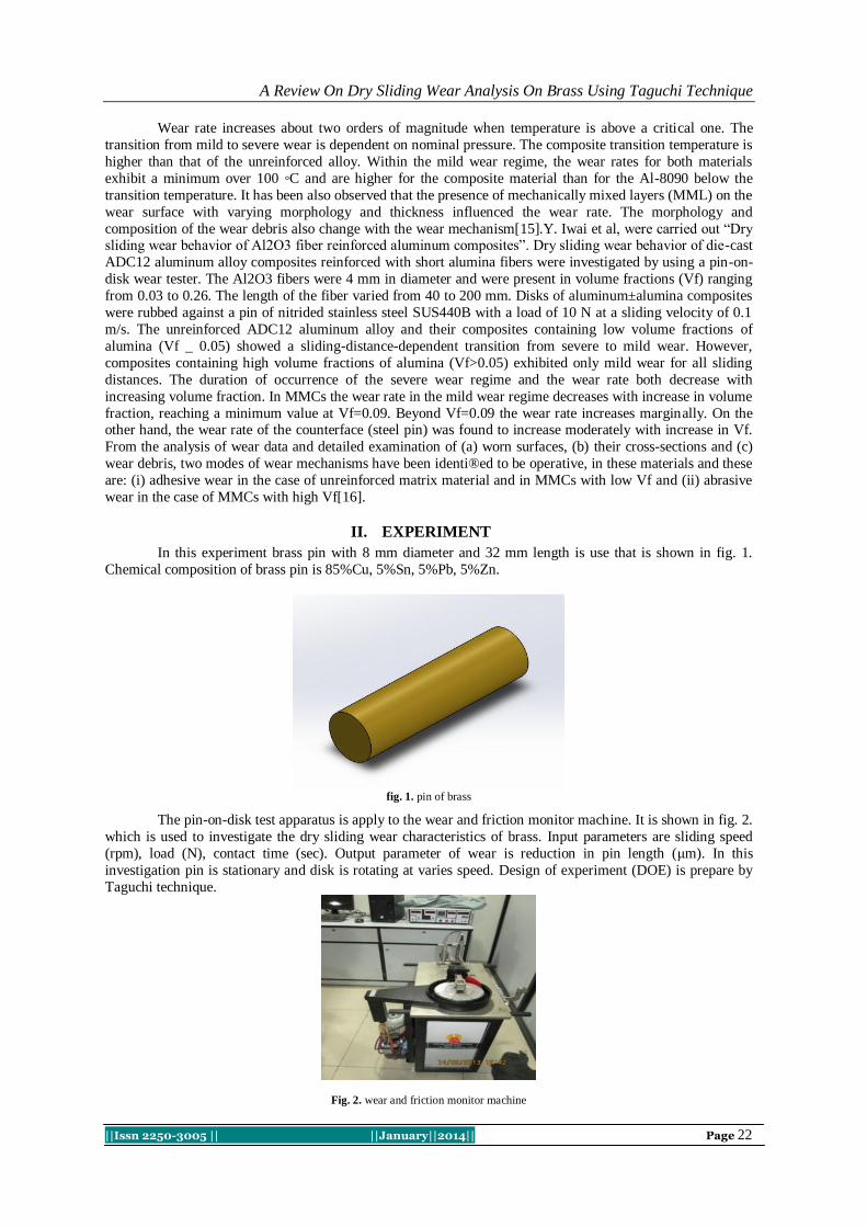
A Review On Dry Sliding Wear Analysis On Brass Using Taguchi Technique
||Issn 2250-3005 || ||January||2014|| Page 22
Wear rate increases about two orders of magnitude when temperature is above a critical one. The
transition from mild to severe wear is dependent on nominal pressure. The composite transition temperature is
higher than that of the unreinforced alloy. Within the mild wear regime, the wear rates for both materials
exhibit a minimum over 100 ◦C and are higher for the composite material than for the Al-8090 below the
transition temperature. It has been also observed that the presence of mechanically mixed layers (MML) on the
wear surface with varying morphology and thickness influenced the wear rate. The morphology and
composition of the wear debris also change with the wear mechanism[15].Y. Iwai et al, were carried out “Dry sliding wear behavior of Al2O3 fiber reinforced aluminum composites”. Dry sliding wear behavior of die-cast
ADC12 aluminum alloy composites reinforced with short alumina fibers were investigated by using a pin-on-
disk wear tester. The Al2O3 fibers were 4 mm in diameter and were present in volume fractions (Vf) ranging
from 0.03 to 0.26. The length of the fiber varied from 40 to 200 mm. Disks of aluminum±alumina composites
were rubbed against a pin of nitrided stainless steel SUS440B with a load of 10 N at a sliding velocity of 0.1
m/s. The unreinforced ADC12 aluminum alloy and their composites containing low volume fractions of
alumina (Vf _ 0.05) showed a sliding-distance-dependent transition from severe to mild wear. However,
composites containing high volume fractions of alumina (Vf>0.05) exhibited only mild wear for all sliding
distances. The duration of occurrence of the severe wear regime and the wear rate both decrease with
increasing volume fraction. In MMCs the wear rate in the mild wear regime decreases with increase in volume
fraction, reaching a minimum value at Vf=0.09. Beyond Vf=0.09 the wear rate increases marginally. On the other hand, the wear rate of the counterface (steel pin) was found to increase moderately with increase in Vf.
From the analysis of wear data and detailed examination of (a) worn surfaces, (b) their cross-sections and (c)
wear debris, two modes of wear mechanisms have been identi®ed to be operative, in these materials and these
are: (i) adhesive wear in the case of unreinforced matrix material and in MMCs with low Vf and (ii) abrasive
wear in the case of MMCs with high Vf[16].
II. EXPERIMENT
In this experiment brass pin with 8 mm diameter and 32 mm length is use that is shown in fig. 1.
Chemical composition of brass pin is 85%Cu, 5%Sn, 5%Pb, 5%Zn.
fig. 1. pin of brass
The pin-on-disk test apparatus is apply to the wear and friction monitor machine. It is shown in fig. 2.
which is used to investigate the dry sliding wear characteristics of brass. Input parameters are sliding speed
(rpm), load (N), contact time (sec). Output parameter of wear is reduction in pin length (μm). In this
investigation pin is stationary and disk is rotating at varies speed. Design of experiment (DOE) is prepare by
Taguchi technique.
Fig. 2. wear and friction monitor machine

A Review On Dry Sliding Wear Analysis On Brass Using Taguchi Technique
||Issn 2250-3005 || ||January||2014|| Page 23
III. CONCLUSION:- This investigation give information about
1. Influence of wear parameters on wear rate.
2. One best set of parameters where wear rate is very low.
3. change in friction force and temperature as wear parameter is change.
REFERENCES [1] C.N. Panagopoulos,“Lubricated wear behavior of leaded (α+β) brass”, Tribology International 50 (2012) 1–5, 31
st january
2012.
[2] J.Paulo Davim,“An experimental study of the tribological behaviour of the brass/steel pair”, Journal of Materials Processing
Technology 100 (2000) 273-277.
[3] Khaled Elleuch,“Sliding wear transition for the CW614 brass alloy”, Tribology International 39 (2006) 290–296.
[4] H. Mindivan, “Microstructures and wear properties of brass synchroniser rings”, Wear 254 (2003) 532–537.
[5] Al-Dhifi SZS,“Improvement in the wear resistance of brass components by the ball burnishing process”,Journal of Materials
Processing Technology 1999;96:73–80.
[6] Satpal Kundu, Dr. B.K. Roy, Ashok Kr Mishra, “study of dry sliding wear behavior of aluminium/SiC/Al2O3/graphite hybride
metal metrix composite using taguchi technique”, International Journal of Scientific and Research Publications, Volume 3,
Issue 8, August 2013 1 ISSN 2250-3153.
[7] A.Baradeswaran, A.Elayaperumal, R. Franklin Issac, “A Statistical Analysis of Optimization of Wear Behaviour of Al-Al2O3
Composites Using Taguchi Technique”, Procedia Engineering 64 ( 2013 ) 973 – 982.
[8] S. Basavarajappa, G. Chandramohan, J. Paulo Davim, “Application of Taguchi techniques to study dry sliding wear behaviour
of metal matrix composites”, Materials and Design 28 (2007) 1393–1398.
[9] Sakip Koksal, Ferit Ficici, Ramazan Kayikci, Omer Savas, “Experimental optimization of dry sliding wear behavior of in situ
AlB2/Al composite based on Taguchi‟s method”, Materials and Design 42 (2012) 124–130.
[10] R.N. Rao, S. Das, D.P. Mondal, G. Dixit, “Dry sliding wear behaviour of cast high strength aluminium alloy (Al–Zn–Mg) and
hard particle composites”, Wear 267 (2009) 1688–1695.
[11] D.E. Lozano, R.D. Mercado-Solis, A.J. Perez, J. Talamantes, F. Morales, “Tribological behaviour of cast hypereutectic Al–Si–
Cu alloy subjected to sliding wear”, Wear 267 (2009) 545–549.
[12] Feng Tang, Xiaoling Wu, Shirong Ge, Jichun Ye, Hua Zhu, “Dry sliding friction and wear properties of B4C particulate-
reinforced Al-5083 matrix composites”, Wear 264 (2008) 555–561.
[13] S. Basavarajappa, G. Chandramohan, R. Subramanian, A. Chandrasekar , “Dry sliding wear behavior of Al 2219/SiC metal
matrix composites”, Materials Science-Poland, Vol. 24, No. 2/1, 2006.
[14] Tiejun Ma, Hideki Yamaura, Donald A. Koss, Robert C. Voigt; “Dry sliding wear behavior of cast SiC-reinforced Al MMCs‟,
Materials Science and Engineering A360 (2003) 116_/125.
[15] J. Rodrıguez , P. Poza, M.A. Garrido, A. Rico, “Dry sliding wear behaviour of aluminium–lithium alloys reinforced with SiC
particles”, Wear 262 (2007) 292–300.
[16] Y. Iwai, T. Honda, T. Miyajima, Y. Iwasaki, M.K. Surappa, “Dry sliding wear behavior of Al2O3 fiber reinforced aluminum
composites”, Composites Science and Technology 60 (2000) 1781±1789.

International Journal of Computational Engineering Research||Vol, 04||Issue, 1||
||Issn 2250-3005 || ||January||2014|| Page 24
Survey on Various Techniques of Brain Tumor Detection from
MRI Images
Mr.Deepak .C.Dhanwani 1,
Prof. Mahip M.Bartere 2
1, 2, Department of Computer Science and Engineering, G.H.R.C.E.M, Amravati, India,
I. INTRODUCTION Brain is the center of human central nervous system. The brain is a complex organ as it contains 50-100
billions neurons forming a gigantic network. Brain tumor is a group of abnormal cells that grows inside of the
brain or around the brain. Brain tumor can be benign or malignant, benign being non cancerous and malignant
are cancerous. Malignant tumors are classified into two types, primary and secondary tumors Benign tumor is
less harmful than malignant as in malignant tumor it spreads rapidly invading other tissues of brain,
progressively worsening the condition causing death. Brain tumor detection is very challenging problem due to
complex structure of brain. The exact boundary should be detected for the proper treatment by segmenting
necrotic and enhanced cells. Magnetic Resonance Imaging (MRI) is an ideal source that provides the detailed
information about the brain anatomy. Fig. 1 shows some of the data sets of MRI images of brain. The MRI of the brain can be divided into three regions: white matter (WM), gray matter (GM) and cerebrospinal fluid (CSF)
because most brain structures are defined by boundaries of these tissue classes and a method to segment tissue
into these categories is an important step in brain tumor detection.
Detection of brain tumor from MRI images involves various Phases such as Preprocessing, Feature
extraction, Segmentation and classification. Fig 2 shows different stages in brain tumor detection. Image
Preprocessing techniques are applied to improve the quality of image. MR Image segmentation is based on set
of measurable features which are extracted. In this process of brain tumor detection, pixel intensity based
features are extracted. Image Segmentation group pixels into regions and hence defines the object regions.
Segmentation uses the features extracted from an image. Classification is the last step in the process of brain
tumor detection used to classify the image into normal or abnormal and classify the abnormality type whether it
is benign or malignant. This study evaluates various techniques which are used in tumor detection from brain MRI.
Fig 1: MRI brain Image dataset
ABSTRACT Brain tumor is an abnormal growth of brain cells within the brain. Detection of brain tumor is
challenging problem due to complex structure of brain.MRI can provide the detail information about
human soft tissue anatomy, which is helpful in diagnosis of brain tumor. Detection of brain tumor
involves different stages such as image preprocessing, segmentation, feature extraction and
classification. This paper summarizes the study of various techniques of brain tumor from MRI images.
Keywords: Classification, Feature extraction, MRI, Neural Network, Preprocessing, Rough set,
Segmentation

Survey on Various Techniques of…
||Issn 2250-3005 || ||January||2014|| Page 25
Fig 2 : Stages in Brain Tumor Detection
Literature Survey Bhagwat et al [1] presented a paper that shows comparison of K-means, Fuzzy C-means and Hierarchical
clustering algorithms for detection of brain tumor, These Three clustering algorithms K-means, fuzzy c-means and hierarchical clustering were tested with MRI brain image in non medical format (.jpg, .png, .bmp etc) as well as DICOM image. It is prove that DICOM images produce more efficient result compare to non medical images. Time required for hierarchical clustering is least and fuzzy c-means is maximum to detect the brain tumor where as K-means algorithm produce more accurate result compared to Fuzzy c-means and hierarchical clustering. Detection of brain tumor involves various stages such as image preprocessing, feature extraction, segmentation and classification. Pulse couple neural network (PCNN) uses for image smoothing, feature extraction and image segmentation and Back Propagation Neural Network (BPNN) is used for classification that classify the image whether it is normal or abnormal. [2]Roy et al [3] introduce the
symmetric analysis to detect the brain tumor by making the calculations on the area of tumor. It s application with several data sets with different tumor size, intensity and location shows that it can automatically detect and segment the brain tumor. MR images gives better result compare to other technique used in the field of medical science like CT images and X-rays Segmentation is one of the essential tasks in medical area but is boring and time consuming.
Image pre-processing including converting RGB image into grey scale then passing that image to the high pass filter in order to remove noise is done and finally the last we get enhanced image for post-processing that will include watershed segmentation and thresholding as well as morphological operation. For the extraction of text region.
Morphological operator is used since text regions are composed of vertical edges, horizontal edges and diagonal edge. At different orientation these text are connected together differently. In recent years the concepts of ontology has taken a wide leap from formal specification to the area of artificial intelligence in the domain of experts system. Ontology has been common on World Wide Web. This concept basically deals with classes, sub-classes and their association from the basic categorization of product along with their features.[4] Aboul Ella Hassanien et al [5] presented review paper that shows how the rough set approach and near set approach are useful to solve various problems in medical imaging such as medical image segmentation ,object extraction and image classification .This paper also shows how the rough set framework hybridized with various computing technologies such neural network (NN), support vector machine (SVM) and fuzzy sets .A combination of various computational intelligence technologies in medical image problem has become one of the most
promising avenues in image processing research. Magdi et al [6] used an intelligent Model for brain tumor diagnosis from MRI images .which consist of three different stages such as preprocessing, Feature extraction and classification. Preprocessing used to reduce the noise by filtration and to enhance the MRI image through adjustment and edge detection .texture features are extracted and principal component analysis (PCA) is applied to reduce the features of the image and finally back propagation neural network (BPNN) based Person correlation coefficient was used to classify the brain image.N.senthilal kumaran. et al [7] presented a hybrid method for white matter separation from MRI brain image that consist of three phase. First phase is to preprocess
an image for segmentation, second phase is to segment an image using granular rough set and third phase is to separate white matter from segmented image using fuzzy sets This method was compared with mean shift algorithm and it was
found that hybrid segmentation performs better result Rajesh patil et al [8] presented a method to detect and extract
the tumor from patients MRI image of brain by using MATLAB software. This method performs noise removal
function, Segmentation and morphological operations which are the basic concept of image processing . Tumour
is extracted from MRI image for this it has an intensity more than that of its background so it becomes very easy locates.

Survey on Various Techniques of…
||Issn 2250-3005 || ||January||2014|| Page 26
Mehdi Jafri and Reza Shafaghi [9] proposed a hybrid approach for detection of brain tumor tissue in
MRI based on Genetic algorithm (GA) and support vector machine (SVM).In the preprocessing stage noise is
removed and contrast is enhanced. For removing high frequency noises low pass filter is used for enhancing
histogram stretching method is used. in segmentation undesired tissue such as nose, eyes and skull are deleted
and features are extracted by different ways like FFT,GLCM and DWT. In feature selection GA is used with
PCA by using this calculations complexity is reduced. Finally the selected features are applied to SVM classifier
used to classify the image into normal or abnormal.A Sivaramkrishnan [10] presented a novel based approach in which Fuzzy C-mean (FCM) clustering algorithm was used to find the centroids of cluster groups to obtained
brain tumor patterns. It is also preferred as faster clustering by using this centroid point can be located easily.
The histogram equalization calculates the intensity of gray level image and PCA was used to reduce
dimensionality of wavelet coefficient.
II. CONCLUSION From Literature survey ,it is conclude that MR images provides much better information about human
soft tissues of brain compared to computerized tomography(CT) images. DICOM images (.dcm) produce more
efficient result compare to non medical images (.jpg,.png,.bmp). MRI segmentation is one of the essential tasks in medical area. The accurate segmentation is crucial otherwise the wrong identification of disease can
lead to several consequences. As diagnosis tumor is a complicated task; therefore accuracy and reliability are
always assigned much importance.
REFERENCES [1] Kshitij Bhagwat, Dhanshri More, Sayali Shinde, Akshay Daga, Assistant Prof. Rupali Tornekar “ Comparative Study of Brain
Tumor Detection Using K-means ,Fuzzy C means and Hierarchical Clustering Algorithms ” International Journal of Scientific
& Engineering Research , Volume 2,Issue 6,June 2013,pp 626-632
[2] Monica subashini .M, Sarat Kumarn Sahoo,” Brain MR image Segmentation for Tumor Detection Using Artificial Neural
Networks”, International Journal of Engineering and Technology (IJET), ISSN: 0975-1024, Vol 5No.2 Apr-May 2013,pp 925-
930
[3] S.Roy and S.K.Bandoyopadhyay”Detection and qualification of Brain Tumor from MRI of Brain and Symmetric
Analysis”International Journal of Information and communication Technology Research, Volume 2 No.6, June 2012 pp584-588
[4] Monika Sinha, Khushboo Mathur “Improved Brain Tumor Detection With Ontology”, International Journal Of Computational
Engineering Research ISSN: 2250–3005 Vol.2, Issue No.2, Mar-April-2012 pp 584-588
[5] Aboul Ella Hassanien,” Rough Sets and Near Sets in Medical Imaging: A Review” Inforamation Technology in
Biomedicine,IEEE,ISSN: 1089-7771,volume 13,Issue 6,Nov 2009,pp 955-968
[6] Magdi B.M Amien, Ahmed Abd-elrehman and Walla Ibrahim,”An Intelligant Model for Automatic Brain Tumor Diagnosis
Based on MRI Images”International Journal of Computer Applications(0975-8887) Volume72-No.23,June 2013,pp 21-24
[7] N.Senthilkumaran,R.Rajesh,C.Thilagavathy,”Hybrid Method for White Matter Separation In Brain Images Using Granular
Rough Sets and Fuzzy Thresholding ”Proceedings of 2010 IEEE 17 International Conference on Image Processing September
26-29,2010,Hong Kong,978-1-42447993,2010,IEEE,pp:3037-3040
[8] Rajesh C. Patil, Dr. A. S. Bhalchandra “Brain Tumour Extraction From MRI Images using MATLAB”International Journal of
Electronics, Communication & Soft Computing Science and Engineering ISSN: 2277-9477, Volume 2, Issue 1
[9] Ahmed Kharrat, Karim Gasmi, “A Hybrid Approach for Automatic Classification of Brain MRI Using Genetic Algorithm and
Support Vector Machine”, Journal of Sciences, pp.71-82, 2010.
[10] A.Sivaramakrishnan,Dr.M.Karnan,” A Novel based Approach for Extraction of Brain Tumor in MRI Images Using Soft
Computing Techniques”, International Journal of Advanced Research in Computer and Communication Engineering, ISSN
2278-1021, volume 2,Issue 4,April 2013 ,pp1845-1848
International Journal of Computational Engineering Research||Vol, 04||Issue, 1||
||Issn 2250-3005 || ||January||2014|| Page 27
Transforming Satellite Campuses of Tertiary-education
Institutions in Nigeria through Appropriate Application of
Information Technology: A Case Study
Adu Michael K.
Federal Polytechnic Ado-Ekiti, Ekiti State, Nigeria, Department of Computer Science
I. INTRODUCTION Satellite campuses are set-up to providing tertiary education for students who may not be able to attend the main
campus as a result of distance, work and some other important reasons. It may be located in a different city, state or country, and is often smaller than the main campus of an institution. It may be under the same accreditation and share resources or the same administration but maintain separate budgets, resources and governing bodies (Wikipedia, 2013). The availability of
satellite campuses may increase higher education enrollment by nontraditional students (James et al., 2007). As good as the aim of setting up satellite campuses in Nigeria is, they are marred with different problems which often have resulted in giving bad impressions about them. Nigeria government at various point in time stopped the operations and citing of satellite campuses across the country as a result of poor management and ineffective teaching and learning processes that have resulted to half baked graduates. Only those operated within the region of their main campuses are allowed. Despite this, they also do have many challenges that negatively affect the quality of their graduates. However, attempts are being made by the government to find solutions to these problems by making regulations and policies to govern the way and manner by which these campuses are run. The regulations and policies include but not limited to the following;
Satellite campuses are to be operated within few kilometers to their main campuses.
Accreditation of courses are also extended to the satellite campuses
Monitoring of the activities of the satellite campuses by the appropriate governing bodies established by government.
However, with all these in place, coupled with adequate provision of classrooms and laboratories, there are still
peculiar problems associated with management of satellite campuses. According to Bainbridge (1996), transformation is necessary to ensure a better fit between an institution and the unique needs of a changing environment. Transformation may be thought of as “drastic changes triggered by external environmental factors”. Also according to the New Oxford Dictionary of English, the concept of transformation refers to a “thorough or dramatic change in form or appearance” (Pearsall, 1998). Transformation is a specific type of change which can be distinguished from other types of changes in the sense that it implies not only a change of form but also the creation of something new. Transformation in the management of satellite campuses in Nigeria therefore requires that previous management practices and ways of doing things are discontinued. These transformation must be triggered by external environmental changes most especially student population increase (Pendlebury
et al., 1998).
ABSTRACT Satellite Campus is a campus of a college or university that is physically at a distance from the original
university or college (main campus) area. In Nigeria, managing Satellite campuses is seen to be a very
difficult task and hence has not been accepted fully as a dependable avenue to gain tertiary education
by those who are constrained either by the nature of their work and those of other reasons to attend them. Most people have only seen satellite campuses as a means of generating funds only for the
institutions. However, this paper opens up areas that make management of satellite campuses very
difficult which have contributed mostly to the negative impression about them. They are students’ result
processing, general students’ affairs management, financing and inappropriate and ineffective means of
addressing part-time lecturers’ honorarium. Effective management of these deficiencies through
appropriate application of Information Technology (IT) tools is proposed and implemented in this work.
These are expected to produce positive results and further boost the image of satellite campuses in
Nigeria. The Continuing Education Centre (CEC), Federal polytechnic, Ado-Ekiti, as the case study for
this work is the satellite campus of the institution, about 30 minutes drive from the main campus and one
of the best managed with enviable graduates.
Keywords: Financing, Honorarium, Information Technology, Management, Result processing, Satellite
Campus.

Transforming Satellite Campuses of Tertiary-education Institutions…
||Issn 2250-3005 || ||January||2014|| Page 28
Khosa (1996) noted that tertiary-education institutions are an integral part of the social environment. The
notable agent of transformation regarding the ills against management of satellite campuses in Nigeria is
adequate application of Information Technology beyond the level of using computers for word processing and
office decorations. Core areas that are very sensitive should be computerized. It is necessary therefore that the
educational institutions should change its strategy and form in order to adapt to a new type of challenges that
will affect both the students and workers (Swart et al., 1998). Software engineering has the objective of solving
these challenges by producing good quality, maintainable software, on time, within budget (Aggarwal et al., 2008).
The research carried out in the Continuing Education Centre (CEC), the satellite campus of the Federal
Polytechnic, Ado-Ekiti, opened up the main causes of these challenges and subsequent attempts at providing
solution through appropriate application of Information Technology tools was implemented.
II. RESEARCH METHOD 2.1. Research Design
The objective of the research design is to analyze the experiences of the students and concerned
stakeholders without predetermined expectancies, and to try to understand the data from their point of view
(Moustakas, 1994). This is expected to assist in our getting solutions that are reliable.
2.2. Analysis and Result
There was data collection through the use of the instrument of questionnaire. Stakeholders provided
information on those areas they considered as the main cause of problem for the management of satellite
campuses all over Nigeria that negatively affect the standard of their products. They mostly attributed it to the
following major points;
Lack of adequate records of students unlike in the main campus where students’ records are adequately kept, probably as a result of manageable population size and closeness to the authority of the various
institutions.
Payment of lecturers’ honorarium that is not regular. Lecturers are not paid on a regular monthly basis,
rather on unit of course(s) taught. Opinions show that some lecturers do compromise on integrity by
engaging in practices that are inimical to the standard of the institutions. However, opinions believe
that if payment is made on time, it will reduce the trend.
Opinions also show that the lecturers might be able to perpetrate these atrocities as a result of the fact
that they were always considered as thin gods in the mind sets of their students because of the power
the students believed the lecturers possessed as a result of being in custody of continuous assessment
and examination scores which the students thought could be manipulated at will by the lecturers. A
system that enforces the lecturers to submit continuous assessment score and examination scores immediately they are conducted will go a long way in sanitizing the process. The collation and
production of final score sheets for result processing centrally done using appropriate software on a
computer system as a tool is proposed.
It is believed that if the money generated is adequately appropriated and no area of the school system is
not developed, including sport, medical, library, laboratory, infrastructure, et cetera. All sectors will be
optimally functional. To achieve this, computerizing the school fees payment analysis system is
proposed.
The collation and analysis of the research instruments administered on students, non-academic and
academic staff members considered as stakeholders are detailed below;
Table 1: Percentage of responses to the negative influence of not keeping adequate record in the
management of satellite campuses in Nigeria tertiary-education system
Category Enrollment Agree % Partially
Agree
% Disagree % No comment %
Students 84 80 95.2% 2 2.3% 2 2.3% 0 0%
Non-academic
staff
65 56 86.2% 4 6.2% 3 4.6% 2 3.1%
Academic Staff
50 42 84.0% 4 8.0% 3 6.0% 1 2.0%

Transforming Satellite Campuses of Tertiary-education Institutions…
||Issn 2250-3005 || ||January||2014|| Page 29
Table 2: Percentage of responses to the negative influence of delay or inappropriate payment of lecturers’
honorarium
Category Enrollment Agree % Partially
Agree
% Disagree % No comment %
Students 84 63 75.0% 10 12.0% 10 12.0% 1 1.0%
Non-academic
staff
65 56 86.2% 4 6.2% 3 4.6% 2 3.1%
Academic Staff
50 26 52.0% 10 20.0% 13 26.0% 1 2.0%
Table 3: Percentage of responses to the negative influence of allowing lecturers to individually collate
continuous assessment and examination scores for result processing
Category Enrollment Agree % Partially Agree % Disagree % No comment %
Students 84 65 77.4% 10 11.9% 8 9.5% 1 1.2%
Non-academic staff
65 45 69.2% 15 23.1% 3 4.6% 2 3.1%
Academic Staff
50 24 48.0% 14 28.0% 9 18.0% 3 6.0%
Table 4: Percentage of responses to the negative influence of not separating school fees payment for
different developmental projects in management of satellite campuses in Nigeria.
Category Enrollment Agree % Partially Agree % Disagree % No comment %
Students 84 80 95.2% 2 2.4% 1 1.2% 1 1.2%
Non-academic staff
65 60 92.3% 4 6.2% 1 1.5% 0 0.0%
Academic
Staff
50 48 96.0% 1 2.0% 0 0.0% 1 2.0%
Table 1 shows that 95.2 % of the students population, 86.2% of the non-academic staff and 84% of
academic staff members of the polytechnic community agreed to the negative influence arising from lack of
adequate record keeping of students’ details on the overall standard of satellite campuses in Nigeria when
compared with main campuses where adequate records are kept and maintained. Table 2 indicates that 75% of
the students sampled, 86.2% of non-academic staff members and 52.0% of the academic staff members believe
that when the part time lecturers of the satellite campuses are not paid their honorarium on time due to either
logistic or whatever reason, the lecturers’ may not give their best unlike the regularly paid full time lecturers of
the main campuses. It is also believed that this may make some lecturers to comprise on integrity. The opinions of the stakeholders on giving the duties of assessing, collating and producing final score sheets of examination
by part time lecturers is another issue that may affect standard. 77.4%, 69.2% and 48% of students, non-
academic and academic staff members respectively agreed to this. 95.2%, 92.3% and 96.0% of the sampled
students’ population, non-academic and academic staff respectively believed that separation of fees payment by
comprehensive analysis of students’ school fees into the various units for even development of each section is
desirable.
III. SYSTEM IMPLEMENTATION The outcome of the data collection formed the basis for development of some fundamental software
packages to handle the identified areas that were considered to be the problems of satellite campus management
in Nigeria. The system is implemented with Visual BASIC.NET as front end and MYSQL server as the back
end. Sample reports generated in some of the developed software packages, tested (with hypothetical data) and
implemented only for the purpose of this research work are as follows;
3.1. Lecturers’ Honorarium Payment System (LEHOPAS)
This is a software package developed to be used in processing lecturers’ payment claim, the software
will make it easy to pay lecturers based on the total unit allocated.

Transforming Satellite Campuses of Tertiary-education Institutions…
||Issn 2250-3005 || ||January||2014|| Page 30
Figure 1: Example of output of calculated honorarium for lecturers
3.1. Mark Sheet processing System This is software that makes inputting of scores into score sheet a lot easier. It enables raw scores of students in
continuous assessments and semester examination to be automatically added up by the software to generate a final score sheet print-out which will then be taken for further processing to generate semester results. It will make this processing faster and easier.
Figure 2: Entry form for entering continuous assessments and examination scores

Transforming Satellite Campuses of Tertiary-education Institutions…
||Issn 2250-3005 || ||January||2014|| Page 31
Figure 3: Sample score-sheet with totals of continuous assessments and examination scores
3.2 School Fees Payment Analysis System (SFPAS)
This is an accounting software tested and can be used to generate monthly/yearly financial statement of
any institution in different formats. It produces the breakdown of the fees paid by students and thereby
providing easy means of allocating funds to the various units appropriately such as sports, medical, laboratories, transportation and examinations.

Transforming Satellite Campuses of Tertiary-education Institutions…
||Issn 2250-3005 || ||January||2014|| Page 32

Transforming Satellite Campuses of Tertiary-education Institutions…
||Issn 2250-3005 || ||January||2014|| Page 33
Figure 4: Output with summary of distribution of school fees payments

Transforming Satellite Campuses of Tertiary-education Institutions…
||Issn 2250-3005 || ||January||2014|| Page 34
IV. CONCLUSION The outcome of data collection which informed the development of these application packages will no
doubt yield good results in any of the satellite campuses in Nigeria today when fully adopted. The application
packages were developed in such a way that an individual with a fore knowledge of normal administration of such educational centre (without computer knowledge) should be able to use them effectively with confidence
within few days. The packages will afford the centres the ability to keep and maintain adequate records of
students and staff. Important decisions will be taken with dispatch and academic results will be more credible
and timely. The task to match the need of stakeholders and bringing the system on board were successfully
achieved.
ACKNOWLEDGEMENTS I thank the management and staff of the Continuing Education Centre, Federal Polytechnic, Ado-Ekiti,
Nigeria for their understanding throughout the long period it took to achieve the desired results in this research
work, most especially Engr. T.D Adegboyega, the Dean and Engr. J. Adams, the Sub-Dean. Many thanks to Femi Adefaka and Godwin Udeji for their technical assistance.
REFERENCES [1] K.K. Aggarwal and Yogesh Surgh. Software Engineering, New Age International Publishers Limited, 2008.
[2] C. Bainbridge. Designing for change- A practicalguide to business transformation, Chichester West Sussex Willey, 1996.
[3] W.F. James and P.B. Charles. Under the Radar- Branch Campus take off, University Bussiness Magazine, 2007.
[4] M.M. Khosa. Leaders or followers? Transforming South African universities. Indicator South Africa, 13(4): 73-77, 1996.
[5] J. Pearsall. The New Oxford Dictionary of English, Oxford: Clarendon Press, 1998.
[6] J. Pendlebury, B. Grouard and F. Meston. The ten keys to successful change management, Chichester, West Sussex Wiley, 1998.
[7] J. Swart and L.J. Vuuren. Cognitive style and the interpretation of organisational change. Journal of Industrial Psychology, 24(3):
22-31, 1998.
[8] Wikipedia- encyclopedia –http://en.wikipedia.org/wiki/satellite_campus, 2013.
International Journal of Computational Engineering Research||Vol, 04||Issue, 1||
||Issn 2250-3005 || ||January||2014|| Page 35
Effect of boundary roughness on Kelvin-Helmholtz instability in
Couple stress fluid layer bounded above by a porous layer and
below by rigid surface
1, Krishna B. Chavaraddi,
2, N. N. Katagi,
3, V. B. Awati,
4, Priya M. Gouder
1Department of Mathematics, Government First Grade College, Yellapur (U.K)-581 359, Karnataka, India
2Department of Mathematics, Manipal Institute of Technology,
Manipal-576104, India 3Department of Mathematics, Rani Channamma University,
Belgaum-590020, Karnataka, India 4Department of Mathematics, K.L.E’s Dr. M. S. Sheshagiri
College of Engineering and Technology, Belgaum-590008, Karnataka, India
I. INTRODUCTION Kelvin-Hemholtz instability after Lord Kelvin (1910) and Hermann Von Helmholtz (1868) can occur
when velocity shear is present within a continuous fluid or when there is sufficient velocity difference between
two fluids. One example is wind blowing over a water surface where the wind causes the relative motion
between the stratified layers (i.e., water and air). Helmholtz(1868) studied the dynamics of two fluids of
different densities when a small disturbance such as a wave is introduced at the boundary connecting the fluids.
If surface tension can be ignored and for some short enough wavelengths, two fluids in parallel motion with
different velocities and densities yielded an interface that is unstable for all speeds. The KHI is important in
understanding a variety of space and astrophysical, geophysical phenomena involving plasma flow. Without
surface tension, this streaming is unstable no matter how small the velocity difference between the layers may
be. It was shown by Kelvin[1910] that the surface tension will suppress the instability if the difference in
velocity is sufficient small. From an industrial view point, the momentum transfer and the KHI in composite
region provides impetus for effective, design of porous bearings in lubrication process, particularly in the slider
bearings and in the effective design of target in inertial fusion energy(IFE). Because of these importances the KHI is investigated in this paper using the linear stability analysis. The experimental observation of KHI has
been given by Francis(1954). The linear study of the KHI was investigated by Chandrasekhar (1961) gave an
introduction to classical KHI. He discussed the effect of surface tension, variable density, rotation and applied
magnetic field on the behaviour of stability.
ABSTRACT The effect of boundary roughness on Kelvin-Helmholtz instability (RTI) of a couple-stress fluid layer
bounded above by a porous layer and below by a rigid surface with roughness boundary is studied using
linear stability analysis. Because of the growing importance of non-Newtonian fluids (Couple-stress
fluid) in modern technology and industries as well as various practical applications investigations on
such fluids are desirable. An expression for the growth rate of KHI is derived using suitable boundary
and surface conditions in addition to couple-stress boundary conditions. Also in order to observe the
effect of boundary layer applying the Beavers-Joseph (BJ) slips condition. From this it is clear that the
effects of couple stress parameter, roughness parameter, bond number and porous parameter play a
significant role in maintaining the stability on the two fluid systems. The couple stress fluid is found to be stabilizing effect and the influence of the various parameters of the problem on the interface stability is
thoroughly analyzed.
Key Words: Couple-stress fluid, KHI, B-J Condition, dispersion relation, porous media, boundary
roughness.

Effect of boundary roughness on Kelvin-Helmholtz instability in…
||Issn 2250-3005 || ||January||2014|| Page 36
The study of electrohydrodynamic(EHD) KHI of free surface charges, separating two semi-infinite
dielectric fluids and influence by an electric field has been discussed by Melcher(1963). The effect of rotation
and a general oblique magnetic field on the KHI has been studied by Sharma and Srivastava(1968). The main
difference between KH and RT instabilities is inclusion of qq
).( which is a nonlinear term in the
perturbation equations. EHD studies the interplay of mechanical and electrical forces in fluids. In the first
approximation it is assumed that the electrical currents are very weak and therefore magnetic effects are negligible. Maxwell’s equations are then reduced to Gauss’ law and the charge conservation law. Within the
past few years, a number of paper have appeared on studies of surface instability in the presence of electric field
(El-Dib and Moatimid(1994)). Singh and Khare(1991) have studied the stability of two semi-infinite
homogenous gravitating streams of infinite conductivity under uniform horizontal magnetic field and uniform
rotation. Bhatia and Hazarika(1995) were discussed this stability for superposed viscous gravitating fluids. The
importance of the KHI problem has been demonstrated by Benjamin and Bridges (1997) who have given an
excellent reappraisal of the classical KHI problem in hydrodynamics. They have shown that the problem admits
of canonical Hamiltonian formulation and obtained several new results.
The KHI of two superposed viscous fluids in a uniform vertical magnetic field is discussed in the
presence of effects of surface tension and permeability of porous medium by Bhatia and Sharma (2003).
Following Babchin et al(1984) and Rudraiah et al (1996), a simple theory based on Stokes and lubrication approximations is used in this study by replacing the effect of the boundary layer with a Beavers and
Joseph(1967) slip condition with the primary objective of using porous layer to suppress the growth rate of KHI.
In the above studied the fluid has been considered to be Newtonian. Nevertheless, much attention has not been
given in the literature to the study of KHI in a poorly conducting non-Newtonian fluid like Couple stress fluid
layer bounded above by a porous material and below by rigid surface that in spite of frequently occurring in
many engineering and physical situations namely, inertial fusion energy (IFE), geophysics and supernova, the
consideration of such fluids is desirable. The couple-stress effects are considered as result of the action of one
part of a deforming body on its neighbourhood. Stokes (1966) has formulated the theory of a couple-stress fluid.
The theory of Stokes (1966) allows for the polar effects such as the presence of couple-stresses and body
couples and has been applied to the study of some simple lubrication problems (see Sinha et al.(1981), Bujurke
and Jayaraman(1982)). According to Stokes (1966), couple-stresses appear in fluids with very high molecules. Since the long chain hylauronic acid molecules are found as additives in synovial fluids, Walicki and
Walicka(1999) were modeled synovial fluid as couple-stress fluid in human joints. The presence of small
amounts of additives in a lubricant can improve the bearing performance by increasing the lubricant viscosity
and thus producing an increase in the load capacity. This additive in a lubricant also reduces the coefficient of
friction and increases the temperature range in which bearing can operate. The RTI of two superposed infinitely
conducting couple-stress fluids of uniform densities in a porous medium in the presence of a uniform magnetic
field by Sunil et al.,(2002). It is clear notice that the couple-stress fluid in region -1 with proper choice of
couple-stress parameter and porous parameter in reducing the asymmetry of the two fluid composite systems at
the interface. The electrorheological KHI of fluid sheet have been discussed by El-Dib and Matoog (2005). Due
to the rather complicated nature of the problem a mathematical simplification is considered where the weak
effects of viscoeleastic fluids are taken into account. Recently, Chavaraddi et al (2011) have investigated the
effect of KHI of fluid layer bounded above by a porous layer and below by a rigid surface in presence of magnetic field. It is clear that magnetic field is found to be stabilizing effect and the influence of the various
fluid parameters of the problem on the interface stability.
Keeping in mind the importance of non-Newtonian fluids like couple-stress fluid in modern technology
and industries as well as various applications mentioned above, the objective of the predict to study the KHI in a
poorly conducting couple-stress fluid layer bounded above by a porous layer and below by a rigid surface with
the effect of boundary roughness which were formulated by Miksis and Davis(1994) at the interface and the
plan of this paper is as follows. The mathematical formulation subjected to the boundary and surface conditions
is given in Section 2. The expression for the dispersion relation is derived using the basic equations with
boundary and surface conditions in section 3. The cutoff and maximum wave numbers and the corresponding
maximum growth rate are also obtained in section 4 and some important conclusions are drawn in final section of this paper.

Effect of boundary roughness on Kelvin-Helmholtz instability in…
||Issn 2250-3005 || ||January||2014|| Page 37
II. MATHEMATICAL FORMULATION The physical configuration is shown in Fig.1. The system under consideration is composed of two
incompressible couple-stress fluid and fluid saturated porous media separated by the plane y=h. The above fluid
is of infinite extent while the below on is of finite extent with rigid rough boundary. We take y=h at the mean
level of the interface and the y-axis pointing vertically upwards into the upper fluid. The fluids in both the
regions are set in relative motion by acceleration normal to the interface and small perturbations are amplified
when fluid in the thin film to the heavy fluid saturated porous media above the interface. The interface between
couple stress fluid and fluid saturated porous media is described by ),( tx as the perturbed interface between
two fluids in region-1 and 2. The two fluids are influenced by a couple-stress and porous parameters which
acting along the positive x-direction, where the f
u and p
u along the positive x-direction, where the x-axis is
mean level of the wave. Also, the fluids are streaming with velocities f
u and p
u long the same direction.
Acceleration due to gravity acts in the negative y-direction. A schematic diagram of the configuration in the
steady state is given in Figure-1.
Fig. 1: Schematic diagram of the system
The upper fluid has density p
while the lower one has density f
and surface tension exist between the two
fluids and is denoted by .
To investigate the problems posed in the paper the following combined lubrication and Stokes
approximations are used.
(i) The clear dense liquid is homogeneous and isotropic. (ii) The film thickness h is much smaller than the thickness H of the porous layer bounded above the film.
That is,
h < < H.
(iii) The Strouhal number S is assumed to be negligibly small.
(iv) The surface elevation is assumed to be small compared to film thickness h. That is,
< < h. (v) Nonuniform polarization and electric charge injection are negligible.
(vi) The fluid viscosity and thermal conductivity are assumed to be constants.
Following these assumptions and approximations, the basic equations are
Region-1:
0 q
(2.1)
2 4
. pq
q q q qt
(2.2)
Region-2 :
x
pkQ
(2.3)

Effect of boundary roughness on Kelvin-Helmholtz instability in…
||Issn 2250-3005 || ||January||2014|| Page 38
where ( , )q u v
the fluid velocity, the couple-stress parameter, e
the dielectric constant, p the pressure,
x
p
the pressure gradient, the fluid viscosity, )0,0,(QQ the uniform Darcy velocity and the fluid
density.
Let us non-dimensionalize the equations using
2 2, , , ,
/ /
x y u v px y u v p
h h h h h
,
/,
/
*
2h
tt
h
(2.4)
Following the assumptions and approximations as stated above (i.e., Stokes and lubrication approximations),
assuming that the heavy fluid in the porous layer is almost static because of creeping flow approximation and
substituting Eq.(2.4) into Eqs.(2.1) and (2.2), we obtain (after neglecting the asterisks for simplicity)
Region-1: 0
u v
x y
(2.5)
2 4
2 4
2
00
p
x y y
u uM
(2.6)
0
p
y
(2.7)
Region-2 :
x
pQ
p
2
1
(2.8)
where 2
0/M h is the couple-stress parameter and
k
h
p the porous parameter .
III. 3. DISPERSION RELATION To find the dispersion relation, first we have to find the velocity distribution from Eq. (2.6) using the
following boundary and surface conditions in addition to couple-stress boundary conditions.
(i) Boundary roughness condition
01
yatu
y
u (3.1)
(ii) B-J condition
1)(
yatQu
y
u
Bpp (3.2)
where 1 yatuuB
. (3.2a)
(iii) Couple-stress conditions:
2
20 0 & 1
ua t y
y
(3.3)
(iv) Kinematic condition: vt
at y =1 (3.4)
(v) Dynamic condition:
2
2
1p
B x
at y =1. (3.5)
where 2
/B h is the Bond number and ( , , )x y t is the elevation of the interface.
The solution of (2.6) subject to the above conditions is
PyM
MySinhCMyCyCCu
2
0
040321
2
1)/()/cosh( (3.6)

Effect of boundary roughness on Kelvin-Helmholtz instability in…
||Issn 2250-3005 || ||January||2014|| Page 39
where
x
pP
, ,
03PMC )]/1(sec)/1(1[
000121MhCoMCothMCC
0
3200
0
4
00
0
1
3
2
00
2
11)/1()/1(
1
)/1()/1(1
)]1(1[
MMMMSinhMCosh
MC
MCoshMSinhMC
C
p
p
pppp
pppp
pp
)]/1(sec)/1([0014
MhCoMCothCC
After integrating Eq.(2.5) with respect to y between y = 0 and 1 and using Eq.(3.6), we get
1 2
1 2
0
(1)u p
v v d y Nx x
(3.7) where
0
004003
2
1
6
1}1)/1({)/1(
2 MMCoshMCMSinhMC
CCN
Then Eq.(3.4), using Eqs.(3.5) and (3.7), becomes
2 4
2 4
1N
t Bx x
. (3.8)
To investigate the growth rate, n, of the periodic perturbation of the interface, we look for the solution of
Eq.(3.8) in the form
( ) ex p { }y i x n t (3.9)
where is the wave number and ( )y is the amplitude of perturbation of the interface.
Substituting Eq.(3.9) into Eq.(3.8), we obtain the dispersion relation in the form
22
1nB
N
. (3.10)
In the absence of couple-stress parameters, that is 0
0M , the growth rate given
by Eq.(3.10) reduces to b
n . Now the dispersion formula can be expressed in the form
b an n v (3.11)
where
B1
3n
22
b
,
2
1a
v NB
,
2
2
1 31
3
1
N
N B
B
.
Setting n = 0 in Eq.(3.10), we obtain the cut-off wavenumber, ct in the form
c tB . (3.12)
The maximum wavenumber, m obtained from Eq.(3.10) by setting / 0n is
22
c t
m
B
. (3.13)
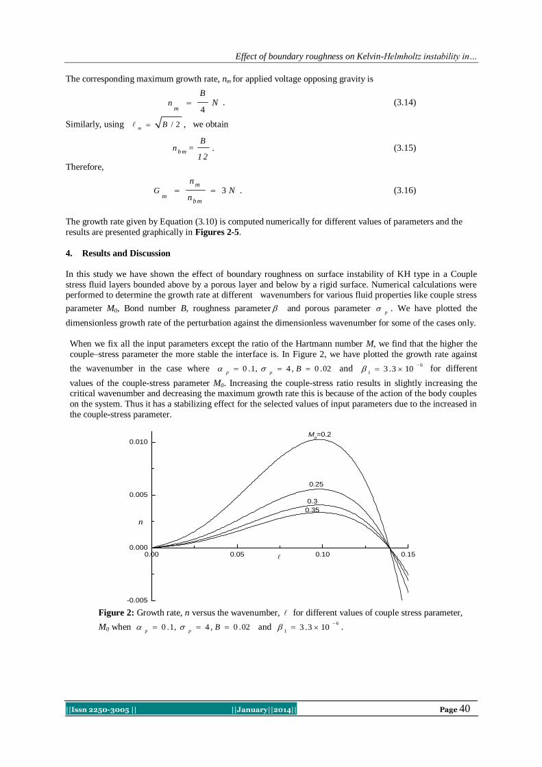
Effect of boundary roughness on Kelvin-Helmholtz instability in…
||Issn 2250-3005 || ||January||2014|| Page 40
The corresponding maximum growth rate, nm for applied voltage opposing gravity is
4m
n
BN . (3.14)
Similarly, using / 2m
B , we obtain
b m
Bn =
1 2. (3.15)
Therefore,
3m
mb m
G
nN
n . (3.16)
The growth rate given by Equation (3.10) is computed numerically for different values of parameters and the
results are presented graphically in Figures 2-5.
4. Results and Discussion
In this study we have shown the effect of boundary roughness on surface instability of KH type in a Couple
stress fluid layers bounded above by a porous layer and below by a rigid surface. Numerical calculations were performed to determine the growth rate at different wavenumbers for various fluid properties like couple stress
parameter M0, Bond number B, roughness parameter and porous parameter p
. We have plotted the
dimensionless growth rate of the perturbation against the dimensionless wavenumber for some of the cases only.
When we fix all the input parameters except the ratio of the Hartmann number M, we find that the higher the
couple–stress parameter the more stable the interface is. In Figure 2, we have plotted the growth rate against
the wavenumber in the case where 02.0,4,1.0 Bpp
and 6
1103.3
for different
values of the couple-stress parameter M0. Increasing the couple-stress ratio results in slightly increasing the critical wavenumber and decreasing the maximum growth rate this is because of the action of the body couples
on the system. Thus it has a stabilizing effect for the selected values of input parameters due to the increased in
the couple-stress parameter.
0.00 0.05 0.10 0.15
-0.005
0.000
0.005
0.010
n
0.35
0.3
0.25
M0=0.2
Figure 2: Growth rate, n versus the wavenumber, for different values of couple stress parameter,
M0 when 02.0,4,1.0 Bpp
and 6
1103.3
.

Effect of boundary roughness on Kelvin-Helmholtz instability in…
||Issn 2250-3005 || ||January||2014|| Page 41
Figure 3: Growth rate, n versus the wavenumber, for different values of Bond number B when
3.0,4,1.00 M
pp and
6
1103.3
.
0.00 0.05 0.10 0.15
-0.002
0.000
0.002
0.004
n
3.3x10⁻²
3.3x10⁻³
0
Figure 4: Growth rate, n versus the wavenumber, for different values of roughness parameter,
1 when a 02.0,3.0,1.0
0 BM
p and 4
p .
0.00 0.05 0.10 0.15 0.20
-0.002
0.000
0.002
0.004
0.006
0.008
n
0.01
0.02
0.03
B=0.04
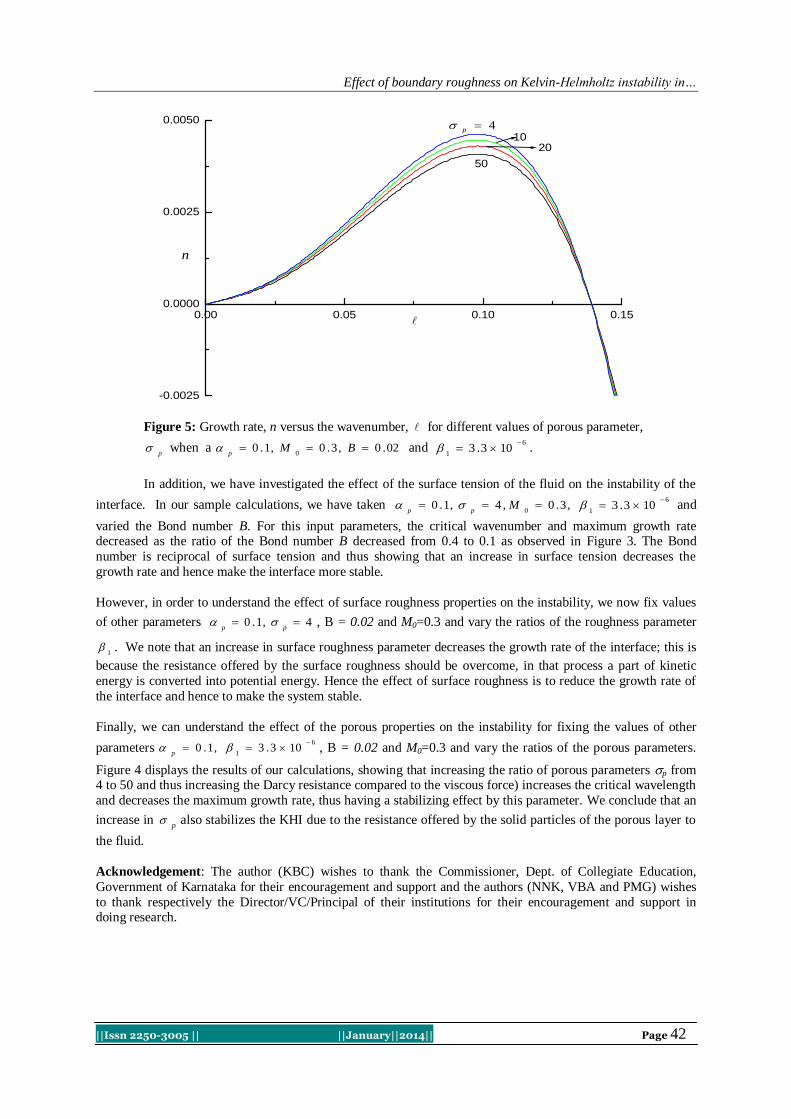
Effect of boundary roughness on Kelvin-Helmholtz instability in…
||Issn 2250-3005 || ||January||2014|| Page 42
0.00 0.05 0.10 0.15
-0.0025
0.0000
0.0025
0.0050
50
2010
n
4p
B
C
D
E
Figure 5: Growth rate, n versus the wavenumber, for different values of porous parameter,
p when a 02.0,3.0,1.0
0 BM
p and
6
1103.3
.
In addition, we have investigated the effect of the surface tension of the fluid on the instability of the
interface. In our sample calculations, we have taken ,3.0,4,1.00 M
pp
6
1103.3
and
varied the Bond number B. For this input parameters, the critical wavenumber and maximum growth rate decreased as the ratio of the Bond number B decreased from 0.4 to 0.1 as observed in Figure 3. The Bond
number is reciprocal of surface tension and thus showing that an increase in surface tension decreases the
growth rate and hence make the interface more stable.
However, in order to understand the effect of surface roughness properties on the instability, we now fix values
of other parameters 4,1.0 pp
, B = 0.02 and M0=0.3 and vary the ratios of the roughness parameter
1 . We note that an increase in surface roughness parameter decreases the growth rate of the interface; this is
because the resistance offered by the surface roughness should be overcome, in that process a part of kinetic
energy is converted into potential energy. Hence the effect of surface roughness is to reduce the growth rate of
the interface and hence to make the system stable.
Finally, we can understand the effect of the porous properties on the instability for fixing the values of other
parameters6
1103.3,1.0
p, B = 0.02 and M0=0.3 and vary the ratios of the porous parameters.
Figure 4 displays the results of our calculations, showing that increasing the ratio of porous parameters p from 4 to 50 and thus increasing the Darcy resistance compared to the viscous force) increases the critical wavelength
and decreases the maximum growth rate, thus having a stabilizing effect by this parameter. We conclude that an
increase in p
also stabilizes the KHI due to the resistance offered by the solid particles of the porous layer to
the fluid.
Acknowledgement: The author (KBC) wishes to thank the Commissioner, Dept. of Collegiate Education,
Government of Karnataka for their encouragement and support and the authors (NNK, VBA and PMG) wishes
to thank respectively the Director/VC/Principal of their institutions for their encouragement and support in doing research.

Effect of boundary roughness on Kelvin-Helmholtz instability in…
||Issn 2250-3005 || ||January||2014|| Page 43
REFERENCES [1]. L. Kelvin(1910), Hydrokinetic solutions and observations , On the motion of free solids through a liquid, 69-75, “ Influence of
wind and capillary on waves in water superposed frictionless, 76-85, Mathematical and Physical Papers IV, Hydrodynamics and
General Dynamics, Cambridge, England.
[2]. H. Helmholtz (1868), Under discontinuirliche Flussigkeitsbewegungen, Wissenschaftliche Abhandlungen, 146-157 or Phil. Mag.
Ser. 4(36), 337.
[3]. S. Chandrasekhar (1961), Hydrodynamic and Hydromagnetic Stability, Dover Publications, New York.
[4]. J. R. D. Francis (1954), Wave motions and the aerodynamic drag on a free oil surface, Phil. Mag. Ser. 7, 45, 695.
[5]. Melcher, J. R., (1963), Field coupled surface waves, Cambridge, Massachussets, MIT Press.
[6]. Sharma, R.C., and Srivastava, K. M., (1968), Effect of horizontal and vertical magnetic fields on Rayleigh-Taylor instability,
Aust. J. Phys., 21, 923.
[7]. Y.O.El-Dib, and G. M. Moatimid(1994), On the stability of a rotating electric field liquid jet. Effect of an axial electric field,
Physica A, 205,511.
[8]. R. P. Singh and H. C. Khare(1991), Stability of rotating gravitating superposed streams in a uniform magnetic field, Proc. Nat.
Acad. Sci., City, vol.43,55.
[9]. P.K. Bhatia and A. B. Hazarika(1995), Gravitational instability of partially ionized plasma in an oblique magnetic field, Physica
Scripts, Vol. 51(6), 775.
[10]. T. R. Benjamin and T. J. Bridges(1997), Reappraisal of the K-H problem, Part-2: Introduction of the Kelvin-Helmholtz
superharmonic and Benjamin-Feir instabilities, J. Fluid Mech., 333, 327.
[11]. P. K. Bhatia and A. Sharma(2003), KHI of two viscous superposed conducting fluids, Proc. Nat. Acad. Sci. India, 73(A), IV.
[12]. A. J. Babchin, A. L. Frenkel, B. G. Levich, G. I. Shivashinsky(1983), Nonlinear Saturation of Rayleigh-Taylor Instability in
Thin Films, Phys. Fluids, 26, 3159.
[13]. N. Rudraiah, B. S. Krishnamurthy and R. D. Mathad(1996), The effect of oblique magnetic field on the surface instability of a
finite conducting fluid layer, Acta, Mech., 119, 165.
[14]. G.S. Beavers and D.D. Joseph(1967), Boundary conditions at a naturally permeable wall, J. Fluid Mech., 30, 197.
[15]. V.K. Stokes(1966), Couple stresses in Fluids, Phys. Fluids. 9, 1709.
[16]. P. Sinha, P., C. Singh and K. R. Prasad(1981), Couple Stresses in Journal Bearings Lubricants and the Effect of Cavitations,
WEAR, 67(1), 15.
[17]. N. M. Bujurke, and G. Jayaraman(1982), The influence of couple stresses in squeeze films, Int. J. Mech. Sci., 24, 369.
[18]. E. Walicki and A. Walicka(1999), Flows of generalized second grade fluids in rectilinear channels, Appl. Mech. Engg. 4, 363.
[19]. Sunil, R.C., Sharma, and R. S. Chandel(2002), On superposed fluids in porous medium in hydrodynamics, Z. Naturforsch, 57a,
955.
[20]. Y. O. El-Dib and R. T. Matoog(2005), Electrorheological Kelvin– Helmholtz instability of a fluid sheet, Journal of Colloid and
Interface Science 289, 223.
[21]. K. B. Chavaraddi, N. N. Katagi and V. B. Awati(2012), Kelvin-Helmholtz instability in a fluid layer bounded above by a porous
layer and below by a rigid surface in presence of magnetic field, Applied Mathematics, 3, 564.
[22]. M.J. Miksis and S.H. Davis(1994), Slip over rough and coated surfaces, J. Fluid Mech., 273, 125.

International Journal of Computational Engineering Research||Vol, 04||Issue, 1||
||Issn 2250-3005 || ||January||2014|| Page 44
Combinational Study of Mineral Admixture and Super Plasticizer
in Usual Concrete
Debabrata Pradhan1, D. Dutta
2, Dr. Partha Ghosh
3
1,Lecturer, Civil Engineering Department, A.J.C.Bose Polytechnic, Berachampa, North 24 Parganas, West
Bengal, India 2, Asst Professor, Camellia School of Engineering & Technology, Barasat, Kolkata, West Bengal, India.
3,Asst. Professor, Department of Construction Engineering, Jadavpur University, Kolkata, India
I. INTRODUCTION Silica fume is very fine non-crystalline silica derived in electric arc furnaces and it is a by-product
resulting during the manufacture of elemental silicon or an alloy containing silicon as defined by the American
Concrete Institute (ACI). Numerous researchers made widespread experiments around the world and observed
that the incorporation of silica fume in concrete develops the various mechanical properties like concrete
strengths, durability, modulus of elasticity, corrosion protection, chemical and abrasion resistance. But no sole
conclusion regarding the optimum percentage of cement replacement by silica fume is obtained, while some
researchers have reported different replacement levels [1, 2 and 3]. Bhanja and Sengupta experimented silica
fume concrete to observe the effect of silica fume on compressive and tensile strength of high performance
concrete (HPC) and the mathematical model using statistical methods was developed for prediction of 28-days
compressive strength of silica fume concrete with water- cementitious material (w/cm) ratios ranged from 0.30
to 0.42 and cement replacement by silica fume from 5 to 30 %.
The authors observed that optimum cement replacement level by silica fume is not constant for all
water-binder ratios but depends on water content of mix. The authors also reported that compressive strength of
silica fume concrete depends on w/cm, total cementitious material content and cement-admixture ratio [4, 5 and
6]. Song et al. observed the diffusivity procedure of high strength concrete on the basis of a microstructure
model and water-to-binder ratio, silica fume replacement ratio, and degree of hydration are the key factor which
control the diffusivity and reported that incorporation of silica fume decrease the diffusivity and makes the
microstructure of concrete denser [7]. Mazloom et al. investigated the effects of various levels of silica fume on
fresh and mechanical properties of high-strength concrete and reported that the various properties like
compressive strength, shrinkage, swelling, secant modulus of elasticity, strain due to creep and moisture
movement are enhanced [8].
ABSTRACT: Now a days the tailor made high strength and high performance concrete embodied with silica fume
into the normal concrete are being widely used all over the world and it is a common practice in the
present days. The presence of silica fume makes the mix proportioning difficult and increase the
design parameters in conventional concrete. The principal object of this paper is to observe the
several mechanical properties like compressive strength, compacting factor, and slump of silica fume
concrete. In this present paper silica fume concrete are cast for 5 (five) mixes to execute
experiments. Various percentages of silica fumes are used for cement replacement to carry out these
experimentations at a single unchanging water-cementitious materials ratio keeping other mix design
variables unvarying. The various cement replacement levels by silica fume are 0%, 5%, 10%, 15%
and 20% for a single water-cementitious materials (w/cm) ratio of 0.50. Different sizes like 100 and
150 mm cubes are used to find out the compressive strengths for all mixes at age levels of 24 hours, 7
and 28 days. Except the compressive strengths, other properties like compacting factor, slump of
concrete are also resoluted for five mixes of concrete. To overcome low workability problem, high
range water reducer chemical admixture is used.
KEYWORDS: Silica fume, high strength concrete, high performance concrete and strength.

Combinational Study Of Mineral Admixture…
||Issn 2250-3005 || ||January||2014|| Page 45
Rao experimented to investigate the influence of silica fume on various properties of cement pastes and
mortars like air content, normal consistency of cement, specific gravity and workability of mortar with different
silica fume contents and reported that incorporation of silica fume lead the considerable change in the behavior
of cement pastes and mortars [9]. Katkhuda*1
, Hanayneh2 and Shatarat
1 experimented to observe the isolated
effect of silica fume on compressive, flexural and tensile strengths on high strength lightweight concrete and
showed that the compressive, flexural and tensile strengths enhanced with silica fume incorporation but the
optimal replacement percentage is not invariable because it depends on the water–cementitious material (w/cm)
ratio of the mix [10]. Yaqub* and Bukhari reported that smaller sizes (10 mm and 5mm) and rounded shape of
coarse aggregates should be used to obtain the high strength concrete than other sizes and shape respectively
[11]. It is reported that to overcome the unfavorable effect on workability, higher percentage of super plasticizer
would be used in silica fume concrete for higher percentage of cement replacement by silica fume [12, 13]. In
this paper our effort is made to examine the different mechanical properties like compressive strength, slump,
compacting factor of silica fume concrete taking into account of a single fixed water-cementitious material
ratio of 0.50.
II. AIMS AND OBJECTIVES OF THE PRESENT EXPERIMENTATION To observe the different mechanical properties i.e., compressive strength, compacting factor and slump
of concrete incorporating silica fume at different replacement levels of cement by silica fume.
III. SCOPE OF THE PRESENT WORK High-strength and high performance concrete of grade M60, the replacement levels of cement by silica
fume are selected as 0%, 5%, 10%, 15% and 20% for 100 and 150 mm cubes for testing.
IV. EXPERIMENTAL INVESTIGATION 4.1. Materials
4.1.1. Cement
Ordinary Portland Cement of ACC brand of 43 grade is used in the present research wok which
surpasses BIS Specifications (IS 8112-1989) on compressive strength levels.
4.1.2. Fine Aggregate
Locally available River sand (i.e. natural sand) as per IS: 383-1970 is used, the bulk density of which is
2610 kg/m3. The properties of fine aggregate are shown in Table 1.
Table 1: Properties of fine aggregate
Sl. No. Property Result
1. Specific Gravity 2.61
2. Fineness modulus 3.10
3. Grading zone II
4.1.3. Coarse Aggregate
Crushed aggregate used is in compliance to IS: 383-1970. The size, specific gravity and fineness
modulus of coarse aggregate used are 12.5 mm, 2.83 and 6.28 respectively.
4.1.4. Silica Fume (Grade 920 D)
Silica fume used is compliant to ASTM- C (1240-2000) which is supplied by “ELKEM
INDUSTRIES” is named Elkem – micro silica 920 D and also the cement is partially replaced by silica fume.
The properties of silica fume are shown in tabular form in Table 2.

Combinational Study Of Mineral Admixture…
||Issn 2250-3005 || ||January||2014|| Page 46
Table 2: Silica Fume- chemical & physical analysis report
Sl.no. PHYSICAL TESTS ANALYSIS
1. Oversize - % retained on 45
m sieve (wet sieved) 1.13%
2. Density – (specific gravity) 2.27
3. Bulk Density – (per ASTM)
187.91 kg/m3
11.73 lb/ft3
4. Specific Surface Area (by
BET)*
22.21 m2/kg
5. Accelerated Pozzo;anic
Activity Index with
Portland Cement
134.90%
*As per manufacturers manual
4.1.5. Super Plasticizer In these experimentations for development of the workability of concrete, super plasticizer-
CONPLAST-SP 430 with the form of sulphonated Naphthalene polymers in compliance to IS: 9103-1999 and
ASTM 494 type F is used. Conplast SP 430 has been specially formulated to report high range of water
reductions up to 25% without losing workability or to turn out high quality concrete of lesser permeability. The
properties of super plasticizer are shown below in Table 3.
Table 3: Properties of super plasticizer
Sl.no. PHYSICAL TESTS ANALYSIS
1. Specific Gravity 1.224
2. Chloride content NIL
3. Air entrainment 11.73 lb/ft3
*As per manufacturers manual
4.2. Mix Proportioning
In these experiments the mixes of concrete are intended as per the guidelines specified in I.S. 10262-
1982 though some restriction is mandatory by restricting the amount of cementitious material content is equal to
450 Kg/m3. The Table 4 shows mix fraction of concrete (Kg/m
3):
Table 4: Mix Proportioning
W/cm Cement
(Kg/m3)
Fine Aggregate
(Kg/m3)
Coarse Aggregate
(Kg/m3)
Water
(Kg/m3)
Compacting
factor
0.50 400 639.800 1121.070 200 0.815 – 0.840
Sl.No. CHEMICAL
ANALYSIS
ANALYSIS
1. SO2 95.00 %
2. SO3 0.18 %
3. CL 0.12 %
4. Total Alkali 0.66%
5. Moisture Content 0.16%
6. Loss of ignition 1.92%
7. pH 7.90%

Combinational Study Of Mineral Admixture…
||Issn 2250-3005 || ||January||2014|| Page 47
V. TEST RESULTS AND DISCUSSION
Table 5: Compressive strength and fresh concrete properties
W/c
m
Cementitio
us material
(Kg/m3)
% of
MA
(SF)
Compressive Strength (MPa) %
of
SP
Slump
(mm) CF
150 mm cubes 100 mm cubes
24
Hrs.
7
days
28
days
24
Hrs.
7
days
28
days
0.5
400
0 18.07 30.5
2
44.2 19.20 32.6
0
48.00 0.00 25,25,2
3
0.815
5 21.63 36.6
3
45.11 23.70 38.0
0
55.33 0.50 18,15,1
5
0.84
10 29.93 39.5
6
57.45 30.30 40.7
8
58.00 1.00 22,20,1
8
0.82
15 32.74 40.6
0
60.20 33.60 40.8
0
57.20 1.30 20,25,2
1
0.80
20 37.04 40.1
1
60.46 38.10 43.3
3
61.00 1.75 15,20,1
8
0.83
In this paper experiments are executed for 5 (five) mix of concrete embodied with undensified silica
fume. Due to use of smaller size of coarse aggregate (i.e. 12.5 mm) in the experiments, better bonding at the
interfacial zone is occurred between coarse aggregates and paste matrix, because of exposure of larger surface
area for smaller size of coarse aggregates. As a result, the interfacial zone between coarse aggregate and paste
matrix is more strengthened and denser, so strength in silica fume concrete is higher than concrete without
silica fume. Different cement replacement levels by silica fume (i.e. 0%, 5%, 10%, 15% and 20%) are used to
carry out the experiments at a fixed constant water-cementitious materials ratio of 0.40 but at the same time
other design mix parameters are keeping constant. Compressive strengths are observed at different age levels
(i.e. at 24 hours, 7 and 28 days) for 150 mm and 100 mm cubes for all mixes. Experiments are also executed to
survey the results of other properties like compacting factor and slump for all mixes of concrete. It is
investigated from experimental results that at all cement replacement levels by silica fume (i.e. at 5 %, 10%,
15% and 20%) and at all age levels (i.e. at 24 hours, 7 days and 28 days), compressive strengths are higher than
concrete without silica fume. It is evident from experimental results that higher compressive strengths of 100
mm cubes are obtained than 150 mm cubes at all age and cement replacement levels by silica fume. It is also
determined that the maximum compressive strength is found at 20% cement replacement by silica fume. It is
found that 28 days compressive strength is 60.46 MPa and 61.00 MPa for 150 mm and 100mm cubes
respectively at 20% cement replacement by silica fume but for control concrete (i.e. concrete without silica
fume) it is 44.20 MPa and 48.00 MPa respectively. For workability, compacting factor and slump value ranges
from 0.815 to 0.84 and 15 to 25mm respectively are obtained. The values of slump show the mixes are cohesive
in nature.
VI. CONCLUSIONS The highest value of compressive strength is obtained at all age levels (i.e. at 24 hours, 7 and 28 days)
at 20% cement replacement by silica fume. Slump value may be increased by increasing the dosages of
superplasticizer without hampering the strength for further investigation but the range of compacting factor from
0.815 to 0.84 is good for using concrete in the field in control system. Higher compressive strength is reported
as per IS code recommendations that the concrete incorporated with silica fume is high strength concrete (HSC).
During the testing of cubes at 28 days, it is found that the failure plane of cubes cut the aggregates but not along
the inter facial zone. Hence it is concluded that the interfacial zone attained much higher strength than control
concrete i.e. concrete without silica fume. It is seemed that improved pore structures at transition zone of silica
fume concrete converted to it as high performance concrete but durability tests are yet to be surveyed.

Combinational Study Of Mineral Admixture…
||Issn 2250-3005 || ||January||2014|| Page 48
REFERENCES [1] F.P. Zhou, B.I.G. Barr, F.D. Lydon, “Fracture properties of high strength concretes with varying silica fume content and
aggregates”, Cement and Concrete Research, 25 (3) (1995) 543–552.
[2] S.A. Khedr, M.N. Abou-Zeid, “ Characteristics of silica-fume concrete”, J. Mater. Civ. Eng. ASCE , 6 (3) (1994) 357–375. [3] V. Yogendran, B.W. Langan, M.N. Haque, M.A. Ward, “Silica fume in high strength concrete”, ACI Material Journal. 84 (2)
(1982) 124–129
[4] S. Bhanjaa,*, B. Sengupta,” Influence of silica fume on the tensile strength of concrete “, Cement and Concrete Research, 35 (2005) 743-747.
[5] S. Bhanjaa,*, B. Sengupta ,” Investigations on the compressive strength of silica fume concrete using statistical methods”, Cement
and Concrete Research, 32 (2002) 1391-1394. [6] S. Bhanjaa,*, B. Sengupta ,”Modified water–cement ratio law for silica fume concretes”, Cement and Concrete Research, 33
(2003), 447-450.
[7] Ha-Won Song, Jong-Chul Jang, Velu Saraswathy, Keun-Joo Byun,” An estimation of the diffusivity of silica fume concrete”, Building andEnvironment, 42 (2007) 1358–1367.
[8] M. Mazloom a,*, A.A. Ramezanianpour b, J.J. Brooks ,” Effect of silica fume on mechanical properties of high-strength concrete”,
Cement &Concrete Composites ,26 (2004) 347–357. [9] G. Appa Rao ,”Investigations on the performance of silica fume incorporated cement pastes and mortars”, Cement and Concrete
Research, 33 (2003) 1765–1770.
[10] H. Katkhuda*1, B. Hanayneh2 and N. Shatarat1, “Influence of Silica Fume on High Strength Lightweight Concrete”, World
Academy of Science, Engineering and Technology 34 2009.
[11] Yaqub* M., Bukhari I.,“Effect of Size of Coarse Aggregate on Compressive Strength of High Strength Concerts”, 31st Conference
on Our World In Concrete & Structures: 16 - 17 August 2006, Singapore. [12] Bayasi Zing, Zhou Jing, (1993). “Properties of Silica Fume Concrete and Mortar”, ACI Materials Journal 90 (4) 349 - 356.
[13] Hooton, R.D., “Influence of Silica Fume Replacement of Cement on Physical Properties and Resistance to Sulfate Attack, Freezing
and Thawing, and Alkali-Silica Reactivity",ACI Materials Journal,Vol.90, No. 2,March/April 1993, pp. 143 - 151.

International Journal of Computational Engineering Research||Vol, 04||Issue, 1||
||Issn 2250-3005 || ||January||2014|| Page 49
Design of Closed Loop Electro Mechanical Actuation System
Poondla.Chiranjeevi1, J.Venkatesu Naik
2
1PG Student, Department of Mechanical Engineering, Chadalawada Ramanamma Engineering College.
2Assistant Professor, Department of Mechanical Engineering, Chadalawada Ramanamma Engineering College, Tirupati, AP, India.
I. INTRODUCTION This document covers the description, design, inputs and specifications of the Actuation System for aerodynamic control of an Aero-vehicle. The document also describes the actuator specifications, mechanical
components, BLDC motor, position sensor and the control system including simulation.
1.1. Actuator
An actuator is a mechanism that converts energy into motion. It can also be used to apply a force. An
actuator typically is a mechanical device that takes energy, usually created by air, electricity, or liquid, and
converts that into some kind of motion. That motion can be anything from blocking to clamping to ejecting.
Actuators are typically used in manufacturing or industrial applications and may be used in things like motors,
pumps, switches, and valves. The most common type of actuator is powered by air — the pneumatic cylinder,
also known as the aircylinder. Air cylinders are air-tight cylinders, typically made from metal, that use the
energy of compressed air to move a piston. Air cylinders are most commonly used in manufacturing and
assembly processes. Grippers, which are used in robotics, use actuators driven by compressed air to work much like human fingers.Actuators can also be powered by electricity or hydraulics. Much like there are air cylinders,
there are also electric cylinders and hydraulic cylinders where the cylinder converts electricity or hydraulics into
motion. Hydraulic cylinders are often used in certain types of vehicles.
Many actuators have more than one type of power source. Solenoid valves, for example, can be
powered by air and electricity. Electricity powers the solenoid, and the solenoid, powered by air actuates the
valve. Alternatively, the solenoid can be powered by hydraulics and electricity.Actuators can create a linear
motion, rotary motion, or oscillatory motion. That is, they can create motion in one direction, in a circular
motion, or in opposite directions at regular intervals. Hydraulic and air cylinders can be classified as single
acting, meaning that the energy source causes movement in one direction and a spring is used for the other
direction. Alternatively, these cylinders can be double acting cylinders, meaning the energy is used in two directions. While actuators are typically discussed in terms of mechanical implements, muscles are sometimes
given as an example of an actuator. Energy (e.g., created by eating carbohydrates) is converted by the muscle
(i.e., the actuator) into motion (e.g., kicking a ball).
ABSTRACT: An Actuator is basically a position servo control system used in industries and vehicles.
A rotary electro mechanical actuation system is an angular positioning system used in aerospace
applications such as control of rudder and ailerons of aero planes and control of control surfaces, jet
vanes, etc. This position loop system is to steer the vehicle to move in required direction.
A servo controller is a driver to accurately control the position of the actuation system by getting the
command signals from the on-board computer of the vehicle. It involves a class of DSP controller optimized for digital motor motion control and power conversion applications.
In this thesis, Closed loop Rotary Electro Mechanical Actuating system is designed for the derived
specifications by using the CAD software UNIGRAPHICS, and simulated the design with the help of
FEA software ANSYS and MATLAB.
KEYWORDS: Actuator, ANSYS, CAD, DSP controller, UNIGRAPHICS.

Design Of Closed Loop Electro Mechanical…
||Issn 2250-3005 || ||January||2014|| Page 50
Fig 1.Mechanism of Actuator Fig 2. Block diagram of actuator
II. DESCRIPTION AND CONFIGURATION OF ACTUATOR The actuator configuration is as follows….
Prime mover is a 3 phase BLDC motor.
Transmission by Planetary gear train.
Position feedback element is Rotary potentiometer.
Servo control by DSP controller.
Fig 3.Electro mechanical actuator Fig 4.Servo controller
III. CONCEPTUAL DESIGN Based on the available space, torque and speed specifications, the rated torque of the motor is taken as
0.075Nm. To get a rated torque of 2.5Nm, the gear ratio of the gear box is taken as aprox.50:1. To meet this
gear ratio at output shaft, the gear train taken is one simple gear train and two stage planetary gear train.
Keeping in view of available space and above consideration that is taken, the conceptual design and final
modeling is done in CAD software unigraphics.
Fig 5. Exploded view of electro mechanical actuator
Fig 6. Exploded view of servo controller

Design Of Closed Loop Electro Mechanical…
||Issn 2250-3005 || ||January||2014|| Page 51
IV. DESIGN OF ACTUATOR 4.1 Defining motor inputs for motor selection
To achieve the given specifications, the gear ratio is taken as 50 and after conceptual design by taking
module of 0.6, the final gear ratio achieved is 49.25:1
4.2 Gear box efficiency
S
p
u
r
G
ear Efficiency = 96.13 %
Planetary Gear Efficiency = 79.28%
Total Gear Box Efficiency = 76.21%
Stall torque of motor should be considered greater than 0.1183 N-m for 49.25 gear
Rated torque of motor should be considered greater than 0.0679 N-m for 49.25
4.3 Gear box design From outline specifications and space availability the gear box sizes finalized as Ø40 x 41 and selected
Gear Ratio as 49.25
The total gear ratio divided to spur gear reduction and planetary gear reduction.
Spur Gear Reduction = 3.8
Planetary Gear Reduction for two stages = 12.96
Each Stage Planetary Reduction = 3.6
Fig 7. Gear box construction
1.3.1 spur gear & planetary gear design
Table 1. Spur gear design parameters Table 2. Planetary gear design parameters
Gear Type F sign of Rg term
External spur cos α (Rg+1)
Internal Spur α (Rg-1)

Design Of Closed Loop Electro Mechanical…
||Issn 2250-3005 || ||January||2014|| Page 52
If consider 3Nos of Planet Gears of 2.6 (Excluding chamfers) mm face width than Factor of safety = 5
If consider 5Nos of Planet Gears of 4 mm (Excluding chamfers) face width than Factor of safety =
2.2 (Since we are calculated for Peak Torque)
V. STRUCTURAL ANALYSIS OF OUTPUT SHAFT Type of element: tetrahedron in ansys
Stress developed in the shaft due twisting and bending force material : SS 420
No. of nodes: 262440
No. of elements: 181487 Fig 8. Meshing of output shaft
5.1 Supports & Load Conditions:
Cylindrical support at bearing surfaces Fixed support at key way Moment at output of shaft (4500 N
mm)
Fig 9. Supports and Loads on output shaft
5.2 Solution:
Equivalent stress (Von Mises)
Fig 10. Equivalent stresses on output shaft

Design Of Closed Loop Electro Mechanical…
||Issn 2250-3005 || ||January||2014|| Page 53
Part Allowable stress(N/mm2) Results in ANSYS(N/mm2),MAX
Output shaft 448 315.37
Table-3
Structural analysis of housing in ansys
Stress developed in the housing due to twisting(motor and bending load:
Material : 1. Output shaft= SS420
o 2. Housing= Al(HE 15)
Type of element : Tetrahedron
No. of nodes: 226198
No. of Elements : 146290
Fig 11. Meshing of stator housing and output shaft Fig 12. Boundary conditions on housing
6.1 Boundary Conditions
2 bearings are fixed to housing
Output shaft is fixed to 2 bearings
Bending load applied at shaft is 360N
Moment applied at stator position is 4.5Nm
6.2 Solution

Design Of Closed Loop Electro Mechanical…
||Issn 2250-3005 || ||January||2014|| Page 54
Fig 13. Equivalent stress on housing
Part Allowable stress(N/mm2) Results in ANSYS(N/mm2),MAX
Output shaft 448 75.283
Housing 37.5 18.138
Table- 4
VI. CONTROL SYSTEM SIMULATION BY USING MAT LAB
Fig 14. Actuator simulation model
Fig 15. Dead band response at 90mV Based on system parameters given on table and explanation given at
control block diagram, dynamic simulation model was prepared on matlab simulink and controller gains were
tuned to its optimal values to meet required position output as well as frequency response specifications given.
Fig 16. Frequency response at 1V Fig 17. Step response

Design Of Closed Loop Electro Mechanical…
||Issn 2250-3005 || ||January||2014|| Page 55
From the frequency response of the closed loop system, we get Bandwidth of the system at -90deg phase is
equal to 37.4Hz
6.1 STEP RESPONSE Applying step input to the model, response of the system as shown below.
Observations:
SL No. Description Specification value Simulation Value Remarks
1 Rise time Less than 12 m sec 9.95m sec
Table-5
VII. CONCLUSION Based on the results achieved in ANSYS and MATLAB we conclude that the closed loop electro
mechanical actuation system will meet the required design specification.
VIII. FUTURE SCOPE Electro Pneumatic, Electro Hydraulic, and Hot Gas System etc. can be replaced with the Electro
mechanical actuation system. An accurate position movement and sensing can be achieved with the Electro
mechanical actuation systems. The high precision machinery and equipments in which Electro mechanical
actuation systems used are robots, CNC machines, missile systems, spacecrafts etc. The Electro mechanical
actuation system has to fulfill the requirements of being able to function reliably in a typical environment
involving adverse and extreme climatic conditions, field transportation and storage conditions imposing severe
vibrations, bumps, mechanical shocks and extreme temperature conditions.
REFERENCES [1] S. C. J. Jensen, G.D. Dawson, D. , "Flight test experience with an electromechanical actuator on the F- 18 Systems Research
Aircraft."
[2] L. U. Gokdere, S. L. Chiu, K. J. Keller et al., “Lifetime control of electromechanical actuators,” in Aerospace Conference, 2005
IEEE, Big Sky, MT, 2005, pp. 3523-3531.
[3] Sclater, N., Mechanisms and Mechanical Devices Source book, 4th Edition (2007), 25, McGraw-Hill
[4] Howstuffworks "Transmission Basics"
[5] ANSI/AGMA 1012-G05, "Gear Nomenclature, Definition of Terms with Symbols".
[6] Khurmi, R.S, Theory of Machines, S.CHAND
[7] Schunck, Richard, "Minimizing gearbox noise inside and outside the box.", Motion System Design.
[8] MARK’S Calculations for mechanical design by Thomas H. Brown
[9] Machine Design by R.S. KHURMI, J.K. GUPTA
[10] Mechanical Engineering Design by Budynas−Nisbett
[11] O. C. Zienkiewicz, R. L. Taylor, J. Z. Zhu : The Finite Element Method: Its Basis and Fundamentals, Butterworth-Heinemann,
(2005).
[12] The Finite Element Methods in Engineering, by SS Rao
[13] G. W. Younkin, Industrial Servo Control Systems - Fundamentals and Applications - Second Edition, Taylor and Francis, 2007.
[14] Cassandras, Christos (2007-11-27). "Introduction to Discrete-Event Simulation". Springer US. Retrieved 2009-11-03
International Journal of Computational Engineering Research||Vol, 04||Issue, 1||
||Issn 2250-3005 || ||January||2014|| Page 56
Effect Of In-Band Crosstalk For Datapath Routing In
WDM/DWDM Networks
1 Praveen Singh
2 Prof. R.L.Sharma
1 M.Tech Student
2 Professor Department of Electronics & Communication Engineering
Ajay Kumar Garg Engineering College, Ghaziabad
I. INTRODUCTION: Fiber-Optic communication system has an important advantage of exploiting the large bandwidth
(nearly equal to THz) of an optical fiber [1, 2]. However, it is extremely difficult to exploit all of the huge
bandwidth of a fiber using a single high capacity wavelength channel due to optical-electronic bandwidth
mismatch [3]. A major breakthrough occurred with the advent of wavelength division multiplexing (WDM),
which is a method of sending many light beams of different wavelengths simultaneously down the core of an
optical fiber [4]. In WDM networks, prisms and diffraction gratings can be used to multiplex or de-multiplex
different wavelength signals. However, as a result of their imperfect filtering characteristics, the separation of
the wavelengths at the receiver may not be ideal, leading to performance degradation due to crosstalk [5, 6].
Incoherent or in-band crosstalk occurs in optical networks when a desired signal and unwanted optical
fields with the same nominal wavelength arrive simultaneously at a receiver. If the desired and interfering fields are not
phase co-related, they beat at the receiver, causing power fluctuations that increase the bit-error rate (BER). This
phenomenon has long been recognized as a serious problem in optical networks [7, 8]. One of the major
crosstalk in optical networks with WDM transmission is component crosstalk. Component crosstalk occurs in
optical networks when a desired signal and an unwanted signal from neighboring input ports, with the same
wavelength arrive simultaneously at a channel [9, 10]. The desired and the unwanted signal are not
correlated in phase due to power fluctuation of laser. Therefore, they interact with each other, causing power
fluctuations and increasing bit error probability of the system. Bit error rate of the receiver can be evaluated
by calculating the noise in the photo-detector output due to crosstalk in addition to the noise of the detector
itself [11]. In many cases, the probability density function (pdf) of overall noise is assumed Gaussian to
calculate bit error rate. However, the Gaussian model, despite its simplicity, cannot accurately describe the
signal-crosstalk noise, especially when the number of interfering channels is not very large. The maximum
number of channels that can be used in a WDM system is limited by the total noise (including crosstalk) in
the receiver system [12]. Therefore, several non-Gaussian models are developed to get a better estimate of the
system performance. The pdf of such non-Gaussian models developed for finite interferers uses different
techniques, such as saddle point approximation, numerical integration, Gram-Charlier series, and modified
Chernoff bound [15,16]. However, these are often computationally complex and in many cases give little
physical insight. In this paper, the effects of component crosstalk with finite interferers on the performance of
a WDM receiver are studied [17]. Bit error rate (BER) and power penalty in the receiver are calculated using a
ABSTRACT: Physical layer impairments are the major limitation for the high speed optical
WDM/DWDM networks. They significantly affect the signal quality resulting poor quality of
transmission which is normally expressed in terms of bit-error rate. To cope up with the future
demand, increase in the no. of channels and data speed further enhances these impairments. Hence
new techniques are needed, which mitigate these impairments and ensure a better quality of
transmission. Among the physical layer impairments we have studied the impact of in-band crosstalk
on transmission performance of a transparent WDM/DWDM network. In this paper, the effects of
component crosstalk with finite interferers on the performance of a WDM receiver are studied.
Bit error rate (BER) and power penalty in the receiver are calculated using a simplified analysis
which can represent the performance of the WDM receiver in case of small number of
interferers. Some optimum detection thresholds are suggested for minimum bit error rate.
Optimum detection thresholds for minimum bit error rates in the WDM receiver in presence of
component crosstalk are investigated.
KEYWORDS: Bit error rate, crosstalk, detection threshold, optical network, wavelength
division multiplexing (WDM)

Effect Of In-Band Crosstalk for Datapath…
||Issn 2250-3005 || ||January||2014|| Page 57
simplified analysis which can represent the performance of the WDM receiver in case of small number of
interferers[18]. Based on this study, optimum detection thresholds for minimum BER in the presence of
component crosstalk are suggested, which is important for the best possible design to minimize this crosstalk.In
Section 2, crosstalk and its mathematical model are discussed. The bit error rate & power penalty at the receiver
output is calculated in Section 3 while the results of the analysis are given in Section 4. Finally, in Section 5, a
conclusion is given.
II. IN-BAND CROSSTALK: In WDM/DWDM network, a message is sent from one node to another node using a
wavelength continuous route called light paths (LPs) without requiring any O-E-O conversion and
buffering at the routing node. Multiplexing, de-multiplexing and switching are done in the optical domain
using prisms and diffraction gratings.Non-ideal nature of these component results in-band crosstalk, which
has the same wavelength as the signal and degrades the transmission performance of the network. In-band
crosstalk can be divided into coherent crosstalk, whose phase is correlated with the desired signal
considered, and incoherent crosstalk whose phase is not correlated with the signal considered [19, 20].Coherent
crosstalk is believed not to cause noise but causes small fluctuation of signal power. In this paper, we
considered in-coherent crosstalk which has the more adverse effect than coherent crosstalk. Incoherent crosstalk
is often analyzed using the pdf of the noise in the received photocurrent. The pdf can be derived from the
fields of the wanted signal and of each interfering signal.
Desired optical signal and each interfering signal are assumed to be
(1)
(2)
Where all the fields have same nominal optical frequency, ω, Φ(t) represents the independent phase fluctuation
of each optical source, ps is the optical power in the desire signal, and Eεk is the optical power of the kth
interference relative to the signal. bs,k(t) =0,1 depending on whether zero or one is transmitted by the desired and
interference signal at time t. The total incident optical field on the photo detector can be written as for N
crosstalk term
(3)
(4)
For unit detector responsivity and for worst-case assumption of identical polarization of signal and crosstalk, the
photocurrent i(t) is given by
(5)
(6)
Where θk(t) = Φ
k(t) - Φ
s(t), k=1,…..N, are random phase. Ignoring the small terms in the order of ε
k, the overall
receiver noise in the photo-detector is
(7)
When ZERO is transmitted by the signal channel, there is no crosstalk and noise n0(t) = ng(t), where ng(t) is
the usual Gaussian noise in the receiver. When ONE is transmitted by the signal,
Channel Crosstalk generates a total noise of
(8)
For N interferers and Gaussian noise, the pdf of the noise in the received photocurrent can be obtained by
integrating the Gaussian noise over all possible values of phase offset between signal and each interferences
[13, 14]. Assuming the phase difference between signal and interferers are independent and uniformly
distributed between (0, π), the noise photocurrent pdf is given by

Effect Of In-Band Crosstalk for Datapath…
||Issn 2250-3005 || ||January||2014|| Page 58
(9)
Where and σ is the variance of thermal noise. The effect of Crosstalk is maximum when
phase difference is close to 0 and the pdf can be approximated by expanding the cosine term by first order
Taylor Series [13] up to the term ϴk2
(10)
Expanding the square term and keeping term up to ϴk2 , the pdf for noise when signal is transmitting 1 is given
by
(11)
III. CALCULATION OF BER & POWER PENALTY: BER in the presence of in-band crosstalk is given by fraction of the received photocurrent pdf’s
that fall on the wrong side of some decision variable d, for each combination of data “1”s and “0” of the signal
and crosstalk[14]. Here we followed a simplified approach as given by Santu Sarkar et. al for extreme case
when all interferers are transmitting “1”, so that we have an upper bound for BER during our routing and
wavelength assignment algorithm[21,22].
(12)
Where
Here the weighting function f(y) is approximated as f (Is-d) to make the integral possible. σ2 is the variance of
the receiver of the receiver noise when “1” is transmitted by the signal channel and σth2 is the variance of the
receiver thermal noise when “0” is transmitted. Expansion for BER at the WDM receiver is given by [14]:
(13)
The Power Penalty is found by comparing the photocurrents at receiver that produce the same BER with and
without crosstalk

Effect Of In-Band Crosstalk for Datapath…
||Issn 2250-3005 || ||January||2014|| Page 59
(14)
Is/NC being the photocurrent when there is no crosstalk (NC). Now the BER in case of no crosstalk is
(15)
Where
BNC = Is/NC /2σ is the SNR of receiver. The BER with crosstalk is
(16)
Where B= Is /2σ is the SNR with crosstalk, Therefore,
(17)
Without component crosstalk, the required SNR to achieve a BER of 10-9
is BNC = 6. So, for a BER of 10-9
in
the presence component crosstalk, the Power Penalty is given by PP = 10log10 (B/6).
IV. SIMULATION AND RESULTS: In this paper, we discuss the simulation result for an optimal lightpath selection mechanism based on a
guaranteed QoT. We use MATLAB for our simulation work. In Figure 1 dotted lines shows different channels
from one node to another in an optical network and dark lines shows the optimum path with minimum bit error
rate . There are multiple paths from one node to another but if we consider two nodes, there is only one optimal
path from source to destination.
Fig.1 different paths between various nodes in optical network
The performance degradation due to In-band crosstalk depends very much on the no. of crosstalk
interferences. In the following figures, the BER is plotted as a function of input power for different
number of interfering channels (N).

Effect Of In-Band Crosstalk for Datapath…
||Issn 2250-3005 || ||January||2014|| Page 60
These figures show that BER increases significantly as the no. of crosstalk component increases. Here we have
neglected the effect of shot noise and assumed that all interferers have same amount of crosstalk level. Fig.
2(a), 2(b), 2(c), 2(d), 2(e), 2(f) shows the graph between BER and Input Power for different number of
Interfering Channels (N) at a fixed crosstalk level of -25 dB,
Fig. 2(a) Plot of BER with the Input Power for N=0 Fig. 2(b) Plot of BER with Input Power for N=1
Fig. 2(c) Plot of BER with the Input Power for N=2 Fig. 2(d) Plot of BER with the Input Power for N=3
Fig. 2(e) Plot of BER with the Input Power for N=4 Fig. 2(f) Plot of BER with the Input Power for N=5

Effect Of In-Band Crosstalk for Datapath…
||Issn 2250-3005 || ||January||2014|| Page 61
Fig. 3 shows variation of Power Penalty with Crosstalk level (total) for different number of interfering channels,
Fig. 3 Plot of Power Penalty with total crosstalk level for different number of interfering channels (N)
V. CONCLUSION: In this paper, we have done a comprehensive survey on physical layer impairments and their impacts on
transparent optical networks. Among the impairments we mainly focused on in-band crosstalk. Bit error rate and power
penalties due to component crosstalk in a WDM Receiver has been calculated using a Taylor series and computed results are
shown as a function of number of interfering channels, input power and crosstalk levels. Receiver Noise should be
minimized to get the improvement through crosstalk minimization.
ACKNOWLEDGEMENT:
The author thanks Ajay Kumar Garg Engineering College, Ghaziabad for allowing the research work in
the lab and all possible help. The author is also very thankful to Prof. P.K. Chopra, HoD, ECE Department and
Mr. Amit Choudhary, Asstt. Professor, ECE Department, Ajay Kumar Garg Engineering College, Ghaziabad for
his valuable suggestions.
REFERENCES: [1] Chava Vijay Saradhi and Suresh Subramaniam,“Physical layer impairments Aware Routing (PLIAR) In WDM Optical Network Issues and
Challenges,”IEEE Communication survey & Tutorials, vol. 11, no. 4, pp.109-129.fourth quarter.2009.
[2] Siamak Azodolmolky and et al, “A Survey on Physical layer impairments Aware Routing and Wavelength Assignment
Algorithms in Optical Networks,”Computer Networks, vol.53, pp. 926-944, December 2008.
[3] Yurong Huang and et al, “Connection Provisioning with Transmission Impairment Consideration in Optical WDM Networks With High-Speed
Channels,” Journal of Lightwave Technology, vol. 23, no. 3,pp.982-993, march 2005.
[4] I. Tomkos, “Transport Performance of WDM metropolitan area transparent optical networks,” in Proc., OFC, pp.350-352Mar.2002.
[5] Smita Rai, Ching-Fong Su and Biswanath Mukherjee, “On Provisioning in All- Optical Network: An Impairment-Aware Approach,”IEEE/ACM
Transaction on Networking, vol. 17, no. 6, pp. 1989-2001, Dec.2009.
[6] Namik Sengezer and Ezhan Karasan, “Static Light path Establishment in Multilayer Traffic Engineering under Physical Layer
Impairments,” J.Opt.Communication & Networking, vol.2, no.9, Sept 2010.
[7] Konstantinos Christodoulopoulos and et al, “ Offline Routing and Wavelength Assignment in Transparent WDM Networks,”IEEE/ACM Transaction
on Networking, vol. 18, no. 5, pp. 1557-1570, Oct.2010.
[8] I, Tomkos et al., “Impairment Constrained Based Routing in Mesh Optical Networks,” Proc. OFC 2007.
[9] C. Politi et al., “Physical Layer Impairments Aware Routing Algorithms based on Analytical calculated Q-Factor”, Proc. OFC 2006.
[10] B. Ramamurty et al.,“Impact of Transmission Impairments on the Teletraffic Performance of Wavelength Routed Optical
Networks,”Journal of Lightwave Technology, vol. 17, pp.1713-1723, Oct. 1999.
[11] T. Deng and S. Subramaniam, “Adaptive QoS Routing in Dynamic Wavelength Routed Optical Networks,” Proc. Broadnets 2005.
[12] R. Ramaswami and K. Sivrajan, “Optical Networks: A Practical Perspective,
[13] Sarah D.Dods Trevoer B. Anderson “Calculation of bit-error rates and power penalties due to incoherent crosstalk in optical
networks using taylor series expansions,” j. Lightwave Technoloy., vol.23,No.4,pp.1828-1836,April.2005.
[14] Santu Sarakar and Nikhil R. Das, “Study of component crosstalk and obtaining optimum detection threshold for minimum bit-error-rate in a WDM
receiver,” j. Lightwave Technology., vol.27,No.19,pp.4366-4373,Oct.2009.
[15] Jun He, Maite, Brandt-Pearce and Suresh Subramaniam,“ QOS- Aware wavelength assignment with BER and latency Constraints for All-Optical
networks,” j. Lightwave Technology., Vol.27,No.5,pp.462-474,March 2009.
[16] Marcelo R. Jimenez, Rogerio Passy,Marco A. Grivet and Pierre Von Der, “Computation of power penalties due to intraband crosstalk [24] in optical
system,” IEEE Photonics Technology Letters, Vol.15, No.1, pp 156-158, Jan.2003.
[17] Keang-Po Ho, “Analysis of homodyne crosstalk in optical networks using Gram- Charlier Series”, j. Lightwave Technology., Vol.17, No.2,
pp.149-154, Feb- 1999.
[18] Yunfeng Shen, Kejie Lu and Wanyi Gu, “Coherent and Incoherent crosstalk in WDM networks “, j. Lightwave Technology.,Vol.17,No.5,pp.462-
474,May 2003.
[19] I.T. Monroy and E.Tangliongga,“Perfomance evaluation of optical crossconnects by saddlepoint approximation,” J. Lightwave Technol. vol. 16, pp.
317–323, Mar. 1998.
[20] T. Kamalakis and T. Sphicopoulos, “ Asymptotic behavior of in-band crosstlalk noise in WDM networks,” IEEE Photon. Technol. Lett vol. 15, pp.
476–478, Mar. 2003.
[21] Aneek Adhya, Debasish Datta,“Design Methodology for WDM backbone networks using FWM-aware heuristic algorithm,”Optical
Switching and Networking, vol. 6, pp. 10-19, june 2008.
[22] Aneek Adhya and Debasish Datta,“Lightpath Topology Design for Wavelength-Routed Optical Networks in the Presence of Four- Wave
Mixing,”J.Opt.Communication Network, vol. 4, No. 4, pp. 314-325, Apr. 2012.