International Conference on Advances in Engineering and ...
129
Interscience Research Network Interscience Research Network Interscience Research Network Interscience Research Network Conference Proceedings - Full Volumes IRNet Conference Proceedings 11-26-2011 International Conference on Advances in Engineering and International Conference on Advances in Engineering and Technology Technology Prof.Srikanta Patnaik Mentor IRNet India, [email protected] Follow this and additional works at: https://www.interscience.in/conf_proc_volumes Part of the Biomedical Engineering and Bioengineering Commons, Chemical Engineering Commons, Civil and Environmental Engineering Commons, Computational Engineering Commons, Computer Engineering Commons, and the Electrical and Computer Engineering Commons Recommended Citation Recommended Citation Patnaik, Prof.Srikanta Mentor, "International Conference on Advances in Engineering and Technology" (2011). Conference Proceedings - Full Volumes. 69. https://www.interscience.in/conf_proc_volumes/69 This Book is brought to you for free and open access by the IRNet Conference Proceedings at Interscience Research Network. It has been accepted for inclusion in Conference Proceedings - Full Volumes by an authorized administrator of Interscience Research Network. For more information, please contact [email protected].
-
Upload
khangminh22 -
Category
Documents
-
view
0 -
download
0
Transcript of International Conference on Advances in Engineering and ...

Interscience Research Network Interscience Research Network
Interscience Research Network Interscience Research Network
Conference Proceedings - Full Volumes IRNet Conference Proceedings
11-26-2011
International Conference on Advances in Engineering and International Conference on Advances in Engineering and
Technology Technology
Prof.Srikanta Patnaik Mentor IRNet India, [email protected]
Follow this and additional works at: https://www.interscience.in/conf_proc_volumes
Part of the Biomedical Engineering and Bioengineering Commons, Chemical Engineering Commons,
Civil and Environmental Engineering Commons, Computational Engineering Commons, Computer
Engineering Commons, and the Electrical and Computer Engineering Commons
Recommended Citation Recommended Citation Patnaik, Prof.Srikanta Mentor, "International Conference on Advances in Engineering and Technology" (2011). Conference Proceedings - Full Volumes. 69. https://www.interscience.in/conf_proc_volumes/69
This Book is brought to you for free and open access by the IRNet Conference Proceedings at Interscience Research Network. It has been accepted for inclusion in Conference Proceedings - Full Volumes by an authorized administrator of Interscience Research Network. For more information, please contact [email protected].

Interscience Research Network (IRNet)
Bhubaneswar, India
Proceedings of International Conference on
Advances in Engineering and Technology
(ICAET-2011) 26th November, 2011
BHUBANESWAR, India

Editorial
The new economic millennium is surprisingly rushing with Innovation and Technology. There is a
sharper focus on deriving value from the widespread global integration in almost all spheres of
social, economic, political and technological subsystems. All the dignified fields of Engineering are
becoming highly interdisciplinary and endowed with computational complexities. In the present
era of science and technology, much attention has been given to the association of Soft Computing
with other engineering disciplines. Soft Computing as a computational science dedicated to system
solutions using certain logically enriched techniques. It is basically a high profile study deals with a
fusion of research Evolutionary Algorithm and Genetic Programming, Neural Science and Neural
Network Systems, Fuzzy Set theory and Fuzzy Systems, Chaos Theory and Chaotic Systems. In all
perspectives the core objective is to reduce the complexity and uncertainty in the functioning of
various engineering designs. The broad area provides a unifying platform that fosters comparisons,
extensions and new applications.
In the advent of modern research there is a significant growth in Mechanical Engineering as
Computer Aided Design has become instrumental in many industrialized nations like USA,
European Countries, Scotland and GermOther CAE programs commonly used by mechanical
engineers include product lifecycle management (PLM) tools and analysis tools used to perform
complex simulations. Analysis tools may be used to predict product response to expected loads,
including fatigue life and manufacturability. These tools include Finite Element Analysis (FEA),
Computational Fluid Dynamics (CFD), and Computer-Aided Manufacturing (CAM). Using CAE
programs, a mechanical design team can quickly and cheaply iterates the design process to develop
a product that better meets cost, performance, and other constraints. No physical prototype need be
created until the design nears completion, allowing hundreds or thousands of designs to be
evaluated, instead of a relative few. In addition, CAE analysis programs can model complicated
physical phenomena which cannot be solved by hand, such as viscoelasticity, complex contact
between mating parts, or non-Newtonian flows.
Almost every researcher will not deny the fact that Computational Complexity is increasing with
the advanced trend multidisciplinary approach to the field of Computation. In many instances the
intricacies are not being solved through programming languages. MATLAB is an interactive
environment designed to perform scientific and engineering calculations and to create computer
simulations. MATLAB is a customized computing solution to the engineering researchers.
MATLAB is a high-level language and interactive environment that enables you to perform
computationally intensive tasks faster than with traditional programming languages such as C, C++,
and FORTRAN. MATLAB is attributed to the pioneering work of Cleve Moler, head of Computer

Science Department, University of New Mexico during 1970s. The development of the field is
credited to the works of MathWorks during 1984.
As the area is broad and requires cross functionally expert reviewers for technical scrutiny of the
papers, we have tried to impart justice to all the paper in its publication in the proceeding. In all
sense we have been transcendental in this field in developing the fauna of the conference. In
meeting the professional commitments we maintained the sanctity by adhering to ethics, ontology
and semiotics. I beg apology for any inconveniency caused to the participants and delegates in the
journey of this conference. I have regards for the IRNet family members, reviewers, and support
staffs for their generous gifts of time, energy and effort. Specifically I owe indebtedness to the
authors for their intellectual contributions in this conference.
Prof. (Dr.) Srikanta PatnaikPresident, IRNet India and Chairman IIMT
Intersceince Campus, Bhubaneswar
Email: [email protected]

International Conference on Advances in Engineering and Technology, 26th November, 2011, Bhubaneswar.
1
Utility of Resource Allocation and Frequency Off-set Estimation for
MB-OFDM based UWB
Ravi Gugulothu & Vijaya
Vaagdevi College of Engineering, Jawaharlal Nehru Technological University, Hyderabad,
Warangal-506002, India
Abstract - Most of the wireless services (like MB-OFDM, OFDM-MIMO) with variable rate transmission; both average rate and rate
oscillation are important performance metrics. The traditional performance criterion, utility of average transmission rate, boosts the
average rate. We introduce a utility function of instantaneous transmission rates. It is capable of facilitating the resource allocation
with flexible combinations of average rate. Based on the new utility, we consider the time and power allocation in a time-shared
wireless network. Two adaptation policies are developed, namely, time sharing (TS) and joint time sharing and power control
(JTPC). We address low-complexity; highly-accurate frequency offset estimation for multi-band orthogonal frequency division
multiplexing (MB-OFDM) based ultra-wide band systems in time-invariant as well as time-variant channels. We investigate the
unique characteristics of MB-OFDM systems, namely, different frequency offsets, channel responses, received energies, and
preamble structures in different frequency bands. Utilizing them, we develop frequency offset estimators based on the best linear
unbiased estimation principle for the utility of resource allocation. If compared to the reference estimators, our proposed methods
achieve significantly better estimation performance (4 to 6.4 dB (5 to 20 dB) estimation mean-square error advantage in the time-
invariant (time-variant) channels) for all preamble patterns of the MB-OFDM system.
Keywords - Utility function, Time sharing, UWB, BLUE, frequency offset, OFDM, JTPC.
I. INTRODUCTION
One promising approach for addressing this issue is
to dynamically allocate limited resources based on
channel information and system preferences. Traditional
investigations on wireless resource allocation pay much
attention to hard real-time services. There in, the goal is
to smooth out channel variation and build “bit pipes”
that deliver data at a fixed rate. The rapid growth of the
Internet has led to an increasing demand for supporting
transmissions of best-effort service in wireless systems.
These applications allow variable-rate transmission.
Therefore, opportunistic communications [1] have been
introduced to achieve higher system throughput. The
concept of opportunistic communications is essentially
to transmit more information in good channel states and
less in poor ones. If constant-rate transmission
algorithms are used, the transmission efficiency would
be very low. On the other hand, opportunistic
scheduling schemes, such as [2] and [3], whose
objective is to maximize a utility of average rates, can
improve efficiency in terms of average rate but result in
high oscillation in instantaneous transmission rates. This
thus motivated the need for a new criterion that can be
used to facilitate the choice of the combinations of
average rate and rate oscillation.
Ultra-Wide band (UWB) systems (e.g., impulse
radios [4], [5] and transmitted reference schemes [6] to
name a few) offer improved ranging precision, better
penetration through obstacles, higher data rate, and
increased multipath or frequency diversity. Due to ultra-
wide bandwidth, UWB systems can operate at low
power spectral density which allows overlay with other
narrow-band systems. The coexistence issue and the
spectral analysis of UWB systems have been
investigated in [7] . Another approach to realize UWB
systems is multi-band orthogonal frequency division
multiplexing (MB-OFDM) which has been proposed
for the IEEE 802.15.3a standard and adopted in
European Computer Manufacturers Association
(ECMA) standard . The very high data rate (480 Mbps
and beyond) capability of the UWB technology would
provide a compelling cable-replacement wireless
technology. OFDM is a relatively mature technology
and has been adopted in digital broadcasting, wireless
LAN and MAN standards. OFDM has several
advantages such as low complexity equalization in
dispersive channels and the spectral density
scalability/adaptability (e.g., adaptive bit loading ).
However, OFDM has some is advantages such as larger
susceptibility to nonlinear distortion at the transmit
power amplifier and larger sensitivity to frequency

Utility of Resource Allocation and Frequency Off-set Estimation for MB-OFDM based UWB
International Conference on Advances in Engineering and Technology, 26th November, 2011, Bhubaneswar.
2
offsets. The application of OFDM technology in UWB
systems demands highly accurate frequency offset
estimation, since frequency offset causes a loss of
orthogonality among the subcarriers thereby introducing
inter sub-carrier interference and significantly degrading
the error performance. In the MB-OFDM system in [8] ,
a preamble is used to aid receiver algorithms related to
timing and frequency synchronization, and channel
estimation. There are several preamble-based frequency
offset in the research literature. However, we have not
observed frequency offset estimators derived for the
MB-OFDM systems. In MB-OFDM systems, the
oscillator frequency offset (OFO) causes different
carrier frequency offsets (CFOs) for the different bands.
The channel frequency responses and the channel
energies for the different bands are different as well.
The frequency hopping of the MB-OFDM system
results in different preamble structures for some of the
frequency bands. These characteristics neither exist in
typical OFDM systems nor have been fully reported in
the MB-OFDM literature. To our best knowledge, no
frequency offset estimator has been developed utilizing
all of the above characteristics of MBOFDM systems
for performance improvement. The statistics of UWB
channels reported in the literature are mainly time-
invariant. However, moving scatterers can cause time-
varying UWB channels. The typical channel variations
due to moving persons in UWB applications would be
very slow and their effects on frequency offset
estimation are negligible. Best knowledge, there is no
frequency offset estimator designed to be robust against
sudden channel changes. In this paper, we characterize
the unique features of MBOFDM systems. Using a
simple channel model capturing occasional abrupt
channel change behavior, we develop an efficient
detection algorithm to track a sudden channel change
and propose frequency offset estimators suitable for
(sudden) time-variant as well as time-invariant UWB
systems. We apply the best linear unbiased estimation
(BLUE) principle and fully utilize the unique
characteristics of the MB-OFDM systems in developing
our frequency offset estimators. Our proposed
estimators offer significant MSE improvement over the
reference estimators (about 4-6.4 dB (5-20 dB)
estimation mean-square error (MSE) advantage in time-
invariant (time-variant) UWB channels).
The rest of this paper is organized as follows.
Section II describes the signal and channel models and
the proposed frequency offset estimation methods are
presented. Section III discusses the design parameters
Simulation results and discussions are provided, in
Section IV the paper is concluded.
II. SYSTEM MODEL
A. Time-average Aggregate concave Utility of
resource allocation and transmission Rate
We consider a single cell consisting of N mobile
users communicating with a common base station. The
communication link between each user and the base
station is modeled as a slowly time-varying fading
channel with additive white Gaussian noise (AWGN).
The channel coefficients remain approximately
unchanged during each time frame, but can vary from
one frame to another. Let the instantaneous channel gain
of user i at any given time frame t be denoted by
( )ig t The network channel gain is denoted by the
tupleN g(t) _ (g1(t), g2(t), . . . , ( )Ng t ), and has a joint
probability density function (PDF) f(g). Let
( )ip t denote the transmit power allocated to or from
user i. The achievable transmission rate of user is in the
absence of other users can be expressed
2
( ) ( )( ) log [1 ]i i
i
O
p t g tc t
Nβ= + (1)
Where 0N is the noise power, and β is the signal-to-
noise ratio (SNR) gap [4]. We assume that each time
frame can be accessed by all the N users in an adaptive
time-sharing fashion. Let ( )gρ = (ρ1, ρ2, . . . , Nρ )
denote the time-sharing adaptation policy with respect to
the network channel gain g, where iρ represents the
fraction of the frame duration allocated to user i.
Without loss of generality, the interval of a time frame is
normalized. The actual transmission rate of user i at the
t-th time frame, ( )ir t is given by ( ) ( )i i ir t c tρ= .The
frame index t in ( )ir t and ( )ig t may be omitted
hereafter if no confusion occurs. The utility considered
here is a function of the instantaneous transmission rate.
For user i, we denote its utility as ( ( ) )i i
U r t . The
analysis throughout this paper is valid for any utility
function that is increasing, differentiable and concave.
B. Time sharing
In this section, we assume that the transmission
powers between BS and mobiles are constant and
identical for different users, i.e., ( )i
p t p= ,i∀ , t, and
that the wireless network is fully loaded. We choose the
aggregate utility, which is the sum of individual user
utilities, as the performance measure. The goal is to find
the optimal time-sharing adaptation policy ρ∗(g) relative
to the instantaneous network channel condition g, so as
to maximize the TAUR of the system. Since the channel

Utility of Resource Allocation and Frequency Off-set Estimation for MB-OFDM based UWB
International Conference on Advances in Engineering and Technology, 26th November, 2011, Bhubaneswar.
3
processes are ergodic, the optimization problem can be
expressed mathematically as
[ ( ( ))]( ) 1
NMax I E U r tt i iTsg iρ
∆ ∑=
(2)
1
( ( ), ) ( )N
i i i
ig
U g g f g dgρ
=
= ∑∫
1
( ) 1N
i
i
p g=
=∑ (3)
Where notation Et[・] represents the time average.
Since the constraint (3) is defined for all channel states,
the average aggregate utility maximization in (2) is
equivalent to maximizing the instantaneous aggregate
utility for every channel state. Furthermore, since the
utility ( . )i
U is a concave function of ir by assumption,
( . )i
U is also concave in ip .
C. Signal and channel models
C.1. UWB Signal Model
We will adopt two types of UWB technologies
which are presently emerging for technical and
commercial purposes: the impulse radio UWB (IR-
UWB) and the multiband OFDM UWB (MB-OFDM
UWB) [8]. IR-UWB uses a short pulse (less than 1ns)
that occupies a large bandwidth to modulate the
information. Three typical modulation techniques are:
time hopping pulse position modulation (TH-PPM),
time hopping pulse amplitude modulation (TH-PAM),
and direct sequence pulse amplitude modulation (DS-
PAM) .The PPM-TH-UWB signal can be written as:
( ) ( ) ( )
1 [ / ]( ) ( )k k k
s j c j N s
j
s t g t jT C T dε∞
=−∞
= − − −∑ (4)
The PAM-TH-UWB signal may be expressed as
follows:
( )( ) ( )
2[ / ]
( ) ( )s
kk k
s j cj j N
j
S t e g t jT C T∞
=
=−∞
= − −∑ (5)
PAM-DS-UWB signal is donated as:
( )
3 ( ) ( )k
j s
j
S t d g t jT∞
=−∞
= −∑ (6)
In Equation (1)-(3), Ts represents the pulse repetition
period without modulation; j
C (k) is the thj symbol of
the pseudorandom time hopping sequence of the thk
user; cT is donated as the unit transmit pulse delay
controlled by time hopping symbol; ε is a constant term;
ei €-1,+1, di (k) €0,1; “[]” represents rounding
operation, and one binary symbol is transmitted within
every Ns pulses; g(t) is the
Gaussian pulse waveform and may be given by:
2
2
2 2
2
5( )
2
rt
g t e σσ
σ
−= ±
Π
(7)
Where σ is an index correlated to the width of pulse,
indicating the shape of pulse.
In this paper, MB-OFDM PHY layer model is based on
IEEE802.15.3a proposal, as shown in Fig. 1. And fig. 2.
Fig.1 : PHY layer model of MB-OFDM
C.2. UWB Channel Model:
The Saleh and Valenzuela (S-V) multipath channel
model proposed by IEEE802.15.3a, which is on the
basis of modification of classical broadband indoor S-V
model, is used as UWB channel model. The modified
model retains the characteristics of the classical model,
e.g. multiple paths appear in the form of clusters, and
energy is subject to double-exponential distribution.
Moreover, S-V model with a lognormal fading
distribution on the amplitudes is superior to Rayleigh
channels.
C.3. The MB-OFDM-based UWB system
The carrier frequency is hopped within a pre-
defined set of carrier frequencies f1, f2, f3
(corresponding to disjoint frequency bands) from
symbol to symbol, according to a time-frequency code.
The MB-OFDM system from has 4 different preamble
patterns (for 4 pico-nets), each associated with a
different time-frequency code. Each preamble pattern is
constructed by successively repeating a time-domain
preamble sequence(symbol) over 21 periods as PS0,
PS1, . . . , PS20 . The preamble patterns 1 and 2 (or, 3
and 4) have the same structure, except for the ordering

Utility of Resource Allocation and Frequency Off-set Estimation for MB-OFDM based UWB
International Conference on Advances in Engineering and Technology, 26th November, 2011, Bhubaneswar.
4
of the carrier frequencies. The preamble pattern 3 or 4,
however, has a structure distinct from pattern 1 or 2. For
details of the preamble structures of preamble 3 or4,In
the MB-OFDM-based system from [8], zero-padded
guard intervals pre
N prefix and suf
N suffix zero
samples; Ng = pre
N +suf
N are used instead of the
conventional cyclic prefix guard interval.
Fig. 2 : A simple time-variant UWB channel model
capturing occasional sudden channel changes.
The total number of samples in one OFDM symbol
(including the guard samples) is M0 = N + Ng. The low-
pass-equivalent time-domain samples sq(k = mM0
+pre
N + n) : n = −pre
N , . . . , N + suf
N − 1 (sampled
at N/T = 1/Ts, N times the sub-carrier spacing)
transmitted during the m-th symbol interval in the q-th
frequency band are generated by taking the N-point
inverse discrete Fourier transform of the corresponding
sub-carrier symbols ,
( )q m
C l (zeros for null sub-
carriers; all zeros if no symbols are transmitted in the q-
th band during the m-th interval) and inserting zero
guard-samples as
12 ln/
,
0
1/ ( ) ,0 1
0, 0;( )
Nj N
q m
t
pre suf
N C l e n N
q N n N n N NS k
π
−
=
≤ ≤ −
− ≤ < ≤ < +
∑=
(8)
The IEEE 802.15.3a UWB RF channel model described
and is given by
, ,
0 0
( ) ( )k
l
L k
RF k i k l
l k
h t X t T Tα
= =
= − −∑∑ (9)
where ,k lα , Tl ,
,k lτ , and X are random variables
representing the multipath gain coefficients, the delay of
the l-th cluster, the delay (relative to the l-th cluster
arrival time) of the k-th multipath component of the l-th
cluster, and the log-normal shadowing on the amplitude,
respectively. 1hL+
is the number of the clusters and K +
1 is the number of the multi-path components per
cluster. In this paper, we consider a low-pass equivalent
system that absorbs the carrier-frequency hopping into
the channel impulse response (CIR). The sample-spaced
low-pass-equivalent CIR for the q-th band is given by
0, ,( )2 ( )
,
0 0
( )h
i kq l k l l
L knT T T tf T T
q k l
l k
h n X e pπ
α
− − −− +
= =
= ∑∑ (10)
where the effect of the combined transmit and receive
filter with the impulse response p(t) has been included in
the CIR and t0 is a delay for the causality.
The above UWB channel model does not include
time varying behavior. However, the movements of the
transmitter, the receiver, and/or the scatterers result in a
time-varying channel. For the UWB system in [8], the
channel variations due to the Doppler spread are too
slow and can be neglected in the CFO estimation.
However, occasionally when a fast scatterer moves
through and thus blocks one or more of the UWB
channel paths, an abrupt change in the CIR will occur. A
scatterer can move into or out of a position that blocks
some channel paths. We consider that the paths affected
by the fast moving scatterer correspond to the cL -th
cluster, which is a random variable.
For convenience, we assume that arbitrary J
adjacent rays of the cL -th cluster are completely
blocked. Note that 0 ≤ J ≤ K and J = 0 corresponds to a
time invariant channel while J = K with k0 = 0 defines
that the whole cL -th cluster is blocked. Due to non-
negligible physical sizes of moving scatters in typical
UWB environments, after an abrupt change occurs, the
channel will most likely remain the same for the
mandatory Mode-1 of the MB-OFDM system , the three
carrier frequencies are generated from one oscillator.
The normalized (by the sub-carrier spacing) OFO υ
causes different normalized CFOs υq for the three
bands, and their relationship4 is given by
q qV b V= , for q=1,2,3 (11)
1 2 3
13 15 17[ , , ] [ , , ]
16 16 16b b b = (12)
We assume that the timing synchronization eliminates
inter symbol-interference. Define q
t = ql
t (i) : i = 0,
. . . , N −1; l = 1, . . ., q
L where ql
t (i) : i = 0, 1, . . . ,
N −1 denotes the time-domain sample index set
corresponding to the l-th non-zero preamble symbol
period in the q-th band. Lq is the number of nonzero
preamble symbols in the q-th band and depends on the
preamble pattern and band index q. Let ( )qx k denote
the low-pass-equivalent time domain channel output

Utility of Resource Allocation and Frequency Off-set Estimation for MB-OFDM based UWB
International Conference on Advances in Engineering and Technology, 26th November, 2011, Bhubaneswar.
5
(noise-free) signal samples corresponding to the q-th
band, where q
x (k) ∆=q
x (t0+ skT ).
D. Frequency offset estimation
As discussed in the previous section, UWB systems
may undergo abrupt channel changes. When an abrupt
channel change occurs in the middle of the preamble
transmission, the CFO estimation can be significantly
affected due to the coherence loss in the periodicity of
the received preamble symbols. In this section, we
develop a BLUE-based OFO estimator for time-
invariant/time-variant UWB channels. The novelty of
the proposed approach compared to existing BLUE
based approaches is the incorporation of the MB OFDM
characteristics in the estimator development. For time-
variant UWB channels, we first split the preamble in
each band into two5 parts (left and right) by a simple
abrupt channel change detection algorithm, which will
be described in Section IV. We denote these parts by p-
th preamble part with p = 1 and 2 for the left and right
part, respectively.
The underlying idea is that correlation-based
estimators require identical channel output preamble
symbols, and due to the abrupt change, the channel
outputs corresponding to these two parts will not be
identical, and hence should not be cross correlated. Next
we estimate CFO based on each part, and then
appropriately average the CFO estimates. For time-
invariant UWB channels, since they are the special cases
of time-variant channels with the steady-state
probability vector [1, 0]T , we can apply the method
developed for the time-variant channel except with the
following changes: we skip the abrupt channel change
detection step, set the left part of the preamble in each
band to be the preamble itself and hence null the right
part. 4Our proposed estimator can be applied to other
implementations of carrier frequencies generation by
changing the values in (7) accordingly. 5Due to non-
negligible physical sizes of moving scatters, the channel
change occurs only once (if it does) during the preamble
transmission, and hence we just need to consider two
parts.
D.1. OFO Estimation:
The proposed OFO estimator is based on the
BLUE principle and the correlation among the non-zero
received preamble symbols within the same part of the
band. For every preamble pattern, the channel output
preamble of each part in a single band has identical
symbols. The channel output preambles of different
preamble parts are not the same due to distinct channel
responses.
III. EXPERIMENTAL RESULTS
We use the simulation parameters as specified in
:N = 128, Ng = 37, carrier frequencies f1 = 3432 MHz,f2 =
3960 MHz, f3 = 4488 MHz, the sub-carrier spacing 1/T
= 4.125 MHz, and four different preambles. The channel
model CM-2 with hL = 6 and K = 6 is adopted.
Fig. 3 : Performance comparison of different resource
allocation schemes.
Fig.3 shows the no. of users for different resource
allocation and the utility considered here is a function of
the instantaneous transmission rate. For user i, we
denote its utility as ( ( ))i iU r t . The exact expression for
the utility (.)iU is not crucial. The analysis throughout
this paper is valid for any utility function that is
increasing, differentiable and concave.
Fig. 4 : Average rate and standard deviation of rate
versus average SNR using TS and GS
In Fig. 4 compares the mean and the standard
deviation of the transmission rate achieved by TS and
GS policies for A = 0.1, 1 and 10 with N = 32. The
performances of the GS policy at different values of A
are identical due to the channel symmetry among the
users. In fact, it is an extreme case of our TS.

Utility of Resource Allocation and Frequency Off-set Estimation for MB-OFDM based UWB
International Conference on Advances in Engineering and Technology, 26th November, 2011, Bhubaneswar.
6
Fig. 2 shows the simulated TAUR in the network by
using the proposed TS policy and the existing GS
policy. Here the utility of both policies is specified to
have the form
( ) ln(1 )r
U rA
= +
(13)
where A > 0 is a concavity indicator. The channels are
assumed to be Rayleigh fading and the SNR gap is set to
8.2 dB for all users which corresponds to a bit-error-rate
requirement of 10−5 when adaptive quadrature
amplitude modulation (QAM) is used. The number of
users in the network varies from 8 to 32 and their
channel conditions are symmetric.
The concavity indicator A is set at 0.1.
Fig. 5 : The normalized OFO estimation performance of
the proposed method in two time-variant channels
(defined by blocking one whole cluster and blocking
two adjacent rays, respectively, when an abrupt
In Fig. 5, we evaluate the proposed method in two
time Variant channels. In the first channel, we use J = K
and k0 =0, i.e., the whole cluster is blocked when a
moving scatterer affects the channel. In the second
channel, we use J = 2, i.e., only two adjacent rays are
blocked when a moving scatterer affects the channel.
We only apply method B here since the estimation
performance of the other method is similar. The
simulation result shows that the proposed method works
well in both channels.
IV. CONCLUSION
We develop a new framework for resource
allocation in wireless networks for variable-rate
transmission. The time-average aggregate utility of
instantaneous transmission rate is proposed to jointly
optimize the resulting average rate and rate oscillation.
In particular, a time-sharing policy and a joint time-
sharing and power control policy are designed to exploit
the channel fluctuation.We have presented enhanced
OFO estimators based on the BLUE principle for MB-
OFDM based UWB systems by exploiting several
characteristics of the MB-OFDM system –such as
different CFOs, channel responses, received energies
and preamble structures in different bands. We develop
our estimators to be robust against sudden channel
changes which can occur in some UWB systems with
fast moving scatters. The proposed estimators are
adaptive such that when a sudden channel change is
detected during the preamble duration, the estimator
designed for such a time-variant scenario is used,
otherwise the estimator developed for the time-invariant
channel is applied. For systems with no sudden channel
changes, the latter estimator can be solely implemented
for implementation simplicity. Our proposed approach
can be applied to other multi-band systems or similar
frequency hopped systems.
REFERENCES
[1] P. Viswanath, D. Tse, and R. Laroia,
“Opportunistic beamforming using dumb
antennas,” IEEE Trans. Inform. Theory, vol. 48,
no. 6, pp. 1277–1294, June 2002.
[2] A. Jalali, R. Padovani, and R. Pankaj, “Data
throughput of CDMA-HDR a high efficiency-
high data rate personal communication wireless
system,” in Proc. Veh. Technol. (VTC), 2000.
[3] A. L. Stolyar, “On the asymptotic optimality of
the gradient scheduling algorithm for multiuser
throughput allocation,” Operation Research, vol.
53, no. 1, pp. 12–25, Jan. 2005.
[4] M. Z. Win and R. A. Scholtz, “Impulse radio:
how it works,” IEEECommun. Lett, vol. 2, no. 2,
pp. 36-38, Feb. 1998.
[5] M. Z. Win and R. A. Scholtz, “Ultra-wide
bandwidth time-hopping spread-spectrum
impulse radio for wireless multiple-access
communications,”IEEE Trans. Commun., vol. 48,
no. 4, pp. 679-691, Apr. 2000.
[6] T. Q. S. Quek and M. Z. Win, “Analysis of UWB
transmitted reference communication systems in
dense multipath channels,” IEEE J. Select Areas
Commun., vol. 23, no. 9, pp. 1863-1874, Sept.
2005.
[7] A. Giorgetti, M. Chiani, and M. Z. Win, “The
effect of narrowband interference on wideband
wireless communication systems,” IEEE Trans.
Commun., vol. 53, no. 12, pp. 2139-2149, Dec.
2005.
[8] M. Z. Win, “A unified spectral analysis of
generalized time-hopping spread-spectrum
signals in the presence of timing jitter,” IEEE J.
Select. Areas Commun., vol. 20, no. 9, pp. 1664-
1676, Dec. 2002.

International Conference on Advances in Engineering and Technology, 26th November, 2011, Bhubaneswar.
7
Hybrid Neuro Fuzzy Temperature Controller using
High Resolution Multifunction Card
R.T.Jadhav1 & R.T.Patil
2
1Dept. of Technology, Shivaji University, Kolhapur, Maharashtra, India 2Dept. of Electronics, TKIET College, Warananagar, Maharashtra, India
E-mail: [email protected], [email protected]
Abstract - The performance of Neuro-fuzzy techniques for a real time temperature controller system has been investigated in detail.
A study of efficiency and superiority of control techniques of Neuro-fuzzy controller related to structure, system and design
experience over conventional controller is carried out. The construction of circuit, design of the neuro-fuzzy system and
experimental investigations has been reported. The designed controller was based on user friendly interface LabVIEW, one of the
most important industrial platforms, which allows us to move from design to implementation in only few steps. The experimental
result shows the system performance improvement with respect to oscillations around set point and settling time.
Key words - Neuro-fuzzy controller; conventional controller; PCI add-on card; temperature measurement; LabVIEW.
I. INTRODUCTION
The past decade has witnessed a significant
breakthrough in the field of intelligent controllers. The
field has been experiencing constant upgrades at a rate
considered to be revolutionary. This tremendous
breakthrough was a strong motivation for expanding our
research in this field.
Real time control of non-linear systems is often a
quite complex and computationally intensive task. It is
for this reason that Neural Networks (NNs) and Fuzzy
Systems (FSs) which are two branches of artificial
intelligence are gaining widespread acceptance in the
field of learning and intelligent control. This is due
mainly to their intrinsic parallelism, their learning and
adaptation capabilities and, to some extent, also to their
increased fault tolerance. Fuzzy control and Neural
Network control have many control advantages as
above, but fuzzy control also has a drawback that you
have to set new control laws and membership functions
every time types of system change even after you set
control laws and membership functions. And neural
network has a drawback that while learning, it can easily
fail onto local minimum instead of global minimum, and
it take much time to make as many neurons learn as how
complicated the system.
In order to make up for the defects, research on
integration of neural network and fuzzy logic that is
hybrid Neuro-fuzzy controller (HNFC) is under way. A
proposed HNFC is an intelligent system that combines
qualitative knowledge of symbolic fuzzy rules and
learning capabilities of neural networks. Temperature
control is an important factor in many process control
system. If the temperature is too high or too low, the
final product or the product under observation is
seriously affected. Therefore it is necessary to reach
some desired temperature points quickly and avoid large
overshoot. Since the process control system are often
non linear, complex in nature and tend to change in an
unpredictable way, they are not easy to control
accurately. Therefore, the proposed HNFC is expected
to be a better alternative in accurately modeling and
controlling the non linear thermal system.
In this paper the performance of neuro-fuzzy
controller is tested on real time temperature controller
system. To train the neuro-fuzzy controller generally
input-output characterization or desired output of the
plant is sufficient. The error and derivative error is given
as an input to the system and the neural network’s
output is given to the fuzzy logic. Neural network will
decided which fuzzy set is selected out of five fuzzy
sets. The maximum membership set is selected [1].
II. FUZZY SYSTEMS
A. Fuzzy variables and basic operations
In contrary to Boolean logic where variables can
have only binary states in fuzzy logic all variables may
have any values between zero and one. The fuzzy logic
consists of the some basic Λ - AND, V - OR and NOT
operations.
USER
Rectangle

Hybrid Neuro Fuzzy Temperature Controller using High Resolution Multifunction Card
International Conference on Advances in Engineering and Technology, 26th November, 2011, Bhubaneswar.
8
A Λ B Λ C ⇒ min (A, B, C) - Smallest value of A or
B or C
A V B V C ⇒ max (A, B, C) - Largest value of A or B
or C.
Ā ⇒ 1 - A- One minus value of A
For example: 0.1 Λ 0.8 Λ 0.4 = 0.1, 0.1 V 0.8 V 0.4 =
0.8, 0.3 = 0.7
All above rules are known as zadeh AND, OR and NOT
operators
B. Fuzzy Controller
The principle operation of fuzzy controller is
different from neural networks. The fuzzy controller is
divided in to three steps .In first step, analog inputs are
converted into a set of fuzzy variables. In this step we
use five fuzzy sets which is given in (1). Each fuzzy
variable has analog value between zero and one. In the
next step, a fuzzy logic is applied to the input fuzzy
variables and resulting set of output variables is
generated. The last step is known as defuzzification.
From the set of output fuzzy variables one output
variable is selected [2]
very small, small, medium, large, very large (1)
Fig. 1 : Fuzzy set.
III. HYBRID NEURO FUZZY SYSTEM
Neural networks and fuzzy systems are different in
two aspects. First, neural networks are adaptable and
trainable. Secondly, the neural networks are in nature
large scale and parallel. The weights attached to data
play an important role in the operation of a neural
network .It is however difficult to understand the
behavior of neural network. Fuzzy logic is mainly
concerned with the imprecision and can express
knowledge of field experts. Since fuzzy logic rules are
constituted by human intuitions fuzzy logic has no
adaptable and trainable properties. In a complex system,
the more rules, the more complex the calculations is the
longer it will take to identify and set up this rules. These
properties limit the applicability of fuzzy logic [3].
When two technologic are combined, the advantages of
both are useful for various applications. Advantages of
hybrid system is given below
• Amalgamation of different pieces of knowledge is
possible by application of fuzzy rules.
• A large scale knowledge base can be effectively
handled and reduced by fuzzy front end or backend
processor making learning easy and fast.
• Non precise and context depend knowledge is
represented using fuzzy logic.
• Reorganization and learning from noisy data is
possible.
• The neural network processes the data and
knowledge by combining these two constructed
inductively and dependently.
• The technique is robust in that only some rules in
fuzzy knowledge base require to be updated with
changing input condition avoiding the need to
retrain the neural network. [4]
IV. CASCADE NEURO – FUZZY CONTROLLER
There are several fusion techniques to fuse the
neural network and fuzzy logic out of that most suitable
and simple is cascade. In this type the neural network
gives output to fuzzy logic and selects the fuzzy set
accordingly (Fig.2). There is another way is that the
fuzzy logic gives input to the neural network. In this
paper we use first approach.
Fig. 2 : Cascade Control Syste
The function of the neural fuzzy compensator is to
compensate for any unsatisfactory performance of the
basic fuzzy controller. The model structure of neuro-
fuzzy compensator is shown in Fig.3. The neural
network has one hidden layer and one output layer. All
the neurons have sigmoid function .The neural fuzzy
compensator is trained in an on line back propagation
algorithm. The updating of weight is given in (2).

Hybrid Neuro Fuzzy Temperature Controller using High Resolution Multifunction Card
International Conference on Advances in Engineering and Technology, 26th November, 2011, Bhubaneswar.
9
Fig. 3 : Neuro Fuzzy Controller.
Wij (t +1) = Wij (t) + ∆Wji (2)
Where Wij (t) is the weight from unit i to unit j at time t
(or tth
iteration) and ∆Wji is the weight adjustment. The
weight change is computed by
∆Wji = η δj oi (3)
Where η is a trial independent learning rate, δj is the
error gradient at unit j and oi is activation level [5].
The neural network select the one set out of five fuzzy
set .When error is more the output category is very
large. When the error is minimum or zero, the selected
category is zero set. The defuzzified output is given to
the DAC.
V. DESCRIPTION OF THE SYSTEM
The schematic diagram of the implemented control
system is shown in Fig.4. The system consists of six
main components, a heater assembly, a sensor (K-type
thermocouple) and an instrument amplifier (IC AD
595), 16-bit, 250kS/s high-resolution multifunction, I/O
interface card (PCI 1716, Advantech make), a PC in
which the software for neuro- fuzzy controller is written
in LabVIEW and final control element.
Fig. 4 : System Diagram
VI. HARDWARE SYSTEM
A. Temperature Measurement
The heater assembly consists of a sample holder
(heating element) made of kanthol metal strip of size 3 ×
1.5 cm is used. The chromel alumel (K- type)
thermocouple is spot welded on the bottom of the
sample holder (kanthol metal strip) to measure the
temperature of the sample. A 4 V, 50 amps transformer
is used to heat the kanthol strip.
The signal generated by the junction of the K-type
thermocouple due to thermal changes was fed to an
instrumentation amplifier (IC AD595) specially
designed for cold junction compensation and very low
signal amplification as shown in figure 5. It combines an
ice point reference with a precalibrated amplifier to
produce a high level (10 mV/°C) output directly from a
thermocouple signal. The output of the instrumentation
amplifier IC AD595 is fed to the single ended analog
channel of PCI 1716 PC add-on card.
Fig. 5 : Temperature measurement circuit
B. High Resolution Data Acquisition Card
The PCI 1716 is a high performance, multifunction
analog interface card for IBM/PC/XT/AT and
compatible computers. It uses the hardware based
analog to digital conversion process, providing a
conversion time of 2.5 µs and 250K samples per second
acquisition rate. The output channel provides fast
settling time of 5µs with high accuracy. A high quality
multiplexer in the input stage provides 16 single ended
analog inputs or 8-channel Differential A/D Input.
Standard input and output voltage ranges is user
selectable, independent of each other. The A/D trigger
and data transfer are controlled through programming.
The block diagram is shown in figure 6.

Hybrid Neuro Fuzzy Temperature Controller using High Resolution Multifunction Card
International Conference on Advances in Engineering and Technology, 26th November, 2011, Bhubaneswar.
10
Fig. 6 : Block Diagram of PCI 1716 Card
C. Final Control Element
The temperature of the system through K-type
thermocouple is measured with the help of PCI 1716 PC
add-on card at constant intervals of a few milliseconds
and is compared with the setpoint. The difference forms
the digital error ‘µ’. The heater power controlling signal
is derived from this Neuro-fuzzy controller program
residing in the PC. This digital value‘µ’ is converted to
analogue in the range of 0V to 10V using an on board
16-bit digital to analogue converter. This analogue
signal is fed to the triac based power controller for the
heater. The power controller works on the principle of
phase delay technique (7-8) (which is dependent on the
analogue controlling signal) to fire the triac which
delivers the final power to the heater. In this, unijunction
transistor 2N2646 is used for triggering SCR 2N2326
which in turn triggers TRIAC 15A6. As the output of
DAC was changing, the frequency of the relaxation
oscillator using unijunction transistor 2N2646 was
changing. In turn, the firing angle of the SCR 2N2326
and hence the TRIAC 15A6 was changing accordingly.
Fig.7 shows solid-state power controller, which is used
to control the power to the heater.
Fig. 7: Circuit diagram of solid-state power controller
VII. SOFTWARE
Software running on a standard PC controls the
temperature of the system. This software mainly
consists of controlled heating program modules which is
described below .
A. Controlled Heating Program
This program essentially implements the Neuro-
fuzzy algorithm (4) to generate the power controlling
signal required by the control unit from the error signal
developed between the actual temperature and the
expected programmed temperature at frequent intervals.
The Neuro-fuzzy algorithm includes process constants
of the system required to generate controlled signal for
the generated error. This way temperature controlling is
achieved in a closed feedback loop. Controlling the
temperature from software provides significant
advantages in the flexibility of the measurement. Fig.8
shows the flow chart for temperature control system.
Fig. 8 : Flow chart for temperature control system

Hybrid Neuro Fuzzy Temperature Controller using High Resolution Multifunction Card
International Conference on Advances in Engineering and Technology, 26th November, 2011, Bhubaneswar.
11
VIII. RESULT
A simple PC program was written in LabVIEW
and experiments were conducted on the system. In this
experiment we measured temperature at constant
intervals of a few milliseconds. First open-loop heating
characteristic of the controller was observed and
recorded. As it can be shown in Fig.9, heating
characteristic is a non-linear process. For non-linear
system control, neuro-fuzzy logic is a powerful and
useful tool.
Fig. 9 : Heating Graph.
As presented in figure 10, the desired temperature is
set to 45°C and initial temperature is about 24°C (room
temperature). After one overshoot, the environmental
temperature is arranged to desired set point by neuro-
fuzzy logic.
Fig. 10 : Measured temperature for 45°C set point.
As shown in Fig.11, the desired set point is 45°C.
The measured temperature starts from 40°C and in a
short time period it rises to the set point. Also the
fluctuations about desired point could be seen.
Fig. 11: Measured temperature rises from 40°C to the
set point 45°C.
IX. CONCLUSION
This paper gives an idea that superiority of control
techniques of neuro-fuzzy hybrid controller. In this
paper the experimental results is also shown the better
result when we theoretically compare with conventional
controller. Neuro-fuzzy logic controller designed and
implemented in this study has a range of from room
temperature to 300°C. In this range, maximum
fluctuations of ±0.1 °C around the set point are
observed. Figure 10 and figure 11 are selected examples
of desired set points in given range. The system
performance improves in setting time, rise time,
overshoots as compared to conventional controller. In
this paper has gone over how fuzzy logic and neural
networks can be combined to work with one another. If
necessary the neural network can be altered for the
needs of the user. This technique is robust in that only
some rules in fuzzy knowledge required to be updated
with change in input condition (set point), avoiding the
need to retraining of the neural network. The neural
network processes the data and knowledge
representation in fuzzy logic is easy by combining these
two technologies constructed inductively and
independently found better result. This paper has gone
over the simplest manner to investigate the connection
between fuzzy logic and neural networks. These are two
technologies that can work together to help people
complete their jobs more efficiently and with a greater
amount of accuracy especially in the field of
uncertainty.
REFERENCES
[1] Hideyuki Takagi., “Fusion technology of neural
network and fuzzy Systems: a chronicled
progression from the laboratory to our daily live,”
Int. Journal of Applied Mathematics and
Computer Science, vol. 10, no.4 pp. 647-673
(2000).

Hybrid Neuro Fuzzy Temperature Controller using High Resolution Multifunction Card
International Conference on Advances in Engineering and Technology, 26th November, 2011, Bhubaneswar.
12
[2] Bogdan M. Wilamowki, “Neuro –Fuzzy System
and Their Application,”IEEE 1998 pp.T35-T50.
[3] Weihong wang, xiaoming zhao, “A New Model
of Fuzzy Neural Networks and its applications”
5th world congress on intelligent control and
automation, pp2020-2022 June 15-19 2004.
[4] D.Srinivasan, A.C.Liew, C.S.Chang,
“Forecasting daily load curves using a hybrid
fuzzy-neural approach” IEEE pro-General Trans
Distrib, Vol141, No6 Nov.1994.
[5] Dr. Valluru B. Rao and Hayagriva V. Rao. C++
neural networks and fuzzy logic, MIS: press,
New York, NY, 1995.
[6] J.B.Mhatre, M.R.Ponkshe and J.K.Samuel.
BARC/I-499 (1978)
[7] A.G.I.Dalvi, M.D.Sastry, and B.D. Joshi Journal
of Physics E. Science 13, 1106 (1980).

International Conference on Advances in Engineering and Technology, 26th November, 2011, Bhubaneswar
13
Development of VLIW Processor by using SIME and GALS Concept
A. Rama Krishna & B.V.V. Subramanya Kumar
Dept. of Department of ECE, A.S.R Engineering College E-mail : [email protected]
Abstract - Modern FPGA chips, with their larger memory capacity and re-configurability potential, are opening new frontiers in rapid prototyping of embedded systems. With the advent of high density FPGAs it is now possible to implement a high performance VLIW processor core in an FPGA Architecture based on Very Long Instruction Word (VLIW) processors is an optimal choice in the attempt to obtain high performance level in embedded system. In VLIW architecture, the effectiveness of these processors depends on the ability of compilers to provide sufficient instruction level parallelism (ILP) in program code. In this project we are developing VLIW architecture. In superscalar architecture there is SIME(single instruction multiple execution) concept but in VLIW technique there is both SIME and GALS(Globally asynchronous locally synchronous) in order to work VLIW processor more efficiently and to reduce the power consumption GALS is sometimes used in system-on-a-chip (SoC).GALS is a compromise between a completely synchronous system (a single clock domain, perhaps with clock gating on some registers) and a completely asynchronous circuit. Each synchronous subsystem can run on its own independent clock frequency. For the entire development VLIW processor VHDL code is used. VHDL code is simulated by using tool MODELSIM simulator.
Key words - Rapid Prototyping, VLIW, Super Scalar, FIR, VHDL-Code, FPGA.
I. INTRODUCTION
For the design of systems on chip (SoCs), the usage of FPGAs is increasing more and more. In many situations, where normally an ASIC would have been designed, an FPGA design has more advantages. Designing for FPGAs brings lower non-recurring engineering (NRE) costs than designing the same SoC for an ASIC. This is mainly caused by the fact that no external NRE costs have to be made, the IC itself is already manufactured. The manufacturing process of the IC is responsible for a large part of the costs. A mask set for an ASIC in the 90 nm process cost about $1M[4]. The FPGA (Field Programmable Gate Array), with its re-configurability and easy integration capacity becomes a key solution for rapid prototyping of embedded system. In the standard FPGA base prototyping methodology, algorithms are first developed on a personal computer or workstation in standard software programming languages such as C or Matlab. When the algorithm is later implemented in hardware, that code is translated into a hardware description language such as VHDL or Verilog. Finally, the design is synthesized for an FPGA-based environment where it can be tested [5].
A) Globally asynchronous locally synchronous
GALS is a circuit that consists of a set of locally synchronous modules communicating with each other via asynchronous wrappers. Advantages include lower power consumption and electromagnetic interference (EMI). GALS is sometimes used in system-on-a-chip (SoC). GALS is a compromise between a completely
synchronous system (a single clock domain, perhaps with clock gating on some registers) and a completely asynchronous circuit (every register can be considered its own independent clock domain). Each synchronous subsystem ("clock domain") can run on its own independent clock frequency.
II. EXISTING TECHNIQUE
A) Super scalar architecture
A superscalar architecture Implements a form of parallelism called Instruction level parallelism” within a single processor. Super scalar structure executes on current operations. But it is not having the capability in which order they should have to do.
B) Instruction-level parallelism
ILP is a measure of how many of the operations in a computer program can be dealt with at once. Consider the following program:
e = a+b f = c+d g = e*f
Operation 3 depends on the results of operations 1 and 2, so it cannot be calculated until both of them are completed. However, operations 1 and 2 do not depend on any other operation, so they can be calculated simultaneously. If we assume that each operation can be completed in one unit of time then these three instructions can be completed in a total of two units of
USER
Rectangle

Development of VLIW Processor by using SIME and GALS Concept
International Conference on Advances in Engineering and Technology, 26th November, 2011, Bhubaneswar
14
time, giving an ILP of 3/2.to go for any excellent technique. C) Existing block diagram
Fig. 1: Existing block diagram
III. PRESENT TECHNIQUE
The GALS basically consists of a large number of synchronous modules, which are synchronized by a clock locally and communicate asynchronously with other synchronous blocks. As the global clock net gets divided, the constraints of clock skew on the synchronous modules get eased. The self-timed approach is efficient, since it does away with the need to time align the operation of all modules within the frame work of a common base clock period we can reduce power by power by applying clock pulse to selected components through control logic.
A) Present block diagram
Fig. 2 : Present block diagram
B) Globally Asynchronous Locally Synchronous
Systems (GALS)
Globally Asynchronous Locally Synchronous (GALS) Systems have provoked renewed interest over recent years as they have the potential to combine the benefits of asynchronous and synchronous de- sign
paradigms. It has been applied to ASICs, but not yet applied to FPGAs. In this paper we propose applying GALS techniques to FPGAs in order to overcome the limitation on timing imposed by slow routing.
IV. VLIW PROCESSOR
VLIW processor use a long instruction word that is a combination Information about the machine needed by the compiler is broken down into six types of information, each of which has an associated hierarchy of sections.
Fig. 3 : The instruction for a VLIW microprocessor ( F =Fetch, E = Decode, E = Execute, and W = Write back)
Register information several operations combined into one single long instruction word. This allows a VLIW microprocessor to execute multiple operations in parallel [1] [3] [7]. Figure 2 shows the instruction execution for a VLIW microprocessor. Although both superscalar pipeline and VLIW microprocessors can execute multiple instructions in parallel, each microprocessor is very different and has its own set of advantages and disadvantages.
Fig. 4 : VLIW Processor signaling model.

Development of VLIW Processor by using SIME and GALS Concept
International Conference on Advances in Engineering and Technology, 26th November, 2011, Bhubaneswar
15
V. EXPERIMENTAL RESULTS
The experimental results can be observed by using the simulator tool ModelSim simulator. The simulation results for synchronous and asynchronous operation for FIR filter in VLIW processor can observed in the simulation results.
The following figure5 represents the simulation result of SIME (Single instruction single execution) for asynchronous operations. Where the mathematical operations can perform asynchronously in SIME.
Fig. 5 : Simulation result of SIME (single instruction single execution) for asynchronous operation,
The following figure 6 represents the simulation result of SIME (Single instruction single execution) for synchronous operations. Where the mathematical operations can perform synchronously in SIME.
Fig. 6 : Simulation result of SIME (single instruction single execution) for synchronous operation
The following figure 7 represents the simulation result of asynchronous fir filter. Where the mathematical operations can perform asynchronously in FIR filter.
Fig. 7: Simulation result for asynchronous fir filter
The following figure 8 represents the simulation result of synchronous fir filter. Where the mathematical operations can perform synchronously in FIR filter.
Fig. 8: Simulation result for synchronous fir filter
The following figure 9 represents the simulation result of GALS FIR Filter. Where the mathematical operations can perform in GALS FIR filter.
Fig. 9: Simulation Result For GALS FIR Filter

Development of VLIW Processor by using SIME and GALS Concept
International Conference on Advances in Engineering and Technology, 26th November, 2011, Bhubaneswar
16
VI. CONCLUSION AND PERSPECTIVES
This project describes how to develop execution unit of VLIW processor by using Single instruction multiple execution and global asynchronous and local synchronous concepts. FIR filter is used in Global Asynchronous Local synchronous concepts. In Previous technique single instruction single execution is developed. In the present technique Single instruction Multiple execution is developed along with GALS ( global asynchronous local synchronous) that is two instruction is executed instead of executing single instruction. So by using SIME (single instruction multiple execution) within the less time multiple instructions can be executed and by using GALS(global asynchronous local synchronous) delay of execution unit will be reduced. This technique is implemented in order to optimize the execution time and improve the performance with low power & energy efficient processor. The entire design of the project can be designed by using VHDL code. The MODELSIM simulator tool is used for the simulation results.
REFERENCES
[1] “Design Space Exploration for a custom VLIW Architecture : Direct photo printer hardware setting using VEX Compiler,” In Proc of the 4th International Conference of SITIS 2008, November 2008.
[2] Gelato.org, “Impact Advanced Compiler Technology”, http://gelato.uiuc.edu, 2009.
[3] “ Embedded Computing : A VLIW Approach to Architecture, Compilers and Tools, Elsevier Morgan Kauffman, New York, 2005.
[4] “HMDES Version 2.0 Specification Technical Report IMPACT-96-3, 1996.
[5] “ Rapid protoyping for wireless design,” the five-ones approaches, Signal Processing, 2003.
[6] “ Cost effective strategies for asic masks”, In Cost and Performance in Integrated Circuit Creation, 2003.
[7] “VLIW Microprocessor Hardware Design For ASIC and FPGA”, Mc Graw Hill Proffesional,2008.
[8] “ Multiple modular VLIW processors based on FPGA”, Journal of Electronic Imaging, SPIE, 16(2):110, April-June 2007.

International Conference on Advances in Engineering and Technology, 26th November, 2011, Bhubaneswar
17
OFDM Based Bit Interleaved Coded Analysis
P. Hareesh & B. Jaya
Vaagdevi College of Engineering, Warangal – 506002,
Jawaharlal Nehru Technological University, Hyderabad, India.
E-mail : [email protected], [email protected]
Abstract - Bit interleaved coded space–time modulation (BICSTM) for Orthogonal frequency division multiplexing (OFDM) is an
attractive strategy to achieve high power– and bandwidth–efficiency over multiple–input and multiple–output (MIMO) fading
channels due to coding and diversity gains promised by the serial concatenation of an outer convolutional code, a bitwise interleaved
and an inner high order space– time modulation (STM). In this paper, Bit interleaved coded space time modulation with iterative
decoding (BICSTM-ID) for OFDM including non-iterative decoding as a special case is considered. For designing the inner STM,
two parameters based on bitwise pairwise error probabilities (B-PEP) for the cases with and without a priori knowledge are proposed
as new measures for designing labeling rules for the STM code words set suited to iterative decoding. On the other hand, the
BICSTM-ID scheme is analyzed from an information theoretical aspect, and Information Processing Characteristic (IPC) analysis is
developed for MIMO systems in order to fully characterize the BICSTM-ID scheme based on a new equivalent model of combined
binary input channels. The analysis results show that the IPC analysis offers a unified perspective for BICSTM and BICSTM-ID
from an information theoretical point of view and provides a comprehensive insight into the whole BICSTM-ID scheme as well.
Additionally, IPC based upper and lower bounds on bit error ratio (BER) performance are extended to BICSTM-ID, and are
confirmed by simulations. These bounds are of significant practical interest for estimating the BER performance of the bit-
interleaved concatenated schemes with general nonlinear inner systems.
Key words - Bit interleaved coded space–time modulation (BICSTM), Iterative Decoding, EXIT chart, MIMO fading channels. OFDM.
I. INTRODUCTION
It was recognized first by Zehavi in [1] that a bit–
interleaved coding scheme provides a diversity order for
transmission over flat Rayleigh fading channels equal to
the smallest number of distinct bits along any error
event (rather than channel symbols). This scheme was
later referred to as bit-interleaved coded modulation
(BICM) in [2], where non–iterative decoding was
considered and Gray labeling was thereby preferred. For
frequency–selective fading channels, BICM schemes
could also provide a high diversity order together with
orthogonal frequency division multiplexing (OFDM)
technique as discussed in [3], where again Gray labeling
is chosen for a non–iterative decoding strategy. On the
other hand, a question naturally arises whether Gray
labeling is still preferred if an enhanced decoding
method is applied to take the inter-dependence between
the labeling bits into account.
By addressing the former problem of investigating
an optimal decoder, a possible way is to consider the
encoder, bit-interleaving and the mapper jointly with
maximum likelihood (ML) decoding by means of a
super-trellis diagram [4], but the trellis complexity may
be extremely high in most cases with long interleaver.
As an alternative, a suboptimal, iterative decoding
method, which has been originally proposed for Turbo
codes [5] could be adapted in principle to BICM with
necessary modifications to take advantage of the inter-
dependence between coded bits by updating a-priori information on labeling bits. This has been originally
introduced by Li and Ritcey in [6] with a harddecision
feedback method and the effects of different labeling
strategies were discussed with the result that set
partitioning (SP) [6] rather than Gray labeling performs
best. Furthermore, iterative decoding (ID) employing
soft decision feedback, cf. [7], [8], was applied to BICM
(i.e., BICM-ID), too, yielding the result that when the
inter–dependence introduced by high order modulation
is somewhat exploited, a properly designed labeling rule
different from Gray labeling will bring significant
benefits. Later on, this iterative decoding with bit
interleaver was further adapted to multiple input and
multiple output (MIMO) systems in several different
approaches, cf. [9], and we preferred to denote this by
bit interleaved coded space–time modulation with
iterative decoding (BICSTM-ID) in [10], since it closely
resembles BICM in many aspects. As a natural
consequence, designing a well suited labeling rule for
space–time mod -ulation (STM) is certainly essential as
well. For designing the labeling rules, some analytical
methods for BICM-ID can serve as a good starting point
USER
Rectangle

OFDM Based Bit Interleaved Coded Analysis
International Conference on Advances in Engineering and Technology, 26th November, 2011, Bhubaneswar
18
such as the harmonic mean of the minimum squared
distance d2 h in [2] and modified one in[11] by
assuming ideal feedback information. The advantage of
this modified parameter in [11] is that an analytical bit
error ratio (BER) upper bound for the nonlinear scheme
can be provided. However, in the low signalto- noise
ratio (SNR) region, this upper bound is not reliable and
even lower than the simulation results due to the fact
that in this region only part of ideal a-priori information
may be actually fed back by iterative decoding.
Moreover, it suffers from its inability to predict the cliff
region. In addressing the convergence issue, an
alternative approach, namely extrinsic information
transfer (EXIT) chart technique for visualizing the
convergence behavior of Turbo codes becomes
attractive, andis already applied to BICM-ID in [7].
Although the EXIT chart analysis provides a powerful
tool for selecting a suitable labeling by investigating the
transfer characteristic (TC) of the soft demapper, it may
become problematic for large constellation sizes.
Because this method is simulation-based, the generation
of a high number of TC curves for all possible labeling
rules would be very complex.
Due to limitations of the existing analysis for
designing the labeling rule, in this paper, we propose
two analytical parameters based on pairwise error
probability, which effectively yield almost the same
results as those obtained from TCs without having to
resort to extremely long simulations. Beside EXIT chart
analysis, Information Processing Characteristic (IPC)
analysis is another attractive tool for analysis and design
of the (concatenated) coding scheme with soft output
decoding. It was originally proposed in [13] for binary
coding over the additive white Gaussian noise (AWGN)
channel (single transmit and receive antenna) and is
closely related to EXIT chart analysis, because both of
them are based on bitwise mutual information.
However, the IPC is a function mapping the capacity of
the underlying channel to the bitwise mutual
information between input bits and soft output a posteriori knowledge.In the second part of this work, we
extend the IPC analysis to the BICSTM-ID scheme over
a MIMO system to provide a comprehensive insight into
BICSTM-ID schemes. In order to obtain the IPC for
BICSTM-ID, we propose a new equivalent model for
BICSTM-ID with two combined binary input channels,
by which available a priori information can also be
taken into account. With this simple model, IPC is
calculated directly from EXIT chart analysis by taking
advantage of information combining [14], [15]. The
results show that IPC provides the same insight as
capacity of BICSTM when assuming no a priori information and gives an interpretation of the superiority
of BICSTM-ID with some non-Gray mapping schemes
compared to Gray mapping when assuming a priori
information is available. On the other hand, tight upper
and lower bounds on BER performance based on IPC
analysis are extended to BICSTM-ID as well, which
allow for an analytical performance estimation for the
concatenated coding scheme with general inner STM.
For the sake of clarity we apply the following rules on
notation:
• Lower case symbols in boldface denote column
vectors, e.g. s.
• Upper case symbols in boldface denote matrices,
e.g. X and we do not distinguish between
random matrices and their realizations.
• Upper case symbols in calligraphic typeface denote
sets, e.g. X.
• (・)H denotes Hermitian transposition of a matrix.
• H(・) refers to the entropy of a random variable
(please notice the difference to the channel matrix
H of MIMO channels).
• p(・) denotes a probability density function (pdf),
e.g. p(Y), p(・|・) a conditional pdf, e.g. p(Y|X,H),
Pr(・) the probability of a discrete event, e.g. Pr(X)
and P(・→・) pairwise error probability,
e.g. P(X → ˆX).
• Ex・ denotes the expectation with respect to x.
• trace(・) denotes the trace of a matrix.
• diag(・) denotes a diagonal matrix.
Trellis coded modulation is a transmission
technique to combine channel coding and modulation.
However, the combination of channel coding and
modulation may not be the best solution for fading
channels, especially for fast Rayleigh fading channels.
In fading channel environments, we can achieve better
performance by separating the channel coding and
modulation [16][17]. Bit-interleaved Coded OFDM is a
technique which separates the coding and modulation
with a bit-level interleaver. For the decoding of the
received signal, it is necessary to obtain a soft-bit metric
for the input of the Viterbi decoder.
The remainder of the paper is organized as follows:
In section II, we propose system model of BICSTM-ID
and MIMO In section III, Proposed OFDM concept and
Bit interleaved coded OFDM. In section IV, Decoding
of code Modulation. In section V Simulation results.
Finally in section VI, we conclude illustrating the
performance of proposed system with BER.

OFDM Based Bit Interleaved Coded Analysis
International Conference on Advances in Engineering and Technology, 26th November, 2011, Bhubaneswar
19
II. SYSTEM MODEL
A. System model of BICSTM-ID
.
Fig.1 : Block diagram of bit interleaved coded space time modulation with iterative decoding
.
An outer encoder with code rate Rc operates on the
binary information sequence u[ι], i € Z. The output data
of the encoder are serialized to a binary sequence c[l’] and organized to frames of length N, ' €l 1, . . .,N.
Within one frame the data stream is permuted bitwise by
an interleaver. The interleaved data c[l] are mapped onto
signal points taken from an M-ary quadrature amplitude
modulation/ phase–shift keying (QAM)/(PSK)
constellation applying a suitable labeling rule. Here, we
assume N/nc € N and let K = N/nc. Finally, these groups
of modulation symbols sT[k] are the inputs of the
encoder of an STBC, which can be fully specified by a
code matrix GT×nT(sT[k]). The actual codeword X[k] is
given by X[k] = GT×nT(sT[k])T, which will be
transmitted at the k-th time interval consisting of T MIMO channel uses. Thus, the overall rate of the
concatenated coded modulation scheme measured in bits
per MIMO channel use is
∆
overall
Q×log2(MR Re× ) (1)
T
Transmission of a matrix code word X[k] through the
MIMO channel can be modeled in normalized form by
[ ] [ ] [ ] [ ] , 1, ..., ,
0
EsY k H k X k N k k K
N nT
= + =
(2)
with Es denoting average received energy per MIMO
channel use and receive antenna and N0 the one-sided
noise power spectral density of complex additive white
Gaussian noise (AWGN). Moreover, the code words
X[k] are normalized to have unit variance elements.
Y[k] € CnR×T denotes the received symbol at nR
receive antennas in the k-th time interval and N[k] € CnR×T is the corresponding complex € additive noise
with independent CN(0,1) elements.. H[k] € CnR×nT
denotes a complex matrix of spatially independent
normalized Rayleigh fading variables with CN(0, 1).
This model can be assumed when the transmit and
receive antennas are spatially sufficiently separated
Furthermore, the channel coefficients are assumed to be
constant in each time interval representing one STM
codeword duration. In addition, the long bitwise
interleaved involved in this scheme ensures mutual
independence between groups of coded bits associated
with one matrix codeword, and thus can be considered
as a symbol wise interleaver, too. Therefore, the
products of H[k]X[k] are fully interleaved, spatially and
temporally independent according to
( ),
( ,..., ) 0
0 0
H HH X X k H k
Diag T T forn nT Tfor
H k X kε κ κ
κ
κ
+ +
=
=≠ (3)
In addition, the channel state information (CSI) is
assumed to be perfectly known at the receiver. With the
above normalization, /E Nos in Eq. (2) is linked to
SNR as
( )
( ) 0
,
0
HH X trace HXHX
Es EsS
Htrace N N
NRN n NT
ε
ε
∆ = (4)
For comparing the power efficiency of coding
schemes, another important measure is the ratio of the
average received energy per information bit b
E and the
one-sided noise power spectral density N0. For the BICSTM scheme, it is related to E s/N0. At the receiver
side, the iterative decoder uses a module with BCJR
algorithm for the outer convolutional code (CC) and a
soft-in soft-out demapper for the inner space-time
modulation. The soft demapper can be simply derived

OFDM Based Bit Interleaved Coded Analysis
International Conference on Advances in Engineering and Technology, 26th November, 2011, Bhubaneswar
20
from Bayes’ theorem. In order to present the iterative
decoding with sufficient clarity, we briefly review the
soft demapper for our scheme. We collect nc consecutive coded symbols C
ν [k] = C[(k − 1)nc +1+ν], ν € 0,......... , nc − 1, which are mapped onto one
transmit matrix codeword X[k], in a row vector of
binary symbols, i.e.,
10[ ] [ ]...... [ ]nT cC k C k C k−∆
(5)
then, with the use of the long bitwise interleaver and the
notation in , the log-likelihood ratio (LLR) a posteriori information of each coded bit cν conditioned on Y in
one time interval can be derived as
( ) / 0,..., 1, , 1 .j
J X j j n jcν
ν δ= − =∆ ≠
(6)
Moreover ( )( )( )
Pr 1ln
Pr 0
cL ca
c
ν
ν
ν
=
∆
=
(7)
denotes the LLR a priori information on cν and Le(cν ) denotes the LLR extrinsic information on coded bits as
usual. The extrinsic knowledge of code bits is exchanged between inner demapper and outer decoder
as shown in Fig.
III. OFDM CONCEPT
An OFDM signal consists of a number of closely
spaced modulated carriers. When modulation of any
form - voice, data, etc. is applied to a carrier, then sidebands spread out either side. It is necessary for a
receiver to be able to receive the whole signal to be able
to successfully demodulate the data. As a result when
signals are transmitted close to one another they must be
spaced so that the receiver can separate them using a filter and there must be a guard band between them.
This is not the case with OFDM. Although the
sidebands from each carrier overlap, they can still be
received without the interference that might be expected
because they are orthogonal to each another. This is
achieved by having the carrier spacing equal to the
reciprocal of the symbol period.
Fig. 2 : A block diagram of Bit-interleaved coded
OFDM
A. Bit interleaved coded OFDM
Trellis coded modulation is a transmission technique
to combine channel coding and modulation. However, thecombination of channel coding and modulation may
not be the best solution for fading channels, especially
for fast Rayleigh fading channels In fading channel
environments, we can achieve better performance by
separating the channel coding and modulation. Bit-
interleaved Coded OFDM is a technique which
separates the coding and modulation with a bit-level
interleaver. For the decoding of the received signal, it is
necessary to obtain a soft-bit metric for the input of the
Viterbi decoder. Figure 2 shows a block diagram of a
transmitter and receiver using bit-interleaved coded
modulation. Input data are encoded with a channel encoder which is characterized by the coding rate and
the minimum distance between two nearest data
sequences. The coded bits are interleaved at the
interleaver. The interleaved bits are mapped to a point in
a modulation constellation. The modulation scheme can
be M-ary PSK or QAM, where M is assumed to be a power of 2. A mapper is a memory less mapper between
the interleaved bits bk and a constellation symbol xn that
will be sent over the channel. Log2M interleaved bits
are mapped to one modulation symbol. The relation
between the position k of interleaved bit position bk and the position of the modulation symbol is
n = k/ log2M
i = k Mod log2M
where i is the location of the interleaved bit in a
modulation symbol. The channel response for the n-th
modulation symbol is assumed to be ρn. The received signal yn at the receiver is given as
y I nn n n nρ= +
(8)
At the receiver, a demapper computes the
maximum-likelihood (ML) soft metric of each
interleaved bit based on the received signal. The ML
soft metric is deinterleaved and sent to a Viterbi
decoder. The Viterbi decoder chooses a sequence ˆc which satisfies
max Pr , ..., /1
ˆ ˆy yNC C
C Cµ
=
∈ (9)
where C is the set of all possible data sequence and N is
the number of modulation symbols.
A.1 Coded OFDM
Coded OFDM (COFDM) is one of the widely used
transmission techniques for overcoming the frequency
selectivity of the channel. The basic idea of coded
OFDM is to encode input data and interleave the coded
Channel
Encoder
Channel
Decoder
Interleaver Mapper OFDM
Modulatator
Channel
OFDM
Demodulatator Demapper Deinterleaver
Data
Received
Data

OFDM Based Bit Interleaved Coded Analysis
International Conference on Advances in Engineering and Technology, 26th November, 2011, Bhubaneswar
21
symbols. The interleaved symbols are split into several
sub channels to achieve frequency diversity. Even
though the uncoded symbol error rate is high for the subcarriers with low channel gains, with the channel
coding and interleaving it is possible to correct the
errors in the low gain channels. With the channel coding
and interleaving, coded OFDM provides a robust
communication link for many wireless channel
environments. This technique is very effective for channels with narrow coherence bandwidth. However, if
the coherence bandwidth is large, then the channel gains
of neighboring subchannels are highly correlated, and
this may limit the diversity gain of coded OFDM
systems.
IV. DECODING OF CODE MODULATION
The optimum decoding scheme for Trellis-coded
modulation is to find the data sequence ĉ. The
Maximum likelihood (ML) decoding can be
implemented with a Viterbi decoder . The ML detection
of multi-level bit-interleaved coded modulation requires
a joint demodulation and decoding . However, this joint
detection is very complex to implement in real systems
because of the interleaver located between the mapper
and the channel coder. Zehavi proposed a sub-optimal
simple detection scheme which includes computation of
a soft metric to be used in a Viterbi decoder. For each
received symbol yn, the receiver computes the soft
metric mi(yn, ck)
( ) , log Pr /m y c c b yn ni k k= =
(10)
where i = 1, 2, ..., log2M and b = 0, 1. Based on the soft
metrics, the ML decoding is performed to find the data
sequence which satisfies With no a priori information
assumption and the approximation of logi zi ≈ maxi log
zi, we have a soft metric of
ˆ arg max ,C m y CnC C i kkµ
= ∑
∈
(11)
( )
( )
, log Pr /
, log max Pr /
m y c y xn n ni k ckSi
m y c y xn n ni k ckSi
α
α
α
α
= =∑
∈
≈ =
∈ (12)
where Sck i is the set of constellations for which the i-th
bit is ck. The conditional probability Pryn|xn = α is a
complex Gaussian distribution with pdf where σ2 is the
variance of the AWGN. With the distribution of
Equation (11), the metric is equivalent to
2( . )1
/ exp[ ]22 2
yn nP y xr n nρ α
α
πσ σ
−
= = − (13)
2( ) min .,m y c yn ni k ρ α= − (14)
Tosato proposed a decoding scheme which includes a
simple soft-output demapper and a standard soft-input
Viterbi decoder . The demapper computes the soft decision information of the coded bit bk of which the
sign is the hard decision bit and the absolute value is the
reliability of the decision. The soft outputs of the
demapper are deinterleaved and decoded by the standard
soft-input Viterbi decoder.
V. SIMULATION RESULTS
The BER performance curves of OFDM BICSTM-
ID schemes employing Gray and modified SP labeled
16-QAM symbols with corresponding upper and lower
bounds are depicted in Fig.3 As described in the channel
coefficients are assumed to be constant during the
transmission of one STBC codeword but may vary from
one codeword to another in a statistically independent
manner. The interleaver length is N = 120000 coded bits
and sufficiently many iterations that yield convergence
are performed for both cases. Moreover, since the Gray
labeling can not gain from iterative decoding, its BER
curve goes slowly down to about 2.4X10⁻²
at ¯ Eb/N0 = 5 dB. Significantly better and as predicted by IPC and
EXIT charts, a cliff occurs in the BER diagram at about
4.2 dB, which results in a BER below 10−4
at that
¯ Eb/N0, only 1.5 dB away from the theoretical limit of (
¯ Eb/N0)min ≈ 2.7 dB. Although the simulation curve for this case is slightly above the upper bound in the cliff
region. The reason is that in the cliff region, much more
iterations are required and hence, a very large
interleaver (much larger than N = 120000) is needed to
ensure the assumed independence of a-priori and
extrinsic information. However, in spite of this little
deficiency of the upper bound in the cliff region, these
upper and lower bounds are still very useful for the
performance estimation of the STBC MIMO OFDM
scheme.
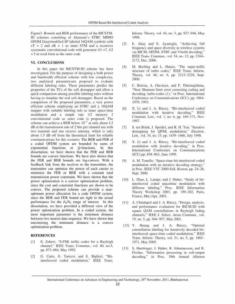
OFDM Based Bit Interleaved Coded Analysis
International Conference on Advances in Engineering and Technology, 26th November, 2011, Bhubaneswar
22
Figure3. Bounds and BER performance of the BICSTM-
ID schemes consisting of Alamouti’s STBC MIMO
OFDM Gray/modified SP labeled 16QAM symbols with nT = 2 and nR = 1 as inner STM and a recursive
systematic convolutional code with generator G1 =7, G2
= 5 in octal form as the outer code
VI. CONCLUSIONS
In this paper the BICSTM-ID scheme has been
investigated. For the purpose of designing a both power
and bandwidth efficient scheme with low complexity,
two analytical parametersare proposed to evaluate
different labeling rules. These parameters predict the
properties of the TCs of the soft demapper and allow a
quick comparison among possible labeling rules without
having to simulate the real soft demapper. Based on the comparison of the proposed parameters, a very power
efficient scheme employing an STBC and a 16QAM
mapper with suitable labeling rule as inner space-time
modulation and a simple rate 1/2 memory 2
convolutional code as outer code is proposed. The
scheme can achieve a BER below 10−4
at only about 4.2
dB at the transmission rate of 2 bits per channel use with
two transmit and one receive antenna, which is only
about 1.5 dB off from the theoretical limit for reliable
communications for this scenario. The BER and FER of
a coded OFDM system are bounded by sums of
exponential functions or Q-functions. In this
dissertation, we have shown that the FER and BER
bounds are convex functions. We have also shown that
the FER and BER bounds are log-convex. With a
feedback link from the receiver to the transmitter, the
transmitter can optimize the power of each carrier to minimize the FER or BER with a constant total
transmission power constraint. We have shown that the
power optimization is a convex optimization problem,
since the cost and constraint functions are shown to be
convex. The proposed scheme can provide a near-
optimum power allocation for a code OFDM system,
since the BER and FER bound are tight to the actual
performance for the Eb/N0 range of interest. In this
dissertation, we have provided a different view of the
power optimization problem. In a coded system, the
most important parameter is the minimum distance
between two nearest data sequence. We have shown that
maximizing the minimum distance is a convex
optimization problem.
REFERENCES
[1] E. Zehavi, “8-PSK trellis codes for a Rayleigh
channel,” IEEE Trans. Commun., vol. 40, no.5, pp. 873–884, May 1992.
[2] G. Caire, G. Taricco, and E. Biglieri, “Bit-
interleaved coded modulation,” IEEE Trans.
Inform. Theory, vol. 44, no. 3, pp. 927–946, May
1998.
[3] E. Akay and E. Ayanoglu, “Achieving full frequency and space diversity in wireless systems
via BICM, OFDM, STBC and Viterbi decoding,”
IEEE Trans. Commun., vol. 54, no. 12, pp. 2164–
2172, Dec. 2006.
[4] M. Breiling and L. Hanzo, “The super-trellis
structure of turbo codes,” IEEE Trans. Inform.
Theory, vol. 46, no. 6, pp. 2212–2228, Sept.
2000.
[5] C. Berrou, A. Glavieux, and P. Thitimajshima,
“Near Shannon limit error correcting coding and
decoding: turbo-codes (1),” in Proc. International
Conference on Communications (ICC), pp. 1064-1070, 1993.
[6] X. Li and J. A. Ritcey, “Bit-interleaved coded
modulation with iterative decoding,” IEEE
Commun. Lett., vol. 1, no. 6, pp. 169–171, Nov.
1997.
[7] S. ten Brink, J. Speidel, and R. H. Yan, “Iterative
demapping for QPSK modulation,” Electron.
Lett., vol. 34, no. 15, pp. 1459–1460, July 1998.
[8] X. Li and J. A. Ritcey, “Bit-interleaved coded
modulation with iterative decoding,” in Proc.
International Conference on Communications
(ICC),pp. 858–863, June 1999.
[9] A. M. Tonello, “Space-time bit-interleaved coded
modulation with an iterative decoding strategy,”
in Proc. IEEE VTC 2000-Fall, Boston, pp. 24–28,
Sept. 2000.
[10] L. Zhao, L. Lampe, and J. Huber, “Study of bit-
interleaved coded spacetime modulation with
different labeling,” Proc. IEEE Information
Theory Workshop 2003, pp. 199–202, Paris,
France, Mar./Apr. 2003.
[11] A. Chindapol and J. A. Ritcey, “Design, analysis,
and performance evaluation for BICM-ID with square QAM constellations in Rayleigh fading
channels,” IEEE J. Select. Areas Commun., vol.
19, no. 5, pp. 944–957, May 2001.
[12] Y. Huang and J. A. Ritcey, “Optimal
constellation labeling for iteratively decoded bit-interleaved space-time coded modulation,” IEEE
Trans. Inform. Theory, vol. 51, no. 5, pp. 1865–
1971, May 2005.
[13] S. Huettinger, J. Huber, R. Johannesson, and R.
Fischer, “Information processing in soft-output
decoding,” in Proc. 39th Annual Allerton

OFDM Based Bit Interleaved Coded Analysis
International Conference on Advances in Engineering and Technology, 26th November, 2011, Bhubaneswar
23
Conference on Communications, Control and
Computing, UIUC University, Oct. 2001.
[14] J.Huber and S. Huettinger, “Information processing and combining in channel coding,” in
Proc. 3rd International Symposium on Turbo
Codes & Related Topics, Brest, France, Sept.
2003.
[15] I. Land, S. Huettinger, P. A. Hoeher, and J.
Huber, “Bounds on information combining,” in
Proc. 3rd International Symposium on Turbo
Codes & Related Topics, Brest, France, Sept.
2003.
[16] E. Zehavi, ”8-PSK Trellis Codes for a Rayleigh
Channel,” IEEE Trans. on Commun.,vol. 40, no.
5, pp. 873-884., May 1992.
[17] G. Caire, G. Taricco and E. Biglieri, ”Bit-
Inreleaved Coded Modulation,” IEEETrans. on
Inf. Theory, vol. 44, pp. 927-946, May 1998.

International Conference on Advances in Engineering and Technology, 26th November, 2011, Bhubaneswar
24
Design of Pipelined Architecture of 9/7
Lifting-Based DWT using FPGA
Maninee Patel & Jobbin Abraham Ben
Dept. of Electronics & Communication Engineering,
Hindustan Institute of Technology & Science, Chennai, India
E-mail : [email protected], [email protected]
Abstract - This paper presents a high speed 9/7 lifting 2-D algorithm which is implemented on FPGA with multi-stage pipelining
structure. Compared with the architecture which without multi-stage pipeline, the proposed architecture has higher operating
frequency. The hardware architecture is suitable for high speed implementation. An advanced two dimensional (2-D) discrete
wavelet transform (DWT) implementation, with an efficient memory area, is designed to produce one output in every clock cycle.
As a result, a very high speed is attained.
Key words - Discrete wavelet transform (DWT); lifting scheme; multi-stage pipelining.
I. INTRODUCTION
The discrete wavelet transform has been widely
used as a powerful tool in many applications such as
signal analysis, image processing and compression due
to its characters of multi-resolution analysis[1], and it
has also become an ingredient of many new image
compression standards, such as JPEG2000.
Early implementations of the wavelet transform
were based on filters' convolution algorithms[2-3]. This
approach requires a huge amount of computational
resources. In fact at each resolution, the algorithm
requires the convolution of the filters used with the
approximation image. A relatively recent approach uses
the lifting scheme for the implementation of the discrete
wavelet transform (DWT). This method still constitutes
an active area of research in mathematics and signal
processing.
Image compression techniques can compress with
or without loss of data of original image. The lossy
compression can achieve higher ratio than lossless
compression. As a result, the 9/7 DWT which is
recommended by JPEG2000 for lossy compression has
been widely used in image compression area. The high-
speed implementation of lifting-based 9/7 DWT on
field-programmable gate array (FPGA) using multi-
stage pipelining is presented in this paper.
A. Discrete Weblet Transform.
The transform of a signal is just another form of
representing the signal. It does not change the
information content present in the signal. The Wavelet
Transform provides a time-frequency representation of
the signal. It was developed to overcome the short
coming of the Short Time Fourier Transform (STFT),
which can also be used to analyze non-stationary
signals. While STFT gives a constant resolution at all
frequencies, the Wavelet Transform uses multi-
resolution technique by which different frequencies are
analyzed with different resolutions.
A wave is an oscillating function of time or space
and is periodic. In contrast, wavelets are localized
waves. They have their energy concentrated in time or
space and are suited to analysis of transient signals.
While Fourier Transform and STFT use waves to
analyze signals, the Wavelet Transform uses wavelets of
finite energy.
The wavelet analysis is done similar to the STFT
analysis. The signal to be analyzed is multiplied with a
wavelet function just as it is multiplied with a window
function in STFT, and then the transform is computed
for each segment generated. However, unlike STFT, in
Wavelet Transform, the width of the wavelet function
changes with each spectral component. The Wavelet
Transform, at high frequencies, gives good time
resolution and poor frequency resolution, while at low
USER
Rectangle

Design of Pipelined Architecture of 9/7 Lifting-Based DWT using FPGA
International Conference on Advances in Engineering and Technology, 26th November, 2011, Bhubaneswar
25
frequencies; the Wavelet Transform gives good
frequency resolution and poor time resolution.
(a) (b)
Fig. 1 : Demonstrations of (a) a Wave and (b) a Wavelet
B. Multi-resolution Analysis using Filter Banks.
Filters are one of the most widely used signal
processing functions. Wavelets can be realized by
iteration of filters with rescaling. The resolution of the
signal, which is a measure of the amount of detail
information in the signal, is determined by the filtering
operations, and the scale is determined by upsampling
and downsampling (sub sampling) operations.
The DWT is computed by successive lowpass and
highpass filtering of the discrete time-domain signal as
shown in Fig.2. This is called the Mallat algorithm or
Mallat-tree decomposition. Its significance is in the
manner it connects the continuous-time multiresolution
to discrete-time filters. In the figure, the signal is
denoted by the sequence x[n], where n is an integer. The
low pass filter is denoted by G0 while the high pass filter
is denoted by H0. At each level, the high pass filter
produces detail information; d[n], while the low pass
filter associated with scaling function produces coarse
approximations, a[n].
Fig. 2 : Three-level wavelet decomposition tree.
At each decomposition level, the half band filters
produce signals spanning only half the frequency band.
This doubles the frequency resolution as the uncertainty
in frequency is reduced by half. In accordance with
Nyquist’s rule if the original signal has a highest
frequency of ω, which requires a sampling frequency of
2ω radians, then it now has a highest frequency of ω/2
radians. It can now be sampled at a frequency of ω
radians thus discarding half the samples with no loss of
information. This decimation by 2 halves the time
resolution as the entire signal is now represented by only
half the number of samples. Thus, while the half band
low pass filtering removes half of the frequencies and
thus halves the resolution, the decimation by 2 doubles
the scale. With this approach, the time resolution
becomes arbitrarily good at high frequencies, while the
frequency resolution becomes arbitrarily good at low
frequencies. The filtering and decimation process is
continued until the desired level is reached. The
maximum number of levels depends on the length of the
signal. The DWT of the original signal is then obtained
by concatenating all the coefficients, a[n] and d[n],
starting from the last level of decomposition.
Fig.3 shows the reconstruction of the original signal
from the wavelet coefficients. Basically, the
reconstruction is the reverse process of decomposition.
The approximation and detail coefficients at every level
are upsampled by two, passed through the low pass and
high pass synthesis filters and then added. This process
is continued through the same number of levels as in the
decomposition process to obtain and the original signal.
The Mallat algorithm works equally well if the analysis
filters, G0
and H0, are exchanged with the synthesis
filters, G1 1
.
Fig. 3 : Three-level wavelet reconstruction tree.
II. LIFTING BASED WAVELET TRANSFORM
A. DWT & Lifting Implementation.
In traditional convolution (filtering) based approach
for computation of the forward DWT, the input signal
(x) is filtered separately by a low-pass filter (˜h) and a
high-pass filter (˜ g). The two output streams are then
sub-sampled by simply dropping the alternate output
samples in each stream to produce the low-pass (yL) and
high-pass (yH) sub band outputs as shown in Fig. 4. The
two filters (˜h, ˜ g) form the analysis filter bank. The
original signal can be reconstructed by a synthesis filter
bank (h, g) starting from yL and yH as shown in Fig.4.
Given a discrete signal x (n), the output signals yL(n)
and yH(n) can be computed as follows:
(1)

Design of Pipelined Architecture of 9/7 Lifting-Based DWT using FPGA
International Conference on Advances in Engineering and Technology, 26th November, 2011, Bhubaneswar
26
Where τL and τH are the lengths of the low-pass (˜h)
and high-pass (˜g) filters respectively. During the
inverse transform computation, both yL and yH are first
up-sampled by inserting zeros in between two samples
and then filtered by low-pass (h) and high-pass (g)
filters respectively. Then they are added together to
obtain the reconstructed signal (x’) as shown in Fig.
below.
Fig. 4 : Signal analysis and reconstruction in 1D DWT
For multi resolution wavelet decomposition, the
low pass sub band (yL) is further decomposed in a
similar fashion in order to get the second-level of
decomposition, and the process repeated. The inverse
process follows similar multi-level synthesis filtering in
order to reconstruct the signal.
Since two dimensional wavelet filters are separable
functions, 2D DWT can be obtained by first applying
the 1D DWT row-wise (to produce L and H sub bands
in each row) and then column-wise as shown below:
Fig. 5 : First level of decomposition
In the first level of decomposition, four sub bands
LL1, LH1, HL1 and HH1 are obtained. Repeating the
same in the LL1 sub band, it produces LL2, LH2, HL2
and HH2 and so on, as shown below:
Fig. 6 : Second & Third of decomposition
The conditions for perfect reconstruction of a signal are
given by
(2)
Where h(z) is the Z-transform of the FIR filter h. h can
be expressed as a Laurent polynomial of degree p as:
(3)
Which can also be expressed using a poly phase
representation as:
(4)
Where he contains the even coefficients and ho contains
the odd coefficients of the FIR filter h. Similarly,
(5)
Based on the above formulation, we can define the poly
phase matrices as:
(6)
Often P(z) is called the dual of ˜P (z) and for perfect
reconstruction, they are related as P(z) ˜P (z−1)T = I ,
where I is the 2 × 2 identity matrix. Now the wavelet
transform in terms of the poly phase matrix can be
expressed as:
(7)
B. 2D DWT Architecture.
The basic idea of lifting based approach for DWT
implementation is to replace the parallel low pass and
high pass filtering by sequence of alternating smaller
filters. The computations in each filter can be partitioned
into prediction and update stages as shown in Fig. 7.
Here the row module reads the data from MEM1,
performs the DWT along the rows (H and L) and writes
the data into MEM2. The prediction filter of the column
module reads the data from MEM2, performs column
wise DWT along alternate rows (HH and LH) and writes
the data into MEM2. The update filter of the column

Design of Pipelined Architecture of 9/7 Lifting-Based DWT using FPGA
International Conference on Advances in Engineering and Technology, 26th November, 2011, Bhubaneswar
27
module reads the data from MEM2, performs column
wise DWT along the remaining rows, and writes the LL
data into MEM1 for higher octave computations and HL
data to external memory.
Fig. 7 : Overview of lifting based 2D DWT architecture.
The architecture can compute a large set of filters
for both the 2D forward and inverse transforms. It
supports two classes of architectures based on whether
lifting is implemented by one or two lifting steps. The
one step architecture corresponds to implementation
using one lifting step.
Fig. 8 : One step lifting based architecture.
RP1, RP2-row processors
CP1, CP2- column processor
MEM1, MEM2- memory
The block diagram shows one step lifting
architecture is shown in Fig. 8. It consists of the row and
column computation modules and two memory units,
MEM1 and MEM2. The row module consists of two
processors RP1 and RP2, along with a resister file
REG1, and column module consists of two processors
CP1 and CP2 along with register file REG2. All the four
processor RP1, RP2, CP1, CP2 contain 2 adders, 1
multiplier and 1shifter. RP1 and CP1 are predicting
filters and RP2 and CP2 are update filters.
C. Lifting Scheme.
The second generation of wavelets, which is under
the name of lifting scheme, was introduced by
Sweldens. The main feature of the lifting-based discrete
wavelet transform scheme is to break up the high-pass
and low-pass wavelet filters into a sequence of smaller
filters that in turn can be converted into a sequence of
upper and lower triangular matrices[4]. The basic idea
behind the lifting scheme is to use data correlation to
remove the redundancy.
The lifting algorithm can be computed in three main
phases, namely: the split phase, the predict phase and
the update phase, as illustrated in Fig. 9.
Fig. 9 : Split, predict, update phases of lifting based
DWT
A. Split phase: In this split phase, the data set x(n) is
split into two subsets to separate the even samples from
the odd ones:
Xe = X (2n), Xo = X (2n +1) (8)
B. Prediction phase: In the prediction stage, the main
step is to eliminate redundancy left and give a more
compact data representation.
At this point, we will use the even subset x(2n) to
predict the odd subset x(2n+1) using a prediction
function P.
Y (2n+1) = Xo (2n+1) – P (Xe) (9)
C. Update phase: In this stage the coefficient
x(2n) is lifted with the help of the neighboring wavelet
coefficients.
Y (2n) = Y (2n+1) + U (Xe) (10)
Where, U is the new update operator.
After the two-dimensional wavelet transform of the
first level, the image is divided into four parts. There are
the horizontal low frequency-vertical low frequency
component (LL), the horizontal low frequency-vertical
high frequency component (LH), the horizontal high
frequency-vertical low frequency (HL), and the

Design of Pipelined Architecture of 9/7 Lifting-Based DWT using FPGA
International Conference on Advances in Engineering and Technology, 26th November, 2011, Bhubaneswar
28
horizontal high frequency-vertical high frequency (HH),
respectively.
D. Block Diagram of 9/7 Lifting DWT.
Fig. 10 : Block Diagram of 9/7 Lifting DWT
There are four lifting coefficient α, β, γ, δ and scaling
factor k.
TABLE I. LIFTING COEFFICIENTS: ORIGINAL
9/7, RATIONAL 9/7 AND FIXED POINT BINARY OF
RATIONAL 9/7
III. PROPOSED SYSTEM
A. Pipeline Architecture of Lifting Based DWT.
Fig. 11: Basic pipeline architecture of 1D-DWT
Generic multipliers usually have high area cost.
Multiplication by constant can be performed by shifted
additions when the number of bits in the multiplication
is large.
According to the binary representation of multiplier
constants presented in table1, the multiplication by γ
needs 9 adders, the first one performs c6+c8, the next
seven are to perform the sum of shifted partial products
of c6+c8, and the last one performs the sum with c9.
The multiplication by α needs 4 adders β needs 3 adders
and the multiplication by δ needs 5 adders. The
architecture of lifting DWT can be naturally pipelined,
but the add/shift stages represent the worst delay path
between registers. Pipelining these stages increases the
data throughput (operating frequency).
The original arithmetic stage structure to perform
the multiplication by γ is shown as:
Fig. 12 : Original arithmetic stage structure
If x=c6+c8, the multiplication by γ can be expressed as
(11)
Hence, this design promotes only integer sums,
reducing the area cost thus increasing the maximum
operating frequency.
Fig. 13 : The pipelining arithmetic stage structure
B. Algorithm for Piprlined LDWT.
First, the input sequences Xi are split into even and
odd parts and . After the Splitting step, the two
split sequences then perform the lifting steps
respectively and the outputs are denoted as and ,(
n = 1,2). Finally, through the normalization factor K0
and K1, we can obtain the low-pass and high-pass
wavelet coefficients si and di.

Design of Pipelined Architecture of 9/7 Lifting-Based DWT using FPGA
International Conference on Advances in Engineering and Technology, 26th November, 2011, Bhubaneswar
29
In the pipeline design method, the critical path is
dominated in the propagation delay between two
registers (2 adders and 1 multiplier). To solve the delay
time problem, we reschedule the pipe stage and propose
a fast-pipeline architecture for 2D DWT.
Since the prediction or update step dominants the
propagation delay in the direct mapping hardware
implementation, we substitute Eq (15) into Eq (14) to
merge the predictor and updater into one equation only.
Thus, we can obtain a flattened equation and each
computation is processed by one addition or
multiplication at a time. The first lifting step equations
are written as
(20)
In the second lifting step, we substitute Eq (17) into
Eq (16) as the first lifting step.
Finally, since the effect of high pass coefficients,
the scaling step can be rewritten as
(21)
From the above modified equations, six constant
multipliers
are used in the process of lifting and scaling steps as the
primitive algorithms. Then, we adopt the pipeline design
method to implement the transformation.
Fig. 14: DFG for pipeline scheduling
IV. IMPLEMENTATION RESULTS
A 2D input is first simulated by using MATLAB.
Pipelining is implemeted by using XILINX, then again
MATLAB code is used to obtain denoised 2D output or
image. Now the local changes in brightness in the
original image can be determined. The pipelined
increases the area cost but reduces worst dalay path
between registers, hence increases operating frequency.
Design 1 is shown in Fig. 12 and design 2 in Fig.
13. These 2 designs are compiled and simulated using
XILINX.
TABLE II. IMPLEMENTATION RESULTS
From one observation the operating frequency of
design 2 is higher than design 1 as shown in above table.
The value of operating frequency can be different for
different observation.
V. CONCLUSION
This paper presents an efficient FPGA
implementation of the DWT algorithm with lifting
scheme. It uses the multi-stage pipeline technique
architecture for the purpose of speeding up the
performance. The performance evaluation has proven
that the proposed architecture has much higher operating
frequency than the architecture which without multi-
stage pipelining.
REFERENCES
[1] A. S. Lewis and G. Knowles, “Image
compression using the 2-D wavelet transform,”
IEEE Trans. Image Process., 1992, 1(3), pp.
244–250
[2] T. Park and S. Jung, “High speed lattice based
VLSI architecture of 2D discrete wavelet
transform for real-time video signal processing,”
IEEE Trans. Consum. Electron., 2002, 48(4), pp.
1026–1032
[3] K. A. Kotteri, S. Barua,et.al,"A Comparison of
Hardware Implementations of the Biorthogonal
9/7 DWT: Convolution Versus Lifting,"IEEE
Trans. on circuit and systems,2005,52(5),256-260
[4] S.Khanfir, M. Jemni, “Reconfigurable Hardware
Implementations for Lifting-Based DWT Image

Design of Pipelined Architecture of 9/7 Lifting-Based DWT using FPGA
International Conference on Advances in Engineering and Technology, 26th November, 2011, Bhubaneswar
30
Processing Algorithms,” ICESS’08, 2008, pp.
283-290.
[5] S.V. Silva, S. Bampi, “Area and Throughput
Trade-Offs in the Design of Pipelined Discrete
Wavelet Transform Architectures,” Proceedings
of the Design Automation and Test in Europe
Conference and Exhibition (DATE’05),
2005,1530-1591
[6] W.Sweldens, “The lifting scheme: a custom-
design construction of biorthogonal wavelets,”
Applied and Computational Harmonic Analysis,
1996, 3(15), pp. 186-200
[7] K.K. Parhi, “VLSI digital signal processing
systems: design and implementation”, John
Wiley & Sons, Inc, 1999, pp.508-510

International Conference on Advances in Engineering and Technology, 26th November, 2011, Bhubaneswar
31
Design of Advanced On-Chip Bus Implementation with Open Core
Protocol Interface using Finite State Machines
T. Subhasri & P. Krishna Chaitanya
Dept. of Electronics & Communication Engineering, NOVA College of Engineering & Technology, Vegavaram, India
E-mail : [email protected], [email protected]
Abstract - The on-chip bus design can be divided into two parts, the interface and the internal architecture of the bus. Here we adopt
the well-defined interface standard, the Open Core Protocol (OCP), and focus on the design of the internal bus architecture. We
develop an efficient bus architecture to support most advanced bus functionalities defined in OCP, including burst transactions, lock
transactions, pipelined transactions, and out-of-order transactions. We first model and design the on-chip bus with transaction level
modeling for the consideration of design flexibility and fast simulation speed. We then implement the RTL models of the bus for
synthesis and gate-level simulation. Experimental results show that the proposed TLM model is quite efficient for the whole system
simulation and the real implementation can significantly save the communication time.
I. INTRODUCTION
A group of lines shared for interconnection of the
functional modules by a standard interface is called a
Bus. The interconnections may be point-to-point, on-
chip bus and on-chip network. The characteristic of a
traditional bus is that I/O pins are fixed and form a
shared I/O with dedicated address decoding. But for an
OCB, the routing resource is in a target device like
FPGA, ASIC. OCP (Open Core Protocol) is an interface
standard that interconnects IP cores to on-chip bus. A
designer selects only those signals and features from the
palette of OCP configurations needed to fulfill all of an
IP coreXs unique data, control and test signaling
requirements. The bus interface involves a set of
interface signals and their corresponding timing
relationship, while the bus architecture refers to the
internal components of buses and the interconnections
among the IP cores. When the number of integrated IP
cores increases, the communication between IP cores
also increase and it becomes quite frequent that two or
more master IPs would request data from different
slaves at the same time. The shared bus architecture
often cannot provide efficient communication since only
one bus transaction can be supported at a time. To solve
this problem, two bus protocols have been proposed
recently. One is the Advanced eXtensible Interface
protocol (AXI) and the other is bus interface protocol is
proposed by a non-profitable organization, the Open
Core Protocol.
The main features of OCP interface are: 1) Master -
slave interface with unidirectional signals: 2) Driven and
sampled by the rising edge of the OCP clock; 3) Fully
synchronous, no multi-cycle timing paths; 4) All signals
are strictly point-to point (except clock & reset); 5)
Simple request / acknowledge protocol; 6) Supports data
transfer on every clock cycle; 7) Allows master or slave
to control transfer rate; 8) Configurable data word
width; 9) Configurable address width; 10) Pipelined or
blocking reads; 11) Specific description formats for core
characteristics, interfaces (signals, timing &
configuration), performance OCP interface is a user-
settable, so the designer can define interface attribute,
such as address and data bus width.
OCP is an interface (or socket) aiming to
standardize and thus simplify the system integration
problems. It facilitates system integration by defining a
set of concrete interface (I/O signals and the
handshaking protocol) which is independent of the bus
architecture. In this paper we propose a high
performance on-chip bus design with OCP as the bus
interface. We choose OCP because it is open to the
public and OCP-IP has provided some free tools to
verify this protocol.
Our proposed bus architecture features
crossbar/partial-crossbar based interconnect and realizes
most transactions defined in OCP, including 1) single
transactions, 2) burst transactions, 3) lock transactions,
4) pipelined transactions, and 5) out-of-order
transactions.
Basic OCP includes only data flow signals and is
based on simple request and acknowledge protocol.
However, the optional extensions support more
functionality in control, verification and testing. Simple
Extension and Complex Extension support burst
transaction and pipelined write operations. In addition,
Sideband Extension supports user-defined signals and
USER
Rectangle

Design of Advanced On-Chip Bus Implementation with Open Core Protocol Interface using Finite State Machines
International Conference on Advances in Engineering and Technology, 26th November, 2011, Bhubaneswar
32
asynchronous reset. Also, Debug and Test Interface
Extension supports JTAG (Join Test Action Group) and
clock control. This is the reason why, when integrated in
SoC, the OCP protocol allows debugging and IP block
test generating.
In addition, the proposed bus is flexible such that
one can adjust the bus architecture according to the
system requirement. One key issue of advanced buses is
how to manipulate the order of transactions such that
requests from masters and responses from slaves can be
carried out in best efficiency without violating any
ordering constraint. In this work we have developed a
key bus component called the scheduler to handle the
ordering issues of out-of-order transactions. We will
show that the proposed crossbar/partial-crossbar bus
architecture together with the scheduler can significantly
enhance the communication efficiency of a complex
SOC. We employ both transaction level modeling
(TLM) and register transfer level (RTL) modeling to
design the bus.
Fig. 1 : On-chip bus overview
We start from the TLM for the consideration of
design flexibility and fast simulation speed. We then
refine the TLM design into synthesizable and cycle-
accurate RTL codes which can be synthesized into gate
level hardware to facilitate accurate timing and
functional simulation. The remainder of this paper is
organized as follows. The various advanced
functionalities of on-chip buses are described in Section
2. Section 3 details the hardware architecture of the
proposed bus. Section 4 gives the experimental results
which show the efficiency on both simulation speed and
data communication. Conclusions are then drawn in
Section 5.
II. ON-CHIP BUS FUNCTIONALITIES
The various bus functionalities include 1) burst, 2)
lock, 3) pipelined, and 4) out-of-order transactions.
• The burst transactions allow the grouping of
multiple transactions that have a certain address
relationship, and can be classified into multi-request
burst and single-request burst according to how
many times the addresses are issued. FIGURE 1
shows the two types of burst read transactions.
where the address information must be issued for
each command of a burst transaction (e.g., A11,
A12, A13 and A14). This may cause some
unnecessary overhead
Fig. 2 : Burst transactions
• Lock is a protection mechanism for masters that
have low bus priorities. Without this mechanism the
read/write transactions of masters with lower
priority would be interrupted whenever a higher-
priority master issues a request. Lock transactions
prevent an arbiter from performing arbitration and
assure that the low priority masters can complete its
granted transaction without being interrupted.
• For a pipelined transaction as shown in FIGURE 3
this hard link is not required. Thus A21 can be
issued right after A11 is issued without waiting for
the return of data requested by A11 (i.e.,D11-D14)
Fig. 3: Pipelined transactions
• The out-of-order transactions allow the return order
of responses to be different from the order of their
requests. These transactions can significantly
improve the communication efficiency of an SOC
system containing IP cores with various access
latencies as illustrated in FIGURE 4.
Fig. 4 : With-out-order transactions
III. HARDWARE DESIGN OF THE ON-CHIP BUS
The architecture of the proposed on-chip bus is
illustrated in FIGURE 5, where we show an example
with two masters and two slaves. A crossbar architecture
is employed such that more than one master can

Design of Advanced On-Chip Bus Implementation with Open Core Protocol Interface using Finite State Machines
International Conference on Advances in Engineering and Technology, 26th November, 2011, Bhubaneswar
33
communicate with more than one slave simultaneously.
If not all masters require the accessing paths to all
slaves, partial crossbar architecture is also allowed.
For a crossbar or partial crossbar architecture,
resource contention occurs when more than one master
is to access the same slave simultaneously. In the
proposed design each slave IP is associated with an
arbiter that determines which master can access the
slave.
Fig. 5 : Top view of proposed architecture
3.1 Decoder
Since more than one slave exists in the system, the
decoder decodes the address and decides which slave
return response to the target master. In addition, the
proposed decoder also checks whether the transaction
address is illegal or nonexistent and responses with an
error message if necessary.
3.2 FSM-M & FSM-S
Depending on whether a transaction is a read or a
write operation, the request and response processes are
different. For a read operation, the address of the target
slave is first sent out and the target slave will issue an
accept signal when it receives the message. The slave
then generates the required data and sends it to the bus
where the data will be properly directed to the master
requesting the data. The read transaction finally
completes when the master accepts the response and
issues an acknowledge signal. For a write transaction,
the data to be written is sent out together with the
address of the target slave, and the transaction is
complete when the target slave accepts the data and
acknowledges the reception of the data. FSM-M acts as
a master and generates the OCP signals of a master,
while FSM-S acts as a slave and generates those of a
slave. These finite state machines are designed in a way
that burst, pipelined, and out-or-order read/write
transactions can all be properly controlled.
3.3 Scheduler
The OCP protocol, each out-of order transaction is
tagged with a TagID by a master. For those transactions
with the same TagID, they must be returned in the same
order as requested, but for those with different TagID,
they can be returned in any order. Conventional bus
scheduling algorithms tend to favor the in-order
transactions, while the ordering mechanism favors out-
of order transactions.
3.4 Multiplexer
In FIGURE 6 MUX1 is used to solve the problem of
resource contention when more than one slave returns
the responses to the same master. It selects the response
from the slave that has the highest priority. The recorder
shown in the figure is used to keep track of the ID of the
target slave and the TagID of every out-of-order
transaction. Whenever a response arrives, the
comparator determines whether the ordering restriction
is violated or not by comparing the ID of the target slave
and TagID. If no ordering restriction is violated, the
response is sent forward to the priority setter. If the
restriction is violated, the response is sent backward to
one of the inputs of MUX2, which is always a preferred
input over the input from MUX1. For the transactions
without TagID, which are regarded as in-order
transactions, the priority setter sets the priority to 0 or
the largest value to reflect whether in-order first or out-
of-order first policy is used. To further improve the
efficiency of the scheduler, the response can be
forwarded to the master directly without going through
the priority queue when the priority queue is empty.
Fig. 6 : Block diagram of scheduler
IV. EXPERIMENTAL RESULTS
We design the proposed bus with both TLM and
RTL models. The RTL model can be further synthesized
into gate-level description. The specification and the
synthesis results when 4 masters and 6 slaves are used
are shown in TABLE 1, where all masters can issue
burst, lock, pipelined and out-of-order transactions.

Design of Advanced On-Chip Bus Implementation with Open Core Protocol Interface using Finite State Machines
International Conference on Advances in Engineering and Technology, 26th November, 2011, Bhubaneswar
34
TABLE 1.Bus specifications and synthesis results
Architecture of bus Factor
Address width
Data width
64-bits
128-bits
Number of Slave Ports
Number of Master Ports
12
8
Total area (µm2)
Operating frequency
About 60K gates
333.33MHz
The total area of the proposed on-chip bus at
333MHz using TSMC 0.13_m CMOS process is
153,823 um2 (about 60K gates). We find that for each
additional master, about 3,682 x2 and 4,531x2 more
gates are needed for a port without and with the out-of-
order capability, respectively. On the other hand, about
1,456x2 gates are required for one slave port. Originally
the on-chip bus is a multi-layer bus consisting of two
AHB-lite busses modeled with a commercial bus library
(CoWare [4]). The ARM9 processor is connected to one
AHB-lite bus, and the PAC DSP processor is connected
to the other. In the experiment, we replace the AHB-lite
bus connecting the PAC DSP processor with the
proposed on-chip bus and verify the whole SOC design
with an H.264 decoding procedure. Experimental results
show that the proposed on-chip bus deals with all the
communications in the SOC well.
Fig. 7 : Burst Transactions
The simulation times of decoding one frame are
about 48.6 and 44.3 seconds before and after the
replacement, respectively. It should be pointed out that
even though both the proposed bus and the one using
CoWare bus library are cycle-accurate; our proposed
bus is further a pin-accurate one but the one from
CoWare is not. Thus the proposed TLM bus model
provides better simulation speed since it contains more
implementation details. To focus on the efficiency
evaluation of the crossbar bus architecture, we design an
SOC system as shown in FIGURE 8 which contains two
masters (IP1 and IP2) and three slaves (IP3, IP4 and
IP5).
Fig. 8 : SOC System for bus evaluation
In this experiment we compare the communication
efficiency of the SOC systems with the shared bus
architecture and the crossbar bus architecture. The
transactions used in the experiment are described as
follows:
1. Master IP2 first requests a series of burst WR
transactions to slave IP4 and a WR transaction to
slave IP3.
2. Master IP1 then requests a series of burst RD
transactions to slave IP4.
3. Master IP1 then requests a series of burst WR
transactions to slave IP5, and master IP2 requests a
series of burst WR transactions to slave IP4.
4. Master IP2 requests a series of burst RD
transactions to slave IP5.
The procedure from step2 to step4 is iterated for
100 iterations. The execution of these transactions on
the factor architecture can be illustrated in FIGURE 9,
where parallel communication between different masters
and slaves happens in time intervals B, D, F, H and J.
The behavior on the shared bus architecture is all in
series without any parallel communication.
Experimental results show that the proposed bus
with crossbar interconnection reduces about 23.35%
communication cycles as comparing to the tradition
shared bus architecture such as AHB. In the last
experiment, we evaluate the efficiency of out-of-order
transactions using the proposed scheduler. We assume
that the access latency of the slave IP3 and IP4 in
FIGURE 8 are 1 cycle and 3 cycles, respectively. The
slave IP5 has the access latency of 5 cycles when it is
accessed by master IP1 and two cycles when it is
accessed by master IP2.
In the simulation, IP1 first requests a series of out-
of-order WR transactions, IP2 then requests a series of
out-of-order RD transactions. After that, IP2 requests a
series of out-of-order WR transactions, and IP1 finally
requests a series of out-of-order RD transactions. The
simulation results show that when each series of these
requests contain 6000 transactions, the proposed

Design of Advanced On-Chip Bus Implementation with Open Core Protocol Interface using Finite State Machines
International Conference on Advances in Engineering and Technology, 26th November, 2011, Bhubaneswar
35
scheduler reduces 67.16% communication cycles as
comparing to a bus that supports only in-order
transactions.
Fig. 9 : Performance analysis of parallel transactions
V. CONCLUSION
The bus standard must be able to define an explicit
bus interface and leave the internal bus architecture to
the bus designer. The design which complies with the
bus interface protocol to carry out the various advanced
bus functionality consequently dominates the
communication efficiency of an SOC system. In this
work, we develop an on-chip bus employing OCP as the
bus interface. Various bus transactions defined in AXI
and OCP to reduce the communication latency and
increase the bus throughput are supported by the
proposed bus architecture. Experimental results
demonstrate the efficiency of the proposed bus in both
simulation speed and execution performance.
REFERENCES
[1] Open Core Protocol (OCP)
Specification, http://www.ocpip.org/home.
[2] C.-K. Lo and R.-S. Tsay, “Automatic Generation
of Cycle Accurate and Cycle Count Accurate
Transaction Level Bus Models from a Formal
Model,” Asia and South Pacific Design
Automation Conference, pages 558-563, 2009.
[3] N.Y.-C. Chang, Y.-Z. Liao and T.-S. Chang,
“Analysis of Shared-link IET Computers &
Digital Techniques, Volume 3, Issue 4, pages
373-383, 2009.
[4] CoWare website, http://www.coware.com
[5] Sudeep Pasricha & Nikil Dutt “On-chip
communication architectures (system on-chip
interconnect)”

International Conference on Advances in Engineering and Technology, 26th November, 2011, Bhubaneswar
36
Power Quality Improvement by Utilizing Super Capacitor in
Electrical Power Transmission System
W. A. Augusteen, V. Nandhakumar & R. K. Balaji
Indira Institute of Engineering and Technology, India
E-mail : [email protected], [email protected]
Abstract - Power quality problem manifested in voltage, current or frequency deviations that result in failure or mis-
operation of customer equipment. In distribution network, the sensitive industrial loads and critical commercial
operations suffer from outages and service interruptions which cause financial losses to both utility and consumers.
This paper is to improve the power quality in transmission system by adopting and replacing the super capacitor instead
of existing capacitor bank. This super capacitor resembles a regular capacitor with the exception that it offers very high
capacitance in a small package and considerably improves the power factor and efficiency of the transmission system.
This approach has been tested in T type & PI type model of medium and long transmission distribution systems by
replacing super capacitor with existing capacitor bank. This approach simulated through the software package of
Matlab 6.5 and the results shows considerable Power Quality improvements.
I. INTRODUCTION
Power quality is an issue that is becoming
increasingly important to electricity consumers at all
levels of usage. Sensitive equipment and non-linear
loads are commonplace in both the industrial and the
domestic environment; because of this a heightened
awareness of power quality is developing. The source of
problems that can disturb the power quality are: power
electronic device ,arcing device, load switching, large
motor starting ,embedded generation, sensitive
equipment storm and environment related damage,
network equipment and design.
The solution to improve the energy quality ( PQ-
Power Quality) at the load side is of great importance
when the production processes get more complicated
and require a bigger liability level, which includes aims
like to provide energy without interruption, without
harmonic distortion and with tension regulation between
very narrow margins. The devices that can fulfill these
requirements are the custom power; a concept that we
could include among the super capacitor, but that is
different to them because of their final use. In fact the
topologies that they employ are identical to the ones in
the super capacitor device with little modification and
adaptations to tension levels, therefore they are most
oriented to be used in distribution networks of low and
medium tension, sometimes replacing the active filters.
Recent developments in electrical powers system
such as deregulation, open access, and cogeneration are
creating scenarios of transmission congestion and forced
outage. Addition of new transmission lines is an almost
impossible solution due to environmental and other
consideration, and developing new approaches to power
system operation and control is the need of the hour for
overload relief, efficient and reliable operation [1].
Benefits of utilizing Super capacitor:
The benefits of utilizing super capacitor in electrical
transmission system can be summarized as follows:
Electrochemical Double Layer Capacitors (EDLCs) –
also called super capacitors (SC) - are electrochemical
capacitors that have high capacitance and high energy
density when compared to common capacitors, and
higher power density when compared to batteries.
Most EDLC's are constructed from two carbon
based electrodes (mostly activated carbon with a very
high surface area), an electrolyte (aqueous or organic)
and a separator (that allows the transfer of ions, but
provides electronic insulation between the electrodes).
As voltage is applied, ions in the electrolyte solution
diffuse across the separator into the pores of the
electrode of opposite charge. Charge accumulates at the
interface between the electrodes and the electrolyte (the
double layer phenomenon that occurs between a
conductive solid and a liquid solution interface), and
forms two charged layers with a separation of several
angstroms – the distance from the electrode surface to
the center of the ion layer (in Fig. 1). The double layer
capacitance is the result of charge separation in the
interface. Since capacitance is proportional to the
USER
Rectangle

Power Quality Improvement by Utilizing Super Capacitor in Electrical Power Transmission System
International Conference on Advances in Engineering and Technology, 26th November, 2011, Bhubaneswar
37
surface area and the reciprocal of the distance between
the two layers, high capacitance values are achieved.
Fig.1
Electrical double layer capacitor constructed by
inserting two electrodes in a beaker and applying a
voltage. The voltage persists after the switch is opened
(right), creating two series-connected capacitors.
Charges in the electric double layer are separated by
only about 1 nm [4].
EDLC's store electrical charge electro statically,
and almost no reaction occurs between the electrodes
and the electrolyte. Consequently, electrochemical
capacitors can undergo hundreds of thousands of charge
and discharge cycles.
The first electrical device using double layer charge
storage was reported in 1957 by General Electric. This
was followed by the development from the Standard Oil
Company of Ohio (SOHIO), who patented a device that
shaped the format commonly used today. In 1978, NEC
was the first to introduce super capacitors commercially
as low voltage devices with high ESR, primarily
designed for backup applications. Since then, EDLC's
have evolved: high voltage and very high capacitance
(thousands of Farads) on the one hand, and low ESR
pulse super capacitors with a capacitance range of few
milli -Farads, up to 1- 2 Farads, on the other hand.
Significant improvements in materials, design and the
process of production of pulse super capacitors has lead
to low profile prismatic devices that can supply high
peak currents of up to 2 – 3 A. These devices are suited
to meet the peak power demands of many battery-
powered electronics and other consumer and industrial
devices with current-limited energy sources.
Why we use super capacitors for energy storage?
Supercapacitors represent one of the latest
innovations in the field of electrical energy storage, and
find their place in many applications where energy
storage is needed, or can help in smoothing strong and
short-time power solicitations of a distribution network.
In comparison with classical capacitors, these new
components allow a much higher energy density,
together with a high power density. Even if the energy
density is not comparable to that of electrochemical
accumulators, the possible amount of stored energy,
along with storage time are compatible with many
industrial requirements [5], [6].
Batteries are widely used for energy storage in
industrial and consumer electronic devices because of
their high energy density, but are limited in their power
density. With its limited power the battery often cannot
supply the required power while still retaining its open
circuit voltage. The larger the voltage drop of the battery
the larger the load on the battery. Often, when a battery
needs to supply high power at short pulse widths, the
voltage drop may be too large, causing lower voltage
than required by the end product. The large load
decreases the energy stored in the battery, harming it
and shortening its life-span.
When high power is required in battery operated
devices (i.e. in pulse applications), the combination of
the super capacitor connected in parallel to the battery
gives the advantages of both, enhancing the
performance of the battery and extending its life,
exploiting the batteries to its maximum potential. The
super capacitor connected to the battery in parallel
produces a voltage damping effect - low impedance
super capacitors can be charged in seconds with a low
current during standby times between high current
pulses. Adding the super capacitor to the battery in
parallel decreases the voltage drop, leading to: Better
energy and power management, Battery life and
operational range extension, Superior energy density in
the battery, Power to be produced by both the EDLC
and the battery, each supplying power inversely to its
own ESR, Fewer battery replacements in some of the
applications .
Batteries are very inefficient at low temperatures.
Their internal resistance increases due to the slower
kinetics of the chemical reaction within the battery. The
internal resistance is reduced by incorporating a super
capacitor into the system with the battery. The internal
resistance of pulse type super capacitors is much lower
than that of batteries, even at low temperatures down to
-40 C. Super capacitors have several advantages and
disadvantages relative to batteries.
II. PROBLEM FORMATION
This paper is to obtain the design and operation of a
transmission line by determination of voltage drop, line
losses and efficiency of transmission system. These
values are greatly influenced by the line constants R, L,

Power Quality Improvement by Utilizing Super Capacitor in Electrical Power Transmission System
International Conference on Advances in Engineering and Technology, 26th November, 2011, Bhubaneswar
38
and C of the transmission line. For instance, the voltage
drop in the line depends upon on the value of above
three line constants .Similarly, the resistance of the
transmission line conductor is the most important cause
of power loss in the line and determines the transmission
of efficiency.
In this paper, we shall develop problem formation
by calculating voltage regulation, line losses and
efficiency of transmission lines. In this paper we have
taken the formation of Nominal Method and Nominal
T Method of radial distribution systems
Nominal Method:
In this method in which capacitance is divided into
two halves with one half lumped near sending end and
other half near the receiving end. This is shown in the
following figure 2.1. The capacitor near the sending end
does not contribute any line voltage drop but it should
be added with line current to get total sending end
current. The phasor diagram is shown in the following
figure2.2. VR is taken as the reference phasor. The
current lags behind VR by angle R.
The current through capacitor C1 is leading the voltage
VR by an angle of 90 . The phasor sum of IR
Schematic Fig. 2.1
and IC1 gives the line current IL. The drop ILR is in phase
with IL whereas drop ILXL is leading by 90 . The phasor
sum of these drops with VR gives the sending end
voltage VS. The capacitor current IC2 is leading voltage
VS by 90 . The phasor sum of IS and IC2 gives the
sending end line current IS.
Phasor Diagram 2.2
Thus sending end voltage is given as
(2.1)
%Voltage Regulation= (2.2)
Efficiency= (2.3)
Where
VS = Sending end voltage
VR = Receiving end voltage
IR = Load current or receiving end current
R = Resistance per phase
XL = Inductive reactance per phase
C = Capacitance per phase
P.f at receiving end
(2.4)
Load current,
(2.5)
Charging current at receiving end,
=
=j =j
We get the line current as,
= + (2.6)
Sending end current, = (2.7)
The efficiency and the regulation of the
transmission line can be obtained in the similar manner
as explained in the earlier sections.
Nominal T Method:
In this paper we have taken Nominal T Method
additionally and especially this method of calculation is
utilized for medium transmission line.
In this method the total line capacitance is lumped
or concentrated at the midpoint of the line. The
resistance and reactance of the line are divided with half
the resistance and reactance on one side and remaining
half on other side of capacitor. Half of the line carries
full charging current with this arrangement. The
following diagram shows the arrangement used in
nominal T method for one phase. It is desirable to work
in phase instead of line values.
XIR I
LOAD VR VS
IIC IC

Power Quality Improvement by Utilizing Super Capacitor in Electrical Power Transmission System
International Conference on Advances in Engineering and Technology, 26th November, 2011, Bhubaneswar
39
Schematic Diagram 2.3
The corresponding phasor diagram is represented as
follows
Phasor Diagram 2.4
Here the receiving end voltage VR is taken as reference.
The drop PQ is in phase with IR. The drop QR
is leading IR by The phasor sum of these
drops with VR gives the voltage V1 which is the voltage
across the capacitor. The capacitor current IC leads V1
by 90 . The phasor sum of IR and IC gives IS. The drop
RS is in phase with IS whereas drop ST is
loading IS by 90 . The phasor sum of these drops along
with V1 gives the sending end voltage VS.
Let
IR = Receiving end load current per phase
R = Resistance per phase
XL = Inductive resistance
C = Capacitance per phase
= p.f. at receiving end
VS = Sending end voltage
V1 = Voltage across capacitor
%Voltage Regulation=
Transmission Efficiency=
Receiving end voltage, (2.8)
Load current, (2.9)
Voltage across capacitor,
=
Current through capacitor, =j
Sending end current,
Sending end voltage,
= (2.10)
The efficiency and regulation can be calculated in the
similar manner explained in earlier sections.
III. TEST SYSTEM
A supercapacitive-storage-based substation for the
compensation of resistive voltage drops in transportation
networks has been proposed. It allows to feed as a
current source in any voltage conditions of the line. The
system has been designed as a compensation substation
to be placed at week points like end-of-line stations,
instead of additional feeding substations. A dedicated
control system for the stabilization of the voltage level
in case of strong perturbations is also proposed.
Practical results have been recorded from a reduced-size
prototype and are also presented[2].
Super capacitor Specification Ratings
Charging Current
Voltage
Super Capacitor Rating
Tank/Bank Size
200A
60v
75F
24*1800F
A scaled prototype of the “Val-Vert” substation has
been realized in order to show the operation and
behavior of such a system. The scaled system is
represented in the pic of figure.8.the model has the
following characteristics: 60-v dc rectifier and line
voltage, 100-a maximum load current, 60-v/200-a/75F
super capacitor tank (24 ) series - connected.
The power converter is realized with standard IGBT
modules[2].
IR
IC
I R/ XL/2 R/2
XL/2
V1 VR VS

Power Quality Improvement by Utilizing Super Capacitor in Electrical Power Transmission System
International Conference on Advances in Engineering and Technology, 26th November, 2011, Bhubaneswar
40
By taking a sample of A 3 phase,50 Hz overhead
transmission line 100 km long has the
resistance/km/phase=.1Ω,inductive
reactance/km/phase=.02Ω , capacitance susceptance
/km/phase = 0.04×10⁻⁴ mho[3].
The result shows the high build up in voltage and
also much improved efficiency for a sample of 1800F
much improved in sending end voltage.
IV. CONCLUSION
In this paper we would like to replace the existing
capacitor bank with the new proposed super capacitor.
By applying this supper capacitor results shows the
improved efficiencies and much improved sending and
receiving end voltages depends about the requirement.
By using this super capacitor in much less size we can
get the same performances of existing capacitor. In this
paper work opens up the research ideas towards radial
distribution systems, optimization etc., and also opens
up the designing of capacitor etc.
REFERENCES:
[1] M.P.Donsion , J. A. Guemes, J. M. Rodgriguez
“Power quality. Benefits of utilizing Facts
Devices in electrical power systems” university
of Vigo Spain, university of Basque country.
[2] Alfred Rufer,senior Member,IEEE ,David
Hotellier and Philippe , Member ,IEEE “A
Supercapacitor-Based Energy Storage Substation
for Voltage Compensation in Weak
Transportation Networks” .
[3] U.A.Bakshi , M.V.Bakshi Text Book Reference
“Transmission and Distribution” Technical
Publication.
[4] “Fundamentals Of Electrochemical Capacitor
Design And Operation” by John R. Miller and
Patrice Simon.
[5] A. Rufer and P. Barrade, “Key developments for
supercapacitive energy storage: Power electronic
converters, systems and control,” in Proc. Int.
Conf. Power Electron. Intell. Motion Power
Quality, Nuernberg, Germany, June 19–21, 2001,
ISBN 3-928 643-27-4, pp. 17–25.
[6] “A supercapacitor-based energy-storage system
for elevators with soft commutated interface,”
IEEE Trans. Ind. Applicat., vol. 38, pp. 1151–
1159, Sept./Oct. 2002.

International Conference on Advances in Engineering and Technology, 26th November, 2011, Bhubaneswar
41
Blind Adaptive Equalization using CMA Algorithm
with Variable Step Size
T. Rambabu1 & P. Rajesh Kumar
2
1Dept. of ECE, Sarojini Institute of Technology, Telaprolu, Krishna(Dt.)
2Dept. of ECE, A. U. college of Engineering, Andhra University,Visakhapatnam
E-mail : [email protected], [email protected]
2
Abstract - The approach in this paper integrates a technique for variable-step- size (VSS) with the constant-modulus
algorithm(CMA) for blind adaptive equalization for QAM signals.. This leads to the saving of some amount of computations for the
VSS technique. Simulation results show that algorithms with the VSS technique exhibit lower steady-state mean-squared error
(MSE) for the same speed of convergence.
Key words - component; Blind Adaptive Equalization, CMA, MMA,VSS, QAM, MSE.
I. INTRODUCTION
Blind adaptive equalization achieve channel
equalization without the need of a training sequence
[1][2]. The constant-modulus algorithm (CMA) has
gained widespread practical use for equalizing channels
in digital communication systems [3]. The multi
modulus algorithm (MMA) [4] separates the equalizer
output into in-phase and quadrature components and
penalizes the dispersion of each around separate straight
contours. Hybrid approaches for blind equalization are
reported in [5]-[8].
It is known that the choice of the step size
determines the performance characteristics of the
adaptive algorithm in terms of the convergence rate and
the amount of steady-state mean-square-error (MSE). In
general, a smaller step size results in a smaller state-
state MSE but also a slower rate of convergence. On the
other hand, a larger step size results in a faster rate in
convergence but a large steady-state MSE. To eliminate
the trade off between the convergence rate and the state-
state MSE, one would use a variable-step-size (VSS)
technique [9]-[11].
In this paper, we propose a VSS technique suitable
for QAM signals and integrate it with a stop-and-go
(SAG) procedure to reduce the amount of computations.
The technique is applied to CMA and MMA.
Simulation results show that the VSS technique
integrated with either CMA or MMA exhibits faster
time to convergence than the original algorithm.
The rest of the paper is organized as follows.
Section II presents fractionally-spaced equalizers.
Section III reviews CMA and MMA for blind adaptive
equalization while the proposed VSS technique is
introduced in section IV. Simulation results applied to
CMA presented in section V, while conclusions are
given in section VI.
II. FRACTIONALLY-SPACE CMA
Figure 1 represents a noisy communication system
with an FIR channel model and a fractionally-spaced
equalizer (FSE) [12] with sampling interval T/2 where
T is the sampling period. In the figure, s(n) represents
the baud-spaced source symbol, c is the Nc-length vector
representing the fractionally-spaced channel impulse
response, h is the Nh-length vector comprising the
fractionally-spaced equalizer coefficients, and y(n) is the
baud-spaced equalizer output. In addition to the inter
symbol interference, the T/2-spaced received signal x(k)
is also corrupted by an additive noise process v(k). The
received signal can be put in the form:
)()()( nnn νsCx +=
where x(n) and v(n) are Nh-length vectors containing the
previous values for received signal and the channel
noise process, respectively, and C is the
2/)1( −+× chh NNN fractionally-spaced
convolution matrix of the form [12]:
USER
Rectangle

Blind Adaptive Equalization using CMA Algorithm with Variable Step Size
International Conference on Advances in Engineering and Technology, 26th November, 2011, Bhubaneswar
42
2 2 c h s(n) y(n)
v(k)
x(k)
Fig. 1 : Fractionally spaced equalizer(T/2)
III. BLIND ADAPTIVE ALGORITHMS
In the following, CMA briefly presented.
3.1 CMA
CMA is a stochastic gradient algorithm minimizes
the dispersion of the equalizer output around a circular
contour. The CMA coefficient update algorithm is
equivalent to the Godard coefficient update algorithm
when p = 2, and is defined as [3];
)()()()1( *nnenn CMA xhh µ+=+ with
( )2)()()( nynyne CCMA −= γ
where )1( +nh and )(nh are the vectors comprising
the next and current equalizer coefficients, respectively,
is the step size, y(n) is the complex equalizer output,
x(n) is the vector of equalizer input samples in the
tapped-delay line, while * denotes the complex
conjugate operation. The constant Cγ is referred to as
the dispersion constant and is chosen in accordance
chosen in accordance with the source statistics
according to the relation:
2
4
)(
)(
nsE
nsEC =γ Where ⋅E is the expectation
operation with s(n) being the transmitted signal.
)(
)(2
4
naE
naEM =γ Where )(Re)( nsna = .
IV. PROPOSED VSS TECHNIQUE
When using an adaptive step size, The equalizer
coefficient update takes the form:
)()()()1( *nnenn xhh µ+=+
Where n) is adjusted according to a certain rule and
e(n) is the error signal. The proposed VSS technique is
a modified version of that which has been proposed in
[11] for least-mean-square (LMS) algorithm integrated
with a SAG algorithm and is summarized in the
following steps:
1. Input 0)
2. Initialize h(0)
3. Loop n = 0, 1, 2, …
Calculate )()( nene CMA= or )()( nene MMA=
)()()()()1( *nnennn xhh µ+=+
2)()(1
)()1(
nen
nn
µλ
µµ
+
=+
where
( ) ( )( ) ( )
otherwise
)1(Imsgn)(Imsgn
&)1(Resgn)(Resgnif
0if
1
0
1
−=
−=
=
=nene
nene
n
λ
with sgn ⋅ denotes signum function.
V. SIMULATION RESULTS
Simulations were carried out in a 35-dB SNR
environment using 4-QAM. The channels were T/2-
spaced microwave channels from SPIB where T is the
symbol period. The equalizers were 16-tap T/2-spaced
finite-duration impulse response (FIR) filters, initiated
by a unitary double center spike as in [5]. The MSE was
calculated as the average instantaneous-squared error
over 100 trials using microwave channel #2 [13].
Figure 2 shows the convergence curves for CMA
and CMA with VSS for 72)( −
== µµ n for the CMA,
and for 72)0( −
=µ for the CMA with VSS. It is clear
that VSS technique has resulted in less steady-state
MSE for the same convergence speed as shown by the
MSE curves in the transient region. Figure 3
demonstrates the constellation diagrams for the outputs
which also shows the advantage of using the VSS
technique. Figure 4 illustrates the variations of the step
T
NN
NN
NN
cc
cc
cc
cc
cc
cccc
cc
cc
=
−−
−−
−−
21
21
0121
01
01
MMO
OMM
MM
C

Blind Adaptive Equalization using CMA Algorithm with Variable Step Size
International Conference on Advances in Engineering and Technology, 26th November, 2011, Bhubaneswar
43
size with the iterations. It was calculated that the step
size does not change in 25% of the number of samples
due to the SAG approach within the VSS technique.
This leads to reduction in the amount of computations in
calculating the step size update.
VI. CONCLUSION
In this paper, a VSS has been proposed to suit blind
equalization for QAM signals. The technique has also
used a SAG approach to either vary the stepsize or to
hold the previous step depending on the relative sign of
the current-sample error from that of the previous
sample error. This leads to the reduction of the amount
of computations involved. Simulation results show that
integrating the proposed VSS to the CMA the exhibits
in lower steady-state MSE for the same speed of
convergence which means better overall performance of
the receiver system.
REFERENCES
[1] S. Haykin, Adaptive Filter Theory, 3rd
Ed.,
Prentice-Hall, 2003.
[2] S. Bellini, “Blind equalization and
deconvolution”, SPIE vol. 1565 Adaptive Signal
Processing, pp. 88-101, 1991.
[3] J.R. Treichler and B. G. Agee, “A new approach
to multipath correction of constant modulus
signals”, IEEE Trans. Acoustics, Speech, Signal
Processing, vol. 31, pp. 459-472, Apr 1983.
[4] J. Yang, J.-J. Werner, and G. A. Dumont, “The
multimodulus blind equalization and its
generalized algorithms,” IEEE Journal on
selected areas in communication, 20(5):997–
1015, June 2002.
[5] K. Banovic, E. Abdel-Raheem, and M.A.S.
Khalid, “A novel radius-adjusted approach for
blind adaptive equalization,” IEEE Signal
Processing Lett., vol. 13, No.1, pp. 37-40, Jan.
2006.
[6] K. Banovic, Blind Adaptive Algorithms for QAM
Signals: New Algorithms and Hardware
Implementation, M.Sc. Thesis, University of
Windsor, Canada, 2006.
[7] Godard, D. N., “Self-recovering equalization and
carrier tracking in two-dimensional data
communication systems,” IEEE T r a n s . on
Communications.1980
[8] Fijalkow, I., C. E. Manlove, and C. R. Johnson,
Jr., “Adaptive fractionally spaced blind CMA
equalization: Excess MSE,” IEEE Trans. on
Signal Processing, Vol. 46, No. 1, 227–231,
1998.
[9] Ding, Z., R. A. Kennedy, B. D. O. Anderson
and C. R. John- son, Jr., “Ill-convergence of
godard blind equalizers in data communication
systems,” IEEE Tra ns . on Communications,
Vol. 39.
[10] Johnson, Jr., C. R., S. Dasgupta, and W. A.
Sethares, “Averaging analysis of local stability of
a real constant modulus algorithm adaptive filter,”
IEEE
[11] Brown, D.R., P. B. Schniter, and C . R.
Johnson, Jr., “Computationally efficient blind
equalization,” 35th Annual Allerton
Conference on Communication, Control, and
Computing, September 1997.
[12] Casas, R. A., C. R. Johnson, Jr., R. A.
Kennedy, Z. Ding, and R. Malamut, “Blind
adaptive decision feedback equalization: A class
of channels resulting in ill-convergence from a
zero initialization,” International Journal on
Adaptive Control and Signal Processing
Special Issue on Adaptive Channel
Equalization
[13] Johnson, Jr., C. R. and B. D. O. Anderson,
“Godard blind equalizer error surface
characteristics: White, zero-mean, binary source
case,” International Journal of Adaptive Control
and Signal Processing, Vol. 9, 301–324.
[14] Al-Kamali, F. S., M. I. Dessouky, B. M.
Sallam, and F. E. Abd El-Samie, “Frequency
domain interference cancellation ,” Progress In
Electromagnetics Research.
[15] Hanks and H.Zeng and Lang Tong “The Mse
Perfromance Of Constant Modulus Algorithm”.
[16] Sridha vambu, Sergio Verdu, Rodney A.
Kennedy and William Sethares “Convex Cost
functions in Blind Equalization”. IEEE trans on
signal processing vol 42., no. 8. 1994.
[17] J. J. Shynk et al., “A comparative performance
study of several blind equalization algorithms”,
SPIE vol. 1565 Adaptive Signal Processing, pp.
102-117, 1991.
[18] L. He, M. G. Amin, Jr. C. Reed, and R. C.
Malkemes. A hybrid adaptive blind equalization
algorithm for QAM signals in wireless
communications. IEEE Transactions on Signal
Processing, 52(7):2058–2069, July 2004.
[19] T. Aboulnasr and K. Mayyas, “A robust variable
step-size LMS algorithm: analysis and
simulation,” IEEE Trans. Signal Processing, vol.
45, no. 3, pp. 631-639, March 1997.
[20] P. Sristi, W.-S. Lu, and A. Antoniou, “A new
variable-step-size LMS algorithm and its

Blind Adaptive Equalization using CMA Algorithm with Variable Step Size
International Conference on Advances in Engineering and Technology, 26th November, 2011, Bhubaneswar
44
application in subband adaptive filtering for echo
cancellation,” Proc. IEEE Int. Symp. On Cir. &
Syst., pp. II-721-724, May 2001.
[21] Z. Ramadan and A. Poularikas, “Performance
analysis of a new variable step-size LMS
algorithm with error nonlinearities,” Proc. IEEE
ISSEC, pp. 384-388, 2004.
Fig. 2: Convergence Analysis with CMA and VSS CMA
[22] C.R. Johnson, Jr. et al. “Blind equalization using
the constant modulus criterion: A review,” Proc.
of the IEEE, vol. 86, pp. 1927-50, Oct. 1998.
Fig. 3 : The variation of µ versus samples.
.
Fig. 4 : Adaptive blind equalization using CMA without variable step size( µ)
Fig. 5 : Adaptive blind equalization using CMA with variable step size (µ)
Fig. 6 : Convergence curves for CMA using 112)( −
== µµ n , and for CMA with VSS using 92)0( −
=µ
.

International Conference on Advances in Engineering and Technology, 26th November, 2011, Bhubaneswar
45
A fast and Accurate Method for Computing Semi Analytic BER for
PSK with ISI and AWGN
Naveen Kumar. M & Baskar Reddy
Dept. of ECE, QISCET, Ongole, A.P.,
E-mail : [email protected], [email protected]
Abstract - Digital modulation is undoubtedly significant portion in wireless communication technology. It allows the transmission
of digital data via the air on high frequency carrier waves. In, Digital transmission the number of bit errors is the number of received
bits of a data stream over a communication channel that have been altered due to noise, interference, distortion or bit
synchronization errors. There are several techniques for accelerating the estimation of BER. The method considered here is called
the semi analytic or quasi analytic method.
Semi analytic bit error rate (New approach) estimation is a well-known method for evaluating the BER of a digital communication
system. The main utility of the method is the significant time savings in computation relative to Monte Carlo simulation. Despite this
advantage, no known reference defines the procedure for computing exact BER for M-array phase shift keying(PSK) with ISI and
AWGN using the semi analytic method. This paper defines an efficient procedure for computing exact semi analytic BER for
modulation formats with circular constellations when the noise component of the decision variable has a circularly symmetric
Gaussian distribution. Technique is demonstrated for 8-PSK over Digital Video Broadcasting Satellite Second Generation (DVB-S2)
channel.
Key words - Computer aided analysis, digital communication, error analysis, phase shift keying, simulation.
I. INTRODUCTION
COMPUTER methods for determining the
probability of bit error Pb or BER of a digital
communication system are widely used when an accurate
Analytic expression for BER is not available. The most
general technique for BER estimation is the Monte Carlo
method. A simulation is performed by passing a known
data sequence through a system model and counting the
bit errors at the receiver decision device. A simple and
unbiased estimator of the BER is the sample mean of the
simulated BER. If N is the number of bits evaluated,
then as N →∞ the estimate will converge to the true
BER. In practice, the rule of thumb that N should be on
the order of 10/Pb produces a 90% confidence interval
of about two on the BER estimate. Simulations of
systems operating at very low error probabilities
therefore require prohibitively large run times to
accurately estimate BER using the Monte Carlo method.
There are several techniques for accelerating the
estimation of BER [1]-[4]. The method considered here
is called the semi analytic or quasi analytic method.With
this method the problem is broken into two parts, the first
dealing with the signal component, and the second
dealing with the noise component of the decision
variable at the receiver. For a known data sequence and
a static channel, the demodulated and sampled signal
component at the decision device is deterministic and
can be evaluated by simulation.
The Data sequence used in the simulation should
have specific properties in order to emulate random data
with equi probable symbols. Using this noise free
sequence of demodulated and detected decision
variables, then if the probability density of the noise
component is known, the BER can be computed. This is
done by integrating the noise probability density function
(pdf) centered about each of the simulated noise free
decision variable points over each error event region.
Each integral is then weighted by the corresponding
number of bit errors and the sample mean over all the
weighted integrals produces the BER. Because of the
complexity of this procedure for M-array PSK, previous
references have presented only approximations [4]. For
ideal M-array PSK with known symbol probabilities and
arbitrary symbol bit-mapping it is possible to compute
the exact BER for the additive white Gaussian noise
(AWGN) channel in an efficient way [5]. By extending
these methods to include the effects of inter symbol
interference(ISI), an efficient procedure for computing
semi analytic BER was developed.
USER
Rectangle
USER
Rectangle

A fast and Accurate Method for Computing Semi Analytic BER for PSK with ISI and AWGN
International Conference on Advances in Engineering and Technology, 26th November, 2011, Bhubaneswar
46
II. PSK CONSTELLATION WITH ISI AND
AWGN
The M signal waveforms for ideal M-ary PSK are
represented as
Where g(t) is a pulse waveform used to shape the
spectrum of the transmitted signal and θm is the
information-bearing phase angle which takes M
possible values
If an ideal PSK signal is optimally demodulated,
then using complex phasor notation, each of the
complex decision variables takes one of the following
M values
Where ε is the energy of the spectrum shaping pulse and
is given in terms of bit energy Eb by
Fig. 1 shows the ideal symbol locations Sm and decision
regions Rm for 8PSK.
When distortions due to channel effects or modem
imperfections are present, the received decision
variables will differ from the M ideal points, and their
locations will data dependent due to ISI. In this context,
ISI will refer to the effects of both linear and non-linear
time invariant distortions with memory. Assuming equi
probable symbols, then in order to completely
characterize the ISI of a channel with L symbol periods
of memory, it is sufficient to consider all possible
sequences of L symbols.
A maximal length pseudorandom symbol
sequence will satisfy this property. For M=2, linear
feedback shift registers can be used to generate maximal
length pseudorandom bit sequences.For M>2, efficient
methods for generating maximal length pseudorandom
symbol sequences have also been proposed [6][7].With
the addition of cyclic prefixes and postfixes of L
symbols each, a simulation using one cycle of a
length pseudorandom symbol sequence is sufficient to
emulate equi probable data symbols. Therefore,
performing a simulation using Symbols
from a maximal length symbol sequence, and
discarding the first and last L demodulated and detected
decision variable points, the resulting decision
variable points will completely characterize the effect of
the system ISI on the signal. This set of decision
variables can be defined in terms of their respective
magnitudes and phases or in-phase and quadrature
components
When AWGN is present at the receiver input, the
decision variables are
For a receiver having an arbitrary discrete time
detection filter with impulse response h(n), the noise
component nk at the filter output is a sequence of
complex Gaussian distributed random variables each
with mean zero and variance given by
where σ2 r and σ2 i are the variances of the real and
imaginary components respectively, and N0 is the one-
sided power spectral density (psd) of the AWGN.

A fast and Accurate Method for Computing Semi Analytic BER for PSK with ISI and AWGN
International Conference on Advances in Engineering and Technology, 26th November, 2011, Bhubaneswar
47
III. BIT ERROR RATE CALCULATION
Since a pseudorandom symbol sequence emulates
equiprobable symbols, averaging the BER over all of the
resulting decision variable points will determine the
BER of the system. The bit error probability is therefore
given by
Where Pb(sk,m) is the bit error probability for decision
variable sk with correct decision region Rm. An
expression for Pb(sk,m) is
The term is the probability that the
received decision variable from region would
fall in decision region under the influence of noise,
and is the number of bit errors that occurs in this
event. For an arbitrary bit mapping, the bit error weight
matrix W with elements can be generated from
the weight matrix for the binary bit mapping by
swapping rows and then columns according to the
desired symbol assignment.
Equation (8) can be simplified by noting
that each received decision variable can be rotated to
decision region provided that the bit error weight
matrix W is appropriately tansformed as well. The
rotated decision variable from decision region is
The required transformation for the W matrix
consists of a cyclic left shift of row m by m positions.
This operation can be expressed as
In terms of the transformed variables, (8) becomes
In this way, only the error event probabilities for
decision variables from decision region R0 need to be
computed. This situation is depicted in Fig. 2.
Expressing (11) in vector notation produces
Where p(k) is a column vector with elements
for n=1,2,. . . ,M-1 and is a row
vector with elements taken from row m and columns 1
through M-1 of the weight matrix W’. Note that column
0 need not be included because this corresponds to a
correct decision, and the weight is therefore always 0.
Substituting (12) into (7) produces
The main difficulty in evaluating (13) is the
computation of the individual error event probabilities
for n=1,2,. . . ,M-1. The probabilities could
be evaluated for each decision variable point by
numerically computing M-1 double integrals over the
error event regions. By generalizing the method
presented in [5] to include ISI, a significant
improvement in computational speed and accuracy can
be achieved relative to direct numerical integration. This
is done by expressing a set of half-plane, quarter-plane,
and correction plane probabilities in terms of the
desired and solving this system of equations
for For an M-ary PSK decision variable
specified by as shown in Fig. 2 and
circularly symmetric additive Gaussian distributed
noise, M/2 independent half-plane probabilities and M/4
independent quarter-plane probabilities can be written as
In addition to the 3M/4 probabilities specified by
(14) and (15), the remaining required M/4-1
independent probabilities can be found using the
following correction plane probabilities
Where ik = rk cos(θk) and qk = rk sin(θk). The
expressions for the probabilities (14)-(16) are given by
integrating the circularly symmetric Gaussian pdf over
the specified regions.
Evaluating the inner integral of (16) produces

A fast and Accurate Method for Computing Semi Analytic BER for PSK with ISI and AWGN
International Conference on Advances in Engineering and Technology, 26th November, 2011, Bhubaneswar
48
Where the integrand term is
The values for the correction plane probabilities
ci(k) specified by (17) and (18) can be evaluated by
numerical integration. Expressions for the half-plane,
quarter plane, and correction plane probabilities can also
be written in terms of the desired probabilities Pn/0(s’k)
The system of linear equations specified by (19)-
(21) can be expressed compactly in matrix-vector
notation as
Where z(k) is a known column vector of h(k), q(k), and
c(k) values, A is a matrix of known coefficients, and
p(k) is an unknown column vector of Pn/0(s’k) values.
The matrix A and the form of the vector z(k) are
determined by the PSK modulation order M. For 8PSK
they are given by
The system of equations specified by (22) can be
solved for the unknown probabilities
Substituting (24) into (13) produces the desired
expression for the bit error probability
Fig. 3 : Simulation Model

A fast and Accurate Method for Computing Semi Analytic BER for PSK with ISI and AWGN
International Conference on Advances in Engineering and Technology, 26th November, 2011, Bhubaneswar
49
IV. APPLICATION EXAMPLE
To serve as an example of the proposed method, the
BER for un coded 8PSK with the DVB-S2 satellite
channel was evaluated and compared to the results of
Monte Carlo simulation. A block diagram of the model
used for the simulations is shown in Fig. 3. The
characteristics of the channel model are specified in the
DVB-S2 standard [8].The complex baseband
simulations were performed using an 8PSK
pseudorandom symbol sequence sampled at 16
samples/symbol. A Gray coded symbol bit mapping was
used and the symbol pulse shaping filter had a square-
root raised cosine magnitude response with a roll-off
factor of 0.35. A 10th order rational transfer function
was used to approximate the specified frequency
response of the input multiplexer (IMUX) filter and a
6th order rational transfer function was used for the
output multiplexer (OMUX) filter. The signal at the
traveling wave tube amplifier (TWTA) model input was
scaled to a level corresponding to 1dB of input back off
(IBO). The TWTA produces a pass band nonlinearity
that was modeled using the non-linearised amplitude
modulation-to amplitude modulation (AM/AM) and
amplitude modulation to-phase modulation (AM/PM)
conversions specified in the standard. The output from
the OMUX filter was applied to a square-root raised-
cosine detection filter with roll-off factor 0.35 and then
interpolated by 4. The optimal sample phase, carrier
phase, and gain were then jointly determined to produce
decision variables with the minimum mean squared
error relative to the ideal symbol locations.
From [8] it can be seen that the pass band channel
memory spans approximately 5 symbol periods due to
the IMUX and OMUX filters, so a value of L=5 was
chosen. For the Semi analytic BER computation, only
one cycle of a length 32768 pseudorandom symbol
sequence with a small cyclic prefix and postfix was
simulated. After discarding the decision variable points
corresponding to the prefix and postfix, the resulting set
of points shown in Fig. 4 was used to compute the BER
according to (25).
For the Monte Carlo BER estimate, 10173 cycles of
the 32768 length pseudorandom symbol sequence were
simulated for a total of approximately 109 bits. AWGN
was applied to the receiver detection filter and the
resulting decision variable noise components were
scaled and added to the deterministic components to
emulate the desired effective SNR at the receiver input.
Bit errors were then counted to produce BER estimates.
The results of the semi analytic and Monte Carlo
simulations are plotted in Fig. 5. The differences
between the results are consistent with the expected
estimation error for a Monte Carlo simulation of 109
bits in length. While the Monte Carlo simulation
produced no errors when the SNR was greater than
22dB, the semi analytic method produced accurate
results at all signal-to-noise ratios.
V. CONCLUSION
A fast and accurate method for computing semi
analytic BER for PSK with ISI and AWGN has been
presented. Two simplifications were applied relative to
directly evaluating the Semi analytic BER using
numerical integration. First, the decision variable points
were each rotated to decision region R0, and the bit error
weight matrix was appropriately transformed. Second,
the process of numerically computing M-1 double
integrals for each decision variable point was simplified
to require only the evaluation of complementary error
functions and M/4-1 single integrals. The technique is
applicable to ideally demodulated and matched filter
detected PSK with a static channel distortion, and
produces an exact BER result when the received noise
has a circularly symmetric Gaussian distribution. The
basic approach can also be applied for any circularly
symmetric noise distribution by simply re-deriving the
half-plane and correction-plane probabilities of (14) and
(16) for the desired pdf.
An extension of the technique to include
synchronization errors in the demodulator is described
in [3] and is referred to as the statistical averaging
method. In a similar way, the technique can also be
extended to frequency non-selective slowly fading
channels [9]. The BER specified by (25) that accounts
for time invariant distortions such as high power
amplifier nonlinearity and non-ideal filtering is first
expressed as a function of αrk, αik , and αqk, where α
accounts for the effect of fading. The resulting
expression is then averaged over the pdf of α.
Depending on the pdf considered, some of the integrals
may be evaluated analytically to produce a
computationally efficient procedure for determining
exact BER in a flat fading environment.
REFERENCES
[1] M. Jeruchim, “Techniques for estimating the bit
error rate in the simulation of digital
communication systems," IEEE J. Select. Areas
Commun., vol. SAC-2, pp. 153-170, Jan. 1984.
[2] W. Tranter and K. Kosbar, “Simulation of
communication systems," IEEE Commun. Mag.,
vol. 32, no. 7, pp. 26-35, July 1994.
[3] M. Jeruchim, P. Balaban, and K. Shanmugan,
Simulation of Communications Systems. New
York: Plenum,

A fast and Accurate Method for Computing Semi Analytic BER for PSK with ISI and AWGN
International Conference on Advances in Engineering and Technology, 26th November, 2011, Bhubaneswar
50
[4] F. Gardner and J. Baker, Simulation Techniques:
Models of Communications Signals and
Processes. New York: Wiley, 1997.
[5] M. Irshid and I. Salous, “Bit error probability for
coherent M-ary PSK systems," IEEE Trans.
Commun., vol. COM-39, pp. 349-352, Mar.
1991.
[6] E. Pinto and J. Brandao, “On the efficient use of
computer simulated digital signals to evaluate
performance parameters," IEEE J. Select. Areas
Commun., vol. SAC-6, pp. 52–57, Jan. 1988.
[7] M. Kavehrad and P. Balaban, “Digital radio
transmission modeling and simulation," in Proc.
IEEE GLOBECOM ‘89, Dallas, TX, pp. 1289-
1294,Nov. 1989.
[8] ETSI EN 302 307 V1.1.1 (2005-03); “Digital
video broadcasting (DVB);second generation
framing structure, channel coding and modulation
systems for broadcasting interactive services,
news gathering and other broadband satellite
applications."
[9] J. Proakis, Digital Communications, 3rd ed. New
York: McGraw Hill, 1995.

International Conference on Advances in Engineering and Technology, 26th November, 2011, Bhubaneswar
51
Performance Analysis of Mimo Wireless System in
Frequency Selective Channel
Shuvabrata Bandopadhaya, Soumya Mishra & Jibendu Sekhar Roy
Dept. of E&TC, Silicon Institute of Technology, Bhubaneswar, Odisha, India
E-mail : [email protected], [email protected], [email protected]
Abstract - The frequency-selectivity property of channel is the major bottleneck for the next generation wireless communication
systems, which demands both high data rate transmission and a better quality of service guarantee. This paper analyses the impact of
frequency selectivity on signal and the system performance through fading channel with feasible combinations of antennas at
transmitter and receiver.
Key words - Frequency selectivity, MIMO, R.M.S.delay-spread, Rayleigh Fading channel, Rician- K factor.
I. INTRODUCTION
The frequency-selectivity property of channel is the
major bottleneck for the next generation wireless
communication systems, which demands both high data
rate transmission and a better quality of service
guarantee. Frequency selectivity occurs only if the
signal’s bandwidth is too large as compared to the
channel’s coherence bandwidth. The capacity of the
fading channel is severely effected by frequency
selectivity and described by
(1)
Where Pa (γ) is the power adaptation and P(γ) is the
distribution of fading SNR(γ)[1]. Implementation of
multiple transmissions and receiving antenna popularly
known as MIMO system exploits spatial diversity to
combat feeding and considerably increase capacity.
This paper analyses the impact of frequency
selectivity on signal and the system performance
through fading channel with feasible combinations of
antennas at transmitter and receiver. The performance
of the system is judged considering the Rayleigh and
Rician fading channels with different Doppler
frequency
II. FREQUENCY SELECTIVE PROPERTY OF
CHANNEL
In wireless communication systems, the transmitted
signal propagates via several paths from transmitter to
receiver leading to multi-path propagation. The multi-
path components experiences different attenuations and
phase changes, sum up at the receiver. This
phenomenon leads to frequency selectivity. Generally
the received multi-path band pass waveform can be
written as [2]:
)](~
))((2(exp)(1
n
M
n
ndce tStffjanRtR ττπ −
−+= ∑
=
(2)
Where = complex envelope of transmitter signal,
fc = carrier frequency.
fd =Doppler’s Frequency and n is number of multi-path.
More over due to non-static behavior of the channel
impulse response, the channel parameters like path
attenuation (an)) and path delay (τn) undergoes random
variation. Hence the channel may be described with it’s
statistical parameters like average delay Dτ(1) and rms
delay spread Dτ(2) which are derived from power delay
profile described by
∫∞
∞−
= dffGG ),()( τττ
(3)
Where Gτ(τ) is a 2D-scattering function. The average
delay Dτ(1) is the first moment of the power delay
profile described by
∑
∑=
k
k
k
kk
k
k
k G
G
D)(
)(
)1(τ
ττ
τ
τ
τ (4)
USER
Rectangle

Performance Analysis of Mimo Wireless System in Frequency Selective Channel
International Conference on Advances in Engineering and Technology, 26th November, 2011, Bhubaneswar
52
The rms delay spread Dτ(2) is the second central
moment of the power delay profile given by [3]
(5)
A channel is called as frequency selective when the rms
delay spread Dτ(2) is greater than the bit duration.
A Rayleigh frequency selective fading signal having
Doppler power spectrum s(v) is modeled as[4]
2
1
1)(
−
=
d
df
vf
vs
π
(6)
Where v is the frequency shift relative to the carrier
frequency and
-fd≤v≤ fd,
Where fd is the Doppler frequency.
The Rician distribution of a circularly symmetric
complex Gaussian random variable (Z) applying central
limit theorem is given by
]2/)cos2(exp[2
),( 222
2σθ
πσθ uu CzCz
ZZP +−−= , Z≥0
(7)
The Rician k-factor is defined as the ratio of signal
power in dominant component over the local mean
scattered power. Thus
2
2
2σ
uCK = (8)
Where uC is the amplitude of the dominant component
of line of sight(LOS) signal and 2σ is the local mean
scattered power .Assuming the scatterers being
uniformly distributed around a circle at angle nα
with
“k” rays emerging from each scatterer and with ‘M’
such scatterers, the Rayleigh frequency selective fading
of the kth waveform over time t, can be modeled as[5]:
∑−
++=
M
n
nnnnk tfCosjnAM
KtR1
)2()sin)(cos(2
),( θπββ
(9)
Where )(nAk is the weighting function used in eq-(9)
Herenα ,
nβ , ,n kθ are model parameters with α set to
zero.
(10)
And θn, k used to generate multiple waveforms.
(11)
III. IMPLEMENTATION OF DIVERSITY
THROUGH MIMO
Spatial diversity exploits the random nature of radio
propagation by finding independent but highly
uncorrelated signal path for communication. If P(γ<γs)
is the probability that a SNR of path will flow below the
given threshold γs, then we can describe the Cumulative
Density Function of a Rayleigh channel as[6]:
(12)
Where Γ= mean SNR
γ= instantaneous SNR
N=No of antennas/branches
In a MIMO system, the equivalent low pass
channel, impulse response between jth
transmitting
antenna and ith
receiving antenna.
Hji(τ;t) where ‘τ’ is the delay & ‘t’ is the time variable.
(13)
If a signal Xj(t) is transmitting antenna then the receiving
signal at ith receiving antenna is
(14)
Where ηi(t) is the additive noise.[7,8]
IV. SIMULATION RESULTS
A. Fading envelope.
Fig.-1 shows the fading envelope of various fading
channel having different r.m.s. delay spreads. The
channel having higher delay spread undergoes deeper
fades.

Performance Analysis of Mimo Wireless System in Frequency Selective Channel
International Conference on Advances in Engineering and Technology, 26th November, 2011, Bhubaneswar
53
Fig. 1: Envelope of various fading channel having
different r.m.s. delay spreads
B. Space diversity effect
Fig.-2 shows the impact of space diversity in a
communication system. The performance curve is
plotted for various feasible combinations of transmitting
and receiving antennas.
Fig. 2 : Impact of space diversity in a communication
system
C. Effect of line of sight component on MIMO channel.
The strength of line of sight component of a
communication channel is measured through K-factor.
Fig-3 shows that with the increase of K-factor the
system performance increase.
Fig.3 : Effect of K-factor in 4X1 MIMO channel
D. Doppler’s effect on MIMO channel
Doppler’s effect is a measure of the relative
velocity between the transmitter and receiver causing
spread in signal frequency. Fig-4 shows that increase of
Doppler shift degrades the Quality of Service of a
communication system
Fig. 4 : Effect of Doppler shift in MIMO channel

Performance Analysis of Mimo Wireless System in Frequency Selective Channel
International Conference on Advances in Engineering and Technology, 26th November, 2011, Bhubaneswar
54
V. CONCLUSION
This paper analyses various aspects of frequency
selective nature of the channel on communication
system. The paper discusses varying combinations of
multiple transmitting antenna with single receiving
antenna to optimize design circuitry and power drain of
small hand-held receiving devices. Additionally. the
paper highlights the effect of frequency dispersion
leading to signal fading. The paper also shows the effect
of LOS component, improving the system performance
with increase in K-factor. OFDM technique can be
implemented on a frequency selective channel through
proper equalization in order to mitigate the signal
degradation due to fading.
REFERENCES
(1) A Blurr, “Evaluation of Capacity of indoor
wireless MIMO channelizing ray racing” Proc.
International Zurich Seminar on Communication,
pp 28.1-6, 2002
(2) M. Patzold, “Methods of Modeling of Specified
and Measured Multipath Power-Delay Profiles”.
IEEE Transactions on Vehicular Technology,
Vol.51, NO.5, Sep 2002
(3) R.H Clarke “A statistical theory of Mobile
Radio reception”, Bell systems Technical Journal
47(6):pp-957-1000, 1968.
(4) W..C.Jakes, Microwave Mobile
Communications.New York:John Wiley & Sons
Inc., 1975.
(5) S. Bandopadhaya et al,"Design of DFE Based
MIMO Communication System
for Mobile Moving with High Velocity".S.
Bandopadhaya et al. / (IJCSIT) International
Journal of Computer Science and Information
Technologies, Vol. 1 (5) , 2010,pp-319-323.
(6) J.G. Proakis, and Salehi, M, Communication
system Engineering, Prentice Hall, 1994.
(7) S.M. Bahari, F.T. Bendi Merad , “Transmitter
Design for LMS-MIMO-MCCDMA system with
pilot channel estimates and Zero forcing
equalizer”. International Journal of Computer pp-
258-263, Feb 2008

International Conference on Advances in Engineering and Technology, 26th November, 2011, Bhubaneswar
55
A Low Complexity Fast Converging Selective Partial Update
Adaptive Algorithm Employing Variable Step-Size for
Acoustic Echo Cancellation
Andy W. H. Khong1 , Woon-Seng Gan
2, Patrick A. Naylor
3 & Mike Brookes4
1,3&4Dept. of Electrical and Electronic Engineering, Imperial College London, UK 2School of Electrical and Electronic Engineering, Nanyang Technological University, Singapore
Abstract - Partial update adaptive algorithms have been proposed as a means of reducing complexity for adaptive filtering. The
MMax tap-selection is one of the most popular tap-selection algorithms. It is well known that the performance of such partial
update algorithm reduces with reducing number of filter coefficients selected for adaptation. We propose a low complexity
and fast converging adaptive algorithm that exploits the MMax tap-selection. We achieve fast convergence with low complexity
by deriving a variable step-size for the MMax normalized least-mean-square (MMax-NLMS) algorithm using its mean square
deviation. Simulation results verify that the proposed algorithm achieves higher rate of convergence with lower computational
complexity compared to the NLMS algorithm.
Key words - acoustic echo cancellation, partial update adap- tive filtering, variable step-size, adaptive algorithms.
I. INTRODUCTION
The profound interest in adaptive filtering with
finite impulse response (FIR) arises due to its
extensive application in signal processing. One of the
most popular adaptive algorithms is the normalized
least-mean-square (NLMS) algorithm [1][2] which has
been applied to many applications including acoustic
echo cancellation (AEC). To achieve effective echo
cancellation, a replica of the echo is generated by
means of modelling the Loudspeaker-Room-
Microphone (LRM) system using an adaptive filter as
shown in Fig. 1. Implementation of an acoustic echo
canceller poses great challenges due to (i) the highly
time-varying nature of the impulse response [3] and
(ii) the long duration of the LRM system, which can
require several thou- sands of filter coefficients for
accurate modeling. Much recent re- search has aimed
to develop fast converging algorithms that are necessary
to track time variations in the LRM system. In
addition, a typical room impulse response in the
region of 50 to 300 ms re- quires an FIR adaptive
filter with 400 to 2400 taps at 8 kHz sampling
frequency. Since the NLMS algorithm requires
O(2L) multiply-accumulate (MAC) operations per
sampling period, it is very desirable to reduce the
computational workload of the processor, especially
for the real-time implementation of AEC
algorithms in portable devices where power budget is
a constraint. As a result, a class of partial update
adaptive filtering algorithms has been pro- posed that
share the characteristic of executing tap update
operations on only a subset of the filter coefficients at
each iteration.
Partial update adaptive algorithms differ in the
criteria used for selecting filter coefficients to
update at each iteration. The Periodic-LMS and
Sequential-LMS algorithms [4] employ tap-
selection schemes that are independent of the input
data. In the Periodic-LMS algorithm, reduction in
computation is achieved at x(n)
Fig. 1: Acoustic echo cancellation.
each time iteration by updating a subset of filter
coefficients periodically whereas the Sequential-
LMS algorithm employs the instantaneous gradient
estimate at each time iteration by decimation in the
tap space. In contrast, data dependent tap-selection
criteria are employed in later algorithms including

A Low Complexity Fast Converging Selective Partial Update Adaptive Algorithm Employing Variable Step-Size for Acoustic Echo Cancellation
International Conference on Advances in Engineering and Technology, 26th November, 2011, Bhubaneswar
56
T
−
Max-LMS [5] and MMax- NLMS [6][7]. Block-
based and transform domain algorithms which
generalized MMax-NLMS [8] have also been
proposed. More recently, the MMax tap-selection
criterion has been extended to a class of selective-
tap algorithms including the MMax affine projection
(MMax-AP) and MMax recursive least squares
(MMax-RLS) algorithms [9]. The performance of
these MMax-based adaptive algorithms for time-
varying LRM systems has also been analyzed [9] and
extended for the multichannel case [10]. It has been
shown that the performance of MMax tap-selection is
better than Periodic- and Sequential-LMS algorithms
[11].
It is found that as the number of filter coefficients
updated per iteration in a partial update adaptive
filter is reduced, the computational complexity is also
reduced but at the expense of some loss in
performance. Hence the goal of the designers of such
algorithms is to find ways to reduce the number of
coefficients updated per iteration in a manner which
degrades algorithm performance as little as possible.
The aim of this paper is to propose a low complexity,
fast converging adaptive algorithm for AEC. It has
been shown in [9] that the convergence performance
of MMax-NLMS is dependent on the step-size when
identifying a LRM system. This motivates us to
jointly utilize the low complexity of MMax tap-
selection and the improvement in convergence
performance brought about by a vari- able step-size.
We begin by first analyzing the mean-square devia-
tion of MMax-NLMS and deriving a variable step-
size in order to increase its rate of convergence. We
show through simulation examples that the proposed
variable step-size MMax-NLMS (MMax- NLMSvss
) algorithm achieves higher rate of convergence with
lower computational complexity compared to NLMS
for both white Gaus-sian noise (WGN) and speech
inputs.
II. THE MMAX-NLMS ALGORITHM
Figure 1 shows an echo canceller in which, at
the nth iteration, y(n) = xT (n)h(n) where (n)
= [x(n), . . . , x(n − L + 1)]T is the tap-input vector
while the unknown LRM system h(n) =
[h0 (n), . . . , hL−1 (n)]T is of length L. An adaptive
filter h (n) = [ h0 (n), . . . , hL−1 (n)]T, which we
assume [3] to be of equal length to the unknown
system h(n), is used to estimate h(n) by adaptively
minimizing the a priori error signal e(n) using n)
defined by
e(n) = xT (n)h(n) - y(n) + w(n), (1)
y(n) = xT (n)h (n − 1) (2)
with w(n) being the measurement noise.
In the MMax-NLMS algorithm [6], only those
taps correspond- ing to the M largest magnitude tap-
inputs are selected for updating at each iteration with
1 ≤ M ≤ L. Defining the subselected tap-input
vector
x(n) = Q(n)x(n), (3)
Where Q (n) = diagq(n) is a L × L tap
selection matrix and q(n) = [q0 (n), . . . , qL−1
(n)], element qi (n) for i = 0, 1, . . . , L − 1 is
given by,
1 |x(n − i)| M maxima of |x(n)|
0 otherwise (4)
Where |x(n)| =
|x(n)|, . . . , |x(n − L + 1)| T
.
Defining. 2 as the squared l2 -norm, the MMax-
NLMS tap-update equation is then
Where δ is the regularization parameter. Defining
IL×L as the L × L identity matrix, we note that if
Q(n) = IL×L , i.e., with M = L, the update
equation in (5) is equivalent to the NLMS
algorithm. Similar to the NLMS algorithm, the step-
size µ in (5) controls the ability of MMax-NLMS to
track the unknown system which is re- flected by its
rate of convergence. To select the M maxima of |x(n)| in (4), MMax-NLMS employs the SORTLINE
algorithm [12] which requires 2 log2 L sorting
operations per iteration. The computational complexity in terms of multiplications for MMax-
NLMS is O(L + M ) compared to O(2L) for NLMS.
As explained in Section 1, the performance of
MMax-NLMS normally reduces with the number of
filter coefficients updated per iteration. This tradeoff
between complexity and convergence can be illustrated
by first defining
η(n) = h(n) − h(n)2 h(n)2 (6)
as the normalized misalignment. Figure 2 shows the
variation in convergence performance of MMax-NLMS
with M for the case of L = 2048 and µ = 0.3 using a
white Gaussian noise (WGN) input. For this illustrative
example, WGN w(n) is added to achieve a signal-to-
noise ratio (SNR) of 20 dB. It can be seen that the rate
qi(n) =

A Low Complexity Fast Converging Selective Partial Update Adaptive Algorithm Employing Variable Step-Size for Acoustic Echo Cancellation
International Conference on Advances in Engineering and Technology, 26th November, 2011, Bhubaneswar
57
of convergence reduces with reducing M as expected.
The dependency of the asymptotic performance and rate
of convergence on M for MMax-NLMS has been
analyzed in [9].
III. MEAN SQUARE DEVIATION OF MMAX-
NLMS
It has been shown in [9] that the convergence
performance of MMax- NLMS is dependent on the step-
size µ when identifying a LRM system. Since our aim is
to reduce the degradation of convergence performance
due to partial updating of the filter coefficients, we
propose to derive an adaptive step-size for MMax-
NLMS. A similar approach was adopted in [13] for
NLMS by analyzing the mean square deviation (MSD)
of NLMS. Similar to the analysis of MMax-NLMS
under time-varying unknown system conditions as
shown in [9], we assume that the MMax-NLMS
algorithm is able to track the unknown system.
Fig. 2 : MMax-NLMS: Variation of convergence rate
with number of filter coefficients selected for adaptation
M for L = 2048, µ = 0.3, SNR=20 dB.
The MSD of MMax-NLMS can be obtained by first
defining the system deviation as
Subtracting (8) from (7) and using (5), we obtain
Defining E· as the expectation operator and taking the
mean square of (9), the MSD of MMax-NLMS can be
expressed iteratively as
Where
and similar to [13], we assume that the effect of the
regularization term δ on the MSD is small. The
subselected tap-input vector (n) is defined by (3). As can
be seen from (10), in order to increase the rate of
convergence for the MMax-NLMS algorithm, we
choose step-size µ such that Eψ(µ) is maximized.
IV. THE PROPOSED MMAX-NLMSVSS
ALGORITHM
Following the approach of [13], we differentiate
(11) with respect to µ. Setting the result to zero, we
obtain,
giving the variable step-size
where 0 < µmax ≤ 1 limits the maximum of µ(n) and we
have defined [9]
as the ratio between energies of the sub selected tap-
input vector (n) and the complete tap-input vector x(n),
while σ2w = Ew2 (n). To simplify the numerator of
µ(n) further, we utilize the relationship x(n)xT(n) = x(n)
xT(n) giving
We can now simplify µ(n) further by letting
from which we can then show that

A Low Complexity Fast Converging Selective Partial Update Adaptive Algorithm Employing Variable Step-Size for Acoustic Echo Cancellation
International Conference on Advances in Engineering and Technology, 26th November, 2011, Bhubaneswar
58
Following the approach in [13], and defining 0 << α < 1 as the smoothing parameter, we can estimate
(n) and p(n) iteratively by
where we have used e(n) = xT (n) (n − 1) in (16)
while the error ea (n) due to active filter coefficients
x(n) in (15) is given as
It is important to note that since T(n)h(n) is unknown,
we need to approximate ea (n). Defining Q(n) = IL×L − Q(n) as the tap-selection matrix which selects the
inactive taps, we can express
as the error contribution due to the inactive filter
coefficients such that the total error e(n) = ea (n) + ei (n). As explained in [9], for 0.5L ≤ M < L, the
degradation in M(n) due to tap-selection is negligible.
This is because, for M large enough, elements in
Q(n)x(n) are small and hence the errors ei (n) are small,
as is the general motivation for MMax tap-selection [7].
We can then approximate ea (n) ≈ e(n) in (15) giving
Using (16) and (18), the variable step-size is then given
as
Where C = M2 (n)σ2 . Since σ2 is unknown, it is
shown that we can approximate C by a small constant,
typically 0.01 [13].
We note that the computation of (16) and (18) each
requires M additions. In order to reduce computation
even further, and since for M large enough the elements
in Q(n)x(n) are small, we can approximate p(n)2 ≈ p(n)
2
giving
p(n) 2
µ(n) ≈ µmax + C (20)
M2(n) p(n)
Table 1. The MMax-NLMSvss algorithm
When Q(n) = IL×L, i.e., M = L, MMax-NLMS is
equivalent to the NLMS algorithm and from (12), M(n)
= 1 and (n) = p(n) 2 . As a consequence, the variable
step-size µ(n) in (20) is consistent with that presented in
[13] for M = L. The proposed MMax-NLMSvss is
summarized in Table 1.
V. COMPUTATIONAL COMPLEXITY
We now discuss the computational complexity in
terms of the number of multiplications required for the
proposed MMax-NLMSvss algorithm at each sample
iteration. Computation of (18) and p(n)2 for (20)
require M multiplications each. The computation
of x(n) 2 and x(n) 2 for M(n) in (12) requires 2
multiplications and a division using recursive means
[11]. More importantly, since the term x(n)[xT
(n)x(n)]−1 e(n) is already computed in (18), no
multiplications are now required for the update
equation in (5).
Hence, including the computation of
x = (n)h (n − 1) for e(n)MMax-NLMSvss
requires O(L + 2M ) multiplications per sample
period compared to O(2L) for NLMS. The number
of multiplication required for MMax-NLMS is thus less
than NLMS when M < L/2. We note that although
MMax-NLMSvss requires an additional 2 log2 L sorting
operations per iteration using the SORTLINE algorithm
[12], its complexity is still lower than NLMS. As with
MMax-NLMS, we would expect the convergence
performance for MMax-NLMSvss to degrade with
reducing M. However, we shall show through simulation
results that any such degradation is offset by the
improvement in convergence rate due to µ(n).

A Low Complexity Fast Converging Selective Partial Update Adaptive Algorithm Employing Variable Step-Size for Acoustic Echo Cancellation
International Conference on Advances in Engineering and Technology, 26th November, 2011, Bhubaneswar
59
VI. SIMULATION RESULTS
We demonstrate the performance of MMax-
NLMSvss in terms of the normalized misalignment η(n)
defined in (6) using both WGN and speech inputs.
Impulse response h(n) is generated using the method of
images [14] in a room of dimension 4 × 5 × 3 m. The
microphone and source positions are placed at
coordinates 2.01, 2.5, 1.6 and 2.1, 1.5, 1.6 respectively. With a sampling rate of 8 kHz and a
reverberation time of 256 ms, the length of the impulse
response is L = 2048. Similar to [13], we have used C =
0.01, α = 0.95 and we added WGN w(n) to y(n) in order
to achieve an SNR of 20 dB. We have used µmax = 1
for MMax-NLMSvss while step-size µ for the NLMS
algorithm is adjusted so as to achieve the same steady-
state performance for all simulations.
We illustrate first the improvement in convergence
rate due to the variable step-size µ(n) for the MMax-
NLMSvss algorithm. Figure 3 shows the improvement
in convergence performance of MMax-5N1L2M. Svss
over MMax-NLMS for the cases of M = 1024 and 512.
For each case, the proposed MMax-NLMSvss
algorithm achieves an improvement of approximately 7
and 5.5 dB over MMax-NLMS in terms of normalized
misalignment during initial convergence.
Fig. 3 : Comparison between MMax-NLMSvss and
MMax-NLMS for L =2048 and SNR= 20 dB using
WGN input.
Fig. 4 : WGN input: Comparison between convergence
performance of MMax-NLMSvss with NLMS for L =
2048 and SNR= 20 dB.
We next illustrate the tradeoff between
computational complexity and convergence
performance for the MMax-NLMSvss algorithm. We
also compare the performance of MMax-NLMSvss and
NLMS for a WGN input as shown in Fig. 4. The step-
size of NLMS has been adjusted in order to achieve the
same steady-state normalized misalignment. This
corresponds to µ = 0.3. The number of multiplications
per sample iteration required for each case is depicted
between braces in the figure. As can be seen from Fig.4,
for the same number of multiplications of 4096, the
improvement of MMax-NLMSvss in terms of
normalized misalignment compared with NLMS is
approximately 8 dB during initial convergence. More
importantly, the proposed MMax-NLMSvss algorithm
outperforms NLMS even with lower complexitywhen M = 512. This improve- ment in normalized misalignment
of 7 dB (together with a reduction of 25% in terms of
multiplications) over NLMS is due to variable step-size
for MMax-NLMSvss . The MMax-NLMSvss achieves
the same convergence performance as the NLMSvss
[13] when M = L.
The performance of MMax-NLMSvss for a male
speech input is depicted in Fig. 5. For this simulation,
we have used L =2048 and an SNR=20 dB as before. In
order to illustrate the benefits of our proposed algorithm,
we used M = 512 for both MMax-NLMS and MMax-
NLMSvss . This gives a 25% savings in multiplications
per iteration for MMax-NLMSvss over NLMS. As can
be seen, even with this computational savings, the
proposed MMax-NLMSvss al- gorithm achieves an
improvement of 3.5 dB in terms of normalized
misalignment over NLMS.
VII. CONCLUSIONS
We have proposed a low complexity fast
converging partial update SPU-NLMSvss algorithm by
introducing a variable step-size during adaptation.

A Low Complexity Fast Converging Selective Partial Update Adaptive Algorithm Employing Variable Step-Size for Acoustic Echo Cancellation
International Conference on Advances in Engineering and Technology, 26th November, 2011, Bhubaneswar
60
Fig. 5 : Speech input: Comparison between
convergence performance of MMax-NLMSvss with
NLMS for L = 2048, M = 512 and SNR= 20 dB.
This is derived by analyzing the mean-square
deviation of SPU-NLMSvss. In terms of convergence
performance, the proposed MMax-NLMSvss algorithm
achieves approximately 5 dB improvement in
normalized misalignment over NLMS for WGN and
speech input respectively. More importantly, the
proposed algorithm can achieve higher rate of
convergence with lower computational complexity
compared to NLMS.
REFERENCES
[1] B. Widrow, “Thinking about thinking: the
discovery of the LMS algorithm,” IEEE Signal
Processing Mag., vol. 22, no. 1, pp. 100–106,
Jan.2005.
[2] S. Haykin, Adaptive Filter Theory, 4th ed., ser.
Information and System Science. Prentice Hall,
2002.
[3] E. Ha¨nsler, “Hands-free telephones- joint
control of echo cancellation and postfiltering,”
Signal Processing, vol. 80, no. 11, pp. 2295–
2305, Nov. 2000.
[4] S. C. Douglas, “Adaptive filters employing
partial updates,” IEEE Trans. Circuits Syst. II,
vol. 44, no. 3, pp. 209–216, Mar. 1997.
[5] “Analysis and implementation of the MAX-
NLMS adaptive filter,” in Proc. Twenty-Ninth
Asilomar Conference on Signals, Systems and
Computers, vol. 1, 1995, pp. 659–663.
[6] T. Aboulnasr and K. Mayyas, “Selective
coefficient update of gradient based adaptive
algorithms,” in Proc. IEEE Int. Conf. Acoustics
Speech Signal Processing, vol. 3, 1997, pp.
1929–1932.
[7] “MSE analysis of the M-Max NLMS adaptive
algorithm,” in Proc. IEEE Int. Conf. Acoustics
Speech Signal Processing, vol. 3, 1998, pp.
1669–1672.
[8] K. Dogancay and O. Tanrikulu, “Adaptive
filtering algorithms with selective partial
updates,” IEEE Trans. Circuits Syst. II, vol. 48,
no. 8, pp. 762–769, Aug. 2001.
[9] A. W. H. Khong and P. A. Naylor, “Selective-tap
adaptive filtering with performance analysis for
identification of time-varying systems,” IEEE
Trans. Audio Speech Language Processing, vol.
15, no. 5, pp. 1681 –1695, Jul. 2007.
[10] “Stereophonic acoustic echo cancellation
employing selective tap adaptive algorithms,”
IEEE Trans. Speech Audio Processing, vol. 14,
no. 3, pp. 785–796, Jul. 2006.
[11] A. W. H. Khong, “Adaptive algorithms
employing tap selection for single channel and
stereophonic acoustic echo cancellation,” Ph.D.
dissertation, Imperial College London, Feb. 2006.
[12] I. Pitas, “Fast algorithms for running ordering and
max/min calculation,” IEEE Trans. Circuits Syst.,
vol. 36, no. 6, pp. 795–804, Jun. 1989.
[13] H. C. Shin, A. Sayed, and W.-J. Song, “Variable
step-size NLMS and affine projection
algorithms,” IEEE Signal Processing Lett., vol.
11, no. 2, pp. 132–135, Feb. 2004.
[14] J. B. Allen and D. A. Berkley, “Image method for
efficiently simulating small-room acoustics,” J.
Acoust. Soc. Amer., vol. 65, no. 4, pp. 943–950,
Apr. 1979.

International Conference on Advances in Engineering and Technology, 26th November, 2011, Bhubaneswar
61
Study of Software Maintenance is Optional
M. D. Acharya1 & R. R. Deshmukh
2
1Yogeshwari College, Ambajogai 2Dr. B.A.M.University, Aurangabad
E-mail : [email protected] & [email protected]
Abstract - Software maintenance and evolution is a considerably understudied area while taking into account its cost effects. thirty years
ago software maintenance was characterized as an iceberg. We hope that what is immediately visible is all there is to it but we know that an
enormous mass of potential problems and cost lies under the surface. The maintenance of existing software can account for over 60 percent
of all effort expended by a development organsation and the percentage continues to rise as more software is produced. There is very low
maintenance when we concentrate on the first two stages of software that is Analysis and design.
I. SOFTWARE MAINTENANCE
Maintenance takes up a considerable amount of
software engineer’s time. The goal of the study was to
gain insight into the origin of maintenance and reduced
the intensity of maintenance. The study is an example
of analysis and design of the software engineering
process. Analysis and design of a software process
should lead to improvement of that process. data on the
development process are required to be able to analyze
it. The need for measurement and data collection of
software development and maintenance is often stressed.
Software engineering research is on the
development of new software products means that
software engineer is finished by the time the product
fulfills the requirements and the software is installed
Boehm suggest that the three kinds of maintenance.
1) Corrective maintenance is maintenance
performed in response to processing,
performance, or implementation failures.
2) Adaptive maintenance is maintenance in
response to chances in data and processing
environments.
3) Perfective maintenance is maintenance
performed to eliminate processing
inefficiences, enhance performance or improve
maintainability.
Software maintenance is often associated with
software faults and failures. An error is defined as a
defect in the human thought process. Faults are
concentrate manifestations of errors within the software.
Failures are departures of the software system form
software requirements
II. ANALYSIS
The requirements gathering process is intensified
and focused on software, to understand the nature of the
programs to be built, the software analyst must
understand the information domain behavior,
performance and interface. requirements for both the
system and the software are documented and reviewed
with the customer. The distinction of construction of a
software product and analysis of the software process is
useful to direct improvement efforts. Analytic and
constructive activities are distinguished
Analytic and constructive activities are
distinguished, as well as analytic and constructive
methods and tools are concerned with building products,
analytic methods and tools are concerned with analyzing
the constructive process and the resulting products. ‘We
need to clearly distinguish between the role of
constructive and analytical activities. Only improved
construction process will result in higher quality
software. Quality cannot be tested or inspected into
software. Analytic process (e.g. quality assurance)
cannot serve as a substitute for constructive process but
will provide control of the constructive process”.
This distinction as made by Basili and Rombach
provides insight into the control of software
development. Data on the development process are
required to be above to analyze software development.
This is the appropriate place to quote Lord Kelvin from
a century ago: ‘When you measure what you are
speaking about, and express it in numbers, you know
something about it: but when you cannot measure it,
when you cannot express it in numbers, you knowledge
is of a meager and unsatisfactory kind; it may be the
beginning of knowledge, but you have scarcely in your
thoughts advanced to the stage of science.
USER
Rectangle

Study of Software Maintenance is Optional
International Conference on Advances in Engineering and Technology, 26th November, 2011, Bhubaneswar
62
Analysis and measurements should focus on one or a
few aspects of the software process because they are
time consuming activities. For example, it is possible to
focus on reasons for delay in software development, on
the impact of new tools, or on the impact of change
requests on the development process. Anyway, the goal
of the analysis should be clear. The goal should be
quantified to allow for analysis and measurement. The
Goad/Question/Metric paradigm can be an aid in goal
setting and operationalization of analysis of software
development. The paradigm represents an approach by
which analysis goals are tailored to the needs of an
organization. The goals are relined into a set of
quantifiable questions that, in tits turn, specifies a set of
metrics and data for collection. As such, analysis of
software development is incorporated into the
development process. The study described in this paper
can be perceived as an example of the application of the
Goal/Question/Metric paradigm.
III. DESIGN
It is actually a multistep process that focuses on
four distinct attributes of a program. Data structure,
software architecture, interface representations and
algorithmic detail. The design process translates
requirements into representation of the software that can
be assessed for quality before coding begins, the design
is documented and becomes part of the software
configuration. The maintenance study took place in a
department that was concerned with development and
integration of system software in the operating system
and data communications field. The department
employed 175 software engineers and covered a range
of 300 products. The quality assurance department
consisted of 10 people and the methods and tools
department employed five people. The maintenance
study was a consequence of an earlier study on reasons
for delay in software development9. Reasons for delay
were studied because insight revealed from these can
lead to improvement measures that should enable future
projects to follow the plan more closely.
Analysis of 160 activities, comprising over 15 000
hours of work, resulted in a number of improvement
measures, of which two will be named. The first
measure was the introduction of maintenance weeks.
Analysis of the collected data showed that maintenance
activities in particular were a constant interruption to
development and caused a considerable part of the
delay. A number of possible ways of separating
development and maintenance was discussed. It was
decided to concentrate the maintenance work as far as
possible in maintenance weeks and to include two
maintenance weeks in each quarter. By carrying out
most of the maintenance during these two weeks,
development could proceed more quickly and with
fewer interruptions during the other weeks.
A second measure was the start of the study that is
discussed in this paper. The goal of the study was to
increase the insight into the origin of maintenance. The
reasons for the delay study focused on the control
aspects of time and cost, while the maintenance study
focused on the aspect of quality. This study focused on
maintenance reports. Pettijohn10
pointed out that
maintenance reports are one of the two primary sources
of quality data; the other source is inspection data.
Maintenance reports were named ‘problem reports’ by
the department concerned. A problem report can be
written by engineers within the development
department, employees outside the development
department, or customers who perceive a problem. A
problem can be a software failure. Problem reports can,
however, also be abused, An additional requirement
may be formulated, incorrectly, by a user as a problem
in a problem report. The term problem will in this paper
refer to a shortcoming of a software product, as
perceived by the writer of a problem report. Whether a
problem is related to a software fault is still to be
determined.
The study addressed four questions that will be
discussed subsequently. They will be referred to as
‘analysis questions’ and represent the questions in the
Goal/ Question/Metric paradigm.
(1) How much efforts does it take to solve a problem?
The study of reasons for delay made it clear that
maintenance troubled development. It was not yet clear
how much effort it took to correct faults. Knowledge of
the distribution of the correction time can, for example,
be used to plan maintenance activities.
(2) How is error occurrence distributed over the
development phases?
Knowledge of the distribution of error occurrence
over the phases of development pinpoints software
construction problems and, as such, identifies areas for
improvement. The long-term solution is improvement
of the construction process. A short-term improvement
measure may be to focus inspection and test emphasis
on the phases that are most error prone.
V- Model of development and testing

Study of Software Maintenance is Optional
International Conference on Advances in Engineering and Technology, 26th November, 2011, Bhubaneswar
63
3) Do late corrections require more effort?
It would be expected that the cost of fix faults
increases towards the end of the project because when
an error is detected in a test not only must the fault be
corrected, but also the upstream documents must be
updated as well. Figure I gives the relative cost to fix
failures in subsequent phases of development, as they
were found by Boehm11
.
The authors wanted to check whether the figure
reflected the experience in the department concerned.
Additional efforts can be spent to avoid errors in the
earlier phases of development if the figure reflected
experience. If not, the department should ask itself why
it does not behave as expected.
(4) Does the V model of development and resting
work?
The department had adopted the V model of
development and testing introduced by Myers12
(see
Figure 2).
Table 1 . Three multiple-choice questions added to
problem report
(1) How many hours did it take to solve the problem?
Less than one hour
1 to 2 hours
2 to 4 hours
4 to 8 hours
Over 8 hours
(2) In what phase did the error occur?
Requirements
Design
Implementation
Other ..
(3) In what test was the fault detected?
Integration test
Verification test
Validation test
The V model shows the phases as distinguished by
the department concerned. The phase are requirements,
architectural design, implementation, integration, and
verification and validation.
The V model shows that a development team test a
concept exploration document in the validation test, a
requirements specification in the verification test, and a
design document in the integration test. It would be
expected that the fault-detection phase is related to the
error-occurrence phase.
The metric is derived from the four analysis
questions above. The metric consisted of the answers to
three multiple-choice questions are derived from
questions proposed by Basili and Rombach14
. The three
questions were stated for every problem that was solved
during four months. Eleven project leaders and some of
their team members were involved in data collection.
The data collection did not take much time for the
project leaders involved. The authors’ experience is that
this is a prerequisite for successful data collection in
software development. Another prerequisite is feedback
of the results to the participating project leaders. This
will be returned to when the results of the study are
discussed in the next section.
IV. RESULTS
Over 400 problem reports were analyzed. The most
important results of the study are presented in Table .
Table comprises the answer to the first two analysis
questions sated in the previous section. It shows the
correction time versus the phase of error occurrence.
For example, 22 errors that were incurred in the
requirements phase took less than an hour to solve.
A large number of errors is classified in Table as
‘other’.
Phase of
occurrence Time to correct fault hours
Requirements
design
Implementatio
n other
Total
<1 1-
2
2-
4
4-
8
>8 Total
(%)
22 10 7 0 1 40 10
12
93
103
8
37
25
6
15
16
1
6
7
4
12
26
31
163
177
7
40
43
230 80 44 14 43 411 100
56 20 11 3 10 100
Specif ication
Design
Impementation
1
2
3
Distribution of error occurrence

Study of Software Maintenance is Optional
International Conference on Advances in Engineering and Technology, 26th November, 2011, Bhubaneswar
64
It became clear during the study that some problems
that were reported were not related to software errors or
could not be attributed to a particular phase.
Number of problem reports, distributed over
correction time and error occurrence Table Number of
problem reports, distributed over correction time and
error occurrence.
An example of the first case is change requests that
are reported as problems.
Now focus is switched to the analysis questions that
were stated in the third section. The first analysis
question was ‘How much effort does it take to solve a
problem?’ Table shows that over 50 per cent of the
problems are solved within must one hour. Apparently,
most of the problems are not too difficult to solve. A
conclusion is that the maintenance problem is more a
lead-time than an effort problem: it takes more time to
get the problem to the right developer than to solve the
problem.
The second analysis question was ‘How is the
occurrence of efforts distributed over the project?’ The
distribution of errors over the requirements, design, and
implementation phases is given in Table 2 and is
presented in the pie chart in Figure 3. The errors that
were classified as other are left out of the diagram.
Figure 3 shows that the majority of errors was
reported as implementation errors. A comparison with
other studies shows that errors distributions depend on
the development process and environments. Two studies
by Basili et al. show different result. The first study
concerned a general-purpose program for satellite
planning studies. The error distributions shows that 48
per cent of the errors was attributed to incorrect or
misinterpreted functional specifications or requirements.
The second study concerned a ground support system.
A large amount of software was reused. The errors
distribution showed that 78 percent of the errors was
related to design or implementation errors of a single
component . The two studies by Basili et al. and the
study described in this paper show that the error
distributions are determined by the software engineers,
the kind of application, and the development process. It
is recommended that every software development
organization gains insight into the distribution of errors
to be able to take improvement measures that allow the
number of errors to be able to take improvement
measures that allow the number of errors to be reduced
in the future.
The third analysis question stated was ‘Do late
corrections require more effort?’ Figure 4 shows the
distribution percentage of requirements, design, and
implementation errors, distributed over the classes of
correction time. For example 55 per cent of
requirements errors, 39 percent of design errors, and 57
per cent of implementation errors are solved within the
hour.
It was expected to find that, for example,
requirements efforts take more time to solve than design
and implementation errors. At first sight there is no
relation between error occurrence and correction time.
The analysis question was stated in terms of the
hypothesis ‘There is no relationship between the error
occurrence phase and the solution time’. Non-linear
analysis16 was used to test this hypothesis. Non-linear
analysis can be used to analyze cross-table. The cross-
table concerned gives the distribution of problems over
the error-detection phase on the one hand and correction
time of the fault on the other. The structure of the table
can be described by the independence and the
association model as well. The hypothesis is therefore
not rejected. This indicates that there is no relation
between error occurrence and solution time, contrary to
what the authors expected and what Boehm has found.
The reasons behind this will be discussed after the last
analysis question, related to the one just discussed, has
been dealt with.
The last analysis question was ‘Does the V model of
development and testing work?’ Figure 5 the number of
requirements, design, and implementation faults found
in the various tests, with the integration, verification and
validation test on the horizontal axis. The number of
faults that are detected is distributed over the phases in
which the errors occurred. For example, three
requirements errors, and 19 implementation errors are
found in the integration test.
At first glance, there is no clear relation between the
kind of error and the phase in which a fault was
detected. This was confirmed when the hypothesis.
‘There is no relationship between the kind of error and
the phase in which a fault is detected’ was tested.
Longlinear analysis showed that the hypothesis did not
need to be rejected. It is concluded that the empirical
data did not reflect the use of the V model.
The answer to the last two analysis questions did not
confirm expectations. The result were discussed with
the relevant project leaders and their manager. The
authors consider it to be important to discuss the results
with the participants. This is a general starting point
that Bemelmans has called closed-loop information
supply . The idea is that the people who have to provide
input to an information system should benefit from the
output of that information system. The fact that they

Study of Software Maintenance is Optional
International Conference on Advances in Engineering and Technology, 26th November, 2011, Bhubaneswar
65
benefit from correct output and are harmed by incorrect
output is the incentive to provide accurate input. The
principle could be summarized by ‘nothing for nothing’.
The closed-loop principle can be applied to information
supply in software development: the data that are
collected by software engineers should support the
engineers in doing their job.
From discussion of the results, the authors concluded
that there was serious misfit between the methods as
they were supposed to be applied and reality. There will
always be some kind of gap between the theoretical
concepts and the application in reality; its is important,
however, to access the size of the gap. For example,
one explanation for the fact that there was no relation
between the kind of error and the solution time could be
the fact that any fault is resolved in the code. It is to be
expected that a requirements error that is detected in a
test will take more time to solve because upstream
documents, such as design and requirements documents,
will have to be updated. If the upstream documents are
not updated there is a serious gap between theory and
practice, returning to code and fix practices. The fact
illuminated the misfit between theoretical concepts and
reality. This has led to a renewed discussion of the role
of theoretical concepts and their application in the
department concerned. A major difference is that the
discussions can now be based on facts provided by this
empirical study.
Another result of the study is the questions that it
raised. For example, the fact that this study showed that
handling maintenance is mainly a lead-time problem
raised the question ‘How can maintenance be organized
so that lead time is shortened?’ A second questions that
was raised was: ‘Are change requests handled
properly?’ This question was raised because this study
has shown that many users formulated their change
requests as problem reports. The answering of these and
similar questions will require additional data collection
and analysis that should result in future improvement of
the software development process.
V. CONCLUSION AND RECOMMENDATIONS
This paper has discussed an empirical study of
software maintenance. When we concentrate on two
phases of SDLC modifications are reduced with the
help of iterations.
Maintenance takes a considerable part of the total
expenditure on software. The study is an example of
analysis of the software process. The distinction of
construction of a software product and analysis of the
software process is useful to direct improvement efforts.
Basili and Rombach state that there needs to be a clear
distinction between the role of constructive and
analytical activities. Analysis requires measurement and
data collection in software development. The lack of
data collection in current software process indicates a
lack of interest in analysis of the software process.
This study is an example of the fact that
measurement and analysis can be done in a way that is
simple and provides useful insight. It is not possible to
measure everything at the same time, and therefore
attention should be limited to one or a few aspects of the
software construction process. The Goal
/Question/Metric paradigm may be helpful in this focus.
Examples of analysis studies that are similar to this
study have been reported .
This study focused on maintenance, particularly error
occurrence and fault detection. It was not possible to
show a relation between phase or error occurrence and
phase of fault detection. It was also not possible to
show a relation between the phase of error occurrence
and solution time. This indicated a gap between the
methods as they were supposed to be applied and
reality. The study also showed, once more, that data
should be collected and used by every software
department. It makes little sense to try to gain insight
from somebody else’s data because software
development differs considerably from place to place.
An important requirement for data collection and
analysis in software development is the cooperation of
the engineers involved.
Another typical result of this study was that it raised
more questions than in answered. The authors intend to
continue to raise and answer questions that increase
insight into the software engineering process.
ACKNOWLEDGEMENTS
The authors than the participating project leaders for
their cooperation in the study. They also thank Ben
Smit and Rob Stobberingh for their support and for
entertaining discussion during the study. Finally, thanks
to Stephen Speirs for his comments.
REFERENCES
1 Conte, S D, Sunsmore, H E And Shen, V Y
Software engineering metrics and models
Benjamin/Cummings (1986)
2 Lehman, M Mm Heemstra, F. J and van der Stelt,
H ‘Cost control in automation projects, an
empirical study’
3 Genuchten, M.J.I.M.van towards a software
kluwer academic. Dordreecht
4 IEEE ‘IEEE standard glossary of software
engineering terminology.

Study of Software Maintenance is Optional
International Conference on Advances in Engineering and Technology, 26th November, 2011, Bhubaneswar
66
5 Bohem,B W software engineering economics
Prentice Hall (1981)
6 Basili, V R and Rombach, H D ‘Tailoring the
software process to project goals and
enironemtns/ in Proc. 9th Int. Conf. Software
Engineering (1987).
7 Basili, V R and Perricone, B T ‘Software errors
and complexity : an empirical investigation’
Common. ACM Vol 27 No. 1 (January 1984)
8 Bemelmans, T M A ‘Management information
systems; questions, no answers’ Informatie Vol.
31 (June 1989) (in Dutch)

International Conference on Advances in Engineering and Technology, 26th November, 2011, Bhubaneswar
67
Connected Boundary RegionTracing
for Object Hole Filling
Mokhtar M. Hasan & Pramod K. Mishra
Computer Science Department, Banaras Hindu University, Uttar Pradesh, India
E-mail : [email protected], [email protected]
Abstract - The object detection algorithms may result with some noises that affect the final object shape, a novel approach is introduced in this paper for filling the holes in that object for better object detection and for correct feature extraction, this method is based on the hole definition which is the black pixel surrounded by a connected boundary region, and hence trying to find a connected contour region that surrounds the background pixel using roadmap racing algorithm, our method shows a great results in 2D space for objects.
Keywords- object filling; object detection; object holes; noise removal; scanning 2D objects.
I. INTRODUCTION
We can define the object hole as “a black pixel
surrounded by a connected boundary region”, this
definition is mentioned for each pixel; another definition
of the object holes taken from [1] literally is
“background region surrounded by a connected border
of foreground pixels”, the other definition from [2]
literally is “an object has a hole whenever it contains a
closed path which cannot be transformed into a single
point by a sequence of elementary deformations inside
the object”, one more final hole definition taken from
[3] literally is “break in a surface mesh”.
The term “hole” has not good interpretation in case
of 3D objects since in these objects the view is changed
and we need to define a new term(s), 3D objects contain
cavities and concavities [2], the cavity is the existence
of a hollow [2] in the object, or a bounded connected
component of the background [2], while the concavity is
considered to be a contour with concave shape [2].
The image transformation and segmentation
techniques cause some noise to be added inside the
object that they working on [2], this detected object in
his current state can cause some problems since some
parts of that objects are missing due to the noise, for the
correct feature extraction phase or any future
manipulation with that object; the noise should be
removed, and we are talking about the noise within the
object which is more difficult to handle than outside.
Furthermore, for object fitting and building the best
model [4] that describes the object distribution, we need
to scan or formulate the model from a completed object,
any missing in these data will can a false or incorrect
fitting that will affect the simulation process, however,
for a correct parameter estimations [4] and fitting
process, a correct filling algorithm should be applied.
This step can be postponed to be a post-processing step
after applying all the pre-processing steps on object and
hence, the new emerged holes from pre-processing step
will be processed as well [4], and also this will reduce
the computational time since the operation will be
applied close to hole area [4] rather than spending time
with un-processed object .
We have present in this paper a 2D object filling model
that based on locating the black pixels (background)
surrounded by a connected white (foreground) region
(pixels), we have applied a binary image representation
for object filling operation.
II. GENERAL SYSTEM DESCRIPTION
Our suggested filling algorithm composed of two
main stages, thee stages are show in Fig. 1, the second
stage with more detailed is shown in Fig. 2.
III. DETERMINING MASK SIZE
The mask is very important to locate the pixel hole,
we have applied a diamond mask shape with certain
diameter which is the distance between two opposite
vertex of the diamond, Fig. 3 shows some masks with
difference diameters.
As seen by Fig. 3; the centre pixel of the mask is
zero which means a black pixel which means a hole
pixel, whereas the surrounded pixels are foreground
pixels.
USER
Rectangle

Connected Boundary RegionTracing for Object Hole Filling
International Conference on Advances in Engineering and Technology, 26th November, 2011, Bhubaneswar
68
However, the mask size is important in this process
since it is the tool for finding the pixel hole, we can
estimate the mask size so that it covers the maximum
hole region, the mask selection is controlled by the
following assumption:
Let the Hij represents the hole j of object i, which
means the input image may has a collection of objects
each with many holes, let d represent the diameter of the
mask and chosen according to (1).
d > length (Hij). (1)
Figure 1.Two Stages of our Suggested System.
Figure 2. Hole Filling Algorithm
0 0 1 0 0
0 1 1 1 0
1 1 0 1 1
0 1 1 1 0
0 0 1 0 0
a
a) 5x 5 mask sizes. b) 11x11 mask size.
Figure 3. Different Mask Sizes Employed by our
System.
Where length (w) is the maximum distance between
each opposite hole region, in other words, the mask
should cover the hole completely.
After deciding the mask size, the processing speed will
be enhanced as the mask size goes down, we can make
the mask size bigger enough to cover whole the input
object but this will slow the algorithm down, so, a
careful estimation of the mask size will enhance and
speed up the processing time.
IV. SYSTEM IMPLEMENTATION
The following sections describe the detailed
implementation of the proposed system, according to the
cycle of Fig. 2.
A. Presenting New Input
In this stage a new input is presented to the system,
the input take the form of an object or an image with
multiple objects, however, the system performs pixel
wide operations and the number of objects in the input
image has no impact, this input is converted to binary
image for discriminating between the foreground pixels
and background pixels.
B. Building the Roadmap
The system iterates for each pixels in the input
object and seeking for a hole pixel which is the
background pixel, and foreground pixels are ignored.
In order to understand the roadmap, we will
consider the following objects in Fig. 4.
Both of the latter objects are convolved with the
mask of size 11x11 that mentioned in Fig. 3b, the
resulting will be in Fig. 5 which is called the masked
window.
We can notice that the resulting convolved window
is 11x11 since the mask size is. After that convolution
operation, we have to look to see if there is any way out
starting from the middle of the masked window to the
border, there are many possibilities and combinations of
such path, in either meaning, we try to find a border that
surrounding the centre background pixel, the pixel to be
considered as a hole pixel if such border exists. Fig. 6
shows differed samples of sub-masked window which is
very difficult to trace.
As seen in latter figure, we have presented a two
sub-masked window, Fig. 6a shows that this background
pixel x is a hole pixel whereas Fig. 6b shows not.
Now, to find such connected border around the
centre window background pixel, we expanded the
above masked window into an equal length of tracing
paths, each path represents a full diamond, so, we will
have r tracing paths where r represents the vertical
radius of the diamond (vertical and horizontal are the
same).
0 0 0 0 0 1 0 0 0 0 0
0 0 0 0 1 1 1 0 0 0 0
0 0 0 1 1 1 1 1 0 0 0
0 0 1 1 1 1 1 1 1 0 0
0 1 1 1 1 1 1 1 1 1 0
1 1 1 1 1 0 1 1 1 1 1
0 1 1 1 1 1 1 1 1 1 0
0 0 1 1 1 1 1 1 1 0 0
0 0 0 1 1 1 1 1 0 0 0
0 0 0 0 1 1 1 0 0 0 0
0 0 0 0 0 1 0 0 0 0 0
b

Connected Boundary RegionTracing for Object Hole Filling
International Conference on Advances in Engineering and Technology, 26th November, 2011, Bhubaneswar
69
a b
a) closed object, b) opened object
Figure 4. Two Objects Will be Considered as an
Example.
a) convolution of figure(4a) and figure (3b)
b) convolution of figure(4b) and figure (3b)
Figure 5. Convolution Operation Applied Between
Object Window And 11x11 Mask
a b
a) hole pixel, b) non hole pixel
Figure 6: two different sub-masked window.
There is a problem facing this expansion which is;
the number of pixels in each tracing path is different
since produced from different size diamond, the formula
in (2) shows the size for each diamond in the mask,
considering the diamond diameter is d and radius is r.
NOP=DN * 4 (2)
Where NOP =number of pixels, and DN=diamond
number, the diamonds are start numbering from the
centre of the mask, the following example shows the
5x5 mask with their diamonds and the tracing paths.
Consider we have 9x9 mask coded as in Fig. 7 for a
better understanding.
We have labeled the diamond pixels with symbols so the
expansion will be more digested. In order to make the
length of the tracing path for each one equal, we have to
repeat some points, these repeated points is the vertices
of the diamond. This repetition is controlled by (3).
RP=rglobal - rlocal (3)
Where RP is the number of repeated points, rglobal is
the radius of the bigger diamond (mask), and rlocal is
the radius of that diamond, in this equation we have
controlled the number of repeated pixels in order to
formulate a unique length tracing paths, Table 1 shows
the tracing paths of the latter figure.
0 0 0 0 5 0 0 0 0
0 0 0 5 L 5 0 0 0
0 0 5 K g M 5 0 0
0 5 H f 4 h N 5 0
5 G e 3 x 1 a A 5
0 5 F d 2 b B 5 0
0 0 5 E c C 5 0 0
0 0 0 5 D 5 0 0 0
0 0 0 0 5 0 0 0 0
Figure 7. 9x9 Labeled Mask.
What we have done is, starting with vertex 1 of the
inner diamond and places it in the path, then we are
repeating the next point as equation (3), the shaded cells
represent the repeated codes. As seen in latter figure, all
the tracing paths are equally length which enable us to
proceed to the next level for hole pixel discovering.
C. Tracing the Winning Roadmap
In this level we are trying to trace the road paths
(maps) that are produced for each pixel, the key point is
to find a full paths starting from the beginning and
reaching to the end of path.
Consider a path P=w0, w1, ...., wt, where t is the
roadmap length, and consider RMbk is the roadmap for
a given background pixel bkx, y , then this pixel is said
to be a hole pixel hx, y the following formula (4) and(5)
holds:
P=Tracing (r, t, RMbk) (4)
and then,
(5)
0 0 0 0 0 0 0 0
0 0 1 1 1 1 1 0
0 0 1 0 0 0 1 0
0 0 1 0 0 0 1 0
0 0 1 0 0 0 1 0
0 0 1 1 1 1 1 0
0 0 0 0 0 0 0 0
0 0 0 0 0 0 0 0
0 0 0 0 0 0 0 0
0 0 1 1 1 1 1 0
0 0 1 0 0 0 1 0
0 0 0 0 0 0 1 0
0 0 1 0 0 0 1 0
0 0 1 1 1 1 1 0
0 0 0 0 0 0 0 0
0 0 0 0 0 0 0 0
0 0 0 0 0 0 0 0 0 0 0
0 0 0 0 0 0 0 0 0 0 0
0 0 0 1 1 1 1 1 0 0 0
0 0 0 1 0 0 0 1 0 0 0
0 0 0 1 0 0 0 1 0 0 0
0 0 0 1 0 0 0 1 0 0 0
0 0 0 1 1 1 1 1 0 0 0
0 0 0 0 0 0 0 0 0 0 0
0 0 0 0 0 0 0 0 0 0 0
0 0 0 0 0 0 0 0 0 0 0
0 0 0 0 0 0 0 0 0 0 0
0 0 0 0 0 0 0 0 0 0 0
0 0 0 0 0 0 0 0 0 0 0
0 0 0 1 1 1 1 1 0 0 0
0 0 0 1 0 0 0 1 0 0 0
0 0 0 0 0 0 0 1 0 0 0
0 0 0 1 0 0 0 1 0 0 0
0 0 0 1 1 1 1 1 0 0 0
0 0 0 0 0 0 0 0 0 0 0
0 0 0 0 0 0 0 0 0 0 0
0 0 0 0 0 0 0 0 0 0 0
0 0 0 0 0 0 0 0 0 0 0
1 1 0 0 0 0 0 0 0
1 1 1 1 1 1 1 1 1
0 1 1 0 0 0 1 0 0
0 1 0 1 1 1 1 1 0
0 0 0 1 x 0 0 1 0
0 1 1 1 1 1 0 1 0
0 1 0 1 0 0 0 1 1
0 1 0 0 0 1 0 0 1
0 0 1 1 1 1 1 1 1
0 1 1 1 1 1 1 1 1
0 1 0 0 0 0 0 0 1
0 1 0 1 1 1 1 0 1
0 1 0 1 1 0 1 0 1
0 1 0 1 x 0 1 0 0
0 1 0 0 0 0 1 1 1
0 1 1 1 1 1 1 0 0
0 1 0 0 0 0 0 0 0
0 1 1 1 1 1 1 1 1

Connected Boundary RegionTracing for Object Hole Filling
International Conference on Advances in Engineering and Technology, 26th November, 2011, Bhubaneswar
70
Where Tracing(r, t, P, RM) is our tracing algorithm.
For better understanding, we can put this in two cases,
each road path in Table 1 represents a full diamond,
furthermore, if this path are connected without any black
pixel; this means the diamond is closing the centre pixel
which, in turns, leads to hole pixel declaration, since it is
surrounded by a connected region, this is the first case,
the other and the most encountered case, like Fig. 6a,
there is no connected diamond but these is an connected
region formed by multiple diamonds, our aim is to
verify the first case which is faster, it not, we continue
with second case which finds the hole pixels if such
exist.
Table 2 shows the paths expansion corresponding to
Fig. 4a which has a connected region around pixel (3,
3).
As we have seen above, this point is considered to
be a hole pixel since we traced a connected path from
start point to end point, on the contrary, Fig. 4b should
declare no hole point since there is a crack in the
structure, Table 3 shows the trace.
The trace stops since there is no more connection,
and furthermore, you can notice that there are a gap in
the middle of tracing paths, this gap of zeroes is caused
since the structure is opened.
.
TABLE 1 . TRACING PATHS THAT CORRESPONDS TO FIG. (7).
diamond r=1 1 2 2 2 2 3 3 3 3 4 4 4 4 1 1 1
diamond r=2 a b c c c d e e e f g g g h a a
diamond r=3 a b c d d e f g g h k l l m n a
diamond r=4 5 5 5 5 5 5 5 5 5 5 5 5 5 5 5 5
TABLE 2 . TRACING THE PATHS FOR FIGURE (4A).
start point
0 0 0 0 0 0 1 1 1 1 1 0 0 0 0 0 0 0 0 0
end point
0 0 1 1 1 1 1 0 0 0 0 1 1 1 1 1 0 0 0 0
1 0 1 0 0 0 1 0 0 0 0 0 1 0 0 0 1 0 1 1
0 1 1 0 0 0 0 0 0 0 0 0 0 0 0 0 0 1 1 0
0 0 1 0 0 0 0 0 0 0 0 0 0 0 0 0 0 0 1 0
TABLE 3. TRACING THE PATHS FOR FIGURE (4B).
start point
0 0 0 0 0 0 0 0 0 0 0 0 0 0 0 0 0 0 0 0
end point
0 0 1 1 1 1 1 0 0 0 0 1 1 1 1 1 0 0 0 0
1 0 1 0 0 0 1 0 0 0 0 0 1 0 0 0 1 0 1 1
0 1 1 0 0 0 0 0 0 0 0 0 0 0 0 0 0 1 1 0
0 0 1 0 0 0 0 0 0 0 0 0 0 0 0 0 0 0 1 0
Tracing Algorithm
Input: r represents mask radius, t represents total
number of points in bigger diamond (roadmap
length)
StatusMap is a matrix with size r x t contains the
on, off pixels of the road paths
Output: background pixel or hole pixel.
Method:
Step 1: [initialization]
initialize k[i] for all i=0, .., r-1 with true
values, k represents the tracing status vector at
each step.
StepCounter=0;
Step 2: [repeat]
Repeat to step ( ) while StepCounter<t
Step 3: [repeat for the current step]
For each i where i=0, 1,…, r-1 do up to step
(7) the following:

Connected Boundary RegionTracing for Object Hole Filling
International Conference on Advances in Engineering and Technology, 26th November, 2011, Bhubaneswar
71
CurrentStatus=StatusMap(i, StepCounter)
Step 4: [update the upper pixels in the current step]
If CurrentStatus is on and k[i] is on then update
all k[j] for all j<i with the following:
k[j]=k[j] ANDing StatusMap ( j, StepCounter )
Step 5: [update the lower pixel in the current step]
Update k[j] where j=i+1 with the following:
k[j]=k[j] ANDing StatusMap ( j, StepCounter )
Step 6: [update the current status of tracing status
vector]
k[i]=CurrentStatus ANDing k[i]
Step 7: [gap checking checking]
If all k[j] for j=0, 1,.., r-1 are off, then declare
that this is an background pixel, stop.
Else go back to step (3).
Step 8: [stop]
Declare that this is a hole pixel, stop.
V. EXPERIMENTAL RESULTS
We have tested our suggested algorithm with
different of images, some of them with objects and other
with text images and the result was as expected, the
following Fig. 8 shows some of these tested images.
VI. SUMMARY
Hole filling algorithms are considered to be
important to close the fill the noise inside the object,
especially before the feature extraction phase for an
object since these noises may give a wrong feature
translation, and also help to fill the un wanted holes
during the scanning operation for images that has some
artifacts.
In this study we have introduced an algorithm for
hole filling that looks and seeks for the a background
pixel lie inside a connected region, and hence, this
background pixel is announced as hole pixel.
REFERENCES
[1] Rafael C. Gonzalez, Richard E. Woods, “Digital
Image Processing”,Pearson Prentice Hall, First
Impression, 2009.
[2] Zouina Aktouf, Gilles Bertrand, and Laurent
Perroton, “A threedimensional holes closing
algorithm”, ELSEVIER Pattern Recognition
Letters, vol. 23 :523–531, 2002.
[3] Eric Firestone, “An Exploration Of Hole Filling
Algorithms”, M.Sc. Thesis, Faculty Of California
Polytechnic State University, San Luis Obispo,
2008.
[4] Elaine Cohen , Lavanya Sita Tekumalla , and
Elaine Cohen,”A Hole-Filling Algorithm for
Triangular Meshes”, School of Computing,
University of Utah, USA, 2004.
[5] Matteo Dellepiane, Andrea Venturi, and Roberto
Scopigno,” Image guided reconstruction of un-
sampled data: a coherent filling for uncomplete
Cultural Heritage models”, International Journal
of Computer Vision, vol. 94(1), USA, 2011.
[6] Kwan-Jung Oh, Sehoon Yea,and Yo-Sung Ho,”
Hole-Filling Method Using Depth Based In-
Painting For View Synthesis in Free Viewpoint
Television (FTV) and 3D Video”, IEEE 27th
conference on Picture Coding Symposium,
Chicago, IL, 2009, pp. 1-4.
[7] Alan Brunton, Stefanie Wuhrer, Chang Shu,
Prosenjit Bose, and Erik Demaine, “Filling Holes
in Triangular Meshes Using Digital Images by
Curve Unfolding”, International Journal of Shape
Modeling, vol. 16(1-2), NRC Institute for
Information Technology, 2011.
[8] Mingqiang Wei, Jianhuang Wu, and Mingyong
Pang, “An Integrated Approach To Filling Holes
In Meshes”, IEEE International Conference on
a b
c d
(a and c) are input images, (b and d) are output
images
Figure 8. Some Testing Images.

Connected Boundary RegionTracing for Object Hole Filling
International Conference on Advances in Engineering and Technology, 26th November, 2011, Bhubaneswar
72
Artificial Intelligence and Computational
Intelligence, 2010, pp. 306 – 310.
[9] Xiao J. Wu, Michael Y. Wang, and B. Han, “An
Automatic Hole-Filling Algorithm for Polygon
Meshes”, Computer-Aided Design and
Applications, vol. 5( 6):889-899, 2008.
[10] Chun-Yen Chen, Kuo-Young Cheng, and H. Y.
Mark Liao,” ASharpness Dependent Approach to
3D Polygon Mesh Hole Filling”, Proceedings of
EuroGraphics, 2005, pp. 13-16.
[11] Amitesh Kumar, Alan Shih, Yasushi Ito, Douglas
Ross, and Bharat Soni,”A Hole-filling Algorithm
Using Non-uniform Rational B-splines”,
Department of Mechanical Engineering,
University of Alabama at Birmingham,
Birmingham, AL, U.S.A., >2008.

International Conference on Advances in Engineering and Technology, 26th November, 2011, Bhubaneswar
73
AUTOMATIC MELAKARTA RAAGA IDENTIFICATION
SYSTEM FOR CARNATIC MUSIC USING K-NEAREST
NEIGHBOUR AND EARTH MOVER DISTANCE
B. Tarakeswara Rao1, Sivakoteswararao Ch2, & Prasad Reddy P.V.G.D3 1 & 2 School of Computing, Vignan University, Guntur, India
Department of CS&SE, Andhra University, Visakhapatnam, India
Abstract - Perhaps the most straightforward classifier in the arsenal or machine learning techniques is the Nearest Neighbour Classifier – classification is achieved by identifying the nearest neighbours to a query example and using those neighbours to determine the class of the query. This approach to classification is of particular importance today because issues of poor run-time performance are not such a problem these days with the computational power that is available. This paper presents an overview of techniques for Nearest Neighbour classification focusing on; mechanisms for finding distance between neighbours using Cosine Distance, Earth Movers Distance and formulas are used to identify nearest neighbours, algorithm for classification in training and testing for identifying Melakarta raagas. From the results it is concluded that Earth Movers Distance is producing better results than Cosine Distance measure.
Keywords - Music, Melakarta Raaga, Cosine Distance, Earth Movers Distance, K-NN.
I. INTRODUCTION
Underlying the two systems of classical music in the Indian subcontinent is a melodic system known as raaga. Performance in Indian classical music is always within a Melakarta raaga, except for solo percussion. Melakarta raaga is a system within which performers improvise and compose. Melakarta raagas are often summarized by the notes they use, though many Melakarta raagas in fact share the same notes. Melakarta raaga recognition is a difficult task even for humans. A Melakarta raaga is popularly defined as a specified combination, decorated with embellishments and graceful consonances of notes within a mode which has the power of evoking a unique feeling distinct from all other joys and sorrows. It possesses something of a transcendental element. A Melakarta raaga is characterized by several attributes, like its Vaadi-Samvaadi, Aarohana-Avrohana and Pakad [17], besides the sequence of notes. It is of utmost importance to note here that no two performances of the same Melakarta raaga, even two performances by the same artist, will be identical. A certain music piece is considered a certain Melakarta raaga, as long as the attributes associated with it are satisfied. This concept of Indian classical music, in that way, is very open.
Given an audio sample, find the underlying Melakarta raaga for the input, complexity of a Melakarta raaga is highly variable in performance. Though tried to
be very general in the approach, some constraints have to be placed on the input.
Through this work the following major contributions to the study of musical raagas and KNN with CD and EMD are made. In first place, our solutions based primarily on techniques from speech processing and pattern matching, which shows that techniques from other domains can be purposefully extended to solve problems in computational musical raagas, Secondly, the two note transcription methods presented are novel ways to extract notes from sample raagas of Indian classical music. This approach has given very encouraging results.
The rest of the paper is organized as follows. Section 2 highlights some of the useful and related previous research work in the area. The solution strategy is discussed in detail in Section 3. The test procedures and experimental results are presented in Section 4, Finally, Section 5 lists out the conclusions.
II. PEVIOUS WORK
Previous work in Carnatic music retrieval is on a slow pace compared to western music. Some work is being done in Swara identification [1] and Singer identification [2] of Carnatic music. In Hindustani music work has been done in identifying the Melakarta raaga of Hindustani music [3]. In [3][19] the authors have created a HMM based on which they have identified two

AUTOMATIC MELAKARTA RAAGA IDENTIFICATION SYSTEM FOR CARNATIC MUSIC USING K-NEAREST NEIGHBOUR AND EARTH MOVER DISTANCE
International Conference on Advances in Engineering and Technology, 26th November, 2011, Bhubaneswar
74
raagas of Hindustani music. The fundamental difference between Hindustani Raaga pattern and Carnatic Raaga pattern is that in Hindustani R1, R2 are present as against R1, R2, R3 in Carnatic. Similarly G, D, N all has three distinct frequencies in Carnatic music as compared to two frequencies in Hindustani [8]. This reduces the confusion in identifying the distinct frequencies in Hindustani music as compared to Carnatic music. The authors have not used polyphonic music signal and have assumed that the input music signal is a voice only signal. The fundamental frequency of the signal was also assumed and based on these features the Melakarta raaga identification process was done for two Hindustani raagas. On the western music aspect, melody retrieval is being performed by researchers. The one proposed by [9] is based on identifying the change in frequency in the given query. The query is received in the form a humming tune and based on the rise and fall in the pitch of the received query, the melody pattern that matches with the query’s rise and fall of pitch is retrieved. The melody retrieval based on features like distance measures and gestalt principles. The approach is based on low level signal features and the Melakarta raaga is identified by considering different instrument signal as input to our system. In the present work Melakarta raaga identification is done using KNN with two different distance metrics one CD and the other EMD.
III. PRESENT WORK
K Nearest Neighbour has rapidly become one of the booming technologies in today’s world for developing convoluted control systems. Melakarta raaga Recognition is one the fascinating applications of KNN – which is basically used in Melakarta raaga identification for many cases, Melakarta raaga detection is considered as a rudimentary nearest neighbour problem. The problem becomes more fascinating because the content is an audio – given an audio find the audio closest to the query from the trained database.
The intuition underlying Nearest Neighbour Classification is quite straight forward, classified based on the class of their nearest neighbours. It is often useful to take more than one neighbour into account so the technique is more commonly referred to as k-Nearest Neighbour (k-NN) Classification where k nearest neighbours are used in determining the class. Since the training examples are needed at run-time, i.e. they need to be in memory at run-time, it is sometimes also called Memory-Based Classification. Because induction is delayed to run time, it is considered a Lazy Learning technique. Because classification is based directly on the training examples it is also called Example-Based Classification or Case-Based Classification. The basic idea is as shown in Figure 6.1 which depicts a 3-Nearest
Neighbour Classifier on a two-class problem in a two-dimensional feature space. In this example the decision for q1 is straightforward – all three of its nearest neighbours are of class O so it is classified as an O. The situation for q2 is a bit more complicated at it has two neighbours of class X and one of class O. This can be resolved by simple majority voting or by distance weighted voting (see below). So k−NN classification has two stages; the first is the determination of the nearest neighbours and the second is the determination of the class using those neighbours. The following section describes the techniques CD and EMD which is used to raaga classification.
Fig. 1 A simple example of 3-Nearest Neighbour Classification
3.1 COSINE DISTANCE
Cosine similarity (CD) between two vectors x and y is defined as:
CD(x; y) = (xT * y)/(||x||*||y||) ------- (1)
Cosine similarity has a special property that makes it suitable for metric learning: the resulting similarity measure is always within the range of -1 and +1. this property allows the objective function to be simple and effective.
3.2 EARTH MOVER DISTANCE (EMD)
The EMD is based on the solution to a discrete optimal mass transportation problem. EMD represents the minimum cost of moving earth from some source locations to fill up holes at some sink locations. In other words, given any two mass (or probability) distributions, one of them can be viewed as a distribution of earth and the other a distribution of holes, then the EMD between the two distributions is the minimum cost of rearranging the mass in one distribution to obtain the other. In the continuous setting, this problem is known as the Monge-Kantorovich optimal mass transfer problem and has been well studied over the past 100 years the importance

AUTOMATIC MELAKARTA RAAGA IDENTIFICATION SYSTEM FOR CARNATIC MUSIC USING K-NEAREST NEIGHBOUR AND EARTH MOVER DISTANCE
International Conference on Advances in Engineering and Technology, 26th November, 2011, Bhubaneswar
75
here is that EMD can be used to measure the discrepancy between two multidimensional distributions.
3.3. METHODOLOGY/ALGORITHM FOR
MELAKARTA RAAGA RECOGNITION
SYSTEM
The following is the methodology is used for the Melakarta raaga Recognition for training and testing. Initially first k-Nearest Neighbour Classifier is determined on a two-class problem in a two-dimensional feature space which is shown in the following diagram raagas in horizontal axis and neighbours of raaga on the vertical axis. In this proposed approach the decision for raaga is straightforward – one of its nearest neighbours is of class O and one of class X.
Fig. 2 1-Nearest Neighbour classification of Raagas
A training dataset D is made up of (xi), I Є[1,|D|] training samples where xi is the raaga. The raaga is divided in to 15 samples by eliminating unwanted frequencies (disturbances, accompanied instruments) by using low level filter-Fourier Transform of a Signal (Spft). The same process is repeated for each raaga in database D. Then these samples are trained by using Self- Organizing and Learning Vector Quantization Nets. The grouping process is carried by us. Each training example is labeled with a class label yj Є Y. Our objective is to classify an unknown example raaga q. Now training process is completed. Next the testing phase is performed by using KNN classification.
The KNN approach carried in two phases
1. Determination of Nearest Neighbours
2. Determination of the class using those neighbours
Determination of Nearest Neighbours :
For each xi Є D the distance between q and xi is calculated as follows:
∑∈
=
Ff
fiffi xqxqd ),(),( δϖ
------(2)
Where xi = trained raaga ,
q = testing raaga,
f = feature(flow pattern)
wf = weighted feature of raaga
There are huge ranges of possibilities for this distance metric; a basic version for continuous and discrete attributes would be:
−
≠
=
=
continuousfxq
xqanddiscretef
xqanddiscretef
xq
fif
fif
fif
fif
||
1
0
),(δ
(3)
The k nearest neighbours is selected based on this distance metric. In order to determine the class of q the majority class among the nearest neighbours is assigned to the query. It will often make sense to assign more weight to the nearer neighbours in deciding the class of the query.
Determination of the class using those neighbours:
If more than one of the neighbours is identified then it can be resolved by simple majority voting or by distance weighted voting. A fairly general technique to achieve this is distance weighted voting where the neighbours get to vote on the class of the query case with votes weighted by the inverse of their distance to the query.
∑=
=
k
c
cjn
c
i yyxqd
yVote1
),(1),(
1)(
------ (4)
Thus the vote assigned to class yj by neighbour xc is 1 divided by the distance to that neighbour, i.e. 1(yj , yc) returns 1 if the class labels match and 0 otherwise. From the above equation would normally be 1 but values greater than 1 can be used to further reduce the influence of more distant neighbours. Now the distance measures Cosine and EMD measures applied to our KNN process is discussed.
3.3.1 COSINE DISTANCE MEASURE
The cosine similarity measure is the cosine of the angle between these two vectors, suppose di and dj are the paths between ai and aj in instance xi and instance xj, respectively. di and dj are represented as vectors of term frequencies in the vector-space model. The cosine is calculated by using the following formula
----- (5)

AUTOMATIC MELAKARTA RAAGA IDENTIFICATION SYSTEM FOR CARNATIC MUSIC USING K-NEAREST NEIGHBOUR AND EARTH MOVER DISTANCE
International Conference on Advances in Engineering and Technology, 26th November, 2011, Bhubaneswar
76
3.3.2 EARTH MOVER DISTANCE
The Earth Mover Distance (EMD) is a distance measure that overcomes many of problems that arise from the arbitrariness of binning. As the name implies, the distance is based on the notion of the amount of effort required to convert one instrumental music to another based on the analogy of transporting mass from one distribution to another. If two instrumental music are viewed as distributions and view one distribution as a mass of earth in space and the other distribution as a hole (or set of holes) in the same space then the EMD is the minimum amount of work involved in filling the holes with the earth. Some researchers analysis of the EMD argue that a measure based on the notion of a signature is better than one based on a histogram. A signature sj = mj ,wmj is a set of j clusters where mj is a vector describing the mode of cluster j and wmj is the fraction of features falling into that cluster. Thus a signature is a generalization of the notion of a histogram where boundaries and the number of partitions are not set in advance; instead j should be ‘appropriate’ to the complexity of the instrumental music. The example in Figure 6.3 illustrates this idea. The clustering can be thought as a quantization of the instrumental music in some frequency space so that the instrumental music is represented by a set of cluster modes and their weights. In the figure the source instrumental music is represented in a 2D space as two points of weights 0.6 and 0.4; the target instrumental music is represented by three points with weights 0.5, 0.3 and 0.2. In this example the EMD is calculated to be the sum of the amounts moved (0.2, 0.2, 0.1 and 0.5) multiplied by the distances they are moved. Calculating the EMD involves discovering an assignment that minimizes this amount.
Fig. 3. An example of the EMD between two 2D
signatures with two points (clusters) in one signature and three in the other.
For two instrumental music described by signatures S = mj ,wmj nj =1 and Q = pk,wpkr k=1 . The work required to transfer from one to the other for a given flow pattern F:
∑∑= =
=
n
j
r
k
kijk fdFQSWORK1 1
),,(
---- (6)
where djk is the distance between clusters mj and pk and fjk is the flow between mj and pk that minimizes overall cost. Once the transportation problem of identifying the flow that minimizes effort is solved by using dynamic programming. The EMD is defined as:
∑ ∑
∑ ∑
=
= =
=n
j
r
k jk
n
j
r
k kjjk
f
fdQSDME
1
1 1),(
-----(7)
EMD is expensive to compute with cost increasing more than linearly with the number of clusters. Nevertheless it is an effective measure for capturing similarity between instrumental music. It is identified that the EMD approach is giving better results than Cosine measure.
IV. RESULTS AND DISCUSSION
The input signal is sampled at 44.1 KHz. The identification of different Raagams for the purpose of evaluating this algorithm is considered. For the purpose of Melakarta raaga identification seven different instruments are considered. The signal is made to pass through the signal separation algorithm, and segmentation algorithm.
The result showing the segmentation points for one input is shown in below Figures. This is the first level of segmentation where the protruding lines indicate the points of segmentation. After identifying the segmentation points the frequency components are determined using the HPS algorithm and tabulated the frequency values which have the dominant energy. Using the raaga identification system, the confusion matrix is determined.
Fig.4 Plot Graph for Begada Raaga
Fig. 5 Plot Graph for Kharaharapriya Raaga
0 0.5 1 1.5 2 2.5 3 3.5 4
x 106
-1
-0.8
-0.6
-0.4
-0.2
0
0.2
0.4
0.6
0.8
1
0 0.5 1 1.5 2 2.5 3 3.5 4
x 106
-0.8
-0.6
-0.4
-0.2
0
0.2
0.4
0.6
0.8

AUTOMATIC MELAKARTA RAAGA IDENTIFICATION SYSTEM FOR CARNATIC MUSIC USING K-NEAREST NEIGHBOUR AND EARTH MOVER DISTANCE
International Conference on Advances in Engineering and Technology, 26th November, 2011, Bhubaneswar
77
Fig. 6 Bhiravi raaga for Edge detection
Fig. 7 Bhiravi raaga for Song Filtered
Fig. 8 Malahari raaga for Edge detection
Fig. 9 Malahari raaga for Song Filtered
The following are the results obtained by applying Cosine Distance measure .
Cosine Distance: The Data is same for Train and Sample
Table 1 Confusion Matrix: Same data for Train and Sample
Name of the Raaga
Recognized Raagas (%)
Begada
Vanasapathi
sundavinodini
Desh Hindil
om
Begada 92 56 56 60 65
Vanasapathi
58 92 63 70 72
sundavinodini
58 68 92 68 70
Desh 62 70 76 92 75
Hindilom 65 72 70 85 92
Cosine Distance: The Data is different for Train and Sample
Table 2 Confusion Matrix: Different data for Train and Sample
Name of the Raaga
Recognized Raagas (%)
Begada Vanasapathi
sundavinodini
Desh Hindilom
Sri 90 58 58 62 65
Bhiravi 58 88 63 70 72
Abheri 58 68 78 68 70
Malahari 62 70 76 84 75
Sahana 65 72 70 85 86
The following are the results obtained by applying EMD Distance measure
EMD: The Data is same for both Train and Sample
Name of the Raaga
Recognized Raagas (%)
Begada
Vanasapathi
sundavinodini
Desh Hindilo
m
Begada 96 66 57 74 68
Vanasapathi
78 96 65 82 80
sundavinodini
72 78 96 88 70
Desh 72 70 76 96 85
Hindilom 66 74 72 86 96
Table 3 Confusion Matrix: Same data for Train and Sample
Name of the Raaga
Recognized Raagas (%)
Begada
Vanasapathi
sundavinodini
Desh Hindilo
m
Begada 96 66 57 74 68
Vanasapathi
78 96 65 82 80
sundavinodini
72 78 96 88 70
Desh 72 70 76 96 85
Hindilom 66 74 72 86 96
0 20 40 60 80 100
-1
-0.8
-0.6
-0.4
-0.2
0
0.2
0.4
0.6
0.8
1
Song & Detected Edges
Time (s)
Am
plitude / E
dge
0 20 40 60 80 100-0.5
0
0.5
1
Song Filtered
Time (s)
Amplitude
0 10 20 30 40 50 60 70 80 90
-1
-0.8
-0.6
-0.4
-0.2
0
0.2
0.4
0.6
0.8
1
Song & Detected Edges
Time (s)
Amplitude / E
dge
0 10 20 30 40 50 60 70 80 90-0.5
0
0.5
1
Song Filtered
Time (s)
Am
plit
ude

AUTOMATIC MELAKARTA RAAGA IDENTIFICATION SYSTEM FOR CARNATIC MUSIC USING K-NEAREST NEIGHBOUR AND EARTH MOVER DISTANCE
International Conference on Advances in Engineering and Technology, 26th November, 2011, Bhubaneswar
78
Table 4 Confusion Matrix: Different data for Train and Sample
Name of the Raaga
Recognized Raagas (%)
Begada Vanasap
athi sundavinodini
Desh Hindilo
m
Sahana 89 68 78 62 65
Todi 68 88 63 70 72
Sri 58 68 78 68 70
Bhiravi 72 70 76 84 75
Abheri 75 72 70 85 86
Malahari 70 75 68 78 80
VI. CONCLUSION
K-NN is very simple to understand and easy to implement. So it should be considered in seeking a solution to any classification problem. In some circumstances where an explanation of the output of the classifier is useful, K-NN can be very effective if an analysis of the neighbours is useful as explanation. In order to improve classification process an EMD approach is used for fast convergence. K-NN is very sensitive to irrelevant or redundant features because all features contribute to the similarity and thus to the classification. This can be ameliorated by EMD approach and feature selection or feature weighted voting. The EMD results are compared with Cosine distance measure and observed that EMD gives better results.
REFERENCES
[1] Rajeswari Sridhar, Geetha T. V, “Swara Indentification for South Indian Classical Music”, ICIT '06 Proceedings of the 9th International Conference on Information Technology, IEEE Computer Society, ISBN:0-7695-2635-7.
[2] Youngmoo E. Kim, Brian Whitman” Singer Identification in Popular Music Recordings Using Voice Coding Features”, citeseerx.ist.psu.edu/viewdoc/download?doi=10.1.1.115.
[3] Paul G., Corine G.M., Christophe C., Vincent F. “automatic classification of environmental noise events by hidden Markov models”, citeseerx.ist.psu.edu/viewdoc/download?doi=10.1.1.52
[4] Berger. “Some factors in the recognition of timbre“. J. Audio. Eng. Soc. 30, pp. 396-406.
[5] Clark, Milner. “Dependence of timbre on the tonal loudness produced by musical instruments“. J. Audio. Eng. Soc. 12, pp. 28-31.
[6] Eagleson, H. W., Eagleson, O. W. “Identification of musical instruments when heard directly and over a public-address system“. J. Acoust. Soc. Am. 19, pp. 338-342.
[7] Strong, Clark. “Perturbations of synthetic orchestral wind instrument tones“. J. Acoust. Soc. Am., Vol. 41, pp. 277-285.
[8] Bhatkande.V (1934), Hindusthani Sangeet Paddhati.Sangeet Karyalaya, 1934.
[9] Schroeder.M.R (1968), ” Period histogram and product spectrum: New methods for fundamental-frequency measurement”, Journal of the Acoustical Society of America, , vol. 43, no. 4, 1968.
[10]. A. Ghias, J. Logan, D. Chamberlin and B. C. Smith: “Query by Humming – Musical Information Retrieval in an Audio Database”: Proc. ACM Multimedia, pp. 231-236: 1995.
[11]. H. Deshpande, U. Nam and R. Singh: “MUGEC: Automatic Music Genre Classi- fication”: Technical Report, Stanford University: June 2001.
[12]. S. Dixon: “Multiphonic Note Identification”: Proc. 19th Australasian Computer Science Conference: Jan-Feb 2003.
[13]. W. Chai and B. Vercoe: “Folk Music Classification Using Hidden Markov Models”: Proc. Internation Conference on Artificial Intelligence: June 2001.
[14]. A. J. Viterbi: “Error bounds for convolutional codes and an asymptotically optimal decoding algorithm”: IEEE Transactions on Information Theory, Volume IT-13, pp.260-269: April 1967.
[15]. L. E. Baum: “An inequality and associated maximization technique in statistical estimation for probabilistic functions of Markov processes”: Inequalities, Volume 3, pp. 1-8: 1972.
[16]. L. E. Baum and T. Petrie: “Statistical inference for probabilistic functions of finite state Markov chains”: Ann.Math.Stat., Volume 37, pp. 1554-1563: 1966.

AUTOMATIC MELAKARTA RAAGA IDENTIFICATION SYSTEM FOR CARNATIC MUSIC USING K-NEAREST NEIGHBOUR AND EARTH MOVER DISTANCE
International Conference on Advances in Engineering and Technology, 26th November, 2011, Bhubaneswar
79
[17]. Gaurav Pandey, Chaitanya Mishra, and Paul Ipe “TANSEN: a system for automatic raga identification”
[18]. A. Prasad et al. “Gender Based Emotion Recognition System for Telugu Rural Dialects using Hidden Markov Models” Journal of Computing: An International Journal, Volume2 ,Number 6 June 2010 NY, USA, ISSN: 2151-9617
[19]. Tarakeswara Rao B et. All “A Novel Process for Melakartha Raaga Recognitionusing Hidden Markov Models (HMM)”, International Journal of Research and Reviews in Computer Science (IJRRCS), Volume 2, Number 2,April 2011, ISSN: 2079-2557.

International Conference on Advances in Engineering and Technology, 26th November, 2011, Bhubaneswar
80
Standardization of Requirement Elicitation
For International Projects
1Pankaj Yadav,
2Umesh Kumar Yadav &
3Saru Bajwa
1&3 Singhania University &
2Bhagwant University
Abstract - The elicitation of end-user requirements is primarily focusing on the industry, where companies endeavor to discover and
satisfy their customer’s requirements. Increasingly however, companies which are working in the same or in different fields are
getting together, in order to do joint research and development, despite the fact that they may be potential competitors. These kinds
of projects have varying motivations, are often supported by governmental incentives, and participated by academic partners and
other for-profit, as well as non-profit organizations. These projects also have to deal with the elicitation of end-user requirements.
Current processes however, are not able to take the special characteristics, presented by such project consortia, into account. In this
paper we are evaluating the suitability of the wide-audience requirements engineering method, with its new and unique
characteristics, for the requirements elicitation process in such international research projects.
Keywords : Requirements Elicitation, Requirements Gathering, Wide-Audience Requirements Engineering (WARE) , WARE
Method, International Cooperation, Research Projects.
I. INTRODUCTION
In requirements engineering, requirements
elicitation is the practice of obtaining the requirements
of a system from users, customers and other
stakeholders. [1]
The practice is also sometimes referred
to as requirements gathering. The term elicitation is
used in books and research to raise the fact that good
requirements can not just be collected from the
customer, as would be indicated by the name
requirements gathering. Requirements elicitation is non-
trivial because you can never be sure you get all
requirements from the user and customer by just asking
them what the system should do. Requirements
elicitation practices include interviews, questionnaires,
user observation, workshops, brain storming, use cases,
role playing and prototyping.
Before requirements can be analyzed, modeled, or
specified they must be gathered through an elicitation
process. Requirements elicitation is a part of the
requirements engineering process, usually followed by
analysis and specification of the requirements.
Commonly used elicitation processes are the
stakeholder meetings or interviews. For example, an
important first meeting could be between software
engineers and customers where they discuss their
perspective of the requirements.
Especially in information and communication
technology (ICT) research, but also in other fields, it has
in recent years become increasingly common for
researchers to work in international research projects.
These kinds of projects often involve many different
types of partners, even competitors, in a global and
culturally very diverse environment. The projects are
often funded in part by governmental and non-profit
organizations, and in part by private companies and
other institutions. The participating organizations form
international project consortia, bringing together
researchers from different countries, with varying
backgrounds and with different interests and expertise.
II. INTERNATIONAL RESEARCH PROJECTS
While national research and development projects
are often an attempt to promote local research, while
bringing academia and industry closer together,
international research projects are often motivated by
the development of a common (technical) standard, or
by promoting special, frequently new technologies or
techniques. Often their wide-spread, even global
introduction is most beneficial or even required for their
success. Examples are typical standardization efforts,
such as the GSM standard, or the research and
development efforts of the World Wide Web
Consortium (W3C1
). In other cases the project goals are
more politically oriented and include for instance the
involvement of partners from specific countries, which
are to be brought closer to ongoing global research and
development.
Whereas challenges in the globalization of
information systems have been covered in previous
research (e.g., Ives, B. and Jarvenpaa, S. L. (1991), or
Tractinsky, N. and Jarvenpaa, S. L. (1995)), this paper

Standardization of Requirement Elicitation For International Projects
International Conference on Advances in Engineering and Technology, 26th November, 2011, Bhubaneswar
81
focuses on the requirements engineering stage of
international research projects. Although such projects
have a specific set of goals, already the initial
requirements are often not well understood. Current
methods of requirement elicitation (RE) are geared
towards the industry, which is trying to discover and
satisfy the customer’s needs. The methods are thus
typically not very well suited for these kinds of research
projects.
While the potential end-users can often be found
within the project consortium itself, for example
developers and researchers, their very special
characteristics and constraints need to be taken into
account as well. This concerns not only the varying
cultural background and the physical distribution. Since
the end-user is intimately involved with the project, it
also involves the differing approaches towards research
methodology and development work itself.
Many factors have to be considered, such as the
background of the individual researcher or research
groups, as well as the type and the goals of the
organizations that take part in the project. Researchers
that take part in such a project have often different
backgrounds, different fields of expertise and different
goals. For them the project often presents a mean to
validate their particular research ideas. These different
objectives can make the coordination of such project a
major challenge, as conflicts have to be avoided. At the
same time, the differing goals result in very different,
potentially conflicting requirements for the whole
project.
III. REQUIREMENTS ENGINEERING
TECHNIQUES
The unique structure of these international research
projects makes the process of finding requirements very
difficult. Normal requirement elicitation techniques,
such as group elicitation, prototyping, contextual or
cognitive techniques, as classified by Nuseibeh, B. and
Easterbrook, S. (2000) are difficult to apply, due to the
varying goals of the participating parties, as well as their
physical distribution over different countries.
Traditional techniques, such as questionnaires,
surveys, etc. are not suitable due to their direct and
immediate involvement of the end-user, which is limited
by the international character of the projects discussed
here. The prototyping technique as described by Davis,
G. B. (1982) with its iterated approach is certainly more
suitable in international projects, does however not fit
with their research character, as the outcome cannot be
prototyped easily. Group elicitation techniques, like
brain storming or group support systems (GSS), such as
TeamSpirit (Liou, YiChing, Chen, Minder, Fan, Y.W.
and Jeffery Chi, Y.P. (2003)) would also be very
suitable for the elicitation of end-user requirements, but
lack the integration with existing software engineering
processes (Herlea, D. E. (1998)). These techniques are
furthermore not able to compensate for the lack of
knowledge the end user may have, with regard to
specific technologies or other contextual information.
These are however addressed by contextual techniques
(Goguen, J. and Linde, C. (1993)), such as ethno-
methodology or conversation analysis. Even though,
also those techniques are less suitable for the widely
distributed end-users in an international research project.
For very special fields, the use of cognitive techniques
(Browne, G. J. and Ramesh, V. (2002)), such as protocol
analysis can be useful, but it needs to be adapted for
more general application.
IV. REQUIREMENTS ELICITATION
TECHNIQUES IN INTERNATIONAL
RESEARCH PROJECTS
Requirements elicitation techniques, such as wide-
audience requirements engineering (WARE) (Tuunanen,
T., Peffers, K. and Gengler, C. E. (2004)), which
explicitly take the reach of the user into account, can
help the RE process in international research projects
significantly. Based on a laddering approach, it can be
considered a model-driven technique, even though it
does not necessarily rely on a very specific model of the
type of information that is gathered. The WARE method
also addresses other characteristics of international
research projects, such as the differing context of the
project participants and the flexible modeling of their
goals, or the involvement of decision makers and their
need for information.
Identification of end-users
In order to gather requirements it is necessary to
identify the potential end-user, the targeted beneficiary
of the effort. As mentioned earlier, international
research projects can have a wide variety of goals which
often already determine what kind of end-users are
targeted. Occasionally it is the case that end-users are
explicitly defined and at times not directly related to the
project itself. While also in these cases the WARE
method can be applied, they are not in the focus of this
paper. Instead we are here concentrating on cases where
the end-user, the beneficiary, is directly participating the
project. Especially in the field of information and
communication technology (ICT) one common goal is
often the development and implementation of a common
standard, in order to ensure later interoperability. In
these kinds of cases the beneficiary – the end-user – is a
group of companies, not primarily a group of individual
persons, even though eventually those will benefit from
the interoperability of, for instance, consumer products.

Standardization of Requirement Elicitation For International Projects
International Conference on Advances in Engineering and Technology, 26th November, 2011, Bhubaneswar
82
It needs to be taken into account that these companies
are typically more in the role of competitors, but are in
such a project driven by the common goal of
profitability. Usually also involved are other types of
groups, with varying goals and priorities. The different
organizations that take part in these kinds of
international projects can be divided at least into the
following categories:
• Governmental funding organizations, such as the
European Commission2
, which often provide partial
funding for projects, while they are participating
only on an advisory and management level, and
ensure the proper use of funding. Their goal is
typically more politically oriented, such as the
general promotion of a particular industrial field,
the promotion of international cooperation, or the
integration of new member-countries.
• Other non-profit organizations, especially research
organizations, which have a specific field of own
research and expertise. These are usually heavily
involved in the actual research and mostly
interested in the successful dissemination of
research results in the academic or industrial field.
They are ideally not bound by concerns related to
funding or profit, even though they may also benefit
from it. This results in the possibility of doing long-
term and more theoretical research.
• Industrial research centers, which are usually
affiliated with a company, have typically a very
high level of expertise and a lot of practical
experience. While the final goal is for the company
to make profit, the researchers and managers often
have different levels of freedom of decision making
and are able to direct efforts toward long term
research. At the same time the practical experience
and the close affiliation with the company itself
enables the use of latest technologies and products,
while bringing research results into early use.
• Companies and for-profit organizations are usually
motivated to mature the research results as soon as
possible and bring them to market, in order to
ensure a competitive advantage of the company.
These organizations share the goal of profitability,
which forces them to focus on short-term and more
practical research. Besides this goal of profitability,
the organizations are often competitors in the same
field and are driven by their own, internal goals,
which often are not communicated to other
members of the consortium.
These factors result in unique problems in such
projects, already in the requirements elicitation process.
While for instance a company may be interested in very
concrete requirements that can be used in a product in
the near future, a research organization may be
interested in a more general approach and thus an
entirely different set of requirements, whose benefits
may be become apparent only over a longer period of
time.
Other factors, such as cultural differences, also need
to be taken into account, especially in the project
management. Excluding possible localization
requirements, they do however play a lesser role in the
requirements elicitation process itself.
In this document we will focus on the different
project participants themselves as the beneficiaries and
thus as the considered end-users. Especially the
researchers in these projects need to be motivated to
actively and most of all creatively contribute to the
project, which requires taking into account their perhaps
individual fields of interest and expertise. The end-users
discussed here cannot be considered to belong either to
the group of external users or organizational users, as
described by Kotonya, G. and Sommerville, I. (1998).
Applicability of the WARE method
In the past, ICT research projects have dealt with
the problem of gathering requirements in different ways.
In some cases it was possible to use conventional
methods, such as described by Davis, A. M. (1993), to
internally gather and present the elicited requirements.
In most cases however the RE process has been less
structured, as normal processes could not be applied, or
required major adaptation efforts.
The WARE method of Tuunanen, T., Peffers, K.
and Gengler, C. E. (2004) takes several of the key
problems, such as the distribution of the end-users, into
account and considers specific RE problems in wide-
audience information systems (WAIS):
• Context, dealing with the relationship between the
end-user and the firm, and the lack of context
information available to the end-user. The
significance of this problem depends on the
research project itself. While sometimes the
participants share a common field of expertise,
there are often cases in which explicitly partners
from different fields are involved.
• Reach: the problem of having the end-user available
for further clarification of gathered requirements
and the collection of further requirements for
another product version. In international projects
this problem can perhaps be considered less severe,
as the participants are usually well known, and
reachable by means of modern telecommunication.
Project meetings also ensure the communication
between partners, the exchange of further
information and the clarification of difficult issues.

Standardization of Requirement Elicitation For International Projects
International Conference on Advances in Engineering and Technology, 26th November, 2011, Bhubaneswar
83
However, in practice there are limits to the ability
of finding solutions by remote communication and,
especially in the RE phase, a more efficient
mechanism would be very beneficial.
• The Modeling and Model Aggregation issues deal
with the lack of common knowledge between the
actual product developer and the eventual end-user,
as well as between different end-users. Similar to
the problem of common context, mentioned above,
this is often dependent on the project itself and the
composition of the project consortium. Having the
project participants themselves as potential end-
users can reduce this problem. However, in case the
project partners are from sufficiently different
backgrounds, this problem can become very
serious, as different experts have different
backgrounds, knowledge and experience, which can
easily lead to unnecessary misunderstandings and
controversy. Sometimes this problem can be
resolved by partners providing a basic level of
education within the consortium.
• Presentation and Consensus making refer to the
problem of differing perspectives and
understanding between management and end-users
or management and developers respectively. Also
in the case of international research projects this
problem is very frequent. The end-users, being
members of the project, have typically different
interests from those of the decision makers, who are
constrained by the goals of the affiliated
organization, as described earlier. Researchers are
typically motivated by being able to do research in
their own field of expertise, whereas management is
typically driven by other goals. In same cases this
problem can be decreased, or altered by having a
researcher responsible for management tasks. If this
is not the case, often also the understanding
between decision makers and developers differs
significantly, causing further problems.
• Eventually, WARE also deals with the problem of
the Requirements-design interface, the
methodology to model the results of the RE process
in such a way as to be understandable by the end-
user. This problem is perhaps less applicable in the
case of research projects, where the end-user and
the developer are essentially in the same group.
The WARE method addresses these problems
directly. However, in international research projects
another problem can be identified:
• Organizational restrictions and goals often play an
integral part of the RE process of the individual
organization. Even though this could be attributed
to the Model Aggregation problem above, it is in
fact a separate obstacle, as it refers not to the lack of
common knowledge, but instead to un-
communicated constraints of the individual
organization. These can be related for instance to
the long-term goals of the organization, or to
established internal conventions.
This problem can however only be generally taken
into account during the RE process, as it is more related
to project management, whose problems with
globalization have already been studied previously (e.g.,
Ives, B. and Jarvenpaa, S. L. (1991)).
V. EVALUATION
The WARE method applies altogether very well to
the problems, faced in the requirements elicitation
process of international research projects, especially in
the field of ICT. At the same time, the size of these
kinds of projects is sufficient to gather all requirements
and also provides “lead users”, which are quickly
adopting new technologies (Rogers, E. M. (1995)).
Within a limited amount of time it is possible to conduct
the necessary interviews and gather the requirements,
using the laddering method (Peffers, K., Gengler, C. E.
and Tuunanen, T. (2003)), which WARE is based upon.
A follow-up analysis can then be carried out
separately, and without the needed presence of all end-
users, resulting in a well-defined set of functional, as
well as non-functional requirements. If necessary it is
still possible to consult with experts inside the
consortium, in order to refine the results further.
In the case of an iterative development approach in
the project, a very early evaluation of the use of the
WARE method for the requirements elicitation process
may be possible. The process provides the priorities for
the different requirements, which can be implemented
iteratively. As part of each iterative cycle, the
fulfillment of requirements can be already be evaluated.
It is possible to correct or refine requirements and select
those requirements that should be implemented as part
of the next development iteration. In case another
development approach is taken, an evaluation can be
done similar to the method described by Peffers, K. and
Tuunanen, T. (2005).
VI. CONCLUSION AND FURTHER RESEARCH
In this paper we presented the requirements
elicitation process of international research projects,
specifically in the field of information and
communication technology. We studied the suitability of
the wide-audience requirements engineering (WARE)
method for eliciting end-user requirements in these
kinds of projects. We analyzed how the problems,
identified for the WARE method relate to the special

Standardization of Requirement Elicitation For International Projects
International Conference on Advances in Engineering and Technology, 26th November, 2011, Bhubaneswar
84
restrictions in these types of projects and how the
method itself can be applied in such an environment.
We intend to apply the WARE method in proposed
and in currently starting projects, in order to evaluate its
practical usability in such international research of
projects. We believe that its application will
significantly benefit the project and result in a set of
well defined and clearly understood requirements, as
well as their motivation.
REFERENCES
1. Browne, G. J. and Ramesh, V. (2002), Improving
Information Requirements Determination: A
Cognitive Perspective, Information & Management,
39, 625-645.
2. Davis, A. M. (1993), Software Requirements:
Objects, Functions and States, Prentice-Hall.
3. Davis, G. B. (1982), Strategies for information
requirements determination, IBM Systems Journal
21(1): 4-30.
4. Goguen, J. and Linde, C. (1993), Techniques for
requirements elicitation, Requirements Engineering,
IEEE, 152-164.
5. Herlea, D. E. (1998), Users involvement in
requirements engineering, Proceedings of the
Workshop on Internet-based groupware for users
involvement in software development, Seattle,
USA.
6. Kotonya, G. and Sommerville, I. (1998),
Requirements Engineering: Processes and
Techniques, John Wiley, 1998.
7. Liou, YiChing, Chen, Minder, Fan, Y.W. and
Jeffery Chi, Y.P. (2003), TeamSpirits: The Design,
Implementation, and Evaluation of a Web-based
Group Problem Solving Support System for
Distributed Teams, First Annual Pre-ICIS
Workshop on Decision Support Systems: Research
Directions on Decision Support, Seattle, WA, Dec.
14, 2003.
8. Nuseibeh, B. and Easterbrook, S. (2000),
Requirements engineering: A roadmap, Proceedings
of The Future of Software Engineering, ICSE 2000,
Limerick, Ireland, pp. 35 – 46.
9. Peffers, K., Gengler, C. E. and Tuunanen, T.
(2003), Extending Critical Success Factors
Methodology to Facilitate Broadly Participative
Information Systems Planning, Journal of
Management Information Systems 20 (1), 51 – 85.
10. Rogers, E. M. (1995), Diffusion of Innovations, the
Free Press, 2003.
11. Tuunanen, T., Peffers, K. and Gengler, C. E.
(2004), Wide audience requirements engineering
(WARE): a practical method and case study,
working paper series W-378 Helsinki School of
Economics; submitted to Journal of Management
Information Systems, 52 – 100.
12. Ives, B. and Jarvenpaa, S. L. (1991), Applications
of global information technology: Key issues for
management, MIS Quarterly, 15 (1), 33-49.
13. Tractinsky, N. and Jarvenpaa, S. L. (1995),
Information systems design decisions in a global
versus domestic context, MIS Quarterly, 19 (4),
507-534.
14. Peffers, K. and Tuunanen, T. (2005), Using rich
information to plan mobile financial services
applications with maximum positive impact: A case
study, Information and Management, 42 (3), 483-
501.

International Conference on Advances in Engineering and Technology, 26th November, 2011, Bhubaneswar
85
A Review of Correctness of Requirement Specifications
Pankaj Yadav1, Saru Bajwa
2 & Shipra Srivastava
3
1&2 Singhania University, 3Amity
Abstract - In order to identify the determinants for getting information requirements right, cognitive research has been conducted to
study the process of information requirement analysis. As a result, three important determinants for the correctness of requirement
specifications have been identified: the knowledge of information analysts, requirement analysis techniques, and problem domains.
In order to identify and explain the important variables for the correctness of requirement specifications, various cognitive models
have been built on the basis of different cognitive theories such as normative models, problem solving models, mental models, and
comprehension models. However, they are inadequate because they are focused on some rather than all of the three determinants. As
a result, two issues related to requirement analysis techniques cannot be accounted for: First, no requirement analysis technique can
consistently outperform the others.
Second, experienced information analysts use multiple requirement analysis techniques in analyzing complex information systems.
This research suggests that an adequate cognitive model need to meet two requirements: first, it can explicate the interactive
relationships among the three determinants of information requirement analysis, and second, it can explain the two unsolved issues
for requirement analysis techniques
The importance of an adequate cognitive model can be shown in four aspects: (1) it provides an adequate model for information
requirement analysis; (2) it provides a basis for empirical validation; (3) it provides a framework for viewing and comparing
important aspects of information requirement analysis; and (4) it provides a theoretical basis for the design of computer-aided
software engineering tools.
I. INTRODUCTION
In order to identify the determinants for getting
information requirements right, cognitive research has
been conducted to study the process of information
requirement analysis. One stream of research has
investigated the differences in analytical behaviors
between novice and expert information analysts. Richer
domain knowledge and modeling knowledge have been
recognized as the qualities of expert information
analysts for better performance in information
requirement analysis. Another stream of research has
focused on comparing the effectiveness of various
requirement analysis techniques in specifying
information requirements. However, the research results
are contradictory No requirement analysis technique has
shown consistently better performance than the others
(Kim and Larch, 1992; Yadav, Bravoco, Raikumar,
1988). In addition, experienced information analysts use
multiple requirement analysis techniques in analyzing
complex information systems (Littman, 1989). In order
to explain the contradictory results, some researchers
have suggested that requirement analysis techniques
should be matched to types of problem domains
(Fitzgerald, 1996; Jackson, 1994; Vessey and Glass,
1994). In addition, several frameworks have been
proposed to classify requirement analysis techniques on
the basis of problem domains (Davis, 1988; Iivari, 1989;
Marca, and McGowan, 1993; Vessey and Glass; Fall
1994).In order to identify and explain the important
variables for the correctness of requirement
specifications, various cognitive models have been built
on the basis of different cognitive theories such as
normative models, problem solving models, mental
models, and comprehension models.
However, they are inadequate because they are
focused on some rather than all of the three
determinants: the knowledge of information analysts,
requirement analysis techniques, and problem domains.
As a result, two issues related to requirement analysis
techniques cannot be accounted for: First, no
requirement analysis technique can consistently
outperform the others. Second, experienced information
analysts use multiple requirement analysis techniques in
analyzing complex information systems.
Without an adequate model of information
requirement analysis, research studies may miss
important influential variables in viewing and
comparing the cognitive processes of information
requirement analysis, resulting in erroneous findings.
Therefore, this research argues that an adequate
cognitive model can not only explicate the interactive
relationships among the three determinants of

A Review of Correctness of Requirement Specifications
International Conference on Advances in Engineering and Technology, 26th November, 2011, Bhubaneswar
86
information requirement analysis, but also explain the
two unsolved issues for requirement analysis techniques.
The importance of an adequate cognitive model can
be shown in four aspects: (1) it provides an adequate
model for information requirement analysis; (2) it
provides a basis for empirical validation; (3) it provides
a framework for viewing and comparing important
aspects of information requirement analysis; and (4) it
provides a theoretical basis for the design of computer-
aided software engineering tools.
The rest of this article will be organized into two
sections. First, I review the cognitive Models used in
current cognitive research of information requirement
analysis. Then, the conclusion is made in the final
section.
II. A REVIEW ON COGNITIVE MODELS OF
INFORMATION REQUIREMENT ANALYSIS
In order to identify and explain important variables
for the correctness of requirement specifications, various
cognitive models have been proposed on the basis of
different cognitive theories. Basically, four approaches
have been used to derive cognitive models of
information requirement analysis: normative models,
problem solving models, mental models, and
comprehension models.
First, normative models are referred to as the
models of information requirement analysis
That is built on the basis of the researchers’
experiences or opinions. Normative models are often
built for comparing or evaluating requirement analysis
techniques. Examples can be found in the research
papers of Yadav, Bravoco and Raikumar (1988). This
class of models provides a set of criteria about what
should be achieved by good requirement analysis
techniques. However, without an understanding of the
cognitive behaviors of information analysts, those
models provide no guideline for how to support
information analysts in understanding problem domains
and in specifying correct information requirements.
Second, some researchers believe that information
requirement analysis is similar to the Cognitive process
of problem solving (Amphora, etal., 1980; Schenk,
Vitalari, and Davis, 1998; Sutcliffe and Mainden, 1992).
They focus on the reasoning processes that information
analysts use to analyze information requirements.
Specifically, they focus on “the frequency, ordering, and
association with analysts’ performance of the clues,
goals, strategies, heuristics, hypotheses, information,
and knowledge manifested in the thought process of the
information analysts” (Vitalari and Dickson, 1983, p.
949). Some examples can be found in the research
papers of Malhotra, et al. (1980); Vitalari and Dickson
(1983); and Sutcliffe and Mainden (1992). On the basis
of the problem solving paradigm, this class of cognitive
models provides a framework for understanding the
influence of knowledge and reasoning processes on the
correctness of requirement specifications. However,
these models cannot identify the interaction among
cognitive variables in determining the correctness of
requirement specifications. In addition, problem
domains have not been identified as a variable in these
models. Third, mental models have also been used to
identify important determinants for the correctness of
requirement specifications. A mental model is a
collection of interconnected autonomous objects
(Williams, Hollan, and Stevens; 1983, p.133).
According to Williams, Hollan, and Stevens,
autonomous objects are mental objects that have their
own internal rules to guide their behaviors. The
interactions among autonomous objects achieve the task
of human reasoning. Some mental models for
information requirement analysis can be found in the
research papers of Adelson and Soloway (1985);
Guindon and Curtis (1988); Guindon, Krasner, and
Curtis (1990); and Vessey and Conger (1993). On the
basis of the mental models, problem statements, domain
knowledge of information analysts, and methodology
knowledge of information analysts are identified as
three sources of knowledge for specifying information
requirements. However, those models provide no
theoretical basis for explaining the interactive
relationships between problem domains and requirement
analysis techniques.
Finally, some researchers view information
requirement analysis as a comprehension process. They
believe that information requirement analysis is a
process of translating the knowledge of problem
statements into that of requirement analysis techniques.
Therefore, good requirement analysis techniques should
be able to make the translation process easy for
information analysts. For example, Kim and Lerch
(1992) focus the required skills for the translation of
information requirements. They believe that object-
oriented techniques are better than functional oriented
techniques because the required skill for object oriented
techniques (symbolic simulation) is easier than that for
functional-oriented techniques (test case). Batra and
Sein (1994), on the other hand, suggest that the
constructs used by requirement analysis techniques
should be close to those of problem domains. By
modeling information requirement analysis as a
comprehension process, the above two models provide
some insights about the required features for good
requirement analysis techniques. However, they do not
explain the interactive relationships between
requirement analysis techniques and problem domains.

A Review of Correctness of Requirement Specifications
International Conference on Advances in Engineering and Technology, 26th November, 2011, Bhubaneswar
87
In addition, the knowledge of information analysts is not
included in those models.
In this section I have discussed various cognitive
models used by researchers to explain the cognitive
process of information requirement analysis. The
cognitive models have focused on different aspects of
information requirement analysis like knowledge of
information analysts, requirement analysis techniques,
or modeling behaviors of information analysts.
However, due to the lack of an integrated view of
information requirement analysis, it is unknown what
the Interactive relationships between the different
cognitive variables are. Even worse, some research
Studies may reach conflicting or contradictory
conclusions because of the negligence of confounding
Variables.
III. CONCLUSION
This research argues that an adequate cognitive
model of information requirement analysis needs to
meets two requirements: first, it can explicate the
interactive relationships among the three determinants
for the correctness of requirement specifications; and
second, it can provide an explanation for the two
unsolved issues related to requirement analysis
techniques.
An adequate cognitive model is important and
deserves further research because it contributes to the
research in information requirement analysis in four
aspects as follows.
First, the cognitive model provides a more adequate
theory of information requirement analysis. In addition
to explicating the relationships among the knowledge of
information analysts, requirement analysis techniques,
and problem domains, the cognitive model can explain
two important phenomena in information requirement
analysis: (1) no requirement analysis technique can
consistently outperform the others; and (2) experienced
information analysts use multiple requirement analysis
techniques in analyzing complex information systems.
Second, the cognitive model provides a basis for
empirical validation. On the basis of this cognitive
model, empirical research can be conducted to test the
influence of the knowledge of information analysts,
requirement analysis techniques, problem domains, and
the interactive relationships among the three
determinants on the correctness of requirement
specifications.
Third, the cognitive model provides a framework to
view and to compare important aspects of information
requirements. According to the cognitive model, the
knowledge of information analysts, requirement analysis
techniques, and problem domains are interactive in
determining the correctness of requirement
specifications. Therefore, effective research studies in
the cognitive processes of information requirement
analysis should consider interactive relationships among
these three determinants.
Finally, the cognitive model provides a theoretical
basis for the development of compute raided software
engineering (CASE) tools.
REFERENCE :
[1] Adelson, B., and Soloway, E. (1985). The role of
domain experience in software design. IEEE
Transactions On Software Engineering, se-11
(11), 1351-1360. Allied Academies International
Conference page 243, Proceedings of the Allied
Academies, Volume 15, Number 2 Reno, 2008
[2] Batra, D., and Sein, M. K. (1994). Improving
conceptual database design through feedback.
International Journal of Human-Computer
Studies, 40, 653-676.
[3] Davis, A. M. (1988). A comparison of techniques
for the specification of external system behavior.
Communications of the ACM, 31(9), 1098-1115.
[4] Guindon, R., and Curtis, B. (1988). Control of
cognitive process during software design: what
tools are needed? Proceedings of CHI’88. 263-
268.
[5] Guindon, R., Krasner, H., and Curtis, B. (1987).
Cognitive process in software design: Activities
in early, upstream
[6] Design. in Bullinger, H. J., and Shackel, B. (eds).
Human-computer Interaction-INTERACT’97.
North-Holland, 383-388.
[7] Kim J., and Lerch, F. J. (1992). Towards a model
of cognitive process in logical design: Comparing
object-oriented and traditional functional
decomposition software methodologies.
Proceedings of CHI’92, 489-498
[8] Malhotra, A., Thomas, J. C., Carroll, J. M., and
Miller, L. A. (1980). Cognitive processes in
design. International Journal of Man-Machine
Studies, 12, 119-140.
[9] Schenk, K.D., Vitalari, N.P., and Davis, K.S.
(1998). Differences between novice and expert
system analysts: What do we know and what do
we do? Journal of Management Information
Systems, 15(1), 9-50.
[10] Sutcliffe, A., and Maiden, N. (1992). Analysing
the novice analyst: cognitive model in software

A Review of Correctness of Requirement Specifications
International Conference on Advances in Engineering and Technology, 26th November, 2011, Bhubaneswar
88
engineering. International Journal of Man-
Machine Studies, 36, 719-740.
[11] Vessey, I., and Conger, S. (1993). Learning to
specify information requirements: the
relationship between application and
methodology. Journal of Management
Information Systems, 10 (2), 177-201.
[12] Vitalari, N. P., and Dickson, G. W. (1983).
Problem solving for effective system analysis: An
experimental exploration. Communications of the
ACM, 26(11), 948-956.
[13] Williams, M. D., Hollan, J. D., and Stevens, A. L.
(1983). Human reasoning about a simple physical
system. in Gentner.
[14] D., and Stevens, A. L. (eds). Mental Models.
Lawrence Erlbaum Associates, Publishers,
Hillsdale, New Jersey. 131-153.
[15] Yadav, S. B., Bravoco, R. R., Chatfield, A. T.,
and Rajkumar, T. M. (1988) Comparison of
analysis techniques for information requirement
determination. Communication of the ACM,
31(9), 1090-1097.

International Conference on Advances in Engineering and Technology, 26th November, 2011, Bhubaneswar
89
Speech Analysis and Synthesis in MATLAB
Srishtee Chaudhary1 & Jagdev Singh Kaleka
2
1NITTTR, Chandigarh India 2 Dept. of ECE, Government Polytechnic College for Girls, Patiala, Punjab, India
E-mail : [email protected], [email protected]
Abstract – The demand for telecommunications applications of automatic speech recognition has exploded in recent years. Simplifying the interface between user and machine is one major goal of speech recognition research and development. Speech coding refers to the process of reducing the bit rate of digital speech representations for transmission or storage, while maintaining a speech quality that is acceptable for the application. LPC (Linear Predictive Coding) is a technique for speech analysis-synthesis at low bit rates. The analysis consists finding a time-based series of n-pole IIR filters whose coefficients better adapt to the formants of a speech signal. Dynamic Time Warping is a technique for aligning some new recording with some known one. DTW is a cost minimization matching technique, in which a test signal is stretched or compressed according to a reference template. DTW is widely used in the small-scale embedded-speech recognition systems such as those embedded in cell phones. The reason for this is owing to the simplicity of the hardware implementation of the DTW engine, which makes it suitable for many mobile devices. Technological innovators around the world rely on MATLAB to accelerate their research, reduce analysis and development time, and produce advanced products. It integrates mathematical computing, visualization, and a powerful technical language. Unlike most traditional languages, MATLAB gives you the freedom to focus on high-level technical concepts and ignore programming details such as memory management and variable declarations. MATLAB and its companion products are used in a broad range of applications, including signal and image processing, DSP and control design, medical research, finance, and earth and space exploration.
Key words - Speech recognition, analysis and synthesis, Linear Predictive Coding, Dynamic Time Warping, MATLAB.
I. INTRODUCTION
Real time speech recognition is an active area of speech research. Human perception of speech is, in part, reliant on detection of formant frequencies and their transitions times. Subjects utilize formant transition length to categorize sounds. Speech recognition systems can be classified according to the type of speech, the size of the vocabulary, the basic units and the speaker dependence. The position of a speech-recognition system in these dimensions determines which algorithm can or has to be used. Speaker independence is the typical aspect of a speech-recognition application where the rate of success is independent of the user.
Speech coding refers to the process of reducing the bit rate of digital speech representations for transmission or storage, while maintaining a speech quality that is acceptable for the application. LPC (Linear Predictive Coding) is a well-known technique for speech analysis-synthesis at low bit rates. The model of the human vocal tract mechanism assumed by LPC presupposes that speech can be reduced to a succession of voiced or unvoiced sounds.
Technological innovators around the world rely on MATLAB to accelerate their research, reduce analysis and development time, and produce advanced products.
MATLAB and its companion products are used in a broad range of applications, including signal and image processing, DSP and control design, medical research, finance, and earth and space exploration.
II. LINEAR PREDICTIVE CODING
The principle behind the use of LPC is to minimize the sum of the squared differences between the original speech signal and the estimated speech signal over a finite duration. This could be used to give a unique set of predictor coefficients. LPC takes into account the redundancy in the speech signal and thus enables speech coding at low bit rate possible.
Speech can generally be classified as voiced (vowels), unvoiced (consonants). Voiced speech is quasi-periodic in the time-domain and harmonically structured in the frequency-domain while unvoiced speech is random-like and broadband. In addition, the energy of voiced segments is generally higher than the energy of unvoiced segments. Unvoiced sounds are also of higher frequency.
The LPC analysis of each frame involves the decision-making process of concluding if a sound is voiced or unvoiced. If a sound is decided to be voiced, an impulse train is used to repesent it, with nonzero taps
USER
Rectangle

Speech Analysis and Synthesis in MATLAB
International Conference on Advances in Engineering and Technology, 26th November, 2011, Bhubaneswar
90
occurring every pitch period. A pitch-detecting algorithm is employed to determine to correct pitch period / frequency. The autocorrelation function can be used to estimate the pitch period. However, if the frame is unvoiced, then white noise is used to represent it and a pitch period of T=0 is transmitted. Therefore, either white noise or impulse train becomes the excitation of the LPC synthesis filter. It is important to re-emphasize that the pitch, gain and coefficient parameters will be varying with time from one frame to another.
The linear prediction problem can be stated as finding the coefficients ak which result in the best prediction of the speech sample in terms of the past samples. The predicted sample is given by:
In order to find the filter coefficients that best match the current segment being analyzed the encoder attempts to minimize the mean squared error. The first step in minimizing the average mean squared error is to take the derivative.
Autocorrelation requires that yn be stationary and that the yn sequence is zero outside of the current segment. In autocorrelation, each E[yn-iyn-j] is converted into an autocorrelation function of the form Ryy(| i-j |). The estimation of an autocorrelation function Ryy(k) can be expressed as:
Using Ryy(k), the M equations that were acquired from taking the derivative of the mean squared error can be written in matrix form RA = P where A contains the filter coefficients.
In order to determine the contents of A, the filter coefficients, the equation A = R-1P must be solved. This equation cannot be solved with out first computing R-1. This is an easy computation if one notices that R is symmetric and more importantly all diagonals consist of
the same element. This type of matrix is called a Toeplitz matrix and can be easily inverted.
The Levinson-Durbin (L-D) Algorithm is a recursive algorithm that is considered very computationally efficient since it takes advantage of the properties of R when determining the filter coefficients.
For voiced segments a pulse is used as the excitement signal. For unvoiced segments white noise produced by a pseudorandom number generator is used as the input for the filter. This combination of voice/unvoiced determination and pitch period is the only things that are needed to produce the excitement signal.
At the encoder we use an analysis system that has as input the speech signal and uses linear prediction to determine the filter coefficients and the appropriate excitation signal. The synthesis system consists of an all pole filter that uses the coefficients obtained from the analysis system and by using appropriate excitation it generates a synthetic speech signal.

Speech Analysis and Synthesis in MATLAB
International Conference on Advances in Engineering and Technology, 26th November, 2011, Bhubaneswar
91
III. SPEECH ANALYSIS AND SYNTHESIS
The basic steps involved in analysis include:
Pre-emphasis : The speech signal is passed through low-order digital system to spectrally flatten the signal and prevent the precision effects to affect the analysis.
Frame Blocking : In this step, the already pre-emphasized signal is divided into frames of N samples (256), with adjacent frames being separated by M (128) samples. Since speech signals are not stationary, interest is in the similarities between signals only over a short time duration.
Windowing : Each frame is processed through a window to minimize the discontinuities at the beginning and end of each frame. A rectangular window has an abrupt discontinuity at the edge in the time domain. As a result there are large side lobes and undesirable ringing effects in the frequency domain representation of the rectangular window. To discard the large oscillations, we should use a window without abrupt discontinuities in the time domain.
Autocorrelation Analysis : Each windowed frame is auto-correlated to give:
LPC Analysis : Linear prediction is a method of modeling speech signals. In linear prediction, the human vocal tract is modeled as an infinite impulse response (IIR) system that produces the speech signal. Here, Durbin’s method is used for converting auto-correlation coefficients to an LPC parameter set.
LPC Synthesis : The filter that is used by the decoder to recreate the original input signal is created based on a set of coefficients. These coefficients are extracted from the original signal during encoding and are transmitted to the receiver for use in decoding. Each speech segment has different filter coefficients or parameters that it uses to recreate the original sound.
IV. THE MATLAB CODE:
[x, fs] = wavread('f:\speech\eight.wav'); p=10;
p=number of predictor coefficients
w=256; h=w/2;
%% Analysis %%
npts = length(x); nhops = 1+ floor((npts-w)/h);
a = zeros(nhops, p+1); e = zeros(1, npts);
pre = [1 -0.9]; x = filter(pre,1,x);
for hop = 1:nhops
xx = x((hop - 1)*h + [1:w]);
wxx = xx .* hamming(w);
rxx = xcorr(wxx);
rxx = rxx(w+[0:p]);
R = toeplitz(rxx(1:p));
an = inv(R)*rxx(2:(p+1));
rs = filter([1 -an'],1,wxx);
G = sqrt(mean(rs.^2)); a(hop,:) = [G -an'];
e((hop - 1)*h + [(1+h/2):(w-h/2)]) = rs([(1+h/2):(w-h/2)])/G;
end
%% Synthesis %%
e = [ ]; [nhops,p] = size(a);
npts = w + (nhops - 1)*h;
if length(e) == 0 e = randn(1,npts);
end
if length(e) == 1
pd = e; e = sqrt(pd) * (rem(1:npts,pd) == 0);
end
d = 0*e;
for hop = 1:nhops
hbase = (hop-1)*h;
oldbit = d(hbase + [1:h]);
aa = a(hop,:);
G = aa(1);
an = -aa(2:p);
newbit = G*filter(1, [1 -an], e(hbase + [1:w])); d(hbase + [1:w]) = [oldbit, zeros(1,(w-h))] + (hanning(w)'.*newbit); % d(hbase + [1:w]) = newbit; end pre = [1 -0.9]; % De-emphasis d = filter(1,pre,d);
Fig. 4: DTW Simulation in MATLAB of same word

Speech Analysis and Synthesis in MATLAB
International Conference on Advances in Engineering and Technology, 26th November, 2011, Bhubaneswar
92
Fig. 5: DTW Simulation in MATLAB of different word
V. CONCLUSION
The demand for telecommunications applications of automatic speech recognition has exploded in recent years. This area seems a natural candidate for speech recognition systems, since it embraces a tremendous variety of applications that rely entirely on audio signals and serial interfaces. However, the telecommunication environment strains the capabilities of current technology, given its broad range of uncontrollable variables, from speaker characteristics to telephone handsets and line quality.
REFERENCES
[1] Claudio Becchetti, “Speech Recognition Systems”, Wiley, April 1999.
[2] LR Rabiner, MR Sambur, “Speaker Independent Recognition of Connected Digits”, IEEE International Conference on Acoustics, Speech, and Signal Processing, April 1976.
[3] L. R. Rabiner, R. W. Schafer, “Digital processing of speech signals”, Prentice-Hall, Sept. 1978.
[4] Wai C. Chu, “Speech Coding Algorithms”, Wiley, April 2003.
[5] “Speech Coding with Linear Predictive Coding”, www.dspexperts.com/projects.
[6] Richard V. Cox, Peter Kroon, “Low Bit-Rate Speech Coders for Multimedia Communication”, IEEE Communication Magazine, Dec 1996.
[7] O. M. Ibarra, F. Curatelli, “A Brief Introduction to Speech Analysis and Recognition”, May 2000, www.mor.itesm.mx.
[8] Christian Plessl, Simon Maurer, Hardware/Software Codesign in speech compression applications”, Feb 2000, www.tik.ee.ethz.ch
[9] Speech processing in MATLAB www.mathworks.com

International Conference on Advances in Engineering and Technology, 26th November, 2011, Bhubaneswar
93
Modeling and Simulation of A Hysteresis Band Pulse Width
Modulated Current Controller Applied to A Three Phase Voltage
Source Inverter by using Mat lab
Madichetty Sreedhar & Sambeet Mishra
Dept. of Electrical Engineering, KIIT University, Bhubaneswar-751024, Odisha E-mail : [email protected], [email protected]
Abstract - In This Paper It has been designed a hysteresis band PWM (HBPWM) current controller for a three level voltage source inverter (VSI) .The HBPWM approach has been selected for the research, since it has the potential to provide an improved method of deriving non-linear models which is complementary to conventional techniques. To illustrate the validity of this approach, an indirect vector controlled induction motor (IVCIM) drive has been considered as its application. The induction motor (IM) is modeled using d-q transform called Park’s transformation as it adequately simulates the transient performance. network acquires the features of an HBPWM controller. The simulation model of an IVCIM drive employing HBPWM current controller is developed in SIMULINK/MATLAB environment. The performance of the proposed method is compared with conventional PWM current control scheme. HBPWM current controller is more efficient in terms of fault tolerance, switching loss and total harmonic distortion thus improving the performance of the drive.
Key words - Hysteresis band pulse width modulated controller(HPWM),Indirect vector control of Induction Motor(IVCIM),Voltage
source Inverter(VSI).
I. INTRODUCTION
The effective way of varying speed of an Induction Motor(IM) drive is to supply with three phase Inverter of variable frequency and variable voltage. It can be obtained through a dc voltage link via a current controlled inverter. In order to maintain the proper magnetic conditions in the core the applied voltage /frequency ratio must be constant.
The various methods for the control of output voltage [6] of inverters are (i) External control of ac output voltage. (ii)External control of dc input voltage. If the available voltage is dc, then the dc voltage input to the inverter is controlled by means of chopper. This method is not much used as it involves more losses, reduced efficiency, high cost and complexity. (iii)Internal control of inverter control with in the inverter itself. The most efficient method of doing this is by Pulse Width Modulation (PWM) control used within the inverter. PWM inverters are quiet popular and most widely used in all industrial applications. In the present paper the output voltage of inverter is controlled by using HBPWM control.
The PWM principle, different methods of PWM techniques and HBPWM controller is discussed in detail and description of modeling of HBPWM controller in SIMULINK/MATLAB. Simulation block diagram of
IVCIM using HBPWM current controller for the inverter is presented and the simulation results are Shown.
II. PWM CONTROL
In this method, a fixed dc input voltage is given to the inverter and a controlled ac output voltage is obtained by adjusting the on and off periods of the inverter components. Inverters employing PWM principle are called PWM inverters. PWM techniques are characterized by constant amplitude pulses. The width of these pulses is modulated to obtain inverter output voltage control and to reduce its harmonic content. The advantages possessed by PWM technique are [8]
(i) The output voltage control with this method can be obtained without any additional components.
(ii) With this method, lower order harmonics can be eliminated or minimized along with its output voltage control. As higher order harmonics can be filtered easily, the filtering requirements are minimized.[1]
The main disadvantage of this method is that the SCRs are expensive as they must possess low turn on and turn off times. This is the most popular method of
USER
Rectangle

Modeling and Simulation of A Hysteresis Band Pulse Width Modulated Current Controller Applied to A Three Phase Voltage Source Inverter by using Mat lab
International Conference on Advances in Engineering and Technology, 26th November, 2011, Bhubaneswar
94
controlling the output voltage of an inverter in industrial applications.[2]
III. TYPES OF PWM TECHNIQUES
There are several types of PWM techniques [4] Sinusoidal PWM (SPWM),Selected harmonic elimination (SHE) PWM, Minimum ripple current PWM, Space vector PWM, Hysteresis band current control PWM (HBPWM),Sinusoidal PWM with instantaneous current control, Sigma-delta modulation
The hysteresis band current control PWM has been used because of its simple implementation, fast transient response, direct limiting of device peak current and practical insensitivity of dc link voltage ripple that permits a lower filter capacitor.
IV. HBPWM CURRENT CONTROL
The HBPWM is basically an instantaneous feedback current control method of PWM where the actual current continually tracks the command current within a specified hysteresis band.[3]
Fig. 1: Principle of Hysteresis Band current control
The Fig 1 explains the operation principle of HBPWM for a half bridge inverter. The control circuit generates the sine reference current wave of desired magnitude and frequency, and it is compared with the actual phase current wave. As the current exceeds a prescribed hysteresis band, the upper switch in the half-bridge is turned off and the lower switch is turned on. As a result the output voltage transitions from +0.5Vd to -0.5Vd, and the current starts to decay. As the current crosses the lower band limit, the lower switch is turned off and the upper switch is turned on. The actual current wave is thus forced to track the sine reference wave within the hysteresis band by back- and-forth switching of the upper and lower switches. The inverter then essentially becomes a current source with peak to peak current ripple, which is controlled within the hysteresis band irrespective of Vd fluctuation. The peak-to peak current ripple and the switching frequency are related to
the width of the hysteresis band. The HBPWM inverter control method is shown in the Fig 2. The inputs to the HBPWM controller are three phase current errors and the outputs are the switching patterns to the PWM inverter. k in the figure represents the normalization factor and is used for the purpose of scaling the current error input to the HBPWM controller. PS is the pulse separation circuit for the separation of pulses to the IGBTs in the upper and lower leg of the inverter.[4]
Fig. 2 : Conventional HBPWM Inverter Control method
The hysteresis current controller gives output pulses to the inverter according to this rule [7]
| mrefm ii −, | < ε keeps the output pulse at the same
state mrefm ii −, > ε let output pulse =1(high)
mrefm ii −, < -ε let output pulse =0(low)
Where m=a, b, c phases and ε is the hysteresis band
The algorithm for this scheme is:
( ) ( )wtIti refmrefm sin,, =
Upper band ( ) itii refmu ∆+= , (1)
Lower band ( ) itii refml ∆−= , (2)
Where i∆ =hysteresis band limit
If ,um ii > 2
dcmo
VV −= (3)
If ,lm ii < 2
dcmo
VV = (4)
Else, maintain the same state. Where m=a, b, c
phases i is load current and dcV is the dc link voltage of
the inverter.[3]

Modeling and Simulation of A Hysteresis Band Pulse Width Modulated Current Controller Applied to A Three Phase Voltage Source Inverter by using Mat lab
International Conference on Advances in Engineering and Technology, 26th November, 2011, Bhubaneswar
95
Fig. 3 : Control block diagram for HBPWM
The main drawback of this method is that the PWM frequency is not constant and, as a result non optimum harmonics will result.
V. SIMULINK MODELOF HBPWM CURRENT
CONTROLLER
The HBPWM current controller block diagram using SIMULINK/MATLAB is shown below in Fig 4. Current errors for the three phases are determined and a hysteresis block is employed for each phase. The outputs of HBPWM controller, which are pulses, are given to inverter feeding the 3-ø IM. The hysteresis block is available in SIMULINK library in discontinuities and fixed point block set.
Fig. 4 : Block diagram of HBPWM current controller
VI. SIMULINK MODEL OF IVCIM DRIVE
USING HBPWM CONTROLLER
To illustrate the operation of HBPWM current controller the simulation model of an IVCIM drive using HBPWM current controller is developed and simulated. The model is shown in Fig 5. The IM block is available in the SIMULINK library in Sim Power Systems block set. The motor specifications can be specified by double clicking the block. The IM is squirrel cage type and the synchronous reference frame is selected. The motor block is internally d-q modeled.[5]
The reference inputs to the system are the reference speed (ωref) in radians per second, the flux linkages (flux*) and the load torque (Load torque) The required
outputs are the developed electromagnetic torque (Te) and the rotor speed (ωm).
Fig. 5 : Block diagram of IVCIM drive using HBPWM current controller.
VI . VECTOR CONTROLLER
The Fig 6 shows the vector controller for the IM drive.
Fig . 6 : Vector Controller block diagram
The inputs to the vector controller are rotor reference flux (flux*) and difference in reference speed and actual motor speed (ωerr ). Flux* is used to generate ids
* . ids*is the control current to control ids, where ids is
the d-axes component of stator current.
*dsmr iL=Ψ (5)
m
rds
Li
Ψ=
* (6)
iqs* is the control current to control iqs,
where iqs is the q-axes component of stator current. ωerr is used to calculate iqs
*using algorithm. A PI controller is used to generate the reference torque Te
* from ωerr. The gain constants KP

Modeling and Simulation of A Hysteresis Band Pulse Width Modulated Current Controller Applied to A Three Phase Voltage Source Inverter by using Mat lab
International Conference on Advances in Engineering and Technology, 26th November, 2011, Bhubaneswar
96
and KI of the PI controller chosen are 16 and 32 and are selected by performance. The Rotor flux flux is calculated from the equation (5)
+=Ψ 1s
r
LiL
r
r
dsmr (7) 3.2
The dynamic part of the flux is omitted while calculating the reference rotor flux. This is because the rotor flux is constant in steady state. The iqs
* is calculated using Te
* and flux*.
**
22
3qsr
r
m
e IL
LPT Ψ= (8)
** 12
3
2e
rm
rqs T
L
L
Pi
Ψ= (9)
Slip speed denoted by ωsl in rad/sec is calculated using Phir (rotor flux) and iqs (q-axes component of stator current) from the following equation 4.
r
i
L
rL
qs
r
r
mreslΨ
=−=ˆ
)('
ωωω (10)
The synchronous speed ωe and therefore theta are calculated using the equations 5 and 6 respectively.
slre ωωω += (11)
∫ ∫ +=+== slrslree dtdt θθωωωθ )( (12) 3.5
VII. a-b-c TO d-q TRASNFORMATION
The a-b-c to d-q transformation can be implemented by the SIMULINK model shown in the Fig 7.
Fig. 7 : Block diagram for a-b-c to d-q Transformation
Transformation matrix used for a-b-c to d-q transformation is given by the following equation 13.
[ ]
+−
+−
=
2
1
2
1
2
1
)3
2sin()
3
2sin()sin(
)3
2cos()
3
2cos()cos(
3
2)(0
πθ
πθθ
πθ
πθθ
θqdT (13)
VIII. d-q to a-b-c (DQ-ABC) TRANSFORMATION
The d-q to a-b-c transformation can be implemented by the SIMULINK model shown in the Fig 8.
[ ]
++
−−=−
1)3
2sin()
3
2cos(
1)3
2sin()
3
2cos(
1)sin()cos(
)(1
0
πθ
πθ
πθ
πθ
θθ
θqdT (14)
Fig. 8 : Block diagram for d-q to a-b-c Transformation
Transformation matrix used for d-q to a-b-c transformation is given by the equation (14).
IX. SIMULATION RESULTS AND DISCUSSIONS
The simulation results of the IVCIM drive employing HBPWM controller with an inverter and an IM with the following specifications are considered.
Inverter: DC link voltage (Vdc) = 428.76V
The dc link voltage Vdc should be around 1.453VL where VL is R.M.S value of line voltage.
Sampling time (Ts ): 1.8µs,Hysterisis Band width of HBPWM current controller is 0.03.Induction motor: 3 phase, 6 hp, 440 V, 4-pole Frequency: 50 Hz Stator resistance ( rs): 0.007 ohm.Rotor resistance ( rr׳): 0.028 ohm.Stator Leakage inductance (Lls): 0.8 mH. Rotor Leakage inductance (Llr׳): 0.8 mH. Magnetizing inductance (Lm):34.7 mH

Modeling and Simulation of A Hysteresis Band Pulse Width Modulated Current Controller Applied to A Three Phase Voltage Source Inverter by using Mat lab
International Conference on Advances in Engineering and Technology, 26th November, 2011, Bhubaneswar
97
Fig. 9 : Speed response of IVCIM using HBPWM controller without any disturbance.
The motor has high starting torque of about 10 to 12 times the load torque. But in the graph the starting torque is seen to be constant at three times the load torque. In the vector controller circuit for iqs
* generation where a PI controller is used to generate the reference torque, a saturation limit of three times the load torque is set.
Fig. 10 : Torque response of IVCIM using HBPWM controller without any disturbance
Fig. 11 : Speed response of IVCIM using HBPWM controller with step disturbance
It can be seen from the graph that the disturbance in load is given even before the drive reached the post disturbance speed 160 rad/sec. Now if the drive is left as such without any further disturbance, it stabilizes at around 3.277 sec. But the step disturbance of 50 rad/sec in speed given at 2.2 sec causes the drive to stabilize at around 3.5 sec.
Fig. 12 : Torque response of IVCIM using HBPWM controller with step disturbance
HBPWM controller, when there is a step disturbance in load torque and speed at 1.9 sec and 2.2 sec respectively. Pre and post disturbance values of load torque are 100 N-m and 150 N-m respectively.. This dip can be reduced by proper selection of gain constants of the PI controller generating the reference torque Te
*. As the speed of motor reaches the reference value of 100 rad/sec, the developed torque reaches a final value of 170 N-m.
Fig. 13: Stator current of IVCIM using HBPWM controller with normalization factor k=1

Modeling and Simulation of A Hysteresis Band Pulse Width Modulated Current Controller Applied to A Three Phase Voltage Source Inverter by using Mat lab
International Conference on Advances in Engineering and Technology, 26th November, 2011, Bhubaneswar
98
Fig. 14(a) : Stator current of IVCIM using HBPWM controller with k=0.003
Fig. 14(b) : Zoomed portion of stator current of IVCIM using HBPWM controller with k=0.003
It can be observed from the graphs shown in Figs 13 and 14(a) that when the current error input to the HBPWM controller is not normalized i.e. k=1, the input current to the stator of IM is smooth but with the normalization factor k=0.003 the input current to the stator of IM is distorted and there is an increase in torque pulsations in the developed torque. The Fig 3.14(b) shows the zoomed portion of the stator current in the in the Fig 3.14 (a). Further normalization causes further distortion of input current and increase in the pulsations in the torque waveform.
Fig. 15 : Stator current of IVCIM with HBPWM when A-phase current error is zero
The switching loss of the inverter using HBPWM controller in the IVCIM drive is calculated by defining a ratioα as follows:
α =
switchings possible ofnumber
switchings device actual ofnumber
Reduction of α decreases the inverter switching loss. The values of α calculated for different values k is given below:
α for k=1 is 0.26
α for k=0.1 is 0.64
α for k=0.003 is 0.96
Total Harmonic Distortion
The total harmonic distortion (THD) is a measure of closeness in shape between a waveform and its fundamental component and is defined as
THD =
1
21
,..3,2
22
I
n
I
n
n
∑∞
= = ( ) 21
21
2
1
1II
I−
where, nI = RMS value of the nth harmonic component
of the current 1I = RMS value of the fundamental
component of the current . I = RMS value of the total current. The % total harmonic distortion (%THD) of the input current to the stator of the IVCIM using HBPWM controller for hysteresis band widths of 0.02 and 0.5 are shown in the Table 1:
Table 1: %THD
Hysteresis Band Width
%THD of stator current (phase-A) of IVCIM using HBPWM controller
0.02 3.679
0.5 4.210
X. CONCLUSIONS
In this Paper the working principle of HBPWM current controller and its modeling in SIMULINK for an inverter control is discussed. As its application, an IVCIM drive is modeled and the results are shown. The hysteresis band width of the HBPWM current controller is 0.02. The speed, torque responses, stator current waveforms, inverter switching losses and %THD of the stator current of the IVCIM .

Modeling and Simulation of A Hysteresis Band Pulse Width Modulated Current Controller Applied to A Three Phase Voltage Source Inverter by using Mat lab
International Conference on Advances in Engineering and Technology, 26th November, 2011, Bhubaneswar
99
REFERENCES
[1] Masao Yano, Shigeru Abe, Eiichi Ohno: “History of Power Electronics for Motor Drives in Japan”, IEEE Publishers.
[2] Jacek M. Zurada: “Introduction to Artificial Neural Systems”-West Publishing Company, 2002.
[3] MATLAB 6.5: Help Documentation-Release Notes 13.
[4] I.Boldea & S.A.Nasar:”Vector control of AC Drives”.
[5] Bimal K. Bose: “Modern Power Electronics and Ac Drives”-Pearson Education,
[6] Dr. P. S. Bimbhra: “Power Electronics”-Khanna Publications, 2nd Edition, 1998.
[7] Bor-Ren Lin and Richard G.Hoft: “Power Electronics Inverter Control with Neural Network”, in IEEE-APEC, (San Diego), pp. 128-134, 1993.
[8] Fumio Harashima, Yuzo Demizu, Seiji Kondo, Hideki Hashinmoto: “Application of Neural Networks to Power Converter Control”, IEEE-IAS, Ann. Mtg. conf. Record, pp.1086-1091, 1989.
[9] Marian P Kazmierkowski, Dariusz Sobczuk: “Improved Neural Network Current Regulator for VS-PWM Inverters” IEEE, pp. 1237-1241, 1994.

International Conference on Advances in Engineering and Technology, 26th November, 2011, Bhubaneswar
100
Ant Colony Optimization and Gradient for Capacitor Placement
in Electrical Systems
Bharat Solanki 1 & Manish Srivastava
2
1R.G.P.V , Bhopal, India,
2E.C Dept. T.I.T Bhopal, India
E-mail : [email protected], [email protected]
Abstract - The optimal capacitor placement problem involves determination of the location, number, type and sizes of capacitor to be
placed in a distribution system in the most efficient manner. The main objective of optimal capacitor allocation is to reduce the peak
power losses of the system while striving to minimize the cost of the capacitors in the system. This paper describes an approach to
minimize the active losses in electrical distribution systems with the help of the optimal capacitor bank placement. Ant Colony
Optimization (ACO) technique along with the gradient method is employed in order to have the perfect placement of the Capacitor
Banks. We have used the gradient method along with the metaheuristic so as to accelerate the convergence of the ACO algorithm.
The optimization algorithm described here has been applied successfully in two real systems. Results obtained by simulation of real
systems, are presented to validate the proposed solution method.
Key words - load flow, ACO metaheuristic, Gradient, Capacitor Placement
I. INTRODUCTION
The complex social behaviors of insects have been
intensively studied in science and in research of
computer technology. The attempt is to develop
algorithms inspired by insect behavior to solve
optimization problems. These behavior patterns can
offer models for solving difficult combinatorial
(distributed) optimization problems. Real ants which can
indirectly communicate by pheromone information
without using visual cues are able of finding the shortest
path between food sources and their nest. Artificial ants
imitate the behavior of real ants how they forage the
food [1], but can solve much more complicated problem
than real ants can. One of search algorithms with such
concept is Ant Colony Optimization (ACO) [3]. ACO
has been widely applied to solving various
combinatorial optimizations problems such as
Travelling Salesman Problem (TSP) [2, 4, 5], Quadratic
Assignment Problem (QAP) [3], Weapon-Target
Assignment problems (WTA) [16, 17], etc
Since 1970s, researchers are working towards the
goal of producing computational methods in order to
optimize power systems. In the late 80s and early 90s,
work oriented to distribution systems became more
common, after the emergence of efficient computational
methods, such as, the power summation load flow
method [1] used for simulating electricity distribution
radial systems. At that time, also began to emerge
general purpose heuristics, called metaheuristics,
applied successfully in many optimization problems. For
capacitor placement optimization, it is emphasized the
Tabu Search [2], [3], Genetic Algorithms [4], [5] and
Ant Colony [6], [7], [8], due to the frequency with
which they are addressed in technical literature and
survey.
The capacitor placement problem consist of finding
places to install capacitor bank in an electrical
distribution network aiming to reduce losses due to the
compensation of the reactive component of power flow.
The capacitor placement is hard to solve in sense of
global optimization due to the high non linear and mixed
integer problem.
The current work presented here helps in the
minimization of the active losses in distribution systems,
with the help of placement of capacitor banks. In [9], the
solution of this problem was formulated by the gradient
method combined with a clustering algorithm that, may
be fast, but does not guarantee to find the global
optimized solution. The algorithm proposed here
combines the gradient method with the ACO
metaheuristic. The gradient vector provides a measure
of the impact caused by the injection of reactive power
losses in the system. The metaheuristic uses this
measure to guide and accelerate the search. The final
result is a method which is able to find the global
optimum solution very easily.
This paper is organized as follows. Section II
describes the problem of optimal capacitor placement.
In Section III, it presents a brief introduction to the ACO
metaheuristic. In Sections IV and V, it describes the
proposed ACO algorithm for capacitor bank placement.
In Section VI, it shows the various experimental results
USER
Rectangle

Ant Colony Optimization and Gradient for Capacitor Placement in Electrical Systems
International Conference on Advances in Engineering and Technology, 26th November, 2011, Bhubaneswar
101
of the proposed algorithm. Finally, it presents the
conclusions in Section VII.
II. PROBLEM FORMULATION
Capacitor placement problem basically determines
the location and sizes of capacitors in order to
minimizing the active losses. An Alternate, application
can be correction of the power factor, increase the
capacity of transmission lines. In this work, the function
to be optimized is defined as the total active losses of
the system. In the form of the mathematical equation the
problem can be written as:
Reduce Lt = ∑ Li where i ranges from 1 to n (1)
Where n is the number of lines and Li is the active
losses in line i.
III. ANT COLONY OPTIMIZATION
A. Basic ACO
Initially ants wander randomly, and upon finding
food source return to their colony while laying down a
pheromone trails. During the return trip, the quantity of
pheromone that an ant leaves on the ground may depend
on the quantity and quality of the food. When other ants
find such a path, they are likely to follow the trail, rather
than keep traveling at random.
On the passage of some time, the pheromone trail
starts to evaporate, which reduces its attractive strength.
If an ant takes more time to travel down and come back
to colony, it gives more time to pheromones to
evaporate. A shortest path, by comparison, gets marched
over more frequently, and thus the pheromone density
grows heavily on shortest path as compared to the other
longer paths. With the help of the pheromone
evaporation convergence to a locally optimized solution
can be converged which is the main advantage of
pheromone evaporation. This makes the ACO algorithm
more accurate in finding the shortest and the most
reliable path for the journey. If there were no
evaporation at all, the paths chosen by the first ants
would tend to be excessively attractive to the following
ones. In that case, the exploration of the solution space
would be constrained.
So when one ant finds a good or shortest path from
the colony to a food source, other ants are more likely to
follow that path, and this positive feedback eventually
leads all the ants following a single path. The idea of the
ant colony algorithm is to mimic this behavior with
"simulated ants" walking around the graph which
represents a method to solve a given problem.
B. Basic ACO Methodology
(a) (b)
(c) (d)
Fig. 1: Natural ACO
1. In Figure 1 (a), initially all ants are in the Nest.
There is no pheromone in the environment.
2. In Figure 1 (b) the foraging starts. 50% of the ants
take the short path (symbolized by circles), and
50% of the ants take the long path to the food
source(symbolized rhombus).
3. As shown in figure 1 (c), the ants that have taken
short path have arrived earlier than the ants which
followed the longer path.. So while returning the
probability to take short path is higher.
4. As shown in figure 1 (d), the pheromone trail on
the short path receives in probability a stronger
reinforcement and thus the probability to follow
this path grows.
5. Finally due to the evaporation of the pheromone
on the longer path, the whole colony will, in
probability, use the short path.
C. ACO metaheuristic Algorithm
ACO metaheuristic is briefly described in this
section. Further details can be found in [10].
In nature, after finding the food source an ant
returns to its nest or colony. Ant leaves a trail of
pheromone (a chemical) between the food source and its
colony. If other ants manage to find this trail, they will
be attracted by the pheromone as it is attractive in
nature. So the other ants will mostly follow the same
path with some probability. As a result these new ants
reinforce the pheromone trail. Future ants choose to
follow the same trail with higher probability, due to the
increase in the percentage of pheromone on the trail.
The final result is a strong pheromone scent on the trail
connecting the colony to the food source, which attract
even more ants. The ACO metaheuristic algorithm
mimics this behavior of ants to build the solution of
search and optimization problems.

Ant Colony Optimization and Gradient for Capacitor Placement in Electrical Systems
International Conference on Advances in Engineering and Technology, 26th November, 2011, Bhubaneswar
102
1: initialize
2: while termination condition not met do
3: for all ant k do
4: repeat
5: add a bank to a node for ant k by rule of Eq. (3)
6: until there is no more improvement in Lt(k)
, Eq.(1)
7: compute Lt(k)
by Eq.(1)
8: if Lt(k)
< L* then
9: x* = x
(k)
10: L* = Lt
(k)
11: end if
12: end for
13: update the pheromone by Eq. (5) and (6)
14: end while
15: return x* (the best solution found)
Fig. 2 : ACO Algorithm
Artificial ants basically implement constructive
algorithms. Generally, these algorithms start with a
partial solution. With the help of step by step addition of
a component (e.g., capacitors banks) to this partial
solution, the algorithm builds a complete solution. At
each step, the ant takes a decision which is probabilistic
in nature, for the choice of the next component
(capacitor bank) to be added to partial solution. This
decision depends on two types of information:
1. The pheromone percentage which represents the
desirability of a solution component.
2. The heuristic information which represents prior
information about the problem statement.
As soon as artificial ant builds a solution (finds a
path), it deposits pheromones on the path that lead the
ant to the final solution. The amount of the pheromone
deposited depends on the nature and quality of the food
source. This procedure is repeated until it satisfies some
predetermined criteria.
IV. THE PROPOSED APPROACH
This section describes the proposed algorithm for
the efficient capacitor placement.
A. Representation of Solution
A solution for the capacitor placement problem
statement is represented by a vector x of size n. The
component xi of the vector x represents the number of
capacitor banks in node i of the system (e.g., if there are
Seven capacitor banks in node i, then xi = 7).
B. Constructing the Solution
Artificial ant builds a solution in a step by step
manner. In each step, artificial ant selects a node where
the capacitor bank is to be deposited and add a capacitor
bank to this selected node. The ant stops addition of
capacitor banks to the nodes, when there is no more
improvement in the objective function value.
In the current work, ACO metaheuristic uses a
probabilistic rule involving pheromone and heuristic
information for the selection of the node in order to add
capacitor bank. More specifically, an ant k with xj(k)
capacitor banks in node j, has probability pj of selecting
the node j. The value pj is calculated by the following
equation:
(2)
where
Г is the performance matrix.
ηj is the heuristic information associated with node j.
α and β are the scaling factors defined by user.
zj refers to the next bank to be added.
C. The Pheromone
The pheromone τ is a n × 7 matrix. The row i of the
matrix refer to node i and the column j refer to the
number of capacitor banks in each node. The maximum
number of capacitor banks in a node is limited to the
seven banks. The matrix element τij is a pheromone
level representing the desirability of adding the jth
capacitor bank to the node i.
D. Heuristic Information
The Heuristic Information is denoted as ηj and it
represents the desirability of adding a capacitor bank of
the node j. In the current work, ηj is defined as jth
component of gradient vector ηj helps to provide a
measure of the impact caused by the injection of
reactive power losses in the system.
With the help of a mathematical equation ηj can be
written as:
(3)
here δQc,j is the capacitive reactive power at node j.
E. Updating status of Pheromone Trails
After the completion of tasks of all the artificial
ants, the pheromone trail needs to be updated. There are

Ant Colony Optimization and Gradient for Capacitor Placement in Electrical Systems
International Conference on Advances in Engineering and Technology, 26th November, 2011, Bhubaneswar
103
two important events which affects this process, the
evaporation of pheromone and the deposition of
pheromone.
Evaporation reduces the level of pheromone in the
pheromone matrix г as follows:
(4)
for i = 1 to 7 and j = 1 to n. Г is the pheromone
evaporation rate, whose value ranges in between 0 to 1.
The evaporation process avoids the pheromone level to
grow rapidly. Thus it avoids convergence to suboptimal
solutions.
After the evaporation process, pheromone deposition
process continues. During the deposition process the
pheromone matrix is updated as per the following
equation:
Гij = Гij + ∑ ∆ гij(k))
…………((( (5)
Here k is the constant which takes values from 0 to m.
(m is the ant population) for i = 1 to 7 and j = 1to n, the
term ∆ гij(k))
is the amount of pheromone that the ant k
deposits on the element Гij .
V. IMPLEMENTATION OF THE PROPOSED
APPROACH
In the case of analytical method the computation
of the, Eq. (1), demands the expensive analysis of a
power flow. But the ACO algorithm requires a
computation of the objective function in each simple
step of the solution formation. As a result, much
processing time would be needed to run the ACO
algorithm. In the current work in order to reduce the
processing time, it was implemented a memory to save
the N last power flow computations. This approach
significantly reduced the processing time.
VI. EXPERIMENTAL ANALYSIS
To analyze the performance of the algorithm
proposed here we have used two distributed real time
systems.
1. System I - 55 nodes with total load of 2.5 MVA;
2. System II - 27 nodes with total load of 1.4 MVA;
The proposed ACO algorithm uses populations of
55 and 27 ants, respectively, and a maximum of 25
iterations. For computation of power flow, we have used
the algorithm given in [1].
Table 1 : Active Losses for different systems
Initial
State
100
kVAr
200
kVAr
300
kVAr
System 1 0.6793 0.5743 0.6791 0.6795
System 2 4.3017 3.5361 3.6223 4.3027
Second column of Table 1, shows the value of total
losses for the initial configuration without the addition
of the capacitor banks. The last three columns indicates
the resultant losses obtained by proposed ACO
algorithm using units of capacitor banks of 100, 200,
and 300 kVAr, respectively.
Table 2 : Capacitor Banks Added
100kVAr 200kVAr 300kVAr
System 1 1 0 0
System 2 3 1 0
Table 2 specifies the number of capacitor banks added
in each system. From the results it can be said that the
ACO algorithm worked perfectly in its task of
placement as it has not added capacitors of 200 MVA
and 300 MVA to the system 1, since these capacitors
have high powers for the system 1 and its addition
would lead to the increase in the losses.
Table 3 : Iterations for the optimal solution
100kVAr 200kVAr 300kVAr
System 1 7 0 0
System 2 5 1 0
In Table 3, shows the number of iterations performed by
the proposed ACO algorithm for obtaining the optimal
solution. While the simulation, in all the cases, the best
solution was found with few iterations only.
Table 4 : Gradient influence to the result
With Heuristic Without Heuristic
System 1 22 31
System 2 11 17
In Table 4 specifies a different experimental study
results to know the influence of the gradient. In this
study we have used heuristic information of the ACO
algorithm, as per the according to Equation 3. The
algorithm was applied to the systems using two different
methods: with information heuristic and without

Ant Colony Optimization and Gradient for Capacitor Placement in Electrical Systems
International Conference on Advances in Engineering and Technology, 26th November, 2011, Bhubaneswar
104
information heuristic. Table 4 shows the number of
iterations to find the optimal solution. While using the
heuristic information the number of iterations is less in
both the cases.
VII. CONCLUSION
The ACO metaheuristic algorithm is proved to be
efficient to find the optimal solution in the capacitor
placement problems studied in this work. The proposed
algorithm described here, which uses the gradient vector
as heuristic information to the colony of artificial ants,
was effective, efficient and promising in the
experiments studied here. Also in this current work the
ACO approach is implemented with innovations like
method of finding solution and the use of the pheromone
matrix.
REFERENCES
[1] E. Bonabeau, M. Dorigo, and G. Theraulaz,
“Swarm intelligence from natural to artificial
systems,” Oxford University Press, 1999.
[2] M. Dorigo and L. M. Gambardella, “The colony
system: A cooperative learning approach to the
traveling salesman problem,” IEEE Transactions
on Evolutionary Computation, Vol.1, No.1,
April, 1997.
[3] A. Colorni, M. Dorigo, and V. Maniezzo,
“Distributed optimization by ant colonies,” Proc.
of ECAL91-European Conference on Artificial
Life, pp. 134-142, 1991.
[4] M. Dorigo, V. Maniezzo, and A. Colorni, “The
ant system: Optimization by a colony of
cooperating agents,” IEEE Transactions on
System, Man, and Cybernetics, Part B, Vol.26,
pp. 29-41, 1996.
[5] T. St¨utzle and H. H. Hoos, “Max-min ant
system,” Future Generation Computer System,
Vol.16, pp. 889-914, 2000.
[6] Z.-J. Lee, S.-F. Su, and C.-Y. Lee, “An immunity
based ant colony optimization algorithm for
solving weapon-target assignment problems,”
Applied Soft Computing, Vol.2, pp. 39-47, 2002.
[7] Z.-J. Lee, S.-F. Su, and C.-Y. Lee, “A heuristic
based ant colony system applied to weapon-target
assignment problems,” Journal of Applied
Systems Studies, Vol.4, No.2, 2003.
[8] G. R. Cespedes, “New method for analysis of
distribution networks,” IEEE Transactions on
Power Delivery, vol. 5, no. 1, 1990.
[9] R. A. Gallego, A. J. Monticelli, and R. Romero,
“Optimal capacitor placement in radial
distribution networks,” IEEE Transactions on
Power Systems, vol. 16, no. 4, pp. 630–637,
2001.
[10] Y.-C. Huang, H.-T. Yang, and C.-L. Huang,
“Solving the capacitor placement problem in a
radial distribution system using tabu search
approach,” IEEE Transactions on Power
Systems, vol. 11, no. 4, pp. 868–873, 1996.
[11] T. Ghose, S. Goswami, and S. Basu, “Energy loss
reduction in distribution system by capacitor
placement through combined ga-sa technique,” in
TENCON ’98 - IEEE Region 10 International
Conference on Global Connectivity in Energy,
Computer, Communication and Control, vol. 2,
1998, pp. 502–505.
[12] K.-H. Kim and S.-K. You, “Voltage profile
improvement by capacitor placement and control
in unbalanced distribution systems using ga,” in
IEEE Power Engineering Society Summer
Meeting 1999, vol. 2, 1999, pp. 800–805.
[13] R. Annaluru, S. Das, and A. Pahwa, “Multilevel
ant colony algorithm for optimal placement of
capacitors in distribution systems,” in Congress
on Evolutionary Computation CEC2004, 2004.
[14] P. Gardel, B. Baran, H. Estigarribia, U.
Fernandez, and S. Duarte, “Multiobjective
reactive power compensation with an ant colony
optimization algorithm,” in The 8th IEE
International Conference on AC and DC Power
Transmission, 2006. ACDC 2006, 2006.
[15] C.-F. Chang, “Reconfiguration and capacitor
placement for loss reduction of distribution
systems by ant colony search algorithm,” IEEE
Transactions on Power Systems, vol. 23, no. 4,
pp. 1747–1755, 2008.
[16] M. F. M. Junior and M. C. P. Filho, “Optimal
power flow in distribution networks by newton’ s
optimization methods,” in Proceedings of the
1998 IEEE International Symposium on Circuits
and Systems, Montrey, CA, 1998.
[17] M. Dorigo and T. Stützle, Ant Colony
Optimization. MIT Press, 2004.

International Conference on Advances in Engineering and Technology, 26th November, 2011, Bhubaneswar
105
Real Time Implementation of Differential Time Lapse Video
Sardhara Ravin1, Abhishek Choubey
2 & Bharat Solanki
3
1&3R.G.P.V , Bhopal, India
2 Dept. of E.C., R. K. D. F Bhopal, India
E-mail : [email protected], [email protected]
3
Abstract - Time lapse method is one of the cinematography technique in which each frame is captured with a rate which is very
much lesser as compared to the speed in which it is played back. Recorded frames when played back at a normal rate, time seems to
be running at a faster rate which is known as lapsing. The procedures such as plant growing, motion of the sun and stars in the sky
generally appears to be stable for human eye. Times lapse approach is an efficient technique to record extremely slowly
processing/developing/moving procedures. Basically in this approach, a series of snaps of the subject under study are taken at
regular or irregular intervals and finally arranged sequentially to create a small movie of all those snaps. Generally video recording
requires very less information as compared to the normal video. One of the main features of differential time-lapse technique is that
it allows to remove unnecessary frames from the normal video, so that the time to visualize gets reduced and also decreases the
storage requirements. A vital application of Time-lapse techniques can be for documentation of the processes for getting the finer
details of the slowly changing processes, One of the drawback of the differential time lapse video is that it does not provide the
information about the time at which an event is recorded. This limitation can be overcome by using real time loss less visual
watermarking. The proposed algorithm has been implemented in MATLAB for generating the differential time lapse video along
with the date and time stamping with the help of loss less visual watermarking. The results have been tested for five different
processes.
Keywords - Time Lapse Video, Lossless Watermarking, Pixel threshold value, Pixel difference value.
I. INTRODUCTION
Time-Lapse is proved to be an effective tool for
visualizing processes that changes too slowly and which
needs to be perceived in real-time. Time-Lapse videos
are mostly used to capture natural phenomenon like
motion of sun, a plant growing or any other natural
process which takes very large amount of time in terms
of days or years for its completion. In the case of Time-
lapse approach the frames are captured at a much slower
rate as compared to its playback speed. Camera
connected to the system captures the live streams of
frames which can be directly accessed by the Matlab
algorithm. Periodic form of Time Lapse Video can be
created by sampling the live frames at regular interval.
These Periodic Time Lapse Videos can be very much
useful to effectively represent natural phenomenon. For
representing non-natural phenomena effectively, a
special type of non periodic time lapse Video, known as
differential time lapse video can be used [1]. A
differential time lapse video can be generated by the
arranging the different frames captured with the help of
a capturing device in specific order. Initial frame is
stored in the video file. The next frame is compared with
the previously stored frame by a pixel to pixel bit
mapping algorithm. Only when the pixel value is
differed by an amount larger than the Pixel Difference
Value (PDV), that particular pixel is treated as a
modified pixel [2,3]. Overall the total number of such
modified pixels are recorded and If the total number of
modified pixels are greater than 15% (Value can change
according to the application requirements) of total
number of pixels in the frame, than that particular frame
is selected and stored in the video file. If the modified
pixels are less than the specified value (15% here) than
the frame is discarded. All the frames selected by pixel
to pixel mapping algorithm are processed by visual
watermarking algorithm so as to get date and time stamp
on each of the frame. Lossless watermarking technique
is used so as to get the finer details.
II. DIFFERENTIAL TIME LAPSE VIDEO
For selecting the frame from the live streaming
captured by the video capturing device, edge detection
technique, bit wise pixel mapping technique etc can be
used. The simplest algorithm should be choosing so as
to make it run faster for the real time application [4].
Here we have used a simple bit by bit pixel mapping
based algorithm to detect the motion. A simplified
algorithm for differential time lapse video is as shown in
figure 1. The first frame captured by the capturing
device, gets stored as default in the video file for every
process. The next frame undergoes a test via pixel
USER
Rectangle

Real Time Implementation of Differential Time Lapse Video
International Conference on Advances in Engineering and Technology, 26th November, 2011, Bhubaneswar
106
mapping algorithm to check the variations as compared
with the previously stored frame. If variations are found
upto a specific level decided than the the frame is
chosen to be stored in video file and if the variations are
less the frame is discarded [5]. This variation calculation
is obtained by pixel mapping algorithm. If pixel
intensity having the difference value larger than the
specified pre-define Pixel Difference Threshold (PDT)
level than, this is considered to be as the change in the
pixel. Now if the changes in the intensity of the frame is
due to the environmental changes than such image may
not be useful to be taken in to the final video file. Such
images are to be discarded which has changes in the
intensity level but does not have any remarkable
modifications on the subject under study.
Fig. 1 : Algorithm for Differential Time Lapse Video
III. EFFECT OF ENVIRONMENTAL CHANGES
The figure 2 describes the sequence of images
where the pixel values are multiplied by the factor of 1.5
according to which the contrast level changes.
Fig. 2 : Effect of variation in Contrast
The figure 3 describes the sequence of images
where the pixel value is added up with a factor of 12, so
as to increase the brightness of the frame. The changes
in the effects may not be visible for the images in the
sequence taken at regular intervals. The changes can be
seen if we compare the first and the last image and so
on. As per the proposed algorithm the frames should not
be selected in the final video file based on differential
time lapse video only due to the changes in the
brightness or contrast or both which are the
environmental factors and does not show much changes
in the subject under study. To avoid such situations the
pixel difference threshold value is targeted to be set
around 20 or higher, so that the effect of the brightness
and contrast are eliminated from the differential time
lapse video.
Fig. 3 : Effect of variation in Brightness
IV. SELECTION CRITERIA OF FRAME
The effect of the pixel difference cutoff can be
studied and understood with the help of an example in
which the sequences of photographs are taken at
periodic or regular interval of time as described in the
figure 4.
Table 1 - THE PIXEL DIFFERENCE VALUE FOR
DIFFERENT PDT AND PDC FOR FIGURE 2.4
(READING X/150)

Real Time Implementation of Differential Time Lapse Video
International Conference on Advances in Engineering and Technology, 26th November, 2011, Bhubaneswar
107
0
374
1318
1993
2477
2905
3472
4064
4365
4572
4695
4947
5023
5352
5405
5411
374
0
674
1659
2289
2762
3452
4124
4500
4709
4841
5036
5186
5617
5627
5653
1318
674
0
572
1410
2077
2806
3492
3980
4204
4422
4617
4793
5184
5287
5309
1993
1659
572
0
425
198
2146
2838
3338
3646
3924
4256
4457
4867
4955
5027
2477
2289
1410
425
0
467
1521
2395
3035
3408
3707
4105
4328
4812
4861
4984
2905
2762
2077
198
467
0
635
1788
2619
2981
3414
3887
4157
4742
4842
4943
3472
3452
2806
2146
1521
635
0
583
1496
2103
2578
3080
3382
3394
4257
4404
4064
4124
3492
2838
2395
1788
583
0
396
1125
375
2234
2716
3292
3514
3769
4365
4500
3980
3338
3035
2619
1496
396
0
403
1088
1787
2307
2847
3117
3413
4572
4709
4204
3646
3408
2981
2103
1125
403
0
391
1139
1820
2492
2766
3034
4695
4841
4422
3924
3707
3414
2578
375
1088
391
0
360
1160
1983
2377
2739
4947
5036
4617
4256
4105
3887
3080
2234
1787
1139
360
0
314
1092
1714
2194
5023
5186
4793
4457
4328
4157
3382
2716
2307
1820
1160
314
0
348
1000
1653
5352
5617
5184
4867
4812
4742
3394
3292
2847
2492
1983
1092
348
0
290
837
5405
5627
5287
4955
4861
4842
4257
3514
3117
2766
2377
1714
1000
290
0
193
5411
5653
5309
5027
4984
4943
4404
3769
3413
3034
2739
2194
1653
837
193
0
The pixel difference values are calculated for pixel
difference threshold equals to 20 and 30, shown in table
1. The reading on right-top above diagonal zero are for
pixel difference threshold set to 20, while the reading on
left-down below diagonal zero are for pixel difference
threshold set to 30. The color cutoff map is shown for
different pixel difference cutoff values set to 5000,
9000, 12000, 17000, 21000 and 25000. The reading
shown in the table should be multiply by 100 to get
actual value of pixel difference cutoff. It is easily seen
from the table as the time difference increased the
difference in pixel values are increased. However, at one
stage this difference cross the reference level and that
frames are selected for store. It is easily seen from the
table that, the effect of threshold again makes large
contribution in selection of the frame. If the threshold is
kept low too, fine details are also covered. If threshold is
kept high, only large movement will be covered.
However, we have to trade off between the fine detail
and size of the video.
Fig. 4 : Sequential Snapshot
The number of the frame if selected are high some
fine details can be covered however size of the video
increases does not help the cause too, hence depends on
the applications the threshold and the selection criteria
should be finalized. The table along with the graph for
the sequence of the figure is shown above for the
different threshold value like 10, 15 and 20 respectively.
In the graph the different color maps are used to shows
the different pixel difference value. From the table 1, it
is seen that as the time difference increased, the pixel
difference value are increases. The pixel difference
values are increasing more rapidly in pixel difference
threshold set to 20 compared 30. The change in color are
made to show that the different cutoff values set to
5000, 9000, 12000, 17000, 21000 and 25000. The
selection of PDC value decides which photos are going
to be selected for the differential time lapse video.

Real Time Implementation of Differential Time Lapse Video
International Conference on Advances in Engineering and Technology, 26th November, 2011, Bhubaneswar
108
Case I: PDT = 20; PDC = 3000;
Frames selected are: a, c, e, g, I, j, l, p, s;
Total: 9 Frames
Case II: PDT = 20; PDC = 5000;
Frames selected are: a, d, h, k, q;
Total: 5 Frames
Case III: PDT = 20; PDC = 3000;
Frames selected are: a, c, e, g, I, j, l, p, s;
Total: 9 Frames
Case IV: PDT = 30; PDC = 3000;
Frames selected are: a, d, h, j, m, p, s;
Total: 7 Frames
Case V: PDT = 40; PDC = 3000;
Frames selected are: a, f, I, k, n, q, s;
Total: 7 Frames
V. DATE & TIME STAMPING
The selected frames which have changes as per the
algorithm are stored in the final video file. While
capturing the frames for the video file, the date and time
at which that particular frame has been captured
becomes very much important in understanding the finer
details of the subject under study such as plant growing
or location of the stars in the sky etc. For these date and
time stamping a lossless visual watermarking method is
used. Here the date and time of the system with which
the frame capturing device is connected while
implementation is considered to be as the reference
time. The stamping method results into the numeric
characters that are represented with the help of the
binary representation as shown in the figure 5 [6,7,8,9].
Fig. 5 : Time-stamping using Visual lossless
Watermarking
With the help of the lossless watermarking
algorithm the pattern for each character to be stamped if
found. Algorithm also produces resultant pixel image of
size 20x18. For each predefined location pixel to pixel
mapping is done. In the numeric character if the pixel
value is equal to 1, than the respective image pixel is
kept as it is. If the pixel value is not equal to 1 than the
pixel value is increased by a factor of 30 percent or
reduced by same percentage depending on whether the
pixel is bright or dark. Figure 6 shows the original, time
stamped and recovered image.
Original Image Watermarked Recovered Image
Fig. 6 : Time & Date stamping Analysis
The numbers are stored in the form of binary digits
having array of 20x18 characters. The numbers which
are denoted by ‘0’ are highlighted and it represents the
character to be displayed. With the help of a MATLAB
based algorithm time stamping is done for the recorded
images. The locations where the time stamp is to be
done are fixed within the pixel values ranging from 1:20
x 1:144 for date stamping and 21:40 x 1:144 for time-
stamping.
111111111111111111
111111111111111111
111111000011111111
111111000011111111
111100000011111111
111100000011111111
110000000011111111
110000000011111111
111111000011111111
111111111111111111
111111111111111111
111100000000001111
111000000000000111
110000111111000011
110000111111000011
110000111111000011
110000111111000011
110000111111000011
111111111111111111
111111111111111111
111111111100001111
111111111100001111
111111110000001111
111111110000001111
111111000000001111
111111000000001111
111100001100001111
111111111111111111
111111111111111111
110000000000000011
110000000000000011
110000111111111111
110000111111111111
110000111111111111
110000111111111111
110000000000001111

Real Time Implementation of Differential Time Lapse Video
International Conference on Advances in Engineering and Technology, 26th November, 2011, Bhubaneswar
109
VI. CONCLUSION
One of the vital features of the proposed work is
that it plays crucial role in studying the processes which
takes large span of time for its completion. The work
describes such processes in a very short video file (.avi).
The resultant video file size is very less as compared to
the total size of the frames taken for that particular
subject under study. Generally video file transfer
contains information which may not be really needed to
describe that event. With the help of the proposed work
unwanted information can be removed as it selects only
smaller number of frames in which the pixel difference
is greater than the specified value. Due to this the
bandwidth requirement gets reduced and also the overall
transmission cost comes down to an economical value in
terms of time and money.
REFERENCES:
[1] http://en.wikipedia.org/wiki/Time-lapse
[2] Handbook of image and video processing by Alan
Conrad Bovik, Elsevier Inc., ISBN 0-12-119192-1
[3] Digital Video Processing by A. Murat Tekalp,
Prentice Hall Signal Processing Series.
[4] R. Schaphorst, “Videoconferencing and
videotelephony,” Boston, MA: Artech House
Publishers, 1996.
[5] /www.mathworks.com/products/imaq/demos.html?
file=/products/demos/shipping/imaq/demoimaq_ti
melapse1.html.
[6] /www.mathworks.com/matlabcentral/fileexchange
/12262-datetime-stamp-in-a-plot
[7] Lossless Visible Watermarking- Shu-Kei Yip
[8] Adnan M. Alattar, “Reversible watermark using
the difference expansion of a generalized integer
transform”, IEEE Trans. On Image Processing,
vol. 13, no.8, Aug, 2004.
[9] Avcibas, N. Memon, and B. Sankur “ Steganalysis
using image quality metrics”, IEEE Trans. IP,
VOL. 12, PP.221-229, Feb. 2003

2nd International Conference on Control, Communication and Computer Technology, Bangalore, 19th November, 2011
110
Simulation of the effect of DIE Radius
on Deep Drawing Process
Kopanathi Gowtham, K.V.N.S. Srikanth & K.L.N. Murty.
CAD-CAM, Dept. of Mechanical Engineering, Godavari Institute of Engg. & Tech., Rajahmundry, INDIA.
Email: [email protected]. in, [email protected], [email protected]
Abstract - This paper “SIMULATION OF THE EFFECT OF DIE RADIUS ON DRAWING PROCESS” is one of the most used
Metal Forming Process within the industrial field. Different analytical, numerical, empirical and experimental methods have been
developed in order to analyze it. This work reports on the initial stages of finite element analysis (FEA) of a Deep drawing process.
The objective of this study is to determine the factors influencing a drawing process and analyzing the process by varying the Die
radius and keeping the Friction, Punch radius and Blank Thickness as constant.
In this paper Punches, blank thickness of same geometry and dies of various geometries were drawn by using CATIA software. And
an effort is made to study the simulation effect of main process variant namely die radius using finite element analysis. As the FEM
code, the commercially available software DEFORM-3D is used here. Aluminium alloy 6061 is used for deep drawing with initial
diameter as 56mm.
Keywords- Die radius; FEA; CATIA V5; Deep drawing process; DEFORM 3D
I. INTRODUCTION
Mathematical description of the processes of Deep-
drawing is very complicated because of varying loading
history and complex stress state in each point of
material. The parameters introduced in the mathematical
models of deep drawing are normally taken from a
simplest mechanical test such as uni-axial traction test.
Lately some new tests were developed which are closed
to forming processes. Deep-drawing of a cylindrical cup
occupies a particular place between these tests since it
allows to study material hardening, conditions of
friction, wrinkling, plastic flow instability, fracture,
some others effects.
Drawing is a manufacturing process very used in
the industry due to its versatility and good mechanical
properties (as good surface finish and dimensional
accuracy) of the parts. Successful drawing operations
require careful selection of process parameters and
consideration of many factors.
The main variables involved in this type of process are :
1. Die radius
2. Friction
3. Punch Radius
4. Blank Thickness.
Deep Drawing
“Deep drawing is a compression metal forming
process in which a sheet metal blank is radially drawn
into a forming die by the mechanical action of a punch”.
A cup-like cylindrical part, having the depth greater
than its diameter, is formed as a result of deep drawing.
Fig. 1.1 Deep Drawing
Method Of Analysis
In general, the complexity of these processes and
the great number of factors involved in them making
very difficult to select the parameter values properly.
Then, different analytical, numerical and experimental
methods are being developed in order to analyze the best
combination of them.
USER
Rectangle

Simulation of the effect of DIE Radius on Deep Drawing Process
2nd International Conference on Control, Communication and Computer Technology, Bangalore, 19th November, 2011
111
Now-a-days analytical methods still continue
being studied and developed in spite of numerical
methods allow obtaining solutions with high precision
and detail levels in the analysis of this type of process.
Finite element method has been used as well in
several studies about metal forming processes recently.
The main objective of this paper presented in it is
the multi stage deep drawing analysis. According to
John Monaghon [1] et al, as the die radius is reduced,
this increases the amount of force required to draw the
material. The increased force on the punch and the
greater difficulty in getting the material around the die
radius causes stretching marks on the cup wall and an
uneven thickness distribution. To verify the above
experimental results and to validate the simulation done,
several simulations were performed by varying the die
radius. Furthermore, the effect of the above process
parameters on the formability and quality issues are
studied.
Outline of this Paper
The outline of this paper is to present the CATIA
V5 and DEFORM-3D software, also gives the
methodology of various process variables used and how
deep drawing has been simulated for those combinations
with more emphasis on finite element tool used. The
results of Deep Drawing process are in the form of
graphs and also figures with short discussions. And
lastly of this paper, the main conclusions are
recapitulated.
II. LITERATURE REVIEW
The stamping of thin metallic sheets is a widely
used industrial material forming process. It allows
production of thin walled parts with complicated shapes
such as automotive panels or structural parts. The
process consists of the plastic deformation of an initial
at blank subjected to the action of a rigid punch and die
while constrained on the periphery by a blank holder.
The main variables involved in this type of process are :
Die Radius
Friction
Punch Radius
Blank Thickness.
These factors determine the maximum punch load
in drawing, the sheet-thickness variation after drawing,
and the maximum limit drawing ratio. If the height of
the work piece in industrial production is too high,
multi-redrawing is necessary in order to obtain a
successful product.
The finite element method has recently been
sufficiently developed for the analysis of metal forming
processes. Hence, much research has been performed
using the finite element method. The purpose of this
study is to clarify the mechanics of ductile fracture in
bulk metal forming processes.
The following four kinds of ductile fracture
criteria, that is to say, freudenthal’s fracture criterion,
Cockcroft and latham’s fracture criterion, Brozzo et al.’s
fracture criterion and oyane’s fracture criterion are used.
These four kinds of ductile fracture criteria are used in
the analysis of deep drawing. The analytical results of
the work using Cockcroft and latham’s fracture criterion
and using Brozzo et al.’s fracture criterion agree
satisfactorily with the experimental result.
Damage Mechanics
Damage specifies the damage factor at each
element. Fracture occurs when the damage factor has
reached its critical value. Critical value of Damage
Factor must be found through physical experimentation.
The basic idea of damage mechanics is to translate the
underlying microscopical failure phenomena to a
macroscopical description that can be used in a
phenomelogical model. In all cases, the models are
considering one or more parameters and when these
parameters reach a critical value failure is expected.
In this case more properties are needed, for instance
the strain rate, stress tri-axiality and temperature. Most
crash simulations of today do not use damage models
due to a lack of information on which damage models
that under given conditions give reliable predictions,
and how the damage parameters should be determined.
Phenomelogic Failure Models :
The Phenomelogical models describe the failure in
the material in terms of mechanical variables such as
stress, strain, temperature, strain rate etc. In all models
presented in this paper the failure model is a function
which depends of these variables and if the functions
reach a critical value, failure is expected in the material.
Stress Dependent Failure Criteria
One of the simplest models to predict failure is to
consider that failure occurs when the stress reaches a
critical value. Below follows a short review of some of
the basic stress dependent failure criteria. All the models
presented are isotropic, i.e. they have the same property
in all directions of the material.
Maximum Principle Stress Criterion
The maximum principle stress criterion is also
known as the Coulomb or Rankine failure criterion. It
only depends on the principle stress to predict failure.
To predict failure one considers two material parameters

Simulation of the effect of DIE Radius on Deep Drawing Process
2nd International Conference on Control, Communication and Computer Technology, Bangalore, 19th November, 2011
112
describing the maximum allowed stress in compression
σc and tension σt, respectively, and state that failure is
not to be expected as long as the principle stresses is in
between these values, i.e
.
III OVERVIEW
Deep Drawing
“Drawing is a operation in which the cross-
sectional area of a bar is reduced by pulling it through a
converging die’’ i.e. the process consists of reducing or
changing the cross-section of work piece such as wires,
rods, plates, making pass them through a die by means
of a pulling force (a tensile force), applied on the exit
side of the die.
Fig. 3.1 – Deep drawing for a circular cup (a) initial
stage and (b) intermediate stage.
Typical Stages of a Deep Drawing process are as
follows:
1. Shearing a blank (round rectangular or other
shape).
2. Clamping the blank on the die.
3. Stretching the blank by the punch forcing it into
the die cavity.
4. Returning the punch and removal the part from the
die.
5. Trimming the excess blank.
IV. METHODOLOGY
The Deep drawing processes have been analyzed
for different combinations of process variables. The
various assumptions and combinations are used in this
study to investigate an effect of process variables on
deep drawing process is presented in this chapter.
The material used in this analysis is Al 6061 an
Aluminum alloy. The initial diameter is taken as 56 mm.
The Deep drawing speed used here is 0.9 mm/sec. The
friction between the blank and the punch, die interface
has taken constant as 0.3.
Combinations Of Process Variables
The various combinations of the process variables
are i.e. Die radius, friction, damage value, effective
stresses and strains, Max. Principle stresses and strains.
1. Variation Of Die Radii With Constant Friction
And
Effective Stress
1) 4------0.3-------148.
2) 5------0.3-------155.
3) 6------0.3-------163.
4) 7------0.3-------188.
5) 8------0.3-------172.
2. Variation Of Die Radius With Constant Friction
And Damage Value
1) 4------0.3-------6.51.
2) 5------0.3-------5.35.
3) 6------0.3-------8.30.
4) 7------0.3-------3.99.
5) 8------0.3-------5.50.
3. Variation Of Die Radius With Constant Friction
And Effective Strain
1) 4------0.3-------5.48.
2) 5------0.3-------4.46.
3) 6------0.3-------4.45.
4) 7------0.3-------2.83.
5) 8------0.3-------4.79.
4. Variation Of Die Radius With Constant Friction
And Max. Principal Stress
1) 4------0.3-------199.
2) 5------0.3-------169.
3) 6------0.3-------178.
4) 7------0.3-------203.
5) 8------0.3-------175.

Simulation of the effect of DIE Radius on Deep Drawing Process
2nd International Conference on Control, Communication and Computer Technology, Bangalore, 19th November, 2011
113
5. Variation Of Die Radius With Constant Friction
And Max. Principal Strain
1) 4------0.3-------4.40.
2) 5------0.3-------4.02.
3) 6------0.3-------3.85.
4) 7------0.3-------2.45.
5) 8------0.3-------3.69.
6. Variation Of Die Radius With Constant Friction
And Max. Load per Stroke.
1) 4------0.3-------12749.17.
2) 5------0.3-------13507.11.
3) 6------0.3-------13913.89.
4) 7------0.3-------13971.84.
5) 8------0.3-------13952.45.
V. RESULTS AND DISCUSSION
Different simulations with different die radii were
performed. According to John Monaghon [1] et al. , as
the die radius is reduced, it increases the amount of
force to draw the material, the increased force on the
punch & greater difficulty getting the material around
the die radius causes stretching marks on the cup wall
and an uneven thickness distribution.
To verify the above experimental results and to
validate the simulation done, several simulations were
performed by varying the die radius.
Fig. 6.1 : Geometry of The Die Profile
The following figures from 6.1 to 6.5 are the drawn
cups showing effective stress values for different die
radii ranging from 4mm to 8mm respectively.
Fig. 6.2 Effective stress Fig. 6.3 Effective stress
Values for 4mm Die radius. values for 5mm Die radius
Fig. 6.4 Effective stress Fig. 6.5 Effective stress
values for 6mm Die radius. values for 7mm Die radius.
Fig. 6.6 Effective stress values for 8mm Die radius.
Comparing the effective stress values of the drawn
cups, it was found that, effective stress value was
increasing as the die radius is decreased as shown in Fig.
6.1-6.5. Comparing the Max. principal stress values of
the drawn cups, it was found that, max. Principal stress
values are increasing as the die radius is decreasing.
Comparing the effective strain values of the drawn
cups, it was found that, effective strain value is
decreasing as the die radius is decreasing.
Comparing the Max. Principal strain values of the
drawn cups, it was found that, max. Principal strain
values are decreasing as the die radius is decreasing.
Comparing the damage values of the drawn cups, it
was found that, damage value is minimum for a die
radius of 7mm and this die radii is recommended as an
optimum die radii.
Comparing the load required of the drawn cups, it
was found that, load is increasing as the die radius is
decreasing.
Further, when the die radius was too small, the
material, after considerable thinning process
experienced Ear-ring type defect because, as the die
radius was too small, the amount of force required to

Simulation of the effect of DIE Radius on Deep Drawing Process
2nd International Conference on Control, Communication and Computer Technology, Bangalore, 19th November, 2011
114
draw the material was large and the shear component of
the load required in the deformation process is
increased.
As for the above case, more force is needed to draw
the material, it causes Stretching Marks and the end face
of the cup twisted itself in its edge, forming earring type
of error.
From the simulation performed, it is proved that, As the
die radius is reduced,
This increases the amount of force to draw the
material
The increased force on the punch & greater
difficulty getting the material around the die
radius causes stretching marks on the cup wall.
Uneven thickness distribution.
With the above results, it can be seen that the
simulation performed is validated.
Effect Of Process Variables On Damage Value
Fig. 6.7 shows the analysis result to investigate the
effect of variation in die radii on damage value when the
friction between the die and the blank are considered to
be constant as 0.3 respectively and the die radii varies as
4, 5, 6, 7, 8mm.
For the die radii equal to 4mm, as the 56mm blank
passes through the first die, damage value near the blank
is found to be about 2.34 and damage value increases
gradually and the region that damage increased its value
is generated after it passes through 5th
die. Similarly for
other die radii equal to5, 6, 7, 8mm the damage value as
the blank passes through the dies is tabulated and it is
shown in table 6.1.
From fig. 6.7, By comparing the damage values of
the drawn cups, it was found that, damage value is
minimum for a die radius of 7mm and this die radii is
recommended as an optimum die radii.
Table 6.1: Damage Values After Each Die Pass For
Different Die Radius
No. of
Drawing
Die
Max. Principal Stress
Die
radius
of
4mm
Die
radius
of
5mm
Die
radius
of
6mm
Die
radius
of
7mm
Die
radius
of
8mm
1 199 169 178 203 175
2 161 122 155 172 146
3 122 94 96.74 111.2 87.4
4 65.5 50.7 31.1 67.4 28.1
5 11.79 14.5 4.85 4.28 8.21
Table 6.2: Effective strain after each die pass for
different Die radius.
No. of
Drawin
g Die
Damage Values
Die
radius
of
4mm
Die
radius
of
5mm
Die
radius
of
6mm
Die
radius
of
7mm
Die
radius
of
8mm
1 6.51 5.35 8.30 3.99 5.50
2 5.47 4.54 5.87 3.22 4.64
3 4.53 3.56 4.54 2.51 3.77
4 3.60 2.72 3.44 1.47 2.42
5 2.34 1.31 2.79 0.49 1.21
Fig. 6.7 : Damage Values After Each
Die Pass For Different Die Radius.
Effect Of Process Variables On Effective Strain
Fig.6.8 shows the analysis result to investigate the
effect of variation in die radii on effective strain when
the friction between the die and the blank are considered
to be constant as 0.3 respectively and the die radii varies
as 4, 5, 6, 7, 8mm. Table 6.2 shows effective strain
developed in drawing operation during each pass, for
different die radii.
Comparing the effective strain values of the
different die radii, it was found that, effective strain is
decreasing gradually for a given die radii with lower
strain after first pass. For a given constant friction,
effective strain is decreasing with increase in die radii.
Table.6.8 shows the values of these effective
strains. Effective strains is decreasing for larger die
radii. For die radii of 4, 5, 6, 8mm the effective strain is
almost constant with little variation and for 7mm die
radii showing an decrease in effective strain.

Simulation of the effect of DIE Radius on Deep Drawing Process
2nd International Conference on Control, Communication and Computer Technology, Bangalore, 19th November, 2011
115
Fig. 6.8 : Effective strain after each die pass for
different Die radius
Table 6.3: Effective stress after each die pass for
different Die radius.
No. of
Drawing
Die
Effective Strain
Die
radius
of
4mm
Die
radius
of
5mm
Die
radius
of
6mm
Die
radius
of
7mm
Die
radius
of
8mm
1 5.48 4.46 4.45 2.83 4.79
2 4.29 3.58 3.89 2.67 4.08
3 3.31 2.85 3.38 1.93 3.33
4 2.58 2.32 2.11 1.06 2.28
5 1.46 1.27 1.32 0.49 1.13
EFFECT OF PROCESS VARIABLE ON LOAD
REQUIRED
Effect of die radii
Fig. 6.12 shows the analysis result to investigate the
effect of variation in die radii on load required during
drawing operation, when the friction between the die
and the blank are considered to be constant as 0.3
respectively and the die radii varies as 4, 5, 6, 7, 8mm.
Table 6.6 shows the load required in drawing operation
during each pass, for different die radii.
The load required for a given die radii increases as
the blank passes through the next die with highest load
required for the third pass. For a given constant friction,
the load required increases with increase in die radii.
This is because for larger die radii the length of contact
between the blank and die is high, thus it cause
significantly high frictional losses, thus load required is
high.
The load fluctuates periodically with increase in
time. The load in actual drawing operation fluctuates
gradually with time, while the load in the analysis
fluctuates significantly for each die pass with increase in
time. The reason for the fluctuation of the load in the
analysis is, since the number of elements which come
into contact with the drawing die is limited, the load
fluctuates markedly when a node comes into contact
with the drawing die or separates from the drawing die.
Fig. 6.12 Load per stroke for different Die radius.
VI CONCLUSIONS
It is a finite element analysis based simulation has
been done using Deform-3D for the deep drawing
process.
1. The effect of die radius on the formability and
quality characteristics of deep drawing
process has been done.
2. It has been found that as the die radius is
reduced, the amount of fore required to draw
the material is increased.
3. A decreased die radius created stretching
marks and earring type quality problems.
4. Because of the above issues, an optimum die
radius was an important parameter to be
obtained from the simulation studies.

Simulation of the effect of DIE Radius on Deep Drawing Process
2nd International Conference on Control, Communication and Computer Technology, Bangalore, 19th November, 2011
116
5. It has been found that a die radius of 7mm
gave an optimum deform levels with
minimum damage.
6. It was found that the result of the simulation
studies were in line with the experiments
conducted by prof. john monaghon[1] et al.,
whose results have been published in journal
of material processing technology.
7. The developed model, as it is validated can be
used to simulate any problems in deep
drawing process for any material.
REFERENCE :
[1] MARK COLGAN, JOHN MONAGHAN, Deep Drawing
Process : Analysis And Experiment, Journal Of Materials
Processing Technology 132(2003)35– 41.
[2] DIETER G. E., (1986), Mechanical Metallurgy.
Mcgraw-Hill.
[3] Metal Forming Process by R.KALPAKKAM
JAIN.
[4] B.AVITZUR, Handbook of Metal Forming
Processes, Willey, NewYork,1983.
[5] M.G. COCKCROFT, LATHAM D.J., Ductility
and the Workability of Metals, Journal Of The
Institute Of Metals, 1968; 96:33-9.
[6] Development Of An Analytical Model For Warm
Deep Drawing Of Aluminum Alloys,
HONGSEOK KIMB, MUAMMER
KOC,JUNNIB, Journal Of Materials Processing
Technology 197(2008)393–407.
[7] J. BEDDOES, M.J. BIBBY, Principles Of Metal
Manufacturing Processes, ARNOLD PARIS,
1999, pp. 152–161.
[8] Influence Of The Die Arc On Formability In
Cylindrical Cup-Drawing, YOU-MIN HUANG,
JIA-WINE CHEN, Journal Of Materials
Processing Technology 55 (1995) 360-369.
[9] M. COLGAN, J. MONAGHAN, An Elastoplastic
Finite Element Analysis Of A Deep Drawing
Process, J. MATER. Process. Technol. (2000).
[10] Numerical Simulation And Analysis On The
Deep Drawing, R. PADMANABHANA,,
M.C.OLIVEIRAA, J.L. ALVESB, L.F.
MENEZESA, Journal Of Materials Processing
Technology 200(2008)416–423.
[11] Numerical Damage Prediction In Deep-Drawing
Of Sheet Metals, M. KHELIFAA, M.
OUDJENEB, Journal Of Materials Processing
Technology 200(2008)71–76.
[12] Analytical Model For Deep-Drawing Of A
Cylindrical Cup, R.A. NAZAROV, Z. AYADI,
S.A. NIKULIN.
[13] Influence Of Process Parameters On The Deep
Drawing, R. PADMANABHANA,∗, M.C.
OLIVEIRAA, J.L. ALVESB, L.F. MENEZESA.
Finite Elements In Analysis And Design
43(2007)1062–1067.

2nd International Conference on Control, Communication and Computer Technology, Bangalore, 19th November, 2011
117
Simulation of Vehicular Frontal Crash-Test
Tejasagar Ambati, K.V.N.S. Srikanth & P. Veeraraju
Dept. Mechanical Engineering, Godavari Institute of Engg & Tech., Rajahmundry, INDIA
E-mail: [email protected], [email protected], [email protected]
Abstract - This paper “SIMULATION OF FRONTAL CRASH-TEST” The simulation of vehicle crashes by using computer
softwares has become an indispensible tool for shortening automobile development time and lowering costs. It also has huge impact
on the crashworthiness of an automobile.
This work reports on the simulated crash test of an automobile. The objective of this work is to simulate a frontal impact crash of an
automobile and validate the results. The aim is also to alter some of the materials of the components with a view to reduce the forces
experienced during the crash. Computer models were used to test the crash characteristics of the vehicle in the crash. The model used
here was that of a Chevrolet C1500 pick-up truck.
The software used for the simulation is LS-DYNA. It is widely used by the automotive industry to analyze vehicle designs. It
accurately predicts a car's behavior in a collision.
The results obtained by the simulation were then validated by comparing it with the test results of the same test performed by the
NCAC (National Crash Analysis Center)..
Keywords - CRASH TESTS; FEA; LS-DYNA; Proposing alternative materials;
I. INTRODUCTION
In modern engineering analysis it is rare to find a
project that does not require some type of simulation for
analyzing the behavior of the model under certain
specified conditions. The advantages of simulation are
numerous and important. A new design concept may be
modeled to determine its real world behavior under
various load environments, and may therefore be refined
prior to the creation of drawings, when few dollars have
been committed and changes are inexpensive. Once a
detailed CAD model has been developed, simulations
can analyze the design in detail, saving time and money
by reducing the number of prototypes required. An
existing product which is experiencing a field problem,
or is simply being improved, can be analyzed to speed
an engineering change and reduce its cost.
The finite element method is comprised of three
major phases: (1) pre-processing, in which the analyst
develops a finite element mesh to divide the subject
geometry into sub-domains for mathematical analysis,
and applies material properties and boundary conditions,
(2)solution, during which the program derives the
governing matrix equations from the model and solves
for the primary quantities, and (3) post-processing, in
which the analyst checks the validity of the solution,
examines the values of primary quantities (such as
displacements and stresses), and derives and examines
additional quantities (such as specialized stresses and
error indicators).
Crash- Test
A crash-test is a form of destructive testing usually
performed in order to ensure safe design standards in
crashworthiness and crash compatibility for automobiles
or related components. To test the cars safety
performance under various conditions and during varied
types of crashes, vehicle manufacturers crash test their
cars from different angles, different sides and with
different objects, including other vehicles.
The most common types of crash tests are listed below.
Front impact test
Front offset crash test
Side impact test
Roll over test
Method Of Analysis (LS-DYNA)
Crash-testing requires a number of the test vehicle
to be destroyed during the course of the tests and is also
USER
Rectangle

Simulation of Vehicular Frontal Crash-Test
2nd International Conference on Control, Communication and Computer Technology, Bangalore, 19th November, 2011
118
time consuming and uneconomical. One new recent
trend that is gaining vast popularity is computer
simulated crash-testing. Here instead of a real vehicle, a
FE (Finite Element) model of the vehicle is generated
and is used to carry out the different tests that were
carried out before using actual vehicles.
There are several software packages that are
equipped to handle the crash-testing of vehicles, but one
of the most popular is from Livermore Software
Technology Corporation called LS-DYNA.
With LS-DYNA, automotive companies and their
suppliers can test car designs without having to tool or
experimentally test a prototype, thus saving time and
expense. While the package continues to contain more
and more possibilities for the calculation of many
complex, real world problems, its origins and core-
competency lie in highly nonlinear transient dynamic
finite element analysis (FEA) using explicit time
integration. The application of LS-DYNA covers a wide
range of industries.
Outline of this Paper
The outline of this paper is to present the dynamic
analysis of a vehicle using LS-DYNA software, also
proposes some alternative materials in order to reduce
impact shock and to increase the toughness of the body
parts and decrease the weight. The main purpose was
the reduction of the weight of the vehicle, the lower
values of the results is not unexpected. The Test model 2
will experience lower forces as a result of its lower
weight. Than the test model .
II. LITERATURE REVIEW
Simulated crash-testing is being increasingly by
various institutes to study the outcome of a vehicular in
various situations under different conditions. The
advantage of simulation is that the FE models can be
reused again and again and also the user has the freedom
to change any of the parameters of the test and also the
user can vary the material properties as well as the type
of material of the parts in the vehicle.
The FE model was then used to simulate crash test.
The FE software used here to carry out the simulation
was LS-DYNA. One of the tests carried out was the
Frontal-offset crash at 40 mph. Before the simulation
could be carried out, several other preprocessing
conditions have to be specified. The test results were
verified using results from actual crash-test reports.
Present runtimes on high-end workstations for LS-
DYNA vehicle models are still measured in days, while
multi-body run-times are typically less than 1h, even for
the most complex models.
Thacker et.al [1] conducted crash-testing
simulation study of a 1997 Honda Accord. Originally, a
real vehicle was obtained and then the vehicle was
stripped down to its basic parts, each component was
identified, labeled, and the material evaluated. Data that
could be efficiently extrapolated from existing sources
were collected
A similar study was carried out by Cheng et.al [2],
wherein the aim of the study was to reverse engineer a
1997 Honda Accord DX Sedan and to develop a FE
model of the vehicle to be that can be successfully used
in computational simulations of full frontal, offset
frontal, side, and oblique car-to-car impact testing
The crashworthiness was then compared to
existing physical data of a 2007 Jeep Wrangler that has
been manufactured with all safety standards and
technology. These comparisons were made to evaluate
the crashworthiness of the pre safety standards.
NHTSA Crashworthiness
Every year the NHTSA (National Highway Traffic
Safety Administration) evaluates crash safety for cars
and trucks. NHTSA chooses new vehicles, which are
predicted to have high sales volume or have improved
safety equipment.
Tests are conducted to measure how well occupants
are protected in a head-on collision. Based on the result
from the test, the vehicle is given a one to five star
rating, five stars being the most protective and one
being the worst. The crash test ratings are only
meaningful when comparing vehicles within the same
weight class. Federal law requires all passenger cars to
pass a 30 mph frontal crash while the NCAP test involve
crashing into a fixed barrier at 35 mph. Instruments are
placed in the vehicle to record the response of the
structure during the crash. Anthropomorphic dummies
are placed in the driver and passenger seats for the test,
they measure the force of the impact to the chest, head
and leg. These readings are the basis for the five start
rating. The test program deals only with crashworthiness
and indicates how well a car can protect its occupants in
a frontal collision
Alternative Materials
Due to the age of the vehicle, the majority of the
components were constructed of mild steel. However, in
light of recent developments in manufacturing
processes, the use of lighter substitutes to steel in the
construction of the vehicle components has been
steadily increasing. One of the most widely substitutes
for steel is aluminum. In considering the total life-cycle
of an automobile covering four stages (pre-
manufacturing, manufacturing, use, and post-use), it is
apparent that during the operational stage of a vehicle,

Simulation of Vehicular Frontal Crash-Test
2nd International Conference on Control, Communication and Computer Technology, Bangalore, 19th November, 2011
119
aluminum is proven to be a reliable alternative for
traditional materials currently used in automotive body
structures largely due to its cost effectiveness and
superior performance due to light weight
In Test model 1, the materials used are the original
materials that were used to manufacture the vehicle.
However, in Test model 2, the materials used were
updated in relation to the increased use of lighter alloy
metals for manufacturing automobiles. The materials
that were use in the two test models are
AA 3005
AA 5182
AA 5454
A 319
ASTM A 514
Material
Test Model 2
Aluminium
AA 3005 Radiator
AA 5182 Door, Hood, Fonder,
Wheel housing
AA 5454 Tire rim
A 319 Engine
Steel ASTM A514 Rail
Tab: Materials Used for Test model 2
III. OVERVIEW
Simulation a frontal impact crash-test of a vehicle
model moving at a velocity of 15.65m/s or 35mph
(≈56.3kmph) in to a rigid immovable barrier is to be
carried out and analyzed. It is assumed that the brakes
are not applied during the crash event. The results
obtained will then be validated and compared with the
results of the same crash analysis performed by the
NCAC (National Crash Analysis Center). The reason for
comparing with the NCAC is that the institute has
already conducted the same test under the same
conditions by using a physical test vehicle. Then
developed a finite element model of the vehicle by the
process of reverse engineering. Then again carried out
the same test under the same test conditions on the finite
element model and validated their results by comparing
with the results obtained from the physical test.
Fig: FE model of a Chevrolet C-1500
NCAC
Model
Test
Model1
Test
Model2
Weight(kg ) 2013 1884 1654
Number of
parts
251 65 65
Number of
elements
58313 10729 10729
Tab: Comparison NCAC model and Test models
IV. METHODOLOGY
The frontal-impact crash-testing is conducted using
a Chevrolet C1500 as the test FE model. The vehicle has
an initial velocity of 35 mph (approx. 56 kmph) before it
impacts the wall. The simulation is given a termination
time of 0.15secs. The reason for termination time is that
for rigid barriers, deceleration rates are very high.
Numerous instrumental tests carried out in the past show
that most energy transfer in a head-on or frontal vehicle
impact with a rigid barrier occurs within 0.2 seconds
and can be as short as 0.07 to 0.02 seconds
To the generated model simulation is done in 3 steps
1. Pre processing
2. Solver
3. Post processing
The post-processor is used to read the database file
from the simulation engine and displaying the results
graphically.

Simulation of Vehicular Frontal Crash-Test
2nd International Conference on Control, Communication and Computer Technology, Bangalore, 19th November, 2011
120
ELEMENT FORMULATION
The completed model contains approximately 65
parts, 61 materials and 10693 elements and 11060
nodes. Structural components and specific element types
used in the model include
• Solid elements
• Belytschko - say shell element
• Hughes-Liu beam element
BOUNDARY CONDITIONS
The function of the boundary conditions is to
create and define constraints and loads on finite element
models. To simulate a full vehicle car crash, all loads
and boundary conditions that occur in the actual crash
event need to be modeled. Just as a car is subjected to
gravitational loads in real life, the simulated model
should have a representative gravity force applied.
Friction forces between the tires and the road surface
play an important role in how the vehicle behaves on
impact, so these have to be accounted for in the
simulation. The tires in real life are filled with air and
will affect the severity of the impact. Modeling of the
tires has to be able to simulate the interaction of the tires
upon impact. A velocity has to be applied to the vehicle
in a manner as to not impart any unrealistic acceleration
or cause the simulation to run for an extended amount of
time. Fortunately, Ls-Dyna provides methods to
simulate all of these requirements
V. RESULTS AND DISCUSSION
Two simulations were carried out for the frontal
impact; the Test model 1 had the same materials as the
NCAC model while in the Test model 2, newer
materials for the parts were employed. The results
obtained were then validated with the results obtained of
similar simulations performed by the NCAC.
The sequence of images shown below is the image
of the vehicle before and after it impacts the rigid wall
with the specified velocity of 35mph (≈56kmph). A
collection of images showing the impact of the Test
model 1 as it impacts the wall from time t=0 to
t=0.15secs at time intervals 0, 0.05, 0.10 and 0.15sec.
Fig Crash sequence of Test model1
Fig Crash sequence of Test model 2
ENERGY BALANCE GRAPHS
First of all, the energy balance graphs between the
Test model 1 and Test mode 2 are compared to
comprehend the performance of Test model 2 with
respect to Test model 1
Graphs showing the Kinetic energy, Internal energy
and the Total energy Vs Time obtained after the
simulation are displayed for both the simulations and
also for the NCAC test.
Fig: Energy balance graph of test model1

Simulation of Vehicular Frontal Crash-Test
2nd International Conference on Control, Communication and Computer Technology, Bangalore, 19th November, 2011
121
Fig: Energy balance of Test model 2.
As observed, the most of the energy of the impact is
absorbed by the bumper, radiator, engine and the rails.
These components absorb most of the energy of the
crash before the tires impacts the wall. The maximum
values of kinetic energy of the Test model 1 and Test
model 2 are 239.126kJ and 208.301kJ respectively. For
the Test model 2, whose main purpose was the reduction
of the weight of the vehicle, the lower values of the
results is not unexpected. The Test model 2 will
experience lower forces as a result of its lower weight.
DECELERATION Vs TIME
Fig: Acceleration Vs Time graph of Test Model 1
Fig: Acceleration Vs Time graph of Test Model 2
As can be seen from the graph, there is a small
difference between the deceleration profile of the Test
model 1 and the Test model 2 The maximum
deceleration for the Test model 1 and the Test model 2
are found to be 98.94 g and 84.83 g respectively
Since the deceleration is related to the mass of the
body and as is known that the Test model 2 has a lower
mass than Test model 1 as given in Tab 3.1. Therefore,
the lower value of the deceleration of the Test model 2
is not unexpected
VELOCITY Vs TIME
Fig: Velocity Vs Time graph of Test model 1
Fig: Velocity Vs Time graph of Test model 2
As can be seen from the graph, the velocity profiles
of both the Test models follow very similar profiles.
Here also there is the presence of a small negative
velocity towards the end of the crash event. This is
caused as a result of the forces generated due to the
impact of the vehicle against the wall.
SCOPE OF FUTURE WORK .
The FE model can be used for further simulation of
in the simulations of the offset frontal impact test, where
one side of the front of the vehicle is impacted against a

Simulation of Vehicular Frontal Crash-Test
2nd International Conference on Control, Communication and Computer Technology, Bangalore, 19th November, 2011
122
barrier or another vehicle. Other tests include the side
impact test, where a vehicle is impacted from the side by
and oncoming vehicle and oblique car-to-car impacts the
two or more vehicle take part in a collision. Rollover
simulation can also be carried out wherein the vehicle
rolls on its sides due to the cause of an impact or other
factors
Further crash-testing involving the effects of the
crash forces on the occupants of the vehicle can also be
carried by using FE models of test dummies. Human-
surrogate dummies called Anthropomorphic Test
Devices (ATDs) could be placed inside the FE vehicle
models and an entire crash test event could be
simulated. The FE dummies are used to simulate the
behavior of a vehicle occupant in the event of a crash.
These FE dummies can then be placed inside the vehicle
and the crash-simulation performed, they can provide
various insights into the dynamic behavior of the human
body in the event of a crash. This, however, requires
detailed occupant compartment geometry as well as a
detailed dummy model. This could easily double the FE
models complexity and greatly increase the needed
computer resources
VI. CONCLUSIONS
The overall objective of the work was to simulate a
Frontal crash-test and validate the results of the
simulations obtained from the crash-test. Simulation was
performed using the LS-DYNA software package.
1. The results of the simulations were validated by
comparing with the results of the NCAC model
simulation.
2. As was observed, the bumper, engine and the rails
absorb most of the energy before the wheel impacts
the wall. Almost half of the energy of the crash is
absorbed by these components after about 0.04sec
of the crash initiation.
3. It has been observed that there is minimum
deformation of the cabin and also there was
minimum intrusion of the components into the
cabin. Therefore, it can be assumed that the
occupants in the cabin would not be caused any
injury by a component intruding into the cabin in
the event of the crash.
4. Due to the limited availability of computer
resources, a simpler model of the test vehicle was
chosen, which ultimately caused the inaccuracies of
the results. As the number of elements of the test
models is lower than that of the NCAC model,
therefore, there are certain inaccuracies in the
results.
5. For more accurate results a more accurate model
would be required but the computer resources
required for the simulations would have been much
higher. Therefore a compromise had to be found
wherein the simulation could be performed without
the result deviating too much.
6. The graphical results obtained all showed that the
test models behavior were similar to that of the
NCAC model throughout the crash event.
7. The slightly different behavior of the Test model 2
can be attributed to the fact the material of the
components were changed which had change the
some of the outcome of the simulation.
VII REFERENCES
[1] J.G. Thacker, S.W. Reagan, J.A. Pellettiere, et.al,
“Experiences during development of a dynamic
crash response automobile model”, Journal of
Finite Element Analysis and Design 30 (1998)
279-295.
[2] Z.Q. Chenga, J.G. Thackera, W.D. Pilkeya, W.T.
Hollowellb, et.al, “Experiences in reverse-
engineering of a finite element automobile crash
model”, Journal of Finite Elements in Analysis
and Design 37 (2001) 843–860.
[3] Abdullatif K. Zaouk , Nabih E. Bedewi, Cing-
Dao Kan, et.al, “Validation of a non-linear finite
element vehicle model using multiple impact
data”, The George Washington University
FHWA/NHTSA National Crash Analysis Center.
[4] M.A. Virginia, “Crashworthiness of a Pre-NCAP
Safety Standard Light Truck and Corresponding
Suspension Analysis”, Wichita State University
(2001).
[5] Gary R. Consolazio, Jae H. Chung, Kurtis R.
Gurley, “Impact simulation and full scale crash
testing of a low profile concrete work zone
barrier”, Journal of Computers and Structures 81
(2003) 1359–1374.
[6] S. W. Kirkpatrick, “Development and Validation
of High Fidelity Vehicle Crash Simulation
Models”, SAE Publications, Presented at the
2000 International Congress and Exposition
(2000) SAE Paper No. 00PC-248.
[7] Geoff Davis, “Materials for Automobile Bodies”,
Elsevier, U. K. (2003) 10-60.
[8] J.O. Hallquist, “LS-DYNA Keyword Users
Manual”, Livermore Software Technology
Corporation (1997).

Simulation of Vehicular Frontal Crash-Test
2nd International Conference on Control, Communication and Computer Technology, Bangalore, 19th November, 2011
123
[9] Zhipeng Zeng, Yanshu Zhang,Yi Zhouc, et.al,
“Superplastic Forming of Aluminum Alloy Car
Body Panels”, Materials Science Forum 475-479
(2005) 3025-3028.
[10] U.N. Gandhi and S. J. Hu, “Data-Based
Approach in Modeling Automobile Crash”,
Jouranal of Impact Engineering 16 (1995) 95-
118.
[11] A. Deba, M.S. Mahendrakumara, C. Chavan, J.
Karve, D. Blankenburg, S. Storenb, “Design of
an Aluminium-Based Vehicle Platform For Front
Impact Safety”, Journal of Impact Engineering 30
(2004) 1055–1079.

International Conference on Advances in Engineering and Technology, 26th November, 2011, Bhubaneswar
124
Application of Conditional Shortest Path Routing in
Delay Tolerant Networks
Vamsi Krishna Pichika
Sri Vasavi Engineering College , Tadepalligudem
Abstract - This article studies Delay tolerant networks (DTNs) where each node knows the probabilistic distribution of contacts with
other nodes. Delay tolerant networks are characterized by the sporadic connectivity between their nodes and therefore the lack of
stable end-to-end paths from source to destination. Since the future node connections are mostly unknown in these networks,
opportunistic forwarding is used to deliver messages. Based on the observations about human mobility traces and the findings of
previous work, we introduce a new metric called conditional intermeeting time. We propose Conditional Shortest Path Routing
(CSPR) protocol that route the messages over conditional shortest paths in which the cost of links between nodes is defined by
conditional intermeeting times rather than the conventional intermeeting times. When a node receives a message from one of its
contacts, it stores the message in its buffer and carries the message until it encounters another node which is at least as useful (in
terms of the delivery) as itself. Through trace-driven simulations, we demonstrate that CSPR achieves higher delivery rate and lower
end-to-end delay compared to the shortest path based routing protocols that use the conventional intermeeting time as the link
metric.
I. EXISTING SYSTEM
A connected hypercube with faulty links and/or
nodes is called an injured hypercube. A distributed
adaptive fault-tolerant routing scheme is proposed for an
injured hypercube in which each node is required to
know only the condition of its own links. Despite its
simplicity, this scheme is shown to be capable of routing
messages successfully in an injured n-dimensional
hypercube as long as the number of faulty components
is less than n. Moreover, it is proved that this scheme
routes messages via shortest paths with a rather high
probability, and the expected length of a resulting path
is very close so that of a shortest path.
Since the assumption that the number of faulty
components is less than n in an n-dimensional
hypercube might limit the usefulness of the above
scheme, a routing scheme based on depth-first search
which works in the presence of an arbitrary number of
faulty components is introduced. Due to the insufficient
information on faulty components, however, the paths
chosen by this scheme may not always be the shortest.
To guarantee all messages to be routed via shortest
paths, the authors propose to equip every node with
more information than that on its own links. The effects
of this additional information on routing efficiency are
analyzed, and the additional information to be kept at
each node for the shortest path routing is determined.
II. PROPOSED SYSTEM
In this proposed system, we redefine the
intermeeting time concept between nodes and introduce
a new link metric called conditional intermeeting time.
It is the intermeeting time between two nodes given that
one of the nodes has previously met a certain other
node. This updated definition of intermeeting time is
also more convenient for the context of message routing
because the messages are received from a node and
given to another node on the way towards the
destination. Here, conditional intermeeting time
represent the period over which the node holds the
message. To show the benefits of the proposed metric,
we propose conditional shortest path routing (CSPR)
protocol in which average conditional intermeeting
times are used as link costs rather than standard
intermeeting times and the messages are routed over
conditional shortest paths (CSP). We compare CSPR
protocol with the existing shortest path (SP) based
routing protocol through real trace- driven simulations.
The results demonstrate that CSPR achieves higher
delivery rate and lower end-to-end delay compared to
the shortest path based routing protocols. This show
how well the conditional intermeeting time represents
internode’s link costs (in the context of routing) and
helps making effective forwarding decisions while
routing a message. Routing algorithms in DTN’s utilize
a paradigm called store-carry-and-forward.

Application of Conditional Shortest Path Routing in Delay Tolerant Networks
International Conference on Advances in Engineering and Technology, 26th November, 2011, Bhubaneswar
125
We generated the multiple messages from a
random source node to a random destination node at
each t seconds. Clearly, CSPR algorithm delivers more
messages than SPR algorithm.
III. ALGORITHM DESCRIPTION
Our algorithm basically finds conditional shortest
paths (CSP) for each source-destination pair and routes
the messages over these paths. We define the CSP from
a node n0 to a node nd as follows:
CSP (n0, nd) = n0, n1, . . . , nd−1, nd | Rn0 (n1|t) + d−1
∑ Τni (ni+1|ni−1) is minimized.
i=1
Here, t represents the time that has passed since the last
meeting of node n0 with n1 and Rn0 (n1|t) is the expected
residual time for node n0 to meet with node n1 given that
they have not met in the last t time units. Rn0 (n1|t) can
be computed as in with parameters of distribution
representing the intermeeting time between n0 and n1. It
can also be computed in a discrete manner from the
contact history of n0 and n1.
Assume that node i observed d intermeeting times with
node j in its past.
Let τ i 1 (j), τ i
2 (j), . . . τ i d(j) denote these values. Then,
d
Ri (j|t) = (∑ f ki (j)/| T ki (j≥t|) where, k=1
f k i(j) = T ki(j)-t if T ki(j) ≥t
0 otherwise
Here, if none of the d observed intermeeting times is
bigger than t (this case occurs less likely as the contact
history grows), a good approximation can be to assume
Ri(j|t) = 0.
IV. MODULES DESCRIPTION
1. Networking Module
Client-server computing or networking is a
distributed application architecture that partitions tasks
or workloads between service providers (servers) and
service requesters, called clients. Often clients and
servers operate over a computer network on separate
hardware.
2. Shortest Path Module
In multi-hop wireless networks, packets are
transferred through routes that could be composed of
multiple relay nodes between sources and destinations.
In many multi-hop wireless networks, shortest path
routing is often used for its simplicity and scalability,
and this is closely approximated by straight line routing
for large multi-hop wireless networks. Thus, in this
paper, we will focus on straight line routing for
delivering packets from sources to destinations.
3. Straight Line Routing Module
Both simulations and analysis show that the relay
load over the network, imposed by straight line routing,
depends on the model of the traffic pattern. Even if the
system settings are identical and straight line routing is
commonly adopted, the relay load induced by “random”
traffic could be distributed differently over the network.
This paradoxical result is a consequence of the famous
Bertrand’s paradox. Thus, in contrast to traditional
belief, there are many scenarios in which straight line
routing itself can balance the load over the network, and
in such cases explicit load-balanced routing may not
help mitigate the relaying load.
4. Multi Hop Module
Analyze the load for a homogeneous multi-hop
wireless network for the case of straight line routing in
shortest path routing is frequently approximated to
straight line routing in large multi-hop wireless
networks. Since geographical and geometric attributes
of nodes and routes affect the nodal load, we employ
results from geometric probabilities to solve the problem
Based on our analytical results, we are able to show
the precise relationship between the number of nodes
and the load at each node, and the geographical
distribution of the relaying load over the network for
different scenarios. Interestingly, straight line routing
itself can balance the relay load over the disk in certain
cases.
V. FUTURE ENHANCEMENT:
In future work, we will look at the performance of
the proposed algorithm in different data sets to see the
effect of conditional intermeeting time in different
environments. Moreover, we will consider extending
our CSPR algorithm by using more information (more
than one known meetings) from the contact history
while deciding conditional intermeeting times. For this,
we plan to use probabilistic context free grammars
(PCFG) and utilize the construction algorithm. Such a
model will be able to hold history information concisely,
and provide further generalizations for unseen data.